Sustainability and Intertemporal Equity:

a Multicriteria Approach

Cinzia Colapinto∗ Danilo Liuzzi† Simone Marsiglio‡

Forthcoming in Annals of Operations Research

Abstract

In (macro)economics literature, the need to consider sustainability and intertemporal equity issues

leads to propose different criteria (discounted utilitarianism, green golden rule, Chichilnisky criterion) in

order to define social welfare. We compare and assess the outcomes associated to such alternative criteria

in a simple macroeconomic model with natural resources and environmental concern (Chichilnisky et al.,

1995), by relying on a multicriteria approach. We show that among these three criteria, the green golden

rule (discounted utilitarianism) yields the highest (lowest) welfare level, while the Chichilnisky criterion

leads to an intermediate welfare level which turns out to be increasing in the weight attached to the

asymptotic utility. These results suggest that completely neglecting finite-time utilities and focusing only

on the asymptotic utility is not only more sensible from a sustainability point of view but also from a

social welfare maximization standpoint.

Keywords: Sustainability, Intertemporal Equity, Social Welfare, Multicriteria

1 Introduction

Traditionally macroeconomics wishes to assess the impact of different events or policies on the wellbeing

of the society as a whole. This is critical since it requires to understand how to define social welfare.

The approach widely used in literature relies on the so-called discounted utilitarianism. According to such

a criterion, social welfare coincides with the discounted sum of instantaneous per capita utilities. Such

an approach is very convenient since it allows to state a canonical macroeconomic problem as an optimal

control problem in which the objective function, coinciding with social welfare, is bounded and thus standard

mathematical techniques can be borrowed and directly applied to find its solution. However the recent

growing interest towards sustainability raises several questions about the effective ability of discounted

utilitarianism to provide meaningful investigations of the underlying problems1 (see Heal, 2005). Even if

the notion of sustainability is still controversial, the most widely spread definition has been provided by the

World Commission on Environment and Development which labels sustainable development as that kind

∗Ca’ Foscari University of Venice, Department of Management, Venice, Italy. Email: cinzia.colapinto@unive.it.†University of Milan, Department of Economics, Management and Quantitative Methods, Milan, Italy. Email:

danilo.liuzzi@unimi.it.‡University of Wollongong, School of Accounting, Economics and Finance, Northfields Avenue, Wollongong 2522 NSW,

Australia. Email: simonem@uow.edu.au.1Another critical aspect associated to the use of the utilitarian approach is related to the role of the population size and its

eventual growth. Specifically, two different utilitarian approaches have been proposed in literature, the average (welfare coincides

with individual or average utility) and total (welfare is the sum of individual utilities across the population) utilitarianism. See

Palivos and Yip (1993) or more recently Marsiglio and La Torre (2012), Boucekkine and Fabbri (2013), and Marsiglio (2014)

for a discussion of the implications of different utilitarian approaches. Since we abstract from population growth and normalize

the population size, in our paper average and total utilitarianism coincide, thus we do not explicitly relate to this branch of the

literature.

1

of development satisfying “the needs of the present without compromising the ability of future generations

to meet their own needs” (WCED, 1987). As it may be clear from such a definition, any sustainability

discourse requires to carefully take into consideration two different aspects: respect of natural resources and

intertemporal equity (Chichilnisky et al., 1995). Thus, the discounting utilitarianism, requiring to discount

at a certain (generally constant) rate instantaneous utilities, is not compatible with intergenerational equity

since it attaches less weight to future generations. Almost one century ago Ramsey (1928) recognized that

“discounting of future utilities is ethically indefensible and arises purely from a weakness of the imagination”

(Ramsey, 1928).

In order to fix the shortcoming related to discounted utilitarianism, several proposals have been advanced2

(Ramsey, 1928; von Weizcker, 1967). Probably the most interesting and discussed approaches are the green

golden rule and the Chichilnisky criterion. The green golden rule defines social welfare as the asymptotic

utility level thus allowing to determine the highest indefinitely maintainable utility level (Chichilnisky et

al., 1995). The Chichilnisky criterion defines social welfare as a weighted average between the discounted

utilitarianism and the green golden rule welfare (Chichilnisky, 1997). Despite its simplicity this latter

notion generates several problems in order to identify optimal paths3 (Figuieres and Tidball, 2012), thus

understanding how to assess sustainability outcomes is still an open question. The goal of this paper is to

shed some light on this issue by developing a multicriteria approach which will allow us to compare how

the definition of social welfare might impact on the outcomes of alternative economic choices. We thus

consider a simple model with natural resources and environmental concern, as in Chichilnisky et al. (1995),

to assess the performance of these criteria to achieve sustainable outcomes. Differently from Chichilnisky et

al. (1995), we abstract from capital accumulation and focus only on the interactions between consumption

choices and the evolution of natural assets in order to emphasize the trade-off between the (short run)

economic benefits and the (long run) environmental costs associated to human activities.

This paper proceeds as follows. Section 2 proposes our macroeconomic model, which is simply an optimal

control problem with one state and one control variable, plus a scrap function depending on both the control

and state variable (consumption level and stock of natural resources, respectively). Section 3 briefly reviews

the rationale behind multicriteria analysis and focuses on the two approaches, namely the scalarization and

the goal programming techniques, which we will then use to translate our dynamic macroeconomic problem

into a multicriteria model. This is explicitly done in section 4, where we develop both the scalarized and

goal programming versions of the multicriteria model we employ in order to assess the impact of alternative

notions of social welfare on consumption, natural resources and welfare level; we also discuss the results of our

analysis for a certain parametrization of the model, and compare the outcomes under the two alternative

specifications of the multicriteria problem. We show that for a realistic set of parameter values a clear

ranking (in terms of welfare achievements) of welfare criteria exists: the green golden rule yields the highest

level of welfare, the Chichilnisky criterion an intermediate level, and the discounted utilitarianism the lowest

welfare level. Section 5 as usual concludes and proposes directions for future research.

2 The Model

According to the traditional macroeconomic literature, we consider a Ramsey-type (1928) model of optimal

growth where a benevolent social planner tries to maximize social welfare. Social welfare, W , is defined

according to the Chichilnisky criterion (Chichilnisky, 1997), meaning that it is a weighted average between

the discounted utilitarian and green golden rule approach. Time is continuous, the time horizon is infinite and

the pure rate of time preference is denoted by ρ > 0; the instantaneous utility function depends on the level

2Several other criteria have been proposed in literature but to a large extent they turn out to be ad hoc proposal or do not

allow a direct comparison with discounted utilitarianism (Pezzey, 1997; Arrow et at., 2004; Marsiglio, 2011).3Another interesting related work is Le Kama’s (2001), showing that by choosing the green golden rule utility level as

Ramsey’s bliss point for the non-discounted problem the optimal utilitarian path converges to the green golden rule outcome.

2

of consumption, ct, and the stock of natural resources, et, and it is assumed to take the following isoelastic

form: u(ct, et) =(cte

βt )

1−σ−11−σ , where σ > 0 is the inverse of the intertemporal elasticity of substitution

and β ≥ 0 represents the weight of the environment in the planner’s preferences (the green preferences

parameter). Population is constant and its size is normalized to 1, thus aggregate and per capita variables

coincide. Natural resources accumulate according to their renewal capacity, assumed to be logistic, but

are depleted by consumption activities; the rate of natural regeneration is r and ec denotes the carrying

capacity of the environment (Chichilnisky et al., 1995). Given the initial level of natural resources, e0, the

planner’s problem consists of choosing the consumption level in order to maximize social welfare by taking

into account the dynamic evolution of natural assets:

maxct

W = θ

∫ ∞0

c1−σt eβ(1−σ)t − 1

1− σe−ρtdt+ (1− θ) lim

t→∞

c1−σt eβ(1−σ)t − 1

1− σ(1)

s.t. et = ret

(1− et

ec

)− ct (2)

Note that the objective function (1) corresponds to the Chichilnisky criterion, in which social welfare is

defined as the weighted average between the discounted utilitarian welfare (∫∞0 u(ct, et)e

−ρtdt) and the

green golden rule welfare (limt→∞ u(ct, et)). The parameter θ ∈ [0, 1] represents the weight assigned to the

discounted integral of utilities. Specifically, when θ = 1 (θ = 0) social welfare is defined according to the

discounted utilitarian (green golden rule) criterion, while for any θ ∈ (0, 1) social welfare takes into account

both the discounted utilitarian and green golden rule approach. Since analytical solutions cannot be found

(unless in the extreme cases in which θ = 0 or θ = 1), in order to understand the role of the parameter θ in

determining the evolution path of consumption and natural resources, and thus the social welfare level, we

need to rely on a multicriteria approach.

As we will see later, the problem above turns out to be a particular case of a more general problem that

can be tackled with the help of the multiple criteria decision analysis, in which two alternative (the discounted

utilitarian and green golden rule) criteria are simultaneously pursued. Specifically, the maximization problem

in (1) and (2) can be recast as the following multicriteria problem:

max W = [WDU ,WGGR], (3)

where WDU and WGGR represent the discounted utilitarian (DU) and green golden rule (GGR) welfare

criteria respectively, defined as follows:

WDU ≡∫ ∞0

c1−σt eβ(1−σ)t − 1

1− σe−ρtdt (4)

WGGR ≡ limt→∞

c1−σt eβ(1−σ)t − 1

1− σ, (5)

and the maximization problem is subject to the dynamical constraint in (2). This ability to transform our

macroeconomic model into a simple multicriteria problem is very convenient since it allows us to borrow

from the operational research literature in order to understand the impact of alternative notions of social

welfare (i.e., different values of θ) on consumption, natural resources and welfare levels.

3 Multicriteria Decision Analysis

Multiple criteria decision analysis (MCDA, also known as multiple criteria decision making, MCDM) explic-

itly considers multiple and conflicting criteria such as cost, price, quality, time, performance, and others,

in complex decision-making contexts and provides an alternative to the classical cost-benefit analysis (a

popular tool in the 1970s and the 1980s), extensively used in economics in order to compare alternative

3

policies or projects. Decision aid tools aim at establishing formulations of propositions to be submitted to

the judgment of a decision maker or a group of decision makers (the social planner in our macroeconomic

framework). As in any decision, since we have to consider different points of view and perspectives (dealing

with finance, human resources, security, quality, etc.), a multicriteria approach appears more suitable to

describe all different components of a decision-making process. Indeed, structuring complex problems as

multiple criteria models leads to take better decisions. Since the beginning of the modern MCDA discipline

in the early 1960s, many approaches and methods have been developed, also supported by many advanced

and computationally-efficient decision-making software. MCDA methods are applied wherever there are

several alternatives, which must be ranked in accordance with their significance in respect with the aim of

the research or where the best alternative among the available ones must be identified. In other words, the

primary purpose of analysis is a search for a compromise solution (Guitoni and Martel, 1998). By focusing

only on projects that involve compromises between environmental costs and economic benefits, applications

of MCDA in different areas have been proposed, such as industrial development (Nijkamp and van Delft,

1977), environmental policy issues (Janssen, 2001; Gamper and Turcanu, 2007), sustainability assessment

at macroeconomic level (Shmelev, 2011), and macroeconomic policy (Andre et al., 2009).

There exist several alternatives to deal with a MCDA context (see for example Sawaragi et al., 1985; and

Steuer, 1986); in the sequel we will mainly focus on two of them, namely the scalarization technique and the

goal programming (GP) approach. The former method, namely the scalarization technique, represents the

easiest way to deal with a MCDA model. Scalarizing a MCDA problem consists of constructing a single-

objective optimization problem such that optimal solutions of the single-objective optimization problem are

the Pareto optimal solutions of the MCDA problem (Hwang and Masud, 1979). Scalarizing functions play

an essential role in this decision-making context: in literature several different scalarizing functions have

been proposed based on different approaches and philosophies. Probably the simplest specification is the

weighted scalarization, which simply attaches a specific weight to each of the criteria. Mathematically, if

f1(x), f2(x), ..., fp(x) are p criteria to be maximized, and wi ∈ [0, 1] are weights such that∑p

i=1wi = 1, a

weighted scalarized model takes the form:

max

p∑i=1

wifi(x)

The optimal solution of the MCDA problem will be depending on the chosen weights, and vary with them.

The latter approach, that is the GP technique, is one of the most well-known MCDA models in which the

solution of the best compromise minimizes the absolute deviations between the achievement levels fi(x) and

the aspiration levels gi, ∀i = 1, ..., p. In fact, given a certain aspiration level both positive, δ+i , and negative,

δ+i , deviations are unwanted. It is an a priori method, which means that the information regarding the goals

is first decided by the decision maker and then a solution is determined by minimizing the difference between

the achievement levels and the corresponding goals. In other words the original objectives of the problem

are transformed into constraints and the optimization of the deviations from the goals results indirectly to

optimize the initial objectives. The first formulation of the GP model has been presented by Charnes et al.

(1955), and Charnes and Cooper (1959, 1968). Among all different GP formulations the weighted GP model

with satisfaction function is the most suitable for our purposes. In this framework the decision maker (social

planner) compares the performances of every possible action through the satisfaction function Fi(δi) (for

more details see Martel and Aouni, 1990). The decision maker wishes to maximize his/her satisfaction, thus

the greatest deviations are associated with lowest degrees of satisfaction. The mathematical formulation of

the weighted GP program with satisfaction function can be expressed as follows:

max Z =

p∑i=1

[wiF

+i (δ+i ) + wiF

−i (δ−i )

]s.t. fi(x)− δ+1 + δ−1 = gi

4

0 ≤ δ+i ≤ δ+iν , ∀i = 1, ..., p

0 ≤ δ−i ≤ δ−iν , ∀i = 1, ..., p

In the above specification the parameters δ+iν and δ−iν represent veto thresholds, such that both positive and

negative deviations, δ+i and δ−i , cannot exceed such threshold values, δ+iν and δ−iν respectively.

Both the scalarization and GP approaches can be used in order to define a multicriteria problem, allowing

to deal with a model like ours in (1) and (2). They both are easy to implement and can be solved through

some powerful mathematical programming software such as LINGO and CPLEX. However, they both have

pros and cons. Specifically, some positive aspects of goal programming are its simplicity and ease of use,

especially because of its applicability to real problems (Aouni and Kettani, 2001), and the ability to allow

decision makers to have a better control on the decision making context, since they can explicitly set their

preferences. Moreover, when the parameters are subject to noise or uncertainty the problem can be easily

analyzed by relying on stochastic GP models (see Aouni et al. 2012a, 2012b, 2013; Aouni and La Torre,

2010). With respect to the weighted scalarization approach, goal programming is not always able to produce

solutions that are Pareto optimal. In fact, the GP model is based on the so-called “satisfying philosophy”,

meaning that the optimization task is replaced by the satisfaction in reaching certain levels for each criterion.

We will use both these approaches to analyze our macroeconomic problem, showing that they will lead

to qualitatively equivalent results. The multicriteria optimization problem, both it its scalarized and GP

versions, is solved with LINGO 14; given the dynamic nature of the problem and thus its large number of

variables, we do not report LINGO’s solution in our paper but we summarize it by showing the (optimal)

dynamic evolution of our control (consumption) and state (natural resources) variables.

4 A Multicriteria Approach

We now propose two different methods in order to deal with our problem in (1) and (2), based on the weighted

scalarization technique and the weighted GP with satisfaction function, respectively. We first show how to use

these two alternative methodologies in order to study our problem and then compare the solution obtained

under these two formulations of the multicriteria problem. Note that, since in the dynamical problem (3)

time is continuous, in order to perform our numerical simulations we need firstly to discretize the problem.

Moreover, since the time horizon is infinite, we also approximate this by assuming that time is finite, with

the final time T being sufficiently remote in the future to be actually seen as a plausible simplification of an

infinite horizon. Since the utility contribution to the integral decays exponentially with time, a final time

as T = 100 is enough to appropriately do so. It is however possible to show that the results are robust with

respect to the choice of the final time T . Since our main goal in the paper consists of assessing the impact

of the different notions of social welfare on the dynamics of consumption, natural resources and welfare

level, in both the formulations of the problem, we emphasize the role of the parameter θ which allows us to

distinguish the discounted utilitarian (θ = 1), the green golden rule (θ = 0) and the Chichilnisky (0 < θ < 1)

criteria. Specifically, we analyze the behavior of the solution for different values of θ in the range θ ∈ [0, 1].

A critical aspect of any simulation is related to the value of the parameters employed. When possible

we rely on standard values traditionally used in macroeconomics literature, while when not possible we rely

on broad estimates of the parameters. Specifically, the value of the parameters used in our simulations is

summarized in Table 1.

σ ρ β r ec e0

2 0.04 0.2 0.05 3 1

Table 1: Parameter values employed in our simulations.

5

The pure rate of time preference, ρ, and the inverse of the intertemporal elasticity of substitution, σ, are set

equal to 0.04 and 2, respectively (Barro and Sala-i-Martin, 2004). The green preference parameter, β, as in

Mohtadi (1996)is set equal to 0.2. Note however that different values of the green preference parameter would

yield the same qualitative results, apart from the extreme case β = 0 (no environmental concern), which

is not interesting for our analysis. The parameter values corresponding to the stock of natural resources

strongly depend on the specific resource we are analyzing. Since we focus on a wide concept of natural

resources, thus encompassing a broad range of natural assets, we rely on broad estimates related to fishery

and forestry which can describe quite well the notion of natural resource we are adopting in our model. The

initial value of the stock of natural resources, e0, is set equal to 1 for the sake of simplicity. The carrying

capacity, ec, is set equal to 3; such a value is chosen since being relatively close to the initial stock allows

to better stress the nature of the economic and environmental trade off. Nevertheless the results are robust

for different values of the carrying capacity parameter. We assume the rate of natural regeneration, r, to be

equal to 0.05 (see Eliasson and Turnovsky, 2004).

4.1 Scalarization Technique

According to the scalarization technique, we scalarize the vector W = [W1,W2] with the help of two weights,

such that what we need to optimize is a traditional single-criterion problem:

maxct

W = wDUWDU + wGGRWGGR

where wDU = θ and wGGR = 1−θ, represent the relative importance the decision maker (the social planner)

assigns to each objective Wi, i = DU,GGR, while WDU and WGGR are defined in (4) and (5), respectively.

Note that this specification is exactly equivalent to our problem in (1) and (2), in which the objective function

corresponds to the Chichilnisky criterion. By proceeding with the discretization, the infinite integral in (4)

is substituted with a finite sum, while the limit in (5) with the value taken by the utility function at the

final time T ; the dynamic constraint instead is substituted with a set of difference equations. Hence the

problem to be solved numerically is the following:

maxct

W = θT∑t=0

c1−σt eβ(1−σ)t − 1

1− σe−ρt + (1− θ)

c1−σT eβ(1−σ)T − 1

1− σ(6)

s.t. et+1 − et = ret

(1− et

ec

)− ct ∀t = 0, ....T − 1 (7)

0 = reT

(1− eT

ec

)− cT (8)

e0 given (9)

Some comments on the equations (6) to (9) are needed. When the final time T is reached the economy is

frozen, meaning that a steady state has been achieved and thus the second addendum in the equation (6)

can be interpreted as lasting forever, approximating the idea of the maximum indefinitely substainable level

of utility. Therefore there is no dynamics after T , as described by the equation (8).

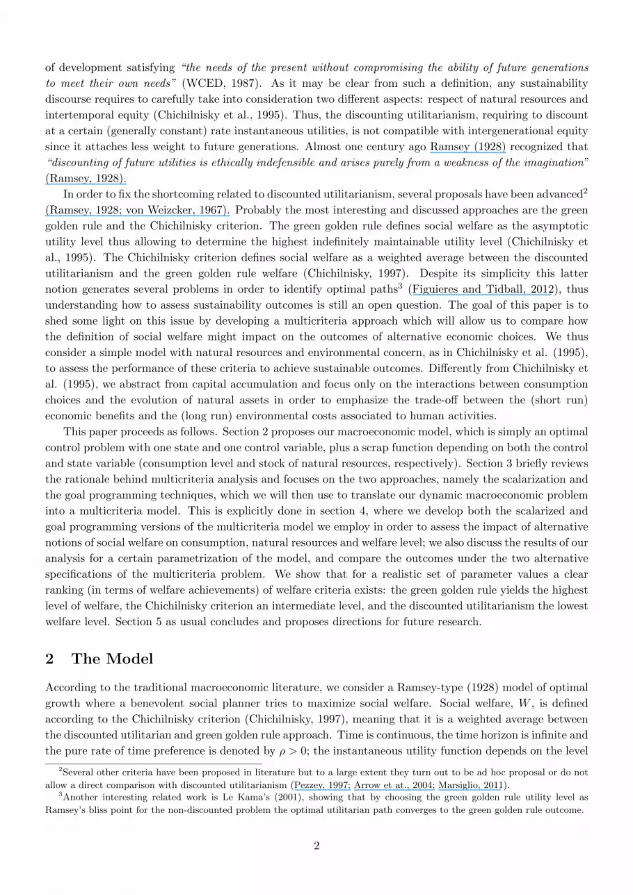
The results of our numerical simulations are shown in Figure 1 and Figure 2. Figure 1 shows the optimal

path of consumption and natural resources for different values of θ, ranging from 0 to 1, corresponding to

social welfare functions relying on different approaches, varying from the green golden rule (θ = 0) to the

discounted utilitarianism (θ = 1). The intermediate values of θ correspond to the Chichilnisky criterion,

in which higher values of θ represent more importance attached to discounted utilitarianism. As the figure

clearly shows, the closer θ to 0, the more parsimonious is the consumption path and the more abundant

the long run level of natural resources. Intuitively, the more emphasis we place on the steady state utility,

the more we favor environmental preservation rather than economic activities; we thus consume less and

preserve more natural resources for the (remote) future. Note that in the figure, the green golden rule case

6

(θ = 0) is reported with a dashed line in order to remind us that this represents only a steady state level,

thus there is no dynamics from 0 to T .

Figure 1: Scalarization technique: evolution of consumption (on the left) and natural resources (on the

right) for different values of θ.

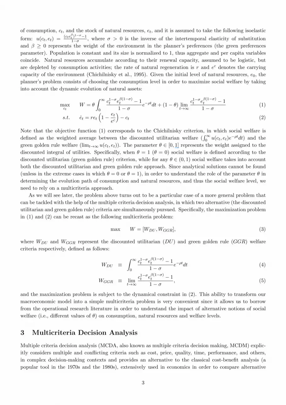
Figure 2 represents the value of social welfare, W (equation (6)), as a function of the parameter θ ∈ [0, 1].

Social welfare is clearly decreasing in θ, meaning that it achieves its maximum when θ = 0, corresponding to

the green golden rule case, and its minimum when θ = 1, corresponding to the discounted utilitarian case.

Thus the green golden rule approach does yield a higher social welfare than both the Chichilnisky criterion

and the discounted utilitarian approach. This result suggests that completely neglecting finite-time utilities

and focusing only on the steady state utility, as suggested by the green golden rule, is not only sensible from

a sustainability point of view but it is also from a social welfare maximization standpoint.

Figure 2: Scalarization technique: social welfare as a function of θ.

4.2 Goal Programming Technique

According to the chosen GP technique, the preferences on the deviations from the fixed aspiration levels are

explicitly taken into account with the help of satisfaction functions Fi(δi), and our multicriteria problem

can be expressed as the following maximization problem:

max wDUF+DU (δ+DU ) + wDUF

−DU (δ−DU ) + wGGRF

+GGR(δ+GGR) + wGGRF

−GGR(δ−GGR)

7

s.t. WDU − δ+DU + δ−DU = GDU

WGGR − δ+GGR + δ−GGR = GGGR

0 ≤ δ+DU ≤ δ+DUν

0 ≤ δ−DU ≤ δ−DUν

0 ≤ δ+GGR ≤ δ+GGRν

0 ≤ δ−GGR ≤ δ−GGRν ,

given the dynamic equation (2), and the initial condition e0. In the expression above δ+DUν , δ−DUν , δ+GGRνand δ−GGRν are the veto thresholds for the positive and negative deviations from the two goals: the social

planner needs to find the optimal solution satisfying these constraints on the deviations δ+DU , δ−DU , δ+GGRand δ−GGR, respectively. The aspirations levels can be chosen freely by the social planner, in accordance to

some feasibility and/or desirability criterion. In our case the most natural choice is letting the aspiration

levels coincide with each goal independently considered, that is:

GDU = maxct

∫ ∞0

c1−σt eβ(1−σ)t − 1

1− σe−ρtdt

s.t. et = ret

(1− et

ec

)− ct

GGGR = maxct

limt→∞

c1−σt eβ(1−σ)t − 1

1− σs.t. et = ret

(1− et

ec

)− ct

In order to apply our GP model, we need to define the satisfaction functions Fi(δ+i ), Fi(δ

−i ). For sake

of simplicity we assume that the shape and the properties of the satisfaction functions are the same with

respect to both positive and negative deviations, and identical for each criterion. An appropriate satisfaction

function may take the following form (Martel and Aouni, 1990):

Fα(δ) =1

1 + α2δ2

Indeed, such a specification implies that: F (0) = 1, F (∞) = 0; F ′′(δ) = 0 if and only if δ = 12α ; 0.9 ≤

F (δ) ≤ 1 if δ ≤ 13α ; 0 ≤ F (δ) ≤ 0.1 if δ ≥ 3

α . This means that this particular function allows to achieve

a level of satisfaction between 90% and 100% when δ ≤ 13α , and a level of satisfaction between 0% and

10% when δ ≥ 3α . With these properties in mind, we can now proceed to define two threshold levels: the

indifference threshold, δind, and the dissatisfaction threshold, δdis. A natural choice for these threshold

values is the following: δind = 13α and δdis = 3

α . Similarly, we need to identify the size of the veto threshold,

which we assume to be given by δv = 2 ∗ δdis = 6α . Note that the parameter α plays a critical role in our

satisfaction function, Fα(δ), and in particular it allows us to obtain different indifference, dissatisfaction and

veto thresholds by simply changing its value. It thus may be convenient to compare our results for different

choices of this parameter, for example for α = 0.1, α = 0.01 and α = 0.001. It is possible to show that our

conclusions are not significantly affected by this parameter value, and thus in what follows we set it equal

to 0.1 for the sake of simplicity (see Aouni et al., 2013).

Now we can proceed with the discretization of our problem. First of all, GDU and GGGR in a discrete

framework read as follows:

GDU = maxct

T∑t=0

c1−σt eβ(1−σ)t − 1

1− σe−ρt

s.t. et+1 − et = ret

(1− et

ec

)− ct ∀t = 0, ....T − 1

8

0 = reT

(1− eT

ec

)− cT

e0 given

GGGR = maxcT

c1−σT eβ(1−σ)T − 1

1− σs.t. 0 = reT

(1− eT

ec

)− cT

Note that the values GDU and GGGR correspond to the cases θ = 1 and θ = 0 in equation (6), respectively.

As before, some comments are needed: there is no dynamics after T , and the weights are set as wDU = θ

and wGGR = 1− θ. The GP problem consists of maximizing the social planner’s satisfaction, Z, and in its

entire form it reads as follows:

max Z =θ

1 + (αδ+DU )2+

θ

1 + (αδ−DU )2+

1− θ1 + (αδ+GGR)2

+1− θ

1 + (αδ−GGR)2(10)

T∑t=0

c1−σt eβ(1−σ)t − 1

1− σe−ρt − δ+DU + δ−DU = GDU (11)

c1−σT eβ(1−σ)T − 1

1− σ− δ+GGR + δ−GGR = GGGR (12)

et+1 − et = ret

(1− et

ec

)− ct ∀t = 0, ....T − 1 (13)

0 = reT

(1− eT

ec

)− cT (14)

e0 given (15)

0 ≤ δ+DU ≤ δ+DUν (16)

0 ≤ δ−DU ≤ δ−DUν (17)

0 ≤ δ+GGR ≤ δ+GGRν (18)

0 ≤ δ−GGR ≤ δ−GGRν . (19)

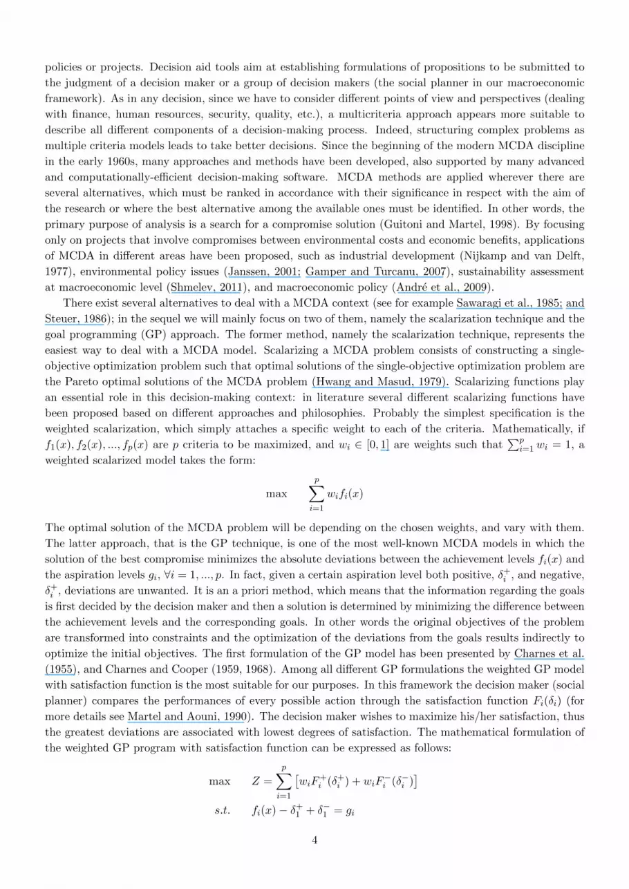
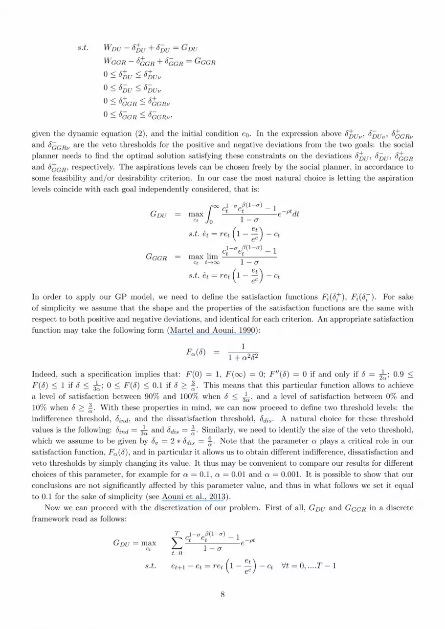
Figure 3: Goal programming: evolution of consumption (on the left) and natural resources (on the right)

for different values of θ.

The results of our simulations are presented in Figure 3 and in Figure 4. The optimal time paths of

consumption and natural resources are qualitatively similar to those found earlier with the scalarization

approach. The dashed line still represents the green golden rule (θ = 0) case, in which no dynamics from 0

to T is present. On the left panel of Figure 3 we can see that consumption is generally decreasing over time

9

(apart in the θ = 1 case), and it increases with θ. The other side of the same coin can been seen on the

right panel of Figure 3: the more emphasis we put on discounted utilitarianism, the less resources are left

for the long run outcome, with the extreme case being represented by the discounted utilitarian approach

in which no resources are left at the end of the time horizon. Since the results qualitatively coincide, their

interpretation is exactly equivalent to what discussed earlier concerning the scalarization technique4.

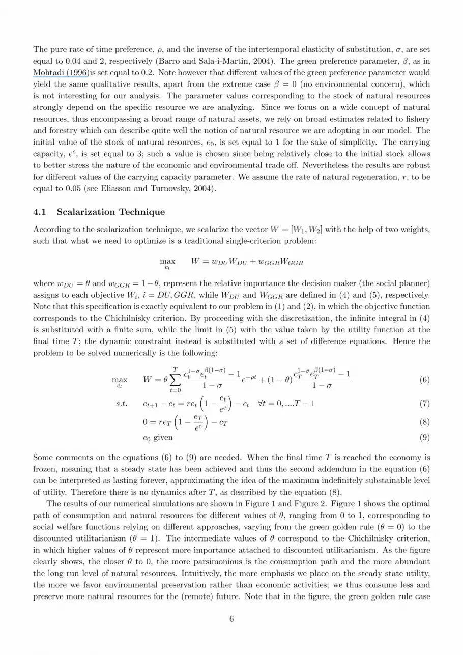
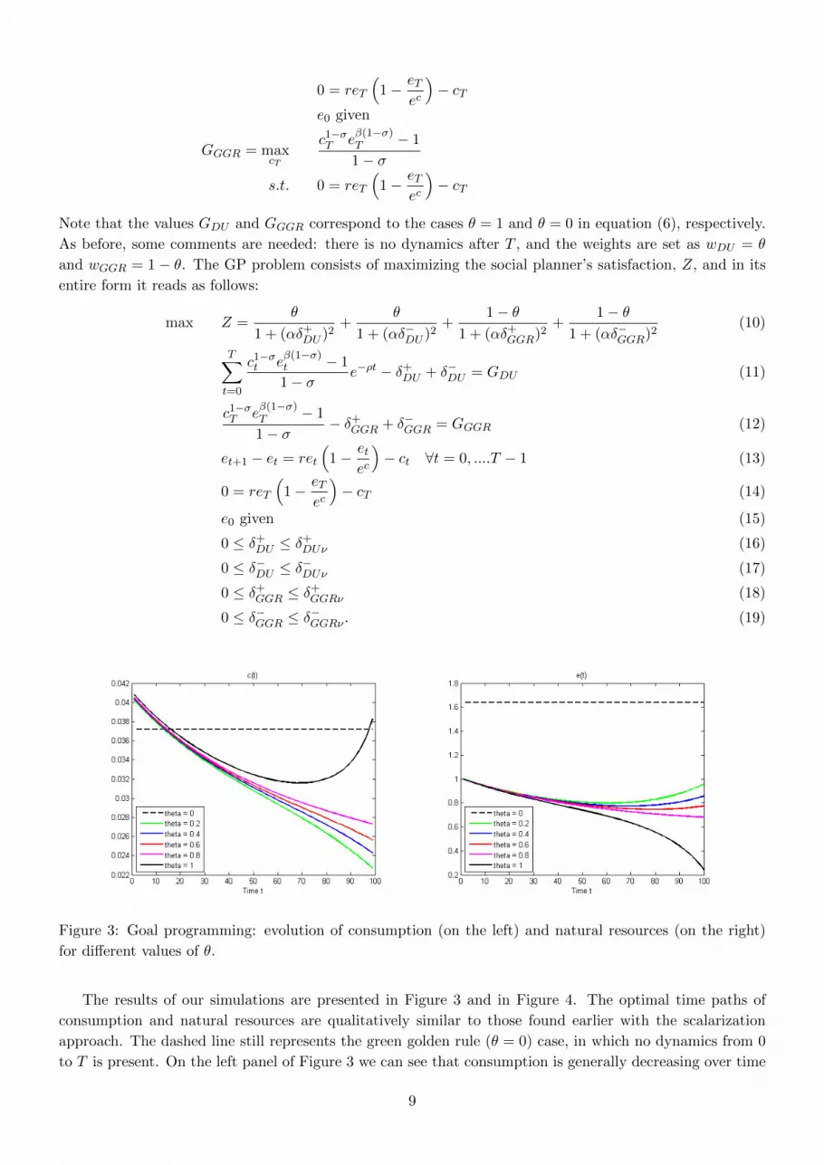
Figure 4: Goal programming: social welfare as a function of θ.

Figure 4 shows the different levels of social welfare (as in equation (6)), W , for values of θ ranging from

0 to 1. Since the time paths of consumption and natural resources are similar to those obtained with the

scalarization approach, then it is also reasonable to expect that the behavior of the social welfare function

will be equivalent to what discussed earlier. This is confirmed in Figure 4, from which we can see that social

welfare is decreasing in θ, and thus it achieves its maximum when θ = 0, corresponding to the green golden

rule criterion. Even with a GP approach, our results confirm that the green golden rule is not only the

preferred criterion from a sustainability point of view but also from a welfare maximization standpoint.

5 Conclusion

In (macro)economics literature the notion employed in order to define social welfare is critical, especially

whenever we wish to take into account also sustainability issues. This is due to the fact that the most

commonly used criterion, namely the discounted utlitarianism, attaches less weight to future generations’

wellbeing. Alternative criteria, like the green golden rule and the Chinchilnisky criterion, have been proposed

in order to overcome this problem. In this paper we assess and compare the outcomes associated to different

welfare criteria by simply relying on a multicriteria model. We consider two alternative specification of the

multicriteria problem, based on the scalarization and GP technique respectively, in order to fully analyze

the problem in a very simple macroeconomic model with environmental interactions, as in Chichilnisky et al.

(1995). For a specific and realistic parametrization of the model, we show that social welfare is a decreasing

function of the weight attached to the discounted sum of utilities (θ). Thus, it is possible to identify a

clear ranking of criteria in terms of social welfare achievements: the green golden rule leads to the highest

level of welfare, the Chichilnisky criterion to an intermediate level, and the discounted utilitarianism to the

lowest welfare level. Both the scalarization and the GP techniques, even if relying on different multicriteria

4The scalarization and the GP approach coincide when the objectives values of the GP are chosen exactly equal to each

objective taken singularly. When we introduce the preferences via the satisfaction function the outcome of the two approaches is

generally different and the similarities occurring in our results are given by the above mentioned matching of the GP objectives

with each objective taken singularly.

10

philosophies, lead to the same results (see Figure 2 and Figure 4). Such concordant conclusions corroborate

a result that is absolutely not obvious a priori: the green golden rule does have to be preferred to the

discounted utilitarianism not only because of its ability to take into account sustainability issues, but also

because it allows to achieve higher social welfare levels.

To the best of our knowledge, ours is the first paper trying to assess the implications of different no-

tions of social welfare on the economic and environmental trade off. It is thus natural to wonder to what

extent the simplicity of our model specification affects our results. Specifically, in our model natural re-

sources are only used for consumption purposes; however, this is quite a strong simplification of reality.

Natural resources represent also an important production factor, without which it may not be possible at

all to produce any consumable good. Moreover, production activities, apart from using natural resources,

may even be detrimental for the environment through the pollution channel. Furthermore, pollution may

generate perverse effects on the production possibilities, thus the nexus between economic activities and

environmental dynamics is definitely more complex that what we have considered thus far. Extending the

analysis along these directions is needed in order to obtain a wider comprehension of sustainability issues

and their implications on social welfare. This is left for future research.

References

1. Andre, F.J., Cardenete, M.A., Romero, C. (2009). A goal programming approach for a joint design

of macroeconomic and environmental policies: a methodological proposal and an application to the

Spanish economy, Environmental Management 43, 888–898

2. Aouni, B., Kettani, O. (2001). Goal programming model: a glorious history and a promising future,

European Journal of Operational Research 133, 225–231

3. Aouni, B., Colapinto, C., La Torre, D. (2013). A cardinality constrained stochastic goal programming

model with satisfaction functions for venture capital investment decision making, Annals of Operations

Research 205, 77–88

4. Aouni, B., La Torre, D. (2010). A generalized stochastic goal programming model, Applied mathe-

matics and computation 215, 4347–4357

5. Aouni A., Ben Abdelaziz, F., La Torre, D. (2012a). The stochastic goal programming model: theory

and applications, Journal of Multicriteria Decision Analysis 19, 185–200

6. Aouni, B., Colapinto, C., La Torre, D. (2012b). Stochastic goal programming model and satisfaction

function for media selection and planning problem, International Journal of Multi-criteria Decision

Making 2, 391–407

7. Arrow, K., Dasgupta, P., Goulder, L., Daily, G., Ehrlich, P., Heal, G., Levin, S., Maler, K.G., Schnei-

der, S., Starrett D., Walker, B. (2004). Are we consuming too much?, Journal of Economic Perspectives

18, 147–172

8. Barro, R.J., Sala-i-Martin, X. (2004). Economic growth (Cambridge, Massachusetts: MIT Press)

9. Boucekkine, R., Fabbri, G. (2013). Assessing Parfit’s repugnant conclusion within a canonical endoge-

nous growth set-up, Journal of Population Economics 26, 751–767

10. Charnes, A., Cooper, W.W. (1959). Chance-constrained programming, Management Science 6, 73–80

11. Charnes, A., Cooper, W.W. (1968). Deterministic equivalents for optimising and satisfying under

chance constraints, Operations Research 11, 11–39

12. Charnes, A., Cooper, W.W., Ferguson, R. (1955). Optimal estimation of executive compensation by

linear programming, Management Science 1, 138-151

13. Chinchilnisky, G., Heal, G., Beltratti, A. (1995). The green golden rule, Economics Letters 49, 174–179

14. Chinchilnisky, G. (1997). What is sustainable development?, Land Economics 73, 476–491

11

15. Eliasson, L. Turnovsky, S.J. (2004). Renewable resources in an endogenously growing economy: bal-

anced growth and transitional dynamics, Journal of Environmental Economics and Management 48,

1018-1049

16. Figuieres, C., Tidball, M. (2012). Sustainable exploitation of a natural resource: a satisfying use of

Chichilnisky’s criterion, Economic Theory 49, 243-265

17. Gamper, C.D., Turcanu, C. (2007). On the governmental use of multi-criteria analysis, Ecological

Economics 62, 298-307

18. Guitouni, A., Martel, J.M. (1998). Tentative guidelines to help choosing an appropriate MCDA

method, European Journal of Operational Research 109, 501-521

19. Heal, G. (2005). Intertemporal welfare economics and the environment, in Maler, K.G., Vincent, J.R.

(eds.), “Handbook of Environmental Economics”, vol. 3 (North-Holland: Amsterdam)

20. Hwang, C.L., Masud, A.S. (1979). Multiple objective decision making, methods and applications: a

state-of-the-art survey (Springer-Verlag)

21. Janssen, R. (2001). On the use of multi-criteria analysis in environmental impact assessment in the

Netherlands, Journal of Multi-Criteria Decision Analysis 10, 101-109

22. Le Kama, A.D.A. (2001). Sustainable growth, renewable resources and pollution, Journal of Economic

Dynamics & Control 25, 1911–1918

23. Marsiglio, S. (2011). On the relationship between population change and sustainable development,

Research in Economics 65, 353–364

24. Marsiglio, S. (2014). Reassessing Edgeworth’s conjecture when population dynamics is stochastic,

Journal of Macroeconomics 42, 130–140

25. Marsiglio, S., La Torre, D. (2012). Population dynamics and utilitarian criteria in the Lucas-Uzawa

model, Economic Modelling 29, 1197–1204

26. Martel, J.M., Aouni, B. (1990). Incorporating the decision-maker’s preferences in the goal-programming

model, Journal of the Operational Research Society 41, 1121–1132

27. Mohtadi, H. (1996). Environment, growth, and optimal policy design, Journal of Public Economics

63, 119-140

28. Nijkamp, P., van Delft, A. (1977). Multicriteria analysis and regional decisionmaking (Boston: Kluwer

Nijhoff)

29. Palivos, T., Yip, C.K. (1993). Optimal population size and endogenous growth, Economics Letters 41,

107–110

30. Pezzey, J.C.V. (1997). Sustainability constraints versus “optimality” versus intertemporal concern,

and axioms versus data, Land Economics 73, 448–466

31. Ramsey, F. (1928). A mathematical theory of saving, Economic Journal 38, 543–559

32. Romero, C. (1991). Handbook of critical issues in goal programming (Pergamon Press, Oxford)

33. Sawaragi, Y., Nakayama, H., Tanino, T. (1985). Theory of multiobjective optimization, (Orlando:

Academic Press)

34. Shmelev, S.E. (2011). Dynamic sustainability assessment: the case of Russia in the period of transition

(1985–2007), Ecological Economics 70, 2039–2049

35. Steuer, R.E. (1986). Multiple criteria optimization: theory, computation, and application (New York:

Wiley & Sons)

36. World Commission on Environment and Development (1987). Our common future (Oxford University

Press, Oxford)

12