Support Vector Machines (SVMs) for MonitoringNetwork Designby Tirusew Asefa1,2, Mariush Kemblowski1, Gilberto Urroz1, and Mac McKee1

AbstractIn this paper we present a hydrologic application of a new statistical learning methodology called support

vector machines (SVMs). SVMs are based on minimization of a bound on the generalized error (risk) model,rather than just the mean square error over a training set. Due to Mercer’s conditions on the kernels, the corre-sponding optimization problems are convex and hence have no local minima. In this paper, SVMs are illustra-tively used to reproduce the behavior of Monte Carlo–based flow and transport models that are in turn used in thedesign of a ground water contamination detection monitoring system. The traditional approach, which is based onsolving transient transport equations for each new configuration of a conductivity field, is too time consuming inpractical applications. Thus, there is a need to capture the behavior of the transport phenomenon in random mediain a relatively simple manner. The objective of the exercise is to maximize the probability of detecting contami-nants that exceed some regulatory standard before they reach a compliance boundary, while minimizing cost (i.e.,number of monitoring wells). Application of the method at a generic site showed a rather promising performance,which leads us to believe that SVMs could be successfully employed in other areas of hydrology. The SVM wastrained using 510 monitoring configuration samples generated from 200 Monte Carlo flow and transport realiza-tions. The best configurations of well networks selected by the SVM were identical with the ones obtained fromthe physical model, but the reliabilities provided by the respective networks differ slightly.

BackgroundThe design of ground water pollution monitoring net-

works entails the selection of sampling points (spatial)and sampling frequency (temporal) to determine physical,chemical, and biological characteristics of ground water(Loaiciga et al. 1992). The current approach to groundwater quality monitoring network design requires thatconsideration be given to (1) the spatial and temporalcoverage of the monitoring sites; (2) the competing ob-jectives of a monitoring program; (3) the complex natureof geologic, hydrologic, and other environmental factors;(4) the stochastic character of transport parameters

(geologic, hydrologic, and environmental) used in thedesign process; and (5) the risk posed to society (failureto detect, poor characterization, etc.). Based on design ob-jectives one can identify three categories of monitoringnetworks: (1) leak detections; (2) characterization; and(3) long-term monitoring. In the following sections wefocus our attention on leak-detection monitoring net-works. Interested readers may refer to the works of Hudakand Loaiciga (1992), Datta and Dhiman (1996), Molinaet al. (1996), Mahar and Datta (1997), Montas et al.(2000), and Reed et al. (2000) for design of characteriza-tion and long-term monitoring networks.

Leak-Detection Monitoring NetworksNetworks in this category enable one to detect unex-

pected leaks before the contaminants reach a complianceboundary, which is usually located at some relativelyshort distance, say 100 m, from a landfill. Solutions tothis problem are complicated due to the facts that thelocation and magnitude of leaks are random and con-taminants travel within systems characterized by poorlydefined boundaries and hydrologic conditions. Massmann

1Department of Civil and Environmental Engineering andUtah Water Research Laboratory, Utah State University, 8200 OldMain Hill, Logan, UT 84321.

2Corresponding author: Tampa Bay Water, 2535 Landmark Drive,Suite 211, Clearwater, FL 33761: fax (435) 797-3663; tasefa@tampabaywater.org

Received February 23, 2004; accepted June 25, 2004.Copyright ª 2005 National Ground Water Association

Vol. 43, No. 3—GROUND WATER—May–June 2005 (pages 413–422) 413

and Freeze (1987a, 1987b) presented a comprehensiveframework and application for the design of landfill oper-ation. The objective was to maximize the net presentvalue of stream of costs, benefits, and risks. Risk is asso-ciated with the cost of failure, with failure being definedas the situation in which the concentration measured is inexcess of a standard at the compliance surface. The deci-sion analysis will then compare different alternativemonitoring networks by calculating the reduction of theprobability of failure. Meyer and Brill (1988) analyzedthe same problem through an integer-programmingmodel of facility location (Church and ReVelle 1974).Their objective was to maximize the detection of plumesthat exceed a concentration standard. Random plumeswere generated from parameters sampled from longitudi-nal and transverse dispersivity distributions, which wereassumed to be positively correlated with a normal distri-bution and uniform velocity vector directions. Fora given number of monitoring wells (representing costconstraint), the integer programming would select loca-tions that resulted in a higher probability of plume detec-tion. Meyer et al. (1994) extended the work of Meyer andBrill (1988) to include an additional objective of mini-mizing the area of contamination at the time of detection.Storck et al. (1997) extended the work of Meyer et al.(1994) to three-dimensional flow and transport problemsand ignored dispersion transport. Instead, they used anadvective particle-tracking approach.

Angulo and Tang (1999) used similar objective crite-ria and uncertainty analysis as in Meyer et al. (1994) butformed the objective function through ‘‘utility criteria’’for a system that consists of a single row of wells perpen-dicular to the flow direction. For a given number of wellsat a given distance from the landfill, the total cost of thesystem was found to be the sum of system constructionand monitoring costs, plus the cost of aquifer remediationassociated with expected volumes of contaminated aqui-fer given detection and no detection. Morisawa and Inoue(1991) presented a methodology for designing an optimalmonitoring network based on fuzzy utility functions. Astochastic simulation of both critical and precursor indi-cator chemicals resulted in a mathematical description ofa four-attribute design problem. An optimum monitoringnetwork was then defined as a network having maximumtotal utility, which was evaluated as the fuzzy expectationof weighted arithmetic sums of the four utilities. All theaforementioned studies assumed that there is continuousmonitoring at potential monitoring well locations. Moni-toring frequency was examined by Jardine et al. (1996)within a decision analysis framework for designing moni-toring networks for fractured rock.

MethodologyIn this paper we present a methodology for the appli-

cation of support vector machines (SVMs) in the designof ground water contamination detection monitoring net-works. The objective of the modeling exercise is to designan optimal monitoring network for an initial detection ofground water contamination that maximizes the probabil-ity of detection while minimizing cost (i.e., number of

monitoring wells). A given topology of monitoring net-work (number and locations) has a corresponding proba-bility of plume detection (reliability). If the number and/or location of a well changes, the monitoring network willhave a different reliability. With an increased number ofwells, one can increase the reliability of a monitoring net-work, but this in turn would result in higher cost. Whilethe cost of monitoring wells in a network can be easilyquantified in monetary values, it is not simple to quantifythe change in reliability (probability of detection) in mon-etary terms. Therefore, we set our objective herein gettingtrade-off curves between monitoring network sizes andcorresponding reliabilities. SVMs will be trained to pro-vide network reliabilities for an arbitrary configuration ofmonitoring wells so that one would be able to select thoseproviding the highest reliabilities without running time-consuming flow and transport models.

Model Domain and UncertaintyThe aquifer is assumed to be represented by a rectan-

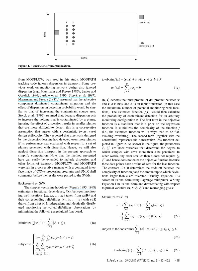
gular box in which a two-dimensional flow takes place.The overall dimensions of the model were 1000 by 500 m(Figure 1). Model cell sizes were 20 by 20 m. The bound-ary conditions for the steady-state flow model were zeroflux at y = 0 m and y = 500 m and constant head along theother two boundaries. These boundary conditions implythat the regional ground water flow direction is relativelywell known. The head values at x = 0 m and x = 1000 mwere chosen to result in an average gradient over thedomain of 0.01. We considered only two types of un-certainties: source location and the spatial distribution ofthe hydraulic conductivity. The method can readily beextended to incorporate additional uncertain parameters(e.g., boundary condition, recharge). The leak is assumedto be equally probable at any location in the landfill cell(equivalent to a numerical cell). The source of hydro-geological uncertainty is limited to spatial variability in thehydraulic conductivity field. The natural logarithm of thehydraulic conductivity, Y = ln(K), was modeled as a Gauss-ian second-order stationary stochastic process with a meanvalue of lY = 0.79. The variance of Y was set at r2Y = 0.96,with correlation scale of l = 100 m and exponential covari-ance function. Meyer et al. (1994) also used a similar casestudy. The method presented by Tompson et al. (1989),based on the turning bands algorithm, was used to generatea stationary, correlated two-dimensional hydraulic conduc-tivity field. Note that this simple representation of theaquifer is not a limitation of the application of SVMs, butrather a simplification of numerical modeling to save com-putational time. The procedure developed here can easilybe extended to more complicated site conditions.

Flow and Transport SimulationsThe USGS finite-difference MODFLOW code

(McDonald and Harbaugh 1988; Harbaugh and McDonald1996) was used to simulate the steady-state ground waterflow problem. MODFLOW was chosen because it hasbeen widely used, and its use has been extensively docu-mented in the technical literature. Transport was simulatedusing a particle-tracking approach. MODPATH (Pollock1988, 1989), which is designed to use the head calculated

414 T. Asefa et al. GROUND WATER 43, no. 3: 413–422

from MODFLOW, was used in this study. MODPATHtracking code ignores dispersion in transport. Some pre-vious work on monitoring network design also ignoreddispersion (e.g., Massmann and Freeze 1987b; James andGorelick 1994; Jardine et al. 1996; Storck et al. 1997).Massmann and Freeze (1987b) assumed that the advectivecomponent dominated contaminant migration and theeffect of dispersion on detection probability would be sim-ilar to that of increasing the contaminant source area.Storck et al. (1997) assumed that, because dispersion actsto increase the volume that is contaminated by a plume,ignoring the effect of dispersion results in smaller plumesthat are more difficult to detect; this is a conservativeassumption that agrees with a pessimistic (worst case)design philosophy. They reported that a network designedby the dispersion-less method detected even more plumesif its performance was evaluated with respect to a set ofplumes generated with dispersion. Hence, we will alsoneglect dispersion transport in the present approach tosimplify computation. Note that the method presentedhere can easily be extended to include dispersion andother forms of transport. MODFLOW and MODPATHwere run in a consecutive manner with a command inter-face made of C/C++ processing programs and UNIX shellcommands before the results were passed to the SVMs.

Background on SVMThe support vector methodology (Vapnik 1995, 1998)

estimates a functional dependency, f(x), between monitor-ing well locations {x1, x2, ., xL} taken from x2RK andtheir corresponding reliabilities {y1, y2, ., yL} with y2Rdrawn from a set of L independent and identically distrib-uted monitoring networks/reliabilities observations byminimizing the following regularized functional:

Minimize1

2kwk2 1C

XL

i = 1

!ni 1 n!i

""1a#

subject to

8>>>>><

>>>>>:

yi2PK

j = 1

PL

i = 1

wjxji2b $ e1 ni

PK

j = 1

PL

i = 1

wjxji 1 b2yi $ e1 n!i

ni; n!i % 0

"1b#

to obtain f "x# = Æw; xæ1 bwithw 2 X; b 2 R

or f "x# =XK

j = 1

wjxj 1 b "1c#

Æw; xæ denotes the inner product or dot product between wand x, b is bias, and K is an input dimension (in this casethe maximum number of potential monitoring well loca-tions). The estimated function, f(x), would then calculatethe probability of contaminant detection for an arbitrarymonitoring configuration x. The first term in the objectivefunction is a stabilizer that is a prior on the regressionfunction. It minimizes the complexity of the function f(i.e., the estimated function will always tend to be flat,avoiding overfitting). The second term (together with theconstraints) represents the e-insensitive loss function de-picted in Figure 2. As shown in the figure, the parametersni, ni* are slack variables that determine the degree towhich samples with error more than e be penalized. Inother words, any error smaller than e does not require ni,ni* and hence does not enter the objective function becausethese data points have a value of zero for the loss function.The constant C > 0 determines the trade-off between thecomplexity of function f and the amount up to which devia-tions larger than e are tolerated. Usually, Equation 1 issolved in its dual form using Lagrange multipliers. WritingEquation 1 in its dual form and differentiating with respectto primal variables (w, b, ni, ni*) and rearranging gives:

Maximize W"a!; a#

= 2eXL

i = 1

"ai 1 a!i #1XL

i = 1

yi"ai2a!i #

21

2

XL

i; j = 1

"ai2a!i #"aj2a!j #k"xi; xj# "2a#

subject to the constraintsXL

i = 1

"a!i 2ai# = 0; 0 $ ai; a!i $ C

"2b#

to obtain f "x# =XN

i = 1

"a!i2ai#k"x; xi#1 b "2c#

Monitoring well

Landfill cell

1000m

1 2

9 10 50

0m

Figure 1. Generic site conceptualization.

T. Asefa et al. GROUND WATER 43, no. 3: 413–422 415

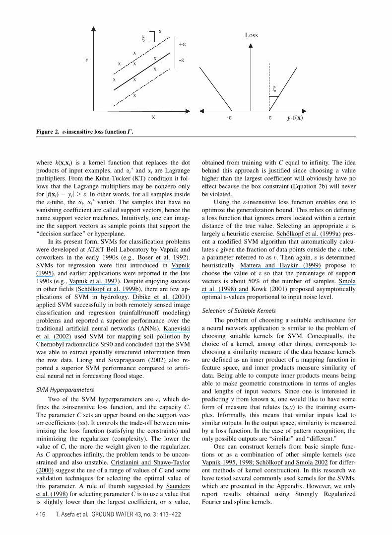
where k(x,xi) is a kernel function that replaces the dotproducts of input examples, and ai* and ai are Lagrangemultipliers. From the Kuhn-Tucker (KT) condition it fol-lows that the Lagrange multipliers may be nonzero onlyfor jf(xi) 2 yij % e. In other words, for all samples insidethe e-tube, the ai, ai* vanish. The samples that have novanishing coefficient are called support vectors, hence thename support vector machines. Intuitively, one can imag-ine the support vectors as sample points that support the‘‘decision surface’’ or hyperplane.

In its present form, SVMs for classification problemswere developed at AT&T Bell Laboratory by Vapnik andcoworkers in the early 1990s (e.g., Boser et al. 1992).SVMs for regression were first introduced in Vapnik(1995), and earlier applications were reported in the late1990s (e.g., Vapnik et al. 1997). Despite enjoying successin other fields (Scholkopf et al. 1999b), there are few ap-plications of SVM in hydrology. Dibike et al. (2001)applied SVM successfully in both remotely sensed imageclassification and regression (rainfall/runoff modeling)problems and reported a superior performance over thetraditional artificial neural networks (ANNs). Kaneviskiet al. (2002) used SVM for mapping soil pollution byChernobyl radionuclide Sr90 and concluded that the SVMwas able to extract spatially structured information fromthe row data. Liong and Sivapragasam (2002) also re-ported a superior SVM performance compared to artifi-cial neural net in forecasting flood stage.

SVM Hyperparameters

Two of the SVM hyperparameters are e, which de-fines the e-insensitive loss function, and the capacity C.The parameter C sets an upper bound on the support vec-tor coefficients (as). It controls the trade-off between min-imizing the loss function (satisfying the constraints) andminimizing the regularizer (complexity). The lower thevalue of C, the more the weight given to the regularizer.As C approaches infinity, the problem tends to be uncon-strained and also unstable. Cristianini and Shawe-Taylor(2000) suggest the use of a range of values of C and somevalidation techniques for selecting the optimal value ofthis parameter. A rule of thumb suggested by Saunderset al. (1998) for selecting parameter C is to use a value thatis slightly lower than the largest coefficient, or a value,

obtained from training with C equal to infinity. The ideabehind this approach is justified since choosing a valuehigher than the largest coefficient will obviously have noeffect because the box constraint (Equation 2b) will neverbe violated.

Using the e-insensitive loss function enables one tooptimize the generalization bound. This relies on defininga loss function that ignores errors located within a certaindistance of the true value. Selecting an appropriate e islargely a heuristic exercise. Scholkopf et al. (1999a) pres-ent a modified SVM algorithm that automatically calcu-lates e given the fraction of data points outside the e-tube,a parameter referred to as t. Then again, t is determinedheuristically. Mattera and Haykin (1999) propose tochoose the value of e so that the percentage of supportvectors is about 50% of the number of samples. Smolaet al. (1998) and Kowk (2001) proposed asymptoticallyoptimal e-values proportional to input noise level.

Selection of Suitable Kernels

The problem of choosing a suitable architecture fora neural network application is similar to the problem ofchoosing suitable kernels for SVM. Conceptually, thechoice of a kernel, among other things, corresponds tochoosing a similarity measure of the data because kernelsare defined as an inner product of a mapping function infeature space, and inner products measure similarity ofdata. Being able to compute inner products means beingable to make geometric constructions in terms of anglesand lengths of input vectors. Since one is interested inpredicting y from known x, one would like to have someform of measure that relates (x,y) to the training exam-ples. Informally, this means that similar inputs lead tosimilar outputs. In the output space, similarity is measuredby a loss function. In the case of pattern recognition, theonly possible outputs are ‘‘similar’’ and ‘‘different.’’

One can construct kernels from basic simple func-tions or as a combination of other simple kernels (seeVapnik 1995, 1998; Scholkopf and Smola 2002 for differ-ent methods of kernel construction). In this research wehave tested several commonly used kernels for the SVMs,which are presented in the Appendix. However, we onlyreport results obtained using Strongly RegularizedFourier and spline kernels.

Figure 2. e-insensitive loss function G.

416 T. Asefa et al. GROUND WATER 43, no. 3: 413–422

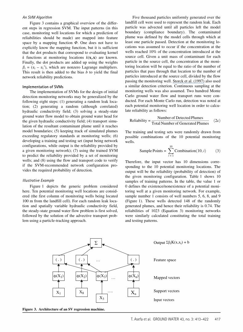
An SVM Algorithm

Figure 3 contains a graphical overview of the differ-ent steps in regression SVM. The input patterns (in thiscase, monitoring well locations for which a prediction ofreliabilities should be made) are mapped into featurespace by a mapping function F. One does not have toexplicitly know the mapping function, but it is sufficientthat the dot products that correspond to evaluating kernelk functions at monitoring locations k(xi,x) are known.Finally, the dot products are added up using the weightsbi = (ai – ai*), which are nonzero Lagrange multipliers.This result is then added to the bias b to yield the finalnetwork reliability predictions.

Implementation of SVMsThe implementation of SVMs for the design of initial

detection monitoring networks may be generalized by thefollowing eight steps: (1) generating a random leak loca-tion; (2) generating a random (although correlated)hydraulic conductivity field; (3) solving a steady-stateground water flow model to obtain ground water head forthe given hydraulic conductivity field; (4) transport simu-lation of the resultant contaminant plume until it reachesmodel boundaries; (5) keeping track of simulated plumesexceeding regulatory standards at monitoring wells; (6)developing a training and testing set (input being networkconfigurations, while output is the reliability provided bya given monitoring network); (7) using the trained SVMto predict the reliability provided by a set of monitoringwells; and (8) using the flow and transport code to verifyif the SVM-recommended network configuration pro-vides the required probability of detection.

Illustrative Example

Figure 1 depicts the generic problem consideredhere. Ten potential monitoring well locations are consid-ered (the first column of monitoring wells being located100 m from the landfill cell). For each random leak loca-tion and spatially variable hydraulic conductivity field,the steady-state ground water flow problem is first solved,followed by the solution of the advective transport prob-lem using a particle-tracking approach.

Five thousand particles uniformly generated over thelandfill cell were used to represent the random leak. Eachparticle was advected until all particles left the modelboundary (compliance boundary). The contaminatedplume was defined by the model cells through which atleast one particle passed. Detection at the monitoring lo-cations was assumed to occur if the concentration at thewells reached 10% of the concentration introduced at thesource cell. Given a unit mass of contaminant for eachparticle in the source cell, the concentration at the moni-toring location will be equal to the ratio of the number ofparticles that pass through that location to the number ofparticles introduced at the source cell, divided by the flowpassing the monitoring well. Storck et al. (1997) also useda similar detection criterion. Continuous sampling at themonitoring wells was also assumed. Two hundred MonteCarlo ground water flow and transport runs were con-ducted. For each Monte Carlo run, detection was noted ateach potential monitoring well location in order to calcu-late reliability as follows:

Reliability =Number of Detected Plumes

Total Number of Generated Plumes"2c#

The training and testing sets were randomly drawn frompossible combinations of the 10 potential monitoringwells.

Sample Points =X10

i = 1

Combination"10; i# "3#

Therefore, the input vector has 10 dimensions corre-sponding to the 10 potential monitoring locations. Theoutput will be the reliability (probability of detection) ofthe given monitoring configuration. Table 1 shows 10samples of training patterns. In the table, the value 1 or0 defines the existence/nonexistence of a potential moni-toring well at a given monitoring network. For example,sample number 1 consists of well numbers 5, 6, 8, and 9(Figure 1). These wells detected 148 of the randomlygenerated plumes, and hence their reliability is 0.74. Thereliabilities of 1023 (Equation 3) monitoring networkswere similarly calculated constituting the total trainingand testing patterns.

Output iK(x,xi) + b

… Feature space

(X1) (X2) … (Xn) Mapped vectors

…. Support vectors

Input vectors

( . )( . )( . )

X3

X1 XnX8

(X3)

Figure 3. Architecture of an SV regression machine.

T. Asefa et al. GROUND WATER 43, no. 3: 413–422 417

Results and DiscussionsThe SVM software developed by Royal Holloway

University of London and AT&T Speech and Image Pro-cessing Service Research Lab (Saunders et al. 1998) wasused in this study. There is also a wide array of otherSVM software available online (e.g., http://www.kernel-machines.org).

Five hundred and ten sample patterns generated frompossible combinations of 10 potential monitoring wellsand corresponding probabilities of detection were used totrain the SVM, and the rest (513) of the generated sam-ples were used for testing. Two types of performance cri-teria are used here: the root mean square error (RMSE)and the absolute mean deviation, as defined below:

RMSE =

##############################################################################P"PredictedValue2SimulatedValue#2

n

s

AMD =

P j"PredictedValue2SimulatedValuejn

where n is sample size. One can also use other perfor-mance measures.

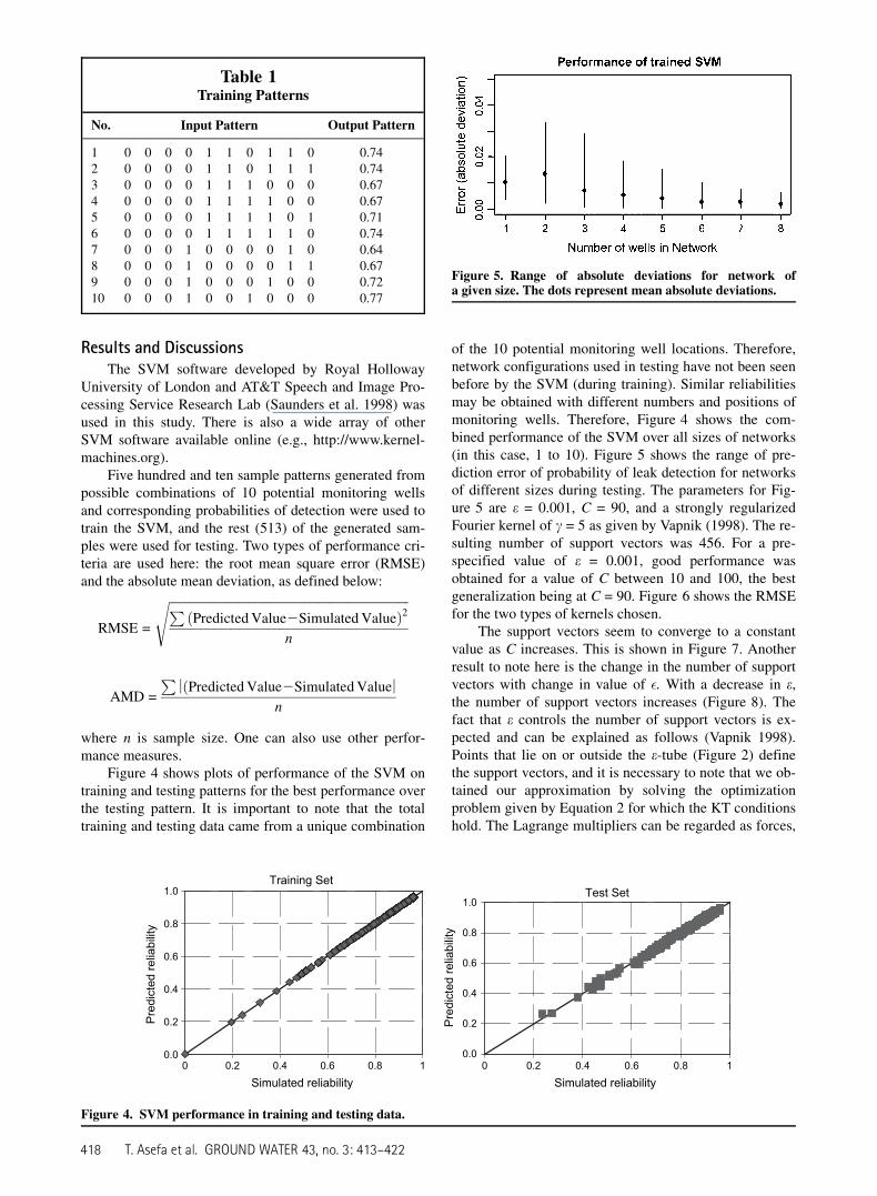
Figure 4 shows plots of performance of the SVM ontraining and testing patterns for the best performance overthe testing pattern. It is important to note that the totaltraining and testing data came from a unique combination

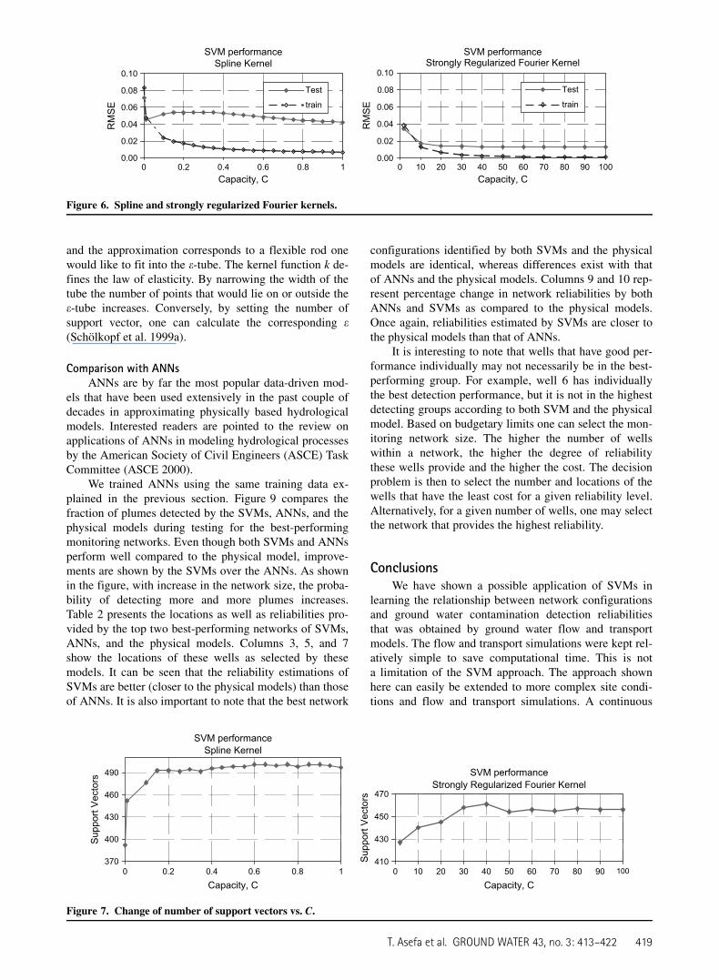
of the 10 potential monitoring well locations. Therefore,network configurations used in testing have not been seenbefore by the SVM (during training). Similar reliabilitiesmay be obtained with different numbers and positions ofmonitoring wells. Therefore, Figure 4 shows the com-bined performance of the SVM over all sizes of networks(in this case, 1 to 10). Figure 5 shows the range of pre-diction error of probability of leak detection for networksof different sizes during testing. The parameters for Fig-ure 5 are e = 0.001, C = 90, and a strongly regularizedFourier kernel of c = 5 as given by Vapnik (1998). The re-sulting number of support vectors was 456. For a pre-specified value of e = 0.001, good performance wasobtained for a value of C between 10 and 100, the bestgeneralization being at C = 90. Figure 6 shows the RMSEfor the two types of kernels chosen.

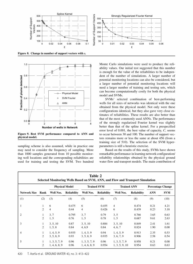
The support vectors seem to converge to a constantvalue as C increases. This is shown in Figure 7. Anotherresult to note here is the change in the number of supportvectors with change in value of !. With a decrease in e,the number of support vectors increases (Figure 8). Thefact that e controls the number of support vectors is ex-pected and can be explained as follows (Vapnik 1998).Points that lie on or outside the e-tube (Figure 2) definethe support vectors, and it is necessary to note that we ob-tained our approximation by solving the optimizationproblem given by Equation 2 for which the KT conditionshold. The Lagrange multipliers can be regarded as forces,

Table 1Training Patterns

No. Input Pattern Output Pattern

1 0 0 0 0 1 1 0 1 1 0 0.742 0 0 0 0 1 1 0 1 1 1 0.743 0 0 0 0 1 1 1 0 0 0 0.674 0 0 0 0 1 1 1 1 0 0 0.675 0 0 0 0 1 1 1 1 0 1 0.716 0 0 0 0 1 1 1 1 1 0 0.747 0 0 0 1 0 0 0 0 1 0 0.648 0 0 0 1 0 0 0 0 1 1 0.679 0 0 0 1 0 0 0 1 0 0 0.7210 0 0 0 1 0 0 1 0 0 0 0.77

Training Set

0.0

0.2

0.4

0.6

0.8

1.0

0 0.2 0.4 0.6 0.8 1Simulated reliability

Pred

icte

d re

liabi

lity

Test Set

0.0

0.2

0.4

0.6

0.8

1.0

0 0.2 0.4 0.6 0.8 1Simulated reliability

Pred

icte

d re

liabi

lity

Figure 4. SVM performance in training and testing data.

Figure 5. Range of absolute deviations for network ofa given size. The dots represent mean absolute deviations.

418 T. Asefa et al. GROUND WATER 43, no. 3: 413–422

and the approximation corresponds to a flexible rod onewould like to fit into the e-tube. The kernel function k de-fines the law of elasticity. By narrowing the width of thetube the number of points that would lie on or outside thee-tube increases. Conversely, by setting the number ofsupport vector, one can calculate the corresponding e(Scholkopf et al. 1999a).

Comparison with ANNsANNs are by far the most popular data-driven mod-

els that have been used extensively in the past couple ofdecades in approximating physically based hydrologicalmodels. Interested readers are pointed to the review onapplications of ANNs in modeling hydrological processesby the American Society of Civil Engineers (ASCE) TaskCommittee (ASCE 2000).

We trained ANNs using the same training data ex-plained in the previous section. Figure 9 compares thefraction of plumes detected by the SVMs, ANNs, and thephysical models during testing for the best-performingmonitoring networks. Even though both SVMs and ANNsperform well compared to the physical model, improve-ments are shown by the SVMs over the ANNs. As shownin the figure, with increase in the network size, the proba-bility of detecting more and more plumes increases.Table 2 presents the locations as well as reliabilities pro-vided by the top two best-performing networks of SVMs,ANNs, and the physical models. Columns 3, 5, and 7show the locations of these wells as selected by thesemodels. It can be seen that the reliability estimations ofSVMs are better (closer to the physical models) than thoseof ANNs. It is also important to note that the best network

configurations identified by both SVMs and the physicalmodels are identical, whereas differences exist with thatof ANNs and the physical models. Columns 9 and 10 rep-resent percentage change in network reliabilities by bothANNs and SVMs as compared to the physical models.Once again, reliabilities estimated by SVMs are closer tothe physical models than that of ANNs.

It is interesting to note that wells that have good per-formance individually may not necessarily be in the best-performing group. For example, well 6 has individuallythe best detection performance, but it is not in the highestdetecting groups according to both SVM and the physicalmodel. Based on budgetary limits one can select the mon-itoring network size. The higher the number of wellswithin a network, the higher the degree of reliabilitythese wells provide and the higher the cost. The decisionproblem is then to select the number and locations of thewells that have the least cost for a given reliability level.Alternatively, for a given number of wells, one may selectthe network that provides the highest reliability.

ConclusionsWe have shown a possible application of SVMs in

learning the relationship between network configurationsand ground water contamination detection reliabilitiesthat was obtained by ground water flow and transportmodels. The flow and transport simulations were kept rel-atively simple to save computational time. This is nota limitation of the SVM approach. The approach shownhere can easily be extended to more complex site condi-tions and flow and transport simulations. A continuous

SVM performanceSpline Kernel

0.00

0.02

0.04

0.06

0.08

0.10

1Capacity, C

RM

SE

Testtrain

SVM performanceStrongly Regularized Fourier Kernel

0.00

0.02

0.04

0.06

0.08

0.10

Capacity, C

RM

SE

Testtrain

0 0.2 0.4 0.6 0.8 0 10 20 30 40 50 60 70 80 90 100

Figure 6. Spline and strongly regularized Fourier kernels.

SVM performanceSpline Kernel

370

400

430

460

490

Capacity, C

Supp

ort V

ecto

rs

SVM performanceStrongly Regularized Fourier Kernel

410

430

450

470

0 0.2 0.4 0.6 0.8 1 0 10 20 30 40 50 60 70 80 90 100

Capacity, C

Supp

ort V

ecto

rs

Figure 7. Change of number of support vectors vs. C.

T. Asefa et al. GROUND WATER 43, no. 3: 413–422 419

sampling scheme is also assumed, while in practice onemay need to consider the frequency of sampling. Morethan 1000 samples generated from 10 possible monitor-ing well locations and the corresponding reliabilities areused for training and testing the SVM. Two hundred

Monte Carlo simulations were used to produce the reli-ability values. Our initial test suggested that this numberis enough for the value of the reliabilities to be indepen-dent of the number of simulations. A larger number ofpotential monitoring locations can also be considered, buta larger number of potential monitoring locations willneed a larger number of training and testing sets, whichcan become computationally costly for both the physicalmodel and SVMs.

SVMs’ selected combination of best-performingwells for all sizes of networks was identical with the oneobtained from the physical model. Not only were theseconfigurations identical, but they also gave very close es-timates of reliabilities. These results are also better thanthat of the most commonly used ANNs. The performanceof the strongly regularized Fourier kernel was slightlybetter than that of the spline kernel. For a prespecifiederror level of 0.001, the best value of capacity, C, seemsto occur between 30 and 100. The number of support vec-tors remains more or less the same at about 456 (from atraining size of 510). The selection of the SVM hyper-parameters is still a heuristic exercise.

Based on the results of this study, SVMs have shownremarkable performance in learning network configuration/reliability relationships obtained by the physical groundwater flow and transport models. The main contribution of

Spline Kernel

100

200

300

400

500

600

0.1

Num

ber o

f Sup

port

Vect

ors

Strongly Regularized Fourier Kernel

50

150

250

350

450

550

0 0.02 0.04 0.06 0.08 0 0.01 0.02 0.03 0.04 0.05 0.06Num

ber o

f Sup

port

Vect

ors

Figure 8. Change in number of support vectors with e.

0.0

0.2

0.4

0.6

0.8

1.0

0 2 4 6 8Number of wells in Network

Fractio

n o

f p

lum

e d

etected

Physical Model

SVM Fourier

ANN

Figure 9. Best SVM performance compared to ANN andphysical model.

Table 2Selected Monitoring Wells Based on SVM, ANN, and Flow and Transport Simulation

Physical Model Trained SVM Trained ANN Percentage Change

Network Size Rank Well Nos. Reliability Well Nos. Reliability Well Nos. Reliability ANN SVM

(1) (2) (3) (4) (5) (6) (7) (8) (9) (10)

1 1 6 0.475 6 0.455 4 0.474 0.21 4.212 4 0.44 4 0.426 6 0.439 0.23 3.18

2 1 3, 7 0.795 3, 7 0.79 3, 5 0.766 3.65 0.632 1, 5 0.76 1, 5 0.78 1, 5 0.687 9.61 2.63

3 1 3, 5, 10 0.87 3, 5, 10 0.884 3, 5, 10 0.849 2.41 1.612 1, 5, 8 0.84 4, 6,9 0.84 4, 6, 7 0.824 1.90 0.00

4 1 1, 4, 5, 9 0.935 1, 4, 5, 9 0.94 1, 4, 5, 9 0.913 2.35 0.532 3, 5, 8, 9 0.93 3, 5, 8, 9 0.935 3, 6, 7, 9 0.906 2.58 0.54

5 1 1, 3, 5, 7, 9 0.96 1, 3, 5, 7, 9 0.96 1, 3, 5, 7, 9 0.958 0.21 0.002 1, 4, 6, 8, 9 0.96 1, 4, 6, 8, 9 0.954 1, 3, 5, 9, 10 0.954 0.63 0.63

420 T. Asefa et al. GROUND WATER 43, no. 3: 413–422

the study lies in reducing the huge efforts required in usingphysically based flow and transport models. One importantapplication of the present research is within the remediationoptimization framework. Once properly trained, SVMswilleffectively replace cumbersome and time-consuming flowand transport codes that have to be run a relatively largenumber of times in order to obtain the best remediationstrategy (Smalley et al. 2000). For example, Rogers andDowla (1994) and Johnson and Rogers (2000) used ANNsto substitute time-consuming flow and transport models inan optimization study of ground water remediation. Othershave used linear and nonlinear regression tools to sub-stitute transport models (Lefkoff and Gorelick 1990; Ejazand Peralta 1995).

SVMs are based on state-of-the-art machine learningtechniques that have a solid statistical background, andthey show good promise in applications in hydrology ingeneral and in ground water in particular. We have showna forward process approximation application of SVMs.Future work will focus on extending SVMs to addresshydrologic inverse problems. There are encouraging pre-liminary applications in this area. For example, densityestimation (Vapnik 1998; Weston et al. 1999; Mukherjeeand Vapnik 1999) is a classical inverse problem that hasbeen tackled successfully using SVMs.

AcknowledgementsWe are grateful for the thoughtful review and sugges-

tions by three anonymous reviewers.

Appendix: KernelsThe following are commonly used kernels for SVMs:

1. Simple dot product

K"xi; xj# = xi d xj

2. Radial basis function

K"xi; xj# = exp "2cjxi2xjj2#

where c is user defined

3. Linear spline with an infinite number of points

For a one-dimensional case,

11 xixj 1 xixjmin"xi; xj#2xi 1 xj

2"min"xi; xj##2

1"min"xi; xj##3

3

For a multidimensional case,

K"xi; xj# =Yn

k = 1Kk"xki ; x

kj #

4. Strongly regularized Fourier kernel

For the one-dimensional case,

12c2

2"122c cos "xi2xj#1 c2#

where c is user defined

For the multidimensional case,

K"xi; xj# =Yn

k = 1Kk"xki ; x

kj #

ReferencesAngulo, M., and W.H. Tang. 1999. Optimal ground water detec-

tion monitoring system design under uncertainty. Geo-technical and Geoenvironmental Engineering 125, no. 6:510–517.

ASCE Task Committee on Application of Artificial NeuralNetworks in Hydrology (Rao Govindaraju). 2000. Artifi-cial neural networks in hydrology. II: Hydrologic applica-tions. Journal of Hydrologic Engineering 5, no. 2: 124–137.

Boser, B.E., I. Guyon, and V. Vapnik. 1992. A training algo-rithm for optimal margin classifiers. In Proceedings of theFifth ACM Workshop on Computational Learning Theory,ed. D. Haussler, 144–152. Pittsburg, Pennsylvania: ACM.

Church, R.L., and C. ReVelle. 1974. The maximal coveringlocation problem. Papers of the Regional Science Associa-tion 32, 101–118.

Cristianini, N., and J. Shawe-Taylor. 2000. An Introduction toSupport Vector Machines and Other Kernel Based Learn-ing Methods, 1st ed. Cambridge, UK: Cambridge Univer-sity Press.

Datta, B. and S.D. Dhiman. 1996. Chance-constrained optimalmonitoring network design for pollutants in ground water.Journal of Water Resources Planning and Management122, no. 3: 180–188.

Dibike, B.Y., S. Velickov, D. Solomatine, and B.M. Abbot.2001. Model induction with support vector machines:Introduction and applications. Journal of Computing inCivil Engineering 15, no. 3: 208–216.

Ejaz, M.S., and R.C. Peralta. 1995. Modeling for optimal man-agement of agricultural and domestic waste water loading tostreams.Water Resources Research 31, no. 4: 1087–1096.

Harbaugh, A.W., and M.G. McDonald. 1996. User’s documenta-tion for MODFLOW-96, an update to the U.S. GeologicalSurvey modular finite-difference ground-water flow model.USGS Open-File Report 96–485.

Hudak, P.F., and H. Loaiciga. 1992. A location modelingapproach for ground water monitoring network augmenta-tion.Water Resources Research 28, no. 3: 643–649.

James, B.R., and S.M. Gorelick. 1994. When enough is enough:The worth of monitoring data in aquifer remediationdesign.Water Resources Research 30, no. 12: 3499–3513.

Jardine, K., L. Smith, and T. Clemo. 1996. Monitoring networksin fractured rocks: A decision analysis approach. GroundWater 34, no. 3: 504–518.

Johnson, V.M., and L.L. Rogers. 2000. Accuracy of neural networkapproximators in simulation-optimization. Journal of WaterResources Planning and Management 126, no. 2: 48–56.

Kaneviski, M., A. Pozdnukhov, S. Canu, and M. Maignan. 2002.Advanced spatial data analysis and modeling with supportvector machines. International Journal of Fuzzy Systems 4,no. 1: 606–615.

Kowk, J.T. 2001. Linear dependency between e and the input noisein e-support vector regression. In ICANN 2001, LNCS2130,ed. G. Dororffner, H. Bishof, and K. Hornik, 405–410.

Lefkoff, L.J., and S.M. Gorelick. 1990. Simulating physicalprocesses and economic behavior in saline, irrigatedagriculture: Model development. Water ResourcesResearch 26, no. 7: 1359–1369.

Liong, S.Y., and C. Sivapragasam. 2002. Flood stage forecastingwith SVM. Journal of the American Water Resources Asso-ciations 38, no. 1: 173–186.

Loaiciga, H.A., R.J. Charbeneau, L.G. Everett, G.E. Fogg,B.F. Hobbs, and S. Rouhani. 1992. Review of ground water

T. Asefa et al. GROUND WATER 43, no. 3: 413–422 421

quality monitoring network design. Journal of HydrologicEngineering 118, no. 1: 11–37.

Mahar, P.S., and B. Datta. 1997. Optimal monitoring network andground water pollution source identification. Journal ofWater Resources Planning Management 123, no. 4: 199–207.

Massmann, J., and R.A. Freeze. 1987a. Ground water contami-nation from waste management sites: The interactionbetween risk-based engineering design and regulatory pol-icy, 1. Methodology. Water Resources Research 23, no. 2:351–367.

Massmann, J., and R.A. Freeze. 1987b. Ground water contamina-tion from waste management sites: The interaction betweenrisk-based engineering design and regulatory policy, 2. Re-sults.Water Resources Research 23, no. 2: 368–380.

Mattera, D., and S. Haykin. 1999. Support vector machinesfor dynamic reconstruction of a chaotic system. InAdvances in Kernel Methods: Support Vector Learning, ed.B. Scholkopf, C.J.C. Burges, and A.J. Smola, 211–242.Cambridge, Massachusetts: MIT Press.

McDonald, M.G., and A.W. Harbaugh. 1988. A modular three-dimensional finite-difference ground-water flow model.Techniques of water resources investigations. USGS 06–A1.

Meyer, P.D., and E.D. Brill. 1988. Method for locating wells in aground water monitoring network under conditions of uncer-tainty.Water Resources Research 24, no. 8: 1277–1282.

Meyer, P.D., A.J. Valocchi, and J.W. Eheart. 1994. Monitor-ing network design to provide initial detection of groundwater contamination. Water Resources Research 30, no. 9:2647–2659.

Molina, G.R., J.J. Beauchamp, and T. Wright. 1996. Determin-ing an optimal sampling frequency for measuring bulk tem-poral changes in ground water quality. Ground Water 34,no. 4: 579–587.

Montas, H.J., R.H. Mohtar, A.E. Hassan, and F. AlKhad. 2000.Heuristic space-time design of the monitoring wells for con-taminant plume characterization in stochastic flow fields.Journal of Contaminant Hydrology 43: no. 3–4: 271–301.

Morisawa, S., and Y. Inoue. 1991. Optimum allocation of moni-toring wells around a solid-waste landfill site using pre-cursor indicators and fuzzy utility functions. Journal ofContaminant Hydrology 7: no. 4: 337–370.

Mukherjee, S., and V. Vapnik. 1999. Support vector method formultivariate density estimation. Center for Biological andComputational Learning. Department of Brain and Cogni-tive Sciences, MIT.C. B.C.L. No. 170.

Pollock, D.W. 1989. Documentation of computer programs tocompute and display pathlines using results from USGSmodular three-dimensional finite-difference ground watermodel. USGS Open-File Report 89–389.

Pollock, D.W. 1988. Semianalytical computation of pathlines for finite difference models. Ground Water 26, no. 6:743–750.

Reed, P., B. Minsker, and A.J. Valocchi. 2000. Cost-effectivelong-term ground water monitoring design using a geneticalgorithm and global mass interpolation. Water ResourcesResearch 36, no. 12: 3731–3741.

Rogers, L.L., and F.U. Dowla. 1994. Optimization of groundwater remediation using artificial neural networks WaterResources Research 30, no. 2: 457–481.

Saunders, C., M.O. Stitson, J. Weston, L. Bottou, B. Scholkopf,and A. Smola. 1998. Support vector machine referencemanual. Royal Holloway Technical Report CSD-TR-98-03.Royal Holloway.

Scholkopf, B., P.L. Bartlett, A. Smola, and R. Williamson.1999a. Shrinking the tube: a new support vector regressionalgorithm. In Advances in Neural Information ProcessingSystems 11, ed. M.S. Kearns, S.A. Solla, and D.A. Cohn,330–336. Cambridge, Massachusetts: MIT Press.

Scholkopf, B., J.C., Burges, and A. Smola. 1999b. Advances inKernel Methods: Support Vector Learning. Cambridge,Massachusetts: MIT Press.

Scholkopf, B., and A. Smola. 2002. Learning with Kernels: Sup-port Vector Machines, Regularization, Optimization andBeyond. Cambridge, Massachusetts: MIT Press.

Smalley, J.B., B.S. Minsker, and D.E. Goldberg. 2000. Risk-basedin situ bioremediation design using noisy genetic algorithm.Water Resources Research 36, no. 20: 3043–3052.

Smola, A., B. Murata, B. Scholkopf, and K.R. Muller. 1998.Asymptotically optimal choice of epsilon-loss for sup-port vector machines. In Proceedings of ICANN ’98,Perspectives in Neural Computing, ed. L. Niklasson,M. Boden, and T. Ziemke, 105–110. Berlin, Germany:Springer Verlag.

Storck, P., J.W. Eheart, and A.J. Valocchi. 1997. A method forthe optimal location of monitoring wells for detection ofground water contamination in three dimensional hetero-geneous aquifers. Water Resources Research 33, no. 9:2081–2088.

Tompson, A.F.B., R. Ababou, and L.W. Gelhar. 1989. Implemen-tation of the 3-dimensional turning bands random field gen-erator.Water Resources Research 25, no. 10: 2227–2243.

Vapnik, V. 1998. Statistical Learning Theory. New York: Wiley.Vapnik, V. 1995. The Nature of Statistical Learning Theory.

New York: Springer.Vapnik, V., S. Golowich, and A. Smola. 1997. Support vector

method for function approximation, regression estimation,and signal processing. In Advances in Neural InformationProcessing Systems 9, ed. M. Mozer, M. Jordan, and T.Petsche, 281–287. Cambridge, Massachusetts: MIT Press.

Weston, J., A. Gammerman, M.O. Stitson, V. Vapnik, V. Vovk,and C. Watkins. 1999. Support vector density estimation.In Advances in Kernel Methods: Support Vector Learning,ed. B. Scholkopf, J.C. Burges, and A. Smola, 293–305.Cambridge, Massachusetts: MIT Press.

422 T. Asefa et al. GROUND WATER 43, no. 3: 413–422