studying the spatial structure evolution of soil water content using multivariate geostatistics

Studying the spatial structure evolution of soil water

content using multivariate geostatistics

G. Buttafuocoa,*, A. Castrignanob, E. Busonic, A.C. Dimased

aCNR-Istituto per i Sistemi Agricoli e Forestali del Mediterraneo, Via Cavour-87030 Rende (CS), ItalybIstituto Sperimentale Agronomico-Via Celso Ulpiani, 5-70125 Bari, Italy

cCNR-Istituto di Ricerca per la Protezione Idrogeologica, P.le delle Cascine, 15-50144 Firenze, ItalydDipartimento di Scienza del Suolo e Nutrizione della Pianta, P.le delle Cascine,18-50144 Firenze, Italy

Received 21 January 2004; revised 10 January 2005; accepted 24 January 2005

Abstract

Soil water content varies widely in space and time as the soil is wetted by rain, drained by gravity and dried by evaporation

and root extraction. Consequently there has been increased interest in modelling and measuring soil water content evolution at

varying spatial scale.

The objective of this study was to examine the utility of multivariate geostatistical models for characterising the spatio-

temporal variability of soil water content. This approach uses the set of t sampled times as a realisation of t correlated random

functions. Estimation of soil water content involved fitting an anisotropic linear model of coregionalization to the t(tC1)/2

simple and cross variograms consisting of four spatial structures: a nugget effect, an isotropic structure and two anisotropic

structures in E–W and N–S directions.

Variography revealed a high temporal correlation between the soil water contents measured at different times, declining as

the interval between the observations increases. The autumn rain events on dry soil produced an erratic distribution pattern of

water in the soil. Inspection of the cokriged maps of soil water revealed the dynamics of soil water redistribution owing to

evapotranspiration or rainfall.

q 2005 Elsevier B.V. All rights reserved.

Keywords: Soil water content; Geostatistics; Linear model of coregionalization; Spatial pattern; Temporal change.

1. Introduction

The distribution of soil water in unsaturated zones

has long played a key role in topics such as crop

productivity (Castrignano and Lopez, 1990; Hupet

0022-1694/$ - see front matter q 2005 Elsevier B.V. All rights reserved.

doi:10.1016/j.jhydrol.2005.01.018

* Corresponding author. Tel.: C39 984 466 036; fax: C39 984

466 052.

E-mail address: [email protected] (G. Buttafuoco).

and Vanclooster, 2002), slope stability, contaminant

transport and remediation. Therefore, there is an

increasing need for high-resolution, transient water

content measurements to describe the unsaturated

flow, to characterize the hydrological properties of the

soil and to test the results of numerical models

(Kachanoski and De Jong, 1988; Grayson and

Western, 1998; Mohanty et al., 1998; Western et al.,

2001; Wilson et al., 2003).

Journal of Hydrology 311 (2005) 202–218

www.elsevier.com/locate/jhydrol

http://www.elsevier.com/locate/jhydrol

G. Buttafuoco et al. / Journal of Hydrology 311 (2005) 202–218 203

Many variables in hydrology can be seen as

spatiotemporal processes, and soil water content

measurements can be considered as complex space–

time functions. Understanding the spatial and tem-

poral variations of soil water content is crucial for soil

parameterisation in the atmospheric and hydrological

models, but soil water content variations in time and

space are controlled by many factors, such as weather,

soil texture, vegetation and topography. Soil water

content affects the partitioning of incoming solar

radiation into sensible heat flux and latent flux and the

partitioning of the incoming rainfall into surface

runoff and infiltration; it is, therefore, one of the key

parameters controlling interactions between atmos-

phere, land surface and groundwater.

Modelling spatiotemporal distributions of dynamic

processes is crucial in many environmental sciences,

and geostatistics offers a variety of methods to model

such processes as realizations of random functions.

There are examples of such geostatistical applications

in studies on soil water content (Goovaerts and

Sonnet, 1993; Heuvelink et al., 1997; Famiglietti

et al., 1998; Western et al., 1998, 2004; Snepvangers

et al., 2003), rainfall or piezometric head fields

(Rouhani and Wackernagel, 1990; Armstrong et al.,

1993), soil impedance (Castrignano et al., 2002) and

ecology (Hohn et al., 1993). An exhaustive review of

geostatistical space–time models was given by

Kyriakidis and Journel (1999).

Geostatistical procedures have primarily been

applied to spatial data, so the first published works

in hydrology showed a tendency to reduce the

influence of the time dimension by a temporal

integration of variables or steady-state assumptions

(Rouhani and Wackernagel, 1990). However, any

averaging procedure alters the original spatiotemporal

correlation and may also lead to considerable loss of

information about the evolution of the process.

Another approach extends the existing spatial

techniques into the space–time domain by adding

the time (t) dimension to the n (1, 2, or 3) spatial

dimensions. In this case a spatiotemporal phenom-

enon is considered as a realization of a random

function in nC1 dimensions. Even if such an

extension may appear quite obvious, there are some

theoretical and practical issues that must be addressed

before successful application of geostatistical to

space–time data. These include fundamental

differences between the coordinate axes of space

and time: the clear ordering of temporal data in past,

present and future cannot be defined in spatial

observations; conversely, isotropy is well defined in

space, but has no meaning in a space–time context due

to the intrinsic ordering and non-reversibility of time.

Moreover, scale units are different between space

and time and cannot be directly compared in a

physical sense. As a consequence, distances between

observations in a coordinate system (x,y,z,t) cannot be

strictly calculated. To resolve this problem, a solution

could be to separate the dependence on space and time

(Rodriguez-Iturbe and Mejia, 1974; De Cesare et al.,

1997), by splitting the spatial–temporal covariance

model into the product or sum of the single spatial and

temporal covariances or variograms.

Another important issue is that many space–time

data very often show some form of temporal

periodicity and spatial non-stationarity. A great

variety of temporal periodicities can be observed,

such as periodic seasonal cycles, climatic and daily

cycles, as well as non-periodic long-term trends. All

these forms of periodicities should be identified and

removed or included in the correlogram or the

variogram (Chatfield, 1984) in order to treat non-

stationarity data series. To increase the difficulties in

dealing with space–time variation, the temporal

periodicities are often superimposed by strong spatial

drifts, causing wide variations in the spatial vario-

grams and thus raising serious doubts about the

stationarity assumption.

In many cases, geohydrologic data, such as piezo-

metric, meteorological and chemical data sets, are

composed of a few scattered clusters of observations

with long, detailed time series at each point. This

means that data are denser in the temporal domain

than in the spatial one, causing quite different degrees

of reliability and accuracy of the estimated temporal

and spatial structures (Goovaerts and Sonnet, 1993;

Kyriakidis and Journel, 1999).

Alternatively, analysis might be focused on

interpolated maps of a given attribute over specific

time instants. In this case, only contemporaneous data

would be processed and the various maps might be

compared to detect persistence or changes in the

spatial patterns over time (Castrignano et al., 2002;

Ventrella et al., 2002).

G. Buttafuoco et al. / Journal of Hydrology 311 (2005) 202–218204

In the light of the above considerations, we decided

to apply a multivariate approach (Goovaerts and

Sonnet, 1993) to analyse our spatiotemporal data of

soil water content, which treats the measurements in

space at each time as separate but correlated two-

dimensional regionalised variables. In other words,

we focused our analysis on the dimension (space) that

was richer in information and deemed that consider-

ing the measurements at each date as a separate

random function is an efficient way to deal with

spatial non-stationarities and temporal trends. The

proposed approach considers the collection of two-

dimensional random functions as a family of corre-

lated random functions. One of its drawbacks is the

number of direct and cross variograms or covariances,

which need to be modelled and estimated. If n time

intervals are considered, the total number of vario-

grams (directCcross) is n(nC1)/2. However, in our

case the number of dates (9) was limited and so the

proposed multivariate approach could be applied quite

easily. The proposed approach allows spatial maps of

the soil water content attribute to be constructed only

for the dates of measurement, but no time interp-

olation is possible without some additional modelling

(Kyriakidis and Journel, 1999).

Therefore, the main objective of this paper was to

prove the utility of the multivariate geostatistical

approach, at each individual date, to assess spatial

variation of data which are dense in space but sparse

over time and describe how spatial structures develop

over time.

2. Materials and methods

2.1. Multivariate approach

Detailed description of multivariate geostatistical

estimation can be found in specific texts (Matheron,

1971; Journel and Huijbregts, 1978; Wackernagel,

2003; Goovaerts, 1997). We consider a spatiotem-

poral data set fZiðxa : iZ1;.;T ;aZ1;.;NÞ of

variables measured at N locations and at T dates,

which can be viewed as a realization of a set of two-

dimensional random functions {Zi(xa):iZ1,.,T}.

Here we deal with a set of soil water contents

measured at N (152) locations over a period of T (9)

dates, taken at irregular time intervals from May to

November 2001. We consider the water content data,

recorded at each date, as the realization of a spatial

random function, which is correlated to the random

functions of the same attribute associated with the

other time instants.

Assuming ‘intrinsic’ stationarity, the spatial incre-

ments Zi(x)KZi(xCh), h spatial interval apart, are

second-order stationary, i.e.

E½ZiðxÞKZiðx ChÞ� Z 0 (1)

E½fZiðxÞKZiðx ChÞfZjðxÞKZjðx Chg� Z 2gijðhÞ

(2)

where gij(h) is defined as the cross variogram, and Zi

and Zj represent the soil water content measured at the

time instants i and j, respectively. E stands for the

‘expected value’ of the stochastic variable Z.

Under the multiple random function approach,

spatiotemporal continuity is modelled via the Linear

Model of Coregionalization (LMC) (Journel and

Huijbregts, 1978), which corresponds to a rather

crude hypothesis, although it has been used satisfac-

torily in a tremendous number of cases. In this model,

the experimental direct and cross variograms of the

observed spatiotemporal data are modelled as sums of

variograms at different spatial scales (u), guijðhÞ, which

in turn can be defined in terms of elementary

variogram functions, gu hð Þ:

gijðhÞ ZXS

uZ0

guijðhÞ Z

XS

uZ0

buijguðhÞ (3)

The elementary variogram functions, gu(h) have

sillZ1 and must be conditionally negative definite,

whereas the matrices of the coefficients buij, for fixed

spatial scale u, must be positive semi-definite. The

multivariate LMC considers the phenomenon of

interest to be generated by the sum of several random

processes, each related to a specific spatial scale, as

defined by the corresponding basic structure gu(h).

Experimentally these basic processes can be

detected only if experimental variograms are mod-

elled as nested functions. In such a case, it is possible

to decompose the variogram into several spatial

variograms, which then disclose the relationships

between the variables at different spatial scales. These

relationships are described by the T!T matrices Bu of

coefficients buij, called coregionalization matrices.


The classical variance–covariance matrix, V, is

related to the Bu by the following relationship

V ZXS

uZ1

Bu (4)

where S is the number of spatial scales. The above

equation suggests that V is apparently a mixture of

correlation structures at different spatial scales, there-

fore, the properties shown by the variables at each

spatial scale may be quite different from the ones

derived from the classical variance–covariance matrix.

Each coregionalization matrix can thus be considered

as the variance–covariance matrix of a particular

spatial scale. It should be remarked that automating the

sill fitting procedure can only be used to infer the sill

coefficients of the models. It does not help to determine

number and type of basic structures, the ranges and the

third coefficient of the basic model (if any) or the

anisotropy. These all have to be defined beforehand on

the basis of the user’s own experience or previous

knowledge. Therefore, the term automatic fitting is a

misnomer. The optimal fitting will be chosen on the

basis of cross-validation. To check the compatibility

between the data and the structural model, we applied

the procedure of cross-validation, which considers

each data point in turn, removing it temporarily from

the data set and using its neighbouring information to

predict the value of the variable at its location. The

estimate is compared with the measured value by

calculating the experimental error, i.e. the difference

between estimate and measurement, which can also be

standardised by estimate standard deviation. Many

statistics can be calculated from the experimental

error. In this paper, the goodness offit was evaluated by

two statistics: the first is the mean error, which proves

the unbiasedness of an estimate if its value is close to 0.

The second is the variance of the standardised error,

which is the ratio between the square of the

experimental estimation error and the kriging variance

and whose value should be close to 1.

Finally, the values of the coregionalized variables

were estimated by cokriging at the nodes of a dense

interpolation grid, using the information provided by

the T variables Zt(x). The temporal measurements

were assumed to be intrinsically stationary, but

temporal stationarity is not required with this

approach (Goovaerts and Sonnet, 1993; Kyriakidis

and Journel, 1999).

All geostatistical analyses were performed with the

geostatistical software package ISATIS (Geovar-

iances, 2003, release 4.02).

2.2. Study site

The study site is located in a laricio pine (Pinus

laricio Poir) forest in the Sila Massif (south Italy:

39828 050 00N, 16830 012 00E) with an East-facing slope of

16.78 on average at about 1090 m above sea level. The

forest stand is approximately 40-years-old, with a

density of 1464 plants haK2 and there is no under-

growth vegetation. The mean annual rainfall is

1179 mm in an average 99 rainy days, and the mean

annual air temperature is 9 8C (Buttafuoco et al.,

2003). The experimental plot is 567 m2 (27 m!21 m)

in size, with the shorter side along the direction of

maximum slope. In relation to the topography, the plot

is positioned on the upper part of the slope (Fig. 1a).

2.3. Soils

The plot is located in an area of granitic rock in the

Sila Massif, which are characterized by strong

weathering of the upper part, strong fracturing and

frequent intrusion by veins of other magmatic rocks

(‘Cassa per il Mezzogiorno’, 1969–1970).

The soils are developed on colluvium of lithologi-

cally mixed material and are classified as Ultic

Haploxeralfs according to the Soil Taxonomy (Soil

Survey Staff, 1999), except a very small area at the

upper right side corner of the plot in which the soil,

here not described, is a Dystric Xerorthent. These

soils are quite common near granitic rocks in the Sila

Massif (Dimase and Iovino, 1996). Tables 1 and 2

show a selection of morphological and analytical

features correlated to hydrological soil properties of

the three described soil profiles (Fig. 1b).

In spite of the small size of the plot, within the

same taxonomic unit, at Subgroup level, there is quite

a large variability of some soil characteristics,

especially texture, content of rock fragments and

thickness of B horizon. This variability, together with

the variability of the biological macropores,

especially the bigger ones, has a strong influence

both on soil permeability and water holding capacity.

The first profile is representative of the soil in the

upper part of the plot, the second one of the middle

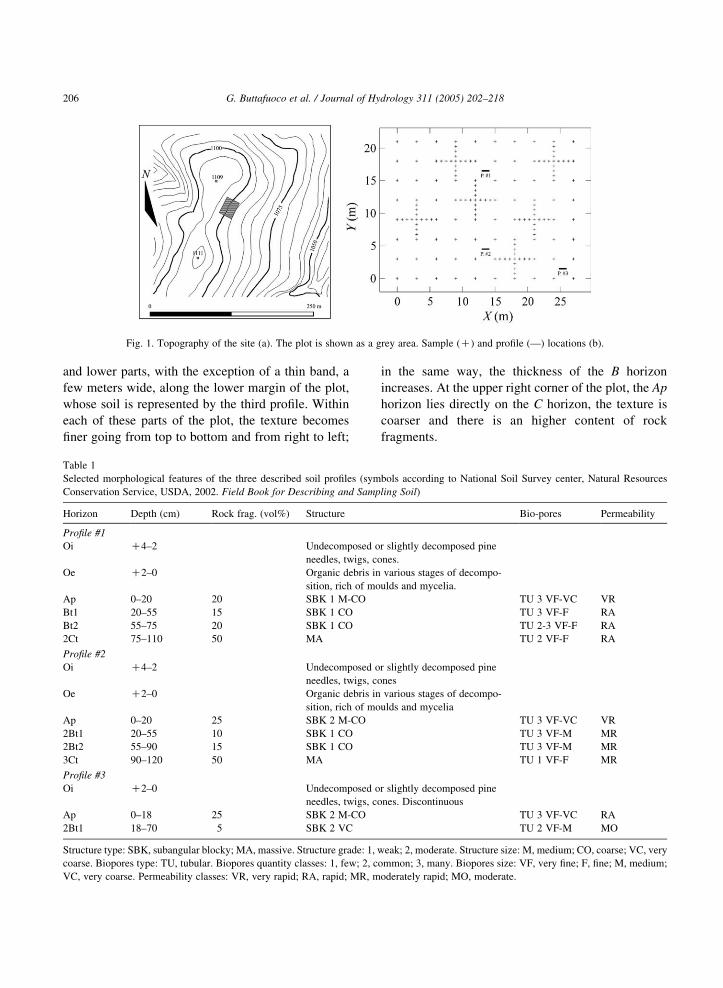
Fig. 1. Topography of the site (a). The plot is shown as a grey area. Sample (C) and profile (—) locations (b).


and lower parts, with the exception of a thin band, a

few meters wide, along the lower margin of the plot,

whose soil is represented by the third profile. Within

each of these parts of the plot, the texture becomes

finer going from top to bottom and from right to left;

Table 1

Selected morphological features of the three described soil profiles (sym

Conservation Service, USDA, 2002. Field Book for Describing and Samp

Horizon Depth (cm) Rock frag. (vol%) Structure

Profile #1

Oi C4–2 Undecomposed o

needles, twigs, co

Oe C2–0 Organic debris in

sition, rich of mo

Ap 0–20 20 SBK 1 M-CO

Bt1 20–55 15 SBK 1 CO

Bt2 55–75 20 SBK 1 CO

2Ct 75–110 50 MA

Profile #2


needles, twigs, co

Oe C2–0 Organic debris in

sition, rich of mo

Ap 0–20 25 SBK 2 M-CO

2Bt1 20–55 10 SBK 1 CO

2Bt2 55–90 15 SBK 1 CO

3Ct 90–120 50 MA

Profile #3


needles, twigs, co

Ap 0–18 25 SBK 2 M-CO

2Bt1 18–70 5 SBK 2 VC

Structure type: SBK, subangular blocky; MA, massive. Structure grade: 1, w

coarse. Biopores type: TU, tubular. Biopores quantity classes: 1, few; 2, c

VC, very coarse. Permeability classes: VR, very rapid; RA, rapid; MR, m

in the same way, the thickness of the B horizon

increases. At the upper right corner of the plot, the Ap

horizon lies directly on the C horizon, the texture is

coarser and there is an higher content of rock

fragments.

bols according to National Soil Survey center, Natural Resources

ling Soil)

Bio-pores Permeability

r slightly decomposed pine

nes.

various stages of decompo-

ulds and mycelia.

TU 3 VF-VC VR

TU 3 VF-F RA

TU 2-3 VF-F RA

TU 2 VF-F RA


nes

various stages of decompo-

ulds and mycelia

TU 3 VF-VC VR

TU 3 VF-M MR

TU 3 VF-M MR

TU 1 VF-F MR


nes. Discontinuous

TU 3 VF-VC RA

TU 2 VF-M MO

eak; 2, moderate. Structure size: M, medium; CO, coarse; VC, very

ommon; 3, many. Biopores size: VF, very fine; F, fine; M, medium;

oderately rapid; MO, moderate.

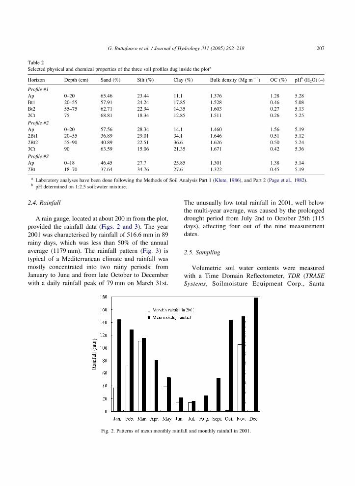
Table 2

Selected physical and chemical properties of the three soil profiles dug inside the plota

Horizon Depth (cm) Sand (%) Silt (%) Clay (%) Bulk density (Mg mK3) OC (%) pHb (H2O) (–)

Profile #1

Ap 0–20 65.46 23.44 11.1 1.376 1.28 5.28

Bt1 20–55 57.91 24.24 17.85 1.528 0.46 5.08

Bt2 55–75 62.71 22.94 14.35 1.603 0.27 5.13

2Ct 75 68.81 18.34 12.85 1.511 0.26 5.25

Profile #2

Ap 0–20 57.56 28.34 14.1 1.460 1.56 5.19

2Bt1 20–55 36.89 29.01 34.1 1.646 0.51 5.12

2Bt2 55–90 40.89 22.51 36.6 1.626 0.50 5.24

3Ct 90 63.59 15.06 21.35 1.671 0.42 5.36

Profile #3

Ap 0–18 46.45 27.7 25.85 1.301 1.38 5.14

2Bt 18–70 37.64 34.76 27.6 1.322 0.45 5.19

a Laboratory analyses have been done following the Methods of Soil Analysis Part 1 (Klute, 1986), and Part 2 (Page et al., 1982).b pH determined on 1:2.5 soil:water mixture.


2.4. Rainfall

A rain gauge, located at about 200 m from the plot,

provided the rainfall data (Figs. 2 and 3). The year

2001 was characterised by rainfall of 516.6 mm in 89

rainy days, which was less than 50% of the annual

average (1179 mm). The rainfall pattern (Fig. 3) is

typical of a Mediterranean climate and rainfall was

mostly concentrated into two rainy periods: from

January to June and from late October to December

with a daily rainfall peak of 79 mm on March 31st.

Fig. 2. Patterns of mean monthly rainf

The unusually low total rainfall in 2001, well below

the multi-year average, was caused by the prolonged

drought period from July 2nd to October 25th (115

days), affecting four out of the nine measurement

dates.

2.5. Sampling

Volumetric soil water contents were measured

with a Time Domain Reflectometer, TDR (TRASE

Systems, Soilmoisture Equipment Corp., Santa

all and monthly rainfall in 2001.

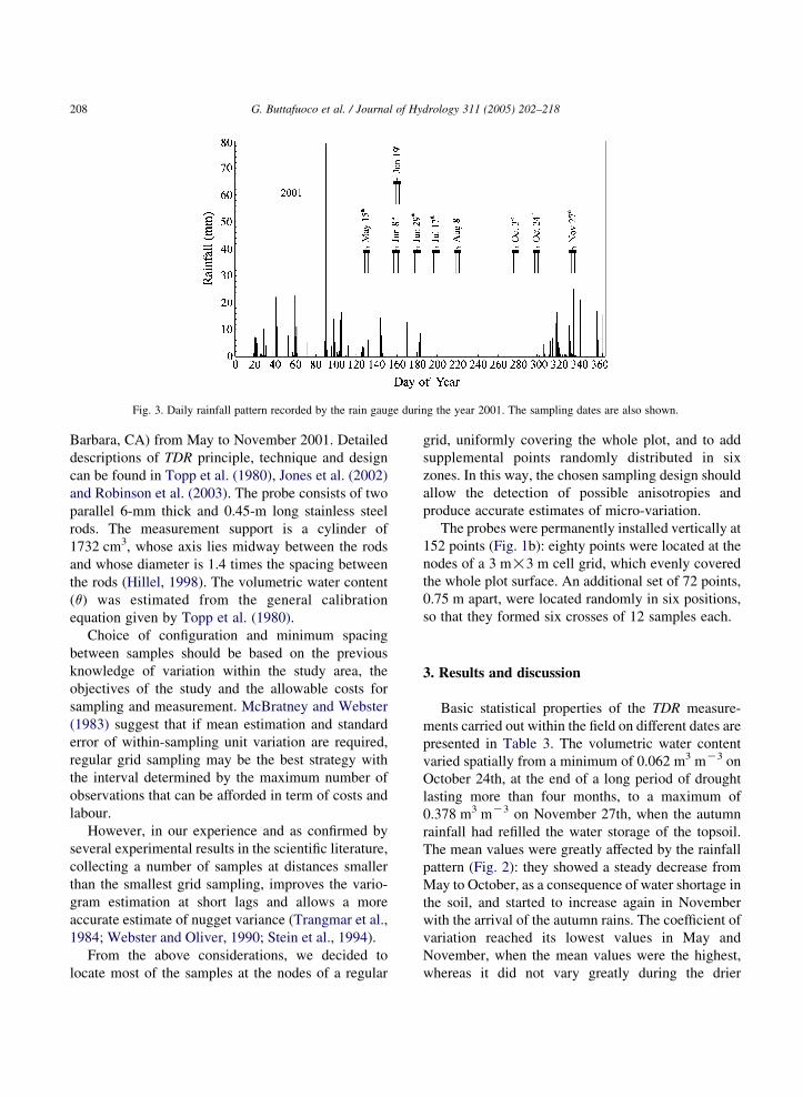
Fig. 3. Daily rainfall pattern recorded by the rain gauge during the year 2001. The sampling dates are also shown.


Barbara, CA) from May to November 2001. Detailed

descriptions of TDR principle, technique and design

can be found in Topp et al. (1980), Jones et al. (2002)

and Robinson et al. (2003). The probe consists of two

parallel 6-mm thick and 0.45-m long stainless steel

rods. The measurement support is a cylinder of

1732 cm3, whose axis lies midway between the rods

and whose diameter is 1.4 times the spacing between

the rods (Hillel, 1998). The volumetric water content

(q) was estimated from the general calibration

equation given by Topp et al. (1980).

Choice of configuration and minimum spacing

between samples should be based on the previous

knowledge of variation within the study area, the

objectives of the study and the allowable costs for

sampling and measurement. McBratney and Webster

(1983) suggest that if mean estimation and standard

error of within-sampling unit variation are required,

regular grid sampling may be the best strategy with

the interval determined by the maximum number of

observations that can be afforded in term of costs and

labour.

However, in our experience and as confirmed by

several experimental results in the scientific literature,

collecting a number of samples at distances smaller

than the smallest grid sampling, improves the vario-

gram estimation at short lags and allows a more

accurate estimate of nugget variance (Trangmar et al.,

1984; Webster and Oliver, 1990; Stein et al., 1994).

From the above considerations, we decided to

locate most of the samples at the nodes of a regular

grid, uniformly covering the whole plot, and to add

supplemental points randomly distributed in six

zones. In this way, the chosen sampling design should

allow the detection of possible anisotropies and

produce accurate estimates of micro-variation.

The probes were permanently installed vertically at

152 points (Fig. 1b): eighty points were located at the

nodes of a 3 m!3 m cell grid, which evenly covered

the whole plot surface. An additional set of 72 points,

0.75 m apart, were located randomly in six positions,

so that they formed six crosses of 12 samples each.

3. Results and discussion

Basic statistical properties of the TDR measure-

ments carried out within the field on different dates are

presented in Table 3. The volumetric water content

varied spatially from a minimum of 0.062 m3 mK3 on

October 24th, at the end of a long period of drought

lasting more than four months, to a maximum of

0.378 m3 mK3 on November 27th, when the autumn

rainfall had refilled the water storage of the topsoil.

The mean values were greatly affected by the rainfall

pattern (Fig. 2): they showed a steady decrease from

May to October, as a consequence of water shortage in

the soil, and started to increase again in November

with the arrival of the autumn rains. The coefficient of

variation reached its lowest values in May and

November, when the mean values were the highest,

whereas it did not vary greatly during the drier

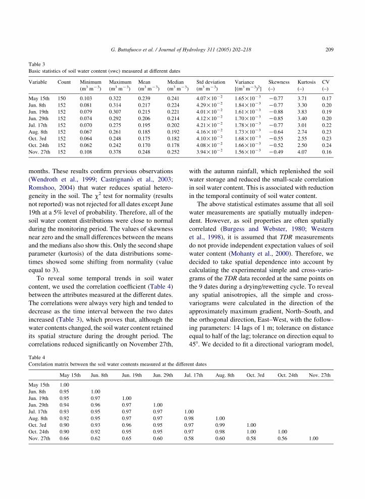
Table 3

Basic statistics of soil water content (swc) measured at different dates

Variable Count Minimum

(m3 mK3)

Maximum

(m3 mK3)

Mean

(m3 mK3)

Median

(m3 mK3)

Std deviation

(m3 mK3)

Variance

[(m3 mK3)2]

Skewness

(–)

Kurtosis

(–)

CV

(–)

May 15th 150 0.103 0.322 0.239 0.241 4.07!10K2 1.65!10K3 K0.77 3.71 0.17

Jun. 8th 152 0.081 0.314 0.217 0.224 4.29!10K2 1.84!10K3 K0.77 3.30 0.20

Jun. 19th 152 0.079 0.307 0.215 0.221 4.01!10K2 1.61!10K3 K0.88 3.83 0.19

Jun. 29th 152 0.074 0.292 0.206 0.214 4.12!10K2 1.70!10K3 K0.85 3.40 0.20

Jul. 17th 152 0.070 0.275 0.195 0.202 4.21!10K2 1.78!10K3 K0.77 3.01 0.22

Aug. 8th 152 0.067 0.261 0.185 0.192 4.16!10K2 1.73!10K3 K0.64 2.74 0.23

Oct. 3rd 152 0.064 0.248 0.175 0.182 4.10!10K2 1.68!10K3 K0.55 2.55 0.23

Oct. 24th 152 0.062 0.242 0.170 0.178 4.08!10K2 1.66!10K3 K0.52 2.50 0.24

Nov. 27th 152 0.108 0.378 0.248 0.252 3.94!10K2 1.56!10K3 K0.49 4.07 0.16


months. These results confirm previous observations

(Wendroth et al., 1999; Castrignano et al., 2003;

Romshoo, 2004) that water reduces spatial hetero-

geneity in the soil. The c2 test for normality (results

not reported) was not rejected for all dates except June

19th at a 5% level of probability. Therefore, all of the

soil water content distributions were close to normal

during the monitoring period. The values of skewness

near zero and the small differences between the means

and the medians also show this. Only the second shape

parameter (kurtosis) of the data distributions some-

times showed some shifting from normality (value

equal to 3).

To reveal some temporal trends in soil water

content, we used the correlation coefficient (Table 4)

between the attributes measured at the different dates.

The correlations were always very high and tended to

decrease as the time interval between the two dates

increased (Table 3), which proves that, although the

water contents changed, the soil water content retained

its spatial structure during the drought period. The

correlations reduced significantly on November 27th,

Table 4

Correlation matrix between the soil water contents measured at the differ

May 15th Jun. 8th Jun. 19th Jun. 29th Ju

May 15th 1.00

Jun. 8th 0.95 1.00

Jun. 19th 0.95 0.97 1.00

Jun. 29th 0.94 0.96 0.97 1.00

Jul. 17th 0.93 0.95 0.97 0.97 1.

Aug. 8th 0.92 0.95 0.97 0.97 0.

Oct. 3rd 0.90 0.93 0.96 0.95 0.

Oct. 24th 0.90 0.92 0.95 0.95 0.

Nov. 27th 0.66 0.62 0.65 0.60 0.

with the autumn rainfall, which replenished the soil

water storage and reduced the small-scale correlation

in soil water content. This is associated with reduction

in the temporal continuity of soil water content.

The above statistical estimates assume that all soil

water measurements are spatially mutually indepen-

dent. However, as soil properties are often spatially

correlated (Burgess and Webster, 1980; Western

et al., 1998), it is assumed that TDR measurements

do not provide independent expectation values of soil

water content (Mohanty et al., 2000). Therefore, we

decided to take spatial dependence into account by

calculating the experimental simple and cross-vario-

grams of the TDR data recorded at the same points on

the 9 dates during a drying/rewetting cycle. To reveal

any spatial anisotropies, all the simple and cross-

variograms were calculated in the direction of the

approximately maximum gradient, North–South, and

the orthogonal direction, East–West, with the follow-

ing parameters: 14 lags of 1 m; tolerance on distance

equal to half of the lag; tolerance on direction equal to

458. We decided to fit a directional variogram model,

ent dates

l. 17th Aug. 8th Oct. 3rd Oct. 24th Nov. 27th

00

98 1.00

97 0.99 1.00

97 0.98 1.00 1.00

58 0.60 0.58 0.56 1.00


because a zonal anisotropy was clearly observed in the

main two directions of the plane.

Fig. 4a and b display the directional simple and

cross-variograms (thin solid lines) in the directions E–

W and N–S, respectively. A linear model of

Fig. 4. Directional simple and cross-variogram models (thick solid lines)

variograms are plotted as thin solid lines. The dotted lines are the hulls of perfe

coregionalization (described afterwards) was then

fitted to all these variograms in a semi-automatic

way (thick solid lines); only the final tuning of the

corresponding sills was performed automatically. The

number, type, range and anisotropy of the basic spatial

of E–W variograms (a) and N–S variograms (b). The experimental

ct correlation and the dash-dotted lines are the experimental variances.

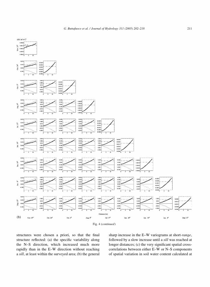
Fig. 4 (continued)


structures were chosen a priori, so that the final

structure reflected: (a) the specific variability along

the N–S direction, which increased much more

rapidly than in the E–W direction without reaching

a sill, at least within the surveyed area; (b) the general

sharp increase in the E–W variograms at short-range,

followed by a slow increase until a sill was reached at

longer distances; (c) the very significant spatial cross-

correlations between either E–W or N–S components

of spatial variation in soil water content calculated at


the different dates; however, the E–W variances were

generally lower than the corresponding N–S

variances.

Four basic structures were used: (1) nugget effect;

(2) isotropic spherical model with a range of 3.42 m;

(3) zonal anisotropic spherical model in the E–W

direction with a range of 10 m and (4) zonal

anisotropic K-Bessel model, with a scale of 27 m

and a gradient parameter equal to 1, in the N–S

direction. K-Bessel model is the function:

gðhÞ Z C 1 Kha

� �a

2aK1GðaÞKKa

h

a

� �� ; aO0

where C is the sill; a the range; a is a gradient

parameter; G($) is the usual gamma function while

KKa($) is the modified Bessel function of second kind

of order Ka. The model is upper bounded for any aO0 (Geovariances and Ecole Des Mines De Paris, 2003;

Chiles and Delfiner, 1999).

We introduced an isotropic structure into the

variogram model, because the model resulting from

the fitting procedure of the two main anisotropy

directions independently is not satisfactory along

intermediate directions (Deraisme, 2002). The multi-

variate model is presented in Table 5, where the

coregionalization matrix is reported for each of the

four basic structures, together with the corresponding

eigenvalues.1 It is clear from inspection of Table 5

that most of spatial variability is concentrated along

the N–S direction (Table 5d), with the highest values

of spatial variance recorded during the driest months

from July to October (diagonal elements). In contrast,

the November monitoring loads the least on the total

variance at the longer spatial scale (27 m). Another

important feature of the fitted LCM is the well-

differentiated behaviour of the wettest sampling in

November from the remainder of the measurements.

This sampling loads on the nugget effect variance

much more than the others and also significantly,

together with the sampling of May, on the isotropic

component at short range (3.42 m).

1 To fit the linear model of coregionalization, it needs to

decompose each coregionalization matrix into an orthogonal matrix

by using the diagonal matrix of eigenvalues. A brief determination

of eigenvalues is given in Davis (1986, pp. 107–148) and Webster

and Oliver (1990, pp. 291–298).

The investigation of the temporal change in spatial

correlation of volumetric water content during the

drying/rewetting period is thus focused on the

possible effects of rainfall. The moderate rainfall in

June did not modify the spatial correlation signifi-

cantly, whereas the several rainfall events in Novem-

ber, the only ones that caused temporal replenishment

of soil water capacity, decreased the structured

component of spatial variation and increased the

random component.

As regards the partitioning of spatial variance into

the different components during the whole period of

monitoring, it is clear from Table 6 that most of the

variation was anisotropic along the approximate

direction of the steepest gradient. This might induce

one to think that the volumetric water content could

not be assumed to be stationary and that it may have

been better to follow some alternative approach of

non-stationary geostatistics, such as kriging in

Intrinsic Random Function (IRF-k) case or kriging

with external drift. However, we preferred to assume

stationarity and fit an upper bounded model (K-Bessel

model) at the scale of field size (27 m) for the N–S

structure of variance. In such a way, we were also able

to perform a multivariate analysis in order to

investigate the temporal continuity of volumetric

water content during the monitoring period. With

respect to this issue, we can state, from the proportion

of variance explained by the first eigenvector

(Table 6), that the multivariate correlation among

the data corresponding to the different dates was

always very high, though the individual temporal

samplings weighed differently on the spatial variance

at the different spatial scales, as can be derived from

the values of the diagonal elements (sills of direct

variograms) in the regionalization matrices. As an

example, the sampling of November affected the

random and short-range (3.42 m) components of

variance at the most, but its impact was minimal for

the components at longer-range (10 and 27 m). That

confirms the essentially erratic nature of soil water

content variation in November.

The overall goodness of fitting was tested by cross-

validation; using two statistics in particular, mean

error and variance of standardised error. The results

(Table 7) show that the estimation was unbiased on all

dates, but the experimental variance was generally

underpredicted (variance of standardised error greater

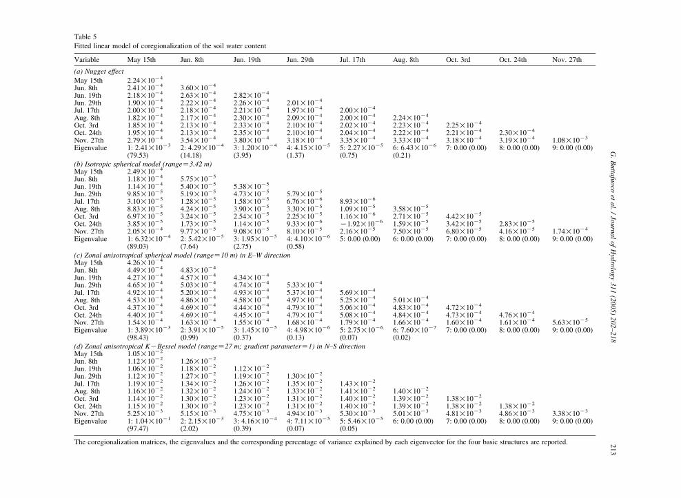
Table 5

Fitted linear model of coregionalization of the soil water content

Variable May 15th Jun. 8th Jun. 19th Jun. 29th Jul. 17th Aug. 8th Oct. 3rd Oct. 24th Nov. 27th

(a) Nugget effect

May 15th 2.24!10K4

Jun. 8th 2.41!10K4 3.60!10K4

Jun. 19th 2.18!10K4 2.63!10K4 2.82!10K4

Jun. 29th 1.90!10K4 2.22!10K4 2.26!10K4 2.01!10K4

Jul. 17th 2.00!10K4 2.18!10K4 2.21!10K4 1.97!10K4 2.00!10K4

Aug. 8th 1.82!10K4 2.17!10K4 2.30!10K4 2.09!10K4 2.00!10K4 2.24!10K4

Oct. 3rd 1.85!10K4 2.13!10K4 2.33!10K4 2.10!10K4 2.02!10K4 2.23!10K4 2.25!10K4

Oct. 24th 1.95!10K4 2.13!10K4 2.35!10K4 2.10!10K4 2.04!10K4 2.22!10K4 2.21!10K4 2.30!10K4

Nov. 27th 2.79!10K4 3.54!10K4 3.80!10K4 3.18!10K4 3.35!10K4 3.33!10K4 3.18!10K4 3.19!10K4 1.08!10K3

Eigenvalue 1: 2.41!10K3

(79.53)2: 4.29!10K4

(14.18)3: 1.20!10K4

(3.95)4: 4.15!10K5

(1.37)5: 2.27!10K5

(0.75)6: 6.43!10K6

(0.21)7: 0.00 (0.00) 8: 0.00 (0.00) 9: 0.00 (0.00)

(b) Isotropic spherical model (rangeZ3.42 m)May 15th 2.49!10K4

Jun. 8th 1.18!10K4 5.75!10K5

Jun. 19th 1.14!10K4 5.40!10K5 5.38!10K5

Jun. 29th 9.85!10K5 5.19!10K5 4.73!10K5 5.79!10K5

Jul. 17th 3.10!10K5 1.28!10K5 1.58!10K5 6.76!10K6 8.93!10K6

Aug. 8th 8.83!10K5 4.24!10K5 3.90!10K5 3.30!10K5 1.09!10K5 3.58!10K5

Oct. 3rd 6.97!10K5 3.24!10K5 2.54!10K5 2.25!10K5 1.16!10K6 2.71!10K5 4.42!10K5

Oct. 24th 3.85!10K5 1.73!10K5 1.14!10K5 9.33!10K6 K1.92!10K6 1.59!10K5 3.42!10K5 2.83!10K5

Nov. 27th 2.05!10K4 9.77!10K5 9.08!10K5 8.10!10K5 2.16!10K5 7.50!10K5 6.80!10K5 4.16!10K5 1.74!10K4


(89.03)2: 5.42!10K5

(7.64)3: 1.95!10K5

(2.75)4: 4.10!10K6

(0.58)5: 0.00 (0.00) 6: 0.00 (0.00) 7: 0.00 (0.00) 8: 0.00 (0.00) 9: 0.00 (0.00)

(c) Zonal anisotropical spherical model (rangeZ10 m) in E–W directionMay 15th 4.26!10K4

Jun. 8th 4.49!10K4 4.83!10K4

Jun. 19th 4.27!10K4 4.57!10K4 4.34!10K4

Jun. 29th 4.65!10K4 5.03!10K4 4.74!10K4 5.33!10K4

Jul. 17th 4.92!10K4 5.20!10K4 4.93!10K4 5.37!10K4 5.69!10K4

Aug. 8th 4.53!10K4 4.86!10K4 4.58!10K4 4.97!10K4 5.25!10K4 5.01!10K4

Oct. 3rd 4.37!10K4 4.69!10K4 4.44!10K4 4.79!10K4 5.06!10K4 4.83!10K4 4.72!10K4

Oct. 24th 4.40!10K4 4.69!10K4 4.45!10K4 4.79!10K4 5.08!10K4 4.84!10K4 4.73!10K4 4.76!10K4

Nov. 27th 1.54!10K4 1.63!10K4 1.55!10K4 1.68!10K4 1.79!10K4 1.66!10K4 1.60!10K4 1.61!10K4 5.63!10K5


(98.43)2: 3.91!10K5

(0.99)3: 1.45!10K5

(0.37)4: 4.98!10K6

(0.13)5: 2.75!10K6

(0.07)6: 7.60!10K7

(0.02)7: 0.00 (0.00) 8: 0.00 (0.00) 9: 0.00 (0.00)

(d) Zonal anisotropical KKBessel model (rangeZ27 m; gradient parameterZ1) in N–S directionMay 15th 1.05!10K2

Jun. 8th 1.12!10K2 1.26!10K2

Jun. 19th 1.06!10K2 1.18!10K2 1.12!10K2

Jun. 29th 1.12!10K2 1.27!10K2 1.19!10K2 1.30!10K2

Jul. 17th 1.19!10K2 1.34!10K2 1.26!10K2 1.35!10K2 1.43!10K2

Aug. 8th 1.16!10K2 1.32!10K2 1.24!10K2 1.33!10K2 1.41!10K2 1.40!10K2

Oct. 3rd 1.14!10K2 1.30!10K2 1.23!10K2 1.31!10K2 1.40!10K2 1.39!10K2 1.38!10K2

Oct. 24th 1.15!10K2 1.30!10K2 1.23!10K2 1.31!10K2 1.40!10K2 1.39!10K2 1.38!10K2 1.38!10K2

Nov. 27th 5.25!10K3 5.15!10K3 4.75!10K3 4.94!10K3 5.30!10K3 5.01!10K3 4.81!10K3 4.86!10K3 3.38!10K3


(97.47)2: 2.15!10K3

(2.02)3: 4.16!10K4

(0.39)4: 7.11!10K5

(0.07)5: 5.46!10K5

(0.05)6: 0.00 (0.00) 7: 0.00 (0.00) 8: 0.00 (0.00) 9: 0.00 (0.00)

The coregionalization matrices, the eigenvalues and the corresponding percentage of variance explained by each eigenvector for the four basic structures are reported.

G.

Bu

ttafu

oco

eta

l./

Jou

rna

lo

fH

ydro

log

y3

11

(20

05

)2

02

–2

18

21

3

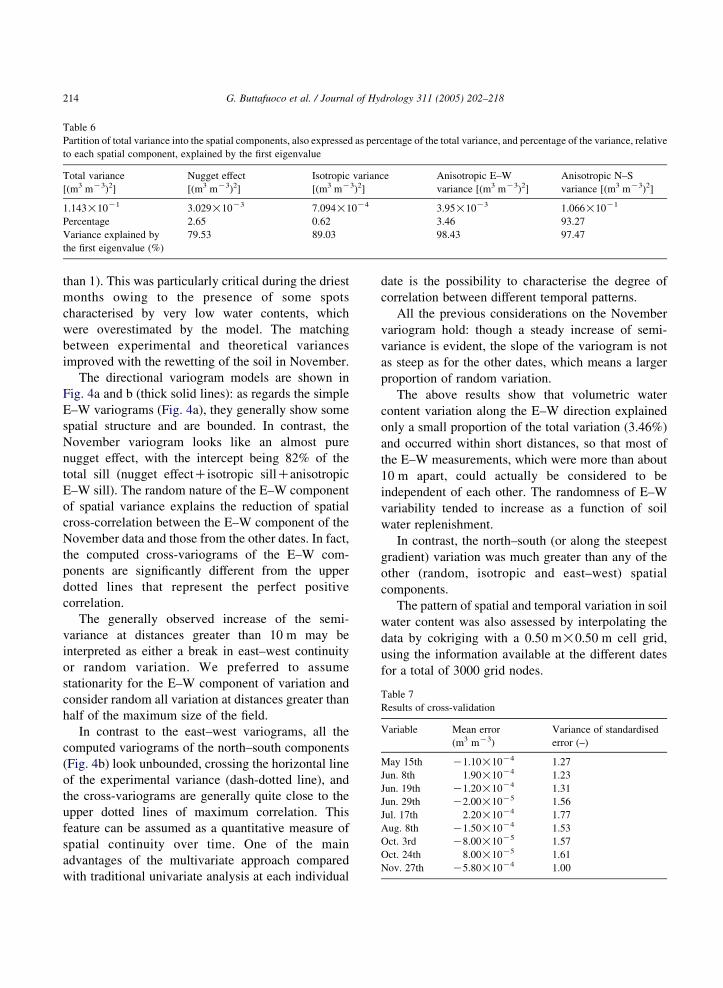
Table 6

Partition of total variance into the spatial components, also expressed as percentage of the total variance, and percentage of the variance, relative

to each spatial component, explained by the first eigenvalue

Total variance

[(m3 mK3)2]

Nugget effect

[(m3 mK3)2]

Isotropic variance

[(m3 mK3)2]

Anisotropic E–W

variance [(m3 mK3)2]

Anisotropic N–S

variance [(m3 mK3)2]

1.143!10K1 3.029!10K3 7.094!10K4 3.95!10K3 1.066!10K1

Percentage 2.65 0.62 3.46 93.27

Variance explained by

the first eigenvalue (%)

79.53 89.03 98.43 97.47

Table 7

Results of cross-validation

Variable Mean error

(m3 mK3)

Variance of standardised

error (–)

May 15th K1.10!10K4 1.27

Jun. 8th 1.90!10K4 1.23

Jun. 19th K1.20!10K4 1.31

Jun. 29th K2.00!10K5 1.56

Jul. 17th 2.20!10K4 1.77

Aug. 8th K1.50!10K4 1.53

Oct. 3rd K8.00!10K5 1.57

Oct. 24th 8.00!10K5 1.61

Nov. 27th K5.80!10K4 1.00


than 1). This was particularly critical during the driest

months owing to the presence of some spots

characterised by very low water contents, which

were overestimated by the model. The matching

between experimental and theoretical variances

improved with the rewetting of the soil in November.

The directional variogram models are shown in

Fig. 4a and b (thick solid lines): as regards the simple

E–W variograms (Fig. 4a), they generally show some

spatial structure and are bounded. In contrast, the

November variogram looks like an almost pure

nugget effect, with the intercept being 82% of the

total sill (nugget effectCisotropic sillCanisotropic

E–W sill). The random nature of the E–W component

of spatial variance explains the reduction of spatial

cross-correlation between the E–W component of the

November data and those from the other dates. In fact,

the computed cross-variograms of the E–W com-

ponents are significantly different from the upper

dotted lines that represent the perfect positive

correlation.

The generally observed increase of the semi-

variance at distances greater than 10 m may be

interpreted as either a break in east–west continuity

or random variation. We preferred to assume

stationarity for the E–W component of variation and

consider random all variation at distances greater than

half of the maximum size of the field.

In contrast to the east–west variograms, all the

computed variograms of the north–south components

(Fig. 4b) look unbounded, crossing the horizontal line

of the experimental variance (dash-dotted line), and

the cross-variograms are generally quite close to the

upper dotted lines of maximum correlation. This

feature can be assumed as a quantitative measure of

spatial continuity over time. One of the main

advantages of the multivariate approach compared

with traditional univariate analysis at each individual

date is the possibility to characterise the degree of

correlation between different temporal patterns.

All the previous considerations on the November

variogram hold: though a steady increase of semi-

variance is evident, the slope of the variogram is not

as steep as for the other dates, which means a larger

proportion of random variation.

The above results show that volumetric water

content variation along the E–W direction explained

only a small proportion of the total variation (3.46%)

and occurred within short distances, so that most of

the E–W measurements, which were more than about

10 m apart, could actually be considered to be

independent of each other. The randomness of E–W

variability tended to increase as a function of soil

water replenishment.

In contrast, the north–south (or along the steepest

gradient) variation was much greater than any of the

other (random, isotropic and east–west) spatial

components.

The pattern of spatial and temporal variation in soil

water content was also assessed by interpolating the

data by cokriging with a 0.50 m!0.50 m cell grid,

using the information available at the different dates

for a total of 3000 grid nodes.

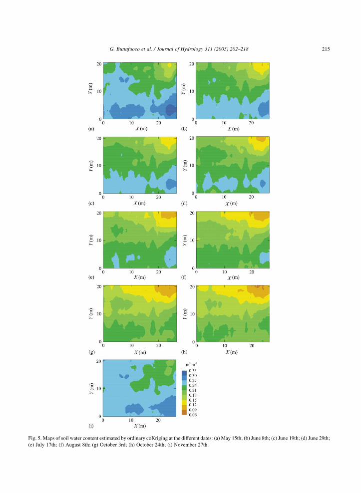
Fig. 5. Maps of soil water content estimated by ordinary coKriging at the different dates: (a) May 15th; (b) June 8th; (c) June 19th; (d) June 29th;

(e) July 17th; (f) August 8th; (g) October 3rd; (h) October 24th; (i) November 27th.



The soil water content maps (Fig. 5) show the

dynamics of the topsoil water content depletion and

replenishment during the period from May to

November 2001. The upper right hand corner of the

field was consistently drier and expanded the parched

area both E–W and N–S, as the drying period

progressed. What results from a visual inspection of

the maps is a clear stratification of soil water content

both E–W and N–S, so that the soil became moister

and moister moving from top to bottom and from right

to left.

Another interesting feature of the above maps is

the persistence of a limited zone on the bottom right

hand side of the field, characterised by higher water

contents compared with the surrounding values,

which caused a break in the steady increase in water

content towards the bottom of the N–S direction.

Going beyond this wetter area, water content began to

decrease again reaching the values observed at greater

elevations.

The spatial patterns of soil water content changed

dramatically after the November rainfall refilled the

dry soil. The distribution looked more random and

was characterised by higher values on the left and at

the bottom of the field. While the clear-cut horizontal

and vertical stratifications had vanished, the zones

with low values (upper right hand corner) and high

values (lower right hand corner) remained, which

implies that some of the soil spatial structures were

conservative, independently of the actual water

contents.

The spatial and temporal variations in soil water

content inside the study plot and during the dryin-

g/rewetting period can be explained by two main

factors that help to modify the distribution of soil

water content: topography and texture. In fact, in the

above description of the site, there is a very high

variability in texture and thickness of the B horizon, so

that the right-hand side is characterised by coarser

particles and thinner B horizons than the left. In the

same way, the slope favours the erosion of the upper

parts and the transport of the finest particles towards

the lower zones, which are, therefore, characterised by

higher water storage capacity. Moreover, the narrow

band of soil along the lower right hand margin of the

plot (described by the third soil profile) is character-

ised by higher clay contents along the Ap horizon,

which may explain its wetter features compared with

the neighbouring areas.

The joint variation of texture and slope affects the

water content in the soil so that the upper right hand

side, where the B horizon is completely absent and the

Ap horizon lies directly on the C horizon, dries more

quickly.

In semi-variogram analysis, small changes in

parameters (sill, range and nugget variance) must

not be over-interpreted because they derive from

several subjective decisions and are also affected by

estimation and measurement errors. Nevertheless, in

this study the conclusions are drawn from distinct

changes in spatial structure, which indicate how

spatial correlation of water content evolves over

time according to the drying and wetting history of the

soil.

In the study site physical and terrain properties

may explain a large proportion of the variability in

water content; however, under vegetation cover the

control of soil water content patterns may also be

partly affected by the plants. As mature forest stands

are big water consumers, root water extraction is

expected to influence spatial variability as much as

physical and terrain properties do. Preferential root

growth into moister soil regions and subsequent

exhaustion of these zones (Taiz and Zeiger, 1998;

Joslin et al., 2001) may offer another cause of

variation during the prolonged drought, so the

resulting water pattern would be an effect of the

interaction between plants and terrain.

The erratic pattern of soil water content after the

repeated rain events in November, which probably

saturated the soil, may also be explained by the fairly

high hydraulic conductivity of the soil that will allow

water to be distributed randomly over longer dis-

tances. Finally, on a long-term perspective, other

factors must be considered as contributing to the

different rewetting patterns, such as the thickness of

the litter layer, soil macro fauna and soil structure,

which can modify infiltration and surface runoff.

4. Conclusions

Spatial continuity of the water content in a forested

soil was studied during a drying/rewetting period. It

was found that the spatial correlation depends on


the drying and rewetting history. Major sources of

variation are textural and topographic properties,

whereas a minor proportion of variation might be

explained by the influence of plants.

The main advantage of the proposed multivariate

approach compared with traditional univariate kriging

is to define the temporal continuity of spatial patterns

quantitatively.

Since the spatial correlation function changes over

time, it derives that a single measurement of soil water

content may be inappropriate for making general

conclusions about spatial dependence. It, therefore,

follows that repeating the measurements over several

drying/rewetting cycles is necessary to assess if the

spatial patterns are conservative over time or may be

significantly modified by infiltration and run-off

processes. Since the different characteristics of spatial

patterns may change over time, they can strongly

influence flow paths (Western et al., 2001). Therefore,

assessing the degree of water content continuity in

both space and time becomes particularly important

when we are interested in processes such as erosion,

salinization and contaminant plume migration.

Acknowledgements

The authors thank the reviewers of this paper for

providing constructive comments which have con-

tributed to improve the published version.

We are grateful to Anthony Green for his help in

polishing the English of this paper.

References

Armstrong, M., Chetboun, G., Hubert, P., 1993. Kriging the rainfall

in Lesotho. In: Soares, A. (Ed.), Geostatistics Troia ’92, vol. 2.

Kluwer Academic Publishers, Dordrecht, pp. 661–672.

Burgess, T.M., Webster, R., 1980. Optimal interpolation and

isarithmic mapping of soil properties. I. The semi-variogram

and punctual kriging. Journal of Soil Science 31, 315–331.

Buttafuoco, G., Castrignano, A., Ricca, N., 2003. Interpolazione del

contenuto d’acqua del suolo in campi non stazionari con le

funzioni aleatorie intrinseche di ordine k. In: De Angelis, P.,

Macuz, A., Bucci, G., Scarascia Mugnozza, G. (Eds.), Atti

del III Congresso della Societa Italiana di Selvicoltura ed

Ecologia Forestale—S.I.S.E.F.: Alberi e foreste per il nuovo

millennio. 15–18 ottobre 2001, Viterbo, Italy, pp. 431–437 (in

Italian).

Cassa per il Mezzogiorno, 1969–1970. Carta Geologica

della Calabria. Scala 1:25.000. Foglio 230, III NO, Monte

Paleparto. Poligrafica e Cartevalori, Ercolano, Napoli, Italy

(in Italian).

Castrignano, A., Lopez, G., 1990. Estimating soil water content

using cokriging. Acta Horticulturae, II 278, 463–470.

Castrignano, A., Maiorana, M., Fornaro, F., Lopez, N., 2002. 3D

Spatial variability of soil strength and its change over time in a

durum wheat field in Southern-Italy. Soil & Tillage Research 65

(1), 95–108.

Castrignano, A., Maiorana, M., Fornaro, F., 2003. Using regiona-

lised variables to assess field-scale spatiotemporal variability of

soil impedance for different tillage management. Biosystem

Engineering 85 (3), 381–392.

Chatfield, C., 1984. The Analysis of Time Series, third ed. Chapman

& Hall, London.

Chiles, J.P., Delfiner, P., 1999. Geostatistics: Modelling Spatial

Uncertainty. Wiley, New York.

Davis, J., 1986. Statistics and Data Analysis in Geology. Wiley,

New York.

De Cesare, L., Myers, D.E., Posa, D., 1997. Spatio-temporal

modeling of SO2 in Milan district. In: Baaffi, E., Schofield, N.

(Eds.), Geostatistics Wollong ’96, vol. 2. Kluwer Academic

Publishers, Dordrecht, pp. 1031–1042.

Deraisme, J., 2002. Zonal anisotropy: how to model the variogram?.

Geovariances Newsletter 14.

Dimase, A.C., Iovino, F., 1996. I suoli dei bacini idrografici del

Trionto, Nica e torrenti limitrofi (Calabria). Accademia Italiana

di Scienze Forestali, Firenze, Italy (in Italian).

Famiglietti, J.S., Rudnicki, J.W., Rodell, M., 1998. Variability in

surface moisture content along a hillslope transect: Rattlesnake

Hill, Texas. Journal of Hydrology 210 (1–4), 259–281.

Geovariances & Ecole Des Mines De Paris, 2003. ISATIS, Software

Manual, Release 4.02. Geovariances, Avon Cedex, France.

Goovaerts, P., 1997. Geostatistics for Natural Resources Evalu-

ation. Oxford University Press, Oxford.

Goovaerts, P., Sonnet, P., 1993. Study of spatial and temporal

variations of hydrogeochemical variables using factorial kriging

analysis. In: Soares, A. (Ed.), Geostatistics Troia ’92, vol. 2.

Kluwer Academic Publishers, Dordrecht, pp. 745–756.

Grayson, R.B., Western, A.W., 1998. Towards areal estimation of

soil water content from point measurements: time and space

stability of mean response. Journal of Hydrology 207, 68–82.

Heuvelink, G.B., Musters, P., Pebesma, E.J., 1997. Spatio-temporal

kriging of soil water content. In: Baaffi, E., Schofield, N. (Eds.),

Geostatistics Wollongong ’96, vol. 2. Kluwer Academic

Publishers, Dordrecht, pp. 1020–1030.

Hillel, D., 1998. Environmental Soil Physics. Academic Press, San

Diego.

Hohn, M.E., Liebhold, A.M., Gribko, L.S., 1993. Geostatistical

model for forecasting spatial dynamics of defoliation caused by

the gypsy moth (Lepidoptera: Lymantriidae). Environmental

Entomology 22 (5), 1066–1075.

Hupet, F., Vanclooster, M., 2002. Intraseasonal dynamics of soil

moisture variability within a small agricultural maize cropped

field. Journal of Hydrology 261 (1–4), 86–101.


Jones, S.B., Wraith, J.M., Or, D., 2002. Time domain reflectometry

(TDR) measurement principles and applications. HP today

scientific briefing. Hydrological Processes 16, 141–153.

Joslin, J.D., Wolfe, M.H., Hanson, P.J., 2001. Factors controlling

the timing of root elongation intensity in a mature oak stand.

Plant and Soil 228, 201–212.

Journel, A.G., Huijbregts, C.J., 1978. Mining Geostatistics.

Academic Press, San Diego, CA.

Kachanoski, R.G., De Jong, E., 1988. Scale dependence and the

temporal persistence of spatial patterns of soil water storage.

Water Resource Research 24, 85–91.

Klute, A., 1986. Methods of Soil Analysis. Part.1. Agronomy No. 9,

Madison, WI, USA 1986.

Kyriakidis, C., Journel, A., 1999. Geostatistical space–time models:

a review. Mathematical Geology 31 (6), 651–684.

Matheron, G., 1971. The Theory of Regionalised Variables and its

Applications, vol. 5. Les Cahiers du Centre de Morphologie

Mathematique de Fontainebleau.

McBratney, A.B., Webster, R., 1983. How many observations are

needed for regional estimation of soil properties. Soil Science

135, 177–183.

Mohanty, B.P., Shouse, P.J., van Genuchten, M.T., 1998. Spatio-

temporal dynamics of water and heat in a field soil. Soil &

Tillage Research 47 (1/2), 133–143.

Mohanty, B.P., Famiglietti, J.S., Skaggs, T.H., 1997. Evolution of

soil moisture spatial structure in a mixed vegetation pixel during

the Southern great plains 1997 (SGP97) hydrology experiment.

Water Resources Research 36 (12), 3675–3686.

National Soil Survey Center, Natural Resources Conservation

Service, USDA, 2002. Field Book for Describing and Sampling

Soils, Lincoln, NE 2002.

Page, A.L., Miller, R.H., Keeney, D.R., 1982. Methods of

Soil Analysis. Part 2. Agronomy No. 9, Madison, WI, USA

1982.

Robinson, D.A., Jones, S.B., Wraith, J.M., Or, D., Friedman, S.P.,

2003. A review of advances in dielectric and electrical

conductivity measurement in soils using time domain reflecto-

metry. Vadose Zone Journal 2, 444–475.

Rodriguez-Iturbe, I., Mejia, J.M., 1974. The design of rainfall

networks in time and space. Water Resources Research 10 (4),

713–728.

Romshoo, S.A., 2004. Geostatistical analysis of soil moisture

measurements and remotely sensed data at different spatial

scales. Environmental Geology 45, 339–349.

Rouhani, S., Wackernagel, H., 1990. Multivariate geostatistical

approach to space–time data analysis. Water Resources

Research 26 (4), 585–591.

Snepvangers, J.J.J.C., Heuvelink, G.B.M., Huisman, J.A., 2003.

Soil water content interpolation using spatio-temporal kriging

with external drift. Geoderma 112 (3/4), 253–271.

Soil Survey Staff, 1999. Soil Taxonomy. Agriculture Handbook

436. USDA–NRCS, Washington, DC, p. 869.

Stein, A., Wopereis, M.C.S., Bouma, J., 1994. Soil sampling

strategies and geostatistical techniques. In: Wopereis, M. et al.

(Ed.), Soil physical properties: measurement and use in rice-

based cropping systems. Int. Rice Research Inst., Los Ba os,

Philippines, pp. 73–85.

Taiz, L., Zeiger, E., 1998. Plant Physiology. Sinauer, Sunderland.

Topp, G.C., Davis, J.L., Annan, A.P., 1980. Electromagnetic

determination of soil water content: measurements in coaxial

transmission lines. Water Resources Research 16 (3), 574–582.

Trangmar, B.B., Yost, R.S., Uehara, G., 1984. Application of

geostatistics to spatial studies of soil properties. Advances in

Agronomy 38, 45–94.

Ventrella, D., Castrignano, A., Maiorana, M., Losavio, N.,

Vonella, A., Fornaro, F., 2002. Irrigation with brackish water:

effects on soil strength of a fine textured soil. In: Pagliai, M.,

Jones, R. (Eds.), Sustainable Land Management—Environmen-

tal Protection. A Soil Physical Approach. Advances in

Geoecology, vol. 35, pp. 279–290.

Wackernagel, H., 2003. Multivariate Geostatistics: An Introduction

with Applications. Springer, Berlin.

Webster, R., Oliver, M.A., 1990. Statistical Methods in Soil and

Land Resource Survey. Oxford University Press, Oxford.

Wendroth, O., Pohl, W., Koszinski, S., Rogasik, H., Ritsema, C.J.,

Nielsen, D.R., 1999. Spatio-temporal patterns and covariance

structures of soil water status in two Northeast-German field

sites. Journal of Hydrology 215 (1–4), 38–58.

Western, A.W., Bloschl, G., Grayson, R.B., 1998. Geostatistical

characterisation of soil moisture patterns in the Tarrawarra

Catchment. Journal of Hydrology 205, 20–37.

Western, A.W., Bloschl, G., Grayson, R.B., 2001. Towards

capturing hydrologically significant connectivity in spatial

patterns. Water Resources Research 37 (1), 83–97.

Western, A.W., Zhou, S.L., Grayson, R.B., McMahon, T.A.,

Bloschl, G., Wilson, D.J., 2004. Spatial correlation of soil moisture

in small catchments and its relationship to dominant spatial

hydrological processes. Journal of Hydrology 286, 113–134.

Wilson, D.J., Western, A.W., Grayson, R.B., Berg, A.A.,

Lear, M.S., Rodell, M., Famiglietti, J.S., Woods, R.,

McMahon, T.A., 2003. Spatial distribution of soil moisture at

6 cm and 30 cm depth, Mahurangi River Catchment, New

Zealand. Journal of Hydrology 276 (1–4), 254–274.

studying the spatial structure evolution of soil water content using multivariate geostatistics

Documents