study on sustainability of groundwater resources in rajshahi
TRANSCRIPT
STUDY ON SUSTAINABILITY OF GROUNDWATER
RESOURCES IN RAJSHAHI DISTRICT OF
BANGLADESH
M. Sc. Engineering Thesis
by
Md. Ashraful Islam
DEPARTMENT OF WATER RESOURCES ENGINEERING
BANGLADESH UNIVERSITY OF ENGINEERING AND TECHNOLOGY
DHAKA-1000
OCTOBER, 2020
i
STUDY ON SUSTAINABILITY OF GROUNDWATER RESOURCES
IN RAJSHAHI DISTRICT OF BANGLADESH
A Thesis Submitted
by
Md. Ashraful Islam
(Roll No. 1015162042P)
In partial Fulfillment of the requirements for the Degree of
MASTER OF SCIENCE IN WATER RESOURCES ENGINEERING
DEPARTMENT OF WATER RESOURCES ENGINEERING
BANGLADESH UNIVERSITY OF ENGINEERING AND TECHNOLOGY
DHAKA-1000
OCTOBER, 2020

iv
ACKNOWLEDGEMENT
At first, the author acknowledges the blessing of almighty Allah for enabling him to
complete the study successfully.
The author is obliged to his thesis supervisor Dr. Umme Kulsum Navera, Professor,
Department of Water Resources Engineering, BUET, for her continuous guidance, and
caring and affectionate encouragement at every stage of this work.
The author also expresses profound gratitude to his thesis committee member Dr. Anika
Yunus, Professor and Head, DWRE, BUET, Dr. Md. Sabbir Mostafa Khan, Professor,
DWRE, BUET and external member of thesis committee Dr. A.F.H. Afzal Hossain,
Ex-DED (P&D), IWM for their nice and careful guidance and constructive suggestions
during final thesis defense which have been immensely contributed to the improvement
of this thesis.
The author wishes his sincere gratitude to Mr. Mohammad Salah Uddin, Senior
Specialist, Irrigation Management Division, IWM, Ms. Anin Dita Dey, Assistant
Engineer, BWDB, Mr. S.M. Sahabuddin, Junior Specialist, IWM and Ms. Swarna
Chowdhury, Junior Engineer, IWM for their continuous support and consultations
regarding this research work.
The author is grateful to IWM authority for giving supports by providing valuable
guidance, necessary data, and permission to use software during this research work.
The author is thankful to all the officials of WRE department and the authority for
allowing him to use the WRE library.
The author finally expresses his profound thanks to his parents for supporting and
inspiring to conduct the M.Sc. in Water Resources Engineering at BUET.
v
ABSTRACT
Bangladesh is predominantly an agricultural country where agriculture sector plays a
significant role in accelerating the economic growth of the country. It is therefore
important to have a sustainable, environment-friendly and profitable agricultural system
in order to ensure long-term food security. Agriculture in Bangladesh is largely
dependent on groundwater resources. But this scarce groundwater resources have been
decreasing alarmingly in Rajshahi district which is one of the most drought prone
districts and driest place of Bangladesh. This situation has threatened the sustainability
of agriculture in this area at present as well as in the near future. Over abstraction of
groundwater, lack of surface water bodies, low rainfall, high elevation, thick clay layer
are the major hindrances in the study area to sustain groundwater resources. As a result,
groundwater level in this district is successively falling in each year. In this study it has
been strived to sustain this valuable groundwater sources for the sustainable agriculture
of this region.
An integrated Surface Water- Groundwater base model from 2012 to 2016 has been
developed, calibrated and validated. It has helped to understand current situation of the
study area. In order to sustain groundwater resources up to year 2030, it is needed to
foresee future condition of groundwater resources from 2017 to 2030. For this reason,
there are ten (10) scenarios have been chosen to understand future groundwater
condition in the study area by considering different driving forces such as Rainfall,
Evaporation, Groundwater Level, Surface Water Level, and Water Demand. These
scenarios have been analyzed to identify the most extreme future scenario that is
needed to be countered by applying suitable interventions.
Model output has been analyzed on eight Upazilas (Upazila wise) to understand the
condition of groundwater precisely instead of taking study area as a whole. In spite of
having different climatic conditions, soil type, cropping pattern, water demand and
water availability most of these Upazilas have shown similar result. Scenario number
10 (S-10) has been found the most extreme scenario in most of the Upazilas (six out of
eight). There are three interventions have been considered out of which intervention 1
(I-1) has shown significant result towards sustainable groundwater resources. In
intervention 1, crop diversification technique has been applied by substituting high
water consumed Boro rice by low water consumed Wheat and the outcome is
vi
remarkable. Groundwater resources of 96.55% of the study area has improved and
additional 3620 million cubic meter saturated zone is increased in the study area in the
most extreme event (April, 2028) of most extreme scenario. Moreover, all analysis has
been done to counter the driest event (April, 2028) of worst scenario so that reaming
events could be could be countered. Based on analysis it can be said that this
intervention will be a suitable solution to sustain groundwater resources for future in
this area. The results that have been found from this study will be very much helpful to
carry out further studies in future.

vii
TABLE OF CONTENTS
ACKNOWLEDGEMENT iv
ABSTRACT v
TABLE OF CONTENTS vii
LIST OF FIGURES x
LIST OF TABLES xiii
LIST OF ABBREVIATIONS xiv
CHAPTER 1 INTRODUCTION
1.1 Background of the Study 1
1.2 Scope of the Study 2
1.3 Objectives of the Study 3
1.4 Organization of the Thesis 3
CHAPTER 2 LITERATURE REVIEW
2.1 General 5
2.2 Previous Studies and Researches on Groundwater 5
2.2.1 Groundwater Related Studies around the World 5
2.2.2 Groundwater Related Studies in Bangladesh 6
2.2.3 Groundwater Sustainability Related Studies in the North-West
Region of Bangladesh 13
2.3 Groundwater and Sustainable Development Goals (SDGs) 15
2.4 Summary 16
CHAPTER 3 THEORY AND METHODOLOGY
3.1 General 17
3.2 Occurrence of Groundwater 18
3.3 Development of Groundwater Theories 18
3.4 Basic Theory of Modelling 20
3.5 Basic Theory and Equation of MIKE SHE 20
3.6 Basic Theory and Equation of MIKE 11 HD 24
3.7 Basic Theory of MIKE 11 NAM 26
viii
3.8 Methodology of the Study 27
3.8.1 Selection of the Study Area 28
3.8.2 Data Collection and Data Processing 28
3.8.3 Base Model Set Up 29
3.8.4 Calibration and Validation of Base Models 30
3.8.5 Selection of Design Year 30
3.8.6 Development of Scenarios 31
3.8.7 Prediction of Data Up to Year 2030 31
3.8.8 Result and Analysis 39
3.9 Summary 39
CHAPTER 4 STUDY AREA AND MODEL SET UP
4.1 General 40
4.2 Study Area 40
4.3 Hydrometeorology of the Study Area 44
4.4 Groundwater Model Set Up 55
4.5 Surface Water Model Set Up 62
4.6 Surface Water-Groundwater Interaction 64
4.7 Summary 65
CHAPTER 5 RESULTS AND DISCUSSIONS
5.1 General 66
5.2 Calibration and Validation of the SW and GW Model 66
5.2.1 Calibration and Validation of SW Model 66
5.2.2 Calibration and Validation of GW Model 67
5.3 Selection of Design Year for Scenario Development 69
5.4 Formulation of Future Scenarios 71
5.5 Determination of Most Extreme Scenario from Different Scenarios 74
5.6 Application of Interventions to Counter Extreme Scenario 89
5.6.1 Result from Non-Structural Intervention 90
5.6.2 Results from Structural Intervention 94
5.6.3 Result from Combined Intervention 95
ix
5.7 Depth of Phreatic Surface under Different Scenarios & Interventions 95
5.8 Results from Analysis 100
5.9 Meeting Goals of SDGs2030 106
5.10 Summary 108
CHAPTER 6 CONCLUSIONS AND RECOMMENDATIONS
6.1 General 109
6.2 Conclusions of the Study 109
6.3 Recommendations for Further Study 110
REFERENCES 111
APPENDIX-A
APPENDIX-B
APPENDIX-C
APPENDIX-D
APPENDIX-E
x
LIST OF FIGURES
Figure No. Title Page No.
Figure 3.1: Hydrologic processes simulation by MIKE SHE hydrologic model 21
Figure 3.2: Schematic representation of the conceptual components in MIKE
SHE hydrologic model 22
Figure 3.3: Flowchart of the Overall Methodology for the Study 27
Figure 3.4: Double mass curve for rainfall data under rainfall station, R170 in
Durgapur Upazila for the year 2012 to 2016 29
Figure 3.5: Irrigation demands considered in the models (2017-2030) 34
Figure 4.1: Map of Study Area 40
Figure 4.2: Diagram of average monthly rainfall (Source: climate-data.org) 42
Figure 4.3: Diagram of average maximum and minimum temperature (Source:
weather-atlas.com) 42
Figure 4.4: Topography of the study area 43
Figure 4.5: Generalized Tectonic Map of Bangladesh and Adjacent Area 44
Figure 4.6: Rainfall stations within/around the Rajshahi district 46
Figure 4.7: Selected Groundwater observation wells (Boundary Wells) under
BWDB within/around the Rajshahi district 48
Figure 4.8: Selected Groundwater observation wells (Calibration Wells) under
BWDB within/around the Rajshahi district 49
Figure 4.9: Yearly average trend of GWL at GT8125009 for the year 1974 to
2016 50
Figure 4.10: River water level hydrograph for river Ganges at Sardah station 51
Figure 4.11: Soil profile map of the study area (SRDI) 52
Figure 4.12: Plan of hydrostat graphic sections 53
Figure 4.13: Lithological cross section S2-N2 along South to North 53
Figure 4.14: Model area for MIKE SHE hydrologic model 56
Figure 4.15: Model domain and grid 57
Figure 4.16: Thiessen polygons for individual rainfall station in the study area 59
Figure 4.17: Initial groundwater level for the model on 1st January, 2012 61
xi
Figure 4.18: River network within model area in Mike 11(HD) 62
Figure 4.19: River network of the study area and surrounding 63
Figure 4.20: Boundary stations of SW model 64
Figure 5.1: Calibration and Validation of Surface water model for surface water
level at Chapai-Nawabganj Station on Mohanda River 67
Figure 5.2: Calibration and Validation of Surface water model for surface water
level at Singra Station on Atrai River 67
Figure 5.3: Calibration and Validation of model for groundwater level at Charghat
Upazila 68
Figure 5.4: Calibration and Validation of model for groundwater level at Puthia
Upazila 68
Figure 5.5: Calibration and Validation of model for groundwater level at Durgapur
Upazila 69
Figure 5.6 : Extreme vs less vulnerable scenarios at Paba Upazila 76
Figure 5.7: Extreme vs less vulnerable scenarios at Charghat Upazila 77
Figure 5.8: Extreme vs less vulnerable scenarios at Mohanpur Upazila 79
Figure 5.9: Extreme vs less vulnerable scenarios at Durgapur Upazila 80
Figure 5.10: Extreme vs less vulnerable scenarios at Tanore Upazila 82
Figure 5.11: Sample graph showing all Scenario s at GT 8172040 station of Paba
Upazila. 88
Figure 5.12: Extent of Boro rice field within Rajshahi district 91
Figure 5.13: GWL of Extreme scenario vs. Intervention 01 at Godagari Upazila
(Well ID: GT8134016) 92
Figure 5.14: GWL of Extreme scenario vs. Intervention 01 at Paba Upazila (Well
ID: GT8172040) 92
Figure 5.15: GWL of Extreme scenario vs. Intervention 01 at Baghmara Upazila
(Well ID: GT8112002) 93
Figure 5.16 : GWL of Extreme scenario vs. Intervention 01 at Mohanpur Upazila
(Well ID: GT8153030) 93
Figure 5.17: Location of proposed and existing structures within Rajshahi 94

xii
Figure 5.18: Depth of phreatic surface of extreme scenario (S-10) 95
Figure 5.19: Depth of phreatic surface of less vulnerable scenario (S-02) 96
Figure 5.20: Depth of phreatic surface of Intervention 01 at 27th April 2028. 97
Figure 5.21: Depth of phreatic surface of Intervention 02 at 27th April 2028. 98
Figure 5.22: Depth of phreatic surface of Intervention 03 at 27th April 2028. 99
Figure 5.23: Average Depth of phreatic surface 100
Figure 5.24: Comparison of depth of phreatic surface of Intervention 01 and
Scenario 10 101
Figure 5.25: Comparison of depth of phreatic surface of Intervention 02 and
Scenario 10 102
Figure 5.26: Localized improvement of groundwater resources 103
Figure 5.27: Comparison of depth of phreatic surface of Intervention 03 and
Scenario 10 103
Figure 5.28: Comparison of River-Aquifer Interaction between 2016 and 2030 105
Fig
xiii
LIST OF TABLES
Table No. Title Page No.
Table 3.1: Upazila-wise Projected Population up to 2030 35
Table 3.2: Upazila-wise Municipal Water Demand in m3/day up to 2030 37
Table 3.3: Upazila-wise Municipal Water Demand in mm/day up to 2030 38
Table 4.1: Average temperature and rainfall statistics of the study area 41
Table 4.2: Details of rainfall stations within/around the Rajshahi district 45
Table 4.3: Aquifer Properties in Rajshahi district 54
Table 4.4: Grid cells used for model setup 58
Table 4.5: Geographical limits of the study area 56
Table 5.1: Summary Table of Calibration and Validation 67
Table 5.2: Return Period for Different Distribution 70
Table 5.3: Selection of Design Year Based on Statistical Analysis 70
Table 5.4: Summary table of all scenarios 72
Table 5.5: Yearly Minimum GWL of Paba Upazila (Well ID: 8172040) 75
Table 5.6: Yearly Minimum GWL of Charghat Upazila (Well ID: 8125006) 76
Table 5.7: Yearly Minimum GWL of Mohanpur Upazila (Well ID: 8153030) 78
Table 5.8: Yearly Minimum GWL of Durgapur Upazila (Well ID: 8131015) 79
Table 5.9: Yearly Minimum GWL of Tanore Upazila (Well ID: 8194044) 81
Table 5.10: Yearly Minimum GWL of Puthia Upazila (Well ID: GT8182043) 82
Table 5.11: Yearly Minimum GWL of Godagari Upazila (Well ID: GT8134016) 84
Table 5.12: Yearly Minimum GWL of Bagmara Upazila (Well ID: GT8194044) 85
Table 5.13: Upazila wise extreme and less vulnerable scenarios 89
Table 5.14: Upazila-wise distribution of Boro rice field 91
Table 5.15: Zonal statistics of S-10, 02 and Intervention 01, 02 and 03 101
Table 5.16: Improved Area after application of intervention 01 101
Table 5.17: Improved Area after application of intervention 02 102
Table 5.18: Improved Area after application of intervention 03 104
xiv
Table 5.19: Improved Area after application of interventions 104
Table 5.20: River-Aquifer Interaction 105
Table 5.21: Positive Trend of GWL within Model Area 106
xiv
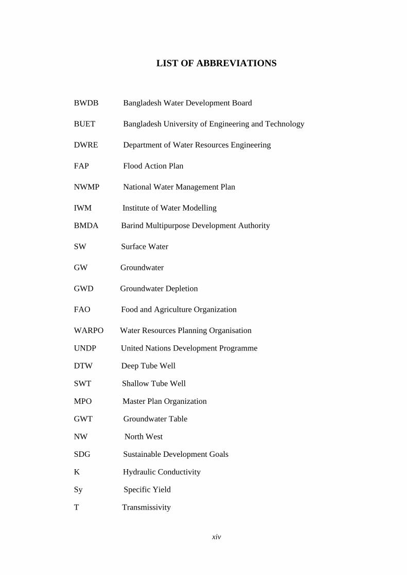
LIST OF ABBREVIATIONS
BWDB Bangladesh Water Development Board
BUET Bangladesh University of Engineering and Technology
DWRE Department of Water Resources Engineering
FAP Flood Action Plan
NWMP National Water Management Plan
IWM Institute of Water Modelling
BMDA Barind Multipurpose Development Authority
SW Surface Water
GW Groundwater
GWD Groundwater Depletion
FAO Food and Agriculture Organization
WARPO Water Resources Planning Organisation
UNDP United Nations Development Programme
DTW Deep Tube Well
SWT Shallow Tube Well
MPO Master Plan Organization
GWT Groundwater Table
NW North West
SDG Sustainable Development Goals
K Hydraulic Conductivity
Sy Specific Yield
T Transmissivity
1
CHAPTER 1
INTRODUCTION
1.1 Background of the Study
Groundwater in Bangladesh transpires at a very shallow depth where the recent river-borne
sediments form prolific aquifers in the floodplains. In the hilly areas, the Pliocene Tipam
sands serve as aquifers. In the higher terraces, the Barind and Madhupur tracts, the
Pleistocene DupiTila sands act as aquifers (Rahman et al., 2012). The groundwater level is
at or very close to the surface during the monsoon whereas it is at maximum depth during the
months of April and May. This trend is common over most of Bangladesh except Dhaka City
and the Barind Tract (Ahmed, 2014).
Barind Tract, the largest Pleistocene physiographic unit of the Bengal basin, covering an area
of about 7,770 sq km (Rahman et al., 2012 and Ahmed, 2014) can be divided into high,
medium and low based on their elevation (IWM, 2012). Elevation of the area varies from 9
m to 47 m PWD (Public Works Datum) (BMDA, 2006). Because of the elevation of high
Barind, Rajshahi is one of the most drought prone districts of Bangladesh (Chowdhury et al.,
2018). The impact of drought can be much higher and can cause greater loss than flood,
cyclone and storm surge (Alam et al., 2012; Paul, 1998; Shahid, 2008). Drought is related to
groundwater recharge.
Groundwater recharging in Bangladesh mainly occurs by monsoon rainfall and flooding. Due
to elevation of high Barind (topography varies from 20.0 m PWD to 47.0 m PWD) (IWM,
2012) it is located in flood free zone. So, main source of groundwater recharging in this area
is rainfall (Islam et al., 2014). With the exception of the relatively dry western region of
Rajshahi, where the annual rainfall is about 1600 mm, most parts of the country receive at
least 2000 mm of rainfall per year (Weatheronline, 2018). Moreover, thick sticky clay surface
of Barind Tract acts as aquitard which impedes groundwater recharging and increases surface
run-off (Rahman et al., 2012). As a result, groundwater level in this part is successively
falling by years with increasing withdrawal of water for irrigation (Rahman et al., 2012).Over
abstraction of groundwater, lack of surface water bodies, low rainfall, high elevation, thick
clay layer etc. are the major hindrances in the study area to sustain groundwater resources.
A recent study shows that groundwater level in some areas falls between 5-10 m in dry season
and most of the tube wells fail to lift sufficient water (Dey et al., 2010). The Groundwater
dependent irrigation system in the area has reached a critical phase as the GW level has
2
dropped below the depth of the shallow tube wells in many places (Adhikary et al., 2013).
Rice dominate the cropping pattern of Barind soil, which suffer from drought in dry season.
Only one crop (Aman paddy) in wet season was cultivated in Barind (IBRD, 1970). With the
rapid expansion of groundwater irrigation after 1980s, High Yielding Variety (HYV) paddies
are introduced in this area. Now Barind Tract produces three crops in one agricultural season
with the blessing of groundwater irrigation (Rahman et al., 2012).
Researchers and policymakers are advocating sustainable development as the best approach
to today’s and future water problems (Loucks, 2000; Cai et al., 2001). But sustainability of
groundwater resources is at risk in terms of quantity in the northwest region (Simonovic,
1997).
1.2 Scope of the Study
Rajshahi is the most water stressed district in Bangladesh. Groundwater level in this area is
successively falling by years due to over extraction of groundwater, climatological
unfavorable condition, geo-morphological condition and reduction of surface water flow of
major transboundary rivers etc. Increasing demand of ground water against decreasing trend
of groundwater resources has created an alarming situation for sustainable development of
this area. For sustainable development of any area, sustainable water resources are a
prerequisite.
There are many studies available in the context of groundwater sustainability in Bangladesh.
Most of these studies are based on statistical analysis and in a broad area basis specially for
whole Barind area. Assessment of state of water resources for 64 districts has been carried
out by WARPO (WARPO, 2016) for updating NWMP. In this study (WARPO, 2016),
statistical analysis has been carried out to assess state of the water resources based on
secondary data up to 2012.
Study of Upazila wise analysis of groundwater sustainability focusing the most water stressed
area of Bangladesh by using state of the art mathematical modeling technology is very
limited. There is a scope to take a study in Rajshahi district and develop possible future
scenarios considering climate change impacts, future water demands etc. to find a way
towards sustainability of this scarce groundwater resources with the help of historical climate,
hydrological data and advanced integrated SW-GW modeling tools. The scope of this study
3
is not limited to the finding of the extreme scenario up to 2030 in this area, there are scope to
explore possible ways to sustain groundwater resources in this study area.
1.3 Objectives of the Study
The objective of the study is to assess the sustainability of groundwater resources of the
underlying aquifer system of the Rajshahi district and also prediction of future scenarios
under different conditions from 2017 to 2030 using MIKE 11(HD)-MIKE SHE coupled
model. However, the specific aims of the study are as follows:
1. To assess the current situation of groundwater resources in Rajshahi district.
2. To develop an integrated surface water-groundwater (MIKE 11-MIKE SHE) model
of the study area.
3. To predict the future groundwater scenarios under different conditions to assess
sustainability of groundwater resources by applying suitable interventions.
Expected outcome of the research based on the above-mentioned objectives may be listed as
follows:
• Hydro-stratigraphic map of the study area.
• Calibrated and validated integrated surface water-groundwater model.
• Spatial and temporal distribution of existing groundwater level.
• Spatial and temporal distribution of future groundwater level for different scenarios
which will be considered in the study.
1.4 Organization of the Thesis
This research work has been carried out step by step through six chapters as given below.
Chapter 1 deals with the background, scope and objectives of the study.
Chapter 2 mainly focuses on the reviews of literature related to the objectives and outcomes
of this study. Findings of the previous research works related to this study have also been
summarized in this chapter.
Chapter 3 deals with the theoretical background of groundwater, development of
groundwater theories, basic theory and equations behind the model study and detail
methodology of this study.
4
Chapter 4 deals with the description of the study area including geographical location,
climate, topography, geomorphology and hydrogeological setting, river system, soil
condition and agricultural system and practices. Model set up for this study has been
discussed in this chapter.
Chapter 5 illustrates the data analysis, results and discussions related to the study. Calibration
and validation of surface water model and groundwater model, selection of design year for
future scenario development, development of future scenarios, finding extreme scenario,
development of interventions to counter extreme scenario, water balance analysis, assessment
of suitable intervention for sustainable groundwater resources have been discussed in this
chapter.
Chapter 6 discusses the major findings of the study. In this chapter the recommendations for
further study have also been discussed.
5
CHAPTER 2
LITERATURE REVIEW
2.1 General
Groundwater is the water in the saturated zone of earth materials under pressure greater
than atmospheric. Water enters to the groundwater through infiltration or percolation.
Again, seepage from surface water bodies also causes groundwater recharge. Discharge to
rivers or lakes causes depletion of groundwater storage in addition to pumping of
groundwater for irrigation. The withdrawal and replenishment of groundwater is slow,
complex phenomena and necessitates carefully investigation. Availability of groundwater
for irrigation has contributed to manifold increase in crop productivity in Bangladesh (Dey
et al. 2013). About 90 percent of irrigation water in Bangladesh is provided from
groundwater (Zahid et al. 2006). This chapter will discuss about some selected previous
studies around the world and in Bangladesh.
2.2 Previous Studies and Researches on Groundwater
A significant number of studies on groundwater resources, water demand, land use for crop
pattern, groundwater sustainability, extension of crop intensity and their effects on
groundwater level were carried out around the world and in Bangladesh. The available
study reports, project documents, published scientific articles have collected and reviewed
to get information on the study area and corresponding groundwater resources related to
this study. Some of the important studies are briefly described below.
2.2.1 Groundwater Related Studies around the World
Döll (2014) showed that groundwater depletion (GWD) compromises crop production in
major global agricultural areas and has negative ecological consequences. To derive GWD
at the grid cell, country, and global levels, they applied a new version of the global
hydrological model WaterGAP that simulates not only net groundwater abstractions and
groundwater recharge from soils but also groundwater recharge from surface water bodies
in dry regions. From their study the rate of global GWD has likely more than doubled since
the period 1960–2000 and estimated GWD of 113 km3/yr during 2000–2009.
Villholth (2018) identified governance and management are critical components of
sustainability. The term governance is evolving, especially with regard to surface water and
6
groundwater resources. No other components cannot bring expected result if there is no
good governance. There should be good coordination between organizations and
stakeholders regarding this sector.
FAO (2016) demonstrated that groundwater governance contains four key elements and
these are (i) effective institutions that integrate stakeholders; (ii) policies and capital that
support local, regional, and global resource goals; (iii) legal systems with the capacity to
create and implement laws effectively; and (iv) local knowledge, customary or cultural
context, and scientific understanding of groundwater systems.
Megdal (2018) summarized the results of efforts to bring attention to the importance of
understanding and improving groundwater governance and management. Discussion of
survey work in the United States and global case studies highlights the importance of
focusing attention on this invisible water resource before pollution or depletion of it causes
severe economic, environmental, and social dislocations. Better governance and
management of groundwater are required to move toward sustainable groundwater use.
Gleeson (2019) showed some important groundwater management tools in his study and
there are (i) Long-term, adaptive and conjunctive groundwater management plans, (ii)
Monitoring, metering, and reporting and (iii) Green to grey infrastructure.
Achiransu (2017) described storage of rainwater through rainwater harvesting and aquifer
recharge through watershed management are the main options for sustainable groundwater
management. Some of the other suggested option are unbundling of irrigation services
much on the lines of unbundling of electricity utilities, use of piped delivery from tertiary
and below tertiary level, better measurement at all levels, construction of farm level storage
ponds to increase flexibility and re-orientation of canal bureaucracy towards better service
delivery.
2.2.2 Groundwater Related Studies in Bangladesh
Abdullah (2019) analysed the trend and extent of the groundwater table in Bogura district
up to the year 2030 because of the expanding status and possible variability of the water
demand. MIKE SHE, an integrated hydrological model has been used to simulate the
fluctuating water table to assess the groundwater resources and future scenario analyses.
Normal rainfall for the period of years 1985 to 2011 has been found 1672 mm. The same
normal rainfall has been considered for the projection years 2012 to 2030. The temporal
7
rainfall fluctuations were taken directly from a different study. Projections of the relevant
hydrological components were anticipated in relation to the suitable projection models. The
simulated result from the year 2006 to 2030 shows the depletion rate of the study area
varies from 0.00 to 2.92 cm/year for mean depth of phreatic surface. In case of maximum
depth of phreatic surface, the depletion rate varies from 1.20 cm/year to 14.45 cm/year.
After a drought of rainfall events, a lower phreatic surface has been observed; this is
however regained in subsequent heavy rainfall events.
WARPO (2016) conducted a comprehensive assessment of state of water resources
throughout the whole Bangladesh (64 districts). This analysis was based on secondary data
and statistical spreadsheet-based calculation. Analysis period is 1965 to 2012. Upazila wise
rainfall, climate and evapotranspiration, flooding, droughts, water demand, water resources
and state of water resources were assessed in this study.
IWM (2006) carried out a study on Deep Tubewell Installation Project in Barind Area. The
main objective of this project was upazilla-wise groundwater resources assessment. Under
this study the exchange rate of groundwater and the rivers Punarbhaba, Mahananda and
Ganges were also investigated using mathematical modeling for the year 2001 (average
year condition). In this study it was found that for the reach of Godagari to Charghat, annual
groundwater loss per kilometer was about 0.33 MCM. The study recommended further
investigation on the interaction between the Ganges river and Barind aquifer.
IWM (2013) carried out a study on Deep Tubewell Installation Project Phase II, of Barind
Multi-Purpose Development Authority (BMDA) covers 65 Upazilas of Pabna, Sirajganj,
Bogra, Gaibandha, Rangpur, Kurigram, Nilphamari and Lalmonirhat districts having gross
area of 17, 455 km2 and cultivable area of 12, 765 km2. The objectives of this project was
to assess Upazilawise groundwater resources and recharge potential; surface water resource
assessment; additional number of required DTWs. To fulfill the above objectives an
extensive field data collection program was taken which includes test drilling, aquifer test,
topographic and cross section survey, water quality test land water level measurement.
Accordingly, hydrogeological investigation upto 150m depth was conducted at 8 locations
and 10 numbers of aquifer test were completed up to interim report. A model up to the
depth of 80m was developed and a number of options were simulated to see the impact of
irrigation expansion as well as impact due to climate change. It was found that within the
study area, groundwater table (GWT) was from 1 to 13m from ground surface in dry period.
8
In some areas of Bogra, Sirajganj & Pabna, groundwater level went below suction limit of
Hand Tubewell (HTW) & Deep Tara Set (DTS) and Shallow Tubewell (STW) became
inoperable in that period, but in monsoon it was recharged fully. Transmissivity and
Hydraulic conductivity of the study area was good and potential for groundwater
development. Upazilawise groundwater resources were estimated through water balance
analysis. In order to meet the future demand, it would be needed to install additional 14,
184 DTWs. It has been seen that due to climate change, the groundwater level may drop
about 0.5 to 1.0m in some study areas. It was also identified that there is no separate aquifer
in deeper strata up to 150m depth.
IWM (2012) carried out a groundwater resources study and DSS development for Barind
covering 25 Upazilas of Rajshahi, Chapai Nawabganj and Naogaon districts with an area
of 7500 km2. A comprehensive model study was carried out for groundwater resources
assessment for the study area. The study findings were limited up to 80m depth. For
sustainable use of groundwater, one of the recommendations of this study was to explore
the groundwater potential below 80m to bring more area under irrigation in resources
constraint and high Barind areas.
HYSAWA (2012) carried out a study covers 31 Upazilas of Rajshahi, Chapai Nawabganj,
Noagaon and Natore districts with an area of 9852 km2. The project area has limited scope
of surface water development and potential for groundwater development. Considering
total requirement, groundwater deficit found in 7 Upazilas, which are Dhamoirhat,
Patnitala, Niamatpur, Godagari, Tanore, Singra and Gurudaspur. Among these,
Dhamoirhat and Tanore are constraint both for potential and available resource; 5 Upazilas
are constraint for available resource which are Patnitala, Niamatpur, Godagari, Singra and
Gurudaspur Upazila. Available resource can be increased by allowing depletion of
groundwater table below 7m which is beyond suction limit of STW and HTW. In that case
STW and HTW would be needed to be replaced by DTW or tara pump for dry season and
it would not be a problem for environment because groundwater table regain to its original
position due to recharge from rainfall in monsoon. In that case only 2 Upazilas would be
considered as resource constraint area however for safe side the less water required crops
should be practiced for these resources’ constraint Upazilas.
9
Hossain and Shamsuddin (1976) carried out a study which dealt with the groundwater in
the Rajshahi district for the year 1968 to 1975. The purpose of this study was to find out
usable volume of groundwater and to study the irrigation potential of the groundwater.
According to this study, the Barind area was divided into five different zones (Zone 2A,
2B, 4, 8A, 8B) among which high prospect of groundwater potential for STW and DTW in
the zone 2 and only DTW in the zone 4 and remaining parts of Barind were not studied.
From their analysis the recommended shallow tube wells for zone 2A, 2B and 8A.
Sondipon (2017) carried out in the Mohananda River at Chapai Nawabganj District. The
main purpose of the study is to investigate the present scenario of groundwater level in the
study area and the impact of replacing groundwater irrigation with surface water irrigation
in 2020 and 2030. Three options such as Option-0 (base condition), Option-1 (without
Rubber Dam) and Option-2 (with Rubber Dam) have been formulated, simulated and
evaluated to attain the study objectives. Due to surface water irrigation, the groundwater
level increased adjacent to the Mohananda River especially in the surface water irrigation
area. The groundwater level decreasing rate is 96 mm/year for option-1 where the rate
reduces to 50 mm/year in option-2 in Surface Water Irrigation Zone. In addition, it has been
observed that, the influence area due to surface water irrigation for year 2020 is 234 sq.km
where it has been found 242 sq. km for year 2029.
Zahid (2015) described in his study that matching long term withdrawals of groundwater
to recharge is the principal objective of sustainable groundwater resource planning.
Maintaining the water balance of withdrawals and recharge is vital for managing human
impact on water and ecological resources. Regional modeling of the groundwater systems
has to be developed for effective water resource management to plan agricultural, rural and
urban water supplies and to forecast the groundwater situation in advance for dry seasons.
UNDP (1982) study identified potential groundwater development areas through
countrywide survey of groundwater. The identification of potential groundwater
development areas was based on (i) annual volume of recharge, (ii) capacity of the system
to act as a long-term storage reservoir, (iii) energy source for the pumping lift and (iv) water
quality. According to this report the current study area has limited thick sandy aquifer
especially in the high Barind area and transmissivity- value ranging from 500 to 1500
m2/day. Annual recharge varied from a minimum of 80 to a maximum of 190 mm. This
study was based on limited data for generalized appraisal of hydrogeological condition of

10
the country and therefore, was in need of a detailed study of available groundwater
resources for formulation of the project.
MacDonald (1983) study described the geology, infiltration rate, permeability range,
storage range, water level fluctuations and finally development potential of its study area.
It was based on existing data analysis and a water balance study. The study area consists
mainly of three aquifers namely Sibganj (1200 km2), High Barind Area (3634 km2) and
Little Jamuna (980 km2). Sibganj aquifer has been classified as semi-confined. The
infiltration rate is 1.7 mm/day in wetland and 12 mm/day in dry land. Permeability ranges
from 30 to 60 m/day with an average of 40 m/day. The specific yield of upper layer is 6%.
Drilling of DTW is not constrained except in deeply flooded areas. The high Barind aquifer
has been classified as semi confined and multi-layered. The infiltration rate is 1.5 mm/day
in wetland and 7.5 mm/day in dry land. Permeability ranges from 25 to 40 m/day with an
average of 30 m/day. Specific yield of the upper layer is approximately 4%. Drilling of
DTW is not promising because of the large depth to poor aquifer and fine materials, which
require special design. Recharge could also be a limiting factor and trial borings were
recommended. The Little Jamuna aquifer has been classified as unconfined to semi-
confined. Infiltration rate is 1.5 mm/day in wetland and 5 mm/day in dry land. Permeability
ranges from 50 to 80 m/day with an average of 65 m/day. Specific yield averages 5%. There
is a good potential for drilling of DTW in this area and the recharge is unlikely to hinder
development.
Asaduzzaman (1983) showed thana-wise recommended number of DTW for 45%
development level (as per Northwest Bangladesh Groundwater Modelling Report), well
fixtures, discharge and thanawise fluctuation of groundwater level (average), and rainfall,
bore log as well as construction procedure of DTW. His detailed study findings and
observations are helpful in this study and other studies in groundwater.
Karim (1984) stated that the potential recharge in the Barind area is in the range of 400 to
700 mm/year, hydraulic conductivity (K) is in the range of 25 to 50 m/day and the specific
yield (Sy) value is in the range of 0.05 to 0.12. Majority of the area is within the value of
K=40 m/day and Sy=0.10.
MPO (1986) studied 8 representative areas spreading all over Bangladesh. A country-wide
contour map of transmissivity was prepared using data based on aquifer tests and
development tests of tube wells. In the current study-area the transmissivity values have
11
been estimated in the range of 1000 to 2000 m2/day; for thin aquifers it may vary from
200-700 m2/day. A contour map of specific yield was also prepared using bore logs and
aquifer test data assuming that the specific yield increases linearly with the increase of
depth from ground surface for increase of sand in the aquifers. Specific yield values have
been assigned for each layer occurring within 25 m depth from ground surface and later to
estimate its average value. The average value of specific yield for the study area is in the
range of 2% to 5%. This value depends on the accuracy of identification of aquifer materials
in the bore-log. The groundwater recharge model was developed from the study of
catchment recharge in the eight representative areas. The catchments were taken as multi-
layer single cell models in which only the vertical components of flow were considered.
Outputs were the annual rates of potential recharge for each catchment area summarized
from simulated ten-day rainfall and soil infiltration using 25 years of climatic data. A
relation between rainfall and annual potential recharge was developed, indicating that the
higher the rainfall, the higher the annual potential recharge for an area. Potential and
available recharge for the study area was estimated to be in the range of respectively 200
to 500 mm, and 100 to 400 mm.
BWDB (1990) studied the groundwater for 17 Upazilas in Rajshahi, Noagaon and
Nowabganj districts. The report was prepared based on existing literature and primary data
of test-drillings, groundwater monitoring wells and aquifer tests. Geologic cross-sections
were prepared to show the thickness and areal extension of sub-surface formations in the
study area. Contour maps of groundwater depth and of average maximum fluctuation of
groundwater level were prepared. Contour maps of specific yield were also prepared using
data from aquifer tests. Field surveys were conducted to determine Upazila-wise irrigation
equipment and their uses. The Upazila-wise actual and available groundwater recharges
were assessed, which varied from 322 to 567 mm and from 243 to 411 mm, respectively.
The balance of available recharge following existing uses was determined assuming all
DTWs were of 2 cfs (0.057 m3/s) capacity and ran 13 hrs/day for 120 irrigation days, and
all STWs were of 0.40 cfs (0.011 m3/s) capacity of the same duration of running and period
of irrigation. It was assessed that there is a prospect of drilling additional 850 DTWs with
50% safety factor.
NWMP (2001) was established to monitor activities within all water related sector, to
provide information and to advice on best practice on water related issues in Bangladesh.
12
With the estimation and prediction of the water resources in all sectors, water demand in
dry period has been estimated and predicted for future 25 years. Study assessed, the main
determinant in overall demand for water resources in the future is the growth of irrigation
demand. As per study, water supply for urban and rural domestic & commercial use will
be more than twice as before and irrigation demand are expected to increase potentially by
at least a quarter (1/4) over the next 25 years.
BMDA (2012) carried out a model study with IWM (integrated both surface water and
groundwater) in the Barind area, which covers 25 Upazilas of Rajshahi, Nawabganj and
Noagaon districts with an area of 7500 km2. Integrated MIKE11-MIKE SHE modeling
system with grids size of 1000m×1000m squares has been applied in the study. Based on
the data available up to 2005 the study confirms that groundwater resources are inadequate
in 11 Upazilas to meet the present water demand for Boro crops while in 5 Upazilas the
present withdrawals of groundwater are more compare to potential recharges and available
groundwater resources.
Islam (2009) investigated Barind Aquifer – Ganges River interaction over 55 km reach of
the Ganges River from Godagari to Charghat, having an area of 916 km2. Study area
covered three Upazilas of Rajshahi District. It has been observed from the study that, the
gain of groundwater from river to aquifer occurs only for a short period from July to
September. On the contrary loss of groundwater from aquifer to river occurs for a longer
period from October to June. The magnitude and duration of groundwater loss from aquifer
to river is higher in upper part than in lower part of the study area. During the study period
the yearly average lateral groundwater outflow from aquifer to river was estimated as 0.29
Mm3 per kilometer varies from 0.20 Mm3 to 0.45 Mm3. The trend of lateral outflow from
groundwater (aquifer to river) has been increasing over the years.
Dey (2013) conducted a study on Sustainability of Groundwater Use for Irrigation in North-
West Bangladesh under National Food Policy Capacity Strengthening Programme
implemented by FAO in collaboration with FPMU/Ministry of Food and Disaster
Management with financial support of EU and USAID. Objective of the study was to
quantitatively assess the trends in water table depths and crop areas in the designated study
area for the past 30 years. Financial & economic profitability of different crops along with
likely changes over time due to decline of water tables. Recommend policies for sustainable
use of irrigation water in northwestern Bangladesh. The study area was five north-western
13
districts of Bangladesh as Rajshahi, Pabna, Bogra, Rangpur and Dinajpur. Sample survey
conducted through structured questionnaire, focus group discussion, consultation meeting
and workshops have been done for this study. Secondary data have been collected from
BWDB, BMDA, BADC and BBS. Study shows, within 10 major crops area, boro alone
increased more than 9 times during 1980/81 to 2009/10. Study suggested according to crop
pattern and benefit-cost ratio (BCR), wheat, potato, maize, mustard and these types of less
irrigation demand crops should be emphasized in future.
Ahmed (2008) exploited thickness of the aquifer ranges from less than 10 m in parts of
Bogra district to over 60 m in the northwest. Aquifer conditions are found to be good in
most parts of the Teesta, Brahmaputra-Jamuna and Ganges river floodplains and on the Old
Himalayan Piedmont plain. Potential aquifers are not found in high Barind area. Based on
pumping tests, the transmissibility of the main aquifer ranges from 300 to 4,000 sq. m/day.
Highest transmissibility’s are common adjacent to the area of Brahmaputra-Jamuna river
and lowest transmissibility’s are common in high Barind area. Highly transmissible aquifer
material indicates excellent opportunity for groundwater development. In most areas, the
lower two aquifers are probably hydraulically interconnected. The main aquifer, in most of
the area, is either semi-confined and leaky or consists of stratified, interconnected,
unconfined water bearing zones which are subject to delayed drainage. Recharge to the
aquifer is predominantly derived from deep percolation of rain and flood water. Lateral
contribution from rivers comprise only a small percentage (0.04%) of total potential
recharge. Hydrographs of observed groundwater tables show that the maximum and
minimum depth to groundwater table occurs at the end of April and end of October
respectively.
2.2.3 Groundwater Related Studies in the North-West Region of Bangladesh
Rahman (2017) demonstrated that unplanned irrigation for the dry season rice production
is the significant responsible factor for groundwater depletion. Moreover, climate-related
factors, like decreasing trend in rainfall, distribution of rainfall (SI and PCI), frequent
drought, are also related to the groundwater depletion. The study also demonstrates that
water resources management also related to the transboundary river relationship. To
achieve sustainability in groundwater resource at first, it is time to take decision about the
land use patterns as rice, which cultivates in about 81% cultivable area during the dry
season, is the highest water consuming crop in the area. Though it is the staple food in the
14
country, it is necessary to reduce this crop cultivation to protect rapid depletion of
groundwater resource. Moreover, water-saving irrigation techniques such alternate drying
and wetting, raised bed techniques need to promote for farming. Surface water irrigation
where and when it is available need to facilitate to minimize the stress on groundwater. The
present study also indicates that groundwater recharge in some Upazilas increases due to
create favorable recharge structures like re-excavation of rivers and Kharis(small channel).
However, the effort is not quite enough for protecting groundwater depletion. As annual
surplus water is higher than the net groundwater recharge, groundwater recharge favorable
structures for rainwater harvesting need to develop. An experimental study on MAR shows
the potentiality of the technique for ensuring drinking water supply especially in the rural
areas. An IWRMP considering the driving forces of groundwater depletion, potentiality of
surface water, and MAR and land use pattern of the area need to prepare and execute the
plan accordingly for achieving the sustainability in water resources management.
Ali (2011) revealed that the depth of water (WT) of almost all the wells is declining slowly.
In many cases, the depth will approximately double by the year 2040, and almost all will
double by 2060, if the present trend continues. If the decline of water-table is allowed to
continue in the long run, the result could be a serious threat to the ecology and to the
sustainability of food production, which is vital for nation's food security. Therefore,
necessary measures should be taken to sustain water resources and thereby agricultural
production. Demand-side management of water and the development of alternative surface
water sources seem to be viable strategies for the area. These strategies could be employed
to reduce pressure on groundwater and thus maintain the sustainability of the resource.
Mojid (2019) showed that most of the NW parts of the study area encounter face water
scarcity during dry months. In 15% of the monitoring wells, located in Bogura, Rajshahi,
Naogaon, Joypurhat, and Chapai Nowabgonj districts, GWTs remained below 6 m
throughout the year. These districts, comprising the Barind track, face severe water
scarcity, especially for domestic supply, due to failure of STWs and HTWs. Therefore, it
is inevitable that the currently practiced groundwater development and use policy in those
areas need to be revised to make groundwater use more sustainable. Strategies such as
artificial recharge to the aquifers and rain water harvesting along with water-saving
technologies and integrated water resources management need to be adopted. Special
attention needs to be given in areas where GWTs drop below the critical suction limit of
15
suction-mode pumps. Alternate technology for pumping groundwater needs to be made
available to provide household water.
Dey (2017) showed that depletion of groundwater table was most evident in Rajshahi,
followed by Dinajpur, Bogra, Pabna and Rangpur, but when other factors interlinked with
the groundwater resources (i.e. river water level, boro rice area, dry season rainfall, wetland
area) was considered, the scenario changed to some extent. Bangladesh has abundant rain
during the monsoon season, and technological solutions need to be explored to artificially
replenish aquifers with rainfall. Efforts should continue to negotiate an increased share of
water from the river system originating in the Himalayas during the dry season. Therefore,
the Government of Bangladesh and other countries associated with this water-sharing issue
and situated upstream should maintain mutually beneficial cooperation. Changes in
cropping patterns should be promoted by the Department of Agriculture Extension
according to his study.
2.3 Groundwater and the Sustainable Development Goals (SDGs)
The concept of sustainability or sustainable development is generally 'meeting the needs of
the present without compromising the ability of future generations to meet their own needs'
(World Commission on the Environment and Development, 1987), which is a foundation
of the widely – adopted UN Sustainable Development Goals. Groundwater is an important
resource for achievement of the UN Sustainable Development Agenda for 2030 yet it is
poorly recognized and weakly conceptualized in the SDGs (Guppy et al., 2018).
Groundwater is an important resource for achievement of the UN Sustainable Development
Goals SDGs. Groundwater could be important to ensuring access to water and sanitation
for all (Goal 6) as well as contributing to a number of other goals: poverty eradication (Goal
1), food security (Goal 2), and combating climate change (Goal 13). Yet even in the targets
of Goal 6, groundwater is only explicitly referenced once and a detailed analysis by Guppy
et al was necessary to highlight the potential relationship between groundwater and many
other targets. More than half of these relationships are reinforcing meaning that
achievement of the target would have a positive impact on groundwater. Yet the few
conflicting relationships where achievement of the target would 5 have a negative impact
on groundwater are important since conflicting relationships are the most critical and
difficult ones to manage. The most important potentially conflicting relationship may be

16
between groundwater and some of the targets for food security (Goal 2) including ending
hunger and doubling agricultural productivity (Guppy et al., 2018).
2.4 Summary
The review of findings of previous study is very much needed before undertaking any
research work. Therefore, the literature review of the previous studies around the world as
well as in Bangladesh has been done in this chapter. It is necessary to gain a clear concept
about the research work and also to identify the scope of the work. Based on these literature
review works, findings of the results are as follows:
Previous studies of groundwater sustainability mainly focused on statistical based
calculation of historical data instead of using groundwater models. Driving forces related
to groundwater sustainability varies largely from region to region, so it is difficult to
replicate sustainable solution of other countries to Bangladesh especially in Rajshahi
district. Sustainability of groundwater resource is dependent on climate change and
transboundary issues, so there are many uncertainties to achieve sustainability in the longer
period. In developed countries, understanding and improving groundwater governance and
management have been given importance towards sustainability of groundwater resources,
Groundwater related studies in North-West region covers a large area while it was not
possible to focus the most drought prone Rajshahi district. Generation of future scenarios
up to 2030 considering climate change and other driving forces to understand future
groundwater condition in this water stressed area to achieve sustainability of groundwater
resources has not been found in the literature review.
Focusing only Rajshahi district, very limited studies have been found that finds some ways
towards sustainable groundwater resources in this area specially by application of state-of-
the-art mathematical modelling tools. Several studies have been done considering the
whole Barind Tract which have been mentioned in Article 2.2.2 and 2.2.3. Based on the
above literatures, there exist scopes to focus in the Rajshahi district and to find ways
towards sustainable groundwater resources, this research has been chosen. Under this
research, a SW-GW interactive model has been developed for this area for better
understanding of the existing situation of groundwater. Future scenarios have been
developed considering climate change issues and other relevant driving factors which will
eventually help to find suitable measures to make the groundwater resources sustainable up
to 2030 to achieve SDG goals.
17
CHAPTER 3
THEORY AND METHODOLOGY
3.1 General
The world's total water resources are estimated at 1.37x 10⁸ million ha-m. Of these global
water resources about 97.2% is salt water, mainly in oceans and remaining 2.8% is
available as fresh water at any time on the planet earth. Out of this 2.8%, about 2.2 % is
available as surface water and 0.6% as groundwater (Raghunath, 1987). Groundwater is
the principle Source of freshwater for rural, industrial and irrigation demands (Buttler et
al., 2003). It provides nearly 70% of world's drinking water and is the major source of water
for most industry and agricultural irrigation. For instance, Florida relies on groundwater
for 95% of its total water supply (Jackson et aI.,1989). Groundwater is commonly
understood to mean water occupying all the voids within a geologic stratum. It constitutes
one portion of the earth's water circulatory system known as the hydrologic cycle.
Utilization of groundwater dates from ancient time, although an understanding of
occurrence and movement of subsurface water as part of hydrologic cycle has come
relatively recent. The science of the occurrence, distribution and movement of water below
the surface of the earth is called groundwater hydrology. The literature is now composed
of interdisciplinary contributions from geologists, hydrologists, engineers, chemists,
mathematicians, petroleum and agricultural scientists.
Water bearing formations of the earth's crust is acting as conduits for transmission and as
reservoirs for storage of water. Water enters these formations from the ground surface or
from bodies of surface water is called recharge after which it travels slowly underneath
varying distances until it returns to the surface by action of natural flow or artificial
abstraction. The storage capacity of the groundwater aquifers with slow rates of flow
combination provides large and extensive sources for water supply. The major reservoirs
of groundwater are called aquifers, which are recharged by rain, snowmelt, or interchange
with surface waters. Groundwater is not stationary, but moves vertically or horizontally in
response to gravity and hydraulic pressure. Groundwater flow rate is frequently only
several meter per year, although in permeable sand and gravel aquifers groundwater can
move one or two meter per day (Rahman, 2005).
18
3.2 Occurrence of Groundwater
The rainfall that percolates below the ground surface passes through the voids of the rocks
and joins the water table. These voids are generally interconnected, permitting the
movement of the groundwater. But some rocks, they may be isolated, and thus, preventing
the movement of water between the interstices. Hence it is evident that the mode of
occurrence of groundwater depends upon the type of formation, and hence upon the
geology of the area. The possibility of occurrence of groundwater mainly depends upon
two geological factors; i.e., (i) the porosity and (ii) the permeability of the water bearing
formation. As we move down below the surface of earth towards its center, water found
exists in different forms in different regions. With regards to the existence of water at
different depths, the earth crust can be divided into various zones, namely, (i) zone of rock
fracture, and (ii) zone of rock flowage. The depth of zone of rock flowage is not accurately
known but is generally estimated as many miles. Interstices are probably absent in this
zone, because the stress are beyond the elastic limits and the rock remains in a state of
plastic flow. Water present in this zone is known as internal water, and hydraulic engineer
has nothing to do with this water. Above the zone of rock flowage, there lies the zone of
rock fracture. In this zone, the stresses are within the elastic limit, and the interstices do
exist. Water is stored in the voids, the amount of which depends upon porosity. The
maximum depth of this zone below the ground surface varies in the range of about 100 m
or less to 1,000 m or more (Garg, 1989). The zone of rock fracture can be further sub-
divided into two zones. One is the zone of saturation, i.e. below the water table, and the
other is the zone of aeration, i.e., above the water table. In the zone of saturation, water
exists within the interstices, and is known as groundwater. This is the most important zone
for a groundwater hydraulics. Water in this zone is under hydrostatic pressure.
3.3 Development of Groundwater Theories
Some European scientists, in the later part of the 17th century first proved the source of
groundwater from rainfall-runoff measurements that yearly precipitation volume is high
enough with respect to river flow, which can contribute to groundwater body and other
surface water bodies. Before that it was widely believed that earth is practically
impermeable to infiltrate rainwater.
19
After the development of equations for viscous flow in capillary tubes by Poiseuille (1840),
Darcy (1856) published his famous empirical equation for flow of water through sand
column. Darcy's law, in a generalized form, remains today the fundamental flow equation
in the analysis of groundwater motion.
Meinzer (1923) evaluated the occurrence and distribution of groundwater. One of the most
important milestones in the development of groundwater resource evaluation was Theis's
(1935) introduction of an equation for the non-steady flow to a well. It was Buckingham
(1907) and then Green and Ampt (1911) dealt the problem of unsaturated flow, and then
finally Richards (1931) was succeeded to develop the Buckingham's (1907) concept of
unsaturated soil water potentials further.
At present, most of the studies of soil water movement are based on Richards (1931)
equation. Childs (1945) and Youngs (1957) described that both the soil water pressure head
and the soil moisture content, approach constant values during a prolonged vertical
infiltration in long columns, in which therefore the hydraulic conductivity equals to the
vertical downward flux. The effect has been used for the measurement of hydraulic
conductivity of unsaturated porous materials (Childs and Collis-George, 1950). For upward
movement caused by evaporation at the soil surface or by root water uptake, it was found
that the water movement can be limited by the soil conditions, being dependent on the depth
of the water table as well as the soil hydraulic properties (Gardner, 1958; Gardner and
Fireman, 1958). Gray and Hassanizadeh (1991) gave unsaturated flow theory including
interfacial phenomena and advance the theory of multiphase flow in general.
In recent decades, much attention has been paid to hill-slope hydrology, as attested by
books edited by Kirkby (1978). In this communication Philip (1991) developed extensions
to infiltration theory for horizontal land surfaces needed to embrace hill-slope conditions.
Two-and three-dimensional soil-water flow problems that arise, present a more difficult
problem for analysis than the one-dimensional flow. In these cases analytical solutions to
Richards' equation have been possible only for particular mathematical forms of the
relationships between soil-water properties and are as good as those relationships which
describe the properties of the given soil (e.g. Wooding, 1968; Philip, 1969). Philip (1986)
recognized that an analogy exists between the quasi-steady absorption of water from
20
cavities and the scattering of the plane acoustic waves around soft obstacles. Large series
of analytical solutions has resulted from this recognition for absorption and infiltration from
cavities of different shapes, as well as for water exclusion from empty subterranean holes
(e.g., Philip, 1986; Philip, 1989; Philip et al., 1989).
3.4 Basic Theory of Modelling
Before working with mathematical modelling tools, it is very necessary to review and
understand basic theory of modelling and basic equations behind the Graphical User
Interface (GUI) of these tools. From this point of view, basic theory of modelling, basic
equations of MIKE SHE, MIKE 11 (HD) and MIKE 11 (NAM) have been reviewed in this
chapter which are used in this study.
“A model is a simplified representation of a complex system.” Modelling (also called
simulation or imitation) of specific elements of the real world could help, considerably in
understanding the hydrological problem. It is an excellent way to organize and synthesize
field data. Modelling should contribute to the perception of the reality, yet applied on the
right way. In general, two main categories of models are widely used.
A physical model or scale model, being a scaled-down duplicate of a full-scale prototype;
A mathematical model; MIKE SHE, MIKE 11 are mathematical models that have been
used in the current study.
3.5 Basic Theory and Equation of MIKE SHE Hydrologic Model
MIKE SHE is an advanced, flexible framework for hydrologic Modelling. From 1977
onwards, a consortium of three European organizations: The Institute of Hydrology in the
United Kingdom, SOGREAH in France, and the Danish Hydraulic Institute in Denmark
have developed MIKE SHE. The integrated hydrological Modelling system of MIKE SHE
is shown in Figure 3.1. MIKE SHE has proven valuable in hundreds of research and
consultancy projects covering a wide range of climatological and hydrological regimes
(Graham and Butts, 2005).
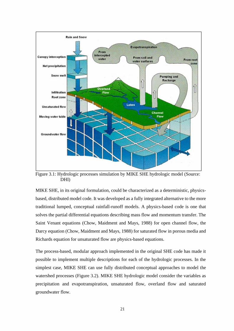
21
Figure 3.1: Hydrologic processes simulation by MIKE SHE hydrologic model (Source:
DHI)
MIKE SHE, in its original formulation, could be characterized as a deterministic, physics-
based, distributed model code. It was developed as a fully integrated alternative to the more
traditional lumped, conceptual rainfall-runoff models. A physics-based code is one that
solves the partial differential equations describing mass flow and momentum transfer. The
Saint Venant equations (Chow, Maidment and Mays, 1988) for open channel flow, the
Darcy equation (Chow, Maidment and Mays, 1988) for saturated flow in porous media and
Richards equation for unsaturated flow are physics-based equations.
The process-based, modular approach implemented in the original SHE code has made it
possible to implement multiple descriptions for each of the hydrologic processes. In the
simplest case, MIKE SHE can use fully distributed conceptual approaches to model the
watershed processes (Figure 3.2). MIKE SHE hydrologic model consider the variables as
precipitation and evapotranspiration, unsaturated flow, overland flow and saturated
groundwater flow.
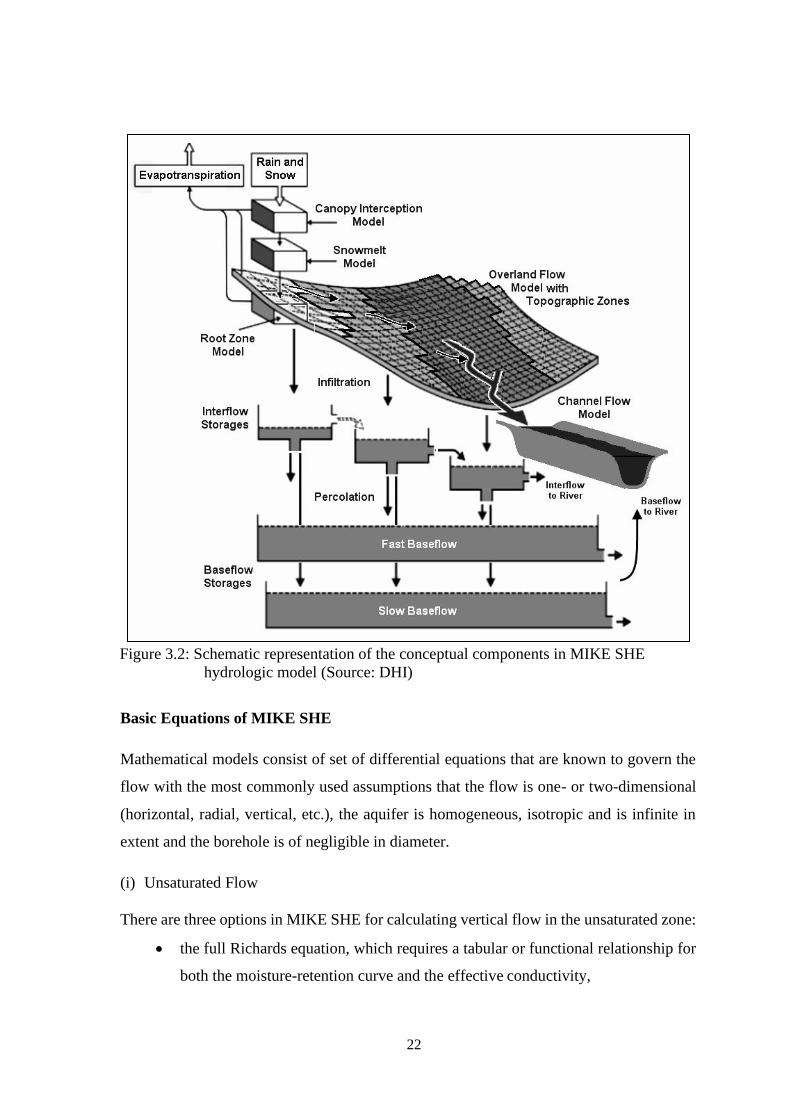
22
Figure 3.2: Schematic representation of the conceptual components in MIKE SHE
hydrologic model (Source: DHI)
Basic Equations of MIKE SHE
Mathematical models consist of set of differential equations that are known to govern the
flow with the most commonly used assumptions that the flow is one- or two-dimensional
(horizontal, radial, vertical, etc.), the aquifer is homogeneous, isotropic and is infinite in
extent and the borehole is of negligible in diameter.
(i) Unsaturated Flow
There are three options in MIKE SHE for calculating vertical flow in the unsaturated zone:
• the full Richards equation, which requires a tabular or functional relationship for
both the moisture-retention curve and the effective conductivity,
23
• a simplified gravity flow procedure, which assumes a uniform vertical gradient
and ignores capillary forces, and
• a simple two-layer water balance method for shallow water tables.
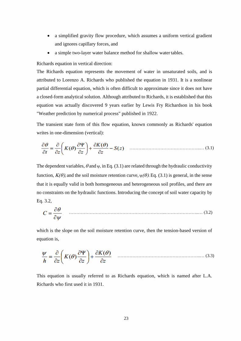
Richards equation in vertical direction:
The Richards equation represents the movement of water in unsaturated soils, and is
attributed to Lorenzo A. Richards who published the equation in 1931. It is a nonlinear
partial differential equation, which is often difficult to approximate since it does not have
a closed-form analytical solution. Although attributed to Richards, it is established that this
equation was actually discovered 9 years earlier by Lewis Fry Richardson in his book
"Weather prediction by numerical process" published in 1922.
The transient state form of this flow equation, known commonly as Richards' equation
writes in one-dimension (vertical):
The dependent variables, and in Eq. (3.1) are related through the hydraulic conductivity
function, (), and the soil moisture retention curve, (). Eq. (3.1) is general, in the sense
that it is equally valid in both homogeneous and heterogeneous soil profiles, and there are
no constraints on the hydraulic functions. Introducing the concept of soil water capacity by
Eq. 3.2,
which is the slope on the soil moisture retention curve, then the tension-based version of
equation is,
This equation is usually referred to as Richards equation, which is named after L.A.
Richards who first used it in 1931.
……….………………………………..… (3.1)
………………………………………………………..…………………..… (3.2)
………………………………………………..… (3.3)
24
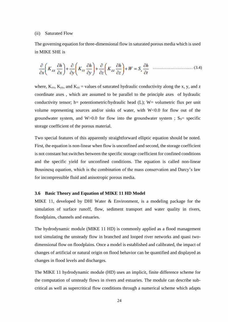
(ii) Saturated Flow
The governing equation for three-dimensional flow in saturated porous media which is used
in MIKE SHE is
where, Kxx, Kyy, and Kzz = values of saturated hydraulic conductivity along the x, y, and z
coordinate axes , which are assumed to be parallel to the principle axes of hydraulic
conductivity tensor; h= potentiometric/hydraulic head (L); W= volumetric flux per unit
volume representing sources and/or sinks of water, with W<0.0 for flow out of the
groundwater system, and W>0.0 for flow into the groundwater system ; SS= specific
storage coefficient of the porous material.
Two special features of this apparently straightforward elliptic equation should be noted.
First, the equation is non-linear when flow is unconfined and second, the storage coefficient
is not constant but switches between the specific storage coefficient for confined conditions
and the specific yield for unconfined conditions. The equation is called non-linear
Bousinesq equation, which is the combination of the mass conservation and Darcy’s law
for incompressible fluid and anisotropic porous media.
3.6 Basic Theory and Equation of MIKE 11 HD Model
MIKE 11, developed by DHI Water & Environment, is a modeling package for the
simulation of surface runoff, flow, sediment transport and water quality in rivers,
floodplains, channels and estuaries.
The hydrodynamic module (MIKE 11 HD) is commonly applied as a flood management
tool simulating the unsteady flow in branched and looped river networks and quasi two-
dimensional flow on floodplains. Once a model is established and calibrated, the impact of
changes of artificial or natural origin on flood behavior can be quantified and displayed as
changes in flood levels and discharges.
The MIKE 11 hydrodynamic module (HD) uses an implicit, finite difference scheme for
the computation of unsteady flows in rivers and estuaries. The module can describe sub-
critical as well as supercritical flow conditions through a numerical scheme which adapts
……………………..… (3.4)

25
according to the local flow conditions (in time and space). Advanced computational
modules are included for description of flow over hydraulic structures, including
possibilities to describe structure operation. The formulations can be applied to looped
networks and quasi two-dimensional flow simulation on flood plains. The computational
scheme is applicable for vertically homogeneous flow conditions extending from steep
river flows to tidal influenced estuaries. The system has been used in numerous engineering
studies around the world.
The MIKE 11 hydrodynamic is applied to compute water level, discharge and flow
velocity. The MIKE11 HD solves the vertically integrated equations of conservation of
energy and momentum called the “Saint Venant Equation” that describe the flow dynamic
in a river system. A network editor assists the schematization of rivers and floodplains as a
system of inter-connected branches. Flood levels and discharges as a function of time are
calculated at specified points along the branches to describe the passage of flood flows
through the model domain. Thus the Model takes into account the river connectivity, river
cross-sections, flood plain level and observed discharge at inlet and stage at outlet locations
of the modelled rivers. The observed discharge and stage applied respectively at the inlet
and outlet are called boundary to the model. The runoff generated in the NAM model from
rainfall occurring inside the basin is taken care of as inflows into the river system. MIKE
11 allows for two different types of bed resistance descriptions: Chezy, and Manning
number.
Basic Equations of MIKE 11(HD)
MIKE 11 HD applied with the dynamic wave description solves the vertically integrated
equations of conservation of continuity and momentum (the ‘Saint Venant´ equations). In
the ‘Saint Venant´ equation flow is calculated as a function of space and time throughout
the system which is governed by continuity and momentum equations.
The basic equations used in MIKE 11:
0=
+
t
A
x
Q
0)(11 2
=−−
+
+
fo SSg
x
yg
A
Q
xAt
Q
A
……………………………………………………………………..… (3.5)
………………………...… (3.6)
26
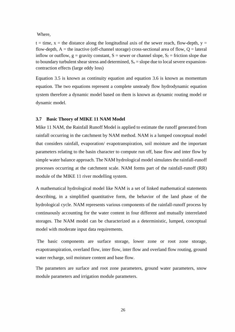
Where,
t = time, x = the distance along the longitudinal axis of the sewer reach, flow-depth, y =
flow-depth, A = the inactive (off-channel storage) cross-sectional area of flow, Q = lateral
inflow or outflow, g = gravity constant, S = sewer or channel slope, Sf = friction slope due
to boundary turbulent shear stress and determined, Se = slope due to local severe expansion-
contraction effects (large eddy loss)
Equation 3.5 is known as continuity equation and equation 3.6 is known as momentum
equation. The two equations represent a complete unsteady flow hydrodynamic equation
system therefore a dynamic model based on them is known as dynamic routing model or
dynamic model.
3.7 Basic Theory of MIKE 11 NAM Model
Mike 11 NAM, the Rainfall Runoff Model is applied to estimate the runoff generated from
rainfall occurring in the catchment by NAM method. NAM is a lumped conceptual model
that considers rainfall, evaporation/ evapotranspiration, soil moisture and the important
parameters relating to the basin character to compute run off, base flow and inter flow by
simple water balance approach. The NAM hydrological model simulates the rainfall-runoff
processes occurring at the catchment scale. NAM forms part of the rainfall-runoff (RR)
module of the MIKE 11 river modelling system.
A mathematical hydrological model like NAM is a set of linked mathematical statements
describing, in a simplified quantitative form, the behavior of the land phase of the
hydrological cycle. NAM represents various components of the rainfall-runoff process by
continuously accounting for the water content in four different and mutually interrelated
storages. The NAM model can be characterized as a deterministic, lumped, conceptual
model with moderate input data requirements.
The basic components are surface storage, lower zone or root zone storage,
evapotranspiration, overland flow, inter flow, inter flow and overland flow routing, ground
water recharge, soil moisture content and base flow.
The parameters are surface and root zone parameters, ground water parameters, snow
module parameters and irrigation module parameters.
27
3.8 Methodology of the Study
Modelling of any physical phenomenon is an iterative development of a process. Model
refinements are based on the availability and quality of data, hydrological understanding
and scopes of the project. The general approach that has been followed in the current study
can be summarized in the flowchart given in Figure 3.3.
`
Figure 3.3: Flowchart of the overall methodology for this study
Selection of the Study Area
Selection of Design Year
Prediction of Future Data up to 2030
Prediction of
Hydrological Data
Prediction of
Water Demand
Prediction of
Boundary GWL Data
Prediction of
Hydraulic Data
Development of Scenarios
Scenario Based SW-GW Interactive Model Set Up
SW Base Model Set Up GW Base Model Set Up
Set Up
SW-GW Interactive
Base Model Set Up
Calibration and Validation of Models
Model Output
Result Analysis
Determination of
Extreme Scenario
Determination of
Suitable Intervention
Result Analysis
Data Collection & Data Processing
28
3.8.1 Selection of the Study Area
Rajshahi district is one of the most drought prone districts of Bangladesh (Chowdhury et
al., 2018). Groundwater level in this area is successively falling at an alarming rate (Aziz
et al., 2015). Groundwater recharge condition is very poor in Tanore, Godagari, Mohanpur
and Baghmara upazilas and vulnerable for Boro rice (Aziz et al., 2015). Groundwater
dependent irrigation system in the area has reached a critical phase (Adhikary et al., 2013)
and GW level has dropped below the depth of the shallow tube wells in many places
(Adhikary et al., 2013). The Bangladesh government is about to declare a “state of water
emergency” in the drought prone Barind tract in the northwest of the country, where over-
extraction of groundwater for rice farming and dwindling rainfall caused by climate
change have combined to create a crisis (thethirdpole.net). These are the reasons for
choosing this district as study area where sustainable GW is a major concern.
3.8.2 Data Collection and Data Processing
According to the model requirements, significant amount of data have been collected from
Institute of Water Modelling (IWM), Bangladesh Water Development Board (BWDB),
Bangladesh Agricultural Development Corporation (BADC) and Soil Resource
Development Institute (SRDI). Only BWDB stations data has taken to prepare MIKE 11
and MIKE SHE model in current study. The data has to be used in this study after checking
quality & consistency, and then processed as per required format for the model running.
In addition to the data quality checking, data analysis has to be carried out for estimation
of different model parameters
(i) Data Requirements for MIKE SHE Hydrologic Model are as follows:
• Hydrometeorology of the study area i.e. precipitation, Evapotranspiration,
stream water level data
• Hydrogeology of the study area i.e. groundwater level & abstraction data
• Land Use of the study area i.e. land use map & crop calendar throughout the year
• Topography of the study area
• Lithology of the study area including hydraulic properties of the aquifer
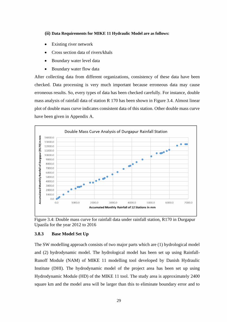
29
(ii) Data Requirements for MIKE 11 Hydraulic Model are as follows:
• Existing river network
• Cross section data of rivers/khals
• Boundary water level data
• Boundary water flow data
After collecting data from different organizations, consistency of these data have been
checked. Data processing is very much important because erroneous data may cause
erroneous results. So, every types of data has been checked carefully. For instance, double
mass analysis of rainfall data of station R 170 has been shown in Figure 3.4. Almost linear
plot of double mass curve indicates consistent data of this station. Other double mass curve
have been given in Appendix A.
Figure 3.4: Double mass curve for rainfall data under rainfall station, R170 in Durgapur
Upazila for the year 2012 to 2016
3.8.3 Base Model Set Up
The SW modelling approach consists of two major parts which are (1) hydrological model
and (2) hydrodynamic model. The hydrological model has been set up using Rainfall-
Runoff Module (NAM) of MIKE 11 modelling tool developed by Danish Hydraulic
Institute (DHI). The hydrodynamic model of the project area has been set up using
Hydrodynamic Module (HD) of the MIKE 11 tool. The study area is approximately 2400
square km and the model area will be larger than this to eliminate boundary error and to
30
use observed water level and discharge stations of BWDB and IWM. The base model has
been set up for 5 years (January, 2012 to December, 2016). Expected major outputs from
this model are water level and discharge at every grid point within model area.
The groundwater model has been set up using MIKE SHE model of DHI. This model has
been set up for 5 years (January, 2012 to December, 2016). Expected major outputs from
this model are groundwater levels at every grid point within model area and water balance
of the model area.
The MIKE 11(HD) and MIKE SHE models have been linked interactively and then it is
capable of producing water balance and changing of storages in the form of groundwater
recharge/discharge and showing fluctuations in water-table.
3.8.4 Calibration and Validation of Base Models
Surface water model has been calibrated for three years (January, 2012 to December, 2014)
and have been validated for next 2 years (January, 2015 to December, 2016). After
calibration and validation of surface water model, it needs to be coupled with groundwater
model to understand the interaction between rivers and aquifers in the study area and to
observe the influence of storage structures on surface water bodies. Then the coupled model
(MIKE 11 and MIKE SHE) has been calibrated and validated with observed groundwater
level data for the same calibration and validation period of surface water model. Main
calibration parameter for MIKE-11(HD) model is Bed Resistance of stream channel
(Manning’s n) and for MIKE SHE model calibration parameters are horizontal hydraulic
conductivity, vertical hydraulic conductivity, specific yield, storage co-efficient etc.
3.8.5 Selection of Design Year
For the development of future scenarios, design year has been selected based on statistical
analysis. In the present study, design year has been selected based on return period of mean
annual rainfall of the study area. The mean annual rainfall has been obtained from the
average of 10 stations falls in the study area. Observed annual rainfall for a period of 47
years (1970-2016) has been considered for statistical analysis. According to the
recommendation of FAP25 study, data has been fitted to 3-parameter Log Normal
distribution to find out the average and extreme dry year. The statistical software HYMOS
4.0 has been used for this purpose. From this analysis 1990 year has been selected as a
31
design year of average hydrological condition and 2014 and 1994 have been selected for
design year of dry (5 years of return period) and extreme dry conations ( 10 years of return
period) respectively.
3.8.6 Development of Scenarios
In order to sustain groundwater resources up to year 2030 we have to foresee future
condition of groundwater resources under different Scenarios. For this reason, there are ten
(10) Scenario s have been chosen to understand future groundwater level considering
rainfall, evaporation, boundary groundwater level and water demand as driving forces.
Summary of these scenarios is given in Table 5.4. Rainfall and Evaporation date for 2017
to 2030 have been collected from Global Circulation Model HADCM3 using Climate
Editor Tool of Mike 11 software. GWL for 2017-2030 have been generated based on
selected design year considering four boundary conditions. Agricultural water demand data
has been calculated from 2017 to 2030 according to the National Water Management Plan
(NWMP) of WARPO and municipal water demand has been calculated from projected
future population data of BBS. After development of scenarios with the help of SW-GW
interactive model, most extreme and suitable scenario has been identified for this study
area up to 2030.
3.8.7 Prediction of Data up to Year 2030
For prediction model of MIKE SHE, required data that has been projected are described
in this article from year 2017 to 2030.
(i) Prediction of Hydrological Data
Precipitation
Monthly precipitation data for 2017 to 2030 have been collected from Global Circulation
Model HADCM3 using Climate Editor Tool of Mike 11 software. Emission scenario has
been chosen for this analysis is SRA2 which is based on the assumption that a very
heterogenous world with continuously incresing global population and regionally oriented
economic growth that is more fragmented and slower than in other storyline.
Evapotranspiration
Monthly evapotranspiration data for 2017 to 2030 have been collected from Global
Circulation Model HADCM3 using Climate Editor Tool of Mike 11 software. Emission
32
scenario has been chosen for this analysis is SRA2 which is based on the assumption that
a very heterogenous world with continuously incresing global population and regionally
oriented economic growth that is more fragmented and slower than in other storyline.
(ii) Prediction of Hydraulic Data
River water level
For projection of groundwater levels up to 2030, it is considered in this study that river
water level data follows the same time series plotted for year 2016 that has to be extended
up to 2030.
(iii) Prediction of Boundary GWL Data
Groundwater level at model boundary
Projected groundwater level data for eight (8) boundary wells are very important variables
of the MIKE SHE hydrologic model. For projected groundwater level of the model
boundary wells, four (4) boundary conditions named as “Boundary Condition 01”,
“Boundary Condition 02”, “Boundary Condition 03” and “Boundary Condition 04” have
been considered.
Boundary Condition 01: Assumption is, same groundwater level of hydrological
condition of the year 2016 (base condition) individual model boundary wells will be
continued over the years up to 2030.
Boundary Condition 02: Assumption is, same groundwater level of hydrological
condition of the year 1990 (average condition of 2.33 years return period) individual
model boundary wells will be continued over the years up to 2030.
Boundary Condition 03: Assumption is, same groundwater level of hydrological
condition of the year 2014 (dry condition of 5 years return period) individual model
boundary wells will be continued over the years up to 2030.
Boundary Condition 04: Assumption is, same groundwater level of hydrological
condition of the year 1994 (extreme dry condition of 10 years return period) individual
model boundary wells will be continued over the years up to 2030.

33
(iv) Prediction of Water Demand
In order to support the food requirement of the increased population, crop production needs
to be increased bringing potential areas under irrigation through optimum utilization of the
available water resources. It is important to assess future water requirement to see whether
it exceeds the safe yield limit of the aquifer and creates any environmental degradation.
Future water demand has been assessed for irrigation and domestic use following the
methodology as mentioned in this section.
Irrigation water demand
Upazila wise crop water requirement for different cropping pattern has been assessed by
IWM under the referenced project according to 2012 survey (IWM, 2012) has shown in
Appendix-C and considered as input data for the study. These data has used in this study
for base irrigation demand in the year 2016.
According to National Water Management Plan (NWMP), irrigation demands are
expected to increase potentially by at least a quarter over the next 25 years (WARPO,
2001). From 2016 to 2030, 3 sets of crop demand increment were taken that exponentially
increased from 1.0 in 2016 to values of (i) no increment; (ii) 1% yearly increment of
present demand; (iii) 1.5% yearly increment demand; (iii) 2% yearly increment demand
and (v) 2.5% yearly increment of present demand respectively in 2030 is shown in Figure
3.5. 2016 is considered as the base year (present demand year). To attain 1%, 1.5% , 2%
and 2.5% yearly incremental demand, demand of base year has been multiplied by 1.010,
1.015, 1.020 and 1.025 respectively. Land use (crop coverage area) expansion within the
gross area is considered as key reason for the increment of water demand.
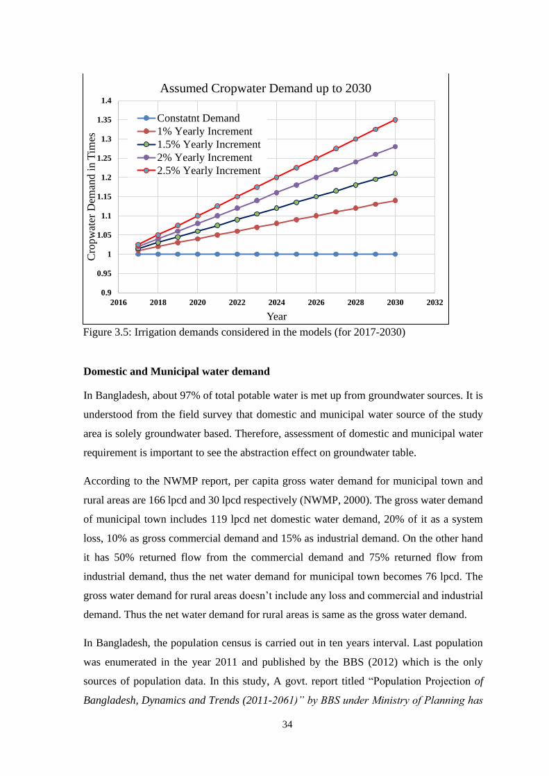
34
Figure 3.5: Irrigation demands considered in the models (for 2017-2030)
Domestic and Municipal water demand
In Bangladesh, about 97% of total potable water is met up from groundwater sources. It is
understood from the field survey that domestic and municipal water source of the study
area is solely groundwater based. Therefore, assessment of domestic and municipal water
requirement is important to see the abstraction effect on groundwater table.
According to the NWMP report, per capita gross water demand for municipal town and
rural areas are 166 lpcd and 30 lpcd respectively (NWMP, 2000). The gross water demand
of municipal town includes 119 lpcd net domestic water demand, 20% of it as a system
loss, 10% as gross commercial demand and 15% as industrial demand. On the other hand
it has 50% returned flow from the commercial demand and 75% returned flow from
industrial demand, thus the net water demand for municipal town becomes 76 lpcd. The
gross water demand for rural areas doesn’t include any loss and commercial and industrial
demand. Thus the net water demand for rural areas is same as the gross water demand.
In Bangladesh, the population census is carried out in ten years interval. Last population
was enumerated in the year 2011 and published by the BBS (2012) which is the only
sources of population data. In this study, A govt. report titled “Population Projection of
Bangladesh, Dynamics and Trends (2011-2061)” by BBS under Ministry of Planning has
0.9
0.95
1
1.05
1.1
1.15
1.2
1.25
1.3
1.35
1.4
2016 2018 2020 2022 2024 2026 2028 2030 2032
Cro
pw
ater
Dem
and i
n T
imes
Year
Assumed Cropwater Demand up to 2030
Constatnt Demand
1% Yearly Increment
1.5% Yearly Increment
2% Yearly Increment
2.5% Yearly Increment

35
been taken as an authentic source for projection of population of Rajshahi district up to
2030.
The projected population is estimated by the following equation:
Pp = Pb (1 + r) n
Where Pp = projected population in the year n
Pb = Base population
r = rate of natural increase of population per year
n = number of years being considered
Domestic and municipal water requirement for future condition is assessed based on the
population projected to the year 2030. Upazila wise projected population and future water
demand for rural and urban areas are given in Table-3.1, Table 3.2 and Table 3.3. In Table
3.1, population has been predicted Upazila-wise within the study area. In Table 3.2,
municipal water demand has been calculated up to 2030 in m3/day unit to understand
Upazila-wise water demand for domestic purposes in future within study period. In Table
3.3, municipal water demand has been calculated up to 2030 in mm/day unit to make this
demand applicable for groundwater model. From this table it is clear that municipal water
demand is very low compared to high agricultural water demand.
Table 3.1: Upazila-wise Projected Population up to 2030
Year Bagha Baghmara Char-
ghat
Durga-
pur Godagari Mohanpur Paba Puthia Tanore Rajshahi
2012 186780 359665 209704 188465 335590 172418 318626 210416 194028 456098
2013 189414 364736 212661 191123 340322 174849 323119 213382 196764 462529
2014 192084 369879 215659 193818 345120 177315 327675 216391 199538 469050
2015 194793 375094 218700 196550 349987 179815 332295 219442 202351 475664
2016 197539 380383 221784 199322 354921 182350 336980 222536 205205 482371
2017 199574 384301 224068 201375 358577 184229 340451 224829 207318 487339
2018 201630 388259 226376 203449 362270 186126 343958 227144 209454 492359
………………………………………………..…...… (3.7)
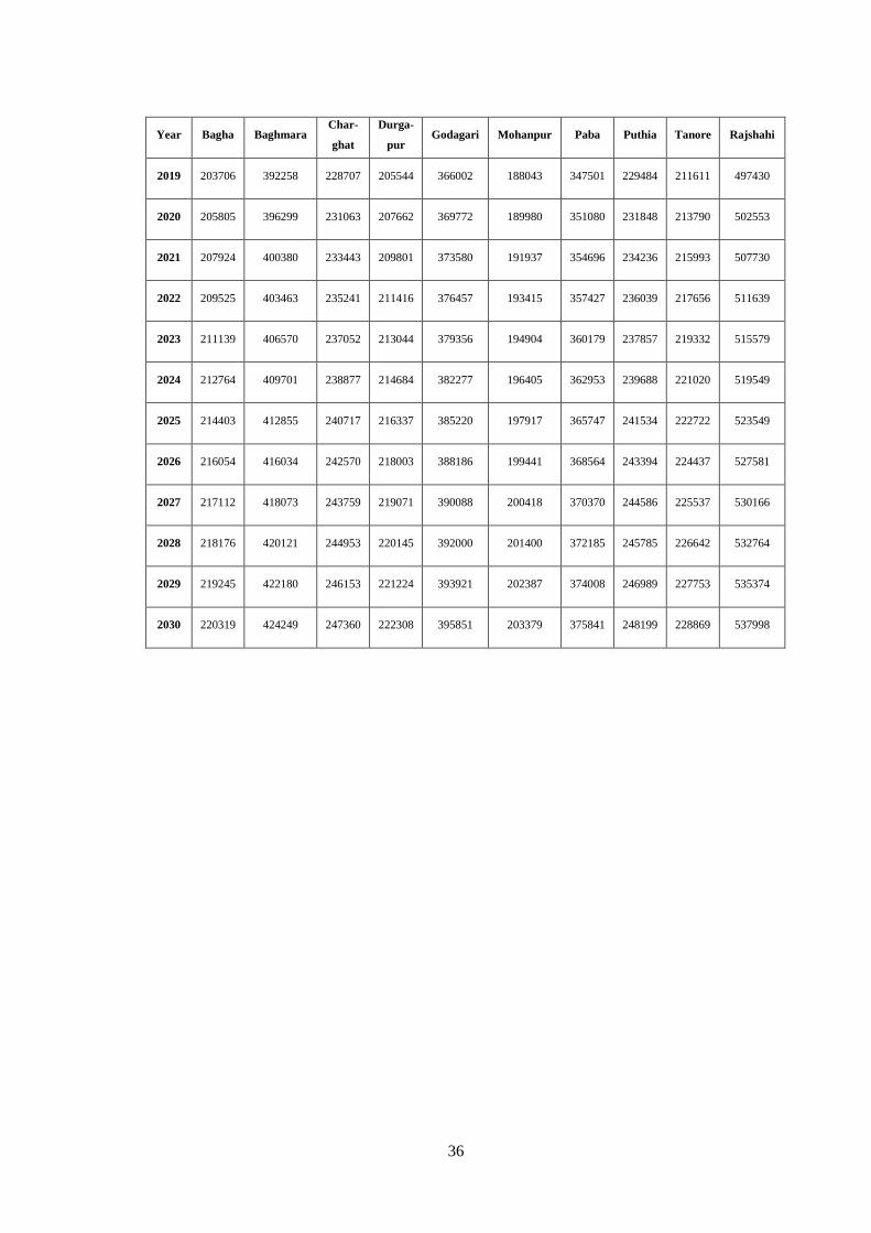
36
Year Bagha Baghmara Char-
ghat
Durga-
pur Godagari Mohanpur Paba Puthia Tanore Rajshahi
2019 203706 392258 228707 205544 366002 188043 347501 229484 211611 497430
2020 205805 396299 231063 207662 369772 189980 351080 231848 213790 502553
2021 207924 400380 233443 209801 373580 191937 354696 234236 215993 507730
2022 209525 403463 235241 211416 376457 193415 357427 236039 217656 511639
2023 211139 406570 237052 213044 379356 194904 360179 237857 219332 515579
2024 212764 409701 238877 214684 382277 196405 362953 239688 221020 519549
2025 214403 412855 240717 216337 385220 197917 365747 241534 222722 523549
2026 216054 416034 242570 218003 388186 199441 368564 243394 224437 527581
2027 217112 418073 243759 219071 390088 200418 370370 244586 225537 530166
2028 218176 420121 244953 220145 392000 201400 372185 245785 226642 532764
2029 219245 422180 246153 221224 393921 202387 374008 246989 227753 535374
2030 220319 424249 247360 222308 395851 203379 375841 248199 228869 537998
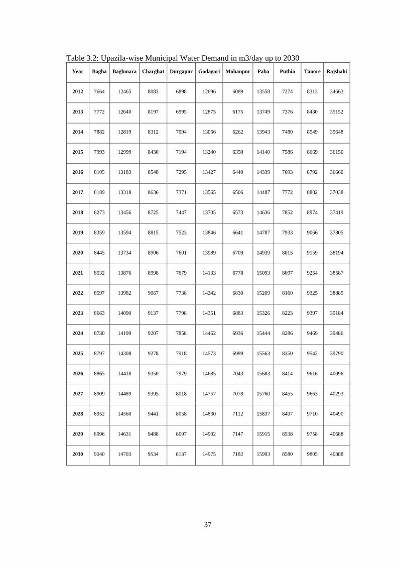
37
Table 3.2: Upazila-wise Municipal Water Demand in m3/day up to 2030
Year Bagha Baghmara Charghat Durgapur Godagari Mohanpur Paba Puthia Tanore Rajshahi
2012 7664 12465 8083 6898 12696 6089 13558 7274 8313 34663
2013 7772 12640 8197 6995 12875 6175 13749 7376 8430 35152
2014 7882 12819 8312 7094 13056 6262 13943 7480 8549 35648
2015 7993 12999 8430 7194 13240 6350 14140 7586 8669 36150
2016 8105 13183 8548 7295 13427 6440 14339 7693 8792 36660
2017 8189 13318 8636 7371 13565 6506 14487 7772 8882 37038
2018 8273 13456 8725 7447 13705 6573 14636 7852 8974 37419
2019 8359 13594 8815 7523 13846 6641 14787 7933 9066 37805
2020 8445 13734 8906 7601 13989 6709 14939 8015 9159 38194
2021 8532 13876 8998 7679 14133 6778 15093 8097 9254 38587
2022 8597 13982 9067 7738 14242 6830 15209 8160 9325 38885
2023 8663 14090 9137 7798 14351 6883 15326 8223 9397 39184
2024 8730 14199 9207 7858 14462 6936 15444 8286 9469 39486
2025 8797 14308 9278 7918 14573 6989 15563 8350 9542 39790
2026 8865 14418 9350 7979 14685 7043 15683 8414 9616 40096
2027 8909 14489 9395 8018 14757 7078 15760 8455 9663 40293
2028 8952 14560 9441 8058 14830 7112 15837 8497 9710 40490
2029 8996 14631 9488 8097 14902 7147 15915 8538 9758 40688
2030 9040 14703 9534 8137 14975 7182 15993 8580 9805 40888
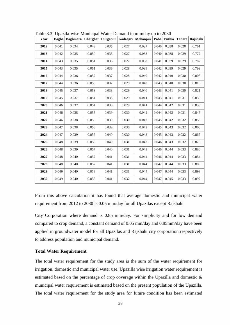
38
Table 3.3: Upazila-wise Municipal Water Demand in mm/day up to 2030 Year Bagha Baghmara Charghat Durgapur Godagari Mohanpur Paba Puthia Tanore Rajshahi
2012 0.041 0.034 0.049 0.035 0.027 0.037 0.040 0.038 0.028 0.761
2013 0.042 0.035 0.050 0.035 0.027 0.038 0.040 0.038 0.029 0.772
2014 0.043 0.035 0.051 0.036 0.027 0.038 0.041 0.039 0.029 0.782
2015 0.043 0.035 0.051 0.036 0.028 0.039 0.042 0.039 0.029 0.793
2016 0.044 0.036 0.052 0.037 0.028 0.040 0.042 0.040 0.030 0.805
2017 0.044 0.036 0.053 0.037 0.029 0.040 0.043 0.040 0.030 0.813
2018 0.045 0.037 0.053 0.038 0.029 0.040 0.043 0.041 0.030 0.821
2019 0.045 0.037 0.054 0.038 0.029 0.041 0.043 0.041 0.031 0.830
2020 0.046 0.037 0.054 0.038 0.029 0.041 0.044 0.042 0.031 0.838
2021 0.046 0.038 0.055 0.039 0.030 0.042 0.044 0.042 0.031 0.847
2022 0.046 0.038 0.055 0.039 0.030 0.042 0.045 0.042 0.032 0.853
2023 0.047 0.038 0.056 0.039 0.030 0.042 0.045 0.043 0.032 0.860
2024 0.047 0.039 0.056 0.040 0.030 0.043 0.045 0.043 0.032 0.867
2025 0.048 0.039 0.056 0.040 0.031 0.043 0.046 0.043 0.032 0.873
2026 0.048 0.039 0.057 0.040 0.031 0.043 0.046 0.044 0.033 0.880
2027 0.048 0.040 0.057 0.041 0.031 0.044 0.046 0.044 0.033 0.884
2028 0.048 0.040 0.057 0.041 0.031 0.044 0.047 0.044 0.033 0.889
2029 0.049 0.040 0.058 0.041 0.031 0.044 0.047 0.044 0.033 0.893
2030 0.049 0.040 0.058 0.041 0.032 0.044 0.047 0.045 0.033 0.897
From this above calculation it has found that average domestic and municipal water
requirement from 2012 to 2030 is 0.05 mm/day for all Upazilas except Rajshahi
City Corporation where demand is 0.85 mm/day. For simplicity and for low demand
compared to crop demand, a constant demand of 0.05 mm/day and 0.85mm/day have been
applied in groundwater model for all Upazilas and Rajshahi city corporation respectively
to address population and municipal demand.
Total Water Requirement
The total water requirement for the study area is the sum of the water requirement for
irrigation, domestic and municipal water use. Upazilla wise irrigation water requirement is
estimated based on the percentage of crop coverage within the Upazilla and domestic &
municipal water requirement is estimated based on the present population of the Upazilla.
The total water requirement for the study area for future condition has been estimated
39
following the procedure as mentioned in the above sections. It can be noted that in the
present situation, the Domestic and Municipal water requirement is very negligible portion
of total water requirement, actually the irrigation water requirement dominates the total
water requirement. Water demand for other sectors are not considered in this study due to
their negligible contribution in total water demand.
3.8.8 Result and Analysis
Yearly minimum and maximum groundwater level have been analyzed for all upazilas and
most emphasis has been given to identify the extreme scenario on minimum groundwater
level. All these mentioned scenarios show decreasing trend of groundwater levels within
the study period. After generation of possible future scenarios, extreme scenario has been
identified. So, in this study, innervations have been applied to this extreme scenario to
sustain future groundwater resources up to 2030. Attempts have been made to stop the rate
of declining groundwater levels and to increase the trends of groundwater levels of the
study area. Three interventions have been applied and they are (i) Structural, (ii) Non-
Structural and (iii) Combined Interventions.
3.9 Summary
Theory and methodology is the backbone of any research work. If the methodology is
sound and clear it is expected that the study result based on this methodology will also be
sound. So in this chapter background theory and overall methodology of this study have
been reviewed. Short description of each section of methodology is described here and
further description and analysis based on this methodology has been discussed in the
following chapter.
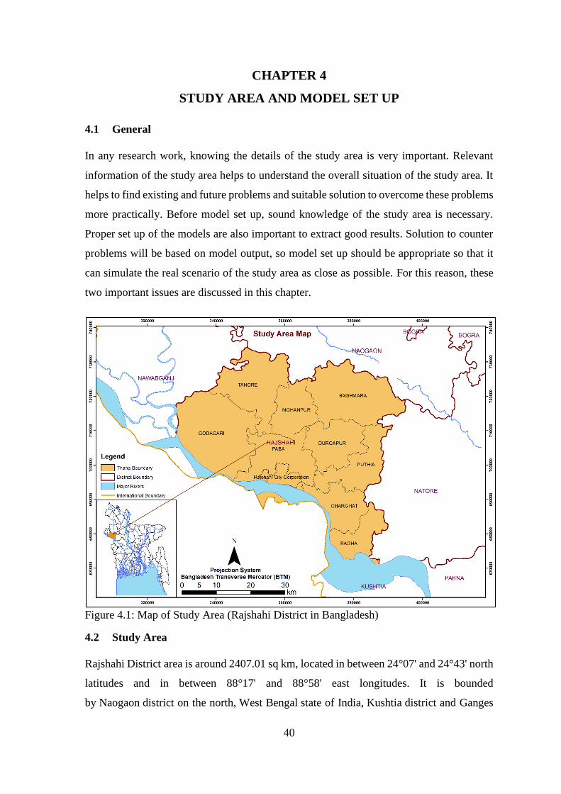
40
CHAPTER 4
STUDY AREA AND MODEL SET UP
4.1 General
In any research work, knowing the details of the study area is very important. Relevant
information of the study area helps to understand the overall situation of the study area. It
helps to find existing and future problems and suitable solution to overcome these problems
more practically. Before model set up, sound knowledge of the study area is necessary.
Proper set up of the models are also important to extract good results. Solution to counter
problems will be based on model output, so model set up should be appropriate so that it
can simulate the real scenario of the study area as close as possible. For this reason, these
two important issues are discussed in this chapter.
Figure 4.1: Map of Study Area (Rajshahi District in Bangladesh)
4.2 Study Area
Rajshahi District area is around 2407.01 sq km, located in between 24°07' and 24°43' north
latitudes and in between 88°17' and 88°58' east longitudes. It is bounded
by Naogaon district on the north, West Bengal state of India, Kushtia district and Ganges
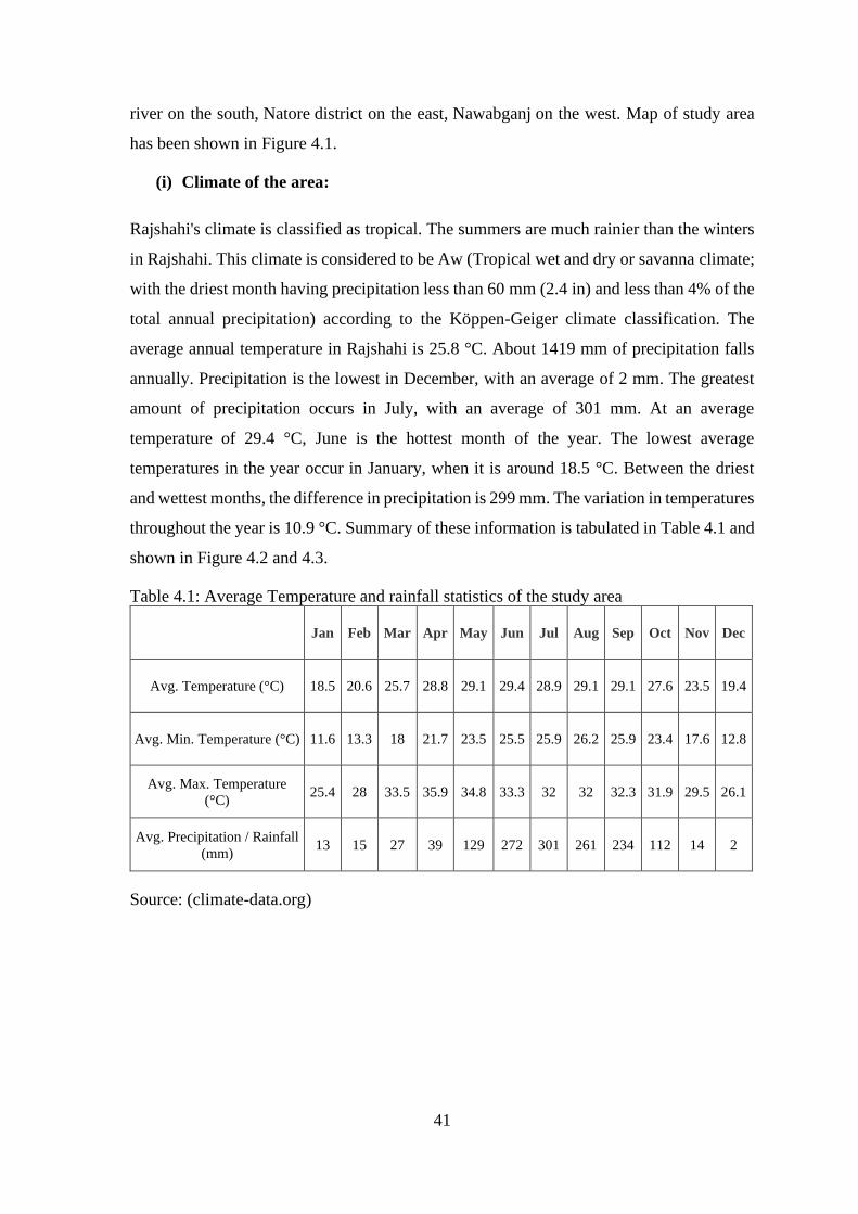
41
river on the south, Natore district on the east, Nawabganj on the west. Map of study area
has been shown in Figure 4.1.
(i) Climate of the area:
Rajshahi's climate is classified as tropical. The summers are much rainier than the winters
in Rajshahi. This climate is considered to be Aw (Tropical wet and dry or savanna climate;
with the driest month having precipitation less than 60 mm (2.4 in) and less than 4% of the
total annual precipitation) according to the Köppen-Geiger climate classification. The
average annual temperature in Rajshahi is 25.8 °C. About 1419 mm of precipitation falls
annually. Precipitation is the lowest in December, with an average of 2 mm. The greatest
amount of precipitation occurs in July, with an average of 301 mm. At an average
temperature of 29.4 °C, June is the hottest month of the year. The lowest average
temperatures in the year occur in January, when it is around 18.5 °C. Between the driest
and wettest months, the difference in precipitation is 299 mm. The variation in temperatures
throughout the year is 10.9 °C. Summary of these information is tabulated in Table 4.1 and
shown in Figure 4.2 and 4.3.
Table 4.1: Average Temperature and rainfall statistics of the study area
Jan Feb Mar Apr May Jun Jul Aug Sep Oct Nov Dec
Avg. Temperature (°C) 18.5 20.6 25.7 28.8 29.1 29.4 28.9 29.1 29.1 27.6 23.5 19.4
Avg. Min. Temperature (°C) 11.6 13.3 18 21.7 23.5 25.5 25.9 26.2 25.9 23.4 17.6 12.8
Avg. Max. Temperature
(°C) 25.4 28 33.5 35.9 34.8 33.3 32 32 32.3 31.9 29.5 26.1
Avg. Precipitation / Rainfall
(mm) 13 15 27 39 129 272 301 261 234 112 14 2
Source: (climate-data.org)
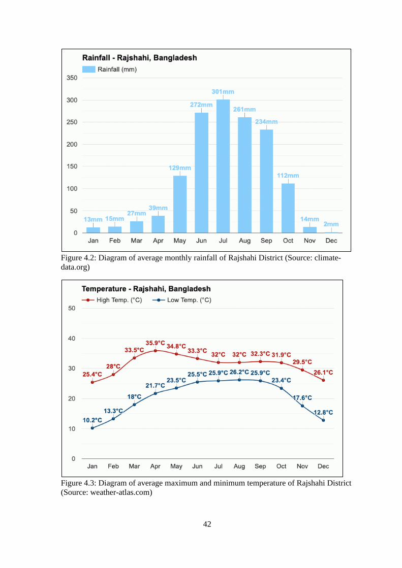
42
Figure 4.2: Diagram of average monthly rainfall of Rajshahi District (Source: climate-
data.org)
Figure 4.3: Diagram of average maximum and minimum temperature of Rajshahi District
(Source: weather-atlas.com)

43
(ii) Topography of the study area:
The topography of the study area varies from 9.72mPWD to 46.85mPWD. Almost 13% of
study area has elevation greater than 25.00mPWD. Slope of this area varies from 0 to 1.35
degree. This area remains flood free because of its high elevation. Topography of the study
area is shown in Figure 4.4.
Figure 4.4: Topography of the study area
(iii) Geomorphology and hydrogeological setting:
Hydrogeological parameters of an area are generally governed by the lithostratigraphy and
prevailing tectonic activities of that area which is a part of regional geological setting,
physiography and geomorphology.
(iv) Study area and regional geological setting:
The present geomorphologic setting of the study area is the result of tectonic adjustment
within the Bengal Basin. Tectonically Bangladesh is lying on the Indian Plate and occupies
the major part of the Bengal Basin. Geological data indicates that the area is traversed by a
basement-controlled faults named Tanor fault. The study area experienced lateral
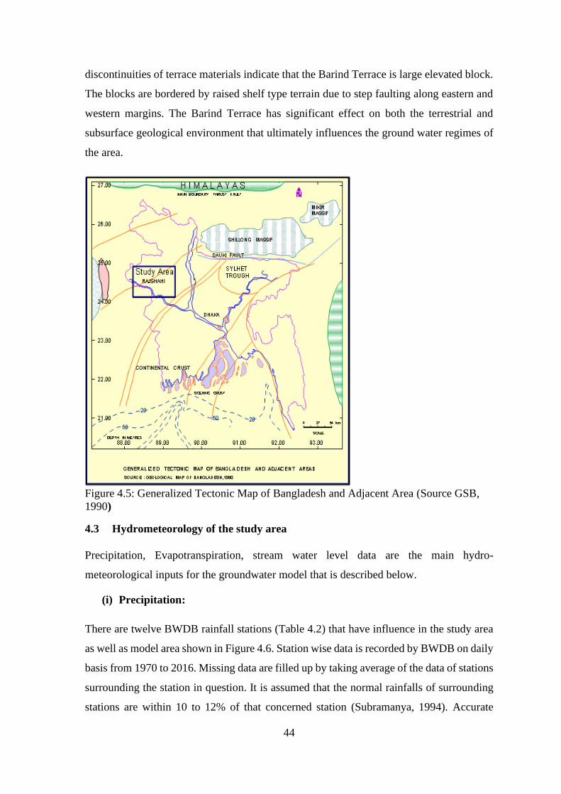
44
discontinuities of terrace materials indicate that the Barind Terrace is large elevated block.
The blocks are bordered by raised shelf type terrain due to step faulting along eastern and
western margins. The Barind Terrace has significant effect on both the terrestrial and
subsurface geological environment that ultimately influences the ground water regimes of
the area.
Figure 4.5: Generalized Tectonic Map of Bangladesh and Adjacent Area (Source GSB,
1990)
4.3 Hydrometeorology of the study area
Precipitation, Evapotranspiration, stream water level data are the main hydro-
meteorological inputs for the groundwater model that is described below.
(i) Precipitation:
There are twelve BWDB rainfall stations (Table 4.2) that have influence in the study area
as well as model area shown in Figure 4.6. Station wise data is recorded by BWDB on daily
basis from 1970 to 2016. Missing data are filled up by taking average of the data of stations
surrounding the station in question. It is assumed that the normal rainfalls of surrounding
stations are within 10 to 12% of that concerned station (Subramanya, 1994). Accurate
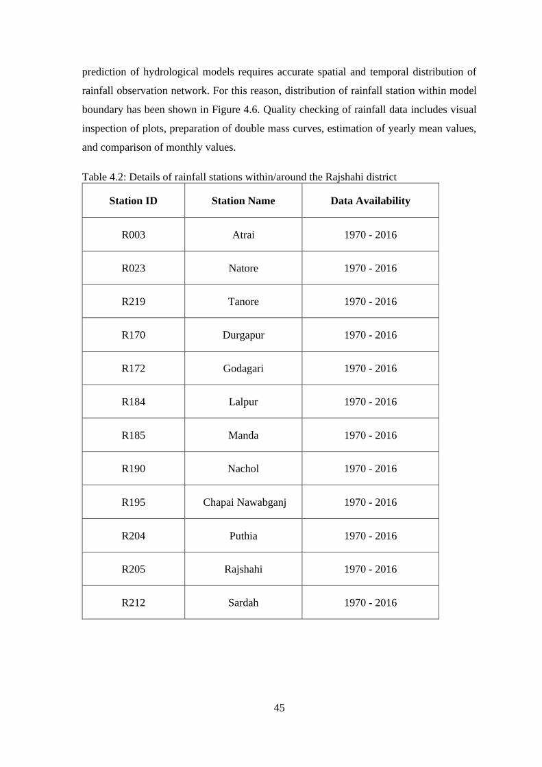
45
prediction of hydrological models requires accurate spatial and temporal distribution of
rainfall observation network. For this reason, distribution of rainfall station within model
boundary has been shown in Figure 4.6. Quality checking of rainfall data includes visual
inspection of plots, preparation of double mass curves, estimation of yearly mean values,
and comparison of monthly values.
Table 4.2: Details of rainfall stations within/around the Rajshahi district
Station ID Station Name Data Availability
R003 Atrai 1970 - 2016
R023 Natore 1970 - 2016
R219 Tanore 1970 - 2016
R170 Durgapur 1970 - 2016
R172 Godagari 1970 - 2016
R184 Lalpur 1970 - 2016
R185 Manda 1970 - 2016
R190 Nachol 1970 - 2016
R195 Chapai Nawabganj 1970 - 2016
R204 Puthia 1970 - 2016
R205 Rajshahi 1970 - 2016
R212 Sardah 1970 - 2016
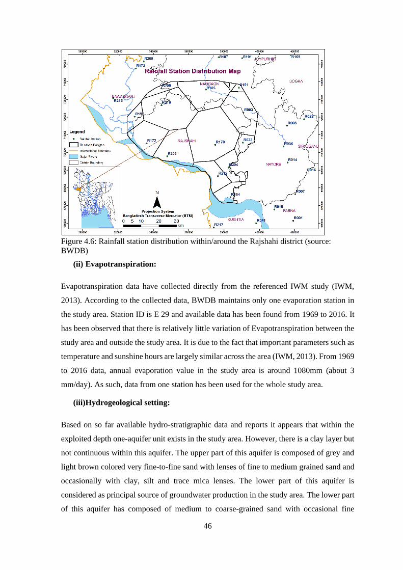
46
Figure 4.6: Rainfall station distribution within/around the Rajshahi district (source:
BWDB)
(ii) Evapotranspiration:
Evapotranspiration data have collected directly from the referenced IWM study (IWM,
2013). According to the collected data, BWDB maintains only one evaporation station in
the study area. Station ID is E 29 and available data has been found from 1969 to 2016. It
has been observed that there is relatively little variation of Evapotranspiration between the
study area and outside the study area. It is due to the fact that important parameters such as
temperature and sunshine hours are largely similar across the area (IWM, 2013). From 1969
to 2016 data, annual evaporation value in the study area is around 1080mm (about 3
mm/day). As such, data from one station has been used for the whole study area.
(iii)Hydrogeological setting:
Based on so far available hydro-stratigraphic data and reports it appears that within the
exploited depth one-aquifer unit exists in the study area. However, there is a clay layer but
not continuous within this aquifer. The upper part of this aquifer is composed of grey and
light brown colored very fine-to-fine sand with lenses of fine to medium grained sand and
occasionally with clay, silt and trace mica lenses. The lower part of this aquifer is
considered as principal source of groundwater production in the study area. The lower part
of this aquifer has composed of medium to coarse-grained sand with occasional fine
47
sediment lenses. The geometry and confining properties of both of this aquifer are variable
with its location in the study area and controlled by local subsurface geology. According
to UNDP (UNDP, 1982) report the study area aquifer systems has the transmissivity value
ranges from 500 m2 /day to 1500 m2 /day. Steep gradient of groundwater elevation exists
in the study area which may have maximum outflow situation and direction is towards the
Padma River.
(iv) Groundwater Level
Groundwater observation level data is an important parameter for the groundwater model
as it is used for calibration, boundary condition and initial condition of the model. There
are 30 groundwater observation wells of BWDB is selected in/around the study area is
shown in Figure 4.7 and Figure 4.8. Among them 8 observation wells are on the study area
boundary, which have used as boundary condition and 22 observation wells are inside the
study area which can be used for calibration purpose.
The frequency of measurement in the observation wells is generally conducted once in a
week. The measured groundwater levels are expressed in terms of national datum, mPWD.
Data has checked by visual inspection of those time series plots of groundwater levels and
missing data is filled up by interpolation of nearby stations. However, topology,
groundwater level fluctuation and rainfall pattern of those nearby stations are taken into
consideration during filling the missing data.
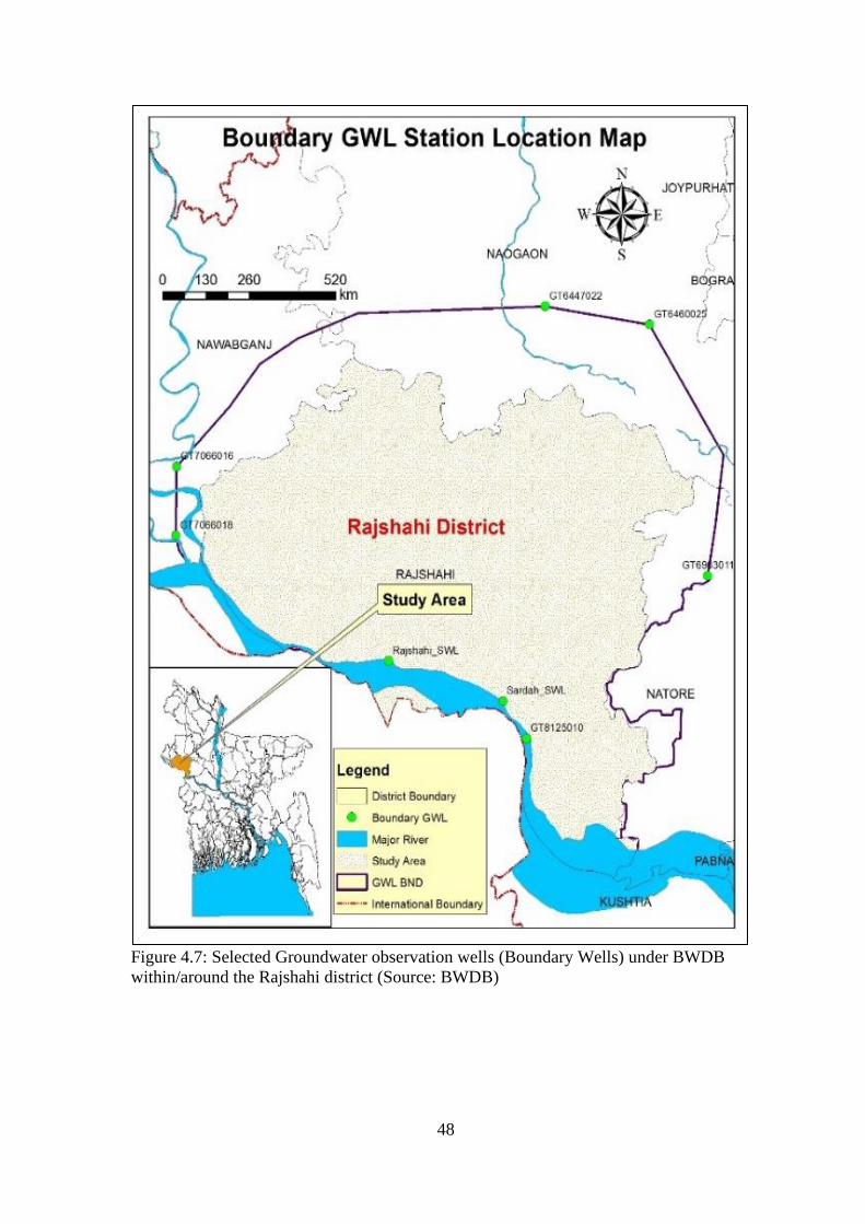
48
Figure 4.7: Selected Groundwater observation wells (Boundary Wells) under BWDB
within/around the Rajshahi district (Source: BWDB)
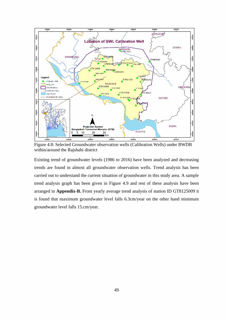
49
Figure 4.8: Selected Groundwater observation wells (Calibration Wells) under BWDB
within/around the Rajshahi district
Existing trend of groundwater levels (1986 to 2016) have been analyzed and decreasing
trends are found in almost all groundwater observation wells. Trend analysis has been
carried out to understand the current situation of groundwater in this study area. A sample
trend analysis graph has been given in Figure 4.9 and rest of these analysis have been
arranged in Appendix-B. From yearly average trend analysis of station ID GT8125009 it
is found that maximum groundwater level falls 6.3cm/year on the other hand minimum
groundwater level falls 15.cm/year.
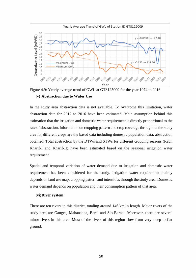
50
Figure 4.9: Yearly average trend of GWL at GT8125009 for the year 1974 to 2016
(v) Abstraction due to Water Use
In the study area abstraction data is not available. To overcome this limitation, water
abstraction data for 2012 to 2016 have been estimated. Main assumption behind this
estimation that the irrigation and domestic water requirement is directly proportional to the
rate of abstraction. Information on cropping pattern and crop coverage throughout the study
area for different crops are the based data including domestic population data, abstraction
obtained. Total abstraction by the DTWs and STWs for different cropping seasons (Rabi,
Kharif-I and Kharif-II) have been estimated based on the seasonal irrigation water
requirement.
Spatial and temporal variation of water demand due to irrigation and domestic water
requirement has been considered for the study. Irrigation water requirement mainly
depends on land use map, cropping pattern and intensities through the study area. Domestic
water demand depends on population and their consumption pattern of that area.
(vi) River system:
There are ten rivers in this district, totaling around 146 km in length. Major rivers of the
study area are Ganges, Mahananda, Baral and Sib-Barnai. Moreover, there are several
minor rivers in this area. Most of the rivers of this region flow from very steep to flat
ground.
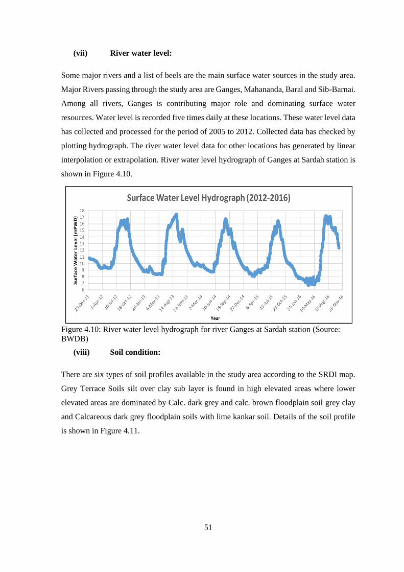
51
(vii) River water level:
Some major rivers and a list of beels are the main surface water sources in the study area.
Major Rivers passing through the study area are Ganges, Mahananda, Baral and Sib-Barnai.
Among all rivers, Ganges is contributing major role and dominating surface water
resources. Water level is recorded five times daily at these locations. These water level data
has collected and processed for the period of 2005 to 2012. Collected data has checked by
plotting hydrograph. The river water level data for other locations has generated by linear
interpolation or extrapolation. River water level hydrograph of Ganges at Sardah station is
shown in Figure 4.10.
Figure 4.10: River water level hydrograph for river Ganges at Sardah station (Source:
BWDB)
(viii) Soil condition:
There are six types of soil profiles available in the study area according to the SRDI map.
Grey Terrace Soils silt over clay sub layer is found in high elevated areas where lower
elevated areas are dominated by Calc. dark grey and calc. brown floodplain soil grey clay
and Calcareous dark grey floodplain soils with lime kankar soil. Details of the soil profile
is shown in Figure 4.11.

52
Figure 4.11: Soil profile map of the study area (Source: SRDI)
(ix) Lithology of the study area:
A general-purpose subsurface lithology of the study area has been prepared by IWM
through analyzing sedimentary structure, its grain size, hydraulic properties, its thickness
and depth. Same litho-logical layers have been taken for this study to prepare MIKE SHE
hydrologic model. A sample hydro-stratigraphic cross sections (Section S2-N2: Figure
4.13) show similar lithological pattern that is used in this study. The plan for hydro-
stratigraphic cross sections are shown in Figure 4.12. Rest of the cross sections (10) have
been shown as Figure C1 to C10 in Appendix-C. Hydro-stratigraphic cross sections show
that the thickness of upper soil thickness is large enough which impedes groundwater
recharge. It is also clear from hydro-stratigraphic cross sections that land slope is very steep
in this region which allows water to runoff rather than infiltration.

53
Figure 4.12: Plan of hydrostat graphic sections
Figure 4.13: Hydro-stratigraphic Cross Section S2-N2 along South to North
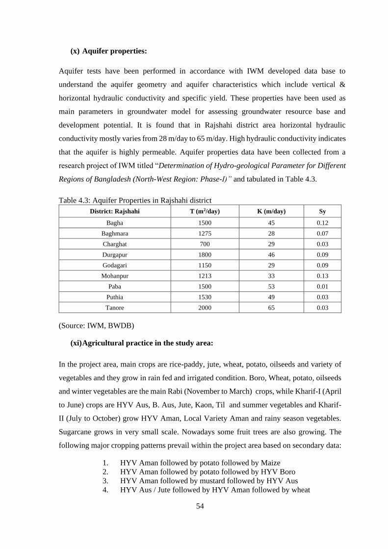
54
(x) Aquifer properties:
Aquifer tests have been performed in accordance with IWM developed data base to
understand the aquifer geometry and aquifer characteristics which include vertical &
horizontal hydraulic conductivity and specific yield. These properties have been used as
main parameters in groundwater model for assessing groundwater resource base and
development potential. It is found that in Rajshahi district area horizontal hydraulic
conductivity mostly varies from 28 m/day to 65 m/day. High hydraulic conductivity indicates
that the aquifer is highly permeable. Aquifer properties data have been collected from a
research project of IWM titled “Determination of Hydro-geological Parameter for Different
Regions of Bangladesh (North-West Region: Phase-I)” and tabulated in Table 4.3.
Table 4.3: Aquifer Properties in Rajshahi district
District: Rajshahi T (m2/day) K (m/day) Sy
Bagha 1500 45 0.12
Baghmara 1275 28 0.07
Charghat 700 29 0.03
Durgapur 1800 46 0.09
Godagari 1150 29 0.09
Mohanpur 1213 33 0.13
Paba 1500 53 0.01
Puthia 1530 49 0.03
Tanore 2000 65 0.03
(Source: IWM, BWDB)
(xi) Agricultural practice in the study area:
In the project area, main crops are rice-paddy, jute, wheat, potato, oilseeds and variety of
vegetables and they grow in rain fed and irrigated condition. Boro, Wheat, potato, oilseeds
and winter vegetables are the main Rabi (November to March) crops, while Kharif-I (April
to June) crops are HYV Aus, B. Aus, Jute, Kaon, Til and summer vegetables and Kharif-
II (July to October) grow HYV Aman, Local Variety Aman and rainy season vegetables.
Sugarcane grows in very small scale. Nowadays some fruit trees are also growing. The
following major cropping patterns prevail within the project area based on secondary data:
1. HYV Aman followed by potato followed by Maize
2. HYV Aman followed by potato followed by HYV Boro
3. HYV Aman followed by mustard followed by HYV Aus
4. HYV Aus / Jute followed by HYV Aman followed by wheat
55
5. HYV Aman followed by HYV Boro
6. HYV Aman followed by wheat
7. HYV Aman followed by potato
8. HYV Aman followed by rabi vegetables
9. HYV Aman followed by Maize
10. HYV Aman followed by pulses
11. Local variety Aman followed by wheat/potato/maize
12. Fruit trees
Drought and inadequate irrigation facilities are the major limitations to intensive land use
and optimum crop production.
(xii) Irrigation System and Coverage:
Scarcity of rainfall from November to May, and scatter and insufficient rains in the months
of September and October, irrigation is essential for intensive use of cultivable land.
Though surface water is available at near the outfall of the Mohananda river into the Ganges
and in the Ganges River, large pumping plants are required for pumping from the river.
Moreover, the water levels of the rivers in some reaches go down beyond the suction limit
of low lift pumps becoming the problems of pumping from river. The study area in major
part is undulating and is not suitable for flood irrigation. Even then, pumping from the
rivers and conserving water by small water control structures now practice limited surface
water irrigation. Main dependence for irrigation is on ground water. Groundwater is being
extracted for irrigation mainly by deep tubewells and very few shallow tubewells. The
irrigation coverage by each DTW is in the range of 12 ha - 25 ha, the average is being 23.68
ha per DTW. Irrigation coverage by each STW is in the range of 1.0 ha-5.0 ha. The average
is 2.42 ha per STW and the average coverage per LLP is 5.63 ha.
4.4 Groundwater Model Set Up
The groundwater model up to a depth of 80m for the study area was developed using MIKE
SHE hydrologic modelling tools to understand the groundwater flow dynamics and to
assess the groundwater resources under the present and various development scenarios.
Model was developed covering entire study area with grids size of 1000m×1000m. After
satisfactory calibration and verification of the model, the model has been applied for
various development options to identify suitable cropping options for groundwater
resources.
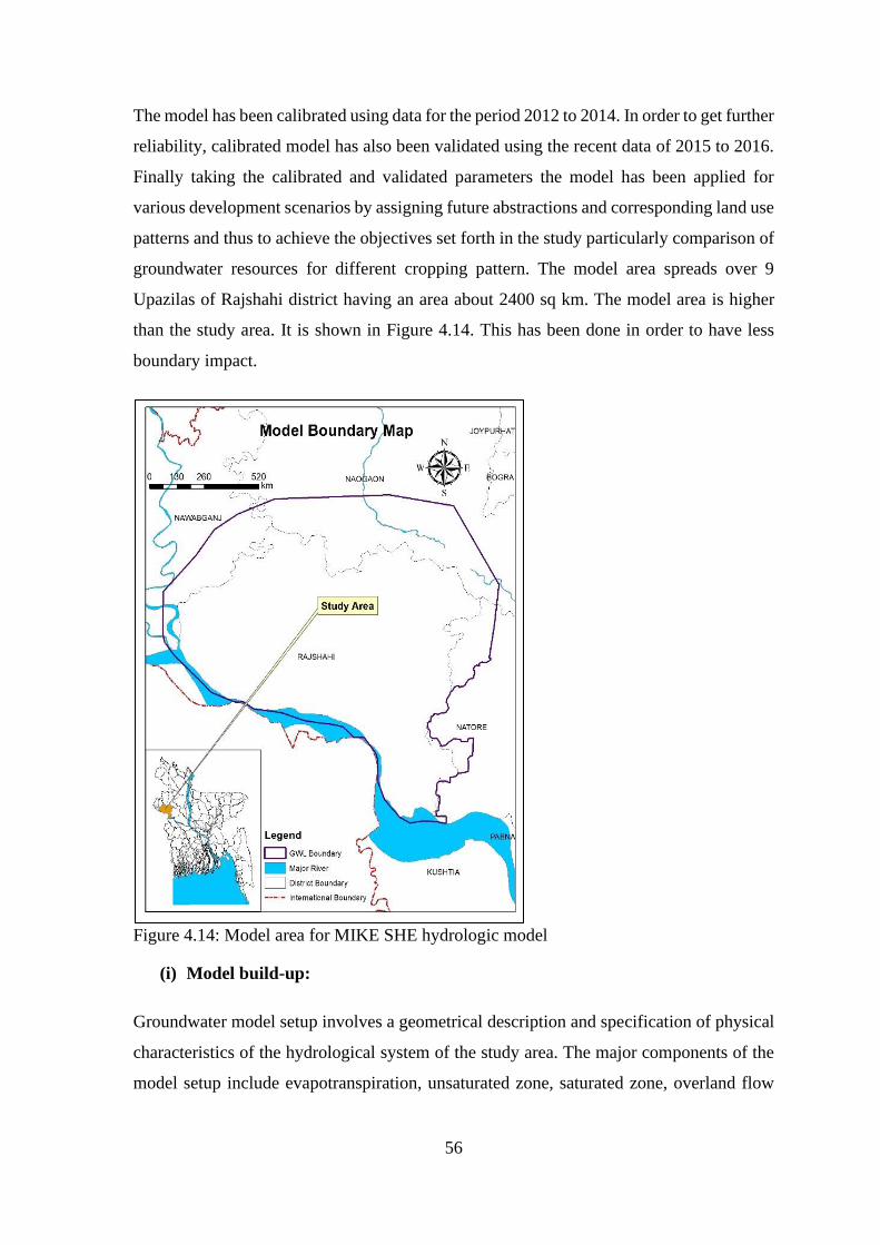
56
The model has been calibrated using data for the period 2012 to 2014. In order to get further
reliability, calibrated model has also been validated using the recent data of 2015 to 2016.
Finally taking the calibrated and validated parameters the model has been applied for
various development scenarios by assigning future abstractions and corresponding land use
patterns and thus to achieve the objectives set forth in the study particularly comparison of
groundwater resources for different cropping pattern. The model area spreads over 9
Upazilas of Rajshahi district having an area about 2400 sq km. The model area is higher
than the study area. It is shown in Figure 4.14. This has been done in order to have less
boundary impact.
Figure 4.14: Model area for MIKE SHE hydrologic model
(i) Model build-up:
Groundwater model setup involves a geometrical description and specification of physical
characteristics of the hydrological system of the study area. The major components of the
model setup include evapotranspiration, unsaturated zone, saturated zone, overland flow
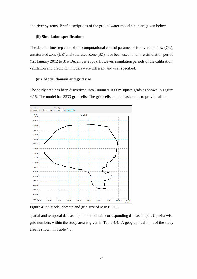
57
and river systems. Brief descriptions of the groundwater model setup are given below.
(ii) Simulation specification:
The default time step control and computational control parameters for overland flow (OL),
unsaturated zone (UZ) and Saturated Zone (SZ) have been used for entire simulation period
(1st January 2012 to 31st December 2030). However, simulation periods of the calibration,
validation and prediction models were different and user specified.
(iii) Model domain and grid size
The study area has been discretized into 1000m x 1000m square grids as shown in Figure
4.15. The model has 3233 grid cells. The grid cells are the basic units to provide all the
Figure 4.15: Model domain and grid size of MIKE SHE
spatial and temporal data as input and to obtain corresponding data as output. Upazila wise
grid numbers within the study area is given in Table 4.4. A geographical limit of the study
area is shown in Table 4.5.
58
Table 4.4: Grid cells used for model setup
Upazilas of the Rajshahi
District
Numbers of Grid Cells (area: 1 km2)
Upazila wise Study area Model area
Godagari 472
2378 3233
Charghat 165
Tanore 295
Durgapur 195
Paba 280
Puthia 193
Baghmara 363
Bagha 184
Mohanpur 163
Geographical limit of the model area falls between 410000 m East, 66000 m North to
320000 m East, 750000 m North in Bangladesh Transverse Mercator (BTM) projection
system.
(iv) Topography:
A well-prepared digital elevation model (DEM) is essential for visualizing the floodplain
topography and for accurate Modelling. A DEM of 30 m resolution has been developed to
define the topography of the study area and used in the model. Topographic data for the
study area has been extracted from USGS Earth Explorer.
(v) Precipitation and evapotranspiration:
Rainfall data is very essential input for the model. There are twelve (12) rainfall stations
are available in and around the model area. To account for the spatial variation in rainfall,
the time series data for each station has been associated with an area. This area has been
estimated by Thiessen Polygon Method. The rainfall data for the relevant stations have
been collected from BWDB office. After checking the consistency of these data, the time
series input files for precipitation have been computed, projected for future scenarios and
incorporated in the model. To account for the spatial variation in rainfall, the time series
data for each station has been assigned to thiessen polygon is shown in Figure 4.16.
Time series data for the potential Evapotranspiration are given as input to the model. The
evaporation data of Rajshahi station, used in the model is discussed earlier.
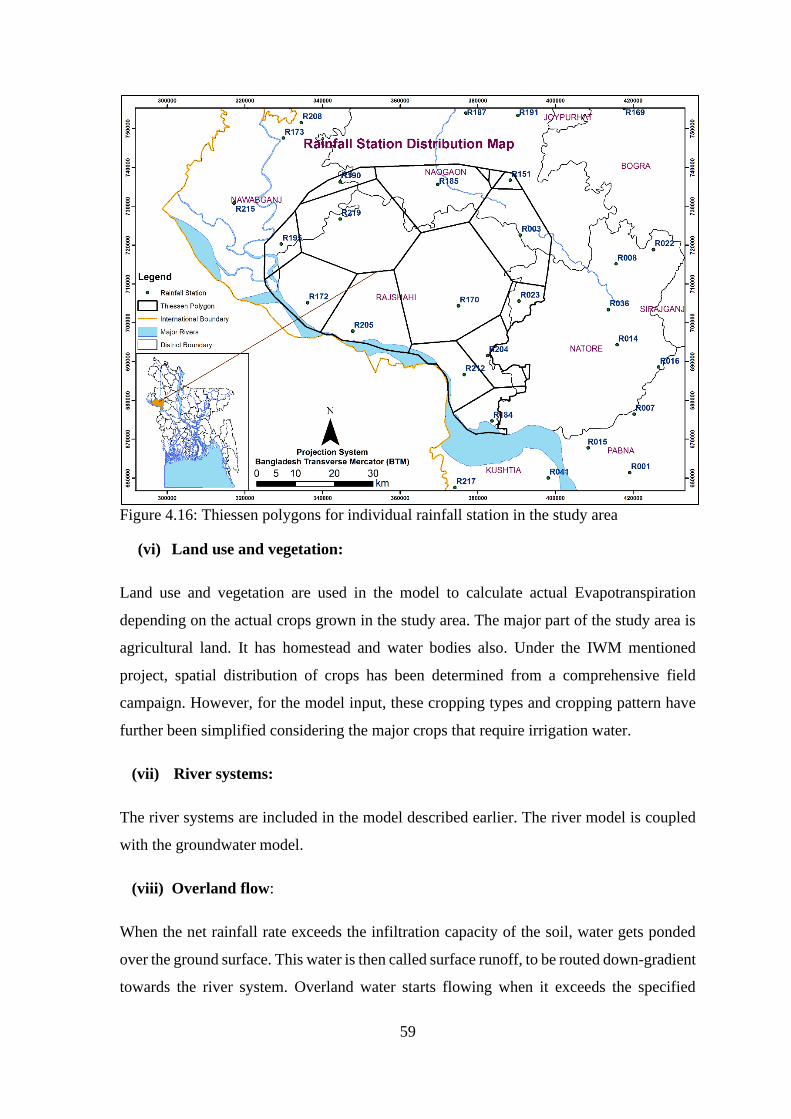
59
Figure 4.16: Thiessen polygons for individual rainfall station in the study area
(vi) Land use and vegetation:
Land use and vegetation are used in the model to calculate actual Evapotranspiration
depending on the actual crops grown in the study area. The major part of the study area is
agricultural land. It has homestead and water bodies also. Under the IWM mentioned
project, spatial distribution of crops has been determined from a comprehensive field
campaign. However, for the model input, these cropping types and cropping pattern have
further been simplified considering the major crops that require irrigation water.
(vii) River systems:
The river systems are included in the model described earlier. The river model is coupled
with the groundwater model.
(viii) Overland flow:
When the net rainfall rate exceeds the infiltration capacity of the soil, water gets ponded
over the ground surface. This water is then called surface runoff, to be routed down-gradient
towards the river system. Overland water starts flowing when it exceeds the specified
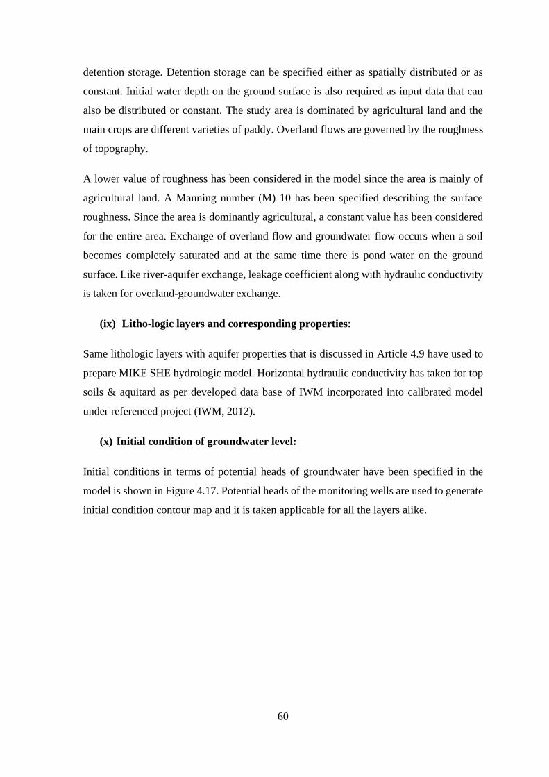
60
detention storage. Detention storage can be specified either as spatially distributed or as
constant. Initial water depth on the ground surface is also required as input data that can
also be distributed or constant. The study area is dominated by agricultural land and the
main crops are different varieties of paddy. Overland flows are governed by the roughness
of topography.
A lower value of roughness has been considered in the model since the area is mainly of
agricultural land. A Manning number (M) 10 has been specified describing the surface
roughness. Since the area is dominantly agricultural, a constant value has been considered
for the entire area. Exchange of overland flow and groundwater flow occurs when a soil
becomes completely saturated and at the same time there is pond water on the ground
surface. Like river-aquifer exchange, leakage coefficient along with hydraulic conductivity
is taken for overland-groundwater exchange.
(ix) Litho-logic layers and corresponding properties:
Same lithologic layers with aquifer properties that is discussed in Article 4.9 have used to
prepare MIKE SHE hydrologic model. Horizontal hydraulic conductivity has taken for top
soils & aquitard as per developed data base of IWM incorporated into calibrated model
under referenced project (IWM, 2012).
(x) Initial condition of groundwater level:
Initial conditions in terms of potential heads of groundwater have been specified in the
model is shown in Figure 4.17. Potential heads of the monitoring wells are used to generate
initial condition contour map and it is taken applicable for all the layers alike.
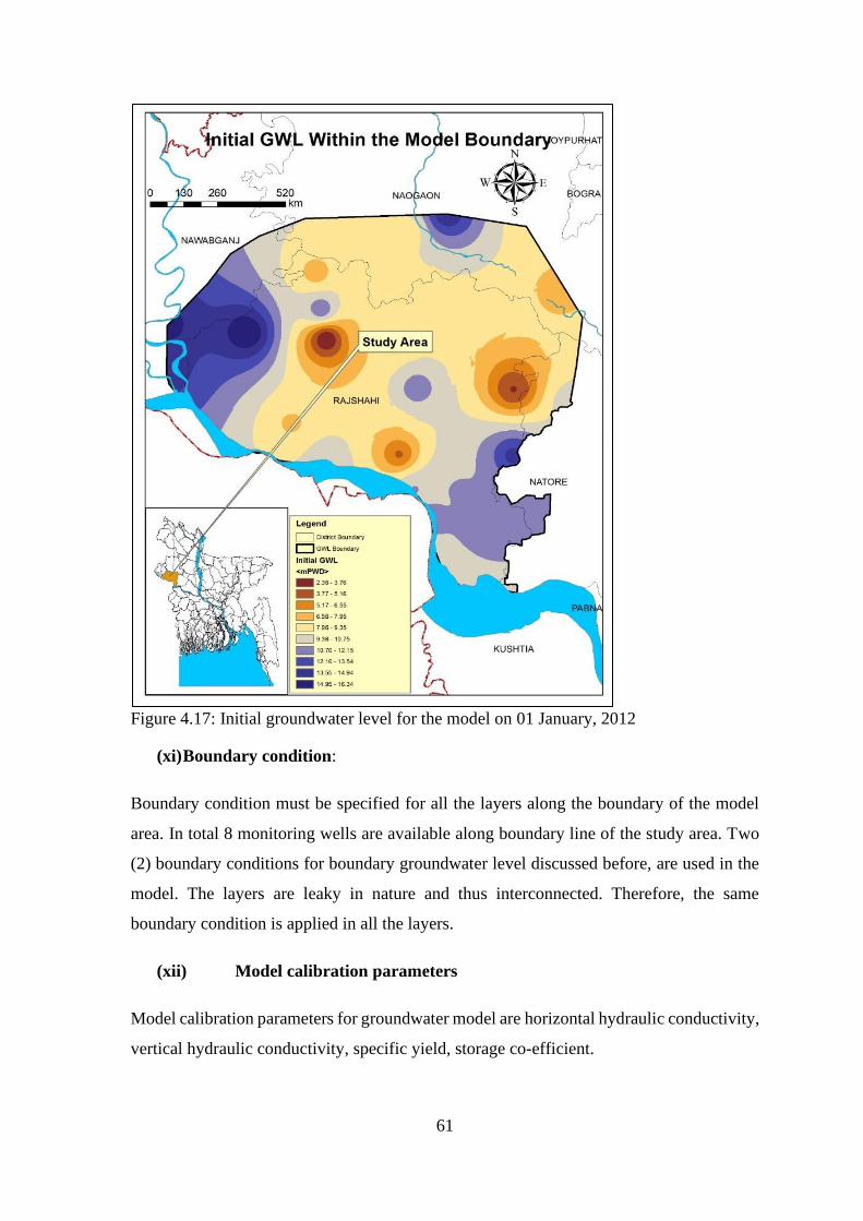
61
Figure 4.17: Initial groundwater level for the model on 01 January, 2012
(xi) Boundary condition:
Boundary condition must be specified for all the layers along the boundary of the model
area. In total 8 monitoring wells are available along boundary line of the study area. Two
(2) boundary conditions for boundary groundwater level discussed before, are used in the
model. The layers are leaky in nature and thus interconnected. Therefore, the same
boundary condition is applied in all the layers.
(xii) Model calibration parameters
Model calibration parameters for groundwater model are horizontal hydraulic conductivity,
vertical hydraulic conductivity, specific yield, storage co-efficient.
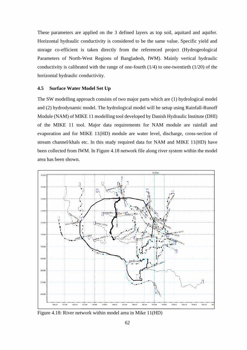
62
These parameters are applied on the 3 defined layers as top soil, aquitard and aquifer.
Horizontal hydraulic conductivity is considered to be the same value. Specific yield and
storage co-efficient is taken directly from the referenced project (Hydrogeological
Parameters of North-West Regions of Bangladesh, IWM). Mainly vertical hydraulic
conductivity is calibrated with the range of one-fourth (1/4) to one-twentieth (1/20) of the
horizontal hydraulic conductivity.
4.5 Surface Water Model Set Up
The SW modelling approach consists of two major parts which are (1) hydrological model
and (2) hydrodynamic model. The hydrological model will be setup using Rainfall-Runoff
Module (NAM) of MIKE 11 modelling tool developed by Danish Hydraulic Institute (DHI)
of the MIKE 11 tool. Major data requirements for NAM module are rainfall and
evaporation and for MIKE 11(HD) module are water level, discharge, cross-section of
stream channel/khals etc. In this study required data for NAM and MIKE 11(HD) have
been collected from IWM. In Figure 4.18 network file along river system within the model
area has been shown.
Figure 4.18: River network within model area in Mike 11(HD)
63
(i) Major rivers within the Surface Water model area:
The study area hasn’t enough major rivers but there are some major rivers surrounding its
area. Some of the name of rivers/khals are given below in a list and shown in Figure 4.19.
Name of Rivers in the Study Area:
S.N. RiverName S.N. RiverName
1 Atrai 15 Little Jamuna
2 Atrai-Sib Link 16 Little Nagor-Atrai Link
3 Baral 17 Little Nagor
4 Baranai Branch 18 Mohanada
5 Borokhari 19 Monohorganga Khal
6 Durgapur Khal 20 Musakhan
7 Fakirni 21 Nandakuja
8 Ganges 22 Narod
9 Ghaelgurhari Khal 23 Pagla
10 Godai 24 Rasulpur Khal
11 Hoja Khal 25 Sabaibeel
12 Joai Khari 26 Sib-Barnai
13 Kamargaon Khari 27 Zia Khal
14 Khalishadingi 28 Pangal
Figure 4.19: River network of the study area and surrounding
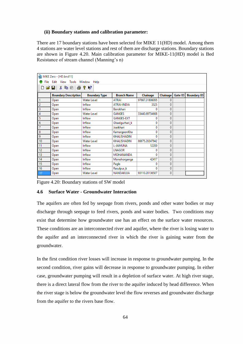
64
(ii) Boundary stations and calibration parameter:
There are 17 boundary stations have been selected for MIKE 11(HD) model. Among them
4 stations are water level stations and rest of them are discharge stations. Boundary stations
are shown in Figure 4.20. Main calibration parameter for MIKE-11(HD) model is Bed
Resistance of stream channel (Manning’s n)
Figure 4.20: Boundary stations of SW model
4.6 Surface Water - Groundwater Interaction
The aquifers are often fed by seepage from rivers, ponds and other water bodies or may
discharge through seepage to feed rivers, ponds and water bodies. Two conditions may
exist that determine how groundwater use has an effect on the surface water resources.
These conditions are an interconnected river and aquifer, where the river is losing water to
the aquifer and an interconnected river in which the river is gaining water from the
groundwater.
In the first condition river losses will increase in response to groundwater pumping. In the
second condition, river gains will decrease in response to groundwater pumping. In either
case, groundwater pumping will result in a depletion of surface water. At high river stage,
there is a direct lateral flow from the river to the aquifer induced by head difference. When
the river stage is below the groundwater level the flow reverses and groundwater discharge
from the aquifer to the rivers base flow.

65
Due to natural discharge and withdrawal for irrigation and domestic purposes the
groundwater level in April attains the lowest level. As soon as the irrigation stopped, there
is a rise of groundwater level due to recovery of groundwater and there is a sharp rise after
June with the beginning of rainfall because about 30% of total rainfall goes to aquifer as
recharge (Karim, 1972).
4.7 Summary
Mathematical modelling tools are used in this study to simulate the existing and future
complex scenarios simply. Before model setup, it is necessary to know every details of the
study area so that actual scenario of study area can be simulated in the model. Detail
analysis of the study area also helps to find sustainable solution of existing problems which
are applicable in field level.

CHAPTER 5
RESULTS AND DISCUSSIONS
5.1 General
Proper calibration and validation of the base model for the study area are the prerequisite
for future scenario development. So, emphasis has been given to this fact and tried to
calibrate and validate this Surface Water-Groundwater integrated model as good as
possible. After completion of calibration and validation of the base model, optional run has
been performed based on assumed scenarios and most extreme scenario and suitable
intervention have been found out.
5.2 Calibration and Validation of the SW and GW Models
Model calibration is the process of adjustment of the model parameters and forcing within
the margins of the uncertainties to obtain a model representation of the processes of interest
that satisfies pre-agreed criteria (Goodness-of-Fit). Model validation is in reality an
extension of the calibration process. Its purpose is to assure that the calibrated model
properly assesses all the variables and conditions which can affect model results and
demonstrate the ability to predict field observations for periods/conditions separate from
the calibration effort.
5.2.1 Calibration and Validation of SW Model
The MIKE 11 model has been calibrated and validated with observed data. This model has
been calibrated for 3 years (January to December of 2012 to 2014) and has been validated
for next 2 years (January to December of 2015 to 2016). Summary table of calibration and
validation has been shown in Table 5.1. Main calibration parameter for MIKE-11(HD)
model is Bed Resistance of stream channel (Manning’s n). Calibration and validation of
surface water model for surface water level at Chapai-Nawabganj Station on Mohananda
River is shown in Figure 5.1. From this figure it is observed that superimposed observed
and simulated results are almost identical which indicates good calibration and validation
of this model at this station. Figure 5.2 shows calibration and validation of surface water
model for surface water level at Singra Station on Atrai River. This superimposed graph
also indicates good model performance at this station. Plots of other stations are shown in
Appendix-D.
66
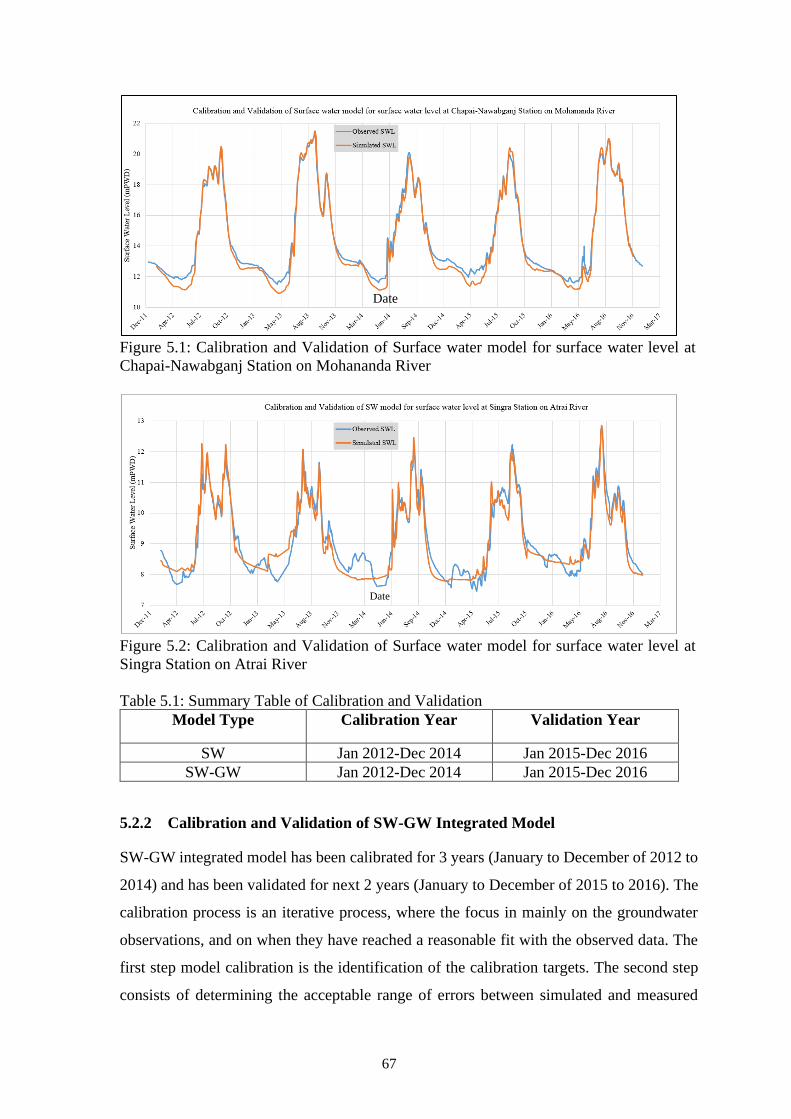
Figure 5.1: Calibration and Validation of Surface water model for surface water level at
Chapai-Nawabganj Station on Mohananda River
Figure 5.2: Calibration and Validation of Surface water model for surface water level at
Singra Station on Atrai River
Table 5.1: Summary Table of Calibration and Validation
Model Type Calibration Year Validation Year
SW Jan 2012-Dec 2014 Jan 2015-Dec 2016
SW-GW Jan 2012-Dec 2014 Jan 2015-Dec 2016
5.2.2 Calibration and Validation of SW-GW Integrated Model
SW-GW integrated model has been calibrated for 3 years (January to December of 2012 to
2014) and has been validated for next 2 years (January to December of 2015 to 2016). The
calibration process is an iterative process, where the focus in mainly on the groundwater
observations, and on when they have reached a reasonable fit with the observed data. The
first step model calibration is the identification of the calibration targets. The second step
consists of determining the acceptable range of errors between simulated and measured
Date
Date
67
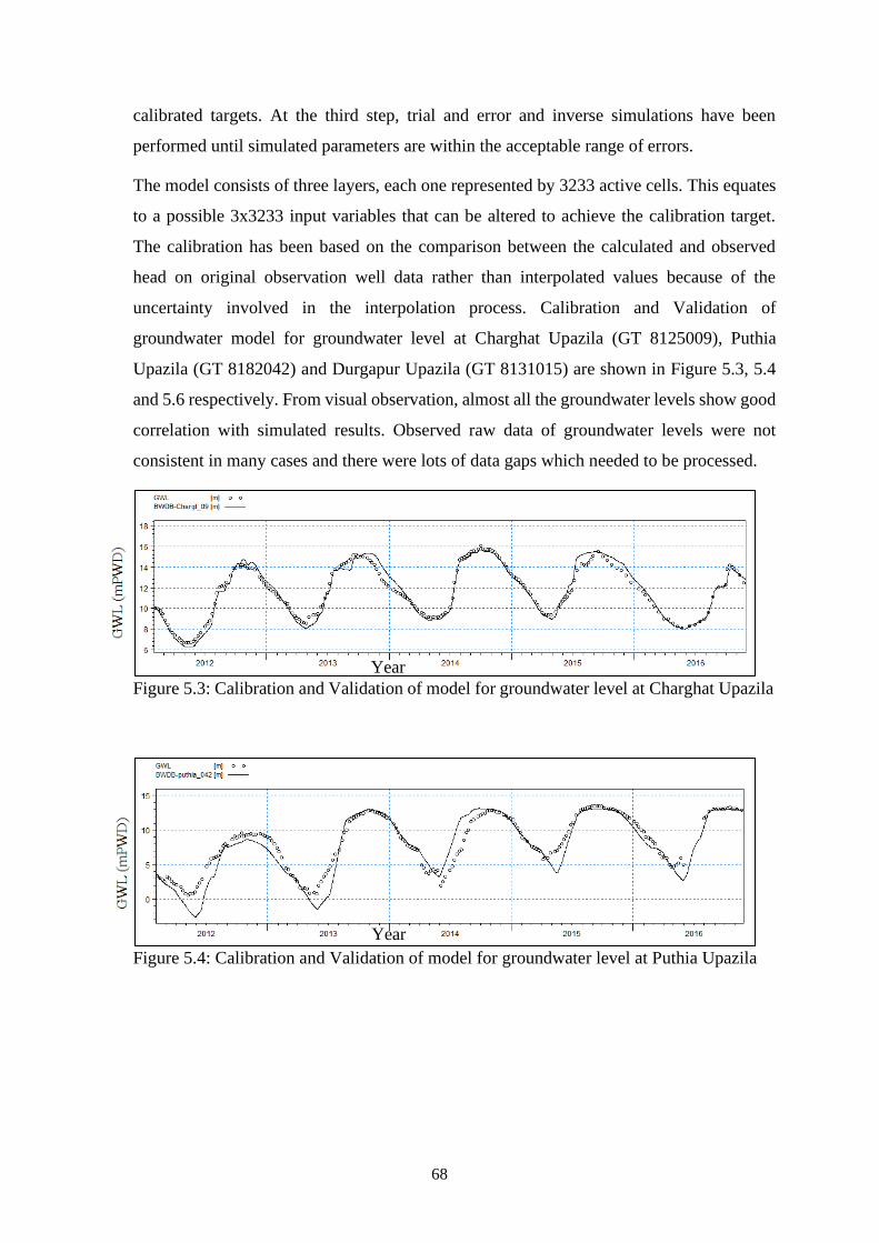
calibrated targets. At the third step, trial and error and inverse simulations have been
performed until simulated parameters are within the acceptable range of errors.
The model consists of three layers, each one represented by 3233 active cells. This equates
to a possible 3x3233 input variables that can be altered to achieve the calibration target.
The calibration has been based on the comparison between the calculated and observed
head on original observation well data rather than interpolated values because of the
uncertainty involved in the interpolation process. Calibration and Validation of
groundwater model for groundwater level at Charghat Upazila (GT 8125009), Puthia
Upazila (GT 8182042) and Durgapur Upazila (GT 8131015) are shown in Figure 5.3, 5.4
and 5.6 respectively. From visual observation, almost all the groundwater levels show good
correlation with simulated results. Observed raw data of groundwater levels were not
consistent in many cases and there were lots of data gaps which needed to be processed.
Figure 5.3: Calibration and Validation of model for groundwater level at Charghat Upazila
Figure 5.4: Calibration and Validation of model for groundwater level at Puthia Upazila
Year
Year
68
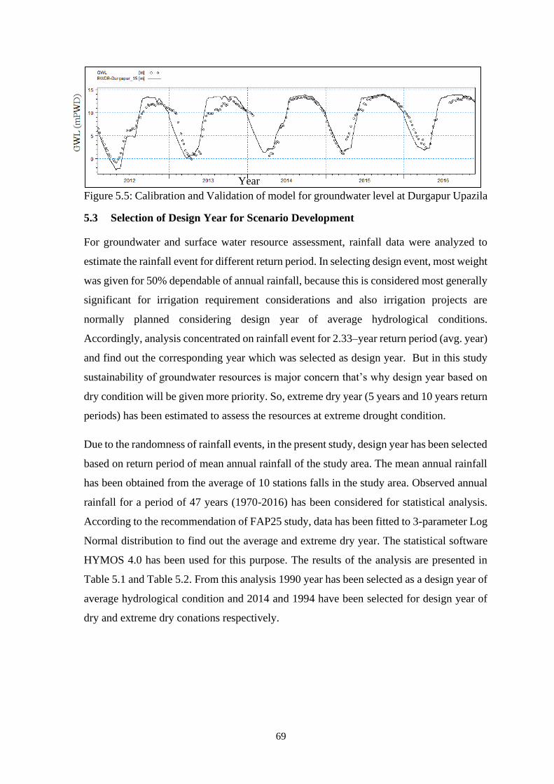
Figure 5.5: Calibration and Validation of model for groundwater level at Durgapur Upazila
5.3 Selection of Design Year for Scenario Development
For groundwater and surface water resource assessment, rainfall data were analyzed to
estimate the rainfall event for different return period. In selecting design event, most weight
was given for 50% dependable of annual rainfall, because this is considered most generally
significant for irrigation requirement considerations and also irrigation projects are
normally planned considering design year of average hydrological conditions.
Accordingly, analysis concentrated on rainfall event for 2.33–year return period (avg. year)
and find out the corresponding year which was selected as design year. But in this study
sustainability of groundwater resources is major concern that’s why design year based on
dry condition will be given more priority. So, extreme dry year (5 years and 10 years return
periods) has been estimated to assess the resources at extreme drought condition.
Due to the randomness of rainfall events, in the present study, design year has been selected
based on return period of mean annual rainfall of the study area. The mean annual rainfall
has been obtained from the average of 10 stations falls in the study area. Observed annual
rainfall for a period of 47 years (1970-2016) has been considered for statistical analysis.
According to the recommendation of FAP25 study, data has been fitted to 3-parameter Log
Normal distribution to find out the average and extreme dry year. The statistical software
HYMOS 4.0 has been used for this purpose. The results of the analysis are presented in
Table 5.1 and Table 5.2. From this analysis 1990 year has been selected as a design year of
average hydrological condition and 2014 and 1994 have been selected for design year of
dry and extreme dry conations respectively.
Year
69
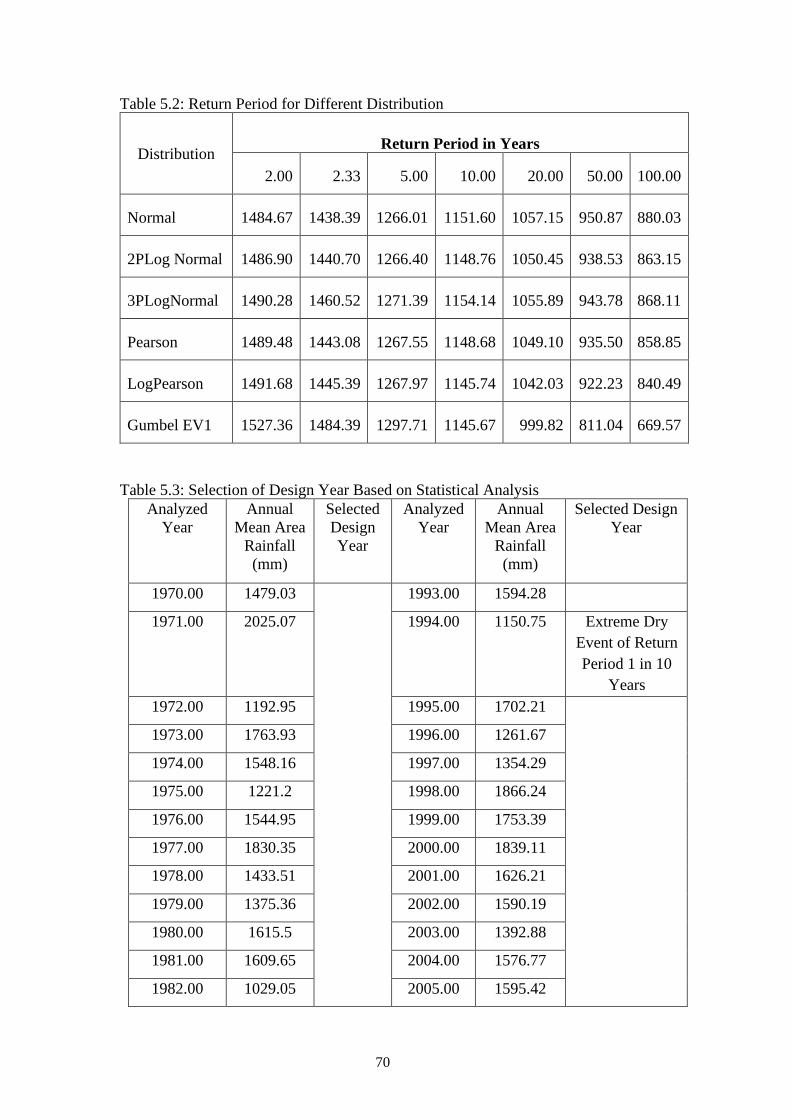
Table 5.2: Return Period for Different Distribution
Distribution Return Period in Years
2.00 2.33 5.00 10.00 20.00 50.00 100.00
Normal 1484.67 1438.39 1266.01 1151.60 1057.15 950.87 880.03
2PLog Normal 1486.90 1440.70 1266.40 1148.76 1050.45 938.53 863.15
3PLogNormal 1490.28 1460.52 1271.39 1154.14 1055.89 943.78 868.11
Pearson 1489.48 1443.08 1267.55 1148.68 1049.10 935.50 858.85
LogPearson 1491.68 1445.39 1267.97 1145.74 1042.03 922.23 840.49
Gumbel EV1 1527.36 1484.39 1297.71 1145.67 999.82 811.04 669.57
Table 5.3: Selection of Design Year Based on Statistical Analysis
Analyzed
Year
Annual
Mean Area
Rainfall
(mm)
Selected
Design
Year
Analyzed
Year
Annual
Mean Area
Rainfall
(mm)
Selected Design
Year
1970.00 1479.03 1993.00 1594.28
1971.00 2025.07 1994.00 1150.75 Extreme Dry
Event of Return
Period 1 in 10
Years
1972.00 1192.95 1995.00 1702.21
1973.00 1763.93 1996.00 1261.67
1974.00 1548.16 1997.00 1354.29
1975.00 1221.2 1998.00 1866.24
1976.00 1544.95 1999.00 1753.39
1977.00 1830.35 2000.00 1839.11
1978.00 1433.51 2001.00 1626.21
1979.00 1375.36 2002.00 1590.19
1980.00 1615.5 2003.00 1392.88
1981.00 1609.65 2004.00 1576.77
1982.00 1029.05 2005.00 1595.42
70
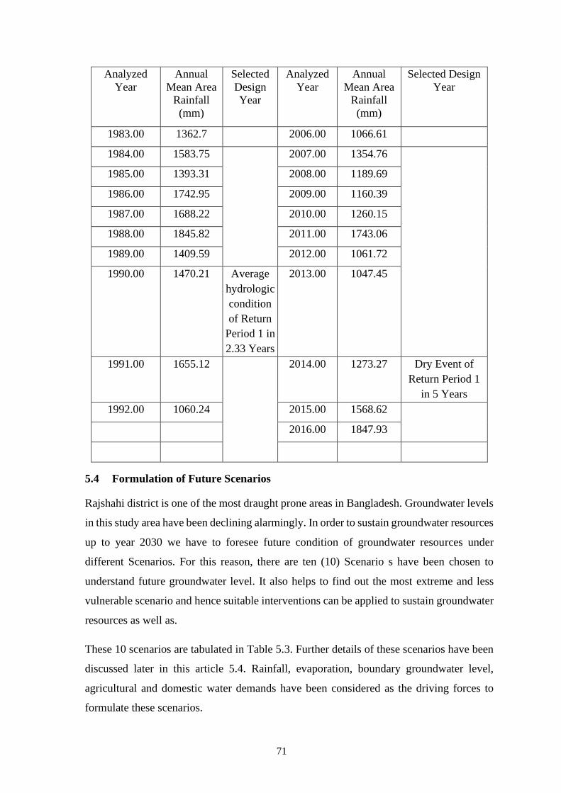
Analyzed
Year
Annual
Mean Area
Rainfall
(mm)
Selected
Design
Year
Analyzed
Year
Annual
Mean Area
Rainfall
(mm)
Selected Design
Year
1983.00 1362.7 2006.00 1066.61
1984.00 1583.75 2007.00 1354.76
1985.00 1393.31 2008.00 1189.69
1986.00 1742.95 2009.00 1160.39
1987.00 1688.22 2010.00 1260.15
1988.00 1845.82 2011.00 1743.06
1989.00 1409.59 2012.00 1061.72
1990.00 1470.21 Average
hydrologic
condition
of Return
Period 1 in
2.33 Years
2013.00 1047.45
1991.00 1655.12 2014.00 1273.27 Dry Event of
Return Period 1
in 5 Years
1992.00 1060.24 2015.00 1568.62
2016.00 1847.93
5.4 Formulation of Future Scenarios
Rajshahi district is one of the most draught prone areas in Bangladesh. Groundwater levels
in this study area have been declining alarmingly. In order to sustain groundwater resources
up to year 2030 we have to foresee future condition of groundwater resources under
different Scenarios. For this reason, there are ten (10) Scenario s have been chosen to
understand future groundwater level. It also helps to find out the most extreme and less
vulnerable scenario and hence suitable interventions can be applied to sustain groundwater
resources as well as.
These 10 scenarios are tabulated in Table 5.3. Further details of these scenarios have been
discussed later in this article 5.4. Rainfall, evaporation, boundary groundwater level,
agricultural and domestic water demands have been considered as the driving forces to
formulate these scenarios.
71
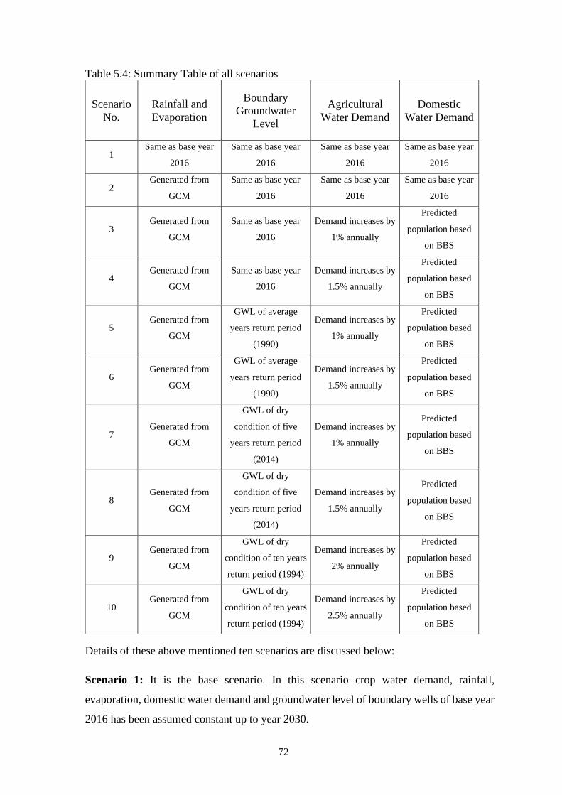
Table 5.4: Summary Table of all scenarios
Scenario
No.
Rainfall and
Evaporation
Boundary
Groundwater
Level
Agricultural
Water Demand
Domestic
Water Demand
1 Same as base year
2016
Same as base year
2016
Same as base year
2016
Same as base year
2016
2 Generated from
GCM
Same as base year
2016
Same as base year
2016
Same as base year
2016
3 Generated from
GCM
Same as base year
2016
Demand increases by
1% annually
Predicted
population based
on BBS
4 Generated from
GCM
Same as base year
2016
Demand increases by
1.5% annually
Predicted
population based
on BBS
5 Generated from
GCM
GWL of average
years return period
(1990)
Demand increases by
1% annually
Predicted
population based
on BBS
6 Generated from
GCM
GWL of average
years return period
(1990)
Demand increases by
1.5% annually
Predicted
population based
on BBS
7 Generated from
GCM
GWL of dry
condition of five
years return period
(2014)
Demand increases by
1% annually
Predicted
population based
on BBS
8 Generated from
GCM
GWL of dry
condition of five
years return period
(2014)
Demand increases by
1.5% annually
Predicted
population based
on BBS
9 Generated from
GCM
GWL of dry
condition of ten years
return period (1994)
Demand increases by
2% annually
Predicted
population based
on BBS
10 Generated from
GCM
GWL of dry
condition of ten years
return period (1994)
Demand increases by
2.5% annually
Predicted
population based
on BBS
Details of these above mentioned ten scenarios are discussed below:
Scenario 1: It is the base scenario. In this scenario crop water demand, rainfall,
evaporation, domestic water demand and groundwater level of boundary wells of base year
2016 has been assumed constant up to year 2030.
72
Scenario 2: Same as scenario 01 except rainfall and evaporation data have been generated
from 2016 to 2030 from GCM model of HADCM3 under emission scenario SRA2 with the
help of Climate change editor module of MIKE software.
Scenario 3: Same as scenario 2 except crop water demand of the base year 2016 has been
increased annually by 1% up to year 2030. Groundwater level of boundary wells of base
year 2016 has been assumed constant up to year 2030.
Scenario 4: Same as scenario 3 except crop water demand of the base year 2016 has been
increased annually by 1.5% up to year 2030. Groundwater level of boundary wells of base
year 2016 has been assumed constant up to year 2030.
Scenario 5: Same as scenario 3 except boundary groundwater level of the average
condition of hydrological year of 1990 (2.33 years of return period) has been assumed
constant up to year 2030.
Scenario 6: Same as scenario 4 except boundary groundwater level of the average
condition of hydrological year of 1990 (2.33 years of return period) has been assumed
constant up to year 2030.
Scenario 7: Same as scenario 3 except boundary groundwater level of the dry condition of
hydrological year of 2014 (5 years of return period) has been assumed constant up to year
2030.
Scenario 8: Same as scenario 4 except boundary groundwater level of the dry condition of
hydrological year of 2014 (5 years of return period) has been assumed constant up to year
2030.
Scenario 9: In this scenario crop water demand of the base year 2016 has been increased
annually by 2% up to year 2030. Rainfall and evaporation data have been generated from
2016 to 2030 from GCM model of HADCM3 under emission scenario SRA2 with the help
of Climate change editor module of MIKE software. Boundary groundwater level of the
extreme dry condition of hydrological year of 1994 (10 years of return period) has been
assumed constant up to year 2030.
Scenario 10: Same as scenario 09 except crop water demand of the base year 2016 has
been increased annually by 2.5% up to year 2030.
73
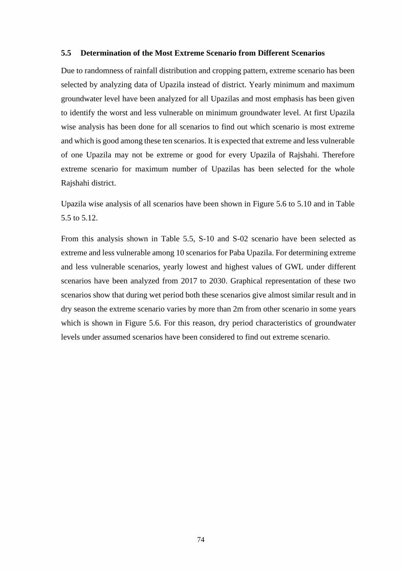
5.5 Determination of the Most Extreme Scenario from Different Scenarios
Due to randomness of rainfall distribution and cropping pattern, extreme scenario has been
selected by analyzing data of Upazila instead of district. Yearly minimum and maximum
groundwater level have been analyzed for all Upazilas and most emphasis has been given
to identify the worst and less vulnerable on minimum groundwater level. At first Upazila
wise analysis has been done for all scenarios to find out which scenario is most extreme
and which is good among these ten scenarios. It is expected that extreme and less vulnerable
of one Upazila may not be extreme or good for every Upazila of Rajshahi. Therefore
extreme scenario for maximum number of Upazilas has been selected for the whole
Rajshahi district.
Upazila wise analysis of all scenarios have been shown in Figure 5.6 to 5.10 and in Table
5.5 to 5.12.
From this analysis shown in Table 5.5, S-10 and S-02 scenario have been selected as
extreme and less vulnerable among 10 scenarios for Paba Upazila. For determining extreme
and less vulnerable scenarios, yearly lowest and highest values of GWL under different
scenarios have been analyzed from 2017 to 2030. Graphical representation of these two
scenarios show that during wet period both these scenarios give almost similar result and in
dry season the extreme scenario varies by more than 2m from other scenario in some years
which is shown in Figure 5.6. For this reason, dry period characteristics of groundwater
levels under assumed scenarios have been considered to find out extreme scenario.
74
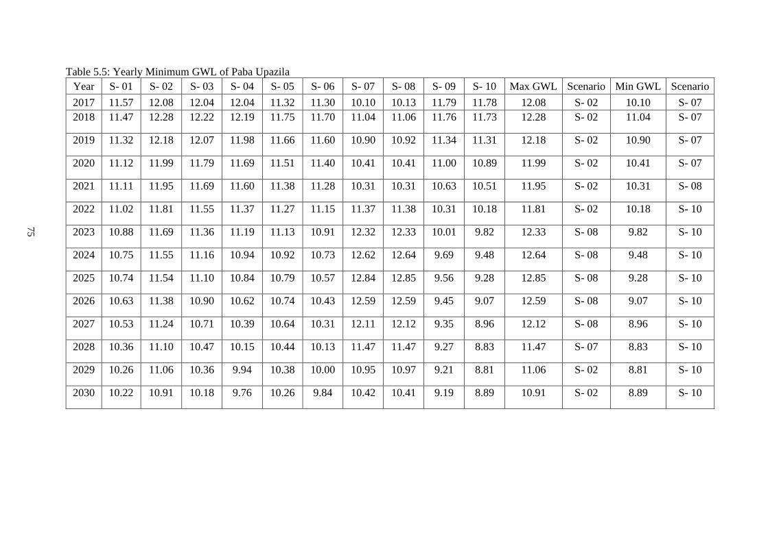
Table 5.5: Yearly Minimum GWL of Paba Upazila
Year S- 01 S- 02 S- 03 S- 04 S- 05 S- 06 S- 07 S- 08 S- 09 S- 10 Max GWL Scenario Min GWL Scenario
2017 11.57 12.08 12.04 12.04 11.32 11.30 10.10 10.13 11.79 11.78 12.08 S- 02 10.10 S- 07
2018 11.47 12.28 12.22 12.19 11.75 11.70 11.04 11.06 11.76 11.73 12.28 S- 02 11.04 S- 07
2019 11.32 12.18 12.07 11.98 11.66 11.60 10.90 10.92 11.34 11.31 12.18 S- 02 10.90 S- 07
2020 11.12 11.99 11.79 11.69 11.51 11.40 10.41 10.41 11.00 10.89 11.99 S- 02 10.41 S- 07
2021 11.11 11.95 11.69 11.60 11.38 11.28 10.31 10.31 10.63 10.51 11.95 S- 02 10.31 S- 08
2022 11.02 11.81 11.55 11.37 11.27 11.15 11.37 11.38 10.31 10.18 11.81 S- 02 10.18 S- 10
2023 10.88 11.69 11.36 11.19 11.13 10.91 12.32 12.33 10.01 9.82 12.33 S- 08 9.82 S- 10
2024 10.75 11.55 11.16 10.94 10.92 10.73 12.62 12.64 9.69 9.48 12.64 S- 08 9.48 S- 10
2025 10.74 11.54 11.10 10.84 10.79 10.57 12.84 12.85 9.56 9.28 12.85 S- 08 9.28 S- 10
2026 10.63 11.38 10.90 10.62 10.74 10.43 12.59 12.59 9.45 9.07 12.59 S- 08 9.07 S- 10
2027 10.53 11.24 10.71 10.39 10.64 10.31 12.11 12.12 9.35 8.96 12.12 S- 08 8.96 S- 10
2028 10.36 11.10 10.47 10.15 10.44 10.13 11.47 11.47 9.27 8.83 11.47 S- 07 8.83 S- 10
2029 10.26 11.06 10.36 9.94 10.38 10.00 10.95 10.97 9.21 8.81 11.06 S- 02 8.81 S- 10
2030 10.22 10.91 10.18 9.76 10.26 9.84 10.42 10.41 9.19 8.89 10.91 S- 02 8.89 S- 10
75
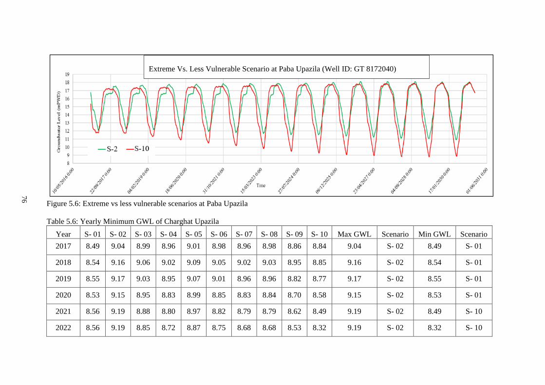
Figure 5.6: Extreme vs less vulnerable scenarios at Paba Upazila
Table 5.6: Yearly Minimum GWL of Charghat Upazila
Year S- 01 S- 02 S- 03 S- 04 S- 05 S- 06 S- 07 S- 08 S- 09 S- 10 Max GWL Scenario Min GWL Scenario
2017 8.49 9.04 8.99 8.96 9.01 8.98 8.96 8.98 8.86 8.84 9.04 S- 02 8.49 S- 01
2018 8.54 9.16 9.06 9.02 9.09 9.05 9.02 9.03 8.95 8.85 9.16 S- 02 8.54 S- 01
2019 8.55 9.17 9.03 8.95 9.07 9.01 8.96 8.96 8.82 8.77 9.17 S- 02 8.55 S- 01
2020 8.53 9.15 8.95 8.83 8.99 8.85 8.83 8.84 8.70 8.58 9.15 S- 02 8.53 S- 01
2021 8.56 9.19 8.88 8.80 8.97 8.82 8.79 8.79 8.62 8.49 9.19 S- 02 8.49 S- 10
2022 8.56 9.19 8.85 8.72 8.87 8.75 8.68 8.68 8.53 8.32 9.19 S- 02 8.32 S- 10
Extreme Vs. Less Vulnerable Scenario at Paba Upazila (Well ID: GT 8172040)
76
Year S- 01 S- 02 S- 03 S- 04 S- 05 S- 06 S- 07 S- 08 S- 09 S- 10 Max GWL Scenario Min GWL Scenario
2023 8.56 9.20 8.82 8.61 8.85 8.65 8.58 8.58 8.36 8.17 9.20 S- 02 8.17 S- 10
2024 8.54 9.16 8.74 8.50 8.77 8.54 8.45 8.46 8.24 8.00 9.16 S- 02 8.00 S- 10
2025 8.56 9.21 8.71 8.40 8.74 8.48 8.35 8.36 8.15 7.89 9.21 S- 02 7.89 S- 10
2026 8.56 9.21 8.64 8.34 8.68 8.36 8.31 8.31 8.04 7.85 9.21 S- 02 7.85 S- 10
2027 8.56 9.21 8.58 8.25 8.60 8.29 8.23 8.23 7.91 7.83 9.21 S- 02 7.83 S- 10
2028 8.52 9.17 8.50 8.11 8.54 8.15 8.10 8.11 7.85 7.74 9.17 S- 02 7.74 S- 10
2029 8.55 9.22 8.48 8.07 8.52 8.10 8.08 8.08 7.85 7.71 9.22 S- 02 7.71 S- 10
2030 8.55 9.21 8.36 7.99 8.39 8.03 8.00 8.00 7.82 7.65 9.21 S- 02 7.65 S- 10
Fig. 5.7: Extreme vs less vulnerable scenarios at Charghat Upazila
Extreme Vs. Less Vulnerable Scenario at Charghat Upazila (Well ID: GT 8125006)
77

Table 5.7: Yearly Minimum GWL of Mohanpur Upazila
Year S- 01 S- 02 S- 03 S- 04 S- 05 S- 06 S- 07 S- 08 S- 09 S- 10 Max GWL Scenario Min GWL Scenario
2017 2.34 2.92 2.70 2.55 2.88 2.85 2.90 2.78 2.82 2.87 2.92 S- 02 2.34 S- 01
2018 2.80 3.12 3.17 3.05 3.17 3.12 2.97 3.08 3.09 2.88 3.17 S- 05 2.80 S- 01
2019 3.18 3.20 3.47 3.09 3.07 3.40 3.17 3.38 3.12 3.16 3.47 S- 03 3.07 S- 05
2020 2.87 3.15 3.17 3.18 3.12 3.07 3.19 2.93 3.22 3.12 3.22 S- 09 2.87 S- 01
2021 3.44 3.59 3.29 3.13 3.24 3.20 3.11 3.21 3.10 3.11 3.59 S- 02 3.10 S- 09
2022 2.75 3.21 3.14 3.18 3.03 2.92 3.01 3.11 3.22 3.05 3.22 S- 09 2.75 S- 01
2023 3.19 3.32 3.36 3.13 3.16 3.28 2.92 2.92 2.90 2.86 3.36 S- 03 2.86 S- 10
2024 2.73 3.23 2.91 2.89 3.16 2.85 3.10 3.05 3.02 2.78 3.23 S- 02 2.73 S- 01
2025 3.16 3.38 3.19 2.90 3.28 3.12 2.89 2.79 3.16 2.90 3.38 S- 02 2.79 S- 08
2026 2.75 3.28 2.92 3.07 3.12 3.18 3.10 2.93 2.90 2.67 3.28 S- 02 2.67 S- 10
2027 3.01 3.20 2.93 2.89 3.14 2.80 2.98 2.94 2.87 2.63 3.20 S- 02 2.63 S- 10
2028 2.88 3.27 3.06 2.90 3.16 2.91 2.95 2.86 2.81 2.64 3.27 S- 02 2.64 S- 10
2029 3.24 3.29 3.08 3.00 3.02 2.87 2.95 2.90 2.70 2.63 3.29 S- 02 2.63 S- 10
2030 2.92 3.35 3.13 2.73 2.82 2.90 2.76 2.89 2.79 2.68 3.35 S- 02 2.68 S- 10
78

Fig. 5.8: Extreme vs less vulnerable scenarios at Mohanpur Upazila
Table 5.8: Yearly Minimum GWL of Durgapur Upazila
Year S- 01 S- 02 S- 03 S- 04 S- 05 S- 06 S- 07 S- 08 S- 09 S- 10 Max
GWL Scenario
Min
GWL Scenario
2017 1.69 2.24 2.23 2.23 2.25 2.23 2.32 2.23 2.23 2.25 2.32 S- 07 1.69 S- 01
2018 2.01 2.96 3.00 2.90 3.03 2.94 2.95 2.99 2.93 2.86 3.03 S- 05 2.01 S- 01
2019 2.11 3.17 3.11 3.08 3.16 3.18 3.16 3.16 3.05 3.03 3.18 S- 06 2.11 S- 01
2020 2.24 3.63 3.17 3.17 3.25 3.45 3.16 3.11 3.11 3.17 3.63 S- 02 2.24 S- 01
2021 2.19 3.15 3.50 3.16 3.41 3.40 3.16 3.11 3.15 3.18 3.50 S- 03 2.19 S- 01
2022 2.19 3.62 3.15 3.30 3.17 3.04 3.11 3.17 3.00 3.18 3.62 S- 02 2.19 S- 01
Extreme Vs. Less Vulnerable Scenario at Mohanpur Upazila (Well ID: GT 8153030)
79
Year S- 01 S- 02 S- 03 S- 04 S- 05 S- 06 S- 07 S- 08 S- 09 S- 10 Max
GWL Scenario
Min
GWL Scenario
2023 2.23 3.54 3.38 2.96 3.15 3.38 3.03 3.15 2.96 2.85 3.54 S- 02 2.23 S- 01
2024 2.23 3.31 3.39 3.07 3.16 3.15 3.11 3.41 2.98 3.16 3.41 S- 08 2.23 S- 01
2025 2.08 3.33 3.16 2.95 3.12 2.98 2.95 2.95 2.90 2.80 3.33 S- 02 2.08 S- 01
2026 2.15 3.63 3.03 2.99 3.12 3.18 2.96 2.93 2.89 2.89 3.63 S- 02 2.15 S- 01
2027 2.11 3.53 2.96 2.93 3.12 3.02 2.93 3.18 2.92 2.93 3.53 S- 02 2.11 S- 01
2028 2.24 3.40 3.41 3.02 3.17 2.98 3.02 3.18 2.93 2.93 3.41 S- 03 2.24 S- 01
2029 2.16 3.37 3.11 2.92 3.30 3.18 3.10 2.96 2.92 2.80 3.37 S- 02 2.16 S- 01
2030 2.19 3.53 2.99 3.15 3.03 3.14 3.14 2.93 2.93 2.88 3.53 S- 02 2.19 S- 01
Figure 5.9: Extreme vs less vulnerable scenarios at Durgapur Upazila
Extreme Vs. Less Vulnerable Scenario at Durgapur Upazila (Well ID: GT 8131015)
80
Table 5.9: Yearly Minimum GWL of Tanore Upazila
Year S- 01 S- 02 S- 03 S- 04 S- 05 S- 06 S- 07 S- 08 S- 09 S- 10 Max
GWL Scenario
Min
GWL Scenario
2017 5.75 5.75 5.74 5.72 5.74 5.72 5.72 5.72 5.70 5.70 5.75 S- 01 5.70 S- 10
2018 5.75 5.96 5.85 5.84 5.85 5.84 5.84 5.84 5.81 5.76 5.96 S- 02 5.75 S- 01
2019 5.60 6.00 5.84 5.79 5.85 5.79 5.79 5.79 5.71 5.66 6.00 S- 02 5.60 S- 01
2020 5.41 5.93 5.73 5.64 5.73 5.64 5.64 5.64 5.56 5.43 5.93 S- 02 5.41 S- 01
2021 5.37 5.87 5.64 5.53 5.65 5.53 5.53 5.53 5.40 5.35 5.87 S- 02 5.35 S- 10
2022 5.32 5.85 5.54 5.39 5.55 5.39 5.39 5.39 5.31 5.17 5.85 S- 02 5.17 S- 10
2023 5.29 5.83 5.40 5.31 5.40 5.31 5.31 5.31 5.14 4.98 5.83 S- 02 4.98 S- 10
2024 5.25 5.78 5.35 5.17 5.35 5.17 5.17 5.17 4.97 4.75 5.78 S- 02 4.75 S- 10
2025 5.22 5.76 5.29 5.04 5.29 5.04 5.04 5.04 4.78 4.49 5.76 S- 02 4.49 S- 10
2026 5.19 5.74 5.19 4.89 5.19 4.89 4.89 4.89 4.57 4.22 5.74 S- 02 4.22 S- 10
2027 5.16 5.73 5.09 4.74 5.09 4.74 4.74 4.74 4.34 3.94 5.73 S- 02 3.94 S- 10
2028 5.13 5.69 4.97 4.55 4.97 4.55 4.55 4.55 4.10 3.64 5.69 S- 02 3.64 S- 10
2029 5.10 5.69 4.87 4.37 4.87 4.37 4.37 4.37 3.87 3.33 5.69 S- 02 3.33 S- 10
2030 5.08 5.66 4.75 4.20 4.75 4.20 4.20 4.20 3.62 3.02 5.66 S- 02 3.02 S- 10
81
Figure 5.10: Extreme vs less vulnerable scenarios at Tanore Upazila
Table 5.10: Yearly Minimum GWL of Puthia Upazila (GT8182043)
Year S-1 S-2 S-3 S-4 S-5 S-6 S-7 S-8 S-9 S-10 Max
GWL Scenario
Min
GWL Scenario
2017 8.73 8.73 8.73 8.73 8.72 8.72 8.80 8.80 8.68 9.42 9.42 S- 10 8.68 S- 09
2018 6.29 6.30 6.29 6.30 6.17 6.17 6.82 6.81 5.61 9.42 9.42 S- 10 5.61 S- 09
2019 7.84 7.89 7.84 7.89 7.79 7.79 8.12 8.11 6.69 9.34 9.34 S- 10 6.69 S- 09
2020 9.35 9.35 9.35 9.35 9.38 9.34 7.91 7.91 8.56 9.22 9.38 S- 05 7.91 S- 08
2021 9.05 9.04 9.05 9.05 8.67 8.67 8.34 8.34 8.16 9.09 9.09 S- 10 8.16 S- 09
2022 8.75 9.26 9.25 9.25 8.91 8.90 7.88 7.88 9.42 8.91 9.42 S- 09 7.88 S- 07
Extreme Vs. Less Vulnerable Scenario at Tanore Upazila (Well ID: GT 8194044)
82
Year S-1 S-2 S-3 S-4 S-5 S-6 S-7 S-8 S-9 S-10 Max
GWL Scenario
Min
GWL Scenario
2023 8.66 9.27 9.27 9.27 9.55 9.55 8.29 8.29 9.42 8.82 9.55 S- 05 8.29 S- 07
2024 8.57 9.25 9.24 9.23 9.53 9.51 7.90 7.90 9.35 8.69 9.53 S- 05 7.90 S- 07
2025 8.51 9.20 9.18 9.17 9.46 9.45 7.60 7.60 9.22 8.60 9.46 S- 05 7.60 S- 07
2026 8.49 9.17 9.15 9.15 9.38 9.37 7.65 7.64 9.09 8.53 9.38 S- 05 7.64 S- 08
2027 8.41 9.10 9.07 9.05 9.27 9.27 7.89 7.89 8.92 8.51 9.27 S- 05 7.89 S- 07
2028 8.29 9.02 8.99 8.97 9.24 9.23 8.32 8.31 8.83 8.52 9.24 S- 05 8.29 S- 01
2029 8.24 8.93 8.89 8.88 9.19 9.17 8.69 8.70 8.70 8.53 9.19 S- 05 8.24 S- 01
2030 8.22 8.91 8.86 8.85 9.13 9.09 8.95 8.94 8.61 8.58 9.13 S- 05 8.22 S- 01
83
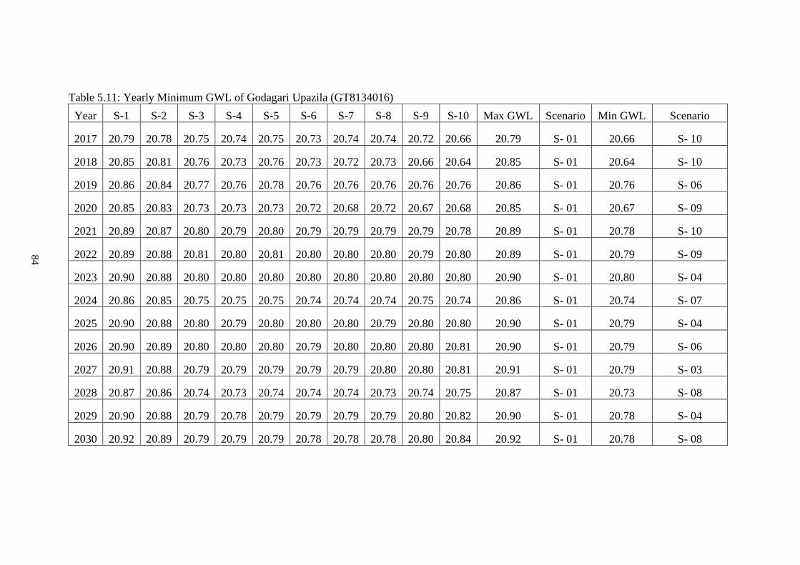
Table 5.11: Yearly Minimum GWL of Godagari Upazila (GT8134016)
Year S-1 S-2 S-3 S-4 S-5 S-6 S-7 S-8 S-9 S-10 Max GWL Scenario Min GWL Scenario
2017 20.79 20.78 20.75 20.74 20.75 20.73 20.74 20.74 20.72 20.66 20.79 S- 01 20.66 S- 10
2018 20.85 20.81 20.76 20.73 20.76 20.73 20.72 20.73 20.66 20.64 20.85 S- 01 20.64 S- 10
2019 20.86 20.84 20.77 20.76 20.78 20.76 20.76 20.76 20.76 20.76 20.86 S- 01 20.76 S- 06
2020 20.85 20.83 20.73 20.73 20.73 20.72 20.68 20.72 20.67 20.68 20.85 S- 01 20.67 S- 09
2021 20.89 20.87 20.80 20.79 20.80 20.79 20.79 20.79 20.79 20.78 20.89 S- 01 20.78 S- 10
2022 20.89 20.88 20.81 20.80 20.81 20.80 20.80 20.80 20.79 20.80 20.89 S- 01 20.79 S- 09
2023 20.90 20.88 20.80 20.80 20.80 20.80 20.80 20.80 20.80 20.80 20.90 S- 01 20.80 S- 04
2024 20.86 20.85 20.75 20.75 20.75 20.74 20.74 20.74 20.75 20.74 20.86 S- 01 20.74 S- 07
2025 20.90 20.88 20.80 20.79 20.80 20.80 20.80 20.79 20.80 20.80 20.90 S- 01 20.79 S- 04
2026 20.90 20.89 20.80 20.80 20.80 20.79 20.80 20.80 20.80 20.81 20.90 S- 01 20.79 S- 06
2027 20.91 20.88 20.79 20.79 20.79 20.79 20.79 20.80 20.80 20.81 20.91 S- 01 20.79 S- 03
2028 20.87 20.86 20.74 20.73 20.74 20.74 20.74 20.73 20.74 20.75 20.87 S- 01 20.73 S- 08
2029 20.90 20.88 20.79 20.78 20.79 20.79 20.79 20.79 20.80 20.82 20.90 S- 01 20.78 S- 04
2030 20.92 20.89 20.79 20.79 20.79 20.78 20.78 20.78 20.80 20.84 20.92 S- 01 20.78 S- 08
84
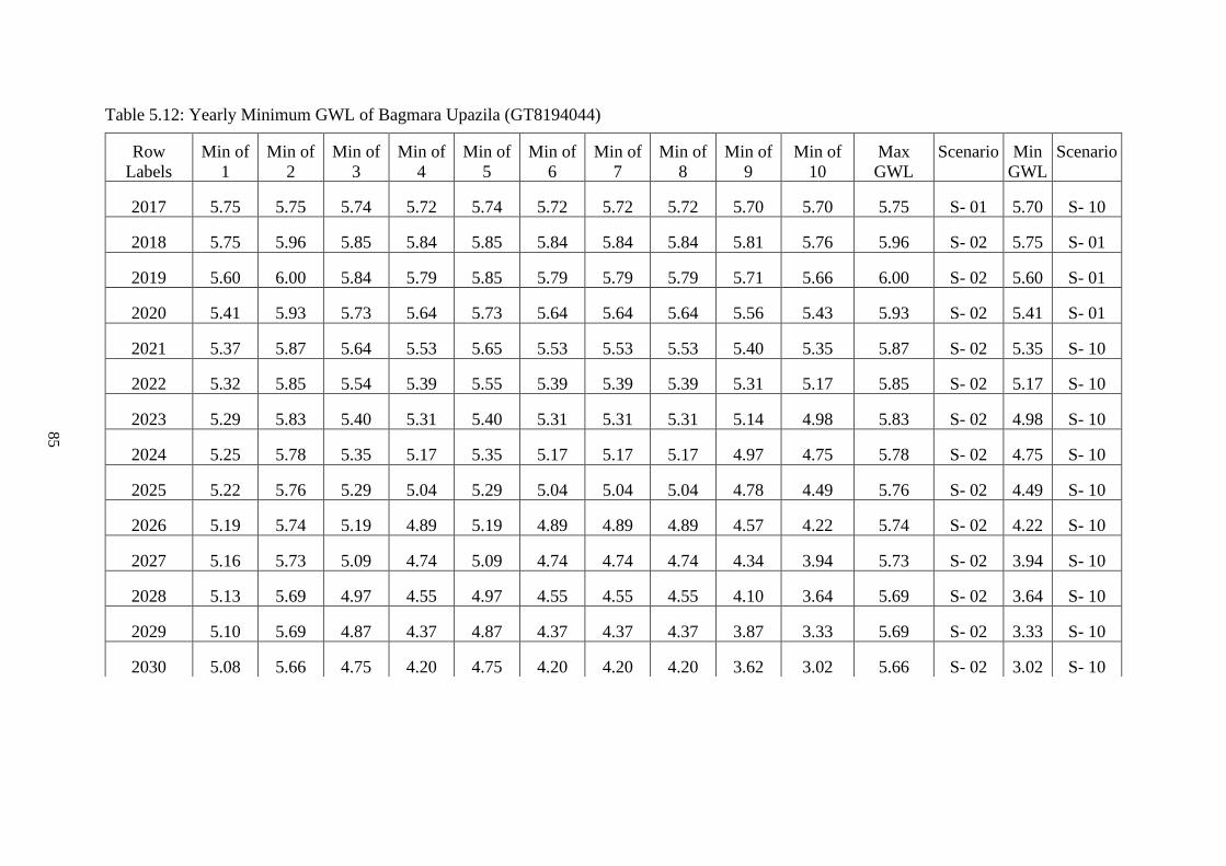
Table 5.12: Yearly Minimum GWL of Bagmara Upazila (GT8194044)
Row
Labels
Min of
1
Min of
2
Min of
3
Min of
4
Min of
5
Min of
6
Min of
7
Min of
8
Min of
9
Min of
10
Max
GWL
Scenario Min
GWL
Scenario
2017 5.75 5.75 5.74 5.72 5.74 5.72 5.72 5.72 5.70 5.70 5.75 S- 01 5.70 S- 10
2018 5.75 5.96 5.85 5.84 5.85 5.84 5.84 5.84 5.81 5.76 5.96 S- 02 5.75 S- 01
2019 5.60 6.00 5.84 5.79 5.85 5.79 5.79 5.79 5.71 5.66 6.00 S- 02 5.60 S- 01
2020 5.41 5.93 5.73 5.64 5.73 5.64 5.64 5.64 5.56 5.43 5.93 S- 02 5.41 S- 01
2021 5.37 5.87 5.64 5.53 5.65 5.53 5.53 5.53 5.40 5.35 5.87 S- 02 5.35 S- 10
2022 5.32 5.85 5.54 5.39 5.55 5.39 5.39 5.39 5.31 5.17 5.85 S- 02 5.17 S- 10
2023 5.29 5.83 5.40 5.31 5.40 5.31 5.31 5.31 5.14 4.98 5.83 S- 02 4.98 S- 10
2024 5.25 5.78 5.35 5.17 5.35 5.17 5.17 5.17 4.97 4.75 5.78 S- 02 4.75 S- 10
2025 5.22 5.76 5.29 5.04 5.29 5.04 5.04 5.04 4.78 4.49 5.76 S- 02 4.49 S- 10
2026 5.19 5.74 5.19 4.89 5.19 4.89 4.89 4.89 4.57 4.22 5.74 S- 02 4.22 S- 10
2027 5.16 5.73 5.09 4.74 5.09 4.74 4.74 4.74 4.34 3.94 5.73 S- 02 3.94 S- 10
2028 5.13 5.69 4.97 4.55 4.97 4.55 4.55 4.55 4.10 3.64 5.69 S- 02 3.64 S- 10
2029 5.10 5.69 4.87 4.37 4.87 4.37 4.37 4.37 3.87 3.33 5.69 S- 02 3.33 S- 10
2030 5.08 5.66 4.75 4.20 4.75 4.20 4.20 4.20 3.62 3.02 5.66 S- 02 3.02 S- 10
85
From this analysis shown in Table 5.6, S-10 and S-02 scenario have been selected as
extreme and less vulnerable among 10 scenarios for Charghat Upazila. For determining
extreme and less vulnerable scenarios, yearly lowest and highest values of GWL under
different scenarios have been analyzed from 2017 to 2030. Graphical representation of these
two scenarios show that during wet period both these scenarios give almost similar result
and in dry season the extreme scenario varies by more than 1m from other scenario in some
years which is shown in Figure 5.7. For this reason, dry period characteristics of
groundwater levels under assumed scenarios have been considered to find out extreme
scenario.
From this analysis shown in Table 5.7, S-10 and S-02 scenario have been selected as
extreme and less vulnerable among 10 scenarios for Mohanpur Upazila. For determining
extreme and less vulnerable scenarios, yearly lowest and highest values of GWL under
different scenarios have been analyzed from 2017 to 2030. Graphical representation of these
two scenarios show that during wet period both these scenarios give almost similar result
and in dry season the extreme scenario varies by less than 0.5m from other scenario in some
years which is shown in Figure 5.8. For this reason, dry period characteristics of
groundwater levels under assumed scenarios have been considered to find out extreme
scenario.
From this analysis shown in Table 5.8, S-01 and S-02 scenario have been selected as
extreme and less vulnerable among 10 scenarios for Durgapur Upazila. For determining
extreme and less vulnerable scenarios, yearly lowest and highest values of GWL under
different scenarios have been analyzed from 2017 to 2030. Graphical representation of these
two scenarios show that during wet period both these scenarios give almost similar result
and in dry season the extreme scenario varies by more than 2m from other scenario in some
years which is shown in Figure 5.9. For this reason, dry period characteristics of
groundwater levels under assumed scenarios have been considered to find out extreme
scenario.
From this analysis shown in Table 5.9, S-10 and S-02 scenario have been selected as
extreme and less vulnerable among 10 scenarios for Tanore Upazila. For determining
extreme and less vulnerable scenarios, yearly lowest and highest values of GWL under
different scenarios have been analyzed from 2017 to 2030. Graphical representation of these
86
two scenarios show that during wet period both these scenarios give almost similar result
and in dry season the extreme scenario varies by more than 2m from other scenario in some
years which is shown in Figure 5.10. For this reason, dry period characteristics of
groundwater levels under assumed scenarios have been considered to find out extreme
scenario.
From this analysis shown in Table 5.10, S-07 and S-05 scenario have been selected as
extreme and less vulnerable among 10 scenarios for Puthia Upazila. For determining
extreme and less vulnerable scenarios, yearly lowest and highest values of GWL under
different scenarios have been analyzed from 2017 to 2030.
From this analysis shown in Table 5.11, S-10 and S-01 scenario have been selected as
extreme and less vulnerable among 10 scenarios for Godagari Upazila. For determining
extreme and less vulnerable scenarios, yearly lowest and highest values of GWL under
different scenarios have been analyzed from 2017 to 2030.
From this analysis shown in Table 5.12, S-10 and S-02 scenario have been selected as
extreme and less vulnerable among 10 scenarios for Bagmara Upazila. For determining
extreme and less vulnerable scenarios, yearly lowest and highest values of GWL under
different scenarios have been analyzed from 2017 to 2030.
From Upazila wise analysis it is clear that scenario 10 and scenario 02 are most extreme
and less vulnerable scenarios respectively in almost all of the Upazilas in Rajshahi district.
A summary table of above analysis is given in Table 5.13.
87
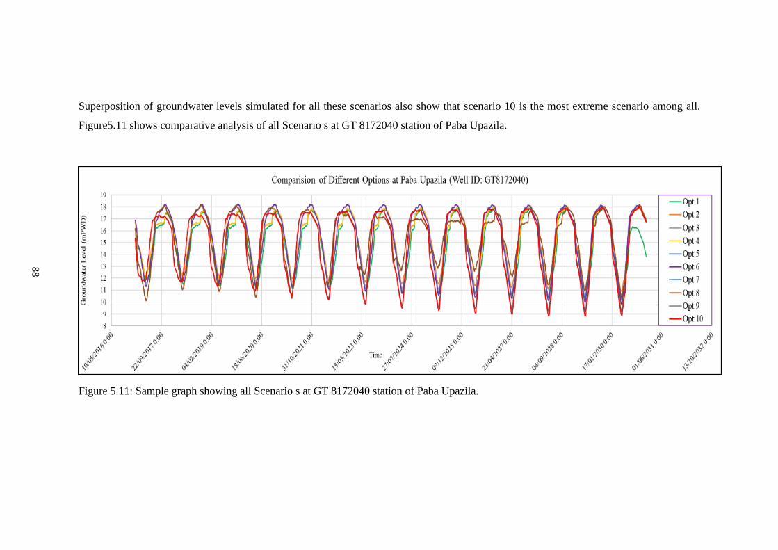
Superposition of groundwater levels simulated for all these scenarios also show that scenario 10 is the most extreme scenario among all.
Figure5.11 shows comparative analysis of all Scenario s at GT 8172040 station of Paba Upazila.
Figure 5.11: Sample graph showing all Scenario s at GT 8172040 station of Paba Upazila.
88
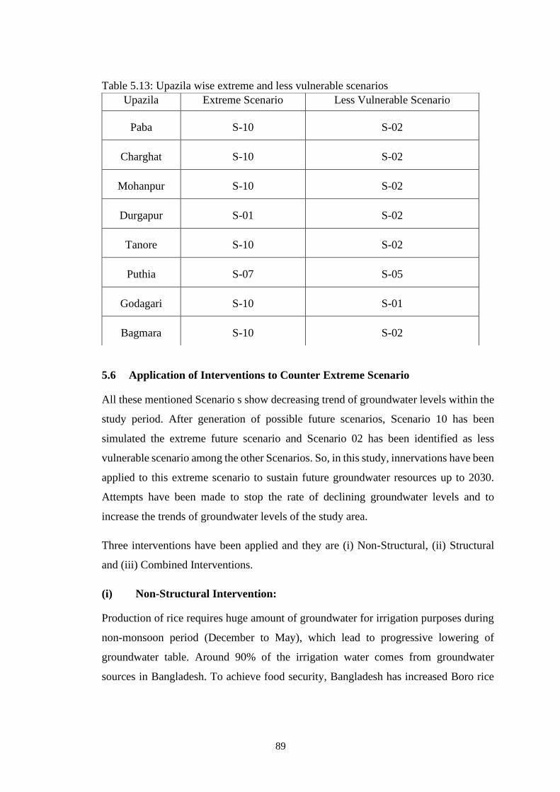
Table 5.13: Upazila wise extreme and less vulnerable scenarios
5.6 Application of Interventions to Counter Extreme Scenario
All these mentioned Scenario s show decreasing trend of groundwater levels within the
study period. After generation of possible future scenarios, Scenario 10 has been
simulated the extreme future scenario and Scenario 02 has been identified as less
vulnerable scenario among the other Scenarios. So, in this study, innervations have been
applied to this extreme scenario to sustain future groundwater resources up to 2030.
Attempts have been made to stop the rate of declining groundwater levels and to
increase the trends of groundwater levels of the study area.
Three interventions have been applied and they are (i) Non-Structural, (ii) Structural
and (iii) Combined Interventions.
(i) Non-Structural Intervention:
Production of rice requires huge amount of groundwater for irrigation purposes during
non-monsoon period (December to May), which lead to progressive lowering of
groundwater table. Around 90% of the irrigation water comes from groundwater
sources in Bangladesh. To achieve food security, Bangladesh has increased Boro rice
Upazila Extreme Scenario Less Vulnerable Scenario
Paba S-10 S-02
Charghat S-10 S-02
Mohanpur S-10 S-02
Durgapur S-01 S-02
Tanore S-10 S-02
Puthia S-07 S-05
Godagari S-10 S-01
Bagmara S-10 S-02
89
production substantially at the cost of unsustainable groundwater depletion that will
hinder water and food security in the long run.
Intervention 01: So, in this intervention area of Boro rice field is replaced by Wheat
which requires around half of water required by rice.
(ii) Structural Intervention:
Intervention 02: So, in this intervention, control structures have been introduced in
major khaal/kharies to regulate dry season flow of surface water to increase seepage
and percolation and recharge groundwater within the area of influence.
(iii) Combined Intervention:
Intervention 03: Combination of interventions of 1 and 2 have been applied.
5.6.1 Result from Non-Structural Intervention
Before application of Non-Structural intervention, it is necessary to explore the extent
of Boro rice field. Total area of Boro rice field within Rajshahi district is approximately
724 km2 which is about one third of the study area. Figure of Boro rice field extent and
Upazila wise distribution of Boro rice filed in percentage have been given in Figure
5.12 and Table 5.14 respectively. From Table 5.14, it is clear that Tanore, Godagari,
Baghmara and Mohanpur are the Boro dominant Upazilas of Rajshahi district.
Replacement of Boro rice by Wheat has significantly improved the water stressed
situation within this study area. Almost all of the wells of the Upazilas have been
responded positively towards this intervention. Wise use of groundwater in the dry
season could be a better solution towards sustainability of this scarce resource.
Upazila-wise recovery of groundwater levels of some of the wells are shown below.
Graphical representation of extreme scenario vs intervention 01at Godagari, Paba,
Baghmara and Mohanpur Upazila is shown in Figure 5.13 to 5.16. In these graphs,
extreme scenario is represented by red line and intervention 01 is represented by green
line. Groundwater level simulated under extreme scenario shows significant recovery
due to application of intervention 01.
90
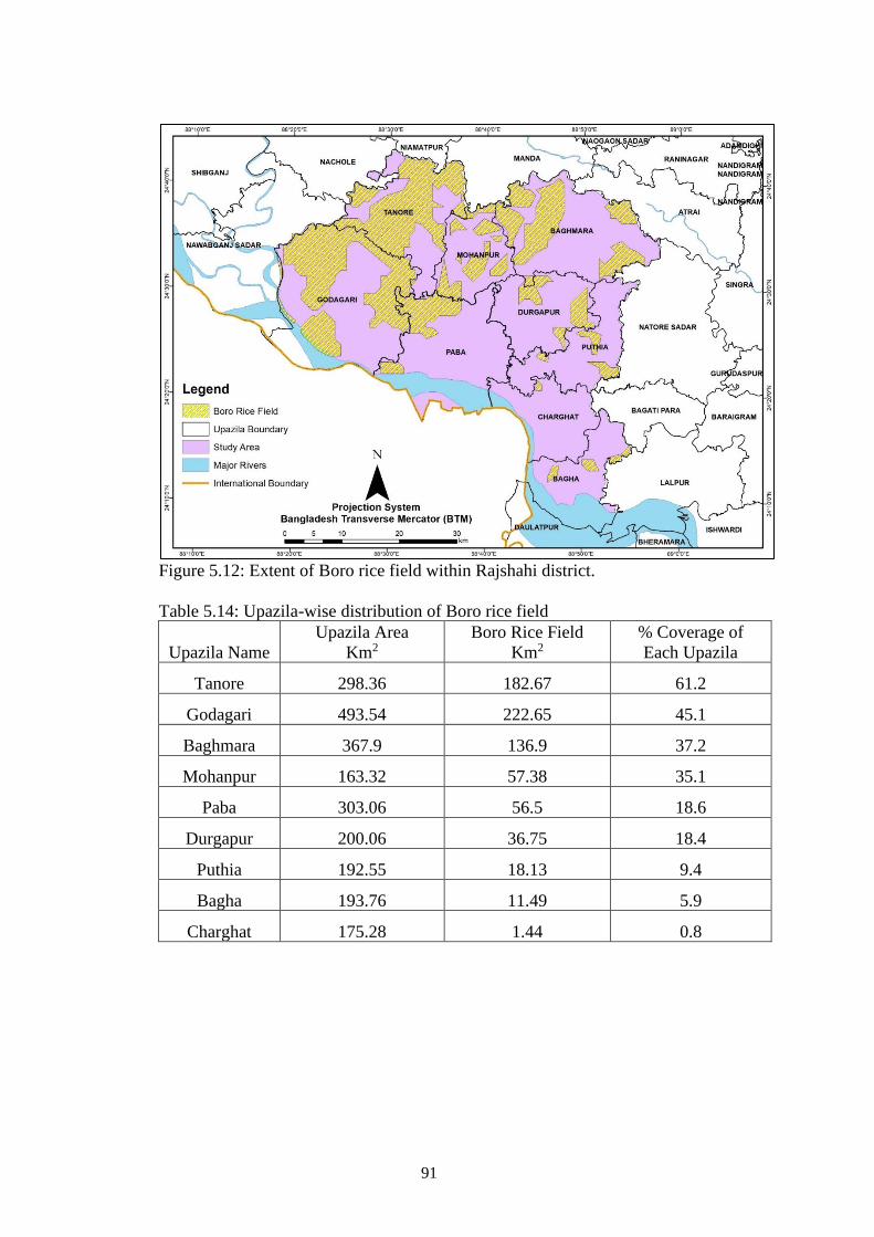
Figure 5.12: Extent of Boro rice field within Rajshahi district.
Table 5.14: Upazila-wise distribution of Boro rice field
Upazila Name
Upazila Area
Km2
Boro Rice Field
Km2
% Coverage of
Each Upazila
Tanore 298.36 182.67 61.2
Godagari 493.54 222.65 45.1
Baghmara 367.9 136.9 37.2
Mohanpur 163.32 57.38 35.1
Paba 303.06 56.5 18.6
Durgapur 200.06 36.75 18.4
Puthia 192.55 18.13 9.4
Bagha 193.76 11.49 5.9
Charghat 175.28 1.44 0.8
91

Figure 5.13: GWL of Extreme scenario vs. Intervention 01 at Godagari Upazila (Well ID: GT8134016)
Figure 5.14: GWL of Extreme scenario vs. Intervention 01 at Paba Upazila (Well ID: GT8172040)
92
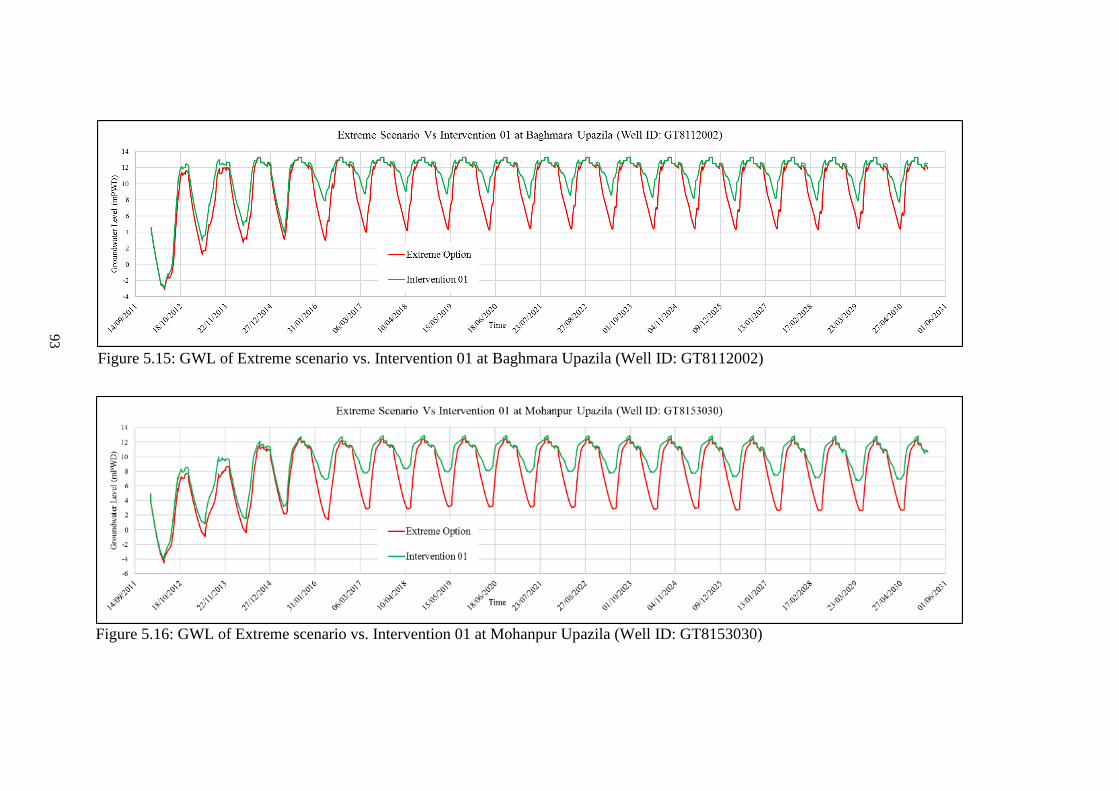
Figure 5.15: GWL of Extreme scenario vs. Intervention 01 at Baghmara Upazila (Well ID: GT8112002)
Figure 5.16: GWL of Extreme scenario vs. Intervention 01 at Mohanpur Upazila (Well ID: GT8153030)
93
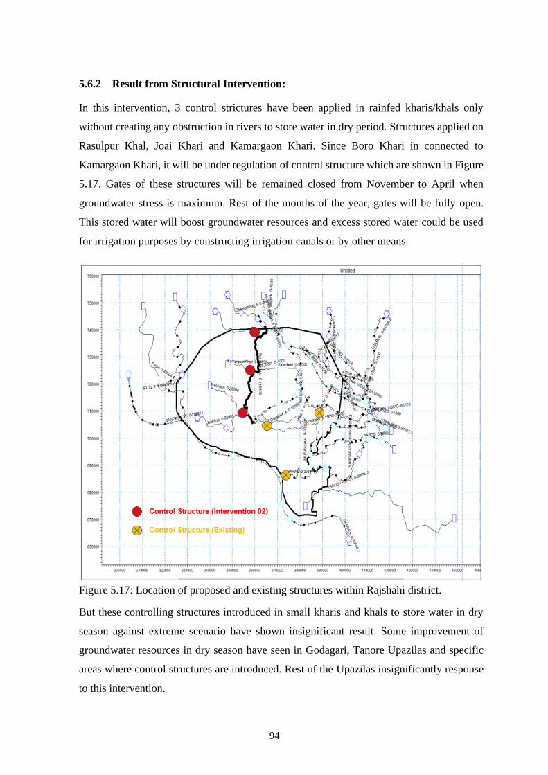
5.6.2 Result from Structural Intervention:
In this intervention, 3 control strictures have been applied in rainfed kharis/khals only
without creating any obstruction in rivers to store water in dry period. Structures applied on
Rasulpur Khal, Joai Khari and Kamargaon Khari. Since Boro Khari in connected to
Kamargaon Khari, it will be under regulation of control structure which are shown in Figure
5.17. Gates of these structures will be remained closed from November to April when
groundwater stress is maximum. Rest of the months of the year, gates will be fully open.
This stored water will boost groundwater resources and excess stored water could be used
for irrigation purposes by constructing irrigation canals or by other means.
Figure 5.17: Location of proposed and existing structures within Rajshahi district.
But these controlling structures introduced in small kharis and khals to store water in dry
season against extreme scenario have shown insignificant result. Some improvement of
groundwater resources in dry season have seen in Godagari, Tanore Upazilas and specific
areas where control structures are introduced. Rest of the Upazilas insignificantly response
to this intervention.
94
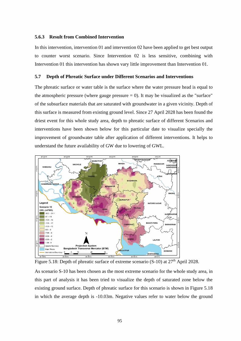
5.6.3 Result from Combined Intervention
In this intervention, intervention 01 and intervention 02 have been applied to get best output
to counter worst scenario. Since Intervention 02 is less sensitive, combining with
Intervention 01 this intervention has shown vary little improvement than Intervention 01.
5.7 Depth of Phreatic Surface under Different Scenarios and Interventions
The phreatic surface or water table is the surface where the water pressure head is equal to
the atmospheric pressure (where gauge pressure = 0). It may be visualized as the "surface"
of the subsurface materials that are saturated with groundwater in a given vicinity. Depth of
this surface is measured from existing ground level. Since 27 April 2028 has been found the
driest event for this whole study area, depth to phreatic surface of different Scenarios and
interventions have been shown below for this particular date to visualize specially the
improvement of groundwater table after application of different interventions. It helps to
understand the future availability of GW due to lowering of GWL.
Figure 5.18: Depth of phreatic surface of extreme scenario (S-10) at 27th April 2028.
As scenario S-10 has been chosen as the most extreme scenario for the whole study area, in
this part of analysis it has been tried to visualize the depth of saturated zone below the
existing ground surface. Depth of phreatic surface for this scenario is shown in Figure 5.18
in which the average depth is -10.03m. Negative values refer to water below the ground
95
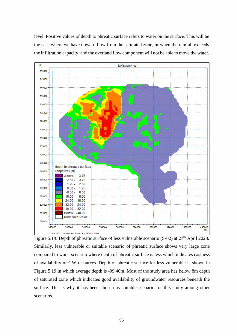
level. Positive values of depth to phreatic surface refers to water on the surface. This will be
the case where we have upward flow from the saturated zone, or when the rainfall exceeds
the infiltration capacity, and the overland flow component will not be able to move the water.
Figure 5.19: Depth of phreatic surface of less vulnerable scenario (S-02) at 27th April 2028.
Similarly, less vulnerable or suitable scenario of phreatic surface shows very large zone
compared to worst scenario where depth of phreatic surface is less which indicates easiness
of availability of GW resources. Depth of phreatic surface for less vulnerable is shown in
Figure 5.19 in which average depth is -09.40m. Most of the study area has below 8m depth
of saturated zone which indicates good availability of groundwater resources beneath the
surface. This is why it has been chosen as suitable scenario for this study among other
scenarios.
96
Figure 5.20: Depth of phreatic surface of Intervention 01 at 27th April 2028.
To counter extreme scenario S-10, three interventions have been applied. In intervention 1,
high water consumed Boro rice has been replaced by low water consumed Wheat. And it
makes a significant improvement of groundwater resources which can be seen in Figure
5.20. It is clear from this figure that this intervention can make the worst scenario (S-10)
better than our suitable scenario (S-2). Depth of phreatic surface for intervention 01 is shown
in Figure 5.18 in which average depth is -08.51m. Lowest average depth of saturated zone
(-8.51m) indicates the overall situation of groundwater availability under this intervention.
92 97
Figure 5.21: Depth of phreatic surface of Intervention 02 at 27th April 2028.
In intervention 2, instead of diversifying crops, regulatory water retaining structures have
been introduced inn small canals/kharis to store water when needed. But this intervention is
not as effective as previous one because stored water by this intervention is very low
compared to high water stress. Depth of phreatic surface for intervention 02 is shown in
Figure 5.21 in which average depth is -09.96m. This result shows positive improvement
from worst scenario but not as good as suitable scenario.
98
Figure 5.22: Depth of phreatic surface of Intervention 03 at 27th April 2028.
In intervention 3, combined effects of intervention 1 and intervention 2 has been analyzed.
And it shows better than intervention 1 by a slight margin. Depth of phreatic surface for
intervention 03 is shown in Figure 5.22 in which average depth is -08.41m.
Overall summary of these findings has been summarized below in Table 5.15 and Figure
5.23. To decide which intervention is most suitable for this area, we have to analyze more
precisely in other ways as well.
Table 5.15: Zonal statistics of S-10, 02 and Intervention 01, 02 and 03
Scenario /Intervention Mean Depth of GWT
Scenario 10 -10.03m
Scenario 02 -9.40m
Intervention 01 -8.51m
Intervention 02 -9.96m
Intervention 03 -8.41m
99

Figure 5.23: Average Depth of phreatic surface
5.8 Results from Analysis
From the above analysis it can be identified that intervention 03 has more suitable among
these interventions. Compared to extreme scenario, intervention 03 has little more
significant than intervention 01. But the difference of intervention 1 and intervention 3 is
slight and by financial point of view intervention 3 is costlier. So another analysis needs to
be carried to determine whether intervention 3 or intervention 1 is more suitable considering
overall issues.
Another comparative analysis has been done against extreme Scenario (S-10) with
Intervention 01, Intervention 02 and Intervention 03. To understand special variation of
groundwater table within the study area and to visualize the improvement of groundwater
table or Phreatic surface after application of different interventions, phreatic surface of
extreme Scenario (S-10) has been deducted from phreatic surface of Intervention 01,
Intervention 02 and Intervention 03. Deducted values have been specially distributed in the
study area where positive values indicate improvement of groundwater level, negative values
indicate further lowering of groundwater level. This analysis has been presented in figures
5.24 to figure 5.27 and summarized in Table 5.19. This analysis is helpful for mutual
comparison for all interventions.
Scenario
10
Scenario
02
Intervention
01
Intervention
02
Intervention
03
Average Depth (m) -10.03 -9.4 -8.51 -9.96 -8.41
-11-10
-9-8-7-6-5-4-3-2-10
Dep
th (
m)
Scenarios/Interventions
Depth of Phreatic Surface
100
Figure 5.24: Comparison of depth of phreatic surface of Intervention 01 and Scenario 10
Comparison of extreme scenario vs intervention 01 is shown in Figure 5.24 where positive
values indicates 96.55% improvement of groundwater level, negative values indicate 3.45%
further lowering of groundwater level compared to extreme scenario. Details of this analysis
have been tabulated in Table 5.16.
Table 5.16: Improved Area after application of intervention 01
Difference of GWL (m) Percentage of Improved (+ve) /Deteriorated
(-ve) Area
-0.98 to 0 -03.45
0 to 2 63.05
2 to 4 27
4 to 6 5.3
6 to 23.94 1.2
This result shows significant improvement of groundwater resources without any structural
construction.
96 101

Figure 5.25: Comparison of depth of phreatic surface of Intervention 02 and Scenario 10
Comparison of extreme scenario vs intervention 02 is shown in Figure 5.25 where positive
values indicates 51.44% improvement of groundwater level, negative values indicate
48.56% further lowering of groundwater level compared to extreme scenario. Details of this
analysis have been tabulated in Table 5.17.
Table 5.17: Improved area after application of intervention 02
Difference of GWL (m) Percentage of Improved (+ve)/Deteriorated
(-ve) Area
-0.34 to 0 -48.56
0 to 2 50.44
2 to 4 0.8
4 to 6 0.1
6 to 11.53 0.1
This result shows insignificant and localized improvement of groundwater resources with
structural construction which is shown in Figure 5.26.
102
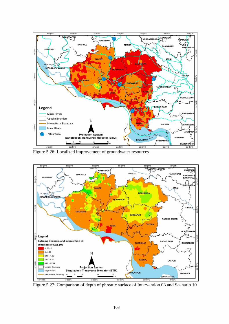
Figure 5.26: Localized improvement of groundwater resources
Figure 5.27: Comparison of depth of phreatic surface of Intervention 03 and Scenario 10
103
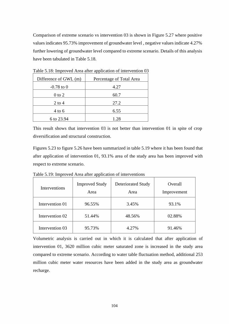
Comparison of extreme scenario vs intervention 03 is shown in Figure 5.27 where positive
values indicates 95.73% improvement of groundwater level , negative values indicate 4.27%
further lowering of groundwater level compared to extreme scenario. Details of this analysis
have been tabulated in Table 5.18.
Table 5.18: Improved Area after application of intervention 03
Difference of GWL (m) Percentage of Total Area
-0.78 to 0 4.27
0 to 2 60.7
2 to 4 27.2
4 to 6 6.55
6 to 23.94 1.28
This result shows that intervention 03 is not better than intervention 01 in spite of crop
diversification and structural construction.
Figures 5.23 to figure 5.26 have been summarized in table 5.19 where it has been found that
after application of intervention 01, 93.1% area of the study area has been improved with
respect to extreme scenario.
Table 5.19: Improved Area after application of interventions
Volumetric analysis is carried out in which it is calculated that after application of
intervention 01, 3620 million cubic meter saturated zone is increased in the study area
compared to extreme scenario. According to water table fluctuation method, additional 253
million cubic meter water resources have been added in the study area as groundwater
recharge.
Interventions Improved Study
Area
Deteriorated Study
Area
Overall
Improvement
Intervention 01 96.55% 3.45% 93.1%
Intervention 02 51.44% 48.56% 02.88%
Intervention 03 95.73% 4.27% 91.46%
104
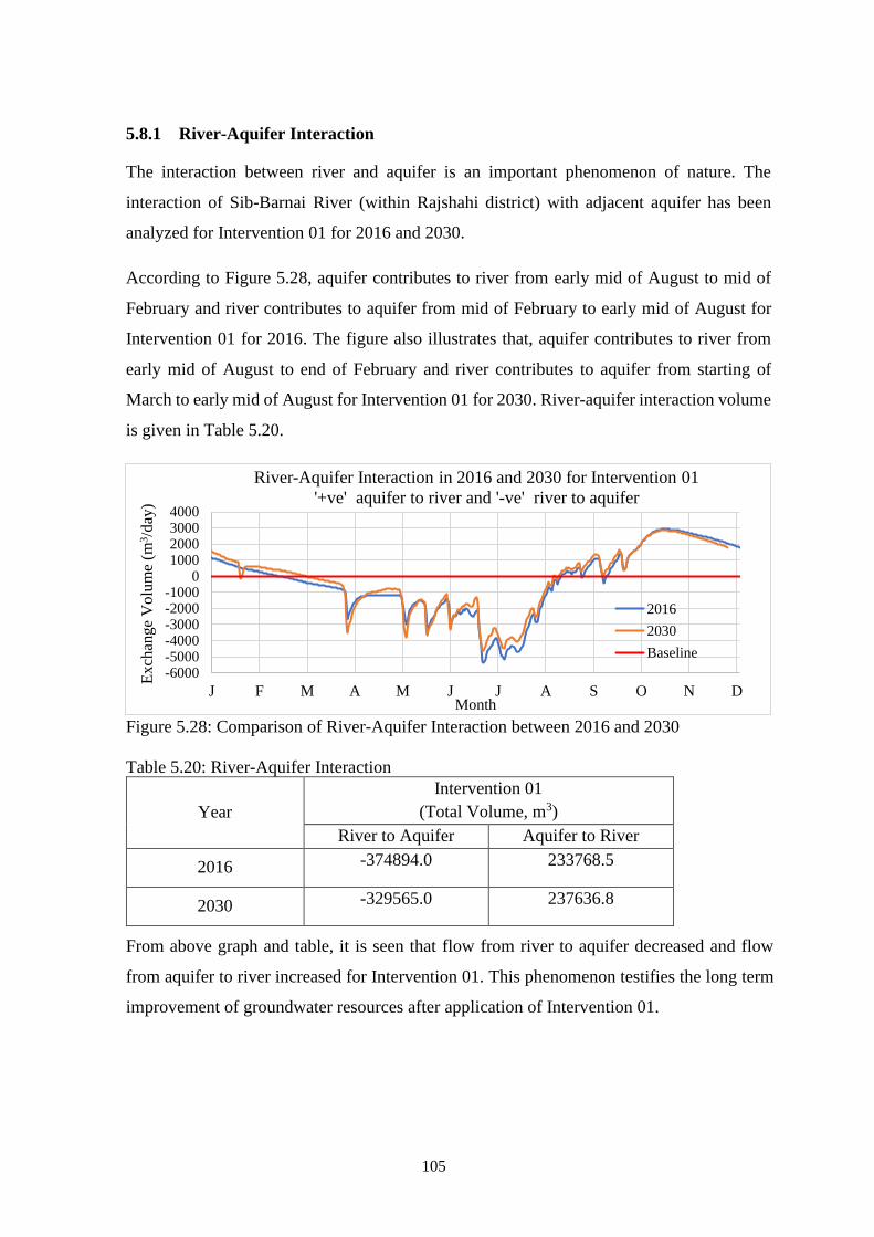
5.8.1 River-Aquifer Interaction
The interaction between river and aquifer is an important phenomenon of nature. The
interaction of Sib-Barnai River (within Rajshahi district) with adjacent aquifer has been
analyzed for Intervention 01 for 2016 and 2030.
According to Figure 5.28, aquifer contributes to river from early mid of August to mid of
February and river contributes to aquifer from mid of February to early mid of August for
Intervention 01 for 2016. The figure also illustrates that, aquifer contributes to river from
early mid of August to end of February and river contributes to aquifer from starting of
March to early mid of August for Intervention 01 for 2030. River-aquifer interaction volume
is given in Table 5.20.
Figure 5.28: Comparison of River-Aquifer Interaction between 2016 and 2030
Table 5.20: River-Aquifer Interaction
Year
Intervention 01
(Total Volume, m3)
River to Aquifer Aquifer to River
2016 -374894.0 233768.5
2030 -329565.0 237636.8
From above graph and table, it is seen that flow from river to aquifer decreased and flow
from aquifer to river increased for Intervention 01. This phenomenon testifies the long term
improvement of groundwater resources after application of Intervention 01.
-6000-5000-4000-3000-2000-1000
01000200030004000
J F M A M J J A S O N D
Exch
ange
Volu
me
(m3/d
ay)
Month
River-Aquifer Interaction in 2016 and 2030 for Intervention 01
'+ve' aquifer to river and '-ve' river to aquifer
2016
2030
Baseline
105
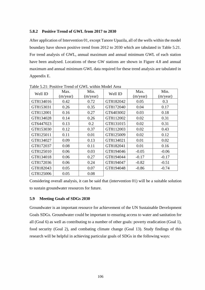
5.8.2 Positive Trend of GWL from 2017 to 2030
After application of Intervention 01, except Tanore Upazila, all of the wells within the model
boundary have shown positive trend from 2012 to 2030 which are tabulated in Table 5.21.
For trend analysis of GWL, annual maximum and annual minimum GWL of each station
have been analysed. Locations of these GW stations are shown in Figure 4.8 and annual
maximum and annual minimum GWL data required for these trend analysis are tabulated in
Appendix E.
Table 5.21: Positive Trend of GWL within Model Area
Well ID Max.
(m/year)
Min.
(m/year) Well ID
Max.
(m/year)
Min.
(m/year)
GT8134016 0.42 0.72 GT8182042 0.05 0.3
GT8153031 0.26 0.35 GT8172040 0.04 0.17
GT8112001 0.16 0.27 GT6403002 0.03 0.18
GT8134028 0.14 0.26 GT8112002 0.02 0.31
GT6447023 0.13 0.2 GT8131015 0.02 0.31
GT8153030 0.12 0.37 GT8112003 0.02 0.43
GT8125011 0.11 0.01 GT8125009 0.02 0.12
GT8134027 0.09 0.13 GT8134021 0.01 0.02
GT8172037 0.08 0.11 GT8182041 0.01 0.16
GT8125010 0.06 0.03 GT8194046 -0.05 -0.06
GT8134018 0.06 0.27 GT8194044 -0.17 -0.17
GT8172036 0.06 0.24 GT8194047 -0.82 -0.51
GT8182043 0.05 0.07 GT8194048 -0.86 -0.74
GT8125006 0.05 0.08
Considering overall analysis, it can be said that (intervention 01) will be a suitable solution
to sustain groundwater resources for future.
5.9 Meeting Goals of SDGs 2030
Groundwater is an important resource for achievement of the UN Sustainable Development
Goals SDGs. Groundwater could be important to ensuring access to water and sanitation for
all (Goal 6) as well as contributing to a number of other goals: poverty eradication (Goal 1),
food security (Goal 2), and combating climate change (Goal 13). Study findings of this
research will be helpful in achieving particular goals of SDGs in the following ways:
106

Goal 1 & 2: (Poverty Eradication & Food Security)
Agriculture is the largest employment sector in Bangladesh. The performance of this
sector has an overwhelming impact on employment generation, poverty
alleviation, human resources development, food security, etc. In this study area, almost
all of the required water demand is agricultural. Because of being one of the most severe
water stressed area of the country, agriculture of this area has been facing threat of
challenging adverse climate effects. It could hamper poverty eradication and food
security in this area where agriculture is the largest source of livelihood. For achieving
poverty eradication & food security, sustainable agriculture is necessary. This study
findings have paved ways to sustain agriculture in this area up to 2030 which will be
helped to achieve Goal 1 and Goal 2 of SDGs 2030.
Goal 6: (Water and Sanitation for All)
Though agricultural water demand is the most prominent in the study area, people relay
complete on groundwater for domestic purposes such as drinking and sanitation. Over
extraction to meet agricultural demand, groundwater level in this area has been falling
continuously posing threat to right of water and sanitation for all. This study has proposed a
probable solution to sustain groundwater resources for sustainable supply of water and
sanitation for all and this measure will be helpful to access to clean drinking water and
adequate sanitation and thus achieve Goal 6 of SDGs 2030.
Goal 13: (Combating Climate Change)
Water resources an essential part of the solution to climate change. Climate change will
affect the availability, quality and quantity of water needed for basic human needs, thus
undermining enjoyment of the basic rights to safe drinking water and sanitation of people.
By sustaining water resources in the study area up to 2030, this study has found a solution
to combat adverse impact of climate change and will be helpful to achieve Goal 13 of SDGs
2030.
107
5.10 Summary
Overall findings of the study can be summarized as follows:
This study is very challenging because the chosen study area is the driest area of the country.
And most extreme dry event of 10 years return period has been chosen to simulate future
worst scenario. Moreover all analysis have been done to counter the driest event (27 April,
2028) of worst scenario so that reaming events could be could be countered.
Lots of difficulties have been faced to counter this extreme future scenario because of adverse
climatic condition and geographic location of this area. Low rainfall, high evaporation, huge
extraction of groundwater, low recharge, thick clay layer, steep slope, high elevation, lack of
water bodies, reduction of surface water flow from prominent transboundary rivers etc. are
associated with the existing water stressed condition of this study area. Groundwater levels
of almost all Upazilas show negative trend and rate of depletion of minimum groundwater
level is higher than rate of depletion of maximum groundwater level. Since agricultural water
demand is the most dominant among all other water demands in this area, therefore
increasing trend of production of Boro rice in dry period is mainly responsible for decreasing
trend of groundwater level. Lack of rainfall and surface water, people are bound to use
groundwater for almost all purses including agriculture. This dependency on groundwater
leads to lowering GWL beyond reach day by day at an alarming rate. To simulate future
scenario of groundwater there are ten scenarios have been formulated. Optional runs have
been carried out in base model (2012-2016) to understand the most extreme and suitable
future situations considering climate change impacts for 2017 to 2030. After finding these
scenarios, there are three interventions have been formulated to counter the most extreme
scenario. Replacement of Boro rice fields by Wheat has shown a significant relief from water
stressed situation in the long run within the study area. Storing of surface water in small
khals/kharies has insignificant influence over the study area under extreme dry scenario.
Replacement of Boro rice by Wheat along with controlling structures has shown almost
similar result with replacement of Boro rice by Wheat only. Therefore from above analysis,
considering driving forces, it can be said that to sustain groundwater resources up to 2030,
replacement of Boro rice by Wheat will be a good solution.
108
109
CHAPTER 6
CONCLUSIONS AND RECOMMENDATIONS
6.1 General
The objective of the study is to assess the current and future situation of groundwater levels
of the underlying aquifer system of the Rajshahi district using MIKE SHE hydrologic
model. To understand future scenarios from 2017 to 2030 there are 10 probable options
have been studied and worst option has been chosen compared to other options. For the
sustainability of groundwater resources up to 2030 there are three interventions have been
applied in the worst condition and most suitable intervention has been identified for this
study area.
6.2 Conclusions of the Study
1. Almost all of the GW Stations within the study area have shown permanent
depletion of GWL for the duration of 30 years period (1986 to 2016). Maximum
depletion rate of maximum and minimum GWL has been found around 0.85m/year
and of 0.67m/year respectively.
2. Out of 10 assumed scenarios, “Scenario 10” has been found the most extreme
scenario up to 2030. In this above mentioned scenario, agricultural water demand
of base year 2016 has been increased by 2.5% up to year 2030, meteorological data
have been generated from GCM up to 2030, boundary GWL of extreme dry event
of 1994 has been assumed constant from 2016 to 2030 and municipal demand has
been calculated based on BBS growth rate prediction.
3. There are three interventions including “Structural”, “Non-Structural” and
“Combined” interventions have been applied to counter worst scenario where only
Non-Structural intervention has been found effective for sustainability of
groundwater resources.
4. Non-Structural intervention has been found significantly effective to reduce water
stress in this heavily water stressed study area. Replacement of Boro rice fields by
Wheat has shown a significant relief from water stressed situation in the long run
110
within the study area. Except Tanore Upazila, all of the GWL observation wells
within the model boundary have shown positive trend of GWL.
5. 27th April 2028 has been as found most dry event within 2016 to 2030 time period.
After application of Non-Structural intervention on this particular date, 95.66% of
the study area has shown improvement of groundwater resources by increasing
volume of saturated zone of 3619 million cubic meter.
6. Structural intervention in which storing of surface water in small khals/kharies has
insignificant influence over the study area under extreme dry scenario and
Combined intervention has almost similar impact as Non-Structural intervention.
6.3 Recommendations for Further Study
The recommendations for the future research are as follows:
1. In this study three interventions have been applied and these are change of crop
pattern, application of control structures to store surface water and their
combination. Other interventions such as rainwater harvesting, artificial recharge
of aquifer etc. are highly recommended to study in this study area.
2. In this study Boro rice has been replaced by Wheat as an intervention. Crop
diversification by introducing other crops or cropping systems are recommended
to observe their influence on groundwater resource improvement.
3. In this study grid size has been taken as 1000m X 1000m. As a result, fluctuation
of groundwater level of small zones less than 1 square km has not been visualized
clearly. It is recommended to use grid size lower than 100mX100m for future study
to get more precise result.
4. In this study small amount of water has been stored by applying control structures
on small kharis that is why improvement of groundwater was insignificant and
localized. It is recommended to explore large storage capacity in major rivers to
see the improvement of groundwater resources in the study area.
111
REFERENCES
Abdullah, M., Rahman, M.S., Rahman, M.A. and Sahabuddin, S.M., 2019, Trend analysis
of the hydrological components in a watershed: A case study for Bogura District in
Bangladesh, Journal of Environmental Hydrology, Vol. 27, Paper 4.
Acharyya, A., 2017, Sustainable Development of Groundwater Resources in India: A Re-
Look at Policy Initiatives, Vol-VIII.
Adhikary, S.K., Das, S.K., Saha, G.C. and Chaki, T., 2013, ‘Groundwater Drought
Assessment for Barind Irrigation Project in Northwestern Bangladesh’, 20th International
Congress on Modelling and Simulation, Adelaide, Australia.
Ahmad, E., Hossain, A.F.M., Hassan, M., 2008, Water Scarcity, Global Changes and
Groundwater Management Responses in the Context of North-west Region of
Bangladesh.
Ahmed, K.M., 2014, Barind Tract, BANGLAPEDIA, viewed 23 November 2018,
Retrieved from http://en.banglapedia.org/index.php?title=Barind_Tract
Alam, A.T., Rahman, M.S., Saadat, A.H. and Huq, M., 2012, “Gamma Distribution and its
Application of Spatially Monitoring Meteorological Drought in Barind, Bangladesh,”
Journal of Environmental Science and Natural Resources, Vol. 5 (2), pp. 287-293.
Ali, M. & Abustan, I., & Rahman, M., Haque, A.AM., 2011, Sustainability of Groundwater
Resources in the North-eastern Region of Bangladesh, Water Resources Management.
Retrieved from DOI: 26. 10.1007/s11269-011-9936-5.
Asaduzzaman, M., 1983, Follow up Report: Barind Tract – Rajshahi, Groundwater
Exploitation., Agriculture and Forest Division, Ministry of Agriculture, GOB.
Aziz, M. A., Majumder, M.A.K., Kabir, M.S., Hossain, M.I., Rahman, N.M.F., Rahman, F.
and Hosen, S., 2015, Groundwater Depletion with Expansion of Irrigation in Barind Tract:
A Case Study of Rajshahi District of Bangladesh. International Journal of Geology,
Agriculture and Environmental Sciences. 3. 32-38.
BANGLAPEDIA, 2014, Groundwater, viewed 23 November 2018, Retrieved from
http://en.banglapedia.org/index.php?title=Groundwater.
BMDA (Barind Multipurpose Development Authority) 2006, “Ground Water Model Study
for Deep Tubewell Installation Project in Barind Area,” Vol. I, pp. 1-2.
BWDB, Bureau of Consulting Engineers Ltd & Etals., 1990, Main Report: Water Survey
for Barind Integrated Area Development Project, Volume l.
Cai, Ximing & McKinney, Daene C. & Rosegrant, Mark W., 2001, ‘Sustainability analysis
for irrigation water management: concepts, methodology, and application to the Aral Sea
region’, NY, USA, International Food Policy Research Institute, Paper No. 86 CGW.

112
Chow, V.T., Maidment, D.R. and Mays, L.W., 1988, Applied Hydrology. McGraw-Hill
Series in Water Resources and Environmental Engineering. McGraw-Hill Book Company.
New York. ISBN 0-07-100174-3.
Chowdhury, S. and Jahan, N., 2018, ‘Drought Analysis of Rajshahi of Bangladesh from
CORDEX Data by Palmer Method’, Journal of Modern Science and Technology, Vol. 6,
No. 2, June 2018 Issue, pp.10-18.
Climate Data Organization, https://en.climate-data.org/asia/bangladesh/rajshahi-division-
2265/, last visited on 18th November, 2018 at 10:00AM
Dey, N., Saha, R., Parvez, M., Bala, S., Islam, A.K.M., Paul, J. and Hossain, M., 2017,
Sustainability of groundwater use for irrigation of dry-season crops in northwest
Bangladesh, Groundwater for Sustainable Development, Vol-4, pp: 66-77
Dey, N.C. and Ali, A.R.M.M., 2010, ‘Changes in the use of safe water and water safety
measures in WASH intervention areas of Bangladesh: a midline assessment. BRAC-RED
Working Paper 27’
Dey, Nepal., Saha, Ratnajit., Parvez, Mahmood., Bala, Sujit., Islam, AKM., Paul, Joyanta.
And Hossain, Mahabub., 2013, Sustainability of Groundwater Use for Irrigation in
Northwest Bangladesh, National Food Policy Capacity Strengthening Programme
(NFPCSP) Phase II.
DHI 1999, MIKE 11 User Manual - a Modelling system for Rivers and Channels.
DHI 1999, MIKE SHE User Manual - Hydrological Modelling System for Groundwater.
Döll, P., Schmied, H.M., Schuh, C., Portmann, F.T., and Eicker, A., 2014, Global-scale
assessment of groundwater depletion and related groundwater abstractions: Combining
hydrological modeling with information from well observations and GRACE satellites,
Water Resource Research., Vol-50, pp: 5698–5720.
Food and Agriculture Organization of the United Nations, International Hydrological
Programme, Global Environment Fund, L. P., International Association of Hydrogeologists
& World Bank., 2016, Shared global vision for Groundwater Governance 2030 and a call
for action (Revised edition).
Gleeson, T., Mark, C., Grant, F. and Debra, P., 2019, Global Groundwater Sustainability,
Resources and Systems in the Anthropocene, EarthArXiv. DOI:10.31223/osf.io/6dvm8.
Guppy, L., Uyttendaele, P., Villholth, K. G., & Smakhtin, V. (2018)., UNU-INWEH
ReportGroundwater and Sustainable Development Goals: Analysis of Interlinkages (Report
No. 4), Hamilton. Retrieved from https://inweh.unu.edu/wp-
content/uploads/2018/12/Groundwater-and-Sustainable-Development-Goals-Analysis-of-
Interlinkages.pdf
Hornberger, G. & Perrone, D., Water Resources: Science and Society (1st ed.), Johns
Hopkins University Press.
113
Hossain, A.F.M.A., Shamsuddin, MD. (1977). Groundwater Potential in Rajshahi District,
Bangladesh. Bachelor of Engineering in Water Resources. Department of Water Resources
Engineering. Bangladesh University of Engineering and Technology.
HYSAWA [Hygiene, Sanitation and Water Supply] (2012). Strengthening BMDA’s
Capacity on Water Resources Management. Final Report. Dhaka, Bangladesh
IBRD (International Bank for Reconstruction and Development), 1970 “IBRD-IDA Tube
Well Project,” East Pakistan Agricultural Development Corporation, Dhaka, Vol. PA- 49a,
p. 5.
Islam, M.N., Chowdhury, A., Islam, K.M. and Rahman, M.Z., 2014, ‘Development of
rainfall recharge model for natural groundwater recharge estimation in Godagari Upazila
of Rajshahi district, Bangladesh’, American Journal of Civil Engineering, Vol. 2(2), March
2014, pp. 48-52.
IWM [Institute of Water Modelling] (2006). Groundwater Model Study for Deep Tube Well
Installation Project in Barind Area. Final Report. Dhaka, Bangladesh.
IWM [Institute of Water Modelling] (2013). Groundwater Resources Study and IIS
Development of Pabna, Sirajgonj, Bogra, Gaibandha, Rangpur, Kurigram, Nilphamari and
Lalmonirhat Districts through Mathematical Model Study. Interim Report.
IWM 2012, Groundwater Resource Study and DSS Development of Rajshahi, Naogaon,
Chapai Nawabganj, Pabna and Natore Districts and also remaining Districts (except
Thakurgaon, Panchagarh, Dinajpur and Joypurhat Districts) of Rajshahi Division through
Mathematical Model Study for Barind Integrated Area Development Project-Phase-III,
Institution of Water Modelling, Dhaka, Bangladesh.
IWM 2012, Groundwater Resource Study for Barind Integrated Area Development Project-
Phase-III, Institution of Water Modelling, Dhaka, Bangladesh.
Karim, M.A., 1984, Upazila wise Groundwater Recharge conditions of Bangladesh.
Lautze, J., De Silva, S., Giordano, M. & Sanford, L., 2011, Putting the cart before the horse:
Water governance and IWRM. Natural Resources Forum, 35(1), 1–8. Retrieved From
https://doi.org/10.1111/j.1477-8947.2010.01339.x
Loucks, D.P., 2000, ‘Sustainable water resources management’, Water International, Vol.
25(1). pp.3-11.
MacDonald, 1983, Final Report: Water Balance Studies Bangladesh.
Megdal, S., 2018, Invisible water: the importance of good groundwater governance and
management., National Project on Clean Water. Retrieved from DOI: 10.1038/s41545-018-
0015-9.
Mojid, M.A., Parvez, M.F., Mainuddin, M. and Hodgson, G., 2019, Water Table Trend- A
Sustainability Status of Groundwater Development in North-West Bangladesh, Water, Vol-
11, pp-1182.
114
MPO., 1986, Technical Report: Groundwater Resources (Report No. 5).
National Water Management Plan (NWMP)., 2001, Main Report, Volume 2, Ministry of
Water Resources, Government of Bangladesh.
Pahl-Wostl, C., Conca, K., Kramer, A., Maestu, J., & Schmidt, F., 2013, Missing Links in
Global Water Governance: a Processes-Oriented Analysis, Ecology and Society, vol:18(2).
https://doi.org/10.5751/ES-05554-180233
Paul, B.K., 1998, ‘Coping mechanisms practiced by drought victims (1994/5) in North
Bengal, Bangladesh’, Applied Geography, Vol. 18, pp. 355–373.
Rahman, A.T.M. Sakiur., Hosono, T., Mazumder, Q. H. and Chowdhury, S.J., 2018,
Sustainable Groundwater Management in Context of Climate Change in Northwest
Bangladesh, Achievements and Challenges of Integrated River Basin Management, chapter
7.
Rahman, M.M. and Mahbub, A.Q.M., 2012, ‘Groundwater Depletion with Expansion of
Irrigation in Barind Tract: A Case Study of Tanore Upazila’, Journal of Water Resource
and Protection, Vol. 4, pp 567-575
Rahman, M.M. and Mahbub, A.Q.M., 2012, ‘Lithological Study and Mapping of Barind
Tract Using Borehole Log Data with GIS: In the Context of Tanore Upazila’, Journal of
Geographic Information System, Vol. 4, pp 349-357
Rahman, M.M., Mahbub, A. Q. M., 2012, "Lithological Study and Mapping of Barind
Tract Using Borehole Log Data with GIS: In the Context of Tanore Upazila", Journal of
Geographic Information System, Vol.4, Article ID: 22153
Shahid, S., 2008, ‘Spatial and Temporal Characteristics of Droughts in the Western Part of
Bangladesh’, Hydro Process, Vol. 22, pp. 2235–2247.
Simonovic, S.P., 1997, Risk in sustainable water resources management. In: Sustainability
of water resources under increasing uncertainties, IAHS Pub. No. 240
Sondipon, P. (2017). Impact of Proposed Rubber Dam in Mohananda River at Chapai
Nawabganj District on Adjacent Groundwater. Master of Engineering in Water Resources.
Department of Water Resources Engineering. Bangladesh University of Engineering and
Technology.
Subramanya, K., 1994, Engineering Hydrology. Second Edition. Tata McGraw Hill
Publishing Company Limited. ISBN 0-07-462449-8.
The Third-pole, https://www.thethirdpole.net/2020/03/10/bangladesh-to-declare-water-
emergency-in-northwest/, last visited on 10th October, 2020 at 10:00AM
UNDP-BWDB., 1982, Ground-Water Survey-Technical Report on Hydrogeologic
Conditions of Bangladesh.
115
Villholth, K. G., López-Gunn, E., Conti, K., Garrido, A., & Van der Gun, J. A. M., 2018,
Groundwater Governance: rationale, definition, current state and heuristic framework,
Leiden, The Netherlands: CRC Press/Balkema.
WARPO, 2016, Final Report: Comprehensive Report on Assessment of State of Water
Resources, Volume 03.
Weather Atlas, https://www.weather-atlas.com/en/bangladesh/rajshahi-climate, last visited
on 18th November, 2018 at 10:00AM
Weather Online, https://www.weatheronline.co.uk/reports/climate/Bangladesh.htm, last
visited on 18th November, 2018 at 10:00AM
Zahid, A. and Ahmed. S. R. U., 2006, Groundwater Resources Development in Bangladesh:
Contribution to Irrigation for Food Security and Constraints to Sustainability.Groundwater
Governance in Asia, Series-1: 25-46.
Zahid, A., 2015, Technical Report: GROUNDWATER MANAGEMENT ASPECTS IN
BANGLADESH.

Appendix A: Double Mass Curve
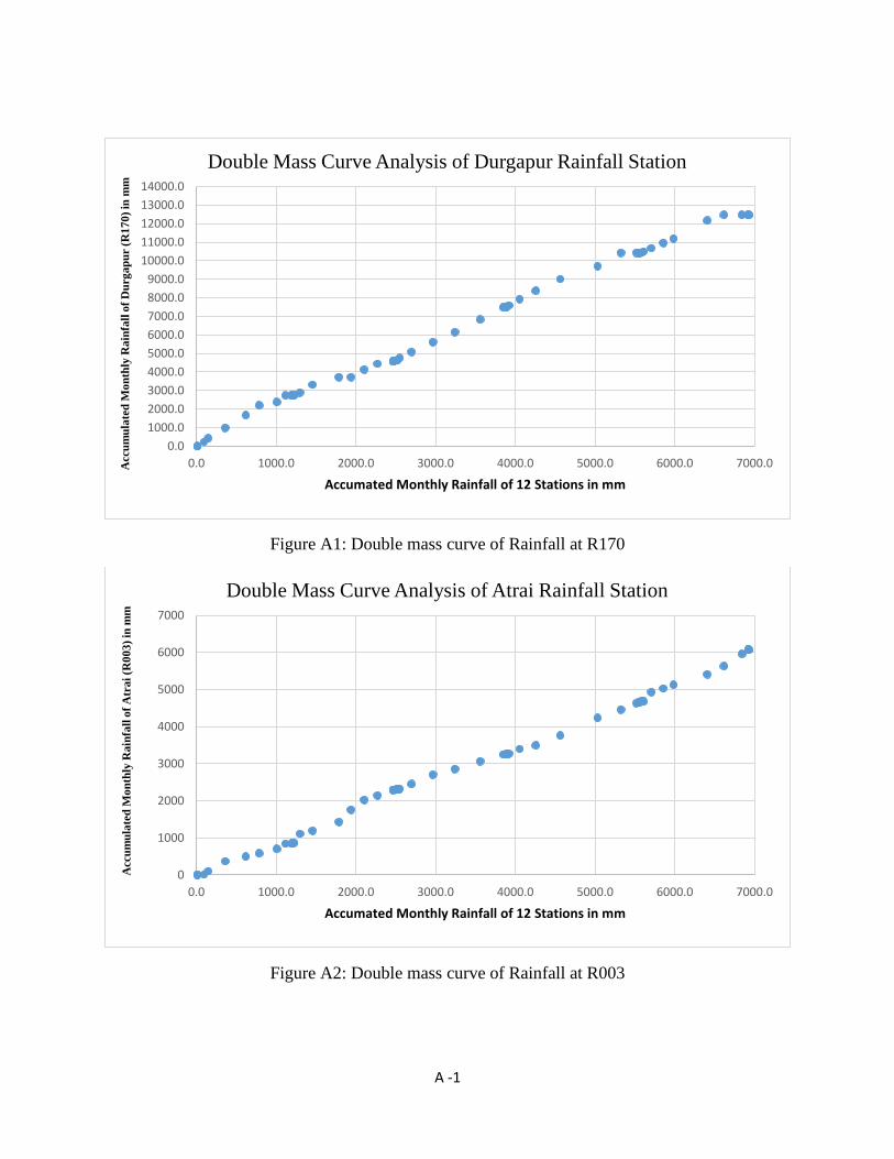
A -1
Figure A1: Double mass curve of Rainfall at R170
Figure A2: Double mass curve of Rainfall at R003
0.0
1000.0
2000.0
3000.0
4000.0
5000.0
6000.0
7000.0
8000.0
9000.0
10000.0
11000.0
12000.0
13000.0
14000.0
0.0 1000.0 2000.0 3000.0 4000.0 5000.0 6000.0 7000.0Accu
mu
late
d M
on
thly
Ra
infa
ll o
f D
urg
ap
ur (
R1
70
) in
mm
Accumated Monthly Rainfall of 12 Stations in mm
Double Mass Curve Analysis of Durgapur Rainfall Station
0
1000
2000
3000
4000
5000
6000
7000
0.0 1000.0 2000.0 3000.0 4000.0 5000.0 6000.0 7000.0
Accu
mu
late
d M
on
thly
Ra
infa
ll o
f A
tra
i (R
00
3)
in m
m
Accumated Monthly Rainfall of 12 Stations in mm
Double Mass Curve Analysis of Atrai Rainfall Station

A -2
Figure A3: Double mass curve of Rainfall at R195
Figure A4: Double mass curve of Rainfall at R172
0
1000
2000
3000
4000
5000
6000
7000
0.0 1000.0 2000.0 3000.0 4000.0 5000.0 6000.0 7000.0
Accu
mu
late
d M
on
thly
Ra
infa
ll o
f C
ha
pa
i-N
aw
ab
ga
nj
(R1
95
) in
mm
Accumated Monthly Rainfall of 12 Stations in mm
Double Mass Curve Analysis of Chapai-Nawabganj Rainfall
Station
0
1000
2000
3000
4000
5000
6000
7000
8000
0.0 1000.0 2000.0 3000.0 4000.0 5000.0 6000.0 7000.0Accu
mu
late
d M
on
thly
Ra
infa
ll o
f G
od
ag
ari (R
17
2)
in m
m
Accumated Monthly Rainfall of 12 Stations in mm
Double Mass Curve Analysis of Godagari Rainfall Station
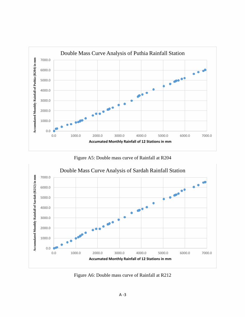
A -3
Figure A5: Double mass curve of Rainfall at R204
Figure A6: Double mass curve of Rainfall at R212
0.0
1000.0
2000.0
3000.0
4000.0
5000.0
6000.0
7000.0
0.0 1000.0 2000.0 3000.0 4000.0 5000.0 6000.0 7000.0
Accu
mu
late
d M
on
thly
Ra
infa
ll o
f P
uth
ia (
R2
04
) in
mm
Accumated Monthly Rainfall of 12 Stations in mm
Double Mass Curve Analysis of Puthia Rainfall Station
0.0
1000.0
2000.0
3000.0
4000.0
5000.0
6000.0
7000.0
0.0 1000.0 2000.0 3000.0 4000.0 5000.0 6000.0 7000.0
Acc
um
ula
ted
Mo
nth
ly R
ain
fall
of
Sa
rd
ah
(R
21
2)
in m
m
Accumated Monthly Rainfall of 12 Stations in mm
Double Mass Curve Analysis of Sardah Rainfall Station
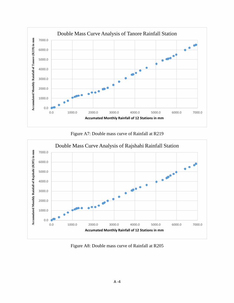
A -4
Figure A7: Double mass curve of Rainfall at R219
Figure A8: Double mass curve of Rainfall at R205
0.0
1000.0
2000.0
3000.0
4000.0
5000.0
6000.0
7000.0
0.0 1000.0 2000.0 3000.0 4000.0 5000.0 6000.0 7000.0
Accu
mu
late
d M
on
thly
Ra
infa
ll o
f T
an
ore (
R2
19
) in
mm
Accumated Monthly Rainfall of 12 Stations in mm
Double Mass Curve Analysis of Tanore Rainfall Station
0.0
1000.0
2000.0
3000.0
4000.0
5000.0
6000.0
7000.0
0.0 1000.0 2000.0 3000.0 4000.0 5000.0 6000.0 7000.0Accu
mu
late
d M
on
thly
Ra
infa
ll o
f R
ajs
ha
hi
(R2
05
) in
mm
Accumated Monthly Rainfall of 12 Stations in mm
Double Mass Curve Analysis of Rajshahi Rainfall Station
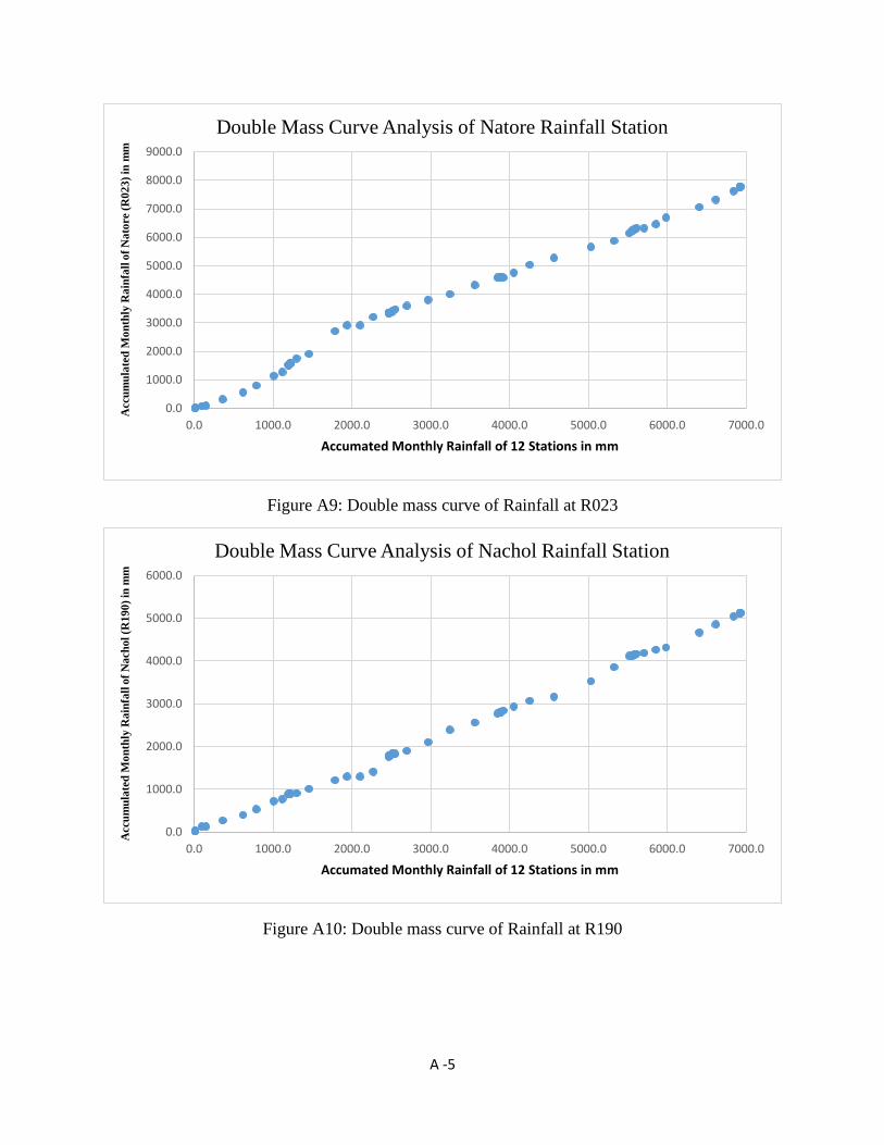
A -5
Figure A9: Double mass curve of Rainfall at R023
Figure A10: Double mass curve of Rainfall at R190
0.0
1000.0
2000.0
3000.0
4000.0
5000.0
6000.0
7000.0
8000.0
9000.0
0.0 1000.0 2000.0 3000.0 4000.0 5000.0 6000.0 7000.0
Acc
um
ula
ted
Mo
nth
ly R
ain
fall
of
Na
tore (
R0
23
) in
mm
Accumated Monthly Rainfall of 12 Stations in mm
Double Mass Curve Analysis of Natore Rainfall Station
0.0
1000.0
2000.0
3000.0
4000.0
5000.0
6000.0
0.0 1000.0 2000.0 3000.0 4000.0 5000.0 6000.0 7000.0
Accu
mu
late
d M
on
thly
Ra
infa
ll o
f N
ach
ol
(R1
90
) in
mm
Accumated Monthly Rainfall of 12 Stations in mm
Double Mass Curve Analysis of Nachol Rainfall Station
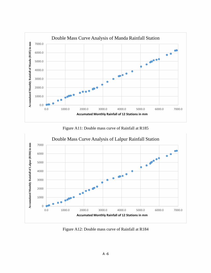
A -6
Figure A11: Double mass curve of Rainfall at R185
Figure A12: Double mass curve of Rainfall at R184
0.0
1000.0
2000.0
3000.0
4000.0
5000.0
6000.0
7000.0
0.0 1000.0 2000.0 3000.0 4000.0 5000.0 6000.0 7000.0
Accu
mu
late
d M
on
thly
Ra
infa
ll o
f M
an
da
(R
18
5)
in m
m
Accumated Monthly Rainfall of 12 Stations in mm
Double Mass Curve Analysis of Manda Rainfall Station
0
1000
2000
3000
4000
5000
6000
7000
0.0 1000.0 2000.0 3000.0 4000.0 5000.0 6000.0 7000.0
Accu
mu
late
d M
on
thly
Ra
infa
ll o
f L
alp
ur (
R1
84
) in
mm
Accumated Monthly Rainfall of 12 Stations in mm
Double Mass Curve Analysis of Lalpur Rainfall Station
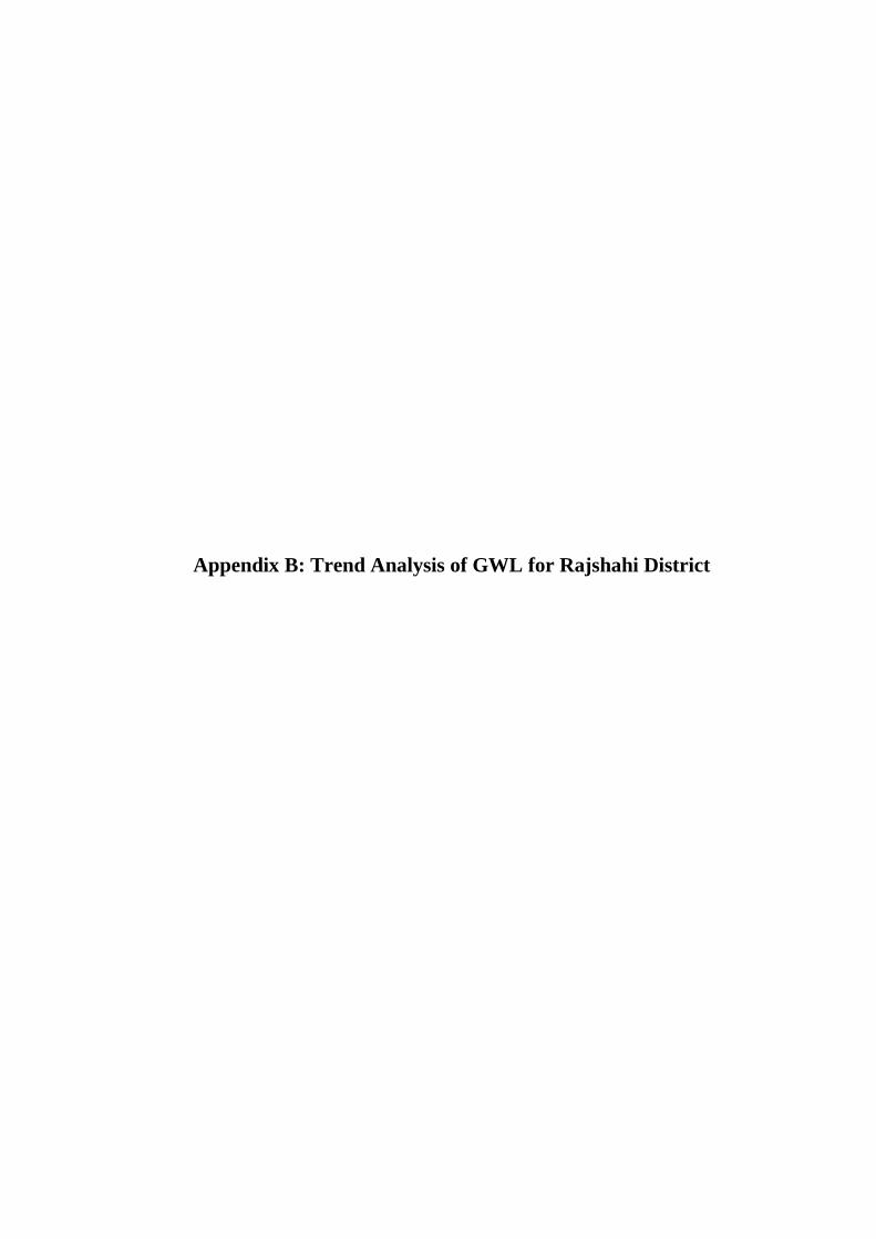
Appendix B: Trend Analysis of GWL for Rajshahi District

Figure B1: Rate of change of Maximum and Minimum GWL at GT6403002
Figure B2: Rate of change of Maximum and Minimum GWL at GT6447023
Rate of Change: -7.47cm/year
Rate of Change: -6.29cm/year
0.00
2.00
4.00
6.00
8.00
10.00
12.00
14.00
1985.00 1988.00 1991.00 1994.00 1997.00 2000.00 2003.00 2006.00 2009.00 2012.00 2015.00 2018.00
WL
(mP
WD
)
Year
Well ID: GT6403002
Max GWL
Min GWL
Linear (Max GWL)
Linear (Min GWL)
Rate of Change: -20.91cm/year
Rate of Change: -15.11cm/year
0
2
4
6
8
10
12
14
16
18
1985.00 1988.00 1991.00 1994.00 1997.00 2000.00 2003.00 2006.00 2009.00 2012.00 2015.00 2018.00
WL
(mP
WD
)
Year
Well ID: GT6447023
Max GWL
Min GWL
Linear (Max GWL)
Linear (Min GWL)
B - 1
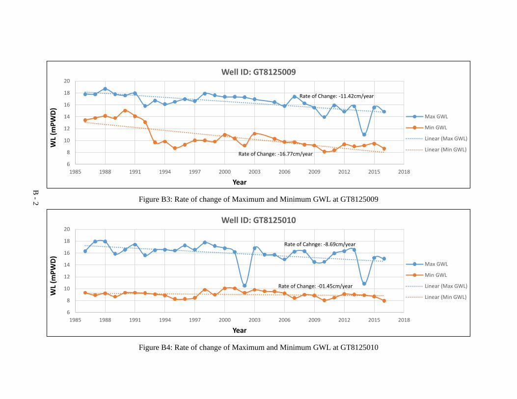
Figure B3: Rate of change of Maximum and Minimum GWL at GT8125009
Figure B4: Rate of change of Maximum and Minimum GWL at GT8125010
Rate of Change: -11.42cm/year
Rate of Change: -16.77cm/year
6
8
10
12
14
16
18
20
1985 1988 1991 1994 1997 2000 2003 2006 2009 2012 2015 2018
WL
(mP
WD
)
Year
Well ID: GT8125009
Max GWL
Min GWL
Linear (Max GWL)
Linear (Min GWL)
Rate of Cahnge: -8.69cm/year
Rate of Change: -01.45cm/year
6
8
10
12
14
16
18
20
1985 1988 1991 1994 1997 2000 2003 2006 2009 2012 2015 2018
WL
(mP
WD
)
Year
Well ID: GT8125010
Max GWL
Min GWL
Linear (Max GWL)
Linear (Min GWL)
B - 2
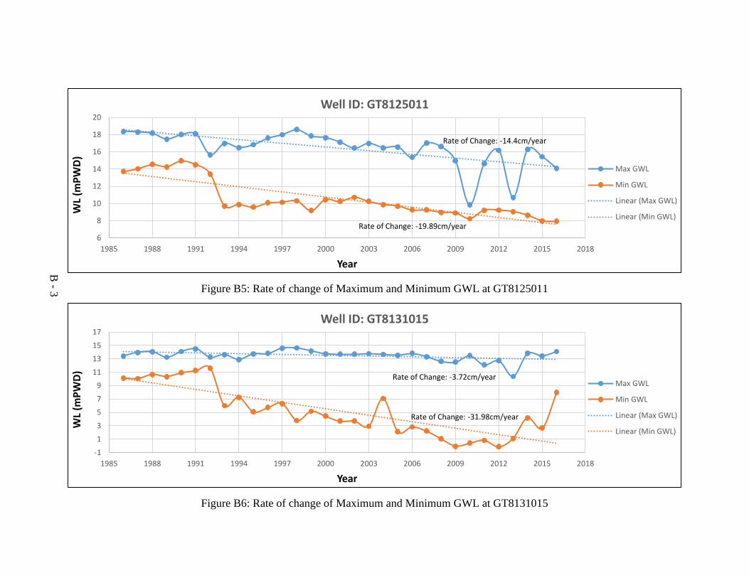
Figure B5: Rate of change of Maximum and Minimum GWL at GT8125011
Figure B6: Rate of change of Maximum and Minimum GWL at GT8131015
Rate of Change: -14.4cm/year
Rate of Change: -19.89cm/year
6
8
10
12
14
16
18
20
1985 1988 1991 1994 1997 2000 2003 2006 2009 2012 2015 2018
WL
(mP
WD
)
Year
Well ID: GT8125011
Max GWL
Min GWL
Linear (Max GWL)
Linear (Min GWL)
Rate of Change: -3.72cm/year
Rate of Change: -31.98cm/year
-1
1
3
5
7
9
11
13
15
17
1985 1988 1991 1994 1997 2000 2003 2006 2009 2012 2015 2018
WL
(mP
WD
)
Year
Well ID: GT8131015
Max GWL
Min GWL
Linear (Max GWL)
Linear (Min GWL)
B - 3
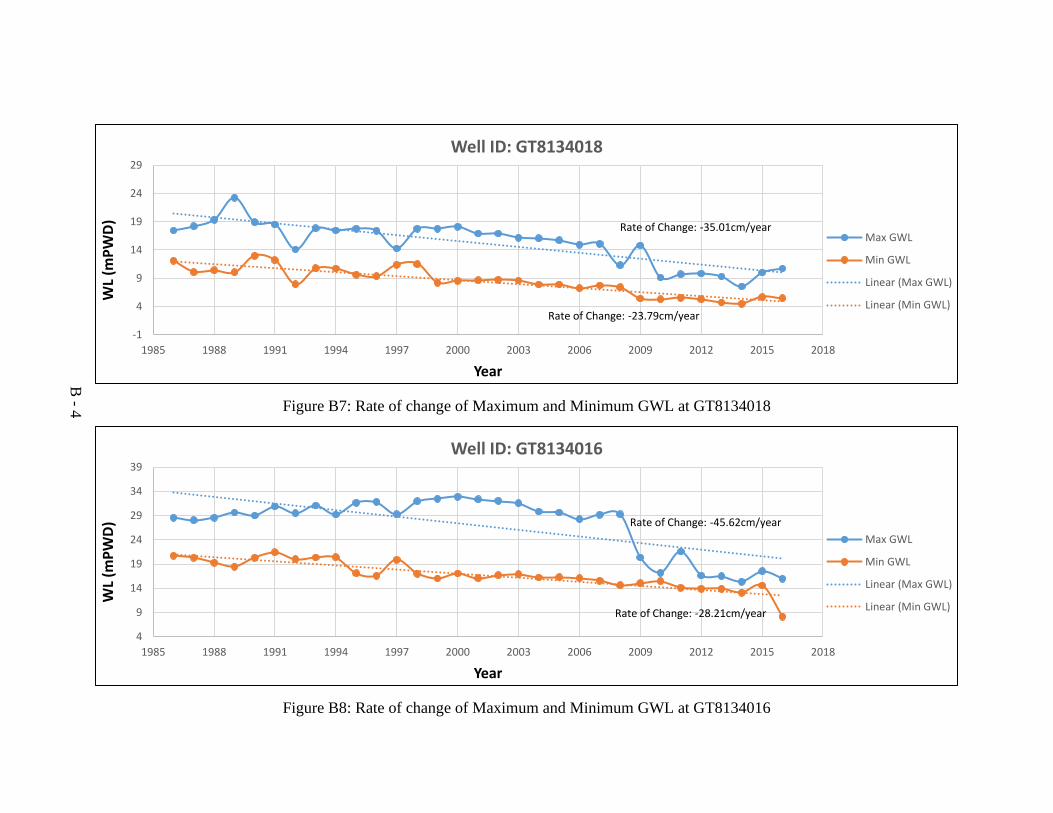
Figure B7: Rate of change of Maximum and Minimum GWL at GT8134018
Figure B8: Rate of change of Maximum and Minimum GWL at GT8134016
Rate of Change: -35.01cm/year
Rate of Change: -23.79cm/year
-1
4
9
14
19
24
29
1985 1988 1991 1994 1997 2000 2003 2006 2009 2012 2015 2018
WL
(mP
WD
)
Year
Well ID: GT8134018
Max GWL
Min GWL
Linear (Max GWL)
Linear (Min GWL)
Rate of Change: -45.62cm/year
Rate of Change: -28.21cm/year
4
9
14
19
24
29
34
39
1985 1988 1991 1994 1997 2000 2003 2006 2009 2012 2015 2018
WL
(mP
WD
)
Year
Well ID: GT8134016
Max GWL
Min GWL
Linear (Max GWL)
Linear (Min GWL)
B - 4
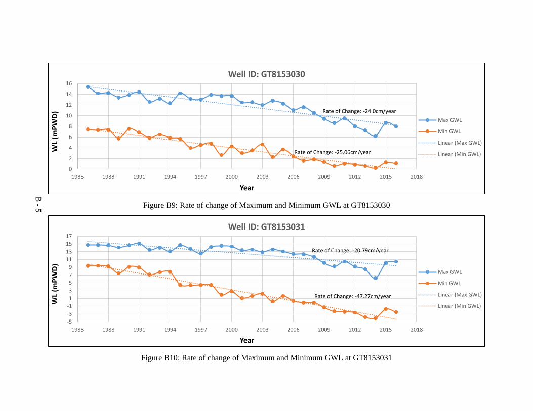
Figure B9: Rate of change of Maximum and Minimum GWL at GT8153030
Figure B10: Rate of change of Maximum and Minimum GWL at GT8153031
Rate of Change: -24.0cm/year
Rate of Change: -25.06cm/year
0
2
4
6
8
10
12
14
16
1985 1988 1991 1994 1997 2000 2003 2006 2009 2012 2015 2018
WL
(mP
WD
)
Year
Well ID: GT8153030
Max GWL
Min GWL
Linear (Max GWL)
Linear (Min GWL)
Rate of Change: -20.79cm/year
Rate of Change: -47.27cm/year
-5
-3
-1
1
3
5
7
9
11
13
15
17
1985 1988 1991 1994 1997 2000 2003 2006 2009 2012 2015 2018
WL
(mP
WD
)
Year
Well ID: GT8153031
Max GWL
Min GWL
Linear (Max GWL)
Linear (Min GWL)
B - 5

Figure B11: Rate of change of Maximum and Minimum GWL at GT8153037
Figure B12: Rate of change of Maximum and Minimum GWL at GT8182042
Rate of Change: -10.68cm/year
Rate of Change: -12.09cm/year
-1
1
3
5
7
9
11
13
15
17
1985 1988 1991 1994 1997 2000 2003 2006 2009 2012 2015 2018
WL
(mP
WD
)
Year
Well ID: GT8153037
Max GWL
Min GWL
Linear (Max GWL)
Linear (Min GWL)
Rate of Change: -5.2cm/year
Rate of Change: -24.53cm/year
0
2
4
6
8
10
12
14
16
1985 1988 1991 1994 1997 2000 2003 2006 2009 2012 2015 2018
WL
(mP
WD
)
Year
Well ID: GT8182042
Max GWL
Min GWL
Linear (Max GWL)
Linear (Min GWL)
B - 6
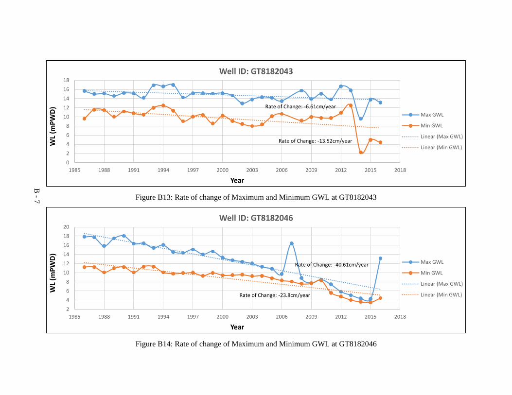
Figure B13: Rate of change of Maximum and Minimum GWL at GT8182043
Figure B14: Rate of change of Maximum and Minimum GWL at GT8182046
Rate of Change: -6.61cm/year
Rate of Change: -13.52cm/year
0
2
4
6
8
10
12
14
16
18
1985 1988 1991 1994 1997 2000 2003 2006 2009 2012 2015 2018
WL
(mP
WD
)
Year
Well ID: GT8182043
Max GWL
Min GWL
Linear (Max GWL)
Linear (Min GWL)
Rate of Change: -40.61cm/year
Rate of Change: -23.8cm/year
2
4
6
8
10
12
14
16
18
20
1985 1988 1991 1994 1997 2000 2003 2006 2009 2012 2015 2018
WL
(mP
WD
)
Year
Well ID: GT8182046
Max GWL
Min GWL
Linear (Max GWL)
Linear (Min GWL)
B - 7
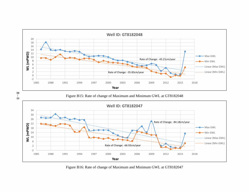
Figure B15: Rate of change of Maximum and Minimum GWL at GT8182048
Figure B16: Rate of change of Maximum and Minimum GWL at GT8182047
Rate of Change: -43.21cm/year
Rate of Change: -35.83cm/year
-2
0
2
4
6
8
10
12
14
16
18
20
1985 1988 1991 1994 1997 2000 2003 2006 2009 2012 2015 2018
WL
(mP
WD
)
Year
Well ID: GT8182048
Max GWL
Min GWL
Linear (Max GWL)
Linear (Min GWL)
Rate of Change: -84.18cm/year
Rate of Change: -66.93cm/year
-2
2
6
10
14
18
22
26
30
34
1985 1988 1991 1994 1997 2000 2003 2006 2009 2012 2015 2018
WL
(mP
WD
)
Year
Well ID: GT8182047
Max GWL
Min GWL
Linear (Max GWL)
Linear (Min GWL)
B - 8

Appendix C: Hydro-Stratigraphic Cross Sections
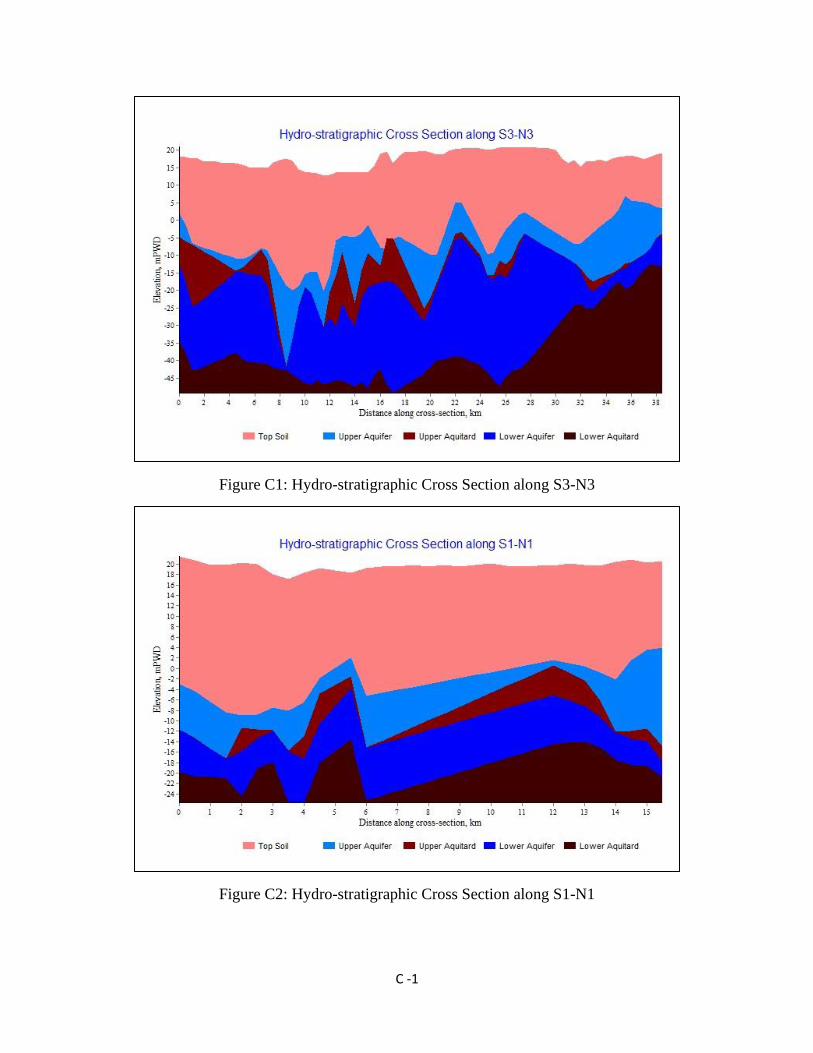
C -1
Figure C1: Hydro-stratigraphic Cross Section along S3-N3
Figure C2: Hydro-stratigraphic Cross Section along S1-N1
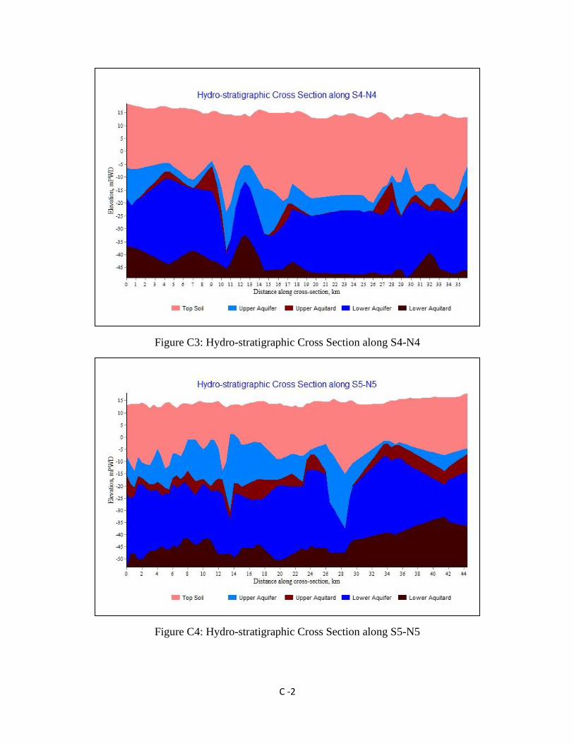
C -2
Figure C3: Hydro-stratigraphic Cross Section along S4-N4
Figure C4: Hydro-stratigraphic Cross Section along S5-N5
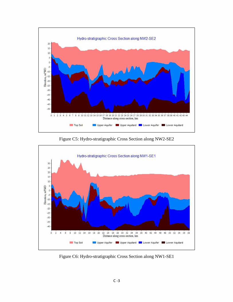
C -3
Figure C5: Hydro-stratigraphic Cross Section along NW2-SE2
Figure C6: Hydro-stratigraphic Cross Section along NW1-SE1

C -4
Figure C7: Hydro-stratigraphic Cross Section along W1-E1
Figure C8: Hydro-stratigraphic Cross Section along W2-E2
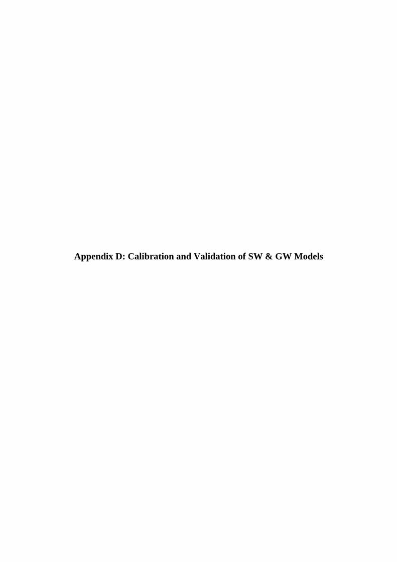
Appendix D: Calibration and Validation of SW & GW Models

D - 1
Calibration and Validation of GW model
Figure D1: Calibration and Validation of GW model for GWL of Station ID GT 8125009
Figure D2: Calibration and Validation of GW model for GWL of Station ID GT 8131015
Figure D3: Calibration and Validation of GW model for GWL of Station ID GT 8153030
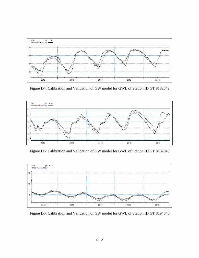
D - 2
Figure D4: Calibration and Validation of GW model for GWL of Station ID GT 8182042
Figure D5: Calibration and Validation of GW model for GWL of Station ID GT 8182043
Figure D6: Calibration and Validation of GW model for GWL of Station ID GT 8194046

D - 3
Figure D7: Calibration and Validation of GW model for GWL of Station ID GT 8194048
Figure D8: Calibration and Validation of GW model for GWL of Station ID GT 8153031
Figure D9: Calibration and Validation of GW model for GWL of Station ID GT 8125011
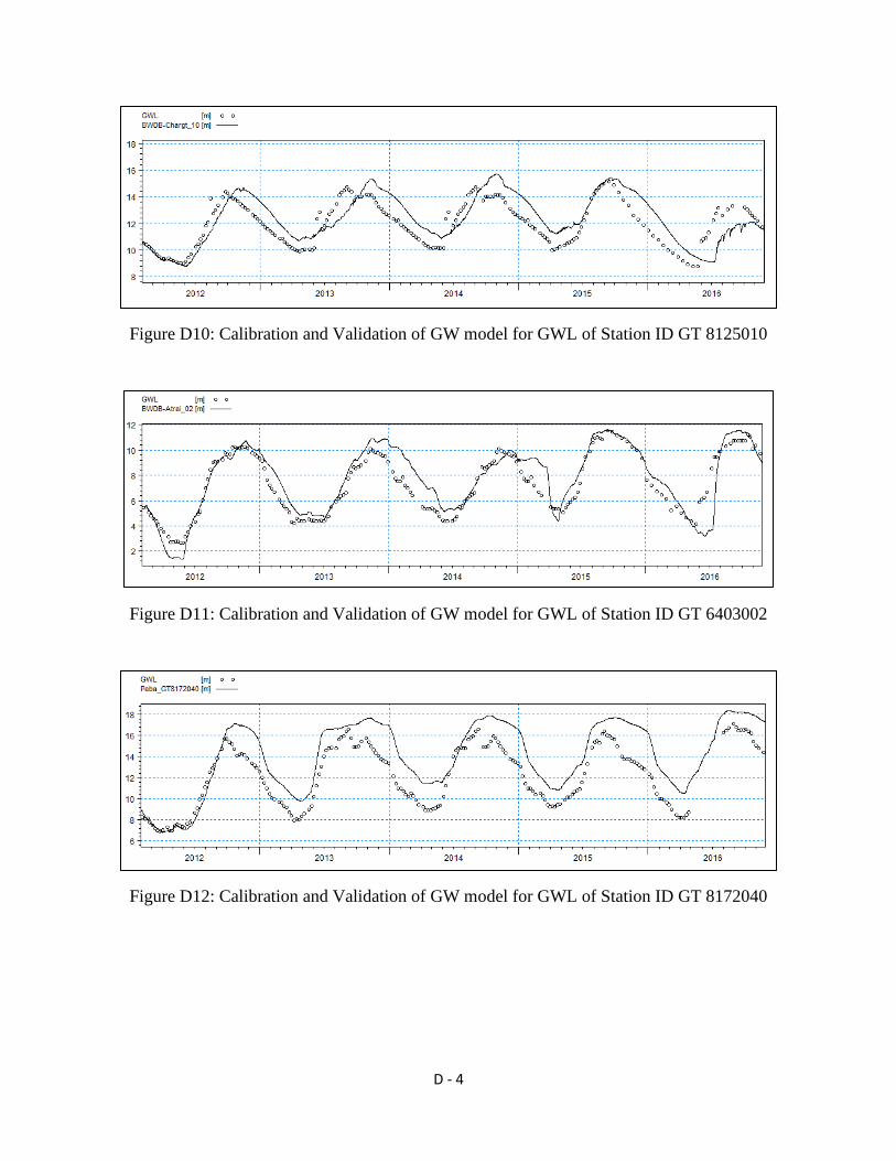
D - 4
Figure D10: Calibration and Validation of GW model for GWL of Station ID GT 8125010
Figure D11: Calibration and Validation of GW model for GWL of Station ID GT 6403002
Figure D12: Calibration and Validation of GW model for GWL of Station ID GT 8172040

D - 5
Figure D13: Calibration and Validation of GW model for GWL of Station ID GT 8134028
Figure D14: Calibration and Validation of GW model for GWL of Station ID GT 8134028
Figure D15: Calibration and Validation of GW model for GWL of Station ID GT 8112001

D - 6
Calibration and Validation of SW model
Figure D16: Calibration and Validation of SW model for SWL of Nowhata Station
Figure D17: Calibration and Validation of SW model for SWL of Naldanga Station
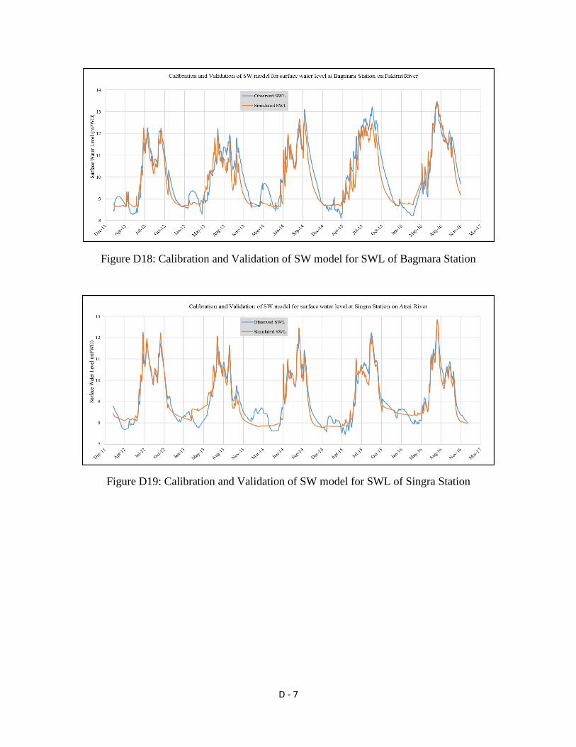
D - 7
Figure D18: Calibration and Validation of SW model for SWL of Bagmara Station
Figure D19: Calibration and Validation of SW model for SWL of Singra Station
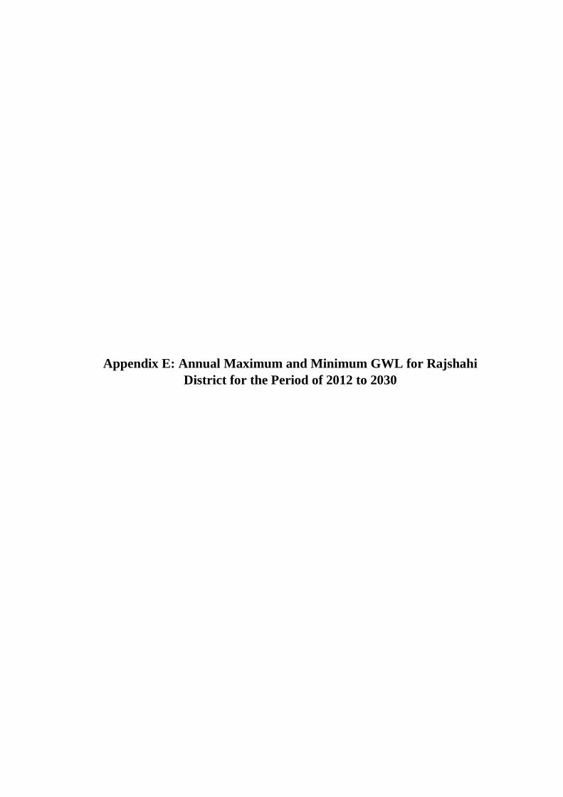
Appendix E: Annual Maximum and Minimum GWL for Rajshahi
District for the Period of 2012 to 2030
E-1
Table E-1: Annual Maximum and Minimum GWL for the Study Period (2012-2030) for GW
Stations of BWDB within the Model Area
Max. GWL (mPWD) Min. GWL (mPWD) Max. GWL (mPWD) Min. GWL (mPWD)
Year GT6403002 GT8125011
2012 10.779 1.277 12.581 5.617
2013 11.133 4.251 14.431 4.566
2014 10.648 4.444 15.950 5.704
2015 11.302 4.825 16.589 6.514
2016 11.292 2.825 15.990 6.636
2017 11.431 6.800 16.588 7.061
2018 11.455 6.661 16.589 7.219
2019 11.376 6.553 16.589 7.108
2020 11.385 6.600 16.589 6.936
2021 11.405 6.453 16.589 6.715
2022 11.459 6.637 16.589 6.558
2023 11.470 6.613 16.589 6.441
2024 11.475 6.505 16.589 6.171
2025 11.497 6.418 16.589 6.077
2026 11.527 6.349 16.589 6.061
2027 11.529 6.343 16.587 6.057
2028 11.525 6.349 16.589 6.031
2029 11.511 6.345 16.589 6.054
2030 11.346 6.356 16.589 6.064
Year GT8125010 GT8125006
2012 14.344 8.629 12.104 4.452
2013 14.932 10.289 13.801 7.037
2014 15.099 10.261 14.549 7.666
2015 14.920 10.698 14.678 8.294
2016 14.419 10.247 14.579 9.026
2017 14.963 11.503 14.660 9.598
2018 15.156 11.619 14.666 9.603
2019 15.178 11.449 14.659 9.502
2020 15.179 11.269 14.641 9.350
2021 15.243 11.079 14.631 9.251
2022 15.293 10.917 14.626 9.111
2023 15.419 10.842 14.626 8.991
2024 15.458 10.834 14.618 8.809
2025 15.523 10.762 14.615 8.748
2026 15.445 10.626 14.616 8.668
2027 15.508 10.547 14.608 8.632
2028 15.596 10.519 14.605 8.544
2029 15.667 10.539 14.605 8.526
2030 15.712 10.563 14.603 8.425
Year GT8125009 GT8131015
2012 14.501 4.975 13.354 -3.524
2013 15.279 6.664 13.525 -1.328
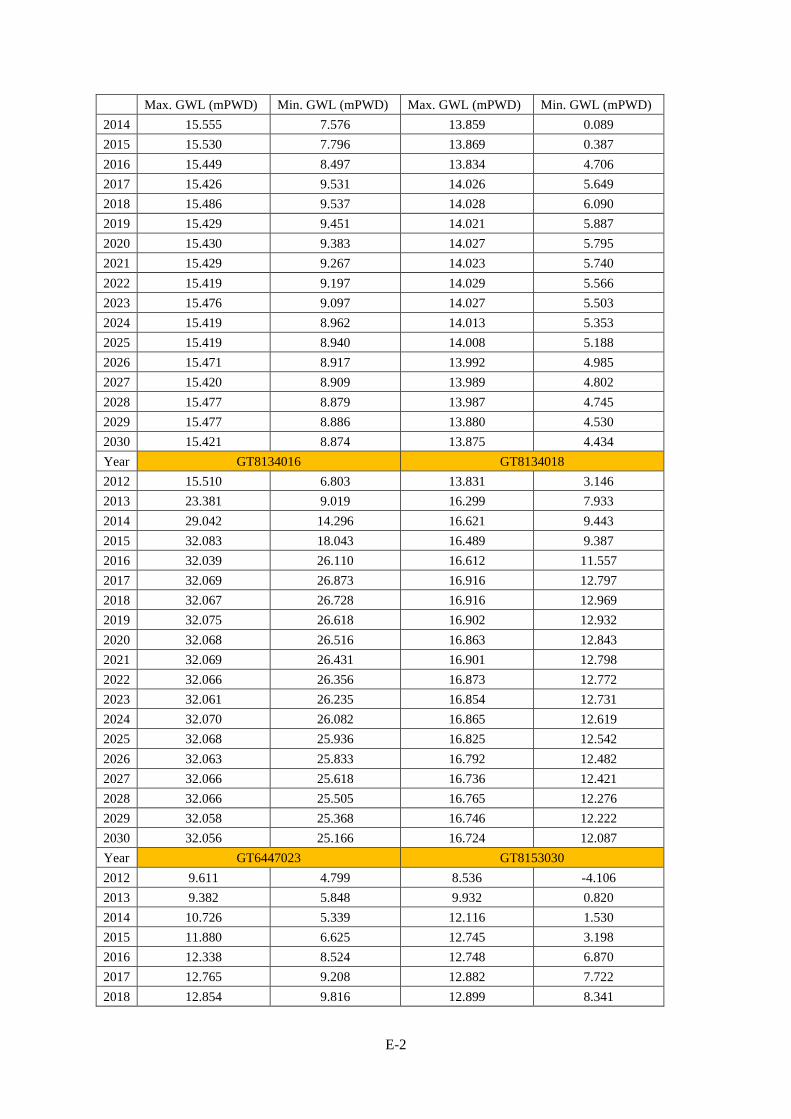
E-2
Max. GWL (mPWD) Min. GWL (mPWD) Max. GWL (mPWD) Min. GWL (mPWD)
2014 15.555 7.576 13.859 0.089
2015 15.530 7.796 13.869 0.387
2016 15.449 8.497 13.834 4.706
2017 15.426 9.531 14.026 5.649
2018 15.486 9.537 14.028 6.090
2019 15.429 9.451 14.021 5.887
2020 15.430 9.383 14.027 5.795
2021 15.429 9.267 14.023 5.740
2022 15.419 9.197 14.029 5.566
2023 15.476 9.097 14.027 5.503
2024 15.419 8.962 14.013 5.353
2025 15.419 8.940 14.008 5.188
2026 15.471 8.917 13.992 4.985
2027 15.420 8.909 13.989 4.802
2028 15.477 8.879 13.987 4.745
2029 15.477 8.886 13.880 4.530
2030 15.421 8.874 13.875 4.434
Year GT8134016 GT8134018
2012 15.510 6.803 13.831 3.146
2013 23.381 9.019 16.299 7.933
2014 29.042 14.296 16.621 9.443
2015 32.083 18.043 16.489 9.387
2016 32.039 26.110 16.612 11.557
2017 32.069 26.873 16.916 12.797
2018 32.067 26.728 16.916 12.969
2019 32.075 26.618 16.902 12.932
2020 32.068 26.516 16.863 12.843
2021 32.069 26.431 16.901 12.798
2022 32.066 26.356 16.873 12.772
2023 32.061 26.235 16.854 12.731
2024 32.070 26.082 16.865 12.619
2025 32.068 25.936 16.825 12.542
2026 32.063 25.833 16.792 12.482
2027 32.066 25.618 16.736 12.421
2028 32.066 25.505 16.765 12.276
2029 32.058 25.368 16.746 12.222
2030 32.056 25.166 16.724 12.087
Year GT6447023 GT8153030
2012 9.611 4.799 8.536 -4.106
2013 9.382 5.848 9.932 0.820
2014 10.726 5.339 12.116 1.530
2015 11.880 6.625 12.745 3.198
2016 12.338 8.524 12.748 6.870
2017 12.765 9.208 12.882 7.722
2018 12.854 9.816 12.899 8.341
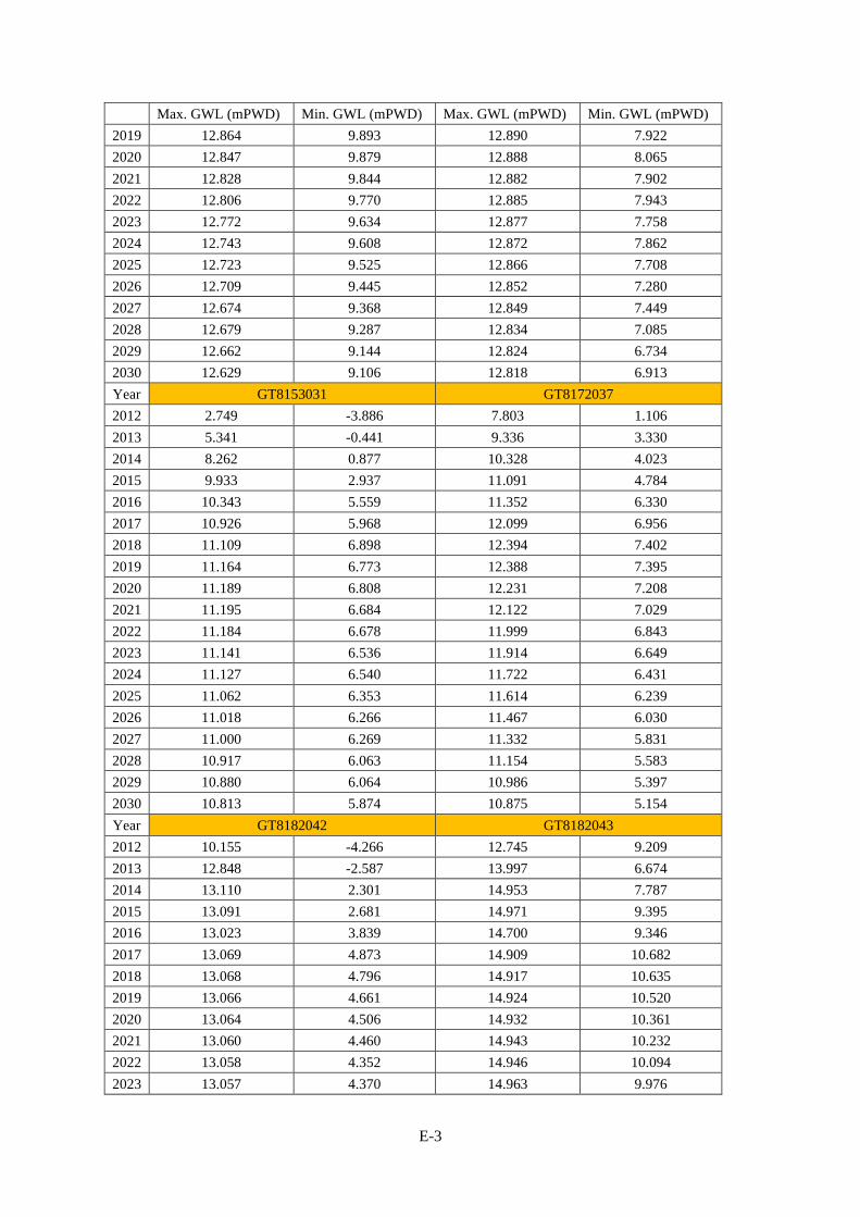
E-3
Max. GWL (mPWD) Min. GWL (mPWD) Max. GWL (mPWD) Min. GWL (mPWD)
2019 12.864 9.893 12.890 7.922
2020 12.847 9.879 12.888 8.065
2021 12.828 9.844 12.882 7.902
2022 12.806 9.770 12.885 7.943
2023 12.772 9.634 12.877 7.758
2024 12.743 9.608 12.872 7.862
2025 12.723 9.525 12.866 7.708
2026 12.709 9.445 12.852 7.280
2027 12.674 9.368 12.849 7.449
2028 12.679 9.287 12.834 7.085
2029 12.662 9.144 12.824 6.734
2030 12.629 9.106 12.818 6.913
Year GT8153031 GT8172037
2012 2.749 -3.886 7.803 1.106
2013 5.341 -0.441 9.336 3.330
2014 8.262 0.877 10.328 4.023
2015 9.933 2.937 11.091 4.784
2016 10.343 5.559 11.352 6.330
2017 10.926 5.968 12.099 6.956
2018 11.109 6.898 12.394 7.402
2019 11.164 6.773 12.388 7.395
2020 11.189 6.808 12.231 7.208
2021 11.195 6.684 12.122 7.029
2022 11.184 6.678 11.999 6.843
2023 11.141 6.536 11.914 6.649
2024 11.127 6.540 11.722 6.431
2025 11.062 6.353 11.614 6.239
2026 11.018 6.266 11.467 6.030
2027 11.000 6.269 11.332 5.831
2028 10.917 6.063 11.154 5.583
2029 10.880 6.064 10.986 5.397
2030 10.813 5.874 10.875 5.154
Year GT8182042 GT8182043
2012 10.155 -4.266 12.745 9.209
2013 12.848 -2.587 13.997 6.674
2014 13.110 2.301 14.953 7.787
2015 13.091 2.681 14.971 9.395
2016 13.023 3.839 14.700 9.346
2017 13.069 4.873 14.909 10.682
2018 13.068 4.796 14.917 10.635
2019 13.066 4.661 14.924 10.520
2020 13.064 4.506 14.932 10.361
2021 13.060 4.460 14.943 10.232
2022 13.058 4.352 14.946 10.094
2023 13.057 4.370 14.963 9.976
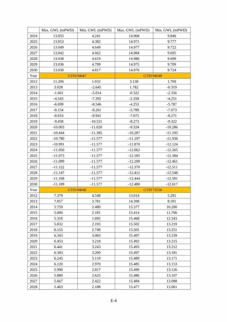
E-4
Max. GWL (mPWD) Min. GWL (mPWD) Max. GWL (mPWD) Min. GWL (mPWD)
2024 13.055 4.241 14.968 9.846
2025 13.053 4.382 14.971 9.777
2026 13.049 4.649 14.977 9.722
2027 13.042 4.662 14.984 9.695
2028 13.038 4.619 14.986 9.699
2029 13.036 4.799 14.975 9.709
2030 13.030 4.817 14.976 9.724
Year GT8194047 GT8194048
2012 11.206 1.032 3.138 1.769
2013 3.028 -2.645 1.782 -0.319
2014 -1.661 -5.014 -0.322 -2.356
2015 -4.543 -7.392 -2.358 -4.251
2016 -6.699 -8.546 -4.253 -5.787
2017 -8.154 -9.261 -5.789 -7.073
2018 -8.816 -9.941 -7.075 -8.271
2019 -9.458 -10.531 -8.273 -9.322
2020 -10.003 -11.020 -9.324 -10.286
2021 -10.444 -11.385 -10.287 -11.195
2022 -10.780 -11.577 -11.197 -11.936
2023 -10.991 -11.577 -11.870 -12.124
2024 -11.050 -11.577 -12.062 -12.265
2025 -11.073 -11.577 -12.185 -12.384
2026 -11.099 -11.577 -12.299 -12.461
2027 -11.122 -11.577 -12.370 -12.511
2028 -11.147 -11.577 -12.412 -12.548
2029 -11.168 -11.577 -12.444 -12.581
2030 -11.189 -11.577 -12.480 -12.617
Year GT8194046 GT8172036
2012 7.379 4.548 13.014 5.281
2013 7.057 3.781 14.398 8.591
2014 5.759 2.480 15.377 10.200
2015 5.000 2.181 15.414 11.766
2016 5.316 1.695 15.468 12.543
2017 5.832 2.193 15.502 13.219
2018 6.155 2.749 15.501 13.251
2019 6.343 3.083 15.497 13.239
2020 6.453 3.218 15.492 13.215
2021 6.441 3.243 15.493 13.212
2022 6.383 3.200 15.497 13.181
2023 6.245 3.110 15.489 13.171
2024 6.120 2.970 15.485 13.153
2025 5.990 2.817 15.490 13.126
2026 5.880 2.625 15.486 13.107
2027 5.667 2.422 15.484 13.088
2028 5.463 2.188 15.477 13.061

E-5
Max. GWL (mPWD) Min. GWL (mPWD) Max. GWL (mPWD) Min. GWL (mPWD)
2029 5.326 1.943 15.477 13.041
2030 5.074 1.689 15.478 13.019
Year GT8134027 GT8134021
2012 9.737 7.669 9.769 4.350
2013 8.612 6.899 11.420 3.146
2014 8.198 6.529 12.586 4.349
2015 7.830 5.900 14.871 4.349
2016 7.551 6.517 13.660 6.430
2017 7.877 6.731 14.116 6.821
2018 8.208 7.056 14.536 7.168
2019 8.543 7.372 14.727 7.243
2020 8.863 7.680 14.716 7.132
2021 9.145 7.972 14.561 7.002
2022 9.384 8.213 14.423 6.738
2023 9.571 8.410 14.216 6.461
2024 9.696 8.555 13.913 6.027
2025 9.764 8.652 13.564 5.681
2026 9.778 8.692 13.253 5.249
2027 9.739 8.685 12.878 4.763
2028 9.652 8.624 12.549 4.295
2029 9.531 8.527 12.274 4.005
2030 9.365 8.399 11.898 3.602
Year GT8134028 GT8172040
2012 13.231 7.229 17.158 6.047
2013 17.174 6.193 18.038 9.574
2014 19.812 10.715 17.838 11.007
2015 19.873 13.119 17.356 10.741
2016 19.844 14.195 17.330 12.259
2017 19.858 14.696 17.773 14.256
2018 19.856 14.723 17.832 14.100
2019 19.848 14.711 17.884 13.657
2020 19.860 14.664 17.907 13.329
2021 19.856 14.594 18.057 13.092
2022 19.856 14.478 18.087 12.831
2023 19.855 14.410 18.109 12.690
2024 19.853 14.365 18.160 12.688
2025 19.857 14.214 18.170 12.688
2026 19.857 14.188 18.179 12.675
2027 19.859 14.169 18.182 12.667
2028 19.857 13.954 18.181 12.674
2029 19.858 13.913 18.190 12.737
2030 19.857 13.769 18.225 12.732
Year GT8182041 GT8194044
2012 12.514 7.482 12.630 8.157
2013 12.764 6.304 10.397 8.958

E-6
Max. GWL (mPWD) Min. GWL (mPWD) Max. GWL (mPWD) Min. GWL (mPWD)
2014 13.079 8.716 9.375 8.286
2015 13.122 10.646 10.278 7.235
2016 12.942 10.406 10.146 7.321
2017 12.999 11.119 10.164 7.732
2018 13.013 11.169 10.319 7.996
2019 13.013 11.170 10.327 8.019
2020 13.002 11.147 10.294 7.887
2021 13.010 11.152 10.211 7.744
2022 13.001 11.123 10.006 7.541
2023 13.009 11.127 9.812 7.272
2024 13.006 11.107 9.547 6.978
2025 12.999 11.123 9.281 6.681
2026 12.996 11.104 8.953 6.310
2027 12.994 11.120 8.645 6.035
2028 12.996 11.104 8.319 5.633
2029 12.996 11.095 7.912 5.395
2030 12.998 11.103 7.520 5.246
Year GT8112003 GT8112002
2012 11.042 -3.272 12.436 -2.886
2013 11.949 1.576 12.993 2.982
2014 11.966 4.121 13.277 4.764
2015 11.981 3.666 13.278 3.915
2016 11.981 7.647 13.276 7.892
2017 11.985 9.163 13.277 8.738
2018 11.985 9.028 13.277 9.050
2019 11.984 9.110 13.276 8.732
2020 11.984 9.080 13.276 8.921
2021 11.984 8.598 13.277 8.222
2022 11.980 8.874 13.277 8.515
2023 11.983 9.427 13.278 8.594
2024 11.983 8.894 13.278 8.305
2025 11.982 8.971 13.277 8.187
2026 11.982 8.563 13.277 7.898
2027 11.979 9.163 13.278 8.169
2028 11.978 9.286 13.277 7.961
2029 11.978 9.303 13.277 7.939
2030 11.977 9.110 13.278 7.734