arX

iv:h

ep-e

x/03

1001

3 v1

8

Oct

200

3

EUROPEAN ORGANIZATION FOR NUCLEAR RESEARCH

CERN-EP/2003-04911 July 2003

Study of Z Pair Production and Anomalous

Couplings in e+e− Collisions at√

s between

190GeV and 209GeV

The OPAL Collaboration

Abstract

A study of Z-boson pair production in e+e− annihilation at center-of-mass energies between190 GeV and 209 GeV is reported. Final states containing only leptons, (ℓ+ℓ−ℓ+ℓ− and ℓ+ℓ−νν),quark and lepton pairs, (qqℓ+ℓ−, qqνν) and only hadrons (qqqq) are considered. In all states with atleast one Z boson decaying hadronically, lifetime, lepton and event-shape tags are used to separate bbpairs from qq final states. Limits on anomalous ZZγ and ZZZ couplings are derived from the measuredcross sections and from event kinematics using an optimal observable method. Limits on low scalegravity with large extra dimensions are derived from the cross sections and their dependence on polarangle.

Submitted to Eur. Phys. J.

The OPAL Collaboration

G. Abbiendi2, C. Ainsley5, P.F. Akesson3, G. Alexander22, J. Allison16, P. Amaral9, G. Anagnostou1,K.J. Anderson9, S. Arcelli2, S. Asai23, D. Axen27, G. Azuelos18,a, I. Bailey26, E. Barberio8,p,R.J. Barlow16, R.J. Batley5, P. Bechtle25 , T. Behnke25, K.W. Bell20, P.J. Bell1, G. Bella22,

A. Bellerive6, G. Benelli4, S. Bethke32, O. Biebel31, O. Boeriu10, P. Bock11, M. Boutemeur31,S. Braibant8, L. Brigliadori2, R.M. Brown20, K. Buesser25, H.J. Burckhart8, S. Campana4,

R.K. Carnegie6, B. Caron28, A.A. Carter13, J.R. Carter5, C.Y. Chang17, D.G. Charlton1, A. Csilling29,M. Cuffiani2, S. Dado21, A. De Roeck8, E.A. De Wolf8,s, K. Desch25, B. Dienes30, M. Donkers6,J. Dubbert31, E. Duchovni24, G. Duckeck31, I.P. Duerdoth16, E. Etzion22, F. Fabbri2, L. Feld10,P. Ferrari8, F. Fiedler31, I. Fleck10, M. Ford5, A. Frey8, A. Furtjes8, P. Gagnon12, J.W. Gary4,G. Gaycken25, C. Geich-Gimbel3, G. Giacomelli2, P. Giacomelli2, M. Giunta4, J. Goldberg21,

E. Gross24, J. Grunhaus22, M. Gruwe8, P.O. Gunther3, A. Gupta9, C. Hajdu29, M. Hamann25,G.G. Hanson4, K. Harder25, A. Harel21, M. Harin-Dirac4, M. Hauschild8, C.M. Hawkes1,

R. Hawkings8, R.J. Hemingway6, C. Hensel25, G. Herten10, R.D. Heuer25, J.C. Hill5, K. Hoffman9,D. Horvath29,c, P. Igo-Kemenes11, K. Ishii23, H. Jeremie18, P. Jovanovic1, T.R. Junk6, N. Kanaya26,

J. Kanzaki23,u, G. Karapetian18, D. Karlen26, K. Kawagoe23, T. Kawamoto23, R.K. Keeler26,R.G. Kellogg17, B.W. Kennedy20, D.H. Kim19, K. Klein11,t, A. Klier24, S. Kluth32, T. Kobayashi23,M. Kobel3, S. Komamiya23, L. Kormos26, T. Kramer25, P. Krieger6,l, J. von Krogh11, K. Kruger8,T. Kuhl25, M. Kupper24, G.D. Lafferty16, H. Landsman21, D. Lanske14, J.G. Layter4, A. Leins31,

D. Lellouch24, J. Lettso, L. Levinson24, J. Lillich10, S.L. Lloyd13, F.K. Loebinger16, J. Lu27,w,J. Ludwig10, A. Macpherson28,i, W. Mader3, S. Marcellini2, A.J. Martin13, G. Masetti2, T. Mashimo23,

P. Mattigm, W.J. McDonald28, J. McKenna27, T.J. McMahon1, R.A. McPherson26, F. Meijers8,W. Menges25, F.S. Merritt9, H. Mes6,a, A. Michelini2, S. Mihara23, G. Mikenberg24, D.J. Miller15,

S. Moed21, W. Mohr10, T. Mori23, A. Mutter10, K. Nagai13, I. Nakamura23,V , H. Nanjo23, H.A. Neal33,R. Nisius32, S.W. O’Neale1, A. Oh8, A. Okpara11, M.J. Oreglia9, S. Orito23,∗, C. Pahl32, G. Pasztor4,g,J.R. Pater16, G.N. Patrick20, J.E. Pilcher9, J. Pinfold28, D.E. Plane8, B. Poli2, J. Polok8, O. Pooth14,

M. Przybycien8,n, A. Quadt3, K. Rabbertz8,r, C. Rembser8, P. Renkel24, H. Rick4,b J.M. Roney26,S. Rosati3, Y. Rozen21, K. Runge10, K. Sachs6, T. Saeki23, E.K.G. Sarkisyan8,j , A.D. Schaile31,

O. Schaile31, P. Scharff-Hansen8, J. Schieck32, T. Schorner-Sadenius8, M. Schroder8, M. Schumacher3,C. Schwick8, W.G. Scott20, R. Seuster14,f , T.G. Shears8,h, B.C. Shen4, P. Sherwood15, G. Siroli2,

A. Skuja17, A.M. Smith8, R. Sobie26, S. Soldner-Rembold16,d, F. Spano9, A. Stahl3, K. Stephens16,D. Strom19, R. Strohmer31, S. Tarem21, M. Tasevsky8, R.J. Taylor15, R. Teuscher9, M.A. Thomson5,

E. Torrence19, D. Toya23, P. Tran4, I. Trigger8, Z. Trocsanyi30,e, E. Tsur22, M.F. Turner-Watson1,I. Ueda23, B. Ujvari30,e, C.F. Vollmer31, P. Vannerem10, R. Vertesi30, M. Verzocchi17, H. Voss8,q,

J. Vossebeld8,h, D. Waller6, C.P. Ward5, D.R. Ward5, M. Warsinsky3, P.M. Watkins1, A.T. Watson1,N.K. Watson1, P.S. Wells8, T. Wengler8, N. Wermes3, D. Wetterling11 G.W. Wilson16,k, J.A. Wilson1,

G. Wolf24, T.R. Wyatt16, S. Yamashita23, D. Zer-Zion4, L. Zivkovic24

1School of Physics and Astronomy, University of Birmingham, Birmingham B15 2TT, UK2Dipartimento di Fisica dell’ Universita di Bologna and INFN, I-40126 Bologna, Italy3Physikalisches Institut, Universitat Bonn, D-53115 Bonn, Germany4Department of Physics, University of California, Riverside CA 92521, USA5Cavendish Laboratory, Cambridge CB3 0HE, UK6Ottawa-Carleton Institute for Physics, Department of Physics, Carleton University, Ottawa, OntarioK1S 5B6, Canada8CERN, European Organisation for Nuclear Research, CH-1211 Geneva 23, Switzerland9Enrico Fermi Institute and Department of Physics, University of Chicago, Chicago IL 60637, USA10Fakultat fur Physik, Albert-Ludwigs-Universitat Freiburg, D-79104 Freiburg, Germany11Physikalisches Institut, Universitat Heidelberg, D-69120 Heidelberg, Germany12Indiana University, Department of Physics, Bloomington IN 47405, USA

1

13Queen Mary and Westfield College, University of London, London E1 4NS, UK14Technische Hochschule Aachen, III Physikalisches Institut, Sommerfeldstrasse 26-28, D-52056 Aachen,Germany15University College London, London WC1E 6BT, UK16Department of Physics, Schuster Laboratory, The University, Manchester M13 9PL, UK17Department of Physics, University of Maryland, College Park, MD 20742, USA18Laboratoire de Physique Nucleaire, Universite de Montreal, Montreal, Quebec H3C 3J7, Canada19University of Oregon, Department of Physics, Eugene OR 97403, USA20CLRC Rutherford Appleton Laboratory, Chilton, Didcot, Oxfordshire OX11 0QX, UK21Department of Physics, Technion-Israel Institute of Technology, Haifa 32000, Israel22Department of Physics and Astronomy, Tel Aviv University, Tel Aviv 69978, Israel23International Centre for Elementary Particle Physics and Department of Physics, University ofTokyo, Tokyo 113-0033, and Kobe University, Kobe 657-8501, Japan24Particle Physics Department, Weizmann Institute of Science, Rehovot 76100, Israel25Universitat Hamburg/DESY, Institut fur Experimentalphysik, Notkestrasse 85, D-22607 Hamburg,Germany26University of Victoria, Department of Physics, P O Box 3055, Victoria BC V8W 3P6, Canada27University of British Columbia, Department of Physics, Vancouver BC V6T 1Z1, Canada28University of Alberta, Department of Physics, Edmonton AB T6G 2J1, Canada29Research Institute for Particle and Nuclear Physics, H-1525 Budapest, P O Box 49, Hungary30Institute of Nuclear Research, H-4001 Debrecen, P O Box 51, Hungary31Ludwig-Maximilians-Universitat Munchen, Sektion Physik, Am Coulombwall 1, D-85748 Garching,Germany32Max-Planck-Institute fur Physik, Fohringer Ring 6, D-80805 Munchen, Germany33Yale University, Department of Physics, New Haven, CT 06520, USA

a and at TRIUMF, Vancouver, Canada V6T 2A3b now at Physikalisches Institut, Universitat Heidelberg, D-69120 Heidelberg, Germanyc and Institute of Nuclear Research, Debrecen, Hungaryd and Heisenberg Fellowe and Department of Experimental Physics, Lajos Kossuth University, Debrecen, Hungaryf and MPI Muncheng and Research Institute for Particle and Nuclear Physics, Budapest, Hungaryh now at University of Liverpool, Dept of Physics, Liverpool L69 3BX, U.K.i and CERN, EP Div, 1211 Geneva 23j and Manchester Universityk now at University of Kansas, Dept of Physics and Astronomy, Lawrence, KS 66045, U.S.A.l now at University of Toronto, Dept of Physics, Toronto, Canadam current address Bergische Universitat, Wuppertal, Germanyn now at University of Mining and Metallurgy, Cracow, Polando now at University of California, San Diego, U.S.A.p now at Physics Dept Southern Methodist University, Dallas, TX 75275, U.S.A.q now at IPHE Universite de Lausanne, CH-1015 Lausanne, Switzerlandr now at IEKP Universitat Karlsruhe, Germanys now at Universitaire Instelling Antwerpen, Physics Department, B-2610 Antwerpen, Belgiumt now at RWTH Aachen, Germanyu and High Energy Accelerator Research Organisation (KEK), Tsukuba, Ibaraki, Japanv now at University of Pennsylvania, Philadelphia, Pennsylvania, USAw now at TRIUMF, Vancouver, Canada∗ Deceased

2

1 Introduction

LEP operation at center-of-mass energies above the Z-pair production threshold has made a carefulstudy of the process e+e− → ZZ possible. In the final data taking runs in 1999 and 2000 LEP deliveredan integrated luminosity of more than 400 pb−1 to the OPAL experiment at energies between 190 GeVand 209 GeV producing of the order of 100 detected Z-pair events. In this paper we present resultson Z-pair production from these data. Previously published studies from OPAL and the other LEPcollaborations can be found in References [1–4].

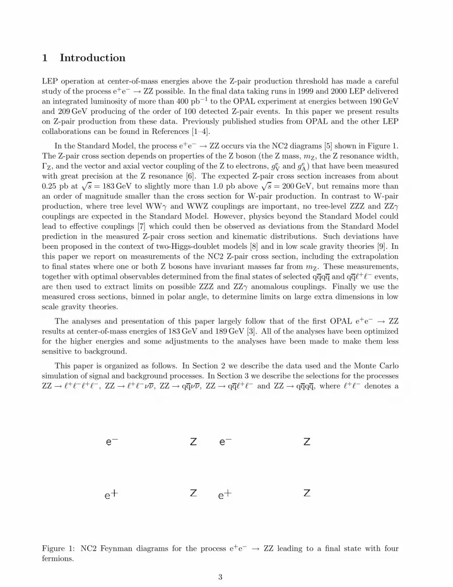
In the Standard Model, the process e+e− → ZZ occurs via the NC2 diagrams [5] shown in Figure 1.The Z-pair cross section depends on properties of the Z boson (the Z mass, mZ, the Z resonance width,ΓZ, and the vector and axial vector coupling of the Z to electrons, ge

V and geA) that have been measured

with great precision at the Z resonance [6]. The expected Z-pair cross section increases from about0.25 pb at

√s = 183 GeV to slightly more than 1.0 pb above

√s = 200 GeV, but remains more than

an order of magnitude smaller than the cross section for W-pair production. In contrast to W-pairproduction, where tree level WWγ and WWZ couplings are important, no tree-level ZZZ and ZZγcouplings are expected in the Standard Model. However, physics beyond the Standard Model couldlead to effective couplings [7] which could then be observed as deviations from the Standard Modelprediction in the measured Z-pair cross section and kinematic distributions. Such deviations havebeen proposed in the context of two-Higgs-doublet models [8] and in low scale gravity theories [9]. Inthis paper we report on measurements of the NC2 Z-pair cross section, including the extrapolationto final states where one or both Z bosons have invariant masses far from mZ. These measurements,together with optimal observables determined from the final states of selected qqqq and qqℓ+ℓ− events,are then used to extract limits on possible ZZZ and ZZγ anomalous couplings. Finally we use themeasured cross sections, binned in polar angle, to determine limits on large extra dimensions in lowscale gravity theories.

The analyses and presentation of this paper largely follow that of the first OPAL e+e− → ZZresults at center-of-mass energies of 183 GeV and 189 GeV [3]. All of the analyses have been optimizedfor the higher energies and some adjustments to the analyses have been made to make them lesssensitive to background.

This paper is organized as follows. In Section 2 we describe the data used and the Monte Carlosimulation of signal and background processes. In Section 3 we describe the selections for the processesZZ → ℓ+ℓ−ℓ+ℓ−, ZZ → ℓ+ℓ−νν, ZZ → qqνν, ZZ → qqℓ+ℓ− and ZZ → qqqq, where ℓ+ℓ− denotes a

e+e

ZZe+

eZZ

Figure 1: NC2 Feynman diagrams for the process e+e− → ZZ leading to a final state with fourfermions.

3

Energy point label Mean center-of-mass energy Approximate integrated luminosity

(GeV) (GeV) (pb−1)

192 191.59 ± 0.04 29

196 195.53 ± 0.04 73

200 199.52 ± 0.04 74

202 201.63 ± 0.04 37

205 204.80 ± 0.05 80

207 206.53 ± 0.05 140

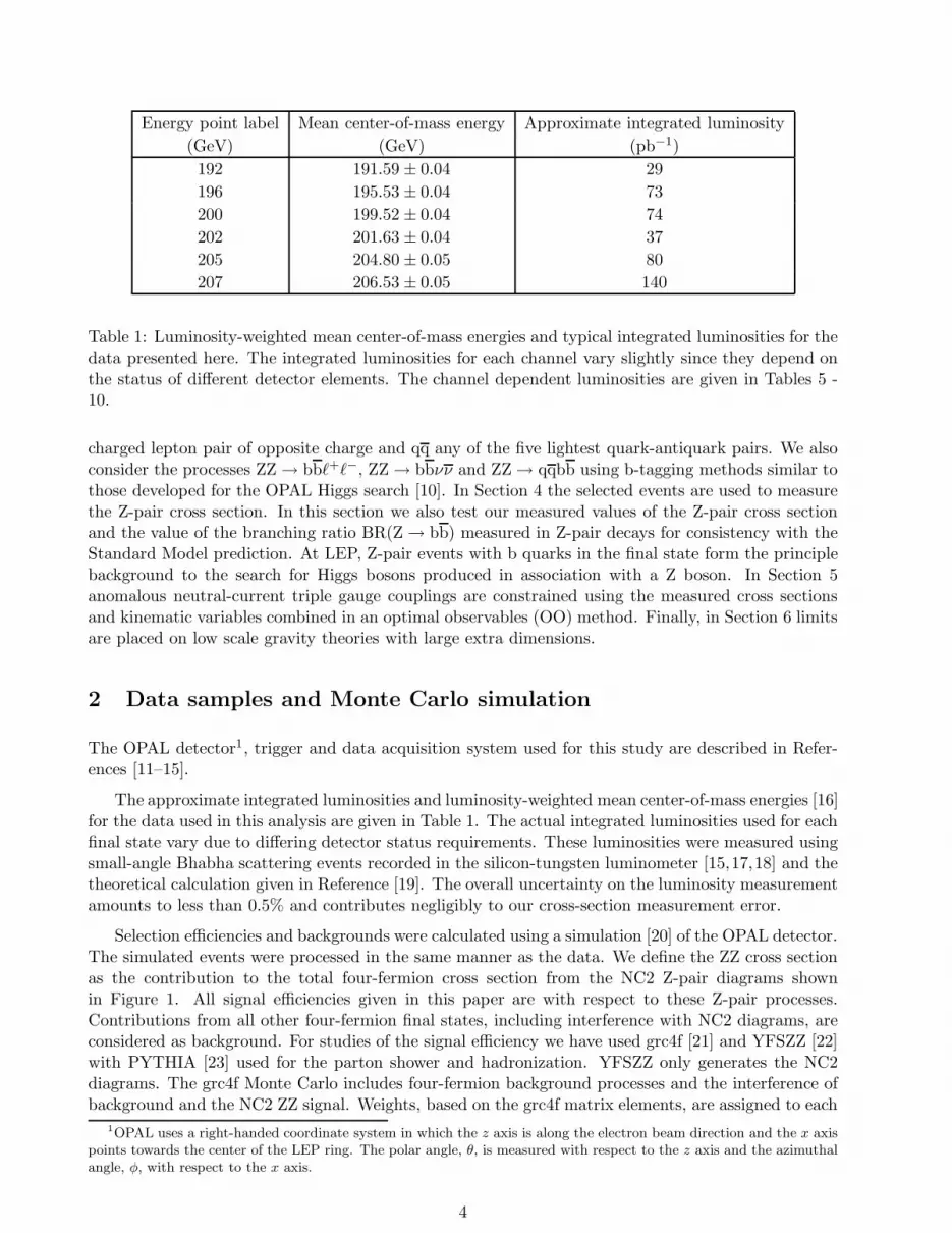
Table 1: Luminosity-weighted mean center-of-mass energies and typical integrated luminosities for thedata presented here. The integrated luminosities for each channel vary slightly since they depend onthe status of different detector elements. The channel dependent luminosities are given in Tables 5 -10.

charged lepton pair of opposite charge and qq any of the five lightest quark-antiquark pairs. We alsoconsider the processes ZZ → bbℓ+ℓ−, ZZ → bbνν and ZZ → qqbb using b-tagging methods similar tothose developed for the OPAL Higgs search [10]. In Section 4 the selected events are used to measurethe Z-pair cross section. In this section we also test our measured values of the Z-pair cross sectionand the value of the branching ratio BR(Z → bb) measured in Z-pair decays for consistency with theStandard Model prediction. At LEP, Z-pair events with b quarks in the final state form the principlebackground to the search for Higgs bosons produced in association with a Z boson. In Section 5anomalous neutral-current triple gauge couplings are constrained using the measured cross sectionsand kinematic variables combined in an optimal observables (OO) method. Finally, in Section 6 limitsare placed on low scale gravity theories with large extra dimensions.

2 Data samples and Monte Carlo simulation

The OPAL detector1, trigger and data acquisition system used for this study are described in Refer-ences [11–15].

The approximate integrated luminosities and luminosity-weighted mean center-of-mass energies [16]for the data used in this analysis are given in Table 1. The actual integrated luminosities used for eachfinal state vary due to differing detector status requirements. These luminosities were measured usingsmall-angle Bhabha scattering events recorded in the silicon-tungsten luminometer [15,17,18] and thetheoretical calculation given in Reference [19]. The overall uncertainty on the luminosity measurementamounts to less than 0.5% and contributes negligibly to our cross-section measurement error.

Selection efficiencies and backgrounds were calculated using a simulation [20] of the OPAL detector.The simulated events were processed in the same manner as the data. We define the ZZ cross sectionas the contribution to the total four-fermion cross section from the NC2 Z-pair diagrams shownin Figure 1. All signal efficiencies given in this paper are with respect to these Z-pair processes.Contributions from all other four-fermion final states, including interference with NC2 diagrams, areconsidered as background. For studies of the signal efficiency we have used grc4f [21] and YFSZZ [22]with PYTHIA [23] used for the parton shower and hadronization. YFSZZ only generates the NC2diagrams. The grc4f Monte Carlo includes four-fermion background processes and the interference ofbackground and the NC2 ZZ signal. Weights, based on the grc4f matrix elements, are assigned to each

1OPAL uses a right-handed coordinate system in which the z axis is along the electron beam direction and the x axispoints towards the center of the LEP ring. The polar angle, θ, is measured with respect to the z axis and the azimuthalangle, φ, with respect to the x axis.

4

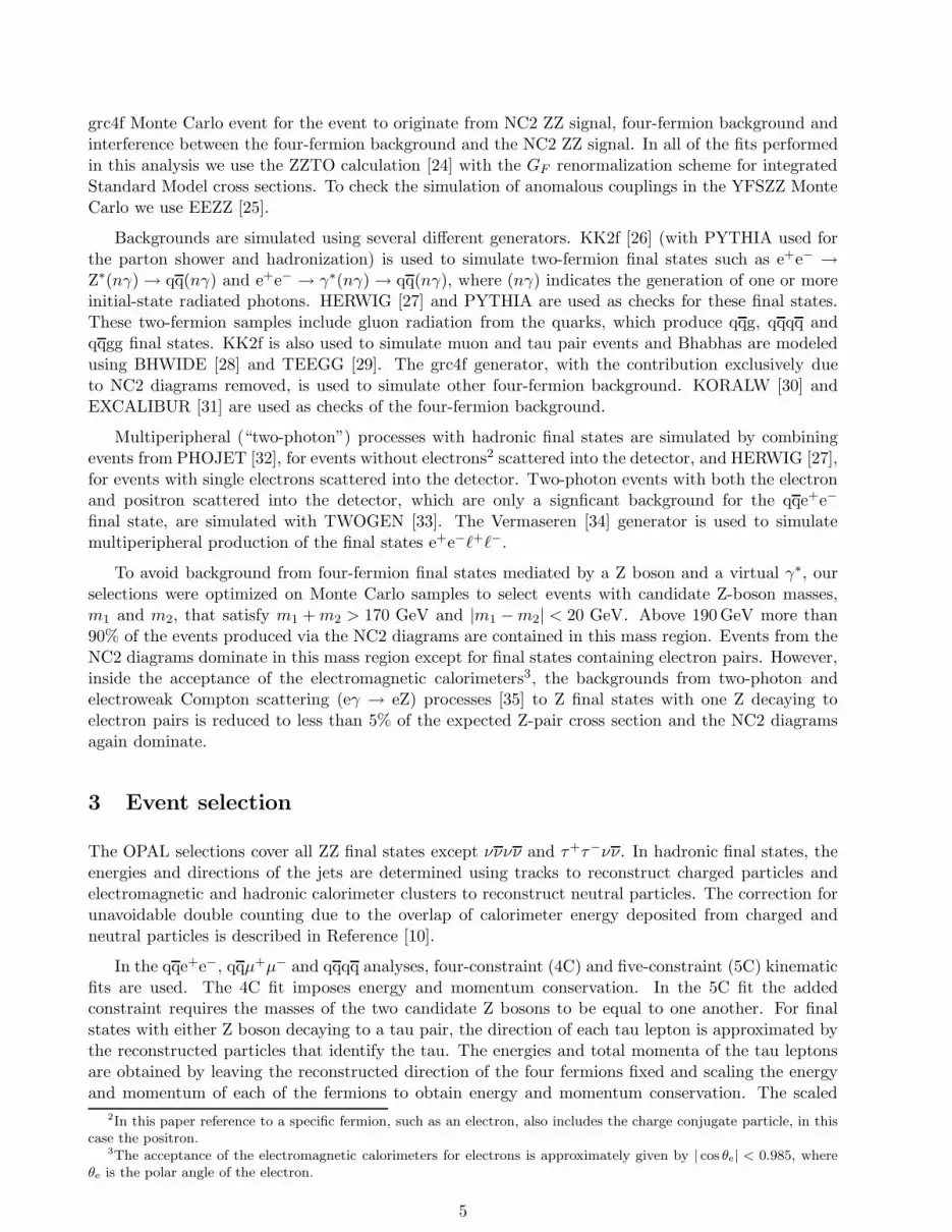
grc4f Monte Carlo event for the event to originate from NC2 ZZ signal, four-fermion background andinterference between the four-fermion background and the NC2 ZZ signal. In all of the fits performedin this analysis we use the ZZTO calculation [24] with the GF renormalization scheme for integratedStandard Model cross sections. To check the simulation of anomalous couplings in the YFSZZ MonteCarlo we use EEZZ [25].

Backgrounds are simulated using several different generators. KK2f [26] (with PYTHIA used forthe parton shower and hadronization) is used to simulate two-fermion final states such as e+e− →Z∗(nγ) → qq(nγ) and e+e− → γ∗(nγ) → qq(nγ), where (nγ) indicates the generation of one or moreinitial-state radiated photons. HERWIG [27] and PYTHIA are used as checks for these final states.These two-fermion samples include gluon radiation from the quarks, which produce qqg, qqqq andqqgg final states. KK2f is also used to simulate muon and tau pair events and Bhabhas are modeledusing BHWIDE [28] and TEEGG [29]. The grc4f generator, with the contribution exclusively dueto NC2 diagrams removed, is used to simulate other four-fermion background. KORALW [30] andEXCALIBUR [31] are used as checks of the four-fermion background.

Multiperipheral (“two-photon”) processes with hadronic final states are simulated by combiningevents from PHOJET [32], for events without electrons2 scattered into the detector, and HERWIG [27],for events with single electrons scattered into the detector. Two-photon events with both the electronand positron scattered into the detector, which are only a signficant background for the qqe+e−

final state, are simulated with TWOGEN [33]. The Vermaseren [34] generator is used to simulatemultiperipheral production of the final states e+e−ℓ+ℓ−.

To avoid background from four-fermion final states mediated by a Z boson and a virtual γ∗, ourselections were optimized on Monte Carlo samples to select events with candidate Z-boson masses,m1 and m2, that satisfy m1 + m2 > 170 GeV and |m1 − m2| < 20 GeV. Above 190 GeV more than90% of the events produced via the NC2 diagrams are contained in this mass region. Events from theNC2 diagrams dominate in this mass region except for final states containing electron pairs. However,inside the acceptance of the electromagnetic calorimeters3, the backgrounds from two-photon andelectroweak Compton scattering (eγ → eZ) processes [35] to Z final states with one Z decaying toelectron pairs is reduced to less than 5% of the expected Z-pair cross section and the NC2 diagramsagain dominate.

3 Event selection

The OPAL selections cover all ZZ final states except νννν and τ+τ−νν. In hadronic final states, theenergies and directions of the jets are determined using tracks to reconstruct charged particles andelectromagnetic and hadronic calorimeter clusters to reconstruct neutral particles. The correction forunavoidable double counting due to the overlap of calorimeter energy deposited from charged andneutral particles is described in Reference [10].

In the qqe+e−, qqµ+µ− and qqqq analyses, four-constraint (4C) and five-constraint (5C) kinematicfits are used. The 4C fit imposes energy and momentum conservation. In the 5C fit the addedconstraint requires the masses of the two candidate Z bosons to be equal to one another. For finalstates with either Z boson decaying to a tau pair, the direction of each tau lepton is approximated bythe reconstructed particles that identify the tau. The energies and total momenta of the tau leptonsare obtained by leaving the reconstructed direction of the four fermions fixed and scaling the energyand momentum of each of the fermions to obtain energy and momentum conservation. The scaled

2In this paper reference to a specific fermion, such as an electron, also includes the charge conjugate particle, in thiscase the positron.

3The acceptance of the electromagnetic calorimeters for electrons is approximately given by | cos θe| < 0.985, whereθe is the polar angle of the electron.

5

values of the tau momentum and energy are then used in the subsequent steps of the analysis. In theqqτ+τ− final state, subsequent kinematic fits are therefore effectively 2C and 3C fits.

The selection procedures for events containing charged leptons or neutrinos (ℓ+ℓ−ℓ+ℓ−,ℓ+ℓ−νν,qqℓ+ℓ− and qqνν) are largely unchanged from the analysis used at 183 GeV and 189 GeV in Refer-ence [3], except that the likelihood functions and some of the cuts have been optimized for the higherenergies. More significant changes have been made to the qqqq and qqbb selections.

3.1 Selection of ZZ → ℓ+ℓ−ℓ+ℓ− events

Z-pairs decaying to final states with four charged leptons (ℓ+ℓ−ℓ+ℓ−) produce low multiplicity eventswith a clear topological signature that is exploited to maximize the selection efficiency. The ℓ+ℓ−ℓ+ℓ−

analysis begins by selecting low multiplicity events (less than 13 reconstructed good tracks and lessthan 13 electromagnetic clusters) with visible energy of at least 0.2

√s and at least one good track

with momentum of 5 GeV or more. Good tracks are required to be consistent with originating fromthe interaction point and to be composed of space points from at least half of the maximum possiblenumber of central tracking detector (Jet Chamber) sense wires.

Using a cone algorithm, the events are required to have exactly four cones of 15 half angle eachcontaining between 1 and 3 tracks. Cones of opposite charge are paired4 to form Z boson candidates.

Lepton identification is only used to classify events as background or to reduce the number of conecombinations considered by preventing the matching of identified electrons with identified muons.Electrons are identified on the basis of energy deposition in the electromagnetic calorimeter, trackcurvature and specific ionization in the tracking chambers. Muons are identified using the associationbetween tracks and hits in the hadron calorimeter and muon chambers.

To reduce background from two-photon events with a single scattered electron detected, we elim-inate events with forward-going electrons or backward-going positrons with the cuts cos θe− < 0.85and cos θe+ > −0.85. Here θe− ( θe+) is the angle of the electron (positron) with respect to the incom-ing electron beam. Background from partially reconstructed qq(nγ) events and two-photon events isreduced by requiring that most of the energy not be concentrated in a single cone. Defining Evis asthe total visible energy of the event and Emax

cone as the energy contained in the most energetic cone werequire Evis − Emax

cone > 0.2√

s.

The invariant masses of the lepton pairs are calculated in three different ways which are motivatedby the possibility of having zero, one or two tau pairs in the event. The events are first classifiedaccording to the assumed number of tau pairs in the event:

1. Events without tau pairs can be selected by requiring a high visible energy. Therefore, eventswith Evis > 0.9

√s are treated as e+e−e+e−, e+e−µ+µ− or µ+µ−µ+µ− events. We also treat all

events with | cos θmiss| > 0.98 (θmiss is the polar angle associated with the missing momentumin the event) as e+e−e+e−, e+e−µ+µ− or µ+µ−µ+µ− events to maintain efficiency for Z-pairswith initial-state radiation. As there are no missing neutrinos in these events, the mass of eachcone-pair combination is evaluated using the measured energies and momenta of the leptons.

2. Events failing (1) with a cone-pair combination that has energy exceeding 0.9mZ are tried asan e+e−τ+τ− or µ+µ−τ+τ− final state. The mass of the tau-pair system is calculated from therecoil mass of the presumed electron or muon pair.

4Two-track cones are assigned the charge of the more energetic track if the momentum of one track exceeds that ofthe other by a factor of 4. Events with a cone which fails this requirement are rejected.

6

3. Events failing (1) with a cone-pair combination failing (2) are treated as τ+τ−τ+τ− final states.The momenta of the tau leptons are determined using the scaling procedure described in theintroduction to Section 3. The invariant masses of the cone pairs are evaluated using the scaledmomenta.

In any event where the lepton identification allows more than one valid combination, each com-bination is tested using invariant mass cuts. For events with one or more combinations of cone-pairings satisfying |mZ − mℓℓ| < 0.1mZ and |mZ − mℓ′ℓ′ | < 0.1mZ the one with the smallest value of(mZ −mℓℓ)

2 + (mZ −mℓ′ℓ′)2 is selected for further analysis. In the other events, the combination with

the smallest value of |mZ − mℓℓ| or |mZ − mℓ′ℓ′ | is selected. These requirements maintain efficiencyfor signal events with a single off-shell Z boson. The final event sample is then chosen with the re-quirement mℓℓ +mℓ′ℓ′ > 160 GeV and |mℓℓ−mℓ′ℓ′ | < 40 GeV. The signal detection efficiency, averagedover all ℓ+ℓ−ℓ+ℓ− final states is approximately 56%. The efficiency for individual final states rangesfrom about 30% for τ+τ−τ+τ− to more than 70% for µ+µ−µ+µ−. These efficiencies have almostno dependence on center-of-mass energy. In Table 2 (line a) we give the efficiency, background andobserved number of events. The errors on the efficiency and background include the systematic uncer-tainties which are discussed in Section 3.6. The invariant masses of all cone pairs passing one of theselections are shown in Figure 2a. A total of four ℓ+ℓ−ℓ+ℓ− events is observed between 190 GeV and209 GeV with an expected background of 1.08± 0.27 events. The remaining background is dominatedby four-lepton events which are not from the NC2 diagrams that define Z-pair production.

3.2 Selection of ZZ → ℓ+ℓ−νν events

The selection of the e+e−νν and µ+µ−νν final states is based on the OPAL selection of W pairsdecaying to leptons [36]. The mass and momentum of the Z boson decaying to νν are calculated usingthe beam-energy constraint and the reconstructed energy and momentum of the Z boson decaying toa charged lepton pair. A likelihood selection based on the visible and recoil masses as well as the polarangle of the leptons, is then used to separate signal from background.

The e+e−νν selection starts with OPAL W-pair candidates where both charged leptons are clas-sified as electrons. Each event is then divided into two hemispheres using the thrust axis. In eachhemisphere, the track with the highest momentum is selected as the leading track. The sum of thecharges of these two tracks is required to be zero. The determination of the visible mass, mvis, andthe recoil mass, mrecoil, is based on the energy as measured in the electromagnetic calorimeter and thedirection of the leading tracks.

The likelihood selection uses three variables: Q cos θ, where θ is the angle of the track with thehighest momentum and Q is its charge, the normalized sum of visible and recoil masses (mvis +mrecoil)/

√s and the difference of visible and recoil masses, mvis − mrecoil. The performance of the

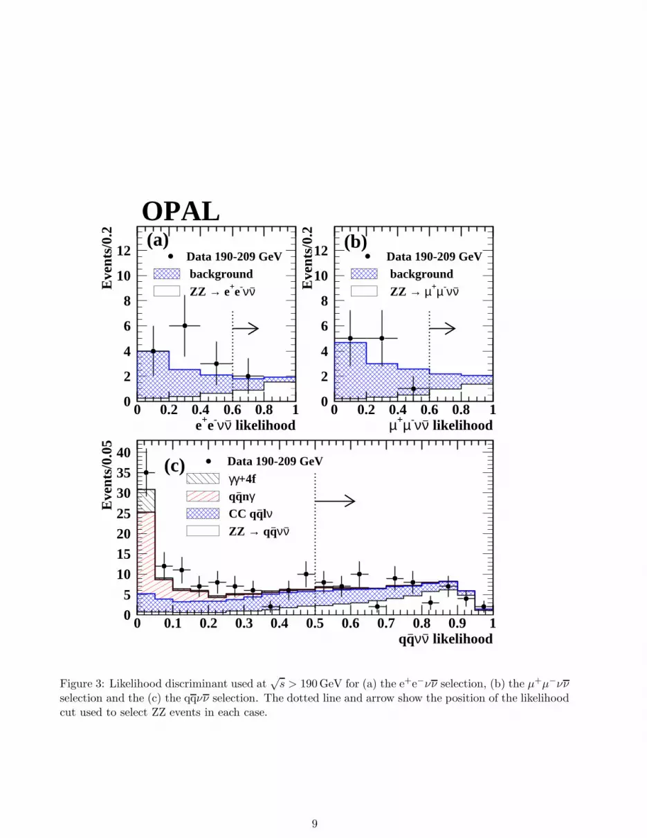
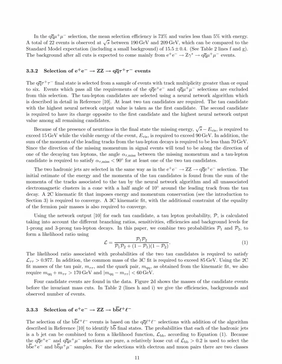
likelihood selection is improved with the following preselection: −25 GeV < mvis − mrecoil < 15 GeVand (mvis +mrecoil) > 170 GeV. Two events with Le+e−νν > 0.60 are selected. See Table 2 (line b) andFigure 3a. The expected background is primarily from W pairs and amounts to 1.28 ± 0.15 events.

The µ+µ−νν selection starts with the OPAL W-pair candidates where both charged leptons areclassified as muons. The selection procedure is the same as for the e+e−νν final states except that mvis

and mrecoil are calculated from the momentum of the reconstructed tracks of the Z boson decaying tomuon pairs. The likelihood preselections −25 GeV < mvis − mrecoil < 25 GeV and (mvis + mrecoil) >170 GeV are applied. No event with Lµ+µ−νν > 0.60 is selected while 4.30 ± 0.39 are expected (seeTable 2 (line c) and Figure 3b). The probability to observe no event when 4.3 ± 0.39 are expected isapproximately 1.4%.

7

‘‘

0

20

40

60

80

100

120

140

160

180

0 50 100 150

e+e- → ZZ → + − + −

acceptedZZ signalregion

m (GeV)

m (

GeV

)

OPAL (190-209 GeV)

(a)

0

20

40

60

80

100

120

140

160

180

0 50 100 150

e+e- → ZZ → qqe+e−

acceptedZZ signalregion

mee (GeV)

mqq

(G

eV)

OPAL (190-209 GeV)

(b)

−

0

20

40

60

80

100

120

140

160

180

0 50 100 150

e+e- → ZZ → qq + −

acceptedZZ signalregion

m (GeV)

mqq

(G

eV)

OPAL (190-209 GeV)

(c)

−

0

20

40

60

80

100

120

140

160

180

0 50 100 150

e+e- → ZZ → qq + −

acceptedZZ signalregion

m (GeV)

mqq

(G

eV)

OPAL (190-209 GeV)

(d)

−

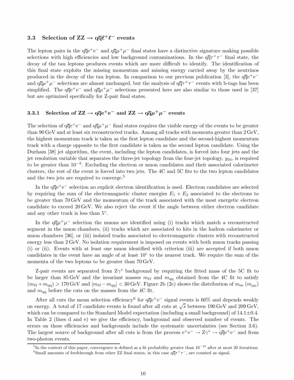
Figure 2: (a) Invariant masses of ℓ+ℓ−ℓ+ℓ− cone pairs. Invariant mass pairs for the (b) qqe+e− (c)qqµ+µ− and (d) qqτ+τ− data. The dashed lines show the final invariant mass cuts. In contrast toReference [3], the qqe+e−, qqµ+µ− unconstrained invariant masses are plotted after the requirementthat the 5C fit mass, with both quark and lepton-pair masses constrained to be the same, exceeds85 GeV. The qqτ+τ− unconstrained invariant masses are shown after a similar cut on the 3C fit mass.

8

0

2

4

6

8

10

12

0 0.2 0.4 0.6 0.8 1

OPAL Data 190-209 GeV

background

ZZ → e+e-νν_

(a)

e+e-νν_ likelihood

Eve

nts/

0.2

0

2

4

6

8

10

12

0 0.2 0.4 0.6 0.8 1

Data 190-209 GeV background

ZZ → µ+µ-νν_

(b)

µ+µ-νν_ likelihood

Eve

nts/

0.2

05

10152025303540

0 0.1 0.2 0.3 0.4 0.5 0.6 0.7 0.8 0.9 1

Data 190-209 GeV

γγ+4fqq

_nγ

CC qq_lν

ZZ → qq_νν

_

(c)

qq_νν

_ likelihood

Eve

nts/

0.05

Figure 3: Likelihood discriminant used at√

s > 190 GeV for (a) the e+e−νν selection, (b) the µ+µ−ννselection and the (c) the qqνν selection. The dotted line and arrow show the position of the likelihoodcut used to select ZZ events in each case.

9

3.3 Selection of ZZ → qqℓ+ℓ− events

The lepton pairs in the qqe+e− and qqµ+µ− final states have a distinctive signature making possibleselections with high efficiencies and low background contaminations. In the qqτ+τ− final state, thedecay of the tau leptons produces events which are more difficult to identify. The identification ofthis final state exploits the missing momentum and missing energy carried away by the neutrinosproduced in the decay of the tau lepton. In comparison to our previous publication [3], the qqe+e−

and qqµ+µ− selections are almost unchanged, but the analysis of qqτ+τ− events with b-tags has beensimplified. The qqe+e− and qqµ+µ− selections presented here are also similar to those used in [37]but are optimized specifically for Z-pair final states.

3.3.1 Selection of ZZ → qqe+e− and ZZ → qqµ+µ− events

The selection of qqe+e− and qqµ+µ− final states requires the visible energy of the events to be greaterthan 90 GeV and at least six reconstructed tracks. Among all tracks with momenta greater than 2 GeV,the highest momentum track is taken as the first lepton candidate and the second-highest momentumtrack with a charge opposite to the first candidate is taken as the second lepton candidate. Using theDurham [38] jet algorithm, the event, including the lepton candidates, is forced into four jets and thejet resolution variable that separates the three-jet topology from the four-jet topology, y34, is requiredto be greater than 10−3. Excluding the electron or muon candidates and their associated calorimeterclusters, the rest of the event is forced into two jets. The 4C and 5C fits to the two lepton candidatesand the two jets are required to converge.5

In the qqe+e− selection no explicit electron identification is used. Electron candidates are selectedby requiring the sum of the electromagnetic cluster energies E1 + E2 associated to the electrons tobe greater than 70 GeV and the momentum of the track associated with the most energetic electroncandidate to exceed 20 GeV. We also reject the event if the angle between either electron candidateand any other track is less than 5.

In the qqµ+µ− selection the muons are identified using (i) tracks which match a reconstructedsegment in the muon chambers, (ii) tracks which are associated to hits in the hadron calorimeter ormuon chambers [36], or (iii) isolated tracks associated to electromagnetic clusters with reconstructedenergy less than 2 GeV. No isolation requirement is imposed on events with both muon tracks passing(i) or (ii). Events with at least one muon identified with criterion (iii) are accepted if both muoncandidates in the event have an angle of at least 10 to the nearest track. We require the sum of themomenta of the two leptons to be greater than 70 GeV.

Z-pair events are separated from Zγ∗ background by requiring the fitted mass of the 5C fit tobe larger than 85 GeV and the invariant masses mℓℓ and mqq obtained from the 4C fit to satisfy(mℓℓ +mqq) > 170 GeV and |mℓℓ−mqq| < 30 GeV. Figure 2b (2c) shows the distribution of mee (mµµ)and mqq before the cuts on the masses from the 4C fit.

After all cuts the mean selection efficiency6 for qqe+e− signal events is 60% and depends weaklyon energy. A total of 17 candidate events is found after all cuts at

√s between 190 GeV and 209 GeV,

which can be compared to the Standard Model expectation (including a small background) of 14.1±0.4.In Table 2 (lines d and e) we give the efficiency, background and observed number of events. Theerrors on these efficiencies and backgrounds include the systematic uncertainties (see Section 3.6).The largest source of background after all cuts is from the process e+e− → Zγ∗ → qqe+e− and fromtwo-photon events.

5In the context of this paper, convergence is defined as a fit probability greater than 10−10 after at most 20 iterations.6Small amounts of feedthrough from other ZZ final states, in this case qqτ+τ−, are counted as signal.

10

In the qqµ+µ− selection, the mean selection efficiency is 73% and varies less than 5% with energy.A total of 22 events is observed at

√s between 190 GeV and 209 GeV, which can be compared to the

Standard Model expectation (including a small background) of 15.5± 0.4. (See Table 2 lines f and g).The background after all cuts is expected to come mainly from e+e− → Zγ∗ → qqµ+µ− events.

3.3.2 Selection of e+e− → ZZ → qqτ+τ− events

The qqτ+τ− final state is selected from a sample of events with track multiplicity greater than or equalto six. Events which pass all the requirements of the qqe+e− and qqµ+µ− selections are excludedfrom this selection. The tau-lepton candidates are selected using a neural network algorithm whichis described in detail in Reference [10]. At least two tau candidates are required. The tau candidatewith the highest neural network output value is taken as the first candidate. The second candidateis required to have its charge opposite to the first candidate and the highest neural network outputvalue among all remaining candidates.

Because of the presence of neutrinos in the final state the missing energy,√

s−Evis, is required toexceed 15 GeV while the visible energy of the event, Evis, is required to exceed 90 GeV. In addition, thesum of the momenta of the leading tracks from the tau-lepton decays is required to be less than 70 GeV.Since the direction of the missing momentum in signal events will tend to be along the direction ofone of the decaying tau leptons, the angle ατ,miss between the missing momentum and a tau-leptoncandidate is required to satisfy ατ,miss < 90 for at least one of the two tau candidates.

The two hadronic jets are selected in the same way as in the e+e− → ZZ → qqe+e− selection. Theinitial estimate of the energy and the momenta of the tau candidates is found from the sum of themomenta of the tracks associated to the tau by the neural network algorithm and all unassociatedelectromagnetic clusters in a cone with a half angle of 10 around the leading track from the taudecay. A 2C kinematic fit that imposes energy and momentum conservation (see the introduction toSection 3) is required to converge. A 3C kinematic fit, with the additional constraint of the equalityof the fermion pair masses is also required to converge.

Using the network output [10] for each tau candidate, a tau lepton probability, P, is calculatedtaking into account the different branching ratios, sensitivities, efficiencies and background levels for1-prong and 3-prong tau-lepton decays. In this paper, we combine two probabilities P1 and P2, toform a likelihood ratio using

L =P1P2

P1P2 + (1 − P1)(1 − P2). (1)

The likelihood ratio associated with probabilities of the two tau candidates is required to satisfyLττ > 0.977. In addition, the common mass of the 3C fit is required to exceed 85 GeV. Using the 2Cfit masses of the tau pair, mττ , and the quark pair, mqq, as obtained from the kinematic fit, we alsorequire mqq + mττ > 170 GeV and |mqq − mττ | < 60 GeV.

Four candidate events are found in the data. Figure 2d shows the masses of the candidate eventsbefore the invariant mass cuts. In Table 2 (lines h and i) we give the efficiencies, backgrounds andobserved number of events.

3.3.3 Selection of e+e− → ZZ → bbℓ+ℓ−

The selection of the bbℓ+ℓ− events is based on the qqℓ+ℓ− selections with addition of the algorithmdescribed in Reference [10] to identify bb final states. The probabilities that each of the hadronic jetsis a b jet can be combined to form a likelihood function, Lbb, according to Equation (1). Becausethe qqe+e− and qqµ+µ− selections are pure, a relatively loose cut of Lbb > 0.2 is used to select thebbe+e− and bbµ+µ− samples. For the selections with electron and muon pairs there are two classes

11

of events since the selected bbℓ+ℓ− events are a subset of the qqℓ+ℓ− events. In Table 2 (lines e andg) we give the efficiencies of the b-tagged samples with respect to the expected fraction of bb events.The efficiencies for samples without b-tags are given with respect to the hadronic decays without bbfinal states.

In the data with√

s above 190 GeV we find three candidate bbe+e− events with 2.49±0.19 expectedand in the bbµ+µ− selection we find seven events with 2.59 ± 0.15 events expected. The probabilityto observe seven or more events when 2.59 ± 0.15 are expected is approximately 1.7%. The invariantmasses of these seven events are consistent with mZ.

For the bbτ+τ− selection the Lττ cut of the qqτ+τ− selection is loosened and combined with Lbb

as follows. Lττ and Lbb are both required to be greater than 0.1. The bbτ+τ− probability for theevent, Lbbττ , is calculated from Equation (1) with Lττ and Lbb as inputs and required to exceed0.95. After the cut on Lbbττ , the remaining cuts of the qqτ+τ− selection are applied. None of theqqτ+τ− events are identified as bbτ+τ− candidates which can be compared with the Standard Modelexpectation of 1.41 ± 0.19. One additional candidate event is found in the sample with the relaxedcut on Lττ with 0.35 ± 0.10 expected. See Table 2 (lines i and j).

3.4 Selection of ZZ → qqνν events

The qqνν selection is based on the reconstruction of the Z boson decaying to qq which producesslightly boosted back-to-back jets. The selection uses events with a two-jet topology where both jetsare contained in the detector. The beam energy constraint is used to determine the mass of the Zboson decaying to νν. The properties of the qq decay and the inferred mass of the νν decay are thenused in a likelihood analysis to separate signal from background.

Two-jet events are selected by dividing each event into two hemispheres using the plane perpen-dicular to the thrust axis. The number of tracks in each hemisphere is required to be four or more.The polar angles of the energy-momentum vector associated with each hemisphere, θhemi1 and θhemi2,are used to define the quantity cos θh ≡ 1

2 (cos θhemi1 − cos θhemi2). Contained events are selected byrequiring |cos θh| < 0.80. The total energy in the forward detectors and in the forward region ofthe electromagnetic calorimeter (| cos θ| > 0.95) is required to be less than 3 GeV. W boson decaysidentified by the OPAL W-pair selection are rejected using the likelihood function for e+e− → qqℓνfrom Reference [36] which includes an optimization for each center-of-mass energy. Only events withLWW < 0.5 are retained.

An important background to our selection is qq(nγ) events with photons that escape detection. Wediscriminate against these events by looking for a significant amount of missing transverse momentum,pt. In each event, pt can be resolved into two components, pti, perpendicular to the transversecomponent of the thrust axis and ptj , along the transverse component of the thrust axis. pti dependsprimarily on the reconstructed angles of the jets and therefore is more precisely measured than ptj

which depends on the energy balance of the jets. We approximate pti as pti = 12Eb sin φ sin θh.

Here Eb =√

s/2 is the beam energy, φ is the acoplanarity calculated from the angle between thetransverse components of the momentum vectors of the two hemispheres and sin θh =

√

1 − cos2 θh.The resolution on pti, σpti

, was parameterized as a function of thrust and cos θh using data taken atthe Z resonance. We construct the variable

Rpti= (pti − p0

ti)/σpti, (2)

which is used as input to the likelihood function described below. Here p0ti corresponds to the transverse

momentum carried by a photon with half the beam energy which just misses the inner edge of ouracceptance ( p0

ti = Eb sin(32 mrad)/2). The likelihood function also uses the related variable cos θmiss,the direction of the missing momentum in the event, to discriminate against the qq(nγ) events.

In the final selection of events, we use a likelihood function based on the following five variables:

12

1. the normalized sum of visible and recoil masses (mvis + mrecoil)/√

s,

2. the difference of visible and recoil masses (mvis − mrecoil),

3. log(y23), where y23 is the jet resolution parameter that separates the two-jet topology from thethree-jet topology as calculated from the Durham jet algorithm,

4. cos θmiss and

5. Rpti.

The mass variables are useful for reducing background from W-pair production and single W (Weν)final states. The jet resolution parameter is useful in reducing the remaining qqℓν final states. Toimprove the performance of the likelihood analysis we use only events with |mvis − mrecoil| < 50 GeV,(mvis + mrecoil) > 170 GeV and Rpti

> 1.2. Events are then selected using Lqqνν > 0.5, where Lqqνν

is the likelihood function for the qqνν selection. The likelihood distribution of data and Monte Carlosimulation is shown in Figure 3c. For the bbνν selection we require, in addition, the b-tag variable ofReference [10] to be greater than 0.65.

The mean efficiency for the qqνν selection alone is 32% and does not have a strong dependence on√s. The efficiency includes corrections to the Monte Carlo simulation for the effects of backgrounds

in the foward detectors and for imperfect detector modeling. The modeling systematic uncertaintiesare discussed below in Section 3.6. A total of 60 candidates is observed in the data to be comparedwith the Standard Model expectation of 64.9±2.9. The efficiencies after considering the results of theb-tagging, as well as the number of events selected are given in Table 2 (lines k and l).

3.5 Selection of ZZ → qqqq events

As in the previous analysis [3] the hadronic selection consists of a preselection followed by two differentlikelihood selections, one of them aiming at an inclusive selection of fully hadronic Z-pair decays, andthe other optimized for selecting final states containing at least one pair of b quarks. The main changeswith respect to the previous analysis are that cuts in the preselection have been modified slightly andthat the quantities used in the qqbb likelihood have changed.

3.5.1 Preselection

The preselection starts from the inclusive multihadron selection described in Reference [17]. Theradiative process e+e− → Zγ → qqγ is suppressed by requiring the effective center-of-mass energyafter initial-state radiation,

√s′, to be larger than 160 GeV.

√s′ is obtained from a kinematic fit [17]

that allows for one or more radiative photons in the detector or along the beam pipe. The final-stateparticles are then grouped into jets using the Durham algorithm [38]. A four-jet sample is formed byrequiring the jet resolution parameter y34 to be at least 0.003 and each jet to contain at least twotracks. In order to suppress Z∗/γ∗ → qq background, the event shape parameter Cpar [39], which islarge for spherical events, is required to be greater than 0.27. A 4C kinematic fit using energy andmomentum conservation is required to converge. A 5C kinematic fit which forces the two jet pairs tohave the same mass is applied in turn to all three possible combinations of the four jets. This fit isrequired to converge for at least one combination.

The most probable pairing of the jets is determined using a likelihood discriminant which is basedon the difference between the two di-jet masses calculated from the results of a 4C kinematic fit, thedi-jet mass obtained from a 5C kinematic fit, and the χ2 probability of the 5C fit.

13

3.5.2 Likelihood for the inclusive ZZ → qqqq event selection

We use a likelihood selection with six input variables for the selection of ZZ → qqqq events. Thelikelihood selection is optimized separately for each energy point. The first variable is the outputvalue of the jet pairing likelihood described above. The second variable is determined by excludingthe jet pairing with the largest difference between the two di-jet masses as obtained from the 4C fit,and then evaluating the 5C-fit masses of the remaining two pairings. The one which is closest to theW mass is selected and the difference between this 5C-fit mass and the W mass is used in order todiscriminate against hadronic W-pair events. The third variable suppresses background events withradiated photons that shift the value of the mass obtained from the kinematic fit. We use the value of√

s′ from the preselection. The fourth variable is used to discriminate against Z∗/γ∗ events. We usethe difference between the largest and smallest jet energies after the 4C fit. The final two variablesare calculated from the momenta of the four jets. They are the effective matrix elements for the QCDprocesses Z∗/γ⋆ → qqgg and Z∗/γ⋆ → qqqq as defined in Reference [40], and the matrix element forthe process WW → qqqq from Reference [31].

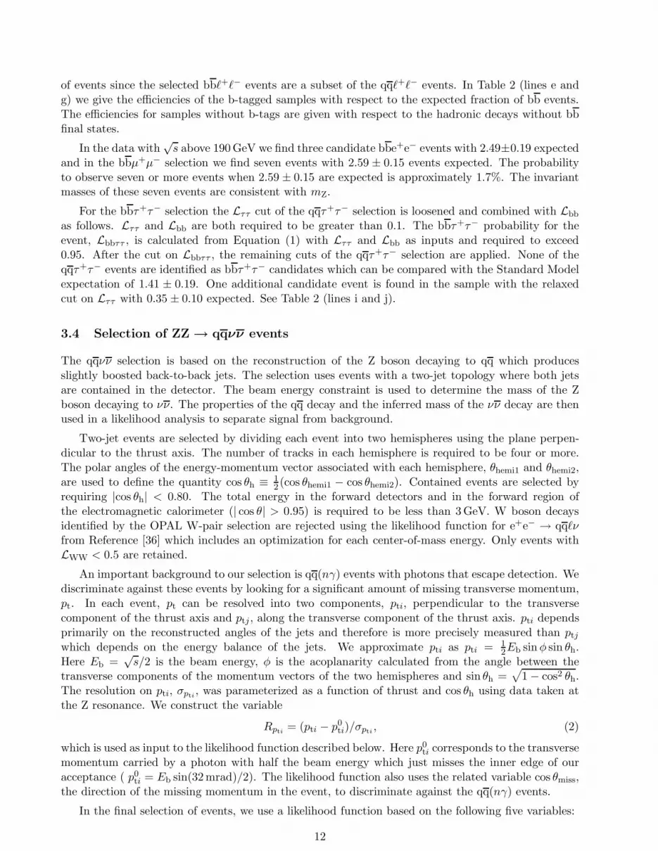
The cut on the likelihood function has been chosen in order to minimize the total expected relativeerror when including a 10% relative systematic uncertainty on the background rate in addition to theexpected statistical error. The qqqq likelihood function for the data is shown in Figure 4a. A total of206 events is observed which can be compared to the total Standard Model expectation of 201.9±13.6which includes a large background of 135.6 ± 13.1 events. In Table 2 (lines m and o) we give theefficiency, background and observed number of events.

3.5.3 Likelihood function for ZZ → qqbb event selection

Jets originating from b quarks are selected using the b-tagging algorithm [10]. We evaluate theprobability for each of the four jets to originate from a primary b quark. The two highest probabilitiesare then used as input variables for a likelihood function to select ZZ → qqbb events. In additionwe use the parameters y34, Cpar, the track multiplicity of the event and the output of the jet pairinglikelihood function. We also use the fit probability of a 6C fit which forces both masses to be equal tothe W mass. Finally we use the variable | cos θbb−cos θqq|, where θbb is the opening angle between themost likely b jets, and θqq is the opening angle between the remaining two jets7. The qqbb likelihoodfunction for the combined data taken at

√s > 190 GeV is shown in Figure 4b. A total of 45 events is

observed which can be compared to the total Standard Model expectation of 43.3 ± 1.8. In Table 2(lines n and o) we give the efficiency, background and observed number of events.

3.6 Systematic uncertainties

Systematic uncertainties have only a modest effect on our final result because of the large statisticalerror associated with the small number of Z-pair events produced at LEP 2.

Detector systematic uncertainties for the qqℓ+ℓ− and ℓ+ℓ−ℓ+ℓ− selections without τ -pairs in thefinal state are small because of the good separation of signal and background. In the qqℓ+ℓ− channelspossible mismodeling of the detector resolution is accounted for by smearing polar and azimuthal jetangles with a Gaussian width of 1 and the energies by 5%. This gives systematic shifts smaller than5%. These shifts are included in the systematic uncertainties on the efficiencies. In the qqτ+τ− selec-tion, the additional systematic uncertainties in the efficiencies are determined by overlaying hadronicand tau decays taken from Z resonance data giving the dominant contribution to the total systematic

7In contrast to our previous publication [3], the probability of the 5C mass fit that constrains one of the candidate Zbosons to the Z mass, as used in the OPAL Higgs [10] analysis, is not an input to the likelihood function.

14

0

20

40

60

80

100

0.1 0.2 0.3 0.4 0.5 0.6 0.7 0.8 0.9 1

OPAL Data 190-209 GeV

Z/γ → qq_

WW → qq_qq

_

ZZ → qq_qq

_

(a)

qq_qq

_ likelihood

Eve

nts/

0.05

0

10

20

30

40

50

60

0.2 0.3 0.4 0.5 0.6 0.7 0.8 0.9 1

Data 190-209 GeV

Z/γ → qq_

WW → qq_qq

_

ZZ → not qq_bb

–

ZZ → qq_bb

–

(b)

qq_bb

– likelihood

Eve

nts/

0.05

Figure 4: The combined distributions of likelihood discriminants used for all energies above 190 GeV.(a) e+e− → ZZ → qqqq selection and (b) e+e− → ZZ → qqbb selection. The dotted line and arrowshow the position of the likelihood cut used to select ZZ events in each case.

15

√s = 190 − 209 GeV

Selection nobs nSM nZZ nback ǫchan BZZ Lint

(pb−1)

a ℓ+ℓ−ℓ+ℓ− 4 3.55 ± 0.29 2.46 ± 0.09 1.08 ± 0.27 0.56 ± 0.02 0.010 433.6

b e+e−νν 2 3.71 ± 0.35 2.43 ± 0.31 1.28 ± 0.15 0.41 ± 0.05 0.013 435.2

c µ+µ−νν 0 4.30 ± 0.39 2.39 ± 0.33 1.91 ± 0.21 0.41 ± 0.06 0.013 435.2

d qqe+e− & bbe+e− 14 11.6 ± 0.4 9.6 ± 0.3 1.98 ± 0.23 0.62 ± 0.03 0.037 424.7

e qqe+e− & bbe+e− 3 2.49 ± 0.19 2.20 ± 0.18 0.30 ± 0.07 0.51 ± 0.05 0.010 424.7

f qqµ+µ− & bbµ+µ− 15 12.9 ± 0.4 12.1 ± 0.4 0.83 ± 0.12 0.77 ± 0.03 0.037 424.7

g qqµ+µ− & bbµ+µ− 7 2.59 ± 0.15 2.43 ± 0.14 0.16 ± 0.06 0.56 ± 0.05 0.010 424.7

h qqτ+τ− & bbτ+τ− 4 5.35 ± 0.41 4.63 ± 0.39 0.72 ± 0.12 0.30 ± 0.03 0.037 424.7

i qqτ+τ− & bbτ+τ− 0 1.41 ± 0.19 1.19 ± 0.18 0.21 ± 0.06 0.28 ± 0.04 0.010 424.7

j bbτ+τ− & qqτ+τ− 1 0.35 ± 0.10 0.29 ± 0.10 0.07 ± 0.03 0.07 ± 0.02 0.010 424.7

k qqνν & bbνν 51 56.4 ± 2.8 30.3 ± 2.5 26.1 ± 1.2 0.33 ± 0.03 0.219 422.1

l qqνν & bbνν 9 8.45 ± 0.74 7.23 ± 0.71 1.22 ± 0.22 0.28 ± 0.03 0.061 422.1

m qqqq & qqbb 185 180.5 ± 13.5 50.2 ± 3.1 130.3 ± 13.1 0.39 ± 0.03 0.300 432.3

n qqbb & qqqq 24 21.9 ± 1.4 13.7 ± 0.8 8.14 ± 1.14 0.17 ± 0.01 0.189 432.3

o qqbb & qqqq 21 21.4 ± 1.2 16.1 ± 0.9 5.30 ± 0.74 0.20 ± 0.02 0.189 432.3

Table 2: Observed number of events, nobs, the total Standard Model expectation, nSM, the expectednumber of Z-pairs, nZZ, background expectation, nback, and efficiencies, ǫchan, for the combined datasample. BZZ is the product branching ratio for the final state which is calculated directly from Zresonance data [6]. An overbar is used to indicate that events from a particular selection are rejected.Note that the efficiencies for selections with b-tags are given relative to the fraction of hadronic finalstates which contain a Z boson decaying to bb. For selections of events with hadronic final states,but without b-tags, the efficiencies are relative to those expected hadronic final states which do notinclude a Z boson decaying to bb. The errors on all quantities include contributions from the systematicuncertainties described in Section 3.6.

uncertainty of 6.2%. In the ℓ+ℓ−ℓ+ℓ− final state the largest effect (3%) is from the modeling of themultiplicity requirement which is important for final states containing τ -pairs.

In the final states with neutrinos, ℓ+ℓ−νν and qqνν, tight cuts are needed to separate signal andbackground. In these selections detector effects can best be studied by comparing calibration datataken at the Z resonance with a simulation of the same process. In these cases, we add additionalsmearing to the total energy and momentum of the simulated events to match data and simulation onthe Z-resonance. We then apply the same smearing to the signal and background Monte Carlo simu-lations for the Z-pair analyses. The reported efficiencies and backgrounds are accordingly corrected.The full difference is used as the systematic uncertainty in these cases. These differences give relativesystematic uncertainties on the efficiency of 2.5% for the e+e−νν final state, 5.2% for the µ+µ−ννfinal state and 3.8% for qqνν final state.

In the qqqq inclusive analysis the sensitivity to the detector description of jet eneriges is muchreduced by the use of kinematic fits. In this case the systematic uncertainties are determined bysmearing the jet energies by an additional 5% and the jet directions by 1 leading to a relativedetector systematic uncertainty of 6%.

Another important detector effect comes from the simulation of the variables used by the OPALb-tag which is discussed in Reference [10]. We allow for a common 5% uncertainty on the efficiencyof the b-tag, consistent with our studies on Z resonance data and Monte Carlo simulation.

In each channel the signal and background Monte Carlo generators have been compared against

16

alternative generators. In almost all cases the observed differences are consistent within the finiteMonte Carlo statistics and the systematic uncertainty has been assigned accordingly.

The largest contribution to the systematic uncertainty from the model dependence of the back-ground prediction is for the qqqq and qqbb final states. This uncertainty has been estimated bycomparing the predictions of KORALW and grc4f for the W-pair background, and the prediction ofPYTHIA and KK2f for the background from hadronic 2-fermion production. The resulting uncer-tainty is 10% on the background for the inclusive selection and 20% for the background of the qqbbselection [10]. The 10% uncertainty has been taken to be fully correlated between energy points andbetween the qqqq and qqbb selections. The correlated error on the qqbb selection from uncertainties inthe background due to b-tagging, has been absorbed into the overall b-tagging efficiency uncertainty.

In the ℓ+ℓ−ℓ+ℓ− channel, which has a large background from two-photon events, we have comparedthe number of selected events at an early stage of the analysis with the Monte Carlo simulation andbased our background systematic uncertainty on the level of agreement. This results in 20% systematicuncertainty on the background.

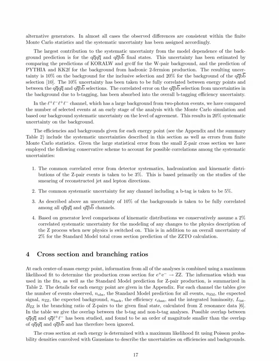
The efficiencies and backgrounds given for each energy point (see the Appendix and the summaryTable 2) include the systematic uncertainties described in this section as well as errors from finiteMonte Carlo statistics. Given the large statistical error from the small Z-pair cross section we haveemployed the following conservative scheme to account for possible correlations among the systematicuncertainties:

1. The common correlated error from detector systematics, hadronization and kinematic distri-butions of the Z-pair events is taken to be 3%. This is based primarily on the studies of thesmearing of reconstructed jet and lepton directions.

2. The common systematic uncertainty for any channel including a b-tag is taken to be 5%.

3. As described above an uncertainty of 10% of the backgrounds is taken to be fully correlatedamong all qqqq and qqbb channels.

4. Based on generator level comparisons of kinematic distributions we conservatively assume a 2%correlated systematic uncertainty for the modeling of any changes to the physics description ofthe Z process when new physics is switched on. This is in addition to an overall uncertainty of2% for the Standard Model total cross section prediction of the ZZTO calculation.

4 Cross section and branching ratios

At each center-of-mass energy point, information from all of the analyses is combined using a maximumlikelihood fit to determine the production cross section for e+e− → ZZ. The information which wasused in the fits, as well as the Standard Model prediction for Z-pair production, is summarized inTable 2. The details for each energy point are given in the Appendix. For each channel the tables givethe number of events observed, nobs, the Standard Model prediction for all events, nSM, the expectedsignal, nZZ, the expected background, nback, the efficiency ǫchan, and the integrated luminosity, Lint.BZZ is the branching ratio of Z-pairs to the given final state, calculated from Z resonance data [6].In the table we give the overlap between the b-tag and non-b-tag analyses. Possible overlap betweenqqqq and qqℓ+ℓ− has been studied, and found to be an order of magnitude smaller than the overlapof qqqq and qqbb and has therefore been ignored.

The cross section at each energy is determined with a maximum likelihood fit using Poisson proba-bility densities convolved with Gaussians to describe the uncertainties on efficiencies and backgrounds.

17

0

0.25

0.5

0.75

1

1.25

1.5

1.75

180 185 190 195 200 205

Cro

ss s

ecti

on (

pb)

√s (GeV)

OPAL

σ(e+e- → ZZ)

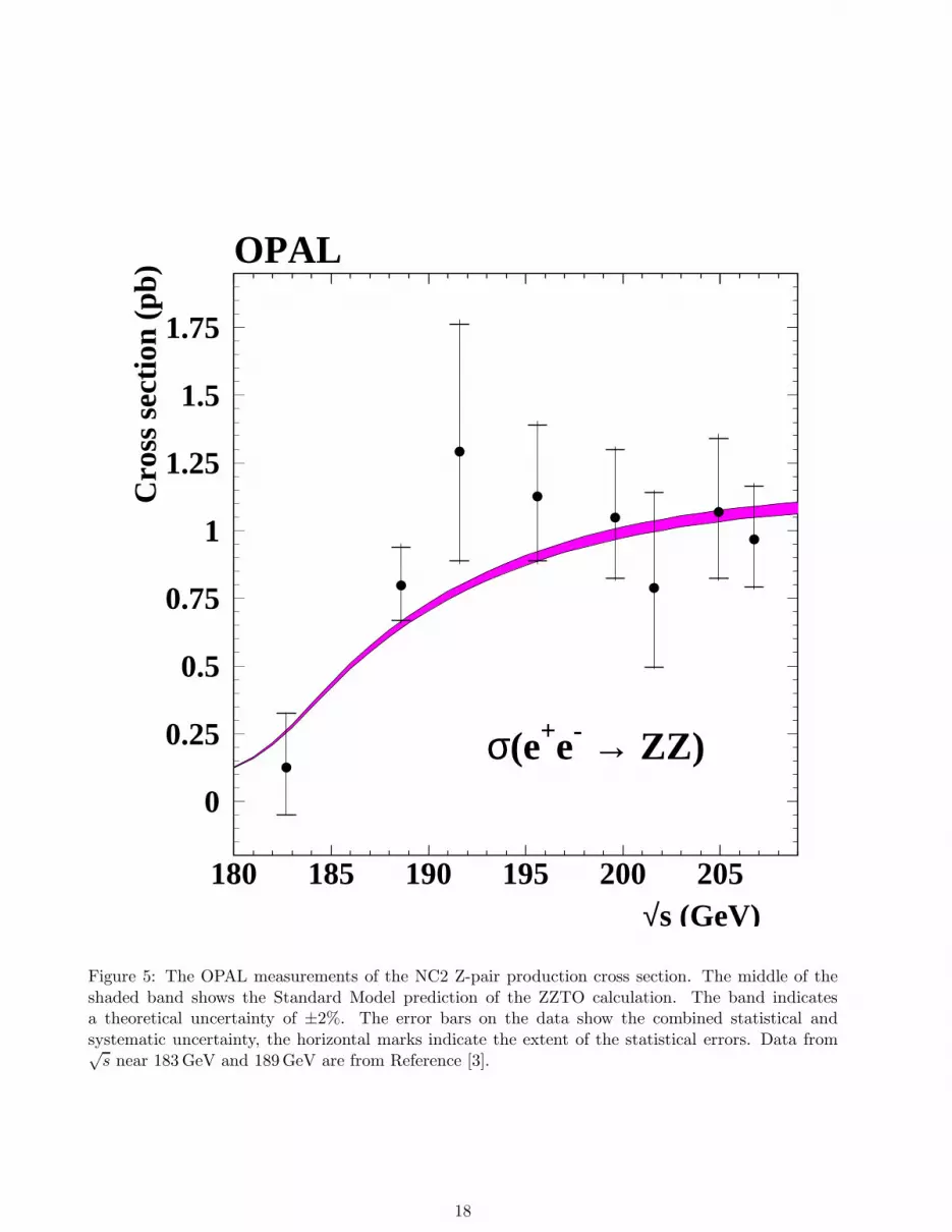
Figure 5: The OPAL measurements of the NC2 Z-pair production cross section. The middle of theshaded band shows the Standard Model prediction of the ZZTO calculation. The band indicatesa theoretical uncertainty of ±2%. The error bars on the data show the combined statistical andsystematic uncertainty, the horizontal marks indicate the extent of the statistical errors. Data from√

s near 183 GeV and 189 GeV are from Reference [3].

18

0.0

1.0

2.0

3.0

192 GeV 196 GeV 200 GeV

0.0

1.0

2.0

3.0

0.0 0.5

202 GeV

0.0 0.5

205 GeV

0.0 0.5 1.0

207 GeV

dσ/d

|cos

ΘZ| (

pb/0

.25)

|cosΘZ|

OPAL

Figure 6: The OPAL measurements of the NC2 Z-pair differential cross section dσZZ/d| cos θZ|. Thecurves show the prediction of the YFSZZ Monte Carlo for the differential cross section, which hasbeen normalized to agree with the total cross section of the ZZTO calculation. The error bars showthe combined statistical and systematic uncertainty. The arrow shows the 95% confidence level upperlimit for the one case where the minimum of the negative log likelihood function was at zero.

19

The expected number of events in each channel, µe, as function of the Z-pair cross section, σZZ, isgiven by

µe = σZZLintǫchanBZZ + nback. (3)

The efficiencies, ǫchan, include the effects of off-shell Z bosons that are produced outside of our kine-matic acceptance. The correlated systematic uncertainties described in the last section are imple-mented by introducing additional parameters which are constrained with Gaussian probability densi-ties given by the size of the systematic uncertainty. Our main results, the NC2 Z-pair cross sectionsobtained from the fits, are

σZZ(192 GeV) = 1.29 +0.47−0.40

+0.12−0.09 pb

σZZ(196 GeV) = 1.13 +0.26−0.24

+0.08−0.07 pb

σZZ(200 GeV) = 1.05 +0.25−0.22

+0.07−0.06 pb

σZZ(202 GeV) = 0.79 +0.35−0.29

+0.08−0.05 pb

σZZ(205 GeV) = 1.07 +0.27−0.24

+0.08−0.07 pb

σZZ(207 GeV) = 0.97 +0.19−0.18

+0.06−0.05 pb.

The first error is statistical and the second error is systematic. The systematic errors are obtained fromthe quadrature difference of the errors when running the fit with and without systematic uncertainties.The comparison of these measurements with the ZZTO prediction is shown in Figure 5. The resultsare consistent with the Standard Model prediction.

We have also analyzed our data in four bins of | cos θZ| where θZ is the polar angle of the Z bosons.Except for channels with one Z boson decaying to neutrinos, the value of | cos θZ| is determined fromkinematic fits which assume no initial-state radiation. In the ℓ+ℓ−νν and qqνν channels, the directionis determined from the reconstructed direction of the visible Z. The comparison of the expected andobserved differential cross sections is shown in Figure 6. The data in Figure 6 have been corrected forsmall amounts of bin migration assuming the Standard Model prediction.

In order to check the consistency of our result with the Standard Model, we have performed amaximum likelihood fit in which the Standard Model ZZTO prediction is scaled by an overall factorR. The fit is based on individual measurements for each channel given in the Appendix in Tables 5to 10 as well as the data presented in Reference [3]. The treatment of the correlated systematicuncertainties is outlined in Section 3.6. The fit yields

R = 1.06+0.11−0.10

where the error includes the correlated experimental systematic uncertainty (3%) and the theoreticaluncertainty on the ZZTO prediction (2%). In a separate fit, we allowed the branching ratio of Zbosons to b quarks, BR(Z → bb), to be a free parameter in the fits at each of the energy points. Theresults are shown in Figure 7. The BR(Z → bb) values tend to lie above the measured value fromLEP 1 data; combining all energies, the average value is 0.196±0.032, which is 1.3 standard deviationsabove the LEP 1 measurement of 0.1514±0.0005 [6].

5 Limits on anomalous triple gauge couplings

Limits on anomalous triple gauge couplings were set using the measured cross sections and kinematicinformation from an optimal observable (OO) method for the qqqq, qqbb and qqℓ+ℓ− selections. In

20

0

0.05

0.1

0.15

0.2

0.25

0.3

0.35

0.4

190 195 200 205√s (GeV)

Br(

Z →

bb- )

OPAL

Figure 7: Determination of Br(Z → bb) from ZZ events. The line shows the measured value fromLEP 1 data. Only statistical errors are shown. The data have a common systematic uncertaintywhich amounts to approximately 5% of the expected branching ratio. The 189 GeV point is fromReference [3]; at 183 GeV the ZZ event samples were too small to allow a meaningful measurement tobe obtained.

21

this study we vary the real part of the ZZZ and ZZγ anomalous couplings parameterized by fZZZ4 ,

fZZZ5 , fZZγ

4 and fZZγ5 as defined in Reference [7] and implemented in the YFSZZ Monte Carlo. In most

cases, the real parts of each coupling were varied separately with all others fixed to zero.

The OO analysis used here is described in detail in Reference [41]. Since the effective Lagrangianused to describe the anomalous couplings is linear in the couplings, the resulting differential crosssection is parabolic and can be parameterized, for a single non-zero coupling αi, as

dσ

dΩ= S(0)(Ω) + αiS

(1)i (Ω) + α2

i S(2)i (Ω) (4)

where Ω is the phase-space point based on the four-momenta of the four out-going fermions from theZ decays. The optimal observables are defined as

Oi1 ≡ S

(1)i (Ω)/S(0)(Ω)

Oi2 ≡ S

(2)i (Ω)/S(0)(Ω).

(5)

To reduce the dependence of our analysis on the tails of the Oi1 and Oi

2 distribution, extreme valuesof Oi

1 and Oi2 were rejected when calculating the mean values. These cuts were chosen based on the

expected distribution of Oi1 and Oi

2 calculated from Monte Carlo and typically reject a few percent ofthe expected events.

The expected average values of the first order optimal observable, 〈O1〉, and the second orderoptimal observable, 〈O2〉, were calculated using the YFSZZ matrix element to reweight acceptedevents from the signal Monte Carlo. The same cuts on extreme values of Oi

1 and Oi2 were used in data

and Monte Carlo simulation. The parameterization used was of the form

〈O1〉 = p0 + p1α + p2α2

d0 + d1α + d2α2

〈O2〉 = q0 + q1α + q2α2

d0 + d1α + d2α2

(6)

where α is the value of the anomalous coupling and the coefficients are determined separately foreach selection, energy and type of anomalous coupling. Note that the mean values of the optimalobservables are normalized to the observed number of events and do not depend on the cross sectionwhich is considered separately below. This can be seen in Equation (6) by noting that the polynomiald0 + d1α + d2α

2 parameterizes the change in cross section with anomalous coupling. The averagevalue of the optimal observable for the exclusive qqe+e−, qqµ+µ− and three categories of qqqq events

( qqqq & qqbb, qqbb & qqqq and qqbb & qqqq ) were calculated from the data at each energy between190 GeV and 207 GeV. The statistical uncertainties on these values were parameterized with a co-variance matrix determined from high statistics Standard Model signal and background Monte Carlosimulations. The covariance matrix was then scaled to match the number of events observed in thedata.

The systematic uncertainties were taken into account by varying the modeling of the StandardModel signal and the backgrounds. Any deviations were interpreted as a systematic error and includedin the covariance matrix. The error associated with the physics simulation of the signal was determinedby comparing the values of 〈O1〉 and 〈O2〉 determined from reweighting the YFSZZ and grc4f MonteCarlo event samples. The error in the background determination was evaluated by using the alternativebackground simulations described in Section 3.6. These differences were taken to be fully correlatedamong energies for a given final state. The systematic uncertainties associated with the accuracy ofthe event reconstruction were evaluated by applying additional smearing to the energies and angles ofthe reconstructed jets and leptons. The resulting contributions to the covariance matrix were taken

22

Coupling 95% C.L. lower limit 95% C.L. upper limit

fZZZ4 −0.45 0.58

fZZZ5 −0.94 0.25

fZZγ4 −0.32 0.33

fZZγ5 −0.71 0.59

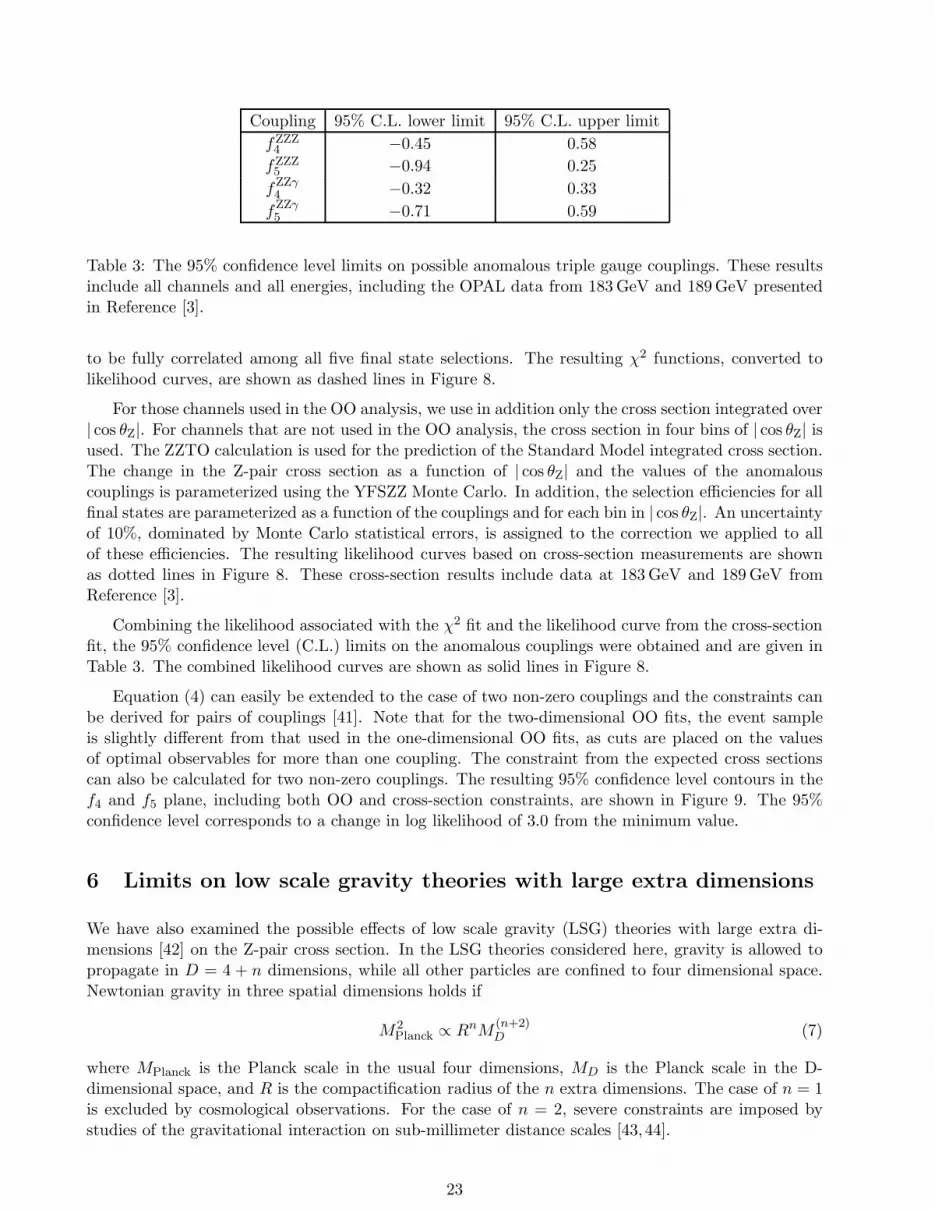
Table 3: The 95% confidence level limits on possible anomalous triple gauge couplings. These resultsinclude all channels and all energies, including the OPAL data from 183 GeV and 189 GeV presentedin Reference [3].

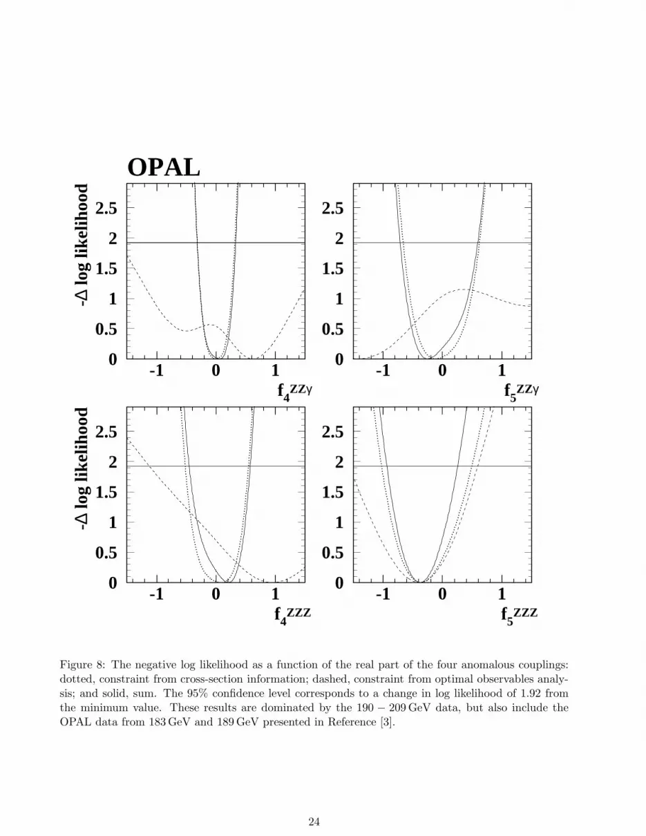
to be fully correlated among all five final state selections. The resulting χ2 functions, converted tolikelihood curves, are shown as dashed lines in Figure 8.

For those channels used in the OO analysis, we use in addition only the cross section integrated over| cos θZ|. For channels that are not used in the OO analysis, the cross section in four bins of | cos θZ| isused. The ZZTO calculation is used for the prediction of the Standard Model integrated cross section.The change in the Z-pair cross section as a function of | cos θZ| and the values of the anomalouscouplings is parameterized using the YFSZZ Monte Carlo. In addition, the selection efficiencies for allfinal states are parameterized as a function of the couplings and for each bin in | cos θZ|. An uncertaintyof 10%, dominated by Monte Carlo statistical errors, is assigned to the correction we applied to allof these efficiencies. The resulting likelihood curves based on cross-section measurements are shownas dotted lines in Figure 8. These cross-section results include data at 183 GeV and 189 GeV fromReference [3].

Combining the likelihood associated with the χ2 fit and the likelihood curve from the cross-sectionfit, the 95% confidence level (C.L.) limits on the anomalous couplings were obtained and are given inTable 3. The combined likelihood curves are shown as solid lines in Figure 8.

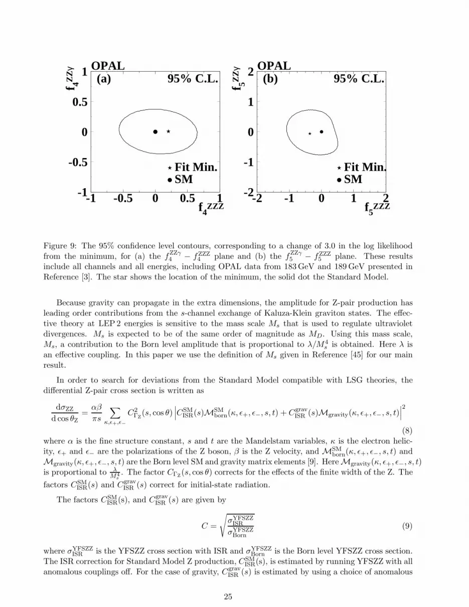
Equation (4) can easily be extended to the case of two non-zero couplings and the constraints canbe derived for pairs of couplings [41]. Note that for the two-dimensional OO fits, the event sampleis slightly different from that used in the one-dimensional OO fits, as cuts are placed on the valuesof optimal observables for more than one coupling. The constraint from the expected cross sectionscan also be calculated for two non-zero couplings. The resulting 95% confidence level contours in thef4 and f5 plane, including both OO and cross-section constraints, are shown in Figure 9. The 95%confidence level corresponds to a change in log likelihood of 3.0 from the minimum value.

6 Limits on low scale gravity theories with large extra dimensions

We have also examined the possible effects of low scale gravity (LSG) theories with large extra di-mensions [42] on the Z-pair cross section. In the LSG theories considered here, gravity is allowed topropagate in D = 4 + n dimensions, while all other particles are confined to four dimensional space.Newtonian gravity in three spatial dimensions holds if

M2Planck ∝ RnM

(n+2)D (7)

where MPlanck is the Planck scale in the usual four dimensions, MD is the Planck scale in the D-dimensional space, and R is the compactification radius of the n extra dimensions. The case of n = 1is excluded by cosmological observations. For the case of n = 2, severe constraints are imposed bystudies of the gravitational interaction on sub-millimeter distance scales [43,44].

23

0

0.5

1

1.5

2

2.5

-1 0 1f4

ZZγ

-∆ lo

g lik

elih

ood

OPAL

0

0.5

1

1.5

2

2.5

-1 0 1f5

ZZγ

0

0.5

1

1.5

2

2.5

-1 0 1f4

ZZZ

-∆ lo

g lik

elih

ood

0

0.5

1

1.5

2

2.5

-1 0 1f5

ZZZ

Figure 8: The negative log likelihood as a function of the real part of the four anomalous couplings:dotted, constraint from cross-section information; dashed, constraint from optimal observables analy-sis; and solid, sum. The 95% confidence level corresponds to a change in log likelihood of 1.92 fromthe minimum value. These results are dominated by the 190 − 209 GeV data, but also include theOPAL data from 183 GeV and 189 GeV presented in Reference [3].

24

-1

-0.5

0

0.5

1

-1 -0.5 0 0.5 1f4

ZZZ

f 4ZZ

γ OPAL95% C.L.(a)

Fit Min.SM

-2

-1

0

1

2

-2 -1 0 1 2f5

ZZZ

f 5ZZ

γ OPAL95% C.L.(b)

Fit Min.SM

Figure 9: The 95% confidence level contours, corresponding to a change of 3.0 in the log likelihoodfrom the minimum, for (a) the fZZγ

4 − fZZZ4 plane and (b) the fZZγ

5 − fZZZ5 plane. These results

include all channels and all energies, including OPAL data from 183 GeV and 189 GeV presented inReference [3]. The star shows the location of the minimum, the solid dot the Standard Model.

Because gravity can propagate in the extra dimensions, the amplitude for Z-pair production hasleading order contributions from the s-channel exchange of Kaluza-Klein graviton states. The effec-tive theory at LEP 2 energies is sensitive to the mass scale Ms that is used to regulate ultravioletdivergences. Ms is expected to be of the same order of magnitude as MD. Using this mass scale,Ms, a contribution to the Born level amplitude that is proportional to λ/M4

s is obtained. Here λ isan effective coupling. In this paper we use the definition of Ms given in Reference [45] for our mainresult.

In order to search for deviations from the Standard Model compatible with LSG theories, thedifferential Z-pair cross section is written as

dσZZ

d cos θZ=

αβ

πs

∑

κ,ǫ+,ǫ−

C2ΓZ

(s, cos θ)∣

∣

∣CSMISR(s)MSM

born(κ, ǫ+, ǫ−, s, t) + CgravISR (s)Mgravity(κ, ǫ+, ǫ−, s, t)

∣

∣

∣

2

(8)where α is the fine structure constant, s and t are the Mandelstam variables, κ is the electron helic-ity, ǫ+ and ǫ− are the polarizations of the Z boson, β is the Z velocity, and MSM

born(κ, ǫ+, ǫ−, s, t) andMgravity(κ, ǫ+, ǫ−, s, t) are the Born level SM and gravity matrix elements [9]. Here Mgravity(κ, ǫ+, ǫ−, s, t)is proportional to λ

M4s

. The factor CΓZ(s, cos θ) corrects for the effects of the finite width of the Z. The

factors CSMISR(s) and Cgrav

ISR (s) correct for initial-state radiation.

The factors CSMISR(s), and Cgrav

ISR (s) are given by

C =

√

σYFSZZISR

σYFSZZBorn

(9)

where σYFSZZISR is the YFSZZ cross section with ISR and σYFSZZ

Born is the Born level YFSZZ cross section.The ISR correction for Standard Model Z production, CSM

ISR(s), is estimated by running YFSZZ with allanomalous couplings off. For the case of gravity, Cgrav

ISR (s) is estimated by using a choice of anomalous

25

couplings which causes the s-channel to dominate. These factors range from 0.84 at 183 GeV to 0.93at 207 GeV. CSM

ISR(s) and CgravISR (s) differ from each other by no more than 5%.

The effect of the finite Z width depends on | cos θZ| and is obtained from

CΓZ(s, cos θ) =

√

√

√

√

√

σYFSZZ| cos θZ|

σΓZ=0| cos θZ|

(10)

where σΓZ=0 is the prediction of Equation (8) with CΓZ(s, cos θ) = 1 and λ = 0. At center-of-mass

energies above 195 GeV, CΓZ(s, cos θ) is within 5% of unity.

In our fit, Equation (8) is used only to compute the expected difference in cross section between theStandard Model with and without LSG switched on. As in the case of the anomalous couplings, theprediction of ZZTO for the Standard Model cross section is used and the expected angular dependenceis taken from YFSZZ.

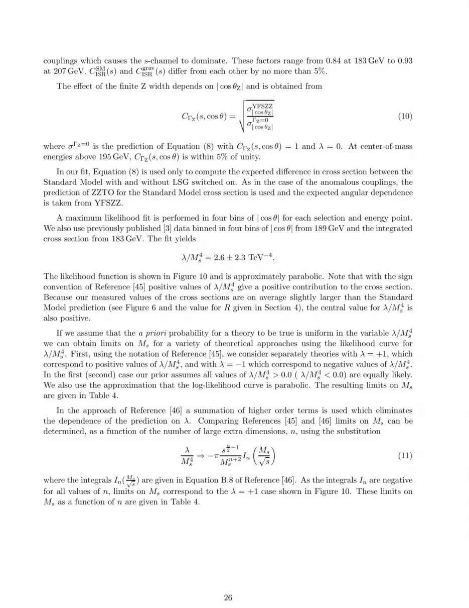
A maximum likelihood fit is performed in four bins of | cos θ| for each selection and energy point.We also use previously published [3] data binned in four bins of | cos θ| from 189 GeV and the integratedcross section from 183 GeV. The fit yields

λ/M4s = 2.6 ± 2.3 TeV−4.

The likelihood function is shown in Figure 10 and is approximately parabolic. Note that with the signconvention of Reference [45] positive values of λ/M4

s give a positive contribution to the cross section.Because our measured values of the cross sections are on average slightly larger than the StandardModel prediction (see Figure 6 and the value for R given in Section 4), the central value for λ/M4

s isalso positive.

If we assume that the a priori probability for a theory to be true is uniform in the variable λ/M4s

we can obtain limits on Ms for a variety of theoretical approaches using the likelihood curve forλ/M4

s . First, using the notation of Reference [45], we consider separately theories with λ = +1, whichcorrespond to positive values of λ/M4

s , and with λ = −1 which correspond to negative values of λ/M4s .

In the first (second) case our prior assumes all values of λ/M4s > 0.0 ( λ/M4

s < 0.0) are equally likely.We also use the approximation that the log-likelihood curve is parabolic. The resulting limits on Ms

are given in Table 4.

In the approach of Reference [46] a summation of higher order terms is used which eliminatesthe dependence of the prediction on λ. Comparing References [45] and [46] limits on Ms can bedetermined, as a function of the number of large extra dimensions, n, using the substitution

λ

M4s

⇒ −πs

n

2−1

Mn+2s

In

(

Ms√s

)

(11)

where the integrals In(Ms√s) are given in Equation B.8 of Reference [46]. As the integrals In are negative

for all values of n, limits on Ms correspond to the λ = +1 case shown in Figure 10. These limits onMs as a function of n are given in Table 4.

26

Parameter 95% C.L. lower limit on Ms

Coupling Method of Reference [45]

λ = +1 0.62 TeV

λ = −1 0.76 TeV

Number of extra dimensions Method of Reference [46]

n = 2 0.92 TeV

n = 3 0.82 TeV

n = 4 0.73 TeV

n = 5 0.67 TeV

n = 6 0.62 TeV

n = 7 0.59 TeV

Table 4: The 95% confidence level on Ms using the approach of References [45] and [46]. These resultsinclude all channels and all energies, including the OPAL data from 183 GeV and 189 GeV presentedin Reference [3].

0123456789

-10 -5 0 5 10λ/Ms

4 (TeV-4 )

-∆ lo

g lik

elih

ood

OPAL

e+e- → ZZ

Figure 10: The negative log likelihood as a function of the λ/M4s . Limits on Ms are determined

separately for theories with λ = +1, which correspond to positive values of λ/M4s and λ = −1 which

correspond to negative values of λ/M4s . The dashed lines indicate the allowed 95% confidence level

regions obtained in the two cases. These results are dominated by the 190 − 209 GeV data, but alsoinclude the OPAL data from 183 GeV and 189 GeV presented in Reference [3].

27

7 Conclusion

The process e+e− → ZZ has been studied at center-of-mass energies between 190 GeV and 209 GeVusing the final states ℓ+ℓ−ℓ+ℓ−, ℓ+ℓ−νν, qqℓ+ℓ−, qqνν, and qqqq. The number of observed events,the background expectation from Monte Carlo and the calculated efficiencies have been combined tomeasure the NC2 cross section for the process e+e− → ZZ. The measured cross sections for the sixenergy points are:

σZZ(192 GeV) = 1.29 +0.47−0.40

+0.12−0.09 pb

σZZ(196 GeV) = 1.13 +0.26−0.24

+0.08−0.07 pb

σZZ(200 GeV) = 1.05 +0.25−0.22

+0.07−0.06 pb

σZZ(202 GeV) = 0.79 +0.35−0.29

+0.08−0.05 pb

σZZ(205 GeV) = 1.07 +0.27−0.24

+0.08−0.07 pb

σZZ(207 GeV) = 0.97 +0.19−0.18

+0.06−0.05 pb.

The measurements at all energies are consistent with the Standard Model expectations. Using infor-mation from the cross-section measurements and from the optimal observables, no evidence is foundfor anomalous neutral-current triple gauge couplings. The 95% confidence level limits are listed inTable 3. We have also derived limits on low scale gravity theories with large extra dimensions whichare summarized in Table 4.

Acknowledgements

We particularly wish to thank the SL Division for the efficient operation of the LEP accelerator at allenergies and for their close cooperation with our experimental group. In addition to the support staffat our own institutions we are pleased to acknowledge theDepartment of Energy, USA,National Science Foundation, USA,Particle Physics and Astronomy Research Council, UK,Natural Sciences and Engineering Research Council, Canada,Israel Science Foundation, administered by the Israel Academy of Science and Humanities,Benoziyo Center for High Energy Physics,Japanese Ministry of Education, Culture, Sports, Science and Technology (MEXT) and a grant underthe MEXT International Science Research Program,Japanese Society for the Promotion of Science (JSPS),German Israeli Bi-national Science Foundation (GIF),Bundesministerium fur Bildung und Forschung, Germany,National Research Council of Canada,Hungarian Foundation for Scientific Research, OTKA T-038240, and T-042864,The NWO/NATO Fund for Scientific Research, the Netherlands.

28

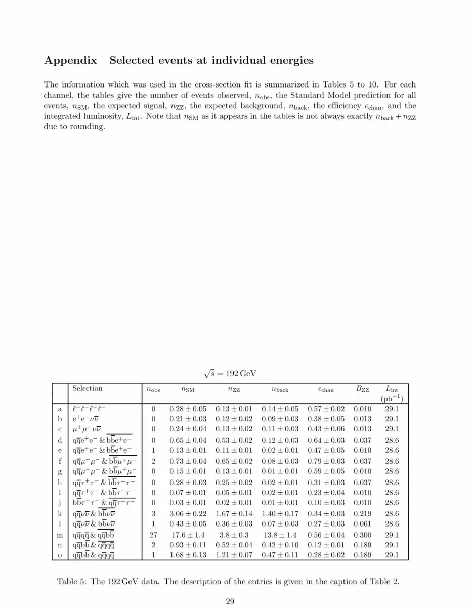
Appendix Selected events at individual energies

The information which was used in the cross-section fit is summarized in Tables 5 to 10. For eachchannel, the tables give the number of events observed, nobs, the Standard Model prediction for allevents, nSM, the expected signal, nZZ, the expected background, nback, the efficiency ǫchan, and theintegrated luminosity, Lint. Note that nSM as it appears in the tables is not always exactly nback +nZZ

due to rounding.

√s = 192 GeV

Selection nobs nSM nZZ nback ǫchan BZZ Lint

(pb−1)

a ℓ+ℓ−ℓ+ℓ− 0 0.28 ± 0.05 0.13 ± 0.01 0.14 ± 0.05 0.57 ± 0.02 0.010 29.1

b e+e−νν 0 0.21 ± 0.03 0.12 ± 0.02 0.09 ± 0.03 0.38 ± 0.05 0.013 29.1

c µ+µ−νν 0 0.24 ± 0.04 0.13 ± 0.02 0.11 ± 0.03 0.43 ± 0.06 0.013 29.1

d qqe+e− & bbe+e− 0 0.65 ± 0.04 0.53 ± 0.02 0.12 ± 0.03 0.64 ± 0.03 0.037 28.6

e qqe+e− & bbe+e− 1 0.13 ± 0.01 0.11 ± 0.01 0.02 ± 0.01 0.47 ± 0.05 0.010 28.6

f qqµ+µ− & bbµ+µ− 2 0.73 ± 0.04 0.65 ± 0.02 0.08 ± 0.03 0.79 ± 0.03 0.037 28.6

g qqµ+µ− & bbµ+µ− 0 0.15 ± 0.01 0.13 ± 0.01 0.01 ± 0.01 0.59 ± 0.05 0.010 28.6

h qqτ+τ− & bbτ+τ− 0 0.28 ± 0.03 0.25 ± 0.02 0.02 ± 0.01 0.31 ± 0.03 0.037 28.6

i qqτ+τ− & bbτ+τ− 0 0.07 ± 0.01 0.05 ± 0.01 0.02 ± 0.01 0.23 ± 0.04 0.010 28.6

j bbτ+τ− & qqτ+τ− 0 0.03 ± 0.01 0.02 ± 0.01 0.01 ± 0.01 0.10 ± 0.03 0.010 28.6

k qqνν & bbνν 3 3.06 ± 0.22 1.67 ± 0.14 1.40 ± 0.17 0.34 ± 0.03 0.219 28.6

l qqνν & bbνν 1 0.43 ± 0.05 0.36 ± 0.03 0.07 ± 0.03 0.27 ± 0.03 0.061 28.6

m qqqq & qqbb 27 17.6 ± 1.4 3.8 ± 0.3 13.8 ± 1.4 0.56 ± 0.04 0.300 29.1

n qqbb & qqqq 2 0.93 ± 0.11 0.52 ± 0.04 0.42 ± 0.10 0.12 ± 0.01 0.189 29.1

o qqbb & qqqq 1 1.68 ± 0.13 1.21 ± 0.07 0.47 ± 0.11 0.28 ± 0.02 0.189 29.1

Table 5: The 192 GeV data. The description of the entries is given in the caption of Table 2.

29

√s = 196 GeV

Selection nobs nSM nZZ nback ǫchan BZZ Lint

(pb−1)

a ℓ+ℓ−ℓ+ℓ− 1 0.58 ± 0.10 0.37 ± 0.01 0.21 ± 0.10 0.56 ± 0.02 0.010 72.5

b e+e−νν 1 0.66 ± 0.08 0.37 ± 0.05 0.28 ± 0.06 0.42 ± 0.06 0.013 72.7

c µ+µ−νν 0 0.72 ± 0.10 0.37 ± 0.05 0.36 ± 0.08 0.41 ± 0.06 0.013 72.7

d qqe+e− & bbe+e− 2 2.05 ± 0.16 1.58 ± 0.07 0.47 ± 0.14 0.67 ± 0.03 0.037 71.3

e qqe+e− & bbe+e− 0 0.39 ± 0.04 0.34 ± 0.03 0.05 ± 0.02 0.52 ± 0.05 0.010 71.3

f qqµ+µ− & bbµ+µ− 3 1.97 ± 0.07 1.83 ± 0.06 0.14 ± 0.04 0.77 ± 0.02 0.037 71.3

g qqµ+µ− & bbµ+µ− 2 0.43 ± 0.03 0.42 ± 0.02 0.01 ± 0.01 0.63 ± 0.05 0.010 71.3

h qqτ+τ− & bbτ+τ− 0 0.81 ± 0.07 0.68 ± 0.06 0.13 ± 0.04 0.29 ± 0.03 0.037 71.3

i qqτ+τ− & bbτ+τ− 0 0.19 ± 0.03 0.17 ± 0.03 0.02 ± 0.02 0.27 ± 0.04 0.010 71.3

j bbτ+τ− & qqτ+τ− 0 0.06 ± 0.01 0.05 ± 0.01 0.01 ± 0.01 0.08 ± 0.02 0.010 71.3

k qqνν & bbνν 11 8.62 ± 0.64 4.79 ± 0.43 3.83 ± 0.47 0.34 ± 0.03 0.219 70.3

l qqνν & bbνν 0 1.29 ± 0.15 1.00 ± 0.10 0.30 ± 0.11 0.26 ± 0.03 0.061 70.3

m qqqq & qqbb 38 42.1 ± 3.3 10.3 ± 0.7 31.8 ± 3.3 0.50 ± 0.03 0.300 75.4

n qqbb & qqqq 4 3.13 ± 0.33 1.89 ± 0.14 1.24 ± 0.30 0.15 ± 0.01 0.189 75.4

o qqbb & qqqq 8 4.69 ± 0.39 3.31 ± 0.21 1.38 ± 0.32 0.26 ± 0.02 0.189 75.4

Table 6: The 196 GeV data. The description of the entries is given in the caption of Table 2.

√s = 200 GeV

Selection nobs nSM nZZ nback ǫchan BZZ Lint

(pb−1)

a ℓ+ℓ−ℓ+ℓ− 0 0.47 ± 0.09 0.43 ± 0.01 0.05 ± 0.08 0.56 ± 0.02 0.010 75.1

b e+e−νν 0 0.63 ± 0.08 0.43 ± 0.06 0.21 ± 0.06 0.43 ± 0.06 0.013 74.3

c µ+µ−νν 0 0.68 ± 0.09 0.39 ± 0.06 0.28 ± 0.07 0.40 ± 0.06 0.013 74.3

d qqe+e− & bbe+e− 3 1.98 ± 0.12 1.69 ± 0.08 0.30 ± 0.09 0.63 ± 0.03 0.037 73.7

e qqe+e− & bbe+e− 0 0.46 ± 0.04 0.41 ± 0.03 0.04 ± 0.03 0.56 ± 0.05 0.010 73.7

f qqµ+µ− & bbµ+µ− 5 2.19 ± 0.08 2.01 ± 0.06 0.18 ± 0.05 0.75 ± 0.02 0.037 73.7

g qqµ+µ− & bbµ+µ− 3 0.43 ± 0.03 0.41 ± 0.03 0.02 ± 0.02 0.56 ± 0.05 0.010 73.7

h qqτ+τ− & bbτ+τ− 1 0.90 ± 0.08 0.76 ± 0.07 0.15 ± 0.05 0.28 ± 0.03 0.037 73.7

i qqτ+τ− & bbτ+τ− 0 0.23 ± 0.03 0.21 ± 0.03 0.02 ± 0.02 0.28 ± 0.04 0.010 73.7

j bbτ+τ− & qqτ+τ− 0 0.07 ± 0.02 0.06 ± 0.02 0.02 ± 0.02 0.07 ± 0.02 0.010 73.7

k qqνν & bbνν 11 10.2 ± 0.7 5.4 ± 0.5 4.79 ± 0.46 0.34 ± 0.03 0.219 73.4

l qqνν & bbνν 0 1.46 ± 0.15 1.23 ± 0.13 0.23 ± 0.07 0.28 ± 0.03 0.061 73.4

m qqqq & qqbb 26 32.4 ± 2.5 9.1 ± 0.6 23.3 ± 2.4 0.40 ± 0.03 0.300 77.7

n qqbb & qqqq 6 4.33 ± 0.41 2.73 ± 0.18 1.60 ± 0.37 0.19 ± 0.02 0.189 77.7

o qqbb & qqqq 2 4.26 ± 0.32 3.16 ± 0.19 1.10 ± 0.26 0.22 ± 0.02 0.189 77.7

Table 7: The 200 GeV data. The description of the entries is given in the caption of Table 2.

30

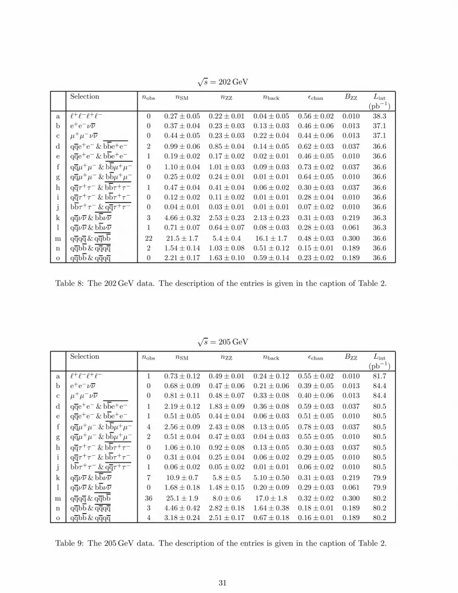
√s = 202 GeV

Selection nobs nSM nZZ nback ǫchan BZZ Lint

(pb−1)

a ℓ+ℓ−ℓ+ℓ− 0 0.27 ± 0.05 0.22 ± 0.01 0.04 ± 0.05 0.56 ± 0.02 0.010 38.3

b e+e−νν 0 0.37 ± 0.04 0.23 ± 0.03 0.13 ± 0.03 0.46 ± 0.06 0.013 37.1

c µ+µ−νν 0 0.44 ± 0.05 0.23 ± 0.03 0.22 ± 0.04 0.44 ± 0.06 0.013 37.1

d qqe+e− & bbe+e− 2 0.99 ± 0.06 0.85 ± 0.04 0.14 ± 0.05 0.62 ± 0.03 0.037 36.6

e qqe+e− & bbe+e− 1 0.19 ± 0.02 0.17 ± 0.02 0.02 ± 0.01 0.46 ± 0.05 0.010 36.6

f qqµ+µ− & bbµ+µ− 0 1.10 ± 0.04 1.01 ± 0.03 0.09 ± 0.03 0.73 ± 0.02 0.037 36.6

g qqµ+µ− & bbµ+µ− 0 0.25 ± 0.02 0.24 ± 0.01 0.01 ± 0.01 0.64 ± 0.05 0.010 36.6

h qqτ+τ− & bbτ+τ− 1 0.47 ± 0.04 0.41 ± 0.04 0.06 ± 0.02 0.30 ± 0.03 0.037 36.6

i qqτ+τ− & bbτ+τ− 0 0.12 ± 0.02 0.11 ± 0.02 0.01 ± 0.01 0.28 ± 0.04 0.010 36.6

j bbτ+τ− & qqτ+τ− 0 0.04 ± 0.01 0.03 ± 0.01 0.01 ± 0.01 0.07 ± 0.02 0.010 36.6

k qqνν & bbνν 3 4.66 ± 0.32 2.53 ± 0.23 2.13 ± 0.23 0.31 ± 0.03 0.219 36.3

l qqνν & bbνν 1 0.71 ± 0.07 0.64 ± 0.07 0.08 ± 0.03 0.28 ± 0.03 0.061 36.3

m qqqq & qqbb 22 21.5 ± 1.7 5.4 ± 0.4 16.1 ± 1.7 0.48 ± 0.03 0.300 36.6

n qqbb & qqqq 2 1.54 ± 0.14 1.03 ± 0.08 0.51 ± 0.12 0.15 ± 0.01 0.189 36.6

o qqbb & qqqq 0 2.21 ± 0.17 1.63 ± 0.10 0.59 ± 0.14 0.23 ± 0.02 0.189 36.6

Table 8: The 202 GeV data. The description of the entries is given in the caption of Table 2.

√s = 205 GeV

Selection nobs nSM nZZ nback ǫchan BZZ Lint

(pb−1)

a ℓ+ℓ−ℓ+ℓ− 1 0.73 ± 0.12 0.49 ± 0.01 0.24 ± 0.12 0.55 ± 0.02 0.010 81.7

b e+e−νν 0 0.68 ± 0.09 0.47 ± 0.06 0.21 ± 0.06 0.39 ± 0.05 0.013 84.4

c µ+µ−νν 0 0.81 ± 0.11 0.48 ± 0.07 0.33 ± 0.08 0.40 ± 0.06 0.013 84.4

d qqe+e− & bbe+e− 1 2.19 ± 0.12 1.83 ± 0.09 0.36 ± 0.08 0.59 ± 0.03 0.037 80.5

e qqe+e− & bbe+e− 1 0.51 ± 0.05 0.44 ± 0.04 0.06 ± 0.03 0.51 ± 0.05 0.010 80.5

f qqµ+µ− & bbµ+µ− 4 2.56 ± 0.09 2.43 ± 0.08 0.13 ± 0.05 0.78 ± 0.03 0.037 80.5

g qqµ+µ− & bbµ+µ− 2 0.51 ± 0.04 0.47 ± 0.03 0.04 ± 0.03 0.55 ± 0.05 0.010 80.5

h qqτ+τ− & bbτ+τ− 0 1.06 ± 0.10 0.92 ± 0.08 0.13 ± 0.05 0.30 ± 0.03 0.037 80.5

i qqτ+τ− & bbτ+τ− 0 0.31 ± 0.04 0.25 ± 0.04 0.06 ± 0.02 0.29 ± 0.05 0.010 80.5

j bbτ+τ− & qqτ+τ− 1 0.06 ± 0.02 0.05 ± 0.02 0.01 ± 0.01 0.06 ± 0.02 0.010 80.5

k qqνν & bbνν 7 10.9 ± 0.7 5.8 ± 0.5 5.10 ± 0.50 0.31 ± 0.03 0.219 79.9

l qqνν & bbνν 0 1.68 ± 0.18 1.48 ± 0.15 0.20 ± 0.09 0.29 ± 0.03 0.061 79.9

m qqqq & qqbb 36 25.1 ± 1.9 8.0 ± 0.6 17.0 ± 1.8 0.32 ± 0.02 0.300 80.2

n qqbb & qqqq 3 4.46 ± 0.42 2.82 ± 0.18 1.64 ± 0.38 0.18 ± 0.01 0.189 80.2

o qqbb & qqqq 4 3.18 ± 0.24 2.51 ± 0.17 0.67 ± 0.18 0.16 ± 0.01 0.189 80.2

Table 9: The 205 GeV data. The description of the entries is given in the caption of Table 2.

31

√s = 207 GeV

Selection nobs nSM nZZ nback ǫchan BZZ Lint

(pb−1)

a ℓ+ℓ−ℓ+ℓ− 2 1.23 ± 0.20 0.83 ± 0.03 0.40 ± 0.20 0.55 ± 0.02 0.010 136.9

b e+e−νν 1 1.16 ± 0.14 0.81 ± 0.11 0.36 ± 0.10 0.41 ± 0.05 0.013 137.6

c µ+µ−νν 0 1.41 ± 0.19 0.79 ± 0.11 0.62 ± 0.15 0.40 ± 0.06 0.013 137.6

d qqe+e− & bbe+e− 6 3.72 ± 0.21 3.12 ± 0.16 0.59 ± 0.13 0.59 ± 0.03 0.037 134.0

e qqe+e− & bbe+e− 0 0.82 ± 0.08 0.72 ± 0.07 0.10 ± 0.05 0.49 ± 0.05 0.010 134.0

f qqµ+µ− & bbµ+µ− 1 4.37 ± 0.15 4.16 ± 0.13 0.21 ± 0.08 0.79 ± 0.03 0.037 134.0

g qqµ+µ− & bbµ+µ− 0 0.82 ± 0.07 0.75 ± 0.05 0.07 ± 0.04 0.51 ± 0.05 0.010 134.0

h qqτ+τ− & bbτ+τ− 2 1.83 ± 0.16 1.61 ± 0.14 0.22 ± 0.08 0.30 ± 0.03 0.037 134.0

i qqτ+τ− & bbτ+τ− 0 0.49 ± 0.08 0.40 ± 0.06 0.09 ± 0.04 0.27 ± 0.05 0.010 134.0

j bbτ+τ− & qqτ+τ− 0 0.09 ± 0.03 0.08 ± 0.03 0.01 ± 0.01 0.06 ± 0.02 0.010 134.0

k qqνν & bbνν 16 18.9 ± 1.2 10.1 ± 0.9 8.80 ± 0.86 0.32 ± 0.03 0.219 133.6

l qqνν & bbνν 7 2.88 ± 0.30 2.53 ± 0.26 0.35 ± 0.15 0.29 ± 0.03 0.061 133.6

m qqqq & qqbb 36 41.8 ± 3.1 13.6 ± 0.9 28.3 ± 3.0 0.32 ± 0.02 0.300 133.3

n qqbb & qqqq 7 7.48 ± 0.69 4.75 ± 0.30 2.73 ± 0.63 0.18 ± 0.01 0.189 133.3

o qqbb & qqqq 6 5.34 ± 0.41 4.23 ± 0.28 1.11 ± 0.29 0.16 ± 0.01 0.189 133.3

Table 10: The 207 GeV data. The description of the entries is given in the caption of Table 2.

32

References

[1] L3 Collab., M. Acciarri et al., Phys. Lett. B450 (1999) 281;L3 Collab., M. Acciarri et al., Phys. Lett. B465 (1999) 363;L3 Collab., M. Acciarri et al., Phys. Lett. B497 (2001) 23.

[2] ALEPH Collab., R. Barate et al., Phys. Lett. B469 (1999) 287.

[3] OPAL Collab., G. Abbiendi, et al., Phys. Lett. B476 (2000) 256.

[4] DELPHI Collab., P. Abreu et al. Phys. Lett. B497 (2001) 199.

[5] R.W. Brown and K.O. Mikaelian, Phys. Rev. D19 (1979) 922.

[6] Particle Data Group, D.E. Groom et al., Eur. Phys. J. C15 (2000) 1;Particle Data Group, K. Hagiwara et al., Phys. Rev. D66 (2002) 010001.

[7] K. Hagiwara, R.D. Peccei, D. Zeppenfeld and K. Hikasa, Nucl. Phys. B282 (1987) 253.

[8] D. Chang, W.-Y. Keung and P.B. Pal, Phys. Rev. D51 (1995) 1326.

[9] K. Agashe and N.G. Deshpande, Phys. Lett. B456 (1999) 60.

[10] OPAL Collab., G. Abbiendi et al., Eur. Phys. J. C7 (1999) 407;OPAL Collab., G. Abbiendi et al., Eur. Phys. J. C12 (2000) 567;OPAL Collab., G. Abbiendi et al., Phys. Lett. B499 (2001) 38;OPAL Collab., G. Abbiendi et al., Eur. Phys. J. C 26 (2003) 479.

[11] OPAL Collab., K. Ahmet et al., Nucl. Instrum. Methods A305 (1991) 275.

[12] S. Anderson et al., Nucl. Instrum. Methods A403 (1998) 326.

[13] M. Arignon et al., Nucl. Instrum. Methods A313 (1992) 103;M. Arignon et al., Nucl. Instrum. Methods A333 (1993) 330.

[14] J.T. Baines et al., Nucl. Instrum. Methods A325 (1993) 271;D.G. Charlton, F. Meijers, T.J. Smith and P.S. Wells, Nucl. Instrum. Methods A325 (1993) 129.

[15] OPAL Collab., G. Abbiendi et al., Eur. Phys. J. C14 (2000) 373.

[16] LEP Energy Working Group, A. Blondel et al., Eur. Phys. J. C11 (1999) 573;Evaluation of the LEP centre-of-mass energy for data taken in 1999, LEP Energy Working Group,00/01, June 2000;Evaluation of the LEP centre-of-mass energy for data taken in 2000, LEP Energy Working Group,01/01, March 2001.

[17] OPAL Collab., K. Ackerstaff et al., Eur. Phys. J. C2 (1998) 441.

[18] OPAL Collab., K. Ackerstaff et al., Eur. Phys. J. C6 (1999) 1.

[19] S. Jadach et al., Comput. Phys. Commun. 102 (1997) 229;S. Jadach, E. Richter-Was, B.F.L. Ward and Z. Was, Comput. Phys. Commun. 70 (1992) 305.

[20] J. Allison et al., Nucl. Instrum. Methods A317 (1992) 47.

[21] J. Fujimoto et al., Comput. Phys. Commun. 100 (1997) 128.

[22] S. Jadach and W. P laczek, B.F.L. Ward, Phys. Rev. D56 (1997) 6939.

33

[23] T. Sjostrand, Comput. Phys. Commun. 82 (1994) 74.

[24] M.W. Grunewald and G. Passarino, et al., Four-Fermion Production in Electron-Positron Colli-

sions, CERN-2000-9-A, arXiv:hep-ph/0005309.

[25] U. Baur and D. Rainwater, Phys. Rev. D 62 (2000) 113011.

[26] S. Jadach, B.F.L. Ward and Z. Was, Phys. Lett. B449 (1999) 97.

[27] G. Marchesini et al., Comput. Phys. Commun. 67 (1992) 465.

[28] S. Jadach, W. P laczek, B.F.L. Ward, Phys. Lett. B390 (1997) 298.

[29] D. Karlen, Nucl. Phys. B289 (1987) 23.

[30] S. Jadach, et al., Comput. Phys. Commun. 119 (1999) 272.

[31] F.A. Berends, R. Pittau and R. Kleiss, Comput. Phys. Commun. 85 (1995) 437.

[32] R. Engel and J. Ranft, Phys. Rev. D54 (1996) 4244.

[33] A. Buijs W.G. Langeveld, M.H. Lehto and D.J. Miller, Comput. Phys. Commun. 79 (1994) 523.

[34] J.A.M. Vermaseren, Nucl. Phys. B229 (1983) 347.

[35] OPAL Collab., G. Abbiendi et al., Phys. Lett. B438 (1998) 391.

[36] OPAL Collab., K. Ackerstaff et al., Phys. Lett. B389 (1996) 416;OPAL Collab., K. Ackerstaff et al., Eur. Phys. J. C1 (1998) 395;OPAL Collab., G. Abbiendi et al., Eur. Phys. J. C8 (1999) 191.

[37] OPAL Collab., G. Abbiendi et al., Phys. Lett. B 544 (2002) 259.

[38] N. Brown and W.J. Stirling, Phys. Lett. B252 (1990) 657;S. Bethke, Z. Kunszt, D. Soper and W. J. Stirling, Nucl. Phys. B370 (1992) 310;S. Catani et al., Phys. Lett. B269 (1991) 432;N. Brown and W.J. Stirling, Z. Phys. C53 (1992) 629.

[39] G. Parisi, Phys. Lett. B74 (1978) 65;J. F. Donoghue, F.E. Low and S.Y. Pi, Phys. Rev. D20 (1979) 2759.

[40] S. Catani and M. H. Seymour, Phys. Lett. B378 (1996) 287.

[41] M. Warsinsky, Untersuchung des Prozesses e+e− → ZZ am LEP-Speicherring mit Hilfe von

optimalen Observablen, Diplomarbeit, Bonn University, February 2001, BONN-IB-2001-05.

[42] N. Arkani-Hamed, S. Dimopoulos and G.R. Dvali, Phys. Lett. B429 (1998) 263.

[43] J.C. Long, et al., Nature 421 (2003) 922.

[44] C.D. Hoyle, et al., Phys. Rev. Lett. 86 (2001) 1418.EOT-WASH Group, E. G. Adelberger, Sub-millimeter tests of the gravitational inverse square

law, arXiv:hep-ex/0202008.

[45] J.L. Hewett, Phys. Rev. Lett. 82 (1999) 4765.

[46] T. Han, J.D. Lykken and R.J. Zhang, Phys. Rev. D59 (1999) 105006, correctionarXiv:hep-ph/9811350 v4.

34

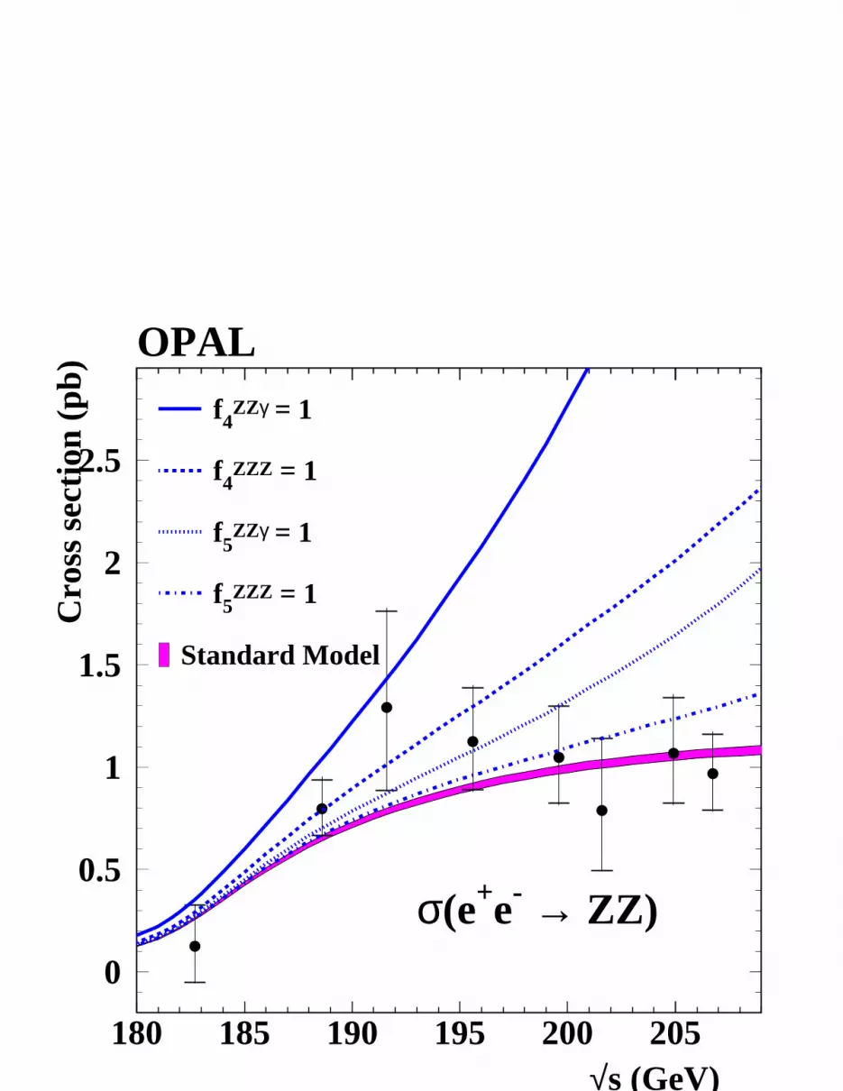
0

0.5

1

1.5

2

2.5

180 185 190 195 200 205

Cro

ss s

ecti

on (

pb)

√s (GeV)

OPAL

σ(e+e- → ZZ)

f4ZZγ = 1

f4ZZZ = 1

f5ZZγ = 1

f5ZZZ = 1

Standard Model