structures of interplanetary magnetic flux ropes and comparison with their solar sources
TRANSCRIPT
arX
iv:1
408.
1470
v1 [
astr
o-ph
.SR
] 7
Aug
201
4
Structures of Interplanetary Magnetic Flux Ropes and
Comparison with Their Solar Sources
Qiang Hu
Department of Space Science/CSPAR, University of Alabama in Huntsville, Huntsville, AL
35805
Jiong Qiu
Department of Physics, Montana State University, Bozeman, MT 59717-3840
and
B. Dasgupta, A. Khare1, and G. M. Webb
Center for Space Plasma and Aeronomic Research (CSPAR), University of Alabama in
Huntsville, Huntsville, AL 35805
Received ; accepted
Submitted April 9, 2014
1Department of Physics and Astrophysics, University of Delhi, Delhi, 110007, India
– 2 –
ABSTRACT
Magnetic reconnection is essential to release the flux rope during its ejec-
tion. The question remains: how does the magnetic reconnection change the flux
rope structure? Following the original study of Qiu et al. (2007), we compare
properties of ICME/MC flux ropes measured at 1 AU and properties of associ-
ated solar progenitors including flares, filaments, and CMEs. In particular, the
magnetic field-line twist distribution within interplanetary magnetic flux ropes
is systematically derived and examined. Our analysis shows that for most of
these events, the amount of twisted flux per AU in MCs is comparable with the
total reconnection flux on the Sun, and the sign of the MC helicity is consistent
with the sign of helicity of the solar source region judged from the geometry of
post-flare loops. Remarkably, we find that about one half of the 18 magnetic
flux ropes, most of them being associated with erupting filaments, have a nearly
uniform and relatively low twist distribution from the axis to the edge, and the
majority of the other flux ropes exhibit very high twist near the axis, of up to
& 5 turns per AU, which decreases toward the edge. The flux ropes are therefore
not linear force free. We also conduct detailed case studies showing the contrast
of two events with distinct twist distribution in MCs as well as different flare and
dimming characteristics in solar source regions, and discuss how reconnection
geometry reflected in flare morphology may be related to the structure of the
flux rope formed on the Sun.
Subject headings: Sun: activities – Sun: magnetic fields – Sun: flares – Sun: coronal
mass ejections – Sun: solar-terrestrial relations

– 3 –
1. INTRODUCTION
Observations of Magnetic Clouds (MCs) obtained in-situ by various spacecraft missions
provide the most direct and definitive evidence for the existence of magnetic flux ropes that
originate from the Sun. Despite the debate on formation mechanisms of such flux ropes, it
is acknowledged that, for a flux rope to erupt out of the Sun, magnetic reconnection has
to be invoked. Magnetic reconnection allows a change of connectivity between different
magnetic domains, or the magnetic topology. Through this change, the magnetic shear
created by turbulent plasma motion in or below the photosphere is transferred to a twisted
magnetic structure, such as a flux rope, which is then ejected from the Sun (Low 1996;
Demoulin 2006) often in the form of a Coronal Mass Ejection (CME). On many grounds,
reconnection on the Sun is a viable mechanism for the formation of flux rope structure as
well as its energetics during its evolution near the Sun; however, it has been a tremendous
challenge to observationally establish an unambiguous and quantitative association between
flux rope properties and relevant magnetic reconnection properties.
We have been able to measure previously the magnetic reconnection flux during flares in
comparison with the flux budget of magnetic clouds observed a few days after the flare/CME
eruption (Qiu et al. 2007). The study, though with a relatively small sample of 9 events,
showed that the total reconnection flux during a flare, spanning two orders of magnitudes in
these events, is comparable with the amount of twisted magnetic flux in the associated MCs,
suggesting that these flux ropes are likely to have been formed by reconnection in the corona
in the wake of its eruption. Apart from the total reconnection flux, morphology evolution
of flares may also provide information on reconnection geometry and the resultant flux rope
structure. To form the flux rope, theoretical models have envisaged a certain sequence of
magnetic reconnection. For example, observations have shown that reconnection in the
early stage forms post-flare loops highly sheared relative to the magnetic polarity inversion

– 4 –
line (PIL), and then ribbons expand in a direction perpendicular to the PIL forming less
sheared post-flare loops (Moore et al. 2001; Fletcher et al. 2004; Su et al. 2007; Qiu et al.
2010; Cheng et al. 2012). These observations are qualitatively consistent with models of flux
rope formation as depicted by van Ballegooijen & Martens (1989), and more recently by
Aulanier et al. (2010, 2012), which would predict that the flux rope is less twisted near its
axis and more twisted further out. Alternatively, Longcope & Beveridge (2007) illustrates a
scenario of sequential reconnection between a flux rope in the making and a sheared arcade,
which starts from one end of the rope axis and progresses to the other end. Such continuous
reconnection produces a highly twisted flux rope. The model predicts that flare ribbons
are not brightened simultaneously but instead sequentially along the PIL, which may be
evident in observations of many two-ribbon flares exhibiting the so-called “zipper effect”,
such as the famous Bastille-day flare (Qiu et al. 2010, and references therein). Being able
to infer reconnection properties by observing flare signatures on the Sun’s surface therefore
provides information to help distinguish these different models, and predict the structure of
the infant flux rope that is formed by reconnection (Longcope et al. 2007; Qiu 2009).
Having formed on the Sun, the magnetic structure of flux ropes has been exclusively
derived from in-situ measurements a few days after their ejection toward the observer.
There has been a continuous effort in modeling flux-rope structures embedded within the
Interplanetary CME (ICME) complex, utilizing in-situ spacecraft measurements across
such structures. These models range from a traditional one-dimensional (1D) configuration
to a fully two-dimensional (2D) model of the Grad-Shafranov (GS) reconstruction. We
employ the GS method here to examine the flux-rope structures for more than a dozen
ICME events by utilizing in-situ measurements from spacecraft ACE, Wind and STEREO.
In particular, we systematically derive the magnetic field-line twist distributions within
the core regions for the events that exhibit a typical flux-rope configuration based on GS
reconstruction results. The study of field-line twist within flux ropes had been reported

– 5 –
before for individual events (Mostl et al. 2009a,b; Liu et al. 2008; Hu & Sonnerup 2002)
and with different approaches (e.g., Dasso et al. 2006), but not in the systematic and
congregated manner that we will report here. The twist of magnetic flux ropes is closely
related to the field-line lengths within the ropes. Theoretically they are all dependent
on models utilized in the analysis of in-situ data. Larson et al. (1997) presented the first
study of energetic electron transit timing observations between the electron release on the
Sun and arrival at 1 AU to derive the field-line length directly for one event. That study
provided support for the linear-force-free flux-rope model of MCs. Kahler et al. (2011b,a)
recently extended that study by examining more events, utilizing the same date sets from
the Wind spacecraft and additional measurements from ACE, following a similar approach.
They showed the comparison of field-line length measurements with certain theoretical
flux-rope models and the general inapplicability of a linear force-free field model. Such a
model possesses a field-line length (and twist) distribution that increases with radius at
a greater rate than that derived from electron onset observations (Kahler et al. 2011b).
However comparison with the corresponding GS reconstruction results showed improved
consistency and will be reported in a separate paper. In this paper, we will employ the GS
reconstruction method to analyze MC observations and measure the twist distribution in
MCs. We present a detailed description of the methodology and a quantitative analysis of
magnetic field-line twist. Moreover we carry out additional studies to connect with their
solar source regions and offer interpretations of such connections.
In this investigation, we strive to examine the role of magnetic reconnection in the
formation and evolution of magnetic flux ropes in the corona by relating the in-situ
analysis results to the corresponding solar source regions in a quantitative manner. We
recognize that such an approach cannot provide direct and deterministic evidence for the
formation process of flux ropes, because flux ropes are magnetically invisible on the Sun
and further out in low corona. The present observations of commonly recognized plasma
– 6 –
structures in flux ropes on the Sun, including filaments, sigmoids, erupting loops/arcades,
and CMEs observed in a variety of wavelengths, are still a large step away from being able
to yield a close estimate of the amount and distribution of twist in these structures (see
review by Vourlidas 2014). Measurements of reconnection flux from flare observations,
alternatively, allow us to indirectly infer magnetic properties that can be related to flux
rope formation and evolution. Direct measurements of magnetic properties of flux ropes
have been nearly exclusively derived from in-situ observations, and there is a large gap,
namely the interplanetary space of distance 1AU starting from the Sun’s corona, between
these two kinds of observations. Nevertheless, it is hoped that large-scale numerical models
can make a crucial link with valid observational constraints at the two ends that we attempt
to provide here, and in this process, elucidate the physical mechanisms governing formation
and evolution of magnetic flux ropes (e.g., Fan 2010; Karpen et al. 2012; Aulanier et al.
2012; Titov et al. 2012).
In this paper, we use an enlarged sample of 19 events observed from 1998 through 2011
by a variety of instruments, the latest being SDO and STEREO, with identified association
between MCs and solar progenitors including CMEs, flares, and filament eruptions. The
comprehensive information of these events is given in Table 1. Identification of these events
will be discussed in the next section. Note that whereas our previous research focused on
events with major flares and fast CMEs, this enlarged sample includes events associated
with filament/prominence eruptions (P.E.) from the quiet Sun without major flares. From
the table, it is also seen that a number of these events are associated with slow or moderate
CMEs. For some of the more recent events, observations by both SDO/AIA and STEREO
are available and examined, allowing us to conduct more detailed case studies of flares
observed on the disk by AIA and CMEs observed by STEREO. We discuss identification of
these events in Section 2, and present methods of flux rope modeling in Section 3, analysis
of solar observations in Section 4, summary and comparison of these measurements in

– 7 –
Section 5, followed by conclusions and discussions in the last section.
2. IDENTIFICATION OF MC, CME, AND SOLAR SURFACE ACTIVITIES
For meaningful comparison between properties of flux ropes observed at 1 AU and
their solar progenitors, identification of MC, CME, and associated solar surface activities
is crucial. Among the 19 events studied in this paper, the first 9 events are samples in
our previous work (Qiu et al. 2007). These events occurred between 1998 and 2005, and
the association between MCs, CMEs, and solar surface activities was identified by seven
different groups listed as references in Table 1 of Qiu et al. (2007), aided with authors’ own
examination of flare and CME observations by a cluster of instruments including LASCO,
EIT, TRACE, and Big Bear Solar Observatory. The other events, except events #16 and
17 in Table 1, are selected from Li et al. (2014, hereafter referred as LI catalog). Event
# 16 is selected from Gopalswamy (2012), and event #17 is identified through private
discussion with Dr. C. C. Wu. These events (#10 - 19) occurred during 2008 through
2011, when CMEs and ICMEs can be observed and tracked in STEREO observations
while associated solar surface activities are observed by AIA onboard SDO (except event
#10). For identification, Li et al. (2014) searched “the LASCO CME catalog for halo or
partial halo CMEs during the five days prior to the MC arrival” and also used “STEREO
coronagraph and HI images for better certainty of the correspondence.” Most of these events
(#10 - 19) are also found in two other catalogs compiled by Phillip Hess and Jie Zhang at
http : //solar.gmu.edu/heliophysics/index.php/GMU CME/ICME List (abbreviated as
HZ hereafter) and by I. Richardson and H. Cane at http : //www.srl.caltech.edu/ACE/ASC/DATA/level3
(denoted as RC hereafter). The LI and HZ catalogs identify CMEs as well as times and
locations of flares or filaments associated with ICMEs, and the RC catalog only lists
CMEs associated with ICMEs. Some of these events have also been analyzed, modeled,

– 8 –
and reported in published literature. These references are provided in Table 1. In the LI,
HZ, and RC catalogs, magnetic clouds are identified from ACE observations, and CME
information is given according to LASCO observations. In some other references such
as Mostl et al. (2014) and Harrison et al. (2012), CMEs are also tracked in STEREO
observations all the way to 1 AU, and arrival times at STEREO and Wind spacecraft are
estimated and compared with observations.
We do notice that these references do not agree on the identification of solar sources
for a few events, and for these cases, we adopt the association recognized by the majority
of these authors. Below we discuss details of event identification by different sources that
can be found in public literature.
For event #11, LI, Lugaz et al. (2012), and Mostl et al. (2014) all identified the MC on
2010 May 28 to be associated with the CME at 18:30 (LASCO C2) on 2010 May 23, and LI
and Lugaz et al. (2012) both recognized the association with an erupting filament and B1
flare on the Sun’s disk. Note that the disk location of the flare/filament event is N19W12,
as reported by Lugaz et al. (2012) and confirmed by our own scrutiny (see Figure 11),
different from the location N20E10 reported in LI. In HZ and RC catalogs, however, the
MC is considered to be associated with a CME at 14:06 UT (LASCO C2) on 2010 May
24. Lugaz et al. (2012) have analyzed and modeled this event, showing that the CME on
May 24 caught up with the one on May 23, and the CME that occurred a day later was
deflected whereas the CME on May 23 reached L1 to be observed by Wind. We therefore
consider the association between the MC on May 28 and CME/flare/filament on May 23 to
be reliable.
For event #12, numerous research groups have reported analysis and modeling of the
CME/flare/filament events on 2010 August 1 possibly associated with the MC on August 4.
Association with a C3.2 flare at 07:32 UT is reported in both LI and HZ catalogs; however,
– 9 –
the three catalogs HZ, RC, and LI, identify three different LASCO CMEs, taking place at
03:54 UT, 09 UT (also identified by Mostl et al. (2014)), and 13:42 UT, respectively, to be
associated with the MC. On 2010 August 1, three filament eruptions were observed roughly
at 3 UT, 8 UT, and 18 UT by AIA and STEREO (e.g., Schrijver & Title 2011; Torok et al.
2011; Titov et al. 2012, and other references listed in Table 1). By studying the STEREO
images, Harrison et al. (2012) further identified four CMEs with reconstructed onset times
at 3 UT, 8 UT, 10 UT, and 16 UT, three of them (at 3, 10, and 16 UT) being associated
with three different filament eruptions, and the one at 8 UT being associated with the C3.2
flare (also see Temmer et al. 2012). Harrison et al. (2012) also predicted the arrival times
of 3 CMEs (at 8, 10, and 16 UT) at Wind spacecraft to be August 3 12 UT, August 4
8 UT and 16 UT, respectively. If identification by Harrison et al. (2012) is accurate, the
MC analyzed in this paper is likely related with either the 8 UT CME with a flare, or the
10 UT CME with a filament eruption. Note that the flare and filament eruption, though
close in time, occurred in two different active regions. Furthermore, CMEs launched at
different times throughout the day probably interacted with each other (e.g., Harrison et al.
2012; Mostl et al. 2012; Temmer et al. 2012). Therefore, there is a great difficulty to find
an unambiguous one-to-one association between the MC and flare/CME/filament. In this
paper, we still report properties measured in the C3.2 flare, which is the only major flare
on this day and is most likely associated with the CME at 8 UT (STEREO; Harrison et al.
2012; Mostl et al. 2014) or 9 UT (LASCO; RC), but with the caution that a direct
comparison between flare and MC properties is not entirely justified for this event before
fully understanding the relationship between all the different events occurring on the same
day.
Event #14 is found in LI and HZ catalogs. The MC on 2011 March 29 is identified
to be associated with a LASCO CME at 14:36 UT on March 25 in LI, but is thought to
be related with a LASCO CME at 02:00 UT on March 25 in HZ. Tracking the event in
– 10 –
STEREO EUVI, COR1, COR2, and HI images, Savani et al. (2013) identified the MC to
be associated with a CME that entered the STEREO COR-2A view at 21:24 UT on March
24. In terms of solar surface activities, both LI and HZ catalogs register a C1.0 flare in
an active region located at S16E31. It appears that four flares (C1.4 at 20:53 on March
24, C1.0 at 00:57, C1.0 at 16:47, and M1.0 at 23:08 on March 25) took place in this same
active region around the times of the above-identified CMEs. Some of these flares or CMEs
are also associated with filament eruptions. For the very large ambiguity in identifying
associated CME and flare or filament, as reflected in the disagreement among the above
references, we cannot determine solar source properties for this event. However, since all
flares or filament eruptions, which are probably candidates of the MC source, occur in the
same active region, the morphology of the flares in the active region allows us to determine
the sign of the helicity (see Section 4). Furthermore, this active region produces small
flares, the biggest one being the M1.0 flare. The reconnection flux measured in this largest
flare and reported in Table 2 serves as an upper limit of reconnected flux, if any, associated
with the MC flux rope.
For event #16, the association between MC, CME, and flare is identified by
Gopalswamy (2012), and the same association is also confirmed in HZ and RC catalogs.
The identification is therefore regarded to be unambiguous.
The MC of event #17 was best observed as well as measured in STEREO A. It is
identified to be associated with a CME and a limb flare, without filament eruption, through
private discussion with C. C. Wu who modeled this event, as well as by authors’ own
examination of AIA, STEREO, and LASCO movies.
Event #18 is reported in all three catalogs LI, HZ, and RC, in all of which the MC
is associated with the CME at 0:05 UT on September 14. LI identifies a C2.9 flare in
active region 11289 at N23W21 (see Figure 9) to be associated with the CME/MC; HZ

– 11 –
also identifies the solar source to be in the same active region at the same location, though
without listing a flare in the catalog. For the general agreement among the above three
catalogs, identification of this event is also regarded to be reliable.
Event #19 is reported in two catalogs LI and HZ, as well as by Mostl et al. (2014). In
LI, the MC is identified to be associated with a LASCO CME at 01:25 UT on 2011 October
22 and a filament eruption at N30W30, which did not produce an obvious flare. Mostl et al.
(2014) associated the MC with a CME seen in STEREO COR-2 at 1:09 UT. However, HZ
identifies the MC to be associated with a LASCO CME at 10:36 UT and an M1 limb flare
peaking at 11:10 UT in a different region at N25W77. For close proximity between LI and
Mostl et al. (2014), aided with authors’ own examination of the AIA and STEREO movies,
we adopt the identification by LI for this event.
In summary, to our best knowledge and based on available published literature
including on-line catalogs, identification of MCs and their solar sources is reliable in most
of the events listed in Table 1. There is a large uncertainty in event #14, limiting our
MC/flare comparison to being only qualitative. The complex nature of event #12 does
not allow us to establish a one-to-one relation between the MC and its solar source. We
still report measurements for these two events for reference. For the rest of the events, we
measure and compare properties of MCs and their solar sources.
3. GRAD-SHAFRANOV RECONSTRUCTION OF MAGNETIC FLUX
ROPES
The structures of magnetic flux ropes embedded within ICMEs propagated from
the low corona and detected in-situ by spacecraft ACE, Wind and STEREO etc. are
examined by the Grad-Shafranov (GS) reconstruction method (Hu & Sonnerup 2001, 2002;

– 12 –
Sonnerup et al. 2006; Hu et al. 2013). The GS method is a truly two-dimensional (2D)
method that yields a solution to the Cartesian GS equation describing a 212D magnetic
field, utilizing the spacecraft measurements of both the magnetic field and bulk plasma
parameters across the structure along a single path.
3.1. General Approach and Output
The general approach of GS reconstruction is based on a cylindrical geometry with the
z-axis being the flux-rope axis of translation symmetry such that ∂/∂z ≈ 0. The transverse
plane (x, y) is perpendicular to z and the GS equation governing the plasma structure in
quasi-static equilibrium is (Sturrock 1994; Hau & Sonnerup 1999)
∂2A
∂x2+∂2A
∂y2= −µ0
dPt
dA= −µ0jz(A), (1)
where a magnetic flux function A is defined such that the transverse magnetic field
components are Bx = ∂A/∂y, and By = −∂A/∂x. The equi-value contours of A represent
transverse magnetic field lines. Therefore the transverse field on the cross-section of a
flux rope is completely determined by the scalar flux function A(x, y) and the magnetic
poloidal flux is directly calculated by taking the difference of the A values between two
iso-surfaces of A, then multiplied by a chosen length L along the z axis (Qiu et al. 2007).
These iso-surfaces of A are nested distinct cylindrical surfaces, called A shells, on which the
magnetic field lines are winding along the z axis.
The other important quantity is the so-called transverse pressure Pt(A) that appears
on the right-hand side of the GS equations (1) and is a single-variable function of A. Its
first-order derivative yields the axial current density jz(A). This function is the sum of
the plasma pressure p and the axial magnetic pressure B2z(A)/2µ0. Both are functions
of A alone. This important feature allows us to devise an algorithm for determining the
– 13 –
invariant z axis, in turn checking for the validity of the translation symmetry and finally
obtaining the axial field distribution over the solution domain once the GS equation (1) is
solved to obtain a solution A(x, y) within a rectangular domain. Detailed description of
the procedures was given in prior works (see, e.g., Hu & Sonnerup 2002). A quantitative
measure Rf that evaluates the goodness-of-fit of spacecraft data to a functional form Pt(A)
was defined in the last few steps of the GS reconstruction to assess, partially, the quality of
the reconstruction results (Hu et al. 2004).
An example of the basic GS reconstruction results is given in Figure 1 for event #18
in Table 1. Figure 1a shows the time series of in-situ ACE spacecraft measurements of
the ICME event on 17 September 2011, from which both the magnetic field vectors and
plasma density, temperature (including electron temperature Te if available) and velocity
were utilized in generating the GS reconstruction results. The interval marked by two
vertical lines is the GS interval given in Table 1 and was chosen for the analysis. It clearly
corresponds to a region of low proton β value in this case. In particular, the total plasma
pressure and the axial magnetic pressure as plotted in the bottom panel indicate a region
dominated by the magnetic field during the GS interval. For this event, no Te data were
included. Based on the recent study of Hu et al. (2013), the inclusion of Te generally has
a negligible effect on the topological properties of the results, such as axis orientation, or
the size and shape of the cross-section, but there is a 10-20% discrepancy in other physical
quantities. Figure 1b shows the plot of Pt versus A typical of a flux-rope solution. The
scattered symbols are measurements while the thick curve represents an analytic functional
fit of Pt(A) to the data points. A fitting residue, Rf , is calculated to show the quality of the
fit, the smaller the Rf value, the more reliable the overall reconstruction results. The rule
of thumb is that in general a value not exceeding 0.20 is considered acceptable. A boundary
value A = Ab is defined and marked such that the GS solution of the flux-rope configuration
is most valid within this boundary (A < Ab in this case), as also highlighted by the thick

– 14 –
white line in panel (c). Figure 1c shows a typical presentation of the GS solution on the
cross-sectional (x−y) plane which represents a cut of the cylindrical structure perpendicular
to the z axis. The concentric contour lines represent the transverse field lines while the
color-filled contours are the axial field distribution with scales indicated by the colorbar to
the right. Therefore this shows the full characterization of the three-component magnetic
field within the solution domain. This cross-sectional map shows a flux-rope solution with
left-handed chirality with closed loops surrounding the center that was crossed by the
spacecraft in close vicinity (the spacecraft path is always along y = 0).
3.2. Magnetic Field-line Twist
To further visualize the GS reconstruction result and facilitate detailed analysis of
magnetic field-line twist and length (the latter to be reported elsewhere), we present a
3D view of the flux-rope solution by drawing selected field lines in a 3D volume extended
along the z axis in Figure 2. So the cross-sectional map of Figure 1c corresponds to a
projection of these spiral field lines as viewed along the z axis. Therefore only the field
lines completing at least one full turn will appear as closed loops in Figure 1c. We denote
the outermost loop with corresponding value A′ = |A − A0| ≡ Ac. In Figure 2, only three
representative field lines are drawn, one near the center (red) and the other two on outer
loops, but are all within A′ = Ac. Therefore the one near the center appears straight and
the other two appear to be winding along the z axis with distinct twist. The field-line twist
can be evaluated from these graphic representation based on the reconstructed magnetic
field vectors in the volume. For example, for each of the blue and pink outer field lines, the
root on the z = 0 plane is denoted by a circle, and the field line can be traced from the root
point in the volume. The point along the field line at which one full turn is completed is
marked by a cross. If we denote the length along z dimension between the circle and the
– 15 –
cross by Lz in AU, then the twist for that particular field line is
τ(A) =1
Lz
, (2)
in unit of turns/AU. This procedure can be done for all points rooted on that particular
loop at z = 0 plane of the same A value, i.e., by moving the circle around the same loop.
Apparently all these field lines should have the same Lz value, thus the twist τ is a function
of A alone. We repeat these procedures for all root points on all closed loops to obtain
an estimate of τ and associated uncertainty as a function of A. A few other methods of
approximating the field-line twist for cylindrical flux ropes are described in the Appendix.
Detailed studies and validation of these methods are presented there for a few analytic
flux-rope models whose field-line twist distributions are exactly known. The test case
studies show that the graphic method described here yields the most reliable estimate
of magnetic field-line twist, and will be utilized primarily in analyzing the events to be
presented. Our interpretations will also be based on the results obtained from this method.
3.3. Summary of GS Reconstruction Results
Various physical quantities have been derived from the GS reconstruction output.
These include the axial field Bz, the toroidal (axial) and poloidal magnetic flux, Φt and
Φp, the relative magnetic helicity Kr, the axial current density jz and current Iz, and the
field-line twist. They all can be calculated and presented as functions of A, as discussed in
Sections 3.1 and 3.2. Together with the field-line twist estimates, we systematically present
the distribution of these quantities along A shells for events #1-19, except for event #13
for which the GS reconstruction results are not available.
Figure 3 shows a summary plot of the distributions of all the aforementioned quantities
versus the shifted flux function A′ = |A − A0|. The integral quantities such as magnetic
– 16 –
flux, helicity and current increase monotonically with A′ since their distributions represent
accumulative sums over increasing area or volume across the A shells from the center
(A′ ≡ 0) to the boundary of the flux rope. The axial magnetic field also shows monotonically
deceasing behavior typical for such flux-rope structures. The axial current density, on the
other hand, shows the greatest variation since it represents the first-order derivative of Pt(A)
along the A shells. The field-line twist, as given here from two approximate methods only
for illustrative purpose, ranges from about 2 to 20 turns/AU. They show a general trend
of rapid decreasing from the center or constant twist and the smaller the size of the flux
rope is, the larger the twist number becomes. Additional and more reliable results from the
graphic method will be presented and discussed below. We further separate the summary
plot of Figure 3 into two subplots in Figure 4 corresponding to the events associated with
P.E. and without P.E., respectively. The two groups show a slight distinction between
them. On average, MCs not associated with P.E. appear to carry slightly larger twist than
those associated with P.E.. We also note a prominent non-P.E. event (#16) of small size
and the greatest twist number. Such a profile, although extreme (note the GS interval
duration is the shortest, about 2 hrs), is reliable since all three estimates of the field-line
twist (especially τdF ) agree with the twist obtained from the graphic method.
Table 2 summarizes some of the results, especially the total magnetic flux and helicity
content within the flux-rope boundary A = Ab (denoted with the additional subscript
“max”). The corresponding estimates of the average twist within such a boundary are
calculated as τH and τF according to equations A1 and A2, for references purposes. They
seem to compare well with the averages and standard deviations of τ(A) listed in the last
column. The axial magnetic field at the flux rope center Bz0 and the helicity sign are also
given, together with the helicity sign of the solar source region and the reconnection flux
Φr to be described in Section 4. The helicity signs agree well with a 13/14 match rate,
excluding events marked with “U”. Detailed comparisons among these quantities will be
– 17 –
discussed in Section 4.
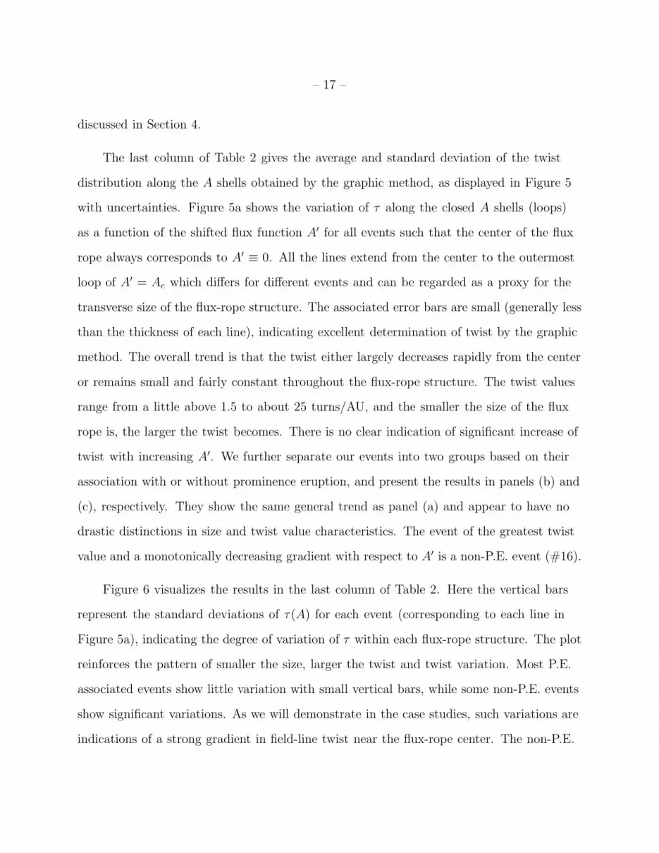
The last column of Table 2 gives the average and standard deviation of the twist
distribution along the A shells obtained by the graphic method, as displayed in Figure 5
with uncertainties. Figure 5a shows the variation of τ along the closed A shells (loops)
as a function of the shifted flux function A′ for all events such that the center of the flux
rope always corresponds to A′ ≡ 0. All the lines extend from the center to the outermost
loop of A′ = Ac which differs for different events and can be regarded as a proxy for the
transverse size of the flux-rope structure. The associated error bars are small (generally less
than the thickness of each line), indicating excellent determination of twist by the graphic
method. The overall trend is that the twist either largely decreases rapidly from the center
or remains small and fairly constant throughout the flux-rope structure. The twist values
range from a little above 1.5 to about 25 turns/AU, and the smaller the size of the flux
rope is, the larger the twist becomes. There is no clear indication of significant increase of
twist with increasing A′. We further separate our events into two groups based on their
association with or without prominence eruption, and present the results in panels (b) and
(c), respectively. They show the same general trend as panel (a) and appear to have no
drastic distinctions in size and twist value characteristics. The event of the greatest twist
value and a monotonically decreasing gradient with respect to A′ is a non-P.E. event (#16).
Figure 6 visualizes the results in the last column of Table 2. Here the vertical bars
represent the standard deviations of τ(A) for each event (corresponding to each line in
Figure 5a), indicating the degree of variation of τ within each flux-rope structure. The plot
reinforces the pattern of smaller the size, larger the twist and twist variation. Most P.E.
associated events show little variation with small vertical bars, while some non-P.E. events
show significant variations. As we will demonstrate in the case studies, such variations are
indications of a strong gradient in field-line twist near the flux-rope center. The non-P.E.

– 18 –
events also show slightly higher twist on average around 4-5 turns/AU than most P.E.
events of about 2-3 turns/AU. Quantitatively, the average (median) value of all P.E.
associated events is 3.3 (2.8), and that for all non-P.E. events is 5.3 (4.2), respectively. If
we exclude the point of the maximum standard deviation for each group, the above values
become 3.4 (2.4) and 4.1 (4.2), respectively. Note that the events of uncertain association
with P.E. are excluded from these statistics.
4. MEASURING PROPERTIES ON THE SUN
As in Qiu et al. (2007), we here measure the reconnection flux in these events from
flare ribbon evolution observed in ultraviolet wavelengths by the Transition Region
And Corona Explorer (TRACE; Handy et al. 1999) or Atmosphere Imaging Assembly
(AIA; Lemen et al. 2012) or optical Hα images from the Big Bear Solar Observatory
(BBSO), combined with magnetograms obtained by the Michelson Doppler Imager (MDI;
Scherrer et al. 1995) or Helioseismic and Magnetic Imager (HMI; Schou et al. 2012)
onboard the Solar Dynamics Observatory (SDO). Although flare ribbons form in the upper
chromosphere or transition region and the longitudinal magnetogram is obtained in the
photosphere, our experiments have shown that using the magnetic field extrapolated to
the chromosphere changes the measured total reconnection flux by up to 20%. In this
paper, we do not extrapolate the magnetic field, but display the reconnection flux measured
using photospheric magnetograms, which we call Φr in the following tables and text. Φr is
measured in both positive and negative magnetic fields, and the mean of the two is taken
as the total reconnection flux. Measurement uncertainties were comprehensively discussed
in Longcope et al. (2007); Qiu et al. (2007, 2010). The uncertainty mainly stems from
thresholding for flaring pixels and the difference between the fluxes measured in positive
and negative fields, which can be up to 30%. In the table, both the reconnection flux Φr
– 19 –
and measurement uncertainty are listed.
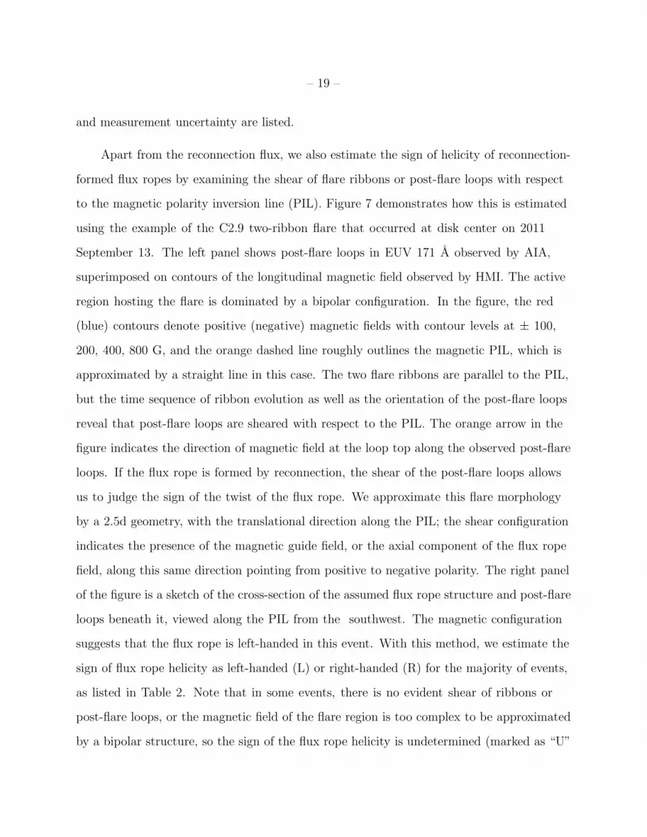
Apart from the reconnection flux, we also estimate the sign of helicity of reconnection-
formed flux ropes by examining the shear of flare ribbons or post-flare loops with respect
to the magnetic polarity inversion line (PIL). Figure 7 demonstrates how this is estimated
using the example of the C2.9 two-ribbon flare that occurred at disk center on 2011
September 13. The left panel shows post-flare loops in EUV 171 A observed by AIA,
superimposed on contours of the longitudinal magnetic field observed by HMI. The active
region hosting the flare is dominated by a bipolar configuration. In the figure, the red
(blue) contours denote positive (negative) magnetic fields with contour levels at ± 100,
200, 400, 800 G, and the orange dashed line roughly outlines the magnetic PIL, which is
approximated by a straight line in this case. The two flare ribbons are parallel to the PIL,
but the time sequence of ribbon evolution as well as the orientation of the post-flare loops
reveal that post-flare loops are sheared with respect to the PIL. The orange arrow in the
figure indicates the direction of magnetic field at the loop top along the observed post-flare
loops. If the flux rope is formed by reconnection, the shear of the post-flare loops allows
us to judge the sign of the twist of the flux rope. We approximate this flare morphology
by a 2.5d geometry, with the translational direction along the PIL; the shear configuration
indicates the presence of the magnetic guide field, or the axial component of the flux rope
field, along this same direction pointing from positive to negative polarity. The right panel
of the figure is a sketch of the cross-section of the assumed flux rope structure and post-flare
loops beneath it, viewed along the PIL from the southwest. The magnetic configuration
suggests that the flux rope is left-handed in this event. With this method, we estimate the
sign of flux rope helicity as left-handed (L) or right-handed (R) for the majority of events,
as listed in Table 2. Note that in some events, there is no evident shear of ribbons or
post-flare loops, or the magnetic field of the flare region is too complex to be approximated
by a bipolar structure, so the sign of the flux rope helicity is undetermined (marked as “U”

– 20 –
in the table).
Finally, the flux rope structure, if formed by reconnection, is related to the sequence
of magnetic reconnection (Longcope et al. 2007; Qiu 2009) which dictates change of
connectivity and therefore exchange of helicity between different magnetic structures.
Without applying a detailed topology analysis, we only report the simple morphology
sequence of flare ribbons, by recognizing the apparent spreading patterns of flare ribbons.
In most eruptive two-ribbon flares, flare ribbons are brightened simultaneously at multiple
locations along the PIL, and the two ribbons exhibit expansion perpendicular to and
away from the magnetic polarity inversion line, much resembling the 2d standard CSHKP
configuration. A good number of two-ribbon flares are also observed to start brightening
at a certain location on the ribbon, and brightening systematically spreads along the
PIL to form the full length before expanding perpendicularly to the PIL. Qualitatively,
the first type may be interpreted as reconnection associated with flux rope eruption that
disturbs the global magnetic field and triggers reconnection at multiple places along the
macroscopic current sheet, and the immediately ensuing perpendicular expansion of the
ribbon reflects reconnection of overlying arcades, as depicted by Moore et al. (2001). The
initial parallel expansion of flare ribbons along the PIL, on the other hand, clearly violates
the 2d configuration, although the organized pattern of ribbon spreading likely implies the
presence of a macroscopic current sheet in the corona. The parallel spreading of the ribbon
may indicate sequential reconnection between adjacent sheared arcades (Longcope et al.
2007), in favor of injecting a large amount of twist into the flux rope. Furthermore,
whether reconnection starts simultaneously at multiple locations along the PIL or takes
place locally and then spreads in an organized manner may help diagnose the initial
triggering mechanism. For example, Shepherd & Cassak (2012) have shown that spreading
of reconnection along the PIL is likely caused by dynamics in the current sheet. In this
spirit, we also report the pattern of morphological evolution of flare ribbons in this paper.
– 21 –
In Table 2, we use ⊥ to indicate perpendicular expansion of the ribbon, and || to denote the
presence of parallel spreading, and “U” refers to flare evolution not exhibiting organized
patterns most likely due to the complex magnetic structure of the flare. It is also noted
that parallel spreading often occurs at the start of the flare; therefore, flare observations
with a low cadence might not capture such evolution pattern during the initial phase.
5. COMPARISON OF FLUX ROPE PROPERTIES WITH SOLAR
SOURCES
5.1. Magnetic Flux Budget
As discussed earlier, the sign of helicity between the flux ropes embedded within ICMEs
and their solar source regions compares very well, where the topology of the erupting field
and subsequently the helicity sign of the corresponding flux-rope structure were inferred
based on Figure 7. They agree to a large extent (see Table 2, the 4th column). There is only
one mismatch, event #12, among the 14 events with both signs identified. As discussed in
Section 2, for this event, it is very difficult to establish a one-to-one association between
the MC and the solar source due to a chain of flare and filament eruptions throughout the
day. The mismatch may suggest that the C3.2 flare might not be the solar source of the
MC flux rope. However, Torok et al. (2011) modeled the three filaments as flux ropes, all
of them also carrying a left-handed twist based on observations. Therefore, it is most likely
that interactions between different CMEs from different regions on the Sun make it difficult
to determine the helicity of the flux rope from only local magnetic field configurations
(e.g., Schrijver & Title 2011). In addition to such a successful comparison, we compare
the magnetic flux content of the flux ropes with that of their solar progenitors, namely,
the magnetic reconnection flux associated with preceding flaring activity, following the
original study of Qiu et al. (2007). We augment the original list of 9 events and show the
– 22 –
magnetic flux comparison among Φp, Φt, and the corresponding flare-associated magnetic
reconnection flux Φr in Table 2. Note that for the previously presented events #1-9, the
results here were further refined and improved. Especially for event #5, the maximum axial
field and flux were updated from Qiu et al. (2007) in the present study.
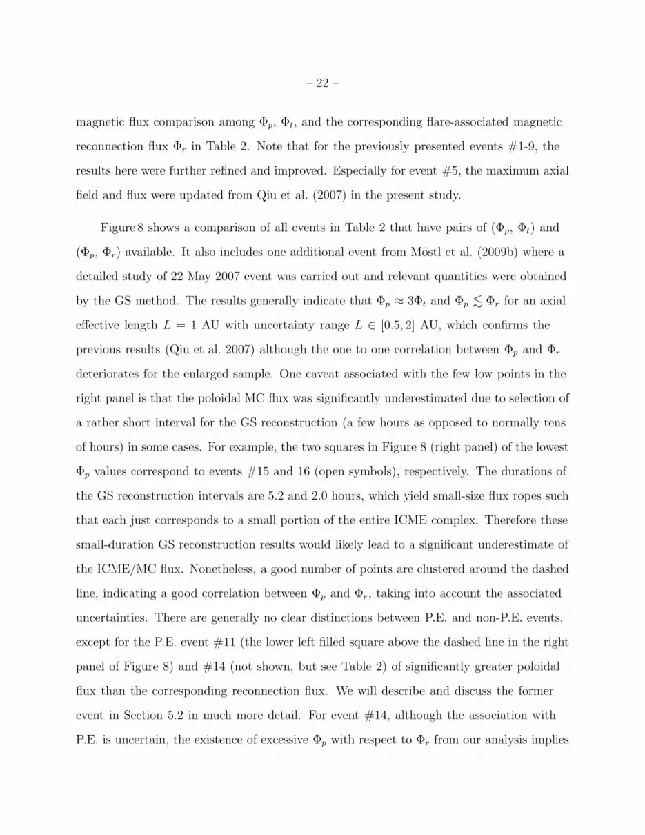
Figure 8 shows a comparison of all events in Table 2 that have pairs of (Φp, Φt) and
(Φp, Φr) available. It also includes one additional event from Mostl et al. (2009b) where a
detailed study of 22 May 2007 event was carried out and relevant quantities were obtained
by the GS method. The results generally indicate that Φp ≈ 3Φt and Φp . Φr for an axial
effective length L = 1 AU with uncertainty range L ∈ [0.5, 2] AU, which confirms the
previous results (Qiu et al. 2007) although the one to one correlation between Φp and Φr
deteriorates for the enlarged sample. One caveat associated with the few low points in the
right panel is that the poloidal MC flux was significantly underestimated due to selection of
a rather short interval for the GS reconstruction (a few hours as opposed to normally tens
of hours) in some cases. For example, the two squares in Figure 8 (right panel) of the lowest
Φp values correspond to events #15 and 16 (open symbols), respectively. The durations of
the GS reconstruction intervals are 5.2 and 2.0 hours, which yield small-size flux ropes such
that each just corresponds to a small portion of the entire ICME complex. Therefore these
small-duration GS reconstruction results would likely lead to a significant underestimate of
the ICME/MC flux. Nonetheless, a good number of points are clustered around the dashed
line, indicating a good correlation between Φp and Φr, taking into account the associated
uncertainties. There are generally no clear distinctions between P.E. and non-P.E. events,
except for the P.E. event #11 (the lower left filled square above the dashed line in the right
panel of Figure 8) and #14 (not shown, but see Table 2) of significantly greater poloidal
flux than the corresponding reconnection flux. We will describe and discuss the former
event in Section 5.2 in much more detail. For event #14, although the association with
P.E. is uncertain, the existence of excessive Φp with respect to Φr from our analysis implies
– 23 –
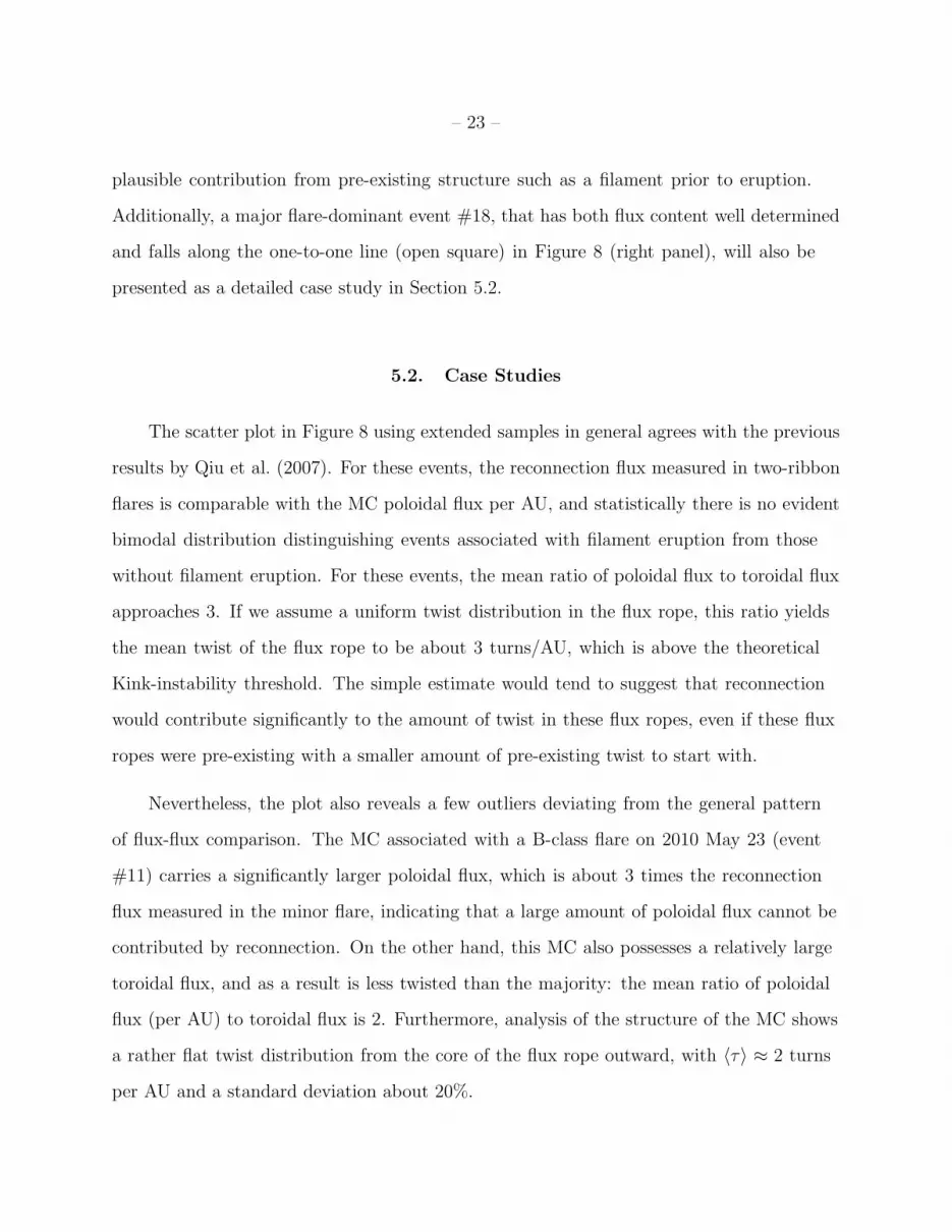
plausible contribution from pre-existing structure such as a filament prior to eruption.
Additionally, a major flare-dominant event #18, that has both flux content well determined
and falls along the one-to-one line (open square) in Figure 8 (right panel), will also be
presented as a detailed case study in Section 5.2.
5.2. Case Studies
The scatter plot in Figure 8 using extended samples in general agrees with the previous
results by Qiu et al. (2007). For these events, the reconnection flux measured in two-ribbon
flares is comparable with the MC poloidal flux per AU, and statistically there is no evident
bimodal distribution distinguishing events associated with filament eruption from those
without filament eruption. For these events, the mean ratio of poloidal flux to toroidal flux
approaches 3. If we assume a uniform twist distribution in the flux rope, this ratio yields
the mean twist of the flux rope to be about 3 turns/AU, which is above the theoretical
Kink-instability threshold. The simple estimate would tend to suggest that reconnection
would contribute significantly to the amount of twist in these flux ropes, even if these flux
ropes were pre-existing with a smaller amount of pre-existing twist to start with.
Nevertheless, the plot also reveals a few outliers deviating from the general pattern
of flux-flux comparison. The MC associated with a B-class flare on 2010 May 23 (event
#11) carries a significantly larger poloidal flux, which is about 3 times the reconnection
flux measured in the minor flare, indicating that a large amount of poloidal flux cannot be
contributed by reconnection. On the other hand, this MC also possesses a relatively large
toroidal flux, and as a result is less twisted than the majority: the mean ratio of poloidal
flux (per AU) to toroidal flux is 2. Furthermore, analysis of the structure of the MC shows
a rather flat twist distribution from the core of the flux rope outward, with 〈τ〉 ≈ 2 turns
per AU and a standard deviation about 20%.
– 24 –
In contrast to this event, which is likely a case of a dominant pre-existing flux rope,
the event that occurred on 2011 September 13-17 (event #18) well fits the scenario that
reconnection may dominantly contribute to the poloidal flux of the MC. In this event,
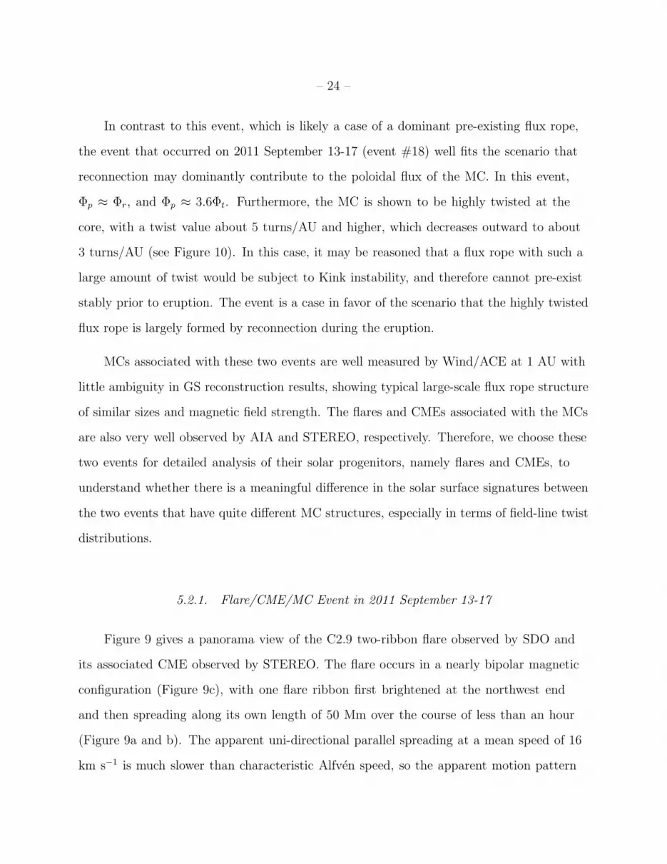
Φp ≈ Φr, and Φp ≈ 3.6Φt. Furthermore, the MC is shown to be highly twisted at the
core, with a twist value about 5 turns/AU and higher, which decreases outward to about
3 turns/AU (see Figure 10). In this case, it may be reasoned that a flux rope with such a
large amount of twist would be subject to Kink instability, and therefore cannot pre-exist
stably prior to eruption. The event is a case in favor of the scenario that the highly twisted
flux rope is largely formed by reconnection during the eruption.
MCs associated with these two events are well measured by Wind/ACE at 1 AU with
little ambiguity in GS reconstruction results, showing typical large-scale flux rope structure
of similar sizes and magnetic field strength. The flares and CMEs associated with the MCs
are also very well observed by AIA and STEREO, respectively. Therefore, we choose these
two events for detailed analysis of their solar progenitors, namely flares and CMEs, to
understand whether there is a meaningful difference in the solar surface signatures between
the two events that have quite different MC structures, especially in terms of field-line twist
distributions.
5.2.1. Flare/CME/MC Event in 2011 September 13-17
Figure 9 gives a panorama view of the C2.9 two-ribbon flare observed by SDO and
its associated CME observed by STEREO. The flare occurs in a nearly bipolar magnetic
configuration (Figure 9c), with one flare ribbon first brightened at the northwest end
and then spreading along its own length of 50 Mm over the course of less than an hour
(Figure 9a and b). The apparent uni-directional parallel spreading at a mean speed of 16
km s−1 is much slower than characteristic Alfven speed, so the apparent motion pattern
– 25 –
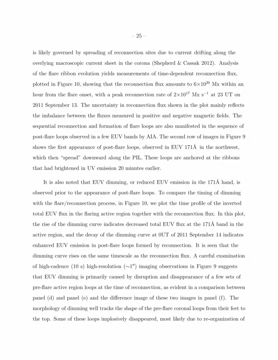
is likely governed by spreading of reconnection sites due to current drifting along the
overlying macroscopic current sheet in the corona (Shepherd & Cassak 2012). Analysis
of the flare ribbon evolution yields measurements of time-dependent reconnection flux,
plotted in Figure 10, showing that the reconnection flux amounts to 6×10²⁰ Mx within an
hour from the flare onset, with a peak reconnection rate of 2×10¹⁷ Mx s−1 at 23 UT on
2011 September 13. The uncertainty in reconnection flux shown in the plot mainly reflects
the imbalance between the fluxes measured in positive and negative magnetic fields. The
sequential reconnection and formation of flare loops are also manifested in the sequence of
post-flare loops observed in a few EUV bands by AIA. The second row of images in Figure 9
shows the first appearance of post-flare loops, observed in EUV 171A in the northwest,
which then “spread” downward along the PIL. These loops are anchored at the ribbons
that had brightened in UV emission 20 minutes earlier.
It is also noted that EUV dimming, or reduced EUV emission in the 171A hand, is
observed prior to the appearance of post-flare loops. To compare the timing of dimming
with the flare/reconnection process, in Figure 10, we plot the time profile of the inverted
total EUV flux in the flaring active region together with the reconnection flux. In this plot,
the rise of the dimming curve indicates decreased total EUV flux at the 171A band in the
active region, and the decay of the dimming curve at 0UT of 2011 September 14 indicates
enhanced EUV emission in post-flare loops formed by reconnection. It is seen that the
dimming curve rises on the same timescale as the reconnection flux. A careful examination
of high-cadence (10 s) high-resolution (∼1′′) imaging observations in Figure 9 suggests
that EUV dimming is primarily caused by disruption and disappearance of a few sets of
pre-flare active region loops at the time of reconnection, as evident in a comparison between
panel (d) and panel (e) and the difference image of these two images in panel (f). The
morphology of dimming well tracks the shape of the pre-flare coronal loops from their feet to
the top. Some of these loops implosively disappeared, most likely due to re-organization of
– 26 –
pre-existing magnetic structures by reconnection. These disrupted pre-flare loops marked in
the figure also appear to be more sheared than the post-flare loops that formed underneath
twenty minutes later. As the dimming morphology largely tracks the shape of the loops,
we cannot unambiguously interpret dimming entirely as being produced by evacuation of
coronal plasmas at the locations where the flux rope is rooted and ejected (Webb et al.
2000).
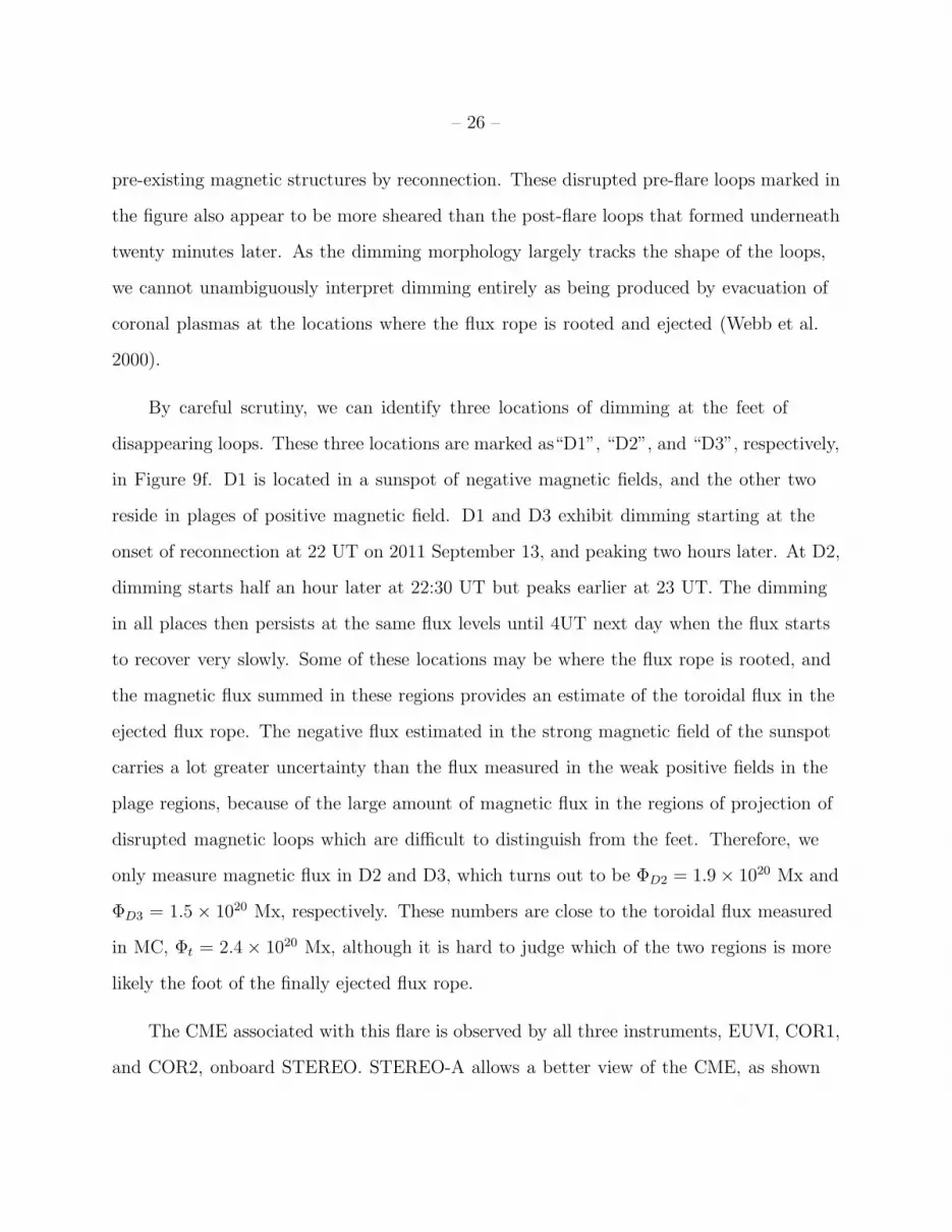
By careful scrutiny, we can identify three locations of dimming at the feet of
disappearing loops. These three locations are marked as“D1”, “D2”, and “D3”, respectively,
in Figure 9f. D1 is located in a sunspot of negative magnetic fields, and the other two
reside in plages of positive magnetic field. D1 and D3 exhibit dimming starting at the
onset of reconnection at 22 UT on 2011 September 13, and peaking two hours later. At D2,
dimming starts half an hour later at 22:30 UT but peaks earlier at 23 UT. The dimming
in all places then persists at the same flux levels until 4UT next day when the flux starts
to recover very slowly. Some of these locations may be where the flux rope is rooted, and
the magnetic flux summed in these regions provides an estimate of the toroidal flux in the
ejected flux rope. The negative flux estimated in the strong magnetic field of the sunspot
carries a lot greater uncertainty than the flux measured in the weak positive fields in the
plage regions, because of the large amount of magnetic flux in the regions of projection of
disrupted magnetic loops which are difficult to distinguish from the feet. Therefore, we
only measure magnetic flux in D2 and D3, which turns out to be ΦD2 = 1.9× 10²⁰ Mx and
ΦD3 = 1.5 × 10²⁰ Mx, respectively. These numbers are close to the toroidal flux measured
in MC, Φt = 2.4 × 10²⁰ Mx, although it is hard to judge which of the two regions is more
likely the foot of the finally ejected flux rope.
The CME associated with this flare is observed by all three instruments, EUVI, COR1,
and COR2, onboard STEREO. STEREO-A allows a better view of the CME, as shown

– 27 –
in the third row of the figure. In the EUV 195A images by EUVI, a coronal structure
hanging at the height of 1.25 solar radii is vaguely visible prior to the onset of the flare at
about 21:45 UT on 2011 September 13, and very slowly rises at almost a constant speed.
The structure and its movement become evident when reconnection on the disk takes place
at 22 UT, and the CME is subsequently observed in the COR1 and COR2 field of views
(FOVs). The CME exhibits a circular front followed by a core structure beneath. To track
its movement, we construct a time-distance plot along a straight slit connecting the solar
center with the top of the rather circular CME structure. These plots constructed using
base difference images by EUVI, COR1, and then COR2 are illustrated at the bottom row
of the figure, which clearly outline the CME core in all three types of images as well as the
front in COR1 and COR2 images. We then made an automated routine to measure the
height of the CME core by following the maximum intensity in the core structure, and the
half width of the core structure is taken as the measurement uncertainty. The measurement
is shown in the blue curve in Figure 10, against the reconnection flux plot. The CME rises
slowly in the first 40 minutes, and then speeds up at a height of 1.5 solar radii.
To derive its velocity, we make a piece-wise linear fit to the measured heights versus
times for data points to up to 5 solar radii; beyond that distance, the CME structure spreads
out giving large uncertainties in determining the centroid of CME mass. Uncertainties in
the velocity measurements are simply standard deviations of the linear fit to each piece.
As shown in the bottom left panel of the figure, the CME reaches the maximum speed
close to 300 km s−1 at 23 UT at around 2 solar radii. The acceleration is obtained by
taking time derivatives of the velocity, and error bars are derived from error propagation.
It appears that peak acceleration, of order 80 m s−2 occurs when the reconnection flux
rises most rapidly at around 23 UT of 2011 September 13, which is consistent with some
previous results, though some of these earlier measurements have used lower-cadence CME
data (Zhang et al. 2001; Qiu et al. 2004; Patsourakos et al. 2010, 2013; Cheng et al. 2014).

– 28 –
Reconnection nearly stops after midnight, when the flux rope is at 2.5 solar radii. In
addition, the height of the CME front is measured in the same way and plotted in violet in
the top left panel. It is probably a compression shock front driven by the CME. Below 2.5
solar radii, the CME velocity reaches over 300 km s−1, fast enough to drive a shock front.
It is evident in these plots that CME acceleration is coincident with the progress of
magnetic reconnection. If reconnection injects magnetic flux into the CME structure, and if
the CME is assumed to undergo a self-similar expansion, in which case, the size of the CME
flux rope Rfr grows proportionally with the height of the CME Hfr, then we can estimate
the rate of flux injection as a function of the size of the infant flux rope when it is close to
the Sun, e.g., Hfr ≤ 2R⊙. The upper right panel of Figure 10 shows the reconnection flux
(Φr; red) and reconnection rate (black) against the height (Hfr) of the CME core, and the
blue curve shows the rate of the flux injection defined by ψfr = dΦr/dHfr. The injection
rate rises rapidly with CME height and peaks at a height of Hfr ≈ 2R⊙ with 8 × 10²⁰
Mx R−1⊙ . As reconnection slows down and eventually stops, the flux injection ceases. The
field-line twist distribution within the flux rope at 1 AU as depicted in the lower right panel
exhibits a clear and largely monotonic decline from the center to about 1/3 way through
the interval, then remaining flat toward the boundary.
5.2.2. Flare/CME/MC Event in 2010 May 23 - 28
In the same way, we present the images and plots for the flare/CME event on 2010 May
23. The top panels of Figure 11 show that the two-ribbon flare evolution, in contrast to
the other event, nearly follows the 2d CSHKP model with ribbons brightening at multiple
locations along the PIL, and then expanding vertically outward in a nearly 2d manner.
The reconnection flux measured in this event is plotted in Figure 12. For this event, the
total reconnection flux amounts to 2.7×10²⁰ Mx, which is only one third of the measured

– 29 –
poloidal flux in the MC observed 5 days later. Figures 13 and 14 show the corresponding
GS reconstruction results of the MC flux rope from Wind spacecraft data.
EUV dimming is also observed. Unlike the other event, the dimming plot in the top
left panel does not track the reconnection flux plot very well; it rises more gradually than
reconnection flux. At some locations, dimming appears to be removal of pre-flare coronal
loops, as in the case of the other flare. But the dimming morphology in this event also
exhibits some differences. It is seen in EUV 171 images that dimming also occurs along
the locations of flare ribbons before they are brightened immediately afterwards. This
morphology evolution much resembles the scenario depicted by Forbes & Lin (2000) and
Moore et al. (2001), that the erupting flux rope stretches overlying coronal field lines, which
then close down by reconnection. There is also a patch located in an EUV moss region next
to the ribbon (indicated by the arrow in panels (e) and (f) in Figure 11), which does not
appear to be parts of high-lying coronal loops. Dimming takes place in the patch by removal
of the moss structure and spreads outward in a way very similar to the event reported by
Webb et al. (2000), making it a viable candidate for a foot of the erupting flux rope. The
patch is located in negative magnetic field, and magnetic flux measured in this dimming
patch amounts to 3.0×10²⁰ Mx, similar to the MC toroidal flux 3.8×10²⁰ Mx. It is, though,
not clear from observations where the other foot of the erupting flux rope is located.
The CME is prominent in the views of COR1 and COR2 onboard STEREO-B. In the
STEREO EUVI images, the erupting structure itself is invisible; however, abrupt dimming
was observed around 16:30 UT (panel (g) in Figure 11) suggesting occurrence of eruption
that expels nearby plasmas. Around this time, the CME front can be observed in the COR1
images. The CME core itself is first seen in the COR1 image at 17 UT. The time-distance
plot along a slit connecting solar center and the top of the CME structure is displayed at
the bottom panel of Figure 11, from which we measure the height of the CME core as well

– 30 –
as its front shown in the top left panel of Figure 12. The bottom panel shows the CME
velocity derived from a piece-wise linear fit and the CME acceleration obtained from time
derivatives of the velocity. The CME evolution is very similar to the other event on 2011
September 13-14: both events experience a short period of fast acceleration, which peaks
around the time reconnection also peaks. Both events reach a maximum velocity of 300 km
s−1, and both arrive at 10 solar radii six hours after onset of eruption.
This event has a much smaller reconnection flux than the other one, although they
exhibit very similar CME evolution. Suppose that this is the same amount of flux injected
into the erupting flux rope, then the flux injection rate per solar radii of the CME height
is smaller by more than half an order of magnitude. The twist distribution for this event
remains fairly flat, at about 2 turns/AU, throughout the flux-rope structure as shown in
Figure 12 (lower right panel). The rapid increase of the green curve toward the outer
boundary is due to increased errors in this estimate (see Appendix).
5.3. How Reconnection Affects CMEs
Joint observations by SDO and STEREO from different view points and with
unprecedented tempo-spatial resolution allow us to track kinematic evolution of CMEs
in their infancy from as low as 250′′ above the surface, and at the same time reliably
measure properties of reconnection beneath the CME flux rope. From comparison of
reconnection properties and CME properties in the two well-observed events, it is evident
that prominent acceleration of the CMEs of order 100-200 m s−2 takes place during the
first 1-2 hrs when reconnection proceeds rapidly; in this stage, the CME flux rope speeds
up from a few tens of km s−1 to a few hundred km s−1 and from the height close to the
Sun (1.3-1.6 solar radii) to about 3 solar radii. These results confirm, with observations
of much better quality, the suggestion from previous flare-CME observations that CME
– 31 –
acceleration and magnetic reconnection manifested in flares appear to be temporally
correlated (Zhang et al. 2001; Qiu et al. 2004; Qiu & Yurchyshyn 2005; Jing et al. 2005;
Patsourakos et al. 2010; Temmer et al. 2010; Patsourakos et al. 2013; Cheng et al. 2014).
Physically, it is not difficult to see why this should happen: reconnection changes the
magnetic configuration, which inevitably changes the magnetic forces acting on the flux
rope. In the specific cases discussed in this paper, it appears that such changes would
result in an overall expulsion force on the flux rope. Just by contrasting these two events,
it also seems that the effect of reconnection on the kinematic evolution of CMEs is not
qualitatively different in a pre-existing flux rope and an in-situ formed flux rope. The
coincident onset of fast reconnection and major acceleration is recently revealed in advanced
magnetohydrodynamic (MHD) simulations that use refined and adaptive grids to resolve
the role of core reconnection in CME acceleration (Karpen et al. 2012).
A more interesting and indeed critical question concerns whether and how reconnection
also changes the structure of the flux rope itself. Most theoretical as well as numerical
models of CME eruption would envision, at least qualitatively, injection of magnetic flux
into the CME flux rope. If this happens, then properties of reconnection in a time sequence
would be responsible for the structure of the infant flux rope from its core outward.
We can discuss three different models, all in a 2.5d scheme, of reconnection and its
effect on flux rope structure on the Sun. In a standard strict 2d CSHKP model, eruption of
a certain kind of pre-existing flux rope such as embodied in a filament pulls the overlying
arcade, which reconnects with itself below the ejecting flux rope (e.g., the cartoon model by
Moore et al. 2001). This process produces a bubble of field lines around the axis, or adds
poloidal flux around a constant pre-existing toroidal flux. Recent 3d numerical simulations
have shown characteristics of such bubble-field lines added to the flux rope (Aulanier et al.
2012) in the later stage of reconnection. Noteworthily, Aulanier et al. (2012) also illustrates

– 32 –
the earlier stage of flux rope formation, showing a less twisted flux rope at the start, with
more twisted flux added to it as reconnection proceeds between overlying coronal fields.
The simulation is used to interpret the observed apparent shear motion of flare ribbons. We
note that in these scenarios, the infant flux rope would therefore have low twist at its axis,
followed by higher twist outward. However, we do not find many examples of this kind in
the analyzed MCs in this sample. Most MCs exhibit either a flat twist distribution or twist
decreasing from the core outwards.
Another type of reconnection proposed by van Ballegooijen & Martens (1989) is that
reconnection takes a few steps to first form the flux rope axis, which is a long sheared loop
along the polarity inversion line; in the following steps, reconnection takes place between a
pair of sheared arcades both above the primary axis, and results in a loop twisting around
the primary axis. In this process, different from the 2d model in which reconnected field
lines are detached from the solar surface, toroidal flux is injected into the flux rope by the
amount of flux carried in one sheared arcade prior to reconnection, and poloidal flux is also
injected, and the amount of added twist is roughly 1.5 turns, i.e., the newly added field
line makes one and half turns from end to end. If this process continues with more and
more pairs of overlying field lines reconnecting with each other, but only once, then the net
consequence is that the flux rope is formed with increasing toroidal flux and a flat twist
of 1.5 turns. We suggest that 2010 May 23 - 28 event may be described by this pattern,
with the entire process of flux rope formation taking place in at least two different stages,
the first stage being formation of the flux rope filament prior to the flare, and the second
stage during the B-class flare, that injects toroidal as well as poloidal flux into the rope,
but with a constant twist distribution of about 1.5. Evidence of such a process includes:
the short dimming along later brightened flare ribbons indicating stretching of a set of
arcade field lines prior to reconnection by eruption, immediately followed by simultaneous
brightening of two flare ribbons at multiple locations along the PIL, and then dominant
– 33 –
apparent ribbon motion perpendicular to the PIL suggesting progressive reconnection
by higher loops. This event also exhibits a significant dimming patch next to the flare
ribbons, which is not brightened later on suggesting that no reconnection takes place at
this location. Morphology of this dimming patch is very similar to that of Webb et al.
(2000). We suspect this is one foot of the primary axis of the pre-existing flux rope. Such a
dimming morphology is not observed in the other flare discussed below.
In the third scenario as demonstrated by Longcope & Beveridge (2007), the first step
reconnection takes place between a pair of sheared arcades to form a flux rope with one
turn and an underlying post-flare loop; in the following steps, the flux rope continues to
reconnect with adjacent sheared arcades sequentially. Each step injects more twist into
the rope whereas maintaining the toroidal flux, which is the amount of the flux from the
first set of reconnecting arcades. We propose that the event on 2011 September 13 - 17
exhibits a few observational signatures indicative of this process though only qualitatively
and possibly mixed with other processes. First it is evident that some pre-flare sheared
loops disappeared at the onset of the flare, producing dimming flux that evolves on the
same timescale of reconnection flux; the post-flare loops formed later on are beneath these
pre-flare arcades and are less sheared. It is likely that dimming, or disappearance of
pre-flare loops, is largely caused by reconnection of pre-existing sheared arcades. Second,
reconnection as inferred from evolution of both the flare ribbons and post-flare loops
exhibits a very regular sequence starting from one end of the ribbon proceeding to the other
end, much as predicted in the sequential reconnection model. This reconnection sequence
along the PIL is then followed by ribbon spreading perpendicular to PIL, but the second
stage of perpendicular spreading is insignificant compared with the first stage of dominant
parallel spreading. We suggest that the first stage produces high twist in the inner part of
the flux rope, whereas the second stage plays a role similar to the second scenario that would
add toroidal flux and a flat twist in the outer part of the flux rope by reconnection between
– 34 –
adjacent overlying arcades. In particular, the dominant early-stage sequential reconnection
along the PIL at a speed of 10-20 km s−1 is hard to be explained by an erupting pre-existing
flux rope stretching field lines and triggering reconnection, in which case, the coronal field
would be violently disturbed at multiple locations and therefore reconnection would take
place in multiple locations without a prescribed order along the PIL. In other words, such
an observed reconnection sequence would be in favor of reconnection governed locally such
as by resistive instabilities or current sheet dynamics than reconnection driven by MHD
instabilities (Karpen et al. 2012; Shepherd & Cassak 2012).
We recognize that there remain a couple of observational details pending explanation
with this scenario, one being posed by the STEREO-EUVI observation that an overlying
coronal structure is present about 15 minutes before the observed onset of the sequential
reconnection, and its evolution later on appears to be consistent with the CME core (the
flux rope) identified in COR1 and COR2 images. It is not clear what is the relation between
this structure and the flux rope being formed by sequential reconnection. It is possible
that weak reconnection and formation of the flux rope already starts before 22 UT but
with very weak signatures on the disk. Another detail concerns the rather long timescale of
reconnection in this event, which proceeds for 60 minutes, with the fast reconnection and
organized pattern of spreading lasting for 40 minutes from 22:50 to 23:30 UT. During this
period, the STEREO-observed CME core moves from 0.5 to 1.5 solar radii above the limb.
The connection between the flux rope and coronal reconnection would imply the presence of
a long current sheet linking the bottom of the flux rope and the top of the post-flare arcade.
Furthermore, whereas the flux rope moves rapidly in the high corona, reconnection below
the flux rope proceeds in an organized “zipper” pattern, which may suggest that there is
only very weak overlying coronal magnetic field. It is possible that a pre-flare break-out
type reconnection has taken place to remove much of the magnetic flux above the core flux
rope.

– 35 –
6. CONCLUSIONS AND DISCUSSION
In conclusion, we have analyzed magnetic clouds and their solar progenitors including
flares, CMEs, and coronal dimming for an enlarged sample containing a total of 19 events.
The magnetic structure of flux ropes is examined by the GS reconstruction method, and is
compared with the properties of flares, filaments, and coronal dimming in the corresponding
source region. We summary our main findings as follows.
1. Our systematic analysis of the magnetic field-line twist distribution within magnetic
flux ropes provides clear evidence for the invalidity of the 1D constant-α force-free
model of a cylindrical flux rope. Such a model predicts increasing twist with increasing
radial distance away from the flux-rope center, approaching infinity at the boundary
where Bz = 0. However our analysis does not show this general trend. Instead our
results are more consistent with a non-linear force-free model. In about half of the
cases, the field line twist is constant at 1.5-3 turns per AU, as in the Gold-Hoyle (GH)
model. The other half exhibit a high twist of & 5 turns per AU near the core, which
decreases outward. There is suggestion that events associated with filament eruptions
have a lower average twist than events not associated with filaments.
2. We compare the MC magnetic structure with properties of solar flares associated
with the CME/MC. It is shown that the sign of the helicty of MCs is consistent with
the sign of helicity of the post-flare coronal arcade, and the amount of twisted flux
(the poloidal flux) in general agrees with the measured amount of flux reconnected in
flares. There is no statistically significant difference between events with or without
filament eruption.
3. We also conduct detailed case studies of two events with typical and comparable
flux-rope geometry but different twist distribution, one with a flat twist of about 2
– 36 –
turns/AU from center to edge, and the other with a high twist about 5 turns/AU
near the axis, which decreases outward. The two events are very well observed by
multiple spacecraft at multiple view points on the Sun and at 1 AU. Comparison
of the MC flux and reconnection flux, as well as the flare and dimming evolution,
suggests that the first event is probably dominated by a pre-existing low-twist flux
rope surrounding a filament, and reconnection at multiple locations along the PIL
appears to add only a small amount of flux with low twist; whereas the second event
is probably a flux rope with significant twist injected by slow sequential reconnection
along the PIL. This case study, though limited in its scope, suggests that the geometry
of reconnection as reflected in flare morphology is related to, and therefore may be
used to diagnose, the magnetic structure of infant flux ropes formed on the Sun. In
terms of the kinematic evolution, in both events, the onset of fast acceleration takes
place when fast reconnection starts regardless of the geometry of reconnection.
The field-line twist distribution in MCs is consistent with a constant-twist non-linear
force-free model (Gold & Hoyle 1960). The force-free parameter α changes with flux surface
in this model, although it remains constant on each distinct surface. This implies that
these flux surfaces are formed at the Sun and are not destroyed while propagating in the
interplanetary space. It seems that finite resistivity is not playing a significant role in
merging these surfaces to give a constant-α relaxed state (see, e.g., Freidberg 1987; Taylor
1986). The GS method is applicable to a non-force free state, but in the large-scale ICME
structures we examined, the magnetic field always dominates and the plasma pressure
gradient does not play a major role, even after including the additional contribution from
Te (Hu et al. 2013). The indication that the flux surfaces are probably preserved during the
transit of the flux rope through 1 AU is significant and may provide validation for direct
comparison of MC properties with magnetic properties directly measured or indirectly
inferred in the Sun’s corona. Ideal MHD proves to be a good approximation in the solar

– 37 –
wind such that the magnetic flux and helicity are conserved, which in turn provides the
ground for our interpretations and discussions about relating in-situ magnetic flux-rope
structures as characterized by the field-line twist (see Appendix) with their solar sources.
These findings pose questions on formation mechanisms of flux ropes: what produces
the high twist at the core of some flux ropes, and what mechanism leads to formation of
flat twist in some other events. Our results hint at the scenario of reconnection forming
high twist at the core, which can be examined by comprehensive models that investigate
the pre-eruptive magnetic field configuration, as well as the change of magnetic topology
and redistribution of magnetic helicity as a result of reconnection.
The biggest uncertainty in our analysis comes from the estimate of the effective length
L of a cylindrical flux rope. We used a nominal value L = 1 AU with a wide range of
uncertainty L ∈ [0.5, 2] AU. Such a value is justified by the study of Kazachenko et al.
(2012), where a length of 1 AU was used and yielded consistent results in both magnetic flux
and helicity conservation for four strong flare-CME-ICME events. In a following companion
paper, we will address the length of field lines within flux ropes employing both in-situ
flux-rope modeling and associated electron burst onset time observations (Kahler et al.
2011b,a). We will show that the length L can be further constrained to be between 1 and 2
AU, based on the analysis of a handful of events in Kahler et al. (2011b).
We thank the referee for a thorough, critical, and constructive review that leads to
the improved work. We are grateful to Dana Longcope and Eric Priest for insightful
discussion and help with improving the manuscript. The work of JQ is supported by
NSF grant ATM-0748428 and by NASA Guest Investigator Program NNX12AH50G.
QH acknowledges NSF SHINE AGS-1062050 and NASA grants NNX12AF97G and
NNX12AH50G for support. We acknowledge SDO and STEREO missions for providing
high quality observations. We thank ACE Science Center and NASA CDAWeb for providing

– 38 –
ACE and Wind spacecraft data.
A. Calculation of Magnetic Field-line Twist of a Cylindrical Magnetic Flux
Rope
For a cylindrical magnetic flux-rope model, the field lines lie on cylindrical isosurfaces
of the flux function A (A shells, nested cylinders of arbitrary cross-sections) and wind along
the z axis (e.g., see Figure 14). The individual field-line twist, τ , in unit of turns/(unit
length), where the unit length is taken as 1 AU in this particular study, can be approximated
by various methods as described below. Since all the field lines lying on the same isosurface
have the same values of τ , the field-line twist thus becomes a single-variable function of A.
In the special case of axi-symmetry, it is a function of radius r only. In some publications
the twist is defined in units of radians/(unit length) which differs from the definition
adopted here by a factor 2π.
Here we employ four different methods with the first three being approximate and
yielding an average field-line twist within each A shell, whereas the forth one, dubbed the
graphic method, yields the field-line twist for each individual field line on each A shell.
The first three approximations, based on magnetic flux (Φp,t) and magnetic helicity (Kr;
(Webb et al. 2010)) calculations, yield the following average field-line twist
τH =Kr
Φ2t
(A1)
τF =Φp
Φt(A2)
τdF = −dΦp
dΦt
≈ −∆Φp
∆Φt
(A3)
The derivations follow the works of Berger & Field (1984) and are briefly presented below,
based on the assumption of a constant (average) field-line twist, T .

– 39 –
From Berger & Field (1984), we have (with the magnetic helicity denoted by H)
dH = ΦpdΦt − ΦtdΦp. (A4)
Then by definition, we have T = −dΦp/dΦt, equation (A3) above. By integrating both
sides of equation (A4) by parts for dΦt and dΦp, respectively, between 0 and the toroidal
flux Φ within certain boundary (A shell), we obtain (keeping T ≡ constant)
H = Φp(Φ)Φt(Φ)− Φp(0)Φt(0) + T [Φ2t (Φ)− Φ2
t (0)],
H = −Φp(Φ)Φt(Φ) + Φp(0)Φt(0)−1
T[Φ2
p(Φ)− Φ2p(0)]. (A5)
To make the above two equations compatible with each other, we can apply Φt(0) =
Φp(Φ) = 0 because they only vary along distinct flux surfaces (e.g., Taylor 1986) as defined
by A subject to a relative shift. Therefore the above equations are reduced to
H = T Φ2t (Φ) =
1
TΦ2
p(0), (A6)
which in turn yields the estimates for T in equations (A1) and (A2). Clearly these twist
estimates are all functions of A alone since all quantities involved in these estimates are
single-variable functions of A. The usual way of calculating the twist locally by 1r
Bφ
Bzis also
applicable for analytic 1D flux-rope models when the magnetic field components are known
in cylindrical coordinates.
The graphic method, by finding the axial length, Lz in AU, of each field line completing
one turn along each A shell, yields the exact field-line twist
τ(A) =1
Lz(A), (A7)
in unit of turns/AU. Because this method requires a field line to complete one turn in the
computational domain (an elongated box in Figures 2 and 14), it only applies to closed
contours of A in the cross-sectional map of GS reconstruction result. In other words, the
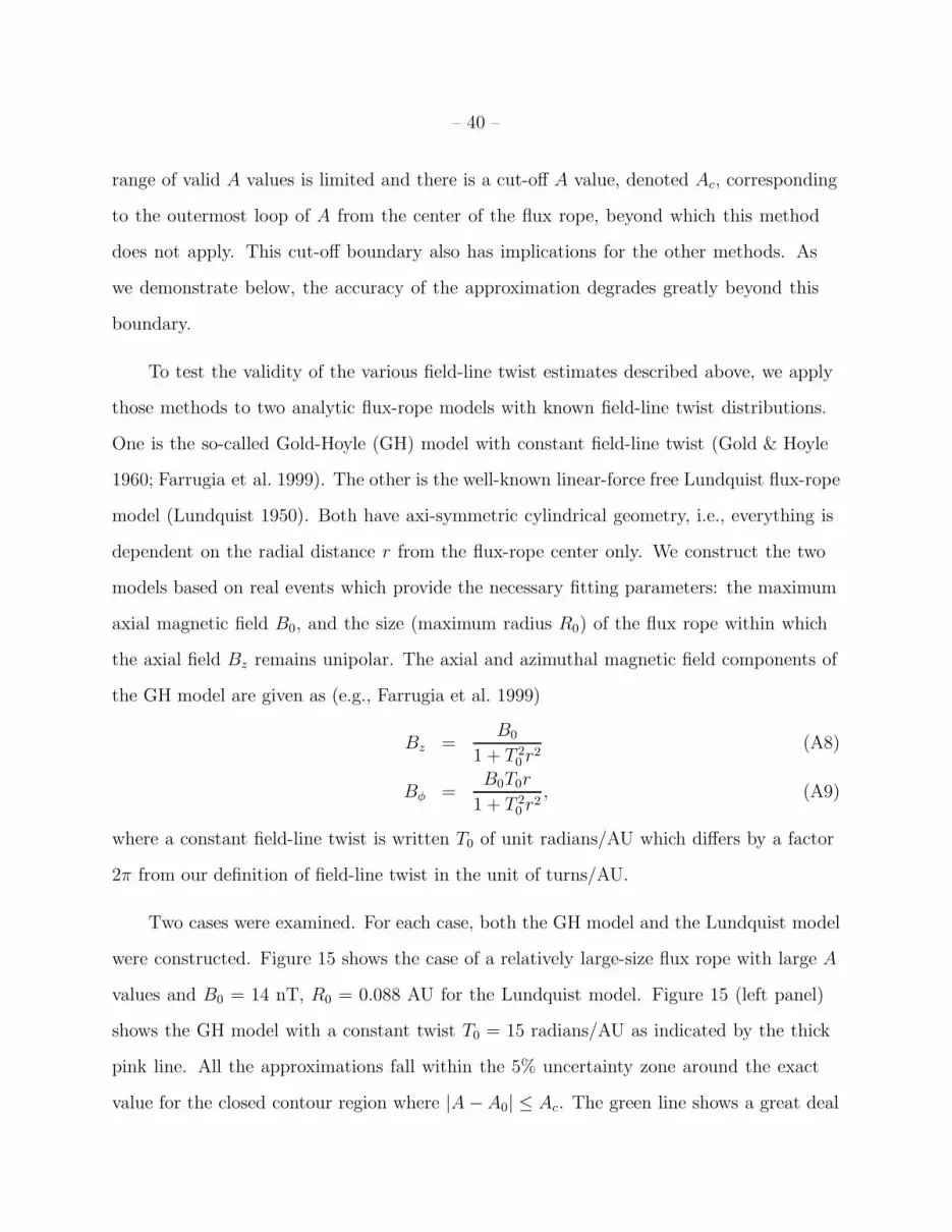
– 40 –
range of valid A values is limited and there is a cut-off A value, denoted Ac, corresponding
to the outermost loop of A from the center of the flux rope, beyond which this method
does not apply. This cut-off boundary also has implications for the other methods. As
we demonstrate below, the accuracy of the approximation degrades greatly beyond this
boundary.
To test the validity of the various field-line twist estimates described above, we apply
those methods to two analytic flux-rope models with known field-line twist distributions.
One is the so-called Gold-Hoyle (GH) model with constant field-line twist (Gold & Hoyle
1960; Farrugia et al. 1999). The other is the well-known linear-force free Lundquist flux-rope
model (Lundquist 1950). Both have axi-symmetric cylindrical geometry, i.e., everything is
dependent on the radial distance r from the flux-rope center only. We construct the two
models based on real events which provide the necessary fitting parameters: the maximum
axial magnetic field B0, and the size (maximum radius R0) of the flux rope within which
the axial field Bz remains unipolar. The axial and azimuthal magnetic field components of
the GH model are given as (e.g., Farrugia et al. 1999)
Bz =B0
1 + T 20 r
2(A8)
Bφ =B0T0r
1 + T 20 r
2, (A9)
where a constant field-line twist is written T0 of unit radians/AU which differs by a factor
2π from our definition of field-line twist in the unit of turns/AU.
Two cases were examined. For each case, both the GH model and the Lundquist model
were constructed. Figure 15 shows the case of a relatively large-size flux rope with large A
values and B0 = 14 nT, R0 = 0.088 AU for the Lundquist model. Figure 15 (left panel)
shows the GH model with a constant twist T0 = 15 radians/AU as indicated by the thick
pink line. All the approximations fall within the 5% uncertainty zone around the exact
value for the closed contour region where |A− A0| ≤ Ac. The green line shows a great deal

– 41 –
of fluctuation due to the nature of the finite-difference approximation in Equation (A3). All
results diverge at the center of the flux rope where the field line simply becomes straight so
that the twist value is arbitrary. Beyond the closed loop boundary as marked by the vertical
line, the approximations begin to deteriorate greatly because there are no more closed A
contours present in the rectangular solution domain. Therefore the twist estimate from the
graphic method ceases to exist beyond this boundary. Both the toroidal flux and helicity
contents also become under-estimated which leads to large deviations from the exact twist
value beyond the cut-off boundary. The estimate τdF (green curve) starts to increase rapidly
due to the significant reduction of ∆Φt while ∆Φp remains properly evaluated.
Figure 15 (right panel) shows the corresponding results for the Lundquist model where
the exact field-line twist increases monotonically from the center of the flux rope toward
the boundary. The result from the graphic method again follows the exact result most
closely, while the green line fluctuates around within a 10% bound and the other two
show greater deviations. Compared with Figure 15 (left panel), the three flux/helicity
based approximation methods perform worse in this case of a non-constant twist. For
completeness, we also examined a second case of a relatively small size but significantly
larger twist, with B0 = 27 nT, R0 = 0.015 AU for the Lundquist model, and T0 = 66
radians/AU for the GH model. Figure 16 shows the field-line twist estimates in the same
format as Figure 15 for the GH flux-rope model and the Lundquist flux-rope model,
respectively. The behavior of these results is very similar to what we have discussed for
Figure 15, despite the significant difference in size and twist value.
Overall we conclude that the graphic method is clearly the most reliable method for
estimating the magnetic field-line twist along the A shell. The results are available and
valid for the region surrounding the center of the flux rope where |A− A0| ≤ Ac excluding
the center where A ≡ A0. Our test results also indicate that all other approximations

– 42 –
are more likely to provide results consistent with the graphic method for a flux-rope
configuration of constant field-line twist. Among them the estimate τdF agrees well
with τ , especially for a varying twist distribution within the cut-off boundary. All these
estimates (Equations A1-A3) are based on magnetic flux and helicity contents which are
well conserved quantities in ideal MHD. We base our discussions in the main body of the
text mostly on these conclusions.
– 43 –
REFERENCES
Aulanier, G., Janvier, M., & Schmieder, B. 2012, A&A, 543, A110
Aulanier, G., Torok, T., Demoulin, P., & DeLuca, E. E. 2010, ApJ, 708, 314
Berger, M. A., & Field, G. B. 1984, Journal of Fluid Mechanics, 147, 133
Cheng, J. X., Kerr, G., & Qiu, J. 2012, ApJ, 744, 48
Cheng, X., Ding, M. D., Guo, Y., et al. 2014, ApJ, 780, 28
Dasso, S., Mandrini, C. H., Demoulin, P., & Luoni, M. L. 2006, A&A, 455, 349
Demoulin, P. 2006, Advances in Space Research, 37, 1269
Fan, Y. 2010, ApJ, 719, 728
Farrugia, C. J., Janoo, L. A., Torbert, R. B., et al. 1999, in American Institute of Physics
Conference Series, Vol. 471, American Institute of Physics Conference Series, ed.
S. T. Suess, G. A. Gary, & S. F. Nerney, 745–748
Fletcher, L., Pollock, J. A., & Potts, H. E. 2004, Sol. Phys., 222, 279
Forbes, T. G., & Lin, J. 2000, Journal of Atmospheric and Solar-Terrestrial Physics, 62,
1499
Freidberg, J. P. 1987, Ideal Magnetohydrodynamics (New York: Plenum Press)
Gold, T., & Hoyle, F. 1960, MNRAS, 120, 89
Gopalswamy, N. 2012, in American Institute of Physics Conference Series, Vol. 1500,
American Institute of Physics Conference Series, ed. Q. Hu, G. Li, G. P. Zank,
X. Ao, O. Verkhoglyadova, & J. H. Adams, 14–19

– 44 –
Handy, B. N., Acton, L. W., Kankelborg, C. C., et al. 1999, Sol. Phys., 187, 229
Harrison, R. A., Davies, J. A., Mostl, C., et al. 2012, ApJ, 750, 45
Hau, L.-N., & Sonnerup, B. U. O. 1999, J. Geophys. Res., 104, 6899
Hu, Q., Farrugia, C. J., Osherovich, V. A., et al. 2013, Sol. Phys., 284, 275
Hu, Q., Smith, C. W., Ness, N. F., & Skoug, R. M. 2004, Journal of Geophysical Research
(Space Physics), 109, 3102
Hu, Q., & Sonnerup, B. U. O. 2001, Geophys. Res. Lett., 28, 467
—. 2002, Journal of Geophysical Research (Space Physics), 107, 1142
Jing, J., Qiu, J., Lin, J., et al. 2005, ApJ, 620, 1085
Kahler, S. W., Haggerty, D. K., & Richardson, I. G. 2011a, ApJ, 736, 106
Kahler, S. W., Krucker, S., & Szabo, A. 2011b, Journal of Geophysical Research (Space
Physics), 116, 1104
Karpen, J. T., Antiochos, S. K., & DeVore, C. R. 2012, ApJ, 760, 81
Kazachenko, M. D., Canfield, R. C., Longcope, D. W., & Qiu, J. 2012, Sol. Phys., 277, 165
Larson, D. E., Lin, R. P., McTiernan, J. M., et al. 1997, Geophys. Res. Lett., 24, 1911
Lemen, J. R., Title, A. M., Akin, D. J., et al. 2012, Sol. Phys., 275, 17
Li, Y., Luhmann, J. G., Lynch, B. J., & Kilpua, E. K. J. 2014, Journal of Geophysical
Research: Space Physics, 119, 3237
Liu, Y., Luhmann, J. G., Huttunen, K. E. J., et al. 2008, ApJ, 677, L133
Longcope, D., Beveridge, C., Qiu, J., et al. 2007, Sol. Phys., 244, 45

– 45 –
Longcope, D. W., & Beveridge, C. 2007, ApJ, 669, 621
Low, B. C. 1996, Sol. Phys., 167, 217
Lugaz, N., Farrugia, C. J., Davies, J. A., et al. 2012, ApJ, 759, 68
Lundquist, S. 1950, Ark. Fys., 2, 361
Moore, R. L., Sterling, A. C., Hudson, H. S., & Lemen, J. R. 2001, ApJ, 552, 833
Mostl, C., Farrugia, C. J., Biernat, H. K., et al. 2009a, Sol. Phys., 256, 427
Mostl, C., Farrugia, C. J., Miklenic, C., et al. 2009b, Journal of Geophysical Research
(Space Physics), 114, A04102
Mostl, C., Farrugia, C. J., Kilpua, E. K. J., et al. 2012, ApJ, 758, 10
Mostl, C., Amla, K., Hall, J. R., et al. 2014, ApJ, 787, 119
Patsourakos, S., Vourlidas, A., & Stenborg, G. 2010, ApJ, 724, L188
—. 2013, ApJ, 764, 125
Qiu, J. 2009, ApJ, 692, 1110
Qiu, J., Hu, Q., Howard, T. A., & Yurchyshyn, V. B. 2007, ApJ, 659, 758
Qiu, J., Liu, W., Hill, N., & Kazachenko, M. 2010, ApJ, 725, 319
Qiu, J., Wang, H., Cheng, C. Z., & Gary, D. E. 2004, ApJ, 604, 900
Qiu, J., & Yurchyshyn, V. B. 2005, ApJ, 634, L121
Savani, N. P., Vourlidas, A., Pulkkinen, A., et al. 2013, Space Weather, 11, 245
Scherrer, P. H., Bogart, R. S., Bush, R. I., et al. 1995, Sol. Phys., 162, 129

– 46 –
Schou, J., Scherrer, P. H., Bush, R. I., et al. 2012, Sol. Phys., 275, 229
Schrijver, C. J., & Title, A. M. 2011, Journal of Geophysical Research (Space Physics), 116,
4108
Shepherd, L. S., & Cassak, P. A. 2012, Journal of Geophysical Research (Space Physics),
117, 10101
Sonnerup, B. U. O., Hasegawa, H., Teh, W.-L., & Hau, L.-N. 2006, Journal of Geophysical
Research (Space Physics), 111, A09204
Sturrock, P. A. 1994, Plasma Physics, An Introduction to the Theory of Astrophysical,
Geophysical and Laboratory Plasmas (Cambridge University Press)
Su, Y., Golub, L., & Van Ballegooijen, A. A. 2007, ApJ, 655, 606
Taylor, J. B. 1986, Reviews of Modern Physics, 58, 741
Temmer, M., Veronig, A. M., Kontar, E. P., Krucker, S., & Vrsnak, B. 2010, ApJ, 712, 1410
Temmer, M., Vrsnak, B., Rollett, T., et al. 2012, ApJ, 749, 57
Titov, V. S., Mikic, Z., Torok, T., Linker, J. A., & Panasenco, O. 2012, ApJ, 759, 70
Torok, T., Panasenco, O., Titov, V. S., et al. 2011, ApJ, 739, L63
van Ballegooijen, A. A., & Martens, P. C. H. 1989, ApJ, 343, 971
Vourlidas, A. 2014, Plasma Physics and Controlled Fusion, 56, 064001
Webb, D. F., Lepping, R. P., Burlaga, L. F., et al. 2000, J. Geophys. Res., 105, 27251
Webb, G. M., Hu, Q., Dasgupta, B., & Zank, G. P. 2010, Journal of Geophysical Research
(Space Physics), 115, 10112

– 47 –
Zhang, J., Dere, K. P., Howard, R. A., Kundu, M. R., & White, S. M. 2001, ApJ, 559, 452
This manuscript was prepared with the AAS LATEX macros v5.2.

–48
–
Table 1. Event Informationa
Event# Flareb Filament CMEd Magnetic Cloud/ICMEe
Date Region Time & Mag. Info. c Time Speed Date GS Interval (mm/dd/yyyy hh:mm:ss) Duration (hrs)
10 2008 - - yes - - Mar 08 03/08/2008 18:42:41-03/09/2008 01:07:45 6.4
11 2010 May 23 N19W12 16:30 B1.1 yes 18:06 258 May 28 05/28/2010 19:05:30-05/29/2010 15:30:30 20
12 2010 Aug 01 N20E36 07:24 C3.2 uncertain uncertain uncertain Aug 04 08/04/2010 03:53:00-08/04/2010 07:47:40 3.9
13 2011 Feb 15 S20W12 02:00 X2.2 no 02:24 669 · · ·
14 2011 Mar 25 S16E30 uncertain uncertain uncertain uncertain Mar 30 03/30/2011 03:17:11-03/31/2011 14:55:51 36
15 2011 Jun 02 S18E28 07:22 C2.2 no 08:12 976 Jun 05 06/05/2011 01:17:32-06/05/2011 06:29:00 5.2
16 2011 Aug 04 N16W38 03:41 M9.1 no 04:12 1315 Aug 05 08/05/2011 20:05:55-08/05/2011 22:03:15 2.0
17 2011 Sep 04 N19W87 23:58 C7.9 no (+1)00:48 622 Sep 09 09/09/2011 01:20:00-09/09/2011 12:28:00 11
18 2011 Sep 13 N23W21 22:30 C2.9 no (+1)00:05 408 Sep 17 09/17/2011 15:18:52-09/18/2011 05:08:44 14
19 2011 Oct 22 N30W30 - yes 01:25 593 Oct 24 10/24/2011 22:16:53-10/25/2011 13:18:13 15
aReferences for event identification and association of the MC, CME, flare and filament eruption are listed below. References are not given for event #13 since the MC
was not successfully analyzed by the GS method. See Section 2 for detailed explanation of the identification by various sources.
10: Li et al. (2014)
11: Li et al. (2014); Lugaz et al. (2012); Mostl et al. (2014)
12: Li et al. (2014); Torok et al. (2011); Schrijver & Title (2011); Titov et al. (2012); Harrison et al. (2012); Mostl et al. (2012, 2014); See Section 2 for details.
14: Li et al. (2014); Savani et al. (2013)
15: Li et al. (2014)
16: Gopalswamy (2012)
17: In this event, the Magnetic Cloud (GS Interval) is measured at the STEREO-A spacecraft, and its association with CME and flare is verified by private communication
with Dr. C. C. Wu and further examined by authors with the STEREO EUVI movies. Since the MC/CME is associated with a limb flare, magnetic reconnection flux is

–49
–not measured in this event.
18: Li et al. (2014)
19: Li et al. (2014); Mostl et al. (2014)
In addition, association between MC and CME of events #11, 12, 16, 18 is also provided in the online catalogue “Near-Earth Interplanetary Coronal Mass Ejections Since
January 1996” compiled by I. Richardson and H. Cane at http : //www.srl.caltech.edu/ACE/ASC/DATA/level3/icmetable2.htm, and association between MC, CME,
and solar surface activities including flares of events #11, 12, 14, 16, 18, 19 is also provided in the online catalogue “GMU CME/ICME List” compiled by Phillip Hess and
Jie Zhang at http : //solar.gmu.edu/heliophysics/index.php/GMU CME/ICME List.
bInformation is obtained from http : //solarmonitor.org/. Time refers to the start time of GOES X-ray flux increase, and magnitude refers to GOES categorization.
c“yes” indicates filament eruption detected, and “no” indicates filament eruption not seen.
dInformation is obtained from http : //cdaw.gsfc.nasa.gov/CME list/. Time refers to when the CME is first observed in LASCO C2 field of view (FOV), and speed,
in units of km s−1, refers to the linear fit to the height-time profile obtained from C2-C3 observations.
eThe intervals were identified and utilized based on GS reconstruction of magnetic flux ropes embedded within each ICME complex, which do not necessarily coincide
with the intervals identified by other criteria. All intervals correspond to in-situ measurements at Earth except for event #17 which is at STEREO-A.
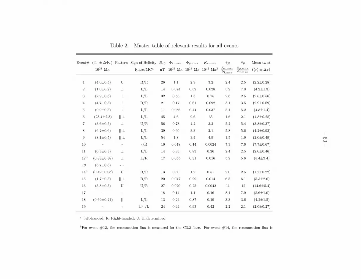
–50
–
Table 2. Master table of relevant results for all events
Event# (Φr ±∆Φr) Pattern Sign of Helicity Bz0 Φt,max Φp,max Kr,max τH τF Mean twist
1021 Mx Flare/MCa nT 1021 Mx 1021 Mx 1042 Mx2Kr,max
Φ2
t,max
Φp,max
Φt,max(〈τ〉 ±∆τ)
1 (4.0±0.5) U R/R 26 1.1 2.9 3.2 2.4 2.5 (2.2±0.28)
2 (1.0±0.2) ⊥ L/L 14 0.074 0.52 0.028 5.2 7.0 (4.2±1.3)
3 (2.9±0.6) ⊥ L/L 32 0.53 1.3 0.75 2.6 2.5 (2.8±0.56)
4 (4.7±0.3) ⊥ R/R 21 0.17 0.61 0.092 3.1 3.5 (2.9±0.69)
5 (0.9±0.5) ⊥ L/L 11 0.086 0.44 0.037 5.1 5.2 (4.8±1.4)
6 (23.4±2.3) || ⊥ L/L 45 4.6 9.6 35 1.6 2.1 (1.8±0.28)
7 (3.6±0.5) ⊥ U/R 56 0.78 4.2 3.2 5.2 5.4 (3.8±0.37)
8 (6.2±0.6) || ⊥ L/L 39 0.60 3.3 2.1 5.8 5.6 (4.2±0.93)
9 (8.1±0.5) || ⊥ L/L 54 1.8 3.4 4.9 1.5 1.9 (2.0±0.49)
10 - - -/R 10 0.018 0.14 0.0024 7.3 7.6 (7.7±0.67)
11 (0.3±0.3) ⊥ L/L 14 0.33 0.83 0.26 2.4 2.5 (2.0±0.46)
12b (0.83±0.38) ⊥ L/R 17 0.055 0.31 0.016 5.2 5.6 (5.4±2.4)
13 (6.7±0.6) · · ·
14b (0.42±0.03) U R/R 13 0.50 1.2 0.51 2.0 2.5 (1.7±0.22)
15 (1.7±0.5) || ⊥ R/R 20 0.047 0.29 0.014 6.5 6.1 (5.5±2.0)
16 (3.8±0.5) U U/R 27 0.020 0.25 0.0042 11 12 (14.6±5.4)
17 - - - 18 0.14 1.1 0.16 8.1 7.9 (5.6±1.0)
18 (0.69±0.21) || L/L 13 0.24 0.87 0.19 3.3 3.6 (4.2±1.5)
19 - - Lc /L 24 0.44 0.93 0.42 2.2 2.1 (2.0±0.27)
a: left-handed; R: Right-handed; U: Undetermined.
bFor event #12, the reconnection flux is measured for the C3.2 flare. For event #14, the reconnection flux is

–51
–measured in the M1.0 flare, only as an upper-limit of reconnected flux possibly associated with the MC, and the sign
of helicity is determined from morphology of flares in the same active region. See Section 2 for details. Both are
excluded from the flux comparison of Φp vs. Φr .
cSign of helicity determined from the filament.
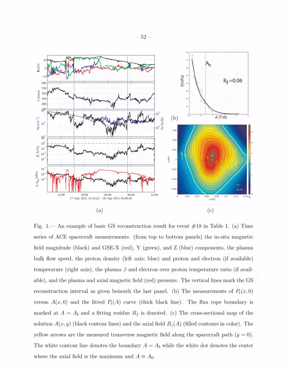
– 52 –
−10
0
10
B (
nT)
350
400
450
500
550
600
V (
km/s
)
10−1
100
101
Np
(cm
−3 )
104
105
Te,
Tp
(K)
10−3
10−2
10−1
100
101
β, T
e/T
p
12:00 18:00 00:00 06:00 12:00
10−3
10−2
10−1
p, p
Bz (
nPa)
17−Sep−2011 15:18:52 − 18−Sep−2011 05:08:44
(a)
(b)−100 −50 0 50 100 1500
0.01
0.02
0.03
0.04
0.05
0.06
0.07
0.08
A (T . m)
P t (n
Pa)
Rf =0.06
Ab
x (AU)
y (A
U)
5 nT
nT
Bz
0 0.02 0.04 0.06 0.08 0.1 0.12 0.14
−0.06
−0.04
−0.02
0
0.02
0.04
0.06
2
4
6
8
10
12
(c)
Fig. 1.— An example of basic GS reconstruction result for event #18 in Table 1. (a) Time
series of ACE spacecraft measurements: (from top to bottom panels) the in-situ magnetic
field magnitude (black) and GSE-X (red), Y (green), and Z (blue) components, the plasma
bulk flow speed, the proton density (left axis; blue) and proton and electron (if available)
temperature (right axis), the plasma β and electron over proton temperature ratio (if avail-
able), and the plasma and axial magnetic field (red) pressure. The vertical lines mark the GS
reconstruction interval as given beneath the last panel. (b) The measurements of Pt(x, 0)
versus A(x, 0) and the fitted Pt(A) curve (thick black line). The flux rope boundary is
marked at A = Ab and a fitting residue Rf is denoted. (c) The cross-sectional map of the
solution A(x, y) (black contour lines) and the axial field Bz(A) (filled contours in color). The
yellow arrows are the measured transverse magnetic field along the spacecraft path (y = 0).
The white contour line denotes the boundary A = Ab while the white dot denotes the center
where the axial field is the maximum and A ≡ A0.
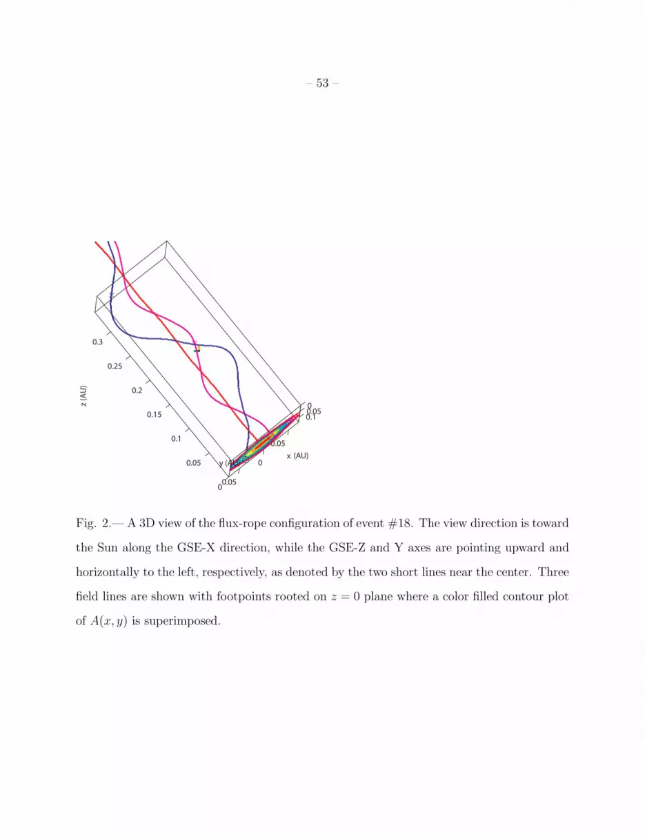
– 53 –
00.050.1
-0.05
0
0.050
0.05
0.1
0.15
0.2
0.25
0.3
x y (AU)
z (A
U)
(AU)
Fig. 2.— A 3D view of the flux-rope configuration of event #18. The view direction is toward
the Sun along the GSE-X direction, while the GSE-Z and Y axes are pointing upward and
horizontally to the left, respectively, as denoted by the two short lines near the center. Three
field lines are shown with footpoints rooted on z = 0 plane where a color filled contour plot
of A(x, y) is superimposed.
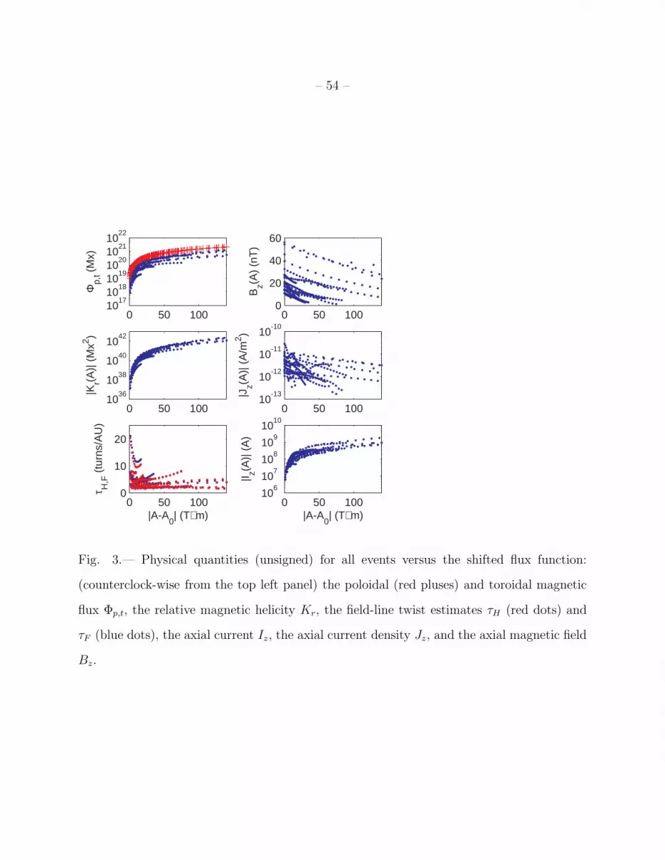
– 54 –
0 50 10010
1710
1810
1910
2010
2110
22
Φp,
t (M
x)
0 50 1000
20
40
60B
z(A)
(nT
)
0 50 10010
36
1038
1040
1042
|Kr(A
)| (
Mx2 )
0 50 10010
-13
10-12
10-11
10-10
|Jz(A
)| (
A/m
2 )
0 50 1000
10
20
τ H,F
(tu
rns/
AU
)
|A-A0| (T⋅ m)
0 50 10010
610
710
810
910
10
|I z(A)|
(A
)
|A-A0| (T⋅ m)
Fig. 3.— Physical quantities (unsigned) for all events versus the shifted flux function:
(counterclock-wise from the top left panel) the poloidal (red pluses) and toroidal magnetic
flux Φp,t, the relative magnetic helicity Kr, the field-line twist estimates τH (red dots) and
τF (blue dots), the axial current Iz, the axial current density Jz, and the axial magnetic field
Bz.
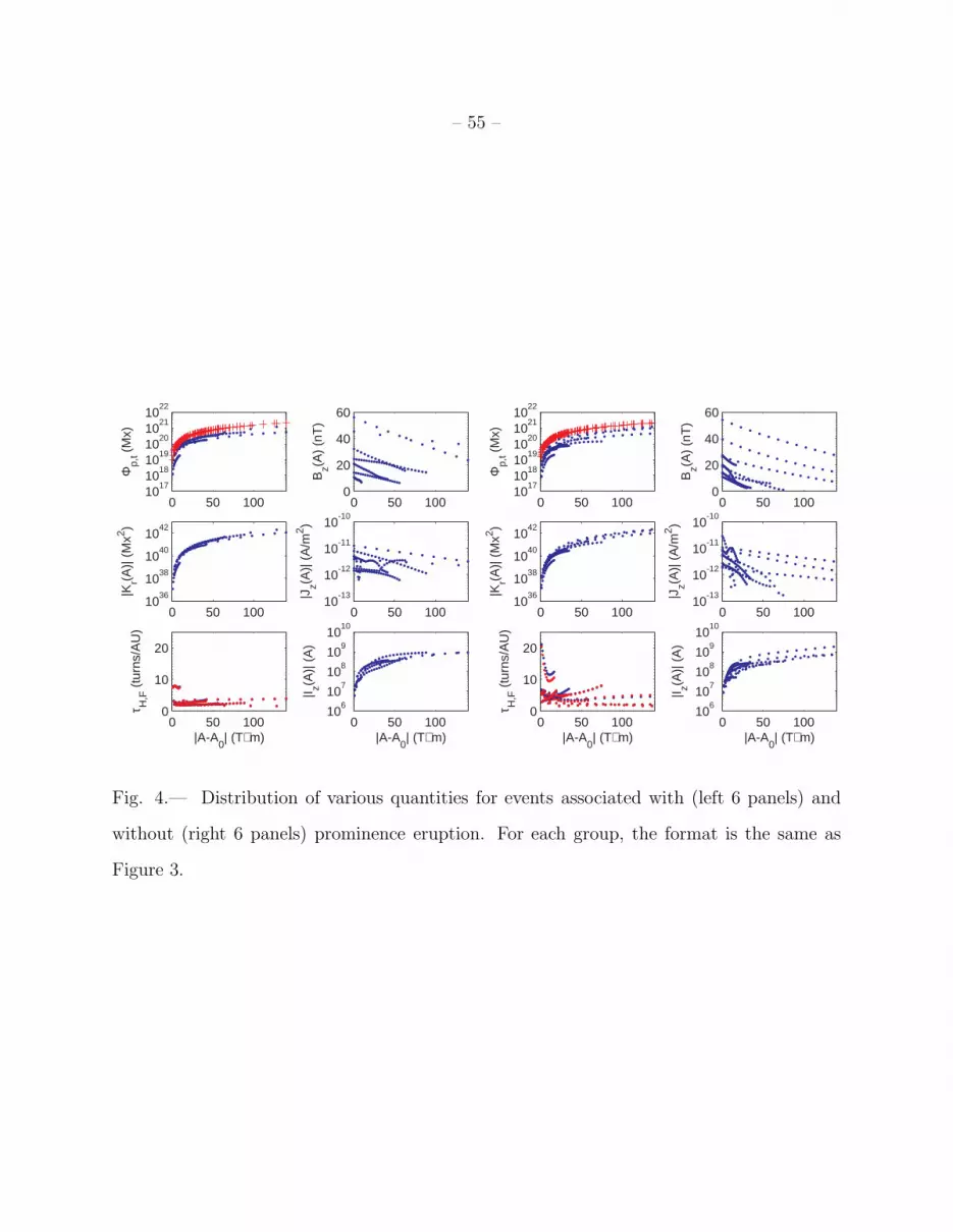
– 55 –
0 50 10010
1710
1810
1910
2010
2110
22
Φp,
t (M
x)
0 50 1000
20
40
60
Bz(A
) (n
T)
0 50 10010
36
1038
1040
1042
|Kr(A
)| (
Mx2 )
0 50 10010
-13
10-12
10-11
10-10
|Jz(A
)| (
A/m
2 )
0 50 1000
10
20
τ H,F
(tu
rns/
AU
)
|A-A0| (T⋅ m)
0 50 10010
610
710
810
910
10
|I z(A)|
(A
)
|A-A0| (T⋅ m)
0 50 10010
1710
1810
1910
2010
2110
22
Φp,
t (M
x)0 50 100
0
20
40
60
Bz(A
) (n
T)
0 50 10010
36
1038
1040
1042
|Kr(A
)| (
Mx2 )
0 50 10010
-13
10-12
10-11
10-10
|Jz(A
)| (
A/m
2 )
0 50 1000
10
20
τ H,F
(tu
rns/
AU
)
|A-A0| (T⋅ m)
0 50 10010
610
710
810
910
10
|I z(A)|
(A
)
|A-A0| (T⋅ m)
Fig. 4.— Distribution of various quantities for events associated with (left 6 panels) and
without (right 6 panels) prominence eruption. For each group, the format is the same as
Figure 3.

– 56 –
0 20 40 60 80 100 120 1400
5
10
15
20
25τ
(Tur
ns/A
U)
(a)ALL
0 20 40 60 80 100 120 1400
5
10
15
20
25
τ (T
urns
/AU
)
(b)PE
0 20 40 60 80 100 120 1400
5
10
15
20
25
|A-A0| (T⋅ m)
τ (T
urns
/AU
) (c)nonPE
Fig. 5.— Field-line twist (τ , turns/AU) distribution along A shells (i.e., vs. A′) for (a)
all events, (b) the ones associated with prominence eruption, and (c) the ones without
prominence eruption. The horizontal dashed line is of value 1.5.
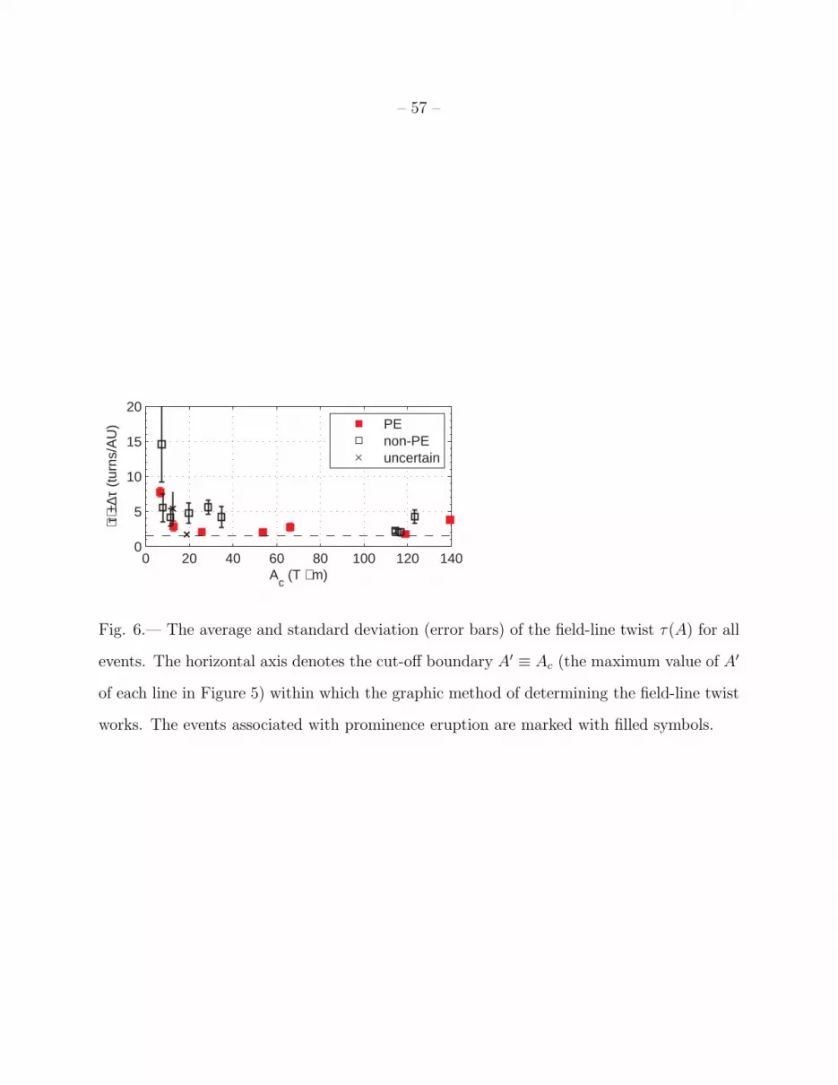
– 57 –
0 20 40 60 80 100 120 1400
5
10
15
20
Ac (T ⋅ m)
⟨τ⟩±∆
τ (t
urns
/AU
)
PEnon-PEuncertain
Fig. 6.— The average and standard deviation (error bars) of the field-line twist τ(A) for all
events. The horizontal axis denotes the cut-off boundary A′ ≡ Ac (the maximum value of A′
of each line in Figure 5) within which the graphic method of determining the field-line twist
works. The events associated with prominence eruption are marked with filled symbols.
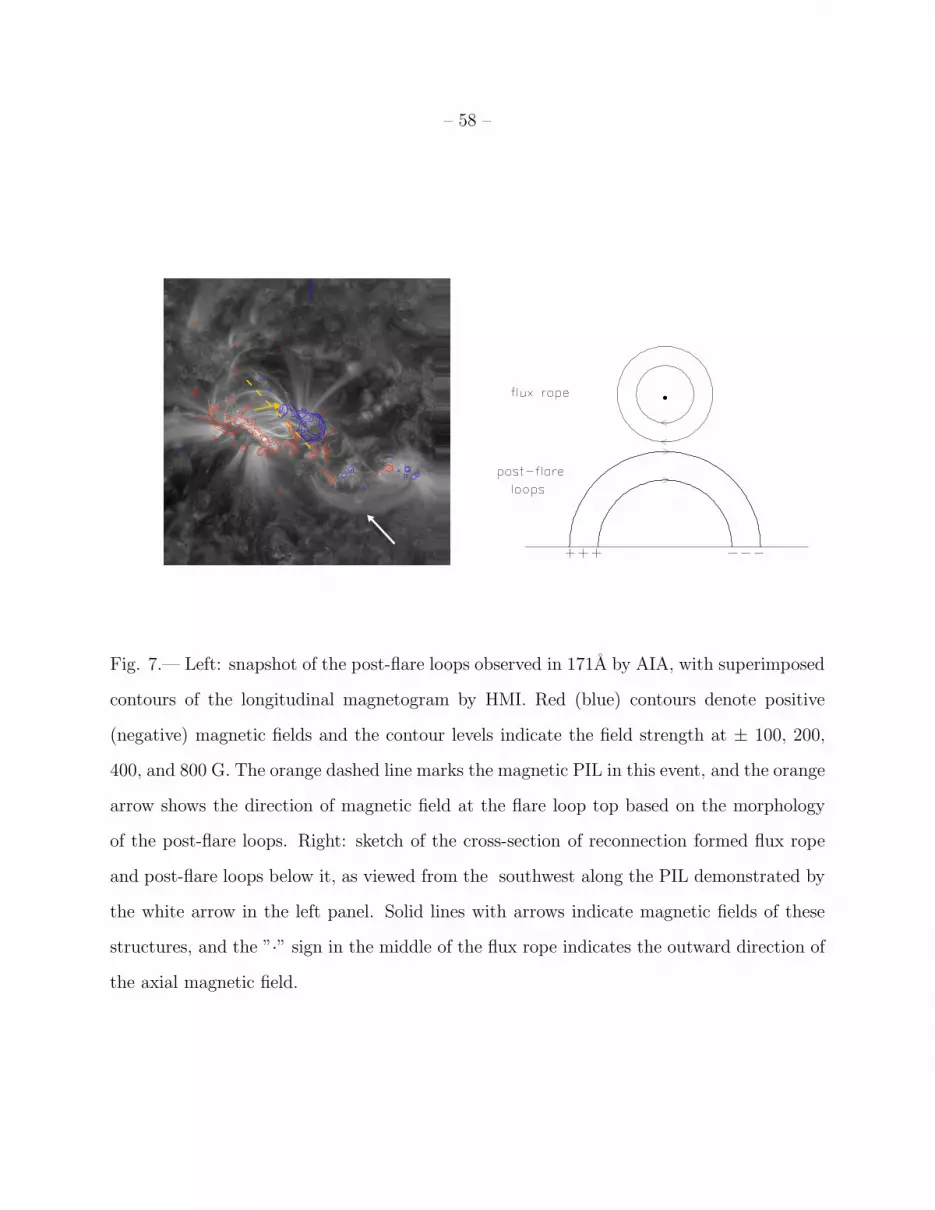
– 58 –
Fig. 7.— Left: snapshot of the post-flare loops observed in 171A by AIA, with superimposed
contours of the longitudinal magnetogram by HMI. Red (blue) contours denote positive
(negative) magnetic fields and the contour levels indicate the field strength at ± 100, 200,
400, and 800 G. The orange dashed line marks the magnetic PIL in this event, and the orange
arrow shows the direction of magnetic field at the flare loop top based on the morphology
of the post-flare loops. Right: sketch of the cross-section of reconnection formed flux rope
and post-flare loops below it, as viewed from the southwest along the PIL demonstrated by
the white arrow in the left panel. Solid lines with arrows indicate magnetic fields of these
structures, and the ”·” sign in the middle of the flux rope indicates the outward direction of
the axial magnetic field.

– 59 –
10-2
10-1
100
101
102
10-1
100
101
102
toroidal MC flux (1021 Mx)
polo
idal
MC
flux
(10
21 M
x)
Φp=2.8Φ
t0.7
10-1
100
101
102
10-1
100
101
102
total reconnection flux (1021 Mx)
polo
idal
MC
flux
(10
21 M
x)
Φp=0.68Φ
r0.61
Fig. 8.— Magnetic flux comparison of poloidal flux Φp vs. toroidal flux Φt (left) and poloidal
flux Φp vs. reconnection flux Φr (right). The events associated with prominence eruption
(P.E.) are marked by filled squares. The ones with uncertain P.E. association (events #12
and #14) are marked by the cross symbols and excluded in the right panel. The least-squares
fit to each data set is given and illustrated by the thick solid line. The dashed line indicates
the one-to-one line. The correlation coefficients are 0.95 and 0.63, respectively.
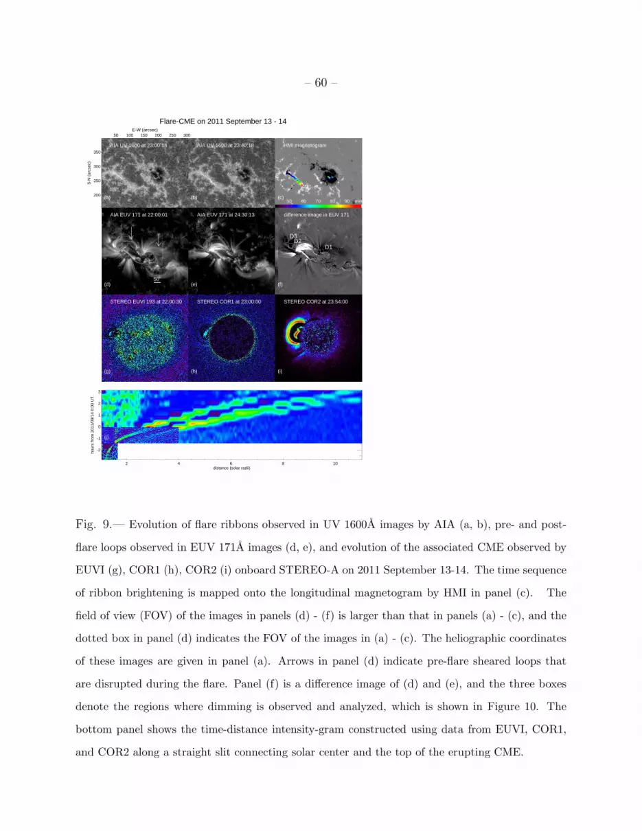
– 60 –
200
250
300
350
S-N
(ar
csec
)
50 100 150 200 250 300E-W (arcsec)
AIA UV 1600 at 23:00:18 AIA UV 1600 at 23:40:18 HMI magnetogram
Flare-CME on 2011 September 13 - 14
50 60 70 80 90 min
50"
D1D2
D3
AIA EUV 171 at 22:00:01 AIA EUV 171 at 24:30:13 difference image in EUV 171
STEREO EUVI 193 at 22:00:30 STEREO COR1 at 23:00:00 STEREO COR2 at 23:54:00
2 4 6 8 10distance (solar radii)
-2
-1
0
1
2
3
hour
s fr
om 2
011/
09/1
4 0:
00 U
T
(a) (b) (c)
(d) (e) (f)
(g) (h) (i)
(j)
Fig. 9.— Evolution of flare ribbons observed in UV 1600A images by AIA (a, b), pre- and post-
flare loops observed in EUV 171A images (d, e), and evolution of the associated CME observed by
EUVI (g), COR1 (h), COR2 (i) onboard STEREO-A on 2011 September 13-14. The time sequence
of ribbon brightening is mapped onto the longitudinal magnetogram by HMI in panel (c). The
field of view (FOV) of the images in panels (d) - (f) is larger than that in panels (a) - (c), and the
dotted box in panel (d) indicates the FOV of the images in (a) - (c). The heliographic coordinates
of these images are given in panel (a). Arrows in panel (d) indicate pre-flare sheared loops that
are disrupted during the flare. Panel (f) is a difference image of (d) and (e), and the three boxes
denote the regions where dimming is observed and analyzed, which is shown in Figure 10. The
bottom panel shows the time-distance intensity-gram constructed using data from EUVI, COR1,
and COR2 along a straight slit connecting solar center and the top of the erupting CME.
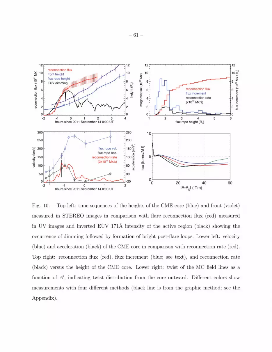
– 61 –
-2 -1 0 1 2 3 4hours since 2011 September 14 0:00 UT
0
2
4
6
8
10
12
reco
nn
ectio
n flu
x (
10
20 M
x)
0
2
4
6
8
10
12
he
igh
t (R
s)
reconnection flux
front height
flux rope height
EUV dimming
1 2 3 4 5 6flux rope height (Rs)
0
2
4
6
8
10
12
ma
gn
etic flu
x (
10
20 M
x)
0
2
4
6
8
10
12
flu
x in
cre
me
nt (1
02
0 M
x / R
s)
reconnection flux
flux increment
reconnection rate
(x1017 Mx/s)
-2 -1 0 1 2hours since 2011 September 14 0:00 UT
0
50
100
150
200
250
300
ve
locity (
km
/s)
-20
30
80
130
180
230
280a
cce
lera
tio
n (
m/s
2)
flux rope vel.
flux rope acc.
reconnection rate
(2x10¹⁵ Mx/s)
0 20 40 600
5
10
tau (
turn
s/A
U)
|A-A0| ( Tm).
Fig. 10.— Top left: time sequences of the heights of the CME core (blue) and front (violet)
measured in STEREO images in comparison with flare reconnection flux (red) measured
in UV images and inverted EUV 171A intensity of the active region (black) showing the
occurrence of dimming followed by formation of bright post-flare loops. Lower left: velocity
(blue) and acceleration (black) of the CME core in comparison with reconnection rate (red).
Top right: reconnection flux (red), flux increment (blue; see text), and reconnection rate
(black) versus the height of the CME core. Lower right: twist of the MC field lines as a
function of A′, indicating twist distribution from the core outward. Different colors show
measurements with four different methods (black line is from the graphic method; see the
Appendix).
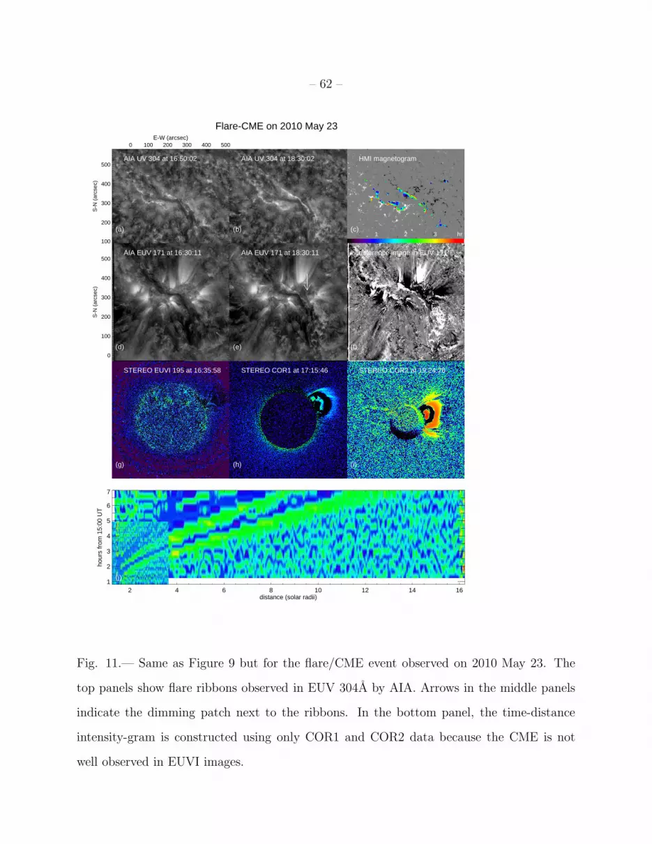
– 62 –
100
200
300
400
500
S-N
(ar
csec
)
0 100 200 300 400 500E-W (arcsec)
AIA UV 304 at 16:50:02 AIA UV 304 at 18:30:02 HMI magnetogram
Flare-CME on 2010 May 23
1 2 3 hr
0
100
200
300
400
500
S-N
(ar
csec
)
AIA EUV 171 at 16:30:11 AIA EUV 171 at 18:30:11 difference image in EUV 171
STEREO EUVI 195 at 16:35:58 STEREO COR1 at 17:15:46 STEREO COR2 at 19:24:28
2 4 6 8 10 12 14 16distance (solar radii)
1
2
3
4
5
6
7
hour
s fr
om 1
5:00
UT
(a) (b) (c)
(d) (e) (f)
(g) (h) (i)
(j)
Fig. 11.— Same as Figure 9 but for the flare/CME event observed on 2010 May 23. The
top panels show flare ribbons observed in EUV 304A by AIA. Arrows in the middle panels
indicate the dimming patch next to the ribbons. In the bottom panel, the time-distance
intensity-gram is constructed using only COR1 and COR2 data because the CME is not
well observed in EUVI images.
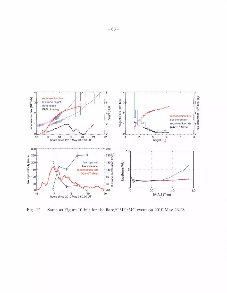
– 63 –
16 17 18 19 20 21 22hours since 2010 May 23 0:00 UT
0
1
2
3
4
reco
nn
ectio
n flu
x (
10
20 M
x)
0
2
4
6
8
he
igh
t (R
ss)
reconnection flux
flux rope height
front height
EUV dimming
1 2 3 4 5 6height (Rs)
0
1
2
3
4
ma
gn
etic flu
x (
10
20 M
x)
0
1
2
3
4
flu
x in
cre
me
nt (1
02
0 M
x / R
s)
reconnection flux
flux increment
reconnection rate
(x4x1016 Mx/s)
16 17 18 19 20hours since 2010 May 23 0:00 UT
0
50
100
150
200
250
300
flu
x r
op
e v
elo
city (
km
/s)
-20
30
80
130
180
230
280
flu
x r
op
e a
cce
lera
tio
n (
m/s
2)
flux rope vel.
flux rope acc.
reconnection rate
(x3x1014 Mx/s)
0 20 40 600
5
10
tau (
turn
s/A
U)
|A-A0| (T m).
Fig. 12.— Same as Figure 10 but for the flare/CME/MC event on 2010 May 23-28.
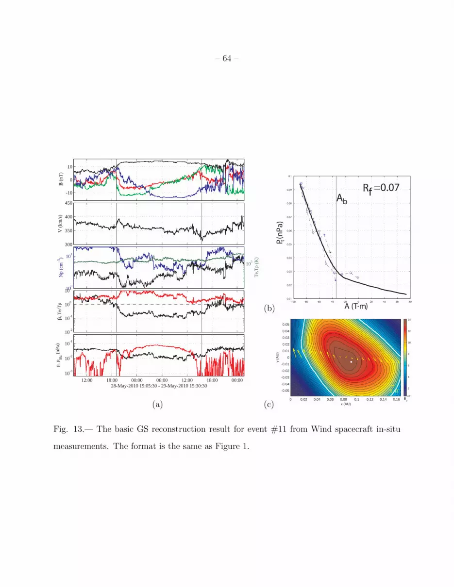
– 64 –
-10
0
10
B (
nT)
300
350
400
450
V (
km/s
)
100
101
Np
(cm
-3)
105
Te,
Tp
(K)
10-2
10-1
100
101
β, T
e/T
p
12:00 18:00 00:00 06:00 12:00 18:00 00:0010
-3
10-2
10-1
p, p
Bz (
nPa)
28-May-2010 19:05:30 - 29-May-2010 15:30:30
(a)
(b)-100 -80 -60 -40 -20 0 20 40 60 80
0.01
0.02
0.03
0.04
0.05
0.06
0.07
0.08
0.09
0.1
A (T m)
P t (n
Pa)
Rf =0.07Ab
.
(c) x (AU)
y (A
U)
5 nT
nTB
z0 0.02 0.04 0.06 0.08 0.1 0.12 0.14 0.16
-0.05
-0.04
-0.03
-0.02
-0.01
0
0.01
0.02
0.03
0.04
0.05
2
4
6
8
10
12
14
Fig. 13.— The basic GS reconstruction result for event #11 from Wind spacecraft in-situ
measurements. The format is the same as Figure 1.
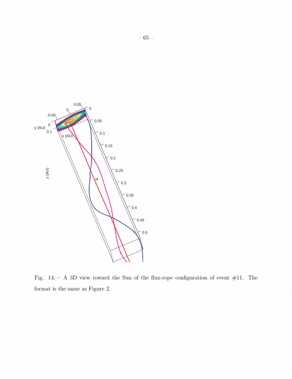
– 65 –
0
0.1
-0.050
0.050
0.05
0.1
0.15
0.2
0.25
0.3
0.35
0.4
0.45
0.5
x (AU)
z (A
U)
y (AU)
Fig. 14.— A 3D view toward the Sun of the flux-rope configuration of event #11. The
format is the same as Figure 2.
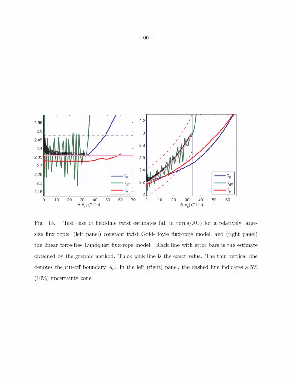
– 66 –
0 10 20 30 40 50 60 70
2.15
2.2
2.25
2.3
2.35
2.4
2.45
2.5
2.55
|A-A0| (T ⋅ m)
τF
τdF
τH
0 10 20 30 40 50 602
2.2
2.4
2.6
2.8
3
3.2
|A-A0| (T ⋅ m)
τF
τdF
τH
Fig. 15.— Test case of field-line twist estimates (all in turns/AU) for a relatively large-
size flux rope: (left panel) constant twist Gold-Hoyle flux-rope model, and (right panel)
the linear force-free Lundquist flux-rope model. Black line with error bars is the estimate
obtained by the graphic method. Thick pink line is the exact value. The thin vertical line
denotes the cut-off boundary Ac. In the left (right) panel, the dashed line indicates a 5%
(10%) uncertainty zone.
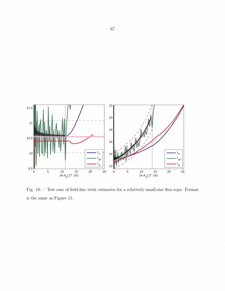
– 67 –
0 5 10 15 20 259.5
10
10.5
11
11.5
|A-A0| (T ⋅ m)
τF
τdF
τH
0 5 10 15 20 25
12
14
16
18
20
22
|A-A0| (T ⋅ m)
τF
τdF
τH
Fig. 16.— Test case of field-line twist estimates for a relatively small-size flux rope. Format
is the same as Figure 15.
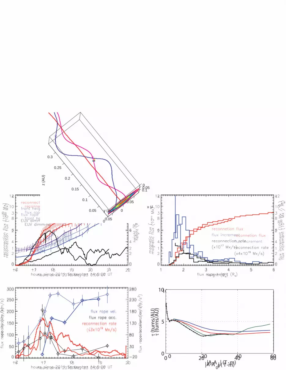
0 20 40 600
5
10
τ (t
urn
s/A
U)
|A-A0| (T m).
0 20 40 600
5
10
τ (t
urn
s/A
U)
|A-A0| ( T m).
00.050.1
-0.05
0
0.050
0.05
0.1
0.15
0.2
0.25
0.3
x (AU)y (AU)
z (A
U)
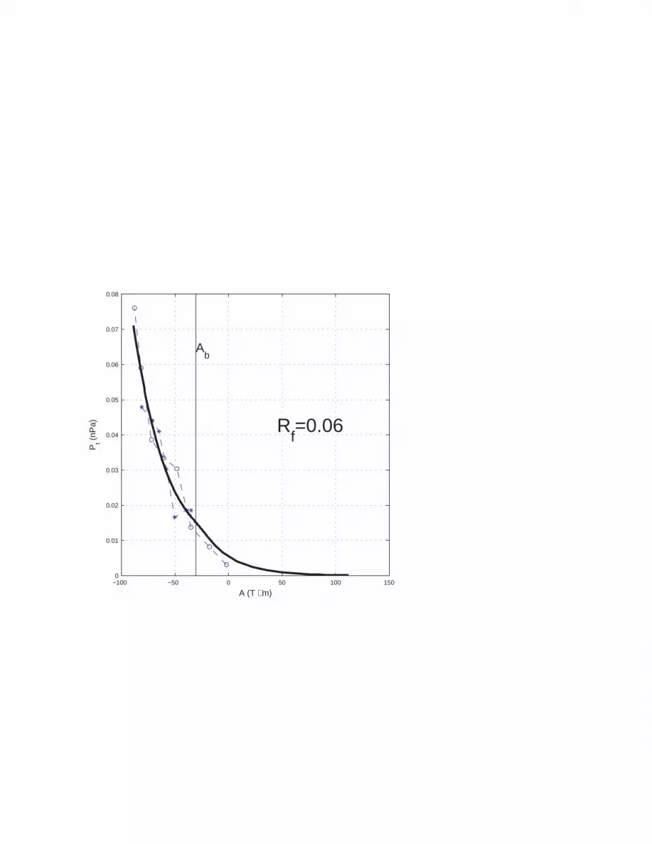
−100 −50 0 50 100 1500
0.01
0.02
0.03
0.04
0.05
0.06
0.07
0.08
A (T ⋅ m)
Pt (
nPa) R
f=0.06
Ab
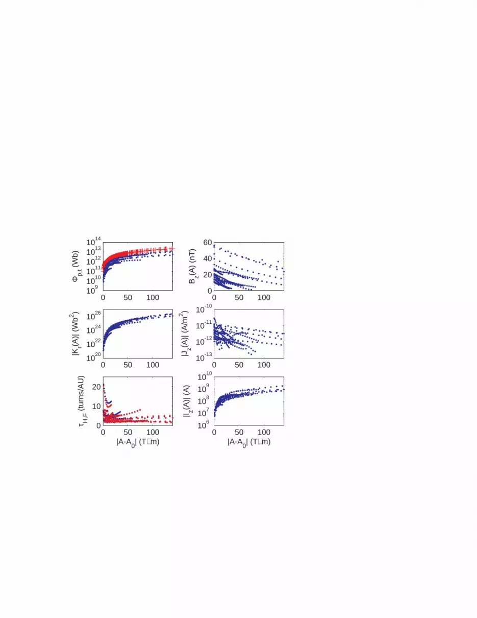
0 50 10010
910
1010
1110
1210
1310
14
Φp,
t (W
b)
0 50 1000
20
40
60
Bz(A
) (n
T)
0 50 10010
20
1022
1024
1026
|Kr(A
)| (
Wb2 )
0 50 10010
-13
10-12
10-11
10-10
|Jz(A
)| (
A/m
2 )
0 50 1000
10
20
τ H,F
(tu
rns/
AU
)
|A-A0| (T⋅ m)
0 50 10010
610
710
810
910
10
|I z(A)|
(A
)
|A-A0| (T⋅ m)
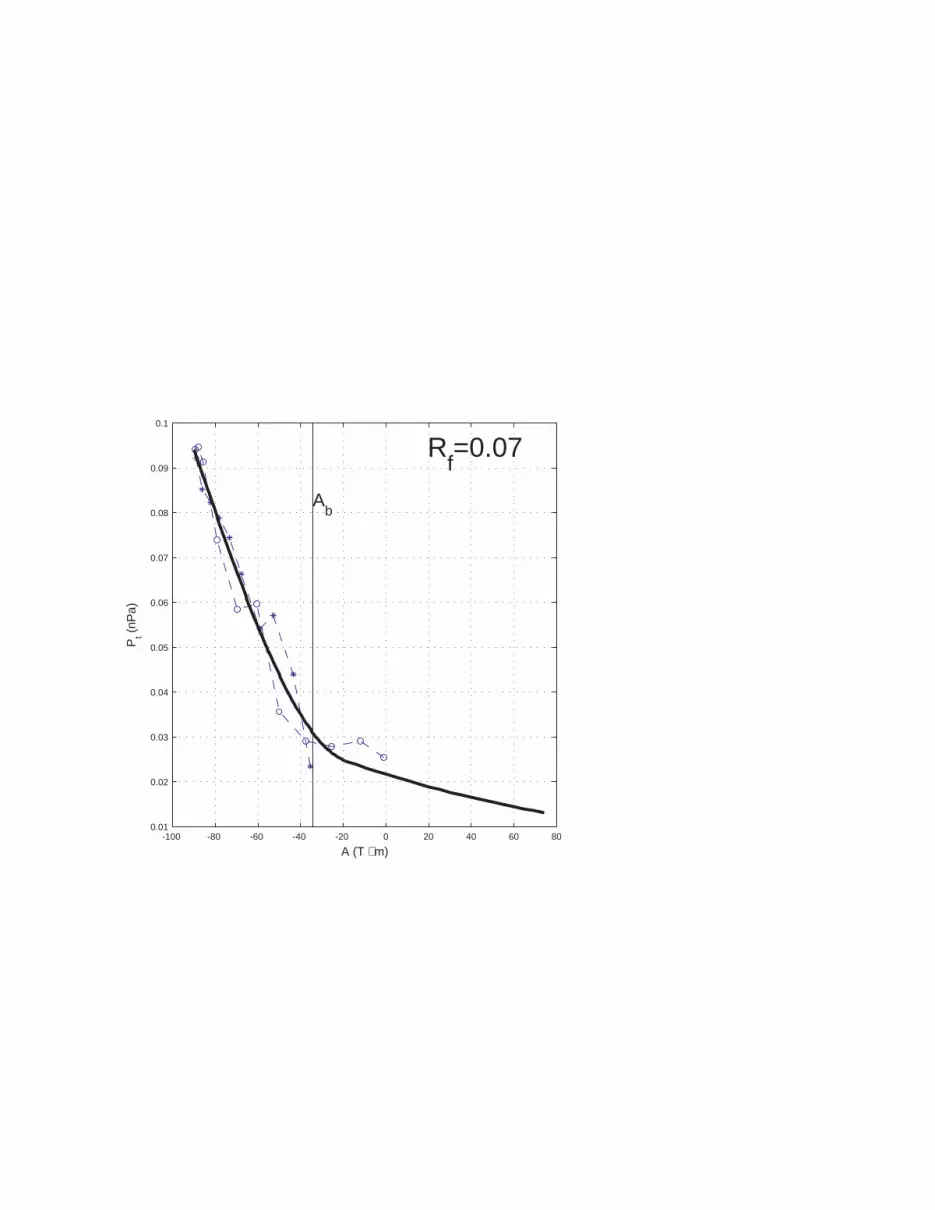
-100 -80 -60 -40 -20 0 20 40 60 800.01
0.02
0.03
0.04
0.05
0.06
0.07
0.08
0.09
0.1
A (T ⋅ m)
Pt (
nPa)
Rf=0.07
Ab