string bracket and flat connections

arX

iv:m

ath/

0602

108v

4 [

mat

h.A

T]

14

Mar

200

7

STRING BRACKET AND FLAT CONNECTIONS

HOSSEIN ABBASPOUR AND MAHMOUD ZEINALIAN

Abstract. Let G → P → M be a flat principal bundle over a compact andoriented manifold M of dimension m = 2d. We construct a map of Lie algebras

Ψ : HS1

2∗ (LM) → O(MC), where HS1

2∗ (LM) is the even dimensional part of theequivariant homology of LM , the free loop space of M , and MC is the Maurer-Cartan moduli space of the graded differential Lie algebra Ω∗(M, adP ), thedifferential forms with values in the associated adjoint bundle of P . For a2-dimensional manifold M , our Lie algebra map reduces to that constructed

by Goldman in [Go2]. We treat different Lie algebra structures on HS1

2∗ (LM)depending on the choice of the linear reductive Lie group G in our discussion.This paper provides a mathematician-friendly formulation and proof of themain result of [CFP] for G = GL(n, C) and GL(n, R) together with its naturalgeneralization to other reductive Lie groups.

Contents

1. Introduction 12. String bracket 43. Invariant functions and principal bundles 54. Symplectic nature of the Maurer-Cartan moduli space 85. Differential forms on free loop spaces 106. Generalized holonomy 127. Hamiltonian vectors field and Poisson bracket 178. String bracket for unoriented strings 219. The 2-dimensional case 23Appendix A. Vector bundles and flat connections 24Appendix B. Parallel transport and iterated integrals 25References 27

1. Introduction

The precursor to Chas-Sullivan string bracket [CS1] was Goldman’s Lie algebrastructures [Go2] on certain vector spaces based on the homotopy classes of closedcurves on a closed and orientable surface S. The simplest one of these was de-fined on the vector space Rπ generated by the set π of free homotopy classes ofclosed and oriented curves on S. There was a similar construction of a Lie algebrabased on unoriented curves. For the moment, let us talk about Rπ for which the

Key words and phrases. free loop space, string bracket, flat connections, Hamiltonian reduc-tion, Chen iterated integrals, generalized holonomy, Wilson loop.

The first author was supported by a ChateauBriand Postdoctoral Fellowship while he was

visiting Ecole Polytechnique 2004-2005.

1

http://arXiv.org/abs/math/0602108v4

2 HOSSEIN ABBASPOUR AND MAHMOUD ZEINALIAN

bracket of two equivalence classes of curves is a signed summation of the curvesobtained by breaking and reconnecting two transversal representatives at each oftheir intersection points one at a time. The relevance, and more importantly theuniversality, of this algebraic object to geometry was established by defining a mapγ 7→ fγ , from Rπ to the Poisson algebra of smooth functions on the symplecticspace Hom(π,G)/G of representations of π into G = GL(n,C) or GL(n,R). Saidslightly differently, to a free homotopy class of a closed curve one assigns a functionon the moduli space of all flat connections modulo the gauge group. The value ofthe function fγ at an equivalence class α is the trace of the holonomy with respectto the flat connection representing α along a oriented closed curve representing thefree homotopy class γ. The Poisson bracket of two such functions is identified as(see [Go2]),

fγ , fλ =∑

p∈γ#λ

ε(p; γ, λ)fγpλp,

where γpλp denotes the product of the elements γp, λp ∈ π1(S; p), and ε(p; γ, λ) =±1 denotes the oriented intersection number of γ and λ at p.

Goldman [Go2] showed that,

(1.1) [γ, λ] =∑

p∈γ#λ

ε(p; γ, λ)γpλp,

defines a Lie bracket on Rπ the free vector space generated by the conjugacy classesof π. In particular this means that the map γ 7→ fγ is a map of Lie algebras.

Similarly, he showed that the Lie algebra structure on the vector space based onthe set of free homotopy classes of unoriented curves corresponds to the case whereG is O(p, q), O(n,C), U(p, q), Sp(n,R), or Sp(p, q). In this case the Poisson brackethas the following formula,

fγ , fλ =1

2

∑

p∈γ#λ

ε(p; γ, λ)(fγpλp− fγpλ−1

p),

where once again γpλp and γpλ−1p denotes the product of γp with λp and its inverse

λ−1p in π1(S; p), respectively. It was also proved in [Go2] that,

[γ, λ] =1

2

∑

p∈γ#λ

ε(p; γ, λ)(γpλp − γpλ−1p ),

defines a Lie bracket on Rπ the free vector space generated by the conjugacy classesof π.

Goldman’s Lie bracket was generalized by Chas and Sullivan to a bracket on the

equivariant homology HS1

∗ (LM) of the free loop space LM of an oriented closedmanifold M of arbitrary finite dimension m,

[·, ·] : HS1

i (LM)⊗HS1

j (LM)→ HS1

i+j+2−m(LM).

This makes HS1

∗ (LM) into a graded Lie algebra, after a shift by m − 2 in thegrading. For an oriented surface M of dimension m = 2 and i = j = 0, the bracket

on Rπ = HS1

0 (LM) coincides with that discovered by Goldman.Inspired by [Go2] and [CFP], we do something similar for the Chas-Sullivan

bracket in this paper. More precisely, let G denote GL(n,R) or GL(n,C), endowedwith the invariant function f(g) = Re tr(g), and g its Lie algebra with the non-degenerate invariant bilinear form 〈x, y〉 = Re tr(xy). Let G → P → M be a

STRING BRACKET AND FLAT CONNECTIONS 3

principal bundle over a compact and oriented manifold M of dimension m = 2d,with a fixed flat connection∇. We construct a map of Lie algebras Ψ from the equi-

variant homology HS1

2∗ (LM) to the Poisson algebra of function on the symplecticspaceMC, the formal completion of the space x ∈

⊕

k≥0 Ω2k+1(M, adP ) | d∇x+

1/2[x, x] = 0/G (see section 4 for definition) of the differential graded Lie algebra(Ω∗(M, adP ), d∇) of differential forms with values in adP , the associated adjointbundle of P (see [GG]). For a description of the natural symplectic structure ofMC see Example 4.2, Proposition 4.3 and Theorem 4.4. Note that using ∇ as apoint of reference, the Maurer-Cartan moduli space contains a copy of the modulispace of flat connection on G → P → M (see the discussion in section 9). Here isone of the main theorems,

Theorem 7.4. For G = GL(n,C) or GL(n,R), the generalized holonomy map,

Ψ : (HS1

2∗ (LM), [·, ·])→ (O(MC), ·, ·),

is a map of Lie algebras.

For a definition of generallized holonomy see section 6 (and [CR]). For a loop

λ ∈ LM , representing an element of HS1

0 (LM), the value of the function Ψλ at aflat connection is the trace of its holonomy along λ. The machinery of the proof isrobust enough to handle other reductive subgroups of GL(n,C). In a manner similarto the discussion in [Go2], different subgroups correspond different Lie algebrastructures on the equivariant homology of free loop spaces. We discuss the cases ofG = O(p, q), O(n,C), U(p, q), Sp(n,R), and Sp(p, q) (see section 7).

We provide a mathematician-friendly formulation and proof of the main resultof [CFP] for G = GL(n,C) and GL(n,R) together with its natural generalizationto other reductive Lie groups. The relevance of the subject matter to the Chern-Simons theory and its applications are explained [Sch].

Let us very briefly review each section. Section 2 is a short description of theloop product and string bracket. In section 3 we recall basic facts about invariantfunctions on Lie groups and some of their byproducts. Section 4 discusses thesymplectic nature of the set of all solutions of the Maurer-Cartan equation ona differential graded algebra. We discuss the symplectic structure of the modulispace of Maurer-Cartan equation via the process of Hamiltonian reduction. Section6 contains the main part of the paper. The main concept here is that of thegeneralized holonomy. Section 7 concerns the construction of the Lie algebra mapfor G = GL(n,C) or GL(n,R). Section 8 deals with several other linear reductiveLie groups which tie with the Lie algebra structure on the vector space based on freehomotopy classes of unoriented curves. Section 9 explains how for a 2-dimensionalmanifold our construction specializes to that described by Goldman in [Go2]. InAppendix A, we recall the moduli space of flat connections and its relation to themoduli space of representations of the fundamental group. We also review the basicfacts about homology and cohomology with local coefficients as well as a relevantversion of Poincare duality. Appendix B describes the formula for the solutionsof the time dependent linear system of equations in terms of the Chen iteratedintegrals.

Acknowledgments: The authors would like to thank Jean Barge, David Chataur,Alberto Cattaneo, Jean Lannes, Riccardo Longoni, and Dennis Sullivan for manyhelpful conversations and comments. We are grateful to Carlo A. Rossi and James


Stasheff who read the first version of the paper and suggested many importantcorrections and improvements. We are also thankful to Victor Ginzburg and JohnTerrila for their useful suggestions regarding the algebraic treatment of the modulispace.

2. String bracket

Let M be an closed oriented manifold of dimension m. In [CS1, CS2], Chas andSullivan forged the term String Topology by introducing various operations on theordinary and equivariant homologies of LM = C∞(S1,M) the free loop space1ofM , where S1 = R/Z. The free loop space LM is therefore a Frechet manifoldbenefiting from such tools as the differential forms, principal bundles, connection,and others (see section 5 for more details). Throughout this paper the coefficientring of the (co)homology is Z unless otherwise it is specified.

Chas and Sullivan’s constructions includes a product on H∗+m(LM), called theloop product, and its equivariant version, the string bracket, defined on the shifted

S1-equivariant homology HS1

∗+m−2(LM) = H∗+m−2(ES1 ×S1 LM). For the pur-

poses of this paper we use a description of the loop product found in [CJ]. LetLM ×M LM = (γ1, γ2) | γ1(0) = γ2(0) ⊂ LM × LM be the space of the pairsof loops with the identical marked points and consider the following commutativediagram,

LM ×M LM −−−−→ LM × LM

y

ev

y

(ev,ev)

M∆

−−−−→ M ×MNote that LM×M LM is a codimension m subspace of LM×LM with a tubular

neighborhood ev∗(vM ) where vM is a normal bundle for the diagonalM →M×M .Consider the map,

(2.1) τ : H∗(LM × LM) → H∗(Thom(ev∗(vM ))) → H∗−m(LM ×M LM),

where the first map is Pontrjagin-Thom collapsing map to the Thom space ofev∗(vM ), and the second is the Thom isomorphism for the normal bundle ev∗(vM ).Also, consider the map,

(2.2) ε : H∗(LM ×M LM)→ H∗(LM),

induced by the concatenation of the loops λ1 and λ2 with the identical markedpoints, that is,

(2.3) λ1 λ2(t) =

λ1(2t) 0 ≤ t ≤ 1/2

λ2(2t− 1) 1/2 ≤ t ≤ 1

The loop product is defined as follows,

• = ε τ : H∗(LM)⊗H∗(LM) ≃ H∗(LM × LM)→ H∗−m(LM).

Remark 2.1. Here we have to modify the definition of λ1 λ2 since the resultmay not be smooth. For that one has to reparameterized the λ1 and λ2 in aneighborhood of 0 using a fixed smooth bijection of [0, 1] whose all derivatives at 0and 1 are zero. This is standard and does not change the homological operationsintroduced above.

1In the literature LM is C0(S1, M) which has the same homotopy type of C∞(S1, M).


Next, we recall the definition of the string bracket on HS1

∗+m−2(LM) (see [CS1]).

Consider the degree one S1-transfer map m∗ : HS1

∗ (LM) → H∗+1(LM), and the

degree zero map e∗ : H∗(LM)→ HS1

∗ (LM) induced by the projection LM×ES1 →

(LM×S1ES1) (see [CV, CKS]). The string bracket [·, ·] : HS1

i (LM)⊗HS1

j (LM)→

HS1

i+j+2−m(LM) is defined as follows,

(2.4) [a, b] = (−1)|a|e∗(m∗a •m∗b).

It was proved in [CS1] that (HS1

∗+m−2(LM), [·, ·]) is a graded Lie algebra and that∆ = m∗ e∗ : H∗+m(LM)→ H∗+m+1(LM) together with the loop product makesH∗+m(LM) into a BV algebra. In fact ∆ is the map induced by the unit circleaction.

Throughout this paper M is a manifold of dimension m = 2d and thereforethe shift in the degrees by the dimension does not change the parity. This means

HS1

2∗ (LM) may simply be regarded as a non-graded Lie algebra. In this case theequation (2.4) becomes,

(2.5) [a, b] = e∗(m∗a •m∗b),

for a, b ∈ HS1

2∗ (LM).

3. Invariant functions and principal bundles

In this section, we briefly recall some basic facts and definitions. Most of thematerial is taken from [Go2]. Let G be a Lie group with Lie algebra g. Assumethat g is equipped with a nondegenerate bilinear form 〈·, ·〉, which is invariant, thatis, 〈[x, y], z〉 = 〈x, [y, z]〉, for all x, y, z ∈ g. We think of an element x ∈ g as a leftinvariant derivation on C∞(G) defined by,

(3.1) (x · f)(g) =d

dtf(g exp(tx))|t=0,

for x ∈ g. The universal enveloping algebra Ug =⊕∞

k=0 g⊗k/〈a⊗ b− b⊗ a− [a, b]〉may then be regarded as the associative algebra of all left invariant differentialoperators on C∞(G). An invariant function f : G → R is a C∞ function whichis invariant under conjugation. The variation function of an invariant functionf : G → R, with respect to a nondegenerate invariant bilinear form 〈·, ·〉, is themap F : G→ g defined by,

(3.2) 〈F (g), x〉 = (x · f)(g).

Note that F is a G-equivariant map with respect to the conjugation action onthe domain and the adjoint action on the range. In fact, one may extend F : G→ g

to F : G× Ug→ g (using the identification G ∼= G× 1 ⊂ G× Ug) as follows.

(3.3) F (g; [x1 ⊗ · · · ⊗ xk]) =∂k

∂t1 · · · ∂tkF (g exp(t1x1) · · · exp(tkxk))|(0,··· ,0).

We will later, in equations 3.8 and 3.9, apply the above to fibers of appropriatebundles.

A case of particular interest is when G ⊂ GL(n,C) is a reductive subgroup,that is, a closed subgroup which is invariant under the operation of conjugatetranspose. It is evident that f(g) = Re trρ(g) is an invariant function. Moreover,reductivity implies that the invariant bilinear form 〈x, y〉 = Re tr(ρ(x)ρ(y)) is in


fact nondegenerate. In fact, slightly more generally, any covering of such a G wouldenjoy the above invariant function and bilinear form.

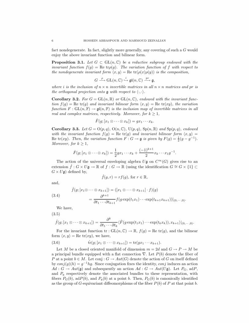
Proposition 3.1. Let G ⊂ GL(n,C) be a reductive subgroup endowed with the

invariant function f(g) = Re trρ(g). The variation function of f with respect to

the nondegenerate invariant form 〈x, y〉 = Re tr(ρ(x)ρ(y)) is the composition,

Gρ−→ GL(n,C)

i→ gl(n,C)

pr

−→ g,

where i is the inclusion of n× n invertible matrices in all n× n matrices and pr is

the orthogonal projection onto g with respect to 〈·, ·〉.

Corollary 3.2. For G = GL(n,R) or GL(n,C), endowed with the invariant func-

tion f(g) = Re tr(g) and invariant bilinear form 〈x, y〉 = Re tr(xy), the variation

function F : GL(n,F) → gl(n,F) is the inclusion map of invertible matrices in all

real and complex matrices, respectively. Moreover, for k ≥ 1,

F (g; [x1 ⊗ · · · ⊗ xk]) = gx1 · · ·xk.

Corollary 3.3. Let G = O(p, q), O(n,C), U(p, q), Sp(n,R) and Sp(p, q), endowed

with the invariant function f(g) = Re tr(g) and invariant bilinear form 〈x, y〉 =Re tr(xy). Then, the variation function F : G→ g is given by F (g) = 1

2 (g − g−1).Moreover, for k ≥ 1,

F (g; [x1 ⊗ · · · ⊗ xk]) =1

2gx1 · · ·xk +

(−1)k+1

2xk · · ·x1g

−1.

The action of the universal enveloping algebra Ug on C∞(G) gives rise to an

extension f : G × Ug → R of f : G → R (using the identification G ∼= G × 1 ⊂G× Ug) defined by,

f(g, r) = rf(g), for r ∈ R,

and,

f(g; [x1⊗ · · · ⊗ xk+1]) = ([x1 ⊗ · · · ⊗ xk+1] · f)(g)

=∂k+1

∂t1 · · ·∂tk+1f(g exp(t1x1) · · · exp(tk+1xk+1))|(0,··· ,0).

(3.4)

We have,

f(g; [x1 ⊗ · · · ⊗ xk+1]) =∂k

∂t1 · · · ∂tk〈F (g exp(t1x1) · · · exp(tkxk)), xk+1〉|(0,··· ,0).

(3.5)

For the invariant function tr : GL(n,C) → R, f(g) = Re tr(g), and the bilinearform 〈x, y〉 = Re tr(xy), we have,

(3.6) tr(g; [x1 ⊗ · · · ⊗ xk+1]) = tr(gx1 · · ·xk+1).

Let M be a closed oriented manifold of dimension m = 2d and G→ P →M bea principal bundle equipped with a flat connection ∇. Let P (b) denote the fiber ofP at a point b ∈M . Let conj : G→ Aut(G) denote the action of G on itself definedby conj(g)(h) = g−1hg. Since conjugation fixes the identity, conj induces an actionAd : G → Aut(g) and subsequently an action Ad : G → Aut(Ug). Let PG, adP ,and Pu respectively denote the associated bundles to these representation, withfibers PG(b), adP (b), and Pu(b) at a point b. Then, PG(b) is canonically identifiedas the group of G-equivariant diffeomorphisms of the fiber P (b) of P at that point b.


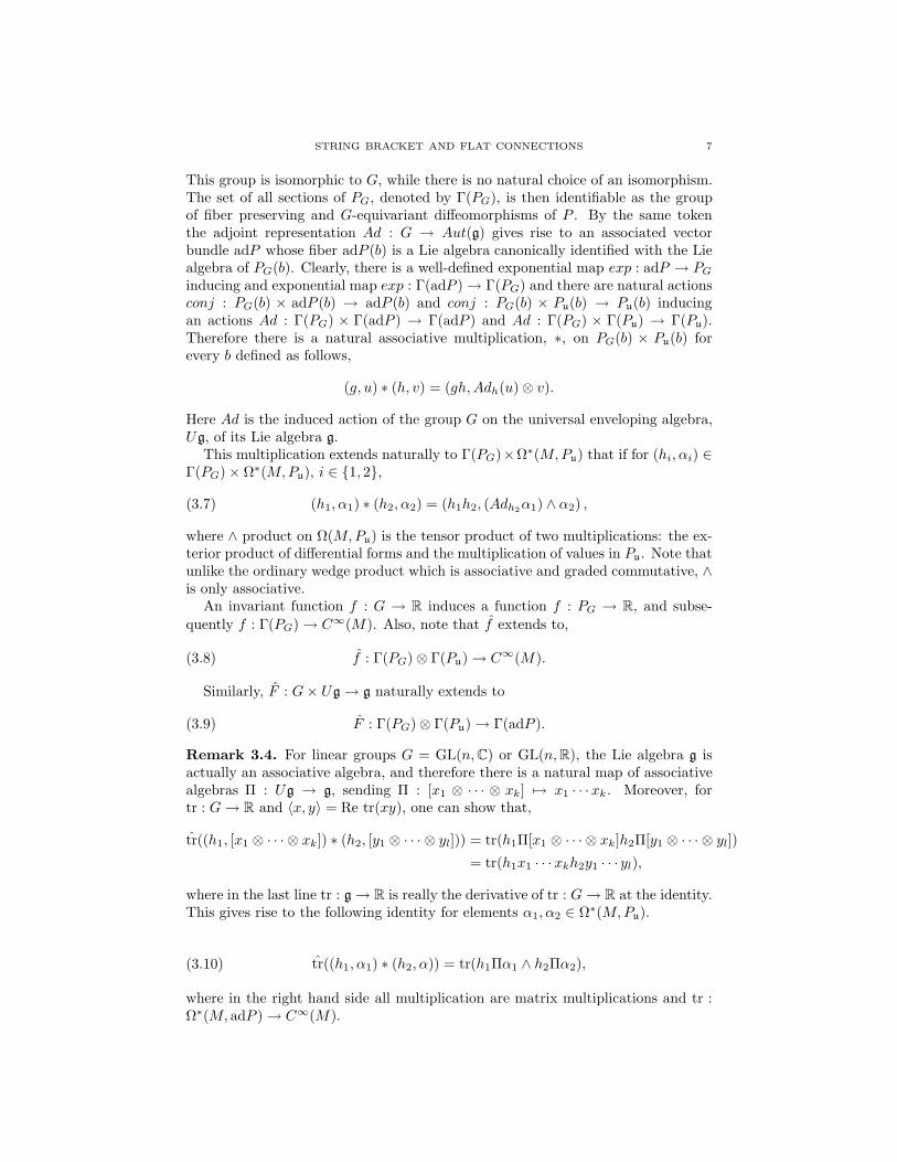
This group is isomorphic to G, while there is no natural choice of an isomorphism.The set of all sections of PG, denoted by Γ(PG), is then identifiable as the groupof fiber preserving and G-equivariant diffeomorphisms of P . By the same tokenthe adjoint representation Ad : G → Aut(g) gives rise to an associated vectorbundle adP whose fiber adP (b) is a Lie algebra canonically identified with the Liealgebra of PG(b). Clearly, there is a well-defined exponential map exp : adP → PG

inducing and exponential map exp : Γ(adP )→ Γ(PG) and there are natural actionsconj : PG(b) × adP (b) → adP (b) and conj : PG(b) × Pu(b) → Pu(b) inducingan actions Ad : Γ(PG) × Γ(adP ) → Γ(adP ) and Ad : Γ(PG) × Γ(Pu) → Γ(Pu).Therefore there is a natural associative multiplication, ∗, on PG(b) × Pu(b) forevery b defined as follows,

(g, u) ∗ (h, v) = (gh,Adh(u)⊗ v).

Here Ad is the induced action of the group G on the universal enveloping algebra,Ug, of its Lie algebra g.

This multiplication extends naturally to Γ(PG)×Ω∗(M,Pu) that if for (hi, αi) ∈Γ(PG)× Ω∗(M,Pu), i ∈ 1, 2,

(3.7) (h1, α1) ∗ (h2, α2) = (h1h2, (Adh2α1) ∧ α2) ,

where ∧ product on Ω(M,Pu) is the tensor product of two multiplications: the ex-terior product of differential forms and the multiplication of values in Pu. Note thatunlike the ordinary wedge product which is associative and graded commutative, ∧is only associative.

An invariant function f : G → R induces a function f : PG → R, and subse-

quently f : Γ(PG)→ C∞(M). Also, note that f extends to,

(3.8) f : Γ(PG)⊗ Γ(Pu)→ C∞(M).

Similarly, F : G× Ug→ g naturally extends to

(3.9) F : Γ(PG)⊗ Γ(Pu)→ Γ(adP ).

Remark 3.4. For linear groups G = GL(n,C) or GL(n,R), the Lie algebra g isactually an associative algebra, and therefore there is a natural map of associativealgebras Π : Ug → g, sending Π : [x1 ⊗ · · · ⊗ xk] 7→ x1 · · ·xk. Moreover, fortr : G→ R and 〈x, y〉 = Re tr(xy), one can show that,

tr((h1, [x1 ⊗ · · · ⊗ xk]) ∗ (h2, [y1 ⊗ · · · ⊗ yl])) = tr(h1Π[x1 ⊗ · · · ⊗ xk]h2Π[y1 ⊗ · · · ⊗ yl])

= tr(h1x1 · · ·xkh2y1 · · · yl),

where in the last line tr : g→ R is really the derivative of tr : G→ R at the identity.This gives rise to the following identity for elements α1, α2 ∈ Ω∗(M,Pu).

tr((h1, α1) ∗ (h2, α)) = tr(h1Πα1 ∧ h2Πα2),(3.10)

where in the right hand side all multiplication are matrix multiplications and tr :Ω∗(M, adP )→ C∞(M).


4. Symplectic nature of the Maurer-Cartan moduli space

In this section, we mostly follow [GG]. For the sake of completeness and claritywe mention some of their result without repeating their proofs.

Definition 4.1. A cyclic differential graded Lie algebra, (L, d, [·, ·], ω(·, ·)), or acyclic DGLA for short, consists of a Z2-graded Lie algebra L = L0 ⊕ L1, with adifferential d, and a bilinear form ω : L× L → R, satisfying,

(i) d(L0) ⊆ L1 and d(L1) ⊆ L0

(ii) d[x, y] = [dx, y] + (−1)|x|[x, dy]

(iii) ω([x, y], z) = ω(x, [y, z])

(iv) ω(dx, y) + (−1)|x|ω(x, dy) = 0

(v) ω(y, x) = (−1)|x||y|ω(x, y)

(vi) ω(·, ·)|L0and ω(·, ·)|L1

are nondegenerate

(vii) ω(x, y) = 0 for x ∈ L0 and y ∈ L1

We furthermore assume that L0 is the Lie algebra of a complex, connected, andsimply-connected linear algebraic group G.

Example 4.2. Let G → P → M be a principal bundle over a compact andoriented manifold M without boundary of dimension m = 2d which is endowedwith a flat connection ∇. Assume that the Lie algebra, g, of G is equippedwith a nondegenerate invariant bilinear form 〈·, ·〉. Recall that invariance means〈[x, y], z〉 = 〈x, [y, z]〉. Consider the graded Lie algebra L = Ω∗(M, adP ) of dif-ferential forms with values in adP , the adjoint bundle of P . In order to see thegraded Lie algebra structure better, recall that the tensor product of a graded com-mutative algebra and a graded Lie algebra is a a graded Lie algebra. Note thatL = Ω∗(M, adP ) = Ω∗(M)⊗C∞(M) Γ(adP ), Here, the graded Lie algebra Γ(adP ) isconcentrated in degree zero. The covariant derivative associated to the connection∇ induces a derivation d∇ : Ω∗(M, adP ) → Ω∗+1(M, adP ). Flatness means thatd∇ is a differential, that is to say d2

∇ = 0. Define a bilinear form ω : L×L → R asthe following composition.

ω : Ωi(M, adP )× Ωj(M, adP )∧→ Ωi+j(M, adP ⊗ adP )

〈·,·〉→ Ωi+j(M,R)

R

M→ R,

if i+ j = 2d, and zero otherwise.Clearly, condition (i) and (iii) are satisfied and condition (ii) and (iv) follow from

Corollaries A.2 and A.3. It follows from the invariance property and nondegeneracyof 〈·, ·〉 that conditions (v)-(vi) hold. Lastly, (vii) is true because the manifold iseven dimensional. This means Ω∗(M, adP ) is a cyclic DGLA.

Given a cyclic DGLA (L, d, [·, ·], ω(·, ·)), clearly (L1, ω|L1) is a symplectic vector

space. To every a ∈ L0, one associates a vector field on L1 by defining ξa(x) =[a, x] − da, for all x ∈ L1. The vector field ξa respects the symplectic structure,that is to say, Lξa

ω = 0. In fact, this infinitesimal action is Hamiltonian and thefollowing proposition describes its moment map. For a discussion and proof seesection 1.5 of [GG].

Proposition 4.3. Let (L, d, [·, ·], ω) be a cyclic DGLA. The map φ : L1 → L∗0

defined by φ(x)(a) = ω(dx + 1/2[x, x], a), for all x ∈ L1 and a ∈ L0, is a moment

map for the action of L0 on the symplectic space (L1, ω|L1).


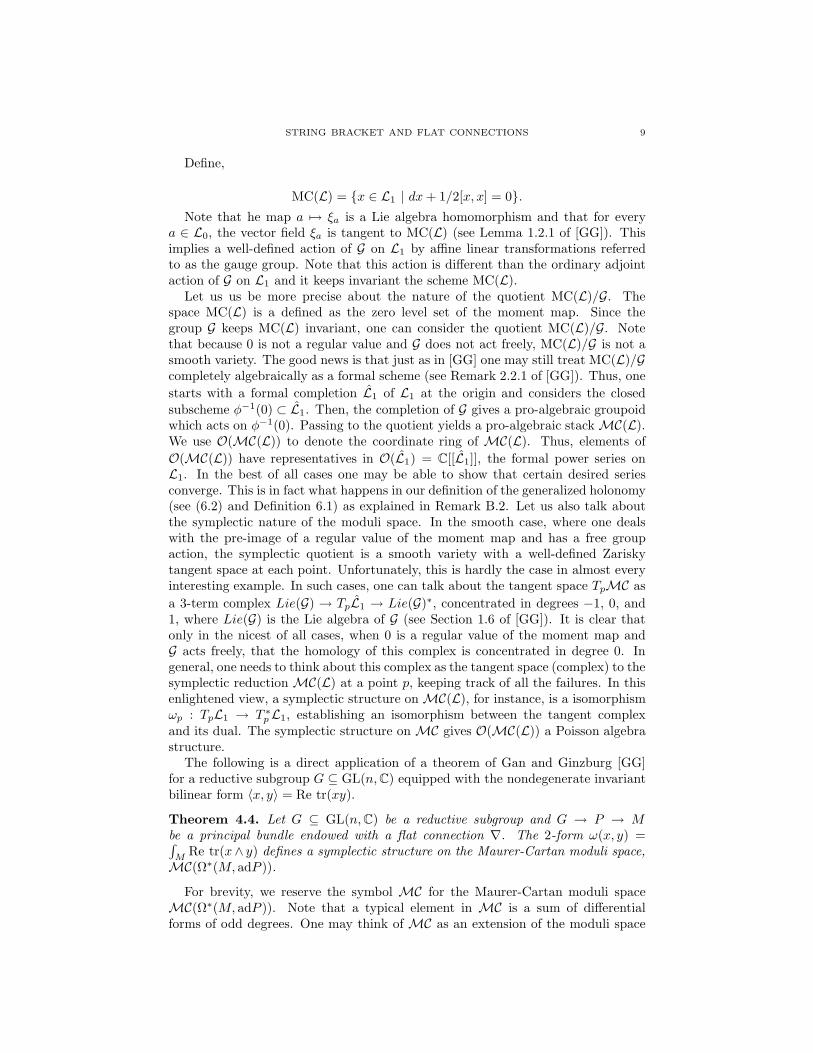
Define,

MC(L) = x ∈ L1 | dx+ 1/2[x, x] = 0.

Note that he map a 7→ ξa is a Lie algebra homomorphism and that for everya ∈ L0, the vector field ξa is tangent to MC(L) (see Lemma 1.2.1 of [GG]). Thisimplies a well-defined action of G on L1 by affine linear transformations referredto as the gauge group. Note that this action is different than the ordinary adjointaction of G on L1 and it keeps invariant the scheme MC(L).

Let us us be more precise about the nature of the quotient MC(L)/G. Thespace MC(L) is a defined as the zero level set of the moment map. Since thegroup G keeps MC(L) invariant, one can consider the quotient MC(L)/G. Notethat because 0 is not a regular value and G does not act freely, MC(L)/G is not asmooth variety. The good news is that just as in [GG] one may still treat MC(L)/Gcompletely algebraically as a formal scheme (see Remark 2.2.1 of [GG]). Thus, one

starts with a formal completion L1 of L1 at the origin and considers the closedsubscheme φ−1(0) ⊂ L1. Then, the completion of G gives a pro-algebraic groupoidwhich acts on φ−1(0). Passing to the quotient yields a pro-algebraic stackMC(L).We use O(MC(L)) to denote the coordinate ring of MC(L). Thus, elements of

O(MC(L)) have representatives in O(L1) = C[[L1]], the formal power series onL1. In the best of all cases one may be able to show that certain desired seriesconverge. This is in fact what happens in our definition of the generalized holonomy(see (6.2) and Definition 6.1) as explained in Remark B.2. Let us also talk aboutthe symplectic nature of the moduli space. In the smooth case, where one dealswith the pre-image of a regular value of the moment map and has a free groupaction, the symplectic quotient is a smooth variety with a well-defined Zariskytangent space at each point. Unfortunately, this is hardly the case in almost everyinteresting example. In such cases, one can talk about the tangent space TpMC as

a 3-term complex Lie(G) → TpL1 → Lie(G)∗, concentrated in degrees −1, 0, and1, where Lie(G) is the Lie algebra of G (see Section 1.6 of [GG]). It is clear thatonly in the nicest of all cases, when 0 is a regular value of the moment map andG acts freely, that the homology of this complex is concentrated in degree 0. Ingeneral, one needs to think about this complex as the tangent space (complex) to thesymplectic reduction MC(L) at a point p, keeping track of all the failures. In thisenlightened view, a symplectic structure onMC(L), for instance, is a isomorphismωp : TpL1 → T ∗

pL1, establishing an isomorphism between the tangent complexand its dual. The symplectic structure on MC gives O(MC(L)) a Poisson algebrastructure.

The following is a direct application of a theorem of Gan and Ginzburg [GG]for a reductive subgroup G ⊆ GL(n,C) equipped with the nondegenerate invariantbilinear form 〈x, y〉 = Re tr(xy).

Theorem 4.4. Let G ⊆ GL(n,C) be a reductive subgroup and G → P → Mbe a principal bundle endowed with a flat connection ∇. The 2-form ω(x, y) =∫

MRe tr(x∧ y) defines a symplectic structure on the Maurer-Cartan moduli space,

MC(Ω∗(M, adP )).

For brevity, we reserve the symbol MC for the Maurer-Cartan moduli spaceMC(Ω∗(M, adP )). Note that a typical element in MC is a sum of differentialforms of odd degrees. One may think of MC as an extension of the moduli space


of flat connections on P . In fact, if the Hard Lefschetz theorem holds for M , thenthe moduli space of flat connections on P may be viewed as a symplectic substackofMC (see section 1.7 of [GG] and section 9 of this paper).

5. Differential forms on free loop spaces

In this section we shall present a model of the free loop space LM which is con-ducive to the notions of the de Rham differential forms and its S1-equivariant model.These differential forms contain the Chen iterated integrals [Ch1, Ch2]. Moreover,the cohomology of these forms, called the de Rham cohomology and the equivariantde Rham cohomology respectively, compute the usual and S1-equivariant singularcohomologies of LM . Such a model of the free loop space must support the usualdifferential geometric notions such as connections and all related pullback diagrams.Since the different parts of the required framework are developed in different ref-erences, we briefly summarize some of the needed definitions and statements andrefer the reader to [H, G, Br, GS] for a fuller discussion.

Let E, F denote locally convex Hausdorff topological vector space and U ⊂ Ean open set, we say that the map f : U → F is of class C1 if the limit df(x, v) =

limt→0

f(x+tv)−f(x)t exists and is continuous as a function of (x, v) ∈ U ×E. Similarly,

we can define functions of class Ck and thus C∞. Then Ωn(U) the space of differ-ential n-forms on U is defined to be the space of smooth functions ω : U ×En → R

which are multilinear and antisymmetric in the last n variables. Then, one definesthe exterior differential d which satisfies d2 = 0 (see [H, Br]). Also, the Poincarelemma holds for convex open subsets of E (see [Br] for a proof).

A differentiable space modeled on E is a Hausdorff space N with a coveringUii∈I and a collection of homeomorphisms φi : Ui → Vi ⊂ E, such that thetransition maps φj φ

−1i are smooth. Then a differential n-form on an open U ⊂ N

is defined to be a collection of ωi ∈ Ωn(φi(U∩Ui)) patched together by the transitionmap φj φ

−1i . This enables us to define the de Rham complex of N denoted

(Ω∗(N), d) and the de Rham cohomology H∗DR(N) of N to be the cohomology of

(Ω∗(N), d).It is known that the de Rham theorem holds (see for example [Br]). This is

shown using sheaf cohomology. The de Rham forms on the opens U ⊂ N define asheaf Ω∗(N) on N which is a resolution of RN the sheaf of the constant functions

(by Poincare lemma). When N is a paracompact differentiable space and thesheaf Ω∗(N) is an acyclic soft sheaf, we can use the natural resolution RN →

Ω(N)∗ to calculate the sheaf cohomology H∗sheaf (N,RN ) implying that H∗

DR(N) ≃

H∗sheaf (N,RN ) (see [Br] 1.4.7 or [G]).

As it turns out, LM = C∞(S1,M) can be made into a paracompact differentiablespace modeled on C∞(S1,Rn) (p. 110 [Br]). The topology of C∞(S1,Rn) is definedusing a family of the norms ‖ · ‖k given by

‖f‖2k =

∫ 1

0

(‖f(t)‖2 + · · ·+ ‖dk

dtkf(t)‖2)dt,

which make C∞(S1,Rn) into a Frechet vector space and LM into a Frechet mani-

fold. This allows us to consider vector bundles with connection on LM and do thedifferential geometry needed in this paper just as in the finite dimensional case (see[H] for the details).


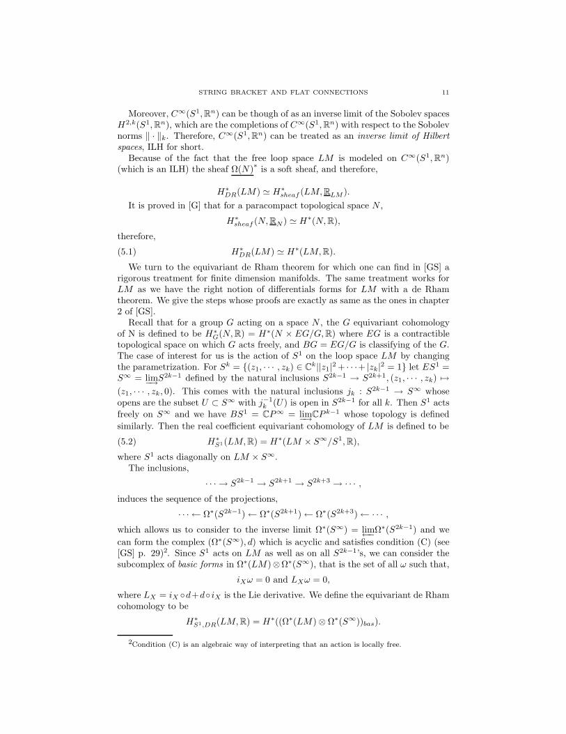
Moreover, C∞(S1,Rn) can be though of as an inverse limit of the Sobolev spacesH2,k(S1,Rn), which are the completions of C∞(S1,Rn) with respect to the Sobolevnorms ‖ · ‖k. Therefore, C∞(S1,Rn) can be treated as an inverse limit of Hilbert

spaces, ILH for short.Because of the fact that the free loop space LM is modeled on C∞(S1,Rn)

(which is an ILH) the sheaf Ω(N)∗

is a soft sheaf, and therefore,

H∗DR(LM) ≃ H∗

sheaf (LM,RLM ).

It is proved in [G] that for a paracompact topological space N ,

H∗sheaf (N,RN ) ≃ H∗(N,R),

therefore,

(5.1) H∗DR(LM) ≃ H∗(LM,R).

We turn to the equivariant de Rham theorem for which one can find in [GS] arigorous treatment for finite dimension manifolds. The same treatment works forLM as we have the right notion of differentials forms for LM with a de Rhamtheorem. We give the steps whose proofs are exactly as same as the ones in chapter2 of [GS].

Recall that for a group G acting on a space N , the G equivariant cohomologyof N is defined to be H∗

G(N,R) = H∗(N × EG/G,R) where EG is a contractibletopological space on which G acts freely, and BG = EG/G is classifying of the G.The case of interest for us is the action of S1 on the loop space LM by changingthe parametrization. For Sk = (z1, · · · , zk) ∈ C

k||z1|2 + · · ·+ |zk|

2 = 1 let ES1 =S∞ = lim−→S

2k−1 defined by the natural inclusions S2k−1 → S2k+1, (z1, · · · , zk) 7→

(z1, · · · , zk, 0). This comes with the natural inclusions jk : S2k−1 → S∞ whoseopens are the subset U ⊂ S∞ with j−1

k (U) is open in S2k−1 for all k. Then S1 acts

freely on S∞ and we have BS1 = CP∞ = lim−→CP k−1 whose topology is defined

similarly. Then the real coefficient equivariant cohomology of LM is defined to be

(5.2) H∗S1(LM,R) = H∗(LM × S∞/S1,R),

where S1 acts diagonally on LM × S∞.The inclusions,

· · · → S2k−1 → S2k+1 → S2k+3 → · · · ,

induces the sequence of the projections,

· · · ← Ω∗(S2k−1)← Ω∗(S2k+1)← Ω∗(S2k+3)← · · · ,

which allows us to consider to the inverse limit Ω∗(S∞) = lim←−Ω∗(S2k−1) and we

can form the complex (Ω∗(S∞), d) which is acyclic and satisfies condition (C) (see[GS] p. 29)2. Since S1 acts on LM as well as on all S2k−1’s, we can consider thesubcomplex of basic forms in Ω∗(LM)⊗Ω∗(S∞), that is the set of all ω such that,

iXω = 0 and LXω = 0,

where LX = iX d+d iX is the Lie derivative. We define the equivariant de Rhamcohomology to be

H∗S1,DR(LM,R) = H∗((Ω∗(LM)⊗ Ω∗(S∞))bas).

2Condition (C) is an algebraic way of interpreting that an action is locally free.


The rest of this section is devoted to the proof of

(5.3) H∗S1,DR(LM,R) ≃ H∗

S1(LM,R).

Consider the diagonal action of S1 on LM × S2k−1 and the projection,

π : LM × S2k−1 → LM × S2k−1/S1.

Since the action is free, the subalgebra π∗(Ω∗(LM×S2k−1/S1)) ⊂ Ω∗(LM×S2k−1)can be characterized as the basic differential forms denoted Ω∗(LM × S2k−1)bas;moreover π∗ is injective. We denote the subcomplex of basic forms by Ω∗(LM ×S2k−1)bas and we have,

(5.4) H∗DR(LM × S2k−1/S1) ≃ H∗(Ω∗(LM × S2k−1)bas).

Using the projections,

· · · ← Ω∗(LM × S2k−1)bas ← Ω∗(LM × S2k+1)bas ← · · · ,

we can form the complex Ω∗(LM × S∞)bas = lim←−Ω∗(LM × S2k−1)bas.

Proposition 5.1. H∗S1(LM,R) ≃ H∗(Ω∗(LM × S∞)bas).

Proof. Similarly to the proof of (5.1), for the differentiable space LM × S2k−1/S1,we have the isomorphism,

H∗DR(LM × S2k−1/S1) = H∗(LM × S2k−1/S1,R),

which is compatible the inclusions LM ×S2k−1/S1 → LM ×S2k+1/S1. Therefore,

H∗S1(LM,R) ≃ lim←−H

∗(LM × S2k+1/S1)

≃ lim←−

H∗DR(LM × S2k−1/S1)

≃ H∗(Ω∗(LM × S∞)bas).

So, to prove (5.3) it suffices to show that,

(5.5) H∗(Ω∗(LM × S∞)bas) ≃ H∗DR((Ω∗(LM)⊗ Ω∗(S∞))bas).

This follows from a standard spectral sequence argument and the fact that inclusionΩ∗(LM × S∞) → Ω∗(LM)⊗Ω∗(S∞) induces an isomorphism in cohomology, andthat Ω∗(S∞) is acyclic and satisfies condition (C)(see [GS] p. 30).

6. Generalized holonomy

Let M be a compact and oriented manifold without boundary. Given a principalbundle G→ P →M endowed with a flat connection ∇, the trace of the holonomyyields a well-defined map on the set of the free homotopy classes of loops in the basemanifold M . It was discussed in [CR] how this may generalize to families of loops,more precisely, to the homology classes in the free loop space of the underlyingmanifold. We will give a mathematical account of this in this section. Throughoutthis section we will be using the notion of differential forms developed in section 5for LM equipped with it natural Frechet manifold structure.

For every n ≥ 0, consider the n-simplex,

∆n = (t0, t1, · · · , tn, tn+1) | 0 = t0 ≤ t1 ≤ · · · ≤ tn ≤ tn+1 = 1.


Define the evaluation maps ev, and evn,i, for 1 ≤ i ≤ n as follows,

ev : ∆n × LM →M,

ev(t0, t1, · · · , tn, tn+1; γ) = γ(0) = γ(1),

evn,i : ∆n × LM →M,

evn,i(t0, t1, · · · , tn, tn+1; γ) = γ(ti).

Let Ti : ev∗n,i(adP )→ ev∗(adP ) denote the map, between pullbacks of the adjointbundles over ∆n × LM , defined at a point (0 = t0, t1, · · · , tn, tn+1 = 1; γ) by theparallel transport along and in the direction of γ from γ(ti) to γ(tn+1) = γ(1), inadP with respect to the flat connection ∇. Note that if R, S, and T denote theparallel transport maps respectively in bundles P , PG, and adP , over a given path,then we have S(φ) = R−1 φ R and T (x) = dSe(x), the derivative at the identityof S evaluated on the vector x.

For αi ∈ Ω∗(M, adP ), 1 ≤ i ≤ n, define α(n, i) ∈ Ω∗(∆n × LM, ev∗adP ) by,

α(n, i) = Tiev∗n,iαi.

Given γ ∈ LM the holonomy along γ from γ(0) to γ(1) in the principal bundleP gives rise to a section hol ∈ Γ(ev∗PG). Note that Γ(ev∗PG) acts by conju-gation on Γ(ev∗PG), and subsequently on Γ(ev∗adP ). Now, define V n

α1,··· ,αn∈

Ω∗(LM, ev∗Pu) as,

(6.1) V 0 = 1,

V nα1,··· ,αn

=

∫

∆n

α(n, 1) ∧ · · · ∧ α(n, n), for n ≥ 1,

and let,

(6.2) Vα =∞∑

n=0

V nα , where V n

α = V nα,··· ,α.

It is noteworthy that the above infinite sum is convergent. This follows from thediscussion in Appendix B, based on the simple fact that the volume of the standardn-simplex is 1

n! (see Remark B.2).Then, consider Wn

α1,··· ,αn∈ Γ(ev∗PG)× Ω∗(LM, ev∗Pu) defined as,

Wnα1,··· ,αn

= (hol, V nα1,··· ,αn

), for n ≥ 0,(6.3)

and,

Wnα = (hol, V n

α,··· ,α) and Wα = (hol, Vα).

We fix an invariant function f : G → R and we shall follow the notationsintroduced in (3.9) and (3.3). Note that the maps

f : Γ(PG)⊗ Γ(Pu)→ C∞(M),

F : Γ(PG)⊗ Γ(Pu)→ Γ(adP ),

naturally induce the maps on the differential forms,

f : Γ(PG)⊗ Ω∗(M,Pu)→ Ω∗(M),

F : Γ(PG)⊗ Ω∗(M,Pu)→ Ω∗(M, adP ),


which in turn induce the following maps on the corresponding pullback bundles,

f : Γ(ev∗PG)⊗ Ω∗(LM, ev∗Pu)→ Ω∗(LM),

F : Γ(ev∗PG)⊗ Ω∗(LM, ev∗Pu)→ Ω∗(LM, ev∗adP ).

Definition 6.1. For a differential form α ∈ Ω∗(M, adP ), the Wilson loop Wα ∈Ω∗(LM,R) is defined as,

Wα = f(Wα).

Proposition 6.2. If α ∈MC, then Wα ∈ Ω∗(LM) is a closed form.

Proof. Using Stokes theorem we have,

dWα = df(hol, 1) +

∞∑

n=1

f(hol, d

∫

∆n

α(n, 1) ∧ · · · ∧ α(n, n))

+

∞∑

n=1

f(hol,

∫

∂∆n

α(n, 1) ∧ · · · ∧ α(n, n)).

Since the connection ∇ is flat, f(hol, 1) = f(hol) is constant on the connected

components of LM therefore df(hol) = 0 on LM . Actually one can say more,hol ∈ Γ(ev∗(PG)) is a flat section. Therefore, by Corollary A.4, we have,

dWα =

∞∑

n=1

f(hol,

∫

∆n

dev∗∇(α(n, 1) ∧ · · · ∧ α(n, n)))

+

∞∑

n=1

f(hol,

∫

∂∆n

α(n, 1) ∧ · · · ∧ α(n, n)).

We analyze different terms separately. For the first part we have,

dev∗∇(α(n, 1) ∧ · · · ∧ α(n, n)) =

n∑

i=1

(−1)iα(n, 1) ∧ · · · ∧ dev∗∇(α(n, i)) ∧ · · · ∧ α(n, n)

=

n∑

i=1

(−1)iα(n, 1) ∧ · · · ∧ (d∇(α))(n, i) ∧ · · · ∧ α(n, n).

Hence,

∞∑

n=1

∫

∆n

f(hol, dev∗∇(α(n, 1) ∧ · · · ∧ α(n, n))) =

∞∑

n=1

n∑

i=1

f(Wnα,··· ,d∇α,···α).

As for the second part we have ∂∆n = ∪ni=0∆

n−1i , where,

∆n−1i = (t0, t1, · · · , tn, tn+1) | 0 = t0 ≤ t1 ≤ · · · ≤ ti = ti+1 ≤ · · · ≤ tn ≤ tn+1 = 1,


and then for n ≥ 1,

f(hol,

∫

∂∆n

α(n, 1) ∧ · · · ∧ α(n, n))

= f(hol, Adhol(ev∗α) ∧

∫

∆n−1

α(n− 1, 1) ∧ · · · ∧ α(n− 1, n− 1))

+

n−1∑

i=1

(−1)if(hol,

∫

∆n−1

α(n− 1, 1) ∧ · · · ∧ (α ∧ α)(n− 1, i) ∧ · · · ∧ α(n− 1, n))

+ (−1)nf(hol,

∫

∆n−1

α(n− 1, 1) ∧ · · · ∧ α(n− 1, n− 1) ∧ ev∗α).

To calculate the first term in the equality above we have used the fact that theparallel transport of adP along a loop γ is give by Adhol where hol is understoodas the parallel transport in the principal bundle P . Now, from the invariance of fand the fact that the components of α have odd degrees, it follows that the firstterm and the last term cancel each other. Therefore, we have,

∞∑

n=1

f(hol,

∫

∂∆n

α(n, 1) ∧ · · · ∧ α(n, n)) =

∞∑

n=2

n−1∑

i=1

(−1)if(hol,

∫

∆n−1

α(n− 1, 1) ∧ · · · ∧ (α ∧ α)(n− 1, i) ∧ · · · ∧ α(n− 1, n− 1))

=

∞∑

n=1

n∑

i=1

(−1)if(Wnα,··· ,α∧α,··· ,α).

Then,

dWα =

∞∑

n=1

n∑

i=1

(−1)if(Wnα,··· ,d∇α,··· ,α) +

∞∑

n=1

n∑

i=1

(−1)if(Wnα,··· ,α∧α,··· ,α)

=

∞∑

n=1

n∑

i=1

(−1)if(Wnα,··· ,d∇α+α∧α,··· ,α).

Note that since α is a sum of forms of odd degrees in Ω∗(M,Pu), α∧α = 1/2[α, α].Therefore,

dWα =

∞∑

n=1

n∑

i=1

(−1)if(Wnα,··· ,d∇α+1/2[α,α],··· ,α) = 0.

We now explain how Wα represents an equivariant cohomology class.

Lemma 6.3. For α ∈MC, there exists a Wα ∈ H∗S1(LM) such that,

(6.4) Wα = e∗(Wα).

Proof. By (5.3) it suffices to show that thatWα ∈ Ω∗(LM)1⊗id→ Ω∗(LM)⊗Ω∗(S∞)

is a basic form. Since Wα is a closed form, it remains to show that ivWα = 0. Thefact that ivWα = 0 for v = ∂

∂t , the fundamental vector field of the S1-action, isobvious sinceWα is obtained by pullback of the evaluation maps, devtk

(v) = γ′(tk)


and iγ′(tk)iγ′(tk) = 0. This shows that Wα determines a cohomology class Wα ∈H∗

S1(LM) which satisfies,

Wα = e∗(Wα).

Since the equivariant de Rham cohomology of LM is isomorphic to the singular

one, we can think of Wα as an element in H∗S1(LM,R). For c ∈ HS1

∗ (LM), defineΨc ∈ O(MC) as,

(6.5) Ψc(α) = 〈c,Wα〉.

The following proposition implies that Ψc descends to O(MC).

Proposition 6.4. For c ∈ H∗(LM) and a ∈ L0 = Ω2∗(M, adP ),

LξaΨc = 0 ∈ O(MC).

Proof. By Cartan’s formula, we have,

(LξaΨc)(α) = (iξa

dΨc + diξaΨc)(α) = iξa

dΨc(α).

Let us calculate dΨc(α)(h) for h ∈ L1 = TαL1,

dΨc(α)(h) =d

dt

(∫

c

Wα+th

)

|t=0 =

∫

c

d

dt(Wα+th)|t=0.

Note that,

d

dtWα+th|t=0 =

d

dt

∞∑

n=1

f(Wnα+th,··· ,α+th)|t=0 =

∞∑

n=1

n∑

i=1

f(Wnα,··· ,h,··· ,α).

So, in order to show that LξaΨc(α) = iξa

dΨc(α) = 0 we have to show thatddtWα+th|t=0 is an exact form for h = ξa(α), or in other words,

∞∑

n=1

n∑

i=1

f(Wnα,··· ,ξa(α),··· ,α),

is exact.


Let Z =∑∞

n=1

∑ni=1(−1)if(Wn

α,··· ,a,··· ,α) ∈ Ω∗(LM,R). Then, by a calculationsimilar to that presentation in the proof of Proposition 6.2 we show that for a ∈ L+,

dZ =

∞∑

n=1

n∑

i=1

(−1)2i(f(Wnα,··· ,d∇a

| z

i

,··· ,α) + f(Wnα,··· ,α ∧ a

| z

i

,··· ,α)− f(Wnα,··· ,a ∧ α

| z

i

,··· ,α)+

∞∑

n=1

n∑

i=1

(−1)i[∑

j<i

(−1)j(f(Wnα,··· ,d∇α

| z

j

,··· , a,|z

i

··· ,α) + f(Wnα,··· ,α ∧ α

| z

j

,··· , a,|z

i

··· ,α))+

∑

i<j≤n

(−1)j(f(Wnα,··· , a,

|z

i

··· ,d∇α| z

j

,··· ,α))] + f(Wnα,··· , a,

|z

i

··· ,α ∧ α| z

j

,··· ,α))

=

∞∑

n=1

n∑

i=1

(−1)2i(f(Wnα,··· ,d∇a

| z

i

,··· ,α) + f(Wnα,··· ,α ∧ a

| z

i

,··· ,α)− f(Wnα,··· ,a ∧ α

| z

i

,··· ,α))+

∞∑

n=1

n∑

i=1

(−1)i(∑

j<i

(−1)j f(Wnα,··· ,d∇α + 1/2[α, α]

| z

j

,··· , a,|z

i

··· ,α)

+∑

i<j≤n

(−1)j f(Wnα,··· , a,

|z

i

··· ,d∇α + 1/2[α, α]| z

j

,··· ,α)).

As d∇α+ 12 [α, α] = 0 for α ∈MC, therefore,

dZ =

∞∑

n=1

n∑

i=1

f(Wnα,··· ,d∇a+[α,a],··· ,α)

=

∞∑

n=1

n∑

i=1

f(Wnα,··· ,ξa(α),··· ,α)

=d

dtWα+tξa(α)|t=0.

This proves the claim.

By Proposition 6.4, Ψa : MC → R is constant along the orbits of G.

Definition 6.5. The generalized holonomy map Ψ : HS1

2∗ (LM) → O(MC) is themap a 7→ Ψa, where,

Ψa(α) = 〈a,Wα〉.

7. Hamiltonian vectors field and Poisson bracket

Let Ψa, and Ψb denote the holonomy functions associated to the equivariant

homology classes a, b ∈ HS1

2∗ (LM), and let Xa and Xb denote their correspondingHamiltonian vector fields. We calculate the Poisson bracket of holonomy functionsby evaluating the symplectic form on their corresponding Hamiltonian vector fields.Note that the Zarisky tangent space of MC/G at a class represented by α can beidentified with the cohomology whose differential is ∇ + α ∧ · or in other wordsadP is equipped with the flat connection ∇+ α ∧ ·. The later is a differential as αsatisfies the Maurer-Cartan equation. We denote the cohomology of this differen-tial by H∗(M, adPα), and similarly the corresponding vector bundle homology byH∗(M, adPα).


We borrow the following lemma from [Go2] to obtain a formula for the Hamil-tonian vector fields.

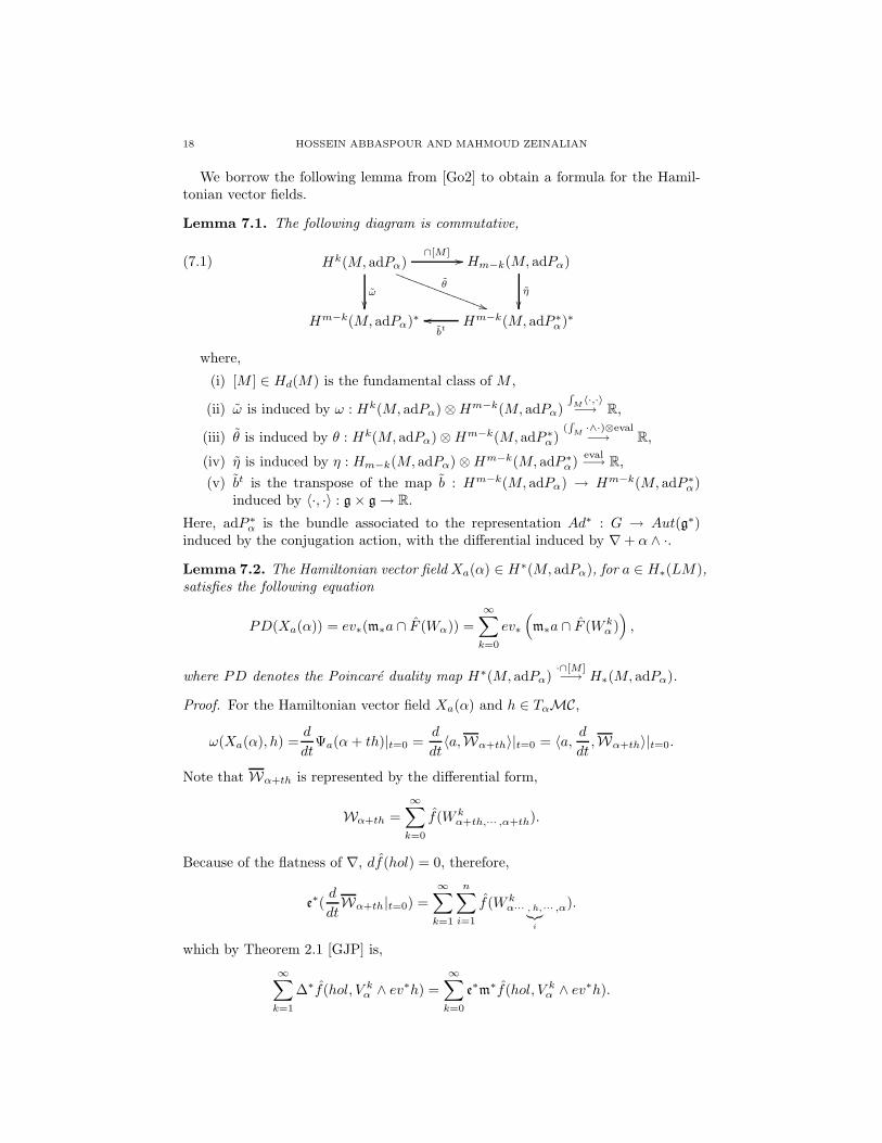
Lemma 7.1. The following diagram is commutative,

(7.1) Hk(M, adPα)

ω

θ

))SSSSSSSSSSSSSS

∩[M ]// Hm−k(M, adPα)

η

Hm−k(M, adPα)∗ Hm−k(M, adP ∗α)∗

bt

oo

where,

(i) [M ] ∈ Hd(M) is the fundamental class of M ,

(ii) ω is induced by ω : Hk(M, adPα)⊗Hm−k(M, adPα)

R

M〈·,·〉−→ R,

(iii) θ is induced by θ : Hk(M, adPα)⊗Hm−k(M, adP ∗α)

(R

M·∧·)⊗eval−→ R,

(iv) η is induced by η : Hm−k(M, adPα)⊗Hm−k(M, adP ∗α)

eval−→ R,

(v) bt is the transpose of the map b : Hm−k(M, adPα) → Hm−k(M, adP ∗α)

induced by 〈·, ·〉 : g× g→ R.

Here, adP ∗α is the bundle associated to the representation Ad∗ : G → Aut(g∗)

induced by the conjugation action, with the differential induced by ∇+ α ∧ ·.

Lemma 7.2. The Hamiltonian vector field Xa(α) ∈ H∗(M, adPα), for a ∈ H∗(LM),satisfies the following equation

PD(Xa(α)) = ev∗(m∗a ∩ F (Wα)) =

∞∑

k=0

ev∗

(

m∗a ∩ F (W kα )

)

,

where PD denotes the Poincare duality map H∗(M, adPα)·∩[M ]−→ H∗(M, adPα).

Proof. For the Hamiltonian vector field Xa(α) and h ∈ TαMC,

ω(Xa(α), h) =d

dtΨa(α+ th)|t=0 =

d

dt〈a,Wα+th〉|t=0 = 〈a,

d

dt,Wα+th〉|t=0.

Note that Wα+th is represented by the differential form,

Wα+th =∞∑

k=0

f(W kα+th,··· ,α+th).

Because of the flatness of ∇, df(hol) = 0, therefore,

e∗(d

dtWα+th|t=0) =

∞∑

k=1

n∑

i=1

f(W kα··· , h,

|z

i

··· ,α).

which by Theorem 2.1 [GJP] is,

∞∑

k=1

∆∗f(hol, V kα ∧ ev

∗h) =

∞∑

k=0

e∗m∗f(hol, V kα ∧ ev

∗h).


Hence by (3.5) and (3.3),

ω(Xa(α), h) = 〈a,m∗∞∑

k=0

f(hol, V kα ∧ ev

∗h)〉

= 〈m∗a,

∞∑

k=0

f(hol, V kα ∧ ev

∗h)〉

= 〈m∗a ∩∞∑

k=0

F (W kα ), ev∗h〉

= 〈ev∗(m∗a ∩

∞∑

k=0

F (W kα )), h〉.

Therefore, by Lemma 7.1,

ev∗(m∗a ∩

∞∑

k=0

F (W kα )) = η−1 (bt)−1(dαΨa)

= ω−1(dαΨa) ∩ [M ]

= Xa(α) ∩ [M ].

The following lemma is a version of the multiplicative property of the formalpower series parallel transport (see [Ch1, Ch2, M]). See (3.7) to recall the definitionof the ∗ product.

Lemma 7.3. Let ε : LM ×M LM → LM be the concatenation map, then,

ε∗(Wα) = pr∗1Wα ∗ pr∗2Wα,

where pr1 and pr2 are the projections on the first and the second factors,

LM ×M LM

pr1

xxqqqqqqqqqq

pr2

&&MMMMMMMMMM

LM LM

Proof. The proof of Proposition 1.5.1 in [Ch1] can be adopted to prove that thatfor two loops γ1 and γ2 with identical marked point,

(7.2) V nα (γ1 γ2) =

∑

i+j=n

Adhol(γ2)Viα(γ1) ∧ V

jα (γ2).

Also hol(γ1γ2) = hol(γ2)hol(γ1). To see the identity (7.2) more clearly, recall thatthe parallel transport in adP along γ2 is given by Adhol(γ2), and that in computingthe differential form V n

α (γ1γ2) (see section 6) the parallel transport Ti along γ1γ2

acts on all the pullbacks ev∗tiα. Split the terms α(n, i) into two collections according

to whether they are obtained by the pullback with respect to evt for 0 ≤ t ≤ 1/2or 1/2 ≤ t ≤ 1. Then, note that one needs to apply an extra action of Adhol(γ2)

on the first collection to account for the parallel transport along the second half ofγ1 γ2, that is γ2.


Recall Definition 6.5 wherein the generalized holonomy map Ψ : HS1

2∗ (LM) →O(MC) is described as the map a 7→ Ψa, where, Ψa(α) = 〈a,Wα〉. For a versionof the following theorem in the BRST setup see [CFP].

Theorem 7.4. For G = GL(n,C) or GL(n,R), the generalized holonomy map,

Ψ : (HS1

2∗ (LM), [·, ·])→ (O(MC), ·, ·),

is a map of Lie algebras.

Proof. Suppose that G = GL(n,C), it is exactly the same argument for G =

GL(n,R). We prove that for a, b ∈ HS1

2∗ (LM) and α ∈ MC,

Ψ[a,b](α) = Ψa,Ψb(α) = ω(Xa(α), Xb(α)).

The left hand side is,

Ψ[a,b](α) = Ψ(e∗(m∗a•m∗b)(α)

= 〈e∗(m∗a •m∗b),Wα〉

= 〈m∗a •m∗b, e∗(Wα)〉

= 〈m∗a •m∗b,Wα〉

= 〈ε∗ τ∗(m∗a×m∗b), tr(Wα)〉

= 〈m∗a×m∗b, tr(τ∗ ε∗(Wα))〉,

which using Lemma 7.3 equals,∫

m∗a×m∗b

(ev × ev)∗(U) ∧ tr(pr∗1Wα ∗ pr∗2Wα),

where U ∈ Ω∗(M ×M) is a differential form supported in a neighborhood of thediagonal realizing the Thom isomorphism. Now, by Lemma 7.2,

Ψa,Ψb(α) = ω(Xa(α), Xb(α))

=

∫

M

tr(Xa(α) ∧Xb(α))

=

∫

M

tr(PD−1(ev∗(m∗a ∩ F (Wα)) ∧ PD−1(ev∗(m∗a ∩ F (Wα))).

Using Remark 3.4 and the inclusion Ω∗(LM, ev∗PG) → Ω∗(LM, ev∗adP ) inducedby GL(n,C) → gl(n,C), and by Corollary 3.2,

F (Wα) = hol ·ΠVα ∈ Ω∗(LM, ev∗adP ).

Thus, the above Poisson bracket equals,∫

tr(ev∗(m∗a∩F (Wα))×ev∗(m∗a∩F (Wα)))

U =

∫

(m∗a×m∗b)∩tr(F (Wα)×F (Wα))

(ev × ev)∗U

=

∫

m∗a×m∗b

(ev × ev)∗U ∧ tr(pr∗1F (Wα) ∧ pr∗2F (Wα))

=

∫

m∗a×m∗b

(ev × ev)∗U ∧ tr(pr∗1(hol · ΠVα) ∧ pr∗2(hol · ΠVα))

=

∫

m∗a×m∗b

(ev × ev)∗U ∧ tr((pr∗1hol · pr∗1ΠVα) ∧ (pr∗2hol · pr

∗2ΠVα)).


But, it follows immediately from Remark 3.4 and line (3.6) that,

tr((pr∗1hol · pr∗1ΠVα) ∧ (pr∗2hol · pr

∗2ΠVα)) = tr(pr∗1Wα ∗ pr

∗2Wα).

This proves the theorem.

8. String bracket for unoriented strings

In this section we calculate the Poisson bracket for the generalized holonomyassociated to a principal G-bundle equipped with a flat connection, where G isone of the proper reductive subgroups of GL(n,C) such as O(n,R), O(n,C), U(n),SL(n,R), or SL(n,C). Let i : LM → LM be the involution which reverses theorientation of a loop. We continue to denote the induced map on the homology

H∗(LM) and the equivariant homology HS1

∗ (LM) by a 7→ i(a). We use i∗ forthe induced map on the cohomologies. It is a direct check that the latter mapscommute with the maps e∗ and m∗ introduced in section 2.

Theorem 8.1. For G = O(p, q), O(n,C),U(p, q), Sp(n,R) and Sp(p, q),

(8.1) Ψa,Ψb =1

2(Ψ[a,b] −Ψ[a,i(b)]),

where a, b ∈ HS1

2∗ (LM).

Proof. Consider

V tα =

∞∑

n=0

(−1)n

∫

∆n

α(n, n) ∧ · · · ∧ α(n, 1).

Notice that first term of the above summation is 1 (compare (6.3)). In a mannersimilar to the proof of Theorem 7.4,

Ψa,Ψb(α) =

∫

m∗a×m∗b

(ev × ev)∗U ∧ tr(pr∗1F (Wα) ∧ pr∗2F (Wα))),

By Corollary 3.3,

F (Wα) =1

2(hol ·ΠVα −ΠV t

α · hol−1) ∈ Ω∗(LM, ev∗adP ),

and all the terms above make sense using the fact G is one of the subgroups listedin the theorem. Since for every g ∈ G, Re tr(A) = Re tr(A−1) it follows,

Ψa,Ψb(α) =1

2

∫

m∗a×m∗b

(ev × ev)∗U ∧ tr(pr∗1(hol)pr∗1(ΠVα) ∧ pr∗2(hol)pr∗2(ΠVα))

−1

2

∫

m∗a×m∗b

(ev × ev)∗U ∧ tr(pr∗1(hol)pr∗1(ΠVα) ∧ pr∗2(ΠV tα)pr∗2(hol−1)).

Also, as in the proof of Theorem 7.4,

1

2(Ψ[a,b](α) −Ψ[a,i(b)](α)) =

1

2

∫

m∗a×m∗b

(ev × ev)∗(U) ∧ tr(pr∗1Wα ∗ pr∗2Wα)

−1

2

∫

m∗a×m∗i(b)

(ev × ev)∗(U) ∧ tr(pr∗1Wα ∗ pr∗2Wα).


Similarly to the proof of Theorem 7.4,∫

m∗a×m∗b

tr(pr∗1(hol)pr∗1ΠVα ∧ pr∗2(hol)pr∗2ΠVα)

=

∫

m∗a×m∗b


So, we only have to show that,∫

m∗a×m∗b

tr(pr∗1(hol)pr∗1ΠVα ∧ pr∗2ΠV t

αpr∗2(hol−1))

=

∫

m∗a×m∗i(b)


(8.2)

Note that ev i = ev, and therefore (ev × ev)∗U = (id× i)∗(ev × ev)∗U . Also,∫

m∗a×m∗i(b)

(ev × ev)∗U ∧ tr(pr∗1Wα ∗ pr∗2Wα)

=

∫

m∗a×m∗b

(id× i)∗((ev × ev)∗(U) ∧ tr(pr∗1Wα ∗ pr∗2Wα))

=

∫

m∗a×m∗b

(ev × ev)∗U ∧ tr(pr∗1Wα ∗ pr∗2(i∗(Wα)).

Note3 that the pullback i∗(Wα) = (hol−1, Adhol−1V tα), and therefore by Remark 3.4

and equation (3.6),

tr(pr∗1Wα ∗ pr∗2(i

∗(Wα))) = tr(pr∗1(hol, Vα) ∗ pr∗2(hol−1, Adhol−1V t))

= tr(pr∗1(hol) · pr∗1ΠVα ∧ pr∗2ΠV t

α · pr∗2(hol−1)).

This verifies equation (8.2).

For a homology class a ∈ HS1

∗ (LM), let a = a+ i(a) which could be thought ofas a homology class of unoriented loops.

Lemma 8.2. For a ∈ HS1

∗ (LM), a 7→ i(a) is a Lie algebra map.

Proof. For a, b ∈ H∗(LM), i(a) • i(b) = ε τ(i(a)× i(b)) = ε (i, i) τ(a× b) as theThom collapsing map commutes with the orientation reversing map. Also,

(8.3) ε (i, i) τ(a× b) = i ε τ(b × a) = (−1)|a||b|b • a.

As for the Lie bracket,

[i(a), i(b)] = (−1)|a|e∗(m∗(i(a)) •m∗(i(b)))

= (−1)|a|(−1)|a||b|e∗(i(m∗b •m∗a))

= (−1)|a|(−1)|a||b|i(e∗(m∗b •m∗a))

= (−1)|a|+|a||b|+|b|i([b, a])

= (−1)|a|+|a||b|+|b|(−1)|b|+|a|+|a||b|i([a, b])

= i([a, b]).

3We remind the reader that in our convention Adg(h) = g−1hg.


Then, it follows from the lemma above that,

[a, b] = [a, b] + [i(a), i(b)] + [i(a), b] + [a, i(b)]

= [a, b] + i([a, b]) + i([a, i(b)]) + [a, i(b)]

= [a, b] + [a, i(b)]

= [a, b] + [a, i(b)].

This motivates a new Lie bracket on HS1

∗ (LM) defined by,

(8.4) [a, b]1 =1

2[a, b] =

1

2([a, b] + [a, i(b)]).

Now, using the above observation, Theorem 8.1 can be reformulated as follows:

Theorem 8.3. For G = O(p, q), O(n,C),U(p, q), Sp(n,R) and Sp(p, q),

(8.5) Ψa,Ψb = Ψ[a,b]1 ,

In other words, the map HS1

2∗ (LM)→ O(MC), defined by a 7→ Ψa, is a map of Lie

algebras.

9. The 2-dimensional case

In this section we will show how our construction relates to the original con-struction of Goldman’s in [Go1, Go2] where he studied the space of flat connectionfrom a representation theory viewpoint.

LetM be a surface with fundamental group π = π1(M). Then the representationvariety Rep(π,G), as a set, is in a one-to-one correspondence with the isomorphismclasses of flat G-bundles over M (see A.1). It is known that Rep(M,π) is a sym-plectic space [Go1, AB]. A connected component of Rep(π,G) determines an iso-morphism class of principal bundles G→ P →M , and the elements of the of eachconnected component are in a one-to-one correspondence with the flat connectionson the corresponding bundle modulo the gauge group.

Let us fix a G-bundle P , or equivalently, a connected component of Rep(π,G).Then the space of all connections on G→ P →M is an affine space modeled overthe vector space Ω1(M, adP ). In particular, for a fixed connection ∇0, the mapα 7→ ∇0 + α form Ω1 to the space of all connections is a bijection. Assuming that∇0 is a flat connection, this map gives a one-to-one correspondence between theset of those 1-forms which satisfy the Maurer-Cartan equation and that of all flatconnection. In fact, the above map induces a bijection between the equivalenceclasses of the solution of the Maurer-Cartan equation in Ω1(M, adP ), denoted byMC1, and the space of flat connections modulo gauge equivalence. In fact, if(M,ω) is a symplectic manifold of dimension m = 2d for which Hard Lefschetztheorem holds, then the moduli space of flat connections on P may be viewed asa symplectic substack of MC (see section 1.7 of [GG]). More specifically, the map∇0 + α 7→ 1/2(α+ α ∧ ωd−1) identifies the moduli space of flat connections with asymplectic sub-stack ofMC (compare [Kar]).

Now, assume M be an orientable manifold of dimension 2. Therefore, for i ≥ 3,we have Ωi(M, adP ) = 0. We therefore haveMC1 =MC. Moreover the symplecticform considered by Goldman for the representation variety corresponds to the oneconsider in section 4 (see [Go1, AB]).


So to make our point it only remains to show how the restriction of the map

Ψ : HS1

2∗ (LM) → O(MC) to the equivariant 0th-homology HS1

0 (LM) is precisely

the map discovered by Goldman in [Go2]. First thing to recall is that HS1

0 (LM)equals Rπ, the vector space generated by the set of all conjugacy classes of the

fundamental group π1(M). Now, for an element a ∈ HS1

0 (LM) look at Ψa ∈

O(MC), where Ψa(α) = 〈a,Wα〉. Recall that Wα = f(Wα), Wα = (hol, Vα), andVα =

∑∞n=0 V

nα , where V n

α = V nα,··· ,α. Since α has to be a 1-form, the discussion

of Appendix B on iterated integrals says that for a loop in γ ∈ LM , Ψa(γ) =〈γ,Wα〉 is nothing but the invariant function f applied to the holonomy of theconnection ∇0 +α along the loop γ. Notice that, via the one-to-one correspondenceof Proposition A.1, this is exactly the function f[γ] on Hom(π,G)/G where [γ] ∈ πis the free homotopy class determined by the curve γ. We therefore have,

Proposition 9.1. For a closed orientable surface M , the restriction of the Lie

algebra map Ψ : HS1

2∗ (LM) → O(MC), to the 0th-equivariant homology HS1

0 (LM)is the same is the map γ 7→ f[γ], from Rπ to the Poisson algebra of functions on

the symplectic space Hom(π,G)/G, discovered by Goldman in [Go2].

Appendix A. Vector bundles and flat connections

In this appendix first we review some basic facts relating the space of represen-tations of π1(M) the fundamental group of a manifold M in a Lie group G andthe space of the isomorphism classes of principal bundles on M equipped with aflat connection. Second we prove some basic facts which at end enables us to showthat Ω∗(M, adP ) is an example of DGLA as it is defined in Section 4. In the endwe recall some homology and cohomology with coefficient in a flat bundle. Formore details, we refer the reader to [Gr]. Notice that a connection on a principalbundle G → P → M gives rise to a connection on the associated vector bundles.Therefore, we denote the connections on its associated vector bundles with the samenotation ∇. The covariant derivative ∇ : Ω0(M,E) → Ω1(M,E) can be extendedby Leibnitz rule to a differential d∇ : Ω∗(M,E)→ Ω∗+1(M,E). The flatness of theconnection translate into the equation d2

∇ = 0.Let π1(M) denote the fundamental group of a manifold M with a based point

b. Let Hom(π1(M), G) denote the set of all group homomorphisms from π1(M)to a Lie group G. Let F denote the set of all pairs (P,∇) of principal G-bundlesP equipped with a flat connection ∇ up to bundle isomorphisms. The universalcovering π1(M)→ M →M may be viewed as a principal π1(M)-bundle overM andtherefore given a homomorphism ρ : π1(M)→ G one can construct the associated

bundle M ×ρ G. The canonical connection given by unique lifting property will

induce a connection on M ×ρ G. This establishes a map Φ : Hom(π1(M), G)→ F

by Φ(ρ) = M ×ρ G. The following statement is the Theorem 6.60 of [Mo].

Proposition A.1. The map that associates to any flat G-bundle over M , its ho-

lonomy is a one-to-one correspondence between the set of conjugacy classes of flat

G-bundles and the set of conjugacy classes of homomorphisms ρ : π1 → G.

In this paper, we are mainly interested in the adjoint bundle g → adP → M ,and the universal enveloping bundle Ug → Pu → M , associated with the adjointrepresentation Ad : G → Aut(g) and Adu : G → Aut(Ug). Below are a fewapplications of the previous results.


Corollary A.2. For x, y ∈ Ω∗(M, adP ) we have,

d∇[x, y] = [d∇x, y] + (−1)|x|[x, d∇y].

Proof. The claim may be verified locally. In a local trivialization U ×G of P , theconnection ∇ is given by a 1-form θ ∈ Ω1(M, g). In the corresponding trivializationU × g of adP , the differential d∇ equals d+ [θ, ·]. Note that both terms are degree1 derivations of the bracket.

Recall the definition of the bilinear form ω from Example 4.2,

ω : Ωi(M, adP )× Ωj(M, adP )∧→ Ωi+j(M, adP ⊗ adP )

〈·,·〉→ Ωi+j(M,R)

R

M→ R,

when i+ j = 2d, and zero otherwise.It follows from an argument similar to the proof of A.2 and the Stokes Theorem

that,

Corollary A.3. For x, y ∈ Ω∗(M, adP ), we have,

ω(d∇x, y) + (−1)|x|ω(x, d∇y) = 0.

Corollary A.4. For a section s ∈ Γ(Pu), we have,

dtr(s) = tr(∇s) ∈ Ω1(M,R).

Therefore, for α ∈ Ω∗(M,Pu),

dtr(α) = tr(d∇α).

Proof. Locally d∇ = d+ [θ, ·] and tr[·, ·] = 0.

Let E,E1, E2, and E3 denote vector bundles over a compact manifold M ofdimension m, each endowed with a flat connection ∇. Given a bundle map β :E1 ⊗ E2 → E3, there is a natural wedge product ∧ : Ω∗(M,E1) ⊗ Ω∗(M,E2) →Ω∗(M,E3). In addition, if β is parallel, this map respects the differentials andconsequently induces a well-defined cup product ∪ : H∗(M,E1) ⊗ H

∗(M,E2) →H∗(M,E3) on the cohomology. A noteworthy special case is the differential gradedalgebra structure of the differential forms with values in a flat bundle whose fi-bres are algebras and the parallel transport maps are algebra maps. For instanceΩ∗(M,Pu) is an associative (not graded commutative) differential graded algebragiving rise to the graded associative algebra H∗(M,Pu). Let us also consider chainsC∗(M,E) with values in a bundle E. More precisely, Ck(M,E) is the vector spacegenerated by pairs (σ, s), where σ : ∆k → M is a singular chain and s is a flatsection of σ∗E. The boundary map ∂ : Ck(M,E) → Ck−1(M,E) is defined as∂(σ, s) = Σk

i=0(−1)i(σi, s|σi), where ∂σ = Σk

i=0(−1)iσi. There is also a cap prod-uct H∗(M,E1) ⊗ H∗(M,E2) → H∗(M,E3). For example Lemma 7.2 uses the

Poincare duality map H∗(M, adP )∩[M ]−→ H∗(M, adP ), induced by the bundle map

β : R ⊗ adP → adP , defined by β(r, x) = rx, where R → R → M is the trivialR-bundle. The Poincare duality map is an isomorphism (see [C]).

Appendix B. Parallel transport and iterated integrals

Let Rk → E →M be a vector bundle endowed with a fixed connection ∇ whichis not necessarily flat. In this appendix we show that the holonomy of any other aarbitrary connection ∇′ (not necessarily flat) along a loop γ in M can be expressedby an iterated integral and the holonomy of ∇. This explains the definition of


generalized holonomy in Section 5. We presume that this is well known but we donot know a good reference for it.

To start, we trivialize E over a given path γ : [a, b]→ M and using this trivial-ization we take ∇+ θ ∧ · a local expression for ∇′. Here, θ ∈ Ω1(M,End(Rk)) is amatrix valued 1-form. We aim at finding t 7→ Pt ∈ End(R

k) the parallel transportalong γ. For a vector v ∈ Rk, t 7→ Pt(v) the parallel transport of v along γ isdefined by the differential equation,

(B.1) ∇′γ(t)Pt(v) = 0.

Since the bundle has been trivialized , we can think of Pt as a matrix valued functionwhich satisfies,

∇γ(t)Pt(v) + θ(γ(t))Pt(v) = 0.

Let ψt be the parallel transport of ∇ and Rt ∈ End(Rk) such that Pt = Rtψt.Since ∇γ(t)ψt = 0, by Leibnitz rule the differential equation (B.1) reduces to,

(B.2)dRt

dt+ θ(γ(t))Rt = 0,

in the matrix valued functions for the initial value R0 = id. Let A(t) = θ(γ(t)), thefirst observation is that (B.2) is equivalent to,

(B.3) Rt = id+

∫ t

0

A(s)Rsds,

thus Rt is the fixed point of the operator φ 7→ T (φ), where,

(B.4) T (φ)(t) = id+

∫ t

0

A(s)φ(s)ds.

Let b ∈ [0, 1] be such that R =∫ 1

0‖ A(s) ‖ ds < 1, then,

(B.5) ‖ T (φ1)− T (φ2) ‖≤ R ‖ φ1 − φ2 ‖,

hence T is a contracting operator on the Banach space of continuous matrix valuedfunctions on [0, b]. It is a known fact that such operators have unique fixed point.In fact the fixed is the limit point of the Cauchy sequence φ, T (φ), T 2(φ), · · · whereφ is arbitrary.

By some classical techniques we can show that this solution can be extended tothe entire interval [0, 1] in order to obtain a fixed point for the operator T on theBanach space of continuous matrix valued function on [0, 1].

Proposition B.1. Equation B.1 with given initial value has a unique solution

which is differentiable and satisfies B.3.

Applying B.3 repeatedly we obtain,


R1 = id+

∫ 1

0

A(t1)Rt1dt1

= id+

∫ 1

0

A(t1)dt1 +

∫ 1

0

∫ t1

0

A(t1)A(t2)Rt2dt2dt1

...

= id+

∫ 1

0

A(t1)dt1 +

∫ 1

0

∫ t1

0

A(t1)A(t2)dt2dt1

+

∫ 1

0

∫ t1

0

∫ t2

0

A(t1)A(t2)A(t3)dt3dt2dt1 + · · ·

+

∫ 1

0

∫ t1

0

· · ·

∫ tn

0

A(t1)A(t2) · · ·A(tn)dtn · · · dt2dt1 + · · · .

(B.6)

Note that since A(ti) = i ∂∂ti

ev∗i (θ), we have,

∫ 1

0

∫ t1

0

· · ·

∫ tn

0

A(t1)A(t2) · · ·A(tn)dtn · · ·dt2dt1 =

∫

γ

∫

∆n

ev∗1(θ)ev∗2(θ) · · · ev∗n(θ).

Hence,

R1 = ψ1 +

∫

γ

∫

∆1

ev∗1(θ)ψ1 +

∫

γ

∫

∆2

ev∗1(θ)ev∗2(θ)ψ1 + · · ·

+

∫

γ

∫

∆n

ev∗1(θ)ev∗2(θ) · · · ev∗n(θ)ψ1 + · · · .

(B.7)

Remark B.2. This explains the formula for the generalized holonomy in section 5and confirms the convergence of the generalized holonomy. To sum up, the solutionof a general time-dependent system of linear equations X = A(t)X with initialcondition X(0) = X0 may be expressed in terms of a power series each of whoseterms is a Chen iterated integral. Note that in dealing with a time-independentsystem, in which A(t) = A, for all t ∈ R, this formula reduces to X(t) = etAX0,since the volume of the n-simplex is 1

n! .

References

[A] M. Atiyah, The geometry and physics of knots. Lezioni Lincee. [Lincei Lectures] Cam-bridge University Press, Cambridge, 1990.

[AB] M. Atiyah, R. Bott, The moment map and equivariant cohomology. Topology 23 (1984),no. 1, 1–28.

[BT] R. Bott, L.W. Tu, Differential Forms in Algebraic Topology. Graduate Texts in Mathe-

matics, 82. Springer- Verlag, New York-Berlin, (1982).[Br] J-L. Brylinski, Loop spaces, characteristic classes and geometric quantization. Progress in

Mathematics, 107. Birkhuser Boston, Inc., Boston, MA, 1993.[CFP] A.S. Cattaneo, J. Frohlich, W. Pedrini, Topological field theory interpretation of string

topology. Comm. Math. Phys. 240 (2003), no. 3, 397–421.[CCR] A.S. Cattaneo, P. Cotta-Ramusino, M. Rinaldi, Loop and path spaces and four-

dimensional BF theories: connections, holonomies and observables. Comm. Math. Phys.

204 (1999), no. 3, 493–524.

[CR] A.S. Cattaneo, C.A. Rossi, Higher-dimensional BF theories in the Batalin-Vilkoviskyformalism: the BV action and generalized Wilson loops. Comm. Math. Phys. 221 (2001),no. 3, 591–657.

[CS1] M. Chas, D. Sullivan, String topology (to appear in Ann. of Math) math.GT/9911159.

http://arXiv.org/abs/math/9911159


[CS2] M. Chas, D. Sullivan, Closed string operators in topology leading to Lie bialgebras andhigher string algebra The legacy of Niels Henrik Abel, (2004), 771–784.

[Ch1] K. T. Chen, Iterated integrals of differential forms and loop space homology. Ann. ofMath. (2) 97 (1973), 217–246.

[Ch2] K. T. Chen, Iterated path integrals. Bull. Amer. Math. Soc. 83 (1977), no. 5, 831–87.[C] J.M. Cohen, Poincare 2-complexes II. Chin. J. Math. 6 (1972), 200–225.[CJ] R. Cohen, J.D. Jones, A homotopy theoretic realization of string topology, Math. Ann.

324 (2002), no. 4, 773–798.[CKS] R. Cohen, J. Klein, D. Sullivan, The homotopy invariance of the string topology loop

product and string bracket, preprint math.GT/0509667.[CV] R. Cohen, A. Voronov, Note on String Topology, String Topology and Cyclic Homology,

Advanced Courses in Mathematics - CRM Barcelona, Birkhauser (2006).[GG] W.L. Gan, V. Ginzburg, Hamiltonian reduction and Maurer-Cartan equations. Mosc.

Math. J. 4 (2004), no. 3, 719–727.[GJP] E. Getzler, J.D. Jones, S. Petrack, Differential forms on loop spaces and the cyclic bar

complex. Topology 30 (1991), no. 3, 339–371.[G] R. Godement, Topologie algbrique et thorie des faisceaux. Actualit’es Sci. Ind. No. 1252.

Publ. Math. Univ. Strasbourg. No. 13 Hermann, Paris 1958.[Go1] W. M. Goldman, The symplectic nature of fundamental groups of surfaces. Adv. in Math.

54 (1984), no. 2, 200–225.[Go2] W. M. Goldman, Invariant functions on Lie groups and Hamiltonian flows of surface group

representations. Invent. Math. 85 (1986), no. 2, 263–302.[Gr] W. Greub, S. Halperin, R. Vanstone, Connections, Curvature, and Cohomology, Vol. II:

Lie Groups, Principal Bundles, and Characteristic Classes, Pure and Applied Mathematics

47-II Academic Press, New York-London, (1973).[GS] V. W. Guillemin; S. Sternberg Supersymmetry and equivariant de Rham theory. With

an appendix containing two reprints by Henri Cartan. Mathematics Past and Present.Springer-Verlag, Berlin, 1999.

[H] R. S. Hamilton, The inverse function theorem of Nash and Moser. Bull. Amer. Math. Soc.(N.S.) 7 (1982), no. 1, 65–222.

[Kar] Y. Karshon, An algebraic proof for the symplectic structure of moduli space. Proc. Amer.

Math. Soc. 116 (1992), no. 3, 591–605.[MQ] V. Mathai, D. Quillen, Superconnections, Thom classes, and equivariant differential forms.

Topology 25 (1986), no. 1, 85–110.[M] S. A. Merkulov, De Rham model for string topology. Int. Math. Res. Not. (2004), no. 55,

2955–2981.[Mo] S. Morita, Geometry of Differential Forms. Translations of Mathematical Monographs

201.[Sch] A. Schwarz, A-model and generalized Chern-Simons theory, Phys. Lett. B 620 (2005), no.

3-4, 180–186.

Centre de Mathematiques, Ecole Polytechnique, Palaiseau 91128, France. 4

E-mail address: [email protected]

Long Island University, C.W. Post College, Brookville, NY 11548, USA.

E-mail address: [email protected]

4The first author has moved to Max-Planck Institut fur Mathematik in Bonn.

http://arXiv.org/abs/math/0509667

string bracket and flat connections

Documents