steady flow of a navier-stokes liquid past an elastic body
TRANSCRIPT

Steady Flow of a Navier-Stokes Liquid Past an
Elastic Body
Giovanni P. Galdi
Department of Mechanical Engineering and Materials Science
University of Pittsburgh, U.S.A
email:[email protected]
Mads Kyed
Institut fur Mathematik
RWTH-Aachen, Germany
email:[email protected]
June 22, 2008
Abstract
We perform a mathematical analysis of the steady flow of a viscous
liquid, L, past a three-dimensional elastic body, B. We assume that Lfills the whole space exterior to B, and that its motion is governed by
the Navier-Stokes equations corresponding to non-zero velocity at infin-
ity, v∞. As for B, we suppose that it is a St.Venant-Kirchhoff material,
held in equilibrium either by keeping an interior portion of it attached to
a rigid body, or by means of appropriate control body force and surface
traction. We treat the problem as a coupled steady state fluid-structure
problem with the surface of B as a free boundary. Our main goal is to
show existence and uniqueness for the coupled system liquid-body, for suf-
ficiently small |v∞|. This goal is reached by a fixed point approach based
upon a suitable reformulation of the Navier-Stokes equation in the refer-
ence configuration, along with appropriate a priori estimates of solutions
to the corresponding Oseen linearization and to the elasticity equations.
1 Introduction
The rigorous study of the problem of a coupled system constituted by a liquidinteracting with an elastic structure is a relatively new branch of applied math-ematics. In fact, the first significant contributions, due to Antman and Lanza
De Cristoforis, date back only to the early nineties; see [15, 16, 1]. In thesepapers the authors establish several properties related to the two-dimensional,irrotational steady flow of an inviscid liquid past nonlinear elastic bodies ofdifferent types.
1

Also in view of the central role that the above problem plays in numerousand diverse engineering [2] and medical [11] applications, more recently mathe-maticians have begun a systematic study of the interaction of a Navier-Stokes(viscous) liquid with elastic bodies, in both steady [17, 12, 18] and unsteady[13, 4, 6, 7] cases. In all these works, the liquid occupies a bounded region ofthe three-dimensional space that surrounds (or is surrounded by) the elasticstructure.
In the present paper we would like to furnish a further contribution to thesubject by investigating the problem of steady state, three-dimensional flow ofa Navier-Stokes liquid past an elastic body, kept in place by suitable mecha-nisms. We believe that, among other things, this study will be useful to setthe appropriate function-analytic framework for further investigations, like, forexample, bifurcation problems related to buckling of the elastic body due to theimpingement of the liquid upon its surface. 1
We shall now describe our problem in more precise terms. Let B be anelastic body fully submerged in a Navier-Stokes liquid, L, whose velocity fieldtends to a nonzero constant vector, v∞, at large distance from B. In the frame,I, with respect to which we describe the motion of L, we suppose that B is inequilibrium. Thus, in order to balance the forces exerted by L on B, we assumeeither that B is attached to (and completely sourrounds) a non-deformable body,S, fixed in I, or that control forces are being applied to B. Furthermore, weassume that L fills the whole space outside B and that the motion of L in I issteady.
The main objective of this paper is to investigate unique solvability for thisproblem, under the assumption that |v∞| is sufficiently small.
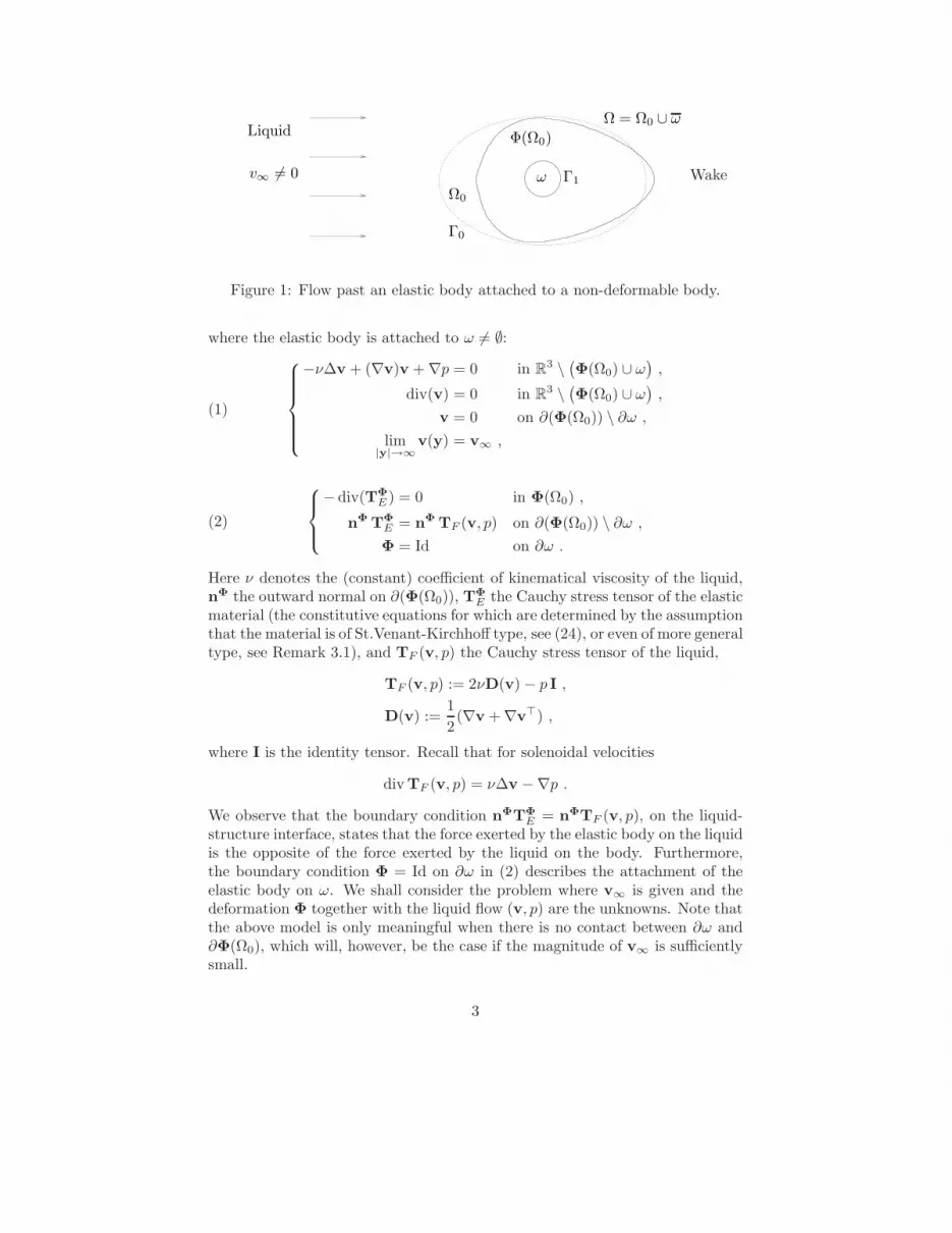
In the case where B is attached to S, we assume they together occupy abounded domain, Ω ⊂ R3, when no applied body or surface forces act on them.We shall denote by ω ⊂ Ω the part occupied by S and by Ω0 = Ω \ ω thatoccupied by B. We assume that B completely sourrounds S, so that ∂ω∩∂Ω = ∅.We shall refer to Ω0 as the reference domain of the elastic body and supposethat Ω0 and ω are of class C2. For simplicity, we contemplate the case where ωis a (bounded) domain 2, and will refer to a coordinate system with the originat some point 0 ∈ ω. We also set Γ0 := ∂Ω and Γ1 := ∂ω; see Figure 1.
If we denote by Φ : Ω0 → R3 the resulting deformation of B due to the forcesexerted on it by the steady flow (v, p) past it, we find that the motion of thecoupled system liquid-solid is governed by the following equations, in the case
1For steady bifurcation results of a steady-state flow of a Navier-Stokes liquidpast a rigid body we refer to [10].
2The case where ω is the union of more than one domain does not introduceany conceptual difficulty.
2
Ω0
ω
Liquid
v∞ 6= 0 WakeΓ1
Φ(Ω0)
Ω = Ω0 ∪ ω
Γ0
Figure 1: Flow past an elastic body attached to a non-deformable body.
where the elastic body is attached to ω 6= ∅:
(1)
−ν∆v + (∇v)v + ∇p = 0 in R3 \
(
Φ(Ω0) ∪ ω)
,
div(v) = 0 in R3 \
(
Φ(Ω0) ∪ ω)
,
v = 0 on ∂(Φ(Ω0)) \ ∂ω ,
lim|y|→∞
v(y) = v∞ ,
(2)
− div(TΦE ) = 0 in Φ(Ω0) ,
nΦ TΦE = nΦ TF (v, p) on ∂(Φ(Ω0)) \ ∂ω ,
Φ = Id on ∂ω .
Here ν denotes the (constant) coefficient of kinematical viscosity of the liquid,nΦ the outward normal on ∂(Φ(Ω0)), TΦ
E the Cauchy stress tensor of the elasticmaterial (the constitutive equations for which are determined by the assumptionthat the material is of St.Venant-Kirchhoff type, see (24), or even of more generaltype, see Remark 3.1), and TF (v, p) the Cauchy stress tensor of the liquid,
TF (v, p) := 2νD(v) − p I ,
D(v) :=1
2(∇v + ∇v⊤) ,
where I is the identity tensor. Recall that for solenoidal velocities
div TF (v, p) = ν∆v −∇p .
We observe that the boundary condition nΦTΦE = nΦTF (v, p), on the liquid-
structure interface, states that the force exerted by the elastic body on the liquidis the opposite of the force exerted by the liquid on the body. Furthermore,the boundary condition Φ = Id on ∂ω in (2) describes the attachment of theelastic body on ω. We shall consider the problem where v∞ is given and thedeformation Φ together with the liquid flow (v, p) are the unknowns. Note thatthe above model is only meaningful when there is no contact between ∂ω and∂Φ(Ω0), which will, however, be the case if the magnitude of v∞ is sufficientlysmall.
3

Ω0
Liquid
v∞ 6= 0 Wake
Γ0
Φ(Ω0)f
g
Ω = Ω0
Figure 2: Flow past an elastic body with control forces f and g.
In the case where the elastic body is kept in place by control forces, f , andsurface tractions, g, we shall use the same notation as above and simply assumethat ω = ∅. In principle, the control parameters f and g can be chosen in anvariety of ways. We shall make the following “simplest” choice
(3) f = c , g = k ∧ n ,
where c,k ∈ R3 and n is the unit outer normal to Ω0; see Figure 2. Of course,the vectors c and k are further unknowns of the problem. Note that our choiceof control parameters in (3) are expressed as forces in the reference domain Ω0
and ∂Ω0. Thus, the equations governing the equilibrium of B in this case are
(4)
− div(TΦE ) = (det∇Φ−1) c in Φ(Ω0) ,
nΦ TΦE = nΦ TF (v, p) + k ∧ (cof ∇Φ−1nΦ) on ∂(Φ(Ω0)) ,
while those governing the motion of L remain the same, and we are led to studythe coupled systems (1) and (4).
For simplicity, in the models above we have assumed that all prescribed bodyforces, b, and surface tractions, t, are equal to zero. In fact, our results, suit-ably restated, continue to hold with non-zero b and t. Also, we have chosen toconsider the no-slip boundary condition v = 0 on the liquid-structure surface,as this is the most interesting situation from a physical point of view. With-out further difficulties, however, more general boundary conditions could behandled.
Our main result is a proof of existence and uniqueness of solutions for thecoupled systems (1)+(2) and for the coupled systems (1)+(4). More precisely,we show that if |v∞| is below a certain quantity, depending on Ω0 and on thematerial constants characterizing L and B, there is one and only one solutionlying in a ball, centered at the origin of a suitable Banach space, whose radiuscontinuously depends on |v∞|.
The above result is obtained by a fixed point contraction argument based ona priori estimates for proper linearizations of the governing equations. Beingv∞ 6= 0, the “natural” linearization of the Navier-Stokes equations is provided
4

by the Oseen equations. Actually, the basic challenge of our approach residesin finding the appropriate function space, S, where the estimates to the fullynon-homogeneous, exterior Oseen boundary-value problem need to be proved.It turns out that S can be chosen as the intersection of suitable Lebesgue andhomogeneous Sobolev spaces; see Lemma 4.1.
Without loss of generality, we shall take v∞ directed along the unit vectore1 and write v∞ = v∞e1 with v∞ > 0.
Remark 1.1. The arbitrary constant up to which the pressure p is defined in(1) is fixed by requiring that p(y) → 0 as |y| → ∞. In other words, we fix theconstant equal to zero. We could fix the constant to be any non-zero number, p0,if we adjust our assumptions on the reference configuration accordingly. Moreprecisely, since p0 determines the force exerted by the liquid on the elastic bodywhen the liquid is at rest, the reference configuration must be assumed to be thedomain occupied by the elastic body when the force determined by p0 is exertedon it.
Remark 1.2. If ω = ∅, that is, if the body does not have a clamped portion of itsboundary, and we were not to introduce any control forces, the liquid-structureproblem would not have a solution. Actually, if ω = ∅ it follows that
0 =
∫
Φ(Ω0)
div(TΦEe1) dy =
∫
∂Φ(Ω0)
nΦ TΦEe1 dS
=
∫
∂Φ(Ω0)
nΦ TF (v, p)e1 dS .
This relation shows that the component of the force exerted by the liquid on thebody in the direction of v∞ (the drag) is zero, a condition that can not be verified(see [9, Theorem IX.5.1]).
The plan of the paper is the following. In Section 2 we introduce the ba-sic notation and prove some preparatory results. Successively, in Section 3, wereformulate the liquid-body problem in the reference configuration. In Section4 we prove existence, uniqueness, and fundamental estimates for the exteriorOseen boundary-value problem in proper function spaces. With the aid of theseresults, we prove similar ones for the fully non-linear exterior Navier-Stokesboundary-value problem. In Section 5, we recall a well-known well-posednesstheorem for the elasticity equations in Sobolev spaces and prove further esti-mates for corresponding solutions. Finally, in Section 6, we combine the resultsof the previous two sections and use the fixed point contraction lemma to showexistence and (local) uniqueness of solutions to the stated liquid-solid problems.
5

2 Notation and Preliminary Considerations.
We begin to recall some classical notation and differential identities. If A,Bdenote second-order tensors in R
3, we set 3
AB = AilBlj ei ⊗ ej ,
where Aik and Blj , i, j, l, k = 1, 2, 3, are the components of A and B in thecanonical base, e1, e2, e3, of R3, and ⊗ denotes dyadic product. Moreover, ifa is a vector with components ai, i = 1, 2, 3, in that base, we set Aa = Aikakei
and aA = Aikaiek. We also define
div A =∂Aij
∂xiej and ∇a =
∂ai
∂xkei ⊗ ek .
We shall use boldface letters to denote vectors and tensors as well as vector-and tensor-valued functions in R3.
Let χ : x ∈ R3 7→ y = χ(x) ∈ R3 be a diffeomorphism of class C1 from R3
onto itself. Thus, setting
F := ∇χ and J := detF
we have (see for example [3])
div(J F−1 A) = J divyA ,(5)
div(J F−1a) = J divy a ,(6)
(∇a)F−1 = ∇ya .(7)
If, in (5), we choose A = I, with I denoting the identity tensor, we obtain thePiola identity
div(J F−1) = 0 .
We shall denote by Wm,q(Ω) the classical non-homogeneous Sobolev spacesand by ‖·‖m,q,Ω the associated norm. When no confusion can arise, we shallsimply write ‖·‖m,q. By Dm,q(Ω) we denote the homogeneous Sobolev spacesdefined by
Dm,q(Ω) := u ∈ L1loc(Ω) | |u|m,q :=
(
∑
|α|=m
∫
Ω
|Dαu|qdx
)1
q
<∞ .
We use D1,q0 (Ω) to denote the completion of C∞
c (Ω) with respect to the norm| · |1,q. Moreover, we use D−1,q(Ω) to denote the dual of the space D1,q′
0 (Ω)with 1 = 1
q + 1q′ . Finally, we shall denote by CB(Ω) the subspace of C(Ω) of
bounded functions. Depending on the context, the function spaces may consistof vector-valued functions.
3Throughout this paper, we shall use the summation convention over re-peated indexes.
6

Next consider u ∈ C1(Ω; R3) and define
Φu : x ∈ Ω 7→ x + u(x) ∈ R3 .
We shall usually denote by u a displacement vector-field of Ω, in which case werefer to Φu as the corresponding deformation of Ω. We now seek to construct,based on u, a mapping deforming the exterior domain E := R3 \ Ω accordingly.To this end, set
Sq,M (Ω) := u ∈ W 2,q(Ω) | ‖u‖2,q,Ω ≤M .
The following lemma holds.
Lemma 2.1. Let q > 3 and let Ω ⊂ R3 be a bounded, Lipschitz domain.Moreover, let BR ⊃ Ω and set δ := dist(∂BR, ∂Ω). Then, there is a K0 =K0(q,Ω, δ) > 0 4 such that for any u ∈ Sq,M (Ω) with 0 ≤ M < K0 we can finda function u ∈W 2,q(R3) ∩ C1(R3) satisfying
u = u in Ω ,(8)
u(x) = 0 for all x ∈ R3 \BR ,(9)
‖u‖2,q,R3 ≤ C0 ‖u‖2,q,Ω with C0 = C0(q,Ω, δ) ,(10)
χu(x) := x + u is a C1-diffeomorphism from E onto R3 \ Φu(Ω).(11)
Proof. For any given u ∈ Sq,M (Ω), we construct the extension u as follows. LetU be an extension of u to R3 with U ∈ W 2,q(R3). By classical results, we knowthat U exists and that
(12) ‖U‖2,q,R3 ≤ c0 ‖u‖2,q,Ω
with c0 = c0(q,Ω) > 0. Let us next choose r < R such that Ω ⊂ Br ⊂ BR, withR − r = δ/2, and let ψ = ψ(x) be a smooth cut-off function that is equal to 1for x ∈ Br and is zero for x ∈ Bc
R. This function can be chosen in such a waythat |Dψ(x)| ≤ c1δ
−1, |D2ψ(x)| ≤ c2δ−2, where ci, i = 1, 2, are independent
of δ, R and r. The desired extension is then given by u := ψU. In fact, (8)and (9) are obviously satisfied, whereas (10) is a consequence of (12) and of theproperties of the function ψ. Consider now the map
χu : x ∈ R3 7→ y = x + u ∈ R
3 .
By the Sobolev embedding theorem we have W 2,q(R3) → C1(R3), and that
‖u‖C1(R3) ≤ c3‖u‖2,q,R3 ,
with c3 = c3(q) > 0. From this, it follows, in particular, that χu ∈ C1(R3).Furthermore, from (10) and from the fact that u ∈ Sq,M (Ω0), we obtain
(13) ‖u‖C1(R3) ≤ c4M ,
4K0 → 0 as δ → 0.
7

and so, since
(14) ∇χu = I + ∇u ,
we have
det(∇χu(x)) =
3∏
j=1
(1 + ∂j uj) +∑
σ∈S3\Id
3∏
j=1
(I + ∇u)jσ(j)
= 1 +∑
j∈A
Mj(∇u) ,
with Mj(∇u) a mononomial with respect to the entries of ∇u and |A| = 12.Thus, if the constant K0 is chosen as small as to satisfy the condition
(15) K0 <1
12 c4
then
(16) det(∇χu(x)) > 1 − 12 c4K0 > 0 .
From [5, Theorem 5.5 -1(b)] and (13)-(14), we then find that χu is injective. Infact, it is easy to show that χu is surjective which, in turn, since χu = Φu onΩ, implies that χu is a diffeomorphism of class C1 of E onto R
3 \ Φu(Ω). Toshow surjectivity, for any fixed y ∈ R3, consider the map
P : x ∈ R3 7→ y − u(x) ∈ R
3 .
We have, by (13), that P ∈ C1(R3) and moreover, by (15), that
supx∈R3
|∇P(x)| < 1 .
Therefore, by well-known results (see for example [14, Theorem 1.XVII]) itfollows that P has a fixed point. This proves that χu is surjective, and theproof of the lemma is thereby completed.
Throughout this paper we shall use small letters (c0, c1, . . .) to denote con-stants in scope of a single proof, and capital letters (C0, C1, . . .) to denote con-stants in scope of the whole paper.
For any exterior domain O we set OR := O ∩BR(0) and OR := O \BR(0).Similarly, for any Banach space X we put XR := x ∈ X | ‖x‖ ≤ R.
We shall from now on fix Ω, Ω0, and ω to be the C2-domains from theintroduction. Moreover, we set E := R3 \Ω and fix R > 0 such that BR(0) ⊃ Ωand put δ := dist(∂BR(0), ∂Ω).
We shall make use of the Landau symbols (Big-O and Little-o notation) in
the sense that f ∈ O(t) iff |f | ≤ C|t| as t→ 0 and f ∈ o(t) iff |f ||t| → 0 as t→ 0.
8

3 Reformulation of the Problem in the Refer-
ence Configuration.
In order to solve (1) coupled with either (2) or (4), we first transform the systemsinto equivalent systems over the reference domain. For this purpose we use themapping constructed in Lemma 2.1. Writing the deformation as the identityplus a displacement field, Φ = Id +u, the corresponding mapping χu, fromLemma 2.1, maps the reference exterior domain E := R3 \
(
Ω0 ∪ ω)
onto the
deformed exterior domain R3 \(
Φ(Ω0) ∪ ω)
. Set y = χu(x),
w = w(x) := v(χu(x)) , p = p(x) := p(χu(x)) ,
andFu := ∇χu , Ju := detFu .
With the help of (5)-(7) we then find
(∇yv)v = (∇w)F−1u w ,(17)
D(v) =1
2[(∇w)F−1
u + F−⊤u (∇w)⊤] := Du(w) ,(18)
divy T(v, p) = J−1u div
[
2νJu F−1u Du(w)
]
− J−1u div(Ju F−1
u pI) ,(19)
div(JuF−1u ∇wF−1
u ) = Ju∇y divy v .(20)
Using (5), (6), (17), (19), and (20) we now obtain that the Navier-Stokes equa-tions (1) can be written over the reference domain as
(21)
−ν div(AuF−⊤u ∇w⊤) + div(AupI) + (∇w)Auw = 0 in E ,
div(Auw) = 0 in E ,
w = 0 on Γ0 ,
lim|x|→∞
w = v∞ ,
wherebyAu := Ju F−1
u = (cof Fu)⊤.
When q > 3, W 1,q(E) is a Banach algebra. In this case the equations in (21)become well-defined in a Sobolev space setting for u ∈ W 2,q(Ω) since the entriesof Fu, and thereby also the those of Au, then belong to W 1,q
loc (E) by Lemma 2.1.Also note that the asymptotic limits at infinity of w and v are identical sinceχu(x) = 1 for large |x|.
Introducing the first Piola-Kirchhoff stress tensor σ(u), and using the PiolaIdentity, we can write the elasticity equation (2) over the reference domain as
(22)
− div(σ(u)) = 0 in Ω0 ,
nσ(u) = nTuF (w, p) on Γ0 ,
u = 0 on Γ1 ,
9

where n is the outward normal on ∂E and
TuF (w, p) = Au(2νDu(w) − pI) .
Similarly, we can write (4) over the reference domain as
(23)
− div(σ(u)) = c in Ω0 ,
nσ(u) = nTuF (w, p) + k ∧ n on Γ0 .
We assume the elastic body is a St.Venant-Kirchhoff material, for which thefirst Piola-Kirchhoff stress tensor takes the form
σ(u) = (λ(TrE(u))I + 2µE(u))(I + ∇u)⊤ , with
E(u) =1
2(∇u⊤ + ∇u + ∇u⊤∇u)
(24)
and λ and µ denoting the Lame constants. We can write the first Piola-Kirchhoffstress tensor above as a sum of a linear, bi-linear, and tri-linear response func-tion,
(25) σ(u) = σL(∇u) + σBL(∇u,∇u) + σT L(∇u,∇u,∇u) ,
with σL : R3×3 → R3×3 linear, σBL : R3×3 × R3×3 → R3×3 bi-linear, andσT L : R3×3 × R3×3 × R3×3 → R3×3 tri-linear. Note that σL is the responsefunction for the classical stress tensor of linear elasticity.
In the following, we show existence of a solution for the coupled systems(1)+(2) and the systems (1)+(4) by solving the equivalent systems (21)+(22)and (21)+(23), respectively.
Remark 3.1. We have chosen to consider a St.Venant-Kirchhoff material be-cause it is one of the most widely used models in applications of nonlinear elas-ticity. Without significant modfictions to the proofs, however, we can also treatother constitutive models. For example, our results continue to hold for the mostgeneral types of constitutive equations of homogeneous, isotropic, elastic mate-rials. In fact, we only need to impose structural conditions on σ which ensurethat the reference configuration is natural, the linearized elasticity equations areelliptic in the sense Agmon-Douglis-Nirenberg and uniquely solvable, and thatthe nonlinear part of the response function is contractive around the rest state(for example only consists of higher order terms of ∇u).
4 The Liquid Equations
In this section, we shall show that the liquid equations (21) over the reference do-main have a unique solution (in suitable function class), provided u ∈ Sq,M (Ω0)and v∞ and M are sufficiently small. We shall also establish some estimates forthe corresponding solutions.
10
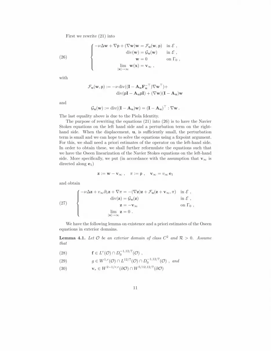
First we rewrite (21) into
(26)
−ν∆w + ∇p + (∇w)w = Fu(w, p) in E ,
div(w) = Gu(w) in E ,
w = 0 on Γ0 ,
lim|x|→∞
w(x) = v∞ ,
with
Fu(w, p) := −ν div((I − AuF−⊤u )∇w⊤)+
div(pI − AupI) + (∇w)(I − Au)w
andGu(w) := div((I − Au)w) = (I − Au)⊤ : ∇w .
The last equality above is due to the Piola Identity.The purpose of rewriting the equations (21) into (26) is to have the Navier
Stokes equations on the left hand side and a perturbation term on the right-hand side. When the displacement, u, is sufficiently small, the perturbationterm is small and we can hope to solve the equations using a fixpoint argument.For this, we shall need a priori estimates of the operator on the left-hand side.In order to obtain these, we shall further reformulate the equations such thatwe have the Oseen linearization of the Navier Stokes equations on the left-handside. More specifically, we put (in accordance with the assumption that v∞ isdirected along e1)
z := w − v∞ , π := p , v∞ = v∞ e1
and obtain
(27)
−ν∆z + v∞∂1z + ∇π = −(∇z)z + Fu(z + v∞, π) in E ,
div(z) = Gu(z) in E ,
z = −v∞ on Γ0 ,
lim|x|→∞
z = 0 .
We have the following lemma on existence and a priori estimates of the Oseenequations in exterior domains.
Lemma 4.1. Let O be an exterior domain of class C2 and R > 0. Assumethat
f ∈ Lr(O) ∩D−1,12/70 (O) ,(28)
g ∈W 1,r(O) ∩ L12/7(O) ∩D−1,12/70 (O) , and(29)
v∗ ∈W 2−1/r,r(∂O) ∩W 5/12,12/7(∂O)(30)
11

for some r ∈ (1,∞). Then the problem
(31)
−∆v + R∂1v + ∇p = f in O ,
div v = g in O ,
v = v∗ on ∂O ,
lim|x|→∞
v = 0
has one and only one solution (v, p) such that
(32) (v, p) ∈ D2,r(O) ∩D1,12/7(O) ∩ L4(O) ∩ L3(O) ×D1,r(O) ∩ L12/7(O) .
Moreover, for any arbitrarily fixed R0 > 0, there exists CΘ = CΘ(O,R0, r) > 0such that for any 0 < R ≤ R0 the corresponding solution of (31) satisfies
|v|2,r+|v|1,12/7 + ‖v‖4 + R1/4 ‖v‖3 + |p|1,r + ‖p‖12/7 ≤
CΘ
(
‖f‖r + |f |−1,12/7 + ‖g‖1,r + ‖g‖12/7 + |g|−1,12/7
+ ‖v∗‖2−1/r,r,∂O + ‖v∗‖5/12,12/7,∂O
)
.
(33)
Proof. Uniqueness in the class (32) follows from standard results (see [8, The-orem VII.6.2] and [8, Exercise VII.6.2]). Existence of a solution in a largerclass than (32) also follows from standard results (see for example [8, TheoremVII.7.2]). Thus we only need to verify that (33) holds. Consider first a solutionof the whole space problem
−∆w + R∂1w + ∇p = f in R3 ,
div w = g in R3 ,
lim|x|→∞
w = 0 ,
with data satisfying (28) with R3 as underlying domain instead of O. From [8,Theorem VII.4.1] we obtain the estimate
(34) |w|2,r,R3 + |p|1,r,R3 ≤ c0(R0) (‖f‖r,R3 + ‖g‖1,r,R3)
and from [8, Theorem VII.4.2] the estimate
(35) R1/4‖w‖3 + |w|1,12/7 + ‖p‖12/7 ≤
c1(R0) (|f |−1,12/7 + |g|−1,12/7 + ‖g‖12/7) .
Using the same technique (using cut-off functions) as in the proof of [8, TheoremVII.7.1] and [8, Theorem VII.7.2], we obtain from (34) and (35) that the solutionof the exterior domain problem (31) satisfies the estimates
(36) |v|2,r,Oρ/2 + |p|1,r,Oρ/2 ≤ c2(R0)(‖f‖r + ‖g‖1,r + ‖v‖1,r,Oρ + ‖p‖r,Oρ)
12

and
R1/4‖v‖3,Oρ/2 + |v|1,12/7,Oρ/2 + ‖p‖12/7,Oρ/2 ≤
c3(R0) (|f |−1,12/7 + |v|−1,12/7,Oρ+ |∇v|−1,12/7,Oρ
+ |p|−1,12/7,Oρ
+ |g|−1,12/7 + ‖g‖12/7 + ‖v‖12/7,Oρ) ,
(37)
whereby the constant ρ > 0 is chosen such that Oc⊂ Bρ/2. Using now the
embedding L12/11(Oρ) → D−1,12/70 (Oρ) and the fact that 12/11 ≤ 12/7, it
follows that |v|−1,12/7,Oρ≤ c4‖v‖12/7,Oρ
. Hence we can reduce (37) to
R1/4‖v‖3,Oρ/2 + |v|1,12/7,Oρ/2 + ‖p‖12/7,Oρ/2 ≤
c5(R0) (|f |−1,12/7 + |g|−1,12/7 + ‖g‖12/7
+ |p|−1,12/7,Oρ+ ‖v‖12/7,Oρ
) .
(38)
Now we seek similar estimates over Oρ. By ellipticity of the Stokes operator(see [8, Theorem IV.6.1] and [8, Exercise IV.6.2]) we have
‖v‖2,r,Oρ+‖p‖1,r,Oρ ≤ c6 (‖f‖r,Oρ + ‖g‖1,r,Oρ + ‖v∗‖2−1/r,r,∂O
+ ‖v‖2−1/r,r,∂Bρ+ ‖v‖r,Oρ + R‖∂1v‖r,Oρ + ‖p‖r,Oρ)
(39)
and
‖v‖1,12/7,Oρ+ ‖p‖12/7,Oρ
≤
c7(R0) (|f |−1,12/7,Oρ+ ‖g‖12/7,Oρ
+ ‖v∗‖5/12,12/7,∂O
+ ‖v‖5/12,12/7,∂Bρ+ ‖v‖12/7,Oρ
+ ‖p‖−1,12/7,Oρ).
(40)
By [8, Theorem II.3.4] we have
(41) ‖v‖2−1/r,r,∂Bρ≤ c8 (|v|2,r,Oρ/2 + ‖v‖1,r,Oρ)
and
(42) ‖v‖5/12,12/7,∂Bρ≤ c9 (|v|1,12/7,Oρ/2 + ‖v‖12/7,Oρ
) .
By the embedding W 1,12/7(Oρ) → L4(Oρ) we furthermore have
(43) ‖v‖3,Oρ/2≤ c10 ‖v‖1,12/7,Oρ/2
.
Finally, from the embedding D1,12/7(O) → L4(O) we obtain
(44) ‖v‖4 ≤ c11 |v|1,12/7 .
Combining now (36), (38), and (39)-(44) yields
|v|2,r + |v|1,12/7 + ‖v‖4 + R1/4 ‖v‖3 + |p|1,r + ‖p‖12/7 ≤
c12(R0) (‖f‖r + |f |−1,12/7 + ‖g‖1,r + ‖g‖12/7 + |g|−1,12/7
+ ‖v∗‖2−1/r,r,∂O + ‖v∗‖5/12,12/7,∂O
+ ‖v‖1,r,Oρ + ‖p‖r,Oρ + ‖v‖12/7,Oρ+ |p|−1,12/7,Oρ
) .
(45)
13

We will now show that
‖v‖1,r,Oρ + ‖p‖r,Oρ + ‖v‖12/7,Oρ+ |p|−1,12/7,Oρ
≤
C(R0) (‖f‖r + |f |−1,12/7 + ‖g‖1,r + ‖g‖12/7 + |g|−1,12/7
+ ‖v∗‖2−1/r,r,∂O + ‖v∗‖5/12,12/7,∂O) ,
(46)
which together with (45) implies (33). Assume there exists no constant C(R0)such that (46) holds for all solutions of (31). This would imply the existence ofsequences
fk , gk ⊂ C∞c (O) , v∗k ⊂W 2−1/r,r(∂O) ∩W 5/12,12/7(∂O) ,
andRk ⊂ (0,R0] , (k = 1, 2, . . .) ,
such that, denoting by (vk, pk) the solutions of the Oseen problems
(47)
−∆vk + R∂1vk + ∇pk = fk in O ,
div vk = gk in O ,
vk = v∗k on ∂O ,
lim|x|→∞
vk = 0 ,
the following conditions hold
‖fk‖r+|fk|−1,12/7 + ‖gk‖1,r + ‖gk‖12/7 + |gk|−1,12/7
+ ‖v∗k‖2−1/r,r,∂O + ‖v∗k‖5/12,12/7,∂O ≤ 1/k ,(48)
‖vk‖1,r,Oρ + ‖vk‖12/7,Oρ+ ‖pk‖r,Oρ + |pk|−1,12/7,Oρ
= 1 ,(49)
and there is an R ∈ [0,R0] such that
limk→∞
Rk = R .
Since (vk, pk) are solutions of (47), they satisfy (45). By (48) and (49) thisimplies that (vk, pk) are bounded in the norms on the left hand side of (45).Thus we can find subsequences, still denoted by (vk, pk), and functions (v, p)in the class (32) such that, as k → ∞,
D2vk → D2v and ∇pk → ∇p weakly in Lr(O) ,
vk → v weakly in L4(O) , and
∇vk → ∇v and pk → p weakly in L12/7(O) .
(50)
By standard compact embeddings of Sobolev spaces we further obtain
vk → v strongly in W 1,r(Oρ) and L12/7(Oρ) , and
pk → p strongly in Lr(Oρ) and W−1,12/7(Oρ) .(51)
14

From (47)-(51) we conclude that (v, p) and R satisfy the conditions
(52)
−∆v + R∂1v + ∇p = 0 in O ,
div v = 0 in O ,
v = 0 on ∂O ,
lim|x|→∞
v = 0 ,
(53) v ∈ D1,12/7(O) , p ∈ L12/7(O) ,
and
(54) ‖v‖1,r,Oρ + ‖v‖12/7,Oρ+ ‖p‖r,Oρ + ‖p‖−1,12/7,Oρ
= 1 .
However, by classical uniqueness theorems for the Oseen (if R > 0) and Stokes(if R = 0) exterior problems (see [8, Theorem VII.6.2, Exercise VII.6.2 andTheorem V.5.1]), (52) and (53) implies v ≡ 0 and p ≡ 0, which contradicts(54). The proof of the lemma is thus completed.
In order to formulate the next results, we find it convenient to define anumber of Banach spaces. For any given v∞ > 0, we set
ZqF (E) := z ∈ L1
loc(E) | ‖z‖ZqF<∞ ,
whereby
(55) ‖z‖ZqF
:= |z|2,q + |z|1,12/7 + ‖z‖4 + v1/4∞ ‖z‖3 .
It is obvious that (55) defines a norm in ZqF (E) and that Zq
F (E), equipped withthis norm, becomes a Banach space. Likewise, set
PqF (E) := p ∈ L1
loc(E) | ‖p‖PqF<∞ ,
whereby
(56) ‖p‖PqF
:= |p|1,q + ‖p‖12/7 .
The space PqF (E) equipped with the norm (56) becomes a Banach space. We
also set
X qF (E) := Zq
F (E) × PqF (E) , ‖(z, p)‖X q
F:= ‖z‖Zq
F+ ‖p‖Pq
F.
Furthermore, we define
YqF (E) := f ∈ L1
loc(E) | ‖f‖YqF<∞ ,
whereby‖f‖Yq
F:= |f |−1,12/7 + ‖f‖q ,
15

andQq
F (E) := g ∈ L1loc(E) | ‖g‖Qq
F<∞ ,
whereby‖g‖Qq
F:= |g|−1,12/7 + ‖g‖12/7 + ‖g‖1,q .
In order to solve (27), we need to estimate all the terms on the right handside. We start with the convective term.
Lemma 4.2. Let q > 3 and z1, z2 ∈ ZqF (E). Then there are constants C1 =
C1(E , q) > 0 and C2 = C2(E) > 0 such that
‖(∇z1)z2‖q ≤ C1 ‖z1‖ZqF‖z2‖Zq
F(57)
|(∇z1)z2|−1,12/7 ≤ C2 v−1/4∞ ‖z1‖Zq
F‖z2‖Zq
F(58)
Proof. We recall the property that if h ∈ Lr(E) ∩D1,q(E), for some r ≥ 1, thenh ∈ L∞(E) and the following inequality holds
(59) ‖h‖∞ ≤ c1 (‖h‖r + |h|1,q) ,
where c1 = c1(E , r, q) > 0 (see for example [8, Remark II.7.2]). Let z ∈ ZqF (E).
From (59), with r = 12/7, it easily follows that
|z|1,q ≤ |z|12/7q1,12/7‖∇z‖1−12/7q
∞
≤ c2 |z|12/7q1,12/7(|z|1,12/7 + |z|2,q)
1−12/7q ≤ c3‖z‖ZqF,
(60)
with ci = ci(E , q) > 0, i = 2, 3. Using again (59), with r = 4, and (60) we alsodeduce
(61) ‖z‖∞ ≤ c4 (‖z‖4 + |z|1,q) ≤ c5‖z‖ZqF,
where ci = ci(E , q) > 0, i = 4, 5. Thus, by (60) and (61), we find, for somec6 = c6(E , q) > 0,
‖(∇z1)z2‖q ≤ ‖z2‖∞|z1|1,q ≤ c6 ‖z1‖ZqF‖z2‖Zq
F,
which proves (57).
Consider now ψ ∈ D1,12/50 (E). By the Holder inequality and by (55), we
obtain
|((∇z1)z2, ψ)| ≤ ‖z2‖3|z1|1,12/7‖ψ‖12
≤ v−1/4∞ ‖z1‖Zq
F‖z2‖Zq
F‖ψ‖12.
Therefore, (58) follows from the latter and from the continuity of the embedding
D1,12/50 (E) → L12(E).
Having estimated the convective term on the right-hand side of (27), we moveon to the perturbation terms. To this end we need the following estimates.
16

Lemma 4.3. Let q > 3 and K0 be as in Lemma 2.1. For u1,u2 ∈ Sq,M (Ω0)with M <M0 := minK0, 1 the following properties hold:
1. The entries of F−1ui
and Aui are in W 1,q(Bρ) for all ρ > 0 (i = 1, 2).
2. There exists a constant C3 = C3(q,Ω0,K0, R, δ) > 0 such that
(62) ‖I− Aui‖1,q,E + ‖I− AuiF−⊤ui
‖1,q,E ≤ C3‖ui‖2,q,Ω0, i = 1, 2 .
3. There exists a constant C4 = C4(q,Ω0,K0, R, δ) > 0 such that
(63) ‖Au1F−⊤
u1− Au2
F−⊤u2
‖1,q,E + ‖Au1− Au2
‖1,q,E
≤ C4‖u1 − u2‖2,q,Ω0.
Proof. Put u = ui, i = 1, 2. By definition, Fu = I + ∇u and u ∈ W 2,q(R3).Since q > 3, W 1,q(Bρ) is a Banach algebra. It follows that the entries of cof(Fu)and hence of Au are in W 1,q(Bρ). Moreover, by Lemma 2.1 the entries of Fu
are continuous, and from (16) we have the pointwise estimate
(64) det(Fu) > c0(K0) > 0.
Since
(65) F−1u =
1
det(Fu)(cof(Fu))⊤ ,
it follows that the entries of F−1u are in Lq(Bρ). Denoting by inv : GL3,3(R) →
M3,3(R) the inversion mapping inv(A) = A−1 and using that 〈∂inv(A), H〉 =−A−1HA−1, we find that
∂i[F−1u ] = ∂i[inv(Fu)]
= −F−1u (∂iFu)F−1
u =1
det(Fu)2(cof Fu)⊤(∂iFu)(cof Fu)⊤.
(66)
Using (64) and the fact that the entries of cof Fu are in CB(Bρ) (due to theembedding W 1,q(Bρ) → CB(Bρ)) we obtain that also the entries of ∂i[F
−1u ] are
in Lq(Bρ). Thus we conclude that the entries of F−1u are in W 1,q(Bρ).
We now estimate
‖I− Au‖21,q = ‖δij − cof(I + ∇u)ji‖
21,q
= ‖1 − cof(I + ∇u)ii‖21,q +
∑
i6=j
‖cof(I + ∇u)ji‖21,q
= ‖1 − det(I + ∇u)ii‖21,q +
∑
i6=j
‖det(I + ∇u)ji‖21,q
=3
∑
i=1
‖1 − (1 + Mi(∇u))‖21,q +
∑
i6=j
‖Mij(∇u)‖21,q ,
(67)
17

with M(∇u) denoting a mononomial with respect to the entries of ∇u. Usingthat ‖u‖2,q ≤ c1 ‖u‖2,q,Ω0
and the fact that, by assumption, ‖u‖2,q,Ω0< 1, we
obtain
(68) ‖I− Au‖21,q ≤ c2 ‖u‖
22,q,Ω0
.
Regarding the second term in (62), we have the estimate
‖I − AuiF−⊤ui
‖1,q = ‖(F⊤u − I + I− Au)F−⊤
u ‖1,q
≤ c3(
‖Fu − I‖1,q + ‖I − Au‖1,q
)
‖F−1u ‖1,q .
(69)
Since ‖Fu− I‖1,q = ‖∇u‖1,q ≤ c4 ‖u‖2,q,Ω0, we just need to show that ‖F−1
u ‖1,q
is bounded. From (64), (65), and (66) we obtain, using the Sobolev embeddingW 1,q(BR) → CB(BR), that
‖F−1u ‖1,q ≤ c5 M(1 + ‖∇u‖1,q) ≤ c6(Ω0, δ, R,K0, q) ,
which together with (69) and (68) implies (62).The last inequality, (63), can be proved in completely similar fashion.
We can now estimate the perturbation terms in (27). More specifically, wehave the following lemma.
Lemma 4.4. Let q > 3 and M0 be as in Lemma 4.3. For ui ∈ Sq,M (Ω0) with0 < M < M0 and (zi, πi) ∈ X q
F (E) (i = 1, 2), the following inequalities hold:
‖Fui(zi + v∞, πi)‖YqF≤
C5M(
(1 + |v∞|)‖(zi, πi)‖X qF
+ ‖(zi, πi)‖2X q
F
)
,(70)
(71) ‖Gui(zi)‖QqF≤ C5M ‖(zi, πi)‖X q
F,
‖Fu1(z1 + v∞, π1) −Fu2
(z2 + v∞, π2)‖YqF≤
C5
(
M (1 + |v∞|) ‖(z1 − z2, π1 − π2)‖X qF+
‖(zi, πi)‖X qF
(1 + |v∞|) ‖u1 − u2‖2,q,Ω0+
M ‖zi‖ZqF‖z1 − z2‖Zq
F+ ‖zi‖
2Zq
F‖u1 − u2‖2,q,Ω0
)
,
(72)
‖Gu1(z1) − Gu2
(z2)‖QqF≤
C5
(
M‖z1 − z2‖ZqF
+ ‖zi‖ZqF‖u1 − u2‖2,q,Ω0
)
,(73)
where C5 = C5(q,Ω0, R, δ,M0).
Proof. We will only show (72). The other estimates can be shown in a com-pletely similar fashion. First we use the algebraic structure of W 1,q(E), Lemma2.1, and Lemma 4.3 to estimate
‖div(
(I − Au1F−⊤
u1)∇z⊤1 − (I − Au2
F−⊤u2
)∇z⊤2)
‖q,E
≤ c0(
‖Au2F−⊤
u2− Au1
F−⊤u1
‖1,q,E‖∇z1‖1,q,ER+
‖I− Au2F−⊤
u2‖1,q,E‖∇z1 −∇z2‖1,q,ER
)
≤ c1(
‖u1 − u2‖2,q,Ω0‖z1‖Zq
F+M‖z1 − z2‖Zq
F
)
.
18
By similar arguments, and using (59), we furthermore obtain
‖div((π1I−Au1π1I) − (π2I − Au2
π2I))‖q,E ≤
c2 (‖u1 − u2‖2,q,Ω0‖π1‖Pq
F+M‖(z1 − z2, π1 − π2)‖X q
F) .
Next we use the embedding W 1,q(BR) → CB(BR), the fact that the support of(I − Aui) is in BR, and Lemma 4.2 to obtain
‖(∇z1)(I−Au1)(z1 + v∞) − (∇z2)(I − Au2
)(z2 + v∞)‖q,E ≤
c3(
M‖z1 − z2‖ZqF(‖z1‖Zq
F+ v∞)+
‖u1 − u2‖2,q,Ω0‖z1‖
2Zq
F+
‖u1 − u2‖2,q,Ω0‖z1‖Zq
Fv∞+
M‖z2‖ZqF‖z1 − z2‖Zq
F
)
.
We now need similar estimates as above in the norm | · |−1,12/7. However, sinceall the terms on the right-hand side above have bounded support in BR, theseestimates follow from the ones above since for any f with supp f ⊂ BR we have|∂if |−1,12/7 ≤ ‖f‖12/7 ≤ C(R)‖f‖q. Thus, combining all of the above estimateswe have shown (72).
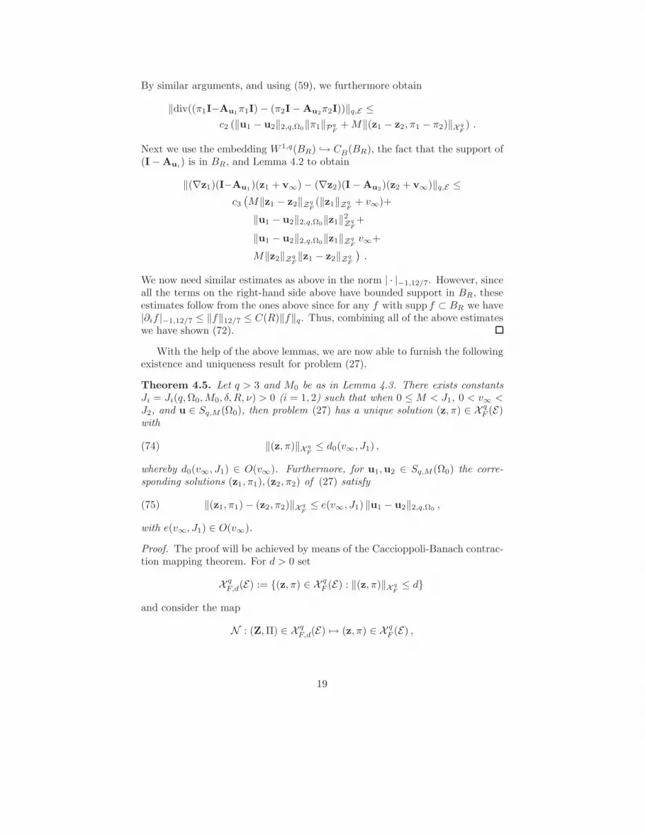
With the help of the above lemmas, we are now able to furnish the followingexistence and uniqueness result for problem (27).
Theorem 4.5. Let q > 3 and M0 be as in Lemma 4.3. There exists constantsJi = Ji(q,Ω0,M0, δ, R, ν) > 0 (i = 1, 2) such that when 0 ≤M < J1, 0 < v∞ <J2, and u ∈ Sq,M (Ω0), then problem (27) has a unique solution (z, π) ∈ X q
F (E)with
(74) ‖(z, π)‖X qF≤ d0(v∞, J1) ,
whereby d0(v∞, J1) ∈ O(v∞). Furthermore, for u1,u2 ∈ Sq,M (Ω0) the corre-sponding solutions (z1, π1), (z2, π2) of (27) satisfy
(75) ‖(z1, π1) − (z2, π2)‖X qF≤ e(v∞, J1) ‖u1 − u2‖2,q,Ω0
,
with e(v∞, J1) ∈ O(v∞).
Proof. The proof will be achieved by means of the Caccioppoli-Banach contrac-tion mapping theorem. For d > 0 set
X qF,d(E) := (z, π) ∈ X q
F (E) : ‖(z, π)‖X qF≤ d
and consider the map
N : (Z,Π) ∈ X qF,d(E) 7→ (z, π) ∈ X q
F (E) ,
19

where (z, π) is a solution to the problem
(76)
−ν∆z + v∞∂1z + ∇π = −(∇Z)Z + Fu(Z + v∞,Π) in E ,
div(z) = Gu(Z) in E ,
z = −v∞ on Γ0 ,
lim|x|→∞
z = 0 .
From Lemma 4.1, Lemma 4.2, and Lemma 4.4 we find that problem (76) has aunique solution (z, π) ∈ X q
F (E), whence N is well-defined. Moreover, by (33),(57), (58), (70), and (71) this solution satisfies the estimate
‖(z, π)‖X qF≤ CΘ(‖(∇Z)Z‖Yq
F+ ‖Fu(Z + v∞,Π)‖Yq
F
+ ‖Gu(Z)‖QqF
+ c0v∞)
≤ CΘ( (C1 + C2v−1/4∞ )‖Z‖2
ZqF
+ C5M((1 + v∞)‖(Z,Π)‖X qF
+ ‖(Z,Π)‖2X q
F)
+ C5M‖(Z,Π)‖X qF
+ c0v∞ ) .
(77)
Choosing J1, J2 < 1 we have both M < 1 and v∞ < 1. Thus, putting
k1(v∞) := CΘ((C1 + C2v−1/4∞ ) + C5)
k2 := 3CΘC5
k3 := CΘc0
we obtain, by (77),
‖(z, π)‖X qF≤ k1(v∞) d2 + k2J1d+ k3v∞ .
It follows that N maps X qF,d(E) into itself if d satisfies
(78) k1(v∞) d2 + (k2J1 − 1) d+ k3 v∞ < 0 .
In order for this inequality to have positive solutions d, we must have
(79) k2J1 − 1 < 0 and (k2J1 − 1)2 > 4 k1(v∞) k3 v∞ .
This is clearly satisfied for J1 and v∞ sufficiently small. Now fix such a J1.Then for v∞ sufficiently small the constant
d0(v∞, J1) :=(1 − k2J1) − (1 − v∞)
√
(k2J1 − 1)2 − 4k1(v∞)k3v∞2k1(v∞)
satisfies (78) and consequently N maps X qF,d0
(E) into itself. Clearly d0 ∈ O(v∞).We now prove that N is also a contraction with the above choice of d0. For
20

(Zi,Πi) ∈ X qF,d0
(E) (i = 1, 2) we use Lemma 4.1, Lemma 4.2, and Lemma 4.4to obtain
‖N (Z1,Π1) −N (Z2,Π2)‖X qF≤
CΘ ( ‖(∇Z1)Z1 − (∇Z2)Z2‖YqF
+ ‖Fu(Z1 + v∞,Π1) −Fu(Z2 + v∞,Π2)‖YqF
+ ‖Gu(Z1) − Gu(Z2)‖QqF
)
≤ CΘ ( 2(C1 + C2v−1/4∞ + C5) d0(v∞) ‖(Z1,Π1) − (Z2,Π2)‖X q
F
+ 3C5J1‖(Z1,Π1) − (Z2,Π2)‖X qF
)
≤ (2 k1(v∞) d0(v∞) + k2 J1) ‖(Z1,Π1) − (Z2,Π2)‖X qF.
(80)
By (79), we have k2J1 < 1. Since furthermore k1(v∞)d0(v∞) → 0 as v∞ → 0, wesee that N becomes a contraction when v∞ is sufficiently small. The existenceof a unique fixpoint for N in X q
F,d0(E) now follows from the Caccioppoli-Banach
Theorem.We end the proof by showing (75). Consider u1,u2 ∈ Sq,M (Ω0) and corre-
sponding solutions (z1, p1), (z2, p2) of (27). Estimating as above, we obtain
‖N (z1, π1) −N (z2, π2)‖X qF≤
≤ (2k1(v∞)d0(v∞) + k2J1)‖(z1, π1) − (z2, π2)‖X qF+
CΘC5(d0(v∞)2 + 2d0(v∞) + d0(v∞)) ‖u1 − u2‖2,q,Ω0,
which completes the proof since N (z1, π1)−N (z2, π2) = (z1, π1)− (z2, π2) andv∞ was chosen above such that 2k1(v∞)d(v∞) + k2J1 < 1.
5 The Elasticity Equations
The objective of this section is to show existence and uniqueness of the elasticityequations. We shall use a fixpoint approach which enables us to easily couplethe elasticity equations with the liquid equations.
Consider first the elasticity equations corresponding to the case where theelastic body Ω0 is attached to a nondeformable body ω. In this case, the de-formation of the elastic body is governed by the traction displacement problemof non-linear elasticity, which we in this section shall treat in the followinggenerality:
(81)
− div(σ(u)) = F(λ,u) in Ω0 ,
nσ(u) = G(λ,u) on Γ0 ,
u = 0 on Γ1 .
We will impose the following conditions on F and G. We assume that for ε,M >0 sufficiently small we can find constants CF (M), CG(M), DF (M), DG(M) > 0,
21
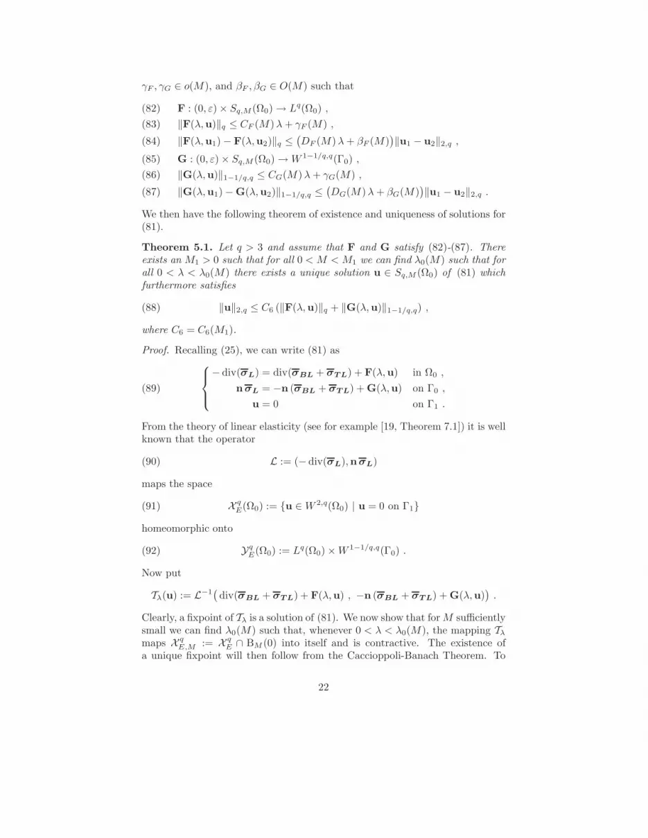
γF , γG ∈ o(M), and βF , βG ∈ O(M) such that
F : (0, ε) × Sq,M (Ω0) → Lq(Ω0) ,(82)
‖F(λ,u)‖q ≤ CF (M)λ+ γF (M) ,(83)
‖F(λ,u1) − F(λ,u2)‖q ≤(
DF (M)λ+ βF (M))
‖u1 − u2‖2,q ,(84)
G : (0, ε) × Sq,M (Ω0) →W 1−1/q,q(Γ0) ,(85)
‖G(λ,u)‖1−1/q,q ≤ CG(M)λ+ γG(M) ,(86)
‖G(λ,u1) − G(λ,u2)‖1−1/q,q ≤(
DG(M)λ+ βG(M))
‖u1 − u2‖2,q .(87)
We then have the following theorem of existence and uniqueness of solutions for(81).
Theorem 5.1. Let q > 3 and assume that F and G satisfy (82)-(87). Thereexists an M1 > 0 such that for all 0 < M < M1 we can find λ0(M) such that forall 0 < λ < λ0(M) there exists a unique solution u ∈ Sq,M (Ω0) of (81) whichfurthermore satisfies
(88) ‖u‖2,q ≤ C6 (‖F(λ,u)‖q + ‖G(λ,u)‖1−1/q,q) ,
where C6 = C6(M1).
Proof. Recalling (25), we can write (81) as
(89)
− div(σL) = div(σBL + σT L) + F(λ,u) in Ω0 ,
nσL = −n (σBL + σT L) + G(λ,u) on Γ0 ,
u = 0 on Γ1 .
From the theory of linear elasticity (see for example [19, Theorem 7.1]) it is wellknown that the operator
(90) L := (− div(σL),nσL)
maps the space
(91) X qE(Ω0) := u ∈W 2,q(Ω0) | u = 0 on Γ1
homeomorphic onto
(92) YqE(Ω0) := Lq(Ω0) ×W 1−1/q,q(Γ0) .
Now put
Tλ(u) := L−1(
div(σBL + σT L) + F(λ,u) , −n (σBL + σT L) + G(λ,u))
.
Clearly, a fixpoint of Tλ is a solution of (81). We now show that forM sufficientlysmall we can find λ0(M) such that, whenever 0 < λ < λ0(M), the mapping Tλ
maps X qE,M := X q
E ∩ BM (0) into itself and is contractive. The existence ofa unique fixpoint will then follow from the Caccioppoli-Banach Theorem. To
22

verify that Tλ becomes a self-mapping we estimate, using the algebraic structureof W 1,q(Ω0) and the properties (83) and (86),
‖T λ(u)‖2,q ≤
‖L−1‖(
‖div(σBL(∇u,∇u) + σT L(∇u,∇u,∇u))‖q
+ ‖n (σBL(∇u,∇u) + σT L(∇u,∇u,∇u))‖1−1/q,q
+ ‖F(λ,u)‖q + ‖G(λ,u)‖1−1/q,q
)
≤ ‖L−1‖(
c1M2 + c2M
3 + (CF + CG)λ+ γF + γG
)
≤ c3(M)λ0(M) + o(M) .
(93)
We conclude that Tλ becomes a self-mapping on X qE,M for M sufficiently small
and λ0(M) < Mc3(M) . Similarly, using now (84) and (87), we estimate
(94) ‖Tλ(u1) − Tλ(u2)‖2,q ≤(
c4(M)λ0(M) +O(M))
‖u1 − u2‖2,q
and conclude that Tλ becomes a contraction when M is sufficiently small andλ0(M) < M
c4(M) . Having established the existence of a unique fixpoint u, we
obtain (88) by an estimate similar to (93).
We now treat the case where the elastic body has no non-deformable core,but is held in place by control forces. We then have ω = ∅ and ∂Ω0 = Γ0. Inthis case we are lead to a free traction problem of the type
(95)
− div(σ(u)) = F(λ,u) in Ω0 ,
nσ(u) = G(λ,u) on Γ0 .
Since this is a problem with a pure Neumann boundary condition, it becomesmore delicate than (81) as we have to ensure that the data on the right hand sidesatisfies compatibility conditions. We thus need to impose additional conditionson F and G. We again split the first Piola Kirchhoff stress tensor, as in (25),into a linear, bi-linear, and tri-linear part, and furthermore put
(96) NE(u) := σBL(∇u,∇u) + σT L(∇u,∇u,∇u) .
We need the following additional assumptions on F and G:∫
Ω0
F(λ,u) dx +
∫
Γ0
G(λ,u) dS = 0 ,(97)
∫
Ω0
x ∧ F(λ,u) dx +
∫
Γ0
x ∧ G(λ,u) dS =
∫
Ω0
(
NE(u)⊤ −NE(u))∨
dx .(98)
Here A∨ ∈ R3 denotes the adjoint of a skew-symmetric A ∈ R3×3 (A∨ isalso called the axial vector of A, see [3]). Problem (95) is invariant underinfinitesimal ridgid displacements. We shall therefore need the space
Sq,M (Ω0) := u ∈ Sq,M (Ω0) |
∫
Ω0
u dx = 0 ,
∫
Ω0
∇u dx =
∫
Ω0
∇u⊤ dx .
23

We can now state the following theorem of existence and uniqueness of solutionsfor (95).
Theorem 5.2. Let q > 3 and assume that F and G satisfy (82)-(87) and (97)-(98). There exists an M2 > 0 such that for all 0 < M < M2 we can find λ0(M)such that for all 0 < λ < λ0(M) there exists a unique solution u ∈ Sq,M (Ω0) of(95) which furthermore satisfies
(99) ‖u‖2,q ≤ C7 (‖F(λ,u)‖q + ‖G(λ,u)‖1−1/q,q) ,
where C7 = C7(M2).
Proof. Put
X qE(Ω0) := u ∈W 2,q(Ω0) |
∫
Ω0
u dx = 0 ,
∫
Ω0
∇u dx =
∫
Ω0
∇u⊤ dx
and
YqE(Ω0) := (f ,g) ∈ Lq(Ω0) ×W 1−1/q,q(Γ0) |
∫
Ω0
f dx+
∫
Γ0
g dS = 0 ,
∫
Ω0
x ∧ f dx+
∫
Γ0
x ∧ g dS = 0 .
From the theory of linear elasticity (see for example [19, Theorem 7.6]) it is wellknown that L, see (90), maps X q
E(Ω0) homeomorphic onto YqE(Ω0). We can now
replace X qE with X q
E and YqE with Yq
E in the proof of Theorem 5.1 and repeatthe proof. Note that assumptions (97)-(98) are necessary in order for Tλ to bewell defined in the case where L is considered to be an operator from X q
E onto
YqE .
6 Unique Solvability of the Liquid-Structure
Problem
In this section we shall prove the main result of the paper, namely, that theliquid-structure problem, described by the coupled systems (1) and, dependingon the model under consideration for the elastic body, (2) or (4), have a locallyunique solution if the magnitude of the datum, v∞, is suitably restricted. Weshall do so by solving the equivalent systems (27) and (22) or (23), respectively.We shall obtain our result as simple consequence of the theorems in the previoussection.
In the case where elastic body is attached to a non-deformable body, wehave the following theorem.
Theorem 6.1. Let q > 3 and M0 be the constant from Lemma 4.3. There existsK1 = K1(q,Ω0, δ, R,M0, λ, µ, ν) > 0 such that if 0 < v∞ < K1 then the coupled
24

system (27)+(22) has a solution (u, (z, π)) ∈ W 2,q(Ω0) × X qF (E) satisfying the
inequality
(100) ‖u‖2,q,Ω0+ ‖(z, π)‖X q
F≤ h ,
where h = h(v∞, q,Ω0, δ, R,M0, λ, µ, ν) > 0 and h ∈ O(v∞). Moreover, thesolution is unique in Sq,M (Ω0) × X q
F,d(E) ⊂ W 2,q(Ω0) × X qF (E) for sufficiently
small M > 0 and d > 0.
Proof. Let J1 and J2 be as in Theorem 4.5. For 0 < M < J1 we can, by thistheorem, associate to any 0 < v∞ < J2 and u ∈ Sq,M (Ω0) a unique solution(z, π) ∈ X q
F (E) of (27) satisfying (74). Thus we can construct a mapping
G : (0, J2) × Sq,M (Ω0) →W 1−1/q,q(Γ0) ,
G(v∞,u) := nTuF (z, π) .
We now verify that G satisfies (86)-(87). Using the boundedness of the traceoperator
TrR : W 1,q(ER) →W 1−1/q,q(Γ0) ,
the algebraic structure of W 1,q(E), Lemma 4.3, and property (59), we obtain
‖nTuF (z, π)‖1−1/q,q,Γ0
= ‖nAu(2νDu(z) − πI)‖1−1/q,q,Γ0
≤ c0 ‖Au(2νDu(z) − πI)‖1,q,ER
≤ c1 (1 + C3M) (‖π‖1,q,ER + (1 + C3M)‖z‖2,q,ER)
≤ c2(M) ‖(z, π)‖X qF.
(101)
Since (z, π) satisfies (74), we conclude that G satisfies (86). Similarly, we esti-mate
‖nTu1
F (z1, π1) − nTu2
F (z2, π2)‖1−1/q,q,Γ0
≤ c3(M) (‖(z1, π1) − (z2, π2)‖X qF
+ ‖u1 − u2‖2,q,Ω0‖(zi, πi)‖X q
F)
(102)
and conclude by (74) and (75) that G satisfies (87). We now apply Theorem5.1 with G as above and F := 0 and obtain a unique solution u ∈ Sq,M (Ω0) of(81) for sufficiently small M and v∞. Clearly this solution together with thecorresponding solution of (27) is a solution of the coupled systems (27)+(22).Moreover, by (88), (101), and (74) it satisfies (100). Finally, we note that anyother solution of (27)+(22) also solves (81) with the same choice of F and G asabove. Hence local uniqueness follows from Theorem 5.1 and Theorem 4.5.
We now move on to the case where the elastic body is held in place by controlforces. We have following theorem.
Theorem 6.2. Let q > 3 and M0 be the constant from Lemma 4.3. There existsK2 = K2(q,Ω0, δ, R,M0, λ, µ, ν) > 0 such that if 0 < v∞ < K2 then the coupledsystem (27)+(23) has a solution (c,k,u, (z, π)) ∈ R3 ×R3 ×W 2,q(Ω0)×X q
F (E)satisfying the inequality
(103) ‖u‖2,q,Ω0+ ‖(z, π)‖X q
F+ |c| + |k| ≤ l ,
25

where l = l(v∞, q,Ω0, δ, R,M0, λ, µ, ν) > 0 and l ∈ O(v∞). Moreover, thesolution is unique in R3×R3×Sq,M (Ω0)×X q
F,d(E) for sufficiently small M > 0and d > 0.
Proof. Without loss of generality, we assume∫
Ω0
xdx = 0. Let J1 and J2 beas in Theorem 4.5. For 0 < M < J1 we can, by this theorem, associate toany 0 < v∞ < J2 and u ∈ Sq,M (Ω0) a unique solution (z, π) ∈ X q
F (E) of (27)satisfying (74). Now define
F : (0, J2) × Sq,M (Ω0) →W 2,q(Ω0) ,
F(v∞,u) :=−1
|Ω0|
∫
Γ0
nTuF (z, π) dS
and
G : (0, J2) × Sq,M (Ω0) →W 1−1/q,q(Γ0) ,
G(v∞,u) :=1
2|Ω0|k(u, v∞) ∧ n + nTu
F (z, π) ,
with
k(u, v∞) :=
∫
Ω0
(
NE(u)⊤ −NE(u))∨
dx−
∫
Γ0
x ∧ (nTuF (z, π)) dS .
We now verify that F and G satisfy the conditions (82)-(87) and (97)-(98). Byestimates similar to (101) and (102), we easily verify that F meets conditions(83)-(84). In a similar manner, we can also deduce
‖G(u, v∞)‖1−1/q,q ≤ c0 |k(u, v∞)| + c1(M) v∞
≤ c2 (M3 +M2) + c3(M) v∞
and
‖G(u1, v∞) − G(u2, v∞)‖1−1/q,q
≤ c4 |k(u1, v∞) − k(u2, v∞)| + c5(M) v∞ ‖u1 − u2‖2,q
≤ c6 (M2 +M)‖u1 − u2‖2,q + c5(M) v∞ ‖u1 − u2‖2,q .
We conclude that G satisfies (86)-(87). Finally, we note that, by construction,F and G satisfy (97)-(98). This follows from the identity
a =1
2|Ω|
∫
Γ0
x ∧ (a ∧ n) dS , ∀a ∈ R3
and the assumption that∫
Ω0
xdx = 0. We can now apply Theorem 5.2, with
F and G as above, and obtain a solution, u, of (95). Let (z, π) denote thecorresponding solution of (27) and put
(104) c :=−1
|Ω0|
∫
Γ0
nTuF (z, π) dS
26

and
(105) k := k(u, v∞) =
∫
Ω0
(
NE(u)⊤ −NE(u))∨
dx−
∫
Γ0
x ∧ (nTuF (z, π)) dS .
Clearly, (c,k,u, (z, π)) is a solution of the coupled system (27)+(23). The bound(103) follows as in the proof of Theorem 6.1. Finally, we note that any othersolution of (27)+(23) satisfies (95) with the above choice of F and G. Thiscan easily be seen by computing the compatibility conditions of (23). Localuniqueness is therefore a consequence of Theorem 5.2 and Theorem 4.5.
Remark 6.3. Inspecting the proof of Theorem 6.1 and Theorem 6.2, one canverify that the dependency of the solution on the data v∞ is continuous.
Remark 6.4. The solutions of the Navier-Stokes equations found in Theorem6.1 and Theorem 6.2 are physically reasonable in the sense of Finn. This followsfrom the fact that the solutions, by construction, belong to D1,2 and hence areso-called D-solutions.
Remark 6.5. We could also treat other types of control forces in Theorem 6.2than the ones chosen in (23). For example, instead of looking for a controlsurface force acting tangential to the normal of the reference domain surface,we could set out to find a control surface force acting tangential to the normalof the deformed domain surface. Such a force would be of type
g = k ∧ (A⊤u n) on ∂Ω0 .
Since Au is close to the identity for small u, our method of proof for Theorem6.2 would yield the same result of existence and local uniqueness in this case.
Acknowledgment. The work of G.P. Galdi was partially supported byNSF Grant DMS-0707281.
References
[1] Stuart S. Antman and Massimo Lanza de Cristoforis. Nonlinear, nonlocalproblems of fluid-solid interactions. Degenerate diffusions (Minneapolis,MN, 1991), 1–18, IMA Vol. Math. Appl., 47, Springer, New York. 1993
[2] Carlos Brebbia and Subrata K. Chakrabarti (Eds.) Fluid structure inter-action. WITpress, Vol. 56. 2001
[3] P. Chadwick. Continuum Mechanics, Concise Theory and Problems. DoverPubl. Inc., 1999.
[4] Antonin Chambolle, Benoıt Desjardins, Maria J. Esteban and CelineGrandmont. Existence of weak solutions for the unsteady interaction ofa viscous fluid with an elastic plate. J. Math. Fluid Mech. 7(3): 368–404,2005
27

[5] Philippe G. Ciarlet. Mathematical elasticity. Volume I: Three-dimensionalelasticity. North Holland, 1988.
[6] Daniel Coutand and Steve Shkoller. Motion of an elastic solid inside anincompressible viscous fluid. Arch. Ration. Mech. Anal., 176(1):25–102,2005.
[7] Daniel Coutand and Steve Shkoller. The interaction between quasilin-ear elastodynamics and the Navier-Stokes equations. Arch. Ration. Mech.Anal., 179(3):303–352, 2006.
[8] Giovanni P. Galdi. An introduction to the mathematical theory of theNavier-Stokes equations. Vol. 1: Linearized steady problems. SpringerTracts in Natural Philosophy., 1994.
[9] Giovanni P. Galdi. An introduction to the mathematical theory of theNavier-Stokes equations. Vol. II: Nonlinear steady problems. SpringerTracts in Natural Philosophy., 1994.
[10] Giovanni P. Galdi. Further properties of steady-state solutions to theNavier-Stokes problem past a three-dimensional obstacle. J. Math. Phys.48(6): 065207, 43 pp, 2007
[11] Giovanni P. Galdi, Anne M. Robertson, Rolf Rannacher and Stefan Turek.Hemodynamical Flows: Modeling, Analysis and Simulation. OberwolfachSeminar Series Vol. 35, Birkhuser-Verlag. 2008
[12] Celine Grandmont. Existence for a three-dimensional steady-state fluid-structure interaction problem. J. Math. Fluid Mech., 4(1):76–94, 2002.
[13] Celine Grandmont and Yvon Maday. Fluid-structure interaction: a theo-retical point of view. Fluid-structure interaction. 1–22, Innov. Tech. Ser.,Kogan Page Sci., London. 2003.
[14] Leonid V. Kantorovich and Gleb P. Akilov. Functional analysis in normedspaces. Pergamon Press., 1964.
[15] Massimo Lanza de Cristoforis and Stuart S. Antman. The large deformationof nonlinearly elastic tubes in two-dimensional flows. SIAM J. Math. Anal.22(5) 1193–1221, 1991
[16] Massimo Lanza de Cristoforis and Stuart S. Antman. The large deformationof non-linearly elastic shells in axisymmetric flows. Ann. Inst. H. PoincarAnal. Non Linaire. 9(4):433–464, 1992
[17] Martin Rumpf. On equilibria in the interaction of fluids and elastic solids.Heywood, J. G. (ed.) et al., Theory of the Navier-Stokes equations. Proceed-ings of the third international conference on the Navier-Stokes equations:theory and numerical methods, Oberwolfach, Germany, June 5–11, 1994.Singapore: World Scientific. Ser. Adv. Math. Appl. Sci. 47, 136-158 (1998).
28

[18] Christina Surulescu. On the stationary interaction of a Navier-Stokes fluidwith an elastic tube wall. Appl. Anal. 86(2):149–165, 2007
[19] Tullio Valent. Boundary value problems of finite elasticity. Local theoremson existence, uniqueness, and analytic dependence on data.. Springer Tractsin Natural Philosophy, Vol. 31, New York etc.: Springer- Verlag. XII, 1988.
29