statistics in historical musicology - open research online oro
TRANSCRIPT

Open Research OnlineThe Open University’s repository of research publicationsand other research outputs
Statistics in Historical MusicologyThesisHow to cite:
Gustar, Andrew James (2014). Statistics in Historical Musicology. PhD thesis The Open University.
For guidance on citations see FAQs.
c© 2014 Andrew Gustar
Version: Version of Record
Link(s) to article on publisher’s website:http://dx.doi.org/doi:10.21954/ou.ro.0000a37b
Copyright and Moral Rights for the articles on this site are retained by the individual authors and/or other copyrightowners. For more information on Open Research Online’s data policy on reuse of materials please consult the policiespage.
oro.open.ac.uk
STATISTICS IN HISTORICAL MUSICOLOGY
by
Andrew James Gustar
MA (Music, Open University, 2009) MA (Mathematics, Cambridge, 1989)
Submitted 2nd May 2014 for the degree of Doctor of Philosophy
Faculty of Arts Open University

Andrew Gustar Statistics in Historical Musicology Page 3 of 297
Abstract
Statistical techniques are well established in many historical disciplines and are used extensively in music analysis, music perception, and performance studies. However, statisticians have largely ignored the many music catalogues, databases, dictionaries, encyclopedias, lists and other datasets compiled by institutions and individuals over the last few centuries. Such datasets present fascinating historical snapshots of the musical world, and statistical analysis of them can reveal much about the changing characteristics of the population of musical works and their composers, and about the datasets and their compilers. In this thesis, statistical methodologies have been applied to several case studies covering, among other things, music publishing and recording, composers’ migration patterns, nineteenth-century biographical dictionaries, and trends in key and time signatures. These case studies illustrate the insights to be gained from quantitative techniques; the statistical characteristics of the populations of works and composers; the limitations of the predominantly qualitative approach to historical musicology; and some practical and theoretical issues associated with applying statistical techniques to musical datasets. Quantitative methods have much to offer historical musicology, revealing new insights, quantifying and contextualising existing information, providing a measure of the quality of historical sources, revealing the biases inherent in music historiography, and giving a collective voice to the many minor and obscure works and composers that have historically formed the vast majority of musical activity but who have been largely absent from the received history of music.
Acknowledgements
I am grateful to my supervisors, Professor David Rowland and Professor Kevin McConway, for their advice and encouragement, and for allowing me to pursue what appeared, at first, to be a somewhat unusual line of research. I also appreciate the many individuals at the Open University and elsewhere who have given me insights, ideas, feedback and comments at presentations or in individual discussions, without which this research would certainly have been more difficult and less coherent. I particularly thank my wife Gill for her support and patience during the last four years.
Total word count: 91,253
Andrew Gustar Statistics in Historical Musicology Page 4 of 297
Contents
1 A Methodological Blind-Spot .............................................................................................. 6
2 Research Objectives and Approach ................................................................................... 27 2.1 The Statistical Approach 32 2.2 The Case Studies 34
3 Musical Datasets ................................................................................................................. 47 3.1 What to Look for in a Musical Dataset 51 3.2 The Characteristics of Musical Datasets 58
4 The Statistical Methodology .............................................................................................. 80 4.1 The Key Concepts of Statistics 82 4.2 Defining the Question 94 4.3 Sampling 100 4.4 Creating Usable Data 120 4.5 Understanding and Exploring the Data 136 4.6 Quantifying the Data 147 4.7 Hypothesis Testing 160 4.8 Presenting and Interpreting Statistical Results 169
5 Musicological Insights ...................................................................................................... 178 5.1 Composers’ Lives 179 5.2 Compositions 196 5.3 Dissemination 217 5.4 Survival, Fame and Obscurity 230
6 Quantitative and Qualitative Research in Music History ............................................... 243
Appendix A: Further detail of Case Studies ........................................................................... 259 A1. Pazdírek Case Study 259 A2. Macdonald Case Study 262 A3. Piano Keys Case Study 267 A4. Recordings Case Study 271 A5. Biographical Dictionaries Case Study 274 A6. Composer Movements Case Study 276 A7. ‘Class of 1810’ and ‘Class of 1837’ Case Studies 278
Appendix B: Musical Datasets ................................................................................................ 282 B1. Historical Datasets 282 B2. Current Datasets 287
Bibliography ............................................................................................................................. 290 Datasets 290 Literature 295 Analytical Tools 297

Andrew Gustar Statistics in Historical Musicology Page 5 of 297
Table of Figures
The numbered Figures listed here include graphs, diagrams and tables used as illustrations. Other tables that are integral to the text are not numbered. Figure 1: Normal Distribution.................................................................................................. 88
Figure 2: Cross-tabulation of Penguin Guides and genres .................................................... 138
Figure 3: Average key signatures ............................................................................................. 140
Figure 4: Destinations of composers ....................................................................................... 141
Figure 5: British Library music holdings by attributed date .................................................. 142
Figure 6: Example correlation coefficients ............................................................................. 143
Figure 7: Average key by age of composer .............................................................................. 144
Figure 8: Modularity classes of composer movements network ............................................ 146
Figure 9: Composers per page in Pazdírek (1904–10) ............................................................ 148
Figure 10: Works per composer (random composers) ........................................................... 155
Figure 11: Works per composer (random works) ................................................................... 156
Figure 12: Implied probability of publication ........................................................................ 158
Figure 13: ‘Rich chart’ of composer exports ........................................................................... 174
Figure 14: Confidence ranges for composer exports and imports ........................................ 175
Figure 15: Distribution of works and composers in Pazdírek’s Universal Handbook .............. 176
Figure 16: Distribution of technical difficulty of piano works ............................................... 177
Figure 17: Composers’ linguistic groupings by period ........................................................... 182
Figure 18: Distribution of number of composer moves......................................................... 185
Figure 19: Duration between composer moves ...................................................................... 185
Figure 20: Distribution of age at time of composer moves .................................................... 185
Figure 21: Top composer destinations .................................................................................... 186
Figure 22: Average length of stay by destination .................................................................... 187
Figure 23: Share of composer imports and exports ............................................................... 187
Figure 24: Metre code vs composition date ............................................................................ 199
Figure 25: Distribution of time signatures ............................................................................. 200
Figure 26: Metre code of song vs other genres ....................................................................... 201
Figure 27: Keyboard works in extreme keys ............................................................................ 203
Figure 28: Average key signature (all genres) by date ............................................................. 203
Figure 29: Average key of keyboard works by composer’s age ............................................... 205
Figure 30: Average key of keyboard works by composer status .............................................. 206
Figure 31: Proportion of major keys (all genres) by date ........................................................ 207
Figure 32: Major keys by region and date............................................................................... 208
Figure 33: Bar of first non-diatonic accidental: mean and sample points ............................ 209
Figure 34: Distribution of changes of key signature ............................................................... 211
Figure 35: Distribution of piano difficulty scores ................................................................... 214
Figure 36: Published music by year ......................................................................................... 217
Figure 37: Repeat publication clusters .................................................................................... 220
Figure 38: Survival and reappearance rates of recordings ..................................................... 227
Figure 39: The possible recency effect in biographical dictionaries ...................................... 234
Figure 40: Triangulation scores of Pazdírek sample ............................................................... 236
Figure 41: Google Ngram chart of four composers from 1837 sample ................................. 241
Andrew Gustar Statistics in Historical Musicology Page 6 of 297
1 A METHODOLOGICAL BLIND-SPOT
Music has attracted the attention of mathematicians since at least the time of the Ancient
Greeks, and there are many examples of mathematics having been used to understand,
describe, explain, and even compose music.1 Many of these applications have been statistical
in nature, and statistical techniques are commonly used in the fields of music analysis, music
psychology and perception, and performance studies. However, statisticians do not seem to
have turned their attention to the many music-related catalogues, databases, dictionaries,
encyclopedias, lists and other datasets that have been meticulously compiled by various
institutions and individual enthusiasts over the last few centuries. Such datasets present rich
and fascinating historical snapshots of the population of musical works, its characteristics,
and its relationship to the populations of composers, publications, recordings, performers
and publishers. They often also reveal much about the compilers of those datasets, and
about the institutions and audiences for whom they were intended.2
The objective of this research is to evaluate whether, when and how musicologists
might use statistical techniques to investigate the many historical datasets relating to the
population of musical works and their composers. The aim is to evaluate a methodology
that has, hitherto, been largely ignored in the field of historical musicology. The research
involves a number of case studies applying statistical techniques to actual datasets, with the
purpose, not only of illuminating the methodological issues, but of discovering new and
interesting findings about those datasets, and about broader musicological questions.
The case studies in this thesis consider the characteristics and dynamics of the
‘populations’ of musical works and their composers. This ‘population’ view appears to be a
1 Despite the common preconception that mathematical ability often goes hand-in-hand with musical ability, there does not appear to be strong evidence that this is the case. See, for example, Haimson et al (2011). 2 So great has been musicologists’ obsession with the creation of lists, that there are also many examples of ‘lists of lists’ to help navigate through the proliferation of datasets. Examples are Brook & Viano (1997), Davies (1969), and Foreman (2003).

Andrew Gustar Statistics in Historical Musicology Page 7 of 297
relatively unusual way of considering music history, and the datasets considered here are
rarely considered as representations of a population. Large collections of works (typically
those studied for the purpose of music analysis) are usually referred to by the term ‘corpus’.
This refers to a body of works, typically in a standardised format, that can be analysed to
understand the detail of the music itself. A ‘corpus’ dataset typically includes works in their
entirety (usually as encoded or audio files), so that each work can contribute all of the
information about itself to the statistical analysis. The term perhaps implies a static and
isolated collection: something to dissect in order to understand how it is constructed. A
‘population’ dataset, by contrast, is more like a census: a snapshot, at a particular time and
place, of a certain community. It contains information about the existence and
categorisation of works, perhaps with basic information such as dates, keys and
instrumentation, and with cross references to composers, publishers, or performers.3
Population data does not tell us anything about how music sounds or how it is constructed
(which tend to be the focus of ‘corpus’ datasets), but rather reveals more about its existence
and where and when it has been observed in different forms. The point of considering
works in this way is that a population is dynamic: with musical works (as in a human
population) there are births, deaths, and migrations; rises and falls; changes of identity;
variations in characteristics by region or period; and even the occasional resurrection. This
perspective is required for the types of questions considered in the case studies presented
here: the patterns of composition and dissemination of works; how and when they become
famous or fall into obscurity; how they appear in different forms; how they are distributed by
region, period, instrumentation, and other factors; and how they relate to and interact with
the (equally dynamic) populations of composers, performers, publishers, record labels, etc.
Moreover, whereas most studies of ‘corpus’ datasets are primarily focused on the data itself
3 Among those whose primary interest is the music itself, the information contained in these ‘population’ datasets is sometimes referred to as ‘meta-data’, i.e. data about data.
Andrew Gustar Statistics in Historical Musicology Page 8 of 297
(the music audio files, for example), with ‘population’ datasets there is much to be learned
from an analysis of their structure and form, and from comparison with other datasets. For
example, the statistical analysis of a catalogue of works might consider the data itself
(including dates, keys, genre, instrumentation, country, etc), variables derived from the
structure of the dataset (such as the number of works listed per composer), and
‘triangulation’ against other catalogues in order to shed light on issues such as popularity,
survival or geographical spread. The techniques required for studying ‘corpus’ and
‘population’ data are therefore often very different.
As well as uncovering interesting musicological patterns and trends, a statistical
analysis can reveal much about the datasets themselves. Any bias inherent in the data can
sometimes be quantified and perhaps related to the individual or institution responsible for
the dataset, or to the time, place and circumstances of its creation. Errors can sometimes
come to light as a result of cleaning sampled data, or by comparing it against other sources.
Data may be gathered and analysed specifically to test hypotheses that have been
arrived at by other means (or are perhaps just ‘hunches’). This research will include
examples of such applications, but also of more general ‘data mining’, where the starting
point is one or more existing datasets, and the purpose is simply to uncover patterns in the
data. Such an objective and dispassionate view of the population of musical works may
provide a novel perspective on aspects of the history of music, the narrative of which has
often been based around the ‘great’ works and composers, and what are commonly regarded
as the most significant events and characters. Thus statistics has the power to reveal and
quantify relationships and trends that would not be visible or measurable using more
traditional techniques.4 Such results must of course be interpreted in the context of existing
knowledge – about both the data and the broader musicological issues – so in that sense
4 ‘Statistics’ as a discipline is a singular noun. The context usually clearly differentiates it from the plural of ‘statistic’, which refers to a particular piece of data or information.
Andrew Gustar Statistics in Historical Musicology Page 9 of 297
statistical techniques need to be used alongside other methodologies.
The importance of a methodical approach to quantitative analysis is underlined by
much psychological research demonstrating that human beings are, on the whole, poor at
taking intuitive account of statistical information in their judgements and decision making.
Daniel Kahneman (2012) discusses the causes and consequences of many of these weaknesses
in human perception and decision making. Among Kahneman’s conclusions are that
people tend to underestimate the effect of chance, often see patterns or ascribe cause and
effect where none exist, and focus on averages without considering the spread or variability
of results. They rely on existing and well-known evidence and ignore that which is absent or
little-known, often jumping to conclusions on the basis of very scant information. They
overstate the significance of, and extrapolate too readily from, small amounts of evidence,
often making predictions that are too extreme. They will often simply ignore quantitative
data that conflicts with their prior beliefs. They will tend to believe things they have seen for
themselves, and disbelieve or discount things they have not seen, despite evidence to the
contrary. These characteristics help to explain why statistics may be underused as a
methodology, and hint at some of the ways in which historical musicology may be weakened
by an over-reliance on qualitative techniques to build on and reinforce an overall narrative
based around the ‘great’ works, individuals, events and institutions of Western music.
Since statistical techniques have so rarely been used to analyse the many historical
datasets relating to musical works, it is no surprise that there is very little literature
demonstrating the use of such techniques, and even less discussing or evaluating the use of
statistical methodologies in relation to these datasets. Nevertheless, a review of the literature
in surrounding fields reveals a number of parallels in related subjects, enabling a tighter
definition to be made of the scope and nature of this research, and suggesting a number of
areas for future investigation.
Andrew Gustar Statistics in Historical Musicology Page 10 of 297
Musicology is a large and diverse discipline. According to the Musicology article in
Oxford Music Online (Duckles et al 2012), as long ago as 1885 Guido Adler distinguished
between ‘historical’ and ‘systematic’ musicology, each of which consists of several
subdisciplines. The Oxford Music Online entry itself lists eleven ‘disciplines of musicology’.
Other sources come up with different categorisations, although all broadly agree on the
subject’s overall scope, which covers historical musicology; music theory, analysis and
composition; acoustics and organology; performance studies; music psychology and
cognition; and various socio-cultural disciplines.
There are many examples of the use of statistical techniques in some of these fields.
It is increasingly common in music analysis to examine the statistical properties of the notes,
rhythms and other characteristics of particular works or of corpuses (as they are invariably
referred to in this field) of works. Examples include Backer & Kranenburg (2005), who use
statistical techniques to attribute a disputed Bach fugue to Johann Ludwig Krebs, or
VanHandel & Song (2010), who investigate links between language and musical style.
Indeed, recent developments in music analysis are typical of modern trends within statistics
to use sophisticated and computer-intensive ‘data mining’ techniques on huge datasets.
Flexer & Schnitzer (2010), for example, analyse over 250,000 thirty-second audio samples
(‘scraped’ from an online music store) to investigate ‘album’ and ‘artist’ effects in algorithms
that assign songs to genres based on audio characteristics.5 Temperley & VanHandel (2013)
comment on the relative recency of the use of statistical techniques to study the
characteristics of corpuses of music, and identify a handful of early examples such as the
work of Jeppesen (1927) and Budge (1947).
Performance research often uses statistical techniques to analyse the details of
5 For another example of a large-scale music analysis application, see the SALAMI (Structural Analysis of Large Amounts of Music Information) project at http://ddmal.music.mcgill.ca/salami. (All internet addresses mentioned in this thesis have been verified during February 2014.)
Andrew Gustar Statistics in Historical Musicology Page 11 of 297
performances, such as variations in tempo and loudness, the use of techniques such as
vibrato and glissando, or the accuracy of tuning.6 Studies of music perception make use of
statistical techniques applied to the results of psychological experiments: indeed it would be
unusual for an experimental psychological study not to include some statistical analysis.
Bolton (1894) is an early example of the use of statistics in the psychology of music.
Müllensiefen et al (2008) describe how large datasets of symbolically encoded music have
become widely available in recent years, and are often used in various forms of analysis and
perception research.
In other branches of musicology, statistical techniques are unusual. Organology is
mostly concerned with the classification and detailed analysis of individual instruments,
although statistical comparisons are occasionally encountered.7 Socio-cultural studies
(including ethnomusicology, gender studies, etc) only rarely make use of quantitative
techniques. An exception would be, for example, Fowler (2006), who uses simple statistics to
demonstrate the underrepresentation of female composers at the Proms. Also of note is the
statistical work done by Alan Lomax in his Cantometrics studies, which aimed to assess
quantitatively the distinctive characteristics of folk melodies from different regions, linking
the conclusions to other socio-cultural factors. Although Lomax’s conclusions were
somewhat controversial, and commentators highlighted a number of methodological
weaknesses, this was an important and unusual application of quantitative techniques to
musical populations.8
There are many examples of books related to music and mathematics, such as Benson
(2007), which typically cover topics such as the physics of sound and acoustics, tunings,
6 The Mazurka Project, run by the Centre for the History and Analysis of Recorded Music (CHARM), has an extensive collection of performance related data, analysis and colourful charts available on its website http://www.mazurka.org.uk. 7 For an example, see Mobbs (2001). 8 See Lomax (1959–72).
Andrew Gustar Statistics in Historical Musicology Page 12 of 297
computer applications, and mathematical approaches to analysis and composition (such as
forms of serialism). There are fewer examples of books on music and statistics, but two
significant ones are Jan Beran’s ‘Statistics in Musicology’ (2004), and David Temperley’s
‘Music and Probability’ (2007). Both of these focus almost exclusively on applications in
music analysis and performance studies. In the preface, Beran claims that ‘statistics is likely
to play an essential role in future developments in musicology’ (p.vii), a prediction that seems
to have been proved correct in music analysis even if it is not yet true of historical
musicology. In his review, David Huron (2006) agrees with this prediction, but observes that
‘unfortunately, Beran has written a book for which there is almost no audience’ (p.95),
referring to the highly mathematical nature of the book – a comment on the mathematical
abilities of musicologists, rather than on the relevance of Beran’s material. Like Beran,
David Temperley is enthusiastic about the value of probabilistic methodologies in
musicology, in his case in the field of music perception. His book is less mathematical than
Beran’s, but more specialised, focusing mainly on various Bayesian approaches to
probabilistic and computational models of the perception of musical parameters such as
metre, pitch and key.
Beran’s and Temperley’s books illustrate the fine quantitative work going on in some
areas of musicology, but they are not of direct relevance to the statistical investigation of
musical datasets as historical snapshots of the population of musical works. Studies in
historical musicology do include some application of statistical techniques, although such
approaches are relatively scarce among the enormous quantity of literature dealing with this
branch of musicology. The predominant style of historical research in musicology is to focus
in detail on a particular work, composer, event or institution, or to develop a broader
narrative from a qualitative assessment and discussion of what are regarded as the key events,
works or characters. The selection of these themes determines the nature of the constructed
Andrew Gustar Statistics in Historical Musicology Page 13 of 297
narrative of the history of music, often reinforcing and elaborating previous accounts.9
Although no research technique can be completely divorced from the influence of human
choice and judgement, one characteristic of statistical methodologies is that they allow a
relatively objective and dispassionate analysis of certain aspects of music history. This has
the benefit of giving a voice to the vast numbers of minor composers and forgotten works
that have historically comprised a substantial amount of actual musical activity in Western
societies, and thereby putting into context the disproportionate success (whether through
talent or good fortune) of those figures and works that have become an established part of
the repertoire or canon.
The accounts of historical musicology that make use of statistics tend to do so in
support of a broader argument based on qualitative methodologies.10 Cyril Ehrlich (an
economic historian) uses statistics to support both his 1976 history of the piano,11 and his
1995 study of the Royal Philharmonic Society.12 Alec Hyatt King (1979) quotes various
statistics to support his account of the development of the music collections of the British
Museum. McFarlane & McVeigh (2004) use statistics to illustrate the changing popularity of
the string quartet, by analysing data relating to the number of concerts advertised by
location, date and composer, and the proportion of those that were for string quartet.
Perhaps the most thorough use of statistics in a historical musicological context is Frederic
Scherer’s 2004 study of the economics of music composition. Scherer (another economist)
9 This approach is described by the influential musicologist Carl Dahlhaus, who comments that ‘the subject matter of music history is made up primarily, if not exclusively, of significant works of music – works that have outlived the musical culture of their age’ (Dahlhaus 1983, p.3). The purpose of music history, for Dahlhaus, is to understand the great works that are ‘primarily aesthetic objects […] [that] represent an element of the present; only secondarily do they cast light on events and circumstances of the past’ (p.4). On this basis, there is limited interest for the music historian in those works (and, presumably, in their composers) that fail to meet the criterion of ‘significant’. 10 A rare exception, i.e. a gratuitously statistical investigation of a musical dataset (albeit one of their own creation), is de Clercq & Temperley’s (2011) analysis of the harmony of rock songs from the 1950s to the 1990s. 11 Ehrlich’s main interest is the piano industry and market after 1851, and he uses both qualitative and quantitative data from sources such as letters, periodicals, recordings and trade journals, among others. He includes many tables of sales and production data for various makers and countries. 12 His Appendix 1, for example gives the numbers of performances in 5-year periods of symphonies, overtures, concertos, tone poems, rhapsodies etc from 1817 to 1977.

Andrew Gustar Statistics in Historical Musicology Page 14 of 297
comments that ‘the methodological approach taken here is unorthodox by the standards of
musicology’ in that it uses ‘the systematic analysis of quantitative data’ (Scherer 2004, p.7).
He goes on to describe, as ‘the most unique new evidence’ (p.7), a constructed dataset of 646
composers, sampled from the Schwann catalogue of recorded music, and supplemented by
information from other sources. Scherer constructs a detailed assessment of the economics
of music composition and publishing in the eighteenth and nineteenth centuries by
analysing this dataset alongside a variety of other sources including economic and
population statistics; figures from the music publishing industry; and data on the estates,
income and expenditure of individual composers. From a historical musicological point of
view, Scherer’s work is innovative and almost unique in the way that it uses quantitative
techniques. From the perspective of economic history, Gerben Bakker’s 2004 review is less
positive, pointing out a number of methodological issues. His main concern, also
mentioned by other reviewers, is the potential bias due to sampling from the modern
Schwann catalogue, which consists of those composers with recordings available in the US in
the mid 1990s. Scherer does recognise this limitation, and makes allowance for it in the
wording of many of his conclusions. A dataset more contemporary with the period in
question might have been preferable,13 although it would be surprising if this materially
affected Scherer’s conclusions. Bakker’s observations are valid concerns in a discipline
where this sort of analysis is an essential part of the methodological repertoire, but, from a
musicological perspective, they might be regarded as minor refinements to an innovative
methodological approach that was able to take huge strides over previously uncharted – or at
least uncertain and unquantified – territory. This point seems to have been lost on
musicologists: while there were several reviews in economic history journals, Scherer’s book
appears to have been missed by all the major musicological journals, with the exception of
13 Such as Pazdírek (1904–10), Eitner (1900), or Detheridge (1936–7)

Andrew Gustar Statistics in Historical Musicology Page 15 of 297
one positive but rather lightweight review in the Music Educators Journal (Jacobs 2005).
Three observations may be made on these examples. Firstly, it is interesting that the
use of statistics in historical musicology is often the work of those whose main specialism is
not musicology. Economic historians such as Ehrlich and Scherer are comfortable with the
use of statistical techniques,14 but it seems that the same cannot be said of many historical
musicologists. Secondly, few of these studies are about the population of musical works. In
fact, it is fair to say that relatively little historical musicology (statistical or otherwise)
considers the demographic characteristics of the population of works. There are a few
historical studies of populations of works, but they make little use of statistical analysis.
Thirdly, those studies that have used statistics have tended to construct bespoke datasets for
the purpose, rather than use the many historical sources of data in their raw form. This is
entirely appropriate where statistical methods are being used to support a broader argument,
but it does introduce the potential for selection bias, and does not reveal much about the
nature and quality of the datasets themselves.
Datasets of musical works have a long history. The concept of the ‘work’, and the use
of notation to give it a physical form, have been (at least until the advent of recording)
applicable almost exclusively to Western music, which therefore provides the main source of
examples and case studies in this research. There are, however, exceptions that may be
suitable for statistical investigation, such as the numerous ancient sources cataloguing
features of Indian music.15 More recently, the development of recording technologies, and
the worldwide market in recorded and broadcast music, have led to datasets (such as iTunes)
encompassing a huge range of ‘world music’ alongside more traditional Western genres and
an ever expanding array of hybrid and ‘crossover’ musics. Notated works, whether as
14 Stone (1956) is another example of music history being studied by an economist, again making use of statistics, in this case to investigate the way that American popular music has been influenced by commercial pressures. 15 A number are discussed by Katz (1992).
Andrew Gustar Statistics in Historical Musicology Page 16 of 297
manuscripts or printed books, have long been collected by individuals and institutions, and
the catalogues of these collections form an important category of historical datasets. As well
as the original historical catalogues, there are also many modern catalogues of surviving
historical collections, which can be very detailed and user-friendly,16 but are of course limited
to those works that have survived.
Of special significance among these catalogues are those of the major national
libraries, and the libraries of the larger universities and conservatories. These are important
because of their huge scale (the British Library claims to have around 1½ million items in its
music collection, whilst the Library of Congress claims to have six million items of sheet
music), the high quality of their catalogues,17 and their long and well-documented histories.18
Many national library music collections evolved as the amalgamation of private and
institutional collections. These collections might have been for performance (domestically or
within an institution), for study purposes, as souvenirs of particular performances, as
attempts to gather the complete works of particular composers, or simply as interesting and
valuable objects in their own right. The catalogues of such collections vary in style, format
and levels of detail, and are generally designed primarily for the purposes of locating
particular items within the collection, although occasionally they also serve to demonstrate
the size or quality of the collection to which they relate. Barclay Squire (1909, preface)
discusses the amalgamation of library collections and the process of subsequent
rationalisation. Hyatt King (1963) surveys ‘the interests and activities of nearly two hundred’
British individual music collectors, using information from library catalogues, auction sale
catalogues and other sources to demonstrate the scale and diversity of this activity dating
16 A good example of a modern catalogue of a historical collection is the National Trust’s catalogue of its music collections, hosted on Copac (http://copac.ac.uk/). 17 The British Library and Library of Congress, for example, have each published many editions of their catalogues which provide valuable historical snapshots of the development of these collections. See, for example Barclay Squire (1912), Hughes-Hughes (1906), Madden & Oliphant (1842), and Sonneck (1908–14). 18 See, for example, Hyatt King (1979).
Andrew Gustar Statistics in Historical Musicology Page 17 of 297
back to before 1600. Another important factor in the development of national libraries has
been, in many countries, legal deposit requirements and practices. In England, records of
the Stationers’ Company date back to the middle of the sixteenth century.19 The larger
national libraries often have the objective of acquiring entire populations of knowledge,
including musical works, and pursue active acquisition strategies to achieve this.20 The
Library of Congress, for example, has a stated goal to ‘acquire, preserve, and provide access
to a universal collection of knowledge and the record of America’s creativity’.21
Another important type of catalogue is that of music publishers. Although smaller
than library catalogues, these have the useful characteristic of listing what was available at the
time, rather than what has survived. Levels of detail range from the sparse to the very
thorough, and although some entries might be ambiguous, even early catalogues usually give
enough information for a modern reader to be able to identify the majority of composers
and works listed. Of particular interest are the thematic catalogues, an innovation started by
Breitkopf in 1762.22 Publishers such as Breitkopf are also useful because of their well
documented histories, which enable a detailed analysis of the catalogues to be made over
long periods of time, as well as providing valuable background and context regarding the
ways in which the published repertoire was determined. A fine example of this is the case of
Novello & Co, the manuscript business records of which were given to the British Library
when the company was sold in 1990, and which have been extensively studied (e.g. Cooper
2003). Of particular interest is the information on sales volumes and print runs of
published music – information (reflecting the ‘demand side’ of the market) that is, in
general, very difficult to obtain.
19 See Arber (1875), Briscoe Eyre (1913) and Kassler (2004). 20 Lai (2010) describes an example of the analysis of a collection, albeit on a rather smaller scale than a national library, in order to optimise its acquisition strategy. 21 From the LoC’s ‘Strategic Plan: Fiscal Years 2011–2016’, available at http://www.loc.gov/about/mission.html. 22 Breitkopf was the first publisher to produce a printed catalogue with incipits of works, although Brook (1972) lists a number of earlier examples of thematic catalogues, mainly in manuscript form.
Andrew Gustar Statistics in Historical Musicology Page 18 of 297
As well as catalogues, there are many reference works which are, in effect, datasets
that could be investigated statistically. Biographical dictionaries and more general
encyclopedias of music – typically including details of works, composers, performers,
instruments, musical theory and terminology – have been produced since at least the
eighteenth century. Examples of biographical dictionaries and music encyclopedias that
contain details of large numbers of composers include those by Mattheson (1740), Gerber
(1790 & 1812), Fétis (1835), Mendel (1870), and Eitner (1900). Modern examples include
Oxford Music Online, and AllMusic. The Oxford Music Online article on ‘dictionaries and
encyclopedias of music’ (Coover & Franklin 2011) has an extensive list dating back to 1,800
BC, although most of the very early examples are principally on the subject of music theory
and terminology, rather than including specific works or individuals. Less structured but
also useful are historical surveys, such as Burney (1789), particularly as snapshots of the
composers and performers who were prominent at the time. Burney includes an index of
names, which would be straightforward to use for statistical purposes.
There are many other examples of musical datasets, including directories of
publishers, thematic dictionaries, chronologies, repertoire surveys, concert listings, and
record guides and catalogues.23 All of these may be historic or modern, contain a variety of
information, and exist in a range of physical and logical formats. Almost without exception,
these datasets have been designed, created and maintained for the purpose of being able to
look up information about individual works (or composers, recordings, etc, as appropriate).
The process of doing so is normally straightforward, although a handful of datasets are
arranged in such a way that it can be difficult or impossible to search them. Difficulties arise
if the entries are not arranged alphabetically by composer. Without a suitable index, it can
be very difficult to determine whether a particular composer or work is listed if the ordering
23 See section 3.2 for further details of these types of dataset.
Andrew Gustar Statistics in Historical Musicology Page 19 of 297
is by date (e.g. Briscoe Eyre 1913), or musical theme (Parsons 2008). It is sometimes possible
to get round these limitations if a book is available electronically in a format that allows
reliable keyword searches. The majority of sources, however, are ordered alphabetically,
many also being cross-referenced in other ways. Most of the modern online datasets offer
great flexibility to search and cross-refer in multiple ways. Although searching these datasets
is usually straightforward (by design), the process of sampling – important for statistical
purposes – can often be difficult or time-consuming. Sampling requires the selection of
entries at random. This is normally straightforward for books, and for electronic sources
which either allow the generation of complete or quantified lists, or provide a ‘random page’
facility. The difficulties typically arise in databases that either cannot generate lists at all, or
that only show part of a list, without specifying how long it is or how it has been ordered.
Only occasionally do the compilers of datasets provide any statistical information,
and even then it usually consists of no more than a statement of the number of entries. This
is particularly true of datasets in book form. Rosenkranz (1904) is a rare exception, stating
the exact numbers of composers and works contained in his catalogue, as well as providing a
table of the numbers of works broken down by genre and country of origin. It is even more
unusual for an editor to recognise the potential of the dataset to shed light on the
‘population’ of works, as well as providing a means to look up individual entries. The
preface to Barlow & Morgenstern (1948), for example, mentions that ‘careful search through
so many hundreds of works by different composers living in different eras in divers [sic]
countries leads the research student to rather interesting generalizations’ (pp.ix–x) and goes
on to discuss similarities in musical themes, as well as observations on national
characteristics in terms of intervals. This does not go so far as to quantify population trends,
but at least hints that there is perhaps something there to be discovered.
There is a rather blurred boundary between datasets that survey particular
Andrew Gustar Statistics in Historical Musicology Page 20 of 297
populations of musical works, and musicological studies of those populations. For the piano
repertoire, for example, there is a continuum of sources ranging from those that simply list
and classify works without comment (Barnard & Gutierrez 2006), through those that also
add comments (Hinson 1987), to those including extended commentaries and comparisons
of works within a broader context (Hutcheson 1949), or that discuss specific works as part of
a more general argument (Westerby 1924). All of these four examples contain data of
statistical interest, but they are progressively intended as studies of the population of piano
works, rather than simply as lists of works. With increasing narrativity comes greater breadth
of context and analysis, a richer understanding of the subject (or at least of those aspects on
which the author has chosen to focus), but also increased subjectivity, less consistency of
data, and more significant practical problems when it comes to using these sources as
datasets for searching and sampling.
William Newman’s epic three-volume survey of the sonata in all its guises from the
baroque to the mid twentieth century (Newman 1959, 1963 & 1969) is a good example of a
narrative study of a population of works that also contains substantial quantities of data.
Despite being well structured and cross-referenced, the data is very difficult to use for
statistical purposes for the two reasons that it is almost entirely contained within the prose of
Newman’s narrative, and that the levels of detail are highly variable, ranging from a passing
reference to a work’s existence, through to detailed descriptions of a work’s structure, history
and context, complete with music examples and anecdotes relating to its composition or
reception. Similar difficulties apply to Newman’s information on composers. Although
lesser-known composers are well represented, there is undoubtedly, as might be expected, a
bias towards discussion of the works of the better known composers. The narrative format
makes it extremely difficult to quantify the extent of this bias. Newman approximately
quantifies the scale of his study (around 1,500 composers and perhaps 50,000 works,
Andrew Gustar Statistics in Historical Musicology Page 21 of 297
although it is unclear how many of these are explicitly discussed in the text), and provides a
number of tabulations covering the production of sonatas by period and region, ‘market
share’ against other genres, and assorted features such as instrumentation, length, and
structure. Beyond the discussion of these figures, however, Newman does not make any
attempt to quantify his many claims about particular composers, regions, schools, or groups
of works. To pick a page at random, in volume two (Newman 1963), page 260, it is asserted
that ‘it is remarkable how many of our Spanish sonata composers were both organists and
clerics… [and] how few sonatas there are to report for instruments other than keyboard.’
Both of these claims would be both testable and quantifiable against the broader population
of sonatas and their composers, or against those from other regions. It would be
unreasonable to suggest that all such claims should be justified in this way (it would greatly
increase the length of the book and become rather tedious for the reader), but the point is
that none of them appear to have been quantified. This contrasts with, for example, Scherer
(2004), who is much more meticulous in supporting his claims with quantitative evidence.
As well as genre-related studies, there are many other accounts of the history of music
which might have benefited from greater awareness of the potential of statistical techniques.
In fact, most accounts of the history of music focus almost entirely on qualitative
descriptions and interpretations of key works, characters or events, and essentially ignore the
opportunity to use statistical information to justify or quantify their claims.24 In many cases,
this is because suitable data simply does not exist, although it can also be argued that the
traditional approaches to historical musicology have created a methodological ‘blind spot’
regarding quantitative techniques. One example that has been examined in detail for this
thesis is Hugh Macdonald’s 1988 paper claiming that composers made increasing use of
extreme key signatures and compound time signatures during the course of the nineteenth
24 This claim would itself, in principle, be testable statistically, although this would be difficult.

Andrew Gustar Statistics in Historical Musicology Page 22 of 297
century. Macdonald eloquently argues his case, drawing on a broad range of qualitative facts
and anecdotes, but does not attempt to quantify any of his claims. In fact, the statistical
analysis lent support for just five out of nineteen general claims made in the paper. There is
some evidence that key signatures did become more extreme (although not to the extent that
Macdonald seems to imply), but little to support his claims regarding time signatures. This
case study is described more fully in section 2.2.2.
The danger of this quantitative blind spot is not only that respected academics can
find themselves making claims that are untrue, but that their readers and students (few of
whom will have been trained in statistical methods) find themselves unquestioningly
accepting such statements, and subsequently repeating and enlarging on them. Thus
centuries of music historiography, with a handful of exceptions as mentioned above, have
been based largely on the interpretation of qualitative information. However, the borderline
cases are perhaps most revealing. Krummel & Sadie (1990, p.129), for example, provide
detailed estimates of the worldwide production of published sheet music, but give no details
or references regarding the source of their figures. It seems extraordinary not only that such
details can go unreferenced by such renowned musicologists, but that this was not picked up
by the editors and peer reviewers, nor, apparently, by any subsequent commentators.25
Historical musicology appears to be unusual in failing to make use of quantitative
techniques alongside qualitative methodologies. Other historical fields are much more
comfortable with a statistical approach. There are examples in subjects with similarities to
the questions that musicologists deal with. There are many textbooks,26 for example, on the
use of statistical and quantitative techniques in archaeology to help reveal broad spatial and
temporal patterns from the analysis of large amounts of archaeological data. In book history,
25 The relevant passage also appears verbatim in Oxford Music Online (Boorman, Selfridge-Field & Krummel 2011) at the start of the section on ‘Music publishing today’. Krummel & Sadie’s figures are reproduced in section 5.3.1 of this thesis. 26 A good introductory example is Drennan (2009), and a more advanced account is Baxter (2003).
Andrew Gustar Statistics in Historical Musicology Page 23 of 297
Eliot (1994) quotes and analyses a great deal of data to shed light on patterns and trends in
British book publishing during the long nineteenth century. Weedon (2007) provides a
broad general discussion of the use of statistical analysis in book history, and cites several
examples of where such techniques have been used. Even here, however, the analysis is
relatively superficial: ‘Much of this work relies on simple counts of titles and quantities
printed. There is still much more that can be done through the use of more sophisticated
statistical methods’ (Weedon 2007, p.3). Buringh & van Zanden (2009) use rather more
sophisticated statistical methods to estimate the total volumes of manuscript and book
production from the sixth to the eighteenth centuries: an approach that could perhaps also
be applied to music sources. Weitzman (1987) and Cisne (2005) each grapple with aspects of
mathematical models of the survival and transmission of medieval manuscripts, whilst
McDonald & Snooks (1985) consider the statistical information to be gleaned from an
analysis of the Domesday Book. There are also many examples reporting the discovery of
‘Zipf’ distributions (a type of very asymmetric statistical distribution, not uncommon in
musical populations) in diverse fields including the size of cities, the frequency of common
words, and rates of publication of academic papers.27
The methods by which one might study populations of works or composers overlap
with those used in other population-based (or demographic) research. Demographic studies
of human and animal populations are plentiful, although applications to inanimate
populations are relatively scarce. The techniques used in the life sciences for assessing birth
and death rates, estimating population size, and modelling migrations and other movements
are readily transferable to populations in general, whether of human beings, animals, plants,
or musical works. Some inanimate populations, particularly those of physical objects such as
vehicles, have very similar demographic characteristics to living populations. Fussey (1981),
27 See Dittmar (2009), Zipf (1935) and Allison et al (1976) respectively. Section 4.6.3 considers the characteristics of Zipf-like distributions in more detail.
Andrew Gustar Statistics in Historical Musicology Page 24 of 297
for example, applies ecological population techniques to cars. Other populations,
particularly of abstract or memetic entities, have additional characteristics that require
special treatment because there is no parallel in the life sciences. Musical works, for
example, can exist in many forms (sheet music, recordings, live performances, mobile phone
ring-tones, etc), and in many guises (arrangements, cover versions, improvisations). They can
also spring back to life after apparently becoming extinct, as has happened in recent years to
the works of Hildegard of Bingen, for example.
Economic history is perhaps the field of the humanities where statistical
methodologies are most firmly established. There are a number of textbooks on statistical
methods for historians, such as Feinstein & Thomas (2002), and Hudson (2000). The
former is essentially a statistics primer, introducing the main techniques that might be useful
to historians, and illustrating them with historical examples, but saying little about the
general role of statistics in historical research. Pat Hudson, on the other hand, presents
statistics much more within the context of the broader historical method, calling it ‘an
essential tool and a necessary skill for everyone interested in the past’ (p.xix), and includes
sections on potential pitfalls, and on the history of statistical and quantitative techniques in
historical research.
Many of Hudson’s observations about the use of statistics in economic history
resonate with its potential application in historical musicology. For example, she states that
the growth of quantitative techniques since the Second World War is partly attributed to a
change ‘from history based almost exclusively upon the lives of great men […] to histories of
the mass of the population’ (p.3), and that ‘quantitative evidence is usually less elitist and
more representative than are qualitative data’ (p.6). Hudson also describes the dangers of
quantitative techniques, including various issues of data quality, and stresses the importance
of the historian’s skills and judgement in terms of both assessing the quality of the data, and
Andrew Gustar Statistics in Historical Musicology Page 25 of 297
interpreting the results of statistical analysis. The main philosophical objections to
quantitative methods, expressed in various ways by post-modernist and anti-positivist
historians, are that numerical data cannot capture the important details and nuances of real
life, and that the statistician will inevitably impose his or her values and prejudices in
selecting the data to be collected, how it is classified, and which techniques are used to
examine it. Hudson points out that this objection is also true of qualitative data, and that
‘what words gain in flexibility they lose vis-à-vis numbers in precision’ (p.41). Ultimately, she
concludes, there is much similarity between qualitative and quantitative methodologies, and
the optimal approach is to use both alongside each other. The argument is captured well by
a quote from Burke (1991, p.15): ‘The introduction into historical discourse of large
numbers of statistics has tended to polarise the profession into supporters and opponents.
Both sides have tended to exaggerate the novelty posed by the use of figures. Statistics can be
faked, but so can texts. Statistics are easy to misinterpret, but so are texts. Machine readable
data are not user friendly, but the same goes for many manuscripts, written in illegible hands
or on the verge of disintegration.’
Does this mean that historical musicologists should learn statistics? Perhaps they
should, at least to the extent that they can appreciate the value of quantitative techniques.
Students of many other historical disciplines, after all, are taught statistical methods.
Parncutt (2007, p.26) outlines the ‘scientific’ and ‘humanities’ approaches to musicology
(though not specifically to historical studies), and concludes that ‘plausible answers to
important musical questions are most likely to be formulated when musicology does not
adopt a purely humanities or science approach, but instead strikes a reasonable balance
between the two.’ He also observes that ‘scholars in the humanities and sciences have quite
different backgrounds and training, and it is hardly possible for one person to become
thoroughly grounded in both supradisciplines. Instead, researchers should strive for a
Andrew Gustar Statistics in Historical Musicology Page 26 of 297
thorough grounding on one side of the humanities-sciences divide, and then work together
with researchers on the other side. This is the best way to do good interdisciplinary
research.’ Perhaps this research will go some way towards developing a more balanced
interdisciplinary approach to historical musicology, by creating appreciation of, and demand
for, statistical expertise among current historical musicologists, and an awareness among
those musicologists with an interest in quantitative methods that their skills may be fruitfully
employed in historical musicology as well as in other corners of the subject.

Andrew Gustar Statistics in Historical Musicology Page 27 of 297
2 RESEARCH OBJECTIVES AND APPROACH
The objective of this thesis is to evaluate the application of statistical techniques to historical
musicology using generally available (as opposed to bespoke) current and historical datasets.
The two main fields of enquiry are
What might historical musicologists learn from the application of statistical techniques?
What practical and theoretical issues arise in using statistical analysis in the field of
historical musicology, and how can they be addressed?
Between them, these questions cover a range of practical, methodological, theoretical,
interpretive and presentational issues.
The remainder of the thesis falls into three main sections. The first (Chapter 3)
considers the datasets and their characteristics. Chapter 4 looks at the statistical techniques
and how they can be applied, and Chapter 5 illustrates some of the things that statistics can
reveal about the history of music. The concluding chapter then discusses what this might
mean for historical musicology.
The topic of this research is a methodology that, as established in Chapter 1, has not
previously been applied to any great extent in historical musicology. Information about this
methodology, in order to evaluate its characteristics, applications and potential difficulties,
has been collected via several case studies, covering a broad (but not exhaustive) range of
statistical techniques, types of dataset, and musicological topics. These are described briefly
in section 2.2, and will be referred to in more detail throughout the course of this thesis.
Case studies are an empirical methodology often used in the social and life sciences
to investigate, in detail, complex subjects that may be unsuitable for more analytical or
reductionist methods. In this thesis, case studies are used as a way of studying the
application of a broad statistical methodology to a group of datasets that have not previously
Andrew Gustar Statistics in Historical Musicology Page 28 of 297
been examined in this way. This approach provides a convenient and rapid ‘hands on’ way
of exploring the datasets, the statistical methodology, and the results obtained. Whilst there
is some validity in the common criticism of the case study approach that its results cannot be
readily extrapolated to draw more general conclusions, the comparison of a number of
different case studies may reveal common themes and significant differences which can form
the initial sketches of a broader theoretical framework. This is the rationale for the use of
case studies for this research.
Flyvbjerg (2011) observes that the case study is an often misunderstood methodology,
and goes on to demonstrate the falsity of five common misunderstandings sometimes
levelled at this approach:
that general, theoretical knowledge is more valuable than concrete, practical knowledge;
that one cannot generalize on the basis of an individual case and, therefore, the case
study cannot contribute to scientific development;
that the case study is most useful for generating hypotheses, whereas other methods are
more suitable for hypothesis testing and theory building;
that the case study contains a bias toward verification, i.e., a tendency to confirm the
researcher’s preconceived notions; and
that it is often difficult to summarize and develop general propositions and theories on
the basis of specific case studies
Flyvbjerg’s counter-arguments include the observations that context-dependent knowledge,
such as that provided by case studies, is essential to human learning and the development of
true expertise in any field; that many scientific breakthroughs have been initiated on the
basis of generalization from careful observation of particular cases; that case studies typically
require a thorough investigation of underlying processes, and are therefore of value in
constructing the details of broader theories; that a single counterexample discovered during a
Andrew Gustar Statistics in Historical Musicology Page 29 of 297
case study can disprove a hypothesis; that case studies are no more susceptible than other
methodologies to the influence and biases of the researcher, and that these issues can be
managed through appropriate design; and that the rich and complex results of a well-
conducted case study tend to mitigate against the risk of theoretical oversimplification due to
the so-called ‘narrative fallacy’ resulting from our natural desire to turn complex facts into
simple stories. Although he argues from the perspective of the social sciences, many of
Flyvbjerg’s points are a valid defence of the case study methodology in other fields.
No explicit restrictions have been placed on this research to consider only music
from a certain region, period, genre, etc. The requirement was simply that the case studies
reveal something useful about the statistical methodology. However, the available historical
datasets inevitably relate to music that has been written down or recorded, which therefore
restricts the scope largely to Western art music, collections of folk music and, from the mid
twentieth century onwards, an ever expanding range of recorded genres and styles. Such
music, together with its composers and performers, naturally forms the subject matter of
most of the case studies.
Whilst they cover a broad range of topics, the case studies presented here are far from
a complete survey. Several types of dataset, statistical techniques and musicological fields of
enquiry are not represented in this thesis. The intention has been to cover a sufficiently
broad range of case studies to illustrate something of the variety of potential applications of
statistics in historical musicology, and to develop a reasonable overview of the sorts of issues
that arise when using statistical techniques in this field. As a previously unresearched topic,
there are few indicators of what is ‘sufficiently broad’, but it is intended that the scope of this
work is enough to convince historical musicologists and statisticians that this is a subject
worthy of further development.
Most of the case studies also fall short of being rigorous academic investigations of
Andrew Gustar Statistics in Historical Musicology Page 30 of 297
the musicological issues to which they refer. They often use relatively small sample sizes and
simple statistical techniques, and are limited in the extent to which the musicological results
are put into a broader context. Each case study could be repeated with a larger sample, more
sophisticated statistical techniques, and a detailed contextual analysis against what is already
known from other sources. These would be substantial investigations in their own right,
which, whilst providing thorough and probably valuable musicological information, would
not necessarily reveal much more about the methodology in general than would have been
possible with the smaller-scale studies that have been carried out for this research. Inevitably,
therefore, particularly regarding some of the musicological results, this thesis will leave a
number of loose ends to be picked up by future researchers.
Each case study was a substantial exercise in its own right, typically requiring between
three and six months of planning, data collection, analysis and writing up. The process
resulted in a series of self-contained papers on the individual case studies (not reproduced
here), each of which revealed characteristics of the datasets used, resulted in greater
understanding of the application of statistical techniques to those datasets, and generated a
range of musicological findings. Each paper was reviewed and discussed in detail, often
leading to further work or revisions. Each section of this thesis therefore typically contains
input from several case studies: the result of a process of dismantling the case study papers
and rebuilding them here, together with the identification of common themes and the
comparison of important differences. As a result, the coherent well-defined narrative of the
individual case studies has been diluted in order to create the broader and more complex
account of this thesis as a whole.
The case studies have revealed much about particular datasets, about the
practicalities of searching for and extracting data from them, and about the application of
various statistical techniques. They have also identified a number of difficulties and

Andrew Gustar Statistics in Historical Musicology Page 31 of 297
limitations of the statistical approach in certain circumstances. A number of common
themes have appeared across several of the case studies with different datasets and
musicological areas of investigation. These studies have also provided some interesting and
unexpected results about the history of music, which is an important justification of the use
of such techniques in this field.
Andrew Gustar Statistics in Historical Musicology Page 32 of 297
2.1 THE STATISTICAL APPROACH
Before introducing the case studies in section 2.2, it may be helpful to expand briefly on
what is meant by a statistical approach.
Statistics is the art and science of extracting meaning from data. ‘Science’ because its
foundations are mathematical, using the theory of probability to analyse and quantify sets of
concrete data. As a discipline it also encompasses broader considerations (the ‘art’), often
requiring judgement and creativity, such as the identification of fields of study, the collection
and preparation of data, the design of experiments, decisions on the type of analytical tests
and techniques to be applied, and the meaningful interpretation and presentation of results,
not to mention the ingenuity required to overcome the practical and theoretical difficulties
that can arise at every stage of the process. Statistics has applications in many disciplines
including the natural sciences, psychology, social science, environmental science, computing,
history, economics and, indeed, the arts and humanities.
Among non-specialists, statistics is often seen as a confusing and difficult subject that
is best avoided. As Hand (2008) observes, ‘Statistics suffers from an unfortunate […]
misconception [that] it is a dry and dusty discipline, devoid of imagination, creativity, or
excitement’ (preface). However, the modern discipline is a far cry from the ‘tedious
arithmetic’ that gave statistics this reputation. Modern statisticians use advanced software ‘to
probe data in the search for structures and patterns, […] [enabling] us to see through the
mists and confusion of the world about us, to grasp the underlying reality’ (pp.1–2). Like
any research technique, some expertise is necessary to apply statistics appropriately, to get the
most out of it, and to understand its limitations. Although some of the underlying
mathematics is complex, the main concepts are largely intuitive and straightforward, and it is
certainly possible, without having to understand the technicalities, to appreciate the power
of statistics, to understand its limitations, and to identify opportunities where it might
Andrew Gustar Statistics in Historical Musicology Page 33 of 297
(perhaps with some help) be fruitfully applied. The aim of this thesis is to cover these issues
in the context of historical musicology. It is not intended to be a statistics textbook, and will
not (except for a handful of occasions where the issue is particularly relevant to historical
musicology) get into the mathematical or technical details of probability or statistical theory.
The interested reader can easily find this information elsewhere.28
The essence of the statistical approach is that the analysis of a representative sample
can be used to draw conclusions about the characteristics of the larger population from
which the sample was drawn. Thus a polling company might ask 1,000 people how they
intend to vote, and use the analysis of their responses to estimate the voting intentions of the
population at large. Because they are extrapolated from the analysis of a sample, conclusions
about the population are subject to a level of confidence or uncertainty: another thousand
people would almost certainly answer differently. Statistical methods allow us to quantify
and manage this uncertainty, and thus to reach informed judgements about the extent to
which the evidence supports various conclusions or hypotheses about the population.
In practice, there are many difficulties and refinements that apply in particular
circumstances, and Chapter 4 discusses these issues in much more detail in the context of
the data and issues pertinent to the study of historical musicology. However, in order to
fully appreciate these issues, it is useful to have an overview of the case studies that have
formed the basis for this work, and of the datasets themselves (Chapter 3).
28 Books such as those by Hudson (2000) and Feinstein & Thomas (2002) are useful introductions. Online resources, such as Wikipedia (http://www.wikipedia.org/), Wolfram Mathworld (http://mathworld.wolfram.com/), and many other sites, are also plentiful and generally useful.
Andrew Gustar Statistics in Historical Musicology Page 34 of 297
2.2 THE CASE STUDIES
The case studies have formed the bulk of the work on this thesis, and an introduction to
them here is important preparation for much of the content of later chapters. On the other
hand, many of the detailed results from the case studies only make sense with some
understanding of the datasets and methodological issues to be discussed later. The level of
detail to be included in this section, therefore, is a balance between presenting the reader
with a short but frustratingly brief account, or a detailed but confusing one that pre-empts
material better suited to later sections of this thesis. The approach has been taken of
focusing on the main issues and highlights, and of flagging the principal later sections where
the details of each case study are developed in more depth. A more detailed ‘pro-forma’
description of each of the case studies, the sources and approach used, and a full list of cross-
references where each is discussed in more detail elsewhere, appears in Appendix A.
Some of the case studies, as investigations in their own right, generated material that
has not found its way into this thesis, either because it was not relevant to the broader
argument or because it was similar to findings from other case studies that serve as better
examples for the current purposes. Some of the uninteresting or negative results in the case
studies (such as failing to find patterns, correlations or significant differences) have also not
been reported here. Although they do not provide good examples for understanding the
methodology, such negative results are nevertheless often important in, for example,
confirming assumptions or eliminating certain lines of enquiry.
2.2.1 Pazdírek Case Study
This initial case study was intended as a ‘proof of concept’ to demonstrate that historical
datasets could be usefully analysed using statistical techniques to make a positive
contribution to historical musicology. It was a statistical investigation of Franz Pazdírek’s

Andrew Gustar Statistics in Historical Musicology Page 35 of 297
1904–10 nineteen-volume Universal Handbuch der Musikliteratur, compiled as a catalogue of
(as far as possible) all music in print, worldwide, in the first decade of the twentieth century.
The objectives of the case study were to investigate the size of the Handbook and the
distribution of works and composers contained therein, to compare the data with a number
of modern sources, and to evaluate the methodological issues arising in such an exercise.
100 pages were selected at random from the Handbook, and data were collected on
the numbers of works and composers mentioned per page, details of the first attributed work
(and its composer) mentioned after the start of the page, and information on the second
composer (including the number of works, and details of a random work) mentioned after
the start of the page. This produced a dual sample: the ‘first attributed works’ formed the
‘W’ sample of random works, biased towards those composers with more works, whereas the
‘second composer’ information formed the ‘C’ sample of random composers.
It was estimated that the Handbook covers approximately 730,000 works by around
90,000 composers, issued by about 1,400 publishers. The study considered how published
music is distributed by genre and region (see 5.1.1, 5.2.1 and 5.3.1), and examined the
distribution of the number of works per composer (see Figure 15). About two thirds of
works were songs or for solo piano. The dual sample (random work and random composer)
enabled some detailed analysis of the long-tailed distribution of works per composer
(described in 4.6.3). This type of distribution (which recurs in several of the case studies)
results in some statistical difficulties, as well as causing extreme ‘length-biased sampling’,
where the most prolific composers are far more likely to be selected in a random sample than
those with only one or two works, simply because they take up more space (see 4.3.7).
The study also ‘triangulated’ against several modern sources including WorldCat,
Oxford Music Online, and AllMusic: i.e. the sampled works and composers were checked for
mentions in these other sources. Around 50% of works, and 25% of composers, could not

Andrew Gustar Statistics in Historical Musicology Page 36 of 297
be found in any of the triangulated sources, indicating that large numbers of works and
composers have essentially disappeared from view during the twentieth century (see 5.4).
German and British works and composers were most likely to have survived. A couple of
‘almost lost’ composers were followed up using a more intensive search. The triangulation
process also provided some information about the different sources, and enabled additional
data to be collected, such as publication dates: most of the works that could be dated were
composed in the 25 years prior to compilation of the Handbook.
A number of other practical issues arose, including difficulties in defining a ‘work’,
language problems (such as the transliteration of Cyrillic names), and the discovery of a
number of likely pseudonyms, duplicates, and mistakes in the Handbook. Overall this was a
useful case study that illustrated some important aspects of the statistical approach and of
musical datasets, many of which recurred in other case studies. It also provided valuable
information about the music publishing market, the productivity of composers, and the
survival patterns of works.
2.2.2 Macdonald Case Study
One important application of statistical techniques is the testing of hypotheses (see 4.7), and
this case study set out to test a number of claims made by Hugh Macdonald (1988) in a
paper arguing that music gravitated towards remote key signatures and compound time
signatures during the nineteenth century. The memorable title of Macdonald’s paper was a
short section of stave with a treble clef, a time signature, and six flats representing the key
of Gb major.29 It considers the claim that ‘music in the period between, say, Haydn and
Strauss betrays a clear trend toward extreme keys […] and toward compound (triple) time
29 Macdonald, Avis Blewett Professor Emeritus of Music at Washington University in St Louis, is an expert on nineteenth century French music, particularly Berlioz. Interestingly, his first degree was in Mathematics and Music (Cambridge 1961).
Andrew Gustar Statistics in Historical Musicology Page 37 of 297
signatures’ (p.221). Macdonald eloquently discusses the characteristics of extreme keys and
time signatures, relating them to contemporary aesthetics, and giving examples of anecdotes
and musical works by composers including Beethoven, Mozart, Schubert, Chopin, Wagner
and Verdi. He concludes that, whilst it ‘always remained possible to write in an extreme key
and a simple , or in C major in
, […] there existed a definite point toward which expressive
music seemed naturally to gravitate for almost a century, toward writing in Gb major in ’
(p.237). Nevertheless, in his final sentence, Macdonald acknowledges that ‘not one piece of
music I have mentioned in this article bears the time signature and key signature of my title.’
Nineteen claims were identified in Macdonald’s paper, and translated into a form
that could be tested quantitatively (these are reproduced in Appendix A, from p.264). A
sample was collected from three sources: 175 works from IMSLP (the ‘International Music
Score Library Project’, an online repository of public domain scores submitted by individuals
and institutions worldwide), and 100 works from each of Barlow & Morgenstern’s
instrumental (1948) and vocal (1950) dictionaries of musical themes. For each work, data
were collected on the composer’s dates and nationality, the number of flats or sharps in the
key signature, the time signature, the mode (i.e. major or minor), and the genre
(instrumental forces).
Each of Macdonald’s claims was tested using a range of standard statistical
techniques. Some were straightforward. Others, being quite difficult to express in a
quantifiable form, were rather harder to test reliably. The analysis only supported five of
Macdonald’s claims: although there was some evidence in support of his arguments
regarding greater use of extreme key signatures (see 5.2.3), there was no support for those
relating to the greater use of complex time signatures (5.2.2).
Whilst, from a qualitative musicological perspective, Macdonald presents a
reasonable, plausible and interesting argument to describe and explain a trend that most
Andrew Gustar Statistics in Historical Musicology Page 38 of 297
classically trained musicians would probably accept as broadly true, this case study identified
a number of weaknesses in Macdonald’s methodology, which are likely to apply more
generally in research relying entirely on qualitative research. They are
that he focused on, and wrongly extrapolated from, the works of canonic composers,
implicitly assuming that they are representative of the broader composing population;
that he made no attempt to test his claims quantitatively, i.e. quantitative claims were
only justified qualitatively;
that he did not consider the existence of, did not search for, or too readily dismissed
counterexamples;30
that he overstated his case (even the trends that were supported by the evidence were
rather weak);
and that he failed to put the observed increase in extreme key and time signatures into
context with the growth in the entire population of works during the nineteenth century
(so the fact that he found more examples of extreme characteristics from the end of the
century was simply because the population of works was much higher than at the start of
the century, not because the characteristics had become relatively more common).
Further exploration of the data revealed a number of interesting and unexpected
trends, such as historical trends in average key signatures (Figure 28), and differences
between regions and genres in average key and time signatures (5.2.2 and 5.2.3), and in the
use of major and minor modes (5.2.4). One of these findings led directly to the Piano Keys
case study described below. Many of these discoveries could not have been found using
purely qualitative methods. The case study was a valuable example of the ‘hypothesis testing’
approach to statistical analysis, and also highlighted a number of important potential
weaknesses in relying solely on qualitative research methods. Useful experience was gained
30 ‘The exception that proves the rule’ is a common way of discounting evidence that does not support the desired conclusions. Logically, exceptions are actually good ways of disproving rules!
Andrew Gustar Statistics in Historical Musicology Page 39 of 297
in translating qualitative claims into testable hypotheses, and of interpreting the conclusions.
Methods were also developed to handle unusual data such as time signatures.
2.2.3 Piano Keys Case Study
This case study investigated an unexpected result that emerged from the Macdonald case
study: that well-known keyboard works are, on average, in sharper key signatures than more
obscure keyboard works. The objective, in methodological terms, was to use a complex
multiple sample to investigate a single question in detail. New samples (totalling about 260
works) were drawn from a variety of sources, including those used in the original Macdonald
study, as well as repertoire guides (relating to technical difficulty), recording catalogues, and
surveys of the ‘domestic’ piano repertoire. The sampled works were also triangulated
between these sources, against Concert-Diary (an online database of concert performances at
http://www.concert-diary.com/), and against a series of lists of ‘top composers’ which served as
an approximate indicator of a composer’s canonic status. Separate analyses were carried out
to calibrate the measures of difficulty across different sources and the repertoire lists of the
Associated Board of the Royal Schools of Music (ABRSM) (see 4.4.3 and 5.2.6), and to
isolate the effect of mid-movement changes of key signature (an artefact of the sampling
approach in the Macdonald study).
The original result was replicated, and a number of possible hypotheses were tested
using standard statistical techniques. To be significant, a factor had both to be associated
with different average keys, and to be reflected differently in well-known works (represented
by the Dictionary of Musical Themes) compared to lesser known ones (represented by
IMSLP). No significant effect was found relating to major or minor mode, region, period, or
difficulty. The difference in key signatures was, however, decomposed into three significant
parts related to mid-movement changes of key signature (5.2.5), the age of the composer
Andrew Gustar Statistics in Historical Musicology Page 40 of 297
(with composers in their thirties writing works in significantly sharper keys than either
younger or older composers), and a difference between ‘professional’ and ‘domestic’
repertoires (more detail of the analysis is given in 5.2.3). Further interesting and surprising
results were found relating to how the difficulty of keyboard works varies by period,
popularity, and the composer’s canonic status (5.2.6); how the relative canonic status of
composers varies by age; and differences in national characteristics regarding the relative
sharpness of major and minor keys, with French and German composers having opposite
preferences (5.2.4).
This case study illustrates the power of statistics to identify patterns that would be
difficult or impossible to find by other means. Although it failed to explain the reasons for
the observed patterns, it helped to reduce the initial finding into more specific questions
that might be more amenable to further analysis. It also provided valuable experience of
sampling across, and calibrating between, multiple sources.
2.2.4 Recordings Case Study
There is a great deal of data related to recorded music (see 3.2.3), and one objective of this
case study was to examine its characteristics. The Penguin Record Guides (Greenfield et al
1963–2007) are one of the few datasets to be repeated, reasonably consistently, over a long
period, and the case study also sought to apply some time-related analysis to follow the
development of these datasets over time. 50 works were selected at random from each of
four of the Guides from 1975, 1988, 1999 and 2007, and from three record catalogues: the
World’s Encyclopedia of Recorded Music (Clough & Cuming 1952), the Gramophone CD
Catalogue (Maycock & McSwiney 1990) and the modern database AllMusic. The Penguin
samples were triangulated against the other Penguin guides, and against their near-
contemporary catalogues (e.g. the 1988 guide against the 1990 Gramophone catalogue).

Andrew Gustar Statistics in Historical Musicology Page 41 of 297
Data were collected on works and composers, as well as on the couplings of works on
individual discs, and information about the length of the entries in the Guides.
The analysis revealed a few interesting results, although no major surprises. These
covered the selection criteria of the Penguin editors (showing, for example, a clear bias
towards orchestral music), the survival and rediscovery rates of works and recordings, the
characteristics of the recorded repertoire of major and minor composers, and other
observations relating to period, genre, nationality, etc (see section 5.3.2). Recordings
represent a very complex set of data, due partly to the multiple relationships between works,
composers, performers, ‘couplings’, recorded tracks and physical discs, and partly to practical
difficulties in handling changes of format and record company, multiple issues of the same
recording, and varying definitions of what constitutes a work.
There were some practical issues to do with sampling from sources organised in
different ways, and with tracking the same recording across different formats and record
companies, as well as statistical difficulties caused by extreme skew distributions, similar to
those encountered in the Pazdírek study. A major discrepancy between two alternative ways
of estimating the total population of recordings was only partially resolved, but illustrates a
potential difficulty with certain calculations involving these distributions. The discrepancy
provided a useful opportunity to create an artificial Penguin Guide (a simulated source,
using the structure of the actual sources, but with variable parameters and known properties)
as a way of investigating the nature of the problem (see 4.6.1).
2.2.5 Biographical Dictionaries Case Study
This case study set out to study the characteristics of biographical dictionaries of composers,
which are large and important sources for both qualitative and quantitative research (see
3.2.7). This comparison of several biographical dictionaries from the nineteenth century,

Andrew Gustar Statistics in Historical Musicology Page 42 of 297
triangulated against several other sources, examined the relationships between different
sources, and shed some light on how composers rise to fame or fall into obscurity. The
sample was of 50 random composer biographies from each of Gerber (1812), Fétis (1835),
Mendel (1870) and Eitner (1900). These were triangulated against each other, as well as
against other editions of Gerber (the 1790 first edition) and Fétis (the 1862 second edition),
Grove (1879), Pazdírek (1904–10), Detheridge (1937), and three modern sources, Oxford
Music Online, AllMusic, and IMSLP. Data were collected on the length of entries (a proxy
for the amount of information known about a composer), as well as dates and places of birth
and death. Various difficulties were encountered with variant names, the extraction of data
in foreign languages and, in the case of Gerber, with deciphering Gothic script.
The analysis revealed a high degree of interdependence between the sources (see
4.1.7), and showed patterns and variations in the distribution of composers from different
regions and periods, and in the probabilities of their being forgotten, remembered or
rediscovered during the nineteenth and twentieth centuries. About half of the composers
forgotten or only sporadically mentioned during the nineteenth century had been
remembered or rediscovered by the end of the twentieth century, and, among those
consistently mentioned in the nineteenth century, over 70% were still appearing in
biographical sources at the end of the twentieth century. The familiar long-tailed
distribution of space-per-composer was found (as in Pazdírek), although less extreme than in
other studies. An important issue that emerged was a significant regional variation in the
likelihood of a composer being mentioned in one of these influential sources, and the
consequences of this for how the history of music has been written. Even obscure British or
German composers had a good chance of inclusion in such sources, whereas any Portuguese
or Russian composers had to be quite successful in order to be included. The data also
suggested the existence of a ‘recency effect’, where biographical dictionaries are more likely to

Andrew Gustar Statistics in Historical Musicology Page 43 of 297
include recent and contemporary composers who subsequently fall into obscurity (see 5.4).
The analysis highlighted a fundamental difficulty in estimating the total population
of composers, due to the large but essentially unquantifiable number of minor composers,
and the high levels of interdependence between these sources that make impossible the use
of certain population-estimation techniques such as capture-recapture analysis.
2.2.6 Composer Movements Case Study
Following the theme of composers’ biographies, this case study was designed to test the
issues arising with the collection, analysis and interpretation of geographical data. The case
study aimed to analyse the migration patterns of composers, based on their biographical
entries in Oxford Music Online. A first version of the case study used a sample of 333
composers from Oxford Music Online, collecting information on the dates and places of
birth and death, and of places they lived for more than a year. A second version repeated the
analysis with a new sample of another 333 composers, in order to shed some light on the
reliability of the conclusions from the first analysis.
The location data was ‘geocoded’ to latitude and longitude coordinates, enabling the
calculation of distances and directions of travel (see 4.4.3). This was a particularly time-
consuming process due to difficulties in locating all of the places mentioned, many of which
had changed name, become part of neighbouring states, or were known by various names in
different languages. In several cases dates or places had to be interpolated in order to create
an unbroken chain of times and locations for each composer. The resulting sample was used
to investigate trends in migration patterns and the import/export trade in composers
between regions. Composers were found to move according to an approximate ‘Poisson
process’ with one move every 14 years on average, independently of period or region, and the
average distances travelled approximately doubled every 100 years between 1550 and 1950.
Andrew Gustar Statistics in Historical Musicology Page 44 of 297
Paris and London were identified as the most popular destinations, and significant
differences were found between the catchment areas of different cities, and the length of
time that composers stayed in them. Italy has been the greatest exporter of composers, and
France and the USA the biggest importers. (Further details of these results are discussed in
section 5.1.2). A number of maps and other graphical techniques were used to present the
results of the analysis,31 highlighting the inevitable trade-off between showing the rich
complexity of the data and reflecting the inherent uncertainty of statistical results, and
leading to the observation that an important role of statistical analysis can be to provoke
debate by presenting familiar stories in new ways, even if some of the normal statistical
warnings and caveats are disregarded (see the discussion of Figure 13).
This research highlighted some difficulties with handling geographical data,
particularly in a historical context, since changes in national boundaries and other issues can
make definition and interpretation challenging. Analysis by region or period can quickly
split even a relatively large sample into rather small categories which, as a consequence, are
subject to large random variations that can mask the effect of underlying trends.
The first sample also included data from Oxford Music Online on the different
occupations of composers (see 5.1.4) and the prevalence of variant names. Variant names
were found to be a significant potential problem, with around one composer in four having
more than one surname, and an average of about three names for every two composers. The
incidence is greatest among pre-1800 composers from regions other than Britain and Iberia
(see 5.1.3).
This case study provided valuable experience of handling the complexities of
biographical and geographical data, and enabled experimentation with a number of
interpretation and presentation techniques with different audiences.
31 Examples include Figure 4, Figure 8, Figure 13 and Figure 21.
Andrew Gustar Statistics in Historical Musicology Page 45 of 297
2.2.7 ‘Class of 1810’ and ‘Class of 1837’ Case Studies
The original intention was to investigate the characteristics of library catalogues as sources,
and to perform a generational study of a particular group of works, in order to shed light on
their differing fates. This series of case studies evolved from an initial objective to find, and
then investigate the fate of, all piano works first published in the years 1810 and 1820. Due
to a lack of suitable data from those years, the objective was shifted to studying piano works
from 1837, using data from Leipzig music publisher Friedrich Hofmeister’s Monatsberichte,
reporting music publications in the German speaking countries.32 A final phase of the
‘1837’ study focused on investigating the publication history of the 113 original solo piano
works mentioned in the 1837 editions of Hofmeister, with repeat publication being used as
an indicator that a work had established a place in the repertoire.
The initial 1810/20 investigation, and the publication data for the 1837 sample,
involved extracting data from library catalogues, particularly the composite catalogues
WorldCat and Copac. This revealed a number of difficulties with these sources, including
missing data, inconsistent formatting (both between and within libraries), approximate date
attributions,33 and large amounts of duplication (see 4.4.2). The identification of original
solo piano music on the basis of the short titles and descriptions given in Hofmeister and
the library catalogues required difficult and sometimes arbitrary judgements to be made.
Such studies will inevitably require such judgements, since any representative sample will
include obscure works and composers for which further information is impossible or
impractical to obtain. This illustrates, and is a symptom of, an inherent asymmetry in the
amount and quality of information available (and therefore the ability to select and filter the
32 Hofmeister’s publication is freely available online at Hofmeister XIX: http://www.hofmeister.rhul.ac.uk 33 An additional short study investigated the tendency of date attributions in the British Library music catalogue to cluster around dates ending in 0 or 5, concluding that around 40% of publications between 1700 and 1850 have estimated dates. This data is illustrated in Figure 5.
Andrew Gustar Statistics in Historical Musicology Page 46 of 297
data) between well-known composers and works and their more obscure counterparts.
Copies of just over half of the piano works from 1837 have survived in the libraries
represented in Copac and WorldCat. Triangulation against various sources suggested that
the modern recorded repertoire from 1837 is about twice as large as the concert repertoire,
which is itself about twice as extensive as the repertoire currently in publication. Statistical
analysis of the works’ publication histories (found by searching in Copac and WorldCat for
all published editions of the 1837 works, an exercise also requiring considerable amounts of
cleaning and deduplication) identified three ‘clusters’ of works – those that were published
once (most of which could not be traced in modern library catalogues), those that achieved
immediate fame and have enjoyed continued repeat publication, and a middle group with
some initial success but a rate of repeat publication that declined to zero over about 100
years. Works first published in Leipzig were found to have a significantly higher repeat
publication record than those first published elsewhere. More details appear in 5.3.1.
A critical review of the methodology for this case study identified several issues,
including the importance of clear objectives, the inevitability of certain methodological
problems (such as those mentioned above), and the impact of the role of the researcher.
This series of case studies provided a useful insight into the nature of library
catalogue data, and the practical issues involved in collecting and cleaning samples from such
sources. It also provided valuable quantification of the processes by which composers and
their works either fall into obscurity or ascend to canonic status. However, these results are
limited to piano works from a single year, so any generalisation must be done with care.
Andrew Gustar Statistics in Historical Musicology Page 47 of 297
3 MUSICAL DATASETS
The potential value of statistical techniques in historical musicology depends on the quality,
relevance and nature of the datasets available for study. As illustrated by the broad but far
from comprehensive list of datasets set out in Appendix B, the extent and diversity of these
sources is considerable. Before examining their characteristics in more detail, it is worth
stepping back to consider such datasets in the context of musical activity as a whole, and the
limitations which this imposes on the scope and quality of the information they contain.
A musical dataset can be regarded as a snapshot of part of the entirety of musical
activity. Analysis of the dataset may allow us (or at least tempt us) to extrapolate beyond the
limited scope of the dataset, perhaps even to encompass all musical activity. Whilst this
thesis contains several such generalisations, it is important to realise that, however good the
data and the analysis, there are fundamental reasons why such extrapolations are only ever
valid within relatively narrow limits, restricting our ability to draw conclusions about the
entire population of musical works or composers. The first reason relates to the definition
of a musical work. In order to be included in a dataset, a piece of music has to be
identifiable as a distinct entity, separate from other pieces of music, and usually reproducible
in the form of a score or recording. In the broadest sense, any creation of music can be
considered a ‘work’, but our modern Western concept of a work is not necessarily shared by
other musical cultures. Even if we agree what a work is, the identity of individual works is
not stable and well-defined. How do we know if two performances (particularly in genres
such as jazz and folk music that incorporate elements of improvisation) are of the same work
or of different works? Arrangements, fantasies, cover versions, improvisations, tributes and
variations can all be considered as either new or existing works depending on the context.
Similar issues arise in copyright law, which aims (not always successfully) to define a musical
work in unambiguous legal terms, based largely on a definitive notated version. Disputes
Andrew Gustar Statistics in Historical Musicology Page 48 of 297
inevitably arise where the essential character of the ‘work’ cannot be represented on the page:
improvised passages, chord sequences, structure, instrumentation, performance practice can
all be at least as important to a work’s identity as the written music itself. Further confusion
can result from the nested hierarchies of works – movements within symphonies, piano
pieces within suites or sets, arias within acts within operas within cycles, etc.
The second, related, issue is to do with the classification of musical works. Most
datasets classify works, either implicitly or explicitly, into different categories. This may be by
relatively objective measures such as the performing forces (piano, wind band, choir, etc), but
it is also often by less well-defined subjective measures such as form (symphony, minimalist,
etc), context (operetta, ‘muzak’), value judgement (light music), genre (nocturne, hip-hop,
blues), period (baroque, romantic) or region (‘Western music’, ‘world music’, etc). These
classifications often overlap, and may be inconsistently defined and applied by those
involved in compiling musical datasets, and by those who study, discuss or perform music.
The different snapshots of musical activity represented by the datasets are seen through a
variety of such categorical filters (which themselves vary by period, region and other cultural
factors), and are thus often distorted and hard to compare.
Third is the question of survival. Music performance is a transient process, and for a
work to survive it must continue to exist in some form – usually as a recording or a notated
score. Precise notation is, with very few exceptions, peculiar to Western music, and has
existed for less than 1,000 years. Forms of imprecise notation exist in other cultures, but
there is a great deal of music (including much Western music) that is largely improvised or
based on patterns and structures that are only partially notated or are handed down aurally.
Even though performances of a great deal of non-Western music have been recorded in the
last century or so, the proportion of informal, improvised and unnotated music that is
actually recorded is extremely small. Several of the case studies in this thesis discuss the issue
Andrew Gustar Statistics in Historical Musicology Page 49 of 297
of survival of musical works, and there is an assumption implicit in this that a necessary (but
not always sufficient) criterion for survival is that the work in question is mentioned in a
dataset. Whilst the non-appearance in subsequent datasets of a published work of Western
music may be regarded as a failure to survive, the same conclusion cannot be drawn about all
the improvised, non-notated, unpublished, and aurally-transmitted music from both Western
and other traditions that does not, indeed cannot, appear in these datasets. ‘Survival’ may
not be a meaningful concept in such cases, or it may take a different form that does not
depend on datasets as we know them.
Even with those well-defined works that have survived, the fourth consideration is
whether they receive any attention from those who compile musical datasets. As we shall see,
there is a strong tendency among historical musicologists, as well as among performers,
audiences, and others with a stake in the music market, to focus on a small number of ‘great
works’ by a handful of ‘great composers’ (with similar tendencies, albeit in a slightly different
form, in jazz, popular music, and other genres). The same is true, perhaps less narrowly but
with very few exceptions, of those individuals and institutions who have collected and
catalogued music in its various forms. There are also differential levels of interest in music
from different periods or regions, of particular genres or for different combinations of
performers. There is evidence in several of the case studies that the compilers of datasets are
more likely to include works and composers that are closer to home – sharing a country,
period, language or culture, for example – than those that are more remote, harder to find,
and less familiar. Even a very thorough search can fail to find the published works of the
most obscure composers, as demonstrated several times in this thesis, in particular in the
Pazdírek and Class of 1837 case studies.
So the proportion of the totality of musical activity that can be explored through the
surviving datasets is rather small: one cannot realistically hope to look very far beyond that
Andrew Gustar Statistics in Historical Musicology Page 50 of 297
portion of Western music from the last half-millennium that has been either written down
or recorded. Although, in the early twenty-first century, the ubiquity of recording and
Western notation might suggest that this is not a serious limitation, from a historical and
global perspective it is an unquantifiable but undoubtedly small proportion of total musical
activity. Nevertheless, it is a large and significant body of work, from which much can be
learned by the use of quantitative techniques. Moreover, many of the above concerns also
apply to traditional qualitative research techniques, so a statistical view of music history is no
less representative than the received narrative of music history based almost entirely on
qualitative research. Indeed, quantitative methods can give a more balanced voice to the
huge numbers of minor works and little-known composers that are mostly ignored in
qualitative research.
A further consideration that applies to almost all datasets is that they were usually
created for the purpose of being able to find information about a particular work or
composer. They were not, on the whole, intended to be viewed as snapshots of a larger
population, and it can sometimes be difficult to access their contents in a way that allows
such a perspective to be taken.

Andrew Gustar Statistics in Historical Musicology Page 51 of 297
3.1 WHAT TO LOOK FOR IN A MUSICAL DATASET
Section 3.2 considers the characteristics of particular types of dataset, but first it is useful to
consider a typology of datasets, and the features that are helpful or obstructive to their use
for statistical purposes. These datasets, whilst commonly used as sources for looking up
specific information, would not normally be regarded by musicologists as objects of study in
their own right. Indeed, the characteristics of such sources of historical data, whether in
musicology or other fields, appear to have received relatively little attention from statisticians.
Whilst this chapter is largely descriptive, it nevertheless presents a novel perspective on some
familiar musicological sources.
3.1.1 A Typology of Datasets
A musical dataset, for the purposes of this research, is any list, catalogue or database of
musical works, composers, recordings, or related material of relevance to the history of
music. Such sources can be categorised according to a number of attributes: Focus,
Timestamp, Scope, Form and Format.
Focus The focus is the type of entity listed in the dataset. Musical datasets tend to
focus on one or more of the following: printed music; manuscripts; works in
general; recordings; composers; concerts; and musical themes. There are also
examples of relevant sources with different foci, such as newspaper references
(Tilmouth 1961), and music publishers (Kidson 1900). Some datasets have
more than one focus, perhaps incorporating several lists within the same work
or utilising a multi-dimensional database structure.
Andrew Gustar Statistics in Historical Musicology Page 52 of 297
Timestamp The timestamp is the date of creation of the dataset. It can be either historical
or current. A historical dataset will tend to retain traces of the style,
aesthetics, and biases from when it was produced, whereas a current dataset
reflects those of the present.
Scope Most datasets are explicitly restricted in scope. Although a few claim to be
universal, attempting objectively to collate a broad range of sources without
restricting or biasing the results, there may still be implicit hidden biases, for
example due to the choice of language. The main types of scope are:
Universal
Region
Institution
Genre34
Period
Select (where the entries are selected according to the compiler’s taste
or judgement)
Form Datasets typically exist in one of two forms – a computer database, or a
physical book (or other paper record). These categories largely (but not
completely) correlate with the current and historical timestamps respectively.
Format The format is the way in which information is presented. Sources such as
library catalogues and many electronic databases are in ‘fixed format’, with
34 The term is being used loosely here, to indicate different categories of musical work defined by style, instrumentation, structure or context (e.g. jazz, orchestral music, sonatas, folk music).
Andrew Gustar Statistics in Historical Musicology Page 53 of 297
standardised entries containing the same data fields. Encyclopedias, concert
reviews, etc, are usually in ‘free format’: prose that may mention many facts,
but not in any predefined order. A third option, ‘mixed format’, has a fixed
structure including sections containing free text.
3.1.2 Statistical Suitability
The dimensions of the typology above are statistically neutral, in the sense that they do not,
per se, affect the viability of a statistical analysis (although they may present bias and various
practical challenges). This section considers some factors that have a more direct impact on
the extent to which datasets are useful for statistical purposes.
Size The size of a dataset (number of works, composers, pages, etc) is sometimes
stated, but, if not, can often be estimated, for example by a rough analysis of
entries per page. For some datasets (especially those also containing non-
musical entries, such as AbeBooks), it might be impossible to quantify the
volume of musical material.
Information The information contained in different datasets varies enormously. Some
publishers’ catalogues list only the composer and work. Other sources include
dates, places, genre, publishers, recordings, etc. Details such as key, metre,
form and instrumentation are also sometimes found. The richest sources are
often the ‘free format’ ones, but details can be missing, hard to locate, or
inconsistently presented.

Andrew Gustar Statistics in Historical Musicology Page 54 of 297
Samplability Sampling is the process of selecting a representative subset of records from a
dataset. This requires the data to be organised such that entries can be
selected from across the whole dataset (for example using random numbers,
or by choosing records at regular intervals). Most printed sources, often as a
list in a book with numbered pages, can be sampled relatively easily. Many
databases can be ‘browsed’ in such a way that samples can be taken.
Sampling subject to criteria (such as between dates) can often be done
by simply ignoring unsuitable entries, although this may be impractical in
some cases. Some databases (such as library catalogues) can be sampled
subject to criteria (by sampling from a list of search results), even though
unrestricted sampling might be impractical or impossible.
Searchability The ability to search a dataset is important for establishing the existence of a
particular entry, to triangulate between datasets, or to generate lists for
sampling. Databases can usually be searched effectively. Books are often
arranged alphabetically by composer, so searching for works or composers is
usually straightforward. For books sorted by factors such as genre, shelf mark,
or publication date, searching is difficult and may be unreliable. Similarly, it
is hard to search alphabetically-listed books for, say, sonatas in Eb, published
in Leipzig in the 1860s, if the titles and composers are unknown. The many
books available online (usually in PDF format) can often be searched
electronically for keywords, provided the file contains a text layer.35
35 PDF (Portable Document Format) enables a page of text and graphics to be accurately reproduced on different computer platforms. As well as, in effect, an image of the page itself, PDF files often include a text layer, containing the text as combinations of encoded letters, as in a word processor, which can be searched for particular words. The text layer is not always present, in which case the document is simply a photograph of a page and is not searchable.
Andrew Gustar Statistics in Historical Musicology Page 55 of 297
Context It is important (though not always straightforward) to understand the context
within which a dataset was created, in order to assess potential sources of bias
and the likely quality of the data. Who created the dataset, for whom, and for
what purpose? On what basis might things have been included or excluded,
emphasised or glossed over? What sources were used in its compilation? How
have it and its author been regarded by contemporaries and by subsequent
scholars?
Availability Most sources considered in this research have been freely accessible online,
downloadable as PDF books, or obtained relatively cheaply through second-
hand book dealers. Others are more difficult to access. Some databases, such
as Oxford Music Online, require a paid subscription. Some books are hard to
find, expensive to purchase, or only available in the reading rooms of the
British Library, which imposes practical constraints on, for example,
extracting a statistical sample (often a time-consuming procedure).
Language Differences in the language used, between the researcher, the dataset and the
data within it, can lead to difficulties. Datasets in languages in which the
researcher is not sufficiently proficient can be difficult or impossible to use for
anything beyond simple data collection. Many online sources (such as library
catalogues) have the ability to work in English or other common languages,
but the efficacy of such systems cannot always be relied upon, particularly, as
is often the case, for operations requiring complex search terms.
Many large databases are based around English terms for cataloguing
and searching, although this can lead to a false sense of security, since it might
Andrew Gustar Statistics in Historical Musicology Page 56 of 297
simply mask unreliable translation elsewhere in the process, especially with
composite databases that link to other sources, perhaps in several languages,
around the world.
Language may well also indicate an implicit bias in the scope or
representativeness of the dataset. The Biographical Dictionaries case study
found evidence of bias in favour of works and composers from regions sharing
the language in which the dictionaries were written.
Legibility For scanned documents, such as those available from sites such as archive.org
or Google Books, the text layer, if present, is generated by character-
recognition software. Poor legibility can cause problems for the scanning
process as well as for the reader. Unclear characters, accents, unusual
typefaces, hyphenated words and typographical marks can all result in the
software failing to recognise words in the scanned image. Dirt, damage, and
movement during the scanning process can also result in illegible scans.
Searches of such documents may thus be impossible or unreliable.
Data
Quality
In addition to factual and typographic errors, several sources suffer from
duplicate records. This is most obvious in library catalogues, where several
copies or editions of a work may be listed. Recording-based datasets in
particular often include the same work under two or more categories or
reflecting multiple issues of the same recording.
Other quality issues include incomplete data, duplication due to
multiple translations in different languages, and problems in ascribing dates
or authors (especially to manuscripts, but also to much sheet music).
Andrew Gustar Statistics in Historical Musicology Page 57 of 297
A more general data quality question is whether a dataset has been
compiled in a methodical or scholarly way. Although most sources used or
mentioned in this paper would score reasonably well on this criterion, some
older sources do not meet modern standards of scholarship, and a few
modern databases appear to be derivative, commercially biased, or less than
rigorous in their selection and verification of sources. A common problem
with many older sources is incomplete specification of works, particularly in
publishers’ catalogues. An entry such as ‘Bach: Gavotte’ is not enormously
helpful. Older sources also have a greater tendency to express the author’s
subjective views of a work or musical figure.
Compilation
Bias
As well as their explicit scope, datasets also reflect the constraints, objectives,
biases and preferences of their compilers. With a few exceptions that
probably come close to being objectively comprehensive (such as Pazdírek
1904–10), almost all datasets are biased in some way. Compilers are often
unaware of the bias they cause, arguing both that they have excluded certain
categories, and that they have been objective. The following quote is typical of
the application of editorial judgement: ‘This Chronology [...] contains about
2,500 names [...] of composers who have taken a part in the history and
development of music and whose works are still in existence. [...] Authors of
the type of music which is merely popular and of passing value are not
catalogued; nor, indeed, are the many writers whose works, worthy though
they may be, are considered insufficient. [...] No personal opinion or criticism
is expressed, as we are here concerned only with facts’ (Detheridge 1936, v).

Andrew Gustar Statistics in Historical Musicology Page 58 of 297
3.2 THE CHARACTERISTICS OF MUSICAL DATASETS
This section discusses the categories of musical dataset in more detail, as at the date of
writing in 2013. Some of these datasets are being rapidly affected by technology, so certain
aspects of this section are likely to become out of date. Ongoing developments include
(among other things) new databases on various topics; increased digitisation of historical
books, manuscripts and other datasets (including better quality scanning leading to improved
usability); improvements in the scope and functionality of existing databases, including
enhanced search and analysis capabilities; and increasingly sophisticated and user-friendly
tools and techniques for the ad hoc identification, extraction, cleaning and analysis of data
from various forms of dataset. The downside, however, of technological development is that
a number of databases fall into disuse, perhaps because they are built on old technology or
are superseded by other projects.36
Appendix B contains a long list of datasets encountered during the research for this
thesis, with brief descriptions and estimates of size. Full references of the datasets are given
in the first part of the Bibliography (page 290).
3.2.1 Institutional and Composite Library Catalogues
Library catalogues are an important source of information, not only on individual works and
composers, but on the populations of works and composers as a whole. Their main focus is
on printed music, but many libraries also include music manuscripts and sound recordings.
Most major libraries are catalogued, and most of these catalogues can now be
consulted online. Some smaller libraries are not fully catalogued, and even the larger ones
sometimes have parts of their collections not available online – typically manuscripts, maps,
36 An example of a database that is no longer maintained is La Trobe University’s Medieval Music Database, whose website was still promising (in February 2014) that an ‘updated version of the Medieval Music Database is currently under construction and should be available in 2008’. In effect it has been superseded by projects such as DIAMM.
Andrew Gustar Statistics in Historical Musicology Page 59 of 297
sound recordings and other materials that are hard to catalogue in the same way as books.
In addition, historical catalogues in book form are available for many of the larger libraries.
These are often large and hard to find outside of the library in question, although some are
readily available as electronic books or occasionally via second-hand bookshops.37 Historical
catalogues are, at least in principle, useful snapshots of the population of works at the time
of their compilation. In practice, however, they are usually simply subsets of the modern
catalogue, and rarely exist in a useful form at the dates in which one is interested. Moreover,
most of the readily available historical catalogues are too small to be of broad use other than
as part of a study of the particular institution to which they pertain. Conversely, the
historical printed catalogues of major libraries, such as the British Library, are so enormous
that there are serious practical constraints in using them for statistical purposes. Perhaps
most interesting and potentially useful are the historical catalogues of libraries that no longer
exist. Examples are the catalogues of the libraries of medieval monasteries, although the
works are often so vaguely specified that they are of limited statistical value. Wathey (1988)
lists 174 lost books of pre-1500 polyphony from English libraries (mainly churches,
monasteries and colleges), demonstrating both the difficulties of the works’ specification and
the potential quantity of music that has not survived. The catalogue of the music holdings
of the Portuguese Royal Library (Craesbeek 1649), whose 70,000 volumes were destroyed in
the Lisbon earthquake of 1755, also illustrates these difficulties.
The history of an institution and its collections has a considerable impact on the
nature and contents of its catalogue. Almost all libraries show an implicit or explicit bias
towards works from their own country or region, for example. Hyatt King (1979) describes
the development of the music collections of the British Library (then part of the British
37 Several historical catalogues from the British Library (for example Barclay Squire 1912, Hughes-Hughes 1906, Madden & Oliphant 1842) and the Library of Congress (such as Sonneck 1908 and 1912, and Sonneck & Schatz 1914) are available online at https://archive.org/.
Andrew Gustar Statistics in Historical Musicology Page 60 of 297
Museum), originating from the amalgamation of numerous private collections, less-than-
complete legal deposit of works published in Britain, and the active acquisition of foreign
and historical works deemed to be of particular significance. Although most libraries aim for
a broad collection of holdings, in some cases the history of the collections can result in a
distinct bias by genre or period. A glance through the catalogue of the Allen A Brown
collection forming the bulk of Boston library’s music holdings (Brown 1910), for example,
suggests a disproportionately high volume of orchestral music and relatively little piano
music, no doubt a reflection of the personal tastes and interests of the benefactor.38
Library catalogues are among the largest datasets of information on musical works.
The Library of Congress, for example, claims to have 5.6 million items of sheet music, and
the British Library 1.5 million items of printed music in addition to extensive manuscript
collections.39 The scale of these catalogues does not, however, mean that they are
comprehensive. Not everything, even with the requirements of legal deposit in many
countries, ends up in a library. The Pazdírek case study found that over half the works in
print in the early years of the twentieth century could not be found in any of the modern
sources searched, including both the British Library Catalogue and WorldCat (which itself
incorporates the catalogues of many of the world’s national libraries). This was consistent
with the Class of 1837 case study, where around 40% of the original solo piano music
published in that year could not be found today in either of the two large composite
catalogues Copac and WorldCat, although it is likely that some of these works are held in
smaller libraries. Indeed there is some indirect evidence, based on the much higher
proportion of works in the Class of 1810 case study found only in Copac, compared to those
found only in WorldCat, that the most rare and obscure music publications are more likely
to be held in the smaller specialist libraries, than in major national collections.
38 See http://www.bpl.org/research/music/spmusic.htm for further details of the Allen A Brown Collection. 39 These figures include many duplicates, particularly multiple editions of the more well-known works.
Andrew Gustar Statistics in Historical Musicology Page 61 of 297
More useful, in many ways, from a statistical perspective, are the various composite
library catalogues now available online. These enable multiple libraries to be searched
simultaneously. The largest of these is WorldCat, which claims to cover 72,000 libraries
worldwide, including 44 national libraries, although these do not include several important
European countries such as Portugal, Belgium, Norway, Italy, Austria, Poland and all of the
Balkan and former Soviet states. Copac is a similar composite catalogue, covering all major
UK research libraries as well as several smaller collections. A different approach is taken by
the Karlsruhe Virtual Catalog,40 which lists separate search results for each of the many
major European national and academic libraries represented, and other sources, rather than
one combined list. The disadvantage of this approach is that further information can only
be obtained from the holding library, which may have less sophisticated search capabilities
and require some proficiency in the relevant language.
The Répertoire International des Sources Musicales (RISM) is an international
project to catalogue music collections worldwide. RISM Series A/I includes over 100,000
records of printed music from the period 1600-1800. Series A/II, both in book form and
freely available online, boasts over 850,000 records, mostly music manuscripts after 1600
‘from over 900 libraries, museums, archives, churches, schools, and private collections in
more than 35 countries’.41 RISM UK has a user-friendly online catalogue of around 55,000
seventeenth and eighteenth century manuscripts from UK collections. Both the general and
UK versions of RISM can be searched and sampled in various ways, including, unusually, for
many manuscripts, by incipit.
Library catalogues are designed to be searched, and it is generally straightforward to
look up individual entries, making these excellent sources for triangulation. Sampling,
however, is more difficult. The historical catalogues in book form can be sampled (for
40 http://www.ubka.uni-karlsruhe.de/kvk_en.html 41 From http://www.rism.info/en/publications.html
Andrew Gustar Statistics in Historical Musicology Page 62 of 297
example by using random page numbers), but the online catalogues are, on the whole,
difficult to view in a way that facilitates sampling. The only practical approach is to perform
a search and use the resulting list of entries as a source for sampling. This is acceptable if the
required sample is of the form where its parameters can be expressed as search criteria (for
example, restricted by dates or genre), but other forms of sample may be impossible to
formulate in this way, and more general lists might generate too many results for the system
to cope with (there is usually a maximum number of records returned from a search query).42
This approach also depends on the ability to capture the list of search results and transfer it,
for example to a spreadsheet, for further processing or sampling. Whilst WorldCat and
Copac are good from this point of view, it is less common with some of the individual
library catalogues. A number of online catalogues limit the number of entries that can be
displayed to, for example, 50 at a time, making the handling of thousands of records very
time-consuming and prone to errors or connection problems. As libraries ‘improve’ their
online catalogues to facilitate searching, it is often the case that the ability to capture large
numbers of records becomes more restricted. The current version of the British Library
online catalogue, for example, has a maximum of 50 items per page, and no facility to
download longer lists. The previous version of the BL catalogue (in late 2009, when the
research for this thesis began) allowed a much longer list of records to be easily captured.
The information typically contained in library catalogues includes the title of the
work and the composer, the publisher and date of publication; often some sort of genre
classification (sometimes in the form of a Dewey or Library of Congress cataloguing code);
the composer’s dates and some descriptive notes; plus other information such as shelfmarks,
format and other publishing or cataloguing information. Unfortunately there is very little
consistency, often within a single catalogue, and certainly between different libraries, on how
42 Copac, for example, limits the number of records that can be downloaded to 2,500.
Andrew Gustar Statistics in Historical Musicology Page 63 of 297
such data are presented. Composers’ names may be spelt in several ways, the titles of works
may also appear in various forms and in different languages, and the format of dates,
particularly approximate dates, can involve endless and arbitrary combinations of square
brackets, question marks, dashes, spaces and abbreviations such as ‘c.’ and ‘ca.’ Combined
with very high levels of duplicate holdings both within and between libraries, this makes the
cleaning of data extracted from library catalogues very time-consuming and prone to error.
This is particularly the case where the sampling is subject to genre-related criteria. It is very
difficult, on the basis of the sometimes brief description of works, to be confident of
judgements made about genre, form or instrumentation.
An investigation for the Class of 1810 case study found that the attributed
publication years of works in the British Library music catalogue showed a marked tendency
to cluster around years ending in ‘0’ or ‘5’, at least for works published between 1700 and
1850. Analysis of this data indicates that around 40% of attributed publication dates during
this period are likely to be approximate.43 In addition, some attributed publication dates for
well known works were found to be before the actual publication date (from other sources
such as Oxford Music Online). The dates in library catalogues cannot therefore be assumed
to be better than approximate.
Whilst the quality of the data in library catalogues is reasonably good, there are
inevitably typographical errors and questionable date estimates that require a certain amount
of manual checking before an extracted sample can be confidently used. Overall, however,
the size, accessibility and search capabilities outweigh these problems and make library
catalogues a valuable source for statistical analysis.
43 See Figure 5.
Andrew Gustar Statistics in Historical Musicology Page 64 of 297
3.2.2 Sheet Music Catalogues and Repositories
Sheet music datasets range from the historical catalogues of individual publishers through to
composite catalogues and legal deposit records, and a variety of online sources offering new
or second hand sheet music for sale, or freely downloadable out-of-copyright sheet music.
Whereas library catalogues reflect what was actually purchased by the institution or
individual benefactor, sheet music catalogues represent the works that were available – i.e.
they represent the supply side of the market, rather than the demand side.44
The catalogues of individual publishers, whilst fascinating historical documents, are
often limited in their suitability for statistical analysis. Many are available in libraries, and a
few are online via sites such as Google Books and archive.org, and they cover a period from at
least the middle of the eighteenth century (such as Boivin & Ballard (1742) or the Breitkopf
thematic catalogue of 1762) through to the early twentieth century and beyond. Although
there are exceptions, such as the Peters catalogue (Vogel 1894), the amount of detail given in
these catalogues is often disappointing: works are poorly specified and dates are often
omitted. Works are often listed by instrumentation, which is not always a convenient
ordering for the purposes of searching, for example, for a particular composer. Moreover,
the music publishing industry has always had a large number of small firms as well as a few
major players, and there have been many mergers and takeovers. Individual catalogues may
therefore be limited in their usefulness, other than as part of a study of a particular
institution, region or period.
Composite catalogues are much more useful. Some of these are essentially lists of
publications across a large number of publishers, perhaps as legal deposit or copyright
records, such as the long running series of entries at Stationers’ Hall (Arber (1875), Kassler
44 The only exceptions to this supply-side orientation are sites like IMSLP (an online repository of out-of-copyright sheet music contributed by individuals and institutions worldwide), and retailers selling second hand sheet music.
Andrew Gustar Statistics in Historical Musicology Page 65 of 297
(2004) and Briscoe Eyre (1913) between them cover the period from 1554 to 1818), or simply
as reference sources for the music-buying public. Leipzig publisher Friedrich Hofmeister’s
Monatsberichte ran from 1829 to 1900 and catalogued over 330,000 music publications
primarily from the German-speaking world. Although sources of this nature can be hard to
use, being typically organised by date and instrumentation rather than alphabetically,
Hofmeister has been put online, so is readily searchable in many ways, and can be browsed
and searched to facilitate sampling. Although it has a distinct Germanic bias, Hofmeister is
one of the largest and most useful sources for published music in the nineteenth century.
On an even larger scale, Franz Pazdírek’s ‘Universal handbook of musical literature’
claims to be a complete catalogue of all printed music available worldwide at the time of its
compilation between 1904 and 1910. The Pazdírek case study estimated that the Handbook
lists around 730,000 works (over two thirds of which were songs or pieces for solo piano) by
about 90,000 composers and issued by over 1,400 publishers. Although it only lists
composers, works, forces, publishers and prices (no dates, for example), it is one of the most
comprehensive sources of any type, particularly for the more obscure works and composers.
The websites of music retailers can be a useful source of information on sheet music.
They fall into two groups – second-hand and new. Second-hand retailers tend to be general
booksellers, and include sites such as Abe Books, Amazon and eBay. Retailers of new sheet
music include general book retailers such as Amazon, and specialist firms such as Musicroom
and SheetMusicPlus. Quantifying these sources is difficult, unless the source itself quotes a
figure, but they tend to be very large. Amazon, for example, currently claims to have over
100,000 items in its ‘Scores, Songbooks and Lyrics’ category, whilst Musicroom claims
‘60,000 titles’. All of these sites are very difficult or impossible to sample, but easy to search,
so are most useful as triangulation sources.
A further source of sheet music is IMSLP, the International Music Scores Library
Andrew Gustar Statistics in Historical Musicology Page 66 of 297
Project. This contains mainly scanned out-of-copyright sheet music contributed by
individuals and institutions worldwide. It currently (as at February 2014) contains over
267,000 scores of around 76,000 works by around 7,500 composers.45 As well as the scores
themselves (and a growing number of recordings), the site contains information on
publishers and composers, dates of publication and composition, instrumentation, and
other information depending on the work. It is arranged by composer and work and,
although the search facilities are basic, they are adequate for most purposes. IMSLP also has
a ‘random page’ facility, which provides a convenient method of sampling.
Sheet music catalogues and repositories form a large and valuable group of sources
that are, on the whole, suitable for statistical examination. Unfortunately, they sometimes
contain limited information, and there is little consistency between different sources over
time. Their scope is also, on occasion, biased by commercial considerations (either demand-
side or supply-side), although some sources, such as Hofmeister and Pazdírek, are probably
among the most neutral and objective of all sources in this respect.
3.2.3 Record Guides, Catalogues and Databases
During the twentieth century, many datasets of recorded music have been created. These
include complete catalogues and databases of available recordings, including the various
Gramophone catalogues (such as Darrell 1936, or Maycock & McSwiney 1990) or the
World’s Encyclopedia of Recorded Music (Clough & Cuming 1952); guides to
recommended recordings, such as the long-running series of Penguin Record Guides by
Greenfield et al; discographies of individual record labels, such as Stuart (2009);46 catalogues
of collections of recorded music, such as the British Library Sound Archive; trade catalogues
45 The corresponding figures when first investigating IMSLP in February 2010 were 51,000 scores, 21,000 works, 2,800 composers, and the number of scores and composers looks set to continue growing. 46 An long list of record catalogues is available at http://www.charm.rhul.ac.uk/discography/disco_catalogues.html
Andrew Gustar Statistics in Historical Musicology Page 67 of 297
for the record industry, such as the Music Master series (e.g. Humphries 1988); directories of
the popular music record ‘charts’, such as Guinness British Hit Singles (Roberts 2000); price
guides of rare and collectible recordings, such as Shirley (2012); and online repositories of
recordings for sale or reference, such as iTunes, or the Naxos Music Library.
Most of these sources are fairly broad in scope, usually relating to categories such as
‘classical’ or ‘popular’ music. These terms are, however, somewhat flexible at the
boundaries, and it is worth consulting the preface to these sources to determine where the
line has been drawn. The definition of terms such as ‘Classical’ is often at the discretion of
the editors and might or might not, for example, include ‘Light Music’ or other subgenres.
Whilst most of these sources are in a ‘fixed’ format, with standard data including the work,
composer, performer, record label, catalogue number and sometimes other details, the
record guides and some other sources also include free text containing a variety of other facts
and opinions. The sources in book form are generally arranged alphabetically by composer,
genre and work, and are readily sampled and searched. The online databases, whilst good
for searching, can be difficult or impossible to sample effectively due to limitations of the
interface. It is often impossible to quantify such datasets, or to use a direct method of
accessing random records, and even search results may be limited in size or ordered
according to an unknown metric such as ‘popularity’ or ‘relevance’.47
The scale of these datasets is impressive. Even in the 1930s, Darrell (1936) lists
around 10,000 recorded works. About 5,000 piano roll recordings are listed at
http://www.rprf.org/, dating primarily from the first three decades of the twentieth century.
As the Recordings case study found, the growth over the last twenty years has been even
more dramatic, with AllMusic currently claiming a total of over 33 million tracks on around
47 As is the case for some library catalogues, the trend seems to be towards making sampling more difficult. In the Recordings case study in autumn 2010, for example, it was possible to sample AllMusic by generating random numeric database codes when accessing the database online. The database has since been restructured to use abbreviated text descriptions rather than numeric codes, thus making such an approach impossible.

Andrew Gustar Statistics in Historical Musicology Page 68 of 297
3,400,000 albums (across all genres). There are also vast and virtually unquantifiable
numbers of non-commercial recordings on sites such as YouTube or SoundCloud.
Recordings is one of the few areas where it is possible to examine a series of similar
datasets extending at intervals over a period of time, such as the series of Gramophone
catalogues or Penguin guides. The data relating to recordings is, however, messy and difficult
to work with. This is due to a complex interrelationship between the physical media, the
recorded sound, the work, the individual tracks on a recording, and the ‘couplings’ of
different works on the same physical media. There is also a strong focus on the performer as
well as on the composer and the work. On top of this complexity there are many reissues of
recordings, often under different record labels, in different countries, with different
couplings, or in alternative or updated formats (LP, cassette, CD, etc). Tracking the same
recording over time is by no means straightforward, particularly when a performer has also
recorded the same work multiple times. Over the last decade the situation has further
increased in complexity with the rapid growth in electronic downloads of recorded music
(and the consequent optional disaggregation of tracks from albums), and the ease with which
anybody can now make a recording available for purchase or download.
Despite these difficulties, datasets of recorded music are large and rich sources of
information that are amenable to statistical analysis, and which tell an important part of the
story of music over the last century.
3.2.4 Concert Programmes, Reviews and Listings
Although there are several large archives of concert programmes, such as the Concert
Programmes Project (a combined catalogue of several hundred thousand programmes from
the largest UK collections),48 they are generally difficult to use for statistical purposes, due to
48 http://www.concertprogrammes.org.uk/
Andrew Gustar Statistics in Historical Musicology Page 69 of 297
the difficulty of cataloguing such collections (short of actually reproducing or transcribing
them) in a way that provides sufficient information to be of statistical use (although a
statistical investigation of the catalogues might nevertheless be of some interest). Concert
reviews are also rather difficult to use, although the ability to search in sources such as the
Times Online Archive and other periodicals gives them some use for triangulation purposes
and gathering supplementary data in certain circumstances.
The online concert listings are rather more promising. These include sites such as
Concert-Diary, and Organ Recitals.49 Both of these are predominantly UK based, with
entries contributed by the organisations promoting the concerts, and give information about
the works, composers, performers, venues and other details. They are probably far from
comprehensive, but this is true of any such source, and at least the bias is perhaps less
systematic than those sites (such as city ‘what’s on’ pages) where there is often a clear bias in
favour of the larger venues or more prominent performers. Sites like Concert-Diary are
probably as representative of concert activity as can be achieved in practical terms, and have
good search capabilities. Sampling is possible, depending on the criteria, although care is
needed as selecting by random date, for example, might not take proper account of seasonal
variations in concert activity. Concert-Diary is one of the few such sites that allow access to
historic data as well as future events: its records go back to 2000.
There are a few examples of historical concert series whose details have been
collected in a useful form. These are normally based around a particular institution.50 The
Prague Concert Database contains details, from numerous sources, of all concerts in Prague
in the years 1850–1881, and includes details of programmes, performers, times and venues,
as well as other details mentioned in various sources.51 Whilst the search facilities are good
49 http://www.concert-diary.com/, and http://www.organrecitals.com 50 See, for example, Elliott (2000). 51 http://prague.cardiff.ac.uk/
Andrew Gustar Statistics in Historical Musicology Page 70 of 297
there is no easy way of browsing or sampling. Another source with potential for statistical
analysis is the online BBC Proms Archive, which contains details of works, performers and
specific events for all Promenade Concerts since 1895, and can be searched and browsed in a
variety of ways, making it suitable for both searching and sampling.
3.2.5 Genre and Repertoire Surveys and Databases
The datasets covering specific genres and repertoires form a diverse group in terms of scope,
objectives and form.52 The scope ranges from a focus on the repertoire for specific
instruments or combinations (piano music, woodwind, orchestral music, choral music, etc),
through to structural and contextual definitions (operas, symphonies), and may also have a
historical or geographical constraint (fifteenth century English liturgical music, or Romanian
folk songs). The objectives include creating a complete catalogue, repository or survey of a
particular repertoire or genre, such as William Newman’s 1959–69 three-volume survey of
the sonata; or the provision of practical information for performers, such as Daniels (1982),
which lists the length and instrumentation of orchestral works, or Hinson (1987), which
evaluates the technical difficulty of works in the piano repertoire. The form varies from
books to databases, from fixed format to eloquent prose, and from simple lists to repositories
of scores and recordings.
Whilst there are a few early examples,53 the genre and repertoire survey appears to
have developed mainly from the late nineteenth century onwards. Today there are examples
of such studies covering most individual instruments, combinations and larger scale forms,
not only in classical music but also in jazz, popular music, world music, and folk music.
Many of these are of impressive scale: Towers (1967 [1910]), for example, lists over 28,000
operas by around 6,000 composers, and the Medieval Music Database covers around 70,000
52 ‘Genre’ is used here in a broad sense (see footnote 34) 53 Such as Allacci (1755 [1666])
Andrew Gustar Statistics in Historical Musicology Page 71 of 297
works from the fourteenth century.54 Others focus on the better known works (such as
Barnard & Gutierrez 2006) and are therefore more prone to some selection bias.
The information contained in these sources varies according to their objectives.
Some focus on specific information in a relatively fixed format (Barnard & Gutierrez 2006,
Towers 1967), whereas others describe some works in great depth whilst passing briefly over
others (Newman 1959–69). Between these extremes, many sources provide a reasonable
overview of each work, usually in a mixed format, perhaps including examples or incipits
from the work itself, and details about its history and character. Most of these sources are
well structured and cross-referenced and are generally easy to search and to sample from.
The exceptions to this are the prose-style repertoire surveys (Newman 1959–69, Hutcheson
1949), which can nevertheless often be searched and sampled via an index.
Folk music and ethnomusicological datasets are particularly rich and interesting
sources, often including ethnographic data as well as details of the performers and collectors.
The historical folk music collections, such as Bartók (1967) and Sharp (1974), often included
transcriptions, and more recent online examples sometimes provide links to recordings made
in the field. The collections of Alan Lomax are an interesting example: they are all available
online and can be searched or browsed in various ways, including a map view, which is a way
of organising data rarely found in musicological datasets.55
Overall these datasets are rich sources of information, and are suitable for statistical
analysis, both in their own right and as triangulation sources in broader investigations.
3.2.6 Theme Based Sources
Thematic catalogues have existed for many years. The first printed publisher’s catalogue to
include thematic incipits was that of Breitkopf & Co in 1762, but there are earlier
54 http://www.lib.latrobe.edu.au/MMDB/ (Unfortunately this impressive site is no longer maintained) 55 http://www.culturalequity.org/
Andrew Gustar Statistics in Historical Musicology Page 72 of 297
manuscript examples, as well as some printed editions such as Barton’s book of Psalm tunes
(1644).56 These are essentially work-based datasets: the themes are given as part of the
information about each work. In a similar vein are the thematic catalogues of the works of
individual composers, which also present opportunities for statistical analysis (although they
have not been considered further in this research).
True theme-based sources enable the identification of a musical work from its theme.
There are several examples in book form, such as the two volumes by Barlow & Morgenstern
(1948 & 1950), which respectively cover around 10,000 instrumental and 6,500 vocal
themes. The first part of each book is organised alphabetically by composer and work, listing
the main themes as musical incipits. The second part is a ‘notation index’, where the
themes are ordered alphabetically by note names, as if played on the white notes of a piano.
Most entries are about six notes long to ensure their uniqueness, although a few extend to a
dozen notes. So the sequence ABEBAB, for example, corresponds to theme T296, which,
according to the first part of the book, is the B form of the first theme of Joaquin Turina’s
Danzas Fantásticas. Parsons (2008) takes a different approach: his 10,000 themes are
described simply in terms of whether successive notes go up, down or repeat the previous
note. No more than fifteen of these U/D/R codes suffice to specify most tunes uniquely.
Whilst Parsons’ book is designed for a single purpose and has limited use for searching or
sampling in other circumstances, Barlow & Morgenstern contains other information about
the composers and works, and is cross-referenced so that it can be easily searched or used for
sampling. However, Parsons’ key-neutral notation system is perhaps more robust than that of
Barlow & Morgenstern, where a ‘white-note’ version of a theme with many chromatic notes
is not necessarily easy to determine unambiguously. Both of these sources are based largely
on the repertoire of recorded music in the USA in the mid twentieth century, which clearly
56 See Brook & Viano (1997) for a long list of thematic catalogues.
Andrew Gustar Statistics in Historical Musicology Page 73 of 297
tends to favour certain works and composers, reflects the fashions of the time, and is likely
to have been influenced by the characteristics of recording technology at that period.57
These do not tend to be reliable sources, not because of errors in the data, but
because of the inherent difficulty of representing remembered musical themes in an encoded
form (different listeners might disagree, for example, on where a theme begins, on the
treatment of repeated or grace notes, or on its key), and, in the case of folk music in
particular, because of the rather flexible nature of many of these tunes. As an example, the
‘Peachnote’ melody search is based on an automatic scan of PDF files in various sources
including IMSLP.58 These are of variable format and legibility, with an assortment of
standard and non-standard musical symbols. The system attempts to read the scores and
encode them in a form that can then be searched, allowing for possible transposition.
Entering a short extract of melody generates a list of page references of the scores of works
containing that theme, together with a graph showing how frequently it appears (by date).
Unfortunately, following the links to the scores in question often fails to reveal an example
of the theme where it was reported to have been found. The automatic scanning and
encoding of musical scores (particularly with multiple parts across several staves) is a
notoriously difficult computational problem, and there is still some way to go before these
systems are reliable enough to be useful.
There is little standardisation of the encoding of melodies. Most systems ignore the
duration of notes and only search for the pitches. Barlow & Morgenstern and some of the
online systems use encoding based on the note names of the melody played in the key of C,
and allow for possible transposition in the results. Other systems use a simple
Up/Repeat/Down code (e.g. Parsons 2008). Some of the online tune finders (such as
57 Barlow and Morgenstern state that this is their primary source, and Parsons bases his directory largely on Barlow & Morgenstern’s list of works. 58 http://www.peachnote.com/
Andrew Gustar Statistics in Historical Musicology Page 74 of 297
Peachnote) use a graphical approach, where notes are played on an on-screen keyboard.
Others, such as Themefinder,59 offer a range of alternative systems. One commonly used
system that does take account of rhythm as well as pitch is the ‘ABC’ format, used in the
Fiddler’s Companion, and the ABC Tunefinder.60 This is often used for folk music, and is a
convenient system for noting down tunes without having to use music notation. As the basis
of searches for statistical purposes, however, it requires a certain amount of expertise to use,
and is probably unreliable, given the somewhat flexible nature of many folk tunes. Other
forms of music encoding (sometimes related to tablature or other systems intended to
facilitate performance) may also be encountered and may have some statistical use.
As more music is encoded in a searchable form, online thematic sources are
constantly developing, largely driven by researchers in music analysis wishing to apply
statistical techniques to large and representative corpuses of music of different styles and
genres. Beyond their intended use for the analysis and comparison of the characteristics of
the music itself, such datasets may, depending on their structure and the data they contain,
also be of use for historical statistical studies similar to those considered in this thesis.61
3.2.7 Histories, Encyclopedias and Biographical Dictionaries
There are numerous histories, encyclopedias and dictionaries giving details of composers
and/or works. The large historical biographical dictionaries, in particular, are useful sources
that are suitable for statistical analysis. These contain biographical articles on composers
and other prominent musical figures, usually covering dates and places, key events, and lists
of works. They are normally in free prose format, although certain key information such as
dates and places of birth and death is sometimes in a relatively fixed format at the start of the
59 http://www.themefinder.org/ 60 http://www.ibiblio.org/fiddlers/, and http://trillian.mit.edu/~jc/cgi/abc/tunefind 61 Huron (2013) gives a summary of the current state of development in the field of musical corpuses and their statistical analysis.
Andrew Gustar Statistics in Historical Musicology Page 75 of 297
entry, as are lists of works (usually at the end). The first edition of Gerber (1790) contained
around 3,000 names, but by the time of his second edition (1812), this had grown to 5,000.
The other big biographical dictionaries of the nineteenth century, Fétis (1835 & 1862) and
Mendel (1870) each included around 8,000 names, which compares well with the 10,000 or
so pre-1900 composers listed in modern equivalents such as Oxford Music Online. Eitner
(1900) listed around 16,000 entries, including a large number of pre-1700 composers not
mentioned elsewhere. As well as these general dictionaries there are examples with a
particular focus, such as Brown & Stratton (1897), covering about 4,000 musical figures born
in Britain and its colonies.
There are also more selective publications focusing on smaller numbers of the most
famous composers.62 These are less useful as statistical sources, and are prone to the tastes
and preferences of their compilers, but are nevertheless useful indicators of the changing
views regarding which are the most important composers (other sources such as record
guides can also provide useful information on this issue).
Histories such as Burney (1789) and Hawkins (1776) can also be used as statistical
datasets, although the information is often embedded within long thematic chapters, rather
than being divided into articles on specific composers. Burney includes an index of around
2,100 names, which in itself is a potentially useful searchable and samplable dataset that can
be readily cross-referenced to the main text in order to gather additional information. An
alternative historical format is the chronology, such as Detheridge (1936–7), which lists (in a
relatively fixed format) around 2,500 composers in order of year of birth.
Some dictionaries focus entirely on works. These include Quarry (1920) and Latham
(2004), both of which only list named works, a criterion that includes works with a title
(‘Dante Symphony’) but does not mention those known only by a description or number
62 Examples include Mattheson (1740), Urbino (1876), and Cross & Ewen (1953).
Andrew Gustar Statistics in Historical Musicology Page 76 of 297
(‘Symphony No.2’). Whilst these books might be useful sources of additional information,
they probably have little statistical value.
Perhaps the most useful general sources about composers and their works are the
online music encyclopedias. Oxford Music Online, comprising, among other things, the
modern incarnation of Grove (1879), is one of the largest, containing biographical details on
46,000 composers, performers and other musical figures, and partial or complete works lists
for many of these.63 Oxford Music Online is mainly free format and can be searched
reasonably effectively. Sampling is not easy, but can be done from the output of a search, or
by browsing various categories of biographical entry.
Although primarily focused on recordings, AllMusic also contains a wealth of
information about a large number of composers and their works. It may be larger than
Oxford Music Online in its scope,64 though less detailed and authoritative. Search facilities
are good, although sampling is rather difficult, as there is no straightforward way to quantify
or list the data. Recent structural changes to the site have made it harder to use statistically
than when it was used for some of the case studies for this research.
3.2.8 Other Sources
As well as the above categories of musical dataset, there are other miscellaneous sources that
might be of statistical value in certain contexts, of which the following are a few examples.
Academic Books
and Papers
Academic publications occasionally include useful statistical information,
but they can also be regarded as sources in their own right. Many are
available in electronic form and are thus suitable for searching, for example
63 The first edition of Grove (1879) only ran to about 2,000 names. 64 Over 700,000 composers, although this includes all genres.

Andrew Gustar Statistics in Historical Musicology Page 77 of 297
for additional information, or to check whether a particular work or
composer has ever been studied academically.
Directories of
Publishers
Music publishers have attracted the attention of historians, and there are
several books listing them. Kidson (1900), for example, is a catalogue of
around 500 British music printers and publishers from 1533–1830, giving
biographical information on the individuals and businesses, including
dates, business dealings, and examples of publications. Humphries &
Smith (1970) is a more recent publication along similar lines, and
Hopkinson (1954) is a similar survey of Parisian publishers.
Student Lists Student lists of conservatories and other institutions can be of interest,
although the data may be hard to obtain and may be disappointingly vague.
The list of composition students from the Royal Academy of Music between
1884 and 1919, for example, consists of just 43 individuals, and there is
little information available other than names and dates (for example
teachers, grades, prizes, specialisms). Whilst there is perhaps some
statistical potential in these sources covering the ‘supply side’ of the
composer population, it is likely to prove difficult to work with.
Publishers’
Archives
Many of the large publishers have archives, although few are readily
accessible. A particularly interesting example is the Novello Archive: 278
volumes of the business records of Novello & Co and associated companies
from 1809 to 1976. The archive includes, amongst other things, detailed
records of published works, including sales volumes, prices, distribution
Andrew Gustar Statistics in Historical Musicology Page 78 of 297
agreements, reprint dates and other information that is otherwise very
difficult to find. There is much here that might be used statistically, as well
as providing useful background for other investigations. The archive is held
in large manuscript volumes in the British Library, which imposes certain
practical constraints on accessing it to use for statistical purposes.
Newspapers Sources such as the Times online archive are searchable and can be used for
triangulation purposes, typically for announcements and reviews of
concerts, but also for information on performers, composers, venues, and
other musical issues. Tilmouth (1961) is essentially a calendar of all 1,200
or so music-related items in the London press between 1660 and 1719. It is
available electronically, so could be readily searched, and even sampled if
required. Tilmouth (1962) is an index to it.
Broadcast
Playlists
The BBC archives, and probably those of other broadcasters, contain
information on historic playlists. Similar information can be gained from
broadcast listings in the press and publications such as Radio Times, first
published in 1923. The BBC has recently completed digitising the Radio
Times listings archive, although it is currently only available to BBC staff.65
A few programme playlists are now available online: that for BBC Radio 3’s
‘In Tune’, for example, is available daily from June 2004 to August 2008.66
Television and radio schedules also appear in some newspaper archives such
as The Times digital archive.
65 Part of the BBC Genome project. See http://www.bbc.co.uk/news/technology-20625884 66 The archive playlists are available at http://www.bbc.co.uk/radio3/intune/pip/archive/. Unfortunately for later episodes (after the advent of the BBC iPlayer) only a brief headline is available, not the complete playlists.

Andrew Gustar Statistics in Historical Musicology Page 79 of 297
Instrument
Catalogues
There are many collections of musical instruments, typically with their own
catalogues including historical details, descriptions, dimensions and often
diagrams and photographs. In addition there are a number of larger
surveys, such as Boalch (1995) covering over 2,000 surviving harpsichords
and clavichords. Although instrument catalogues have not been considered
in great detail for this thesis, this is a large and diverse family of datasets
that may well be a fruitful subject for quantitative research.
Andrew Gustar Statistics in Historical Musicology Page 80 of 297
4 THE STATISTICAL METHODOLOGY
This chapter discusses the methodological issues involved in applying statistical techniques to
datasets relating to music history. The first section introduces, for the benefit of readers who
are less familiar with these techniques, some of the key ideas and concepts upon which
statistics is based. The subsequent sections consider particular aspects of the statistical
methodology, following the typical process from planning the research, via sampling,
triangulation and organising the data, through to the various analytical techniques, and
interpreting and presenting the results.
It is not intended here to provide a primer on statistical methods or to go into detail
on the theory of statistical techniques. Such matters are amply explained elsewhere. Rather,
the objective is to discuss the use and application of the various aspects of the statistical
method, and of different types of test and analysis, in the context of the data and issues that
have been the subject of the case studies described in Chapter 2. The statistical techniques
used here would be regarded by statisticians as relatively straightforward, so the original
material in this chapter resides principally in the application and evaluation of such
techniques in a historical musicological context, rather than in the development of new
statistical theory. Many of the observations described here relate in various ways to the
nature of historical datasets, which themselves appear to have been largely neglected as
statistical sources both in musicology and in many other fields of the arts and humanities.
There also appears to be relatively little published material covering the important statistical
activities of data management and cleaning (section 4.4) and of communicating with non-
statistical audiences, both in terms of translating statements and questions into testable
objectives and hypotheses (section 4.2) and of interpreting and presenting statistical results
in an appropriate and meaningful way (section 4.8).
In practice, a statistical research project rarely follows the linear procedure suggested

Andrew Gustar Statistics in Historical Musicology Page 81 of 297
by the structure of this chapter. There is typically a certain amount of revision and rework as
the process uncovers new problems to overcome or avenues to explore. Often the objectives
and methodology are not fully defined at the start, and only become clear as the dataset and
its characteristics are explored. The most time-consuming parts of the process, and therefore
those to get right first time if possible, are the data collection and the cleaning of the
resulting sample. A typical case study for this research involved a day or two in planning,
perhaps two to four weeks of data collection, another week or two to clean and organise the
data, and usually no more than a week to carry out the bulk of the analysis, with further fine-
tuning during the two or three weeks of writing-up. Once the data is prepared, the analysis
is relatively easy to do and re-do, but if it subsequently emerges that an important piece of
information has not been collected, going back to the data collection stage can be time-
consuming, particularly for a large sample.
Andrew Gustar Statistics in Historical Musicology Page 82 of 297
4.1 THE KEY CONCEPTS OF STATISTICS
4.1.1 Randomness, Probability and Distributions
Statistics is largely based on the mathematical theory of probability, which aims to quantify
and explain the characteristics of random events. Randomness is a key concept in statistics
for two reasons. Firstly, the data with which statistics deals are usually inherently random (or
at least unpredictable) – whether a voter will support one candidate or another, how many
accidents a driver will be involved in during a year, how many times a composer’s work will
be republished, etc. Secondly, statisticians often infer the characteristics of such data from
the analysis of a sample, a random subset from the total population.67
Where there is randomness, there is probability, a measure of the likelihood of
different possible outcomes. The probabilities of all possible outcomes are represented by a
probability distribution, which assigns, to each possibility, a number between 0 (impossible) and
1 (certain), representing the chance of that possibility being the actual outcome in any
particular case. The total probability of all possible options is always 1 (since something must
happen), and so the probability of an event not happening is one minus the probability of it
happening. Probability distributions can be discrete, where there are distinct alternative
outcomes (e.g. heads or tails, number of publications, etc), or continuous, where the outcome
can be any numerical value within a certain range (e.g. how long you have to wait for the
next bus to arrive). Some of the mathematics differs slightly between discrete and
continuous distributions, but the underlying concepts are the same.
In some cases, distributions take convenient mathematical forms that enable useful
calculations to be made. However, with most data from the real world, particularly those
generated by human behaviour, probability distributions are arbitrary, unknown and
67 The first sort of randomness, the uncertainty inherent in a system, is known as aleatory. The second type, due to limitations in our ability to know everything about a system, is epistemic.

Andrew Gustar Statistics in Historical Musicology Page 83 of 297
mathematically messy. The discipline of statistics is essentially the application of the abstract
and idealised mathematical theory of probability to the messy problems and empirical
distributions of actual data in the real world.
4.1.2 Samples and Populations
In most situations, the statistician is trying to find out about a population. The definition of
this term in this context is broader than that used previously (as in ‘the population of
musical works’) in that it refers to the entirety of the subject under investigation – all possible
tosses of a coin, all possible waiting times for a bus, all performances of Beethoven’s fifth
symphony, etc. Sometimes this population is tangible and well-defined, in other cases it may
be unknown and conceptual.
Apart from the rare occasions where it is possible and practical to study a population
in its entirety, statistical analysis is normally performed on a sample of data, and the
conclusions are then extrapolated to the whole population. In the Pazdírek case study, for
example, the population in question was the contents of the Universal Handbook of Musical
Literature (Pazdírek 1904–10), a listing of all printed music, worldwide, in publication
between the years 1904–1910. In principle, it would be possible to look at every entry in the
nineteen thick volumes and to assess how much music was in print at that time and how it
was distributed between genres or regions. However, even with the benefit of an electronic
copy of the Handbook, this would be impossibly time-consuming. So, in the case study, 100
pages were selected at random, and data were collected that enabled estimates to be made of,
for example, the total number of works and composers in the Handbook, and the proportions
of works in different genres and from different regions. Obviously such estimates depend on
which 100 pages were selected for the sample: repeating the calculations with another sample
would produce different results. Statistical theory, however, tells us, provided the sample is

Andrew Gustar Statistics in Historical Musicology Page 84 of 297
selected in a reasonable way (such as using random page numbers), that the sample is likely
to be representative of the population; that estimates based on the sample may, with
quantified margins of error and degrees of confidence, be extrapolated to the population;
and that the margins of error of these estimates depend on the size of the sample, not that of
the population as a whole.68
4.1.3 Variables and Data
A statistical sample may usually be set out in tabular form, with each row representing one
element or data point (a single page, work, composer, or whatever is being sampled), and each
column being a variable, such as nationality, eye colour, number of works, year of birth, etc.
There are several generic types of variable, which need different statistical treatment:
Cardinal
numbers
Cardinal numbers – 1, 2, 3, 4.762, –13.8, etc – can be discrete or
continuous, and are suitable for many forms of statistical analysis.
Ordinal
numbers
Ordinal numbers, 1st, 3rd, 28th, etc represent an ordering of data. A
limitation of ordinal numbers is that the (cardinal) differences between them
are unknown, and many common statistical calculations and tests are
therefore inappropriate, although there are other techniques designed
specifically for this type of data.
Ordered
categories
Ordered categories are non-numerical variables with a well-defined ordering.
An example would be musical major keys, where one possible ordering is C,
68 This is true provided the population is large enough, which for most practical purposes (including all but one of the examples in this thesis), it usually is. The exception is the Class of 1837 case study, where the ‘sample’, strictly speaking, was the entire population of 113 original solo piano works published in 1837 within the orbit of Hofmeister’s Monatsberichte.
Andrew Gustar Statistics in Historical Musicology Page 85 of 297
G, D, A, E, B, F#, Db, Ab, Eb, Bb, F, (C). This is also an example of a circular
variable, where the ordering ends up back at the start.
It is sometimes convenient to use ordered categories in place of
cardinal numbers, because they are amenable to certain types of test, such as
the ‘Chi-squared’ test discussed in section 4.7.2. So, for example,
composers’ dates of birth could be used to create a derived variable (i.e. one
calculated from the collected data) representing the period in which they
lived – perhaps Baroque, Classical, Romantic, etc, or 17th Century, 18th
Century, 19th Century, etc – which can be treated as ordered categories.
Unordered
categories
Unordered categories, like ordered categories, are amenable to quite a lot of
statistical analysis. Examples would be nationality or genre.
Logical
indicators
These are a type of categorical variable that indicate certain characteristics of
the data. Indicators might be used to flag whether or not a date of
composition is known, or whether a work or composer also appears in
another source. Logical indicators are often given numerical names (such as
0 for no, 1 for yes), but should not, other than in limited circumstances, be
treated as numerical variables – they are categories (maybe ordered).
Text Text data, such as composers’ names, are rarely of direct statistical value, but
can be useful for identifying the data points so that they can be triangulated
against other sources, correcting errors or omissions in the data, or making
sense of certain results in the light of historical context.
Andrew Gustar Statistics in Historical Musicology Page 86 of 297
Any of these types can also appear as multidimensional variables – two or more variables that
only make sense as a group. Examples are latitude and longitude (for geographical data), or
the numbers of strings, winds, brass, etc (for a work’s required musical forces).
4.1.4 Summary and Descriptive Statistics
One of the first things to do with a new sample is to produce some summary and descriptive
statistics, in order to indicate the nature of the data. Some common ones are the following:
Averages These are often the first (sometimes the only) statistics that people consider.
The mean (the total divided by the number of entries) is most common, but
the median (the central value), mode (the most common value) and other
variants can also be useful.
Variability Measures of the spread or variability of data are important for assessing the
reliability and confidence of many other statistical tests. Most common is
the standard deviation (the square root of the mean squared deviation from
the mean), but other measures are sometimes encountered.
Skewness Skewness is a measure of the lop-sidedness of a distribution. The skewness
of a symmetrical distribution is zero, and it is positive for a distribution with
a long tail of large values (where the mean exceeds the most common value),
with negative skewness defined similarly. Although the usual measure is
complicated and of limited statistical use, skewness is an important concept
in this thesis, where several highly skewed distributions are encountered.69
69 A typical strongly positively skewed distribution is illustrated in Figure 9.

Andrew Gustar Statistics in Historical Musicology Page 87 of 297
Correlation Correlation is a measure of the extent to which the values of two variables
tend to be related. The most common measure is Pearson’s correlation
coefficient, a number between –1 (meaning that a high value of X is always
associated with a low value of Y, and vice versa) and +1 (meaning that X and
Y are always both high or both low). A value of zero means that there is no
linear relationship between X and Y, or that they may be independent
(although there might be a non-linear dependence between them). A
correlation matrix, showing the correlation between all pairs of numerical
variables, is often a useful indicator of where further investigation might be
worthwhile. See section 4.5.4 for further discussion of correlation.
Cross-
tabulations
Category variables (or ranges of numerical variables) can be usefully cross-
tabulated against each other to reveal patterns in the data. Cross tabulations
are discussed further in section 4.5.2.
Graphical
Distributions
A graph can sometimes say more than numbers or tables, and it is often
useful to draw a few graphs – pie charts, histograms, cumulative
distributions, etc – to indicate how the data is distributed. See 4.5.3.
4.1.5 The Central Limit Theorem and the Normal Distribution
An important result known as the ‘central limit theorem’ underpins the mathematics of
many standard statistical tests. It states that, whenever a variable can be regarded as the sum
of many independent small items added together, the distribution of that variable, as the
number of items increases, gets increasingly close to a bell-shaped ‘Normal’ distribution,
irrespective of the distribution of the items themselves. The ‘sum of many small items’ may

Andrew Gustar Statistics in Historical Musicology Page 88 of 297
be real, such as individual tosses of a coin or the numerous genetic and other factors that
determine an individual’s height (which tends to have a roughly Normal distribution in the
population as a whole), or they might be statistical, such as the individual values that are
combined together to calculate an average.70 This is one of the most useful applications of
the central limit theorem: that the average value of a variable calculated from a sample of size
N tends, as N becomes larger, to be Normally distributed. Moreover, the expected value of
the sample average is the (unknown) average for the population as a whole, and the standard
deviation of the sample average (often called the standard error) is roughly, for N not too
small, the standard deviation of the individual values in the sample divided by the square
root of N. Armed with these facts we can calculate the probability that the true population
average falls within a certain range.
Figure 1 shows the Normal distribution with mean (‘mu’) and standard deviation
(‘sigma’), indicating the
proportions falling within
one, two or three standard
deviations of the mean.
Thus 68.2% (around two-
thirds) of values will lie
within one standard deviation of the mean, 95.4% within two standard deviations, and
99.8% within three.
Whilst the central limit theorem is valid in many situations, it is not always so. Very
small samples or unusual distributions (perhaps highly skewed or with multiple peaks) may
invalidate the theorem, although alternative (more robust but usually less powerful) so-called
non-parametric statistical tests can often be used instead. Statistics that depend on many small
70 The term ‘average’ will, unless otherwise stated, be used synonymously with ‘mean’ as defined above.
Figure 1: Normal Distribution

Andrew Gustar Statistics in Historical Musicology Page 89 of 297
items, but not in a linear way (such as those whose calculation involves multiplication,
division or powers), will not follow the central limit theorem directly, although there are
analogous results that can be used to estimate the distribution of some of these non-linear
statistics (including, for example, standard deviations and correlation coefficients).
4.1.6 Significance and Confidence
Results obtained from the analysis of a sample are dependent on the particular sample
chosen: a different random sample will produce a different estimate. The mathematics of
probability provides a way of quantifying the uncertainty resulting from this effect. There are
two common approaches, the first being to express an estimate as a range or confidence
interval. This allows us to say that we are, for example, 95% confident that the true
‘population’ value lies between A and B. The larger the sample, the closer A and B will be,
for the same level of confidence. If we wanted to be more confident (99%, for example),
then A and B would inevitably be further apart. The choice of an appropriate confidence
level depends in part on the consequences of reaching wrong conclusions. In medicine and
engineering, where lives are at stake, a very high degree of confidence is required in any
conclusions drawn from statistical tests. In historical musicology the stakes are rather lower,
and 95% or even 90% may be reasonable.
The second approach, commonly used when testing statistical hypotheses, is to
express the result as a significance level or p-value. Thus we might test the null hypothesis that,
for example, there is no correlation between composers’ years of birth and the numbers of
their works in a particular catalogue. In the sample, we might find a high correlation
coefficient between these two variables with a p-value of, say, 1%, meaning that, if the null
hypothesis were true, there would be only a one-in-a-hundred chance that a random sample
drawn from that population would result in a coefficient as extreme as that actually found.

Andrew Gustar Statistics in Historical Musicology Page 90 of 297
We might therefore (with 99% confidence) conclude that the null hypothesis is false, and
that a significant correlation does exist. Other things being equal, the smaller the p-value, the
more likely it is that the null hypothesis is false. However the p-value is not the probability
that the null hypothesis is true.
4.1.7 The Dangers of Dependence and Bias
There are potential dangers and difficulties with statistical techniques, as with any research
methodology, but two particular hazards are worth bearing in mind from the start.
The first is dependence, or rather a lack of independence. Many statistical tests require
that, for example, the elements of a sample are selected independently of one another, i.e.
that the chance of a particular element being selected for the sample does not depend on
which elements have already been included. A lack of independence can invalidate the
foundations on which many statistical tests are based, leading to erroneous conclusions.
One situation (though sometimes difficult to avoid) where a lack of independence can lead
to overconfidence in potentially wrong conclusions is where a pattern is found in a set of
data, and an assessment of its statistical significance is made using the same data. This will
tend to overstate the significance of the pattern because, by definition, the sample already
contains evidence supporting it. It is possible that the pattern is simply the result of random
variations (truly random numbers often contain, to the human eye, all sorts of apparently
non-random patterns), and it is thus important, wherever possible, to test such conclusions
with a new sample, preferably from another source. Huron (2013) discusses this issue
eloquently and at length in the context of corpus datasets used for music analysis studies.
Another example of a lack of independence occurred in the Biographical
Dictionaries case study, where it was apparent that the compilers of these sources drew
heavily on their predecessors. One cannot assume, for example, that whether a particular

Andrew Gustar Statistics in Historical Musicology Page 91 of 297
composer appears in Mendel (1870) is independent of whether he or she was mentioned by
Gerber (1812). Consequently it is impossible to use techniques requiring independence,
such as the ‘Capture-Recapture’ methods used to estimate the size of animal populations,
even though, on the face of it, there are obvious parallels with composers being ‘captured’ by
inclusion in biographical dictionaries.
The second hazard is that of bias, where statistical estimates from a sample tend to
fall to one side of the true value for the population. Unbiased estimators will typically be
evenly distributed around the true value, but biased ones will be distributed around a
different value. Bias can take many forms and is not always easy to spot or to quantify. A
common type that we shall encounter is data bias, where the dataset being sampled is not
representative of the underlying population, perhaps because of deliberate or implicit
selection, limits on the availability of primary sources, or a lack of independence between
sources. Data bias is often unavoidable in historical research, where we must work with the
data that is available, rather than being able to design and create our own datasets.
Almost every dataset will tend to over-represent certain types of work, composer, etc,
and under-represent others. The bias might be due to various factors:
an explicit focus on certain periods, genres, styles, regions, etc;
an explicit focus on recordings, published music, concert performances, etc;
a subjective selection by the dataset’s compilers, such as guides to ‘recommended’
recordings, or the ‘great’ composers;
an implicit constraint due to the period, region, language or perspective of the compiler;
an implicit commercial bias (such as online retailers or historical publishers’ catalogues);
an implicit general ‘availability bias’, where the works and composers that are best
known, more highly regarded, most studied, and more familiar will inevitably win out
over those that are obscure or unknown.

Andrew Gustar Statistics in Historical Musicology Page 92 of 297
Data bias can be quite subtle. For example, the Class of 1837 case study identified a
cluster of works that were only published once. The German-biased source from which the
data was drawn would have included foreign works that were published several times, since
the objective of republishing was usually to increase international distribution, so many of
these successful foreign works would have been published in Germany. The source would
not, however, have included many of the foreign works that were only published once. The
proportion of works falling in the ‘published once’ cluster, as calculated from the sample (or
indeed any regionally constrained sample) must therefore understate the proportion of such
works in the overall population – a form of data bias resulting from the characteristics of the
publishing market and the way the data has been analysed.
Another type of bias is sampling bias, where a sample may not be representative of the
source from which it is drawn. This is similar to data bias (regarding a dataset as a biased
sample from a larger population, as selected by the dataset’s creator) except that sampling
bias is largely within the control of the researcher and can often be minimised by a well-
designed sampling strategy, although sometimes, due to the structure or nature of the data, it
might be unavoidable. This will be discussed further in section 4.3.4.
A third common type of bias is calculation bias. In statistical parlance this is often
called the ‘bias of an estimator’, the extent to which the calculated value of an estimator
tends to differ from the value that it is attempting to estimate. The standard deviation of a
sample, for example, tends to slightly understate the true population value, and is thus a
biased estimator. Calculation bias can usually be overcome (or at least quantified) by using
appropriate techniques, but it may be unavoidable with, for example, very complex data,
variables correlated in a non-linear way, or unusually shaped distributions. It can be difficult
to identify or deal with calculation bias resulting from data with a complex or unusual
distribution. In the Recordings case study, for example, there was a marked discrepancy

Andrew Gustar Statistics in Historical Musicology Page 93 of 297
between two approaches to estimating the size of the total population of recordings. Some
progress could be made by creating an artificial ‘Penguin Guide’ with known parameters,
and using this to model the sampling and calculation process to understand the causes of the
apparent discrepancies in the calculations, which appeared to be a combination of long-
tailed distributions and a high degree of correlation between certain variables.
Andrew Gustar Statistics in Historical Musicology Page 94 of 297
4.2 DEFINING THE QUESTION
4.2.1 Objectives, scoping and definition
In an ideal world, the researcher will set out with a clear and well-defined objective, develop a
coherent research plan, collect data from appropriate sources, carry out methodical and
rigorous analysis, and reach clear conclusions that can be presented in an objective and
relevant way to interested parties. In practice, of course, in quantitative as much as in
qualitative research, this is usually no more than an aspirational ideal (and a framework for
subsequent writing-up). Objectives, plans, questions and answers are often unclear,
ambiguous, or subject to change as the work progresses; and data, its analysis and
interpretation are often messy and less than wholly objective.
Nevertheless, the clearer the objectives at outset, the more efficient the research
process becomes. The case studies for which the objectives were least clear – Recordings and
the Class of 1810 – were those which, in the first case, were least satisfactory in terms of the
analysis and conclusions, and, in the second, required most iteration before useful progress
could be made. The benefits of clear objectives include the following:
The research questions largely determine the analysis to be performed, and thus what
sort of data (and how much of it) will be needed, and what computational tools and
knowledge will be required.
The sources of data can be better chosen, as can the criteria for sampling. Potential data
bias or quality issues can be recognised and addressed at an early stage.
When organising, cleaning and deduplicating the data, judgements often have to be
made, for example whether to include a particular record, or how to correct or complete
missing data. A clear objective can be helpful in guiding these judgements.
Changes in approach may be needed during the course of a study, and a clear objective

Andrew Gustar Statistics in Historical Musicology Page 95 of 297
will help in determining the extent to which this might affect the process or results. The
Class of 1810/20/37 case studies, for example, evolved from a study of the survival of
piano works from single years into a study of their publication histories. Had this been
an objective from the outset, the restriction to a single year could have been dropped,
and a more general study of publication histories might have been pursued.
A clear objective often provides a more coherent narrative for presenting the results.
Four questions to address in coming up with a research objective are what is the subject, how
is it defined, what do you want to find out, and can it be done?
The subject What is the primary subject matter? It might be a particular dataset (as in
the Pazdírek case study), some specific questions (as in the Macdonald case
study), or a musicological theme (such as recorded music).
Definitions Some subjects require careful definition, perhaps requiring a restriction to
a particular period, genre or region. It is important to consider how such
constraints are defined, as there will always be borderline cases that need to
be either included or excluded. The Class of 1837 case study, for example,
focused on original works for solo piano, which excluded arrangements of
other works but left some ambiguity about whether to include intermediate
derivative forms such as variations, ‘pot-pourris’ or ‘reminiscences’.
What are the
aims?
From a statistical point of view, there are four generic answers to this
question, in the context of the case studies for this research:
Whether there is anything interesting in the data. This type of
Andrew Gustar Statistics in Historical Musicology Page 96 of 297
exploratory investigation may be an end in itself or a prelude to further,
more specific, questions. The Pazdírek case study is an example.
Testing a hypothesis. Statistical analysis may be used to test whether
specific claims or hypotheses are supported by the quantitative
evidence. The Macdonald case study is a good example.
Quantification – how many, how big, to what extent, etc? Several case
studies sought to estimate the size of a population or dataset. The
Class of 1837 study aimed to quantify the repeat publication rates of
different ‘clusters’ of works.
Deconstruction. Statistical techniques can be used to deconstruct
complex phenomena into component parts. The difference in average
key signatures between well-known and obscure piano works, in the
Piano Keys case study, was analysed into several component parts, each
just as mysterious as the main result (see section 5.2.3).
Can it be done? It is useful to have a view of the likely degree of difficulty before embarking
on statistical research. The main issues are whether suitable data can be
found (does it exist, is it accessible, is it usable, is it relevant), and whether
the researcher has the skills and resources required (technical or language
skills, knowledge and experience, computational tools, time and money,
etc). The scope and objectives may require modification to improve the
practicality (such as changing the year of the ‘1810/20’ case study so that
the subsequent Class of 1837 study could use the valuable Hofmeister data).
Andrew Gustar Statistics in Historical Musicology Page 97 of 297
It is rarely possible to answer all of these questions in advance: some only become clear after
initial analysis, and there are often unexpected problems and discoveries that necessitate
revisions to the objectives as the work progresses. Indeed, over-planning can sometimes lead
to a blinkered approach that reduces the opportunity for serendipitous discoveries, for
pursuing the unexpected patterns that emerge, and for getting to grips with the detail
required to overcome the practical difficulties. A balance must be struck between having a
clear plan and objectives, and retaining an open mind and the flexibility to change direction
or pursue new avenues as the secrets hidden within the data are revealed.
4.2.2 Quantifying hypotheses
For studies testing claims or hypotheses, there is a further definition to consider at the
outset, because it will influence the data required and the approach to sampling and analysis:
the translation of (sometimes loosely worded) claims into specific hypotheses that can be
quantified and tested statistically. This is best illustrated by some examples from the
Macdonald case study, which aimed to test a number of claims made by Hugh Macdonald
(1988) about trends in key and time signatures during the nineteenth century. The following
table lists the first three claims in Macdonald’s paper, alongside the hypotheses derived from
them (the full list is reproduced in Appendix A, p.264).
Andrew Gustar Statistics in Historical Musicology Page 98 of 297
Claim Hypotheses
c-1 “music in the period between, say, Haydn and
Strauss betrays a clear trend toward extreme
keys […] and toward compound (triple) time
signatures” (p.221)
h-1 The average number of sharps or
flats in music from the fourth
quarter of the nineteenth century
(19C Q4) is greater than in the
second half of the eighteenth
century (18C H2).
h-2 The prevalence of compound time
signatures in music from 19C Q4 is
greater than the corresponding
figure in 18C H2.
c-2 “F# major never carried the same sense of
remoteness as Gb […]. Similarly, Eb minor
came to be a familiar key […], while D# minor
remained resolutely infrequent. Even Ab minor
acquired a disproportionate currency in
comparison with G# minor” (p.222)
h-3 In the 19C, keys with five or more
flats are more common than those
with five or more sharps.
c-3 “it seems most unlikely that equal temperament
was adopted with any consistency until the
second half of the nineteenth century […] [so]
music for keyboard in six sharps or six flats
would strike a contemporary at once as
something distinctively odd, unpleasant even”
(pp.223–4)
h-4 Before 1850, extreme keys in
keyboard music are less common
than extreme keys in other genres.
The objective of this translation is to interpret Macdonald’s claims in terms that can, at least
in principle, be tested by collecting suitable data and performing the appropriate statistical
tests. In several cases, this required an approximate interpretation of a statement that was
hard to quantify precisely. Others had to be modified at the analysis stage: h-4 could only be
Andrew Gustar Statistics in Historical Musicology Page 99 of 297
tested on four sharps or flats, since the number of keyboard works in the sample with five or
more (the definition used in h-3) was too small to have sufficient statistical significance.
Whilst most hypotheses were straightforward to test, a few proved rather difficult to analyse.
For example, h-6 and h-17 were hard to test due to limitations of the data (although with a
larger sample this might have been possible) and the vagueness of the hypotheses. Both,
however, could be argued (though with questionable rigour) on the basis of graphical
evidence. Detailed explanations of the testing of hypotheses h-1 and h-3 are given in 4.7.1.
This translation process inevitably requires a certain degree of ingenuity and poetic
licence. What ends up being tested is often not quite the same as the original claim. On the
other hand, claims in historical musicological writing are rarely specific enough to be easily
quantifiable and testable: indeed Macdonald is probably better in this respect than many
other authors. Given that the quantitative evidence only supported five of Macdonald’s
nineteen hypotheses, it could be argued that such claims in the musicological literature may
occasionally be stated in rather imprecise terms precisely because there is actually no basis on
which they are supported by hard data. This is perhaps a consequence of the quantitative
methodological blind spot among historical musicologists as previously discussed.
Andrew Gustar Statistics in Historical Musicology Page 100 of 297
4.3 SAMPLING
This section considers the collection of data to create a useable sample, including
considerations of sampling strategy (sample size and sampling method), the data to be
collected (both the sources and the information to be collected from them), and the creation
of a fair and representative sample.
Sampling is the process of selecting from one or more datasets, at random or
otherwise, the set of data points on which a statistical analysis is to be performed.
Triangulation is the process of extracting further information about these data points from
other sources. So, for example, sampling might generate a list of composers from a particular
source. Triangulation against other sources might then provide information about, for
example, where each of these composers studied, or whether any of their works are held in
the British Library. The sample is the entire set of information relating to the sampled data
points, whether from the originally sampled source, from other triangulated sources, or
‘derived’ data (discussed in section 4.4.3).
4.3.1 Sample Size
Other things being equal, a larger sample leads to better statistical estimates. The
improvement depends on what is being calculated, but, for many simple statistics such as
mean values and proportions, it is roughly the case that, for a given level of confidence, the
width of the interval within which a statistic is likely to fall is inversely proportional to the
square root of the sample size: thus quadrupling the sample size halves the width of the
estimates. More complex calculations, such as estimates of correlation coefficients or
standard deviations, have more complicated relationships to the sample size, but all show an
improvement for larger samples.
The simplest case is perhaps an estimate of a population mean based on the mean of
Andrew Gustar Statistics in Historical Musicology Page 101 of 297
a sample. In that case, if the N values of the sample have mean X and sample standard
deviation S (i.e. the square root of the sum of the squared differences between each value and
X, divided by N–1),71 then it can be shown (subject to certain conditions) that X
approximately follows the familiar bell-shaped Normal distribution with a mean equal to the
population mean, and standard deviation S/√N. Thus larger values of N reduce the
standard deviation of the estimate, and therefore the width of the confidence interval, in
inverse proportion to the square root of N (see section 4.1.5).
Collecting a sample can be a laborious and time-consuming process. The choice of
sample size will therefore usually be a balance between the desired level of statistical
significance and the amount of time and resources available for collecting the sample. There
are four observations of relevance in helping to determine the appropriate balance between
these factors. Firstly, for an initial exploration of an unfamiliar dataset, a small sample is
often sufficient to reveal the most significant patterns and trends, and to indicate possible
areas for further investigation. The case studies for this thesis were all based on quite small
samples and, although larger numbers would be needed for a thorough study of these topics,
many of the conclusions from these small samples are quite robust.
Secondly, it is sometimes possible, particularly when testing specific hypotheses or
researching issues that have been roughly quantified by previous research, to calculate the
approximate size at which a sample will provide sufficient statistical power. The Piano Keys
case study used results from the Macdonald case study to estimate that a sample of 150 or
more would be required to confirm the observed difference in average key signatures (of
about one sharp) with confidence of at least 95%.
Thirdly, it is often possible to extend a sample if the first attempt is too small to
produce conclusive results. An initial small sample might reveal enough about the data to
71 For technical reasons, division by N–1 rather than N results in S having better mathematical properties as an estimator of the population standard deviation.
Andrew Gustar Statistics in Historical Musicology Page 102 of 297
enable a more accurate calculation of the sample size needed to achieve a desired level of
accuracy or resolution.
Fourthly, the quality of the sample is key to all of the subsequent analysis and
interpretation, and to the credibility of the research. Investment in creating a sufficiently
large, high quality sample can pay substantial dividends in subsequent stages of the process.
The effort involved in analysing and interpreting the results of a large sample is little more
than that for a small sample, but if a sample is too small for the results to be significant or
credible, this effort is effectively wasted. In the Composer Movements case study, the entire
initial analysis was repeated on a second sample to test the robustness of some of the
conclusions drawn from the first. Many proved to be rather weak, and even with the larger
combined sample it was easy for a decomposition of the data by region and period to result
in too few members in each group to have any statistical power (i.e. the inherent variability
from the small sub-sample was larger than the size of the effects under investigation).
4.3.2 Selecting Appropriate Sources
Any statistical investigation requires one or more suitable datasets from which to draw a
sample, or against which to triangulate. Ideally, there will exist a dataset that contains the
right sort of data for the topic in hand, which is accessible and is organised in a way that
enables a suitable sample to be drawn. The data should be representative of the population
(or any bias should at least be manageable or identifiable): this may also mean that it should
be large enough to contain a sufficient number of minor or obscure works or composers.
In practice, the ideal dataset might not exist, although it might be possible to find a
proxy that contains similar data, or from which something suitable can be derived. The
question then is how good a proxy the data is – is it likely to be biased or limited in any way,
and can this be offset through the sampling approach or in subsequent analysis? In the
Andrew Gustar Statistics in Historical Musicology Page 103 of 297
Piano Keys case study, for example, a sample of ‘domestic’ piano works was required. An
imperfect but workable proxy was found in a combination of two sources – a list of ‘salon’
works mentioned by Westerby (1924), and another of ‘solos’ (aimed at the amateur pianist)
by Wilkinson (1915). If there is no single dataset meeting all the criteria for selection, it
might be possible to use two or more sources that complement each other. For example, one
dataset with an obvious German bias might be counterbalanced with others that have
British, French and Italian biases. The combined sample might present other difficulties
(especially if the sources are incompatible in other ways), but, if regional bias is an important
consideration, this would be one way of managing it. When sampling from several sources,
some calibration may be required so that the combined sample is representative. In the
example above, one might structure the sample so that the distribution of nationalities is the
same as the expected population proportions from the different territories.
Much statistical research in other fields is performed on data created specifically for
that research – such as the results of an experiment or questionnaire. This is rarely an
option with historical research, although it is sometimes practical to construct a dataset by
amalgamating data from several sources, perhaps including original research, for example
among sources not previously studied or catalogued. An example of this approach is the
bespoke dataset used by Scherer (2004) (discussed on page 13). Bespoke datasets have not
been considered at length in this thesis, since the creation of such data is dependent on the
topic in question, and may require specialist knowledge of that topic and of relevant sources.
Nevertheless, it is possible, using multiple sources for sampling and triangulation, to create a
tailor-made sample for complex topics. The Piano Keys case study used samples from six
sources covering the issues under investigation, and triangulated them against several other
sources. The combined sample was not representative of the population of piano works, but
was rather designed to be able to test particular hypotheses about subsets of that population.
Andrew Gustar Statistics in Historical Musicology Page 104 of 297
The criteria for triangulation sources are slightly different, inasmuch as the purpose
of triangulation is to gather additional information or to establish the existence or otherwise
of a particular entry in a given dataset. In this case the primary considerations might be, for
example, the date and region to which the triangulated dataset relates, the extent to which it
is representative (of that particular time, region, or whatever) and whether it can be
effectively searched for each of the entries from the main sample. Some sources, whilst
containing much useful information, are practically impossible to use for sampling, but can
be used for triangulation: they include, for example, ‘black box’ computer databases with
reasonable search facilities. A further reason for triangulation might be to reveal some of the
characteristics of the triangulated sources themselves. In the Pazdírek case study,
triangulation sources included library catalogues, online bookstores, record guides and
recording databases, simply to test how representative they were of the larger population.
4.3.3 What Data to Collect?
Having established the objectives and sources, it is important to collect the right data. There
are four broad categories of data that might be collected.
Subject Data This is the data of direct relevance to the subject in hand. For example, in
the Composer Movements case study, the subject data was the information
about where and when each composer was born, lived and died.
Classification
Data
Classification data is all of the other contextual information about each data
point: dates, countries, genres, publishers, prices, etc. This sort of
information greatly expands the value of the subject data. Although it is
interesting to know, for example, that average key signatures became more
Andrew Gustar Statistics in Historical Musicology Page 105 of 297
‘flat’ during the nineteenth century, it is more useful if differences can be
identified between regions or genres.
Structural
Data
Structural data relates to the way the data is organised and represented.
Examples include how long an entry is (in lines, pages, or some other
measure), whether specific information is mentioned (such as a work’s first
publication date), how many other entries are on the same page, or how
many publications or recordings are mentioned of a particular work.
Structural data can reveal much about the nature and quality of the
dataset. They may provide the only practical means of estimating the total
number of entries (for example by calculating the average number of entries
per sampled page multiplied by the total number of pages).
Reference Data For triangulation or checking details in the source, reference data (such as a
title, name, URL or page number) enables the data points to be located.
It is usually preferable to err on the side of collecting more data, rather than less, as it can be
disproportionately time-consuming to go back to collect additional data. In several of the
case studies the most interesting results were unexpected relationships between the subject
data and the classification or structural data, so the more data there is, the better the chance
of finding something of interest. If the dataset is in fixed format and in electronic form, it is
often possible to copy and paste all of the data for each entry in the sample (although
structural data usually needs to be collected separately). However, if the data is in free
format, and especially if there are practical problems such as foreign language entries, very
long articles, or inconsistent levels of content, style and layout, it can be counterproductive
Andrew Gustar Statistics in Historical Musicology Page 106 of 297
to collect large amounts of data which may be unreliable or patchy. In such cases it may be
preferable to focus on the collection of data that can be reliably identified, and that exists for
the majority of entries. In the Biographical Dictionaries case study, for example, there was
great variation in the data available for different composers, and extracting detailed
information from the German or French text often exceeded the capabilities of the
researcher. However, items such as dates and places of birth and death could be readily
identified, and the length of each article (estimated in tenths of a page) was used as an
indicator of the overall level of knowledge about and interest in each composer.
Section 4.4 discusses the formatting and preparation of data in more detail, but it is
worth considering the most useful form in which to record the raw data. It is important to
use consistent terms, abbreviations and definitions (for regions, genres, etc), and to avoid a
mixture of numerical and text formats which will usually cause problems with subsequent
analysis. For example, rather than having one field mixing exact and approximate dates
(‘1685’ and ‘c.1685’) it might be preferable to use two fields, a numeric one containing the
date, and a second to indicate (perhaps with a ‘1’ or a ‘0’) whether the date is approximate.
It is also important to retain as much relevant information as possible. It would be perverse,
for example, knowing a composer’s years of birth and death, to record simply ‘17th century’
or ‘baroque’: such classifications can be easily derived from the actual years, but it is
impossible to reverse the process. On the other hand, it might not be necessary to record a
work’s full instrumentation when broader categories such as ‘orchestra’, ‘chamber’, etc would
be sufficient.
The types of triangulation data depend on its purpose, and fall into five categories:
Existence data The purpose of triangulation may be to establish whether sample points are
mentioned in other sources, so a simple indicator (such as 1 for ‘yes’, 0 for
Andrew Gustar Statistics in Historical Musicology Page 107 of 297
‘no’) may suffice. In several case studies a more complex coding system was
used, where 0 means ‘composer not found’, 1 means ‘composer found, but
not the work’, and 2 means ‘work found’. Similar schemes can be devised in
other applications depending on the criteria of interest.
Comparative
data
Triangulation might also be used to compare the state of knowledge at
different times, or from different authors. In the Recordings case study, for
example, a sample from one Penguin Record Guide was triangulated against
guides from other years to see if the same works and recordings were
mentioned, and how much space was devoted to them.
Supplementary
data
The triangulated source might contain additional information not included
in the primary sample. This might be the main purpose of triangulation, as
was the case in the construction of the multi-source sample for the Piano
Keys case study, where different sources were needed to provide data on a
work’s composer (dates, nationality), its composition and publication dates,
its key signature and technical difficulty, whether it had been recorded, and
whether it could be considered to be in the ‘domestic’ repertoire.
Structural data The considerations for structural data in triangulation are similar to those in
sampling. Sometimes they can be combined with existence data by
recording more information than a simple yes or no. The length of the
article in the triangulated source, for example (with zero corresponding to
‘no’), might be a more useful way of recording this information. In the
Biographical Dictionaries and Recordings case studies, noting the article
Andrew Gustar Statistics in Historical Musicology Page 108 of 297
length in this way enabled the measurement not only of whether each work
or composer appeared in the triangulated sources, but also gave an
indication (after some standardisation for the features of different sources)
of whether interest in them increased or decreased over time.
Reference Data Reference data might also be useful in triangulation, particularly if searching
is difficult (perhaps requiring a key word search, or where there are many
near-duplicates).
4.3.4 Selecting a Representative Sample
Given a dataset and a required sample size, a set of records must be selected to form the
sample. In most situations, the sampled records should be independent (i.e. the chance of
selecting a particular record should not depend on which records have already been
included), and they should be representative of the dataset as a whole (perhaps subject to
certain selection criteria).
Independence is usually easy to achieve. The two main approaches are either to
select entries at random, or to select them at regular intervals. The choice depends to some
extent on the nature of the dataset. If the data is in book form, it is straightforward to select
pages (either randomly or regularly spaced) and to choose the entry at the start of the page,
or the Nth entry (where N is a small fixed or random number) beginning after the start of the
page, or some similar formula. If the data is in a list, perhaps on a spreadsheet, then entries
can be directly selected at random or regularly. For datasets that are not ordered (such as
many computer databases) a regularly spaced sample is a meaningless concept, and random
selection is the only practical option unless some form of list can be generated, perhaps as
the result of a search. Some databases, such as IMSLP, incorporate a ‘random page’ facility
Andrew Gustar Statistics in Historical Musicology Page 109 of 297
that is helpful in drawing a sample. The quality of the randomness of these facilities is
generally good (i.e. they appear to be genuinely random), although irrelevant pages might
also be generated (and can simply be ignored).
Selecting records at regular intervals rather than randomly might improve
representativeness. Although random samples are usually, on average, representative of the
dataset, random variations, particularly with small sample sizes, present a risk of drawing a
sample with rather unrepresentative characteristics. Regular interval sampling can reduce
this risk by forcing representativeness according to certain criteria. For example, if it is
particularly important for the sample to be representative of the composers’ dates of birth,
then sorting the dataset by date of birth and then selecting items at regular intervals will
produce a sample with a distribution of composers’ dates that is representative of the dataset
as a whole. This procedure can be generalised to two or more criteria – such as sorting by
nationality and then, within each nationality, sorting by date – although the more criteria to
be satisfied, the harder it is to ensure representativeness with a given sample size (although it
will be no worse than that of a random sampling procedure).
This approach is a special case of ‘stratified sampling’, where appropriately sized
subsamples are drawn from different strata of the overall dataset (or from different datasets)
selected to ensure representativeness according to a particular characteristic. For example, if
the population proportions of composers of different nationalities are known, subsamples of
composers could be drawn in these proportions of nationality. If the dataset can be split by
nationality, this would involve taking a random (or regularly spaced) sample from each. If
the dataset cannot be readily split in this way, randomly selected composers could simply be
ignored once the quota for their nationality had been reached.
When sampling at regular intervals, it is wise to consider whether there are any
regularities in the data that could lead to biased results. Is the regular sampling interval
Andrew Gustar Statistics in Historical Musicology Page 110 of 297
likely to favour particular types of entry? For example, sampling a list of SATB part books
with an interval that is a multiple of four would result in a rather biased sample. Although
this has not been a problem with any of the datasets used in this thesis, there may be
examples where it is. Random sampling, or an alternative sampling interval (such as a
moderately large prime number), will generally solve the problem.
Difficulties that often arise during sampling include illegible data (poor quality scans,
for example), missing or invalid data, the wrong type of record (such as an article about a
musical instrument in a dictionary of composers), or the sampling process resulting in
duplicate records or overshooting the end of the dataset. In such cases, the approach might
be to ignore the records in question, or to use the next item in the dataset that is valid or
legible. Ignoring invalid records will result in a smaller sample than expected, unless the
sampling process allows for more records to be generated to allow for the ones lost (this is
easily done with random sampling, less so with regular sampling, although a few random
records to top up an otherwise regularly spaced sample are unlikely to cause a problem).
Using the next valid item in the dataset maintains the desired sample size, although
duplication can occur if, for example, a large section of the dataset is illegible and the first
legible item is beyond the next point in a regular sample. In either case, there is a risk in
some situations that the approach to handling illegible or invalid data will introduce bias
into the sample: for example, if entries in Cyrillic text are particularly prone to being illegible
due to poor-quality scanning, then the resulting sample might under-represent Russian
works.

Andrew Gustar Statistics in Historical Musicology Page 111 of 297
4.3.5 Sampling from Multiple Sources
A sample may come from multiple sources, as in the Piano Keys case study, where the sample
required sufficiently many ‘well-known’ and ‘domestic’ piano works to test the differences
between them. In fact, six sources were used, with members taken from different datasets in
batches until the required number in each category had been collected. This was done in
parallel with some of the triangulation: it was important to have enough works that could be
found in the triangulated sources to provide sufficient information on technical difficulty.
The sampling procedure for multiple sources is much the same as for a single source.
Unless it is carefully constructed, it is unlikely that a sample from multiple sources will be
representative of a larger population. Multiple sources are most appropriate when testing
particular hypotheses, the data for which cannot be found in a single source, and where
overall representativeness is not of importance. In this case, it is best thought of as multiple
subsamples (each representative of a different population) which can be tested against each
other, and within themselves. Care must be taken, however, in drawing conclusions from an
analysis of the whole sample as if it were representative of something larger.
Different sources do not necessarily record the same information consistently, so data
should be recorded in a way that facilitates any necessary recalibration (see 4.4.3). Some
adjustment may be required, for example, in the measures of the length of entries. Sources
vary in page size, typeface, language, and levels of detail, so an article that occupies half a
page in a particular edition of a biographical dictionary may well take significantly more or
less in a foreign edition of the same work.72 The important thing at this stage is to be aware
of the potential problem and to record enough data to be able to adjust for it later.
72 The Biographical Dictionaries case study used sources in German, French and English, and there was a potential difference in the amount of space needed to say the same thing in each of these languages. An analysis of several translations of the Bible (a widely translated text that is readily available online) revealed that, despite German using 10–15% fewer words than English (with French between the two), it has a higher average word length, and the total lengths of the text in the three languages were within 2% of each other.
Andrew Gustar Statistics in Historical Musicology Page 112 of 297
4.3.6 Sampling Subject to Criteria
It is often necessary to draw a sample subject to criteria. In the Piano Keys case study, for
example, a sample of solo keyboard works was drawn from sources that included all forms of
instrumental music. There are at least three approaches to sampling subject to criteria:
Ignore It may be best simply to ignore entries not meeting the criteria. This might
be the only practical approach if using a database’s ‘random page’ function.
However it can be very inefficient, with many rejected entries for each valid
one, if the criteria are restrictive or the topic of interest is unusual.
Find next An approach that works best with data in a linear format that can be quickly
scanned (such as books), is to pick a random point (such as a page number)
and select the next occurrence meeting the criteria. This approach was used
to sample piano works from Barlow & Morgenstern (1948) in the Piano Keys
case study. It can be inefficient or time-consuming if the criteria are rare or
complex, or if scanning is slow due, for example, to foreign languages or
multiple ways of expressing the same thing (it is surprising, for example, how
many ways there are of describing someone as a composer, in any language,
without using that word).
If the criteria are rare (the number of matching records in the dataset
is not much larger than the desired sample size), then the same record might
be selected more than once. If there is a large gap (say, 25% of the entire
dataset) between one occurrence of, say, a Spanish tuba concerto from the
1820s and the next, then the latter will be selected about 25% of the time
Andrew Gustar Statistics in Historical Musicology Page 113 of 297
using this procedure. Similarly, if there are two adjacent such entries on the
same page, there is no chance of the second ever being selected. This is a
form of ‘length-biased sampling’, discussed in 4.3.7.
Select If practical, the most convenient way of sampling subject to criteria is to
create a subset of the data containing only the records meeting the criteria,
and then to sample from that subset. With opaque, unlistable and
unquantifiable databases this may be the only practical method of sampling
at all, since the output of a search query might be the only form in which it
is possible to view, access or download groups of records. Search queries for
the generation of these subsets are discussed further in section 4.3.8 below.
Some databases, including many library catalogues, limit the number
of records returned from a search query, or that can be displayed or
downloaded at one time. These constraints can often be circumvented by
splitting the search into several smaller searches (by restricting the date
periods, for example), and working through several (perhaps many) pages of
results.
A more serious problem occurs with databases and search algorithms
that include approximate as well as exact matches, or that sort the results
according to unknown metrics such as ‘relevance’ or ‘popularity’. These are
discussed further in section 4.3.9.
When a list of records has been generated, it is often desirable to
clean the list before drawing the sample. Data cleaning is discussed in 4.4.2.

Andrew Gustar Statistics in Historical Musicology Page 114 of 297
4.3.7 Length-biased Sampling
Certain types of dataset are prone to a form of bias known as ‘length-biased sampling’. This
is where some entries are more likely to be chosen simply because they take up more space.
In the 2008 Penguin Record Guide,73 for example, the entry for Mozart occupies 87 of the
1,588 pages – about 5½%. Selecting the composer whose entry is in progress at the start of a
randomly generated page will, on average, result in Mozart more than 5% of the time. The
next composer alphabetically, William Mundy, occupies about a sixth of a page. His chance
of being selected is slim – around one in ten thousand. If each composer is to have an equal
chance of appearing in the sample, an approach based simply on generating random
locations in the dataset will not suffice.
Length bias exists in many datasets of interest to musicologists, particularly those in
book form, including catalogues, dictionaries and lists of all kinds. Sometimes these sources
contain the same entries in another form (such as an index or cross-reference table) that can
be used for sampling without length bias. The World’s Encyclopedia of Recorded Music
(Clough & Cuming 1952), for example, despite being listed alphabetically by composer, also
includes an alphabetical index of composers, the entries of which do not suffer from the
length bias present in the main body of the text. In other cases, entries might be numbered,
and these numbers could be sampled as an alternative to page numbers. However, in most
cases, the main body of the source must be sampled directly, and there is no practical
alternative to the use of page numbers (and, in many cases, volume numbers) as the point of
reference by which random entries may be generated.
One approach to reducing (but not eliminating) the effect is simply to ignore
repeated entries. This reduces the over-representation of the longest entries, but does not
help the smaller ones. In the example above, in a sample of 100 we are still very likely to
73 Greenfield, Layton et al (2007)
Andrew Gustar Statistics in Historical Musicology Page 115 of 297
draw Mozart (and Bach, Beethoven, Wagner, etc) at least once each, but the chance of
William Mundy appearing remains much smaller.
A better approach is to select a random page number and pick the composer who is
Nth to appear after the start of that page, where N is a fixed small number, such as 2 or 3, or
(better) a random number between, say, 2 and 10. This procedure will generate a sample of
composers with probabilities that are independent of the length of their entries, provided
there is no autocorrelation between the lengths of adjacent entries (i.e. provided the length of
an entry is independent of the length of those entries close to it). In most cases, there is no
reason why there should be correlation between the lengths of entries that are close
alphabetically (or however the dataset is ordered), so this is usually a reasonable assumption.
However, some autocorrelation may arise with families of composers (such as the Bach
dynasty), which is why it is preferable to have N a little higher (five, say, rather than two).
Although a sample drawn in this way will be representative of (rather than biased by)
the lengths of entries in the overall dataset, it is not the case that every composer stands an
equal chance of being included. If N=1, for example, then William Mundy would benefit
from the length of Mozart’s entry, and be selected 5½% of the time. For this reason,
duplicate entries should be rejected from the sample and, preferably, N should also be
random. Even though individual composers do not have equal chances of being chosen
under this procedure, the resulting sample will be representative of the overall population in
terms of the amount of space taken up by each composer, i.e. the ‘small’ and ‘large’
composers overall are proportionately reflected in the sample.
The effect of length bias can be very significant. In the Pazdírek case study, dual
samples were drawn based on the same set of random page numbers. The first sample (the
W sample) took the composer of the first work listed after the start of the page (i.e. the
composer whose entry was in progress at the beginning of the page). The second sample (the
Andrew Gustar Statistics in Historical Musicology Page 116 of 297
C sample) took a random work by the second composer mentioned after the start of the
page. The composers in the W sample were thus biased towards those with the longest
entries, while those in the C sample were representative of the population (subject to the
caveats discussed above). The W sample revealed that 80% of works are by composers who
had more than eight works in print, whereas a similar calculation using the C sample showed
that 80% of composers had fewer than ten works in print. A comparison of the
characteristics of the two samples enabled a good estimate to be made of the distribution of
works per composer, which was a slightly modified form of the ‘Zipf’ distribution, a very
long-tailed (i.e. positively skewed) distribution in which the probability of a variable taking
the value is inversely proportional to for some parameter (see section 4.6.3).
4.3.8 Search Queries
Sampling from a database subject to criteria often requires the use of the list of results from a
suitable search of that database. Databases vary significantly in structure and design, in the
ways in which they can be searched, and in the results generated. It is useful to understand
these issues for the source in question before attempting to generate a list of search results.
Unfortunately, it is often difficult to establish the behaviour of database search procedures
other than by trial and error. Some things to consider include the following:
Consistency It cannot be assumed that databases are consistent in the way they hold data.
Some (particularly library catalogues) are simply electronic transcriptions of
historical paper-based records, with all the inconsistencies one would expect
from many individuals recording similar information in their own ways over
many years. There might be different abbreviations for the same thing,
inconsistencies in capitalisation and punctuation, and a wide range of ways
Andrew Gustar Statistics in Historical Musicology Page 117 of 297
to indicate approximate or estimated data ([1860], c.1860, 1850–1870, 1860?,
mid-19C, etc).
Exact or Fuzzy
Search terms
There is a wide spectrum of ways in which search functions interpret the
terms in a query. At one end of the scale, a search for ‘piano’ will fail to find
‘Piano’ because it is case sensitive. At the other, it might successfully return
‘Piano’, ‘pf’, ‘Pianoforte’ and ‘Klavier’, and perhaps ‘Pianola’ and ‘Toy
Piano’. Such searches based on ‘fuzzy’ logic can be useful, but there are
occasions when they go too far, finding spurious close spellings or phonetic
equivalents of names, for example.
Data Fields It is worth investigating the different fields in which a database might hold
the information of interest. A work might be identified as for piano, for
example, in a number of places (perhaps inconsistently) such as the title of
the work, via a classification code (such as the Dewey or LoC systems), or in
a ‘notes’ or ‘comments’ field. In many databases it is possible to search for
items in specified fields, as well as to look for them across all fields.
Language Constructing search queries in languages with which the researcher is not
sufficiently fluent can be difficult. Even if the researcher is fluent, the
designers of the database might not be, and it is usually worth checking how
foreign-language items are catalogued, and whether the search function is
smart enough automatically to check, for example, ‘Klavier’ as well as
‘piano’.

Andrew Gustar Statistics in Historical Musicology Page 118 of 297
Order of
Records
Provided the entire list of selected records can be captured in some way, the
order of them is not important, since they can be sorted appropriately at a
later stage. However, if the list is limited, the order can be important in
deciding whether the partial list is likely to be representative of the (invisible)
total list. This is discussed further in section 4.3.9 below.
Missing Data Databases might include or exclude records with missing data from search
results. In a search for composers born within a certain period, if records
are excluded where the date of birth is not known, a separate search based
on date of death, or the publication date of their works, might be a
worthwhile cross-check.
Duplicates Some databases will return all copies of duplicate records, others simply
indicate that duplicates exist. Searches using Google, for example, tend to
mention that there are ‘similar results’ that are not automatically listed.
4.3.9 Black Box datasets
Ordinary users of computer databases only see what the system allows them to. Whilst it
might be possible for a user to infer what is going on, how large the database might be, or
how many records match a particular search query, for example, this is not always the case.
Some databases are designed in such a way (often to improve the user’s experience of the
purpose for which the database was intended) that makes them difficult to use for sampling.
A typical example of such a ‘black box’ database is iTunes, Apple’s online music
store, which contains recordings of works of all genres by large numbers of composers and
performers. There are several characteristics that make iTunes difficult to use for sampling:
Andrew Gustar Statistics in Historical Musicology Page 119 of 297
It is difficult to find how many tracks, composers, performers, etc are represented on
iTunes. It does not even reveal (above a certain limit) how many records match a search
query: it produces a limited list followed by ‘less relevant items are not displayed’.
Search results are ordered by an unknown metric called ‘relevance’. There is no way to
tell if the most ‘relevant’ results are a representative set that could be used for sampling.
Built primarily around popular music, iTunes is geared towards performers rather than
composers. It has limited capabilities to browse by composer’s name. The composer
information is among the detail of individual pages rather than on the list of search
results (although it may appear in the album title), making it time-consuming to check.
In fact, the option to ‘show composers’ in iTunes is off by default and must be enabled.
The amount of detail given in the listings of search results is in many cases insufficient
positively to identify a classical work.
In fact, much data appears to have been hidden – it is difficult to find, for example,
record company or recording date, which was accessible in earlier versions of iTunes
Like many recording-based databases, the same track may be listed several times on
multiple albums or from different record labels. There are also many versions of some
classical works by different performers.
In practical terms, despite containing a vast amount of potentially useful information,
iTunes is unusable for sampling. The same is true of AllMusic,74 Musicroom and several
other freely available online databases. However, it is usually possible to use them for
triangulation.
74 Before its recent redesign, it was possible (though tricky) to sample from AllMusic since each type of entry was represented by a different series of numerical database codes. It was possible (as in the Recordings case study) to quantify the different types of page (works, composers, recordings, etc) and to generate database codes at random which, entered into a web browser, produced a random page of the required type. This procedure is not possible with the current database since the pages are now referenced in a different way, using shortened titles (as at February 2014).
Andrew Gustar Statistics in Historical Musicology Page 120 of 297
4.4 CREATING USABLE DATA
Statistical data from datasets created for other purposes are rarely useable directly. This
section discusses, among other things, the collection, recording, reorganisation, cleaning,
adjustment and calibration of the data to get it into a form in which it can be analysed.
4.4.1 Collecting, recording and organising the data
Collecting data is usually straightforward, although time-consuming. Following the sampling
strategy, it is simply a case of going to each entry in the dataset and collecting the data
required. The process of triangulation is essentially the same, except that each entry needs to
be searched for individually.
Data in electronic form in a fixed format can often be collected by copying and
pasting from the source into a spreadsheet. Alternatively, as is often the case with library
catalogues, there might be a facility to download the data in various formats. However, if the
data is not in electronic form (such as a book), cannot be easily copied (perhaps being an
image of a page, rather than the text itself), or requires translation or interpretation (such as
inferring a key or other characteristic from musical notation, or the identification of specific
information in a block of free text), then each item must be read from the source,
interpreted appropriately, and manually entered into a spreadsheet or other file.
It is important to collect as much data as might be needed at the first attempt, and to
keep a note of where it came from, as it can be time-consuming to return to a source to
collect additional data, to clean and organise it and then to re-analyse the sample. Data
should be collected in its most precise and useful form, for example as a date rather than
simply a period, or as an ordinary number (12.6) rather than as text (‘twelve point six’) or a
range (‘10–15’). It is important to be consistent in transcribing the data. Use a consistent
method to signify approximate dates, for example. Use consistent abbreviations so that they
Andrew Gustar Statistics in Historical Musicology Page 121 of 297
do not need to be cleaned later on (just one of ‘po’, ‘pf’, ‘kbd’, ‘piano’, ‘klav.’, etc). Place
names should be in a consistent language (Munich or München) and at a consistent level of
detail (do you need Brooklyn and Manhattan as well as New York?)
A spreadsheet is convenient for recording sampled data. The cleaned and formatted
sample can be exported to another programme for further analysis if required, although a lot
of statistical analysis can easily be done in the same spreadsheet.75 It would be usual to store
data in rows, with each row representing one sampled record, and the columns
corresponding to the items of information or variables. Spreadsheets offer a number of tools
and functions to get data into this form and, once it is there, to sort, filter, and view it in
different ways in order to carry out visual and automated checks for anything that looks odd
– perhaps missing data, or an unusual format such as text in a numeric field.
Records downloaded from certain databases, including many library catalogues, take
the form of a list, with each row consisting of the name of a data field (‘Name’, ‘Date’,
‘Publisher’, etc, or perhaps abbreviations or codes representing these terms) followed by the
value for that field. Copying these records into a spreadsheet results in a long columnar list
which must then be converted into an array of data elements with one sample point per row.
This conversion can be messy, particularly if records do not always contain the same data
fields, or if there are continuation rows for long text fields. One approach is to use ‘IF’
functions to identify the header field of each record (perhaps a name or reference number),
and the data fields associated with that record. The task of moving the fields into different
columns can be achieved using similar formulae.76
It is sometimes necessary or desirable to reformat certain types of data into, in
75 In all of the case studies for this thesis, the statistical analysis has been performed manually within Excel spreadsheets, in order to maximise the visibility and control over the process. Other statistical software might provide more sophisticated analytical tools, but the researcher would have less control over the intermediate processes and calculations. 76 The records can be enumerated with a formula along the lines of [IF (header text) then (increase counter by one)]. Fields can be moved into columns with a formula in each column along the lines of [IF (this field) then (data value)].

Andrew Gustar Statistics in Historical Musicology Page 122 of 297
essence, a new sample that can be analysed separately from the original sample. A simple
example is the dual ‘C-type’ and ‘W-type’ samples drawn in the Pazdírek case study, which
were collected together but mostly analysed separately, and had different characteristics (see
the description of these samples at the end of section 4.3.7). An example requiring more
complex reformatting was the sample taken for the Composer Movements case study. The
original sample had one row per composer, listing the years and places of birth and death,
and up to ten years and places of moves that the composer made. Whilst this was suitable
for certain elements of the analysis, it was not convenient for analysing the movements
themselves, so the data was reformatted so that each item consisted of a single birth, death or
movement. Each row contained the name of the composer, the year of the move, a ‘to’ place
and a ‘from’ place, the composer’s ‘home’ birthplace, the number of the move (first, second,
etc) and the total number of moves made by that composer. Once the latitude and longitude
of each place were found (see 4.4.3), this form of the data facilitated the calculation and
identification of, for example, where each composer was at age 20, or the maximum distance
attained from the place of birth.
It is advisable to keep the original data as extracted from the sources, and to do all of
the reformatting, cleaning and analysis on separate copies. If things go wrong (and they
usually do), the original data is still there to enable the problem to be corrected.
4.4.2 Data Cleaning
‘Cleaning’ is the process of correcting the omissions, duplication, errors and inconsistencies
in the data so that it is in a form suitable for analysis. Cleaning is often underplayed or
overlooked in accounts of statistical research, despite being important in many statistical
situations (particularly those involving third party data) to maximise both the quality of the
sample and the efficiency of the data management and analysis. This neglect might be, in

Andrew Gustar Statistics in Historical Musicology Page 123 of 297
part, because cleaning is usually an ad hoc procedure that depends a great deal on the
sources involved. There are a considerable number of ways in which a given dataset can be
‘dirty’, and the means by which such problems can be identified and rectified depend on the
nature and structure of the data, and the skills and resources of the researcher.
Cleaning may be required before, during or after sampling. It is often necessary to
clean a list (perhaps the result of a search query) before sampling from it, especially if the
wastage rate (i.e. the proportion of the list removed by the cleaning process) is likely to be
high. The following table, from the Class of 1810/20 case study, shows the number of works
found in various sources, before and after cleaning, and illustrates the high wastage rates
(here well over 90%) that can be expected if the sampling criteria do not readily translate
into a reliable search query.
Data used for any quantitative or qualitative research often needs to be cleaned, in
the sense that information may be missing, illegible, unclear, ambiguous, or in conflict with
other sources. Whilst many of the considerations are the same, the primary difference is
that, whereas with qualitative research each item of data can (and should) be considered in
depth, statistical methodologies invariably require the cleaning of data in bulk. From a
practical perspective this reduces the need and opportunity to go into great detail on every
piece of data, but also introduces some additional considerations to do with the consistency
Source: WorldCat Copac IMSLP OMO
1. Initial Search 1810: 1,147 1820: 1,856
1810: 2,021 1820: 2,271
1810: 33 1820: 76
n/a
2. After Initial Cleaning 1810: 100 1820: 138
1810: 148 1820: 190
1810: 11 1820: 11
1810: 29 1820: 52
3. Merged 1810: 288 1820: 391
4. Deduplicated 1810: 213 1820: 329
5. Further Cleaning 1810: 201 (by 112 composers) 1820: 292 (by 154 composers)
6. Unique works by Source (Duplicate 1810: 56, 1820: 50)
1810: 29 1820: 79
1810: 91 1820: 132
1810: 6 1820: 7
1810: 19 1820: 24
Andrew Gustar Statistics in Historical Musicology Page 124 of 297
of data content and formatting, and the representativeness of the overall sample.
Data cleaning can be laborious and generally requires a lot of manual intervention
and judgement. However, a number of simple spreadsheet tools can facilitate the process.
Searching for particular words or strings of characters can identify cells that might contain
invalid data. Sorting can highlight values that fall outside the expected range or appear in
the wrong order. Dates formatted as text rather than as numbers, for example, will appear in
the wrong place when sorted. Filtering can be used to hide rows that meet certain criteria,
so that attention can be focused on the remainder. A range of logical functions can help to
identify suspect records, and provide more sophisticated functionality than simple searching
and sorting. One approach to finding duplicates, for example, is to sort the records and
then to use a logical function to flag those that are the same as the previous record.
Poorly cleaned data can affect a statistical analysis in many ways. Some of the
information may not be available, because it is in the wrong place, wrong format, or is
illegible. A sample may not be representative due to duplication of certain types of record,
or to the inclusion of records that do not meet the sampling criteria. Inconsistent formatting
or nomenclature can distort results through apparent duplication (such as when the same
work, composer or place name is expressed in different languages). Dirty data makes many
analytical operations more difficult, less efficient, less accurate, and harder to interpret.
Some of the main ways in which data may need to be cleaned include the following:
Restoring
missing data
Data missing from certain fields can sometimes be restored from other
sources (via triangulation, for example), from other records in the same
source (some records may include a composer’s dates, even if others do not),
or from information in other data fields (the ‘notes’ field in library catalogue
records often contains information on publication year, title, composer,
Andrew Gustar Statistics in Historical Musicology Page 125 of 297
opus number, etc that is not mentioned where it should be).
It is sometimes appropriate to estimate or interpolate missing data
(such as places or dates). This was done, for example, in the Composer
Movements case study, where the timing or location of a move were not
stated in the biography in Oxford Music Online, but could be estimated or
inferred from other known dates and places.
Moving data
to the correct
fields
Data can sometimes appear in the wrong field, such as the ‘notes’ field as
mentioned in the example above. It might also be necessary for data in one
field to be split between separate columns in the spreadsheet, perhaps on a
conditional basis. For example, if the dataset contains a single field for
information on a composer’s dates, these might be transcribed into one or
more of three ‘birth’, ‘death’ and ‘active’ columns in the spreadsheet.
Correcting
formatting
For analysing data in a spreadsheet it is important that, for each variable, it
is all in the same format (such as a number, text, date or logical value).
Apparently numerical data (such as dates or prices) can often appear as text
data, especially if it contains other characters such as spaces, punctuation
marks or explanatory notes. Similarly, text data, such as record or library
catalogue numbers, can appear as numerical data.
Approximate
data
Dates, in particular, are often expressed in approximate terms. There are
many ways of expressing an approximate date, or range of dates. It is usually
necessary to ensure that dates are expressed as single numerical values, and
that approximations are marked consistently. This can be time-consuming

Andrew Gustar Statistics in Historical Musicology Page 126 of 297
and require a lot of manual intervention.
Places can also be approximately expressed, such as a region rather
than a specific town. If a precise location is important, then the main
population centre in the region is a reasonable proxy. This was done in the
Composer Movements case study, where latitude and longitude coordinates
were required for each place so that distances and directions could be
calculated and analysed.
Deduplication Some sampling procedures may generate duplicate entries, or the datasets
themselves may contain duplicate records. Composite library catalogues
often list several copies of the same item in different libraries, and record
catalogues may list the same recording of a work in different formats or with
alternative couplings. Duplicates might be identically described, but often
they are not, and it can be time-consuming to find all the variously described
versions of the same item. Partial duplicates are also common in library
catalogues – a record with some data missing (such as details of a publisher),
might be otherwise identical (or at least plausibly similar) to another. It can
be difficult (and often arbitrary) to judge whether such partial duplicates
should be merged or left as separate items.
Standardising
variant names
Variant names, titles of works, place names, publisher names, etc should be
standardised so that there is a single version in use in the sample.
Variant composer names can be a significant difficulty when
triangulating across several sources. Data collected for the Composer
Movements case study found that among composers born before 1800, and

Andrew Gustar Statistics in Historical Musicology Page 127 of 297
speaking French, German, Italian, Russian or any of the Scandinavian or
East European languages, over 40% have more than one variant surname,
with around 175 names per 100 individuals. The incidence of variant names
is lower for later composers and other languages. As well as problems in
triangulation, variant names could also result in unexpected duplication in
sampling, with the same individual appearing under different guises.
Variant titles of works can be equally difficult. Records downloaded
from composite library catalogues for the Class of 1810/20/37 case studies
included many ways of describing the same work. As well as language
differences in titles, keys and instrumentation, there are assorted ways of
expressing opus and catalogue numbers, and great variation in the order and
punctuation of descriptive titles.
Many places have alternative names in different languages (Munich/
München) or have changed over time (Leningrad/ St. Petersburg). Suburbs
of larger cities can also appear (Westminster/ Southwark/ Bloomsbury) in
place of the city name. Many places have at various times been in different
states or political regions as historical borders have changed.
Removing
invalid or over-
selected data
It is often impossible to construct a search query that will return all and only
those records that meet the sampling criteria. In the Class of 1837 case
study, for example, the sample was meant to exclude derivative works, such
as arrangements and transcriptions, but there is no reliable way of describing
such works in a search query. Post-search cleaning is therefore required to
remove the records that do not meet the criteria, either because of the
limitations inherent in the ability to search the dataset, or perhaps because

Andrew Gustar Statistics in Historical Musicology Page 128 of 297
data has been wrongly categorised (such as the handful of duets listed in the
‘solo piano’ section of Hofmeister’s Monatsberichte.)
This is one of the most difficult and time-consuming parts of the
cleaning process. It is possible to select invalid records by looking for rogue
terms and then (semi-automatically) removing all records containing those
terms. However, this is not wholly reliable, as there might be valid
exceptions to such rules. In the example above, searching for the word
‘arrangement’ (or its abbreviation ‘arr.’, its derivatives, such as ‘arranged’,
and the equivalent terms in French, German and other languages present in
the dataset) is a reasonably effective way of identifying a minority of invalid
records. A similar search for ‘opera’ (and its related terms) also finds many
invalid records, since many of the piano arrangements and transcriptions
from 1837 were based on the popular operas of the time. However, this
search also returns a number of valid entries, such as original works written
in response to a particular opera, not to mention those where ‘opera’, being
an Italian term for ‘opus’, appears in a completely different context.
The consequence of this is that a great deal of manual examination
of the data may be needed, requiring a good understanding of the nature of
the data, some familiarity with the languages encountered, and considerable
time and effort. Even with careful checking, many items require an
essentially arbitrary judgement because there is insufficient evidence on
which to make an informed decision. In the Class of 1837 case study, for
example, one work rejected as a derivative was J. Eykens’ Souvenirs de Robert le
Diable, Fantaisie Op.10, yet Franz Liszt’s Reminiscenses des Puritains, Grande
Fantaisie Op.7 was included. Without examining the scores (including those
Andrew Gustar Statistics in Historical Musicology Page 129 of 297
of the operas from which these Fantaisies are derived), it is impossible to say
whether either is mainly the original creation of its composer, or an
arrangement of another composer’s material. The decision to include one
and exclude the other was essentially arbitrary, and it is hard to see how such
situations can be avoided when detailed information about some works or
composers is virtually impossible to find.
The reason that cleaning can be such a messy process is that there are so many ways in which
data can be erroneous, missing, duplicated, wrongly specified or badly formatted. Each form
of invalid data can only be identified and corrected by using a number of techniques, often
involving several data fields, and frequently requiring more-or-less arbitrary judgements by
the researcher, on the basis of limited information. The process is therefore iterative, with
each scan removing a small set of invalid records. This poses two significant problems. The
first is that it can be difficult or impossible to decide when a sample is clean – i.e. when to
stop the process. If the sample is relatively small, it may be possible to inspect every member
and verify its validity, but for large samples (or for long lists from which a sample is to be
drawn) this may be impractical. It is therefore likely that, even after a thorough cleaning
process, some residual invalid records will remain in the sample. A few invalid records in the
‘1810/20/37’ series of case studies only came to light during the analysis, when slightly
unexpected results were found. Provided such rogue records are few in number, they should,
in most circumstances, have minimal effect on the results of the analysis, although they can
nevertheless undermine its credibility.
The second problem is that the risks of error are asymmetric: wrongly included
invalid entries have many chances to be subsequently rejected, whereas wrongly excluded
valid entries, once rejected by the iterative procedure, do not have a chance to be reinstated.

Andrew Gustar Statistics in Historical Musicology Page 130 of 297
This problem could be avoided by not rejecting any records but instead scanning every
record for every cleaning operation and simply flagging whether each record passes or fails
each test. With large datasets, and with wastage rates in excess of 90% not uncommon, this
is a significant extra amount of effort. A more practical, partial solution to the problem is to
avoid deleting records, to mark the pass or failure of each cleaning test, but only to test the
‘passes’ in the next stage of cleaning. This allows records to be re-examined if it subsequently
transpires that a particular cleaning operation was applied too aggressively. This approach
was used in the Class of 1837 case study (having learnt a lesson from the ‘1810/20’ work!)
There is an additional problematic asymmetry, inherent in the nature of musical
data, that can affect data cleaning. That is the inevitable difference in the level of knowledge
about famous composers and their works compared to what is known about their obscure
counterparts. Cleaning a sample point relating to a work by Beethoven, for example, is a
reliable process due to the large amount of information (in many other sources) that can be
used to verify or supplement the sample data, or to inform a decision as to whether the work
meets the sampling criteria. The same cannot be said of a work by Beethoven’s
contemporary Peter Anton Freiherr von Kreusser (1765–1832). A couple of works by
Kreusser appeared, via listings in WorldCat, in the ‘1810/20’ case study sample. He is not
listed in Oxford Music Online or IMSLP, although he has a brief biographical entry on
Wikipedia. It would be difficult or impossible to find much information about Kreusser, or
about his works, such as composition dates. There are few alternative sources and it would
be extremely difficult to track down copies of his works. Judgements as to his inclusion or
exclusion in a sample might only be possible on the basis of the limited information
available in the source from which the sample is drawn – in this case a brief descriptive entry
in a library catalogue. Giving composers like Kreusser the benefit of the doubt will result in
them being overrepresented in the sample compared to more famous names: a harsher
Andrew Gustar Statistics in Historical Musicology Page 131 of 297
approach will lead to their underrepresentation. The only approach to selecting them in a
representative way that does not favour or penalise them may be to include some records and
exclude others arbitrarily (i.e. randomly), perhaps by tossing a coin. This is an inevitable but
rather unsatisfactory approach that, whilst minimising the bias and maximising the
representativeness of the sample, could easily undermine the credibility of the research
among those who are not familiar with the subtleties of managing statistical bias. As obscure
composers greatly outnumber the famous ones, this is potentially a significant effect.
4.4.3 Derived, Calibrated, Recoded and Transformed Variables
It is often necessary or useful to derive new variables (the items of data held for each sample
point) from the raw data collected from the dataset, to facilitate subsequent analysis. This
can be done before any analysis takes place, or it can be an extension of the data between
stages of analysis (for example, a new variable indicating which cluster each data point is
assigned to, following cluster analysis: see section 4.5.5). There are many reasons for adding
variables to a sample, including the following used in the case studies for this research:
Triangulation
indicators
Indicators to show whether the item in question (work, composer, etc)
appears in another source. They may be marked as either ‘0’ or ‘1’, or
perhaps as the amount of space occupied in the other source.
Lookup data Data from other sources can sometimes be looked up semi-automatically
and appended to sample data. Composers’ dates of birth, for example, can
be added from a master spreadsheet of composer information using a
simple ‘lookup’ function (provided the names correspond). In the
Recordings case study, and elsewhere, this approach was used to assign a
Andrew Gustar Statistics in Historical Musicology Page 132 of 297
‘canonic rank’ score to each composer based on whether they appeared in
AllMusic’s list of the ‘top 50’, ‘top 200’ or ‘top 500’ composers.
Shape indicators An indicator showing the movement in a series of variables. In the
Recorded Music and Biographical Dictionaries case studies, for example,
shape indicators were used to categorise those works or composers whose
entries in several triangulated sources over a period (e.g. the Penguin
Record Guides) had increased steadily / decreased steadily / stayed about
the same / disappeared / disappeared but been rediscovered / etc.
Region, period
and genre codes
It may be convenient to simplify variables into categories, including:
dates, for example centuries or 25-year periods
genres, such as Song / Keyboard / Chamber / Orchestral, rather than
the detailed combinations of forces in these categories
regions (or sometimes languages), such as Scandinavia, South America,
Germanic Countries, etc.
One reason for reducing data into categories is to apply certain tests that
require categorical data. It might also be done to ensure that there are
sufficient data points in each category for results to be statistically
significant. One or two composers from each of several East European
countries, for example, is unlikely to suffice for firm conclusions to be
drawn, whereas twenty or more composers from a combined ‘Eastern
Europe’ category provides greater statistical significance, albeit at a lower
geographical resolution, and at the cost of assuming a degree of
homogeneity among those countries that might not actually be present.
Andrew Gustar Statistics in Historical Musicology Page 133 of 297
‘Active’ dates It is often convenient to have a single date to which a composer can be
attributed, perhaps to facilitate the categorisation into periods. In several
case studies an ‘active’ date was calculated as
the year in which the composer was aged 35 (if birth date known, and
life longer than 35 years or death date unknown)
the year of death (if birth date known and died before age 35)
five years before death (if birth date unknown but death date known)
a ‘flourished’ date if neither birth nor death dates known.
Geocoding Geocoding is the process of assigning latitude and longitude coordinates to
places, enabling them to be plotted on a map, and distances and directions
calculated. Several online applications (such as ZeeMaps and Google
Maps) can help with geocoding. They will produce quick and accurate
results from, say, a clean file of UK postcodes, but with a list of historical
place names in assorted foreign languages in countries that may no longer
exist, a considerable amount of manual checking is required.
In the Composer Movements case study, with place names
downloaded or transcribed from Oxford Music Online, few places had a
country assigned to them, so ZeeMaps, defaulting to the US, mis-coded a
large number of locations. This was partially corrected by associating a
country with each entry, although this was not always straightforward due
to changes of names and borders. ZeeMaps also objected to accented
characters, and to places described as ‘near’ somewhere else. Oxford Music
Online also contained a few spelling mistakes (such as confusing the
German suffixes -berg and -burg), and other places had changed their names.

Andrew Gustar Statistics in Historical Musicology Page 134 of 297
Some remote locations in Russia and Scandinavia were particularly hard to
find. The same place was sometimes described in different ways (often as
suburbs of cities, for example), and these had to be deduplicated. Such
were the difficulties that every place had to be manually verified before the
analysis could proceed with any confidence.77
Recalibrated
combined data
Data may need to be recalibrated, for example to ensure consistency
between the measurement scales used in different sources. In the Piano
Keys case study, two sources, Hinson (1987) and Barnard & Gutierrez
(2006), were used to provide an assessment of the technical difficulty of
piano works. Each author used a different difficulty scale. To maximise
the number of works for which a difficulty could be assigned, a new
variable was created consisting of a recalibrated combination of the scores
from the two sources. The calibration was based on the works for which
both sources had provided a score, which indicated a linear relationship,
with Barnard & Gutierrez’ score being approximately 0.75 of Hinson’s,
and a reasonably strong correlation coefficient of 0.6 between them.
Musical
characteristics
Musical characteristics such as key and time signatures might be easier to
analyse if separated into different components. A key signature could be
separated into a major/minor indicator and a number between –7 and +7
representing the number of flats (negative numbers) or sharps (positive).
Modulations could be represented using a similar approach. Time
77 The births, deaths and movements of 666 composers generated 779 distinct locations after cleaning and deduplication.
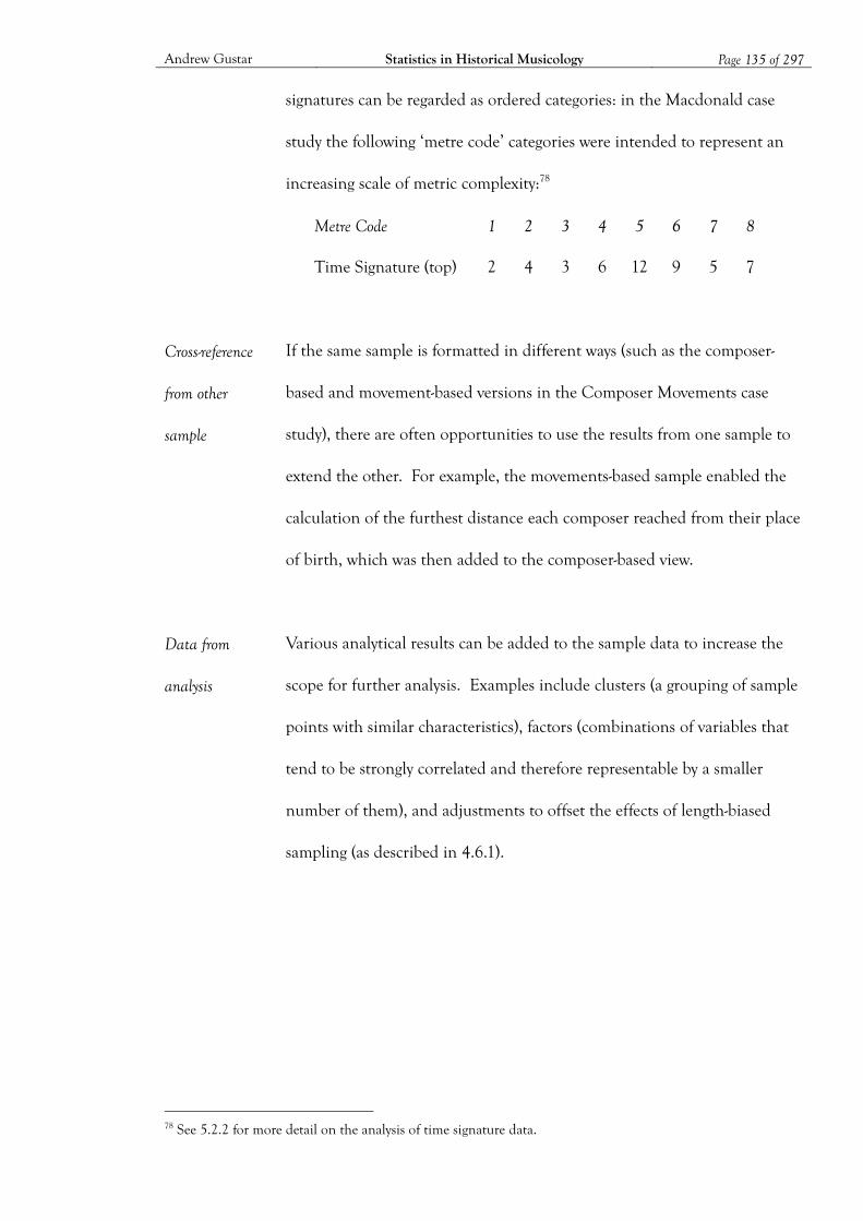
Andrew Gustar Statistics in Historical Musicology Page 135 of 297
signatures can be regarded as ordered categories: in the Macdonald case
study the following ‘metre code’ categories were intended to represent an
increasing scale of metric complexity:78
Metre Code 1 2 3 4 5 6 7 8
Time Signature (top)
2 4 3 6 12 9 5 7
Cross-reference
from other
sample
If the same sample is formatted in different ways (such as the composer-
based and movement-based versions in the Composer Movements case
study), there are often opportunities to use the results from one sample to
extend the other. For example, the movements-based sample enabled the
calculation of the furthest distance each composer reached from their place
of birth, which was then added to the composer-based view.
Data from
analysis
Various analytical results can be added to the sample data to increase the
scope for further analysis. Examples include clusters (a grouping of sample
points with similar characteristics), factors (combinations of variables that
tend to be strongly correlated and therefore representable by a smaller
number of them), and adjustments to offset the effects of length-biased
sampling (as described in 4.6.1).
78 See 5.2.2 for more detail on the analysis of time signature data.
Andrew Gustar Statistics in Historical Musicology Page 136 of 297
4.5 UNDERSTANDING AND EXPLORING THE DATA
This and the next two sections look at analytical techniques that can be applied to a
statistical sample. It is not the intention to present a comprehensive survey of statistical
techniques, but to illustrate some of the methods that have proved useful or interesting in
the case studies, and that might have more general applications in historical musicology.
With one or two exceptions, there will be little mathematical detail, and the techniques and
their rationale will only be described in broad terms. Further details of these techniques can
readily be found in statistical textbooks and online sources.
The exploration of data is a common first step in any statistical investigation. Even if
the primary objective is the testing of specific hypotheses, a little data exploration may enable
more reasoned choices to be made about the ways in which the hypotheses might best be
tested. The range of exploratory techniques is wide, from simple descriptive calculations and
tables through to advanced classification, modelling and pattern recognition techniques.
4.5.1 Descriptive statistics
Describing the features of a sample (and thus, subject to considerations of statistical
significance, the population from which it was drawn) is often a useful first step in assessing
the characteristics of the data, what sort of features and patterns it might contain, the types
of further analysis that would be appropriate, and where potential difficulties might lie.
The most common descriptive statistics are the averages – the mean (the sum of the
values divided by the number of them), median (the central value when sorted in ascending
order) and mode (the most common value) – that measure the typical or central value of a
variable. The mean, which is the most commonly used, is usually only valid for cardinal
numbers, whereas the median and mode can also be used for ordinal values or ordered
categories (the mode also applies to unordered categories). These measures can give a useful
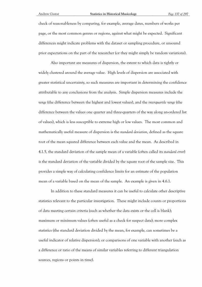
Andrew Gustar Statistics in Historical Musicology Page 137 of 297
check of reasonableness by comparing, for example, average dates, numbers of works per
page, or the most common genres or regions, against what might be expected. Significant
differences might indicate problems with the dataset or sampling procedure, or unsound
prior expectations on the part of the researcher (or they might simply be random variations).
Also important are measures of dispersion, the extent to which data is tightly or
widely clustered around the average value. High levels of dispersion are associated with
greater statistical uncertainty, so such measures are important in determining the confidence
attributable to any conclusions from the analysis. Simple dispersion measures include the
range (the difference between the highest and lowest values), and the interquartile range (the
difference between the values one quarter and three-quarters of the way along an-ordered list
of values), which is less susceptible to extreme high or low values. The most common and
mathematically useful measure of dispersion is the standard deviation, defined as the square
root of the mean squared difference between each value and the mean. As described in
4.1.5, the standard deviation of the sample mean of a variable (often called its standard error)
is the standard deviation of the variable divided by the square root of the sample size. This
provides a simple way of calculating confidence limits for an estimate of the population
mean of a variable based on the mean of the sample. An example is given in 4.6.1.
In addition to these standard measures it can be useful to calculate other descriptive
statistics relevant to the particular investigation. These might include counts or proportions
of data meeting certain criteria (such as whether the data exists or the cell is blank);
maximum or minimum values (often useful as a check for suspect data); more complex
statistics (the standard deviation divided by the mean, for example, can sometimes be a
useful indicator of relative dispersion); or comparisons of one variable with another (such as
a difference or ratio of the means of similar variables referring to different triangulation
sources, regions or points in time).
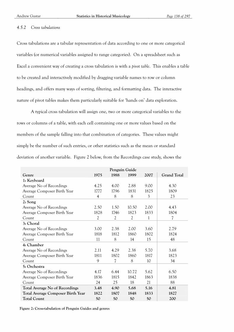
Andrew Gustar Statistics in Historical Musicology Page 138 of 297
4.5.2 Cross tabulations
Cross tabulations are a tabular representation of data according to one or more categorical
variables (or numerical variables assigned to range categories). On a spreadsheet such as
Excel a convenient way of creating a cross tabulation is with a pivot table. This enables a table
to be created and interactively modified by dragging variable names to row or column
headings, and offers many ways of sorting, filtering, and formatting data. The interactive
nature of pivot tables makes them particularly suitable for ‘hands on’ data exploration.
A typical cross tabulation will assign one, two or more categorical variables to the
rows or columns of a table, with each cell containing one or more values based on the
members of the sample falling into that combination of categories. These values might
simply be the number of such entries, or other statistics such as the mean or standard
deviation of another variable. Figure 2 below, from the Recordings case study, shows the
Penguin Guide
Genre 1975 1988 1999 2007 Grand Total 1: Keyboard
Average No of Recordings 4.25 4.00 2.88 9.00 4.30 Average Composer Birth Year 1777 1796 1831 1825 1809 Count 4 8 8 3 23 2: Song
Average No of Recordings 2.50 1.50 10.50 2.00 4.43 Average Composer Birth Year 1828 1746 1823 1833 1804 Count 2 2 2 1 7 3: Choral
Average No of Recordings 3.00 2.38 2.00 3.60 2.79 Average Composer Birth Year 1818 1812 1860 1802 1824 Count 11 8 14 15 48 4: Chamber
Average No of Recordings 2.11 4.29 2.38 5.70 3.68 Average Composer Birth Year 1811 1802 1860 1817 1823 Count 9 7 8 10 34 5: Orchestra
Average No of Recordings 4.17 6.44 10.72 5.62 6.50 Average Composer Birth Year 1836 1815 1842 1863 1838 Count 24 25 18 21 88 Total Average No of Recordings 3.48 4.90 5.68 5.16 4.81 Total Average Composer Birth Year 1822 1807 1848 1833 1827 Total Count 50 50 50 50 200
Figure 2: Cross-tabulation of Penguin Guides and genres

Andrew Gustar Statistics in Historical Musicology Page 139 of 297
average number of recordings, the average composer’s birth year, and the number of sample
points for each combination of genre and sampled Penguin Guide.
The index of values (the actual number as a proportion of that expected pro rata the
row and column totals) can be a useful indicator of values that are unusually high or low
compared to other cells, or of variables that may not be independent. All index values will
be close to one if, for example, the distribution of works by genre within each region is
similar to that across all regions combined. Index values much smaller or larger than one
may indicate a lack of independence between genre and region that can be explored further.
It is important to consider whether any observed anomaly is likely to be statistically
significant. This is largely a function of the number of elements falling into that cell of the
table. If a sample contains three works from Portugal, one of which is for zither quartet, it
cannot be concluded that this was a particularly important genre in the history of Portuguese
music. On the other hand, if there were 90 Portuguese works, of which 30 were for zither
quartet, this would be a much more significant finding. A useful rule of thumb is that the
standard deviation of an observed proportion is roughly equal to where is
the observed proportion and is the total number of observations. In the example above,
one work out of three gives a standard deviation of the square root of (1/3) x (2/3) x (1/3),
which is about 0.27. So the actual proportion of zither quartets in Portuguese music might
reasonably lie anywhere within plus or minus twice this value of the observed proportion of
1/3 – a rather large range. Thirty works out of ninety, on the other hand, gives a standard
deviation of the square root of (1/3) x (2/3) x (1/90), or about 0.05. In this case, plus or
minus two standard deviations from the observed value gives a likely true proportion (with
about 95% confidence) in the range 0.23 to 0.43.

Andrew Gustar Statistics in Historical Musicology Page 140 of 297
4.5.3 Graphs and charts
The visual display of data may suggest patterns that are not obvious from the numbers
alone.79 Simple charts are useful for revealing the distribution of variables (pie charts,
histograms, cumulative distribution charts, bar charts, maps) and for exploring the
relationships between them (scatter plots, time series, line charts). Distributions can be
plotted either directly (as histograms), with the height of the graph indicating the proportion
of sample points in each category, or cumulatively, where the height of the graph is the
proportion of points less than or equal to each value.80 Cumulative charts are particularly
useful for data that is not in categories or ranges.
There are many ways of portraying the relationship between variables. A scatter plot
of one numerical variable against another might indicate a relationship between the two, or
suggest clusters where the points tend to bunch together. A categorical variable plotted
against the average of another might illustrate possible trends. Figure 3, from the
Macdonald case study, shows the average key signature across the sample, analysed by date of
composition, together with approximate 95% confidence bands (dotted lines).81 The
significant move towards flat key
signatures during the first half of
the nineteenth century (perhaps
related to the increasing use of
flat-favouring instruments, such
as clarinets and brass) is much
clearer when portrayed
79 Charts are also invaluable in the presentation of statistical results, a topic discussed further in section 4.8. 80 Examples of these two types are given in Figure 9 and Figure 10 respectively. 81 Data such as this is often plotted as bars or points for each category, rather than as lines. The lines in Figure 3 (and similar charts elsewhere in this thesis) are simply there to join data points and do not show intermediate values derived from the sample. They do, however, arguably illustrate the indicated trends more clearly.
Figure 3: Average key signatures
-2.0
-1.0
0.0
1.0
2.0
to 1700
18C H1
18C H2
19C Q1
19C Q2
19C Q3
19C Q4
20C H1
Flat
s - -
- - -
- - -
Sha
rps
Average Key and 95% confidence bands
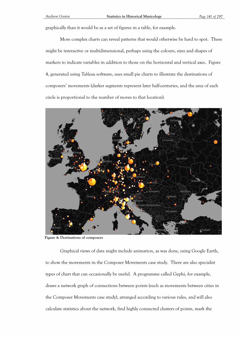
Andrew Gustar Statistics in Historical Musicology Page 141 of 297
graphically than it would be as a set of figures in a table, for example.
More complex charts can reveal patterns that would otherwise be hard to spot. These
might be interactive or multidimensional, perhaps using the colours, sizes and shapes of
markers to indicate variables in addition to those on the horizontal and vertical axes. Figure
4, generated using Tableau software, uses small pie charts to illustrate the destinations of
composers’ movements (darker segments represent later half-centuries, and the area of each
circle is proportional to the number of moves to that location).
Graphical views of data might include animation, as was done, using Google Earth,
to show the movements in the Composer Movements case study. There are also specialist
types of chart that can occasionally be useful. A programme called Gephi, for example,
draws a network graph of connections between points (such as movements between cities in
the Composer Movements case study), arranged according to various rules, and will also
calculate statistics about the network, find highly connected clusters of points, mark the
Figure 4: Destinations of composers

Andrew Gustar Statistics in Historical Musicology Page 142 of 297
Figure 5: British Library music holdings by attributed date
10
100
1000
10000
1650 1700 1750 1800 1850 1900
British Library date attributions
Number of Records 5y average
strongest connections, etc. Although difficult to interpret, such charts can suggest patterns
and links that would otherwise be invisible (see 4.5.5 for an example).
Trends may be clearer on graphs with non-linear axes. Of particular use are
logarithmic scales where each interval on the axis represents an increase or decrease by a
constant factor (such as 10 or 2), rather than by an additive increment. Figure 5 shows the
number of music scores in the British Library catalogue by publication year, and uses a
logarithmic vertical scale to show
a relatively constant growth rate
of roughly tenfold per century. It
also illustrates the spikes, every
fifth year from 1700 to about
1850, where publication dates
have been approximately
ascribed.
4.5.4 Correlation
Correlation is a linear relationship between two variables, where an increase of X in one will
tend to be accompanied by an increase or decrease of Y in the other. Variables that are
independent will have zero correlation. The most common measure is Pearson’s correlation
coefficient, which takes a value of +1 for perfect correlation (an increase in one variable always
means a linear increase in the other), 0 for no linear relationship, and –1 for perfect negative
correlation (where an increase in one variable is associated with a decrease in the other). It is
important to remember that correlation does not imply cause and effect, although it can
highlight where further investigation of causal relationships might be fruitful.
The most common statistical test for correlation calculates the chance of obtaining a
Andrew Gustar Statistics in Historical Musicology Page 143 of 297
coefficient as high as that from the sample, assuming that there is actually no correlation in
the population (the null hypothesis). If this chance is very small, the null hypothesis can be
rejected, suggesting that there is correlation in the population. For a sample of size greater
than 30 or so, if the population correlation is zero, then the correlation coefficient of the
sample will be approximately Normally distributed with standard deviation roughly equal to
. Thus for a sample of 100, a sample correlation coefficient greater than ±0.2 (i.e. at
least two standard deviations away from zero) is statistically significant at 95% confidence.
The strength of correlation may be more important than its significance. A
coefficient less than about 0.5, even if statistically significant, represents rather weak
correlation, as illustrated by the following examples (Figure 6, taken from Wikipedia):
The strength of correlation should also be considered in the context of the range and
magnitude of the variables concerned. Even if X and Y are perfectly correlated, if a change
in X from its lowest to highest value only produces a small change in Y (so Y goes from, say,
100 to 101 as X increases from –1 to +1), this might not, depending on the context, be
regarded as ‘significant’ in anything other than statistical terms.
Correlation only measures linear relationships between variables. It will not
necessarily produce a significant result if the variables have a non-linear (i.e. curved)
relationship, such as in Figure 7, from the Piano Keys case study, indicating a non-linear
relationship between the average key signature of piano music and the age of the composer.
A correlation matrix (a table of the correlation coefficients between each pair of
numerical variables) can be useful for indicating relationships to be investigated in more
detail. This has been a routine part of the analysis in most of the case studies, and has
Figure 6: Example correlation coefficients
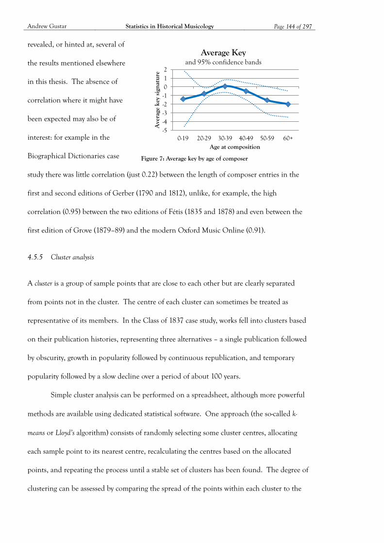
Andrew Gustar Statistics in Historical Musicology Page 144 of 297
revealed, or hinted at, several of
the results mentioned elsewhere
in this thesis. The absence of
correlation where it might have
been expected may also be of
interest: for example in the
Biographical Dictionaries case
study there was little correlation (just 0.22) between the length of composer entries in the
first and second editions of Gerber (1790 and 1812), unlike, for example, the high
correlation (0.95) between the two editions of Fétis (1835 and 1878) and even between the
first edition of Grove (1879–89) and the modern Oxford Music Online (0.91).
4.5.5 Cluster analysis
A cluster is a group of sample points that are close to each other but are clearly separated
from points not in the cluster. The centre of each cluster can sometimes be treated as
representative of its members. In the Class of 1837 case study, works fell into clusters based
on their publication histories, representing three alternatives – a single publication followed
by obscurity, growth in popularity followed by continuous republication, and temporary
popularity followed by a slow decline over a period of about 100 years.
Simple cluster analysis can be performed on a spreadsheet, although more powerful
methods are available using dedicated statistical software. One approach (the so-called k-
means or Lloyd’s algorithm) consists of randomly selecting some cluster centres, allocating
each sample point to its nearest centre, recalculating the centres based on the allocated
points, and repeating the process until a stable set of clusters has been found. The degree of
clustering can be assessed by comparing the spread of the points within each cluster to the
Figure 7: Average key by age of composer
-5 -4 -3 -2 -1 0 1 2
0-19 20-29 30-39 40-49 50-59 60+
Ave
rage
key
sig
nat
ure
Age at composition
Average Key and 95% confidence bands
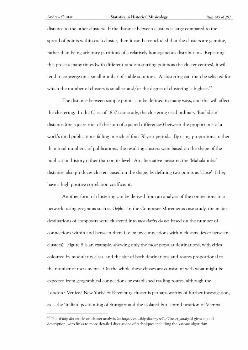
Andrew Gustar Statistics in Historical Musicology Page 145 of 297
distance to the other clusters. If the distance between clusters is large compared to the
spread of points within each cluster, then it can be concluded that the clusters are genuine,
rather than being arbitrary partitions of a relatively homogeneous distribution. Repeating
this process many times (with different random starting points as the cluster centres), it will
tend to converge on a small number of stable solutions. A clustering can then be selected for
which the number of clusters is smallest and/or the degree of clustering is highest.82
The distance between sample points can be defined in many ways, and this will affect
the clustering. In the Class of 1837 case study, the clustering used ordinary ‘Euclidean’
distance (the square root of the sum of squared differences) between the proportions of a
work’s total publications falling in each of four 50-year periods. By using proportions, rather
than total numbers, of publications, the resulting clusters were based on the shape of the
publication history rather than on its level. An alternative measure, the ‘Mahalanobis’
distance, also produces clusters based on the shape, by defining two points as ‘close’ if they
have a high positive correlation coefficient.
Another form of clustering can be derived from an analysis of the connections in a
network, using programs such as Gephi. In the Composer Movements case study, the major
destinations of composers were clustered into modularity classes based on the number of
connections within and between them (i.e. many connections within clusters, fewer between
clusters). Figure 8 is an example, showing only the most popular destinations, with cities
coloured by modularity class, and the size of both destinations and routes proportional to
the number of movements. On the whole these classes are consistent with what might be
expected from geographical connections or established trading routes, although the
London/ Venice/ New York/ St Petersburg cluster is perhaps worthy of further investigation,
as is the ‘Italian’ positioning of Stuttgart and the isolated but central position of Vienna.
82 The Wikipedia article on cluster analysis (at http://en.wikipedia.org/wiki/Cluster_analysis) gives a good description, with links to more detailed discussions of techniques including the k-means algorithm.
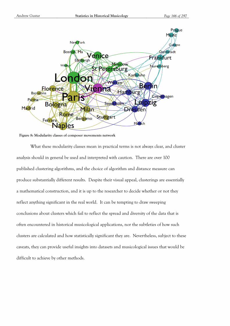
Andrew Gustar Statistics in Historical Musicology Page 146 of 297
What these modularity classes mean in practical terms is not always clear, and cluster
analysis should in general be used and interpreted with caution. There are over 100
published clustering algorithms, and the choice of algorithm and distance measure can
produce substantially different results. Despite their visual appeal, clusterings are essentially
a mathematical construction, and it is up to the researcher to decide whether or not they
reflect anything significant in the real world. It can be tempting to draw sweeping
conclusions about clusters which fail to reflect the spread and diversity of the data that is
often encountered in historical musicological applications, nor the subtleties of how such
clusters are calculated and how statistically significant they are. Nevertheless, subject to these
caveats, they can provide useful insights into datasets and musicological issues that would be
difficult to achieve by other methods.
Figure 8: Modularity classes of composer movements network
Andrew Gustar Statistics in Historical Musicology Page 147 of 297
4.6 QUANTIFYING THE DATA
One objective of statistical analysis might be to quantify aspects of the population under
investigation. This section considers two examples of this: the estimation of population size,
and the fitting of mathematical distributions.
4.6.1 Population estimates
It is often useful to estimate the number of entries in a dataset. This can be done in several
ways, depending on the characteristics of the dataset. For some online databases, the
estimation of population size can be difficult or impossible (although there is sometimes a
statement of the number of entries on the website). Search queries often quote the number
of entries found, and this can indicate the size of subsets of the data. Other tricks are
sometimes possible: in the Recordings case study, the number of classical composers on the
AllMusic database was estimated at about 10,000 by establishing (by trial and error) the
numerical database codes that gave valid composer entries.83 In other cases, it might be
practically impossible to estimate the number of entries due to the ‘black box’ nature of the
database (see section 4.3.9).
For datasets in book form, there will occasionally be a statement in the preface of the
number of entries, or this can sometimes be estimated by analysing the index rather than the
entire book. Where this is not possible, recording the number of entries per page whilst
sampling enables the estimation of the mean number of entries per page, which can be
multiplied by the number of pages to give an estimate of the total number of entries. A
similar calculation can be done for subsets of the data, for example by counting the number
of composer entries per page, if the source also contains other types of information. The
standard deviation of works per page enables confidence limits to be put on the estimated
83 This approach is no longer possible – see the discussion in footnote 74.
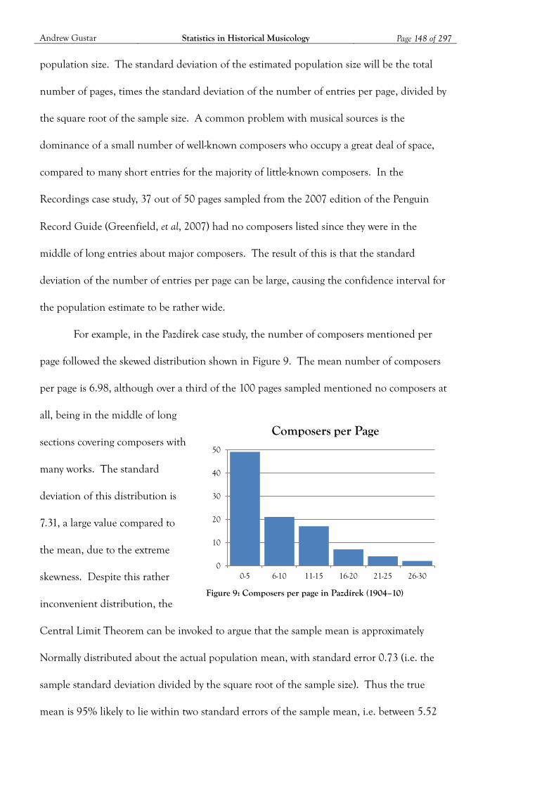
Andrew Gustar Statistics in Historical Musicology Page 148 of 297
population size. The standard deviation of the estimated population size will be the total
number of pages, times the standard deviation of the number of entries per page, divided by
the square root of the sample size. A common problem with musical sources is the
dominance of a small number of well-known composers who occupy a great deal of space,
compared to many short entries for the majority of little-known composers. In the
Recordings case study, 37 out of 50 pages sampled from the 2007 edition of the Penguin
Record Guide (Greenfield, et al, 2007) had no composers listed since they were in the
middle of long entries about major composers. The result of this is that the standard
deviation of the number of entries per page can be large, causing the confidence interval for
the population estimate to be rather wide.
For example, in the Pazdírek case study, the number of composers mentioned per
page followed the skewed distribution shown in Figure 9. The mean number of composers
per page is 6.98, although over a third of the 100 pages sampled mentioned no composers at
all, being in the middle of long
sections covering composers with
many works. The standard
deviation of this distribution is
7.31, a large value compared to
the mean, due to the extreme
skewness. Despite this rather
inconvenient distribution, the
Central Limit Theorem can be invoked to argue that the sample mean is approximately
Normally distributed about the actual population mean, with standard error 0.73 (i.e. the
sample standard deviation divided by the square root of the sample size). Thus the true
mean is 95% likely to lie within two standard errors of the sample mean, i.e. between 5.52
Figure 9: Composers per page in Pazdírek (1904–10)
0
10
20
30
40
50
0-5 6-10 11-15 16-20 21-25 26-30
Composers per Page
Andrew Gustar Statistics in Historical Musicology Page 149 of 297
and 8.44 composers per page. Multiplying this by the total number of pages in Pazdírek’s
Handbook (11,962) provides a 95% confidence interval for the total number of composers
mentioned, between 66,000 and 101,000, with a mean (expected) value of 83,500.
It is also possible to estimate the population if the distribution of composers is
subject to length bias. If is the probability that a random composer occupies a fraction
of the book, then , the probability that a randomly selected work is by a composer
who occupies a fraction of the book, is equal to the proportion of the book occupied by
composers who take up , i.e. , where is the total number of composers.
Dividing both sides by , and summing over all values of (noting that the sums of both
and must equal one, and that, in the sample, , where is the sample
size), we see that can be estimated as ,84 where is the page length of each
entry in the sample (for ) and is the total number of pages. Returning to the
2007 Penguin Guide, triangulated data was available for 193 works, randomly sampled across
four of the Guides. The above calculation produced an estimate of 535 composers, and a
95% confidence interval (using a similar approach to calculate the standard deviation) of
between 360 and 710 composers. This can be compared with a calculation based on the
number of composers per page for the 50 sampled pages in the Guide, which gave an
estimate of 635 composers, and a 95% confidence interval of 296 – 975. As expected,
roughly quadrupling the sample size resulted in halving the width of the confidence interval.
A particular problem arose with the Recordings case study where two approaches
were used to estimate the number of distinct recordings in several datasets, each giving
substantially different results. The first method estimated the total as the average number of
recordings per page, times the number of pages, divided by a duplication factor representing
the average number of works per recording (since record guides are listed by work, and thus
84 The (sigma) symbol here simply means ‘sum of’ the terms immediately following it.

Andrew Gustar Statistics in Historical Musicology Page 150 of 297
each recording is listed under each work that it contains). The second method calculated the
number of unique works (works per composer, divided by pages per composer, times number
of pages), multiplied by the average number of recordings per work, divided by the average
number of works per recording. The estimates using these methods for the 2007 Penguin
Record Guide, for example, were 7,851 and 23,208 respectively. Although this large
difference was not fully reconciled, the investigation highlighted several issues:
Complex data Recordings data is complex, in terms of the linkages between composers,
works, recordings, couplings, performers, record companies, and formats.
There is a lot that can go wrong in any calculation and the complex structure
of the data makes it difficult to analyse what is going on.
Unquantifiable
assumptions
It was not wholly true that a recording was listed under each of its works, if
one of those works is not mentioned in its own right (perhaps being a minor
work or part of a larger set). With the data that was collected, it was not
possible to quantify the extent of this potential problem.
Statistics and
their
reciprocals
It is not generally the case that the mean of 1/X is equal to 1/(the mean of
X), and similarly for other statistics such as standard deviations.
Calculations involving ratios and their inverses (composers per page, pages
per composer) must be thought through carefully, and it is easy (and
occasionally unavoidable) to introduce calculation bias in these situations.
Skewness and
correlation
The highly skewed distributions of the number of works and the entry
length per composer result in wide margins of error and may also exaggerate

Andrew Gustar Statistics in Historical Musicology Page 151 of 297
any calculation bias as described above. Correlation between variables (such
as between the number of a composer’s works and the length of article per
work) may also amplify these problems.
Simulation To investigate the discrepancy, an artificial Penguin Guide was constructed,
using the same data structure as the real guides, but a smaller (known)
number of composers, works and recordings. A random simulation was run
many times, and the distribution of the calculated population size revealed a
certain amount of calculation bias, and identified ‘recordings per work’ as a
particularly troublesome skewed distribution. One conclusion was that in a
complex situation such as this, there might not exist a methodical way of
estimating population size in an unbiased way.
The experience from this case study suggests that, despite its apparent simplicity, the
estimation of population size can be far from straightforward. A fundamental difficulty lies
in the dominance of a relatively small number of famous composers and their works,
alongside huge numbers of minor composers and works which, even with large samples, go
largely undetected and are therefore inherently unquantifiable.
A similar problem occurs if one attempts to use multiple sources to estimate the size
of a larger population, such as the total number of composers. In principle, this could be
estimated by using a ‘Capture-Recapture’ method, a technique used for estimating animal
populations by capturing and marking individuals, and examining the frequency with which
the same individuals are subsequently recaptured. In its simplest form, if A individuals are
captured and marked in the first capturing session, and B are captured in the second session,
of which R are recaptures of those marked in the first session, then the total population can
Andrew Gustar Statistics in Historical Musicology Page 152 of 297
be estimated as AB/R. There are refinements of this approach to allow for multiple sessions,
and for groups of individuals with varying propensities to be captured. Applied to
composers, a ‘capture’ would be an appearance in a historical dataset such as a biographical
dictionary. Unfortunately these methods assume independence between the individuals
captured at different times. Composers are not like this: several names appear without fail in
every list of composers (Bach, Mozart, Beethoven, etc), but there are others who never
appear, perhaps because their one published composition lies in an uncatalogued archive
and they have yet to be ‘discovered’. In between there is a spectrum of names with an
increasing tendency to appear in such sources if they have already been mentioned in a
previous source. Where there is high correlation between capture sessions, and where each
composer has a different capture probability (perhaps varying over time), the assumptions
break down and capture-recapture techniques do not work.
This is a deeper problem than simply not being able to use a particular technique.
Any sample-based population estimate (for composers, works, and probably other entities
such as recordings and publications) will fall at the same hurdle: a large but unknown
number of obscure members of the population will always be missed, and their
characteristics will not be reliably inferable from those of their better known colleagues.
4.6.2 Fitting a distribution
In the real world, certainly with data from the arts and humanities, there is no reason why a
statistical distribution should fit a simple mathematical form. Nevertheless, there are
occasions where an empirical distribution can be well approximated by a mathematical
formula. This can be used for statistical or modelling applications that would have been
impossible (or less straightforward) with purely empirical data. For example, a mathematical
formula closely approximating the long-tailed distribution of the length of entries in the
Andrew Gustar Statistics in Historical Musicology Page 153 of 297
Recordings case study was used to generate the simulated Penguin guides described in 4.6.1.
A more important reason for seeking a mathematical distribution to fit empirical
data is that it can indicate the existence of a simple structure in the underlying processes.
Many mathematical distributions arise as a consequence of simple assumptions regarding
random processes: the appearance of those distributions in empirical data might indicate
that similar assumptions apply. The bell-shaped ‘Normal’ distribution, for example, is often
found where many small random effects combine additively, almost irrespective of the
distributions of the effects themselves.
The first stage in fitting a distribution is normally to examine a graph of the data to
see if it appears to approximate to a common mathematical form. Two types of graph are
particularly useful. A plot of the distribution as a histogram (such as Figure 9), where the
area of each column corresponds to the number of sample points in each category, gives a
good impression of the overall shape of the distribution – skewed, symmetrical, bell-shaped,
flat, irregular, etc – and whether it is likely to be a good fit to a common mathematical form.
The other form of graph is the cumulative distribution, where the values are sorted
in ascending order, summed cumulatively, and plotted against the cumulative proportion
from 0 to 100%. Figure 10, in the next section, is an example of a cumulative distribution
chart. This sort of chart can be plotted directly for continuous data, whereas a histogram
needs data to be converted into ranges. Cumulative charts are less susceptible to random
variations, which tend to cancel out over quite small scales and result in a relatively smooth
line, even for small sample sizes. Certain distributions have a characteristic form when
plotted in this way, perhaps with logarithmic scales on either or both of the horizontal or
vertical axes.
Once a candidate for a standard distribution has been identified (and there might be
several), the next stage is to estimate the parameters of the distribution. These are the

Andrew Gustar Statistics in Historical Musicology Page 154 of 297
numbers that define the location, size and shape of the distribution. A Normal distribution,
for example, has two parameters – the mean, which defines its location, and the standard
deviation, which defines its size. The shape of the ‘duration of stay’ graph (Figure 19, p.185),
for example, suggests a Poisson process, a random process in which events happen with a
constant probability, independent of the time since the previous event (with, in this case,
some adjustment to allow for practical limits to human life). The Poisson process has a
single parameter, in this case estimated as one move per 14 years. Parameters can often be
estimated by simple calculations from the sample, although for certain distributions the
parameters can only be obtained by more complex calculations or (more likely) by trial and
error and successive approximations. One approach is to find the parameters of the assumed
population distribution for which the observed sample distribution would be most likely. A
test such as the Chi-squared test (see section 4.7.2) can be used to quantify the extent to which
an observed distribution is consistent with that predicted by a particular set of parameters.
The parameters can be set to maximise the likelihood of the observed distribution in the
sample. Section 4.6.3 illustrates this procedure in more detail.
The final stage is to test whether the standard distribution is actually a good fit to the
observed data or, if there are several possible options, which one is most appropriate. A
visual comparison of the graphs of the observed and fitted distributions can be useful,
perhaps suggesting the limitations of the approximation (such as a range of values for which
it is not valid), or possible adjustments to the standard formula to fine-tune the fit. More
rigorous quantification of the fit can be done with tests such as the Chi-squared test.85
85 A useful shortcut through some of this is provided by a free program called CumFreq (available from http://www.waterlog.info/cumfreq.htm), which attempts to fit a large number of standard mathematical distributions to observed data, and produces various charts and metrics illustrating the quality of the fit.
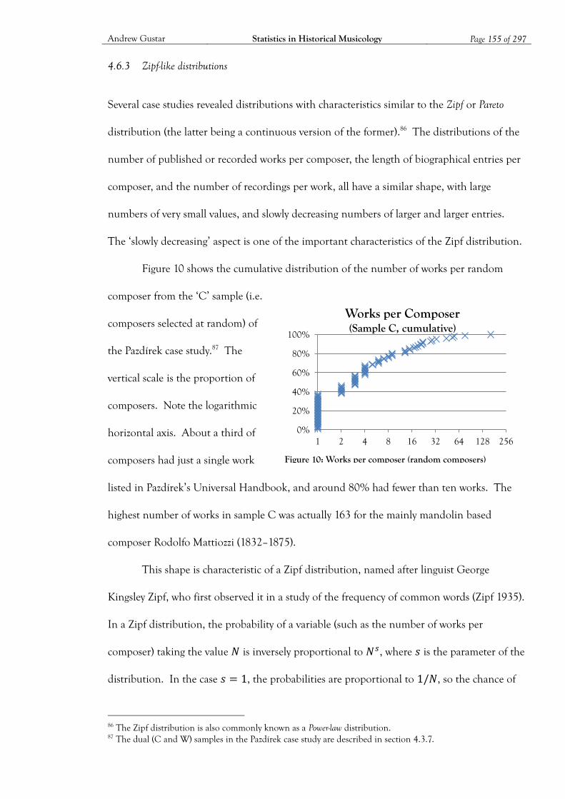
Andrew Gustar Statistics in Historical Musicology Page 155 of 297
4.6.3 Zipf-like distributions
Several case studies revealed distributions with characteristics similar to the Zipf or Pareto
distribution (the latter being a continuous version of the former).86 The distributions of the
number of published or recorded works per composer, the length of biographical entries per
composer, and the number of recordings per work, all have a similar shape, with large
numbers of very small values, and slowly decreasing numbers of larger and larger entries.
The ‘slowly decreasing’ aspect is one of the important characteristics of the Zipf distribution.
Figure 10 shows the cumulative distribution of the number of works per random
composer from the ‘C’ sample (i.e.
composers selected at random) of
the Pazdírek case study.87 The
vertical scale is the proportion of
composers. Note the logarithmic
horizontal axis. About a third of
composers had just a single work
listed in Pazdírek’s Universal Handbook, and around 80% had fewer than ten works. The
highest number of works in sample C was actually 163 for the mainly mandolin based
composer Rodolfo Mattiozzi (1832–1875).
This shape is characteristic of a Zipf distribution, named after linguist George
Kingsley Zipf, who first observed it in a study of the frequency of common words (Zipf 1935).
In a Zipf distribution, the probability of a variable (such as the number of works per
composer) taking the value is inversely proportional to , where is the parameter of the
distribution. In the case , the probabilities are proportional to , so the chance of
86 The Zipf distribution is also commonly known as a Power-law distribution. 87 The dual (C and W) samples in the Pazdírek case study are described in section 4.3.7.
Figure 10: Works per composer (random composers)
0%
20%
40%
60%
80%
100%
1 2 4 8 16 32 64 128 256
Works per Composer (Sample C, cumulative)

Andrew Gustar Statistics in Historical Musicology Page 156 of 297
exactly 2 works per composer would be , 100 works per composer would be , and
so on, where is a constant such that the sum of all probabilities adds up to 1.
Herein lies the problem with the Zipf distribution: the sum of the probabilities for all
possible values turns out to be infinite for values of less than or equal to 1, so the value of
cannot be meaningfully defined. If is greater than 1, we can set so that the probabilities
sum to 1, but if is less than or equal to 2 we encounter the same problem when calculating
the mean, so for these values of the average value of is effectively infinite.
Zipf and others got round this problem by pointing out that in the real world there is
usually an upper limit to the value of statistical variables, so we never actually have to
perform an infinite sum. The maximum number of works that a single composer could have
listed in a directory such as Pazdírek’s Handbook is more than 2,000, as such an example
(Mozart) was found in the ‘W’ sample of random works.88 It is hard to conceive of a famous
and productive composer producing more than, say, 10,000 published works over a long
career (including subsequent editions, arrangements, translations, etc), so this might be an
effective upper limit to the distribution.
It is interesting to compare the graph above with that for the W sample (Figure 11),
which, because of length-biased sampling, is biased towards those composers who wrote more
works. The vertical scale here is the
proportion of works. In this chart,
the single-work composers only
account for about 10% of the total
number of works. 80% of works
are by composers with fewer than
88 Although the Köchel catalogue of Mozart’s works only extends as far as K626 (the Requiem), Pazdírek also lists arrangements for other instruments, editions in different languages, and individual movements of larger works, treating them as separate published works
Figure 11: Works per composer (random works)
0%
20%
40%
60%
80%
100%
1 2 4 8 16 32 64 128 256 512 1024 2048
Works per Composer (Sample W, cumulative)

Andrew Gustar Statistics in Historical Musicology Page 157 of 297
250 works in the Handbook, implying that the remaining 20% are by composers with more
than 250 works, a number greater than the highest figure in the C sample.
If sample C follows a Zipf distribution, then sample W also has a Zipf distribution. If
the probability of a random composer having works is , then the probability of a
random work being by a composer with works is proportional to , since such a
composer occupies a space works long in the Handbook. But this is just another Zipf
distribution with parameter rather than . Unfortunately, the two Pazdírek samples
cannot quite be reconciled with a standard Zipf distribution, indicating that the empirical
distribution is not exactly represented by a simple formula (it would be more surprising if it
were). The C sample data is close to a Zipf distribution with , which means that the
equivalent W distribution has parameter , for which the sum of probabilities
would be infinite. This problem can be eliminated by introducing another parameter that
allows to rise as increases, thus guaranteeing that eventually the probabilities diminish
fast enough to sum to a finite number. A close fit to both the C and W distributions was
obtained by replacing with .89 These parameters were found (using
Excel’s ‘Solver’ facility) to minimise the combined Chi-squared statistic comparing the
observed and expected C and W distributions.90 The following table shows the observed
and expected values for the two samples using these best-fit parameters.
89 is the natural logarithm function, sometimes written as . 90 The Chi-squared statistic is the sum of the values , where and are the observed and expected numbers of observations in each cell. See section 4.7.2 for further details.
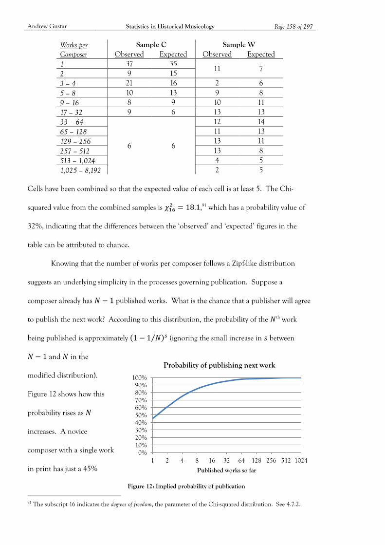
Andrew Gustar Statistics in Historical Musicology Page 158 of 297
Works per Composer
Sample C Sample W Observed Expected Observed Expected
1 37 35 11 7
2 9 15 3 – 4 21 16 2 6 5 – 8 10 13 9 8 9 – 16 8 9 10 11 17 – 32 9 6 13 13 33 – 64
6 6
12 14 65 – 128 11 13 129 – 256 13 11 257 – 512 13 8 513 – 1,024 4 5 1,025 – 8,192 2 5
Cells have been combined so that the expected value of each cell is at least 5. The Chi-
squared value from the combined samples is ,91 which has a probability value of
32%, indicating that the differences between the ‘observed’ and ‘expected’ figures in the
table can be attributed to chance.
Knowing that the number of works per composer follows a Zipf-like distribution
suggests an underlying simplicity in the processes governing publication. Suppose a
composer already has published works. What is the chance that a publisher will agree
to publish the next work? According to this distribution, the probability of the th work
being published is approximately (ignoring the small increase in between
and in the
modified distribution).
Figure 12 shows how this
probability rises as
increases. A novice
composer with a single work
in print has just a 45%
91 The subscript 16 indicates the degrees of freedom, the parameter of the Chi-squared distribution. See 4.7.2.
Figure 12: Implied probability of publication
0% 10% 20% 30% 40% 50% 60% 70% 80% 90%
100%
1 2 4 8 16 32 64 128 256 512 1024
Published works so far
Probability of publishing next work

Andrew Gustar Statistics in Historical Musicology Page 159 of 297
chance of the second being published (presumably related to sales of the first), but if this
happens, the third’s chance of publication rises to 60%. A composer with 100 works in
print can be more than 98% confident that the next will be accepted for publication. For an
established composer with 1,000 works, the odds are 99.8% – just a 1 in 500 chance of
rejection. This is certainly a plausible explanation of why Pazdírek’s Handbook has this
distribution of composers and works, although it does not explain why publishers follow this
particular rule.92 It would be interesting to compare this with a more detailed investigation
of the processes by which publishers actually select new works for publication.
92 See also the discussion in section 5.3.1.
Andrew Gustar Statistics in Historical Musicology Page 160 of 297
4.7 HYPOTHESIS TESTING
An important role of statistics is the testing of hypotheses. The objective of such tests is to
quantify the extent to which the characteristics of the sample are consistent with the
hypothesis in question. The usual procedure is to assume that a neutral null hypothesis (often
symbolised as H0) is true of the population, and to calculate the probability that the observed
sample was drawn from such a population. If this probability is below a certain value (such
as, commonly, 5%), then the null hypothesis can be rejected. Common hypotheses would be
that X is greater than Y for some statistics or values X and Y (for which the null hypothesis
H0 would be that X and Y are equal);93 that the distribution of two variables X and Y are
independent; or that X fits a particular distribution (see the examples in 4.2.2). Section
4.7.1 discusses the first of these types of hypothesis test, whilst the second two types are
covered by section 4.7.2. Section 4.7.3 briefly discusses the situation where it is not possible
or practical to collect a second sample to test hypotheses derived from data exploration.
4.7.1 Tests of inequality
Tests of inequality form a large category. Example hypotheses include
the mean of variable X is greater than the mean of variable Y;
the standard deviation of variable X is different from that of variable Y;
the correlation coefficient between X and Y is not equal to zero;
the means of variables X, Y, and Z are unequal.
The null hypothesis in such cases is usually that there is no difference in the values, or that
93 A typical hypothesis might be that there is correlation between two variables, i.e. that the population correlation coefficient r is not equal to zero. In this case, the null hypothesis would be that there is no correlation (i.e. that r = 0), and the test would calculate the probability that the correlation found in the sample, if drawn from a population with zero correlation, can be attributed to chance. If this probability is low, then the sample correlation is probably not entirely due to chance, and the null hypothesis is rejected. One reason for assuming a null hypothesis and testing for rejection, rather than directly testing whether the hypothesis can be accepted, is that the null hypothesis usually provides a simpler and more tractable mathematical problem. Working with r = 0, a definite value, is mathematically much easier than assuming that r ≠ 0.
Andrew Gustar Statistics in Historical Musicology Page 161 of 297
the variables are independent. The variables in such comparisons might be from the same or
different samples, or they might be derived statistics, such as proportions, rank positions,
ratios, etc. The variables might be paired, where they both refer to different characteristics of
the same sample point, or unpaired. Note that the inequality can be one-sided ( ) or two-
sided ( ), and this needs to be reflected in the usage of the statistical test.94
Mathematically, hypothesis tests fall into two families, known as parametric and non-
parametric tests. Parametric tests assume an underlying distribution (usually based on the
‘Normal’ distribution that emerges from the Central Limit Theorem, as discussed in 4.1.5),
and use its properties to estimate the required probabilities. Non-parametric tests do not
invoke these underlying distributions, and rely instead on ‘first principles’ probabilistic
arguments which often ignore some of the available data (this also means that such tests can
be used where there is insufficient data for a parametric test). They thus have broader
application than parametric tests, but tend to be less powerful in situations where both types
can be used. An example would be the testing of correlation: parametric tests built on
Pearson’s correlation coefficient would compute a Normally distributed statistic that can be
used to test hypotheses or derive confidence intervals. A non-parametric test might use
Spearman’s rank correlation coefficient, calculated from the rank order of the variables rather
than their actual values (i.e. ordinal rather than cardinal numbers). If the full data is
available, then the parametric test is more powerful. However, if only rank information is
available, then the parametric test cannot be used. Note also that the non-parametric test
would be more appropriate for the investigation of some types of non-linear correlation (i.e.
where two variables are related by a monotonic curve rather than a straight line).
For a given hypothesis, there are often several possible tests, both parametric and
94 By way of examples, a two-sided, paired hypothesis might be ‘second movements of piano sonatas tend to be in a different key from first movements’; a one-sided, unpaired hypothesis might be ‘French composers tend to write piano music in sharper keys than German composers’.

Andrew Gustar Statistics in Historical Musicology Page 162 of 297
non-parametric, which differ in their assumptions, in the details of the calculations, and in
their statistical power under different conditions. It can be assumed that such tests will tend
to be in broad agreement in cases where a hypothesis is very likely or very unlikely to be true:
the distinctions will be in the balance of probabilities of the less clear-cut cases. The choice
of test is a judgement to be made by the statistician, based on the validity of the assumptions
required for each test, the nature of the investigation and of the data, and the required
accuracy. In this research it has not been appropriate to strive for a high degree of accuracy
or statistical sophistication, because music history is uncharted statistical territory, and the
validity of many of the assumptions underlying the more sophisticated tests is hard to assess.
Moreover, in this broad survey of the potential value of statistics in historical musicology,
rough results based on relatively small samples are sufficient to test the methodologies and to
hint at some of the results that might emerge from more robust investigations.
The great variety of possible inequality hypotheses results in a large range of statistical
tests to be used in different situations. This is not the place to describe these tests in detail:
such information can be readily found in statistics textbooks and online resources. However,
it is appropriate to illustrate the approach with a couple of examples from the Macdonald
case study (see the hypotheses listed in section 4.2.2 and in Appendix A).
A parametric test was used for hypothesis h-1, that ‘the average number of sharps or
flats in music from the fourth quarter of the nineteenth century (19C Q4) is greater than the
corresponding figure in the second half of the eighteenth century (18C H2)’. The data from
the combined sample gave the following figures
18C H2 19C Q4 Number of works 51 64 Mean number of sharps or flats 1.76 2.28 Standard deviation of number of sharps or flats 1.18 1.46 Standard error of the mean 0.165 0.183
The ‘Standard error of the mean’ is calculated as the standard deviation divided by the
Andrew Gustar Statistics in Historical Musicology Page 163 of 297
square root of the number of works. The statistical test used was the ‘one-sided, unequal
sample, equal variance, two sample t-test’, which estimates the probability of the observed
difference in sample means, assuming the null hypothesis H0 that the population means are
in fact equal. The difference between the two sample means is 2.28 – 1.76 = 0.52. The
estimate of the standard deviation of this statistic is 0.252 (calculated as the square root of a
weighted sum of the squares of the ‘standard errors’ above). The t-statistic is the ratio of
these, i.e. 0.52 / 0.252 = 2.06. Looking up this value in tables of the t113 distribution,95 we
find that, if H0 were true, the probability of this result occurring by chance is just 2.1%. This
is sufficiently unlikely (assuming, for example, a 95% confidence requirement) that H0 can
be rejected and we thus conclude that h-1 is likely to be true.
A simple non-parametric test was used for hypothesis h-3, that ‘in the 19C, keys with
five or more flats are more common than those with five or more sharps’. The sample
contained ten nineteenth-century works in extreme flat keys, and three in extreme sharp keys
(out of a total of 194). The null hypothesis would be that an extreme key signature is equally
likely to be flat or sharp. Thus the test is reduced to the question, of the 13 such works
found, what is the likelihood that three or fewer will be sharp, if the odds of each being flat
or sharp are actually 50:50? This probability is given by the following expression:
The first term on the right is the probability of any particular combination of 13 flat or
sharp keys, assuming a 50% chance of each. The following term sums the number of ways
this can happen if 0, 1, 2 or 3 of them are sharp. So there is just one way for all 13 to be flat
and none to be sharp, and there are 13 ways for one to be sharp and the rest flat. For two
sharps, the first can be in any one of 13 possible positions, and the second can be any of the
95 113, the ‘degrees of freedom’ parameter of the t distribution, is two less than the total of the two sample sizes 51 and 64. See 4.7.2 for further discussion of degrees of freedom. For large samples, the t-distribution approximates to the Normal distribution. For small samples, it has rather thicker ‘tails’.
Andrew Gustar Statistics in Historical Musicology Page 164 of 297
remaining 12, although the two sharps could appear in either order, hence the division by 2.
The probability for three sharps is calculated in a similar way. The expression above equals
378/8192 = 4.6%. So, with 95% confidence, we can reject H0 and conclude that extreme
flat keys were indeed more common than extreme sharp keys in the nineteenth century.
A couple of hypotheses in the Macdonald case study could not easily be tested using
these techniques, due to the fact that they were rather vaguely specified, or the data was
insufficient. For example, h-17 was that ‘any shift towards remote keys and compound
metres during the 19C occurred at the same time in all genres’. There was no evidence to
support a shift in the use of compound metres during the nineteenth century, so this part of
the hypothesis can be ignored. As for the shift towards remote keys, this is a rather difficult
thing to test statistically, partly because the hypothesis is poorly specified, inasmuch as there
is no specific time at which a transition took place – it was a gradual process. An
examination of charts of the 95% confidence ranges of the average number of sharps or flats
by genre for each quarter-century (calculated as the mean from the sample plus or minus two
standard errors) suggested that there was no evidence to reject this hypothesis. A rigorous
test of a hypothesis such as this would require, for example, the fitting of a mathematical
model to each genre, the parameters of which indicate the rate and timing of changes in the
use of remote keys. These parameters could then, perhaps, be compared statistically. In this
case, the sample sizes were clearly too small for such an exercise to be worthwhile.
Graphical approaches such as these can be useful, but there is a danger of
misinterpretation. Although a single value may be accepted or rejected with 95%
confidence, the same does not apply when a number of variables are considered together. It
is likely, for example, that among twenty simultaneous 95% confidence intervals, each with a
1-in-20 chance of error, at least one will turn out not to contain the actual value.
Andrew Gustar Statistics in Historical Musicology Page 165 of 297
4.7.2 Chi-squared and variants
The Chi-squared (χ2) test is a convenient way of testing whether a sample is consistent with an
assumed distribution, or whether the variables represented by the rows and columns of a
cross-tabulation are consistent with an assumption of independence. The procedure is to
count the number of observed (O) and expected (E) data points falling into each category (or
range), and then to calculate the χ2 statistic, being the sum of (O–E)2/E over all the
categories. This value is then looked up in standard tables to give a probability value. An
example of the test in action was given in section 4.6.3 where it compared the observed data
with a modified Zipf distribution (itself derived by minimising a Chi-squared statistic).
The χ2 distribution has a single parameter called the degrees of freedom (which had a
value of 16 in the example cited above). The meaning of the degrees of freedom is the
number of independent values in the expected distribution. In the example in 4.6.3, the
expected numbers were set so that, in total, they add up to the total number of observed
values. Thus, for sample C, although there are seven categories, there are only six
independent numbers, since the seventh can always be derived as a balancing item to make
the totals agree. Hence, for this example, one degree of freedom is lost for each of sample C
and sample W, reducing the total number of 18 categories to 16 independent values.
The Chi-squared test is a parametric test whose assumptions are valid provided no
more than 20% of categories have fewer than five expected values. If too many values are
less than five, the usual approach is to merge categories (as was done in 4.6.3), adjusting the
degrees of freedom accordingly. Another option is to use a modified test: the G-test, for
example, is less susceptible to small values, and is used in exactly the same way as χ2 except
that the test statistic G is calculated as the sum, over all categories, of , where
and are the observed and expected values, and ‘loge’ is the natural logarithm. The G
statistic follows the χ2 distribution, with the same degrees of freedom as discussed above.

Andrew Gustar Statistics in Historical Musicology Page 166 of 297
Perhaps the most common use of the χ2 test and its variants is to test for
independence of two variables. As an example, the following table is taken from the Piano
Keys case study. It shows the distribution of works in the sample according to the period in
which their composer reached age 40 (or died, if sooner), and their composer’s ‘canonic
status’, defined in terms of modern lists of ‘top composers’ from AllMusic and elsewhere.
Observed Top 50 Top 200 Top 500 Top 1,103 Rest Total Pre-1800 21 4 3 - 1 29 19C H1 25 10 2 5 2 44 19C H2 31 15 16 12 62 136 20C 10 19 8 4 12 53 Total 87 48 29 21 77 262
Suppose we wish to test the hypothesis that canonic status and period are independent, i.e.
that the chance of a random work being by a composer of a certain status is independent of
the period, and vice versa. In this case, we would expect each row of the above table to be
distributed in the same proportions as the ‘total’ row, and similarly with the columns. Using
this observation, it is easy to calculate the ‘expected’ values for each cell as (row total) x
(column total) / (grand total): so the number of works from pre-1800, top-50 composers, for
example, would be 29 x 87 / 262 = 9.6. The expected values, on this basis, are as follows:96
Expected Top 50 Top 200 Top 500 Top 1,103 Rest Total Pre-1800 9.6 5.3 3.2 2.3 8.5 29 19C H1 14.6 8.1 4.9 3.5 12.9 44 19C H2 45.2 24.9 15.1 10.9 40.0 136 20C 17.6 9.7 5.9 4.2 15.6 53 Total 87 48 29 21 77 262
Five of these values (i.e. more than 20%) are less than five, so a G test is more appropriate
than χ2. The G statistic as defined above has a value of 82.0. Because each row and column
total is fixed, the number of degrees of freedom is (rows–1) x (columns–1), or 12.97 Looking
up the value of 82.0 in the χ212 distribution reveals that the probability of observing a result
96 These values are rounded to one decimal place, so some of the totals are apparently incorrect. 97 That is to say, on the basis of the row and column totals being fixed, only 12 of the 20 values in the table are needed to be able to reproduce the entire table.

Andrew Gustar Statistics in Historical Musicology Page 167 of 297
like this is infinitesimal: about 2 x 10–12. We can therefore safely conclude that period and
canonic status are not independent.
This does not tell us how the variables in question are dependent on each other, only
that they are, in some way, not independent. Further investigation might involve looking at
correlation coefficients, or the average year of birth of composers of different canonic status.
In this case, earlier composers appear more likely to be of higher canonic status. Often the
pattern is less clear-cut, particularly if the categories are not ordered (regions or genres, for
example). In such cases the individual (O–E)2/E components of the χ2 statistic can be useful
indicators of the most significant deviations (unfortunately the G test does not work in quite
the same way). For the data above, the χ2 statistic is 76.6, and the largest contributors to this
total are pre-1800/top-50 (13.4), 19C H2/Rest (12.1), 19C H1/Rest (9.2), and 20C/top-200
(8.9), suggesting that the relationship is perhaps not quite as simple as described above.
4.7.3 Assessing significance of discovered patterns where a second sample is not possible
Wherever possible, a trend or pattern identified by exploring a sample of data should be
tested using different data, preferably from another source. David Huron summarises the
problem well, in the context of large musical ‘corpus’ datasets:
This problem of ‘‘double-use data’’ is an omnipresent danger in database studies. Once a
researcher looks at some data, any theory formed is now post hoc. One cannot then claim that
the theory was a priori and use the observations as evidence that tests the theory. Once you
make an observation, you cannot pretend that you predicted that observation. With post hoc
theories, one cannot legitimately use the language of prediction that is the essence of
hypothesis testing. (Huron 2013, p.6)
Collecting new data from a different source is not always possible or practical: there might
only be one relevant source, or the collection of a second sample might not be feasible due to
time, cost or accessibility. In such situations, care must be taken in the interpretation and
Andrew Gustar Statistics in Historical Musicology Page 168 of 297
presentation of any results, particularly those that are unexpected or counterintuitive.
From a statistical perspective, when no further information is available, it is
important to squeeze as much information as possible from the sample, particularly about
the variability of the result in question. As well as simple calculations such as the standard
error of the mean, there are other (computationally intensive) techniques that can be used to
assess the variability in more complex situations. One approach that may be useful is to
create an artificial model of the data that can be run and analysed many times: see the
discussion of the artificial Penguin Guides in 4.6.1.
A technique known as bootstrapping can also be used. This is also a simulation
approach, where samples are drawn and analysed many times, and the results compared to
give a measure of the variability of the statistics of interest. The samples in this case are
random samples of size N, drawn from the original sample (also of size N) with replacement, so
that any of these bootstrap samples is likely to contain a number of duplicates. Bootstrap
techniques have not been used in the case studies for this research and will not be discussed
further, other than to say that there is plenty of information on their use in statistics
textbooks and online sources.
Andrew Gustar Statistics in Historical Musicology Page 169 of 297
4.8 PRESENTING AND INTERPRETING STATISTICAL RESULTS
The interpretation and presentation of statistical results are important roles of the
statistician, who may be the only party who understands the assumptions, meaning and
caveats associated with the procedures used, but may be less familiar with the subject matter
(in this case music history) than the audience. This section considers the interpretation and
presentation of results, and discusses some of the approaches and tools that have proved
useful during the presentations to different audiences during the research for this thesis.
An audience of musicians, music historians and general musicologists (apart from
those working in certain analytical and perceptual fields) is unlikely to contain many people
familiar with statistics. Indeed, such an audience might harbour a degree of suspicion, even
hostility, towards quantitative methodologies. On the other hand, the history of music is a
field in which such a group will be both highly interested and often more knowledgeable (at
least in certain aspects) than the statistical researcher. Statistical techniques often reveal
aspects of music history that are not amenable to purely qualitative methodologies, so the
statistician may be in the position of presenting surprising or novel results, familiar patterns
seen in a new light, or the quantification of previously purely qualitative knowledge.
The purpose of presenting results in such circumstances is to convey the important
conclusions to a musicological audience in an understandable way.98 Judging what
constitutes ‘understandable’ depends on the audience and the nature of the research, but
also often requires a trade-off between providing a simple and coherent picture, and the
messiness and uncertainty that are an integral part of most statistical investigations.
Assessing the ‘important’ conclusions can also be difficult, particularly with a complex
investigation. These will inevitably tend towards the topics most of interest to the researcher,
98 This differs from the approach that would be taken, for example, in presenting results to fellow statisticians, where the focus might be more on statistical rigour, thoroughness, and, perhaps, the replicability of the study.
Andrew Gustar Statistics in Historical Musicology Page 170 of 297
but will also need to take into account the objectives of the study and the likely interests of
the audience, as well as requiring a view about the completeness with which the conclusions
should be reported: is it better to focus on the two or three most significant findings, or to
report everything, even those results where nothing unexpected was found? There are thus
always difficult compromises to be struck in the presentation of results – between a simple
message and a rich, nuanced explanation, or between the interests of researcher and
audience. In striking this balance the researcher always imposes a particular interpretation
of the data at the expense of others. Of course the same comment applies to most research,
whether quantitative or qualitative, in most fields of study, but it is perhaps more pertinent
in fields such as this where there will often be a considerable gap in expertise and interests
between the researcher and the likely audience.
Much has been said in this thesis about the interpretation of statistical findings in
terms of the relationships between variables, degrees of confidence, and the size and
significance of statistical quantities. However, further translation is usually required to locate
these results in the world of the musicologist. This includes putting the results into context
with the existing body of knowledge about music, history, or music history. Such contextual
awareness is important throughout any research process (whether qualitative or quantitative),
but particularly so when the final conclusions are being formulated, both to improve the
quality and coherence of the interpretation, and to support the credibility of the research.
Contextual knowledge, for example, might enable certain results to be reinforced, or their
validity called into question. It might be possible to ascribe tentative cause and effect
relationships to otherwise purely empirical trends and correlations. A broader context can
also be helpful in fitting the separate parts of a quantitative study into a coherent overall
narrative. There are many examples from the case studies: from the three charts in section
4.5.3, for example, knowledge of the differing political and musical conservatory systems
Andrew Gustar Statistics in Historical Musicology Page 171 of 297
helps explain why London and Paris were the major destinations for composers visiting
Britain and France, yet migrants to Germany were spread across several cities; an
understanding of the history of musical instruments sheds some light on the changing trends
in key signatures; and the large number of approximately dated works in the British Library’s
music collections is partly explained by the history of those collections,99 and by broader
trends in music publishing.
A little contextual knowledge can also help to avoid reaching misleading or
erroneous conclusions. One presentation related to this research involved a light-hearted
analysis of composers’ astrological signs. The analysis concluded that composers were about
85% more likely to be born under Aquarius than under Virgo (and that this was statistically
significant), and even found supporting evidence from an astrological website linking the
most common composer star signs to musical aptitude. The injection of a little context,
however, revealed that the results were entirely consistent (at least within the confidence
limits of the sample, and allowing for variation by region and period) with the overall
seasonality in birth rates during the year: there tend to be more births in the winter months
and fewer in the summer (Aquarius begins in January, and Virgo in August).100 Composers
are affected by this cycle in the same way as any other profession.
The second aspect of translation is to do with perspective. The history of music, as
written by mainly qualitative researchers, has a strong sense of narrative, linking the detailed
stories of the works, people, events and institutions deemed most worthy of study.
Quantitative historical findings are often less clear, lack a linear narrative, and typically
concern the majority of minor and little-known works, people, events and institutions that
99 Such as that by Hyatt King (1979), who describes considerable backlogs in cataloguing new material during the early days of the British Museum’s music collections. 100 The composers’ pattern of star signs was entirely consistent with that of other populations with a similar geographical and chronological distribution. There are, however, significant regional differences (such as, predictably, between the northern and southern hemisphere, and between the US and Europe) as well as major shifts during the twentieth century as the populations of Western countries became increasingly urbanised.
Andrew Gustar Statistics in Historical Musicology Page 172 of 297
are often ignored by qualitative researchers. The difference between these perspectives can
lead to difficulties in reconciling the quantitative and qualitative evidence, perhaps because
they relate to rather different populations, such as leading composers versus obscure ones; to
cries of ‘so what?’ from a musicological audience unaccustomed to thinking about the overall
population of works or composers; and to difficulty in relating to quantitative results unless
they are supported by specific examples that fit with the qualitative perspective. It can be
helpful to mention exemplars, such as, in the Class of 1837 case study, the names of some of
the composers who fell into the three publication history clusters (see section 5.3.1).
Bridging this gap in perspective is not always straightforward. Thinking like a
qualitative historical musicologist can help: anticipating possible audience responses,
challenges and questions; identifying examples to link the results to an existing narrative or
familiar figures; and demonstrating an awareness of the relevant context. However, it is easy
to go too far in this direction and, in the search for a credible story, to ignore or underplay
the caveats, uncertainties and objectivity that are essential to the responsible use of statistical
methodologies. Similarly, it is possible to fall into some of the traps observed in the
Macdonald case study: overstating rather weak trends, drawing conclusions based only on
famous works or composers, or failing to consider counterexamples. A methodological
critique of the Class of 1837 case study mentioned the danger of using emotive phrases (such
as describing clusters containing works that ‘disappeared without trace’) that might tempt
the reader to unwarranted or exaggerated conclusions, as well as that of presenting
conclusions in a way that could lead to unjustified generalisation, since that case study only
considered a small body of works from one, possibly unusual, year.
To present the results effectively (whether in a written report, a spoken presentation,
a slide pack, a poster, or other medium), it is important to establish some objectives. What
are the things that must be conveyed (the question, the methodology, the sources, major
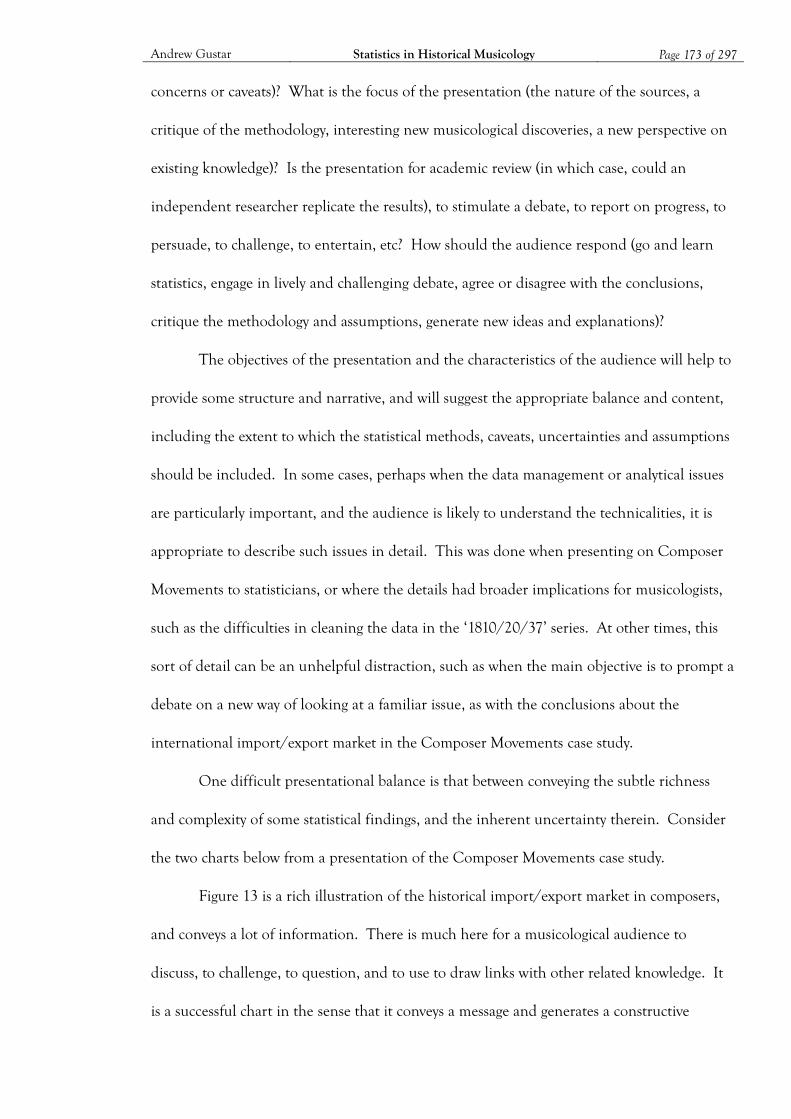
Andrew Gustar Statistics in Historical Musicology Page 173 of 297
concerns or caveats)? What is the focus of the presentation (the nature of the sources, a
critique of the methodology, interesting new musicological discoveries, a new perspective on
existing knowledge)? Is the presentation for academic review (in which case, could an
independent researcher replicate the results), to stimulate a debate, to report on progress, to
persuade, to challenge, to entertain, etc? How should the audience respond (go and learn
statistics, engage in lively and challenging debate, agree or disagree with the conclusions,
critique the methodology and assumptions, generate new ideas and explanations)?
The objectives of the presentation and the characteristics of the audience will help to
provide some structure and narrative, and will suggest the appropriate balance and content,
including the extent to which the statistical methods, caveats, uncertainties and assumptions
should be included. In some cases, perhaps when the data management or analytical issues
are particularly important, and the audience is likely to understand the technicalities, it is
appropriate to describe such issues in detail. This was done when presenting on Composer
Movements to statisticians, or where the details had broader implications for musicologists,
such as the difficulties in cleaning the data in the ‘1810/20/37’ series. At other times, this
sort of detail can be an unhelpful distraction, such as when the main objective is to prompt a
debate on a new way of looking at a familiar issue, as with the conclusions about the
international import/export market in the Composer Movements case study.
One difficult presentational balance is that between conveying the subtle richness
and complexity of some statistical findings, and the inherent uncertainty therein. Consider
the two charts below from a presentation of the Composer Movements case study.
Figure 13 is a rich illustration of the historical import/export market in composers,
and conveys a lot of information. There is much here for a musicological audience to
discuss, to challenge, to question, and to use to draw links with other related knowledge. It
is a successful chart in the sense that it conveys a message and generates a constructive
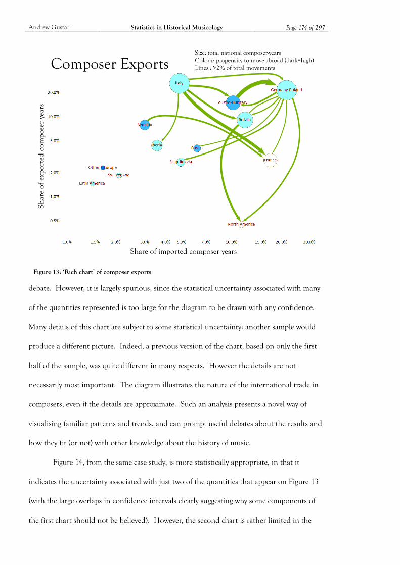
Andrew Gustar Statistics in Historical Musicology Page 174 of 297
debate. However, it is largely spurious, since the statistical uncertainty associated with many
of the quantities represented is too large for the diagram to be drawn with any confidence.
Many details of this chart are subject to some statistical uncertainty: another sample would
produce a different picture. Indeed, a previous version of the chart, based on only the first
half of the sample, was quite different in many respects. However the details are not
necessarily most important. The diagram illustrates the nature of the international trade in
composers, even if the details are approximate. Such an analysis presents a novel way of
visualising familiar patterns and trends, and can prompt useful debates about the results and
how they fit (or not) with other knowledge about the history of music.
Figure 14, from the same case study, is more statistically appropriate, in that it
indicates the uncertainty associated with just two of the quantities that appear on Figure 13
(with the large overlaps in confidence intervals clearly suggesting why some components of
the first chart should not be believed). However, the second chart is rather limited in the
Composer Exports
Share of imported composer years
Shar
e of
exp
orte
d co
mpo
ser
year
s
Size: total national composer-yearsColour: propensity to move abroad (dark=high)Lines : >2% of total movements
Figure 13: ‘Rich chart’ of composer exports

Andrew Gustar Statistics in Historical Musicology Page 175 of 297
light that it sheds on composer movements, and is less successful at stimulating debate
among musicologists. Unfortunately the creation of a ‘rich’ chart that adequately represents
the statistical uncertainties whilst remaining legible and meaningful is, in most cases,
practically impossible to achieve. The issue comes down to the objective in presenting these
results to a particular audience. In cases where the numbers themselves are important, the
second chart is much more appropriate. In other cases, the priority may be to illustrate the
nature of the processes at work, even if the exact details are no better than speculative. The
first chart illustrates the complexity and nature of the composer export market, despite
uncertainty over some of the details. It is the nature of the process that is most important (at
least on this occasion, for that particular audience), not the numbers themselves.
Graphs, charts and diagrams are useful tools in conveying complex statistical results,
particularly to non-statisticians. Their form in a presentation tends to be rather more
polished than when they are used for data exploration (see section 4.5.3), and it is often
95% confidence intervals for regional share of exported (blue) and imported (red) composer-years
0% 5% 10% 15% 20% 25% 30% 35%
0% 5% 10% 15% 20% 25% 30% 35%
North America
Latin America
Switzerland
Other S Europe
France
Scandinavia
Russia
Iberia
Benelux
Britain
Austro-Hungary
Germany Poland
Italy
Figure 14: Confidence ranges for composer exports and imports
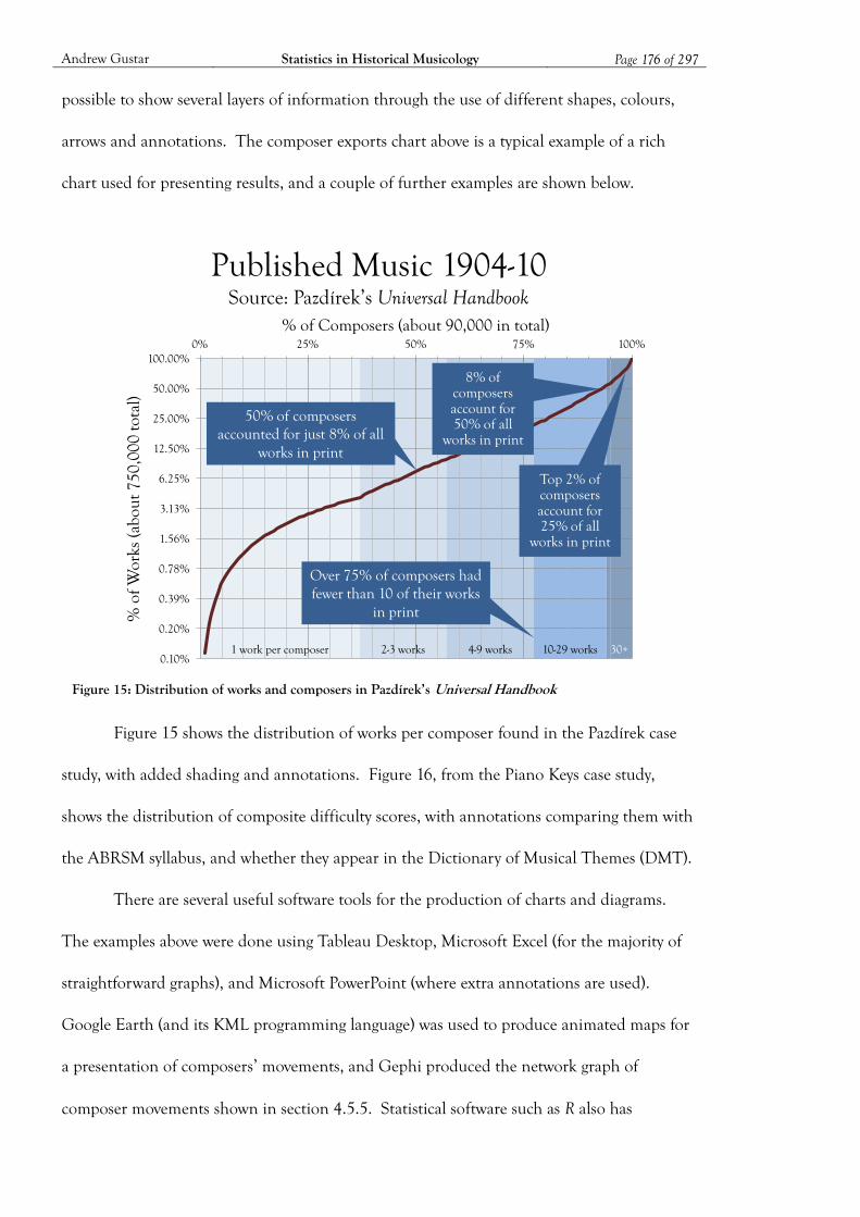
Andrew Gustar Statistics in Historical Musicology Page 176 of 297
possible to show several layers of information through the use of different shapes, colours,
arrows and annotations. The composer exports chart above is a typical example of a rich
chart used for presenting results, and a couple of further examples are shown below.
Figure 15 shows the distribution of works per composer found in the Pazdírek case
study, with added shading and annotations. Figure 16, from the Piano Keys case study,
shows the distribution of composite difficulty scores, with annotations comparing them with
the ABRSM syllabus, and whether they appear in the Dictionary of Musical Themes (DMT).
There are several useful software tools for the production of charts and diagrams.
The examples above were done using Tableau Desktop, Microsoft Excel (for the majority of
straightforward graphs), and Microsoft PowerPoint (where extra annotations are used).
Google Earth (and its KML programming language) was used to produce animated maps for
a presentation of composers’ movements, and Gephi produced the network graph of
composer movements shown in section 4.5.5. Statistical software such as R also has
Published Music 1904-10Source: Pazdírek’s Universal Handbook
0.10%
0.20%
0.39%
0.78%
1.56%
3.13%
6.25%
12.50%
25.00%
50.00%
100.00%0% 25% 50% 75% 100%
% o
f Wor
ks (a
bout
750
,000
tota
l)
% of Composers (about 90,000 in total)
50% of composers accounted for just 8% of all
works in print
Over 75% of composers had fewer than 10 of their works
in print
8% of composers account for 50% of all
works in print
Top 2% of composers account for 25% of all
works in print
30+ 1 work per composer 2-3 works 4-9 works 10-29 works
Figure 15: Distribution of works and composers in Pazdírek’s Universal Handbook

Andrew Gustar Statistics in Historical Musicology Page 177 of 297
powerful graphics capabilities. This is a rapidly developing field, and new applications (many
of them free) appear frequently, whilst existing ones are regularly improved and updated.
Such tools can be invaluable both for exploring data and for presenting statistical
results, but their appeal for researchers and audiences can also present a risk of ‘over-
interpretation’. This is where patterns in data are seen, interpreted, and emphasised, even
though, in statistical terms, they are not significant or may simply be the artefacts of random
‘noise’ in the data. The elaborate chart of composers exports above is (at least in terms of
the detail) an example of this, and it is easy to spot apparent trends and patterns in many
other charts that, on detailed investigation, would turn out to be entirely spurious. For this
reason, such charts must be accompanied by suitable caveats.
Difficulty of Piano WorksDMT = Dictionary of Musical Themes (Barlow & Morgenstern 1948)
01020304050607080
Num
ber
of w
orks
Composite Difficulty ScoreBased on Hinson 1987 and Barnard & Gutierrez 2006
Distribution of Difficulty Scores
Gra
de 5
Gra
de 8
Not in DMT
Dip
lom
a
LRSM
FRSM
In DMT
Figure 16: Distribution of technical difficulty of piano works
Andrew Gustar Statistics in Historical Musicology Page 178 of 297
5 MUSICOLOGICAL INSIGHTS
This chapter discusses some musicological insights that have been gained, through the case
studies, by applying statistical techniques to historical musical datasets. The aim is to
demonstrate what statistics can reveal about the history of music, as well as raising some
statistical characteristics and difficulties that arise in this field of research.
The primary objective of the case studies has been to test the statistical methodology
rather than thoroughly to investigate musicological topics. The findings presented here
illustrate some types of discovery in historical musicology that can be revealed by quantitative
methods, and suggest several topics that could be taken forward in more depth and rigour by
future researchers. Although possible explanations are postulated for some of the findings in
this chapter, establishing cause and effect usually requires detailed qualitative research that is
beyond the scope of this thesis. Quantitative techniques are good at answering the ‘what’
questions, but often provide little help with the ‘why’.
The organisation of this chapter does not directly follow the case studies as described
in section 2.1 and Appendix A. Instead it groups the findings into themes based on the lives
of composers (section 5.1), the nature of their works (5.2), the subsequent life of those works
(5.3), and the processes of achieving fame or obscurity (5.4). There is some overlap between
these themes, and many gaps that fall outside the scope of the case studies. Nevertheless,
this material is hopefully sufficient to illustrate the nature and breadth of the potential for
these methodologies, and perhaps to suggest avenues for further research.
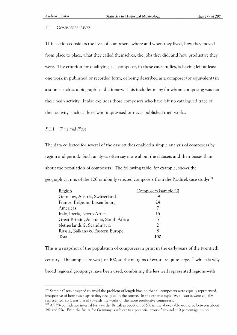
Andrew Gustar Statistics in Historical Musicology Page 179 of 297
5.1 COMPOSERS’ LIVES
This section considers the lives of composers: where and when they lived, how they moved
from place to place, what they called themselves, the jobs they did, and how productive they
were. The criterion for qualifying as a composer, in these case studies, is having left at least
one work in published or recorded form, or being described as a composer (or equivalent) in
a source such as a biographical dictionary. This includes many for whom composing was not
their main activity. It also excludes those composers who have left no catalogued trace of
their activity, such as those who improvised or never published their works.
5.1.1 Time and Place
The data collected for several of the case studies enabled a simple analysis of composers by
region and period. Such analyses often say more about the datasets and their biases than
about the population of composers. The following table, for example, shows the
geographical mix of the 100 randomly selected composers from the Pazdírek case study:101
Region Composers (sample C) Germany, Austria, Switzerland 39 France, Belgium, Luxembourg 24 Americas 7 Italy, Iberia, North Africa 15 Great Britain, Australia, South Africa 5 Netherlands & Scandinavia 2 Russia, Balkans & Eastern Europe 8 Total 100
This is a snapshot of the population of composers in print in the early years of the twentieth
century. The sample size was just 100, so the margins of error are quite large,102 which is why
broad regional groupings have been used, combining the less well represented regions with
101 Sample C was designed to avoid the problem of length bias, so that all composers were equally represented, irrespective of how much space they occupied in the source. In the other sample, W, all works were equally represented, so it was biased towards the works of the more productive composers. 102 A 95% confidence interval for, say, the British proportion of 5% in the above table would be between about 1% and 9%. Even the figure for Germany is subject to a potential error of around ±10 percentage points.
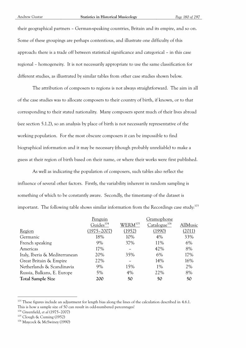
Andrew Gustar Statistics in Historical Musicology Page 180 of 297
their geographical partners – German-speaking countries, Britain and its empire, and so on.
Some of these groupings are perhaps contentious, and illustrate one difficulty of this
approach: there is a trade off between statistical significance and categorical – in this case
regional – homogeneity. It is not necessarily appropriate to use the same classification for
different studies, as illustrated by similar tables from other case studies shown below.
The attribution of composers to regions is not always straightforward. The aim in all
of the case studies was to allocate composers to their country of birth, if known, or to that
corresponding to their stated nationality. Many composers spent much of their lives abroad
(see section 5.1.2), so an analysis by place of birth is not necessarily representative of the
working population. For the most obscure composers it can be impossible to find
biographical information and it may be necessary (though probably unreliable) to make a
guess at their region of birth based on their name, or where their works were first published.
As well as indicating the population of composers, such tables also reflect the
influence of several other factors. Firstly, the variability inherent in random sampling is
something of which to be constantly aware. Secondly, the timestamp of the dataset is
important. The following table shows similar information from the Recordings case study:103
Region
Penguin Guides104
(1975–2007) WERM105
(1952)
Gramophone Catalogue106
(1990) AllMusic
(2011) Germanic 18% 10% 4% 33% French speaking 9% 37% 11% 6% Americas 17% – 42% 8% Italy, Iberia & Mediterranean 20% 35% 6% 17% Great Britain & Empire 22% – 14% 16% Netherlands & Scandinavia 9% 15% 1% 2% Russia, Balkans, E. Europe 5% 4% 22% 8% Total Sample Size 200 50 50 50
103 These figures include an adjustment for length bias along the lines of the calculation described in 4.6.1. This is how a sample size of 50 can result in odd-numbered percentages! 104 Greenfield, et al (1975–2007) 105 Clough & Cuming (1952) 106 Maycock & McSwiney (1990)

Andrew Gustar Statistics in Historical Musicology Page 181 of 297
Compared to Pazdírek, these sources from the second half of the twentieth century are less
dominated by the Germans and French, and include many more English-speaking
composers. This is not surprising, given what we know about the development of music
during the twentieth century and, just as importantly, about the development of the
recording industry and, for that matter, the record guide industry. The national or linguistic
bias of datasets and their compilers is our third factor influencing the apparent distribution
of composers. This table, relating to recordings rather than publications, also differs from
the Pazdírek data because of the fourth factor: the purpose or subject of the dataset.
A fifth factor is the particular interests or circumstances of the dataset’s compiler.
Consider the following table from the Biographical Dictionaries case study:
Region Gerber Fétis Mendel Eitner Total Germanic 21 16 26 8 71 French 6 9 7 10 32 Italian 12 12 8 23 55 Iberian 1 3 1 - 5 British 6 6 6 7 25 Eastern European 4 4 2 2 12 Total 50 50 50 50 200
These are all nineteenth-century European sources, hence the absence of American
composers (at least in the sample). Gerber (1812), Fétis (1835) and Mendel (1870) all show
broadly similar distributions, but Eitner (1900) is markedly heavy with Italian composers.
Many of Eitner’s Italians appear to be new discoveries, dating largely from the sixteenth and
seventeenth centuries, that are not mentioned in the other dictionaries. This appears to be a
particular field of interest for Eitner.
The period in which composers lived is, of course, another important factor (our
sixth). It is possible that Eitner was not interested in Italians per se, but in the sixteenth and
seventeenth centuries, a period when Italy was arguably the dominant centre of musical
activity. Figure 17, from the Composer Movements case study, shows this more objectively
since the entire sample in this case comes from a single source, Oxford Music Online. The
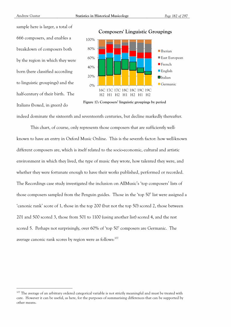
Andrew Gustar Statistics in Historical Musicology Page 182 of 297
sample here is larger, a total of
666 composers, and enables a
breakdown of composers both
by the region in which they were
born (here classified according
to linguistic groupings) and the
half-century of their birth. The
Italians (boxed, in green) do
indeed dominate the sixteenth and seventeenth centuries, but decline markedly thereafter.
This chart, of course, only represents those composers that are sufficiently well-
known to have an entry in Oxford Music Online. This is the seventh factor: how well-known
different composers are, which is itself related to the socio-economic, cultural and artistic
environment in which they lived, the type of music they wrote, how talented they were, and
whether they were fortunate enough to have their works published, performed or recorded.
The Recordings case study investigated the inclusion on AllMusic’s ‘top composers’ lists of
those composers sampled from the Penguin guides. Those in the ‘top 50’ list were assigned a
‘canonic rank’ score of 1, those in the top 200 (but not the top 50) scored 2, those between
201 and 500 scored 3, those from 501 to 1100 (using another list) scored 4, and the rest
scored 5. Perhaps not surprisingly, over 60% of ‘top 50’ composers are Germanic. The
average canonic rank scores by region were as follows:107
107 The average of an arbitrary ordered categorical variable is not strictly meaningful and must be treated with care. However it can be useful, as here, for the purposes of summarising differences that can be supported by other means.
Figure 17: Composers’ linguistic groupings by period
0%
20%
40%
60%
80%
100%
16C H2
17C H1
17C H2
18C H1
18C H2
19C H1
19C H2
Composers' Linguistic Groupings
Iberian
East European
French
English
Italian
Germanic
Andrew Gustar Statistics in Historical Musicology Page 183 of 297
Average canonic rank Germanic 1.24 French 1.52 East European 1.55 Scandinavian 2.17 Mediterranean 2.28 American 2.54 British 2.70
These scores reflect the fact that more of the best known and highly regarded composers are
German, French and Russian / East European than other nationalities. They also reflect the
English-speaking bias of the Penguin guides, which are more likely to include lesser names by
British and American composers than to list equally obscure German or French composers.
There are probably other factors in addition to the seven identified here that can
affect the distribution of composers by region. Indeed, similar arguments can be put forward
in relation to many of the distributions to be discussed in this chapter. In practice it is more
or less impossible to derive a ‘true’ distribution of composers by region, because other
contextual factors (relating to the dataset and its compilers, variations over time,
geographical and fame-related asymmetries, etc) are always present. In some cases, the
potential bias is simple and easily identified, at least qualitatively: Pazdírek’s Universal
Handbook, for example, is a relatively objective source, but is restricted to published music at
a particular point in time, so its geographical bias will reflect that of the music publishing
industry in the early twentieth century. In most cases, however, there are likely to be many
sources of bias that cannot be readily untangled – national, personal and linguistic factors, a
focus on the more well-known names, and data that has been collected from many sources at
different times and on unknown but maybe inconsistent bases.
The conclusions to be drawn from such analyses are thus more about the nature of
the datasets than the population of composers. We cannot even be confident about such
apparently consistent results as the predominance of Germanic composers. Although they
appear to form the largest group (at least from the eighteenth century onwards), the
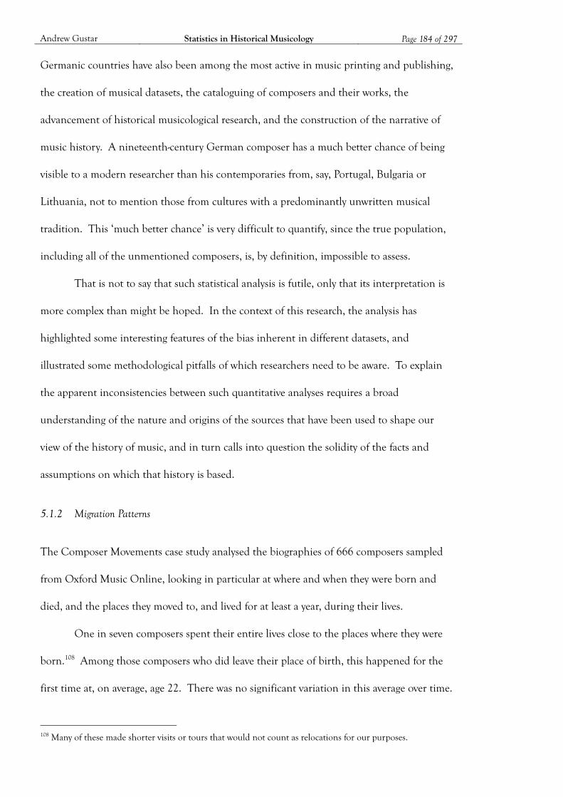
Andrew Gustar Statistics in Historical Musicology Page 184 of 297
Germanic countries have also been among the most active in music printing and publishing,
the creation of musical datasets, the cataloguing of composers and their works, the
advancement of historical musicological research, and the construction of the narrative of
music history. A nineteenth-century German composer has a much better chance of being
visible to a modern researcher than his contemporaries from, say, Portugal, Bulgaria or
Lithuania, not to mention those from cultures with a predominantly unwritten musical
tradition. This ‘much better chance’ is very difficult to quantify, since the true population,
including all of the unmentioned composers, is, by definition, impossible to assess.
That is not to say that such statistical analysis is futile, only that its interpretation is
more complex than might be hoped. In the context of this research, the analysis has
highlighted some interesting features of the bias inherent in different datasets, and
illustrated some methodological pitfalls of which researchers need to be aware. To explain
the apparent inconsistencies between such quantitative analyses requires a broad
understanding of the nature and origins of the sources that have been used to shape our
view of the history of music, and in turn calls into question the solidity of the facts and
assumptions on which that history is based.
5.1.2 Migration Patterns
The Composer Movements case study analysed the biographies of 666 composers sampled
from Oxford Music Online, looking in particular at where and when they were born and
died, and the places they moved to, and lived for at least a year, during their lives.
One in seven composers spent their entire lives close to the places where they were
born.108 Among those composers who did leave their place of birth, this happened for the
first time at, on average, age 22. There was no significant variation in this average over time.
108 Many of these made shorter visits or tours that would not count as relocations for our purposes.
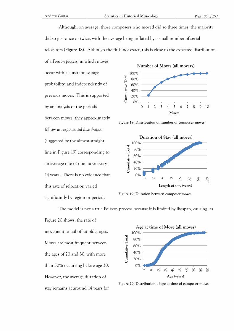
Andrew Gustar Statistics in Historical Musicology Page 185 of 297
Although, on average, those composers who moved did so three times, the majority
did so just once or twice, with the average being inflated by a small number of serial
relocators (Figure 18). Although the fit is not exact, this is close to the expected distribution
of a Poisson process, in which moves
occur with a constant average
probability, and independently of
previous moves. This is supported
by an analysis of the periods
between moves: they approximately
follow an exponential distribution
(suggested by the almost straight
line in Figure 19) corresponding to
an average rate of one move every
14 years. There is no evidence that
this rate of relocation varied
significantly by region or period.
The model is not a true Poisson process because it is limited by lifespan, causing, as
Figure 20 shows, the rate of
movement to tail off at older ages.
Moves are most frequent between
the ages of 20 and 30, with more
than 50% occurring before age 30.
However, the average duration of
stay remains at around 14 years for
Figure 18: Distribution of number of composer moves
0%
20%
40%
60%
80%
100%
0 1 2 3 4 5 6 7 8 9 10
Cum
ulat
ive
Tot
al
Moves
Number of Moves (all movers)
Figure 19: Duration between composer moves
0%
20%
40%
60%
80%
100% 1 2 4 8 16
32
64
128
Cum
ulat
ive
Tot
al
Length of stay (years)
Duration of Stay (all moves)
Figure 20: Distribution of age at time of composer moves
0%
20%
40%
60%
80%
100%
0 10
20
30
40
50
60
70
80
90
Cum
ulat
ive
Tot
al
Age (years)
Age at time of Move (all moves)
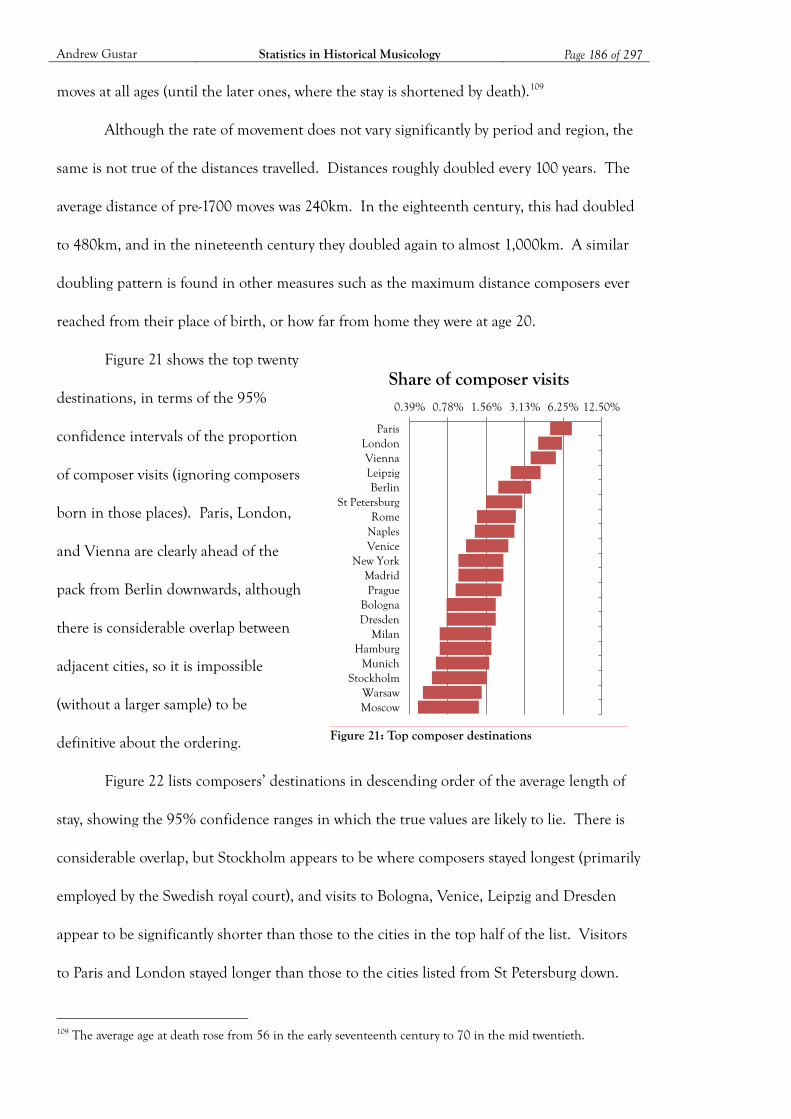
Andrew Gustar Statistics in Historical Musicology Page 186 of 297
moves at all ages (until the later ones, where the stay is shortened by death).109
Although the rate of movement does not vary significantly by period and region, the
same is not true of the distances travelled. Distances roughly doubled every 100 years. The
average distance of pre-1700 moves was 240km. In the eighteenth century, this had doubled
to 480km, and in the nineteenth century they doubled again to almost 1,000km. A similar
doubling pattern is found in other measures such as the maximum distance composers ever
reached from their place of birth, or how far from home they were at age 20.
Figure 21 shows the top twenty
destinations, in terms of the 95%
confidence intervals of the proportion
of composer visits (ignoring composers
born in those places). Paris, London,
and Vienna are clearly ahead of the
pack from Berlin downwards, although
there is considerable overlap between
adjacent cities, so it is impossible
(without a larger sample) to be
definitive about the ordering.
Figure 22 lists composers’ destinations in descending order of the average length of
stay, showing the 95% confidence ranges in which the true values are likely to lie. There is
considerable overlap, but Stockholm appears to be where composers stayed longest (primarily
employed by the Swedish royal court), and visits to Bologna, Venice, Leipzig and Dresden
appear to be significantly shorter than those to the cities in the top half of the list. Visitors
to Paris and London stayed longer than those to the cities listed from St Petersburg down.
109 The average age at death rose from 56 in the early seventeenth century to 70 in the mid twentieth.
Figure 21: Top composer destinations
0.39% 0.78% 1.56% 3.13% 6.25% 12.50%
Paris London Vienna Leipzig Berlin
St Petersburg Rome
Naples Venice
New York Madrid Prague
Bologna Dresden
Milan Hamburg
Munich Stockholm
Warsaw Moscow
Share of composer visits
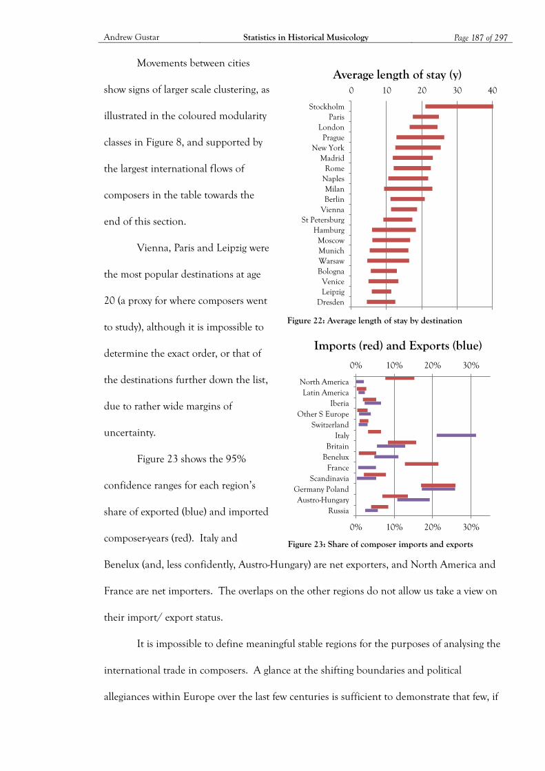
Andrew Gustar Statistics in Historical Musicology Page 187 of 297
Movements between cities
show signs of larger scale clustering, as
illustrated in the coloured modularity
classes in Figure 8, and supported by
the largest international flows of
composers in the table towards the
end of this section.
Vienna, Paris and Leipzig were
the most popular destinations at age
20 (a proxy for where composers went
to study), although it is impossible to
determine the exact order, or that of
the destinations further down the list,
due to rather wide margins of
uncertainty.
Figure 23 shows the 95%
confidence ranges for each region’s
share of exported (blue) and imported
composer-years (red). Italy and
Benelux (and, less confidently, Austro-Hungary) are net exporters, and North America and
France are net importers. The overlaps on the other regions do not allow us take a view on
their import/ export status.
It is impossible to define meaningful stable regions for the purposes of analysing the
international trade in composers. A glance at the shifting boundaries and political
allegiances within Europe over the last few centuries is sufficient to demonstrate that few, if
Figure 23: Share of composer imports and exports
0% 10% 20% 30%
0% 10% 20% 30%
Russia Austro-Hungary
Germany Poland Scandinavia
France Benelux Britain
Italy Switzerland
Other S Europe Iberia
Latin America North America
Imports (red) and Exports (blue)
Figure 22: Average length of stay by destination
0 10 20 30 40
Dresden Leipzig Venice
Bologna Warsaw Munich Moscow
Hamburg St Petersburg
Vienna Berlin Milan
Naples Rome
Madrid New York
Prague London
Paris Stockholm
Average length of stay (y)

Andrew Gustar Statistics in Historical Musicology Page 188 of 297
any, of the regions listed in the chart of imports and exports can be considered as stable and
homogeneous political, cultural or linguistic entities over a long period. It would be more
appropriate to consider the flows of composers over shorter periods, although this would
require a larger sample: breaking down the figures by both region and period quickly results
in small numbers of observations in each category and consequently large margins of
uncertainty.
Analysis of the proportion of time spent abroad reveals that French composers had a
lower propensity to do so than those from Italy, Benelux, Germany-Poland or Austro-
Hungary. There is too much overlap between the other regions to draw firm conclusions.
The ten largest international flows of composers in the combined sample, as
percentages of the total exported composer-years, were as shown in the table below. The first
two of these are clearly ahead of the rest, although the eight others all overlap considerably,
so the ranking shown here between these eight should be regarded as indicative.
From To Share Standard Error110 Austro-Hungary Germany-Poland 9.5% 1.3% Italy France 7.4% 1.1% Britain North America 4.9% 0.9% Italy Britain 4.8% 0.9% Italy Austro-Hungary 4.7% 0.9% Benelux France 4.1% 0.9% Germany-Poland Austro-Hungary 3.9% 0.8% Germany-Poland North America 3.6% 0.8% Italy Germany-Poland 3.4% 0.8% Germany-Poland Scandinavia 3.3% 0.8%
As illustrated in Figure 13 it is possible to draw ‘rich’ diagrams illustrating various aspects of
the international market in composers, although it is difficult to represent the appropriate
levels of statistical uncertainty in such diagrams. Nevertheless they can be useful in
illustrating the nature, if not the exact details, of complex data such as this.
It is likely that the conclusions above are influenced by the bias in Oxford Music
110 An approximate 95% confidence interval for the actual share is the observed share plus or minus twice the standard error.

Andrew Gustar Statistics in Historical Musicology Page 189 of 297
Online (such as the greater representation of British composers) and, more generally, by that
in the historical sources on which it draws. These sources (other biographical dictionaries,
academic papers, and surveys of works or institutions) will be concentrated most strongly on
the major centres of historical musicological research and activity, particularly Germany,
Britain and France. It is likely that the migration patterns involving composers from, or
moves to, these regions will be over-represented in this analysis compared to those relating to
parts of the world where musicological activity (but not necessarily musical activity) has been
less intense. This geographical bias in the sources available to historical musicologists is a
pervasive effect that impacts on both qualitative and quantitative research.
5.1.3 Names
Variant names can be problematic when trying to find a composer, sampled from one
dataset, in a different source. In the Biographical Dictionaries case study, for example, the
German sources were good at retaining the original forms of non-German names, although
Fétis ‘Frenchifies’ almost all forenames and place names (e.g. ‘Beethoven, Louis van’),
leading to some difficulty identifying individuals at the triangulation stage. In other cases,
names were sometimes inconsistent. A middle name might differ between sources, even
though dates and places were the same. A particular problem was with variations in spelling,
not just between the French and German sources, but also over time. Sometimes these were
mentioned as variants in the original sampled source, such as Bononcini/Buononcini or
Dauvergne/d’Auvergne, but others only came to light during triangulation, requiring re-
triangulation of the revised name.111 Other similar names might have been variants, but
could not be verified as such.112 Although some sources helpfully list known variants, and
others can be guessed, the process is rather hit-and-miss, and some names could probably 111 Examples were ‘Frederick’ (from Gerber), later identified as Frederic Duvernoy; Pierre Desforges, also known as Pierre Hus-Deforges; and Carlo Chiabrano, better known under his Parisian alter ego of Charles Chabran. 112 For example, ‘Tomisch, Flosculus’ might be the same person as ‘Tomich, F’.
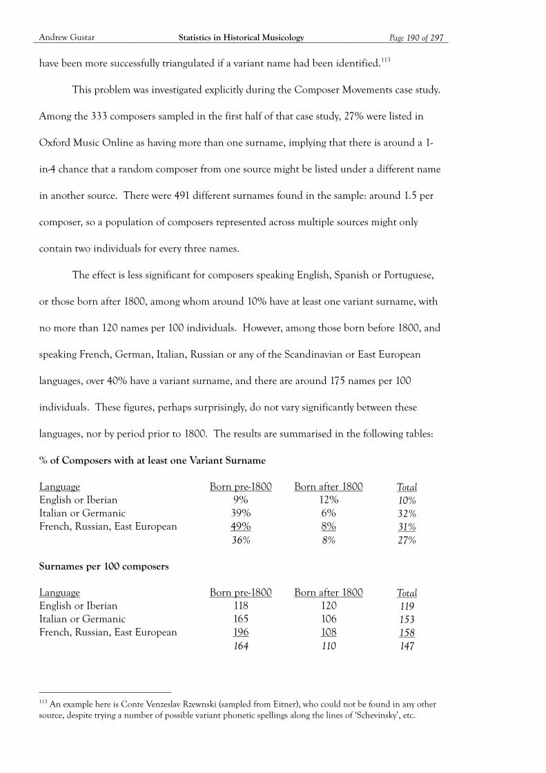
Andrew Gustar Statistics in Historical Musicology Page 190 of 297
have been more successfully triangulated if a variant name had been identified.113
This problem was investigated explicitly during the Composer Movements case study.
Among the 333 composers sampled in the first half of that case study, 27% were listed in
Oxford Music Online as having more than one surname, implying that there is around a 1-
in-4 chance that a random composer from one source might be listed under a different name
in another source. There were 491 different surnames found in the sample: around 1.5 per
composer, so a population of composers represented across multiple sources might only
contain two individuals for every three names.
The effect is less significant for composers speaking English, Spanish or Portuguese,
or those born after 1800, among whom around 10% have at least one variant surname, with
no more than 120 names per 100 individuals. However, among those born before 1800, and
speaking French, German, Italian, Russian or any of the Scandinavian or East European
languages, over 40% have a variant surname, and there are around 175 names per 100
individuals. These figures, perhaps surprisingly, do not vary significantly between these
languages, nor by period prior to 1800. The results are summarised in the following tables:
% of Composers with at least one Variant Surname Language Born pre-1800 Born after 1800 Total English or Iberian 9% 12% 10% Italian or Germanic 39% 6% 32% French, Russian, East European 49% 8% 31% 36% 8% 27% Surnames per 100 composers Language Born pre-1800 Born after 1800 Total English or Iberian 118 120 119 Italian or Germanic 165 106 153 French, Russian, East European 196 108 158 164 110 147
113 An example here is Conte Venzeslav Rzewnski (sampled from Eitner), who could not be found in any other source, despite trying a number of possible variant phonetic spellings along the lines of ‘Schevinsky’, etc.
Andrew Gustar Statistics in Historical Musicology Page 191 of 297
A closer analysis of the variant surnames reveals that the situation is not quite as problematic
as it at first appears. Of the 91 composers with a variant, only 16 (just 5% of the sample) had
one that was completely different from their first-listed name. These were mainly maiden or
married names, pseudonyms,114 nicknames and titles. In most other cases, variants were
phonetically similar. Thirteen composers had variants starting with a different letter from
that of the first-listed name, making them harder to find in alphabetical sources, although
most of these were relatively predictable alternatives: Ch/K, C/G, P/B, V/W, J/Y, etc. The
other forms of variant tend to be less widely separated in alphabetical lists: mid-name
changes of consonant (largely as above), changes of vowels, added vowels (especially an i or e
at the end of a name), repeated or single consonants (particularly l and t, and especially
among Italian names), and the omission or insertion of spaces and apostrophes (especially in
French names, such as Dauvergne/d’Auvergne, or Du Phly/Duphly).
One composer in seven had a variant forename, mostly minor spelling variations or
versions of the same name in different languages (e.g. Jan/Jean/Johann).
This brief analysis illustrated the extent of the problem of variant names, and
highlighted some areas where it is particularly likely to occur. It might be possible, with
further research, to outline some guidelines to maximise the chance of finding different
types of name, or in some circumstances to automate parts of the process. This is an
established field of research in genealogy, and there exist a number of automatic tools, such
as NameX, for generating, and searching for, similar and variant names.115 However, whilst a
search on the NameX website generated 143 possible variants of ‘Cavalli’, these did not
include any of the five alternatives mentioned in Oxford Music Online.
114 For example Schulze/Praetorius 115 Described at http://www.origins.net/namex/aboutnamex.html
Andrew Gustar Statistics in Historical Musicology Page 192 of 297
5.1.4 Occupations
The 333 names sampled from Oxford Music Online in the first half of the Composer
Movements case study were all listed as ‘composers’ in their biographical articles, and many
were also described in other ways. Just 25% were listed only as ‘composers’, with the rest
having at least one additional occupation. The majority of these – about 50% of all
composers – were also listed as performers (singers or instrumentalists), with around 13%
also being conductors and the same number listed as teachers. The proportion of
performers is relatively constant for all periods and regions, the exception being British
composers, where a significantly higher proportion (about two-thirds) were also
performers.116 There was a significant increase over time in the proportion of conductors
and teachers: 6% of pre-1800 composers were also described as conductors or teachers, but
after 1800 this rises to around 30% for each. This is unsurprising in the case of conducting,
which only became a common activity during the nineteenth century. Other occupations
mentioned included Writer on Music (7%), Theorist (4%), Musicologist (4%), Poet, Patron,
Publisher, Instrument Maker, Dancer, Ethnomusicologist and Librettist. Many composers,
particularly pre-1800, carried out their duties within religious institutions.
Unfortunately, Oxford Music Online does not indicate the primary occupation for
which an individual is known nor, more significantly, that for which they were best known in
the past (although this can sometimes be inferred). An additional weakness of this
composer-based sample is that it tells us nothing about the proportion of performers (or of
other occupations) who were also composers. A further study with a broader sample would
be required in order to make further progress on this question.
116 It is possible that this is a result of a British bias within Oxford Music Online, whereby additional occupations are more likely to be mentioned for British composers than for other nationalities.
Andrew Gustar Statistics in Historical Musicology Page 193 of 297
5.1.5 Productivity
Statistical techniques can shed a little light on the question of composers’ productivity,
although further (qualitative) research would be needed to draw conclusions with any
confidence. As discussed in section 4.6.3, the distribution of published works per composer
in the early twentieth century follows a Zipf-like distribution.117 Over a third of composers
had just a single work in print, 80% had fewer than ten, and the highest number of works
for a composer in the sample of 100 random composers was 163. Looked at from the
perspective of works, these are dominated by the most productive composers: the one-or-two-
work composers only account for about 10% of works, whereas around 25% of all works are
by composers who had more works in print than the 163 of the most productive of the
sample of random composers. The highest number of works found for a composer in the
‘random works’ sample was around 2,000, for Mozart.118
Of course these figures do not include unpublished works, nor those previously
published that were no longer in print (or in stock) at the time Pazdírek’s Handbook was
compiled. It would in principle be possible to estimate the volume of unpublished works by
examining the biographies and manuscript legacies of a random sample of composers, and
comparing this with their published material, although finding sufficient data on the output
of the little-published composers would be difficult. Previously published but unavailable
material could also be approximately quantified by counting the number of unique works by
each random composer in a composite library catalogue such as WorldCat.
It is also possible to consider opus numbers. The use of opus numbers was relatively
low, with just 29 of the 100 random composers in the Pazdírek ‘C’ sample having opus
117 See also the ‘Published Music’ chart in section 4.8 (Figure 15). 118 Although Mozart has around 2,000 works listed in Pazdírek’s Handbook, the Köchel catalogue of his works only extends to K626 (the Requiem). The difference is due to the publication of partial works (many K numbers encompass several short pieces, for example), as well as the publication of arrangements and transcriptions, and of the same work under multiple titles (for example in different languages).
Andrew Gustar Statistics in Historical Musicology Page 194 of 297
numbers assigned to their works. Of those composers, only about two-thirds of their works
mentioned had an opus number. The highest opus number mentioned for each composer
(presumably an indicator of total compositional output) was, on average, more than five
times the number of their works with opus numbers listed, suggesting that over 80% of opus-
numbered works had gone out of print. Although opus numbers are rare before the mid
eighteenth century, and tend to be used by the more productive composers, this indicates a
possibly substantial volume of previously published material beyond Pazdírek’s scope.119
The work on repeat publication as part of the Class of 1837 case study (described
more fully in 5.3.1) suggested, subject to the caveat of only considering original solo piano
music from a single year, that over half of published works are never republished. Earlier
composers (typically the more prolific ones) with republished works will still be relatively well
represented in a catalogue such as Pazdírek’s, whereas those early composers with few
published works, most of which were never republished, will be underrepresented.120 The
Recordings case study found several composers represented by a single famous work, despite
being relatively prolific in their day. It is possible that a similar effect happens in publishing,
and that there are, among Pazdírek’s single-work composers, some extremely productive
composers whose sole source of enduring fame lies in a single work. Some of the composers
found in the Class of 1837 case study would support this argument: Karl Czerny, Sigismund
Thalberg and Stephen Heller are examples of prolific composers whose works are difficult
(though by no means impossible) to find in print today.
It is thus very difficult to get a fair picture of composers’ productivity from the
historical data that have come down to us, skewed as they are by the factors mentioned
above. Scherer (2004) uses a measure of productivity based on the length of composers’ 119 In some cases, a composer’s published opus numbers may not run consecutively from op.1 upwards, although it is hard to tell whether this practice was common. 120 However, there is some evidence that Pazdírek’s list includes publishers’ old stock of minor works by minor composers that was printed, probably in the second half of the nineteenth century, sold very few copies, but was never destroyed.

Andrew Gustar Statistics in Historical Musicology Page 195 of 297
entries in the Schwann recordings catalogue, and concludes that productivity on this measure
shows little correlation with financial success. He also observes that differences in the basis
on which composers earned their livings (freelance; employed by the church or a rich patron;
combined with teaching, performing and other duties; etc) appear to have an effect on
productivity as well as on their financial fortunes. The implication of the case studies is that
it is unlikely that many composers were able to earn a living primarily from composing: the
number of composers with many works and evidence of substantial sales is very small as a
proportion of the total. Generalisation, of course, is dangerous. Nevertheless, this sort of
analysis does enable conclusions to be drawn about topics such as publication, recordings,
the processes leading to fame and obscurity, and the characteristics of the various datasets,
which are covered elsewhere in this thesis.

Andrew Gustar Statistics in Historical Musicology Page 196 of 297
5.2 COMPOSITIONS
This section looks at the characteristics of the music itself – the genres, key and time
signatures, and technical difficulty – that have been covered in the case studies.
5.2.1 Genres
‘Genre’ in this thesis is used to mean any classification of music by type. In most cases this is
by the performing forces required. For the purposes of the case studies, these categories have
been drawn fairly broadly, although in some cases (such as an investigation into the changing
size and composition of orchestras) a more detailed approach would be appropriate.
Rather like the geographical distribution of composers, and for similar reasons, it is
hard to be definitive about the distribution of musical works by genre. The answer depends
on the context, and is not readily generalisable. Differences between periods and regions are
likely to have a significant effect on the mix of genres, although the samples used in the case
studies were too small for much to be said on either of these issues with any great
confidence. Nevertheless, interesting conclusions can be drawn about the differences, for
example between publications and recorded music, or the preferences of composers,
audiences, publishers and editors, as well as the characteristics of the sources themselves.
The Pazdírek and Recordings case studies both collected data on the distribution of
random samples of works according to genre, summarised in the following table:121
Pazdírek case study Recordings case study
Forces
Works of random
composers Random
works Penguin Guides Catalogues
Solo Keyboard (2 or 4 hands) 48% 42% 11% 16% Solo Song (plus accompaniment) 20% 26% 4% 18% Vocal Group (with or without acc.) 10% 20% 24% 23% Chamber / Other solo instrument 17% 8% 17% 15% Orchestra / Band / Concerto 5% 4% 44% 27%
121 The Macdonald case study also collected this information, although the sample was drawn from several genre-based sources, so is not representative of a broader population.
Andrew Gustar Statistics in Historical Musicology Page 197 of 297
One striking feature of Pazdírek is the large proportion of published music – over
two thirds – consisting of piano pieces and songs. Pazdírek recognises this in the preface to
the first volume of the Handbook, where he concludes that leaving out explicit reference to
the forces required for these works will save him ‘many hundreds of pages’.122 Much of the
music published in the early years of the twentieth century thus appears to have been firmly
aimed at the domestic market, with songs and small piano and instrumental pieces (many
being arrangements of familiar works such as operatic arias and overtures) occupying, in
some ways, the niche that popular music came to fill once recording and broadcasting had
become widespread. The distinction between ‘high’ and ‘low’ status music, which during the
course of the twentieth century became based largely on questions of style and genre, was, at
the time of Pazdírek’s survey, more to do with the music’s technical difficulty, the status of
the composer, and whether it was targeted and marketed at the domestic or professional
musician. By mid-century the classical / popular distinction enabled the creation of record
guides and catalogues that excluded most of the ‘popular’ works that Pazdírek would have
included. This is evidenced by the relatively small proportion of keyboard works and songs
appearing in the recorded repertoire represented by the ‘Catalogues’ column. Compared to
these, the ‘Penguin Guides’ figures are further influenced by the compilers’ preferences,
which are clearly ‘pro’ orchestral music and ‘anti’ solo song.
The two Pazdírek samples show statistically significant differences in the proportions
of larger scale vocal and chamber works. Larger scale vocal works are over-represented in the
sample of random works, which is biased towards the more prolific composers. This
suggests, perhaps not surprisingly, that the less productive composers tend not to write pieces
for large vocal forces. Interestingly, large instrumental works do not show the same trend,
although the sample sizes here are too small to draw firm conclusions. Chamber and other
122 Pazdírek (1904–10), vol.1, IV
Andrew Gustar Statistics in Historical Musicology Page 198 of 297
small instrumental works are more numerous in the sample that is more representative of
the large numbers of composers with fewer works. Closer examination of the data reveals
that much of this category consists of specialist arrangements (e.g. transcriptions of operatic
tunes for zither or mandolin), often by relatively unproductive composers.
The differences between the figures for published and recorded music are revealing.
The ratio of the Pazdírek ‘Random Work’ column and the Recordings ‘Catalogues’ column
ranges from 2.6 for piano works to 0.15 for orchestral works, indicating that a random
published piano work is (subject to some statistical uncertainty) around eighteen times less
likely to have been recorded than a random orchestral work. This is partly explained by the
huge volumes of domestic music for piano: pieces intended for consumption by the
performer rather than the listener. It may also be influenced by the fact that orchestral
music is less likely to be published until after it has achieved some success on the concert
platform. It is also, surely, a reflection of the greater esteem in which orchestral music is
held, by the record companies and the population at large, relative to smaller-scale works (as
illustrated by the bias of the editors of the Penguin Guides).
5.2.2 Time Signatures
Time signatures were one of the topics investigated in the Macdonald case study, which
aimed to carry out statistical tests of various claims made by Hugh Macdonald, in his 1988
paper, that both time and key signatures became more extreme during the course of the
nineteenth century. The claims tested are set out in full in Appendix A (page 264). Of
these, twelve hypotheses (h-2 and h-9–h-19) relate to time signatures. The conclusions
regarding key signatures, including the subsequent Piano Keys case study, are discussed in
the next section.
For the purposes of the analysis, time signatures were assigned a ‘metre code’, rating

Andrew Gustar Statistics in Historical Musicology Page 199 of 297
the degree of complexity based on the top number of the time signature, as follows:
Metre Code 1 2 3 4 5 6 7 8 Time Signature (top) 2 4 3 6 12 9 5 7
The metre code reflects rhythmic complexity by sorting the time signatures according to the
smallest prime factors of the top number. Thus powers of 2 come first, then multiples of 3n
for increasing n, then the same for the next prime numbers 5 and 7. This particular scale
represents only those time signatures encountered in this sample. The metre code simply
indicates whether one metre is more complex than another, it does not attempt to quantify
the relative levels of complexity. There may be some debate about the order of complexity
here: is, for example, more complex than
? Macdonald suggests that
is the most complex
of the simple (2 and 3 based) metres, but nevertheless, other orderings are possible.
Few of Macdonald’s claims held up to statistical scrutiny. His most common mistake
regarding the supposed increase in prevalence of compound metres during the nineteenth
century can be illustrated by Figure 24, which plots the metre code versus the composition
date for the sample used in this case study. On the face of it, there does appear to be a
spread, over time, towards the higher metre codes. Although code 4 ( ) metres were quite
common from the beginning of the eighteenth century onwards, code 5 (
) was rare before
the second half of the nineteenth century, and codes 6 and above did not appear (at least in
this sample) until around the middle
of the nineteenth century. However,
there was also a substantial increase
in the total number of works over
the period. The more works in total,
the greater the chance of finding, in
a sample such as this, an example of Figure 24: Metre code vs composition date
0
1
2
3
4
5
6
7
8
1500 1550 1600 1650 1700 1750 1800 1850 1900 1950
Metre Code vs Date
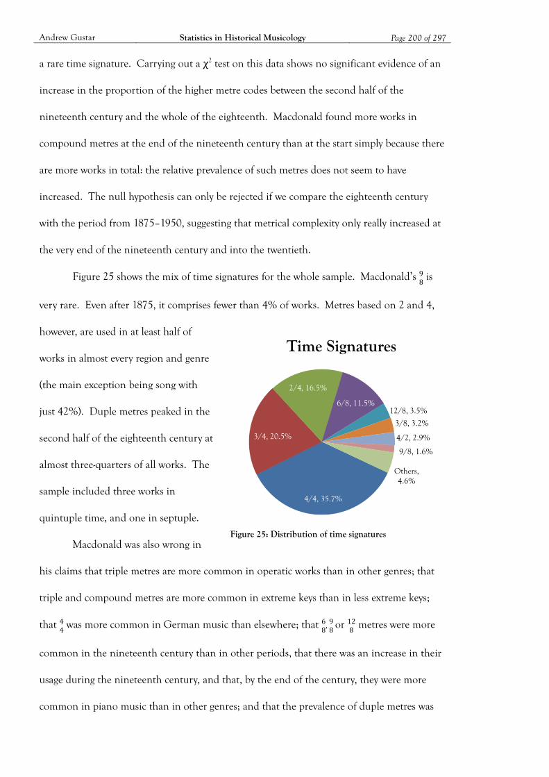
Andrew Gustar Statistics in Historical Musicology Page 200 of 297
a rare time signature. Carrying out a χ2 test on this data shows no significant evidence of an
increase in the proportion of the higher metre codes between the second half of the
nineteenth century and the whole of the eighteenth. Macdonald found more works in
compound metres at the end of the nineteenth century than at the start simply because there
are more works in total: the relative prevalence of such metres does not seem to have
increased. The null hypothesis can only be rejected if we compare the eighteenth century
with the period from 1875–1950, suggesting that metrical complexity only really increased at
the very end of the nineteenth century and into the twentieth.
Figure 25 shows the mix of time signatures for the whole sample. Macdonald’s is
very rare. Even after 1875, it comprises fewer than 4% of works. Metres based on 2 and 4,
however, are used in at least half of
works in almost every region and genre
(the main exception being song with
just 42%). Duple metres peaked in the
second half of the eighteenth century at
almost three-quarters of all works. The
sample included three works in
quintuple time, and one in septuple.
Macdonald was also wrong in
his claims that triple metres are more common in operatic works than in other genres; that
triple and compound metres are more common in extreme keys than in less extreme keys;
that was more common in German music than elsewhere; that
,
or
metres were more
common in the nineteenth century than in other periods, that there was an increase in their
usage during the nineteenth century, and that, by the end of the century, they were more
common in piano music than in other genres; and that the prevalence of duple metres was
Figure 25: Distribution of time signatures
4/4, 35.7%
3/4, 20.5%
2/4, 16.5%
6/8, 11.5% 12/8, 3.5%
3/8, 3.2%
4/2, 2.9%
9/8, 1.6%
Others, 4.6%
Time Signatures
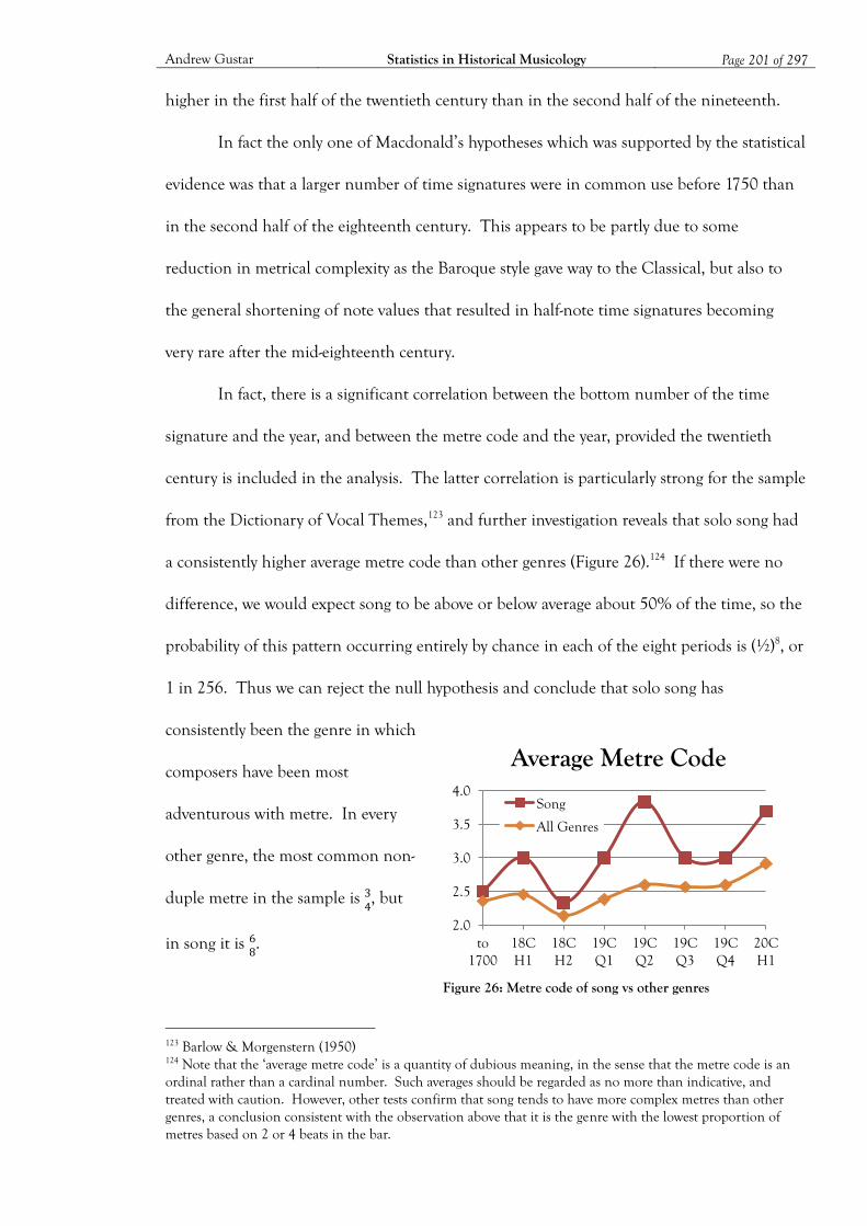
Andrew Gustar Statistics in Historical Musicology Page 201 of 297
higher in the first half of the twentieth century than in the second half of the nineteenth.
In fact the only one of Macdonald’s hypotheses which was supported by the statistical
evidence was that a larger number of time signatures were in common use before 1750 than
in the second half of the eighteenth century. This appears to be partly due to some
reduction in metrical complexity as the Baroque style gave way to the Classical, but also to
the general shortening of note values that resulted in half-note time signatures becoming
very rare after the mid-eighteenth century.
In fact, there is a significant correlation between the bottom number of the time
signature and the year, and between the metre code and the year, provided the twentieth
century is included in the analysis. The latter correlation is particularly strong for the sample
from the Dictionary of Vocal Themes,123 and further investigation reveals that solo song had
a consistently higher average metre code than other genres (Figure 26).124 If there were no
difference, we would expect song to be above or below average about 50% of the time, so the
probability of this pattern occurring entirely by chance in each of the eight periods is (½)8, or
1 in 256. Thus we can reject the null hypothesis and conclude that solo song has
consistently been the genre in which
composers have been most
adventurous with metre. In every
other genre, the most common non-
duple metre in the sample is , but
in song it is .
123 Barlow & Morgenstern (1950) 124 Note that the ‘average metre code’ is a quantity of dubious meaning, in the sense that the metre code is an ordinal rather than a cardinal number. Such averages should be regarded as no more than indicative, and treated with caution. However, other tests confirm that song tends to have more complex metres than other genres, a conclusion consistent with the observation above that it is the genre with the lowest proportion of metres based on 2 or 4 beats in the bar.
Figure 26: Metre code of song vs other genres
2.0
2.5
3.0
3.5
4.0
to 1700
18C H1
18C H2
19C Q1
19C Q2
19C Q3
19C Q4
20C H1
Average Metre Code
Song
All Genres
Andrew Gustar Statistics in Historical Musicology Page 202 of 297
5.2.3 Key Signatures
The Macdonald case study also considered key signatures. Ten of the hypotheses related to
key signatures: h-1, h-3–h-8, and h-17–h-19 (see Appendix A, page 264). The statistical tests
supported Macdonald’s assertion that the usage of extreme key signatures increased during
the nineteenth century, specifically that the average number of sharps or flats in music from
the fourth quarter of the nineteenth century is greater than the corresponding figure in the
second half of the eighteenth century. They also supported his claim that in the nineteenth
century, keys with five or more flats were more common than those with five or more sharps.
The statistical evidence could not disprove Macdonald’s assertion that the shift towards
remote keys during the nineteenth century occurred at the same time in all genres.
However, there was no evidence to support Macdonald’s claims that before 1850,
extreme keys were less common in keyboard music than in other genres; that there had been
a rise in the use of extreme key signatures by the second quarter of the nineteenth century;
that there was a difference between keyboard music and other genres in the extent or timing
of any increase in the use of remote keys; that in the final quarter of the nineteenth century,
key signatures were uniformly distributed (i.e. used equally); that the proportion of works in
C major fell during the nineteenth century; or that the trends towards remote keys observed
in the canonic repertoire during the nineteenth century are also seen in music as a whole.
Figure 27 shows the proportion of works in four or more sharps or flats using the
data from the Macdonald study, split between keyboard music and other genres. It is
striking that for each period, the proportion of keyboard works in remote keys is higher than
that of non-keyboard works. If there were no difference, the chances of being higher or
lower would be 50:50, and the likelihood of keyboard being higher in all five periods would
be (½)5 or 1 in 32 (about 3%). Thus, at 95% confidence, we can reject the hypothesis that
they are the same and conclude that extreme keys are more common in keyboard works.

Andrew Gustar Statistics in Historical Musicology Page 203 of 297
The data suggest that
remote keys are also more
common than average in solo
song after 1800, perhaps because
a piano is the normal form of
accompaniment. Orchestral
music, by comparison, is
consistently less likely to use
extreme keys, perhaps because of the practical need to use keys that are equally playable on a
range of (primarily wind and brass) instruments that have a sharp or flat preference. There is
some evidence (although the sample sizes are rather small) that British music, at least until
the twentieth century, had a consistently lower average number of sharps or flats than that
from the rest of the world.
Figure 28 shows the average key signature across the entire sample, with 95%
confidence bands. The key signature is expressed as the number of sharps, with a flat
corresponding to a negative sharp. In the eighteenth century, sharp keys became more
common (perhaps related to the
growth in popularity of sharp-
biased instruments such as the
transverse flute), and reached a
peak around the first quarter of
the nineteenth century.125
Within 50 years, flat keys had
125 The data for this analysis was based on key signatures as they would be written today, i.e. adjusting for the common pre-1750 practice of notating flat keys with one fewer flat than would be used today.
Figure 27: Keyboard works in extreme keys
0%
10%
20%
30%
40%
50%
60%
18C H2 19C Q1 19C Q2 19C Q3 19C Q4
Works in 4+ sharps or flats Keyboard Non-Keyboard Total
Figure 28: Average key signature (all genres) by date
-2.0 -1.5 -1.0 -0.5 0.0 0.5 1.0 1.5 2.0
to 1700
18C H1
18C H2
19C Q1
19C Q2
19C Q3
19C Q4
20C H1
Flat
s - -
- - -
- - -
Sha
rps
Average Key and 95% confidence bands
Andrew Gustar Statistics in Historical Musicology Page 204 of 297
taken over as the more common option. This might be related to the greater use of remote
keys (which are more likely to be flat than sharp), to the increasing use of the minor mode
(see 5.2.4), or perhaps to the rise of flat-biased instruments such as Bb clarinets and many
members of the brass family. Within this overall pattern, there are some interesting
differences by region and genre. For example, there is some evidence (hampered by small
sample sizes), that French music moved in the opposite direction (i.e. from flat to sharp)
during the nineteenth century. In the IMSLP sample, Italian and Iberian music was more
likely than average to be in a sharp key in every period before the twentieth century,
although the samples from the Dictionaries of Musical and Vocal Themes did not strongly
support this.126
One of the most unexpected results was that the Dictionary of Musical Themes
(DMT) sample shows keyboard works being in keys consistently sharper than average,
whereas IMSLP shows them consistently flatter than average. These are small samples and
the 95% confidence bands by period are rather wide, but despite this, if there were no
difference between the underlying populations, the probability of this being the case in all
seven of the relevant periods is (½)7, or 1 in 128. The implication is that keyboard works in
sharp keys are more likely than those in flat keys to become part of the recorded repertoire
on which DMT was based; or, equivalently, that keyboard music intended for amateur,
domestic purposes (more strongly represented in IMSLP than in DMT) has a greater
tendency to use flat keys than that aimed at the professional performer or public concert.
This surprising conclusion became the subject of the Piano Keys case study, which
analysed the effect in more detail. It reproduced the result with a new sample, and identified
four factors responsible (in part) for the observed difference of 1.14 sharps between the
average key signature of the samples of piano works taken from IMSLP and DMT:
126 Barlow & Morgenstern (1948 & 1950)
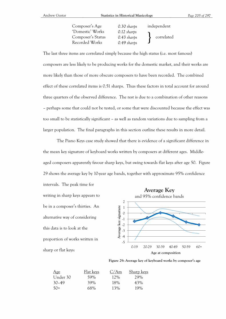
Andrew Gustar Statistics in Historical Musicology Page 205 of 297
Composer’s Age 0.30 sharps independent ‘Domestic’ Works 0.12 sharps
} correlated Composer’s Status 0.43 sharps
Recorded Works 0.49 sharps
The last three items are correlated simply because the high status (i.e. most famous)
composers are less likely to be producing works for the domestic market, and their works are
more likely than those of more obscure composers to have been recorded. The combined
effect of these correlated items is 0.51 sharps. Thus these factors in total account for around
three quarters of the observed difference. The rest is due to a combination of other reasons
– perhaps some that could not be tested, or some that were discounted because the effect was
too small to be statistically significant – as well as random variations due to sampling from a
larger population. The final paragraphs in this section outline these results in more detail.
The Piano Keys case study showed that there is evidence of a significant difference in
the mean key signature of keyboard works written by composers at different ages. Middle-
aged composers apparently favour sharp keys, but swing towards flat keys after age 50. Figure
29 shows the average key by 10-year age bands, together with approximate 95% confidence
intervals. The peak time for
writing in sharp keys appears to
be in a composer’s thirties. An
alternative way of considering
this data is to look at the
proportion of works written in
sharp or flat keys:
Age Flat keys C/Am Sharp keys Under 30 59% 12% 29% 30–49 39% 18% 43% 50+ 68% 13% 19%
Figure 29: Average key of keyboard works by composer’s age
-5
-4
-3
-2
-1
0
1
2
0-19 20-29 30-39 40-49 50-59 60+
Ave
rage
key
sig
natu
re
Age at composition
Average Key and 95% confidence bands

Andrew Gustar Statistics in Historical Musicology Page 206 of 297
The chance of this pattern occurring if there were no difference between the age bands is just
p=2.2%, using a Chi-squared test.
There was also a significant difference in the age distribution of the IMSLP and
DMT samples (p=1.8%):
Under 30 30–49 50+
IMSLP 30% 42% 28% DMT 38% 57% 5%
The DMT sample is biased towards the sharp-loving middle-aged composers, whereas IMSLP
has a more substantial population of flat-favouring older composers.
‘Domestic’ music was defined as belonging to either the ‘salon’ or ‘solo’ repertoire,
with samples taken from Wilkinson (1915) and Westerby (1924). Domestic works had a
mean key signature of –1.18, compared with –0.46 for the rest. 22% of the IMSLP sample
was domestic, significantly more than the 6% of the DMT sample.
There was also some evidence (see Figure 30) that more canonic composers (using
the AllMusic ‘top composer’ lists as described in section 5.1.1) use sharper keys on average
than more obscure composers.
The distinction seems to be
mainly between the Top 200 and
the rest. The average key
signatures for these two
categories are –0.38 and –1.20
respectively, which is a
significant difference (p=2.1%).
As would be expected, the table below shows significant differences in the distribution of
composer status between the IMSLP and DMT samples, with DMT having a much stronger
representation of Top 200 composers (p=0.0005%):
Figure 30: Average key of keyboard works by composer status
-4
-3
-2
-1
0
1
Ave
rage
key
sig
natu
re
Composer Status
Average Key and 95% confidence bands
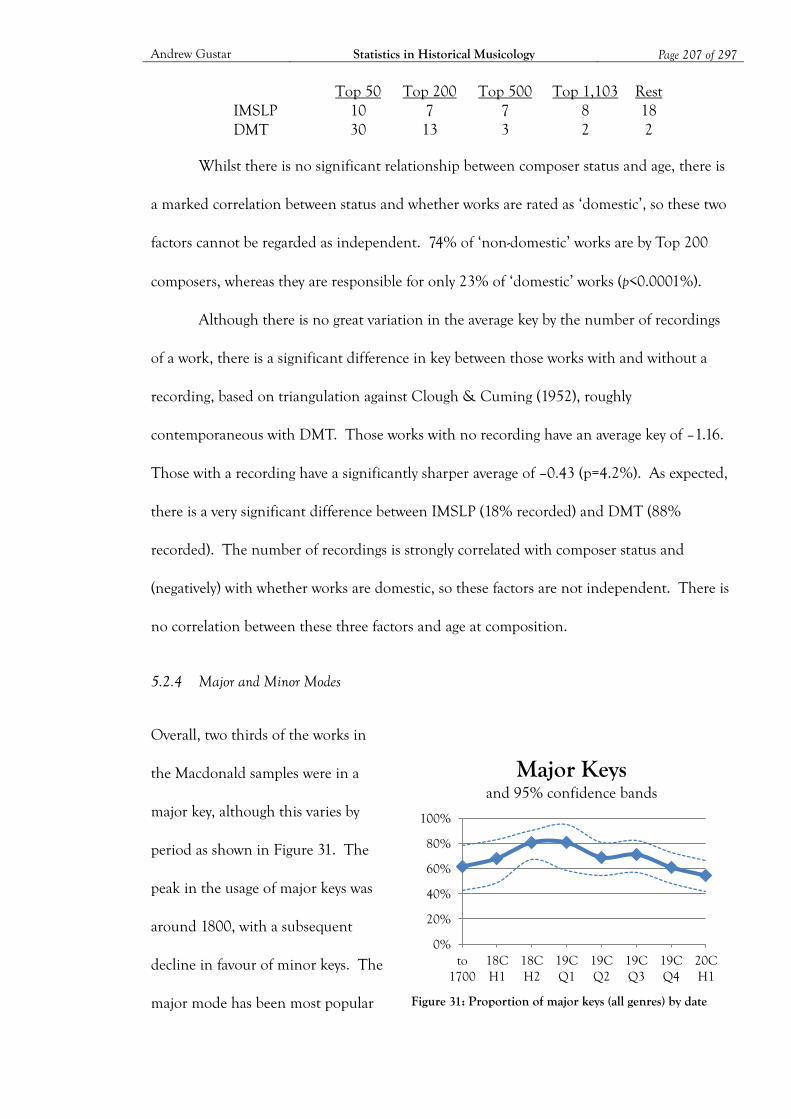
Andrew Gustar Statistics in Historical Musicology Page 207 of 297
Top 50 Top 200 Top 500 Top 1,103 Rest
IMSLP 10 7 7 8 18 DMT 30 13 3 2 2
Whilst there is no significant relationship between composer status and age, there is
a marked correlation between status and whether works are rated as ‘domestic’, so these two
factors cannot be regarded as independent. 74% of ‘non-domestic’ works are by Top 200
composers, whereas they are responsible for only 23% of ‘domestic’ works (p<0.0001%).
Although there is no great variation in the average key by the number of recordings
of a work, there is a significant difference in key between those works with and without a
recording, based on triangulation against Clough & Cuming (1952), roughly
contemporaneous with DMT. Those works with no recording have an average key of –1.16.
Those with a recording have a significantly sharper average of –0.43 (p=4.2%). As expected,
there is a very significant difference between IMSLP (18% recorded) and DMT (88%
recorded). The number of recordings is strongly correlated with composer status and
(negatively) with whether works are domestic, so these factors are not independent. There is
no correlation between these three factors and age at composition.
5.2.4 Major and Minor Modes
Overall, two thirds of the works in
the Macdonald samples were in a
major key, although this varies by
period as shown in Figure 31. The
peak in the usage of major keys was
around 1800, with a subsequent
decline in favour of minor keys. The
major mode has been most popular
Figure 31: Proportion of major keys (all genres) by date
0%
20%
40%
60%
80%
100%
to 1700
18C H1
18C H2
19C Q1
19C Q2
19C Q3
19C Q4
20C H1
Major Keys and 95% confidence bands

Andrew Gustar Statistics in Historical Musicology Page 208 of 297
in all periods and genres, with the exception of solo song, which was strongly major until the
third quarter of the nineteenth century, but then switched to become 75% minor during the
first half of the twentieth century.
During the eighteenth and nineteenth centuries, works from France were
consistently more likely than average to be in minor keys, and works from Italy and Iberia
were more likely to be in major keys. If there were no regional bias, the probability of either
of these trends occurring entirely by
chance would be (½)6, or 1 in 64 (see
Figure 32).
Choral and operatic works are
consistently more likely than average
to be in major keys. There is also a
significant correlation between key
signature and whether a work is in a
major or minor key. Minor keys are much more likely to have flat than sharp key signatures.
Overall, the minor mode occurs in 45% of works with flat key signatures, but in just 28% of
those with sharp key signatures. This is perhaps to be expected since the leading note in
sharp minor keys (beyond two sharps) requires some awkward notation, such as B#, E#, or
double-sharps. Interestingly, only 17% of works with no key signature are in A minor rather
than C major.
The Piano Keys case study also considered the key signatures used for major and
minor modes. Significant regional variations were found in the average key signatures of
major and minor key piano works: Germanic major key works tend to be 1.4 sharps sharper
than minor key works (p=4.1%), whereas French major key works tend to be 1.7 sharps flatter
than minor key works (p=3.4%). Less significantly, Scandinavian works appear to share the
Figure 32: Major keys by region and date
0%
20%
40%
60%
80%
100%
to 1700
18C H1
18C H2
19C Q1
19C Q2
19C Q3
19C Q4
20C H1
Major Keys
France Italy/Iberia All Regions

Andrew Gustar Statistics in Historical Musicology Page 209 of 297
Germanic major-sharp bias, and East European works the French major-flat bias. The study
also found that major key salon works are 2.1 sharps flatter than those in a minor key (p=3.5),
and that major key works written before 1800 tend to be 2.7 sharps sharper than minor key
works from this period (p=0.1%). It is hard to suggest explanations for these differences.
5.2.5 Accidentals and Key Changes
One statistic collected from the IMSLP sample in the Macdonald case study was the bar in
which the first non-diatonic accidental occurs (i.e. ignoring diatonic accidentals, such as the
raised leading note in minor keys, or the common baroque practice of using a key signature
with one fewer flat than would be used today). As might be expected, the period until the
first accidental is significantly negatively correlated with the year of composition, reflecting a
trend over time towards using non-diatonic notes earlier and earlier in a work. In fact, there
is a broad range for all periods, as Figure 33 shows (note the logarithmic vertical scales). The
average delay before the first non-diatonic note seems to have peaked early in the eighteenth
century, fell steadily during the 1700s, and since the early nineteenth century appears to have
shown little further change. The reasons for this trend are probably complex, relating to
changes in musical aesthetics, particularly the development of a more adventurous approach
to harmony during the first half of the nineteenth century. It is also possible that the results
Figure 33: Bar of first non-diatonic accidental: mean and sample points
0
4
8
12
16
20
to 1700
18C H1
18C H2
19C Q1
19C Q2
19C Q3
19C Q4
20C H1
Bar of first accidental mean and 95% confidence bands
1
2
4
8
16
32
64
1500 1600 1700 1800 1900
Bar of first accidental IMSLP Sample points

Andrew Gustar Statistics in Historical Musicology Page 210 of 297
are affected by the changing proportions of very short works (such as some baroque dance
forms or the piano ‘miniatures’ of the nineteenth century), although data to test this effect
were not collected for this case study.
The Piano Keys case study investigated mid-movement changes of key signature. The
original analysis in the Macdonald study used a sample from IMSLP, taking the key
signatures from the beginning of works, and a sample from DMT using the key signatures
indicated on the incipits of the catalogued themes. For a small number of works, the DMT
sample included second or subsequent themes in a key signature that differed from that of
the first theme. The difference between the IMSLP and DMT samples therefore included
the effect of this notated modulation. Although this produced a small sharp bias in the
Macdonald case study, this was on the basis of just three works, so it was necessary to
investigate if the effect could equally have skewed the result to be more flat, or whether there
is actually a systematic sharp bias of second themes compared with first themes. One might
expect this to be so, since arguably the most common modulations (major keys to the
dominant, minor to the tonic major) are in the sharp direction (+1 and +3 respectively). But
are these really more common than modulations to the subdominant and tonic minor which
have an equal and opposite effect?
To test this, a new sample from DMT was taken of 50 works where there was a
change of notated key within the same movement. The main conclusions of the analysis
were as follows:
Key Bias As Figure 34 shows, the first change was negatively correlated with the opening
key (correlation –0.73). Sharp first themes tend to be followed by flatter second
themes and vice versa, with the average move roughly proportional to the
starting key. This is not surprising, as keys are constrained to the range ±7, so
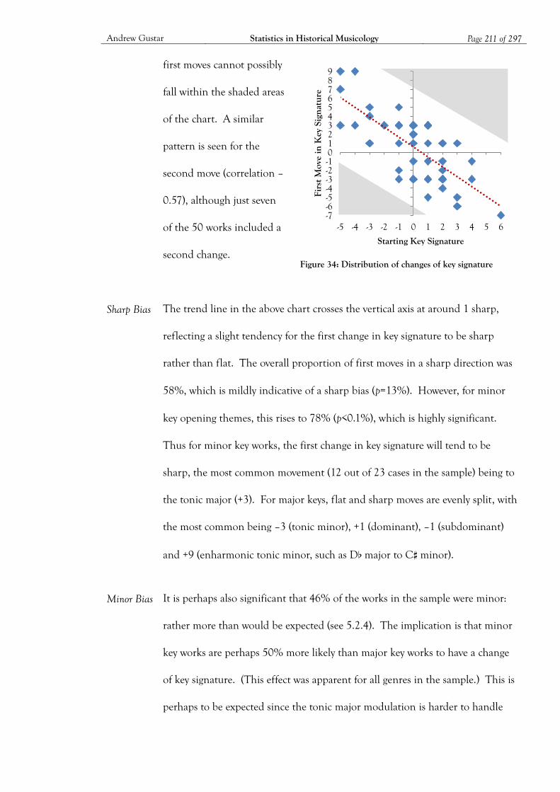
Andrew Gustar Statistics in Historical Musicology Page 211 of 297
first moves cannot possibly
fall within the shaded areas
of the chart. A similar
pattern is seen for the
second move (correlation –
0.57), although just seven
of the 50 works included a
second change.
Sharp Bias The trend line in the above chart crosses the vertical axis at around 1 sharp,
reflecting a slight tendency for the first change in key signature to be sharp
rather than flat. The overall proportion of first moves in a sharp direction was
58%, which is mildly indicative of a sharp bias (p=13%). However, for minor
key opening themes, this rises to 78% (p<0.1%), which is highly significant.
Thus for minor key works, the first change in key signature will tend to be
sharp, the most common movement (12 out of 23 cases in the sample) being to
the tonic major (+3). For major keys, flat and sharp moves are evenly split, with
the most common being –3 (tonic minor), +1 (dominant), –1 (subdominant)
and +9 (enharmonic tonic minor, such as Db major to C# minor).
Minor Bias It is perhaps also significant that 46% of the works in the sample were minor:
rather more than would be expected (see 5.2.4). The implication is that minor
key works are perhaps 50% more likely than major key works to have a change
of key signature. (This effect was apparent for all genres in the sample.) This is
perhaps to be expected since the tonic major modulation is harder to handle
Figure 34: Distribution of changes of key signature
-7 -6 -5 -4 -3 -2 -1 0 1 2 3 4 5 6 7 8 9
-5 -4 -3 -2 -1 0 1 2 3 4 5 6
Firs
t Mov
e in
Key
Sig
nat
ure
Starting Key Signature
Andrew Gustar Statistics in Historical Musicology Page 212 of 297
with accidentals alone than is a shift to the dominant, and appears to be more
common than movement to the tonic minor in major key works.
Keyboard
Bias
The sample included works from all genres. Chamber and orchestral works
were evenly split between sharp and flat first moves, but keyboard works had an
average first move of +2.7 (p=4%), with 78% of them being sharp (p=2.3%).
Period None of the pre-1800 works had a key signature change of more than ±3 sharps.
More surprising is the finding that moves in a sharp direction were particularly
favoured in the first half of the nineteenth century (19C H1), whereas flat and
sharp moves are evenly balanced pre-1800, in 19C H2, and in the twentieth
century. However, closer examination of the sample shows a relatively high
proportion of keyboard works in 19C H1, so this effect is probably an artefact of
the keyboard bias described above and is not significant in its own right.
Note that this is not a measure of modulation in general, but only of those modulations that
involve a change of key signature. Many modulations can be handled simply by the use of
accidentals. A change of key signature represents a more significant modulation, either for a
distinct section of music, or one that would be messy to notate with accidentals alone.
5.2.6 Technical Difficulty
The Piano Keys case study collected data on the technical difficulty of piano works, to test
whether this might affect the difference in average key signatures between well-known and
obscure works. The assessment of difficulty was done in two stages, the first looking at the
published piano syllabus of the Associated Board of the Royal Schools of Music (ABRSM),

Andrew Gustar Statistics in Historical Musicology Page 213 of 297
and the second calibrating this data against the difficulty ratings given by Hinson (1987) and
Barnard & Gutierrez (2006).
The Piano Syllabus from the ABRSM has, since at least 1991, been reissued every two
years, and includes a repertoire of pieces for each Grade from 1 to 8. There is also a
Diploma Repertoire, updated less frequently, giving longer lists of works for the advanced
qualifications of DipABRSM, LRSM and FRSM. Many of these works are listed as being in
a particular key, and the key of many others can be identified from sources such as IMSLP.
The analysis considered grades 5 and 8 (taking works from the 2007–8 and 2009–10
syllabuses) and the current diploma lists. This gave a total sample of 417 works.
Among those works whose key could be identified, the proportion of minor keys was
about 43%: slightly higher than expected, but perhaps reflecting a deliberate balance. Minor
key works were, on average, more flat (by 0.74 sharps) than major key works (p=1.4%).
Grade 5 uses a significantly more limited range of keys, never exceeding three flats or sharps.
However, there are no evident trends in terms of the average keys by level of difficulty – for
every level of difficulty, the average key is about the same, and the proportions sharp and flat
are relatively constant. All of this points, perhaps reassuringly, to a deliberately balanced
selection of repertoire for piano teaching.
Hinson and Barnard & Gutierrez both rate the level of difficulty on a four-point
scale. Hinson’s categories 1–4 are described as Easy, Intermediate, Moderately Difficult, and
Difficult respectively; Barnard’s are Intermediate, First Year University, Graduate Level, and
Virtuoso. The two sources broadly agree on relative difficulty (correlation coefficient 0.6 on
the ABRSM sample above), and they are roughly linearly related, with Barnard’s score being
on average 0.75 of Hinson’s. A composite difficulty score was thus defined by rescaling
Barnard’s score to Hinson’s (by dividing it by 0.75) and taking the average of the two (or the
single score if just one was available). This resulted in a composite difficulty score between 1
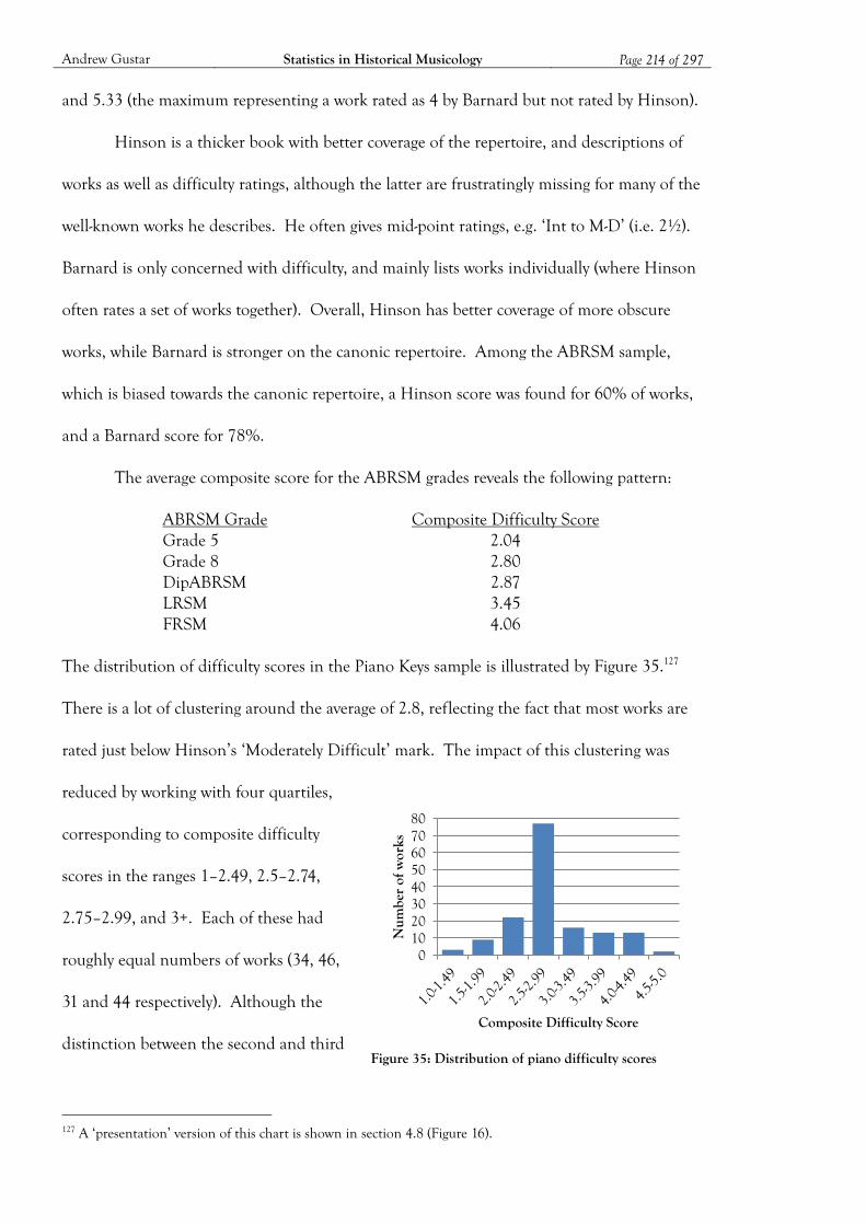
Andrew Gustar Statistics in Historical Musicology Page 214 of 297
and 5.33 (the maximum representing a work rated as 4 by Barnard but not rated by Hinson).
Hinson is a thicker book with better coverage of the repertoire, and descriptions of
works as well as difficulty ratings, although the latter are frustratingly missing for many of the
well-known works he describes. He often gives mid-point ratings, e.g. ‘Int to M-D’ (i.e. 2½).
Barnard is only concerned with difficulty, and mainly lists works individually (where Hinson
often rates a set of works together). Overall, Hinson has better coverage of more obscure
works, while Barnard is stronger on the canonic repertoire. Among the ABRSM sample,
which is biased towards the canonic repertoire, a Hinson score was found for 60% of works,
and a Barnard score for 78%.
The average composite score for the ABRSM grades reveals the following pattern:
ABRSM Grade Composite Difficulty Score Grade 5 2.04 Grade 8 2.80 DipABRSM 2.87 LRSM 3.45 FRSM 4.06
The distribution of difficulty scores in the Piano Keys sample is illustrated by Figure 35.127
There is a lot of clustering around the average of 2.8, reflecting the fact that most works are
rated just below Hinson’s ‘Moderately Difficult’ mark. The impact of this clustering was
reduced by working with four quartiles,
corresponding to composite difficulty
scores in the ranges 1–2.49, 2.5–2.74,
2.75–2.99, and 3+. Each of these had
roughly equal numbers of works (34, 46,
31 and 44 respectively). Although the
distinction between the second and third
127 A ‘presentation’ version of this chart is shown in section 4.8 (Figure 16).
Figure 35: Distribution of piano difficulty scores
0 10 20 30 40 50 60 70 80
Num
ber
of w
orks
Composite Difficulty Score
Andrew Gustar Statistics in Historical Musicology Page 215 of 297
quartiles is quite small, due to the clustering, comparison between the first and fourth
quartiles enabled some meaningful analysis.
Although no significant links were found between difficulty and keys, the following
interesting results were found:
Composer
Status
Works by composers in the Top 200, but outside the Top 50, are, on average
0.36 ‘Hinson points’ more difficult than works by other composers (p=0.2%).
21% of first quartile works (i.e. the easiest) are by these ‘group 2’ composers,
but they wrote 45% of those in the fourth quartile (p=2.2%). These ‘second
division’ composers might fail to reach the top 50 because their works are too
difficult, or perhaps they are just trying too hard to reach the first division.
DMT Works listed in the Dictionary of Musical Themes are less difficult (by an
average of 0.25 Hinson points) than those not listed in DMT (p=1.7%).
Perhaps themes from simpler works are more likely to become well-known.
Domestic
repertoire
68% of first quartile works were classed as ‘domestic’ by triangulation in
Westerby (1924), whereas only 36% of fourth quartile works were (p=0.6%).
‘Solos’, triangulated against Wilkinson (1915), are 0.32 points easier on average
than non-solos (p=0.7%). Solos comprise 35% of first quartile, but 9% of
fourth quartile works (p=0.4%).
Period Perhaps not surprisingly, works written in the twentieth century are 0.42 points
more difficult than those from before 1900 (p=0.06%). 18% of first quartile
Andrew Gustar Statistics in Historical Musicology Page 216 of 297
works are from the twentieth century, but 36% of fourth quartile works are
from this period (p=6.9%).
Age There is some evidence that piano works written by composers over 40 are 0.24
points more difficult than those written by younger composers (p=5.9%). This
is not a very significant result, and the distribution of first and fourth quartile
works (16% and 32% from the over-40s respectively) is only significant at
p=11.4%.
On the basis of this analysis, it seems plausible that works from the 20th century, and those
by ‘second division’ composers, are more difficult than average; and that those containing
memorable themes, and those suitable as ‘solos’ for amateur players, tend to be less difficult
than average.
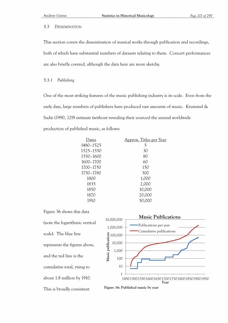
Andrew Gustar Statistics in Historical Musicology Page 217 of 297
5.3 DISSEMINATION
This section covers the dissemination of musical works through publication and recordings,
both of which have substantial numbers of datasets relating to them. Concert performances
are also briefly covered, although the data here are more sketchy.
5.3.1 Publishing
One of the most striking features of the music publishing industry is its scale. Even from the
early days, large numbers of publishers have produced vast amounts of music. Krummel &
Sadie (1990, 129) estimate (without revealing their sources) the annual worldwide
production of published music, as follows:
Dates Approx. Titles per Year 1480–1525 5 1525–1550 30 1550–1600 80 1600–1700 60 1700–1750 150 1750–1780 300
1800 1,000 1835 2,000 1850 10,000 1870 20,000 1910 50,000
Figure 36 shows this data
(note the logarithmic vertical
scale). The blue line
represents the figures above,
and the red line is the
cumulative total, rising to
about 1.8 million by 1910.
This is broadly consistent
Figure 36: Published music by year
1
10
100
1,000
10,000
100,000
1,000,000
10,000,000
1450 1500 1550 1600 1650 1700 1750 1800 1850 1900 1950
Mus
ic p
ublic
atio
ns
Year
Music Publications
Publications per year
Cumulative publications

Andrew Gustar Statistics in Historical Musicology Page 218 of 297
with the estimate of 730,000 works in print at that time as listed by Pazdírek, bearing in
mind that many works would be out of print, whilst others would be available in several
editions from multiple publishers. The data also appears to be broadly consistent with the
music holdings of the British Library, as illustrated in Figure 5 (section 4.5.3).
Pazdírek lists the publishers who submitted their catalogues to his Handbook. The
list varies slightly between volumes, but, as a typical example, volume 5 mentions 1,420
separate publishers and their cities of origin, including representatives from countries such
as Algeria, Argentina, Australia and Mexico. The actual distribution is as follows:
Region Number of publishers
Percent of Total
Germany, Austria, Switzerland 551 39% France, Belgium, Luxembourg 370 26% Americas 172 12% Italy, Iberia, North Africa 103 7% Great Britain, Australia, South Africa 98 7% Netherlands & Scandinavia 79 6% Russia, Balkans & Eastern Europe 47 3% Total 1,420 100% A comparison of these figures with the geographical distribution of composers and
works in the Pazdírek samples (see 5.1.1) reveals some interesting differences. The fourth
regional group, dominated by Italy, has a disproportionately high number of works and
composers relative to the number of publishers. This perhaps reflects the Italian market
being more dominated by its largest publishers (principally Ricordi) than the markets in
France and Germany.128 The same could be argued for Russia, although the sample size here
is rather too small to be able to draw firm conclusions. In the Americas, Netherlands and
Scandinavia, the opposite appears to be the case, with disproportionately many publishers
relative to the number of works and composers, indicating that the publishing markets here
were less dominated by the large companies than in most of continental Europe. In the case
128 This is supported by the article on Ricordi in Oxford Music Online: ‘In the entire history of music publishing there has been no other firm that through its own efforts, astuteness, initiative and flair has achieved a position of dominance such as Ricordi enjoyed in Italy in the 19th century’ (Macnutt 2013)

Andrew Gustar Statistics in Historical Musicology Page 219 of 297
of the US, this can perhaps be attributed to a relatively young and vibrant market, in which
many small publishers were able to make a living, with no single company having achieved a
dominant position. There is an additional, difficult to quantify, complication to the
interpretation of these figures, in the international scope of the larger publishers, who
published the works of composers from many countries. Similarly, the most prolific and
more famous composers were often published in many countries other than their own.
As shown in 5.2.1, the publishing market in the early twentieth century (as reflected
in Pazdírek’s Handbook) was dominated by small-scale piano pieces and songs aimed primarily
at the domestic market. The demand for printed large-scale works is inevitably limited, so
small-scale works intended for the amateur market have long formed the bread and butter of
the music publishing industry. Amongst piano works alone, the Class of 1810/20/37 case
study series found large quantities of arrangements, derivative works, studies, tutors and
albums aimed at the domestic market. The table in section 4.4.2 illustrates the small
proportion of piano works from 1810 and 1820 that survived the process of data cleaning,
intended to remove all but original solo piano music. A similar pattern was found for the
1837 data from Hofmeister’s Monatsberichte, where 311 piano publications listed were
reduced by almost two thirds to leave just 113 original works.
The Class of 1837 case study enabled the identification of three clusters of works,
based on their repeat publication history.129 The following two charts (Figure 37) illustrate
the characteristics of these clusters. The largest cluster, P1, with 79 members (70% of the
total), has no significant level of republication after 1837. P2, with 21 members (19%), has a
higher initial rate of publication and a healthy rate of republication over the subsequent 25
years or so, but this rate tails off over the following 100 years. P3, with 13 members (11%),
129 The clustering used the k-means algorithm based on a Euclidean distance measure applied to the proportion of each work’s publications falling within the four 50-year periods from 1813 to 2012 (see 4.5.5). The smallest value, across the three clusters, of the ratio (distance to the nearest other cluster centre) / (average distance of the members of the cluster from its centre) was 2.26, indicating a reasonable degree of cluster separation.

Andrew Gustar Statistics in Historical Musicology Page 220 of 297
also starts at a higher publication rate, but the rate of republication then rises for 75 years
before settling down to around 2½ editions every 25 years (i.e. one per decade, on average).
In terms of the economics of publishing, P3 contains the long-term sellers that generate
steady profits. P2 works perhaps generate profits for a while, but have a limited lifespan and
never achieve the popularity necessary to become a P3-style ‘cash cow’. The works in P1 are
of transient appeal. Some may have been popular for a short time and would have sold in
significant quantities (such as the many derivative works riding the wave of success of the
latest operatic success), but many others would have sold few copies and not covered their
costs of publication. Indeed, 60% of the works in P1 could not be found in the composite
library catalogues Copac or WorldCat, suggesting that few copies were purchased or survive.
Cluster P3 included works by Chopin, Liszt, Schumann and Mendelssohn, as well as
some now less familiar names including William Sterndale Bennett, Henry Bertini, Ignaz
Moscheles and Sigismund Thalberg. P2 also included works by Liszt, Bertini and Sterndale
Bennett, as well as names such as Henri Herz, Friedrich Burgmüller, Anton Diabelli and
Louise Farrenc. P1 included some of the above names, a couple of other moderately familiar
composers such as Carl Czerny and Stephen Heller, plus a large number of composers that
Figure 37: Repeat publication clusters
0
1
2
3
4
5
Publications per Work
P1 (79)
P2 (21)
P3 (13)
0
25
50
75
100
125
150
175
Total Publications
P1 (79)
P2 (21)
P3 (13)
Andrew Gustar Statistics in Historical Musicology Page 221 of 297
are virtually unknown today: those that could not be found by triangulation (and, indeed,
whose first names remain a mystery) included C. G. Stückrad, G. A. Muth, and F. Wewetzer.
Music publishing can thus be financially precarious, and it is no surprise that there
have been many mergers, takeovers and closures among publishing firms. The location of
publishers appears to be important to their success. Works published in cities mentioned
five or more times by Hofmeister are distributed among the clusters as follows:
P1 P2 P3 Leipzig 17 10 8 Berlin 15 – 2 Vienna 8 2 1 Mainz 5 3 – Brunswick 5 1 1 Hamburg 4 3 – Bonn 6 – 1 Frankfurt 5 1 –
Not surprisingly, given Hofmeister’s remit, this list consists entirely of German cities (plus
Vienna). In total, Hofmeister mentions 36 publishers from 19 cities (all German, Austrian
or Polish), yet among the records of these works in WorldCat and Copac from 1837 and
earlier there are 23 publishers and nine cities (including London, Paris and St Petersburg)
not on Hofmeister’s list. All members of P3, and all-but-one of P2, are accounted for by the
cities in the above table. The twelve works first published in cities only mentioned once or
twice by Hofmeister all ended up in P1.130 First publication in one of the major publishing
centres appears to be an important factor for a work’s long-term success.
Leipzig shows an unusually high success rate for the works first published there. 23%
of them ended up in P3, and another 29% in P2 (compared with the overall averages of 11%
and 19% respectively). Berlin and Vienna fared much less well.131 This is largely explained
130 70% of all works were in P1, so this may not seem wholly surprising, given the small numbers involved. However, the probability of this happening entirely by chance is about 1.4%, which is quite significant. 131 Again, given the small numbers involved, one might be suspicious of these conclusions. Just looking at works from Leipzig, Berlin and Vienna, a Chi-squared test gives a probability of about 5.5% of the above distribution occurring by chance, which is moderately significant though not conclusive.
Andrew Gustar Statistics in Historical Musicology Page 222 of 297
by the fact that Leipzig was (and is) the home of several major publishing houses whose
distribution capabilities would have greatly exceeded those of the smaller firms. The P3
results above are dominated by Breitkopf & Härtel, Hofmeister and Kistner (in Leipzig), and
by Challier in Berlin and Haslinger in Vienna. Hofmeister also mentions three less active
Leipzig publishers (Schuberth, Klemm and Peters), but also three from Vienna (Mechetti,
Diabelli and Artaria) and a disproportionately high six (Lischke, Muth, Schlesinger,
Westphal, Cranz and Fröhlich) from Berlin. It is notable that all three of the ‘P3’ Leipzig
firms – Breitkopf & Härtel, Hofmeister and Kistner (now Kistner & Siegel) – remain
independent to this day. Berlin’s Challier was acquired by Birnbach, which is still operating,
and Vienna’s Haslinger was acquired by Schlesinger, which seems to have gone out of
business in the late nineteenth century. Among the less active names on Hofmeister’s 1837
Leipzig list, Peters continues to thrive, Klemm seems to have gone out of business around
1880, and Schuberth was acquired by Siegel prior to its merger with Kistner. In Vienna,
Diabelli was acquired by Cranz, now an imprint of Schott, and Artaria closed its publishing
business in 1858. No further information could be found about Mecchetti, Lischke, Muth,
Westphal or Fröhlich.132 Thus location appears to be important not only for the success of
the works, but for the long term survival of the publishers themselves. There appears to have
been a significant economic advantage (at least in 1837) of being based in Leipzig.
This insight into the economics of music publishing perhaps fits with the implied
probability distribution (described in 4.6.3) reflecting the likelihood that a composer’s next
work will be accepted for publication. A successful publisher will have a strong incentive to
stick with composers with a proven track record, and quickly to drop those whose appeal
appears to be limited. The result is the Zipf-like distribution of published works per
composer (and similar patterns found in recordings, concert performances, and elsewhere).
132 The information in this paragraph is from Oxford Music Online, cross checked with Google searches.

Andrew Gustar Statistics in Historical Musicology Page 223 of 297
Despite the huge growth in music publishing throughout the nineteenth and much
of the twentieth centuries, there is some evidence that new editions of ‘classical’ works are in
decline. The Class of 1837 case study triangulated the piano works and composers found in
Hofmeister’s listings from 1837 against various sources including the online sheet music
retailer Musicroom (see table on p.239). Only five of the 113 works could be found in this
source, and 27 of the 69 composers. Although a respectable number of composers were
mentioned in Musicroom, many were represented by quite a small selection of works. None
of the five 1837 works by Liszt,133 for example, could be found in Musicroom, although it is
likely that some are included in albums whose full contents were not listed on the website.
5.3.2 Recording
There are several early complete catalogues of recorded music, the repertoire of which
expanded surprisingly rapidly during the 1920s and 30s. In one such catalogue, Darrell
(1936, p.iv) writes,
The whole field of musical art is being covered with breath-taking swiftness by the
gramophone. There are still many unenlightened musicians who think of phonograph
records as exploiting chiefly a repertoire of semi-popular operatic and symphonic warhorses.
But today most of the greatest music in existence has been recorded. The repertoire that is
available today for students and gramophone enthusiasts will amaze those who have not kept
pace with its recent extensions. Not only have virtually all the standard works been recorded,
but much of the rarest works of the past, known only by name to many musicians and music
lovers, have now been transferred to the discs.
Today, the number of recordings has grown to such a scale that a complete catalogue (even
an online one) would probably be impractical, bearing in mind the shift away from physical
media and towards purely digital recordings, together with the ease with which modern 133 Apparitions, Reminiscenses des Puritains, Rondeau fantastique sur un thème espagnol, Grande Valse di Bravoura, and the Fantaisie romantique sur deux melodies suisses

Andrew Gustar Statistics in Historical Musicology Page 224 of 297
technology enables anyone easily to produce and release their own high quality recordings
and upload them to services such as iTunes, Spotify, Soundcloud and YouTube.
The Recordings case study produced some estimates of the number of composers
represented in three general catalogues – the World’s Encyclopedia of Recorded Music
(WERM) (1950),134 the Gramophone Catalogue (GramCat) (1990),135 and AllMusic.
Unfortunately, due to the nature of the Zipf-like distribution of article length per composer
(see 4.6.1), the confidence intervals of these estimates are rather wide. However, WERM
includes an index of all composers mentioned, differentiating (by typeface) between those in
the main work and those in the 1952 Supplement, and between those with their own
entries, and those listed as minor names coupled with better known composers. In total,
there are around 1,900 names on this index, of which perhaps 35% (about 670) are those
with their own entries in the main 1950 listing. This can be compared with the number of
valid database codes in AllMusic, indicating that it includes around 10,000 composers.
The distribution of works per page is statistically better behaved than that of
composers. There are an estimated 11,400 works in WERM, and 18,200 in GramCat, with
95% confidence limits about 2,000 either side of these estimates. AllMusic’s population of
works is harder to estimate, although its statistics page claims that it lists over 306,000
classical compositions, including some (perhaps the majority) that have not been recorded.
Simply multiplying the number of pages by the average number of recordings per
page overstates the total number of recordings, since the same recording will typically be
mentioned under the listing of each work it contains. It is possible to adjust for this
duplication to arrive at an estimate of around 16,000 recordings in each of WERM and
GramCat. The high number of recordings mentioned in WERM is probably due to many of
them being listed in a number of different formats, since at the time the industry was in
134 Clough & Cuming (1952) 135 Maycock & McSwiney (1990)

Andrew Gustar Statistics in Historical Musicology Page 225 of 297
transition between ‘78s’ and ‘LPs’. AllMusic, according to its valid database codes, lists
around 260,000 recordings. Although this certainly contains some duplicated data, it seems
likely that there are perhaps 200,000 different classical CDs currently available. A great
many of these, particularly for the more famous works, are reissues of the same handful of
original performances. In the last twenty years there has also been an enormous increase in
the availability of recordings of lesser-known works and of works by a range of obscure
composers, as well as many re-releases of more obscure historical recordings.
As expected, the distribution of the number of works per composer is highly skewed.
The four Penguin Guides used for the Recordings case study reveal the following breakdown:
Number of Recorded Works per Composer
Proportion of Composers
Proportion of Recordings
Average Recordings Per Work
1 43% 4% 1.5 2–3 21% 4% 1.0 4–7 7% 4% 1.9 8–15 8% 6% 3.1 16–31 14% 15% 2.6 32+ 7% 67% 6.0
Thus around two-thirds of the space in the Penguin Guides is devoted to composers with
more than 32 recorded works, but this accounts for just 7% of composers. The proportion
of the sample occupied by such composers is boosted not only by the greater number of
recorded works, but by a significantly larger number of recordings of each work (and,
typically, longer commentaries on those recordings).
The distribution of the number of recordings per work is less highly skewed, and is
broadly consistent between the four complete Penguin Guides and WERM and GramCat:
Recordings per Work Penguin Guides WERM/GramCat 1 35% 40%
2–3 30% 17% 4–7 14% 11% 8–15 14% 13% 16+ 7% 19%
The distribution for AllMusic is very different, with 56% of the sample falling into the ‘16+’

Andrew Gustar Statistics in Historical Musicology Page 226 of 297
category. Indeed over a quarter of the AllMusic works sampled had 100 or more recordings,
and two had around 800 (Beethoven’s 5th Piano Concerto and his 6th Symphony). The
majority of these appeared to be re-issues of old recordings on compilation CDs, often by
relatively obscure record labels. The number of distinct recorded performances of these
works is likely to be very much smaller than the number of issued recordings.
Unsurprisingly, more recent works and those by more obscure composers tend to
have fewer recordings. The works with 16+ recordings are predominantly German,
orchestral, and from the late-eighteenth and nineteenth centuries. Triangulating the 1988
Penguin Guide sample against its near contemporary GramCat revealed on average about
twice as many recordings available as were listed in the Penguin Guide. Triangulating the
2007 Penguin Guide against AllMusic, this ratio had increased to almost 14 times. Although
much of this can be accounted for by multiple issues of the same recorded performance, the
editors of the Penguin Guides have clearly been forced to become much more selective in
recent years, given the extraordinary increase in the population of recorded music.
The main determinants of the number of works on a physical recording are the
average length of works (influenced primarily by the genre) and the average length of the
recording medium (determined by the technology – e.g. LPs at various speeds, cassette, or
CD – prevalent at the time). The following table shows the impact of these factors:
Number of works per physical recording 1950 (est.)
1975 LPs
Post-1988 CDs
Small-scale works (keyboard, song) 3.4 4.6 6.1 Large scale works (choral, chamber, orch.) 1.8 2.4 3.2
About 75% of the recordings in the sample contained only works by a single composer, and
the average number of composers on a disc was just over 1.4, with little variation in this
figure between guides, genres, or periods.
Using the proportion of pages occupied by composers in the four sampled complete
Penguin Guides, it was possible to categorise composers into five ‘shape categories’:
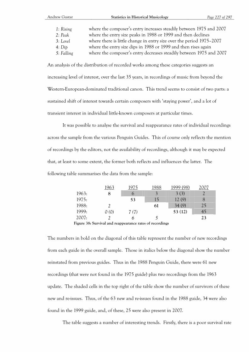
Andrew Gustar Statistics in Historical Musicology Page 227 of 297
1: Rising where the composer’s entry increases steadily between 1975 and 2007 2: Peak where the entry size peaks in 1988 or 1999 and then declines 3: Level where there is little change in entry size over the period 1975–2007 4: Dip where the entry size dips in 1988 or 1999 and then rises again 5: Falling where the composer’s entry decreases steadily between 1975 and 2007
An analysis of the distribution of recorded works among these categories suggests an
increasing level of interest, over the last 35 years, in recordings of music from beyond the
Western-European-dominated traditional canon. This trend seems to consist of two parts: a
sustained shift of interest towards certain composers with ‘staying power’, and a lot of
transient interest in individual little-known composers at particular times.
It was possible to analyse the survival and reappearance rates of individual recordings
across the sample from the various Penguin Guides. This of course only reflects the mention
of recordings by the editors, not the availability of recordings, although it may be expected
that, at least to some extent, the former both reflects and influences the latter. The
following table summarises the data from the sample:
The numbers in bold on the diagonal of this table represent the number of new recordings
from each guide in the overall sample. Those in italics below the diagonal show the number
reinstated from previous guides. Thus in the 1988 Penguin Guide, there were 61 new
recordings (that were not found in the 1975 guide) plus two recordings from the 1963
update. The shaded cells in the top right of the table show the number of survivors of these
new and re-issues. Thus, of the 63 new and re-issues found in the 1988 guide, 34 were also
found in the 1999 guide, and, of these, 25 were also present in 2007.
The table suggests a number of interesting trends. Firstly, there is a poor survival rate
1963 1975 1988 1999 (98) 2007 1963: 8 6 3 3 (3) 2 1975: 53 15 12 (9) 8 1988: 2 61 34 (9) 25 1999: 0 (0) 7 (7) 53 (12) 45 2007: 2 6 5 23
Figure 38: Survival and reappearance rates of recordings
Andrew Gustar Statistics in Historical Musicology Page 228 of 297
of new issues from one guide to the next (less than a third of the 53 new issues in 1975 make
it to 1988), although the rate appears to be increasing as time goes on. However, the survival
rate of the recordings that last the ten years or so from one guide to the next then improves
dramatically, so that more than two-thirds of the survivors make it to their third guide.
Secondly, the rate of inclusion of genuinely new issues seems to be falling. In 1988,
61 of the 81 recordings in the triangulated sample were new, with two re-issues and the
remaining 18 continuing from 1975 and 1963. By 2007, this balance had changed to just 23
new issues out of 116 total recordings, with 13 re-issues. This trend is perhaps inevitable
since, as time goes on, the population of potential re-issues increases substantially, and the
hurdle that new recordings have to clear in order to win a place in each Penguin Guide
(defined largely by what has gone before) moves inexorably higher.
The numbers in parentheses next to the 1999 figures are for the 1998 ‘Bargain’
guide.136 Compared to the ‘full price’ 1999 edition, they suggest that the 1998 guide
includes a higher proportion of older recordings, both survivors and reissues, and relatively
few recent releases. The majority of the reissues and long-term survivors in 1999 were clearly
‘bargain price’ records that also earned a mention in the ‘complete’ guide the following year.
Record guides and catalogues do not routinely provide information on the date of
recordings, although such information is occasionally mentioned in the commentary. This
information would enable a more accurate and detailed analysis to be made of survival rates.
Recordings is an area which offers much scope for asking questions of a statistical
nature, but where the great complexity of data, and inconsistencies between datasets, present
some real challenges to making meaningful progress. Further research would be of value.
136 The 1998 guide was only triangulated and not sampled directly, so (as for the 1963 guide) the overall figures are smaller.

Andrew Gustar Statistics in Historical Musicology Page 229 of 297
5.3.3 Performances
None of the case studies looked in detail at concert performances, although Concert-Diary
(an online database covering over 100,000 concerts, largely in the UK, since 2000) was used
for triangulation in both the Piano Keys and Class of 1837 case studies.
As would be expected, well-known works are more likely to be performed in concert.
The IMSLP sample in the Piano Keys case study had 20% of its works appearing on Concert-
Diary, whereas in the sample from the Dictionary of Musical Themes (DMT) the proportion
was 76%. 60% of the DMT sample had four or more performances on Concert-Diary: for
IMSLP this figure was 10%. The number of concert performances was also strongly
correlated with the composers’ ‘canonic rank’ (as described in 5.1.1) (correlation coefficient
r=0.65), the number of recordings in the World’s Encyclopedia of Recorded Music (WERM)
(r=0.73), and negatively with whether works were classified as ‘salon’ pieces (r=–0.42).
Eleven of the 113 works from the Class of 1837 case study were found in Concert-
Diary, as were 15 of the 69 composers. The number of works performed in concert was
around double the number available in modern printed editions from Musicroom, although
the number of composers represented was rather fewer. This perhaps reflects a tendency for
concert programmers to stick with well-known composers, but perhaps to explore more of
their lesser-known works, whereas publishers seem to be more likely to experiment with
lesser-known composers, whilst focusing on the major works of the bigger names. (This
pattern is likely also to be partly due to the tendency for minor and obscure works to be
published within larger albums, the full contents of which do not always appear on a search
on Musicroom). This suggests that there is a significant difference between the performed
and published repertoires, at least for the small sample of piano works from 1837 considered
in this study. The modern recorded repertoire, as represented by AllMusic, appears to be
broader still in terms of both works and composers.
Andrew Gustar Statistics in Historical Musicology Page 230 of 297
5.4 SURVIVAL, FAME AND OBSCURITY
The case studies touched on the questions of the ‘canon’ of musical works and ‘great’
composers, and in particular how and why this small group managed to fare so much better
than the huge majority of composers and works that now lie in various levels of obscurity.
The processes leading to fame or obscurity are complex, but some light can be shed on them
by the use of statistical methods.
The analysis of survival rates can be achieved primarily via triangulation, typically by
finding evidence of a work’s or composer’s existence in a historic dataset, and checking for
mentions in later, or modern, datasets. In this context, ‘survival’ means that a historical
work or composer is still appearing in later datasets, i.e. it has not been forgotten. Of course,
given that the historical datasets themselves survive, all of the names therein remain
accessible to modern researchers, so they have not completely disappeared. However, by
failing to appear in subsequent datasets, the non-survivors have fallen outside the view or
beyond the sphere of interest of subsequent researchers.
Survival, perhaps in a library or record catalogue, or on a concert programme, is no
evidence that a composer or work has achieved any meaningful level of fame or success. For
this they must, in some sense, enter the repertoire. A key test of this is some evidence of
demand or interest in the work or composer. In the absence (at least in the public domain)
of useful ‘demand side’ information about the market for musical works, the lowest rung of
the ladder of fame is represented by a second publication or recording, or a repeat
performance. Once this hurdle is cleared, some works go no further, whilst others enjoy
multiple publications, recordings and performances, and attract much attention from
researchers and audiences. This level of fame might decline over time, or it might become
persistent. Section 5.3.1 describes the three clusters by repeat publication history from the
Class of 1837 case study. Whilst about one in nine of the piano works from 1837 have
Andrew Gustar Statistics in Historical Musicology Page 231 of 297
enjoyed continued repeat publication for the last 175 years, 42% of them have disappeared
from view (in the sense that copies of them cannot be found today in the composite library
catalogues Copac or WorldCat), and a further 12% survived but never made it into the
repertoire, in the sense that there is no evidence in these sources of a second publication.137
Obscurity, the fate of the majority of composers and of works (including many by
successful composers), also occupies a range of levels. Most obscure are those published,
performed or recorded works and their composers that are not mentioned in any known
dataset. Although it is impossible to quantify these, the implication of the analysis in the
case studies is that the number of such works and composers may be very large, extrapolating
from the common pattern that the numbers of works or composers rise significantly as the
level of obscurity increases. Then there are the works and composers with perhaps a single
mention in a library or publisher’s catalogue, with little else known about them. These are
also very numerous: dates of birth and death, for example, could not be found for around a
third of the 427 composers in the Class of 1810/20 case study (identified primarily in Copac
and WorldCat). Similar figures were observed in the Pazdírek case study, where about half of
the works and a quarter of the composers were not found in any of the triangulated sources.
A more thorough search can sometimes reveal a little more information on these
almost-lost composers and works. Foreign library catalogues, general internet searches,
specialised online searches (such as Google Books), genealogical sources and historical
biographical dictionaries can all be fruitful, as can a search for possible variant names.138 As
an example, take Carlotta Cortopassi, just one of the many thousands of almost-lost
composers listed in Pazdírek’s Handbook. She is mentioned as the composer of a single
work: a piano piece called Desolazione, published by Venturini of Florence. An online search
137 As described in 4.1.7, the regional bias of the Hofmeister dataset implies that these figures are an underestimate of the true proportion of obscure works. 138 See 5.1.3.
Andrew Gustar Statistics in Historical Musicology Page 232 of 297
revealed that the Italian National Library has a copy of Desolazione,139 cataloguing it as an
undated notturnino per Pianoforte of five pages. It also lists two other undated works by her
(not mentioned by Pazdírek): Melodia religiosa per Pianoforte and Non ti scordar: polka per
Pianoforte, as well as a 32-page monograph cataloguing the works of the Cortopassi family:
Marcello, Domenico (1875–1961), Carlotta, Alemanno and Massimo. Further searching
revealed that the website of the Ellis Island Foundation (http://www.ellisisland.org/) records
the arrival in New York of Carlotta Cortopassi, married, aged 41, from San Gimignano in
Tuscany, aboard the Campania, which sailed from Genoa in 1908. She was accompanied by
her three children: Pietro (11), Mario (9), and Giuseppe (8). Genealogical website
www.ancestry.com also lists a Charlotte Cortopassi (born 1867) living in California with her
husband Louis in the 1920 US census, and her death there in 1951. Louis might be the
Luigi Cortopassi who had arrived from Genoa at Ellis Island in 1903. This might be enough
information from which Carlotta’s story could be researched more fully.
Triangulation is an imperfect guide to the survival of composers and their works
because of the bias, inconsistency and other limitations of musical datasets. There are few
examples of consistent families of datasets that can be compared across a period of time.
Many datasets only exist as one-offs, and the degree of compatibility with other datasets is
often overshadowed by uncertainties about selection criteria, geographical bias or other
factors. The Recordings case study investigated the Penguin Record Guides, a consistent
series of datasets produced since the 1960s under almost unchanged editorship. Whilst
certain trends can be discerned, the major limitation of these sources is that they are a
selection of the editors’ recommended recordings and, as illustrated in 5.3.2, are not
representative of the overall population of recordings. Indeed, the consistent authorship of
these guides over half a century arguably imposes an inflexible set of selection criteria in a
139 http://opac.sbn.it/
Andrew Gustar Statistics in Historical Musicology Page 233 of 297
market that has seen huge changes in technology, scope, volume and taste. The selection
bias, relative to the overall population of recordings, is thus not necessarily consistent.
The Biographical Dictionaries case study also attempted to examine a relatively
consistent family of datasets, despite the obvious differences in authorship and geography.
Samples of 50 composers from each of four nineteenth-century biographical dictionaries
were triangulated against each other, and against other editions by the same authors, the
original and current versions of Grove, and a handful of other sources.140 This enabled an
analysis of patterns of survival both during the nineteenth century and since 1900. The
triangulation was revealing about the nature of the sources themselves. Gerber, for example,
clearly worked on improving his coverage of early composers, particularly Germans and
Iberians, for the second edition of his dictionary. Grove was rather disappointing in his
coverage compared to his continental counterparts, and noticeably biased towards British
composers. Similar triangulation scores for Grove and Detheridge suggest that the former
(or perhaps a later edition) may have been the main source for the latter.
As composers’ careers develop and their works become better known, they are more
likely to appear in contemporary sources such as biographical dictionaries. Some of these
composers will go on to be remembered for many years, others will be of passing interest and
not stand the test of time. Contemporary and more recent composers should thus have a
higher than average chance of being included in each dictionary, with lower than average
scores for those in the more distant past; and there should be a below average chance of
those composers contemporary with the compilation of these dictionaries being remembered
in twenty-first-century sources. This is indeed suggested by the data. The following table
shows the triangulation probabilities, as a proportion of the overall triangulation score (the
bottom row), for composers in 25-year bands (based on their calculated ‘active dates’). The
140 These sources are listed in the description of this case study in Appendix A (page 274).

Andrew Gustar Statistics in Historical Musicology Page 234 of 297
shading represents the recency of each group of composers, with the darkest shading being
for those composers active around the time each dictionary was being compiled.141
There is some evidence here of the expected artefacts of a ‘recency effect’. The
darker shaded figures in each column appear to be, on the whole, larger than the lighter or
unshaded figures, indicating that contemporary and recent composers are more likely to be
included than those from further back.142 This effect seems to last for perhaps 50–75 years,
suggesting that this was how long it took in the nineteenth century for a composer’s fate,
between fame or obscurity, to be decided. The figures for Oxford Music Online suggest that
nineteenth-century composers are indeed underrepresented, reflecting the fact that our
sample contained a proportion of composers of contemporary but transient fame. (It is
difficult to draw firm conclusions from this data without a larger sample. In particular, it is
impossible to decide conclusively that this effect is relative to the compilation date of the
sources, rather than simply due to the general growth in the population of composers during
141 So, for example, of the 23 composers in the entire sample whose active date fell in the third quarter of the 18th Century, the proportion of them found in Gerber 1790 is 148% of the overall proportion of composers found in this source (i.e. 148% of 35%, or 52%). 142 The low figure for Fétis (1862) and 19C Q3 may in part be due to this dictionary appearing only half-way through this quarter century, and the approximate nature of the calculated ‘active dates’. Eitner’s relatively flat set of scores are partly attributable to there being little room for improvement on his overall triangulation score of 95%. Grove’s erratic scores are probably related to his overall low rate and thus high statistical variability.
Count Ger
ber
1790
Ger
ber
1812
Fétis
183
5
Fétis
186
2
Men
del 1
870
Gro
ve 1
879
Eitn
er 1
900
Oxf
ord
Mus
ic
Onl
ine
2011
pre-1700 77 33% 91% 79% 87% 87% 37% 101% 101% 18C Q1 9 126% 100% 83% 93% 104% 53% 82% 118% 18C Q2 13 218% 92% 114% 118% 114% 220% 105% 136% 18C Q3 23 148% 78% 104% 97% 99% 83% 105% 108% 18C Q4 39 230% 127% 126% 121% 100% 208% 103% 100% 19C Q1 17 284% 115% 123% 123% 118% 0% 87% 83% 19C Q2 10 150% 112% 111% 107% 95% 105% 53% 19C Q3 12 69% 134% 238% 88% Total 200 35% 67% 67% 72% 75% 21% 95% 57% Figure 39: The possible recency effect in biographical dictionaries
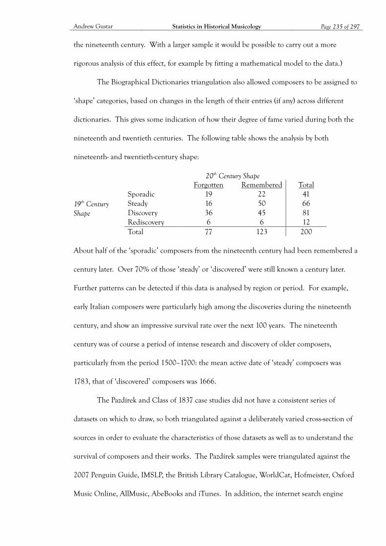
Andrew Gustar Statistics in Historical Musicology Page 235 of 297
the nineteenth century. With a larger sample it would be possible to carry out a more
rigorous analysis of this effect, for example by fitting a mathematical model to the data.)
The Biographical Dictionaries triangulation also allowed composers to be assigned to
‘shape’ categories, based on changes in the length of their entries (if any) across different
dictionaries. This gives some indication of how their degree of fame varied during both the
nineteenth and twentieth centuries. The following table shows the analysis by both
nineteenth- and twentieth-century shape:
20th Century Shape Forgotten Remembered Total
19th Century Shape
Sporadic 19 22 41 Steady 16 50 66 Discovery 36 45 81 Rediscovery 6 6 12
Total 77 123 200 About half of the ‘sporadic’ composers from the nineteenth century had been remembered a
century later. Over 70% of those ‘steady’ or ‘discovered’ were still known a century later.
Further patterns can be detected if this data is analysed by region or period. For example,
early Italian composers were particularly high among the discoveries during the nineteenth
century, and show an impressive survival rate over the next 100 years. The nineteenth
century was of course a period of intense research and discovery of older composers,
particularly from the period 1500–1700: the mean active date of ‘steady’ composers was
1783, that of ‘discovered’ composers was 1666.
The Pazdírek and Class of 1837 case studies did not have a consistent series of
datasets on which to draw, so both triangulated against a deliberately varied cross-section of
sources in order to evaluate the characteristics of those datasets as well as to understand the
survival of composers and their works. The Pazdírek samples were triangulated against the
2007 Penguin Guide, IMSLP, the British Library Catalogue, WorldCat, Hofmeister, Oxford
Music Online, AllMusic, AbeBooks and iTunes. In addition, the internet search engine
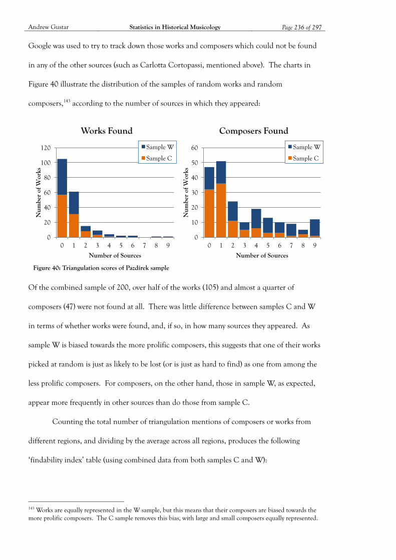
Andrew Gustar Statistics in Historical Musicology Page 236 of 297
Google was used to try to track down those works and composers which could not be found
in any of the other sources (such as Carlotta Cortopassi, mentioned above). The charts in
Figure 40 illustrate the distribution of the samples of random works and random
composers,143 according to the number of sources in which they appeared:
Of the combined sample of 200, over half of the works (105) and almost a quarter of
composers (47) were not found at all. There was little difference between samples C and W
in terms of whether works were found, and, if so, in how many sources they appeared. As
sample W is biased towards the more prolific composers, this suggests that one of their works
picked at random is just as likely to be lost (or is just as hard to find) as one from among the
less prolific composers. For composers, on the other hand, those in sample W, as expected,
appear more frequently in other sources than do those from sample C.
Counting the total number of triangulation mentions of composers or works from
different regions, and dividing by the average across all regions, produces the following
‘findability index’ table (using combined data from both samples C and W):
143 Works are equally represented in the W sample, but this means that their composers are biased towards the more prolific composers. The C sample removes this bias, with large and small composers equally represented.
Figure 40: Triangulation scores of Pazdírek sample
0
20
40
60
80
100
120
0 1 2 3 4 5 6 7 8 9
Num
ber
of W
orks
Number of Sources
Works Found
Sample W
Sample C
0
10
20
30
40
50
60
0 1 2 3 4 5 6 7 8 9
Num
ber
of W
orks
Number of Sources
Composers Found
Sample W
Sample C
Andrew Gustar Statistics in Historical Musicology Page 237 of 297
Region Composer
findability index Work findability
index Germany, Austria, Switzerland 127% 164% France, Belgium, Luxembourg 85% 67% Americas 28% 39% Italy, Iberia, North Africa 78% 31% Great Britain, Australia, South Africa 150% 108% Netherlands & Scandinavia 25% 39% Russia, Balkans & Eastern Europe 71% 67% Total 100% 100%
The findability index indicates the relative number of sources in which composers or works
from different regions are found, compared to the average, which is by definition 100%.
Thus British composers are found most easily, with 50% more mentions than average, while
American, Dutch and Scandinavian composers are around four times harder to find than
average. Germanic works, not surprisingly, are most likely to appear in other sources, with
those from America, Italy, and Scandinavia four or five times less likely to be mentioned.
This data may be skewed by the choice of sources, although factors such as legal deposit, or
the existence of long-established international publishers, are also likely to be important.
The index can also be calculated according to forces rather than region:
Forces Work findability index Solo Keyboard (2 or 4 hands) 81% Solo Song (plus accompaniment) 116% Vocal Group (with or without acc.) 181% Chamber / Other solo instrument 69% Orchestra / Band / Concerto 26% Total 100%
Thus vocal works are easier to track down than instrumental works, with large scale vocal
works around seven times more likely to be mentioned in other sources than large scale
instrumental works. These figures probably reflect the sales volumes of editions of these
works: one would expect to sell rather fewer copies of large orchestral works, for example,
than of songs (including part-songs) or piano pieces aimed at the domestic market. The low
figure here for large scale instrumental works appears to be inconsistent with the observation
that such works are often only published once they have achieved some popular success (such

Andrew Gustar Statistics in Historical Musicology Page 238 of 297
as a repeat performance). However, this effect might be offset by the very small volumes in
which published versions of such works are likely to have sold.
The Pazdírek triangulation also provided interesting data about the sources
themselves. The following table summarises some of the key statistics:
% mentioned Unique source for… Source Works Composers Works Composers Hofmeister 26% 54% 17% 15% WorldCat 23% 50% 7% 3% BL Catalogue 18% 47% 6% 6% AbeBooks 6% 37% 1% 2% AllMusic 4% 22% 0% 1% Oxford Music Online 5% 21% 1% 0% iTunes 4% 20% 0% 0% IMSLP 2% 16% 1% 0% Penguin Guide 1% 6% 0% 0%
So, for example, 26% of works mentioned in the Handbook (across the combined samples C
and W) are also mentioned in Hofmeister. 17% of the works sampled are mentioned only in
Hofmeister (among these nine sources). It is perhaps not surprising that Hofmeister, being a
similar comprehensive consolidation of publishers’ catalogues, as well as the only other
‘supply-side’ source, has the greatest degree of overlap with Pazdírek’s Handbook. The major
library catalogues are also, as expected, reasonably rich sources. Perhaps most surprising are
the high position for second-hand bookseller AbeBooks (which was particularly strong on
the solo song repertoire), and the disappointing score for Oxford Music Online. Hofmeister
was unsurprisingly strongest on the Germanic market, and the BL Catalogue’s main strength
was for British works. The Penguin Guide also scored best among Germanic works (perhaps
reflecting the bias of the canonic repertoire), although both AllMusic and iTunes were
strongest for the British market, perhaps indicating that British works are most likely to have
been recorded, even if they have not found their way into the highest echelons of the canon.
Pazdírek does not give dates for composers or works, but triangulation enabled birth
and death dates to be established for 72 composers in the combined sample. Of these, just
Andrew Gustar Statistics in Historical Musicology Page 239 of 297
11 were born before 1800, and around half (35) were still alive at the time Pazdírek was
compiling his list. The birth and death dates are negatively correlated with the number of
mentions in other sources, meaning that older composers tend to appear in more sources
than do more recent ones (the correlation coefficient is about –0.5, which is both statistically
significant and moderately strong). This suggests that the older composers whose work had
survived long enough to make it into the Handbook had a better chance of surviving
another century to appear in the modern sources, than did those who were more recent and
less well established at the time. The triangulation process also provided the publication
dates for 87 of the works in the combined sample, although these should be treated with
some caution as it is not always clear whether this is the date of first publication. Well over
half of these (49) were published after 1880.
The Class of 1837 case study also triangulated against a range of sources chosen to
span the period between 1837 and the present. The following table shows the number of
works and composers found in each of these sources:
Works found (113 total)
Composers found (69 total)
1862 Fétis 23 49 1870 Mendel – 53 1879 Grove – 25 1904 Pazdírek 68 63 1909 RCM Library Catalogue 14 27 1910 Boston Library Catalogue 8 32 1948 Barlow & Morgenstern 4 4 1949 Hutcheson 5 13 1952 WERM 5 6 1987 Hinson 13 15 1990 Gramophone Catalogue 8 11 2006 Barnard 5 5 2012 AllMusic 18 30 2012 British Library Catalogue 35 56 2012 WorldCat 66 62 2012 Concert-Diary 11 15 2012 Oxford Music Online 28 34 2012 Musicroom 5 27 2012 IMSLP 23 39
Andrew Gustar Statistics in Historical Musicology Page 240 of 297
It is interesting that Oxford Music Online does not score much better than Fétis in terms of
the number of works, and is noticeably worse when it comes to composers. The modest
improvement in Oxford Music Online compared to the first edition of Grove is rather
disappointing. A surprising number of 1837 works, including many quite obscure ones,
appear in Pazdírek. In some cases it is possible that these are simply unsold stock from 1837
still listed in publishers’ catalogues. Even in the best modern source (WorldCat) only just
over half of the works from 1837 have survived. Other composite library catalogues (such as
Copac and the University of Karlsruhe ‘Virtual Catalogue’) might improve on this slightly.
The following table shows the distribution of the 1837 works and composers by the
total numbers of mentions across all of the above triangulated sources:144
Triangulation Score Works (113 total) Composers (69 total) 0 29 4 1 23 3
2–3 32 5 4–7 15 22 8–15 9 27 16+ 5 8
As expected, the composers do rather better than specific works, with just four (Becht, C.;
Engel, A.; Hahn, C.G.; and Wewetzer, F.) not found in any triangulated source. These, and
others, may be found under variant names, although none of the obvious alternatives yielded
any success. The three composers found in just one source (Chodowiecki, A.; Muth, G.A.;
and Stückrad, C.G.) were all found in Pazdírek. About a quarter of works were not found in
any other source, and of the 23 found in only one source, 11 were in Pazdírek, eight in
WorldCat, three in Fétis, and one in the British Library. Even after a general online search,
the years of birth could not be found for 11 composers, and years of death for 16.
The frequency with which composers are mentioned in books or scholarly journals
can also be an interesting, though difficult to interpret, measure of their shifting levels of
144 Note that the maximum triangulation score is 17 for works and 19 for composers.
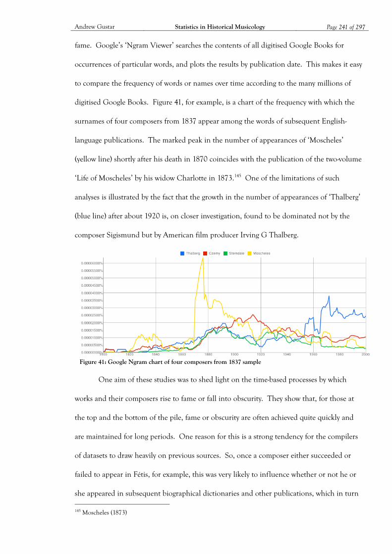
Andrew Gustar Statistics in Historical Musicology Page 241 of 297
fame. Google’s ‘Ngram Viewer’ searches the contents of all digitised Google Books for
occurrences of particular words, and plots the results by publication date. This makes it easy
to compare the frequency of words or names over time according to the many millions of
digitised Google Books. Figure 41, for example, is a chart of the frequency with which the
surnames of four composers from 1837 appear among the words of subsequent English-
language publications. The marked peak in the number of appearances of ‘Moscheles’
(yellow line) shortly after his death in 1870 coincides with the publication of the two-volume
‘Life of Moscheles’ by his widow Charlotte in 1873.145 One of the limitations of such
analyses is illustrated by the fact that the growth in the number of appearances of ‘Thalberg’
(blue line) after about 1920 is, on closer investigation, found to be dominated not by the
composer Sigismund but by American film producer Irving G Thalberg.
One aim of these studies was to shed light on the time-based processes by which
works and their composers rise to fame or fall into obscurity. They show that, for those at
the top and the bottom of the pile, fame or obscurity are often achieved quite quickly and
are maintained for long periods. One reason for this is a strong tendency for the compilers
of datasets to draw heavily on previous sources. So, once a composer either succeeded or
failed to appear in Fétis, for example, this was very likely to influence whether or not he or
she appeared in subsequent biographical dictionaries and other publications, which in turn 145 Moscheles (1873)
Figure 41: Google Ngram chart of four composers from 1837 sample
Andrew Gustar Statistics in Historical Musicology Page 242 of 297
influenced whether prospective academics, publishers, performers, concert programmers or
recording companies had heard of his or her work. Hence, fame or otherwise tends to be
determined early on and is difficult to shift in either direction (although there are many
exceptions to this).
The most significant problem with tracking fame over time is a lack of consistent
sources by which works’ and composers’ popularity can be assessed at different times. Over
the last hundred years, catalogues of recorded works have perhaps come closest to this,
although, as we have seen, they can be difficult to analyse, and popularity in the world of
recordings does not equate to that in the worlds of live performance, published music, or
scholarly attention. Sources covering these different fields cannot be readily compared
against each other, and it is thus doubtful whether it is possible to define a single meaningful
measure of ‘popularity’. With the rise of continually updated online databases over the last
20 years, it could be argued that future historians will have more difficulty finding
contemporary snapshots of the population of works ‘as at’ specific years after the late
twentieth century.
Andrew Gustar Statistics in Historical Musicology Page 243 of 297
6 QUANTITATIVE AND QUALITATIVE RESEARCH IN MUSIC HISTORY
This thesis has aimed to demonstrate whether statistical methodologies might be useful to
historical musicologists. There is a simple affirmative answer to this question, based on the
scarcity of such methodologies in historical musicology to date (despite an abundance of
suitable data), on their use in related fields, and on there being little to lose by having such
techniques available to make use of, or not, as appropriate. There are also more detailed
reasons, discussed below, why historical musicologists should make use of these techniques.
This was not an inevitable conclusion. There are at least three scenarios in which
this thesis might have reached a negative verdict. The first is that quantitative techniques
might simply be redundant, in that they reveal nothing that cannot be discovered more
effectively by other means. Many of the results from the case studies in this thesis could not
have been obtained by purely qualitative methods, so this objection can be easily countered.
Secondly, the data to which quantitative techniques may be applied might be so
problematic that it is impossible to draw any firm conclusions from such analysis. There are
some datasets for which this objection has some validity, but there are many others where the
quality, structure and relevance of the data are good enough to be confident in conclusions
drawn from quantitative analysis. Even where data is problematic, some robust conclusions
can often be drawn from quantitative analysis, even if they are simply about the nature and
quality of the source. The fact that some relevant and useful data exists, to which such
techniques can be fruitfully applied, is sufficient to justify their use.
Thirdly, it might be argued that a statistical approach to historical musicology is
misleading: that it simply misses the point and produces a superficial account of music
history that lacks the depth, complexity and nuanced interpretation that can be obtained by
the traditional qualitative methods used in this field. Advocates of such a view might argue,
for example, that whilst Macdonald may have been factually wrong in many of his claims

Andrew Gustar Statistics in Historical Musicology Page 244 of 297
(when considered in the context of the entire population of musical works), his analysis and
arguments were actually exploring important and subtle changes in musical aesthetics during
the nineteenth century as exemplified by the canonical works of the ‘great’ composers.146
Such an antipositivist perspective is not uncommon in historical musicology, nor indeed in
many other fields in the arts and humanities. Whilst the fact that this philosophy has
hitherto been predominant in the study of music history is not necessarily an argument in its
favour (it says more about historical musicologists than about the actual history of music), it
must be acknowledged that it has resulted in an extraordinarily rich, detailed and diverse
understanding of music history, and in the development and refinement of many complex,
subtle and innovative qualitative methodologies of broad applicability. Nevertheless, as this
thesis has demonstrated, there are other fruitful ways of looking at music history that go
beyond this traditional approach. A scientific, quantitative, positivist philosophy has become
more common in many fields of research since the middle of the twentieth century, and
(despite occasional tensions) can and should co-exist alongside traditional qualitative
approaches, since both philosophical standpoints have strengths and weaknesses that are
often complementary. Qualitative techniques get into the detail of the what, why and how
questions, but usually produce quite specific conclusions that are difficult to generalise.
Quantitative methods are more suited to testing hypotheses and identifying patterns and
trends, but tend not to reveal much about individual cases, nor to explain cause and effect.
In most fields of research, qualitative and quantitative techniques are used alongside each
other to provide a broad understanding. Whatever one’s individual preferences and
philosophical standpoint, it is surely difficult to argue against the case for using a
combination of both qualitative and quantitative methodologies in order to maximise the
breadth, depth, complexity and appeal of our understanding of the history of music.
146 Macdonald’s use of the description ‘expressive music’ (see the quote in section 2.2.2) perhaps supports this interpretation, although he does not define the term.
Andrew Gustar Statistics in Historical Musicology Page 245 of 297
This thesis clearly demonstrates that the use of statistical methodologies to analyse
current and historical musical datasets can offer significant benefits to the discipline of
historical musicology. Quantitative methods present an important complementary
perspective to that achievable through qualitative methods alone. More questions can be
answered, in greater depth, with better contextual understanding, and with a more precise
assessment of the confidence that can be ascribed to any conclusions. Most significantly (at
least as a vindication of these techniques), there are insights from the use of statistics that
could not be obtained through the sole use of qualitative methodologies. Whilst qualitative
techniques might conceivably have revealed that orchestral and chamber music shifted
towards flatter key signatures during the first half of the nineteenth century, it is hard to
envisage how, in the absence of statistical analysis, it would have been discovered that well-
known piano works tend to be in sharper keys than their more obscure counterparts.
Qualitative research, not surprisingly, tends to focus on the composers, works,
phenomena, events and institutions of most interest to researchers, and where there is
sufficient available information to analyse in depth. Quantitative research, in taking a high-
level view of large amounts of data, is less concerned with specific composers and works, but
rather with the broad population, its characteristics and dynamics, and the patterns and
trends it contains. Because they are rarely concerned with the ‘quality’, ‘value’ or ‘fame’ of
individual composers or works, quantitative methods can provide a reasonably objective view
of the musical world, thereby giving a voice (albeit only a collective one) to the huge numbers
of obscure composers and works that are largely ignored by qualitative researchers and have
been conspicuous by their absence from the established narrative of music history.
Redressing this balance is important not only for the obscure names (some of whom might
be rediscovered by coming to light during such quantitative exercises), but also, by providing
a more robust historical context against which their achievements can be assessed, for the
Andrew Gustar Statistics in Historical Musicology Page 246 of 297
more famous composers and the ‘great’ works.
Although far from perfect, the dispassionate analysis of datasets provides a certain
amount of objectivity that is sometimes lacking in purely qualitative research. This, together
with a better quantitative understanding of the musical context, and an awareness of the
nature of statistical analysis, should enable historical musicologists to avoid occasionally
making false, questionable, unfounded, or exaggerated claims. The Macdonald case study
demonstrated how qualitative research, when detached from quantitative evidence, can lead
both the researcher and the reader to spurious conclusions. It is worth reiterating the five
traps into which Macdonald (and no doubt others) appears to have fallen:
Failing to consider quantitative evidence: a few examples cannot prove a general
statement.
Not considering, searching for, or recognising counterexamples, or too readily dismissing
them.
Overstating the case: the ‘decisive moves’ described by Macdonald are actually rather
weak and subtle trends in a very diverse musical landscape.
Extrapolating too readily from the canonic repertoire. The case studies have shown
many times that the most famous composers and works are highly atypical of the
generality of musical activity.
Assuming that an increasing number of examples constitutes a trend, without
considering the underlying population. The fact that Macdonald found more examples
of metres at the end of the nineteenth century was simply because the total
population of works was much higher than at the start of the century, not because
had
become relatively more common.
The last two of these, not uncommon in purely qualitative research, are examples of
what Daniel Kahneman calls the ‘availability heuristic’, a tendency in human reasoning

Andrew Gustar Statistics in Historical Musicology Page 247 of 297
which ‘substitutes one question for another: you wish to estimate the size of a category or the
frequency of an event, but you report an impression of the ease with which instances come
to mind’ (Kahneman 2012, p.130). Examples from the well-known repertoire or the most
prolific periods, regions or genres are the most easily recalled, but cannot be used as a
reliable basis for inferring that the population as a whole exhibits similar characteristics.
Statistical techniques are also of benefit in enabling the quantification of aspects of
music history, thereby establishing a more robust contextual framework. Most of the case
studies have quantified findings that are known to be true (or are at least unsurprising) from
qualitative research: the distribution of works by period, region and genre; the extent to
which London and Paris were dominant in different periods as musical centres; patterns of
re-publication; differences in the performed, recorded and published repertoires; and the
extent of data problems such as estimated dates and variant names. Few of these findings (or
of the many other similar examples from this thesis) are surprising or original, but the
quantification of them is new and enables the narrative of the history of music to be placed
in a context based on much firmer foundations than has hitherto been the case.
In some circumstances quantitative results can shed light on qualitative processes.
Such information might emerge directly from the data (as in the patterns of composer
imports and exports described in 5.1.2), or from a consideration of relationships within the
data (such as the comparison of the geographical distributions of publishers and works, and
what this implies about the publishing industry in different territories, as discussed in 5.3.1).
Underlying processes may also be indicated by the fact that standard probability distributions
are based on simple sets of assumptions. If sampled data approximates to a standard
distribution derived from particular assumptions, this might suggest that similar assumptions
could apply to the processes reflected in the data, perhaps to be investigated with more
detailed research. Examples from the case studies include the Zipf distribution of published

Andrew Gustar Statistics in Historical Musicology Page 248 of 297
works per composer and its implications regarding music publishers’ decision making (see
4.6.3), or the Poisson process governing composers’ rates of migration (see 5.1.2).
In a similar vein, analysis of the datasets themselves can help in assessing the
potential errors and biases to which any methodologies, whether quantitative or qualitative,
are at risk. The Class of 1810/1820 case study revealed much about the problems of
duplication and data quality associated with library catalogues; other case studies assessed
the significance of variant names and estimated dates; the triangulation scores in the
Pazdírek case study revealed how some sources were rather more or less comprehensive than
might be expected; and geographical bias has been identified, and partly quantified, in many
sources including biographical dictionaries and Penguin guides.
One by-product of this quantification is that, in its discrepancies, it draws attention
to some of the inherent biases in our received view of music history. Different measures of,
for example, the proportion of composers from Germanic countries, or of works written for
solo piano, often vary substantially, and consideration of the reasons for this lead inevitably
into questions about the differing viewpoints of those who have compiled historical datasets
and, by association, those who have contributed in various ways to the standard history of
music as we understand it. This in turn prompts questions about the extent to which the
perspectives of scholars, historians, biographers, critics and others, biased by weight of
numbers in particular regional, linguistic, cultural or aesthetic groupings, have distorted our
picture of what was really going on in the musical world. Whilst these issues present
practical methodological problems to the quantitative researcher, who must recognise and, if
possible, make some allowance for them, they do not, on the whole, directly impact on
qualitative methodologies, and have thus perhaps been under-recognised by music historians.
Almost all of the datasets considered here are biased in some way, inasmuch as they
are not truly representative of the population of musical works or composers. Explicit bias

Andrew Gustar Statistics in Historical Musicology Page 249 of 297
(by date, region, genre, etc) can usually be managed within the scope and objectives of a
study, but other biases, such as an editor’s personal selection or the bias resulting from the
interdependence between sources, are harder to take into account. More fundamentally,
there are two forms of deep bias that have emerged as frequent concerns during this thesis,
which apply to the aggregation of qualitative research in historical musicology as much as to
individual quantitative studies. Both are, in effect, consequences of the ‘availability
heuristic’ mentioned above: a bias in favour of evidence and data that is most available and
most familiar. The first is a temporal and geographical bias in favour of those periods and
regions where music scholarship, collecting, record keeping, commentary and debate have
been most active. Consequently some regions and periods are simply much better
represented than others in musical datasets, and thus in the research derived from them.
The much higher chance of a nineteenth-century German work or composer appearing in
historical datasets compared to one from, say, fourteenth-century Spain, is to a large extent
the result of more interest in, and better records of, music in the former region and period
than the latter. It does not necessarily mean that a typical occupant of nineteenth-century
Germany encountered more or better music than someone in fourteenth-century Spain, but
simply that the music and composers from the former region and period have a higher
probability of being visible to musicologists. Quantifying the extent of this bias is extremely
difficult because there are few, if any, unbiased sources that provide a neutral benchmark.147
The second form of deep bias, just as intractable as the first and related in its origins,
is the asymmetry of information between well-known works and composers and their more
obscure counterparts. It is much easier to find information about the life and works of
147 The influence of music scholarship on music aesthetics means that this effect goes rather deeper than a simple statistical bias. The disproportionate attention given to, say, nineteenth-century German music compared to that from fourteenth-century Spain has inevitably affected the repertoire that has been, and continues to be, performed, studied, taught and listened to in much of the Western world. This biased repertoire will inevitably have influenced the views and aesthetics of those exposed to it, many of whom will consequently regard nineteenth-century German music as ‘better’ in some sense than that of fourteenth-century Spain, which, to them, may be unfamiliar and less stylistically accessible.
Andrew Gustar Statistics in Historical Musicology Page 250 of 297
Franz Schubert than about those of Carlotta Cortopassi,148 and thus the availability and
accuracy of the data required for statistical analyses, or the quality of judgements derived
from them (such as those involved in data cleaning), are much better for one than the other.
As a result, it can be difficult to treat well-known and obscure composers on a fair and
consistent basis. Whilst it is possible to manage aspects of this asymmetry, statistically, in an
unbiased way (for example by applying genuinely random decisions to data cleaning, as
discussed in 4.4.2), it is nevertheless inherently impossible to treat all works or composers
consistently in such studies. This asymmetry increases the potential for sampling and
calculation bias, and is likely to understate the true variability of statistical results (causing
calculated confidence intervals to be too narrow, and levels of significance to be too high) by
an unknown amount. This is an area where further research would be useful.
This thesis has frequently observed that, despite the obvious differences in the nature
and application of qualitative and quantitative techniques, they actually have many features
in common. Both are prone to similar limitations in the quality and bias of historical
sources; they are both influenced by the interests, values and capabilities of the researcher;
and they both require similar levels of caution and contextualisation in their application and
interpretation. There is, however, an important difference between the priorities of
qualitative and quantitative researchers. Whereas a good qualitative researcher will take care
to question the accuracy and meaning of sources in great detail, the quantitative researcher is
likely to be more concerned with questions of representativeness, bias, and the confidence
with which conclusions can be drawn. Quantitative researchers must usually live with the
presence of dirty, inaccurate and incomplete data, but, subject to this unavoidable situation,
maximising the integrity of the sample as a whole is of paramount concern. It is in the
treatment of such imperfect data that priorities are likely to differ. In the example in section
148 See section 5.4
Andrew Gustar Statistics in Historical Musicology Page 251 of 297
4.4.2 mentioned above, the best way (i.e. that which minimised statistical bias) of handling
works that could not be definitely identified as ‘original’ or ‘derivative’ compositions in the
Class of 1837 case study was to allocate them to these categories at random. Despite the
statistical logic, such an approach may reduce the credibility of the methodology in the eyes
of qualitative researchers, for whom the integrity and context of individual items of data is
likely to be a higher priority than the representativeness of the sample as a whole.
Both statistics and historical musicology are broad, sophisticated and complex
disciplines. The potential ways in which the former could be applied to study the latter are
limited only by the imagination and skill of the researcher and the availability of suitable
data. This thesis, intentionally, has only considered a small number of straightforward
statistical techniques, a handful of broad topics in music history, and (in most cases) freely
and readily available data. The aim has been to cover a range of applications that illustrate
the potential benefits of using quantitative methodologies in this field, and that expose the
practical issues arising in their application. More specifically, the objectives of this thesis
have been threefold: to provide a ‘proof of concept’ that statistical methodologies can be
usefully and successfully applied to questions in historical musicology; to demonstrate the
value, for historical musicologists, of using quantitative techniques; and to identify some of
the practical and theoretical issues involved in using statistics to extract meaningful
quantitative information from datasets relating to the history of music.
Like any research methodology, statistical techniques must be used and interpreted
with care if they are to be both useful and credible. In historical musicology, as in any field
in which such techniques are employed, questions of statistical significance, bias, lack of
independence and data quality must be carefully considered at all stages between the design
of the study and the interpretation and presentation of the results. Time and thought need
to be invested in the design of such studies; in identifying suitable datasets; in developing the
Andrew Gustar Statistics in Historical Musicology Page 252 of 297
sampling strategy; in collecting, cleaning and formatting the data; in the analysis itself; and
in interpreting the results alongside the broader musicological and historical context. Care
must also be taken in presenting quantitative results and conclusions in a meaningful and
responsible way to an often non-specialist audience. This thesis has illustrated these
considerations in various contexts, and identified a number of issues that arise particularly
(though probably not uniquely) in the quantitative study of music history. Whilst many
statistical applications in other fields use clean and consistent data, often designed
specifically for the purpose, the historical datasets considered here are not, on the whole,
designed for statistical analysis. Data is often dirty in various ways; there may be high levels
of duplication; there can be problems with variant names and titles; and foreign languages
and historical geographical changes can make data difficult to understand, gather, or clean.
All of these issues can be managed, but this must be done with care in order to avoid further
bias. Some promising datasets, such as iTunes, turn out to be practically impossible to use
for sampling, although they can still be of use for triangulation. Historical musical datasets
appear to be a rich source of highly skew ‘Zipf-like’ distributions, with very large numbers of
small members and small but significant numbers of very large members. Such distributions
present certain statistical challenges and tend to result in rather wide margins of error in
most statistical tests. In particular, they can lead to extreme length-biased sampling that can
significantly distort statistical results unless it is recognised and allowed for appropriately.
One potential difficulty with statistical techniques, particularly among practitioners
not entirely comfortable with their use, is a risk of reaching over-simplistic conclusions. This
is easily done when the focus is on average values, linear trends, and simple comparisons. In
fact, as most of the case studies have shown, music is a hugely diverse and changeable activity
that cannot be easily reduced to simple rules. The trends in average key signatures
discovered in the Macdonald and Piano Keys case studies, for example, are both non-linear
Andrew Gustar Statistics in Historical Musicology Page 253 of 297
(rising and falling as different orchestral instruments come into favour, and tastes and
fashions change) and weak, in the sense that the trend refers to small changes in the average
value of a distribution with, at any point in time, a very wide spread of key signatures actually
in use. Similar arguments could be made about composers’ movements, publication
histories, and other topics considered here. On the other hand, it is just as easy to
overcomplicate statistical analysis, leading to results that are difficult or impossible to
interpret, and complex relationships that cannot be identified or calibrated without a very
large sample. The tendency in this research has been to use relatively small samples, so in
principle more could be done, with larger samples, to understand phenomena such as the
recency effect in biographical dictionaries, or the international import/export market in
composers. The point is that a balance has to be struck between simplicity and complexity,
and that this may be a judgement requiring the rare combination of practical experience in
both statistics and historical musicology.
There are of course situations where statistical techniques are not useful. In much
historical research, qualitative techniques are more appropriate, although quantitative
methods might nevertheless provide a broader context. In some situations, the data can be
unavailable or too complex or biased to be of use. The complex nature of the data in the
Recordings case study, for example, presented various difficulties that limited the extent to
which constructive progress could be made with the statistical analysis. In the Class of 1837
case study, the triangulation against several disparate datasets spanning the late nineteenth
and twentieth centuries turned out to be of limited use because the substantial differences
between the datasets masked any of the possible time-related effects that were the topic of
interest. Nevertheless, despite the various caveats and limitations (which are no more
significant or numerous than those applicable to qualitative methodologies), all of the case
studies investigated for this thesis have been informative. Even if the topic at hand has not
Andrew Gustar Statistics in Historical Musicology Page 254 of 297
been particularly illuminated by the quantitative approach, light has often been shed on the
datasets themselves, or on methodological issues that might have broader relevance for
quantitative or qualitative techniques.
Just as the subject of this research is an essentially unstudied field, so its objective –
the evaluation of a methodology – also appears to be relatively novel. It has not been
possible, to any great extent, to inform either the subject or the objective of this research
through reference to existing literature, other than by analogy and contrast with other fields.
In the absence of an established approach, the method used here for evaluating the statistical
methodology has been to gain ‘hands-on’ evidence through a series of case studies, applying
statistical techniques to real data in order to investigate particular musicological issues. The
case studies were chosen to cover a range of musicological topics and different types of
dataset, and to employ a selection of statistical techniques. The output from these case
studies, in addition to the musicological results discussed mainly in chapter 5 of this thesis,
included learning about the characteristics of the datasets; the practicalities of managing the
data, applying the statistical techniques, and interpreting the results; and forming
judgements as to the overall reliability, robustness and usefulness of the exercise.
Each of the case studies could be expanded into a thorough musicological
investigation, with larger samples, more sophisticated analysis, and a detailed comparison
and reconciliation of the findings against existing knowledge of the topic in hand. This level
of detail was neither possible nor appropriate, given the time and resources available for this
thesis, and the primary focus on evaluating the most significant methodological issues. The
limited nature of the case studies considered here does not weaken the conclusion that
historical musicologists should use statistics, although it is likely that further research might
identify new issues associated with certain types of dataset or statistical technique, or that
arise particularly in large-scale investigations. Whilst the statistical methodology has been
Andrew Gustar Statistics in Historical Musicology Page 255 of 297
tested reasonably thoroughly (bearing in mind the novelty of quantitative methods in this
field), there inevitably remain several loose ends in the musicological conclusions. Hopefully
what has been learnt here about the application of statistical methods in historical
musicology will facilitate the further exploration and analysis of these (and other)
musicological topics by future researchers.
Since the use of statistics in historical musicology is essentially a new field, the overall
argument of this thesis covers ground that has not been crossed before. That is not to say
that all of the conclusions about statistics, datasets, or the history of music are necessarily
original. Nevertheless, there do appear to be a number of original aspects to this work. In
statistical methods, for example, the method to adjust for length-biased sampling (described
in 4.6.1) appears to be original, as does the approach to handling time signatures as ordered
categorical data (5.2.2). Many of the discoveries about musical datasets do not appear to
have been made before. These include the typology of datasets and the assessment of their
suitability for sampling and statistical analysis (3.1.1); the quantification of many of them
(summarised in Appendix B); as well as more specific findings such as the periodicity in
attributed dates in the British Library catalogue (4.5.3); the commonness of ‘Zipf-like’
distributions in historical musical data (4.6.3); and the prevalence of variant names (5.1.3).
Many of the musicological findings from the case studies are also original. These include the
quantification of known (or at least unsurprising) facts, such as the international movements
in composers (5.1.2); the numbers of composers and their works (5.1.5); the changes in
average key signatures during the nineteenth century (5.2.3); the technical difficulty ratings
of piano works (5.2.6); the dominant position of Leipzig as a music publishing centre (5.3.1);
the fate of different clusters of works by publication history (5.3.1); and the survival
probabilities of composers and works in the repertoire, including differences by genre, period
and region (5.4). There have also been some genuinely surprising original discoveries,
Andrew Gustar Statistics in Historical Musicology Page 256 of 297
including the stable 1-in-14-year Poisson process governing composers’ migrations (5.1.2);
that well-known piano works tend to use sharper key signatures than obscure piano works
(5.2.3); that composers in their thirties tend to use sharper key signatures in piano works
than either younger or older composers (5.2.3); that ‘second division’ composers write the
most technically difficult piano works (5.2.6); and the differences between French and
German composers’ treatment of key signatures in major and minor modes (5.2.4). This
thesis may also be unique in identifying the consequences of historical musicology’s
methodological blind-spot for quantitative techniques, whether it is the erroneous
conclusions made by writers like Macdonald (sections 5.2.2 and 5.2.3), or the narrow and
biased nature of the received narrative of music history as discussed above.
This thesis has opened up new ways to approach the study of music history,
demonstrating that there is value to using statistical techniques in this field. Indeed, some
conclusions from this research might perhaps be of interest to researchers in other fields of
the arts and humanities in which quantitative methods are under-utilised. This work has
also suggested many areas for further research. Any of the datasets, case studies or themes
covered in this thesis would be valid topics for more detailed studies. There are inevitably
some other topics of interest that have not been covered here. Further research might
usefully examine other types of dataset including, for example, non-public domain and
commercial data, manuscript sources, catalogues of instruments or publishers, and the many
folk, jazz and popular music datasets. There is also scope to go beyond the relatively simple
statistical methods used in the case studies, and, in particular, to employ some of the pattern
recognition and other analytical tools that are increasingly being developed for studying ‘big
data’. This is the trend in recent years towards analysing entire large datasets rather than
samples, made possible by the ubiquity of fast, sophisticated and interconnected computer
power, which has transformed the speed, quantity and detail with which data can now be
Andrew Gustar Statistics in Historical Musicology Page 257 of 297
collected, stored, accessed and analysed. Many of the statistical considerations and
constraints imposed by sampling do not apply to the analysis of entire datasets. The ability
to analyse entire datasets would facilitate a much better understanding of the extremities of
statistical distributions (such as the population of obscure composers and their works) than
is likely to be possible using a sampling-based approach. Such techniques would not, of
course, avoid the limitations and inherent biases of the datasets themselves.
One significant constraint to a ‘big data’ approach to this topic is that, for the
majority of historical datasets, the extraction of data into a form suitable for statistical
analysis remains difficult and time-consuming, so obtaining entire datasets in a usable form
is impractical and sampling remains the only practical approach to their study. A fruitful
area for further research would be the development of more sophisticated ways of harvesting
information from historical datasets automatically. It remains very difficult to automate the
process of extracting reliable information from books, even if they exist in scanned form,
largely due to the fact that the logical structure of such data is defined (often inconsistently)
by little more than the vagaries of layout, punctuation and typeface. With the many modern
sources existing as online databases, it should be (at least in principle) relatively
straightforward to include functionality that meets the needs of quantitative researchers
(such as standardising the format of information, and facilitating the download of data that
can be used for sampling) as well as those of qualitative researchers (i.e. searching for
information on specific items). Unfortunately the trend towards improving the experience
for users who wish to search online databases often seems to result in making more difficult
the collection of data for quantitative analysis. On the other hand, access to much online
data is becoming increasingly open, provided one has the necessary technical knowledge and
skills. The tools available to find and harvest such data are constantly growing in power and
sophistication. There is scope for historical musicologists to work with experts at online
Andrew Gustar Statistics in Historical Musicology Page 258 of 297
‘data scraping’ as well as with the owners of the databases, in order to make this data more
accessible for quantitative historical research.
For the time being, a qualitative bias remains firmly embedded in historical
musicology: in the skills, outlook and training of researchers; in the scope of books, journals
and conferences; and in the design and content of the datasets themselves. The widespread
adoption of quantitative techniques as part of the methodological toolkit of historical
musicology will doubtless be a slow process.149 Nevertheless, even occasional use of such
techniques would begin to redress the balance, by illustrating the potential benefits of such
methodologies – greater objectivity, quantification of the musical landscape, a voice for the
obscure works and composers, accessing corners of the subject unavailable to purely
qualitative approaches – and, in turn, prompting new questions and areas of research for
both quantitative and qualitative researchers in the history of music (and, indeed, for
statisticians). Although there are many difficult questions for which no data or evidence
exists, or which are methodologically intractable, the case studies have demonstrated that
much can be achieved with readily available data by a researcher with unexceptional skills
and resources, using simple statistical techniques and a little common sense. Between these
extremes lie plenty of potential fields of investigation, requiring creativity, ingenuity, and a
certain amount of speculation, which are often those that present the most valuable
development opportunities for the researcher and the most intriguing and controversial
results for the musicological audience.
149 As a result of the work on this thesis, the Open University’s new taught MA in Music, due for launch at the end of 2014, will contain units on quantitative methods in historical musicology, written by the present author.
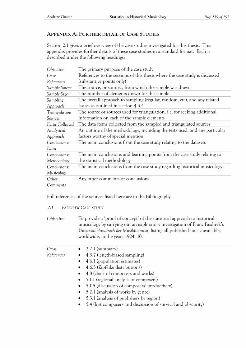
Andrew Gustar Statistics in Historical Musicology Page 259 of 297
APPENDIX A: FURTHER DETAIL OF CASE STUDIES
Section 2.1 gives a brief overview of the case studies investigated for this thesis. This appendix provides further details of these case studies in a standard format. Each is described under the following headings:
Objective The primary purpose of the case study Cross References
References to the sections of this thesis where the case study is discussed (substantive points only)
Sample Source The source, or sources, from which the sample was drawn Sample Size The number of elements drawn for the sample Sampling Approach
The overall approach to sampling (regular, random, etc), and any related issues as outlined in section 4.3.4
Triangulation Sources
The source or sources used for triangulation, i.e. for seeking additional information on each of the sample elements
Data Collected The data items collected from the sampled and triangulated sources Analytical Approach
An outline of the methodology, including the tests used, and any particular factors worthy of special mention
Conclusions: Data
The main conclusions from the case study relating to the datasets
Conclusions: Methodology
The main conclusions and learning points from the case study relating to the statistical methodology
Conclusions: Musicology
The main conclusions from the case study regarding historical musicology
Other Comments
Any other comments or conclusions
Full references of the sources listed here are in the Bibliography.
A1. PAZDÍREK CASE STUDY
Objective To provide a ‘proof of concept’ of the statistical approach to historical musicology by carrying out an exploratory investigation of Franz Pazdírek’s Universal-Handbuch der Musikliteratur, listing all published music available, worldwide, in the years 1904–10.
Cross References
2.2.1 (summary) 4.3.7 (length-biased sampling) 4.6.1 (population estimates) 4.6.3 (Zipf-like distributions) 4.8 (chart of composers and works) 5.1.1 (regional analysis of composers) 5.1.5 (discussion of composers’ productivity) 5.2.1 (analysis of works by genre) 5.3.1 (analysis of publishers by region) 5.4 (lost composers and discussion of survival and obscurity)
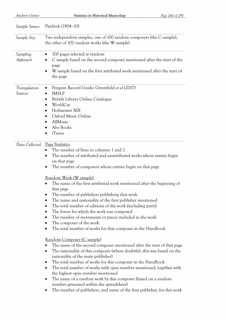
Andrew Gustar Statistics in Historical Musicology Page 260 of 297
Sample Source Pazdírek (1904–10)
Sample Size Two independent samples, one of 100 random composers (the C sample), the other of 100 random works (the W sample)
Sampling Approach
100 pages selected at random C sample based on the second composer mentioned after the start of the
page W sample based on the first attributed work mentioned after the start of
the page
Triangulation Sources
Penguin Record Guide: Greenfield et al (2007) IMSLP British Library Online Catalogue WorldCat Hofmeister XIX Oxford Music Online AllMusic Abe Books iTunes
Data Collected Page Statistics
The number of lines in columns 1 and 2 The number of attributed and unattributed works whose entries begin
on that page The number of composers whose entries begin on that page
Random Work (W sample) The name of the first attributed work mentioned after the beginning of
that page The number of publishers publishing that work The name and nationality of the first publisher mentioned The total number of editions of the work (including parts) The forces for which the work was composed The number of movements or pieces included in the work The composer of the work The total number of works for that composer in the Handbook
Random Composer (C sample) The name of the second composer mentioned after the start of that page The nationality of this composer (where doubtful, this was based on the
nationality of the main publisher) The total number of works for this composer in the Handbook The total number of works with opus number mentioned, together with
the highest opus number mentioned The name of a random work by this composer (based on a random
number generated within the spreadsheet) The number of publishers, and name of the first publisher, for this work
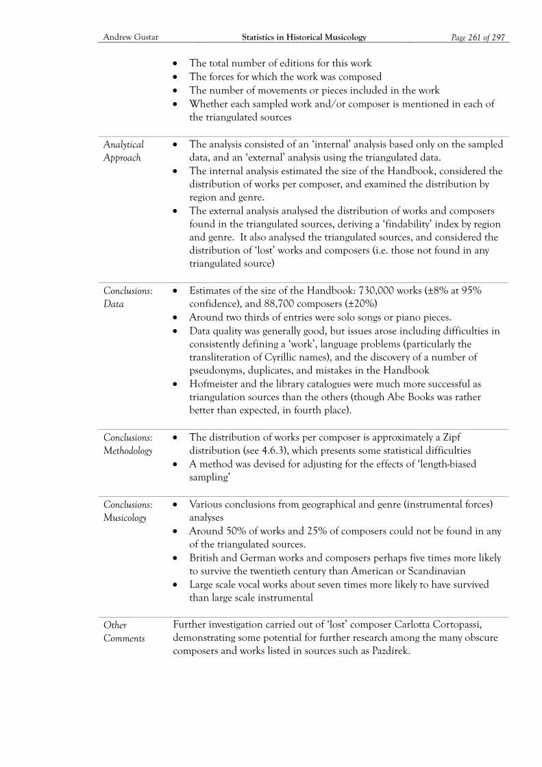
Andrew Gustar Statistics in Historical Musicology Page 261 of 297
The total number of editions for this work The forces for which the work was composed The number of movements or pieces included in the work Whether each sampled work and/or composer is mentioned in each of
the triangulated sources
Analytical Approach
The analysis consisted of an ‘internal’ analysis based only on the sampled data, and an ‘external’ analysis using the triangulated data.
The internal analysis estimated the size of the Handbook, considered the distribution of works per composer, and examined the distribution by region and genre.
The external analysis analysed the distribution of works and composers found in the triangulated sources, deriving a ‘findability’ index by region and genre. It also analysed the triangulated sources, and considered the distribution of ‘lost’ works and composers (i.e. those not found in any triangulated source)
Conclusions: Data
Estimates of the size of the Handbook: 730,000 works (±8% at 95% confidence), and 88,700 composers (±20%)
Around two thirds of entries were solo songs or piano pieces. Data quality was generally good, but issues arose including difficulties in
consistently defining a ‘work’, language problems (particularly the transliteration of Cyrillic names), and the discovery of a number of pseudonyms, duplicates, and mistakes in the Handbook
Hofmeister and the library catalogues were much more successful as triangulation sources than the others (though Abe Books was rather better than expected, in fourth place).
Conclusions: Methodology
The distribution of works per composer is approximately a Zipf distribution (see 4.6.3), which presents some statistical difficulties
A method was devised for adjusting for the effects of ‘length-biased sampling’
Conclusions: Musicology
Various conclusions from geographical and genre (instrumental forces) analyses
Around 50% of works and 25% of composers could not be found in any of the triangulated sources.
British and German works and composers perhaps five times more likely to survive the twentieth century than American or Scandinavian
Large scale vocal works about seven times more likely to have survived than large scale instrumental
Other Comments
Further investigation carried out of ‘lost’ composer Carlotta Cortopassi, demonstrating some potential for further research among the many obscure composers and works listed in sources such as Pazdírek.
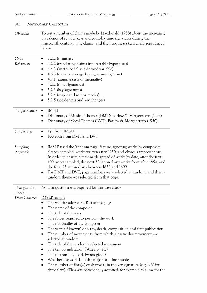
Andrew Gustar Statistics in Historical Musicology Page 262 of 297
A2. MACDONALD CASE STUDY
Objective To test a number of claims made by Macdonald (1988) about the increasing prevalence of remote keys and complex time signatures during the nineteenth century. The claims, and the hypotheses tested, are reproduced below.
Cross References
2.2.2 (summary) 4.2.2 (translating claims into testable hypotheses) 4.4.3 (‘metre code’ as a derived variable) 4.5.3 (chart of average key signatures by time) 4.7.1 (example tests of inequality) 5.2.2 (time signatures) 5.2.3 (key signatures) 5.2.4 (major and minor modes) 5.2.5 (accidentals and key changes)
Sample Sources IMSLP
Dictionary of Musical Themes (DMT): Barlow & Morgenstern (1948) Dictionary of Vocal Themes (DVT): Barlow & Morgenstern (1950)
Sample Size 175 from IMSLP
100 each from DMT and DVT
Sampling Approach
IMSLP used the ‘random page’ feature, ignoring works by composers already sampled, works written after 1950, and obvious transcriptions. In order to ensure a reasonable spread of works by date, after the first 100 works sampled, the next 50 ignored any works from after 1850, and the final 25 ignored any between 1850 and 1899.
For DMT and DVT, page numbers were selected at random, and then a random theme was selected from that page.
Triangulation Sources
No triangulation was required for this case study
Data Collected IMSLP sample The website address (URL) of the page The name of the composer The title of the work The forces required to perform the work The nationality of the composer The years (if known) of birth, death, composition and first publication The number of movements, from which a particular movement was
selected at random The title of the randomly selected movement The tempo indication (‘Allegro’, etc) The metronome mark (when given) Whether the work is in the major or minor mode The number of flats(–) or sharps(+) in the key signature (e.g. ‘–3’ for
three flats). (This was occasionally adjusted, for example to allow for the
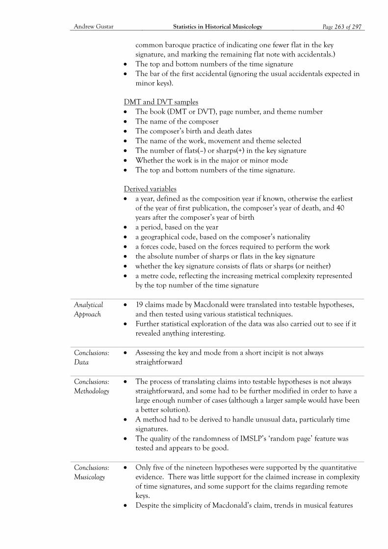
Andrew Gustar Statistics in Historical Musicology Page 263 of 297
common baroque practice of indicating one fewer flat in the key signature, and marking the remaining flat note with accidentals.)
The top and bottom numbers of the time signature The bar of the first accidental (ignoring the usual accidentals expected in
minor keys).
DMT and DVT samples The book (DMT or DVT), page number, and theme number The name of the composer The composer’s birth and death dates The name of the work, movement and theme selected The number of flats(–) or sharps(+) in the key signature Whether the work is in the major or minor mode The top and bottom numbers of the time signature.
Derived variables a year, defined as the composition year if known, otherwise the earliest
of the year of first publication, the composer’s year of death, and 40 years after the composer’s year of birth
a period, based on the year a geographical code, based on the composer’s nationality a forces code, based on the forces required to perform the work the absolute number of sharps or flats in the key signature whether the key signature consists of flats or sharps (or neither) a metre code, reflecting the increasing metrical complexity represented
by the top number of the time signature
Analytical Approach
19 claims made by Macdonald were translated into testable hypotheses, and then tested using various statistical techniques.
Further statistical exploration of the data was also carried out to see if it revealed anything interesting.
Conclusions: Data
Assessing the key and mode from a short incipit is not always straightforward
Conclusions: Methodology
The process of translating claims into testable hypotheses is not always straightforward, and some had to be further modified in order to have a large enough number of cases (although a larger sample would have been a better solution).
A method had to be derived to handle unusual data, particularly time signatures.
The quality of the randomness of IMSLP’s ‘random page’ feature was tested and appears to be good.
Conclusions: Musicology
Only five of the nineteen hypotheses were supported by the quantitative evidence. There was little support for the claimed increase in complexity of time signatures, and some support for the claims regarding remote keys.
Despite the simplicity of Macdonald’s claim, trends in musical features
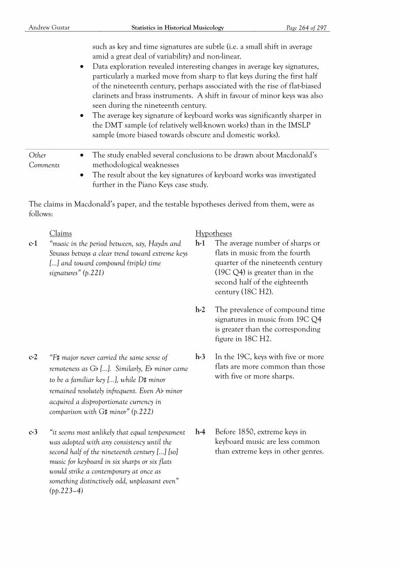
Andrew Gustar Statistics in Historical Musicology Page 264 of 297
such as key and time signatures are subtle (i.e. a small shift in average amid a great deal of variability) and non-linear.
Data exploration revealed interesting changes in average key signatures, particularly a marked move from sharp to flat keys during the first half of the nineteenth century, perhaps associated with the rise of flat-biased clarinets and brass instruments. A shift in favour of minor keys was also seen during the nineteenth century.
The average key signature of keyboard works was significantly sharper in the DMT sample (of relatively well-known works) than in the IMSLP sample (more biased towards obscure and domestic works).
Other Comments
The study enabled several conclusions to be drawn about Macdonald’s methodological weaknesses
The result about the key signatures of keyboard works was investigated further in the Piano Keys case study.
The claims in Macdonald’s paper, and the testable hypotheses derived from them, were as follows: Claims Hypotheses c-1 “music in the period between, say, Haydn and
Strauss betrays a clear trend toward extreme keys […] and toward compound (triple) time signatures” (p.221)
h-1 The average number of sharps or flats in music from the fourth quarter of the nineteenth century (19C Q4) is greater than in the second half of the eighteenth century (18C H2).
h-2 The prevalence of compound time signatures in music from 19C Q4 is greater than the corresponding figure in 18C H2.
c-2 “F# major never carried the same sense of remoteness as Gb […]. Similarly, Eb minor came to be a familiar key […], while D# minor remained resolutely infrequent. Even Ab minor acquired a disproportionate currency in comparison with G# minor” (p.222)
h-3 In the 19C, keys with five or more flats are more common than those with five or more sharps.
c-3 “it seems most unlikely that equal temperament was adopted with any consistency until the second half of the nineteenth century […] [so] music for keyboard in six sharps or six flats would strike a contemporary at once as something distinctively odd, unpleasant even” (pp.223–4)
h-4 Before 1850, extreme keys in keyboard music are less common than extreme keys in other genres.
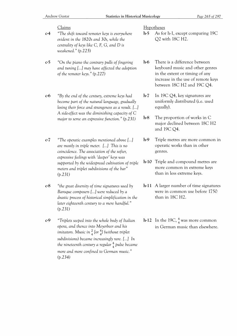
Andrew Gustar Statistics in Historical Musicology Page 265 of 297
Claims Hypotheses c-4 “The shift toward remoter keys is everywhere
evident in the 1820s and 30s, while the centrality of keys like C, F, G, and D is weakened.” (p.225)
h-5 As for h-1, except comparing 19C Q2 with 18C H2.
c-5 “On the piano the contrary pulls of fingering and tuning […] may have affected the adoption of the remoter keys.” (p.227)
h-6 There is a difference between keyboard music and other genres in the extent or timing of any increase in the use of remote keys between 18C H2 and 19C Q4.
c-6 “By the end of the century, extreme keys had become part of the natural language, gradually losing their force and strangeness as a result. […] A side-effect was the diminishing capacity of C major to serve an expressive function.” (p.231)
h-7 In 19C Q4, key signatures are uniformly distributed (i.e. used equally).
h-8 The proportion of works in C major declined between 18C H2 and 19C Q4.
c-7 “The operatic examples mentioned above […] are mostly in triple meter. […] This is no coincidence. The association of the softer, expressive feelings with ‘deeper’ keys was supported by the widespread cultivation of triple meters and triplet subdivisions of the bar” (p.231)
h-9 Triple metres are more common in operatic works than in other genres.
h-10 Triple and compound metres are more common in extreme keys than in less extreme keys.
c-8 “the great diversity of time signatures used by Baroque composers […] were reduced by a drastic process of historical simplification in the later eighteenth century to a mere handful.” (p.231)
h-11 A larger number of time signatures were in common use before 1750 than in 18C H2.
c-9 “Triplets seeped into the whole body of Italian opera, and thence into Meyerbeer and his imitators. Music in
[or
] (without triplet
subdivisions) became increasingly rare. […] In the nineteenth century a regular
pulse became
more and more confined to German music.” (p.234)
h-12 In the 19C, was more common
in German music than elsewhere.

Andrew Gustar Statistics in Historical Musicology Page 266 of 297
Claims Hypotheses c-10 “The barcarolle, the lilting waltz, the
lullaby -
these are as characteristic of the nineteenth century as the broad movement in
or
. By
the end of the century such dependence on multiples of three conditioned the lingua franca of the day, especially in piano music” (p.235)
h-13 Music in
,
or
was more common in the 19C than in other periods.
h-14 There was an increase in the use of
,
and
during the 19C in all regions.150
h-15 In 19C Q4,
,
and
.were more common in piano music than in other genres.
c-11 “Twentieth-century interest in these more complex rhythms, […] and a desire to restore rhythmic rigor as an antidote to the excess of ‘weak’ rhythm have in practice restored duple subdivisions to a higher standing than before” (p.236)
h-16 The prevalence of duple metres was higher in 20C H1 than in 19C H2.
c-12 “the decisive moves away from an allegiance to home keys and duple rhythms (the Classical German style) toward a taste for remote keys and triple rhythms occurred at much the same time in much the same body of music” (p.237)
h-17 Any shift towards remote keys and compound metres during the 19C occurred at the same time in all genres.
c-13 “It always remained possible to write in an extreme key and a simple
, or in C major in
,
yet there existed a definite point toward which expressive music seemed naturally to gravitate for almost a century, toward writing in Gb major in
.” (p.237)
h-18 Any trends towards remote keys and compound metres during the 19C were correlated, rather than independent (i.e. works became more likely to have both of these features, rather than just one of them). (Similar to h-10)
c-14 Macdonald only cites examples from the canonic repertoire, yet seems to imply that his conclusions apply to music in general.
h-19 Any trends towards remote keys and compound metres during the 19C observed in the canonic repertoire can also be observed in music as a whole.
150 The OED defines lingua franca as “any mixed jargon formed as a medium of intercourse between people speaking different languages”. Presumably Macdonald is referring to the widespread use of these metres.
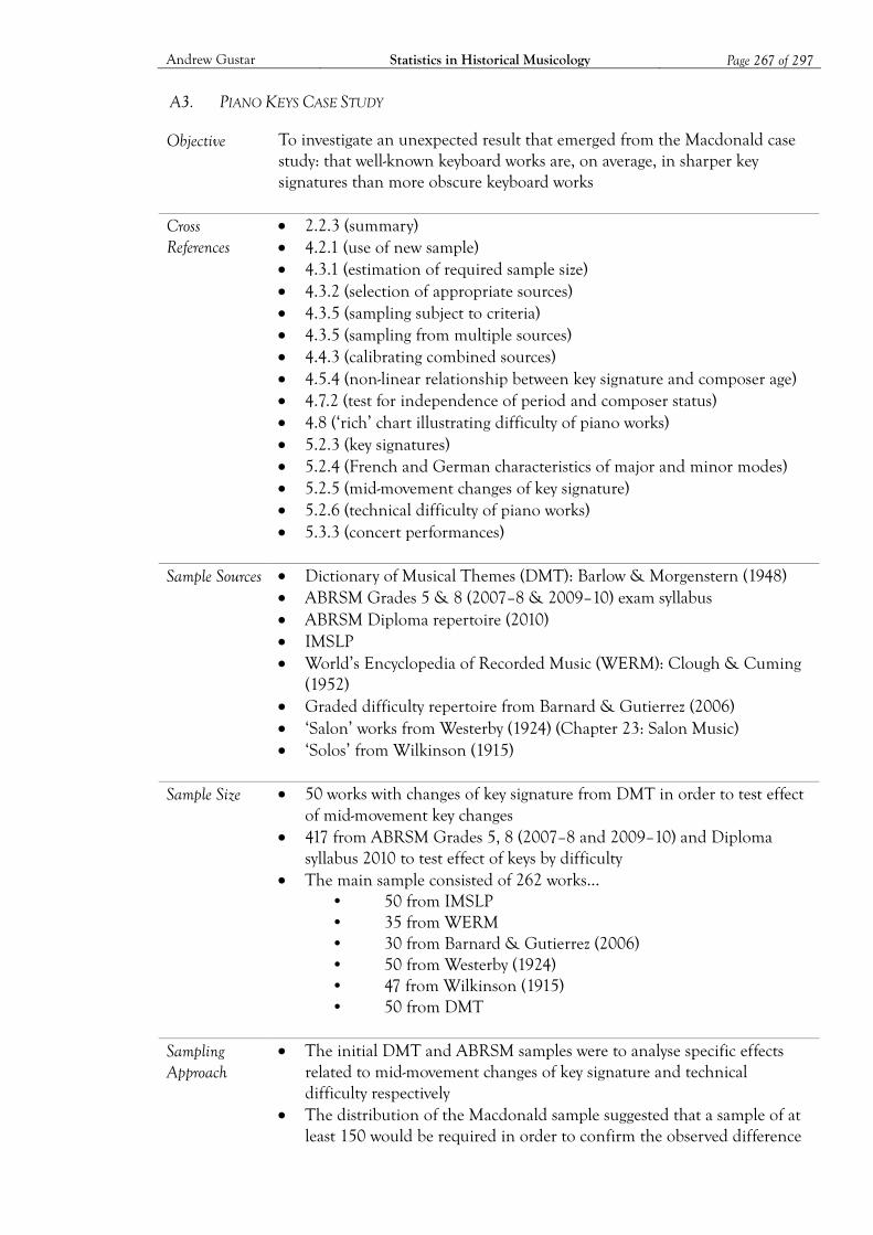
Andrew Gustar Statistics in Historical Musicology Page 267 of 297
A3. PIANO KEYS CASE STUDY
Objective To investigate an unexpected result that emerged from the Macdonald case study: that well-known keyboard works are, on average, in sharper key signatures than more obscure keyboard works
Cross References
2.2.3 (summary) 4.2.1 (use of new sample) 4.3.1 (estimation of required sample size) 4.3.2 (selection of appropriate sources) 4.3.5 (sampling subject to criteria) 4.3.5 (sampling from multiple sources) 4.4.3 (calibrating combined sources) 4.5.4 (non-linear relationship between key signature and composer age) 4.7.2 (test for independence of period and composer status) 4.8 (‘rich’ chart illustrating difficulty of piano works) 5.2.3 (key signatures) 5.2.4 (French and German characteristics of major and minor modes) 5.2.5 (mid-movement changes of key signature) 5.2.6 (technical difficulty of piano works) 5.3.3 (concert performances)
Sample Sources Dictionary of Musical Themes (DMT): Barlow & Morgenstern (1948)
ABRSM Grades 5 & 8 (2007–8 & 2009–10) exam syllabus ABRSM Diploma repertoire (2010) IMSLP World’s Encyclopedia of Recorded Music (WERM): Clough & Cuming
(1952) Graded difficulty repertoire from Barnard & Gutierrez (2006) ‘Salon’ works from Westerby (1924) (Chapter 23: Salon Music) ‘Solos’ from Wilkinson (1915)
Sample Size 50 works with changes of key signature from DMT in order to test effect
of mid-movement key changes 417 from ABRSM Grades 5, 8 (2007–8 and 2009–10) and Diploma
syllabus 2010 to test effect of keys by difficulty The main sample consisted of 262 works…
• 50 from IMSLP • 35 from WERM • 30 from Barnard & Gutierrez (2006) • 50 from Westerby (1924) • 47 from Wilkinson (1915) • 50 from DMT
Sampling Approach
The initial DMT and ABRSM samples were to analyse specific effects related to mid-movement changes of key signature and technical difficulty respectively
The distribution of the Macdonald sample suggested that a sample of at least 150 would be required in order to confirm the observed difference

Andrew Gustar Statistics in Historical Musicology Page 268 of 297
in key signatures at a 95% confidence level. The main sample was built up in stages (with triangulation and cross-
checking at each stage) to ensure that the sample sizes were sufficient to have enough statistical power in the subsequent tests.
Triangulation Sources
ABRSM sample triangulated against Hinson (1987) and Barnard & Gutierrez (2006)
All of the sample points from the main sample were triangulated against all of the sample sources in order to provide as complete a set of data as possible.
They were also triangulated against the ‘top composer’ lists on AllMusic and against another list of 1,103 composers151 to provide information on canonic status and other information such as birth and death dates.
Works were triangulated against performances listed in Concert-Diary Other sources, such as music dictionaries and on-line searches, were used
to identify a few elusive dates and keys.
Data Collected DMT Key-Changes sample composer’s dates genre (keyboard, chamber or orchestral) whether major or minor (first theme) key signatures of the first, second and any subsequent themes ABRSM sample key signature major/minor ABRSM grade or diploma level Difficulty scores from Hinson (1987) and Barnard & Gutierrez (2006) Main sample Name of work and composer Major/Minor mode Date of composition (or publication, or date when composer was active) Age of composer Region of nationality of composer Difficulty scores from Hinson (1987) and Barnard & Gutierrez (2006) Whether the work counts as domestic repertoire, based on triangulation
against Wilkinson (1915) and Westerby (1924) Composer’s canonic status based on appearance on AllMusic’s lists of
the top 50/200/500 composers or the longer list mentioned above. The number of piano works listed in IMSLP for each composer The number of recordings of each sampled work listed in WERM The number of appearances of each work on Concert-Diary since 2000
151 A consolidated list of composers from http://www.classical.net/music/composer/dates/comp7.php and http://www.music.vt.edu/musicdictionary/appendix/composers/Composernationality.html [both accessed 27/05/2009, the latter has since been replaced with http://dictionary.onmusic.org/composers, which appears to be the same list in a different format]
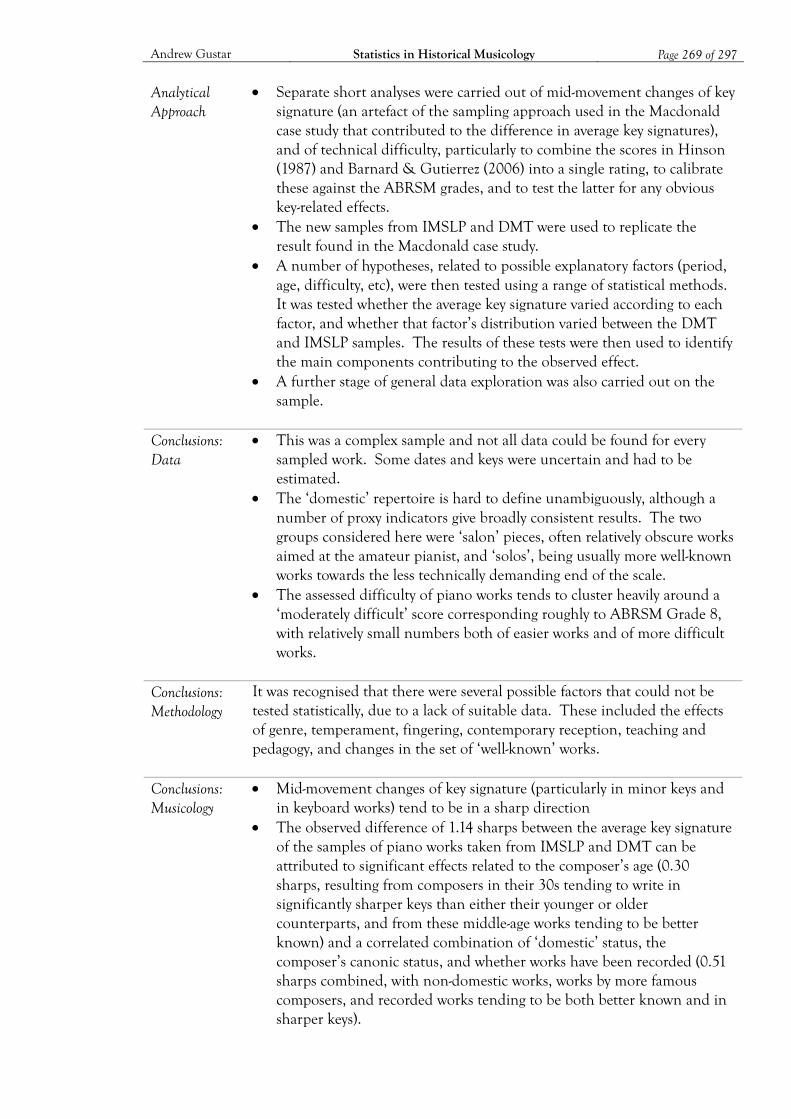
Andrew Gustar Statistics in Historical Musicology Page 269 of 297
Analytical Approach
Separate short analyses were carried out of mid-movement changes of key signature (an artefact of the sampling approach used in the Macdonald case study that contributed to the difference in average key signatures), and of technical difficulty, particularly to combine the scores in Hinson (1987) and Barnard & Gutierrez (2006) into a single rating, to calibrate these against the ABRSM grades, and to test the latter for any obvious key-related effects.
The new samples from IMSLP and DMT were used to replicate the result found in the Macdonald case study.
A number of hypotheses, related to possible explanatory factors (period, age, difficulty, etc), were then tested using a range of statistical methods. It was tested whether the average key signature varied according to each factor, and whether that factor’s distribution varied between the DMT and IMSLP samples. The results of these tests were then used to identify the main components contributing to the observed effect.
A further stage of general data exploration was also carried out on the sample.
Conclusions: Data
This was a complex sample and not all data could be found for every sampled work. Some dates and keys were uncertain and had to be estimated.
The ‘domestic’ repertoire is hard to define unambiguously, although a number of proxy indicators give broadly consistent results. The two groups considered here were ‘salon’ pieces, often relatively obscure works aimed at the amateur pianist, and ‘solos’, being usually more well-known works towards the less technically demanding end of the scale.
The assessed difficulty of piano works tends to cluster heavily around a ‘moderately difficult’ score corresponding roughly to ABRSM Grade 8, with relatively small numbers both of easier works and of more difficult works.
Conclusions: Methodology
It was recognised that there were several possible factors that could not be tested statistically, due to a lack of suitable data. These included the effects of genre, temperament, fingering, contemporary reception, teaching and pedagogy, and changes in the set of ‘well-known’ works.
Conclusions: Musicology
Mid-movement changes of key signature (particularly in minor keys and in keyboard works) tend to be in a sharp direction
The observed difference of 1.14 sharps between the average key signature of the samples of piano works taken from IMSLP and DMT can be attributed to significant effects related to the composer’s age (0.30 sharps, resulting from composers in their 30s tending to write in significantly sharper keys than either their younger or older counterparts, and from these middle-age works tending to be better known) and a correlated combination of ‘domestic’ status, the composer’s canonic status, and whether works have been recorded (0.51 sharps combined, with non-domestic works, works by more famous composers, and recorded works tending to be both better known and in sharper keys).
Andrew Gustar Statistics in Historical Musicology Page 270 of 297
Further data exploration found (amongst other things) that the more canonic works tend to be from earlier periods; that ‘second division’ composers (i.e. top-200 but not top-50) tend to write significantly more difficult piano works than other composers; that Germanic major key works tend to be sharper than minor key works, whereas French major key works tend to be flatter; and that well-known music themes are most likely to come from the less difficult works.
Other Comments
Whilst the analysis successfully separated the effect into its component parts, this raised questions just as mysterious as the original observation!
Andrew Gustar Statistics in Historical Musicology Page 271 of 297
A4. RECORDINGS CASE STUDY
Objective To explore the data relating to recordings, particularly the long-running series of Penguin Record Guides (Greenfield et al 1963–2007)
Cross References
2.2.4 (summary) 3.2.3 (recording based datasets) 4.5.2 (example cross tabulation) 4.6.1 (use of database codes to estimate size of dataset, and problem of
skewed distributions, discrepancy in population estimates, and artificial Penguin Guide)
5.1.1 (regional distribution of composers, and canonic rank) 5.1.5 (composers represented by single famous work) 5.2.1 (distribution of works by genre) 5.3.2 (recordings) 5.4 (Penguin guides)
Sample Sources Penguin Record Guides from 1975, 1988, 1999 and 2007
World’s Encyclopedia of Recorded Music (WERM): Clough & Cuming (1952)
Gramophone CD Catalogue (GramCat): Maycock & McSwiney (1990) AllMusic
Sample Size 200 from the Penguin Guides (50 from each)
50 from each of WERM, GramCat and AllMusic
Sampling Approach
For the Penguin Guides, random page numbers were selected and the first coupling after the start of the page was selected. A work was selected at random for the coupling, and the first mentioned recording of that coupling was identified.
For WERM and GramCat the same procedure was followed, although the random entity was the work, rather than the coupling (due to differences in the organisation of these sources from that of the Penguin Guides)
For AllMusic recordings were selected by generating random database codes. A work from each recording was selected at random.
Triangulation Sources
The Penguin sample was triangulated against the Penguin Guides from 75, 88, 99 and 07, as well as the 1963 ‘Update’ and the 1998 ‘Bargain’ editions of the guide.
The Penguin 88 and 07 samples were also triangulated against their near contemporaries GramCat and AllMusic respectively.
Data Collected Penguin Sample Composer name, years of birth and death, nationality, ‘canonic rank’
(from AllMusic lists) Number of works by that composer mentioned in the guide (estimated
for large entries) Number of pages allocated to this composer (to the nearest 0.1 page)
Andrew Gustar Statistics in Historical Musicology Page 272 of 297
Work name and genre Number of recordings of this work mentioned in the guide Catalogue number and performer of selected recording *Number of composers represented on the disc *Number of works represented on the disc Number of composer entries beginning on the page Number of works mentioned on the page Number of recordings mentioned on the page *Number of pages devoted to this composer in each of the other Penguin
Guides *Whether a recording of this work appears in each of the other guides *Whether this recording appears in each of the other guides *For the 1988 and 2007 samples only, the number of recordings of this
work listed in GramCat 90 or AllMusic respectively
The same data were collected for the WERM and GramCat samples, except those items marked with an asterisk. The AllMusic sample contained the same data as for WERM, except for the number of pages per composer, and the numbers of composers, works and recordings per page (since a ‘page’ is not a meaningful concept in the case of a database such as AllMusic).
Analytical Approach
The analysis consisted of general exploration of the data – estimating populations, examining distributions, considering the breakdown by region, period and genre, analysing rates of survival, and trying to understand the characteristics of the data.
A discrepancy between two calculations of the number of recordings led to further analysis using an artificially constructed Penguin Guide.
Conclusions: Data
Recordings data is very complex due to the large number of different related entities – works, movements, couplings, composers, performers, recordings, physical media, record companies, etc. This makes it difficult to ensure consistency of approach and results in analytical complexity and some calculation bias.
The definition of a work is particularly problematic: any of the sources might, for example, treat (inconsistently) a single aria, a song, a song cycle, or a whole opera as a ‘work’.
It is also very difficult to track the same recording across different formats, reissues, changes of record label, and compilations, or (in some cases) to differentiate between separate recordings of the same work by the same performer. For some classic recordings of major works there are huge numbers (hundreds) of listings in the modern AllMusic catalogue, often extracts, compilation discs, and reissues from different companies or ‘budget’ labels. Tracking recordings is not helped by the fact that the dates of recordings are rarely stated in these datasets.
Although the Penguin Guides are a rare example of a dataset repeated consistently over a period of time, the subjective nature of the content of the guides makes it difficult to draw useful conclusions about recordings in general.
Andrew Gustar Statistics in Historical Musicology Page 273 of 297
Conclusions: Methodology
Different dataset structures meant that they could not all be sampled in a consistent way.
Highly skewed distributions result in rather wide confidence intervals for many of the statistics calculated, leading to few firm conclusions (a substantially larger sample would be required).
Conclusions: Musicology
The distribution of works or recordings per composer, or recordings per work, is (like publications) a highly skewed ‘Zipf-like’ distribution.
The Penguin Guides show a clear bias towards orchestral music and the better known composers.
There has been huge growth in the number of recordings over the last twenty years. As well as multiple recordings and reissues of the most popular works, there has been a substantial increase in the availability of recordings of works by obscure and non-European composers.
Other Comments
Discrepancies in the calculation of the numbers of recordings by different methods were never fully resolved.
Andrew Gustar Statistics in Historical Musicology Page 274 of 297
A5. BIOGRAPHICAL DICTIONARIES CASE STUDY
Objective To explore four significant nineteenth-century biographical dictionaries, and the relationships between them and more recent sources of information on composers.
Cross References
2.2.5 (summary) 4.1.7 (lack of independence between biographical dictionaries) 4.3.3 (entry length as a triangulation indicator) 4.3.5 (effect of different languages on article length) 4.4.2 (handling illegible and missing data) 4.4.3 (shape indicator variables) 4.5.4 (significant absence of correlation) 5.1.1 (geographical distribution of composers) 5.1.3 (triangulation problems with variant names) 5.4 (patterns of survival and recency effect)
Sample Sources Gerber (1812) (the second edition)
Fétis (1835) (the first edition) Mendel (1870) Eitner (1900)
Sample Size 200 (50 from each)
Sampling Approach
50 pages were randomly chosen from each source, and the second composer after the start of each page was selected (to avoid length-biased sampling)
Triangulation Sources
All of the four sample sources were used for triangulation, as were… Gerber (1790) (the first edition) Fétis (1862) (the second edition) Grove (1879) Pazdírek (1904–10) Detheridge (1937) Oxford Music Online AllMusic IMSLP
Data Collected Source data: the biographical dictionary, volume and page number
The name of the entry at the start of the page (usually beginning on a previous page), together with a note of the type of entry (composer, theorist, musical term, etc), and its length in pages.
The total number of entries starting on the page, the number of composers among these entries, and the number of other people.
The name of the second composer mentioned after the start of the page. The total number of entries after the start of the page at which the second composer is mentioned. The length of the entry in pages. Dates and locations of birth, death and activity (where mentioned).
Length of entries for that composer in each of the triangulated sources
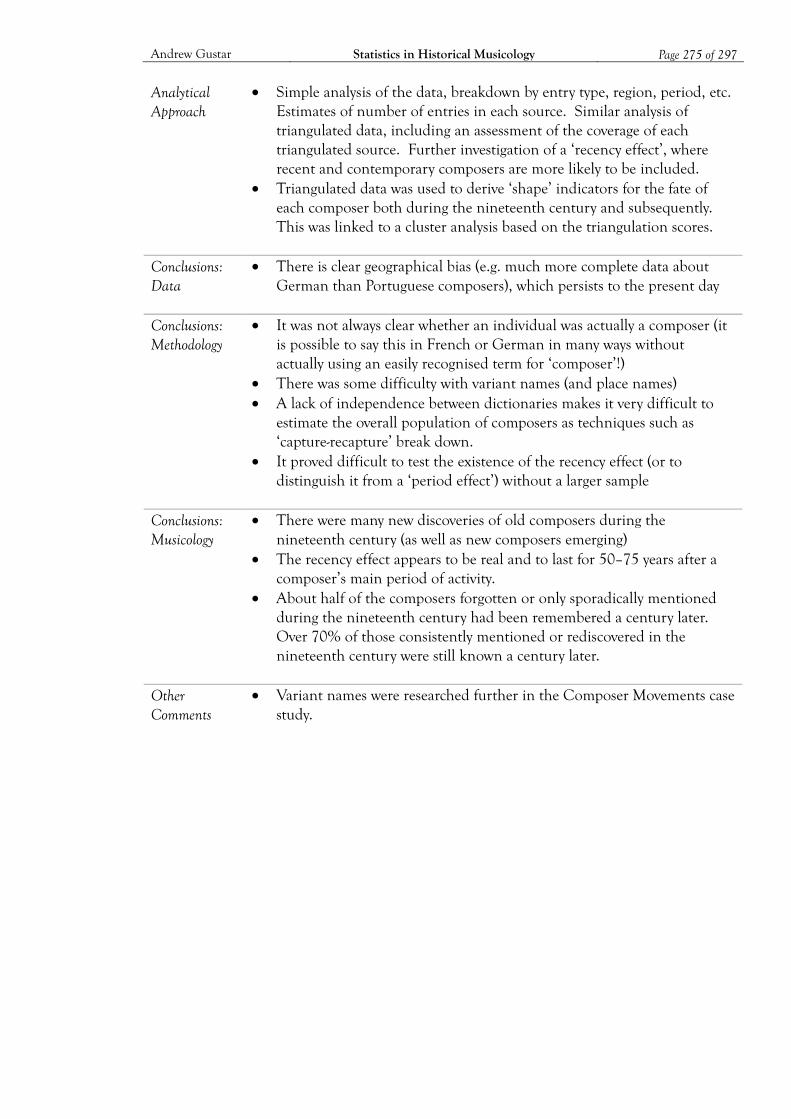
Andrew Gustar Statistics in Historical Musicology Page 275 of 297
Analytical Approach
Simple analysis of the data, breakdown by entry type, region, period, etc. Estimates of number of entries in each source. Similar analysis of triangulated data, including an assessment of the coverage of each triangulated source. Further investigation of a ‘recency effect’, where recent and contemporary composers are more likely to be included.
Triangulated data was used to derive ‘shape’ indicators for the fate of each composer both during the nineteenth century and subsequently. This was linked to a cluster analysis based on the triangulation scores.
Conclusions: Data
There is clear geographical bias (e.g. much more complete data about German than Portuguese composers), which persists to the present day
Conclusions: Methodology
It was not always clear whether an individual was actually a composer (it is possible to say this in French or German in many ways without actually using an easily recognised term for ‘composer’!)
There was some difficulty with variant names (and place names) A lack of independence between dictionaries makes it very difficult to
estimate the overall population of composers as techniques such as ‘capture-recapture’ break down.
It proved difficult to test the existence of the recency effect (or to distinguish it from a ‘period effect’) without a larger sample
Conclusions: Musicology
There were many new discoveries of old composers during the nineteenth century (as well as new composers emerging)
The recency effect appears to be real and to last for 50–75 years after a composer’s main period of activity.
About half of the composers forgotten or only sporadically mentioned during the nineteenth century had been remembered a century later. Over 70% of those consistently mentioned or rediscovered in the nineteenth century were still known a century later.
Other Comments
Variant names were researched further in the Composer Movements case study.
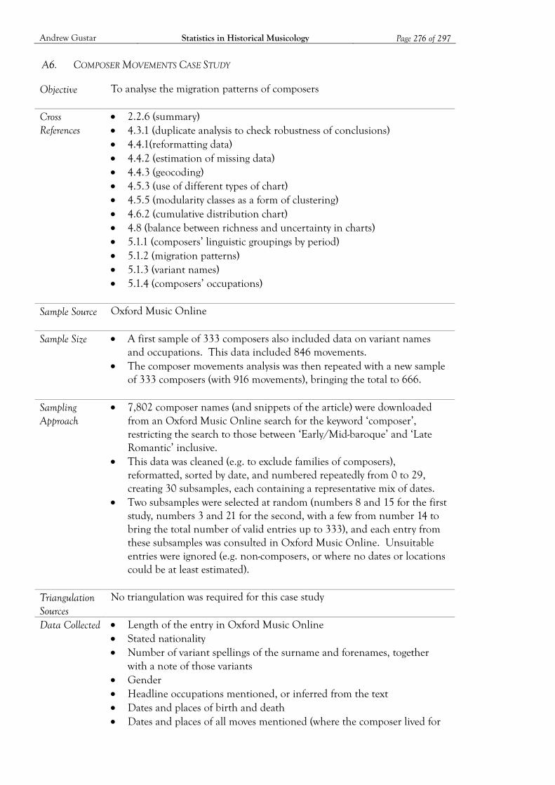
Andrew Gustar Statistics in Historical Musicology Page 276 of 297
A6. COMPOSER MOVEMENTS CASE STUDY
Objective To analyse the migration patterns of composers
Cross References
2.2.6 (summary) 4.3.1 (duplicate analysis to check robustness of conclusions) 4.4.1(reformatting data) 4.4.2 (estimation of missing data) 4.4.3 (geocoding) 4.5.3 (use of different types of chart) 4.5.5 (modularity classes as a form of clustering) 4.6.2 (cumulative distribution chart) 4.8 (balance between richness and uncertainty in charts) 5.1.1 (composers’ linguistic groupings by period) 5.1.2 (migration patterns) 5.1.3 (variant names) 5.1.4 (composers’ occupations)
Sample Source Oxford Music Online
Sample Size A first sample of 333 composers also included data on variant names
and occupations. This data included 846 movements. The composer movements analysis was then repeated with a new sample
of 333 composers (with 916 movements), bringing the total to 666.
Sampling Approach
7,802 composer names (and snippets of the article) were downloaded from an Oxford Music Online search for the keyword ‘composer’, restricting the search to those between ‘Early/Mid-baroque’ and ‘Late Romantic’ inclusive.
This data was cleaned (e.g. to exclude families of composers), reformatted, sorted by date, and numbered repeatedly from 0 to 29, creating 30 subsamples, each containing a representative mix of dates.
Two subsamples were selected at random (numbers 8 and 15 for the first study, numbers 3 and 21 for the second, with a few from number 14 to bring the total number of valid entries up to 333), and each entry from these subsamples was consulted in Oxford Music Online. Unsuitable entries were ignored (e.g. non-composers, or where no dates or locations could be at least estimated).
Triangulation Sources
No triangulation was required for this case study
Data Collected Length of the entry in Oxford Music Online Stated nationality Number of variant spellings of the surname and forenames, together
with a note of those variants Gender Headline occupations mentioned, or inferred from the text Dates and places of birth and death Dates and places of all moves mentioned (where the composer lived for
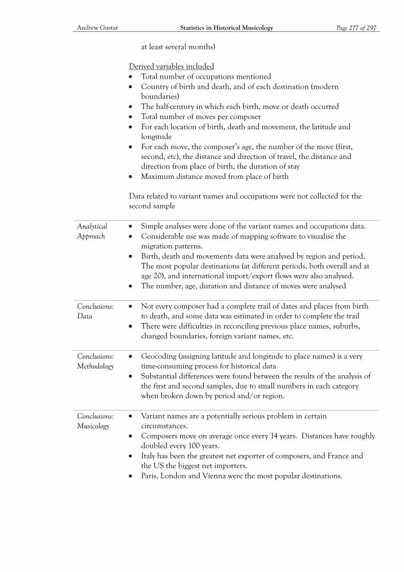
Andrew Gustar Statistics in Historical Musicology Page 277 of 297
at least several months) Derived variables included Total number of occupations mentioned Country of birth and death, and of each destination (modern
boundaries) The half-century in which each birth, move or death occurred Total number of moves per composer For each location of birth, death and movement, the latitude and
longitude For each move, the composer’s age, the number of the move (first,
second, etc), the distance and direction of travel, the distance and direction from place of birth, the duration of stay
Maximum distance moved from place of birth
Data related to variant names and occupations were not collected for the second sample
Analytical Approach
Simple analyses were done of the variant names and occupations data. Considerable use was made of mapping software to visualise the
migration patterns. Birth, death and movements data were analysed by region and period.
The most popular destinations (at different periods, both overall and at age 20), and international import/export flows were also analysed.
The number, age, duration and distance of moves were analysed
Conclusions: Data
Not every composer had a complete trail of dates and places from birth to death, and some data was estimated in order to complete the trail
There were difficulties in reconciling previous place names, suburbs, changed boundaries, foreign variant names, etc.
Conclusions: Methodology
Geocoding (assigning latitude and longitude to place names) is a very time-consuming process for historical data
Substantial differences were found between the results of the analysis of the first and second samples, due to small numbers in each category when broken down by period and/or region.
Conclusions: Musicology
Variant names are a potentially serious problem in certain circumstances.
Composers move on average once every 14 years. Distances have roughly doubled every 100 years.
Italy has been the greatest net exporter of composers, and France and the US the biggest net importers.
Paris, London and Vienna were the most popular destinations.
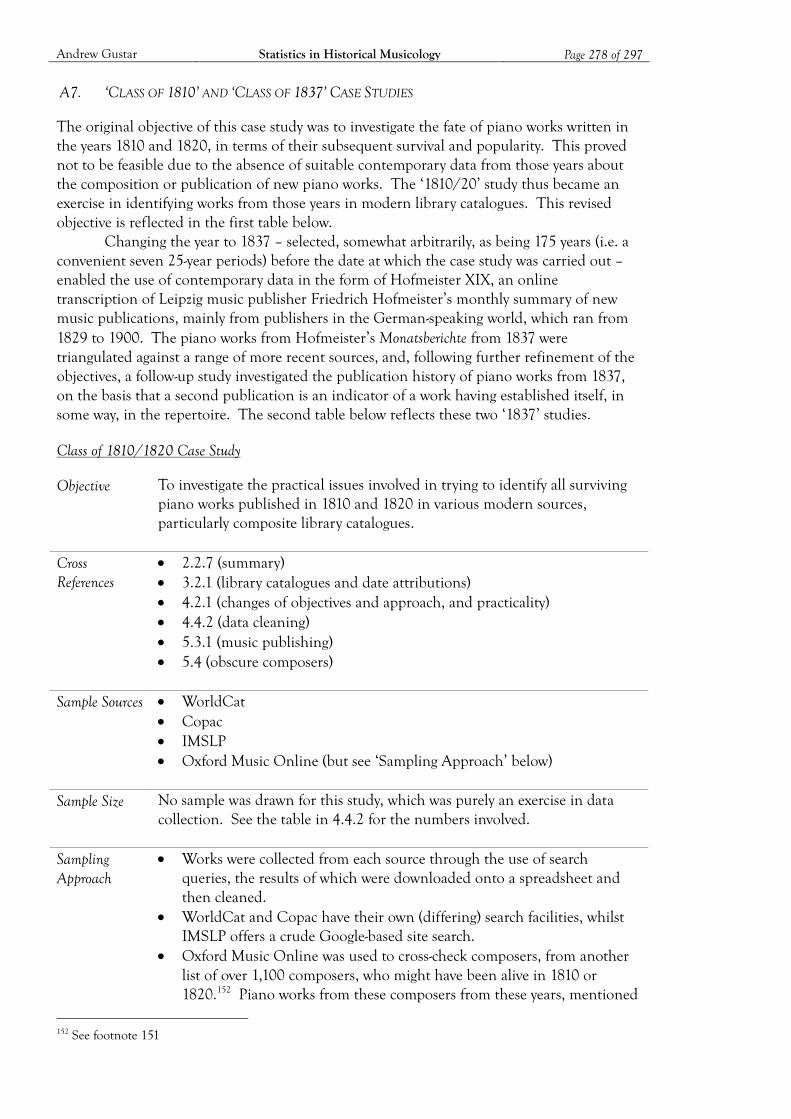
Andrew Gustar Statistics in Historical Musicology Page 278 of 297
A7. ‘CLASS OF 1810’ AND ‘CLASS OF 1837’ CASE STUDIES
The original objective of this case study was to investigate the fate of piano works written in the years 1810 and 1820, in terms of their subsequent survival and popularity. This proved not to be feasible due to the absence of suitable contemporary data from those years about the composition or publication of new piano works. The ‘1810/20’ study thus became an exercise in identifying works from those years in modern library catalogues. This revised objective is reflected in the first table below.
Changing the year to 1837 – selected, somewhat arbitrarily, as being 175 years (i.e. a convenient seven 25-year periods) before the date at which the case study was carried out – enabled the use of contemporary data in the form of Hofmeister XIX, an online transcription of Leipzig music publisher Friedrich Hofmeister’s monthly summary of new music publications, mainly from publishers in the German-speaking world, which ran from 1829 to 1900. The piano works from Hofmeister’s Monatsberichte from 1837 were triangulated against a range of more recent sources, and, following further refinement of the objectives, a follow-up study investigated the publication history of piano works from 1837, on the basis that a second publication is an indicator of a work having established itself, in some way, in the repertoire. The second table below reflects these two ‘1837’ studies.
Class of 1810/1820 Case Study
Objective To investigate the practical issues involved in trying to identify all surviving piano works published in 1810 and 1820 in various modern sources, particularly composite library catalogues.
Cross References
2.2.7 (summary) 3.2.1 (library catalogues and date attributions) 4.2.1 (changes of objectives and approach, and practicality) 4.4.2 (data cleaning) 5.3.1 (music publishing) 5.4 (obscure composers)
Sample Sources WorldCat
Copac IMSLP Oxford Music Online (but see ‘Sampling Approach’ below)
Sample Size No sample was drawn for this study, which was purely an exercise in data
collection. See the table in 4.4.2 for the numbers involved.
Sampling Approach
Works were collected from each source through the use of search queries, the results of which were downloaded onto a spreadsheet and then cleaned.
WorldCat and Copac have their own (differing) search facilities, whilst IMSLP offers a crude Google-based site search.
Oxford Music Online was used to cross-check composers, from another list of over 1,100 composers, who might have been alive in 1810 or 1820.152 Piano works from these composers from these years, mentioned
152 See footnote 151
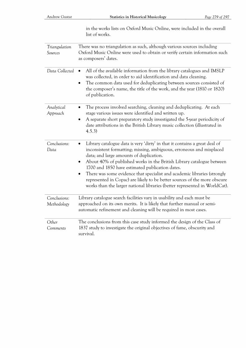
Andrew Gustar Statistics in Historical Musicology Page 279 of 297
in the works lists on Oxford Music Online, were included in the overall list of works.
Triangulation Sources
There was no triangulation as such, although various sources including Oxford Music Online were used to obtain or verify certain information such as composers’ dates.
Data Collected All of the available information from the library catalogues and IMSLP was collected, in order to aid identification and data cleaning.
The common data used for deduplicating between sources consisted of the composer’s name, the title of the work, and the year (1810 or 1820) of publication.
Analytical Approach
The process involved searching, cleaning and deduplicating. At each stage various issues were identified and written up.
A separate short preparatory study investigated the 5-year periodicity of date attributions in the British Library music collection (illustrated in 4.5.3)
Conclusions: Data
Library catalogue data is very ‘dirty’ in that it contains a great deal of inconsistent formatting; missing, ambiguous, erroneous and misplaced data; and large amounts of duplication.
About 40% of published works in the British Library catalogue between 1700 and 1850 have estimated publication dates.
There was some evidence that specialist and academic libraries (strongly represented in Copac) are likely to be better sources of the more obscure works than the larger national libraries (better represented in WorldCat).
Conclusions: Methodology
Library catalogue search facilities vary in usability and each must be approached on its own merits. It is likely that further manual or semi-automatic refinement and cleaning will be required in most cases.
Other Comments
The conclusions from this case study informed the design of the Class of 1837 study to investigate the original objectives of fame, obscurity and survival.
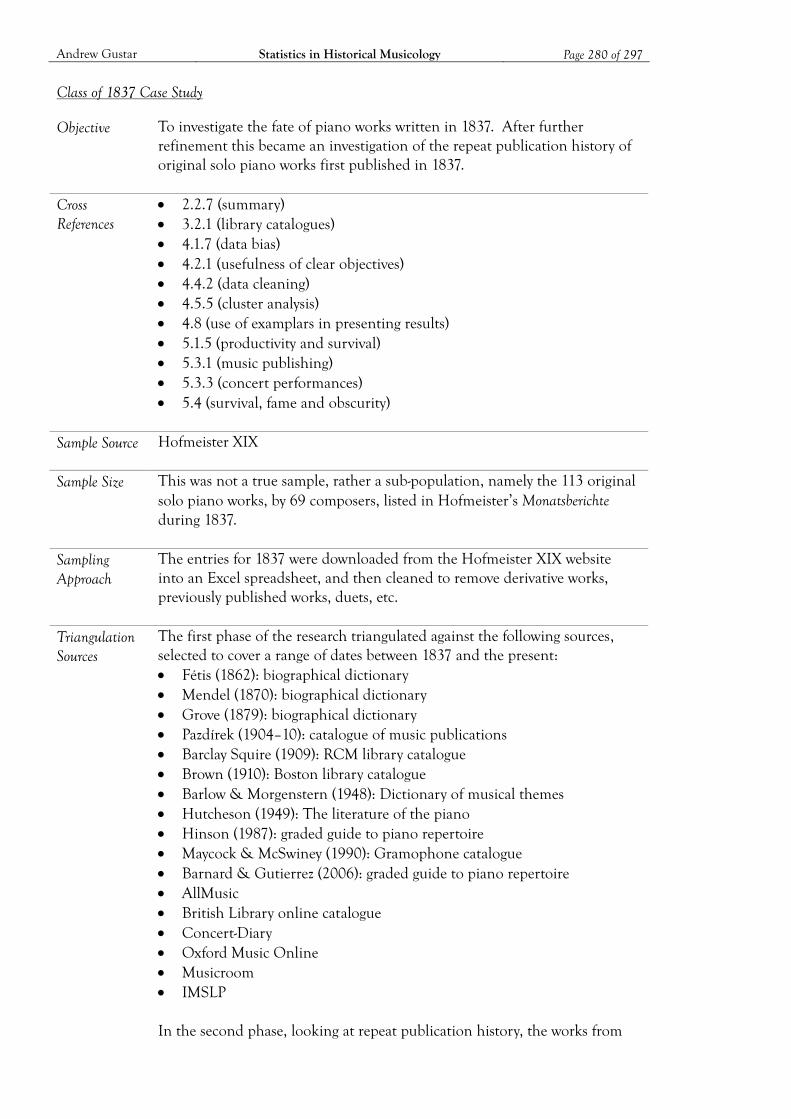
Andrew Gustar Statistics in Historical Musicology Page 280 of 297
Class of 1837 Case Study
Objective To investigate the fate of piano works written in 1837. After further refinement this became an investigation of the repeat publication history of original solo piano works first published in 1837.
Cross References
2.2.7 (summary) 3.2.1 (library catalogues) 4.1.7 (data bias) 4.2.1 (usefulness of clear objectives) 4.4.2 (data cleaning) 4.5.5 (cluster analysis) 4.8 (use of examplars in presenting results) 5.1.5 (productivity and survival) 5.3.1 (music publishing) 5.3.3 (concert performances) 5.4 (survival, fame and obscurity)
Sample Source Hofmeister XIX
Sample Size This was not a true sample, rather a sub-population, namely the 113 original
solo piano works, by 69 composers, listed in Hofmeister’s Monatsberichte during 1837.
Sampling Approach
The entries for 1837 were downloaded from the Hofmeister XIX website into an Excel spreadsheet, and then cleaned to remove derivative works, previously published works, duets, etc.
Triangulation Sources
The first phase of the research triangulated against the following sources, selected to cover a range of dates between 1837 and the present: Fétis (1862): biographical dictionary Mendel (1870): biographical dictionary Grove (1879): biographical dictionary Pazdírek (1904–10): catalogue of music publications Barclay Squire (1909): RCM library catalogue Brown (1910): Boston library catalogue Barlow & Morgenstern (1948): Dictionary of musical themes Hutcheson (1949): The literature of the piano Hinson (1987): graded guide to piano repertoire Maycock & McSwiney (1990): Gramophone catalogue Barnard & Gutierrez (2006): graded guide to piano repertoire AllMusic British Library online catalogue Concert-Diary Oxford Music Online Musicroom IMSLP In the second phase, looking at repeat publication history, the works from
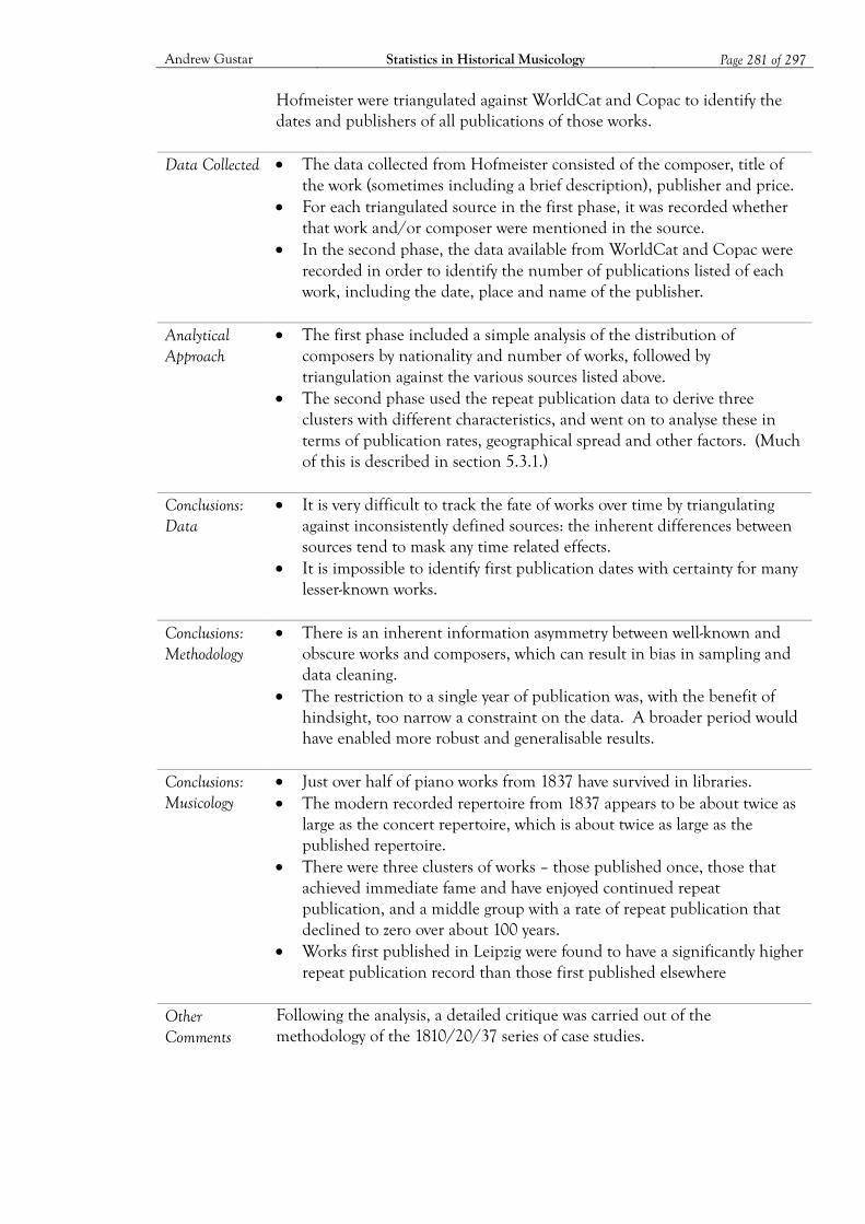
Andrew Gustar Statistics in Historical Musicology Page 281 of 297
Hofmeister were triangulated against WorldCat and Copac to identify the dates and publishers of all publications of those works.
Data Collected The data collected from Hofmeister consisted of the composer, title of the work (sometimes including a brief description), publisher and price.
For each triangulated source in the first phase, it was recorded whether that work and/or composer were mentioned in the source.
In the second phase, the data available from WorldCat and Copac were recorded in order to identify the number of publications listed of each work, including the date, place and name of the publisher.
Analytical Approach
The first phase included a simple analysis of the distribution of composers by nationality and number of works, followed by triangulation against the various sources listed above.
The second phase used the repeat publication data to derive three clusters with different characteristics, and went on to analyse these in terms of publication rates, geographical spread and other factors. (Much of this is described in section 5.3.1.)
Conclusions: Data
It is very difficult to track the fate of works over time by triangulating against inconsistently defined sources: the inherent differences between sources tend to mask any time related effects.
It is impossible to identify first publication dates with certainty for many lesser-known works.
Conclusions: Methodology
There is an inherent information asymmetry between well-known and obscure works and composers, which can result in bias in sampling and data cleaning.
The restriction to a single year of publication was, with the benefit of hindsight, too narrow a constraint on the data. A broader period would have enabled more robust and generalisable results.
Conclusions: Musicology
Just over half of piano works from 1837 have survived in libraries. The modern recorded repertoire from 1837 appears to be about twice as
large as the concert repertoire, which is about twice as large as the published repertoire.
There were three clusters of works – those published once, those that achieved immediate fame and have enjoyed continued repeat publication, and a middle group with a rate of repeat publication that declined to zero over about 100 years.
Works first published in Leipzig were found to have a significantly higher repeat publication record than those first published elsewhere
Other Comments
Following the analysis, a detailed critique was carried out of the methodology of the 1810/20/37 series of case studies.
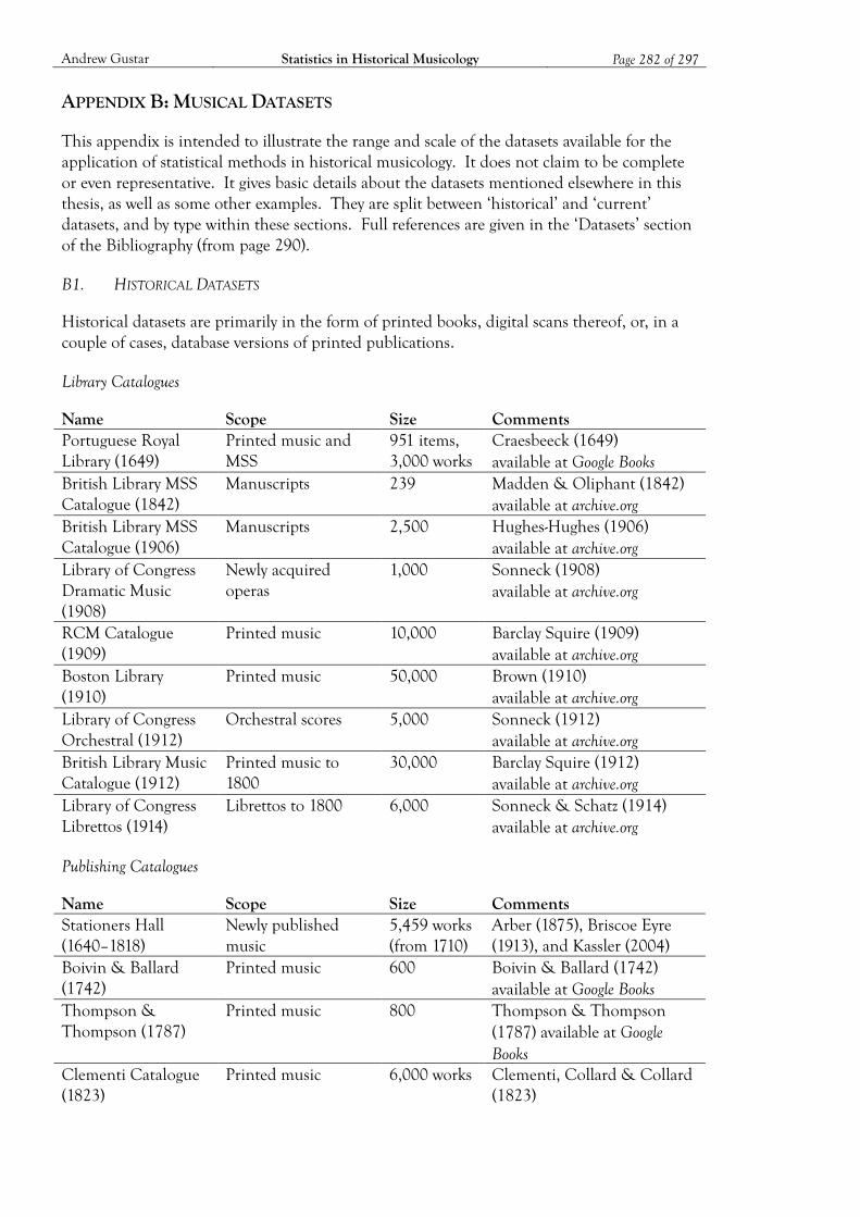
Andrew Gustar Statistics in Historical Musicology Page 282 of 297
APPENDIX B: MUSICAL DATASETS
This appendix is intended to illustrate the range and scale of the datasets available for the application of statistical methods in historical musicology. It does not claim to be complete or even representative. It gives basic details about the datasets mentioned elsewhere in this thesis, as well as some other examples. They are split between ‘historical’ and ‘current’ datasets, and by type within these sections. Full references are given in the ‘Datasets’ section of the Bibliography (from page 290).
B1. HISTORICAL DATASETS
Historical datasets are primarily in the form of printed books, digital scans thereof, or, in a couple of cases, database versions of printed publications.
Library Catalogues
Name Scope Size Comments Portuguese Royal Library (1649)
Printed music and MSS
951 items, 3,000 works
Craesbeeck (1649) available at Google Books
British Library MSS Catalogue (1842)
Manuscripts 239 Madden & Oliphant (1842) available at archive.org
British Library MSS Catalogue (1906)
Manuscripts 2,500 Hughes-Hughes (1906) available at archive.org
Library of Congress Dramatic Music (1908)
Newly acquired operas
1,000 Sonneck (1908) available at archive.org
RCM Catalogue (1909)
Printed music 10,000 Barclay Squire (1909) available at archive.org
Boston Library (1910)
Printed music 50,000 Brown (1910) available at archive.org
Library of Congress Orchestral (1912)
Orchestral scores 5,000 Sonneck (1912) available at archive.org
British Library Music Catalogue (1912)
Printed music to 1800
30,000 Barclay Squire (1912) available at archive.org
Library of Congress Librettos (1914)
Librettos to 1800 6,000 Sonneck & Schatz (1914) available at archive.org
Publishing Catalogues
Name Scope Size Comments Stationers Hall (1640–1818)
Newly published music
5,459 works (from 1710)
Arber (1875), Briscoe Eyre (1913), and Kassler (2004)
Boivin & Ballard (1742)
Printed music 600 Boivin & Ballard (1742) available at Google Books
Thompson & Thompson (1787)
Printed music 800 Thompson & Thompson (1787) available at Google Books
Clementi Catalogue (1823)
Printed music 6,000 works Clementi, Collard & Collard (1823)
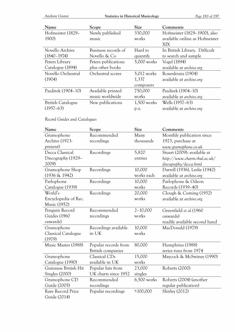
Andrew Gustar Statistics in Historical Musicology Page 283 of 297
Name Scope Size Comments Hofmeister (1829–1900)
Newly published music
330,000 works
Hofmeister (1829–1900), also available online as Hofmeister XIX
Novello Archive (1840–1974)
Business records of Novello & Co
Hard to quantify
In British Library. Difficult to search and sample
Peters Library Catalogue (1894)
Peters publications plus other books
5,000 works Vogel (1894) available at archive.org
Novello Orchestral (1904)
Orchestral scores 5,012 works 1,337 composers
Rosenkranz (1904) available at archive.org
Pazdírek (1904–10) Available printed music worldwide
750,000 works
Pazdírek (1904–10) available at archive.org
British Catalogue (1957–63)
New publications 1,500 works p.a.
Wells (1957–63) available at archive.org
Record Guides and Catalogues
Name Scope Size Comments Gramophone Archive (1923-present)
Recommended recordings
Many thousands
Monthly publication since 1923, purchase at www.gramophone.co.uk
Decca Classical Discography (1929–2009)
Recordings 5,820 entries
Stuart (2009): available at http://www.charm.rhul.ac.uk/ discography/decca.html
Gramophone Shop (1936 & 1942)
Recordings 10,000 works each
Darrell (1936), Leslie (1942) available at archive.org
Parlophone Catalogue (1939)
Recordings 10,000 works
Parlophone & Odeon Records (1939–40)
World’s Encyclopedia of Rec. Music (1952)
Recordings 20,000 works
Clough & Cuming (1952) available at archive.org
Penguin Record Guides (1960 onwards)
Recommended recordings
2–10,000 works
Greenfield et al (1960 onwards) readily available second hand
Gramophone Classical Catalogue (1979)
Recordings available in UK
10,000 works
MacDonald (1979)
Music Master (1988) Popular records from British companies
80,000 Humphries (1988) series runs from 1974
Gramophone Catalogue (1990)
Classical CDs available in UK
15,000 works
Maycock & McSwiney (1990)
Guinness British Hit Singles (2000)
Popular hits from UK charts since 1952
23,000 singles
Roberts (2000)
Gramophone CD Guide (2005)
Recommended recordings
6,500 works Roberts (2004) (another regular publication)
Rare Record Price Guide (2014)
Popular recordings >100,000 Shirley (2012)
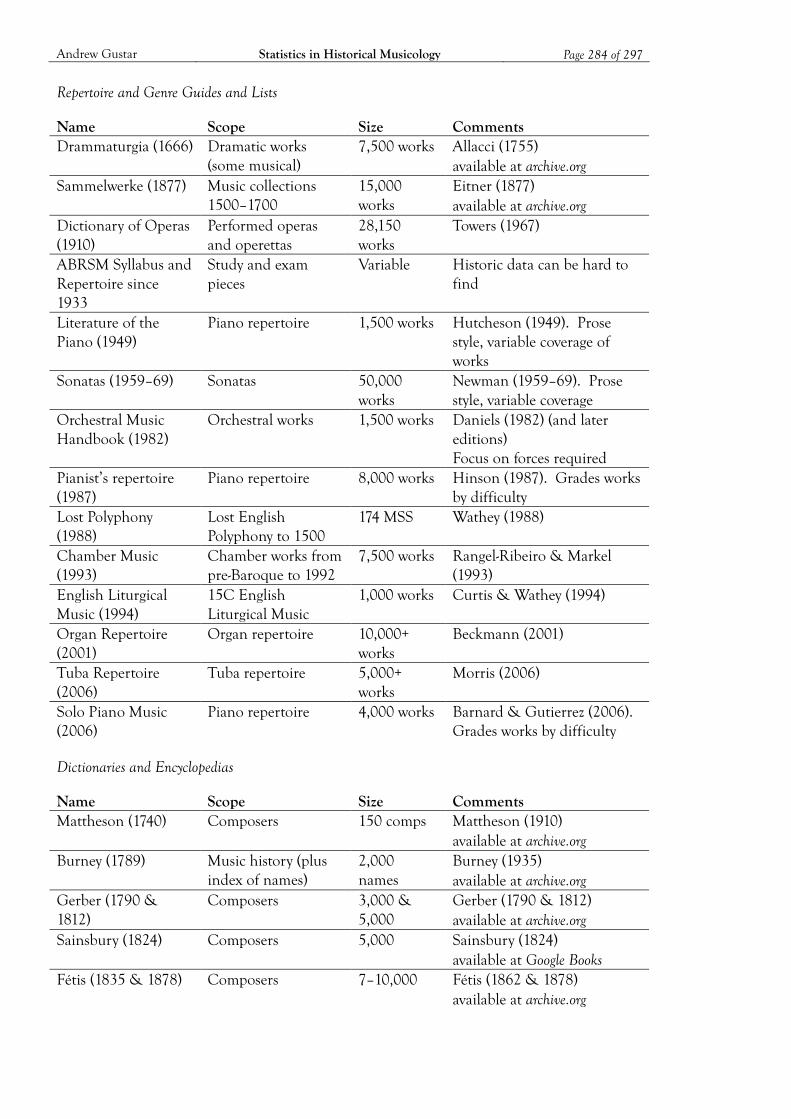
Andrew Gustar Statistics in Historical Musicology Page 284 of 297
Repertoire and Genre Guides and Lists
Name Scope Size Comments Drammaturgia (1666) Dramatic works
(some musical) 7,500 works Allacci (1755)
available at archive.org Sammelwerke (1877) Music collections
1500–1700 15,000 works
Eitner (1877) available at archive.org
Dictionary of Operas (1910)
Performed operas and operettas
28,150 works
Towers (1967)
ABRSM Syllabus and Repertoire since 1933
Study and exam pieces
Variable Historic data can be hard to find
Literature of the Piano (1949)
Piano repertoire 1,500 works Hutcheson (1949). Prose style, variable coverage of works
Sonatas (1959–69) Sonatas 50,000 works
Newman (1959–69). Prose style, variable coverage
Orchestral Music Handbook (1982)
Orchestral works 1,500 works Daniels (1982) (and later editions) Focus on forces required
Pianist’s repertoire (1987)
Piano repertoire 8,000 works Hinson (1987). Grades works by difficulty
Lost Polyphony (1988)
Lost English Polyphony to 1500
174 MSS Wathey (1988)
Chamber Music (1993)
Chamber works from pre-Baroque to 1992
7,500 works Rangel-Ribeiro & Markel (1993)
English Liturgical Music (1994)
15C English Liturgical Music
1,000 works Curtis & Wathey (1994)
Organ Repertoire (2001)
Organ repertoire 10,000+ works
Beckmann (2001)
Tuba Repertoire (2006)
Tuba repertoire 5,000+ works
Morris (2006)
Solo Piano Music (2006)
Piano repertoire 4,000 works Barnard & Gutierrez (2006). Grades works by difficulty
Dictionaries and Encyclopedias
Name Scope Size Comments Mattheson (1740) Composers 150 comps Mattheson (1910)
available at archive.org Burney (1789) Music history (plus
index of names) 2,000 names
Burney (1935) available at archive.org
Gerber (1790 & 1812)
Composers 3,000 & 5,000
Gerber (1790 & 1812) available at archive.org
Sainsbury (1824) Composers 5,000 Sainsbury (1824) available at Google Books
Fétis (1835 & 1878) Composers 7–10,000 Fétis (1862 & 1878) available at archive.org
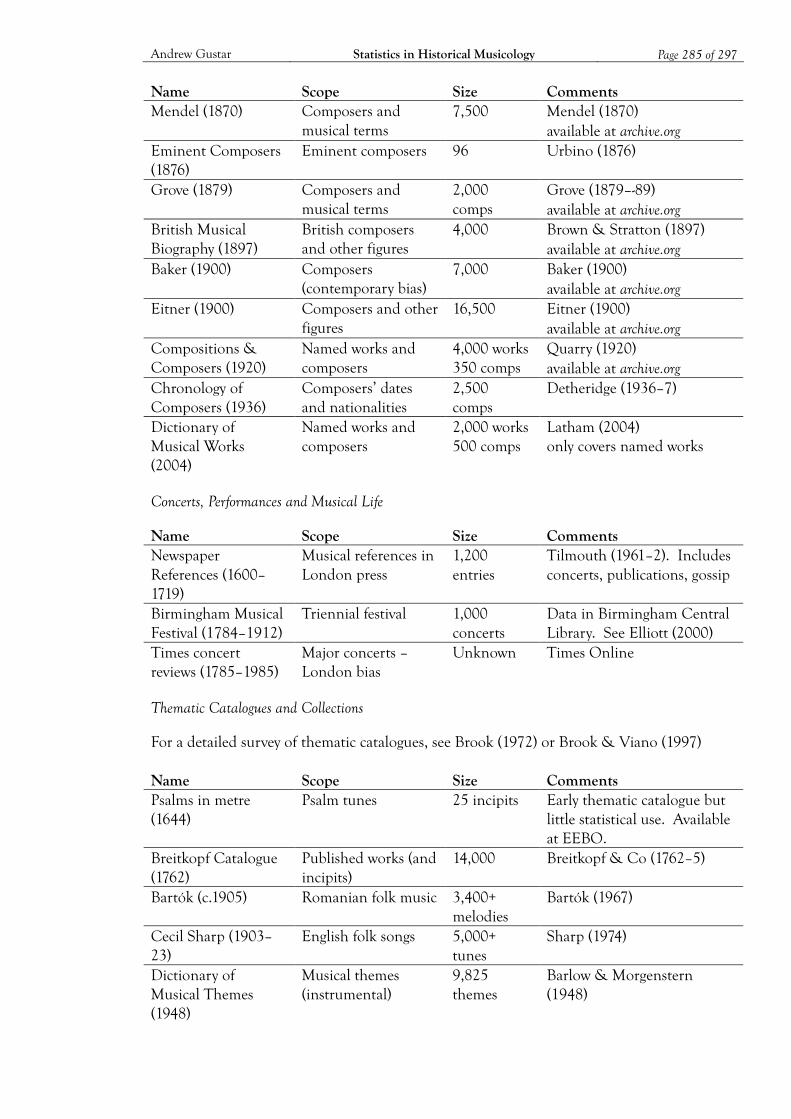
Andrew Gustar Statistics in Historical Musicology Page 285 of 297
Name Scope Size Comments Mendel (1870) Composers and
musical terms 7,500 Mendel (1870)
available at archive.org Eminent Composers (1876)
Eminent composers 96 Urbino (1876)
Grove (1879) Composers and musical terms
2,000 comps
Grove (1879–-89) available at archive.org
British Musical Biography (1897)
British composers and other figures
4,000 Brown & Stratton (1897) available at archive.org
Baker (1900) Composers (contemporary bias)
7,000 Baker (1900) available at archive.org
Eitner (1900) Composers and other figures
16,500 Eitner (1900) available at archive.org
Compositions & Composers (1920)
Named works and composers
4,000 works 350 comps
Quarry (1920) available at archive.org
Chronology of Composers (1936)
Composers’ dates and nationalities
2,500 comps
Detheridge (1936–7)
Dictionary of Musical Works (2004)
Named works and composers
2,000 works 500 comps
Latham (2004) only covers named works
Concerts, Performances and Musical Life
Name Scope Size Comments Newspaper References (1600–1719)
Musical references in London press
1,200 entries
Tilmouth (1961–2). Includes concerts, publications, gossip
Birmingham Musical Festival (1784–1912)
Triennial festival 1,000 concerts
Data in Birmingham Central Library. See Elliott (2000)
Times concert reviews (1785–1985)
Major concerts – London bias
Unknown Times Online
Thematic Catalogues and Collections
For a detailed survey of thematic catalogues, see Brook (1972) or Brook & Viano (1997)
Name Scope Size Comments Psalms in metre (1644)
Psalm tunes 25 incipits Early thematic catalogue but little statistical use. Available at EEBO.
Breitkopf Catalogue (1762)
Published works (and incipits)
14,000 Breitkopf & Co (1762–5)
Bartók (c.1905) Romanian folk music 3,400+ melodies
Bartók (1967)
Cecil Sharp (1903–23)
English folk songs 5,000+ tunes
Sharp (1974)
Dictionary of Musical Themes (1948)
Musical themes (instrumental)
9,825 themes
Barlow & Morgenstern (1948)
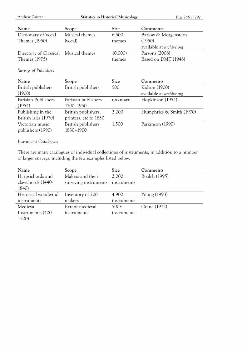
Andrew Gustar Statistics in Historical Musicology Page 286 of 297
Name Scope Size Comments Dictionary of Vocal Themes (1950)
Musical themes (vocal)
6,500 themes
Barlow & Morgenstern (1950) available at archive.org
Directory of Classical Themes (1975)
Musical themes 10,000+ themes
Parsons (2008) Based on DMT (1948)
Surveys of Publishers
Name Scope Size Comments British publishers (1900)
British publishers 500 Kidson (1900) available at archive.org
Parisian Publishers (1954)
Parisian publishers 1700–1950
unknown Hopkinson (1954)
Publishing in the British Isles (1970)
British publishers, printers, etc to 1850
2,200 Humphries & Smith (1970)
Victorian music publishers (1990)
British publishers 1830–1900
1,500 Parkinson (1990)
Instrument Catalogues
There are many catalogues of individual collections of instruments, in addition to a number of larger surveys, including the few examples listed below.
Name Scope Size Comments Harpsichords and clavichords (1440-1840)
Makers and their surviving instruments
2,000 instruments
Boalch (1995)
Historical woodwind instruments
Inventory of 200 makers
4,900 instruments
Young (1993)
Medieval Instruments (400-1500)
Extant medieval instruments
500+ instruments
Crane (1972)
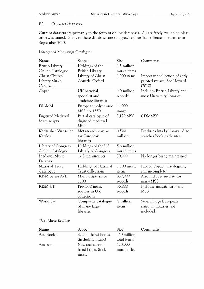
Andrew Gustar Statistics in Historical Musicology Page 287 of 297
B2. CURRENT DATASETS
Current datasets are primarily in the form of online databases. All are freely available unless otherwise stated. Many of these databases are still growing: the size estimates here are as at September 2013.
Library and Manuscript Catalogues
Name Scope Size Comments British Library Online Catalogue
Holdings of the British Library
1.5 million music items
Christ Church Library Music Catalogue
Library of Christ Church, Oxford
1,000 items Important collection of early printed music. See Howard (2010)
Copac UK national, specialist and academic libraries
‘40 million records’
Includes British Library and most University libraries
DIAMM European polyphonic MSS pre-1550
14,000 images
Digitized Medieval Manuscripts
Partial catalogue of digitized medieval MSS
3,129 MSS CDMMSS
Karlsruher Virtueller Katalog
Meta-search engine for European libraries
‘>500 million’
Produces lists by library. Also searches book trade sites
Library of Congress Online Catalogue
Holdings of the US Library of Congress
5.6 million music items
Medieval Music Database
14C manuscripts 70,000 No longer being maintained
National Trust Catalogue
Holdings of National Trust collections
1,300 music items
Part of Copac. Cataloguing still incomplete
RISM Series A/II Manuscripts since 1600
850,000 records
Also includes incipits for many MSS
RISM UK Pre-1850 music sources in UK collections
56,000 records
Includes incipits for many MSS
WorldCat Composite catalogue of many large libraries
‘2 billion items’
Several large European national libraries not included
Sheet Music Retailers
Name Scope Size Comments Abe Books Second hand books
(including music) 140 million total items
Amazon New and second hand books (incl. music)
190,000 music titles
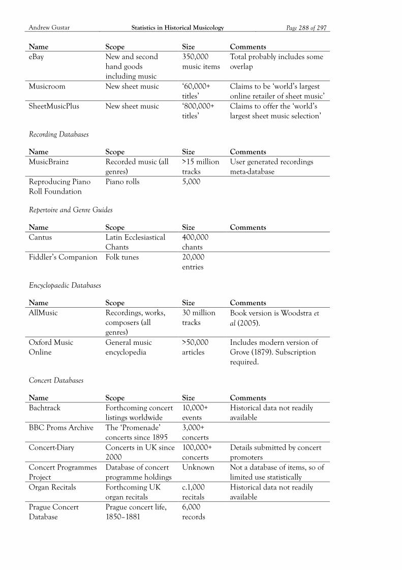
Andrew Gustar Statistics in Historical Musicology Page 288 of 297
Name Scope Size Comments eBay New and second
hand goods including music
350,000 music items
Total probably includes some overlap
Musicroom New sheet music ‘60,000+ titles’
Claims to be ‘world’s largest online retailer of sheet music’
SheetMusicPlus New sheet music ‘800,000+ titles’
Claims to offer the ‘world’s largest sheet music selection’
Recording Databases
Name Scope Size Comments MusicBrainz Recorded music (all
genres) >15 million tracks
User generated recordings meta-database
Reproducing Piano Roll Foundation
Piano rolls 5,000
Repertoire and Genre Guides
Name Scope Size Comments Cantus Latin Ecclesiastical
Chants 400,000 chants
Fiddler’s Companion Folk tunes 20,000 entries
Encyclopaedic Databases
Name Scope Size Comments AllMusic Recordings, works,
composers (all genres)
30 million tracks
Book version is Woodstra et al (2005).
Oxford Music Online
General music encyclopedia
>50,000 articles
Includes modern version of Grove (1879). Subscription required.
Concert Databases
Name Scope Size Comments Bachtrack Forthcoming concert
listings worldwide 10,000+ events
Historical data not readily available
BBC Proms Archive The ‘Promenade’ concerts since 1895
3,000+ concerts
Concert-Diary Concerts in UK since 2000
100,000+ concerts
Details submitted by concert promoters
Concert Programmes Project
Database of concert programme holdings
Unknown Not a database of items, so of limited use statistically
Organ Recitals Forthcoming UK organ recitals
c.1,000 recitals
Historical data not readily available
Prague Concert Database
Prague concert life, 1850–1881
6,000 records
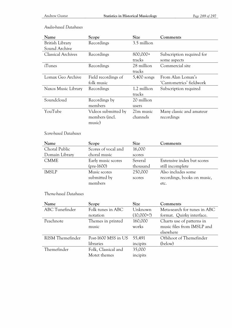
Andrew Gustar Statistics in Historical Musicology Page 289 of 297
Audio-based Databases
Name Scope Size Comments British Library Sound Archive
Recordings 3.5 million
Classical Archives Recordings 800,000+ tracks
Subscription required for some aspects
iTunes Recordings 28 million tracks
Commercial site
Lomax Geo Archive Field recordings of folk music
5,400 songs From Alan Lomax’s ‘Cantometrics’ fieldwork
Naxos Music Library Recordings 1.2 million tracks
Subscription required
Soundcloud Recordings by members
20 million users
YouTube Videos submitted by members (incl. music)
21m music channels
Many classic and amateur recordings
Score-based Databases
Name Scope Size Comments Choral Public Domain Library
Scores of vocal and choral music
16,000 scores
CMME Early music scores (pre-1600)
Several thousand
Extensive index but scores still incomplete
IMSLP Music scores submitted by members
250,000 scores
Also includes some recordings, books on music, etc.
Theme-based Databases
Name Scope Size Comments ABC Tunefinder Folk tunes in ABC
notation Unknown (10,000+?)
Meta-search for tunes in ABC format. Quirky interface.
Peachnote Themes in printed music
160,000 works
Charts use of patterns in music files from IMSLP and elsewhere
RISM Themefinder Post-1600 MSS in US libraries
55,491 incipits
Offshoot of Themefinder (below)
Themefinder Folk, Classical and Motet themes
35,000 incipits
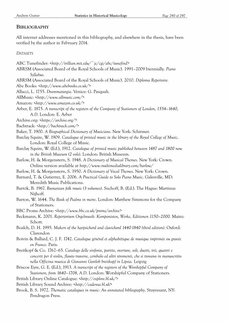
Andrew Gustar Statistics in Historical Musicology Page 290 of 297
BIBLIOGRAPHY
All internet addresses mentioned in this bibliography, and elsewhere in the thesis, have been verified by the author in February 2014.
DATASETS
ABC Tunefinder: <http://trillian.mit.edu/~jc/cgi/abc/tunefind> ABRSM (Associated Board of the Royal Schools of Music). 1991–2009 biennially. Piano
Syllabus. ABRSM (Associated Board of the Royal Schools of Music). 2010. Diploma Repertoire. Abe Books: <http://www.abebooks.co.uk/> Allacci, L. 1755. Drammaturgia. Venice: G. Pasquali. AllMusic: <http://www.allmusic.com/> Amazon: <http://www.amazon.co.uk/> Arber, E. 1875. A transcript of the registers of the Company of Stationers of London, 1554–1640,
A.D. London: E. Arber Archive.org: <https://archive.org/> Bachtrack: <http://bachtrack.com/> Baker, T. 1900. A Biographical Dictionary of Musicians. New York: Schirmer. Barclay Squire, W. 1909. Catalogue of printed music in the library of the Royal College of Music.
London: Royal College of Music. Barclay Squire, W. (Ed.), 1912. Catalogue of printed music published between 1487 and 1800 now
in the British Museum (2 vols). London: British Museum. Barlow, H. & Morgenstern, S. 1948. A Dictionary of Musical Themes. New York: Crown.
Online version available at http://www.multimedialibrary.com/barlow/ Barlow, H. & Morgenstern, S. 1950. A Dictionary of Vocal Themes. New York: Crown. Barnard, T. & Gutierrez, E. 2006. A Practical Guide to Solo Piano Music. Galesville, MD:
Meredith Music Publications. Bartók, B. 1967. Rumanian folk music (3 volumes). Suchoff, B. (Ed.). The Hague: Martinus
Nijhoff. Barton, W. 1644. The Book of Psalms in metre. London: Matthew Simmons for the Company
of Stationers. BBC Proms Archive: <http://www.bbc.co.uk/proms/archive> Beckmann, K. 2001. Repertorium Orgelmusik: Komponisten, Werke, Editionen 1150–2000. Mainz:
Schott. Boalch, D. H. 1995. Makers of the harpsichord and clavichord 1440-1840 (third edition). Oxford:
Clarendon Boivin & Ballard, C. J. F. 1742. Catalogue général et alphabétique de musique imprimée ou gravée
en France. Paris. Breitkopf & Co. 1762–65. Catalogo delle sinfonie, partite, overture, soli, duetti, trii, quattri e
concerti per il violin, flauto traverse, cembalo ed altri stromenti, che si trovano in manuscritto nella Officina musica di Giovanni Gottlob breitkopf in Lipsia. Leipzig
Briscoe Eyre, G. E. (Ed.), 1913. A transcript of the registers of the Worshipful Company of Stationers, from 1640–1708, A.D. London: Worshipful Company of Stationers.
British Library Online Catalogue: <http://explore.bl.uk/> British Library Sound Archive: <http://cadensa.bl.uk> Brook, B. S. 1972. Thematic catalogues in music: An annotated bibliography. Stuyvesant, NY:
Pendragon Press.

Andrew Gustar Statistics in Historical Musicology Page 291 of 297
Brook, B. S. & Viano, R. J. 1997. Thematic catalogues in music: an annotated bibliography. Stuyvesant, NY: Pendragon Press.
Brown, A. A. 1910. Catalogue of the Allen A. Brown collection of music in the Public library of the city of Boston. Boston.
Brown, J. D. & Stratton, S. S. 1897. British Musical Biography. Birmingham: S. S. Stratton. Burney, C. 1935 [1789]. A General History of Music, from the Earliest Ages to the Present Period.
Mercer, F. (Ed.). New York; London: Dover Publications. Cantus: <http://cantusdatabase.org/> CDMMSS (Catalogue of Digitized Medieval Manuscripts): <http://manuscripts.cmrs.ucla.edu>
Choral Public Domain Library: <http://www.cpdl.org> Christ Church Library Music Catalogue: <http://library.chch.ox.ac.uk/music>
Classical Archives: <http://www.classicalarchives.com> Clementi, Collard & Collard. 1823. A catalogue of instrumental and vocal music. London:
Clementi, Collard & Collard Clough, F. F. & Cuming, G. J. 1952. The World’s Encyclopedia of Recorded Music. London:
Sidgwick & Jackson. CMME (Computerised Mensural Music Editing): <http://www.cmme.org> Concert-Diary: <http://www.concert-diary.com/> Concert Programmes Project: <http://www.concertprogrammes.org.uk/> Copac (previously stood for CURL Online Public Access Catalogue): <http://copac.ac.uk/> Craesbeeck, P. 1649. Primeira parte do index da livraria de musica do muyto alto. Lisbon. Crane, F. 1972. Extant Medieval Musical Instruments: A Provisional Catalogue by Types.
University of Iowa Press Cross, M. & Ewen, D. 1953. Encyclopedia of the Great Composers and their Music. New York:
Doubleday. Curtis, G. & Wathey, A. 1994. Fifteenth-Century English Liturgical Music: A List of the
Surviving Repertory. Royal Musical Association Research Chronicle, 1–69. Daniels, D. 1982. Orchestral Music: a Handbook. Metuchen, NJ: Scarecrow. Darrell, R. D. (Ed.), 1936. The Gramophone Shop Encyclopedia of Recorded Music. New York:
The Gramophone Shop. Davies, J. H. 1969. Musicalia: sources of information in music. Oxford: Pergamon Press. Detheridge, J. 1936. Chronology of Music Composers: 820–1810. Birmingham: J. Detheridge. Detheridge, J. 1937. Chronology of Music Composers: Volume 2 1810 to 1937. Birmingham: J.
Detheridge. DIAMM (Digital Image Archive of Medieval Music): <http://www.diamm.ac.uk/> eBay: <http://www.ebay.co.uk/> EEBO (Early English Books Online): <http://eebo.chadwyck.com> Eitner, R. 1877. Bibliographie der Musik-Sammelwerke des XVI. und XVII. Jahrunderts. Im Vereine
mit F. X. Haberl, Dr. A. Lagerberg und C. F. Pohl bearbeitet und herausgegeben von R. E. Berlin: Leo Liepmannssohn.
Eitner, R. 1900. Biographisch-bibliographisches Quellen-Lexikon der Musiker und Musikgelehrten christlicher Zeitrechnung bis Mitte des neunzehnten Jahrhunderts. 2. verbesserte Auflage, etc. Leipzig.
Fétis, F.-J. 1862 [1835]. Biographie universelle des musiciens et bibliographie générale de la musique. Paris: Firmin-Didot.
Fétis, F.-J. 1878. Biographie universelle des musiciens et bibliographie générale de la musique: Supplément et complément. Paris: Firmin-Didot.
Fiddler’s Companion: <http://www.ibiblio.org/fiddlers>

Andrew Gustar Statistics in Historical Musicology Page 292 of 297
Foreman, L. (Ed.), 2003. Information Sources in Music. München: K.G. Saur. Gerber, E. L. 1790. Historisch-biographisches Lexicon der Tonkünstler. Leipzig. Gerber, E. L. 1812. Neues historisch-biographisches Lexikon der Tonkünstler, etc. Leipzig. Greenfield, E., March, I. & Stevens, D. 1963. The Stereo Record Guide Volume III. London:
The Long Playing Record Library Ltd. Greenfield, E., March, I. & Stevens, D. 1966. The Penguin Guide to Bargain Records. London:
Penguin. Greenfield, E., Layton, R. & March, I. 1975. The Penguin Stereo Record Guide. London:
Penguin. Greenfield, E., Layton, R. & March, I. 1979. The Penguin Cassette Guide. London: Penguin. Greenfield, E., Layton, R. & March, I. 1988. The New Penguin Guide to Compact Discs and
Cassettes. London: Penguin. Greenfield, E., Layton, R. & March, I. 1989. The New Penguin Guide to Compact Discs and
Cassettes Yearbook 1989. London: Penguin. Greenfield, E., Layton, R. & March, I. 1998. The Penguin Guide to Bargain Compact Discs.
London: Penguin. Greenfield, E., Layton, R. & March, I. 1999. The Penguin Guide to Compact Discs. London:
Penguin. Greenfield, E. & Layton, R., et al. 2007. The Penguin Guide to Recorded Classical Music.
London: Penguin. Grove, G. (Ed.), 1879–89. A dictionary of music and musicians (AD 1450–1880). London:
Macmillan. Hawkins, J. 1776. A General History of the Science and Practice of Music. London. Hinson, M. 1987. Guide to the pianist’s repertoire. Bloomington: Indiana University Press. Hofmeister, F. 1829–1900. Musikalisch-literarischer Monatsbericht. Leipzig: F. Hofmeister Hofmeister XIX: <http://www.hofmeister.rhul.ac.uk/2008/index.html> [database transcription
of Hofmeister (1829–1900)] Hopkinson, C. 1954. A Dictionary of Parisian Music Publishers, 1700–1950. London: The
Author. Hughes-Hughes, A. (Ed.), 1906. Catalogue of manuscript music in the British museum (3 vols).
London: British Museum. Humphries, C. & Smith, W. C. 1970. Music publishing in the British Isles from the earliest times
to the middle of the nineteenth century: A dictionary of engravers, printers, publishers and music sellers, with a historical introduction. Oxford: Oxford University Press.
Humphries, J. 1988. The Music Master Record Catalogue. Hastings: John Humphries. Hutcheson, E. 1949. The Literature of the Piano. London: Hutchinson. IMSLP (International Music Score Library Project): <http://www.imslp.org/wiki> iTunes: available from <http://www.apple.com/itunes> Karlsruher Virtueller Katalog: <http://www.ubka.uni-karlsruhe.de/kvk_en.html> Kassler, M. 2004. Music Entries at Stationers’ Hall, 1710–1818. Abingdon: Ashgate. Kidson, F. 1900. British music publishers, printers and engravers: London, Provincial, Scottish, and
Irish. London: W.E.Hill & Sons. Latham, A. 2004. Oxford Dictionary of Musical Works. Oxford: Oxford University Press. Leslie, G. C. (Ed.), 1942. The Gramophone Shop Encyclopedia of Recorded Music. New York:
Simon & Schuster. Library of Congress Online Catalogue: <http://www.loc.gov> Lomax Geo Archive: <http://www.culturalequity.org/lomaxgeo/> MacDonald, C. 1979. Gramophone Classical Catalogue. London: David & Charles
Andrew Gustar Statistics in Historical Musicology Page 293 of 297
Madden, F. & Oliphant, T. (eds), 1842. Catalogue of the Manuscript Music in the British Museum. London: British Museum.
Mattheson, J. 1910 [1740]. Grundlage einer Ehren-pforte, woran der tüchtigsten Capellmeister, Componisten, Musikgelehrten, Tonkünstler &c. Leben, Wercke, Verdienste &c. erscheinen sollen. Berlin: L. Liepmannssohn.
Maycock, M. & McSwiney, K., et al. 1990. Gramophone Compact Disc Digital Audio Catalogue. Harrow: General Gramophone Publications Ltd.
Medieval Music Database: <http://www.lib.latrobe.edu.au/MMDB/index.htm> Mendel, H. 1870. Musikalisches Conversations-Lexikon. Eine Encycklopädie der gesammten
musikalischen Wissenschaften. Bearbeitet und herausgegeben von H. Mendel. (Fortgesetzt von August Reissmann.-Ergänzungsband.). Leipzig.
Morris, R. W. (Ed.), 2006. Guide to the Tuba Repertoire, Second Edition: The New Tuba Source Book. Bloomington: Indiana University Press
Musicroom: <http://www.musicroom.com> National Trust Library Catalogue: see <http://copac.ac.uk/about/libraries/national-trust.html> Naxos Music Library: <http://www.naxosmusiclibrary.com> Newman, W. S. 1959. The Sonata in the Baroque Era. Chapel Hill: University of North
Carolina Press. Newman, W. S. 1963. The Sonata in the Classic Era. Chapel Hill: University of North
Carolina Press. Newman, W. S. 1969. The Sonata since Beethoven. Chapel Hill: University of North Carolina
Press. Organ Recitals: <http://www.organrecitals.com> Oxford Music Online: <http://www.oxfordmusiconline.com> (subscription required) Page, C. 1976. A Catalogue and Bibliography of English Song from Its Beginnings to c1300.
R.M.A. Research Chronicle, 67–83. Parkinson, J. A. 1990. Victorian Music Publishers: an annotated list. Michigan: Harmonie Park
Press. Parlophone and Odeon Records Complete Catalogue 1939–1940. 1940. Hayes: The Parlophone
Company. Parsons, D. 2008. The Directory of Classical Themes. London: Piatkus. Pazdírek, F. (Ed.), 1904–10. The Universal handbook of musical literature. Practical and complete
guide to all musical publications (19 vols). Vienna: Pazdírek & Co. Peachnote: <http://www.peachnote.com>
Prague Concert Database: <http://prague.cardiff.ac.uk> Quarry, W. E. 1920. Dictionary of musical compositions and composers. New York: E.P. Dutton &
Co. Rangel-Ribeiro, V. & Markel, R. 1993. Chamber Music: An International Guide to Works and
Their Instrumentation. New York: Facts on File. Reproducing Piano Roll Foundation: <http://www.rprf.org> RISM (Répertoire International des Sources Musicales): <http://www.rism.info> RISM Themefinder:<http://rism.themefinder.org/> RISM UK (Répertoire International des Sources Musicales): <http://www.rism.org.uk> Roberts, D. (Ed.), 2000. Guinness British Hit Singles. London: Guiness World Records. Roberts, D. (Ed.), 2004. The Gramophone Classical Good CD & DVD Guide 2005. Teddington:
Gramophone Publications Ltd. Rosenkranz, A. (Ed.), 1904. Novello’s catalogue of orchestral music. London: Novello.
Andrew Gustar Statistics in Historical Musicology Page 294 of 297
Sainsbury, J. S. 1824. A dictionary of musicians: From the earliest ages to the present time. London: Sainsbury.
Schwann Catalogue: <http://schwann.odyssi.com> (subscription required) Sharp, C. J. 1974. Cecil Sharp’s Collection of English Folk Songs. Edited by Maud Karpeles.
London: Oxford University Press. SheetMusicPlus: <http://www.sheetmusicplus.com> Shirley, I. 2012. Rare Record Price Guide 2014. London: Diamond Publishing Group. Sonneck, O. G. T. 1908. Dramatic Music: Catalogue of Full Scores. Washington: Government
Printing Office. Sonneck, O. G. T. 1912. Orchestral Music Catalogue Scores. Washington: Government Printing
Office. Sonneck, O. G. T. & Schatz, A. 1914. Catalogue of opera librettos printed before 1800 (2
Volumes). Washington: Government Printing Office. Soundcloud: <http://www.soundcloud.com>
Spotify: available from <http://www.spotify.com> Stuart, P. 2009. Decca Classical Discography 1929–2009 (draft). n.p. [see
http://www.charm.rhul.ac.uk/discography/decca.html]. Themefinder: <http://www.themefinder.org> Thompson, S. A. & Thompson, P. 1787. A catalogue of vocal and instrumental music. London:
St Paul’s Church Yard. Tilmouth, M. 1961. Calendar of References to Music in Newspapers Published in London
and the Provinces (1660–1719). R.M.A. Research Chronicle, II–107. Tilmouth, M. 1962. A Calendar of References to Music in Newspapers Published in London
and the Provinces (1660–1719). R.M.A. Research Chronicle, 1–viii. Times Online: <http://find.galegroup.com> (subscription required) Towers, J. 1967 [1910]. Dictionary-Catalogue of Operas and Operettas (2 Volumes). New York: Da
Capo. Urbino, L. B. 1876. Biographical sketches of eminent musical composers: arranged in chronological
order. Boston: Ditson. Vogel, E. 1894. Katalog der Musikbibliothek Peters. Leipzig: C.F. Peters. Novello Archive: Volume IX. Commission Book 8. 1892-c.1914. (Manuscript) BL Add MSS
69524. Wathey, A. 1988. Lost Books of Polyphony in England: A List to 1500. Royal Musical
Association Research Chronicle, 1–19. Wells, A. J. (Ed.), 1957–63. The British Catalogue Of Music. London: The Council of the
British National Bibliography Ltd. Westerby, H. 1924. The History of Pianoforte Music. London: J. Curwen. Wikipedia: <http://www.wikipedia.org> Wilkinson, C. W. 1915. Well-known piano solos: how to play them. Philadelphia: Theo. Presser
Co. Woodstra, C., Brennan, G. & Schrott, A. (eds), 2005. All music guide to classical music: The
definitive guide to classical music. San Francisco: Backbeat. WorldCat: <http://www.worldcat.org> Young, P. T. 1993. 4900 historical woodwind instruments: an inventory of 200 makers in
international collections. London: T. Bingham YouTube: <http://www.youtube.com>
Andrew Gustar Statistics in Historical Musicology Page 295 of 297
LITERATURE
Allison, P. D. & Price, D. D. S., et al. 1976. Lotka’s Law: A Problem in Its Interpretation and Application. Social Studies of Science, 6, 269–76.
Backer, E. & van Kranenburg, P. 2005. On musical stylometry - a pattern recognition approach. Pattern Recognition Letters, 26, 299–309.
Bakker, G. 2004. Review: Quarter Notes and Bank Notes: The Economics of Music Composition in the Eighteenth and Nineteenth Centuries, by Scherer, F. M. The Economic History Review, 57, 796–7.
Baxter, M. J. 2003. Statistics in Archaeology. London: Wiley Benson, D. J. 2007. Music: A Mathematical Offering. Cambridge: Cambridge University Press. Beran, J. 2004. Statistics in Musicology. London: Chapman & Hall. Bolton, T. L. 1894. Rhythm. The American Journal of Psychology, 6, 145–238. Boorman, S., Selfridge-Field, E. & Krummel, D. W. 2010. Printing and publishing of music,
§II: Publishing. Grove Music Online (ed. L. Macy). Oxford Music Online, <http://www.oxfordmusiconline.com> (Accessed: 20 January 2010)
Budge, H. 1943. A study of chord frequencies based on the music of representative composers of the eighteenth and nineteenth centuries (Unpublished doctoral dissertation). Columbia University, New York.
Buringh, E. & van Zanden, J. L. 2009. Charting the “Rise of the West”: Manuscripts and Printed Books in Europe, A Long-Term Perspective from the Sixth through Eighteenth Centuries. Journal of Economic History, 69, 410–46.
Burke. P. (ed.) 1991. New perspectives on historical writing. Cambridge: Polity Press. Cisne, J. L. 2005. How Science Survived: Medieval Manuscripts’ “Demography” and Classic
Texts’ Extinction. Science, 307, 1305–7. de Clercq, T. & Temperley, D. 2011. A corpus analysis of rock harmony. Popular Music, 30,
47–70. Cooper, V. L. 2003. The House of Novello: Practice and Policy of a Victorian Music Publisher,
1829–1866. Aldershot: Ashgate. Coover, J. B. & Franklin, J. C. 2011. Dictionaries & encyclopedias of music. Grove Music
Online. Oxford Music Online, <http://www.oxfordmusiconline.com> (accessed March 24, 2011).
Dahlhaus, C. 1983. Foundations of Music History. Cambridge University Press. Dittmar, J. 2009. Cities, Institutions, and Growth: The Emergence of Zipf’s Law. University of
California, Berkeley. Drennan, R. D. 2009. Statistics for Archaeologists: A Common Sense Approach. New York:
Springer Duckles, V., Pasler, J. & Various. 2012. Musicology. Grove Music Online (ed. L. Macy). Oxford
Music Online, <http://www.oxfordmusiconline.com> (Accessed: 12 December 2012) Ehrlich, C. 1976. The piano: a history. London: J.M. Dent. Ehrlich, C. 1995. First Philharmonic: A History of the Royal Philharmonic Society. Oxford:
Clarendon Press. Eliot, S. 1994. Some patterns and trends in British publishing, 1800–1919. London:
Bibliographical Society. Elliott, A. 2000. The music makers: A brief history of the Birmingham Triennial Music Festivals
1784–1912. Birmingham: Birmingham Library Services. Feinstein, C. H. & Thomas, M. 2002. Making History Count: A primer in quantitative methods
for historians. Cambridge: Cambridge University Press.

Andrew Gustar Statistics in Historical Musicology Page 296 of 297
Flexer, A. & Schnitzer, D. 2010. Effects of Album and Artist Filters in Audio Similarity Computed for Very Large Music Databases. Computer Music Journal, 34, 20–8.
Flyvbjerg, B. 2011. Case Study. The Sage Handbook of Qualitative Research. 4th ed. Thousand Oaks, CT: Sage. 301–16.
Fowler, J. 2006. The Proms 2006 - Where are the Women? <http://www.womeninmusic.org.uk/proms06.htm> (Accessed: 8 February 2007)
Fussey, G. D. 1981. Age structure and survivorship in cars: Another inanimate population ecology study. Journal of Biological Education, 15, 219–24.
Haimson, J., Swain, D. & Winner, E. 2011. Do Mathematicians Have Above Average Musical Skill? Music Perception: An Interdisciplinary Journal, 29, 203–213.
Hand, D. J. 2008. Statistics: A Very Short Introduction. Oxford: Oxford University Press. Howard, A. 2010. Christ Church Library Music Catalogue. By John Milsom. Music and
Letters, 91, 91–4. Hudson, P. 2000. History by Numbers: An introduction to quantitative approaches. London:
Arnold. Huron, D. 2006. Review: Statistics in Musicology by Jan Beran. Notes, 63, 93–5. Huron, D. 2013. On the Virtuous and the Vexatious in an Age of Big Data. Music Perception:
An Interdisciplinary Journal, 31, 4–9. Hyatt King, A. 1963. Some British Collectors of Music c.1600–1960. Cambridge: Cambridge
University Press. Hyatt King, A. 1979. Printed Music in the British Museum. London: Clive Bingley. Jacobs, A. 2005. Review: Quarter Notes and Bank Notes by F. M. Scherer. Music Educators
Journal, 91, p.63. Jeppesen, K. 1927. The style of Palestrina and the dissonance. New York: Oxford. Kahneman, D. 2012. Thinking, Fast and Slow. London: Penguin. Katz, J. 1992. The Traditional Indian theory and practice of music and dance. Leiden: Brill. Krummel, D. W. & Sadie, S. (eds), 1990. Music printing and publishing. Basingstoke:
Macmillan. Lai, K. 2010. A Revival of the Music Conspectus: A multi-dimensional assessment for the
score collection. Notes, 66, 503–18. Lomax, A. 1959. Folk Song Style. American Anthropologist, 61, 927–954. Lomax, A. 1962. Song Structure and Social Structure. Ethnology, 1, 425–451. Lomax, A. 1968. Folk song style and culture. Piscataway, New Jersey: Transaction Books. Lomax, A. 1972. Brief Progress Report: Cantometrics-Choreometrics Projects. Yearbook of the
International Folk Music Council, 4, 142–145. Macdonald, H. 1988. [G-Flat Major Key Signature]. 19th-Century Music, 11, 221–37. Macnutt, R. 2013. Ricordi. Grove Music Online. Oxford Music Online.
<http://www.oxfordmusiconline.com> (accessed 13 November 2013) Mazurka Project: <http://www.mazurka.org.uk> McDonald, J. & Snooks, G. D. 1985. Statistical Analysis of Domesday Book (1086). Journal
of the Royal Statistical Society. Series A (General), 148, 147–60. McFarlane, M. & McVeigh, S. 2004. The String Quartet in London Concert Life 1769–99.
Wollenberg, S. & McVeigh, S. (Eds.), Concert Life in Eighteenth Century Britain. Abingdon: Ashgate. 161–96.
Mobbs, K. 2001. A Performer’s Comparative Study of Touchweight, Key-Dip, Keyboard Design and Repetition in Early Grand Pianos, c. 1770 to 1850. The Galpin Society Journal, 54, 16–44.
Andrew Gustar Statistics in Historical Musicology Page 297 of 297
Moscheles, C. 1873. The Life of Moscheles. trans. A. D. Coleridge. London: Hurst and Blackett
Müllensiefen, D., Wiggins, G. A. & Lewis, D. 2008. High-level feature descriptors and corpus-based musicology: Techniques for modelling music cognition. Schneider, A. (Ed.), Hamburger Jahrbuch für Musikwissenschaft, 24. Frankfurt: Peter Lang. 133–55.
Parncutt, R. 2007. Systematic Musicology and the History and Future of Western Musical Scholarship. Journal of Interdisciplinary Music Studies, 1, 1–32.
SALAMI (Structural Analysis of Large Amounts of Music Information) <http://ddmal.music.mcgill.ca/salami>
Scherer, F. M. 2004. Quarter Notes and Bank Notes: The Economics of Music Composition in the Eighteenth and Nineteenth Centuries. Princeton, N.J: Princeton University Press.
Stone, J. H. 1956. The Merchant and the Muse: Commercial Influences on American Popular Music before the Civil War. The Business History Review, 30, 1–17.
Temperley, D. 2007. Music and Probability. Cambridge: MIT Press. Temperley, D. & VanHandel, L. 2013. Introduction to the Special Issues on Corpus
Methods. Music Perception: An Interdisciplinary Journal, 31, 1–3. VanHandel, L. & Song, T. 2010. The Role of Meter in Compositional Style in 19th Century
French and German Art Song. Journal of New Music Research, 39, 1–11. Weedon, A. 2007. The Uses of Quantification. Eliot, S. & Rose, J. (Eds.), A Companion to the
History of the Book. Oxford: Blackwell. Weitzman, M. P. 1987. The Evolution of Manuscript Traditions. Journal of the Royal Statistical
Society. Series A (General), 150, 287–308. Zipf, G. K. 1935. The Psychobiology of Language. Houghton-Mifflin.
ANALYTICAL TOOLS
CumFreq: available from <http://www.waterlog.info/cumfreq.htm> Gephi: available from <http://gephi.org/> Google Earth: available from <http://www.google.com/earth> Google Maps: <http://maps.google.com> Google Ngram Viewer: <http://books.google.com/ngrams> OpenRefine: <http://openrefine.org/> R (statistical computing software): available from <http://www.r-project.org/>
Tableau Desktop: available from <http://www.tableausoftware.com> ZeeMaps: <http://www.zeemaps.com>