arX

iv:1

103.

4977

v1 [

mat

h.ST

] 2

5 M

ar 2

011

Statistical Inference for Renyi Entropy Functionals

David Kallberg2, Nikolaj Leonenko1, Oleg Seleznjev2

1 School of Mathematics, Cardiff University,

Senghennydd Road, Cardiff CF24 4YH, UK,2Department of Mathematics and Mathematical Statistics

Umea University, SE-901 87 Umea, Sweden

Abstract

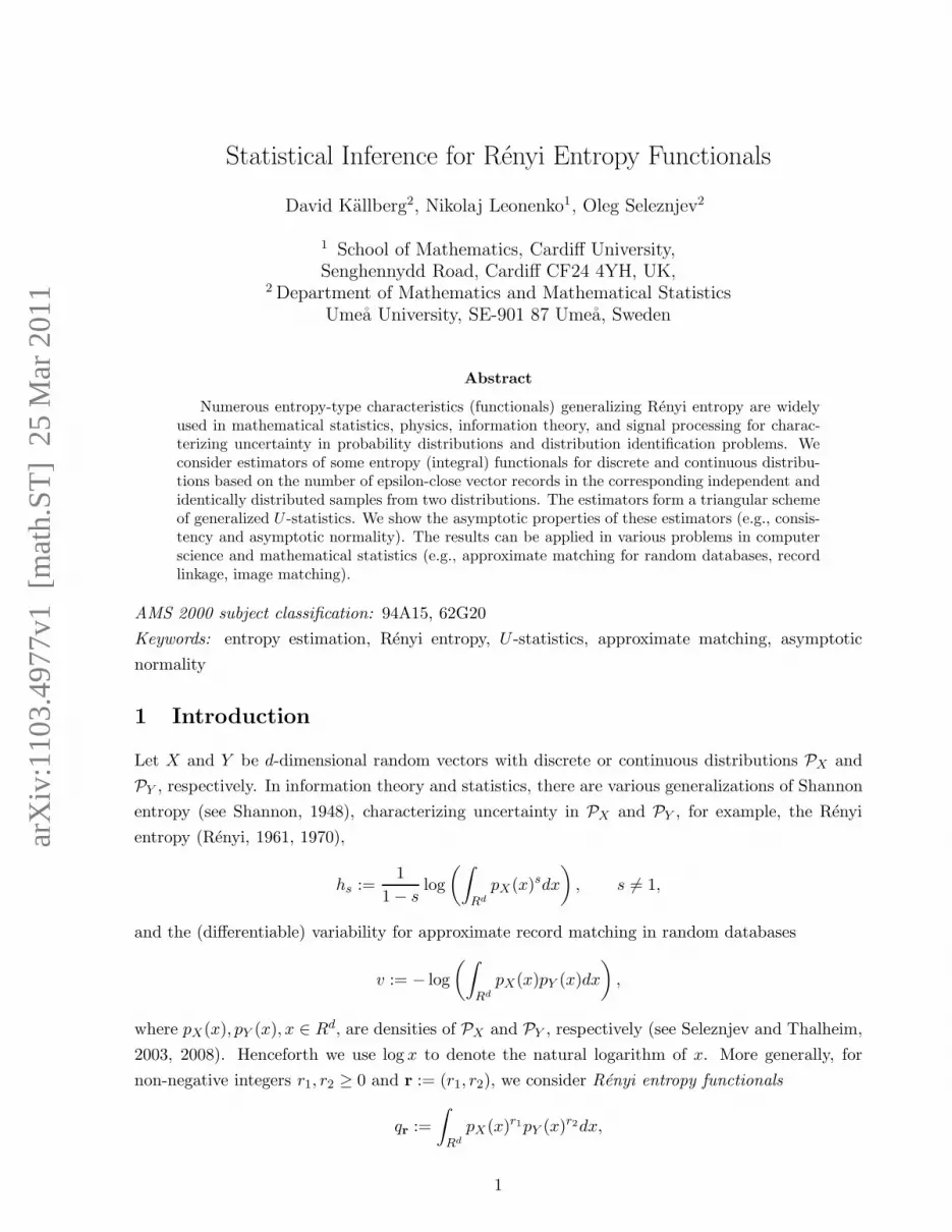
Numerous entropy-type characteristics (functionals) generalizing Renyi entropy are widelyused in mathematical statistics, physics, information theory, and signal processing for charac-terizing uncertainty in probability distributions and distribution identification problems. Weconsider estimators of some entropy (integral) functionals for discrete and continuous distribu-tions based on the number of epsilon-close vector records in the corresponding independent andidentically distributed samples from two distributions. The estimators form a triangular schemeof generalized U -statistics. We show the asymptotic properties of these estimators (e.g., consis-tency and asymptotic normality). The results can be applied in various problems in computerscience and mathematical statistics (e.g., approximate matching for random databases, recordlinkage, image matching).

AMS 2000 subject classification: 94A15, 62G20

Keywords: entropy estimation, Renyi entropy, U -statistics, approximate matching, asymptotic

normality

1 Introduction

Let X and Y be d-dimensional random vectors with discrete or continuous distributions PX and

PY , respectively. In information theory and statistics, there are various generalizations of Shannon

entropy (see Shannon, 1948), characterizing uncertainty in PX and PY , for example, the Renyi

entropy (Renyi, 1961, 1970),

hs :=1

1− slog

(∫

Rd

pX(x)sdx

)

, s 6= 1,

and the (differentiable) variability for approximate record matching in random databases

v := − log

(∫

Rd

pX(x)pY (x)dx

)

,

where pX(x), pY (x), x ∈ Rd, are densities of PX and PY , respectively (see Seleznjev and Thalheim,

2003, 2008). Henceforth we use log x to denote the natural logarithm of x. More generally, for

non-negative integers r1, r2 ≥ 0 and r := (r1, r2), we consider Renyi entropy functionals

qr :=

∫

Rd

pX(x)r1pY (x)r2dx,

1

and for the discrete case, PX = pX(k), k ∈ Nd and PY = pY (k), k ∈ Nd,

qr :=∑

k

pX(k)r1pY (k)r2 ,

i.e., qr = qr1,r2 . Then, for example, the Renyi entropy hs = hs,0 = log(qs,0)/(1 − s) and the

variability v = h1,1 = − log(q1,1). LetX1, . . . ,Xn1and Y1, . . . , Yn2

be mutually independent samples

of independent and identically distributed (i.i.d.) observations from PX and PY , respectively. We

consider the problem of estimating the entropy-type functionals qr and related characteristics for

PX and PY from the samples X1, . . . ,Xn1and Y1, . . . , Yn2

.

Various entropy applications in statistics (e.g., classification and distribution identification prob-

lems) and in computer science and bioinformatics (e.g., average case analysis for random databases,

approximate pattern and image matching) are investigated in, e.g., Kapur (1989), Kapur and Ke-

savan (1992), Leonenko et al. (2008), Szpankowski (2001), Seleznjev and Thalheim (2003, 2008),

Thalheim (2000), Baryshnikov et al. (2009), and Leonenko and Seleznjev (2010). Some average

case analysis problems for random databases with entropy characteristics are investigated also in

Demetrovics et al. (1995, 1998a, 1998b).

In our paper, we generalize the results and approach proposed in Leonenko and Seleznjev

(2010), where the quadratic Renyi entropy estimation is studied for one sample. We consider

properties (consistency and asymptotic normality) of kernel-type estimators based on the number

of coincident (or ǫ-close) observations in d-dimensional samples for more general class of entropy-

type functionals. These results can be used, e.g., in evaluating of asymptotical confidence intervals

for the corresponding Renyi entropy functionals.

Note that our estimators of entropy-type functionals are different form those considered by

Kozachenko and Leonenko (1987), Tsybakov and van der Meulen (1996), Leonenko et al. (2008),

and Baryshnikov et al. (2009) (see Leonenko and Seleznjev, 2010, for a discussion).

First we introduce some notation. Throughout the paper, let X and Y be independent random

vectors in Rd with distributions PX and PY , respectively. For the discrete case, PX = pX(k), k ∈Nd and PY = pY (k), k ∈ Nd. In the continuous case, let the distributions be with densities

pX(x) and pY (x), x ∈ Rd, respectively. Let d(x, y) = |x − y| denote the Euclidean distance in Rd

and Bǫ(x) := y : d(x, y) ≤ ǫ an ǫ-ball in Rd with center at x, radius ǫ, and volume bǫ(d) = ǫdb1(d),

b1(d) = 2πd/2/(dΓ(d/2)). Denote by pX,ǫ(x) the ǫ-ball probability

pX,ǫ(x) := PX ∈ Bǫ(x).

We write I(C) for the indicator of an event C, and |D| for the cardinality of a finite set D.

Next we define the following estimators of qr when r1 and r2 are non-negative integers. Let the

i.i.d. samples X1, . . . ,Xn1and Y1, . . . , Yn2

be from PX and PY , respectively. Denote n := (n1, n2),

n := n1 + n2, and say that n → ∞ if n1, n2 → ∞ and let pn := n1/n→ p, 0 < p < 1, as n → ∞.

For an integer k, denote by Sm,k the set of all k-subsets of 1, . . . ,m. For S ∈ Sn1,r1 , T ∈ Sn2,r2 ,

and i ∈ S, define

ψ(i)n (S;T ) := I(d(Xi,Xj) ≤ ǫ, d(Xi, Yk) ≤ ǫ,∀j ∈ S,∀k ∈ T ),

2

i.e., the indicator of the event that all elements in Xj , j ∈ S and Yk, k ∈ T are ǫ-close to Xi.

Note that by conditioning we have

Eψ(i)n (S;T ) = EpX,ǫ(X)r1−1pY,ǫ(X)r2 =: qr,ǫ,

say, the ǫ-coincidence probability. Let a generalized U -statistic for the functional qr,ǫ be defined as

Qn = Qn,r,ǫ :=

(

n1r1

)

−1(n2r2

)

−1∑

(n1,r1)

∑

(n2,r2)

ψn(S;T ),

where the symmetrized kernel

ψn(S;T ) :=1

r1

∑

i∈S

ψ(i)n (S;T ),

and by definition, Qn is an unbiased estimator of qr,ǫ = EQn. Define for discrete and continuous

distributions

ζ1,0 := Var(pX(X)r1−1pY (X)r2) = q2r1−1,2r2 − q2r1,r2 ,

ζ0,1 := Var(pX(Y )r1pY (Y )r2−1) = q2r1,2r2−1 − q2r1,r2 ,

κ := p−1r21ζ1,0 + (1− p)−1r22ζ0,1.

LetD→ and

P→ denote convergence in distribution and in probability, respectively.

The paper is organized as follows. In Section 2, we consider estimation of Renyi entropy

functionals for discrete and continuous distributions. In Section 3, we discuss some applications of

the obtained estimators in average case analysis for random databases (e.g., for join optimization

with approximate matching), in pattern and image matching problems, and for some distribution

identification problems. Several numerical experiments demonstrate the rate of convergence in the

obtained asymptotic results. Section 4 contains the proofs of the statements from the previous

sections.

2 Main Results

2.1 Discrete Distributions

In the discrete case, set ǫ = 0, i.e., exact coincidences are considered. Then Qn is an unbiased

estimator of the ǫ-coincidence probability

qr,0 = qr = EI(X1 = Xi = Yj, i = 2, . . . , r1, j = 1, . . . , r2) = EpX(X)r1−1pY (X)r2 .

Let Qn,r := Qn,r,0 and

Kn := p−1nr21(Qn,2r1−1,2r2 −Q2

n,r) + (1− pn)−1r22(Qn,2r1,2r2−1 −Q2

n,r),

and kn := max(Kn, 1/n), an estimator of κ. Denote by Hn := log(max(Qn, 1/n))/(1 − r), an

estimator of hr := log(qr)/(1 − r).

3

Remark. Instead of 1/n in the definition of a truncated estimator, a sequence an > 0, an → 0 as

as n → ∞, can be used (cf. Leonenko and Seleznjev, 2010).

The next asymptotic normality theorem for the estimator Qn follows straightforwardly from

the general U -statistic theory (see, e.g., Lee, 1990, Koroljuk and Borovskich, 1994) and the Slutsky

theorem.

Theorem 1 If ζ1,0, ζ0,1 > 0, then

√n(Qn − qr)

D→ N(0, κ) and√n(Qn − qr)/k

1/2n

D→ N(0, 1);

√n(1− r)

Qn

k1/2n

(Hn − hr)D→ N(0, 1) as n → ∞.

2.2 Continuous Distributions

In the continuous case, denote by Qn := Qn/bǫ(d)r−1 an estimator of qr. Let qr,ǫ := EQn =

qr,ǫ/bǫ(d)r−1 and v2

n:= Var(Qn).

Henceforth, assume that ǫ = ǫ(n) → 0 as n → ∞. For a sequence of random variables Un, n ≥ 1,

we say that Un = OP(1) as n → ∞ if for any ǫ > 0 and n large enough there exists A > 0 such

that P (|Un| > A) ≤ ǫ, i.e., the family of distributions of Un, n ≥ 1, is tight, and for a numerical

sequence wn, n ≥ 1, say, Un = OP(wn) as n → ∞ if Un/wn = OP(1) as n → ∞. The following

theorem describes the consistency and asymptotic normality properties of the estimator Qn.

Theorem 2 Let pX(x) and pY (x) be bounded and continuous or with a finite number of disconti-

nuity points.

(i) v2n= O(n−1ǫd(1/r−1)) and EQn → qr as n → ∞, and hence if nǫd(1−1/r) → ∞ as n → ∞,

then Qn is a consistent estimator of qr.

(ii) If nǫd → ∞ as n → ∞ and ζ1,0, ζ0,1 > 0, then

√n(Qn − qr,ǫ)

D→ N(0, κ) as n → ∞.

In order to evaluate the functional qr, we denote by H(α)(C) , 0 < α ≤ 2, C > 0, a linear

space of bounded and continuous in Rd functions satisfying α-Holder condition if 0 < α ≤ 1 or if

1 < α ≤ 2 with continuous partial derivatives satisfying (α− 1)-Holder condition with constant C.

Furthermore, let

Kn := p−1nr21(Qn,2r1−1,2r2,ǫ − Q2

n,r,ǫ) + (1− pn)−1r22(Qn,2r1,2r2−1,ǫ − Q2

n,r,ǫ),

and define kn := max(Kn, 1/n). It follows from Theorem 2 and Slutsky’s theorem that kn is a

consistent estimator of the asymptotic variance κ. Denote by Hn := log(max(Qn, 1/n))/(1− r), anestimator of hr := log(qr)/(1− r). Let L(n) be a slowly varying function. We obtain the following

asymptotic result.

4

Theorem 3 Let pX(x), pY (x) ∈ H(α)(C).

(i) Then the bias |qr,ǫ − qr| ≤ C1ǫα, C1 > 0.

(ii) If 0 < α ≤ d/2 and ǫ ∼ cn−α/(2α+d(1−1/r)) , 0 < c <∞, then

Qn − qr = OP(n−α/(2α+d(1−1/r))) and Hn − hr = OP(n

−α/(2α+d(1−1/r))) as n → ∞.

(iii) If α > d/2 and ǫ ∼ L(n)n−1/d and nǫd → ∞, then

√n(Qn − qr)

D→ N(0, κ) and√n(Qn − qr)/k

1/2n

D→ N(0, 1);

√n(1− r)

Qn

k1/2n

(Hn − hr)D→ N(0, 1) as n → ∞.

3 Applications and Numerical Experiments

3.1 Approximate Matching in Stochastic Databases

Let tables (in a relational database) T1 and T2 be matrices with m1 and m2 i.i.d. random tuples

(or records), respectively. One of basic database operations, join, combines two tables into a third

one by matching values for given columns (attributes). For example, the join condition can be

the equality (equi-join) between a given pairs of attributes (e.g., names) from the tables. Joins

are especially important for tieing together pieces of disparate information scattered throughout

a database (see, e.g., Kiefer et al. 2005, Copas and Hilton, 1990, and references therein). For

the approximate join, we match ǫ-close tuples, say, d(t1(j), t2(i)) ≤ ǫ, tk(j) ∈ Tk, k = 1, 2, with a

specified distance, see, e.g., Seleznjev and Thalheim (2008). A set of attributes A in a table T is

called an ǫ-key (test) if there are no ǫ-close sub-tuples tA(j), j = 1, . . . ,m. Knowledge about the set

of tests (ǫ-keys) is very helpful for avoiding redundancy in identification and searching problems,

characterizing the complexity of a database design for further optimization, see, e.g., Thalheim

(2000). By joining a table with itself (self-join) we identify also ǫ-keys and key-properties for a set

of attributes for a random table (Seleznjev and Thalheim, 2003, Leonenko and Seleznjev, 2010).

The cost of join operations is usually proportional to the size of the intermediate results and so

the joining order is a primary target of join-optimizers for multiple (large) tables, Thalheim (2000).

The average case approach based on stochastic database modelling for optimization problems is

proposed in Seleznjev and Thalheim (2008), where for random databases, the distribution of the

ǫ-join size Nǫ is studied. In particular, with some conditions it is shown that the average size

ENǫ = m1m2q1,1,ǫ = m1m2ǫdb1(d)(e

−h1,1 + o(1)) as ǫ→ 0,

that is the asymptotically optimal (in average) pairs of tables are amongst the tables with maximal

value of the functional h1,1 (variability) and the corresponding estimators of h1,1 can be used for

samplesX1, . . . ,Xn1and Y1, . . . , Yn2

from T1 and T2, respectively. For discrete distributions, similar

results from Theorem 1 for ǫ = 0 can be applied.

3.2 Image Matching using Quadratic-entropy Measures

Image retrieval and registration fall in the general area of pattern matching problems, where the

best match to a reference or query image I0 is to be found in a database of secondary images

5

Iini=1 . The best match is expressed as a partial re-indexing of the database in decreasing order of

similarity to the reference image using a similarity measure. In the context of image registration,

the database corresponds to an infinite set of transformed versions of a secondary image, e.g.,

rotation and translation, which are compared to the reference image to register the secondary one

to the reference.

Let X be a d-dimensional random vector and let p(x) and q(x) denote two possible densities for

X. In the sequel, X is a feature vector constructed from the query image and a secondary image

in an image database and p(x) and q(x) are densities, e.g., for the query image features and the

secondary image features, respectively, say, image densities. When the features are discrete valued

the p(x) and q(x) are probability mass functions.

The basis for entropy methods of image matching is a measure of similarity between image

densities. A general entropy similarity measure is the Renyi α-divergence, also called the Renyi

α-relative entropy, between p(x) and q(x)

Dα(p, q) =1

α− 1log

∫

Rd

q(x)

(

p(x)

q(x)

)α

dx =1

α− 1log

∫

Rd

pα(x)q1−α(x)dx, α 6= 1.

When the density p(x) is supported on a compact domain and q(x) is uniform over this domain,

the Renyi α-divergence reduces to the Renyi α-entropy

hα(p) =1

1− αlog

∫

Rd

pα(x)dx.

Another important example of statistical distance between distributions is given by the following

nonsymmetric Bregman distance (see, e.g., Pardo, 2006)

Bs(p, q) =

∫

Rd

[

q(x)s +1

s− 1p(x)s − s

s− 1p(x)q(x)s−1

]

dx, s 6= 1,

or its symmetrized version

Ks(p, q) =1

s[Bs(p, q) +Bs(q, p)] =

1

s− 1

∫

Rd

[p(x)− q(x)][p(x)s−1 − q(x)s−1]dx.

For s = 2, we get the second order distance

B2(p, q) = K2(p, q) =

∫

Rd

[p(x)− q(x)]2dx.

Now, for an integer s, applying Theorem 1 and 3 one can obtain an asymptotically normal estimator

of the Renyi s-entropy and a consistent estimator of the Bregman distance.

3.3 Entropy Maximizing Distributions

For a positive definite and symmetric matrix Σ, s 6= 1, define the constants

m = d+ 2/(s − 1), Cs = (m+ 2)Σ,

and

As =1

|πCs|1/2Γ(m/2 + 1)

Γ((m− d)/2 + 1).

6

Among all densities with mean µ and covariance matrix Σ, the Renyi entropy hs, s = 2, . . . , is

uniquely maximized by the density (Costa et al. 2003)

p∗s(x) =

As(1− (x− µ)TC−1s (x− µ))1/(s−1), x ∈ Ωs

0, x /∈ Ωs,(1)

with support

Ωs = x ∈ Rd : (x− µ)TC−1s (x− µ) ≤ 1.

The distribution given by p∗s(x) belongs to the class of Student-r distributions. Let K be a class

of d-dimensional density functions p(x), x ∈ Rd, with positive definite covariance matrix. By the

procedure described in Leonenko and Seleznjev (2010), the proposed estimator of hs can be used

for distribution identification problems, i.e., to test the null hypothesis H0 : X1, . . . ,Xn is a sample

from a Student-r distribution of type (1) against the alternative H1 : X1, . . . ,Xn is a sample from

any other member of K.

3.4 Numerical Experiments

Example 1. Figure 1 shows the accuracy of the estimator for the cubic Renyi entropy h3,0 of

discrete distributions in Theorem 1, for a sample from a d-dimensional Bernoulli distribution and

n observations, d = 3, n = 300, with Bernoulli Be(p)-i.i.d. components, p = 0.8. Here the

coincidence probability q3,0 = (p3 + (1 − p)3)3 and the Renyi entropy h3,0 = − log(q3,0)/2. The

histogram for the normalized residuals r(i)n := 2

√nQn(Hn−hr)/k1/2n , i = 1, . . . , Nsim are compared

to the standard normal density, Nsim = 500. The corresponding qq-plot and p-values for the

Kolmogorov-Smirnov (0.4948) and Shapiro-Wilk (0.7292) tests also support normality hypothesis

for the obtained residuals.

Histogram of res

res

Densi

ty

−4 −2 0 2 4

0.00.1

0.20.3

0.4

−3 −2 −1 0 1 2 3

−3−2

−10

12

Normal Q−Q Plot

Theoretical Quantiles

Samp

le Quan

tiles

Figure 1: Bernoulli d-dimensional distribution; d = 3, Be(p)-i.i.d. components, p = 0.8, samplesize n = 200. Standard normal approximation for the empirical distribution (histogram) for thenormalized residuals, Nsim = 500.

7

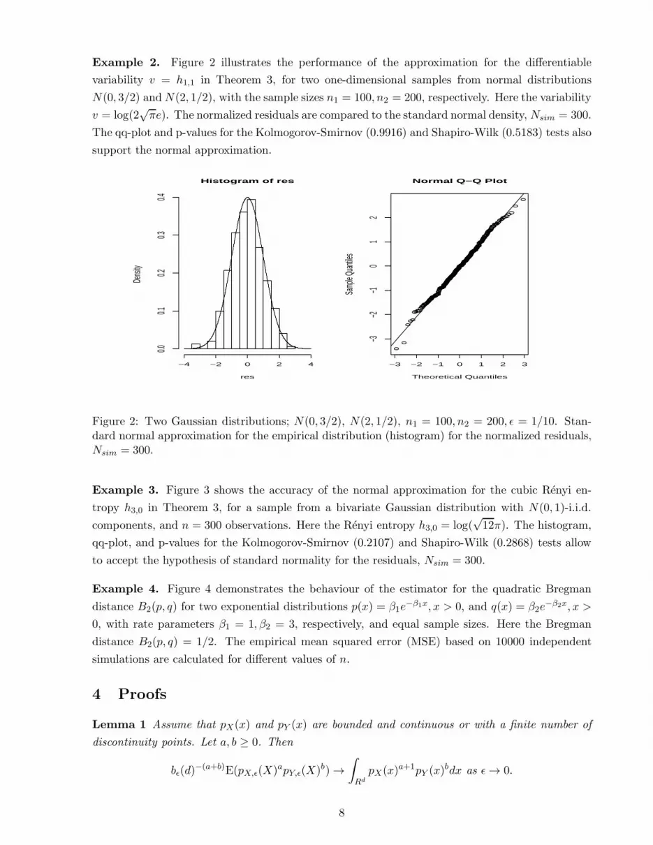
Example 2. Figure 2 illustrates the performance of the approximation for the differentiable

variability v = h1,1 in Theorem 3, for two one-dimensional samples from normal distributions

N(0, 3/2) andN(2, 1/2), with the sample sizes n1 = 100, n2 = 200, respectively. Here the variability

v = log(2√πe). The normalized residuals are compared to the standard normal density, Nsim = 300.

The qq-plot and p-values for the Kolmogorov-Smirnov (0.9916) and Shapiro-Wilk (0.5183) tests also

support the normal approximation.

Histogram of res

res

Densi

ty

−4 −2 0 2 4

0.00.1

0.20.3

0.4

−3 −2 −1 0 1 2 3

−3−2

−10

12

Normal Q−Q Plot

Theoretical Quantiles

Samp

le Quan

tiles

Figure 2: Two Gaussian distributions; N(0, 3/2), N(2, 1/2), n1 = 100, n2 = 200, ǫ = 1/10. Stan-dard normal approximation for the empirical distribution (histogram) for the normalized residuals,Nsim = 300.

Example 3. Figure 3 shows the accuracy of the normal approximation for the cubic Renyi en-

tropy h3,0 in Theorem 3, for a sample from a bivariate Gaussian distribution with N(0, 1)-i.i.d.

components, and n = 300 observations. Here the Renyi entropy h3,0 = log(√12π). The histogram,

qq-plot, and p-values for the Kolmogorov-Smirnov (0.2107) and Shapiro-Wilk (0.2868) tests allow

to accept the hypothesis of standard normality for the residuals, Nsim = 300.

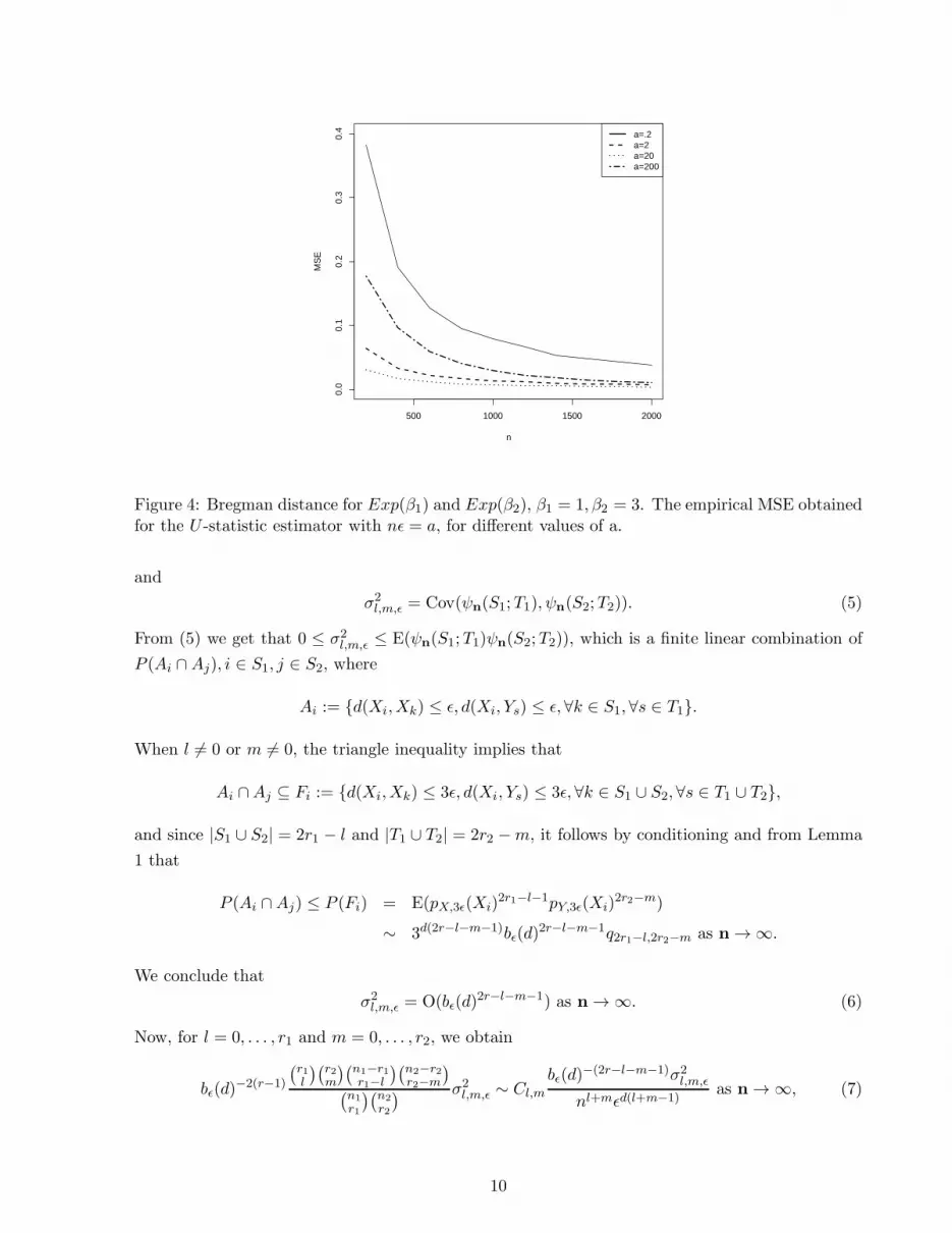
Example 4. Figure 4 demonstrates the behaviour of the estimator for the quadratic Bregman

distance B2(p, q) for two exponential distributions p(x) = β1e−β1x, x > 0, and q(x) = β2e

−β2x, x >

0, with rate parameters β1 = 1, β2 = 3, respectively, and equal sample sizes. Here the Bregman

distance B2(p, q) = 1/2. The empirical mean squared error (MSE) based on 10000 independent

simulations are calculated for different values of n.

4 Proofs

Lemma 1 Assume that pX(x) and pY (x) are bounded and continuous or with a finite number of

discontinuity points. Let a, b ≥ 0. Then

bǫ(d)−(a+b)E(pX,ǫ(X)apY,ǫ(X)b) →

∫

Rd

pX(x)a+1pY (x)bdx as ǫ→ 0.

8

Histogram of res

res

Densi

ty

−4 −2 0 2 4

0.00.1

0.20.3

0.4

−3 −2 −1 0 1 2 3

−2−1

01

23

Normal Q−Q Plot

Theoretical Quantiles

Samp

le Quan

tiles

Figure 3: Bivariate normal distribution with N(0, 1)-i.i.d. components; sample size n = 300, ǫ =1/2. Standard normal approximation for the empirical distribution (histogram) for the normalizedresiduals, Nsim = 300.

Proof: We have

bǫ(d)−(a+b)E(pX,ǫ(X)apY,ǫ(X)b) = E(gǫ(X)),

where gǫ(x) := (pX,ǫ(x)/bǫ(d))a(pY,ǫ(x)/bǫ(d))

b. It follows by definition that gǫ(x) → pX(x)apY (x)b

as ǫ → 0, for all continuity points of pX(x) and pY (x), and that the random variable gǫ(X) is

bounded. Hence, the bounded convergence theorem implies

E(gǫ(X)) → E(pX(X)apY (X)b) = qa+1,b as ǫ→ 0.

2

Proof of Theorem 2: (i) Note that for k = 1, . . . , r,

nkǫd(k−1) = (nǫd(1−1/k))k ≥ (nǫd(1−1/r))k ≥ nǫd(1−1/r). (2)

We use the conventional results from the theory of U -statistics (see, e.g., Lee, 1990, Koroljuk and

Borovskich, 1994). For l = 0, . . . , r1, and m = 0, . . . , r2, define

ψl,m,n(x1, . . . , xl; y1, . . . , ym) := Eψn(x1, . . . , xl,Xl+1, . . . ,Xr1 ; y1, . . . , ym, Ym+1, . . . , Yr2)

=1

r1

r1∑

i=1

Eψ(i)n (x1, . . . , xl,Xl+1, . . . ,Xr1 ; y1, . . . , ym, Ym+1, . . . , Yr2), (3)

and

σ2l,m,ǫ := Var(ψl,m,n(X1, . . . ,Xl;Y1, . . . , Ym)).

Let S1, S2 ∈ Sn1,r1 and T1, T2 ∈ Sn2,r2 have l andm elements in common, respectively. By properties

of U -statistics, we have

v2n= Var(Qn) = bǫ(d)

−2(r−1)r1∑

l=0

r2∑

m=0

(r1l

)(r2m

)(n1−r1r1−l

)(n2−r2r2−m

)

(n1

r1

)(n2

r2

) σ2l,m,ǫ, (4)

9

500 1000 1500 2000

0.0

0.1

0.2

0.3

0.4

n

MS

E

a=.2a=2a=20a=200

Figure 4: Bregman distance for Exp(β1) and Exp(β2), β1 = 1, β2 = 3. The empirical MSE obtainedfor the U -statistic estimator with nǫ = a, for different values of a.

and

σ2l,m,ǫ = Cov(ψn(S1;T1), ψn(S2;T2)). (5)

From (5) we get that 0 ≤ σ2l,m,ǫ ≤ E(ψn(S1;T1)ψn(S2;T2)), which is a finite linear combination of

P (Ai ∩Aj), i ∈ S1, j ∈ S2, where

Ai := d(Xi,Xk) ≤ ǫ, d(Xi, Ys) ≤ ǫ,∀k ∈ S1,∀s ∈ T1.

When l 6= 0 or m 6= 0, the triangle inequality implies that

Ai ∩Aj ⊆ Fi := d(Xi,Xk) ≤ 3ǫ, d(Xi, Ys) ≤ 3ǫ,∀k ∈ S1 ∪ S2,∀s ∈ T1 ∪ T2,

and since |S1 ∪ S2| = 2r1 − l and |T1 ∪ T2| = 2r2 −m, it follows by conditioning and from Lemma

1 that

P (Ai ∩Aj) ≤ P (Fi) = E(pX,3ǫ(Xi)2r1−l−1pY,3ǫ(Xi)

2r2−m)

∼ 3d(2r−l−m−1)bǫ(d)2r−l−m−1q2r1−l,2r2−m as n → ∞.

We conclude that

σ2l,m,ǫ = O(bǫ(d)2r−l−m−1) as n → ∞. (6)

Now, for l = 0, . . . , r1 and m = 0, . . . , r2, we obtain

bǫ(d)−2(r−1)

(r1l

)(r2m

)(n1−r1r1−l

)(n2−r2r2−m

)

(n1

r1

)(n2

r2

) σ2l,m,ǫ ∼ Cl,m

bǫ(d)−(2r−l−m−1)σ2l,m,ǫ

nl+mǫd(l+m−1)as n → ∞, (7)

10

for some constant Cl,m > 0. Hence, from (2), (4), (6), and (7) we get that v2n= O((nǫd(1−1/r))−1)

as n → ∞. Moreover, it follows from Lemma 1 that EQn → qr as n → ∞, so when nǫd(1−1/r) → ∞,

then

E(Qn − qr)2 = v2

n+ (E(Qn − qr))

2 → 0,

and the assertion follows.

(ii) Let

h(1,0)n (x) := ψ1,0,n(x)/bǫ(d)

r−1 − qr,ǫ, h(0,1)n (x) := ψ0,1,n(x)/bǫ(d)

r−1 − qr,ǫ. (8)

The H-decomposition of Qn is given by

Qn = qr,ǫ + r1H(1,0)n + r2H

(0,1)n +Rn, (9)

where

H(1,0)n :=

1

n1

n1∑

i=1

h(1,0)n (Xi), H

(0,1)n :=

1

n2

n2∑

i=1

h(0,1)n (Yi).

The terms in (9) are uncorrelated, and since Var(h(1,0)n (X1)) = bǫ(d)

−2(r−1)σ21,0,ǫ and Var(h(0,1)n (Y1)) =

bǫ(d)−2(r−1)σ20,1,ǫ, we obtain from (4) that

Var(Rn) = Var(Qn)−Var(r1H(1,0)n )−Var(r2H

(0,1)n )

= Var(Qn)− bǫ(d)−2(r−1)r21n

−11 σ21,0,ǫ − bǫ(d)

−2(r−1)r22n−12 σ20,1,ǫ

= K1,nbǫ(d)−2(r−1)n−1σ21,0,ǫ +K2,nbǫ(d)

−2(r−1)n−1σ20,1,ǫ

+ bǫ(d)−2(r−1)

∑

E

(r1l

)(r2m

)(n1−r1r1−l

)(n2−r2r2−m

)

(n1

r1

)(n2

r2

) σ2l,m,ǫ, (10)

where E := (l,m) : 0 ≤ l ≤ r1, 0 ≤ m ≤ r2, l +m ≥ 2, and

K1,n := r21pn

((

n1−r1r1−1

)(

n2−r2r2

)

(

n1−1r1−1

)(

n2

r2

) − 1

)

, K2,n := r22(1− pn)

((

n1−r1r1

)(

n2−r2r2−1

)

(

n1

r1

)(

n2−1r2−1

) − 1

)

.

Note that K1,n,K2,n = O(n−1) as n → ∞ so if nǫd → a, 0 < a ≤ ∞, then (6), (7), and (10) imply

that Var(Rn) = O((n2ǫd)−1) as n → ∞. In particular, for a = ∞,

Var(Rn) = o(n−1) ⇒ n1/2Rn

P→ 0 as n → ∞. (11)

By symmetry, we have from (3)

ψ1,0,n(x) =1

r1

(

pX,ǫ(x)r1−1pY,ǫ(x)

r2 + (r1 − 1)E(ψ(2)n (x,X2, . . . ,Xr1 ;Y1, . . . , Yr2))

)

. (12)

Let x be a continuity point of pX(x) and pY (x). Then, changing variables y = x + ǫu and the

bounded convergence theorem give

E(ψ(2)n (x,X2, . . . ,Xr1 ;Y1, . . . , Yr2) = E(E(ψ

(2)n (x,X2, . . . ,Xr1 ;Y1, . . . , Yr2)|X2))

=

∫

Rd

I(d(x, y) ≤ ǫ)pX,ǫ(y)r1−2pY,ǫ(y)

r2pX(y)dy

= ǫd∫

Rd

I(d(0, u) ≤ 1)pX,ǫ(x+ ǫu)r1−2pY,ǫ(x+ ǫu)r2pX(x+ ǫu)du (13)

∼ bǫ(d)r−1pX(x)r1−1pY (x)

r2 as n → ∞.

11

From (12) we get that

ψ1,0,n(x) ∼ bǫ(d)r−1pX(x)r1−1pY (x)

r1 as n → ∞,

and hence

limn→∞

h(1,0)n (x) = pX(x)r1−1pY (x)

r2 − qr, (14)

and similarly,

limn→∞

h(0,1)n (x) = pX(x)r1pY (x)

r2−1 − qr. (15)

Let max(pX(x), pY (x)) ≤ C, x ∈ Rd. Then max(pX,ǫ(x), pY,ǫ(x)) ≤ bǫ(d)C, x ∈ Rd. It follows

from (12) and (13) that ψ1,0,n(x) ≤ bǫ(d)r−1Cr−1, x ∈ Rd, and hence h

(1,0)n (x) ≤ 2Cr−1, x ∈ Rd.

Similarly, we have that h(0,1)n (x) ≤ 2Cr−1, x ∈ Rd. Therefore, h

(1,0)n (X1) and h

(0,1)n (Y1) are bounded

random variables. Hence, from (14), (15), and the bounded convergence theorem we obtain

Var(h(1,0)n (X1)) → ζ1,0, Var(h

(0,1)n (Y1)) → ζ0,1 as n → ∞.

Let Zn,i := n−1/21 h

(1,0)n (Xi), i = 1, . . . , n1, and observe that, for δ > 0,

n1∑

i=1

EZ2n,i = Var(h

(1,0)n (X1)) → ζ1,0 > 0 as n → ∞,

limn→∞

n1∑

i=1

E(|Zn,i|2I(|Zn,i| > δ)) = limn→∞

E(|h(1,0)n (X1)|2I(|h(1,0)n (X1)| > δn1/21 ))

≤ limn→∞

4C2(r−1)E(I(|h(1,0)n (X1)| > δn1/21 )) = 0,

where the last equality follows from the boundedness of h(1,0)n (X1). The Lindeberg-Feller Theorem

(see, e.g., Theorem 4.6, Durrett, 1991) gives that

Zn,1 + . . .+ Zn,n1= n

1/21 H

(1,0)n

D→ N(0, ζ1,0) as n → ∞,

and similarly n1/22 H

(0,1)n

D→ N(0, ζ0,1) as n → ∞. Hence, by independence we get that

n1/2(r1H(1,0)n + r2H

(0,1)n )

=r1

p1/2n

n1/21 H

(1,0)n +

r2(1− pn)1/2

n1/22 H

(0,1)n

D→ N(0, κ) as n → ∞,

so from (11) and Slutsky’s theorem,

n1/2(Qn − qr,ǫ)

= n1/2(r1H(1,0)n + r2H

(0,1)n ) + n1/2Rn

D→ N(0, κ) as n → ∞.

This completes the proof. 2

Proof of Theorem 3: The proof is similar to that of the corresponding result in Leonenko and

Seleznjev (2010) so we give the main steps only. First we evaluate the bias term Bn := qr,ǫ − qr.

12

Let V := (V1, . . . , Vd)′ be an auxiliary random vector uniformly distributed in the unit ball B1(0),

say, V ∈ U(B1(0)). Then by definition, we have

Bn =

∫

Rd

pX,ǫ(x)r1−1pY,ǫ(x)

r2pX(x)dx −∫

Rd

pX(x)r1pY (x)r2dx = E(Dǫ(X)),

where

Dǫ(x) := pX,ǫ(x)r1−1pY,ǫ(x)

r2 − pX(x)r1−1pY (x)r2

= pX,ǫ(x)r1−1(pY,ǫ(x)

r2 − pY (x)r2) + pY (x)

r2(pX,ǫ(x)r1−1 − pX(x)r1−1).

It follows by definition that

Dǫ(x) = P1(x)(pY,ǫ(x)− pY (x)) + P2(x)(pX,ǫ(x)− pX(x))

= E(

P1(x)(pY (x− ǫV )− pY (x)) + P2(x)(pX(x− ǫV )− pX(x)))

where P1(x) and P2(x) are polynomials in pX(x), pY (x),E(pX (x− ǫV )), and E(pY (x− ǫV )). Now

the boundedness of pX(x) and pY (x) and the Holder condition for the continuous differentiable

cases imply

|Dǫ(x)| ≤ CC1ǫα, C1 > 0,

and the assertion (i) follows.

For ǫ ∼ cn−1/(2α+d(1−1/r)) , 0 < c <∞, α < d/2, by (i) and Theorem 1, we have

B2n+ v2

n= O(n−2α/(2α+d(1−1/r))).

Now for some C > 0 and any A > 0 and large enough n1, n2, we obtain

P(

|Qn − qr| > An−α/(2α+d(1−1/r)))

≤ n−2α/(2α+d(1−1/r))B2n+ v2

n

A2≤ C

A2,

and the assertion (ii) follows. Similarly for α = d/2.

Finally, for α > d/2 and ǫ ∼ L(n)n−1/d and nǫd → ∞, the assertion (iii) follows from Theorem

2 and the Slutsky theorem. This completes the proof. 2

Acknowledgment

The third author is partly supported by the Swedish Research Council grant 2009-4489 and the

project ”Digital Zoo” funded by the European Regional Development Fund. The second author is

partly supported of the Commissions the European Communities grant PIRSES-GA 2008-230804

”Marie Curie Actions”.

References

Baryshnikov, Yu., Penrose, M., Yukich, J.E.: Gaussian limits for generalized spacings. Ann. Appl.

Probab., 19 (2009) 158–185

13

Beirlant, J., Dudewicz, E.J., Gyorfi, L., van der Meulen, E.C.: Non-parametric entropy estimation:

An overview. Internat. Jour. Math. Statist. Sci. 6 (1997) 17–39

Copas, J.B., Hilton, F.J.: Record linkage: statistical models for matching computer records. Jour.

Royal Stat. Soc. Ser A. 153 (1990) 287–320

Costa, J., Hero, A., Vignat, C.: On Solutions to Multivariate Maximum α-entropy Problems.

Lecture Notes in Computer Science 2683 (2003) 211–228

Demetrovics, J., Katona, G.O.H., Miklos, D., Seleznjev, O., Thalheim, B.: The average length of

keys and functional dependencies in (random) databases. In: Proc. ICDT95 Eds: G. Gottlob

and M. Vardi, LN in Comp. Sc. Springer: Berlin 893 (1995) 266–279

Demetrovics, J., Katona, G.O.H., Miklos, D., Seleznjev, O., Thalheim, B.: Asymptotic properties

of keys and functional dependencies in random databases. Theor. Computer Science 190 (1998)

151–166

Demetrovics, J., Katona, G.O.H., Miklos, D., Seleznjev, O., Thalheim, B.: Functional dependencies

in random databases. Studia Scien. Math. Hungarica 34 (1998) 127–140

Durrett, R.: Probability: Theory and Examples. Brooks/Cole Publishing Company, New York

(1991)

Kapur, J.N.: Maximum-entropy Models in Science and Engineering. Wiley New York (1989)

Kapur, J.N., Kesavan, H.K.: Entropy Optimization Principles with Applications. Academic Press,

New York (1992)

Kiefer, M., Bernstein, A., Lewis, Ph. M. Database Systems: An Application-Oriented Approach.

Addison Wesley (2005)

Koroljuk, V.S., Borovskich, Yu.V.: Theory of U -statistics. Kluwer, London (1994)

Kozachenko, L.F., Leonenko, N.N.: On statistical estimation of entropy of random vector. Problems

Infor. Transmiss. 23 (1987) 95–101

Lee, A.J.: U -Statistics: Theory and Practice. Marcel Dekker, New York (1990)

Leonenko, N., Pronzato, L., Savani, V.: A class of Renyi information estimators for multidimen-

sional densities. Ann. Stat. 36 (2008) 2153–2182. Corrections, Ann. Stat., 38, N6 (2010)

3837-3838

Leonenko, N., Seleznjev, O.: Statistical inference for the ǫ-entropy and the quadratic Renyi entropy.

Jour. Multivariate Analysis 101 (2010) 1981–1994

Neemuchwala, H., Hero, A., Carson, P.: Image matching using alpha-entropy measures and entropic

graphs. Signal Processing 85 (2005) 277–296

Pardo, L.: Statistical Inference Based on Divergence Measures. Chapman and Hall (2006)

Renyi, A.: On measures of entropy and information. In: Proc. 4th Berkeley Symp. Math. Statist.

Prob. Volume 1. (1961)

Renyi, A.: Probability Theory. North-Holland, London (1970)

Seleznjev, O., Thalheim, B.: Average case analysis in database problems. Methodol. Comput.

Appl. Prob. 5 (2003) 395-418

14

Seleznjev, O., Thalheim, B.: Random databases with approximate record matching. Methodol.

Comput. Appl. Prob. 12 (2008) 63–89

Shannon, C.E.: A mathematical theory of communication. Bell Syst. Tech. Jour. 27 (1948) 379–

423, 623–656

Szpankowski, W.: Average Case Analysis Of Algorithms On Sequences. John Wiley, New York

(2001)

Thalheim, B.: Entity-Relationship Modeling. Foundations of Database Technology. Springer Ver-

lag, Berlin, (2000)

Tsybakov, A.B., Van der Meulen, E.C.: Root-n consistent estimators of entropy for densities with

unbounded support. Scandinavian Jour. Statistics 23 (1996) 75-83

15