arX

iv:1

012.

1584

v1 [

astr

o-ph

.SR

] 7

Dec

201

0

Statistical Distribution of Size and Lifetime of Bright Points

Observed with the New Solar Telescope

Valentyna Abramenko, Vasyl Yurchyshyn, Philip Goode, Ali Kilcik

Big Bear Solar Observatory, 40386 N. Shore Lane, Big Bear City, CA 92314

ABSTRACT

We present results of two-hour non-interrupted observations of solar

granulation obtained under excellent seeing conditions with the largest aperture

ground-based solar telescope - the New Solar Telescope (NST) - of Big Bear Solar

Observatory. Observations were performed with adaptive optics correction using

a broad-band TiO filter in the 705.7 nm spectral line with a time cadence of 10 s

and a pixel size of 0.0375”. Photospheric bright points (BPs) were detected and

tracked. We find that the BPs detected in NST images are co-spatial with those

visible in Hinode/SOT G-band images. In cases where Hinode/SOT detects one

large BP, NST detects several separated BPs. Extended filigree features are

clearly fragmented into separate BPs in NST images. The distribution function

of BP sizes extends to the diffraction limit of NST (77 km) without saturation

and corresponds to a log-normal distribution. The lifetime distribution function

follows a log-normal approximation for all BPs with lifetime exceeding 100 s. A

majority of BPs are transient events reflecting the strong dynamics of the quiet

sun: 98.6% of BPs live less than 120 s. The longest registered life time was 44

minutes. The size and maximum intensity of BPs were found to be proportional

to their life times.

Subject headings: Sun: activity - Sun: photosphere - Sun: surface magnetism -

Physical Data and Processes: turbulence

1. Introduction

Bright points (BPs) observed in the solar photosphere in FeI 6173 A filtergrams

(Muller et al. 2000) and in G-band images (Berger & Title 2001; Ishikawa et al. 2007)

are shown to be co-spatial and co-temporal with magnetic elements. However, only about

20% of magnetic elements in intranetwork areas are related to BPs (de Wijn et al. 2008;

Ishikawa et al. 2007). Photospheric BPs, therefore, represent a subset of the magnetic

– 2 –

elements. The relationship between BPs and magnetic field seems to be so solid that the

former are frequently addressed as magnetic bright points (e.g., Utz et al. 2009, 2010). The

mechanism for the formation of BPs is thought to be a convective collapse of a magnetic

flux tube (Parker 1978; Spruit 1979) implying strong downflows and evacuation of the flux

tube allowing us to look deeper and see hotter plasma. Analysis of statistical distributions

of BPs can shed a light on the fundamental properties of smallest magnetic elements.

Another strong reason for enhanced interest in BPs is that they are very reliable

tracers of transverse motions of the footpoints of photospheric magnetic flux elements.

These motions are thought to be an ultimate source of the energy needed to heat the

chromosphere and corona, either via waves or via magnetic reconnection of intertwined flux

tubes (e.g., reviews by Cranmer (2002), Cranmer & van Ballegooien (2005), and Klimchuk

(2006) and references herein). These and other considerations stimulated numerous studies

of transverse (to the line-of- sight) velocities and various applications of the results to the

problems of wave generation (Cranmer & van Ballegooien 2005) and reconnection (Cranmer

& van Ballegooien 2010 and references therein).

Studies of BPs size and lifetime distributions, however, are rather scanty. Based on

Hinode/SOT (Kosugi et al. 2007; Tsuneta et al. 2008) observations, Utz et al. (2009,

2010) studied statistical distributions of G-band BP’s sizes and lifetimes. They used a 5.7

hour data with a pixel size of 0.054′′ and 0.109′′, and a time cadence of about 32 s. The

authors reported a nearly Gaussian distribution of BP’s size, with the peak located near

the diffraction limit of the telescope (157 km). For the lifetime distribution, an exponential

fit was found.

Now, with the New Solar Telescope (NST) at Big Bear Solar Observatory (BBSO)

operational, we attempt to reveal the BPs distribution functions on the basis of more

accurate data, which are described in detail in the next session.

2. Data

Observations of solar granulation were performed with the NST (Goode et al. 2010)

with a 1.6 meter clear aperture using a broadband TiO filter centered at a wavelength of

705.7 nm. This spectral line is sensitive to temperature, and it is usually used to observe

the sunspot umbra/penumbra (Berdyugina et al. 2003; Reithmuller et al. 2008). When

observing granulation with this line, a dual effect presents itself: for granules and BPs the

intensity is the same as observed in continuum, whereas for dark cool intergranular lanes,

the observed intensity is lowered due to absorption in the TiO line. Thus, TiO images

– 3 –

provide an enhanced gradient of intensity around BPs, which is very beneficial for imaging

them.

The FOV of the broadband filter imager is 76.8 × 0.76.8′′, and the pixel scale of the

PCO.2000 camera we used is 0.0375′′. This pixel size is 2.9 times smaller than the Rayleigh

diffraction limit of NST, θ1 = 1.22λ/D = 0.11′′ = 77 km, and 2.5 times smaller than the

FWHM of the smallest resolved feature1 (θ2 = 1.03λ/D = 65 km).

Uninterrupted observations of a quiet sun area near the disk center were performed

on August 3, 2010 between 17:06 UT and 18:57 UT. The observations were made with

tip-tilt and adaptive optics corrections (Cao et al. 2010). The time cadence of the speckle

reconstructed images was 10 s. To obtain one speckle reconstructed image, we took a burst

of 70 recorded with 1 ms exposure time, Then we applied the KISIP speckle reconstruction

code (Woger & von der Luhe 2008) to each burst. Resulting images were carefully aligned

and de-stretched. In the present study, we utilized only the central part (28.3×26.2′′ of

the FOV, where the adaptive optics corrections were most efficient. The resulting data set

consisting of 648 images was used to detect and trace BPs. A movie of this data set can be

found on the BBSO website2.

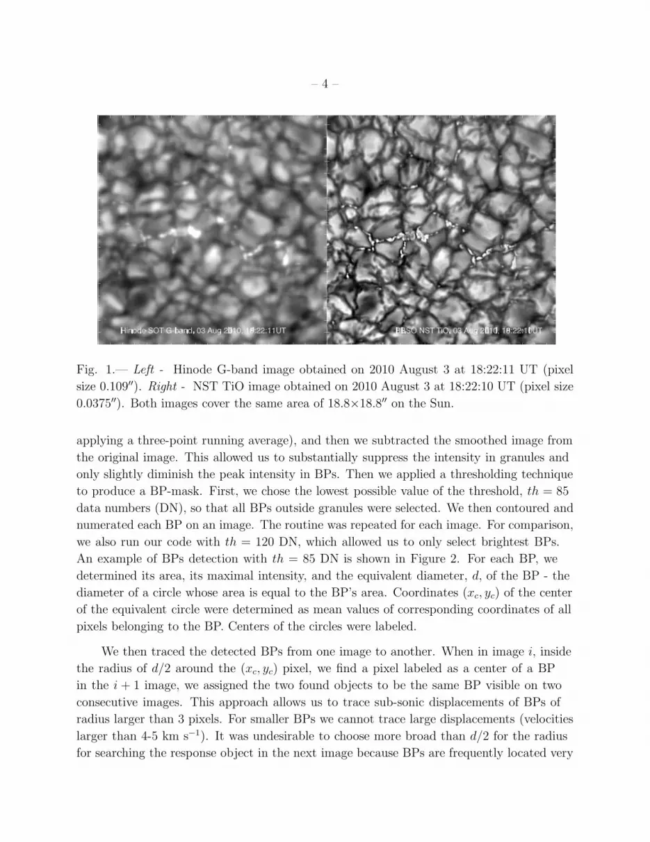
On the same day, Hinode/SOT obtained a synoptic G-band image within the time

interval of our observations. In Figure 1 we show two images of the same area on the Sun

simultaneously recorded with the Hinode/SOT (left) and NST (right). The Hinode image

was processed with standard data-reduction Solar SoftWare prep-fg.pro package3. All BPs

visible in the Hinode image are present in the NST image. In addition, NST sees much

more: small single BPs are clearly visible inside dark intergranular lanes (examine the

bottom halves of the images). Moreover, in places where Hinode/SOT detects a single large

BP, NST detects several separated BPs (center of the image). Extended filigree features are

clearly fragmented into separate BPs in the NST image.

3. Method

To detect and track BPs, we took advantage of the three most important properties

of BPs (Utz et al. 2009): small size, enhanced intensity and strong gradient in intensity

around BPs. We calculated a BP-mask as follows. First, we smoothed each image (by

1http://www.telescope-optics.net/telescope-resolution.htm

2http://bbso.njit.edu/nst-galery.html

3http://msslrx.mssl.ucl.ac.uk:8080/SolarB/AnalysisSoftware.jsp

– 4 –

Fig. 1.— Left - Hinode G-band image obtained on 2010 August 3 at 18:22:11 UT (pixel

size 0.109′′). Right - NST TiO image obtained on 2010 August 3 at 18:22:10 UT (pixel size

0.0375′′). Both images cover the same area of 18.8×18.8′′ on the Sun.

applying a three-point running average), and then we subtracted the smoothed image from

the original image. This allowed us to substantially suppress the intensity in granules and

only slightly diminish the peak intensity in BPs. Then we applied a thresholding technique

to produce a BP-mask. First, we chose the lowest possible value of the threshold, th = 85

data numbers (DN), so that all BPs outside granules were selected. We then contoured and

numerated each BP on an image. The routine was repeated for each image. For comparison,

we also run our code with th = 120 DN, which allowed us to only select brightest BPs.

An example of BPs detection with th = 85 DN is shown in Figure 2. For each BP, we

determined its area, its maximal intensity, and the equivalent diameter, d, of the BP - the

diameter of a circle whose area is equal to the BP’s area. Coordinates (xc, y

c) of the center

of the equivalent circle were determined as mean values of corresponding coordinates of all

pixels belonging to the BP. Centers of the circles were labeled.

We then traced the detected BPs from one image to another. When in image i, inside

the radius of d/2 around the (xc, y

c) pixel, we find a pixel labeled as a center of a BP

in the i + 1 image, we assigned the two found objects to be the same BP visible on two

consecutive images. This approach allows us to trace sub-sonic displacements of BPs of

radius larger than 3 pixels. For smaller BPs we cannot trace large displacements (velocities

larger than 4-5 km s−1). It was undesirable to choose more broad than d/2 for the radius

for searching the response object in the next image because BPs are frequently located very

– 5 –

Fig. 2.— NST TiO image taken at 17:08:15 UT (left). The right panel shows the same image

with detected BPs denoted by yellow pixels.The image size is 16.9′′ × 13.9′′.

close to each other. When a BP merged with another BP, or when we could not find a BP

in four consecutive images, we concluded that this BP ceased to exist. We thus were able

to determine the lifetime of each tracked BP. The diameter, D, of each BP was determined

by averaging over the lifetime equivalent diameter, d. Below in this paper, by ”BP” we

mean an object observed at several consecutive images, but not a single spot of enhanced

brightness observed in a single image.

When tracking BPs, we discarded all events with the area smaller than 2 pixels, all

events detected at only one image, as well as events with maximal intensity below the mean

intensity of the image. All these restrictions resulted in total of N =13597 tracked BPs in

case of th =85 DN threshold and N =7148 BPs for th =120 DN.

4. Results

Figure 3 shows the probability distribution functions (PDFs) for the diameter, D,

lifetime, LT , and maximum intensity, Imax

, of BPs. In the left panels, results for two runs

are shown: the black lines correspond to th =85 DN and the red lines to th =120 DN. The

right panels show PDFs only from the th =85 DN run. For all the PDFs in the figure,

the difference between the two runs is small: for higher threshold the relative number

of large-size events slightly decreases, and the relative number of brighter events slightly

increases. The lifetime distribution does not appear to be affected by the threshold at all.

The reason for this might be the very sharp gradient of intensity around BPs, so that the

– 6 –

change in the cutoff level has little effect on the size of the selected BP. This is in line with

Utz et al. (2009), who reported that a change in the cutoff level by 30% results in change

of sizes by only about 10%. Further, in the text, we only discuss the PDFs obtained for the

th =85 DN threshold.

The PDF of diameters displays a nearly linear behavior in the linear-logarithmic plot

(Figure 3, a). The monotonous increase is present down to the diffraction limit, θ1, of

NST. The saturation and the turnover of the observed PDF at scales smaller than θ1 (to

the left from the dashed vertical line) might be caused either by the fact than the NST

does not purely resolve elements smaller than 77 km, or that elements much smaller than

77 km do not exist. For comparison, in the same panel we show the BP size distribution

as derived from Hinode/SOT G-band images by Utz et al. (2009). In spite of a drastic

difference in the shape of the PDFs derived from the two instruments, physically, they are

consistent. The Hinode PDFs also saturate at scales corresponding to the diffraction limit

of the instrument, which is 157 km for SOT observations in the G-band.

From these results, we may conclude that the real minimum size of magnetic BPs (or

magnetic flux tubes) has not yet been detected in observations with modern high resolution

telescopes. As to the maximum size of BPs, the upper boundary for it seems to exist: as

soon as BPs defined as those located inside intergranular lanes, the diameter of BPs cannot

be larger than characteristic width of the intergranular lanes, which varies in a range of

150-400 km.

To determine the analytical fit for the distribution functions, PDF(u), where u denotes

D,LT, Imax

, we applied three different approximations: exponential, power law, and

log-normal. The exponential function can be written as

PDF (u) = exp(−βu+ c1), (1)

where β and c1 are free parameters, while the power law approximation can be presented as

PDF (u) = 10c2uα (2)

with free parameters α and c2. The log-normal distribution function (the logarithm of u is

normally distributed, e.g., see Aitchison & Brown 1957; Romeo et al. 2003; Abramenko &

Longcope 2005) is

PDF (u) =1

us√2π

exp

−1

2

(

ln(u)−m

s

)2

, (3)

where m and s are the mean value and the standard deviation of ln(u).

– 7 –

We applied the above approximations covering the largest possible interval, ∆, where

the fit was performed with a minimum reduced χ2 test. Results are presented in Figure 3

and the parameters of the fits are listed in Table 1.

For the BP size distribution function, PDF(D), is a log-normal fit since it has the

lowest χ2 while the fitting interval is the largest. The mode of the log-normal distribution,

em, occurs at D = 64 km, which is lower than the diffraction limit. It is not excluded that

observations with even higher resolution will show the mode at even smaller scales. What is

obvious now is that the size distribution is not scale-free, since the corresponding power-law

fit is applicable over only a narrow range. Moreover, the power-law χ2 is the worst.

The lifetime distribution function (Figure 3, c, d and Table 1, 3rd column) can be fitted

very well by all three approximations, however, differently for different intervals. Short-lived

BPs are better approximated by the power-law fit, while medium lifetime BPs (500 - 1200

s) better obey an exponential law. When we include long-lived BPs, the log-normal fit

seems to be the best suitable for all observed BPs that live longer than 100 s. Note that the

longest living BP in our data set was observed during 44.2 minutes, which is less than half

of the length of the data set.

The maximum intensity distribution function (Figure 3, e, f; Table 1, the right-most

column) can be equally satisfactorily fitted with an exponential or power law with the best

χ2 test favoring the power law. At the same time, the log-normal fit is not suitable at all

for PDF(Imax

). Inside the range of approximately 3800 - 4500 DN, the function is flat

indicating a nearly uniform distribution of BPs with the maximum intensities in this range.

Note that this is an interval of typical intensities found inside granules. Recall that we

discarded all BPs with Imax

< 〈I〉 ≈ 3400 DN, so that the saturation of the PDF(Imax

) at

3800 - 4500 DN is not related to the BP selection routine. The flat range of PDF(Imax

)

might be caused either by insufficient sensitivity of NST to weak BPs, or by a real deficit of

weak BPs.

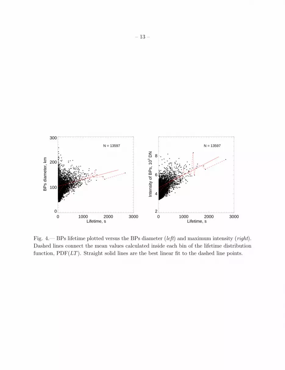
The regression plots of the diameter and maximum intensity of BPs versus their

lifetime (Figure 4) show the presence of a direct proportionality: BPs that live longer, tend

to be larger and brighter.

5. Conclusions

A two-hour data set of quiet sun granulation obtained with highest to-date spatial

and temporal resolution (77 km diffraction limit NST images with a time cadence of 10

s) was analyzed to obtain statistical distributions of size, lifetime and maximum intensity

– 8 –

of photospheric BPs. An NST TiO image was compared with co-temporal and co-spatial

image from Hinode/SOT obtained in G-band.

NST BPs are co-spatial with those visible in Hinode/SOT G-band data. This result

allows us to take advantages of observations with the TiO filter, in contrast to the G-band

filter: the adaptive optics system and the speckle reconstruction code are more efficient

when observing at longer wavelengths. We see a clear improvement caused by the higher

resolution of the NST: in cases where Hinode/SOT detects one large BP, NST detects

several separated BPs. In addition, NST detects numerous small and weak BPs which are

not visible in the Hinode/SOT data. Extended filigree features are clearly fragmented into

separate BPs in the NST images. The majority of BPs have a circular shape, however,

some of them are elongated.

We found a weak positive proportional relationship between the lifetime, on one hand,

and the BP’s size and intensity, on the other hand. So that brighter and larger BPs tend to

live longer.

The distribution function, PDF(D), of the BP’s size extents down to the diffraction

limit of NST (77 km). The saturation and the turnover of PDF(D), visible at smaller

scales, might be caused by the fact that NST does not resolve properly elements smaller

than 77 km. This result is consistent with PDFs derived from Hinode/G-band data (Utz

et al. 2009): the Hinode PDFs also saturate at the diffraction limit of the instrument. The

best approximation for the observed PDF(D) is found to be a log-normal fit with a mean

value m = 4.157 and a standard deviation s = 0.382 of ln(D). The log-normal fit performs

better than the exponential and power laws over the entire range of diameters above 67 km.

The mode of the log-normal distribution, em, occurs at D = 64 km, which is lower than

the diffraction limit. Unlike the power law, the log-normal distribution is not scale-free,

therefore, there is a limit on a minimal size of an elementary flux tube. However, the real

minimum size may not have been achieved yet from observations with modern telescopes.

The log-normal nature of the size distribution implies that the fragmentation and merging

processes are important mechanisms contributing into evolution and dynamics of BPs (e.g.,

Abramenko & Longcope 2005). Frequent fragmentation and coalescence are clearly visible

in the data set movie4.

The observed distribution function of the BP’s lifetimes can be best fitted with a

log-normal approximation. The NST lifetime distribution function qualitatively agrees with

that reported by de Wijn et al. (2005) inside the overlap interval, while Utz et al (2010)

reported an exponential distribution for the lifetime of Hinode BPs in the interval of 2-12

4http://bbso.njit.edu/nst-galery.html

– 9 –

minutes. In out study, the overall slope of the PDF(LT ) in this particular 2-12 minutes

interval is nearly the same as reported by Utz et al. (2010), however, it appears that the

power law is the best analytical fit inside this particular interval.

About 98.6% of all BPs live less than 120 s (12 time steps). This remarkable fact was

not obvious from previous studies because an extremely high time cadence was required.

The fact indicates that the majority of BPs appear for very short time (tens of seconds),

similar to other transient features, for example, chromospheric rapid blue-shift events

(RBEs), Rouppe van der Voort et al. (2009). The most important point here is that

these small and short living BPs significantly increase dynamics (flux emergence, collapse

into BPs, and magnetic flux recycling) of unipolar network areas. These unipolar fields

make it difficult to invoke reconnection between the emerging and pre-existing flux as an

explanation for the RBEs. However, the fact that the network field is more dynamic than

expected may allow to apply the component reconnection approach. The magnetic field is

fragmented into flux concentrations with well defined interfaces between them known as

current sheets. Random motions of BPs, as well as often appearance/disappearance of new

flux concentrations, will change the spatial distribution of the current sheets thus leading

to component reconnection and to release of energy.

It is interesting that we did not find a power law to be the best fit inside a whole

available scale interval for any of the tested parameters. Two reasons for that might

be advanced. First, a reign of the power law inside the interval from zero to infinity is

impossible unless the analyzed field is a computer-generated monoflactal. Second, a power

law implies self-similarity - scaling with the same index - inside the entire range where this

law reigns. This means a monofractal structure of the field, and, therefore, an absence of

multifractality. At the same time, processes and structures formed in a natural way possess

different scaling indices for different scale intervals; in other words, they are multifractals.

As broader range of scales becomes available for observations, the stronger is the deviation

of the observed distributions from a pure power law.

This work was supported by NSF grants ATVI-0716512, ATM-0745744 and

ATM0847126, and NASA grants VNX08AJ20G, NNX08AQ89G, and NNX08BA22G,

AFOSR (FA9550-09-1-0655) and SOLAR-B subcontract through Lockheed (8100000779).

Hinode is a Japanese mission developed and launched by ISAS/JAXA, with NAOJ as

domestic partner and NASA and STFC (UK) as international partners. It is operated by

these agencies in co-operation with ESA and NSC (Norway).

– 10 –

Table 1: Parameters of the Distribution Functions for BP’s Diameter, Lifetime and Intensity

Parameter D, km LT , s Imax, DN

Exponential

Distribution

c1 0.404±0.091 -3.20±0.29 6.18±0.31

β -0.406±0.0008 -0.00427±0.00032 -0.00204±1e-05

χ2 0.26 1.11 3.04

∆ 68 - 159 516 - 1226 4472 - 7540

Power Law

Distribution

c2 15.50±1.18 3.05±0.18 43.2±1.3

α -8.27±0.51 -1.99±0.07 -12.1±0.3

χ2 0.60 0.06 0.63

∆ 160 - 254 91 - 706 4724 - 7804

Log-Normal

Distribution

m 4.157±0.034 4.64±0.12 8.29±0.01

s 0.382±0.018 1.00±0.06 0.150±0.005

χ2 0.030 0.071 18.0

∆ >67 >100 >4200

REFERENCES

Abramenko, V. I., Longcope, D. W. 2005, ApJ, 619, 1160

Aitchison, J., Brown, J.A.C. 1957,”The Lognormal Distribution”, London, Eng.: Cambridge

University Press.

Berdyugina, S. V., Solanki, S. K., Frutiger, C. 2003, A& A, 412, 513

Berger, T.E., Title, A.M. 2001,ApJ, 533, 449

Cao, W., Gorceix, N., Coulter, R., Ahn, K., Rimmele, T. R., Goode, P. R. 2010,

Astronomische Nachrichten, 331, 636

Cranmer, S.R., 2002, Space Sci. Rev., 101, 229

Cranmer, S. R., van Ballegooijen, A. A. 2005, ApJ Suppl. Ser., 156, 265

Cranmer, S. R., van Ballegooijen, A. A. 2010, ApJ, 720, 824

de Wijn, A. G., Rutten, R. J., Haverkamp, E. M. W. P., Stterlin, P. 2005, A& A, 441, 1183

– 11 –

de Wijn, A. G., Lites, B. W., Berger, T. E., Frank, Z. A., Tarbell, T. D., Ishikawa, R. 2008,

ApJ, 648, 1469

Goode, P. R., Yurchyshyn, V., Cao, W., Abramenko, V., Andic, A., Ahn, K., Chae, J. 2010,

ApJ, 714, L31

Ishikawa, R., Tsuneta, S., Kitakoshi, Y., Katsukawa, Y., Bonet, J. A., Vargas Domnguez,

S., Rouppe van der Voort, L. H. M., Sakamoto, Y., Ebisuzaki, T. 2007, A& A, 472,

911

Rouppe van der Voort, L., Leenaarts, J., de Pontieu, B., Carlsson, M., Vissers, G. 2009,

ApJ, 705, 272

Klimchuk, J.A., 2006, Solar Phys., 234, 41

Kosugi, T., Matsuzaki, K., Sakao, T., Shimizu, T., Sone, Y. and 20 co-authors 2007, Solar

Phys.,243, 3

Muller, R., Dollfus, A., Montagne, M., Moity, J., Vigneau, J. 2000, A& A, 359, 373

Parker, E. 1978, ApJ, 221, 368

Riethmuller, T. L., Solanki, S. K., Zakharov, V., Gandorfer, A. 2008, A& A, 492, 233

Romeo, M., Da Costa, V. & Bardou, F., 2003, Eur. Phys. J. B, 32, 513

Spruit, H.C. 1979, Solar Phys., 61, 363

Tsuneta, S., Ichimoto, K., Katsukawa, Y., Nagata, S., Otsubo, M., and 20 co-authors 2008,

Solar Phys., 249, 167

Utz, D., Hanslmeier, A., Mostl, C., Muller, R., Veronig, A., Muthsam, H. 2009, A& A, 498,

289

Utz, D., Hanslmeier, A., Muller, R., Veronig, A., Rybak, J., Muthsam, H.2010, A& A, 511,

A39

Woger, F., von der Luhe, O., Reardon, K. 2008, A& A, 488, 375

This preprint was prepared with the AAS LATEX macros v4.0.

– 12 –

0 50 100 150 200 250 300BPs diameter, D, km

10-5

10-4

10-3

10-2

10-1

100

PD

F(D

)

a

100BPs diameter, D, km

b

0 1000 2000 3000BPs lifetime, LT, s

10-5

10-4

10-3

10-2

10-1

100

PD

F(L

T)

c

100 1000BPs lifetime, LT, s

d

3 4 5 6 7 8 9Intensity of BPs, 103 DN

10-5

10-4

10-3

10-2

10-1

100

PD

F(I

max

)

e

10Intensity of BPs, 103 DN

f

Fig. 3.— PDFs of the BPs diameter (a,b),lifetime (c,d), and maximum intensity (e,f). Left

column shows the data for both runs: for the mask threshold of 85 DN (black), and 120 DN

(red). Straight thick blue lines in all left frames show the exponential fit to the data points

calculated inside a range between the vertical thin blue lines. In all the right frames, the log-

normal and power-law fits were applied inside intervals, ∆, covered by the purple and green

lines, respectively. In the frames a,b, the vertical dashed segment shows the position of the

Rayliegh diffraction limit of NST for observations with the TiO filter. Blue and green double

curves show the distribution of BPs size from Hinode G-band observations as reported by

Utz et al. (2009): blue (green) line for the pixel size of 0.109′′ (0.054′′).

– 13 –

0 1000 2000 3000 Lifetime, s

0

100

200

300

BP

s di

amet

er, k

m

N = 13597

0 1000 2000 3000 Lifetime, s

2

4

6

8

Inte

nsity

of B

Ps,

103 D

NN = 13597

Fig. 4.— BPs lifetime plotted versus the BPs diameter (left) and maximum intensity (right).

Dashed lines connect the mean values calculated inside each bin of the lifetime distribution

function, PDF(LT ). Straight solid lines are the best linear fit to the dashed line points.