static spherically symmetric solutions of the so(5) einstein yang-mills equations

arX

iv:0

907.

3975

v1 [

gr-q

c] 2

3 Ju

l 200

9

STATIC SPHERICALLY SYMMETRIC SOLUTIONS OF THE

SO(5) EINSTEIN YANG-MILLS EQUATIONS

ROBERT BARTNIK, MARK FISHER, AND TODD A. OLIYNYK

Abstract. Globally regular (ie. asymptotically flat and regular interior), spher-ically symmetric and localised (“particle-like”) solutions of the coupled Ein-

stein Yang-Mills (EYM) equations with gauge group SU(2) have been knownfor more than 20 years, yet their properties are still not well understood. Spher-ically symmetric Yang–Mills fields are classified by a choice of isotropy genera-tor and SO(5) is distinguished as the simplest model with a non-Abelian resid-ual (little) group, SU(2)×U(1), and which admits globally regular particle-likesolutions. We exhibit an algebraic gauge condition which normalises the resid-ual gauge freedom to a finite number of discrete symmetries. This generalisesthe well-known reduction to the real magnetic potential w(r, t) in the originalSU(2) YM model. Reformulating using gauge invariant polynomials dramat-ically simplifies the system and makes numerical search techniques feasible.We find three families of embedded SU(2) EYM equations within the SO(5)system, one of which was first detected only within the gauge-invariant polyno-mial reduced system. Numerical solutions representing mixtures of the threeSU(2) sub-systems are found, classified by a pair of positive integers.

1. Introduction

The LHC experiments currently underway at CERN are expected to settle promi-nent vexing questions such as the origin of the Higgs mechanism, the existence ofsupersymmetry in nature, and the meaning of dark matter. However, regardless ofthe discoveries still to flow from the LHC, we can with confidence predict that thegoverning equations will incorporate the Einstein equations for the gravitationalfield and the Yang-Mills equations for some non-Abelian gauge group. From thisperspective, the spherically symmetric solutions of the SU(2)-EYM equations dis-covered numerically in [11]1 are particularly important, for several reasons. First,the particle-like properties exhibited by the solutions, namely static, asymptoticallyflat, and globally regular with spatial topology R

3, confound previous expectations,based on the known non-existence results for the vacuum Einstein equations andfor the YM equations separately, that such solutions could not exist. On the otherhand, they confirm Wheeler’s “geon” hypothesis [15], that localised semi-boundgravitational (and with hindsight, Yang–Mills) configurations might exist.

Numerical and perturbation results [17,18] show that the SU(2) EYM sphericallysymmetric solutions may be viewed as an unstable balance between a dispersive YMand the attractive gravitational force. However, there are many aspects of thesesystems which have not yet been studied in depth, and it seems premature toconclude that instability is inevitable — see the review [16].

2000 Mathematics Subject Classification. 83C20, 65L10.1Existence of global solutions was proved rigorously in [12, 13].

1

http://arxiv.org/abs/0907.3975v1

2 R. BARTNIK, M. FISHER, AND T.A. OLIYNYK

The most detailed results have generally been obtained in the static sphericallysymmetric setting with the simplest YM gauge group SU(2), which exhibits manyof the basic properties of the general non-Abelian group models. The sphericallysymmetric reduction of the EYM equations can be viewed as a 2D EYM-Higgssystem with a residual gauge group, GΛ3 , a residual Higgs field (to be defined below),and a “Mexican hat” potential. Most attention has focused on the case where thegauge group is SU(n) and the residual group is Abelian, primarily because in thiscase it is possible to completely fix the gauge freedom. If the residual group isnon-Abelian, then it is known [4, 5] that the issue of gauge fixing becomes muchmore challenging.

To better understand gauge fixing and solutions to the the static sphericallysymmetric EYM equations we study G = SO(5), which is the simplest gauge groupthat supports a globally regular model with non-Abelian residual group. This modelwas discussed in [4], but the questions of gauge fixing and the existence of solutionswere not resolved. We solve this problem here by using a related system satisfied bypolynomials in the gauge fields which are invariant under the action of the residualgauge group.

2. Static spherically symmetric field equations

Spherical symmetry for Yang-Mills fields is complicated to define because thereare many ways to lift an SO(3) action on space-time to an action on the Yang-Mills connections. For real compact semisimple gauge groups G, it was shownin [1, 3] that equivalent spherically symmetric Yang-Mills connections correspondto conjugacy classes of homomorphisms of the isotropy subgroup, U(1), into G. Thelatter, in turn, are given by their generator Λ3, the image of the basis vector τ3 ofsu(2) (where τi, i = 1, . . . , 3 is a standard basis with [τi, τj ] = ǫk

ijτk), lying in anintegral lattice I of a Cartan subalgebra h0 of the Lie algebra g0 of G. This vectorΛ3, when nontrivial, then characterizes up to conjugacy an su(2) subalgebra.2

With the vector Λ3 ∈ g0 fixed, a gauge and a coordinate system (t, r, θ, φ) canbe chosen [1, 3] so that the metric and gauge potential take the form

ds2 = −S(r)2(

1 − 2m(r)

r

)

dt2 +

(

1 − 2m(r)

r

)−1

dr2 + r2(

dθ2 + sin2 θ dφ2)

,

and3

A = Λ1(r)dθ + (Λ2(r) sin θ + Λ3 cos θ)dφ,

where Λ1(r), Λ2(r) are g0-valued maps satisfying

(2.1) [Λ3, Λ1(r)] = Λ2(r), and [Λ2(r), Λ3] = Λ1(r).

It is more convenient to use the following variables,

(2.2) Λ0 := 2iΛ3, and Λ± := ∓Λ1 − iΛ2,

which lie in g, the complexification of g0. The conditions (2.1) on Λ1, Λ2 thenimply that the connection functions Λ± are valued in the residual Higgs bundles,V±2, defined by

(2.3) Λ±(r) ∈ V±2 := X ∈ g | [Λ0, X ] = ±2X .

2This ignores some interesting effects due to the fact that SO(3) is not simply connected. Foran analysis of SO(3) actions on SU(2) bundles see [2].

3Here we are assuming the ansatz, that the gauge potential is “purely magnetic”.

STATIC SPHERICALLY SYMMETRIC SOLUTIONS OF THE SO(5) EYM EQUATIONS 3

The residual (gauge) group GΛ3 is defined as the connected Lie subgroup withLie algebra

gΛ3 := X ∈ g0 | [Λ3, X ] = 0 .We call the residual group (non-)Abelian if this is a (non-)Abelian Lie algebra. ForgΛ3 to be non-Abelian it is necessary but not sufficient that Λ0 lies on the boundaryof a Weyl chamber of h, a Cartan subalgebra of g.

In the variables (2.2), the EYM equations become [6]

m′ =N

2||Λ′

+||2 +1

8r2||Λ0 − [Λ+, Λ−]||2,(2.4)

r2(

S2NΛ′+

)′+ S

(

Λ+ − 1

2[[Λ+, Λ−], Λ+]

)

= 0,(2.5)

[Λ′+, Λ−] + [Λ′

−, Λ+] = 0,(2.6)

S−1S′ =1

r||Λ′

+||2,(2.7)

where N = (1 − 2m/r). The S parameter can be decoupled from the system,decreasing the order of the overall system by one but introducing a first order termin (2.5). Also note that the second term in (2.5) is proportional to the gradient of thesecond term in (2.4). Requiring that the solutions are regular and asymptoticallyflat gives boundary conditions

[Λ+, Λ−] = Λ0, and [[Λ+, Λ−], Λ+] = 2Λ+

at r = 0, and as r → ∞, respectively.The ||·||-norm is proportional, on each irreducible component of g, to the the real

part of the Hermitean inner-product derived from the Killing form [6]. Multiplying|| · || by a constant factor leads via a global rescaling of m and r to the originalequations. Specifically, we have:

Proposition 1. If (m(r), Λ+(r)) satisfies (2.4)-(2.6), then (αm(r/α), Λ+(r/α))satisfies the equations obtained by replacing || · || in equations (2.4)-(2.6) with α|| · ||.Proof. Substitution.

The EYM system (2.4)-(2.6) typically admits subfamilies of solutions which alsosatisfy the original SU(2) but with rescaled norm || · || (see Section 5). We mayregard such solutions are equivalent to the original SU(2), since all values areconsistently rescaled from the values in the original reports [7–9].

3. An SO(5) model

We now specialize to the gauge group G = SO(5). The complexified Lie algebrag = so(5, C) has the Cartan decomposition

g = h ⊕⊕

α∈R

Ceα,

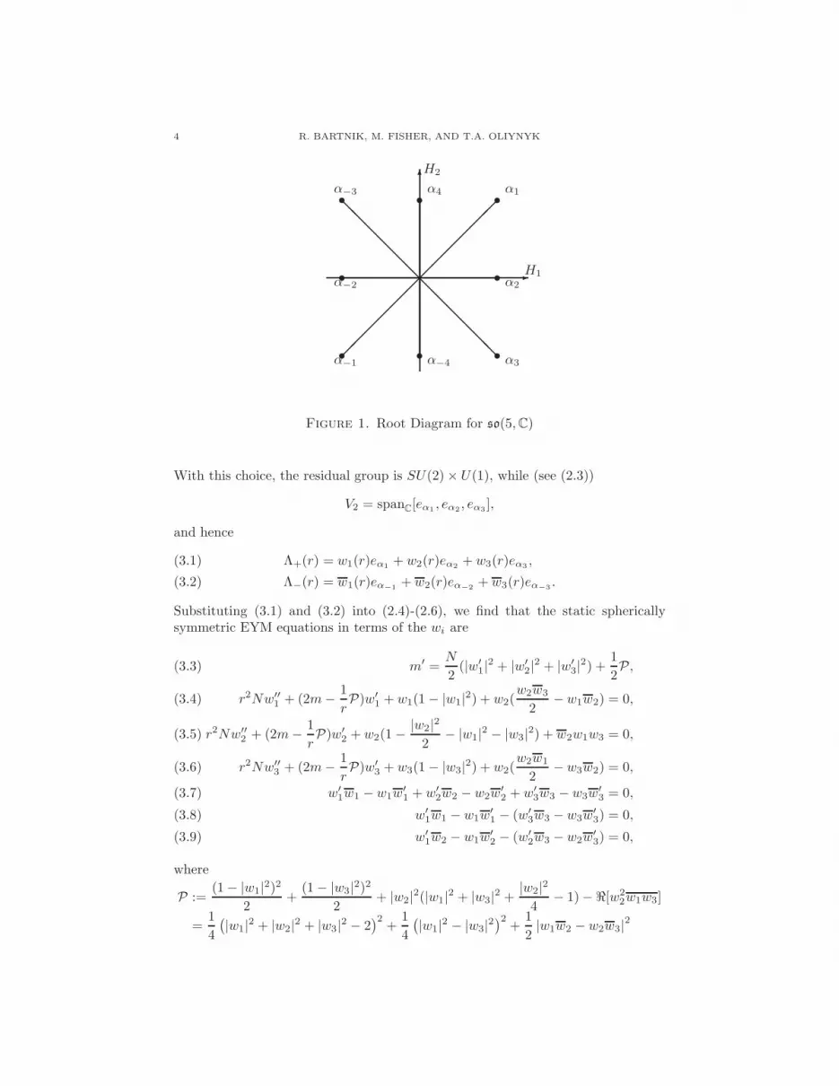
where h = spanC[hα1, hα2

] is the Cartan subalgebra, R = α±i, i = 1, . . . , 4 is aroot system in h∗ with root diagram as in Figure 1.

The reduced spherically symmetric EYM model depends strongly on the choiceof isotropy generator Λ0. For G = SO(5), we choose [4]

Λ0 = 2H1.


s s s

s s

s s s

-

6

@@

@@

@@

@@

@@

@@

H1

H2

α−1

α−2

α−3

α−4

α4

α3

α2

α1

Figure 1. Root Diagram for so(5, C)

With this choice, the residual group is SU(2) × U(1), while (see (2.3))

V2 = spanC[eα1, eα2

, eα3],

and hence

Λ+(r) = w1(r)eα1+ w2(r)eα2

+ w3(r)eα3,(3.1)

Λ−(r) = w1(r)eα−1

+ w2(r)eα−2

+ w3(r)eα−3

.(3.2)

Substituting (3.1) and (3.2) into (2.4)-(2.6), we find that the static sphericallysymmetric EYM equations in terms of the wi are

m′ =N

2(|w′

1|2 + |w′2|2 + |w′

3|2) +1

2P ,(3.3)

r2Nw′′1 + (2m − 1

rP)w′

1 + w1(1 − |w1|2) + w2(w2w3

2− w1w2) = 0,(3.4)

r2Nw′′2 + (2m − 1

rP)w′

2 + w2(1 − |w2|22

− |w1|2 − |w3|2) + w2w1w3 = 0,(3.5)

r2Nw′′3 + (2m − 1

rP)w′

3 + w3(1 − |w3|2) + w2(w2w1

2− w3w2) = 0,(3.6)

w′1w1 − w1w

′1 + w′

2w2 − w2w′2 + w′

3w3 − w3w′3 = 0,(3.7)

w′1w1 − w1w

′1 − (w′

3w3 − w3w′3) = 0,(3.8)

w′1w2 − w1w

′2 − (w′

2w3 − w2w′3) = 0,(3.9)

where

P :=(1 − |w1|2)2

2+

(1 − |w3|2)22

+ |w2|2(|w1|2 + |w3|2 +|w2|2

4− 1) −ℜ[w2

2w1w3]

=1

4

(

|w1|2 + |w2|2 + |w3|2 − 2)2

+1

4

(

|w1|2 − |w3|2)2

+1

2|w1w2 − w2w3|2


The boundary conditions are

|w1|2 + |w2|2 + |w3|2 = 2,(3.10)

|w1| − |w3| = 0,(3.11)

w1w2 − w2w3 = 0,(3.12)

at r = 0, and

w1(1 − |w1|2) + w2(w2w3

2− w1w2) = 0,(3.13)

w2(1 − |w2|22

) − w2(|w1|2 + |w3|2) + w2w1w3 = 0,(3.14)

w3(1 − |w3|2) + w2(w2w1

2− w3w2) = 0,(3.15)

as r → ∞.The sets of boundary conditions (3.10)-(3.12) and (3.13)-(3.15) define algebraic

varieties on C3 and as such they do not restrict the initial and final values to oneparticular point in C3 (or indeed a discrete set of such points). Given a point lyingon one of these varieties there will in general be a set of gauge-equivalent points butit is not immediately obvious what these equivalence classes of points are from thedefining equations. This is a problematic feature of all models with a non-Abelianresidual gauge group and will be discussed elsewhere.

4. Gauge fixing and the reduced equations

For the SO(5) model, a direct computation shows that the ansatz

(4.1) Λ+(r) = u(r)eα1+ 0eα2

+ v(r)eα3, u(r), v(r) ∈ R

automatically satisfies the constraint equations (2.6) (equivalently (3.7)-(3.9)), whilethe equations (2.4)-(2.5) (equivalently (3.3)-(3.6)) reduce to

r2Nu′′ +

(

2m − (1 − u2)2 + (1 − v2)2

2r

)

u′ + u(1 − u2) = 0,(4.2)

r2Nv′′ +

(

2m − (1 − u2)2 + (1 − v2)2

2r

)

v′ + v(1 − v2) = 0,(4.3)

m′ =N

2((u′)2 + (v′)2) +

1

4r2((1 − u2)2 + (1 − v2)2),(4.4)

with boundary conditions

(4.5) u2 + v2 = 2, |u| = |v|at r = 0 and

(4.6) u(1 − u2) = 0, v(1 − v2) = 0

as r → ∞.The above results show that (4.1) is a consistent ansatz for the static spherically

symmetric EYM equations. In fact the equations that result could have been ob-tained from a model with gauge group SU(2) × SU(2). However, it is not obvious


that the choice (4.1) is equivalent to fixing a section of the gauge fields. To see thiswe use the fact that the following two polynomials

K1 := 2||Λ+||2 =2(

|w1|2 + |w2|2 + |w3|2)

,

K2 := 2||[Λ−, Λ+]||2 =4|w1|4 + 2|w2|4 + 4|w3|4

+8|w1|2|w2|2 + 8|w3|2|w2|2 − 8Re[w22w1w3],

are a complete set of generators4 for the ring of residual-group-invariant polynomialsin Λ+. When (w1, w2, w3) = (u, 0, v) for real u, v, these become

K1 = 2(u2 + v2), and K2 = 4(u4 + v4).

These equations can be inverted to give

u = ±1

(

K1

4±3

√

2K2 − K21

4

)1

2

, and v = ±2

(

K1

4∓3

√

2K2 − K21

4

)1

2

which are well-defined for all K1, K2 since the inequalities

2K2 − K21 ≥ 0, and K2 − K2

1 ≤ 0

follow directly from the definition of K1 and K2. The ±-signs amount to choosingwhich function is u and which is v and deciding on an arbitrary convention for theirinitial values.

5. Numerical results

From the form of the reduced equations (4.2)-(4.4), it is clear that we can maketwo distinct simplifying assumptions u = v or v = ±1 (equivalently u = ±1).

(i) Setting u = v, the reduced equations (4.2)-(4.4) become

r2Nu′′ +

(

2m − (1 − u2)2

r

)

u′ + u(1 − u2) = 0,

m′ = N(u′)2 +1

2r2(1 − u2)2.

which is the SU(2) equation and has the well-known Bartnik-McKinnon family ofsolutions [7,11]. We note that these correspond to the embedded SU(2) solutions asthey satisfy Λ±(r) = u(r)Ω± where Ω± are fixed vectors satisfying [Λ0, Ω±] = 2Ω±

and [Ω+, Ω−] = Λ0.

(ii) Setting v = 1, the reduced equations (4.2)-(4.4) become

r2Nu′′ +

(

2m − (1 − u2)2

2r

)

u′ + u(1 − u2) = 0,

m′ =N

2(u′)2 +

1

4r2(1 − u2)2.

As in Proposition 1, rescaling these equations by√

2 in m and r results in theSU(2)-equations above, giving another family of solutions where the u field is aradially-scaled Bartnik-McKinnon solution with smaller mass and the v field re-mains constant.

4This can be established by computing the Molien function to determine the appropriate ordersof the polynomials and then verifying K1 and K2 are algebraically independent. See [10] for someuseful formulae.


Figure 2. A plot of the solutions in the space of the invariantpolynomials. All solutions start at (4, 8).The type (i) SU(2) so-lutions lie on the K2 = 1

2K21 curve, while the type (ii) SU(2)

solutions lie on the K2 = (K1 − 2)2 + 4 curve. The type (iii) so-lutions are curves in the combined interior of the three parabolastouching the boundaries tangentially (an illustration of the (2,1)type (iii) solution is shown)

For the above two special situations, existence of a countably infinite numberof solutions is guaranteed by the existence theorems in [7, 12, 13]. Integrating thereduced equations (4.2)-(4.4) numerically, we also find evidence for solutions thatare not of the type (i) or (ii) above. We will call these solutions type (iii). Figure 2indicates where these solutions lie in the space of invariant polynomials. All threetypes of solutions can be characterized by the number of nodes of the functions uand v. Figure 3 enumerates all of the solutions that were found numerically or thatare known to exist analytically. The type (i) solutions lie on the diagonal nu = nv,while the type (ii) solutions lie on either the horizontal nv = 0 or vertical axisnu = 0. The remaining solutions are of type (iii) and are indicated on the nodediagram by the larger circles. We conjecture, based on the diagram, that for each(nu, nv) ∈ Z≥0 × Z≥0 there exists a solution to the reduced equations (4.2)-(4.4)satisfying the boundary conditions (4.5)-(4.6).

For the numerical analysis we use the “shooting to a fitting point” method [14],using the Matlab routine ode45 which is a fourth-order Runge-Kutta solver. Using


b

r

r

r

r

r

r r r r r

b

u

u

u

b

u

u

u

b

b

b

-

-

-

-

-

- -

- -

- -

- -

-

0 1 2 3 4 5

1

2

3

4

5

-

6

nu

nv

Figure 3. Node Diagram for solutions to the reduced equation

the power series expansions

u = 1 + a1r2 + (

2

5a31 +

2

5a1a

22 +

3

10a21)r

4 + O(r6),

v = 1 + a2r2 + (

2

5a2a

21 +

2

5a32 +

3

10a22)r

4 + O(r6),

m = (a21 + a2

2)r3 + (

4

5a31 +

4

5a32)r

5 + O(r7),

near r = 0, and

u = ±1 +b1

r+ O(

1

r2),

v = ±1 +b2

r+ O(

1

r2),

m = m∞ + O(1

r3),

near r = ∞. We shoot from the origin out trying to maximise (by searching in theparameters ai evaluated at r = 0.01) the r-value that is attained before the solutionviolates one of the necessary conditions for a global smooth solution. Suitablelarge r-values will then give an indication what the bi and m∞ parameters shouldapproximately be for the shooting back from some large r-value (we use r = 10000).We then use these parameter values as an initial guess in the “shooting to a fittingpoint” search, where the fitting was done at r = 10.

6. Discussion

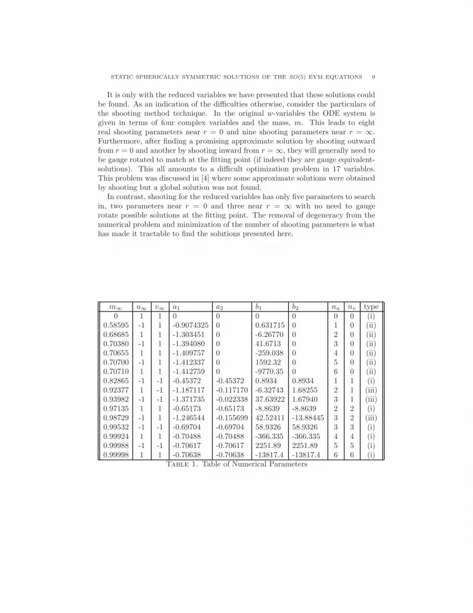
We have found three solutions using the numerical technique from the previoussection. When combined with the two families of SU(2) type solutions, they suggestthat there is a solution for each point (nu, nv) on the nonnegative integer lattice,where nu, nv denote the number of nodes of u and v respectively. The numericalvalues are given in Table 1 and some type (iii) solutions are displayed in Figures 4and 5.


It is only with the reduced variables we have presented that these solutions couldbe found. As an indication of the difficulties otherwise, consider the particulars ofthe shooting method technique. In the original w-variables the ODE system isgiven in terms of four complex variables and the mass, m. This leads to eightreal shooting parameters near r = 0 and nine shooting parameters near r = ∞.Furthermore, after finding a promising approximate solution by shooting outwardfrom r = 0 and another by shooting inward from r = ∞, they will generally need tobe gauge rotated to match at the fitting point (if indeed they are gauge equivalent-solutions). This all amounts to a difficult optimization problem in 17 variables.This problem was discussed in [4] where some approximate solutions were obtainedby shooting but a global solution was not found.

In contrast, shooting for the reduced variables has only five parameters to searchin, two parameters near r = 0 and three near r = ∞ with no need to gaugerotate possible solutions at the fitting point. The removal of degeneracy from thenumerical problem and minimization of the number of shooting parameters is whathas made it tractable to find the solutions presented here.

m∞ u∞ v∞ a1 a2 b1 b2 nu nv type0 1 1 0 0 0 0 0 0 (i)

0.58595 -1 1 -0.9074325 0 0.631715 0 1 0 (ii)0.68685 1 1 -1.303451 0 -6.26770 0 2 0 (ii)0.70380 -1 1 -1.394080 0 41.6713 0 3 0 (ii)0.70655 1 1 -1.409757 0 -259.038 0 4 0 (ii)0.70700 -1 1 -1.412337 0 1592.32 0 5 0 (ii)0.70710 1 1 -1.412759 0 -9770.35 0 6 0 (ii)0.82865 -1 -1 -0.45372 -0.45372 0.8934 0.8934 1 1 (i)0.92377 1 -1 -1.187117 -0.117170 -6.32743 1.68255 2 1 (iii)0.93982 -1 -1 -1.371735 -0.022338 37.63922 1.67940 3 1 (iii)0.97135 1 1 -0.65173 -0.65173 -8.8639 -8.8639 2 2 (i)0.98729 -1 1 -1.246544 -0.155699 42.52411 -13.88445 3 2 (iii)0.99532 -1 -1 -0.69704 -0.69704 58.9326 58.9326 3 3 (i)0.99924 1 1 -0.70488 -0.70488 -366.335 -366.335 4 4 (i)0.99988 -1 -1 -0.70617 -0.70617 2251.89 2251.89 5 5 (i)0.99998 1 1 -0.70638 -0.70638 -13817.4 -13817.4 6 6 (i)

Table 1. Table of Numerical Parameters


−2 −1 0 1 2 3 4

−1

−0.8

−0.6

−0.4

−0.2

0

0.2

0.4

0.6

0.8

1

m u

v

log10(r)

Figure 4. The (2, 1) type (iii) solution. The mass, m, increasesmonotonically from 0 to 0.924, u starts and ends at 1 with twonodes and v goes from +1 to −1 with one node.

−2 −1 0 1 2 3 4

−1

−0.8

−0.6

−0.4

−0.2

0

0.2

0.4

0.6

0.8

1

m

u

v

log10(r)

Figure 5. The (3, 2) type (iii) solution. The mass, m, increasesmonotonically from 0 to 0.987, u goes from 1 to −1 with threenodes and v goes from +1 to +1 with two nodes.

References

[1] R. Bartnik, The spherically symmetric Einstein Yang-Mills equations, Relativity Today, ed.Z. Perjes (Tihany, Nova, Science, Commack, XY, 1992), 221-240.

[2] R. Bartnik, The structure of spherically symmetric su(n) Yang-Mills fields, J. Math. Phys.38 (1997), 3623-3638.

[3] O. Brodbeck and N. Straumann, A generalized Birkhoff theorem for the Einstein-Yang-Millssystem, J. Math. Phys 34 (1993), 2412-2423.

[4] T.A. Oliynyk and H.P. Kunzle, On all possible static spherically symmetric EYM solitonsand black holes, Class. Quantum Grav. 19 (2002), 457-482.

[5] T.A. Oliynyk and H.P. Kunzle, On global properties of static spherically symmetric EYMfields with compact gauge groups, Class. Quantum Grav. 20 (2003), 4653-4682.


[6] T.A. Oliynyk and H.P. Kunzle, Local existence proofs for the boundary value problem forstatic spherically symmetric Einstein-Yang-Mills fields with compact gauge groups, J. Math.Phys. 43 (2002), 2363-2393.

[7] P. Breitenlohner, P. Forgacs and D. Maison, Static spherically symmetric solutions of theEinstein-Yang-Mills equations, Comm. Math. Phys. 163 (1994), 141-172.

[8] H.P. Kunzle, Analysis of the static spherically symmetric SU(n)-Einstein-Yang-Mills equa-tions, Comm. Math. Phys. 162 (1994), 371-397.

[9] B. Kleihaus, J. Kunz and A. Sood, SU(3) Einstein Yang-Mills Sphalerons And Black Holes,Phys. Lett. B 354 (1995), 240-246.

[10] M. Forger, Invariant Polynomials and Molien Functions. J. Math. Phys. 39 (1998), 1107–1141.

[11] R. Bartnik and J. McKinnon, Particle-like solutions of the Einstein-Yang-Mills equations.Phys. Rev. Lett. 61 (1988), 141-144.

[12] J.A. Smoller, A.G. Wasserman, S.-T. Yau and J.B. McLeod, Smooth static solutions of theEinstein/Yang-Mills equations, Comm. Math. Phys. 143 (1991), 115-147.

[13] J.A. Smoller and A.G. Wasserman, Existence of infinitely many smooth, static, global solu-tions of the Einstein/Yang-Mills equations, Comm. Math. Phys. 151 (1993), 303-325.

[14] W.H. Press, S.A. Teukolsky, W.T. Vetterling and B.P. Flannery, Numerical recipes in C++.The art of scientific computing. Second edition, updated for C++. Cambridge University

Press, Cambridge, 2002.[15] J.A. Wheeler, Geons, Phys. Rev. 97 (1957), 511-536.[16] M.S. Volkov and D.V. Gal’tsov, Gravitating non-Abelian solitons and black holes with Yang-

Mills fields Phys.Rept.319 (1999), 1-83.[17] O. Brodbeck and N. Straumann, Instabilities of Einstein-Yang-Mills Solitons for Arbitrary

Gauge Groups, Phys.Lett. B 324 (1994), 309-314.[18] M.W. Choptuik, T. Chmaj and P. Bizon, Critical Behaviour in Gravitational Collapse of a

Yang-Mills Field, Phys.Rev.Lett. 77 (1996), 424-427.

School of Mathematical Sciences, Monash University, VIC 3800, Australia

E-mail address: [email protected]





static spherically symmetric solutions of the so(5) einstein yang-mills equations

Documents