BANK OF FINLAND DISCUSSION PAPERS

28 • 2004

Antti Suvanto – Juhana Hukkinen Economics Department

30.12.2004

Stable price level and changing prices

Suomen Pankin keskustelualoitteita Finlands Banks diskussionsunderlag

Suomen Pankki Bank of Finland

P.O.Box 160 FIN-00101 HELSINKI

Finland � + 358 10 8311

http://www.bof.fi

BANK OF FINLAND DISCUSSION PAPERS

28 • 2004

Antti Suvanto – Juhana Hukkinen Economics Department

30.12.2004

Stable price level and changing prices*

The views expressed are those of the authors and do not necessarily reflect the views of the Bank of Finland.

* Paper presented in the Western Economic Association International Meeting in Vancouver, Canada, in 2 July 2004. The first version of the paper was written in fall 2001, when the first of the authors listed was a Visiting Fellow at the European University Institute in Fiesole, Italy. The paper has benefited from comments by Michael Artis, Lars Jonung, James W. Kolari, Jouko Vilmunen and Naoyuki Yoshino.

Suomen Pankin keskustelualoitteita Finlands Banks diskussionsunderlag

http://www.bof.fi

ISBN 952-462-180-0 ISSN 0785-3572

(print)

ISBN 952-462-181-9 ISSN 1456-6184

(online)

Multiprint Oy Helsinki 2004

3

Stable price level and changing prices

Bank of Finland Discussion Papers 28/2004

Antti Suvanto – Juhana Hukkinen Economics Department Abstract

The paper investigates the relationship between relative price movements and changes in the aggregate price level using monthly data on Finland’s Consumer Price Index and its components from the period covering the past eight and a half years. This was a period of very low inflation. The rate of growth in the aggregate price level was occasionally very close to zero. The paper shows that declining nominal prices were a rather common phenomenon during this period of low or no inflation. The declining prices cannot, however, be explained by lack of demand or any generalized deflationary tendencies. Hence, the downward rigidity of nominal prices has not prevented relative price adjustments under price stability. The paper develops a new method for looking at the composition of inflation and illustrating how relative price dynamics interact with changes in the aggregate price level. The correlation of relative price variability and aggregate inflation has been negligible, but the correlation between the skewness of price change distribution and aggregate inflation is high. This is in accordance with the predictions of the menu cost models. A significant proportion of the relative price changes appear to have been persistent, suggesting the dominance of productivity and other supply shocks. Key words: price level, inflation, deflation, prices, business cycles JEL classification numbers: E3, E31

4

Vakaa hintataso ja muuttuvat hinnat

Suomen Pankin keskustelualoitteita 28/2004

Antti Suvanto – Juhana Hukkinen Kansantalousosasto Tiivistelmä

Tässä tutkimuksessa selvitetään suhteellisten hintojen muutosten ja yleisen hinta-tason muutosten välisiä yhteyksiä. Havaintoaineistona käytetään kuukausitietoja Suomen kuluttajahintaindeksistä ja sen alaeristä kahdeksan ja puolen viime vuo-den aikana. Tänä ajanjaksona inflaatio oli Suomessa varsin hidas. Ajoittain ku-luttajahintaindeksin vuotuinen nousu oli lähellä nollaa. Tavaroiden ja palveluiden hintojen lasku oli varsin yleistä. Kysymys ei kuitenkaan ollut kysynnän puutteesta johtuvasta yleisestä deflaatiosta. Päinvastoin kulutuskysyntä kasvoi tasaisesti. Tämä osoittaa, että hintojen laskua jäykistävät tekijät eivät estä suhteellisten hin-tojen muutoksia, vaikka hintataso kokonaisuudessaan pysyykin vakaana. Tutki-muksessa esitellään menetelmä, jonka avulla voidaan kuvata suhteellisten hintojen muutosten voimakkuutta ja yhteyksiä koko hintaindeksin muutoksiin. Suhteellis-ten hintojen muutosintensiteetin ja keskimääräisen hintojen muutoksen välinen korrelaatio osoittautuu heikoksi. Sitä vastoin korrelaatio hintojen muutosjakauman vinouden ja keskimääräisen inflaation välillä on vahva, mikä vastaa uusien hinnoittelumallien (menu cost) tuloksia. Merkittävä osa suhteellisten hintojen muutoksista on pysyvää tai ainakin hyvin pitkäaikaista, mikä viittaa siihen, että tuottavuuden muutokset ja muut tarjontatekijät pitkälti määräävät suhteellisten hintojen muutokset. Avainsanat: hintataso, inflaatio, deflaatio, hinnat, suhdannevaihtelut JEL-luokittelu: E3, E31

5

Contents

Abstract ....................................................................................................................3 Tiivistelmä ...............................................................................................................4 1 Introduction ......................................................................................................7 2 How common are declining prices?..............................................................11 3 Measurement methodology ...........................................................................15 3.1 The composition of inflation: the cumulative sum of ordered contributions...............................................................................15 3.2 The intensity of relative price changes: the cumulative sum of ordered deviations....................................................................................17 4 Inflation and relative price movements........................................................19 5 Dealing with longer horizons.........................................................................24 6 Interpretation .................................................................................................26 References..............................................................................................................29

6

7

1 Introduction

Like many other countries, Finland has experienced an extended period of low inflation. Some years can be even characterised as periods of no inflation. Price stability does not imply a lack of dynamism in price movements. Indeed, relative price dynamics are an essential part of the workings of the price mechanism. A positive productivity shock should, under competitive conditions, lead to a decline in the relative price of the product concerned. A shift of preferences from one good to another should be reflected in a change in the relative price of these goods and possibly in other goods as well. In principle, the price mechanism can work equally well and relative prices could move in the same manner irrespective of the behaviour of the price level at least as long as the rate of inflation or deflation is stable and well anticipated. Then there should be no problems in distinguishing relative price movements from fluctuations in the general price level. On the other hand, if both the rate of inflation and inflation variability are high, the quality of price information deteriorates, weakening the functioning of the price mechanism.1 This is the well-known sand effect of inflation, also known as the Friedman argument (Friedman 1977). The Chairman of the Federal Reserve Board, Alan Greenspan, has defined price stability as follows2: “Price stability obtains when economic agents no longer take account of the prospective change in the general price level in their economic decision making.” One could argue that under price stability the functioning of the price mechanism is more efficient, because a change in a price set by one seller immediately signals a change in its relative price, to which the buyers and other sellers can react without delay. Furthermore, if the price level is expected to remain stable, a seller cannot react to his local cost pressure by raising the price of the product because customers would search for other suppliers who have not raised their prices. Only those relative price increases would be accepted

1 The inability of the agents to distinguish relative price movements from changes in the aggregate price level is the underlying assumption of the Lucas supply function, which has become a cornerstone of modern macroeconomics (Lucas 1973). 2 In his opening Address to the Federal Reserve Bank of Kansas City 1966 Symposium; see Annual Report 1996, p. 13.

8

which are known to be based on a change in the structure of demand or the reduction of supply.3 What about absolute price declines under price stability? Any buyer would be happy to accept a decline in the price of a good as long as he is sure that the quality has not declined. Any producer should start to consider price reductions if his productivity improves, provided that there is competition amongst sellers. In the case of a positive productivity shock, the downward flexibility of prices does not even require that wages are equally flexible downwards. It follows that under conditions of price stability, absolute price declines should be a frequently observed phenomenon just like absolute price increases. If, however, individual prices are more rigid downwards than upwards, then aiming at price stability may weaken the functioning of the price mechanism because the dynamics of relative price movements are weakened. It has, indeed, been argued that for this reason too low an inflation rate may hurt the economy. This is the well-known grease effect of inflation, also known as the Tobin argument (Tobin 1972; see also Akerlof, Dickens and Perry 1996, Andersen 2001). Relative price changes, or rather the factors that cause them, are usually described as supply shocks or real shocks. A real shock is one that calls for a change in relative prices but has no predictable effect on the aggregate price level. These have to be distinguished from aggregate demand shocks or nominal or monetary shocks, as they are also called. A nominal shock is one that only affects the price level but has no predictable effect on relative prices. The relationship between the rate of inflation and the distribution of relative price changes has for long been the subject of empirical research. A number of empirical studies have found that there is a positive correlation between the rate of inflation and the variability of relative prices (Vining and Elwertowski 1976, Fischer 1971, Domberger 1987, Mizon, Safford and Thomas 1991, and Parsley 1996). The second empirical regularity seems to be a strong positive correlation between the rate of inflation and the skewness of the distribution of price changes (Vining and Elwertowski 1976, Ball and Mankiw 1995, and Balke and Wynne 2000). Indeed, many studies indicate that the correlation between inflation and the

3 This argument is spelled out elegantly by Jerry Jordan, the President of the Federal Reserve Bank of Cleveland: “If an economy’s monetary unit is known to be a stable standard of value, then changes in money prices will accurately reflect changes in the relative values of goods and assets. That is, price fluctuations signal changes in the demand for and supply of goods and assets. Resource utilization then shifts toward more valued uses and away from those less valued. According to a former Governor of the Federal Reserve, ‘a place that tolerates inflation is a place where no one tells the truth.’ So true changes in the relative values of things cannot be observed from stated prices when the purchasing power of money is not stable. The standard of value is stable when people can make decisions in the confident expectation that all observed changes in money prices are changes in relative price” (Jordan 2000).

9

skewness of the price change distribution is higher than the correlation between the mean and the standard deviation of price changes. In the literature there are two broad categories of explanations for the correlation between mean inflation, the standard deviation and the skewness of price changes. The first category of models assumes a nominal rigidity of prices, while in the second category of models full price flexibility is assumed. In the first category of models, price stickiness is typically explained by some form of menu costs of price adjustment (Mankiw 1985, Ball, Mankiw and Romer 1988).4 Based on a particular type of a menu cost model, Ball and Mankiw (1995) give a theoretical explanation for these types of correlation. In their model, each firm sets the price before a real shock arrives. The shock affects the desired structure of the relative prices in such a manner that the general price level should not change. If, however, it affects different firms differentially, and if only some firms are willing to pay the menu cost and adjust the price, while others are not, the general price level is affected as a result. A large positive asymmetric shock, such as an oil price increase, makes those firms for which oil is an important cost willing to adjust the price despite the menu cost, while for most other firms the required price decline is so small that they are not yet willing to adjust the price. Because some prices increase but others do not fall, the general price index increases. In the second category of models, a positive correlation between the rate of inflation and the skewness of the distribution of price changes is consistent with full price flexibility. Balke and Wynne (2000) present a multi-sector flexible price model, where the productivity shocks are immediately reflected in prices. A positive productivity shock in one sector raises output and lowers prices.5 Hence technology shocks and price changes are negatively correlated. The positive mean-skewness correlation may result from the asymmetric distribution of technology shocks across sectors but also from the input-output structure of the economy. If some sectors produce products that are important inputs in other sectors, then the distribution of price changes may be skewed even if technology shocks are symmetric across sectors. This approach can be extended to cover other types of real shocks, such as terms-of-trade shocks. For instance, an increase in oil prices affects different sectors differentially. Prices rise in those sectors for

4 For a survey of the menu cost literature, see Cassino (1995). Before the menu cost models became popular, price (and wage) stickiness were since Tobin (1972) simply assumed by referring to social customs and fairness (in the case of wages) (Kahneman et al 1986) or to macroeconomic policy rules (Fischer 1981). 5 From Tobin (1972) to Andersen (2001), the literature emphasising the grease effects of inflation pays attention to the downward rigidity of wages, whereas real business cycle models, such as the one formulated by Balke and Wynne (2000), assume full price flexibility. Nominal wage flexibility and nominal price flexibility need not go hand in hand. With flexible prices, positive productivity shocks lead to declining prices in the sectors affected while wages may stay constant or even increase.

10

which oil is an important input whereas in most other sectors prices decline slightly. The price level may go up to the extent the real output declines with nominal demand remaining constant. The relationship between inflation and relative price variability as measured by the standard deviation is less clear in these kinds of models. While it is clear that relative price variability is positively related to the distribution of technology shocks, a precondition for a positive correlation between inflation and relative price variability is that the mean of the technology shocks is negatively correlated to their standard deviation, which is not obvious. Also the positive correlation between the rate of inflation and the skewness of the distribution of price changes has been disputed. For example, Bryan and Cecchetti (1999) argue that the observed mean-skewness correlation suffers from a small-sample bias, which is particularly serious for distributions with fat tails. They make Monte Carlo simulations in order to show that there is no correlation once the data are corrected for this bias. Commenting on the paper by Bryan and Cecchetti, Verbrugge (1999) presents alternative Monte Carlo simulations that show the presence of the mean-skewness correlation at a horizon of one month while at a horizon of one year the reverse may be true. However, he admits that it is unclear whether his findings have any economic significance. Ball and Mankiw (1999), in turn, argue that the Bryan and Cecchetti results have no obvious economic interpretation because their purely statistical model deviates from the classical constraint according to which sectoral shocks can determine only N-1 relative prices while the price level and N nominal prices are determined by monetary factors. This paper aims to address some of the issues discussed above. It investigates the relationship between relative price movements and changes in the aggregate price level in Finland during the past eight years. We use the monthly data on the Consumer Price Index (CPI) from January 1995 to May 2004. The full set of data covers information on the aggregate price index as well as on the price indices of all components of the CPI and their respective weights. The initial motivation to look at this data was, in fact, our curiosity to know how common absolutely declining prices have been in a country where price stability has prevailed over an extended period. Interestingly, this question has seldom been raised. This curiosity led us to develop a new method for looking at the composition of inflation in order to illustrate how relative price dynamics interact with changes in the aggregate price level. This, in turn, led us to construct a new indicator to measure the intensity of relative price changes. The remainder of the paper is organised as follows. Section 2 describes the history of inflation in Finland since 1996, paying special attention to the prevalence of absolutely declining prices. Section 3 presents the measurement methodology and applies it to selected months from each of the eight years. Section 4 describes the development of the intensity of the relative price

11

movements over time. Section 5 extends the analysis to horizons longer than 12 months. Section 6 concludes the paper with an attempt to interpret relative price dynamics and the interaction with inflation in terms of different types of shocks. 2 How common are declining prices?

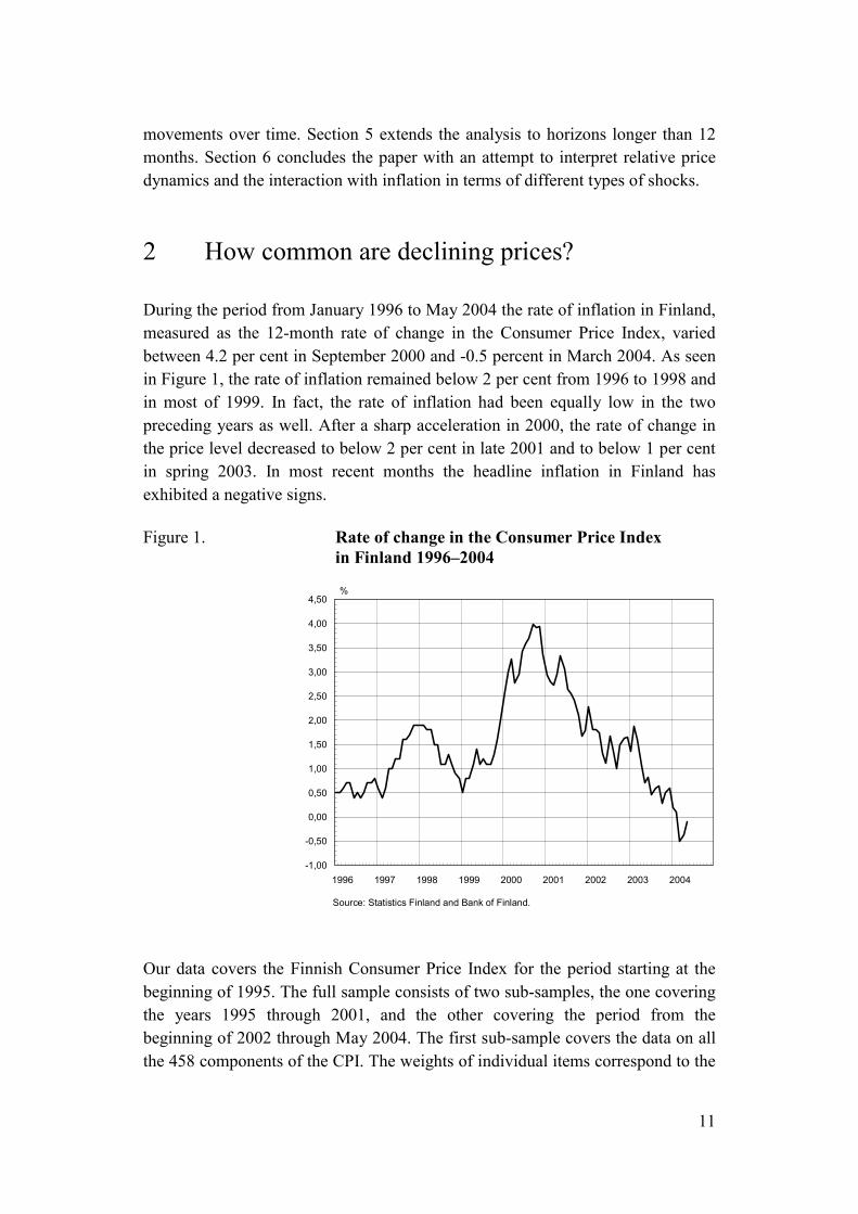
During the period from January 1996 to May 2004 the rate of inflation in Finland, measured as the 12-month rate of change in the Consumer Price Index, varied between 4.2 per cent in September 2000 and -0.5 percent in March 2004. As seen in Figure 1, the rate of inflation remained below 2 per cent from 1996 to 1998 and in most of 1999. In fact, the rate of inflation had been equally low in the two preceding years as well. After a sharp acceleration in 2000, the rate of change in the price level decreased to below 2 per cent in late 2001 and to below 1 per cent in spring 2003. In most recent months the headline inflation in Finland has exhibited a negative signs. Figure 1. Rate of change in the Consumer Price Index in Finland 1996–2004

-1,00

-0,50

0,00

0,50

1,00

1,50

2,00

2,50

3,00

3,50

4,00

4,50

1996 1997 1998 1999 2000 2001 2002 2003 2004

%

Source: Statistics Finland and Bank of Finland. Our data covers the Finnish Consumer Price Index for the period starting at the beginning of 1995. The full sample consists of two sub-samples, the one covering the years 1995 through 2001, and the other covering the period from the beginning of 2002 through May 2004. The first sub-sample covers the data on all the 458 components of the CPI. The weights of individual items correspond to the

12

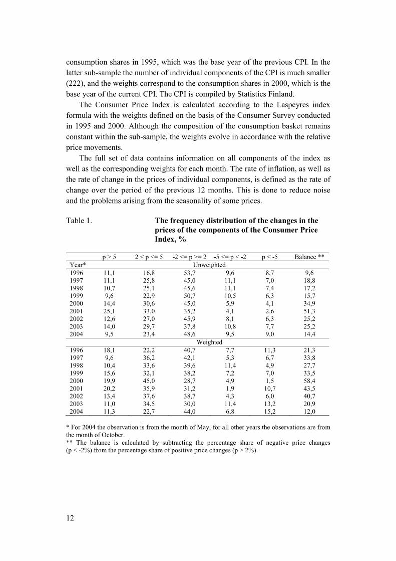
consumption shares in 1995, which was the base year of the previous CPI. In the latter sub-sample the number of individual components of the CPI is much smaller (222), and the weights correspond to the consumption shares in 2000, which is the base year of the current CPI. The CPI is compiled by Statistics Finland. The Consumer Price Index is calculated according to the Laspeyres index formula with the weights defined on the basis of the Consumer Survey conducted in 1995 and 2000. Although the composition of the consumption basket remains constant within the sub-sample, the weights evolve in accordance with the relative price movements. The full set of data contains information on all components of the index as well as the corresponding weights for each month. The rate of inflation, as well as the rate of change in the prices of individual components, is defined as the rate of change over the period of the previous 12 months. This is done to reduce noise and the problems arising from the seasonality of some prices. Table 1. The frequency distribution of the changes in the prices of the components of the Consumer Price Index, %

p > 5 2 < p <= 5 -2 <= p >= 2 -5 <= p < -2 p < -5 Balance ** Year* Unweighted 1996 11,1 16,8 53,7 9,6 8,7 9,6 1997 11,1 25,8 45,0 11,1 7,0 18,8 1998 10,7 25,1 45,6 11,1 7,4 17,2 1999 9,6 22,9 50,7 10,5 6,3 15,7 2000 14,4 30,6 45,0 5,9 4,1 34,9 2001 25,1 33,0 35,2 4,1 2,6 51,3 2002 12,6 27,0 45,9 8,1 6,3 25,2 2003 14,0 29,7 37,8 10,8 7,7 25,2 2004 9,5 23,4 48,6 9,5 9,0 14,4 Weighted 1996 18,1 22,2 40,7 7,7 11,3 21,3 1997 9,6 36,2 42,1 5,3 6,7 33,8 1998 10,4 33,6 39,6 11,4 4,9 27,7 1999 15,6 32,1 38,2 7,2 7,0 33,5 2000 19,9 45,0 28,7 4,9 1,5 58,4 2001 20,2 35,9 31,2 1,9 10,7 43,5 2002 13,4 37,6 38,7 4,3 6,0 40,7 2003 11,0 34,5 30,0 11,4 13,2 20,9 2004 11,3 22,7 44,0 6,8 15,2 12,0

* For 2004 the observation is from the month of May, for all other years the observations are from the month of October. ** The balance is calculated by subtracting the percentage share of negative price changes (p < -2%) from the percentage share of positive price changes (p > 2%).

13

As mentioned above, the initial motivation for writing this paper was our curiosity to see how common declining prices have been compared to rising prices. A simple way to find an answer to this question is to look at the raw data. Table 1 shows the frequency distribution of the price changes of all the components of the price index classified in five groups according to the magnitude of the price movement. The observations in the table have been selected from the month of October in each year, except for 2004, when the observation is from the month of May, the latest observation in our sample. The choice of the month does not matter much, because the rates of changes in the prices have been calculated over a 12-month period. The column on the right hand side shows the balance between the percentage share of positive price changes and the percentage share of negative price changes. Price changes close to zero per cent, between -2 and 2 per cent, have not been taken into account. This choice is admittedly arbitrary. The upper panel shows the frequency distribution of unweighted price changes, whereas in the lower panel the price changes have been weighted by the importance of the respective components in the price index. The upper panel of the table reveals that declining prices were rather common in the years of no inflation in 1996–1998. Close to 20 per cent of all the items of the Consumer Price Index showed then declining prices, while close to 50 per cent of items had prices that remained more or less constant. Nevertheless, rising prices were more common than declining prices with the balance rising from 7 to 17 per cent between 1996 and 1998. As expected, the relative frequency of declining prices came down and the balance rose in 2000 when inflation accelerated from below 2 to above 4 per cent. It is interesting to note that declining prices became even rarer between 2000 and 2001 despite a sharp slowdown of inflation. Since 2002 declining prices have again become more common, and the balance between rising and declining prices has reached the levels obtained in the first years of the sample. The lower panel, where the relative frequencies have been weighted by the relative importance of the components in the price index, gives essentially a similar picture. In 2000–2001 rising prices became more important in the aggregate index relative to declining prices. Since 2002 the relative contribution of declining prices to the aggregate index has again become more prominent. The differences between the upper and the lower column reflect the fact that the acceleration and the deceleration of inflation usually reflect the price movements of a few items, such as energy or rents, which weigh heavily in the consumer price index. In general the drift of the frequency distribution from the right to the left (in the table) reflects the fact that rising prices are becoming more common. This should be a warning concerning the risk of accelerating inflation despite the fact that the headline inflation may be temporarily decelerating.

14

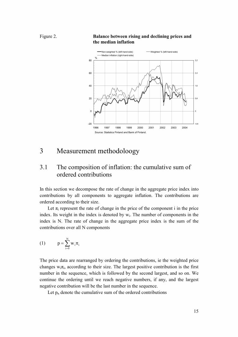
Figure 2 depicts the balance between the rising and declining prices calculated in a way similar to that in Table 1 for the full sample period. A curve showing the median inflation rate is also included. Because of the skewness of the distribution of price changes, the median typically deviates from the mean. This indicator is often used in monitoring inflation, because it is not prone to being influenced by extremes.6 The acceleration of inflation in 2000 shows up, as expected, in a pronounced increase in the number of rising prices. Both the unweighted and weighted balances more than doubled. The consumption-share weighted balance started to increase already in the first half of 1999 and peaked around the end of 2000, at which time over 65% of the CPI prices rose and only about 5% fell. Since then it has been trending downward while the unweighted balance continued to increase until the end of 2001. This provides further evidence that first the acceleration and later the slowing-down of inflation were tied to just a few heavily-weighted products (energy). The fact that the unweighted balance followed the weighted balance with a lag when inflation was accelerating probably reflects the fact that inflation was gradually becoming more generalized. It is interesting to note that the unweighted balance goes hand-in-hand with median inflation. We have some difficulties in interpreting the figures for early 2002 because of the discontinuity in the data. Nevertheless, it seems that both the balance indicators and the median inflation have returned to the same level that had been observed in the previous period of no inflation.

6 For example, see the section on prices in Economic Trends of the Federal Reserve Bank of Cleveland. The median is an extreme version of the trimmed mean approach to the measurement of core inflation; see Bryan and Cecchetti (1994), Clark (2001), and Vega and Wynne (2001).

15

Figure 2. Balance between rising and declining prices and the median inflation

-20

0

20

40

60

80

1996 1997 1998 1999 2000 2001 2002 2003 2004

%

-0,8

0

0,8

1,6

2,4

3,2

Non-weighted % (left-hand-side) Weighted % (left-hand-side)Median inflation (right-hand-side)

Source: Statistics Finland and Bank of Finland. 3 Measurement methodoloogy

3.1 The composition of inflation: the cumulative sum of ordered contributions

In this section we decompose the rate of change in the aggregate price index into contributions by all components to aggregate inflation. The contributions are ordered according to their size. Let πi represent the rate of change in the price of the component i in the price index. Its weight in the index is denoted by wi. The number of components in the index is N. The rate of change in the aggregate price index is the sum of the contributions over all N components

(1) ∑=

π=

N

0iiiwp

The price data are rearranged by ordering the contributions, ie the weighted price changes wiπi, according to their size. The largest positive contribution is the first number in the sequence, which is followed by the second largest, and so on. We continue the ordering until we reach negative numbers, if any, and the largest negative contribution will be the last number in the sequence. Let pn denote the cumulative sum of the ordered contributions

16

(2) N,...,1n,wp k

n

1kkn =π=∑

=

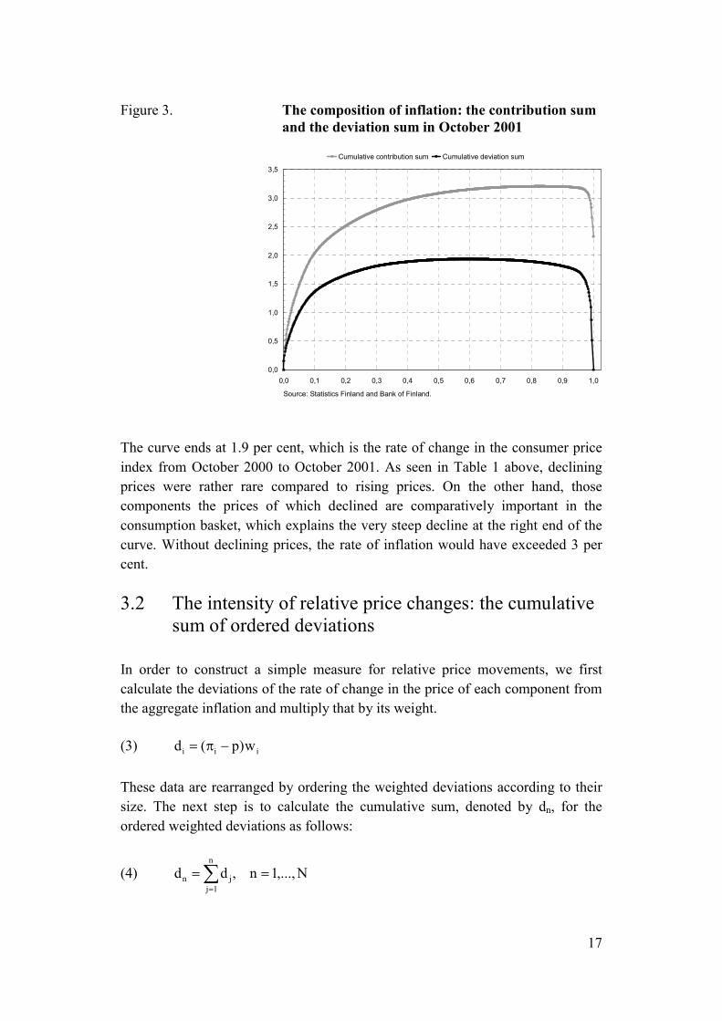
Note that pN = p, that is, the sum of all contributions is equal to the measure of aggregate inflation. For illustrative purposes we add p0 = 0 to the beginning of the sequence. Note that the subscript i has been replaced by k in order to illustrate the ordering of the contributions by their size. The shape of the ordered sequence is concave in its construction. In the beginning pn rises with n, although at a diminishing rate. Moving to the right the curve becomes flatter and turns downwards when the components showing absolute price declines, if any, are added to the sequence. The sequence pn, ie the cumulative sum of ordered contributions, can be used to illustrate relative price movements and aggregate inflation in the same diagram. At the same time, it reveals immediately how common absolute price declines are compared to price increases for individual components of the price index. The more curvy the diagram, the larger the movements in relative prices. The cumulative sum of ordered contributions would be concave even in the absence of any relative price changes, ie if πk = p for all k, as long as the weights are not identical for all components. The curve becomes a straight line if all components have equal weights and there are no relative price movements at all. In this case the weight for each component is 1/N, and the cumulative sum of ordered contributions reduces to pn = (n/N)p. We use data from the Finnish Consumer Price Index from October 2001 as an illustration. The upper curve in Figure 3 depicts the composition of inflation in terms of the cumulative sum of ordered contributions of the price changes of all 458 components of the price index. The lower curve is the cumulative sum of ordered deviations, which will be defined below. The horizontal axis has been normalised to the range [0,1].

17

Figure 3. The composition of inflation: the contribution sum and the deviation sum in October 2001

0,0

0,5

1,0

1,5

2,0

2,5

3,0

3,5

0,0 0,1 0,2 0,3 0,4 0,5 0,6 0,7 0,8 0,9 1,0

Cumulative contribution sum Cumulative deviation sum

Source: Statistics Finland and Bank of Finland. The curve ends at 1.9 per cent, which is the rate of change in the consumer price index from October 2000 to October 2001. As seen in Table 1 above, declining prices were rather rare compared to rising prices. On the other hand, those components the prices of which declined are comparatively important in the consumption basket, which explains the very steep decline at the right end of the curve. Without declining prices, the rate of inflation would have exceeded 3 per cent. 3.2 The intensity of relative price changes: the cumulative

sum of ordered deviations

In order to construct a simple measure for relative price movements, we first calculate the deviations of the rate of change in the price of each component from the aggregate inflation and multiply that by its weight. (3) iii w)p(d −π= These data are rearranged by ordering the weighted deviations according to their size. The next step is to calculate the cumulative sum, denoted by dn, for the ordered weighted deviations as follows:

(4) N,...,1n,ddn

1jjn ==∑

=

18

As above, we set d0 = 0 in order to make the sequence start from the origin. Note again that the subscript i has been replaced by j in order to illustrate the ordering of the weighted deviations by size. Note that the ordering need not be identical to the ordering of pn defined above. By construction dn > 0 for n = 1, …, N-1. The last number of the sequence, dN, is zero, as can be seen by replacing dj with πj-p in equation (4). The resulting diagram begins from zero and ends up at zero. In between, it is rising with n in the beginning and declining towards the end of the range [0,N]. In the absence of any relative price change, ie when all individual prices change exactly in proportion, all deviations are equal to zero as is the cumulative sum of deviations. The more common and the larger the relative price movements are, the higher the surface is between the horizontal axis and the curve. The area can be approximated by the cumulative sum of ordered deviations. Dividing this by the total number of components gives a measure for the intensity of relative price changes, which we denote by IRPC,

(5) ∑=

=

N

0nn .N/dIRPC

The lower curve in Figure 3 illustrates the idea using, once again, the data from October 2001. The cumulative sum of deviations rises sharply in the beginning and continues to rise at a diminishing rate until about 40 per cent of the components have been accounted for. It stays rather flat over the range [0.4, 0.8], after which it starts to decline progressively. The last 5 per cent of the components account for most of the decline. The measure of the intensity of the relative price movements obtains the value 1.7, which as a number in itself is of little significance unless it is compared with the similar statistics from other periods. This will be done below. The shape of the curve may reveal interesting information on the structure of relative prices changes. The two extreme shapes are that of a rectangle and that of a triangle. A rectangle is obtained if there is one good the relative price of which rises and one good the relative price of which declines with all other prices rising at the same rate as the aggregate price index. The two goods at the extreme ends of the ordering must have a high weight in the index or the relative price changes must be huge. A symmetric triangle would be obtained for identical weights if one half of all prices were to rise at a rate which is a given percentage point above the aggregate inflation and the other half of the prices were to fall at a rate which is below the average by the same percentage point. In practice the skewness of the

19

distribution of weights affects the shape of the curve by making the curve rise rather steeply in the beginning and decline steeply at the end. The shape of the curve depicting the cumulative sum of ordered deviations in Figure 3 is typical for the distributions of price changes. It is, therefore, useful to compare it to more commonly used statistical frequency distribution functions. The steepness of the curve at both ends of the diagram reflects the presence of fat tails (high kurtosis) in the frequency distribution function. The long flat stretch, in turn, is a reflection of the fact that a large proportion of price changes are concentrated around the peak of the distribution. The deviation sum is skewed to the left (right) when large positive (negative) deviations dominate. In an ordinary frequency function this shows up as skewness to the right (left). 4 Inflation and relative price movements

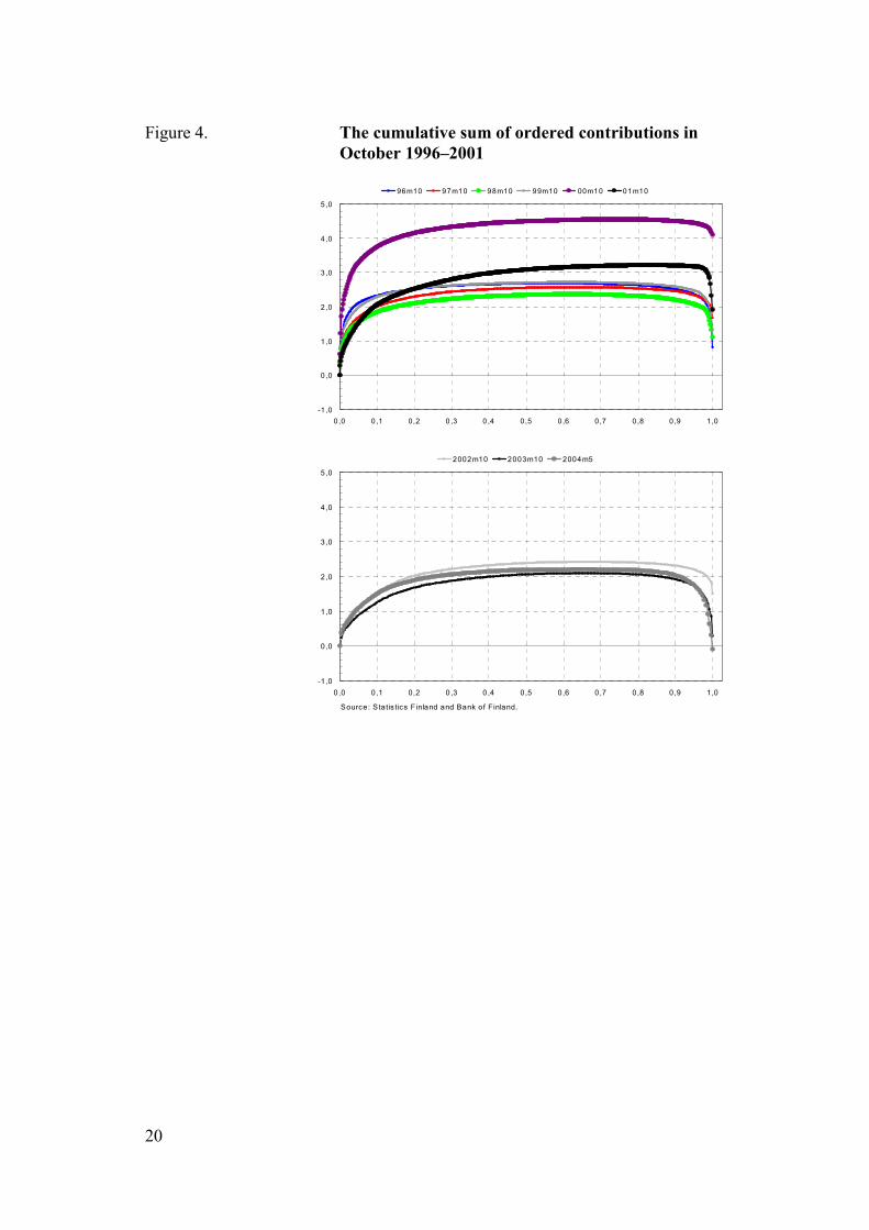
Figure 4 exhibits the cumulative sum of ordered contributions to the 12-month rate of change in the Consumer Price Index as well as the cumulative sum of deviations in October in each of the eight years 1996–2003 as well as in May 2004. The number of data points (components of the CPI) is smaller in the second sub-sample than in the first, for which reason the observations for 2002–2004 are presented in a separate chart in the lower panel. Figure 4 shows that the contribution sums are very similar for the two no inflation periods 1996–1999 and 2003–2004. In 1996–1999 the curves have a wide flat area in the range (0.2, 0.9). Rising prices were slightly more common than declining prices. In 2003–2004 the falling part of the curve was somewhat shorter, indicating that declining prices were rarer than in 1996–1999. Between October 1999 and October 2000 the curve jumped to an entirely new level as the rate of aggregate inflation rose from below 2 percent to 4 percent. It is evident that this rise was caused by the price increases of a small number of components which either were important in the index or experienced large price increases or both. Indeed, the price increases of around 10 percent of all 458 components accounted for most of the 4 per cent inflation. The shift of the curve between October 2000 and October 2001 is equally interesting. Although the rate of inflation slowed down by 2 percentage points, declining prices became even less common than 12 months earlier. The deceleration of inflation was to a large extent caused by the reversal of price changes in a few important components. In other respects price increases were becoming increasingly common.

20

Figure 4. The cumulative sum of ordered contributions in October 1996–2001

-1 ,0

0,0

1,0

2,0

3,0

4,0

5,0

0,0 0,1 0,2 0 ,3 0 ,4 0,5 0,6 0,7 0,8 0,9 1,0

96m10 97m10 98m10 99m10 00m10 01m10

-1,0

0,0

1,0

2,0

3,0

4,0

5,0

0,0 0,1 0,2 0 ,3 0 ,4 0,5 0,6 0,7 0,8 0,9 1,0

2002m10 2003m10 2004m5

Source: Statis tics Finland and Bank of Finland.

21

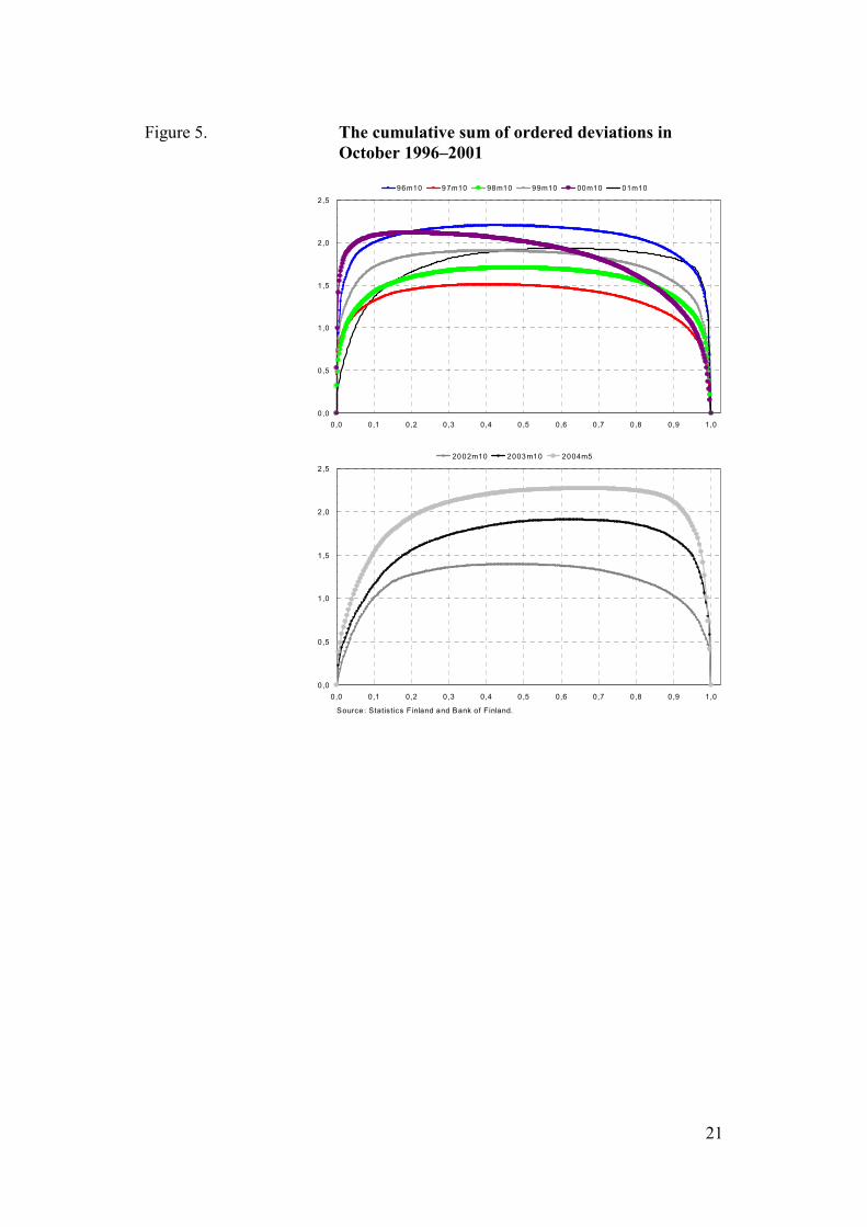
Figure 5. The cumulative sum of ordered deviations in October 1996–2001

0,0

0,5

1,0

1,5

2,0

2,5

0,0 0,1 0,2 0 ,3 0,4 0 ,5 0,6 0,7 0,8 0,9 1,0

96m10 97m10 98m10 99m10 00m10 01m10

0,0

0,5

1,0

1,5

2,0

2,5

0,0 0,1 0,2 0 ,3 0,4 0 ,5 0,6 0,7 0,8 0,9 1,0

2002m10 2003m10 2004m5

Source : Statistics Finland and Bank of Finland.

22

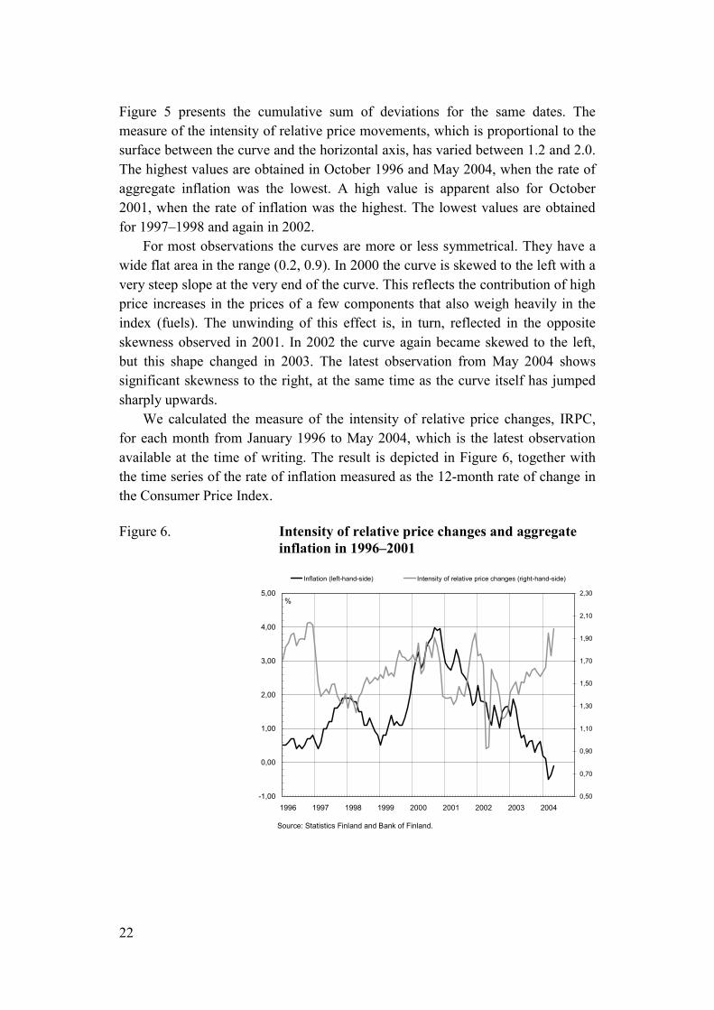
Figure 5 presents the cumulative sum of deviations for the same dates. The measure of the intensity of relative price movements, which is proportional to the surface between the curve and the horizontal axis, has varied between 1.2 and 2.0. The highest values are obtained in October 1996 and May 2004, when the rate of aggregate inflation was the lowest. A high value is apparent also for October 2001, when the rate of inflation was the highest. The lowest values are obtained for 1997–1998 and again in 2002. For most observations the curves are more or less symmetrical. They have a wide flat area in the range (0.2, 0.9). In 2000 the curve is skewed to the left with a very steep slope at the very end of the curve. This reflects the contribution of high price increases in the prices of a few components that also weigh heavily in the index (fuels). The unwinding of this effect is, in turn, reflected in the opposite skewness observed in 2001. In 2002 the curve again became skewed to the left, but this shape changed in 2003. The latest observation from May 2004 shows significant skewness to the right, at the same time as the curve itself has jumped sharply upwards. We calculated the measure of the intensity of relative price changes, IRPC, for each month from January 1996 to May 2004, which is the latest observation available at the time of writing. The result is depicted in Figure 6, together with the time series of the rate of inflation measured as the 12-month rate of change in the Consumer Price Index. Figure 6. Intensity of relative price changes and aggregate inflation in 1996–2001

-1,00

0,00

1,00

2,00

3,00

4,00

5,00

1996 1997 1998 1999 2000 2001 2002 2003 2004

%

0,50

0,70

0,90

1,10

1,30

1,50

1,70

1,90

2,10

2,30

Inflation (left-hand-side) Intensity of relative price changes (right-hand-side)

Source: Statistics Finland and Bank of Finland.

23

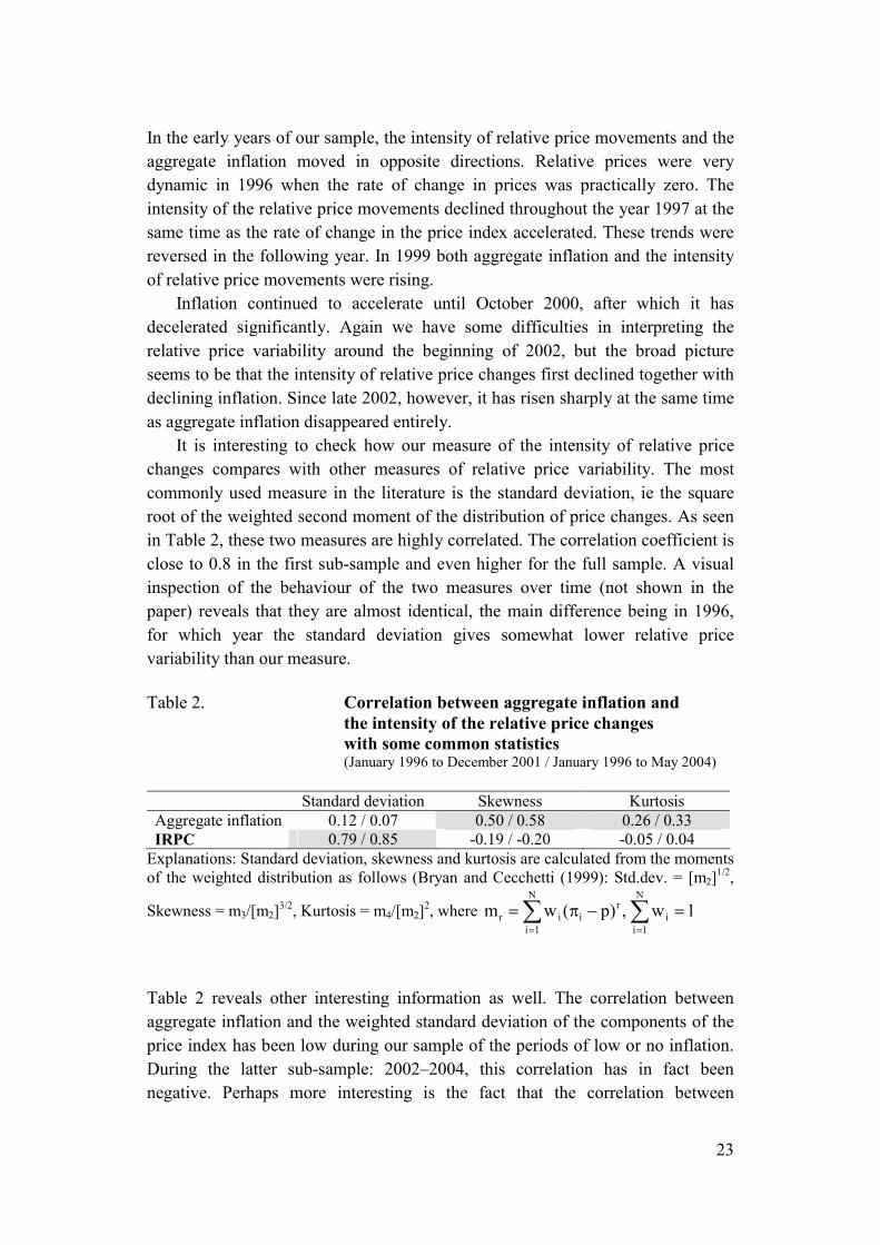
In the early years of our sample, the intensity of relative price movements and the aggregate inflation moved in opposite directions. Relative prices were very dynamic in 1996 when the rate of change in prices was practically zero. The intensity of the relative price movements declined throughout the year 1997 at the same time as the rate of change in the price index accelerated. These trends were reversed in the following year. In 1999 both aggregate inflation and the intensity of relative price movements were rising. Inflation continued to accelerate until October 2000, after which it has decelerated significantly. Again we have some difficulties in interpreting the relative price variability around the beginning of 2002, but the broad picture seems to be that the intensity of relative price changes first declined together with declining inflation. Since late 2002, however, it has risen sharply at the same time as aggregate inflation disappeared entirely. It is interesting to check how our measure of the intensity of relative price changes compares with other measures of relative price variability. The most commonly used measure in the literature is the standard deviation, ie the square root of the weighted second moment of the distribution of price changes. As seen in Table 2, these two measures are highly correlated. The correlation coefficient is close to 0.8 in the first sub-sample and even higher for the full sample. A visual inspection of the behaviour of the two measures over time (not shown in the paper) reveals that they are almost identical, the main difference being in 1996, for which year the standard deviation gives somewhat lower relative price variability than our measure. Table 2. Correlation between aggregate inflation and the intensity of the relative price changes with some common statistics (January 1996 to December 2001 / January 1996 to May 2004) Standard deviation Skewness Kurtosis Aggregate inflation 0.12 / 0.07 0.50 / 0.58 0.26 / 0.33 IRPC 0.79 / 0.85 -0.19 / -0.20 -0.05 / 0.04

Explanations: Standard deviation, skewness and kurtosis are calculated from the moments of the weighted distribution as follows (Bryan and Cecchetti (1999): Std.dev. = [m2]1/2,

Skewness = m3/[m2]3/2, Kurtosis = m4/[m2]2, where 1w,)p(wmN

1ii

ri

N

1iir =−π= ∑∑

==

Table 2 reveals other interesting information as well. The correlation between aggregate inflation and the weighted standard deviation of the components of the price index has been low during our sample of the periods of low or no inflation. During the latter sub-sample: 2002–2004, this correlation has in fact been negative. Perhaps more interesting is the fact that the correlation between

24

aggregate inflation and the weighted skewness of the distribution of price changes is surprisingly high, 0.50 or above. As explained above, this is consistent with the predictions of theoretical models and conforms to the evidence found elsewhere. It is interesting to note that this theoretical hypothesis gets support also from data that does not include periods of high or even moderate inflation. The correlation between aggregate inflation and the fourth moment (kurtosis) is positive and statistically significant, probably reflecting the importance of the price changes of some high-weight components of the price index. 5 Dealing with longer horizons

So far our analysis has been based solely on the 12-month changes in the price index and its components. We believe that relative price movements at this horizon most likely have an impact on the behaviour of firms and households irrespective of whether price changes are expected to be permanent or temporary. For example, significant changes in the relative price of some important products, such as fuels, are likely to affect behaviour even though their prices are known to be volatile and therefore the reversal of the relative price change is expected to take place before long. Month-to-month price changes contain predictable seasonal patterns and a lot of noise. But one could argue that the 12-month horizon is too short. While some relative price movements may indeed be temporary, the changes in the relative price of some other goods are likely to be persistent. For example, relative price movements arising from productivity shocks can be expected to be persistent or even diverging. Fortunately, our data and method allow us to make preliminary inferences about the intensity of relative price changes over longer time horizons. Because of the significance of some heavily-weighted items, such as fuels, food and housing-related items, the relative prices of which have shown large but reversible swings, we can expect that the intensity of relative price changes will diminish with the length of the horizon over which price changes have been calculated. If all prices were to be cointegrated, we should expect our measure of relative price variability to approach zero as the length of the horizon increases. In order to examine the effects of lengthening the horizon, we have calculated the cumulative sums of ordered deviations for price changes at the 24, 36, 48, 60 and 72-month horizons. Because of the discontinuity in the data, a 72-month horizon is the longest we can obtain from our first sub-sample covering the years 1996–2001. In order to preserve comparability, price changes and aggregate inflation are expressed as annual percentage changes. Figure 7 depicts the cumulative sums of ordered deviations calculated for price changes over the

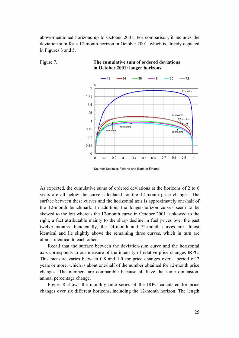
25

above-mentioned horizons up to October 2001. For comparison, it includes the deviation sum for a 12-month horizon in October 2001, which is already depicted in Figures 3 and 5. Figure 7. The cumulative sum of ordered deviations in October 2001: longer horizons

0

0.25

0.5

0.75

1

1.25

1.5

1.75

2%

12 24 36 48 60 72

0 0.1 0.2 0.3 0.4 0.5 0.6 0.7 0.8 0.9 1

12 months

24 months

72 months

60 months

48 months36 months

Source: Statistics Finland and Bank of Finland. As expected, the cumulative sums of ordered deviations at the horizons of 2 to 6 years are all below the curve calculated for the 12-month price changes. The surface between these curves and the horizontal axis is approximately one-half of the 12-month benchmark. In addition, the longer-horizon curves seem to be skewed to the left whereas the 12-month curve in October 2001 is skewed to the right, a fact attributable mainly to the sharp decline in fuel prices over the past twelve months. Incidentally, the 24-month and 72-month curves are almost identical and lie slightly above the remaining three curves, which in turn are almost identical to each other. Recall that the surface between the deviation-sum curve and the horizontal axis corresponds to our measure of the intensity of relative price changes IRPC. This measure varies between 0.8 and 1.0 for price changes over a period of 2 years or more, which is about one-half of the number obtained for 12-month price changes. The numbers are comparable because all have the same dimension, annual percentage change. Figure 8 shows the monthly time series of the IRPC calculated for price changes over six different horizons, including the 12-month horizon. The length

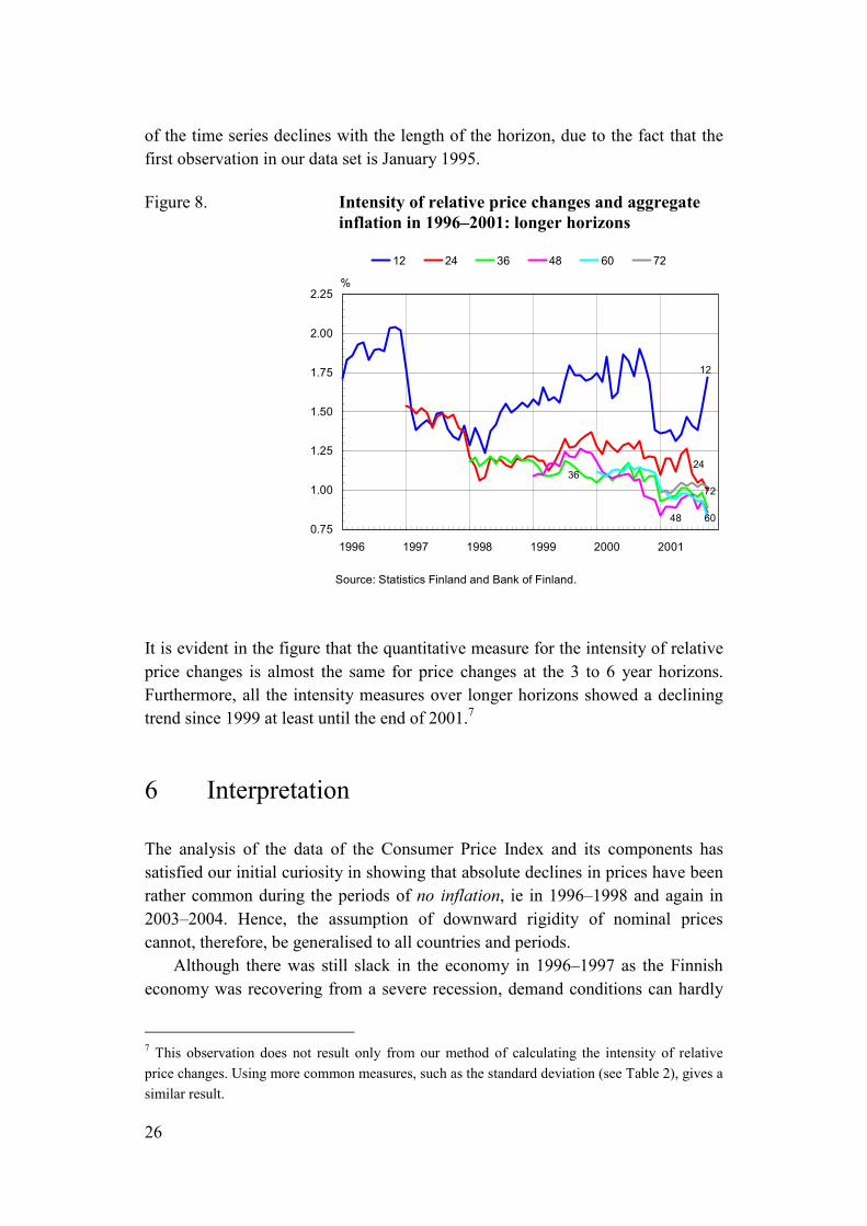
26

of the time series declines with the length of the horizon, due to the fact that the first observation in our data set is January 1995. Figure 8. Intensity of relative price changes and aggregate inflation in 1996–2001: longer horizons

0.75

1.00

1.25

1.50

1.75

2.00

2.25

1996 1997 1998 1999 2000 2001

%

12 24 36 48 60 72

12

2436

48 60

72

Source: Statistics Finland and Bank of Finland. It is evident in the figure that the quantitative measure for the intensity of relative price changes is almost the same for price changes at the 3 to 6 year horizons. Furthermore, all the intensity measures over longer horizons showed a declining trend since 1999 at least until the end of 2001.7 6 Interpretation

The analysis of the data of the Consumer Price Index and its components has satisfied our initial curiosity in showing that absolute declines in prices have been rather common during the periods of no inflation, ie in 1996–1998 and again in 2003–2004. Hence, the assumption of downward rigidity of nominal prices cannot, therefore, be generalised to all countries and periods. Although there was still slack in the economy in 1996–1997 as the Finnish economy was recovering from a severe recession, demand conditions can hardly

7 This observation does not result only from our method of calculating the intensity of relative price changes. Using more common measures, such as the standard deviation (see Table 2), gives a similar result.

27

be characterised as deflationary. GDP, real incomes and employment were all rising at respectable rates. Although exports and industrial output have suffered from recession, household sector confidence has remained high and private consumption has continued to grow at a robust rate in the past couple of years. The aggregate demand situation, therefore, cannot explain the extent of price declines observed in those years. A number of supply-side shocks can be identified in the period since 1996 up to the resent. The years 1995–1996 were characterised by a major real shock brought about by Finland’s entry into the European Union. It increased competition across the board and opened the previously protected food sector to competition. Apparently these effects gradually withered away, which may also explain the declining trend in the intensity of relative price changes calculated over longer horizons. Positive real shocks may have contributed to lower inflation and a higher intensity of relative price movements in 1998 and 1999 as the prices of ICT products were declining rapidly. On the other hand, housing prices were on the rise, affecting the headline Consumer Price Index through the depreciation of housing capital, which is an important component in the index. Another identifiable real shock hit the economy in the third quarter of 2000. The prices of fuels started to rise in August 2000, raising both the general price index and the intensity of relative price movements. Once its first-round effects were over, both inflation and the measure of the intensity of relative price changes came down. Declining prices became less common at the same time as aggregate inflation started to decelerate. The change in the shape of both the contribution-sum and the deviation-sum curves reveal that the deceleration of inflation was narrowly based, mainly due to fuel prices, while underlying inflation was in fact accelerating. This is consistent with the interpretation that a positive nominal shock had hit the economy together with some important real shocks. A move to easier monetary policy by the ECB in 2001 may have represented such a nominal shock. Supply shocks have again played an important role in the past few years. The entry of competition from abroad into retail trade, and the lowering of taxes on cars and alcoholic beverages have contributed both to the disappearance of aggregate inflation and the increase in the occurrence of absolute price declines in 2003 and 2004. While it is true that the price movements of some products that have a high weight in the Consumer Price Index are policy-induced, it is also true that there are a large number of small-weight goods and services, the prices of which are either rising or declining. These are mostly market-based changes in prices. As far as the relative price changes reflect changes in productivity, these changes should be irreversible. Our inspection of relative price changes in the periods over horizons of up to six years shows that many changes have in fact

28

been permanent. For instance, we found that in October 2001 there were 110 components in the Consumer Price Index the prices of which were in absolute terms below the prices prevailing in October 1995. This is not a negligible number. The average annual rate of inflation in the same period was 1.7 per cent, implying that the price level had increased by 10.6 per cent. Of the items exhibiting declining prices over the six-year period, the most important were interest rates, personal computers, coffee, second-hand cars, mobile phones, mobile phone fees and television sets. While the cumulative sum of ordered contributions is an interesting method for descriptive analysis of low inflation experiences, it may not be very illustrative for moderate-to-high inflation periods. The cumulative sum of ordered deviations and the related measure for the intensity of relative price changes should be workable for such episodes as well. It would, therefore, be interesting to apply our methodology to longer time periods in order to look at the robustness of the correlations between relative price variability and aggregate inflation as well as between inflation and the skewness of the price distribution over time.

29

References

Akerlof, G A, Dickens, W T and Perry, G L (1996) The Macroeconomics of Low Inflation. Brookings Papers on Economic Activity, No. 1, 1–74.

Andersen, T (2001b) Can Inflation be too low? Kyklos 54, 591–602. Balke, N S, and Wynne, M A (2000) An equilibrium analysis of relative price

changes and aggregate inflation. Journal of Monetary Economics 45, 269–292.

Ball, L and Mankiw, N G (1995) Relative-price changes as aggregate supply

shocks. Quarterly Journal of Economics 110, 161–193. Ball, L and Mankiw, N G (1999) Interpreting the correlation between inflation

and the skewness of relative prices: A comment on Bryan and Cecchetti. Review of Economics and Statistics 81, 197–198.

Ball, L, Mankiw, N G and Romer, D (1988) The New Keynesian economics and

the output-inflation tradeoff. Brookings papers on economic activity, No. 1. Bryan, M F and Cecchetti, S G (1994) Measuring core inflation. In Mankiw,

N G (ed.), Monetary Policy, Chicago: University of Chicago Press, 195–215. Bryan, M F and Cecchetti, S G (1999) Inflation and the Distribution of Price

Changes. Review of Economics and Statistics 81, 188–196. Cassino, V (1995) Menu cost – a review of the literature. Reserve Bank of new

Zealand Discussion Paper G95/1. Cecchetti, S G and Groschen, E L (2000) Understanding inflation: Implications

for monetary policy. NBER Working Paper 7482, January 2000. Clark, T E (2001) Comparing measures of core inflation. Federal Reserve Bank

of Kansas City Economic Review, Second Quarter 2001, 5–31. Domberger, S (1987) Relative price variability and inflation: a disaggregated

analysis. Journal of Political Economy 95, 547–566. Federal Reserve Bank of Kansas City (1997) Annual Report 1996.

30

Fischer, S (1981) Relative shocks, relative price variability and inflation. Brookings Papers on Economic Activity, No. 2. 381–441.

Friedman, M (1977) Inflation and unemployment. Journal of Political Economy

85, 451–472. Jordan, J (2000) Money, Central Banking and Monetary Policy in the Global

Financial Arena. The Mont Pelerin Society General Meeting, Chile. http://www.clev.frb.org/ccca/Speech00/jj111400.htm

Kahneman, D, Knetsch, J L and Thaler, R (1986) Fairness as a constraint on

profit seeking: Entitlements in the market. American Economic Review 76, 728–741.

Lucas, R E (1973) Some international evidence on output-inflation tradeoffs.

The American Economic Review 63, 326–334. Mankiw, N G (1985) Small menu costs and large business cycles: A macro-

economic model of monopoly. Quarterly Journal of Economics 100, 529–537.

Mizon, G E, Safford, J C and Thomas, S H (1991) The distribution of consumer

prices in the UK. Economica 57, 219–230. Parsley, D (1996) Inflation and relative price variability in the short and long

run: New evidence from the United States. Journal of Money, Credit and Banking 28, 323–241.

Tobin, J (1972) Inflation and Unemployment. American Economic Review 62,

1–18. Vega and Wynne (2001) An evaluation of some measures of core inflation for

the euro area. European Central Bank Working paper No. 53. Verbrugge, R J (1999) Cross-sectoral inflation asymmetries and core inflation:

A Comment on Bryan and Cecchetti. Review of Economics and Statistics 81, 199–202.

Vining, D R and Elwertowski, T C (1976) The relationship between relative

prices and the general price level. American Economic Review 66, 699–708.

BANK OF FINLAND DISCUSSION PAPERS ISSN 0785-3572, print; ISSN 1456-6184, online 1/2004 Jukka Railavo Stability consequences of fiscal policy rules. 2004. 42 p.

ISBN 952-462-114-2, print; ISBN 952-462-115-0, online. (TU) 2/2004 Lauri Kajanoja Extracting growth and inflation expectations from financial

market data. 2004. 25 p. ISBN 952-462-116-9, print; ISBN 952-462-117-7, online. (TU)

3/2004 Martin Ellison – Lucio Sarno – Jouko Vilmunen Monetary policy and

learning in an open economy. 2004. 24 p. ISBN 952-462-118-5, print; ISBN 952-462-119-3, online. (TU)

4/2004 David G. Mayes An approach to bank insolvency in transition and

emerging economies. 2004. 54 p. ISBN 952-462-120-7, print; ISBN 952-462-121-5, online. (TU)

5/2004 Juha Kilponen Robust expectations and uncertain models – A robust

control approach with application to the New Keynesian economy. 2004. 43 p. ISBN 952-462-122-3, print; ISBN 952-462-123-1, online. (TU)

6/2004 Erkki Koskela – Roope Uusitalo Unintended convergence – how Finnish

unemployment reached the European level. 2004. 32 p. ISBN 952-462-124-X, print; ISBN 952-462-125-8, online. (TU)

7/2004 Berthold Herrendorf – Arilton Teixeira Monopoly rights can reduce income

big time. 2004. 38 p. ISBN 952-462-126-6, print; ISBN 952-462-127-4, online. (TU)

8/2004 Allen N. Berger – Iftekhar Hasan – Leora F. Klapper Further evidence on the

link between finance and growth: An international analysis of community banking and economic performance. 2004. 50 p. ISBN 952-462-128-2, print; ISBN 952-462-129-0, online. (TU)

9/2004 David G. Mayes – Matti Virén Asymmetries in the Euro area economy.

2004. 56 p. ISBN 952-462-130-4, print; ISBN 952-462-131-2, online. (TU) 10/2004 Ville Mälkönen Capital adequacy regulation and financial conglomerates.

2004. 29 p. ISBN 952-462-134-7, print; ISBN 952-462-135-5, online. (TU)

11/2004 Heikki Kauppi – Erkki Koskela – Rune Stenbacka Equilibrium unemployment and investment under product and labour market imperfections. 2004. 35 p. ISBN 952-462-136-3, print; ISBN 952-462-137-1, online. (TU)

12/2004 Nicolas Rautureau Measuring the long-term perception of monetary policy

and the term structure. 2004. 44 p. ISBN 952-462-138-X, print; ISBN 952-462-139-8, online. (TU)

13/2004 Timo Iivarinen Large value payment systems – principles and recent and

future developments. 2004. 57 p. ISBN 952-462-144-4, print, ISBN 952-462-145-2, online (RM)

14/2004 Timo Vesala Asymmetric information in credit markets and

entrepreneurial risk taking. 2004. 31 p. 952-462-146-0, print, ISBN 952-462-147-9, online (TU)

15/2004 Michele Bagella – Leonardo Becchetti – Iftekhar Hasan The anticipated and

concurring effects of the EMU: exchange rate volatility, institutions and growth. 2004. 38 p. 952-462-148-7, print, ISBN 952-462-149-5, online (TU)

16/2004 Maritta Paloviita – David G. Mayes The use of real time information in

Phillips curve relationships for the euro area. 2004. 51 p. 952-462-150-9, print, ISBN 952-462-151-7, online (TU)

17/2004 Ville Mälkönen The efficiency implications of financial conglomeration.

2004. 30 p. 952-462-152-5, print, ISBN 952-462-153-3, online (TU) 18/2004 Kimmo Virolainen Macro stress testing with a macroeconomic credit risk

model for Finland. 2004. 44 p. 952-462-154-1, print, ISBN 952-462-155-X, online (TU)

19/2004 Eran A. Guse Expectational business cycles. 2004. 34 p. 952-462-156-8, print,

ISBN 952-462-157-6, online (TU) 20/2004 Jukka Railavo Monetary consequences of alternative fiscal policy rules.

2004. 29 p. 952-462-158-4, print, ISBN 952-462-159-2, online (TU) 21/2004 Maritta Paloviita Inflation dynamics in the euro area and the role of

expectations: further results. 2004. 24 p. 952-462-160-6, print, ISBN 952-462-161-4, online (TU)

22/2004 Olli Castrén – Tuomas Takalo – Geoffrey Wood Labour market reform and the sustainability of exchange rate pegs. 2004. 35 p. 952-462-166-5, print, ISBN 952-462-167-3, online (TU)

23/2004 Eric Schaling – Sylvester Eijffinger – Mewael Tesfaselassie Heterogeneous

information about the term structure, least-squares learning and optimal rules for inflation targeting. 2004. 47 p. 952-462-168-1, print, ISBN 952-462-169-X, online (TU)

24/2004 Helinä Laakkonen The impact of macroeconomic news on exchange rate

volatility. 2004. 41 p. 952-462-170-3, print, ISBN 952-462-171-1, online (TU) 25/2004 Ari Hyytinen – Tuomas Takalo Multihoming in the market for payment

media: evidence from young Finnish consumers. 2004. 38 p. 952-462-174-6, print, ISBN 952-462-175-4, online (TU)

26/2004 Esa Jokivuolle – Markku Lanne Trading Nokia: The roles of the Helsinki vs

the New York stock exchanges. 2004. 22 p. 952-462-176-2, print, ISBN 952-462-177-0, online (RM)

27/2004 Hanna Jyrkönen Less cash on the counter – Forecasting Finnish payment

preferences. 2004. 51 p. 952-462-178-9, print, ISBN 952-462-179-7, online (RM)

28/2004 Antti Suvanto – Juhana Hukkinen Stable price level and changing prices.

2004. 30 p. 952-462-180-0, print, ISBN 952-462-181-9, online (KT)