Stability Analysis of

One-Dimensional Asynchronous Swarms ∗

Yang Liu and Kevin M. Passino † Marios Polycarpou

Dept. Electrical Engineering Dept. ECECS

The Ohio State University University of Cincinnati

2015 Neil Avenue, Columbus, Ohio 43210 Cincinnati, OH 45221-0030

Abstract

Coordinated dynamical swarm behavior occurs when certain types of animals forage for food or tryto avoid predators. Analogous behaviors can occur in engineering systems (e.g. in groups of autonomousmobile robots or air vehicles). In this paper we characterize swarm “cohesiveness” as a stability propertyand provide conditions under which collision-free convergence can be achieved for an asynchronousswarm with finite-size swarm members that have proximity sensors and neighbor position sensors thatonly provide delayed position information. Moreover, we give conditions under which an asynchronousmobile swarm following (pushed by) an “edge-leader” can maintain cohesion during movements even inthe presence of sensing delays and asynchronism. Such stability analysis is of fundamental importanceif one wants to understand the coordination mechanisms for groups of autonomous vehicles or robotswhere inter-member communication channels are less than perfect and collisions must be avoided.

1 Introduction

A variety of organisms have the ability to cooperatively forage for food while trying to avoid predators andother risks. For instance, when a school of fish searches for prey, or if it encounters a predator, the fishoften make coordinated maneuvers as if the entire group were one organism [1]. Analogous behavior is seenin flocks of birds, herds of wildebeests, groups of ants, and swarms of social bacteria [2, 3]. We call thiskind of aggregate motion “swarm behavior.” A high-level view of a swarm suggests that the organisms arecooperating to achieve some purposeful behavior and achieve some goal. Naturalists and biologists havestudied such swarm behavior for decades. Moreover, computer scientists in the field of “artificial life” havestudied how to model and simulate biological swarms to understand how such “social animals” interact,achieve goals, and evolve [4, 5].

Recently, there has been a growing interest in biomimicry of the mechanisms of foraging and swarmingfor use in engineering applications since the resulting swarm intelligence can be applied in optimization(e.g., in telecommunication systems) [2, 3], robotics [6, 7], traffic patterns in intelligent transportationsystems [8, 9, 10], and military applications [11]. For instance, there has been a growing interest in groups(swarms) of flying vehicles [12, 13]. Moreover, it has been proposed that swarms of robots may providethe possibility of enhanced task performance, high reliability (fault tolerance), low unit complexity, anddecreased cost over traditional systems. Also, it has been argued that a swarm of robots can accomplishsome tasks that would be impossible for a single robot to achieve. Particular research includes that

∗This work was supported by DAGSI and AFRL. We include an appendix with some simulations that provide some insights

into swarm behavior. It is proposed that the appendix will not be published, but that a URL will be provided to the interested

readers.†Please address all correspondence to K. Passino, ((614) 292-5716; passino@ee.eng.ohio-state.edu.

1

of Beni [7] who introduced the concept of cellular robotic systems, and the related study in [14]. Thebehavior-based control strategy put forward by Brooks [15] is quite well known and it has been appliedto collections of simple independent robots, usually for simple tasks. Mataric [16] describes experimentswith a homogeneous population of robots acting under different communication constraints. Suzuki [17]considered a number of two-dimensional problems of formation of geometric patterns with distributedanonymous mobile swarm robots. Other approaches and results in this area are summarized in [6, 18].

In this paper, we are interested in mathematical modeling and analysis of stability properties of swarms.We think of stability as characterizing the cohesiveness of the swarm as it moves. Stability is a basicqualitative property of swarms since if it is not present, then it is typically impossible for the swarmto achieve any other group objective. Stability analysis of swarms is still an open problem but therehave been several areas of relevant progress. In biology, researchers have used “continuum models” forswarm behavior based on non-local interactions, and have studied stability properties [19]. Jin et al. in[20] studied stability of synchronized distributed control of one-dimensional and two-dimensional swarmstructures. Interestingly, the model and stability analysis in [20] are quite similar to the model and proofof stability for the load balancing problem in computer networks [21, 22]. Next, we would note that therehave been several investigations into the stability of inter-vehicle distances in “platoons” in intelligenttransportation systems (e.g., in [23, 24] or of the “slinky effect” in [25, 26], and traffic flow in [8, 10]).Finally, we would note that the study of stability properties of aircraft (spacecraft) formations is a relevantand active research area [12, 13].

This paper presents a single finite-size swarm member model, and then builds a one-dimensional asyn-chronous swarm model by putting many single swarm members together. In contrast to related existingresults, the contribution of this paper lies in that we provide conditions under which the swarm will keep itscohesiveness even in the presence of sensing delays and asynchronism. In particular, we will conclude thatfor one-dimensional stationary edge-member asynchronous swarms, total asynchronism leads to asymptoticconvergence and partial asynchronism leads to finite time convergence (both collision-free). Furthermore,we present conditions under which one-dimensional asynchronous mobile swarms following, or pushed by,an “edge-leader” can maintain collision-free cohesion during movements even with sensing delays and asyn-chronism. Our desire to consider collision-free cohesion for finite-size vehicles significantly complicates theanalysis compared to the case where point-size vehicles are studied and collisions are allowed (e.g., asin [17]). Our study uses a discrete time discrete event dynamical system [21] approach and unlike thestudies of platoon stability in intelligent transportation systems we avoid detailed characteristics of lowlevel “inner-loop control” and vehicle dynamics in favor of focusing on high level mechanisms underlyingqualitative swarm behavior when there are imperfect communications. Swarm stability for the M ≥ 2dimensional case will be studied in a forthcoming paper.

2 Modeling

First we explain the capabilities of a single swarm member and then we provide a mathematical model for aone-dimensional N -member asynchronous swarm. Moreover, we give mathematical models for N -memberasynchronous mobile swarms following (being pushed by) an “edge-leader.”

2.1 Single Swarm Member Model

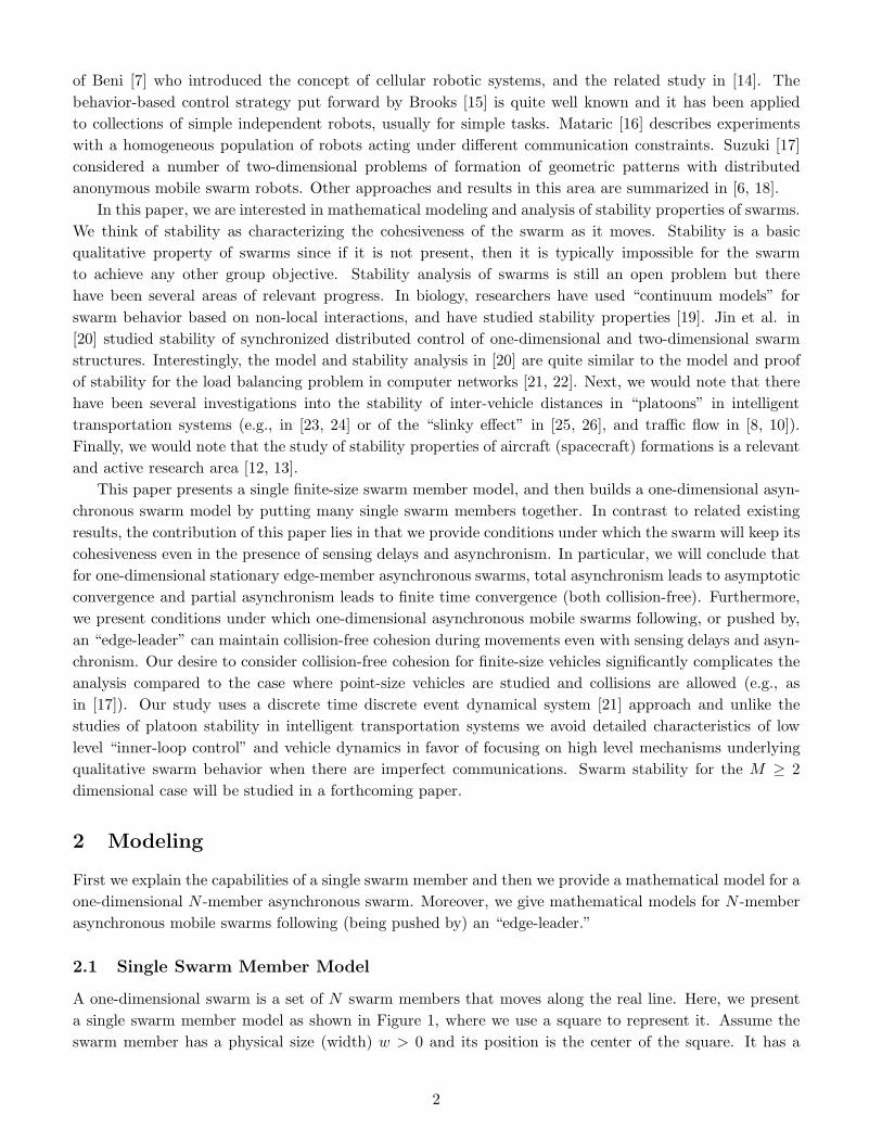
A one-dimensional swarm is a set of N swarm members that moves along the real line. Here, we presenta single swarm member model as shown in Figure 1, where we use a square to represent it. Assume theswarm member has a physical size (width) w > 0 and its position is the center of the square. It has a

2

“proximity sensor” for both sides. This sensor has a sensing range ε > w, which means that once anotherswarm member reaches a distance of ε from it, the sensor instantaneously indicates the position of theother member. However, if its neighbors are not in its sensing range, the proximity sensor for the leftneighbor will return −∞ (or, practically, some large negative number), and the one for the right neighborwill return ∞. The proximity sensor is used to help avoid swarm member collisions and ensures that ourframework allows for finite-size vehicles, not just points. Each swarm member also has a “neighbor positionsensor,” which can sense the positions of neighbors to its left and right if they are present. We assumethat there is no restriction on how close a neighbor must be for the neighbor position sensor to providea sensed value of its position. The sensed position information may be subjected to random delays (i.e.,each swarm member’s knowledge about its neighbors’ positions may be outdated). We assume that eachswarm member knows its own position with no delay. Notice that we define the position, distance andsensor sensing range of the finite-size swarm member with respect to its center, not its left or right edge.

Swarm members like to be close to each other, but not too close. Suppose d > 0 is the desired“comfortable distance” between two adjacent swarm neighbors, and that d > ε. Each swarm membersenses the inter-swarm member distance via both neighbor position and proximity sensors and makesdecisions for movements according to the error between the sensed distance and the comfortable distanced via its “decision-making” mechanism. And then, the decisions are inputed to its “driving device,” whichprovides locomotion for it (for the one-dimensional case, movement either to the left or right). Each swarmmember will try to move to maintain a comfortable distance to its neighbors. This will tend to make thegroup move together in a cohesive “swarm.”

Decision−making

w

Right−lookingproximity sensor

Neighborposition sensors

Left−looking

(left and right)

proximity sensor

for movementsDriving device

Figure 1: Single swarm member with a finite size w, one-dimensional case.

2.2 One-Dimensional Asynchronous Swarm Model

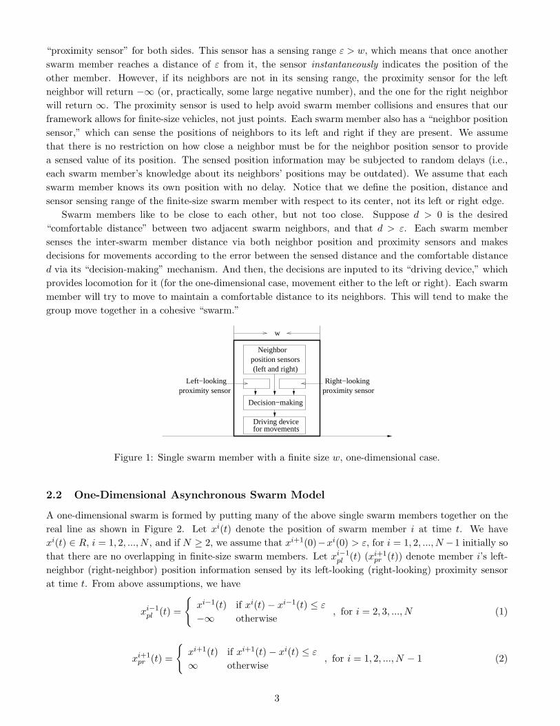
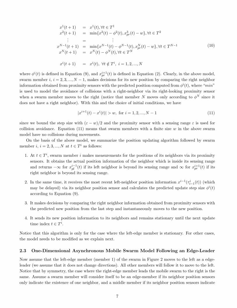
A one-dimensional swarm is formed by putting many of the above single swarm members together on thereal line as shown in Figure 2. Let xi(t) denote the position of swarm member i at time t. We havexi(t) ∈ R, i = 1, 2, ..., N , and if N ≥ 2, we assume that xi+1(0)−xi(0) > ε, for i = 1, 2, ..., N −1 initially sothat there are no overlapping in finite-size swarm members. Let xi−1

pl (t) (xi+1pr (t)) denote member i’s left-

neighbor (right-neighbor) position information sensed by its left-looking (right-looking) proximity sensorat time t. From above assumptions, we have

xi−1pl (t) =

{xi−1(t) if xi(t)− xi−1(t) ≤ ε

−∞ otherwise, for i = 2, 3, ..., N (1)

xi+1pr (t) =

{xi+1(t) if xi+1(t)− xi(t) ≤ ε

∞ otherwise, for i = 1, 2, ..., N − 1 (2)

3

We assume that every swarm member knows d, and there is a set of times T = {0, 1, 2, ...} at which one ormore swarm members update their positions. Let T i ⊆ T, i = 1, 2, ..., N , be a set of times at which the ith

member’s position xi(t), t ∈ T i, is updated. Notice that the elements of T i should be viewed as the indicesof the sequence of physical times at which updates take place, not the real times. These time indices arenon-negative integers and can be mapped into physical times. The T i, i = 1, 2, ..., N , are independent ofeach other for different i. However, they may have intersections (i.e., it could be that T i ∩ T j �= ∅ fori �= j, so two or more swarm members may move simultaneously). Here, our model assumes that swarmmembers sense their neighbor positions and update their positions only at time indices t ∈ T i and at alltimes t /∈ T i, xi(t) is left unchanged. A variable τ i

i−1(t) ∈ T (respectively, τ ii+1(t) ∈ T ) for i = 2, 3, ..., N

(i = 1, 2, ..., N − 1) is used to denote the time index of the real time where position information aboutneighbor i− 1 (i+ 1) was obtained by member i at t ∈ T i and it satisfies 0 ≤ τ i

i−1(t) ≤ t (0 ≤ τ ii+1(t) ≤ t)

for t ∈ T i. Of course, while we model the times at which neighbor position information is obtained asbeing the same times at which one or more swarm members decide where to move and actually move, itcould be that the real time at which such neighbor position information is obtained is earlier than the realtime where swarm members moved. The difference t − τ i

i−1(t) (t − τ ii+1(t)) between current time t and

the time τ ii−1(t) (τ

ii+1(t)) can be viewed as a form of communication delay (of course the actual length

of the delay depends on what real times correspond to the indices t, τ ii−1(t), or τ

ii+1(t)). Moreover, it is

important to note that we assume that τ ii−1(t) ≥ τ i

i−1(t′) (respectively, τ i

i+1(t) ≥ τ ii+1(t

′)) if t > t′ fort, t′ ∈ T i. This ensures that member i will use the most recently obtained neighbor position information.Furthermore, we assume swarm member i will use the real-time neighbor position information xi−1(t)and/or xi+1(t) provided by its proximity sensors instead of information from its neighbor position sensorsxi−1(τ i

i−1(t)) and/or xi+1(τ i

i+1(t)) if their neighbors are inside the sensing range of its proximity sensors.This information will be used for position updating until member i gets more recent information, forexample, from its neighbor position sensor.

Left-edge

1 2 N3 N-1

x

Member

(Stationary)

Figure 2: One-dimensional asynchronous swarm, all members moving to be adjacent to the stationary edgemember.

Next, based on [22] we specify two assumptions that we use to characterize asynchronism for swarms.

Assumption 1. (Total Asynchronism): Assume the sets T i, i = 1, 2, ..., N , are infinite, and if foreach k, tk ∈ T i and tk → ∞ as k → ∞, then limk→∞ τ i

j(tk) = ∞ for j = i− 1, i+ 1.

This assumption guarantees that each swarm member moves infinitely often and the old position informa-tion of neighbors of each swarm member is eventually purged from it. More precisely, given any time t1,there exists a time t2 > t1 such that τ i

j(t) ≥ t1, ∀i, j and j = i − 1, i + 1 and t ≥ t2. On the other hand,the delays t− τ i

j(t) in obtaining position information of neighbors of member i can become unbounded ast increases. Next, we specify a more restrictive type of asynchronism, but one which is usually easy toimplement in practice.

4

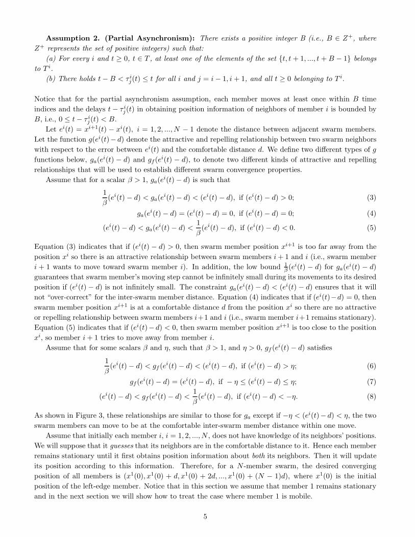
Assumption 2. (Partial Asynchronism): There exists a positive integer B (i.e., B ∈ Z+, whereZ+ represents the set of positive integers) such that:

(a) For every i and t ≥ 0, t ∈ T , at least one of the elements of the set {t, t+ 1, ..., t +B − 1} belongsto T i.

(b) There holds t−B < τ ij(t) ≤ t for all i and j = i− 1, i + 1, and all t ≥ 0 belonging to T i.

Notice that for the partial asynchronism assumption, each member moves at least once within B timeindices and the delays t− τ i

j(t) in obtaining position information of neighbors of member i is bounded byB, i.e., 0 ≤ t− τ i

j(t) < B.Let ei(t) = xi+1(t) − xi(t), i = 1, 2, ..., N − 1 denote the distance between adjacent swarm members.

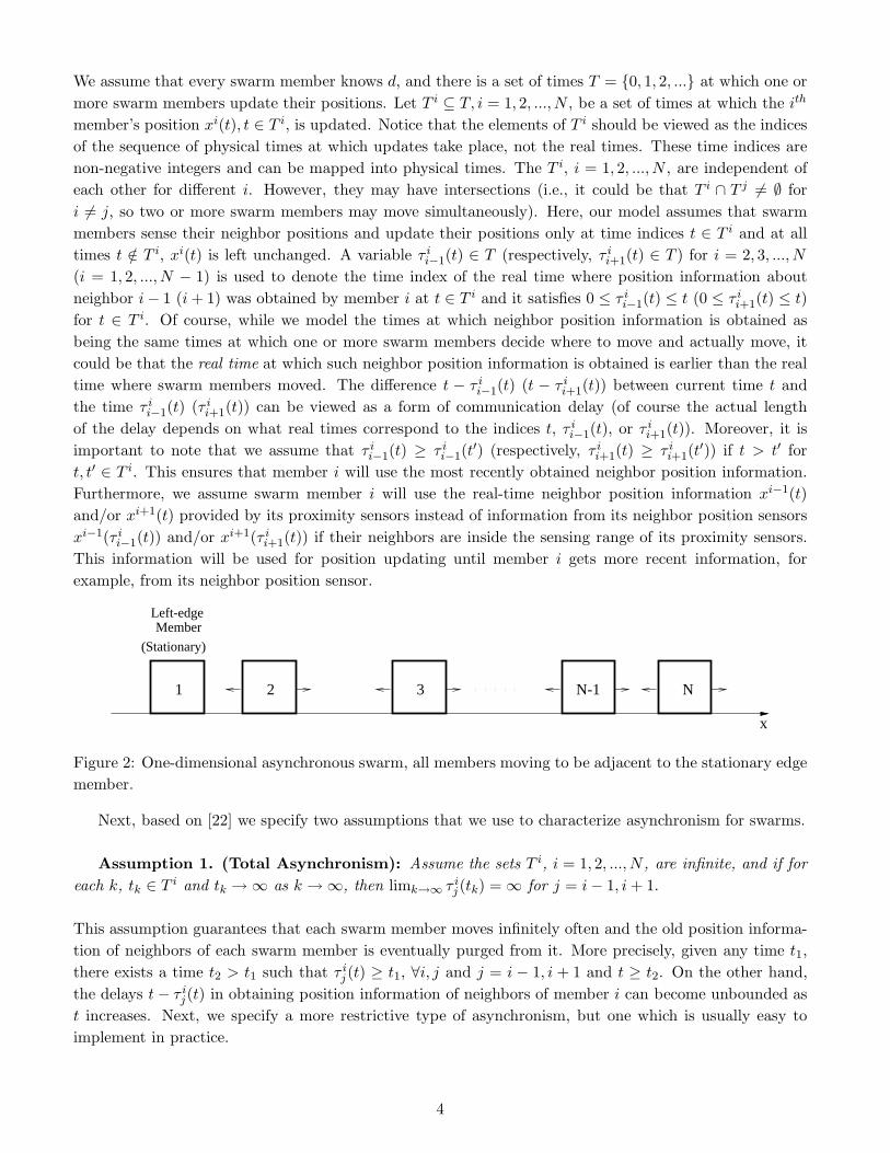
Let the function g(ei(t)− d) denote the attractive and repelling relationship between two swarm neighborswith respect to the error between ei(t) and the comfortable distance d. We define two different types of gfunctions below, ga(ei(t) − d) and gf (ei(t) − d), to denote two different kinds of attractive and repellingrelationships that will be used to establish different swarm convergence properties.

Assume that for a scalar β > 1, ga(ei(t)− d) is such that

1β(ei(t)− d) < ga(ei(t)− d) < (ei(t)− d), if (ei(t)− d) > 0; (3)

ga(ei(t)− d) = (ei(t)− d) = 0, if (ei(t)− d) = 0; (4)

(ei(t)− d) < ga(ei(t)− d) <1β(ei(t)− d), if (ei(t)− d) < 0. (5)

Equation (3) indicates that if (ei(t) − d) > 0, then swarm member position xi+1 is too far away from theposition xi so there is an attractive relationship between swarm members i+ 1 and i (i.e., swarm memberi + 1 wants to move toward swarm member i). In addition, the low bound 1

β (ei(t) − d) for ga(ei(t) − d)

guarantees that swarm member’s moving step cannot be infinitely small during its movements to its desiredposition if (ei(t)− d) is not infinitely small. The constraint ga(ei(t)− d) < (ei(t) − d) ensures that it willnot “over-correct” for the inter-swarm member distance. Equation (4) indicates that if (ei(t)−d) = 0, thenswarm member position xi+1 is at a comfortable distance d from the position xi so there are no attractiveor repelling relationship between swarm members i+1 and i (i.e., swarm member i+1 remains stationary).Equation (5) indicates that if (ei(t)− d) < 0, then swarm member position xi+1 is too close to the positionxi, so member i+ 1 tries to move away from member i.

Assume that for some scalars β and η, such that β > 1, and η > 0, gf (ei(t)− d) satisfies

1β(ei(t)− d) < gf (ei(t)− d) < (ei(t)− d), if (ei(t)− d) > η; (6)

gf (ei(t)− d) = (ei(t)− d), if − η ≤ (ei(t)− d) ≤ η; (7)

(ei(t)− d) < gf (ei(t)− d) <1β(ei(t)− d), if (ei(t)− d) < −η. (8)

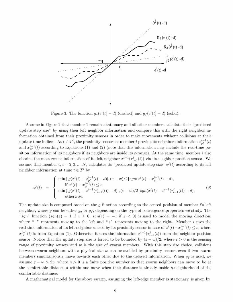
As shown in Figure 3, these relationships are similar to those for ga except if −η < (ei(t)− d) < η, the twoswarm members can move to be at the comfortable inter-swarm member distance within one move.

Assume that initially each member i, i = 1, 2, ..., N , does not have knowledge of its neighbors’ positions.We will suppose that it guesses that its neighbors are in the comfortable distance to it. Hence each memberremains stationary until it first obtains position information about both its neighbors. Then it will updateits position according to this information. Therefore, for a N -member swarm, the desired convergingposition of all members is (x1(0), x1(0) + d, x1(0) + 2d, ..., x1(0) + (N − 1)d), where x1(0) is the initialposition of the left-edge member. Notice that in this section we assume that member 1 remains stationaryand in the next section we will show how to treat the case where member 1 is mobile.

5

e (t) -d

(e (t) -d)i

β1

(e (t) -d)i

(e (t) -d)ig a

(e (t) -d)ig

i

f

−ηη

Figure 3: The function ga(ei(t)− d) (dashed) and gf (ei(t)− d) (solid).

Assume in Figure 2 that member 1 remains stationary and all other members calculate their “predictedupdate step size” by using their left neighbor information and compare this with the right neighbor in-formation obtained from their proximity sensors in order to make movements without collisions at theirupdate time indices. At t ∈ T i, the proximity sensors of member i provide its neighbors information xi−1

pl (t)and xi+1

pr (t) according to Equations (1) and (2) (note that this information may include the real-time po-sition information of its neighbors if its neighbors are inside its ε-range). At the same time, member i alsoobtains the most recent information of its left neighbor xi−1(τ i

i−1(t)) via its neighbor position sensor. Weassume that member i, i = 2, 3, ..., N , calculates its “predicted update step size” φi(t) according to its leftneighbor information at time t ∈ T i by

φi(t) =

min{|g(xi(t)− xi−1pl (t)− d)|, (ε −w)/2}sgn(xi(t)− xi−1

pl (t)− d),if xi(t)− xi−1

pl (t) ≤ ε;min{|g(xi(t)− xi−1(τ i

i−1(t))− d)|, (ε − w)/2}sgn(xi(t)− xi−1(τ ii−1(t))− d),

otherwise.

(9)

The update size is computed based on the g function according to the sensed position of member i’s leftneighbor, where g can be either ga or gf , depending on the type of convergence properties we study. The“sgn” function (sgn(z) = 1 if z ≥ 0, sgn(z) = −1 if z < 0) is used to model the moving direction,where “−” represents moving to the left and “+” represents moving to the right. Member i uses thereal-time information of its left neighbor sensed by its proximity sensor in case of xi(t)−xi−1

pl (t) ≤ ε, wherexi−1

pl (t) is from Equation (1). Otherwise, it uses the information xi−1(τ ii−1(t)) from the neighbor position

sensor. Notice that the update step size is forced to be bounded by (ε− w)/2, where ε > 0 is the sensingrange of proximity sensors and w is the size of swarm members. With this step size choice, collisionsbetween swarm neighbors with a physical size w can be avoided by proximity sensors even if two swarmmembers simultaneously move towards each other due to the delayed information. When gf is used, weassume ε − w > 2η, where η > 0 is a finite positive number so that swarm neighbors can move to be atthe comfortable distance d within one move when their distance is already inside η-neighborhood of thecomfortable distance.

A mathematical model for the above swarm, assuming the left-edge member is stationary, is given by

6

x1(t+ 1) = x1(t),∀t ∈ T 1

x2(t+ 1) = min{x2(t)− φ2(t), x3pr(t)− w},∀t ∈ T 2

... =...

xN−1(t+ 1) = min{xN−1(t)− φN−1(t), xNpr(t)− w},∀t ∈ TN−1

xN (t+ 1) = xN (t)− φN (t),∀t ∈ TN

xi(t+ 1) = xi(t), ∀t /∈ T i, i = 1, 2, ..., N

(10)

where φi(t) is defined in Equation (9), and xi+1pr (t) is defined in Equation (2). Clearly, in the above model,

swarm member i, i = 2, 3, ..., N − 1, makes decisions for its new position by comparing the right neighborinformation obtained from proximity sensors with the predicted position computed from φi(t), where “min”is used to model the avoidance of collisions with a right-neighbor via its right-looking proximity sensorwhen a swarm member moves to the right (notice that member N moves only according to φN since itdoes not have a right neighbor). With this and the choice of initial conditions, we have

|xi+1(t)− xi(t)| > w, for i = 1, 2, ..., N − 1 (11)

since we bound the step size with (ε − w)/2 and the proximity sensor with a sensing range ε is used forcollision avoidance. Equation (11) means that swarm members with a finite size w in the above swarmmodel have no collisions during movements.

On the basis of the above model, we summarize the position updating algorithm followed by swarmmember i, i = 2, 3, ..., N at t ∈ T i as follows:

1. At t ∈ T i, swarm member i makes measurements for the positions of its neighbors via its proximitysensors. It obtains the actual position information of the neighbor which is inside its sensing rangeand returns −∞ for xi−1

pl (t) if its left neighbor is beyond its sensing range and ∞ for xi+1pr (t) if its

right neighbor is beyond its sensing range.

2. In the same time, it receives the most recent left-neighbor position information xi−1(τ ii−1(t)) (which

may be delayed) via its neighbor position sensor and calculates the predicted update step size φi(t)according to Equation (9).

3. It makes decisions by comparing the right neighbor information obtained from proximity sensors withthe predicted new position from the last step and instantaneously moves to the new position.

4. It sends its new position information to its neighbors and remains stationary until the next updatetime index t ∈ T i.

Notice that this algorithm is only for the case where the left-edge member is stationary. For other cases,the model needs to be modified as we explain next.

2.3 One-Dimensional Asynchronous Mobile Swarm Model Following an Edge-Leader

Now assume that the left-edge member (member 1) of the swarm in Figure 2 moves to the left as a edge-leader (we assume that it does not change directions). All other members will follow it to move to the left.Notice that by symmetry, the case where the right-edge member leads the mobile swarm to the right is thesame. Assume a swarm member will consider itself to be an edge-member if its neighbor position sensorsonly indicate the existence of one neighbor, and a middle member if its neighbor position sensors indicate

7

the existence of both left and right neighbors. The edge-leader is the left edge member if the swarm movesto the left and is the right edge member if the swarm moves to the right.

For some γ > 0, we assume [d − γ, d + γ] is a “comfortable distance neighborhood” relative to xi(t)and xi+1(t) (i.e., when xi+1(t) − xi(t) ∈ [d − γ, d + γ], we say that they are in the comfortable distanceneighborhood), where 2γ is the comfortable distance neighborhood size. Assume that 0 < ε < d − γ sothat we do not consider swarm member i+ 1 to be at a comfortable distance to member i if it is too closeto it, where ε is the sensing range of swarm members’ proximity sensors.

Consider the two assumptions about asynchronism we specified earlier. Clearly only Assumption 2(partial asynchronism) will result in cohesiveness for a mobile swarm since the delays in Assumption 1(total asynchronism), which could be unbounded, will make swarm members lose track of their edge-leaderor their neighbors during movements, i.e., the distance between swarm members could become unboundedjust because swarm members use arbitrarily old sensed information. Hence, we will build our model basedon Assumption 2 (partial asynchronism), which has a positive integer B which we view as an asynchronismmeasure.

For convenience, assume that xi+1(0) − xi(0) = d, for i = 1, 2, ..., N − 1 initially, i.e., at the beginningall the swarm members are at a comfortable distance to their neighbors. Assume the edge-leader moveswith a step s(t) when t ≥ 0, where 0 < s(t) ≤ r, i.e., s(t) is bounded by a finite positive number r. So wehave

x1(t+ 1) = x1(t)− s(t),∀t ∈ T 1

Member 2 remains stationary until it gets the leader’s new position information. Then this member triesto follow the leader and update its position according to the new position information since it wants tobe at the comfortable distance to the edge-leader. Similarly, all the other swarm members will begin tomove and follow their moving neighbors. They all try to be at the comfortable distance to their neighbors.We think of the swarm as maintaining the cohesiveness if all the swarm members are in the comfortabledistance neighborhood to their neighbors during the moving process. Notice that the leader’s moving stepbound r can be used as a measure of how fast a cohesive asynchronous swarm moves.

Next, we will show that in the above mobile swarm, when swarm members only update their positionsaccording to the g function, they will never have collisions even without proximity sensors. Accordingly,we define the predicted update step size φi(t) of swarm member i according to its left neighbor informationfor this case as

φi(t) = g(xi(t)− xi−1(τ ii−1(t))− d), for i = 2, 3, ..., N

Here, “g” can be either ga or gf , and it denotes the attractive and repelling relationship between two swarmneighbors. Moreover, we will introduce another such function later and analyze the swarm cohesivenessproperties that it achieves.

At the beginning when t = 0, ei(0) = xi+1(0) − xi(0) = d, for i = 1, 2, ..., N − 1. When t ≥ 0, t ∈ T 1,the edge-leader begins to move and we then have e1(t) = x2(t) − x1(t) > d. Member 2, the edge-leader’sright neighbor, remains stationary until it gets the leader’s new position information x1(τ2

1 (t)). FromAssumption 2 (partial asynchronism), we know

t−B < τ21 (t) ≤ t (12)

and we have x1(τ21 (t)) ≥ x1(t). And so

x2(t)− x1(τ21 (t))− d ≤ x2(t)− x1(t)− d (13)

According to the definition of g (i.e., both ga and gf ) and Equation (13), we have

g(x2(t)− x1(τ21 (t))− d) ≤ x2(t)− x1(τ2

1 (t))− d ≤ x2(t)− x1(t)− d (14)

8

At the beginning, member 2’s proximity sensors cannot sense its neighbors since at this time e1(t) is greaterthan or equal to d. So member 2 updates its position only according to x1(τ2

1 (t)) and the update step isequal to g(x2(t) − x1(τ2

1 (t)) − d). From Equation (14), we know the update step of member 2 is alwaysless than or equal to the error between the real distance from member 2 to the edge-leader and d (i.e,x2(t) − x1(t)− d). Hence, the inter-member distance between members 1 and 2 is always greater than orequal to d. Clearly, a similar result holds for all swarm members, so we have

ei(t) ≥ d,∀t ∈ T i, i = 1, 2, ..., N − 1 (15)

Equation (15) implies that all the mobile swarm members’ proximity sensors will never sense their neighborsduring movements. This also implies that members will never have collisions in the above swarm, evenwithout proximity sensors. Thus, we can write a model in the below for the above mobile swarm,

x1(t+ 1) = x1(t)− s(t),∀t ∈ T 1

x2(t+ 1) = x2(t)− g(x2(t)− x1(τ21 (t))− d),∀t ∈ T 2

... =...

xN−1(t+ 1) = xN−1(t)− g(xN−1(t)− xN−2(τN−1N−2 (t))− d),∀t ∈ TN−1

xN (t+ 1) = xN (t)− g(xN (t)− xN−1(τNN−1(t))− d),∀t ∈ TN

xi(t+ 1) = xi(t), ∀t /∈ T i, i = 1, 2, ..., N (16)

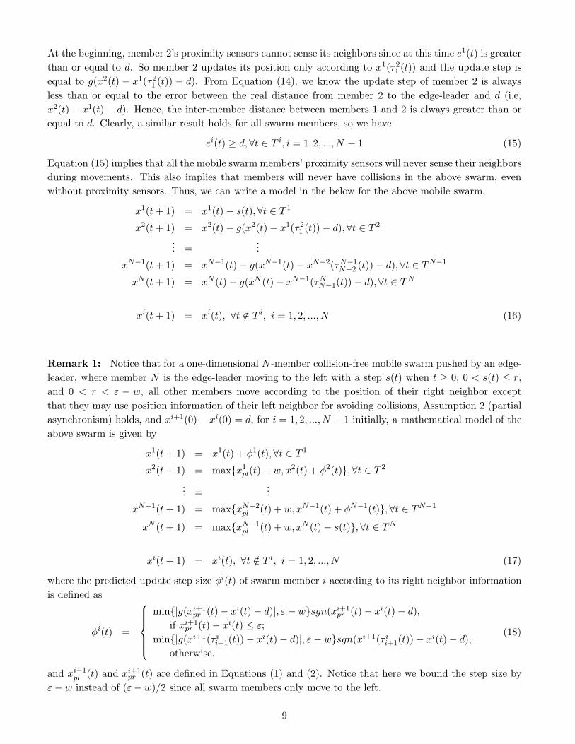
Remark 1: Notice that for a one-dimensional N -member collision-free mobile swarm pushed by an edge-leader, where member N is the edge-leader moving to the left with a step s(t) when t ≥ 0, 0 < s(t) ≤ r,and 0 < r < ε − w, all other members move according to the position of their right neighbor exceptthat they may use position information of their left neighbor for avoiding collisions, Assumption 2 (partialasynchronism) holds, and xi+1(0)− xi(0) = d, for i = 1, 2, ..., N − 1 initially, a mathematical model of theabove swarm is given by

x1(t+ 1) = x1(t) + φ1(t),∀t ∈ T 1

x2(t+ 1) = max{x1pl(t) + w, x2(t) + φ2(t)},∀t ∈ T 2

... =...

xN−1(t+ 1) = max{xN−2pl (t) + w, xN−1(t) + φN−1(t)},∀t ∈ TN−1

xN (t+ 1) = max{xN−1pl (t) + w, xN (t)− s(t)},∀t ∈ TN

xi(t+ 1) = xi(t), ∀t /∈ T i, i = 1, 2, ..., N (17)

where the predicted update step size φi(t) of swarm member i according to its right neighbor informationis defined as

φi(t) =

min{|g(xi+1pr (t)− xi(t)− d)|, ε − w}sgn(xi+1

pr (t)− xi(t)− d),if xi+1

pr (t)− xi(t) ≤ ε;min{|g(xi+1(τ i

i+1(t))− xi(t)− d)|, ε − w}sgn(xi+1(τ ii+1(t))− xi(t)− d),

otherwise.

(18)

and xi−1pl (t) and xi+1

pr (t) are defined in Equations (1) and (2). Notice that here we bound the step size byε− w instead of (ε− w)/2 since all swarm members only move to the left.

9

3 Convergence Analysis of One-Dimensional Asynchronous Swarms

In this section, we will study stability properties of one-dimensional asynchronous swarms on the basis ofmathematical models we built earlier and provide conditions under which the swarm will obtain and keepthe cohesiveness even in the presence of sensing delays and asynchronism. First we will consider stationaryedge-member asynchronous N -member swarms, and then we will investigate N -member asynchronousmobile swarms following, or pushed by an edge-leader.

3.1 Convergence Analysis of Stationary Edge-Member Asynchronous Swarms

Here, we will provide conditions under which the swarm in Figure 2 will converge to be adjacent to astationary left-edge member. By symmetry, the case for convergence to a stationary right-edge memberis the same. We begin with the two-member case, then consider the general N -member case where theproofs will depend on the N = 2 case.

3.1.1 Convergence for a Two-Member Swarm

Suppose there is a one-dimensional two-member swarm, which has member i and i − 1. Assume at thebeginning we have xi(0) − xi−1(0) > ε and member i− 1 remains stationary so that proximity sensors ofmember i will never sense member i − 1. Therefore, we define the update step size φi(t) of member i insuch a two-member swarm as follows,

φi(t) = g(xi(t)− xi−1(τ ii−1(t)) − d) (19)

where the step size only depends on the g function.

Lemma 1. For an N = 2 totally asynchronous swarm modeled by

xi−1(t+ 1) = xi−1(t),∀t ∈ T

xi(t+ 1) = xi(t)− φi(t),∀t ∈ T i

xi(t+ 1) = xi(t),∀t /∈ T i (20)

where xi−1(t) = xi−1c , xi−1

c is a constant, xi(0)−xi−1(0) > ε, and φi(t) is defined in Equation (19) with g =ga, it is the case that for any γ, 0 < γ < d−ε, there exists a time t′ such that xi(t′) ∈ [xi−1

c +d−γ, xi−1c +d+γ]

and also limt→∞ xi(t) = xi−1c + d.

Proof. First, for the model in Equation (20), note that at the beginning member i remains stationaryuntil it senses member i− 1’s information xi−1(τ i

i−1(t)), which is equal to xi−1c since member i− 1 always

stays at the position of xi−1c . Hence, we can write Equation (20) as follows,

xi−1(t+ 1) = xi−1c ,∀t ∈ T

xi(t+ 1) = xi(t)− ga(xi(t)− xi−1c − d),∀t ∈ T i

xi(t+ 1) = xi(t),∀t /∈ T i (21)

Next, define a Lyapunov-like function (note that it is not a Lyapunov function since x = [x1, ..., xN ] is notthe state of the system in Equation (10)),

Vi(t) = |xi(t)− (xi−1c + d)|,∀t ∈ T i,

10

that measures how close swarm member i is to the comfortable distance from member i− 1. Notice that

Vi(t+ 1) = |xi(t+ 1)− (xi−1c + d)|

= |xi(t)− ga(xi(t)− (xi−1c + d)) − (xi−1

c + d)|= |(xi(t)− xi−1

c − d)− ga(xi(t)− xi−1c − d)|,∀t ∈ T i.

We will do a case analysis. First, for any t ∈ T i such that xi(t)− xi−1c = d, we have

ga(xi(t)− (xi−1c + d)) = ga(0) = 0

according to Equation (4), so we get

xi(t+ 1) = xi(t)− 0 = xi−1c + d,

which means member i will stay at the position (xi−1c + d). Next, we will analyze the cases where at some

t ∈ T i, xi(t)− xi−1c > d or xi(t)− xi−1

c < d.Note that if at any time t ∈ T i, xi(t)− xi−1

c > d (xi(t)− xi−1c < d), it will be the case that ∀t′ ≥ t, t′ ∈

T i, xi(t′)−xi−1c > d (xi(t′)−xi−1

c < d). Due to this, in our analysis of bounds on the time required to reachthe comfortable distance neighborhood, we can treat the cases of xi(t) − xi−1

c > d and xi(t) − xi−1c < d

separately.Case 1: If at some t ∈ T i, xi(t)− xi−1

c > d, then

ga(xi(t)− xi−1c − d) > 0 (22)

and

Vi(t) = xi(t)− (xi−1c + d). (23)

According to Equation (3), we have for this t ∈ T i

ga(xi(t)− xi−1c − d) ≤ (xi(t)− xi−1

c − d)

so for this t ∈ T i

Vi(t+ 1) = xi(t)− xi−1c − d− ga(xi(t)− xi−1

c − d), (24)

and then using Equations (22), (23), and (24),

∆Vi = Vi(t+ 1)− Vi(t) = −ga(xi(t)− xi−1c − d) < 0. (25)

Moreover, if at some t ∈ T i, xi(t)−xi−1c > d, from Equations (3) and (21), we have xi(t+1)−xi−1

c > d.So Equation (25) always holds in this case.

From Equations (3) and (25), we know that if member i is beyond the γ−range of position (xi−1c + d)

(i.e., xi(t)− xi−1c > d+ γ), we get

γ

β<

1β(xi(t)− xi−1

c − d) < ga(xi(t)− xi−1c − d)

So it will move toward this range with a moving step at least larger than γβ . Hence, member i needs at

mostβ

γ(xi(0)− xi−1

c − d− γ)

11

update time steps, and at least one update time step, to reach the γ−range of position (xi−1c + d), where

xi(0) is the initial position of member i (in this case, we have (xi(0) − xi−1c − d) ≥ (xi(t) − xi−1

c − d), fort ≥ 0). So there exists a time t′ such that xi(t′) ∈ (xi−1

c + d, xi−1c + d+ γ].

Case 2: If at some t ∈ T i, xi(t)− xi−1c < d, then

ga(xi(t)− xi−1c − d) < 0 (26)

and

Vi(t) = (xi−1c + d)− xi(t). (27)

According to Equation (5), we have

(xi(t)− xi−1c − d) ≤ ga(xi(t)− xi−1

c − d)

so

Vi(t+ 1) = ga(xi(t)− xi−1c − d)− (xi(t)− xi−1

c − d), (28)

and then using Equations (26), (27), and (28), for this t ∈ T i

∆Vi = Vi(t+ 1)− Vi(t) = ga(xi(t)− xi−1c − d) < 0. (29)

Similar to Case 1, from Equations (5) and (21), if at some t ∈ T i, xi(t)− xi−1c < d, we have xi(t+1)−

xi−1c < d. So Equation (29) always holds in this case. Also, similar to Case 1, from Equation (5) and (29)

we know that if xi(t)− xi−1c < d− γ, we get

ga(xi(t)− xi−1c − d) <

1β(xi(t)− xi−1

c − d) < −γ

β

So it will move toward this range with a moving step at least larger than γβ . Hence, we can show that

member i needs at mostβ

γ(xi−1

c + d− xi(0) − γ)

update time steps, and at least one update time step, to reach the γ−range of position (xi−1c + d), where

xi(0) is the initial position of member i (in this case, we have (xi−1c + d− xi(0)) ≥ (xi−1

c + d − xi(t)), fort ≥ 0). So there exists a time t′ such that xi(t′) ∈ [xi−1

c + d− γ, xi−1c + d).

Finally, for asymptotic convergence, from Equations (25) and (29), we know that for t ∈ T i, Vi(t) willasymptotically tend to zero (i.e., limt→∞ xi(t) = xi−1

c + d). Q.E.D.

Corollary 1. For a two-member swarm in Lemma 1, if member i− 1, instead of remaining station-ary at xi−1

c , monotonically approaches the position xi−1c as t → ∞ (i.e., xi−1

c ≤ xi−1(t + 1) < xi−1(t) orxi−1(t) < xi−1(t+ 1) ≤ xi−1

c , ∀t ∈ T i−1), and |xi−1(0)− xi−1c | < γ, where 0 < γ < d− ε, the conclusion of

Lemma 1 still holds.

Proof. First, we define δi−1(t) = |xi−1(t)−xi−1c |, which denotes member i−1’s distance to its desired

position xi−1c at time t ∈ T i−1. Since xi−1(t) monotonically goes to xi−1

c as t → ∞, we have

limt→∞ δi−1(t) = 0 (30)

12

And also we know |xi−1(0)− xi−1c | < γ. Hence, we have |xi−1(t)− xi−1

c | < γ, i.e.,

0 ≤ δi−1(t) < γ (31)

Next, let

δi(t) = xi(t)− xi−1c − d, t ∈ T i (32)

which is member i’s distance to its desired position xi−1c +d at time t ∈ T i. Note that δi(t) can be negative,

where a negative value means member i stays on the left side of xi−1c + d. A positive value means it is on

the right side of xi−1c + d. Member i will move according to

xi(t+ 1) = xi(t)− ga(xi(t)− xi−1(τ ii−1(t))− d),∀t ∈ T i (33)

Hence, we have

δi(t+ 1) = xi(t)− xi−1c − d− ga(xi(t)− xi−1(τ i

i−1(t))− d)

= δi(t)− ga(xi(t)− xi−1(τ ii−1(t))− d) (34)

So

∆δi(t) = δi(t+ 1)− δi(t) = −ga(xi(t)− xi−1(τ ii−1(t))− d) (35)

Since member i− 1 monotonically approaches its desired position xi−1c from the left,

xi−1(t) = xi−1c − δi−1(t),∀t

and due to the definition of the delays, so

xi−1(τ ii−1(t)) = xi−1

c − δi−1(τ ii−1(t)) (36)

From Equations (32) and (35), we have

∆δi(t) = −ga(xi(t)− (xi−1c − δi−1(τ i

i−1(t)))− d)

= −ga(δi(t) + δi−1(τ ii−1(t))) (37)

We will study different possible cases when member i−1 monotonically approaches its desired positionxi−1

c from the left (i.e, xi−1(t) < xi−1(t + 1) ≤ xi−1c , ∀t ∈ T i−1). By symmetry, the cases where member

i − 1 monotonically approaches xi−1c from the right (i.e, xi−1

c ≤ xi−1(t + 1) < xi−1(t), ∀t ∈ T i−1) are thesame.

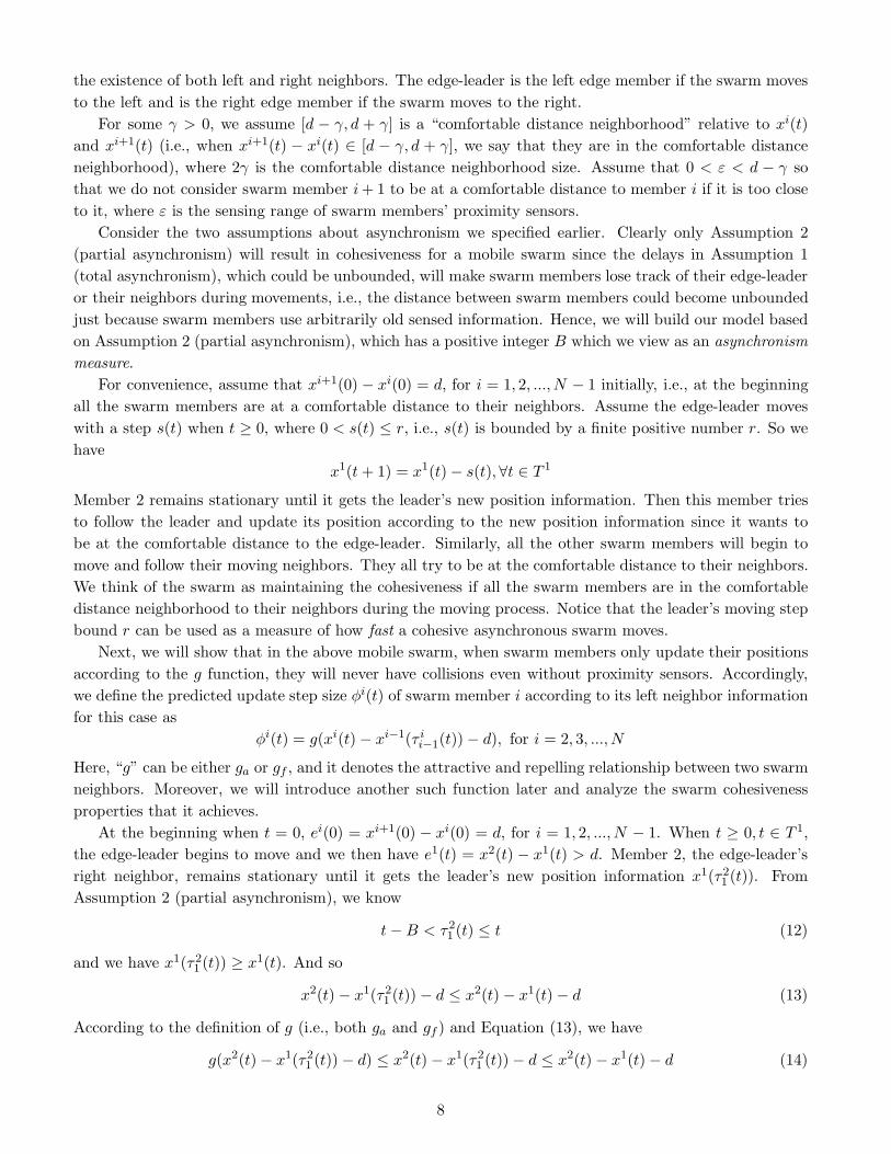
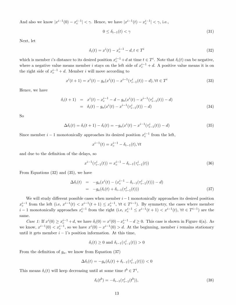
Case 1: If xi(0) ≥ xi−1c +d, we have δi(0) = xi(0)−xi−1

c −d ≥ 0. This case is shown in Figure 4(a). Aswe know, xi−1(0) < xi−1

c , so we have xi(0) − xi−1(0) > d. At the beginning, member i remains stationaryuntil it gets member i− 1’s position information. At this time,

δi(t) ≥ 0 and δi−1(τ ii−1(t)) > 0

From the definition of ga, we know from Equation (37)

∆δi(t) = −ga(δi(t) + δi−1(τ ii−1(t))) < 0

This means δi(t) will keep decreasing until at some time tb ∈ T i,

δi(tb) = −δi−1(τ ii−1(t

b)), (38)

13

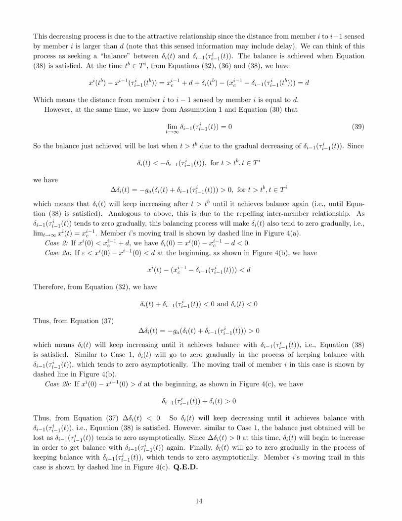
This decreasing process is due to the attractive relationship since the distance from member i to i−1 sensedby member i is larger than d (note that this sensed information may include delay). We can think of thisprocess as seeking a “balance” between δi(t) and δi−1(τ i

i−1(t)). The balance is achieved when Equation(38) is satisfied. At the time tb ∈ T i, from Equations (32), (36) and (38), we have

xi(tb)− xi−1(τ ii−1(t

b)) = xi−1c + d+ δi(tb)− (xi−1

c − δi−1(τ ii−1(t

b))) = d

Which means the distance from member i to i− 1 sensed by member i is equal to d.However, at the same time, we know from Assumption 1 and Equation (30) that

limt→∞ δi−1(τ i

i−1(t)) = 0 (39)

So the balance just achieved will be lost when t > tb due to the gradual decreasing of δi−1(τ ii−1(t)). Since

δi(t) < −δi−1(τ ii−1(t)), for t > tb, t ∈ T i

we have∆δi(t) = −ga(δi(t) + δi−1(τ i

i−1(t))) > 0, for t > tb, t ∈ T i

which means that δi(t) will keep increasing after t > tb until it achieves balance again (i.e., until Equa-tion (38) is satisfied). Analogous to above, this is due to the repelling inter-member relationship. Asδi−1(τ i

i−1(t)) tends to zero gradually, this balancing process will make δi(t) also tend to zero gradually, i.e.,limt→∞ xi(t) = xi−1

c . Member i’s moving trail is shown by dashed line in Figure 4(a).Case 2: If xi(0) < xi−1

c + d, we have δi(0) = xi(0) − xi−1c − d < 0.

Case 2a: If ε < xi(0)− xi−1(0) < d at the beginning, as shown in Figure 4(b), we have

xi(t)− (xi−1c − δi−1(τ i

i−1(t))) < d

Therefore, from Equation (32), we have

δi(t) + δi−1(τ ii−1(t)) < 0 and δi(t) < 0

Thus, from Equation (37)∆δi(t) = −ga(δi(t) + δi−1(τ i

i−1(t))) > 0

which means δi(t) will keep increasing until it achieves balance with δi−1(τ ii−1(t)), i.e., Equation (38)

is satisfied. Similar to Case 1, δi(t) will go to zero gradually in the process of keeping balance withδi−1(τ i

i−1(t)), which tends to zero asymptotically. The moving trail of member i in this case is shown bydashed line in Figure 4(b).

Case 2b: If xi(0)− xi−1(0) > d at the beginning, as shown in Figure 4(c), we have

δi−1(τ ii−1(t)) + δi(t) > 0

Thus, from Equation (37) ∆δi(t) < 0. So δi(t) will keep decreasing until it achieves balance withδi−1(τ i

i−1(t)), i.e., Equation (38) is satisfied. However, similar to Case 1, the balance just obtained will belost as δi−1(τ i

i−1(t)) tends to zero asymptotically. Since ∆δi(t) > 0 at this time, δi(t) will begin to increasein order to get balance with δi−1(τ i

i−1(t)) again. Finally, δi(t) will go to zero gradually in the process ofkeeping balance with δi−1(τ i

i−1(t)), which tends to zero asymptotically. Member i’s moving trail in thiscase is shown by dashed line in Figure 4(c). Q.E.D.

14

i-1

δi-1 (t)xi-1c - xi-1

c

i

xi(0)xi-1c + d

i-1

δi-1 (t)xi-1c - xi-1

c xi-1c

(a)

+ dxi(0)

i

(b)

i-1

δi-1 (t)xi-1c - xi-1

c

i

xi(0) xi-1c + d

(c)

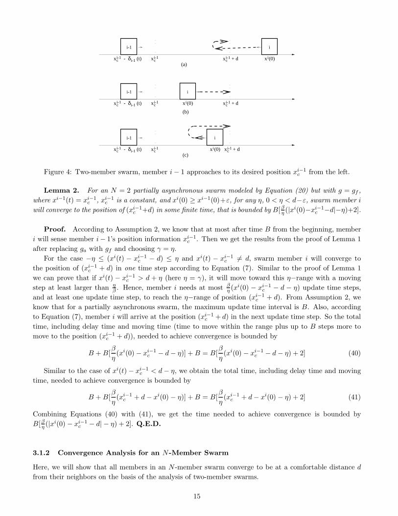
Figure 4: Two-member swarm, member i− 1 approaches to its desired position xi−1c from the left.

Lemma 2. For an N = 2 partially asynchronous swarm modeled by Equation (20) but with g = gf ,where xi−1(t) = xi−1

c , xi−1c is a constant, and xi(0) ≥ xi−1(0)+ε, for any η, 0 < η < d−ε, swarm member i

will converge to the position of (xi−1c +d) in some finite time, that is bounded by B[βη (|xi(0)−xi−1

c −d|−η)+2].

Proof. According to Assumption 2, we know that at most after time B from the beginning, memberi will sense member i− 1’s position information xi−1

c . Then we get the results from the proof of Lemma 1after replacing ga with gf and choosing γ = η.

For the case −η ≤ (xi(t) − xi−1c − d) ≤ η and xi(t) − xi−1

c �= d, swarm member i will converge tothe position of (xi−1

c + d) in one time step according to Equation (7). Similar to the proof of Lemma 1we can prove that if xi(t) − xi−1

c > d + η (here η = γ), it will move toward this η−range with a movingstep at least larger than η

β . Hence, member i needs at most βη (x

i(0) − xi−1c − d − η) update time steps,

and at least one update time step, to reach the η−range of position (xi−1c + d). From Assumption 2, we

know that for a partially asynchronous swarm, the maximum update time interval is B. Also, accordingto Equation (7), member i will arrive at the position (xi−1

c + d) in the next update time step. So the totaltime, including delay time and moving time (time to move within the range plus up to B steps more tomove to the position (xi−1

c + d)), needed to achieve convergence is bounded by

B +B[β

η(xi(0)− xi−1

c − d− η)] +B = B[β

η(xi(0) − xi−1

c − d− η) + 2] (40)

Similar to the case of xi(t)− xi−1c < d− η, we obtain the total time, including delay time and moving

time, needed to achieve convergence is bounded by

B +B[β

η(xi−1

c + d− xi(0)− η)] +B = B[β

η(xi−1

c + d− xi(0) − η) + 2] (41)

Combining Equations (40) with (41), we get the time needed to achieve convergence is bounded byB[βη (|xi(0) − xi−1

c − d| − η) + 2]. Q.E.D.

3.1.2 Convergence Analysis for an N-Member Swarm

Here, we will show that all members in an N -member swarm converge to be at a comfortable distance dfrom their neighbors on the basis of the analysis of two-member swarms.

15

Theorem 1. (Total Asynchronism, Asymptotic Convergence): For an N -member swarmwhich is modeled by Equation (10) with g = ga, N > 1, Assumption 1 (total asynchronism) holds, andxi+1(0) − xi(0) > ε, i = 1, 2, ..., N − 1, the swarm members’ positions (x1, x2, ..., xN ) will asymptoticallyconverge to (x1(0), x1(0) + d, x1(0) + 2d, ..., x1(0) + (N − 1)d), where x1(0) is the initial position of thestationary left-edge member.

Proof. We will use a mathematical induction method, where our induction hypothesis will be that kof N swarm members asymptotically converge to (x1(0), x1(0)+d, x1(0)+2d, ..., x1(0)+(k−1)d) and fromthis we will show that k + 1 of N members converge.

First, for k = 1, which is the left-edge member, it converges to x1(0) since it remains stationary. Nextwe must show that given the induction hypothesis, the first k + 1 members in the N -member swarm willasymptotically converge to the positions (x1(0), x1(0) + d, x1(0) + 2d, ..., x1(0) + kd).

According to our induction hypothesis we know that there exists a time t∗ such that swarm memberi, for i = 2, 3, ...k, will stay in the range between x1(0) + (i − 1)d − γ and x1(0) + (i − 1)d + γ, where0 < γ < d − ε. Assume δi(t) = xi(t) − (x1(0) + (i − 1)d) for i = 2, 3, ...k, which represents member i’sdistance to its desired position, where δi(t) ∈ [−γ, γ] for t ≥ t∗.

Therefore, after t ≥ t∗, we have

xi(t+ 1) = x1(0) + (i− 1)d+ δi(t),∀t ∈ T i, for i = 2, 3, ..., k

for the first k members in the swarm except the stationary member 1 and from member k + 1 to memberN , we have

xk+1(t+ 1) = min{xk+1(t)− φk+1(t), xk+2pr (t)− w},

... =...

xN−1(t+ 1) = min{xN−1(t)− φN−1(t), xNpr(t)− w},∀t ∈ TN−1

xN (t+ 1) = xN (t)− φN (t),∀t ∈ TN (42)

where g in φi(t) is ga.Now considering member k + 1’s movements after t ≥ t∗, we will do a case analysis.Case 1: If for some t ∈ T k+1, t ≥ t∗, member k + 1’s proximity sensor senses member k, i.e.,

xkpl(t) = xk(t) = x1(0) + (k − 1)d+ δk(t)

from Equation (9), member k + 1 will move away from member k according to

xk+1(t+ 1) = min{xk+1(t)−min{|ga(xk+1(t)− (x1(0) + (k − 1)d+ δk(t))− d)|, (ε −w)/2}·

sgn(xk+1(t)− (x1(0) + (k − 1)d+ δk(t))− d), xk+2pr (t)− w

},∀t ∈ T k+1 (43)

Case 2: If member k + 1’s proximity sensor cannot sense member k, it will update its position by

xk+1(t+ 1) = min{xk+1(t)−min{|ga(xk+1(t)− xk(τk+1

k (t))− d)|, (ε − w)/2}·sgn(xk+1(t)− xk(τk+1

k (t))− d), xk+2pr (t)− w

},∀t ∈ T k+1 (44)

Case 2a: If member k + 1 moves towards to member k, due to its outdated information xk(τk+1k (t))

about member k, such that after some time its proximity sensor senses member k, then it will be the sameas Case 1.

16

Case 2b: If member k + 1 moves according to Equation (44), but its proximity sensor never sensesmember k, then according to Assumption 1, given time t∗, there exists a time tc > t∗ such that τk+1

k (t) ≥ t∗,∀k and t ≥ tc. So after t ≥ tc, member k + 1 knows member k is at the position x1(0) + (k − 1)d + δk(t).It will move according to Equation (43).

According to our induction hypothesis, we already know

limt→∞ δi(t) = 0, for i = 2, 3, ...k

So if member k + 2 does not prevent its movements (i.e., xk+1(t + 1) is never equal to xk+2pr (t) − w in

Equation (43)), as δk(t) goes to zero, member k + 1 will move to its desired position as δk(t) by

xk+1(t+ 1) = xk+1(t)−min{|ga(xk+1(t)− (x1(0) + (k − 1)d+ δk(t))− d)|, (ε − w)/2} ·sgn(xk+1(t)− (x1(0) + (k − 1)d+ δk(t))− d),∀t ∈ T k+1 (45)

If |ga(xk+1(t) − (x1(0) + (k − 1)d + δk(t)) − d)| is always less than (ε − w)/2 in Equation (45), memberk + 1 will move by

xk+1(t+ 1) = xk+1(t)− ga(xk+1(t)− (x1(0) + (k − 1)d+ δk(t))− d),∀t ∈ T k+1

so that it will asymptotically converge to (x1(0) + (k − 1)d + d) = (x1(0) + kd) by Corollary 1. If|ga(xk+1(t)−(x1(0)+(k−1)d+δk (t))−d)| is larger than (ε−w)/2 member k+1 will move to the directionwhere |xk+1(t) − (x1(0) + (k − 1)d + δk(t)) − d| becomes smaller with a step (ε − w)/2. Therefore, thereexists some time ts that after t > ts, |ga(xk+1(t) − (x1(0) + (k − 1)d + δk(t)) − d)| is always less than(ε− w)/2 so that it will be the same as the above.

If member k + 1’s proximity sensor finds member k + 2 nearby at time tp ∈ T k+1, we have

xk+1(tp + 1) = xk+2(tp)− w

Note that at the same time member k+2 also gets member k+1’s current position via its proximity sensorsince their current adjacent distance is w. There exists a time tu ≥ tp + 1, tu ∈ T k+2 that member k + 2will update its position according to

xk+2(t+ 1) = min{xk+2(t)−min{|ga(xk+2(t)− (xk+2(tp)− w)− d)|, (ε − w)/2}·

sgn(xk+2(t)− (xk+2(tp)− w)− d), xk+3pr (t)− w

},∀t ∈ T k+2, t ≥ tu

Member k + 2’s temporary destination is the position of (xk+2(tp) − w + d) (we say “temporary” sinceas swarm member k + 1 converges the ultimate desired position may be somewhere else). Similarly, fromEquation (42) member k+3 could prevent member k+2’s further moving, and member k+4 could preventmember k + 3, etc. In the end, member N could prevent member N − 1. However, member N is free tomove to the right.

Since we assume the sets T i are infinite, and each swarm member moves infinitely often, we know thatin the above cases after some time, member N could move away from member N − 1, and member N − 1could move away from member N −2, etc. So after member k+2 moves away from member k+1, memberk + 1 will continue moving to the position (x1(0) + kd).

However, member k + 2 may prevent member k + 1 again after t > tu due to the total asynchronism.It is similar for member k + 3, k + 4, and so on. In that case, it will repeat the above process. We knowthat member k + 2’s distance to the position (x1(0) + kd) is finite, and there are only a finite numberof members in the swarm, and swarm member’s movements cannot be infinitely small if the distance to

17

its desired position is not infinitely small via the definition of ga. So there exists a time tnp > tp suchthat member k + 2 will have moved beyond the position (x1(0) + kd). After t > tnp, member k + 2 willnever prevent member k + 1 again. From Corollary 1 and our induction hypothesis, member k + 1 willasymptotically converge to the position (x1(0) + kd). This ends the induction step. Q.E.D.

Theorem 2. (Partial Asynchronism, Finite Time Convergence): For an N -member swarmwhich is modeled by Equation (10) with g = gf , N > 1, Assumption 2 (partial asynchronism) holds, andxi+1(0) − xi(0) > ε, i = 1, 2, ..., N − 1, for any η, 0 < η < (ε − w)/2, the swarm members’ positions(x1, x2, ..., xN ) will converge to (x1(0), x1(0) + d, x1(0) + 2d, ..., x1(0) + (N − 1)d) in some finite time, thatis bounded by

B2N−2[β

η(max

i(|xi(0)− x1(0) − (i− 1)d|) − η) + 2] (46)

for i = 2, 3, ..., N , where x1(0) is the initial position of the stationary left-edge member.

Proof. We use the same induction method as the proof of Theorem 1 except that the swarm is partiallyasynchronous now. So we will use Assumption 2 and Lemma 2, instead of Assumption 1 and Corollary 1,to deduce member k + 1 will arrive at the position (x1(0) + kd) in some finite time, instead of its desiredposition neighborhood after some time.

Next, we will try to bound the amount of converging time for the N -member swarm. In Lemma 2 wededuce that for a two-member swarm the time needed to achieve convergence is bounded by

B[β

η(|xi(0)− xi−1

c − d| − η) + 2]

For the N -member swarm, it is possible that blockades never occur among swarm members (i.e., membersdo not hinder their neighbors’ movements). As we know, swarm members move to their desired positionswith a step at least larger than η

β when they are beyond η-range of their desired positions due to thedefinition of gf and 0 < η

β < η < (ε − w)/2. Therefore, for this special case, similar to Lemma 2 we canbound the total converging time by

BN [β

η(max

i(|xi(0)− x1(0)− (i− 1)d|) − η) + 2], for i = 2, 3, ..., N.

This is the bound for the case that blockade never happens. As we know, blockades will prolong theconverging time. In order to get the bound for the blockade case, we go to another extremely specialworse case, that all middle swarm members will be blocked by their neighbors in every moving step andcannot move until the blockades are released. Moreover, we know that the first member (left-edge mem-ber) remains stationary, and the Nth member (right-edge member) is free to move to the right. In thisspecial case, we know from analysis in Theorem 1 that each middle swarm member’s distance to its desiredposition, which is |xi(0)− x1(0)− (i− 1)d| is finite, and they are blocked by their neighbors and can onlymove after their neighbors do not prevent them any more. This process repeats until they arrive at theirdesired positions. We know that each of their moving steps is at least larger than η

β . In this special case,for member 2, there are N − 2 members preventing it. Similarly for member 3, N − 3 members prevent it;for member 4, N − 4 members prevent it, and so on, until for member N − 1, only one member prevent it.Since we know (N − 2) + (N − 3) + (N − 4) + ...+ 1 < 2N−2, we can estimate that the maximum possibletotal update time steps will be 2N−2[βη (maxi (|xi(0) − x1(0)− (i− 1)d|)− η) + 2]. Then we can bound thetotal converging time by Equation (46) for this special case since the maximum update time interval isB. In fact, we know that there are many possibilities on how the N -member swarm moves. But all the

18

moving cases can be seen as one or different combinations of the above two special cases, and their boundslies in between the above two bounds, which are for two special cases. So we can bound the amount ofconverging time for the N -member swarm by the largest bound in Equation (46). Q.E.D.

Remark 2: Note that for an N -member swarm, if τ ii−1(t) = t (respectively, τ i

i+1(t) = t) for i = 2, 3, ..., N(i = 1, 2, ..., N − 1), for all t ∈ T i, which means member i obtains position information about its neighbori− 1 (i + 1) without delay, then we can get the same results as in Theorem 1 and 2 by the swarm modelwithout proximity sensors.

3.2 Convergence Analysis of Asynchronous Mobile Swarms Following an Edge-Leader

Next, we will study cohesiveness of a mobile swarm. First, we will study the case of using the gf function,and then what happens if a different g function is used that does not require a swarm member to move tobe adjacent to its neighbor in one step if it gets very close to it. While we only consider a left-edge memberleading a swarm to the left, by symmetry, the case where the right-edge member leads the mobile swarmto the right is the same (only the model is different).

3.2.1 Convergence for an N-Member Asynchronous Mobile Swarm

First, we choose gf as the g function in Equation (16) and assume γ = η (η is used in the definitionof gf ). We will show that all members in a N -member mobile swarm will be in a comfortable distanceneighborhood from their neighbors during movements if there are constraints on the leader’s moving stepbound, the partial asynchronism measure, and the comfortable distance neighborhood size.

Theorem 3. For an N -member asynchronous mobile swarm modeled by Equation (16), where g is gf ,N > 1, Assumption 2 (partial asynchronism) holds, and xi+1(0) − xi(0) = d, i = 1, 2, ..., N − 1, if

0 < r ≤ γ

NB − 1(47)

for a given γ, all the swarm members will be in the comfortable distance neighborhood [d, d + γ] of theirneighbors during the moving process, where r is the upper bound of the edge-leader’s moving step s(t),B ∈ Z+ is the partial asynchronism measure and γ (choose γ = η) is the comfortable distance neighbor-hood size.

Proof. For such a N -member mobile swarm, each swarm member follows its left neighbor exceptthat the edge-leader moves by itself. We know from Equation (15) that there are no collisions betweenmembers. This decouples the problem so that we can consider each pair of neighboring swarm membersindividually.

Consider the relationship between member 1, the edge-leader, and member 2. According to Assumption2, for every t ≥ 0, t ∈ T i, swarm member i updates its position at least at a time represented by one ofthe elements of the set {t, t+ 1, ..., t +B − 1}, and from Equation (12), we have

0 ≤ t− τ21 (t) < B, for t ∈ T 2, t ≥ 0

which means member 2’s delay in knowing about member 1 can be as large as B − 1.In order to show the cohesiveness of the first two members, we will show that member 2 can keep

the distance from member 1 in the range of comfortable distance neighborhood even in the “worst” case.Here, the worst case means that member 1 will update its position with a maximum possible step r in

19

every time index in T (i.e., when T 1 = T ), and member 2 only updates its position at the last elementof {t, t + 1, ..., t + B − 1} for t ∈ T 2, t ≥ 0 (i.e., at t + B − 1). Moreover, in the worst case, member 2’ssensed information about member 1 has the maximum delay B − 1. So in the worst case we have member2 senses member 1’s position as

x1(τ21 (t)) = x1(t−B − 1), t ∈ T 2 (48)

Assume when t = 0, the initial position of member 1 is x1(0), so member 2’s initial position is x2(0) =x1(0) + d. Considering the worst case above, in the first time set {0, 1, ..., B − 1} from t = 0, the distancebetween members 1 and 2 increases as the edge-leader moves with a step r. When t = B − 1, i.e, the lasttime index of the first time set {0, 1, ..., B − 1}, the leader member 1’s position will be

x1(t) = x1(0)− (B − 1)r

since it updates its position with a step r in every time index. From Equation (48), member 2’s sensedinformation about member 1 at t = B − 1 is

x1(τ21 (B − 1)) = x1(0)

Hence, member 2 remains stationary at x1(0) + d at this time index since it thinks it is still at thecomfortable distance to member 1. In fact, their actual distance at this time is

e1(B − 1) = x2(B − 1)− x1(B − 1) = x1(0) + d− (x1(0)− (B − 1)r) = d+ (B − 1)r

Next, in the worst case, member 2 will move at the last possible time and have the oldest possibleinformation about the position of member 1. Hence, in the second time set {B,B + 1, ..., 2B − 1} fromt = 0, when t = B, member 1’s position will be

x1(t) = x1(0)−Br

and member 2 still remains stationary at x1(0)+d since in the worst case it is not the time for it to updateits position. Their distance now is

e1(B) = x1(0) + d− (x1(0) −Br) = d+Br

From time index B to 2B−1, the distance between members 1 and 2, e1(t), will increase by r in each timestep since member 1 keeps updating by steps of size r and member 2 remains stationary. When t = 2B−1,member 1’s position will be

x1(2B − 1) = x1(0)− (2B − 1)r

Member 2 stays at the position x1(0) + d at t = 2B − 1, and will update its position according to

x2(t+ 1) = x2(t)− gf (x2(t)− x1(τ21 (t))− d) (49)

and then, the distance between them at t = 2B − 1 is

e1(2B − 1) = d+ (2B − 1)r

which is the maximum distance achieved during the times {B,B + 1, ..., 2B − 1}. The minimum distanceis d+Br when t = B. From Equation (48), we know

x1(τ21 (2B − 1)) = x1(B) = x1(0) −Br

20

and so, the argument of gf in Equation (49) is

x2(2B − 1)− x1(τ21 (2B − 1)) − d = x1(0) + d− (x1(0)−Br)− d = Br (50)

From Equation (47) and the fact that N > 1, B ∈ Z+, we have

Br ≤ (2B − 1)r ≤ (NB − 1)r ≤ γ (51)

Since we choose γ = η, from Equations (50), (51), and the definition of gf , we then have

gf (x2(2B − 1)− x1(τ21 (2B − 1))− d) = x2(2B − 1)− x1(τ2

1 (2B − 1))− d = Br

So

x2(2B) = x2(2B − 1)−Br = x1(0) + d−Br (52)

In the third time set {2B, 2B + 1, ..., 3B − 1}, when t = 2B, member 1’s position will be

x1(t) = x1(0)− 2Br

from Equation (52), we have

e1(2B) = x2(2B)− x1(2B) = x1(0) + d−Br − (x1(0)− 2Br) = d+Br

The inter-member distance decreases back to d + Br due to the position update of member 2, and thenit will repeat the above distance increasing process. When t = 3B − 1, it reaches the maximum distanced+ (2B − 1)r in this time set.

We find that in the worst case the distance between members 1 and 2 will change from the minimumd+ Br to the maximum d + (2B − 1)r periodically and the period is B. Thus, we can conclude that themaximum possible inter-member distance for members 1 and 2 is d+(2B−1)r during the moving process.

Next, we try to find the maximum possible inter-member distance between members 2 and 3 so that aspecial case (that is different from the worst case for members 1 and 2 above) is considered as follows. Aswe know, in the above worst case for members 1 and 2, when t = 2B − 1,

x1(2B − 1) = x1(0)− (2B − 1)r

andx2(2B − 1) = x1(0) + d

At this time, member 3 stays at the position of x1(0)+2d. Now different from above, we assume that sincet = 2B− 1, member 2 gets the position information of member 1 without any delay (i.e., x1(τ2

1 (2B− 1)) =x1(2B − 1) = x1(0) − (2B − 1)r) and member 1 still updates its position with a maximum possiblestep r in every time index in T . Moreover, member 3 only updates its position at the last element of{t, t+ 1, ..., t +B − 1} for t ∈ T 3, t ≥ 0 (i.e., at t+B − 1). And then, when t = 2B,

x1(2B) = x1(0)− 2Br

From Equation (47) and the fact that N > 1

x2(2B − 1)− x1(τ21 (2B − 1))− d = x1(0) + d− (x1(0) − (2B − 1)r)− d = (2B − 1)r ≤ (NB − 1)r ≤ γ

21

(note that this is different from Equation (51) above since for this case we assume that there is no delayin member 2 getting member 1’s position information). From the definition of gf , we then have

gf (x2(2B − 1)− x1(τ21 (2B − 1))− d) = x2(2B − 1)− x1(τ2

1 (2B − 1)) − d = (2B − 1)r

Therefore, from Equation (49) we get

x2(2B) = x1(0) + d− (2B − 1)r

and the distance between members 1 and 2 at t = 2B is

e1(2B) = x2(2B)− x1(2B) = d+ r

which is clearly smaller than the worst case when we consider only members 1 and 2 above. Here, we arecreating a worst case for members 2 and 3, which is different from the worst case for members 1 and 2.Next, note that member 3 remains at the position of x1(0)+2d since the distance between members 2 and3 is equal to d at time t = 2B − 1. And so, their distance at t = 2B is

e2(2B) = x3(2B)− x2(2B) = x1(0) + 2d− (x1(0) + d− (2B − 1)r) = d− (2B − 1)r

We further assumed members 1 and 2 will update their positions synchronously (i.e., they have the sameupdate time sets and member 2 obtains the position information of member 1 without any delay) aftert = 2B so that they will keep their distance as d past the time t = 2B + 1. Consequently, in the followingtime set {2B+2, ..., 3B− 2}, members 1 and 2 will update their positions with a maximum possible step rsynchronously while maintaining an inter-member distance d. During this time period, member 3 remainsat the position of x1(0) + 2d since in order to create the worst case, we assume it only updates its positionat the last element of {2B, 2B+1, ..., 3B − 1} (i.e., t = 3B− 1). Therefore, the distance between members2 and 3 will keep increasing until t = 3B − 1.

When t = 3B − 1,x1(3B − 1) = x1(0)− (3B − 1)r

andx2(3B − 1) = x1(0) + d− (3B − 1)r

So, the distance between members 1 and 2 is

e1(3B − 1) = x2(3B − 1)− x1(3B − 1) = d

Furthermore, member 3 remains at the position x1(0) + 2d and will update its position according to itssensed information of member 2, so that the inter-member distance of members 2 and 3 at this time

e2(3B − 1) = x3(3B − 1)− x2(3B − 1) = (x1(0) + 2d) − (x1(0) + d− (3B − 1)r) = d+ (3B − 1)r

which is the maximum possible distance in this time period. Notice that this maximum possible inter-member distance of members 2 and 3 is larger than the maximum possible inter-member distance formembers 1 and 2, which is d+(2B−1)r. In fact, this is also the maximum possible inter-neighbor distanceof members 2 and 3 in all their updating time sets T 2 and T 3. The reason is that this distance will decreaseat t = 3B due to the position updating of member 3, and then in the future time indices, even in the worstcase, the maximum possible distance between members 2 and 3 will only be equal to d+ (2B − 1)r. Here,the worst case is similar to that of members 1 and 2 we discussed above, where members 1 and 2 keepupdating synchronously their positions with a maximum possible step r in every time index, and member

22

3 has the maximum sensing delay B − 1 about the position member 2 and can only updates its positionat the last element of {t, t+ 1, ..., t +B − 1} for t ∈ T 3, t ≥ 0.

In the same way, we can find that the maximum possible inter-member distance between membersN−1 and N is d+(NB−1)r when t = NB−1, which is the largest of all possible inter-neighbor distancesin the time set T . Hence, we conclude that the maximum possible inter-neighbor distance for N membersis d+ (NB − 1)r.

From Equation (47), we haved+ (NB − 1)r ≤ d+ γ

and from Equation (15), we then have

d ≤ ei(t) ≤ d+ (NB − 1)r ≤ d+ γ, for i = 1, 2, ..., N − 1

which means all members will always be in the comfortable distance neighborhood [d, d + γ] with theirneighbors. So all members can keep the distance from their neighbors in the range of comfortable distanceneighborhood even in the worst case. Q.E.D.

Remark 3: Note the following about Equation (47):

• For a given B and γ, it provides bound on how fast a N -member swarm can move and still maintainthe type of cohesiveness characterized by γ. For example, increases in swarm size, communicationdelays, or swarm cohesiveness (smaller γ) require decreases in the rate of movement of the leader.

• For a given r and B, it provides the size of the neighborhood that will be maintained and hencespecifies a degree of cohesiveness of a N -member swarm.

• For a given r and γ, it provides constraints on how to design a communication system (i.e., what isneeded for B) for a N -member swarm between swarm members and indicates how often they mustupdate their positions.

Remark 4: From Theorems 1 and 2, we can see that if the edge-leader stops moving (i.e., s(t) = 0, t ≥ t1

for some t1 ∈ T 1), all other N − 1 members will converge to be adjacent to the edge-leader with acomfortable distance d.

3.2.2 Alternative Convergence Conditions

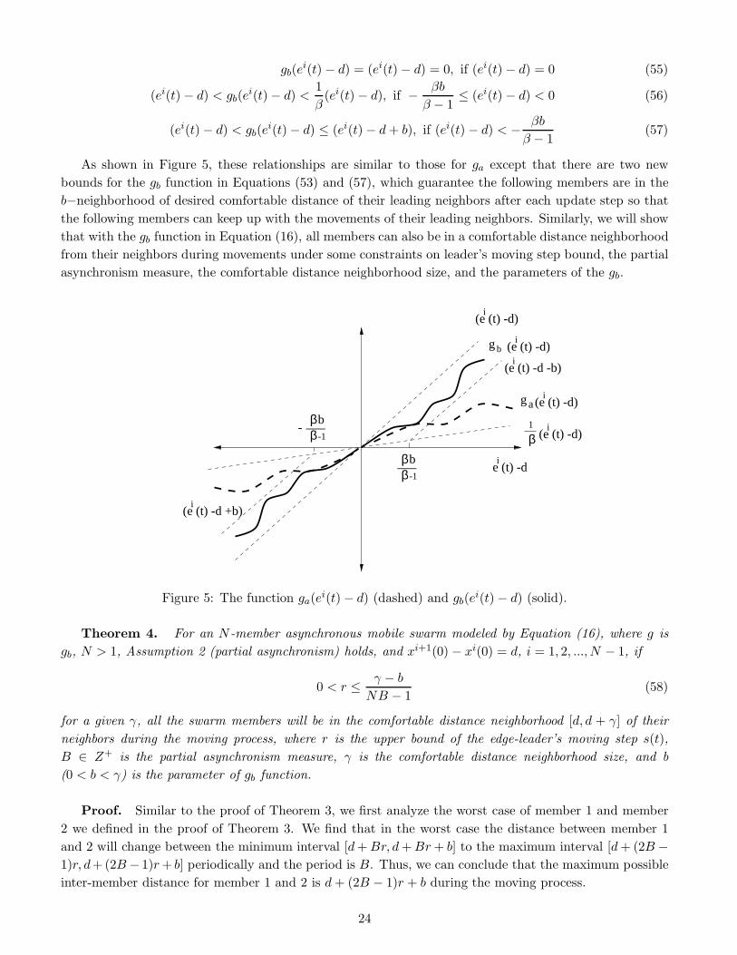
Now we consider the case of using the ga function in Equation (16), as shown in Figure 5. Intuitively,we can see that for some ga function it is possible that the distance between two swarm neighbors willdiverge since the following member’s update step ga cannot keep up with the moving rate of the leadingmember. Hence, not all ga functions can make asynchronous mobile swarms maintain their cohesivenessduring movements. However, we can add some constraints on ga function to create a new function, say gb,which will result in asynchronous mobile swarms maintaining their cohesiveness under some conditions onleader’s moving step bound, the partial asynchronism measure, and the comfortable distance neighborhoodsize.

Assume that for some scalars β and b, such that β > 1, and b > 0, gb(ei(t)− d) is such that

(ei(t)− d− b) ≤ gb(ei(t)− d) < (ei(t)− d), if (ei(t)− d) >βb

β − 1(53)

1β(ei(t)− d) < gb(ei(t)− d) < (ei(t)− d), if 0 < (ei(t)− d) ≤ βb

β − 1(54)

23

gb(ei(t)− d) = (ei(t)− d) = 0, if (ei(t)− d) = 0 (55)

(ei(t)− d) < gb(ei(t)− d) <1β(ei(t)− d), if − βb

β − 1≤ (ei(t)− d) < 0 (56)

(ei(t)− d) < gb(ei(t)− d) ≤ (ei(t)− d+ b), if (ei(t)− d) < − βb

β − 1(57)

As shown in Figure 5, these relationships are similar to those for ga except that there are two newbounds for the gb function in Equations (53) and (57), which guarantee the following members are in theb−neighborhood of desired comfortable distance of their leading neighbors after each update step so thatthe following members can keep up with the movements of their leading neighbors. Similarly, we will showthat with the gb function in Equation (16), all members can also be in a comfortable distance neighborhoodfrom their neighbors during movements under some constraints on leader’s moving step bound, the partialasynchronism measure, the comfortable distance neighborhood size, and the parameters of the gb.

e (t) -d

(e (t) -d)i

β1

(e (t) -d)i

g a (e (t) -d)i

g b (e (t) -d)i

i(e (t) -d -b)

i(e (t) -d +b)

___-1

i

ββb

___-1β

βb-

Figure 5: The function ga(ei(t)− d) (dashed) and gb(ei(t)− d) (solid).

Theorem 4. For an N -member asynchronous mobile swarm modeled by Equation (16), where g isgb, N > 1, Assumption 2 (partial asynchronism) holds, and xi+1(0) − xi(0) = d, i = 1, 2, ..., N − 1, if

0 < r ≤ γ − b

NB − 1(58)

for a given γ, all the swarm members will be in the comfortable distance neighborhood [d, d + γ] of theirneighbors during the moving process, where r is the upper bound of the edge-leader’s moving step s(t),B ∈ Z+ is the partial asynchronism measure, γ is the comfortable distance neighborhood size, and b(0 < b < γ) is the parameter of gb function.

Proof. Similar to the proof of Theorem 3, we first analyze the worst case of member 1 and member2 we defined in the proof of Theorem 3. We find that in the worst case the distance between member 1and 2 will change between the minimum interval [d+Br, d+Br+ b] to the maximum interval [d+ (2B −1)r, d+(2B − 1)r+ b] periodically and the period is B. Thus, we can conclude that the maximum possibleinter-member distance for member 1 and 2 is d+ (2B − 1)r + b during the moving process.

24

Next, we find the bound of all possible inter-member distance of members 2 and 3 is d+ (3B− 1)r+ b.In the same way, we can find that the bound for possible inter-member distance between members N − 1and N is d+ (NB − 1)r+ b, which is actually the largest bound of all possible inter-neighbor distances inthe time set T . Hence, we conclude that a bound for all possible inter-neighbor distance in a N -membermobile asynchronous swarm is d+ (NB − 1)r + b.

From Equation (58), we have d+ (NB− 1)r+ b ≤ d+ γ and according to Equation (15), we then have

d ≤ ei(t) ≤ d+ (NB − 1)r + b ≤ d+ γ, for i = 1, 2, ..., N − 1

which means all members in a N -member mobile swarm will always be in the comfortable distance neigh-borhood [d, d+ γ] with their neighbors. So all members can keep the distance from their neighbors in therange of comfortable distance neighborhood even in the worst case. Q.E.D.

3.3 Convergence Analysis of Asynchronous Mobile Swarms Pushed by an Edge-

Leader

Next, we provide different conditions under which an N -member asynchronous mobile swarm pushed byan edge-leader can maintain cohesiveness during movements on the basis of the model in Equation (17).While we only consider a right-edge member pushing a swarm to the left, by symmetry, the case wherethe left-edge member pushes the mobile swarm to the right is the same. We can conclude the followingtwo theorems via the similar analysis ideas above on the basis of the model in Equation (17) with the gf

and gb functions, respectively.

Theorem 5. For an N -member asynchronous mobile swarm modeled by Equation (17), where g is gf ,N > 1, Assumption 2 (partial asynchronism) holds, 0 < γ < d−ε, and xi+1(0)−xi(0) = d, i = 1, 2, ..., N−1,if

0 < r ≤ γ

NB − 1(59)

for a given γ, all the swarm members will be in the comfortable distance neighborhood [d − γ, d] of theirneighbors during the moving process, where r is the upper bound of the edge-leader’s moving step s(t),B ∈ Z+ is the partial asynchronism measure, γ (choose γ = η, and 0 < η < ε − w) is the comfortabledistance neighborhood size, and ε is the sensing range of proximity sensors.

Theorem 6. For an N -member asynchronous mobile swarm modeled by Equation (17), where g is gb,N > 1, Assumption 2 (partial asynchronism) holds, 0 < γ < min{d − ε, ε − w}, and xi+1(0) − xi(0) = d,i = 1, 2, ..., N − 1, if

0 < r ≤ γ − b

NB − 1(60)

for a given γ, all the swarm members will be in the comfortable distance neighborhood [d−γ, d] of their neigh-bors during the moving process, where r is the upper bound of the edge-leader’s moving step s(t), B ∈ Z+

is the partial asynchronism measure, γ is the comfortable distance neighborhood size, b (0 < b < γ) is theparameter of gb function, and ε is the sensing range of proximity sensors.

Here, we have 0 < γ < ε−w so that swarm neighbors move only according to the corresponding g functionwhen their distance is already inside γ-neighborhood of the comfortable distance. The proof of these two

25

theorems is similar to that of Theorems 3 and 4, where we analyze the worst case to find the minimumor the lower bound of all possible inter-member distances and show that this minimum or lower bound isinside the comfortable distance neighborhood [d− γ, d] under the constraint in Equation (59) or Equation(60).

4 Conclusions

We construct mathematical models of one-dimensional asynchronous swarms by putting N identical singleswarm members together. We allow for finite-size swarm members and ensure collision-free swarming inall of our analysis. We show that for one-dimensional stationary edge-member asynchronous swarms, totalasynchronism leads to asymptotic convergence and partial asynchronism leads to finite time convergence.Moreover, we provide conditions under which an asynchronous mobile swarm following (pushed by) a edge-leader can keep the cohesiveness during movements even in the presence of delays and partial asynchronismbased on our model with different g functions. In particular, all members in a N -member mobile swarmwill be in a comfortable distance neighborhood [d, d+ γ] ([d− γ, d]) from their neighbors while the swarmmoves if there are constraints on leader’s moving step bound r, the partial asynchronism measure B, andthe comfortable distance neighborhood size γ. In this way, we have shown conditions under which a one-dimensional asynchronous swarm in different cases can maintain cohesion even in the presence of delaysand asynchronism. Notice that the conditions obtained from our analysis provide extra constraints on thelow level vehicle dynamics when we consider designing an actual vehicular swarm.

References

[1] E. Shaw, “The schooling of fishes,” Sci. Am., vol. 206, pp. 128–138, 1962.

[2] E. Bonabeau, M. Dorigo, and G. Theraulaz, Swarm Intelligence: From Natural to Artificial Systems.NY: Oxford Univ. Press, 1999.

[3] K. Passino, “Biomimicry of bacterial foraging for distributed optimization and control.” To appear inIEEE Control Systems Magazine, 2001.

[4] C. Reynolds, “Flocks, herds, and schools: A distributed behavioral model,” Comp. Graph, vol. 21,no. 4, pp. 25–34, 1987.

[5] M. Millonas, “Swarms, phase transitions, and collective intelligence,” in Artificial Life III, pp. 417–445,Addison-Wesley, 1994.

[6] R. Arkin, Behavior-Based Robotics. Cambridge, MA: MIT Press, 1998.

[7] G. Beni and J. Wang, “Swarm intelligence in cellular robotics systems,” in Proceedings of NATOAdvanced Workshop on Robots and Biological System, pp. 703–712, 1989.

[8] R. Rule, “The dynamic scheduling approach to automated vehicle macroscopic control,” Tech. Rep.EES-276A-18, Transport. Contr. Lab., Ohio State Univ., Columbus, OH, Sept. 1974.

[9] R. Fenton and R. Mayhan, “Automated highway studies at the Ohio State University - an overview,”IEEE Trans. on Vehicular Technology, vol. 40, pp. 100–113, Feb. 1991.

[10] D. Swaroop and K. Rajagopal, “Intelligent cruise control systems and traffic flow stability,” Trans-portation Research Part C: Emerging Technologies, vol. 7, no. 6, pp. 329–352, 1999.

26

[11] M. Pachter and P. Chandler, “Challenges of autonomous control,” IEEE Control Systems Magazine,pp. 92–97, April 1998.

[12] S. Singh, P. Chandler, C. Schumacher, S. Banda, and M. Pachter, “Adaptive feedback linearizingnonlinear close formation control of UAVs,” in Proceedings of the 2000 American Control Conference,(Chicago, IL), pp. 854–858, 2000.

[13] Q. Yan, G. Yang, V. Kapila, and M. Queiroz, “Nonlinear dynamics and output feedback controlof multiple spacecraft in elliptical orbits,” in Proceedings of the 2000 American Control Conference,(Chicago, IL), pp. 839–843, 2000.

[14] T. Fukuda, T. Ueyama, and T. Sugiura, “Self-organization and swarm intelligence in the society ofrobot being,” in Proceedings of the 2nd International Symposium on Measurement and Control inRobotics, (Tsukuba Science City, Japan), pp. 787–794, Nov. 1992.

[15] R. Brooks, ed., Cambrian Intelligence: The Early History of the New AI. Cambridge, MA: MIT Press,1999.

[16] M. Mataric, “Minimizing complexity in controlling a mobile robot population,” in IEEE Int. Conf.on Robotics and Automation, (Nice, France), pp. 830–835, May 1992.

[17] I. Suzuki and M. Yamashita, “Distributed anonymous mobile robots: formation of geometric patterns,”SIAM J. COMPUT., vol. 28, no. 4, pp. 1347–1363, 1997.

[18] G. Dudek and et al., “A taxonomy for swarm robots,” in IEEE/RSJ Int. Conf. on Intelligent Robotsand Systems, (Yokohama, Japan), pp. 441–447, July 1993.

[19] A. Mogilner and L. Edelstein-Keshet, “A non-local model for a swarm,” Journal of MathematicalBiology, vol. 38, pp. 534–570, 1999.

[20] K. Jin, P. Liang, and G. Beni, “Stability of synchronized distributed control of discrete swarmstructures,” in IEEE International Conference on Robotics and Automation, (San Diego, California),pp. 1033–1038, May 1994.

[21] K. Passino and K. Burgess, Stability Analysis of Discrete Event Systems. New York: John Wiley andSons Pub., 1998.

[22] D. Bertsekas and J. Tsitsiklis, Parallel and Distributed Computation Numerical Methods. NJ: PrenticeHall, 1989.

[23] J. Bender and R. Fenton, “On the flow capacity of automated highways,” Transport. Sci., vol. 4,pp. 52–63, Feb. 1970.

[24] D. Swaroop, String Stability of Interconnected Systems: An Application to Platooning in AutomatedHighway Systems. PhD thesis, Department of Mechanical Engineering, University of California, Berke-ley, 1995.

[25] R. Fenton, “A headway safety policy for automated highway operation,” IEEE Trans. Veh. Technol.,vol. VT-28, pp. 22–28, Feb. 1979.

[26] J. Hedrick and D. Swaroop, “Dynamic coupling in vehicles under automatic control,” Vehicle SystemDynamics, vol. 23, no. SUPPL, pp. 209–220, 1994.

27

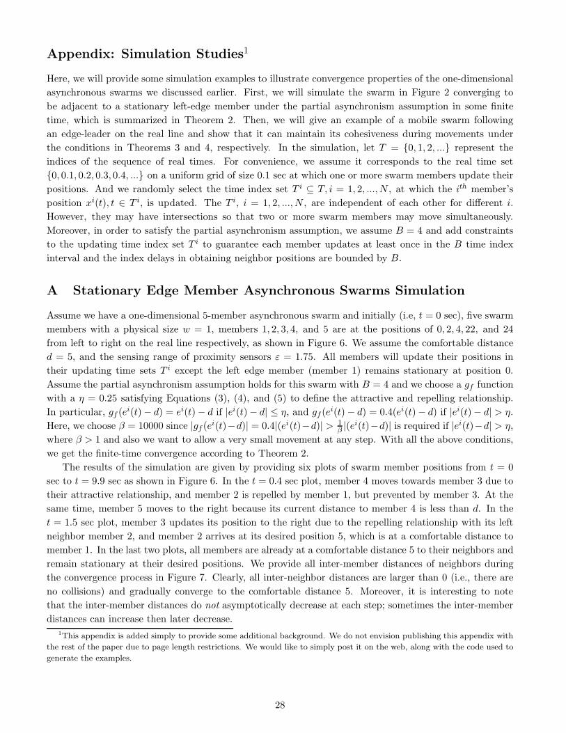
Appendix: Simulation Studies1

Here, we will provide some simulation examples to illustrate convergence properties of the one-dimensionalasynchronous swarms we discussed earlier. First, we will simulate the swarm in Figure 2 converging tobe adjacent to a stationary left-edge member under the partial asynchronism assumption in some finitetime, which is summarized in Theorem 2. Then, we will give an example of a mobile swarm followingan edge-leader on the real line and show that it can maintain its cohesiveness during movements underthe conditions in Theorems 3 and 4, respectively. In the simulation, let T = {0, 1, 2, ...} represent theindices of the sequence of real times. For convenience, we assume it corresponds to the real time set{0, 0.1, 0.2, 0.3, 0.4, ...} on a uniform grid of size 0.1 sec at which one or more swarm members update theirpositions. And we randomly select the time index set T i ⊆ T, i = 1, 2, ..., N , at which the ith member’sposition xi(t), t ∈ T i, is updated. The T i, i = 1, 2, ..., N , are independent of each other for different i.However, they may have intersections so that two or more swarm members may move simultaneously.Moreover, in order to satisfy the partial asynchronism assumption, we assume B = 4 and add constraintsto the updating time index set T i to guarantee each member updates at least once in the B time indexinterval and the index delays in obtaining neighbor positions are bounded by B.

A Stationary Edge Member Asynchronous Swarms Simulation

Assume we have a one-dimensional 5-member asynchronous swarm and initially (i.e, t = 0 sec), five swarmmembers with a physical size w = 1, members 1, 2, 3, 4, and 5 are at the positions of 0, 2, 4, 22, and 24from left to right on the real line respectively, as shown in Figure 6. We assume the comfortable distanced = 5, and the sensing range of proximity sensors ε = 1.75. All members will update their positions intheir updating time sets T i except the left edge member (member 1) remains stationary at position 0.Assume the partial asynchronism assumption holds for this swarm with B = 4 and we choose a gf functionwith a η = 0.25 satisfying Equations (3), (4), and (5) to define the attractive and repelling relationship.In particular, gf (ei(t)− d) = ei(t)− d if |ei(t)− d| ≤ η, and gf (ei(t)− d) = 0.4(ei(t)− d) if |ei(t)− d| > η.Here, we choose β = 10000 since |gf (ei(t)−d)| = 0.4|(ei(t)−d)| > 1

β |(ei(t)−d)| is required if |ei(t)−d| > η,where β > 1 and also we want to allow a very small movement at any step. With all the above conditions,we get the finite-time convergence according to Theorem 2.

The results of the simulation are given by providing six plots of swarm member positions from t = 0sec to t = 9.9 sec as shown in Figure 6. In the t = 0.4 sec plot, member 4 moves towards member 3 due totheir attractive relationship, and member 2 is repelled by member 1, but prevented by member 3. At thesame time, member 5 moves to the right because its current distance to member 4 is less than d. In thet = 1.5 sec plot, member 3 updates its position to the right due to the repelling relationship with its leftneighbor member 2, and member 2 arrives at its desired position 5, which is at a comfortable distance tomember 1. In the last two plots, all members are already at a comfortable distance 5 to their neighbors andremain stationary at their desired positions. We provide all inter-member distances of neighbors duringthe convergence process in Figure 7. Clearly, all inter-neighbor distances are larger than 0 (i.e., there areno collisions) and gradually converge to the comfortable distance 5. Moreover, it is interesting to notethat the inter-member distances do not asymptotically decrease at each step; sometimes the inter-memberdistances can increase then later decrease.

1This appendix is added simply to provide some additional background. We do not envision publishing this appendix with

the rest of the paper due to page length restrictions. We would like to simply post it on the web, along with the code used to

generate the examples.

28

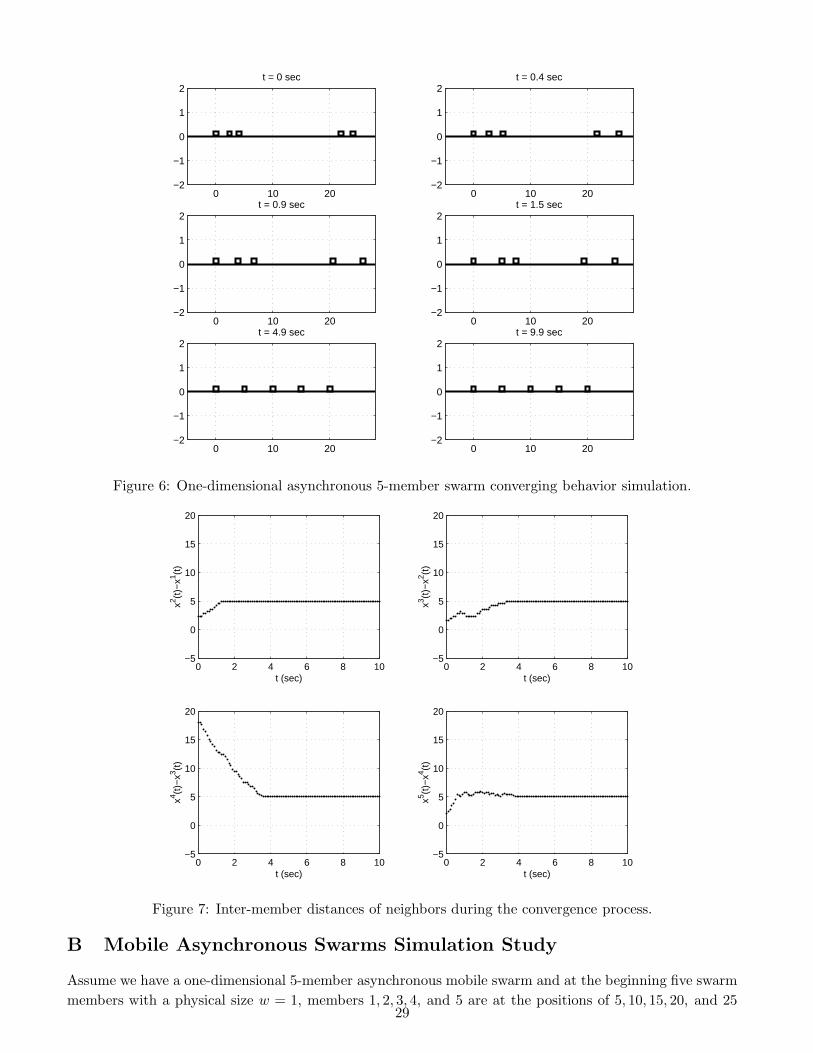
0 10 20−2

−1

0

1

2t = 0 sec

0 10 20−2

−1

0

1

2t = 0.4 sec

0 10 20−2

−1

0

1

2t = 0.9 sec

0 10 20−2

−1

0

1

2t = 1.5 sec

0 10 20−2

−1

0

1

2t = 4.9 sec

0 10 20−2

−1

0

1

2t = 9.9 sec

Figure 6: One-dimensional asynchronous 5-member swarm converging behavior simulation.

0 2 4 6 8 10−5

0

5

10

15

20

t (sec)

x2 (t)−

x1 (t)

0 2 4 6 8 10−5

0

5

10

15

20

t (sec)

x3 (t)−

x2 (t)

0 2 4 6 8 10−5

0

5

10

15

20

t (sec)

x4 (t)−

x3 (t)

0 2 4 6 8 10−5

0

5

10

15

20

t (sec)

x5 (t)−

x4 (t)

Figure 7: Inter-member distances of neighbors during the convergence process.

B Mobile Asynchronous Swarms Simulation Study

Assume we have a one-dimensional 5-member asynchronous mobile swarm and at the beginning five swarmmembers with a physical size w = 1, members 1, 2, 3, 4, and 5 are at the positions of 5, 10, 15, 20, and 25

29

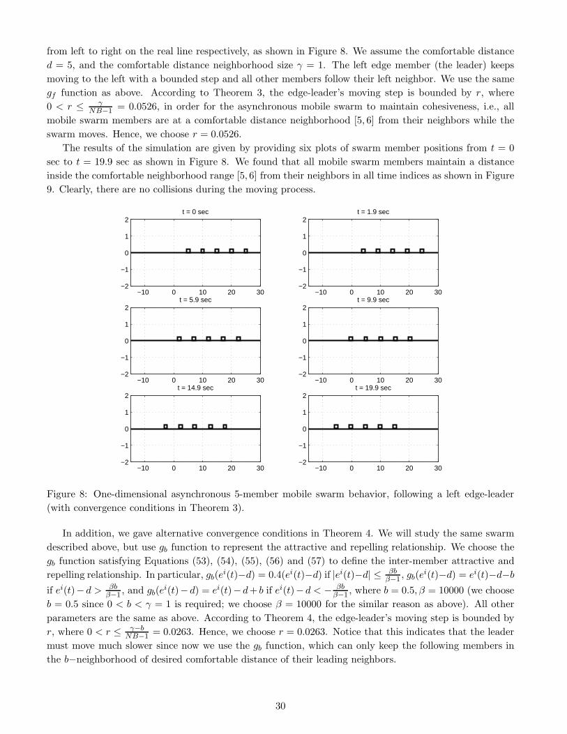
from left to right on the real line respectively, as shown in Figure 8. We assume the comfortable distanced = 5, and the comfortable distance neighborhood size γ = 1. The left edge member (the leader) keepsmoving to the left with a bounded step and all other members follow their left neighbor. We use the samegf function as above. According to Theorem 3, the edge-leader’s moving step is bounded by r, where0 < r ≤ γ

NB−1 = 0.0526, in order for the asynchronous mobile swarm to maintain cohesiveness, i.e., allmobile swarm members are at a comfortable distance neighborhood [5, 6] from their neighbors while theswarm moves. Hence, we choose r = 0.0526.

The results of the simulation are given by providing six plots of swarm member positions from t = 0sec to t = 19.9 sec as shown in Figure 8. We found that all mobile swarm members maintain a distanceinside the comfortable neighborhood range [5, 6] from their neighbors in all time indices as shown in Figure9. Clearly, there are no collisions during the moving process.

−10 0 10 20 30−2

−1

0

1

2t = 0 sec

−10 0 10 20 30−2

−1

0

1

2t = 1.9 sec

−10 0 10 20 30−2

−1

0

1

2t = 5.9 sec

−10 0 10 20 30−2

−1

0

1

2t = 9.9 sec

−10 0 10 20 30−2

−1

0

1

2t = 14.9 sec

−10 0 10 20 30−2

−1

0

1

2t = 19.9 sec

Figure 8: One-dimensional asynchronous 5-member mobile swarm behavior, following a left edge-leader(with convergence conditions in Theorem 3).

In addition, we gave alternative convergence conditions in Theorem 4. We will study the same swarmdescribed above, but use gb function to represent the attractive and repelling relationship. We choose thegb function satisfying Equations (53), (54), (55), (56) and (57) to define the inter-member attractive andrepelling relationship. In particular, gb(ei(t)−d) = 0.4(ei(t)−d) if |ei(t)−d| ≤ βb

β−1 , gb(ei(t)−d) = ei(t)−d−bif ei(t)− d > βb

β−1 , and gb(ei(t)− d) = ei(t)− d+ b if ei(t)− d < − βbβ−1 , where b = 0.5, β = 10000 (we choose

b = 0.5 since 0 < b < γ = 1 is required; we choose β = 10000 for the similar reason as above). All otherparameters are the same as above. According to Theorem 4, the edge-leader’s moving step is bounded byr, where 0 < r ≤ γ−b

NB−1 = 0.0263. Hence, we choose r = 0.0263. Notice that this indicates that the leadermust move much slower since now we use the gb function, which can only keep the following members inthe b−neighborhood of desired comfortable distance of their leading neighbors.

30

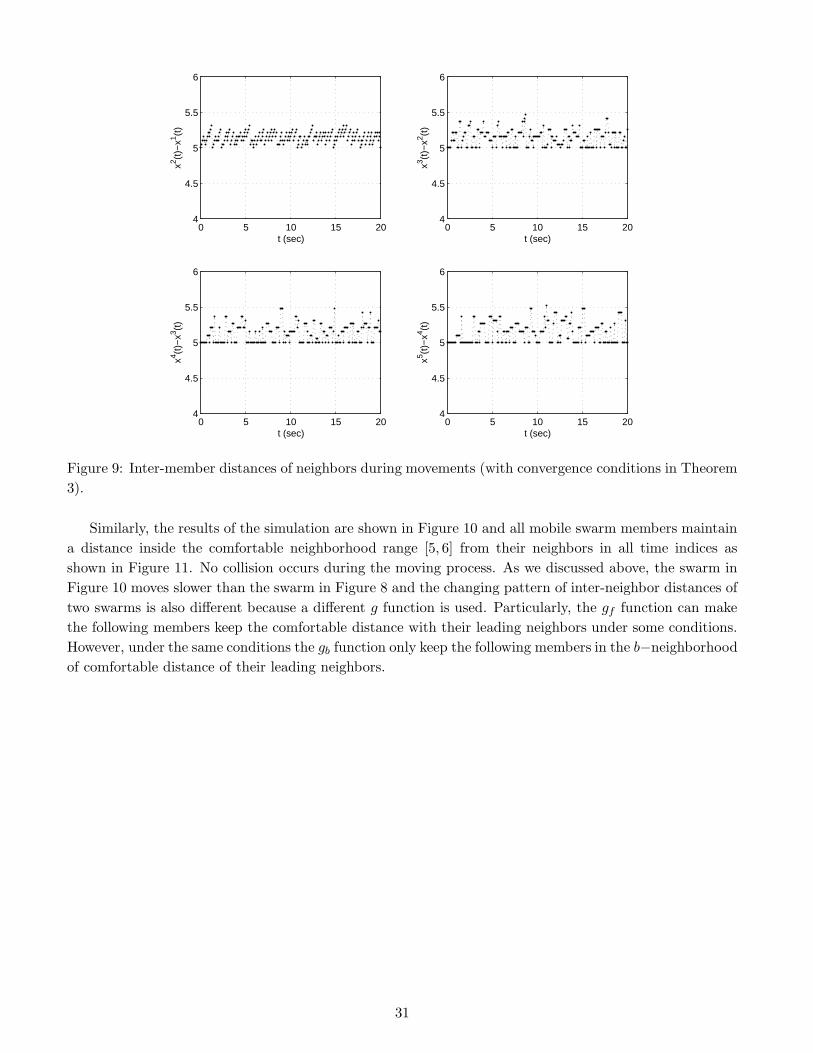
0 5 10 15 204

4.5

5

5.5

6

t (sec)

x2 (t)−

x1 (t)

0 5 10 15 204

4.5

5

5.5

6

t (sec)

x3 (t)−

x2 (t)

0 5 10 15 204

4.5

5

5.5

6

t (sec)

x4 (t)−

x3 (t)

0 5 10 15 204

4.5

5

5.5

6

t (sec)x5 (t

)−x4 (t

)

Figure 9: Inter-member distances of neighbors during movements (with convergence conditions in Theorem3).

Similarly, the results of the simulation are shown in Figure 10 and all mobile swarm members maintaina distance inside the comfortable neighborhood range [5, 6] from their neighbors in all time indices asshown in Figure 11. No collision occurs during the moving process. As we discussed above, the swarm inFigure 10 moves slower than the swarm in Figure 8 and the changing pattern of inter-neighbor distances oftwo swarms is also different because a different g function is used. Particularly, the gf function can makethe following members keep the comfortable distance with their leading neighbors under some conditions.However, under the same conditions the gb function only keep the following members in the b−neighborhoodof comfortable distance of their leading neighbors.

31

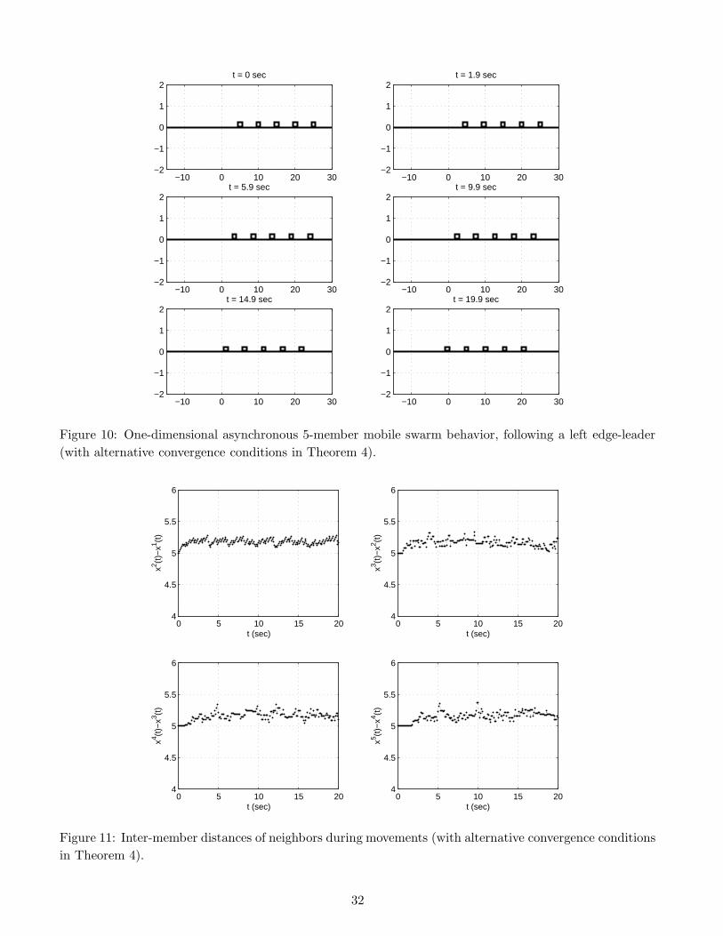
−10 0 10 20 30−2

−1

0

1

2t = 0 sec

−10 0 10 20 30−2

−1

0

1

2t = 1.9 sec

−10 0 10 20 30−2

−1

0

1

2t = 5.9 sec

−10 0 10 20 30−2

−1

0

1

2t = 9.9 sec

−10 0 10 20 30−2

−1

0

1

2t = 14.9 sec

−10 0 10 20 30−2

−1

0

1

2t = 19.9 sec

Figure 10: One-dimensional asynchronous 5-member mobile swarm behavior, following a left edge-leader(with alternative convergence conditions in Theorem 4).

0 5 10 15 204

4.5

5

5.5

6

t (sec)

x2 (t)−

x1 (t)

0 5 10 15 204

4.5

5

5.5

6

t (sec)

x3 (t)−

x2 (t)

0 5 10 15 204

4.5

5

5.5

6

t (sec)

x4 (t)−

x3 (t)

0 5 10 15 204

4.5

5

5.5

6

t (sec)

x5 (t)−

x4 (t)

Figure 11: Inter-member distances of neighbors during movements (with alternative convergence conditionsin Theorem 4).

32