spectroscopy of heavy mesons expanded in 1/ m q
TRANSCRIPT

arX
iv:h
ep-p
h/97
0236
6v2
6 M
ar 1
997
TKU-97-3 Feb. 1997
Spectroscopy of Heavy Mesons Expanded in 1/mQ
Takayuki Matsuki ∗
Tokyo Kasei University, 1-18-1 Kaga, Itabashi, Tokyo 173, JAPAN
Toshiyuki Morii †
Faculty of Human Development, Kobe University, 3-11 Tsurukabuto,
Nada, Kobe 657, JAPAN
Abstract
Operating just once with the naive Foldy-Wouthuysen-Tani transformation
on the relativistic Fermi-Yang equation for Qq bound states described by the
semi-relativistic Hamiltonian which includes Coulomb-like as well as confining
scalar potentials, we have calculated heavy meson mass spectra of D and B
together with higher spin states. Based on the formulation recently proposed,
their masses and wave functions are expanded up to the second order in 1/mQ
with a heavy quark mass mQ and the lowest order equation is examined care-
fully to obtain a complete set of eigenfunctions for the Schrodinger equation.
Heavy quark effective theory parameters, Λ, λ1, and λ2, are also determined
at the first and second order in 1/mQ.
12.39.Hg, 12.40.Yx
Typeset using REVTEX
∗E-mail: [email protected]
†E-mail: [email protected]
1
I. INTRODUCTION
Hadrons are composed of quarks and anti-quarks and are considered to be governed by
Quantum Chromodynamics, at least in principle. Since QCD describes a strong coupling
interaction, perturbative calculation of physical quantities of hadrons is not so reliable other
than the deep inelastic region where the coupling constant becomes weak due to asymptotic
freedom and hence other methods like lattice gauge theory have been developed to take into
account nonperturbative effects. However, the situation has dramatically changed when it
is discovered that the system of heavy hadrons, composed of one heavy quark Q and light
quarks q or anti-quarks q, can be systematically expanded in 1/mQ with a heavy quark
mass, mQ. The numerator of this expansion in 1/mQ could be either ΛQCD or mq.
This theory, HQET (Heavy Quark Effective Theory), [1] is applied to many aspects of
high energy theories and many kinds of physical quantities of QCD which can be pertur-
batively calculated in 1/mQ. Especially those regarding B meson physics, e.g., the lowest
order form factor ( which is now called Isgur-Wise function ) of the semileptonic weak decay
process B → Dℓν and the Kobayashi-Maskawa matrix element Vcb, have been calculated by
many people. [2] However, since applications of HQET to higher order perturbative calcu-
lations are very restricted, only forms of higher order operators are obtained. Their Wilson
coefficients are calculable but some of the matrix elements of those operators are obtained
so that the whole quantity be somehow fitted with the experimental data. [3] This is be-
cause most of the calculations based on HQET do not introduce realistic heavy meson wave
functions and hence there is no way to determine those quantities completely within the
model.
In the former papers [4,5], using the Foldy-Wouthuysen-Tani transformation [6] we have
developed a formulation so that the Schrodinger equation for a Qq bound state can be
expanded in terms of 1/mQ, i.e., the resulting eigenvalues as well as wave functions are
obtained order by order in 1/mQ. In this paper, as one of the applications of our formulation
we will calculate heavy meson spectrum of D and B, and their higher spin states. In order
2

to do so, we would like to start from introducing phenomenological dynamics, i.e., assuming
Coulomb-like vector and confining scalar potentials to Qq bound states (heavy mesons),
expand a hamiltonian in 1/mQ then perturbatively solve Schrodinger equation in 1/mQ.
Angular part of the lowest order wave function is exactly solved. After extracting asymptotic
forms of the lowest order wave function at both r → 0 and r → ∞ and adopting the
variational method, we numerically obtain radial part of the trial polynomial wave function
which is expanded in powers of radial variable r. Then fitting the smallest eigenvalues of a
hamiltonian with masses of D and D∗ mesons, a strong coupling αs and other parameters
included in scalar and vector potentials are determined uniquely. Using parameters obtained
this way, other mass levels are calculated and compared with the experimental data for D/B
mesons up to the second order of perturbation. The lowest degenerate eigenvalues of the
Schrodinger equation gives the so-called Λ parameters for u, d and s light quarks, which is
defined by
Λ = limmQ→∞
(EH −mQ)
where EH is a calculated heavy meson mass and mQ a heavy quark mass. [3] Meson wave
functions obtained thereby and expanded in 1/mQ may be used to calculate ordinary form
factors as well as Isgur-Wise functions and its corrections in 1/mQ for semileptonic weak
decay processes.
All the above calculations are calculated up to 1/m2Q and analyzed order by order in
1/mQ to determine parameters as well as to compare with results of Heavy Quark Effective
Theory, e.g., the parameters, λ1, λ2, and Λ in Sect. IV. The final goal of this approach is to
obtain higher order corrections to Isgur-Wise functions, decay constants of heavy mesons,
and the Kobayashi-Maskawa matrix element, Vcb, by using wave functions of heavy mesons
obtained so that heavy meson spectrum is fitted with the experimental data.
Below in Sects. II and III we will first give formulation of this study and next in Sects. IV
and V give quantitative and qualitative discussions on the obtained results.
3

II. HAMILTONIAN
The hamiltonian density for our problem is given by
H0 =∫
dx3[
q† c(x) (~αq · ~pq + βqmq) qc(x) +Q†(x) (~αQ · ~pQ + βQmQ)Q(x)
]
, (1)
Hint =∫ ∫
dx3dx′3 qc(x)Oi qc(x)Vi(x− x′) Q(x′)OiQ(x′), (2)
where we consider only a scalar confining potential, Os = 1, Vs = S(r), and a vector poten-
tial, Ov = γµ, Vv = V (r), with a relative radial variable r, which we think the best choice to
phenomenologically describe the meson mass levels. [7,8] The state of Qq is defined by
|ψ〉 =∫
d3x∫
d3y ψαβ(x− y) qcα
†(x) Q†β(y) |0〉 , (3)
where qc(x) is a charge conjugate field of a light quark q and the conjugate state of Qq by
〈ψ| = |ψ〉† with 〈0| ≡ |0〉†. From these definitions, we obtain the Schrodinger equation as
H ψ = (mQ + E)ψ, (4)
where the bound state mass, E, is split into two parts, mQ and E (= E −mQ), so that it
expresses the fact that the heavy quark mass is dominant in the bound state, Qq, and ψ is
nothing but the wave function which appears in the rhs of Eq. (3).
Operating with the FWT transformation and a charge conjugation operator, which are
defined in the Appendix A, only on a heavy quark sector in this equation at the center of
the mass system of a bound state, one can modify the Schrodinger equation given by Eq. (4)
as,
(HFWT −mQ) ⊗ ψFWT = E ψFWT , (5)
where a notation ⊗ is introduced to denote that gamma matrices of a light anti-quark is
multiplied from left while those of a heavy quark from right. The problem of this paper
is to solve this equation, Eq. (5) in powers of 1/mQ. As described first in this section,
interaction terms are given by a confining scalar potential and a Coulomb vector potential
with transverse interaction [9] and a total hamiltonian is given by
4

H= (~αq · ~pq + βqmq) + (~αQ · ~pQ + βQmQ) + βqβQ S
+
1 − 1
2[ ~αq · ~αQ + (~αq · ~n) (~αQ · ~n) ]
V, (6)
where scalar and vector potentials are given by
S (r) =r
a2+ b, V (r) = −4
3
αs
rand ~n =
~r
r, (7)
and the vector potential is averaged over longitudinal as well as transverse as given in the
last term of Eq. (6). The transformed hamiltonian is expanded in 1/mQ as
HFWT −mQ = H−1 +H0 +H1 +H2 + · · · , (8)
where
H−1 = − (1 + βQ)mQ, (9a)
H0 = ~αq · ~p + βqmq − βqβQ S +
1 +1
2[ ~αq · ~αQ + (~αq · ~n) (~αQ · ~n) ]
V, (9b)
H1 = − 1
2mQ
βQ ~p2 +
1
mQ
βq ~αQ ·(
~p+1
2~q)
S +1
2mQ
~γQ · ~q V
− 1
2mQ
[
βQ
(
~p +1
2~q)
+ i ~q × βQ~ΣQ
]
· [ ~αq + (~αq · ~n)~n ]V, (9c)
H2 =1
2m2Q
βqβQ
(
~p+1
2~q)2
S − i
4m2Q
~q × ~p · βqβQ~ΣQ S − 1
8m2Q
~q 2V − i
4m2Q
~q × ~p · ~ΣQ V
− 1
8m2Q
[
(~p+ ~q) (~αQ · ~p) + ~p (~αQ · (~p+ ~q) ) + i ~q × ~p γ5Q
]
· [ ~αq + (~αq · ~n)~n ] V, (9d)
...
Here Hi stands for the i-th order expanded hamiltonian and since a bound state is at rest,
~p = ~pq = −~pQ, ~p ′ = ~pq′ = −~pQ
′, ~q = ~p ′ − ~p, (10)
are defined, where primed quantities are final momenta and the relation of these momenta
with particles is depicted in Fig. 1.
5

FIGURES
Fig. 1
pQ
p 'Q
q
Definition of momenta of Qq_
pq_
p 'q_
FIG. 1. Each momentum is defined.
Details of derivation of equations in this section are given in the Appendix A.
III. PERTURBATION
Using the hamiltonian obtained in the last section, we give in this section the Schrodinger
equation order by order in 1/mQ. Details of the derivation in this section are given in the
Appendix B. First we introduce projection operators:
Λ± =1 ± βQ
2, (11)
which correspond to positive-/negative-energy projection operators for a heavy quark sector
at the rest frame of a bound state. These are given by (1 ± v/)/2 in the moving frame of a
bound state with vµ the four-velocity of a bound state. Then we expand the mass and wave
function of a bound state in 1/mQ as
E = E −mQ = Eℓ0 + Eℓ
1 + Eℓ2 + . . . , (12)
ψFWT = ψℓ0 + ψℓ
1 + ψℓ2 + . . . , (13)
where ℓ stands for a set of quantum numbers that distinguish independent eigenfunctions of
the lowest order Schrodinger equation, and a subscript i of Eℓi and ψℓ
i stands for the order
of 1/mQ.
6

A. -1st order
The -1st order Schrodinger equation in 1/mQ gives
ψℓ0 = Λ− ⊗ ψℓ
0, (14)
whose explicit form is solved in the Appendix C and is given by
ψℓ0 = Ψ+
ℓ = ( 0 Ψkj m(~r) ) . (15)
Here ℓ stands for a set of quantum numbers, j, m, and k and
Ψkj m(~r) =
1
r
uk(r)
−i vk(r) (~σ · ~n)
ykj m(Ω), (16)
where j is a total angular momentum of a meson, m is its z component, k is a quantum
number which takes only values, k = ±j, ±(j + 1) and 6= 0, and uk(r) and vk(r) are
polynomials of a radial variable r. ykj m(Ω) are functions of angles and spinors of a total
angular momentum, ~j = ~l + ~sq + ~sQ. The corresponding operator for the quantum number
k is given by
−βq
(
~Σq · ~ℓ+ 1)
, (17)
which satisfies
−βq
(
~Σq · ~ℓ+ 1)
( 0 Ψkj m(~r) ) = k ( 0 Ψk
j m(~r) ) , (18)
i.e.,
[
−βq
(
~Σq · ~ℓ+ 1)
, H−−0
]
= 0, (19)
with H−−0 being given in the Appendix D, the lowest order non-trivial hamiltonian,
H−−0 ⊗ ψℓ
0 = Ek0ψ
ℓ0.
Note that since charge conjugation operates on the heavy quark sector the Λ− projec-
tion operator appears in Eq. (14), i.e., positive components of Q corresponds to negative
components of Uc Q.
7
B. Zero-th order
The zero-th order equations are given by
[ ~αq · ~p+ βq (mq + S) + V ] ⊗ ψℓ0 = Eℓ
0 ψℓ0, (20)
− 2mQΛ+ ⊗ ψℓ1 + 1
2Λ− [ ~αq · ~αQ + (~αq · ~n) (~αQ · ~n) ]V ⊗ ψℓ
0 = 0. (21)
Eq. (20) gives the lowest non-trivial Schrodinger equation with a solution given by Eq. (15)
and ~n = ~r/r . Detailed analysis of this equation is given in Appendix C. Λ+ components of
wave functions can be expanded in terms of the eigenfunctions,
Ψ−ℓ = (Ψk
j m(~r) 0 ) . (22)
Expanding Λ+ ⊗ ψℓ1 in terms of this set of eigenfunctions, one can obtain the solution for
Eq. (21) as
Λ+ ⊗ ψℓ1 =
∑
ℓ ′
cℓ ℓ ′
1− Ψ−ℓ ′, (23)
with the coefficients,
cℓ ℓ ′
1− =1
4mQ
⟨
Ψ−ℓ ′
∣
∣
∣ [ ~αq · ~αQ + (~αq · ~n) (~αQ · ~n) ]V∣
∣
∣Ψ+ℓ
⟩
. (24)
Here the inner product is defined to be
〈Ψαℓ |O
∣
∣
∣Ψβℓ ′
⟩
=∫
d3r tr(
Ψαℓ†(
O ⊗ Ψβℓ ′
))
, (25)
and the zero-th order wave functions are normalized to be 1,
〈Ψαℓ
∣
∣
∣Ψβℓ ′
⟩
= δℓ ℓ ′δα β for α, β = + or − . (26)
C. 1st order
The 1st order equation is given by
−2mQΛ+ ⊗ ψℓ2 +H0 ⊗ ψℓ
1 +H1 ⊗ ψℓ0 = Eℓ
0ψℓ1 + Eℓ
1ψℓ0. (27)
8
Multiplying projection operators Λ± from right with the above equation, and expanding ψℓ1
in terms of Ψ±ℓ as
ψℓ1 =
∑
ℓ
(
cℓ ℓ ′
1+ Ψ+ℓ ′ + cℓ ℓ ′
1− Ψ−ℓ ′
)
, (28)
one obtains
Eℓ1 =
∑
ℓ ′
cℓ ℓ ′
1−
⟨
Ψ+ℓ
∣
∣
∣Λ+H0Λ−
∣
∣
∣Ψ−ℓ ′
⟩
+⟨
Ψ+ℓ
∣
∣
∣Λ−H1Λ−
∣
∣
∣Ψ+ℓ
⟩
, (29)
which gives the first order perturbation correction to the mass when one calculates matrix
elements of the rhs among eigenfunctions and
cℓ k1+ =
1
Eℓ0 −Ek
0
[
∑
ℓ ′
cℓ ℓ ′
1−
⟨
Ψ+k
∣
∣
∣Λ+H0Λ−
∣
∣
∣Ψ−ℓ ′
⟩
+⟨
Ψ+k
∣
∣
∣Λ−H1Λ−
∣
∣
∣Ψ+ℓ
⟩
]
, for k 6= ℓ (30)
ck k1+ = 0. (31)
This completes the solution for ψℓ1 since Λ−ψ
ℓ1, or cℓ ℓ ′
1− , is obtained in the last subsection.
Here we have used the normalization for the total wave function, ψℓ, as
⟨
ψℓ∣
∣
∣ ψℓ ′⟩
= δℓ ℓ ′, (32)
where we have neglected color indices in this paper and hence a color factor, Nc = 3, in
the above equation since it does not change the essential arguments. This definition of
Eq. (32) is admitted because here we are not calculating the absolute value of the form
factors. The appropriate normalization (normally given by 2E with a bound state mass E)
will be adopted in future papers in which we will calculate some form factors. This way
of solving Eq. (27) is unique and we will use this method below to solve similar equations
appearing subsection Actually this method has been already used to obtain Eqs. (20, 21)
and to solve Eq. (21) obtaining the coefficients cℓ ℓ ′
1− by Eq. (24).
One obtains Λ+ ⊗ ψℓ2 as in the former subsection,
Λ+ ⊗ ψℓ2 =
∑
ℓ ′
cℓ ℓ ′
2− Ψ−ℓ ′, (33)
with the coefficients,
cℓ ℓ ′
2− =1
2mQ
⟨
Ψ−ℓ ′
∣
∣
∣
((
H0 − Eℓ0
)
Λ+ ⊗ ψℓ1 +H1Λ+ ⊗ ψℓ
0
)⟩
. (34)
9

D. 2nd order
The 2nd order equation is given by
−2mQΛ+ ⊗ ψℓ3 +H0 ⊗ ψℓ
2 +H1 ⊗ ψℓ1 +H2 ⊗ ψℓ
0 = Eℓ0ψ
ℓ2 + Eℓ
1ψℓ1 + Eℓ
2ψℓ0. (35)
As in the above case (1st order), we obtain
Eℓ2 =
∑
ℓ ′
cℓ ℓ ′
2−
⟨
Ψ+ℓ
∣
∣
∣Λ+H0Λ−
∣
∣
∣Ψ−ℓ ′
⟩
+⟨
Ψ+ℓ
∣
∣
∣H1Λ− ⊗ψℓ1
⟩
+⟨
Ψ+ℓ
∣
∣
∣Λ−H2Λ−
∣
∣
∣Ψ+ℓ
⟩
, (36)
which gives the second order perturbation corrections to the mass and
cℓ k2+ =
1
Eℓ0 − Ek
0
[
∑
ℓ ′
cℓ ℓ ′
2−
⟨
Ψ+k
∣
∣
∣Λ+H0Λ−
∣
∣
∣Ψ−ℓ ′
⟩
+⟨
Ψ+k
∣
∣
∣Λ+H1 ⊗ψℓ1
⟩
+⟨
Ψ+k
∣
∣
∣Λ−H2Λ−
∣
∣
∣Ψ+ℓ
⟩
− Eℓ1 c
ℓ k1+
]
, for k 6= ℓ (37)
ck k2+ = −1
2
∑
ℓ
(
∣
∣
∣ck ℓ1+
∣
∣
∣
2+∣
∣
∣ck ℓ1−
∣
∣
∣
2)
. (38)
This completes the solution for ψk2 since Λ−ψ
k2 , or cℓ ℓ ′
2− , is obtained in the last subsection.
Although we do not need in this paper, one obtains Λ+ ⊗ ψℓ3 as
Λ+ ⊗ ψℓ3 =
∑
ℓ ′
cℓ ℓ ′
3− Ψ−ℓ ′, (39)
with the coefficients,
cℓ ℓ ′
3− =1
2mQ
⟨
Ψ−ℓ ′
∣
∣
∣
((
H0 −Eℓ0
)
Λ+ ⊗ ψℓ2 +
(
H1 −Eℓ1
)
Λ+ ⊗ ψℓ1 +H2Λ+ ⊗ ψℓ
0
)⟩
. (40)
IV. NUMERICAL ANALYSIS
In this section, we give numerical analysis of our analytical calculations obtained in the
former sections order by order in 1/mQ. In order to solve Eq. (20), we have to numerically
obtain a radial part of the wave function, Ψ+ℓ = ( 0 Ψk
j m ), given by
Ψkj m(~r) =
1
r
uk(r)
−i vk(r) (~σ · ~n)
ykj m(Ω), (41)
10

detailed properties of which are described in the Appendix C. As described in the same
Appendix, the lowest order, non-trivial Schrodinger equation is reduced into Eq. (C25),
mq + S + V −∂r + kr
∂r + kr
−mq − S + V
uk (r)
vk (r)
= Ek0
uk (r)
vk (r)
, (42)
This eigenvalue equation is numerically solved by taking into account the asymptotic be-
haviors at both r → 0 and r → ∞ and the forms of uk(r) and vk(r) are given by
uk(r), vk(r) ∼ wk(r)(
r
a
)γ
exp
(
− (mq + b) r − 1
2
(
r
a
)2)
, (43)
where
γ =
√
k2 −(
4αs
3
)2
(44)
and wk(r) is a finite series of a polynomial of r
wk(r) =N−1∑
i=0
aki
(
r
a
)i
, (45)
which takes different coefficients for uk(r) and vk(r).
i) We have fixed the value of a light quark mass, mq, to be 0.01 GeV as listed in Table I
since only in the vicinity of this value the D and D∗ masses can be fitted with the experi-
mental values. We believe that when the mass, mq = mu = md, is running with momentum
these are the correct current quark mass since the momentum is given by the order of the
B meson mass (∼ 5 GeV) [13] though we have not used the running mass to solve the
Schrodinger equation. We have adopted N − 1 = 7 for the highest power of r that gives
sixteen solutions to Eq. (42), half of which corresponds to negative energies and another
half to positive ones of qc state. The lowest eigenvalue of the positive energies is assigned
to the physical state. That is, although we have a node quantum number, n, other than j,
m, and k, for Eq. (42), we take only the n = 0 solution for each value of k and j quantum
numbers and we do not take into account higher order node solutions in this paper. The
lowest positive eigenvalue solution for N = 8 gives the one closest to the zero node compared
with other N . That is, other N gives a rather oscillatory solution.
11

In the case of a Hydrogen atom, for instance, only the Coulomb potential V ∼ 1/r
survives in the above problem and a radial function, wk(r), becomes a hypergeometric
function and its finite series of a polynomial gives discrete energy levels. In our case, since the
potential includes a scalar term we can not analytically solve the above reduced Schrodinger
equation, Eq. (42). If we force to make the functions, uk(r) and vk(r), finite series and relate
the coefficients of those functions via recursive equations, it leads us to inconsistency among
coefficients of each term, ri, of a polynomial. We just assume in this paper that uk(r) and
vk(r) are trial finite polynomial functions of r.
ii) To first determine the parameters, αs, a, and b appearing in the potentials given by
Eq. (7), and mc, we have calculated the chi square defined by
χ2 =(MD −ED)2
σ2D
+(MD∗ −ED∗)2
σ2D∗
, (46)
where MD, D∗ and ED, D∗ are the observed and calculated masses of D and D∗, respectively
and σD, D∗ are the experimental errors for each meson mass. As mentioned already mq =
md = mu is fixed to be 10 MeV. Masses, MD, D∗, are averaged over charges since we have
not taken into account the electromagnetic interaction. We have determined the values for
these parameters which give the least value of χ2, which is given in Table II.
iii) The s quark mass, ms, is determined so that the similar equation to Eq. (46) takes
the minimum value where we substitute Ds and D∗s meson masses instead of D and D∗,
while the b quark mass, mb, is determined by B and B∗ meson masses. The input values to
determine these parameters are given in Table I.
Table I
iv) There are two types of solutions to optimal values for these parameters, i.e., one set
for b < 0 which is listed in Table II, and another for b > 0. However, the solution for b > 0
gives large difference between calculated values and observed ones for higher order spins and
also gives negative values for some spectrum even though the lowest lying sates are in good
agreement with the observed ones. Hence we disregard this set of parameters.
Tables III ∼ X give calculated values, Mcalc, together with the zero-th order masses, M0
12

that are degenerate with the same value of k, ratios, pi/M0 and ni/M0, and the observed
values, Mobs. Here the heavy meson mass, EH , is expanded in 1/mQ up to the n-th order as
EH = M0 +n∑
i=1
pi +n∑
i=1
ni, (47)
with M0 = mQ + E0 being the degenerate mass, pi the i-th order correction from positive
components of a heavy meson wave function, and ni the i-th order correction from negative
components. Note also that the exponential factor in the brackets in the first row of each
table should be multiplied with a value of each column except for those with the explicit
exponential factor.
Table III ∼ X
Strictly speaking each state is classified by two quantum numbers, k and j, and also approx-
imately classified by the upper component of the light anti-quark sector in terms of the usual
notation, 2S+1LJ . Studying the functions ykj m carefully, one finds the upper component of
Ψkj m(~r) corresponds to the following Table XI, respectively.
Table XI
Here J in JP and 2S+1LJ is the same as a total angular momentum, j, in the Table XI.
Although the states can be completely classified in terms of two quantum numbers, k and j,
we would like ordinarily to classify them in terms of 2S+1LJ . However, the states classified
by JP = 1+ and 2−, are mixtures of two states in terms of 2S+1LJ as given by the Table
XI. We would approximately regard the state (k, j)=(1, 1) with ”3P1”, (-2, 1) with ”1P1”
and (2, 2) with ”3D2”, respectively, whose legitimacy can be supported by calculating the
coefficient of each state 2S+1LJ included in the mixture state. We denote them with double
quotations so that they remind us an approximate representation of the state in terms of
2S+1LJ . Using Eq. (C6) in Appendix C, their relations are given by
|”3P1”〉
|”1P1”〉
=1√3
√2 1
−1√
2
| 3P1 〉
| 1P1 〉
, (48)
13

|”3D2”〉
|”1D2”〉
=1√5
√3
√2
−√
2√
3
| 3D2 〉
| 1D2 〉
. (49)
v) From Tables III ∼ X we see that the perturbative calculation with these parameters
might not work well for higher k. Namely masses of 1− and 2− for k = +2 give some odd
values. They become even negative for ”3D2” of Ds and Bs at the second order as shown in
Tables VIII and X. Hence we disregard in this paper all calculated masses of 3D1(1−) and
”3D2”(2−) states in any order. In order to remedy this problem, we may need to improve
the potential form or adopt some other methods. [14] Hence here only the first order mass
spectra are depicted without higher spin states (3D1(1−) and ”3D2”(2−)) in Figs. 2∼5.
1.85
1.95
2.05
2.15
2.25
2.35
2.45
D meson mass spectrum (first order)
Mas
s (G
ev)
States
1.867(1.867)
2.008(2.008)
2.418
(2.422?)
2.449
2.383
(2.459)
2.428
Fig.2
1S03S1
3P0" 3P1
" " 1P1" 3P2
FIG. 2. The first order plot of D meson masses. Values in the brackets are the observed values.
14

1.95
2.05
2.15
2.25
2.35
2.45
2.55
2.65
DS meson mass spectrum (first order)
Mas
s (G
ev)
States
(1.969)1.966
(2.112?)
2.125
2.339
2.487
(2.535)
2.4962.540
Fig.3
(2.574?)
1S03S1
3P0" 3P1
" " 1P1" 3P2
FIG. 3. The first order plot of Ds meson masses. Values in the brackets are the observed values.
5.25
5.35
5.45
5.55
5.65
5.75
B meson mass spectrum (first order)
Mas
s (G
ev)
States
5.281(5.279)
(5.325)
5.323
5.697
5.740
5.6795.692
Fig.4
1S03S1
3P0" 3P1
" " 1P1" 3P2
FIG. 4. The first order plot of B meson masses. Values in the brackets are the observed values.
15
5.35
5.45
5.55
5.65
5.75
5.85BS meson mass spectrum (first order)
Mas
s (G
ev)
States
(5.369)5.393
5.440
5.716
5.760
5.796 5.809
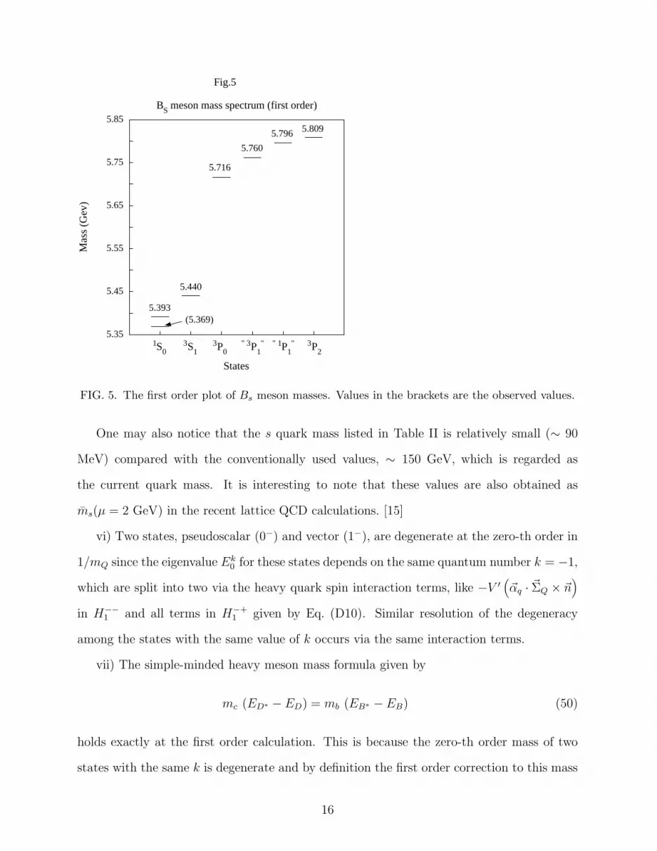
Fig.5
1S03S1
3P0" 3P1
" " 1P1" 3P2
FIG. 5. The first order plot of Bs meson masses. Values in the brackets are the observed values.
One may also notice that the s quark mass listed in Table II is relatively small (∼ 90
MeV) compared with the conventionally used values, ∼ 150 GeV, which is regarded as
the current quark mass. It is interesting to note that these values are also obtained as
ms(µ = 2 GeV) in the recent lattice QCD calculations. [15]
vi) Two states, pseudoscalar (0−) and vector (1−), are degenerate at the zero-th order in
1/mQ since the eigenvalue Ek0 for these states depends on the same quantum number k = −1,
which are split into two via the heavy quark spin interaction terms, like −V ′(
~αq · ~ΣQ × ~n)
in H−−1 and all terms in H−+
1 given by Eq. (D10). Similar resolution of the degeneracy
among the states with the same value of k occurs via the same interaction terms.
vii) The simple-minded heavy meson mass formula given by
mc (ED∗ −ED) = mb (EB∗ −EB) (50)
holds exactly at the first order calculation. This is because the zero-th order mass of two
states with the same k is degenerate and by definition the first order correction to this mass
16
is proportional to 1/mQ as given by H1 of Eq. (9) or by Hα β1 of Eq. (D10). To see Eq. (50)
as an prediction, replacing EX with the observed values MX we obtain at the first order,
MB∗ −MB
MD∗ −MD
=mc
mb
= 0.299, (51)
which should be compared with the experimental value, 0.326. This discrepancy between
the calculated and the observed comes from our calculation of B meson mass spectrum listed
in Table V which give B and B∗ meson masses slightly different values from the observed
ones. Hold also similar equations to Eq. (50) for higher spin states with the same k quantum
number because of the same reason given above.
viii) The so-called Λ parameter can be calculated using the definition [3]
Λ = limmQ→∞
(EH −mQ) = M0 −mQ = E−10 (52)
where EH , M0, and mQ are calculated heavy meson mass, the lowest degenerate bound state
mass, and a heavy quark mass, respectively. Difference of M0 and mQ is nothing but the
lowest leading eigenvalue, Ek0 , with k = −1 in our model. From Tables III and IV and
mc = 1.457 listed in Table II, one obtains at the first order
Λu,d = M0D −mc = M0D∗ −mc = 0.412 GeV, (53)
Λs = M0Ds−mc = M0D∗
s−mc = 0.529 GeV, (54)
and from Tables III and IV and mc = 1.347 listed in Table II, one obtains at the second
order
Λu,d = M0D −mc = M0D∗ −mc = 0.518 GeV, (55)
Λs = M0Ds−mc = M0D∗
s−mc = 0.629 GeV, (56)
where M0D(s), M0D∗
(s)are the calculated lowest order D meson mass defined by Eq. (52).
ix) Parameters which give nonperturbative corrections to inclusive semileptonic B decays
are defined as [16,17],
17

λ1 =1
2mQ〈H(v)| hv(iD)2hv |H(v)〉 , (57)
λ2 =1
2dH mQ〈H(v)| hv
g
2σµ νG
µ νhv |H(v)〉 , (58)
where hv is the heavy quark field in the HQET with velocity v. dH = 3, −1 for pseudoscalar
or vector mesons, respectively. Then the heavy meson mass can be expanded in terms of
the heavy quark mass, λ1, λ2, and Λ, as
EH = mQ + Λ − λ1 + dHλ2
2mQ
+ . . . . (59)
The first order calculation in 1/mQ makes 2λ2 equal to Eq. (50) and the λ1 can be calculated
using the above equation as
λ1 = 2mb
(
mb + Λu − EB
)
− 3λ2, (60)
λ2 =mb
2
(
EB∗ − EB
)
, (61)
where EB and EB∗ are the calculated B meson masses without the second order corrections.
The results are given by, at the first order,
λ1 = −0.378 GeV2, λ2 = 0.112 GeV2. (62)
and at the second order,
λ1 = −0.238 GeV2, λ2 = 0.0255 GeV2. (63)
Here we notice that although the first term in Eq. (60) is expected to be ∼ O(1) we find it
to be small from Table V at the first order and obtain the approximate relation,
λ1 ∼ −3λ2. (64)
These values should be compared with those in Ref. [18], which give Λu = 0.39± 0.11 GeV,
λ1 = −0.19 ± 0.10 GeV2, and λ2 ≃ 0.12 GeV2.
x) Recently, it has been pointed out that the kinetic energy of heavy quark in-
side a heavy meson plays an important role in the determination of the ratios fB/fD,
18
(MB∗ −MB) / (MD∗ −MD), and |Vub/Vcb|, in which use has been made the Gaussian form
for the heavy meson wave function and has been adopted the so-called Cornell potential,
the same as ours. [19] They have derived the relation of these physical quantities in terms of
the Fermi momentum, pF , introduced in [20] in which pF is related to a heavy quark recoil
momentum, ~p , by
⟨
~p 2⟩
=∫
d3p ~p 2 φ(~p ) =3
2p2
F . (65)
where the momentum probability distribution function is given by
φ(~p ) =
(
2√πpF
)3
e−~p 2/p2F . (66)
They calculated the lhs of Eq. (65) to obtain pF by using the Gaussian form of the wave
function and then derive the relations between physical quantities and this pF . [19] We have
the radial wave function given by Eq. (43) different from a Gaussian one and hence should
have relations among physical qunatities and our parameters, a, b, αs, and mc, independent
of pF and hence we may calculate the lhs of Eq. (65) to check if our calculation gives the
value similar to other calculations. Our value of the lhs of Eq. (65) gives for 〈~p 2 〉 of the B
meson at the first order
⟨
~p 2⟩
= 0.560 GeV2, (67)
and the second order gives 〈~p 2 〉 = 0.562 GeV2, which should be compared with the latest
values pF = 0.5−0.6 GeV calculated in [19] which correspond to 〈~p 2 〉 = 0.375−0.540 GeV2.
xi) When one takes an overall look at the calculated masses, the negative component
contributions, ni/M0, are relatively large for both scalar states, 0±, at the first as well as
second order even though they become very small for higher spin states. Positive components
constantly contribute to all states. When one compares the first order with the second order
calculations, one can not conclude that the second order is better than the first as a whole
although higher spin states of D and B are largely improved at the second order. This
conclusion may be also supported by the comparison of the first and second order calculations
19

of the parameters, λ1, λ2, and Λ with other calculations. [18] In order to incorporate the
second order effects properly, one may need to introduce a different potential and/or method
from ours as mentioned in v) in this section.
We have used the following algorithms to numerically calculate the heavy meson masses,
Gauss-Hermite quadrature to evaluate integrals and the tridiagonal QL implicit method to
determine the eigenvalues and eigenvectors of a finite dimensional real matrix. [21]
V. COMMENTS AND DISCUSSIONS
In this paper, we have calculated heavy meson masses like D(s), D∗(s), B(s), and B∗
(s) based
on the formulation proposed before, [4] which develops the perturbation potential theory in
terms of inverse power of a heavy quark mass. The first and second order calculations of
masses are in good agreement with the experimental data except for the higher spin states
even though the second order calculation does not much improve the first order. The first
order calculation of the HQET quantities, λ1, λ2, and Λ, are also in good agreement with
the other calculations. [18] A new study on the HQET introduced the Fermi momentum,
pF , to obtain other physical quantities. [19] Although we have not had pF in our mind at
the begining of this study, the obtained value given by Eq. (67) is in good agreement with
what they have obtained. [19]
We have also found a new symmetry already mentioned in the paper [4] and realized by
the operator, Eq. (17),
−βq
(
~Σq · ~ℓ+ 1)
,
which is always present when one considers a centrally symmetric potential model for two
particles or when one takes a rest frame limit of a general relativistic form of the wave
function and is related to a light quark spin structure, i.e., ykj m(Ω). That is, this is quite a
general symmetry, not a special feature peculiar to our potential model.
One can easily see degeneracy among the lowest lying pseudoscalar and vector states as
follows. Define
20
|P 〉 = U−1c ( 0 Ψ−1
0 0 ) , |V, λ〉 = U−1c ( 0 Ψ−1
1 λ ) , (68)
where the inverse of the charge conjugate operator, U−1c , is defined in the Appendix A
Eqs. (A2), Ψkj m is an eigenfunction obtained in the last chapter, The explicit forms of these
wave functions are given in the Appendix C, Eqs. (C28, C29). and the quantum number k
can take only ±j, or ± (j + 1). Assigning these states to D mesons, one can have
|P 〉 =∣
∣
∣D±⟩
, or∣
∣
∣D0⟩
, |V, λ〉 = |D∗〉 . (69)
Since these states have the same quantum number k = −1, these have the same masses as
well as the same wave functions up to the zero-th order calculation in 1/mQ. That is, the
degeneracy among these states is simply the result of the special property of the eigenvalue
equation. Higher order corrections can be obtained by developing perturbation of energy
and wave function for each state in terms of ΛQCD/mQ as given by Eqs. (12, 13),
E ≡ E −mQ = Eℓ0 + Eℓ
1 + Eℓ2 + . . . ,
ψFWT = ψℓ0 + ψℓ
1 + ψℓ2 + . . . ,
Finally we would like to discuss qualitative features of form factors/ Isgur-Wise functions.
Let us think about to calculate form factors for semileptonic decay of B meson into D.
Taking a simple form for the lowest lying wave function both for B and D as
Ψ1S ∼ e−b2 r2/2,
where a parameter b is determined by a variational principle, δ(Ψ1S †HΨ1S) = 0. Then form
factors are given by
F (q2) ∼ exp[
const. E2 (q2 − q2max)
]
, or ξ(ω) ∼ exp[
const. E2 (ω − 1)]
,
where
q2 = (pB − pD)2, ω = vB · vD, q2max = (mB −mD)2 ↔ ωmax = 1,
with vµB,D being four-velocity of B and/or D meson. This means behavior of form factors
strongly depends on an eigenvalue, E = E−mQ of the eigenvalue equation, Eq. (21), which
21

is often called ”inertia” parameter Λq when mQ → ∞. This quantity E does not depend
on any heavy quark properties at the zero-th order. This result also means that the slope
at the origin of the Isgur-Wise function includes the term proportional to E2. The constant
term (−1/4 like the Bjorken limit [22]) for this slope should be given by a kinematical factor
multiplied with the above expression.
To conclude, although there have been various relativistic bound state equations proposed
so far, nobody has yet determined what the most preferable is. We believe that our approach
presented here must be a promising candidate.
ACKNOWLEDGMENTS
The authors would like to thank Koichi Seo for critical comments on our paper. One of
the authors (TM) would like to thank the theory group of Institute for Nuclear Study for a
warm hospitality where a part of this work has been done.
APPENDIX A: SCHRODINGER EQUATION
In order to derive Eq. (4) or Eq. (5), we need to calculate the expectation value,
〈ψ| (H0 + Hint − E) |ψ〉 , (A1)
by using the equal-time anti-commutation relations among quark fields,
qcα(x), qc †
β (x′)
x0=x′
0
= δα βδ3 (~x− ~x′) ,
Qα(x), Q†β(x′)
x0=x′
0
= δα βδ3 (~x− ~x′) .
Since the wave function, ψα β(x− y) defined in Eq. (3), is normalized to be constant, what
we need to do is to variate Eq. (A1) in terms of ψα β(x−y) and to set it equal to zero. Then
we can easily obtain Eq. (4) with the effective hamiltonian given by Eq. (6). In the course
of this derivation, it appears to be clear that ~p only operates on wave functions while ~q only
on potentials.
22
To derive the FWT and charge conjugate transformed Schrodinger equation given by
Eq. (5), we have used the following definitions:
HFWT = Uc UFWT
(
p′Q)
H U−1FWT (pQ) U−1
c , ψFWT = Uc UFWT (pQ)ψ, (A2a)
UFWT (p) = exp(
W (p) ~γQ · ~p)
= cosW + ~γQ · ~p sinW, (A2b)
~p =~p
p, tanW (p) =
p
mQ + E, E =
√
~p 2 +m2Q, (A2c)
Uc = i γ0Qγ
2Q = −U−1
c . (A2d)
Note that the argument of the FWT transformation, UFWT , operating on a hamiltonian from
left is different from the right-operating one, since an outgoing momentum, ~pQ′, is different
from an incoming one, ~pQ. However, here in our study we work in a configuration space
which means momenta are nothing but the derivative operators and when we write them
differently, for instance as ~pQ and ~pQ′, their expressions are reminders of their momentum
representation. Hence although the arguments of UFWT and U−1FWT look different ~pQ and
~pQ′ are the same derivative operator, −i~∇. Here the difference between ~pQ and ~pQ
′ is ~q
which operates only on potentials and gives nonvanishing results. The FWT transformation
is introduced so that a heavy quark inside a heavy meson be treated as a non-relativistic
color source. The charge conjugation operator, Uc, is introduced so that gamma matrices of
a light anti-quark is multiplied from left while those of a heavy quark from right, which is
expressed by using a notation ⊗.
To derive Eqs. (9), we need to first expand HFWT in 1/mQ and then take into account
the following properties of a charge conjugation operator, Uc = i γ0Qγ
2Q, to obtain the final
expressions,
U−1c γµ
Q Uc = −γµQ
T, (A3)
i.e.,
Uc βQ U−1c = −βQ
T , Uc ~αQ U−1c = −~αT
Q, Uc~ΣQ U
−1c = −~ΣT
Q,
Uc ~γQ U−1c = −~γT
Q, Uc γ5Q U
−1c = −γ5
QT, (A4)
where a superscript T means its transposed matrix.
23
APPENDIX B: DERIVATION OF PERTURBATION
In this Appendix we will follow the paper [4] to derive perturbative Schrodinger equation
for a hamiltonian given by Eq. (6) for consistency. Following that paper, we will give an
equation at each order by using the explicit interaction terms given by Eqs. (9). Here we
quote the same equations given in the former sections for clarification of derivation. The
fundamental Schrodinger equation is given by
(HFWT −mQ) ⊗ ψFWT = E ψFWT , (B1)
and expansion of each quantity in 1/mQ is given by
HFWT −mQ = H−1 +H0 +H1 +H2 + · · · , (B2a)
E = Eℓ0 + Eℓ
1 + Eℓ2 + . . . , (B2b)
ψFWT = ψℓ0 + ψℓ
1 + ψℓ2 + . . . , (B2c)
With a help of projection operators defined by
Λ± =1 ± βQ
2, (B3)
we will derive the Schrodinger equation at each order.
1. -1st order
From Eqs. (B1) and (B2), the -1st order Schrodinger equation in 1/mQ is given by
−2mQΛ+ ⊗ ψℓ0 = 0, (B4)
which means
ψℓ0 = Λ− ⊗ ψℓ
0. (B5)
Remember that matrices of a heavy quark should be multiplied from right. That is, the
zero-th order wave function has only a positive component of the heavy quark sector and is
given by
24
ψℓ0 = Ψ+
ℓ =
0 fℓ (~r)
0 gℓ (~r)
, (B6)
where fℓ and gℓ are 2 by 2 matrices. More explicit form of this wave function is given in the
Appendix C.
2. Zero-th order
The zero-th order equation is given by
−2mQΛ+ ⊗ ψℓ1 +H0 ⊗ ψℓ
0 = Eℓ0ψ
ℓ0. (B7)
Multiplying projection operators, Λ±, from right, respectively, we obtain
H0Λ− ⊗ ψℓ0 = Eℓ
0ψℓ0, (B8)
−2mQΛ+ ⊗ ψℓ1 +H0Λ+ ⊗ ψℓ
0 = 0, (B9)
whose explicit forms are given by Eqs. (20) and (21), where use has been made of
Λ+ ⊗ ψℓ0 = 0.
Detailed analysis of Eq. (B8) is given in the Appendix C. When one expands Λ+ components
of ψℓ1 in terms of the eigenfunctions,
Ψ−ℓ =
fℓ (~r) 0
gℓ (~r) 0
. (B10)
like
Λ+ ⊗ ψℓ1 =
∑
ℓ ′
cℓ ℓ ′
1− Ψ−ℓ ′ , (B11)
one can solve Eq. (B9) to obtain coefficients, cℓ ℓ ′
1− , as
cℓ ℓ ′
1− =1
2mQ
⟨
Ψ−ℓ ′
∣
∣
∣Λ−H0Λ+
∣
∣
∣Ψ+ℓ
⟩
, (B12)
whose explicit form is given by Eq. (24). Here in this paper the eigenfunctions, Ψ±ℓ are
normalized to be 1,
〈Ψαℓ
∣
∣
∣Ψβℓ ′
⟩
= δℓ ℓ ′δα β for α, β = + or − . (B13)
25

3. 1st order
The 1st order equation is given by
−2mQΛ+ ⊗ ψℓ2 +H0 ⊗ ψℓ
1 +H1 ⊗ ψℓ0 = Eℓ
0ψℓ1 + Eℓ
1ψℓ0. (B14)
As in the above case, multiplying projection operators from right, we obtain
H0Λ− ⊗ ψℓ1 +H1Λ− ⊗ ψℓ
0 = Eℓ0Λ− ⊗ ψℓ
1 + Eℓ1ψ
ℓ0, (B15)
−2mQΛ+ ⊗ ψℓ2 +H0Λ+ ⊗ ψℓ
1 +H1Λ+ ⊗ ψℓ0 = Eℓ
0Λ+ ⊗ ψℓ1. (B16)
The first equation, Eq. (B15), can be solved like in the ordinary perturbation theory of
quantum mechanics. First expanding ψk1 in terms of Ψ±
k as
ψℓ1 =
∑
ℓ
(
cℓ ℓ ′
1+ Ψ+ℓ ′ + cℓ ℓ ′
1− Ψ−ℓ ′
)
, (B17)
and next taking the inner product of the whole Eq. (B15) with⟨
Ψ+k
∣
∣
∣, one obtains
Ek0 c
ℓ k1+ +
∑
ℓ ′
cℓ ℓ ′
1−
⟨
Ψ+k
∣
∣
∣Λ+H0Λ−
∣
∣
∣Ψ−ℓ ′
⟩
+⟨
Ψ+k
∣
∣
∣Λ−H1Λ−
∣
∣
∣Ψ+ℓ
⟩
= Eℓ0 c
ℓ k1+ + Ek
1 δℓ k, (B18)
where we have used the orthogonality condition, Eq. (B13), and the lowest Schrodinger
equation, Eq. (B8), to obtain the first term of the lhs and two terms of the rhs of Eq. (B18).
When one sets k = ℓ in Eq. (B18), one obtains
Eℓ1 =
∑
ℓ ′
cℓ ℓ ′
1−
⟨
Ψ+ℓ
∣
∣
∣Λ+H0Λ−
∣
∣
∣Ψ−ℓ ′
⟩
+⟨
Ψ+ℓ
∣
∣
∣Λ−H1Λ−
∣
∣
∣Ψ+ℓ
⟩
, (B19)
which gives the first order perturbation correction to the mass when one calculates matrix
elements of the rhs among eigenfunctions, Ψ±k , like in the ordinary perturbation of quantum
mechanics. When one sets k 6= ℓ in Eq. (B18), one obtains
cℓ k1+ =
1
Eℓ0 − Ek
0
[
∑
ℓ ′
cℓ ℓ ′
1−
⟨
Ψ+k
∣
∣
∣Λ+H0Λ−
∣
∣
∣Ψ−ℓ ′
⟩
+⟨
Ψ+k
∣
∣
∣Λ−H1Λ−
∣
∣
∣Ψ+ℓ
⟩
]
. (B20)
The coefficient ck k1+ cannot be determined by the above equation, which can be derived by
calculating a normalization of the total wave function up to the first order,
26

⟨
ψℓ∣
∣
∣ψℓ ′⟩
= δℓ ℓ ′ , (B21)
giving
ck k1+ = 0. (B22)
This completes the solution for ψℓ1 since Λ−ψ
ℓ1, or cℓ ℓ ′
1− , is obtained in the last chapter,
Eq. (B12). The definition of the normalization, Eq. (B21), is already mentioned in the main
text below Eq. (32 and hence we will not repeat that argument here. This way of solving
Eq. (B15) is unique and we will use this method below to solve similar equations appearing
the subsection IIID as well.
Eq. (B16) gives a Λ+ component of ψℓ2 as in the case of Λ+ ⊗ ψℓ
1 in the subsection IIIB,
i.e., setting
Λ+ ⊗ ψℓ2 =
∑
ℓ ′
cℓ ℓ ′
2− Ψ−ℓ ′ , (B23)
one obtains coefficients, cℓ ℓ ′
2− , as
cℓ ℓ ′
2− =1
2mQ
⟨
Ψ−ℓ ′
∣
∣
∣
((
H0 −Eℓ0
)
Λ+ ⊗ ψℓ1 +H1Λ+ ⊗ ψℓ
0
)⟩
. (B24)
4. 2nd order
The 2nd order equation is given by
−2mQΛ+ ⊗ ψℓ3 +H0 ⊗ ψℓ
2 +H1 ⊗ ψℓ1 +H2 ⊗ ψℓ
0 = Eℓ0ψ
ℓ2 + Eℓ
1ψℓ1 + Eℓ
2ψℓ0. (B25)
As in the above cases, multiplying projection operators from right we obtain
H0Λ− ⊗ ψℓ2 +H1Λ− ⊗ ψℓ
1 +H2Λ− ⊗ ψℓ0 = Eℓ
0Λ− ⊗ ψℓ2 + Eℓ
1Λ− ⊗ ψℓ1 + Eℓ
2ψℓ0, (B26)
− 2mQΛ+ ⊗ ψℓ3 +H0Λ+ ⊗ ψℓ
2 +H1Λ+ ⊗ ψℓ1 +H2Λ+ ⊗ ψℓ
0
= Eℓ0Λ+ ⊗ ψℓ
2 + Eℓ1Λ+ ⊗ ψℓ
1. (B27)
Again to solve the first equation, Eq. (B26), first expanding ψℓ2 in terms of Ψ±
ℓ as
27
ψℓ2 =
∑
ℓ
(
cℓ ℓ ′
2+ Ψ+ℓ ′ + cℓ ℓ ′
2− Ψ−ℓ ′
)
, (B28)
and next taking the inner product of the whole Eq. (B26) with⟨
Ψ+k
∣
∣
∣, one obtains
Ek0 c
ℓ k2+ +
∑
ℓ ′
cℓ ℓ ′
2−
⟨
Ψ+k
∣
∣
∣Λ+H0Λ−
∣
∣
∣Ψ−ℓ ′
⟩
+⟨
Ψ+k
∣
∣
∣H1Λ− ⊗ψℓ1
⟩
+⟨
Ψ+k
∣
∣
∣Λ−H2Λ−
∣
∣
∣Ψ+ℓ
⟩
= Eℓ0 c
ℓ k2+ + Eℓ
1 cℓ k1+ + Eℓ
2 δℓ k, (B29)
where we have used the orthogonality condition, Eq. (B13), and the lowest Schrodinger
equation, Eq. (B8), to obtain the first term of the lhs and three terms of the rhs of Eq.
(B29). When one sets k = ℓ in Eq. (B29), since cℓ ℓ1+ = 0 one obtains
Eℓ2 =
∑
ℓ ′
cℓ ℓ ′
2−
⟨
Ψ+ℓ
∣
∣
∣Λ+H0Λ−
∣
∣
∣Ψ−ℓ ′
⟩
+⟨
Ψ+ℓ
∣
∣
∣H1Λ− ⊗ψℓ1
⟩
+⟨
Ψ+ℓ
∣
∣
∣Λ−H2Λ−
∣
∣
∣Ψ+ℓ
⟩
, (B30)
which gives the second order perturbation corrections to the mass when one calculates matrix
elements of the rhs among eigenfunctions. When one sets k 6= ℓ in Eq. (B29), one obtains
cℓ k2+ =
1
Eℓ0 − Ek
0
[
∑
ℓ ′
cℓ ℓ ′
2−
⟨
Ψ+k
∣
∣
∣Λ+H0Λ−
∣
∣
∣Ψ−ℓ ′
⟩
+⟨
Ψ+k
∣
∣
∣H1Λ− ⊗ψℓ1
⟩
+⟨
Ψ+k
∣
∣
∣Λ−H2Λ−
∣
∣
∣Ψ+ℓ
⟩
− Eℓ1 c
ℓ k1+
]
. (B31)
The coefficient ck k2+ can be derived by calculating a normalization of the total wave function
up to the second order, Eq. (B21), which gives
ck k2+ = −1
2
∑
ℓ
(
∣
∣
∣ck ℓ1+
∣
∣
∣
2+∣
∣
∣ck ℓ1−
∣
∣
∣
2)
. (B32)
This completes the solution for ψk2 since Λ−ψ
k2 , or cℓ ℓ ′
2− , is obtained in the last chapter,
Eq. (B24).
Although we do not use, Eq. (B27) gives a Λ+ component of ψℓ3 as in the cases of Λ+⊗ψℓ
1
and Λ+ ⊗ ψℓ2 given in the subsections III B and IIIC, i.e., setting
Λ+ ⊗ ψℓ3 =
∑
ℓ ′
cℓ ℓ ′
3− Ψ−ℓ ′ , (B33)
one obtains coefficients, cℓ ℓ ′
3− , as given by Eq. (40)
28

APPENDIX C: ZERO-TH ORDER SOLUTION
There have been a couple of trials to solve Eq. (20). [10,11,7] In order to solve the lowest
non-trivial eigenvalue equation given by Eq. (20), i.e.,
[ ~αq · ~p+ βq (mq + S) + V ] ⊗ ψℓ0 = Eℓ
0ψℓ0, (C1)
we summarize and refresh the previous results. First we need to introduce the so-called
vector spherical harmonics which are defined by
~Y(L)j m = −~n Y m
j , (C2)
~Y(E)j m =
r√
j(j + 1)~∇Y m
j , (C3)
~Y(M)j m = −i~n× ~Y
(E)j m =
−ir√
j(j + 1)~n× ~∇Y m
j , (C4)
where Y mj are spherical polynomials (or surface harmonics). These vector spherical harmon-
ics satisfy the orthogonality condition:
∫
dΩ~Y(A)j m (Ω)† · ~Y (B)
j′ m′(Ω) = δj j′δm m′δAB,
where dΩ = sin θdθdφ. This is nothing but a set of eigenfunctions for a spin-1 particle. In
this paper we need their spinor representation and also need to unitary-transform them to
obtain the functions, ykj m, as
y−(j+1)j m
yjj m
= U
Y mj
~σ · ~Y (M)j m
,
yj+1j m
y−jj m
= U
~σ · ~Y (L)j m
~σ · ~Y (E)j m
(C5)
where
U =1√
2j + 1
√j + 1
√j
−√j
√j + 1
. (C6)
~Y(A)j m (A=L, M, E) are eigenfunctions of ~j2 and jz, having the eigenvalues, j(j + 1) and m.
Parities are assigned as (−)j+1, (−)j , (−)j+1 for A=L, M, E, respectively, and Y mj has a
parity (−)j . Here
29

~j = ~ℓ+ ~sq + ~sQ, (C7)
and ~sq = ~σq/2 and ~sQ = ~σQ/2 are spin operators of light anti-quark and heavy quark,
respectively. ykj m are 2 × 2-matrix eigenfunctions of three operators, ~j 2, jz, and ~σ · ~ℓ with
eigenvalues, j(j + 1), m, and −(k + 1), and satisfy
1
2tr(∫
dΩ yk′
j′ m′
†yk
j m
)
= δk k′
δj j′δm m′ . (C8)
Here the quantum number k can take only values, ±j, or ±(j+ 1), and 6= 0 since ~Y(M)0 0 does
not exit. The eigenfunction of the zero-th order hamiltonian depends on three quantum
numbers, j, m, and k as described next. Functions, ~Y(A)j m and yk
j m, have the following
correspondence to those defined in Ref. [7] as:
y−(j+1)j m ↔ yj m
1 , yjj m ↔ yj m
2 ,
yj+1j m ↔ yj m
+ , y−jj m ↔ yj m
− ,(C9)
and
~Y(L)j m ↔ ~Y m
j (−),~Y
(E)j m ↔ ~Y m
j (+),
~Y(M)j m ↔ ~Xm
j j .(C10)
The explicit expressions of the first few ykj m are given by
y−100 =
1√4π, y1
00 = − 1√4π
(~σ · ~n) , (C11)
y−11m =
i√4πσm, y1
1m = − i√4π
(~σ · ~n) σm, (C12)
where we have used
Y 00 =
1√4π, Y 0
1 = i
√
3
4πcos θ, Y ±
1 = ∓i√
3
8πsin θ e±iϕ. (C13)
In order to solve Eq. (C1), one can in general assume the form of the solution as
ψℓ0 = Ψ+
ℓ = ( 0 Ψkj m(~r) ) , (C14)
where ℓ stands for all the quantum numbers, j, m, and k and
Ψkj m(~r) =
Fk(~r)
Gk(~r)
ykj m(Ω), (C15)
30

Since the effective lowest order hamiltonian does not include the heavy quark matrices, one
can exclude the symbol ⊗ from Eq. (C1). The form of a radial wave function is in general
given by
Fk(~r)
Gk(~r)
=
f1 k(r) − f2 k(r) (~σ · ~n)
g1 k(r) − g2 k(r) (~σ · ~n)
. (C16)
Substituting this into Eq. (C1), multiplying ykj m
†from left and using the orthogonality
equation for ykj m, Eq. (C8), the simultaneous equations for fi k and gi k are obtained and
after some calculations the final form of the wave function is determined to be either
Ψkj m =
f1 k (r)
−g2 k (r) (~σ · ~n)
ykj m =
f1 k (r) ykj m
g2 k (r) y−kj m
, (C17)
or
Ψkj m =
−f2 k (r) (~σ · ~n)
g1k (r)
ykj m =
f2 k (r) y−kj m
g1 k (r) ykj m
=
f2 k (r)
−g1 k (r) (~σ · ~n)
y−kj m, (C18)
where Pauli matrices ~σ are all for a light quark. Because of Eq. (C18), we generally define
the eigenfunction, Ψkj m, given by Eq. (C17). Then the reduced Schrodinger equation is given
by
[
i(
∂r +1
r
)
ρ1 +k
rρ2 + (mq + S (r)) ρ3 + V (r)
]
Ψk(r) = Ek0 Ψk(r), (C19)
with
Ψk(r) ≡
f1 k (r)
g2 k (r)
. (C20)
Here defined also are
~αq =
0 ~σq
~σq 0
= ρ1 ~σ, βq =
1 0
0 −1
= ρ3 12×2, (C21)
ρ1 =
0 1
1 0
, ρ2 =
0 −i
i 0
, ρ3 =
1 0
0 −1
. (C22)
Finally introducing the unitary matrix,
R =
1 0
0 −i
, R−1 =
1 0
0 i
, (C23)
31

one can transform eigenvalue equation as well as eigenfunctions into
r R
[
i(
∂r +1
r
)
ρ1 +k
rρ2 + (mq + S (r)) ρ3 + V (r)
]
1
rR−1
Φk(r) = Ek0 Φk(r), (C24)
or
mq + S + V −∂r + kr
∂r + kr
−mq − S + V
uk (r)
vk (r)
= Ek0
uk (r)
vk (r)
, (C25)
with
Φk(r) ≡
uk (r)
vk (r)
= r RΨk(r) =
r f1 k (r)
−ir g2 k (r)
. (C26)
Then the solution to Eq. (20) is given by
Ψkj m =
1
r
uk (r)
−i vk (r) (~σ · ~n)
ykj m(Ω) =
1
r
uk (r) ykj m(Ω)
i vk (r) y−kj m(Ω)
. (C27)
Throughout the above derivation, use has been made of formulae given in the next Appendix.
In order to see the spin-flavor symmetry in our case, the explicit form of each lowest
order wave function is given as follows in the case of JP = 0−, 1−. That these states
are degenerate can be easily seen from the eigenvalue equation where the eigenvalue Ek0
depends only on the quantum number k and these states have the same value k = −1. The
pseudo-scalar state (JP = 0−) is given by
( 0 Ψ−10 0 ) =
1√4π r
0 u−1 (r)
0 −i v−1 (r) (~r · ~σ)
, (C28)
and the vector state (JP = 1−) is given by
∑
m
ǫm ( 0 Ψ−11 m ) =
i√4π r
0 u−1 (r)
0 −i v−1 (r) (~r · ~σ)
(~ǫ · ~σ) , (C29)
where use has been made of Eqs. (C11, C12). These are transformed into each other via the
unitary rotation
exp(
π
2~ǫ · ~σ
)
. (C30)
Here one has to remember that ~ǫ 2 = −1 and also that we omit the U−1c operation on the
wave function for simplicity. Similar degeneracy can be seen for a pair of states with the
same value of k.
32

APPENDIX D: MATRIX ELEMENTS
In this appendix, we evaluate matrix elements of the rhs of Eqs. (29, 36) to obtain
mass corrections, Ek1 , E
k2 , those of the rhs of Eqs. (30, 37, 38) to obtain the corrections
of Λ− components of wave functions, cℓ k1+, c
ℓ k2+, and to evaluate Eqs. (24, 34) to obtain
the corrections of Λ+ components of wave functions ψℓi up to the second order (i = 1, 2),
cℓ k1−, c
ℓ k2−.
Summarizing Λ−−Λ− and/or Λ−−Λ+ matrix elements of the hamiltonian, the following
equations are obtained. The rhs of Eq. (24) is given here again as
cℓ k1− =
1
2mQ
⟨
Ψ−k
∣
∣
∣H−+0
∣
∣
∣Ψ+ℓ
⟩
=1
4mQ
⟨
Ψ−k
∣
∣
∣ [ ~αq · ~αQ + (~αq · ~n) (~αQ · ~n) ]V∣
∣
∣Ψ+ℓ
⟩
, (D1)
which requires to calculate the zero-th order matrix elements. Here one must notice the
following relation,
cℓ k1− = ck ℓ
1−
∗=
1
2mQ
⟨
Ψ+ℓ
∣
∣
∣H+−0
∣
∣
∣Ψ−k
⟩†. (D2)
The coefficient cℓ k1+ is given by, for ℓ 6= k,
cℓ k1+ =
1
Eℓ0 −Ek
0
[
2mQ
∑
ℓ ′
cℓ ℓ ′
1− cℓ ′ k1− +
⟨
Ψ+k
∣
∣
∣H−−1
∣
∣
∣Ψ+ℓ
⟩
]
. (D3)
Using Eq. (D2), the first order energy correction is given by
Eℓ1 = 2mQ
∑
ℓ ′
∣
∣
∣cℓ ℓ ′
1−
∣
∣
∣
2+⟨
Ψ+ℓ
∣
∣
∣H−−1
∣
∣
∣Ψ+ℓ
⟩
. (D4)
Simplifying Eq. (34), one obtains
cℓ k2− =
∑
ℓ′cℓ ℓ′
1+cℓ′ k1− +
1
2mQ
[
(
Ek0 − Eℓ
0
)
cℓ k1− − 2
∑
ℓ′cℓ ℓ′
1−
⟨
Ψ−k
∣
∣
∣ βq S∣
∣
∣Ψ−ℓ′
⟩
+⟨
Ψ−k
∣
∣
∣H−+1
∣
∣
∣Ψ+ℓ
⟩
]
, (D5)
cℓ k2+ =
1
Eℓ0 − Ek
0
[
2mQ
∑
ℓ ′
cℓ ℓ ′
2− cℓ ′ k1− +
∑
ℓ ′
(
cℓ ℓ ′
1+
⟨
Ψ+k
∣
∣
∣H−−1
∣
∣
∣Ψ+ℓ ′
⟩
+ cℓ ℓ ′
1−
⟨
Ψ+k
∣
∣
∣H+−1
∣
∣
∣Ψ−ℓ ′
⟩)
+⟨
Ψ+k
∣
∣
∣H−−2
∣
∣
∣Ψ+ℓ
⟩
−Eℓ1c
ℓ k1+
]
for ℓ 6= k, (D6)
Eℓ2 = 2mQ
∑
ℓ ′
cℓ ℓ ′
2− cℓ ′ ℓ1− +
∑
ℓ ′
(
cℓ ℓ ′
1+
⟨
Ψ+ℓ
∣
∣
∣H−−1
∣
∣
∣Ψ+ℓ ′
⟩
+ cℓ ℓ ′
1−
⟨
Ψ+ℓ
∣
∣
∣H+−1
∣
∣
∣Ψ−ℓ ′
⟩)
+⟨
Ψ+ℓ
∣
∣
∣H−−2
∣
∣
∣Ψ+ℓ
⟩
. (D7)
33

Although it is apparent that Ek1 is always real from Eq. (D4), it is not clear whether Eq. (D7)
is real or not. We will rewrite Eq. (D7) so that reality of Ek2 is manifest as follows.
Eℓ2=
∑
ℓ ′
∑
ℓ′′cℓ
′ ℓ1−
⟨
Ψ−ℓ ′
∣
∣
∣H++0
∣
∣
∣Ψ−ℓ′′
⟩
cℓ ℓ′′
1− − Eℓ0
∑
ℓ ′
∣
∣
∣cℓ ℓ ′
1−
∣
∣
∣
2+ 2Re
∑
ℓ ′
cℓ′ ℓ
1−
⟨
Ψ−ℓ ′
∣
∣
∣H−+1
∣
∣
∣Ψ+ℓ
⟩
+∑
ℓ ′
1
Eℓ0 −Eℓ ′
0
4m2Q
∣
∣
∣
∣
∣
∑
ℓ′′cℓ ℓ′′
1− cℓ′′ ℓ ′
1−
∣
∣
∣
∣
∣
2
+∣
∣
∣
⟨
Ψ+ℓ
∣
∣
∣H−−1
∣
∣
∣Ψ+ℓ ′
⟩∣
∣
∣
2
+4mQRe∑
ℓ′′cℓ ℓ′′
1− cℓ′′ ℓ ′
1−
⟨
Ψ+ℓ
∣
∣
∣H−−1
∣
∣
∣Ψ+ℓ ′
⟩
]
+⟨
Ψ+ℓ
∣
∣
∣H−−2
∣
∣
∣Ψ+ℓ
⟩
, (D8)
whose expression is apparently real.
In the above derivation, we have used the projected hamiltonian at each order, Hαβi ,
which is defined by
ΛαHiΛβ ≡ ΛαHα βi Λβ = ΛαH
α βi = Hα β
i Λβ, (D9)
where Hαβi is composed of Dirac matrices, ~α, β, ~Σ, and γ5. [12]
H−−0 = ~αq · ~p+ βq (mq + S) + V, (D10a)
H−+0 =
1
2[ ~αq · ~αQ + (~αq · ~n) (~αQ · ~n) ]V, (D10b)
H+−0 = H−+
0 , (D10c)
H++0 = ~αq · ~p+ βq (mq − S) + V, (D10d)
H−−1 =
1
2mQ
~p 2 + V [(~αq · ~p) − i (~αq · ~n) ∂r] − V ′
[
i (~αq · ~n) +1
2
(
~αq · ~ΣQ × ~n)
]
−1
rV[
i (~αq · ~n) − 1
2
(
~αq · ~ΣQ × ~n)
]
, (D10e)
H−+1 =
1
mQ
[
−Sβq (~αQ · ~p) +i
2(βq S
′ + V ′) (~αQ · ~n)]
, (D10f)
H+−1 =
1
mQ
[
−Sβq (~αQ · ~p) +i
2(βq S
′ − V ′) (~αQ · ~n)]
, (D10g)
H++1 = −H−−
1 , (D10h)
H−−2 =
1
2m2Q
−βq
(
~p+1
2~q)2
S +1
4∆V +
1
2r(βq S
′ − V ′)(
~ΣQ · ~ℓ)
, (D10i)
H−+2 = − 1
8m2Q
2V [(~αq · ~p) − i (~αq · ~n) ∂r] (~αQ · ~p) − 2iV ′ (~αq · ~n) (~αQ · ~p)
−iV ′ (~αQ · ~n) [(~αq · ~p) − i (~αq · ~n) ∂r] +1
rV ′(
~αq · ~ℓ)
γ5Q
+1
8m2QrV
3i (~αq · ~n) (~αQ · ~p)
34

+ [(~αq · ~αQ) − 2 (~αq · ~n) (~αQ · ~n)] ∂r +1
r
(
~αq · ~ℓ)
γ5Q
, (D10j)
H+−2 = H−+
2 , (D10k)
H++2 =
1
2m2Q
βq
(
~p+1
2~q)2
S +1
4∆V − 1
2r(βq S
′ + V ′)(
~ΣQ · ~ℓ)
. (D10l)
Use has been made of the following formulae for the gamma matrices,
βQΛ± = ±Λ±, ~αQΛ± = Λ∓~αQ, ~ΣQΛ± = Λ±~ΣQ, ~γQΛ± = Λ∓~γQ = ∓αQΛ±,
βQ~ΣQΛ± = ±Λ±
~ΣQ, γ5QΛ± = Λ∓γ
5Q. (D11)
Matrix elements of interaction terms among eigenfunctions are calculated below. Degen-
eracy can be resolved by heavy quark spin-dependent terms which includes ~αQ and/or ~ΣQ
dependent terms, i.e., the last terms of H−−1 and H−−
2 together with contributions from
negative components of the wave functions coming from H−+0 and H−+
1 .
The formulae necessary for calculating the matrix elements are given below when oper-
ators, (~σq · ~n ),(
~σq · ~ℓ)
, (~σq · ~p ),(
~σQ · ~ℓ)
, ~σq · (~σQ × ~n), (~σq · ~σQ ), (~σQ · ~n ), and (~σQ · ~p ),
operate on the function, ykj m(Ω) or f(r) yk
j m(Ω). The symbol, ⊗, is used in the same meaning
for 4× 4 gamma matrices, i.e., Pauli matrices for a light anti-quark are multiplied from left
while those for a heavy quark from right.
(~σq · ~n) ⊗ ykj m = −y−k
j m, (D12)
(
~σq · ~ℓ)
⊗ ykj m = −(k + 1) yk
j m, (D13)
(~σq · ~p) ⊗ f (r) ykj m = i
(
∂r +k + 1
r
)
f (r) y−kj m
= −i(
∂r +k + 1
r
)
f (r) (~σq · ~n) ⊗ ykj m, (D14)
(
~σQ · ~ℓ)
⊗
y−(j+1)j m
yjj m
=1
2j + 1
j(2j + 3) 2√
j(j + 1)
2√
j(j + 1) −(2j − 1)(j + 1)
y−(j+1)j m
yjj m
,
(D15)
(
~σQ · ~ℓ)
⊗
yj+1j m
y−jj m
=
j + 2 0
0 −(j − 1)
yj+1j m
y−jj m
,
35

(~σq · ~σQ × ~n) ⊗
y−(j+1)j m
yjj m
=2i
2j + 1
−(j + 1)√
j(j + 1)√
j(j + 1) −j
yj+1j m
y−jj m
,
(D16)
(~σq · ~σQ × ~n) ⊗
yj+1j m
y−jj m
=−2i
2j + 1
−(j + 1)√
j(j + 1)√
j(j + 1) −j
y−(j+1)j m
yjj m
.
(~σq · ~σQ) ⊗
y−(j+1)j m
yjj m
=1
2j + 1
2j + 3 −4√
j(j + 1)
−4√
j(j + 1) 2j − 1
y−(j+1)j m
yjj m
,
(D17)
(~σq · ~σQ) ⊗
yj+1j m
y−jj m
= −
yj+1j m
y−jj m
,
(~σQ · ~n) ⊗
y−(j+1)j m
yjj m
=−1
2j + 1
1 −2√
j(j + 1)
−2√
j(j + 1) −1
y−(j+1)j m
yjj m
,
(D18)
(~σQ · ~n) ⊗
yj+1j m
y−jj m
=−1
2j + 1
1 −2√
j(j + 1)
−2√
j(j + 1) −1
yj+1j m
y−jj m
,
(~σQ · ~p) ⊗
f(r) y−(j+1)j m
f(r) yjj m
=i
2j + 1
∂r − jr
−2√
j(j + 1)(
∂r + j+1r
)
−2√
j(j + 1)(
∂r − jr
)
−(
∂r + j+1r
)
f(r) y−(j+1)j m
f(r) yjj m
,
(D19)
(~σQ · ~p) ⊗
f(r) yj+1j m
f(r) y−jj m
=i
2j + 1
∂r + j+2r
−2√
j(j + 1)(
∂r + j+2r
)
−2√
j(j + 1)(
∂r − j−1r
)
−(
∂r − j−1r
)
f(r) yj+1j m
f(r) y−jj m
,
1. Λ− − Λ− matrix elements
a. First order terms
To calculate Eqs. (29, 30), one needs the following Λ− − Λ− matrix elements,
36

⟨
Ψ+ℓ ′
∣
∣
∣H−−1
∣
∣
∣Ψ+ℓ
⟩
=⟨
Ψ+ℓ ′
∣
∣
∣
1
2mQ
~p 2 + V [(~αq · ~p) − i (~αq · ~n) ∂r] − V ′(
~αq · ~ΣQ × ~n) ∣
∣
∣Ψ+ℓ
⟩
=1
2tr∫
d3rΨk′
j m
† 1
2mQ
~p 2 + V [(~αq · ~p) − i (~αq · ~n) ∂r] − V ′ (~αq · ~σQ × ~n)
⊗ Ψkj m, (D20)
where the sets of quantum numbers are given by ℓ = (j, m, k) and ℓ ′ = (j, m, k′). Some
simplification occurs because V (r) ∼ 1/r hence V ′ = −V/r. Each matrix element of the
first order interaction terms is given below.
1
2tr∫
d3r Ψkj m
†~p 2 ⊗ Ψk
j m =1
2tr∫
d3r Ψkj m
†(
~Σq · ~p)2 ⊗ Ψk
j m
=∫
dr Φ†k
−∂2r + k(k+1)
r2 0
0 −∂2r + k(k−1)
r2
Φk, (D21)
1
2tr∫
d3r Ψkj m
†V [(~αq · ~p) − i (~αq · ~n) ∂r] ⊗ Ψk
j m
=∫
dr Φ†k
0 −V(
2∂r − k+1r
)
V(
2∂r + k−1r
)
0
Φk, (D22)
where Φk(r) is defined by Eq. (C26) in the Appendix C. Some non-vanishing matrix elements
of the last term of Eq. (D20) are given by
⟨
Ψ+ℓ ′
∣
∣
∣ V ′(
~αq · ~ΣQ × ~n) ∣
∣
∣Ψ+ℓ
⟩
=
−2k2k+1
∫
dr Φ†kV
′
0 1
1 0
Φk for k = − (j + 1) , j,
2k2k−1
∫
dr Φ†kV
′
0 1
1 0
Φk for k = j + 1, −j,
2√
j(j+1)
2j+1
∫
dr Φ†jV
′
0 1
1 0
Φ−(j+1),
−2√
j(j+1)
2j+1
∫
dr Φ†−jV
′
0 1
1 0
Φj+1,
(D23)
and their complex conjugates.
37

b. Second order terms
To calculate Eqs. (36, 37), one needs the following Λ− − Λ− matrix elements,
⟨
Ψ+ℓ ′
∣
∣
∣H−−2
∣
∣
∣Ψ+ℓ
⟩
=⟨
Ψ+ℓ ′
∣
∣
∣
1
2m2Q
−βq
(
~p+1
2~q)2
S +1
4∆V +
1
2r(βq S
′ − V ′)(
~αQ · ~ℓ)
∣
∣
∣Ψ+ℓ
⟩
,
=1
2tr∫
d3rΨk′
j m
† 1
2m2Q
−βq
(
~p+1
2~q)2
S +1
4∆V +
1
2r(βq S
′ − V ′)(
~σQ · ~ℓ)
⊗ Ψkj m. (D24)
Each matrix element of the second order interaction terms is given below.
1
2tr∫
d3r Ψkj m
†βq
(
~p+1
2~q)2
S ⊗ Ψkj m =
∫
dr Φ†k
S+ 0
0 −S−
Φk, (D25)
where
S± = S
[
−∂2r +
k (k ± 1)
r2
]
− S ′
(
∂r −1
2r
)
. (D26)
Since V = −4αs/3r and ∆1r
= −4πδ3(~r), we need to calculate
1
2tr∫
d3r Ψk′
j m
†∆
1
r⊗ Ψk
j m = − |Φk(0)|2 δk, k′. (D27)
Nonvanishing matrix elements of the last term of Eq. (D24) are given by
⟨
Ψ+ℓ ′
∣
∣
∣
1
r(βq S
′ − V ′)(
~αQ · ~ℓ) ∣
∣
∣Ψ+ℓ
⟩
=
∫
dr Φ†k
− (k+1)(2k−1)2k+1
(
S′
r− V ′
r
)
0
0 (k − 1)(
S′
r+ V ′
r
)
Φk for k = − (j + 1) , j,
∫
dr Φ†k
(k + 1)(
S′
r− V ′
r
)
0
0 − (k−1)(2k+1)2k−1
(
S′
r+ V ′
r
)
Φk for k = j + 1, −j,
2√
j(j+1)
2j+1
∫
dr Φ†j
(
S′
r− V ′
r
)
1 0
0 0
Φ−(j+1),
−2√
j(j+1)
2j+1
∫
dr Φ†−j
(
S′
r+ V ′
r
)
0 0
0 1
Φj+1,
(D28)
and their complex conjugates.
38

2. Λ− − Λ+ matrix elements
a. Zero-th order terms
Among the many Λ− − Λ+ components, that of the rhs of Eq. (24) is the only matrix
element to be needed in the later calculations at the zero-th order, which is again given here,
⟨
Ψ−ℓ ′
∣
∣
∣H−+0
∣
∣
∣Ψ+ℓ
⟩
=⟨
Ψ−ℓ ′
∣
∣
∣
1
2[ ~αq · ~αQ + (~αq · ~n) (~αQ · ~n) ]V
∣
∣
∣Ψ+ℓ
⟩
,
=1
2tr∫
d3rΨk′
j m
† 1
2[ ~αq · ~σQ + (~αq · ~n) (~σQ · ~n) ]V ⊗ Ψk
j m. (D29)
Non-vanishing matrix elements are given by
⟨
Ψ−ℓ ′
∣
∣
∣ (~αq · ~αQ) V∣
∣
∣Ψ+ℓ
⟩
=
∫
drΦ†−k
0 −1
2k−12k+1
0
V Φk for k = −(j + 1), j,
−4√
j(j+1)
2j+1
∫
drΦ†−j
0 0
0 1
VΦ−(j+1),
−4√
j(j+1)
2j+1
∫
drֆj
1 0
0 0
V Φj+1,
(D30)
and
⟨
Ψ−ℓ ′
∣
∣
∣ (~αq · ~n) (~αQ · ~n)V∣
∣
∣Ψ+ℓ
⟩
=
i2k+1
∫
drΦ†−k
0 −1
1 0
VΦk for k = −(j + 1), j,
2i√
j(j+1)
2j+1
∫
drΦ†−j
0 −1
1 0
VΦ−(j+1),
(D31)
and their complex conjugates.
b. First order terms
The first order Λ− − Λ+ matrix element is given by
39

⟨
Ψ−ℓ ′
∣
∣
∣H−+1
∣
∣
∣Ψ+ℓ
⟩
=⟨
Ψ−ℓ ′
∣
∣
∣
1
mQ
[
−Sβq (~αQ · ~p) +i
2(βq S
′ + V ′) (~αQ · ~n)]
∣
∣
∣Ψ+ℓ
⟩
,
=1
2tr∫
d3rΨk′
j m
† 1
mQ
[
−Sβq (~σQ · ~p) +i
2(βq S
′ + V ′) (~σQ · ~n)]
⊗ Ψkj m. (D32)
Non-vanishing matrix elements are given by, for k = −(j + 1), or j,
⟨
Ψ−ℓ ′
∣
∣
∣Sβq (~αQ · ~p)∣
∣
∣Ψ+ℓ
⟩
=
−i2k+1
∫
drΦ†−kS
∂r + k+1r
0
0 −∂r + k−1r
Φk,
−2i√
j(j+1)
2j+1
∫
drֆk+1S
∂r − kr
0
0 −∂r + k−1r
Φk,
(D33)
and
⟨
Ψ−ℓ ′
∣
∣
∣ (βq S′ + V ′) (~αQ · ~n)
∣
∣
∣Ψ+ℓ
⟩
=
12k+1
∫
drֆk
S ′ + V ′ 0
0 −S ′ + V ′
Φk,
2√
j(j+1)
2j+1
∫
drֆj
S ′ + V ′ 0
0 −S ′ + V ′
Φ−(j+1),
(D34)
and their complex conjugates. Note that when one takes complex conjugate, derivative
operators do not operate on S ′ and V ′ but on a wave function, Φℓ.
Matrix elements of interaction terms, H−−1 and H−−
2 , between eigenfunctions (Ψkj m)
obtained above are summarized below. Degeneracy can be resolved by diagonal as well as off-
diagonal matrix elements of the last terms ofH−−1 andH−−
2 together with contributions from
negative components of the wave functions coming from H−+0 and H−+
1 as mentioned earlier.
Here matrix elements computed by eigenfunctions with the same k’s are called “diagonal”
and others with different k’s are “off-diagonal”. Calculating all the matrix elements from
the hamiltonian given in the Section II, total mass matrix is given by, up to the second order
in 1/mQ,
40

E−1+U−1,0 0 0 0 0 0 0 0
0 E−1+U−1,1 0 0 0 0 V 1−1,2 0
0 0 E1+U1,0 0 0 0 0 0
0 0 0 E1+U1,1 V 11,−2 0 0 0
0 0 0 V 1−2,1 E−2+U−2,1 0 0 0
0 0 0 0 0 E−2+U−2,2 0 0
0 V 12,−1 0 0 0 0 E2+U2,1 0
0 0 0 0 0 0 0 E2+U2,2
, (D35)
where
Ek = mQ + Ek0 + Ek
1 + Ek2 , Uk, j = U
(1)k, j + U
(2)k, j, V j
k, k′ = V(1) jk, k′ + V
(2) jk, k′ , (D36)
Here superscripts mean the order of 1/mQ, k and k′ stand for k quantum number, and j
for the total angular momentum. For instance, V(2) jk, k′ means the matrix element of the third
term of H−−2 between Ψk
j m†
and Ψk′
j m given by Eq. (D24).
As for the Λ−−Λ+ matrix element, we only need non-vanishing matrix elements of H−+0
or cℓ k1− as one can see from Eqs. (D1 ∼ D8) up to the second order in 1/mQ, which are given
below.
0 0 c−1,11− (0) 0 0 0 0 0
0 0 0 c−1,11− (1) c−1,−2
1− (1) 0 0 0
c1,−11− (0) 0 0 0 0 0 0 0
0 c1,−11− (1) 0 0 0 0 c1,2
1−(1) 0
0 c−2,−11− (1) 0 0 0 0 c−2,2
1− (1) 0
0 0 0 0 0 0 0 c−2,21− (2)
0 0 0 c2,11−(1) c2,−2
1− (1) 0 0 0
0 0 0 0 0 c2,−21− (2) 0 0
, (D37)
where the integer in the brackets is a value of a total angular momentum, j, and it turns
out that this matrix is hermitian, i.e., cℓ k1−(j0) = ck ℓ
1−(j0)∗ for the same value of j = j0.
41

REFERENCES
[1] M. Voloshin and M. Shifman, Sov. J. Nucl. Phys. 45, 292 (1987) and 47, 511 (1988);
N. Isgur and M. Wise, Phys. Lett. B232, 113 (1989) and B237, 527 (1990);
E. Eichten and B. Hill, Phys. Lett. B234, 511 (1990);
B. Grinstein, Nucl. Phys. B339, 253 (1990);
H. Georgi, Phys. Lett. B240, 447 (1990);
A. Falk, H. Georgi, B. Grinstein, and M. Wise, Nucl. Phys. B343, 1 (1990);
J.D. Bjorken, I. David, and J. Taron, Nucl. Phys. B371, 111 (1990).
[2] See for review,
N. Isgur and M. B. Wise, B Decays, (ed. S. Stone, World Scientific, Singapore, 1992);
M. Neubert, Phys. Rep. 245, 259 (1994).
[3] M. E. Luke, Phys. Lett. B252, 447 (1990);
J. G. Korner and G. Thompson, Phys. Lett. B264, 185 (1991);
T. Mannel, W. Roberts and Z. Ryzak, Nucl. Phys. 368, 204 (1992);
S. Balk, J. G. Korner and D. Pirjol, Nucl. Phys. B428, 499 (1994);
[4] T. Matsuki, Mod. Phys. Letters A11, 257 (1996).
[5] A preliminary version of this paper is already presented in the following papers.
A talk given by T. Matsuki at Confinement’95 and also at Wein’95 held at RCNP (Os-
aka Univ.), Proceedings of the International RCNP Workshop on Color Confinement and
Hadrons (ed. H. Toki et. al. World Scientific, Singapore, 1995), p.299;
Proceedings of the IV International Symposium on Weak and Electromagnetic Interac-
tions in Nuclei (ed. H. Ejiri, T. Kishimoto, and T. Sato, World Scientific, Singapore,
1995), p.536;
A talk given by T. Matsuki at Quarks, Hadrons, and Nuclei held at Institute for Theo-
retical Physics, Univ. of Adelaide, Aust. J. Phys. 50, 163 (1997).
[6] L. L. Foldy and S. A. Wouthuysen, Phys. Rev. 78, 29 (1950);
42

S. Tani, Prog. Theor. Phys. 6, 267 (1951).
[7] J. Morishita, M. Kawaguchi and T. Morii, Phys. Rev. D37, 159 (1988); Phys. Rev. D49,
579 (1994).
[8] S. N. Mukherjee, R. Nag, S. Sanyal, T. Morii, J. Morishita and M. Tsuge, Phys. Rep.
231, 201 (1993).
[9] H. Bethe and E.E. Salpeter, Handbuch der Physik (ed. by H. von S. Fluge, Band XXXV
ATOMS I), p.256.
[10] C. L. Critchfield, J. of Math. Phys. 17, 261 (1976).
[11] D. W. Rein, Nuovo Cim. 38, 19 (1977).
[12] Eq. (D10e) of our paper corresponds to Eq. (3d) in the paper by Morishita et. al. [7] which
includes errors and we corrected it by adding the last terms of the curly brackets.
[13] H. D. Politzer, Nucl. Phys. B117, 397 (1976).
[14] T. Matsuki, T. Morii, and T. Shiotani, work in progress;
T. Matsuki and K. Seo, work in progress.
[15] P. B. Mackenzie, hep-ph/9609261; B. J. Gough, et. al., hep-ph/9610223; R. Gupta, hep-
lat/9605039.
[16] I.I. Bigi et al., Phys. Lett. B293, 430 (1992);B297, 477(E) (1993); I.I. Bigi et al., Phys.
Rev. Lett. 71, 496 (1993).
[17] A.V. Manohar and M.B. Wise, Phys. Rev. D49, 1310 (1994);
B. Blok et al., Phys. Rev. D49, 3356 (1994); D50, 3572(E) (1994);
T. Mannel, Nucl. Phys. B413, 396 (1994).
[18] M. Gremm, A. Kapustin, Z. Ligeti, and M.B. Wise, Phys. Rev. Lett. 77, 20 (1996).
[19] D. S. Hwang, C. S. Kim and W. Namgung, Phys. Rev. D53 (1996) 4951; D. S. Hwang,
43

C. S. Kim and W. Namgung, Phys. Rev. D54 (1996) 5620; D. S. Hwang, C. S. Kim and
W. Namgung, hep-ph/9608392 to be published in Phys. Lett. B.
[20] G. Altarelli, N. Cabbibo, G. Corbo, L. Maiani, and G. Marinelli, Nucl. Phys. B208 (1982)
365;
[21] W. H. Press, S. A. Teukolsky, W. T. Vettering, and B. P. Flannery, Numerical Recipes in
C (Cambridge University Press, 1988).
[22] J.D. Bjorken, Invited talk given at Les Recontre de la Valle D’Aoste, La Thuile, Italy,
1990;
See also the paper by J.D. Bjorken, I. David, and J. Taron in the reference [1] and M.
Suzuki, Nucl. Phys. B258, 553 (1985).
44

TABLES
TABLE I. Input values to determine parameters (Units are in GeV.)
mq = mu = md MD MD∗ MDs MD∗
sMB MB∗
0.01 1.867 2.008 1.969 2.112 5.279 5.325
TABLE II. Most optimal values of parameters determined by the least chi square method.
parameters αs a (GeV−1) b (GeV) mc (GeV) ms (GeV) mb (GeV) χ2
first order 0.3998 2.140 -0.04798 1.457 0.09472 4.870 2.5 × 10⁻¹²
second order 0.2834 1.974 -0.07031 1.347 0.08988 4.753 6.8 × 10⁻⁹
TABLE III. D meson mass spectrum (first order)
State (JP ) M0 p1/M0 n1/M0 Mcalc Mobs
1S0 (0−) 1.869 -2.01 (×10−2) 1.93 (×10−2) 1.867 1.867
3S1 (1−) 7.37 0.101 2.008 2.008
3P0 (0+) 2.276 -0.373 1.59 2.304 -
”3P1” (1+) 7.50 0.0883 2.449 2.422(?)
”1P1” (1+) 2.216 7.51 0.0210 2.383 -
3P2 (2+) 9.54 4.72×10⁻⁷ 2.428 2.459
3D1 (1−) 2.440 181 0.0242 6.850 -
”3D2” (2−) 177 4.28×10⁻⁷ 6.747 -
45

TABLE IV. Ds meson mass spectrum (first order)
state (JP ) M0 p1/M0 n1/M0 Mcalc Mobs
1S0 (0−) 1.986 -2.66 (×10−2) 1.67 (×10−2) 1.966 1.969
3S1 (1−) 6.95 0.0851 2.125 2.112(?)
3P0 (0+) 2.288 0.769 1.45 2.339 -
”3P1” (1+) 8.62 0.0835 2.487 2.535
”1P1” (1+) 2.335 6.87 0.0194 2.496 -
3P2 (2+) 8.79 8.87×10⁻⁷ 2.540 2.574(?)
3D1 (1−) 2.401 159 0.0282 6.230 -
”3D2” (2−) 126 8.63×10⁻⁷ 5.428 -
TABLE V. B meson mass spectrum (first order)
state (JP ) M0 p1/M0 n1/M0 Mcalc Mobs
1S0 (0−) 5.281 -2.13 (×10−3) 2.05 (×10−3) 5.281 5.279
3S1 (1−) 7.80 0.107 5.323 5.325
3P0 (0+) 5.689 -0.447 1.90 5.697 -
”3P1” (1+) 8.98 0.106 5.740 -
”1P1” (1+) 5.629 8.85 0.0247 5.679 -
3P2 (2+) 11.2 5.56×10⁻⁸ 5.692 -
3D1 (1−) 5.853 225 0.0302 7.172 -
”3D2” (2−) 220 5.34×10⁻⁸ 7.141 -
46
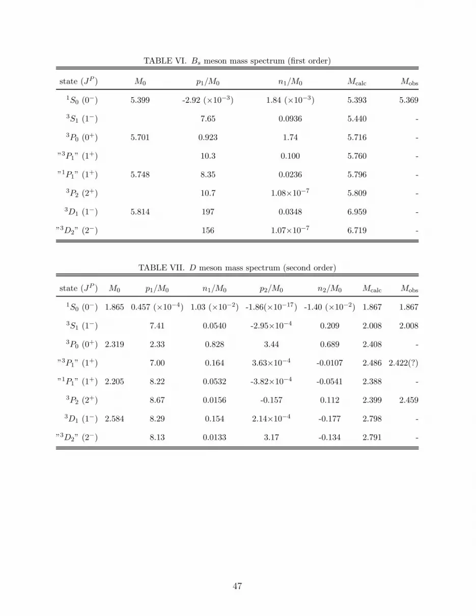
TABLE VI. Bs meson mass spectrum (first order)
state (JP ) M0 p1/M0 n1/M0 Mcalc Mobs
1S0 (0−) 5.399 -2.92 (×10−3) 1.84 (×10−3) 5.393 5.369
3S1 (1−) 7.65 0.0936 5.440 -
3P0 (0+) 5.701 0.923 1.74 5.716 -
”3P1” (1+) 10.3 0.100 5.760 -
”1P1” (1+) 5.748 8.35 0.0236 5.796 -
3P2 (2+) 10.7 1.08×10⁻⁷ 5.809 -
3D1 (1−) 5.814 197 0.0348 6.959 -
”3D2” (2−) 156 1.07×10⁻⁷ 6.719 -
TABLE VII. D meson mass spectrum (second order)
state (JP ) M0 p1/M0 n1/M0 p2/M0 n2/M0 Mcalc Mobs
1S0 (0−) 1.865 0.457 (×10−4) 1.03 (×10−2) -1.86(×10−17) -1.40 (×10−2) 1.867 1.867
3S1 (1−) 7.41 0.0540 -2.95×10⁻⁴ 0.209 2.008 2.008
3P0 (0+) 2.319 2.33 0.828 3.44 0.689 2.408 -
”3P1” (1+) 7.00 0.164 3.63×10⁻⁴ -0.0107 2.486 2.422(?)
”1P1” (1+) 2.205 8.22 0.0532 -3.82×10⁻⁴ -0.0541 2.388 -
3P2 (2+) 8.67 0.0156 -0.157 0.112 2.399 2.459
3D1 (1−) 2.584 8.29 0.154 2.14×10⁻⁴ -0.177 2.798 -
”3D2” (2−) 8.13 0.0133 3.17 -0.134 2.791 -
47
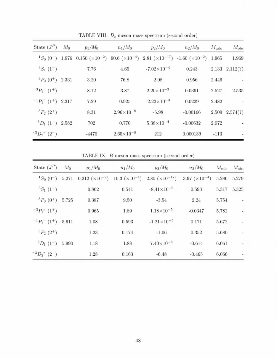
TABLE VIII. Ds meson mass spectrum (second order)
State (JP ) M0 p1/M0 n1/M0 p2/M0 n2/M0 Mcalc Mobs
1S0 (0−) 1.976 0.150 (×10−2) 90.6 (×10−4) 2.81 (×10−17) -1.60 (×10−2) 1.965 1.969
3S1 (1−) 7.76 4.65 -7.02×10⁻⁴ 0.243 2.133 2.112(?)
3P0 (0+) 2.331 3.20 76.8 2.08 0.956 2.446 -
”3P1” (1+) 8.12 3.87 2.20×10⁻³ 0.0361 2.527 2.535
”1P1” (1+) 2.317 7.29 0.925 -2.22×10⁻³ 0.0229 2.482 -
3P2 (2+) 8.31 2.96×10⁻⁸ -5.98 -0.00166 2.509 2.574(?)
3D1 (1−) 2.582 702 0.770 5.38×10⁻⁴ -0.00632 2.072 -
”3D2” (2−) -4470 2.65×10⁻⁸ 212 0.000139 -113 -
TABLE IX. B meson mass spectrum (second order)
State (JP ) M0 p1/M0 n1/M0 p2/M0 n2/M0 Mcalc Mobs
1S0 (0−) 5.271 0.212 (×10−2) 10.3 (×10−4) 2.80 (×10−17) -3.97 (×10−4) 5.286 5.279
3S1 (1−) 0.862 0.541 -8.41×10⁻⁶ 0.593 5.317 5.325
3P0 (0+) 5.725 0.387 9.50 -3.54 2.24 5.754 -
”3P1” (1+) 0.965 1.89 1.18×10⁻⁵ -0.0347 5.782 -
”1P1” (1+) 5.611 1.08 0.593 -1.21×10⁻⁵ 0.171 5.672 -
3P2 (2+) 1.23 0.174 -1.06 0.352 5.680 -
3D1 (1−) 5.990 1.18 1.88 7.40×10⁻⁶ -0.614 6.061 -
”3D2” (2−) 1.28 0.163 -6.48 -0.465 6.066 -
48
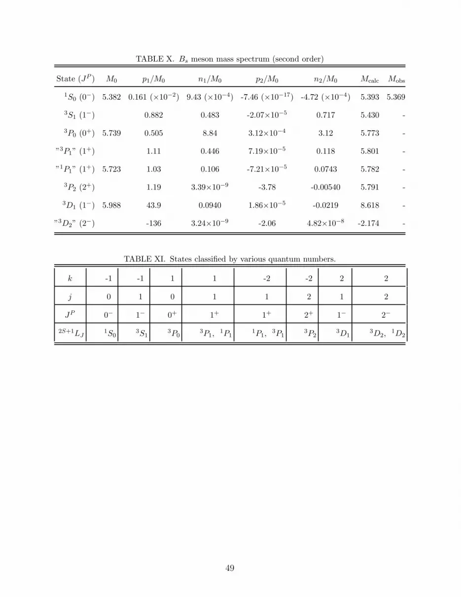
TABLE X. Bs meson mass spectrum (second order)
State (JP ) M0 p1/M0 n1/M0 p2/M0 n2/M0 Mcalc Mobs
1S0 (0−) 5.382 0.161 (×10−2) 9.43 (×10−4) -7.46 (×10−17) -4.72 (×10−4) 5.393 5.369
3S1 (1−) 0.882 0.483 -2.07×10⁻⁵ 0.717 5.430 -
3P0 (0+) 5.739 0.505 8.84 3.12×10⁻⁴ 3.12 5.773 -
”3P1” (1+) 1.11 0.446 7.19×10⁻⁵ 0.118 5.801 -
”1P1” (1+) 5.723 1.03 0.106 -7.21×10⁻⁵ 0.0743 5.782 -
3P2 (2+) 1.19 3.39×10⁻⁹ -3.78 -0.00540 5.791 -
3D1 (1−) 5.988 43.9 0.0940 1.86×10⁻⁵ -0.0219 8.618 -
”3D2” (2−) -136 3.24×10⁻⁹ -2.06 4.82×10⁻⁸ -2.174 -
TABLE XI. States classified by various quantum numbers.
k -1 -1 1 1 -2 -2 2 2
j 0 1 0 1 1 2 1 2
JP 0− 1− 0+ 1+ 1+ 2+ 1− 2−
2S+1LJ1S0
3S13P0
3P1,1P1
1P1,3P1
3P23D1
3D2,1D2
49