arX

iv:c

ond-

mat

/051

1677

v1 [

cond

-mat

.mes

-hal

l] 2

8 N

ov 2

005

Spectral properties of exciton polaritons in one-dimensional

resonant photonic crystals

M. V. Erementchouk, L. I. Deych, and A. A. Lisyansky

Physics Department, Queens College,

City University of New York, Flushing, New York 11367, USA

Abstract

The dispersion properties of exciton polaritons in multiple-quantum-well based resonant photonic

crystals are studied. In the case of structures with an elementary cell possessing a mirror symmetry

with respect to its center, a powerful analytical method for deriving and analyzing dispersion laws

of the respective normal modes is developed. The method is used to analyze band structure

and dispersion properties of several types of resonant photonic crystals, which would not submit to

analytical treatment by other approaches. These systems include multiple quantum well structures

with an arbitrary periodic modulation of the dielectric function and structures with a complex

elementary cell. Special attention was paid to determining conditions for superradiance (Bragg

resonance) in these structures, and to the properties of the polariton stop band in the case when

this condition is fulfilled (Bragg structures). The dependence of the band structure on the angle

of propagation, the polarization of the wave, and the effects due to exciton homogeneous and

inhomogeneous broadenings are considered, as well as dispersion properties of excitations in near-

Bragg structures.

1

I. INTRODUCTION

Optical properties of artificial structures with periodically modulated dielectric constant

has been attracting a great deal of interest since pioneering papers Refs. 1 and 2, where

such systems have been first discussed. Periodic modulation of the dielectric function signif-

icantly modifies spectral properties of electromagnetic waves. Instead of a simple continuous

spectrum with a linear dispersion law, the electromagnetic spectrum in such structures is

characterized by the presence of allowed and forbidden bands similar to electronic band

structure of crystals. For this reason, the new class of optical materials was dubbed pho-

tonic crystals.3 Changing the spatial distribution of the dielectric constant one can effectively

control such fundamental properties as the group velocity of light, the rate of spontaneous

emission, etc. This fact has important repercussion for both fundamental physics and for

applications, where it opens up possibilities for new concepts of optical and optoelectronic

devices.

Modulation of the dielectric function, however, is not the only way to affect light prop-

agation and its interaction with matter. It was shown in Ref. 4 that closely packed dipole

active atoms can become coherently coupled by light, and this coupling significantly changes

their emission properties resulting in the so called “super-radiance” effect. In the origi-

nal Dicke’s model4 the distance between the atoms was assumed to be much smaller than

the wavelength of their emission, but similar effect can also arise if dipole active elements

form a one-dimensional periodic lattice with the period coinciding with the emission half-

wavelength (Bragg resonance). Such an arrangement is possible with a so called optical

lattice of cold atoms5 and with their semiconductor analogs – Bragg multiple quantum well

(MQW) structures.6,7,8,9 The latter are semiconductor heterostructures, in which very thin

layers of a narrower band gap semiconductor (quantum well) are separated from each other

by much thicker layers of a wider band gap semiconductor (barrier) in such a way that the

period of the structure coincides with the half-wavelength of light emitted by excitons con-

fined in a quantum well (QW). In these systems, excitons play the role of the dipole active

excitations, which become radiatively coupled and demonstrate the superradiance effect.

If, however, the size (the number of periods) in an optical lattice increases, the properties

of the system change10,11. In particular, the dark modes form two branches of collective

excitations, in which light is coupled with the material resonances, and which can be called

2

optical lattice polaritons. At the same time, the super-radiance mode develops into a stop

band, which is a spectral gap between the two polariton branches, characterized by almost

complete reflection of a normally incident radiation. The distinction between Bragg struc-

tures and other arrangements, in which the period of the structure is not in the resonance

with radiation emitted by the active elements, can, in this case, be described in terms of

formation of a significantly (by orders of magnitude) enhanced stop band.

There is, however, an important difference between optical lattices of atoms and semi-

conductor heterostructures. In the latter case, the interaction of light with active elements

(excitons) is accompanied by multiple reflection of light from interfaces between wells and

barrier layers caused by difference in their refractive indexes. Thus, in structures like

MQWs optical lattice effects coexist with photonic crystal-like effects, which results in a

number of new and interesting optical properties and opportunities for applications. Such

structures, called resonant photonic crystals (RPC), have recently started attracting sig-

nificant attention.12,13,14,15,16,17,18,19A general characteristic of this type of structures is the

co-existence of dipole active material excitations (excitons, phonons, plasmons) described

by optical susceptibilities of the resonant type and the periodic modulation of the back-

ground dielectric constant. Two most fundamental problems in the focus of current research

in this area are concerned with the effects of the interplay between resonances and spatial

non-uniformity of the dielectric function on the band structure of these systems and their

optical spectra. While these two questions are interconnected, they have to be recognized

as two separate problems, one dealing with normal modes of closed (or infinite) systems and

their dispersion laws and the other with the interaction of an internal radiation with a finite

size structure.

The main interest of studies in this field is a spectral region in the vicinity of the resonant

frequency, where the interplay effects play the most important role. A theoretical description

of RPC’s in this spectral region is a challenging problem and its complete solution has not

yet been obtained even for a simplest case of one-dimensional structures, such as MQWs.

Of course, it is always possible to carry out numerical calculations of the optical spectra and

the dispersion laws, which are particularly easy in one-dimensional case. However purely

numerical approach does not provide a real understanding of physics of these structures.

Therefore, it is very important to be able to carry out analytical analysis, which would not

only provide a better understanding of physical processes taking place in these structures,

3

but would also be instrumental in designing structures with pre-determined properties, which

is crucial for their possible applications.

Different aspects of this problem have been, of course, considered in a number of previous

publications. In particular, in Ref. 20 the necessity of a modification of the Bragg resonance

(super-radiance) condition for one-dimensional resonant photonic crystals compared to the

case of optical lattice structures was shown. Later, this result was confirmed21 and an exact

Bragg condition in such structures was found for the particular case of normal propagation

of the electromagnetic wave. It was also noted in Ref. 21 that, when the resonance condition

is met, the spectral gap between the polariton branches becomes wider than in the case of a

passive photonic crystal characterized by the same modulation of the dielectric function or of

an optical lattice with the same strength of radiative coupling between the active elements.

In the case of structures of higher (2 or 3) dimensions, no analytical results are available

yet, but one can note recent numerical calculations presented in Refs. 18 and 22, where it

was also found that the resonances may enhance polariton related band gaps compared to a

purely passive photonic crystal with the same spatial distribution of the dielectric constant.

It is important to emphasize that this enhancement of the band gap in RPC structures is not

a trivial effect. In order to illustrate this point we can mention another, in a certain sense,

opposite effect, which also results from the interplay between the resonances and periodic

inhomogeneities of the dielectric function. It was shown in Ref. 23 that there always exists a

frequency where the reflection coefficient of the incident light vanishes due to the destructive

interference between the two channels of interaction between light and the structure.

These examples show the richness of the optical properties of even one-dimensional res-

onant photonic crystals. In order to achieve a complete understanding of relationships

between optical and geometrical characteristics of these structures, one needs a general

analytical method, which could be applied to a variety of RPCs independently of a partic-

ular spatial dependence of their dielectric function. In our previous paper, Ref. 23, such a

method was developed for studying reflection, transmission, and absorption spectra of one-

dimensional RPC structures. The present paper presents a general analytical approach to

calculating the band structure of these materials. This method allows one to analyze disper-

sion laws of one-dimensional RPCs with an arbitrary form of the periodic modulation of the

dielectric function, propagation angle of the electromagnetic wave and its polarization state.

This method naturally incorporates resonant excitations of the medium into the theory. For

4

concreteness, we assume that the resonances are related to exciton states in QWs, but this

approach can be easily applied to any other type of the resonance excitations. In Sections II

and, particulary, in subsection IIB we show that by choosing an appropriate basis for rep-

resenting transfer matrices one can significantly simplify the analysis of the band structure

and dispersion laws of electromagnetic excitations in the structures under consideration. In

Sections IV and V we illustrate the power of the approach by applying it to a number of

examples, some of which deal with already well studied situations (passive one-dimensional

photonic crystals, optical lattices, MQWs with a piece-wise spatial dependence of the dielec-

tric function), while the others demonstrate the possibilities of our approach in obtaining

results that could not have been obtained by other methods.

II. THE (a, f)-REPRESENTATION OF THE TRANSFER MATRIX

A. Transfer matrix approach in resonant photonic crystals

A propagation of the electromagnetic wave in structures under discussion is governed by

the Maxwell equation

∇×∇×E =ω2

c2[ǫ∞(z)E + 4πPexc], (1)

where z axis is chosen along the growth direction and Pexc is the excitonic contribution to

the polarization, which can be presented in the following form:

Pexc = −χ(ω)∑

m

Φm(z)

∫dz Φm(z′)E⊥(z′), (2)

where Φm(z) = Φ(z − zm) is the envelope wave function of an exciton localized in the m-th

QW. The summation in Eq. (2) is performed over all QWs and zm are the positions of their

centers. We assume that the distance between the consecutive wells, d = zm+1−zm, coincides

with the period of the spatial modulation of the dielectric function, ǫ(z+d) = ǫ(z). Also, we

assume that the profile of the dielectric function is symmetrical with respect to the position

of the center of the QW, ǫ(zm + z) = ǫ(zm − z) (see Fig. 1). We restrict ourselves to the

consideration of 1s states of heavy-hole excitons and neglect their in-plane dispersion. The

dipole moment of these excitons lies in the plane of the well, therefore, they can only interact

with the in-plane component of the electric field, E⊥. This fact is reflected in Eq. (2), where

only this component of the field is included.

5

01 10

()z

z d

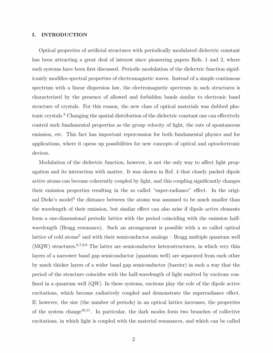
FIG. 1: An example of the modulation of the dielectric function, ǫ(z) = ǫ+∆ǫ(z) (solid line). The

dashed vertical lines show the positions of the centers of QWs.

The frequency dependence of the excitonic response is given by the function, χ(ω), defined

as

χ(ω) =α

ω0 − ω − iγ, (3)

where ω0 is the exciton resonance frequency, γ is the non-radiative decay rate of the exciton,

and α is the microscopic exciton-light coupling parameter, proportional to the dipole moment

of the electron – heavy hole transition.

Eq. (1) can be analyzed by presenting the direction of the electric field as a vector sum

of two mutually perpendicular polarizations. These, so called s- and p-polarizations, define

two possible eigen directions, and accordingly, the respective electric fields satisfy two inde-

pendent equations, which can be considered separately. In the structures modulated in the

z-direction, normal modes of the system are characterized by the wave vector perpendicular

to the modulation (growth) direction, which is a conserving quantity. The direction of this

vector can be also used to define the eigen polarizations of the waves.

The absence of an overlap of the exciton wave functions localized in different QWs makes

it possible to use the transfer matrix technique for solving Maxwell equations, Eq. (1). The

general idea of this technique is to characterize the electric field of the wave with a certain

polarization by a two-component column vector, |c(z)〉 whose change along the structure is

governed by a 2×2 matrix. The main property of this matrix can be described as following.

If |c(z1)〉, |c(z2)〉, and |c(z3)〉 characterize the field at points z1, z2, and z3, respectively, and

6

if T (zi, zj) satisfies the equation |c(zi)〉 = T (zi, zj)|c(zj)〉, then T (z1, z3) = T (z1, z2)T (z2, z3).

The relations between the values of the field and the vector |c(z)〉 as well as the form of the

matrix T (zi, zj) depend on the choice of the particular representation of the field. Several

possible representations will be discussed in the subsequent sections of the paper for both

polarizations.

1. S-polarization

In the s-polarized wave the electric field E is perpendicular to the plane formed by the

direction of z axis and in-plane wave vector, k. Accordingly, it can be presented in the form

E(z, ρ) = esE(z)eikρ, (4)

where ρ is the coordinate in the (x, y)-plane and es = ek × ez is a unit polarization vector,

defined in terms of unit vectors in z- and k-directions. For E(z) we obtain an integro-

differential equation

d2E(z)

dz2+ κ2

s(z) = −χ(ω)4πω2

c2

∑

m

Φm(z)

∫dz Φm(z′)E(z′), (5)

where κ2s(z) = ω2ǫ(z)/c2 − k2.

We first consider the transfer matrix corresponding to the propagation of the field across

one elementary cell of the structure, i.e. from point z− + 0 at the left boundary of the cell,

inside it, to the point z+ + 0 just outside of the right boundary of the cell. The complete

transfer matrix connecting the field at the right boundary of the entire system with the field

at its left boundary can then be obtained as a product of the transfer matrices for each

cell. Considering only one cell, we can, without any loss of generality, choose the origin of

our coordinate system coinciding with a position of the QW in the cell under consideration.

When z coordinate is confined to a single cell, the summation over QWs and the index

enumerating them in Eq. (5) can be dropped.

The term with the exciton polarization at the r.h.s. of Eq. (5) can be considered as an

inhomogeneity in a second order differential equation

d2E(z)

dz2+ κ2

s(z)E = F(z), (6)

7

whose general solution can be written in the form24

E(z) = c1h1(z) + c2h2(z) + (G ⋆ F)(z), (7)

where

(G ⋆ F)(z) =

∫ z

z−

dz′F(z′)h1(z

′)h2(z) − h1(z)h2(z′)

W (h1, h2; z′). (8)

Here we have introduced h1,2(z), a pair of linearly independent solutions of the homogeneous

equationd2E(z)

dz2+ κ2

s(z)E = 0, (9)

and W (h1, h2; z) = h1h′2 − h′

1h2 is the Wronskian of these solutions. For the case under

consideration the Wronskian does not depend on z and will be denoted by Wh in what

follows.

Alternatively, a solution of Eq. (5) can be presented as

E(z) = c1(z)h1(z) + c2(z)h2(z), (10)

E ′(z) = c1(z)h′1(z) + c2(z)h′

2(z).

In the regions outside of the QW, where Φ(z) ≡ 0, functions c(z) remain constants, making

representations given by Eq. (7) and Eq. (10) equivalent, but ci(z) change when z traverses

from one boundary of the QW to the other. Our goal now is to use Eq. (7) along with

Eq. (8) in order to relate the values of ci(z) at the right boundary of the QW to their values

at the left boundary. Using these equations we can obtain the expression for the electric

field for points to the right from the QW as

E(z) =h1

[c1 + χ

4πω2ϕ2

c2(c1ϕ1 + c2ϕ2)

]

+h2

[c2 − χ

4πω2ϕ1

c2(c1ϕ1 + c2ϕ2))

],

(11)

where ϕ1,2 are “projections” of the solutions h1,2 onto the exciton states

ϕ1,2 =1

Wh

∫

QW

dz′Φ(z′)h1,2(z′). (12)

and the modified excitonic response function χ can be presented as

χ =χ

1 − ∆ωχ/α, (13)

8

where

∆ω = α

∫

QW

dz Φ(z)(G ⋆ Φ)(z) (14)

gives the radiative shift of the exciton frequency in the photonic crystal. Eq. (14) is a

generalization of the well-known expression for the radiative shift in MQW structures with

a homogeneous dielectric function.11,25,26

Comparing Eq. (11) with Eq. (10), and taking into account that the coefficients ci do not

change outside of the QW, we can find a relation between the coefficients ci determined at

the two inner boundaries of the elementary cell, z = z− + 0, and z = z+ − 0

c1

c2

(z+ − 0) = Th

c1

c2

(z− + 0), (15)

with matrix Th given as

Th = 1 +4πω2χ

c2

ϕ2ϕ1 ϕ22

−ϕ21 −ϕ2ϕ1

, (16)

where 1 is the unit matrix. It should be noted that Eq. (16) is valid for an arbitrary form

of the exciton envelope wave function and spatial modulation of the dielectric function.

Eq. (16) can be significantly simplified if we use freedom in the choice of the functions

hi(z). In the case when ǫ(z) is invariant with respect to the mirror reflection relatively to the

center of the QW, h1,2 can be chosen to have a definite parity, with one of them being even

with respect to the center of the QW, and the other being odd. With such a choice of these

functions we can always turn one of ϕ1,2 to zero.50 It should be understood, however, that h1

and h2 are not actual normal modes of the photonic crystal. The latter must be defined as

solutions of the appropriate boundary problem, and do not have to be even or odd functions

with respect to the center of the elementary cell. Moreover, due to the Bloch theorem the

modes of a photonic crystal can have a definite parity only at specific frequencies that are

naturally identified with boundaries of the forbidden gap in the spectrum. However, all

normal modes of the photonic crystal can be represented as superpositions of the even and

odd solutions h1,2. A formal discussion of the relation between the functions h1 and h2 and

the normal modes can be found in Ref. 27 where the similar approach has been used for the

analysis of spectral properties of a Schrodinger equation with a periodic potential.

Obviously, fixing the parity of the solutions does not determine functions h1 and h2

uniquely since a multiplication by a constant determined by initial conditions does not

9

change their symmetry. It can be shown, however, that results obtained for observable

quantities, such as band structure, do not depend on this ambiguity. We will present our

general results in a form independent on the choice of initial conditions. However, for

discussions of particular examples it is more convenient to fix them in the form

h1(0) = 1, h′1(0) = 0,

h2(0) = 0, h′2(0) = 1,

(17)

for which Wh = 1.

Let us assume that h1 is the even solution, then ϕ2 ≡ 0 and the expression for the matrix

Th simplifies to

Th = 1 + Ssqs

0 0

1 0

, (18)

where qs = κs(z+) is the value of κs(z) at the boundary of the elementary cell and

Ss = −χ(ω)2πω2ϕ2

1

qsc2Wh

. (19)

Substitution of χ yields

Ss =Γs

ω − ω0 − ∆ω + iγ, (20)

where Γs is the radiative decay rate,

Γs =2παω2ϕ2

1

qsc2. (21)

The function Ss(ω), which we shall refer to as exciton susceptibility, describes the contribu-

tion of the exciton-light interaction to the optical properties of the structures under consid-

eration. For instance, the resonant absorption of light occurs at the frequency ω0 = ω0 +∆ω

determined by the pole of Ss(ω). We will treat ω0 as an experimentally accessible exciton

frequency, which along with the radiative decay rate Γs can be measured in optical exper-

iments with a single QW. In what follows we will drop the tilde from ω0 and assume that

the radiative shift is included in this parameter.

Coefficients ci in Eq. (15) are the two components of the vector |c〉 characterizing the

field in the transfer matrix formalism while matrix Th given by Eq. (16) is the transfer

matrix itself. The functions hi(z), which we used to derive Eqs. (15) and (18) form a basis

for this particular representation of the transfer matrix. Using this basis we are able to

obtain a simple and convenient expression for the transfer matrix describing the evolution

10

of the electric field inside a single elementary cell. However, in order to obtain the transfer

matrix through the period of the structure, we have to relate the field and its derivative at

points to the left (z+ −0) and to the right (z+ +0) of the boundary between two elementary

cells. Since there is no discontinuity of the dielectric constant at this point, it might appear

that all the continuity conditions would be satisfied automatically. One should remember,

however, that functions hi(z) are different in different elementary cells. For two adjacent

m-th and (m + 1)-th cells, the respective functions, hmi (z) and hm+1i (z), are related to each

other as hmi (z) = hm+1i (z−d), and in order to establish connection between vectors |cm〉 and

|cm+1〉 at the boundary between these cells, one would need to express hm+1i (z) in the basis

of hmi (z). This problem can be solved, but it turns out to be more convenient to convert our

transfer matrices to a more conventional basis of plane waves

E(z) = E+eiqsz + E−e−iqsz (22)

using the conversion rule, Eq. (A9), derived in the Appendix. The resulting transfer matrix

describing the evolution of the field across an entire elementary cell can then be presented

in the form

T =

af (af − af)/2

(af − fa)/2 af

, (23)

which, as will be seen shortly is particularly convenient for analysis of the spectrum of the

system under consideration. This representation is extensively used in the present paper

and, in what follows, we will refer to it as (a, f)-representation. The parameters of this

representation, a and f , are defined as

a = g2, f = g1 − iSsg2,

a = g∗2, f = g∗

1 + iSsg∗2,

(24)

where

g1 =1√Wh

[h1(z+) +

h′1(z+)

iqs

],

g2 =1√Wh

[iqsh2(z+) + h′2(z+)] .

(25)

2. p-polarization

A representation similar to Eq. (23) for a transfer matrix describing p-polarized light can

also be obtained along the similar lines. An important difference is that the electric field in

11

the p-polarized waves is not transverse (∇ · E 6= 0) and, therefore, satisfies a more complex

system of two differential equations. For conventional photonic crystals the p-polarized

waves are conveniently described in terms of the magnetic field (see e.g., Ref. 3). However,

the presence of the dipole active excitations significantly reduces the convenience of this

approach because in order to close the equation for this field, one would have to express the

interaction with excitons in terms of the magnetic field. While it can be done, we find it

more convenient to continue working with electric field, E.

The electric field for the p-polarization can be presented in the following form:

E(z, ρ) = [ekEx(z) + ezEz(z)] eikρ. (26)

Amplitudes Ex,z(z) satisfy the system of equations

d2Ex

dz2− ik

dEz

dz+ κ2

p(z)Ex =

−χ(ω)∑

m

Φm(z)

∫dz Φm(z′)Ex(z

′),

−ikdEx

dz+[κ2p(z) − k2

]Ez(x) = 0,

(27)

where κ2p(z) = ω2ǫ(z)/c2. Deriving these equations we again have explicitly taken into

account that only the in-plane component of the electric field interacts with the heavy-hole

excitons. Solving the second equation with respect to Ez we obtain the closed equation for

Ex(z)

d

dz

[p(z)

dEx

dz

]+ κ2

p(z)Ex =

−χ(ω)4πω2

c2

∑

m

Φm(z)

∫dz Φm(z′)Ex(z

′),(28)

where p(z) = κ2p(z)/[κ2

p(z) − k2]. This function is related to the local angle of propagation

of the wave, θ(z): p(z) = 1/ cos θ(z).

The derivation of the transfer matrix for the p-polarized field follows exactly the same

steps as in the previous subsection with one important change. The Wronskian of two

solutions of the “homogeneous” (that is with χ ≡ 0) version of Eq. (28) depends on the

coordinate z.24 This, however, does not present a major problem, because if one takes into

account that this dependence can be presented in the form

W (z) = Whp(z+)

p(z), (29)

12

one can immediately reproduce all the main results of the previous subsection. In particular,

the transfer matrix in the basis of plane waves can again be written down in the (a, f)-

representation, Eq. (23). The parameters of this representation are given by the same

Eqs. (24) and (25), where, however, one has to consider functions h1,2 as even and odd

solutions of the “homogeneous” version of Eq. (28). Also, the function Sp, which retains the

same form as in Eq. (20), is now characterized by a modified radiative shift of the exciton

frequency and the decay rate. The expression for the frequency shift is obtained by replacing

the expression given by Eq. (8) with

(G ⋆ F)(z) =1

Whp(z+)

∫ z

z−

dz′F(z′) [h1(z′)h2(z) − h1(z)h2(z

′)] (30)

in Eq. (14) for the radiative shift. The rate of exciton’s decay into the p-polalized light is

given by

Γp =2παω2ϕ2

1

qpc2p(z+), (31)

where qp = κp(z+). One can notice that these expressions and corresponding expressions for

the s-polarized wave coincide in the case of normal propagation, i.e. when k = 0.

B. General properties of the (a, f)-representation

The fact that the transfer matrices for both polarizations allow for the (a, f)-

representation is not a coincidence but is related to a well-known feature of the Maxwell

equations. To demonstrate it let us consider Eq. (28) in a particular case corresponding to

the passive structure (χ ≡ 0). If E(z) is a solution to this equation, its complex conjugate

E∗(z) is also a solution. Having this in mind one can show that that

d

dz

[p(z)

(EE∗′ − E ′E∗

)]= 0. (32)

Now, representing the electric field in the form of Eq. (22) we can find that

d

dz

[qpp(z)

(|E+|2 − |E−|2

)]= 0. (33)

This relation expresses conservation of the flux of the Poynting vector through a plane

perpendicular to the z-axis and represents the fact that there are no sources or drains of the

energy in the system. The similar expression for the s-polarized wave can be obtained by

substitution qp → qs, p(z) → 1. It follows from Eq. (33) that the transfer matrices through

13

the period for both s and p polarizations must preserve the combination |E+|2 − |E−|2,which means that the transfer matrix written in the basis of plane waves belongs to SU(1, 1)

group.28 A general form of an element of this group is28

T =

T1 T2

T ∗2 T ∗

1

, (34)

where T1,2 are complex numbers and |T1|2 − |T2|2 = 1. Matrices allowing for the (a, f)-

representation correspond to a particular case of SU(1, 1) matrices, for which T2 is purely

imaginary. It can be shown that such matrices describe structures that posses a mirror

symmetry. Indeed, a transfer matrix of such a structure satisfies the following condition

σxTσx = T−1, where σx is the Pauli matrix. Substitution of Eq. (34) into this equation gives

T ∗2 = −T2. The converse statement can also be verified. This property of transfer matrices

can also be proven in the general case of matrices corresponding to Maxwell equations with

external polarization (5) and (28), but the proof is rather technical and we do not provide

it here.

Owing to the (a, f)-representation, the description of structures with mirror symmetry

can be significantly simplified. At the same time, they demonstrate a rich variety of inter-

esting phenomena, and, therefore these structures attract a great deal of attention (see e.g.

Ref. 29). If such a structure is built of blocks that have mirror symmetry by themselves then

the transfer matrix through the entire structure can be written in terms of matrix elements

describing the individual blocks. Indeed, let us consider a structure with the period BAB

where the transfer matrices of the blocks A and B have the form T (a1, f1) and T (a2, f2),

respectively, in the (a, f)-representation. Then it can be shown that the transfer matrix

through the period is

T (a2, f2)T (a1, f1)T (a2, f2) = T (a, f), (35)

where

a = a1a2f2 −a1

2

(a2f2 − a2f2

),

f = f2f1a2 +f1

2

(a2f2 − a2f2

).

(36)

We will illustrate the “multiplication rule”, Eq. (35), considering a simple but very im-

portant for the rest of the paper example of an elementary cell in an optical lattice. In this

system, the block A corresponds to an active element, for instance, a QW, and two blocks

14

B describe barriers, which have the same refractive index as block A. The blocks B are

described by a transfer matrix given by Tb(φb) = diag [exp(iφb), exp(−iφb)]. In this case one

has a2 = f2 = exp(iφb/2) in Eq. (35) and thus

Tb(φb)T (a, f)Tb(φb) = T (aeiφb , feiφb). (37)

If, however, one needs to take into account the difference between refractive indices of

the blocks B, and the block A, a new type of transfer matrix products emerges. Introduc-

ing matrix Tρ, describing propagation of light across a boundary between two media with

different indexes of refraction

Tρ =1

1 + ρ

1 ρ

ρ 1

. (38)

where ρ is the Fresnel reflection coefficient30 (see below Eq. (49)), we can describe propa-

gation of light through BA and AB interfaces and across the block A using the following

combination of the transfer matrices: Tρ(ρ)−1T (a, f)Tρ(ρ). An important property of the

(a, f)-representation is that this product can be expressed in the following form:

Tρ(ρ)−1T (a, f)Tρ(ρ) =1

1 − ρ2T (a + aρ, f − fρ). (39)

The real factor in Eq. (39) can be incorporated into a and f due to the useful relation (with

real λ)

λT (a, f) = T (λa, f) = T (a, λf). (40)

Eqs. (35), (37), and (39) will be extensively used throughout the paper for obtaining

the (a, f)-representation of various transfer matrices. This method is often more practical

than solving corresponding differential equations. Thereby, it is interesting to note that the

parameters of the (a, f)-representation are essentially boundary values of solutions of the

corresponding Cauchy problem.

III. THE DISPERSION EQUATION IN RESONANT PHOTONIC CRYSTALS:

THE METHOD OF ANALYSIS AND THE BAND STRUCTURE

A. Dispersion equation in the (a, f)-representation

The dispersion equation characterizing normal modes (polaritons) in an infinite periodic

one-dimensional structure can be expressed in terms of elements of a transfer-matrix across

15

one period of the structure31

cos Kd =1

2Tr T, (41)

where K is the Bloch wave number, d is the period of the structure, and the transfer matrix is

assumed to be written in the plane wave basis. If this structure possesses a mirror symmetry,

one can show that the condition det T = 1 can be presented as fa + fa = 2. Using this

identity we can rewrite the polariton dispersion law in the form

cos2

(Kd

2

)= ℜ(a)ℜ(f), (42)

where

ℜ(a) = (a + a)/2. (43)

Equivalently, this dispersion equation can be presented as

sin2

(Kd

2

)= ℑ(a)ℑ(f), (44)

where

ℑ(a) = (a − a)/2i. (45)

If the exciton susceptibility S is a real function (no homogeneous broadening of excitons),

the a coincides with a conjugated, a = a∗. In this case, ℜ(a) and ℑ(a) are equivalent to

regular real or imaginary parts of a respectively: ℜ(a) = Re(a) and ℑ(a) = Im(a). When

homogeneous broadening is taken into account, Eq. (42) remains valid, but identification of

ℜ(a) and ℑ(a) with Re(a) and Im(a) can no longer be made. In this case, one has to use

definitions given in Eqs. (43) and (45).

If the homogeneous broadening can be neglected, the r.h.s of Eq. (42) and Eq. (44) are

real valued. Therefore, we can analyze the band structure in the vicinity of the exciton

resonance using the notion that for allowed bands (real K) these expressions should be

positive and less than unity, while for the band gaps (complex K) they should be negative

or greater than unity. Thus, there are two types of conditions determining the boundary of

the bands. From Eq. (42) we have that the band boundary occurs when either ℜ(a)ℜ(f)

or ℜ(a)ℜ(f) − 1 changes sign, and Eq. (44) defines as the boundaries those frequencies at

which the change of sign occurs for expressions ℑ(a)ℑ(f) or ℑ(a)ℑ(f) − 1. One can show

that these two pairs of conditions are equivalent to each other. More precisely, expression

ℜ(a)ℜ(f) changes sign at the same frequencies as expression ℑ(a)ℑ(f) − 1. The same is

16

true for the pair ℜ(a)ℜ(f) − 1 and ℑ(a)ℑ(f). Thus, all the band boundaries can be found

by considering changes of sign of expressions ℜ(a)ℜ(f) and ℑ(a)ℑ(f), with negative values

corresponding to the band gaps. The factorized form of right-hand sides of the polariton

dispersion equation, Eqs. (42) and (44), drastically simplifies the analysis of the spectrum,

as it will be seen in the subsequent sub-sections.

The factorization of the dispersion equations, Eqs. (42) and (44) becomes possible only

owing to the (a, f)-representation of the transfer-matrix, which makes this representation

particularly suitable for studying the band structure and dispersion laws of polaritons in

resonant photonic crystals. At the same time, this representation is not very convenient

for calculating relfection/transmission spectra of finite structures because of a cumbersome

relation between the parameters of a single layer transfer matrix and a matrix describing

the entire structure. This problem, however, can be conveniently solved with the help of

a different representation introduced in our recent paper, Ref. 23. It is useful to establish

a direct relationship between these two representations. First we notice that an arbitrary

matrix of the form (23) can be written in the form of a transfer matrix describing propa-

gation of a wave across a single QW [see Eq. (55) below]. This can be done by introducing

an effective optical width of one period of the structure, φ, and an effective excitonic sus-

ceptibility, S. The relation between the parameters of the (a, f)-representation and these

effective parameters can be found by comparing Eqs. (23) and (55)

S =1

2i(af − af), eiφ =

a

a. (46)

The usefulness of this relation is twofold. First, it shows that for any resonant photonic

crystal the transfer matrix through the period can be represented as a transfer matrix

through a conventional MQW structure. Second, Eq. (46) can be used for a consideration

of reflection and transmission spectra of a structure described by a transfer matrix in (a, f)-

representation. This is where the introduction of S and φ and then, consecutively, the

representation the transfer matrix in terms of parameters θ and β of Ref. 23 becomes very

convenient. However, this representation misses the possibility to factorize the dispersion

equation, so it is not very suitable for a constructive analysis of the dispersion law. One can

see, therefore, that the representations of the transfer matrix in terms of parameters (a, f)

and S and φ compliment each other in a sense that each of them is suited best for its own

set of problems.

17

b

w

FIG. 2: The periodic structure built of two blocks. Vertical dashed lines show the boundary of the

elementary cell. The angles of propagation inside the blocks are related by Snell’s law.

B. MQW structures with a simple elementary cell

As it was mentioned in Introduction, MQW structures present one example of RPCs,

in which effects due to reflection of light from well-barrier interfaces coexist with effects

due to the resonant light-exciton coupling. The spatial profile of the refractive index

in these structures is particulary simple, and is described by a piece-wise constant func-

tion [Fig.(2)]. Various properties of these structures have been studied in a number of

publications20,21,23,25,32,33,34, including papers Refs.20,21,23 dealing particularly with disper-

sion laws and the band structure of their normal modes. Nevertheless, we find it useful to

consider this case in details in this paper because it gives a clear illustration of using the

(a, f)-representation for the analysis of complex dispersion equations.

We start by considering two particular cases: a passive photonic crystal (no resonances)

and an optical lattice (no refractive index mismatch). This will give us useful benchmarks for

discussing the general situation. In the latter case we will neglect the exciton homogeneous

broadening, which allows us to identify operations ℜ and ℑ with taking regular real and

imaginary parts of the respective expressions. The same is obviously true for the case of

passive structures.

1. Passive photonic crystals

Let us consider a structure built of a periodic sequence of two blocks characterized by

the widths db,w and the indices of refraction nb,w. To emphasize the mirror symmetry we

choose the elementary cell as shown in Fig. 2. The transfer matrix through the period of

the structure has the form

T = T1/2b T−1

ρ TwTρT1/2b , (47)

18

where

Tb,w =

eiφb,w 0

0 e−iφb,w

, (48)

φb,w = ωnb,wdb,w cos θb,w/c and θb,w are the angles of propagation of the wave.

The scattering of the electromagnetic wave at the interface between different blocks de-

pends on both the angle of incidence of the wave and its polarization state. These effects

are described by Fresnel coefficients ρs and ρp,

ρs =nw cos θw − nb cos θbnw cos θw + nb cos θb

,

ρp =nw cos θb − nb cos θwnw cos θb + nb cos θw

, (49)

for s and p polarizations, respectively. Below we denote the Fresnel coefficients simply by

ρ having in mind that for a particular polarization only one of these expressions should be

used.

Using Eqs. (37) and (39) we can find parameters of the (a, f)-representation of the transfer

matrix, which in this case take the following form

a =eiωτ+ + ρeiωτ−

1 − ρ2, f = eiωτ+ − ρeiωτ− , (50)

where τ± = (φb ± φw)/2ω. Now we can use general dispersion equations, Eq. (42) and

(44) to analyze the structure of the allowed and forbidden bands of this system. As we

discussed in Section IIIA there are two types of forbidden bands, determined by conditions

Re (a)Re (f) < 0, and, Im (a)Im (f) < 0 respectively. If τ+ and τ− are incommensurate,

these band gaps alternate along the frequency axis and can be classified as either odd (first,

third, etc.) or even (second, forth, etc.).

Since the coefficients of the dispersion equation in the passive photonic crystals do not

contain any singularities, its right hand side can only change the sign by passing through zero.

Thus, the band boundaries are situated at the frequencies where either Re (a)Re (f) = 0 or

Im (a)Im (f) = 0. For instance, if ρ > 0, the boundaries of odd band gaps are determined

by equations

Re [a(Ω+)] = 0, Re [f(Ω−)] = 0, (51)

where Ω− and Ω+ correspond to the lower and higher frequency boundaries of a given band

gap respectively. The explicit form of these equations can be obtained using definitions,

19

Eq. (50):

cos(Ω−τ+) − ρ cos(Ω−τ−) = 0,

cos(Ω+τ+) + ρ cos(Ω+τ−) = 0.(52)

In the simplest case, when the layers have the same optical width, one has τ− = 0 and the

positions of the edges of the forbidden gap are ωr(1 ± 2 arcsin(ρ)/π), where

ωrτ+ =π

2. (53)

While this case gives a convenient reference point, however, having in mind applications to

MQW structures, an opposite situation, when the optical widths of the layers are different,

is of more interest. Generally, as one can see from Eq. (52), the boundaries of the gap are

situated asymmetrically with respect to ωr. Under the assumption of narrow gaps, which is

fulfilled for a not very strong contrast of the refraction indexes, and for angles not too close

to the angle of the total internal reflection, the positions of the boundaries are given by

Ω± = ωr

(1 ± 2ρ sin φw

π(1 ± ρ cos φw)

). (54)

2. Semiconductor optical lattice

In this case we assume that all layers in the structure have the same index of refraction,

n, but there are dipole active excitations in QWs. The propagation of light through a QW

is described by the transfer matrix of the form

Tw =

eiφw(1 − iS) −iS

iS e−iφw(1 + iS)

, (55)

where φw = ωndw cos θw/c. The parameters of the (a, f)-representation of Tw are

a = eiφw/2, f = eiφw/2(1 − iS). (56)

The excitonic contribution to the scattering of light is described by

S =Γ0

ω − ω0 + iγ. (57)

The radiative decay rate, Γ0, depends on the angle of incidence. As follows from Eqs. (21)

and (31), for structures with homogeneous dielectric function these dependencies for different

polarizations are20,35,36

Γ(s)0 = Γ0/ cos θw, Γ

(p)0 = Γ0 cos θw. (58)

20

The transfer matrix through the period of the structure is

T = T1/2b TwT

1/2b . (59)

Taking into account the multiplication rule (37), we can find parameters of the (a, f)-

representation for the entire matrix (59) and the respective dispersion equation6,8,37

cos2

(Kd

2

)= cos ωτ+(cos ωτ+ + S sin ωτ+). (60)

Unlike the case of the passive photonic crystal, the coefficients of the (a, f)-representation

now contain a singularity at the frequency of the exciton resonance (we neglect the homo-

geneous broadening of the excitons here). Therefore, the r.h.s. of the dispersion equation

(60) can change its sign by passing not only through zero, but also through infinity. The

latter happens at ω0, which becomes one of the boundaries of the band gap associated with

the exciton resonance. In general case, the width of this and all other allowed and forbidden

bands are proportional to Γ, which is many orders of magnitude smaller than ω0. Therefore,

usually, exciton related modifications of the photon dispersion law in the optical lattice are

negligible. This situation changes, however, if we require that this singularity is canceled by

the term cos(ωτ+), which happens if cos(ω0τ+) = 0. This is equivalent to the condition for

the Bragg resonance, when the half-wavelength of the radiation at the exciton frequency is

equal to an odd multiplier of the period of the structure

ω0τ+ =π

2+ πn. (61)

The spectrum of such structures is characterized by a much wider band gap with the width

equal to

∆Γ = 2

√Γ0

τ+= 2

√2Γ0ω0

π(1 + 2n)(62)

and is indicative of enhanced coupling between light and QW excitons.

3. MQW structures with a mismatch of the indices of refraction

Now we are ready to discuss the general case of MQW structures with the contrast of

the refractive indices. The transfer matrix for this structure is obtained from Eq. (59) by

taking into account the scattering at the interfaces between the QWs and the barriers,

T = T1/2b T−1

ρ TwTρT1/2b . (63)

21

The dispersion equation following from the (a, f)-representation of this transfer matrix has

the form

cos2

(Kd

2

)=

1

1 − ρ2Re(aPC)[Re(fPC) + S Im(aPC)], (64)

where aPC and fPC are calculated for a passive multilayer structure and are given by

Eqs. (50).

Similarly to the case of the optical lattice, the structure of the spectrum near the exciton

frequency is complicated by the singular character of the excitonic susceptibility (see Fig. 3),

which gives rise to new branches of exciton related collective excitations15 and respective

band gaps. We, however, will again focus on Bragg structures, characterized by the can-

cellation of the excitonic singularity. As a result, an anomalously broad band gap in the

vicinity of the exciton frequency is formed. As one can see from Eq. (44), such a cancelation

occurs when either Re(aPC(ω0)) = 0 or Im(aPC(ω0)) = 0. Both these cases imply that the

exciton frequency coincides with a boundary of one of the photonic band gaps. Most exper-

iments with these systems tend to deal with structures having as short period as possible.

Therefore, we only consider the case, when ω0 = Ω+, where Ω+ is the boundary of the lowest

band gap of the respective photonic crystal, determined by the first of equations (51). The

exciton related band gap in this case appears at the frequencies where the r.h.s. of Eq. (64)

is negative.

Assuming a smallness of the gap we can expand aPC and fPC near the frequencies Ω±

Re[aPC(ω)] = (Ω+ − ω)t+, Re[fPC(ω)] = (Ω− − ω)t−, (65)

and write the equation for the boundaries of the forbidden gaps in the form

(ω − Ω+)(ω − Ω−) − Γ0Im(aPC)

t−= 0, (66)

where

t+ =

∣∣∣∣d

dωRe [aPC(ω)]

∣∣∣∣Ω+

, t− =

∣∣∣∣d

dωRe[fPC(ω)]

∣∣∣∣Ω

−

. (67)

In Eqs. (65) we explicitly have taken into account the negative sign of these derivatives. In

Eq. (66) the radiative decay rate, Γ0, is defined in Eqs. (58) should be taken according to

the polarization of the wave and the angle of propagation.

Using these approximations we can present the boundaries of the polariton band gap as

ω± = Ωc ±1

2∆, (68)

22

0.97 0.98 0.99 1.00 1.01-1.0

-0.5

0.0

0.5

1.0

x 10

3

/ 0

FIG. 3: The figure plots the r.h.s. of Eq. (64) scaled by 103 for a structure slightly detuned from

the Bragg resonance as a function of frequency. The material parameters are chosen to be close

to typical parameters of GaAs/AlxGa1−xAs structures: ρ = 0.03, Γ0 = 60 µeV, ω0 = 1.5 eV. The

frequencies where this expression is negative or exceeds unity (not shown in this plot) correspond

to band gaps. The vertical line shows the position of the exciton frequency.

where Ωc = (Ω− + Ω+)/2 is the center of the gap and ∆ is its width. The expression for ∆

can be written in the following form:

∆ =

√∆2PC + ∆2

Γ (69)

and is equal to “Pythagorean sum” of the widths of the passive photonic gap, ∆PC =

|Ω+ − Ω−|, and the modified excitonic gap,

∆2Γ = Γ0

4Im(aPC)

t−≈ ∆2

Γ

1 + ρ

1 − ρ. (70)

The last formula in this equation is obtained by using approximate expressions Im(aPC) ≈1+ ρ and t− ≈ τ+(1− ρ) which are valid provided that the optical width of the wells is very

small compared to the width of the barriers.

The equation

ω0 = Ω+ (71)

generalizes the condition for the Bragg resonance given by Eq. (61) for optical lattices.

Indeed, normal modes in photonic crystals are characterized by the Bloch wave number KPC,

rather than by the wave number of a homogeneous medium ωn/c. For the band boundaries

23

ω = Ω± one has KPC(Ω±)d = π, so that ω0 = Ω+ is equivalent to KPC(ω0)d = π, which is

a direct generalization of Eq. (61), expressed in terms of the appropriate wave number.

While the results presented have been obtained using the assumption that ρ > 0 (that

is, for the normal propagation, nw > nb) they remain valid in the opposite case due to the

symmetry of the transfer matrix under the transformations ρ → −ρ and aPC ↔ fPC . In

other words, when we have the opposite relation between nw and nb all the arguments used

above can be repeated with the mirror reflection of the frequency axis with respect to the

center of the photonic gap. In particular, the Bragg resonance occurs when the exciton

frequency coincides with the left (low frequency) edge of the photonic band gap.

4. Angular dependence of the band structure

In previous publications on the band structure of MQW systems21 only modes propagat-

ing along the growth direction of the structure were considered. In this paper, thanks to

a general nature of our approach, we can consider waves propagating at an arbitrary angle

treating both s- and p- polarizations of the electromagnetic waves on equal footing. The

foundation for this consideration is laid by the results of the previous subsections of the

paper, where the expressions for the parameters defining the band structure were derived in

terms of Fresnel coefficients, Eqs. (49). The latter contains all the information about angular

and polarization dependencies of resonant as well as refractive index contrast contributions

to the band structure.

It is clear from Eq. (54) that the Bragg frequency defined by the generalized Bragg

condition, Eq. (71), depends on the propagation angle of the wave. This dependence is

presented in Fig. 4 for both s- and p-polarized modes. Due to the narrowness of the QWs

the position of the Bragg resonance approximately follows the renormalization of the optical

width of the period of the structure ∝ cos(θb) for both polarizations. This effect can be used

to tune the position of the band gap of the structure. Indeed, if one changes the position

of the exciton frequency, by, for instance, using quantum confined Stark effect,38 the system

can be tuned back to the Bragg resonance by changing the propagation angle of the wave.

Assuming that the structure remains tuned to the Bragg condition with the changing angle

we can consider the angular dependence of the width of the polariton band gap. One can see

from Fig. 4, where this width is presented by vertical bars, that its angular dependence is

24

0.0 0.2 0.4 0.6 0.8 1.0

1.0

1.2

1.4

1.6

1.8

2.0

P

ωB /

ωr

θb

S

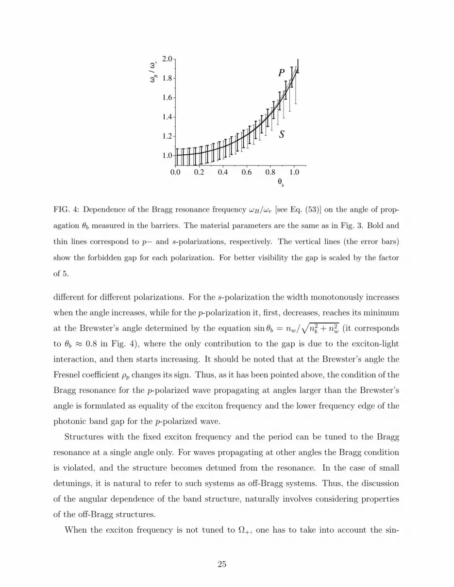
FIG. 4: Dependence of the Bragg resonance frequency ωB/ωr [see Eq. (53)] on the angle of prop-

agation θb measured in the barriers. The material parameters are the same as in Fig. 3. Bold and

thin lines correspond to p− and s-polarizations, respectively. The vertical lines (the error bars)

show the forbidden gap for each polarization. For better visibility the gap is scaled by the factor

of 5.

different for different polarizations. For the s-polarization the width monotonously increases

when the angle increases, while for the p-polarization it, first, decreases, reaches its minimum

at the Brewster’s angle determined by the equation sin θb = nw/√

n2b + n2

w (it corresponds

to θb ≈ 0.8 in Fig. 4), where the only contribution to the gap is due to the exciton-light

interaction, and then starts increasing. It should be noted that at the Brewster’s angle the

Fresnel coefficient ρp changes its sign. Thus, as it has been pointed above, the condition of the

Bragg resonance for the p-polarized wave propagating at angles larger than the Brewster’s

angle is formulated as equality of the exciton frequency and the lower frequency edge of the

photonic band gap for the p-polarized wave.

Structures with the fixed exciton frequency and the period can be tuned to the Bragg

resonance at a single angle only. For waves propagating at other angles the Bragg condition

is violated, and the structure becomes detuned from the resonance. In the case of small

detunings, it is natural to refer to such systems as off-Bragg systems. Thus, the discussion

of the angular dependence of the band structure, naturally involves considering properties

of the off-Bragg structures.

When the exciton frequency is not tuned to Ω+, one has to take into account the sin-

25

gularity of the exciton susceptibility when looking for the boundaries between allowed and

forbidden bands. This singularity results in a narrow band gap situated between zeros of

Eq. (44), i.e. where sin2(Kd/2) < 0. This band gap occupies the region between ω0 and

ω0 + Ωδ, where

Ωδ =π

2τ+δ∆2

Γ (72)

and δ = ω0 − Ω+ 6= 0. For slightly off-Bragg structures, the width of this addition to the

band gap is small, and we will neglect its existence in the future discussions. Thus, the

band boundaries are determined by zeros of r.h.s. of Eq. (42), and as the result the band

structure is determined by four frequencies: ω0 and the roots of the equation

(ω − Ω+)

[(ω − Ω−)(ω − ω0) −

∆2Γ

4

]= 0. (73)

The band structure is characterized by two band gaps and one allowed band between

them. If we put these four frequencies in ascending order, the band gaps will lie between

the first and second pairs of frequencies separated by a transparency window (see Fig. 3).

The exact order of the band boundaries depends on relation between ω0 and Ω+. If ω0 < Ω+

then the band gaps are between ω′− and ω0 and between Ω+ and ω′

+, where

ω′± = Ωc +

δ

2± 1

2

√(∆PC − δ)2 + ∆2

Γ, (74)

while the allowed band is between ω0 and Ω+. Thus, detuning the exciton resonance fre-

quency away from Ω+ leads to the appearance of the transparency window between ω0 and

Ω+ inside the band gap obtained for the Bragg case ω0 = Ω+, and to a slight modification of

the external edges of the gap. This result is in a qualitative agreement with the earlier anal-

ysis of the off-resonant MQW structures.10 The transparency window would manifest itself

in optical spectra as a dip in the reflection coefficient. A similar dip was actually observed in

Refs. 9,23,39, where structures with the period satisfying the non-modified Bragg condition,

Eq. (61), were considered. Since the well and barrier materials had different, albeit close,

values of the refractive indexes, the real Bragg period should have been determined from

Eq. (71), and the structures considered in those papers were actually slightly off-Bragg. It

should be mentioned, however, that the detuning from the real Bragg condition could be

not the only cause for the observed dip in reflection. The inhomogeneous broadening of the

excitons could also contribute to this effect.40

26

0.0 0.2 0.4

0.98

1.00

1.02

1.04

1.06

1.08

ω /

ωr

θb

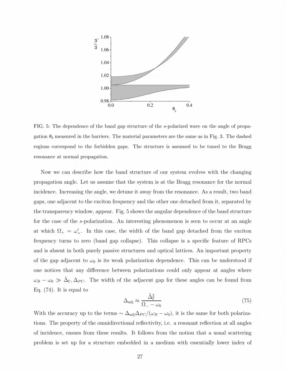
FIG. 5: The dependence of the band gap structure of the s-polarized wave on the angle of propa-

gation θb measured in the barriers. The material parameters are the same as in Fig. 3. The dashed

regions correspond to the forbidden gaps. The structure is assumed to be tuned to the Bragg

resonance at normal propagation.

Now we can describe how the band structure of our system evolves with the changing

propagation angle. Let us assume that the system is at the Bragg resonance for the normal

incidence. Increasing the angle, we detune it away from the resonance. As a result, two band

gaps, one adjacent to the exciton frequency and the other one detached from it, separated by

the transparency window, appear. Fig. 5 shows the angular dependence of the band structure

for the case of the s-polarization. An interesting phenomenon is seen to occur at an angle

at which Ω+ = ω′+. In this case, the width of the band gap detached from the exciton

frequency turns to zero (band gap collapse). This collapse is a specific feature of RPCs

and is absent in both purely passive structures and optical lattices. An important property

of the gap adjacent to ω0 is its weak polarization dependence. This can be understood if

one notices that any difference between polarizations could only appear at angles where

ωB − ω0 ≫ ∆Γ, ∆PC . The width of the adjacent gap for these angles can be found from

Eq. (74). It is equal to

∆adj ≈∆2

Γ

Ω− − ω0

(75)

With the accuracy up to the terms ∼ ∆adj∆PC/(ωB − ω0), it is the same for both polariza-

tions. The property of the omnidirectional reflectivity, i.e. a resonant reflection at all angles

of incidence, ensues from these results. It follows from the notion that a usual scattering

problem is set up for a structure embedded in a medium with essentially lower index of

27

refraction (air or vacuum). As the result, the angles of propagation inside the structure can-

not exceed the angle of the internal reflection θc at the boundary between the structure and

surrounding medium. Therefore, for all angles of incidence the range of frequencies between

ω0 and ω′−(θc) corresponds to the forbidden gap and, therefore, to a resonant reflection. The

similar effect has been considered for the case of passive photonic crystals in a number of

publications.41,42,43,44 Here we want to emphasize the feature specific for the RPC. If the an-

gle of total internal reflection is small (for the air-GaAs interface θc ≈ 0.28), we can describe

the change of the edges of the photonic band gap by a simple renormalization of the optical

width of the period, Ω± → Ω±/ cos θ. It results in the width of the region corresponding to

the omnidirectional reflection in the form

∆omni ≈1

2

∆2Γ

Ω+ sin2 θc − 2∆PC

, (76)

where we have assumed that the photonic forbidden gap is not too wide, i.e. Ω+ sin2 θc >

2∆PC . One can see that the presence of QWs essentially weakens the condition of the

omnidirectionality in comparison with passive photonic crystals.

C. General modulation of the dielectric function

1. Resonant photonic crystals

The formalism developed in this paper allows us to analyze the band structure in

RPCs with an arbitrary periodic modulation of the dielectric function. Using the (a, f)-

representation for transfer matrices and expressions for the parameters a and f given by

Eqs. (24), we can derive the dispersion equation for such a structure in the form similar to

Eq. (42):

cos2

(Kd

2

)=

h′2(z+)

Wh

[h1(z+) + Sqh2(z+)] (77)

or Eq. (44)

sin2

(Kd

2

)= −h2(z+)

Wh[h′

1(z+) + Sqh′2(z+)] . (78)

These dispersion equations can be used to describe waves of all polarizations by choosing

appropriate for a given polarization parameters S, q, and h1,2. The band structure of a

passive photonic crystal can be obtained from these equations by setting χ ≡ 0. The band

28

0.0 0.5 1.0 1.5 2.0 2.5 3.0

-1

0

1

-0.4-0.20.00.20.4

0.0 0.5 1.0 1.5 2.0 2.5 3.0

-1

0

1

-0.4-0.20.00.20.4

FIG. 6: Dependence of Im(Kd) (solid lines, left axes) and wave functions and its derivative (dashed

and dotted lines, respectively, right axes) on the frequency for a passive structure (S ≡ 0). The

non-zero values of Im(Kd) correspond to the band gaps. The index of refraction is n(z) = 3 +

cos20(πz/2). (a) Kd is the solution of Eq. (77), h1(ω), the dotted line depicts h′2(ω). (b) Kd has

been found from Eq. (78), the dashed line represents h2(ω), the dotted line depicts h′1(ω)/5. One

can see how zeroes of the wave function and its derivative determine consecutive band boundaries.

boundaries, Ω±, in this case are determined by equations

h1(z+, Ω−) = 0, h′2(z+, Ω+) = 0, (79)

and

h′1(z+, Ω−) = 0, h2(z+, Ω+) = 0, (80)

where Ω∓ in the argument denote that the functions h1,2 are solutions of corresponding

homogenous equations [Eqs. (5) or (28) with χ ≡ 0] for ω = Ω∓ respectively. Thus the

zeroes of even and the maxima of odd solutions given by Eqs. (79) and (80) determine

the boundaries of the consecutive band gaps in the band structure of the system under

consideration (see Fig. 6).

The analysis of the full dispersion equations, with the resonance terms restored, repeats

the analysis of the previous subsection, where one needs to make substitutions aPC = g2

and fPC = g1. In particular, the parameters t± of the equation for the boundaries of the

forbidden gap, Eq. (66), are defined in terms of boundary values of f1,2 as

t− =1√Wh

∣∣∣∣∂h1(Ω−)

∂ω

∣∣∣∣ , t+ =1√Wh

∣∣∣∣∂h′

2(Ω+)

∂ω

∣∣∣∣ . (81)

29

The general structure of the spectrum is similar to the one discussed in the case of the

piece-wise modulation of the refractive index, and we can generalize the condition for the

Bragg resonance, when the exciton related allowed band collapses, and the spectrum of

our system in the vicinity of the exciton frequency consists of a single wide band gap. We

again require that the singularity of the excitonic susceptibility at ω0 is canceled by the

first term h′2(z+) in Eq. (77). This corresponds to the condition ω0 = Ω+, where Ω+ is the

high frequency boundary of the respective photonic gap. From the dispersion equation (79)

it follows again that the Bragg condition can be casted in the form KPC(ω0)d = π. One

can rewrite the last equation in yet another form emphasizing the role of the phase in the

formation of Bragg structures. Let us consider the effective optical width of the period of

the structure, φ [see Eq. (46)]. At the point where h′2 = 0 one finds that a/a = −1 yielding

φ(Ω+) = π. Thus, the phase form of the Bragg condition, which is particularly convenient

for practical calculations, becomes φ(ω0) = π.

We can also generalize the expression for the width of the band gap in the case of the

Bragg resonance. Performing the expansion similar to Eqs. (65) we can obtain the equation

for boundaries of the forbidden gap:

(ω − Ω+)

(ω − Ω− − ∆2

Γ/4

ω − ω0

)= 0, (82)

with ∆2Γ given by the first part of Eq. (70). The analysis of Eq. (82) completely repeats that

of Eq. (66). In particular, the width of the forbidden gap is determined by the Pythagorean

sum of the photonic and excitonic contributions,

∆2 = ∆2PC + ∆2

Γ, (83)

where ∆PC = |Ω+−Ω−|, and expression for the excitonic contribution, ∆Γ, can be presented

as (∆Γ

∆Γ

)2

=πc2qs

4Ω−ω0u(1)s

and

(∆Γ

∆Γ

)2

=πc2qpp(z+)

4Ω−ω0u(1)p

(84)

for s- and p-polarizations, respectively. Here we have introduced

u(1)s,p =

1

2

∫dz ǫ(z)E(1)

s,p

2, (85)

where E(1)s,p is the s- and p-polarized electric fields corresponding to the even mode of the

photonic crystal. This expression represents the energy associated with the even mode of

30

the photonic crystal concentrated in a single elementary cell. The r.h.p. of Eqs. (84) can be

shown to be proportional to u(1)qw/u(1), where u

(1)qw is the energy of the even mode concentrated

within the QW. This means that the contribution of the exciton-light interaction into band

structure of the resonant photonic crystal depends on the distribution of the energy of the

electric field inside the elementary cell at the frequency corresponding to Ω−. The greater

amount of energy stored within the well the larger the role of the excitonic effects is.

2. Off-Bragg structures

Our analysis so far was limited to consideration of the band boundaries and the properties

of the band gaps in the resonant photonic crystals. To complete the consideration of the

normal modes in these structures we need to discuss solutions of Eqs. (79) and (79) in the

allowed bands of the spectrum. These solutions determine dispersion laws ω(K) of the

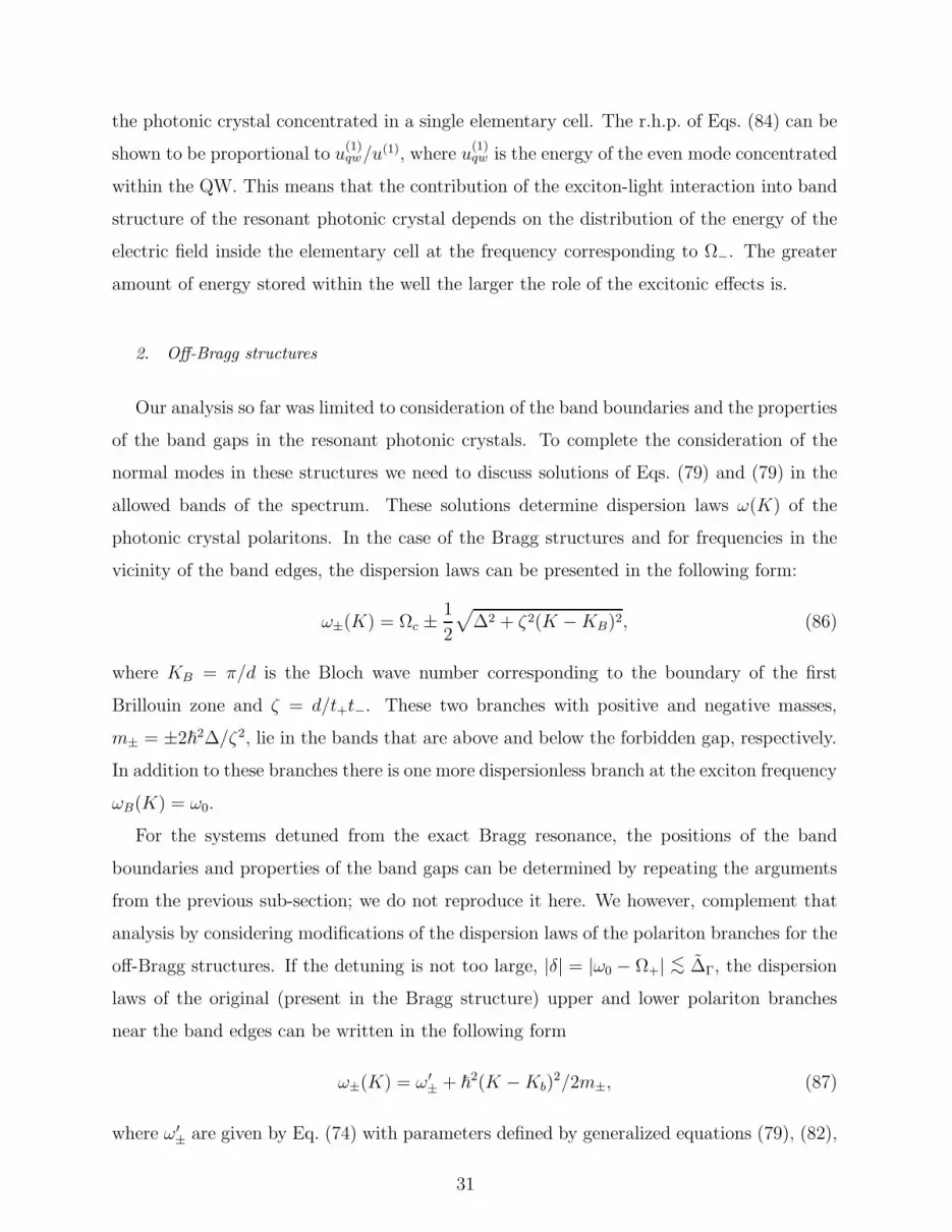
photonic crystal polaritons. In the case of the Bragg structures and for frequencies in the

vicinity of the band edges, the dispersion laws can be presented in the following form:

ω±(K) = Ωc ±1

2

√∆2 + ζ2(K − KB)2, (86)

where KB = π/d is the Bloch wave number corresponding to the boundary of the first

Brillouin zone and ζ = d/t+t−. These two branches with positive and negative masses,

m± = ±2~2∆/ζ2, lie in the bands that are above and below the forbidden gap, respectively.

In addition to these branches there is one more dispersionless branch at the exciton frequency

ωB(K) = ω0.

For the systems detuned from the exact Bragg resonance, the positions of the band

boundaries and properties of the band gaps can be determined by repeating the arguments

from the previous sub-section; we do not reproduce it here. We however, complement that

analysis by considering modifications of the dispersion laws of the polariton branches for the

off-Bragg structures. If the detuning is not too large, |δ| = |ω0 − Ω+| <∼ ∆Γ, the dispersion

laws of the original (present in the Bragg structure) upper and lower polariton branches

near the band edges can be written in the following form

ω±(K) = ω′± + ~

2(K − Kb)2/2m±, (87)

where ω′± are given by Eq. (74) with parameters defined by generalized equations (79), (82),

31

and (84). The renormalized mass parameters m± are defined as

m±(δ) = m±

(1 − ∆PCδ

∆2± 2δ

∆ ∓ ∆PC

). (88)

Comparing this result with Eq. (86) one can notice that detuning from the Bragg resonance

results in two main modifications of the dispersion laws: first, the position of the band

boundaries have changed and, second, the magnitudes of the masses of the upper and the

lower polariton branches are no longer equal to each other.

The most dramatic changes occur, however, with the third, originally dispersionless

branch. In off-Bragg structures this branch acquires dispersion, which, of course, agrees

with the opening of the allowed band in the vicinity of the exciton frequency. The disper-

sion law characterizing this band is given by

ωB(K) = Ω+ +ζ2δ

∆2Γ

(K − KB)2. (89)

This branch corresponds to excitations dubbed “Braggaritons” in Ref. 15. The mass of this

mode, given by mB = ∆2Γ/2ζδ, is very sensitive to the amount of detuning from the Bragg

condition and can be effectively controlled, for instance, by the electric field via the quantum

confined Stark effect. This property of the ”Braggariton” branch invited proposal to use it

for slowing, stopping and storing light in BMQW structures.45,46

3. Homogenous broadening

We finish our consideration of dispersion properties of RPCs with an arbitrary periodic

distribution of the refractive index by discussing effects due to the exciton homogeneous

broadening. In the presence of dissipation the concept of band gaps becomes ill-defined

because the imaginary part of the Bloch wave-number, generally speaking, is not zero at all

frequencies. Nevertheless, the properties of this imaginary part are of great interest, since

they determine the spectral and transport properties of the structures under consideration in

the vicinity of what would have been band boundaries in the absence of dissipation. In order

to access these properties we have to consider solutions of Eq. (77). Taking into account

that in the spectral region of interest, the real part of K is close to π/d, we look for solutions

to this equation in the form

Kd = π + iλ. (90)

32

0.985 0.990 0.995 1.000 1.0050.000

0.005

0.010

0.015

0.020

0.025

MQW-PC

MQW

Im(Kd)

/ 0

PC

FIG. 7: Dependence of Im(Kd) on frequency for different structures in the vicinity of the first for-

bidden gap when the exciton homogeneous broadening is taken into account. Dashed line represents

the passive structure from Fig. 6. Solid line shows a Bragg MQW structure with a homogeneous

dielectric function. Dotted line represents the structure with combination of QWs and the smooth

modulation of the dielectric function. The characteristic feature is a divergence of the penetration

length (Im K)−1 at the exciton frequency.

The unknown parameter λ here has a simple physical meaning: the inverse of its real part

determines a characteristic length on which the amplitude of the mode decays. The same

length determines the penetration depth of incident radiation, therefore it is often called a

penetration length. Assuming that λ is small we can find an approximate expression for it

in the form:

λ2 = 4t+t−(Ω+ − ω)

(ω − Ω− − ∆2

Γ/4

ω − ω0 − iγ

). (91)

An important feature described by this expression is that λ vanishes at the frequency cor-

responding to the right edge of the photonic band gap, signifying the divergence of the

respective penetration length. The similar effect takes place in MQW10 structures without

the refractive index contrast. The important difference is that in the latter case the diver-

gence occurs at the exciton frequency that lies at the center of the forbidden gap rather

than at the band’s boundary. Fig. 7 shows the comparison of the solutions of the disper-

sion equation for different structures with the exciton homogenous broadening taken into

account.

33

D. MQW structures with complex elementary cells

In this section we illustrate the application of the developed technique to structures with

complex elementary cells, which were first studied in Ref. 21. In that paper the mismatch

between refractive indexes of different elements of the structure had to be neglected because

the combination of the complex elementary cell and the spatial modulation of the refrac-

tive index turned out to be an insurmountable obstacle for the standard transfer-matrix

approach. In this section we show that the approach developed in the present paper al-

lows us to overcome the technical difficulties associated with the consideration of a complex

structure, and to generalize the results of Ref. 21 for the case of structures with modulated

refractive index.

We will focus here on one particular example, when the elementary cell consists of two

QWs with different exciton frequencies, ω1 and ω2, located half a period apart from each

other (see Fig. 8). It was found in Ref. 21 that despite the presence of two different exciton

frequencies, it is still possible to generalize the notion of the Bragg resonance for such systems

and design structures whose spectrum would consist of only two polariton branches separated

by a wide band gap. However, unlike the case of structures with a simple elementary cell,

the formation of such a wide band gap requires not only the period of the structure to

have a certain value, but also imposes a condition on the spectral separation between the

excitonic frequencies of the wells constituting the elementary cell. When both generalized

Bragg conditions are fulfilled for such a structure, the width of the polariton band gap, ∆CS,

becomes larger than that in the case of structures with a simple elementary cell:

∆CS =√

2∆Γ. (92)

This broadening of the gap by almost 40% reflects a possibility to effectively strengthen the

exciton-photon interaction by increasing the density of QWs in the structure.

In this section we consider how the mismatch of the refractive indices affects the spectral

properties of such structures. We simplify our consideration assuming that all elements of

the structure except the wells with the exciton frequency ω2 have the same refractive index.

Formally, the dispersion equation describing modes propagating in such a structure in the

normal direction has been obtained in Ref. 21 by more conventional methods, but that

equation turned out to be too cumbersome to allow for any non-numerical analysis. Using

34

1 2 1 2

d

FIG. 8: The periodic structure with two QWs (dark rectangles) in the elementary cell. Dash

lines show the boundaries of the elementary cell having the mirror symmetry. The QW with the

exciton frequency ω2 is assumed to have the index of refraction different from other elements of

the structure.

(a, f)-representation of the transfer matrices, we show here that the dispersion equation can

be rewritten in a much more transparent form with a factorized right hand side.

To apply the technique developed in the present paper it is necessary to choose the

elementary cell with the explicit mirror symmetry. It can be done as shown in Fig. 8. The

problem of determining the transfer matrices through the right and left halves of the QW

can be resolved in the following way. We note that the QW transfer matrix Tw determined

by Eq. (55) can be written in a factorized form

Tw = Tb(φw/2)TwTb(φw/2), (93)

where Tw is derived from the expression for Tw by setting φw = 0. After this factorization

the transfer matrix through the elementary cell takes the form similar to Eq. (35)

T =

√T

(1)w Tb(φb + φw/2) T−1

ρ T (2)w TρTb(φb + φw/2)

√T

(1)w . (94)

The difference between the indices of refraction is again taken into account by introducing

the special transfer matrix Tρ, which describes propagation of the wave across the interface

and contains respective Fresnel coefficients. The transfer matrices through different QWs,

T(1,2)w , are obtained from Eq. (55) by substituting different excitonic susceptibilities

S1,2 =Γ0

ω − ω1,2 + iγ. (95)

The matrix square root

√T

(1)w can be found to be equal to

√T

(1)w =

1 − iS1/2 −iS1/2

iS1/2 1 + iS1/2

. (96)

35

Now, we can apply Eqs. (36), (37) and (39) to derive (a, f)-representation for T . The

dispersion equation following from this representation has a relatively simple form:

cos2

(Kd

2

)=

1

1 − ρ2[Re(a) + S1 Im(a)] [Re(b) + S2 Im(b)] , (97)

where a = exp(iφ+) − ρ exp(iφ−), b = exp(iφ+) + ρ exp(iφ−) [compare with Eqs. (50)], and

φ± = ω(2dbn + dwn ± dwn2)/2c.

As usual, the positions of band boundaries are determined by frequencies at which the

r.h.s. of Eq. (97) changes its sign, which can occur either by passing this expression through

zero or through infinity. The other set of boundaries, which we do not consider here can be

obtained as before by converting Eq. (97) to the form with sin2(Kd2

)on the left. We can show

that in the immediate proximity of the exciton frequencies, there are six band boundaries,

which define three band gaps separated by two allowed bands. We again will be interested

in finding conditions, under which these allowed bands collapse resulting in formation of one

continuous band gap. As we already know from the previously considered examples, the

collapse of the allowed bands associated with the singularities of the exciton susceptibility,

S, takes place when the exciton frequency coincides with one of the band boundaries of a

certain effective structure. In the case of a simple elementary cell this effective structure was

a respective passive photonic crystal, however, in the case under consideration, the effective

structure is comprised of one of the sublattices of our system. More precisely, in order to

cancel the exciton singularity at, for example, ω1, we have to require that ω1 coincides with

the zero of the expression inside the second parenthesis on the r.h.s. of Eq. (97). This

zero, obviously gives the position of some band boundaries of a structure made up of the

sub-lattice 2. Similarly, in order to cancel the singularity at ω2 we need to make it equal to

one of the band boundaries originating from the sub-lattice 1, particulary that which turns

to zero the expression in the first parenthesis of the r.h.s of Eq. (97). Let us assume for

concreteness that ω2 > ω1, then more specifically we have to require that ω1 is equal to the

low-frequency boundary of the band gap associated with polariton branches in sub-lattice 2,

and ω2 should coincide with the high-frequency boundary of the band gap originating from

polariton branches in sublattice 1. Let us denote frequencies of these two band boundaries as

ω±1,2, where the lower index shows from which sublattice the respective boundary originates,

and ± denotes high- and low-frequency boundaries, respectively. The frequencies ω±1,2 can

36

be found to be equal to

ω±1 =

1

2(ω1 + Ω−) ± 1

2

√(ω1 − Ω−)2 + ∆2

Γ,

ω±2 =

1

2(ω2 + Ω+) ± 1

2

√(ω2 − Ω+)2 + ∆2

Γ,(98)

where Ω∓ are determined by Eqs. (52), and for simplicity, we assumed the same value

of the effective exciton-light interaction for both sublattices, i.e. we neglected a possible

difference between exciton radiative decay rates in different wells. We also neglected the

renormalization of Γ0 due to the spatial modulation of the dielectric function [see Eqs. (70)

and (84)]. The generalization of these expressions is straightforward but does not lead to

anything new while making the resulting expressions much more cumbersome.

Let us, first, consider the case when the index of refraction of the wells of the second type

is higher, i.e. ρ > 0. The conditions of absence of transparency windows inside the gap (the

Bragg resonance conditions) are in this case formulated as ω+1 = ω2 and ω−

2 = ω1. Resolving

these equations with respect to the exciton frequencies one obtains

ω1 + ω2

2= Ωc, ω1 − ω2 =

1

2

(√2∆2

Γ + ∆2PC − ∆PC

), (99)

which generalize the results of Ref. 21 to the case of structures with the refractive index

mismatch. Substituting these results into the expression for the width of the band gap,

which is equal to ∆ = ω+2 − ω−

1 , we obtain a familiar result

∆ =√

∆2CS + ∆2

PC . (100)

The case of ρ < 0 is described by the same formulas with substitution ∆PC → −∆PC , which

changes the Bragg condition [the second equation of Eqs. (99)] but leaves the width of the

gap, Eq. (100), the same.

Thus, taking into account the mismatch of the indices of refraction in the system with

a complex elementary cell leads to modification of the Bragg condition in comparison with

what one has in the case without the mismatch. This modification has a different character

than in structures with a simple cell. The mean value of the exciton frequencies stays at

the center of the forbidden gap and only the difference between the frequencies must be

corrected to take into account the mismatch. The resultant gap is, similar to the case of

simple cell, again the Pythagorean sum of the photonic and the excitonic contributions.

37

IV. CONCLUSION

We considered the band structure associated with normal excitations of one-dimensional

resonant photonic crystals using as a particular example the exciton polaritons multiple

quantum well structures. Properties of normal modes of such structures are determined

by the interplay of two mechanisms: the interaction of light with internal resonances of

constituting materials, such as excitons in MQW case, and multiple reflection of light due

to periodic spatial modulation of the index of refraction of the structure. The necessity to

take into account both mechanisms of the light-matter interaction in these structures on

equal footing makes the analytical description of their properties more complicated than in

the case of regular passive photonic crystals. In this paper we developed a powerful method

of analyzing band structure and dispersive properties of such structures, which allowed us

to obtain analytical solutions for problems that could not be solved by other approaches.

This method is based on two key features. First, we construct transfer matrices us-

ing solutions of the appropriate Cauchy (rather than boundary value) problems as a basis.

This makes calculations of the transfer matrices more convenient since it allows for avoid-

ing difficult questions about eigenmodes of the system under consideration. Second, we

use a special representation of the transfer matrix valid for structures with an elementary

cell possessing a mirror symmetry. This representation automatically yields the dispersion

equation of normal modes in a factorized form, which drastically simplifies the analysis of

the spectrum. In particular, using this representation we were able to analyze dispersion

properties of certain type of resonant photonic crystals with complex elementary cells. We

also believe that besides situations explicitly considered in the paper, the suggested method

allows for effective treatment of other problems such as exciton luminescence from MQW

photonic crystals, or for analysis of more complicated systems, e.g. quantum graphs.47,48 An

important benefit of the developed approach consists also in the fact that polarization and

angular dependencies of the elements of transfer matrices appear in this approach only via

respective Fresnel coefficients. This enabled us to obtain band structures of modes of both

s- and p-polarizations in MQW based photonic crystals from essentially the same dispersion

equation and easily analyze their angular dependencies.

We illustrated the developed method by applying it to a number of problems, some of

which were considered previously in the framework of other approaches, while others were

38

analyzed in this paper for the first time. In particular, we considered polariton spectrum

in several systems: MQW structures with the mismatch of the indices of refraction of the

barriers and wells materials, MQW with an arbitrary periodic modulation of the dielectric

function, and MQW with a complex elementary cell consisting of two equidistant QWs

characterized by different exciton frequencies. We showed that in all these cases one can

construct a structure, in which multiple photon and polariton bands can be collapsed in

just two polariton branches separated by an anomalously broad stop band. Such a band

structure is characteristic of so called Bragg structures, which in the case of MQWs were

studied in a number of previous publications. We showed here that in the case of RPCs with

a simple elementary cell the condition for formation of such a spectrum can be formulated as

a requirement for the exciton frequency to coincide with one of the edges of the respective

passive photonic crystal. Formulated in this form this condition demonstrates a direct

connection with earlier formulations of the Bragg resonance in MQW structures without the

refractive index contrast. In the case of crystals with complex elementary cells, we showed

that our method allows for taking into account the mismatch of the refractive indices between

different elements of the structure and found the generalized Bragg conditions for this system

as well. In the last case, this condition consists of two equations: one relating the period of

the structure to the exciton frequencies of the constituent elements and the other specifying

a relation between those frequencies.

One of the surprising results is that for all these structures the width of the polariton band

gap in the case of the Bragg resonance can be presented in the form of a Pythagorean sum of

the photonic and the excitonic contributions, ∆2 = ∆2PC + ∆2

Γ. The excitonic contribution

in the presence of the refractive index modulation, however, is modified compared to the

case of simple optical lattices. It is interesting that this modification can be presented in the

form of a ratio of the electric field energy concentrated inside QW to the the total energy

stored in the entire elementary cell of the structure.

Acknowledgments

The work has been supported by AFOSR grant F49620-02-1-0305.

39

APPENDIX A: TRANSFER MATRIX FORMALISM

The transfer matrix technique has been reviewed in a number of publications. Here,

however, we use this technique in a somewhat unusual form. Therefore, we find it useful to

recall some important results. While the general idea of the transfer matrix establishing a

linear connection between values of a function representing a solution of a linear differential

equation at two different values of the argument is inherent to all formulations, the explicit

form of the transfer matrix and its properties depend upon a choice of the representation

of the matrix. As a basic representation one often chooses a 2 × 2 matrix operating on a

two-dimensional vector, whose components are the value of a function, which represents a

solution at a given point, and its derivative. The formal reason for this choice is the fact

that a linear equation of a second order can always be naturally reformulated as a system

of two first order equations for the function and its derivative:

E(z + d)

E ′(z + d)

= Tψ(z + d, z)

E(z)

E ′(z)

. (A1)

Another approach to constructing transfer matrices is more convenient for problems in-

volving scattering of waves. This problem is most naturally described by specifying an

amplitude of an incident wave and relating to it amplitudes of transmitted and reflected

waves. In this approach, the field is sought in the form eiκz + re−iκz at the one side of the

system, and in the form teiκz at the the other side. More generally, the field is represented

in the form

E(z) = a+eiκz + a−e−iκz,

E(z + d) = a′+eiκz + a′

−e−iκz(A2)

and the transfer matrix relates the amplitudes at the left and the right boundaries

a′+

a′−

= T

a+

a−

. (A3)

As follows from Eqs. (A2), the transfer matrices written in these two bases are related by a

similarity transformation, T = W−1e (z)Tψ(z + d, z)We(z), where

We(z) =

eiκz e−iκz

iκeiκz −iκe−iκz

. (A4)

40

Another important way to introduce the transfer matrix (see e.g. Ref. 49) is based on

a possibility of a representation of the solution of the Maxwell equation as a sum of two

linearly independent functions, f1,2(z), with modulated amplitudes

E(z) = c1(z)h1(z) + c2(z)h2(z),

E ′(z) = c1(z)h′1(z) + c2(z)h′

2(z).(A5)

Now, the transfer matrix gives the relation between the amplitudes at different points,

usually a period of a structure apart,

c1(z + d)

c2(z + d)

= Th(d)

c1(z)

c2(z)

. (A6)

¿From Eq. (A5) it follows that

Th(d) = W−1h (z + d)Tψ(z + d, z)Wh(z), (A7)

where Wh(z) is the Wronsky matrix

Wh(z) =

h1(z) h2(z)

h′1(z) h′

2(z)

. (A8)

Eq. (A8) allows one to derive a relation between transfer matrices obtained for a different

choice of the basis functions h1,2.

The relation between the transfer matrices written in the bases of plane waves and a pair

of linearly independent functions can be written as

T = M(d/2)Th(d)M−1(−d/2), (A9)

where M(z) = W−1e (0)Wh(z). Using Eqs. (A4), (A8), and (A9) one obtaines

M(z) =1

2

h1(z) +

h′1(z)

iκh2(z) +

h′2(z)

iκ

h1(z) − h′1(z)

iκh2(z) − h′

2(z)

iκ

. (A10)

All types of transfer matrices have their advantages and disadvantages. For instance, a

basis of a pair of linearly independent functions can be most naturally related to solutions of

the Cauchy problem for the respective differential equation. Such a basis is easy to find but

it is inconvenient for the solution of scattering problems. The fact that, generally, it is not

41

related to Tψ by a similarity transformation [see Eq. (A7)] makes it also difficult to consider

the spectral problems using this basis. Indeed, the knowledge of the transfer matrix itself

is not sufficient for solving this problem, and one has to separately consider a boundary

value problem for amplitudes c1,2. On the contrary, the basis of plane waves is the most

suitable for solving this particular problem since the transfer matrix itself contains all needed

information. In this basis, the difficulty of having to solve the boundary value problem is

moved to the process of finding the transfer matrix itself. Therefore, the conversion rule

from one basis to another presented in Eq. (A9) is very useful for practical calculations as

it is demonstrated in our paper.

1 E. Yablonovitch, Phys. Rev. Lett. 58, 2059 (1987).

2 S. John, Phys. Rev. Lett. 58, 2486 (1987).

3 J. D. Joannopoulos, R. D. Meade, and J. N. Winn, Photonic crystals: Molding the flow of light

(Princeton University Press, 1995).

4 R. N. Dicke, Phys. Rev. 93, 99 (1954).

5 I. Deutsch, R. Spreeuw, S. Rolston, and W. Phillips, Phys. Rev. A 52, 1394 (1995).

6 L. V. Keldysh, Superlattices Microstruct. 4, 637 (1988).

7 E. L. Ivchenko, A. I. Nesvizhinskii, and S. Jorda, Phys. Solid State 36, 1156 (1994).

8 E. L. Ivchenko, Sov. Phys. Solid State 33, 1344 (1991).

9 M. Hubner, J. P. Prineas, C. Ell, P. Brick, E. S. Lee, G. Khitrova, H. M. Gibbs, and S. W.

Koch, Phys. Rev. Lett. 83, 2841 (1999).

10 L. I. Deych and A. A. Lisyansky, Phys. Rev. B 62, 4242 (2000).

11 T. Ikawa and K. Cho, Phys. Rev. B 66, 085338 (2002).

12 V. Kuzmiak and A. Maradudin, Phys. Rev. B 55, 7427 (1997).

13 L. Deych, D. Livdan, and A. Lisyansky, Phys. Rev. E 57, 7254 (1998).

14 S. Nojima, Phys. Rev. B 61, 9940 (2000).

15 A. Y. Sivachenko, M. E. Raikh, and Z. V. Vardeny, Phys. Rev. A 64, 013809 (2001).

16 A. Christ, S. Tikhodeev, N. Gippius, J. Kuhl, and H. Giessen, Phys. Rev. Lett. 91, 183901

(2003).

17 K. Huang, P. Bienstman, J. Joannopoulos, K. Nelson, and S. Fan, Phys. Rev. Lett. 90, 196402

42

(2003).

18 O. Toader and S. John, Phys. Rev. E 70, 046605 (2004).

19 L. Pilozzi, A. D’Andrea, and K. Cho, Phys. Rev. B 69, 205311 (2004).

20 E. L. Ivchenko, V. P. Kochereshko, A. V. Platonov, D. R. Yakovlev, A. Waag, W. Ossau, and

G. Landwehr, Phys. Solid State 39, 1852 (1997).

21 E. L. Ivchenko, M. M. Voronov, M. V. Erementchouk, L. I. Deych, and A. A. Lisyansky, Phys.

Rev. B 70, 195106 (2004).

22 E. Ivchenko and A. Poddubny (2005), cond-mat/0505510, unpublished.

23 M. V. Erementchouk, L. I. Deych, and A. A. Lisyansky, Phys. Rev. B 71, 235335 (2005).

24 P. M. Morse and H. Feshbach, Methods of theoretical physics, vol. 1 (McGraw-Hill, Tokyo, 1953).

25 F. Tassone, F. Bassani, and L. C. Andreani, Phys. Rev. B 45, 6023 (1992).

26 L. C. Andreani, G. Panzarini, A. V. Kavokin, and M. R. Vladimirova, Phys. Rev. B 57, 4670

(1998).

27 B. Vainberg and S. Molchanov (2005), math.CA/0503075, unpublished.

28 B. A. Dubrovin, S. P. Novikov, and A. T. Fomenko, Modern geometry: methods and applications

(Springer, New York, 1992), 2nd ed.

29 J. Bendickson, J. Dowling, and M. Scalora, Phys. Rev. E 53, 4107 (1996).

30 M. Born and E. Wolf, Principles of Optics (Cambridge University Press, Cambridge, 1999), 7th

ed.

31 A. Yariv and P. Yeh, Optical waves in crystals (John Wiley & Sons, New Jersey, 2003).

32 A. Kavokin and M. Kaliteevski, Solid St. Commun. 95, 859 (1995).

33 S. Haas, T. Stroucken, M. Hubner, J. Kuhl, B. Grote, A. Knorr, F. Jahnke, S. W. Koch, R. Hey,

and K. Ploog, Phys. Rev. B 57, 14860 (1998).

34 D. Ammerlahn, B. Grote, S. W. Koch, J. Kuhl, M. Hubner, R. Hey, and K. Ploog, Phys. Rev.

B 61, 4801 (2000).

35 L. C. Andreani, F. Tassone, and F. Bassani, Solid State Commun. 77, 641 (1991).

36 D. S. Citrin, Phys. Rev. B 47, 3832 (1993).

37 D. S. Citrin, Solid State Commun. 89, 139 (1994).

38 S. Schmitt-Rink, D. Chemla, and D. Miller, Adv. in Phys. 38, 89 (1989).

39 J. P. Prineas, C. Ell, E. S. Lee, G. Khitrova, H. M. Gibbs, and S. W. Koch, Phys. Rev. B 61,

13863 (2000).

43

40 L. I. Deych, M. V. Erementchouk, and A. A. Lisyansky, Phys. Rev. B 69, 75308 (2004).

41 J. Winn, Y. Fink, S. Fan, and J. Joannopoulos, Optics Letters 23, 1573 (1998).

42 D. Chigrin, A. Lavrinenko, D. Yarotsky, and S. Gaponenko, Appl. Phys. A 68, 25 (1999).

43 A. Bruyant, G. Lerondel, P. Reece, and M. Gal, Appl. Phys. Lett. 82, 3227 (2003).

44 T. Yonte, J. Monzon, A. Felipe, and L. Sanchez-Soto, J. Opt. A: Pure Appl. Opt. 6, 127 (2004).

45 Z. Yang, N. Kwong, R. Binder, and A. Smirl, J. Opt. Soc. Am B 22, 2144 (2005).

46 Z. Yang, N. Kwong, R. Binder, and A. Smirl, Opt. Lett. 30, 2790 (2005).

47 P. Kuchment, Waves Random Media 12, R1 (2002).

48 P. Kuchment, Waves Random Media 14, S107 (2004).

49 R. Perez-Alvarez, C. Trallero-Herrero, and F. Garcia-Moliner, Eur. J. Phys. 22, 275 (2001).

50 It raises a question is it possible to have both ϕ1,2 equal to 0. Generally it can be proven that it

is impossible below the frequency of the first photonic band gap, so the latter is always effected

by the exciton-light interaction. This impossibility can be proven also for all frequencies for

considered here model of symmetric QWs and spatial modulation of the dielectric function, and

for δ-functional approximation for the envelope wave function. These results make the question

about the possibility for the effective exciton-light interaction to be completely inhibited rather

academic.

44