Syst. Biol. 52(1):70–88, 2003DOI: 10.1080/10635150390132786

Speciation on a Conveyor Belt: Sequential Colonization of the Hawaiian Islandsby Orsonwelles Spiders (Araneae, Linyphiidae)

GUSTAVO HORMIGA,1 MIQUEL ARNEDO,2,3 AND ROSEMARY G. GILLESPIE2

1Department of Biological Sciences, George Washington University, Washington, D.C. 20052, USA; E-mail: hormiga@gwu.edu2Division of Insect Biology, ESPM, 201 Wellman Hall, University of California, Berkeley, California 94720-3112, USA;

E-mail (R.G.G.): gillespi@nature.berkeley.edu

Abstract.— Spiders of the recently described linyphiid genus Orsonwelles (Araneae, Linyphiidae) are one of the most conspic-uous groups of terrestrial arthropods of Hawaiian native forests. There are 13 known Orsonwelles species, and all are single-island endemics. This radiation provides an excellent example of insular gigantism. We reconstructed the cladistic relation-ships of Orsonwelles species using a combination of morphological and molecular characters (both mitochondrial and nuclearsequences) within a parsimony framework. We explored and quantified the contribution of different character partitions andtheir sensitivity to changes in the traditional parameters (gap, transition, and transversion costs). The character data showa strong phylogenetic signal, robust to parameter changes. The monophyly of the genus Orsonwelles is strongly supported.The parsimony analysis of all character evidence combined recovered a clade with of all the non-Kauai Orsonwelles species;the species from Kauai form a paraphyletic assemblage with respect to the latter former clade. The biogeographic patternof the Hawaiian Orsonwelles species is consistent with colonization by island progression, but alternative explanations forour data exist. Although the geographic origin of the radiation remains unknown, it appears that the ancestral colonizingspecies arrived first on Kauai (or an older island). The ambiguity in the area cladogram (i.e., post-Oahu colonization) is notderived from conflicting or unresolved phylogenetic signal among Orsonwelles species but rather from the number of taxaon the youngest islands. Speciation in Orsonwelles occurred more often within islands (8 of the 12 cladogenic events) thanbetween islands. A molecular clock was rejected for the sequence data. Divergence times were estimated by using the non-parametric rate smoothing method of Sanderson (1997, Mol. Biol. Evol. 14:1218–1231) and the available geological data forcalibration. The results suggest that the oldest divergences of Orsonwelles spiders (on Kauai) go back about 4 million years.[Biogeography; cladistics; colonization; Hawaii; Linyphiidae; Orsonwelles; phylogenetics; speciation; spiders.]

The Hawaiian archipelago offers an unparalleled op-portunity to study evolutionary patterns of species di-versification because of its exceptional geographic posi-tion and geological history. The seclusion and isolation ofthe archipelago has resulted in a truly unique terrestrialbiota, characterized by a large number of species thatrepresent a relatively small number of species groups(Simon, 1987). The terrestrial biota of the HawaiianIslands is the result of dispersal from many differentparts of the world (Carlquist, 1980; Wagner and Funk,1995). Some of the best-known animal radiations in-clude the Hawaiian honeycreepers (Freed et al., 1987;Tarr and Fleischer, 1995), land snails (Cowie, 1995),and several groups of terrestrial arthropods (Howarthand Mull, 1992; Roderick and Gillespie, 1998). The ra-diations of Hawaiian terrestrial arthropods are partic-ularly impressive because of the extremely high pro-portion of endemics (99% of the native arthropodsare endemic; Eldredge and Miller, 1995). These radia-tions include, among others, drosophilid flies (Carsonand Kaneshiro, 1976; DeSalle and Hunt, 1987; DeSalleand Grimaldi, 1992), crickets (Otte, 1994; Shaw, 1995,1996a, 1996b), carabid beetles (Liebherr, 1995, 1997, 2000;Liebherr and Zimmerman, 1998), damselflies (Jordanet al., 2003), and tetragnathid spiders (Gillespie, 1991a,1991b, 1992, 1993, 1994; Gillespie and Croom, 1992, 1995;Gillespie et al., 1994, 1997). Unfortunately, a large frac-tion of the biodiversity of the archipelago remains un-known and undocumented (Eldredge and Miller, 1995).This situation is particularly tragic given the ecologi-

3Present address: Department de Biologie Animal, Universitatde Barcelona, Av. Diagonal 645, E-08028 Barcelona, Spain. E-mail:marnedo@porthos.bio.ub.es

cal fragility of the few remaining native habitats. TheHawaiian Islands have now acquired the less salubri-ous reputation of being a “hotbed of extinction” (Mlot,1995), and many species have gone and will continue togo extinct before they have been described.

The geological history of the Hawaiian archipelago isrelatively well understood (Stearns, 1985; Carson andClague, 1995), with individual islands arranged linearlyby age. Niihau and Kauai are the oldest of the currenthigh islands (ca. 5.1 million years old). Oahu is about3.7 million years old and is located southeast of Kauai.Molokai, Maui, Lanai, and Kahoolawe (0.8–1.9 millionyears old) are situated on a common platform and wereat some point connected above sea level forming the so-called Maui-Nui complex. Hawaii, the youngest island(<0.5 million years old), is currently located over the hotspot and still has active volcanoes. This chain contin-ues northwest of the current eight high islands with sev-eral lower islands and atolls and a series of submergedseamounts.

The linyphiid spiders of the genus Orsonwelles(Fig. 1A) are some of the most conspicuous terrestrialarthropods of Hawaiian native forests. Their huge sheetwebs (Fig. 1B), reaching some times up to 1 m2 in surfacearea, are familiar to local biologists and naturalists be-cause they are common and often reach high densitiesin native Hawaiian wet and mesic habitats. Neverthe-less, Orsonwelles spiders are seldom seen or collectedbecause they are nocturnal and hide in retreats dur-ing the day. At night, these large spiders can be seenwalking upside-down on their webs. Not until very re-cently was this group identified as an endemic radiationand its taxonomic diversity evaluated. Recent work onOrsonwelles has revealed that the genus contains at least

70

2003 HORMIGA ET AL.—RADIATION OF ORSONWELLES SPIDERS 71

FIGURE 1. (A) Orsonwelles graphicus (female) from Hawaii. (B) The web of Orsonwelles othello from Molokai.

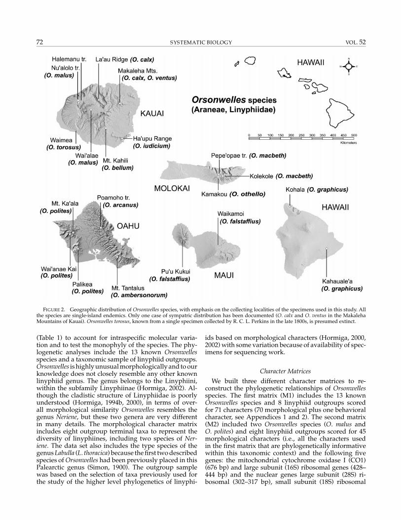
13 species, 11 of which were undescribed (Hormiga,2002). All Orsonwelles species are single-island endemic,and most of them have very small, nonoverlappingdistributions (Fig. 2). Furthermore, many Orsonwellesspecies are restricted to a single mountaintop (e.g.,O. iudicium in Ha’upu, Kauai) or the higher elevationsof a particular range (e.g., O. bellum on Mount Kahili,Kauai).

Until very recently, the only work on Orsonwelles spi-ders were the original taxonomic descriptions by EugeneSimon (1900). Simon’s work was based on relatively fewspecimens, most of them juveniles (in spiders, very of-ten only genitalic morphology can provide reliable di-agnostic features for species, especially when they areclosely related). He recognized only two species (O.torosus and O. graphicus) and concluded, largely basedon his misidentifications of juveniles, that these specieswere widespread in the archipelago. Simon placed thesetwo Hawaiian taxa in the European genus Labulla. Recentwork on this group by Hormiga (2002) has uncovered thehighly underestimated species diversity of this Hawai-ian group (which includes ≥13 species) and highlightedthe remote phylogenetic affinities of Orsonwelles to thetype species of the genus Labulla, L. thoracica, requiringthe creation of a new genus. Hormiga also detailed thehighly local endemicity of these Hawaiian spiders. Themonophyly of the genus Orsonwelles is strongly sup-ported by numerous morphological synapomorphies,both somatic and genitalic, and by at least one web ar-chitecture character (Hormiga, 2002). Perhaps the singlemost striking morphological feature of Orsonwelles spi-ders is their extraordinarily large size, with some females(O. malus) reaching a total length of >14 mm, whichmakes them the largest known linyphiids (the nextlargest described linyphiid species seems to beLaminacauda gigas, an erigonine from the Chilean JuanFernandez Islands, in which the females can reach upto 9.9 mm total length, Millidge, 1991). Thus, the genusOrsonwelles represents a genuine case of insular gigan-tism. As yet, the closest ancestor to this Hawaiian radia-

tion is unknown, a situation that has three possible expla-nations: (1) its geographic origin remains unknown andthe highly autapomorphic nature of this lineage hindersthe search for close relatives on the basis of morpholog-ical characters; (2) our knowledge of the diversity andtaxonomy of the circumpacific linyphiid fauna rangesfrom fragmentary to very poor; and (3) the higher levelcladistic structure of Linyphiidae (the second largest spi-der family in terms of described species and the largestin terms of genera) is only poorly understood (Hormiga,1994a, 1994b, 2000).

The objectives of our study were to reconstruct thespecies-level phylogenetic relationships of Orsonwellesspecies so as to understand better the importance ofthe geological history of the archipelago in shaping thecladogenic events and to study the biogeographic hy-potheses implied by the phylogenetic reconstructions.To reconstruct the cladistic relationships of Orsonwellesspecies, we used a combination of morphological andmolecular (both mitochondrial and nuclear sequencecharacters) data. The nature of these different charactersystems allowed us to explore and contrast the contri-bution of these different markers in reconstructing thecladistic patterns of these Hawaiian spiders. In addition,the nucleotide sequence data, in combination with thereconstructed phylogenetic trees, allowed us to estimatethe divergence times within Orsonwelles.

MATERIALS AND METHODS

Taxonomic Sampling

We collected specimens of 12 of the 13 Orsonwellesspecies. Orsonwelles torosus, known from a single mu-seum specimen, has not been seen since R. C. L. Perkinscollected the type specimen in the Waimea area (Kauai)in the 1890s. We have searched this area, now highlydisturbed ecologically, and have not been able to findO. torosus, which we presume is extinct. For most of theremaining Orsonwelles species, we used multiple spec-imens (haplotypes) from several geographic localities

72 SYSTEMATIC BIOLOGY VOL. 52

FIGURE 2. Geographic distribution of Orsonwelles species, with emphasis on the collecting localities of the specimens used in this study. Allthe species are single-island endemics. Only one case of sympatric distribution has been documented (O. calx and O. ventus in the MakalehaMountains of Kauai). Orsonwelles torosus, known from a single specimen collected by R. C. L. Perkins in the late 1800s, is presumed extinct.

(Table 1) to account for intraspecific molecular varia-tion and to test the monophyly of the species. The phy-logenetic analyses include the 13 known Orsonwellesspecies and a taxonomic sample of linyphiid outgroups.Orsonwelles is highly unusual morphologically and to ourknowledge does not closely resemble any other knownlinyphiid genus. The genus belongs to the Linyphiini,within the subfamily Linyphiinae (Hormiga, 2002). Al-though the cladistic structure of Linyphiidae is poorlyunderstood (Hormiga, 1994b, 2000), in terms of over-all morphological similarity Orsonwelles resembles thegenus Neriene, but these two genera are very differentin many details. The morphological character matrixincludes eight outgroup terminal taxa to represent thediversity of linyphiines, including two species of Ner-iene. The data set also includes the type species of thegenus Labulla (L. thoracica) because the first two describedspecies of Orsonwelles had been previously placed in thisPalearctic genus (Simon, 1900). The outgroup samplewas based on the selection of taxa previously used forthe study of the higher level phylogenetics of linyphi-

ids based on morphological characters (Hormiga, 2000,2002) with some variation because of availability of spec-imens for sequencing work.

Character Matrices

We built three different character matrices to re-construct the phylogenetic relationships of Orsonwellesspecies. The first matrix (M1) includes the 13 knownOrsonwelles species and 8 linyphiid outgroups scoredfor 71 characters (70 morphological plus one behavioralcharacter, see Appendices 1 and 2). The second matrix(M2) included two Orsonwelles species (O. malus andO. polites) and eight linyphiid outgroups scored for 45morphological characters (i.e., all the characters usedin the first matrix that are phylogenetically informativewithin this taxonomic context) and the following fivegenes: the mitochondrial cytochrome oxidase I (CO1)(676 bp) and large subunit (16S) ribosomal genes (428–444 bp) and the nuclear genes large subunit (28S) ri-bosomal (302–317 bp), small subunit (18S) ribosomal

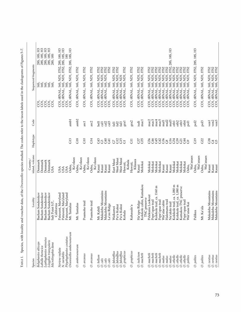
TAB

LE

1.Sp

ecie

s,w

ith

loca

lity

and

vouc

her

dat

a,of

the

Ors

onw

elle

ssp

ecie

sst

udie

d.T

heco

des

refe

rto

the

taxo

nla

bels

used

inth

ecl

adog

ram

sof

Figu

res

5–7.

Cou

ntry

/Sp

ecie

sL

ocal

ity

isla

nd,v

olca

noH

aplo

type

Cod

eSe

quen

ced

frag

men

ts

Bol

ypha

ntes

alti

ceps

Bae

lum

Sond

ersk

ovD

enm

ark

CO

1,16

S,28

S,18

S,H

3La

bulla

thor

acic

aB

aelu

mSo

nder

skov

Den

mar

kC

O1,

16S,

28S,

18S,

H3

Lept

hyph

ante

sm

inut

usB

aelu

mSo

nder

skov

Den

mar

kC

O1,

16S,

28S,

18S,

H3

Liny

phia

tria

ngul

aris

Bae

lum

Sond

ersk

ovD

enm

ark

CO

1,16

S,28

S,18

S,H

3M

icro

linyp

hia

dana

Salt

Poin

tS.P

.,U

SAC

O1,

16S,

28S,

18S

Cal

ifor

nia

Ner

iene

radi

ata

Patu

xent

,Mar

ylan

dU

SAC

O1,

tRN

AL

,16S

,ND

1,IT

S2,2

8S,1

8S,H

3N

.var

iabi

lisPa

tuxe

nt,M

aryl

and

USA

CO

1,tR

NA

L,1

6S,N

D1,

ITS2

,28S

,18S

,H3

Pit

yohy

phan

tes

cost

atus

Patu

xent

,Mar

ylan

dU

SAC

O1,

16S,

18S

Ors

onw

elle

sam

bers

onor

umM

t.Ta

ntal

usO

ahu,

G13

amb1

CO

1,tR

NA

L,1

6S,N

D1,

ITS2

,28S

,18S

,H3

Ko’

olau

sO

.am

bers

onor

umM

t.Ta

ntal

usO

ahu,

G18

amb2

CO

1,tR

NA

L,1

6S,N

D1,

ITS2

Ko’

olau

sO

.arc

anus

Poam

oho

trai

lO

ahu,

G10

arc1

CO

1,tR

NA

L,1

6S,N

D1,

ITS2

Ko’

olau

sO

.arc

anus

Poam

oho

trai

lO

ahu,

G14

arc2

CO

1,tR

NA

L,1

6S,N

D1,

ITS2

Ko’

olau

sO

.bel

lum

Mt.

Kah

iliK

auai

G43

bel1

CO

1,tR

NA

L,1

6S,N

D1,

ITS2

O.c

alx

Mak

aleh

aM

ount

ains

Kau

aiG

3ca

l1C

O1,

tRN

AL

,16S

,ND

1,IT

S2O

.cal

xM

akal

eha

Mou

ntai

nsK

auai

G40

cal2

CO

1,tR

NA

L,1

6S,N

D1,

ITS2

O.c

alx

La’

auR

idge

Kau

aiG

41ca

l3C

O1,

16S,

ITS2

O.f

alst

affiu

sW

aika

moi

Eas

tMau

iG

7fa

l1C

O1,

tRN

AL

,16S

,ND

1,IT

S2O

.fal

staf

fius

Pu’u

Kuk

uiW

estM

aui

G12

fal2

CO

1,tR

NA

L,1

6S,N

D1,

ITS2

O.f

alst

affiu

sPu

’uK

ukui

Wes

tMau

iG

15fa

l3C

O1,

tRN

AL

,16S

,ND

1O

.gra

phic

usK

ohal

aH

awai

i,G

1gr

a1C

O1,

tRN

AL

,16S

,ND

1,IT

S2K

ohal

aO

.gra

phic

usK

ahau

ale’

aH

awai

i,G

11gr

a2C

O1,

tRN

AL

,16S

,ND

1,IT

S2K

ilaue

aO

.iud

iciu

mH

a’up

uR

idge

Kau

aiG

37iu

di

CO

1,tR

NA

L,1

6S,N

D1,

ITS2

O.m

acbe

thK

olek

ole

cabi

n,K

amak

ouM

olok

aiG

55m

ac1

CO

1,tR

NA

L,1

6S,N

D1,

ITS2

TN

Cpr

eser

veO

.mac

beth

Pele

kunu

Loo

kout

Mol

okai

G56

mac

2C

O1,

tRN

AL

,16S

,ND

1,IT

S2O

.mac

beth

Pepe

’opa

etr

ail

Mol

okai

G46

mac

3C

O1,

tRN

AL

,16S

,ND

1,IT

S2O

.mac

beth

Kol

ekol

etr

ail,

ca.1

160

mM

olok

aiG

45m

ac4

CO

1,tR

NA

L,1

6S,N

D1,

ITS2

O.m

acbe

thPe

pe’o

pae

trai

lM

olok

aiG

42m

ac5

CO

1,tR

NA

L,1

6S,N

D1,

ITS2

O.m

alus

Wai

’ala

eca

bin

Kau

aiG

36m

al1

CO

1,tR

NA

L,1

6S,N

D1,

ITS2

O.m

alus

Hal

eman

utr

ail

Kau

aiG

8m

al2

CO

1,tR

NA

L,1

6S,N

D1,

ITS2

O.m

alus

Nu’

alol

otr

ail

Kau

aiG

16m

al3

CO

1,tR

NA

L,1

6S,N

D1,

ITS2

,28S

,18S

,H3

O.o

thel

loK

olek

ole

trai

l,ca

.1,0

80m

Mol

okai

G54

oth1

CO

1,tR

NA

L,1

6S,N

D1,

ITS2

O.o

thel

loK

olek

ole

trai

l,ca

.1,0

80m

Mol

okai

G39

oth2

CO

1,tR

NA

L,1

6S,N

D1,

ITS2

O.o

thel

loK

amak

ouT

NC

pres

erve

Mol

okai

G21

oth3

CO

1,tR

NA

L,1

6S,N

D1,

ITS2

O.o

thel

loPe

pe’o

pae

trai

lM

olok

aiG

44ot

h4C

O1,

tRN

AL

,16S

,ND

1,IT

S2O

.pol

ites

Wai

’ana

eK

aiO

ahu,

G9

pol1

CO

1,tR

NA

L,1

6S,N

D1,

ITS2

Wai

’ana

esO

.pol

ites

Palik

eaO

ahu,

G19

pol2

CO

1,tR

NA

L,1

6S,N

D1,

ITS2

,28S

,18S

,H3

Wai

’ana

esO

.pol

ites

Mt.

Ka’

ala

Oah

u,G

22po

l3C

O1,

tRN

AL

,16S

,ND

1,IT

S2W

ai’a

naes

O.v

entu

sM

akal

eha

Mou

ntai

nsK

auai

G38

ven1

CO

1,tR

NA

L,1

6S,N

D1,

ITS2

O.v

entu

sM

akal

eha

Mou

ntai

nsK

auai

G4

ven2

CO

1,tR

NA

L,1

6S,N

D1,

ITS2

O.v

entu

sM

akal

eha

Mou

ntai

nsK

auai

G5

ven3

CO

1,tR

NA

L,1

6S,N

D1,

ITS2

73

74 SYSTEMATIC BIOLOGY VOL. 52

(771–775 bp), and histone H3 (H3) (328 bp). The thirdmatrix (M3) has the 13 known Orsonwelles species, rep-resented by 32 individuals, and 2 linyphiid outgroupsscored for 71 morphological characters (50 of them arephylogenetically informative within this context) and thefollowing five genes: the mitochondrial CO1 (439 bp), 16S(464–468 bp), tRNALEU(CUN) (tRNAL) (45 bp), and theNADH dehydrogenase subunit I (ND1) (367 bp) and thenuclear internal transcribed spacer 2 (ITS2) (353–416 bp).Each sequenced individual was considered a terminaltaxon in the analyses, and the morphological charactersscored for each of them were those corresponding to thespecies in which the individual was included. When in-formation regarding any of the gene fragments was notavailable, all the characters of that data set were scored asmissing. Outgroups for this matrix (Neriene radiata and N.variabilis) were chosen based on the sister taxa obtainedfrom the analysis of the second matrix (M2). Differentgene fragments have been used in the two molecular ma-trices because one was used to reconstruct cladogeneticevents between genera (i.e., the phylogenetic structure ofOrsonwelles outgroups) and the other was used to eval-uate more recent divergences (i.e., the cladogenic eventsamong Orsonwelles species).

Morphological Data

Seventy morphological and one behavioral characterwere scored for 21 taxa (the 13 Orsonwelles species plus 8outgroup linyphiid species; matrix M1). The methods ofstudy and most of the characters have been described andillustrated in detail by Hormiga (2002). The 15 characterdescriptions not provided by Hormiga (2002) are givenin Appendix 1.

Molecular Data

Live specimens were collected in the field and fixedin 95% ethanol. Alternatively, when fresh material wasnot available specimens from museum collections (pre-served in 75% ethanol) were used for extractions, withrelative success mostly dependent on the length ofpreservation. Only one or two legs were used for extrac-tion, except for specimens preserved in 75% ethanol, forwhich as many as four legs plus the carapace were used.The remainder of the specimen was kept as a voucher(deposited at the National Museum of Natural History,Smithsonian Institution, Washington, D.C.).

Total genomic DNA was extracted following the phe-nol/chloroform protocol of Palumbi et al. (1991) orusing Qiagen DNeasy Tissue Kits. The approximate con-centration and purity of the DNA obtained was eval-uated through spectophotometry, and the quality wasverified using electrophoresis in an agarose/Tris-borate-EDTA (TBE) (1.8%) gel. Partial fragments of four mi-tochondrial genes and four nuclear genes were ampli-fied using the following primer pairs. The mitochondrialCO1 was amplified by means of C1-J-1490 and C1-N-2198 (Folmer et al., 1994) or C1-J-1751 and C1-N-2191(Simon et al., 1994). A fragment including the 5′ half ofthe mitochondrial 16S ribosomal gene, the tRNAL, and

the 3′ half of the ND1 was amplified with the primersLR-N-13398 (Simon et al., 1994) and N1-J-12261 (Hedin,1997a) or N1-J-12307 (CATATTTAGAATTTGAAGCTC)(M. Rivera, pers. comm.). Alternatively, the amplifica-tion was carried out in two different fragments us-ing the primer combinations of LR-N-13398 with LR-J-12864 (CTCCGGTTTGAACTCAGATCA) (Hsiao, pers.comm.) and LR-N-12866 with either LR-N-13398 or N1-J-12307. Nuclear markers were obtained for the follow-ing genes and primer combinations: 28S ribosomal DNAwith primers 28SA and 28SB (Whiting et al., 1997), 18S ri-bosomal DNA with primers 5F or 18Sa2.0 and 9R (Giribetet al., 1999), H3 with H3aF and H3aR (Colgan et al., 1998),and ITS2 with ITS2-28S and ITS2-5.8S (Hedin, 1997b).The thermal cyclers, Perkin Elmer 9700, Perkin Elmer9600, or BioRad iCycle, were used to perform either 25(mitochondrial genes) or 40 (nuclear genes) iterations ofthe following cycle: 30 sec at 95◦C, 45 sec at 42–48◦C(depending on the primers), and 45 sec at 72◦C, begin-ning with an additional single cycle of 2 min at 95◦C andending with another cycle of 10 min at 72◦C. The PCRmix contained primers (0.48 µM each), dNTPs (0.2 mMeach), and 0.6 U Perkin Elmer AmpliTaq DNA poly-merase (for a 50-µl reaction) with the supplied bufferand, in some cases, an extra amount of MgCl2 (0.5–1.0mM). PCR results were visualized on an agarose/TBE(1.8%) gel. PCR products were cleaned using GenecleanII (Bio 101) or Qiagen QIAquick PCR Purification Kitsfollowing the manufacturer’s specifications. DNA wasdirectly sequenced in both directions with the cycle se-quencing method using dye terminators (Sanger et al.,1977) and the ABI PRISM BigDye Terminator Cycle Se-quencing Ready Reaction with the AmpliTaq DNA Poly-merase FS kit. Sequenced products were cleaned usingPrinceton Separations CentriSep columns and run out onan ABI 377 automated sequencer.

Sequence errors and ambiguities were edited us-ing the Sequencher 3.1.1 software package (GeneCodes Corp.). Sequences were subsequently exportedto the program GDE 2.2 (Genetic Data Environ-ment) running on a Sun Enterprise 5000 Server, andmanual alignments were built taking into accountsecondary structure information from secondarystructure models available in the literature for 16S(Arnedo et al., 2001), 28S (Ajuh et al. 1991), and 18S(Guttell et al., http://www.rna.icmb.utexas.edu/).Alignment of the protein-coding genes was trivialbecause no length variation was observed in the se-quences. Sequences have been deposited in GenBank,with the following accession numbers: 16S-tRNAleu-ND1=AY078660–AY078666 and AY078711–AY078725;18S=AY078667–AY078677; 28S=AY078688–AY078686;CO1=AY078689–AY078699 and AY078744–AY078759;H3=AY078700–AY078709; ITS2=AY078774–AY078806.

Phylogenetic Analyses

The parsimony analyses of the morphological ma-trix were performed using the computer programsHENNIG86 version 1.5 (Farris, 1988) and NONA version

2003 HORMIGA ET AL.—RADIATION OF ORSONWELLES SPIDERS 75

2.0 (Goloboff, 1993). WinClada version 0.9.99m24 (Nixon,1999) and NDE version 0.4.9 (Page, 2001) were used tostudy character optimizations on the cladograms and tobuild and edit the character matrix, respectively. Am-biguous character optimizations were resolved usingFarris optimization (ACCTRAN), which maximizes ho-mology by favoring reversal or secondary loss over con-vergence. Multistate characters were treated as nonad-ditive (unordered or Fitch minimum mutation model;Fitch, 1971) (see Hormiga, 1994a, for justification). Suc-cessive character weighting (Farris, 1969) was performedusing HENNIG86 1.5, which reweights characters by therescaled consistency index (Farris, 1988, 1989a, 1989b).NONA (Goloboff, 1993) was used to calculate Bremersupport indices (BS) (Bremer, 1988, 1994).

Cladistic analysis of the molecular data matrices wasperformed using direct optimization (Wheeler, 1996) asimplemented in the computer program POY (Wheelerand Gladstein, 2000). This method, first suggested bySankoff (1975), approaches the alignment problem byincorporating insertion/deletion events as additionaltransformations during the optimization step in treeevaluation instead of trying to reconcile sequence lengthsby adding gaps as additional states. Unlike competingmethods, which dissociate the process of aligning se-quences from the phylogenetic analysis (i.e., search foroptimal trees), in direct optimization gap assignment isan intrinsic and inseparable part of the phylogenetic in-ference. Nonetheless, the alignment implied by a partic-ular tree can be recovered. Although such an alignment isparticular to the tree selected, it is as much a result of theanalysis as the reconstructed most-parsimonious trees.Moreover, direct optimization explores the sensitivity ofthe results to perturbations in the parameters (e.g., gapcosts, bases transformations, morphology weights) of theanalysis. Manual alignments based on secondary struc-ture information were used to define smaller fragmentsof unambiguous homology. We used the secondary struc-ture information for data management purposes and,most importantly, for identifying fragments of the differ-ent ribosomal genes that could be unambiguously con-sidered homologous. These fragments were flanked byseries of either identical nucleotides (about 10 bp), whichwas the case for most of the fragments into which the18S and 28S were spliced, or recognized fully comple-mentary stems (most of the fragments of the 16S). Oncethe fragments were identified, all the gaps manually in-serted in them were removed and all the fragments wereanalyzed simultaneously by POY. Splitting the gene intosmaller fragments of unambiguous homology has twoadvantages. It restricts the assignment of indels by thedirect optimization algorithm to regions for which ho-mology is not disputed; thus, the results are biologicallymore feasible. It also speeds up the analyses by reducingthe computation time (Giribet, 2001).

Heuristic parsimony searches were implemented byperforming 10 rounds of tree building by random addi-tion of taxa using approximate algorithms, retaining thebest round and subjecting it to sequential rounds of SPRand TBR branch swapping. This protocol was repeated

until minimum-length trees were obtained in at least 3 it-erations after a minimum of 10 iterations were performedup to a maximum of 100 iterations. Tree fusion and treedrifting techniques (Goloboff, 1999) were applied to thebest trees retained in each iteration and to the best treesobtained overall.

Two rounds of tree fusion were applied to all pair-wise combinations of the retained trees (a first roundusing SPR and a second round using the more thor-ough but computationally intensive TBR); only cladeswith a minimum of five taxa were fused. This strat-egy can optimize computation time and search efficiency(W. Wheeler, pers. comm.). Thirty branch-swapping re-arrangements, one round using SPR and another roundusing TBR, were applied on the trees kept after fusion.Rearranged trees equal to or better than the originals un-der a criterion based on character fit and tree length wereaccepted and subsequently subjected to full SPR and TBRbranch swapping, accepting only minimal trees. To copewith the effect of the heuristics of tree length calculationshortcuts, an extra TBR branch-swapping round was ap-plied to all cladograms found within 1% of the minimumtree length. Heuristic BS values (Bremer, 1988) were es-timated as a measure of clade support.

Sensitivity of the results to different parameter val-ues (gap cost and transversion weighting) were inves-tigated (Wheeler, 1995). Ten different parameter combi-nations were analyzed: equal cost of gaps, transversions,and transitions (hereinafter referred to as 111); gaps twice(211), four times (411), and eight times (811) the cost ofthe nucleotide transformations; and transversions twice(221, 421, 821), four times (441, 841), and eight times (881)the cost of transitions. Transversions were never given ahigher cost than gaps. In all cases, morphological charac-ters were assigned the same weight as the gap cost. Theparameter combinations we explored are a small and ar-bitrarily chosen fraction of the almost infinite combina-tions available. Character and topological congruence,as measured by the incongruence length difference in-dex (ILD; Mickevich and Farris, 1981) and the topologicalILD (TILD; Wheeler, 1999) has been proposed as an ob-jective criterion for choosing among the results of a par-ticular parameter cost combination (but see Barker andLutzoni, 2002, who concluded that the ILD test is a poorindicator of homogeneity and combinability and a poorindicator of congruence/incongruence). However, nei-ther ILD nor TILD are comparable across different datamatrices, their values being influenced by the actual pa-rameter combination selected (Faith and Trueman, 2001;M. Ramirez, pers. comm.). Also, ILD and TILD values candiffer depending on the actual data partition chosen, andselecting one data partition over another is usually verysubjective. Because of the lack of such an objective cri-terion to decide among alternative weighting schemes,results from equal costs were preferred. Results underadditional parameter value combinations were used toassess clade stability.

Simultaneous and partial analyses of the charactermatrices were performed to characterize the contribu-tion of the different character partitions to the total

76 SYSTEMATIC BIOLOGY VOL. 52

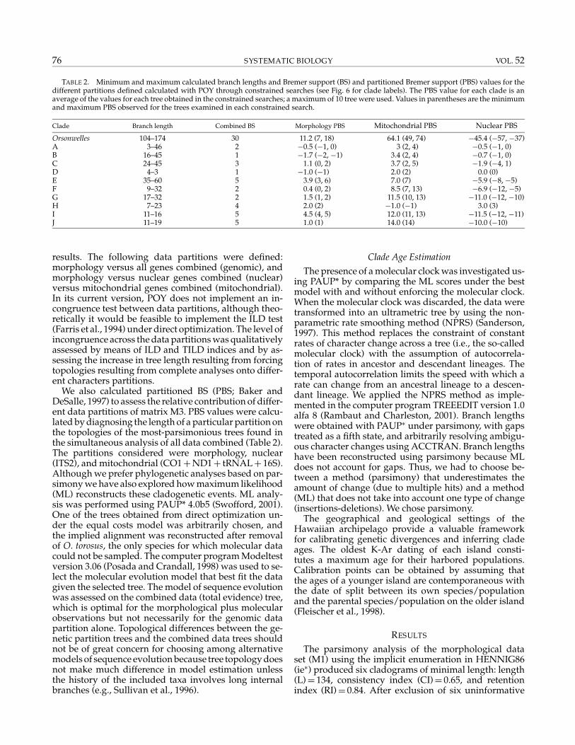
TABLE 2. Minimum and maximum calculated branch lengths and Bremer support (BS) and partitioned Bremer support (PBS) values for thedifferent partitions defined calculated with POY through constrained searches (see Fig. 6 for clade labels). The PBS value for each clade is anaverage of the values for each tree obtained in the constrained searches; a maximum of 10 tree were used. Values in parentheses are the minimumand maximum PBS observed for the trees examined in each constrained search.

Clade Branch length Combined BS Morphology PBS Mitochondrial PBS Nuclear PBS

Orsonwelles 104–174 30 11.2 (7, 18) 64.1 (49, 74) −45.4 (−57, −37)A 3–46 2 −0.5 (−1, 0) 3 (2, 4) −0.5 (−1, 0)B 16–45 1 −1.7 (−2, −1) 3.4 (2, 4) −0.7 (−1, 0)C 24–45 3 1.1 (0, 2) 3.7 (2, 5) −1.9 (−4, 1)D 4–3 1 −1.0 (−1) 2.0 (2) 0.0 (0)E 35–60 5 3.9 (3, 6) 7.0 (7) −5.9 (−8, −5)F 9–32 2 0.4 (0, 2) 8.5 (7, 13) −6.9 (−12, −5)G 17–32 2 1.5 (1, 2) 11.5 (10, 13) −11.0 (−12, −10)H 7–23 4 2.0 (2) −1.0 (−1) 3.0 (3)I 11–16 5 4.5 (4, 5) 12.0 (11, 13) −11.5 (−12, −11)J 11–19 5 1.0 (1) 14.0 (14) −10.0 (−10)

results. The following data partitions were defined:morphology versus all genes combined (genomic), andmorphology versus nuclear genes combined (nuclear)versus mitochondrial genes combined (mitochondrial).In its current version, POY does not implement an in-congruence test between data partitions, although theo-retically it would be feasible to implement the ILD test(Farris et al., 1994) under direct optimization. The level ofincongruence across the data partitions was qualitativelyassessed by means of ILD and TILD indices and by as-sessing the increase in tree length resulting from forcingtopologies resulting from complete analyses onto differ-ent characters partitions.

We also calculated partitioned BS (PBS; Baker andDeSalle, 1997) to assess the relative contribution of differ-ent data partitions of matrix M3. PBS values were calcu-lated by diagnosing the length of a particular partition onthe topologies of the most-parsimonious trees found inthe simultaneous analysis of all data combined (Table 2).The partitions considered were morphology, nuclear(ITS2), and mitochondrial (CO1+ND1+ tRNAL+ 16S).Although we prefer phylogenetic analyses based on par-simony we have also explored how maximum likelihood(ML) reconstructs these cladogenetic events. ML analy-sis was performed using PAUP* 4.0b5 (Swofford, 2001).One of the trees obtained from direct optimization un-der the equal costs model was arbitrarily chosen, andthe implied alignment was reconstructed after removalof O. torosus, the only species for which molecular datacould not be sampled. The computer program Modeltestversion 3.06 (Posada and Crandall, 1998) was used to se-lect the molecular evolution model that best fit the datagiven the selected tree. The model of sequence evolutionwas assessed on the combined data (total evidence) tree,which is optimal for the morphological plus molecularobservations but not necessarily for the genomic datapartition alone. Topological differences between the ge-netic partition trees and the combined data trees shouldnot be of great concern for choosing among alternativemodels of sequence evolution because tree topology doesnot make much difference in model estimation unlessthe history of the included taxa involves long internalbranches (e.g., Sullivan et al., 1996).

Clade Age Estimation

The presence of a molecular clock was investigated us-ing PAUP* by comparing the ML scores under the bestmodel with and without enforcing the molecular clock.When the molecular clock was discarded, the data weretransformed into an ultrametric tree by using the non-parametric rate smoothing method (NPRS) (Sanderson,1997). This method replaces the constraint of constantrates of character change across a tree (i.e., the so-calledmolecular clock) with the assumption of autocorrela-tion of rates in ancestor and descendant lineages. Thetemporal autocorrelation limits the speed with which arate can change from an ancestral lineage to a descen-dant lineage. We applied the NPRS method as imple-mented in the computer program TREEEDIT version 1.0alfa 8 (Rambaut and Charleston, 2001). Branch lengthswere obtained with PAUP∗ under parsimony, with gapstreated as a fifth state, and arbitrarily resolving ambigu-ous character changes using ACCTRAN. Branch lengthshave been reconstructed using parsimony because MLdoes not account for gaps. Thus, we had to choose be-tween a method (parsimony) that underestimates theamount of change (due to multiple hits) and a method(ML) that does not take into account one type of change(insertions-deletions). We chose parsimony.

The geographical and geological settings of theHawaiian archipelago provide a valuable frameworkfor calibrating genetic divergences and inferring cladeages. The oldest K-Ar dating of each island consti-tutes a maximum age for their harbored populations.Calibration points can be obtained by assuming thatthe ages of a younger island are contemporaneous withthe date of split between its own species/populationand the parental species/population on the older island(Fleischer et al., 1998).

RESULTS

The parsimony analysis of the morphological dataset (M1) using the implicit enumeration in HENNIG86(ie∗) produced six cladograms of minimal length: length(L)= 134, consistency index (CI)= 0.65, and retentionindex (RI)= 0.84. After exclusion of six uninformative

2003 HORMIGA ET AL.—RADIATION OF ORSONWELLES SPIDERS 77

characters, the new cladograms had L= 127, CI= 0.63,and RI= 0.84 (Fig. 3). The same results were alsofound using various heuristic search strategies inNONA. These topological results were stable undersuccessive character weighting. In all the minimal-length trees, the six species from Kauai formed amonophyletic group, that was sister to a clade thatincluded all the remaining species, with the threespecies from Oahu as the most basal lineages. Thestrict consensus cladogram indicated conflict in theplacement of two taxa within the outgroups andone within the ingroup (Fig. 3). The monophyly ofOrsonwelles was supported by at least 22 unambigu-ous synapomorphies (up to 26 under ambiguous op-timizations). Within the ingroup, only the placementof O. torosus was ambiguously supported: half of themost-parsimonious trees had this species as sister to aclade with all the remaining five species from Kauaiand the other half had it as sister to all the other Or-sonwelles species from Kauai except O. malus, whichwas placed as the most basal taxon of this Kauai clade.In other words, O. malus and O. torosus switched po-sitions as the most basal taxon within a clade con-taining all the species from Kauai. Three equally par-simonious alternatives exist for the sister group ofOrsonwelles: Linyphia plus Neriene sister to Microlinyphia;Neriene plus Linyphia (with Microlinyphia sister to thisclade plus Orsonwelles); or Linyphia plus Microlinyphiasister to Neriene. The genus Labulla, which had con-tained the first Orsonwelles species described, is very dis-tantly related to Orsonwelles and was placed as the mostbasal lineage within the Linyphiini of this taxonomicsample.

The analysis of M2 resulted in a single most-parsimonious tree (Fig. 4) 1,308 steps long. The ILD andTILD were 0.05 and 0.111, respectively, for the morphol-ogy versus genomic partitions and 0.014 and 0.233, re-spectively, for the morphology versus mitochondrial ver-sus nuclear partitions. This cladogram placed Labullaand Pityohyphantes as the most basal lineages within theLinyphiinae. This topology is congruent with the anal-ysis of the exclusively morphological matrix (M1). Theanalysis of M2 also supports Microlinyphia as sister toLinyphia, which was also found in two of the six most-parsimonious trees resulting from the M1 matrix. Theanalysis of M2 supports the monophyly of Orsonwellesand Neriene species and placed Neriene as the single sis-ter group to Orsonwelles. The sister group relationshipbetween Neriene and Orsonwelles was not recovered inthe analysis of the morphological matrix (M1), whichsuggested that Linyphia or Microlinyphia plus Linyphiais the sister group to Neriene. The analyses of the ge-nomic (1 tree, 1,231 steps) and nuclear (3 trees, 398 steps)partitions were fully compatible with the tree from thetotal data set, except for the sister group relationshipof Labulla and Pityohyphantes. The mitochondrial parti-tion produced a polyphyletic Neriene, with N. variabilissister to a clade consisting of a monophyletic Orson-welles sister to the clade ((N. radiata, Pityohyphantes) (Mi-

crolinyphia, Linyphia)). Five of the seven nodes in themost-parsimonious tree from the M2 matrix under equalcosts are robust (stable) to all the variations of morphol-ogy, gap, and transition and transversion costs that weexplored (Fig. 4). Only under three combinations of highcosts for the morphology, gaps, and transversions (821,441, 881) was the monophyly of Neriene and the mono-phyly of Neriene plus Orsonwelles lost. Accordingly, Ne-riene radiata and N. variabilis were selected as outgroupsfor analyses of the matrix M3. In general, Bremer sup-ports and clade sensitivity to parameter perturbationswere closely correlated, and the weakest support was forclades most sensitive to changes in the parameter costs.

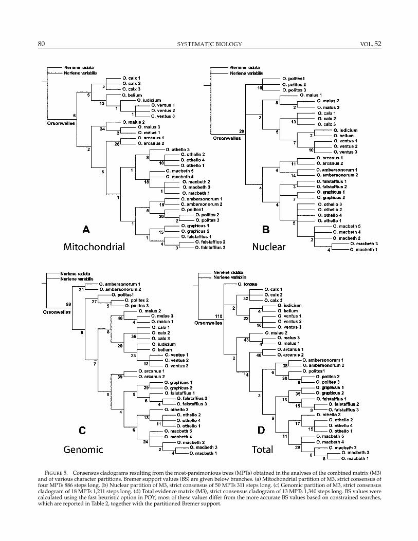
Results from the combined and partial analyses of thematrix M3 under equal parameter values are shown inFigure 5. Fifty trees of minimal length (311 steps) wererecovered from the analysis of the nuclear ITS2 (Fig. 5b).The combined mitochondrial genes resulted in four trees886 steps long (Fig. 5a), and the simultaneous analysis ofall the molecular data sets combined yielded 18 trees oflength 1,211 (Fig. 5c). The analysis of the complete ma-trix (M3, all the available character evidence) resultedin 13 trees of minimal length, 1,340 steps long (Fig. 5d).The ILD and TILD were 0.029 and 0.183, respectively, forthe morphology versus genomic partitions and 0.04 and0.16, respectively, for the morphology versus mitochon-drial versus nuclear partitions. Forcing the complete (allcharacter evidence) topology on each of the partitions re-sulted in an increase in length of 4 steps in the morphol-ogy partition, 1 in the genomic, 2 in the mitochondrial,and 13 in the nuclear.

BS values were estimated as a measure of clade sup-port. POY implements a fast but very heuristic com-mand to calculate BS consisting on additional rounds ofbranch swapping on the targeted tree, which can resultin the gross overestimation of the actual clade support.A more accurate calculation of the BS was conductedfor the simultaneous analysis of the M3 matrix by usingmore exhaustive constrained searches combined withthe “–disagree” command implemented in POY. Boththe nuclear and the mitochondrial partitions support-ed the monophyly of the individuals sampled for eachspecies, except for some of the trees of the nuclearpartition that showed O. othello paraphyletic with re-gard to O. macbeth. The complete analyses depictedonly one ambiguity at the species level, the place-ment of O. torosus, which can be either sister to aclade that includes all the other species from Kauai(except for O. malus) or sister to a large clade thatincludes O. malus plus all the non-Kauai species.Orsonwelles torosus, presumably extinct, is known byfrom a single female and could not be coded for the malecharacters or the molecular characters. To test the effectof the presence of missing data, an additional analysiswas conducted with O. torosus excluded. The 12 result-ing trees (1,338 steps) supported the existence of a cladeof Kauaian species, contradicting the results of the com-plete data matrix (in which O. malus was sister to a cladethat included all the non-Kauai species).

FIG

UR

E3.

One

ofth

esi

xm

ost-

pars

imon

ious

tree

sth

atre

sult

sfr

omth

ean

alys

isof

the

mor

phol

ogic

alch

arac

ter

mat

rix

M1

(L=

134

step

s,C

I=0.

65,R

I=0.

84;a

fter

excl

usio

nof

six

unin

form

ativ

ech

arac

ters

,L=

127

step

s,C

I=0.

63,R

I=0.

84).

The

basa

ltri

chot

omy

isar

bitr

arily

reso

lved

.The

nod

esth

atco

llaps

ein

the

stri

ctco

nsen

sus

clad

ogra

mar

em

arke

dw

ith

aso

lidbo

x.B

rem

ersu

ppor

tval

ues

are

repo

rted

und

erth

ebr

anch

es;c

hara

cter

sar

eop

tim

ized

usin

gFa

rris

opti

miz

atio

n.O

pen

circ

les

repr

esen

thom

opla

stic

char

acte

rch

ange

s.

78

2003 HORMIGA ET AL.—RADIATION OF ORSONWELLES SPIDERS 79

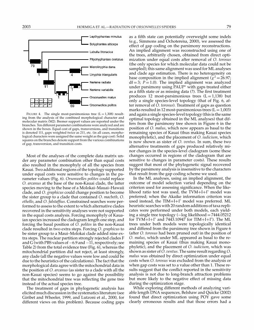
FIGURE 4. The single most-parsimonious tree (L= 1,308) result-ing from the analysis of the combined morphological character andmolecular matrix (M2). Bremer support values are reported under thebranches. Ten different parameter combinations were analyzed and areshown in the boxes. Equal cost of gaps, transversions, and transitionsis denoted 111, gaps weighted twice as 211, etc. (in all cases, morpho-logical characters were assigned the same weight as the gap cost). Solidsquares on the branches denote support from the various combinationsof gap, transversion, and transition costs.

Most of the analyses of the complete data matrix un-der any parameter combination other than equal costsalso resulted in the monophyly of all the species fromKauai. Two additional regions of the topology supportedunder equal costs were sensitive to changes in the pa-rameter values (Fig. 6). Orsonwelles polites could replaceO. arcanus at the base of the non-Kauai clade, the latterspecies moving to the base of a Molokai–Mauai–Hawaiiclade, and O. graphicus could change position to becomethe sister group to a clade that contained O. macbeth, O.othello, and O. falstaffius. Constrained searches were per-formed to assess to the extent to which alternative cladesrecovered in the sensitivity analyses were not supportedin the equal costs analysis. Forcing monophyly of Kaua-ian species increased the cladogram length one step, andforcing the basal position of O. polites in the non-Kauaiclade resulted in two extra steps. Forcing O. graphicus tobe sister group to a Maui–Molokai clade added nine ex-tra steps. The nuclear partition strongly rejected clades Fand G (with PBS values of−6.9 and−11, respectively; seeTable 2) from the total evidence tree (Fig. 6), whereas themitochondrial partition did not reject, at least strongly,any clade (all the negative values were low and could bedue to the heuristics of the calculations). The fact that themorphological data agree with the mitochondrial data inthe position of O. arcanus (as sister to a clade with all thenon-Kauai species) seems to go against the possibilitythat the mitochondrial tree was reflecting the gene treeinstead of the actual species tree.

The treatment of gaps in phylogenetic analysis haselicited much discussion in the systematics literature (seeGiribet and Wheeler, 1999, and Lutzoni et al., 2000, fordifferent views on this problem). Because coding gaps

as a fifth state can potentially overweight some indels(e.g., Simmons and Ochoterena, 2000), we assessed theeffect of gap coding on the parsimony reconstructions.An implied alignment was reconstructed using one ofthe trees, arbitrarily chosen, obtained from direct opti-mization under equal costs after removal of O. torosus(the only species for which molecular data could not besampled); this same alignment was used for ML analysesand clade age estimation. There is no heterogeneity onbase composition in the implied alignment (χ2= 26.97;df= 3; P= 1.0). The implied alignment was analyzedunder parsimony using PAUP∗ with gaps treated eitheras a fifth state or as missing data (?). The first treatmentproduces 12 most-parsimonious trees (L= 1,138) butonly a single species-level topology (that of Fig. 6, af-ter removal of O. torosus). Treatment of gaps as questionmarks resulted in 12 most-parsimonious trees (L= 1,003)and again a single species-level topology (this is the sameoptimal topology obtained in the ML analyses) that dif-fers from the parsimony tree shown in Figure 6 in theposition of O. malus, which now appears as basal to theremaining species of Kauai (thus making Kauai speciesmonophyletic), and the placement of O. iudicium, whichis now shown as sister of O. ventus. In sum, these twoalternative treatments of gaps produced relatively mi-nor changes in the species-level cladogram (some thesechanges occurred in regions of the cladogram that aresensitive to changes in parameter costs). These resultssuggest that most of the phylogenetic signal recoveredby the parsimony analysis is insensitive to the charactersthat result from the gap coding scheme we used.

In the ML analyses, using an implied alignment, theoutcome of model selection varied depending on thecriterion used for assessing significance. When the like-lihood ratio test was used, the TVM+I+0 model waspreferred; when the Akaike information criterion wasused instead, the TIM+I+0 model was preferred. MLheuristic searches with 20 random additions of taxa repli-cates were performed under both models, each yield-ing a single tree topology (−log likelihood= 7444.05212for TVM+I+0 and 7443.10947 for TIM+I+0). The MLtrees under both models were topologically identicaland differed from the parsimony tree shown in Figure 6(after O. torosus had been pruned out) in the position ofO. malus, which under ML appeared as basal to the re-maining species of Kauai (thus making Kauai mono-phyletic), and the placement of O. iudicium, which wasshown as sister of O. ventus. The same result regarding O.malus was obtained by direct optimization under equalcosts when O. torosus was excluded from the analysis orwhen gap costs was set to a value other than 1. These re-sults suggest that the conflict reported in the sensitivityanalysis is not due to long-branch attraction problemsbut more likely to the negative effect of missing dataduring the optimization stage.

While exploring different methods of analyzing vari-able length DNA sequences, Belshaw and Quicke (2002)found that direct optimization using POY gave someclearly erroneous results and that those errors had a

80 SYSTEMATIC BIOLOGY VOL. 52

FIGURE 5. Consensus cladograms resulting from the most-parsimonious trees (MPTs) obtained in the analyses of the combined matrix (M3)and of various character partitions. Bremer support values (BS) are given below branches. (a) Mitochondrial partition of M3, strict consensus offour MPTs 886 steps long. (b) Nuclear partition of M3, strict consensus of 50 MPTs 311 steps long. (c) Genomic partition of M3, strict consensuscladogram of 18 MPTs 1,211 steps long. (d) Total evidence matrix (M3), strict consensus cladogram of 13 MPTs 1,340 steps long. BS values werecalculated using the fast heuristic option in POY; most of these values differ from the more accurate BS values based on constrained searches,which are reported in Table 2, together with the partitioned Bremer support.

2003 HORMIGA ET AL.—RADIATION OF ORSONWELLES SPIDERS 81

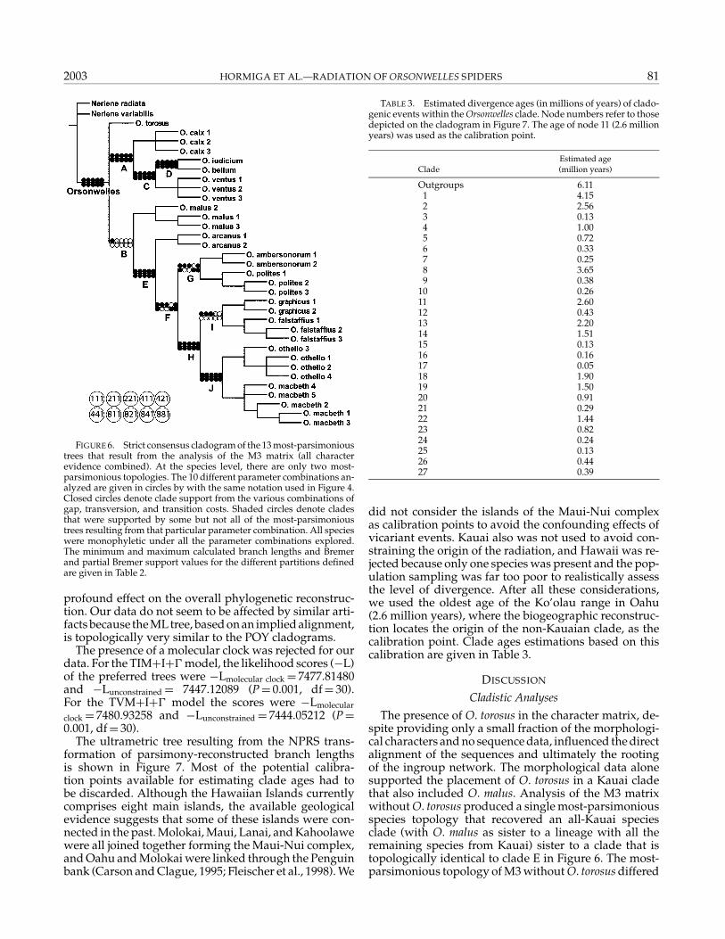
FIGURE 6. Strict consensus cladogram of the 13 most-parsimonioustrees that result from the analysis of the M3 matrix (all characterevidence combined). At the species level, there are only two most-parsimonious topologies. The 10 different parameter combinations an-alyzed are given in circles by with the same notation used in Figure 4.Closed circles denote clade support from the various combinations ofgap, transversion, and transition costs. Shaded circles denote cladesthat were supported by some but not all of the most-parsimonioustrees resulting from that particular parameter combination. All specieswere monophyletic under all the parameter combinations explored.The minimum and maximum calculated branch lengths and Bremerand partial Bremer support values for the different partitions definedare given in Table 2.

profound effect on the overall phylogenetic reconstruc-tion. Our data do not seem to be affected by similar arti-facts because the ML tree, based on an implied alignment,is topologically very similar to the POY cladograms.

The presence of a molecular clock was rejected for ourdata. For the TIM+I+0model, the likelihood scores (−L)of the preferred trees were −Lmolecular clock= 7477.81480and −Lunconstrained= 7447.12089 (P= 0.001, df= 30).For the TVM+I+0 model the scores were −Lmolecular

clock= 7480.93258 and −Lunconstrained= 7444.05212 (P=0.001, df= 30).

The ultrametric tree resulting from the NPRS trans-formation of parsimony-reconstructed branch lengthsis shown in Figure 7. Most of the potential calibra-tion points available for estimating clade ages had tobe discarded. Although the Hawaiian Islands currentlycomprises eight main islands, the available geologicalevidence suggests that some of these islands were con-nected in the past. Molokai, Maui, Lanai, and Kahoolawewere all joined together forming the Maui-Nui complex,and Oahu and Molokai were linked through the Penguinbank (Carson and Clague, 1995; Fleischer et al., 1998). We

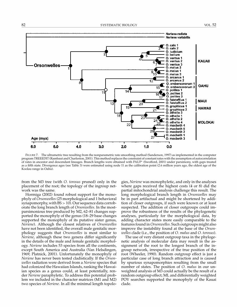
TABLE 3. Estimated divergence ages (in millions of years) of clado-genic events within the Orsonwelles clade. Node numbers refer to thosedepicted on the cladogram in Figure 7. The age of node 11 (2.6 millionyears) was used as the calibration point.

Estimated ageClade (million years)

Outgroups 6.111 4.152 2.563 0.134 1.005 0.726 0.337 0.258 3.659 0.38

10 0.2611 2.6012 0.4313 2.2014 1.5115 0.1316 0.1617 0.0518 1.9019 1.5020 0.9121 0.2922 1.4423 0.8224 0.2425 0.1326 0.4427 0.39

did not consider the islands of the Maui-Nui complexas calibration points to avoid the confounding effects ofvicariant events. Kauai also was not used to avoid con-straining the origin of the radiation, and Hawaii was re-jected because only one species was present and the pop-ulation sampling was far too poor to realistically assessthe level of divergence. After all these considerations,we used the oldest age of the Ko’olau range in Oahu(2.6 million years), where the biogeographic reconstruc-tion locates the origin of the non-Kauaian clade, as thecalibration point. Clade ages estimations based on thiscalibration are given in Table 3.

DISCUSSION

Cladistic Analyses

The presence of O. torosus in the character matrix, de-spite providing only a small fraction of the morphologi-cal characters and no sequence data, influenced the directalignment of the sequences and ultimately the rootingof the ingroup network. The morphological data alonesupported the placement of O. torosus in a Kauai cladethat also included O. malus. Analysis of the M3 matrixwithout O. torosus produced a single most-parsimoniousspecies topology that recovered an all-Kauai speciesclade (with O. malus as sister to a lineage with all theremaining species from Kauai) sister to a clade that istopologically identical to clade E in Figure 6. The most-parsimonious topology of M3 without O. torosus differed

82 SYSTEMATIC BIOLOGY VOL. 52

FIGURE 7. The ultrametric tree resulting from the nonparametric rate smoothing method (Sanderson, 1997) as implemented in the computerprogram TREEEDIT (Rambaut and Charleston, 2001). This method replaces the constraint of constant rates with the assumption of autocorrelationof rates in ancestor and descendant lineages. Branch lengths were obtained with PAUP∗ (Swofford, 2001) under parsimony, with gaps treatedas a fifth state. Divergence ages (see Table 3) were estimated using node 11 as the calibration point (2.6 million years ago, the oldest age of theKoolau range in Oahu).

from the M3 tree (with O. torosus pruned) only in theplacement of the root; the topology of the ingroup net-work was the same.

Hormiga (2002) found robust support for the mono-phyly of Orsonwelles (25 morphological and 1 behavioralsynapomorphy, with BS> 10). Our sequence data corrob-orate the long branch length of Orsonwelles. In the most-parsimonious tree produced by M2, 62–81 changes sup-ported the monophyly of the genus (18–29 base changessupported the monophyly of its putative sister genus,Neriene). Although the closest relatives of Orsonwelleshave not been identified, the overall male genitalic mor-phology suggests that Orsonwelles is most similar toNeriene, although these two genera differ significantlyin the details of the male and female genitalic morphol-ogy. Neriene includes 53 species from all the continents,except South America and Australia (Van Helsdingen,1969; Platnick, 2001). Unfortunately the monophyly ofNeriene has never been tested cladistically. If the Orson-welles radiation were derived from a Neriene species thathad colonized the Hawaiian Islands, ranking the Hawai-ian species as a genus could, at least potentially, ren-der Neriene paraphyletic. To address this potential prob-lem we included in the character matrices (M1 and M2)two species of Neriene. In all the minimal length topolo-

gies, Neriene was monophyletic, and only in the analyseswhere gaps received the highest costs (4 or 8) did thepartial mitochondrial analysis challenge this result. Thelong morphological branch length in Orsonwelles maybe in part artifactual and might be shortened by addi-tion of closer outgroups, if such were known or at leastsuspected. The addition of closer outgroups could im-prove the robustness of the results of the phylogeneticanalyses, particularly for the morphological data, byadding character states more easily comparable to thefeatures found in Orsonwelles. Such outgroups might alsoimprove the instability found at the base of the Orson-welles clade (i.e., the position of O. malus and O. torosus).

The use of very distant outgroup taxa in the phyloge-netic analysis of molecular data may result in the as-signment of the root to the longest branch of the in-group network, irrespective of the true position of theroot (Wheeler, 1990). Random outgroup effect is just aparticular case of long branch attraction and is causedby spurious synapomorphies resulting from the smallnumber of states. The position of O. malus in our un-weighted analysis of M3 could actually be the result of arandom outgroup effect; ML and differentially weightedPOY searches supported the monophyly of the Kauaiclade.

2003 HORMIGA ET AL.—RADIATION OF ORSONWELLES SPIDERS 83

Biogeographic Patterns

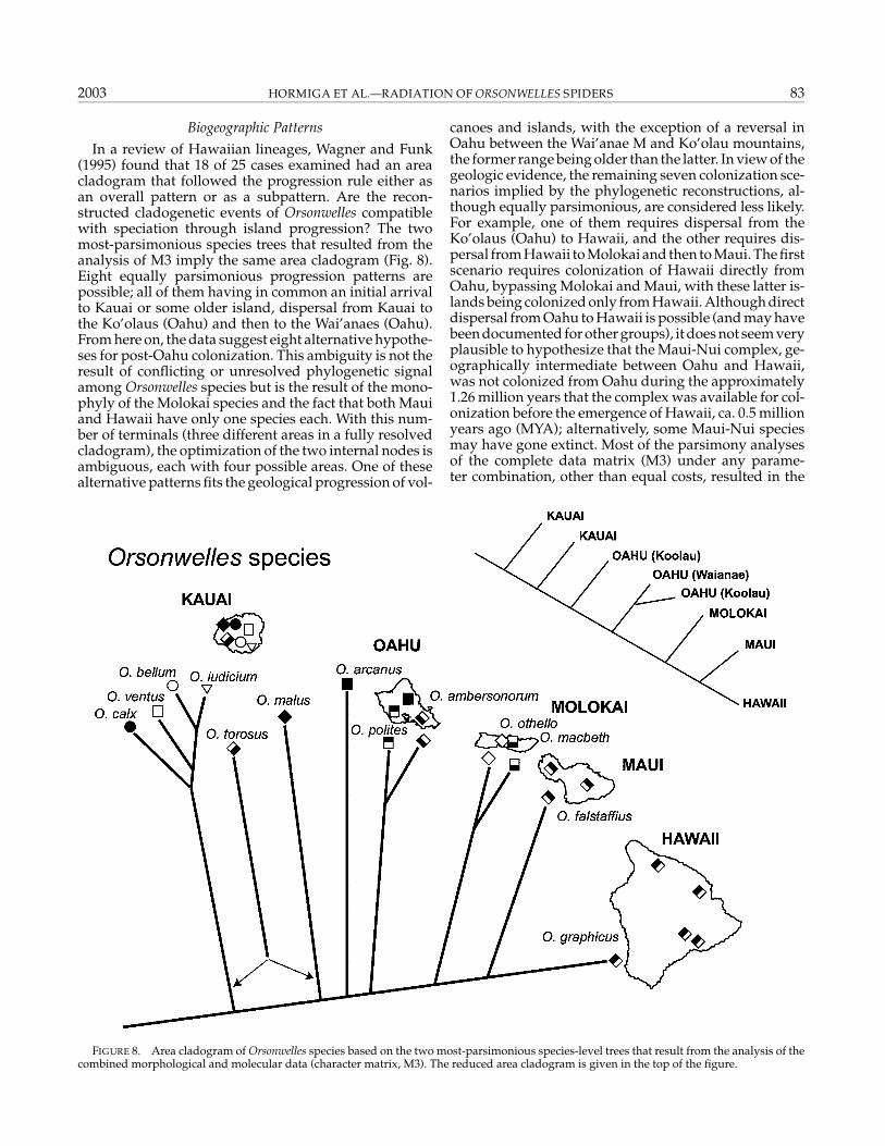
In a review of Hawaiian lineages, Wagner and Funk(1995) found that 18 of 25 cases examined had an areacladogram that followed the progression rule either asan overall pattern or as a subpattern. Are the recon-structed cladogenetic events of Orsonwelles compatiblewith speciation through island progression? The twomost-parsimonious species trees that resulted from theanalysis of M3 imply the same area cladogram (Fig. 8).Eight equally parsimonious progression patterns arepossible; all of them having in common an initial arrivalto Kauai or some older island, dispersal from Kauai tothe Ko’olaus (Oahu) and then to the Wai’anaes (Oahu).From here on, the data suggest eight alternative hypothe-ses for post-Oahu colonization. This ambiguity is not theresult of conflicting or unresolved phylogenetic signalamong Orsonwelles species but is the result of the mono-phyly of the Molokai species and the fact that both Mauiand Hawaii have only one species each. With this num-ber of terminals (three different areas in a fully resolvedcladogram), the optimization of the two internal nodes isambiguous, each with four possible areas. One of thesealternative patterns fits the geological progression of vol-

FIGURE 8. Area cladogram of Orsonwelles species based on the two most-parsimonious species-level trees that result from the analysis of thecombined morphological and molecular data (character matrix, M3). The reduced area cladogram is given in the top of the figure.

canoes and islands, with the exception of a reversal inOahu between the Wai’anae M and Ko’olau mountains,the former range being older than the latter. In view of thegeologic evidence, the remaining seven colonization sce-narios implied by the phylogenetic reconstructions, al-though equally parsimonious, are considered less likely.For example, one of them requires dispersal from theKo’olaus (Oahu) to Hawaii, and the other requires dis-persal from Hawaii to Molokai and then to Maui. The firstscenario requires colonization of Hawaii directly fromOahu, bypassing Molokai and Maui, with these latter is-lands being colonized only from Hawaii. Although directdispersal from Oahu to Hawaii is possible (and may havebeen documented for other groups), it does not seem veryplausible to hypothesize that the Maui-Nui complex, ge-ographically intermediate between Oahu and Hawaii,was not colonized from Oahu during the approximately1.26 million years that the complex was available for col-onization before the emergence of Hawaii, ca. 0.5 millionyears ago (MYA); alternatively, some Maui-Nui speciesmay have gone extinct. Most of the parsimony analysesof the complete data matrix (M3) under any parame-ter combination, other than equal costs, resulted in the

84 SYSTEMATIC BIOLOGY VOL. 52

monophyly of all the species from Kauai. This topolog-ical change would produce an area cladogram in whichthe optimization of the ingroup basal node would beambiguous (as would the optimization of the distal cladeincluding the species from Molokai, Maui, and Hawaii,because this topology remains unchanged). The ambi-guity of such an area cladogram again would not bethe result of conflicting or unresolved phylogenetic sig-nal among Orsonwelles species but rather the result ofthe monophyly of the Kauai species combined with themonophyly of the Molokai species and the fact that bothMaui and Hawaii have only one species each. As in thearea cladogram presented in Figure 8, with this num-ber of unique terminals (areas) the optimization of mostnodes is ambiguous. Among this many equally parsimo-nious optimizations, there is one optimal area cladogramthat is fully compatible with the progression rule. The un-ambiguous optimization of the ingroup basal node de-pends in part on the paraphyly of the species from Kauai.

The estimated ages of the cladogenic events withinOrsonwelles (Fig. 7, Table 3) are largely congruent withthe available geological evidence (Carson and Clague,1995). Dispersal from Kauai into the Ko’olau range wasused to calibrate the cladogram (2.6 MYA). The oldestdivergence within the genus (node 1) was estimated tohave occurred in Kauai about 4.15 MYA. Most of thecladogenesis in Kauai is estimated to have startedafter Oahu was colonized, around 2.56 MYA. The onlyspecies presently found in the Wai’anae Range of Oahu,O. polites, arrived there relatively late. The divergencebetween O. polites and O. ambersonorum is estimatedto have occurred about 1.5 MYA, although the oldestparts of that range are ca. 3.7 million years old. Thisobservation can be considered biogeographically odd,given the Wai’anae’s older age and closer distance toKauai, the actual source for colonizers. A reconciliationbetween the recovered phylogenetic pattern and thegeology and geography of the islands could be achievedby suggesting the extinction of a former Waianae speciesor population ancestral to the current species of Oahu.Alternatively, the Ko’olau species may have covered theentire island, with the Wai’anae species arising relativelyrecently from this widespread stock. In some of theanalyses, i.e., those under parameter combinationswith higher gap cost to any of the base transformations(411, 811, 821), located the extant Waianae species, O.polites, as the sister group to the remaining non-Kauaianspecies, providing a pattern more compatible with thegeological and geographical data.

The divergence between O. macbeth and O. othello, bothfrom Molokai, is also consistent with the age of the east-ern part of the island (ca. 1.76 million years). The only in-consistency between the estimated divergence ages andthe geological evidence is provided by the divergence be-tween O. falstaffius and O. graphicus (node 19, 1.50 MYA).The oldest parts of Hawaii are only about 0.5 millionyears old; thus, the divergence between O. falstaffius andO. graphicus implies that these species diverged beforethe emergence of Hawaii and that the split between thetwo clades was probably due to causes other than the col-

onization of the new island. The position of O. graphicusis also sensitive to changes in parameter costs. High gapcosts (421, 441, 811, 821, 841, 881) favored a sister grouprelationship of O. graphicus to the Maui-Nui species. Thistopology would be compatible with a split of O. graph-icus early during the colonization of Maui-Nui and itssubsequent dispersal to Hawaii once the island wasavailable for colonization. However, the reconstructedscenario would be extremely complex, requiring severalextinction events.

Speciation in Orsonwelles occurred within islands moreoften (8 of the 12 cladogenic events) than between is-lands. This scenario seems to fit the general pattern re-ported for diverse Hawaiian taxa. Wagner and Funk(1995) found that speciation on the Hawaiian Islandsoccurred approximately one-third interisland and two-thirds intraisland. In Orsonwelles, more than half (five ofeight) of these speciation events have occurred in Kauai.

Although allopatric speciation seems to be the domi-nant mode of speciation of Orsonwelles in the HawaiianIslands, partially overlapping distributions of somespecies could be compatible with cases of sympatric orparapatric speciation. There are no obvious geographicbarriers separating the distributions of the species pairsO. arcanus and O ambersonorum in Oahu’s Ko’olau Moun-tains. Similarly, no obvious barriers separate O. othelloand O. macbeth on Molokai, although on only one occa-sion have these two species been collected together (wecollected a single female of O. othello along Pepe’opaetrail, an area of high abundance of O. macbeth). In at leastone locality, the higher elevations of the Makaleha Moun-tains of Kauai, O. calx and O. ventus are found livingcompletely intermixed. In this case, the existence of ad-ditional localities exclusively inhabited by O. calx (e.g.,La’au Ridge) suggests that the coexistence of these twospecies could be due to secondary range expansion. Lo-calities where the two species pairs have been collectedtogether, from the Ko’olaus and Molokai, the two mem-bers of each pair tend to differ in preferred elevationand, more importantly, in type of forest. Orsonwelles ar-canus in Oahu and O. macbeth in Molokai seem to preferhigher altitude and very wet forests, whereas Oahu’s O.ambersonorum and Molokai’s O. othello have been largelycollected in mesic forests (Hormiga, 2002). Therefore, theexistence of parapatric speciation events, resulting froman ecological shift driven by adaptation to ecosystemswith different humidity regimes, cannot be completelydiscarded, at least to explain the origin of these speciespairs. More field and experimental data should be gath-ered to address this issue.

The prospects for determining the geographic originof Orsonwelles are weak because of the highly unusualmorphology of the genus and the difficulties involvedin identifying its closest sister group. The widespreaddistribution of the genus in the islands leads to an in-teresting paradox. Given that Orsonwelles species havecolonized every high Hawaiian island, why are noneof the 13 species found on more than one island? Whyare all Orsonwelles species single island endemics? Thepresence of these spiders throughout the archipelago

2003 HORMIGA ET AL.—RADIATION OF ORSONWELLES SPIDERS 85

suggests that their dispersal abilities, despite their largesize, are not impaired, otherwise they could not havecolonized all the high islands. Most Orsonwelles specieslive in similar habitats, and some tolerate substantialhabitat degradation (Hormiga, 2002). They are morpho-logically fairly uniform, except for genitalic differences.Their sheet webs are architecturally very similar, andthey are generalist predators. All these characteristicssuggest that it would be logical to find at least somespecies of Orsonwelles on more than one island, but suchis not the case.

ACKNOWLEDGMENTS

Most of the Orsonwelles specimens studied were collected duringthree 1-month field trips to the Hawaiian Islands. All islands were vis-ited at least twice except Lanai, which was visited only once. Additionalspecimens for study, including outgroup taxa, were made available bythe following individuals and institutions: Janet Beccaloni (NaturalHistory Museum, London), Jonathan Coddington (Smithsonian Insti-tution, Washington, D.C.), the late Ray Forster and Anthony Harris(Otago Museum, Dunedin, New Zealand), Charles Griswold(California Academy of Sciences, San Francisco), Frank Howarthand Gordon Nishida (Bishop Museum, Honolulu), Bernar Kumashiro(Hawaii Agriculture Department, Honolulu), Norman Platnick (Amer-ican Museum of Natural History, New York), and Christine Rollard(Museum National d’Histoire Naturelle, Paris). George Roderick andDan Polhemus provided additional Orsonwelles specimens from Oahuand Maui and information on their webs. Adam Asquith was instru-mental for the field work in Kauai; he also collected the first specimensof O. calx and O. bellum and made us aware of the importance of theMakaleha Mountains and Mt. Kahili as areas of endemism for Orson-welles spiders. Nikolaj Scharff, Jonathan Coddington, and Ingi Agnars-son have accompanied us on field trips to various parts of the HawaiianIslands and collected numerous specimens. Nikolaj Scharff also pro-vided specimens of outgroup taxa for molecular work. The followingindividuals have also provided specimens or information on locali-ties: Greta Binford, Todd Blackledge, Curtis Ewing, Jessica Garb, LauraGarcía de Mendoza, Scott Larcher, Jim Liebherr, Geoff Oxford, MaliaRivera, Warren Wagner, and Ken Wood. Brian Farrell (Harvard Univer-sity, Cambridge) hosted G.H. in his lab to test the suitability of some ofthe mitochondrial primers and to gather some preliminary moleculardata. Gonzalo Giribet (Harvard University) ran in his computer clustersome of most computationally intensive POY analyses. The followingindividuals and organizations have facilitated collecting and researchpermits and/or access to restricted areas: David Foote (Hawaii Volca-noes National Park), Betsy Gagné (State Natural Area Reserves Sys-tem), Edwin Pettys (State Department of Land and Natural Resources[DLNR]), Robin Rice (Kauai, access to Mt. Haupu), Victor Tanimoto(DLNR), and Joan Yoshioka (The Nature Conservancy). Randy Bartlett(Maui Pineapple Co.) provided access and helicopter transportation tothe Puu Kukui area and collected specimens in West Maui. The NatureConservancy has consistently provided excellent logistic support andeasy access to their reserves. Alexander & Baldwin Properties and Cas-tle & Cooke granted access to their land for fieldwork. Funding for thisresearch has been provided by grants from the National GeographicSociety (6138-98), the National Science Foundation (DEB-9712353), andthe Research Enhancement Fund from George Washington Universityto G.H., the Ministerio de Educacion y Cultura (Spain) to M.A., and theNational Science Foundation (DEB-0096307) to R.G.G., with additionalsupport from Dr. Evert Schlinger. Additional travel funds were grantedby the Smithsonian Institution. M. Kuntner provided comments on anearlier draft of this manuscript. We thank Keith Crandall, Rob DeSalle,Marshal Hedin, and Chris Simon for their thorough reviews that sub-stantially improved this manuscript.

REFERENCES

AJUH, P. M., P. A. HEENEY, AND B. E. MADEN. 1991. Xenopus borealis andXenopus laevis 28S ribosomal DNA and the complete 40S ribosomal

precursor RNA coding units of both species. Proc. R. Soc. Lond. BBiol. Sci. 245:65–71.

ARNEDO, M. A., P. OROMI, AND C. RIBERA. 2001. Radiation of the spidergenus Dysdera (Araneae, Dysderidae) in the Canary Islands: Cladisticassessment based on multiple data sets. Cladistics 17:313–353.

BAKER, R. H., AND R. DESALLE. 1997. Multiple sources of characterinformation and the phylogeny of Hawaiian Drosophila. Syst. Biol.46:654–673.

BARKER, F. K., AND F. M. LUTZONI. 2002. The utility of the incongruencelength difference test. Syst. Biol. 51:625–637.

BELSHAW, R., AND D. L. J. QUICKE. 2002. Robustness of ancestral stateestimates: Evolution of life history strategy in ichneumonoid para-sitoids. Syst. Biol. 51:450–477.

BREMER, K. 1988. The limits of amino acid sequence data in angiospermphylogenetic reconstruction. Evolution 42:795–803.

BREMER, K. 1994. Branch support and tree stability. Cladistics 10:295–304.

CARLQUIST, S. 1980. Hawaii, a natural history: Geology, climate, nativeflora and fauna above the shoreline, 2nd edition. Pacific TropicalBotanical Gardens, Lawai, Kauai.

CARSON, H. L., AND D. A. CLAGUE. 1995. Geology and biogeography ofthe Hawaiian Islands. Pages 14–29 in Hawaiian biogeography (W. L.Wagner and V. A. Funk, eds.). Smithsonian Institution, Washington,D.C.

CARSON, H. L., AND K. Y. KANESHIRO. 1976. Drosophila of Hawaii:Systematics and ecological genetics. Annu. Rev. Ecol. Syst. 15:97–131.

COLGAN, D. J., A. MCLAUCHLAN, G. D. F. WILSON, S. P. LIVINGSTON,G. D. EDGECOMBE, J. MACARANAS, G. CASSIS, AND M. R. GRAY.1998. Histone H3 and U2 snRNA DNA sequences and arthropodmolecular evolution. Aust. J. Zool. 46:419–437.

COWIE, R. H. 1995. Variation in species diversity and shell shape inHawaiian land snails: In situ speciation and ecological relationships.Evolution 49:1191–1202.

DESALLE, R., AND D. GRIMALDI. 1992. Characters and the systematicsof Drosophilidae. J. Hered. 83:182–188.

DESALLE, R., AND J. A. HUNT. 1987. Molecular evolution in Hawaiiandrosophilids. Trends Ecol. Evol. 2:212–216.

ELDREDGE, L. G., AND S. E. MILLER. 1995. How many species are therein Hawaii? Bishop Mus. Occas. Pap. 41:3–18.

FAITH, D. P., AND J. W. H. TRUEMAN. 2001. Towards an inclusive phi-losophy for phylogenetic inference. Syst. Biol. 50:331–350.

FARRIS, J. S. 1969. A successive approximations approach to characterweighting. Syst. Zool. 18:374–385.

FARRIS, J. S. 1988. HENNIG 86, version 1.5. Program and documen-tation. Available from D. Lipscomb, Dept. of Biological Sciences,George Washington University, Washington, DC 20052, USA.

FARRIS, J. S. 1989a. The retention index and the homoplasy excess. Syst.Zool. 38:406–407.

FARRIS, J. S. 1989b. The retention index and the rescaled consistencyindex. Cladistics 5:417–419.

FARRIS, J. S., M. KALLERSJO, A. G. KLUGE, AND C. BULT. 1994. Testingsignificance of incongruence. Cladistics 10:315–320.

FITCH, W. M. 1971. Toward defining the course of evolution: Minimumchange for a specific tree topology. Syst. Zool. 20:404–416.

FLEISCHER, R. C., C. E. MCINTOSH, AND C. L. TARR. 1998. Evolutionon a volcanic conveyor belt: Using phylogeographic reconstructionsand K-Ar-based ages of the Hawaiian Islands to estimate molecularevolutionary rates. Mol. Ecol. 7:533–545.

FOLMER, O., M. BLACK, W. HOEH, R. LUTZ, AND R. VRIJENHOEK. 1994.DNA primers for amplification of mitochondrial cytochrome c oxi-dase subunit I from diverse metazoan invertebrates. Mol. Mar. Biol.Biotechnol. 3:294–299.

FREED, L. A., S. CONANT, AND R. C. FLEISCHER. 1987. Evolutionaryecology and radiation of Hawaiian Usa passerine birds. Trends Ecol.Evol. 2:196–203.

GILLESPIE, R. G. 1991a. Hawaiian species of the genus Tetragnatha: I.Spiny leg clade. J. Arachnol. 19:174–209.

GILLESPIE, R. G. 1991b. Predation through impalement of prey: Theforaging behavior of Doryonichus raptor (Araneae, Tetragnathidae).Psyche 98:337–350.

GILLESPIE, R. G. 1992. Hawaiian spiders of the genus Tetragnatha: II.Species from natural areas of windward East Maui. J. Arachnol.20:1–17.

86 SYSTEMATIC BIOLOGY VOL. 52

GILLESPIE, R. G. 1993. Biogeographic patterns of phylogeny in aclade of endemic Hawaiian spiders (Araneae, Tetragnathidae). Mem.Queensl. Mus. 33:519–526.

GILLESPIE, R. G. 1994. Hawaiian spiders of the genus Tetragnatha: III.Tetragnatha acuta clade. J. Arachnol. 22:161–168.

GILLESPIE, R. G., AND H. B. Croom. 1992. Pattern and process in speci-ation: A comparative approach using a Hawaiian spider radiation.Am. J. Bot. 79:127.

GILLESPIE, R. G., AND H. B. CROOM. 1995. Comparison of speciationmechanisms in web-building and non-web-building groups withina lineage of spiders. Pages 121–146 in Hawaiian biogeography: Evo-lution on a hot spot archipelago (W. L. Wagner and V. A. Funk, eds.).Smithsonian Institution, Washington, D.C.

GILLESPIE, R. G., H. B. CROOM, AND G. L. HASTY. 1997. Phylogeneticrelationships and adaptive shifts among major clades of Tetragnathaspiders (Araneae: Tetragnathidae) in Hawai’i. Pac. Sci. 51:380–394.

GILLESPIE, R. G., H. B. CROOM, AND S. R. PALUMBI. 1994. Multipleorigins of a spider radiation in Hawaii. Proc. Natl. Acad. Sci. USA91:2290–2294.

GIRIBET, G. 2001. Exploring the behavior of POY, a program for directoptimization of molecular data. Cladistics 17:S60–S70.

GIRIBET, G., S. CARRANZA, M. RIUTORT, J. BAGUNA, AND C. RIBERA.1999. Internal phylogeny of the Chilopoda (Myriapoda, Arthropoda)using complete 18S rDNA and partial 28S rDNA sequences. Philos.Trans. R. Soc. Lond. B Biol. Sci. 354:215–222.

GIRIBET, G., AND W. C. WHEELER. 1999. On gaps. Mol. Phylogenet.Evol. 13:132–143.

GOLOBOFF, P. A. 1993. NONA, version 2.0. Program available athttp://www.cladistics.com.

GOLOBOFF, P. A. 1999. Analyzing large data sets in reasonable times:Solutions for composite optima. Cladistics 15:415–428.

HEDIN, M. C. 1997a. Molecular phylogenetics at the popula-tion/species interface in cave spiders of the southern Appalachians(Araneae: Nesticidae: Nesticus). Mol. Biol. Evol. 14:309–324.

HEDIN, M. C. 1997b. Speciational history in a diverse clade of habitat-specialized spiders (Araneae: Nesticidae: Nesticus): Inferences fromgeographic-based sampling. Evolution 51:1929–1945.

HORMIGA, G. 1994a. Cladistics and the comparative morphologyof linyphiid spiders and their relatives (Araneae, Araneoidea,Linyphiidae). Zool. J. Linn. Soc. 111:1–71.

HORMIGA, G. 1994b. A revision and cladistic analysis of the spiderfamily Pimoidae (Araneoidea: Araneae). Smithson. Contrib. Zool.549:1–104.

HORMIGA, G. 2000. Higher level phylogenetics of erigonine spiders(Araneae, Linyphiidae, Erigoninae). Smithson. Contrib. Zool. 609:1–160.

HORMIGA, G. 2002. Orsonwelles, a new genus of giant linyphiid spiders(Araneae) from the Hawaiian Islands. Invertebr. Syst. 16:369–448.

HOWARTH, F. G., AND W. P. MULL. 1992. Hawaiian insects and theirkin. Univ. Hawaii Press, Honolulu.

JORDAN, S., C. SIMON, AND D. POLHEMUS. 2003. Molecular system-atics and adaptive radiation of Hawaii’s endemic damselfly genusMegalagrion (Odonata: Coenagrionidae). Syst. Biol. 52:89–109.

LIEBHERR, J. K. 1995. Description of the larval stages of Disenochusfractus Sharp and the origin of the Hawaiian platynine Carabidae(Coleoptera). Syst. Entomol. 20:17–26.

LIEBHERR, J. K. 1997. Dispersal and vicariance in Hawaiian platyninecarabid beetles (Coleoptera). Pac. Sci. 51:424–439.

LIEBHERR, J. K. 2000. The unity of characters: Ecological and mor-phological specialisation in larvae of Hawaiian platynini Carabidae(Coleoptera). Invertebr. Taxon. 14:931–940.

LIEBHERR, J. K., AND E. C. ZIMMERMAN. 1998. Cladistic analysis, phy-logeny and biogeography of the Hawaiian Platynin (Coleoptera:Carabidae). Syst. Entomol. 23:137–172.

LUTZONI, F., P. WAGNER, V. REEB, AND S. ZOLLER. 2000. Integrating am-biguously aligned regions of DNA sequences in phylogenetic anal-yses without violating positional homology. Syst. Biol. 49:628–651.

MICKEVICH, M. F., AND J. S. FARRIS. 1981. The implications of incon-gruence in Menidia. Syst. Zool. 30:351–370.

MILLIDGE, A. F. 1991. Further linyphiid spiders (Araneae) from SouthAmerica. Bull. Am. Mus. Nat. Hist. 205:1–199.

MLOT, C. 1995. Biological surveys in Hawaii, taking inventory of abiological hot spot. Science 269:322–323.

NIXON, K. C. 1999. WinClada, version 0.9.99m24. Program available athttp://www.cladistics.com.

OTTE, D. 1994. The crickets of Hawaii: Origin, systematics and evolu-tion. Orthopterists’ Society, Philadelphia.

PAGE, R. D. M. 2001. NDE (Nexus data editor), version 0.4.9. Pro-gram available at http://taxonomy.zoology.gla.ac.uk/rod/NDE/nde.html.

PALUMBI, S. A., S. MARTIN, S. ROMANO, W. O. MCMILLAN, L. STICE,AND G. GRABOWSKI. 1991. The simple fool’s guide to PCR, version2.0. Department of Zoology. Univ. Hawaii, Honolulu.

PLATNICK, N. I. 2001. The world spider catalog, version 2.0. Availableat http://research.amnh.org/entomology/.

POSADA, D., AND K. A. CRANDALL. 1998. Modeltest: Testing the modelof DNA substitution. Bioinformatics 14:817–818.

RAMBAUT, A., AND M. CHARLESTON. 2001. TREEEDIT, version 1.0 alfa8. Program available at http://evolve.zoo.ox.ac.uk.

RODERICK, G. K., AND R. G. GILLESPIE. 1998. Speciation and phy-logeography of Hawaiian terrestrial arthropods. Mol. Ecol. 7:519–531.

SANDERSON, M. J. 1997. A nonparametric approach to estimating diver-gence times in the absence of rate constancy. Mol. Biol. Evol. 14:1218–1231.

SANGER, F., S. NICKLEN, AND A. R. COULSEN. 1977. DNA sequenc-ing with chain terminating inhibitors. Proc. Natl. Acad. Sci. USA74:5463–5468.

SANKOFF, D. 1975. Minimal mutation trees of sequences. Soc. Ind. Appl.Math. J. Appl. Math. 28:35–42.

SHAW, K. L. 1995. Biogeographic patterns of two independent Hawai-ian cricket radiations (Laupala and Prognathogryllus). Pages 39–56in Hawaiian biogeography: Evolution on a hot spot archipelago(W. L. Wagner and V. A. Funk, eds.). Smithsonian Institution Press,Washington, D.C.

SHAW, K. L. 1996a. Sequential radiations and patterns of speciation inthe Hawaiian cricket genus Laupala inferred from DNA sequences.Evolution 50:237–255.

SHAW, K. L. 1996b. Polygenic inheritance of a behavioral phenotype:Interspecific genetics of song in the Hawaiian cricket genus Laupala.Evolution 50:256–266.

SIMMONS, M. P., AND H. OCHOTERENA. 2000. Gaps as characters insequence-based phylogenetic analyses. Syst. Biol. 49:369–381.

SIMON, C. 1987. Hawaiian evolutionary biology: An introduction.Trends Ecol. Evol. 2:175–178.

SIMON, C., F. FRATI, A. BECKENBACH, B. CRESPI, H. LIU, AND P. FLOOK.1994. Evolution, weighting, and phylogenetic utility of mitochon-drial gene sequences and a compilation of conserved polymerasechain reaction primers. Ann. Entomol. Soc. Am. 87:651–701.

SIMON, E. 1900. Arachnida. Pages 443–519 in Fauna Hawaiiensis, orthe zoology of the Sandwich Isles: Being results of the explorationsinstituted by the Royal Society of London promoting natural knowl-edge and the British Association for the Advancement of Science,London. Royal Society, London.

STEARNS, H. T. 1985. Geology of the state of Hawaii, 2nd edition. PacificBooks, Palo Alto, California.

SULLIVAN, J., K. E. HOLSINGER, AND C. SIMON. 1996. The effect oftopology on estimates of among-site rate variation. J. Mol. Evol. 42:308–312.

SWOFFORD, D. L. 2001. PAUP∗: Phylogenetic analysis using parsimony(∗and other methods), version 4.0b5 (PPC). Sinauer, Sunderland,Massachusetts.

TARR, C. L., AND R. C. FLEISCHER. 1995. Evolutionary relationshipsof the Hawaiian honeycreepers (Aves, Drepanidinae). Pages 147–158 in Hawaiian biogeography: Evolution on a hot spot archipelago(W. L. Wagner and V. A. Funk, eds.). Smithsonian Institution Press,Washington, D.C.

VAN HELSDINGEN, P. J. 1969. A reclassification of the species of LinyphiaLatreille, based on the functioning of the genitalia (Araneida,Linyphiidae) I. Zool. Verh. (Leiden) 105:1–303.

VAN HELSDINGEN, P. J. 1970. A reclassification of the species of LinyphiaLatreille, based on the functioning of the genitalia (Araneida,Linyphiidae) II. Zool. Verh. (Leiden) 111:1–86.

WAGNER, W. L., AND V. A. FUNK (eds.). 1995. Hawaiian biogeography:Evolution on a hot spot archipelago. Smithsonian Institution Press,Washington, D.C.

2003 HORMIGA ET AL.—RADIATION OF ORSONWELLES SPIDERS 87

WHEELER, W. C. 1990. Nucleic acid sequence phylogeny and randomoutgroups. Cladistics 6:363–368.

WHEELER, W. C. 1995. Sequence alignment, parameter sensitivity, andthe phylogenetic analysis of molecular data. Syst. Biol. 44:321–331.

WHEELER, W. C. 1996. Optimization alignment: The end of multiplesequence alignment in phylogenetics? Cladistics 12:1–9.

WHEELER, W. C. 1999. Measuring topological congruence by extendingcharacter techniques. Cladistics 15:131–135.

WHEELER, W. C., AND D. GLADSTEIN. 2000. POY. Program and docu-mentation, available at ftp://amnh.org/pub/molecular.

WHITING, M. F., J. C. CARPENTER, Q. D. WHEELER, AND W. C. WHEELER.1997. The strepsiptera problem: Phylogeny of the holometabolousinsect orders inferred from 18S and 28S ribosomal DNA sequencesand morphology. Syst. Biol. 46:1–68.

WIEHLE, H. 1956. Spinnentiere oder Arachnoidea. X. 28. FamilieLinyphiidae. Tierwelt Dtsch 44:1–337.

First submitted 1 October 2001; reviews returned 25 January 2002;final acceptance 22 October 2002

Associate Editor: Keith Crandall

APPENDIX 1MORPHOLOGICAL CHARACTERS AND CHARACTER

STATESCharacters for Orsonwelles were described and illustrated by

Hormiga (2002); additional characters are denoted with an asteriskafter the character number. Illustrations refer to figures of Hormiga(2002) unless otherwise stated. All multistate characters were treatedas nonadditive.

Male Genitalia1. Male pedipalpal tibial length: 0= short (less than twice its width);

1= long (more than twice its width).2. Paracymbium morphology: 0=flat, large; 1= small, thin; 2=

knob.3. Paracymbium apophyses: 0=present; 1= absent.4. Retromarginal cymbial apophysis: 0= absent; 1=present.

5∗. Mesal cymbial apophysis: 0= absent; 1=present (Hormiga, 2002:figs. 15C, 15D).

6. Cymbial orifice: 0= absent; 1=present.7. Distal end of tegulum: 0= round; 1= subtle to medium projection;

2= elongated and projected.8. Apex of tegular projection: 0= round; 1=pointed.9. Suprategular base: 0= same width; 1= enlarged.

10. Suprategular base enlargement: 0=flat; 1=with depression.11. Suprategular ectal margin: 0= thick; 1= thin or membranous.12. Embolus base: 0= broad; 1=narrow.13. Embolus apical half: 0=filiform; 1=not threadlike.14. Embolic membrane: 0= absent; 1=present.15. Column position on suprategulum: 0=distal; 1=proximal.16. Fickert’s gland: 0= absent; 1=present.17. Terminal apophysis position: 0= apical-ectoventral; 1=mesal;

2= ectal.18∗. Terminal apophysis dimension: 0= longer than wide (Hormiga,

2002: fig. 17D); 1= as wide as long or wider (Hormiga, 2002:fig. 29C).

19. Terminal apophysis size: 0= small; 1= large (similar in size tolamella characteristica); 2 = tiny.

20. Terminal apophysis shape: 0= entire; 1= tri (or tetra)-lobed.21. Terminal apophysis coiling: 0=not coiled; 1= spirally coiled.

22∗. Terminal apophysis basal process: 0= round, straight (Hormiga,2002: fig. 27E); 1= angulated, twisted (Hormiga, 2002:fig. 19E).

23. Terminal apophysis apical process: 0=pointed; 1= round.24. Terminal sclerite: 0= absent; 1=present.

25∗. Terminal sclerite: 0=membranous or bladelike (Hormiga, 2002:figs. 19B, 19G); 1= globular (Hormiga, 2002: figs. 25C, 25G).

26∗. Terminal sclerite tooth crest: 0= absent (Hormiga, 2002: fig. 27F);1=present (Hormiga, 2002: figs. 25C, 25G).

27. Transversal sclerite: 0= absent; 1=present.28. Lamella characteristica (LC): 0= small; 1= large.

29. Ectal process of lamella: 0=flat, thin, or membranous (bladelike);1= thick (round section); 2= blunt.

30∗. Elongated ectal process of lamella: 0= straight (Hormiga, 2002:figs. 21A, 21D); 1= curved, falciform (Hormiga, 2002: fig. 27A).

31. Striated area of LC: 0= long (at least three times longer thanwider); 1= short (less than three times longer than wider).

32∗. Striated area of LC: 0=parallel to ectal process of LC (Hormiga,2002: figs. 17D, 39B); 1=perpendicular to ectal process of LC(Hormiga, 2002: figs. 35C, 57C).

33. Mesal tooth of LC: 0= absent; 1=present.34. Mesal tooth of LC, size: 0= small; 1= large.35. Mesal tooth of LC, position: 0=medial (open curve at LC base);

1= basal (more closed curve).36. Prolateral trichobothria in male pedipalpal tibia: 0= 1; 1= 3; 2= 4.37. Retrolateral trichobothria in male pedipalpal tibia: 0= 2; 1= 3;

2= 4 or more.

Female Genitalia38. Epigynal dimension (ventral view): 0= longer than wider; 1= as

wide as long or wider.39. Epigynum caudal region (ventral view): 0= straight to round; 1=

V-shaped; 2=U-shaped.40. Dorsal plate scape: 0= absent; 1=present.41. Ventral plate scape: 0= absent; 1=present.42. Dorsal plate epigynal socket: 0=present; 1= absent.

43∗. Ventral plate epigynal socket: 0= absent (Wiehle, 1956: figs. 482,483); 1=present (Wiehle, 1956: figs. 263, 264).

44. Median epigynal septum: 0= absent; 1=present.45∗. Epigynal lateral edges: 0= continuous (Hormiga, 2002: figs. 20D–

F); 1= interrupted in medial region (Hormiga, 2002: figs. 30A–C).46. Epigynum lateral edge: 0= curved; 1= straight; 2= sigmoid.47. Dorsal plate incision: 0= absent; 1=present.48. Atrium: 0= absent; 1=present.

49∗. Atrium: 0= large and conspicuous (Van Helsdingen, 1969: fig. 21);1= small and inconspicuous (Van Helsdingen, 1970: fig. 38).

50∗. Atrium: 0= spiral grooves (Van Helsdingen, 1969: figs. 316, 321);1= spiral folds (Van Helsdingen, 1969: fig. 21); 2= smooth (VanHelsdingen, 1970: fig. 38)

51∗. Copulatory duct: 0= separate from fertilization duct (VanHelsdingen, 1969: fig. 21); 1= spirals around fertilization duct(Van Helsdingen, 1970: fig. 38).

52. Copulatory duct turning point: 0= absent; 1=present.53. Fertilization duct orientation: 0=posterior; 1=mesal; 2=

anterior.

Somatic Morphology54. PME: 0=not on black tubercles or without entire black rings; 1=

on black tubercles.55. Male chelicerae: 0= smooth; 1=with stridulatory striae.56. Cheliceral stridulatory striae: 0= ridged; 1= scaly; 2= imbricated.

57∗. Dorsal spur on male chelicerae: 0= absent; 1=present.58. Prolateral teeth in female chelicerae: 0= 6 or less; 1= 9–13; 2= 14

or 15; 3 = 16 or more.59. Retrolateral teeth in female chelicerae: 0= 6 or less; 1 = 7–9; 2 =

10 or more.60. Prolateral teeth in male chelicerae: 0= 5 or less; 1= 9–11; 2= 12–14;

3 = 15 or more.61. Retrolateral teeth in male chelicerae: 0 = 5 or less; 1 = 7–9; 2 = 10

or more.62. Retrolateral spines tibia III, female: 0=none; 1= 1 or more.63. Retrolateral spines tibia IV, female: 0=none; 1= 1 or more.64. Femur II–IV spines: 0= absent; 1=present.65. Femur II dorsal spines, female: 0= 3 or less; 1= 4 or more.66. Trichobothria femur III: 0= absent; 1=present.

67∗. Trichobothria femur III female: 0 = 1 or 2; 1 = 3 or more.68. Trichobothria femur IV: 0= absent; 1=present.

69∗. Trichobothria femur IV, female: 0 = 1 or 2; 1 = 3 or more.70. Trichobothrium metatarsus IV: 0=present; 1= absent.

Behavior71. Web: 0=without funnel: 1=with funnel leading into a retreat.

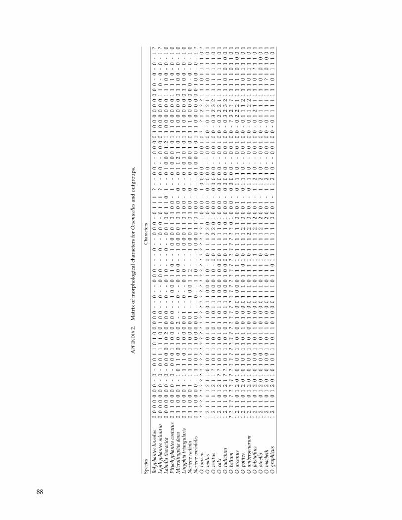
AP

PE

ND

IX2.

Mat

rix

ofm

orph

olog

ical

char

acte

rsfo

rO

rson

wel

les

and

outg

roup

s.

Spec

ies

Cha

ract

ers

Bol

ypha

ntes

lute

olus

00

00

00

0-

0-

00

11

01

00

00

0-

-0

--

00

0-

--

0-

-0

00

-0

11

1?

--

00

--

00

00

10

00

00

00

00

-0

-0

-1

?Le

pthy

phan

tes

min

utus

00

00

00

0-

0-

00

11

11

00

10

0-

-0

--

00

0-

--

0-

-0

00

-0

11

1?

--

00

--

00

00

10

00

00

01

10

-0

-0

-1

?La

bulla

thor

acic

a0

00

00

00

-0

-0

00

01

02

00

00

--

0-

-0

10

--

-0

--

00

10

01

10

1-

-0

10

00

12

11

00

00

00

11

10

0-

0-

10

Pit

yohy

phan

tes

cost

atus

01

10

00

0-

0-

00

01

10

00

00

0-

-1

00

01

10

--

10

00

01

01

00

-1

--

01

00

01

01

11

00

00

01

11

10

-0

-1

0M

icro

linyp

hia

dana

01

10

00

1-

10

11

00

10

-0

2-

--

-0

--

01

00

--

10

00

01

01

00

-0

--

01

12

11

01

11

00

00

00

11

00

-0

-1

0Li

nyph

iatr

iang

ular

is0

11

00

01

-1

11

10

11

00

00

01

--

0-

-0

10

--

-1

00

01

10

10

0-

0-

-0

10

10

10

11

10

00

00

01

10

0-

0-

10

Ner

iene

radi

ata

01

10

00

1-

11

10

11

10

00

00

1-

-1

00

11

2-

--

10

00

11

01

00

-0

--

01

00

01

00

11

10

00

00

00

-0

-0

-1

0N

erie

neva

riab

ilis

01

10

00

0-

11

10

11

10

00

00

1-

-0

--

11

0-

--

10

00

11

01

00

-0

--

01

00

01

01

11

00

00

00

01

00

-0

-1

?O

.tor

osus

??

??

??

??

??

??

??

??

??

??

??

??

??

??

??

??

??

??

?1

10

00

-1

00

00

--

00

10

?-

?1

2?

?1

11

01

11

10

?O

.mal

us1

21

11

12

11

01

01

11

01

01

10

01

10

00

10

-0

01

11

22

01

00

0-

01

00

0-

-0

01

00

-0

11

21

11

10

11

11

01

O.v

entu

s1

21

11

12

11

?1

01

11

01

01

10

11

10

00

10

-0

01

11

22

01

00

0-

00

00

0-

-0

01

00

-0

32

32

11

11

11

11

01

O.c

alx

12

11

01

21

??

10

11

10

10

11

01

11

00

01

00

00

11

11

10

10

00

-0

00

00

--

00

10

0-

02

22

11

11

11

11

10

1O

.iud

iciu

m1

21

10

12

1?

?1

01

11

01

01

10

11

10

00

10

00

01

11

11

01

00

0-

00

00

0-

-0

01

00

-0

32

32

11

10

10

10

01

O.b

ellu

m?

??

??

??

??

??

??

??

??

??

??

??

??

??

??

??

??

??

??

01

00

0-

00

00

0-

-0

01

00

-?

32

??

11

11

10

11

01

O.a

rcan

us1

21

10

12

01

01

01

11

01

00

10

00

10

00

11

11

01

11

11

10

00

1-

01

11

0-

-0

01

00

-0

22

21

11

11

10

10

01

O.p

olit

es1

21

10

12

01

01

01

11

01

10

10

00

11

10

11

01

01

11

12

10

00

1-

01

11

0-

-0

01

00

-0

11

12

11

10

11

11

01

O.a

mbe

rson

orum

12

11

01

20

10

10

11

10

10

01

00

01

11

01

11

10

11

12

21

00

01

-0

11

10

--

00

10

0-

01

12

21

11

01

11

10

1O

.fal

staf

fius

12

11

01

20

10

10

01

10

11

01

00

01

11

01

11

11

11

11

21

20

01

-1

12

10

--

00

10

0-

01

21

11

11

01

?1

10

1O

.oth

ello

12

11

01

20

10

10

01

10

11

01

00

01

11

01

11

10

11

11

21

20

01

-1

12

10

--

00

10

0-

01

11

11

11

01

01

00

1O

.mac

beth

12

11

01

20

10

10

01

10

11

01

00

01

11

01

11

10

11

11

11

20

01

-1

12

10

--

00

10

0-

01

11

11

11

?1

01

00

1O

.gra

phic

us1

21

10

12

01

01

01

11

01

10

10

00

11

10

11

01

11

11

11

10

00

1-

11

21

0-

-0

01

00

-0

11

11

11

10

11

11

01

88