speaker distinguishing distances: a comparative study

Int J Speech Technol (2007) 10: 95–107DOI 10.1007/s10772-009-9022-z

Speaker distinguishing distances: a comparative study

Ananth N. Iyer · Uchechukwu O. Ofoegbu ·Robert E. Yantorno · Brett Y. Smolenski

Received: 8 March 2007 / Accepted: 16 February 2009 / Published online: 10 March 2009© Springer Science+Business Media, LLC 2009

Abstract Speaker discrimination is a vital aspect of speakerrecognition applications such as speaker identification, ver-ification, clustering, indexing and change-point detection.These tasks are usually performed using distance-based ap-proaches to compare speaker models or features from ho-mogeneous speaker segments in order to determine whetheror not they belong to the same speaker. Several distancemeasures and features have been examined for all the dif-ferent applications, however, no single distance or featurehas been reported to perform optimally for all applicationsin all conditions. In this paper, a thorough analysis is madeto determine the behavior of some frequently used distancemeasures, as well as features, in distinguishing speakers fordifferent data lengths. Measures studied include the Maha-lanobis distance, Kullback-Leibler (KL) distance, T 2 sta-tistic, Hellinger distance, Bhattacharyya distance, General-ized Likelihood Ratio (GLR), Levenne distance, L2 and L∞distances. The Mel-Scale Frequency Cepstral Coefficient(MFCC), Linear Predictive Cepstral Coefficients (LPCC),Line Spectral Pairs (LSP) and the Log Area Ratios (LAR)comprise the features investigated. The usefulness of thesemeasures is studied for different data lengths. Generally, alarger data size for each speaker results in better speaker

A.N. Iyer (�)Conversay, Redmond, WA, USAe-mail: [email protected]

U.O. OfoegbuMongomery College, Rockville, MD, USA

R.E. YantornoTemple University, Philadelphia, PA, USA

B.Y. SmolenskiRADC, Rome, NY, USA

differentiating capability, as more information can be takeninto account. However, in some applications such as seg-mentation of telephone data, speakers change frequently,making it impossible to obtain large speaker-consistent ut-terances (especially when speaker change-points are un-known). A metric is defined for determining the probabilityof speaker discrimination error obtainable for each distancemeasure using each feature set, and the effect of data size onthis probability is observed. Furthermore, simple distance-based speaker identification and clustering systems are de-veloped, and the performances of each distance and featurefor various data sizes are evaluated on these systems in or-der to illustrate the importance of choosing the appropri-ate distance and feature for each application. Results showthat for tasks which do not involve any limitation of datalength, such as speaker identification, the Kullback Leiblerdistance with the MFCCs yield the highest speaker differ-entiation performance, which is comparable to results ob-tained using more complex state-of-the-art speaker identifi-cation systems. Results also indicate that the Hellinger andBhattacharyya distances with the LSPs yield the best perfor-mance for small data sizes.

Keywords Speaker discrimination · Distances · Speakeridentification · Speaker clustering

1 Introduction

Several speech processing applications, such as speakerrecognition (speaker identification (SID) and speaker veri-fication (SV)), speaker indexing, speaker change-point de-tection and automatic speaker count systems are based ondifferentiating between speakers. Techniques used in per-forming these tasks usually rely on distance/divergence

mailto:[email protected]

96 Int J Speech Technol (2007) 10: 95–107

measures, be it statistical or probabilistic. Some commondistances used for speaker recognition include Euclidean,Mahalanobis and L∞ (Cityblock) distances (Ong and Yang1998). For speaker indexing and change-point detection, theKullback Leibler and Gaussian Likelihood Ratio (Delacourtand Welkens 2000) distances have been used. Recently, theT 2 statistic was applied in an automatic speaker count sys-tem (Ofoegbu et al. 2006c). These are just a few of theuses of distance measures in speech processing. It must benoted that other speaker differentiating methods exists suchas the use of Gaussian Mixture Models (GMM) (Reynolds1992), Hidden Markov Models (HMM) (Matsui and Furui1994) and Neural Networks (Rudasi and Zahorian 1991),and have been used widely especially in speaker recogni-tion (Naik 1990); nevertheless, such methods have severalrestrictions such as data length and parametric assumptions.For instance, the use of GMM for speaker recognition re-quires that the training and test speech files be at least 5 sec-onds in length (Chaudhari et al. 2001). Moreover, these ap-proaches also involve some similarity or likelihood mea-surements. The use of distance measures, on the other hand,allows for flexibility with such factors, as the particular typeof distance computation can be selected based the intendedapplication. This flexibility is more desirable since, in sev-eral applications, requirements such as large data length maynot be realizable.

Although many distance measures have similar proper-ties, no single distance measure can be said to be optimumfor all speaker discrimination applications. In other words,some measures possess properties that enable them performbetter than others with certain data lengths, probability den-sity functions, channel conditions, etc. Lack of informationon the distance measure to be used based on the applica-tion in question, could result in the sub-optimal or even un-desirable performance of an otherwise technically valid ap-proach. This problem is sometimes circumvented by the fu-sion of several distance measures so as to take advantageof the positive effects of all of them, and possibly nullifythe negative effects (Delacourt and Welkens 2000). Fusionis not always the most advantageous since all distances usedmay not be uncorrelated; moreover, it could be unnecessar-ily very computationally expensive and redundant. A moreappropriate solution would be to thoroughly examine severaldistance measures as they are implemented in various appli-cations under different conditions and then utilize the infor-mation obtained to more suitably select a distance measurefor the speaker discrimination task.

Distance measures have been applied in various applica-tions involving speaker differentiation. Some of these previ-ous efforts are discussed below. Ong and Yang (1998) per-formed a comparative study of the use of distance measuresas well Gaussian probability density estimates in speaker

identification. Their results showed that, in general, like-lihood estimates yielded higher results than distance mea-sures, however, this was possibly due to the fact that thedistance measures studied, which include the Euclidean andCityblock distances, were simplified models of the Gaussianprobability estimates themselves. Moreover, when a weight-ing function was applied to the Euclidean distance, resultingin the Mahalanobis distance, it outperformed all other fea-tures. For speaker indexing, Delacourt and Welkens (2000)made an effort to improve the performance of the BayesianInformation Criterion (BIC) technique developed by Chenand Gopalakrishnan (1998a) by combining decisions of theGeneralized Likelihood Ratio (GLR) and Kullback-Leibler(KL) distances as well as four similarity measures in or-der to tentatively detect speaker change points, which werethen refined using the BIC algorithm. This modification wasshown to enhance considerably their speaker indexing sys-tem. One observation made by Delacourt and Wellekens wasthat the distance-based parameters varied significantly withvarying data lengths. An effort was also made by Ofoegbuet al. (2006c) to determine the number of speakers in a tele-phone conversation using the T 2 statistic. It was reportedthat the performance of the distance statistic improved withincreasing data lengths. All the above mentioned observa-tions depict the sensitivity of distance measures and pro-vide a motivation for a comprehensive study of distancesand their performances under various conditions.

In 1976, Gray and Markel (1976) presented a review ofdistance measures for speech processing. The Root MeanSquare (RMS) log spectral distance, cepstral distance, like-lihood ratio, and a cosh measure were investigated. Al-though a detailed explanation of these measures and theirbehaviors was given, there was no discussion or conclu-sion about their implementation in speaker discriminationor even any speech processing application. In 1980, Grayet al. (1980) performed another speech processing distancestudy which was very similar to the former, except that moredistances were observed, and a more careful and compre-hensive analysis was performed. Nevertheless, the distanceswere still not directly related to their relevance in speechprocessing applications. Bimbot and Magrin-Chagnolleau(1995) later investigated the use of similarity measuresfor SID which include the Gaussian likelihood measure,the Arithmetic-geometric sphericity measure, and the sym-metrization measure. Although the research also involved acomparison of the performance of these measures in SIDsystems, the only varying factors in the experiments werethe distances themselves and the relative amounts of train-ing and testing data. Moreover, the distance study focusedmainly on SID, as opposed to the general speaker dis-crimination task. With regards to features, de Souza (1977)presented a study of statistical distances for differentiatingshort segments of Linear Predictive Coefficients (LPCs) of

Int J Speech Technol (2007) 10: 95–107 97

speech. The distances studied included Itakura’s χ2 test,Quenoille’s test and the regression test. However, the studywas not directly linked to any specific speech processing ap-plication. Moreover, the use of Cepstral coefficients, ratherthan LPCs, for speech or speaker discrimination, is morestate-of-the art.

In this research, an effort has been made to thoroughlyexamine several commonly used distance measures in cur-rent speaker discrimination applications. The goal of thisresearch is to provide a comprehensive guide for the se-lection of distances for any speaker discrimination basedtask depending on the features being used, the applica-tion considered and the average length of speaker consis-tent data available for comparison. The measures studiedinclude The Mahalanobis distance, Kullback-Leibler (KL)distance, T 2 statistic, Hellinger distance, Bhattacharyya dis-tance, Gaussian Likelihood Ratio (GLR), Levenne, L2 andL∞ distances. The most common features applied in dif-ferentiating speakers are the Mel-Scale Frequency CepstralCoefficient (MFCC) and the Linear Predictive Cepstral Co-efficients (LPCC); hence the distance study is performed onthese features. Other features considered include the LineSpectral Pairs (LSP) and the Log Area Ratio (LAR). Testsare carried out in order to observe and compare the perfor-mance of all the various distances in speaker discriminationapplications such as SID and speaker clustering.

This paper is organized as follows: a detailed descrip-tion of all the distances observed is given in Sect. 2. Acomprehensive comparison of the distances is presented inSect. 3, followed by illustrations and comparisons of the per-formances of the distances in specific applications in Sect. 4,and a summary with conclusions based on the results alongwith possible future investigations are discussed in Sect. 5.

2 Distance measures

The distance measures considered in this study can bedivided into three major groups—(i) statistical distances,(ii) distances based on the f -divergence and (iii) non-parametric distances. The former two groups assume a para-metric probability density function (pdf) for the data sam-ples being used to compute the distance, whereas the latergroup measures the separation between two sets of points.The general approach to compute a distance between twosegments of speech is to extract short-time feature vectorsfrom the two segments and treat them as samples generatedby a random process. To streamline the presentation in thefollowing sections, the following notation is introduced. Let

X � {xi; i = 1,2, . . . ,N}, (1)

Y � {yi; i = 1,2, . . . ,M} (2)

represent the two sets of feature vectors extracted from thetwo segments, where xi and yi represent a p-dimensionalfeature vector, and px(x) and py(y) represent the pdfs of thetwo sets. In the first two groups of distances (parametric), thepdf is assumed to follow a multivariate Gaussian distributiongiven by:

px(x) = 1

(2π)p2 |�x | 1

2

exp

{−1

2(x − μx)

T �−1x (x − μx)

}.

(3)

The distances comprised in the third group do not assumeany parametric form of the underlying distribution of fea-ture vectors and hence are aptly termed non-parametric dis-tances. A function d(X , Y ) is regarded as a distance mea-sure between the two sets, if it obeys the following funda-mental properties:

d(X , Y ) ≥ 0, (4)

d(X , Y ) = 0 iff X = Y , (5)

d(X , Y ) = d(Y , X ), (6)

d(X , Y ) ≤ d(X , Z) + d(Z, Y ). (7)

Functions satisfying the above properties may be related be-tween the pdfs px(x) and py(y), their parameters {μx,�x}and {μy,�y}, or simple, the sample vectors themselves. Thedistance measures studied in this work are presented below.

2.1 Statistical distance measures

In general, the statistical distances are formed as a result ofa hypothesis test, formulated to determine the significanceof difference in parameters extracted from the two sets ofsamples.

2.1.1 Mahalanobis distance

The Mahalanobis distance was one of the earliest distancemeasures used for speaker identification (Gish and Schmidt1994) for a minimum distance classifier and is defined as:

dMAH(X , Y ) = (μx − μy)T �−1(μx − μy). (8)

The Mahalanobis distance is also referred to as the weightedEuclidean distance as it takes into account the covari-ance matrix and thus weighing each dimension inverse-proportionally to the variance.

2.1.2 Hotelling T 2 statistic

The most commonly used statistical test for significance ofdifference in mean vectors μx and μy between two setsof vectors is the Hotelling T 2 Statistic (Manly 1995). The


T 2 statistic is a multivariate generalization of the t-statisticwhich is applied to univariate densities. Assuming the co-variance matrices of the two sets to be approximately equal,a pooled estimate of the matrix is given by:

� = ((N − 1)�x + (M − 1)�y

)/(N + M − 2). (9)

The T 2 statistic is defined as:

dTS(X , Y ) = NM

N + M(μx − μy)

T �−1(μx − μy). (10)

A significantly large value for this statistic is evidence thatthe mean vectors are different for the two sets. Note that theT 2 statistic is a scaled version of Mahalanobis distance, withthe scaling factor obtained using the cardinalities of the twosets.

2.1.3 Levenne’s distance

Levenne’s distance (dL(X , Y )) is built upon the hypothe-sis test for significance of difference in variation of pointsin the two sets. Classical approaches to accomplish this arethe F -test and the Bartlett test (Srivastava and Carter 1983).However these tests are not reliable if the Gaussian assump-tion is violated by the data being compared (Manly 1995;Levene 1960). Alternatively, Levenne’s test, which shouldbe more robust is applied as follows: (i) The points in eachset are transformed into absolute deviations (along each di-mension) from the mean vector. By doing so, it can be real-ized that the problem of comparing variation translates intothe problem of comparing means of the transformed data.(ii) The T 2 statistic is applied on the transformed data.

2.1.4 Generalized likelihood ratio

The generalized likelihood ratio (GLR) is derived based ona hypothesis test constructed to determine whether or not thetwo feature sets X and Y are generated from the same un-derlying model. The hypothesis test can be formally writtenas:

H0: X and Y were generated from same speaker and,H1: X and Y were generated from different speakers.

Mathematically, the hypothesis can be tested using the gen-eralized likelihood test, which is formulated as (Delacourtand Welkens 2000; Gish et al. 2001; Anderson 2003):

L(Z,pz(z))L(X ,px(x))L(Y ,py(y))

H0≷H1

1 (11)

where Z = X ∪ Y and pz(z) is the pdf estimated using thevectors in the set Z . Since it is desired to obtain a distanceusing the hypothesis test, the negative of the logarithm of theratio is considered:

dGLR(X , Y ) = − log(L(Z,μz,�z)) + log(L(X ,μx,�x))

+ log(L(Y ,μy,�y)). (12)

Note that in (12), the pdfs are assumed to follow theGaussian densities with appropriate parameters. The valuefor dGLR can be computed directly by relating the likelihoodfunction and (3) as

L(X ,μx,�x) =N∏

k=1

px(xk). (13)

However, for Gaussian densities, the distance can be writtenas (Anderson 2003):

dGLR(X , Y ) = − log(λμλ�) (14)

where the likelihood ratio is divided into two parts λ� andλμ representing the likelihood ratios for the covariance andthe mean respectively. The expressions for these ratios aregiven by:

λ� =( |�x |α|�y |1−α

|�|)N+M

2

, (15)

where α = NN+M

and � is the pooled covariance as definedin (9), and

λμ =(

1 + NM

(N + M)2(μx − μy)

T �−1(μx − μy)

)− N+M2

.

(16)

2.2 Distances based on f -divergence

A class of general distance measures was introduced to mea-sure the distance between two pdfs with the aid of the “dis-persion” of the likelihood ratio with respect to one of thedensities (Basseville 1989). Formally, this class of distancescan be written as:

d(X , Y ) = g

(Ex

{f

(py(y)

px(x)

)}), (17)

where g is an increasing function on the real line R, f isa continuous convex real function on the positive real do-main R+, and Ex represents the expectation operation withrespect to the random variable x. The general form of thef -divergence leads to the formation of several fundamentaldistances in information theory and pattern recognition andsome of these distances are discussed below.

2.2.1 Kullback Leibler distance

The most commonly used distance measure obtained frominformation theory is the Kullback Leibler Distance (KL)(Basseville 1989). In this measure, the functions f (x) =


(x −1) log(x) and g(x) = x are used to obtain the followingexpression:

dKL(X , Y ) =∫

F(py(ξ) − px(ξ)) log

(py(ξ)

px(ξ)

)dξ, (18)

where F represents the probability space spanned by themultivariate random variables. Under the Gaussian assump-tion, the KL distance becomes:

dKL(X , Y ) = 1

2(μy − μx)

T (�−1x + �−1

y )(μy − μx)

+ 1

2tr

(�−1

x �y + �−1y �x − 2I

). (19)

It should be noted that if the covariance matrices of the twosets of feature vectors are the same, the KL distance be-comes the Mahalanobis distance as in (8).

2.2.2 Bhattacharyya distance

The choice of functions f (x) = −√x and g(x) = − log(−x)

results in the Bhattacharyya distance. The distance has thegeneral expression:

dB(X , Y ) = − log(ρ(px(x),py(y))), (20)

where

ρ(px(x),py(y)) =∫

F

√px(ξ)py(ξ)dξ, (21)

is called the Bhattacharyya coefficient, which gives a mea-sure of separability between the two sets of vectors. It has ageometric interpretation of being the cosine of the angle be-tween the two pdfs. The Bhattacharyya distance is formallydefined as:

dB(X , Y ) = 1

4(μx − μy)

T (�x + �y)−1(μx − μy)

+ 1

2log

(|�x + �y |2√|�x�y |

). (22)

2.2.3 Hellinger distance

The Hellinger distance is used for estimating densities andis considered superior to the maximum likelihood densityestimates under certain conditions (Lu et al. 2003). In anearlier study, by Basseville (1989), it was concluded thatthe Hellinger distance is the basis for solving complex ap-plied problems and has significant theoretical corrobora-tion. Hence, the study of Hellinger distance is includedin this work. The Hellinger distance is derived from thef -divergence using the functions f (x) = (

√x − 1)2 and

g(x) = 12x. The general form of the distance is expressed

as:

dH (X , Y ) = 1

2

∫F

(

√py(ξ) − √

px(ξ))2dξ. (23)

Note that the Hellinger distance can be derived from theBhattacharyya distance as:

dH (X , Y ) = 1 − ρ(px(x),py(y)) (24)

= 1 − exp{−dB(X , Y )}. (25)

2.3 Non-parametric distances

The distances considered so far are based on the assump-tion that the two sets of points to be observed were gener-ated from a Gaussian process. Such an assumption may notbe true in many cases, and hence a class of non-parametricdistances, which do not impose any structure on the set, arestudied. This class of distances is based on the points/vectorsin the sets themselves. The Euclidean (L2) and the cityblock(L∞) distances will be used in this study.

2.3.1 L2 distance

The L2 distance is defined as the L2 norm of the differencevector e = μx − μy . The vectors μx and μy are represen-tative vectors from the sets X and Y respectively. The rep-resentative vectors can be the median, mean-center or themedian-center (Theodoridis and Koutroumbas 1999) of thetwo sets. In this study, the mean-center is chosen as the setrepresentatives based on preliminary experimentation. Thedistance can be mathematically expressed as:

dL2(X , Y ) =√

NM

N + M‖e‖2 (26)

where ‖e‖2 =√∑

k |ek|2 with ek being the elements of the

difference vector e = [e1, e2, . . . , ep]T .

2.3.2 L∞ distance

Similarly, the use of the L∞ norm in (26) results in the L∞distance (dL∞(X , Y )). The L∞ norm is defined as:

‖e‖∞ = maxk

|ek|. (27)

3 Comparative study

In this section the distances described above are compared toeach other, and their performance is evaluated when appliedusing various speech features. A study is also performed


Fig. 1 Histogram of theMahalanobis and T 2 distancesfor the same and differentspeaker data

with varying amounts of data available to compute the dis-tances. In order to maintain the large number of scenariosbeing considered tractable, it is best to determine a mea-sure to quantify the discriminative capability of the distanceand/or the speech feature used. This measure is discussed inSect. 3.1, which is followed by a detailed explanation of thecomparison parameters given in Sect. 3.2.

3.1 Equal error probability

The discriminative capability of a distance is quantified us-ing equal error probability (EEP). EEP serves as a measureof separability between the same and different speaker dis-tance pdfs by computing the lowest attainable classificationerror. It can be realized that the discriminative capability isinversely proportional to EEP of the distance. An analyticalestimate of EEP can be determined if the distributions fol-lowed by the distances are known or assumed. Due to thevery large amount of comparisons being performed, it is im-practical to determine the distributions of each distance, andhence a numerical approach is adopted to compute the EEP.Other measures, such as the commonly used t-statistic, areineffective as, some of the distances are theoretically knownto have non-Gaussian distributions (also can be clearly seenin Fig. 1). The t-statistic, on the other hand, is based on theassumption that the pdfs follow the Gaussian density dis-tribution. Figure 1 presents the histograms of two distances:the Mahalanobis and T 2 distance for inter- and intra-speakercomparisons.

The computation of the EEP is performed as follows: letp(d|ωs) and p(d|ωd) represent the distance pdfs associatedwith the data used, i.e., intra- or inter-speaker data respec-tively. The EEP can be computed by solving:∫ τ

−∞p(x|ωd)dx =

∫ ∞

τ

p(x|ωs)dx, (28)

with respect to τ , which is the equal error threshold. Theintegral equation is solved numerically, and thus the needto assume parametric forms of the distributions p(d|ωs) and

Fig. 2 Graphical illustration of the segmentation procedure withNs = 3

p(d|ωd) is unnecessary. The integrals in (28) are graphicallyrepresented by the shaded regions in Fig. 2.

3.2 Comparison parameters

One of the main variables of interest is the amount of datanecessary for the distance computation. To determine thesegment size (Ns ) dependency of the distance measures, theEEP value is observed as a function of segment size. As anexample, a curve showing the variation of EEP for the Ma-halanobis distance with increasing segment size is shown inFig. 3. It can be noted that the EEP reduces with the in-crease in the data size used for distance computation. This isan expected result as, using more data results in using morephonemes and thus making the distance computation text-independent.


Another parameter of interest in speech processing ap-plications is the choice of features. The LPC based cep-stral coefficients (LPCC) and Mel-Frequency Cepstral co-efficients (MFCC) have been predominantly used in manyapproaches. Reynolds and Rose (1995) has reported text-independent speaker identification results using the MFCCs,whereas Furui (1981) has applied LPCCs for speaker veri-

Fig. 3 Illustration of the equal error probability (EEP) determined asa function of the segment size. In this case the Mahalanobis distance isshown

fication. Similarly, the LPCCs were initially incorporated inthe popular speech recognition system SPHINX (Lee et al.1990); however, MFCCs were used in later developmentsof the system (Huang et al. 1993). Both speech recogni-tions systems aimed to be speaker-independent. These am-biguous/contradicting reports lead to the question—“canspeech/phonetic and speaker differentiation be performedusing the same set of features?” An attempt is made toanswer this question based on experimental comparisonsof four features, popularly used in speech processing:(i) LPCCs, (ii) MFCCs, (iii) Line Spectral Pairs (LSPs) and(iv) Log-Area Ratios (LARs). A detailed description of eachfeature and some computation methods are summarized byDeller et al. (2000).

It was mentioned earlier, that most of the distances stud-ied in this research assume that the two populations of fea-ture vectors follow a multivariate Gaussian distribution. Thefirst concern in using the speech features is the validity of theGaussian assumption. The χ2 probability plot is a graphicaltool for assessing whether a set of features could be mul-tivariate Gaussian (Johnson 1998). Figure 4 shows the χ2

probability plots of the four features. A feature set can besaid to follow a Gaussian distribution if its χ2 plot follows astraight line. Note that the LSPs are true Gaussian, whereasthe other features are less Gaussian, with the LPCCs havingthe least deviation and MFCCs having the most.

In Fig. 5 the comparison of various features, when usedwith different distances to discriminate speakers, is pre-

Fig. 4 χ2 probability plots toinvestigate the validity ofmultivariate Gaussianassumption for speech features


Fig. 5 The EEP values used as a measure to test the difference be-tween the same and different speaker distances. Each graph shows afamily of curves (generated using all the distances) as a function of the

segment size in seconds. The sub-figures correspond to different fea-tures used in the distance computation: (a) LPCC, (b) MFCC, (c) LSPand (d) LAR

sented. In each graph a family of curves are presented, onecurve representing the variation of the EEP with the increasein the segment size for each distance. Inferences about re-sults shown by these curves are described in Sect. 5.

4 Applications

The discriminative capability of the distances and speechfeatures has (so far) been compared without any mentionof their relevance to specific applications. However, in realworld problems, the EEP might not be an optimal measure-ment of the effectiveness of these distances. In this study,speaker identification and speaker clustering in telephoneconversations are chosen as applications, and the effective-ness of each of the distances and speech features are deter-mined using appropriate performance metrics. In this sec-tion, a review of the applications, the evaluation methodsand results is presented.

4.1 Speaker identification

The task of analyzing speech data from an unknown speakerand associating it with one of the speakers in a knownpopulation of people is referred to as speaker identifica-tion (SID). A generic strategy to perform SID is to builda database of speaker models, and then match the test datafrom the unknown speaker with a set of speaker models(model database). The unknown speaker is associated withthe identity of the model that results in the highest match.Under this framework, the solution to the SID task hasbeen proposed in various ways (Reynolds and Rose 1995;Assaleh and Mammone 1994; Gish and Schmidt 1994).When distances are incorporated to perform the matchingprocedure, the unknown speaker can be associated with themodel which yields the lowest distance. The block diagramin Fig. 6 summarizes the basic steps performed in a distancebased SID system.

The SID evaluation procedure was carried out in twostages: (i) the training stage and (ii) the testing stage. The


training stage involved generating the model database usingthe speech data available in the HTIMIT corpus (Reynolds1997). The corpus consists of speech data recorded on a tele-phone line from a total of 384 speakers, with ten files foreach speaker. The models were generated using three filesof each speaker and the remaining seven files were usedfor testing. Note that the models were composed of threeparameters, and represented as C = {μ,�,n}, where μ, �

and n are the mean-vector, covariance matrix and the num-ber of features used to generate the model respectively. Themodel used is in this research was chosen to be very basic as

Fig. 6 Block diagram showing the setup of a distance based speakeridentification system

compared with Vector Quantization (VQ) and GMM mod-els, which are normally used in other methods. This is dueto the fact that the aim of this research is to present com-parative performances of distances and features in variousconditions rather than to develop complex techniques for en-hancing speaker recognition systems.

To perform the testing stage, the S speakers in thedatabase � = {1,2, . . . , S} were represented by modelsC1,C2, . . . ,CS . The objective was to find the speaker modelwhich had the minimum distance from the unknown obser-vation X . Formally,

C = arg min1≤k≤S

d(Ck, X ). (29)

The experimental setup consisted of a model databasewith S = 50 speakers. The experiment was run for 100 trials,with a random selection of speakers in each trial. The testingstage was achieved using (29) and the number of unknownspeakers that were correctly identified was noted. The ex-periment was repeated with varying lengths of speech dataX used in the testing stage. The average SID accuracy [%]is presented in Fig. 7.

Fig. 7 Results of speaker identification experiments: Average accuracy [%] is presented as a function of the data length used in the testing stage.Each plot shows a family of curves generated for the various distances for the different features (a) LPCC, (b) MFCC, (c) LSP and (d) LAR


4.2 Speaker clustering

The second application investigated in this study is speakerclustering which involves grouping speakers participatingin a telephone conversation based on their voices. Speakerclustering is generally adopted in systems such as speechrecognizers or meeting transcribers, where the temporal ac-tivity of the speakers in a conversation is usually not known.Also, in general, the speaker count (i.e., the number ofspeakers participating in the conversation) is not known. Inthis study, the speaker count is assumed to be known asthe goal here is to simply compare the clustering perfor-mance. Moreover, separate investigations have already beenperformed to determine the speaker in a given conversation(Ofoegbu et al. 2006b, 2006c; Iyer et al. 2006). Note thatthe task of speaker clustering is different from SID, due tothe fact that telephone conversations are analyzed, where thepresence of long speaker homogeneous utterances is limited.Speaker clustering has been addressed by a variety of dif-ferent approaches, however, the use of hierarchical cluster-ing can be found to be the most prominent method (Dela-court and Welkens 2000; Chen and Gopalakrishnan 1998b).Therefore, a basic hierarchical clustering algorithm was ap-plied to the various distances and features being tested inthis investigation.

The first step in performing speaker clustering is to seg-ment the conversation being analyzed into speaker homoge-neous utterances. It is assumed that portions of the conversa-tion of Ns seconds is uttered by the same speaker and henceconsecutive sections of the speech data form utterances (Uk ,k = 1,2, . . . ,K). The utterance length Ns is varied and itseffect on the clustering performance is studied. The hierar-chical procedure starts with assigning each utterance into acluster and thus forming K singleton clusters. The clustersare successively merged until the desired number of clustersis obtained. The criterion used to merge the clusters is theminimum variance criterion, i.e., the sum of the squared dis-tance in each cluster is minimized. The minimum variancecriterion can be expressed as:

J =K∑

k=1

∑Uj ∈Uk

d2(Uj , Uj ) (30)

where Uk represents the set of utterances present in clusterk and Uj is the centroid of that cluster. This criterion canbe minimized by the application of the step-wise optimalalgorithm, which is summarized in the following two steps:

(1) Determine two clusters Ui and Uj such that their mergerchanges the criterion the least.

(2) Merge Ui and Uj .

These steps are repeated until the desired number of clus-ters is obtained. At each iteration, each pair of groups are

tentatively linked and their centroid is determined. The av-erage squared distance to the centroid (variance) is calcu-lated and the pair that produced the smallest variance in themerged group are linked. This procedure is sometimes re-ferred to as the Ward’s algorithm. A more detailed descrip-tion of hierarchical clustering methods can be found in pat-tern recognition texts (Theodoridis and Koutroumbas 1999;Duda et al. 2003; Jain and Dubes 1988).

Experimental evaluation of the described clustering ap-proach was performed using the Switchboard database(Godfrey et al. 1992). The Switchboard database consistsof telephone conversations between two speakers, and datafrom each speaker is available in a different channel. Thetwo channels were added together on a sample-by-samplebasis to simulate a single channel recording. The groundtruth, indicating the temporal activity of each speaker, wasobtained by the transcriptions provided by the MississippiState University.1 Two hundred and forty-five conversations,each of duration 1 minute, were extracted from the databaseand clusters were obtained.

The accuracy of a speaker clustering algorithm is gen-erally obtained by computing the cluster purity index(Solomonoff et al. 1998), computed by:

pk = 1

m2k

∑j

m2kj , (31)

and defined as the purity pk associated with cluster k. Thesymbol mk represents the number of speech frames in thekth cluster and mkj represents the number of speech win-dows in the kth cluster that belong to the j th speaker. Thepurity measures the extent to which all speech data in a clus-ter comes from the same speaker. The highest achievablepurity value is 1, when all the speech data in a cluster is as-sociated with the same speaker. The average purity used tomeasure the overall performance of the clustering algorithm,is defined as:

p = 1∑k mk

∑k

mkpk. (32)

As in the case of speaker identification experiments, theperformance of the clustering algorithm was determinedwith the various distances, features and varied utterancelengths Ns ; and is presented in Fig. 8. Observations of theresults are discussed in the following section.

5 Discussion and conclusions

In general, the MFCC features seem to outperform the otherfeatures in distinguishing speakers. Figure 5 illustrates the

1The transcriptions are available online at http://www.cavs.msstate.edu/hse/ies/projects/switchboard/index.html.

http://www.cavs.msstate.edu/hse/ies/projects/switchboard/index.html

http://www.cavs.msstate.edu/hse/ies/projects/switchboard/index.html


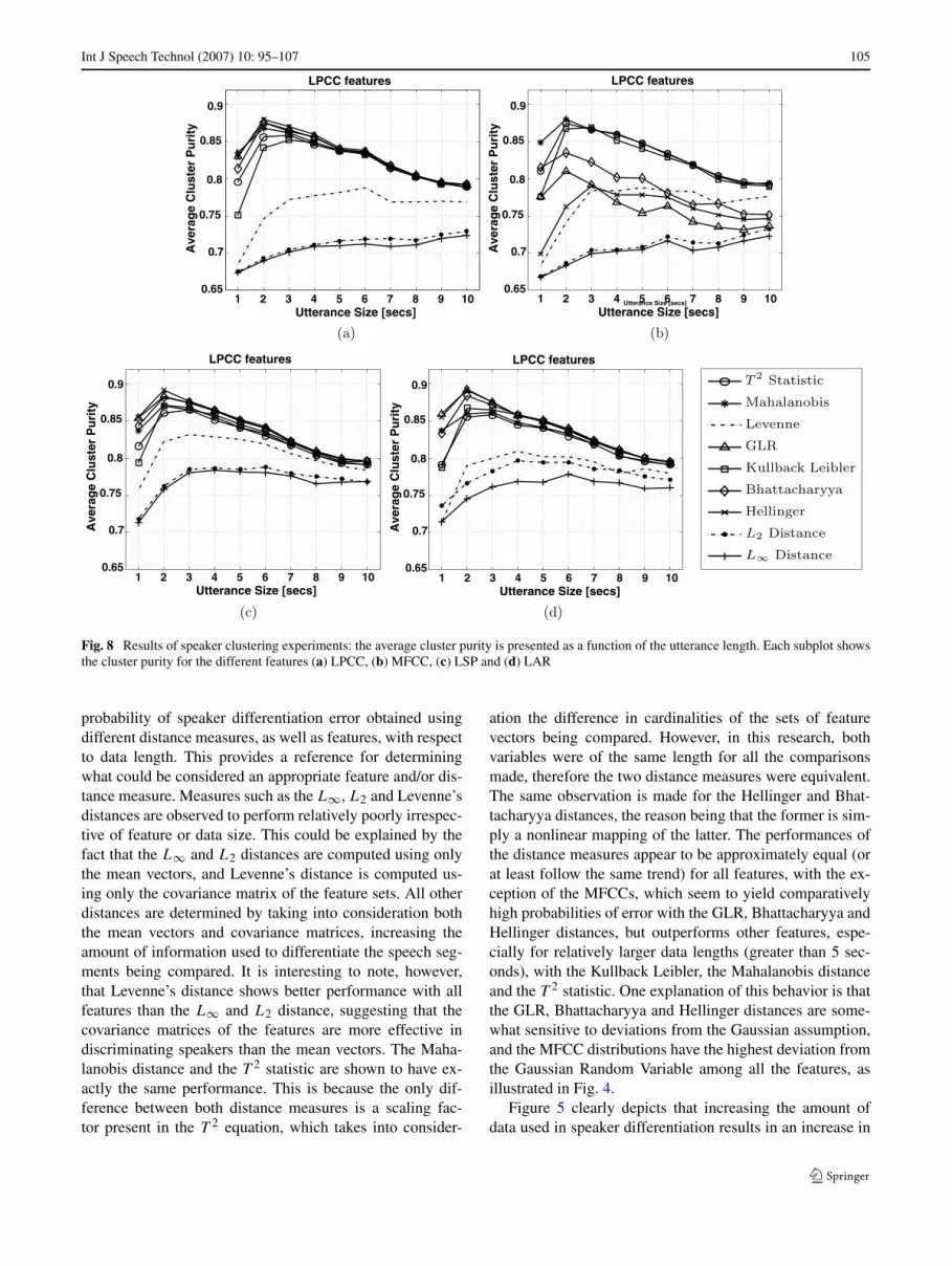
Fig. 8 Results of speaker clustering experiments: the average cluster purity is presented as a function of the utterance length. Each subplot showsthe cluster purity for the different features (a) LPCC, (b) MFCC, (c) LSP and (d) LAR

probability of speaker differentiation error obtained usingdifferent distance measures, as well as features, with respectto data length. This provides a reference for determiningwhat could be considered an appropriate feature and/or dis-tance measure. Measures such as the L∞, L2 and Levenne’sdistances are observed to perform relatively poorly irrespec-tive of feature or data size. This could be explained by thefact that the L∞ and L2 distances are computed using onlythe mean vectors, and Levenne’s distance is computed us-ing only the covariance matrix of the feature sets. All otherdistances are determined by taking into consideration boththe mean vectors and covariance matrices, increasing theamount of information used to differentiate the speech seg-ments being compared. It is interesting to note, however,that Levenne’s distance shows better performance with allfeatures than the L∞ and L2 distance, suggesting that thecovariance matrices of the features are more effective indiscriminating speakers than the mean vectors. The Maha-lanobis distance and the T 2 statistic are shown to have ex-actly the same performance. This is because the only dif-ference between both distance measures is a scaling fac-tor present in the T 2 equation, which takes into consider-

ation the difference in cardinalities of the sets of featurevectors being compared. However, in this research, bothvariables were of the same length for all the comparisonsmade, therefore the two distance measures were equivalent.The same observation is made for the Hellinger and Bhat-tacharyya distances, the reason being that the former is sim-ply a nonlinear mapping of the latter. The performances ofthe distance measures appear to be approximately equal (orat least follow the same trend) for all features, with the ex-ception of the MFCCs, which seem to yield comparativelyhigh probabilities of error with the GLR, Bhattacharyya andHellinger distances, but outperforms other features, espe-cially for relatively larger data lengths (greater than 5 sec-onds), with the Kullback Leibler, the Mahalanobis distanceand the T 2 statistic. One explanation of this behavior is thatthe GLR, Bhattacharyya and Hellinger distances are some-what sensitive to deviations from the Gaussian assumption,and the MFCC distributions have the highest deviation fromthe Gaussian Random Variable among all the features, asillustrated in Fig. 4.

Figure 5 clearly depicts that increasing the amount ofdata used in speaker differentiation results in an increase in


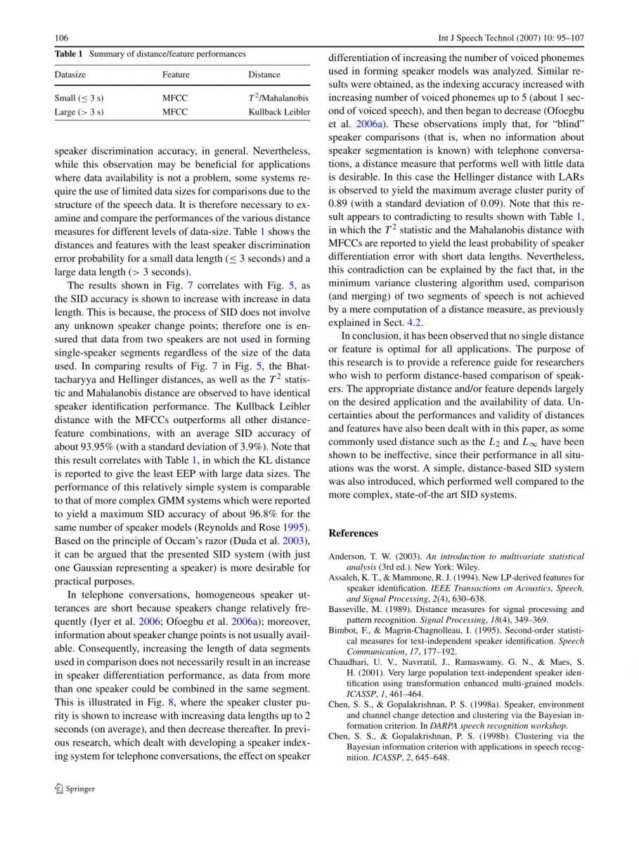
Table 1 Summary of distance/feature performances

Datasize Feature Distance

Small (≤ 3 s) MFCC T 2/Mahalanobis

Large (> 3 s) MFCC Kullback Leibler

speaker discrimination accuracy, in general. Nevertheless,while this observation may be beneficial for applicationswhere data availability is not a problem, some systems re-quire the use of limited data sizes for comparisons due to thestructure of the speech data. It is therefore necessary to ex-amine and compare the performances of the various distancemeasures for different levels of data-size. Table 1 shows thedistances and features with the least speaker discriminationerror probability for a small data length (≤ 3 seconds) and alarge data length (> 3 seconds).

The results shown in Fig. 7 correlates with Fig. 5, asthe SID accuracy is shown to increase with increase in datalength. This is because, the process of SID does not involveany unknown speaker change points; therefore one is en-sured that data from two speakers are not used in formingsingle-speaker segments regardless of the size of the dataused. In comparing results of Fig. 7 in Fig. 5, the Bhat-tacharyya and Hellinger distances, as well as the T 2 statis-tic and Mahalanobis distance are observed to have identicalspeaker identification performance. The Kullback Leiblerdistance with the MFCCs outperforms all other distance-feature combinations, with an average SID accuracy ofabout 93.95% (with a standard deviation of 3.9%). Note thatthis result correlates with Table 1, in which the KL distanceis reported to give the least EEP with large data sizes. Theperformance of this relatively simple system is comparableto that of more complex GMM systems which were reportedto yield a maximum SID accuracy of about 96.8% for thesame number of speaker models (Reynolds and Rose 1995).Based on the principle of Occam’s razor (Duda et al. 2003),it can be argued that the presented SID system (with justone Gaussian representing a speaker) is more desirable forpractical purposes.

In telephone conversations, homogeneous speaker ut-terances are short because speakers change relatively fre-quently (Iyer et al. 2006; Ofoegbu et al. 2006a); moreover,information about speaker change points is not usually avail-able. Consequently, increasing the length of data segmentsused in comparison does not necessarily result in an increasein speaker differentiation performance, as data from morethan one speaker could be combined in the same segment.This is illustrated in Fig. 8, where the speaker cluster pu-rity is shown to increase with increasing data lengths up to 2seconds (on average), and then decrease thereafter. In previ-ous research, which dealt with developing a speaker index-ing system for telephone conversations, the effect on speaker

differentiation of increasing the number of voiced phonemesused in forming speaker models was analyzed. Similar re-sults were obtained, as the indexing accuracy increased withincreasing number of voiced phonemes up to 5 (about 1 sec-ond of voiced speech), and then began to decrease (Ofoegbuet al. 2006a). These observations imply that, for “blind”speaker comparisons (that is, when no information aboutspeaker segmentation is known) with telephone conversa-tions, a distance measure that performs well with little datais desirable. In this case the Hellinger distance with LARsis observed to yield the maximum average cluster purity of0.89 (with a standard deviation of 0.09). Note that this re-sult appears to contradicting to results shown with Table 1,in which the T 2 statistic and the Mahalanobis distance withMFCCs are reported to yield the least probability of speakerdifferentiation error with short data lengths. Nevertheless,this contradiction can be explained by the fact that, in theminimum variance clustering algorithm used, comparison(and merging) of two segments of speech is not achievedby a mere computation of a distance measure, as previouslyexplained in Sect. 4.2.

In conclusion, it has been observed that no single distanceor feature is optimal for all applications. The purpose ofthis research is to provide a reference guide for researcherswho wish to perform distance-based comparison of speak-ers. The appropriate distance and/or feature depends largelyon the desired application and the availability of data. Un-certainties about the performances and validity of distancesand features have also been dealt with in this paper, as somecommonly used distance such as the L2 and L∞ have beenshown to be ineffective, since their performance in all situ-ations was the worst. A simple, distance-based SID systemwas also introduced, which performed well compared to themore complex, state-of-the art SID systems.

References

Anderson, T. W. (2003). An introduction to multivariate statisticalanalysis (3rd ed.). New York: Wiley.

Assaleh, K. T., & Mammone, R. J. (1994). New LP-derived features forspeaker identification. IEEE Transactions on Acoustics, Speech,and Signal Processing, 2(4), 630–638.

Basseville, M. (1989). Distance measures for signal processing andpattern recognition. Signal Processing, 18(4), 349–369.

Bimbot, F., & Magrin-Chagnolleau, I. (1995). Second-order statisti-cal measures for text-independent speaker identification. SpeechCommunication, 17, 177–192.

Chaudhari, U. V., Navrratil, J., Ramaswamy, G. N., & Maes, S.H. (2001). Very large population text-independent speaker iden-tification using transformation enhanced multi-grained models.ICASSP, 1, 461–464.

Chen, S. S., & Gopalakrishnan, P. S. (1998a). Speaker, environmentand channel change detection and clustering via the Bayesian in-formation criterion. In DARPA speech recognition workshop.

Chen, S. S., & Gopalakrishnan, P. S. (1998b). Clustering via theBayesian information criterion with applications in speech recog-nition. ICASSP, 2, 645–648.


de Souza, P. (1977). Statistical tests and distance measures for LPCcoefficients. IEEE Transactions on Acoustics, Speech, and SignalProcessing, 25(6), 554–559.

Delacourt, P., & Welkens, C. J. (2000). DISTBIC: A speaker based seg-mentation for audio data indexing. Speech Communication, 32,111–126.

Deller, J. R., Hansen, J. H. L., & Proakis, J. G. (2000). Discrete-timeprocessing of speech signals. New York: IEEE Press.

Duda, R. O., Hart, P. E., & Stork, D. G. (2003). Pattern classification(2nd ed.). New York: Wiley.

Furui, S. (1981). Cepstral analysis technique for automatic speakerverification. IEEE Transactions on Acoustics, Speech, and SignalProcessing, 29(2), 254–272.

Gish, H., & Schmidt, M. (1994). Text-independent speaker identifica-tion. IEEE Signal Processing Magazine, 11(4), 18–32.

Gish, H., Siu, H., & Rohlicek, R. (2001). Segregation of speakersfor speech recognition and speaker identification. In ICASSP(pp. 873–876).

Godfrey, J., Holliman, E. C., & McDaniel, J. (1992). SWITCH-BOARD: Telephone speech corpus for research and development.In ICASSP (pp. 517–520).

Gray, A., & Markel, J. (1976). Distance measures for speech process-ing. IEEE Transactions on Acoustics, Speech, and Signal Process-ing, 24(5), 380–391.

Gray, R., Gray, A., Buzo, A., & Matsuyama, Y. (1980). Distortionmeasures for speech processing. IEEE Transactions on Acoustics,Speech, and Signal Processing, 28(4), 367–376.

Huang, X., Alleva, F., Hon, H.-W., Hwang, M.-Y., & Rosenfeld, R.(1993). The SPHINX-II speech recognition system: an overview.Computer Speech and Language, 7(2), 137–148.

Iyer, A. N., Ofoegbu, U. O., Yantorno, R. E., & Smolenski, B. Y.(2006). Blind speaker clustering. In ISPACS (pp. 343–346).

Jain, A. K., & Dubes, R. C. (1988). Algorithms for clustering data.New York: Prentice Hall.

Johnson, D. E. (1998). Applied multivariate methods for data analysts.N. Scituate: Duxbury.

Lee, K. F., Hon, H. W., & Reddy, R. (1990). An overview ofthe SPHINX speech recognition system. IEEE Transactions onAcoustics, Speech, and Signal Processing, 38(1), 35–45.

Levene, H. (1960). Robust tests for equality of variances. In I. Olkin,S. G. Ghurye, W. Hoeffding, W. G. Madow, & H. B. Mann (Eds.),

Contributions to probability and statistics (pp. 278–292). Stan-ford: Stanford University Press.

Lu, Z., Hui, Y. V., & Lee, A. H. (2003). Minimum Hellinger distanceestimation for finite mixtures of Poisson regression models and itsapplications. Biometrics, 59(4), 1016–1026.

Manly, B. F. J. (1995). Multivariate statistical methods (2nd ed.). Lon-don: Chapman & Hall.

Matsui, T., & Furui, S. (1994). Comparison of text-independentspeaker recognition methods using vq-distortion and dis-crete/continuous HMM’s. IEEE Transactions on Acoustics,Speech, and Signal Processing, 2(3), 456–459.

Naik, J. M. (1990). Speaker verification: a tutorial. IEEE Communica-tions Magazine, 28(1), 42–48.

Ofoegbu, U. O., Iyer, A. N., Yantorno, R. E., & Smolenski, B. Y.(2006a). A simple approach to unsupervised speaker indexing. InISPACS (pp. 339–342).

Ofoegbu, U. O., Iyer, A. N., Yantorno, R. E., & Smolenski, B. Y.(2006b). A speaker count system for telephone conversations. InISPACS (pp. 331–334).

Ofoegbu, U. O., Iyer, A. N., Yantorno, R. E., & Wenndt, S. J. (2006c).Detection of a third speaker in telephone conversations. In ICSLP.

Ong, S., & Yang, C. (1998). A comparative study of text-independentspeaker identification using statistical features. InternationalJournal of Computer and Engineering Management, 6(1).

Reynolds, D. (1997). HTIMIT and LLHDB: Speech corpora for thestudy of handset transducer effects. In ICASSP (pp. 1535–1538).

Reynolds, D. A. (1992). A Gaussian mixture modeling approach totext-independent speaker. Ph.D. thesis, Georgia Institute of Tech-nology, August 1992.

Reynolds, D. A., & Rose, R. C. (1995). Robust text-independentspeaker identification using Gaussian mixture models. IEEETransactions on Speech and Audio Processing, 3(1), 72–83.

Rudasi, L., & Zahorian, S. A. (1991). Text-independent talker identifi-cation with neural networks. ICASSP, 1, 389–392.

Solomonoff, A., Mielke, A., Schmidt, M., & Gish, H. (1998). Cluster-ing speakers by their voices. ICASSP, 2, 757–760.

Srivastava, M. S., & Carter, E. M. (1983). An introduction to appliedmultivariate statistics. Amsterdam: North-Holland.

Theodoridis, S., & Koutroumbas, K. (1999). Pattern recognition. SanDiego: Academic Press.

speaker distinguishing distances: a comparative study

Documents