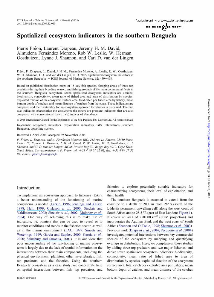
ICES Journal of Marine Science, 62: 459e468 (2005)doi:10.1016/j.icesjms.2004.12.010

http://icesjms.oxfordjournals.org

Dow

nloaded from

Spatialized ecosystem indicators in the southern Benguela

Pierre Freon, Laurent Drapeau, Jeremy H. M. David,Almudena Fernandez Moreno, Rob W. Leslie, W. HermanOosthuizen, Lynne J. Shannon, and Carl D. van der Lingen

Freon, P., Drapeau, L., David, J. H. M., Fernandez Moreno, A., Leslie, R. W., Oosthuizen,W. H., Shannon, L. J., and van der Lingen, C. D. 2005. Spatialized ecosystem indicators inthe southern Benguela. e ICES Journal of Marine Science, 62: 459e468.

Based on published distribution maps of 15 key fish species, foraging areas of three toppredators during their breeding season, and fishing grounds of the main commercial fleets inthe southern Benguela ecosystem, seven spatialized ecosystem indicators are derived:biodiversity, connectivity, mean ratio of fished area and area of distribution by species,exploited fraction of the ecosystem surface area, total catch per fished area by fishery, meanbottom depth of catches, and mean distance of catches from the coast. These indicators arecompared and their suitability for an ecosystem approach to fisheries is discussed. The firsttwo indicators characterize the ecosystem; the others are pressure indicators that are alsocompared with conventional (catch rate) indices of abundance.

� 2005 International Council for the Exploration of the Sea. Published by Elsevier Ltd. All rights reserved.

Keywords: ecosystem indicators, exploitation indicators, GIS, interactions, southernBenguela, upwelling system.

Received 1 April 2004; accepted 29 November 2004.

P. Freon, L. Drapeau, and A. Fernandez Moreno: IRD, 213 rue La Fayette, 75480 Paris,Cedex 10, France. L. Drapeau, J. H. M. David, R. W. Leslie, W. H. Oosthuizen, L. J.Shannon, and C. D. van der Lingen: MCM, Private Bag X2, Rogge Bay 8012, Cape Town,South Africa. Correspondence to P. Freon: tel: C33 4 99 57 32 02; fax: C33 4 99 57 3296; e-mail: pierre.freon@ird.fr.

by guest on June 8, 2013/

Introduction

To implement an ecosystem approach to fisheries (EAF),

a better understanding of the functioning of marine

ecosystems is needed (Larkin, 1996; Jennings and Kaiser,

1998; Hall, 1999; Gislason et al., 2000; Sinclair and

Valdimarsson, 2002; Sinclair et al., 2002; Moloney et al.,

2004). One way of achieving this is to make use of

indicators, i.e. pointers that can be used to reveal or to

monitor conditions and trends in the fisheries sector, as well

as in the marine environment (FAO, 1999; Smeets and

Weterings, 1999; Garcia and Staples, 2000; Garcia et al.,

2000; Sainsbury and Sumaila, 2001). It is our view that

poor understanding of the functioning of marine ecosys-

tems is largely due to the lack of spatial information on the

interactions between their main components, including the

physical environment, plankton, other invertebrates, fish,

top predators, and the fisheries. Using the southern

Benguela ecosystem as a case study, we concentrate here

on spatial interactions between fish, top predators, and

1054-3139/$30.00 � 2005 International Coun

fisheries to explore potentially suitable indicators for

characterizing ecosystems, their level of exploitation, and

their health.

The southern Benguela is assumed to extend from the

coastline to a depth of 2000 m from 28(S (south of the

Luderitz permanent upwelling cell) along the west coast of

South Africa and to 28.5(E (east of East London; Figure 1).

It covers an area of 250 000 km2 (UTM projection) and

incorporates the Agulhas Bank and the west coast of South

Africa (Shannon and O’Toole, 1998; Shannon et al., 2003).

Previous work (Drapeau et al., 2004; Pecquerie et al., 2004)

investigated potential interactions between key commercial

species of the ecosystem by mapping and quantifying

overlaps in distribution. Here, we complement those studies

by adding three top predators and two major fisheries, and

derive seven spatialized ecosystem indicators: biodiversity,

connectivity, mean ratio of fished area to area of

distribution by species, exploited fraction of the ecosystem

surface area, total catch per exploited area per fishery, mean

bottom depth of catches, and mean distance of the catches

cil for the Exploration of the Sea. Published by Elsevier Ltd. All rights reserved.

460 P. Freon et al.

http://icesjD

ownloaded from

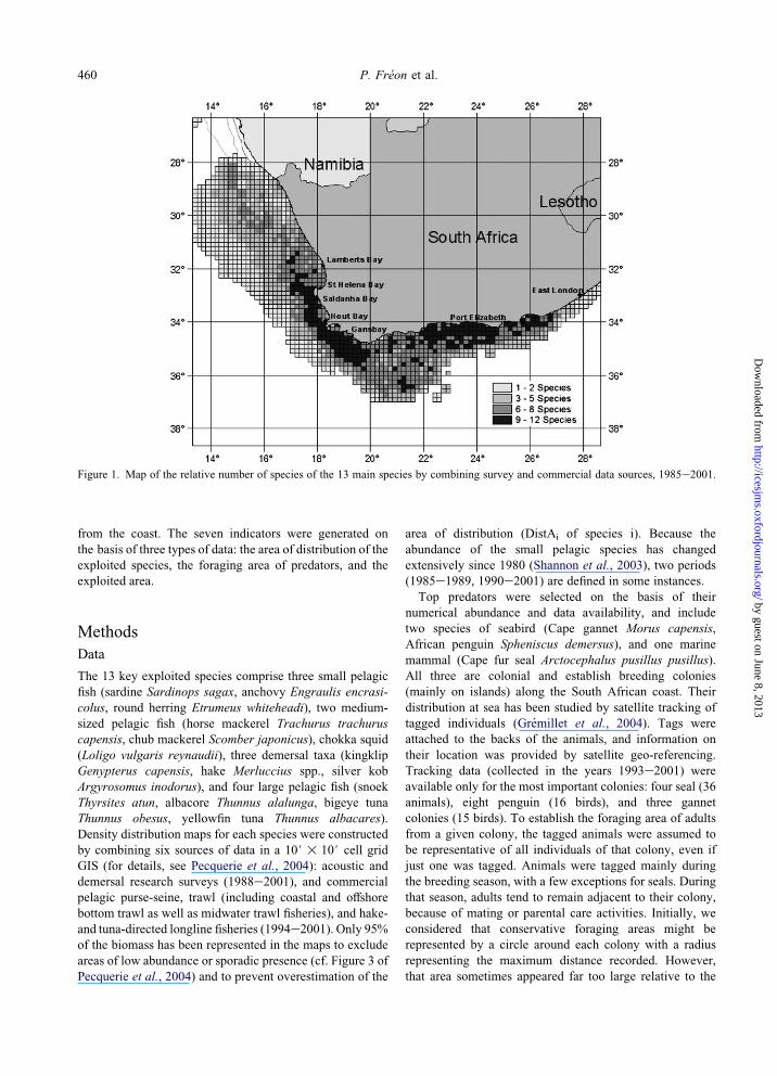
Figure 1. Map of the relative number of species of the 13 main species by combining survey and commercial data sources, 1985e2001.

by guest on June 8, 2013m

s.oxfordjournals.org/

from the coast. The seven indicators were generated on

the basis of three types of data: the area of distribution of the

exploited species, the foraging area of predators, and the

exploited area.

Methods

Data

The 13 key exploited species comprise three small pelagic

fish (sardine Sardinops sagax, anchovy Engraulis encrasi-

colus, round herring Etrumeus whiteheadi), two medium-

sized pelagic fish (horse mackerel Trachurus trachurus

capensis, chub mackerel Scomber japonicus), chokka squid

(Loligo vulgaris reynaudii), three demersal taxa (kingklip

Genypterus capensis, hake Merluccius spp., silver kob

Argyrosomus inodorus), and four large pelagic fish (snoek

Thyrsites atun, albacore Thunnus alalunga, bigeye tuna

Thunnus obesus, yellowfin tuna Thunnus albacares).

Density distribution maps for each species were constructed

by combining six sources of data in a 10#! 10# cell grid

GIS (for details, see Pecquerie et al., 2004): acoustic and

demersal research surveys (1988e2001), and commercial

pelagic purse-seine, trawl (including coastal and offshore

bottom trawl as well as midwater trawl fisheries), and hake-

and tuna-directed longline fisheries (1994e2001). Only 95%of the biomass has been represented in the maps to exclude

areas of low abundance or sporadic presence (cf. Figure 3 of

Pecquerie et al., 2004) and to prevent overestimation of the

area of distribution (DistAi of species i). Because the

abundance of the small pelagic species has changed

extensively since 1980 (Shannon et al., 2003), two periods

(1985e1989, 1990e2001) are defined in some instances.

Top predators were selected on the basis of their

numerical abundance and data availability, and include

two species of seabird (Cape gannet Morus capensis,

African penguin Spheniscus demersus), and one marine

mammal (Cape fur seal Arctocephalus pusillus pusillus).

All three are colonial and establish breeding colonies

(mainly on islands) along the South African coast. Their

distribution at sea has been studied by satellite tracking of

tagged individuals (Gremillet et al., 2004). Tags were

attached to the backs of the animals, and information on

their location was provided by satellite geo-referencing.

Tracking data (collected in the years 1993e2001) were

available only for the most important colonies: four seal (36

animals), eight penguin (16 birds), and three gannet

colonies (15 birds). To establish the foraging area of adults

from a given colony, the tagged animals were assumed to

be representative of all individuals of that colony, even if

just one was tagged. Animals were tagged mainly during

the breeding season, with a few exceptions for seals. During

that season, adults tend to remain adjacent to their colony,

because of mating or parental care activities. Initially, we

considered that conservative foraging areas might be

represented by a circle around each colony with a radius

representing the maximum distance recorded. However,

that area sometimes appeared far too large relative to the

461Spatialized ecosystem indicators in the southern Benguela

by guest on Jhttp://icesjm

s.oxfordjournals.org/D

ownloaded from

tracking observations, because of an asymmetrical distri-

bution. In such cases, we used two radii, one on each side of

the colony, plus a bathymetric limit to estimate the foraging

area (ForAi of species i). When appropriate, the area was

modified manually to reflect available observations and

a common-sense perception of the real distribution. When

just one animal was tagged, an arbitrary 10% of the largest

distance recorded from the colony was added to the radius

in computing the foraging area. ArcView 3.2 GIS software

was used to visualize, explore, query, and analyse the data.

Three types of commercial fishery were considered:

pelagic purse-seine, trawl, and longline fisheries. These

three fisheries yielded on average 98% of the total catches

made in the southern Benguela ecosystem in the 1990s. The

exploited area (ExplAi,j for fishery i in year or period j) was

estimated by summing the surface of every individual grid

cell where at least one catch was taken. Although

a sensitivity analysis indicated that the absolute value of

ExplA was sensitive to setting a threshold for a minimum

number of catches recorded per grid cell, trends and

interannual variations remained unaffected. Prior to 1985,

ExplA for the pelagic fishery was estimated after digitizing

a series of maps of fishing effort distribution in 1951, 1955,

1958, 1964, and 1974, given by Crawford (1986). Data are

unavailable for the demersal fishery prior to 1985. Depth is

recorded for demersal trawls in skipper logbooks, but not for

the pelagic fishery. Because the geo-referencing system of

the pelagic fishery is based only on a 10# grid, the ETOPO2bathymetry from NOAA with a spatial resolution of 3 km

was used to estimate depth at the centre of every grid cell,

and this estimate of bottom depth was linked to individual

catches (BDC). Similarly, distance from the coast of pelagic

and demersal catches (DCC) was estimated by calculating

the distance between the centre of a grid cell and the nearest

point of the coastline.

u

Indicators

An index of spatial biodiversity ISBj during period j was

defined as the average relative number of species (exploited

and top predators):

ISBjZð100=nÞ!Xn

gZ1

sg;j=S ð1Þ

where (sg,j) is the number of species per grid cell g, S the

total number of species in the databases, and n is the

number of grid cells with observations. This index is

associated with the map of the relative number of species

per grid cell (sg,j/S).

A spatial-overlap (connectivity) index (OIj) during each

period j is defined as the average of relative overlapping areas

(ROAa/b,j) between any two of the three areas described

above (DistAi,j, ForAi,j, ExplAi,j) for species/species or

species/fishery pairs (a, b) in the ecosystem characterized by

a trophic (or exploitational) relationship (predation, compe-

tition), based on available literature and expert judgement

(Table 1). ROA is simply the ratio of the overlapping area

between two distributions (Da and Db) to the total area

occupied by these two distributions together (Figure 2):

ROAa=b;jZ100!�Da;jXDb;j

�=Da;jWDb;j ð2Þ

where X and W are standard symbols for intersection

(overlap) and union (total area), respectively. Although

each ROA may be considered individually as a potential

indicator of interaction (Drapeau et al., 2004), the mean of

all ROAs relating to interactions (Table 1) may serve as an

ecosystem indicator of overall degree of interaction (OIj).

The ratio of fished area and distribution area by species

(REDj) is defined as

REDjZ100!�DistAi;jXExplAi;j

�=DistAi;j ð3Þ

ne 8, 2013

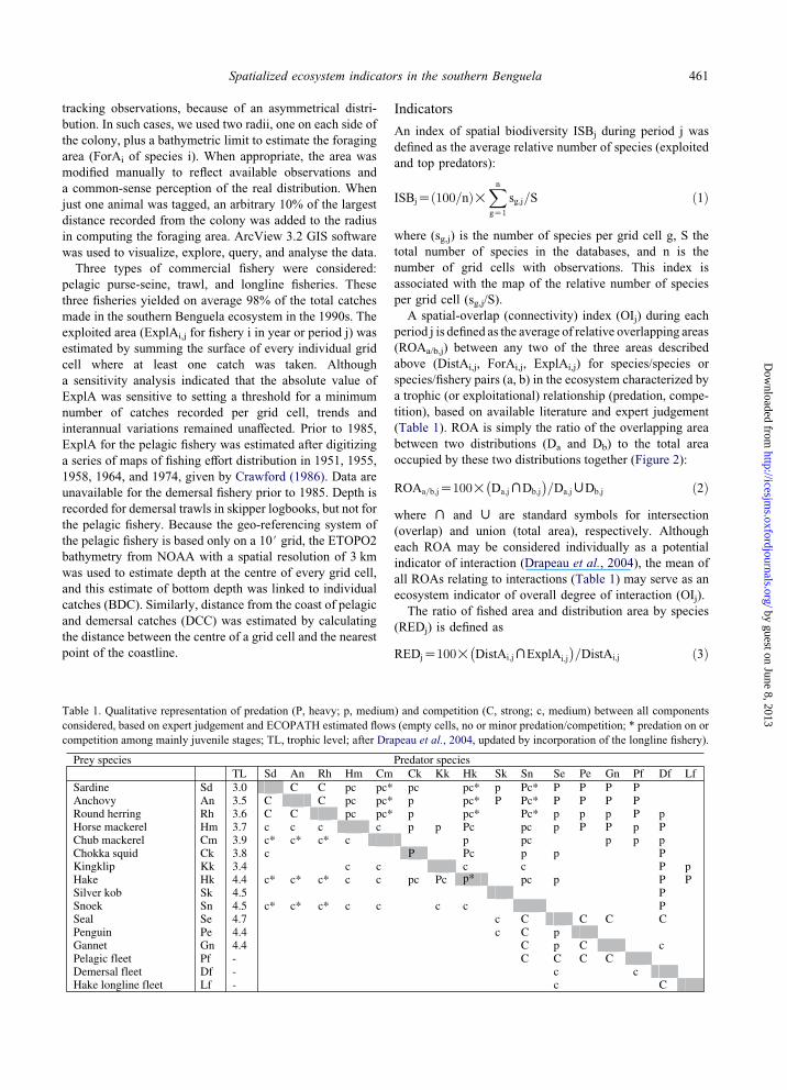
Table 1. Qualitative representation of predation (P, heavy; p, medium) and competition (C, strong; c, medium) between all components

considered, based on expert judgement and ECOPATH estimated flows (empty cells, no or minor predation/competition; * predation on or

competition among mainly juvenile stages; TL, trophic level; after Drapeau et al., 2004, updated by incorporation of the longline fishery).

Prey species Predator speciesTL Sd An Rh Hm Cm Ck Kk Hk Sk Sn Se Pe Gn Pf Df Lf

Sardine Sd 3.0 C C pc pc* pc pc* p Pc* P P P PAnchovy An 3.5 C C pc pc* p pc* P Pc* P P P PRound herring Rh 3.6 C C pc pc* p pc* Pc* p p p P pHorse mackerel Hm 3.7 c c c c p p Pc pc p P P p PChub mackerel Cm 3.9 c* c* c* c p pc p p pChokka squid Ck 3.8 c P Pc p p PKingklip Kk 3.4 c c c c P pHake Hk 4.4 c* c* c* c c pc Pc p* pc p P PSilver kob Sk 4.5 PSnoek Sn 4.5 c* c* c* c c c c PSeal Se 4.7 c C C C CPenguin Pe 4.4 c C pGannet Gn 4.4 C p C cPelagic fleet Pf - C C C CDemersal fleet Df - c cHake longline fleet Lf - c C

462 P. Freon et al.

http://icD

ownloaded from

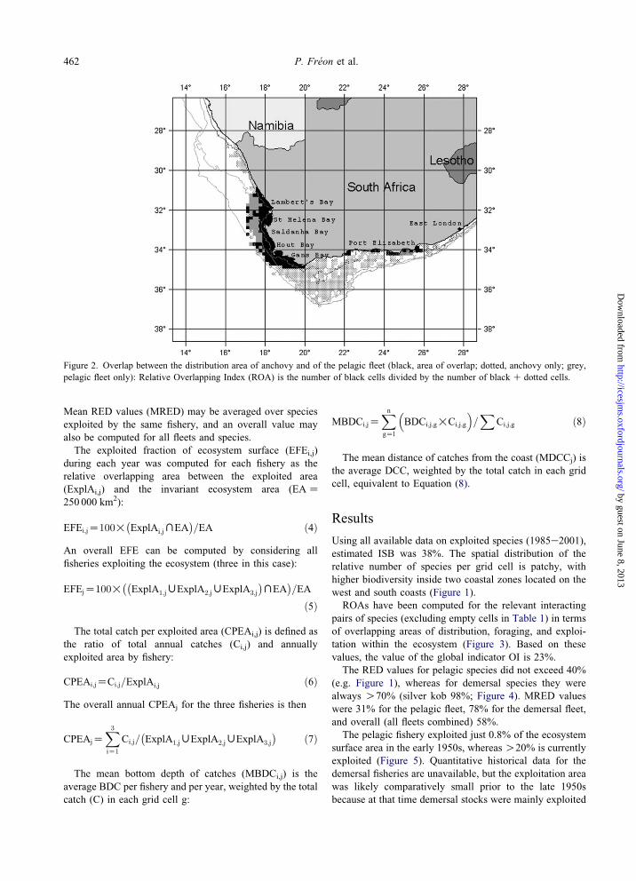
Figure 2. Overlap between the distribution area of anchovy and of the pelagic fleet (black, area of overlap; dotted, anchovy only; grey,

pelagic fleet only): Relative Overlapping Index (ROA) is the number of black cells divided by the number of blackC dotted cells.

by guest on June 8, 2013esjm

s.oxfordjournals.org/

Mean RED values (MRED) may be averaged over species

exploited by the same fishery, and an overall value may

also be computed for all fleets and species.

The exploited fraction of ecosystem surface (EFEi,j)

during each year was computed for each fishery as the

relative overlapping area between the exploited area

(ExplAi,j) and the invariant ecosystem area (EAZ250 000 km2):

EFEi;jZ100!�ExplAi;jXEA

�=EA ð4Þ

An overall EFE can be computed by considering all

fisheries exploiting the ecosystem (three in this case):

EFEjZ100!��ExplA1;jWExplA2;jWExplA3;j

�XEA

�=EA

ð5Þ

The total catch per exploited area (CPEAi,j) is defined as

the ratio of total annual catches (Ci,j) and annually

exploited area by fishery:

CPEAi;jZCi;j=ExplAi;j ð6Þ

The overall annual CPEAj for the three fisheries is then

CPEAjZX3

iZ1

Ci;j=�ExplA1;jWExplA2;jWExplA3;j

�ð7Þ

The mean bottom depth of catches (MBDCi,j) is the

average BDC per fishery and per year, weighted by the total

catch (C) in each grid cell g:

MBDCi;jZXn

gZl

�BDCi;j;g!Ci;j;g

�=X

Ci;j;g ð8Þ

The mean distance of catches from the coast (MDCCj) is

the average DCC, weighted by the total catch in each grid

cell, equivalent to Equation (8).

Results

Using all available data on exploited species (1985e2001),

estimated ISB was 38%. The spatial distribution of the

relative number of species per grid cell is patchy, with

higher biodiversity inside two coastal zones located on the

west and south coasts (Figure 1).

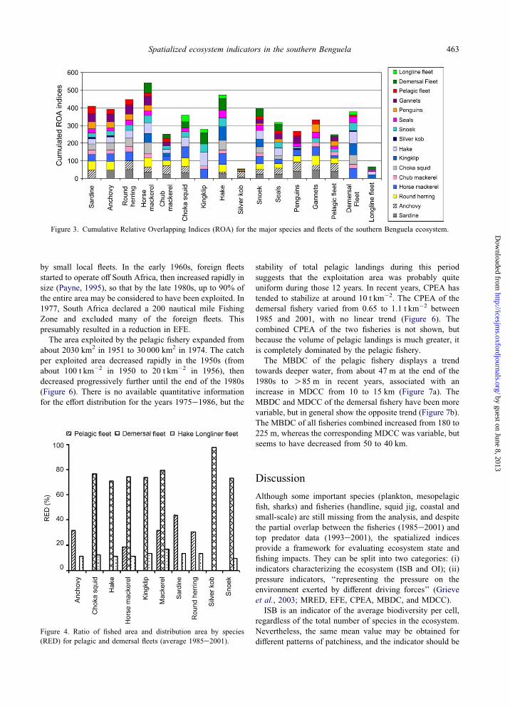
ROAs have been computed for the relevant interacting

pairs of species (excluding empty cells in Table 1) in terms

of overlapping areas of distribution, foraging, and exploi-

tation within the ecosystem (Figure 3). Based on these

values, the value of the global indicator OI is 23%.

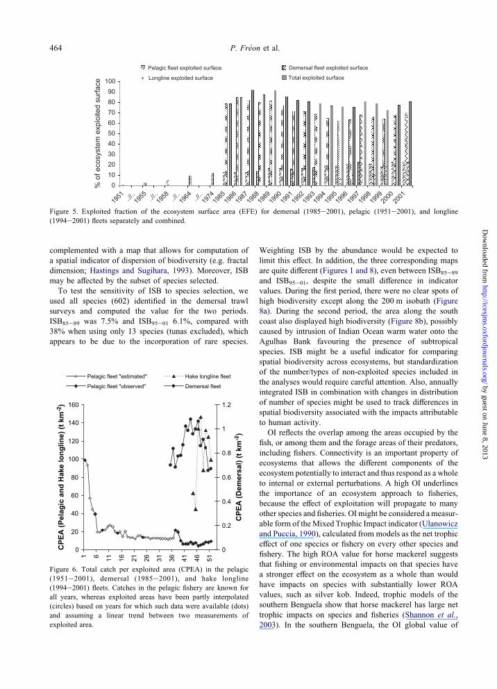
The RED values for pelagic species did not exceed 40%

(e.g. Figure 1), whereas for demersal species they were

always O70% (silver kob 98%; Figure 4). MRED values

were 31% for the pelagic fleet, 78% for the demersal fleet,

and overall (all fleets combined) 58%.

The pelagic fishery exploited just 0.8% of the ecosystem

surface area in the early 1950s, whereas O20% is currently

exploited (Figure 5). Quantitative historical data for the

demersal fisheries are unavailable, but the exploitation area

was likely comparatively small prior to the late 1950s

because at that time demersal stocks were mainly exploited

463Spatialized ecosystem indicators in the southern Benguela

Dow

Figure 3. Cumulative Relative Overlapping Indices (ROA) for the major species and fleets of the southern Benguela ecosystem.

by guest on June 8, 2013http://icesjm

s.oxfordjournals.org/nloaded from

by small local fleets. In the early 1960s, foreign fleets

started to operate off South Africa, then increased rapidly in

size (Payne, 1995), so that by the late 1980s, up to 90% of

the entire area may be considered to have been exploited. In

1977, South Africa declared a 200 nautical mile Fishing

Zone and excluded many of the foreign fleets. This

presumably resulted in a reduction in EFE.

The area exploited by the pelagic fishery expanded from

about 2030 km2 in 1951 to 30 000 km2 in 1974. The catch

per exploited area decreased rapidly in the 1950s (from

about 100 t km�2 in 1950 to 20 t km�2 in 1956), then

decreased progressively further until the end of the 1980s

(Figure 6). There is no available quantitative information

for the effort distribution for the years 1975e1986, but the

Figure 4. Ratio of fished area and distribution area by species

(RED) for pelagic and demersal fleets (average 1985e2001).

stability of total pelagic landings during this period

suggests that the exploitation area was probably quite

uniform during those 12 years. In recent years, CPEA has

tended to stabilize at around 10 t km�2. The CPEA of the

demersal fishery varied from 0.65 to 1.1 t km�2 between

1985 and 2001, with no linear trend (Figure 6). The

combined CPEA of the two fisheries is not shown, but

because the volume of pelagic landings is much greater, it

is completely dominated by the pelagic fishery.

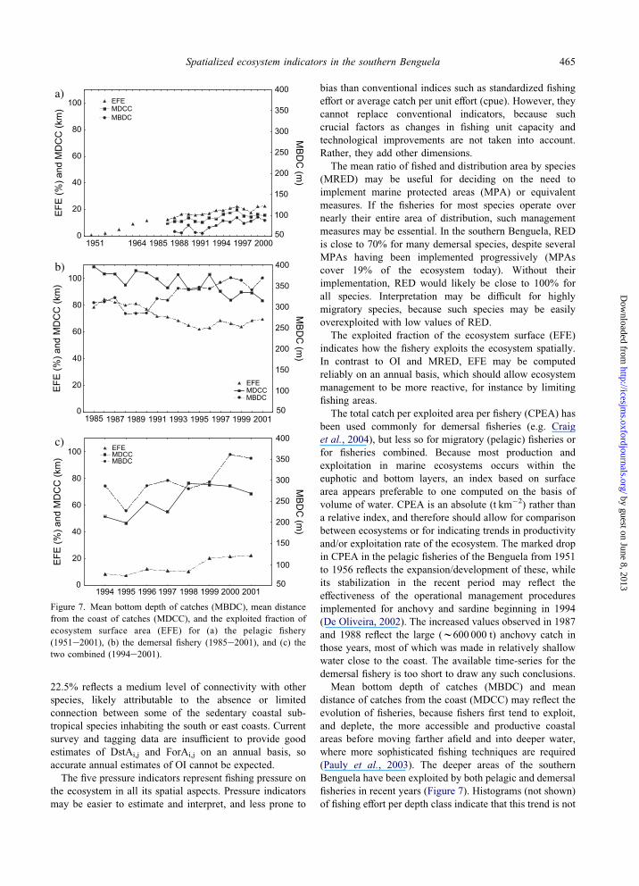
The MBDC of the pelagic fishery displays a trend

towards deeper water, from about 47 m at the end of the

1980s to O85 m in recent years, associated with an

increase in MDCC from 10 to 15 km (Figure 7a). The

MBDC and MDCC of the demersal fishery have been more

variable, but in general show the opposite trend (Figure 7b).

The MBDC of all fisheries combined increased from 180 to

225 m, whereas the corresponding MDCC was variable, but

seems to have decreased from 50 to 40 km.

Discussion

Although some important species (plankton, mesopelagic

fish, sharks) and fisheries (handline, squid jig, coastal and

small-scale) are still missing from the analysis, and despite

the partial overlap between the fisheries (1985e2001) and

top predator data (1993e2001), the spatialized indices

provide a framework for evaluating ecosystem state and

fishing impacts. They can be split into two categories: (i)

indicators characterizing the ecosystem (ISB and OI); (ii)

pressure indicators, ‘‘representing the pressure on the

environment exerted by different driving forces’’ (Grieve

et al., 2003; MRED, EFE, CPEA, MBDC, and MDCC).

ISB is an indicator of the average biodiversity per cell,

regardless of the total number of species in the ecosystem.

Nevertheless, the same mean value may be obtained for

different patterns of patchiness, and the indicator should be

464 P. Freon et al.

D

Figure 5. Exploited fraction of the ecosystem surface area (EFE) for demersal (1985e2001), pelagic (1951e2001), and longline

(1994e2001) fleets separately and combined.

by guest on June 8, 2013http://icesjm

s.oxfordjournals.org/ow

nloaded from

complemented with a map that allows for computation of

a spatial indicator of dispersion of biodiversity (e.g. fractal

dimension; Hastings and Sugihara, 1993). Moreover, ISB

may be affected by the subset of species selected.

To test the sensitivity of ISB to species selection, we

used all species (602) identified in the demersal trawl

surveys and computed the value for the two periods.

ISB85e89 was 7.5% and ISB95e01 6.1%, compared with

38% when using only 13 species (tunas excluded), which

appears to be due to the incorporation of rare species.

0

20

40

60

80

100

120

140

160

1 6 11 16 21 26 31 36 41 46 51

CP

EA

(P

elag

ic an

d H

ake lo

ng

lin

e) (t km

-2)

0

0.2

0.4

0.6

0.8

1

1.2

CP

EA

(D

em

ersal) (t km

-2)

Pelagic fleet "estimated" Hake longline fleet

Pelagic fleet "observed" Demersal fleet

Figure 6. Total catch per exploited area (CPEA) in the pelagic

(1951e2001), demersal (1985e2001), and hake longline

(1994e2001) fleets. Catches in the pelagic fishery are known for

all years, whereas exploited areas have been partly interpolated

(circles) based on years for which such data were available (dots)

and assuming a linear trend between two measurements of

exploited area.

Weighting ISB by the abundance would be expected to

limit this effect. In addition, the three corresponding maps

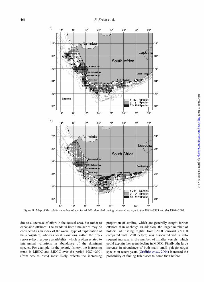
are quite different (Figures 1 and 8), even between ISB85e89

and ISB95e01, despite the small difference in indicator

values. During the first period, there were no clear spots of

high biodiversity except along the 200 m isobath (Figure

8a). During the second period, the area along the south

coast also displayed high biodiversity (Figure 8b), possibly

caused by intrusion of Indian Ocean warm water onto the

Agulhas Bank favouring the presence of subtropical

species. ISB might be a useful indicator for comparing

spatial biodiversity across ecosystems, but standardization

of the number/types of non-exploited species included in

the analyses would require careful attention. Also, annually

integrated ISB in combination with changes in distribution

of number of species might be used to track differences in

spatial biodiversity associated with the impacts attributable

to human activity.

OI reflects the overlap among the areas occupied by the

fish, or among them and the forage areas of their predators,

including fishers. Connectivity is an important property of

ecosystems that allows the different components of the

ecosystem potentially to interact and thus respond as a whole

to internal or external perturbations. A high OI underlines

the importance of an ecosystem approach to fisheries,

because the effect of exploitation will propagate to many

other species and fisheries. OI might be considered ameasur-

able form of theMixed Trophic Impact indicator (Ulanowicz

and Puccia, 1990), calculated from models as the net trophic

effect of one species or fishery on every other species and

fishery. The high ROA value for horse mackerel suggests

that fishing or environmental impacts on that species have

a stronger effect on the ecosystem as a whole than would

have impacts on species with substantially lower ROA

values, such as silver kob. Indeed, trophic models of the

southern Benguela show that horse mackerel has large net

trophic impacts on species and fisheries (Shannon et al.,

2003). In the southern Benguela, the OI global value of

465Spatialized ecosystem indicators in the southern Benguela

by guest on June 8, 2013http://icesjm

s.oxfordjournals.org/D

ownloaded from

22.5% reflects a medium level of connectivity with other

species, likely attributable to the absence or limited

connection between some of the sedentary coastal sub-

tropical species inhabiting the south or east coasts. Current

survey and tagging data are insufficient to provide good

estimates of DstAi,j and ForAi,j on an annual basis, so

accurate annual estimates of OI cannot be expected.

The five pressure indicators represent fishing pressure on

the ecosystem in all its spatial aspects. Pressure indicators

may be easier to estimate and interpret, and less prone to

EFE

(%) a

nd M

DC

C (k

m)

MBD

C (m

)M

BDC

(m)

50

100

150

200

250

300

350

400

50

50

100

150

200

250

300

350

400

MBD

C (m

)

100

150

200

250

300

350

400

0

20

40

60

80

100 EFEMDCCMBDC

a)

EFE

(%) a

nd M

DC

C (k

m)

0

20

40

60

80

100

EFE

(%) a

nd M

DC

C (k

m)

0

20

40

60

80

100

1985 1987 1989 1991 1993 1995 1997 1999 2001

1951 1964 1985 1988 1991 1994 1997 2000

EFEMDCCMBDC

b)

1994 1995 1996 1997 1998 1999 2000 2001

EFEMDCCMBDC

c)

Figure 7. Mean bottom depth of catches (MBDC), mean distance

from the coast of catches (MDCC), and the exploited fraction of

ecosystem surface area (EFE) for (a) the pelagic fishery

(1951e2001), (b) the demersal fishery (1985e2001), and (c) the

two combined (1994e2001).

bias than conventional indices such as standardized fishing

effort or average catch per unit effort (cpue). However, they

cannot replace conventional indicators, because such

crucial factors as changes in fishing unit capacity and

technological improvements are not taken into account.

Rather, they add other dimensions.

The mean ratio of fished and distribution area by species

(MRED) may be useful for deciding on the need to

implement marine protected areas (MPA) or equivalent

measures. If the fisheries for most species operate over

nearly their entire area of distribution, such management

measures may be essential. In the southern Benguela, RED

is close to 70% for many demersal species, despite several

MPAs having been implemented progressively (MPAs

cover 19% of the ecosystem today). Without their

implementation, RED would likely be close to 100% for

all species. Interpretation may be difficult for highly

migratory species, because such species may be easily

overexploited with low values of RED.

The exploited fraction of the ecosystem surface (EFE)

indicates how the fishery exploits the ecosystem spatially.

In contrast to OI and MRED, EFE may be computed

reliably on an annual basis, which should allow ecosystem

management to be more reactive, for instance by limiting

fishing areas.

The total catch per exploited area per fishery (CPEA) has

been used commonly for demersal fisheries (e.g. Craig

et al., 2004), but less so for migratory (pelagic) fisheries or

for fisheries combined. Because most production and

exploitation in marine ecosystems occurs within the

euphotic and bottom layers, an index based on surface

area appears preferable to one computed on the basis of

volume of water. CPEA is an absolute (t km�2) rather than

a relative index, and therefore should allow for comparison

between ecosystems or for indicating trends in productivity

and/or exploitation rate of the ecosystem. The marked drop

in CPEA in the pelagic fisheries of the Benguela from 1951

to 1956 reflects the expansion/development of these, while

its stabilization in the recent period may reflect the

effectiveness of the operational management procedures

implemented for anchovy and sardine beginning in 1994

(De Oliveira, 2002). The increased values observed in 1987

and 1988 reflect the large (w600 000 t) anchovy catch in

those years, most of which was made in relatively shallow

water close to the coast. The available time-series for the

demersal fishery is too short to draw any such conclusions.

Mean bottom depth of catches (MBDC) and mean

distance of catches from the coast (MDCC) may reflect the

evolution of fisheries, because fishers first tend to exploit,

and deplete, the more accessible and productive coastal

areas before moving farther afield and into deeper water,

where more sophisticated fishing techniques are required

(Pauly et al., 2003). The deeper areas of the southern

Benguela have been exploited by both pelagic and demersal

fisheries in recent years (Figure 7). Histograms (not shown)

of fishing effort per depth class indicate that this trend is not

466 P. Freon et al.

by guest on June 8, 2013http://icesjm

s.oxfordjournals.org/D

ownloaded from

Figure 8. Map of the relative number of species of 602 identified during demersal surveys in (a) 1985e1989 and (b) 1990e2001.

due to a decrease of effort in the coastal area, but rather to

expansion offshore. The trends in both time-series may be

considered as an index of the overall type of exploitation of

the ecosystem, whereas local variations within the time-

series reflect resource availability, which is often related to

interannual variations in abundance of the dominant

species. For example, in the pelagic fishery, the increasing

trend in MBDC and MDCC over the period 1987e2001

(from 5% to 35%) most likely reflects the increasing

proportion of sardine, which are generally caught farther

offshore than anchovy. In addition, the larger number of

holders of fishing rights from 2000 onward (O100

compared with !20 before) was associated with a sub-

sequent increase in the number of smaller vessels, which

could explain the recent decline in MDCC. Finally, the large

increase in abundance of both main small pelagic target

species in recent years (Griffiths et al., 2004) increased the

probability of finding fish closer to home than before.

467Spatialized ecosystem indicators in the southern Benguela

by guest on June 8, 2013http://icesjm

s.oxfordjournals.org/D

ownloaded from

Rather than ranking different ecosystem indicators for

electing the best, more might be learned about ecosystem

state and fishing impacts by trying to interpret the similarity

and discrepancies among them. For instance, the high

correlation among EFE, MBDC, and MDCC for the pelagic

fleet (j0.87j! r! j0.97j) appears to reflect the expansion

of that fishery, whereas the correlation between those three

indicators and both CPEA and cpue was weaker

(j0.64j! r! j0.71j). The latter seems mainly to be

a consequence of the exceptionally good recruitment of

anchovy and sardine from 2000 on. For the demersal

fishery, the correlation between all indices is weaker

(j0.49j! r! j0.78j), indicating that each indicator re-

sponds differently to the development in the fishery.

The seven indicators proposed meet the three main

criteria often applied to the evaluation of indicators, i.e.

simplification, quantification, and communication (Grieve

et al., 2003): easy to compute and interpret; quantitative;

and expressed in units (% for the first four; t km�2, m and

km for the others) that facilitate communication. Nonethe-

less, the practical use of OI and MRED is limited by data

for computing them on an annual basis, and their value

depends on the time scale of measurement. Therefore, OI

and MRED may be more useful as ‘‘scientific’’ indicators

for comparing different ecosystems under controlled

applications. The others are more appropriate for ecosystem

monitoring and the effects of policy on an annual basis.

EFE, for instance, could be translated to a target reference

point and operational objective in an ecosystem approach to

fisheries management.

Acknowledgements

This study is a contribution to the joint South African/

French programme IDYLE, which involves the Institut de

Recherche pour le Developpement (IRD), Marine and

Coastal Management (MCM), and the University of Cape

Town. The authors thank Laure Pecquerie for her pro-

duction of interaction maps and useful comments, Janet

Coetzee, Dagmar Merkle, Mark Prowse, and Johan Rade-

man for their help with pelagic fish information, and Jean

Glazer and Frances Le Clus for similar help with demersal

data. We also thank Liesl Jansen and Marc Griffiths for

providing the tuna and longline databases, Jan van der

Westhuizen for the pelagic commercial database and Pheby

Mullins for making the hake longline database available.

Finally we thank the guest editor Niels Daan and Alida

Bundy for their useful suggestions on the first version.

References

Craig, J. F., Halls, A. S., Barr, J. J. F., and Bean, C. W. 2004. TheBangladesh foodplain fisheries. Fisheries Research, 66:271e291.

Crawford, R. J. M. 1986. Long term changes in the distribution offish catches in the Benguela. In Long Term Changes in Marine

Fish Populations, pp. 449e480. Ed. by T. Wyatt, and M. G.Larraneta. Consejo Superior de Investigaciones Cientificas, Vigo.

De Oliveira, J. A. A. 2002. The development and implementation ofa joint management procedure for the South African pilchard andanchovy resources. PhD thesis, University of Cape Town. 319 pp.

Drapeau, L., Pecquerie, L., Freon, P., and Shannon, L. J. 2004.Quantification and representation of potential spatial interactionsin the southern Benguela ecosystem. African Journal of MarineScience, 26: 141e159.

FAO. 1999. Indicators for sustainable development of marinecapture fisheries. FAO Technical Guidelines for ResponsibleFisheries, 8. 68 pp.

Garcia, S. M., and Staples, D. J. 2000. Sustainability referencesystems and indicators for responsible marine capture fisheries:a review of concepts and elements for a set of guidelines. Marineand Freshwater Research, 51: 385e426.

Garcia, S. M., Staples, D. J., and Chesson, J. 2000. The FAOguidelines for the development and use of indicators forsustainable development of marine capture fisheries and anAustralian example of their application. Ocean and CoastalManagement, 43: 537e556.

Gislason, H., Sinclair, M., Sainsbury, K., and O’Boyle, R. 2000.Symposium overview: incorporating ecosystem objectiveswithin fisheries management. ICES Journal of Marine Science,57: 468e475.

Gremillet, D., Dell’Omo, G., Ryan, P. G., Peters, G., Ropert-Coudert, Y., and Weeks, S. J. 2004. Offshore diplomacy, or howseabirds mitigate intra-specific competition. A case study basedon GPS tracking of Cape gannets from neighbouring breedingsites. Marine Ecology Progress Series, 268: 265e279.

Grieve, C., Sporrong, N., Coffey, C., Moretti, S., and Martini, N.2003. Review and gap analysis of environmental indicators forfisheries and aquaculture. Institute for European EnvironmentalPolicy Report, London. 61 pp.

Griffiths, C. L., Van Sittert, L., Best, P. B., Brown, A. C., Cook,P. A., Crawford, R. J. M., David, J. H. M., Davies, B. R., Griffiths,M. H., Hutchings, K., Jerardino, A., Kruger, N., Lamberth, S.,Leslie, R. W., Melville-Smith, R., Tarr, R. J. Q., and van derLingen, C. D. 2004. Impacts of human activities on marineanimal life in the Benguela: a historical overview. Oceanographyand Marine Biology. An Annual Review, 42: 303e392.

Hall, S. J. 1999. The Effect of Fishing on Marine Ecosystems andCommunities. Fish Biology and Aquatic Resources Series 1.Blackwell, Oxford. 274 pp.

Hastings, H. M., and Sugihara, G. 1993. Fractals. Oxford SciencePublications, Oxford. 235 pp.

Jennings, S., and Kaiser, M. J. 1998. The effects of fishing onmarine ecosystems. Advances in Marine Biology, 34: 201e352.

Larkin, P. A. 1996. Concepts and issues in marine ecosystemmanagement. Reviews in Fish Biology and Fisheries, 6:139e164.

Moloney, C. L., van der Lingen, C. D., Hutchings, L., and Field,J. G. 2004. Contributions of the Benguela Ecology Programmeto pelagic fisheries management in South Africa. African Journalof Marine Science, 26: 37e51.

Pauly, D., Alder, J., Bennett, E., Christensen, V., Tyedmers, P., andWatson, R. 2003. The future for fisheries. Science, 302:1359e1361.

Payne, A. I. L. 1995. Cape hakes. In Oceans of Life off SouthernAfrica, 2nd edn, pp. 136e147. Ed. by A. I. L. Payne, andR. J. M. Crawford. Vlaeberg, Cape Town.

Pecquerie, L., Drapeau, L., Freon, P., Coetzee, J. C., Leslie, R. W.,and Griffiths, M. H. 2004. Distribution patterns of key fishspecies of the southern Benguela ecosystem: an approachcombining fishery-dependent and fishery-independent data.African Journal of Marine Science, 26: 115e139.

Sainsbury, K., and Sumaila, U. R. 2001. Incorporating ecosystemobjectives into management of sustainable marine fisheries,

468 P. Freon et al.

including ‘best practice’ reference points and use of marineprotected areas. In Responsible Fisheries in the MarineEcosystem, pp. 343e361. Ed. by M. Sinclair. CABI Publishing,Oxford. 448 pp.

Shannon, L. J., Moloney, C. L., Jarre, A., and Field, J. G. 2003.Trophic flows in the southern Benguela during the 1980s and the1990s. Journal of Marine Systems, 39: 83e116.

Shannon, L. V., and O’Toole, M. J. 1998. Integrated overview ofthe oceanography and environmental variability of the BenguelaCurrent region. Second Regional Workshop on the BenguelaCurrent Large Marine Ecosystem (BCLME). BCLME ThematicReport, 2. 58 pp.

Sinclair, M., Arnason, R., Csirke, J., Karnicki, Z., Sigurjonsson, J.,Skjoldal, H. R., and Valdimarsson, G. 2002. Responsiblefisheries in the marine ecosystem. Fisheries Research, 58:255e265.

Sinclair, M., and Valdimarsson, G. (Eds). 2002. ResponsibleFisheries in the Marine Ecosystem. CABI Publishing, Oxford.448 pp.

Smeets, E., and Weterings, R. 1999. Environmental indicators:typology and overview. European Environment Agency Tech-nical Report, 25. Copenhagen. 19 pp.

Ulanowicz, R. E., and Puccia, C. J. 1990. Mixed trophic impacts inecosystems. Coenoses, 5: 7e16.

by guest on June 8, 2013http://icesjm

s.oxfordjournals.org/D

ownloaded from