MPIDR WORKING PAPER WP 2010-030OCTOBER 2010 (REVISED MARCH 2013)

Mikołaj Szołtysek (szoltysek@demogr.mpg.de)Siegfried Gruber (gruber@demogr.mpg.de)Sebastian Klüsener (kluesener@demogr.mpg.de)Joshua R. Goldstein (goldstein@demogr.mpg.de)

Spatial variation in householdstructures in 19th-century Germany

Max-Planck-Institut für demografi sche ForschungMax Planck Institute for Demographic ResearchKonrad-Zuse-Strasse 1 · D-18057 Rostock · GERMANYTel +49 (0) 3 81 20 81 - 0; Fax +49 (0) 3 81 20 81 - 202; http://www.demogr.mpg.de

© Copyright is held by the authors.

Working papers of the Max Planck Institute for Demographic Research receive only limited review.Views or opinions expressed in working papers are attributable to the authors and do not necessarily refl ect those of the Institute.

1

Mikołaj Szołtysek Siegfried Gruber

Sebastian Klüsener Joshua R. Goldstein∗ --------------------------

Spatial variation in household structures in 19th-century Germany ABSTRACT: Historical Germany represents a perfect laboratory for studying interregional demographic

differences, yet the historical family structures in this part of the European continent remain largely unexplored.

This study seeks to fill this gap by documenting the variability of living arrangements using an aggregate

measure of household complexity based on published statistics of the German census of 1885. We apply

descriptive methods and spatially sensitive modelling techniques to this data in order to examine existing

hypotheses on the determinants of household complexity in historical Europe. We investigate how regional

variation in agricultural structures and employment, inheritance practices, ethnic background, and other socio-

demographic characteristics relate to regional variation in household structures. Our results show that areas

with low levels of household complexity were concentrated in south-western and southern Germany, while areas

with high levels of household complexity were mostly situated in northern and north-eastern Germany. Contrary

to our expectations, we found that the supposedly decisive socio-economic and cultural macro-regional

differences that are known to have existed in late 19th-century Germany were at most only weakly associated

with existing spatial patterns of household complexity. Our results tend to support Ruggles’ (2009) view that

spatial variation in household structures is mostly linked to the degree of employment in agriculture and

demographic characteristics.

1 Introduction Post-World War II Germany—and, more recently, post-unification Germany—has provided

scholars with a unique opportunity to study demographic differentials in a single linguistic

area in which the populations living in the eastern and the western parts of the country were

exposed to two very distinct political systems over a period of 45 years. The differences in the

ideological principles that guided the policies implemented in the two parts of Germany

unquestionably altered the demographic development of their respective populations (see,

e.g., Kreyenfeld 2004). These disparities were later confirmed by the unification process,

which brought to the surface pervasive differences in individual demographic behaviour,

particularly regarding marriage and fertility (Conrad et al. 1996; Kreyenfeld 2003).

Pre-1945 Germany offers researchers an even more interesting set-up. For centuries,

Germany was governed by a weak central power structure, as most of the political power was

∗ Max Planck Institute for Demographic Research; Konrad-Zuse-Strasse 1, Rostock, 18057, Germany. Correspondence: Mikołaj Szołtysek, Laboratory of Historical Demography, Max Planck Institute for Demographic Research; Konrad-Zuse-Strasse 1, Rostock, 18057, Germany. E-mail: Szoltysek@demogr.mpg.de

2

concentrated in the hands of the rulers of the dozens of German states that constituted the

Holy Roman Empire, which was succeeded by the German Union and the German Empire.

As a result, the German Empire exhibited a high degree of spatial variation in demographic

behaviour and socio-economic characteristics1. As historical Germany was situated in the

centre of Europe, it had within its borders many of the cultural, economic, and religious

variations found across the European continent. Thus, it represents an ideal laboratory for

studying interregional demographic differences, as has been shown in studies on fertility,

family formation, mortality, and migration (Knodel 1974; Vögele 1998; Hochstadt 1999; Lee

2001). However, the co-residence patterns in historical Germany have thus far been largely

unexplored (Janas 2005; Rosenbaum 1996; Hennings 1995; Weber-Kellermann 1982; Lee

1981)2. An exception is a study by Kemper (1983), which looked at the spatial variation of

household complexity in 1933. But in that period, the pattern was already heavily influenced

by industrialisation and modernisation processes.

Our aim in this paper is to fill this significant gap in demographic studies of historical

family structures in Europe by analysing spatial variation in household structures in 19th-

century Germany. We use aggregate data from published statistics of the census of 1885 to

document the spatial variability of co-residence pattern based on a measure of household

complexity (marital units per household, or MUH). We intend to address four main research

questions:

(1) Are the household complexity patterns in the German Empire consistent with

the hypothesised European east-west distinction proposed by Hajnal and others

(Hajnal 1965, 1982)? In this case we are particularly interested in cultural

interpretations of the Hajnal line that have emphasised differences between

Slavic and non-Slavic populations (Macfarlane 1981).

(2) Are the historical German east-west differences in land ownership and

agricultural organisation, also referred to as the East Elbian socio-economic

divide, an important organising principle of household and family structure, as

some scholars believe (Alderson and Sanderson 1991)?

1 Empirical evidence shows that east-west differences in family formation pattern already existed before 1945

(Klüsener and Goldstein, 2012). This suggests that the East and West German policies between 1945 and 1990

did not create a new difference, but rather amplified an existing gap. 2 The terms “co-residence”, “living arrangements”, and “household patterns” are used interchangeably in this

paper.

3

(3) To what extent are spatial household structure patterns consistent with the

arguments most recently advocated by Ruggles (2009, 2010), who stated that

most of the spatial variation can be explained by agricultural employment

levels and demographic characteristics?

(4) Are patterns of household complexity within Germany congruent with the

spatial distribution of inheritance practices (Berkner 1976; Robisheaux 1998)?

Our paper is organised as follows. We open with a discussion of the place of Germany

within the scholarly discourse on European historical family systems, and of how this

previous research led to the formulation of our four main research questions. The section that

follows focuses on data and methodological issues. In the results section, we first provide a

descriptive and explorative assessment of the spatial patterns of household complexity in

1885, offering some initial insights on the question of whether the spatial patterns are

consistent with the existing hypotheses on determinants of household complexity. Our

methods include maps and the Theil index of inequality, which allow us to compare variation

patterns at the regional Regierungsbezirk level (N=83) with variation patterns at the more

finely gridded district level (N=892). In the second part, we apply spatially sensitive

multivariate modelling techniques to our regional-level dataset in order to further investigate

the relevance of the existing hypotheses on the determinants of household complexity for

understanding the spatial variation in household structures within Germany. In these models,

we examine how the regional variation in agricultural structures and employment, inheritance

practices, ethnic background, and other socio-demographic variables is associated with the

regional variation in household complexity. In addition, we explore the extent to which our

models are able to explain the existing regional variation in household complexity across

Germany. We do this by examining the residual portion of the variation that remains

unexplained by our models, trying to discern whether it exhibits systematic spatial patterns.

This is followed by a general conclusion.

2 What is so special about Germany? According to Hajnal, the entire German Empire was dominated by the classic “(Western)

European marriage pattern” (Hajnal 1965, Hajnal 1982), in which family formation was

contingent upon an individual’s ability to establish an adequate, independent livelihood. Local

studies have confirmed this view (Imhof 1976, 202). Other researchers have tentatively

argued that the German household and family pattern represented an intermediate category

4

between the extremes of the “Western” (nuclear or stem) and “Eastern” (joint) family types

(Laslett 1983, 526-530; also Robisheaux 1998, 129-130; Rothenbacher 2002, 276). This

intermediate form was characterised by a high age at marriage, high proportions of stem-

family households, and high proportions of households with life-cycle servants; as well as by

generally low proportions of co-resident kin and of other types of complex residential

arrangements (Laslett 1983, 526-527). Laterally extended households were said to be non-

existent in Germany’s distant past, as well as in more recent years (Rothenbacher 2002, 276).

Local studies have indicated, however, that such a homogenous picture of family patterns in

Germany may be misleading (Berkner 1976; Schlumbohm 1994).

German ethnologists and demographers of the 19th and early 20th centuries have

generally asserted that the “typical” German family type has always been the paternalistically

administrated two-generation small family with co-residing servants. Researchers have also

argued that there was a fundamental contrast between German and Slavic patterns of family

composition and household formation (see discussion in Schlumbohm 2009). This “familial

divide” was supposed to have still existed at the end of the 19th century, and to have

determined the diverging demographic trajectories of the Germanic and Slavic populations

during the demographic changes associated with the first demographic transition (e.g., Knodel

1974, 144-147; also Conze 1966).

In a similar vein, Macfarlane observed that Hajnal's division of Europe seemed to

follow the Slav/non-Slav division (Macfarlane 1981), and suggested that the family and

household patterns uncovered in Europe by historical demographers were coterminous with

broad “cultural regions.” Laslett and his associates from the Cambridge Group also argued for

the presence of a strong “cultural element in the shaping of the domestic group organisation”

on the continent, and asserted that the pattern of household composition across Europe cannot

be interpreted in purely economic terms (e.g., Laslett 1983, 558). The latter view has recently

been reiterated in sociological research (Therborn 2004).

Scholars have cited a range of institutional, economic, and/or environmental factors in

seeking to explain the variation in household structures. Alderson and Sanderson (1991)

suggested that the key element in the formation of co-residence groups in historic East Central

Europe (east of the river Elbe) was the pattern of land ownership and agricultural

organisation, which was dominated by the agrarian estate system of manorialism. Ruggles

(2009) also stressed the role of economic factors, arguing that the differences in the family

systems in both historical Northwest Europe and North America, as well as in contemporary

developed and developing countries, can be explained by agricultural employment levels and

5

demographic characteristics (fertility and mortality in particular), with no recourse to

geographical or cultural hypotheses. In a later article, Ruggles (2010) however stated that this

explanation applied to stem families only, and not to joint families. Elsewhere scholars have

argued that household composition strategies were also determined by inheritance practices

(Rudolph 1995). With direct reference to Germany, the role of inheritance rules in

determining residential patterns was demonstrated by Berkner, who found differences in

peasant household structures in two micro regions of Germany that resulted from different

patterns of property transfer (Berkner 1976).

Systematic analysis of regional distribution of household patterns appears to be

particularly worthwhile in the German context. The area of the German Empire represents a

missing link in the existing spatial models of the European family, following recent

comprehensive investigations of historical Iberian, French, and even Eastern European

patterns (Le Bras and Todd 1981; Rowland 2002; Szołtysek 2008). A European geography of

family forms is not complete without a spatial reconstruction of household composition

within Germany. Inter-regional comparisons of co-residence patterns from the published

statistics in Germany provide an excellent background against which more detailed studies of

family composition in the 19th-century German Empire might be carried out in the future.

Studying patterns of co-residence in the German context might also contribute substantially to

the formulation of further theories regarding the underlying factors of differentials in

household composition.

3 Data and Methodology 3.1 Data

In this study we make use of published aggregate-level statistics from the German censuses

(see references for the used sources). Although census micro-data have survived for

individual locations, and even for several regions of 18th- and 19th-century Germany, the

options for using these data to construct a “nationally representative sample” are still very

limited (Gehrmann 2009). An aggregate-level approach therefore seems indispensable when

attempting to determine the spatial variation in household complexity in historical Germany.

There are a number of reasons why we decided to use the 1885 census as the basis for

this study, in which we analyse Germany at the level of 83 regions3 (Regierungsbezirke and

3 When we refer to regions in our paper, we mean the 83 Regierungsbezirke and smaller states. When we refer to

the more finely gridded district-level data, these are explicitly called districts.

6

smaller states). First, the information contained in the census allows us to conduct a

systematic analysis of household complexity patterns for all of Germany just before the onset

of the fertility decline4. While the later census of 1910 provided more informative statistics on

households than the census of 1885, it did so for the largest administrative units only (states

and provinces of bigger states). In addition, we were able to obtain from the 1885 census

finely gridded district-level data for our MUH measure, which allows us to explore spatial

patterns at a high level of spatial detail5.

The German census data of 1885 are in general of good quality, as at that period the

German Empire had already established high standards for census-taking (see, e.g., Gehrmann

2009 on the evolution until 1871 and Lee and Schneider 2005, 60-67, on developments

between 1872-1939). Since the foundation of the German Empire in 1871, the census results

for the whole of Germany had been published by the German Imperial Statistical Office.

However, the implementation of the censuses remained in the hands of the statistical offices

of the federated German states, which then communicated their results to the German

Imperial Statistical Office. This decentralised arrangement had some implications for the

comparativeness of the data across the federated states, as the German states had different

traditions in census-taking and were sometimes reluctant to give up longstanding statistical

definitions which deviated from standards used in other states of the German Empire (Lee and

Schneider 2005). While by 1885 an agreement had been reached on how to define a

household6 (Rothenbacher 2002), differences remained in other areas, such as on the question

of whether to count the “de facto” or the “de jure” population. Most German states counted

the de facto population, but Saxony and the Hanseatic towns of Hamburg, Lübeck, and

Bremen reported the de jure population. A unified standard on this issue was not achieved

until after World War I (Lee and Schneider 2005).

4 In Germany, the decline in fertility did not become a widespread phenomenon until 1890 ( see Knodel 1974:

64ff). 5 Unfortunately, it was not possible to also obtain data for all of our socio-economic covariates at the district

level; we thus had to use the regional-level dataset for the models. 6 The census definition of “household” between 1875 and 1910 encompassed both biological and other kin

relations criteria, as well as socio-economic criteria. A group of people was considered to be a co-residential

household group if they were living together on the basis of shared resources. This category included not only

biological members of the family and other related persons, but also servants, boarders, and lodgers

(Rothenbacher 2002, 278).

7

Another matter with potential implications for spatial variation in data quality was that

the financial resources of the statistical offices varied across the German states. While Prussia

spent 170,000 Reichsmark (RM) on its statistical office (5.77 RM per 1,000 inhabitants) in

1889, some of the smaller states spent substantially less. For example, the joint statistical

office of six Thuringian states had a budget of just 768 RM (0.93 RM per 1,000 inhabitants)

(Lee and Schneider 2005, 61; own calculations). The state of Mecklenburg-Strelitz did not

even have a separate statistical office in its administration. The smaller states also suffered

from being unable to invest in cost-intensive technologies, such as counting machines that

partly automated the counting process (Lee and Schneider 2005). As a result, some of the

spatial variation visible in our data might stem from regional differences in census-taking

standards and the resources invested in collecting and checking the census data, as these

differences have potential implications for the quality of the data. We will come back to this

issue in the discussion of our results.

3.2 Marital Units per Household as a Measure of Household Complexity

Using the tabulated returns of the 1885 census for household structure analysis does, of

course, have some limitations. Because the specification of kin membership in co-residence

groups was not provided, the available census data are not useful in conducting an analysis

that seeks to provide a more detailed breakdown of living arrangements. However, household

complexity can be measured from routine aggregate census data on the number of households,

and on the population classified by age, sex, and marital status, by using the indices

commonly applied in family demography (Burch 1980; Burch et. al. 1987; Parish & Schwartz

1972). The number of marital units per household (MUH) is obtained by dividing the sum of

the absolute numbers of married, widowed, and divorced males, as well as of widowed and

divorced females, by the total number of households in a given region (see Parish & Schwartz

1972, 157)7. In our paper we provide this measure per 100 households. In an ideal population

that follows neo-local household formation rules8 and practices universal marriage, no

married individual would co-reside with anyone except his or her spouse and unmarried

offspring, and all widowed and divorced persons would live alone. In such a society, the

index MUH per 100 households would be expected to equal 100. Figures above 100 indicate

7 Only family households were taken into account. 8 Neo-local residence rules imply that, upon marriage, each partner is expected to move out of his or her parents'

household and establish a new residence, thus forming the core of an independent nuclear family.

8

either the co-residence of married couples or the co-residence of a married couple with

widowed or divorced individuals.

Since most servants were unmarried, the presence of servants in a household does not

increase the number of marital units, and therefore does not interfere with the MUH index.

Meanwhile, married, widowed, or divorced individuals who co-resided in the household, but

who were not related to the head’s family (and were not counted as a separate economic unit),

increase this figure, even if there is no direct indication that more kin were co-resident in the

household. On the other hand, unmarried co-resident relatives are insensitive to the measure,

even though their presence in the household served to extend the family beyond the conjugal

core.

It should be noted that a measure such as marital units per household is a very crude

indicator of household behaviour and household composition strategies. MUH represents

household complexity only in the broadest possible sense; i.e., it suggests the extent to which

adults of all types tended to co-reside, rather than to live independently in their own

households (Burch 1980, 28-29). Relying upon MUH is much more problematic if the goal is

to gain greater insight into the nature and character of the actual co-residence, and to arrive at

a more elaborate classification of household types or living arrangements (e.g., Hammel and

Laslett 1974).

For 19th-century France, Parish and Schwartz (1972, 160-162) proposed two inflection

points between the nuclear and stem family systems, and between the stem and joint family

systems, of 106 and 123, respectively (the “full” joint family system value of MUH would

equal 144). The German median MUH value of 108 is very close to the first of the two

inflection points, which might suggest a prevalence of stem family composition in 50% of the

German regions studied. However, without more detailed household-level statistics, it is

difficult to determine whether the household extensions observed in Germany result primarily

from the stem family life cycle and its related pattern of headship transmission, or whether

they represent the reincorporation of extended kin at some point in the development of the

household (Berkner 1976, 84-91; Ehmer 2009).

In order to justify the use of MUH as a measure of household complexity, Parish and

Schwartz (1972, 159) compared MUH with information on secondary families, as well as on

ascendants, from the 1962 census in France. In both cases, they obtained a correlation

coefficient of 0.92. But as these findings are not directly applicable to the German context, we

also performed a check for Germany. Unfortunately, there are no micro-data available for the

whole of Germany in the 19th century. But we were able to obtain a sample of ten spatially

9

dispersed rural locations from the 1846 census of the German Customs Union (MPIDR

2012a)9, which allows us to compare location-wise the MUH levels with the prevalence of

household typologies based on the Hammel-Laslett classification (Hammel and Laslett 1974).

This comparison yields a correlation of 0.79 (significance level 0.007) for MUH and the

proportion of complex family households (extended and multiple family households

combined) for these ten German rural regions. If we exclude one outlier (a region in

Thuringia), the correlation increases to 0.97 (significance level 0.000). These results are based

on a small number of regions, but they at least give us no reason to doubt our assumption that

the MUH measure can be used to investigate household complexity in Germany with

aggregate data if individual-level data cannot be obtained.

3.3 Methods

In the descriptive part of our analysis, we use maps to provide a general overview of the

spatial variation in household structures. In addition, we are able to explore the question of

whether the macro-regional data used in our regression models accurately reflect the spatial

variation that existed in Germany in 1885, or whether these regional values hide substantial

spatial heterogeneity at the more finely gridded district level. To answer this question, we

apply hierarchical measures of inequality based on the Theil index (Theil 1965), which allows

us to decompose the overall variation in MUH values observed at the district level into the

variation observed between and within the larger regions (Regierungsbezirke and smaller

German states). The between-region variation relates to dissimilarities between the means of

the district MUH values derived for each region, while the within-region differences comprise

the MUH variation observed between the districts of each region. Formally, the Theil index is

defined as follows:

1) ∑∑∑∈==

+=ri

rirrir

rr

rrr snsssnnsT )(log)/(log ,,11

ωω

with

∑ ∑∈

=ri

n

iiric yys /, and ∑

=

=rn

iririri yys

1,,, /

with yi denoting the MUH value in district i, n standing for the total number of districts, and nr

denoting the number of districts in each region r. The index can range from zero (no

9 This sample comprises a total population of 18,134 persons.

10

inequality/differences between districts) to log (n) (total inequality). Equation 1 can be

rewritten as follows:

2) WB TTT +=

where TB represents the between-region component of inequality, and TW denotes the within-

region component.

In the second part of our analysis, we specify regression models based on the

Regierungsbezirk-level dataset. Due to limitations in the available variables and the usage of

aggregate regional data, the regression models should not be interpreted as attempts to

establish causality. In total, we calculate three models. In the first we only include two

geographical variables denoting the longitude and latitude of the regional centroid10 to

investigate to what degree spatial trends are visible in the dependent variable. In the second

model, we control for four variables related to our four central research questions: the

percentage of the population who were Slavic (in reference to the cultural interpretations of

the Hajnal line), the ratio of day labourers to farmers (in reference to the East Elbian

agricultural divide), the percentage of the population working in agriculture (in reference to

Ruggles’ agricultural employment hypothesis), and a regional dummy variable for partible

inheritance. In our third preferred model, we include in addition five demographic and

cultural covariates: the male singulate mean age at marriage, an indirect control for fertility

differences (children under age five per 1000 females aged 15-49 years), the percentage of

widowed and divorced people, the percentage of the population aged 65 and above, and the

percentage of the population who were Catholic. A comparison of models 2 and 3 will then

allow us to see whether the introduction of the demographic and cultural covariates influences

the estimates we obtain for the four variables related to our main research questions. In all

three model specifications we apply population weights to control for variation in the

population size of the regions. In order to examine to what degree our models are able to

explain the variation in the dependent variable, we also use plots in which we compare the

observed MUH values with the predicted values.

As spatial data are used in these models, it is possible that our model estimates are

distorted by spatial autocorrelation problems (see Anselin 1988 for details). One of the

underlying assumptions of an OLS regression model is that the sample consists of

independently drawn observations. This assumption is often violated in spatial analyses of

regional data, as adjacent spatial units are likely to have many similarities. Nevertheless,

10Derived from a GIS file of the administrative borders of German regions in 1885 (MPIDR, 2012b).

11

standard regression models treat these adjacent observations as independent, which could lead

to biases in coefficient estimates and derived significance levels.

In order to test for spatial autocorrelation, we calculate a Moran’s I test11 on the

dependent variable for our dataset of 83 regions, which results in an index of 0.32

(significance level 0.000). This indicates that positive spatial autocorrelation might cause

problems in our models. Spatial autocorrelation is not a problem for the model process as long

as similar spatial autocorrelation pattern are also present in the covariates. Thus, in order to

determine whether our models are able to account for the spatial autocorrelation pattern

present in the dependent variable, we perform Moran’s I tests on the unexplained model

residuals. If these tests report insignificant results, we can be assured that our model outcomes

are not biased by spatial autocorrelation. As we are also interested in the question of whether

our models are able to explain the spatial pattern of household complexity, we check whether

any spatial trends are still visible in the residuals by regressing them on our latitude and

longitude variables.

3.4 Variables

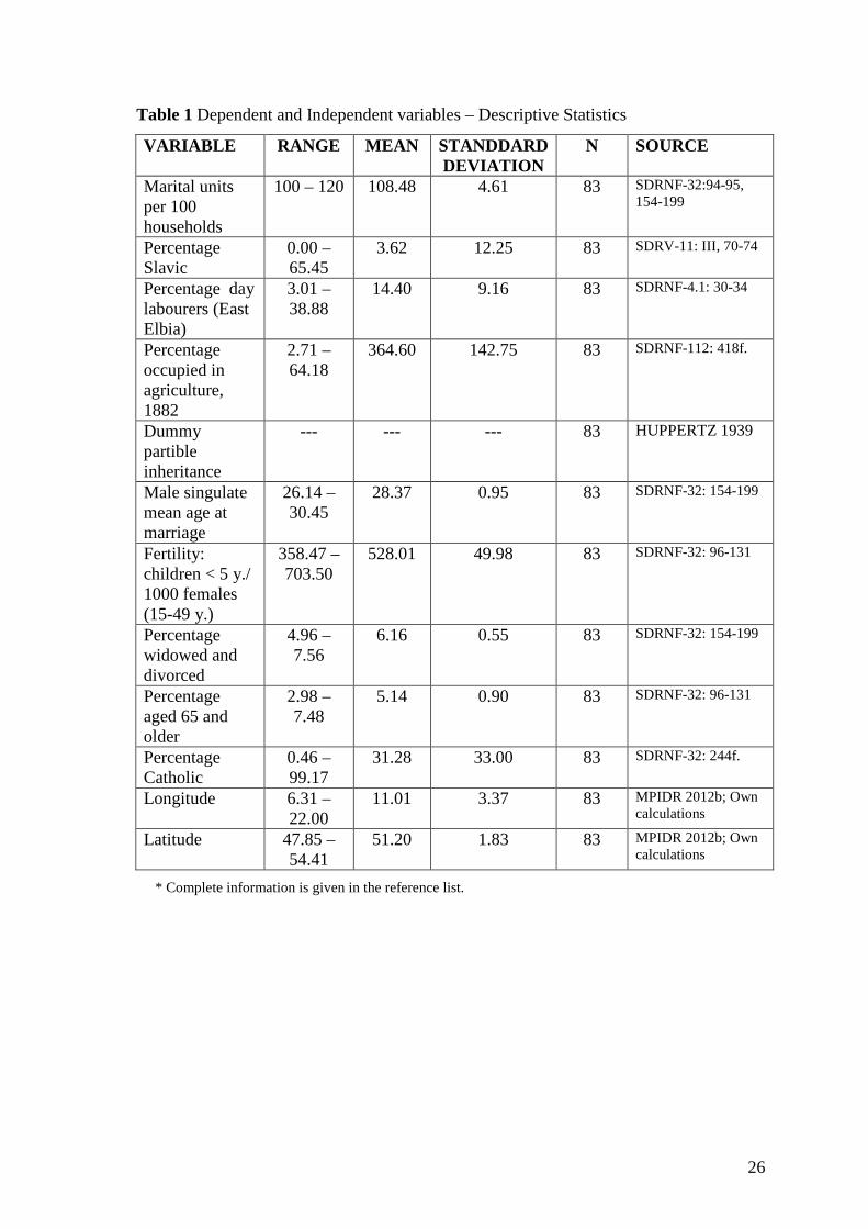
In this section, we will provide information on the specifications of our covariates, as well as

on our reasons for selecting them. Some general statistics on these variables and information

on the sources from which we obtained the data are provided in Table 1.

[Tab. 1 about here]

1. Slavic: As some authors have linked the Hajnal line to cultural differences between

Slavs and non-Slavs (Macfarlane 1981), we want to control for this effect. We use for

11 The Moran’s I index is very similar to Pearson’s product moment correlation coefficient, except that instead of

looking for the correlation between the values of two variables x and y by each unit i, it looks for the correlation

between the values of a variable x in each region i, with the mean value of the same variable x in the regions j,

which are adjacent to region i. This adjacency can be defined in different ways. We use a first order queen

definition of adjacency, which considers all of the regions which border each other at a minimum of one point as

neighbours. The Moran’s I Index can take on values from -1 (strong negative spatial autocorrelation) over zero

(no spatial autocorrelation) to one (strong positive spatial autocorrelation).

12

this variable the percentage of the population who spoke Slavic languages12. We

assume that a higher share of Slavs in the population is associated with a higher

number of marital units per household (Le Play 1982, 259).

2. East Elbia: In order to account for differences between West and East Elbia, we need a

variable that controls for this effect. We decided to use the ratio of day labourers to

farmers in 188213. In regions with a high ratio of day labourers (such as East Elbia),

we expect to find a lower degree of neo-local household formation.

3. Agriculture: In the specification of the third variable on agricultural employment, we

follow Ruggles (2009), who found a positive association with household complexity

in a worldwide comparison. Our variable is the proportion of the population employed

in agriculture (including relatives without an occupation and servants) based on

regional data from the employment census of 1882.

4. Inheritance: In order to control for differences in inheritance systems, we use a dummy

variable for all of the regions in which partible inheritance dominated14. Regions with

partible inheritance are expected to have fewer marital units per household (Berkner

and Mendels 1978, 212-214).

5. Age at marriage: Regional variation in the number of married persons (“marital units”)

might be dependent on differences in the age at marriage. We therefore include the

male singulate mean age at marriage (SMAM) as a measure of nuptiality. In this

context, the male age at marriage is considered to be the most important influence on

generation length. In turn, generation length is—along with life expectancy—a

principle determinant of the extent of the overlap of the generations (Ruggles 1987,

12 Data on the Slavic-speaking population are not available for 1885 or for any earlier period. For the Prussian

Regierungsbezirke, we used values from 1890, while for the other 48 regions of the German Empire, we had to

rely upon values for 1900. Both decisions are rather unproblematic, as the share of the population who are Slavic

changes little over time in most regions. This holds even true if we consider the migration of Slavic people from

eastern Prussia to the Ruhr area, as the share of Slavic inhabitants in the Ruhr area was still very low in 1890.

This is also the case for the 48 regions outside of Prussia in 1900. Our definition of Slavic languages does not

include the Baltic languages (e.g., Lithuanian). 13 Employment data was not available for the census year, but for 1882, where an employment census was

carried out in the German Empire. In the model, we used the 1882-data without further modifications as we do

not expect that the regional differences in the share of people working in specific jobs and sectors would have

changed drastically over such a short period of time. 14 This information is based on a map showing the regional distribution of inheritance patterns (Huppertz 1939,

map 1). It was elaborated on the basis of voluminous local studies from the 1890s.

13

63). If men form families later in life, the prospects for many three-generational

families will be limited.

6. Fertility: The likelihood of co-residing with a married child might also depend on the

overall number of children a couple have. We therefore use as a measure of fertility

the number of children under age five per 1,000 females aged 15-49.

7. Widowhood: We also control for the share of widowed and divorced people, as most

of the complex households detected in Germany in 1885 were likely to have included

widowed people. The variable is defined as the proportion of widowed and divorced

people in the population in 1885.

8. Elderly people: In order to check for the incidence of multigenerational families, we

use the share of the population aged 65 and older as another variable. A higher share

of elderly people could lead to a higher share of marital units per household (Preston

and King 1990)15.

9. Catholic: In addition to looking at the effects of demographic variables, in model 3 we

also control for the effect of Catholics in the population. As a legacy of the Augsburg

Peace Agreement (1555), the German Empire was still divided into predominantly

Protestant or Catholic territories at the end of the 19th century. Following the findings

of many contemporary social scientists on the role of religion in residence patterns and

intergenerational support, we assume that Catholics would have had more marital

units per household than Protestants (e.g., Goldscheider and DaVanzo 1989; Pampel

1992; Treas and Cohen 2006). We therefore include the percentage of Catholics in

1885 as a variable in our model.

4 Results 4.1 Descriptive analysis

In presenting our results, we will first turn to our descriptive analysis of spatial variation in

household complexity in the German Empire in 1885. While data availability constraints

forced us to run our models at the level of the 83 Regierungsbezirke, for our dependent

variable of marital units per household we were able to obtain data at the more finely gridded

district level for most of the German states (in total, 892 districts and small regions). This

allows us to investigate to what extent the regional-level data mask variation at a smaller

15 This, however, depends very much on household living arrangements of the aged.

14

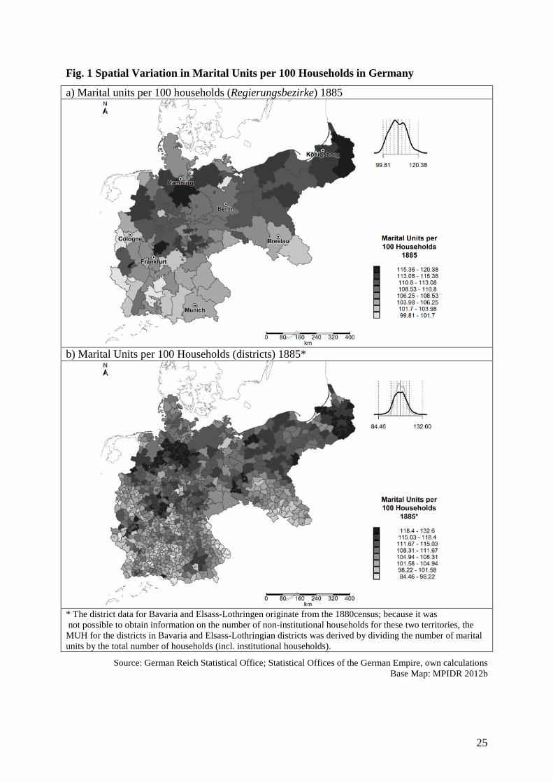
geographical scale. The maps displaying the spatial variation in MUH at the Regierungsbezirk

and the district levels are presented in Figure 1.

[Fig. 1 about here]

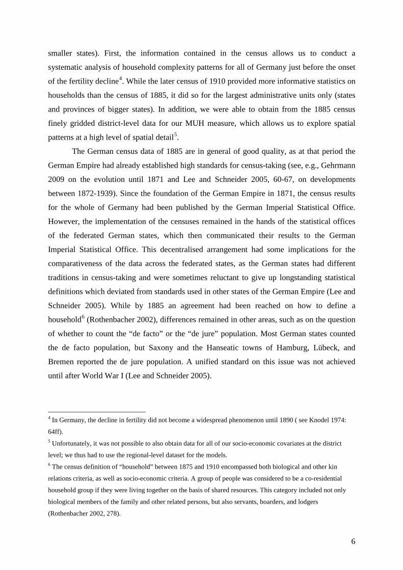
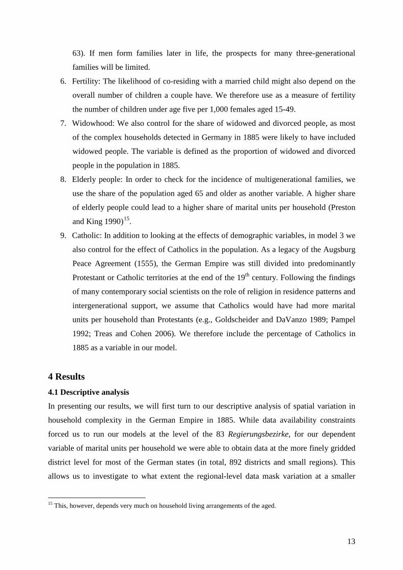
The maps reveal a relatively well-defined clustering of the MUH levels across space.

Generally, the MUH levels were higher in northern and north-eastern Germany, and they were

lower in the southern and south-western areas of the empire. Among the regions with the

highest MUH levels were the easternmost part of the German Empire that bordered the

Russian Empire (East Prussia), an area in north-western Germany south of the city of

Hamburg (part of the Prussian province of Hanover), and an area in the central part of western

Germany north of Frankfurt (Oberhessen) (see maps in Fig. 1). The hot spot in East Prussia

was situated in an area with a high share of non-German speakers, where the agricultural

structure was dominated by big estates. While this cluster appears to be in line with the Slavic

and East Elbia hypothesis, the other two hot spots are not. The hot spot in the province of

Hanover is situated in a region characterised by poor soil quality (mostly heath and

moorlands), low population density, and family farmsteads. More detailed household

statistics, which are available for Prussia in 1880 (Galloway et al. 1994), reveal that the two

MUH hot spots in East Prussia and the province of Hanover were both characterised by a low

share of (male) family members in the household and a high share of servants and helpers. By

contrast, the MUH hot spot in the central part of western Germany (Oberhessen) appears to be

largely attributable to a high number of female widows per household.

Areas with low MUH values were mostly concentrated in the south-western part of

Germany (Elsass-Lothringen, Württemberg (Swabia), Bavarian Swabia). Smaller territories

with low MUH levels included the Lower Rhine valley area around Cologne, the Bavarian

Forest region along the border to Bohemia, and a region in the south-eastern part of Germany

(in Upper and Middle Silesia). The majority—but not all—of these areas were in areas of

Germany in which partible inheritance practises dominated (e.g., Württemberg, Elsass-

Lothringen and parts of Upper Silesia; Huppertz 1939).

However, we can also find smaller regional cold spots with low MUH levels in the

north-eastern part of the German Empire, an area that was generally characterised by high

MUH levels. These included two Catholic exclaves: Ermland in East Prussia and Eichsfeld in

Thuringia. The latter was also an exclave in terms of inheritance practises, as partible

inheritance practises were dominant there (Grabein 1900). However, as these small cold spots

15

were embedded in bigger regions that were predominantly Protestant and were dominated by

non-partible inheritance, they are hidden in our models. Mecklenburg-Strelitz, situated north

of Berlin, also stood out as a cold spot of household complexity, but we have reasons to

believe that this finding is related to data quality problems (see below). On the other hand,

there were areas with high MUH levels in southern Germany as well, such as a region in

Upper Bavaria north of Munich, as well as a region along the border to Luxembourg (in the

Eifel and Saar area).

Overall, the maps suggest that a clear east-west division in MUH cannot be detected in

Germany in 1885. A larger concentration of marital units in the households of the east was

counterbalanced by similar tendencies seen among the regions situated to the northwest,

despite the large Slavic population and the dominance of a manorial agrarian regime in the

east. But there are indications that areas with partible inheritance had lower MUH levels. It

should be noted, however, that the spatial variation at the regional level in the patterns of co-

residence observed in Germany in 1885 seems to have been smaller than the spatial variation

of other European areas of or prior to that time, including France (Parish and Schwartz 1972),

Italy (Barbagli 1991), the Iberian Peninsula (Rowland 2002), and historical Poland-Lithuania

(Szołtysek 2008). Looking at Germany’s within-country variation provides certain insights

into the differences in family organisation in different regions in the mid-1880s. However,

compared to historical Germany’s spatial heterogeneity in political and socio-economic

structures, the within-country variation visible in the MUH is comparatively small.

4.2 Theil analysis

We will now turn to the results of the Theil analysis, which allows us to investigate whether

the spatial variation in household complexity was characterised by large-scale between-region

variation, or by small-scale within-region variation. A finding that the former dominated

would provide support for the view that the spatial variation across Germany was

predominantly shaped by large-scale differences in economic or cultural characteristics. By

contrast, a finding that the latter dominated would suggest that the variation in local

conditions was very important, and would seem to refute broad cultural explanations, as the

German regions were internally quite homogenous in terms of culture in 1885. This part of

the analysis will also allow us to explore to what extent small-scale spatial variation at the

district level is hidden in the macro-regional dataset that we use for our models.

For the Theil analysis, we had to exclude a number of medium-sized and smaller

German states for which we were unable to obtain district-level data. We therefore restrict

16

ourselves here to six German states and territories which together represent approximately

84% of the German population at that time16. This reduced sample contains information for

58 of our 83 regions, which are subdivided into 850 districts. Based on the Theil index, we

decompose the overall variation in MUH in our dataset of 850 districts into differences

between the mean district values of each region (between-region variation) and the

differences observed between the districts of each region (within-region variation). Our

results show that approximately 50.4% of the overall variation can be attributed to regional

differences between the Regierungsbezirke, while 49.6% of variation relates to differences

within the Regierungsbezirke. This suggests that almost 50% of the variation was not

operating at large scale, but rather at a medium to small scale. However, as we substantially

increased the number of units by splitting our 58 regions into 850 districts, the amount of

variation which can be attributed to regional-level differences is very substantial.

In order to examine these findings at a higher level of detail, we further decompose the

variation observed within our 58 regions. To do this we make use of the fact that, in the Theil

index, the overall within-region variation is obtained by summing up the within-region

variation contributed by each region (see equation 1). The results of this decomposition show

that large parts of the within-Regierungsbezirk variation were concentrated in a small number

of regions: 50% of the within-Regierungsbezirk variation is contributed by just 12 of the 58

regions. The level of internal variation was especially high in Bavaria, where the regions

Upper Bavaria, Lower Bavaria, and Middle Franconia alone contribute 21.4% of the total

within-region variation observed across all 58 regions. In these Bavarian regions, the variation

mostly stems from the fact that the urban areas had very low MUH values relative to the rural

districts. This descriptive finding for Bavaria (and a number of other regions) is in line with

Ruggles’ hypothesis (2009) that a large part of the variation stems from differences in the

shares of the population employed in agriculture.

The Theil analysis shows that a large share of the overall variation is attributable to

within-region variation, but that most of this within-region variation was concentrated in a

small number of regions, where it was primarily related to urban-rural differences. Overall,

however, there also seemed to be substantial variation between the regions. We will look at 16 These six states and territories are Prussia, Bavaria, Württemberg, Baden, Hessen, and Elsass-Lothringen. The

district data for Bavaria and Elsass-Lothringen come from the 1880 census. Because it was not possible to obtain

information on the number of non-institutional households for these two territories, the MUH for the Bavarian

and Elsass-Lothringian districts was derived by dividing the number of marital units by the total number of

households (incl. institutional households).

17

this between-region variation in detail in the following section, in which we present our

model results.

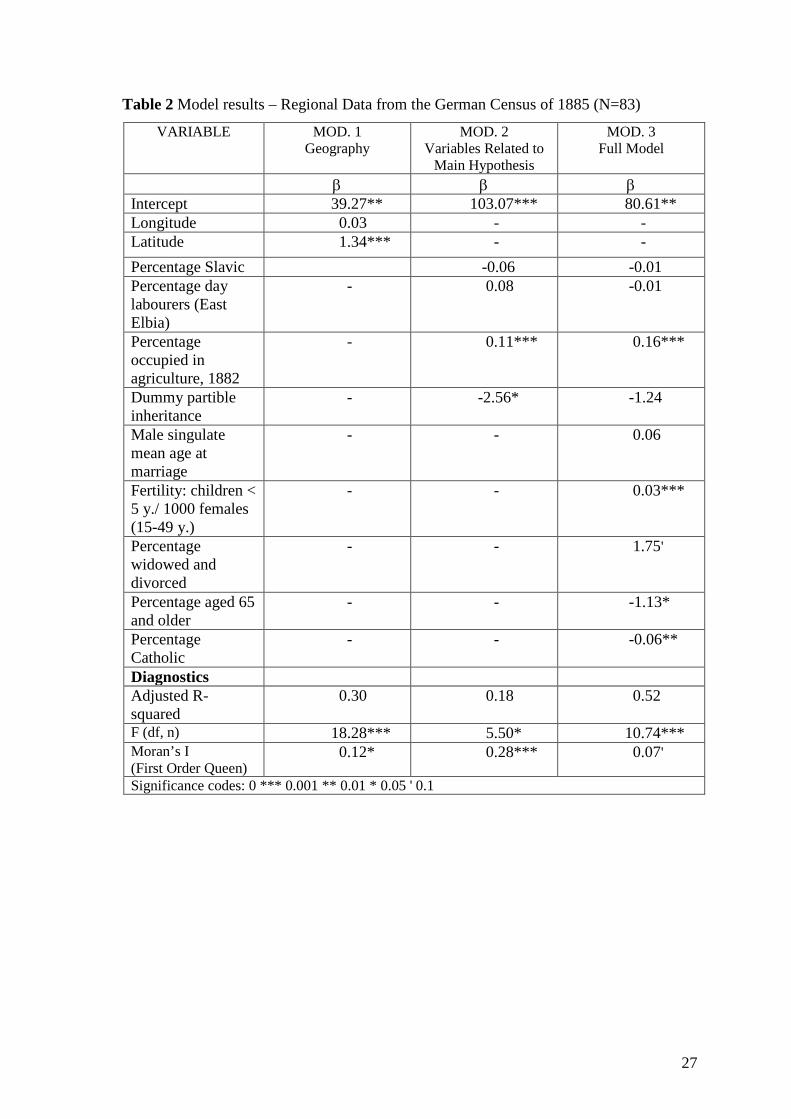
4.3 Regression analysis

As we noted in the methods section, the models are designed to explore the extent to which

existing spatial patterns persist if we control for a number of socio-economic and

demographic covariates. In our first model, we only include the latitude and longitude values

of the centroids of the 83 regions in order to explore to what extent the model detects

significant spatial trends in the data (see results in Tab. 2). As was already suggested by the

maps, the model emphasises a north-south rather than an east-west pattern, which is contrary

to our expectations. The longitude variable is positive, indicating that MUH values increased

towards the east, but it is not significant. The latitude variable, on the other hand, shows a

highly significant increase in the MUH values the farther north a region is located.

[Tab. 2 about here]

We will now turn to model 2, in which we control for the four variables directly

related to our four main research questions. Of these variables, only agricultural employment

and partible inheritance pattern provide significant results, with both exhibiting the expected

sign. However, model 2 is able to explain the spatial pattern to a limited extent only, as the

Moran’s I test on the residuals returns a highly significant value of 0.28, which is still very

close to the value observed in the dependent variable (0.32). The residuals also continue to

exhibit a significant spatial trend in the latitude variable, which implies that model 2 is only

partially able to explain the north-south differences in household complexity in Germany.

Our preferred model 3, in which we also control for demographic and cultural

covariates, is far better at explaining the spatial variation. The Moran’s I on the residuals is

substantially reduced to a value of 0.07, which is only significant at the level of 0.1. This

implies that there might still be some small biases in our estimates due to spatial

autocorrelation, but the likelihood is much lower than for model 2. When we regress the

residuals of model 3 on our longitude and latitude variables, we obtain a non-significant result

for both, which implies that we are able to explain large-scale trends in the MUH pattern. The

results for our four main variables change substantially only for partible inheritance, when we

introduce the demographic and cultural controls, as this variable becomes insignificant. The

Slavic and day labourer variables remain insignificant, while the agricultural employment

18

variable returns a higher coefficient. The other demographic and cultural control variables are,

apart from the male singulate mean age of marriage, all significant at least at the 0.1 level, and

most of them exhibit the expected sign. The exceptions are the elderly people and Catholic

variables. Among the possible explanations for the unexpected negative sign for the share of

elderly people is that many retired people may have chosen to move to a separate hut/cottage

on the farmstead rather than to live in the household of the younger generation; evidence that

this was the case has been found for some parts of rural Germany (Berkner 1972). The

Catholic variable also has an unexpected negative sign. We believe this could be related to the

fact that, with a few exceptions, almost all of the regions with a partible inheritance pattern

were predominantly Catholic, while very few of the regions with an impartible inheritance

pattern were Catholic. Thus, these two variables seem to be closely linked. If, for example, we

omit the dummy variable of partible inheritance, the Catholic variable becomes even more

negative and highly significant.

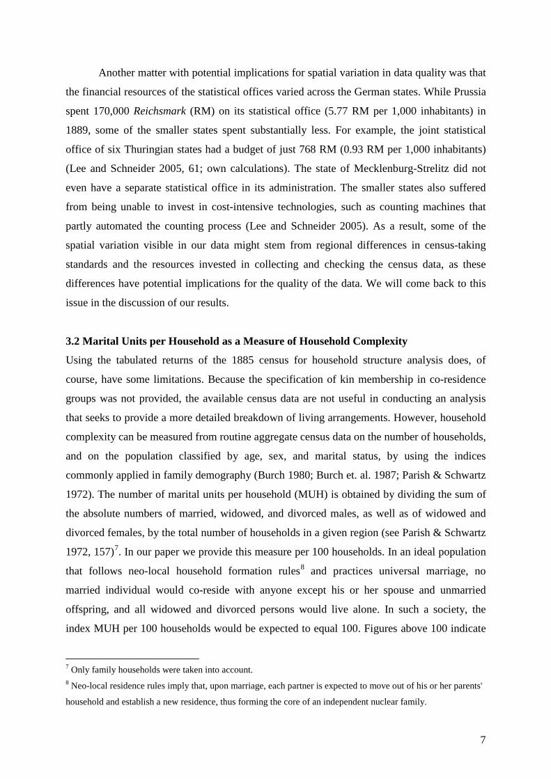
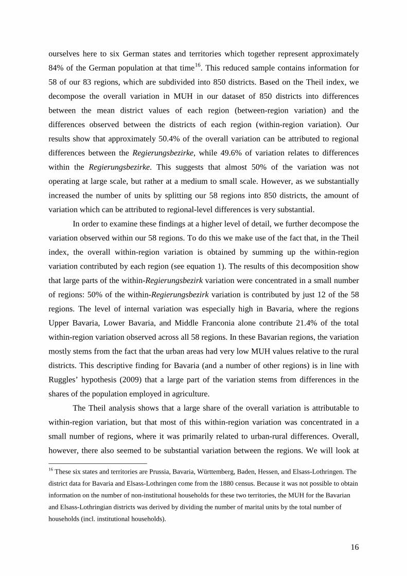
To further investigate the spatial fit of model 3, we plotted the predicted and observed

values in a graph in order to determine to what extent outliers cluster in certain regions (see

Fig. 2). Overall, the graph supports the view that the model is able to account for most of the

spatial MUH variation at the macro-regional level. Some of the outliers are among the regions

identified above as having data quality issues. These areas include Mecklenburg-Strelitz and

the Thuringian states (Saxony Weimar, Saxony Meiningen), where data collection activities

were heavily constrained by small financial budgets. In addition, a substantial number of the

outliers are regions with very small population sizes (e.g., Waldeck, Lippe-Detmold, the

Principality of Lübeck, and the Principality of Birkenfeld). Meanwhile, Bremen’s outlier

status might be related to the fact that the city counted the de jure population. Especially in a

harbour town, where sailors were away on their ships for weeks or months, a de jure

population count tended to result in higher MUH values than a de facto count would have.

But there are also a number of outliers for which we have no indications of data quality or

data comparability problems. This suggests that we are missing some important covariates for

these regions. This group of outliers includes the MUH hot spots in the province of Hanover

and Oberhessen, as well as the Bavarian region of Upper Bavaria.

5 Conclusions In this paper, we investigated the spatial variation in household structures in late 19th-century

Germany using an aggregate measure of household complexity (marital units per household,

19

or MUH). Our analysis allowed us to examine the relevance of the existing theoretical

considerations related to household complexity for understanding regional MUH differences

in Germany. Several clusters with different incidence rates of marital units per domestic

group existed in the German Empire at the time, with higher proportions of households with

more than one marital unit found in the north and north-east, and lower proportions found in

the south and south-west of the country. Contrary to our expectations, some of the supposedly

decisive socio-economic and cultural borders within late 19th-century Germany do not appear

to have corresponded with the observed spatial patterns of family composition. In our

descriptive analysis and our models based on 83 regions (Regierungsbezirke and smaller

states), we did not find evidence to support the hypothesis that the East Elbian divide can also

be seen in the spatial variation in household complexity. Although the East Elbian part of

Germany had a higher degree of household complexity than southern Germany, this area of

high MUH levels also extended into north-western Germany, where the agricultural structures

were dominated by family farmsteads and life-cycle service. We also did not find any

indications that the Slavic population had higher levels of household complexity, with the

possible exception of elevated levels of household complexity in the far eastern part of

Germany. Our results generally confirmed Hajnal’s view (which had been challenged by, for

example, Laslett 1983) that all of the German Empire was part of the Western European

Family System.

We found indications that differences in inheritance patterns might have played a role,

as regions with partible inheritance initially appeared to have had lower levels of household

complexity. But in our complete model, the variable was not significant. The most compelling

pieces of evidence we found in support of Ruggles’ “agricultural employment hypothesis”

(2009) as the share of the population working in agriculture, as well as a number of the

demographic indicators, were strongly associated with levels of household complexity. The

results of our explorative analysis of household complexity at the more finely gridded district

level provided support for the view that urban-rural differences were even more closely

related to household complexity at this geographic level. This suggests that, if we had been

able to model household complexity at the district rather than the regional level, we may have

found even stronger support for Ruggles’ hypothesis.

However, to properly understand the geography of historical family systems, it is

essential to consider the intrinsically complex interplay of economic, demographic, and

cultural factors; which are, in turn, further differentiated by local and environmental contexts,

and by historical path dependencies. This research can serve as a starting point for more

20

contextual and place-specific future investigations17. Linking together the analyses

undertaken at different aggregation levels should allow us to account for aggregate constraints

on people’s household strategies, without losing sight of individual behaviour and the

complexities of local histories.

Acknowledgements

We thank M. Dinter (MPIDR) for the data management and his research assistance.

References

Published sources:

SDRAF:

Statistik des Deutschen Reichs Alte Folge, vol. 57 (1883).

SDRNF:

Statistik des Deutschen Reichs Neue Folge, vol. 2 (1884), 4.1 (1884), 5 (1885), 32 (1888), 112 (1898),

240 (1915).

SDRM:

Monatshefte zur Statistik des Deutschen Reichs, vol. 1884.1, III: 1-17

SDRV:

Vierteljahrshefte zur Statistik des Deutschen Reichs, vol. 11, III: 70-74

Literature:

ALDERSON A. S., SANDERSON S. K., 1991, ″Historic European household structures and the

capitalist world-economy″, Journal of Family History 16 (4), pp. 419-432.

ANSELIN L., 1988, Spatial Econometrics: Methods and Models. Dordrecht [et al.], Kluwer Academic

Publications, 284 p. 17 The on-going data collection and harmonising project “Mosaic” will soon bring to light historical census

micro-data for several dozen local communities from different parts of 19th-century Germany

(seewww.censusmosaic.org).

21

BARBAGLI M., 1991, ″Three Household Formation Systems in Eighteenth- and Nineteenth-Century

Italy″ in KERTZER D. I. and SALLER R. P. (eds.), The Family in Italy from Antiquity to the

Present, New Haven [et al.], Yale University Press, pp. 255-269.

BERKNER L. K., 1972, ″Rural Family Organization in Europe: A Problem in Comparative History″,

Peasant Studies Newsletter 1, pp. 145-156.

BERKNER L. K., 1976, ″Inheritance, Land Tenure and Peasant Family Structure: A German Regional

Comparison″ in GOODY J., THIRSK J. and THOMPSON E. P. (eds.), Family and Inheritance

in Rural Western Europe, 1200-1700, Cambridge [et al.], University Press, pp. 71-95.

BERKNER L. K., MENDELS F. F., 1978, ″Inheritance Systems, Family Structure, and Demographic

Patterns in Western Europe″ in TILLY C. (eds.), Historical Studies of Changing Fertility,

Princeton, N. J., Princeton University Press, pp. 200-224.

BURCH T. K., 1980. ″The index of overall headship: a simple measure of household complexity

standardized for age and sex″, Demography 17 (1), pp. 25-37.

BURCH T. K., HALLI S. S., MADAN A. K., THOMAS K., WEI L., 1987, ″Measures of household

composition and headship based on aggregate routine census data″ in BONGAARTS J.,

BURCH T. K. and WACHTER K. W. (eds.), Family Demography: Methods and their

Application, Oxford [et al], Oxford University Press, pp. 19-39.

CONRAD C., LECHNER M., WERNER W., 1996, ″East German fertility after unification: Crisis or

adaptation? ″, Population and Development Review 22 (2), pp. 331-358.

CONZE W., 1966, ″Vom "Pöbel" zum "Proletariat", Sozialgeschichtliche Voraussetzungen für den

Sozialismus in Deutschland″ in WEHLER H.-U. (ed.), Moderne deutsche Sozialgeschichte.

Köln [et al.], Kiepenheuer & Witsch, pp. 111-136.

EHMER J., 2009, ″House and the stem family in Austria″ in FAUVE-CHAMOUX A. and OCHIAI E.

(eds.), The Stem Family in Eurasian Perspective. Revisiting House Societies, 17th-20th

centuries, Bern, Peter Lang AG, International Academic Publishers, pp. 103-131.

GALLOWAY P. R., HAMMEL E. A., LEE R. D., 1994, ″Fertility decline in Prussia, 1875-1910: A

pooled cross-section time series″, Population Studies 48 (1), pp. 135-158.

GEHRMANN R., 2009, ″German census taking before 1871″, MPIDR Working Paper wp-2009-023,

Rostock, 24 p.

GOLDSCHEIDER F. K., DAVANZO J., 1989, ″Pathways to independent living in early adulthood:

Marriage, semiautonomy, and premarital residential independence″, Demography 26 (4), pp.

597-614.

GRABEIN M., 1900, ″Die Vererbung des ländlichen Grundbesitzes im Königreich Preussen (ed. by

M. Sering): VII. Provinz Sachsen” Berlin, Verlagsbuchhandlung Paul Parey.

HAJNAL J., 1965, ″European marriage patterns in perspective″ in GLASS D. V. and EVERSLEY D.

E. C. (eds.), Population in History. Essays in Historical Demography, London: Edward

Arnold, pp. 101-143.

22

HAJNAL J., 1982, ″Two kinds of preindustrial household formation system″, Population and

Development Review, 8 (3), pp. 449-494.

HAMMEL E. A., LASLETT P., 1974, ″Comparing household structure over time and between

cultures″, Comparative Studies in Society and History 16, pp. 73-109.

HENNINGS L., 1995, ″Familien- und Gemeinschaftsformen am Übergang zur Moderne. Haus, Dorf,

Stadt und Sozialstruktur zum Ende des 18. Jahrhunderts am Beispiel Schleswig-Holsteins″ in

Beiträge zur Sozialforschung, Schriftenreihe der Ferdinand-Tönnies-Gesellschaft e. V. Kiel,

Band 7. Berlin, Duncker & Humblot, 183 p.

HOCHSTADT S., 1999, ″Mobility and Modernity: Migration in Germany 1820–1989″, Ann Arbor,

University of Michigan Press, 331 p.

HUPPERTZ B., 1939, ″Räume und Schichten bäuerlicher Kulturformen in Deutschland: Ein Beitrag

zur deutschen Bauerngeschichte″, Bonn, Röhrscheid, 315 p.

IMHOF A. E., 1976, ″Ländliche Familienstrukturen an einem hessischen Beispiel: Heuchelheim 1690-

1900″ in CONZE W. (ed.), Sozialgeschichte der Familie in der Neuzeit Europas. Stuttgart,

Klett, pp. 197-230.

JANAS C., 2005, ″Zum Wandel von Familienstrukturen. Ein deutsch-polnischer Vergleich″, Aachen,

Mainz, 208 p.

KEMPER F.-J., 1983, ″Household structure in Germany, 1933: Indices of household complexity and

determinant of regional variation″, Erdkunde 37, pp. 11-21.

KLÜSENER S., GOLDSTEIN J. R., 2012, ″The long-standing demographic East-West-divide in

Germany″. Rostock. MPIDR Working Paper WP-2012-007 (revised in December 2012).

KNODEL J. E., 1974, ″The Decline of Fertility in Germany, 1871-1939″, Princeton, N.J.: Princeton

University Press, 306 p.

KREYENFELD M., 2003, ″Crisis or adaptation – reconsidered: A comparison of East and West

German fertility patterns in the first six years after the 'Wende'″, European Journal of

Population 19 (3), pp. 303-329.

KREYENFELD M., 2004, ″Fertility decisions in the FRG and GDR: An analysis with data from the

German fertility and family survey″, Demographic Research, Special Collection 3, No. 11.

LASLETT P., 1983, ″Family and household as work group and kin group: areas of traditional Europe

compared″ in WALL R. and ROBIN J. (eds.), Family Forms in historic Europe. Cambridge,

Cambridge University Press, pp. 513-563.

LE BRAS H., TODD E., 1981, ″L 'invention de la France″, Paris, Le Livre de Poche, 511 p.

LE PLAY F., 1982 [1872], ″Le Réforme Sociale″ in SILVER C. B. (ed. and trans.), Frederic Le Play

on Family, Work, and Social Change. Chicago [et al.], Chicago University Press: pp. 259-262.

LEE W. R., 1981, ″The German Family: A critical survey of the current state of historical research″ in

EVANS R. J. and LEE W. R. (eds.), The German Family: Essays on the social History of the

23

Family in Nineteenth- and Twentieth-Century, London [et. al.], Croom Helm [et. al.], pp. 19-

50.

LEE W. R., 2001, ″Bastardy and the socioeconomic structure of South Germany″ in ROTBERG R. I.

(ed.), Population History and the Family: A Journal of Interdisciplinary History reader,

Cambridge, Mass. [et al.], MIT Press, pp. 237-260.

LEE W. R., SCHNEIDER M. S., 2005, ″Amtliche Statistik zwischen Staat und Wissenschaft, 1872-

1939″ in MACKENSEN R. and REULECKE J. (eds.), Das Konstrukt „Bevölkerung“ vor, im

und nach dem „Dritten Reich“, Wiesbaden, VS Verlag für Sozialwissenschaften, pp. 50-91.

MACFARLANE A., 1981, ″Demographic structures and cultural regions in Europe″, Cambridge

Anthropology 6, pp. 1-17.

MPIDR [MAX PLANCK INSTITUTE FOR DEMOGRAPHIC RESEARCH] 2012a. ″1846

MOSAIC German Customs Union census, Version 1.1 [SPSS data file]″, Rostock,

Max Planck Institute for Demographic Research.

MPIDR [MAX PLANCK INSTITUTE FOR DEMOGRAPHIC RESEARCH] 2012b. ″MPIDR

Population History GIS Collection″, Rostock, Max Planck Institute for Demographic

Research.

PAMPEL F. C., 1992, ″Trends in living alone among the elderly in Europe″ in ROGERS A. (ed.),

Elderly Migration and Population Redistribution: A comparative Study. Belhaven, London, pp

97-117.

PARISH W. L. Jr., SCHWARTZ M., 1972, ″Household complexity in nineteenth century France″,

American Sociological Review 37 (2), pp. 154-173.

PRESTON M., KING S., 1990, ″Who lives with whom? Individual versus household measures″,

Journal of Family History 15, pp. 117-132.

ROBISHEAUX T., 1998, ″The peasantries of Western Germany, 1300-1750″ in SCOTT T. (ed.), The

Peasantries of Europe from the Fourteenth to the Eighteenth Centuries, London [et al.],

Longman, pp. 111-142.

ROSENBAUM H., 1996, ″Formen der Familie. Untersuchungen zum Zusammenhang von

Familienverhältnissen, Sozialstruktur und sozialem Wandel in der deutschen Gesellschaft des

19. Jahrhunderts″, Frankfurt am Main, Suhrkamp-Taschenbuch Wissenschaft 374: 7. Auflage ,

633 p.

ROTHENBACHER F., 2002, ″The Societies of Europe. The European Population 1850-1945″,

Houndmills [et al.], Palgrave Macmillan, 846 p.

ROWLAND R., 2002, ″Household and family in the Iberian Peninsula″, Portuguese Journal of Social

Science 1 (1), pp. 62-75.

RUDOLPH R. L., 1995, ″The European Peasant Family and Society: Historical Studies″, Liverpool,

Liverpool University Press, 256 p.

24

RUGGLES S., 1987, ″Prolonged Connections: The Rise of the Extended Family in Nineteenth-

Century England and America”, Madison, University of Wisconsin Press, 282 p.

RUGGLES S., 2009, ″Reconsidering the Northwest European family system: Living arrangements of

the aged in comparative historical perspective″, Population and Development Review 35 (2),

pp. 249-273.

RUGGLES S., 2010, ″Stem families and joint families in comparative historical perspective″,

Population and Development Review 36 (3), pp. 563-577.

SCHLUMBOHM J., 1994, ″Lebensläufe, Familien, Höfe. Die Bauern und Heuerleute des

Osnabrückischen Kirchspiels Belm in proto-industrieller Zeit, 1650–1860″, Göttingen,

Vandenhoeck & Ruprecht, 690 p.

SCHLUMBOHM J., 2009, ″Strong myths and flexible practices: House and stem family in Germany″

in FAUVE-CHAMOUX A. and OCHIAI E. (eds.), The Stem Family in Eurasian Perspective.

Revisiting House Societies, 17th-20th Centuries, Bern: Peter Lang AG, International Academic

Publishers, pp. 81-102.

SZOŁTYSEK M., 2008, ″Rethinking Eastern Europe: household formation patterns in the Polish-

Lithuanian Commonwealth and European family systems″, Continuity and Change 23, pp.

389-427.

THEIL H., 1965, “The information approach to demand analysis”, Econometrica 33 (1), pp. 67-87.

THERBORN G., 2004, ″Between Sex and Power: Family in the World 1900–2000″, London,

Routledge, 379 p.

TREAS J., COHEN P., 2006, ″Maternal coresidence and contact: Evidence from cross-national

surveys. In allocating public and private resources across generations″, International Studies in

Population 3, pp. 117-137.

VÖGELE J., 1998, ″Urban Mortality Change in England and Germany, 1870–1913″, Liverpool,

Liverpool University Press, 299 p.

WEBER-KELLERMANN I., 1982, ″Die deutsche Familie. Versuch einer Sozialgeschichte″, Frankfurt

am Main, Suhrkamp, 268 p.

25

Fig. 1 Spatial Variation in Marital Units per 100 Households in Germany

a) Marital units per 100 households (Regierungsbezirke) 1885

b) Marital Units per 100 Households (districts) 1885*

* The district data for Bavaria and Elsass-Lothringen originate from the 1880census; because it was not possible to obtain information on the number of non-institutional households for these two territories, the MUH for the districts in Bavaria and Elsass-Lothringian districts was derived by dividing the number of marital units by the total number of households (incl. institutional households).

Source: German Reich Statistical Office; Statistical Offices of the German Empire, own calculations Base Map: MPIDR 2012b

26

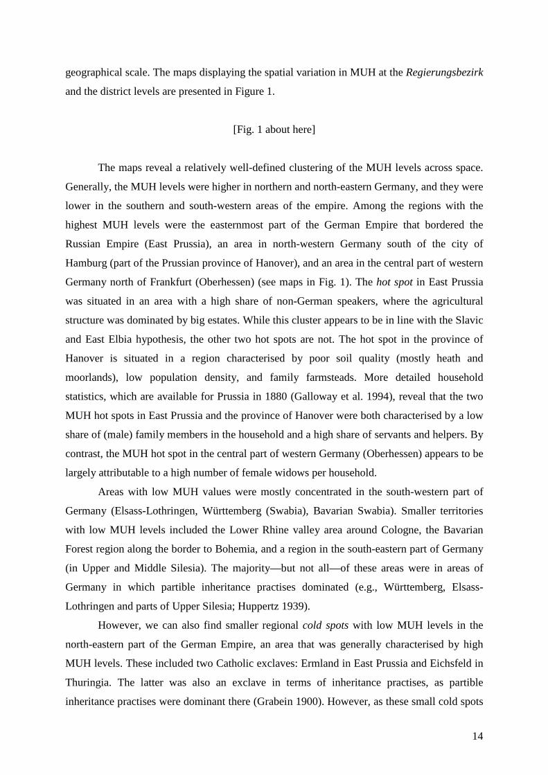
Table 1 Dependent and Independent variables – Descriptive Statistics

VARIABLE RANGE MEAN STANDDARD DEVIATION

N SOURCE

Marital units per 100 households

100 – 120 108.48 4.61 83 SDRNF-32:94-95, 154-199

Percentage Slavic

0.00 – 65.45

3.62 12.25 83 SDRV-11: III, 70-74

Percentage day labourers (East Elbia)

3.01 – 38.88

14.40 9.16 83 SDRNF-4.1: 30-34

Percentage occupied in agriculture, 1882

2.71 – 64.18

364.60 142.75 83 SDRNF-112: 418f.

Dummy partible inheritance

--- --- --- 83 HUPPERTZ 1939

Male singulate mean age at marriage

26.14 – 30.45

28.37 0.95 83 SDRNF-32: 154-199

Fertility: children < 5 y./ 1000 females (15-49 y.)

358.47 – 703.50

528.01 49.98 83 SDRNF-32: 96-131

Percentage widowed and divorced

4.96 – 7.56

6.16 0.55 83 SDRNF-32: 154-199

Percentage aged 65 and older

2.98 – 7.48

5.14 0.90 83 SDRNF-32: 96-131

Percentage Catholic

0.46 – 99.17

31.28 33.00 83 SDRNF-32: 244f.

Longitude 6.31 – 22.00

11.01 3.37 83 MPIDR 2012b; Own calculations

Latitude 47.85 – 54.41

51.20 1.83 83 MPIDR 2012b; Own calculations

* Complete information is given in the reference list.

27

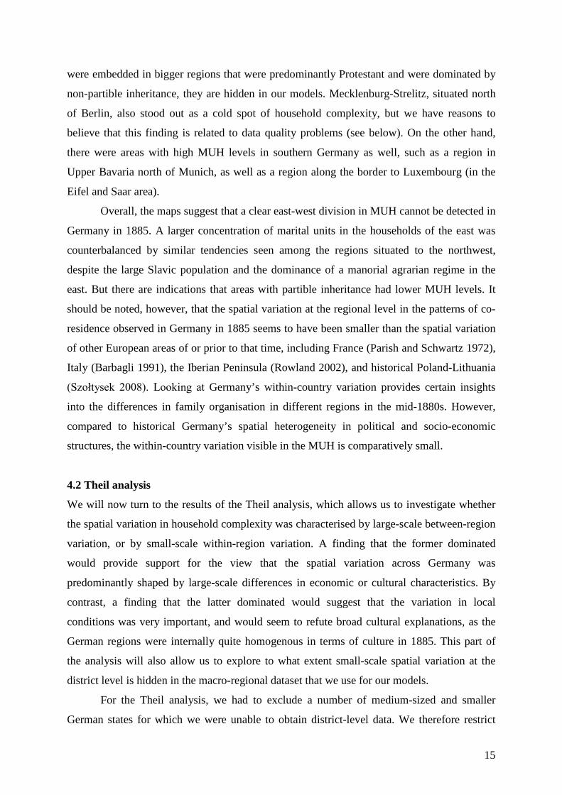
Table 2 Model results – Regional Data from the German Census of 1885 (N=83)

VARIABLE MOD. 1 Geography

MOD. 2 Variables Related to

Main Hypothesis

MOD. 3 Full Model

β β β Intercept 39.27** 103.07*** 80.61** Longitude 0.03 - - Latitude 1.34*** - - Percentage Slavic -0.06 -0.01 Percentage day labourers (East Elbia)

- 0.08 -0.01

Percentage occupied in agriculture, 1882

- 0.11*** 0.16***

Dummy partible inheritance

- -2.56* -1.24

Male singulate mean age at marriage

- - 0.06

Fertility: children < 5 y./ 1000 females (15-49 y.)

- - 0.03***

Percentage widowed and divorced

- - 1.75'

Percentage aged 65 and older

- - -1.13*

Percentage Catholic

- - -0.06**

Diagnostics Adjusted R-squared

0.30 0.18 0.52

F (df, n) 18.28*** 5.50* 10.74*** Moran’s I (First Order Queen)

0.12* 0.28*** 0.07'

Significance codes: 0 *** 0.001 ** 0.01 * 0.05 ' 0.1

28

Fig. 2 Observed vs. Predicted Values of Model 318

18 Region names are included for all of the regions in which the difference between the observed and the

predicted values (residuals) is higher than the standard deviation of the residuals across the whole dataset.