i

A SPATIAL ANALYSIS OF ILLINOIS AGRICULTURAL CASH RENTS

BY

SHANNON M. WOODARD

THESIS

Submitted in partial fulfillment of the requirements for the degree of Master of Science in Agricultural and Consumer Economics

in the Graduate College of the University of Illinois at Urbana-Champaign, 2010

Urbana, Illinois

Advisor: Professor Nicholas Paulson

ii

Abstract

Following the commodity price shocks in 2007, anecdotal evidence shows that tenant farmers

experienced large increases in cropland rental rates and input prices. However, it is unclear how

residual profits (crop revenue less non-land costs) resulting from the price increases within this

sector (if any) have been allocated among tenant farmers, landowners and input suppliers. This

work provides statistical evidence regarding how increases in corn prices and the associated

increases in profitability ultimately flow through to the rental market, and which participants

benefit the most.

The purpose of this paper is to help fill the gap in the existing academic literature with

respect to how the recent price shocks affected the agricultural rental market. Using unique

farm-level, longitudinal data from the Illinois Farm Bureau Farm Management (FBFM) office, a

hedonic model of the determinants of Illinois’ cash rents per acre is constructed and the marginal

contributions of parcel characteristics to the market price are derived. A novel spatial

econometric panel estimation method is employed to model the spatial error structure and ensure

consistent estimators of the model parameters. Lastly, the marginal benefits appropriated by

each commodity production participant are estimated and the validity of Ricardian Rent Theory

(RRT) is tested.

The primary findings indicate that marginal output price increases have a significant

effect on cash rents with strong spatial correlations detected in the data. The estimated effect of

increasing prices on cropland rents is substantially larger at the farm level, in comparison to a

county aggregated model using similar data. County level results find that marginal increases in

the harvest futures price increases rents by around $24.00. Under the farm level analysis, this

iii

measure rises to over $41.00, perhaps implying that the aggregation process has a significant loss

of information. Second, as would be predicted by land rent theories, we find substantiating

evidence that both inter-county and intra-county soil productivity variations have considerable

impacts on cash rent levels, in that rents are positively associated with higher soil quality. Third,

we find that there is a risk premium embedded in the cash rental rate, in that parcels with a

higher perceived yield risk result in a negative impact on the cash rent. This is expected given

the likely risk aversion of tenant operators. Parcels within relatively rural areas as well as those

operated by farmers with large scale operations also exhibit tendencies for higher rent levels,

although this impact is rather minimal. Lastly, we find limited support for RRT with a majority

of increased revenues due to output price increases accruing to the farmer. Tenant farmers

capture 89% of the marginal increases in commodity prices while the landowner and input

suppliers absorb only 3.3% and 7.7%, respectively. The relatively large amount that is captured

by the tenant farmer may be a form of ‘compensation’ for bearing price risk. This would imply

that tenant farmers cash renting cropland receive both a premium for yield risk as well as price

risk.

iv

Table of Contents

Chapter 1 Introduction ................................................................................................................1

1.1 Purpose and Contribution ......................................................................................................2

1.2 Overview ...............................................................................................................................4

Chapter 2 Background .................................................................................................................6

2.1 Illinois Agriculture and Recent Cash Rent Trends ................................................................6

2.2 Commodity Price Levels and Volatility ................................................................................8

2.3 A New Era? .........................................................................................................................10

2.4 Charts and Figures ...............................................................................................................12

Chapter 3 Land Rent Theories and Literature Review ..........................................................15

3.1 Classical Rent Theory ..........................................................................................................15

3.2 Neo-Classical Rent Theory ..................................................................................................17

3.3 Capitalized Values and Rate of Return ................................................................................18

3.4 Empirical Land Rent Models ...............................................................................................19

3.5 Empirical Land Value Models .............................................................................................22

3.6 Figures ..................................................................................................................................23

Chapter 4 Theoretical Framework ............................................................................................24

4.1 Hedonic Model .....................................................................................................................24

4.2 Spatial Considerations ..........................................................................................................26

4.3 Spatial Autoregressive Models (SAR) .................................................................................29

Chapter 5 Data, Methods and Procedures ...............................................................................33

5.1 Data ......................................................................................................................................33

5.2 Variables Used in the Hedonic Rent Model .........................................................................34

5.3 Assumptions .........................................................................................................................39

5.4 Empirical Model ...................................................................................................................40

5.5 Tables and Figures ...............................................................................................................44

Chapter 6 Results ........................................................................................................................53

6.1 Results Tables ......................................................................................................................58

Chapter 7 Summary and Conclusion ........................................................................................60

References .....................................................................................................................................63

1

Chapter 1 Introduction

Following the commodity price shocks in 2007, anecdotal evidence implied that tenant farmers

experienced large increases in cropland rental rates and input prices. However, it is unclear how

residual profits (crop revenue less non-land costs) resulting from the price increases within this

sector are allocated among tenant farmers, landowners and input suppliers. Theories of land

economics generally posit that a tenant farmer’s residual profits accrue to the landowner in the

form of rent (Barlowe, 1986; Hubacek, 2002; O’Sullivan, 2003). Given this approach, it is

expected that the recent increases in agricultural rents would capture the bulk of additional

revenues from rising commodity prices. As land is an undeniably intricate piece of the

agricultural system, identifying how rising commodity prices impact agricultural agents is an

important question. Such information is relevant to commodity producers in making informed

planting decisions, landowners in valuing their property, policy makers during the development

and implementation of new agricultural programs, and grain markets when faced with

forecasting. This research empirically analyzes the impact of the recent commodity price shocks

on Illinois agricultural cash rents. Specifically, this work provides statistical evidence regarding

increases in corn prices and the associated increases in profitability in the rental market, and

which participants benefit most.

Research exploring the factors affecting agricultural land values and rents has persisted

with much focus on topics including biofuels (Henderson and Gloy, 2009; Du, Hennessy, and

Edwards, 2008), government payments, conservation and land retirement programs (Nickerson

and Lynch, 2001; Kirwan, 2009; Goodwin and Mishra, 2005; Taylor and Brester, 2005; Patton

et. al, 2008; Shaik, 2007; Shaik, Helmers and Atwood, 2006), global warming (Mendelsohn and

2

Dinar, 2003), and urbanization pressures (Plantinga, Lubowski and Stavins, 2002; Livanis et. al,

2006). However, the empirical impact of increasing commodity price levels on agricultural cash

rents and respective land values has not gained as much attention as the recent disturbances in

commodity price levels have not existed since the early 1970’s. During the summer of 2008,

corn and soybean futures prices rose approximately 119.8% and 91.9%, respectively, compared

to the previous year. The resulting nominal prices were the highest in history. Agricultural land

values quickly followed suit with Illinois experiencing a 19.3% increase in cropland values

between 2007 and 2008, the largest year-over-year increase ever in the Corn Belt (USDA,

2008a). Du et. al presents a paper within this conceptual framework focusing in on impacts of

corn futures prices on farmland cash rents in Iowa. Searches for other contemporary, academic

articles covering this topic lack any results with the exception of numerous condensed articles

targeting farmers and landowners.

1.1 Purpose and Contribution

This study fills the gap in the existing academic literature and estimates the impact of the recent

price shocks on the agricultural rental market. Using unique farm-level, longitudinal data from

the Illinois Farm Bureau Farm Management (FBFM) office, a hedonic model is constructed of

the determinants of Illinois’ cash rents per acre and used to derive the marginal contributions of

parcel characteristics to the market price. Primary focus is placed upon anticipated and

unanticipated commodity price movements and impacts on annual cash rental prices. A novel

spatial econometric panel estimation method is employed to model the spatial error structure and

ensure consistent estimators of the model parameters. Lastly, the marginal benefits appropriated

3

to each commodity production participant are approximated and the validity of Ricardian Rent

Theory (RRT)1

Previous empirical studies analyzing cropland cash rents have generally been limited to

aggregated county-level data which may hinder the extraction of information as opposed to

analyzing the underlying unit data. The aggregation process also severely restricts the number of

observations available to the analyst. The contributions of this paper are as follows. First, it uses

unique farm-level data allowing for more efficient and accurate estimates of the factors affecting

land rents, including important spatial effects. The use of farm-level data also provides nearly

six times as many observations, relative to an aggregated county-level option, allowing for

improved estimator precision. Second, we include data through 2008 to observe the full impact

of the price shocks experienced that summer in which corn and soybean futures prices reached

an all time high. Third, this analysis extends existing literature on the valuation of

heterogeneous agricultural parcels. By explicitly accounting for variations in soil quality,

urbanization pressures, economies of scale, and economic characteristics, a clearer view of how

commodity price changes ultimately flow through to rental markets is observed. Lastly, we

allow for heterogeneity across tenant farmers while explicitly controlling for the spatial nature

inherent in the data by using a leading-edge spatial panel error component method (Kapoor et al.,

2007). This approach to analyzing agricultural rents, or the impact that output prices have on

rents has not, to the knowledge of the author, been used in previous studies.

is tested.

The primary findings indicate that marginal output price increases have a significant

effect on cash rents with strong spatial correlations. The estimated effect of increasing prices on

cropland rents is substantially larger at the farm level, compared to a county aggregated model

1 RRT predicts that any permanent increase in revenues will ultimately accrue to the landowner in the form of rent.

4

using similar data. This may imply that valuable information is lost during the aggregation

process. Second, as implied by land rent theories, substantiating evidence is found that both cross

county and intra-county soil productivity variations impact cash rent levels. Third, a risk

premium is embedded in the cash rental rate, in that parcels with higher yield risk have lower

rental prices. This is expected given the likely risk aversion of tenant operators. Parcels within

relatively rural areas as well as those operated by farmers with large scale operations also exhibit

tendencies for higher rent levels, although this impact is rather minimal. Last, we find limited

support for RRT with a vast majority of increased revenues accumulated by the tenant farmer in

lieu of the landowner and input suppliers.

1.2 Overview

This study is organized as follows. Chapter 2.1 describes the scope of Illinois' agricultural sector

and recent trends in Illinois cash rents. A discussion of recent commodity price drivers and the

current price environment is then presented (Chapter 2.2 and 2.3).

Chapter 3 provides a literature review of the basic theories on land rents and land value

capitalization (Chapters 3.1-3.3). The remainder of the chapter provides a summary of previous

studies investigating agricultural land rents. This section is subdivided into studies using hedonic

approach estimations and those using income approaches. A brief review of recent agricultural

land value studies is provided in Chapter 3.5.

Chapter 4 presents the theoretical framework for this study. A review of the hedonic

model and the implicit price approach as applied to agricultural cash rents is provided in section

4.1. An underlying hypothesis of this study is that agricultural cash rents are related by an

underlying spatial component. The motivation for considering a spatial framework is presented

5

in section 4.2 including a brief overview of spatial correlation, its implications, and the definition

of a “neighbor” within a spatial context. Section 4.3 concludes with a discussion of the Spatial

Autoregressive Error Model considered in this article (Anselin, 2002).

Chapter 5 presents the data employed in this study. Section 5.2 presents the dependent

and independent variables used as well as their construction and the hypothesized effects of the

independent variables on agricultural cash rents. The remainder of the chapter describes the

empirical method employed for estimation.

Chapter 6 presents the results along with a discussion of the findings and implications.

Chapter 7 concludes and suggests potential extensions and areas of future research.

6

Chapter 2 Background

2.1 Illinois Agriculture and Recent Cash Rent Trends

According to USDA-NASS estimates, approximately 27 million acres, or 75%, of Illinois’ total

available land is dedicated to farming activities, with 88.5% of total farmland used in the

cultivation of commodity products (USDA 2009a). In 2007, corn made up the majority of all

farm receipts in Illinois constituting 48.6% of the states $11.7 billion total commodity revenue

(USDA 2009b). At a national level, Illinois currently contributes an estimated 17.1% and 14.6%

to the U.S. total value of production for corn and soybean respectively. Illinois’ commodity

contributions are primarily produced on flat rate rented cropland with current estimates of cash

rented cropland ranging between 60%-80% of Illinois’ total cropland (Schnitkey and Lattz,

2002). Estimates from NASS 2007 Census data have produced figures as high as 73% for total

Illinois cropland being cash rented. During 2002, the Census of Agriculture (USDA, 2004)

estimated only 69% of cropland was being cash rented, implying that approximately 765,891

additional acres were being harvested by tenant farmers in 2007.

The increase in cash rental contracts has come at the expense of other land transaction

types. Between 1996 and 2008, the prevalence of operators farming owned land decreased by

nearly 9% and engagements in share leasing contracts dropped by 27.5%23

2 General share leasing contracts consist of the tenant farmer and landowner entering into an agreement in which each party contributes equal value towards crop production and shares in the generated revenue at harvest. Such contracts drastically reduce the risk faced by the tenant farmer by ensuring a consistent ratio between the input costs and generated revenues thereby stabilizing the farmer’s net income (Barry, 2000). However, the risk faced by the landowner is increased relative to flat-rate cash rental arrangements given the variability in net returns.

. In 1992, it is

estimated that share leasing contracts constituted around 70% of total leasing arrangements

versus 45% in 2008. Leasing contracts, in general, are considered beneficial given the relatively

3 Figures obtained from FBFM data on share leased and cash rented acres.

7

small transaction costs in comparison to purchasing additional cropland and obtaining credit

sources. In previous years, the typical institutionalized share contracts across Illinois were

viewed as optimal financing alternatives for farmers given the near perfect, positive correlation

between the unknown harvest commodity price and the rental obligation to the landowner

(Barry, 2000). Despite this risk efficiency, it appears that both Illinois' farmers and landowners

have tended to shy away from these agreements over recent years.

Barry, Sotomayor and Moss (1998-99) cite several reasons for the movement to cash

leases based on landowner and farm operator-driven incentives. Amongst the items on their list

are the avoidance of risk-sharing by the landowner, and ability to take advantage of high land

prices to increase their income stream. Incentives on the tenant farmer’s side include the

simplification of leasing specifications, avoidance of management/marketing sharing, the ease of

bidding for additional acreage and competition to gain additional cropland.

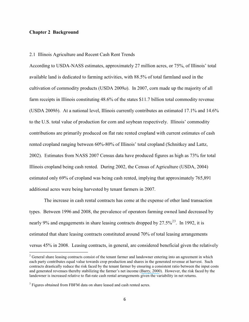
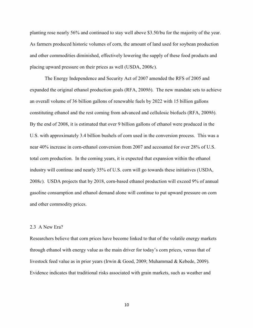
With increasing cash rent agreements, Illinois has also experienced relatively large

increases in cropland rent levels as seen in Figure 1. According to USDA estimates, cash rents

increased on average by 6.8% and 13.5% in 2007 and 2008, respectively. The magnitude of

these increases is much more apparent when comparing the average historical increases between

1996-2005 at a mere 2.2% with the average rent per acre only $117.50. The latest USDA reports

show that 2008 cash rents topped $160 per acre on average in Illinois; the second highest rank

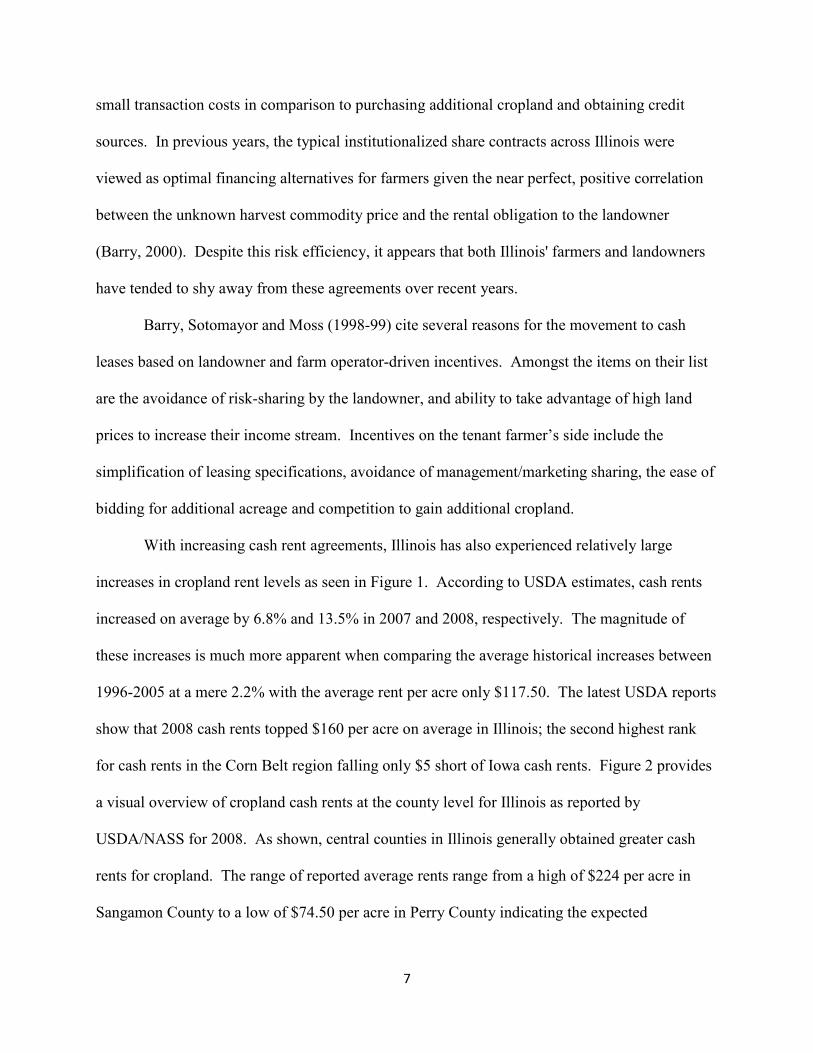
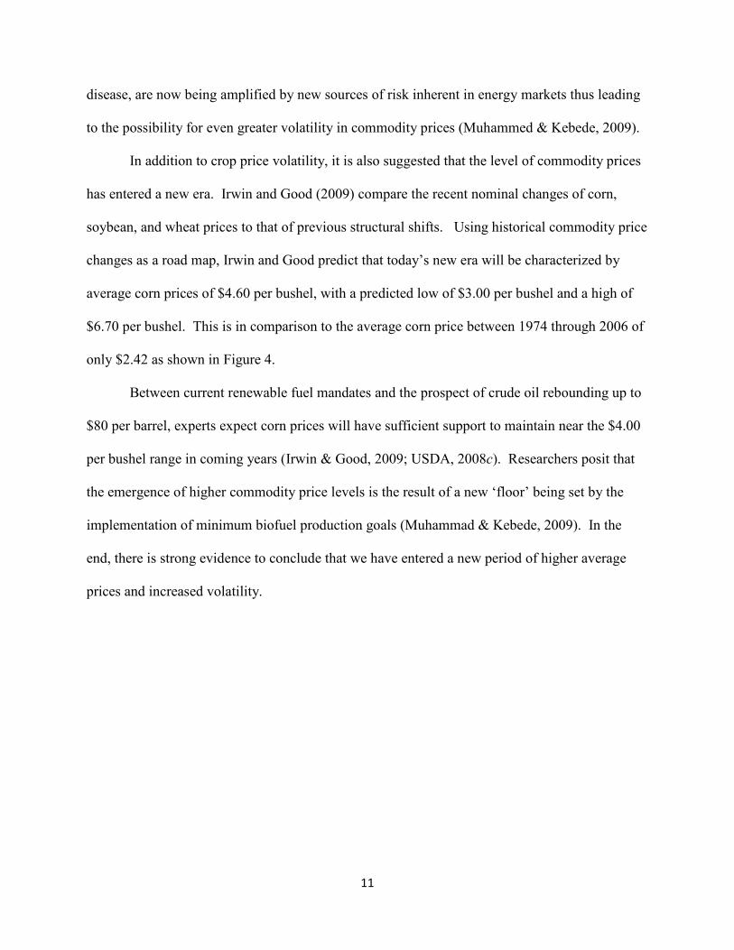
for cash rents in the Corn Belt region falling only $5 short of Iowa cash rents. Figure 2 provides

a visual overview of cropland cash rents at the county level for Illinois as reported by

USDA/NASS for 2008. As shown, central counties in Illinois generally obtained greater cash

rents for cropland. The range of reported average rents range from a high of $224 per acre in

Sangamon County to a low of $74.50 per acre in Perry County indicating the expected

8

heterogeneity across Illinois’ farmland. However, anecdotal evidence and data report that 2008

rents were being observed at unprecedented levels of $300-$400 per acre in key central Illinois'

counties including Macon, McLean, Logan, Champaign and Tazewell.

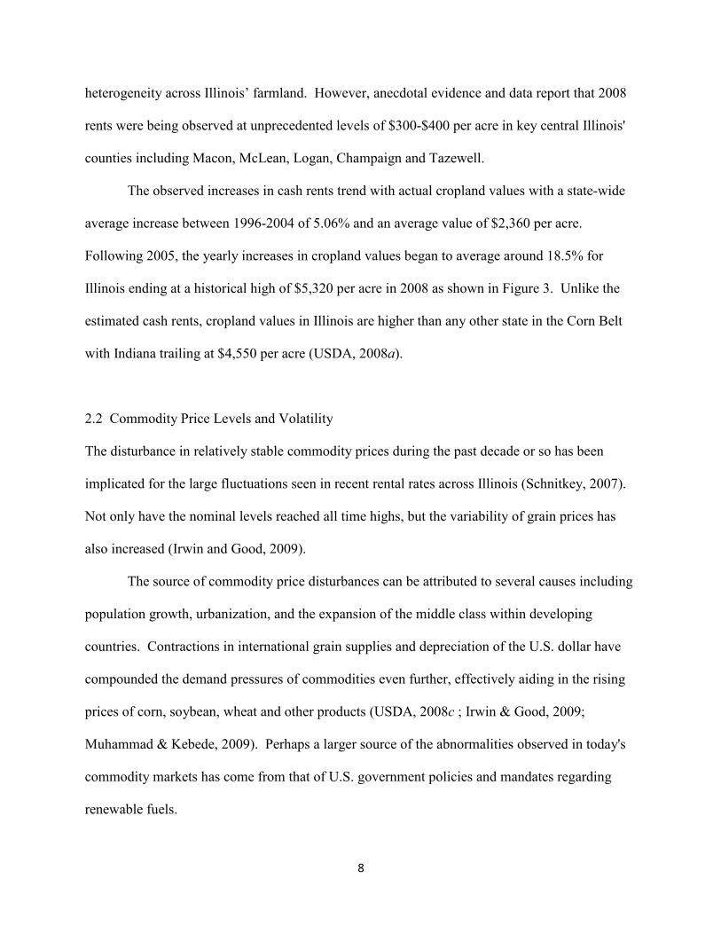
The observed increases in cash rents trend with actual cropland values with a state-wide

average increase between 1996-2004 of 5.06% and an average value of $2,360 per acre.

Following 2005, the yearly increases in cropland values began to average around 18.5% for

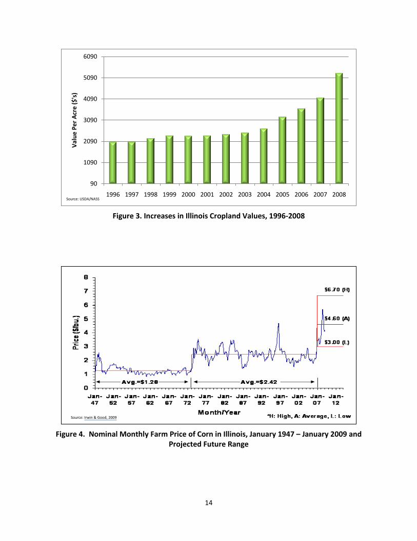
Illinois ending at a historical high of $5,320 per acre in 2008 as shown in Figure 3. Unlike the

estimated cash rents, cropland values in Illinois are higher than any other state in the Corn Belt

with Indiana trailing at $4,550 per acre (USDA, 2008a).

2.2 Commodity Price Levels and Volatility

The disturbance in relatively stable commodity prices during the past decade or so has been

implicated for the large fluctuations seen in recent rental rates across Illinois (Schnitkey, 2007).

Not only have the nominal levels reached all time highs, but the variability of grain prices has

also increased (Irwin and Good, 2009).

The source of commodity price disturbances can be attributed to several causes including

population growth, urbanization, and the expansion of the middle class within developing

countries. Contractions in international grain supplies and depreciation of the U.S. dollar have

compounded the demand pressures of commodities even further, effectively aiding in the rising

prices of corn, soybean, wheat and other products (USDA, 2008c ; Irwin & Good, 2009;

Muhammad & Kebede, 2009). Perhaps a larger source of the abnormalities observed in today's

commodity markets has come from that of U.S. government policies and mandates regarding

renewable fuels.

9

The Clean Air Act Amendments of 1990 provided revisions for fuel quality which would

require gasoline to contain an oxygenating additive resulting in cleaner burning and reduced air

pollution beginning in 1995. As stated in the legislation, the Environmental Protection Agency

(EPA) began enforcing this condition with many refineries utilizing methyl tertiary-butyl ether

(MTBE) as the required additive creating "reformulated gasoline", or RFG (U.S. EPA). Studies

later found MTBE to contaminate ground water and some states began banning its use including

California (U.S. GAO, 2002). The Energy Policy Act of 2005 later amended the Clean Air Act

and added a new provision establishing the Renewable Fuel Standards program (RFS). The

RFS set forth the goal of producing 4 billion gallons of domestic ethanol in 2006 and 7.5 billion

gallons of ethanol by 2012. In addition, the EPA was charged with setting regulations by August

2006 requiring that gasoline contain an average of 2.78% renewable fuels. At the same time, the

act also eliminated the 1995 fuel oxygenation requirement for RFG beginning May 5, 2006 and

declined any liability protection for refineries who continued using MTBE as their choice

renewable fuel additive. This effectively left refineries with ethanol as the main alternative to

produce RFG and comply with new EPA regulations (U.S. EPA, 2005; FTC, 2006; Gustafson,

2008). Following the implementation of the RFS in late summer 2006, U.S. farmers planted an

estimated 93.5 million acres of corn going into the 2007 crop season according to NASS

statistics. This was a 19.4% increase over 2006 and the most corn planted since 1944 (USDA,

2009c). By the end of 2007, ethanol production had increased over 30% from the previous year

using over 2.3 billion bushels of corn (Renewable Fuels Association, 2009a). As a matter of

comparison, only 1.4 billion bushels were used in ethanol production prior to the signing of the

Energy Policy Act of 2005, implying a near 67% increase of corn as a feedstock in ethanol

production alone. Accordingly, the futures price of corn between the 2006 harvest and 2007

10

planting rose nearly 56% and continued to stay well above $3.50/bu for the majority of the year.

As farmers produced historic volumes of corn, the amount of land used for soybean production

and other commodities diminished, effectively lowering the supply of these food products and

placing upward pressure on their prices as well (USDA, 2008c).

The Energy Independence and Security Act of 2007 amended the RFS of 2005 and

expanded the original ethanol production goals (RFA, 2009b). The new mandate sets to achieve

an overall volume of 36 billion gallons of renewable fuels by 2022 with 15 billion gallons

constituting ethanol and the rest coming from advanced and cellulosic biofuels (RFA, 2009b).

By the end of 2008, it is estimated that over 9 billion gallons of ethanol were produced in the

U.S. with approximately 3.4 billion bushels of corn used in the conversion process. This was a

near 40% increase in corn-ethanol conversion from 2007 and accounted for over 28% of U.S.

total corn production. In the coming years, it is expected that expansion within the ethanol

industry will continue and nearly 35% of U.S. corn will go towards these initiatives (USDA,

2008c). USDA projects that by 2018, corn-based ethanol production will exceed 9% of annual

gasoline consumption and ethanol demand alone will continue to put upward pressure on corn

and other commodity prices.

2.3 A New Era?

Researchers believe that corn prices have become linked to that of the volatile energy markets

through ethanol with energy value as the main driver for today’s corn prices, versus that of

livestock feed value as in prior years (Irwin & Good, 2009; Muhammad & Kebede, 2009).

Evidence indicates that traditional risks associated with grain markets, such as weather and

11

disease, are now being amplified by new sources of risk inherent in energy markets thus leading

to the possibility for even greater volatility in commodity prices (Muhammed & Kebede, 2009).

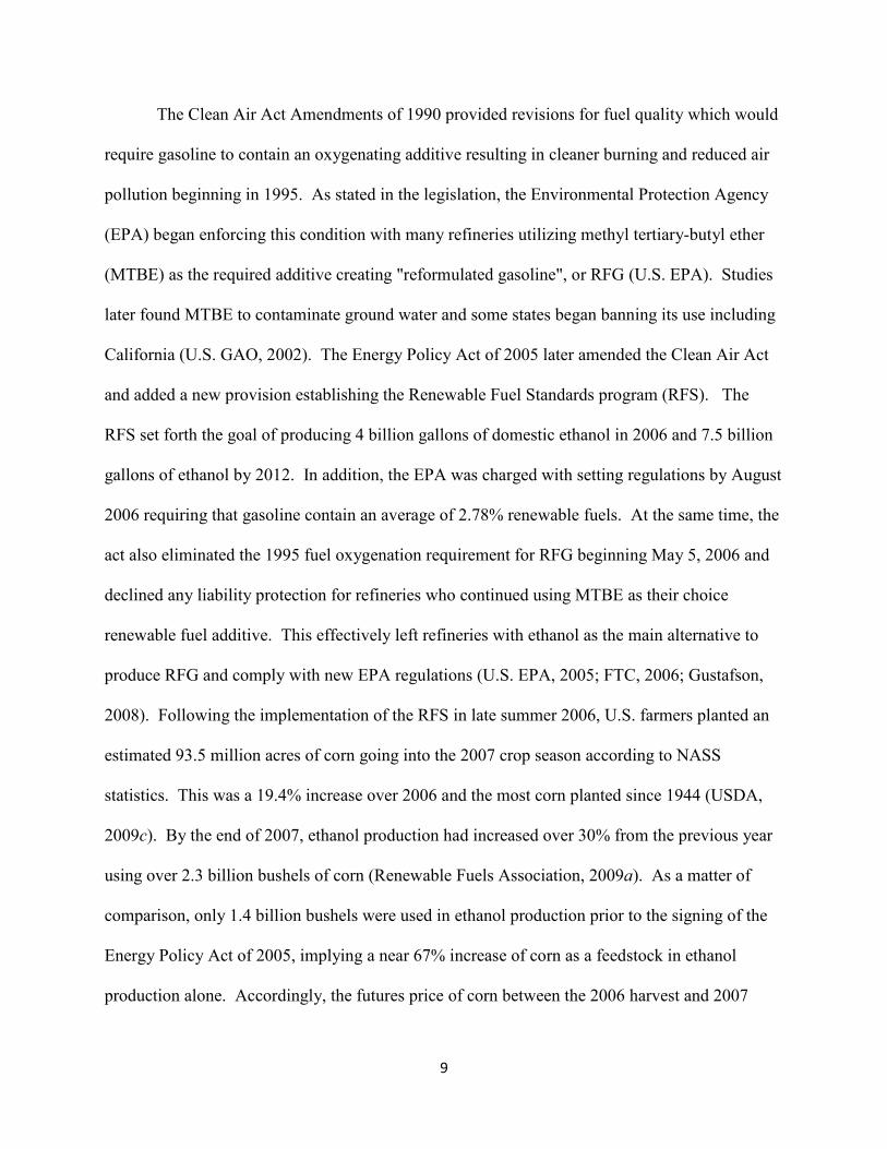
In addition to crop price volatility, it is also suggested that the level of commodity prices

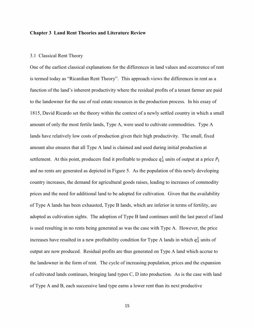
has entered a new era. Irwin and Good (2009) compare the recent nominal changes of corn,

soybean, and wheat prices to that of previous structural shifts. Using historical commodity price

changes as a road map, Irwin and Good predict that today’s new era will be characterized by

average corn prices of $4.60 per bushel, with a predicted low of $3.00 per bushel and a high of

$6.70 per bushel. This is in comparison to the average corn price between 1974 through 2006 of

only $2.42 as shown in Figure 4.

Between current renewable fuel mandates and the prospect of crude oil rebounding up to

$80 per barrel, experts expect corn prices will have sufficient support to maintain near the $4.00

per bushel range in coming years (Irwin & Good, 2009; USDA, 2008c). Researchers posit that

the emergence of higher commodity price levels is the result of a new ‘floor’ being set by the

implementation of minimum biofuel production goals (Muhammad & Kebede, 2009). In the

end, there is strong evidence to conclude that we have entered a new period of higher average

prices and increased volatility.

12

2.4 Charts and Figures

Figure 1. Increases in Illinois Agricultural Cash Rents, 1996-2008

90

100

110

120

130

140

150

160

170

1996 1997 1998 1999 2000 2001 2002 2003 2004 2005 2006 2007 2008

Cash

Ren

t Per

Acr

e ($

's)

Source: USDA/NASS

13

Figure 2. NASS Cash Rents for Illinois, 2008

Will

Lee

Pike

Cook Ogle

McLean

La Salle

Knox

Fulton

Iroquois

Henry

Adams

Bureau

Shelby

Ford

Livingston

Edgar

Kane

Clay

Wayne

Lake

Logan

Peoria

Piatt Vermilion

Fayette

Clark

Hancock

DeKalb

Coles

Macoupin

Champaign

Macon

Madison

White

Mason

Mercer

St. Clair Marion

Perry

Sangamon Christian

Tazewell

Warren

Cass

Morgan

Jasper

Carroll

Whiteside

Greene

Bond

Jackson

Clinton

McHenry

Union

Kankakee

Pope

Jefferson

Randolph

Saline

Grundy

Jo Daviess

Woodford

Jersey Montgomery

Stark

De Witt

Franklin

Monroe

Schuyler

Douglas Scott

McDonough

Stephenson

Crawford

Brown

Hamilton

Marshall

Winnebago

Effingham

Washington

Boone

Kendall

Moultrie

DuPage

Gallatin

Menard

Richland

Johnson

Williamson

Rock Island

Lawrence

Cumberland

Hardin

Henderson

Calhoun

Massac

Wabash

Pulaski

Edwards

Alexander

Putnam

Rents Per Acre ($'s) No Data 0 - 131 131 - 166 166 - 186 186 - 224

14

Figure 3. Increases in Illinois Cropland Values, 1996-2008

Figure 4. Nominal Monthly Farm Price of Corn in Illinois, January 1947 – January 2009 and Projected Future Range

90

1090

2090

3090

4090

5090

6090

1996 1997 1998 1999 2000 2001 2002 2003 2004 2005 2006 2007 2008

Valu

e Pe

r Acr

e ($

's)

Source: USDA/NASS

Source: Irwin & Good, 2009

15

Chapter 3 Land Rent Theories and Literature Review

3.1 Classical Rent Theory

One of the earliest classical explanations for the differences in land values and occurrence of rent

is termed today as “Ricardian Rent Theory”. This approach views the differences in rent as a

function of the land’s inherent productivity where the residual profits of a tenant farmer are paid

to the landowner for the use of real estate resources in the production process. In his essay of

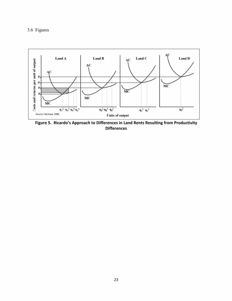
1815, David Ricardo set the theory within the context of a newly settled country in which a small

amount of only the most fertile lands, Type A, were used to cultivate commodities. Type A

lands have relatively low costs of production given their high productivity. The small, fixed

amount also ensures that all Type A land is claimed and used during initial production at

settlement. At this point, producers find it profitable to produce 𝑞𝑞𝐴𝐴1 units of output at a price 𝑃𝑃1

and no rents are generated as depicted in Figure 5. As the population of this newly developing

country increases, the demand for agricultural goods raises, leading to increases of commodity

prices and the need for additional land to be adopted for cultivation. Given that the availability

of Type A lands has been exhausted, Type B lands, which are inferior in terms of fertility, are

adopted as cultivation sights. The adoption of Type B land continues until the last parcel of land

is used resulting in no rents being generated as was the case with Type A. However, the price

increases have resulted in a new profitability condition for Type A lands in which 𝑞𝑞𝐴𝐴2 units of

output are now produced. Residual profits are thus generated on Type A land which accrue to

the landowner in the form of rent. The cycle of increasing population, prices and the expansion

of cultivated lands continues, bringing land types C, D into production. As is the case with land

of Type A and B, each successive land type earns a lower rent than its next productive

16

predecessor. In the end, landowners with Land Type A will earn larger rent differentials than

those of landowners with land of Type B, and so on.

Prior to Ricardo publishing his work regarding land rents, James Anderson suggested a

rather intuitive explanation for the existence of rents in his 1777 article “An Inquiry into the

Nature of the Corn Laws, with a View to the Corn Bill Proposed for Scotland ” (Hubacek and

Van den Bergh, 2002):

"The farmer, however, who cultivates the rich spots, will be able to sell his corn

at the same rate with those who occupy poorer fields; he will consequently,

receive more than the intrinsic value of the corn he raises…It is this premium

which we now call rent; a medium by which the expense of cultivating soils of

different degrees of fertility is reduced to a perfect equality."

This concept was later adopted by Ricardo in developing his land rent theory (Hubacek and Van

den Bergh, 2002). With competition amongst tenant farmers and free entry and exit within the

agricultural sector, this ‘perfect equality’ in crop production expenses is ensured to be

represented in the land rent structure.

The evolution of economic land rent theory has also extended to use other land

characteristics to explain differences in rents. Another well known treatment of agricultural rents

was developed by Johann Heinrich von Thünen in his book The Isolated State published in 1826.

Von Thünen proposed that the distance to the terminal market drives rent differentials. He

argued that agricultural land use would form a concentric circle pattern around the terminal

market representing differences in transportation costs. The more perishable or bulky the good,

the closer to the terminal market the land it was produced on would be. This follows from the

logic that the rent would be the value of the crop less production and transportation costs. For

17

example, producers of highly perishable crops, which are not easily stored and become worthless

once spoiled, would bid up the rent of the land near the terminal market creating the highest

possible value for their commodity. Von Thünen complemented this suggestion with another

view, rather from an intra-crop perspective. Given a single type of crop, the same price will be

received for that crop irrespective of where it was grown or the transportation costs imposed on

the farmer. Within a sub-concentric circle ring of crops, the lowest transportation cost to the city

center will be the land at the inner most area of the sub-concentric ring. Farmers will bid up the

rent of this land trying to capitalize on the lower costs associated with it. However, in the end,

increases in rent price will offset the lower transportation costs. This scenario will happen with

every stratum within the sub-concentric circle, ensuring cost equality across all cropland parcels.

While the strict assumptions made by von Thünen, such as a lack of geographic obstructions

(rivers, mountains) and direct (straight line) transportation routes from the parcels to the city

center, do not lend well to real world conditions, his interpretation gives important insight into

the inherent spatial aspects of land rents.

3.2 Neo-Classical Rent Theory4

Neo-classical economists began a different approach when introducing their perspectives on rent

formation. Mainly, they criticized the assumptions that land had no alternative use as imposed

by classical economists. Neo-classical economists also claimed that the classical approach

ignored any associated opportunity costs. They argued that lands could be transitioned to

cultivate other commodities and therefore, the demand for land in producing a particular

commodity would increase prices of other commodities since the prices of commodities are

4 Adapted from Hubacek and van den Bergh, 2002.

18

determined by supply and demand forces. Rent was seen as the difference between the amount

paid for the factor of production and the amount needed to keep the factor of production in its

current use given other possible uses. They concluded that rent was part of the production

function and treated as such.

Neoclassical theory also tends to lump together factors of production ignoring that land

was a specialized production input and assuming it was substitutable. As a result of the

substitutability away from land and towards other factors of production, rent could be described

as any other factor by means of its marginal product. Within this definition, rent was computed

through its shadow price and the additional value gained in a particular production process when

land was increased marginally.

3.3 Capitalized Values and Rate of Return

Agricultural land can be viewed as an income generating asset. Within this context, rent and

land valuation phenomena can be viewed in a financial investment framework whereby the value

is equated to the discounted future cash flows generated by the land. Thus, the current land

value (LV0) can formally be expressed by:

(1) 𝑳𝑳𝑳𝑳𝟎𝟎 = ∑ 𝑹𝑹𝒕𝒕(𝟏𝟏+𝒊𝒊)𝒕𝒕

𝒏𝒏𝒕𝒕=𝟏𝟏 ,

where R is the expected annual cash rent in period t, and i is the risk-free rate of interest. In

determining the expected rate of return for agricultural land, it is beneficial to consider the long-

run average of regional cash rents to land values (Dhyuvetter and Kastens, 2002). Such a figure

can be seen as the best guess of what one may expect as a yield (Dhyuvetter and Kastens, 2002).

If this value represents the largest return given all other practical investments, then the land will

be rented. From this description, agricultural rent represents compensation that must be paid to

19

the landowner for the use of his/her scarce resource. The tenant farmer will agree to pay 𝑅𝑅

dollars in rent up until they are indifferent between renting and purchasing the property outright.

Such an approach tends to follow that of the Neo-classical thought of how land rent values are

generated.

3.4 Empirical Land Rent Models

3.4.1 Hedonic Approach

The hedonic approach of analyzing land rents views the overall price of land parcels as being

determined by market participants (landowners and tenant farmers). However, with land parcels

being a heterogeneous product, the valuation is not done in a straight-forward equilibrium setting

of supply and demand. Rather, the overall price of each parcel is determined by the summation

and interaction of the ‘values’ of each underlying characteristic. To further complicate matters,

these individual characteristics do not technically have a market themselves given they cannot be

separated from the parcel and sold as a separate product. Thus, the hedonic approach of

analyzing land rents takes the observed market price as given and determines how each inherent

characteristic contributes to the overall value of the parcel.

There have been very few recent studies focusing on agricultural cash rents, and

applications of hedonic models to this area are scarce. Barry et. al (2000) develop a lease pricing

model to determine equitable combinations of leasing arrangements (i.e. share rents, hybrid

leases and cash leases) hypothesizing that the key foundation to leasing principles lies in the

relationship between soil productivity, crop returns, and levels of share rent. A hedonic

approach is used to validate the premise that the share of crop returns attributable to farmland is

directly related to soil productivity, a crop price index, and total acres owned amongst other

20

variables. Through both cross-sectional and pooled analysis using Park's GLS methods, they

find consistent, statistical evidence that soil productivity affects crop returns attributable to

farmland while controlling for other potential variables of interest. Forster et al. (2003)

examined farm leasing markets in Ohio using survey data. They use linear regression techniques

to explain cash rents as a function of region, soil productivity and development pressures

amongst other variables. They find statistical evidence that nearby development places

downward pressure on cash rents while soil productivity has an expected positive effect. The

authors cite several possible reasons for this occurrence including increased costs due to smaller

parcels, difficulties in navigating bulky farming equipment on congested city roads, and lack of

access to nearby farm-related services including grain elevators and seed suppliers. Kirwan

(2009) employs a fixed effects model to farm level data from the U.S. Census of Agriculture

Quin-quennial Census (1992 & 1997) to explore the effects of government subsidy payments on

cash rents. He finds statistical evidence that government subsidies increase cash rents by $0.21

for each marginal subsidy dollar in contrast with theoretical arguments that nearly all of the

marginal subsidy dollar will accrue to landowners.

3.4.2 Income Approach

The income approach of analyzing cash rents takes a more ‘Ricardian’ approach in that revenue

and costs are explicitly modeled within the regression equation. By contrast, the hedonic

approach assumes that this step is embedded within the hedonic schedule of observed prices and

subsequently does not model the difference in revenue and costs to explain rent levels. In other

words, the income approach explains rent as a function of residual rent, whereas the hedonic

approach explains residual rent as a function of inherent parcel characteristics.

21

Featherstone and Baker (1988) estimate cash rents as a function of residual rent and time

lagged rents. These estimates are in turn used to estimate their respective land values. They find

that the current year's cash rent will increase by 8.1 cents in the short-run and 60.3 cents in the

long-run for every dollar change in the prior year's residual rent. However, the likely

implications of endogeneity bias as a result of using lagged rents as an independent variable are

not discussed. Patten et al. (2008) also employ a rental estimator using expected net returns and

subsidy payments while correcting for expectation bias through IV estimation and GMM

techniques.

Recognizing that agricultural rents likely contain a spatial component, Du, Hennessy and

Edwards (2007) develop a variable profit function approach within a spatial framework to

explore Iowa cash rents and their response to high corn prices. Their study uses annual, county-

aggregated survey data and employs a spatial error autoregressive model while also controlling

for temporal correlations within the disturbances. Specifically, they find that cash rents

increased by approximately $79 in the short run given a $1 increase in corn futures prices. They

also find that other choice variables have an impact on cash rents such as urbanization, adoption

of genetically engineered crops, and distance from large metropolitan areas. While not discussed

in the paper, caution should be observed when interpreting the results of this study. Given the

theoretical base of the profit function used in the analysis, strict restrictions had to be imposed on

the parameter estimates. If these conditions constrained the estimator, such a modeling approach

may not be appropriate and may be leading to artificial results. The profit function approach also

explicitly models costs in the regression equation, making the calculated effects of increasing

output prices truly "ceteris paribus". This may produce results that are slightly misleading.

Namely, it is very rare that output prices rise while input costs stay constant.

22

3.5 Empirical Land Value Models

The farmland value literature is strongly correlated with the cropland cash rent literature. Phipps

(1984) concludes that residual returns, or rents, unidirectionally cause farmland values with

farmland prices being determined within the farm sector. In other words, agricultural rents

determine the overall value of agricultural land, but land values do not determine rent levels.

Awokuse (2006) finds that land price changes are sensitive to residual return fluctuations.

Various empirical studies and extension reports use the Constant Discount Rate-Present Value

Model (CDR-PVM) approach to model land values from a financial investment framework

whereby the market value of land is equated to the discounted future cash rent flows generated

by the land (Schnitkey, 2007; Moss, 1997; Robison, Lins, and VenKataraman, 1985; Veeman,

Dong, and Veeman, 1993). Other land value studies derive values through the implicit prices of

heterogeneous land characteristics using a hedonic framework (Bastian et. al, 2002; Chicoine,

1981; Shi, Phipps and Colyer, 1997; Palmquist 1989; Palmquist and Danielson 1989). Huang et.

al (2006) apply a spatial lag method to their hedonic model of Illinois farmland values using

county-level, cross-sectional time-series data. They find that the inclusion of spatial and serial

components substantially improve their model fit. Statistical evidence from this study suggests

that parcel size, urbanization, and soil productivity have significant impacts on farmland values.

These findings coincide with those in the farmland rent literature reinforcing the idea of a strong

relationship between land values and land rents.

23

3.6 Figures

Figure 5. Ricardo’s Approach to Differences in Land Rents Resulting from Productivity

Differences

Source: Barlowe 1986

24

Chapter 4 Theoretical Framework

4.1 Hedonic Model

Assuming a competitive market and homogenous goods, prices are determined by supply and

demand. If goods within a market are not homogenous, however, the supply and demand model

must be augmented to allow for market pricing of the good’s various underlying attributes. A

hedonic model allows for the analysis of such heterogeneous commodities by depicting the

relationship between the price of a composite good and its individual attributes, facilitating the

estimation of each characteristic's implicit price and contribution to the overall market value of

the "bundled" good (Palmquist, 1989). Within the context of cropland cash rents, the hedonic

framework suggests that the equilibrium rent per acre, 𝑅𝑅(𝑧𝑧), is a manifestation of those

individual attributes into a single price. The relationship can be represented by the hedonic

equation

(2) 𝑹𝑹 = 𝑹𝑹(𝒛𝒛𝟏𝟏, … . . , 𝒛𝒛𝒏𝒏),

where 𝑅𝑅 is the rental price of the parcel per acre, and 𝑧𝑧 = (𝑧𝑧1, … . . , 𝑧𝑧𝑛𝑛) is a vector of 𝑛𝑛 unique

characteristics of the land (Palmquist, 1989). The implicit price of each characteristic 𝑧𝑧𝑖𝑖 can then

be calculated as the partial derivative of the hedonic equation with respect to that particular

characteristic5

(3) 𝑴𝑴𝑴𝑴𝑴𝑴(𝒛𝒛𝒊𝒊) = 𝝏𝝏𝑹𝑹𝝏𝝏𝒛𝒛𝒊𝒊

:

The hedonic approach, developed in the work of Lancaster (1966, 1971), Rosen (1974),

amongst others, has been extensively employed in the study of housing values (Can, 1990;

5 This general framework assumes each underlying attribute of the good is valued by agent’s independently from other characteristics. This assumption can be modified by the addition of interaction terms within the model in which case the implicit price derivation would need to be modified accordingly.

25

Olmo, 1995; Benjamin and Sirmans, 1996; Palmquist, Roka and Vukina, 1997; Basu and

Thibodeau, 1998; Luttik, 2000; Downes and Zabel, 2002; Nelson, 2004; Pope, 2008),

housing/office rent values (Guntermann and Norrbin, 1987; Dunse and Jones, 1998; Bollinger,

1998; Smith and Islam, 1998; Valente et. al, 2005; Löchl, 2007), and agricultural land values

(Bastian et. al 2002, Chicoine 1981, Shi, Phipps, Colyer, 1997; Palmquist, 1989; Palmquist and

Danielson, 1989; Huang et. al, 2006). However, its use in analyzing agricultural cash rents is

disparate.

As indicated by land rent theory and adopted by the literature, characteristics such as soil

fertility, climate and location/distance to the terminal market are important attributes which

collectively help determine the value of the land to production. The output price for

commodities produced on the land is proportional to the revenues generated by the land.

Commodity prices can then be considered as an attribute of the land to be estimated. This is

especially true to the extent that cash prices may differ by location from some basis spread

creating another heterogeneous characteristic. As a last consideration, the characteristics of the

tenant farmer may have a common impact on cash rents and should be included in the hedonic

model. While it is possible to observe and collect information on soil productivity, ruralness,

and commodity price measures, a proxy for the tenant farmer's ability may not be available at

which point this will be absorbed by the error component of the hedonic model, 𝜀𝜀. This suggests

that perhaps a hedonic model of agricultural rents would be best suited within a random effects

panel framework. The above discussion implies that the hedonic model to be estimated takes the

form:

(4) 𝑹𝑹 = 𝜶𝜶 + 𝑿𝑿𝑿𝑿 + 𝒁𝒁𝒁𝒁 + 𝑾𝑾𝑾𝑾 + 𝜺𝜺

26

where 𝑋𝑋 is a matrix of physical land characteristics, 𝑍𝑍 a matrix of local characteristics, and 𝑊𝑊 a

matrix of economic characteristics. The parameters 𝛼𝛼,𝛽𝛽, 𝛾𝛾 and 𝛿𝛿 are all to be estimated, where 𝜀𝜀

is considered for further decomposition to allow for heterogeneity across parcels.

4.2 Spatial Considerations

Previous research indicates that the process by which land values and cash rents are generated

likely exhibit spatial effects (Anselin, 1992; Du, Hennessy and Edwards, 2007; Du, Hennessy

and Edwards, 2008; Huang et. al, 2006; Soto, 2004). In general, data that are close together in a

spatial aspect are likely to be spatially correlated to some extent (Benirschka and Binkley, 1994).

Spatial autocorrelation, otherwise known as spatial dependence, can be defined as the

correlation between the distribution of a variable and its location (Anselin and Bera, 1998). For

positive spatial autocorrelation, high or low values of a random variable exhibit apparent spatial

clustering. As the correlation between agents or economic units increase, we expect there to be a

loss of information as the sample we are using for statistical correlation and inference is no

longer a true random draw.

Formally, spatial autocorrelation can be expressed by the moment condition:

(5) 𝑪𝑪𝑪𝑪𝑪𝑪�𝒚𝒚𝒊𝒊,𝒚𝒚𝒋𝒋� = 𝑬𝑬�𝒚𝒚𝒊𝒊,𝒚𝒚𝒋𝒋� − 𝑬𝑬[𝒚𝒚𝒊𝒊] ∗ 𝑬𝑬�𝒚𝒚𝒋𝒋� ≠ 𝟎𝟎 𝒇𝒇𝑪𝑪𝒇𝒇 𝒊𝒊 ≠ 𝒋𝒋 ,

where 𝑖𝑖 and 𝑗𝑗 are individual units (counties, farming operations, markets ect.) and 𝑦𝑦𝑖𝑖 and 𝑦𝑦𝑗𝑗 are

the values of a random variable in space. It should be noted that there is nothing necessarily

spatial with a non-zero covariance. However, in light of a spatial structure, interaction or

arrangement of units, the pairs 𝑖𝑖 and 𝑗𝑗 develop a meaningful spatial interpretation (Anselin and

Bera, 1998). The correlation between units causes OLS to no longer be the best linear unbiased

estimator yielding biased coefficient estimates, downward bias variance estimates, or both

27

(Anselin, 1992).6

To detect spatial correlation, simple preliminary steps can be taken such as visually

inspecting the data through GIS software mapping techniques and observing spatial patterns. A

more formal approach to detecting spatial correlations is known as the Moran’s I test which is

used to determine whether neighboring areas are more similar than would be expected under the

null hypothesis of spatial independence. The test statistic of the Moran’s I is computed as

follows:

In the case where the variances are estimated as smaller than the truth, the

corresponding coefficients may appear to be statistically significant when, in fact, they are not.

As stated by Anselin (2002), "The main objective of the econometric exercise is to obtain

unbiased/consistent and efficient estimates for the regression parameters in the model (β), while

taking into account the spatial structure incorporated in the error covariance matrix."

(6) 𝑴𝑴 = 𝑵𝑵∑ ∑ 𝒘𝒘𝒊𝒊𝒋𝒋𝒋𝒋𝒊𝒊

∗∑ ∑ 𝒘𝒘𝒊𝒊𝒋𝒋�𝒀𝒀𝒊𝒊−𝒀𝒀�(𝒀𝒀𝒋𝒋−𝒀𝒀�)𝒋𝒋𝒊𝒊

∑ (𝒊𝒊 𝒀𝒀𝒊𝒊−𝒀𝒀�) ,

where 𝑁𝑁 is the number of spatial units indexed by 𝑖𝑖 and 𝑗𝑗, 𝑌𝑌 is the dependent variable, and 𝑤𝑤𝑖𝑖𝑗𝑗 is

a weight matrix defining the relationship between observations and will be discussed in more

detail shortly. The Moran's I is a weighted correlation coefficient to detect departures from

spatial randomness (Anselin, 1992). Values of the Moran's I fall between −1 ≤ 𝐼𝐼 ≤ 1, with −1

indicating perfect spatial dispersion, 1 perfect spatial correlation and near zero implying a

random spatial pattern.

6 In the case where the dependent variable exhibits spatial correlation with its neighboring values and is considered only a function of those lagged dependent values, resulting parameter estimates will be biased when applying OLS. In the case that the spatially correlated dependent variable is found to be a function of independent variables plus some spatially correlated error term, the estimated variances of the parameters will be downward bias, but the parameters estimates themselves will remain unbiased.

28

4.2.1 Weight Matrix

The weights matrix is simply an exogenous structural element which defines the spatial

relationship between observations. This structure allows researchers to implement testing for

spatial correlations as well as correction techniques during the estimation process to explicitly

model spatial correlations (these techniques are discussed in the next section). While it would be

optimal to estimate the connectedness between each spatial unit by using a complete variance-

covariance matrix, structure must be imposed in order for testing and estimation to be feasible

(Anselin, 1992). By construction, the weights matrix allows for individual units to be correlated

with contiguous or distance defined neighboring units. As a result, all units are indirectly

correlated with the interaction dissipating as the distance between units grows. This captures the

essential feature of geographical systems in that nearness matters and those economic units

closest to you should have the largest effect, declining as distance between neighbors increases.

Defining a weight matrix is central to addressing the implications of spatial correlation.

Unfortunately, tests do not exist to define the "correct" weighting scheme for a particular process

and this decision is ultimately left up to the researcher. Weighting structures commonly used in

applied research include contiguity matrices (rook and queen), k-nearest neighbors, and distance

decay functions (Anselin, 1992). In the case where the data do not include specific borders or

latitude-longitude coordinates, the lesser known block weights matrix can be used in which units

that belong to a larger system are considered neighbors (Anselin, 2002). This is a hierarchical

spatial structure which adheres to the standard assumption that choices are influenced by the

behavior of others in their immediate vicinity (Case, 1992). The properties of this weighting

scheme make the block structure a very attractive option in modeling the effects of neighbors on

individual farmers. In the case of agricultural producers, this structure may help depict the

29

spatial correlation of choices such as the adoption of new hybrid seeds, chemical pest control and

the extent to which farmers have been educated on the adoption of new technologies. Similarly,

the county-level weights matrix may reflect county-level rules, such as property-taxes, that might

commonly affect their residents. These examples may indirectly affect rent levels paid by tenant

farmers by impacting overall revenue levels. However, empirical use of this structure deems that

caution be taken given the inherent side-effects. Since each weight is expressed as 𝑤𝑤𝑖𝑖𝑗𝑗 = 1/𝑛𝑛𝑐𝑐 ,

where nc denotes the number of farmers in county c, the neighbor effect will tend to zero as

𝑛𝑛𝑐𝑐 → ∞.

Depending on the specified structure, the observations are assigned a "neighborhood set"

represented by an 𝑁𝑁 𝑥𝑥 𝑁𝑁 positive weight matrix. For each observation 𝑖𝑖, 𝑤𝑤𝑖𝑖𝑗𝑗 defines 𝑗𝑗 as a

neighbor with a non-zero entry in row 𝑖𝑖 and column 𝑗𝑗. The matrices are typically row

standardized such that:

(7) 𝒘𝒘𝒊𝒊𝒋𝒋𝒔𝒔 = 𝒘𝒘𝒊𝒊𝒋𝒋

∑ 𝒘𝒘𝒊𝒊𝒋𝒋𝒋𝒋 ,

where 𝑤𝑤𝑖𝑖𝑖𝑖 = 0 representing that an economic unit cannot be a neighbor of itself.

In the case of the Moran’s I test statistic, this neighbor structure allows for the matrix

multiplication of the weight matrix and a vector of independent variables resulting in a matrix of

neighbor-weighted average values for each observation. The use of the weights matrix extends

beyond the simple identification of spatial correlations and is also used in explicitly accounting

for spatial relationships in the data.

4.3 Spatial Autoregressive Models (SAR)

Two main models are generally employed to explicitly model spatial interactions; the spatial lag

and the spatial error model. The spatial lag model assumes that the dependent variable is a

30

function of independent variables plus its neighbors spatially weighted (lagged) observations and

a normally behaved error component. In comparison, the spatial error model assumes the

dependent observation is a function of exogenous independent variables plus a non-normal error

term in which the individual disturbances are spatially correlated with each other.

While the spatial lag specification tends to result from theory such as resource

competition or spillover effects, the spatial error model is typically used to contend with data

"problems" (Anselin, 1992). The spatial error model is a special case of a so-called non-

spherical error model where the OLS assumptions of homoskedastic and uncorrelated errors are

violated (Anselin, 1992). Following is a brief overview of the theoretical construction of the

spatial error model within a panel data context where the cross-sectional errors show systematic

spatial patterns.

Consider a simple pooled linear regression model where 𝑖𝑖 = 1, … . ,𝑁𝑁 denotes the cross-

sectional dimension, 𝑡𝑡 = 1, … . ,𝑇𝑇 denotes the time dimension and observations are stacked as

successive cross-sections for each time period:

(8) 𝒚𝒚𝒊𝒊𝒕𝒕 = 𝒙𝒙𝒊𝒊𝒕𝒕𝑿𝑿 + 𝒖𝒖𝒊𝒊𝒕𝒕 ,

where y is an 𝑁𝑁 𝑥𝑥 1 vector of observations on the dependent variable, x is an 𝑁𝑁 𝑥𝑥 𝑘𝑘 matrix of

observations on the explanatory variables, β is a 𝑘𝑘 𝑥𝑥 1 vector of regression coefficients, and u is

an 𝑁𝑁 𝑥𝑥 1 vector of error terms. Further, let u be defined as a first order spatial autoregressive

process:

(9) 𝒖𝒖𝒊𝒊𝒕𝒕 = 𝝆𝝆𝑾𝑾𝒖𝒖𝒊𝒊𝒕𝒕 + 𝜺𝜺𝒊𝒊𝒕𝒕 ,

Where 𝜌𝜌 is a scalar denoting the magnitude of correlation, otherwise known as a spatial

autocorrelation coefficient or nuisance parameter, W is the previously described weight matrix

and 𝜀𝜀 is a vector of innovations with a mean of zero and constant variance 𝜎𝜎𝜀𝜀2. The error

31

structure in this statistical model represents all of the unexplained factors not captured by the

explanatory variables and allows for the spatial connectedness between observations to be

accounted for effectively removing the correlation. This concept is similar to that employed in

time series applications. In a spatial context, nuisance correlations within this specification are

modeled using the so-called "spatial filter" approach by rewriting equation (8) as:

(10) 𝒖𝒖𝒊𝒊𝒕𝒕 = (𝑴𝑴 − 𝝆𝝆𝑾𝑾)−𝟏𝟏𝜺𝜺𝒊𝒊𝒕𝒕 ,

resulting in the panel model:

(11) 𝒚𝒚𝒊𝒊𝒕𝒕 = 𝒙𝒙𝒊𝒊𝒕𝒕𝑿𝑿 + (𝑴𝑴 − 𝝆𝝆𝑾𝑾)−𝟏𝟏𝜺𝜺𝒊𝒊𝒕𝒕 ,

where (𝐼𝐼 − 𝜌𝜌𝑊𝑊)−1 is the spatial filter, and I is an identity matrix with ones along the main

diagonal. The resulting error covariance is:

(12) 𝑬𝑬[𝜺𝜺𝜺𝜺′ ] = 𝝈𝝈𝟐𝟐(𝑴𝑴 − 𝝆𝝆𝑾𝑾)−𝟏𝟏(𝑴𝑴 − 𝝆𝝆𝑾𝑾′)−𝟏𝟏 = 𝝈𝝈𝟐𝟐[(𝑴𝑴 − 𝝆𝝆𝑾𝑾)′(𝑴𝑴 − 𝝆𝝆𝑾𝑾)]−𝟏𝟏 ,

in which the magnitude of connectedness between units readily decreases as contiguity is

exhausted. By rewriting equation (11), it is easily shown that the panel model could successfully

be estimated by OLS using spatially filtered dependent and explanatory variables (Anselin

1992):

(13) 𝒚𝒚𝒊𝒊𝒕𝒕(𝑴𝑴 − 𝝆𝝆𝑾𝑾) = 𝒙𝒙𝒊𝒊𝒕𝒕𝑿𝑿(𝑴𝑴 − 𝝆𝝆𝑾𝑾) + 𝒖𝒖𝒊𝒊𝒕𝒕 ,

or equivalently,

(14) 𝒚𝒚𝒊𝒊𝒕𝒕 − 𝝆𝝆𝑾𝑾𝒚𝒚𝒊𝒊𝒕𝒕 = 𝒙𝒙𝒊𝒊𝒕𝒕𝑿𝑿 − 𝝆𝝆𝑾𝑾𝒙𝒙𝒊𝒊𝒕𝒕𝑿𝑿 + 𝒖𝒖𝒊𝒊𝒕𝒕 ,

where Wy and Wx are the spatially weighted average of the lagged dependent and independent

variables and u is a well behaved error term following classical linear regression assumptions.

However, as noted by Anselin (1992), the correlation coefficient 𝝆𝝆 is rarely, if ever, known and

must be jointly estimated with the regression coefficients (Anselin, 1992). With such a

possibility ruled out, estimation must rely on the specification in equation (11).

32

If the error at each location depends on the errors at other locations, the expectation is

that 𝜌𝜌 > 0, implying that the errors are correlated within a spatial structure. In this case, the

classic assumptions of homoskedastic and uncorrelated errors are not satisfied. Of course, if

𝜌𝜌 = 0, then the model results in a typical pooled panel analysis with uncorrelated disturbances

across units. By explicitly modeling the possible presence of spatially autocorrelated error terms

within the data, efficient estimates can be generated and statistical inference carried out.

The modeling of non-spherical models requires special attention as described above, and

also gives rise to additional provisions. Namely, the standard R2 measure is no longer applicable

and substitutions must be implemented. As suggested by Anselin (1992b), there are two pseudo-

R2 statistics that can be used as alternatives with the first simply being the ratio of the predicted

value variances and the observed value variances:

(15) 𝑹𝑹�𝟐𝟐 =𝝈𝝈𝒑𝒑𝒇𝒇𝒑𝒑𝒑𝒑𝒊𝒊𝒑𝒑𝒕𝒕𝒑𝒑𝒑𝒑𝟐𝟐

𝝈𝝈𝑪𝑪𝒐𝒐𝒔𝒔𝒑𝒑𝒇𝒇𝑪𝑪𝒑𝒑𝒑𝒑𝟐𝟐

The second model fit uses the squared correlation between the predicted and observed values:

(16) 𝑹𝑹�𝟐𝟐 = 𝒑𝒑𝑪𝑪𝒇𝒇𝒇𝒇(𝒚𝒚,𝒚𝒚�)𝟐𝟐

Both measures will be provided in this study to give an approximate range for the fit of the

overall model.

33

Chapter 5 Data, Methods and Procedures

5.1 Data

This study employs certified farm level data from the Illinois Farm Bureau Farm Management

Association (FBFM) in conjunction with NASS county corn yield data and CBOT corn futures

price data to model farmland rents. The FBFM data span the years 1996 through 2008, and

contain over 5,000 participating farmers. FBFM data provide information on cash rents, Soil

Productivity Ratings (SPR), annual production costs (seed, fertilizer, fuel & oil), the farmer’s

county, total number of operator acres, tillable and cash rented acres, as well as annual yields for

each farmer.

While this study is mainly interested in using farm-level data to explore commodity price

level effects on cash rents, a county-level analysis is also included as a matter of comparison.

The observations used in the farm-level analysis were limited to only those records containing

data for all thirteen years, resulting in a balanced panel. To construct the county-level data, the

farm data was generated into a weighted average of rent values by the acreage cash rented.7 The

observations were allowed to contain farmers who did not have a complete thirteen year profile;

however, the counties themselves were required to have thirteen years of continuous

observations. Cash rents reported as negative or zero and farms with a zero SPR were also

excluded, as well as those who reported cash rent, but had zero cash rented acres or zero operator

acres.8

7 The weighting process is described in the next section.

The resulting farm level data includes 408 individual farmers and the county weighted

8 In order to account for outliers, each county was looked at individually as well as each year within the county. An observation was deemed an outlier if the observed rent was three times the interquartile range of the sub data resulting from the county and year. This is generally considered a conservative approach when dealing with outliers according to statisticians. Discussions with FBFM staff indicated that rents in excess of $600 per acre—those observations which were excluded—were most likely the result of data collection errors.

34

data consists of 78 of Illinois’102 counties per cross-section. Table 1 and 2 provide summary

statistics for both data sets.

5.2 Variables Used in the Hedonic Rent Model

5.2.1 Dependent Variable

The dependent variable for each analysis is cash rent per tillable cash rented acre as reported by

the FBFM.9

(17) ∑ [𝒇𝒇𝒑𝒑𝒏𝒏𝒕𝒕𝒊𝒊∗𝒇𝒇𝒑𝒑𝒏𝒏𝒕𝒕𝒑𝒑𝒑𝒑 𝒂𝒂𝒑𝒑𝒇𝒇𝒑𝒑𝒔𝒔𝒊𝒊]𝒏𝒏𝒊𝒊=𝟏𝟏∑ 𝒇𝒇𝒑𝒑𝒏𝒏𝒕𝒕𝒑𝒑𝒑𝒑 𝒂𝒂𝒑𝒑𝒇𝒇𝒑𝒑𝒔𝒔𝒊𝒊𝒏𝒏𝒊𝒊=𝟏𝟏

∀ 𝒋𝒋,

While the farm-level rent is the actual value reported in the FBFM data, the county

level was constructed via the farm-level data through a weighted aggregation process as follows:

where 𝑖𝑖 = 1, … . ,𝑛𝑛 is the individual farmer in county 𝑗𝑗.

5.2.2 Independent Variables

The parcel characteristics considered in the analysis are expected corn yield, expected corn price,

intra-county soil productivity differences, crop yield risk, urbanization pressures and the total

amount of operator acreage. Table 3 provides a brief description of the characteristics and

expected signs. Since the form of inflation most relevant to farmers is the cost of their inputs, all

price measures (including the dependent variable) are adjusted to 2008 dollars using a (county)

farmer specific producer price index based on (weighted) non-land costs.10

9 All contract data used are standard fixed rate rental agreements and share rents or hybrid contracts were explicitly excluded. FBFM differentiates between these leasing types allowing us to specifically study only cash rent arrangements.

Thus, all coefficients

will be in real terms.

10 As the FBFM data consists of extensive cost data include fertilizer, seed, pesticide and fuel & oil, we seen it fit to create unique producer price indices for each farmer (county) to capitalize on the additional information gained from modeling actual cost structures. This is in comparison to using a very generic PPI as supplied by the BLS. A 2008-base index was created for each farmer (county) given their individual (weighted) costs over time on a per acre basis

35

The primary objective of this paper is to examine how rents are impacted by changing

output prices and how these higher prices are allocated amongst tenant farmers, landowners and

input suppliers. In deciding on an appropriate proxy for corn prices in terms of futures prices,

we assume farmers typically enter into rental agreements prior to the next year's cropping season.

PRICE is thus defined as the average settlement for corn futures in November for the far

December contract. The public nature, wide accessibility and reliance of futures markets by

commodity producers is seen to represent the best available information (at the time a rental

contract is signed) for the expected price of the crop received by the farmer. For example, when

modeling the rent contract for the 2008 harvest season, we assume the farmer will use the futures

price observed in November 2007 for the contract ending in December 2008.

A stylized fact throughout rural land literature is that soil productivity is a main driver of

farmland values and rents. A yield variable, ExpYield is included as an inter-county measure of

productivity across Illinois farms. A majority, if not all, cropland rental analyses include some

measure of the lands productive capacity whether it be a soil productivity rating (Barry et. al,

2000), a corn suitability rating (Du, Hennessy, and Edwards, 2007), simulated yield potentials

(Kurkalova, Burkart, and Secchi, 2004), or qualitative land class categories based on yield ranges

(Forster et. al, 2003). This study takes advantage of detrended county corn yields using data

from 1979 through 2008 as a proxy of the land’s natural capacity to cultivate commodities. Such

a measure is seen to be an accurate proxy for inter-county land productivity versus a more

conventional measure, such as SPR, which assigns an index number based on individual soil

types. For example, a particular silt loam soil may have an SPR of 75 on a scale of 100

as to account for a relative aspect. The unique index was then used a sort of deflator for prices over time (rents and futures prices). This structure also has the added benefit of creating cross-sectional variations in the futures price to proxy a basis structure that would be observed across individual markets.

36

indicating that the soil is relatively productive. However, silt loam in a central Illinois' county

may produce drastically different yields than the same silt loam in a southern county as a result

of differing environmental conditions. By using detrended yields, productivity differences

across counties are more effectively captured as the erroneous similarities in productivity

between two entirely different soil capacities are removed. It is expected that higher county

yields will have a positive effect on cash rents within that county given the intuition that parcels

which produce more bushels per acre (resulting in greater revenues) must be compensated for

through higher rental rates. Graphical representations of the expected yields used in this study

are presented in Figure 6. As shown, central counties in Illinois tend to have higher yields, with

McDounough County having the highest expected yield of approximately 181 bushels of corn

per acre. Moving towards southern Illinois, yields tend to decrease with Perry County

representing the lowest yielding county in Illinois at approximately 106 bushels per acre. Note

that the pattern of high (low) crop yields nearly mirrors that of high (low) cash rents as seen in

Figure 2.

To capture farm-specific productivity, FtoCSPR is defined as the proportion of the

farmer-specific SPR, as provided by FBFM, to the county average SPR. For example, take a

county that has an average SPR of 80. When a tenant farmer is observed with a tract of land that

has an SPR of 90, we would expect this to plot to be "worth" more than the neighbor's average

plot. Controlling for intra-county variations will aid in the examination of heterogeneous

cropland within counties and the corresponding cash rent.

As documented in Barry et. al (2000), cash rents include a risk premium which is

reflected in the rent price paid by tenant farmers to landowners. This is due to the fact that,

unlike share rent agreements, the tenant farmer bears all yield, price and marketing risks. CV is

37

included to capture the yield risk bourn onto the tenant farmer being defined as the normalized

measure of dispersion constructed from the probability distribution of individual county

historical yields, and is calculated as follows:

(18) 𝑪𝑪𝑳𝑳𝒕𝒕 = 𝝈𝝈𝒕𝒕𝝁𝝁𝒕𝒕

,

where 𝜎𝜎 is the standard deviation for the historical detrended yields up to time 𝑡𝑡 and 𝜇𝜇 is the

expected detrended yield at time 𝑡𝑡. The yield risk is updated every year within the panel to

simulate the tenant farmers current knowledge at time 𝑡𝑡 and thus is a changing expectation of

yield risk based on data that would have been available to the farmer through time. In other

words, the construction of CV takes into consideration that the perceived yield risk to a farmer

will change over time with the accumulation of additional information as more history is

“observed” of the estimated amount of yield risk faced. For example, consider a tenant farmer

negotiating his/her rental rate for the 1997 crop year. At that point in time, the farmer has

historical yield information from 1979 through 1996 and is able to construct both an expected

yield from the rented land and the spread of the historical yield distribution (i.e., yield risk).

When this same farmer begins rent negotiations for 2007, they will have ten additional years of

yield data in which to construct expectations. We expect that as historical yield risk increases,

the rental rate per acre will fall given the likely assumption that farmer’s are risk averse and will

take into account the perceived risk of yield variations during rental agreements.

Previous literature also includes some measure of urban/development pressures on land

rents. Urban pressures can change the opportunity costs of land on the fringes of expanding

cities, thus increasing the market price of rented land. Previous measures of urbanization used in

empirical studies include respondent survey perceptions of development pressures, county

normalized distance from major metropolitan areas and the USDA-ERS Beale Rural-Urban

38

Continuum Code (Forster et. al, 2003; Du, Hennessy, and Edwards, 2007; Huang et. al, 2006).

This study uses the percent of total county acres used for planting purposes, including corn,

soybean and wheat as a proxy. The data on planted acres was obtained through NASS, which

reports yearly acreage uses across Illinois counties. As measures such as the Beale Code and

distances to metropolitan areas tend to remain static through the panel data, this proxy

construction will allow for the urbanization pressures of a county to change through time.

Figure 4 provides a visual representation of county urbanization pressures depicted as

“ruralness”. The most urban area, according to the proxy variable, is Williamson County in

Southern Illinois with only 15.1% of its land used for cultivation of major crops. According to

U.S. Census figures, Williamson County is rapidly growing giving additional credibility to this

proxy measure for urbanization. Other counties deemed as relatively urban include Peoria as

well as Kane, Will, and McHenry counties which border Chicago's Cook County. The most

rural county is Piatt, which also has one of the highest county corn yields. Other counties seen as

rural include other high yielding counties such as DeKalb, Stark, Livingston, Iroquois, Ford and

Logan.

There are conflicting expectations for how development pressures influence farmland

rental rates and it is important that there be a distinction between cropland rents and cropland

values. While it is generally accepted and expected that land values will naturally be higher in

more populated areas for a variety of reasons, there is no reason to expect that the corresponding

land rents will also be higher. Downward pressure on cropland rental markets in highly

populated areas may be expected due to several factors. Parcel sizes would likely be smaller as

land is allocated for residential or commercial purposes inhibiting economies of scale/scope and

increasing transportation costs between multiple parcels. Accessibility to both land and farming

39

materials would be hindered as routes to the parcels would likely become more indirect (new

roadways being formed to serve new residential/business areas) and as non-farm neighbors

become the majority extinguishing the need for grain mills and farm-related input suppliers.

Also, highly congested areas would cause difficulties when moving bulky farming equipment

and parcels may be more exposed to major traffic veins leaving crops vulnerable to

car/factory/household pollution adversely affecting crops. These factors may decrease the

competition for parcels in highly urbanized areas resulting in lower rental rates. On the other

hand, if a parcel is highly productive, the rent for the parcel may be pushed up as the tenant

farmer bids the parcel away from its next best residential/commercial use.

The last variable considered is a farmer's total operator acres as reported by FBFM. We

hypothesize that larger operations would indicate economies of scale implying the ability to

outbid competing, less cost efficient farmers and inflate rental rates. In this sense, the variable

OpAcre can be seen to capture the tenant farmer's ability to some extent given that more efficient

(skilled) farmer's will have the cost structure to acquire additional land through outbidding less

skilled, less efficient farmers.

5.3 Assumptions

Some data limitations should be noted. Although a majority of cash leases are renegotiated

yearly, the length of the contract is ultimately unknown. This missing information could cause

issues when analyzing rents as the observed figures would not be the best indicator of how the

market views the various attributes of the land from one year to the next. The actual timing of

the lease signing is also unknown. However, according to previous studies using survey data

reports from farmers and landowners, it appears that assuming the contracts are signed yearly in

40

late fall is an acceptable assumption. In addition, it is likely that some reported rentals are ones

in which the landowner rents directly to a family member. Such circumstances are unlikely to

reflect the true market value of the hedonic characteristics. However, there is anecdotal evidence

that share rents and hybrid agreements are favored among family rental situations leading to the

conclusion that the data used in this analysis is not overcast with such perplexities (Forster et. al,

2003).

To help determine if the above issues severely impact the rental observations used in this

article, Table 4 supplies yearly average cropland cash rents reported by NASS and compares

them to our yearly average county and farm level data. The NASS estimates and rental figures

originating from the FBFM are very similar in magnitude and tend to trend together throughout

the years of observation. This evidence suggests that the FBFM data is representative as

compared to yearly NASS estimates.

5.4 Empirical Model11

This paper takes advantage of a novel econometric approach to examine agricultural cash rents

which explicitly takes into account 1) spatial correlation structures between farming units; 2)

temporal correlations due to time-lagged behaviors when establishing cash rents; and 3)

individual heterogeneity across farming units.

12

11 Special thanks to Gianfranco Piras for developing the implementation of the spatial panel error component model in R. Without this, the following estimations would not be possible.

Figure 2 presented preliminary visual evidence

as to the postulated spatial structure present in the data. As shown, there is apparent spatial

clustering with the higher rents, depicted in dark red, and lower rents, shown by dark and light

orange. To formally test the presence of spatial correlations within the data, a Moran’s I test is

12 The model is adapted from Kapoor et al. 2007.

41

conducted for each year and reported in Table 5.13 Consistent and positive spatial correlations

are observed for both data sets. A Joint LM test with H0: No spatial dependence, random effects,

or serial correlation, was rejected at the .01% level of significance as was a Conditional LM test

with H0: No spatial dependence given random effects and serial correlation.14

The resulting specification follows a typical spatial error process as described extensively

in the spatial econometric literature and integrates additional error assumptions often used in the

error component literature.

It is concluded

that the hypothesized spatial correlation in the data is reasonably validated and that a random

effects spatial-temporal panel regression method is warranted.

15

(19) 𝒚𝒚𝒊𝒊𝒕𝒕 = 𝒙𝒙𝒊𝒊𝒕𝒕𝑿𝑿 + 𝒖𝒖𝒊𝒊𝒕𝒕,

A generalized spatial panel data model that demonstrates these

specifications is given as follows:

where 𝑖𝑖 = 1, … . ,𝑁𝑁 is the cross-sectional index and 𝑡𝑡 = 1, … . ,𝑇𝑇 is the index for the time

dimension. With interest focused on the spatial effects, the observations are stacked as

consecutive cross sections with 𝑦𝑦𝑡𝑡 an N x 1 vector of cross-sectional observations for period 𝑡𝑡, 𝑋𝑋𝑡𝑡

an N x K matrix of exogenous variables, 𝛽𝛽 a K x 1 vector of corresponding regression

coefficients and 𝑢𝑢𝑡𝑡 an N x 1 vector of disturbance terms. As commonly documented in the

spatial econometric literature (Anselin, 2002), a first order spatial autoregressive process is then

used to describe the disturbance structure as:

13 A block matrix was used for the farm data while a queen-contiguity matrix was used for the county data. Different weighting schemes were used for the county data and did not show a significant difference in the results. 14 Spatial panel tests used in this paper are created by Gianfranco Piras and available in the SPLM package for R. 15 See Baltagi 2008 for a complete treatment of the one-way error component model.

42

(20) 𝒖𝒖𝒕𝒕 = 𝝆𝝆𝑾𝑾𝒖𝒖𝒕𝒕 + 𝜺𝜺𝒕𝒕 ,

where 𝜌𝜌 is a scalar representing the spatial autoregressive parameter, 𝑊𝑊 is the N x N time

invariant spatial weights matrix and 𝜀𝜀𝑡𝑡 is an N x 1 vector of innovations. Similar to a shift

operator used in time series analysis (e.g. 𝑡𝑡 − 1), spatial econometrics constructs the so-called

"spatial lag operator", a new variable consisting of the weighted averages of neighboring

observations as specified through the weights matrix. Stacking the observations in the panel, the

vector of spatially lagged error terms for the above equation is as follows:

(21) 𝑾𝑾𝒖𝒖𝑵𝑵 = (𝑴𝑴𝑻𝑻⨂𝑾𝑾𝑵𝑵)𝒖𝒖𝑵𝑵 ,

with 𝐼𝐼𝑇𝑇 an identity matrix with dimension 𝑇𝑇. The disturbance process can be rewritten in stacked

notation as:

(22) 𝒖𝒖𝑵𝑵 = 𝝆𝝆(𝑴𝑴𝑻𝑻⨂𝑾𝑾𝑵𝑵)𝒖𝒖𝑵𝑵 + 𝜺𝜺𝑵𝑵,

or,

(23) 𝒖𝒖𝑵𝑵 = (𝑴𝑴𝑻𝑻⨂𝑩𝑩𝑵𝑵−𝟏𝟏)𝜺𝜺𝑵𝑵,

where 𝐵𝐵 = (𝐼𝐼 − 𝜌𝜌𝑊𝑊) and is commonly recognized as the spatial filter. Therefore, the

innovation 𝜀𝜀 may be temporally autocorrelated, but is not spatially correlated across units. The

remainder error 𝜀𝜀 is specified as a one way error component model to allow for the innovations

to be correlated over time:

(24) 𝜺𝜺𝑵𝑵 = (𝜾𝜾𝑻𝑻⨂𝑴𝑴𝑵𝑵)𝝁𝝁𝑵𝑵 + 𝑪𝑪𝑵𝑵,

with 𝜇𝜇𝑁𝑁 the N x 1 vector of cross-sectional random components (i.e. the unobservable and time-

invariant individual specific effect) and 𝑣𝑣𝑁𝑁 the remainder disturbance varying over both the

cross-sectional and temporal dimensions and 𝜄𝜄𝑁𝑁 is a vector of ones. The specification of the error

term is identical to that presented by Baltagi (2008) with the exception of the data are grouping.

43

Kapoor, Kelejian and Prucha (2007) maintain that both remaining error components,

𝜇𝜇𝑖𝑖𝑡𝑡 𝑎𝑎𝑛𝑛𝑎𝑎 𝑣𝑣𝑖𝑖𝑡𝑡 , are i.i.d. with mean zero, variance 𝜎𝜎𝜇𝜇2 and 𝜎𝜎𝑣𝑣2, respectively, and finite fourth

moments. In estimating the spatial autoregressive parameter and variance components, a

generalized moment estimator is used as suggested by Kelejian and Prucha (1999). The GM

estimators use all moment conditions and an optimal weighting scheme based on the inverse of

the variance covariance matrix of the sample moments at the true parameter values under the

assumption of normally distributed innovations. Kapoor, Kelejian and Prucha (2007) note that,

while this matrix may not be strictly optimal in the absence of normality, it can be viewed as a

reasonable approximation of the true variance covariance matrix. The estimates of the spatial

coefficient and variance components are then used to define a feasible generalized least square

estimator (FGLS) by further transforming the (spatially transformed) model by pre-multiplying it

by 𝐼𝐼𝑁𝑁𝑇𝑇 − 𝜃𝜃𝑄𝑄1 , where 𝐼𝐼𝑁𝑁𝑇𝑇 is an identity matrix, 𝜃𝜃 = 1 − 𝜎𝜎𝑣𝑣 𝜎𝜎1� and 𝑄𝑄1 is the standard

transformation matrix well known in the error component literature. The result is a doubly

transformed model with estimators identical to that of OLS (Baylis, Garduño-Rivera, and Piras

2009).

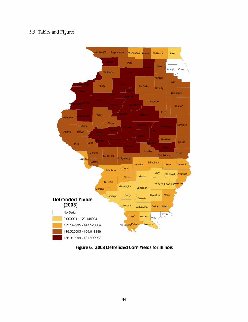
44

5.5 Tables and Figures

Figure 6. 2008 Detrended Corn Yields for Illinois

Will

Lee

Pike

Cook Ogle

McLean

La Salle

Knox

Fulton

Iroquois

Henry

Adams

Bureau

Shelby

Ford

Livingston

Edgar

Kane

Clay

Wayne

Lake

Logan

Peoria

Piatt Vermilion

Fayette

Clark

Hancock

DeKalb

Coles

Macoupin

Champaign

Macon

Madison

White

Mason

Mercer

St. Clair Marion

Perry

Sangamon Christian

Tazewell

Warren

Cass

Morgan

Jasper

Carroll

Whiteside

Greene

Bond

Jackson

Clinton

McHenry

Union

Kankakee

Pope

Jefferson

Randolph

Saline

Grundy

Jo Daviess

Woodford

Jersey Montgomery

Stark

De Witt

Franklin

Monroe

Schuyler

Douglas Scott

McDonough

Stephenson

Crawford

Brown

Hamilton

Marshall

Winnebago

Effingham

Washington

Boone

Kendall

Moultrie

DuPage

Gallatin

Menard

Richland

Johnson

Williamson

Rock Island

Lawrence

Cumberland

Hardin

Henderson

Calhoun

Massac

Wabash

Pulaski

Edwards

Alexander

Putnam

Detrended Yields (2008)

No Data 0.000001 - 129.149994 129.149995 - 148.520004 148.520005 - 166.919998 166.919999 - 181.199997

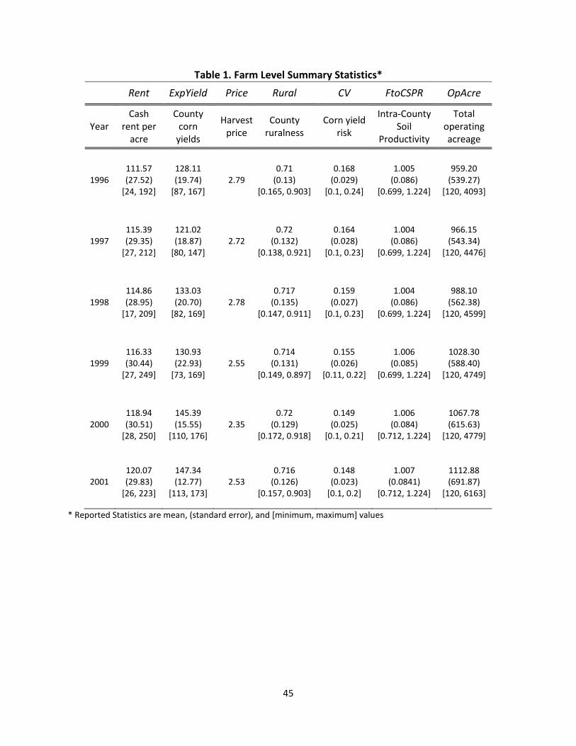
45

Table 1. Farm Level Summary Statistics*

Rent ExpYield Price Rural CV FtoCSPR OpAcre

Year Cash

rent per acre

County corn

yields

Harvest price

County ruralness

Corn yield risk

Intra-County Soil

Productivity

Total operating acreage

1996 111.57 (27.52)

[24, 192]

128.11 (19.74)

[87, 167] 2.79

0.71 (0.13)

[0.165, 0.903]

0.168 (0.029)

[0.1, 0.24]

1.005 (0.086)

[0.699, 1.224]

959.20 (539.27)

[120, 4093]

1997 115.39 (29.35)

[27, 212]

121.02 (18.87)

[80, 147] 2.72

0.72 (0.132)

[0.138, 0.921]

0.164 (0.028)

[0.1, 0.23]

1.004 (0.086)

[0.699, 1.224]

966.15 (543.34)

[120, 4476]

1998 114.86 (28.95)

[17, 209]

133.03 (20.70)

[82, 169] 2.78

0.717 (0.135)

[0.147, 0.911]

0.159 (0.027)

[0.1, 0.23]

1.004 (0.086)

[0.699, 1.224]

988.10 (562.38)

[120, 4599]

1999 116.33 (30.44)

[27, 249]

130.93 (22.93)

[73, 169] 2.55

0.714 (0.131)

[0.149, 0.897]

0.155 (0.026)

[0.11, 0.22]

1.006 (0.085)

[0.699, 1.224]

1028.30 (588.40)

[120, 4749]

2000 118.94 (30.51)

[28, 250]

145.39 (15.55)

[110, 176] 2.35

0.72 (0.129)

[0.172, 0.918]

0.149 (0.025)

[0.1, 0.21]

1.006 (0.084)

[0.712, 1.224]

1067.78 (615.63)

[120, 4779]

2001 120.07 (29.83)

[26, 223]

147.34 (12.77)

[113, 173] 2.53

0.716 (0.126)

[0.157, 0.903]

0.148 (0.023)

[0.1, 0.2]

1.007 (0.0841)

[0.712, 1.224]

1112.88 (691.87)

[120, 6163]

* Reported Statistics are mean, (standard error), and [minimum, maximum] values

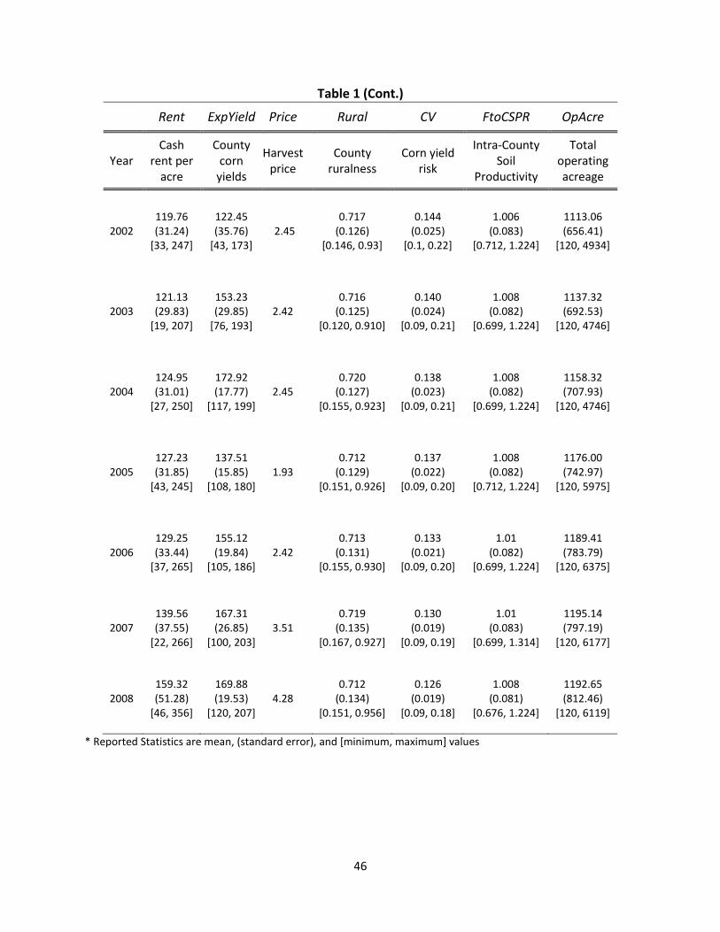
46

Table 1 (Cont.)

Rent ExpYield Price Rural CV FtoCSPR OpAcre

Year Cash

rent per acre

County corn

yields

Harvest price

County ruralness

Corn yield risk

Intra-County Soil

Productivity

Total operating acreage

2002 119.76 (31.24)

[33, 247]

122.45 (35.76)

[43, 173] 2.45

0.717 (0.126)

[0.146, 0.93]

0.144 (0.025)

[0.1, 0.22]

1.006 (0.083)

[0.712, 1.224]

1113.06 (656.41)

[120, 4934]

2003 121.13 (29.83)

[19, 207]

153.23 (29.85)

[76, 193] 2.42

0.716 (0.125)

[0.120, 0.910]

0.140 (0.024)

[0.09, 0.21]

1.008 (0.082)

[0.699, 1.224]

1137.32 (692.53)

[120, 4746]

2004 124.95 (31.01)

[27, 250]

172.92 (17.77)

[117, 199] 2.45

0.720 (0.127)

[0.155, 0.923]

0.138 (0.023)

[0.09, 0.21]

1.008 (0.082)

[0.699, 1.224]

1158.32 (707.93)

[120, 4746]

2005 127.23 (31.85)

[43, 245]

137.51 (15.85)

[108, 180] 1.93

0.712 (0.129)

[0.151, 0.926]

0.137 (0.022)

[0.09, 0.20]

1.008 (0.082)

[0.712, 1.224]

1176.00 (742.97)

[120, 5975]

2006 129.25 (33.44)

[37, 265]

155.12 (19.84)

[105, 186] 2.42

0.713 (0.131)

[0.155, 0.930]

0.133 (0.021)

[0.09, 0.20]

1.01 (0.082)

[0.699, 1.224]

1189.41 (783.79)

[120, 6375]

2007 139.56 (37.55)

[22, 266]

167.31 (26.85)

[100, 203] 3.51

0.719 (0.135)

[0.167, 0.927]

0.130 (0.019)

[0.09, 0.19]

1.01 (0.083)

[0.699, 1.314]

1195.14 (797.19)

[120, 6177]

2008 159.32 (51.28)

[46, 356]

169.88 (19.53)

[120, 207] 4.28

0.712 (0.134)

[0.151, 0.956]

0.126 (0.019)

[0.09, 0.18]

1.008 (0.081)

[0.676, 1.224]

1192.65 (812.46)

[120, 6119]

* Reported Statistics are mean, (standard error), and [minimum, maximum] values

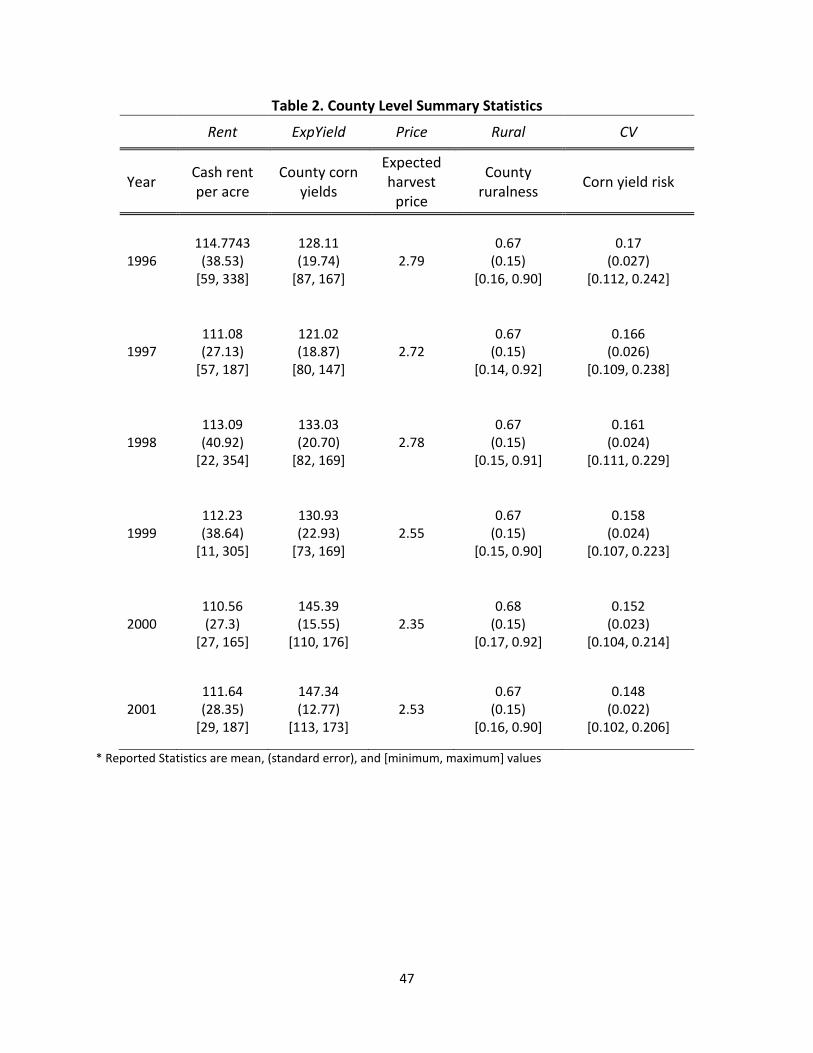
47

Table 2. County Level Summary Statistics

Rent ExpYield Price Rural CV

Year Cash rent per acre

County corn yields

Expected harvest

price

County ruralness Corn yield risk

1996 114.7743

(38.53) [59, 338]

128.11 (19.74)

[87, 167] 2.79

0.67 (0.15)

[0.16, 0.90]

0.17 (0.027)

[0.112, 0.242]

1997 111.08 (27.13)

[57, 187]

121.02 (18.87)

[80, 147] 2.72

0.67 (0.15)

[0.14, 0.92]

0.166 (0.026)

[0.109, 0.238]

1998 113.09 (40.92)

[22, 354]

133.03 (20.70)

[82, 169] 2.78

0.67 (0.15)

[0.15, 0.91]

0.161 (0.024)

[0.111, 0.229]

1999 112.23 (38.64)

[11, 305]

130.93 (22.93)

[73, 169] 2.55

0.67 (0.15)

[0.15, 0.90]

0.158 (0.024)

[0.107, 0.223]

2000 110.56 (27.3)

[27, 165]

145.39 (15.55)

[110, 176] 2.35

0.68 (0.15)

[0.17, 0.92]

0.152 (0.023)

[0.104, 0.214]

2001 111.64 (28.35)

[29, 187]

147.34 (12.77)

[113, 173] 2.53

0.67 (0.15)

[0.16, 0.90]

0.148 (0.022)

[0.102, 0.206]

* Reported Statistics are mean, (standard error), and [minimum, maximum] values

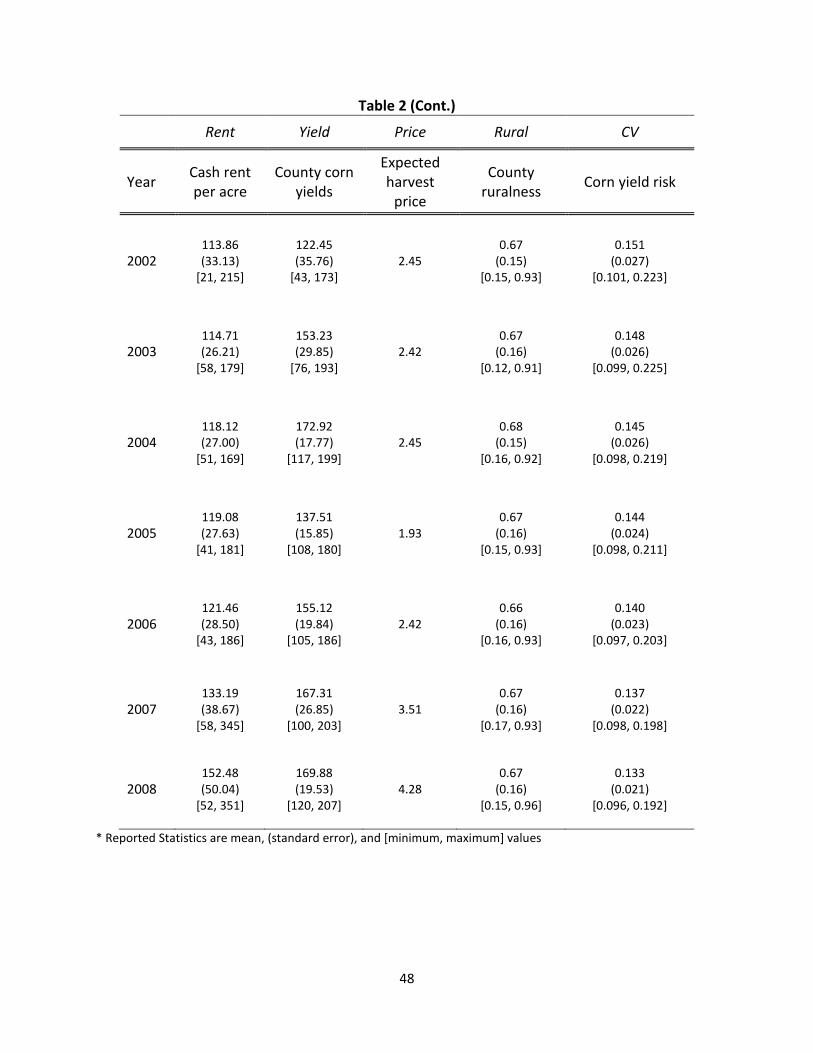
48

Table 2 (Cont.)

Rent Yield Price Rural CV

Year Cash rent per acre

County corn yields

Expected harvest

price

County ruralness Corn yield risk

2002 113.86 (33.13)

[21, 215]

122.45 (35.76)

[43, 173] 2.45

0.67 (0.15)

[0.15, 0.93]

0.151 (0.027)

[0.101, 0.223]

2003 114.71 (26.21)

[58, 179]

153.23 (29.85)

[76, 193] 2.42

0.67 (0.16)

[0.12, 0.91]

0.148 (0.026)

[0.099, 0.225]

2004 118.12 (27.00)

[51, 169]

172.92 (17.77)

[117, 199] 2.45

0.68 (0.15)

[0.16, 0.92]

0.145 (0.026)

[0.098, 0.219]

2005 119.08 (27.63)

[41, 181]

137.51 (15.85)

[108, 180] 1.93

0.67 (0.16)

[0.15, 0.93]

0.144 (0.024)

[0.098, 0.211]

2006 121.46 (28.50)

[43, 186]

155.12 (19.84)

[105, 186] 2.42

0.66 (0.16)

[0.16, 0.93]

0.140 (0.023)

[0.097, 0.203]

2007 133.19 (38.67)

[58, 345]

167.31 (26.85)

[100, 203] 3.51

0.67 (0.16)

[0.17, 0.93]

0.137 (0.022)

[0.098, 0.198]

2008 152.48 (50.04)

[52, 351]

169.88 (19.53)

[120, 207] 4.28

0.67 (0.16)

[0.15, 0.96]

0.133 (0.021)

[0.096, 0.192]

* Reported Statistics are mean, (standard error), and [minimum, maximum] values

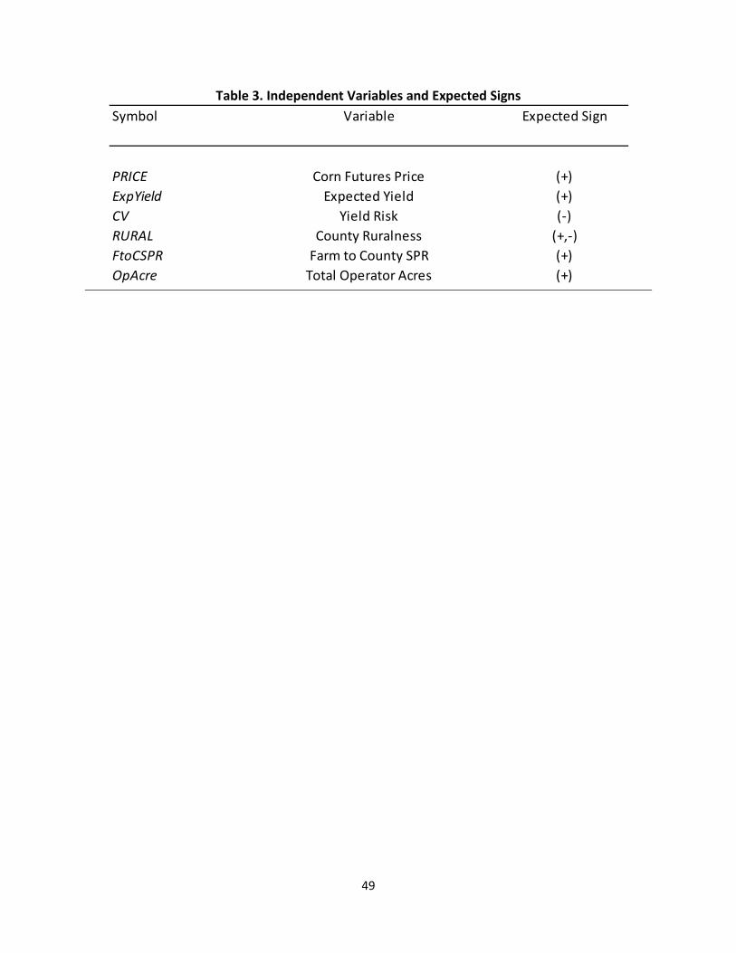
49

Table 3. Independent Variables and Expected Signs

PRICEExpYieldCVRURALFtoCSPROpAcre

Symbol Variable Expected Sign

Corn Futures Price

Yield RiskCounty Ruralness

Farm to County SPRTotal Operator Acres

(+)(+)(-)

(+,-)(+)(+)

Expected Yield

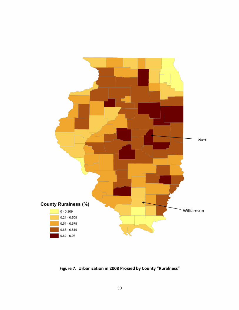
50

Figure 7. Urbanization in 2008 Proxied by County “Ruralness”

County Ruralness (%) 0 - 0.209 0.21 - 0.509 0.51 - 0.679 0.68 - 0.819 0.82 - 0.96

Williamson

Piatt

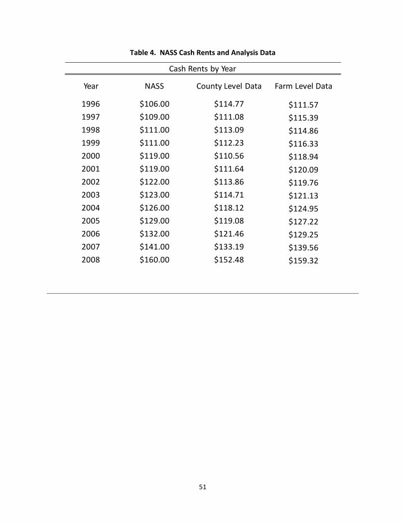
51

Table 4. NASS Cash Rents and Analysis Data

Cash Rents by Year

Year NASS County Level Data Farm Level Data

1996 $106.00 $114.77 $111.571997 $109.00 $111.08 $115.391998 $111.00 $113.09 $114.861999 $111.00 $112.23 $116.332000 $119.00 $110.56 $118.942001 $119.00 $111.64 $120.092002 $122.00 $113.86 $119.762003 $123.00 $114.71 $121.132004 $126.00 $118.12 $124.952005 $129.00 $119.08 $127.222006 $132.00 $121.46 $129.252007 $141.00 $133.19 $139.562008 $160.00 $152.48 $159.32

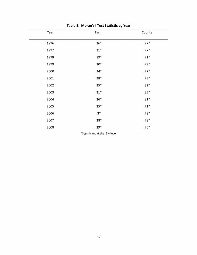
52

Table 5. Moran's I Test Statistic by Year

Year Farm County

1996 .26* .77*

1997 .21* .77*

1998 .19* .71*

1999 .20* .79*

2000 .24* .77*

2001 .28* .78*

2002 .25* .82*

2003 .21* .85*

2004 .26* .81*

2005 .25* .71*

2006 .3* .78*

2007 .28* .78*

2008 .29* .70*

*Significant at the .1% level

53

Chapter 6 Results

Table 6 reports the results for the farm- and county-level spatial panel data analysis along with

additional models for robustness checks. All models regress cash rent per acre against the

various attributes as previously discussed. The coefficients have intuitively correct signs with

the exception of the ruralness indicator, which was undetermined, and the risk measure in the

county analysis. The findings suggest there are significant spatial error correlations in both

models with 𝜌𝜌 = 0.42 and 𝜌𝜌 = 0.50 for the main farm and county analysis, respectively.

First, there is strong evidence that the expected output price has a positive effect on real

cropland cash rents and both analyses show this to be highly statistically significant. The effect

also appears to be very robust to different model specifications. County level results find that

marginal increases in the harvest futures price increases rents by around $24.00. Under the farm

level analysis, this measure rises to over $41.00, perhaps implying that the aggregation process

has a significant loss of information. The fact that these numbers are much smaller than previous

studies is no surprise given that the hedonic framework allows for increasing prices and costs to

interact dynamically within the hedonic price schedule.

We also find strong evidence that the effect of inter-county soil productivity is positively

associated with variations in rent levels. Statistical evidence also implies that intra-county

variations impact rents positively, reinforcing the idea that soil quality is a prime indicator of

agricultural returns and land rent. In the county model, marginal increases in bushels per acre

are associated with an approximate $1.94 rise in cash rents per acre. At the farm level, cross-

county variations in yield increase rents by approximately $1.49 per acre. Farm level SPR

deviations from the overall county SPR are shown to have an approximate $8.67 increase

54

(decrease) for every 10% increment above (below) the county SPR mean. This implies there is a

premium for high quality land within counties and a discount for inferior land, as expected.

The yield risk measure for the county analysis produced a positive coefficient, but was

insignificant. With the disaggregation of the county data, the farm level analysis produced a

negative coefficient and was significant at the 5% level. Specifically, the study finds that a 10%

increase in a farmer's perceived risk has a negative impact on cash rent of $3.48 per acre. Under

the likely assumption that tenant farmers are risk averse, a negative coefficient on the risk

variable is expected. The production risk premium being observed is a result of this assumption

and implies that the rental market is working efficiently in this capacity.

The measure used for urbanization pressure was both significant and positive for both

levels of estimation. The hypothesized impact of this measure was initially undetermined. This

study provides evidence that urbanization has the opposite effect on agricultural cash rents as it

does on agricultural land values (Huang et al. 2006). The more rural a county or the county a

farmer produces in, the higher the rent which can be expected. We find that a 1% increase in

county ruralness increases rents by approximately $37 per acre. This phenomenon can be

explained by the efficiencies gained in relatively rural counties. It would be expected that

counties relying more heavily on agriculture, and hence more rural areas, will have superior

access to farm related inputs and machinery, such as grain elevators and large machinery leasing

facilities. Financing through agricultural lending institutions may also be more readily available

in agricultural counties and the transaction costs relatively low given the lending institutions

ability to keep close relationships with fewer clients. Other considerations leading to this

outcome, as described previously, may also include ease of bulky equipment navigation on

public roadways and larger parcels uninterrupted by residential pockets and subdivisions.

55

The results indicate that the total acreage that a tenant farmer operates is associated with

higher rents although the impact is rather minimal, yet statistically significant. This study finds

that marginal acreage increases are associated with a $0.01 increase in cash rents per acre. This

may be capturing a tenant farmer’s ability in that superior farming skills result in lower overall

implicit costs enabling the tenant farmer to bid up the price of potential new tracts when

attempting to increase their working land. This describes the economies of scale that are

associated with large-scale farming initiatives.

Lastly, we find limited support for RRT with a majority of increased revenues due to

output price increases accruing to the farmer. Using the farm-level analysis, we find that the

tenant farmer captures 89% of the marginal increases in commodity prices while the landowner

and input suppliers absorb only 3.3% and 7.7%, respectively. The relatively large amount that is

captured by the tenant farmer may be a form of ‘compensation’ for bearing price risk. This

would imply that tenant farmers cash renting cropland receive both a premium for yield risk as

well as price risk.

Overall, both model specifications resulted in the expected signs of statistically

significant variables with the farm level analysis obtaining a better overall fit to the sample data

according to the pseudo-R2 measures as presented in the results table. This is likely the result of

the additional information gained when using disaggregated data, as well as the possibility for

the inclusion of the additional variables capturing intra-county differences in soil productivities

and the effects of operating efficiencies as measured by a tenant farmer’s scale of operation.

Table 7 presents robustness checks using multiple alternative model specifications for the

farm level. The differing estimators use the fixed effects method rather than random effects as in

the main model. While the random effects may be seen as capturing the random components of

56

the tenant farmers, the fixed effects estimators are more explicitly capturing parcel-level

heterogeneity. Each alternative fixed effects specification uses a different method as to which

effects are ultimately being captured, including cross-sectional specific effects, time-wise effects

and both cross sectional and time-wise effects. In other words, the cross-sectional variations first

difference the individual observations across time to obtain the unobserved individual parcel

affects whereas the time-wise fixed effects is capturing the unobserved variations across the

individual panels as a whole. In addition, the first four alternative specifications use a spatial lag

variation instead of a spatial error component. This form implies that the rent a tenant farmer

pays is a function of his neighbors’ rent levels and that there are no spatial correlations present

within the remainder error term. If this is the case, the spatial lag model is seen to be an

unbiased estimator.

The coefficients for the price effect and productivity are similar to that of the main model

implying that spatial error components model is not necessarily driving the results. If the spatial

lag estimator is in fact an unbiased estimator, it appears that the original error component model

is also unbiased. However, as compared to the first three alternative specifications, the error

components model is more efficient as expected. The coefficients for land productivity and the

total amount of operator acres are also quite robust to the alternative specifications indicating

that these are perhaps good measures of how these variables ultimately affect rent levels. The

coefficients association with yield risk, ruralness and intra-county productivity deviations change

considerably between alternative specifications implying that the estimates given by the spatial

error component model may not be a good measure of the true impact on rent levels.

With the main focus of this paper being placed upon how commodity price levels affect

rent levels, the results in Table 7 suggest that the estimates of the primary variable are not

57

particularly sensitive to the use of reasonable alternative specifications. As this is a good fit of

the data, the baseline results for the price measure, land productivity and the validity of

Ricardian Rent Theory are seen as reasonable estimates for the final results.

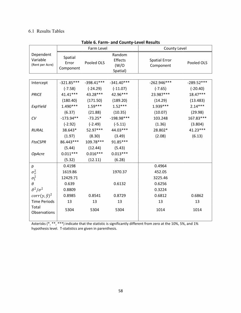
58

6.1 Results Tables

Table 6. Farm- and County-Level Results

Dependent Variable (Rent per Acre)

Farm Level County Level

Spatial Error

Component Pooled OLS

Random Effects (W/O

Spatial)

Spatial Error Component Pooled OLS

Intercept -321.85*** -398.41*** -341.40*** -262.946*** -289.52***

(-7.58) (-24.29) (-11.07) (-7.65) (-20.40) PRICE 41.41*** 43.28*** 42.96*** 23.987*** 18.47***

(180.40) (171.50) (189.20) (14.29) (13.483) ExpYield 1.490*** 1.59*** 1.52*** 1.939*** 2.14***

(6.37) (21.88) (10.35) (10.07) (29.98) CV -173.94** -73.25* -198.98*** 103.248 167.83***

(-2.92) (-2.49) (-5.11) (1.36) (3.804) RURAL 38.643* 52.97*** 44.03*** 28.802* 41.23***

(1.97) (8.30) (3.49) (2.08) (6.13) FtoCSPR 86.443*** 109.78*** 91.85*** (5.44) (12.44) (5.43) OpAcre 0.011*** 0.016*** 0.013*** (5.32) (12.11) (6.28) ρ 0.4198 0.4964 𝜎𝜎𝑣𝑣2 1619.86 1970.37 452.05 𝜎𝜎1

2 12429.71 3225.46 𝜃𝜃 0.639 0.6132 0.6256 𝜎𝜎�2/𝜎𝜎2 0.8809 0.3224 𝑐𝑐𝑐𝑐𝑐𝑐𝑐𝑐(𝑦𝑦,𝑦𝑦�)2 0.8985 0.8541 0.8729 0.6812 0.6862 Time Periods 13 13 13 13 13 Total Observations 5304 5304 5304 1014 1014

Asterisks (*, **, ***) indicate that the statistic is significantly different from zero at the 10%, 5%, and 1% hypothesis level. T-statistics are given in parenthesis.

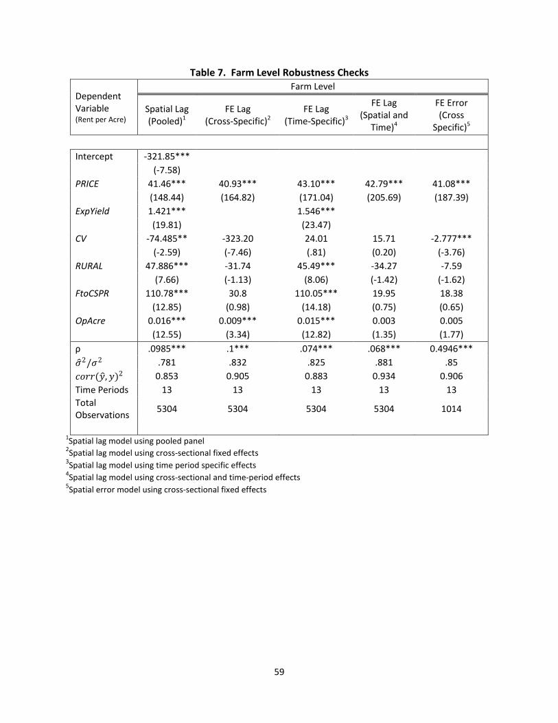
59

Table 7. Farm Level Robustness Checks

Dependent Variable (Rent per Acre)

Farm Level

Spatial Lag (Pooled)1

FE Lag (Cross-Specific)2

FE Lag (Time-Specific)3

FE Lag (Spatial and

Time)4

FE Error (Cross

Specific)5

Intercept -321.85*** (-7.58) PRICE 41.46*** 40.93*** 43.10*** 42.79*** 41.08***

(148.44) (164.82) (171.04) (205.69) (187.39) ExpYield 1.421*** 1.546*** (19.81) (23.47) CV -74.485** -323.20 24.01 15.71 -2.777***

(-2.59) (-7.46) (.81) (0.20) (-3.76) RURAL 47.886*** -31.74 45.49*** -34.27 -7.59

(7.66) (-1.13) (8.06) (-1.42) (-1.62) FtoCSPR 110.78*** 30.8 110.05*** 19.95 18.38

(12.85) (0.98) (14.18) (0.75) (0.65) OpAcre 0.016*** 0.009*** 0.015*** 0.003 0.005

(12.55) (3.34) (12.82) (1.35) (1.77) ρ .0985*** .1*** .074*** .068*** 0.4946*** 𝜎𝜎�2/𝜎𝜎2 .781 .832 .825 .881 .85 𝑐𝑐𝑐𝑐𝑐𝑐𝑐𝑐(𝑦𝑦�,𝑦𝑦)2 0.853 0.905 0.883 0.934 0.906 Time Periods 13 13 13 13 13 Total Observations 5304 5304 5304 5304 1014

1Spatial lag model using pooled panel 2Spatial lag model using cross-sectional fixed effects 3Spatial lag model using time period specific effects 4Spatial lag model using cross-sectional and time-period effects 5Spatial error model using cross-sectional fixed effects

60

Chapter 7 Summary and Conclusion

It has generally been assumed that landowners would capture a large majority of increasing

revenues when record-high corn prices are experienced. However, this study indicates that

landowners actually receive a very small portion. Using more precise farm-level data, this study

employs a novel spatial panel econometric approach by exploiting unique panel data from the

Illinois FBFM data collection to analyze the determinants of agricultural cash rents. We find

that cropland cash rental rates in Illinois are largely determined by expected output prices, soil

productivity, urbanization pressures, perceived risk and scale of farming operations. In addition,

we find very limited evidence to support RRT with a majority of increased revenues as a result

of high commodity prices being capture by the tenant farmer. In addition, the results indicate

that substantial variation in cash rental rates exist across the state given the above characteristics.

In contrast to previous studies, this aspect of heterogeneity across farmland parcels is

investigated using a hedonic framework. This study demonstrates that fluctuations in future

output price expectations translate into substantial real cash rent movements with cash rents

increasing by $41 for a $1 increase in corn prices. These findings are less than those found in

previous studies using a variable profit function approach and are likely the result of allowing the

analysis to be set within a dynamic process where corresponding movements in input costs are

built into the hedonic price schedule. Ultimately, the hedonic framework allows for a more

precise view of how output price movements flow through to the rental market and affect the

unavoidable land costs borne onto tenant farmers. The marginal value of land quality across

Illinois counties is approximately $1.50, while intra-county quality variations are valued around

$9.00 for 10% deviations from the respective county SPR mean. Urbanization pressures are

61

found to have a negative effect on cash rents with a 1% increase in ruralness increasing rents by

approximately $38.00. Perceived production risks decrease rents by nearly $3.50, while the

scale of farming initiatives increases rents marginally by only $0.01.

This study also suggests that the use of farm level data outperforms that of aggregated

county level. The difference in the impacts of the price variable is hypothesized to be the result

of the information lost when data is aggregated. The use of farm level data appears to allow for

increased accuracy in estimating the coefficients as noted by the overall model fit in comparison

to the county level analysis. The occurrence of significant spatial correlations lends supporting

evidence that the spatial model is also more efficient when estimating agricultural rental rates in

comparison to a non spatial error component model. Explicitly taking into account spatial

considerations within the empirical model gives additional confidence when applying statistical

inference to the coefficients as the standard BLUE assumptions are fully met. Future research

pertaining to cash rents and their land value counterparts can benefit from the spatial

observations presented in this study and aid researchers in deciding whether explicitly

accounting for spatial connectedness between neighbors is an appropriate assumption and

avoiding erroneous inferences from ordinary least squares estimation.

There are many opportunities to take the results and approaches of this study and extend

them to other questions. Many studies have focused on the impacts of government programs on

cash rents and whether the landlord or tenant is the ultimate beneficiary. These studies include

Kirwan (2009), Lambert and Griffin (2004), Rosine & Helmberger (1974), Featherstone and

Baker (1988) and Goodwin and Ortalo-Magne (1992), amongst others. These studies have

produced conflicting evidence as to who ultimately receives government payments and the

distribution of these payments among the two parties. Using the framework and data presented

62

in this study will help provide a robust approach and more accurate information towards this

question. In correctly identifying and modeling the determinants of the cash rental process while

incorporating the effects of government payments is expected to provide improved information

for both public and private decisions.

Exploring different weight matrix schemes at the farm level is another extension. There

are no tests to determine the correct spatial structure when applying spatial lag or error models.

It would be interesting to generate multiple weighting schemes and see how the results change, if

at all. For example, this study uses a block structure in which every farmer within a county is a

neighbor of all other farmers within that same county. This ignores the fact that a farmer may be

on the fringe of his/her county and may be a closer neighbor to a farmer in an adjacent county.

Creating a weight structure that allows a farmer to be a neighbor of all farmers within his county

as well as a neighbor to farmers in adjacent counties would be an alternative weight matrix.

However, issues surrounding the asymptotics of the weight matrix must be observed. By

limiting the total number of neighbors a farmer may have at one time to an arbitrary number and

through repeated random sampling of potential neighbors, multiple weight matrices can be

formed and compared. This would lend evidence to the overall efficiency of the resulting

coefficient standard errors obtained and aid in future research with respect to farm level

agricultural rents and statistical inference.

63

References

Anselin, L. 1992a. “Space and Applied Econometrics.” Regional Science and Urban Economics.

22(3): 307-316.

Anselin, L. 1992b. “SpaceStat Tutorial: A Workbook for Using SpaceStat in the Analysis of

Spatial Data.” Technical Report no. S-92-1, National Centre for Geographic Information

and Analysis, University of California.

Anselin, L. and Bera, A. 1998. “Spatial dependence in linear regression models with an

introduction to spatial econometrics.” In: Giles, D., Ullllah, A. (Eds.), Handbook of

Applied Economic Statistics, pages 237–289. Marcel Dekker, New York.

Anselin, L. 2002. “Under the Hood: Issues in the Specification and Interpretation of Spatial

Regression Models.” Agricultural Economics. 27: 247-267.

Awokuse, T., J.M. Duke. 2006. “The Causal Structure of Land Price Determinants.” Canadian

Journal of Agricultural Economics. 54(2): 227-245.

Baltagi, B.H. 2008. Econometric Analysis of Panel Data, 4th edition. New York: Wiley.

Barlowe, R. 1986. Land Resource Economics: The Economics of Real Estate. 6th edition.

Englewood Cliffs, N.J.: Prentice-Hall.

Barry, P.J., N.L. Sotomayor, and L.M. Moss. 1998-1999. “Professional Farm Managers Views

on Leasing Contracts and Land Control: An Illinois Perspective.” J. Amer. Soc. Farm

Managers and Rural Appraisers. 62:15–19.

Barry, P.J., L.M. Moss, N.L. Sotomayor, and C. Escalante. 2000. “Lease Pricing for Farm Real

Estate.” Review of Agricultural Economics 12(1):2-16.

64

Bastian, C., D. McLeod, M. Germino, W. Reiners and B. Blasko. 2002. “Environmental

Amenities and Agricultural Land Values: A Hedonic Model Using Geographic

Information Systems Data.” Ecological Economics. 40(3): 337-349.

Basu, S., T. Thibodeau. 1998. “Analysis of Spatial Autocorrelation in House Prices.” Journal of

Real Estate Finance and Economics. 17(1): 61-85.

Baylis, K., R. Garduño-Rivera, and G. Piras. 2009. “The Distributional Effects of NAFTA in

Mexico.” Available at: http://works.bepress.com/kathy_baylis/20.

Benirschka, M. & Binkley, J. K. 1994. “Land Price Volatility in a Geographically Dispersed

Market.” American Journal of Agricultural Economics. 76:185-195.

Benjamin, J. D. and G. S. Sirmans. 1996. “Mass Transportation, Apartment Rent and Property

Values.” Journal of Real Estate Research. 12(1): 1–8.

Bollinger, C. 1998. “Spatial Variation in Office Rents within the Atlanta Region” Urban Studies.

35(7): 1097-1118.

Can, A. 1990. “The Measurement of Neighborhood Dynamics in Urban House Prices.”

Economic Geography. 66(3): 254-272.

Case, A.C., 1992. “Neighborhood influence and technological change.” Regional Science and

Urban Econonomics. 22: 491–508.

Chicoine, D. 1981. “Farmland Values at the Urban Fringe: An Analysis of Sale Prices.” Land

Economics. 57(3): 353-362.

Dhyuvetter, K. and T. Kastens. 2002. “Landowner vs. Tenant: Why are Land Rents so High?”

Paper prepared for presentation at the Risk and Profitability Conference, Manhattan,

KS, August 15-16, 2002.

65

Downes, T.A., and J.E. Zabel. 2002. “The Impact of School Characteristics on House Prices:

Chicago 1987–1991.” Journal of Urban Economics. 52(1): 1-25.

Du, X., D.A. Hennessy, and W.M. Edwards. 2007. “Determinants of Iowa Cropland Cash

Rental Rates: Testing Ricardian Rent Theory.” Working Paper 07-WP 454.

Du, X., D.A. Hennessy, and W.M. Edwards. 2008. “Does a Rising Biofuels Tide Raise All

Boats? A Study of Cash Rent Determinants for Iowa Farmland under Hay and Pasture.”

Journal of Agriculture and Food Industrial Organization. 6(2).

Dunse, N., and C. Jones. 1998. “A Hedonic Price Model of Office Rents.” Journal of Property

Valuation and Investment. 16(3): 297-312.

Evans, Alan. 2004. Economics, Real Estate, and the Supply of Land. Oxford: Blackwell

Featherstone, A. M., and T. G. Baker. 1988. “Effects of Reduced Price and Income Supports on

Farmland Rent and Value.” North Central J. Agricultural Econonics. 10 (July): 177–89.

Federal Trade Commission (FTC). 2006. “The FTC’S Role in the Gasoline Industry.” Available

at: http://www.ftc.gov/ftc/oilgas/archive/060504.htm

Forster, L., C.A. Pohlman, M.T. Batte, and B.L. Sohngen. 2003. “Ohio Farm Real Estate

Markets.” Technical Report. Department of Agricultural, Environmental, and

Development Economics, Ohio State University.

Goodwin, B. K., and F. Ortalo-Magne. 1992. “The Capitalization of Wheat Subsidies into

Agricultural Land Values.” Canadian J. Agricultural Econonics. 40 (March):37–54.

Goodwin, B., A.K. Mishra, F. Ortalo-Magné. 2005. “Landowners’ Riches: The Distribution of

Agricultural Subsidies.” Working Paper. School of Business, University of Wisconsin.

Guntermann, K.L., and S. Norbin. (1987). Explaining the Variability of Apartment Rents.

Journal of the American Real Estate and Urban Economics Association. 15(4): 321–340.

66

Gustafson, Cole. 2008. “Biofuel Economics: 2007 Energy Act Charts a New Biofuel Roadmap”

NDSU Extension Service. North Dakota State University, Available at

http://www.ag.ndsu.edu/news/columns/biofuels-economics.

Henderson, J., B.A. Gloy. 2009. “The Impact of Ethanol Plants on Cropland Values in the Great

Plains.” Agricultural Finance Review. 69(1): 36-48.

Huang, H., G. Miller, B. Sherrick, and M. Gomez. 2006. “Factors Influencing Illinois Farmland

Values.” American Journal of Agricultural Economics. 88(2): 458-470.

Hubacek, K. and, J. Van den Bergh. 2002. “The Role of Land in Economic Theory.” Interim

report. IR-02-037. International Institute for Applied System Analysis (IIASA).

Irwin, S., D. Good. 2009. “Market Instability in a New Era of Corn, Soybean and Wheat Prices.”

Choices. 24(1): 6-11.

Kapoor, M., Kelejian, H.H., & Prucha, I.R. 2007. “Panel Data Model with Spatial Correlated

Error Components.” Journal of Econometrics. 140(1): 97-130.

Kelejian, H.H., & Prucha, I.R. 1999. “A Generalized Moments Estimator for the Autoregressive

Parameter in a Spatial Model.” International Economic Review. 40(2): 509-533.

Kirwan, B. 2009. “The Incidence of U.S. Agricultural Subsidies on Farmland Rental Rates.”

Journal of Political Economy. 117(1): 138-164.

Krause, J. and Brorsen B. 1995. “The Effect of Risk on the Rental Value of Agricultural Land.”

Review of Agricultural Economics. 17(1): 71-76.

Kurkalova, L., C. Burkart, and S. Secchi. 2004. “Cropland Cash Rental Rates in the Upper

Mississippi River Basin.” Technical Report. Center for Agricultural and Rural

Development, Iowa State University.

67

Lambert, D. and T. Griffin. 2004. “Analysis of Government Farm Subsidies on Farmland Cash

Rental Rates Using a Fixed Effect Spatial Distributed Lag.” Paper prepared for

presentation at the American Agricultural Economics Association Annual Meeting,

Denver, August 1-4, 2004.

Lancaster, K. 1966. “A New Approach to Consumer Theory.” Journal of Political Economy.

74(1): 132-157.

Lancaster, K. 1979. Variety, Equity and Efficiency. Oxford: Basil Blackwell.

Livanis, G., C.B. Moss, V.E. Breneman, R.F. Nehring. 2006. “Urban Sprawl and Farmland

Prices.” American Journal of Agricultural Economics. 88(4): 915-929.

Löchl, M. 2007. “Considering Spatial Dependence in Hedonic Rent Price Regression.” Paper

prepared for presentation at the 7th Swiss Transport Research Conference, Monte Verità

/ Ascona, September 12-14, 2007.

Luttik, J. 2000. “The Value of Trees, Water and Open Space as Reflected by House Prices in the

Netherlands.” Landscape and Urban Planning. 48(3): 161-167.

Mendelsohn, R., A. Dinar. 2003. “Climate, Water, and Agriculture.” Land Economics. 79(3):

328-341.

Moss, C.B. 1997. “Returns, Interest Rates and Inflation: How They Explain Changes in

Farmland Values.” American Journal of Agricultural Economics. 79(4): 1311-1318.

Muhammad, A. and E. Kebede. 2009. “The Emergence of an Agro-Energy Sector: Is Agriculture

Importing Instability from the Oil Sector?” Choices. 24(1): 12-15.

Nelson, J. 2004. “Meta-Analysis of Airport Noise and Hedonic Property Values: Problems and

Prospects.” Journal of Transport Economics and Policy. 38(1): 1-27.

68

Nickerson, C., L. Lynch. 2001. “The Effect of Farmland Preservation Programs on Farmland

Prices.” American Journal of Agricultural Economics. 83(2): 341-351.

Olmo, J.C. 1995. “Spatial Estimation of Housing Prices and Locational Rents.” Urban Studies.

32(8): 1331-1344.

O’Sullivan, A. 2003. Urban Economics, 5th Edition. McGraw-Hill/Irwan.

Palmquist, R.B. 1989. “Land as a Differentiated Factor of Production: A Hedonic Model and Its

Implications for Welfare Measurement.” Land Economics. 65(1): 23-28.

Palmquist, R.B. and L. Danielson. 1989. “A Hedonic Study of the Effects of Erosion Control

and Drainage on Farmland Values.” American Journal of Agricultural Economics. 71(1):

55-62.

Palmquist, R.B., F.M. Roka and T. Vukina. 1997. “Hog Operations, Environmental Effects, and

Residential Property Values.” Land Economics. 73(1): 114-124.

Patton, M., P. Kostov, S. McErlean, J. Moss. 2008. “Assessing the Influence of Direct Payments

on the Rental Value of Agricultural Land.” Food Policy. 33(5): 397-405.

Phipps, T. 1984. “Land Prices and Farm-Based Returns.” American Journal of Agricultural

Economics. 66(4): 422-429.

Plantinga, A., R. Lubowski, R. Stavins. 2002. “The Effects of Potential Land Development on

Agricultural Land Prices.” Journal of Urban Economics. 52(3): 561-581.

Pope, J.C. 2008. “Buyer Information and the Hedonic: The Impact of a Seller Disclosure on the

Implicit Price for Airport Noise.” Journal of Urban Economics. 63(2): 498-516.

Renewable Fuels Association. 2009a. Statistics. Washington, D.C., Available at:

http://www.ethanolrfa.org/industry/statistics.

69

Renewable Fuels Association. 2009b. Renewable Fuel Standards. Washington, D.C., Available

at: http://www.ethanolrfa.org/resource/standard/

Ricardo, David. “An Essay on the Influence of a Low Price of Corn on the Profits of Stock”

[Originally published, 1815], in Pieor Sraffa and Maurice Dobb, eds., The Works and

Correspondence of David Ricardo, Vol. 4. Cambridge: Cambridge University Press,

1951-1973, pp. 1-42.

Roberts, M., B. Kirwan, and J. Hopkins. 2003. “The Incidence of Government Program

Payments on Agricultural Land Rents: The Challenges of Identification.” American

Journal Agricultural Economics. 85 (August): 762–69.

Robison, L.J., D.A. Lins, and R. VenKataraman. “Cash Rents and Land Values in U.S.

Agriculture.” American Journal of Agricultural Economics. 67(4): 794-805.

Rosen, J. 1974. “Hedonic Prices and Implicit Markets” Journal of Political Economy. 56 82: 34-

55 .

Schnitkey, Gary, and Dale Lattz. 2002. “Cash Rents and Equivalent Cash Rents in Illinois”

Report No. FEFO 02-23. Farmdoc: Farm Business Management, University of Illinois.

Available at:

http://www.farmdoc.uiuc.edu/manage/newsletters/fefo02_23/fefo02_23.html.

Schnitkey, Gary. 2007. “Are Farmland Prices in Line with Farmland Returns?” Report No.

FEFO 07-15. Farmdoc: Farm Business Management, University of Illinois. Available at:

http://www.farmdoc.uiuc.edu/manage/newsletters/fefo07_15/fefo07_15.html.

70

Schnitkey, Gary, and Dale Lattz. 2008. “2009 Rental Decisions Given Volatile Commodity

Prices and Higher Input Costs” Report No. IFEU 08-05. Farmdoc: Farm Business

Management, University of Illinois. Available at:

http://www.farmdoc.illinois.edu/ifeu/IFEU_08_05/IFEU_08_05.html.

Shaik, S. 2007. “Farm Programs and Land Values in Mountain States: Alternative Panel

Estimators.” Paper prepared for presentation at the 2007 Western Agricultural

Economics Association Annual Meeting, Portland, Oregon, July 29- Aug. 1, 2007.

Shaik, S., G.A. Helmers, J.A. Atwood. 2006. “Farm Programs and Agricultural Land Values:

The Case of Southern Agriculture.” Paper prepared for presentation at the 2006

Southern Agricultural Economics Association Annual Meeting, Feb. 5-8, 2006.

Shi, Y., T. Phipps, D Colyer. 1997. “Agricultural Land Values Under Urbanization Influences”

Land Economics. 73(1):90-100.

Smith, C. A.and Islam A.M. 1998. “Apartment Rents - Is There a ‘Complex’ Effect?” The

Appraisal Journal. 263-268.

Soto, P. 2004. Spatial Econometric Analysis on Louisiana Rural Real Estate Values. Ph.D.

Dissertation. Louisiana State University. 187 p.

State of Illinois Business Portal. 2009. “Illinois-Access to Key Industries.” Available at:

http://business.illinois.gov/io_keyIndustries.cfm.

Taylor, M.R., G.W. Brester. 2005. “Noncash Income Transfers and Agricultural Land Values.”

Review of Agricultural Economics. 27(4): 526-541.

USDA, National Agricultural Statistics Service. 2008a. Land Values and Cash Rents 2008

Summary. National Agricultural Statistics Service, USDA, Washington, D.C.

71

USDA, National Agricultural Statistics Service. 2008b. Crop Values 2008 Summary. National

Agricultural Statistics Service, USDA, Washington, D.C.

USDA, Office of the Chief Economist. 2008c. USDA Agricultural Projections to 2017. Long-

term Projections Report OCE-2008-1. USDA, Washington, D.C.

USDA, National Agricultural Statistics Service. 2009a. 2007 Census of Agriculture: Illinois

State and County Data. National Agricultural Statistics Service, USDA, Washington,

D.C.

USDA, Economic Research Service. 2009b. State Facts Sheet: Illinois. USDA, Washington,

D.C.

USDA, NASS. 2009c. Available at: http://www.nass.usda.gov/QuickStats/index2.jsp (Corn

Planting Information).

USDA, NASS 2007. Available at: http://www.ers.usda.gov/Data/farmbalancesheet/fbsdmu.htm

(Balance Sheet Information).

USDA-NASS. 2004. 2002 Census of Agriculture: Illinois State and County Data. National

Agricultural Statistics Service, USDA, Washington, D.C.

USDA, NRCS. 2003. Soil Survey of Champaign County, IL. USDA, Washington, D.C.

United States Environmental Protection Agency. 2005. "EPA Completes Regulations Clarifying

the Default Standard for 2006 Under the Renewable Fuel Standard Program" Regulatory

Announcement EPA420-F-05-057. Office of Transportation and Air Quality. Available

at: http://www.epa.gov/OMS/renewablefuels/420f05057.pdf.

U.S. Environmental Protection Agency. “Clean Air Act.” Available at:

http://www.epa.gov/air/caa/.

72

U.S. General Accounting Office. 2002. “U.S. Ethanol Market: MTBE Ban in California.”

Publication No. GAO-02-440R. Available at:

http://www.gao.gov/new.items/d02440r.pdf.

Valente, J., S. Wu, A. Gelfand and C. F. Sirmans. 2005. “Apartment Rent Prediction Using

Spatial Modeling.” Journal of Real Estate Research. 27(1): 105-136.

Veeman, M.M., X.Y. Dong, T.S. Veeman. 1993. “Price Behavior of Canadian Farmland.”

Canadian Journal of Agricultural Economics. 41(2): 197-208.

Wilson, B., and J. Frew. 2007. “Apartment Rents and Locations in Portland, Oregon: 1992-

2002.” Journal of Real Estate Research. 29(2): 201-217.