space-charge effects

Space-Charge Effects

N. ChauvinCommissariat à l’Énergie Atomique et aux Énergies Alternatives, Gif-sur-Yvette, France

AbstractFirst, this chapter introduces the expressions for the electric and magneticspace-charge internal fields and forces induced by high-intensity beams. Then,the root-mean-square equation with space charge is derived and discussed. Inthe third section, the one-dimensional Child–Langmuir law, which gives themaximum current density that can be extracted from an ion source, is exposed.Space-charge compensation can occur in the low-energy beam transport lines(located after the ion source). This phenomenon, which counteracts the space-charge defocusing effect, is explained and its main parameters are presented.The fifth section presents an overview of the principal methods to performbeam dynamics numerical simulations. An example of a particles-in-cellscode, SolMaxP, which takes into account space-charge compensation, is given.Finally, beam dynamics simulation results obtained with this code in the caseof the IFMIF injector are presented.

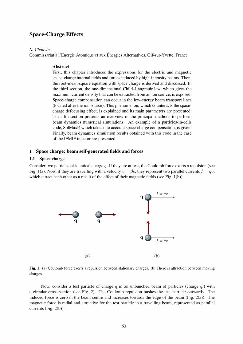
1 Space charge: beam self-generated fields and forces1.1 Space chargeConsider two particles of identical charge q. If they are at rest, the Coulomb force exerts a repulsion (seeFig. 1(a). Now, if they are travelling with a velocity v = βc, they represent two parallel currents I = qv,which attract each other as a result of the effect of their magnetic fields (see Fig. 1(b)).

...

q..

q

q I = qv

qI = qv

(a) (b)

Fig. 1: (a) Coulomb force exerts a repulsion between stationary charges. (b) There is attraction between movingcharges.

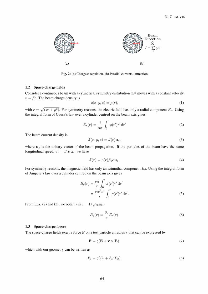
Now, consider a test particle of charge q in an unbunched beam of particles (charge qi) witha circular cross-section (see Fig. 2). The Coulomb repulsion pushes the test particle outwards. Theinduced force is zero in the beam centre and increases towards the edge of the beam (Fig. 2(a)). Themagnetic force is radial and attractive for the test particle in a travelling beam, represented as parallelcurrents (Fig. 2(b)).

63

. .

.

.

.

. .

.

.

.

..

..

.

.

.

.

.

.

.

.

.

.

.

.

...

.

.

.

.

.

..

.

..

.

.

.

.

.

.

.

.

..

..

.

.

.

.

.

.

.

.

. .

.

.

.

.

.

.

.

.

.

.

.

.

.

...

.

.

.

.

.

.

.

.

.

.

.

.. .

. ..

.

..

.

.

.

.

.

.

.

.

.

.

.

.

.

.

.

.

.

.

.

.

.

..

..

.

.

.

.

.

.

.

. .

.

.

.

.

.

.

.

....

.

.

.

.

.

.

.

.

.

.

.

..

.

.

.

.

.

.

.

.

.

.

.

..

..

.

.

.

.

.

.

.

.

.

.

..

.

..

Beam

.Direction

.

I =∑i

qiv

(a) (b)

Fig. 2: (a) Charges: repulsion. (b) Parallel currents: attraction

1.2 Space-charge fieldsConsider a continuous beam with a cylindrical symmetry distribution that moves with a constant velocityv = βc. The beam charge density is

ρ(x, y, z) = ρ(r), (1)

with r =√

(x2 + y2). For symmetry reasons, the electric field has only a radial component Er. Usingthe integral form of Gauss’s law over a cylinder centred on the beam axis gives

Er(r) =1

ε0r

∫ r

0ρ(r′)r′ dr′ (2)

The beam current density isJ(x, y, z) = J(r)uz, (3)

where uz is the unitary vector of the beam propagation. If the particles of the beam have the samelongitudinal speed, vz = βzcuz , we have

J(r) = ρ(r)βzcuz. (4)

For symmetry reasons, the magnetic field has only an azimuthal component Bθ. Using the integral formof Ampere’s law over a cylinder centred on the beam axis gives

Bθ(r) =µ0r

∫ r

0J(r′)r′ dr′

=µ0βzc

r

∫ r

0ρ(r′)r′ dr′. (5)

From Eqs. (2) and (5), we obtain (as c = 1/√ε0µ0 )

Bθ(r) =βzcEr(r). (6)

1.3 Space-charge forcesThe space-charge fields exert a force F on a test particle at radius r that can be expressed by

F = q(E + v ×B), (7)

which with our geometry can be written as

Fr = q(Er + βzcBθ). (8)

N. CHAUVIN

64

If the particle trajectories obey the paraxial assumption, one can write

β2 = β2x + β2y + β2z ≈ β2z . (9)

From Eqs. (6) and (8), it follows finally that

Fr = qEr(1− β2) =qErγ2

. (10)

The following should be noted about this derivation:

– In Eq. (10), the 1 represents the electric force and the β2 the magnetic force.– The electric force is defocusing for the beam; the magnetic force is focusing.– The ratio of magnetic to electric forces, −β2, is independent of the beam density distribution.– For relativistic particles, the beam magnetic force almost balances the electric force.– For non-relativistic particles (like low-energy ion beams), the space magnetic force is negligible:

in the ion source extraction region and in the low-energy beam lines, the space charge has a defo-cusing effect.

1.3.1 Uniform beam densityA uniform beam density is expressed by

ρ(r) =

{ρ0 if r ≤ r0,0 if r > r0.

(11)

The charge per unit length isλ = ρ0πr

20. (12)

The total beam current can be expressed by

I = βc

∫ r0

02πρ(r′)r′ dr′ (13)

So, we obtain

ρ0 =I

βcπr20. (14)

From Eqs. (2) and (14):

Er(r) =I

2πε0βcr20r if r ≤ r0, (15a)

Er(r) =I

2πε0βcrif r > r0. (15b)

The following should be noted:

– The field is linear inside the beam.– Outside of the beam, it varies according to 1/r.

Similarly, from Eqs. (5) and (13):

Bθ(r) = µ0I

2πr20r if r ≤ r0, (16a)

Bθ(r) = µ0I

2πrif r > r0. (16b)

SPACE-CHARGE EFFECTS

65

1.3.2 Space-charge forces – Gaussian beam densityA Gaussian beam density is expressed by

ρ(r) = ρ0g exp

(−r22σ2r

). (17)

The charge per unit length isλ = 2ρ0gπσ

2r . (18)

The space-charge electric field is

Er(r) =ρ0gε0

σ2rr

[1− exp

(−r22σ2r

)]. (19)

The following should be noted:

– The field is nonlinear inside the beam.– Far from the beam (several σr), it varies according to 1/r.

1.4 Space-charge expansion in a drift regionConsider a particle (charge q, mass m0) beam of current I , propagating at speed v = βc in a drift region,with the following hypotheses:

1. The beam has cylindrical symmetry and a radius r0.

2. The beam is paraxial (βr � βz).

3. The beam has an emittance equal to 0.

4. The beam density is uniform.

Newton’s second law for the transverse motion of the beam particles gives

d(m0γβrc)

dt= m0γ

d2r

dt2= qEr(r)− qβcBθ(r). (20)

Using Eqs. (15a) for Er and (16a) for Bθ in Eq. (20) gives

m0γd2r

dt2=

qIr

2πε0r20βc(1− β2), (21)

withd2r

dt2= β2c2

d2r

dz2. (22)

Equation (21) becomesd2r

dz2=

qIr

2πε0r20m0c3β3γ3. (23)

We will now introduce several parameters used in the literature on beams with space charge. Thecharacteristic current I0 is defined by

I0 =4πε0m0c

3

q. (24)

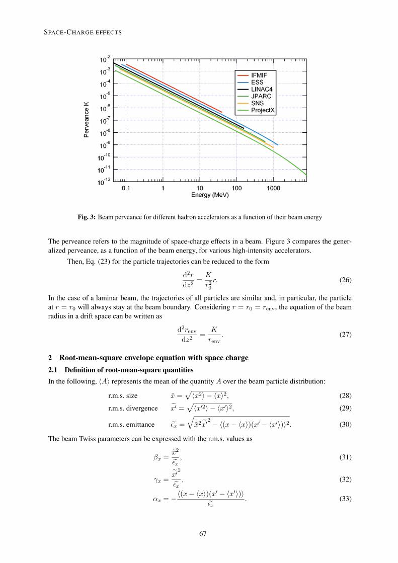
The generalized perveance K, a dimensionless parameter, is defined by

K =qI

2πε0m0c3β3γ3. (25)

N. CHAUVIN

66

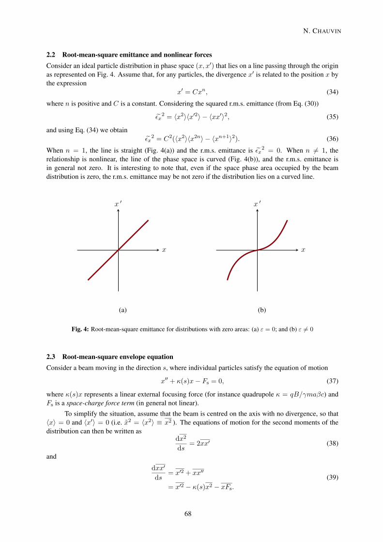
2.2 Root-mean-square emittance and nonlinear forcesConsider an ideal particle distribution in phase space (x, x′) that lies on a line passing through the originas represented on Fig. 4. Assume that, for any particles, the divergence x′ is related to the position x bythe expression

x′ = Cxn, (34)

where n is positive and C is a constant. Considering the squared r.m.s. emittance (from Eq. (30))

εx2 = 〈x2〉〈x′2〉 − 〈xx′〉2, (35)

and using Eq. (34) we obtainεx

2 = C2(〈x2〉〈x2n〉 − 〈xn+1〉2). (36)

When n = 1, the line is straight (Fig. 4(a)) and the r.m.s. emittance is εx2 = 0. When n 6= 1, therelationship is nonlinear, the line of the phase space is curved (Fig. 4(b)), and the r.m.s. emittance isin general not zero. It is interesting to note that, even if the space phase area occupied by the beamdistribution is zero, the r.m.s. emittance may be not zero if the distribution lies on a curved line.

x

x ′

x

x ′

(a) (b)

Fig. 4: Root-mean-square emittance for distributions with zero areas: (a) ε = 0; and (b) ε 6= 0

2.3 Root-mean-square envelope equationConsider a beam moving in the direction s, where individual particles satisfy the equation of motion

x′′ + κ(s)x− Fs = 0, (37)

where κ(s)x represents a linear external focusing force (for instance quadrupole κ = qB/γmaβc) andFs is a space-charge force term (in general not linear).

To simplify the situation, assume that the beam is centred on the axis with no divergence, so that〈x〉 = 0 and 〈x′〉 = 0 (i.e. x2 = 〈x2〉 ≡ x2 ). The equations of motion for the second moments of thedistribution can then be written as

dx2

ds= 2xx′ (38)

and

dxx′

ds= x′2 + xx′′

= x′2 − κ(s)x2 − xFs.

(39)

N. CHAUVIN

68

Differentiating Eq. (28) twice and using Eq. (38) gives

x′′ =x′′ + x2

x− xx′

x3. (40)

Using Eqs. (39) and (30), we have finally that

x′′ + κ(s)x− εx2

x3− xFs

x= 0. (41)

Equation (41) is the r.m.s. envelope equation and expresses the motion of the r.m.s. beam size. In threedimensions, one can write three envelope equations that are coupled through the space charge and candepend on the beam dimension in the three directions. These equations can be useful to find an analyticsolution for simple problems. Furthermore, they are very important in the space-charge community.

2.4 Example: elliptical continuous beam of uniform densityAn elliptical uniform beam density is expressed by

ρ(r) =

{ρ0 if x2/r2x + y2/r2y < 1,0 otherwise.

(42)

As the distribution is uniform, the semi-axes of the ellipse, rx and ry, are related to the r.m.s. beam sizes:rx = 2x and ry = 2y. So, the r.m.s. envelope equations are given by

x′′ + κx(s)x− εx2

x3− K

2(x+ y)= 0, (43)

y′′ + κy(s)y −εy

2

y3− K

2(x+ y)= 0. (44)

The second term of Eqs. (43) and (44) is a focusing term. The third term is the emittance term, which isdefocusing (negative sign). The fourth term is the space-charge term, which is also defocusing. It can beseen that the two planes are coupled through the space-charge term of the r.m.s. envelope equation.

2.5 Linear space-charge force and equivalent beamThe space-charge force is linear only if the beam density is uniform, which is very unlikely in the caseof practical beams. So the space-charge force is fundamentally nonlinear. Nevertheless, it was shownby Sacherer [16] that, for ellipsoidal bunches, where the r.m.s. emittance is either constant or specifiedin advance, the evolution of the r.m.s. beam projection is nearly independent of the beam density. Thismeans that for calculation of the r.m.s. dynamics, the actual distribution can be replaced by an equivalentuniform beam that has the same intensity and the same r.m.s. second moments.

3 The Child–Langmuir lawThe Child law states the maximum current density that can be carried by charged-particle flow across aone-dimensional extraction gap. The limit arises from the longitudinal electric fields of the beam spacecharge. It is a very important result in beam physics of collective effects and also in ion source fieldswhere the extracted beam current is one of the most important parameters of an ion source.

In this section, the Child–Langmuir law for a one-dimensional extraction gap will be derived. It isenough to emphasize the fundamental physical phenomena that limit the beam current extracted from aparticle source. However, for a practical extraction system, it is necessary to perform three-dimensionalcalculations by including form factors that depend on the geometry of the extraction electrodes.


69

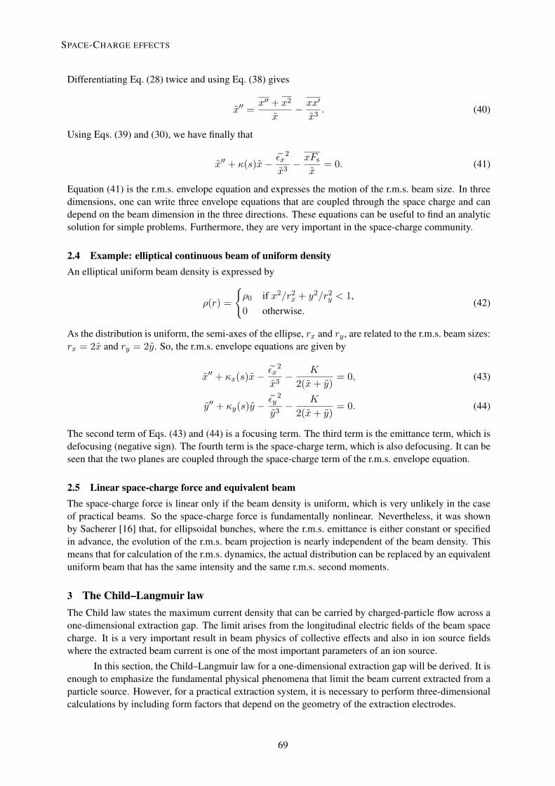
3.1 Extraction gapThe extraction gap is the first stage of an accelerator: low-energy charged particles from a source areaccelerated to moderate energy (∼10 keV to ∼1 MeV) and formed into a beam. The Child law calcula-tion applies to the one-dimensional gap of Fig. 5. A voltage −V0 is applied across the vacuum gap ofwidth d. Charged particles with low kinetic energy enter at the grounded boundary. The particles haverest mass m0 and carry positive charge q. Particles leave the right-hand boundary with kinetic energyqV0. We shall assume that the exit electrode is an ideal mesh that defines an equipotential surface whiletransmitting all particles.

.. Cathode.Anode.

0

.

z

.

d

.

ϕ = 0

.

ϕ = −V0

.

.

q

Fig. 5: Geometry of an infinite planar extraction gap

3.2 One-dimensional Child law for non-relativistic particlesTo simplify the calculation, the following assumptions are made:

1. Particle motion is non-relativistic (qV0 � m0c2).

2. The source on the left-hand boundary can supply an unlimited flux of particles. Flow restrictionwould result only from space-charge effects.

3. The transverse dimension of the gap is large compared with d.

4. The transverse magnetic force generated by particle current across the gap is negligible comparedwith the axial electric force. Consequently, the particle trajectories are straight across the gap. Thisassumption is valid for an ion beam, but can be violated in the case of a high-current relativisticelectron gun.

5. Particles flow continuously; the electric field and particle density at all z are constant.

The steady-state condition means that the space-charge density, ρ(z), is constant in time

∂ρ(z)

∂t= 0. (45)

This equation implies that the current density, J0, is the same at all positions in the gap. The chargedensity can be expressed by

ρ(z) =J0vz(z)

. (46)

N. CHAUVIN

70

According to the above assumptions, the particle velocity in the gap is

v2z(z) =2qφ(z)

m0. (47)

Using Eqs. (46) and (47) we obtain

ρ(z) =J0√

2qφ(z)/m0

. (48)

Now, consider the one-dimensional Poisson equation:

∇2φ =d2φ(z)

dz2= −ρ(z)

ε0. (49)

Substituting Eq. (48) into Eq. (49) gives

d2φ(z)

dz2= − J0

ε0√

2q/m0

1

φ1/2. (50)

If we introduce the dimensionless variables ζ = z/d and Φ = −φ/V0, Eq. (50) becomes

d2Φ(z)

dζ2= − α

φ1/2, (51)

with

α =J0d

2

ε0V0√

2qV0/m0

. (52)

Three boundary conditions are needed to integrate Eq. (51): Φ(0) = 0, Φ(1) = 1 and dΦ(0)/dζ =0. Multiplying both sides of Eq. (51) by Φ′ = dΦ/dζ, we can integrate and obtain

(Φ′)2 = 4α√

Φ(ζ). (53)

A second integration givesΦ3/4 = 3

4

√4αζ, (54)

or, coming back to the initial variables,

φ(z) = −V0(zd

)4/3. (55)

In Eq. (54), the condition Φ(1) = 1 implies α = 49 . Substituting in Eq. (52) gives

J0 =4

9ε0

(2q

m0

)1/2 V3/20

d2. (56)

This is the Child–Langmuir law, which represents the maximum current density that can be achieved inthe diode by increasing the ion supply by the anode. This limitation is only due to space charge. Theonly way to increase the extracted current is to increase the electric field in the gap (i.e. increase the gapvoltage or decrease the cathode–anode spacing). In a real ion source, the extracting electric field cannotbe increased infinitely, as electrodes break down at fields exceeding a value around 10 MV m−1.

For a given gap voltage and geometry, the current density is proportional to the square root of thecharge-to-mass ratio of the particles,

√q/m0.

Let us compare the electrostatic potential for a space-charge-limited flow given by Eq. (55), withthe potential in the same gap without space charge. In that case, the potential between the anode and the


71

cathode of the extraction gap (see Fig. 5) can be calculated from Laplace’s equation (as there is no spacecharge, ρ = 0),

∇2φ =d2φ(z)

dz2= 0, (57)

with the solutionφ(z) = −V0

dz. (58)

By comparing Eq. (55) with Eq. (58), it can be seen that the space charge of the extracted particle lowersthe potential (in absolute value) at any given point between the two electrodes of the planar diode.

3.3 Child–Langmuir law, orders of magnitudesThe Child–Langmuir current for non-relativistic electrons is

J0 = 2.33× 10−6V

3/20

d2(A m−2), (59)

where V0 is in volts and d in metres. For ions, Eq. (56) becomes

J0 = 5.44× 10−8√Z

A

V3/20

d2(A m−2), (60)

where Z is the charge state of the ion and A is its atomic number. For a given extraction voltage andgeometry, the possible current density of electrons is around 43 times higher than that of protons.

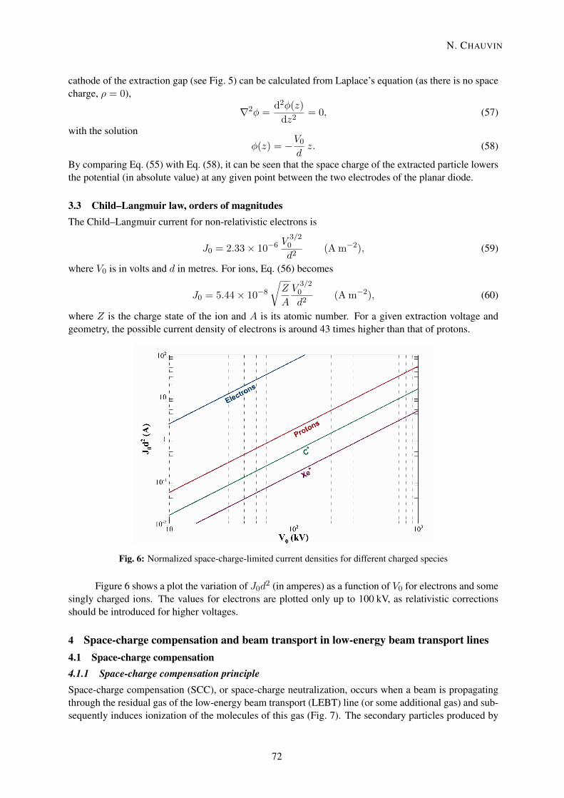
Fig. 6: Normalized space-charge-limited current densities for different charged species

Figure 6 shows a plot the variation of J0d2 (in amperes) as a function of V0 for electrons and somesingly charged ions. The values for electrons are plotted only up to 100 kV, as relativistic correctionsshould be introduced for higher voltages.

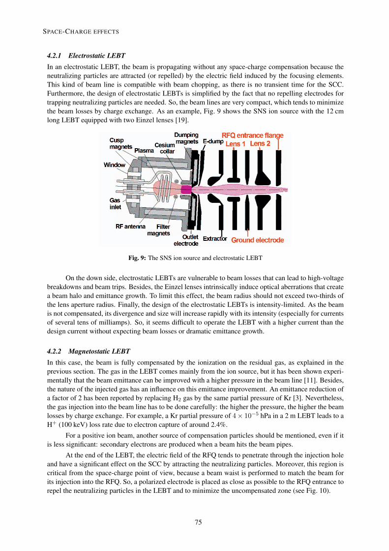
4 Space-charge compensation and beam transport in low-energy beam transport lines4.1 Space-charge compensation4.1.1 Space-charge compensation principleSpace-charge compensation (SCC), or space-charge neutralization, occurs when a beam is propagatingthrough the residual gas of the low-energy beam transport (LEBT) line (or some additional gas) and sub-sequently induces ionization of the molecules of this gas (Fig. 7). The secondary particles produced by

N. CHAUVIN

72

By integrating these equations with the boundary condition, φ(rP) = 0, we obtain

φ(r) =IB

4πε0βBc

[1 + 2 ln

(rPrB

)− r

r2B

]if r ≤ rB, (63a)

φ(r) =IB

2πε0βBclnrPr

if rB ≤ r ≤ rP. (63b)

The potential on the beam axis (i.e. potential well) created by a uniform beam, without SCC, isgiven by Eq. (63a) for r = 0:

φ0 =IB

4πε0βBc

[1 + 2 ln

(rPrB

)](64)

During the SCC process, the neutralizing particles created by gas ionization are trapped by this potentialwell. Equation (64) shows that the potential well (i.e. the space-charge force) increases if the radius ofthe beam decreases. So, achieving a beam waist in a LEBT could be critical for the quality of the beam.

Now, consider a compensated beam at steady state. If we define by φc its potential on axis, theSCC degree is given by

η = 1− φcφ0. (65)

The beam potential well of the compensated beam can be experimentally measured. The values foundfor the 75 keV, 130 mA proton beam of the LEDA range from 95% to 99% [9]. Along the LEBT, theSCC degree is not constant, as the neutralizing particle trajectories can be modified by external fields ofthe focusing element, for example. This phenomenon induces strongly non-uniform space-charge forcesthat can lead to beam emittance growth

4.1.3 Space-charge compensation timeThe characteristic SCC transient time, τscc, can be determined by considering the time it takes for aparticle of the beam to produce a neutralizing particle on the residual gas. It is given by

τscc =1

σionizngβBc, (66)

where σioniz is the ionization cross-section of the incoming particles on the residual gas and ng is the gasdensity in the beam line. The space-charge compensation is expected to reach a steady state after two orthree τscc times. As an example, the SCC transient time for a 95 keV proton beam propagating in H2 gasof pressure 5× 10−5 hPa is 15 µs.

4.2 Beam transportOnly the transport in the LEBT (Low Energy Beam Transport) will be considered here. Nevertheless,the source extraction system is a critical part, especially for a high-intensity injector, as the beam has tobe properly formed under strong space-charge forces to be correctly transported in the LEBT. Thus, itseems mandatory to perform simultaneously both the design and simulations of the ion source extractionand the LEBT.

Once the beam is created and extracted from the ion source, it has to be transported and matchedby the LEBT to the first accelerating structure like a radio frequency quadrupole (RFQ). The focus canbe achieved with electrostatic or magnetic elements. After the ion source, because of the geometryof the extraction system, the beam usually presents a cylindrical symmetry. In order to preserve thissymmetry and to simplify the beam tuning, magnetic solenoid lenses or electrostatic Einzel lenses aremore commonly used than quadrupoles.

N. CHAUVIN

74

..

RFQ InnerFlange

..

.

e-.

.

e-

.

.

e-.

.

e-

.

.

e-.

.

e-

.

.

e-.

.

e- .

.

e-

.

.

e-.

.

e-.

.

e-.

.

e-.

.

e-

.

RFQ

Electron repellerRFQ Inner

Flange

e-e-

e-e-

e-e-

e-e- e-

e-

e-e-

RFQ

(a) (b)

Fig. 10: (a) No electron repeller: neutralizing particles (electrons in this case) are attracted by the RFQ electricfield. (b) Electrode repeller located before the RFQ: some neutralizing particles are repelled into the LEBT; theuncompensated zone is minimized.

In a magnetic LEBT, the rise time of the pulsed beams is dominated by the SCC transient time (i.e.several tens of microseconds). A fast chopping system has to be inserted to reach a rise time of the orderof hundreds of nanoseconds. In the case of H− ion beams, a phenomenon of overcompensation occursduring the SCC transient time [2]. When the beam is fully compensated, neutralizing particles (in thatcase H+) are still created, but, as they are significantly slower than the electrons, the SCC degree can begreater than 1 during the time it takes for the excess H+ to be expelled from the beam. During that time,the beam is over-focused and instabilities can be observed.

5 Beam dynamics simulation codes with space charge5.1 Numerical codes for ion source extraction systemsSome 2D- or 3D-like codes AXCEL-INP [18], PBGUNS [20] and IBSimu [13] have been successfullyused to design sophisticated ion source extraction systems as well as electrostatic LEBTs.

With these codes, one can shape the electrodes, compute the generated electric field and trackthe particle in the defined domain. Over the past few years, elaborate optimization of the geometry ofthe extraction system has been performed to increase the extracted beam intensity while minimizing theoptical aberration and the beam divergence. As an example, the extraction system of the SILHI source,which has an intermediate and a repelling electrode, forming, together with the plasma and groundedelectrodes, a pentode extraction system (see Fig. 11) [7], has been developed using AXCEL-INP.

Fig. 11: Five-electrode beam extraction system of the SILHI source

N. CHAUVIN

76

5.2 Numerical codes for beam dynamics transportIn a classical numerical code, the beam is represented by N macro-particles (N is normally less than theactual particle number in the beam) that can be considered as a statistical sample of the beam with thesame dynamics as the real particles. The macro-particles are transported through the accelerator step bystep and at each time step dt:

– external forces acting on each macro-particle are calculated,– space-charge fields and the resulting forces are calculated, and– tyhe equation of motion is solved for each macro-particle.

The space-charge electric field can be computed by a particle–particle interaction (PPI) method or aparticles-in-cells (PIC) method, which are briefly described in the next subsections.

5.2.1 Particle–particle interaction methodFor each macro-particle i of charge q, it is assumed that the applied space-charge electrostatic field, ~Ei,is the sum of all the fields induced by all the other macro-particles:

~Ei =q

4πε0

∑

i 6=j

~rj − ~ri‖~rj − ~ri‖3

. (67)

The advantages of this method are that it is easy to code and the electric field is directly computedon the macro-particles. The main drawbacks are that the method is time-consuming for calculation(proportional to the square of the number of macro-particles) and the obtained space-charge field map isnot smooth (the lower the macro-particle number, the more granularity), which can lead to non-physicalemittance growth.

5.2.2 Particles-in-cells methodIn this case, the physical simulated space is meshed. The mesh geometry depends on the situation. Themeshing can be in one, two or three dimensions, depending on the symmetry of the simulated geometryand the beam.

The average beam density at each node of the mesh is obtained by counting the number of particlesthat are located close to it (an interpolation can induce smoothing). Once the density function is obtained,the field at each node is computed by solving the Poisson equation. Several techniques can be used tosolve this equation at each node of the mesh.

1. A direct method. The field is directly calculated at each node of the mesh. The calculation time isproportional to the square of the mesh number.

2. A fast Fourier transform (FFT) method. The field at one node is given by the convolution productof the density and a Green’s function. This can be solved by using the fact that a Fourier transformof a convolution product is equal to the product of the Fourier transforms. If n is the mesh number,the calculation time is proportional to n log(n). One drawback is that the FFT method does nottake into account the boundary conditions of the conductors.

3. A relaxation method [14], which is an iterative method. If n is the mesh number, the calculationtime is proportional to n log(n). It can take into account the particular boundary conditions asconductive items, for instance.

Once the field at each node is known, the field at the macro-particle location is calculated byinterpolation from the closest nodes. After the evaluation of the beam density and the field for each


77

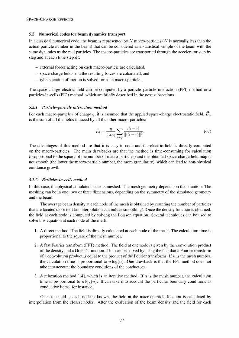
particle, the computing time is proportional to the macro-particle number. The algorithm of a PIC codeis presented in Fig. 12.

The PIC codes are the most commonly used for space-charge calculations, as they are the fastestand most efficient. A compromise has to be found between the mesh size and the particle number inorder reach a sufficient resolution while avoiding some numerical noise that can lead to non-physicaleffects.

PIC codes that are commonly used for beam dynamics simulations with space charge are: TRACK[1], IMPACT [15] and TraceWin [21].

MotionIntegration−→Fn →

−→V ′n →

−→Xn

Interpolationof the forces

(−→En,−→Bn) →

−→Fn

Interpolationof currents andcharges in a grid

(−→Xn,−→Vn → (ρn,

−→Jn)

EM fieldscalculation

(ρn,−→Jn) → (

−→E ,−→B )

t

Fig. 12: Algorithm of a PIC code dedicated to particle transport with space charge

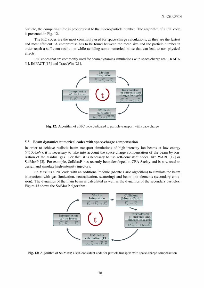
5.3 Beam dynamics numerical codes with space-charge compensationIn order to achieve realistic beam transport simulations of high-intensity ion beams at low energy(≤100 keV), it is necessary to take into account the space-charge compensation of the beam by ion-ization of the residual gas. For that, it is necessary to use self-consistent codes, like WARP [12] orSolMaxP [5]. For example, SolMaxP, has recently been developed at CEA-Saclay and is now used todesign and simulate high-intensity injectors.

SolMaxP is a PIC code with an additional module (Monte Carlo algorithm) to simulate the beaminteractions with gas (ionization, neutralization, scattering) and beam line elements (secondary emis-sion). The dynamics of the main beam is calculated as well as the dynamics of the secondary particles.Figure 13 shows the SolMaxP algorithm.

MotionIntegration−→Fn →

−→V ′n →

−→Xn

Collisions(Monte Carlo)−→V ′n →

−→Vn

Interpolationof the forces

(−→En,−→Bn) →

−→Fn

Interpolationof currents andcharges in a grid

(−→Xn,−→Vn → (ρn,

−→Jn)

EM fieldscalculation (FD)

(ρn,−→Jn) → (

−→E ,−→B )

t

Fig. 13: Algorithm of SolMaxP, a self-consistent code for particle transport with space-charge compensation

N. CHAUVIN

78

The SolMaxP code inputs are the particle distribution of the beam, the applied external fields (e.g.focusing elements, electron repeller) and the beam line geometry and gas pressure. The outputs are theparticle distributions (ions, electrons, neutral) all along the beam line and the electric field map derivedfrom the potential map created by the space charge along the beam line.

5.4 Example of numerical simulations of a high-intensity injector: IFMIF5.4.1 Simulation conditionsFirst, the modelling of the IFMIF/EVEDA ion source extraction system [8] has been done with AXCEL-INP. The D+, D+

2 and D+3 particle distributions coming from this model are the input of these simulations.

Then, the simulations presented have been done under the following conditions or hypotheses:

1. D+, D+2 and D+

3 beams are transported.

2. The electric field map of the source extraction system is included to get relevant boundary condi-tions.

3. The gas pressure is considered to be homogeneous in the beam line.

4. The gas ionization is produced by ion beam and electron impact.

5. No beam scattering on gas is considered.

6. No secondary electrons are created when the beam hits the beam pipe.

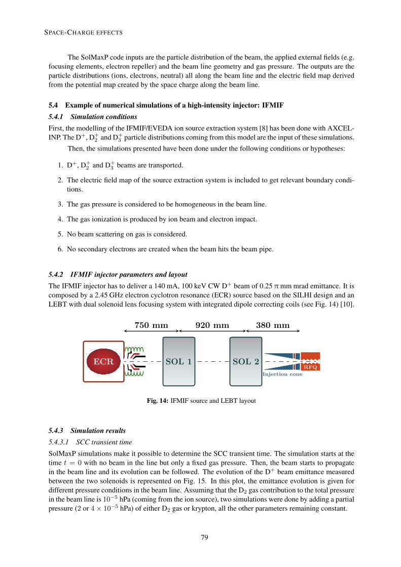
5.4.2 IFMIF injector parameters and layoutThe IFMIF injector has to deliver a 140 mA, 100 keV CW D+ beam of 0.25 π mm mrad emittance. It iscomposed by a 2.45 GHz electron cyclotron resonance (ECR) source based on the SILHI design and anLEBT with dual solenoid lens focusing system with integrated dipole correcting coils (see Fig. 14) [10].

ECR SOL 1 SOL 2

750 mm 920 mm 380 mm

Injection coneRFQ

Fig. 14: IFMIF source and LEBT layout

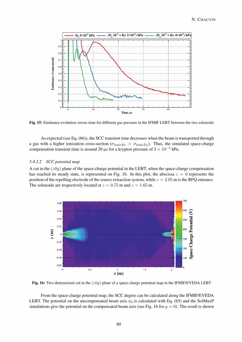
5.4.3 Simulation results5.4.3.1 SCC transient time

SolMaxP simulations make it possible to determine the SCC transient time. The simulation starts at thetime t = 0 with no beam in the line but only a fixed gas pressure. Then, the beam starts to propagatein the beam line and its evolution can be followed. The evolution of the D+ beam emittance measuredbetween the two solenoids is represented on Fig. 15. In this plot, the emittance evolution is given fordifferent pressure conditions in the beam line. Assuming that the D2 gas contribution to the total pressurein the beam line is 10−5 hPa (coming from the ion source), two simulations were done by adding a partialpressure (2 or 4× 10−5 hPa) of either D2 gas or krypton, all the other parameters remaining constant.


79

sµTime 0 10 20 30 40

mm

.mra

d)π

Em

itta

nce

(

0

0.1

0.2

0.3

0.4

0.5

0.6

0.7

0.8

0.9

1

hPa-510× 52D ) hPa-510× + Kr 2-5 102

(D ) hPa-510× + Kr 4-5 102

(D

Fig. 15: Emittance evolution versus time for different gas pressure in the IFMIF LEBT between the two solenoids

As expected (see Eq. (66)), the SCC transient time decreases when the beam is transported througha gas with a higher ionization cross-section (σionizKr > σionizD2). Thus, the simulated space-chargecompensation transient time is around 20 µs for a krypton pressure of 2× 10−5 hPa.

5.4.3.2 SCC potential map

A cut in the (z0y) plane of the space-charge potential in the LEBT, when the space-charge compensationhas reached its steady state, is represented on Fig. 16. In this plot, the abscissa z = 0 represents theposition of the repelling electrode of the source extraction system, while z = 2.05 m is the RFQ entrance.The solenoids are respectively located at z = 0.75 m and z = 1.65 m.

Fig. 16: Two-dimensional cut in the (z0y) plane of a space-charge potential map in the IFMIF/EVEDA LEBT

From the space-charge potential map, the SCC degree can be calculated along the IFMIF/EVEDALEBT. The potential on the uncompensated beam axis φ0 is calculated with Eq. (65) and the SolMaxPsimulations give the potential on the compensated beam axis (see Fig. 16 for y = 0). The result is shown

N. CHAUVIN

80

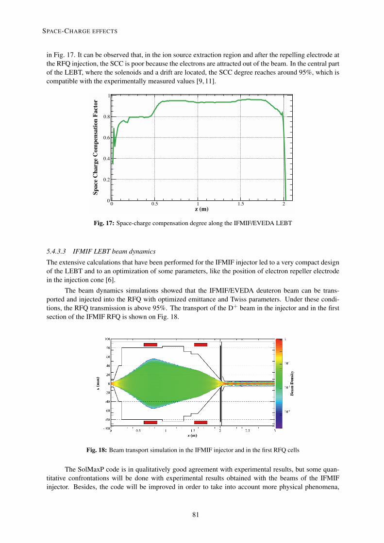
in Fig. 17. It can be observed that, in the ion source extraction region and after the repelling electrode atthe RFQ injection, the SCC is poor because the electrons are attracted out of the beam. In the central partof the LEBT, where the solenoids and a drift are located, the SCC degree reaches around 95%, which iscompatible with the experimentally measured values [9, 11].

z (m)0 0.5 1 1.5 2

Spac

e C

harg

e C

ompe

nsat

ion

Fac

tor

0

0.2

0.4

0.6

0.8

1

Fig. 17: Space-charge compensation degree along the IFMIF/EVEDA LEBT

5.4.3.3 IFMIF LEBT beam dynamics

The extensive calculations that have been performed for the IFMIF injector led to a very compact designof the LEBT and to an optimization of some parameters, like the position of electron repeller electrodein the injection cone [6].

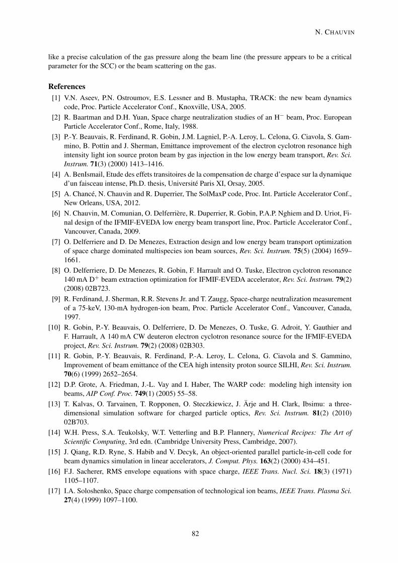
The beam dynamics simulations showed that the IFMIF/EVEDA deuteron beam can be trans-ported and injected into the RFQ with optimized emittance and Twiss parameters. Under these condi-tions, the RFQ transmission is above 95%. The transport of the D+ beam in the injector and in the firstsection of the IFMIF RFQ is shown on Fig. 18.

Fig. 18: Beam transport simulation in the IFMIF injector and in the first RFQ cells

The SolMaxP code is in qualitatively good agreement with experimental results, but some quan-titative confrontations will be done with experimental results obtained with the beams of the IFMIFinjector. Besides, the code will be improved in order to take into account more physical phenomena,


81

like a precise calculation of the gas pressure along the beam line (the pressure appears to be a criticalparameter for the SCC) or the beam scattering on the gas.

References[1] V.N. Aseev, P.N. Ostroumov, E.S. Lessner and B. Mustapha, TRACK: the new beam dynamics

code, Proc. Particle Accelerator Conf., Knoxville, USA, 2005.[2] R. Baartman and D.H. Yuan, Space charge neutralization studies of an H− beam, Proc. European

Particle Accelerator Conf., Rome, Italy, 1988.[3] P.-Y. Beauvais, R. Ferdinand, R. Gobin, J.M. Lagniel, P.-A. Leroy, L. Celona, G. Ciavola, S. Gam-

mino, B. Pottin and J. Sherman, Emittance improvement of the electron cyclotron resonance highintensity light ion source proton beam by gas injection in the low energy beam transport, Rev. Sci.Instrum. 71(3) (2000) 1413–1416.

[4] A. BenIsmail, Etude des effets transitoires de la compensation de charge d’espace sur la dynamiqued’un faisceau intense, Ph.D. thesis, Université Paris XI, Orsay, 2005.

[5] A. Chancé, N. Chauvin and R. Duperrier, The SolMaxP code, Proc. Int. Particle Accelerator Conf.,New Orleans, USA, 2012.

[6] N. Chauvin, M. Comunian, O. Delferrière, R. Duperrier, R. Gobin, P.A.P. Nghiem and D. Uriot, Fi-nal design of the IFMIF-EVEDA low energy beam transport line, Proc. Particle Accelerator Conf.,Vancouver, Canada, 2009.

[7] O. Delferriere and D. De Menezes, Extraction design and low energy beam transport optimizationof space charge dominated multispecies ion beam sources, Rev. Sci. Instrum. 75(5) (2004) 1659–1661.

[8] O. Delferriere, D. De Menezes, R. Gobin, F. Harrault and O. Tuske, Electron cyclotron resonance140 mA D+ beam extraction optimization for IFMIF-EVEDA accelerator, Rev. Sci. Instrum. 79(2)(2008) 02B723.

[9] R. Ferdinand, J. Sherman, R.R. Stevens Jr. and T. Zaugg, Space-charge neutralization measurementof a 75-keV, 130-mA hydrogen-ion beam, Proc. Particle Accelerator Conf., Vancouver, Canada,1997.

[10] R. Gobin, P.-Y. Beauvais, O. Delferriere, D. De Menezes, O. Tuske, G. Adroit, Y. Gauthier andF. Harrault, A 140 mA CW deuteron electron cyclotron resonance source for the IFMIF-EVEDAproject, Rev. Sci. Instrum. 79(2) (2008) 02B303.

[11] R. Gobin, P.-Y. Beauvais, R. Ferdinand, P.-A. Leroy, L. Celona, G. Ciavola and S. Gammino,Improvement of beam emittance of the CEA high intensity proton source SILHI, Rev. Sci. Instrum.70(6) (1999) 2652–2654.

[12] D.P. Grote, A. Friedman, J.-L. Vay and I. Haber, The WARP code: modeling high intensity ionbeams, AIP Conf. Proc. 749(1) (2005) 55–58.

[13] T. Kalvas, O. Tarvainen, T. Ropponen, O. Steczkiewicz, J. Ärje and H. Clark, Ibsimu: a three-dimensional simulation software for charged particle optics, Rev. Sci. Instrum. 81(2) (2010)02B703.

[14] W.H. Press, S.A. Teukolsky, W.T. Vetterling and B.P. Flannery, Numerical Recipes: The Art ofScientific Computing, 3rd edn. (Cambridge University Press, Cambridge, 2007).

[15] J. Qiang, R.D. Ryne, S. Habib and V. Decyk, An object-oriented parallel particle-in-cell code forbeam dynamics simulation in linear accelerators, J. Comput. Phys. 163(2) (2000) 434–451.

[16] F.J. Sacherer, RMS envelope equations with space charge, IEEE Trans. Nucl. Sci. 18(3) (1971)1105–1107.

[17] I.A. Soloshenko, Space charge compensation of technological ion beams, IEEE Trans. Plasma Sci.27(4) (1999) 1097–1100.

N. CHAUVIN

82

[18] Axcel INP code, http://www.aetassociates.com/software.php?inp.[19] M.P. Stockli, B. Han, S.N. Murray, T.R. Pennisi, M. Santana and R.F. Welton, Ramping up the

spallation neutron source beam power with the H− source using 0 mg Cs/day, Rev. Sci. Instrum.81(2) (2010) 02A729.

[20] PBGINS code, http://far-tech.com/pbguns/index.html.[21] TraceWin code, http://irfu.cea.fr/Sacm/en/logiciels/index3.php.[22] J.L. Vay and C. Deutsch, Intense ion beam propagation in a reactor sized chamber, Nucl. Instrum.

Methods Phys. Res. A464(1–3) (2001) 293–298.

Further readingsA. BenIsmail, R. Duperrier, D. Uriot and N. Pichoff, Space charge compensation studies of hydrogen

ion beams in a drift section, Phys. Rev. ST Accel. Beams 10(7) (2007) 070101.

M. Reiser, Theory and Design of Charged Particle Beams (John Wiley & Sons, New York, 2008).

F. Sacherer, RMS envelope equations with space charge, CERN Internal Report, SI/DL/70-12 (1970).

K. Schindl, Space charge, CERN Accelerator School 2003: Intermediate Course on Accelerators, CERN-2006-002 (2006).

T.P. Wangler, RF Linear Accelerators (Wiley-VCH, Weinheim, 2008).


83

space-charge effects

Documents