1

1

2

3

4

Sources and Measurement of Agricultural Productivity and 5

Efficiency in Canadian Provinces: Crops and Livestock 6

7

8

Abstract 9 10 This paper measures and assesses the variation in total factor productivity (TFP) growth 11 among Canadian provinces in crops and livestock production over the period 1940-2009. It 12 also determines if agricultural productivity growth in Canada has recently slowed down as 13 indicated by earlier studies. The paper uses the stochastic frontier approach which 14 incorporates inefficiency to decompose TFP growth into technical change, scale effect, and 15 technical efficiency change. The results indicate that productivity changes were mainly driven 16 by technical changes for crops, while the productivity changes in livestock was mainly driven 17 by scale effects and technical progress. Though change in technical efficiency is mainly 18 positive (except for New Brunswick and Nova Scotia), its contribution to productivity growth 19 was very little for the provinces. We also found that over the entire period, the productivity 20 growth rates for the crop sub-sector are on average higher for the Prairie provinces than for 21 the Eastern and Atlantic provinces. On the other hand, the productivity growth rates in the 22 livestock sub-sector are on the average higher in the Eastern and Atlantic provinces than in 23 the Prairie region with the exception of Manitoba. Finally, we found that though there is some 24 evidence of a recent decline in productivity growth for the crops subsector, there is no such 25 evidence in the livestock subsector. 26 27 28 29 30 31 32 33 JEL Classification: Q1, Q10, Q13, Q22. 34 35 Keywords: Agricultural Productivity; Growth, Crops Farming, Livestock Farming, Total 36 Factor Productivity, Technical Progress, Technical Efficiency, Scale Effect, Canada, 37 Stochastic Production Frontier. 38 39 40 41

42

2

Sources and Measurement of Agricultural Productivity and 43

Efficiency in Canadian Provinces: Crops and Livestock 44

45 Introduction 46

47

This paper uses Canadian provincial data from 1940 to 2009 to measure and assess 48

variation in total factor productivity (TFP) growth in the crops and livestock sub-49

sectors. Measuring agricultural productivity growth is a difficult task, but very 50

important for various reasons. Firstly, agricultural productivity growth is an important 51

indicator for the analysis of the overall economic growth, improvement of living 52

standards, and international competitiveness. Secondly, agricultural productivity 53

growth is an important concept in the discussions on global food security and poverty 54

alleviation, especially in the developing world. Bruinsma (2009) stated that by 2050 55

the world population is expected to grow by 40% and allowing for increase in income 56

and changes in diet, global demand for food and fiber is expected to grow by 70%. 57

Hence, agricultural productivity growth would have to keep pace with the expected 58

global demographic changes in order to avoid global food security problems and 59

make significant progress towards poverty alleviation in the developing world. 60

Against this background, there have been some recent discussions on the 61

direction of global agricultural productivity growth in the literature. Alston et al. 62

(2010a,b) used a range of partial productivity measures to examine productivity 63

growth in the world. They found that with the exception of China and Latin America, 64

agricultural productivity growth rates in most of the world have slowed down since 65

the early 1990s. They also concluded that in some part of the world the decline in 66

agricultural productivity growth rates have been substantial and widespread. Fuglie 67

(2008, 2010) concluded differently when he examined long-run productivity trends in 68

the global agriculture sector using an index number approach. He found that there was 69

3

no evidence of a general decline in agricultural productivity, at least through 2007. 70

He stated that the growth rates in agricultural TFP have actually accelerated in recent 71

decades because of rapid productivity gains in several developing countries, led by 72

Brazil and China, and more recently due to a recovery of agricultural growth in the 73

countries of the former Soviet Bloc. In the case of Canada, Rao et al (2008), and 74

Agriculture and Agri-Food Canada (2009) have indicated that agricultural 75

productivity growth has significantly slowed down and lagged behind that of the U.S. 76

and many OECD countries. Stewart et al (2009) have also concluded that TFP 77

growth rates for crops and livestock in the prairies have slowed down considerably. 78

Veeman and Gray (2009) agreed with Stewart et al (2009) by concluding that 79

productivity growth in crops production has slowed down since 1990. On the 80

contrary, de Avillez (2011 a, b) concluded that over the period 1961-2007, the 81

primary agriculture sector in Canada experienced impressive productivity growth. He 82

also reported that the productivity growth performance in the agricultural sector by far 83

exceeded productivity growth in the Canadian business sector as a whole. 84

From the studies discussed above, and to some extent, the general agricultural 85

productivity literature, it could be concluded that the methodologies and assumptions 86

used in measuring agricultural productivity growth could affect the magnitude of the 87

estimated productivity growth rates and the direction of effects. For example, most 88

agricultural productivity studies have the underlying assumption that farms are fully 89

efficient. If this assumption is incorrect, then the productivity measures could be 90

misleading. Though some studies have allowed for inefficiencies at the farm level, 91

those that focused on Canada have mainly used data on a specific crop or type of 92

livestock production within a specific province (Samarajeewa et al 2012; Giannakas 93

et al 2001; Amara et al 1999; Cloutier and Rowley 1993; Amara and Romain 1990, 94

4

Weersink et al 1990) or used data on crops and livestock sectors for a few provinces 95

(Stewart et al 2009). None of these studies used data on all the provinces for both the 96

crop and livestock sub-sectors. 97

The main focus of this paper is to address the concerns raised above by using 98

provincial level data on the crops and livestock sub-sectors for the period 1940-2009 99

and a stochastic frontier approach which incorporates inefficiency, to decompose the 100

TFP growth in the Canadian agricultural sector into technical change, scale effect, and 101

technical efficiency change1. The paper also determines if agricultural productivity 102

growth in Canada has recently slowed down as claimed by earlier studies. To the best 103

of our knowledge, this is the first paper that examines TFP growth decomposition for 104

all provinces (except for Newfoundland) in Canada for both the crops and livestock 105

sub-sectors. The use of provincial data is very essential in measuring productivity 106

growth in order to reveal any possible provincial idiosyncrasies for the design and 107

implementation of appropriate policies. 108

The rest of the paper is organized as follows. Section 2 provides a brief 109

overview of productivity and efficiency studies. Section 3 describes the theory 110

behind the stochastic frontier approach used to decompose the TFP growth and 111

provides a brief description of the data used in the estimation (detail descriptions of 112

the data are relegated to Appendix A). Section 4 describes the estimation procedure, 113

while section 5 presents and discusses the main estimation results. Concluding 114

remarks and policy implications are given in section 6. 115

1 We decomposed total factor productivity into three components: technological progress; scale effect;

and technical efficiency. Technological progress captures the idea that production function can shift

overtime. It refers to the situation in which a firm can achieve more output from a given combination

of inputs or equivalently, the same amount of output from fewer inputs. Scale effect refers to the

proportionate increase in output due to a given proportionate increase in all inputs in the production

process. Technical efficiency is the situation where it is impossible for a firm to produce with a given

technology either (a) more output from the same inputs, or (b) the same output with less of one or more

inputs without increasing the amount of other inputs. Hence, technical inefficiency indicates the

amount by which actual output falls short of the maximum possible output.

5

2. Review of Productivity Growth and Efficiency Studies 116

The literature on productivity growth and efficiency is vast in both theory and applied. 117

Hence, the purpose of this section is not to provide a comprehensive review of the 118

literature but to provide a summary of relevant literature that is closely related to our 119

analysis below. A comprehensive review of this literature is given in recent work by 120

Darku et al. (2013), and interested readers can refer to their paper for more complete 121

review. The approaches used in the analysis of productivity growth and efficiency can 122

be classified into three main groups: (i) the regression approach such as stochastic 123

frontier analysis (SFA) which can be parametric or nonparametric2; (ii) linear 124

programming approach such as deterministic Data Envelopment Analysis (DEA) 125

which is purely nonparametric; and (iii) the Index Number (IN) and/or growth 126

accounting approach3. 127

The SFA approach was originally and independently proposed by Aigner et al 128

(1977), and Meeusen and Van den Broeck (1977). The approach utilizes a standard 129

regression equation with a two-component error term. The first component is a two-130

sided symmetric error term representing random shocks (e.g. weather) and the second 131

component is a one-sided error term representing technical inefficiency. The basic 132

formulation of the stochastic frontier approach was extended by Pitt and Lee (1981), 133

and Schmidt and Sickles (1984) for the panel data case. Battese and Coelli (1992) 134

introduced further enhancements where the technical inefficiency term was modeled 135

to be time variant. The SFA approach has been applied to agricultural studies by 136

Battese and Tessema (1993), Giannakas et al (2000), Aigner et al (1977), Seyoum et 137

2 By nonparametric we mean the functional form of the frontier is left unspecified.

3 There are other approaches that combine DEA with some sort of regressions analysis to overcome the

deterministic nature of DEA (this approach is known as stochastic DEA), and others that combine IN

with production or cost regression in order to decompose the total factor productivity growth into

various components.

6

al (1998), Abdulai and Huffman (1998) and Färe et al. (1994) just to name a few. 138

Recent studies such as Constantin et al. (2009), and Pires and Garcia (2012) have used 139

the SFA framework and the "Bauer-Kumbhakar" technique to decompose total factor 140

productivity into technical and allocative efficiency, technical change, and scale 141

effect. 142

Another strand of studies dubbed “the efficiency literature” has mostly used 143

the DEA technique to determine technical efficiency level of firms or industries. This 144

literature began with Charnes et al. (1978) who used the DEA technique to pursue 145

Farrell's (1957) approach to technical efficiency measurement. They simply extended 146

the measurement of technical efficiency from a single output and multiple input case 147

to a multiple output and multiple input case. Färe et al. (1994) utilized the DEA 148

approach to decompose TFP into technical changes and efficiency changes. At the 149

same period that the DEA technique became popular in measuring agricultural 150

productivity, the indexing approach to measuring productivity and efficiency also 151

gained importance with the introduction of the Malmquist Index. Caves et al (1982), 152

Shephard (1970) and Färe (1988) calculated the Malmquist TFP index as geometric 153

mean of output and input Malmquist Indexes, and found that the TFP can be 154

decomposed into technical changes and technical efficiency changes. Hsun et al. 155

(2003) and Nin Pratt and Yu (2008) have also used the DEA technique to decompose 156

TFP into technical changes and efficiency changes. Further development in the 157

efficiency literature has led to the combination of the Malmquist Index and the DEA 158

techniques to yield the Malmquist DEA method. This approach has been applied in 159

some studies to evaluate technical changes and efficiency changes using variety of 160

7

data set and countries (Lambert and Parker 1998; Hsu et al 2003; Ludena 2010; Coelli 161

and Walding 2005; and Tipi and Rehber 2006)4. 162

Bravo-Ureta et al. (2007) used meta-regression analysis of previous 167 163

frontier studies of technical efficiency in the agricultural sectors to determine the 164

commonalities and trends within that set of literature, and try to explain the patterns 165

that emerge in efficiency levels. They concluded that the methodological 166

characteristics (estimation technique) and other study-specific characteristics 167

(functional form, sample size, product analysis, and geographical region) affect the 168

empirical estimates of technical efficiency. The mean technical efficiency of all the 169

167 frontier studies was 76.6%, suggesting that farms are not fully efficient. 170

The literature on agricultural efficiency for Canadian farms is limited but 171

growing. These studies have mostly used various methodologies identified in the 172

literature to determine the level of efficiency of Canadian crop farms. Haghiri et al. 173

(2004) used non-parametric stochastic frontier model to estimate technical efficiency 174

between dairy farmers in Ontario and New York. They concluded that Ontario dairy 175

farmers are less efficient than their New York counterpart. Mbaga et al. (2003) used 176

parametric and non-parametric approaches to measure the level of technical efficiency 177

of Quebec dairy farmers. The analysis revealed that Quebec dairy farmers are very 178

homogenous in terms of efficiency. Cloutier and Rowley (1993) used the DEA and 179

found the same result for Quebec dairy farmers. Amara et al. (1999) used the 180

4 However, the malmquist index has been criticized by O’Donnel (2009 and 2010) who indicated that

the malmquist TFP index is not complete and using it for decomposition yields bias estimate of

technical changes and efficiency changes. He then used the Hicks Moorsteen and Fisher Indexes to

construct complete and recognizable TFP indexes and decomposed them into meaningful measures of

technical changes and efficiency changes. In a series of further papers, O’Donnel (2012a, 2012b)

demonstrated that like other multiplicative complete TFP indexes (Laspeyres, Paache, Fisher and

Tornqvist), the Hicks-Moorsteen index has some weakness in terms of satisfying some important

axioms. He proposed a new TFP index (the Lowe TFP index) that satisfies all axioms and used it to

decompose TFP into technical changes and efficiency changes.

8

deterministic statistical frontier production function to measure production efficiency 181

using data on potato farmers in Quebec. They found that, farming experience and the 182

adoption of concentration technologies are both significant variables for improving 183

technical efficiency. They also found that environmental factors such as farmers 184

awareness of environmental degradation as a problem and his/her attitude towards 185

technological innovation determine technical efficiency. Samarajeewa et al. (2012) 186

used the SFA technique and data on cow-calf farmers in Alberta to conduct an 187

analysis similar to Amara et al. (1999). They found that farmers are generally not 188

fully efficient and that government support, smaller herd size, lower share of family 189

labour and lower expense for bedding material reduced efficiency. Hailu et al. (2005) 190

used SFA to compare the cost efficiency of Alberta and Ontario dairy farms. Results 191

indicated that Ontario dairy farms may be more cost efficient than Alberta dairy 192

farms, but the statistical evidence was inconclusive. Slade and Hailu (2011) extended 193

Hailu et al. (2005) analysis on Ontario and New York dairy farms by using stochastic 194

DEA analysis to examine allocative and cost efficiency. They concluded that 195

efficiency generally increased with farm size in both regions. However, New York 196

benefited more from the presence of larger dairy farms. Farms operating under the 197

system of supply management were found to make poorer allocative decision when 198

compared to farms in a competitive environment. 199

Whereas the above studies focused on one or two provinces for their 200

productivity and efficiency analysis, other studies have used data on all the provinces 201

to study Canadian agricultural productivity. Echevarria (1998) used provincial data on 202

agriculture to compute the TFP growth rates across all the ten provinces. Her results 203

indicated that the Canadian agriculture sector is less labor intensive than both services 204

and manufacturing sectors, though the level of capital intensity is similar in the three 205

9

sectors. In addition, the average TFP growth rate in the agriculture sector is 206

approximately 0.3% which is similar to that of TFP growth in the Canadian 207

manufacturing sector. Beside the provincial level studies, Fantino and Veeman 208

(1997), and Veeman and Gray (2009, 2010) have used national level data to analyze 209

Canadian agricultural productivity. 210

A few Canadian studies have undertaken TFP decomposition analysis. 211

Giannakas et al (2001) used stochastic decomposition method to determine the level 212

and driving force of technical efficiency using data on Saskatchewan dairy farmers. 213

They found that TFP contributed significantly more to output growth than input 214

usage. They also found that technical change contributed almost twice as much as 215

technical efficiency to TFP growth. Stewart et al (2009) used prairie region (Alberta, 216

Saskatchewan and Manitoba) agriculture data on crops and livestock along with four 217

factors of production (capital, labor, land and materials) for the period 1940 to 2004 to 218

decompose TFP growth into technological progress and scale effects. Their approach 219

is based on Tornqvist-Theil indexing procedure coupled with econometric estimation 220

of a Translog cost system. They found that productivity growth rate in the prairie 221

agriculture sector was 1.56% per year, and that the productivity growth rate in crops is 222

significantly higher than that of livestock. Furthermore, their results indicated that, 223

whereas the productivity growth in the crops sector was mainly driven by 224

technological progress, economies of scale was the main source of productivity 225

growth in the livestock sector. 226

227

3. Methodology 228

The method used in this paper is based on the stochastic production frontier approach 229

originally proposed by Aigner et al (1977), and Meeusen and Van den Broeck (1977). 230

10

The specification of a stochastic production frontier function can be generally written 231

as: 232

( , ; )exp( )it it it itY f X t v u (1) 233

where itY denotes the output of province i at time t ,

itX is a 1k vector of input 234

factors used in the production process, t is a time trend which captures the technical 235

change, is a 1k vector of unknown parameters to be estimated, itv is an i.i.d 236

symmetric random disturbance such that 2(0, )it vv N , 0

itu is an i.i.d 237

nonnegative random variable representing technical inefficiency and the function 238

(.,.)f is the production technology which takes a specific form. The idea behind 239

model (1) is that, for a given technology and at any point in time the provinces are not 240

fully efficient in implementing the best possible practice from the stock of knowledge. 241

Following the stochastic frontier literature, we assume that 2(0, )it uu N , albeit 242

other nonnegative distributions such as exponential and gamma could be considered. 243

However, it is known that the estimation results are not sensitive to the distributional 244

assumption on itu (see Greene 2003). 245

Let lnit ity Y and ln

it itx X . Assuming that price information is available, 246

we can follow Kumbhakar and Knox Lovell (2000) to decompose TFP changes into 247

four components: technical change (TC), scale effect (SE), technical efficiency 248

change (TEC) and changes in allocative inefficiency (AEC). To do this, let z denotes 249

the growth rate of a variableZ , that is, ln /z Z t , and define TFP growth as 250

output growth unexplained by input growth. That is: 251

1

k

j jj

TFP y s x (2) 252

11

where js is the thj input share of production cost and ln /

j jx X t . By using 253

Farrell’s (1957) definition of technical efficiency, (2) can be rewritten as5: 254

1 1

( 1)k k

j j

j j jj j

TFP TC x TE s x (3) 255

The first term on the right hand side of (3) measures the TC which relates to the 256

technological progress including not only advances in physical technologies but also 257

innovation in the overall knowledge base that lead to better decision making and 258

planning. It captures the upward shift of the production function. The second term on 259

the right hand side of (3) measures the SE which refers to the proportionate increase 260

in output due to proportionate increase in all inputs in the production process. Note 261

that in the presence of constant returns to scale, 1 , this term vanishes. The third 262

term on the right hand side of (3) measures the changes in TEC and the last term 263

measures AEC which refers to the deviation of each input value of marginal 264

productivity from output normalized cost. The AEC will vanish if the 265

provinces/regions/farms are allocatively efficient. However, in the present study we 266

do not make adjustment for the AEC since input prices data are incomplete. 267

The data used in this paper come from Statistics Canada (2011a, b). We used 268

nine provinces in this study. Newfoundland, Yukon and the Northwest Territories are 269

excluded because there are many missing observations from their data. The period 270

chosen for this study is from 1940 to 2009. The length of this data series is unique 271

since few studies of Canadian agricultural productivity have used approximately 70 272

years of data. This enables us to make assessment of provincial agriculture growth 273

5See Kumbhakar and Knox Lovell (2000) for detailed derivation.

12

and productivity performances both for relatively long period of time and for different 274

time periods. 275

Most of the data were retrieved from CANSIM and in some situation multiple 276

tables had to be combined in order to cover the time period of interest, as some tables 277

had been terminated. The census data (Census years 2001 and 2006) which were 278

required for input allocation was retrieved from CANSIM. Data from the census years 279

1940 to 1996 were retrieved from printed Census of Agriculture documents found in 280

the University of Lethbridge Library. Census data are available online through 281

CANSIM for the census years between 1991 and 2006. Other selected historical data 282

were also available. 283

The outputs considered in this paper are the aggregate crops and livestock 284

outputs deflated by the appropriate Farm Product Price Index (1997 = 100) in order to 285

remove the price effect. Inputs are aggregated into the four main input categories: 286

capital (K), including machinery and equipment, and livestock inventory; labor (L) 287

including paid and unpaid labor; land and buildings (LB), including cropped land, 288

pasture, summer fallow and buildings; and materials (M), including fertilizer, seed, 289

pesticides, feed, fuel, electricity, irrigation and other miscellaneous expenses. To 290

minimize aggregation bias, inputs of different qualities were valued by the price of 291

each input-quality type. Brief descriptions of the data for crops and livestock are 292

provided in Appendix A. 293

294

4. Estimation Procedure 295

For the estimation purpose, we need to specify a functional form for the production 296

function (.)f . In this paper, we used the flexible Translog form: 297

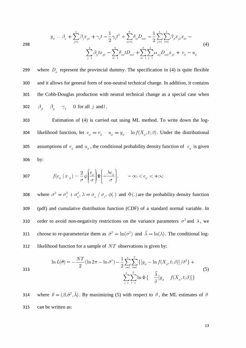
13

4 8 4 42

1 21 1 1 1

4 8 8 4

1 1 1 1

1 1

2 2it o j jit m mit jl jit litj m j l

tj jit mt mit mj mit jit it itj m m j

y x t t D x x

tx tD D x v u

(4) 298

where itD represent the provincial dummy. The specification in (4) is quite flexible 299

and it allows for general form of non-neutral technical change. In addition, it contains 300

the Cobb-Douglas production with neutral technical change as a special case when 301

20

jl tj for all j andl . 302

Estimation of (4) is carried out using ML method. To write down the log-303

likelihood function, let ln ( , ; )it it it it ite v u y f X t . Under the distributional 304

assumptions of itv and

itu , the conditional probability density function of

ite is given 305

by: 306

2( | ) ,it itit it it

e ef e x e 307

where 2 2 2, / , (.)v u u v

and (.)are the probability density function 308

(pdf) and cumulative distribution function (CDF) of a standard normal variable. In 309

order to avoid non-negativity restrictions on the variance parameters 2 and , we 310

choose to re-parameterize them as 2 2ln( ) and ln( ) . The conditional log-311

likelihood function for a sample of NT observations is given by: 312

2 2

1 1

1 1

1ln ( ) (ln2 ln ) {[ ln ( , ; )]/ }

2 2

ln { [ ( , ; )]}

n T

it iti t

n T

it iti t

NTL y f X t

y f X t

(5) 313

where 2( , , ) . By maximizing (5) with respect to , the ML estimates of 314

can be written as: 315

14

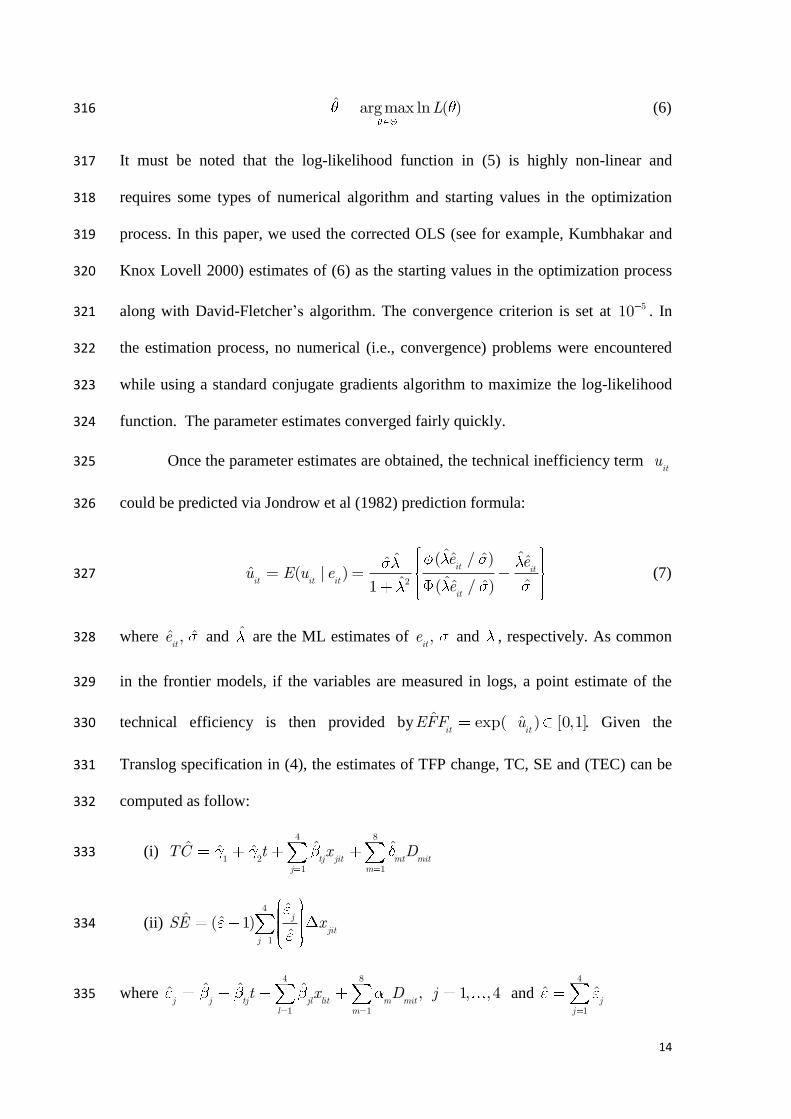
ˆ argmax ln ( )L (6) 316

It must be noted that the log-likelihood function in (5) is highly non-linear and 317

requires some types of numerical algorithm and starting values in the optimization 318

process. In this paper, we used the corrected OLS (see for example, Kumbhakar and 319

Knox Lovell 2000) estimates of (6) as the starting values in the optimization process 320

along with David-Fletcher’s algorithm. The convergence criterion is set at 510 . In 321

the estimation process, no numerical (i.e., convergence) problems were encountered 322

while using a standard conjugate gradients algorithm to maximize the log-likelihood 323

function. The parameter estimates converged fairly quickly. 324

Once the parameter estimates are obtained, the technical inefficiency term itu 325

could be predicted via Jondrow et al (1982) prediction formula: 326

2

ˆ ˆˆ ˆˆ ( / ) ˆˆˆ ( | )

ˆˆ ˆˆ ˆ( / )1

it itit it it

it

e eu E u e

e (7) 327

where ˆ ˆ,ite and ˆ are the ML estimates of ,

ite and , respectively. As common 328

in the frontier models, if the variables are measured in logs, a point estimate of the 329

technical efficiency is then provided by ˆ ˆexp( ) [0,1]it it

EFF u . Given the 330

Translog specification in (4), the estimates of TFP change, TC, SE and (TEC) can be 331

computed as follow: 332

(i) 4 8

1 21 1

ˆ ˆ ˆˆ ˆtj jit mt mit

j m

TC t x D 333

(ii) 4

1

ˆˆ ˆ( 1)

ˆj

jitj

SE x 334

where 4 8

1 1

ˆ ˆ ˆˆ , 1, ,4j j tj jl lit m mit

l m

t x D j and 4

1

ˆj

j

335

15

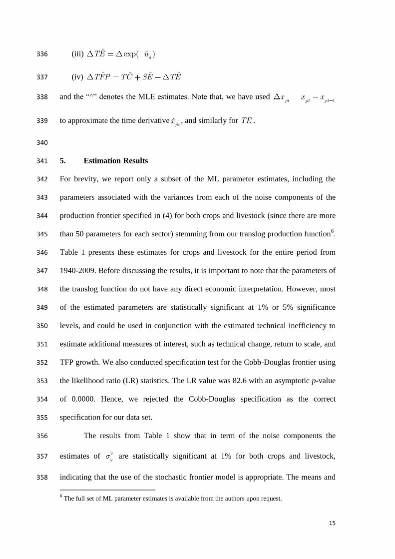
(iii) ˆ ˆexp( )it

TE u 336

(iv) ˆ ˆ ˆ ˆTFP TC SE TE 337

and the “^” denotes the MLE estimates. Note that, we have used 1jit jit jit

x x x 338

to approximate the time derivativejitx , and similarly for TE . 339

340

5. Estimation Results 341

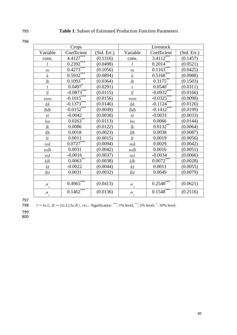
For brevity, we report only a subset of the ML parameter estimates, including the 342

parameters associated with the variances from each of the noise components of the 343

production frontier specified in (4) for both crops and livestock (since there are more 344

than 50 parameters for each sector) stemming from our translog production function6. 345

Table 1 presents these estimates for crops and livestock for the entire period from 346

1940-2009. Before discussing the results, it is important to note that the parameters of 347

the translog function do not have any direct economic interpretation. However, most 348

of the estimated parameters are statistically significant at 1% or 5% significance 349

levels, and could be used in conjunction with the estimated technical inefficiency to 350

estimate additional measures of interest, such as technical change, return to scale, and 351

TFP growth. We also conducted specification test for the Cobb-Douglas frontier using 352

the likelihood ratio (LR) statistics. The LR value was 82.6 with an asymptotic p-value 353

of 0.0000. Hence, we rejected the Cobb-Douglas specification as the correct 354

specification for our data set. 355

The results from Table 1 show that in term of the noise components the 356

estimates of 2

u are statistically significant at 1% for both crops and livestock, 357

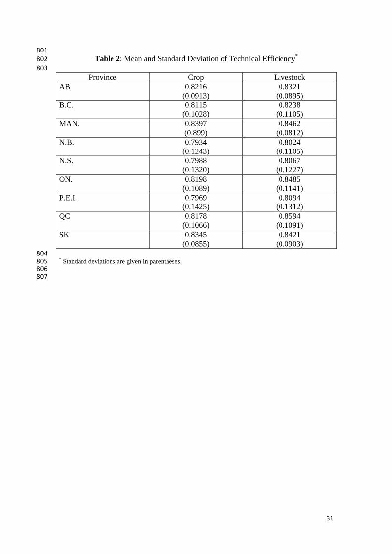
indicating that the use of the stochastic frontier model is appropriate. The means and 358

6 The full set of ML parameter estimates is available from the authors upon request.

16

standard deviations of the estimated technical efficiency measure for each province 359

are displayed in Table 2. The means of technical efficiency are different from 360

province to province for both crops and livestock, albeit relatively small. For crops, 361

the most technically efficient province is Manitoba (83.97%) and the least technically 362

efficient is New Brunswick (79.34%). For livestock, the most technically efficient 363

province is Quebec (85.94%) and the least technically efficient province is New 364

Brunswick (80.24%). 365

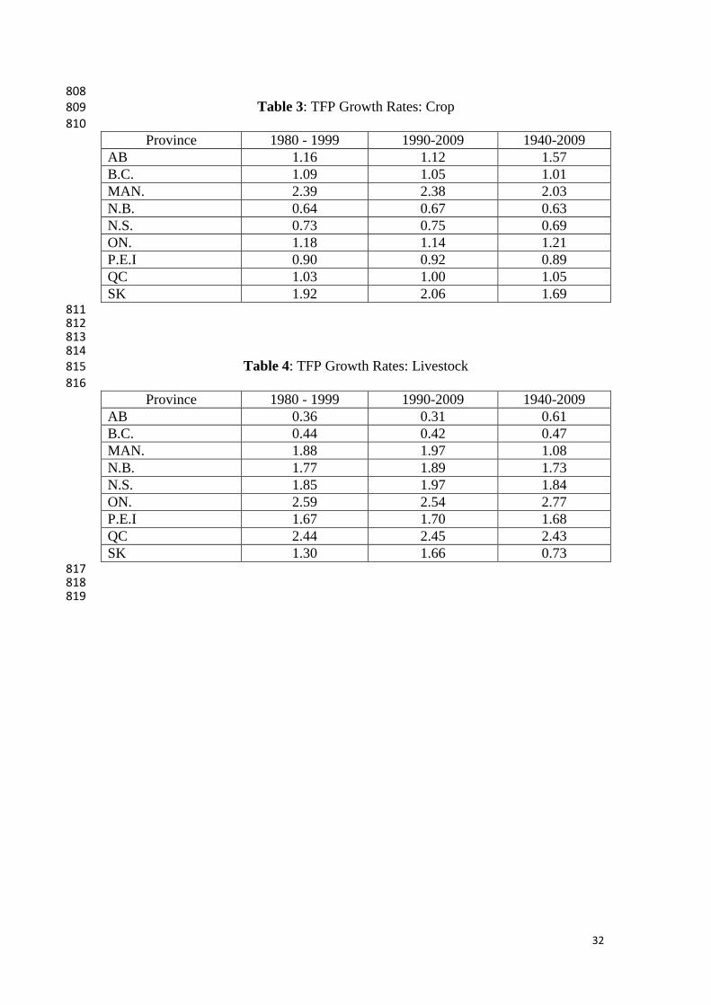
We now turn our attention to the results of the TFP growth and its 366

decompositions. The average annual TFP growth rates for crops and livestock for the 367

entire period are reported in Tables 3 and 4 respectively. For comparison purposes, 368

we also provided the average annual TFP growth for two overlapping periods of 369

1980-1999 and 1990-2009. This enables us to determine if there has been decline in 370

agricultural productivity growth in Canada as indicated by other studies.7 From 1940 371

to 2009, the TFP growth rates are on average higher for crops in each of the Prairie 372

provinces (Alberta, Saskatchewan and Manitoba) than for the Eastern and Atlantic 373

provinces. For example, the annual average TFP growth in Alberta, Saskatchewan and 374

Manitoba are 1.57%, 1.69% and 2.03% respectively, compared to 1.21% in Ontario, 375

1.05% in Quebec and less than 1% in the Atlantic provinces. 376

Comparing average productivity growth in the crops sector between the two 377

overlapping periods (1980-1999 and 1990-2009), we observe that with the exception 378

of Saskatchewan, the crops productivity growth in the remaining major crops 379

producing provinces: Alberta, British Columbia, Manitoba, Ontario and Quebec are 380

lower for the period 1990-2009 than those of the period 1980-1999. Our finding 381

suggests some evidence of a recent decline in productivity growth for crops subsector 382

7 We would like to thank an anonymous referee for suggesting this to us.

17

in Canada, at least in the major crop producing provinces. This result is also 383

qualitatively consistent with recent findings in the literature, at least for the Prairie 384

provinces (see for example, Stewart et al 2009; and Veeman and Gray 2009, 2010). 385

Specifically, compared to the results of Stewart et al (2009) for the Prairie provinces, 386

our results show that the magnitudes of the average annual TFP growth rates are 387

slightly lower. These differences are perhaps due to the presence of the technical 388

inefficiency term in the model as well as larger sample size. 389

For livestock, the average annual TFP growth rates for the period 1940-2009 390

are on average higher in Eastern and Atlantic provinces than in the prairie region. 391

Higher productivity growth rates are found in Ontario and Quebec (2.77% and 2.43% 392

respectively) followed by New Brunswick, Nova Scotia, Prince Edwards Island and 393

Manitoba. The average annual productivity growth rates for B.C. and the Prairie 394

provinces with the exception of Manitoba are all less than 1%. 395

Comparing the results to those of the periods 1980-1999 to 1990-2009, we 396

observe that the average livestock productivity growth in Saskatchewan, Manitoba, 397

Quebec and the Atlantic provinces were higher during the latter 20 years. However, it 398

is noted that Alberta, Ontario and British Columbia experienced lower livestock 399

productivity growth during the same period. The results suggest that there is no clear 400

evidence to support the claim that TFP growth rates in the livestock sector in Canada 401

has declined during the latter two decades. For the period 1990 to 2009 the 402

productivity growth rates in the livestock sub-sector are on the average still higher in 403

Eastern and Atlantic provinces than in the prairie region with the exception of 404

Manitoba which has TFP growth rate similar to those of the Atlantic provinces. As in 405

the case for crops, comparing our results to Stewart et al. (2009) for the Prairie 406

provinces shows some qualitative similarities but reveals some differences in 407

18

magnitude in the productivity growth rates. Our estimates of productivity growth rates 408

in the crop and livestock sectors for all the Prairie provinces are smaller than those of 409

Stewart et al. (2009). This implies that perhaps including the technical inefficiency 410

term in the model is relevant in determining the true magnitudes of productivity 411

growth rates. 412

The finding of higher productivity growth rates for crops relative to livestock 413

for the Prairie provinces compared to Eastern and Atlantic provinces could be 414

explained by longer production cycle and slower progress in controlled genetic 415

technology associated with Cattle production in the Prairie region, especially in 416

Alberta and Saskatchewan8. Manitoba is an exception since traditionally livestock in 417

the province has been more diversified and it is possible that farms have benefited 418

more from faster progress in controlled genetics. Conversely, the finding of higher 419

productivity growth rates for livestock relative to crops in Eastern and Atlantic 420

provinces compare to the West may be due to improvement of genetics, feed 421

conversion, and exploitation of economies of scale (intensive livestock operations 422

especially regarding feedlots and hog barn) in the livestock production. Finally, it 423

was noted that productivity growth in the agriculture sector in Alberta slowed down 424

possibly due to the reallocation of financial and human resources from the agriculture 425

sector to the oil and gas sector. 426

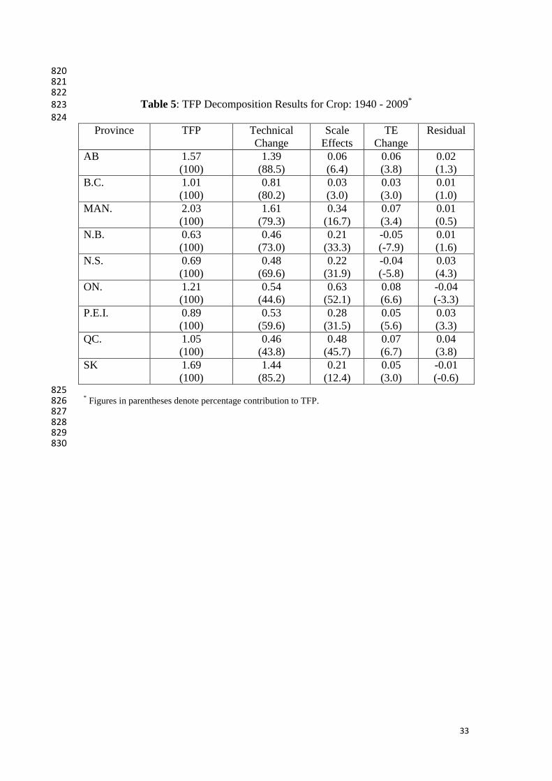
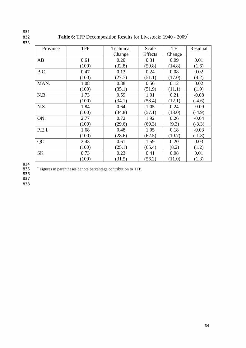
To get more insights into how crops and livestock productivity growth 427

occurred, we turn our attention to the TFP growth decomposition using data for the 428

entire period (1940-2009). Table 5 and 6 provide the decomposition of estimated TFP 429

growth into technical change, scale effects, and technical efficiency change for the 430

crops and livestock sectors respectively. 431

8 The results are consistent with Stewart et al. (2009).

19

As seen in Table 5, technical change seems to be the dominant component of 432

the estimated productivity growth for crops in all the provinces except Ontario and 433

Quebec. For example, in Alberta, Saskatchewan, Manitoba, New Brunswick and 434

Nova Scotia, technical change contributed 88.5%, 85.2%, 79.3%, 73.0% and 69.6% 435

respectively to the TFP growth. For these provinces, with the exception of Alberta, 436

the role of scale effects is also economically important, ranging from 15.8 % in 437

British Columbia to 33.3% in New Brunswick. The scale effect is much less for 438

Alberta crops with only 6.4% contribution to TFP growth. For Ontario and Quebec, 439

both technological progress (44.6 and 43.8% respectively) and scale effects (52.1 and 440

45.7% respectively) played important role in the estimated TFP growth. An important 441

implication of these results is that the TFP growth in crops is mainly driven by 442

technological progress. The results re-enforces the vital role research and 443

development (the adoption of new seed varieties and cropping practice) and extension 444

activities play in the overall development of the Canadian agriculture sector. The 445

change in technical efficiency is mainly positive (except for New Brunswick and 446

Nova Scotia) but has relatively small contributions to the TFP growth for most 447

provinces. Finally, the residuals which account for the unexplained component of the 448

TFP growth are very small. This indicates that factors such as measurement errors and 449

changes in allocative efficiency play very little role in crops productivity growth. 450

For the livestock sector, table 6 shows that the scale effects play a significant 451

role in TFP growth for all provinces, especially in the Eastern and the Atlantic. In 452

addition, improvement in the degree of technical efficiency is relative significant for 453

the sector. These results suggest that economies of scale associated with the 454

expansion of aggregate livestock output have been the main driver of the productivity 455

growth during the period 1940 to 2009. Perhaps the main explanation for the role of 456

20

economies of scale and improvements in the degree of technical efficiency in 457

livestock productivity growth is the shift to more intensive livestock operations such 458

as improvements in genetics, feedlots conversion, and management practices as 459

aggregate provincial livestock output expands over time. 460

461

6. Concluding Remarks 462

Agricultural productivity growth is important with regards to economic efficiency, 463

living standards, international competitiveness, and economic sustainability. Recent 464

studies have concluded that agricultural productivity growth in Canada lags behind 465

that of the U.S and many OECD countries. Other research evidence suggests that 466

agricultural productivity growth in Canada has significantly slowed down. However, 467

studies by de Avillez (2011a, b) have showed that the Canadian agricultural sector has 468

experienced significant labour productivity growth. Furthermore, some Canadian 469

studies have used various methodologies to examine agricultural productivity growth 470

and efficiency for a specific crop or type of livestock farm within a specific province 471

or a collection of few provinces. The results from those studies have showed that 472

methodological characteristics (estimation technique) and other study-specific 473

characteristics (functional form, sample size, product analysis, dimensionality, and 474

geographical region) could affect the empirical estimates of productivity growth and 475

technical efficiency. 476

To the best of our knowledge, there is no study that examines productivity 477

growth using data on crops and livestock production in all the provinces in Canadian 478

while allowing for production inefficiencies as well as further decomposing TFP 479

growth into scale effects, technical efficiency change and technical change. Hence, in 480

this paper, we address the above issues by using a stochastic frontier approach that 481

allows for inefficiencies, and provincial level agricultural data on crops and livestock 482

21

from 1940 to 2009 to examine and decompose TFP growth into scale effects, 483

technical efficiency change and technical change. The paper also investigates the 484

claim that agricultural productivity growth in Canada has recently slowed down. 485

The results indicate that from 1940 to 2009 the productivity growth rates for 486

the crops sub-sector were on average higher for the Prairie provinces than for the 487

Eastern and Atlantic provinces. During the same period, the productivity growth rates 488

in the livestock sub-sector were on the average higher in Eastern and Atlantic 489

provinces than in the prairie region with the exception of Manitoba where TFP growth 490

has been similar to those of the Atlantic provinces for the period 1990 to 2009. 491

Comparing average productivity growth in both the crops and livestock sub-sectors 492

for the period 1940-2009 to the periods 1989-1999 and 1990-2009, our results 493

indicate that for most of the provinces the recent average productivity growth rate are 494

higher than the overall average for the entire period. However, by looking at the two 495

overlapping periods of 1989-1999 and 1990-2009, our results suggest some evidence 496

of a recent decline in crops productivity growth but the evidence of a recent decline in 497

the livestock sub-sector is not clear, since half of the major livestock producing 498

provinces experienced a decline while the other half show a rise in productivity 499

growth. 500

The productivity changes in the two sub-sectors were mainly driven by 501

technical changes (such as new seed varieties, progress in controlled genetic 502

technology; better quality machinery and equipment) and scale effects (arising from 503

intensive livestock operations, and cropping practices). Specifically, technical change 504

is the dominant component of the estimated productivity growth for crops in all the 505

provinces except Ontario and Quebec. However, scale effect is the dominant 506

component of the estimated productivity growth for livestock in all the provinces. 507

22

The contribution of technical progress to productivity growth in livestock was also 508

significant. Finally, though change in technical efficiency is mainly positive for both 509

sectors (except for New Brunswick and Nova Scotia for the crop sector), its 510

contribution to productivity growth was rather very little for the provinces. 511

There is no guarantee that the productivity growth rates of the Canadian 512

agricultural sector during the last few decades would continue into the future. A 513

number of recent studies have suggested that agricultural productivity growth rates for 514

developed countries have slowed down significantly over the past decade or two. The 515

decomposition analysis undertaken in this paper showed that technical progress and 516

scale effect are the two most important determinants of productivity growth among 517

Canadian provinces. Therefore, government policies directed towards increasing 518

funding for agricultural research that improves technical progress and enables farms to 519

benefit from scale of operations should form an essential part of the overall 520

agriculture policies. For instance public investment in agricultural science and 521

technological innovations such as increasing investment in innovation (improving the 522

stock of knowledge/basic research, new seed varieties, progress in controlled genetic 523

technology, cost-effective cropping practices and livestock operations), fostering and 524

facilitating innovation adoption, and improving R&D infrastructure, could be 525

intensified to improve agricultural productivity growth significantly. 526

There is, however, an important limitation to the analysis in this paper. Given 527

the nature of advances in technology, it would have been reasonable to allow for time-528

varying parameters in our model. However, with the flexible form, allowing for time-529

varying coefficients often creates problems in the estimation process because the 530

parameters become much more difficult to estimate. We could have used a more 531

restrictive form of the production function to deal with the situation. However, our 532

23

specification test rejected the simpler form of the frontier (the Cobb-Douglas form). 533

We could have also used the standard random coefficients model. The problem with 534

that approach is the identification of the variance parameters in the model since we 535

would have more than 2 error terms. We therefore leave this for future research. 536

537

24

References 538

Abdulai, A. and W.E. Huffman. 1998. An Examination of Profit Inefficiency of 539 Rice Farmers in Northern Ghana. Staff Paper #296, Department of Economics, Iowa 540 State University, Ames, IA 50011. 541

542 Agriculture and Agri-Food Canada. 2009. An Overview of the Canadian 543 Agriculture and Agri-Food System. Research and Analysis Directorate, Research and 544 Analysis Directorate, Strategic Policy Branch, Agriculture and Agri-Food Canada, 545 Publication No. 11054E. Ottawa, ON. 546

547 Aigner, D., C.A.K. Lovell and P. Schmidt. 1977. Formulation and estimation of 548

stochastic frontier production function models. Journal of Econometrics 6(1): 21-37. 549 550 Alston, J.M., B.A. Babcock and P.G. Pardey. 2010a. Shifting patterns of global 551 agricultural productivity: synthesis and conclusion. In The Shifting Patterns of 552 Agricultural Production and Productivity Worldwide edited by J.M. Alston, B.A. 553

Babcock and P.G. Pardey, pp.449-482. CARD-MATRIC Electronic Book, Ames, IA: 554 Center for Agricultural and Rural Development. 555

556 Alston, J.M., J.M. Beddow and P.G. Pardey. 2010b. Global patterns of crop yields 557

and other partial productivity measures and prices. In The Shifting Patterns of 558 Agricultural Production and Productivity Worldwide edited by J.M. Alston, B. A. 559 Babcock and P.G. Pardey, pp. 39-61. CARD-MATRIC Electronic Book, Ames, IA: 560

Center for Agricultural and Rural Development. 561

562 Amara, N. and R. Romain. 1990. Efficience technique dans le secteur laitier 563 Québecois. Canadian Journal of Agricultural Economics 38(4): 1024-1024. 564

565 Amara, N., N. Traoré, R. Landry and R. Romain. 1999. Technical efficiency and 566

farmers' attitudes toward technological innovation: the case of the potato farmers in 567 Quebec. Canadian Journal of Agricultural Economics 47(1): 31-43. 568 569

Battese, G.E. and T.J. Coelli. 1992. Frontier production functions, technical 570 efficiency and panel data: with application to paddy farmers in India. Journal of 571

Productivity Analysis 3(1-2): 153-169. 572

573

Battese, G.E. and G.A. Tessema. 1993. Estimation of stochastic frontier production 574 functions with time-varying parameters and technical efficiencies using panel data 575 from Indian villages. Agricultural Economics 9(4): 313-333. 576 577

Bravo-Ureta, B.E., D. Solís, V.H.M. López, J.F. Maripani, A. Thiam and T. 578 Rivas. 2007. Technical efficiency in farming: A meta-regression analysis. Journal of 579 Productivity Analysis 27(1): 57-72. 580 581 Bruinsma, J. 2009. The Resource Outlook to 2050: By How Much Do Land, Water 582 and Crop Yields Need to Increase By 2050? Paper presented at the FAO Expert 583

Meeting on How to Feed the World in 2050, Food and Agriculture Organization of 584

the United Nations, Economic and Social Development Department. Rome, Italy, 585 June 24-26. 586

25

587 Charnes, A., W.W. Cooper and E. Rhodes. 1978. Measuring the efficiency of 588 decision making units. European Journal of Operational Research 2(6): 429-444. 589 590 Cloutier, L.M., and R. Rowley. 1993. Relative technical efficiency: Data 591

envelopment analysis and Quebec’s dairy farms. Canadian Journal of Agricultural 592 Economics 41(2): 169–176. 593 594 Coelli, T. and S. Walding. 2005. Performance Measurement in the Australian Water 595 Supply Industry. Working Paper Series #01/2005, Centre for Efficiency and 596

Productivity Analysis, School of Economics, University of Queensland, St. Lucia, 597 Australia. 598

599 Constantin, P.D., D.L. Martin and E.B. Rivera Y Rivera. 2009. Cobb-Douglas, 600 translog stochastic production function and data envelopment analysis in total factor 601 productivity in Brazilian agribusiness. The Flagship Research Journal of 602 International Conference of the Production and Operations Management Society 603

2(2): 20-33. 604 605

Darku, A. and S. Malla. 2010. Agricultural productivity growth in Canada: Concepts 606 and evidences. Canadian Agricultural Innovation Research Network (CAIRN) Policy 607

Briefs, Saskatoon, SK. 2010: 21. http://www.ag-innovation.usask.ca/ (accessed 608 September 10, 2012). 609 610

Darku, A., S. Malla and K.C. Tran. 2012. Sources and Measurement of Agricultural 611

Productivity and Efficiency in Canadian Provinces: Crops and Livestock. Publication 612 31, Canadian Agricultural Innovation and Regulation Network (CAIRN), Saskatoon, 613 SK. http://www.ag-innovation.usask.ca/ (accessed September 10, 2012). 614

615 Darku, A., S. Malla and K.C. Tran. 2013. Historical review of agricultural 616

efficiency studies. Publication 33, Canadian Agricultural Innovation and Regulation 617 Network (CAIRN), Saskatoon, SK. http://www.ag-innovation.usask.ca/ (accessed 618 September 10, 2012). 619

620 de Avillez, R. 2011a. A Detailed Analysis of the Productivity Performance of the 621

Canadian Primary Agriculture Sector. CSLS Research Report 2011-06. Prepared for 622

Agriculture and Agri-Food Canada. Ottawa: Centre for the Study of Living 623

Standards. 624

625 de Avillez, R. 2011b. A half-century of productivity growth and structural change in 626 Canadian agriculture: an overview. International Productivity Monitor 22(5): 82-99. 627 Echevarria, C. 1998. A three-factor agricultural production function: the case of 628

Canada. International Economic Journal 12(3): 63-75. 629 630 Fantino, A.A. and T.S. Veeman. 1997. The choice of index numbers in measuring 631 agricultural productivity: A Canadian empirical case study. In Issues in Agricultural 632 Competitiveness: Market and Policies edited by R. Rose, C. Tanner and M.A. 633

Bellamy, 7: 222-230. International Association of Agricultural Economists (IAAE) 634

Occasional Paper. 635 636

26

Färe, R. 1988. Fundamentals of Production Theory. Berlin, Germany: Springer-637 Verlag. 638 639 Färe, R., S. Grosskopf, M. Norris and Z. Zhang. 1994. Productivity growth, 640 technical progress, and efficiency change in industrialized countries. American 641

Economic Review 84(1):66-83. 642 643 Farrell, M.J. 1957. The measurement of productive efficiency. Journal of the Royal 644 Statistical Society Series A (General) 120(3): 253-290. 645 646

Fuglie, K.O. 2008. Is a slowdown in agricultural productivity growth 647 contributing to the rise in commodity prices? Agricultural Economics. 39 648

(Supplement s1): 431–441. 649 650 Fuglie, K.O. 2010. Total factor productivity in the global agricultural economy: 651 Evidence from FAO data. In The Shifting Patterns of Agricultural Production and 652 Productivity Worldwide edited by J.M. Alston, B.A. Babcock and P.G. Pardey, pp. 653

63-95. CARD-MATRIC Electronic Book, Ames, IA: Center for Agricultural and 654 Rural Development. 655

656 Giannakas, K, R. Schoney and V. Tzouvelekas. 2001. Technical efficiency, 657

technological change and output growth of wheat farms in Saskatchewan. Canadian 658 Journal of Agricultural Economics 49(2): 135–152. 659 660

Giannakas, K., K.C. Tran, and V. Tzouvelekas. 2000. Efficiency, technological 661

change and output growth in Greek olive growing farms: A Box-Cox approach. 662 Applied Economics 32(7): 909-916. 663 664

Gray, R. 2009. Agricultural research at a crossroads. Canadian Journal of 665 Agricultural Economics 56(1): 1-11. 666

667 Greene, W.H. 2003. Econometric Analysis, 5th edition. Upper Saddle River, NJ: 668 Prentice Hall. 669

670 Haghiri, M., J.F. Nolan and K.C. Tran. 2004. Assessing the impact of economic 671

liberalization across countries: A comparison of dairy industry efficiency in Canada 672

and the USA. Applied Economics 36(11): 1233-1243. 673

674 Hailu, G., S. Jeffrey and J. Unterschultz. 2005. Cost efficiency for Alberta and 675 Ontario dairy farms: An interregional comparison. Canadian Journal of Agricultural 676 Economics 53(2-3): 141-160. 677 678

Hsu, S.-H., M.-M. Yu and C.-C Chang. 2003. An Analysis of Total Factor 679 Productivity Growth in China's Agricultural Sector. Paper presented at the American 680 Agricultural Economics Association annual meeting, Montreal, Quebec, July 27- 30. 681 682 Jondrow, J., C.A. Knox Lovell, I.S. Materov and P. Schmidt. 1982. On the 683

estimation of technical inefficiency in the stochastic frontier production function 684

model. Journal of Econometrics 19(2-3): 233-238. 685 686

27

Kumbhakar S.C. and C.A. Knox Lovell. 2000. Stochastic Frontier Analysis. 687 Cambridge UK: Cambridge University Press. 688 689 Lambert, D.K. and E. Parker. 1998. Productivity in Chinese provincial agriculture. 690 Journal of Agricultural Economics 49(3): 378-392. 691

692 Ludena, C.E. 2010. Agricultural Productivity Growth, Efficiency Change and 693 Technical Progress in Latin America and the Caribbean. Working paper series #186, 694 Inter-American Development Bank (IDB), Washington, D.C. 695 696

Mbaga, M.D., R. Romain, B. Larue and L. Lebel. 2003. Assessing technical 697 efficiency of Quebec dairy farms. Canadian Journal of Agricultural Economics 51(1): 698

121-137. 699 700 Meeusen, W. and J. Van den Broeck. 1977. Efficiency estimation from Cobb–701 Douglas production functions with composed error. International Economic Review 702 18(2): 435–444. 703

704 Nin Pratt, A. and B. Yu. 2008. An updated look at the recovery of agricultural 705

productivity in Sub-Sahara Africa. International Food Policy Research Institute IFPRI 706 Discussion Paper No.00787 August 2008. Development Strategy and Governance 707

Division. Washington, DC: IFPRI. 708 709 O'Donnell, C.J. 2009. An Aggregate Quantity-Price Framework for Measuring and 710

Decomposing Productivity and Profitability Change. Working Paper Series 711

#WP07/2008, 13 November 2008, Revised February 2009, Centre for Efficiency and 712 Productivity Analysis, ISSN #1932 – 4398, School of Economics, University of 713 Queensland, St. Lucia, Australia. 714

715 O'Donnell, C.J. 2010. Measuring and decomposing agricultural productivity and 716

profitability change. Australian Journal of Agricultural and Resource Economics 717 54(4): 527-560. 718 719

O’Donnell, C.J. 2012a. An aggregate quantity framework for measuring and 720 decomposing productivity change. Journal of Productivity Analysis 38(3): 255-272. 721

722

O'Donnell, C.J. 2012b. Nonparametric estimates of the components of productivity 723

and profitability change in US agriculture. American Journal of Agricultural 724 Economics 94(4): 873-890. 725 726 Pires, J.O. and F. Garcia. 2012. Productivity of nations: A stochastic frontier 727 approach to TFP decomposition. Economics Research International 2012: 1-19. 728

729 Pitt, M.M. and L.F. Lee. 1981. The measurement and sources of technical 730 inefficiency in the Indonesian weaving industry. Journal of Development Economics 731 9(1): 43-64. 732 733

Rao, S., J. Tang and W. Wang. 2008. What explains the Canada-US labour 734

productivity gap? Canadian Public Policy 34(2): 163-192. 735 736

28

Richards, T.J. and S.R. Jeffrey. 1996. Cost and Efficiency in Alberta Dairy 737 Production. Staff Paper #96-13 Department of Rural Economy, Faculty of 738 Agriculture, Forestry, and Home Economics, University of Alberta, Edmonton, AB. 739 740 Richards, T.J. and S.R. Jeffrey. 2000. Efficiency and economic performance: An 741

application of the MIMIC model. Journal of Agricultural and Resource Economics 742 25(1): 232-251. 743 744 Samarajeewa, S., G. Hailu, S.R. Jeffrey, and M. Bredahl. 2012. Analysis of 745 production efficiency of beef cow/calf farms in Alberta. Applied Economics 44(3): 746

313-322. 747 Schmidt, P. and R.C. Sickles. 1984. Production frontiers and panel data. Journal of 748

Business and Economic Statistics 2(4): 367-374. 749 750 Seyoum, E.T., G.E. Battese and E.M. Fleming. 1998. Technical efficiency and 751 productivity of maize producers in eastern Ethiopia: A study of farmers within and 752 outside the Sasakawa - Global 2000 project. Agricultural Economics 19(3): 341-348. 753

754 Shephard, R.W. 1970. Theory of Cost and Production Functions. Princeton, NJ: 755

Princeton University Press. 756 757

Slade, P. and G. Hailu. 2011. Efficiency and Regulation of Dairy Farms: A 758 Comparison of Ontario and New York State. Paper presented at the Agricultural and 759 Applied Economics Associations Annual Meeting, Pittsburgh, Pennsylvania, July 24-760

26. 761

762 Statistics Canada. 2011a. CANSIM database, table no. 001-0010, 001-0014, 002-763 0007, 002-0021, 002-0068. [Accessed May, 2011] 764

765 Statistics Canada. 2011b. CANSIM database, table no. 002-0005, 002-0015, 380-766

0052. [Accessed June, 2011] 767 768 Stewart, B., T. Veeman and J. Unterschultz. 2009. Crops and livestock productivity 769

growth in the prairies: The impacts of technical change and scale. Canadian Journal 770 of Agricultural Economics 57(3): 379-394. 771

772

Tipi, T. and E. Rehber. 2006. Measuring technical efficiency and total factor 773

productivity in agriculture: The case of the South Marmara region of Turkey. New 774 Zealand Journal of Agricultural Research 49(2): 137-145. 775 776 Veeman, T.S. and R. Gray. 2009. Agricultural production and productivity in 777 Canada. Choices 24(4). 778

779 Veeman, T.S. and R. Gray, 2010. The shifting patterns of agricultural production 780 and productivity in Canada. In The Shifting Patterns of Agricultural Production and 781 Productivity Worldwide edited by J.M. Alston, B. A. Babcock and P.G. Pardey, pp. 782 123-147. CARD-MATRIC Electronic Book, Ames, IA: Center for Agricultural and 783

Rural Development. 784

785

29

Weersink, A., C.G. Turvey and A. Godah. 1990. Decomposition measures of 786 technical efficiency for Ontario dairy farms. Canadian Journal of Agricultural 787 Economics 38(3): 439-456. 788 789 790 791

792

793

794

30

Table 1: Subset of Estimated Production Function Parameters 795

796

Crops Livestock

Variable Coefficient (Std. Err.) Variable Coefficient (Std. Err.)

cons. 4.4127***

(0.1316) cons. 3.4112***

(0.1457)

l 0.2392***

(0.0498) l 0.2014***

(0.0521)

m 0.4273***

(0.1056) m 0.1163***

(0.0425)

k 0.5932***

(0.0894) k 0.5168***

(0.0988)

lb 0.1093***

(0.0364) lb 0.3175**

(0.1503)

t 0.0497*

(0.0291) t 0.0540*

(0.0311)

ll -0.0873***

(0.0115) ll -0.0932***

(0.0166)

mm -0.1015***

(0.0156) mm -0.0325***

(0.0098)

kk -0.1373***

(0.0146) kk -0.1124***

(0.0126)

lblb -0.0152***

(0.0049) lblb -0.1412***

(0.0199)

tt -0.0042 (0.0038) tt -0.0031 (0.0033)

lm 0.0263**

(0.0113) lm 0.0066 (0.0144)

lk 0.0086 (0.0122) lk 0.0132**

(0.0064)

llb 0.0018 (0.0023) llb 0.0038 (0.0087)

lt 0.0011 (0.0015) lt 0.0019 (0.0056)

mk 0.0727***

(0.0094) mk 0.0029 (0.0042)

mlb 0.0031 (0.0042) mlb 0.0016 (0.0051)

mt -0.0016 (0.0037) mt -0.0034 (0.0066)

klb 0.0063**

(0.0038) klb 0.0072***

(0.0028)

kt -0.0022 (0.0044) kt 0.0011 (0.0055)

lbt 0.0031 (0.0032) lbt 0.0049 (0.0079)

u 0.4965

*** (0.0413)

u 0.2548

*** (0.0621)

v 0.1462

*** (0.0136)

v 0.1548

*** (0.2516)

797 ln , (ln )(ln ), .;l L lk L K etc Significance:

***: 1% level;

**: 5% level;

*: 10% level. 798

799 800

31

801 Table 2: Mean and Standard Deviation of Technical Efficiency

* 802 803

Province Crop Livestock

AB 0.8216

(0.0913)

0.8321

(0.0895)

B.C. 0.8115

(0.1028)

0.8238

(0.1105)

MAN. 0.8397

(0.899)

0.8462

(0.0812)

N.B. 0.7934

(0.1243)

0.8024

(0.1105)

N.S. 0.7988

(0.1320)

0.8067

(0.1227)

ON. 0.8198

(0.1089)

0.8485

(0.1141)

P.E.I. 0.7969

(0.1425)

0.8094

(0.1312)

QC 0.8178

(0.1066)

0.8594

(0.1091)

SK 0.8345

(0.0855)

0.8421

(0.0903)

804 * Standard deviations are given in parentheses. 805

806 807

32

808 Table 3: TFP Growth Rates: Crop 809

810

Province 1980 - 1999 1990-2009 1940-2009

AB 1.16 1.12 1.57

B.C. 1.09 1.05 1.01

MAN. 2.39 2.38 2.03

N.B. 0.64 0.67 0.63

N.S. 0.73 0.75 0.69

ON. 1.18 1.14 1.21

P.E.I 0.90 0.92 0.89

QC 1.03 1.00 1.05

SK 1.92 2.06 1.69 811 812 813 814

Table 4: TFP Growth Rates: Livestock 815 816

Province 1980 - 1999 1990-2009 1940-2009

AB 0.36 0.31 0.61

B.C. 0.44 0.42 0.47

MAN. 1.88 1.97 1.08

N.B. 1.77 1.89 1.73

N.S. 1.85 1.97 1.84

ON. 2.59 2.54 2.77

P.E.I 1.67 1.70 1.68

QC 2.44 2.45 2.43

SK 1.30 1.66 0.73 817 818

819

33

820 821 822

Table 5: TFP Decomposition Results for Crop: 1940 - 2009*

823 824

Province TFP Technical

Change

Scale

Effects

TE

Change

Residual

AB 1.57

(100)

1.39

(88.5)

0.06

(6.4)

0.06

(3.8)

0.02

(1.3)

B.C. 1.01

(100)

0.81

(80.2)

0.03

(3.0)

0.03

(3.0)

0.01

(1.0)

MAN. 2.03

(100)

1.61

(79.3)

0.34

(16.7)

0.07

(3.4)

0.01

(0.5)

N.B. 0.63

(100)

0.46

(73.0)

0.21

(33.3)

-0.05

(-7.9)

0.01

(1.6)

N.S. 0.69

(100)

0.48

(69.6)

0.22

(31.9)

-0.04

(-5.8)

0.03

(4.3)

ON. 1.21

(100)

0.54

(44.6)

0.63

(52.1)

0.08

(6.6)

-0.04

(-3.3)

P.E.I. 0.89

(100)

0.53

(59.6)

0.28

(31.5)

0.05

(5.6)

0.03

(3.3)

QC. 1.05

(100)

0.46

(43.8)

0.48

(45.7)

0.07

(6.7)

0.04

(3.8)

SK 1.69

(100)

1.44

(85.2)

0.21

(12.4)

0.05

(3.0)

-0.01

(-0.6) 825 * Figures in parentheses denote percentage contribution to TFP. 826

827 828 829

830

34

831 Table 6: TFP Decomposition Results for Livestock: 1940 - 2009

* 832 833

Province TFP Technical

Change

Scale

Effects

TE

Change

Residual

AB 0.61

(100)

0.20

(32.8)

0.31

(50.8)

0.09

(14.8)

0.01

(1.6)

B.C. 0.47

(100)

0.13

(27.7)

0.24

(51.1)

0.08

(17.0)

0.02

(4.2)

MAN. 1.08

(100)

0.38

(35.1)

0.56

(51.9)

0.12

(11.1)

0.02

(1.9)

N.B. 1.73

(100)

0.59

(34.1)

1.01

(58.4)

0.21

(12.1)

-0.08

(-4.6)

N.S. 1.84

(100)

0.64

(34.8)

1.05

(57.1)

0.24

(13.0)

-0.09

(-4.9)

ON. 2.77

(100)

0.72

(29.6)

1.92

(69.3)

0.26

(9.3)

-0.04

(-3.3)

P.E.I. 1.68

(100)

0.48

(28.6)

1.05

(62.5)

0.18

(10.7)

-0.03

(-1.8)

QC 2.43

(100)

0.61

(25.1)

1.59

(65.4)

0.20

(8.2)

0.03

(1.2)

SK 0.73

(100)

0.23

(31.5)

0.41

(56.2)

0.08

(11.0)

0.01

(1.3) 834 * Figures in parentheses denote percentage contribution to TFP. 835

836 837

838

35

APPENDIX A: DATA DESCRIPTION 839 840 In this appendix, we provide a brief description of the data used in the paper. 841

Crops 842

Crop production in Canada is divided into four categories; field crops, potatoes, fruits, 843

and vegetables. Field crops comprise of the majority of crop cash receipts in Canada 844

with the Prairie Provinces having the highest proportions. Saskatchewan has about 98 845

percent of total crop cash receipts coming from field crops. Field crops include 846

eighteen different types of crops: wheat, barley, rye, mixed grain, corn for grain, 847

buckwheat, dry field peas, and others. A number of smaller specialty crops are not 848

included in total output of field crops. These include Triticale, Canary seed, 849

Fababeans, Coriander, Safflower, Caraway seed, Borage seed, and Chick peas. These 850

were left out of total real production because adequate price information was not 851

available to convert them into real terms. Also, the combined total production of these 852

specialty crops was found to be less than one percent of the total production of all 853

field crops in Canada from 1940-2009, and therefore would not affect total production 854

very much. The data for field crops came from CANSIM table 001-0010 (with the 855

exception of potatoes which came from Statistics Canada table 001-0014). Farm 856

Product Price Index (FPPI) is used to deflate the value measures of crop in order to 857

remove the price effect. 858

Livestock 859

Livestock output was found using farm cash receipts from 1940 to 2009. The total 860

production of livestock is comprised of the production of cattle, calves, hogs, sheep, 861

lambs, dairy products, poultry, eggs, and other livestock and products. These are the 862

nominal values of livestock production. The FPPI is then used to deflate the value 863

measures of livestock in order to remove the price effect. 864

The values for individual livestock products (cattle and calves, hogs, poultry, 865

eggs, dairy) from 1971 to 2009 were taken from CANSIM tables 002-0021 and 002-866

0068; and the missing values from 1940 to 1971 have been imputed using the 867

predicted scores from an ARMA(1,0) process. The ARMA (1, 0) was chosen based on 868

the Akaike and Schwarz model selection criterions from a more general class ARMA 869

(p, q) process. 870

36

Inputs 871

The input data was organized following Stewart et al. (2009). The data is organized 872

into four main categories; capital, land, labor, and materials. Capital contains the 873

value of machinery and equipment used in production, the cost of repairs to 874

machinery and equipment, the depreciation value of machinery and equipment, and 875

the value of livestock inventory. Land is comprised of the value of cropped land, land 876

in summer fallow, pasture land, buildings, building repairs, building depreciation, and 877

property tax. Labor contains unpaid and paid labor. Materials include the cost of fuel, 878

electricity, telephone, custom work, twine, business and crop insurance, fertilizer and 879

lime, pesticides, commercial seed, feed, artificial insemination and vet fees, and 880

miscellaneous other expenses. 881

Capital inputs came from three different CANSIM tables. Table 002-0007 882

contained the data needed for machinery and equipment, and livestock inventories. 883

Most of the data for land inputs came from the same tables as capital inputs. Land and 884

building values came from Table 002-0007, depreciation, property tax, and building 885

repair values came from Table 002-0005 and Table 002-0015. Building repairs 886

include any costs of repairing fences as well. Cropped land data was obtained from 887

Table 001-0017, and is calculated as the total area, in acres, of seeded land. 888

Labor consists of unpaid and paid labor. Paid labor is separated into hired 889

labor and operator labor in the nominal section of labor inputs. Hired labor consists of 890

paid wages to employees and family members and was obtained from Table 002-0015 891

for the years 1940-1970 and Table 002-0005 for 1971-2009. These paid wages 892

include room and board as well as cash wages, and the value before rebates was used. 893

Statistics Canada defines operators as those persons responsible for the management 894

decisions made in the operation of a census farm or agricultural operation, and up to 895

three operators can be reported per farm. The net income received by farm operators 896

from farm production was taken as the value of operator labor obtained from Table 897

380-0052. Unpaid labor was calculated as 70 percent of operator labor. 898

For materials, the data came from Table 002-0005 and Table 002-0015. The 899

cost of containers is included in pesticides from 1940-1947. 900

901

902

37

Allocating Inputs 903

Allocating inputs between the livestock and crops sectors requires the use of census of 904

agriculture data, which is more detailed and separates data by farm type. These farm 905

types are categorized as follows; wheat, fruits and vegetables, field crops, cattle, hogs, 906

poultry, mixed farms, and subsistence farms. To be categorized as one of these, at 907

least 51 percent (50 percent prior to 1961) of total output must come from the titled 908

crop (i.e. a farm classified as a cattle farm must have 51 percent of its total output 909

coming from cattle production). In some census years, mixed farms are subdivided 910

into mixed livestock farms, mixed crop farms, and mixed other. A mixed crop farm is 911

a farm that has 51 percent of its total production from two or more crop categories 912

(wheat, fruits and vegetables, field crops). For livestock, it was computed as the sum 913

of all farms classified as cattle, hogs, poultry, and mixed livestock. For crops, it was 914

computed as the sum of all farms classified as wheat, fruits and vegetables, field crop, 915

and mixed crop farms. 916

For cropped land, livestock capital, operator labor, paid labor, and the value of 917

land and buildings, the share of each category was determined for each sector 918

following the methodology outlined by Stewart et al. (2009). These sector shares 919

were then used to allocate the inputs between the Livestock and Crop sectors. The 920

share of machinery and equipment was used to allocate all of the capital inputs except 921

livestock inventory, which did not require allocation as it is solely a livestock input. 922

The allocation was completed by simply taking the total input value of capital and 923

multiplying it by the sector share. All land inputs were allocated using the sector share 924

of the value of land and buildings. Some land was only used for one sector. Cropped 925

land and summer fallow land are entirely crop inputs while pasture land is exclusively 926

a livestock input. Two sector shares were used to allocate labor inputs. The share of 927

operator labor was used to allocate unpaid labor and operator labor, while the share of 928

paid labor was used to allocate paid wages. 929

Irrigation, fertilizer and lime, pesticides, commercial seed, and crop insurance 930

are solely a crop sector input while feed, artificial insemination and vet expenses are 931

livestock sector inputs and thus do not need to be allocated. The remaining materials 932

inputs are allocated using one of the above methods or on the crops and livestock’s 933

share of value of total output. Fuel is allocated using the capital shares, electricity 934

using the land and building shares, and telephone using the labor share. Custom work, 935

38

miscellaneous expenses, business insurance, twine, wire, and containers are allocated 936

using the crop and livestock’s share of value of total output. 937

Finally, all the inputs were valued by the price of each input-quality type to 938

account for changes in qualities overtime. 939