sos lower bound for exact planted clique - electronic
TRANSCRIPT
SOS LOWER BOUND FOR EXACT PLANTED CLIQUE
SHUO PANG
Abstract. We prove a SOS degree lower bound for the planted clique
problem on Erdos-Renyi random graphs G(n, 1/2). The bound we get
is degree d = Ω(ε2 logn/ log logn) for clique size ω = n1/2−ε, which
is almost tight. This improves the result of [BHK+19] on the “soft”
version of the problem, where the family of equality-axioms generated
by x1 + ...+ xn = ω was relaxed to one inequality x1 + ...+ xn ≥ ω.
As a technical by-product, we also “naturalize” previous techniques
developed for the soft problem. This includes a new way of defining
the pseudo-expectation and a more robust method to solve the coarse
diagonalization of the moment matrix.
1. Introduction
1.1. The problem and the proof system. Whether one can find a max-
clique in a random graph G ∼ G(n, 1/2) efficiently and be correct with high
probability has been a long-standing open problem in computational com-
plexity since [Kar76]. In [Jer92, Kuc95], a relaxed formulation as the planted
clique problem was introduced: if we further plant a random clique of size
ω log n to G, can it be efficiently recovered? Information-theoretically
this is possible, since w.h.p. the largest clique in G has size (2 + o(1)) log n.
While computationally, the average-case hardness of this problem is still
widely believed even after it has been intensively studied and has inspired
research directions in an extremely wide range of fields (just to mention
a few: cryptography [ABW10], learning theory [BR13], mathematical fi-
nance [ABBG11], computational biology [PS+00]). So far, the best known
polynomial-time algorithm is for ω = Ω(√n) [AKS98], which is a so-called
spectral algorithm (see e.g. [HKP+17]).
The sum-of-squares (SOS) hierarchy [Sho87, Par00, Las01] is a stronger
family of semidefinite programming (SDP) algorithms which, roughly speak-
ing, is SDP on the extended set of variables xi(1)...xi(d) | i1, ..., id ∈ [n] ac-
cording to the degree parameter d, and it can be significantly more powerful
than spectral algorithms and traditional SDP (see e.g. [BBH+12, HKP+17]).
Recent years have witnessed rapid development on SOS-based algorithms
which turn out to provide a characterization of a wide class of algorithmic
techniques—for a list of evidence, we refer the reader to the survey [BS14]
and the introduction of [HKP+17]. The SOS proof system is the natural
University of Chicago, Department of Mathematics [email protected].
ISSN 1433-8092
Electronic Colloquium on Computational Complexity, Report No. 70 (2021)
2 SOS LOWER BOUND FOR EXACT PLANTED CLIQUE
proof-theoretic counterpart of these algorithms, also known as the Posi-
tivstellensatz system [GV01]: it works with polynomials over R, and given
polynomial equalities (axioms) f1(x) = 0, ..., fk(x) = 0 on x = (x1, ..., xn), a
proof (that is, a refutation of the existence of a solution) is
−1 =
k∑i=1
fiqi +∑j
r2j in R[x1, ..., xn]
where q1, ..., qm and r1, ... are arbitrary polynomials on x1, ..., xn over R.
Under certain conditions, in particular when all variables are boolean (x2i =
xi), such an refutation always exists if the axioms are contradictory. The
degree-d SOS proof system is this plus a degree limitation
maxi,jdeg(fi) + deg(qi), 2 deg(rj) ≤ d.
See [O’D17, RW17] for the relation between SOS proofs and SDP algorithms.
The average-case hardness of the clique problem has a very simple form in
proof complexity: for G ∼ G(n, 1/2), can the proof system efficiently refute
the existence of a size-ω ( log n) clique w.h.p.? Note the system cannot
just say “No” but must search for a certificate—a proof. A lower bound here
would automatically give the hardness on any class of algorithms based on
the proof system. Given that the decision version of the spectral algorithm
of [AKS98] corresponds to a degree-2 SOS proof, a SOS degree lower bound
would bring us a much better understanding of the hardness of the problem.
The standard formulation is the following.
Definition 1.1. Given an n-vertex simple graph G and a number ω, the
Clique Problem for degree-d SOS proof system has the following axioms.
(1.1)
(Boolean) x2i = xi ∀i ∈ [n]
(Clique) xixj = 0 ∀i, j non-edge
(Size) x1 + ...+ xn = ω
To confirm no ω-clique exists is to give a SOS refutation of the above. The
SOS system has the so-called duality: to show degree lower bound it suffices
to consider pseudo-expectation and moment matrix 1. With boolean variables
(which is our case), this can be demonstrated on multi-linear polynomials.
Let X≤a = xS | S ⊆ [n], |S| ≤ a for any a.
Definition 1.2. A degree-d pseudo-expectation for the Clique Problem
on G is a map E : Xd → R satisfying the following four constraints when
extended by R-linearity.
(Default) Ex∅ = 1(1.2)
(Clique) ExS = 0, ∀S : |S| ≤ d, G|S non-clique(1.3)
(Size) E
((x1 + ...+ xn)xS
)= ω · ExS ∀S : |S| ≤ d− 1(1.4)
1The name is simplified; more cautiously, it should be called the pseudo-moment matrix.
SOS LOWER BOUND FOR EXACT PLANTED CLIQUE 3
where in (1.4), xA ·xB := xA∪B. For the last constraint, define the moment
matrix M to be the( [n]≤d/2
)×( [n]≤d/2
)matrix2 with expression M(A,B) =
ExA∪B for all |A|, |B| ≤ d/2, then:
(1.5) (PSDness) M is positive semi-definite.
It is not hard to see that if a degree-d pseudo-expectation exists then
there is no degree-d SOS refutation.
A relaxation of the problem was studied in [BHK+19]: decide whether
there exists E as in Definition 1.2 except by one change—replace Size Con-
straints by one weaker inequality E(x1+...+xn) ≥ ω. Henceforth, we call the
Clique Problem (Def. 1.1) Exact Clique and this relaxation Non-Exact
Clique.3 We will study their average-case hardness over G ∼ G(n, 1/2).
How to deal with the exact problem is a subtle but important open prob-
lem. On the problem itself, lower bounds on the “weak” formulation indeed
gave the important algorithmic message—an integrality gap for many SOS-
based optimization algorithms—but still, they do not rule out the possibility
that SOS can efficiently refute x1 + ...+ xn = k for each individual large k,
and the distinction between “weak” and “strong” formulations also involves
how one thinks the SOS SDP optimization problem should be formulated.
Perhaps more importantly, it is about the limit of existing methods for
proving average-case SOS lower bounds. Current techniques from the so-
called pseudo-calibration heuristic [BHK+19] tend to deal successfully with
“soft” constraints (i.e. inequalities, or usually just one bound on a single
pseudo-expectation value) while being poor at handling “hard” constraints
(i.e. equalities). Finding techniques to deal with the latter is thus in need.
Progress toward this goal is made in [KOS18] for random CSPs, where the
number of hard constraints is at most two4. Their method is to break
such constraint(s) into local ones and satisfy each using real, independent
distributions. For “inherently more rigid” problems like Exact Clique (whose
hard constraints are “almost everywhere”), however, it seems unlikely a
similar strategy could work.
Lastly, there are concrete applications of lower bounds on Exact Clique.
Such a lower bound can give by reduction lower bounds for other problems,
e.g. for the approximated Nash-Welfare, and potentially for the coloring
problem and stochastic block models [KOS18, KM18].
1.2. Previous work. For upper bounds, if ω = Ω(√n) then degree-2 SOS
can refute Exact Clique with high probability [FK00]. On the other hand,
if ω > d ≥ 2.1 log n, a degree-d SOS refutation for Exact Clique is not hard
2d is always assumed to be even.3There is no “planted clique” in the problem’s formulation, but traditionally, the problemis still called the planted clique problems due to the algorithmic motivation behind.4One on the objective value of the CSP, and/or one on the Hamming weight of x.
4 SOS LOWER BOUND FOR EXACT PLANTED CLIQUE
to see; since we have not been able to find it in the literature, we include it
as Observation 1.1 below.
For lower bounds, for Exact Clique, [FK03] showed that the weaker system
d-round Lovasz-Schrijver can refute it only when ω = O(√n/2d); [MPW15]
proved degree-d lower bound on SOS for ω = O(n1/d), and this bound on
ω was improved to O(n1/3) for d = 4 [DM15] and O(n1
bd/2c+1 ) for general d
[HKP+18]. For Non-Exact Clique, [BHK+19] proved the almost tight lower
bound d = Ω(ε2 log n) for ω = n1/2−ε, ε > 0 arbitrary (could depend on n).
Observation 1.1. (Upper bound for Exact Clique if ω > d = 2.1 log n)
Note (x1 + ... + xn)d = ωd modulo the Size Axiom. The LHS can be multi-
linearly homogenized to degree-d by xS = 1ω−|S|
∑i/∈S xS∪i by this axiom
again, after which w.h.p. all terms are 0 by Clique Axioms, as there is no
size-2.1 log n clique in G ∼ G(n, 1/2) w.h.p.. This gives the contradiction
0 = 1. Note this proof is actually in the weaker Nullstellensatz system (for
definition see e.g. [BIK+96]).
1.3. Results of the paper. Our main result is the following.
Theorem 1. Let ε > 0 be any parameter, ω = n1/2−ε. W.p. > 1− n−4 logn
over G ∼ G(n, 12), any SOS refutation of Exact Clique requires degree at
least ε′ log n/ log logn, where ε′ = minε2, 1402/2000.
We also have the following result. It does not allow to improve the lower
bound but provides a new, hopefully simplifying, perspective on certain
techniques that were used for the non-exact problem.
Theorem 2. (Informal) For the Non-Exact Clique problem,
(1). There is a way to define the correct pseudo-expectation from simple
incidence algebra on the vertex-set;
(2). For the resulting moment matrix M , there is a weakened version of
the quadratic equation M = NN> whose solvability is given by, and actu-
ally equivalent to, a general graph-decomposition fact from which a “first-
approximate” diagonalization of M can be deduced.
2. Key technical ideas
The two results use almost completely different ideas, so we treat them
separately in the proof overview:
• Theorem 1: section 2.1 to 2.4.
• Theorem 2: section 2.5.
The presentation of this section is structured for mathematical clarity. On
the other hand, the following picture may provide a clearer bird’s-eye view,
SOS LOWER BOUND FOR EXACT PLANTED CLIQUE 5
where “· · · ” means the corresponding section(s) in the text:
Pseudo-expectation design: A common idea (in below)
→ Non-exact case (2.5 first half · · · 3.1)
→ Exact case (2.1 · · · 3.2).
Proving PSDness: Recursive factorization refresh (5.1, 5.3)
→ Lower bound proof (2.1 to 2.4 · · · 6).
And a “naturalizing” result that can be read independently:
How to deduce the “coarse” diagonalization (2.5 second half · · · 5.2).
Let’s start with a common idea. Suppose we deal with degree-d SOS,
ω = n1/2−ε where ε > 0 is small. To construct pseudo-expectations on size
≤ d-subsets of [n], as is usual in complexity theory, we take a parameter
τ d (think of d τ log n) and make the construction for all size
≤ τ -subsets first, in hope to later have a good control on its behavior on
size ≤ d subsets. This idea is most clearly demonstrated in the nonexact
case (section 3.1.2); it is also the reason for the τ -parameter in (2.1) below.
2.1. The exact pseudo-expectation. We define the pseudo-expectation
for Exact Clique now. To satisfy Size Constraints (1.4), a natural way is to
generate E in a top-down fashion: fix ExS for all |S| = d first, denoted as
vector Edx, then recursively set
ExS ←1
ω − |S|∑i/∈S
ExS∪i ∀|S| < d.
The Clique Constraints (1.3) can be satisfied if EdxS factors through the
clique function on S. Inspired by the non-exact case (Lemma 3.1), we use
Fourier characters and consider
(2.1) ExS =∑
T :|V (T )∪S|≤τ
F (|V (T ) ∪ S|) · χT ∀S : |S| = d
for some function F . We call F a d-generating function.5 Thus
ExS =1(
w−d+uu
) ∑T :|V (T )∪S|≤τ
χT ·[ u∑c=0
(|V (T ) ∪ S| − d+ u
c
)(n− |V (T ) ∪ S|
u− c
)
· F (|V (T ) ∪ S|+ u− c)]
where u := d− |S|, for all S with |S| ≤ d.
One key novelty we bring is the following choice
(2.2) F (x) =(x+ 8τ2)!
(8τ2)!· (ωn
)x.
5To be distinguished from the usual generating functions for sequences.
6 SOS LOWER BOUND FOR EXACT PLANTED CLIQUE
With this F , the resulting moment matrix, denoted by M , is:
M(A,B) =∑
T :|V (T )∪A∪B|≤τ
M(A,B;T )χT ∀A,B : |A|, |B| ≤ d/2
where M(A,B;T ) =
(2.3)
1(ω−d+u
u
)[ u∑c=0
(|V (T ) ∪A ∪B| − (d− u)
c
)(n− |V (T ) ∪A ∪B|
u− c
)
·(|V (T ) ∪A ∪B|+ u− c+ 8τ2
)!
(8τ2)!· (ωn
)|(V (T )∪A∪B)|+u−c︸ ︷︷ ︸F(|V (T )∪A∪B|+u−c
)],
again u = |A ∩B|.
This seemingly mysterious choice of F is ultimately for proving PSDness of
M , which can be seen after a series of technical transformations (Remark 2.2,
3.3). It will be very interesting to know if there is a priori an explanation of
it. See Remark 3.2, 6.2 for why the “traditional” choices from the literature,
which simulate some plant-distributions, seem cannot work here.
2.2. An Hadamard decomposition and Euler transform. For the Ex-
act Clique problem, by a standard SOS homogeneity reduction (Lemma 4.1)
it suffices to prove PSDness of the( [n]d/2
)×( [n]d/2
)principal minor of M .
Denote this minor by M . One unpleasant feature of M is that in its
expression (2.3), the parameter u = |A ∩ B| appears in a deeply nested
way. To make a PSDness analysis on M (in particular, get a clue of how to
diagonalize it), we resolve this intricacy by two steps. First,
(2.4) M =
d2∑c=0
mc Mc
where mc, Mc are matrices s.t. for all |I|, |J | = d/2,
(2.5) mc(I, J) =1(
ω−d+uu
)ωu−c where u denotes |I ∩ J |;
(2.6)
Mc(I, J) =
∑
T :|V (T )∪I∪J |≤τχT ·Mc(|I ∩ J |, |V (T ) ∪ I ∪ J |), if |I ∩ J | ≥ c;
0, o.w.
whose coefficients are
Mc(u, a) =
(a− (d− u)
c
)(n− au− c
)n−(u−c) (a+ u− c+ 8τ2)!
(8τ2)!(ω
n)a,
where u = |I ∩ J |, a = |V (T ) ∪ I ∪ J |. We will analyze mc,Mc’s separately.
SOS LOWER BOUND FOR EXACT PLANTED CLIQUE 7
The “harder” part is Mc. To further remove the dependence on |I ∩J | inMc(I, J), out second step is to consider a decomposition
(2.7) Mc =∑
R∈([n]
≤ d2)
MRc
where for each R the matrix MRc is supported on rows and columns whose
index contains R. To derive the expression ofMRc , we use Euler transform:
if x(·), y(·) are two sequences defined on N s.t. x(m) =∑m
l=0
(ml
)y(l) for all
m, then x(·) is called the Euler transform of y(·), and the inverse transform
is given by y(m) =∑m
l=0(−1)m−l(ml
)x(l). Now apply the inverse Euler
transform to Mc(u, a) in the above6 on u (fixing c, a), we get:
(2.8)
Yc(r, a) =
r∑l=c
(−1)r−l(rl
)(a+l−dc
)(n−al−c)n−(l−c) (a+l−c+8τ2)!
(8τ2)!, if r ≥ c;
0 , o.w.
In summary, the following lemma can be proved.
Lemma 2.1. (ΣΠ-decomposition of M)
M =
d2∑c=0
mc
∑R∈( [n]
≤d/2)
MRc
=∑
R∈( [n]≤d/2)
|R|∑c=0
mc MRc
(2.9)
where each mc is by (2.5), and each MRc has the following expression.
(1) MRc = 0 if |R| < c;
(2) If R 6⊆ I ∩ J , MRc (I, J) = 0;
(3) If |R| ≥ c and R ⊆ I ∩ J , then
MRc (I, J) =
∑T :|V (T )∪I∪J |≤τ
MRc (I, J ;T )χT
where, if denote a = |V (T ) ∪ I ∪ J |,
(2.10) MRc (I, J ;T ) = (
ω
n)a · Yc(|R|, a) (defined by (2.8)).
(4) For all 0 ≤ c ≤ r ≤ d/2 and 0 ≤ a ≤ τ , |Yc(r, a)| < τ5τ .
Intuition for analysis. The intuition behind decomposition (2.9) is that,
the first factor mc is decreases in c and m0 is very positive; while for every
fixed R, MR0 is positive and other MR
c ’s (c > 0) are not too large. This is
expounded by the following two lemmas.
Lemma 2.2. For each c = 0, ..., d/2,
(2.11) m0 = ωm1 = ... = ωd2m d
2 d
2ωId.
6A subtle but important point is that Mc(u, a) is partial (i.e. defined only when u ≥c, a− (d− u) ≥ c), and we need to extend it to (u, a) ∈ N2—see Def. 6.1.
8 SOS LOWER BOUND FOR EXACT PLANTED CLIQUE
Lemma 2.3. (Main Lemma) In decomposition (2.9), w.p. > 1−n−5 logn
the following hold. For all R ∈( [n]≤d/2
), let PR = I ∈
( [n]d/2
)| R ⊆ I, the
following holds.
(1). MR0 n−ddiag(Cl)PR×PR ;(2.12)
(2). ± ω−cMRc n−c/6 ·MR
0 , ∀0 < c ≤ |R|.(2.13)
These two lemmas immediately implyM(G) n−d−1diag(Cl(G))( [n]d/2)×( [n]
d/2)w.h.p., and Theorem 1 is an easy corollary of this (Cor. 6.1, 6.2).
The proof of Lemma 2.2 is relatively easy using Johnson schemes (see
Lemma 6.1). Below we show how to prove the Main Lemma.
2.3. Recursive factorization: an extension. Fix any c,R (|R| ≥ c). To
prove the Main Lemma, an important step is to derive an approximate diag-
onalization of MRc , where we will use the recursive factorization technique
from [BHK+19]. This technique will be refreshed, formalized and extended
properly for our use in section 5.3.
For now, we give a first-approximate factorization of MRc then apply
this technique to get a refined diagonalization by Lemma 2.4.
The next definition in full (Definition 6.3) mentions many terms about a
graph-theoretic structure; we omit the details here.
Definition 2.1. (Side factors) Fix R ∈( [n]
≤ d2
). For i = 0, 1, ..., τ let LR,i
be the matrix of dimension([n]d2
)×( [n]
≤ d2
)defined by equation (6.20) (the ex-
act content is not important for now). Call LR = (LR,0, ..., LR,τ ) the left
factor, and (LR)> the right factor.
We use these factors to give a PSD factorization in the form MR =
LR (−)(LR)>
. The starting point is a coarse, “first approximate” factoriza-
tion. In the definition below, Tm simply means an edge-set and mSepA,B(Tm)
is the set of all minimal separators of vertex-sets A,B (Def. 4.6). Let Dτ
be the diagonal matrix diag(
(ωn )|A|2
)⊗ Id0,...,τ×0,...,τ.
Definition 2.2. For any R ∈( [n]≤d/2
)define the index set
SR = (A, i) ∈(
[n]
≤ d/2
)× 0, ..., τ | A ⊇ R, |A|+ i ≥ d
2.
For c = 0, ..., |R|, define QRc,0 to be the 0, ..., τ × 0, ..., τ-blocked matrix,
each block of dimension( [n]≤d/2
)×( [n]≤d/2
): it is supported on SR×SR, expressed
SOS LOWER BOUND FOR EXACT PLANTED CLIQUE 9
by QRc,0
((A, i), (B, j)
)=
(2.14) ∑Tm:|V (Tm)∪A∪B|≤τA,B∈mSepA,B(Tm)
(ω
n)|V (Tm)∪A∪B|− |A|+|B|
2 ·Yc(|R|, |V (Tm) ∪A ∪B|+ (i+ j)
)︸ ︷︷ ︸defined by (2.8)
·χTm
Then we call LR ·(Dτ ·QRc,0 ·Dτ
)·(LR)>
the first approximate factor-
ization of MRc .
Lemma 2.4. (Recursive factorization; informal) For any R ∈( [n]≤d/2
)and
0 ≤ c ≤ |R|, we have the following decomposition.
(2.15) MRc = LR ·
[Dτ
(QRc,0 −QRc,1 + ...±QRc,d
)Dτ
]·(LR)>
+ ERc .
Here, all QRc,k’s (k = 0, 1, ..., d) are supported within SR×SR with expression
QRc,k
((A, i), (B, j)
)=
∑Tm:|V (Tm)∪A∪B|≤τ
qRc,k(Rm, i, j) · χTm
where Rm denotes the triple (A,B;Tm), and the coefficients qRc,k(·, i, j)’s are
symmetric w.r.t. shapes, satisfying
(2.16) |qRc,k(Rm, i, j)| ≤ τ5τ · ( ω
n1−ε )s−p+k/3 ∀(i, j)
where s = |A|+|B|2 , p is the max number of vertex-disjoint paths from A to B
in Rm.
Moreover, the “error” ERc (G) is supported within rows and columns that
contains R and is clique in G, and w.p. > 1− n−9 logn,∥∥ERc ∥∥ < n−ετ/2.
Remark 2.1. In this factorization, the middle matrices Q’s have a “tensored-
dimension” with (τ+1), i.e. it is a (τ+1)×(τ+1)-blocked matrix, each block
(roughly) of dimension( [n]≤d/2
)×( [n]≤d/2
). This reflects a key difference (at least
technically) between Exact Clique and the non-exact case; see Remark 6.2.
2.4. Proving PSDness: encounter with Hankel matrices. With Lemma
2.2 and the recursive factorization lemma 2.4 at hand, the following is the
key step towards the Main Lemma.
Lemma 2.5. W.p. > 1− n−8 logn over G, the following holds.
(1). ∀R ∈( [n]≤d/2
),
QR0,0 −QR0,1 + ...±QR0, d
2
τ−7τ · diag(
Cl)SR×SR
where recall SR = (A, i) ∈( [n]≤d/2
)× 0, ..., τ | A ⊇ R, |A|+ i ≥ d
2.(2). ∀R, 0 < c ≤ |R|
±ω−c(QRc,0 −QRc,1 + ...±QR
c, d2
) n−c/4 · diag
(Cl)SR×SR
.
10 SOS LOWER BOUND FOR EXACT PLANTED CLIQUE
To prove this lemma, modulo somewhat standard steps (three Lemmas
6.8, 6.9, 6.10) the final technical challenge is:
Show the positiveness of E[QR0,0] (Corollary 6.3).
We describe below how this is done. After simplification, the real task is to
analyze the positiveness of the following matrix7:
(2.17)r∑l=0
(−1)r−l(rl
)l!·Hτ, l+8τ2 for any 0 ≤ r ≤ d/2
where Hm,t is the family of (m+ 1)× (m+ 1)-matrices
Hm,t(i, j) = (i+ j + t)! ∀0 ≤ i, j ≤ m.
This is a special family of the so-called Hankel matrices whose (i, j)th ele-
ment depends only on i+j. General Hankel matrices seem to arise naturally
in moment problems but they are notoriously wild-behaving in many aspects
(see e.g. [Tyr94]). Fortunately enough, for the special family here we can
manage to get a relatively fine understanding; we term this family factorial
Hankel matrices. The key observation is that they have a concrete recur-
sive diagonalization (Proposition 6.2), resulting in the following property.
Proposition 2.1. If parameters m, t, r satisfy
(2.18) t+ 1 > 8 ·maxr2,m,
then Hm,t+1 2r2Hm,t.
Remark 2.2. The condition (2.18) in the above proposition is the reason
of the “8τ2” in the numerator of F , (2.2).
With this proposition, it is relatively easy to complete the proof of the
Lemma 2.5, hence the Main Lemma.
This completes the proof overview of Theorem 1.
2.5. Ideas for Theorem 2. In this subsection, we demonstrate how to
“naturalize” certain techniques that were used for the lower bounds of Non-
Exact Clique.
On defining the pseudo-expectation. (section 3.1) Previously the pseudo-
expectation is obtained via the so-called pseudo-calibration method. We
show how to define the same E in very different terms via the incidence
algebra on the vertex-set, which can also be regarded as a simple refinement
of the construction in [FK03].
The ζ-matrix on [n] is the 2[n]×2[n] 0-1 matrix with ζ(A,B) = 1 iff A ⊆ B.
We observe that ζ reveals the basic linear structure of the true expectation
on cliques in the case of a single planted clique, and we use ζ to define E.
That is, we define a degree-τ approximate-distribution vector pτ (G) first—it
approximates the real planted-clique distribution, with a standard twist so
7The subscripts are not exactly as in the problem but suffice to demonstrate the spirit.
SOS LOWER BOUND FOR EXACT PLANTED CLIQUE 11
as to be supported on cliques in G (3.8)—then take the vector ζd,τ ·pτ (G) as
Ex (Def. 3.3). Here, (·)τ means to truncate the matrix or vector to indices
whose size ≤ τ . In this way, E inherits the linear structure posed by ζ too.
On deducing the first-approximate diagonalization. (section 5) We
deduce a “coarse” diagonalization of the resulting moment matrix from E
in above. The deduction has two steps: 1. Analyze the expectation of
the matrix; 2. The (imaginary) diagonalization of the matrix is in essence
a quadratic equation, which we weaken to a proper “modular” version and
solve the latter. We call step 2 the mod-order analysis (section 5.2), whose
underlying idea is inspired by and similar to the more broad dimension-
analysis in physical sciences: weaken the equation to its most significant
part in a well-defined way (Def. 5.2). One ingredient towards defining the
weakening is the norm information on certain pseudo-random matrices (the
graphical matrices).
The resulting weakened equation has a nice structure to work with (Lem.
5.2, Cor. A.1). Using standard techniques for studying algebraic equations—
actually a simple polarization (Appendix A.2)—we can deduce a solvability
condition for the polarized equation, which translates to the existence of
a general graph-theoretic structure (equation (A.19) and Fact A.1). The
“coarse” diagonalization is then formulated based on this structure.
To demonstrate this equation in more detail, it suffices to concentrate on
the( [n]d/2
)×( [n]d/2
)-minor of the moment matrix, denoted by M ′:
M ′(I, J) =∑
T :|V (T )∪I∪J |≤τ
(ω
n)|V (T )∪I∪J |χT , ∀I, J : |I| = |J | = d/2.
Step 1: expectation. By using Johnson schemes as in [MPW15], we
get an explicit decomposition E[M ′] = CC> where C is( [n]d/2
)×( [n]≤d/2
), and
actually with a fine understanding of the spectrum of E[M ′].
Step 2: mod-order analysis. Given E[M ′] = CC> from Step 1, ideally
we hope to solve the quadratic matrix equation
(2.19) M ′ = NN>
in N with E[N ] = C, and N extending C by non-trivial Fourier characters.
Two observations about (2.19) follow.
(1) Order in ωn . Entries of M ′ all have a clear order in ω
n . Like in fixed-
parameter problems, we treat ωn as a distinguished structural parameter and
try to solve the correct power of ωn in N first.
(2) Norm-match. A closer look into CC> shows
(2.20)∥∥∥CrC>r ∥∥∥ ≈ (d/2r
)· (ωn
)d−rnd/2−r, r = 0, ..., d/2,
12 SOS LOWER BOUND FOR EXACT PLANTED CLIQUE
where assume C = (C0, ..., Cd/2), each Cr having column dimension(
[n]r
).
Assume N = (N0, ..., Nd/2). Then we expect NrN>r to concentrate around
CrC>r for each r, and so expect the norm of the non-constant part of NrN
>r
to be bounded by (2.20). Under this expectation, the known tight norm
bounds on related matrix pieces would tell us, for each possible appearing
term in N , the least order of ωn in its coefficient.
With these observations, we can weaken equation (2.19) to a simple “mod-
ular version” that is more informative about the (imaginary) solution N .
Namely, abstract (ωn ) as a fresh variable α and work in ring R[α, χT ],consider
(2.21)
(M ′ mod high order) = (N mod high order) · (N> mod high order)
where “order” means power of α (think of α as an “infinitesimal”). We call
(2.21) the mod-order equation and its analysis the mod-order analysis. For
details see Definition 5.2.
We feel that this approach leads us more naturally to the realization of
using the graph-theoretic structure beyond guesses, and the simple general
idea behind the mod-order analysis might hopefully find other applications.
2.6. Structure of the paper. In section 3 we define the pseudo-expectations
and show Theorem 2(1). In section 4 we recall some fundamental tools for
analysis. In section 5 we refresh the technique of recursive factorization and
show Theorem 2(2). With all preparations in place, in Section 6 we prove
the main Theorem 1. The paper is concluded in section 7 with open prob-
lems.
Notation. I, J,A,B, S will be used to denote vertex-sets, and T for edge-
sets. E(S) :=(S2
). G denotes a simple graph on the vertex-set [n]. “T ⊆
E([n])” will be omitted in summation when there is no confusion. Finally,
we use y(n) = O(x(n)) to mean that there is some absolute constant c s.t.
y(n) ≤ cx(n) for all n.
Parameter regime. Throughout the paper,
ε = any positive parameter (wlog ε <1
40);
ω = n1/2−4ε;
τ =ε
200log n/ log log n;
d =ε
100τ.
3. Pseudo-expectations
In this section, we define the pseudo-expectations. As a warm-up we start
with the non-exact problem, then move on to the exact case.
SOS LOWER BOUND FOR EXACT PLANTED CLIQUE 13
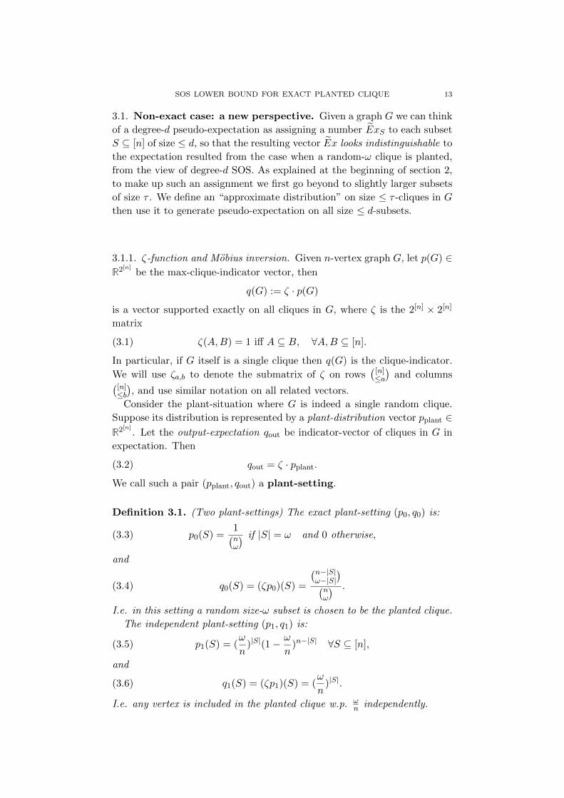
3.1. Non-exact case: a new perspective. Given a graph G we can think
of a degree-d pseudo-expectation as assigning a number ExS to each subset
S ⊆ [n] of size ≤ d, so that the resulting vector Ex looks indistinguishable to
the expectation resulted from the case when a random-ω clique is planted,
from the view of degree-d SOS. As explained at the beginning of section 2,
to make up such an assignment we first go beyond to slightly larger subsets
of size τ . We define an “approximate distribution” on size ≤ τ -cliques in G
then use it to generate pseudo-expectation on all size ≤ d-subsets.
3.1.1. ζ-function and Mobius inversion. Given n-vertex graph G, let p(G) ∈R2[n] be the max-clique-indicator vector, then
q(G) := ζ · p(G)
is a vector supported exactly on all cliques in G, where ζ is the 2[n] × 2[n]
matrix
(3.1) ζ(A,B) = 1 iff A ⊆ B, ∀A,B ⊆ [n].
In particular, if G itself is a single clique then q(G) is the clique-indicator.
We will use ζa,b to denote the submatrix of ζ on rows([n]≤a)
and columns([n]≤b), and use similar notation on all related vectors.
Consider the plant-situation where G is indeed a single random clique.
Suppose its distribution is represented by a plant-distribution vector pplant ∈R2[n] . Let the output-expectation qout be indicator-vector of cliques in G in
expectation. Then
(3.2) qout = ζ · pplant.
We call such a pair (pplant, qout) a plant-setting.
Definition 3.1. (Two plant-settings) The exact plant-setting (p0, q0) is:
(3.3) p0(S) =1(nω
) if |S| = ω and 0 otherwise,
and
(3.4) q0(S) = (ζp0)(S) =
(n−|S|ω−|S|
)(nω
) .
I.e. in this setting a random size-ω subset is chosen to be the planted clique.
The independent plant-setting (p1, q1) is:
(3.5) p1(S) = (ω
n)|S|(1− ω
n)n−|S| ∀S ⊆ [n],
and
(3.6) q1(S) = (ζp1)(S) = (ω
n)|S|.
I.e. any vertex is included in the planted clique w.p. ωn independently.
14 SOS LOWER BOUND FOR EXACT PLANTED CLIQUE
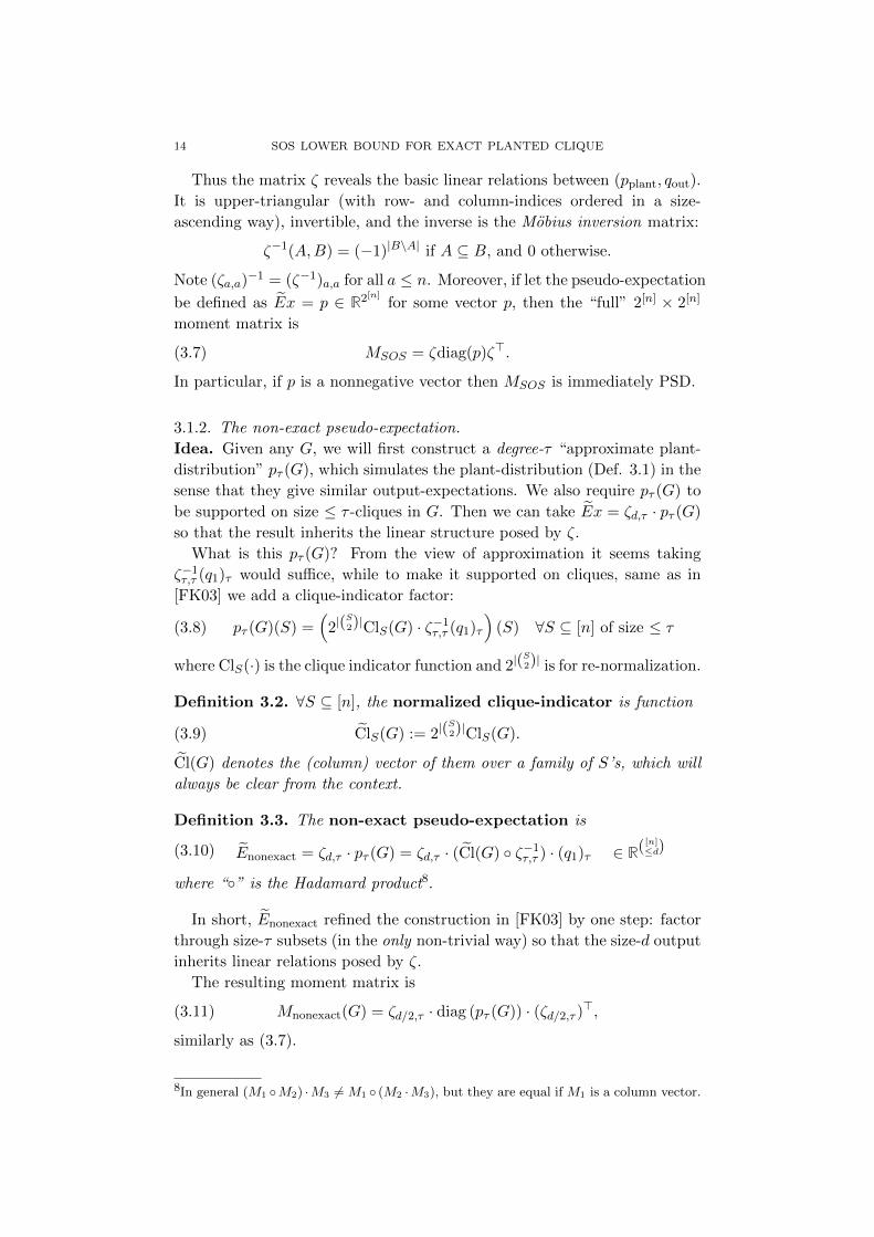
Thus the matrix ζ reveals the basic linear relations between (pplant, qout).
It is upper-triangular (with row- and column-indices ordered in a size-
ascending way), invertible, and the inverse is the Mobius inversion matrix:
ζ−1(A,B) = (−1)|B\A| if A ⊆ B, and 0 otherwise.
Note (ζa,a)−1 = (ζ−1)a,a for all a ≤ n. Moreover, if let the pseudo-expectation
be defined as Ex = p ∈ R2[n] for some vector p, then the “full” 2[n] × 2[n]
moment matrix is
(3.7) MSOS = ζdiag(p)ζ>.
In particular, if p is a nonnegative vector then MSOS is immediately PSD.
3.1.2. The non-exact pseudo-expectation.
Idea. Given any G, we will first construct a degree-τ “approximate plant-
distribution” pτ (G), which simulates the plant-distribution (Def. 3.1) in the
sense that they give similar output-expectations. We also require pτ (G) to
be supported on size ≤ τ -cliques in G. Then we can take Ex = ζd,τ · pτ (G)
so that the result inherits the linear structure posed by ζ.
What is this pτ (G)? From the view of approximation it seems taking
ζ−1τ,τ (q1)τ would suffice, while to make it supported on cliques, same as in
[FK03] we add a clique-indicator factor:
(3.8) pτ (G)(S) =(
2|(S2)|ClS(G) · ζ−1
τ,τ (q1)τ
)(S) ∀S ⊆ [n] of size ≤ τ
where ClS(·) is the clique indicator function and 2|(S2)| is for re-normalization.
Definition 3.2. ∀S ⊆ [n], the normalized clique-indicator is function
(3.9) ClS(G) := 2|(S2)|ClS(G).
Cl(G) denotes the (column) vector of them over a family of S’s, which will
always be clear from the context.
Definition 3.3. The non-exact pseudo-expectation is
(3.10) Enonexact = ζd,τ · pτ (G) = ζd,τ · (Cl(G) ζ−1τ,τ ) · (q1)τ ∈ R([n]
≤d)
where “” is the Hadamard product8.
In short, Enonexact refined the construction in [FK03] by one step: factor
through size-τ subsets (in the only non-trivial way) so that the size-d output
inherits linear relations posed by ζ.
The resulting moment matrix is
(3.11) Mnonexact(G) = ζd/2,τ · diag (pτ (G)) · (ζd/2,τ )>,
similarly as (3.7).
8In general (M1 M2) ·M3 6= M1 (M2 ·M3), but they are equal if M1 is a column vector.
SOS LOWER BOUND FOR EXACT PLANTED CLIQUE 15
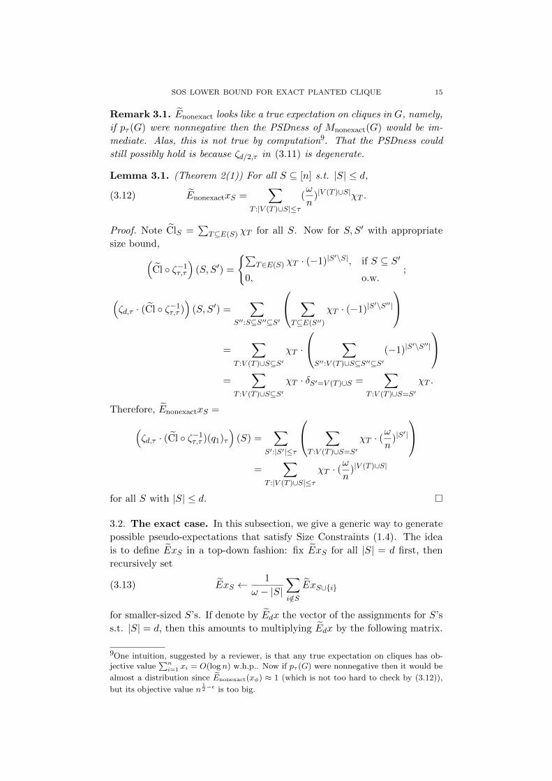
Remark 3.1. Enonexact looks like a true expectation on cliques in G, namely,
if pτ (G) were nonnegative then the PSDness of Mnonexact(G) would be im-
mediate. Alas, this is not true by computation9. That the PSDness could
still possibly hold is because ζd/2,τ in (3.11) is degenerate.
Lemma 3.1. (Theorem 2(1)) For all S ⊆ [n] s.t. |S| ≤ d,
(3.12) EnonexactxS =∑
T :|V (T )∪S|≤τ
(ω
n)|V (T )∪S|χT .
Proof. Note ClS =∑
T⊆E(S) χT for all S. Now for S, S′ with appropriate
size bound,(Cl ζ−1
τ,τ
)(S, S′) =
∑T∈E(S) χT · (−1)|S
′\S|, if S ⊆ S′
0, o.w.;
(ζd,τ · (Cl ζ−1
τ,τ ))
(S, S′) =∑
S′′:S⊆S′′⊆S′
∑T⊆E(S′′)
χT · (−1)|S′\S′′|
=
∑T :V (T )∪S⊆S′
χT ·
∑S′′:V (T )∪S⊆S′′⊆S′
(−1)|S′\S′′|
=
∑T :V (T )∪S⊆S′
χT · δS′=V (T )∪S =∑
T :V (T )∪S=S′
χT .
Therefore, EnonexactxS =(ζd,τ · (Cl ζ−1
τ,τ )(q1)τ
)(S) =
∑S′:|S′|≤τ
∑T :V (T )∪S=S′
χT · (ω
n)|S′|
=
∑T :|V (T )∪S|≤τ
χT · (ω
n)|V (T )∪S|
for all S with |S| ≤ d.
3.2. The exact case. In this subsection, we give a generic way to generate
possible pseudo-expectations that satisfy Size Constraints (1.4). The idea
is to define ExS in a top-down fashion: fix ExS for all |S| = d first, then
recursively set
(3.13) ExS ←1
ω − |S|∑i/∈S
ExS∪i
for smaller-sized S’s. If denote by Edx the vector of the assignments for S’s
s.t. |S| = d, then this amounts to multiplying Edx by the following matrix.
9One intuition, suggested by a reviewer, is that any true expectation on cliques has ob-jective value
∑ni=1 xi = O(logn) w.h.p.. Now if pτ (G) were nonnegative then it would be
almost a distribution since Enonexact(xφ) ≈ 1 (which is not too hard to check by (3.12)),
but its objective value n12−ε is too big.
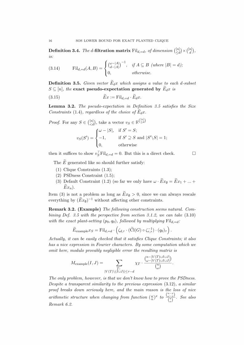
16 SOS LOWER BOUND FOR EXACT PLANTED CLIQUE
Definition 3.4. The d-filtration matrix Fild,=d, of dimension([n]≤d)×([n]d
),
is:
(3.14) Fild,=d(A,B) =
(ω−|A|d−|A|
)−1, if A ⊆ B (where |B| = d);
0, otherwise.
Definition 3.5. Given vector Edx which assigns a value to each d-subset
S ⊆ [n], the exact pseudo-expectation generated by Edx is
(3.15) Ex := Fild,=d · Edx.
Lemma 3.2. The pseudo-expectation in Definition 3.5 satisfies the Size
Constraints (1.4), regardless of the choice of Edx.
Proof. For any S ∈([n]<d
), take a vector vS ∈ R([n]
≤d)
vS(S′) =
ω − |S|, if S′ = S;
−1, if S′ ⊇ S and |S′\S| = 1;
0, otherwise
then it suffices to show v>S Fild,=d = 0. But this is a direct check.
The E generated like so should further satisfy:
(1) Clique Constraints (1.3);
(2) PSDness Constraint (1.5);
(3) Default Constraint (1.2) (so far we only have ω · Ex∅ = Ex1 + ...+
Exn).
Item (3) is not a problem as long as Ex∅ > 0, since we can always rescale
everything by (Ex∅)−1 without affecting other constraints.
Remark 3.2. (Example) The following construction seems natural. Com-
bining Def. 3.5 with the perspective from section 3.1.2, we can take (3.10)
with the exact plant-setting (p0, q0), followed by multiplying Fild,=d:
EexamplexS = Fild,=d ·(ζd,τ · (Cl(G) ζ−1
τ,τ ) · (q0)τ
).
Actually, it can be easily checked that it satisfies Clique Constraints; it also
has a nice expression in Fourier characters. By some computation which we
omit here, modulo provably negligible error the resulting matrix is
Mexample(I, J) =∑T :
|V (T )\(I∪J)|≤τ−d
χT ·
(n−|V (T )∪I∪J |ω−|V (T )∪I∪J |
)(nω
) .
The only problem, however, is that we don’t know how to prove the PSDness.
Despite a transparent similarity to the previous expression (3.12), a similar
proof breaks down seriously here, and the main reason is the loss of nice
arithmetic structure when changing from function (ωn )x to(n−xω−x)(nω)
. See also
Remark 6.2.
SOS LOWER BOUND FOR EXACT PLANTED CLIQUE 17
3.3. The exact pseudo-expectation. Now we pinpoint an exact pseudo-
expectation in Definition 3.5. With the idea stated in detail in the overview
(section 2.1), we give the construction directly.
We take the pseudo-expectation for |S| = d in the form
ExS =∑
T :|V (T )∪S|≤τ
χT · F (|V (T ) ∪ S|)
for some function F . F is called a d-generating function. Then for general
|S| ≤ d, (3.14) gives:
(3.16)
ExS =1(
w−d+uu
) ∑T :|V (T )∪S|≤τ
χT ·[ u∑c=0
(|V (T ) ∪ S| − d+ u
c
)(n− |V (T ) ∪ S|
u− c
)
· F (|V (T ) ∪ S|+ u− c)]
where we have let u := d− |S|.
Lemma 3.3. Any exact pseudo-expectation generated by (3.16) satisfies the
Clique and Size Constraints (1.3),(1.4).
Proof. For Clique Constraints, note (3.16) only depends on |V (T ) ∪ S|, so
by grouping terms ExS =∑
T :|V (T )∪I∪J |≤τ M(I, J ;T )χT factors through
ClI∪J =∑
T⊆E(I∪J) χT . I.e., M(I, J)(G) = 0 if ClI∪J(G) = 0.
It satisfies Size Constraints by Lemma 3.2.
Now we pinpoint a choice of the d-generating function.
Definition 3.6. (Exact d-generating function)
F (x) :=(x+ 8τ2)!
(8τ2)!· (ωn
)x.
Remark 3.3. As is said in the proof overview, the design of F , especially
its first factor, is technical and the ultimate goal is to make the resulting M
positive. The numerator (x + 8τ2)! will be used in Proposition 6.3, where
the term 8τ2 can be replaced by larger polynomials in τ . The (8τ2)! in
denominator is added just for convenience (see Remark 3.4).
Definition 3.7. The exact moment matrix M is
M(A,B) =∑
T :|V (T )∪A∪B|≤τ
M(A,B;T )χT ∀|A|, |B| ≤ d/2
18 SOS LOWER BOUND FOR EXACT PLANTED CLIQUE
where M(A,B;T ) =
(3.17)
1(ω−d+u
u
)[ u∑c=0
(|V (T ) ∪A ∪B| − (d− u)
c
)(n− |V (T ) ∪A ∪B|
u− c
)
·(|V (T ) ∪A ∪B|+ u− c+ 8τ2
)!
(8τ2)!· (ωn
)|(V (T )∪A∪B)|+u−c︸ ︷︷ ︸f(|V (T )∪A∪B|+u−c
)]
and where u = |A ∩B|.
Remark 3.4. In (3.17), the “most significant” factor is (ωn )|V (T )∪A∪B| ·ω−c,
if notice(n−|V (T )∪A∪B|
u−c )(ω−d+uu )
ωun−(u−c) has 0th-order in ω, n. One thing to keep in
mind is that other factors like (|V (T )∪A∪B|+u−c+8τ2)!(8τ2)!
are qualitatively smaller
than ω, within our parameter regime.
4. Preparations
In this section, we prepare some necessary tools for studying the matrices.
4.1. Homogenization for Exact Clique. With the Size Constraints (1.4)
satisfied, any moment matrix can be reduced to its( [n]d/2
)-principal minor,
which is slightly more convenient to work with. The following homogeneity
trick is standard in the SOS literature.
Given any degree-d moment matrix MdSOS(G) that satisfies the Size Con-
straints (1.4), let M(G) be its principal minor on( [n]d/2
)×( [n]d/2
).
Lemma 4.1. MdSOS(G) is PSD ⇔ M(G) is PSD.
Proof. The ⇒ part is trivial. Now suppose MdSOS is not PSD, then
(4.1) ∃a ∈ R( [n]≤d/2) a>MdSOSa = −1.
With the presence of boolean constraints (i.e. define E(x2i · p) := E(xi · p)
for all i and all polynomial p of degree ≤ d− 2), this is equivalent to
(4.2) E(g2) = −1
where g = a>x =∑|S|≤d/2 aSxS is multi-linear. Now substitute every xS
(|S| < d) in (4.2) by the corresponding linear combination of xS′ | |S′| = dfrom (3.13). This does not affect the value of (4.2) since E satisfies these
constraints. We get
(4.3) E(g21) = −1
for some multi-linear, degree-d/2 homogeneous g1. Now translate (4.3) back
(assume g1 = bTx, x = (xS)|S|=d/2) to b>Mb = −1, we see that M is not
PSD.
SOS LOWER BOUND FOR EXACT PLANTED CLIQUE 19
4.2. Concentration bound on polynomials. The following is standard.
Lemma 4.2. Suppose a < log n, and p is a polynomial
p =∑
T : |V (T )|=a
c(T )χT cT ∈ R
and C > 0 is a number s.t. |c(T )| ≤ C for all T . Then W.p. 1 − n−10 logn
over G,
(4.4) |p(G)| < C · na/22a2n4 log logn.
Proof. Power-estimation. For all k ∈ N, (we can think of a < k = o(n/a))
(4.5) p2k =∑
T1,...,T2k: |V (Ti)|=a
c(T1)...c(T2k)χT1 · ... · χT2k
Take expectation of (4.5). Each E[χT1 ...χT2k(G)] 6= 0 (i.e. equals 1) iff every
edge appears even times in T1, ..., T2k, which implies |V (T1 ∪ ... ∪ T2k)| ≤12 · 2ka = ka. There are at most ka
(nka
)< nka many choices of such V (T1 ∪
...∪T2k). For each choice, there are in turn at most(kaa
)·2(a2) < (ka)a ·2a2/2
many ways to choose each Ti. Therefore,
E[p2k] ≤ C2k ·nka(
(ka)a2a2/2)2k
:= N2k where N = Cna/2 · (ka)a ·2a2/2.
By Markov inequality, Pr[p2k > (2N)2k
]< 2−2k. Take k := 10 log2 n, we
get that w.p. > 1− n−10 logn,
|p(G)| < 2N < C · na/22a2n4 log logn
for all large enough n.
4.3. Norm concentration of pseudo-random matrices. Now we state
a concentration bound on pseudo-random matrices which, like in almost all
previous work on the subject, will be a fundamental tool for us.
The pseudo-random matrices refer to the graphical matrices ([MP16]).
Intuitively, such a matrix collects Fourier characters of all embeddings of
a fixed “shape”. Definition 4.1, 4.3 below are implicit in [MP16, MPW15,
HKP15] and is termed explicitly in [BHK+19].
Definition 4.1. A ribbon R is a (ordered) triple (A,B;T ) where A,B are
vertex-sets and T is an edge set. A,B are called the left and right vertex set
of R. The size of R is
|V (R)| = |V (T ) ∪A ∪B|.
By definition, a ribbon R = (A,B;T ) as a graph always has no isolated
vertex outside of A ∪B.
Definition 4.2. We say R = (A,B;T ) is left-generated if every vertex
in V (R) is either in B or can be reached by paths10 from A without touching
B. Being right-generated is symmetrically defined.
10We always stick to the convention of including degenerate paths (one-point path).
20 SOS LOWER BOUND FOR EXACT PLANTED CLIQUE
Definition 4.3. For ribbon (A,B;T ), if further A∪B is totally-ordered, it
is called a shape. Denote a shape by U = (A,B;T ). As before, V (U) =
A ∪B ∪ V (T ), and its size is |V (U)|.
When fixing an underlying vertex-set [n], a ribbon R within vertex set [n]
can always be regarded as shapes, with the induced ordering on vertices. So
in this setting, we may speak of the shape of R and interchangeably use R
to denote shapes.
Definition 4.4. A real-valued function f defined on a set of ribbons within
vertex-set [n] is called symmetric with respect to shapes, if whenever
R and R′ are of the same shape then f(R) = f(R′).
Definition 4.5. ([MP16]) Fix an n, and a shape U = (A,B;T ) Define the
graphical matrix of shape U to be the following 2[n] × 2[n]-matrix MU.
Call a map φ : V (U)→ [n] proper if φ is injective and respects the order on
A ∪B, then
∀I, J ⊆ [n], MU(I, J) =∑
T : ∃proper φ s.t.φ(A)=I,φ(B)=J,φ(T )=T ′
χT ′
(= 0 if no such φ exists). Here, φ on T means the natural induced map on
edges.
Theorem 3. (Norm bounds on MU)([MP16], [BHK+19]) For any shape
U = (A,B;T ) of size t < log n, w.p. > 1− n−10 logn over G,
(4.6) ‖MU(G)‖ ≤ nt−p2 · 2O(t) · (log n)O(t+p−2r)
where r = |A∩B|, p is the maximum number of vertex-disjoint paths between
(A,B) in U. Moreover, this bound is tight up to polylog(n)-factors, for all
MU with the described parameters ([MP16], Thm 38]).
Moreover, under the same notation, if further denote s = |A|+|B|2 then
(4.7) ‖MU(G)‖ ≤ nt−p2 · 2O(t) · (log n)O(t−s).
Theorem 3 is proved by a careful estimation of the trace-power E[tr(M2kU )]
(for some k > 0), which we omit here. Its “moreover” part follows from (4.6)
since t ≥ |A ∪B| = 2s− r, p ≤ s, so
t+ p− 2r ≤ t+ s− 2(2s− t) = 3(t− s).
Remark 4.1. Theorem 3 and its proof is a far-reaching generalization of
that of the concentration bounds on polynomials, Lemma 4.2. Namely, if
take special shapes in the form U = (A,A;T ), then the corresponding matrix
MU is diagonal, so estimating its norm is equivalent to estimating absolute
values of the diagonals which are polynomials.
4.4. Some general notions on graphs. We finish our preparation with
some general graph-theoretic notions.
SOS LOWER BOUND FOR EXACT PLANTED CLIQUE 21
Definition 4.6. (Vertex-separator) Given graph H and two vertex-subsets
A,B ⊆ V (H), call S ⊆ V (H) an (A,B)-vertex-separator if any path11
from A to B in H must pass through S. Let
sA,B(H) := min|S| | S is an (A,B)-vertex-separator.
A vertex-separator achieving this minimum is a min-separator. mSepA,B(H)
denotes the set of all min-separators.
This definition naturally applies to ribbons R = (A,B;T ), by using the
graph H as on V (T )∪A∪B with edge-set T . In that case we can write the
corresponding size and set of the min-separators as
sA,B(T ), mSepA,B(T ) or mSep(R).
Menger’s theorem: For any finite graph H, sA,B(H) equals to the maxi-
mum number of vertex-disjoint paths from A to B in H.
Definition 4.7. For ribbon R = (A,B;T ), let us define its reduced size
to be
(4.8) eA,B(T ) := |V (T ) ∪A ∪B| − sA,B(T ).
The reduced size is double of the exponent in n in the bound of Theorem
3, hence is the controlling parameter of the norm of the graphical matrix.
5. Non-exact case PSDness: a refreshing
In this section, we review and refresh the proof techniques for the non-
exact problem. In section 5.1 and 5.2, we show Theorem 2(2) via the so-
called mod-order analysis, which gives a conceptually different approach to
the techniques. In section 5.3, we formalize the recursive factorization in a
convenient language and extend it properly for later use.
Declaration. Section 5.2 is only for Theorem 2(2). The reader can safely
skip it if she wants to proceed directly to the proof of Theorem 1.
Notation. Thoughout section 5, M ′ denotes the([n]d2
)×([n]d2
)-minor12 of the
non-exact moment matrix.
(5.1) M ′(I, J) =∑
T :|V (T )∪I∪J |≤τ
(ω
n)|V (T )∪I∪J |χT ∀I, J ∈
([n]
d/2
).
Goal of section 5. Diagonalize M ′ approximately, such that the difference
matrix is negligible (w.h.p. when plugging G).
5.1. Step 1: Diagonalization of E[M ′].
11Same as in the previous footnote. In particular, every vertex-separator contains A∩B.12Strictly speaking, PSDness of this minor is not sufficient as we do not have a homogeneityreduction in non-exact case. Nevertheless, it suffices to demonstrate the idea.
22 SOS LOWER BOUND FOR EXACT PLANTED CLIQUE
Proposition 5.1. E[M ′] = CC>, where C is the( [n]d/2
)×( [n]≤d/2
)-matrix
(5.2) C = (ζ>)d/2,≤d/2 · diag
(√t(|A|)
)A∈( [n]
≤d/2)
and t(r) = (1−O(dωn )) · (ωn )d−r for all r = 0, ..., d/2.
This can be shown by a similar calculation as in [MPW15], as below.
Definition 5.1. (See e.g. [Del73]) Fix parameters n, k. A Johnson scheme
J is an([n]k
)×([n]k
)-matrix that satisfies J(I, J) = J(I ′, J ′) whenever |I∩J | =
|I ′ ∩ J ′|.
It can be checked that (fix n, k) all Johnson schemes are symmetric ma-
trices and form a commutative R-algebra, so they are simultaneously diag-
onalizable. In below we fix n and k = d/2. An obvious R-basis for Johnson
schemes is D0, ..., Dd/2 where
(5.3) Dr(I, J) =
1, if |I ∩ J | = r
0, o.w.∀I, J ∈
(S
d/2
).
Another basis which we denote by J0, ..., Jd/2 is
(5.4) Jr(I, J) =
(|I ∩ J |r
), ∀I, J ∈
([n]d2
).
J0, ..., Jd/2 are PSD matrices since
(5.5) Jr =∑
A⊆[n],|A|=r
uAu>A where uA ∈ R([n]k ), uA(B) = 1A⊆B.
Clearly Jd/2 = Id. More generally, we have:
Fact 1. (See e.g. (4.29) in [Del73]) The Johnson schemes (for (n, d/2))
have shared eigenspace-decomposition R( [n]d/2) = V0 ⊕ ...⊕ Vd/2, and
Jr =
d2⊕i=0
λr(i) ·Πi for r = 0, ..., d/2
where Πi is the orthogonal projection to Vi w.r.t. the Euclidean inner prod-
uct, and the eigenvalues are
λr(i) =
(d2 − ir − i
)(n− d
2 − id2 − r
), 0 ≤ i ≤ d
2.
Lemma 5.1. E[M ′] =∑d/2
r=0 t(r)Jr where each t(r) = (1−O(dωn )) · (ωn )d−r.
Proof. By definition, E[M ′] =∑d/2
r=0(ωn )d−rDr. Note each Dr decomposes as
(5.6) Dr =
d/2∑r′=r
(−1)r′−r(r′
r
)· Jr′
SOS LOWER BOUND FOR EXACT PLANTED CLIQUE 23
since RHS(I, J) =d/2∑r′=r
(−1)r′−r(r′
r
)(|I∩J |r′
)=|I∩J |∑r′=r
(−1)r′−r(|I∩J |
r
)(|I∩J |−rr′−r
)=(|I∩J |
r
)· 1|I∩J |=r = 1|I∩J |=r. So together,
(5.7)
E[M ′] =
d/2∑r=0
(ω
n)d−r
d/2∑r′=r
(−1)r′−r(r′
r
)Jr′
=
d/2∑r′=0
Jr′ ·
(r′∑r=0
(ω
n)d−r(−1)r
′−r(r′
r
))
=
d/2∑r′=0
Jr′ · (ω
n)d−r
′(1− ω
n)r′
which proves the lemma.
By Lemma 5.1 and (5.5), if let t(r) = (ωn )d−r′[1− ω
n ]r′
then
E[M ′] =∑
A:|A|≤d/2
t(|A|)uAu>A=(ζ>)d/2,≤d/2 · diag
(t(|A|)
)· ζ≤d/2,d/2 = CC>,
where used that the matrix (ζ>)d/2,≤d/2 has columns uA | |A| ≤ d/2. This
proves Proposition 5.1.
5.2. Step 2: Mod-order analysis toward “coarse” diagonalization.
Given E[M ′] = CC>, ideally we hope to continue to solve for
(5.8) M ′ = NN>
with E[N ] = C, and N extending C by non-trivial Fourier characters. Also,
we restrict ourselves to symmetric solutions w.r.t. shapes (Def. 4.4).
Toward this goal, we define and study a relaxed equation first (Definition
5.2). Let us start with its motivation.
(1) Order in ωn . Entries of M ′ all have a clear order in ω
n . Like in fixed-
parameter problems, we treat ωn as a distinguished structural parameter and
try to solve the correct power of ωn in terms in N .
(2) Norm-match. Let’s have a closer look into
E[M ′] = CC> =
d/2∑r=0
(1−O(dω
n)) · (ω
n)d−rJr.
By fact 1, each Jr b has norm(d/2r
)· nd/2−r so
(5.9)∥∥∥CrC>r ∥∥∥ ≈ (d/2r
)· (ωn
)d−rnd/2−r, r = 0, ..., d/2.
We expect Nr(Nr)> to concentrate around Cr(Cr)
>, so the norm of the
“random” part, i.e. matrix of nontrivial Fourier characters in Nr(Nr)>, is
expected to be bounded by (5.9). The tight bound from Theorem 3 tells
how this may happen, which we review below.
24 SOS LOWER BOUND FOR EXACT PLANTED CLIQUE
It will be convenient to use a scaling of variables: let
L = (L0, ..., L d2) = (Nr · (
ω
n)−|A|
2 )0≤r≤ d2,
then
(5.10) M ′ = L·diag(
(ω
n)|A|)·L> with E[L] = ( Cr ·(
ω
n)−r/2 )r=0,1,...,d/2.
Now suppose
Lr(I, A) =∑
small T
βI,A(T )χT , A ∈(
[n]
r
)where assume as in (1), an order of ω
n can be separated:
(5.11) βI,A(T ) = (ω
n)x︸ ︷︷ ︸
main-order term
· ( factor n
ωand ω
n).
Fix I, A, T , we are looking for the condition on x in order to have the
expected norm control on Lr(ωn )r(Lr)
>. Ignore for a moment the cross-
terms, such a single graphical matrix square in Lr(ωn )rL>r is
(ω
n)2xR(I,A;T ) · (
ω
n)r ·R>(I,A;T )
which has norm13
/ (ω
n)2x+r · neI,A(T ) · 2O(|V (T )∪I∪A|) · (log n)>0
by Theorem 3. Here recall eI,A(T ) = |V (T )∪ I ∪A| − sI,A(T )(≥ |I| − |A| =d2 − r). Compare this with (5.9), we need (ωn )2xneI,A(T ) <
(d/2r
)( ω√
n)d/2−r.
If think of 2d as qualitatively smaller than any positive constant power of
ω, n, the natural bound to put is x ≥ eI,A(T ) which actually is the limit
requirement when logωlogn →
12 . Suggested by this, we will set the restriction
x ≥ eI,A(T ) right from the start in the relaxed equation.
The above motivation leads to the following definition. Take a ring A by
adding fresh variables α and χT ’s to R, where T ranges over subsets of(
[n]2
)and they only satisfy relations χT ′ · χT ′′ = χT : T ′ ⊕ T ′′ = T.
Definition 5.2. The mod-order equation is
(5.12) Lα · diag(α|A|
)· (Lα)> = Mα mod (∗)
on the( [n]d/2
)×( [n]≤d/2
)matrix variable Lα in ring A, where
Mα(I, J) :=∑
T :|V (T )∪I∪J |≤τ
α|V (T )∪I∪J |χT ,
13Here the matrix is naturally truncated from 2[n] × 2[n], which doesn’t change anythingsince the original matrix is always 0 elsewhere.
SOS LOWER BOUND FOR EXACT PLANTED CLIQUE 25
and mod (∗) is the modularity, which means position-wise mod the ideal(α|V (T )∪I∪J |+1χT , χT : |V (T ) ∪ I ∪ J | > τ
).
Moreover, if denote Lα(I, A) =∑
T βI,A(T )χT where βI,A(T ) ∈ R[α], then14
(5.13) αeI,A(T ) | βI,A(T ) ∀I, A, T.
We are interested in solutions that are symmetric, i.e. βI,A(T ′) = βJ,B(T ′′)
whenever (I, A;T ′), (J,B;T ′′) are of the same shape.
The following is the key observation. Its proof demonstrates how to make
deductions from the mod-order equations efficiently, and is presented in
Appendix A.1.
Lemma 5.2. (Order match) If a product α|A| · βI,A(T ′) · βJ,A(T ′′) from the
LHS of (5.12) is nonzero mod (∗), then both of the following hold:
A is a min-separator for both (I, A;T ′), (J,A;T ′′);(5.14) (V (T ′) ∪ I ∪A
)∩(V (T ′′) ∪ J ∪A
)= A.(5.15)
Moreover, (5.14), (5.15) imply that
A is a min-separator of (I, J ;T ) (where T = T ′ ⊕ T ′′);(5.16)
|V (T ′) ∪ I ∪A|, |V (T ′′) ∪ J ∪A| ≤ τ.(5.17)
By this lemma, in an imagined solution we can assume βI,A(T ′) 6= 0 only
when it satisfies its part in conditions (5.14), (5.17).
Using this information, plus a further technique of polarization, we can
deduce the following Proposition 5.2 which is the main takeaway of the anal-
ysis here. A graph-theoretic fact (the “in particular” part below) appears
exactly as the solvability condition. For deductions see Appendix A.2.
Fact 2. ([Esc72]) For any ribbon (I, J ;T ), the set of all min-separators,
mSepI,J(T ), has a natural poset structure: min-separators A1 ≤ A2 iff
A1 separates (I, A2;T ), or equivalently as can be checked, iff A2 separates
(J,A1;T ). The set is actually a lattice under this partial-ordering: ∀A1, A2 ∈mSepI,J(T ) their join and meet exist. In particular, there exist unique min-
imum and maximum.
Denote the minimum by Sl(I, J ;T ) and the maximum by Sr(I, J ;T ),
which is the “leftmost” and “rightmost” min-separator, respectively.
Proposition 5.2. (Mod-order diagonalization) Let
Lα(I, A) :=∑
T ′: |V (T ′)∪I∪A|≤τA=Sl(I,A;T ′)T ′∩E(A)=∅
(I,A;T ′) left-generated (Def. 4.2)
αeI,A(T ′)χT ′ ,
14Recall eI,A(T ′) is the reduced size |V (T ′) ∪ I ∪A| − sI,A(T ′) (Def. 4.7).
26 SOS LOWER BOUND FOR EXACT PLANTED CLIQUE
Q0,α(A,B) :=∑
Tm: |T∪A∪B|≤τA,B∈mSepA,B(Tm)
αeA,B(Tm)χTm
(Tm to indicate “middle”). Then
(5.18) Lα · [diag(α|A|2
)·Q0,α · diag
(α|A|2
)] · L>α = Mα mod (∗)
where recall (∗) means ideal (α|V (T )∪I∪J |+1χT , χT : |V (T )∪ I ∪J | > τ)position-wise on each (I, J).
Equation (5.18) is slightly weaker than a solution to (5.12) but is sufficient
for all use. In particular, it gives the first-approximate diagonalization of
the matrix M ′, recast as Definition 5.3 below. This shows Theorem 2(2).
5.3. Recursive factorization. In this subsection, we give a formalization
and extension of the recursive factorization technique, which is used to refine
the coarse diagonalization from Step 2 above. We give some new notions
that are convenient and extendable to matrix products (Def. 5.5, 5.6), along
with some simplification (Lem. 5.4) and refinement (Prop. 5.4) for later use.
First, the coarse diagonalization (5.18) can be recast in R[χT ]-matrices
as below.
Definition 5.3. Let L be the([n]d2
)×( [n]
≤ d2
)-matrix
(5.19) L(I, A) :=∑
T ′: |V (T ′)∪I∪A|≤τA=Sl(I,A;T ′)T ′∩E(A)=∅
(I,A;T ′) left-generated
(ω
n)|V (T ′)∪I∪A|−|A|χT ′ ,
and Q0 be the( [n]
≤ d2
)×( [n]
≤ d2
)-matrix
(5.20) Q0(A,B) :=∑
Tm:|Tm∪A∪B|≤τA,B∈mSepA,B(Tm)
(ω
n)|V (Tm)∪A∪B|χTm .
Finally, let
(5.21) D := diag(
(ω
n)|A|2
)A∈( [n]
≤d/2).
We call L(DQ0)L> the first-approximate diagonalization of M ′.
Despite of its name (“approximate”), the difference
(5.22) M ′ − L(DQ0D)L>
is, however, far from negligible. This is where the recursive factorization
will be applied, and in the end it will give
(5.23) M ′ = L · [D · (Q0 −Q1 +Q2...±Qd/2) ·D] · L> + E
for some negligible error-matrix E.
SOS LOWER BOUND FOR EXACT PLANTED CLIQUE 27
Remark 5.1. Use of D is superficial in (5.22), (5.23); we keep it so that
the middle matrices Qi are better-positioned. The LD here corresponds to
the “L” matrix in [BHK+19].
Let us start with some necessary notions.
5.3.1. More notion on graphs.
Definition 5.4. ([BHK+19] Def. 6.515) For any ribbon R = (I, J ;T ), its
canonical decomposition is a ribbon-triple
(Rl,Rm,Rr) = ((I, A;Tl), (A,B;Tm), (B, J ;Tr))
determined uniquely by the following. A = Sl(I, J ;T ), B = Sr(I, J ;T ).
V (Rl) is A unioned with the set of vertices reachable by paths from I in T
without touching A, and Tl = T |V (Rl)\E(A). Similarly, V (Rr) is B unioned
with the set of the vertices reachable from J in T without touching B, and
Tr = T |V (Rr)\E(B). Finally, Tm = T\(T ′ t T ′′).Rl, Rm, Rr are called the left-, middle-, right- ribbon of R, respec-
tively.
Remark 5.2. (Properties of the canonical decomposition) A few properties
follow from the definition of the canonical decomposition of R = (I, J ;T ).
A = Sl(I, A;Tl), B = Sr(B, J ;Tr)
(so they are unique separator of Rl,Rr, respectively);
Tl ∩ E(A) = ∅ = Tr ∩ E[A];
Rl is left-generated, Rr is right-generated (Def. 4.2);
A,B ∈ mSepA,B(Tm) (so |A| = |B|).The above four are about each of Rl, Rm, Rm (the “inner” conditions).
Moreover, there is the intersection property on pairs of them (the “outer”
conditions)16:
V (Rl) ∩ V (Rm) ⊆ A, V (Rm) ∩ V (Rr) ⊆ B, V (Rl) ∩ V (Rr) ⊆ A ∩B
which implies
(5.24) e(Rl) + |V (Rm)|+ e(Rr) = |V (R)|.
The canonical decomposition can be reversely described as follows.
Definition 5.5. (Inner and outer canonicality) For a triple of ribbons in
the form
(Rl,Rm,Rr) =
((I, A;Tl), (A,B;Tm), (B, J ;Tr)
)15Similar notions actually appeared implicitly in the mod-order analysis (cf. condition(5.14), (5.15)), while here they appear in a more “canonical” left-, middle-, right- form.16cf. conditions (5.14), (5.15)
28 SOS LOWER BOUND FOR EXACT PLANTED CLIQUE
(Tl, Tm, Tr are arbitrary subsets of an edge-set), their ribbon-sum is ribbon
(I, J ;T ) where T = Tl ⊕ Tm ⊕ Tr.
The triple is called inner-canonical, if they satisfy the “inner” conditions:
(5.25)
A = Sl(I, A;Tl), B = Sr(B, J ;Tr),
Tl ∩ E(A) = ∅ = Tr ∩ E[A],
Rl left-generated, Rr right-generated,
A,B ∈ mSepA,B(Tm).
The triple is outer-canonical if they satisfy the “outer” condition:
(5.26) V (Rl)∩V (Rm) ⊆ A, V (Rm)∩V (Rr) ⊆ B, V (Rl)∩V (Rr) ⊆ A∩B.
The triple is a canonical triple if it is both inner- and outer- canonical.
Proposition 5.3. Canonical triples are 1-1 correspondent to their ribbon-
sum, via the canonical decomposition.
Proof. This follows by an immediate check from the definition.
We further extend the notions to matrix products. Recall R[χT ] is the
ring from adding fresh variables χT ’s into R for every T ⊆(
[n]2
)(fixing an
n), with relations χT ′ · χT ′′ = χT | T ′ ⊕ T ′′ = T.
Definition 5.6. (Approximate form) Suppose matrices X,Y have rows and
columns indexed by subsets of [n] with entries in R[χT ]; and in every entry,
each character regarded as a ribbon on distinguished sets (row, column) has
ribbon size ≤ τ . Suppose X,Y have dimensions s.t. XYX> is defined.
Every nonzero triple product (without collecting like-terms) in
(5.27) XYX>
thus has form
(5.28) X(I, A;Tl)Y (A,B;Tm)X(J,B;Tr)︸ ︷︷ ︸nonzero in R
χTl · χTm · χTr ,
and can be identified with a ribbon-triple in the natural way, with
X(I, A;Tl)Y (A,B;Tm)X(J,B;Tr)χTl⊕Tm⊕Tr ∈ R[χT ]
its resulting term. We say (5.28) is an outer-canonical product if the
ribbon-triple is outer-canonical, and it exceeds degree if |V (T )∪I∪J | > τ .
The approximation form of XYX> is:
(5.29) XYX> =(XYX>
)can
+ (XYX>)non-can + Edeg,
or equivalently,(XYX>
)can
= XYX> − (XYX>)non-can − Edeg,
SOS LOWER BOUND FOR EXACT PLANTED CLIQUE 29
where(XYX>
)out-can
is the matrix collecting all terms of outer-canonical
products that do not exceed degree, (XYX>)non-can collecting all terms of
non-outer-canonical products, and Edeg collecting all rest terms.
Remark 5.3. With this language, Proposition 5.3 gives an a posteriori ex-
planation of the coarse diagonalization (Def. 5.3): M ′ = [L(DQ0D)L>]can.
5.3.2. Recursive factorization: the machinery. We start with the fol-
lowing, which is Definition 5.3 restated in the current language.
Definition 5.7. (First-approximate factorization of M ′)
(5.30) M ′ = L(DQ0D)L> − [L(DQ0D)L>]non-can − E1;deg
where E1;deg is by Def. 5.6, applied to the product L(DQ0D)L>, where the
index “1” is added for later convenience. L(DQ0D)L> is celled the first-
approximate factorization of M ′.
The high-degree error E1;deg is actually negligible in norm17 (we will prove
the analogous statement in the exact case); the main task is to analyze the
“main error”, [L(DQ0D)L>]non-can. For this, the key point of the whole
technique is
[L(DQ0D)L>]non-can itself factors through L,L> approximately, too.
I.e. ∃Q1 s.t.
(5.31) [L(DQ0D)L>]non-can = [L(DQ1D)L>]can + E′1;negl.
for some negligible E′1;negl. And we can repeat this for [L(DQ1D)L>]non-can
and so on. To describe the factorization (5.31), a generalized notion is useful.
Definition 5.8. ([BHK+19], Def. 6.9)18 A generalized ribbon is a usual
ribbon together with a new set of isolated vertices. In symbol, it is denoted
as R∗ = (A,B;T ∗) where
T ∗ = T t I,
T an edge-set, I a vertex set disjoint from V (T )∪A∪B, called the isolated
vertex-set of R∗, denoted as I(R∗). V (R∗) = V (T ) ∪ A ∪ B ∪ I. A usual
ribbon is also a generalized ribbon with I = ∅. (A,B;T ) is called the (unique)
largest ribbon in R.
Remark 5.4. I(R∗) could be different from the isolated set of the underlying
graph, as it excludes vertices in A ∪B.
Definition 5.9. A side-inner-canonical triple is
(Rl,Rm,Rr) = ((I, A;Tl), (A,B;Tm), (B, J ;Tr))
where Rl, Rr are ribbons satisfying the inner-canonical conditions on their
part (the first three of (5.25)), while Rm is just a ribbon.
17Matrices considered all have support on clique-rows and clique-columns, given G.18It was called improper ribbon, but we feel the name here is perhaps more proper.
30 SOS LOWER BOUND FOR EXACT PLANTED CLIQUE
The following operation is the technical core of recursive factorizations.
Definition 5.10. (Separating factorization; Def. 6.10 of [BHK+19]) Given
an side-inner-canonical tripe
(Rl,Rm,Rr) = ((I, A;Tl), (A,B;Tm), (B, J ;Tr)),
denote T = Tl ⊕ Tm ⊕ Tr, and denote by Z the multi-set of “unexpected
intersections” i.e. multi-set of vertices from (Rl ∩Rm)−A, (Rm ∩Rr)−B,
(Rl ∩Rr)− (A ∩B). Call z(Rl,Rm,Rr) = |Z| the intersection size of the
triple. It can be checked that
(5.32) |V (Rl)∪V (Rm)∪V (Rr)| = |V (Rl)|+|V (Rm)|+|V (Rr)|−|A|−|B|−z.
We further separate this triple into an “outer-canonical” one, as follows.
Define S′l to be the leftmost min-separator of (I, A∪ (Z ∩V (Rl));Tl), and
similarly S′r the right-most min-separator of (B ∪ (Z ∩ V (Rr)), J ;Tr). Note
S′l, S′r ⊆ V (T ) ∪ I ∪ J from definition.
Define ribbon R′l = (I, S′l;T′l ), whose vertex set V (R′l) is S′l unioned with
the set of vertices in Rl reachable from I by paths in Tl without touching S′l,
and T ′l is Tl\E(S′l) restricted to V (R′l). Ribbon R′r is symmetrically defined.
In particular, T ′l ∩T ′r = ∅. R∗m is the generalized ribbon (S′l, S′r;T
∗m) where
T ∗m = T\(T ′l t T ′r) t I(R∗m),
I(R∗m) collecting all the rest isolated vertices:
(5.33) I(R∗m) = V (Rl) ∪ V (Rm) ∪ V (Rr) − V (T ) ∪ I ∪ J.
The resulting (R′l,R∗m,R
′r) is called the separating factorization of ribbon
triple (Rl,Rm,Rr), which we denote as
(5.34) (Rl,Rm,Rr)→ (R′l,R∗m,R
′r).
Remark 5.5. (Properties of separating factorization) Some natural proper-
ties follow. Let (Rl,Rm,Rr)→ (R′l,R∗m,R
′r) in the same notation as above.
(1).The resulting triple (R′l, R∗m,R
′r) is side-inner-canonical and outer-
canonical (i.e. their pair-wise vertex intersections are within the correspond-
ing S′l, S′r and S′l ∩ S′r). So the corresponding ribbon triple (from replacing
R∗m with its largest ribbon) is canonical and is disjoint from I(R∗m).
(2). R′l ⊆ Rl, and S′l separates (V (R′l), V (Rl) − V (R′l)) in Rl. In par-
ticular, we can talk about the part of Rl to the right of S′l, which is disjoint
from R′l and actually can be easily checked to be in R∗m. Similar fact holds
for Rr.
(3). Since S′l separates (I, A) in Rl, and A is the unique min-separator of
Rl, there are |A| many vertex-disjoint paths from A to S′l in Rl. Similarly
for Rr.
Lemma 5.3. (Lemma 6.14, 7.14 of [BHK+19]) Suppose (Rl,Rm,Rr) →(R′l,R
∗m,R
′r). In the same notation as in Definition 5.10,
(1). |S′l|+ |S′r| ≥ |A|+ |B|+ 1;
SOS LOWER BOUND FOR EXACT PLANTED CLIQUE 31
(2).19 If further denote s = |A|+|B|2 , p′ the maximum number of vertex-
disjoint paths from S′l to S′r in R∗m, and p the maximum number of vertex-
disjoint paths from A to B in Rm, then
2(s′ − s) + (p− p′) + |I(R∗m)| ≤ z(Rl,Rm,Rr).
Proof. (1). By definition there must be some unexpected pair-wise intersec-
tion between (Rl,Rm,Rr). In either of the three cases of breaking (5.26),
∃v ∈ Z that is in V (Rl) − A or in V (Rr) − B. WLOG suppose the first
happens. Then S′l 6= A since v can be reached from I without passing A by
the left-generated condition on Rl. Similarly, if |S′l| = |A| then it is A as
A is the unique min-separator separating (I, A), so this is impossible. Thus
S′l > A.
(2). We refer the reader to its proof in the original paper.
Now we apply the above machinery to the target, L(DQ0D)L>.
5.3.3. Apply the machinery. Conceptually, the separating factorization
tells us how to “cancel” the terms in [L(DQ0D)L>]non-can using L,L>.
Namely, in L(DQ0D)L>, any product from (Rl,Rm,Rr) (Def.5.6) that is
non-outer-canonical results in a term in [L(DQ0D)L>]non-can at (I, J), and
we can cancel it by the product from its separating factorization (R′l,R∗m,R
′r):
take R′l at position (I, S′l) in L, R′r at position (S′r, J) in L>, and the largest
ribbon of R∗m at (S′l, S′r) in a new middle matrix DQ1D. I.e., we cancel it
by −[L(DQ1D)L>]can.
Of course, there are other triples whose separating factorization result
in the same (R′l, largest ribbon of R∗m, R′r) so we need to collect them all
in DQ1D. More seriously, the (I, S′l)th entry of L is actually a sum of
different R′ls, so we need to make sure that this cancellation works for them
simultaneously in multiplication.
The following is what insures the simultaneous cancellation can work. It
is stated in a refined version that is more than needed here (i.e. we further
distinguish different (i, j) parameters), but this will be needed in the exact
case (Lemma 6.6).
Proposition 5.4. (Solvability condition)(cf. Claim 6.12 in [BHK+19]) Fix
(I, J, S′l, S′r), and a generalized ribbon R∗m on (S′l, S
′r). Let (R′l,R
′r) be inner-
canonical left and right ribbons with distinguished sets (I, S′l), (S′r, J) respec-
tively, as in Definition 5.5. Let (R′′l ,R′′r) be another such ribbon pair, with
the same reduced size
e(R′l) = e(R′′l ), e(R′r) = e(R′′r).
19Recall in our setting Rm is always a ribbon, without any isolated vertex.
32 SOS LOWER BOUND FOR EXACT PLANTED CLIQUE
(Or the same size, equivalently.) Then for every fixed tuple (i, j, z) the fol-
lowing holds: there is an 1-1 matching between ribbon-triples
(Rl,Rm,Rr) s.t.
(Rl,Rm,Rr)→ (R′l,R
∗m,R
′r),
(e(Rl), e(Rr), z(Rl,Rm,Rr)) = (i, j, z).(5.35)
and
(Rl,Rm,Rr) s.t.
(Rl,Rm,Rr)→ (R′′l ,R
∗m,R
′′r),
(e(Rl), e(Rr), z(Rl,Rm,Rr)) = (i, j, z).(5.36)
Moreover, this matching fixes every middle Rm.
Proof. We give a reversible map from the set of (5.35) onto the set of (5.36).
Take a (Rl,Rm,Rr) from (5.35). By Remark 5.5 (2), the part of Rl to the
right of S′l is in R∗m hence is disjoint from both R′l and R′′l . Similarly for R′r,
Rr. Now take the map
(Rl,Rm,Rr) 7→ (φ(Rl),Rm, φ(Rr))
where φ(Rl) replace R′l to R′′l within Rl, and φ(Rr) replaces R′r to R′′r within
Rr. Clearly R∗m, thus Rm, is unchanged. Also, as R′l, R′′l have the same size
by assumption, by the disjointness above this replacement operation keeps
the size of Rl. Moreover, Rl, φ(Rl) have the same right distinguished set
which is the unique min-separator of both, so e(Rl) = e(φ(Rl)). Similarly
for Rr, φ(Rr), so the parameter (i, j) is unchanged by φ. The intersec-
tion parameter z is unchanged too, since the changed part is disjoint from
Z(Rl,Rm,Rr). Finally, the inverse map is given the same way by changing
the role of (R′l,R′r) and (R′′l ,R
′′r).
The following lemma will be repeatedly used.
Lemma 5.4. (One round of factorization) Let L be as (5.19), and Q be any( [n]≤d/2
)×( [n]≤d/2
)-matrix with entries
(5.37) Q(A,B) =∑
Tm: |V (Tm)∪A∪B|≤τ
(ω
n)|V (Rm)|q(Rm) · χTm
where Rm denotes (A,B;Tm), and q(·) is a function symmetric w.r.t. shapes.
Define matrix Q′,E′negl as follows so that
(5.38) (LQL>)non-can = (LQ′L>)can + E′negl
holds. First, let
(5.39) Q′(A,B) =∑
Tm: |V (Tm)∪A∪B|≤τ
(ω
n)|V (Rm)|q′(Rm) · χTm
where q′(Rm) is as follows. Fix any Rm = (A,B;Tm) and let t = |V (Rm)| ≤τ , s = |A|+|B|
2 . For every generalized ribbon R∗m that contains Rm as its
largest ribbon and |V (R∗m)| ≤ τ , fix a ribbon pair (R′l,R′r) s.t. (R′l,R
∗m,R
′r) is
the separating factorization for some ribbon triple with |V (R′l)|, |V (R′r)| ≤ τ
SOS LOWER BOUND FOR EXACT PLANTED CLIQUE 33
(if there is none, exclude this R∗m in the summation below). Then let
(5.40)
q′(Rm) =∑
R∗m: gen. ribbon on (A,B)|V (R∗m)|≤τ
largest ribbon is Rm
(ω
n)|I(R
∗m)| · q′′(R∗m), where
q′′(R∗m) =∑
1≤z≤d/2
∑P=(Rl,R,Rr): side-inn. can.
P→(R′l,R∗m,R
′r) for the fixed R′l,R
′r
z(P)=z
(ω
n)z · q(R).
Note q′(Rm) doesn’t depend on the choice (R′l,R′r) by Proposition 5.4, and
q′(·) is also symmetric w.r.t. shapes. Now define E′negl s.t. (6.32) holds.
Then the conclusions are:
(1). W.p. > 1− n−9 logn over G,∥∥∥E′negl
∥∥∥ ≤ maxq(A,B;T ) · n−ετ ;
(2). If there is a number C for which
(5.41) ∀Rm |q(Rm)| ≤ C · ( ω
n1−ε )s−p
where p denotes the maximum number of vertex-disjoint paths between A,B
in Rm.20 Then
∀Rm |q′(Rm)| ≤ C · ( ω
n1−ε )s−p+1/3.
Proof. We compare [LQ′L>]can with [LQL>]non-can as step (0), then prove
(1), (2).
(0). For any fixed (I, J), recall [LQL>]non-can(I, J) is
(5.42) ∑(Rl,Rm,Rr): side. inn. can.
non-outer-can.all three have size ≤τ
(ω
n)|V (Rl)|+|V (Rm)|+|V (Rr)|−|A|−|B|q(Rm)χTl⊕Tm⊕Tr
where we denoted the distinguished sets of Rm by (A,B) when Rm is given.
For each (Rl,Rm,Rr) in it, there is a unique (R′l,R∗m,R
′r) that is its sepa-
rating factorization: (Rl,Rm,Rr)→ (R′l,R∗m,R
′r). There are two cases.
First case: |V (R∗m)| ≤ τ . In this case, there is the corresponding term
(5.43) (ω
n)|V (R′l)|+|V (R′m)|+V (R′r)|−|S′l |−|S
′r| · (ω
n)z+|I(R
∗m)| · q(R′m)χT ′l⊕T ∗m⊕T ′r
in (LQ′L>)can(I, J), where R′m denotes the largest ribbon of R∗m and χT ∗mmeans the character from R′m, and z ≥ 1 is the intersection size of (Rl,Rm,Rr).
Recall for the separating factorization, T ′l ⊕ T ∗m ⊕ T ′r = Tl ⊕ Tm ⊕ Tr and
|V (Rl) ∪ V (Rm) ∪ V (Rr)| = |V (R′l)|+ |V (R∗m)|+ |V (R′r)| − |S′l| − |S′r|= |V (Rl)|+ |V (Rm)|+ |V (Rr)| − |A| − |B| − z
Also, |V (R∗m)| = |V (R′m)| + |I(R∗m)|. Together we have that the coefficient
in (5.43) equals the one in (5.42) from (R′l,R∗m,R
′r).
20This is also sA,B(Tm) by Menger’s theorem; we use p here for appliance with applyingLemma 5.3(2).
34 SOS LOWER BOUND FOR EXACT PLANTED CLIQUE
Conversely, by definition of Q′ and (5.40) and Prop. 5.4 every outer-
canonical product in LQ′L> corresponds uniquely to a side inner-canonical
triple (Rl,Rm,Rr) in the above case. Therefore, E′negl by definition collects
all terms in the next case.
Second case: |V (R∗m)| > τ . By the above explanation, E′negl(I, J) =
(5.44) ∑(Rl,Rm,Rr): side. inn. can.
non-outer-can.all three has size ≤τresulting |V (R∗m)|>τ
(ω
n)|V (Rl)|+|V (Rm)|+|V (Rr)|−|A|−|B|q(Rm)χTl⊕Tm⊕Tr .
where we omit writing the obvious condition that Rl (Rr) has its left (right)
vertex set as I (J).
(1). Take a triple (Rl,Rm,Rr) in (5.44). Recall
|V (Rl)|+ |V (Rm)|+ |V (Rr)| − |A| − |B| = |V (Rl) ∪ V (Rm) ∪ V (Rr)|+ z
= |V (T ) ∪ I ∪ J |+ |I(R∗m)|+ z.
Also |I(R∗m)| ≤ z + d/2 as a quick corollary of Lemma 5.321. Fix an T =
Tl⊕Tm⊕Tr and a > τ−|V (T )∪I∪J |, we upper bound the number of triples
in (5.44) resulting in (ωn )|V (T )∪I∪J |+a ·χT (ignoring q(Rm) for the moment):
to create such a triple, we need to choose a set as I(R∗m) of size ≤ a/2 + d/4
since a is intended to be |I(R∗m)|+ z so a ≥ 2I(R∗)− d/2; then to decide the
triple over the fixed vertex set there are < 33τ · 23(τ2) many ways. Together,
the coefficient of χT in (5.44) has absolute value smaller than the following:
let B0 = maxq(·),
B0 · (ω
n)|V (T )∪I∪J |+a · n(a+d)/222τ2
= B0(ω
n1−2ε)|V (T )∪I∪J | (n−2ε
)|V (T )∪I∪J | · ( ω√n
)a · nd/222τ2
≤ B0(n−1/2)|V (T )∪I∪J | · n−2ε(|V (T )∪I∪J |+a)nd/222τ2 (ω ≤ n1/2−4ε)
≤ B0(n−1/2)|V (T )∪I∪J | · n−1.5ετ
the last step by |V (T ) ∪ I ∪ J | + a > τ by the case condition and that
d < ετ/10, 22τ < nε/10. Also, all χT appearing in (5.44) has |V (T )| ≤ 3τ .
So by Lemma 4.2, for fixed (I, J), w.p. > 1− n−10 logn
|E′negl(I, J)| <3τ∑a=0
B0n−a/2n−1.5ετ · na/2n4 log logn2a
2< n−1.4ετ .
By union bound over |(I, J)| < nd, w.p. > 1 − n−9 logn∥∥∥E′negl
∥∥∥ < nd ·n−1.4ετ < n−ετ .
21Actually it can be shown that |I(R∗m)| ≤ z but we don’t need this.
SOS LOWER BOUND FOR EXACT PLANTED CLIQUE 35
(2). Fix an Rm. By (5.40),
q′(Rm) =∑z,R∗m:
largest ribbon =Rm
(ω
n)|I(R
∗m)|+z
∑P=(Rl,R,Rr): side-inn. can.
P→(R′l,R∗m,R
′r) for the fixed R′l,R
′r
z(P)=z
q(R).
For a fixed R∗m, there are no more than 8zτ < nεz many triples in the second
summation (recall R′l,R′r is fixed), as after fixing whether each vertex appears
in each of the three ribbons and fixing A,B ⊆ R∗m as distinguished sets of R,
we only need to assign possible edges that appear in more than once in the
original triple, and it can be checked that such an edge must has at least one
end in the already fixed (multi-set) Z of size ≤ z. Further, by Lemma 5.3(2)
and condition (6.36), the second summation in above in absolute value is
≤ nεz(ωn
)z+|I(R∗m)||q(R)| ≤ (
ω
n1−ε )2(s′−s)+(p−p′)+2|I(R∗m)| · C(
ω
n1−ε )s−p
≤ C · (ωn
)2|I(R∗m)| · ( ω
n1−ε )s′−p′+1/2
where (s, p) denotes the corresponding parameter for each R and (s′, p′) for
Rm, and the last step uses s′ − s ≥ 1/2 from Lemma 5.3(1). Finally, in
the outer sum, for fixed i0 there are < ni0 many ways to choose R∗m s.t.
|I(R∗m)| = i0, and 1 ≤ z ≤ 3τ . So together,
|q′(Rm)| ≤ 3τ
d/2∑i0=0
C · ni0(ω
n)2i0 · ( ω
n1−ε )s′−p′+1/2 ≤ C · ( ω
n1−ε )s′−p′+1/3.
Now we can apply Lemma 5.4 to [L(DQ0D)L>]non-can: in (5.30) let Q←(DQ0D), we get
[L(DQ0D)L>]non-can = [L(DQ1D)L>]can + E′1;negl
for some Q1 and E′1;negl. Then we can repeat this on [L(DQ1Q)L>]non-can
and so on, to get a final recursive approximate factorization of M :
(5.45)
M ′ = L
(D(Q0 −Q1 +Q2 − ...±Qd)D
)L> −
(E1;deg − ...± E1+d;deg
)+
(E′1;negl + ...+ E′d;negl
).
Here it implicitly used the following.
Proposition 5.5. ([BHK+19] Claim 6.15) Qd+1 = 0.
Proof. First we show by induction: ∀k, in Qk every appearing ribbon Rm =
(A,B;Tm) has |A| + |B| ≥ k. Case k = 0 is trivial. From k to k + 1,
by Lemma 5.4 every R′m = (A′, B′;T ′m) in Qk+1 is the largest ribbon of
some R∗m in the separating factorization of some non-outer-canonical triple
in L(DQkD)L>. Suppose that triple has the middle part Rm = (A,B;Tm).
Then by the inductive hypothesis |A| + |B| ≥ k, and by Lemma 5.3(1)
36 SOS LOWER BOUND FOR EXACT PLANTED CLIQUE
|A′| + |B′| ≥ |A| + |B| + 1 ≥ k + 1, and the induction is completed. For
k = 1 + d, no ribbon can satisfy this while having both distinguished sets in( [n]d/2
).
We have completed the recursive factorization technique for later use.
Remark 5.6. PSDness of M ′ would follow from (5.45) by a few last steps22.
This part is standard, and similar arguments will be given for the exact case
(section 6) so we omit it here.
6. PSDness of the exact pseudo-expectation
Notation. HenceforthM exclusively refers to the d/2-homogeneous minor
of the moment matrix M in Definition 3.7.
The main theorem of this section is the following.
Theorem 4. W.p. > 1− n−5 logn, M(G) n−d−1diag(
Cl(G))
( [n]d/2)×( [n]
d/2).
Corollary 6.1. W.p. > 1− n−5 logn, Ex∅ > 0.
Proof. By construction (3.13), Ex∅ =(ω−d/2d−d/2)
(ωd)(dd/2)
∑S:|S|=d/2
ExS =(ω−d/2d−d/2)
(ωd)(dd/2)
Tr(M),
and by Theorem 4 this is positive with high probability.
Theorem 1 is a quick corollary of Theorem 4: for our pseudo-expectation
from Definition 3.7, its moment matrix is PSD by Theorem 4 and Lemma
4.1; it satisfies the Default Constraint by Corollary 6.1 and the discussion
above Remark 3.2; and it satisfies the Clique and Size Constraints by Lemma
3.2. The degree-d lower bound follows.
The rest of section 6 is for proving Theorem 4. We first reduce it to the
main lemma (Lemma 6.3) in the next subsection, then prove that lemma.
6.1. An Hadamard product and Euler transform. For proving The-
orem 4, we want to factor the matrix M into an XYX> form as in the
non-exact case. The first problem is that, unlike in the non-exact situa-
tion, here in the expression of M(I, J) (Def. 3.7), the appearance of the
parameter
u = |I ∩ J |makes a similar factorization of terms unlikely23. As a first step towards
resolving this issue, in this subsection, we express M in a ΣΠ-form (6.15)
where in each leaf matrix, the dependence on u is removed. In later subsec-
tions, we will factor each such leaf matrix.
22As noted previously, this is not yet the PSDness of the moment matrix as we do nothave the homogeneous reduction in non-exact case. A full proof is just similar, though.23It doesn’t appear in the non-exact case (5.1) at all.
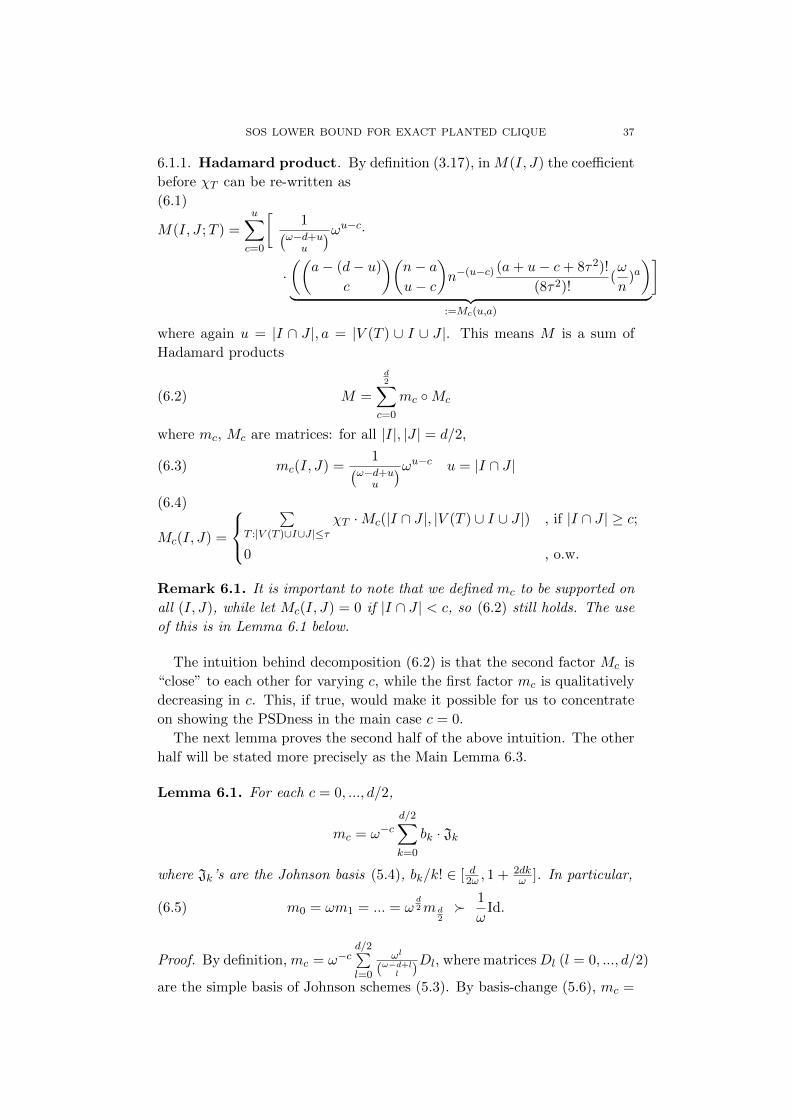
SOS LOWER BOUND FOR EXACT PLANTED CLIQUE 37
6.1.1. Hadamard product. By definition (3.17), in M(I, J) the coefficient
before χT can be re-written as
(6.1)
M(I, J ;T ) =u∑c=0
[1(
ω−d+uu
)ωu−c··((
a− (d− u)
c
)(n− au− c
)n−(u−c) (a+ u− c+ 8τ2)!
(8τ2)!(ω
n)a)
︸ ︷︷ ︸:=Mc(u,a)
]
where again u = |I ∩ J |, a = |V (T ) ∪ I ∪ J |. This means M is a sum of
Hadamard products
(6.2) M =
d2∑c=0
mc Mc
where mc, Mc are matrices: for all |I|, |J | = d/2,
(6.3) mc(I, J) =1(
ω−d+uu
)ωu−c u = |I ∩ J |
(6.4)
Mc(I, J) =
∑
T :|V (T )∪I∪J |≤τχT ·Mc(|I ∩ J |, |V (T ) ∪ I ∪ J |) , if |I ∩ J | ≥ c;
0 , o.w.
Remark 6.1. It is important to note that we defined mc to be supported on
all (I, J), while let Mc(I, J) = 0 if |I ∩ J | < c, so (6.2) still holds. The use
of this is in Lemma 6.1 below.
The intuition behind decomposition (6.2) is that the second factor Mc is
“close” to each other for varying c, while the first factor mc is qualitatively
decreasing in c. This, if true, would make it possible for us to concentrate
on showing the PSDness in the main case c = 0.
The next lemma proves the second half of the above intuition. The other
half will be stated more precisely as the Main Lemma 6.3.
Lemma 6.1. For each c = 0, ..., d/2,
mc = ω−cd/2∑k=0
bk · Jk
where Jk’s are the Johnson basis (5.4), bk/k! ∈ [ d2ω , 1 + 2dkω ]. In particular,
(6.5) m0 = ωm1 = ... = ωd2m d
2 1
ωId.
Proof. By definition, mc = ω−cd/2∑l=0
ωl
(ω−d+ll )Dl, where matricesDl (l = 0, ..., d/2)
are the simple basis of Johnson schemes (5.3). By basis-change (5.6), mc =
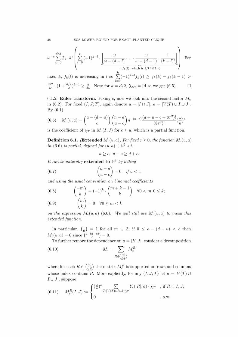
38 SOS LOWER BOUND FOR EXACT PLANTED CLIQUE
ω−cd/2∑k=0
Jk ·k!
k∑l=0
(−1)k−l ·[
ω
ω − (d− l)· ... · ω
ω − (d− 1)· 1
(k − l)!
]︸ ︷︷ ︸
:=fk(l), which is 1/k! if l=0
. For
fixed k, fk(l) is increasing in l sok∑l=0
(−1)k−lfk(l) ≥ fk(k) − fk(k − 1) >
d/2ω · (1 + d/2
ω )k−1 ≥ d2ω . Note for k = d/2, Jd/2 = Id so we get (6.5).
6.1.2. Euler transform. Fixing c, now we look into the second factor Mc
in (6.2). For fixed (I, J ;T ), again denote u = |I ∩ J |, a = |V (T ) ∪ I ∪ J |.By (6.1)
(6.6) Mc(u, a) =
(a− (d− u)
c
)(n− au− c
)n−(u−c) (a+ u− c+ 8τ2)!
(8τ2)!(ω
n)a
is the coefficient of χT in Mc(I, J) for c ≤ u, which is a partial function.
Definition 6.1. (Extended Mc(u, a)) For fixed c ≥ 0, the function Mc(u, a)
in (6.6) is partial, defined for (u, a) ∈ N2 s.t.
u ≥ c, u+ a ≥ d+ c.
It can be naturally extended to N2 by letting
(6.7)
(n− au− c
)= 0 if u < c,
and using the usual convention on binomial coefficients(−mk
)= (−1)k ·
(m+ k − 1
k
)∀0 < m, 0 ≤ k;(6.8) (
m
k
)= 0 ∀0 ≤ m < k(6.9)
on the expression Mc(u, a) (6.6). We will still use Mc(u, a) to mean this
extended function.
In particular,(m0
)= 1 for all m ∈ Z; if 0 ≤ a − (d − u) < c then
Mc(u, a) = 0 since(a−(d−u)
c
)= 0.
To further remove the dependence on u = |I∩J |, consider a decomposition
(6.10) Mc =∑
R∈([n]
≤ d2)
MRc
where for each R ∈( [n]
≤ d2
)the matrix MR
c is supported on rows and columns
whose index contains R. More explicitly, for any (I, J ;T ) let a = |V (T ) ∪I ∪ J |, suppose
(6.11) MRc (I, J) :=
(ωn )a
∑T :|V (T )∪I∪J |≤τ
Yc(|R|, a) · χT , if R ⊆ I, J ;
0 , o.w.
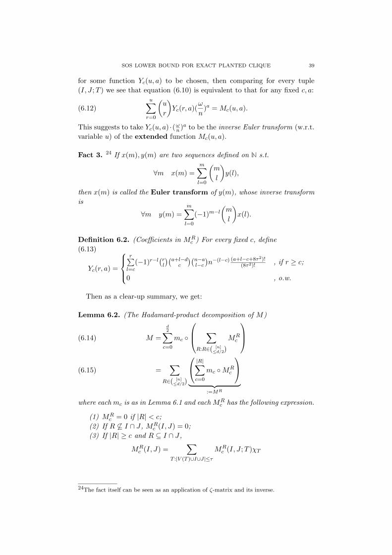
SOS LOWER BOUND FOR EXACT PLANTED CLIQUE 39
for some function Yc(u, a) to be chosen, then comparing for every tuple
(I, J ;T ) we see that equation (6.10) is equivalent to that for any fixed c, a:
(6.12)u∑r=0
(u
r
)Yc(r, a)(
ω
n)a = Mc(u, a).
This suggests to take Yc(u, a) ·(ωn )a to be the inverse Euler transform (w.r.t.
variable u) of the extended function Mc(u, a).
Fact 3. 24 If x(m), y(m) are two sequences defined on N s.t.
∀m x(m) =
m∑l=0
(m
l
)y(l),
then x(m) is called the Euler transform of y(m), whose inverse transform
is
∀m y(m) =
m∑l=0
(−1)m−l(m
l
)x(l).
Definition 6.2. (Coefficients in MRc ) For every fixed c, define
(6.13)
Yc(r, a) =
r∑l=c
(−1)r−l(rl
)(a+l−dc
)(n−al−c)n−(l−c) (a+l−c+8τ2)!
(8τ2)!, if r ≥ c;
0 , o.w.
Then as a clear-up summary, we get:
Lemma 6.2. (The Hadamard-product decomposition of M)
M =
d2∑c=0
mc
∑R:R∈( [n]
≤d/2)
MRc
(6.14)
=∑
R∈( [n]≤d/2)
|R|∑c=0
mc MRc
︸ ︷︷ ︸
:=MR
(6.15)
where each mc is as in Lemma 6.1 and each MRc has the following expression.
(1) MRc = 0 if |R| < c;
(2) If R 6⊆ I ∩ J , MRc (I, J) = 0;
(3) If |R| ≥ c and R ⊆ I ∩ J ,
MRc (I, J) =
∑T :|V (T )∪I∪J |≤τ
MRc (I, J ;T )χT
24The fact itself can be seen as an application of ζ-matrix and its inverse.
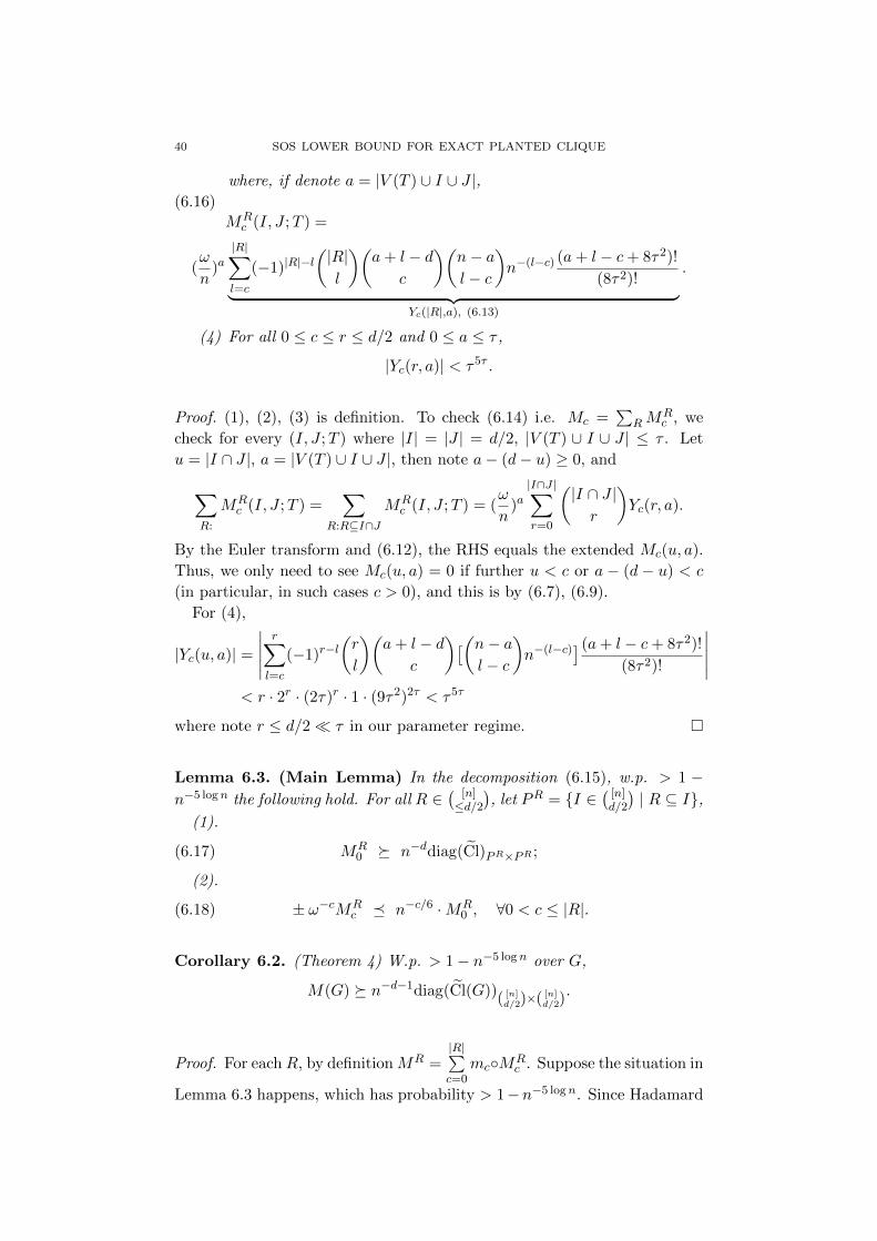
40 SOS LOWER BOUND FOR EXACT PLANTED CLIQUE
where, if denote a = |V (T ) ∪ I ∪ J |,(6.16)
MRc (I, J ;T ) =
(ω
n)a|R|∑l=c
(−1)|R|−l(|R|l
)(a+ l − d
c
)(n− al − c
)n−(l−c) (a+ l − c+ 8τ2)!
(8τ2)!︸ ︷︷ ︸Yc(|R|,a), (6.13)
.
(4) For all 0 ≤ c ≤ r ≤ d/2 and 0 ≤ a ≤ τ ,
|Yc(r, a)| < τ5τ .
Proof. (1), (2), (3) is definition. To check (6.14) i.e. Mc =∑
RMRc , we
check for every (I, J ;T ) where |I| = |J | = d/2, |V (T ) ∪ I ∪ J | ≤ τ . Let
u = |I ∩ J |, a = |V (T ) ∪ I ∪ J |, then note a− (d− u) ≥ 0, and
∑R:
MRc (I, J ;T ) =
∑R:R⊆I∩J
MRc (I, J ;T ) = (
ω
n)a|I∩J |∑r=0
(|I ∩ J |r
)Yc(r, a).
By the Euler transform and (6.12), the RHS equals the extended Mc(u, a).
Thus, we only need to see Mc(u, a) = 0 if further u < c or a − (d − u) < c
(in particular, in such cases c > 0), and this is by (6.7), (6.9).
For (4),
|Yc(u, a)| =
∣∣∣∣∣r∑l=c
(−1)r−l(r
l
)(a+ l − d
c
)[(n− al − c
)n−(l−c)](a+ l − c+ 8τ2)!
(8τ2)!
∣∣∣∣∣< r · 2r · (2τ)r · 1 · (9τ2)2τ < τ5τ
where note r ≤ d/2 τ in our parameter regime.
Lemma 6.3. (Main Lemma) In the decomposition (6.15), w.p. > 1 −n−5 logn the following hold. For all R ∈
( [n]≤d/2
), let PR = I ∈
( [n]d/2
)| R ⊆ I,
(1).
(6.17) MR0 n−ddiag(Cl)PR×PR ;
(2).
(6.18) ± ω−cMRc n−c/6 ·MR
0 , ∀0 < c ≤ |R|.
Corollary 6.2. (Theorem 4) W.p. > 1− n−5 logn over G,
M(G) n−d−1diag(Cl(G))( [n]d/2)×( [n]
d/2).
Proof. For eachR, by definitionMR =|R|∑c=0
mcMRc . Suppose the situation in
Lemma 6.3 happens, which has probability > 1−n−5 logn. Since Hadamard
SOS LOWER BOUND FOR EXACT PLANTED CLIQUE 41
product with a PSD matrix presevres PSDness (the Schur product theorem),
|R|∑c=1
mc MRc
|R|∑c=1
mc (ωcn−c/6 ·MR
0
)(Lemma 6.3(2))
=
|R|∑c=1
n−c/6 ·m0
MR0 (Lemma 6.1)
n−1/6m0 MR0
Similarly,|R|∑c=1
mc MRc −n−1/6m0 MR
c . So
MR (1−n−1/6)m0MR0 n−d−1diag(Cl)PR×PR (Lem. 6.1 and 6.3(2)).
Apply this to (6.15),
(6.19)M = M∅ +
∑∅6=R∈( [n]
≤d/2)
MR M∅ n−d−1diag(Cl)( [n]d/2)×( [n]
d/2).
The rest of section 6 is devoted to proving the Main Lemma 6.3, completed
in subsection 6.7. The key ingredient is Lemma 6.7, stated in section 6.4.
The statement requires the recursive factorization of each MRc , which we
show as Lemma 6.5 in the upcoming subsections 6.2 and 6.3.
6.2. The first-approximate factorization of MRc . In this subsection and
the next, we factorize each matrixMRc in (6.15) by the recursive approximate
factorization.
Terminology established in section 5.3 will be used. We start by defining
the first-approximate factorization (cf. Definition 5.7).
Definition 6.3. Fix R ∈( [n]
≤ d2
). For every i = 0, 1, ..., τ define the left-i-
factor LR,i to be the matrix of dimension([n]d2
)×( [n]
≤ d2
),
(6.20) LR,i(I, A) =
0 , if R 6⊆ I ∩A;∑T : |V (T )∪I∪A|≤τA=Sl(I,A;T )T∩E(A)=∅
(I,A;T ) left-generatedeI,A(T )=i
(ωn )iχT , o.w.
(LR,j)> is called the right-j-factor. Call LR = (LR,0, ..., LR,τ ) the left fac-
tor, (LR)> the right factor. Note these matrices do not depend on “c”.
Definition 6.4. Let Dτ denote the constant diagonal matrix
diag(
(ω
n)|A|2
)A:|A|≤d/2
⊗ Id0,...,τ×0,...,τ
42 SOS LOWER BOUND FOR EXACT PLANTED CLIQUE
of dimension
(( [n]≤d/2
)× (τ + 1)
)×(( [n]≤d/2
)× (τ + 1)
).
Definition 6.5. (Goal factorization of MRc ) Our goal is to find a middle
matrix QRc of dimension(([n]
≤ d2
)× (τ + 1)
)×((
[n]
≤ d2
)× (τ + 1)
)s.t. the following factorization approximately holds:
(6.21) MRc ≈ (LR,0, ..., LR,τ )︸ ︷︷ ︸
LR
·(Dτ ·QRc ·Dτ
)· (LR,0, ..., LR,τ )>︸ ︷︷ ︸(
LR)>
Remark 6.2. Unlike in the non-exact case (section 5.3), here we factorize
MRc by further distinguishing a parameter pair in 0, ..., τ× 0, ..., τ. The
reason is that in (6.13), or more broadly in any exact pseudo-expectation
generated by the method in section 3.2, the parameter
a = |V (T ) ∪ I ∪ J |
appears nestedly in an essential way.
Fixing (I, J ;T ), previously the coefficient (3.12) is intended as
(ω
n)a = (
ω
n)e(Rl)+|V (Rm)|+e(Rr)
as in Remark 5.2, which naturally factors into the left, middle, right terms.
Here, however, there are terms like(a+l−dc
)·(n−al−c)
that are not log-additive
in a. Also, the reason we chose the d-generating function as in Def. 3.6 is
exactly to prove the positiveness of E[QR0,0] in this harder situation. This is
eventually made clear by Prop. 6.3 and Cor. 6.3.
To approach the goal decomposition (6.21), in the coefficients in MRc
(6.16) we separate the main factor
(ω
n)a = (
ω
n)e(Rl) · (ω
n)|V (Rm)| · (ω
n)e(Rr)
into left, right, and middle factors as before, while leave the factor Yc(r, a)
for the middle matrix QRc
((·, el), (·, er)
)to bear , where the index (el, er)
has the natural intended meaning.
Definition 6.6. (First-approximate factorization by QRc,0) Define QRc,0 to be
the 0, ..., τ×0, ..., τ-block matrix, each block of dimension( [n]≤d/2
)×( [n]≤d/2
),
that is 0 outside of the principal minor
(6.22)
SR × SR, SR = (A, i) ∈(
[n]
≤ d/2
)× 0, ..., τ | A ⊇ R, |A|+ i ≥ d
2,
SOS LOWER BOUND FOR EXACT PLANTED CLIQUE 43
and in this principal minor, QRc,0
((A, i), (B, j)
)=
(6.23) ∑Tm:|V (Tm)∪A∪B|≤τA,B∈mSepA,B(Tm)
(ω
n)|V (Tm)∪A∪B|− |A|+|B|
2 ·Yc(|R|, |V (Tm) ∪A ∪B|+ (i+ j)
)︸ ︷︷ ︸defined by (6.13)
·χTm
Correspondingly, define
LR ·(Dτ ·QRc,0 ·Dτ
)·(LR)>
to be the first approximate factorization of MRc .
Some remarks on the definition of QRc,0 follow.
Remark 6.3. (Intended meaning of parameters in QRc,0)
(1). The set SR (6.22) is defined independently of c, where the condition
|A|+ i ≥ d/2 is natural because of the intended meaning of i: it is intended
as |V (T ′)\A| ≥ |I| − |A| for some ribbon (I, A;T ′) in LR. If |A| + i < d/2
the corresponding column in LR is always 0. Similarly for j.
(2). By definition, QRc,0 is supported only on those ((A, i), (B, j)) ∈ SR ×SR with |A| = |B|.
(3). Regarding (6.23), as before by Remark 5.2, in “canonical” situations
i.e. for outer-canonical products in LR ·(Dτ ·QRc,0 ·Dτ
)·(LR)>
,
|V (Tm) ∪A ∪B|+ (i+ j) = |V (T ) ∪ I ∪ J |
for ribbons (I, J ;T ) that take (A,B;Tm) as the middle part of its canonical
decomposition and for which e(Rl) = i, e(Rr) = j.
Recall the terminology on the XYX>-type matrix product, Def 5.6.
Lemma 6.4. (QRc,0 indeed gives the first-approximation) Fix R, c ≤ |R|.For every (I, J ;T ) s.t. |V (T ) ∪ I ∪ J | ≤ τ and R ⊆ I ∩ J , there is exactly
one outer-canonical product in the XYX>-type matrix product
(6.24) LR ·(Dτ ·QRc,0 ·Dτ
)︸ ︷︷ ︸Y
·(LR)>
which corresponds to the canonical decomposition of (I, J ;T ), and which
gives term
MRc (I, J ;T )χT .
Proof. Suppose R ⊆ I∩J . First, note every triple in (6.24) is inner-canonical
by definition of LR, QRc,0, so all outer-canonical triples there 1-1 correspond
to their triple-product (I, J ;T ) via the canonical decomposition.
Fix an (I, J ;T ) and its canonical decomposition, where |V (T ) ∪ I ∪ J | ≤τ . (I, A;T ′) appears exactly once in LR(I, A) in block LR,el , where el =
eI,A(T ′); similarly for (J,B;T ′′) and er = eJ,B(T ′′). And further there is
exactly one outer-canonical product in (6.24) corresponding to this triple,
44 SOS LOWER BOUND FOR EXACT PLANTED CLIQUE
with coefficient
(6.25) LR,el(I, A;T ′) · (ωn
)|A|2 ·QRc,0(A,B;Tm) · (ω
n)|B|2 · LR,er(J,B;T ′′).
By definition (6.20), (6.23), if a := |V (T )| ∪ I ∪ J ≤ τ then the above
coefficient is
(ω
n)a · Yc(|R|, a) = MR
c (I, J ;T ),
by comparing (6.13) and (6.16), noticing that
a = |V (T ) ∪ I ∪ J | (#)= el + |V (Tm) ∪A ∪B|+ er,
where (#) is by canonicality. This proves the lemma.
Definition 6.7. (First error-matrices) Let Ec,1;negl be the matrix of the sum
of all outer-canonical products in (6.24) that exceeds degree, i.e. the resulting
|V (T ) ∪ I ∪ J | > τ.
Let [LR · (DτQRc,0Dτ ) · (LR)>]non-can be the matrix of the sum of all products
that is non-outer-canonical.
Lemma 6.4 can be restated in the terminology of approximate form (Def.
5.6): ∀R ∈( [n]≤d/2
)and 0 ≤ c ≤ |R|,
MRc = [LR ·
(DτQRc,0D
τ)·(LR)>
]can
Equivalently,
(6.26)
MRc = LR ·
(DτQRc,0D
τ)·(LR)>−[LR ·
(DτQRc,0D
τ)·(LR)>
]non-can−ERc,1;deg.
As we will see, the crucial fact is that the error matrix Ec,1;main factorizes
through LR, (LR)> approximately too, as in the non-exact case. In the next
subsection, we show how the recursive factorization method works here in
an extended form.
6.3. Recursive factorization: exact case. The main result of this sub-
section is the following lemma.
Lemma 6.5. (Recursive approximate factorization; exact case) For any
fixed R ∈( [n]≤d/2
)and 0 ≤ c ≤ |R|, we have the following decomposition.
(6.27) MRc = LR ·
[Dτ
(QRc,0 −QRc,1 + ...±QRc,d
)Dτ
]·(LR)>
+ ERc ,
where:
(1). All QRc,k’s are supported on the principal minor SR×SR, where recall
SR = (A, i) ∈(
[n]
≤ d/2
)× 0, ..., τ | A ⊇ R, |A|+ i ≥ d/2.
(2). QRc,0 is by Definition 6.6;
SOS LOWER BOUND FOR EXACT PLANTED CLIQUE 45
(3). ∀1 < k ≤ d/2, QRc,k is a (τ + 1) × (τ + 1)-block-matrix with the
(i, j)-block
(6.28) QRc,k
((A, i), (B, j)
)=
∑Tm:|V (Tm)∪A∪B|≤τ
qRc,k(Rm, i, j) · χTm
(within SR×SR), where we naturally denote Rm = (A,B;Tm); these qRc,k(·, i, j)’sare symmetric w.r.t. shapes, and
(6.29) ∀(i, j) |qRc,k(Rm, i, j)| ≤ τ5τ · ( ω
n1−ε )s−p+k/3,
where as usual s = |A|+|B|2 , p is the max number of vertex-disjoint paths from
A to B in Rm.
(4). For any G, ERc (G) is supported within rows and columns that is clique
in G and contains R. Moreover, w.p. > 1− n−9 logn,
(6.30)∥∥ERc ∥∥ < n−ετ/2.
Proof of Lemma 6.5
Like before, the key is to look at one round of the factorization. The
following lemma is strictly parallel to Lemma 5.4. Again fix R ⊆( [n]d/2
),
c ≤ |R|; for convenience denote n1 :=( [n]d/2
)× (τ + 1) in the following.
Lemma 6.6. (One round of factorization; exact case)
Let LR be from Def. 6.3, QR be any n1×n1-matrix supported on SR×SRand
(6.31) QR((A, i), (B, j)) =∑
Tm: |V (Tm)∪A∪B|≤τ
(ω
n)|V (Rm)|q(Rm, i, j) · χTm
where Rm denotes (A,B;Tm), and q(·, i, j) is symmetric w.r.t. shapes for
any fixed (i, j). Now we define matrix Q′,E′negl so that the following holds:
(6.32) [LR ·Q · (LR)>]non-can = [LR ·Q′ · (LR)>]can + E′negl.
Namely, let Q′ be supported on SR × SR,
(6.33) Q′((A, i), (B, j)) =∑
Tm: |V (Tm)∪A∪B|≤τ
(ω
n)|V (Rm)|q′(Rm, i, j) · χTm
where the coefficients q′(Rm, i, j) are as follows. Fix any Rm = (A,B;Tm)
and (i, j). Let t = |V (Rm)| ≤ τ , s = |A|+|B|2 . For every generalized ribbon
R∗m that contains Rm as its largest ribbon and |V (R∗m)| ≤ τ , fix any a ribbon
pair (R′l,R′r) so that (R′l,R
∗m,R
′r) is the separating factorization for some
ribbon triple, |V (R′l)|, |V (R′r)| ≤ τ and
(6.34) (e(R′l), e(R′r)) = (i, j).
46 SOS LOWER BOUND FOR EXACT PLANTED CLIQUE
If there is no such choice, exclude this R∗m in the summation below. Then:
(6.35)
q′(Rm, i, j) =∑
R∗m: gen. ribbon on (A,B)|V (R∗m)|≤τ
largest ribbon is Rm
(ω
n)|I(R
∗m)| · q′′(R∗m, i, j) where
q′′(R∗m, i, j) =∑
(z,i1,j1):1≤z≤d/2
∑P=(Rl,R,Rr): side-inn. can.
P→(R′l,R∗m,R
′r) for the fixed R′l,R
′r
z(P)=z, e(Rl)=i1,e(Rr)=j1
(ω
n)z · q(R, i1, j1).
Note q′′(Rm, i, j) doesn’t depend on the choice (R′l,R′r) by (the full of)
Proposition 5.4. Thus q′(·, i, j) is also symmetric w.r.t. shapes.
E′negl is defined s.t. (6.32) holds. Then the conclusions are:
(1). W.p. > 1− n−9 logn over G,∥∥E′negl
∥∥ ≤ maxq(·) · n−ετ ;
(2). If there is a number C for which
(6.36) ∀Rm, i, j |q(Rm, i, j)| ≤ C · (ω
n1−ε )s−p
where p denotes the maximum number of vertex-disjoint paths between A,B
in Rm, then
∀Rm, i, j |q′(Rm)| ≤ C · ( ω
n1−ε )s−p+1/3.
Proof. (of Lemma 6.6) The proof is almost the same as that of Lemma 5.4;
we point out and explain the differences below.
The support condition (i.e. supported on SR×SR) doesn’t affect anything
since LR itself is automatically 0 on columns and rows that are not in SR.
As step (0) like before, we expand [LR · Q′ · (LR)>]can to compare with
[LR · Q · (LR)>]non-can term-wise, using Prop. 5.4. Here, notice that when
(i, j) and R∗m are fixed, the size of any choice of (R′l,R′r) satisfying (6.34)
are also fixed, so the proposition is applicable. The comparison for order
on (ωn ) between the two is exactly the same as in step (0) of the proof of
Lemma 5.4, and the conclusion is that the matrix E′negl collects all terms in
[LR ·Q · (LR)>]non-can whose R∗m in the separating factorization exceeds size
τ , i.e. E′negl(I, J) =
(6.37)∑i,j
∑(Rl,Rm,Rr): side. inn. can.
non-outer-can.all three has size ≤τ
|V (R∗m)|>τ, (e(Rl),e(Rr))=(i,j)
(ω
n)|V (Rl)|+|V (Rm)|+|V (Rr)|−|A|−|B|q(Rm, i, j)χT
where T = Tl ⊕ Tm ⊕ Tr, and we omit writing the default requirement that
Rl (Rr) has the left (right) distinguished vertex set I (J).
The numerical conclusions (1), (2) follow from the same estimates as in
Lemma 5.4 (after (5.44) there). We only point out that, for (1), the estimate
SOS LOWER BOUND FOR EXACT PLANTED CLIQUE 47
there is actually loose enough s.t. with even an extra (1 + τ)2-factor (from
union bound on blocks) it is still smaller than n−ετ .
Now we can prove Lemma 6.5.
Proof. (for Lemma 6.5) Apply the one-round factorization Lemma 6.6 to
[LR ·(DτQRc,iD
τ)·(LR)>
]non-can
for i = 0, we get QRc,1, E′1;negl (for ease of notation, we hide the index R, c
for this negligible matrix). Then repeat this for i = 1 we get Ec,1;deg, QRc,2,
and E′2,negl. Continuing this, as the result we get the recursive factorization
(6.38)
MRc =LR ·
[Dτ(QRc,0 −QRc,1 + ...±QRc,d
)Dτ]·(LR)>−(
ERc,1;deg − ERc,2;deg + ...± ERc,d;deg
)+(E′1;negl + ...+ E′d;negl
).
Again, here it uses that QRc,d+1 = 0, by the same proposition 5.5.
(1). All QRc,k is supported within SR × SR by definition of each round
(Lemma 6.6);
(2). By definition.
(3). The coefficients of each QRc,k (k = 0, 1, ..., d), qRc,k(·, i, j) is always
symmetric w.r.t. shapes from Lemma 6.6. Moreover, from definition (6.23),
∀Rm, i, j |qRc,0(Rm)| = |Yc(|R|, |Rm|)| ≤ τ5τ
where the last one is by Lemma 6.2(4). Since QRc,0 is special in that for all
Rm = (A,B;Tm) appearing in it, there are |A| = |B| many vertex-disjoint
paths between A,B in Rm, i.e. s = p, where as usual when Rm is fixed
we use s = |A|+|B|2 and p denotes the max number of vertex-disjoint paths
between A,B. So the above can be equivalently written as
(6.39) ∀Rm, i, j |qRc,0(Rm)| ≤ (ω
n1−ε )s−pτ5τ .
Now use Lemma 6.6(2), where notice the “q(·)” in there corresponds to qRc,khere, since the “Q” matrix isDτQRc,kD so the “(ωn )|V (Rm)|q(·)” is (ωn )|V (Rm)|−s·(ωn )s · qRc,k. As the result, we get the recursive bound
∀Rm, i, j |qRc,k(Rm, i, j)| ≤ τ5τ · ( ω
n1−ε )s−p+k/3.
(4). First, when plugged in any G, both
MRc and LR ·
[Dτ
(QRc,0 −QRc,1 + ...±QRc,d
)Dτ
]·(LR)>
are supported within clique rows and columns that contain R by their def-
inition. So it must be the case for their difference, ERc , too. Next we only
need to give the norm bound. By (6.38), the final error matrix is
ERc = −(ERc,1;deg − ERc,2;deg + ...± ERc,d;deg
)+(E′1;negl + ...+ E′d;negl
).
48 SOS LOWER BOUND FOR EXACT PLANTED CLIQUE
Note by Lemma 6.6(2), by induction all |qRc,k| < τ5τ . For each E′k;negl, by
Lemma 6.6(1) w.p. > 1− n−9 logn,∥∥∥E′k;negl
∥∥∥ < τ5τn−ετ < n−0.9ετ .
As for ERc,k;deg, recall by definition 5.6 on (I, J) it is the sum of outer-
canonical products in LR ·(DτQRc,i−1D
τ)·(LR)>
(I, J) s.t. |V (T )∪I∪J | >τ . So
ERc,k;deg(I, J) =∑
(Rl,Rm,Rr):semi-inn.can.
outer.can.|V (T )∪I∪J |>τ
(ω
n)|V (T )∪I∪J | · qRc,k−1(Rm, e(Rl), e(Rr))χT
where as usual s = s(Rm) is the average of its two side vertex-sets, T =
Tl ⊕ Tm ⊕ Tr, and in the summation Rl (Rr) should have I (J) as the left
(right) set. Note the above uses |V (T ) ∪ I ∪ J | = el + er + |V (Rm)| from
the outer- and semi-inner- canonicality. Moreover, any fixed (I, J ;T ) can
come from at most 33τ triples as their vertex set union is |V (T ) ∪ I ∪ J | by
canonicality. Since 3τ ≥ |V (T )∪ I ∪ J | > τ and w.h.p. |qRc,k−1(·)| < τ5τ , use
Lemma 4.2 and we get that w.p. > 1− n−10 logn,∣∣ERc,k;deg(I, J)∣∣ < τ6τ ·
3τ∑c=0
(ω
n)maxτ,c · (nc/22c
2n4 log logn) < n−2ετ .
So by union bound over (I, J),∥∥∥ERc,k;deg
∥∥∥ < n−d/4n−2ετ < n−ετ w.p. >
1− n−9.5 logn.
Together, sum the two and by union bound over k, we get that w.p.
> 1− n−9 logn,∥∥ERc ∥∥ < n−ετ/2.
6.4. Positiveness the middle matrices: proof overview. Now we use
the approximate decomposition of MRc ’s to prove the Main Lemma 6.3.
Recall for each R, c ≤ |R|, by Lemma 6.5
MRc = LR ·
Dτ
(QRc,0 −QRc,1 + ...±QRc,d
)︸ ︷︷ ︸
:=QRc
Dτ
· (LR)> + ERc .
The key is the following lemma. Recall SR = (A, i) ∈( [n]≤d/2
)× 0, ..., τ |
A ⊇ R, |A|+ i ≥ d2.
Lemma 6.7. W.p. > 1− n−8 logn over G, the following holds.
(1). ∀R ∈( [n]≤d/2
),
QR0,0 −QR0,1 + ...±QR0, d
2
τ−7τ · diag(
Cl)SR×SR
,
where recall SR = (A, i) ∈( [n]≤d/2
)× 0, ..., τ | A ⊇ R, |A|+ i ≥ d
2.(2). ∀R, 0 < c ≤ |R|
±ω−c(QRc,0 −QRc,1 + ...±QR
c, d2
) n−c/4 · diag
(Cl)SR×SR
.
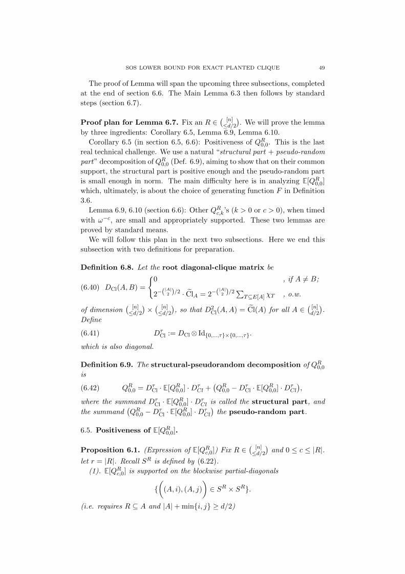
SOS LOWER BOUND FOR EXACT PLANTED CLIQUE 49
The proof of Lemma will span the upcoming three subsections, completed
at the end of section 6.6. The Main Lemma 6.3 then follows by standard
steps (section 6.7).
Proof plan for Lemma 6.7. Fix an R ∈( [n]≤d/2
). We will prove the lemma
by three ingredients: Corollary 6.5, Lemma 6.9, Lemma 6.10.
Corollary 6.5 (in section 6.5, 6.6): Positiveness of QR0,0. This is the last
real technical challenge. We use a natural “structural part + pseudo-random
part” decomposition ofQR0,0 (Def. 6.9), aiming to show that on their common
support, the structural part is positive enough and the pseudo-random part
is small enough in norm. The main difficulty here is in analyzing E[QR0,0]
which, ultimately, is about the choice of generating function F in Definition
3.6.
Lemma 6.9, 6.10 (section 6.6): Other QRc,k’s (k > 0 or c > 0), when timed
with ω−c, are small and appropriately supported. These two lemmas are
proved by standard means.
We will follow this plan in the next two subsections. Here we end this
subsection with two definitions for preparation.
Definition 6.8. Let the root diagonal-clique matrix be
(6.40) DCl(A,B) =
0 , if A 6= B;
2−(|A|2 )/2 · ClA = 2−(|A|2 )/2∑T⊆E[A] χT , o.w.
of dimension( [n]≤d/2
)×( [n]≤d/2
), so that D2
Cl(A,A) = Cl(A) for all A ∈( [n]d/2
).
Define
(6.41) DτCl := DCl⊗ Id0,...,τ×0,...,τ.
which is also diagonal.
Definition 6.9. The structural-pseudorandom decomposition of QR0,0is
(6.42) QR0,0 = DτCl · E[QR0,0] ·Dτ
Cl +(QR0,0 −Dτ
Cl · E[QR0,0] ·DτCl
),
where the summand DτCl · E[QR0,0] · Dτ
Cl is called the structural part, and
the summand(QR0,0 −Dτ
Cl · E[QR0,0] ·DτCl
)the pseudo-random part.
6.5. Positiveness of E[QR0,0].
Proposition 6.1. (Expression of E[QRc,0]) Fix R ∈( [n]≤d/2
)and 0 ≤ c ≤ |R|.
let r = |R|. Recall SR is defined by (6.22).
(1). E[QRc,0] is supported on the blockwise partial-diagonals
(
(A, i), (A, j)
)∈ SR × SR.
(i.e. requires R ⊆ A and |A|+ mini, j ≥ d/2)
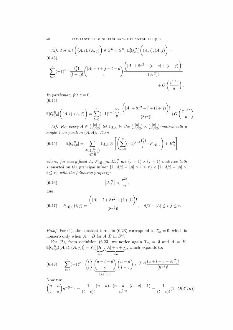
50 SOS LOWER BOUND FOR EXACT PLANTED CLIQUE
(2). For all
((A, i), (A, j)
)∈ SR × SR, E[QRc,0]
((A, i), (A, j)
)=
(6.43)
r∑l=c
(−1)r−l(rl
)(l − c)!
(|A|+ i+ j + l − d
c
)(|A|+ 8τ2 + (l − c) + (i+ j)
)!
(8τ2)!
+O
(τ1.5τ
n
).
In particular, for c = 0,
(6.44)
E[QR0,0]
((A, i), (A, j)
)=
r∑l=0
(−1)r−l(rl
)l!·
(|A|+ 8τ2 + l + (i+ j)
)!
(8τ2)!+O
(τ1.5τ
n
).
(3). For every A ∈( [n]≤d/2
)let 1A,A be the
( [n]≤d/2
)×( [n]≤d/2
)-matrix with a
single 1 on position (A,A). Then
(6.45) E[QR0,0] =∑
A⊆( [n]≤d/2)
A⊇R
1A,A ⊗
[(r∑l=0
(−1)r−l(rl
)l!· P|A|+l
)+ ERA
]
where, for every fixed A, P|A|+landERA are (τ + 1) × (τ + 1)-matrices both
supported on the principal minor i | d/2 − |A| ≤ i ≤ τ × i | d/2 − |A| ≤i ≤ τ with the following property:
(6.46)∥∥ERA∥∥ < τ2τ
n,
and
(6.47) P|A|+l(i, j) =
(|A|+ l + 8τ2 + (i+ j)
)!
(8τ2)!, d/2− |A| ≤ i, j ≤ τ.
Proof. For (1), the constant terms in (6.23) correspond to Tm = ∅, which is
nonzero only when A = B for A,B in SR.
For (2), from definition (6.23) we notice again Tm = ∅ and A = B.
E[QRc,0((A, i), (A, j))] = Yc( |R|︸︷︷︸:=r
, |A|+ i+ j︸ ︷︷ ︸:=a
), which expands to:
r∑l=c
(−1)r−l(r
l
)(a+ l − d
c
)︸ ︷︷ ︸
Def. 6.1
(n− al − c
)n−(l−c) (a+ l − c+ 8τ2)!
(8τ2)!.(6.48)
Now use(n− al − c
)n−(l−c) =
1
(l − c)!(n− a)...(n− a− (l − c) + 1)
nl−c=
1
(l − c)!(1−O(d2/n))
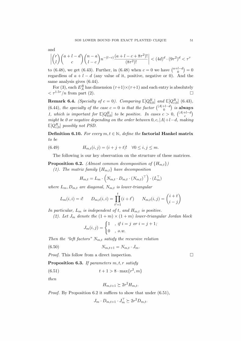
SOS LOWER BOUND FOR EXACT PLANTED CLIQUE 51
and∣∣∣∣(rl)(
a+ l − dc
)(n− al − c
)n−(l−c) (a+ l − c+ 8τ2)!
(8τ2)!
∣∣∣∣ < (4d)d · (9τ2)d < τ τ
to (6.48), we get (6.43). Further, in (6.48) when c = 0 we have(a+l−d
0
)= 0
regardless of a + l − d (any value of it, positive, negative or 0). And the
same analysis gives (6.44).
For (3), each ERA has dimension (τ+1)×(τ+1) and each entry is absolutely
< τ1.5τ/n from part (2).
Remark 6.4. (Specialty of c = 0). Comparing E[QR0,0] and E[QRc,0] (6.43),
(6.44), the specialty of the case c = 0 is that the factor(|A|+l−d
0
)is always
1, which is important for E[QR0,0] to be positive. In cases c > 0,(|A|+l−d
c
)might be 0 or negative depending on the order between 0, c, |A|+l−d, making
E[QRc,0] possibly not PSD.
Definition 6.10. For every m, t ∈ N, define the factorial Hankel matrix
to be
(6.49) Hm,t(i, j) = (i+ j + t)! ∀0 ≤ i, j ≤ m.
The following is our key observation on the structure of these matrices.
Proposition 6.2. (Almost common decomposition of Hm,t)(1). The matrix family Hm,t have decomposition
Hm,t = Lm ·(Nm,t ·Dm,t · (Nm,t)
>)· (L>m)
where Lm, Dm,t are diagonal, Nm,t is lower-triangular
Lm(i, i) = i! Dm,t(i, i) =
t∏t′=1
(i+ t′) Nm,t(i, j) =
(i+ t
i− j
)In particular, Lm is independent of t, and Hm,t is positive.
(2). Let Jm denote the (1 +m)× (1 +m) lower-triangular Jordan block
Jm(i, j) =
1 , if i = j or i = j + 1;
0 , o.w.
Then the “left factors” Nm,t satisfy the recursive relation
(6.50) Nm,t+1 = Nm,t · Jm.
Proof. This follow from a direct inspection.
Proposition 6.3. If parameters m, t, r satisfy
(6.51) t+ 1 > 8 ·maxr2,m
then
Hm,t+1 2r2Hm,t.
Proof. By Proposition 6.2 it suffices to show that under (6.51),
Jm ·Dm,t+1 · J>m 2r2Dm,t.
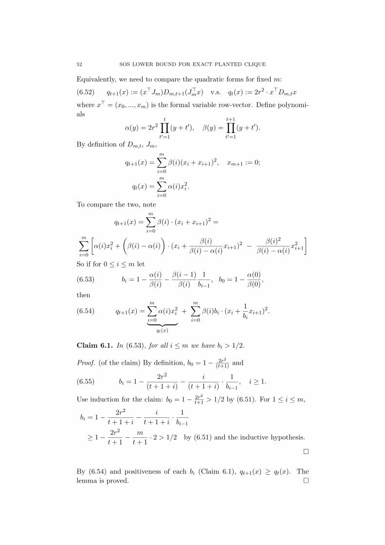
52 SOS LOWER BOUND FOR EXACT PLANTED CLIQUE
Equivalently, we need to compare the quadratic forms for fixed m:
(6.52) qt+1(x) := (x>Jm)Dm,t+1(J>mx) v.s. qt(x) := 2r2 · x>Dm,tx
where x> = (x0, ..., xm) is the formal variable row-vector. Define polynomi-
als
α(y) = 2r2t∏
t′=1
(y + t′), β(y) =t+1∏t′=1
(y + t′).
By definition of Dm,t, Jm,
qt+1(x) =m∑i=0
β(i)(xi + xi+1)2, xm+1 := 0;
qt(x) =m∑i=0
α(i)x2i .
To compare the two, note
qt+1(x) =m∑i=0
β(i) · (xi + xi+1)2 =
m∑i=0
[α(i)x2
i +
(β(i)− α(i)
)· (xi +
β(i)
β(i)− α(i)xi+1)2 − β(i)2
β(i)− α(i)x2i+1
]So if for 0 ≤ i ≤ m let
(6.53) bi = 1− α(i)
β(i)− β(i− 1)
β(i)
1
bi−1, b0 = 1− α(0)
β(0),
then
(6.54) qt+1(x) =m∑i=0
α(i)x2i︸ ︷︷ ︸
qt(x)
+m∑i=0
β(i)bi · (xi +1
bixi+1)2.
Claim 6.1. In (6.53), for all i ≤ m we have bi > 1/2.
Proof. (of the claim) By definition, b0 = 1− 2r2
(t+1) and
(6.55) bi = 1− 2r2
(t+ 1 + i)− i
(t+ 1 + i)· 1
bi−1, i ≥ 1.
Use induction for the claim: b0 = 1− 2r2
t+1 > 1/2 by (6.51). For 1 ≤ i ≤ m,
bi = 1− 2r2
t+ 1 + i− i
t+ 1 + i· 1
bi−1
≥ 1− 2r2
t+ 1− m
t+ 1· 2 > 1/2 by (6.51) and the inductive hypothesis.
By (6.54) and positiveness of each bi (Claim 6.1), qt+1(x) ≥ qt(x). The
lemma is proved.
SOS LOWER BOUND FOR EXACT PLANTED CLIQUE 53
Now we apply Proposition 6.3 to matrices P|A|+l (6.47). Note
P|A|+l =1
(8τ2)!Hτ−(d/2−|A|), d−|A|+8τ2+l
where A is fixed, l varies; below, we regard P|A|+l as a matrix on its support.
Corollary 6.3. (Positiveness of E[QR0,0]) In the decomposition (6.45) of
E[QR0,0],
(6.56)
(r∑l=0
(−1)r−l(rl
)l!· P|A|+l
)+ ERA diag
(τ−6τ
)0≤i≤τ−(d/2−|A|)
where we naturally regarded matrices as on their support
i | d/2− |A| ≤ i ≤ τ)2 ∼= 0, ..., τ − (d/2− |A|)2.
In particular, by (6.45)
(6.57)
E[QR0,0] ∑
A⊆( [n]≤d/2)
A⊇R
1A,A ⊗ diag(τ−6τ
)d/2−|A|≤i≤τ = diag
(τ−6τ
)SR×SR
where recall SR = (A, i) | R ⊆ A, |A|+ i ≥ d/2.
Proof. The “in particular” part is straightforward from (6.56) by checking
the support, and that tensoring with a nonzero PSD matrix preserves the
relation . In below we prove for (6.56).
Fix A, let
(6.58) τ0 = τ − (d/2− |A|), t0 = d− |A|+ 8τ2.
Then
(6.59)r∑l=0
(−1)r−l(rl
)l!· P|A|+l =
1
(8τ2)!· (Xr +Xr−2 + ...)
where, ∀0 ≤ v ≤ br/2c,
Xr−2v =
(r
r−2v
)(r − 2v)!
·(Hτ0,t0+r−2v −
(r − 2v)2
(2v + 1)︸ ︷︷ ︸≤r2
Hτ0,t0+r−2v−1
), Hτ0,−1 := 0.
Since t0 > 8 maxr2, τ0, by Proposition 6.3
Xr−2v (
rr−2v
)(r − 2v)!
·max1
2Hτ0,t0+r−2v, r
2Hτ0,t0+r−2v−1 ∀0 ≤ v ≤ r/2.
So in (6.59), in particular,
(6.60)r∑l=0
(−1)r−l(rl
)l!· P|A|+l
1
(8τ2)!·Hτ0,t0
Prop. 6.2= L
(Nt0 ·
Dt0
(8τ2)!· (Nt0)>
)L
where we temporarily abuse the notation by omitting the index τ0 in the
RHS.
54 SOS LOWER BOUND FOR EXACT PLANTED CLIQUE
Using the following claim, we can finish the proof of (6.56):
RHS of (6.60) L · diag(τ−5τ
)0≤i≤τ0 · L (by Claim 6.2)
diag(τ−5τ
)0≤i≤τ0 ,
while by Proposition 6.1 (3),∥∥ERA∥∥ < τ2τ
n< τ−6τ (parameter regime).
So LHS of (6.56) diag(τ−5τ − τ−6τ
)0≤i≤τ0 RHS of (6.56).
Claim 6.2. In notation of Corollary 6.3, the following hold.
N−1t0
(i, j) = (−1)i−j(i+ t0i− j
)0 ≤ i, j ≤ τ0;(6.61)
Nt0 ·Dt0
(8τ2)!· (Nt0)> diag
(τ−5τ
)0≤i≤τ0 .(6.62)
Proof. For (6.61), multiply this matrix with Nt0 then the (i, j)th entry is∑j≤k≤i
(−1)i−k(i+ t0i− k
)(k + t0k − j
)=
i′∑k′=0
(−1)i′−k′(i′ + j + t0i′ − k′
)(k′ + j + t0
k′
)where i′ = i − j, k′ = k − j. To see this is identity matrix, use generating
functions: let Dm[(1 + x)a] denote the coefficient of xm in (1 + x)a, m ≥0, a ∈ Z, the above RHS is
(−1)i′
i′∑k′=0
Di′−k′ [(1 + x)i′+j+t0 ] ·Dk′ [(1 + x)−(t0+j+1)]
=(−1)i′Di′ [(1 + x)i
′+j+t0−(t0+j+1)] = (−1)i′Di′ [(1 + x)i
′−1] = 1i′=0.
For (6.62), it is equivalent to
(6.63)Dt0
(8τ2)! N−1
t0· τ−5τ · (N−1
t0)>.
To upper bound the RHS, let a0 = τ−5τ , consider the quadratic form
(6.64) x>N−1t0· a0 · (N−1
t0)>x = a0
τ0∑j=0
y2j ,
where by (6.61),
yj =(x>N−1
t0
)j
=
τ0∑i=j
(−1)i−j(i+ t0i− j
)xi.
SOS LOWER BOUND FOR EXACT PLANTED CLIQUE 55
By Cauchy-Schwartz, y2j ≤ τ0 ·
∑τ0i=j
(i+t0i−j)2x2i , so
RHS of (6.64) = a0
τ0∑j=0
y2j ≤ a0
τ0∑i=0
x2i ·
τ0
i∑j=0
(i+ t0i− j
)2
<
τ0∑i=0
(τ−5τ · (9τ2)2i+2
)x2i .
Now (6.63) follows since for each i, in the LHS of (6.63)
Dt0(i, i)
(8τ2)!≥ (8τ2)−(d/2−|A|) (by definition)
> τ−2d > τ−5τ · (9τ2)2i+2
using i ≤ τ0 < τ , d τ . So (6.63) holds.
We get the main conclusion of this subsection:
Corollary 6.4. (Positiveness of the structural part of QR0,0 (Def. 6.9))
DτCl · E[QR0,0] ·Dτ
Cl︸ ︷︷ ︸stractural part of QR0,0
τ−6τ · diag(
Cl)SR×SR
.
Proof. It follows from Corollary 6.3 and that D2Cl(A,A) = Cl(A) for all A
in Definition 6.8.
6.6. Rest bounds: QRc,ks. In this subsection, we bound the rest matrices:
QR0,0 −DτCl · E[QR0,0] ·Dτ
Cl︸ ︷︷ ︸pseudo−random part of QR
0,0 (Def. 6.9)
, QR0,k (k > 0), ω−c ·QRc,k (c > 0, k ≥ 0)
by three Lemmas 6.8, 6.9, 6.10, respectively, which would prove Lemma 6.7.
The arguments are quite standard but somewhat lengthy, as one needs to
be careful on the block structure and the support of the matrices.
Definition 6.11. (0-1 diagonal-clique matrix) Recall the matrix DτCl from
Def. 6.8. Denote by D′ its 0-1 valued version, i.e. D′ is also diagonal and
has entries
D′((A, i), (A, i)) = ClA, ∀A ∈(
[n]
≤ d/2
)∀0 ≤ i ≤ τ.
Lemma 6.8. (Bound on pseudo-random part of QR0,0) W.p. > 1− n−9 logn
the following holds: ∀R ∈( [n]≤d/2
),
(6.65) ± (QR0,0 −DτCl · E[QR0,0] ·Dτ
Cl︸ ︷︷ ︸pseudo−random part of QR0,0
)(G) n−ε · diag(
Cl(G))SR×SR
56 SOS LOWER BOUND FOR EXACT PLANTED CLIQUE
Proof. Fix R. For simplicity, in this proof abbreviate:
Qps := QR0,0 −DτCl · E[QR0,0] ·Dτ
Cl =(Qps,(i,j)
)0≤i,j≤τ
(“ps” for pseudo-random), which is a (τ + 1)× (τ + 1)-block matrix.
In block (i, j), by Def. 6.6 and Prop. 6.1, Qps,(i,j) is supported within
Si,j × Si,j where Si,j := A | |A|+ mini, j ≥ d/2.
And for each A 6= B,
(6.66)
Qps,(i,j)(A,B) = QR0,0((A, i), (B, j)) =∑Tm: |V (Tm)∪A∪B|≤τA,B∈mSepA,B(Tm)
(ω
n)|V (Tm)∪A∪B|− |A|+|B|
2 · q(A,B;Tm) · χTm ;
and
(6.67)
Qps,(i,j)(A,A) =∑
Tm: 1≤|V (Tm)\A|≤τ−|A|
(ω
n)|V (Tm)∪A|−|A| · q(A,A;Tm) · χTm .
Here we have abbreviated q(A,B;Tm) := Y0
(|R|, |V (Tm)∪A∪B|+(i+ j)
)((6.23)) and have omitted the indices |R|, i + j when they are fixed. Two
properties we need:
q(A,B;Tm) depends only on |V (Tm) ∪A ∪B| when fixing (A,B);(6.68) ∣∣∣∣q(A,B;Tm)
∣∣∣∣ < τ5τ (by Lemma 6.2 (4)).(6.69)
By (6.68), Qps,(i,j)(A,B) always factors through ClA∪B and so also through
ClAClB. In particular,
(6.70) Qps = D′ ·Qps ·D′
where D′ is the 0-1 diagonal-clique matrix (Definition 6.11).
Claim 6.3. W.p. > 1− n−9.5 logn the following holds:
∀(i, j) ±Qps,(i,j) ≺ n−1.1ε · diag(
2(|A|2 ))SRmini,j×S
Rmini,j
where SRa := A ∈( [n]≤d/2
)| |A|+ a ≥ d/2.
The lemma follows from this claim and (6.70). Namely, consider a differ-
ent decomposition of Qps as follows. For every b ∈ [0, d2 ], let
Ib := i | d/2− b ≤ i ≤ τ
and Qps;b be the principal minor Wb :=(PRb × Ib
)×(PRb × Ib
)of Qps (0
elsewhere), where PRb = A ⊆ [n] | R ⊆ A, |A| = b. Then we have
((A, i), (B, j)) ∈ SR × SR | 0 ≤ |A| = |B| ≤ d/2 =d/2tb=0
Wb.
SOS LOWER BOUND FOR EXACT PLANTED CLIQUE 57
Since QRc,0 is supported only on those ((A, i), (B, j)) ∈ SR×SR that satisfies
|A| = |B| (Remark 6.3(2)), in particular for c = 0 we have
(6.71) Qps =
d/2∑b=0
Qps;b.
Each Qps;b is block-wise in blocks Ib × Ib, each block a principal minor of
Qps,(i,j). So by Claim 6.3 w.p. > 1−n−9.5 logn any (±) such a block ≺ n−1.5ε ·diag
(2(b2)
)([n]b )×([n]b )
, so±Qps;b ≺ τ2·n−1.5εdiag(
2(b2))Wb
≺ n−εdiag(
2(b2))Wb
.
Hence by (6.71) and the union bound over b, ±Qps ≺ n−εdiag(
2(|A|2 ))SR×SR
w.p. 1 − n−9 logn. Finally, insert this to the middle of (6.70), where notice
ClA = 2(|A|2 ) · ClA, ClA = Cl2A, we get (6.65).
Proof. (of Claim 6.3) We use the norm bounds from section 4. Fix (i, j),
consider
Qdiagps,(i,j) and Qoff
ps,(i,j) = Qps,(i,j) −Qdiagps,(i,j).
Diagonal part. For Qdiagps,(i,j), by (6.67) for any (A,A) in the support (i.e.
|A|+ i ≥ d/2, |A|+ j ≥ d/2),
Qdiagps,(i,j)(A,A) = ClA·
∑Tm: 1≤|V (Tm)\A|≤τ−|A|
Tm∩E[A]=∅
(ω
n)|V (Tm)\A|q(A,A;Tm) · χTm
︸ ︷︷ ︸
:=g(A)
.
For every fixed A in support, this g(A) can be bounded by norms of diagonal
graphical matrices, as follows. First, q(A,A;Tm) depends only on |V (Tm)\A|(we have fixed R, i, j, A), so temporarily denote it as q(|V (Tm)\A|). For
every 1 ≤ v ≤ τ − |A|, let Uv1, ...,Uvh(v) be all different shapes (A,A;T ) (Def.
4.5) s.t. T ∩ E[A] = ∅ and |V (T )\A| = v. Clearly,
(6.72) h(v) ≤ 2|A|v+v2 since we required T ∩ E[A] = ∅.
So w.p. > 1− n−9.6 logn all of the following hold:
|g(A)| =∣∣∣∣τ−|A|∑v=1
(ω
n)vq(v) ·
(h(v)∑x=1
∑Tm:(A,A;Tm) has
shape Uvx
χTm
︸ ︷︷ ︸=MUvx
(A,A) by Def. 4.5
)∣∣∣∣
≤τ−|A|∑v=1
(ω
n)vq(v) ·
h(v)∑x=1
∥∥MUvx
∥∥ (each MUvxis diag.)
≤τ−|A|∑v=1
(ω
n)vτ5τ
h(v)∑x=1
∥∥MUvx
∥∥ (by (6.69))
58 SOS LOWER BOUND FOR EXACT PLANTED CLIQUE
<τ∑v=1
(ω
n)vτ5τ · 2|A|v+v2 · n
v2 2O(|A|+v) (by (6.72) and Thm. 3)
an in our parameter regime this is
<
τ∑v=1
n−3εv · nεv < n−1.2ε.
Off-diagonal part. Similarly, by symmetry of the coefficients (6.68),
Qoffps,(i,j) is a sum of graphical matrices. I.e. let U
s,t1 , ...,Us,th(s,t) be the col-
lection of distinct shapes (A,B;T ) s.t. |A| = |B| = s, A 6= B, A,B ∈mSepA,B(T ) and |V (T ) ∪ A ∪ B| = t, then by (6.66), Qoff
ps,(i,j) is a block-
diagonal matrix for blocks s = d/2 − i, ..., d/2 according to s = |A| = |B|,the sth block being
Qoffps,(i,j)(s) =
∑t: s<t≤τ
(ω
n)t−s
h(s,t)∑x=1
q(Us,tx )MUs,tx
where naturally we denote q(A,B;Tm) = q(Us,tx ) if (A,B;Tm) has shape
Us,tx . By Theorem 3, w.p. > 1− n−9.8 logn,∥∥∥Qoff
ps,(i,j)(s)∥∥∥ ≤ ∑
s<t≤τ(ω
n)t−s · h(t, s) · n
t−s2 2O(t)(log n)O(t−s)(6.73)
Also, clearly h(t, s) ≤ 2(t2)+O(t). Therefore, with the same high probability
RHS of (6.73) ≤∑
d/2−maxi,j≤s≤d/2s<t≤τ
(ω
n)t−s2(t2)+O(t)n
t−s2 (log n)O(t−s)
<∑
d/2−maxi,j≤s≤d/2s<t≤τ
n−2ε(t−s)2O(t)2(s2)(2t+s log n)O(t−s)
<2(s2) · n−1.9ε. (in our parameter regime)
Adding these diagonal blocks, we get that±Qoffps,(i,j) ≺ n−1.9ε·diag
(2(|A|2 )
)SRmini,j×S
Rmini,j
.
Finally, by the union bound we get that w.p. > 1− n−9.5 logn,
±Qps,(i,j) = ±(Qdiagps,(i,j) +Qoff
ps,(i,j)) ≺ n−1.5ε · diag(
2(|A|2 ))SRmini,j×S
Rmini,j
,
completing the proof.
Corollary 6.5. (Positiveness of QR0,0) For every R ∈( [n]≤d/2
), w.p. > 1 −
n−8 logn over G
QR0,0(G) τ−6.1τ · diag(
Cl(G))SR×SR
.
Proof. By Lemma 6.8 and Corollary 6.4, where τ−6.1τ n−ε/10 in our
parameter regime.
SOS LOWER BOUND FOR EXACT PLANTED CLIQUE 59
Lemma 6.9. (Bounds on QR0,k) W.p. > 1 − n−9 logn the following holds.
For all R ∈( [n]≤d/2
)and all 1 ≤ k ≤ d/2,
±QR0,k(G) n−k/10 · diag(
Cl(G))SR×SR
.
Proof. We will use union bound over (R, k) so fix them first. For the fixed
R, k(> 0), in this proof we abbreviate:
QR0,k ↔ Q.
Recall the definition ofQR0,k (Lemma 6.5 (3)): Q is supported within SR×SR,
(6.74) Q
((A, i), (B, j)
)=
∑Tm:|V (Tm)∪A∪B|≤τ
(ω
n)t−sqR0,k(Rm, i, j) · χTm .
where t = |A ∪B|, s = |A|+|B|2 . Abbreviate qR0,k as qk. By Lemma 6.5(3),
qk(·, i, j) is symmetric w.r.t. shapes for all fixed (i, j);(6.75)
|qk(Rm, i, j)| ≤ τ5τ · ( ω
n1−ε )s−p+k/3(6.76)
where t = |A ∪B|, s = |A|+|B|2 , p is the maximum number of vertex-disjoint
paths from A to B in (A,B;Tm).
By symmetry of qk’s, Q((A, i), (B, j)) factors through Cl(A)Cl(B), so
(6.77) Q = D′ ·Q ·D′.
where D′ is by Definition 6.11. It suffices to show:
(6.78) w.p. > 1− n−9.5 logn ±Q ≺ n−k/10 · diag(
2(|A|2 ))SR×SR
.
This is because, like in the proof of Lemma 6.8, we can insert (6.78) to the
middle of (6.77) which proves the lemma for the fixed R, k.
In below we prove (6.78). First, express each block of Q as a sum of
graphical matrices. As a block-matrix, Q = (Q(i,j))0≤i,j≤τ where Q(i,j) is
supported on those A’s s.t. |A|+i ≥ d/2. For any fixed (i, j), any (s1, s2) ∈0, ..., d/22 s.t. s1 + i ≥ d/2, s2 + j ≥ d/2, and any t ≥ maxs1, s2,let U
t;s1,s21 , ...,Ut;s1,s2h(t;s1,s2) be all different shapes (A,B;T ) where |A| = s1,
|B| = s2, |V (T ) ∪A ∪B| = t. Then by (6.74) and symmetry,
Q(i,j) =∑
(t;s1,s2)s1+i,s2+j≥d/2τ≥t≥s1,s2
h(t;s1,s2)∑x=1
qk(U(t;s1,s2)x , i, j) ·M
U(t;s1,s2)x
.
This equation can be naturally viewed block-wise w.r.t. (s1, s2), i.e.
(6.79) Q(i,j) =∑s1,s2
s1+i,s2+j≥d/2
Q(s1,i),(s2,j)
60 SOS LOWER BOUND FOR EXACT PLANTED CLIQUE
where
(6.80) Q(s1,i),(s2,j) :=∑t:
s1,s2≤t≤τ
h(t;s1,s2)∑x=1
qk(U(t;s1,s2)x , i, j) ·M
U(t;s1,s2)x
.
Note that Q(s1,i),(s2,j) is a(
[n]s1
)×(
[n]s2
)-matrix on the (i, j)th block of Q.
By Theorem 3 and (6.76), w.p. > 1− n−10 logn
(6.81)∥∥Q(s1,i),(s2,j)
∥∥ ≤ ∑t: t≤τt≥s1,s2
h(t; s1, s2)·(ωn
)t−s(ω
n1−ε )s−p+k/3·n
t−p2 2O(t)(log n)O(t−s)
where, as usual, s = s1+s22 and p is the maximum number of vertex-disjoint
paths between the two distinguished subsets in the shape. Since
h(t; s1, s2) ≤ 2(t2)+O(t) = 2(s2)+O(t)+(t+s)·(t−s),
we can bound the RHS of (6.81) (note k > 0, 2O(t) < nε/10, τ5τ < n1/30) by
(6.82)∥∥Q(s1,i),(s2,j)
∥∥ < 2(s2) · τ5τn−k/6n−ε(t−s) < 2(s2)n−k/8.
Finally, sum over all double-blocks and use Cauchy-Schwartz. Namely, re-
gard each Q(s1,i),(s2,j) now as on SR × SR (extended by 0’s), then
(6.83) Q =∑
(s1,i),(s2,j)s1+i,s2+j≥d/2
Q(s1,i),(s2,j)
and for each (s1, i), (s2, j) in the summand,
±Q(s1,i),(s2,j) ≺ n−k/8 ·(
2(s12 )Id(s1,i),(s1,i) + 2(s22 )Id(s2,j),(s2,j)
)/2
by (6.82) and Cauchy-Schwartz. So by (6.83), w.p. > 1− n−9.5 logn,
±Q ≺ τ2n−k/8diag(
2(|A|2 ))SR×SR
≺ n−k/10diag(
2(|A|2 ))SR×SR
.
(6.78) is proved.
Lemma 6.10. (Bounds on QRc,k, c > 0) W.p. > 1 − n−9 logn the following
holds: ∀(R, c, k) where R ∈( [n]≤d/2
), 0 < c ≤ |R| and 0 ≤ k ≤ d/2,
(6.84) ± ω−c ·QRc,k n−c/3 · diag(
Cl)SR×SR
.
Proof. The proof is almost the same as the previous one (Lemma 6.9). First,
by a union bound over all such (R, c, k), it suffices to show that w.p. >
1− n−9.5 logn the inequality holds for a fixed (R, c, k); we do it below.
Fix (R, c, k) as in the condition. If k > 0 then the proof is identical to
that of Lemma 6.9 (c = 0), since the same coefficient-size condition and
symmetry condition (6.75), (6.76) hold here by Lemma 6.5, and moreover,
the matrix QRc,k is supported within SR × SR too.
SOS LOWER BOUND FOR EXACT PLANTED CLIQUE 61
So we only need to deal with the case c > 0, k = 0, i.e. QRc,0. By Definition
6.6, the matrix is supported on SR×SR with expressionQRc,0
((A, i), (B, j)
)=
(6.85) ∑Tm:|V (Tm)∪A∪B|≤τA,B∈mSepA,B(Tm)
(ω
n)|V (Tm)∪A∪B|− |A|+|B|
2 ·Yc(|R|, |V (Tm)∪A∪B|+(i+j)
)·χTm
where∣∣Yc(|R|, |V (Tm) ∪A ∪B|+ (i+ j)
)∣∣ < τ5τ by Lemma 6.2 (4). If for
every fixed (A,B;Tm) denote t = |V (Tm)∪A∪B|, s = |A|+|B|2 (= |A| = |B| in
this case), then the coefficient in (6.85) is bounded by (ωn )t−s ·τ5τ . Therefore,
we have the support condition, the symmetry, and the size condition on the
coefficients as in Lemma 6.9, so we can proceed exactly the same as there
till equation (6.81), where a single term in its RHS now becomes
h(t; s1, s2) · (ωn
)t−sτ5τ · nt−p2 2O(t)(log n)O(t−s).
Note in (6.85) any appearing ribbon Rm = (A,B;Tm) satisfies A,B ∈mSepA,B(Tm) so p = s (the specialty of the case k = 0). So we can replace
the bound on the RHS of (6.82) by τ32(s2) · n−3ε(t−s)τ5τ2O(t) < 2(s2)τ6τ , and
then proceed to the last line of the proof there, with the bound now being
±QRc,0 ≺ τ7τ · diag(
2(|A|2 ))SR×SR
.
In particular, since c ≥ 1, ω = n12−4ε (assuming ε < 1/40) and τ7τ < n1/15,
we get ±ω−c ·QRc,0 ≺ n−c/3 · diag(
2(|A|2 ))SR×SR
by our parameters. Once
again like before, using QRc,0 = D′ · QRc,0 · D′ we get that ±ω−c · QRc,0 n−c/3 · diag
(Cl)SR×SR
.
Lemma 6.7 follows immediately from Corollary 6.5, Lemma 6.9, 6.10.
6.7. Last step. Now we prove the Main Lemma 6.3, hence Theorem 4. For
any fixed R, recall the notation PR = I ∈( [n]d/2
)| R ⊆ I.
Lemma 6.3 recast: W.p. 1− n−5 logn it holds that for all R ⊆( [n]d/2
):
MR0 n−d · diag(Cl)PR×PR ;(6.86)
± ω−cMRc n−c/6 ·MR
0 , ∀0 < c ≤ |R|.(6.87)
Further recall that Dτ = diag(
(ωn )|A|2
)A:|A|≤ d
2
⊗ Id0,...,τ×0,...,τ (Def.
6.4), and that SR = (A, i) ∈( [n]≤d/2
)× 0, ..., τ | A ⊇ R, |A|+ i ≥ d
2.
The following lemma will be handy.
62 SOS LOWER BOUND FOR EXACT PLANTED CLIQUE
Lemma 6.11. ∀R ∈( [n]≤d/2
),
LRDτ · diag(
Cl)SR×SR
·Dτ (LR)> (ω
n)d/2diag
(Cl)PR×PR
when evaluated on any G.
Proof. Fix any R ∈( [n]≤d/2
). Without confusion, we omit subscript SR × SR
by regarding the supports as the vertex-set [n′] = [n]−R and regarding the
corresponding matrix indices as( [n′]d′/2
)or( [n′]≤d′/2
), where d′/2 = d/2− |R|. τ
is unchanged. We will still use Cl(X) to mean Cl(X tR) for X ⊆ [n′].
Since Dτdiag(Cl)Dτ is nonnegative and diagonal for any G, we have
(6.88)
LR(Dτ · diag
(Cl)·Dτ
)(LR)> LR,0
(Dτ · diag
(Cl)·Dτ
)(LR,0)>,
where recall LR = (LR,0, ..., LR,τ ). Further, LR,0 = (LR,00 , ..., LR,0d′/2), where
LR,0t is the matrix on column set(n′
t
). In particular,
LR,0d/2−|R| =
(0, ..., 0,diag
(Cl)
( [n′]d′/2)×( [n′]
d′/2)
)since in the definition of LR,0 (Def. 6.3) only ribbons R = (I, A;T ′) with
0-reduced size can occur, and with the other conditions on it this simply
means that A = I and T ′ ⊆ E(I). This implies
RHS of (6.88) (ω
n)d/2 · diag
(Cl)
( [n′]d′/2)×( [n′]
d′/2).
Translated back to [n] and d/2, this is exactly the bound in the lemma.
Proof. (for Lemma 6.3) Fix R ∈( [n]≤d/2
). By Lemma 6.5, for all c ≤ |R|
(6.89) MRc = LR ·
[Dτ
(QRc,0 −QRc,1 + ...±QRc,d
)Dτ
]·(LR)>
+ ERc .
The following bounds all hold w.p. > 1 − n−8 logn from the corresponding
lemmas, and we take union bound so the overall probability is > 1−n−5 logn.
For (6.86). Fix R, we have:
MR0 = LR ·
[Dτ
(QR0,0 −QR0,1 + ...±QR0,d
)Dτ
]·(LR)>
+ ER0
τ−7τ
[LR ·Dτdiag
(Cl)SR×SR
Dτ ·(LR)>]
+ ER0 (Lem. 6.7(1))
τ−7τ (ω
n)d/2 · diag
(Cl)PR×PR
+ ER0 (Lemma 6.11)
(τ−7τ (ω
n)d/2 − n−ετ/2) · diag
(Cl)PR×PR
(Lemma 6.5(4))
n−d · diag(Cl)PR×PR (parameter regime)
SOS LOWER BOUND FOR EXACT PLANTED CLIQUE 63
For (6.87). Fix R, 1 ≤ c ≤ |R|, we have:
MRc = LR ·
[Dτ
(QRc,0 −QRc,1 + ...±QRc,d
)Dτ
]·(LR)>
+ ERc
ωcn−c/4[LRDτ · diag
(Cl)SR×SR
·Dτ(LR)>]
+ ERc (Lem. 6.7(2))
ωcn−c/4[τ7τ (MR
0 − ER0 )]
+ ERc (Lem. 6.7(1) and (6.89))
ωcn−c/5MR0 +
(ωcn−c/4 + 1
)n−ετ/2diag (Cl)PR×PR (Lem. 6.5(4))
So
ω−cMRc n−c/5MR
0 + 2n−ετ/2 · diag (Cl)PR×PR
(n−c/5 + 2ndn−ετ/2)MR0 ((6.86) and Cl ≥ Cl)
n−c/6 ·MR0 (c ≤ |R| ≤ d/2 and parameter regime)
The same analysis holds for −ω−cMRc .
7. Concluding remarks
We established the average Ω(ε2 log n/ log logn) SOS degree lower bound
for Exact Clique with clique-size ω = n1/2−ε, which is nearly optimal in
both parameters ω, d. We also refreshed the techniques for the Non-Exact
Clique problem in hope to make them simpler and generalizable. Some open
problems follow.
1. Can we remove the log log n factor in d? Perhaps it helps to first find a
conceptual explanation of Definition 3.6.
2. How about the same problem on G(n, p), p 6= 12 and for suitable ω?
For Non-Exact Clique, we can define the pseudo-expectation similarly as in
section 3.1.2. Also, using the Fourier orthonormal basis
(7.1) χT =∏e∈T
xe − (2p− 1)
2√p(1− p)
∀T ⊆ E[n],
where xe(G) is the ±1-indicator of edge e, we have the corresponding version
of norm bounds in section 4 since the trace-power method works the same.
The questions is, what is the best meaningful degree lower bound for varying
p (especially small p)? How about the exact case?
3. What can be said when G is drawn from other random models, or is
pseudo-random?
Acknowledgement
I am very grateful to Aaron Potechin for the introduction of the problem
and the encouraging communications, and to Alexander Razborov for the
advice and help on improving the quality of the paper. My thanks also
go to the anonymous CCC reviewers for their constructive criticism of the
presentation.
64 SOS LOWER BOUND FOR EXACT PLANTED CLIQUE
References
[ABBG11] Sanjeev Arora, Boaz Barak, Markus Brunnermeier, and Rong Ge. Computa-
tional complexity and information asymmetry in financial products. Commu-
nications of the ACM, 54(5):101–107, 2011.
[ABW10] Benny Applebaum, Boaz Barak, and Avi Wigderson. Public-key cryptography
from different assumptions. In Proceedings of the forty-second ACM symposium
on Theory of computing, pages 171–180, 2010.
[AKS98] Noga Alon, Michael Krivelevich, and Benny Sudakov. Finding a large hidden
clique in a random graph. Random Structures & Algorithms, 13(3-4):457–466,
1998.
[BBH+12] Boaz Barak, Fernando GSL Brandao, Aram W Harrow, Jonathan Kelner,
David Steurer, and Yuan Zhou. Hypercontractivity, sum-of-squares proofs, and
their applications. In Proceedings of the forty-fourth annual ACM symposium
on Theory of computing, pages 307–326, 2012.
[BHK+19] Boaz Barak, Samuel Hopkins, Jonathan Kelner, Pravesh K Kothari, Ankur
Moitra, and Aaron Potechin. A nearly tight sum-of-squares lower bound for
the planted clique problem. SIAM Journal on Computing, 48(2):687–735, 2019.
[BIK+96] Paul Beame, Russell Impagliazzo, Jan Krajıcek, Toniann Pitassi, and Pavel
Pudlak. Lower bounds on hilbert’s nullstellensatz and propositional proofs.
Proceedings of the London Mathematical Society, 3(1):1–26, 1996.
[BR13] Quentin Berthet and Philippe Rigollet. Complexity theoretic lower bounds
for sparse principal component detection. In Conference on Learning Theory,
pages 1046–1066. PMLR, 2013.
[BS14] Boaz Barak and David Steurer. Sum-of-squares proofs and the quest toward
optimal algorithms. In Proceedings of International Congress of Mathemati-
cians (ICM), 2014.
[Del73] P Delsarte. An algebraic approach to association schemes of coding theory,
phillips j, 1973.
[DM15] Yash Deshpande and Andrea Montanari. Improved sum-of-squares lower
bounds for hidden clique and hidden submatrix problems. In Conference on
Learning Theory, pages 523–562. PMLR, 2015.
[Esc72] Fernando Escalante. Schnittverbande in graphen. In Abhandlungen aus dem
Mathematischen Seminar der Universitat Hamburg, volume 38, pages 199–220.
Springer, 1972.
[FK00] Uriel Feige and Robert Krauthgamer. Finding and certifying a large hidden
clique in a semirandom graph. Random Structures & Algorithms, 16(2):195–
208, 2000.
[FK03] Uriel Feige and Robert Krauthgamer. The probable value of the lovasz–
schrijver relaxations for maximum independent set. SIAM Journal on Com-
puting, 32(2):345–370, 2003.
[GV01] Dima Grigoriev and Nicolai Vorobjov. Complexity of null-and positivstellen-
satz proofs. Annals of Pure and Applied Logic, 113(1-3):153–160, 2001.
[HKP15] Samuel B Hopkins, Pravesh K Kothari, and Aaron Potechin. Sos and planted
clique: Tight analysis of mpw moments at all degrees and an optimal lower
bound at degree four. arXiv preprint arXiv:1507.05230, 2015.
[HKP+17] Samuel B Hopkins, Pravesh K Kothari, Aaron Potechin, Prasad Raghavendra,
Tselil Schramm, and David Steurer. The power of sum-of-squares for detecting
hidden structures. In 2017 IEEE 58th Annual Symposium on Foundations of
Computer Science (FOCS), pages 720–731. IEEE, 2017.
SOS LOWER BOUND FOR EXACT PLANTED CLIQUE 65
[HKP+18] Samuel B Hopkins, Pravesh Kothari, Aaron Henry Potechin, Prasad Raghaven-
dra, and Tselil Schramm. On the integrality gap of degree-4 sum of squares for
planted clique. ACM Transactions on Algorithms (TALG), 14(3):1–31, 2018.
[Jer92] Mark Jerrum. Large cliques elude the metropolis process. Random Structures
& Algorithms, 3(4):347–359, 1992.
[Kar76] R Karp. Probabilistic analysis of some combinatorial search problems. traub,
jf (ed.): Algorithms and complexity: New directions and recent results, 1976.
[KM18] Pravesh K Kothari and Ruta Mehta. Sum-of-squares meets nash: Optimal
lower bounds for finding any equilibrium. arXiv preprint arXiv:1806.09426,
2018.
[KOS18] Pravesh Kothari, Ryan O’Donnell, and Tselil Schramm. Sos lower bounds with
hard constraints: think global, act local. arXiv preprint arXiv:1809.01207,
2018.
[Kuc95] Ludek Kucera. Expected complexity of graph partitioning problems. Discrete
Applied Mathematics, 57(2-3):193–212, 1995.
[Las01] Jean B Lasserre. Global optimization with polynomials and the problem of
moments. SIAM Journal on optimization, 11(3):796–817, 2001.
[MP16] Dhruv Medarametla and Aaron Potechin. Bounds on the norms of uniform
low degree graph matrices. In Approximation, Randomization, and Combina-
torial Optimization. Algorithms and Techniques (APPROX/RANDOM 2016).
Schloss Dagstuhl-Leibniz-Zentrum fuer Informatik, 2016.
[MPW15] Raghu Meka, Aaron Potechin, and Avi Wigderson. Sum-of-squares lower
bounds for planted clique. In Proceedings of the forty-seventh annual ACM
symposium on Theory of computing, pages 87–96, 2015.
[O’D17] Ryan O’Donnell. Sos is not obviously automatizable, even approximately. In
8th Innovations in Theoretical Computer Science Conference (ITCS 2017).
Schloss Dagstuhl-Leibniz-Zentrum fuer Informatik, 2017.
[Par00] Pablo A Parrilo. Structured semidefinite programs and semialgebraic geometry
methods in robustness and optimization. PhD thesis, California Institute of
Technology, 2000.
[PS+00] Pavel A Pevzner, Sing-Hoi Sze, et al. Combinatorial approaches to finding
subtle signals in dna sequences. In ISMB, volume 8, pages 269–278, 2000.
[RW17] Prasad Raghavendra and Benjamin Weitz. On the bit complexity of sum-of-
squares proofs. arXiv preprint arXiv:1702.05139, 2017.
[Sho87] Naum Z Shor. Class of global minimum bounds of polynomial functions. Cy-
bernetics, 23(6):731–734, 1987.
[Tyr94] Evgenij E Tyrtyshnikov. How bad are hankel matrices? Numerische Mathe-
matik, 67(2):261–269, 1994.
Appendix A. Deductions in mod-order analysis (section 5.2)
A.1. Set-up recap. Ring A is got by adding fresh variables α and χT ’s to
R, where T ranges over edge sets on [n], and they only satisfy the relations
χT ′ · χT ′′ = χT whenever T ′ ⊕ T ′′ = T. The mod-order equation is
(A.1) Lα · diag(α|A|
)· (Lα)> = Mα mod (∗)
on the( [n]d/2
)×( [n]≤d/2
)-matrix variable Lα in ring A, where
Mα(I, J) =∑
T :|V (T )∪I∪J |≤τ
α|V (T )∪I∪J |χT ∀I, J : |I| = |J | = d/2,
66 SOS LOWER BOUND FOR EXACT PLANTED CLIQUE
and mod (∗) means to mod the ideal (α|V (T )∪I∪J |+1χT , χT : |V (T ) ∪I ∪ J | > τ) position-wise on each (I, J). We call (∗) the modularity.
Moreover, if denote
L′1(I, A) =∑T ′
βI,A(T ′)χT ′ , βI,A(T ′) ∈ R[α]
then we require
(A.2) αeI,A(T ′) | βI,A(T ′) ∀I, A, T ′
where eI,A(T ′) is the reduced size |V (T ′) ∪ I ∪A| − sI,A(T ′) (Def. 4.7).
Expressed in terms, equations (A.1), (A.2) become the following.
(A.3)∑A∈( [n]
≤d/2)
∑T ′,T ′′:
T ′⊕T ′′=T
α|A| ·βI,A(T ′) ·βJ,A(T ′′) = α|V (T )∪I∪J | mod α|V (T )∪I∪J |+1
for every (I, J ;T ) with |V (T ) ∪ I ∪ J | ≤ τ , and
(A.4) αeI,A(T ′) | βI,A(T ′)
for every (I, A;T ′).
The main observation (Lemma 5.2) is the following.
Lemma A.1. (Order match) In the LHS of equation (A.3), only products
α|A| ·βI,A(T ′) ·βJ,A(T ′′) that satisfies the following are non-zero modulo (∗).
A is a min-separator for both (I, A;T ′), (J,A;T ′′);(A.5) (V (T ′) ∪ I ∪A
)∩(V (T ′′) ∪ J ∪A
)= A.(A.6)
Moreover, (A.5), (A.6) imply that
A is a min-separator of (I, J ;T ) (where T = T ′ ⊕ T ′′);(A.7)
|V (T ′) ∪ I ∪A|, |V (T ′′) ∪ J ∪A| ≤ τ.(A.8)
Proof. Pick a term α|A| ·βI,A(T ′)·βJ,A(T ′′) form the LHS of (A.3). By (A.4),
its order in α ≥ |A|+ |V (T ′)∪I ∪A|−sI,A(T ′)+ |V (T ′′)∪A∪J |−sJ,A(T ′′).
By modularity on the RHS of (A.3), the term is non-zero only if
its order in α ≤ |V (T ) ∪ I ∪ J | and |V (T ) ∪ I ∪ J | ≤ τ
where T = T ′ ⊕ T ′′. This implies
(A.9)
|V (T ′)∪I∪A|+|V (T ′′)∪J∪A| ≤ |V (T ) ∪ I ∪ J |︸ ︷︷ ︸1
+ (sI,A(T ′) + sJ,A(T ′′)− |A|)︸ ︷︷ ︸2
Note 2 ≤ |A| and “=” holds iff sI,A(T ′) = sJ,A(T ′′) = |A|. While the LHS
above
= |(V (T ′) ∪ I ∪A) ∪ (V (T ′′) ∪ J ∪A)|︸ ︷︷ ︸≥|V (T )∪I∪J |= 1
+ |(V (T ′) ∪ I ∪A) ∩ (V (T ′′) ∪ J ∪A)|︸ ︷︷ ︸≥|A|≥ 2
.
SOS LOWER BOUND FOR EXACT PLANTED CLIQUE 67
Therefore, (A.9) could hold only when all “=”’s hold, which means: (1). A
is a min-separator of (I, A;T ′), (J,A;T ′′); (2). (V (T ′) ∪ I ∪ A) ∪ (V (T ′′) ∪J ∪A) = V (T ) ∪ I ∪ J ; (3). (V (T ′) ∪ I ∪A) ∩ (V (T ′′) ∪ J ∪A) = A.
Next, we show (1),(3) imply A ∈ mSepI,J(T ) (and also (2), actually). By
(3), T ′, T ′′ could overlap only in E(A). Now T = T ′ ⊕ T ′′, so
(A.10) T = T ′ t T ′′ modulo E(A)
(also ⇒ V (T ′) ∪ V (T ′′) ⊆ V (T ) ∪ A). By (1) there are |A| many vertex-
disjoint paths p1, , , .p|A| from I to A in T ′, and similarly q1, ..., q|A| from J
to A in T ′′. These paths are also present in T by (A.10)—where it naturally
assumes every path touches A only once at its endpoint. By (3) again,
any pi, qj do not intersect beside endpoint in A so they are paired to |A|many vertex-disjoint paths from I to J in T , all passing A (this also implies
A ⊆ V (T )∪I∪J). On the other hand, if p is a path in T from I not passing
A, then it is a path on I ∪ V (T ′) by induction using (3). Now by (3) again
we have (V (T ′) ∪ I) ∩ J ⊆ A, so p can’t reach J . So A ∈ mSepI,J(T ).
Finally, under the above implications, V (T ′) ∪ I ∪A ⊆ V (T ) ∪ I ∪ J and
similarly for V (T ′′) ∪ J ∪A, so both have size ≤ τ .
By this lemma, we can assume that in an imagined solution, βI,A(T ′) 6= 0
only when it satisfies the conditions (A.5), (A.8) on its part. If assume fur-
ther that the solution is symmetric (which looks plausible), i.e. βI,A(T ′) =
βJ,B(T ′′) whenever (I, A;T ′), (J,B;T ′′) are of the same shape, then this
lemma is particularly informative about some special (I, J ;T )’s.
Corollary A.1. If (I, J ;T ) has a unique min-separator A, then
(A.11)∑
T ′,T ′′: T ′⊕T ′′=T(A.5), (A.6) hold
βI,A(T ′) · βJ,A(T ′′) = αeI,J (T )
where eI,J(T ) = |V (T )∪I∪J |−sI,J(T ). In particular, in symmetric solution,
(A.12)∑
T1⊆E(A)
βI,A(T1 ⊕ T ′)2 = α2·eI,A(T ′)
for all (I, A;T ′) such that
(A.13) A is the unique min-separator of (I, A;T ′).
Proof. The first part is directly from Lemma 5.2. For the “in particular”
part, let (I, A;T ′) satisfy (A.13). By mirroring (I, A;T ′) through A, we
get a (J,A;T ′′) that satisfies the same condition and they together satisfy
(A.5), (A.6). There are always enough vertices in [n] to carry out this
mirroring operation. By the symmetry assumption, βI,A(T ′) = βJ,A(T ′′).
From mirroring it is not hard to see that A is the unique min-separator of
(I, J ;T = T ′ ⊕ T ′′), so for this triple (I, J ;T ) equation (A.11) holds, giving
that∑
T1⊆E(A) βI,A(T ′ ⊕ T1)2 = α|V (T )∪I∪J |−|A| = α2(|V (T ′)∪I∪A|−|A|).
68 SOS LOWER BOUND FOR EXACT PLANTED CLIQUE
We can summarize what we got as follows. If let all βI,A(T ′ ⊕ T1)’s in
equation (A.12) be equal (which is a plausible assumption), then βI,A(T ′) =
2−(|A|2 )/2 · αeI,A(T ′) (take all + signs). Collecting these terms, we get the
following matrix
L′1 : L′1(I, A) =∑
T ′: |V (T ′)∪I∪A|≤τ(A.13) holdsT ′∩E(A)=∅
2−(|A|2 )/2 · α|V (T ′)∪I∪A|−|A|χT ′ · ClA
where ClA =∑
T⊆E(A) χT . To see how far this is from a solution, notice
Cl2
A = 2(|A|2 )ClA and consider
(A.14) L′1 · diag(α|A|
)· (L′1)> = L1 · diag
(α|A| · ClA
)· L>1
where L1 is the matrix in A as below (which is cleaner than L′1 to use).
Definition A.1. ∀I ∈( [n]d/2
), A ∈
( [n]≤d/2
),
(A.15) L1(I, A) :=∑
T ′: |V (T ′)∪I∪A|≤τ(A.13) holdsT ′∩E(A)=∅
α|V (T ′)∪I∪A|−|A|χT ′ .
Surely L′1 is not a solution to the mod-order equation, since (A.14) equals
(mod (*)) only the part of Mα consisting of the special (I, J ;T )’s from
Corollary A.1. For a general (I, J ;T ), Lemma A.1 only says:
(A.16)∑
A,T ′,T ′′: T ′⊕T ′′=TA∈mSepI,J (T )
(A.5),(A.6) hold
βI,A(T ′)βJ,A(T ′′) = αeI,J (T ) mod αeI,J (T )+1.
To see how to proceed further, we inspect a further weakening: polarization.
A.2. Polarized solution. Roughly speaking, polarization weakens linear
equations about “x2i ’s” by replacing these terms with multi-linear “xiyi’s”,
where ~y are fresh variables. Then we can plug in any “tentative” solution
~x0 to solve for ~y more easily (as the equations are linear in ~y), and see how
to modify ~x0 further.
Definition A.2. The polarized mod-order equation w.r.t. L1 is:
(A.17) L1 · diag(α|A| · ClA
)· L>2 = Mα mod (∗)
where (∗) is the modularity in (A.1), L1 is by (A.15), L2 is the variable
matrix
(A.18) L2(I, A) =∑
T ′: |V (T ′)∪I∪A|≤τ
β(2)I,A(T ′)χT ′
satisfying αeI,A(T ′) | β(2)I,A(T ′) for all (I, A, T ′).
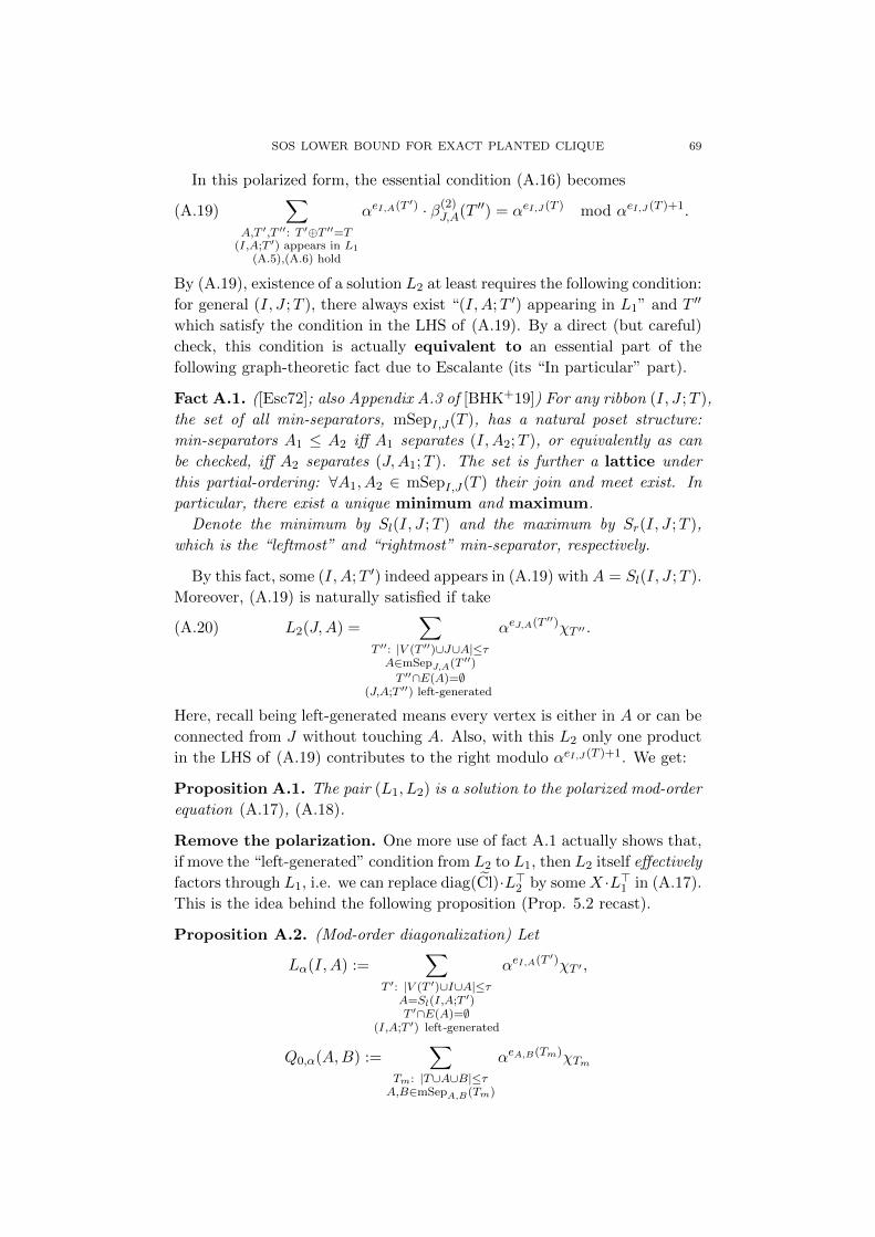
SOS LOWER BOUND FOR EXACT PLANTED CLIQUE 69
In this polarized form, the essential condition (A.16) becomes
(A.19)∑
A,T ′,T ′′: T ′⊕T ′′=T(I,A;T ′) appears in L1
(A.5),(A.6) hold
αeI,A(T ′) · β(2)J,A(T ′′) = αeI,J (T ) mod αeI,J (T )+1.
By (A.19), existence of a solution L2 at least requires the following condition:
for general (I, J ;T ), there always exist “(I, A;T ′) appearing in L1” and T ′′
which satisfy the condition in the LHS of (A.19). By a direct (but careful)
check, this condition is actually equivalent to an essential part of the
following graph-theoretic fact due to Escalante (its “In particular” part).
Fact A.1. ([Esc72]; also Appendix A.3 of [BHK+19]) For any ribbon (I, J ;T ),
the set of all min-separators, mSepI,J(T ), has a natural poset structure:
min-separators A1 ≤ A2 iff A1 separates (I, A2;T ), or equivalently as can
be checked, iff A2 separates (J,A1;T ). The set is further a lattice under
this partial-ordering: ∀A1, A2 ∈ mSepI,J(T ) their join and meet exist. In
particular, there exist a unique minimum and maximum.
Denote the minimum by Sl(I, J ;T ) and the maximum by Sr(I, J ;T ),
which is the “leftmost” and “rightmost” min-separator, respectively.
By this fact, some (I, A;T ′) indeed appears in (A.19) with A = Sl(I, J ;T ).
Moreover, (A.19) is naturally satisfied if take
(A.20) L2(J,A) =∑
T ′′: |V (T ′′)∪J∪A|≤τA∈mSepJ,A(T ′′)
T ′′∩E(A)=∅(J,A;T ′′) left-generated
αeJ,A(T ′′)χT ′′ .
Here, recall being left-generated means every vertex is either in A or can be
connected from J without touching A. Also, with this L2 only one product
in the LHS of (A.19) contributes to the right modulo αeI,J (T )+1. We get:
Proposition A.1. The pair (L1, L2) is a solution to the polarized mod-order
equation (A.17), (A.18).
Remove the polarization. One more use of fact A.1 actually shows that,
if move the “left-generated” condition from L2 to L1, then L2 itself effectively
factors through L1, i.e. we can replace diag(Cl)·L>2 by some X ·L>1 in (A.17).
This is the idea behind the following proposition (Prop. 5.2 recast).
Proposition A.2. (Mod-order diagonalization) Let
Lα(I, A) :=∑
T ′: |V (T ′)∪I∪A|≤τA=Sl(I,A;T ′)T ′∩E(A)=∅
(I,A;T ′) left-generated
αeI,A(T ′)χT ′ ,
Q0,α(A,B) :=∑
Tm: |T∪A∪B|≤τA,B∈mSepA,B(Tm)
αeA,B(Tm)χTm
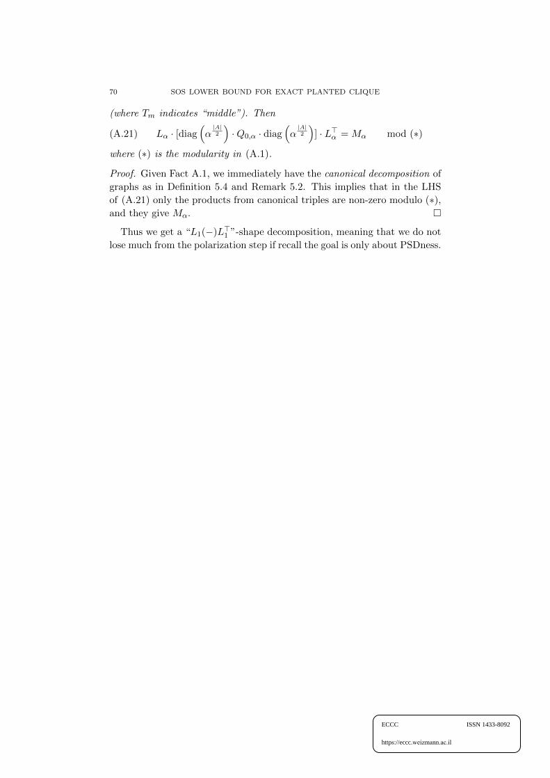
70 SOS LOWER BOUND FOR EXACT PLANTED CLIQUE
(where Tm indicates “middle”). Then
(A.21) Lα · [diag(α|A|2
)·Q0,α · diag
(α|A|2
)] · L>α = Mα mod (∗)
where (∗) is the modularity in (A.1).
Proof. Given Fact A.1, we immediately have the canonical decomposition of
graphs as in Definition 5.4 and Remark 5.2. This implies that in the LHS
of (A.21) only the products from canonical triples are non-zero modulo (∗),and they give Mα.
Thus we get a “L1(−)L>1 ”-shape decomposition, meaning that we do not
lose much from the polarization step if recall the goal is only about PSDness.
ECCC ISSN 1433-8092
https://eccc.weizmann.ac.il