congruence for sos with data

Congruence for SOS with Data

MohammadReza Mousavi, Michel Reniers, Jan Friso Groote

Department of Computer Science,Eindhoven University of Technology (TU/e),

Postbox 513, NL-5600 MB, Eindhoven, The NetherlandsEmail: {m.r.mousavi,m.a.reniers,j.f.groote}@tue.nl

Abstract

While studying the specification of the operational semantics of different programminglanguages and formalisms, one can observe the following three facts. Firstly, Plotkin’s styleof Structured Operational Semantics (SOS) has become a standard in defining operationalsemantics. Secondly, congruence with respect to some notion of bisimilarity is an interest-ing property for such languages and it is essential in reasoning about them. Thirdly, thereare numerous languages that contain an explicit data part in the state of the operationalsemantics.

The first two facts, have resulted in a line of research exploring syntactic formats ofoperational rules to derive the desired congruence property for free. However, the third point(in combination with the first two) is not sufficiently addressed and there is no standardcongruence format for operational semantics with an explicit data state. In this paper, weaddress this problem by studying the implications of the presence of a data state on the notionof bisimilarity. Furthermore, we propose a number of formats for congruence.

1 Introduction

Structured Operational Semantics (called SOS for short) [23] has been very popular in definingoperational semantics for different formalisms and programming languages. Moreover, congruenceproperties of notions of (bi-)simulation have been investigated in many of these languages as akey property for compositional reasoning and refinement. Congruence simply means that if onereplaces a component in an arbitrary system with a (bi-)similar counterpart, the resulting systemis (bi-)similar to the original one. Proofs of congruence for SOS semantics are usually standard butvery tedious involving several pages. This has resulted in a line of research for defining standardsyntactical formats for different types of SOS semantics in order to obtain the congruence propertyfor a given notion of bisimilarity automatically.

From the early beginning, SOS has been used for languages with data as an integrated part oftheir operational state (e.g., the original report on SOS contains several examples of state-bearingtransition system specifications [23]). As systems get more complex, the integration of a data statein their semantics becomes more vital. Besides the systems that have an explicit notion of datasuch as [4] and [9], real-time languages [15, 2, 18, 8] and hybrid languages [11] are other typicalexamples of systems in which a data state shows itself in the operational semantics in one way oranother. However, the introduction of data turns out not to be as trivial as it seems and leads tonew semantical issues such as adapted notions of bisimilarity [15, 11, 8, 21].

To the best of our knowledge, no standard congruence format for these different notions ofbisimilarity with a data state has been proposed so far. Henceforth, most of the congruence proofsare done manually [21] or are just neglected by making a reference to a standard format that doesnot cover the data state [8]. The proposal that comes closest ([7]) is unfinished and encodes rulesfor state-bearing processes into rules without a state, for which a format is given.

1

In this paper, we address the implications of the presence of a data state on notions of bisim-ilarity and propose standard formats that induce congruence with respect to these notions ofbisimilarity.

The rest of this paper is structured as follows. In Section 2, we review the related workin the area of congruence formats for SOS semantics. Then, in Section 3, we set the scene bydefining transition system specifications with data and several notions of bisimilarity. In thissection, we also sketch the relationship between these notions of bisimilarity and point out theirapplication areas. The main contribution of this paper is introduced in Section 4, where wedefine standard syntactic formats for proving congruence with respect to the defined notions ofbisimilarity. Furthermore, we give a full comparison between congruence results for the notionsof bisimilarity with data. Subsequently, Section 5 presents applications of the proposed theory ona number of transition system specifications from the literature. Finally, Section 6 concludes thepaper and presents possible extensions of the proposed approach.

2 Related Work

The first standard format for congruence was proposed by De Simone in [12]. The De Simoneformat allows for deduction rules of the following form:

{xili→ yi|i ∈ I}

f(x0, . . . , xn−1)l→ t

P(−→li , l).

where xi and yi are variables ranging over process terms, f is an n-ary function from the signature(e.g., sequential composition, parallel composition, etc.), I is a subset of the set {0, . . . , n − 1}(indices of arguments of f), t is an arbitrary process term and P is a predicate stating therelationship between the labels of the premises and the label of the conclusion. (It turns out thatside conditions of this kind do not play any role on the congruence result and thus we do notmention them in the remainder.)

Bloom, Istrail and Meyer, in their study of the relationship between bisimilarity and tracecongruence [6], define an extension of the De Simone format, called GSOS, to capture reasonablelanguage definitions. GSOS extends the De Simone format to cover negative premises. In otherwords, it allows for deduction rules of the following form:

{xilij

→ yij |i ∈ I, j ≤ m} ∪ {xjljk

9 |j ∈ J, k ≤ n}

f(x0, . . . , xn−1)l→ t

.

All common notations in the rule above have the same intuition as those of the De Simone format,J is a subset of indices of f (similar to I) and m and n are two natural numbers (to set an upperbound on the number of premises).

Another orthogonal extension of the De Simone format, called tyft/tyxt, is proposed in [17].This format allows for arbitrary terms in the left-hand-sides of the premises and in the right-hand-side of the conclusion but requires the left-hand-side of the conclusion to be a variable or afunction applied to variables only, the right-hand-sides of premises to be variables and all thesevariables to be distinct. In other words, it allows for the following forms of deduction rules:

{tili→ yi|i ∈ I}

f(x0, . . . , xn−1)l→ t

,{ti

li→ yi|i ∈ I}

xl→ t

.

All notations again share the same intuition with those of the De Simone format, apart from I,which is now an arbitrary (possibly infinite) set. The only further restriction on the set of premises,imposed for proving the congruence theorem in [17], is the acyclicity of a variable dependency graph.A variable dependency graph has variables as its nodes and there exists an edge from one variable

2

to another if the former appears in the left-hand-side and the latter in the right-hand-side of apremise. Later, in [13] it is shown that the acyclicity constraint can be relaxed and that for everytyft/tyxt rule with a non-well-founded set of premises (with respect to the variable dependencyordering) there exists a rule that induces the same transition relation and is indeed well-founded.

The merits of the two extensions were merged in [14] where negative premises were addedto the tyft/tyxt format, resulting in the ntyft/ntyxt format. In the premises of ntyft/ntyxt rules

negative transition relations of the form tili9 can appear as well, provided that the transition

system specification can be stratified. Stratification is concerned with defining a measure thatdecreases from the conclusion to negative premises and that does not increase from the conclusionto positive premises.

Finally, the PATH format [3] and the PANTH format [25] extend tyft/tyxt and ntyft/ntyxtwith predicates, respectively. A deduction rule in PANTH format may have predicates, negativepredicates, transitions and negative transitions in its premises and a predicate or a transition inits conclusion.

In [19], the PANTH format is extended for multi-sorted variable binding. This covers theproblem of operators such as recursion or choice over a time domain. The issue of binding operatorsfor multi-sorted process terms is also briefly introduced in [1]. In an unpublished note [7], theissue of state-bearing processes and multi-sorted transition system specifications is treated andthree congruence formats are proposed (Super-SOS, Data-SOS, and Special-SOS). The approachof [7] relies on transforming state-bearing processes to multi-sorted ones and thus, state-bearingtransition system specifications cannot be dealt with in their original representation (whilst thisis possible in our approach). The notion of bisimilarity in [7] seems to be what we call statelessbisimilarity in this paper. However, the formats they propose for this notion of bisimilarity arenot proved to induce congruence and moreover they impose some unneeded restrictions that arenot present in our format for stateless bisimilarity. Furthermore, the formats in [7] do not inducecongruence with respect to the other notions of bisimilarity that we discuss in this paper.

We recognize the problem of multi-sorted process terms and admit that it is an interestingproblem in itself. However, we address a different issue in this paper, that is, the issue of stateshaving a particular structure (possibly from different sorts). In the above works, the data stateis coded into process terms (either naturally due to the definition of operators like time-choiceoperators, e.g., in [19, 24] or artificially by transforming a multi-sorted state to a single-sortedone, e.g., in [7]). Thus, the transition system specification as well as the notion of equivalenceare confined to look at the behavior of process terms (since standard formats allow defining onlyone function symbol at a time in the conclusion of a deduction rule). However, if the data stateis made explicit as a part of the state in the transition system specification, then the transitionsystem specification may not only address process composition operators, but also data compo-sition operators. This allows both for more expressivity in the specification of SOS and for thepossibility of introducing new notions of equivalence (w.r.t. the relationship between data andprocess terms).

In [5], an extension of the tyft/tyxt format is proposed to cover the semantics of higher orderlanguages. The extended format, called promoted tyft/tyxt, allows for putting (open) terms on thelabels as well as on the two sides of the transition relation specification. Since labels are assumedto be of the same sort as process terms, their results do not apply to our problem domain directly(in which we have at least two different signatures for processes and data). However, by assumingtwo disjoint parts of the same signature as data and process signatures we may get a weakerresult for the case of stateless bisimilarity in Section 4 (i.e., the resulting format would be morerestrictive than ours). For the more involved notions of bisimilarity, however, we have to move toa multi-sorted state paradigm in order to define our criteria for the standard format and thus theformat of [5] is not applicable.

In [11], to prove congruence for a specification language with a data state, the transition systemspecification is partially transformed to another transition system specification that is isomorphicto the original one and does not contain a data state. Furthermore, it is shown that the originalnotion of bisimilarity corresponds to strong bisimilarity [20, 22] in the new specification. Since the

3

resulting transition system specification is in PATH format, it is deduced that the original notionof bisimilarity is a congruence. Although, the formal proof for these steps is not given therein detail, the proof sketch seems to be convincing for this particular notion of bisimilarity (i.e.,stateless bisimilarity). We combine all these steps here in one theorem and prove it so that suchtransformations and proofs are not necessary anymore. Furthermore, we give standard formatsfor other notions of bisimilarity for which such a straightforward transformation does not exist.

3 Preliminaries

3.1 Basic Definitions

We assume infinite and disjoint sets of process variables Vp (with typical members x, y, x′, y′, x0,y0 . . .) and data variables Vd (with typical members v and v′). A process signature Σp is a set offunction symbols with their fixed arity. Functions with zero arity are called constants. A processterm t ∈ T (Σp) is defined inductively as follows: a variable x ∈ Vp is a process term, if t0, . . . , tn−1

are process terms then for all f ∈ Σp with arity n, f(t0, . . . , tn−1) is a process term, as well(i.e., constants are indeed process terms). Process terms are typically denoted by t, t′, ti, t

′i, . . ..

Similarly, data terms u ∈ T (Σd) are defined based on a data signature Σd and the set of variablesVd and typically denoted by u, u′, ui, u

′i, . . .. Closed terms C(Σx) in each of these contexts are

defined as expected (closed process terms are typically denoted by p, q, p′, q′, p0, q0, p′0, q

′0 . . .). A

substitution σ replaces a variable in an open term with another (possibly open) term. The set ofvariables appearing in term t is denoted by vars(t).

Definition 3.1 (Transition System Specification) A transition system specification with datais a tuple (Σp,Σd, L,D(Rel)) where Σp is a process signature, Σd is a data signature, L is a setof labels (with typical members l, l′, l0, . . .), and D(Rel) is a set of deduction rules, where Rel is aset of (ternary) relation symbols. For all r ∈ Rel , l ∈ L and s, s′ ∈ T (Σp) × T (Σd) we define that(s, l, s′) ∈ r is a formula. A deduction rule dr ∈ D, is defined as a tuple (H, c) where H is a set offormulas and c is a formula. The formula c is called the conclusion and the formulas from H arecalled premises.

Notions of open and closed and the concept of substitution are lifted to formulas in the natural

way. A formula (s, l, s′) ∈ r is denoted by the more intuitive notation sl→r s

′, as well. A deduction

rule is mostly denoted byH

c.

A proof of a formula φ is a well-founded upwardly branching tree of which the nodes arelabelled by formulas such that

• the root node is labelled by φ, and

• if ψ is the label of a node q and {ψi | i ∈ I} is the set of labels of the nodes directly above q,

then there is a deduction rule{χi | i ∈ I}

χ, a process substitution σ and a data substitution

υ such that application of these substitutions to χ gives the formula ψ, and for all i ∈ I,application of the substitutions to χi gives the formula ψi.

3.2 Notions of Bisimilarity

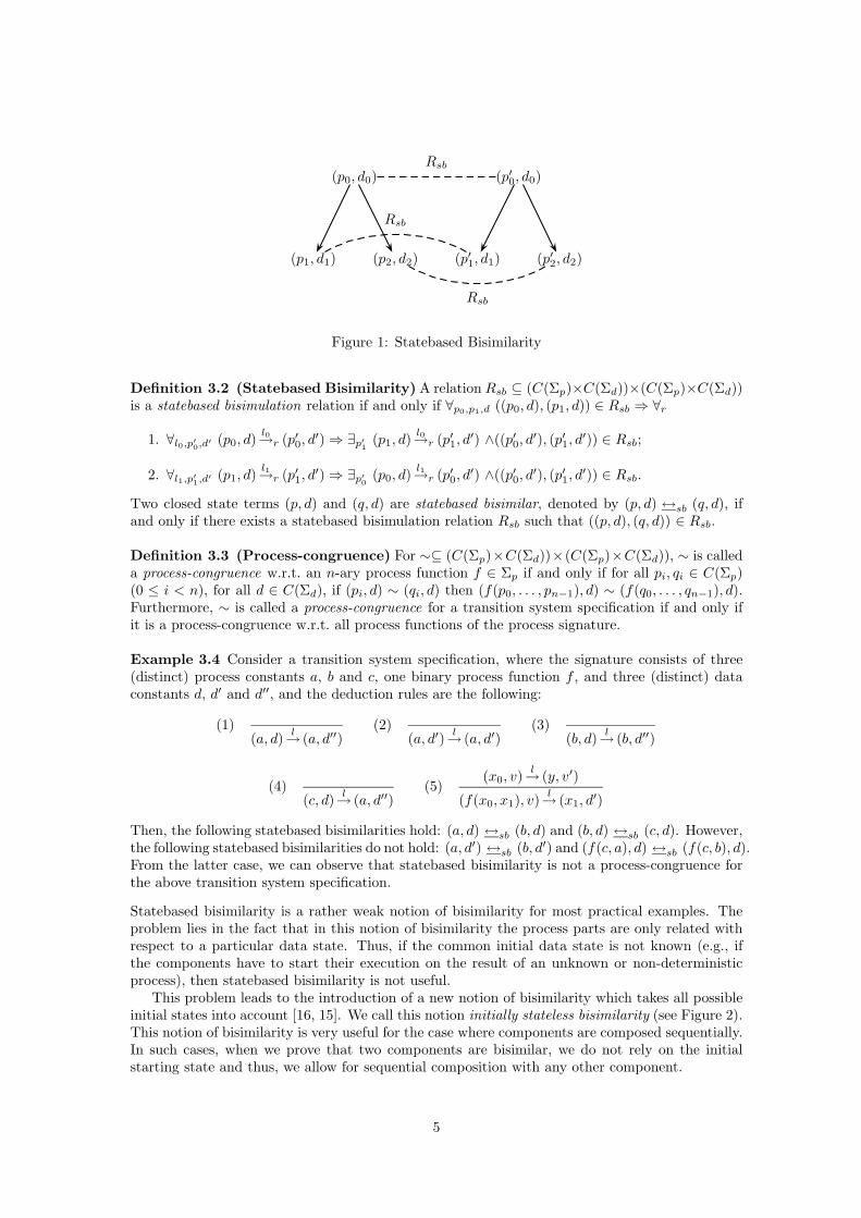
The introduction of data to the state adds a new dimension to the notion of bisimilarity. Onemight think that we can easily deal with data states by imposing the original notion of strongbisimilarity [20, 22] to the extended state. Our survey of the literature has revealed that sucha notion of strong bisimilarity is not used at all. It is clear that a format that respects strongbisimilarity as a congruence must necessarily be very restricted. Therefore, in this paper, werestrict ourselves to comparing processes with respect to the same data state. In this way, we getto what we call a statebased bisimilarity, depicted in Figure 1.

4

(p0, d0)

(p1, d1) (p2, d2)

(p′0, d0)

(p′1, d1) (p′2, d2)

Rsb

Rsb

Rsb

Figure 1: Statebased Bisimilarity

Definition 3.2 (Statebased Bisimilarity) A relation Rsb ⊆ (C(Σp)×C(Σd))×(C(Σp)×C(Σd))is a statebased bisimulation relation if and only if ∀p0,p1,d ((p0, d), (p1, d)) ∈ Rsb ⇒ ∀r

1. ∀l0,p′

0,d′ (p0, d)

l0→r (p′0, d′) ⇒ ∃p′

1(p1, d)

l0→r (p′1, d′) ∧((p′0, d

′), (p′1, d′)) ∈ Rsb;

2. ∀l1,p′

1,d′ (p1, d)

l1→r (p′1, d′) ⇒ ∃p′

0(p0, d)

l1→r (p′0, d′) ∧((p′0, d

′), (p′1, d′)) ∈ Rsb.

Two closed state terms (p, d) and (q, d) are statebased bisimilar, denoted by (p, d) ↔sb (q, d), ifand only if there exists a statebased bisimulation relation Rsb such that ((p, d), (q, d)) ∈ Rsb.

Definition 3.3 (Process-congruence) For ∼⊆ (C(Σp)×C(Σd))×(C(Σp)×C(Σd)), ∼ is calleda process-congruence w.r.t. an n-ary process function f ∈ Σp if and only if for all pi, qi ∈ C(Σp)(0 ≤ i < n), for all d ∈ C(Σd), if (pi, d) ∼ (qi, d) then (f(p0, . . . , pn−1), d) ∼ (f(q0, . . . , qn−1), d).Furthermore, ∼ is called a process-congruence for a transition system specification if and only ifit is a process-congruence w.r.t. all process functions of the process signature.

Example 3.4 Consider a transition system specification, where the signature consists of three(distinct) process constants a, b and c, one binary process function f , and three (distinct) dataconstants d, d′ and d′′, and the deduction rules are the following:

(1)(a, d)

l→ (a, d′′)

(2)(a, d′)

l→ (a, d′)

(3)(b, d)

l→ (b, d′′)

(4)(c, d)

l→ (a, d′′)

(5)(x0, v)

l→ (y, v′)

(f(x0, x1), v)l→ (x1, d

′)

Then, the following statebased bisimilarities hold: (a, d) ↔sb (b, d) and (b, d) ↔sb (c, d). However,the following statebased bisimilarities do not hold: (a, d′) ↔sb (b, d′) and (f(c, a), d) ↔sb (f(c, b), d).From the latter case, we can observe that statebased bisimilarity is not a process-congruence forthe above transition system specification.

Statebased bisimilarity is a rather weak notion of bisimilarity for most practical examples. Theproblem lies in the fact that in this notion of bisimilarity the process parts are only related withrespect to a particular data state. Thus, if the common initial data state is not known (e.g., ifthe components have to start their execution on the result of an unknown or non-deterministicprocess), then statebased bisimilarity is not useful.

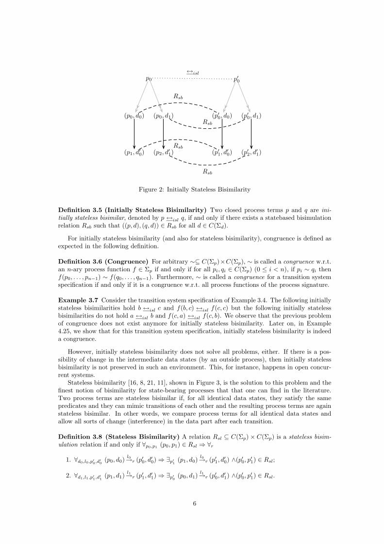
This problem leads to the introduction of a new notion of bisimilarity which takes all possibleinitial states into account [16, 15]. We call this notion initially stateless bisimilarity (see Figure 2).This notion of bisimilarity is very useful for the case where components are composed sequentially.In such cases, when we prove that two components are bisimilar, we do not rely on the initialstarting state and thus, we allow for sequential composition with any other component.

5

p0

(p0, d0)

(p1, d′0)

(p0, d1)

(p2, d′1)

p′0

(p′0, d0)

(p′1, d′0)

(p′0, d1)

(p′2, d′1)

↔isl

Rsb

Rsb

Rsb

Rsb

Figure 2: Initially Stateless Bisimilarity

Definition 3.5 (Initially Stateless Bisimilarity) Two closed process terms p and q are ini-tially stateless bisimilar, denoted by p ↔isl q, if and only if there exists a statebased bisimulationrelation Rsb such that ((p, d), (q, d)) ∈ Rsb for all d ∈ C(Σd).

For initially stateless bisimilarity (and also for stateless bisimilarity), congruence is defined asexpected in the following definition.

Definition 3.6 (Congruence) For arbitrary ∼⊆ C(Σp)×C(Σp), ∼ is called a congruence w.r.t.an n-ary process function f ∈ Σp if and only if for all pi, qi ∈ C(Σp) (0 ≤ i < n), if pi ∼ qi thenf(p0, . . . , pn−1) ∼ f(q0, . . . , qn−1). Furthermore, ∼ is called a congruence for a transition systemspecification if and only if it is a congruence w.r.t. all process functions of the process signature.

Example 3.7 Consider the transition system specification of Example 3.4. The following initiallystateless bisimilarities hold b ↔isl c and f(b, c) ↔isl f(c, c) but the following initially statelessbisimilarities do not hold a ↔isl b and f(c, a) ↔isl f(c, b). We observe that the previous problemof congruence does not exist anymore for initially stateless bisimilarity. Later on, in Example4.25, we show that for this transition system specification, initially stateless bisimilarity is indeeda congruence.

However, initially stateless bisimilarity does not solve all problems, either. If there is a pos-sibility of change in the intermediate data states (by an outside process), then initially statelessbisimilarity is not preserved in such an environment. This, for instance, happens in open concur-rent systems.

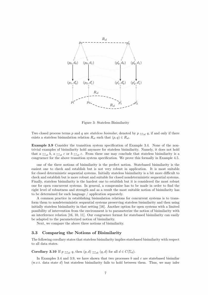
Stateless bisimilarity [16, 8, 21, 11], shown in Figure 3, is the solution to this problem and thefinest notion of bisimilarity for state-bearing processes that that one can find in the literature.Two process terms are stateless bisimilar if, for all identical data states, they satisfy the samepredicates and they can mimic transitions of each other and the resulting process terms are againstateless bisimilar. In other words, we compare process terms for all identical data states andallow all sorts of change (interference) in the data part after each transition.

Definition 3.8 (Stateless Bisimilarity) A relation Rsl ⊆ C(Σp) × C(Σp) is a stateless bisim-ulation relation if and only if ∀p0,p1

(p0, p1) ∈ Rsl ⇒ ∀r

1. ∀d0,l0,p′

0,d′

0(p0, d0)

l0→r (p′0, d′0) ⇒ ∃p′

1(p1, d0)

l0→r (p′1, d′0) ∧(p′0, p

′1) ∈ Rsl;

2. ∀d1,l1,p′

1,d′

1(p1, d1)

l1→r (p′1, d′1) ⇒ ∃p′

0(p0, d1)

l1→r (p′0, d′1) ∧(p′0, p

′1) ∈ Rsl.

6

p0

(p0, d0)

(p1, d′0)

p1

(p0, d1)

(p2, d′1)

p2

p′0

(p′0, d0)

(p′1, d′0)

p′1

(p′0, d1)

(p′2, d′1)

p′2

Rsl

Rsl

Rsl

Figure 3: Stateless Bisimilarity

Two closed process terms p and q are stateless bisimilar, denoted by p ↔sl q, if and only if thereexists a stateless bisimulation relation Rsl such that (p, q) ∈ Rsl.

Example 3.9 Consider the transition system specification of Example 3.4. None of the non-trivial examples of bisimilarity hold anymore for stateless bisimilarity. Namely, it does not holdthat a ↔sl b, a ↔sl c or b ↔sl c. From these one may conclude that stateless bisimilarity is acongruence for the above transition system specification. We prove this formally in Example 4.5.

one of the three notions of bisimilarity is the perfect notion. Statebased bisimilarity is theeasiest one to check and establish but is not very robust in application. It is most suitablefor closed deterministic sequential systems. Initially stateless bisimilarity is a bit more difficult tocheck and establish but is more robust and suitable for closed nondeterministic sequential systems.Finally, stateless bisimilarity is the hardest one to establish but it is considered the most robustone for open concurrent systems. In general, a compromise has to be made in order to find theright level of robustness and strength and as a result the most suitable notion of bisimilarity hasto be determined for each language / application separately.

A common practice in establishing bisimulation relations for concurrent systems is to trans-form them to nondeterministic sequential systems preserving stateless bisimilarity and then usinginitially stateless bisimilarity in that setting [16]. Another option for open systems with a limitedpossibility of intervention from the environment is to parameterize the notion of bisimilarity withan interference relation [16, 10, 11]. Our congruence format for statebased bisimilarity can easilybe adapted to the parameterized notion of bisimilarity.

Next, we compare the above three notions of bisimilarity.

3.3 Comparing the Notions of Bisimilarity

The following corollary states that stateless bisimilarity implies statebased bisimilarity with respectto all data states.

Corollary 3.10 If p ↔sl q, then (p, d) ↔sb (q, d) for all d ∈ C(Σd).

In Examples 3.4 and 3.9, we have shown that two processes b and c are statebased bisimilar(w.r.t. data state d) but stateless bisimilarity fails to hold between them. Thus, we may infer

7

that stateless bisimilarity is finer than statebased bisimilarity (w.r.t. a particular data state). Thefollowing corollary states that if a statebased bisimilarity relation is closed under the change ofdata state then it induces a stateless bisimulation relation.

Corollary 3.11 Consider a statebased bisimulation relation R. If for ∀p,q,d ((p, d), (q, d)) ∈ R⇒∀d′ ((p, d′), (q, d′)) ∈ R then ∀p,q (∃d ((p, d), (q, d)) ∈ R) ⇒ p ↔sl q.

Finally, the following lemma positions initially stateless bisimilarity in between the two othernotions of bisimilarity we have discussed so far.

Corollary 3.12 For two arbitrary closed process terms p and q and an arbitrary closed data termd, we have

1. if p ↔sl q, then p ↔isl q;

2. p ↔isl q if and only if, (p, d) ↔sb (q, d) for all d.

Again, in Examples 3.4 and 3.7, we have shown that a and b are statebased bisimilar withrespect to d but they are not initially stateless bisimilar. Thus, statebased bisimilarity (withrespect to a particular data state) is strictly weaker than initially stateless bisimilarity.

4 Standard Formats for Congruence

In this section we present standard formats and prove congruence results with respect to afore-mentioned notions of bisimilarity. To do this, we extend the tyft format of [15] with data in threesteps for stateless, statebased, and initially stateless bisimilarity. Finally, we present how ourformats can be extended to cover tyxt rules and rules containing predicates and negative premises(thus, extending the PANTH format [25] with data).

4.1 Congruence Format for Stateless Bisimilarity

In this paper, we allow for deduction rules that adhere to the tyft-format with respect to theprocess terms and are not restricted in the data terms. This format is called process-tyft.

Definition 4.1 (Process-tyft) Let (Σp,Σd, L,D(Rel)) be a transition system specification. Adeduction rule dr ∈ D(Rel) is in process-tyft format if it is of the form

(dr){(ti, ui)

li→ri(yi, u

′i)|i ∈ I}

(f(x0, . . . , xn−1), u)l→r (t′, u′)

,

where I is a set of indices, →r ∈ Rel , l ∈ L, f ∈ Σp is a process function of arity n, the variablesx0, . . . , xn−1 and yi (i ∈ I) are all distinct variables from Vp, and, for all i ∈ I: →ri

∈ Rel , li ∈ L,ti, t

′ ∈ T (Σp) and u, u′, ui, u′i ∈ T (Σd).

We name the set of process variables appearing in the left-hand-side of the conclusion Xp andin the right-hand-side of the premises Yp. The two sets Xp and Yp are obviously disjoint followingthe requirements of the format. The above deduction rule is called an f -defining deduction rule.

A transition system specification is in process-tyft format if all its deduction rules are in process-tyft format.

It turns out that for any transition system specification in process-tyft format, stateless bisim-ilarity is a congruence.

Theorem 4.2 If a transition system specification is in process-tyft format, then stateless bisimi-larity is a congruence for that transition system specification.

8

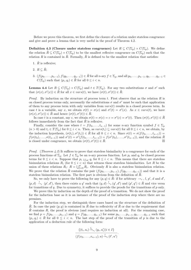
Before we prove this theorem, we first define the closure of a relation under stateless congruenceand give and prove a lemma that is very useful in the proof of Theorem 4.2.

Definition 4.3 (Closure under stateless congruence) Let R ⊆ C(Σp) × C(Σp). We define

the relation R ⊆ C(Σp) × C(Σp) to be the smallest reflexive congruence on C(Σp) such that the

relation R is contained in R. Formally, R is defined to be the smallest relation that satisfies:

1. R is reflexive;

2. R ⊆ R;

3. (f(p0, . . . , pn−1), f(q0, . . . , qn−1)) ∈ R for all n-ary f ∈ Σp, and all p0, . . . , pn−1, q0, . . . , qn−1 ∈

C(Σp) such that (pi, qi) ∈ R for all 0 ≤ i < n.

Lemma 4.4 Let R ⊆ C(Σp) × C(Σp) and t ∈ T (Σp). For any two substitutions σ and σ′ such

that (σ(x), σ′(x)) ∈ R for all x ∈ vars(t), we have (σ(t), σ′(t)) ∈ R.

Proof. By induction on the structure of process term t. First observe that as the relation R ison closed process terms only, necessarily the substitutions σ and σ′ must be such that applicationof them to any process term with only variables from vars(t) results in a closed process term. Incase t is a variable, say x, we obtain σ(t) = σ(x) and σ′(t) = σ′(x). As x ∈ vars(t), we have(σ(x), σ′(x)) ∈ R and hence (σ(t), σ′(t)) ∈ R.

In case t is a constant, say c, we obtain σ(t) = σ(c) = c = σ′(c) = σ′(t). Then (σ(t), σ′(t)) ∈ Rfollows immediately from the fact that R is reflexive.

Finally, consider the case where t = f(t0, . . . , tn−1) for some n-ary function symbol f ∈ Σp

(n > 0) and ti ∈ T (Σp) for 0 ≤ i < n. Then, as vars(ti) ⊆ vars(t) for all 0 ≤ i < n, we obtain, by

the induction hypothesis, (σ(ti), σ′(ti)) ∈ R for all 0 ≤ i < n. Since σ(t) = σ(f(t0, . . . , tn−1)) =

f(σ(t0), . . . , σ(tn−1)) and σ′(t) = σ′(f(t0, . . . , tn−1)) = f(σ′(t0), . . . , σ′(tn−1)), and the relation R

is closed under congruence, we obtain (σ(t), σ′(t)) ∈ R. �

Proof. (Theorem 4.2) It suffices to prove that stateless bisimilarity is a congruence for each of theprocess functions of Σp. Let f ∈ Σp be an n-ary process function. Let pi and qi be closed processterms for 0 ≤ i < n. Suppose that pi ↔sl qi for 0 ≤ i < n. This means that there are statelessbisimulation relations Ri (for 0 ≤ i < n) that witness these stateless bisimilarities. Let R be theunion of these relations Ri: R =

⋃ni=0Ri. Obviously R is also a stateless bisimulation relation.

We prove that the relation R contains the pair (f(p0, . . . , pn−1), f(q0, . . . , qn−1)) and that it is astateless bisimulation relation. The first part is obvious from the definition of R.

So, we only have to prove the following for any (p, q) ∈ R: if for arbitrary →r , l, p′, d and d′,

(p, d)l→r (p′, d′), then there exists a q′ such that (q, d)

l→r (q′, d′) and (p′, q′) ∈ R and vice versa

for transitions of q. Due to symmetry, it suffices to provide the proofs for the transitions of p only.We prove this by induction on the depth of the proof of a transition. We do not show the proof

for the induction base as it is an instance of the proof of the induction step where there are nopremises.

For the induction step, we distinguish three cases based on the structure of the definition ofR. In case the pair (p, q) is contained in R due to reflexivity of R or due to the requirement thatR contains R, the proof is obvious (and requires no induction at all). For the remaining case,we find p = f(p0, . . . , pn−1) and q = f(q0, . . . , qn−1) for some p0, . . . , pn−1, q0, . . . , qn−1 such that(pi, qi) ∈ R for all 0 ≤ i < n. The last step of the proof of the transition of p is due to theapplication of a deduction rule of the following form:

{(ti, ui)li→ri

(yi, u′i)|i ∈ I}

(f(x0, . . . , xn−1), u)l→r (t′, u′)

.

9

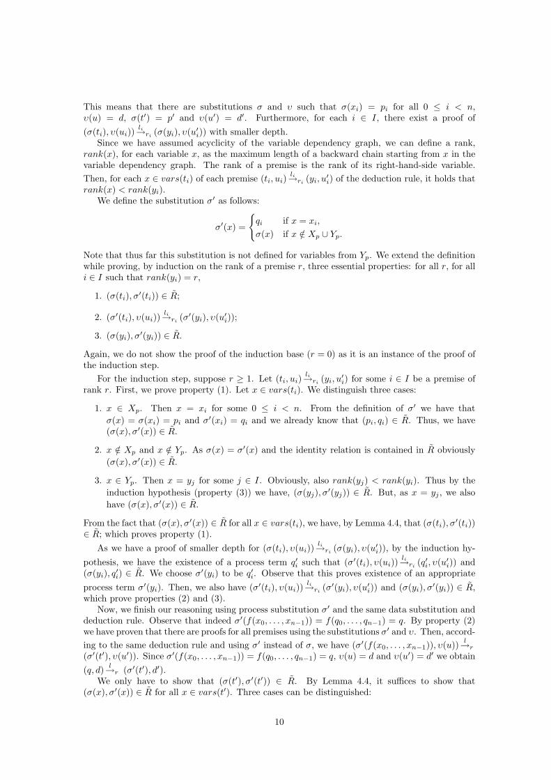
This means that there are substitutions σ and υ such that σ(xi) = pi for all 0 ≤ i < n,υ(u) = d, σ(t′) = p′ and υ(u′) = d′. Furthermore, for each i ∈ I, there exist a proof of

(σ(ti), υ(ui))li→ri

(σ(yi), υ(u′i)) with smaller depth.

Since we have assumed acyclicity of the variable dependency graph, we can define a rank,rank(x), for each variable x, as the maximum length of a backward chain starting from x in thevariable dependency graph. The rank of a premise is the rank of its right-hand-side variable.

Then, for each x ∈ vars(ti) of each premise (ti, ui)li→ri

(yi, u′i) of the deduction rule, it holds that

rank(x) < rank(yi).We define the substitution σ′ as follows:

σ′(x) =

{qi if x = xi,

σ(x) if x /∈ Xp ∪ Yp.

Note that thus far this substitution is not defined for variables from Yp. We extend the definitionwhile proving, by induction on the rank of a premise r, three essential properties: for all r, for alli ∈ I such that rank(yi) = r,

1. (σ(ti), σ′(ti)) ∈ R;

2. (σ′(ti), υ(ui))li→ri

(σ′(yi), υ(u′i));

3. (σ(yi), σ′(yi)) ∈ R.

Again, we do not show the proof of the induction base (r = 0) as it is an instance of the proof ofthe induction step.

For the induction step, suppose r ≥ 1. Let (ti, ui)li→ri

(yi, u′i) for some i ∈ I be a premise of

rank r. First, we prove property (1). Let x ∈ vars(ti). We distinguish three cases:

1. x ∈ Xp. Then x = xi for some 0 ≤ i < n. From the definition of σ′ we have that

σ(x) = σ(xi) = pi and σ′(xi) = qi and we already know that (pi, qi) ∈ R. Thus, we have(σ(x), σ′(x)) ∈ R.

2. x /∈ Xp and x /∈ Yp. As σ(x) = σ′(x) and the identity relation is contained in R obviously

(σ(x), σ′(x)) ∈ R.

3. x ∈ Yp. Then x = yj for some j ∈ I. Obviously, also rank(yj) < rank(yi). Thus by the

induction hypothesis (property (3)) we have, (σ(yj), σ′(yj)) ∈ R. But, as x = yj , we also

have (σ(x), σ′(x)) ∈ R.

From the fact that (σ(x), σ′(x)) ∈ R for all x ∈ vars(ti), we have, by Lemma 4.4, that (σ(ti), σ′(ti))

∈ R; which proves property (1).

As we have a proof of smaller depth for (σ(ti), υ(ui))li→ri

(σ(yi), υ(u′i)), by the induction hy-

pothesis, we have the existence of a process term q′i such that (σ′(ti), υ(ui))li→ri

(q′i, υ(u′i)) and

(σ(yi), q′i) ∈ R. We choose σ′(yi) to be q′i. Observe that this proves existence of an appropriate

process term σ′(yi). Then, we also have (σ′(ti), υ(ui))li→ri

(σ′(yi), υ(u′i)) and (σ(yi), σ

′(yi)) ∈ R,which prove properties (2) and (3).

Now, we finish our reasoning using process substitution σ′ and the same data substitution anddeduction rule. Observe that indeed σ′(f(x0, . . . , xn−1)) = f(q0, . . . , qn−1) = q. By property (2)we have proven that there are proofs for all premises using the substitutions σ′ and υ. Then, accord-

ing to the same deduction rule and using σ′ instead of σ, we have (σ′(f(x0, . . . , xn−1)), υ(u))l→r

(σ′(t′), υ(u′)). Since σ′(f(x0, . . . , xn−1)) = f(q0, . . . , qn−1) = q, υ(u) = d and υ(u′) = d′ we obtain

(q, d)l→r (σ′(t′), d′).

We only have to show that (σ(t′), σ′(t′)) ∈ R. By Lemma 4.4, it suffices to show that(σ(x), σ′(x)) ∈ R for all x ∈ vars(t′). Three cases can be distinguished:

10

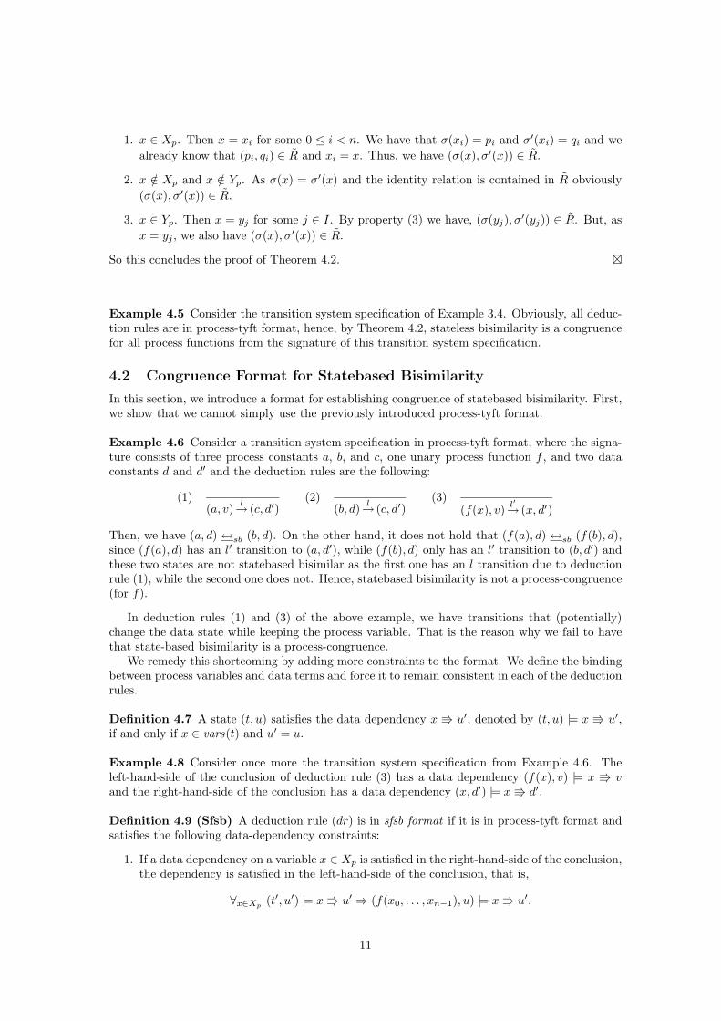
1. x ∈ Xp. Then x = xi for some 0 ≤ i < n. We have that σ(xi) = pi and σ′(xi) = qi and we

already know that (pi, qi) ∈ R and xi = x. Thus, we have (σ(x), σ′(x)) ∈ R.


(σ(x), σ′(x)) ∈ R.

3. x ∈ Yp. Then x = yj for some j ∈ I. By property (3) we have, (σ(yj), σ′(yj)) ∈ R. But, as

x = yj , we also have (σ(x), σ′(x)) ∈ R.

So this concludes the proof of Theorem 4.2. �

Example 4.5 Consider the transition system specification of Example 3.4. Obviously, all deduc-tion rules are in process-tyft format, hence, by Theorem 4.2, stateless bisimilarity is a congruencefor all process functions from the signature of this transition system specification.

4.2 Congruence Format for Statebased Bisimilarity

In this section, we introduce a format for establishing congruence of statebased bisimilarity. First,we show that we cannot simply use the previously introduced process-tyft format.

Example 4.6 Consider a transition system specification in process-tyft format, where the signa-ture consists of three process constants a, b, and c, one unary process function f , and two dataconstants d and d′ and the deduction rules are the following:

(1)(a, v)

l→ (c, d′)

(2)(b, d)

l→ (c, d′)

(3)(f(x), v)

l′→ (x, d′)

Then, we have (a, d) ↔sb (b, d). On the other hand, it does not hold that (f(a), d) ↔sb (f(b), d),since (f(a), d) has an l′ transition to (a, d′), while (f(b), d) only has an l′ transition to (b, d′) andthese two states are not statebased bisimilar as the first one has an l transition due to deductionrule (1), while the second one does not. Hence, statebased bisimilarity is not a process-congruence(for f).

In deduction rules (1) and (3) of the above example, we have transitions that (potentially)change the data state while keeping the process variable. That is the reason why we fail to havethat state-based bisimilarity is a process-congruence.

We remedy this shortcoming by adding more constraints to the format. We define the bindingbetween process variables and data terms and force it to remain consistent in each of the deductionrules.

Definition 4.7 A state (t, u) satisfies the data dependency x V u′, denoted by (t, u) |= x V u′,if and only if x ∈ vars(t) and u′ = u.

Example 4.8 Consider once more the transition system specification from Example 4.6. Theleft-hand-side of the conclusion of deduction rule (3) has a data dependency (f(x), v) |= x V vand the right-hand-side of the conclusion has a data dependency (x, d′) |= xV d′.

Definition 4.9 (Sfsb) A deduction rule (dr) is in sfsb format if it is in process-tyft format andsatisfies the following data-dependency constraints:

1. If a data dependency on a variable x ∈ Xp is satisfied in the right-hand-side of the conclusion,the dependency is satisfied in the left-hand-side of the conclusion, that is,

∀x∈Xp(t′, u′) |= xV u′ ⇒ (f(x0, . . . , xn−1), u) |= xV u′.

11

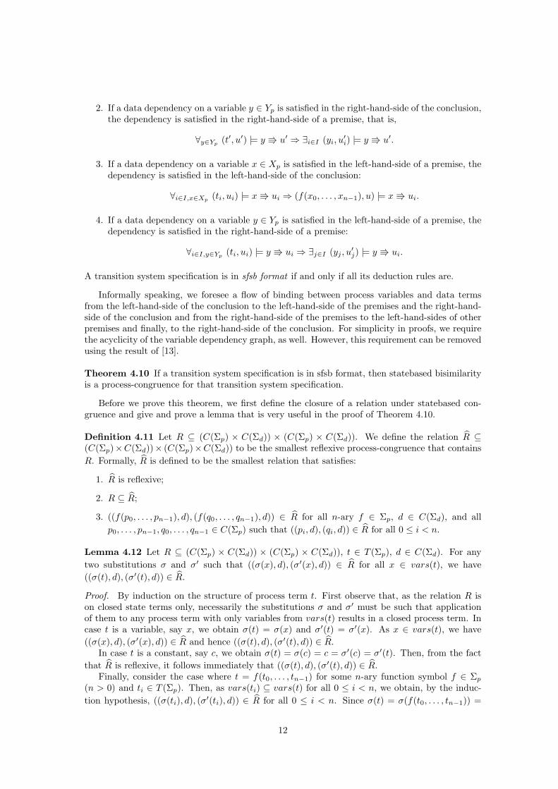
2. If a data dependency on a variable y ∈ Yp is satisfied in the right-hand-side of the conclusion,the dependency is satisfied in the right-hand-side of a premise, that is,

∀y∈Yp(t′, u′) |= y V u′ ⇒ ∃i∈I (yi, u

′i) |= y V u′.

3. If a data dependency on a variable x ∈ Xp is satisfied in the left-hand-side of a premise, thedependency is satisfied in the left-hand-side of the conclusion:

∀i∈I,x∈Xp(ti, ui) |= xV ui ⇒ (f(x0, . . . , xn−1), u) |= xV ui.

4. If a data dependency on a variable y ∈ Yp is satisfied in the left-hand-side of a premise, thedependency is satisfied in the right-hand-side of a premise:

∀i∈I,y∈Yp(ti, ui) |= y V ui ⇒ ∃j∈I (yj , u

′j) |= y V ui.

A transition system specification is in sfsb format if and only if all its deduction rules are.

Informally speaking, we foresee a flow of binding between process variables and data termsfrom the left-hand-side of the conclusion to the left-hand-side of the premises and the right-hand-side of the conclusion and from the right-hand-side of the premises to the left-hand-sides of otherpremises and finally, to the right-hand-side of the conclusion. For simplicity in proofs, we requirethe acyclicity of the variable dependency graph, as well. However, this requirement can be removedusing the result of [13].

Theorem 4.10 If a transition system specification is in sfsb format, then statebased bisimilarityis a process-congruence for that transition system specification.

Before we prove this theorem, we first define the closure of a relation under statebased con-gruence and give and prove a lemma that is very useful in the proof of Theorem 4.10.

Definition 4.11 Let R ⊆ (C(Σp) × C(Σd)) × (C(Σp) × C(Σd)). We define the relation R ⊆(C(Σp)×C(Σd))× (C(Σp)×C(Σd)) to be the smallest reflexive process-congruence that contains

R. Formally, R is defined to be the smallest relation that satisfies:

1. R is reflexive;

2. R ⊆ R;

3. ((f(p0, . . . , pn−1), d), (f(q0, . . . , qn−1), d)) ∈ R for all n-ary f ∈ Σp, d ∈ C(Σd), and all

p0, . . . , pn−1, q0, . . . , qn−1 ∈ C(Σp) such that ((pi, d), (qi, d)) ∈ R for all 0 ≤ i < n.

Lemma 4.12 Let R ⊆ (C(Σp) × C(Σd)) × (C(Σp) × C(Σd)), t ∈ T (Σp), d ∈ C(Σd). For any

two substitutions σ and σ′ such that ((σ(x), d), (σ′(x), d)) ∈ R for all x ∈ vars(t), we have

((σ(t), d), (σ′(t), d)) ∈ R.

Proof. By induction on the structure of process term t. First observe that, as the relation R ison closed state terms only, necessarily the substitutions σ and σ′ must be such that applicationof them to any process term with only variables from vars(t) results in a closed process term. Incase t is a variable, say x, we obtain σ(t) = σ(x) and σ′(t) = σ′(x). As x ∈ vars(t), we have

((σ(x), d), (σ′(x), d)) ∈ R and hence ((σ(t), d), (σ′(t), d)) ∈ R.In case t is a constant, say c, we obtain σ(t) = σ(c) = c = σ′(c) = σ′(t). Then, from the fact

that R is reflexive, it follows immediately that ((σ(t), d), (σ′(t), d)) ∈ R.Finally, consider the case where t = f(t0, . . . , tn−1) for some n-ary function symbol f ∈ Σp

(n > 0) and ti ∈ T (Σp). Then, as vars(ti) ⊆ vars(t) for all 0 ≤ i < n, we obtain, by the induc-

tion hypothesis, ((σ(ti), d), (σ′(ti), d)) ∈ R for all 0 ≤ i < n. Since σ(t) = σ(f(t0, . . . , tn−1)) =

12

f(σ(t0), . . . , σ(tn−1)) and σ′(t) = σ′(f(t0, . . . , tn−1)) = f(σ′(t0), . . . , σ′(tn−1)), and the relation R

is closed under process-congruence, we obtain ((σ(t), d), (σ′(t), d)) ∈ R. �

Proof. (Theorem 4.10) It suffices to prove that statebased bisimilarity is a process-congruencefor each of the process functions of Σp. Let f ∈ Σp be an n-ary process function. Let pi andqi be closed process terms for 0 ≤ i < n and let d ∈ C(Σd). Suppose that (pi, d) ↔sb (qi, d) for0 ≤ i < n. This means that there are statebased bisimulation relations Ri (for 0 ≤ i < n) thatwitness these statebased bisimilarities. Let R be the union of these relations Ri: R =

⋃ni=0Ri.

Obviously R is also a statebased bisimulation relation. We prove that the relation R contains thepair ((f(p0, . . . , pn−1), d), (f(q0, . . . , qn−1), d)) and that it is a statebased bisimulation relation.

The first part is obvious from the definition of R.So, we only have to prove the following for any ((p, d), (q, d)) ∈ R: if for an arbitrary →r , l,

p′ and d′, (p, d)l→r (p′, d′), then there exists a q′ such that (q, d)

l→r (q′, d′) and ((p′, d′), (q′, d′))

∈ R and vice versa for transitions of q. Due to symmetry, it suffices to provide the proofs for thetransitions of p only.

We prove this by induction on the depth of the proof of a transition. We do not show the prooffor the induction base as it is an instance of the proof of the induction step where there are nopremises.

For the induction step, we distinguish three cases based on the structure of the definition ofR. In case the pair ((p, d), (q, d)) is contained in the identity relation or the relation R, the proofis obvious (and requires no induction at all). For the remaining case, we find p = f(p0, . . . , pn−1)

and q = f(q0, . . . , qn−1) for some p0, . . . , pn−1, q0, . . . , qn−1 such that ((pi, d), (qi, d)) ∈ R for all0 ≤ i < n. The last step of the proof of the transition of p is due to the application of a deductionrule of the following form:

{(ti, ui)li→ri

(yi, u′i)|i ∈ I}

(f(x0, . . . , xn−1), u)l→r (t′, u′)

.








σ′(x) =

{qi if x = xi,


Note that thus far this substitution is not defined for variables from Yp. We extend the definitionwhile proving, by induction on the rank of a premise r, three essential properties: for all r, for alli ∈ I such that rank(yi) = r,

1. ((σ(ti), υ(ui)), (σ′(ti), υ(ui))) ∈ R;


(σ′(yi), υ(u′i));

3. ((σ(yi), υ(u′i)), (σ

′(yi), υ(u′i))) ∈ R.




rank r. First, we prove property (1). Let x ∈ vars(ti). We distinguish three cases:

13

1. x ∈ Xp. Then x = xi for some 0 ≤ i < n. The left-hand-side of the premise has a datadependency xi V ui. Hence, by data-dependency constraint 3, this dependency also hasto be satisfied in the left-hand-side of the conclusion. Hence, ui = u. We also have thatσ(xi) = pi and σ′(xi) = qi and we already know that ((pi, d), (qi, d)) ∈ R and υ(u) = d.

Thus, we have ((σ(xi), υ(ui)), (σ′(xi), υ(ui))) ∈ R, i.e., ((σ(x), υ(ui)), (σ

′(x), υ(ui))) ∈ R.


((σ(x), υ(u′)), (σ′(x), υ(u′))) ∈ R.

3. x ∈ Yp. Then x = yj for some j ∈ I. The left-hand-side of the premise has a data dependencyyj V ui. Hence, by data-dependency constraint 4, this dependency also has to be satisfiedin the right-hand-side of a premise. Only the premise with index j is a candidate. Hence,(yj , u

′j) |= x V ui. Hence u′j = ui. Obviously, also rank(yj) < rank(yi). Thus by the

induction hypothesis(property (2)) we have, ((σ(yj), υ(u′j)), (σ

′(yj), υ(u′j))) ∈ R. But, as

x = yj , and u′j = ui, we also have ((σ(x), υ(ui)), (σ′(x), υ(ui))) ∈ R.

From the fact that ((σ(x), υ(ui)), (σ′(x), υ(ui))) ∈ R for all x ∈ vars(ti), by Lemma 4.12, we have

((σ(ti), υ(ui)), (σ′(ti), υ(ui))) ∈ R; which proves property (1).

As we have a proof of smaller depth for (σ(ti), υ(ui))li→ri

(σ(yi), υ(u′i)), by the induction

hypothesis, we have the existence of a process term q′i such that (σ′(ti), υ(ui))li→ri

(q′i, υ(u′i))

and ((σ(yi), υ(u′i)), (q

′i, υ(u

′i))) ∈ R. We choose σ′(yi) to be q′i. Observe that this proves exis-

tence of an appropriate process term σ′(yi). Then, we also have (σ′(ti), υ(ui))li→ri

(σ′(yi), υ(u′i))

((σ(yi), υ(u′i)), (σ

′(yi), υ(u′i))) ∈ R, which prove properties (2) and (3).

Now, we finish our reasoning using process substitution σ′ and the same data substitution anddeduction rule. Observe that indeed σ′(f(x0, . . . , xn−1)) = f(q0, . . . , qn−1) = q. By property (2)we have proven that there are proofs for all premises using the substitutions σ′ and υ. Then, accord-

ing to the same deduction rule and using σ′ instead of σ, we have (σ′(f(x0, . . . , xn−1)), υ(u))l→r


(q, d)l→r (σ′(t′), d′).

We only have to show that ((σ(t′), d′), (σ′(t′), d′)) ∈ R. By Lemma 4.12, it suffices to show

that ((σ(x), d′), (σ′(x), d′)) ∈ R for all x ∈ vars(t′). Three cases can be distinguished:

1. x ∈ Xp. Then x = xi for some 0 ≤ i < n. The right-hand-side of the conclusion ofthe deduction rule has a data dependency (t′, u′) |= x V u′. Hence, by data-dependencyconstraint 1, this data dependency has to be satisfied in the left-hand-side of the conclusion.Therefore, necessarily (f(x0, . . . , xn−1), u) |= x V u′, and thus u = u′. Hence d = υ(u) =υ(u′) = d′. We also have that σ(xi) = pi and σ′(xi) = qi and we already know that

((pi, d), (qi, d)) ∈ R, xi = x, and d = d′. Thus, we have ((σ(x), d′), (σ′(x), d′)) ∈ R.


((σ(x), d′), (σ′(x), d′)) ∈ R.

3. x ∈ Yp. Then x = yj for some j ∈ I. The right-hand-side of the conclusion has a datadependency yj V u′. Hence, by data-dependency constraint 2, this dependency also hasto be satisfied in the right-hand-side of a premise. Only the premise with index j is acandidate. Hence, (yj , u

′j) |= x V u′. This can only be the case if u′j = u′. We obtain

d′ = υ(u′) = υ(u′j). By property (3) we have, ((σ(yj), υ(u′j)), (σ

′(yj), υ(u′j))) ∈ R. But, as

x = yj , and υ(u′j) = d′, we also have ((σ(x), d′), (σ′(x), d′)) ∈ R.


Next, we show that if the proposed format is relaxed in any conceivable way, the congruenceresult is lost. The first example shows that we cannot remove data-dependency constraint 1.

14

Example 4.13 Consider a transition system specification, where the process signature consistsof process constants a and b, and a unary function symbol f ; the data signature consists of dataconstants d and d′; and the following deduction rules:

(1)(a, d′)

l→ (a, d′)

, (2)(f(x), d)

l→ (x, d′)

.

These deduction rules are in process-tyft format. Data-dependency constraint 1 is not satisfiedby deduction rule (2) as the data dependency x V d′ that is satisfied in the right-hand-side ofthe conclusion (i.e., state (x, d′)) is not satisfied in the left-hand-side of the conclusion. The otherdata-dependency constraints are satisfied.

The process-congruence result fails on the above specification. We have (a, d) ↔sb (b, d) (bothcannot perform any transitions). However, it does not hold that (f(a), d) ↔sb (f(b), d) since theformer state can perform a transition due to deduction rule (2) to (a, d′), while the latter is forcedto make the same transition to (b, d′) and it clearly does not hold that (a, d′) ↔sb (b, d′) (seededuction rule (1)).

The next example shows that we cannot remove data-dependency constraint 2.

Example 4.14 Consider a process signature consisting of process constants a and b and a unaryprocess function f ; a data signature consisting of data constants d and d′; and a transition systemspecification with the following deduction rules:

(1)(a, v)

l→ (a, v)

, (2)(b, d)

l→ (b, d)

, (3)(x, d)

l→ (y, d)

(f(x), d)l→ (y, d′)

.

These deduction rules are in process-tyft format and all data-dependency constraints, except forconstraint 2, which is violated by deduction rule (3). This violation results in breaking the process-congruence result. Two states (a, d) and (b, d) are statebased bisimilar. However, (f(a), d) is notstatebased bisimilar to (f(b), d) since the former can perform a transition using deduction rule(3) to (a, d′), while the latter performs a similar transition to (b, d′). These two states are notstatebased bisimilar as the former performs an l-transition and the latter deadlocks.


Example 4.15 Consider a transition system specification, where the process signature consistsof process constants a and b, and a unary function symbol f ; the data signature consists of dataconstants d and d′; and the following deduction rules:

(1)(a, d′)

l→ (a, d′)

, (2)(x, d′)

l→ (y, v′)

(f(x), v)l→ (x, v)

.

The above deduction rules are in process-tyft format and satisfy data-dependency constraints 1, 2,and 4. Data-dependency constraint 3 is violated in deduction rule (3) since the data dependencyxV d′ that is satisfied in the left-hand-side of the premise is not satisfied in the left-hand-side ofthe conclusion.

For this transition system specification, statebased bisimilarity is not a process-congruence.We have (a, d) ↔sb (b, d) (both states deadlock). However, (f(a), d) ↔sb (f(b), d) does not hold,since the former state can make a transition due to deduction rule (2) while the latter cannotmake any transition.


Example 4.16 Consider a process signature consisting of process constants a and b and a unaryprocess function f ; a data signature consisting of data constants d and d′; and a transition system

15

specification with the following deduction rules:

(1)(a, v)

l→ (a, v)

, (2)(b, d)

l→ (b, d)

, (3)(x, d)

l→ (y, d) (y, d′)

l→ (y′, d′)

(f(x), d)l→ (y′, d′)

.

The above deduction rules are in process-tyft format and satisfy all data-dependency constraintsapart from constraint 4. Deduction rule (3) breaks this constraint in the left-hand-side of itssecond premise. This also turns out to be harmful for the congruence property, since we have(a, d) ↔sb (b, d) but not (f(a), d) ↔sb (f(b), d) because deduction rule (3) allows for a transitionof the former but not the latter.

4.3 Congruence Format for Initially Stateless Bisimilarity

Later, when comparing congruence conditions for the different notions of bisimilarity, we showthat the sfsb format works perfectly well for initially stateless bisimilarity. However, it may turnout to be too restrictive in application. The following example shows a common problem in thisregard.

Example 4.17 Consider the following transition system specification (with process constants aand b, unary process function f , and data constants d and d′) and the following deduction rules:

(1)(a, v)

l→ (a, v)

, (2)(b, d)

l→ (b, d)

, (3)(x0, v)

l→ (y, v)

(f(x0, x1), v)l→ (x1, d

′).

This transition system specification does not satisfy the sfsb format and statebased bisimilarityis not a congruence (since (a, d) ↔sb (b, d), but it does not hold that (f(b, a), d) ↔sb (f(b, b), d)).However, it can be checked that initially stateless bisimilarity is indeed a congruence. The reasonis that the change in the data state in deduction rule (3) is harmless since x1’s are now relatedusing all data states including d′ (e.g., the above counterexample does not work anymore since itdoes not hold that a ↔isl b).

This gives us some clue that for initially stateless bisimilarity, we may weaken the data-dependency constraints.

Definition 4.18 (Sfisl) A deduction rule (dr) is in sfisl format if it is in process-tyft format andsatisfies the following local (relaxed) data-dependency constraints:

1. If a data dependency on a variable y ∈ Yp is satisfied in the right-hand-side of the conclusion,the dependency is satisfied in the right-hand-side of a premise, that is,

∀y∈Yp(t′, u′) |= y V u′ ⇒ ∃i∈I (yi, u

′i) |= y V u′.

2. If a data dependency on a variable y ∈ Yp is satisfied in the left-hand-side of a premise, thedependency is satisfied in the right-hand-side of a premise:

∀i∈I,y∈Yp(ti, ui) |= y V ui ⇒ ∃j∈I (yj , u

′j) |= y V ui.

The data-dependency constraints that were required for variables from the set Xp for con-gruence of statebased bisimilarity, need not be satisfied for this format anymore. The reason ofviolating these constraints is that we rely on the fact that certain positions are instantiated byprocess terms that are related for all possible data. To formalize this concept, first we definepositions for which the two constraints are violated and then we check the global consequences ofthis violation.

16

Definition 4.19 A variable x ∈ Xp is called unresolved if

∃i∈I x ∈ vars(ti) ⇒ (ti, ui) 6|= xV u∨x ∈ vars(t′) ⇒ (t′, u′) 6|= xV u.

We define Xup to be the set of unresolved variables.

For each process function f , we define a set IV f that contains indices of f for which we needinitially stateless bisimilarity because a data-dependency is violated with respect to the variablethat occurs in that position in the left-hand-side of the conclusion. The set IV f contains at leastthe indices of the unresolved variables of the f -defining deduction rules, but it may contain moreindices due to the use of f in other deduction rules in the right-hand-side of the conclusion or theleft-hand-side of a premise.

Definition 4.20 For a given transition system specification in process-tyft format, we define, forall f ∈ Σp, the sets IV f as the smallest sets that satisfy, for all f -defining deduction rules dr:

1. the indices of unresolved variables (i.e., variables from Xup ) of dr are in IV f ;

2. for all n-ary process functions g ∈ Σp: for each occurrence of a process term g(t0, . . . , tn−1)in the left-hand-side of a premise or the right-hand-side of the conclusion of dr:

∀i∈IV g∀x∈vars(ti) ∃j∈IV f

x = xj .

Note that with the above definition, it is possible that such a set does not exist. In such cases,the global data-dependency constraint given below cannot be established.

Definition 4.21 (Sfisl) A transition system specification is in sfisl format if all its deductionrules are in sfisl format and furthermore for each process function f the set IV f exists.

Informally, this means that a deduction rule may change the data state associated with aprocess term (arbitrarily) if according to the other rules, the process term is guaranteed to beamong the initial argument of the topmost process function (thus, benefitting from the initiallystateless bisimilarity assumption). The positions of a process function f benefitting from theinitially stateless bisimilarity assumption are thus denoted by IV f .

Theorem 4.22 If a transition system specification is in sfisl format, then initially stateless bisim-ilarity is a congruence for that transition system specification.

Before we prove this theorem, we first define the closure of a relation under initially statelesscongruence and give and prove a lemma that is very useful in the proof of Theorem 4.22.

Definition 4.23 (Closure With Initially Stateless Congruence) Let R ⊆ (C(Σp)×C(Σd))× (C(Σp) × C(Σd)). We define the relation R ⊆ (C(Σp) × C(Σd)) × (C(Σp) × C(Σd)) to be thesmallest relation that satisfies:

1. R is reflexive;

2. R ⊆ R;

3. ((f(p0, . . . , pn−1), d), (f(q0, . . . , qn−1), d)) ∈ R for all n-ary f ∈ Σp, d ∈ C(Σd), and allp0, . . . , pn−1, q0, . . . , qn−1 ∈ C(Σp) such that

(a) ∀i/∈IV f((pi, d), (qi, d)) ∈ R;

(b) ∀i∈IV f ,d′∈C(Σd) ((pi, d′), (qi, d

′)) ∈ R.

17

For a process term t, we define the set V (t) to be the set of variables that appear in the placesindicated by the sets IV f (for all f).

V (x) = ∅,V (f(t0, . . . , tn−1)) =

⋃0≤i<n,i∈IV f

vars(ti) ∪⋃

0≤i<n,i/∈IV f

V (ti).

Lemma 4.24 Let R ⊆ (C(Σp)×C(Σd))× (C(Σp)×C(Σd)), t ∈ T (Σp), d ∈ C(Σd). For any twosubstitutions σ and σ′ such that

1. ((σ(x), d′), (σ′(x), d′)) ∈ R for all x ∈ V (t), d′ ∈ C(Σd), and

2. ((σ(x), d), (σ′(x), d)) ∈ R for all x ∈ vars(t) \ V (t);

we have ((σ(t), d), (σ′(t), d)) ∈ R.

Proof. By induction on the structure of process term t. In case t is a variable, say x, weobtain σ(t) = σ(x) and σ′(t) = σ′(x) and V (t) = V (x) = ∅. As x ∈ vars(t) \ V (t), we have((σ(x), d), (σ′(x), d)) ∈ R and therefore ((σ(t), d), (σ′(t), d)) ∈ R as well.

In case t is a constant, say c, we obtain σ(t) = σ(c) = c = σ′(c) = σ′(t). Then, from reflexivityof R, it follows immediately that ((σ(t), d), (σ′(t), d)) ∈ R.

Finally, consider the case where t = f(t0, . . . , tn−1) for some n-ary (n ≥ 1) function symbolf ∈ Σp and ti ∈ T (Σp) (0 ≤ i < n). If we prove

((σ(ti), d), (σ′(ti), d)) ∈ R (1)

for all i /∈ IV f , and((σ(ti), d

′), (σ′(ti), d′)) ∈ R (2)

for all i ∈ IV f and d′ ∈ C(Σd), then ((σ(t), d), (σ′(t), d)) ∈ R according to Definition 4.23.For the first part, assume that i 6∈ IV f . Then, by definition of V , we have V (ti) ⊆ V (t).

Therefore, by the first assumption on σ and σ′ of Lemma 4.24, we have ((σ(x), d′), (σ′(x), d′)) ∈R for all x ∈ V (ti) and d′ ∈ C(Σd). By the first and second assumption and the fact thatvars(ti) \ V (ti) ⊆ vars(t), we have ((σ(x), d), (σ′(x), d)) ∈ R for all x ∈ vars(ti) \ V (ti). Thus, bythe induction hypothesis, we have ((σ(ti), d), (σ

′(ti), d)) ∈ R.For the second part, assume that i ∈ IV f and that d′ ∈ C(Σd). From the definition of V

we obtain vars(ti) ⊆ V (t). Hence, by the first assumption on σ and σ′ of Lemma 4.24, wehave ((σ(x), d′), (σ′(x), d′)) ∈ R for all x ∈ vars(ti). Thus, by the induction hypothesis, we have((σ(ti), d

′), (σ′(ti), d′)) ∈ R. �

Proof. (Theorem 4.22) It suffices to prove that initially stateless bisimilarity is a congruencefor each of the process functions of Σp. Let f ∈ Σp be an n-ary process function. Let pi andqi be closed process terms for 0 ≤ i < n and let d ∈ C(Σd). Suppose that pi ↔isl qi for 0 ≤i < n. This means that there are statebased bisimulation relations Ri (for 0 ≤ i < n) such that((pi, d), (qi, d)) ∈ Ri for all d ∈ C(Σd). Let R be the union of these relations Ri: R =

⋃ni=0Ri.

Obviously R is also a statebased bisimulation relation. We prove that the relation R containsthe pair ((f(p0, . . . , pn−1), d), (f(q0, . . . , qn−1), d)), for all d ∈ C(Σd), and that it is a statebasedbisimulation relation.

As ((pi, d), (qi, d)) ∈ Ri and Ri ⊆ R ⊆ R, for all 0 ≤ i < n and all d ∈ C(Σd), it follows that((pi, d), (qi, d)) ∈ R, for all 0 ≤ i < n and all d ∈ C(Σd). Hence, by the definition of R obviouslyalso ((f(p0, . . . , pn−1), d), (f(q0, . . . , qn−1), d)) ∈ R, for d ∈ C(Σd).

So, we only have to prove the following for any ((p, d), (q, d)) ∈ R: if for arbitrary →r , l, p′

and d′, (p, d)l→r (p′, d′), then there exists a q′ such that (q, d)

l→r (q′, d′) and ((p′, d′), (q′, d′))

∈ R and vice versa for transitions of q. Due to symmetry, it suffices to provide the proofs for thetransitions of p only.

18

We prove this by induction on the depth of the proof of a transition. We do not show the prooffor the induction base as it is an instance of the proof of the induction step where there are nopremises.

For the induction step, we distinguish three cases based on the structure of the definition of R.In case the pair ((p, d), (q, d)) is contained in R due to reflexivity of R or due to the requirementthat R contains R, the proof is obvious (and requires no induction at all). For the remaining case,we find p = f(p0, . . . , pn−1) and q = f(q0, . . . , qn−1) for some p0, . . . , pn−1, q0, . . . , qn−1 such that

∀i6∈IV f((pi, d), (qi, d)) ∈ R, (3)

and∀i∈IV f ,d′∈C(Σd) ((pi, d

′), (qi, d′)) ∈ R. (4)

The last step of the proof of the transition of p is due to the application of a deduction rule of thefollowing form:

{(ti, ui)li→ri

(yi, u′i)|i ∈ I}

(f(x0, . . . , xn−1), u)l→r (t′, u′)

.








σ′(x) =

{qi if x = xi,


Note that thus far this substitution is not defined for variables from Yp. We extend this definitionwhile proving, by induction on the rank of a premise r, three essential properties: for all r, for alli ∈ I such that rank(yi) = r,

1. ((σ(ti), υ(ui)), (σ′(ti), υ(ui))) ∈ R;


(σ′(yi), υ(u′i));

3. ((σ(yi), υ(u′i)), (σ

′(yi), υ(u′i))) ∈ R.




rank r. First, we prove property (1). We aim at using Lemma 4.24. Hence we prove

∀x∈vars(ti)\V (ti) ((σ(x), υ(ui)), (σ′(x), υ(ui))) ∈ R (5)

and∀x∈V (ti),d′′∈C(Σd) ((σ(x), d′′), (σ′(x), d′′)) ∈ R (6)

by induction on the structure of term ti.

1. Suppose that ti is a variable, say x. Then vars(ti) \ V (ti) = {x} \ ∅ = {x}. For the firstproperty, we distinguish three cases:

19

• x /∈ Xp and x /∈ Yp. Then, we have σ(ti) = σ′(ti). Since R is reflexive we obtain((σ(x), υ(ui)), (σ

′(x), υ(ui))) ∈ R.

• x ∈ Yp. Then x = yj for some j ∈ I. The left-hand-side of the premise has a datadependency yj V ui. Hence, by local data-dependency constraint 2, this dependencyalso has to be satisfied in the right-hand-side of a premise. Only the premise with index jis a candidate. Hence, (yj , u

′j) |= yj V uj . So, ui = u′j . Observe that rank(yj) < r. By

the induction hypothesis (property (3)), we then have ((σ(yj), υ(u′j)), (σ

′(yj), υ(u′j))) ∈

R. Hence, as yj = x and υ(uj) = υ(ui), we have ((σ(x), υ(ui)), (σ′(x), υ(ui))) ∈ R.

• x ∈ Xp. Then, x = xj for some 0 ≤ j < n. We distinguish two cases: (1) If j ∈ IV f ,then we use assumption (4) to obtain ((σ(x), υ(uj)), (σ

′(x), υ(uj))) ∈ R; (2) If j /∈ IV f ,then by assumption (3) we have ((pj , d), (qj , d)) ∈ R. By definition of IV we obtainthat xj is not an unresolved variable. Hence, by definition of unresolved variables, wehave the data-dependency (ti, ui) |= xj V u; and thus ui = u. Hence d = υ(u) = υ(ui).Thus, we have ((σ(x), υ(ui)), (σ

′(x), υ(ui))) ∈ R.

The second property holds trivially, as V (ti) = ∅.

2. Suppose that ti is a process constant, say c. Then both properties hold trivially, as vars(ti) =∅ and V (ti) = ∅.

3. Suppose that ti = g(t′0, . . . , t′n′−1) for some n′-ary process function g ∈ Σp and t′j ∈ T (Σp)

for 0 ≤ j < n′. For the first property observe that x ∈ vars(ti) \ V (ti) implies thatx ∈ vars(t′j)\V (t′j) for some j 6∈ IV g. By the induction hypothesis (first property), we then

have ((σ(x), υ(ui)), (σ′(x), υ(ui))) ∈ R.

For the second property observe that x ∈ V (ti) implies (1) x ∈ vars(t′j) for some 0 ≤ j < n′

such that j ∈ IV g; or (2) x ∈ V (t′j) for some j 6∈ IV g. In the first case, the global data-dependency constraint requires that x = xk for some 0 ≤ k < n such that k ∈ IV f . We haveσ(x) = pk and σ′(x) = qk. Using assumption (4) we then obtain ((σ(x), d′′), (σ′(x), d′′)) ∈ Rfor all d′′ ∈ C(Σd). In the second case, by the induction hypothesis (second property), wehave ((σ(x), d′′), (σ′(x), d′′)) ∈ R for all d′′ ∈ C(Σd).

From property (1), we have that ((σ(ti), υ(ui)), (σ′(ti), υ(ui))) ∈ R. We also have a proof of

smaller depth for (σ(ti), υ(ui))li→ri

(σ(yi), υ(u′i)). Then, by the induction hypothesis, we have the

existence of a process term q′i such that (σ′(ti), υ(ui))li→ri

(q′i, υ(u′i)) and ((σ(yi), υ(u

′i)), (q

′i, υ(u

′i)))

∈ R. We choose σ′(yi) to be q′i. Observe that this proves existence of an appropriate process term

σ′(yi). Then, we also have (σ′(ti), υ(ui))li→ri

(σ′(yi), υ(u′i)) ((σ(yi), υ(u

′i)), (σ

′(yi), υ(u′i))) ∈ R,

which prove properties (2) and (3).Now, we finish our reasoning using process substitution σ′ and the same data substitution and

deduction rule. Observe that indeed σ′(f(x0, . . . , xn−1)) = f(q0, . . . , qn−1) = q. By property (2)we have proven that there exist proofs for all premises using the substitutions σ′ and υ. Then, ac-

cording to the same deduction rule and using σ′ instead of σ, we have (σ′(f(x0, . . . , xn−1)), υ(u))l→r


(q, d)l→r (σ′(t′), d′).

We only have to show that ((σ(t′), d′), (σ′(t′), d′)) ∈ R. We aim at using Lemma 4.24. Hencewe prove

∀x∈vars(t′)\V (t′) ((σ(x), d′), (σ′(x), d′)) ∈ R (7)

and∀x∈V (t′),d′′∈C(Σd) ((σ(x), d′′), (σ′(x), d′′)) ∈ R (8)

by induction on the structure of term t′.

1. Suppose that t′ is a variable, say x. Then vars(t′) \ V (t′) = {x} \ ∅ = {x}. For the firstproperty, we distinguish three cases:

20

• x /∈ Xp and x /∈ Yp. Then, we have σ(ti) = σ′(ti). Since R is reflexive we obtain((σ(x), d′), (σ′(x), d′)) ∈ R.

• x ∈ Yp. Then x = yj for some j ∈ I. The right-hand-side of the conclusion has a datadependency yj V u′. Hence, by local data-dependency constraint 1, this dependencyalso has to be satisfied in the right-hand-side of a premise. Only the premise with indexj is a candidate. Hence, (yj , u

′j) |= yj V uj . So, u′ = u′j . By property (3), we have

((σ(yj), υ(u′j)), (σ

′(yj), υ(u′j))) ∈ R. Hence, as yj = x and υ(uj) = υ(u′) = d′, we have

((σ(x), d′), (σ′(x), d′)) ∈ R.

• x ∈ Xp. Then, x = xj for some 0 ≤ j < n. We distinguish two cases: (1) If j ∈ IV f ,then we use assumption (4) to obtain ((σ(x), d′)), (σ′(x), d′)) ∈ R; (2) If j /∈ IV f , thenby assumption (3) we have ((pj , d), (qj , d)) ∈ R. By definition of IV we obtain that xj

is not an unresolved variable. Hence, by definition of unresolved variables, we have thedata-dependency (t′, u′) |= xj V u; and thus u′ = u. Hence d = υ(u) = υ(u′) = d′.Thus, we have ((σ(x), d′), (σ′(x), d′)) ∈ R.

The second property holds trivially, as V (t′) = ∅.

2. Suppose that t′ is a process constant, say c. Then both properties hold trivially, as vars(t′) =∅ and V (t′) = ∅.

3. t′ = g(t′0, . . . , t′n′−1) for some n′-ary process function g ∈ Σp and t′j ∈ T (Σp) for 0 ≤ j <

n′. For the first property observe that x ∈ vars(t′) \ V (t′) implies that x ∈ vars(t′j) \V (t′j) for some j 6∈ IV g. By the induction hypothesis (first property), we then have

((σ(x), d′), (σ′(x), d′)) ∈ R.

For the second property observe that x ∈ V (t′) implies (1) x ∈ vars(t′j) for some 0 ≤ j < n′

such that j ∈ IV g; or (2) x ∈ V (t′j) for some j 6∈ IV g. In the first case, the global data-dependency constraint requires that x = xk for some 0 ≤ k < n such that k ∈ IV f . We haveσ(x) = pk and σ′(x) = qk. Using assumption (4) we then obtain ((σ(x), d′′), (σ′(x), d′′)) ∈ Rfor all d′′ ∈ C(Σd). In the second case, by the induction hypothesis (second property), wehave ((σ(x), d′′), (σ′(x), d′′)) ∈ R for all d′′ ∈ C(Σd).


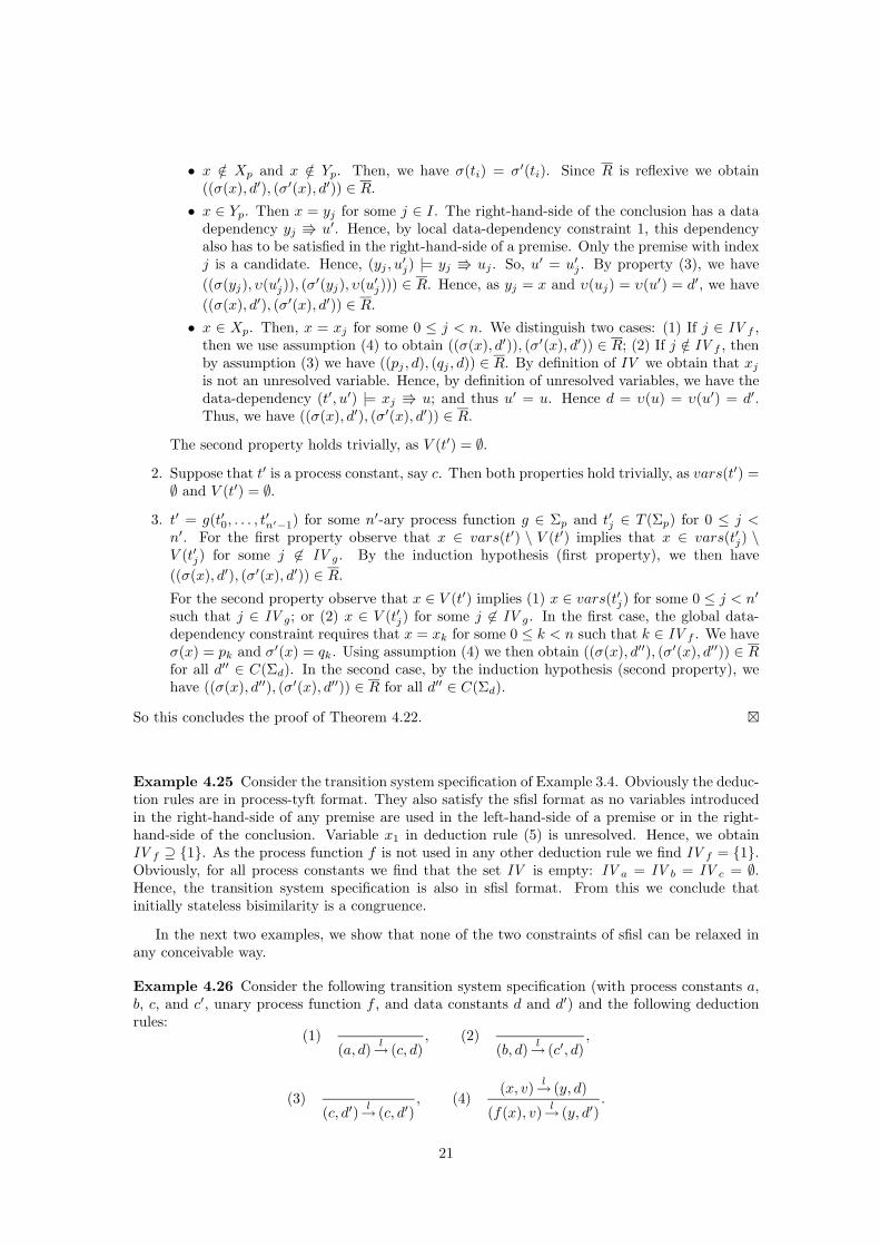
Example 4.25 Consider the transition system specification of Example 3.4. Obviously the deduc-tion rules are in process-tyft format. They also satisfy the sfisl format as no variables introducedin the right-hand-side of any premise are used in the left-hand-side of a premise or in the right-hand-side of the conclusion. Variable x1 in deduction rule (5) is unresolved. Hence, we obtainIV f ⊇ {1}. As the process function f is not used in any other deduction rule we find IV f = {1}.Obviously, for all process constants we find that the set IV is empty: IV a = IV b = IV c = ∅.Hence, the transition system specification is also in sfisl format. From this we conclude thatinitially stateless bisimilarity is a congruence.

In the next two examples, we show that none of the two constraints of sfisl can be relaxed inany conceivable way.

Example 4.26 Consider the following transition system specification (with process constants a,b, c, and c′, unary process function f , and data constants d and d′) and the following deductionrules:

(1)(a, d)

l→ (c, d)

, (2)(b, d)

l→ (c′, d)

,

(3)(c, d′)

l→ (c, d′)

, (4)(x, v)

l→ (y, d)

(f(x), v)l→ (y, d′)

.

21

The deduction rules (1)-(3) are in sfisl format, trivially. Deduction rule (4) does not satisfy localdata-dependency constraint 1, since y V d′ is satisfied in the right-hand-side of the conclusionbut not in the right-hand-side of the premise. Local data-dependency constraint 2 and the globaldata-dependency constraint are satisfied (with IV f = ∅).

That initially stateless bisimilarity is not a congruence w.r.t. f can be seen as follows: wehave that a ↔isl b, but not that f(a) ↔isl f(b) since (f(a), d) can perform a transition to (c, d′)while (f(b), d) is forced to perform the same transition to (c′, d′) and it does not hold that(c, d′) ↔sb (c′, d′).

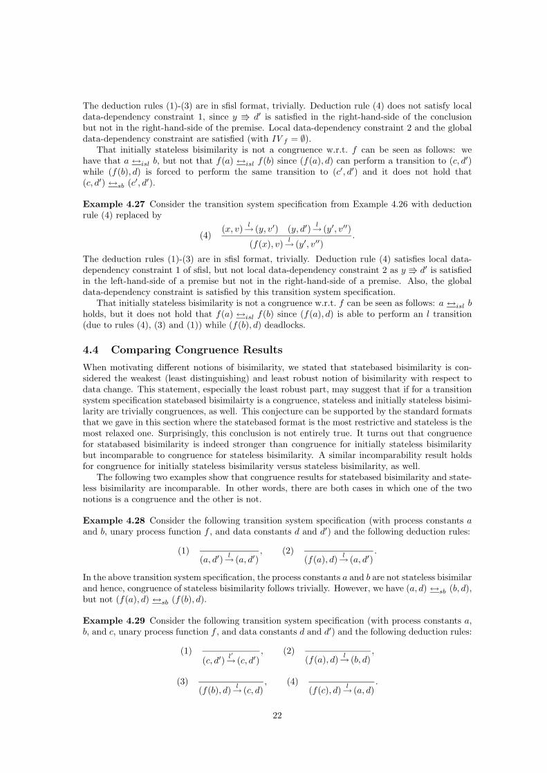
Example 4.27 Consider the transition system specification from Example 4.26 with deductionrule (4) replaced by

(4)(x, v)

l→ (y, v′) (y, d′)

l→ (y′, v′′)

(f(x), v)l→ (y′, v′′)

.

The deduction rules (1)-(3) are in sfisl format, trivially. Deduction rule (4) satisfies local data-dependency constraint 1 of sfisl, but not local data-dependency constraint 2 as y V d′ is satisfiedin the left-hand-side of a premise but not in the right-hand-side of a premise. Also, the globaldata-dependency constraint is satisfied by this transition system specification.

That initially stateless bisimilarity is not a congruence w.r.t. f can be seen as follows: a ↔isl bholds, but it does not hold that f(a) ↔isl f(b) since (f(a), d) is able to perform an l transition(due to rules (4), (3) and (1)) while (f(b), d) deadlocks.

4.4 Comparing Congruence Results

When motivating different notions of bisimilarity, we stated that statebased bisimilarity is con-sidered the weakest (least distinguishing) and least robust notion of bisimilarity with respect todata change. This statement, especially the least robust part, may suggest that if for a transitionsystem specification statebased bisimilairty is a congruence, stateless and initially stateless bisimi-larity are trivially congruences, as well. This conjecture can be supported by the standard formatsthat we gave in this section where the statebased format is the most restrictive and stateless is themost relaxed one. Surprisingly, this conclusion is not entirely true. It turns out that congruencefor statabased bisimilarity is indeed stronger than congruence for initially stateless bisimilaritybut incomparable to congruence for stateless bisimilarity. A similar incomparability result holdsfor congruence for initially stateless bisimilarity versus stateless bisimilarity, as well.

The following two examples show that congruence results for statebased bisimilarity and state-less bisimilarity are incomparable. In other words, there are both cases in which one of the twonotions is a congruence and the other is not.

Example 4.28 Consider the following transition system specification (with process constants aand b, unary process function f , and data constants d and d′) and the following deduction rules:

(1)(a, d′)

l→ (a, d′)

, (2)(f(a), d)

l→ (a, d′)

.

In the above transition system specification, the process constants a and b are not stateless bisimilarand hence, congruence of stateless bisimilarity follows trivially. However, we have (a, d) ↔sb (b, d),but not (f(a), d) ↔sb (f(b), d).

Example 4.29 Consider the following transition system specification (with process constants a,b, and c, unary process function f , and data constants d and d′) and the following deduction rules:

(1)(c, d′)

l′→ (c, d′)

, (2)(f(a), d)

l→ (b, d)

,

(3)(f(b), d)

l→ (c, d)

, (4)(f(c), d)

l→ (a, d)

.

22

Statebased bisimilarity is obviously a congruence though the transition system specification doesnot satisfy the proposed format. Now, consider the processes a and b. These two processes arestateless bisimilar, however, f(a) and f(b) are not stateless bisimilar, since (f(a), d) can make atransition to (b, d), then (f(b), d) is forced to make a transition to (c, d) while b and c are clearlynot stateless bisimilar (due to their difference w.r.t. data d′).

The following lemma states that if statebased bisimilarity is a congruence, then initially state-less bisimilarity is a congruence as well.

Lemma 4.30 For a transition system specification, if statebased bisimilarity is a congruence,then initially stateless bisimilarity is a congruence, as well.

Proof. Suppose that pi ↔isl qi for 0 ≤ i < n. By definition this means that there ex-ist statebased bisimulation relations Ri such that ((pi, d), (qi, d)) ∈ Ri for all d. Since state-based bisimilarity is a congruence (by assumption), we have, for each d, the existence of astatebased bisimulation relation Sd such that ((f(p0, . . . , pn−1), d), (f(q0, . . . , qn−1), d)) ∈ Sd.Let S =

⋃d Sd, and observe that S is a statebased bisimulation relation such that, for all d,

((f(p0, . . . , pn−1), d), (f(q0, . . . , qn−1), d)) ∈ S. This, in turn, means that f(p0, . . . , pn−1) ↔isl

f(q0, . . . , qn−1). �

Corollary 4.31 If a transition system specification is in sfsb format, then initially stateless bisim-ilarity is a congruence for it.

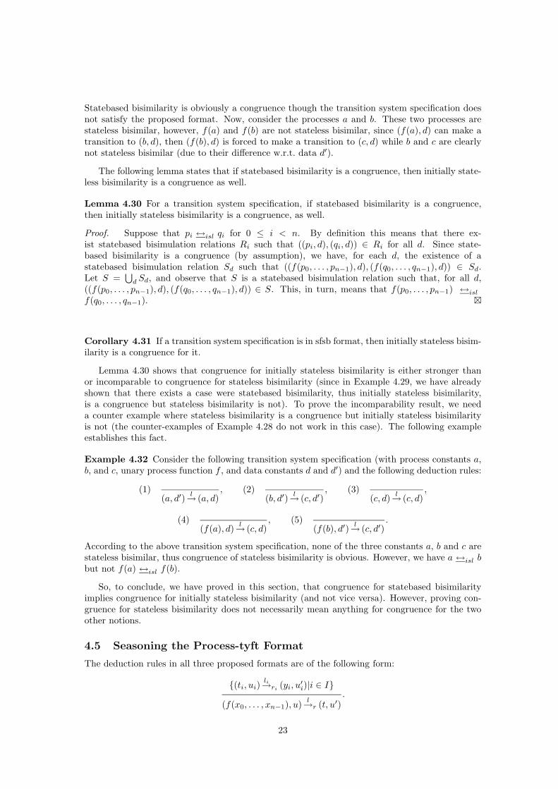
Lemma 4.30 shows that congruence for initially stateless bisimilarity is either stronger thanor incomparable to congruence for stateless bisimilarity (since in Example 4.29, we have alreadyshown that there exists a case were statebased bisimilarity, thus initially stateless bisimilarity,is a congruence but stateless bisimilarity is not). To prove the incomparability result, we needa counter example where stateless bisimilarity is a congruence but initially stateless bisimilarityis not (the counter-examples of Example 4.28 do not work in this case). The following exampleestablishes this fact.

Example 4.32 Consider the following transition system specification (with process constants a,b, and c, unary process function f , and data constants d and d′) and the following deduction rules:

(1)(a, d′)

l→ (a, d)

, (2)(b, d′)

l→ (c, d′)

, (3)(c, d)

l→ (c, d)

,

(4)(f(a), d)

l→ (c, d)

, (5)(f(b), d′)

l→ (c, d′)

.

According to the above transition system specification, none of the three constants a, b and c arestateless bisimilar, thus congruence of stateless bisimilarity is obvious. However, we have a ↔isl bbut not f(a) ↔isl f(b).

So, to conclude, we have proved in this section, that congruence for statebased bisimilarityimplies congruence for initially stateless bisimilarity (and not vice versa). However, proving con-gruence for stateless bisimilarity does not necessarily mean anything for congruence for the twoother notions.

4.5 Seasoning the Process-tyft Format

The deduction rules in all three proposed formats are of the following form:

{(ti, ui)li→ri

(yi, u′i)|i ∈ I}

(f(x0, . . . , xn−1), u)l→r (t, u′)

.

23

Using this form we cannot go far with proving congruence properties of existing theories sincethere are many other constructs and patterns that are not present in the above format. In thissection, we show how to exploit the format in presence of such constructs. A common type ofdeduction rules used in transition system specifications is the tyxt form which has the followingstructure:

(dr){(ti, ui)

li→ri(yi, u

′i)|i ∈ I}

(x, u)l→r (t, u′)

.

Rules of the above form fit within the tyft form if we copy the above rule for all function symbolsf ∈ Σp with (arbitrary) arity n and substitute all occurrences of x with f(x0, . . . , xn−1).

Another common phenomenon is the presence of predicates. Predicates of the form Pred(t, u)may be present in the premises or the conclusion of a deduction rule. Predicates can be dealt within the above formats, as if they are left-hand-side of a transition relation (this can be formallyproved by introducing fresh dummy transition relations for each predicate that always have a freshdummy variable in their right-hand-side [3]).

Regarding negative premises, if we can define a measure on formulas over the signature Σp that,for each deduction rule of the transition system specification, does not increase from conclusionto all positive premises and strictly decreases from conclusion to negative premises (i.e., if astratification for all rules exists) then the congruence results can be used safely. Note that anextension to negative premises requires another definition of what a proof of a transition is (see[14, 25]).

5 Case-Studies and Comparison

In this section, some process languages from literature for which an operational semantics isprovided by means of a transition system specification with a data state are considered.

For each of these languages, we establish which of the bisimilarities introduced in this paper,are used (possibly with a different formulation) and whether the deduction rules are in the cor-responding format. Also, the other notions of bisimilarity defined in this paper are discussed forthese process languages.

5.1 HyPA

In [11], a process algebra is presented for the description of hybrid systems, i.e., systems with bothdiscrete events and continuous change of variables. The process signature of HyPA consists of thefollowing process constants and functions:

• process constants: δ, ε, (a)a∈A, (c)c∈C ;

• unary process functions: (d� )d∈D, (∂H ( ))H⊆A;

• binary process functions: ⊕ , � , I , B , ‖ , ‖ , and | .

The data state consists of mappings from model variables to values, denoted by V al. The datasignature is not made explicit.

The transition system specification defines the following predicate and relations:

• a ‘termination’-predicate X;

• a family of ‘action-transition’ relations(

l→

)

l∈A×V al;

• a family of ‘flow-transition’ relations(

σ

)

σ∈T→V al.

The deduction rules are given in Table 1 and Table 2.On HyPA process terms, a notion of bisimilarity is defined that coincides with our definition

of stateless bisimilarity.

24

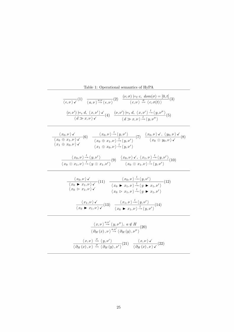
Table 1: Operational semantics of HyPA

〈 ε, ν 〉X(1)

〈 a, ν 〉a,ν→ 〈 ε, ν 〉

(2)(ν, σ) |=f c, dom(σ) = [0, t]

〈 c, ν 〉σ 〈 c, σ(t) 〉

(3)

(ν, ν′) |=r d, 〈x, ν′ 〉X

〈 d� x, ν 〉X(4)

(ν, ν′) |=r d, 〈x, ν′ 〉

l→〈 y, ν′′ 〉

〈 d� x, ν 〉l→〈 y, ν′′ 〉

(5)

〈x0, ν 〉X

〈x0 ⊕ x1, ν 〉X〈x1 ⊕ x0, ν 〉X

(6)〈x0, ν 〉

l→〈 y, ν′ 〉

〈x0 ⊕ x1, ν 〉l→〈 y, ν′ 〉

〈x1 ⊕ x0, ν 〉l→〈 y, ν′ 〉

(7)〈x0, ν 〉X, 〈 y0, ν 〉X

〈x0 � y0, ν 〉X(8)

〈x0, ν 〉l→〈 y, ν′ 〉

〈x0 � x1, ν 〉l→〈 y � x1, ν

′ 〉(9)

〈x0, ν 〉X, 〈x1, ν 〉l→〈 y, ν′ 〉

〈x0 � x1, ν 〉l→〈 y, ν′ 〉

(10)

〈x0, ν 〉X

〈x0 I x1, ν 〉X〈x0 B x1, ν 〉X

(11)〈x0, ν 〉

l→〈 y, ν′ 〉

〈x0 I x1, ν 〉l→〈 y I x1, ν

′ 〉

〈x0 B x1, ν 〉l→〈 y I x1, ν

′ 〉

(12)

〈x1, ν 〉X

〈x0 I x1, ν 〉X(13)

〈x1, ν 〉l→〈 y, ν′ 〉

〈x0 I x1, ν 〉l→〈 y, ν′ 〉

(14)

〈x, ν 〉a,ν′

→ 〈 y, ν′′ 〉, a 6∈ H

〈 ∂H (x) , ν 〉a,ν′

→ 〈 ∂H (y) , ν′′ 〉(20)

〈x, ν 〉σ 〈 y, ν′ 〉

〈 ∂H (x) , ν 〉σ 〈 ∂H (y) , ν′ 〉

(21)〈x, ν 〉X

〈 ∂H (x) , ν 〉X(22)

25

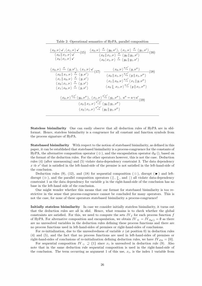
Table 2: Operational semantics of HyPA, parallel composition

〈x0, ν 〉X, 〈x1, ν 〉X

〈x0 ‖x1, ν 〉X〈x0 |x1, ν 〉X

(15)〈x0, ν 〉

σ 〈 y0, ν

′ 〉, 〈x1, ν 〉σ 〈 y1, ν

′ 〉

〈x0 ‖x1, ν 〉σ 〈 y0 ‖ y1, ν

′ 〉

〈x0 |x1, ν 〉σ 〈 y0 ‖ y1, ν

′ 〉

(16)

〈x0, ν 〉σ 〈 y, ν′ 〉, 〈x1, ν 〉X

〈x0 ‖x1, ν 〉σ 〈 y, ν′ 〉

〈x1 ‖x0, ν 〉σ 〈 y, ν′ 〉

〈x0 |x1, ν 〉σ 〈 y, ν′ 〉

〈x1 |x0, ν 〉σ 〈 y, ν′ 〉

(17)〈x0, ν 〉

a,ν′

→ 〈 y, ν′′ 〉

〈x0 ‖x1, ν 〉a,ν′

→ 〈 y ‖x1, ν′′ 〉

〈x1 ‖x0, ν 〉a,ν′

→ 〈x1 ‖ y, ν′′ 〉

〈x0 ‖ x1, ν 〉a,ν′

→ 〈 y ‖x1, ν′′ 〉

(18)

〈x0, ν 〉a,ν′

→ 〈 y0, ν′′ 〉, 〈x1, ν 〉

a′,ν′

→ 〈 y1, ν′′ 〉, a′′ = a γ a′

〈x0 ‖x1, ν 〉a′′,ν′

→ 〈 y0 ‖ y1, ν′′ 〉

〈x0 |x1, ν 〉a′′,ν′

→ 〈 y0 ‖ y1, ν′′ 〉

(19)

Stateless bisimilarity One can easily observe that all deduction rules of HyPA are in sfsl-format. Hence, stateless bisimilarity is a congruence for all constant and function symbols fromthe process signature of HyPA.

Statebased bisimilarity With respect to the notion of statebased bisimilarity, as defined in thispaper, it can be established that statebased bisimilarity is a process-congruence for the constants ofHyPA, the alternative composition operator (⊕ ), and the encapsulation operator ∂H (), based onthe format of the deduction rules. For the other operators however, this is not the case. Deductionrules (4) (after unseasoning) and (5) violate data-dependency constraint 3. The data dependencyxV ν′ that is satisfied in the left-hand-side of the premise is not satisfied in the left-hand-side ofthe conclusion.

Deduction rules (9), (12), and (18) for sequential composition (� ), disrupt (I ) and left-disrupt (B ), and the parallel composition operators ( ‖ , ‖ , and | ) all violate data-dependencyconstraint 1 as the data dependency for variable y in the right-hand-side of the conclusion has nobase in the left-hand side of the conclusion.

One might wonder whether this means that our format for statebased bisimilarity is too re-strictive in the sense that process-congruence cannot be concluded for many operators. This isnot the case, for none of these operators statebased bisimilarity a process-congruence!

Initially stateless bisimilarity In case we consider initially stateless bisimilarity, it turns outthat the deduction rules are all in sfisl. Hence, what remains is to check whether the globalconstraints are satisfied. For this, we need to compute the sets IV f for each process function fof HyPA. For alternative composition and encapsulation, we obtain IV ⊕ = IV ∂H() = ∅ as thereare no unresolved variables in the deduction rules defining these process functions and there areno process functions used in left-hand-sides of premises or right-hand-sides of conclusions.

For re-initialization, due to the unresolvedness of variable x (at position 0) in deduction rules(4) and (5), and the fact that no process functions are used in left-hand-sides of premises orright-hand-sides of conclusions of re-initialization defining deduction rules, we have IV d� = {0}.

For sequential composition IV � ⊇ {1} since x1 is unresolved in deduction rule (9). Alsonote that in the same deduction rule sequential composition is used in the right-hand-side ofthe conclusion. The term occurring as argument 1 of this use, x1, is the index 1 variable from

26

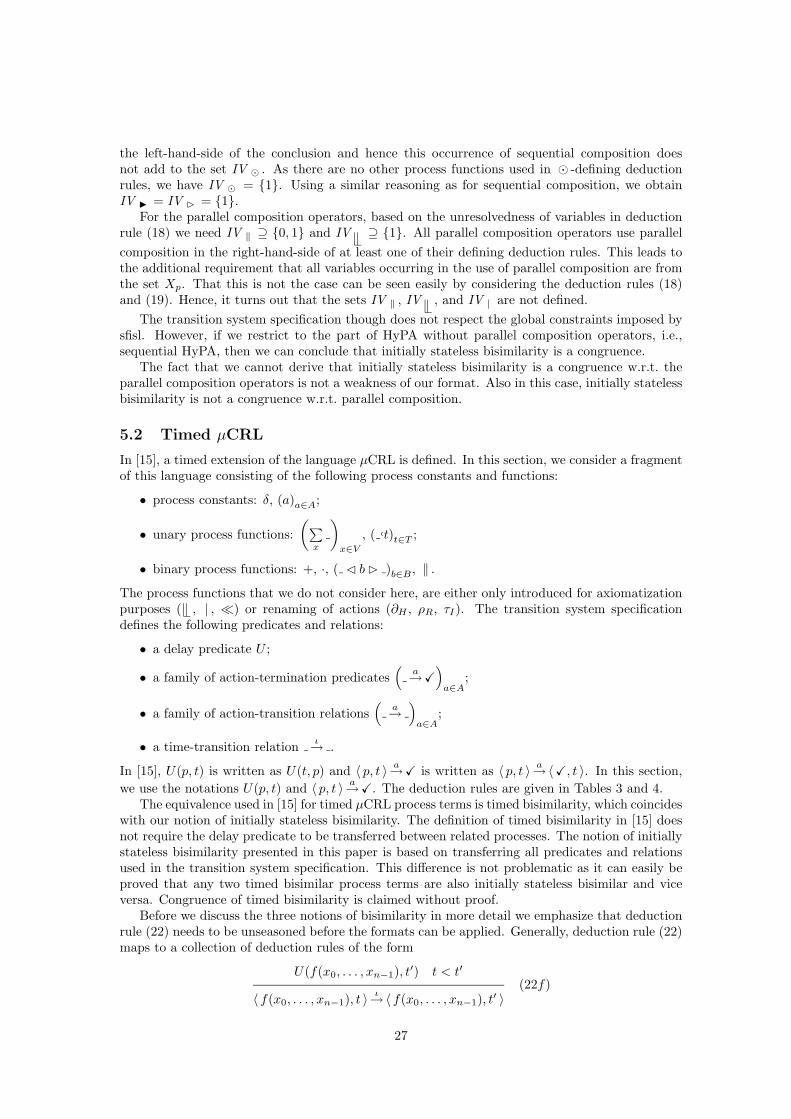
the left-hand-side of the conclusion and hence this occurrence of sequential composition doesnot add to the set IV � . As there are no other process functions used in � -defining deductionrules, we have IV � = {1}. Using a similar reasoning as for sequential composition, we obtainIV I = IV B = {1}.

For the parallel composition operators, based on the unresolvedness of variables in deductionrule (18) we need IV ‖ ⊇ {0, 1} and IV ‖ ⊇ {1}. All parallel composition operators use parallel

composition in the right-hand-side of at least one of their defining deduction rules. This leads tothe additional requirement that all variables occurring in the use of parallel composition are fromthe set Xp. That this is not the case can be seen easily by considering the deduction rules (18)and (19). Hence, it turns out that the sets IV ‖ , IV ‖ , and IV | are not defined.

The transition system specification though does not respect the global constraints imposed bysfisl. However, if we restrict to the part of HyPA without parallel composition operators, i.e.,sequential HyPA, then we can conclude that initially stateless bisimilarity is a congruence.

The fact that we cannot derive that initially stateless bisimilarity is a congruence w.r.t. theparallel composition operators is not a weakness of our format. Also in this case, initially statelessbisimilarity is not a congruence w.r.t. parallel composition.

5.2 Timed µCRL

In [15], a timed extension of the language µCRL is defined. In this section, we consider a fragmentof this language consisting of the following process constants and functions:

• process constants: δ, (a)a∈A;

• unary process functions:

(∑x

)

x∈V

, ( ↪t)t∈T ;

• binary process functions: +, ·, ( C bB )b∈B , ‖ .

The process functions that we do not consider here, are either only introduced for axiomatizationpurposes (‖ , | , �) or renaming of actions (∂H , ρR, τI). The transition system specificationdefines the following predicates and relations:

• a delay predicate U ;

• a family of action-termination predicates(

a→X

)

a∈A;

• a family of action-transition relations(

a→

)

a∈A;

• a time-transition relationι→ .

In [15], U(p, t) is written as U(t, p) and 〈 p, t 〉a→X is written as 〈 p, t 〉

a→〈X, t 〉. In this section,

we use the notations U(p, t) and 〈 p, t 〉a→X. The deduction rules are given in Tables 3 and 4.

The equivalence used in [15] for timed µCRL process terms is timed bisimilarity, which coincideswith our notion of initially stateless bisimilarity. The definition of timed bisimilarity in [15] doesnot require the delay predicate to be transferred between related processes. The notion of initiallystateless bisimilarity presented in this paper is based on transferring all predicates and relationsused in the transition system specification. This difference is not problematic as it can easily beproved that any two timed bisimilar process terms are also initially stateless bisimilar and viceversa. Congruence of timed bisimilarity is claimed without proof.

Before we discuss the three notions of bisimilarity in more detail we emphasize that deductionrule (22) needs to be unseasoned before the formats can be applied. Generally, deduction rule (22)maps to a collection of deduction rules of the form

U(f(x0, . . . , xn−1), t′) t < t′

〈 f(x0, . . . , xn−1), t 〉ι→〈 f(x0, . . . , xn−1), t

′ 〉(22f)

27

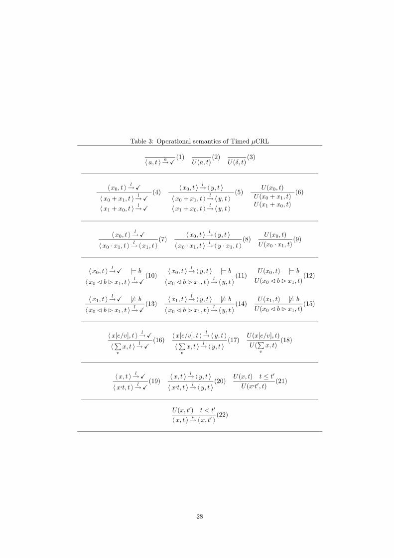
Table 3: Operational semantics of Timed µCRL

〈 a, t 〉a→X

(1)U(a, t)

(2)U(δ, t)

(3)

〈x0, t 〉l→X

〈x0 + x1, t 〉l→X

〈x1 + x0, t 〉l→X

(4)〈x0, t 〉

l→〈 y, t 〉

〈x0 + x1, t 〉l→〈 y, t 〉

〈x1 + x0, t 〉l→〈 y, t 〉

(5)U(x0, t)

U(x0 + x1, t)U(x1 + x0, t)

(6)

〈x0, t 〉l→X

〈x0 · x1, t 〉l→〈x1, t 〉

(7)〈x0, t 〉

l→〈 y, t 〉

〈x0 · x1, t 〉l→〈 y · x1, t 〉

(8)U(x0, t)

U(x0 · x1, t)(9)

〈x0, t 〉l→X |= b

〈x0 C bB x1, t 〉l→X

(10)〈x0, t 〉

l→〈 y, t 〉 |= b

〈x0 C bB x1, t 〉l→〈 y, t 〉

(11)U(x0, t) |= b

U(x0 C bB x1, t)(12)

〈x1, t 〉l→X 6|= b

〈x0 C bB x1, t 〉l→X

(13)〈x1, t 〉

l→〈 y, t 〉 6|= b

〈x0 C bB x1, t 〉l→〈 y, t 〉

(14)U(x1, t) 6|= b

U(x0 C bB x1, t)(15)

〈x[e/v], t 〉l→X

〈∑vx, t 〉

l→X

(16)〈x[e/v], t 〉

l→〈 y, t 〉

〈∑vx, t 〉

l→〈 y, t 〉

(17)U(x[e/v], t)

U(∑vx, t)

(18)

〈x, t 〉l→X

〈x↪t, t 〉l→X

(19)〈x, t 〉

l→〈 y, t 〉

〈x↪t, t 〉l→〈 y, t 〉

(20)U(x, t) t ≤ t′

U(x↪t′, t)(21)

U(x, t′) t < t′

〈x, t 〉ι→〈x, t′ 〉

(22)

28

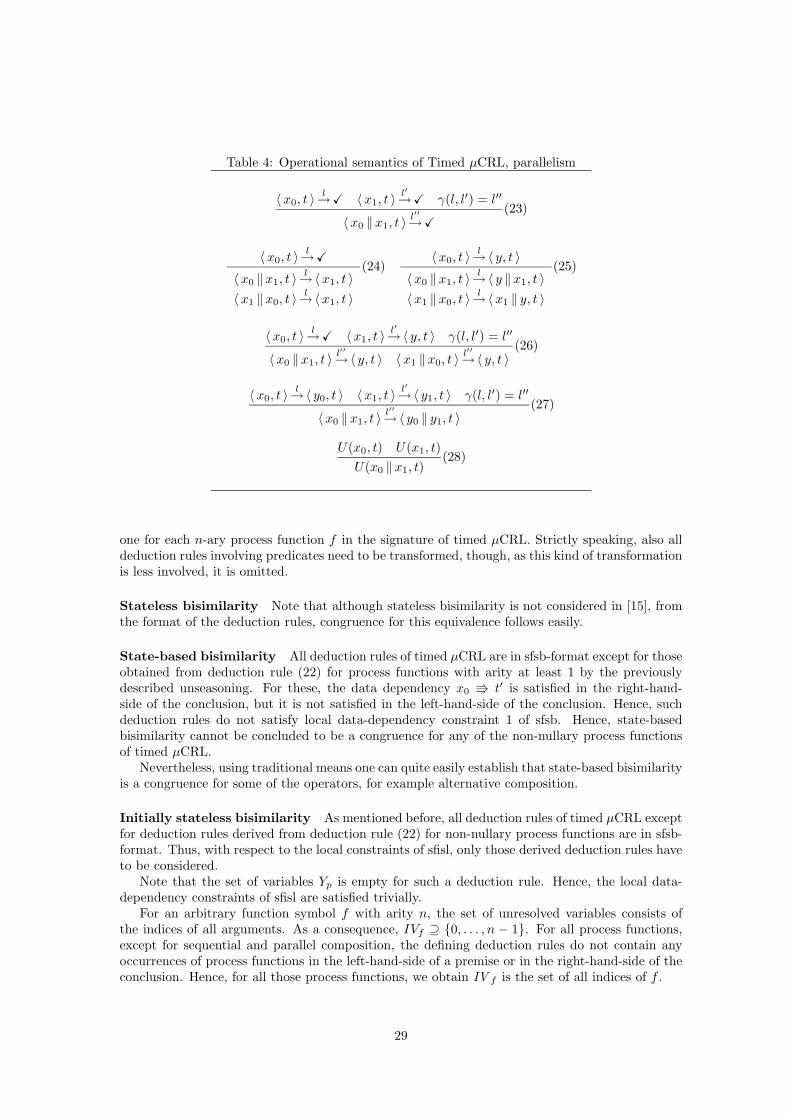
Table 4: Operational semantics of Timed µCRL, parallelism

〈x0, t 〉l→X 〈x1, t 〉

l′→X γ(l, l′) = l′′

〈x0 ‖x1, t 〉l′′→X

(23)

〈x0, t 〉l→X

〈x0 ‖x1, t 〉l→〈x1, t 〉

〈x1 ‖x0, t 〉l→〈x1, t 〉

(24)〈x0, t 〉

l→〈 y, t 〉

〈x0 ‖x1, t 〉l→〈 y ‖x1, t 〉

〈x1 ‖x0, t 〉l→〈x1 ‖ y, t 〉

(25)

〈x0, t 〉l→X 〈x1, t 〉

l′→〈 y, t 〉 γ(l, l′) = l′′

〈x0 ‖x1, t 〉l′′→〈 y, t 〉〈x1 ‖x0, t 〉

l′′→〈 y, t 〉

(26)

〈x0, t 〉l→〈 y0, t 〉〈x1, t 〉

l′→〈 y1, t 〉 γ(l, l′) = l′′

〈x0 ‖x1, t 〉l′′→〈 y0 ‖ y1, t 〉

(27)

U(x0, t) U(x1, t)

U(x0 ‖x1, t)(28)

one for each n-ary process function f in the signature of timed µCRL. Strictly speaking, also alldeduction rules involving predicates need to be transformed, though, as this kind of transformationis less involved, it is omitted.

Stateless bisimilarity Note that although stateless bisimilarity is not considered in [15], fromthe format of the deduction rules, congruence for this equivalence follows easily.

State-based bisimilarity All deduction rules of timed µCRL are in sfsb-format except for thoseobtained from deduction rule (22) for process functions with arity at least 1 by the previouslydescribed unseasoning. For these, the data dependency x0 V t′ is satisfied in the right-hand-side of the conclusion, but it is not satisfied in the left-hand-side of the conclusion. Hence, suchdeduction rules do not satisfy local data-dependency constraint 1 of sfsb. Hence, state-basedbisimilarity cannot be concluded to be a congruence for any of the non-nullary process functionsof timed µCRL.

Nevertheless, using traditional means one can quite easily establish that state-based bisimilarityis a congruence for some of the operators, for example alternative composition.

Initially stateless bisimilarity As mentioned before, all deduction rules of timed µCRL exceptfor deduction rules derived from deduction rule (22) for non-nullary process functions are in sfsb-format. Thus, with respect to the local constraints of sfisl, only those derived deduction rules haveto be considered.

Note that the set of variables Yp is empty for such a deduction rule. Hence, the local data-dependency constraints of sfisl are satisfied trivially.

For an arbitrary function symbol f with arity n, the set of unresolved variables consists ofthe indices of all arguments. As a consequence, IVf ⊇ {0, . . . , n − 1}. For all process functions,except for sequential and parallel composition, the defining deduction rules do not contain anyoccurrences of process functions in the left-hand-side of a premise or in the right-hand-side of theconclusion. Hence, for all those process functions, we obtain IV f is the set of all indices of f .

29

For sequential composition (deduction rule (8)) and parallel composition (deduction rules (25)and (27)) the occurrences of y, y0 and y1 in the use of the process functions do not satisfy therequirement that these should be initial variables (∈ Xp). Hence, for those process functions, theset IV does not exist. Therefore, congruence of initially stateless bisimilarity w.r.t. those processfunctions cannot be concluded. For the other process functions, as they are independently definedoperationally, congruence can be concluded.

We claim that a reformulation of the operational semantics of timed µCRL without the predi-cate U along the following lines results in an ‘equivalent’ transition system specification for whichthe sfisl format can be applied to obtain congruence:

〈x0, t 〉ι→〈 y, t′ 〉

〈x0 · x1, t 〉ι→〈 y · x1, t 〉

,〈x0, t 〉

ι→〈 y0, t

′ 〉〈x1, t 〉ι→〈 y1, t

′ 〉

〈x0 ‖x1, t 〉ι→〈 y0 ‖ y1, t

′ 〉.

The reason is that the first argument of sequential composition and both arguments of parallelcomposition are no longer forced to be part of the set IV which avoids the problem with y, y0 andy1 not being initial variables. Calculation of the sets IV · and IV ‖ gives: IV · = ∅ and IV ‖ = ∅.

5.3 Discrete-event χ

In [8], the process language χσ is presented. This language is used for the specification, simulationand validation of discrete-event systems.

The signature of χσ consists of the following constant and function symbols:

• process constants: δ, ε, skip, (∆t)t∈T , (x := e)x∈V,e∈E , (c!e)c∈C,e∈E , (c?x)c∈C,x∈V ;

• unary process functions: (b→ )b∈B , ∗, (|[s | ]|)s∈S , (∂H)H⊆A, π, (τI)I⊆A

• binary process functions: �, ;, ‖

In the transition system specification of this language both predicates and relations are used.For both types of formulas negative occurrences as a premise occur.

The notion of equivalence that is considered in [8] is stateless bisimilarity. They prove thatthis equivalence is a congruence for the constant and function symbols of χσ by using the so-calledrelaxed PANTH format [19, 2]. We have serious doubts as to the applicability of this format tothe given transition system specification due to the presence of a data state in χσ. Nevertheless,stateless bisimilarity is a congruence since all deduction rules of the transition system specificationare in sfsl format.

6 Conclusion

In this paper, we investigated the impact of the presence of a data state on notions of bisimilarityand standard congruence formats. To do this, we defined three notions of bisimilarity with dataand elaborated on their existing and possible uses. Then, we proposed three standard formatsthat provide congruence results for these three notions. Furthermore, we briefly pointed out therelationships between these notions and between the corresponding congruences. The proposedformats are applied to several examples from the literature successfully. In this paper, we illus-trated the use of our format using a data coordination language, called Linda.

Extending the format for a parameterized notion of bisimilarity (with an explicit interferencerelation or a symbolic / logical representation of interference possibilities) is another interestingextension which should follow the same line as our relaxation of statebased constraints to initiallystateless. Furthermore, we may extend the theory to bisimulation relations which allow for differentdata states but so far we have seen no practical application of such a bisimilarity notion.

Acknowledgements The authors express their best appreciation to Pieter Cuijpers and AnaSokolova for their valuable comments on early versions of this paper.

30

References

[1] Luca Aceto, Wan J. Fokkink, and Chris Verhoef. Structural operational semantics. In Jan A.Bergstra, Alban Ponse, and Scott A. Smolka, editors, Handbook of Process Algebra, Chapter3. Elsevier Science, Dordrecht, The Netherlands, 2001.

[2] Jos C. M. Baeten and Cornelis A. Middelburg. Process Algebra with Timing. EATCS Mono-graphs. Springer-Verlag, Berlin, Germany, 2002.

[3] Jos C. M. Baeten and Chris Verhoef. A congruence theorem for structured operationalsemantics with predicates. In Eike Best, editor, International Conference on ConcurrencyTheory (CONCUR’93), volume 715 of Lecture Notes in Computer Science, pages 477–492.Springer-Verlag, Berlin, Germany, 1993.

[4] Jaco W. de Bakker and Erik P. de Vink. Control Flow Semantics. Foundations of ComputingSeries. The MIT Press, 1996.

[5] Karen L. Bernstein. A congruence theorem for structured operational semantics of higher-order languages. In IEEE Symposium on Logic In Computer Science (LICS’98), pages 153–164. IEEE Computer Society, Los Alamitos, CA, USA, 1998.

[6] Bard Bloom, Sorin Istrail, and Albert R. Meyer. Bisimulation can’t be traced. Journal of theACM (JACM), 42(1):232–268, January 1995.

[7] Bard Bloom and Frits Vaandrager. SOS rules formats for parameterizedand state-bearing processes (draft). Unpublished note, available through:http://www.cs.kun.nl/ita/publications/ papers/fvaan/.

[8] Victor Bos and Jeroen J.T. Kleijn. Redesign of a systems engineering language — formalisa-tion of χ. Formal Aspects of Computing, 15(4), December 2003.

[9] Antonio Brogi and Jean-Marie Jacquet. On the expressiveness of Linda-like concurrent lan-guages. In Ilaria Castellani and Catuscia Palamidessi, editors, Proceedings of Fifth Interna-tional Workshop on Expressiveness in Concurrency (EXPRESS’98), volume 16 of ElectronicNotes in Theoretical Computer Science. Elsevier Science, Dordrecht, The Netherlands, 1998.

[10] Michel R. V. Chaudron. Separating Computation and Coordination in the Design of Paralleland Distributed Programs. PhD thesis, Department of Computer Science, RijksuniversiteitLeiden, Leiden, The Netherlands, 1998.

[11] Pieter J.L. Cuijpers and Michel A. Reniers. Hybrid process algebra. Technical Report 03-07, Department of Computer Science, Eindhoven University of Technology, Eindhoven, TheNetherlands, 2003.

[12] Robert de Simone. Higher-level synchronizing devices in MEIJE-SCCS. Theoretical ComputerScience (TCS), 37:245–267, 1985.

[13] Wan J. Fokkink and Rob J. van Glabbeek. Ntyft/ntyxt rules reduce to ntree rules. Informationand Computation, 126(1):1–10, 1996.

[14] Jan Friso Groote. Transition system specifications with negative premises. Theoretical Com-puter Science, 118(2):263–299, 1993.

[15] Jan Friso Groote. The syntax and semantics of timed µCRL. Technical Report SEN-R9709,CWI - Centrum voor Wiskunde en Informatica, Amsterdam, The Netherlands, June 30, 1997.

[16] Jan Friso Groote and Alban Ponse. Process algebra with guards. combining Hoare logic withprocess algebra. Formal Aspects of Computing, 6(2), 1994.

31

[17] Jan Friso Groote and Frits Vaandrager. Structured operational semantics and bisimulationas a congruence. Information and Computation, 100(2), October 1992.

[18] Jean-Marie Jacquet, Koenraad De Bosschere, and Antonio Brogi. On timed coordinationlanguages. In Antonio Porto and Gruia-Catalin Roman, editors, Proceedings of Coordina-tion Languages and Models, 4th International Conference, Limassol, Cyprus, volume 1906 ofLecture Notes in Computer Science, pages 81–98. Springer-Verlag, Berlin, Germany, 2000.

[19] Cornelis A. Middelburg. Variable binding operators in transition system specifications. Jour-nal of Logic and Algebraic Programming, 47(1):15–45, 2001.

[20] Robin A. Milner. A Calculus of Communicating Systems, volume 92 of Lecture Notes inComputer Science. Springer-Verlag, 1980.

[21] MohammadReza Mousavi, Twan Basten, Michel Reniers, Michel Chaudron, and GiovanniRussello. Separating functionality, behavior and timing in the design of reactive systems:(GAMMA + coordination) + time. Technical Report 02-09, Department of Computer Science,Eindhoven University of Technology, Eindhoven, The Netherlands, 2002.

[22] David M.R. Park. Concurrency and automata on infinite sequences. In Proceedings of 5thGI Conference, volume 104 of Lecture Notes in Computer Science, pages 167–183. Springer-Verlag, Berlin, Germany, 1981.

[23] Gordon D. Plotkin. A structural approach to operational semantics. Technical Report DAIMIFN-19, Computer Science Department, Aarhus University, Aarhus, Denmark, September1981.

[24] Michel A. Reniers, Jan Friso Groote, Mark B. van der Zwaag, and Jos van Wamel. Com-pleteness of timed µCRL. Fundamenta Informaticae, 50(3-4):361–402, 2002.

[25] Chris Verhoef. A congruence theorem for structured operational semantics with predicatesand negative premises. Nordic Journal of Computing, 2(2):274–302, 1995.

32

congruence for sos with data

Documents