soil erosion and conservation
TRANSCRIPT


SOIL EROSION AND CONSERVATION
MSEPR 11/19/04 02:49 PM Page i

THIRD EDITION
R. P. C. Morgan
National Soil Resources Institute,Cranfield University
SOIL EROSION AND
CONSERVATION
MSEPR 11/19/04 02:49 PM Page iii

© 2005 by Blackwell Science Ltda Blackwell Publishing company
BLACKWELL PUBLISHING350 Main Street, Malden, MA 02148-5020, USA108 Cowley Road, Oxford OX4 1JF, UK550 Swanston Street, Carlton, Victoria 3053, Australia
The right of R. P. C. Morgan to be identified as the Author of this Work has been asserted in accordancewith the UK Copyright, Designs, and Patents Act 1988.
All rights reserved. No part of this publication may be reproduced, stored in a retrieval system, ortransmitted, in any form or by any means, electronic, mechanical, photocopying, recording or otherwise,except as permitted by the UK Copyright, Designs, and Patents Act 1988, without the prior permission ofthe publisher.
First published 1986 Longman Group LimitedSecond edition 1995Third edition published 2005 by Blackwell Publishing Ltd
Library of Congress Cataloging-in-Publication Data
Morgan, R. P. C. (Royston Philip Charles), 1942–Soil erosion and conservation / R. P. C. Morgan. – 3rd ed.
p. cm.Includes bibliographical references and index.ISBN 1-4051-1781-8 (pbk. : alk. paper)1. Soil erosion. 2. Soil conservation. I. Title.
S623.M68 2005631.4¢5 – dc22
2004009787
A catalogue record for this title is available from the British Library.
Set in 9 on 111/2 pt Minionby SNP Best-set Typesetter Ltd., Hong KongPrinted and bound in the United Kingdomby MPG Books Ltd, Bodmin, Cornwall
The publisher’s policy is to use permanent paper from mills that operate a sustainable forestry policy, andwhich has been manufactured from pulp processed using acid-free and elementary chlorine-free practices.Furthermore, the publisher ensures that the text paper and cover board used have met acceptableenvironmental accreditation standards.
For further information onBlackwell Publishing, visit our website:www.blackwellpublishing.com
MSEPR 11/19/04 02:49 PM Page iv

Contents
v
Foreword viiPreface ix
1 Soil erosion: the global context 1Box 1. Erosion, population and food supply 9
2 Processes and mechanics of erosion 11Box 2. Initiation of soil particle movement 42
3 Factors influencing erosion 45Box 3. Scale and erosion processes 65
4 Erosion hazard assessment 67Box 4. Upscaling detailed field surveys to national surveys 93
5 Measurement of soil erosion 95Box 5. Sediment budgets 113
6 Modelling soil erosion 116Box 6. Uncertainty in model predictions 149
7 Strategies for erosion control 152Box 7. Planning a soil conservation strategy 172
8 Crop and vegetation management 175Box 8. Selecting vegetation for erosion control 197
9 Soil management 200Box 9. Tillage erosion 210
10 Mechanical methods of erosion control 212Box 10. Laying out terraces and waterways 241
Contents
MSEPR 11/19/04 02:49 PM Page v

11 Implementation 244Box 11. Land Care 254
12 The way ahead 257
References 262Acknowledgements 297Index 299
Contents
vi
MSEPR 11/19/04 02:49 PM Page vi
Foreword
vii
Soil erosion has been an environmental concern in such countries as China and those borderingthe Mediterranean Sea for millennia. In the United States the major impetus to scientific researchon soil erosion and conservation came from Hugh Hammond Bennett, who led the soil conser-vation movement in the 1920s and 1930s. In Western Europe there was growing realization fromthe 1970s that soil erosion could have a major effect on soils, even on lowland arable areas. Morerecently the topic has come on to the political agenda with the Commission of the EuropeanCommunities developing a thematic strategy for soil protection. Integral to this is the recogni-tion that soils perform a range of key functions, including the production of food, the storage oforganic matter, water and nutrients, the provision of a habitat for a huge variety of organismsand preserving a record of past human activity. Any degradation in the quality of the soil resourcethrough erosion can have an impact on the ability of soils to perform this range of functions. Inthe twentieth century and earlier, the main practical concern about soil erosion was with refer-ence to impacts on food production. This is still the case in many parts of the world, but now themore frequent concerns relate to the reduction in soil carbon, the movement of nitrogen and theremoval of phosphorus in soluble and particulate forms. There are also concerns about the effectsof erosion on landscape quality as well as on cultural records. As an example, many archaeolo-gists are concerned about the effects of soil surface lowering through erosion and the conse-quential impacts of deeper ploughing on archaeological features. The publication of this thirdedition of Roy Morgan’s book Soil Erosion and Conservation is thus very timely and reflects thewider concerns regarding the issue. The book is also permeated with Roy Morgan’s own exten-sive and international experience in soil erosion research.
A key theme of this book is that a soil conservation strategy must evolve from detailed know-ledge and understanding of actual erosional processes. Thus Chapters 2 to 6 deal with theprocesses of soil erosion, the assessment of erosion risk at different scales and the monitoring andmodelling of erosion. The treatment of modelling in Chapter 6 is particularly comprehensivethrough discussion of empirical and physically based models, sensitivity analysis and model vali-dation. The inclusion of many worked examples is of great assistance to the reader. The remain-ing chapters focus on conservation strategies with emphases on crop and vegetation management,soil management and mechanical methods of erosion control. A section dealing with tillageerosion reflects recent research that indicates the potential magnitude of this process. In Chapter11 Roy Morgan argues that the successful implementation of soil conservation measures is onlypossible through a combination of scientific, socio-economic and political considerations, exem-plified by the highly successful and integrated approach of the Australian Land Care Programme.
Foreword
MSEPR 11/19/04 02:49 PM Page vii

He argues in the concluding chapter that the weakest part of soil conservation programmes hasbeen the lack of effective legal frameworks. This will only be remedied if there is wider appre-ciation of soil erosion processes and the need for management. This book makes a major contri-bution to achieving that objective.
Donald A. Davidson
Foreword
viii
MSEPR 11/19/04 02:49 PM Page viii
Preface
ix
Soil erosion is a hazard traditionally associated with agriculture in tropical and semi-arid areasand is important for its long-term effects on soil productivity and sustainable agriculture. It is,however, a problem of wider significance occurring additionally on land devoted to forestry, trans-port and recreation. Erosion also leads to environmental damage through sedimentation, pollu-tion and increased flooding. The costs associated with the movement and deposition of sedimentin the landscape frequently outweigh those arising from the long-term loss of soil in eroding fields.Major problems can result from quite moderate and frequent erosion events in both temperateand tropical climates. Erosion control is a necessity in almost every country of the world undervirtually every type of land use. Further, eroded soils may lose 75–80 per cent of their carboncontent, with consequent emission of carbon to the atmosphere. Erosion control has the poten-tial to sequester carbon as well as restoring degraded soils and improving water quality.
Since the second edition of Soil Erosion and Conservation was published in 1995, soil erosionhas assumed even greater importance because of the higher priority now being given to the envi-ronmental issues associated with sediment. This revised edition recognizes more strongly thaterosion is not just an agricultural problem and that loss of soil from construction sites, road banksand pipeline corridors can also result in unwanted and costly downstream damage, as well as hin-dering attempts at land restoration. Nevertheless, rather than these issues and environmental pro-tection being discussed in detail, the decision has been taken to maintain the philosophy of theoriginal book, namely to provide a text that covers soil conservation from a substantive treatmentof erosion. A thorough understanding of the processes of erosion and their controlling factors isa prerequisite for designing erosion control measures on a sound scientific basis wherever theyare needed. The aim of producing a text with a global perspective on research and practice is alsoretained.
The text follows the structure of previous editions but substantial changes have been made tosome chapters and minor revisions to the others. Following major advances in research over thepast ten years, new material is included on the importance of tillage in moving soil over the land-scape, the use of terrain analysis in erosion risk assessment, the use of tracers in erosion mea-surement, the validation of erosion models and problems of uncertainty in their output, definingsoil loss tolerance by performance-related criteria, traditional soil conservation measures, incen-tives for soil conservation and community approaches to land care. The sections on gully erosion,the mechanics of wind erosion, the dynamic nature of soil erodibility, the effects of vegetation onwind erosion and mass movement, economic evaluation of erosion control, the use of geotextilesand the use of legislative instruments in promoting soil conservation have been substantially
Preface
MSEPR 11/19/04 02:49 PM Page ix

rewritten. Updates have been made throughout the text. In line with the comments of reviewersof the previous edition, the chapter on measurement is now placed before the chapter on mod-elling. In the revised text, this is certainly a more logical order. In addition, selected topics havebeen removed from the main text of each chapter and placed in a box at the end. The topics areeither of generic background interest or relate to specific material that is best treated in a discreteway.
Not surprisingly, in order to keep the text at a reasonable length and reasonable price, somematerial has had to be omitted. By trying to restrict omissions to material that is no longer rele-vant, either because scientific understanding has improved or because it is not mainstream toerosion control in practice, it is hoped that nothing vital has been lost. Reference to seminal workof the 1940s to 1970s has been retained, partly to give an important historical context but also tomaintain an awareness of what has been achieved in the past so as to discourage others fromattempting unnecessary repetition.
The text remains based on courses given on the Silsoe campus of Cranfield University and,again, contains material from research and advisory work carried out by myself, my colleaguesand students. As before, the contributions of the last two groups are much appreciated. The textis intended for undergraduate and postgraduate students studying soil erosion and conservationas part of their courses in geography, environmental science, agriculture, agricultural engineer-ing, hydrology, soil science, ecology and civil engineering. In addition, it provides an introduc-tion to the subject for those working on soil erosion and conservation, either as consultants andadvisers or at research and experimental stations.
I am grateful to two anonymous reviewers for their constructive comments on an earlier draftof the manuscript. My thanks also go to students and staff at Silsoe for encouraging me to producea new edition and to Gillian, Richard and Gerald for their support.
R. P. C. MorganSilsoe
Preface
x
MSEPR 11/19/04 02:49 PM Page x
Soil erosion costs the US economy between US$30 billion (Uri & Lewis 1998) and US$44 billion(Pimental et al. 1993) annually. The annual cost in the UK is estimated at £90 million (Environ-ment Agency 2002). In Indonesia, the cost is US$400 million per year in Java alone (Magrath &Arens 1989). These costs result from the effects of erosion both on- and off-site.
On-site effects are particularly important on agricultural land where the redistribution of soilwithin a field, the loss of soil from a field, the breakdown of soil structure and the decline inorganic matter and nutrient result in a reduction of cultivable soil depth and a decline in soil fer-tility. Erosion also reduces available soil moisture, resulting in more drought-prone conditions.The net effect is a loss of productivity, which restricts what can be grown and results in increasedexpenditure on fertilizers to maintain yields. If fertilizers were used to compensate for loss of fer-tility arising from erosion in Zimbabwe, the cost would be equivalent to US$1500 million per year(Stocking 1986), a substantial hidden cost to that country’s economy. The loss of soil fertilitythrough erosion ultimately leads to the abandonment of land, with consequences for food pro-duction and food security and a substantial decline in land value.
Off-site problems arise from sedimentation downstream or downwind, which reduces thecapacity of rivers and drainage ditches, enhances the risk of flooding, blocks irrigation canals andshortens the design life of reservoirs. Many hydroelectricity and irrigation projects have beenruined as a consequence of erosion. Sediment is also a pollutant in its own right and, through thechemicals adsorbed to it, can increase the levels of nitrogen and phosphorus in water bodies andresult in eutrophication. Erosion leads to the breakdown of soil aggregates and clods into theirprimary particles of clay, silt and sand. Through this process, the carbon that is held within theclays and the soil organic content is released into the atmosphere as CO2. Lal (1995) has estimatedthat global soil erosion releases 1.14 Pg C annually to the atmosphere, of which some 15 Tg C isderived from the USA. Erosion is therefore a contributor to climatic change, since increasing thecarbon dioxide content of the atmosphere enhances the greenhouse effect.
The on-site costs of erosion are necessarily borne by the farmer, although they may be passed on in part to the community in terms of higher food prices as yields decline or land goes out of production. The farmer bears little of the off-site costs, which fall on local authori-ties for road clearance and maintenance, insurance companies and all the land holders in the local community affected by sedimentation and flooding. Off-site costs can be considerable.Erosive runoff from arable land in four catchments in the South Downs, England, in October1987 caused damage equivalent to £660,000 (Robinson & Blackman 1990). Sedimentation pondsto trap sediment and runoff generated from arable land in an area of 5516 km2 in central Belgium
Soil erosion: the global context
1
CHAPTER 1
Soil erosion: theglobal context
MSE1 11/19/04 02:28 PM Page 1
cost €38 million to construct and €1.5 million annually to maintain (Verstraeten & Poesen 1999).
Although soil erosion is a physical process with considerable variation globally in its severityand frequency, where and when erosion occurs is also strongly influenced by social, economic,political and institutional factors. Conventional wisdom favours explaining erosion as a responseto increasing pressure on land brought about by a growing world population and the abandon-ment of large areas of formerly productive land as a result of erosion, salinization or alkaliniza-tion. In the loess plateau region of China, for example, annual soil loss has increased exponentiallysince about 220 in a simple relationship with total population (Wen 1993). Population pres-sure forces people to farm more marginal land, often unwisely, especially in the Himalaya, theAndes and many mountainous areas of the humid tropics. In other parts of the world, however,erosion can be seen as a direct response to abandonment of the land associated with rural depop-ulation. A dramatic example comes from the terraced mountain slopes of the Haraz in Yemen,where land abandonment occurred following droughts in the 1900s, the 1940s and between 1967and 1973, and then increased markedly in the 1970s as people migrated to Saudi Arabia and theGulf States. With fewer people on the land, terrace walls were allowed to collapse and erosion isnow reducing the depth of the already shallow soil by 1–3 cm yr-1 (Vogel 1990). In much ofMediterranean Europe, policies to reduce the number of people employed in agriculture and toincrease farm size and the level of mechanization have had a twofold effect. First, traditionalterrace structures are left to decay. Second, the increase in farm size is often accompanied by large-scale earth moving and land levelling, which makes the soil more erodible. Almost every-where that land consolidation programmes have been carried out, rates of soil erosion haveincreased.
The prevention of soil erosion, which means reducing the rate of soil loss to approximatelythat which would occur under natural conditions, relies on selecting appropriate strategies forsoil conservation, and this, in turn, requires a thorough understanding of the processes of erosion.The factors that influence the rate of erosion may be considered under three headings: energy,resistance and protection. The energy group includes the potential ability of rainfall, runoff andwind to cause erosion. This ability is termed erosivity. Also included are those factors that directlyaffect the power of the erosive agents, such as the reduction in the length of runoff or wind blowthrough the construction of terraces and wind breaks respectively. Fundamental to the resistancegroup is the erodibility of the soil, which depends upon its mechanical and chemical properties.Factors that encourage the infiltration of water into the soil and thereby reduce runoff decreaseerodibility, while any activity that pulverizes the soil increases it. Thus cultivation may decreasethe erodibility of clay soils but increase that of sandy soils. The protection group focuses on factorsrelating to the plant cover. By intercepting rainfall and reducing the velocity of runoff and wind,plant cover can protect the soil from erosion. Different plant cover affords different degrees ofprotection, so that human influence, by determining land use, can control the rate of erosion toa considerable degree.
The rate of soil loss is normally expressed in units of mass or volume per unit area per unitof time. Under natural conditions, annual rates are of the order of 0.0045 t ha-1 for areas of mod-erate relief and 0.45 t ha-1 for steep relief. For comparison, rates from agricultural land are in therange of 45–450 t ha-1 (Young 1969). These differences have encouraged many researchers andpractitioners to distinguish between ‘natural’ and ‘accelerated’ erosion, the latter being the resultof human impact on the landscape. In practice, such a distinction is often unhelpful because itleads to a view that all unacceptably high rates of erosion must be accelerated, whereas the ratesare actually dependent on local conditions. So-called accelerated rates of erosion in lowlandEngland may, in fact, be an order of magnitude lower than the natural rates recorded in the
Chapter 1
2
MSE1 11/19/04 02:28 PM Page 2
Himalaya, Karakoram or Andes. Theoretically, whether or not a rate of soil loss is severe may bejudged relative to the rate of soil formation. If soil properties such as nutrient status, texture andthickness remain unchanged through time, it can usually be assumed that the rate of erosion balances the rate of soil formation. More practically, severity is better judged in relation to thedamage caused and the costs of its amelioration.
Soil erosion: the global context
3
1.1
Spatial variations
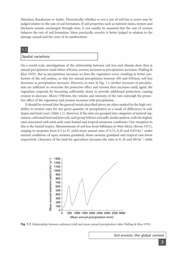
On a world scale, investigations of the relationship between soil loss and climate show that atannual precipitation totals below 450 mm, erosion increases as precipitation increases (Walling &Kleo 1979). But as precipitation increases so does the vegetation cover, resulting in better pro-tection of the soil surface, so that for annual precipitation between 450 and 650 mm, soil lossdecreases as precipitation increases. However, as seen in Fig. 1.1, further increases in precipita-tion are sufficient to overcome the protective effect and erosion then increases until, again, thevegetation responds by becoming sufficiently dense to provide additional protection, causingerosion to decrease. Above 1700 mm, the volume and intensity of the rain outweigh the protec-tive effect of the vegetation and erosion increases with precipitation.
It should be stressed that the general trends described above are often masked by the high vari-ability in erosion rates for any given quantity of precipitation as a result of differences in soil,slopes and land cover (Table 1.1). However, if the rates are grouped into categories of natural veg-etation, cultivated land and bare soil, each group follows a broadly similar pattern, with the highestrates associated with semi-arid, semi-humid and tropical monsoon conditions. One exception tothis is the humid tropics. Measurements of soil loss from hillslopes in West Africa (Roose 1971),ranging in steepness from 0.3 to 4°, yield mean annual rates of 0.15, 0.20 and 0.03 t ha-1 undernatural conditions of open savanna grassland, dense savanna grassland and tropical rain forestrespectively. Clearance of the land for agriculture increases the rates to 8, 26 and 90 t ha-1, while
0 500 1000 1500 2000 2500 3000 3500 40000
100200300400500600700800900
1000110012001300
Mean annual precipitation (mm)
Mea
n a
nn
ual
sed
imen
t yi
eld
(t
km–2
yr–1
)
Fig. 1.1 Relationship between sediment yield and mean annual precipitation (after Walling & Kleo 1979).
MSE1 11/19/04 02:28 PM Page 3
leaving the land as bare soil produces rates of 20, 30 and 170 t ha-1 respectively. Thus, removal ofthe rain forest results in much greater rises in erosion rates than does removal of the savannagrassland. These measurements emphasize the high degree of protection afforded by the rainforest but also reflect the erosive capacity of the high rainfalls in the humid tropics when thatprotection is destroyed. The rates of removal of tropical rain forests over the past twenty yearsare therefore of major concern with respect to present and future erosion problems.
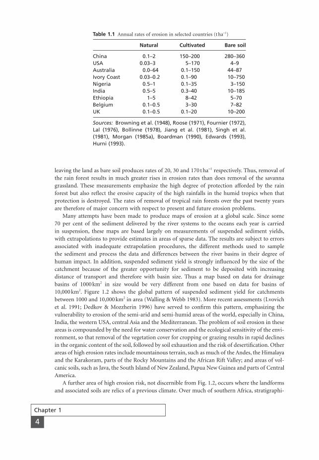
Many attempts have been made to produce maps of erosion at a global scale. Since some 70 per cent of the sediment delivered by the river systems to the oceans each year is carried in suspension, these maps are based largely on measurements of suspended sediment yields,with extrapolations to provide estimates in areas of sparse data. The results are subject to errorsassociated with inadequate extrapolation procedures, the different methods used to sample the sediment and process the data and differences between the river basins in their degree ofhuman impact. In addition, suspended sediment yield is strongly influenced by the size of thecatchment because of the greater opportunity for sediment to be deposited with increasing distance of transport and therefore with basin size. Thus a map based on data for drainage basins of 1000 km2 in size would be very different from one based on data for basins of10,000 km2. Figure 1.2 shows the global pattern of suspended sediment yield for catchmentsbetween 1000 and 10,000 km2 in area (Walling & Webb 1983). More recent assessments (Lvovichet al. 1991; Dedkov & Mozzherin 1996) have served to confirm this pattern, emphasizing the vulnerability to erosion of the semi-arid and semi-humid areas of the world, especially in China,India, the western USA, central Asia and the Mediterranean. The problem of soil erosion in theseareas is compounded by the need for water conservation and the ecological sensitivity of the envi-ronment, so that removal of the vegetation cover for cropping or grazing results in rapid declinesin the organic content of the soil, followed by soil exhaustion and the risk of desertification. Otherareas of high erosion rates include mountainous terrain, such as much of the Andes, the Himalayaand the Karakoram, parts of the Rocky Mountains and the African Rift Valley; and areas of vol-canic soils, such as Java, the South Island of New Zealand, Papua New Guinea and parts of CentralAmerica.
A further area of high erosion risk, not discernible from Fig. 1.2, occurs where the landformsand associated soils are relics of a previous climate. Over much of southern Africa, stratigraphi-
Chapter 1
4
Table 1.1 Annual rates of erosion in selected countries (t ha-1)
Natural Cultivated Bare soil
China 0.1–2 150–200 280–360USA 0.03–3 5–170 4–9Australia 0.0–64 0.1–150 44–87Ivory Coast 0.03–0.2 0.1–90 10–750Nigeria 0.5–1 0.1–35 3–150India 0.5–5 0.3–40 10–185Ethiopia 1–5 8–42 5–70Belgium 0.1–0.5 3–30 7–82UK 0.1–0.5 0.1–20 10–200
Sources: Browning et al. (1948), Roose (1971), Fournier (1972),Lal (1976), Bollinne (1978), Jiang et al. (1981), Singh et al.(1981), Morgan (1985a), Boardman (1990), Edwards (1993),Hurni (1993).
MSE1 11/19/04 02:28 PM Page 4
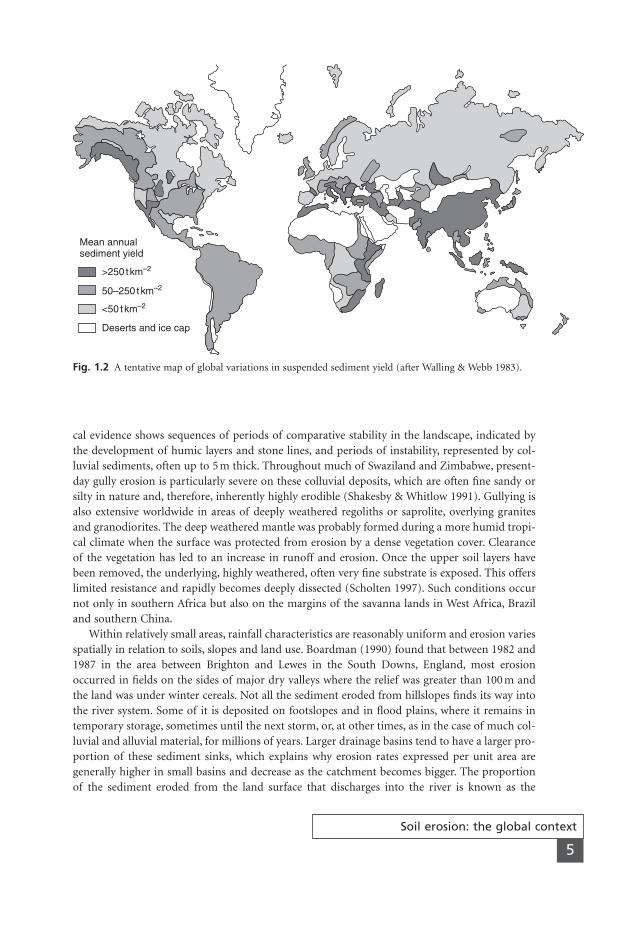
cal evidence shows sequences of periods of comparative stability in the landscape, indicated bythe development of humic layers and stone lines, and periods of instability, represented by col-luvial sediments, often up to 5 m thick. Throughout much of Swaziland and Zimbabwe, present-day gully erosion is particularly severe on these colluvial deposits, which are often fine sandy orsilty in nature and, therefore, inherently highly erodible (Shakesby & Whitlow 1991). Gullying isalso extensive worldwide in areas of deeply weathered regoliths or saprolite, overlying granitesand granodiorites. The deep weathered mantle was probably formed during a more humid tropi-cal climate when the surface was protected from erosion by a dense vegetation cover. Clearanceof the vegetation has led to an increase in runoff and erosion. Once the upper soil layers havebeen removed, the underlying, highly weathered, often very fine substrate is exposed. This offerslimited resistance and rapidly becomes deeply dissected (Scholten 1997). Such conditions occurnot only in southern Africa but also on the margins of the savanna lands in West Africa, Braziland southern China.
Within relatively small areas, rainfall characteristics are reasonably uniform and erosion variesspatially in relation to soils, slopes and land use. Boardman (1990) found that between 1982 and1987 in the area between Brighton and Lewes in the South Downs, England, most erosionoccurred in fields on the sides of major dry valleys where the relief was greater than 100 m andthe land was under winter cereals. Not all the sediment eroded from hillslopes finds its way intothe river system. Some of it is deposited on footslopes and in flood plains, where it remains intemporary storage, sometimes until the next storm, or, at other times, as in the case of much col-luvial and alluvial material, for millions of years. Larger drainage basins tend to have a larger pro-portion of these sediment sinks, which explains why erosion rates expressed per unit area aregenerally higher in small basins and decrease as the catchment becomes bigger. The proportionof the sediment eroded from the land surface that discharges into the river is known as the
Soil erosion: the global context
5
Mean annualsediment yield
>250 t km–2
<50 t km–2
Deserts and ice cap
50–250 t km–2
Fig. 1.2 A tentative map of global variations in suspended sediment yield (after Walling & Webb 1983).
MSE1 11/19/04 02:28 PM Page 5
Chapter 1
6
1.2
Temporal variations
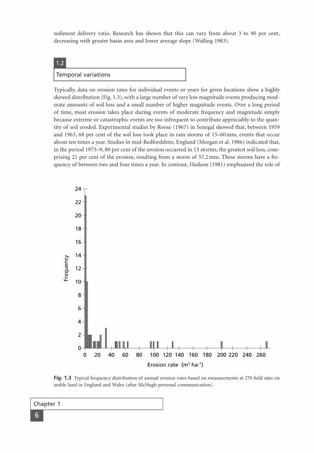
Typically, data on erosion rates for individual events or years for given locations show a highlyskewed distribution (Fig. 1.3), with a large number of very low magnitude events producing mod-erate amounts of soil loss and a small number of higher magnitude events. Over a long period of time, most erosion takes place during events of moderate frequency and magnitude simplybecause extreme or catastrophic events are too infrequent to contribute appreciably to the quan-tity of soil eroded. Experimental studies by Roose (1967) in Senegal showed that, between 1959and 1963, 68 per cent of the soil loss took place in rain storms of 15–60 mm, events that occurabout ten times a year. Studies in mid-Bedfordshire, England (Morgan et al. 1986) indicated that,in the period 1973–9, 80 per cent of the erosion occurred in 13 storms, the greatest soil loss, com-prising 21 per cent of the erosion, resulting from a storm of 57.2 mm. These storms have a fre-quency of between two and four times a year. In contrast, Hudson (1981) emphasized the role of
sediment delivery ratio. Research has shown that this can vary from about 3 to 90 per cent,decreasing with greater basin area and lower average slope (Walling 1983).
0
2
4
6
8
10
12
14
16
18
20
22
24
0 20 40 60 80 100 120 140 160 180 200 220 240 260
Freq
uen
cy
Erosion rate (m3 ha–1)
Fig. 1.3 Typical frequency distribution of annual erosion rates based on measurements at 270 field sites onarable land in England and Wales (after McHugh personal communication).
MSE1 11/19/04 02:28 PM Page 6

the more dramatic event. Quoting from research in Zimbabwe, he stated that 50 per cent of theannual soil loss occurs in only two storms and that, in one year, 75 per cent of the erosion tookplace in ten minutes. Moderate events also account for most of the erosion carried out by wind.Studies on coastal dunes at Cape Moreton, New South Wales, showed that most sand transportoccurred in strong winds of about 14 m s-1, with relatively little in winds of gale force and above because their greater competence was compensated for by their rarity (Chapman 1990).The frequency of the dominant erosion event may vary for different erosion processes. Forexample, for shallow debris slides and mudflows on cultivated fields and grassland in the Mgetaarea of Tanzania the dominant event has a return period of once in five years (Temple & Rapp1972).
The more dramatic events may become important where erosion is not a function of climatealone but depends on the frequency at which potentially erosive events coincide with ground con-ditions that favour erosion. Analysis of 28 years of data for nine small catchments under a four-year rotation of maize–wheat–grass–grass at Coshocton, Ohio (Edwards & Owens 1991) showedthat the three largest storms, all with return periods of 100 years or more, accounted for 52 percent of the erosion and that 92 per cent of the soil loss occurred in the years when the land wasunder maize. Extreme events may also produce landscape features that are both dramatic andlong lasting. A slow-moving equatorial storm deposited 631 mm of rain on 28 December 1926and 1194 mm between 26 and 29 December in the Kuantan area of Malaysia, resulting in exten-sive gully erosion and numerous landslides. The scars produced in the landscape were still visible35 years later (Nossin 1964).
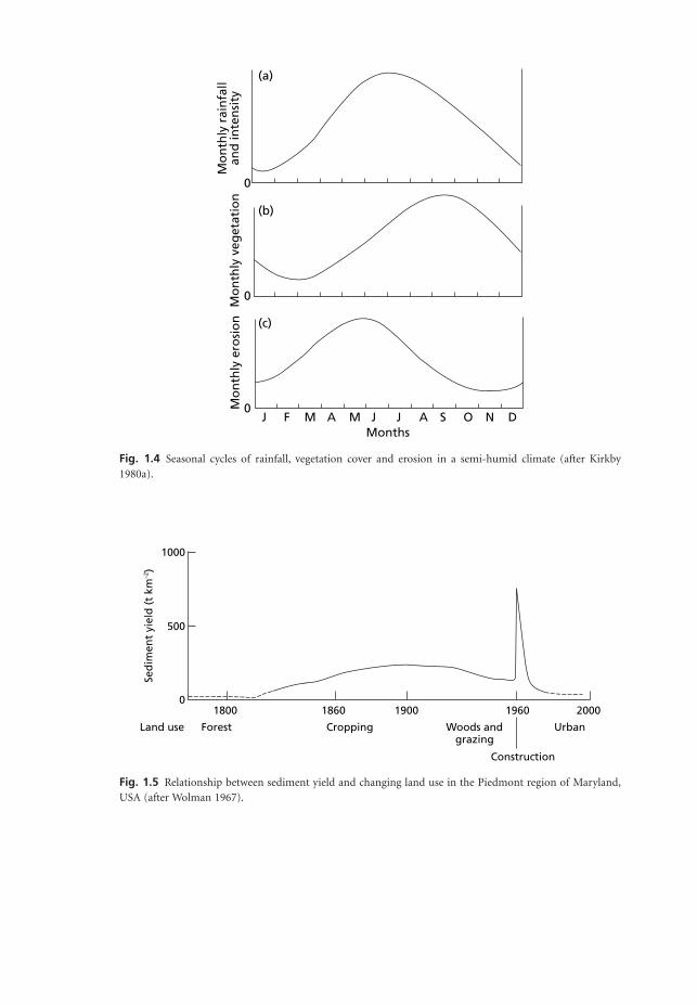
In addition to the variations in erosion associated with the frequency and magnitude of singlestorms, rates of erosion often follow a seasonal pattern. This is best illustrated with reference toa rainfall regime with a wet and dry season (Fig. 1.4). The vegetation growth follows a similarpattern but peaks later than the rainfall. The most vulnerable time for erosion is the early part ofthe wet season when the rainfall is high but the vegetation has not grown sufficiently to protectthe soil. Thus the erosion peak precedes the rainfall peak.
Somewhat more complex seasonal patterns occur with less simple rainfall regimes or wherethe land is used for arable farming. Generally, the period between ploughing and the growth ofthe crop beyond the seedling stage contains an erosion risk if it coincides with heavy rainfall orstrong winds. Thus, in western Europe, the period in spring before the crop cover reaches 20 percent is often a peak time for erosion when rainfall degrades the bare soil surface, causing the devel-opment of a surface seal (Cerdan et al. 2002a).
Longer-term spatial variations in erosion occur in relation to changes in land cover. A typicalsequence of events is described by Wolman (1967) for Maryland, where soil erosion ratesincreased with the conversion of woodland to cropland after 1700 (Fig. 1.5). They declined asthe urban fringe extended across the area in the 1950s and the land reverted to scrub when thefarmers sold out to speculators, before accelerating rapidly, reaching annual rates of 7000 t ha-1,when the area was laid bare during housing construction. With the completion of urban devel-opment, runoff from concrete surfaces is concentrated into gutters and sewers, and annual soilloss falls below 4 t ha-1.
Based on stratigraphical and archaeological evidence of valley floor deposits and archivalmaterial, Bork (1989) reconstructed the history of soil erosion in Niedersachsen, Germany. Fromthe early Holocene, when soils developed under the natural woodlands, up to the early MiddleAges, erosion rates were extremely low. With the clearance of forest for agriculture between 940 and 1340, erosion increased and reached annual rates of about 10 t ha-1. Between 1340 and 1350, annual erosion rates rose dramatically to 2250 t ha-1 as a result of gully erosion in-duced by extreme climatic events such as that on 21 July 1342, when the largest flood ever
Soil erosion: the global context
7
MSE1 11/19/04 02:28 PM Page 7
(a)
0
(b)
0
(c)
0J F M M J J A S N DOA
Months
Mo
nth
ly r
ain
fall
and
inte
nsi
tyM
on
thly
veg
etat
ion
Mo
nth
ly e
rosi
on
Fig. 1.4 Seasonal cycles of rainfall, vegetation cover and erosion in a semi-humid climate (after Kirkby1980a).
1000
500
01800 1900 20001860 1960
Land use Forest Cropping UrbanWoods andgrazing
Construction
Sed
imen
t yi
eld
(t
km–2
)
Fig. 1.5 Relationship between sediment yield and changing land use in the Piedmont region of Maryland,USA (after Wolman 1967).
MSE1 11/19/04 02:28 PM Page 8
recorded in central Europe occurred (Bork et al. 1998). Erosion declined afterwards, partly as aresult of a decrease in the area under arable as land was abandoned due to impoverishment byerosion. The rate of erosion did not return to early mediaeval levels but remained at an averageannual rate of around 25 t ha-1. The higher rate reflected sheet erosion on the land remaining inarable as production went over to the three-field system, with one-third of the land in fallow atany one time. The period between 1750 and 1800 saw a second episode of gullying, with an averageannual soil loss around 160 t ha-1, in response to an increase in the frequency of heavy rainfallevents. The soil loss did not reach mid-fourteenth-century levels, however, because of the estab-lishment of terraces, the use of contour ploughing and grass strips and a higher proportion ofthe land under grass and trees. Since 1800 annual soil loss has averaged 20 t ha-1 but it hasincreased in recent years following land consolidation, which has resulted in larger fields, removalof terraces and grass strips and land levelling. A similar history of fluctuating rates of soil erosionin relation to changes in land use has been reconstructed for the Wolfsgraben in northern Bavaria,Germany (Dotterweich et al. 2003). In periods when the land was under arable cultivation, annualerosion rates averaged 2.8 t ha-1 and sedimentation occurred on the valley floors. In extreme rainfall events in the early fourteenth century and again in the late eighteenth century, these sed-iments were cut through by gullies, up to 5 m deep. Whenever land was taken out of cultivationand reverted to forest, erosion rates were very low and the gullies were infilled.
These historical studies indicate the complex nature of soil erosion. Although erosion is anatural process and, therefore, naturally variable with climate, soils and topography, humanimpact can make the landscape either more or less resilient to climatic events. Rates of erosionquickly accelerate to high levels whenever land is misused.
Soil erosion: the global context
9
Only 22 per cent of the earth’s land area of14,900 million hectares is potentially produc-tive (El-Swaify 1994). Since this has to provide97 per cent of the food supply (3 per centcomes from oceans, rivers and lakes), it isunder increasing pressure as world populationnumbers continue to grow. The fear is thatmeeting the greater demand for food throughmore intensive use of existing agricultural landand expansion of agriculture on to more mar-ginal land will substantially increase erosion.Failure to control erosion will therefore seri-ously endanger global food security. Concernabout the future is based upon:� very high rates of erosion measured from
agricultural land, with annual rates often20 to over 100tha-1;
� declines in the productivity of the soil by asmuch as 15–30 per cent annually;
Box 1
� the difficulty of restoring severely degradedland because of the loss of fertility;
� an estimated loss of some 6 million hectaresannually as a result of degradation byerosion and other causes (Pimental et al.1993).Unfortunately, it is impossible to know
whether the above data represent a realisticpicture because they ignore important issues.First, the data on erosion rates are highlyselective and often based on short periods ofmeasurement; it is statistically invalid toextrapolate them over large areas. Pimental etal. (1995) estimated that Europe was losingsoil at an annual rate of 17tha-1 but,according to Lomborg (2001), this figure islargely based on extrapolating measurementsfrom a 0.1 hectare plot of land in Belgium.Second, most studies of productivity inrelation to erosion come from low-input
Continued
Erosion, population and food supply
MSE1 11/19/04 02:28 PM Page 9
Chapter 1
10
agriculture and therefore ignore the effects ofimproved farming practices, including greateruse of irrigation, pesticides and fertilizers. Inmuch of Western Europe and the USA, annualincreases of 1–2 per cent in productivity canmore than offset the effects of erosion, which,locally, are generally in the 0.1–0.5 per centrange (Crosson 1995). In these areas,agricultural production has allowed increasingnumbers of people to be fed despite the proportion of the population directlyemployed on the land falling to below 10 per cent.
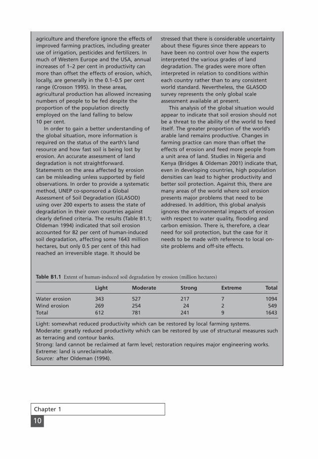
In order to gain a better understanding ofthe global situation, more information isrequired on the status of the earth’s landresource and how fast soil is being lost byerosion. An accurate assessment of landdegradation is not straightforward.Statements on the area affected by erosioncan be misleading unless supported by fieldobservations. In order to provide a systematicmethod, UNEP co-sponsored a GlobalAssessment of Soil Degradation (GLASOD)using over 200 experts to assess the state ofdegradation in their own countries againstclearly defined criteria. The results (Table B1.1;Oldeman 1994) indicated that soil erosionaccounted for 82 per cent of human-inducedsoil degradation, affecting some 1643 millionhectares, but only 0.5 per cent of this hadreached an irreversible stage. It should be
stressed that there is considerable uncertaintyabout these figures since there appears tohave been no control over how the expertsinterpreted the various grades of landdegradation. The grades were more ofteninterpreted in relation to conditions withineach country rather than to any consistentworld standard. Nevertheless, the GLASODsurvey represents the only global scaleassessment available at present.
This analysis of the global situation wouldappear to indicate that soil erosion should notbe a threat to the ability of the world to feeditself. The greater proportion of the world’sarable land remains productive. Changes infarming practice can more than offset theeffects of erosion and feed more people froma unit area of land. Studies in Nigeria andKenya (Bridges & Oldeman 2001) indicate that,even in developing countries, high populationdensities can lead to higher productivity andbetter soil protection. Against this, there aremany areas of the world where soil erosionpresents major problems that need to beaddressed. In addition, this global analysisignores the environmental impacts of erosionwith respect to water quality, flooding andcarbon emission. There is, therefore, a clearneed for soil protection, but the case for itneeds to be made with reference to local on-site problems and off-site effects.
Table B1.1 Extent of human-induced soil degradation by erosion (million hectares)
Light Moderate Strong Extreme Total
Water erosion 343 527 217 7 1094Wind erosion 269 254 24 2 549Total 612 781 241 9 1643
Light: somewhat reduced productivity which can be restored by local farming systems.Moderate: greatly reduced productivity which can be restored by use of structural measures suchas terracing and contour banks.Strong: land cannot be reclaimed at farm level; restoration requires major engineering works.Extreme: land is unreclaimable.Source: after Oldeman (1994).
MSE1 11/19/04 02:28 PM Page 10
Soil erosion is a two-phase process consisting of the detachment of individual soil particles from the soil mass and their transport by erosive agents such as running water and wind. Whensufficient energy is no longer available to transport the particles, a third phase, deposition,occurs.
Rainsplash is the most important detaching agent. As a result of raindrops striking a bare soil surface, soil particles may be thrown through the air over distances of several centimetres.Continuous exposure to intense rainstorms considerably weakens the soil. The soil is also brokenup by weathering processes, both mechanical, by alternate wetting and drying, freezing and thawing and frost action, and biochemical. Soil is disturbed by tillage operations and by the trampling of people and livestock. Running water and wind are further contributors to the detachment of soil particles. All these processes loosen the soil so that it is easily removed bythe agents of transport.
The transporting agents comprise those that act areally and contribute to the removal of a rel-atively uniform thickness of soil, and those that concentrate their action in channels. The firstgroup consists of rainsplash, surface runoff in the form of shallow flows of infinite width, some-times termed sheet flow but more correctly called overland flow, and wind. The second groupcovers water in small channels, known as rills, which can be obliterated by weathering and plough-ing, or in the larger more permanent features of gullies and rivers. A distinction is commonlymade for water erosion between rill erosion and erosion on the land between the rills by the com-bined action of raindrop impact and overland flow. This is termed interrill erosion. To these agentsthat act externally, picking up material from and carrying it over the ground surface, should beadded transport by mass movements such as soil flows, slides and creep, in which water affectsthe soil internally, altering its strength.
The severity of erosion depends upon the quantity of material supplied by detachment over time and the capacity of the eroding agents to transport it. Where the agents have the cap-acity to transport more material than is supplied by detachment, the erosion is described asdetachment-limited. Where more material is supplied than can be transported, the erosion is tran-sport limited.
The energy available for erosion takes two forms: potential and kinetic. Potential energy (PE)results from the difference in height of one body with respect to another. It is the product of mass(m), height difference (h) and acceleration due to gravity (g), so that
(2.1)PE mhg=
Processes and mechanics of erosion
11
CHAPTER 2
Processes andmechanics oferosion
MSE02 11/19/04 02:32 PM Page 11

which, in units of kg, m and m s-2 respectively, yields a value in Joules. The potential energy forerosion is converted into kinetic energy (KE), the energy of motion. This is related to the massand velocity (n) of the eroding agent in the expression
(2.2)
which, in units of kg and m s-1, also gives a value in Joules. Most of this energy is dissipated infriction with the surface over which the agent moves so that only 3–4 per cent of the energy ofrunning water and 0.2 per cent of that of falling raindrops is expended in erosion (Pearce 1976).An indication of the relative efficiencies of the processes of water erosion can be obtained byapplying these figures to calculations of kinetic energy, using eqn 2.2, based on typical velocities(Table 2.1). The concentration of running water in rills affords the most powerful erosive agentbut raindrops are potentially more erosive than overland flow. Most of the raindrop energy isused in detachment, however, so that the amount available for transport is less than that fromoverland flow. This is illustrated by measurements of soil loss in a field in mid-Bedfordshire,England. Over a 900-day period on an 11° slope on a sandy soil, transport across a centimetrewidth of slope amounted to 19,000 g of sediment by rills, 400 g by overland flow and only 20 g byrainsplash (Morgan et al. 1986).
KE m=1
22n
Chapter 2
12
Table 2.1 Efficiency of forms of water erosion
Form Mass* Typical Kinetic Energy for Observedvelocity energy† erosion‡ sediment(ms-1) transport§
(gcm-1)
Raindrops R 6.0 18R 0.036R 20Overland flow 0.5R 0.01 2.5 ¥ 10-5R 7.5 ¥ 10-7R 400Rill flow 0.5R 4¶ 4R 0.12R 19,000
* Assumes rainfall mass of R of which 50 per cent contributes to runoff.† Based on 1/2 mv2.‡ Assumes that 0.2 per cent of the kinetic energy of raindrops and 3 per cent of the kineticenergy of runoff is utilized in erosion.§ Totals observed in mid-Bedfordshire, England, on an 11° slope, on sandy soil, over 900 days. Most of the energy of raindrops contributes to soil particle detachment rather thantransport.¶ Estimated using the Manning equation of flow velocity for a rill, 0.3m wide and 0.2m deep,on a slope of 11°, at bankfull, assuming a roughness coefficient of 0.02.
2.1
Hydrological basis of erosion
The processes of water erosion are closely related to the pathways taken by water in its movementthrough the vegetation cover and over the ground surface. During a rainstorm, part of the waterfalls directly on the land, either because there is no vegetation or because it passes through gapsin the plant canopy. This component of the rainfall is known as direct throughfall. Part of the
MSE02 11/19/04 02:32 PM Page 12
rain is intercepted by the canopy, from where it either returns to the atmosphere by evaporationor finds its way to the ground by dripping from the leaves, a component termed leaf drainage, orby running down the plant stems as stemflow. The action of direct throughfall and leaf drainageproduces rainsplash erosion. The rain that reaches the ground may be stored in small depressionsor hollows on the surface or it may infiltrate the soil, contributing to soil moisture storage, tolateral movement downslope within the soil as subsurface or interflow or, by percolating deeper,to groundwater. When the soil is unable to take in more water, the excess contributes to runoffon the surface, resulting in erosion by overland flow or by rills and gullies.
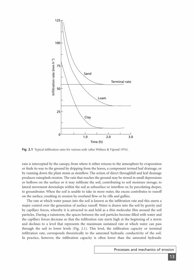
The rate at which water passes into the soil is known as the infiltration rate and this exerts amajor control over the generation of surface runoff. Water is drawn into the soil by gravity andby capillary forces, whereby it is attracted to and held as a thin molecular film around the soilparticles. During a rainstorm, the spaces between the soil particles become filled with water andthe capillary forces decrease so that the infiltration rate starts high at the beginning of a stormand declines to a level that represents the maximum sustained rate at which water can passthrough the soil to lower levels (Fig. 2.1). This level, the infiltration capacity or terminal infiltration rate, corresponds theoretically to the saturated hydraulic conductivity of the soil.In practice, however, the infiltration capacity is often lower than the saturated hydraulic
Processes and mechanics of erosion
13
125
100
75
25
1.0 2.0 3.00
50
Time (h)
Clay
Loam
Terminal rate
Sand
Infi
ltra
tio
n r
ate
(mm
h–1
)
Fig. 2.1 Typical infiltration rates for various soils (after Withers & Vipond 1974).
MSE02 11/19/04 02:32 PM Page 13
conductivity because of air entrapped in the soil pores as the wetting front passes downwardsthrough the soil.
Various attempts have been made to describe the change in infiltration rate over time math-ematically. One of the most widely used equations is the modification of the Green and Ampt(1911) equation proposed by Mein and Larson (1973):
(2.3)
where i is the instantaneous rate of infiltration, A is the transmission constant or saturatedhydraulic conductivity of the soil, B is the sorptivity, defined by Talsma (1969) as the slope of theline when i is plotted against t, and t is the time elapsed since the onset of the rain. This equa-tion has been found to describe well the infiltration behaviour of soils in southern Spain (Scoging& Thornes 1979) and Arizona (Scoging et al. 1992) but Bork and Rohdenburg (1981), alsoworking in southern Spain, obtained better results with the equation proposed by Philip (1957):
(2.4)
while Gifford (1976) found neither equation satisfactory for semi-arid rangelands in northernAustralia and Utah. Kutílek et al. (1988) tested both equations against field measurementsobtained with double-ring infiltrometers and found that neither fitted the data well, giving errorsof between 10 and 59 per cent when used to estimate saturated hydraulic conductivity. One reasonfor the error is the failure to predict infiltration correctly under conditions of surface pondingwhen the soil develops a viscous resistance to air flow. Morel-Seytoux and Khanji (1974) devel-oped the following equation to allow for this:
(2.5)
where ks is the saturated hydraulic conductivity; b is a viscous correction factor, which varies invalue between 1.1 and 1.7, depending on soil type and ponding depth but averages 1.4; qi is theinitial soil moisture content by volume; qt is the actual volumetric moisture content of soil in thezone between the ground surface and the wetting front; H0 is the depth of ponded water; Dy isthe change in y between the soil surface and the wetting front; y is the difference in pressurebetween the pore-water and the atmosphere; and I is the total amount of water already infiltrated.As a result of including the viscous correction factor, eqn 2.5 predicts lower infiltration rates thaneither eqn 2.3 or eqn 2.4.
Infiltration rates depend upon the characteristics of the soil. Generally, coarse-textured soilssuch as sands and sandy loams have higher infiltration rates than clay soils because of the largerspaces between the pores. Infiltration capacities may range from more than 200 mm h-1 for sandsto less than 5 mm h-1 for tight clays (Fig. 2.1). In addition to the role played by the inter-particlespacing or micropores, the larger cracks or macropores exert an important influence over infil-tration. They can transmit considerable quantities of water so that clays with well defined struc-tures can have infiltration rates that are much higher than would be expected from their texturealone. Infiltration behaviour on many soils is also rather complex because the soil profiles arecharacterized by two or more layers of differing hydraulic conductivities; most agricultural soils,for example, consist of a disturbed plough layer and an undisturbed subsoil. Many soils on con-struction sites comprise a heavily compacted subsoil covered by a thinner and less compacted
ik H
Is t i= +
-( ) +( )ÊË
ˆ¯b
q q y1 0 D
i AB
t= +
i AB
t= +
Chapter 2
14
MSE02 11/19/04 02:32 PM Page 14
topsoil. Local variability in infiltration rates can be quite high because of differences in the struc-ture, compaction, initial moisture content and profile form of the soil and in vegetation density.Field determinations of average infiltration capacity using infiltrometers may have coefficients ofvariation of 70–75 per cent. Eyles (1967) measured infiltration capacity on soils of the MelakaSeries near Temerloh, Malaysia, and obtained values ranging from 15 to 420 mm h-1, with a meanof 147 mm h-1.
According to Horton (1945), if rainfall intensity is less than the infiltration capacity of the soil,no surface runoff occurs and the infiltration rate equals the rainfall intensity. If the rainfall inten-sity exceeds the infiltration capacity, the infiltration rate equals the infiltration capacity and theexcess rain forms surface runoff. As a mechanism for generating runoff, however, this compari-son of rainfall intensity and infiltration capacity does not always hold. Studies in Bedfordshire,England (Morgan et al. 1986) on a sandy soil show that measured infiltration capacity is greaterthan 400 mm h-1 and that rainfall intensities rarely exceed 40 mm h-1. Thus no surface runoffwould be expected, whereas, in fact, the mean annual runoff is about 55 mm from a mean annualrainfall of 550 mm. The reason runoff occurs is that these soils are prone to the development ofa surface crust. Two types of crust can be distinguished. Where a crust forms in situ on the soil,it is termed a structural crust; where it results from the deposition of fine particles in puddles, itis called a depositional crust (Boiffin 1985). As shown by studies on loamy soils in north-eastFrance, crusting can reduce the infiltration capacity from 45–60 to about 6 mm h-1 with a struc-tural crust and 1 mm h-1 with a depositional crust (Boiffin & Monnier 1985; Martin et al. 1997).Reductions in infiltration of 50 (Hoogmoed & Stroosnijder 1984) to 100 per cent (Torri et al.1999) can occur in a single storm. The importance of crusting and sealing was also emphasizedby Poesen (1984), who found that infiltration rates were higher on steeper slopes where the highererosion rate prevented the seal from forming.
The presence of stones or rock fragments on the surface of a soil also influences infiltrationrates but in a rather complex way depending on whether the stones are resting on top of thesurface or are embedded within the soil. Generally, rock fragments protect the soil against phys-ical destruction and the formation of a crust, so that infiltration rates are higher than on a com-parable stone-free bare soil. However, on soils that are subject to crusting, a high percentage stonecover can produce a worse situation; a 75 per cent cover of rock fragments embedded in a crustedsurface on a silt-loam soil reduced infiltration rates to 50 per cent of those on a stone-free soil(Poesen & Ingelmo-Sanchez 1992).
The important control for runoff production on many soils is not infiltration capacity but alimiting moisture content. When the actual moisture content is below this value, pore water pres-sure in the soil is less than atmospheric pressure and water is held in capillary form under tensilestress or suction. When the limiting moisture content is reached and all the pores are full of water,pore water pressure equates to atmospheric pressure, suction reduces to zero and surface pondingoccurs. This explains why sands that have low levels of capillary storage can produce runoff veryquickly even though their infiltration capacity is not exceeded by the rainfall intensity. Sincehydraulic conductivity is a flux partly controlled by rainfall intensity, increases in intensity cancause conductivity to rise so that, although runoff may have formed rapidly at a relatively lowintensity, higher rainfall intensities do not always produce greater runoff. This mechanismexplains why infiltration rates sometimes increase with rainfall intensity (Nassif & Wilson 1975).Bowyer-Bower (1993) found that, for a given soil, infiltration capacity was higher with higherrainfall intensities because of their ability to disrupt surface seals and crusts that would otherwisekeep the infiltration rate low.
Once water starts to pond on the surface, it is held in depressions or hollows and runoffdoes not begin until the storage capacity of these is satisfied. On agricultural land, depression
Processes and mechanics of erosion
15
MSE02 11/19/04 02:32 PM Page 15
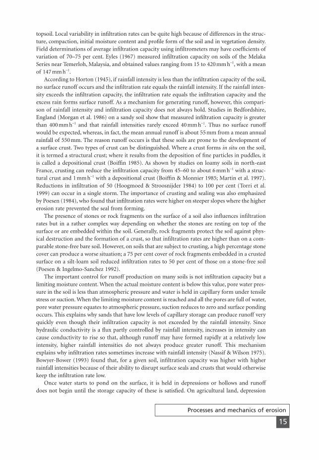
storage varies seasonally depending on the type of cultivation that has been carried out and thetime since cultivation for the roughness to be reduced by weathering and raindrop impact.Table 2.2 gives typical values of depression storage (DS; mm) for surfaces produced by differenttillage implements, based on their roughness index (RFR; cm m-1) (Auerswald, personal communication):
(2.6)
(2.7)
where L0 is the straight-line distance between two points along a transect of the soil surface andLA is the actual distance measured over all the microtopographic irregularities.
RFRL L
LA
A
=-
¥0 100
DS e RFR= 0 14 0 04. .
Chapter 2
16
Table 2.2 Surface roughness (RFR) for different tillage implementscompared to other expressions of random roughness
Implement Roughness Random roughness(RFR) (cmm-1) (RR) (mm)
Moldboard plough 30–33 33–48Chisel plough 24–28 17–26Cultivator 15–23 6–15Tandem disc 25–28 18–26Offset disc 32–35 38–51Paraplough 32–35 10Spike tooth harrow 17–23 8–15Spring tooth harrow 25 18Rotary hoe 21–22 12–13Rototiller 23 15Drill 20–21 10–12Row planter 13–22 5–13
Note: The term, RFR, is essentially an index of the tortuosityof the soil surface. An alternative and widely used descriptorof the roughness of the soil surface is random roughness (RR,mm), defined as the standard deviation of a series of surfaceheight measurements (Currence & Lovely 1970). There is agood correlation between RR and RFR which can be expressedby (Auerswald personal communication):
lnRR = 0.29 + 0.099RFR, r = 0.995, n = 27
RFR = -1.77 + 9.25 lnRR, r = 0.912, n = 27
Surface roughness, expressed by RR, declines over time as afunction of cumulative rainfall (Rc):
where RR(t) is the random roughness at time (t), RR(0) is theoriginal random roughness after tillage and a = 2.8 ¥ 0.3Si,where Si is the silt content of the soil (0–1) (if a ≥ 0, a is set to-1) (Alberts et al. 1989).Source: after Auerswald, personal communication.
RR t RR e Rc( ) = ( ) -0 a
MSE02 11/19/04 02:32 PM Page 16
Surface roughness and therefore depression storage decline over time through weathering andraindrop impact. Auerswald (personal communication) developed the following relationship toexpress the decline in roughness as a function of the cumulative kinetic energy of rainfall:
(2.8)
where RFR(t) is the roughness at a certain time, RFR0 is the initial roughness and KE(t) is theaccumulated kinetic energy of the rain at time (t). Depression storage also varies with the soilwith clay soils having 1.6–2.3 times the storage volume of sandy soils. The roughness values givenin Table 2.2 relate to soils with about 20 per cent clay. These base values (RFRbase) can be adjustedto give roughness for different clay contents (RFRCC) using the relationship:
(2.9)
where CC is the percentage clay content of the soil. This relationship is valid for clay contents upto 25 per cent; for higher clay contents it is recommended to use the 25 per cent value.
RFR RFR CCcc base= +( )0 4 0 025. .
RFR t RFR e KE t( ) = - ( )0
0 7.
Processes and mechanics of erosion
17
2.2
Rainsplash erosion
The action of raindrops on soil particles is most easily understood by considering the momentum of a single raindrop falling on a sloping surface. The downslope component of thismomentum is transferred in full to the soil surface but only a small proportion of the compo-nent normal to the surface is transferred, the remainder being reflected. The transfer of momen-tum to the soil particles has two effects. First, it provides a consolidating force, compacting thesoil; second, it produces a disruptive force as the water rapidly disperses from and returns to thepoint of impact in laterally flowing jets. Whereas the impact velocity of falling raindrops strikingthe soil surface varies from about 4 m s-1 for a 1 mm diameter drop to 9 m s-1 for a 5 mm diame-ter drop, the local velocities of these jets are about twice these (Huang et al. 1982). These fast-moving water jets impart a velocity to some of the soil particles and launch them into the air,entrained within water droplets that are themselves formed by the break-up of the raindrop oncontact with the ground (Mutchler & Young 1975). Thus, raindrops are agents of both consoli-dation and dispersion.
The consolidation effect is best seen in the formation of a surface crust, usually only a few millimetres thick, which results from clogging of the pores by soil compaction and by the infilling of surface pore spaces by fine particles detached from soil aggregates by the raindropimpact. Studies of crust development under simulated rainfall show that crusts have a densesurface skin or seal, about 0.1 mm thick, with well oriented clay particles. Beneath this is a layer,1–3 mm thick, where the larger pore spaces are filled by finer washed-in material (Tackett &Pearson 1965). That raindrop impact is the critical process was shown by Farres (1978), whofound that, after a rainstorm, most aggregates on the soil surface were destroyed, while those inthe lower layer of the crust remained intact, even though completely saturated. A tap of theseaggregates, however, caused their instant breakdown. This evidence indicates that although saturation reduces the internal strength of soil aggregates, they do not disintegrate until struckby raindrops.
MSE02 11/19/04 02:32 PM Page 17

The actual response of a soil to a given rainfall depends upon its moisture content and, there-fore, its structural state and the intensity of the rain. Le Bissonnais (1990) describes three possi-ble responses:
� If the soil is dry and the rainfall intensity is high, the soil aggregates break down quicklyby slaking. This is the breakdown by compression of air ahead of the wetting front.Infiltration capacity reduces rapidly and on very smooth surfaces runoff can be gener-ated after only a few millimetres of rain. With rougher surfaces, depression storage isgreater and runoff takes longer to form.
� If the aggregates are initially partially wetted or the rainfall intensity is low, micro-cracking occurs and the aggregates break down into smaller aggregates. Surface rough-ness thus decreases but infiltration remains high because of the large pore spacesbetween the microaggregates.
� If the aggregates are initially saturated, infiltration capacity depends on the saturatedhydraulic conductivity of the soil and large quantities of rain are required to seal thesurface. Nevertheless, soils with less than 15 per cent clay content are vulnerable tosealing if the intensity of the rain is high.
Over time, the percentage area of the soil surface affected by crust development increases expo-nentially with cumulative rainfall energy (Govers & Poesen 1985), which, in turn, brings aboutan exponential decrease in infiltration capacity (Boiffin & Monnier 1985). Crustability decreaseswith increasing contents of clay and organic matter since these provide greater strength to thesoil. Thus loams and sandy loams are the most vulnerable to crust formation.
Studies of the kinetic energy required to detach one kilogram of sediment by raindrop impactshow that minimal energy is needed for soils with a geometric mean particle size of 0.125 mmand that soils with geometric mean particle size between 0.063 and 0.250 mm are the most vul-nerable to detachment (Fig. 2.2; Poesen 1985). Coarser soils are resistant to detachment becauseof the weight of the larger particles. Finer soils are resistant because the raindrop energy has toovercome the adhesive or chemical bonding forces that link the minerals comprising the clay par-ticles. The wide range in energy required to detach clay particles is a function of different levelsof resistance in relation to the type of clay minerals and the relative amounts of calcium, mag-nesium and sodium ions in the water passing through the pores (Arulanandan & Heinzen 1977).Overall, silt loams, loams, fine sands and sandy loams are the most detachable. Selective removalof particles by rainsplash can cause variations in soil texture downslope. Splash erosion on stonyloamy soils in the Luxembourg Ardennes has resulted in soils on the valley sides becoming defi-cient in clay and silt particles and high in gravel and stone content, whereas the colluvial soils atthe base of the slopes are enriched by the splashed-out material (Kwaad 1977). Selective erosioncan affect soil aggregates as well as primary particles. Rainfall simulation experiments on clay soilsin Italy show that splashed-out material is enriched in soil aggregates of 0.063–0.50 mm in size(Torri & Sfalanga 1986).
The detachability of soil depends not only on its texture but also on top soil shear strength(Cruse & Larsen 1977), a finding that has prompted attempts to understand splash erosion interms of shear. The detachment of soil particles represents a failure of the soil by the combinedmechanism of compression and shear under raindrop impact, an event that is most likely to occur under saturated conditions when the shear strength of the soil is lowest (Al-Durrah & Bradford 1982). Generally, detachment decreases exponentially with increasing shear strength. Broadly linear relationships have been obtained, however, between the quantity of soil particles detached by raindrop impact and the ratio of the kinetic energy of the rainfall to soil shear strength (Al-Durrah & Bradford 1981; Torri et al. 1987b; Bradford et al.1992).
Chapter 2
18
MSE02 11/19/04 02:32 PM Page 18
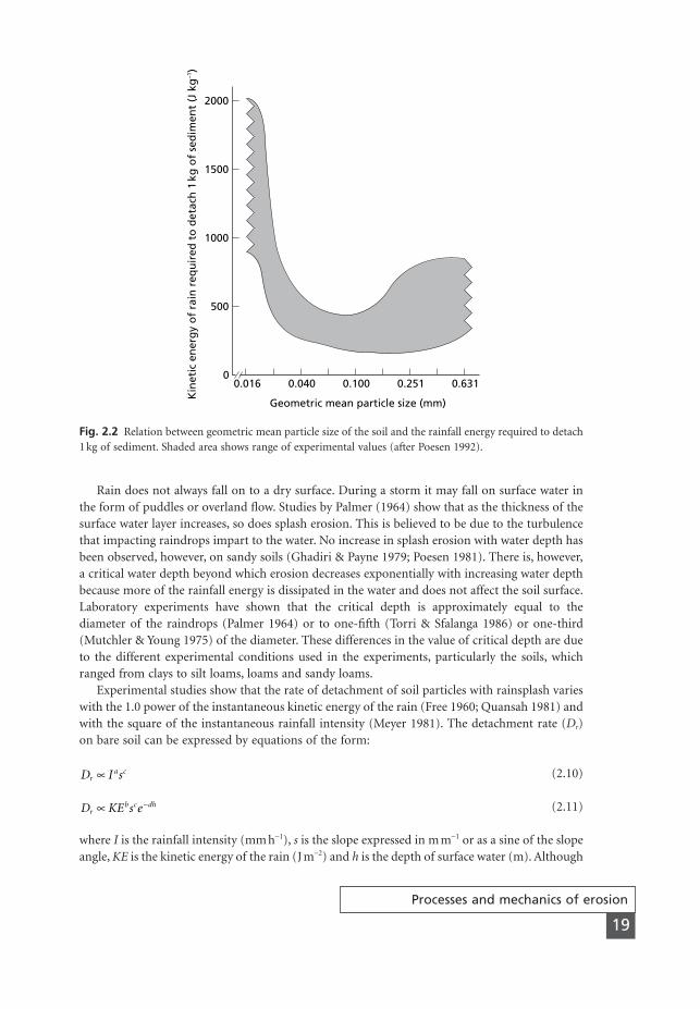
Rain does not always fall on to a dry surface. During a storm it may fall on surface water inthe form of puddles or overland flow. Studies by Palmer (1964) show that as the thickness of thesurface water layer increases, so does splash erosion. This is believed to be due to the turbulencethat impacting raindrops impart to the water. No increase in splash erosion with water depth hasbeen observed, however, on sandy soils (Ghadiri & Payne 1979; Poesen 1981). There is, however,a critical water depth beyond which erosion decreases exponentially with increasing water depthbecause more of the rainfall energy is dissipated in the water and does not affect the soil surface.Laboratory experiments have shown that the critical depth is approximately equal to the diameter of the raindrops (Palmer 1964) or to one-fifth (Torri & Sfalanga 1986) or one-third(Mutchler & Young 1975) of the diameter. These differences in the value of critical depth are dueto the different experimental conditions used in the experiments, particularly the soils, whichranged from clays to silt loams, loams and sandy loams.
Experimental studies show that the rate of detachment of soil particles with rainsplash varieswith the 1.0 power of the instantaneous kinetic energy of the rain (Free 1960; Quansah 1981) andwith the square of the instantaneous rainfall intensity (Meyer 1981). The detachment rate (Dr)on bare soil can be expressed by equations of the form:
(2.10)
(2.11)
where I is the rainfall intensity (mm h-1), s is the slope expressed in m m-1 or as a sine of the slopeangle, KE is the kinetic energy of the rain (J m-2) and h is the depth of surface water (m). Although
D KE s erb c dhµ -
D I sra cµ
Processes and mechanics of erosion
19
2000
1500
1000
500
0
Kin
etic
en
erg
y o
f ra
in r
equ
ired
to
det
ach
1 k
g o
f se
dim
ent
(J k
g–1
)
0.016 0.040 0.100 0.251 0.631
Geometric mean particle size (mm)
Fig. 2.2 Relation between geometric mean particle size of the soil and the rainfall energy required to detach1 kg of sediment. Shaded area shows range of experimental values (after Poesen 1992).
MSE02 11/19/04 02:32 PM Page 19
2.0 is a convenient value for a, the value may be adjusted to allow for variations in soil textureusing the term a = 2.0 - (0.01 ¥ % clay) (Meyer 1981). Similarly, the value of 1.0 for b may bevaried from 0.8 for sandy soils to 1.8 for clays (Bubenzer & Jones 1971). Values for c are in therange of 0.2–0.3 (Quansah 1981; Torri & Sfalanga 1986), also varying with the texture of the soil(Torri & Poesen 1992). It should be remembered that the slope term in this equation refers to thelocal slope for a distance equivalent to only a few drop diameters from the point of raindropimpact – for example, that on the side of a soil clod – and not the average ground slope. Thus,for practical purposes, the slope term is often omitted from calculations of soil particle detach-ment. A value of 2.0 is convenient for d as representative of a range of values between 0.9 and 3.1for different soil textures (Torri et al. 1987b).
In contrast, average ground slope is important when considering the overall transport ofsplashed particles. On a sloping surface more particles are thrown downslope than upslope duringthe detachment process, resulting in a net movement of material downslope. Splash transport perunit width of slope (Tr) can be expressed by the relationship:
(2.12)
where j = 1.0 (Meyer & Wischmeier 1969) and f = 1.0 (Quansah 1981; Savat 1981). There is someevidence to suggest that the value of f decreases on steeper slopes; Mosley (1973) gives a value of 0.8 and Moeyersons and De Ploey (1976) a value of 0.75 where slope angles rise to 20 and 25° respectively. Foster and Martin (1969) and Bryan (1979) found that splash transport in-creases with slope angle to reach a maximum at about 18° and that on steeper slopes f becomesnegative.
These relationships for detachment and transport of soil particles by rainsplash ignore the roleof wind. Windspeed imparts a horizontal force to a falling raindrop until its horizontal velocitycomponent equals the velocity of the wind. As a result, the kinetic energy of the raindrop isincreased. Not surprisingly, detachment of soil particles by impacting wind-driven raindrops canbe some 1.5–3 times greater than that resulting from rains of the same intensity without wind(Disrud & Krauss 1971; Lyles et al. 1974a). Wind also causes raindrops to strike the surface at anangle from vertical. This affects the relative proportions of upslope versus downslope splash.Moeyersons (1983) shows that where the angle between the falling raindrop and the vertical is20°, net splash transport is reduced to zero for slopes of 17–19° and has a net upslope com-ponent for gentler slopes. Where the angle between the falling raindrop and the vertical is 5°,zero splash occurs on a slope of 3°.
Since splash erosion acts uniformly over the land surface its effects are seen only where stonesor tree roots selectively protect the underlying soil and splash pedestals or soil pillars are formed.Such features frequently indicate the severity of erosion. Splash erosion is most important fordetaching the soil particles that are subsequently eroded by running water. However, on the upperparts of hillslopes, particularly those of convex form, splash transport may be the dominanterosion process. In Calabria, southern Italy, under forest and under scattered herb and shrub veg-etation, splash erosion accounts for 30–95 per cent of the total transport of material by watererosion (van Asch 1983). In Bedfordshire, England, splash accounts for 15–52 per cent of totalsoil transport on land under cereals and grass but only 3–10 per cent on bare ground (Morganet al. 1986). As runoff and soil loss increase, the importance of splash transport declines, althoughvery low contributions of splash to total transport were also measured in Bedfordshire underwoodland because of the protective effect of a dense litter layer. Govers and Poesen (1988) foundthat although raindrop impact detached 152 t ha-1 of soil over one year on a bare loam soil on a14° slope in Belgium, splash transport accounted for only 0.2 t ha-1 of the soil loss. The most
T I Srj fµ
Chapter 2
20
MSE02 11/19/04 02:32 PM Page 20
important contribution of splash erosion was to deliver detached particles to overland flow, whichwas the main agent of sediment transport in the interrill areas.
Processes and mechanics of erosion
21
2.3
Overland flow
Overland flow occurs on hillsides during a rainstorm when surface depression storage and either,in the case of prolonged rain, soil moisture storage or, with intense rain, the infiltration capacityof the soil are exceeded. The flow is rarely in the form of a sheet of water of uniform depth andmore commonly is a mass of anastomosing or braided water courses with no pronounced chan-nels. The flow is broken up by stones and cobbles and by the vegetation cover, often swirlingaround tufts of grass and small shrubs.
2.3.1 Hydraulic characteristics
The hydraulic characteristics of the flow are described by its Reynolds number (Re) and its Froudenumber (F), defined as follows:
(2.13)
(2.14)
where r is the hydraulic radius, which, for overland flow, is taken as equal to the flow depth andn is the kinematic viscosity of the water. The Reynolds number is an index of the turbulence ofthe flow. The greater the turbulence, the greater is the erosive power generated by the flow. Atnumbers less than 500 laminar flow prevails and at values above 2000 flow is fully turbulent. Inlaminar flow, each fluid layer moves in a straight line with uniform velocity and there is no mixingbetween the layers, whereas turbulent flow has a complicated pattern of eddies, producing con-siderable localized fluctuations in velocity, and a continuous interchange of water between thelayers. Intermediate values are indicative of transitional or disturbed flow, often a result of tur-bulence being imparted to laminar flow by raindrop impact (Emmett 1970). The Froude numberis an index of whether or not gravity waves will form in the flow. When the Froude number isless than 1.0, gravity waves do not form and the flow, being relatively smooth, is described as tran-quil or subcritical. Froude numbers greater than 1.0 denote rapid or supercritical flow, charac-terized by gravity waves, which is more erosive.
Field studies of overland flow in Bedfordshire reveal Reynolds numbers less than 75 andFroude numbers less than 0.5 (Morgan 1980a). Flows with Reynolds numbers less than 40 andFroude numbers less than 0.13 were observed by Pearce (1976) in the field near Sudbury, Ontario.In various field experiments on semi-arid hillsides in the Walnut Gulch Experimental Watershed,Arizona, Froude numbers in overland flow were consistently less than 0.5 even though Reynoldsnumbers ranged from 100 to 1200, depending upon local variations in flow depths due to stonesand microtopography (Parsons et al. 1990).
2.3.2 Detachment of soil particles by flow
The important factor in the above hydraulic relationships is the flow velocity. Because of an inher-ent resistance of the soil, velocity must attain a threshold value before erosion commences.
Fv
gr=
Revr
=n
MSE02 11/19/04 02:32 PM Page 21
Basically, the detachment of an individual soil particle from the soil mass occurs when the forcesexerted by the flow exceed the forces keeping the particle at rest. Shields (1936) made a funda-mental analysis of the processes involved and the forces at work to determine the critical condi-tions for initiating particle movement over relatively gentle slopes in rivers in terms of thedimensionless shear stress (Q) of the flow and the particle roughness Reynolds number (Re*),defined respectively by:
(2.15)
(2.16)
where Q is known as the Shields number, rw is the density of water, g is the acceleration of gravity,rs is the density of the sediment, D is the diameter of the particle and u* is the shear velocity ofthe flow, expressed as:
(2.17)
When the value of Re* is greater than 40 (turbulent flow), the critical value of Q for particlemovement assumes a constant value of 0.05. Unfortunately, this value does not hold when, as isthe case with overland flow, the particles are not fully submerged or the flow has Reynoldsnumbers in the laminar range. Studies with rock fragments in shallow flows suggest that Qc isabout 0.01 in value (Poesen 1987; Torri & Poesen 1988). Other research (Govers 1987; Guy &Dickinson 1990; Torri & Borselli 1991) indicates that the Shields number consistently overpre-dicts the hydraulic requirements for particle movement. This implies that the initiation of move-ment is not solely a phenomenon of fluid shear stress but is enhanced by other factors. Amongthose not accounted for by the Shields number are the effects of raindrop impact on the flow, theangle of repose of the particle in relation to ground slope, the strong influence of gravity as theslope steepness increases, the cohesion of the soil, changes in the density of the fluid as sedimentconcentration in the flow increases and abrasion between particles moving in the flow and thesoil beneath.
Since the above approach has not proved entirely satisfactory, a more empirical procedure hasbeen adopted based on a critical value of the flow’s shear velocity for initiating particle move-ment. As can be seen in Fig. 2.3 (Savat 1982), for particles larger than 0.2 mm in diameter, thecritical shear velocity increases with particle size. A larger force is required to move larger parti-cles. For particles smaller than 0.2 mm, the critical shear velocity increases with decreasing parti-cle size. The finer particles are harder to erode because of the cohesiveness of the clay mineralsof which they are comprised, unless they have been previously detached and, as a result, lost theircohesion, in which case they can then be moved at very low shear velocities. In practice, the crit-ical shear velocities required to erode soil may differ from those shown in Fig. 2.3 because thelatter are derived for surfaces of uniform particle size. With mixed particle sizes, the finer parti-cles are protected by the coarser ones so that they are not removed until the shear velocity is greatenough to pick up the larger particles. Counteracting this effect, however, is the action of rain-splash, which may detach soil particles and throw them into the flow.
Once the critical conditions for particle movement are exceeded, soil particles may be detachedfrom the soil mass at a rate that is dependent on the shear velocity of the flow and the unit discharge (Govers & Rauws 1986). The direct application of this relationship is only valid,
u grs* =
Reu D
v* *=
Q =-( )
rr r
w
s w
u
g D*2
Chapter 2
22
MSE02 11/19/04 02:32 PM Page 22

however, if the shear velocity is exerted solely on the soil particles, which implies that the resis-tance to the flow is entirely due to grain resistance. This situation is only true for completelysmooth bare soil surfaces. In practice, resistance due to the microtopographic form of the soilsurface and the plant cover is usually more important and grain resistance may be as little as 5per cent of the total resistance offered to the flow (Abrahams et al. 1992). Since it is difficult todetermine the level of grain resistance, only very generalized relationships can be developed fordescribing detachment rate (Df). These depend on a simple relationship between detachment andflow velocity.
The velocity of flow is dependent upon the depth or hydraulic radius (r), the roughness of thesurface and the slope (s). This relationship is commonly expressed by the Manning equation:
(2.18)
where n is the Manning coefficient of roughness. Equation 2.18 assumes fully turbulent flowmoving over a rough surface. Using the continuity and Manning’s velocity equations, Meyer(1965) showed that:
(2.19)
for constant roughness conditions, where Q is discharge or flow rate. Assuming that the detach-ment rate varies with the square of the velocity (Meyer & Wischmeier 1969):
(2.20)
Quansah (1985) obtained experimentally higher exponent values, however, for a range of soiltypes from clay to sand:
(2.21)D Q sf µ 1 5 1 44. .
D Q sf µ 2 3 2 3
v s Qµ 1 2 1 3
vr s
n=
2 3 1 2
Processes and mechanics of erosion
23
100
75
50
25
Cri
tica
l sh
ear
velo
city
(m
m s
–1)
0 10 31.6 100 316 1000 3160 10 000
Median particle size (mm)
Cohesive sediment
Non-cohesive sediment
Fig. 2.3 Critical shear velocity in turbulent water flow for soil particle detachment as a function of particlesize (after Savat 1982).
MSE02 11/19/04 02:32 PM Page 23
Equations 2.20 and 2.21 both relate only to the action of water flow over the soil surface. Quansah(1985) found that the exponents decreased in value when the flow was accompanied by rainfallto give:
(2.22)
indicating that raindrop impact inhibits the ability of flow to detach soil particles.Based on the findings from laboratory experiments by Meyer and Monke (1965), who
observed that the rate of detachment depended on the amount of sediment already in the flow,Foster and Meyer (1972) proposed that the term Df in the above equation applies to the detach-ment capacity rate that occurs only when the flow is clear. Under other conditions, Df dependson the difference between the actual sediment concentration in the flow (C) and the maximumconcentration that the flow can hold (Cmax):
(2.23)
This implies that the detachment rate declines as sediment concentration in the flow increasesand that when the maximum sediment concentration is reached, the detachment rate is zero.Merten et al. (2001), however, found that detachment continued to occur for a short time aftermaximum sediment concentration was attained even though deposition was taking place, indi-cating that the flow takes time adjust to changing sediment loads. Laboratory studies on sandyloam soils by Kamalu (1993) showed that the detachment rate for flow without rainfall remainedat the capacity rate up to the time that maximum sediment concentration was reached, at whichpoint detachment ceased. Thus, there is still considerable uncertainty about the nature of themechanisms involved in soil particle detachment by flow.
2.3.3 Transport of soil particles by flow
Once sediment has been entrained within the flow, it will be transported until such time as depo-sition occurs. Meyer and Wischmeier (1969) proposed that the transporting capacity of the flow(Tf) varies with the fifth power of the velocity, so that:
(2.24)
This compares well with the following relationships derived respectively by Carson and Kirkby(1972) and Morgan (1980a) from a consideration of the hydraulics of sediment transport:
(2.25)
(2.26)
where D84 and D35 define the particle size of the surface material at which respectively 84 and 35 percent of the grains are finer. All these equations relate to the action of overland flow on its own,whereas, in practice, the flow is usually accompanied by rainfall. The interaction with raindropimpact causes a slight rise in the value of the exponents for discharge and slope. Laboratory exper-iments by Quansah (1982) with overland flow and rainfall combined gave the relationship:
(2.27)T Q sf µ 2 13 2 27. .
T Q s n Df = - -0 0061 1 8 1 13 0 1535
1. . . .
T Q s Df = -0 0085 1 75 1 62584
1 11. . . .
T Q sf µ 5 3 5 3
D C Cf maxµ -( )
D Q sf µ 1 12 0 64. .
Chapter 2
24
MSE02 11/19/04 02:32 PM Page 24
Thus, while, as seen by eqns 2.21 and 2.22, the detachment capacity of flow is reduced by rain-drop impact, its transporting capacity is enhanced (Savat 1979; Guy & Dickinson 1990; Proffitt& Rose 1992). The degree of enhancement depends on the resistance of the soil, the diameter ofthe raindrops and the depth and velocity of the flow. Govers (1989) found that high sedimentconcentrations could increase velocity by up to 40 per cent, especially at low discharges and flowdepths. His experiments, however, were carried out for flow without rain, whereas Guy et al.(1990) found that the impact of rain decreased flow velocity by about 12 per cent.
Govers (1990) investigated three different types of equations, based on grain shear velocity,effective stream power and unit stream power for describing the transport capacity of overlandflow, defined as the maximum sediment concentration that can be carried. For ease of use, therelationships based on unit stream power were preferred since this is simply the product of slopeand flow velocity. He found that:
(2.28)
where a and b are empirical coefficients dependent on grain size. Everaert (1991) confirmed theabove equation for flows without simultaneous rainfall, obtaining values of b from 1.5 to 3.5 forparticles with median grain diameters (D50) of 33 and 390 mm respectively. The impact of rain-fall had a negligible influence on the relationship for fine particles but reduced the exponent forcoarser particles to 1.5, indicating that rainfall diminishes the ability of overland flow to trans-port coarse material.
Instead of trying to define transport capacity only in terms of flow properties, some researchershave attempted to relate transport capacity to the maximum sediment concentration that a flowcan carry when a balanced condition exists between detachment and deposition (Rose et al. 1983;Styczen & Nielsen 1989). The rate of deposition (Dp) is:
(2.29)
where vs is the settling velocity of the particles (Proffitt et al. 1991). Torri and Borselli (1991) tookdata from the experiments of Govers (1990) and obtained a good agreement between the trans-port capacity of the flow estimated from a balance-based approach and that estimated from eqn2.28, indicating that the latter is a reasonable expression of the transport capacity of flow.
Given the rather shallow depths of overland flow, the considerable role played by surfaceroughness and the generally low Reynolds and Froude numbers, it can be proposed that most ofthe sediment transported is derived by raindrop impact and that, except on steep slopes or onsmooth bare soil surfaces, grain shear velocity rarely attains the level necessary to detach soil par-ticles. Since, as seen earlier, particles between 0.063 and 0.250 mm in size are the most detachableby raindrop impact and, from Figs 2.2 and 2.3, it can be seen that the most detachable particlesby flow are within the 0.1–0.3 mm range, the sediment carried in overland flow is deficient in par-ticles larger than 1 mm and enriched in finer material. Thus, over time, areas of erosion on a hill-side will become progressively sandier and areas of deposition, particularly in valley floors, willbe enriched with clay particles.
The trend towards increasing sandiness in eroded areas is also brought about by another mechanism. Most of the sediment splashed into the flow is moved only relatively short distancesbefore being deposited. Since deposition is a particle-size selective process, with the coarser particles being deposited first, the deposited layer becomes progressively coarser (Proffitt et al.1991) and, as seen in section 2.2, may develop into a depositional crust. Less of the finer material is then exposed to erosion. This mechanism can take place even within an individual
D v Cp s= ◊
C a svmaxb= -( )0 4.
Processes and mechanics of erosion
25
MSE02 11/19/04 02:32 PM Page 25
storm so that detachment is highest at the beginning of the storm and transport capacity isreached very quickly.
Plots of the relationship between sediment transport by overland flow and discharge, as mea-sured in the field, do not always conform with those expected from the research described above.Work in Bedfordshire, England (Jackson 1984; Morgan et al. 1986), and in southern Italy (vanAsch 1983) shows that sediment transport varies with discharge raised by a power of 0.6–0.8. Thesimilarity of this value to that in equations for bed load transport in rivers implies that the trans-port process is dominantly one of rolling of the particles over the soil surface as bed load. Kinnell(1990) considers that the sediment component contributed to overland flow by raindrop impactis moved as bed load and the component contributed through detachment by the flow itself ismoved as suspended load. This implies that sediment transport may be better expressed by eqn2.20 on low slopes where soil particle detachment is solely by rainsplash but by eqn 2.27 on steeperslopes or with higher flow velocities when particle detachment by flow also takes place. It is alsolikely that the process is extremely dynamic, so that the most relevant equation for describingsediment transport continually changes through time.
2.3.4 Spatial distribution
The dynamic nature of the process is even more apparent when the spatial extent and distribu-tion of overland flow over a hillside is considered. Horton (1945) described overland flow as cov-ering two-thirds or more of the hillslopes in a drainage basin during the peak period of the storm.He viewed overland flow as being the result of the rainfall intensity exceeding the infiltrationcapacity of the soil, with the following pattern of distribution over land surface. At the top of theslope is a zone without flow, which forms a belt of no erosion. At a critical distance from the crestsufficient water accumulates on the surface for flow to begin. Moving further downslope, thedepth of flow increases with distance from the crest until, at a further critical distance, the flowbecomes concentrated into fewer and deeper flow paths, which occupy a progressively smallerproportion of the hillslope (Parsons et al. 1990). Hydraulic efficiency improves, allowing theincreased discharge to be accommodated by a higher flow velocity. Nevertheless, the hydrauliccharacteristics of the flow vary greatly over very short distances because of the influence of bedroughness associated with vegetation and stones. As a result, erosion is often localized and aftera rainstorm the surface of a hillside displays a pattern of alternating scours and sediment fans(Moss & Walker 1978). Eventually, the flow breaks up into rills. That overland flow occurs in sucha widespread fashion has been questioned, particularly in well vegetated areas where such flowoccurs infrequently and covers only that 10–30 per cent of the area of a drainage basin closest tothe stream sources (Kirkby 1969a). Under these conditions its occurrence is more closely relatedto the saturation of the soil and the fact that moisture storage capacity is exceeded, rather thaninfiltration capacity. Although, as illustrated by the detailed studies of Dunne and Black (1970)in a small forested catchment in Vermont, the saturated area expands and contracts, being sensi-tive to heavy rain and snow melt, rarely can erosion by overland flow affect more than a smallpart of the hillslopes.
Since most of the observations testifying to the power of overland flow relate to semi-aridareas or to cultivated land with sparse plant cover, it would appear that vegetation is the criticalfactor. Some form of continuum exists, ranging from well vegetated areas where overland flowoccurs rarely and is mainly of the saturation type, to bare soil where it frequently occurs and isof the Hortonian type. Removal of the plant cover can therefore enhance erosion by overlandflow. The change from one type of overland flow to another results from more rain reaching the
Chapter 2
26
MSE02 11/19/04 02:32 PM Page 26
ground surface, less being intercepted by the vegetation and decreased infiltration as rainbeat anddeposition of material from the flow cause a surface crust to develop. Exceptions to this trendoccur in areas where high rainfall intensities are recorded. Hortonian overland flow is widespreadin the tropical rain forests near Babinda, northern Queensland, where six-minute rainfall inten-sities of 60–100 mm h-1 are common, especially in the summer, and the saturated hydraulic con-ductivity of the soil at 200 mm depth is only 13 mm h-1. As a result, a temporary perched watertable develops in the soil soon after the onset of rain, subsurface flow commences and this quicklyemerges on the soil surface (Bonell & Gilmour 1978).
Where runoff rates are relatively high over most of the hillside, overland flow, or, more strictly,the combined action of overland flow and raindrop impact as interrill erosion, can be the dominant erosion process on the upper and middle slopes, with deposition of material as collu-vium on the footslopes. This appears to be true for many agricultural areas on non-cohesive soils.On loose, freshly ploughed soils on colluvial deposits on 18–22° slopes in Calabria, Italy, van Asch (1983) found that overland flow accounted for 80–95 per cent of the sediment transport.On unvegetated sandy soils in Bedfordshire with an 11° slope, it accounts for 50–80 per cent(Morgan et al. 1986). On a loam soil on a 14° slope in northern Belgium it accounts for 22–46per cent of the total soil loss, with rates ranging from 24 to 100 t ha-1 (Govers & Poesen 1988).Interrill processes can also be the main agent of erosion on well vegetated slopes if the rainfall isvery high.
Processes and mechanics of erosion
27
2.4
Subsurface flow
The lateral movement of water downslope through the soil is known as interflow. Where it takesplace as concentrated flow in tunnels or subsurface pipes its erosive effects through tunnel col-lapse and gully formation are well known. Less is known about the eroding ability of water movingthrough the pore spaces in the soil, although it has been suggested that fine particles may bewashed out by this process. Pilgrim and Huff (1983) measured sediment concentrations as highas 1 g l-1 in subsurface flow through a silt-loam soil on a 17° slope under grass in California instorms of 10 mm h-1 intensity or less. The material, uniformly fine with particles ranging from 4to 8 mm in diameter, was being detached by raindrop impact at the surface and then moved bythe flow through the macropores in the soil. Under tropical rain forest on 8–14° slopes at Pasoh,Negeri Sembilan, Malaysia, where erosion rates are very low, the material removed as dissolvedsolids in the subsurface flow can amount to 15–23 per cent of the total sediment transport (Leigh1982).
Subsurface flow is enhanced where subsurface drainage systems have been installed, which canthen serve as important pathways for sediment movement. On a 30.6 ha catchment with silty clayloam soils at Rosemaund, Herefordshire, flows through tile drains account for up to 50 per centof the annual sediment loss of 0.8 t ha-1 (Russell et al. 2001). More important than the sedimentconcentrations, however, are the concentrations of base minerals, which can be twice those foundin overland flow. Essential plant nutrients, particularly those added by fertilizers, can be removed,thereby impoverishing the soil and reducing its resistance to erosion. In the Syvbroek catchment,Denmark, 58 per cent of the total phosphorus delivered annually to the water course comes fromsubsurface drains (Hansen 1990).
MSE02 11/19/04 02:32 PM Page 27
Chapter 2
28
2.5
Rill erosion
As indicated earlier, it is widely accepted that rills are initiated at a critical distance downslope,where overland flow becomes channelled. The break-up of overland flow into small channels ormicrorills was examined by Moss et al. (1982). They found that, in addition to the main flow pathdownslope, secondary flow paths developed with a lateral component. Where these converged,the increase in discharge intensified particle movement and small channels or trenches were cutby scouring. Studies of the hydraulic characteristics of the flow show that the change from over-land flow to rill flow passes through four stages: unconcentrated overland flow; overland flowwith concentrated flow paths; microchannels without headcuts; and microchannels with head-cuts (Merritt 1984). The greatest differences exist between the first and second stages, suggestingthat the flow concentrations within the overland flow should strictly be treated as part of an in-cipient rill system. In the second stage, small vortices appear in the flow and, in the third stage,develop into localized spots of turbulent flow characterized by roll waves (Rauws 1987) and eddies(Savat & De Ploey 1982). At the point of rill initiation, flow conditions change from subcriticalto supercritical (Savat 1979). The overall change in flow conditions through the four stages seemsto take place smoothly as the Froude number increases from about 0.8 to 1.2, rather than occur-ring when a threshold value is reached (Torri et al. 1987b; Slattery & Bryan 1992). For this reason,attempts to explain the onset of rilling through the exceedance of a critical Froude number havenot been successful and additional factors have had to be included when defining its value. Exam-ples are the particle size of the material (Savat 1979) and the sediment concentration in the flow(Boon & Savat 1981).
Greater success has been achieved relating rill initiation to the exceedance of a critical shearvelocity of the runoff (eqn 2.17). Govers (1985) found that on smooth or plane surfaces, whereall the shear velocity is exerted on the soil particles, the sediment concentration in the flowincreased with shear velocity more rapidly once a critical value of about 3.0–3.5 cm s-1 wasreached. At this point, the erosion becomes non-selective regarding particle size, so that coarsergrains can be as easily entrained in the flow and removed as finer grains. A value of about 3.5 cms-1 for the critical shear velocity only applies to non-cohesive soils or soils, which, because theyare highly sensitive to dispersal or to liquefaction, resemble loose sediments. Rauws and Govers(1988) proposed that, except for soils with high clay contents, the critical shear velocity for rillinitiation (u*crit) is linearly related to the shear strength of the soil (ts) as measured at saturationwith a torvane:
(2.30)
Using a shear vane, the equivalent equation is (Brunori et al. 1989):
(2.31)
An alternative but similarly conceived approach relates rill initiation to a critical value ofthe ratio between the shear stress exerted by the flow (t) and the shear strength of the soil (ts)measured with a shear vane. When t/ts > 0.0001–0.0005, rills will form (Torri et al. 1987a). In allthese relationships, it should be stressed that the shear velocity or shear stress is applied whollyto the soil particles and should be strictly known as the grain shear velocity or the grain shearstress.
u crit s* . .= +0 9 0 3t
u crit s* . .= +0 89 0 56t
MSE02 11/19/04 02:32 PM Page 28
Once rills have been formed, their migration upslope occurs by the retreat of the headcut atthe top of the channel. The rate of retreat is controlled by the cohesiveness of the soil, the heightand angle of the headwall, the discharge and the velocity of the flow (De Ploey 1989a).Downslope extension of the rill is controlled by the shear stress exerted by the flow and thestrength of the soil (Savat 1979). Shear stress also determines the rate of detachment of soil particles by flow within the rill, which can be broadly described by an equation of the type (Foster1982):
(2.32)
where Kr is a measure of the detachability of the soil and tc is the critical shear stress for the soil.The transport capacity of rill flow can be approximately represented by eqns 2.27 or 2.28.
Govers (1992) found experimentally that flow velocity in rills could be related to the dischargeby the relationship:
(2.33)
and that this gave better predictions than the Manning equation (eqn 2.18). This was becauseover a range from 2 to 8° slope had no effect on flow velocity; neither did the grain roughness orthe surface form of the soil. Govers (1992) therefore modified eqn 2.28 by replacing the velocityterm with eqn 2.33 to read:
(2.34)
where a is dependent upon the grain size of the sediment and the value of 0.0074 is interpretedas the critical value of unit stream power. Although this equation expressed the maximum sedi-ment concentration that can be carried by runoff in a rill, the actual sediment concentration and,therefore, the erosion may vary considerably from this. This is because the supply of sediment tothe rill is not solely dependent upon the detachment of soil particles by the flow. Instead, the rillhas to adjust continually for pulse influxes of sediment due to wash-in from interrill flow on thesurrounding land, erosion and collapse of the head wall and collapse of the side walls. Mass failureof the side walls can contribute more than half of the sediment removed in rills, particularly whenheavy rains follow a long dry period during which cracks have developed in the soil (Govers &Poesen 1988).
Since raindrop impact increases the transport capacity of the flow and, through the detach-ment of soil particles, causes higher sediment concentrations, Savat (1979) argued that the inter-action of rainfall with the flow would enhance the probability of rilling. Quansah (1982) andDunne and Aubry (1986), however, found that the particles detached by rain filled in themicrochannels as fast as they could form, so that rilling was inhibited. It appears that the two setsof processes compete so that either the microchannels are short-lived because they drain awaythe overland flow, become laterally isolated and fill in, or the concentration of flow increases itserosive power and the channels deepen, widen and migrate both upslope and downslope.
Since rill flow is non-selective in the particle size it can carry, large grains, even rock fragmentsup to 9 cm in diameter (Poesen 1987), can be moved. Meyer et al. (1975) found that 15 per centof the particles carried in rills on a 3.5° slope of tilled silt loam were larger than 1 mm in size andthat 3 per cent were larger than 5 mm. On a 4.5° slope of bare untilled silt loam, 80 per cent ofthe sediment transported in rills was between 0.21 and 2.0 mm in size and most of the clay par-ticles were removed as aggregates within this size range (Alberts et al. 1980).
C a Q Qmax = -( )3 52 0 00740 294. ..
v Q= 3 52 0 294. .
Df Kr c= -( )t t
Processes and mechanics of erosion
29
MSE02 11/19/04 02:32 PM Page 29
As expected from its considerable erosive power, rill erosion may account for the bulk of thesediment removed from a hillside, depending on the spacing of the rills and the extent of the areaaffected. Govers and Poesen (1988) found that the material transported in rills accounted for54–78 per cent of the total erosion. In a cloud burst on 23 May 1958 near Banská Bystrica, in theCzech Republic, rills accounted for 70 per cent of the total sediment eroded (Zachar 1982). Thesefigures contrast with the situation in mid-Bedfordshire, England, where rills contributed only20–50 per cent of the total erosion (Morgan et al. 1986) and in the Hammerveld-1 catchment in the Belgian loess, where rills accounted for one-third of the erosion over a three-year period(Vandaele & Poesen 1995).
Chapter 2
30
2.6
Gully erosion
Gullies are relatively permanent steep-sided water courses that experience ephemeral flows duringrainstorms. Compared with stable river channels, which have a relatively smooth, concave-upwards long profile, gullies are characterized by a headcut and various steps or knick-pointsalong their course. These rapid changes in slope alternate with sections of very gentle gradient,either straight or slightly convex in long profile. Gullies also have relatively greater depth andsmaller width than stable channels, carry larger sediment loads and display very erratic behav-iour, so that relationships between sediment discharge and runoff are frequently poor (Heede1975a). A widely recognized definition used to separate gullies from rills is that gullies have across-sectional area greater than 1 m2 (actually 929 cm2) (Poesen 1993). Gullies are almost alwaysassociated with accelerated erosion and therefore with instability in the landscape.
2.6.1 Gully formation
At one time it was thought that gullies developed as enlarged rills but studies of the gullies orarroyos of the southwest USA revealed that their initiation is a more complex process. In the firststage small depressions or knicks form on a hillside as a result of localized weakening of the vegetation cover by grazing or fire. Water concentrates in these depressions and enlarges themuntil several depressions coalesce and an incipient channel is formed. Erosion is concentrated atthe heads of the depressions, where near-vertical scarps develop over which supercritical flowoccurs. Some soil particles are detached from the scarp itself but most erosion is associated withscouring at the base of the scarp, which results in deepening of the channel and the undermin-ing of the headwall, leading to collapse and retreat of the scarp upslope. Sediment is also pro-duced further down the gully by bank erosion. This occurs partly by the scouring action ofrunning water and the sediment it contains and partly by slumping of the banks. Between flowssediment is made available for erosion by weathering and bank collapse. This sequence of gullyformation, described by Leopold et al. (1964) in New Mexico, is shown in Fig. 2.4.
Not all gullies develop purely by surface erosion, however. Berry and Ruxton (1960), investi-gating gullies in Hong Kong that formed following clearance of natural forest cover, found thatmost water was removed from the hillsides by subsurface flow in natural pipes or tunnels, andwhen heavy rain provided sufficient flow to flush out the soil in these, the ground surface subsided, exposing the pipe network as gullies. Numerous studies record the formation of gulliesby pipe collapse in many different materials and climatic environments. The essential require-ments are steep hydraulic gradients in a soil of high infiltration capacity through macropores but
MSE02 11/19/04 02:32 PM Page 30
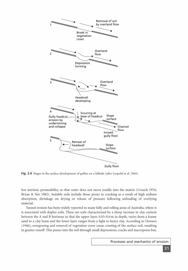
low intrinsic permeability, so that water does not move readily into the matrix (Crouch 1976;Bryan & Yair 1982). Suitable soils include those prone to cracking as a result of high sodiumabsorption, shrinkage on drying or release of pressure following unloading of overlying material.
Tunnel erosion has been widely reported in many hilly and rolling areas of Australia, where itis associated with duplex soils. These are soils characterized by a sharp increase in clay contentbetween the A and B horizons so that the upper layer, 0.03–0.6 m in depth, varies from a loamysand to a clay loam and the lower layer ranges from a light to heavy clay. According to Downes(1946), overgrazing and removal of vegetation cover cause crusting of the surface soil, resultingin greater runoff. This passes into the soil through small depressions, cracks and macropores but,
Processes and mechanics of erosion
31
Removal of soilby overland flow
Break invegetationcover
Overlandflow
Depressionforming
Overlandflow
Headwalldeveloping
Gully headcut,erosion byunderminingand collapse
Scouring atbase of headcut Slope
surface
Channelflow
Incisedgully floor
Retreat ofheadwall Slope
surface
Gully floor
5
4
3
2
1
Fig. 2.4 Stages in the surface development of gullies on a hillside (after Leopold et al. 1964).
MSE02 11/19/04 02:32 PM Page 31
on reaching the top of the B horizon, moves along it as subsurface flow. Localized dispersion ofthe clays in areas of subsurface moisture accumulation is followed by piping. Heavy summer rainscause the water in the pipes to break out on to the surface. Eventually, the roofs of the pipes col-lapse and gullying occurs. In the Loess Plateau of China, tunnel erosion contributes 25–30 percent of the catchment sediment yield (Zhu 2003). Most of this relates to the development of newtunnels rather than enlargement of existing ones and takes place in single storms with returnperiods of 50 years or more. In a storm of 107 mm over 7.5 hours, 67 new tunnels were created;another storm of 37 mm in 115 minutes resulted in the formation of 123 new inlets. Sedimentconcentration in tunnel flow ranges from 8.2 to 893.2 g l-1, which is very similar to that in channelflow (Zhu et al. 2002). Once formed, the tunnels continue to erode both during and betweenstorms through earth falls, slumps, water erosion and roof collapse; in some cases, slumps andearth falls lead to their temporary blockage.
A third way in which gullies are initiated is where linear landslides leave deep, steep-sided scars,which may be occupied by running water in subsequent storms. This type of gully developmenthas been described in Italy by Vittorini (1972) and in central Värmland, Sweden, by Fredén andFuruholm (1978). In the latter case, a 3–20 m deep, 20–40 m wide and 100 m long gully formedin glaciofluvial deposits following the 1977 spring snowmelt, which caused the removal, as a massflow, of 20,000 m3 of saturated silt and sand in less than three days.
2.6.2 Threshold conditions
The main cause of gully formation is too much water, a condition that may be brought about byeither climatic change or alterations in land use. In the first case, increased runoff may occur ifrainfall increases or if less rainfall produces a reduction in the vegetation cover. In the secondcase, deforestation, burning of the vegetation and overgrazing can all result in greater runoff. Ifthe velocity or tractive force of the runoff exceeds a critical or threshold value, gullying will occur.The threshold values, however, can show a very wide range. For example, tc varies from 3.3 to32.2 Pa on cultivated silt-loam soils in Belgium and from 16.8 to 74.4 Pa on cultivated stony sandyloams in the Alentejo area of Portugal (Nachtergaele 2001).
Where the exceedance of the threshold relates to changes in climate or land use, the thresh-old is described as extrinsic (Schumm 1979) because the changes are external to the processesoperating within the gully. Attempts to relate gullying solely to changes in external factors havenot proved entirely successful, however, because not all gullies in an area appear to respond inthe same way. In order to explain the onset of instability in one gully while its neighbours remainstable, Schumm (1979) examined the role of intrinsic thresholds, which are related to the inter-nal working of the gully. From a review of studies in Wyoming, Colorado, New Mexico andArizona, a discriminant function was established between stable and unstable conditions in termsof the size of the catchment area (a), which controls discharge, and the channel slope (s), whichcontrols the velocity of runoff. When, for a given catchment area, channel slope exceeds a criti-cal value, incision occurs, creating a channel characterized by one or more head scarps. Subse-quent scouring causes the gully to become very active: the channel widens, deepens and extendsheadwards. Over time, the channel slope is reduced, promoting a consolidation phase as the gullystabilizes, the channel fills in, the sides and head wall become flatter and vegetation regrows. Depo-sition steepens the slope again and triggers a new phase of gullying. Thus gullies pass throughsuccessive cycles of erosion and deposition. It is not uncommon for the head of a gully to beextremely active while the lower section of the gully is stabilizing or for gullies to contain asequence of alternating stable and unstable sections.
Chapter 2
32
MSE02 11/19/04 02:32 PM Page 32
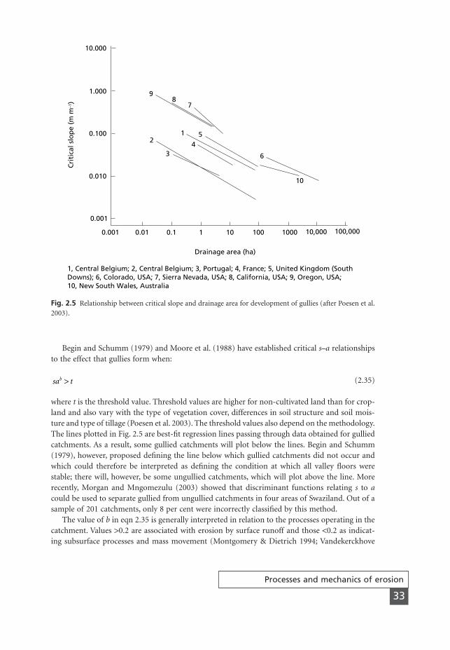
Begin and Schumm (1979) and Moore et al. (1988) have established critical s–a relationshipsto the effect that gullies form when:
(2.35)
where t is the threshold value. Threshold values are higher for non-cultivated land than for crop-land and also vary with the type of vegetation cover, differences in soil structure and soil mois-ture and type of tillage (Poesen et al. 2003). The threshold values also depend on the methodology.The lines plotted in Fig. 2.5 are best-fit regression lines passing through data obtained for gulliedcatchments. As a result, some gullied catchments will plot below the lines. Begin and Schumm(1979), however, proposed defining the line below which gullied catchments did not occur andwhich could therefore be interpreted as defining the condition at which all valley floors werestable; there will, however, be some ungullied catchments, which will plot above the line. Morerecently, Morgan and Mngomezulu (2003) showed that discriminant functions relating s to acould be used to separate gullied from ungullied catchments in four areas of Swaziland. Out of asample of 201 catchments, only 8 per cent were incorrectly classified by this method.
The value of b in eqn 2.35 is generally interpreted in relation to the processes operating in thecatchment. Values >0.2 are associated with erosion by surface runoff and those <0.2 as indicat-ing subsurface processes and mass movement (Montgomery & Dietrich 1994; Vandekerckhove
sa tb >
Processes and mechanics of erosion
33
10.000
1.000
0.100
0.010
0.001
0.001 0.01 0.1 100 1000 10,000 100,0001 10
Cri
tica
l slo
pe
(m m
–1)
Drainage area (ha)
78
9
6
10
51
42
3
1, Central Belgium; 2, Central Belgium; 3, Portugal; 4, France; 5, United Kingdom (SouthDowns); 6, Colorado, USA; 7, Sierra Nevada, USA; 8, California, USA; 9, Oregon, USA;10, New South Wales, Australia
Fig. 2.5 Relationship between critical slope and drainage area for development of gullies (after Poesen et al.2003).
MSE02 11/19/04 02:32 PM Page 33
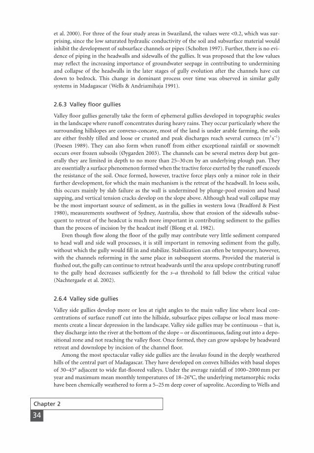
et al. 2000). For three of the four study areas in Swaziland, the values were <0.2, which was sur-prising, since the low saturated hydraulic conductivity of the soil and subsurface material wouldinhibit the development of subsurface channels or pipes (Scholten 1997). Further, there is no evi-dence of piping in the headwalls and sidewalls of the gullies. It was proposed that the low valuesmay reflect the increasing importance of groundwater seepage in contributing to underminingand collapse of the headwalls in the later stages of gully evolution after the channels have cutdown to bedrock. This change in dominant process over time was observed in similar gullysystems in Madagascar (Wells & Andriamihaja 1991).
2.6.3 Valley floor gullies
Valley floor gullies generally take the form of ephemeral gullies developed in topographic swalesin the landscape where runoff concentrates during heavy rains. They occur particularly where thesurrounding hillslopes are convexo-concave, most of the land is under arable farming, the soilsare either freshly tilled and loose or crusted and peak discharges reach several cumecs (m3 s-1)(Poesen 1989). They can also form when runoff from either exceptional rainfall or snowmeltoccurs over frozen subsoils (Øygarden 2003). The channels can be several metres deep but gen-erally they are limited in depth to no more than 25–30 cm by an underlying plough pan. Theyare essentially a surface phenomenon formed when the tractive force exerted by the runoff exceedsthe resistance of the soil. Once formed, however, tractive force plays only a minor role in theirfurther development, for which the main mechanism is the retreat of the headwall. In loess soils,this occurs mainly by slab failure as the wall is undermined by plunge-pool erosion and basalsapping, and vertical tension cracks develop on the slope above. Although head wall collapse maybe the most important source of sediment, as in the gullies in western Iowa (Bradford & Piest1980), measurements southwest of Sydney, Australia, show that erosion of the sidewalls subse-quent to retreat of the headcut is much more important in contributing sediment to the gulliesthan the process of incision by the headcut itself (Blong et al. 1982).
Even though flow along the floor of the gully may contribute very little sediment comparedto head wall and side wall processes, it is still important in removing sediment from the gully,without which the gully would fill in and stabilize. Stabilization can often be temporary, however,with the channels reforming in the same place in subsequent storms. Provided the material isflushed out, the gully can continue to retreat headwards until the area upslope contributing runoffto the gully head decreases sufficiently for the s–a threshold to fall below the critical value(Nachtergaele et al. 2002).
2.6.4 Valley side gullies
Valley side gullies develop more or less at right angles to the main valley line where local con-centrations of surface runoff cut into the hillside, subsurface pipes collapse or local mass move-ments create a linear depression in the landscape. Valley side gullies may be continuous – that is,they discharge into the river at the bottom of the slope – or discontinuous, fading out into a depo-sitional zone and not reaching the valley floor. Once formed, they can grow upslope by headwardretreat and downslope by incision of the channel floor.
Among the most spectacular valley side gullies are the lavakas found in the deeply weatheredhills of the central part of Madagascar. They have developed on convex hillsides with basal slopesof 30–45° adjacent to wide flat-floored valleys. Under the average rainfall of 1000–2000 mm peryear and maximum mean monthly temperatures of 18–26°C, the underlying metamorphic rockshave been chemically weathered to form a 5–25 m deep cover of saprolite. According to Wells and
Chapter 2
34
MSE02 11/19/04 02:32 PM Page 34
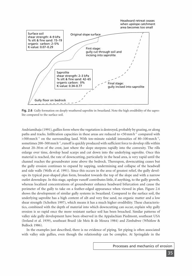
Andriamihaja (1991), gullies form where the vegetation is destroyed, probably by grazing, or alongpaths and tracks. Infiltration capacities in these areas are reduced to <50 mm h-1 compared with>300 mm h-1 on the surrounding land. With ten-minute rainfall intensities of 80–100 mm h-1,sometimes 200–500 mm h-1, runoff is quickly produced with sufficient force to develop rills withinabout 20–30 m of the crest, just where the slope steepens rapidly into the convexity. The rillsenlarge over time, develop head scarps and cut down into the underlying saprolite. Once thismaterial is reached, the rate of downcutting, particularly in the head area, is very rapid until thechannel reaches the groundwater zone above the bedrock. Thereupon, downcutting ceases butthe gully erosion continues to expand by sapping, undermining and collapse of the headwall and side walls (Wells et al. 1991). Since this occurs in the area of greatest relief, the gully devel-ops its typical pear-shaped plan form, broadest towards the top of the slope and with a narrowoutlet downslope. In this stage, upslope runoff contributes little, if anything, to the gully growth,whereas localized concentrations of groundwater enhance headward bifurcation and cause theperimeter of the gully to take on a feather-edged appearance when viewed in plan. Figure 2.6shows the development of similar gully systems in Swaziland. Compared to the surface soil, theunderlying saprolite has a high content of silt and very fine sand, no organic matter and a lowshear strength (Scholten 1997), which means it has a much higher erodibility. These characteris-tics, combined with the depth of material into which downcutting can occur, explain why gullyerosion is so rapid once the more resistant surface soil has been breached. Similar patterns ofvalley side gully development have been observed in the Appalachian Piedmont, southeast USA(Ireland et al. 1939), southeast Brazil (de Meis & de Moura 1984) and Zimbabwe (Whitlow &Bullock 1986).
In the examples just described, there is no evidence of piping. Yet piping is often associatedwith valley side gullies, even though the relationship can be complex. At Springdale in the
Processes and mechanics of erosion
35
Original slope surface
First stage:gully cut through soil andincising into saprolite
Final stage:gully incised into saprolite
Gully floor on bedrock
Headward retreat ceaseswhen upslope catchmentarea becomes too small
Saproliteshear strength: 2–3 kPa% silt & fine sand: 42–65organic carbon: 0%K-value: 0.34–0.77
Surface soilshear strength: 4–9 kPa% silt & fine sand: 15–19organic carbon: 2–5%K-value: 0.07–0.29
Fig. 2.6 Gully formation on deeply weathered saprolite in Swaziland. Note the high erodibility of the sapro-lite compared to the surface soil.
MSE02 11/19/04 02:32 PM Page 35
Riverina area of New South Wales, some gullies clearly owe their origin to the collapse of tunnels,as evidenced by the remnants of the soil forming bridges where the collapse has been incomplete,while others appear to have developed from tunnels initiated after the cutting of the main gully.Developed along permeable zones between layers of relatively impermeable material, they dependon the incision of the gully to expose the permeable seams and form the hydraulic gradient alongwhich water can move (Crouch et al. 1986).
Valley side gullies can often evolve into badlands, particularly where a fragile environment hasbeen disturbed by unwise land use (López-Bermúdez & Romero-Diaz 1989). Marl and clay soilsare particularly susceptible to badland development, as are soils with high contents of gypsum,since these are prone to piping. The processes responsible for badlands depend on how the soilresponds to increases in moisture. Where the soil seals quickly, the badlands develop by surfaceerosion through rills and gullies. Where the soil has a high infiltration rate, water collects withinthe soil, resulting in instability and rapid shallow mass movements (Bouma & Imeson 2000;Moretti & Rodolfi 2000). Once formed, badlands take a long time to heal and many of those foundin the Mediterranean, although very spectacular, record rather low rates of erosion today and arerelics of former periods of active gullying. Those of the Guadix Basin in southeast Spain wereprobably developed around 2000 (Wise et al. 1982). In contrast, in areas of active badlanddevelopment annual erosion rates can exceed 260 t ha-1 (Cervera et al. 1990).
2.6.5 Erosion rates
Although gullies can remove vast quantities of soil, gully densities are not usually greater than 10 km km-2 and the surface area covered by gullies is rarely more than 15 per cent of the total area(Zachar 1982). This results in a considerable contrast between the erosion rate for an individualgully and its contribution to the overall soil loss of an area. Rates of headwall extension can bevery rapid for relatively short periods of time. Measurements on the Mbothoma Gully system,Swaziland, showed very rapid retreats of between 2.5 and 6.3 m yr-1 from 1947 to 1961, followedby a slowing down to 0.13–0.51 m yr-1 for the period 1961–1980 (WMS Associates 1988). A newgully opposite Mbothoma developed in the 1960s and up to 1990 eroded headwards at a rate of14 m yr-1; the rate then decreased to 5 m yr-1 between 1990 and 1998 (Sidorchuk et al. 2003).Erosion from a gully developed on arable land near Cromer, Norfolk, England in 1975 was esti-mated at 195 t ha-1 (Evans & Nortcliff 1978) and erosion from a winter runoff event in southernNorway in January 1990 exceeded 100 t ha-1 in many gullies (Øygarden 2003). In gullies nearBathurst, New South Wales, soil loss from the side walls alone amounted to 1100 t ha-1 over athree-year period beginning April 1984 (Crouch 1990a). These figures contrast with annual ratesfor whole catchments for which typical figures include 3–5 t ha-1 for the gullied watersheds at Treynor, Iowa (Bradford & Piest 1980), 3–16 t ha-1 for the lavakas in Madagascar (Wells &Andriamihaja 1991) and 6.4 t ha-1 for a watershed near Gilgranda, New South Wales, of which 60 per cent came from gully heads (Crouch 1990b).
In a review of worldwide data, Poesen et al. (2003) showed that gully erosion can contributebetween 10 and 94 per cent of overall soil loss from an area, with values between 30 and 75 percent being typical. The contribution of gullies to total erosion is therefore not easily predictable.It depends on the characteristics of the storm, the topography of the catchment and the land coverat the time the storm occurs. In the 94-hectare Blosseville catchment, Normandy, France, a rainstorm of 60 mm on 26 December 1999 with a maximum six-minute intensity of 55 mm h-1 causederosion of 10 t ha-1. Some 93 per cent of the catchment had less than 20 per cent vegetation cover.Ephemeral gullies contributed 24 per cent of the erosion. A 60 mm storm with a maximum six-minute intensity of 105 mm h-1 in the same catchment on 9 May 2000 produced a much lower
Chapter 2
36
MSE02 11/19/04 02:32 PM Page 36
erosion of 1 t ha-1 because some 73 per cent of the catchment had a vegetation cover greater than60 per cent. However, 83 per cent of the erosion occurred in ephemeral gullies (Cerdan et al.2002a).
Processes and mechanics of erosion
37
2.7
Mass movements
Although mass movement has been widely studied by geologists, geomorphologists and engineers,it is generally neglected in the context of soil erosion.Yet Temple and Rapp (1972) found that in thewestern Uluguru Mountains, Tanzania, landslides and mudflows are the dominant erosionprocesses. They occur in small numbers about once every ten years. The quantity of sedimentmoved from the hillsides into rivers by mass movement is far in excess of that contributed bygullies, rills and overland flow. Further, less than 1 per cent of the slide scars are in areas ofwoodland, 47 per cent being on the cultivated plots and another 47 per cent on land lying fallow.The association of erosion with woodland clearance for agriculture is thus very clear. Further evidence for this is provided by Rogers and Selby (1980) in respect of shallow debris slides on clayand silty clay soils derived from greywackes in the Hapuakohe Range, south Auckland, NewZealand. Clearance of the forest for pasture causes a decline in the shear strength of the soil over thefive- to ten-year period needed for the tree roots to decay. As a result, landslides under pasture aretriggered by a storm with a return period of 30 years, whereas a storm with a 100-year return periodis required to produce slides beneath the forest. The close relationship between mass movementand water erosion is illustrated by the studies of the ‘bottle slides’ in the Uluguru Mountains(Temple & Rapp 1972; Lundgren & Rapp 1974), which develop in areas of large subsurface pipes asa result of the flushing out of a muddy viscous mass of debris and subsequent ground collapse.
The stability of the soil mass on a hillslope in respect of mass movement can be assessed by asafety factor (F), defined as the ratio between the total shear strength (s) of the soil material alonga given shear surface and the amount of stress (t) developed along that surface. Thus
(2.36)
The slope is stable if F > 1 and failure occurs if F £ 1. For the simple case of shallow or transla-tional slides, F can be defined as:
(2.37)
where c¢ is the effective cohesion of the soil, g is the unit weight of soil above the slide plane, z isthe vertical depth of soil above the slide plane, gw is the unit weight of water, h is the height ofthe groundwater (piezometric) surface above the slide plane, q is the slope angle and f¢ is theeffective angle of internal friction. Applications of the equation to slides in the Hapuakohe Rangeshow that the value of F is particularly sensitive to changes in c¢ and z. Thus, control measuresshould be directed at influencing these (Rogers & Selby 1980).
Mass movements, in the varied forms of creep, slides, rock falls and mudflows, are givendetailed treatment in numerous books (Sharpe 1938; Zaruba & Mencl 1969; Brunsden & Prior1984; Anderson & Richards 1987), together with details of how eqn 2.37 can be modified forapplication to different types of slope failure.
Fc z h
zw=
¢ + -( ) ¢g g q fg q q
cos tan
sin cos
2
F =st
MSE02 11/19/04 02:32 PM Page 37
Chapter 2
38
2.8
Wind erosion
The main factor in wind erosion is the velocity of moving air. Because of the roughness impartedby soil, stones, vegetation and other obstacles, wind speeds are lowest near the ground surface. Aplane of zero wind velocity can be defined at some height (z0) above the mean aerodynamicsurface. Above z0, windspeed increases exponentially with height so that velocity values plot as astraight line on a graph against the logarithmic values of the height (Fig. 2.7). The change invelocity with height is expressed by the relationship (Bagnold 1941):
(2.38)
where is the mean velocity at height z, k is the von Kármán universal constant for turbulentflow, assumed to equal 0.4 for clear fluids, and u* is the drag or shear velocity.
Although the movement of soil particles can be related to a critical wind velocity, manyworkers have attempted to define the conditions more precisely in terms of a critical value of thedimensionless shear stress. Using eqn 2.15 and substituting ra (the density of air) for rw (thedensity of water), the critical value of Q, the Shields parameter, for initiating soil particle move-ment approximates 0.01 (Bagnold 1941), which is much lower than that obtained for water. Thedifference may be due to the very great difference in the density of the fluids relative to the par-ticle density. A sand grain in air is about 2000 times more massive than the surrounding fluid,whereas it is only about 2.6 times more massive than water (Bagnold 1979). As a result, muchhigher shear velocities are required to move particles by air and the initial particle motion is moreviolent. This violence is rapidly transmitted to neighbouring particles, causing a general chainreaction of motion. At this point, grains are dislodged and entrained in the flow relatively easilyand therefore at relatively low Shields numbers (Iversen 1985).
Although the Shields coefficient has been successfully applied to particle movement in air(Bagnold 1951; Iversen 1985), for most soil conservation work it is sufficient to relate the detach-ment of soil particles by wind to a critical value of the shear velocity, using it as a surrogatemeasure of the drag force exerted by the flow. Shear velocity is directly proportional to the rateof increase in wind velocity with the logarithm of height and is therefore the slope of the line inFig 2.7(d). Its value can be determined by measuring the wind speed at two heights but, in prac-tice, by assuming v = 0 at height z0, it can be obtained by measuring the speed at one height andapplying the formula derived from eqn 2.37:
(2.39)
For use in estimates of sediment transport by wind, the velocities should be measured within 0.2 m of the ground surface (Rasmussen et al. 1985; Mulligan 1988).
Bagnold (1937) identifies two threshold velocities required to initiate grain movement.The static or fluid threshold applies to the direct action of the wind. The dynamic or impactthreshold allows for the bombardment of the soil by grains already in motion. Impact thresholdsare about 80 per cent of the fluid threshold velocities in value. In addition to detaching soil particles at a lower threshold velocity, the detachment potential of sediment-laden air is furtherenhanced by increases of 8–18 per cent in shear velocity close to the ground surface (Sørensen
uk v
z zz
* . log= ◊ ( )2 3 0
v
vk
uz
zz = Ê
ˈ¯
2 3
0
.*log
MSE02 11/19/04 02:32 PM Page 38
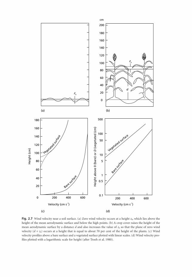
cm
200
180
160
140
120
100
80
60
40
20
0
z0
z0
(a) (b)
(c) (d)
d
180
160
140
120
100
80
60
40
20
0 200 400 600
Hei
gh
t (c
m)
Vegeta
ted
surf
ace
Bare su
rface
Vegetate
d surfa
ce
Bare
surf
ace
500
100
200 400 600
50
5
0.5
0.1
1
10
Velocity (cm s–1) Velocity (cm s–1)
Hei
gh
t ab
ove
0 (
bar
e) o
r D
(ve
get
ated
(cm
)
Fig. 2.7 Wind velocity near a soil surface. (a) Zero wind velocity occurs at a height z0, which lies above theheight of the mean aerodynamic surface and below the high points. (b) A crop cover raises the height of themean aerodynamic surface by a distance d and also increases the value of z0 so that the plane of zero windvelocity (d + z0) occurs at a height that is equal to about 70 per cent of the height of the plants. (c) Windvelocity profiles above a bare surface and a vegetated surface plotted with linear scales. (d) Wind velocity pro-files plotted with a logarithmic scale for height (after Troeh et al. 1980).
MSE02 11/19/04 02:32 PM Page 39
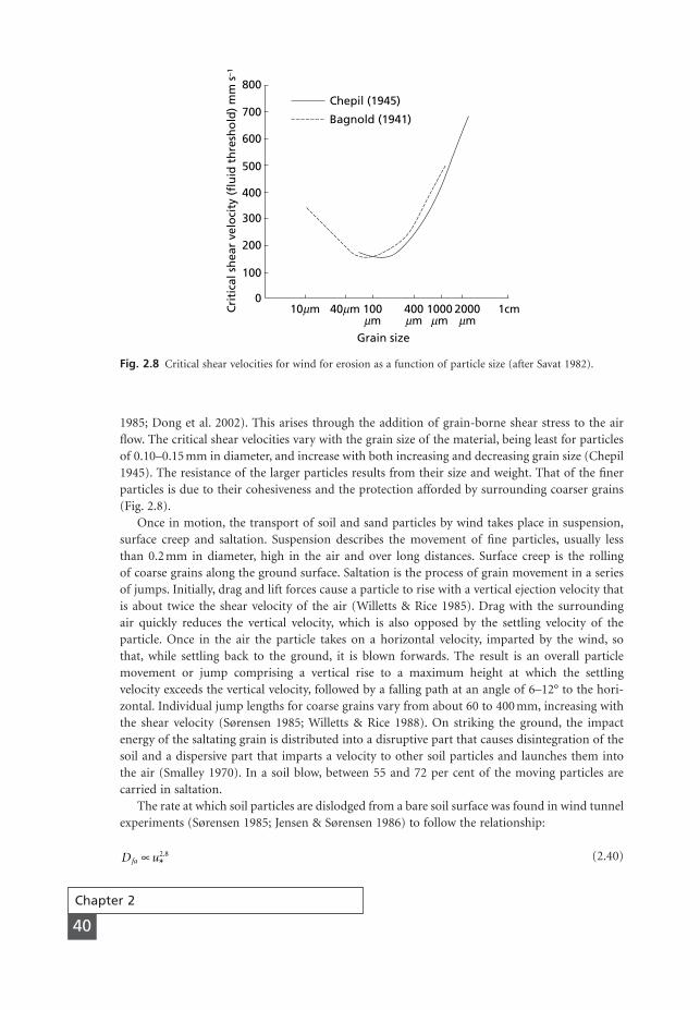
1985; Dong et al. 2002). This arises through the addition of grain-borne shear stress to the airflow. The critical shear velocities vary with the grain size of the material, being least for particlesof 0.10–0.15 mm in diameter, and increase with both increasing and decreasing grain size (Chepil1945). The resistance of the larger particles results from their size and weight. That of the finerparticles is due to their cohesiveness and the protection afforded by surrounding coarser grains(Fig. 2.8).
Once in motion, the transport of soil and sand particles by wind takes place in suspension,surface creep and saltation. Suspension describes the movement of fine particles, usually less than 0.2 mm in diameter, high in the air and over long distances. Surface creep is the rolling of coarse grains along the ground surface. Saltation is the process of grain movement in a seriesof jumps. Initially, drag and lift forces cause a particle to rise with a vertical ejection velocity thatis about twice the shear velocity of the air (Willetts & Rice 1985). Drag with the surrounding air quickly reduces the vertical velocity, which is also opposed by the settling velocity of the particle. Once in the air the particle takes on a horizontal velocity, imparted by the wind, so that, while settling back to the ground, it is blown forwards. The result is an overall particle movement or jump comprising a vertical rise to a maximum height at which the settling velocity exceeds the vertical velocity, followed by a falling path at an angle of 6–12° to the hori-zontal. Individual jump lengths for coarse grains vary from about 60 to 400 mm, increasing withthe shear velocity (Sørensen 1985; Willetts & Rice 1988). On striking the ground, the impactenergy of the saltating grain is distributed into a disruptive part that causes disintegration of thesoil and a dispersive part that imparts a velocity to other soil particles and launches them intothe air (Smalley 1970). In a soil blow, between 55 and 72 per cent of the moving particles arecarried in saltation.
The rate at which soil particles are dislodged from a bare soil surface was found in wind tunnelexperiments (Sørensen 1985; Jensen & Sørensen 1986) to follow the relationship:
(2.40)D ufa µ *.2 8
Chapter 2
40
Chepil (1945)
Bagnold (1941)
800
700
600
500
400
300
200
100
10mm 100mm
400mm
1000mm
2000mm
40mm 1cm0
Cri
tica
l sh
ear
velo
city
(fl
uid
th
resh
old
) m
m s
–1
Grain size
Fig. 2.8 Critical shear velocities for wind for erosion as a function of particle size (after Savat 1982).
MSE02 11/19/04 02:32 PM Page 40
where Dfa is the rate of detachment of soil particles in moving air. Although Willetts and Rice(1988) produce comparable data from their experiments, they caution that the overall data baseis too small to determine the value of the exponent in eqn 2.39. It probably lies, however, between2.0 and 3.0.
In contrast, general agreement exists among researchers that the transport capacity of movingair varies with the cube of the shear velocity. Based on this relationship and considering the trans-port of grains as representing a transfer of momentum from the air to the moving particles,Bagnold (1941) developed the following equation for determining the maximum sediment dis-charge per unit width (Tfa):
(2.41)
where C is an experimentally derived parameter relating to grain size, d is the average diameterof the material, D is a standard grain diameter of 0.25 mm, ra is the density of the air and g is thegravitational constant. Among the more commonly used expressions of eqn 2.40 is that proposedby Lettau and Lettau (1978):
(2.42)
where Tfa is in g m-1 s-1, C is a constant related to grain size and typically is about 6.5 in value,ut is the impact threshold velocity for particle movement (m s-1) and uz is the wind velocity atheight z.
It should be stressed that, at best, eqns 2.41 and 2.42 provide estimates of the maximum sed-iment transport rate (transport capacity) that can occur. They will not necessarily predict theactual rate of sediment transport. Where the soil surface is very resistant, the surface has becomearmoured by rock fragments or a vegetation cover is present, the equations will overpredict. Underthese conditions, sediment transport will vary with the shear velocity of the wind raised to a powerof less than 2.0. Further, sediment transport is a highly dynamic process reflecting the consider-able short-term fluctuations in wind velocity (Sterk et al. 1998). Periods of sediment transportalternate with periods of no transport, even over a duration as short as ten minutes. During indi-vidual wind storms, activity may occur for only 16–21 per cent of the time. The fluctuations insediment transport most probably relate to short-term changes in the turbulent structure of thestorm.
Wind erosion impoverishes the soil and also buries the soil and crops on surrounding land.Although, as already seen, the most erodible particles are 0.10–0.15 mm in size, particles between0.05 and 0.5 mm are generally selectively removed by the wind. Chepil (1946) found that areas ofwind-blown deposits are enriched by particles in the 0.30 and 0.42 mm range. Resistance to winderosion increases rapidly when primary particles and aggregates larger than 1 mm predominate.If erosion results in armouring of the surface so that more than 60 per cent of the surface mate-rial is of this size, the soil is almost totally resistant to wind erosion. Although saltation is the mostimportant process from the viewpoint of soil erosion, wind erosion through the movement ofdust particles in suspension can give rise to additional effects of contamination of food and water,aggravation of respiratory diseases, health risks associated with the transport of pathogens andinterference with switches in machinery. Wind erosion also creates problems of visibility for road,rail and air transport.
T C g u u ufa a t z= ( ) -( )r *3 1
T C d D g ufa a= ( ) ( )1 2 3r *
Processes and mechanics of erosion
41
MSE02 11/19/04 02:32 PM Page 41
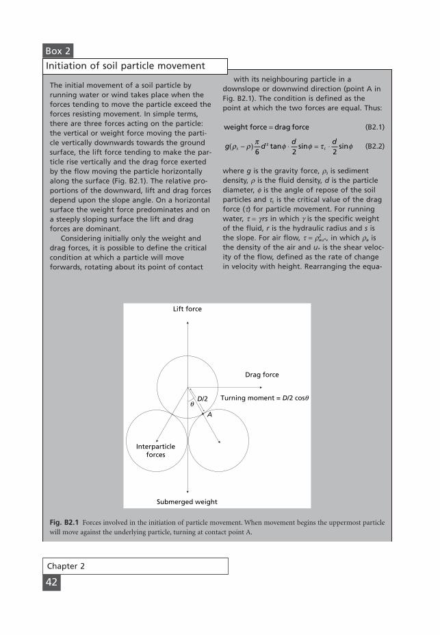
Chapter 2
42
The initial movement of a soil particle byrunning water or wind takes place when theforces tending to move the particle exceed theforces resisting movement. In simple terms,there are three forces acting on the particle:the vertical or weight force moving the parti-cle vertically downwards towards the groundsurface, the lift force tending to make the par-ticle rise vertically and the drag force exertedby the flow moving the particle horizontallyalong the surface (Fig. B2.1). The relative pro-portions of the downward, lift and drag forcesdepend upon the slope angle. On a horizontalsurface the weight force predominates and ona steeply sloping surface the lift and dragforces are dominant.
Considering initially only the weight anddrag forces, it is possible to define the criticalcondition at which a particle will moveforwards, rotating about its point of contact
Box 2
with its neighbouring particle in adownslope or downwind direction (point A inFig. B2.1). The condition is defined as thepoint at which the two forces are equal. Thus:
(B2.1)
(B2.2)
where g is the gravity force, rs is sedimentdensity, r is the fluid density, d is the particlediameter, f is the angle of repose of the soilparticles and tc is the critical value of the dragforce (t) for particle movement. For runningwater, t = grs in which g is the specific weightof the fluid, r is the hydraulic radius and s isthe slope. For air flow, t = r2
au*, in which ra isthe density of the air and u* is the shear veloc-ity of the flow, defined as the rate of changein velocity with height. Rearranging the equa-
g dd d
s cr r p f f t f-( ) ◊ = ◊6 2 2
3 tan sin sin
weight force drag force=
Initiation of soil particle movement
Lift force
Drag force
Submerged weight
D/2q
Interparticleforces
Turning moment = D/2 cosq
A
Fig. B2.1 Forces involved in the initiation of particle movement. When movement begins the uppermost particlewill move against the underlying particle, turning at contact point A.
MSE02 11/19/04 02:32 PM Page 42
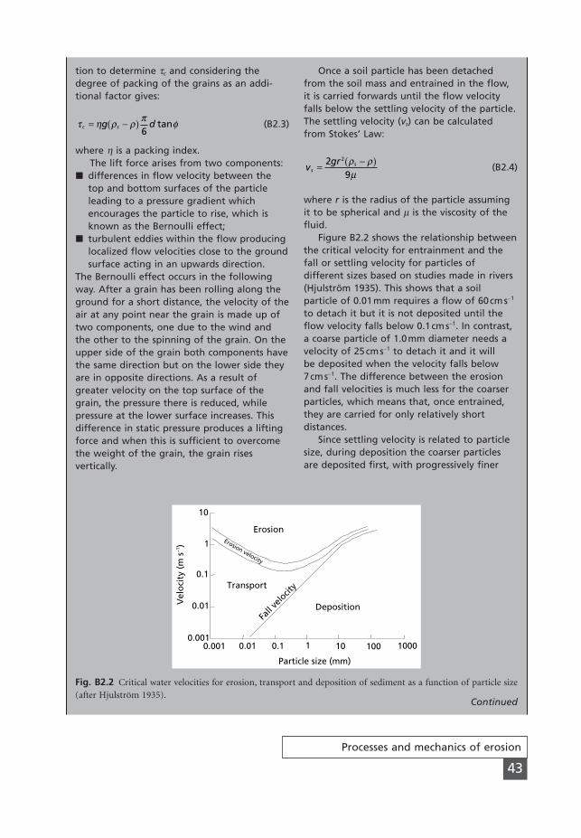
Processes and mechanics of erosion
43
tion to determine tc and considering thedegree of packing of the grains as an addi-tional factor gives:
(B2.3)
where h is a packing index.The lift force arises from two components:
� differences in flow velocity between thetop and bottom surfaces of the particleleading to a pressure gradient whichencourages the particle to rise, which isknown as the Bernoulli effect;
� turbulent eddies within the flow producinglocalized flow velocities close to the groundsurface acting in an upwards direction.
The Bernoulli effect occurs in the followingway. After a grain has been rolling along theground for a short distance, the velocity of theair at any point near the grain is made up oftwo components, one due to the wind andthe other to the spinning of the grain. On theupper side of the grain both components havethe same direction but on the lower side theyare in opposite directions. As a result ofgreater velocity on the top surface of thegrain, the pressure there is reduced, whilepressure at the lower surface increases. Thisdifference in static pressure produces a liftingforce and when this is sufficient to overcomethe weight of the grain, the grain rises vertically.
t h r r p fc sg d= -( )6
tan
Once a soil particle has been detachedfrom the soil mass and entrained in the flow,it is carried forwards until the flow velocityfalls below the settling velocity of the particle.The settling velocity (vs) can be calculatedfrom Stokes’ Law:
(B2.4)
where r is the radius of the particle assumingit to be spherical and m is the viscosity of thefluid.
Figure B2.2 shows the relationship betweenthe critical velocity for entrainment and thefall or settling velocity for particles ofdifferent sizes based on studies made in rivers(Hjulström 1935). This shows that a soilparticle of 0.01mm requires a flow of 60cms-1
to detach it but it is not deposited until theflow velocity falls below 0.1cms-1. In contrast,a coarse particle of 1.0mm diameter needs avelocity of 25cms-1 to detach it and it will be deposited when the velocity falls below 7cms-1. The difference between the erosionand fall velocities is much less for the coarserparticles, which means that, once entrained,they are carried for only relatively shortdistances.
Since settling velocity is related to particlesize, during deposition the coarser particlesare deposited first, with progressively finer
vgr
ss= -( )2
9
2 r rm
10
0.1
0.01
1
0.0010.001 0.01 0.1 1 10 100 1000
Vel
oci
ty (
m s
–1)
Particle size (mm)
Erosion
Transport
Deposition
Erosion velocity
Fall v
elocit
y
Fig. B2.2 Critical water velocities for erosion, transport and deposition of sediment as a function of particle size(after Hjulström 1935).
Continued
MSE02 11/19/04 02:32 PM Page 43

Chapter 2
44
grains dropping out of the flow as the flowvelocity continues to decline. As a result,deposits from slope wash on concave slopes atthe foot of hillsides tend to comprise mainlysands, grading into silts and clays withincreasing slope length and decreasing slopeangle. On many slopes, silts and clays can betransported across the footslope and into theadjacent river. However, these relationships
can sometimes be offset by the redetachmentof the deposits and the trapping of fineparticles in the wake of coarser ones, with theresult that the transport of coarse materialover fines is enhanced (Beuselinck et al. 2002).Deposits of wind-blown material comprisemainly silts and sands, moved in saltation,whereas the clay particles are carried longdistances in suspension in the atmosphere.
MSE02 11/19/04 02:32 PM Page 44
The factors controlling soil erosion are the erosivity of the eroding agent, the erodibility of thesoil, the slope of the land and the nature of the plant cover.
Factors influencing erosion
45
CHAPTER 3
Factorsinfluencingerosion
3.1
Erosivity
3.1.1 Rainfall
Soil loss is closely related to rainfall partly through the detaching power of raindrops striking thesoil surface and partly through the contribution of rain to runoff. This applies particularly toerosion by overland flow and rills, for which intensity is generally considered to be the mostimportant rainfall characteristic. The effect of rainfall intensity is illustrated by the data for 183rain events at Zanesville, Ohio, between 1934 and 1942, which show that average soil loss per rainevent increases with the intensity of the storm (Table 3.1; Fournier 1972).
The role of intensity is not always so obvious, however, as indicated by studies of erosion inmid-Bedfordshire, England, taking data for the ten most erosive storms between May 1973 andOctober 1975. While intense storms, such as the one of 34.9 mm on 6 July 1973, in which 17.7 mm fell at intensities greater than 10 mm h-1, produce erosion, so do storms of long dura-tion and low intensity, like the one of 19 June 1973 when 39.6 mm of rain fell in over 23 hours(Morgan et al. 1986). It appears that erosion is related to two types of rain event, the short-livedintense storm where the infiltration capacity of the soil is exceeded, and the prolonged storm oflow intensity that saturates the soil.
The response of the soil to rainfall may also be determined by previous meteorological con-ditions. This can again be demonstrated by data for Zanesville, Ohio (Fournier 1972). A stormof 19.3 mm on 9 June 1940 fell on dry ground and, despite the quantity, only 25 per cent wentinto runoff, most of the water soaking into the soil. On the following day, in a storm of 13.7 mm,66 per cent of the rain ran off and soil loss almost trebled. The control in this case is the close-ness of the soil to saturation, which is dependent on how much rain has fallen in the previousfew days. The pattern of low soil loss in the first and high loss in the second of a series of stormsis reversed, however, when, between erosive storms, weathering and light rainfall loosen the soilsurface. Most of the loose material is removed during the first runoff event, leaving little for erosion in subsequent storms. This sequence is illustrated by studies in the Alkali Creek
MSE03 11/19/04 02:33 PM Page 45
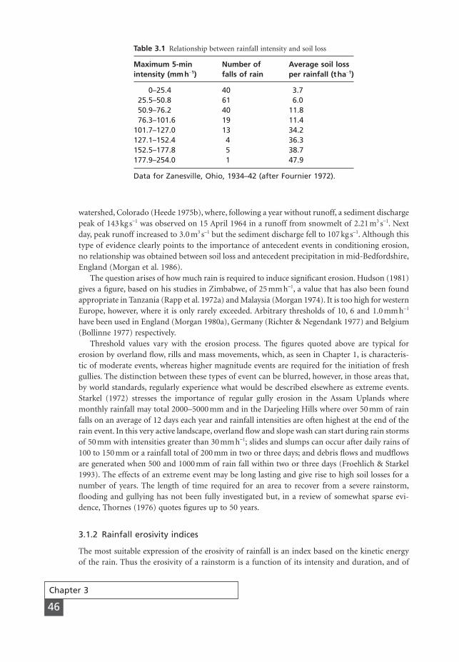
watershed, Colorado (Heede 1975b), where, following a year without runoff, a sediment dischargepeak of 143 kg s-1 was observed on 15 April 1964 in a runoff from snowmelt of 2.21 m3 s-1. Nextday, peak runoff increased to 3.0 m3 s-1 but the sediment discharge fell to 107 kg s-1. Although thistype of evidence clearly points to the importance of antecedent events in conditioning erosion,no relationship was obtained between soil loss and antecedent precipitation in mid-Bedfordshire,England (Morgan et al. 1986).
The question arises of how much rain is required to induce significant erosion. Hudson (1981)gives a figure, based on his studies in Zimbabwe, of 25 mm h-1, a value that has also been foundappropriate in Tanzania (Rapp et al. 1972a) and Malaysia (Morgan 1974). It is too high for westernEurope, however, where it is only rarely exceeded. Arbitrary thresholds of 10, 6 and 1.0 mm h-1
have been used in England (Morgan 1980a), Germany (Richter & Negendank 1977) and Belgium(Bollinne 1977) respectively.
Threshold values vary with the erosion process. The figures quoted above are typical forerosion by overland flow, rills and mass movements, which, as seen in Chapter 1, is characteris-tic of moderate events, whereas higher magnitude events are required for the initiation of freshgullies. The distinction between these types of event can be blurred, however, in those areas that,by world standards, regularly experience what would be described elsewhere as extreme events.Starkel (1972) stresses the importance of regular gully erosion in the Assam Uplands wheremonthly rainfall may total 2000–5000 mm and in the Darjeeling Hills where over 50 mm of rainfalls on an average of 12 days each year and rainfall intensities are often highest at the end of therain event. In this very active landscape, overland flow and slope wash can start during rain stormsof 50 mm with intensities greater than 30 mm h-1; slides and slumps can occur after daily rains of100 to 150 mm or a rainfall total of 200 mm in two or three days; and debris flows and mudflowsare generated when 500 and 1000 mm of rain fall within two or three days (Froehlich & Starkel1993). The effects of an extreme event may be long lasting and give rise to high soil losses for anumber of years. The length of time required for an area to recover from a severe rainstorm,flooding and gullying has not been fully investigated but, in a review of somewhat sparse evi-dence, Thornes (1976) quotes figures up to 50 years.
3.1.2 Rainfall erosivity indices
The most suitable expression of the erosivity of rainfall is an index based on the kinetic energyof the rain. Thus the erosivity of a rainstorm is a function of its intensity and duration, and of
Chapter 3
46
Table 3.1 Relationship between rainfall intensity and soil loss
Maximum 5-min Number of Average soil lossintensity (mmh-1) falls of rain per rainfall (tha-1)
0–25.4 40 3.725.5–50.8 61 6.050.9–76.2 40 11.876.3–101.6 19 11.4
101.7–127.0 13 34.2127.1–152.4 4 36.3152.5–177.8 5 38.7177.9–254.0 1 47.9
Data for Zanesville, Ohio, 1934–42 (after Fournier 1972).
MSE03 11/19/04 02:33 PM Page 46
the mass, diameter and velocity of the raindrops. To compute erosivity requires an analysis ofthe drop-size distributions of rain. Laws and Parsons (1943), based on studies of rain in theeastern USA, show that the drop-size characteristics vary with the intensity of the rain, with themedian drop diameter by volume (d50) increasing with rainfall intensity. Studies of tropical rainfall (Hudson 1963) indicate that this relationship holds only for rainfall intensities up to 100 mm h-1. At higher intensities, median drop size decreases with increasing intensity, presum-ably because greater turbulence makes larger drop sizes unstable. However, at intensities above200 mm h-1, coalescence of smaller drops takes place so that the median drop diameter begins toincrease again (Carter et al. 1974). Considerable variability exists because the relationship betweenmedian drop size and intensity is not constant; both median drop size and drop-size distributionvary for rains of the same intensity but different origins (Mason & Andrews 1960; Carter et al.1974; Kinnell 1981; McIsaac 1990). The drop-size characteristics of convectional and frontal raindiffer, as do those of rain formed at the warm and cold fronts of a temperate depression system.
Despite the difficulties posed by these variations, it is possible to derive general relationshipsbetween kinetic energy and rainfall intensity. Based on the work of Laws and Parsons (1943),Wischmeier and Smith (1958) obtained the equation:
(3.1)
where I is the rainfall intensity (mm h-1) and KE is the kinetic energy (MJ ha-1 mm-1). Manyresearchers (Mason & Ramandham 1953; Carte 1971; Houze et al. 1979; Styczen & Høgh-Schmidt1988) consider the drop-size distribution of rainfall described by Marshall and Palmer (1948) asrepresentative of a wide range of environments. The equivalent formula for calculating kineticenergy is:
(3.2)
For tropical rainfall, Hudson (1965) gives the equation:
(3.3)
based on measurements of rainfall properties in Zimbabwe.Given the variability of rainfall characteristics across the globe, it is not surprising that a large
number of relationships have been established by different workers in different countries (Table3.2). Many of these studies show that at intensities greater than 75 mm h-1, the kinetic energy levelsoff at a value of about 0.29 MJ ha-1 mm-1 (Kinnell 1987). However, much higher values of0.34–0.38 have been obtained in northern Nigeria (Kowal & Kassam 1976; Osuji 1989), Tuscany,Italy (Zanchi & Torri 1980), Okinawa, Japan (Onaga et al. 1988), Cévennes, France (Sempere-Torres et al. 1992), Portugal (Coutinho & Tomás 1995), Hong Kong (Jayawardena & Rezaur 2000)and Spain (Cerro et al. 1998). Carter et al. (1974) found that in the southern USA the kineticenergy increased to a maximum value at about 75 mm h-1, decreased with further increases inintensity up to about 175 mm h-1 and then increased again at still higher intensities. In contrast,other studies in Japan (Mihara 1951) and in the Marshall Islands (McIsaac 1990) have recordedrainfall energies some 6–20 per cent lower than those calculated from eqn 3.1. Rainfall energyalso varies with the density of the air raised to the 0.9 power; as a result, energy increases withaltitude. Tracy et al. (1984) found that the kinetic energy of rainfall at 900–1800 m above sea levelin Arizona was about 15 per cent higher than that predicted by eqn 3.1. Based on a review of pre-vious research, van Dijk et al. (2002) proposed the following as a general equation:
KEI
= -ÊË
ˆ¯0 298 1
4 29.
.
KE I= +0 0895 0 0844 10. . log
KE I= +0 0119 0 0873 10. . log
Factors influencing erosion
47
MSE03 11/19/04 02:33 PM Page 47
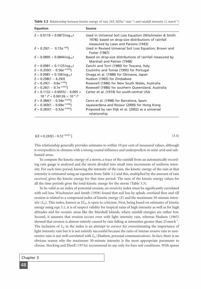
(3.4)
This relationship generally provides estimates to within 10 per cent of measured values, althoughit overpredicts in climates with a strong coastal influence and underpredicts in semi-arid and sub-humid areas.
To compute the kinetic energy of a storm, a trace of the rainfall from an automatically record-ing rain gauge is analysed and the storm divided into small time increments of uniform inten-sity. For each time period, knowing the intensity of the rain, the kinetic energy of the rain at thatintensity is estimated using an equation from Table 3.2 and this, multiplied by the amount of rainreceived, gives the kinetic energy for that time period. The sum of the kinetic energy values forall the time periods gives the total kinetic energy for the storm (Table 3.3).
To be valid as an index of potential erosion, an erosivity index must be significantly correlatedwith soil loss. Wischmeier and Smith (1958) found that soil loss by splash, overland flow and rillerosion is related to a compound index of kinetic energy (E) and the maximum 30-minute inten-sity (I30). This index, known as EI30, is open to criticism. First, being based on estimates of kineticenergy using eqn 3.1, it is of suspect validity for tropical rains of high intensity as well as for highaltitudes and for oceanic areas like the Marshall Islands, where rainfall energies are rather low.Second, it assumes that erosion occurs even with light intensity rain, whereas Hudson (1965)showed that erosion is almost entirely caused by rain falling at intensities greater than 25 mm h-1.The inclusion of I30 in the index is an attempt to correct for overestimating the importance oflight intensity rain but it is not entirely successful because the ratio of intense erosive rain to non-erosive rain is not well correlated with I30 (Hudson, personal communication). In fact, there is noobvious reason why the maximum 30-minute intensity is the most appropriate parameter tochoose. Stocking and Elwell (1973a) recommend its use only for bare soil conditions. With sparse
KE I= -( )-0 283 1 0 52 0 042. . .
Chapter 3
48
Table 3.2 Relationship between kinetic energy of rain (KE, MJ ha-1 mm-1) and rainfall intensity (I, mm h-1)
Equation Source
E = 0.0119 + 0.0873 log10 I Used in Universal Soil Loss Equation (Wischmeier & Smith 1978); based on drop-size distributions of rainfall measured by Laws and Parsons (1943)
E = 0.29(1 - 0.72e-I/20) Used in Revised Universal Soil Loss Equation; Brown and Foster (1987)
E = 0.0895 + 0.0844 log10 I Based on drop-size distributions of rainfall measured by Marshall and Palmer (1948)
E = 0.0981 + 0.1125 log10 I Zanchi and Torri (1980) for Toscana, ItalyE = 0.359(1 - 0.56e-0.034I) Coutinho and Tomás (1995) for PortugalE = 0.0981 + 0.106 log10 I Onaga et al. (1988) for Okinawa, JapanE = 0.298(1 - 4.29/I) Hudson (1965) for ZimbabweE = 0.29(1 - 0.6e-0.04I) Rosewell (1986) for New South Wales, AustraliaE = 0.26(1 - 0.7e-0.035I) Rosewell (1986) for southern Queensland, AustraliaE = 0.1132 + 0.0055I - 0.005 ¥ Carter et al. (1974) for south-central USA
10-2 I2 + 0.00126 ¥ 10-4 I3
E = 0.384(1 - 0.54e-0.029I) Cerro et al. (1998) for Barcelona, SpainE = 0.369(1 - 0.69e-0.038I) Jayawardena and Rezaur (2000) for Hong KongE = 0.283(1 - 0.52e-0.042I) Proposed by van Dijk et al. (2002) as a universal
relationship
MSE03 11/19/04 02:33 PM Page 48

and dense plant covers they obtain better correlations with soil loss using the maximum 15- and 5-minute intensities respectively. The maximum 5-minute intensity was also found superior to I30 forshort duration storms in Mediterranean countries (Usón & Ramos 2001). In order to overcome thelikelihood of overestimating soil loss from high-intensity rainfall, the recommended practice withthe EI30 index is to use a maximum value of 0.28 MJ ha-1 mm-1 for the E component for all rainsabove 76.2 mm h-1 and a maximum value of 63.5 mm h-1 for the I30 term (Wischmeier & Smith1978).
As an alternative erosivity index, Hudson (1965) proposed KE > 25, which, to compute for asingle storm, means summing the kinetic energy received in those time increments when the rain-fall intensity equals or exceeds 25 mm h-1 (Table 3.3). When applied to data from Zimbabwe, abetter correlation was obtained between this index and soil loss than between soil loss and EI30.Stocking and Elwell (1973a) reworked Hudson’s data, taking account of more recent data,and suggested that EI30 was the better index after all. But, since they computed EI30 only for storms yielding 12.5 mm or more of rain and with a maximum 5-minute intensity greater than25 mm h-1, they removed most of the objections to the original EI30 index and produced an indexthat is philosophically very close to KE > 25. Hudson’s index has the advantage of simplicity and less stringent data requirements. Although somewhat limiting for temperate latitudes, it canbe modified by using a lower threshold value such as KE > 10.
By calculating erosivity values for individual storms over a period of 20–25 years, meanmonthly and mean annual data can be obtained. Since the EI30 and KE > 25 indices yield vastlydifferent values because of the inclusion of I30 in the former, the two indices cannot be substi-tuted for each other.
Factors influencing erosion
49
Table 3.3 Calculation of erosivity
Time from start Rainfall Intensity Kinetic energy Total kinetic energyof storm (min) (mm) (mmh-1) (MJha-1 mm-1) (col 2 ¥ col 4) (MJha-1)
0–14 1.52 6.08 0.0877 0.133315–29 14.22 56.88 0.2755 3.918030–44 26.16 104.64 0.2858 7.476145–59 31.50 126.00 0.2879 9.067460–74 8.38 33.52 0.2599 2.177675–89 0.25 1.00 0 0
Erosivity indicesWischmeier index (EI30)Maximum 30-minute rainfall = 26.16 + 31.50mm
= 57.66mmMaximum 30-minute intensity = 57.66 ¥ 2
= 115.32mmh-1
Total kinetic energy = total of column 5= 22.7724MJha-1
EI30 = 22.7724 ¥ 115.32= 2262.12MJmmha-1 h-1
Hudson index (KE > 25)Total kinetic energy for rainfall = total of lines 2, 3, 4 and 5 in column 5 intensity ≥25mmh-1
= 22.64MJha-1
MSE03 11/19/04 02:33 PM Page 49

3.1.3 Wind erosivity
The kinetic energy (KEa; J m-2 s-1) of wind can be calculated from:
(3.5)
where u is the wind velocity (m s-1) and ga is the specific weight of air defined in terms of tem-perature (T) in °C and barometric pressure (P) in kPa by the relationship (Zachar 1982):
(3.6)
For T = 15 °C and P = 101.3 kPa, ga = 0.0625 u2 kg m-2, which converts to 227 u2 J m-2 s-1. Energyvalues for wind storms can be obtained by summing the energies for the different velocitiesweighted by their duration.
In practice, kinetic energy is rarely used as an index of wind erosivity and, instead, a simplerindex based on the velocity and duration of the wind (Skidmore & Woodruff 1968) has beendeveloped. The erosivity of wind blowing in vector j is obtained from:
(3.7)
where EWj is the wind erosivity value for vector j, t is the mean velocity of wind in the ith speedfor vector j above a threshold velocity, taken as 19 km h-1, and fij is the duration of the wind forvector j at the ith speed. Expanding this equation for total wind erosivity (EW) over all vectorsyields:
(3.8)
where vectors j = 0 to 15 represent the 16 principal compass directions beginning with j = 0 = Eand working anticlockwise so that j = 1 = ENE and so on.
EW Vt fij ij
i
n
j
===ÂÂ 3
10
15
V
EW Vt fj ij
i
n
ij==Â 3
1
g aT
P=
+◊
1 293
1 0 00367 101 3
.
. .
KEu
ga
a=g 2
2
Chapter 3
50
3.2
Erodibility
Erodibility defines the resistance of the soil to both detachment and transport. Although a soil’sresistance to erosion depends in part on topographic position, slope steepness and the amountof disturbance, such as during tillage, the properties of the soil are the most important deter-minants. Erodibility varies with soil texture, aggregate stability, shear strength, infiltration capac-ity and organic and chemical content.
The role of soil texture has been indicated in Chapter 2, where it was shown that large parti-cles are resistant to transport because of the greater force required to entrain them and that fineparticles are resistant to detachment because of their cohesiveness. The least resistant particles aresilts and fine sands. Thus soils with a silt content above 40 per cent are highly erodible (Richter& Negendank 1977). Evans (1980) prefers to examine erodibility in terms of clay content, indi-cating that soils with a clay content between 9 and 30 per cent are the most susceptible to erosion.
MSE03 11/19/04 02:33 PM Page 50
The use of the clay content as an indicator of erodibility is theoretically more satisfying becausethe clay particles combine with organic matter to form soil aggregates or clods and it is the stability of these that determines the resistance of the soil.
Soils with a high content of base minerals are generally more stable, as these contribute to thechemical bonding of the aggregates. Wetting of the soil weakens the aggregates because it lowerstheir cohesiveness, softens the cements and causes swelling as water is adsorbed on the clay par-ticles. Rapid wetting can also cause collapse of the aggregates through slaking. The wetting-up ofinitially dry soils results in greater aggregate breakdown than if the soil is already moist because,in the latter case, less air becomes trapped in the soil (Truman et al. 1990). Aggregate stability alsodepends on the type of clay mineral present. Soils containing kaolinite, halloysite, chlorite or fine-grained micas, all of which are resistant to expansion on wetting, have a low level of erodibility,whereas soils with smectite or vermiculite swell on wetting and therefore have a high erodibility;soils with illite are in an intermediate position.
In detail, however, the interactions between the moisture content of the soil and the chemicalcomposition of both the clay particles and the soil water are rather complex. This makes it diffi-cult to predict how clays, particularly those susceptible to swelling, will behave. The erodibility ofclay soils is highly variable (Chisci et al. 1989). Although most clays lose strength when first wettedbecause the free water releases bonds between the particles, some clays, under moist but unsatu-rated conditions, regain strength over time. This process, known as thixotropic behaviour, occursbecause the hydration of clay minerals and the adsorption of free water promote hydrogenbonding (Grissinger & Asmussen 1963). Strength can also be regained if swelling brings about areorientation of the soil particles from an alignment parallel to the eroding water to a morerandom orientation (Grissinger 1966). The strength of smectitic clays is largely dependent uponthe sodium adsorption ration (SAR). As this increases, i.e. the replacement of calcium and magnesium ions by sodium increases, so do water uptake and the likelihood of swelling and aggre-gate collapse. High salt concentrations in the soil water, however, can partly offset this effect sothat aggregate stability is maintained at higher levels of SAR (Arulanandan et al. 1975). Sodic andsaline-sodic soils, where the exchangeable sodium percentage (ESP) exceeds 15 cmol kg-1 or theSAR of the pore water exceeds 13, are highly erodible.
The shear strength of the soil is a measure of its cohesiveness and resistance to shearing forcesexerted by gravity, moving fluids and mechanical loads. Its strength is derived from the frictionalresistance met by its constituent particles when they are forced to slide over one another or tomove out of interlocking positions, the extent to which stresses or forces are absorbed by solid-to-solid contact among the particles, cohesive forces related to chemical bonding of the clay min-erals and surface tension forces within the moisture films in unsaturated soils. These controls overshear strength are only understood qualitatively, so that, for practical purposes, shear strength isexpressed by an empirical equation:
(3.9)
where t is the shear stress required for failure to take place, c is a measure of cohesion, s is thestress normal to the shear plane (all in units of force per unit area) and f is the angle of internalfriction. Both c and f are best regarded as empirical parameters rather than as physical pro-perties of the soil.
Increases in the moisture content of a soil decrease its shear strength and bring about changesin its behaviour. At low moisture contents the soil behaves as a solid and fractures under stress,but with increasing moisture content it becomes plastic and yields by flow without fracture. Thepoint of change in behaviour is termed the plastic limit. With further wetting, the soil will reach
t s f= +c tan
Factors influencing erosion
51
MSE03 11/19/04 02:33 PM Page 51

its liquid limit and start to flow under its own weight. The behaviour of a compressible soil whensaturated depends on whether the water can drain. If drainage cannot take place and the soil issubjected to further loading, pressure will increase in the soil water, the compaction load will notbe supported by the particles and the soil will deform, behaving as a plastic material. If drainagecan occur, more of the load will be supported and the soil is more likely to remain below theplastic limit and retain a higher shear strength. As seen in Chapter 2, shear strength is used as abasis for understanding the detachability of soil particles by raindrop impact. Since the soils areusually saturated and the process is virtually instantaneous, there is no time for drainage andundrained failure occurs. Bradford et al. (1992) found that soil strength measured with a drop-cone penetrometer after one hour of rainfall was a good indicator of a soil’s resistance to splasherosion. The drop-cone apparatus simulates the same kind of failure mechanism, in terms of com-pression and shear, as the impact of a falling raindrop.
The mechanism of soil particle detachment by surface flow involves different failure stresseson the soil surface compared with those generated by raindrop impact. Rauws and Govers (1988)show that these can be represented by measurements of the strength of the soil at saturation,made with a torvane. Equations 2.30 and 2.31 predict the critical shear velocity (u*c; cm s-1) forrill initiation on a smooth bare soil surface as a function of the strength or apparent cohesion ofthe soil measured at saturation by a torvane and a laboratory shear vane respectively.
Infiltration capacity, the maximum sustained rate at which soil can absorb water, is influencedby pore size, pore stability and the form of the soil profile. Soils with stable aggregates maintaintheir pore spaces better, while soils with swelling clays or minerals that are unstable in water tendto have low infiltration capacities. Although estimates of the infiltration capacity can be obtainedin the field using infiltrometers (Hills 1970), it was seen in Chapter 2 that actual capacities duringstorms are often much less than those indicated by field tests. Where soil properties vary withprofile depth, it is the horizon with the lowest infiltration capacity that is critical. For sandy andloamy soils, the critical horizon is often the surface where, as described in Chapter 2, a crust of2 mm thickness may be sufficient to decrease infiltration capacity enough to cause runoff, eventhough the underlying soil may be dry.
The organic and chemical constituents of the soil are important because of their influence onaggregate stability. Soils with less than 2 per cent organic carbon, equivalent to about 3.5 per centorganic content, can be considered erodible (Evans 1980). Most soils contain less than 15 per centorganic content and many sands and sandy loams have less than 2 per cent. Voroney et al. (1981)suggest that soil erodibility decreases linearly with increasing organic content over the range of0–10 per cent, whereas Ekwue (1990) found that soil detachment by raindrop impact decreasedexponentially with increasing organic content over a 0–12 per cent range. These relationshipscannot be extrapolated, however, because some soils with very high organic contents, particularlypeats, are highly erodible by wind and water, whereas others with very low organic content canbecome very hard and therefore stronger under dry conditions. The role played by organic mate-rial depends on its origin. While organic material from grass leys and farmyard manure con-tributes to the stability of the soil aggregates, peat and undecomposed haulm merely protect thesoil by acting like a mulch and do little to increase aggregate strength (Ekwue et al. 1993). Thuspeat soils have very low aggregate stability.
Chemically, the most important control over erodibility is the proportion of easily dispersibleclays in the soil. As seen above, a high proportion of exchangeable sodium can cause rapid deterioration in a soil’s structure on wetting, with consequent loss of strength, followed by theformation of a surface crust and a decline in infiltration as the detached clay particles fill the porespaces in the soil. The addition of sodium-containing fertilizers to support crops such as tobaccocan sometimes lead to quite small increases in exchangeable sodium yet result in very marked
Chapter 3
52
MSE03 11/19/04 02:33 PM Page 52

structural deterioration of a previously stable soil (Miller & Sumner 1988). Excess calcium carbonate within the clay and silt fractions of the soil also leads to high erodibility (Barahona etal. 1990; Merzouk & Blake 1991).
Many attempts have been made to devise a simple index of erodibility based on either theproperties of the soil as determined in the laboratory or the field, or the response of the soil torainfall and wind (Table 3.4). In a review of the indices related to water erosion, Bryan (1968)favoured aggregate stability as the most efficient index. Unfortunately, there is no agreementbetween researchers on the most appropriate method to evaluate aggregate stability. Indices likethe instability index (Is) and the pseudo-textural aggregation index (Ipta) (Table 3.4) are basedon breaking up the aggregates by wet-sieving a sample of the soil. But some researchers considerthat wet-sieving does not adequately simulate the processes of breakdown as they occur in thefield and prefer to measure the proportion of aggregates that can be destroyed by the impact ofwater drops (Bruce-Okine & Lal 1975). Different researchers also follow different methods for theduration and speed of oscillation of the sieves in wet-sieving tests, and for the size and height offall in water-drop tests. Further work on developing an appropriate test probably needs to takeaccount of the factors that contribute to the stability of the aggregates. These are, respectively:for aggregates >10 mm in size, the binding and adhesive effects of plant roots; for aggregates of2–10 mm, the calcium carbonate and organic matter content; for aggregates of 1–2 mm, thenetwork of roots and hyphae; for aggregates of 0.105–1.0 mm, organic matter, roots and hyphae;and for aggregates <0.105 mm, clay mineralogy and cementing agents derived from microbio-logical activity (Boix-Fayos et al. 2001).
Given the above, it is not surprising that attempts have been made to develop a more univer-sally accepted index. The one most commonly used is the K value which represents the soil lossper unit of EI30 as measured in the field on a standard bare soil plot, 22 m long and at 5° slope.Estimates of the K value may be made if the grain-size distribution, organic content, structureand permeability of the soil are known (Wischmeier et al. 1971; Fig. 3.1). Soil erodibility has beensatisfactorily described by the K value for many agricultural soils in the USA (Wischmeier & Smith1978) and for ferrallitic and ferruginous soils in West Africa (Roose 1977). Where K values havebeen determined from field measurements of erosion, they are valid. Difficulties arise, however,with attempts to predict the values from the nomograph (Fig. 3.1). Where it is applied to soilswith similar characteristics to those in the USA, a close correlation exists between predicted andmeasured values, but poorer predictions are obtained where it is necessary to extrapolate thenomograph values. This applies to soils with organic contents above 4 per cent, swelling clays andthose where resistance to erosion is a function of aggregate stability rather than primary particlesize.
The resistance of the soil to wind erosion depends upon dry rather than wet aggregate stabil-ity and on the moisture content, wet soil being less erodible than dry soil, but is otherwise relatedto much the same properties as affect its resistance to water erosion. Chepil (1950), using windtunnel experiments, related wind erodibility of soils to various indices of dry aggregate structure,but little of the work was tested in field conditions. Nevertheless, the results were extrapolated togive an index in t ha-1 yr-1 based on climatic data for Garden City, Kansas. Values range from84–126 for non-calcareous silty clay loams, silt loams and loams to 356–694 for sands. Similarresearch by Dolgilevich et al. (1973) in western Siberia and northern Kazakhstan yields values int ha-1 h-1 (Table 3.5). Both indices are closely related to the percentage of dry stable aggregateslarger than 0.84 mm.
The indices described above treat soil erodibility as constant over time. They thus ignore seasonal variations on agricultural land associated with tillage operations, which alter the bulkdensity and hydraulic conductivity of the soil. Erodibility is four times higher in summer than in
Factors influencing erosion
53
MSE03 11/19/04 02:33 PM Page 53

Tab
le 3
.4In
dice
s of
soil
erod
ibili
ty f
or w
ater
ero
sion
Stat
ic l
abo
rato
ry t
ests
Dis
per
sio
n r
atio
Mid
dle
ton
(19
30)
Cla
y ra
tio
Bo
uyo
uco
s (1
935)
Surf
ace
agg
reg
atio
n r
atio
An
dré
an
d
An
der
son
(19
61)
Ero
sio
n r
atio
Lug
o-L
op
ez (
1969
)
Inst
abili
ty i
nd
ex (
Is)
Hén
in e
t al
. (1
958)
wh
ere
Ag
is t
he
% a
gg
reg
ates
>0.
2m
m a
fter
wet
sie
vin
g f
or
no
pre
trea
tmen
t an
d
pre
trea
tmen
t o
f th
e so
il b
y al
coh
ol
and
ben
zin
e re
spec
tive
ly
Inst
abili
ty i
nd
ex (
Is)
Co
mb
eau
an
d
Mo
nn
ier
(196
1)Ps
eud
o-t
extu
ral
agg
reg
atio
nC
his
chi
et a
l. (1
989)
ind
ex (
Ipta
)
wh
ere
MW
Dw
is t
he
mea
n w
eig
ht
dia
met
er o
f th
e w
et-s
ievi
ng
g
rain
-siz
e d
istr
ibu
tio
n (
mm
), M
WD
tis
th
e m
ean
wei
gh
t d
iam
eter
of
the
pri
mar
y p
arti
cle
gra
in-s
ize
dis
trib
uti
on
(m
m)
and
Xis
th
e m
axim
um
ave
rag
e g
rain
-siz
e d
iam
eter
of
the
par
ticl
es i
n t
he
giv
en g
rain
-siz
e d
istr
ibu
tio
n
MW
Dw
MW
Dt
XM
WD
t-
-¥
100
%%
%.
.%
silt
clay
agg
reg
ates
mm
afte
rw
etsi
evin
gco
arse
san
d+
>(
)-(
)0
20
9
%%
silt
clay
++
+A
gA
gA
gai
ral
cb
enz
dis
per
sio
nra
tio
collo
idco
nte
nt
mo
istu
reeq
uiv
alen
trat
io
surf
ace
area
ofp
arti
cles
mm
silt
clay
ind
isp
erse
dso
ilsi
ltcl
ayin
un
dis
per
sed
soil
>+
()-
+(
)0
05.%
%%
%
%%
%sa
nd
silt
clay+%
%%
%si
ltcl
ayin
un
dis
per
sed
soil
silt
clay
afte
rd
isp
ersa
lof
the
soil
inw
ater
++
MSE03 11/19/04 02:33 PM Page 54

Stat
ic fi
eld
tes
ts
Ero
dib
ility
in
dex
Ch
orl
ey (
1959
)
Soil
coh
esio
nd
irec
t m
easu
re o
f so
il co
hes
ion
at
satu
rati
on
usi
ng
a t
orv
ane
Rau
ws
and
Go
vers
(198
8)
Dyn
amic
lab
ora
tory
tes
ts
Sim
ula
ted
rai
nfa
ll te
stC
om
par
iso
n o
f er
osi
on
of
dif
fere
nt
soils
su
bje
cted
to
a s
tan
dar
d s
torm
Wo
od
bu
rn a
nd
Ko
zach
yn (
1956
)W
ater
-sta
ble
ag
gre
gat
e%
WSA
>0.
5m
m a
fter
su
bje
ctin
g t
he
soil
to r
ain
fall
sim
ula
tio
nB
ryan
(19
68)
(WSA
) co
nte
nt
Wat
er d
rop
tes
t%
ag
gre
gat
es d
estr
oye
d b
y a
pre
-sel
ecte
d n
um
ber
of
imp
acts
by
a st
and
ard
rai
nd
rop
Bru
ce-O
kin
e an
d L
al(e
.g.
5.5
mm
dia
met
er,
0.1
g f
rom
a h
eig
ht
of
1m
)(1
975)
Ero
sio
n i
nd
exV
ozn
esen
sky
and
Art
sru
ui
(194
0)
wh
ere
dis
an
in
dex
of
dis
per
sio
n (
rati
o o
f %
par
ticl
es >
0.05
mm
wit
ho
ut
dis
per
sio
n t
o%
par
ticl
es >
0.05
mm
aft
er d
isp
ersi
on
of
the
soil
by
sod
ium
ch
lori
de)
; h
is a
n i
nd
ex o
fw
ater
-ret
ain
ing
cap
acit
y (w
ater
ret
enti
on
of
soil
rela
tive
to
th
at o
f 1
g o
f co
lloid
s);
and
ais
an
in
dex
of
agg
reg
atio
n (
% a
gg
reg
ates
>0.
25m
m a
fter
su
bje
ctin
g t
he
soil
toa
wat
er fl
ow
of
100
cmm
in-1
for
1h
)
Dyn
amic
fiel
d t
ests
Ero
dib
ility
in
dex
(K
)m
ean
an
nu
al s
oil
loss
per
un
it o
f EI
30W
isch
mei
er a
nd
Man
ner
ing
(19
69)
dh a
1m
ean
shea
rin
gre
sist
ance
per
mea
bilt
y¥
MSE03 11/19/04 02:33 PM Page 55
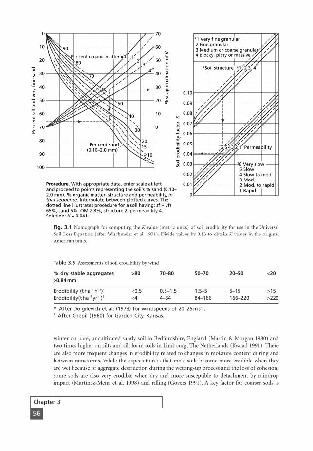
winter on bare, uncultivated sandy soil in Bedfordshire, England (Martin & Morgan 1980) andtwo times higher on silts and silt loam soils in Limbourg, The Netherlands (Kwaad 1991). Thereare also more frequent changes in erodibility related to changes in moisture content during andbetween rainstorms. While the expectation is that most soils become more erodible when theyare wet because of aggregate destruction during the wetting-up process and the loss of cohesion,some soils are also very erodible when dry and more susceptible to detachment by raindropimpact (Martínez-Mena et al. 1998) and rilling (Govers 1991). A key factor for coarser soils is
Chapter 3
56
Table 3.5 Assessments of soil erodibility by wind
% dry stable aggregates >80 70–80 50–70 20–50 <20>0.84mm
Erodibility (tha-1 h-1)* <0.5 0.5–1.5 1.5–5 5–15 >15Erodibility(tha-1 yr-1)† <4 4–84 84–166 166–220 >220
* After Dolgilevich et al. (1973) for windspeeds of 20–25ms-1.† After Chepil (1960) for Garden City, Kansas.
0
10
20
30
40
50
60
70
80
90
100
Per cent organic matter =0 12
34
Per cent sand(0.10–2.0 mm)
90
80
70
60
50
40
30
2015
1050
Per
cen
t si
lt a
nd
ver
y fi
ne
san
d70
60
50
40
30
20
10
0
Firs
t ap
pro
xim
atio
n o
f K
*1 Very fine granular 2 Fine granular 3 Medium or coarse granular 4 Blocky, platy or massive
*Soil structure *1 2 3 4
†6 5 4 3 2 1 Permeability
†6 Very slow 5 Slow 4 Slow to mod. 3 Mod. 2 Mod. to rapid 1 Rapid
0.10
0.09
0.08
0.07
0.06
0.05
0.04
0.03
0.02
0.01
0
Soil
ero
dib
ility
fac
tor,
KProcedure. With appropriate data, enter scale at leftand proceed to points representing the soil's % sand (0.10–2.0 mm). % organic matter, structure and permeability, in that sequence. Interpolate between plotted curves. The dotted line illustrates procedure for a soil having: sf + vfs65%, sand 5%, OM 2.8%, structure 2, permeability 4.Solution: K = 0.041.
Fig. 3.1 Nomograph for computing the K value (metric units) of soil erodibility for use in the Universal Soil Loss Equation (after Wischmeier et al. 1971). Divide values by 0.13 to obtain K values in the originalAmerican units.
MSE03 11/19/04 02:33 PM Page 56
Factors influencing erosion
57
3.3
Effect of slope
Erosion would normally be expected to increase with increases in slope steepness and slope lengthas a result of respective increases in velocity and volume of surface runoff. Further, while on a flatsurface raindrops splash soil particles randomly in all directions, on sloping ground more soil issplashed downslope than upslope, the proportion increasing as the slope steepens. The relation-ship between erosion and slope can be expressed by the equation:
(3.10)
where E is soil loss per unit area, q is the slope angle and L is slope length. Zingg (1940), in astudy of data from five experimental stations of the United States Soil Conservation Service, foundthat the relationship had the form:
(3.11)
To express E proportional to distance downslope, the value of n must be increased by 1.0. Sincethe values for the exponents have been confirmed in respect of m by Musgrave (1947) and m andn by Kirkby (1969b), there is some evidence to suggest that eqn 3.11 has general validity. Otherstudies, however, show that the values are sensitive to the interaction of other factors.
E Lµ tan . .1 4 0 6q
E Lm nµ tan q
their tendency to become hydrophobic when dry, which then leads to an increase in runoff and,until the depth of water becomes sufficient to absorb their impact, an increase in soil particledetachment by raindrops (Terry & Shakesby 1993; Doerr et al. 2000). Freezing and thawing also alter the erodibility of the soil. Conditions of low bulk density and high soil moisture during periods of thaw produce a surface that is highly erodible. The erodibility of agriculturalsoils in Ontario, Canada, is 15 times higher in winter thaw conditions than in summer (Coote et al. 1988).
Under natural conditions, the seasonal activity of burrowing animals is important, giving rise to considerable disturbance of the soil. Earthworms bring to the surface as casts as much as2–5.8 t ha-1 of material on agricultural land (Evans 1948). Rates of 15 t ha-1 have been measuredin temperate woodland in Luxembourg (Hazelhoff et al. 1981) and 50 t ha-1 in tropical forest inthe Ivory Coast (Roose 1976). Other animals and their annual rates of production of sediment at the surface include: ants, with 4 to 10 t ha-1 observed in Utah (Thorp 1949); termites, with 1.2 t ha-1 in tropical forest in the Ivory Coast (Roose 1976); voles and moles, with 19 t ha-1 in tem-perate woodland in Luxembourg (Imeson 1976) and 6 t ha-1 from Pyrenean mountain voles inthe Spanish Pyrenees (Borghi et al. 1990); and isopods and porcupines, with 0.3 to 0.7 t ha-1 onstony land in the Negev Desert, Israel (Yair & Rutin 1981). On coastal sand dunes in the westernNetherlands, rabbits displaced locally between 0.9 and 5.1 t ha-1 of sediment from their burrows(Rutin 1992). In many cases, the material brought to the surface comprises loose sediment withlow bulk density and cohesion, which is rapidly broken down by splash erosion. The materialcontained in earthworm casts, however, consists of soil aggregates that are more stable under rain-drop impact than the surrounding top soil, probably as a result of their higher organic contentand secretions from the gut of the worm. Thus, earthworms have a positive effect on the stabil-ity of soil aggregates and the hydraulic conductivity of the soil (Glasstetter & Prasuhn 1992).
MSE03 11/19/04 02:33 PM Page 57

3.3.1 Exponents for slope steepness
Working with data from experimental stations in Zimbabwe, Hudson and Jackson (1959) foundthat m was close to 2.0 in value, indicating that the effect of slope is stronger under tropical con-ditions where rainfall is heavier. The effect of soil is illustrated by the laboratory experiments ofGabriels et al. (1975), who showed that m increases in value with the grain size of the material,from 0.6 for particles of 0.05 mm diameter to 1.7 for particles of 1.0 mm. The value also changeswith slope, decreasing from 1.6 on slopes of 0–2.5° to 0.7 on slopes between 3 and 6.5°, to 0.4 onslopes over 6.5° (Horváth & Ero�di 1962). On steeper slopes, the value may be expected to decreasefurther as soil-covered slopes give way to rock surfaces and soil supply becomes a limiting factor.In a detailed study of soil loss from 33 road-cut slopes on the Benin–Lagos Highway in Nigeria,Odermerho (1986) found values of m = 1.09 for slopes between 1.4 and 6°, 1.80 for slopes between6 and 8.5°, -2.18 for slopes between 8.5 and 11° and -1.39 for slopes between 11 and 26.5°. Com-bining the results of these studies suggests a curvilinear relationship between soil loss and slopesteepness, with erosion initially increasing rapidly as slope increases from gentle to moderate,reaching a maximum on slopes of about 8–10° and then decreasing with further increases in slope.Such a relationship would apply only to erosion by rainsplash and surface runoff; it would notapply to landslides, piping or gully erosion by pipe collapse.
The exponents in eqn 3.11 also vary in value with slope shape. D’Souza and Morgan (1976)obtained values of m = 0.5 on convex slopes, 0.4 on straight slopes and 0.14 on concave slopes.No studies have been made of the effect of changes of slope in plan, but Jackson (1984) foundfrom erosion surveys and laboratory experiments that discharge varies with an index of contourcurvature to the power of 5.5. If soil loss is assumed to vary with the square of the discharge, thevalue of m becomes 3.5. Contour curvature is here defined as the proportion of a circle centredon a point on a hillside that lies at a higher altitude than that point. The index ranges from 0 to1 in value with values <0.5 indicating diverging slopes, a value of 0.5 a straight slope and values>0.5 converging slopes.
Few studies have looked at the effect of variations in plant cover. Quinn et al. (1980) investigatedthe change in the value of m for soil loss from 1.2 m long plots with slopes of 5–30° under simulatedrainfall in relation to decreasing grass cover brought about by human trampling. They found thatm was 0.7 for fully grassed slopes, rose to 1.9 in the early stages of trampling and fell to 1.1 whenonly about 25 per cent of the grass cover remained. Lal (1976) obtained a value of m = 1.1 for bothbare fallow and maize on erosion plots in Nigeria; use of a mulch, however, reduced m to 0.5.
The exponent values also vary with the process of erosion: m = 1.0 for soil creep, rangesbetween 1.0 and 2.0 for splash erosion and between 1.3 and 2.0 for erosion by overland flow, andmay be as high as 3.0 for rivers (Kirkby 1971). It was shown in Chapter 2 that m was about 0.3–1.0in value for rainsplash and about 0.7 and 1.7–2.0 respectively for detachment and transport ofsoil particles by overland flow.
Increases in slope steepness may also cause an increase in the intensity of wind erosion onwindward slopes and on the crests of knolls. Data from Chepil et al. (1964) and Strednansky(1977) show that m = 0.4 for slopes up to 2° and 1.2 for slopes from 2 to 15°. The increase invalue is attributed to increases in wind speed, shear and turbulence close to the ground as the airmoves upslope (Livingstone and Warren, 1996).
3.3.2 Exponents for slope length
The value of 0.6 for exponent n applies only to overland flow on slopes about 10–20 m long, withsteepnesses greater than 3°. Wischmeier and Smith (1978) propose values of n = 0.4 for slopes of
Chapter 3
58
MSE03 11/19/04 02:33 PM Page 58
3°, 0.3 for slopes of 2°, 0.2 for slopes of 1° and 0.1 for slopes of less than 1°. Kirkby (1971) sug-gests that n = 0 for soil creep and splash erosion, ranges between 0.3 and 0.7 for overland flowand rises to between 1.0 and 2.0 if rilling occurs. This implies that the value of n will vary with distance along a hillside as, for example, soil creep close to the summit gives way first tooverland flow and then to rill flow. Without rills, n may become negative on slopes longer thanabout 10 m. The increasing depth of overland flow downslope protects the soil from raindropimpact so that, even though the transporting capacity of the overland flow increases, erosionbecomes limited by the rate of detachment, which is decreasing with slope length (Gilley et al.1985). Once rills form, soil loss will either increase with slope length (Meyer et al. 1975), par-ticularly if the density of rills is very high, or decrease because, as the flow becomes concentrated,there is no longer sufficient flow on the interrill areas to remove all the material detached by rain-splash (Abrahams et al. 1991). Erosion may also decrease with increasing slope length if, as theslope steepens, the soil becomes less prone to crusting and infiltration rates remain higher thanon the gentler-sloping land at the top of the slope (Poesen 1984). Similarly, if the slope declinesin angle as length increases, soil loss may decrease as a result of deposition. Clearly, with such agreat range of possible conditions, a single relationship between soil loss and slope length cannotexist.
Factors influencing erosion
59
3.4
Effect of plant cover
Vegetation acts as a protective layer or buffer between the atmosphere and the soil. The above-ground components, such as leaves and stems, absorb some of the energy of falling raindrops,running water and wind, so that less is directed at the soil, while the below-ground components,comprising the root system, contribute to the mechanical strength of the soil.
The importance of plant cover in reducing erosion is demonstrated by the mosquito gauzeexperiment of Hudson and Jackson (1959), in which soil loss was measured from two identicalbare plots on a clay loam soil. Over one plot was suspended a fine wire gauze, which had the effectof breaking up the force of the raindrops, absorbing their impact and allowing the water to fallto the ground from a low height as a fine spray. The mean annual soil loss over a ten-year periodwas 126.6 t ha-1 for the open plot and 0.9 t ha-1 for the plot covered by gauze.
Although numerous measurements have been made of erosion under different plant coversfor comparison with that from bare ground, there is little agreement on the nature of the rela-tionship between soil loss and changes in the extent of cover. Elwell (1981) favoured an expo-nential decrease in soil loss with increasing percentage interception of rainfall energy and,therefore, increasing percentage cover. Such a relationship was suggested by Wischmeier (1975)as applicable to covers in direct contact with the soil surface and has been verified experimentallyfor crop residues (Laflen & Colvin 1981; Hussein & Laflen 1982) and grass covers (Lang & McCaffrey 1984; Morgan et al. 1997a). The relationship can be described by the equation:
(3.12)
where SLR is the ratio between the soil loss with the plant cover and that from bare ground,PC is the percentage cover and j varies in value from 0.025 to 0.06, with 0.035 taken as typical (Fig. 3.2). Foster (1982) attributes the exponential form of the relationship for covers in proxim-ity to the ground to the ponding of water behind the plant elements, which reduces the
SLR e j PC= - .
MSE03 11/19/04 02:33 PM Page 59
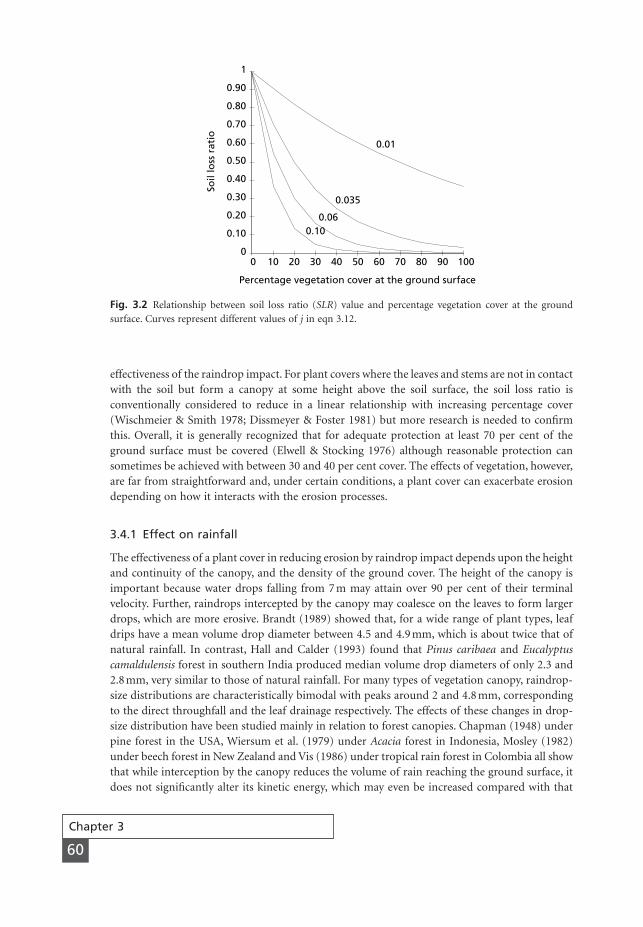
effectiveness of the raindrop impact. For plant covers where the leaves and stems are not in contactwith the soil but form a canopy at some height above the soil surface, the soil loss ratio is conventionally considered to reduce in a linear relationship with increasing percentage cover(Wischmeier & Smith 1978; Dissmeyer & Foster 1981) but more research is needed to confirmthis. Overall, it is generally recognized that for adequate protection at least 70 per cent of theground surface must be covered (Elwell & Stocking 1976) although reasonable protection cansometimes be achieved with between 30 and 40 per cent cover. The effects of vegetation, however,are far from straightforward and, under certain conditions, a plant cover can exacerbate erosiondepending on how it interacts with the erosion processes.
3.4.1 Effect on rainfall
The effectiveness of a plant cover in reducing erosion by raindrop impact depends upon the heightand continuity of the canopy, and the density of the ground cover. The height of the canopy isimportant because water drops falling from 7 m may attain over 90 per cent of their terminalvelocity. Further, raindrops intercepted by the canopy may coalesce on the leaves to form largerdrops, which are more erosive. Brandt (1989) showed that, for a wide range of plant types, leafdrips have a mean volume drop diameter between 4.5 and 4.9 mm, which is about twice that ofnatural rainfall. In contrast, Hall and Calder (1993) found that Pinus caribaea and Eucalyptuscamaldulensis forest in southern India produced median volume drop diameters of only 2.3 and2.8 mm, very similar to those of natural rainfall. For many types of vegetation canopy, raindrop-size distributions are characteristically bimodal with peaks around 2 and 4.8 mm, correspondingto the direct throughfall and the leaf drainage respectively. The effects of these changes in drop-size distribution have been studied mainly in relation to forest canopies. Chapman (1948) underpine forest in the USA, Wiersum et al. (1979) under Acacia forest in Indonesia, Mosley (1982)under beech forest in New Zealand and Vis (1986) under tropical rain forest in Colombia all showthat while interception by the canopy reduces the volume of rain reaching the ground surface, itdoes not significantly alter its kinetic energy, which may even be increased compared with that
Chapter 3
60
Percentage vegetation cover at the ground surface
Soil
loss
rat
io
0 10 20 30 40 50 60 70 80 90 1000
0.10
0.20
0.30
0.40
0.50
0.60
0.70
0.80
0.90
1
0.01
0.035
0.060.10
Fig. 3.2 Relationship between soil loss ratio (SLR) value and percentage vegetation cover at the groundsurface. Curves represent different values of j in eqn 3.12.
MSE03 11/19/04 02:33 PM Page 60
in open ground. As a result, rates of soil particle detachment by rainsplash under the forestcanopies can be between 1.2 and 3.1 times those in open ground, unless the soil surface is pro-tected by a litter layer. It is possible that kinetic energy underplays the importance of leaf dripsin contributing to soil detachment because it emphasizes drop velocity over drop size. Indicessuch as the square of the rainfall momentum (Styczen & Høgh-Schmidt 1988) or the product ofmomentum and drop diameter (Salles et al. 2000), which assign greater importance to drop size,may describe the process better.
Fewer investigations have been made to assess the effects of lower growing canopies.McGregor and Mutchler (1978) found that while cotton reduced the kinetic energy of rainfall by 95 per cent under the canopy and 75 per cent overall, it was locally increased between the rowswhere the leaf drips were concentrated. Armstrong and Mitchell (1987) found that the detach-ment under soya bean was about 94 per cent of that in the open despite the very low canopyheight. Somewhat lower detachment rates were measured in the field by Morgan (1985b), whofound that, with a 90 per cent cover, detachment under soya bean was 0.2 times that in openground for a 100 mm h-1 rainfall intensity and 0.6 times for a 50 mm h-1 intensity. Finney (1984)showed in a laboratory study that detachment rates from leaf drip were 1.7 and 1.3 times thosein open ground for Brussels sprouts and sugar beet at 23 and 16 per cent cover respectively. Inanother laboratory study under Brussels sprouts, Noble and Morgan (1983) found that the averagedetachment rate was the same as that in open ground. In a field study under maize with 88 percent canopy cover at a height of 2 m, detachment was 14 times greater than that in open groundfor a rainfall intensity of 100 mm h-1 and 2.4 times greater for an intensity of 50 mmh (Morgan1985b).
In addition to modifying the drop-size distribution of the rainfall, a plant canopy changes itsspatial distribution at the ground surface. Concentrations of water at leaf drip points can resultin very high localized rainfall intensities, which can considerably exceed infiltration capacities andplay an important role in the generation of runoff. Under mature soya bean, Amstrong andMitchell (1987) found that half of the rainfall reaching the ground in a storm of 25 mm h-1 didso at intensities greater than those in open ground and that 10 per cent of the rain had an inten-sity of 385 mm h-1. Stemflow also concentrates rain at the ground surface. De Ploey (1982) foundthat the effective intensity of stemflow beneath a canopy of tussocky grass was 150–200 per centgreater than the rainfall intensity in open ground. Herwitz (1986) recorded local stemflows of between 830 and 18,878 mm h-1 in a rainstorm of 118 mm h-1 over a six-minute period in atropical rain forest in northern Queensland.
3.4.2 Effect on runoff
A plant cover dissipates the energy of running water by imparting roughness to the flow, therebyreducing its velocity. In most soil conservation work, the roughness is expressed as a value ofManning’s n, which represents the summation of roughness imparted by the soil particles, surfacemicrotopography (form roughness) and vegetation, acting independently of each other. Typicalvalues of Manning’s n are given in Table 3.6 (Petryk & Bosmajian 1975; Temple 1982; Engman1986). The level of roughness with different forms of vegetation depends upon the morphologyand the density of the plants, as well as their height in relation to the depth of flow. When theflow depth is shallow, as with overland flow, the vegetation stands relatively rigid and imparts ahigh degree of roughness, represented for grasses by n values of 0.25 to 0.3. As flow depthsincrease, the grass stems begin to oscillate, disturbing the flow and causing n values to increaseto around 0.4. With further increases in flow depth, the vegetation is submerged; the plants tendto lie down in the flow and offer little resistance, so that n values decrease rapidly (Ree 1949).
Factors influencing erosion
61
MSE03 11/19/04 02:33 PM Page 61
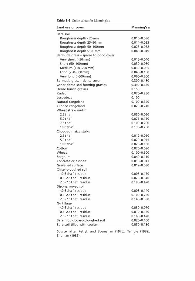
Table 3.6 Guide values for Manning’s n
Land use or cover Manning’s n
Bare soilRoughness depth <25mm 0.010–0.030Roughness depth 25–50mm 0.014–0.033Roughness depth 50–100mm 0.023–0.038Roughness depth >100mm 0.045–0.049
Bermuda grass – sparse to good coverVery short (<50mm) 0.015–0.040Short (50–100mm) 0.030–0.060Medium (150–200mm) 0.030–0.085Long (250–600mm) 0.040–0.150Very long (>600mm) 0.060–0.200
Bermuda grass – dense cover 0.300–0.480Other dense sod-forming grasses 0.390–0.630Dense bunch grasses 0.150Kudzu 0.070–0.230Lespedeza 0.100Natural rangeland 0.100–0.320Clipped rangeland 0.020–0.240Wheat straw mulch
2.5tha-1 0.050–0.0605.0tha-1 0.075–0.1507.5tha-1 0.100–0.20010.0tha-1 0.130–0.250
Chopped maize stalks2.5tha-1 0.012–0.0505.0tha-1 0.020–0.07510.0tha-1 0.023–0.130
Cotton 0.070–0.090Wheat 0.100–0.300Sorghum 0.040–0.110Concrete or asphalt 0.010–0.013Gravelled surface 0.012–0.030Chisel-ploughed soil
<0.6tha-1 residue 0.006–0.1700.6–2.5tha-1 residue 0.070–0.3402.5–7.5tha-1 residue 0.190–0.470
Disc-harrowed soil<0.6tha-1 residue 0.008–0.1400.6–2.5tha-1 residue 0.100–0.2502.5–7.5tha-1 residue 0.140–0.530
No tillage<0.6tha-1 residue 0.030–0.0700.6–2.5tha-1 residue 0.010–0.1302.5–7.5tha-1 residue 0.160–0.470
Bare mouldboard-ploughed soil 0.020–0.100Bare soil tilled with coulter 0.050–0.130
Source: after Petryk and Bosmajian (1975), Temple (1982),Engman (1986).
MSE03 11/19/04 02:33 PM Page 62
Greatest reductions in velocity occur with dense, spatially uniform, vegetation covers. Clumpy,tussocky vegetation is less effective and may even lead to concentrations in flow with localizedhigh velocities between the clumps. When flow separates around a clump of vegetation, the pres-sure exerted by the flow is higher on the upstream face than it is downstream, and eddying andturbulence occur immediately downstream of the vegetation. Vortex erosion is induced bothupstream and downstream (Babaji 1987). Detailed observations during laboratory experimentson overland flow (De Ploey 1981) show that for slopes above about 8°, erosion under grass ishigher than that from an identical plot without grass until the percentage grass cover reaches acritical value. Beyond this point, the grass has the expected protective effect.
3.4.3 Effect on air flow
Vegetation reduces the shear velocity of wind by imparting roughness to the air flow. It increasesthe roughness length, z0, and raises the height of the mean aerodynamic surface by a distance, d,known as the zero plane displacement (Fig. 2.7). Estimates of d and z0 can be obtained from therelationships:
(3.13)
(3.14)
where H is the average height of the roughness elements and F is the fraction of the total surfacearea covered by those elements (Abtew et al. 1989). From this, it follows that the key plant para-meter is the lateral cover (Lc), defined as:
(3.15)
where N is the number of roughness elements per unit area (A), and S is the mean frontal silhouette area of the plants, i.e. the cross-sectional area of the plant facing the wind (Musick &Gillette 1990). An increase in the value of Lc results in an exponential decrease in the proportionof the shear velocity of the wind exerted on the soil surface (Wolfe & Nickling 1996). This, inturn, causes an exponential decrease in sediment transport. Al-Awadhi and Willetts (1999)showed from wind tunnel experiments with cylinders that sediment transport levels off to verylow levels when Lc exceeds 0.18 in value. When Lc reaches 0.5, sediment transport ceases (Gillette& Stockton 1989; Nickling & McKenna Neuman 1995). However, low densities of vegetation cansometimes increase the rate of erosion over bare ground through the development of turbulenteddies in the flow between individual plants (Logie 1982).
The effect of the vegetation can be described by a frictional drag coefficient (Cd) exerted bythe plant layer in bulk and computed from:
(3.16)
where u is the mean velocity measured at a height z, which equals 1.6 times the average height ofthe roughness elements. The coefficient generally decreases in value from about 0.1 in light windsto 0.01 in strong winds for a wide range of crops (Ripley & Redman 1976; Uchijima 1976; Morgan& Finney 1987) but both Randall (1969) in apple orchards and Bache (1986) with cotton canopies
Cu
ud =
2 2
2*
LNS
Ac =
z H d0 0 13= -( ).
D HF=
Factors influencing erosion
63
MSE03 11/19/04 02:33 PM Page 63
found that Cd could also increase with windspeed. When Cd exceeds 0.0104 in value, no regionalscale wind erosion occurs (Lyles et al. 1974b).
Instead of considering these bulk drag coefficients, more insight can be gained by examiningconditions close to the ground surface. Drag coefficients within the plant layer (Cd¢) can be cal-culated from:
(3.17)
where h is the height of the vegetation, A(z) is the leaf area per unit volume for the vegetation atheight z and dz is the difference in height between z and the ground surface. For a wide range ofcrops, values of Cd¢ within the lowest 0.5 m of the plant layer decrease from about 0.1 in low wind-speeds to about 0.001 in high windspeeds. However, when the wind is moderate to strong, con-sistent over time, and the crops are at an early stage of growth, the drag coefficient is found toincrease with windspeed (Morgan & Finney 1987). This is probably due to the waving of the leavesin the wind, which disturbs the surrounding air, creating a wall effect that acts as a barrier to theair flow. The result is that the windspeed is reduced close to the ground surface but remains thesame or even increases at the canopy level, thereby increasing the drag or shear velocity andenhancing the risk of erosion. The effect is particularly marked in crops of young sugar beet andonions. Similar increases in the drag coefficient with windspeed within a crop have been reportedfor maize (Wright & Brown 1967).
3.4.4 Effect on slope stability
It was shown in Chapter 2 that forest covers generally help to protect the land against mass move-ments partly through the cohesive effect of the tree roots. The fine roots, 1–20 mm in diameter,interact with the soil to form a composite material in which root fibres of relatively high tensilestrength reinforce a soil matrix of lower tensile strength. In addition, soil strength is increased bythe adhesion of soil particles to the roots. Roots can make significant contributions to the cohe-sion of a soil, even at low root densities and in materials of low shear strength. Increases in cohe-sion in forest soils due to roots can range from 1.0 to 17.5 kPa (Greenway 1987), although localvariability in this may be as high as 30 per cent (Wu 1995). Grasses, legumes and small shrubscan reinforce a soil down to depths of 0.75–1.0 m and trees can enhance soil strength to depthsof 3 m or more. The magnitude of the effect depends upon the angle at which tree roots cross thepotential slip plane, being greatest for those at right angles, and whether the strain exerted on the slope is sufficient to mobilize fully the tensile strength of the roots. The effect is limited where roots fail by pull-out because of insufficient bonding with the soil, as can occur in stonymaterials, or where the soil is forced into compression instead of tension, as can occur at thebottom of a hillslope, and the roots fail by buckling.
Following observations on the forested slopes of the Serra do Mar, east of Santos, Brazil, DePloey (1981) proposed that trees could sometimes induce landslides through an increase inloading (surcharge) brought about by their weight and an increase in infiltration which allowsmore water to penetrate the soil, lowering its shear strength. Bishop and Stevens (1964) showedthat large trees can increase the normal stress on a slope by up to 5 kPa but that less than half ofthis contributes to an increase in shear stress and the remainder has the beneficial effect of increas-ing the frictional resistance of the soil. While, generally, surcharge enhances slope stability, undercertain circumstances it can be detrimental. Trees planted only at the top of a slope can reduce
¢ =( )Ú
Cu
u A z dzd h
2 2
2
0
*
Chapter 3
64
MSE03 11/19/04 02:33 PM Page 64
stability, as can trees planted on steep slopes with shallow soils characterized by low angles ofinternal friction. In the Serra do Mar, the landslides occurred in a soil with an angle of internalfriction of less than 20°, on slopes greater than 20°, after two days on which respectively 260 and420 mm of rain fell.
A vegetation cover should theoretically contribute to slope stability as a result of evapo-transpiration producing a drier soil environment so that a higher intensity and longer durationrainfall are required to induce a slope failure compared with an unvegetated slope (Greenway1987). Further, since soil moisture depletion can affect depths well below those reached by theroots, increases in slope stability should extend some 4–6 m below ground level. In practice,however, as found by Terwilliger (1990) in southern California, soil moisture levels after a fewstorms reach similar levels in both vegetated and unvegetated soils, so that under the conditionswhen the risk of mass movement is highest, the drying effect of vegetation is unlikely to play arole. Despite this, overall increases in the factor of safety arising from vegetation are generally inthe range of 20–30 per cent (Greenway 1987; Wu 1995).
Factors influencing erosion
65
Erosion processes and the factors that influ-ence them vary according to the scale atwhich they are studied.
Micro-scale (mm2 to 1m2)At this scale, erosion is controlled largely bythe stability of the soil aggregates. Soil mois-ture, organic matter content and the activityof soil fauna, particularly earthworms, aremajor influences. Since aggregate breakdownis largely a result of raindrop impact, the fre-quency and erosivity of individual rainstormscontrol the rate of erosion through the rate ofsoil particle detachment. Soil type, slope andland cover are reasonably uniform over areasof this size so that differences in these can beused to demarcate different micro-scale units.For example, Cammeraat (2002) distinguishedbetween areas of bare crusted soils and areascovered by tussocks of Stipa tenacissima whendescribing erosion processes at this scale in theGuadalentín Basin, Spain. In woodland in theLuxembourg Ardennes, he distinguishedbetween bare soil areas where earthwormsremove and digest the freshly fallen litter, and litter-covered areas with lower bioticactivity.
Box 3
Plot-scale (1m2 to 100m2)Erosion at the plot scale is controlled by theprocesses that generate surface runoff. Theseinclude the infiltration characteristics of thesoil and changes in the microtopography ofthe surface related to crust development andsurface roughness. The spatial distribution ofcrusted and uncrusted areas or vegetated andbare soil areas determines the locations ofrunoff and the patterns of flow and sedimentmovement over the soil surface. Depending onthe size of the plot, interrill erosion will domi-nate, but, on steep slopes or in areas withhighly erodible soils, the flow may exceed thecritical conditions for rills to develop. It is atthis scale that rock fragments can increaserates of soil erosion compared with bareground if the surface between the stonesbecomes sealed (Poesen et al. 1994).
Field scale (100m2 to 10,000m2)At the field scale, there is usually a reasonablywell defined spatial pattern of runoff path-ways in locations such as swales and valleybottoms, separated by areas of either interrillerosion or no erosion. The extent of interrillerosion depends on the severity of the rainfallevent so that the size of the area contributing
Scale and erosion processes
Continued
MSE03 11/19/04 02:33 PM Page 65

Chapter 3
66
runoff is quite dynamic. The direction ofrunoff pathways is often controlled by tillage.There may be spatial variations in soil erodibil-ity and slope within a field. The normallyexpected increases in runoff and erosiondownslope can sometimes be offset by soilswith greater infiltration rates at the bottom ofthe field, resulting in a decrease in runoff, orby gentler slopes, resulting in deposition ofsediment.
Catchment scale (>10,000m2)Depending on the spatial distribution of soils,slope and land cover in a catchment, it is pos-sible to recognize different types of process-domains (De Ploey 1989b):I: areas dominated by rainsplash erosion and
infiltration, typical of soils with high infil-tration rates and high aggregate stability.
II: areas dominated by interrill erosion butwith sediment deposition on the lowerslopes.
III: areas dominated by rill erosion, again withdeposition on the lower slopes.
IV: areas of ephemeral gullies, particularlyalong the valley floors.
The pathways of runoff and sediment move-ment through the catchment are influencedby the patterns of field boundaries, gateways,tracks and roads, as well as the natural topog-raphy. The effectiveness of these pathwaysand the spatial extent of the process-domainsdepend on the magnitude of the erosionevent. In low magnitude events, erosion isgenerally limited to local slope wash, but withhigher rainfall, runoff pathways develop overthe whole hillside with local discharges into
the river; with more extreme events, overlandflow and slope wash may be widespread, withmany points of discharge into the riverchannel (Swiechowicz 2002). Thus, in order tounderstand the sources of sediment and asso-ciated pollutants in water bodies, the dynamicnature of the process-domains and their con-nectivity must be investigated.
The way in which the effectiveness oferosion events depends on the scale ofanalysis was demonstrated by Carver andSchreier (1995) for the Jhikhu Kholawatershed, Nepal (Table B3.1). They examinedthree storms, one of 49.5mm occurring in thepre-monsoon period, one of 35.8mm duringthe monsoon and an extreme event of 90.6mm in the transition period just before theonset of the monsoon season. On a 70m2 areaof a terraced hillslope, erosion in the pre-monsoon storm when the cultivated land wasbare was higher than that from the monsoonstorm when the land was protected by a cropcover; the extreme event was only half asdamaging as the pre-monsoon event. In a sub-watershed of 540ha, the pre-monsoon andmonsoon storms had less overall effect but theextreme event became very important as aresult of erosion of the stream bed. At thescale of the whole watershed, 11,141ha, thedifferences between the pre-monsoon andmonsoon periods disappeared and the effectof the extreme event was much reducedbecause the heavy rain did not extend beyondthe area of the sub-watershed. Thus, what wasan extreme event at a small watershed scalewas no larger than the annual event at thelarger watershed scale.
Table B3.1 Effectiveness of erosion events (t ha-1) with changes in scale
Season Rainfall Peak rainfall Terraced Sub-watershed Jhikhu Kholatotal (mm) intensity hillside (540ha) watershed
(mmh-1) (70m2) (11,141ha)
Pre-monsoon 49.5 109 20 2 0.1Monsoon 35.8 63 0.02 0.4 0.1Extreme event 90.6 103 10 40 2
Source: after Carver and Schreier (1995).
MSE03 11/19/04 02:33 PM Page 66

Erosion hazard assessment aims to identify those areas of land where the maximum sustainedproductivity from a given land use is threatened by excessive soil loss or the off-site damage arisingfrom erosion is unacceptable. A distinction is made between potential erosion risk, reflecting thelocal conditions of soil, climate and slope, and actual erosion risk, which additionally takesaccount of land cover. It is therefore possible to recognize areas of high potential risk but lowactual risk as a result of the protection afforded by vegetation.
Erosion hazard assessment
67
CHAPTER 4
Erosion hazardassessment
4.1
Generalized assessments
4.1.1 Erosivity indices
Erosivity data can be used as an indicator of regional variations in erosion potential. Stocking andElwell (1976) present a generalized picture of erosion risk in Zimbabwe, based on mean annualerosivity values, showing that high-risk areas are in the Eastern Districts, the region east ofMasvingo and the High and Middle Veld north and east of Harare (Fig. 4.1). The area south andwest of Bulawayo, by contrast, has a much lower risk. Temporal variations in erosion risk arerevealed by the mean monthly erosivity values. Hudson (1981; Fig. 4.2) contrasts the erosivitypatterns of Bulawayo and Harare. At Bulawayo, erosivity is low at the beginning of the wet seasonand increases as the season progresses. By the time the maximum values are experienced, the plantcover has had a chance to become established, giving protection against erosion and lowering therisk. At Harare, however, erosivity is highest at the time of minimal vegetation cover. The seasonalpattern of erosivity in Kenya was analysed in by Rowntree (1983) for the Katumani ResearchStation, near Machakos. The mean annual erosivity of 164,352 J mm m-2 h-1 is much higher thanthe values recorded in Zimbabwe. The highest mean monthly value, 69,688 J mm m-2 h-1, occursin April, the beginning of the period when the potential soil moisture deficit is severe and thevegetation cover poorly established. Cultivation of the land at this time creates a great risk oferosion. May has a much lower erosivity, only 20,961 J mm m-2 h-1, and is also a month with goodvegetation cover. Erosivity is very low during the summer with mean monthly values of less than1000 but rises again in the short rainy season, reaching 15,306 in November before falling to meanmonthly values of about 10,000 during the winter.
MSE04 11/19/04 02:34 PM Page 67

Maps of erosivity using the rainfall erosion index, R, have been produced for the USA (Wischmeier & Smith 1978). Originally R was calculated as mean annual EI30/100 with E beingthe rainfall energy in foot-tons per acre and I30 being the maximum 30-minute rainfall intensityin inches per hour; this can be described as an R value in American units. With E calculated inMJ ha-1 and I30 in mm h-1, an R can be derived in metric units as mean annual EI30/100. The con-version is 1 unit of metric R = 17.3 units of American R. Since maps for many parts of the worldexist in both units, care should be taken to ensure which one is being used. The metric versionof the map for the USA is shown in Fig. 4.3. Values range from about 50 in the arid west to over1000 along the Gulf Coast. These are rather low compared to those of more tropical climates.Values in India range from about 250 in western Rajasthan to over 1250 along the coasts ofMaharashtra and Karnataka (Singh et al. 1981; Fig. 4.4). Those in Zambia range from 500 in thesouth to about 800–900 in the Copper Belt and over 1000 in the western part of the NorthernProvince (Lenvain et al. 1988). In South Africa (Smithen & Schulze 1982) values are lowest in thesouthwest of Cape Province where they are about 50–100 and rise eastwards reaching over 400in eastern Transvaal and the midlands of Natal (Fig. 4.5). Very low values are characteristic ofnorthern Europe. Those in France range from 50 in the north and west to 340 in the southernMassif Central and Languedoc (Pihan 1979); those in Belgium and the Netherlands from 60 to75 but rising to 100–150 in the Ardennes (Laurant & Bollinne 1978).
In many countries insufficient rainfall records from autographic gauges are available to cal-culate erosivity nationwide. In such cases, an attempt is made to find a more widely available
Chapter 4
68
0 80 160 km
13 000
11 000
8 0007 000
5 000
3 000
J mm m–2 h–1
Chipinga
Harare
FortVictoriaBulawayo
Fig. 4.1 Mean annual erosivity in Zimbabwe (after Stocking & Elwell 1976).
MSE04 11/19/04 5:15 PM Page 68
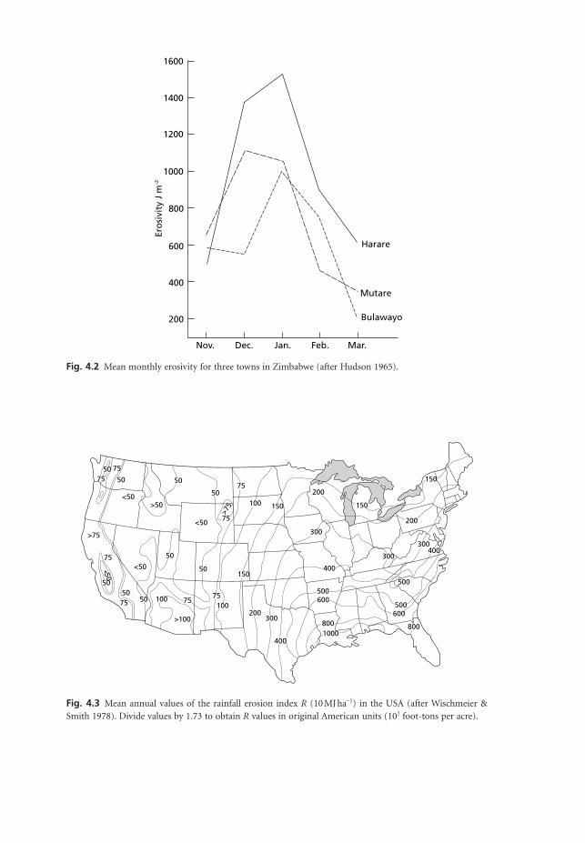
1600
1400
1200
1000
800
600
400
200
Nov. Jan. Feb. Mar.Dec.
Harare
Mutare
Bulawayo
Ero
sivi
ty J
m–2
Fig. 4.2 Mean monthly erosivity for three towns in Zimbabwe (after Hudson 1965).
5075
<50
75
<50
50
75
7550
50 75100
>100
75100
50
50
200300
400
150
500600
800
500
400300
300
200
150
150
200
300
150100
75
>75
7550
50
>50
50
>75
<50
<50
400
500600
8001000
Fig. 4.3 Mean annual values of the rainfall erosion index R (10 MJ ha-1) in the USA (after Wischmeier &Smith 1978). Divide values by 1.73 to obtain R values in original American units (102 foot-tons per acre).
MSE04 11/19/04 02:34 PM Page 69

0 200 400 km
100 200 300 miles0
500
>600
750500
30012501000
750500
1500
1500
1000
1250
1250
500300
500
<300
200
300400
500800 400
5001000
1250
1000
600 750 >2000
10001250
250
500
7501000
500
250
700
750
1000
700600
500
<250
1000
600
1250
300
500
400
200
700
Fig. 4.4 Mean annual values of the rainfall erosion index R (10 MJ ha-1) in India (after Singh et al. 1981).
300
400
200
200300
300 300300
300200
200
100
100
100
100
100
500400
400
400
500150
150150
150
5050
50
200
0 200 km
Fig. 4.5 Mean annual values of the rainfall erosion index R (10 MJ ha-1) in southern Africa (after Smithen& Schulze 1982).
MSE04 11/19/04 02:34 PM Page 70
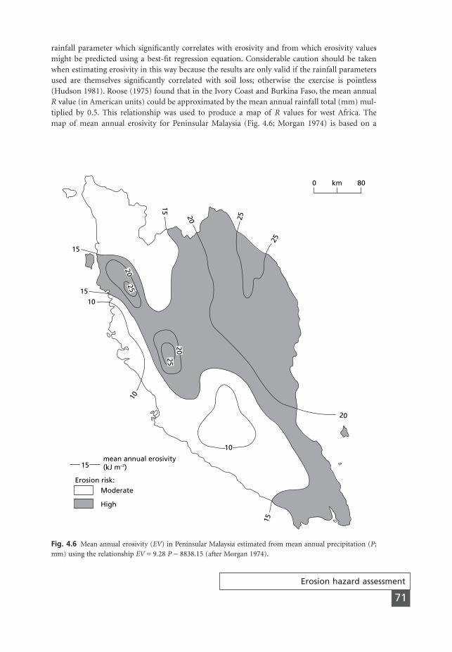
rainfall parameter which significantly correlates with erosivity and from which erosivity valuesmight be predicted using a best-fit regression equation. Considerable caution should be takenwhen estimating erosivity in this way because the results are only valid if the rainfall parametersused are themselves significantly correlated with soil loss; otherwise the exercise is pointless(Hudson 1981). Roose (1975) found that in the Ivory Coast and Burkina Faso, the mean annualR value (in American units) could be approximated by the mean annual rainfall total (mm) mul-tiplied by 0.5. This relationship was used to produce a map of R values for west Africa. The map of mean annual erosivity for Peninsular Malaysia (Fig. 4.6; Morgan 1974) is based on a
Erosion hazard assessment
71
15
0 80km
15
10
10
15
15
25
25
20
20
mean annual erosivity(kJ m–2)
Erosion risk:Moderate
High
15
2025
2520
10
Fig. 4.6 Mean annual erosivity (EV) in Peninsular Malaysia estimated from mean annual precipitation (P;mm) using the relationship EV = 9.28 P - 8838.15 (after Morgan 1974).
MSE04 11/19/04 02:34 PM Page 71
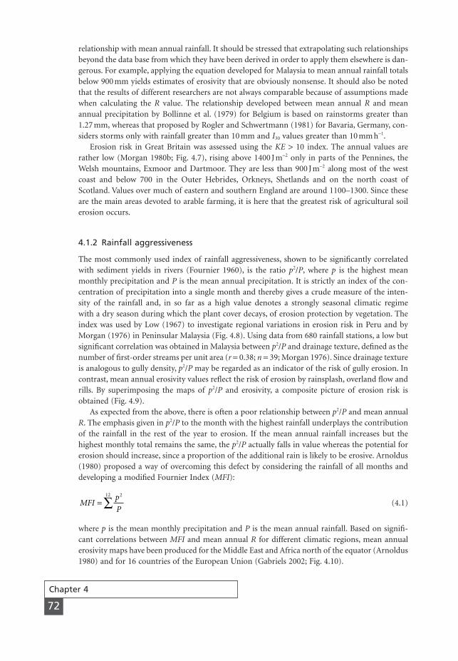
Chapter 4
72
relationship with mean annual rainfall. It should be stressed that extrapolating such relationshipsbeyond the data base from which they have been derived in order to apply them elsewhere is dan-gerous. For example, applying the equation developed for Malaysia to mean annual rainfall totalsbelow 900 mm yields estimates of erosivity that are obviously nonsense. It should also be notedthat the results of different researchers are not always comparable because of assumptions madewhen calculating the R value. The relationship developed between mean annual R and meanannual precipitation by Bollinne et al. (1979) for Belgium is based on rainstorms greater than1.27 mm, whereas that proposed by Rogler and Schwertmann (1981) for Bavaria, Germany, con-siders storms only with rainfall greater than 10 mm and I30 values greater than 10 mm h-1.
Erosion risk in Great Britain was assessed using the KE > 10 index. The annual values arerather low (Morgan 1980b; Fig. 4.7), rising above 1400 J m-2 only in parts of the Pennines, theWelsh mountains, Exmoor and Dartmoor. They are less than 900 J m-2 along most of the westcoast and below 700 in the Outer Hebrides, Orkneys, Shetlands and on the north coast ofScotland. Values over much of eastern and southern England are around 1100–1300. Since theseare the main areas devoted to arable farming, it is here that the greatest risk of agricultural soilerosion occurs.
4.1.2 Rainfall aggressiveness
The most commonly used index of rainfall aggressiveness, shown to be significantly correlatedwith sediment yields in rivers (Fournier 1960), is the ratio p2/P, where p is the highest meanmonthly precipitation and P is the mean annual precipitation. It is strictly an index of the con-centration of precipitation into a single month and thereby gives a crude measure of the inten-sity of the rainfall and, in so far as a high value denotes a strongly seasonal climatic regime with a dry season during which the plant cover decays, of erosion protection by vegetation. Theindex was used by Low (1967) to investigate regional variations in erosion risk in Peru and byMorgan (1976) in Peninsular Malaysia (Fig. 4.8). Using data from 680 rainfall stations, a low butsignificant correlation was obtained in Malaysia between p2/P and drainage texture, defined as thenumber of first-order streams per unit area (r = 0.38; n = 39; Morgan 1976). Since drainage textureis analogous to gully density, p2/P may be regarded as an indicator of the risk of gully erosion. Incontrast, mean annual erosivity values reflect the risk of erosion by rainsplash, overland flow andrills. By superimposing the maps of p2/P and erosivity, a composite picture of erosion risk isobtained (Fig. 4.9).
As expected from the above, there is often a poor relationship between p2/P and mean annualR. The emphasis given in p2/P to the month with the highest rainfall underplays the contributionof the rainfall in the rest of the year to erosion. If the mean annual rainfall increases but thehighest monthly total remains the same, the p2/P actually falls in value whereas the potential forerosion should increase, since a proportion of the additional rain is likely to be erosive. Arnoldus(1980) proposed a way of overcoming this defect by considering the rainfall of all months anddeveloping a modified Fournier Index (MFI):
(4.1)
where p is the mean monthly precipitation and P is the mean annual rainfall. Based on signifi-cant correlations between MFI and mean annual R for different climatic regions, mean annualerosivity maps have been produced for the Middle East and Africa north of the equator (Arnoldus1980) and for 16 countries of the European Union (Gabriels 2002; Fig. 4.10).
MFIp
P= Â
212
MSE04 11/19/04 02:34 PM Page 72
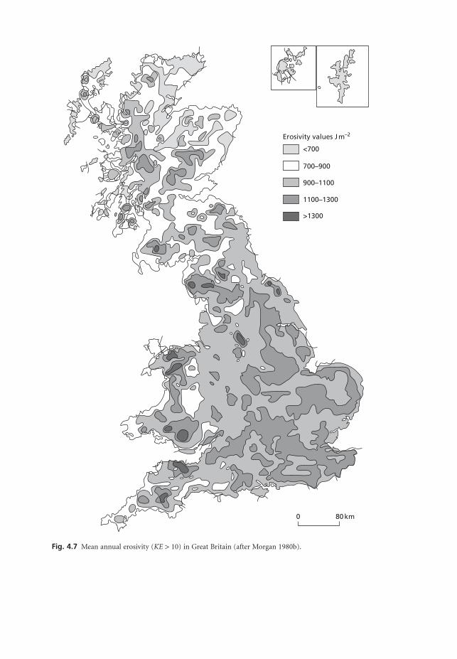
Erosivity values J m–2
<700
>1300
700–900
900–1100
1100–1300
0 80 km
Fig. 4.7 Mean annual erosivity (KE > 10) in Great Britain (after Morgan 1980b).
MSE04 11/19/04 02:34 PM Page 73
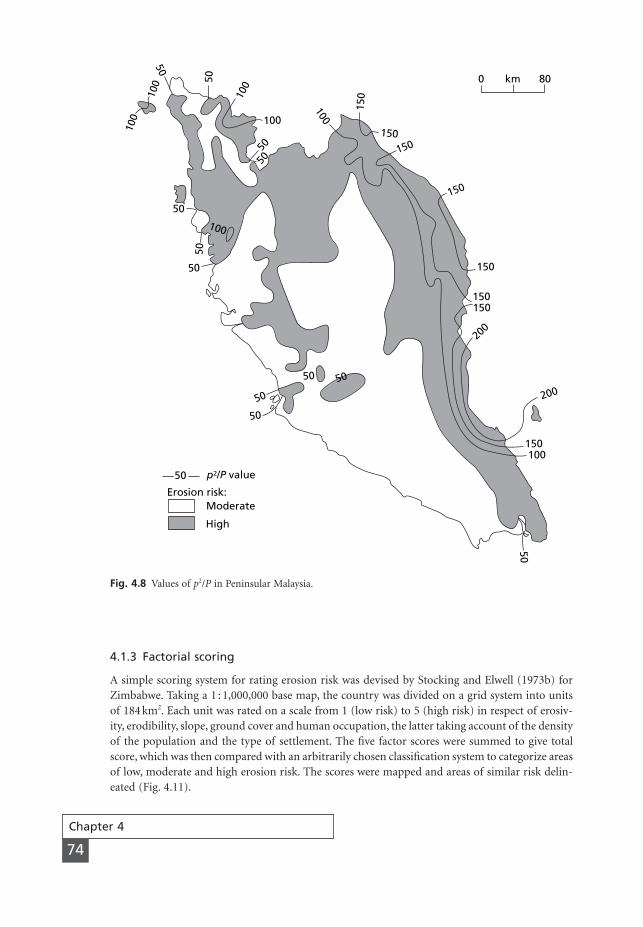
Chapter 4
74
100
100
100
100
100
150
150
150
150
150
150150
150100
200
200
50
50
5050
5050
100
50
50
50
50
50 50
0 80km
50
Erosion risk:Moderate
High
p2/P value
Fig. 4.8 Values of p2/P in Peninsular Malaysia.
4.1.3 Factorial scoring
A simple scoring system for rating erosion risk was devised by Stocking and Elwell (1973b) forZimbabwe. Taking a 1 : 1,000,000 base map, the country was divided on a grid system into unitsof 184 km2. Each unit was rated on a scale from 1 (low risk) to 5 (high risk) in respect of erosiv-ity, erodibility, slope, ground cover and human occupation, the latter taking account of the densityof the population and the type of settlement. The five factor scores were summed to give totalscore, which was then compared with an arbitrarily chosen classification system to categorize areasof low, moderate and high erosion risk. The scores were mapped and areas of similar risk delin-eated (Fig. 4.11).
MSE04 11/19/04 02:34 PM Page 74
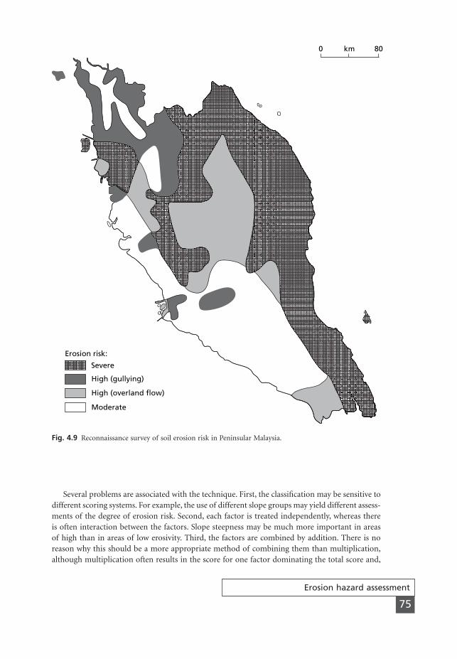
Erosion hazard assessment
75
Erosion risk:
Severe
High (gullying)
High (overland flow)
Moderate
0 80km
Fig. 4.9 Reconnaissance survey of soil erosion risk in Peninsular Malaysia.
Several problems are associated with the technique. First, the classification may be sensitive todifferent scoring systems. For example, the use of different slope groups may yield different assess-ments of the degree of erosion risk. Second, each factor is treated independently, whereas thereis often interaction between the factors. Slope steepness may be much more important in areasof high than in areas of low erosivity. Third, the factors are combined by addition. There is noreason why this should be a more appropriate method of combining them than multiplication,although multiplication often results in the score for one factor dominating the total score and,
MSE04 11/19/04 02:34 PM Page 75
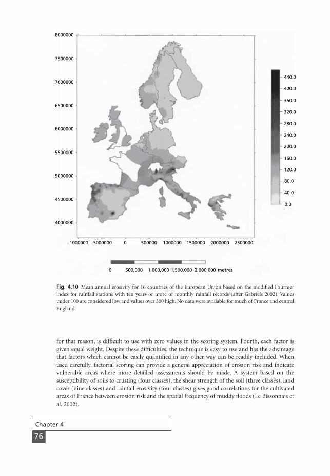
for that reason, is difficult to use with zero values in the scoring system. Fourth, each factor isgiven equal weight. Despite these difficulties, the technique is easy to use and has the advantagethat factors which cannot be easily quantified in any other way can be readily included. Whenused carefully, factorial scoring can provide a general appreciation of erosion risk and indicatevulnerable areas where more detailed assessments should be made. A system based on the susceptibility of soils to crusting (four classes), the shear strength of the soil (three classes), landcover (nine classes) and rainfall erosivity (four classes) gives good correlations for the cultivatedareas of France between erosion risk and the spatial frequency of muddy floods (Le Bissonnais etal. 2002).
Chapter 4
76
8000000
7500000
7000000
6500000
6000000
5500000
5000000
4000000
–1000000 –5000000 500000 1000000 20000001500000 25000000
4500000
440.0
400.0
360.0
320.0
280.0
240.0
160.0
120.0
80.0
40.0
0.0
200.0
0 500,000 1,000,000 1,500,000 2,000,000 metres
Fig. 4.10 Mean annual erosivity for 16 countries of the European Union based on the modified Fournierindex for rainfall stations with ten years or more of monthly rainfall records (after Gabriels 2002). Valuesunder 100 are considered low and values over 300 high. No data were available for much of France and centralEngland.
MSE04 11/19/04 02:34 PM Page 76
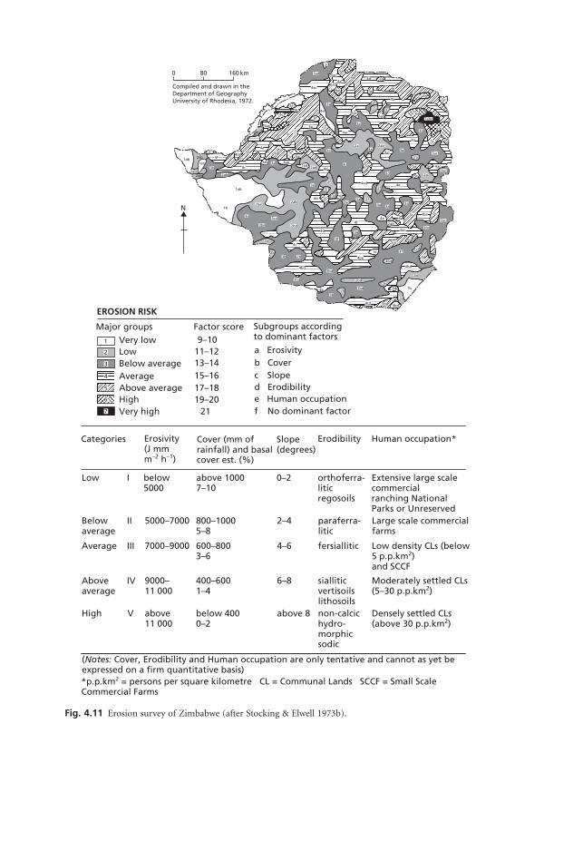
4f
4c3b
4a
3a
3a
5c
5f
5c
6c
5f4a
6f
4a4c
3a
3a
2a
5d
3a
3d
4e
4a
4a 3a
4a
3d
2f
2f4d3d5c
4f
3a
5e
3f
6c
2d
5d
2b
1b
2b
2b
2b3b
4b 5d
5c
3f
4d
5c4c
2b3b
2b
2b
3a
1b
3a
4d
4d
2f
3i3e
3a
5c
3a
2a
5e
2a
4c
5c5c
3a
5a
5c
5e
6a
6a6c
4a
3a
2ad
3bd
3bd
4bd4bd
2bd
3bd
4cd 5bd 4bd
4ae
3ab
3bd
3ac2ab
4ac3ac
5d
2e
5f
2d 4c
4a
5a
5d 4d
5c
5d
5c
4a
3a
6ac
5ac
5ac
4ac
2a
3f
5a
6ac
6ac
2
3
4
5
6
7
EROSION RISK
Major groups Factor score Subgroups accordingto dominant factors9–10
11–1213–1415–1617–1819–20
21
Very low1
LowBelow averageAverage
HighVery high
Above average
a Erosivityb Coverc Sloped Erodibilitye Human occupationf No dominant factor
Categories Erosivity (J mm m–2 h–1)
Cover (mm of rainfall) and basal cover est. (%)
Slope(degrees)
Erodibility Human occupation*
Low
Below average
Average
High
*p.p.km2 = persons per square kilometre CL = Communal Lands SCCF = Small Scale Commercial Farms
(Notes: Cover, Erodibility and Human occupation are only tentative and cannot as yet be expressed on a firm quantitative basis)
Above average
I
II
III
IV
V
below 5000
above 1000 7–10
0–2 orthoferra- liticregosoils
Extensive large scale commercialranching National Parks or UnreservedLarge scale commercial farms
Low density CLs (below5 p.p.km2)and SCCF
Moderately settled CLs(5–30 p.p.km2)
Densely settled CLs(above 30 p.p.km2)
paraferra- litic
fersiallitic
siallitic vertisoilslithosoilsnon-calcichydro-morphicsodic
2–4
4–6
6–8
above 8
800–1000 5–8
600–800 3–6
400–600 1–4
below 4000–2
5000–7000
7000–9000
9000– 11 000
above 11 000
N
0 80 160 km
Compiled and drawn in theDepartment of GeographyUniversity of Rhodesia, 1972.
1ab
2ab
2ab
4ac
4ac
4ad
4ac
2ad
2ab
2bd
3cd
3be
4bd
4be
5ac
2be
2ab
4bd
1ad
2ab
6ac
3ac
4be
4ac
5ce
7abc
3ad
1ab
1ab
1ab
5d
5ac
5f
Fig. 4.11 Erosion survey of Zimbabwe (after Stocking & Elwell 1973b).
MSE04 11/19/04 5:41 PM Page 77

Chapter 4
78
4.2
Semi-detailed assessments
4.2.1 Land capability classification
Land capability classification was developed by the United States Natural Resources ConservationService as a method of assessing the extent to which limitations such as erosion, soil depth, wetnessand climate hinder the agricultural use that can be made of the land. The United States classifi-cation (Klingebiel & Montgomery 1966) has been adapted for use in many other countries(Hudson 1981).
The objective of the classification is to divide an area of land into units with similar kinds anddegrees of limitation. The basic unit is the capability unit. This consists of a group of soil typesof sufficiently similar conditions of profile form, slope and degree of erosion to make them suit-able for similar crops and warrant the use of similar conservation measures. The capability unitsare combined into sub-classes according to the nature of the limiting factor and these, in turn,are grouped into classes based on the degree of limitation. The United States system recognizeseight classes arranged from Class I, characterized by no or very slight risk of damage to the landwhen used for cultivation, to Class VIII, very rough land that can be safely used only for wildlife,limited recreation and watershed conservation. The first four classes are designated as suitable forarable farming (Table 4.1). Assigning a tract of land to its appropriate class is aided by the use ofa flow diagram (Fig. 4.12). The value of land capability assessment lies in identifying the risksattached to cultivating the land and in indicating the soil conservation measures that are required.The classification can be improved by making the conservation recommendations more specific,as is the case with the treatment-oriented scheme developed in Taiwan and tested on hilly landin Jamaica (Sheng 1972a; Table 4.2, Fig. 4.13).
Although the inclusion of many soil properties in the classification may seem to render ituseful for land planning generally, it must be appreciated that, as befits a classification evolved inthe wake of the erosion scare in the United States in the 1930s, its bias is towards soil conserva-tion. Attempts to use the classification in a wider sphere have only drawn attention to its limita-tions. The classification does not specify the suitability of land for particular crops; a separateland suitability classification has been devised to do this (FAO 1976). The assigning of a capabil-ity class is not an indicator of land value, which may reflect the scarcity of a certain type of land,nor is it a measure of whether a farmer can make a profit, which is much influenced by the marketprices of the crops grown and the farmer’s skill. The stress laid by the classification on arablefarming can also be a disadvantage. Insufficient attention is given to the recreational use of land.The capability classification implies that land is set aside for recreation only when it is too mar-ginal for arable or pastoral farming, but such land is often marginal for recreational use too. Thisfact highlights the difficulty of incorporating agricultural and non-agricultural activities in asingle classification. One approach to this problem is provided by the Canada Land Inventory(McCormack 1971), which employs four separate classifications covering agriculture, forestry,recreation and wildlife. In the UK, separate classifications exist for evaluating the suitability ofland for picnic sites and camping sites (George & Jarvis 1979).
Information contained in land capability surveys can be combined with that on erosivity to give a more detailed assessment of erosion risk. A map was produced for England and Wales(Fig. 4.14) by combining data on land capability class (Soil Survey of England and Wales 1979),rainfall erosivity and wind velocity with knowledge of the susceptibility of soils to erosion (SoilSurvey of England and Wales 1983). The inclusion of land capability in the assessment procedure
MSE04 11/19/04 02:34 PM Page 78

Table 4.1 Land capability classes (United States system)
Class Characteristics and recommended land use
I Deep, productive soils easily worked, on nearly level land; not subject to overlandflow; no or slight risk of damage when cultivated; use of fertilizers and lime,cover crops, crop rotations required to maintain soil fertility and soil structure.
II Productive soils on gentle slopes; moderate depth; subject to occasional overlandflow; may require drainage; moderate risk of damage when cultivated; use ofcrop rotations, water-control systems or special tillage practices to controlerosion.
III Soils of moderate fertility on moderately steep slopes, subject to more severeerosion; subject to severe risk of damage but can be used for crops providedplant cover is maintained; hay or other sod crops should be grown instead ofrow crops.
IV Good soils on steep slopes, subject to severe erosion; very severe risk of damagebut may be cultivated if handled with great care; keep in hay or pasture but agrain crop may be grown once in five or six years.
V Land is too wet or stony for cultivation but of nearly level slope; subject to onlyslight erosion if properly managed; should be used for pasture or forestry butgrazing should be regulated to prevent plant cover being destroyed.
VI Shallow soils on steep slopes; use for grazing and forestry; grazing should beregulated to preserve plant cover; if plant cover is destroyed, use should berestricted until land cover is re-established.
VII Steep, rough, eroded land with shallow soils; also includes droughty or swampyland; severe risk of damage even when used for pasture or forestry; strict grazingor forest management must be applied.
VIII Very rough land; not suitable even for woodland or grazing; reserve for wildlife,recreation or watershed conservation.
Classes I–IV denote soils suitable for cultivation.Classes V–VIII denote soils unsuitable for cultivation.
Table 4.2 Treatment-oriented land capability classification
Group Class Characteristics and recommended treatments
Suitable for tillage C1 Up to 7° slope; soil depth normally over 10cm; contourcultivation; strip cropping; broad-based terraces.
C2 Slopes 7–15°; soil depth over 20cm; bench terracing(construction by bulldozers); use of four-wheel tractors.
C3 Slopes 15–20°; soil depth over 20cm; bench terracing ondeep soil (construction by small machines); silt-pits onshallower soils; use of small tractors or walking tractors.
C4 Slopes 20–25°; soil depth over 50cm; bench terracing andfarming operations by hand labour.
P Slopes 0–25°; soil depth too shallow for cultivation; use for improved pasture or rotational grazing system; zero grazing where land is wet.
FT Slopes 25–30°; soil depth over 50cm; use for tree cropswith bench terracing; inter-terraced areas in permanentgrass; use contour planting; diversion ditches; mulching.
F Slopes over 30° or over 25° where soil is too shallow fortree crops; maintain as forest land.
Wet land, liable to P Slopes 0–25°; use as pasture.flood; also stonyland
F Slopes over 25°; use as forest.Gullied land F Maintain as forest land.
The scheme is most suitable for hilly lands in the tropics.Source: after Sheng (1972a).
MSE04 11/19/04 02:34 PM Page 79
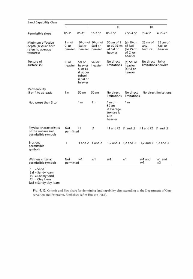
Land Capability Class
I II III IV
Permissible slope 0°–1° 0°–1° 1°–2.5° 0°–2.5° 2.5°–4.5° 4.5°–7°0°–4.5°
Minimum effective depth (Texture here refers to average textures)
1 m of Cl orheavier
Cl orheavier
Sal orheavier
(a) Sal orheavier(b) Cl orheavier
Sal orheavier
Sal orheavierS, or Lsif uppersubsoil is Sal orheavier
50 cm of Sal orheavier
50 cm of Sacl orheavier
(a) 50 cmof Sacl(b) 25 cmof Cl orheavier
25 cm ofanytexture
25 cm ofSacl orheavier
50 cm of S or LS 25 cmof Sal or heavier
Texture of surface soil
No directlimitations
No directlimitations
Permeability5 or 4 to at least:
Not worse than 3 to:
1 m
1 m
t1
1 1 and 2 1 and 2 1,2 and 3 1,2 and 3 1,2 and 3 1,2 and 3
t1 t1 and t2 t1 and t2 t1 and t2 t1 and t2
1 m 1 m or50 cmif averagetexture isCl isheavier
1 m
50 cm 50 cm No directlimitations
No directlimitations
No direct limitations
Physical characteristicsof the surface soil:permissible symbols
Notpermitted
Erosion:permissiblesymbols
Wetness criteria:permissible symbols
Notpermitted
w1 w1 w1 w1 w1 and w2
w1 and w2
S = Sand Sal = Sandy loam Ls = Loamy sand Cl = Clay loamSacl = Sandy clay loam
Fig. 4.12 Criteria and flow chart for dermining land capability class according to the Department of Con-servation and Extension, Zimbabwe (after Hudson 1981).
MSE04 11/19/04 02:34 PM Page 80
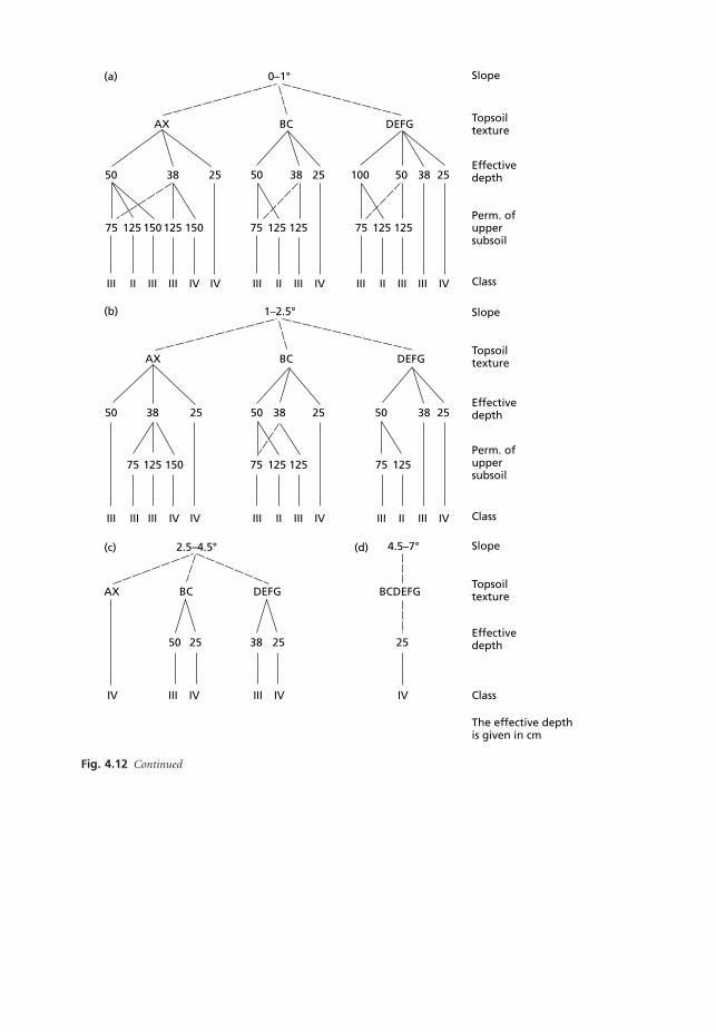
0–1°
AX BC DEFG
50 5038 3825 25 50100
75 125 12575 125 12575 125 150 150125
38 25
III III III IV IVII III III III IV ClassIV IIIII IIIII
Effectivedepth
Perm. ofuppersubsoil
Slope
Topsoiltexture
(a)
1–2.5°
AX BC DEFG
AX BC DEFG BCDEFG
50 5038 3825
38 2550 25
25 50
75 12575 125 12575 125 150
38 25
III III IV
III IV III IV
25
IVIV
IVIII III III IV ClassIV IIIII IIIII
Effectivedepth
Perm. ofuppersubsoil
Slope
Topsoiltexture
Class
Effectivedepth
The effective depthis given in cm
Slope
Topsoiltexture
(b)
2.5–4.5°(c) 4.5–7°(d)
Fig. 4.12 Continued
MSE04 11/19/04 02:34 PM Page 81

Effective depth (m)
12345
DeepModerately deepModerately shallowShallowVery shallow
More than 1.5 m1 m to 1.5 m50 cm to 1 m25 cm to 50 cmLess than 25 cm
Erosion
12
3
4
No apparent, or slight, erosion.Moderate erosion: moderate loss of topsoil generally and/or somedissection by runoff channels or gullies.Severe erosion, severe loss of topsoil generally and/or markeddissection by runoff channels or gullies.Very severe erosion: complete truncation of the soil profile andexposure of the subsoil (B horizon) and/or deep and intricatedissection by runoff channels or gullies.
Wetness
w1w2w3
Wet for relatively short and infrequent periods.Frequently wet for considerable periods.Very wet for most of the season.
Texture of surface soil
AXBCDEFG
SandLoamy sandSandy loamSandy clay loamClay loamSandy clayClayHeavy clay
More than 85% sand80–85% sandLess than 20% clay; 50–80% sand20–30% clay; 50–80% sand20–30% clay; less than 50% sandMore than 30% clay; 50–70% sand30–50% clay;less than 50% sandMore than 50% clay
Permeability
*The rate of flow in mm per hour through saturated undisturbed cores under a head of 12.5 mm of water.
Physical characteristics of surface soil
t1
t2
DescriptionVery slowSlowModerately slowModerateModerately rapidRapidVery rapid
Slightly unfavourable physical conditions. The soil has a tendency tocompact and seal at the surface and a good tilth is not easily obtained.
Unfavourable physical conditions. Compaction and sealing of thesurface soil are more severe. A hard crust forms when the bare soilis exposed to rain and sun and poor emergence of seedlings canseverely reduce the crop. On ploughing, large clods are turned upwhich are not easily broken.
Rate of flow*Less than 1.251.25 to 55 to 2020 to 6565 to 125125 to 250Over 250
Fig. 4.12 Continued
MSE04 11/19/04 02:34 PM Page 82

Additional Requirements
*Factors affecting cultivation
*Erosion
*Permeability
gbosvr
Downgrade Class I to II
Class VI
Gravelly or stonyVery gravelly or stonyBoulderyVery boulderyOutcropsExtensive outcrops
75 to 500;otherwise Class IVNot applicable tobasalts or norites
Class: 11; 21; 2; 3
I:II:
III:
*‘t’ Factors
Class: t1t1; t2t1; t2
II:III:IV:
*Wetness
*Note
Any land not meeting the minimum requirements shown on this sheet is Class VI.
Class: w1w1w2w3
w2 downgrades Class II and III to IVw unless the land is already Class IV on code, in whichcase it remains as Class IV.
II:III:IV:V:
Fig. 4.12 Continued
MSE04 11/19/04 02:34 PM Page 83
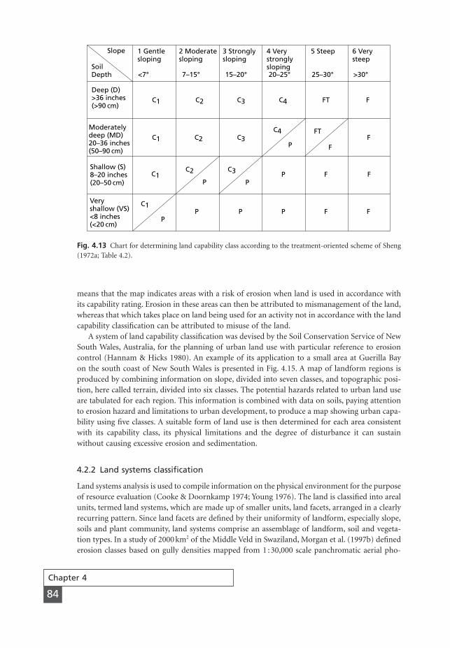
Chapter 4
84
Slope
SoilDepth
1 Gentlesloping
3 Stronglysloping
4 Verystronglysloping
6 Verysteep
5 Steep2 Moderatesloping
Deep (D)>36 inches(>90 cm)
Moderatelydeep (MD)20–36 inches(50–90 cm)
Shallow (S)8–20 inches(20–50 cm)
Veryshallow (VS)<8 inches(<20 cm)
<7° >30°7–15° 15–20° 20–25° 25–30°
C1
C1
C1
C1
C2
C2 C3
C3
C4
C2 C3 C4 FT
FT
F
FF
F F
P
P
PP P P F F
PP
Fig. 4.13 Chart for determining land capability class according to the treatment-oriented scheme of Sheng(1972a; Table 4.2).
means that the map indicates areas with a risk of erosion when land is used in accordance withits capability rating. Erosion in these areas can then be attributed to mismanagement of the land,whereas that which takes place on land being used for an activity not in accordance with the landcapability classification can be attributed to misuse of the land.
A system of land capability classification was devised by the Soil Conservation Service of NewSouth Wales, Australia, for the planning of urban land use with particular reference to erosioncontrol (Hannam & Hicks 1980). An example of its application to a small area at Guerilla Bay on the south coast of New South Wales is presented in Fig. 4.15. A map of landform regions isproduced by combining information on slope, divided into seven classes, and topographic posi-tion, here called terrain, divided into six classes. The potential hazards related to urban land useare tabulated for each region. This information is combined with data on soils, paying attentionto erosion hazard and limitations to urban development, to produce a map showing urban capa-bility using five classes. A suitable form of land use is then determined for each area consistentwith its capability class, its physical limitations and the degree of disturbance it can sustainwithout causing excessive erosion and sedimentation.
4.2.2 Land systems classification
Land systems analysis is used to compile information on the physical environment for the purposeof resource evaluation (Cooke & Doornkamp 1974; Young 1976). The land is classified into arealunits, termed land systems, which are made up of smaller units, land facets, arranged in a clearlyrecurring pattern. Since land facets are defined by their uniformity of landform, especially slope,soils and plant community, land systems comprise an assemblage of landform, soil and vegeta-tion types. In a study of 2000 km2 of the Middle Veld in Swaziland, Morgan et al. (1997b) definederosion classes based on gully densities mapped from 1 : 30,000 scale panchromatic aerial pho-
MSE04 11/19/04 02:34 PM Page 84
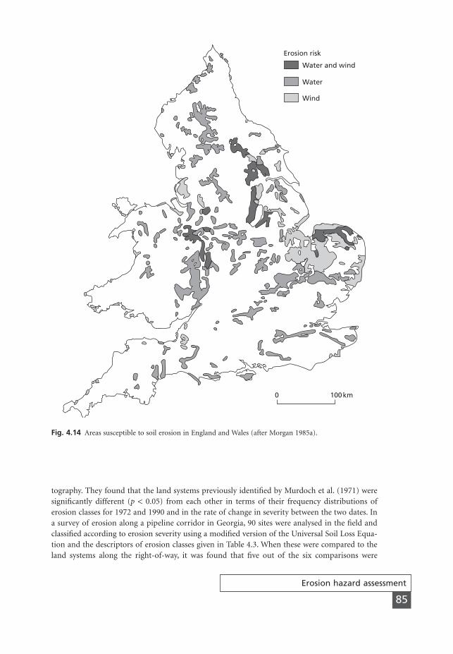
tography. They found that the land systems previously identified by Murdoch et al. (1971) weresignificantly different (p < 0.05) from each other in terms of their frequency distributions oferosion classes for 1972 and 1990 and in the rate of change in severity between the two dates. Ina survey of erosion along a pipeline corridor in Georgia, 90 sites were analysed in the field andclassified according to erosion severity using a modified version of the Universal Soil Loss Equa-tion and the descriptors of erosion classes given in Table 4.3. When these were compared to theland systems along the right-of-way, it was found that five out of the six comparisons were
Erosion hazard assessment
85
Erosion risk
Water and wind
Water
Wind
0 100 km
Fig. 4.14 Areas susceptible to soil erosion in England and Wales (after Morgan 1985a).
MSE04 11/19/04 02:34 PM Page 85
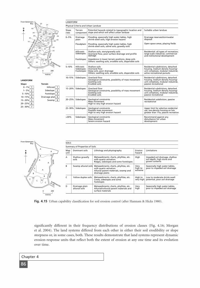
Chapter 4
86
From Batemans Bay 3/2
4/2
3/5
4/5
GEO
RGE
BASS
DRI
VE
BURREWATER
PT RD
5/25/2
6/2 7/2
2/36/2
3/22/6
3/35/2
4/2
5/25/2
3/22/1
3/23/1
6/25/2
4/2
3/34/2
5/23/3
7/2
3/34/2
5/2
3/3
3/2
3/5
4/2
3/3 5/2
2/1
2/1
4/56/2
4/22/5
3/2
3/2
From Batemans Bay
GEO
RGE
BASS
DRI
VE
BURREWATER
PT RD
A
B
C
D
A
B
A
A
A
B
B
CC
CD BE
ACH
RO
AD
BEA
CHRO
AD
LANDFORM
Physical Criteria and Urban Landuse
Slopeclass
Terraincomponent
Potential hazards related to topographic location andslope and which will affect urban landuse
Suitable urban landuse
0–5%
5–10%
10–15%
15–20%
20–25%
25–30%
>30%
Drainage plain
Floodplain
Flooding, seasonally high water-tables, high shrink-swell soils, high erosion hazard
Flooding, seasonally high water-tables, high shrink-swell soils, saline soils, gravelly soils
Drainage reserves/stormwater disposal
Open space areas, playing fields
Shallow soils, stony/gravelly soilsOverland flow, poor surface drainage and profile damage
Impedence in lower terrain positions, deep soilsOthers: swelling soils, erodible soils, dispersible soils
Residential: all types of recreation; large-scale industrial, commercial and institutional development
HillcrestsSideslopes
Footslopes
HillcrestsSideslopesFootslopes
Shallow soilsOverland flowDeep soils, poor drainageOthers: swelling soils, erodible soils, dispersible soils
Sideslopes
Sideslopes
Sideslopes
Sideslopes
Sideslopes
Overland flowGeological constraints, possibility of mass movementSwelling soilsErodible soils
Overland flowGeological constraints, possibility of mass movementSwelling soilsErodible soils
Geological constraintsMass movementHigh to very high erosion hazard
Geological constraintsPossible mass movementHigh to very high erosion hazard
Geological constraintsMass movementSevere erosion hazard
Residential subdivisions, detached housing, medium-density housing/unit complexes, modular industrial, active recreational pursuits
Residential subdivisions, detached housing, medium-density housing/unit complexes, modular industrial, passive recreational
Residential subdivisions, detached housing, medium-density housing/unit complexes, modular industrial, passive recreational
Residential subdivision, passive recreational
Upper limit for selective residentialuse, low-density housing on lotsgreater than 1 ha, passive recreation
Recommend against anydisturbance for urbandevelopment
LANDFORM
Slope Terrain
0–1%
1– 5%
5–10%
10–15%
15– 20%
20– 25%
25– 30%
1
2
3
4
5
6
7
Hillcrest
Sideslope
Footslope
Drainage plan
Swamp
1
2
3
5
6
SOILS
Summary of Properties of Soils
Map unit
Dominant soils Lithology and physiography Erosion hazard
A
B
C
D
Shallow gravelly soils
Metasediments; cherts, phyllites, etc.with quartz veinationRidges, sideslopes and some footslopes
Impeded soil drainage, shallowsoil depth, high stone andgravel contents
Limitations
High
Swamp alluvial soils Metasediments; cherts, phyllites, etc.with quartz veinationAlluvial parent materials, swamp anddrainage plains
Veryhigh toextreme
Seasonally high water-tables,poor to impeded soil drainage
Yellow duplex soils Metasediments; cherts, phyllites, etc.Crests, sideslopes and somefootslopes
High tovery high
Low to moderate shrink-swellpotential, poor soil drainage
Drainage plainalluvial soils
Metasediments; cherts, phyllites, etc.Alluvial/colluvial parent materials andsurface materials
Very high
Seasonally high water-tables,poor to impeded soil drainage
0 200
metres
N
0 200
metres
N
2/5
2/6
4/2
Fig. 4.15 Urban capability classification for soil erosion control (after Hannam & Hicks 1980).
significantly different in their frequency distributions of erosion classes (Fig. 4.16; Morgan et al. 2004). The land systems differed from each other in either their soil erodibility or slopesteepness or, in some cases, both. These results demonstrate that land systems represent dynamicerosion-response units that reflect both the extent of erosion at any one time and its evolutionover time.
MSE04 11/19/04 02:34 PM Page 86
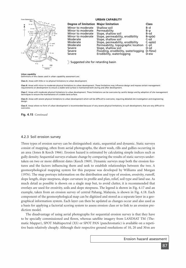
Erosion hazard assessment
87
Urban capabilityDefinitions of the classes used in urban capability assessment are:
Class A. Areas with little or no physical limitations to urban development.
Class B. Areas with minor to moderate physical limitations to urban development. These limitations may influence design and impose certain management requirements on development to ensure a stable land surface is maintained both during and after development.
Class C. Areas with moderate physical limitations to urban development. These limitations can be overcome by careful design and by adoption of site management techniques to ensure the maintenance of a stable land surface.
Class D. Areas with severe physical limitations to urban development which will be difficult to overcome, requiring detailed site investigation and engineering design.
Class E. Areas where no form of urban development is recommended because of very severe physical limitations, to such development, that are very difficult to overcome.
From Batemans Bay
GEO
RGE
BASS
D
RIVE
BURREWATER
PT RD
B– d
B – sd
C– sd
D– ewD– sd
B –p
B – sp(e)
D– f(ew)
C – pt
B – sd
D– ew C– sd
D– ewD– f(ew)
B – sd
C– sdC –pt
C – pt
C– sd
B – dD– sdC
–sd
BEA
CH
RO
AD
B – sdB – sd
C– sp(e)
C– sp(e)
C– sp(e)
C – ptD– ew
C – ptC – pt
D– ew
C – pt
D– ewD– f(ew)
C – pt
D– ew
0 200
metres
N
URBAN CAPABILITY
Degree of limitation Major limitation ClassMinor to moderate Shallow soil
PermeabilitySlope, shallow soilSlope, permeability, erodibilitySlope, shallow soilSlope, permeability, erodibilityPermeability, topographic locationSlope, shallow soilFlooding, erodibility, waterloggingErodibility, waterlogging
Minor to moderateMinor to moderateMinor to moderateModerateModerateModerate
SevereSevereSevere
B–d
D–ew
D–sdC–pt
D–f(ew)
B–sd
C–sdC–ap(e)
B–p
B–sp(e)
Suggested site for retarding basin
B – sd
Fig. 4.15 Continued
4.2.3 Soil erosion survey
Three types of erosion survey can be distinguished: static, sequential and dynamic. Static surveysconsist of mapping, often from aerial photographs, the sheet wash, rills and gullies occurring inan area (Jones & Keech 1966). Erosion hazard is estimated by calculating simple indices such asgully density. Sequential surveys evaluate change by comparing the results of static surveys under-taken on two or more different dates (Keech 1969). Dynamic surveys map both the erosion fea-tures and the factors influencing them and seek to establish relationships between the two. A geomorphological mapping system for this purpose was developed by Williams and Morgan(1976). The map portrays information on the distribution and type of erosion, erosivity, runoff,slope length, slope steepness, slope curvature in profile and plan, relief, soil type and land use. Asmuch detail as possible is shown on a single map but, to avoid clutter, it is recommended thatoverlays are used for erosivity, soils and slope steepness. The legend is shown in Fig. 4.17 and anexample, taken from an erosion survey of central Pahang, Malaysia, is shown in Fig. 4.18. Eachcomponent of the geomorphological map can be digitized and stored as a separate layer in a geo-graphical information system. Each layer can then be updated as changes occur and also used asa basis for applying a factorial scoring system to assess erosion class or to link to an erosion pre-diction model.
The disadvantage of using aerial photographs for sequential erosion survey is that they haveto be specially commissioned and flown, whereas satellite imagery from LANDSAT TM (The-matic Mapper), SPOT Multispectral (XS) or SPOT PAN (panchromatic) is available on a repeti-tive basis relatively cheaply. Although their respective ground resolutions of 10, 20 and 30 m are
MSE04 11/19/04 02:34 PM Page 87

Table 4.3 Coding system for soil erosion appraisal in the field
Code Class Erosion Indicatorsrate(tha-1)
1 Very slight <2 No evidence of compaction or crusting of the soil; no wash marks or scour features; no splash pedestals or exposure of tree roots; over 70% plant cover (ground and canopy).
2 Slight 2–5 Some crusting of soil surface; localized wash but no or minor scouring; rills every 50–100m; small splash pedestals, 1–5mm depth, where stones or exposed trees protect underlying soil, occupying not more than 10% of the area; soil level slightly higher on upslope or windward sides of plants and boulders; 30–70% plant cover.
3 Moderate 5–10 Wash marks; discontinuous rills spaced every 20–50m; splash pedestals and exposed tree roots mark level of former surface, soil mounds protected by vegetation, all to depths of 5–10mm and occupying not more than 10% of the area; slight to moderate surface crusting; 30–70% plant cover; slight risk of pollution problems downstream if slopes discharge straight into water courses.
4 High 10–50 Connected and continuous network of rills every 5–10mor gullies spaced every 50–100m; tree root exposure, splash pedestals and soil mounds to depths of 10–50mm occupying not more than 10% of the area; crusting of the surface over large areas; less than 30% plant cover; danger of pollution and sedimentation problems downstream.
5 Severe 50–100 Continuous network of rills every 2–5m or gullies every 20m; tree root exposure, splash pedestals and soil mounds to depths of 50–100mm covering more than 10% of the area; splays of coarse material; bare soil;siltation of water bodies; damage to roads by erosionand sedimentation.
6 Very severe 100–500 Continuous network of channels with gullies every 5–10m; surrounding soil heavily crusted; severe siltation, pollution and eutrophication problems; bare soil.
7 Catastrophic >500 Extensive network of rills and gullies; large gullies (>100m2) every 20m; most of original soil surface removed; severe damage from erosion and sedimentation on-site and downstream.
Source: after Morgan et al. (2004).
MSE04 11/19/04 02:34 PM Page 88
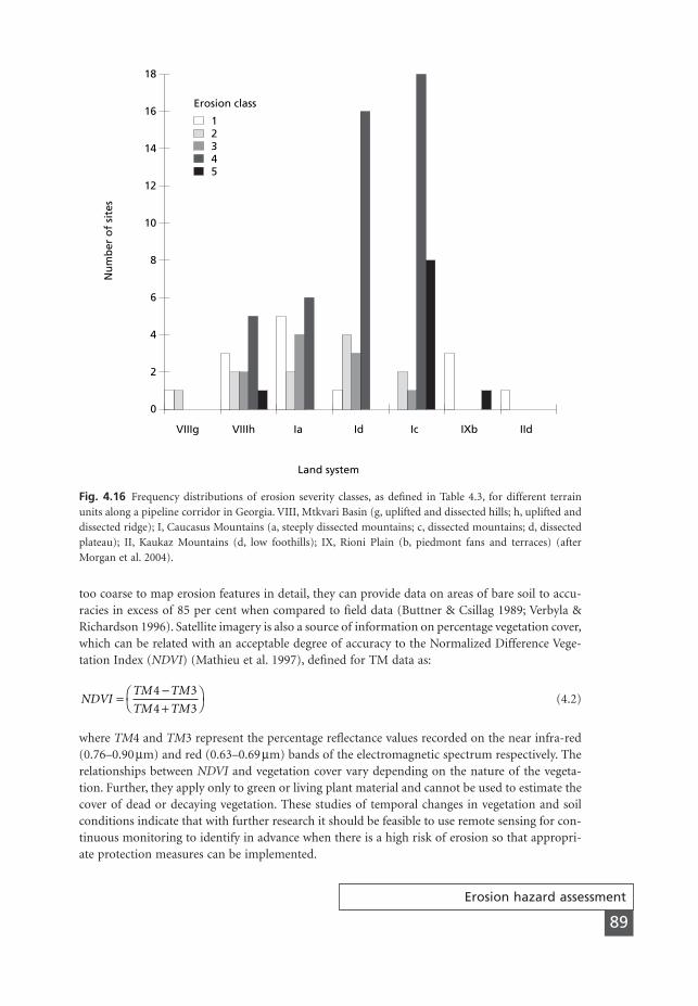
too coarse to map erosion features in detail, they can provide data on areas of bare soil to accu-racies in excess of 85 per cent when compared to field data (Buttner & Csillag 1989; Verbyla &Richardson 1996). Satellite imagery is also a source of information on percentage vegetation cover,which can be related with an acceptable degree of accuracy to the Normalized Difference Vege-tation Index (NDVI) (Mathieu et al. 1997), defined for TM data as:
(4.2)
where TM4 and TM3 represent the percentage reflectance values recorded on the near infra-red(0.76–0.90 mm) and red (0.63–0.69 mm) bands of the electromagnetic spectrum respectively. Therelationships between NDVI and vegetation cover vary depending on the nature of the vegeta-tion. Further, they apply only to green or living plant material and cannot be used to estimate thecover of dead or decaying vegetation. These studies of temporal changes in vegetation and soilconditions indicate that with further research it should be feasible to use remote sensing for con-tinuous monitoring to identify in advance when there is a high risk of erosion so that appropri-ate protection measures can be implemented.
NDVITM TM
TM TM=
-+
ÊË
ˆ¯
4 3
4 3
Erosion hazard assessment
89
VIIIg VIIIh Ia Id Ic IXb IId
0
2
4
6
8
10
12
14
16
18
Land system
Nu
mb
er o
f si
tes
Erosion class
12345
Fig. 4.16 Frequency distributions of erosion severity classes, as defined in Table 4.3, for different terrainunits along a pipeline corridor in Georgia. VIII, Mtkvari Basin (g, uplifted and dissected hills; h, uplifted anddissected ridge); I, Caucasus Mountains (a, steeply dissected mountains; c, dissected mountains; d, dissectedplateau); II, Kaukaz Mountains (d, low foothills); IX, Rioni Plain (b, piedmont fans and terraces) (afterMorgan et al. 2004).
MSE04 11/19/04 02:34 PM Page 89
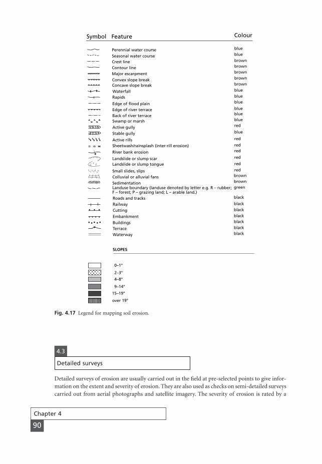
Chapter 4
90
Symbol Feature Colour
Perennial water courseSeasonal water courseCrest lineContour lineMajor escarpmentConvex slope breakConcave slope break
Rapids
Edge of flood plainEdge of river terraceBack of river terrace
Sheetwash/rainsplash (inter-rill erosion)
River bank erosion
Landslide or slump scarLandslide or slump tongue
Small slides, slipsColluvial or alluvial fansSedimentationLanduse boundary (landuse denoted by letter e.g. R – rubber;F – forest; P – grazing land; L – arable land.)
Swamp or marsh
Active gully
Active rills
Stable gully
Waterfall
Roads and tracksRailwayCutting
Embankment
BuildingsTerraceWaterway
SLOPES
blueblue
blueblueblue
blueblueblue
blue
red
red
redred
red
red
red
brownbrownbrownbrownbrown
brownbrowngreen
black
blackblackblackblackblackblack
0–1°
2–3°
4–8°
9–14°
15–19°
over 19°
Fig. 4.17 Legend for mapping soil erosion.
4.3
Detailed surveys
Detailed surveys of erosion are usually carried out in the field at pre-selected points to give infor-mation on the extent and severity of erosion. They are also used as checks on semi-detailed surveyscarried out from aerial photographs and satellite imagery. The severity of erosion is rated by a
MSE04 11/19/04 5:42 PM Page 90
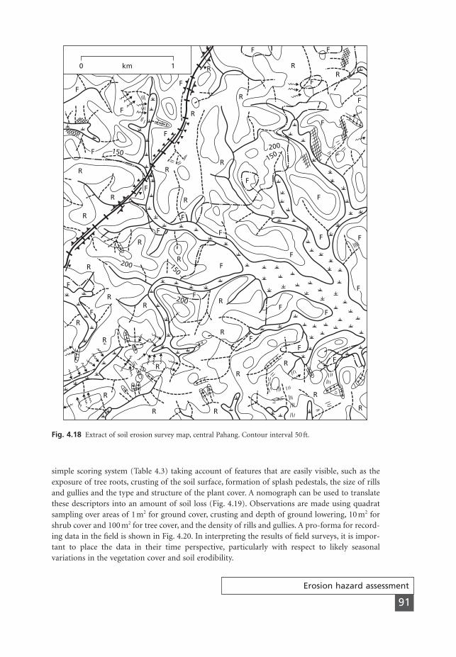
Erosion hazard assessment
91
F F
F
F
F
F
F F
F
F
F
FF
F
FF
F
F
F
R
R
R
R
R
RRR
R
R
R
R
R
R
R
R
R RR
R
R
R
RR
R
R
R
R
F
F
F
F
F
F
F
F
0 1km
F
FF
200
200
200
150
150
150
Fig. 4.18 Extract of soil erosion survey map, central Pahang. Contour interval 50 ft.
simple scoring system (Table 4.3) taking account of features that are easily visible, such as theexposure of tree roots, crusting of the soil surface, formation of splash pedestals, the size of rillsand gullies and the type and structure of the plant cover. A nomograph can be used to translatethese descriptors into an amount of soil loss (Fig. 4.19). Observations are made using quadratsampling over areas of 1 m2 for ground cover, crusting and depth of ground lowering, 10 m2 forshrub cover and 100 m2 for tree cover, and the density of rills and gullies. A pro-forma for record-ing data in the field is shown in Fig. 4.20. In interpreting the results of field surveys, it is impor-tant to place the data in their time perspective, particularly with respect to likely seasonalvariations in the vegetation cover and soil erodibility.
MSE04 11/19/04 02:34 PM Page 91

Recorder:Date:Altitude:
Area:Air photo no:Grid Reference:
Present landuse
Climate
Vegetation
Slope
Soil
Erosion
REMARKS
EROSION CODE 0 11/2 2 3 4 5
Depth Surface texture Erodibility
Permeability Clay fraction
Position DegreeDistancefrom crest Shape
Type % Ground cover % Tree andshrub cover
FACET NO.
Month J F M A M JJ A S O N D Erosivity
Rainfail(mm)
Meantemp (∞C)
Maximum intensity
Cross-sectional area of rill channels (m2) So
il lo
ss (
t ha–1
)
0.1
1
10
100
1,000
10,000 0.50 (2 m)0.20 (5 m)0.10 (10 m)0.05 (20 m)0.02 (50 m)0.01 (100 m)
7
654
32
1Ero
sio
n s
ever
ity
clas
s
Channel density(rill spacing)
0.001 0.01 0.1 1
Fig. 4.19 Relationship between soil loss, soil erosion severity class and cross-sectional area of rill channels,assuming a bulk density of 1.4 Mg m-3 for the soil material. The lines indicate different channel densities (m m-2) and rill spacings (m).
Fig. 4.20 Proforma for recording soil erosion in the field (devised by Baker personal communication).
MSE04 11/19/04 02:34 PM Page 92
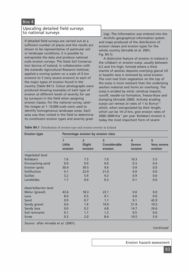
Erosion hazard assessment
93
If detailed field surveys are carried out at asufficient number of places and the results areshown to be representative of particular soilor landscape conditions, it is possible toextrapolate the data and produce nationalscale erosion surveys. The State Soil Conserva-tion Service of Iceland, in collaboration withthe Icelandic Agricultural Research Institute,applied a scoring system on a scale of 0 (noerosion) to 5 (very severe erosion) to each ofthe major types of erosion found in thecountry (Table B4.1). Colour photographs wereproduced showing examples of each type oferosion at different levels of severity for useby surveyors in the field when assigningerosion classes. For the national survey, satel-lite images at 1 :10,000 scale were used toidentify homogeneous landscape areas. Eacharea was then visited in the field to determineits constituent erosion types and severity grad-
Box 4
ings. The information was entered into theArc/Info geographical information system
and maps produced of the distribution oferosion classes and erosion types for thewhole country (Arnalds et al. 2001; Fig. B4.1).
A distinctive feature of erosion in Iceland isthe rofabarQ or erosion scarp, usually between0.2 and 3m high, formed where a thickmantle of aeolian deposits overlying glacial tillor basaltic lava is removed by wind erosion.The root mat from vegetation on the top ofthe scarp is more resistant than the underlyingaeolian material and forms an overhang. Thescarp is eroded by wind, raindrop impacts,runoff, needle-ice formation, freeze-thaw andslumping (Arnalds 2000). Actively erodingscarps can retreat at rates of 1 to 8cmyr-1
which, when extrapolated by their length,which can be 14–21km, give erosion rates of2000–3000tha-1 per year. RofabarQ erosion istoday the most important form of severe
Upscaling detailed field surveys to national surveys
Table B4.1 Distribution of erosion type and erosion severity in Iceland
Erosion type Percentage erosion by erosion class
1 2 3 4 5Little Slight Considerable Severe Very severeerosion erosion erosion erosion erosion
Vegetated landRofabarQ 7.6 7.5 7.0 10.3 5.5Encroaching sand 0.0 0.0 0.0 0.3 0.4Erosion spots 30.4 39.5 9.6 0.9 0.0Solifluction 4.1 22.9 21.0 0.9 0.0Gullies 3.2 5.4 4.3 0.9 0.6Landslides 1.7 0.4 0.3 0.1 0.0
Deserts/barren landMelur (gravel) 43.6 18.3 23.1 0.0 0.0Lava 8.0 0.5 0.1 0.0 0.0Sand 0.9 0.7 1.1 9.1 42.9Sandy gravel 0.0 1.6 19.0 51.9 19.5Sandy lava 0.0 0.2 4.8 14.7 24.6Soil remnants 0.1 1.1 1.2 0.5 0.6Scree 0.3 2.0 8.4 10.5 5.9
Source: after Arnalds et al. (2001).Continued
MSE04 11/19/04 02:34 PM Page 93
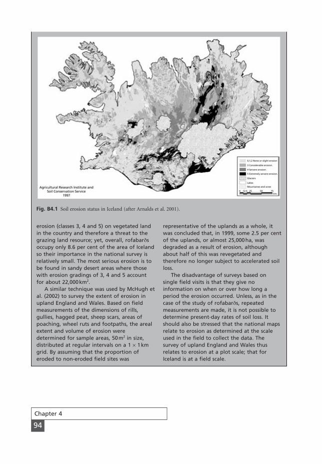
Chapter 4
94
erosion (classes 3, 4 and 5) on vegetated landin the country and therefore a threat to thegrazing land resource; yet, overall, rofabarQsoccupy only 8.6 per cent of the area of Icelandso their importance in the national survey isrelatively small. The most serious erosion is tobe found in sandy desert areas where thosewith erosion gradings of 3, 4 and 5 accountfor about 22,000km2.
A similar technique was used by McHugh etal. (2002) to survey the extent of erosion inupland England and Wales. Based on fieldmeasurements of the dimensions of rills,gullies, hagged peat, sheep scars, areas ofpoaching, wheel ruts and footpaths, the arealextent and volume of erosion weredetermined for sample areas, 50m2 in size,distributed at regular intervals on a 1 ¥ 1kmgrid. By assuming that the proportion oferoded to non-eroded field sites was
representative of the uplands as a whole, itwas concluded that, in 1999, some 2.5 per centof the uplands, or almost 25,000ha, wasdegraded as a result of erosion, althoughabout half of this was revegetated andtherefore no longer subject to accelerated soilloss.
The disadvantage of surveys based onsingle field visits is that they give noinformation on when or over how long aperiod the erosion occurred. Unless, as in thecase of the study of rofabarQs, repeatedmeasurements are made, it is not possible todetermine present-day rates of soil loss. Itshould also be stressed that the national mapsrelate to erosion as determined at the scaleused in the field to collect the data. Thesurvey of upland England and Wales thusrelates to erosion at a plot scale; that forIceland is at a field scale.
Fig. B4.1 Soil erosion status in Iceland (after Arnalds et al. 2001).
MSE04 11/19/04 02:34 PM Page 94
Measurement of soil erosion
95
Data on soil erosion and its controlling factors can be collected in the field or, for simulated con-ditions, in the laboratory. Whether field or laboratory studies are used depends on the objective.For realistic data on soil loss, field measurements are the most reliable, but because conditionsvary in both time and space, it is often difficult to determine the chief causes of erosion or tounderstand the processes at work. Experiments designed to lead to explanation are best under-taken in the laboratory, where the effects of many factors can be controlled. Because of the arti-ficiality of laboratory experiments, however, some confirmation of their results in the field isdesirable.
CHAPTER 5
Measurementof soil erosion
5.1
Experimental design
Experiments are usually carried out to assess the influence of one or more factors on the rate of erosion. In a simple experiment to study the effect of slope steepness, it is assumed that allother factors likely to influence erosion are held constant. The study is carried out by repeatingan experiment for different slope steepnesses. Decisions are necessary on the range of steepnesses,the specific steepnesses within the range and whether these should reflect some regular progres-sion, e.g. 2°, 4°, 6°, rising in intervals of 2°, or 5°48¢, 11°36¢, 17°30¢, rising in intervals of 0.1 sinevalues. The range can be selected to cover the most common slope steepnesses or extended to include extreme conditions. A decision is also needed on what levels to set for the factors being held constant, e.g. whether slope length should be 5 or 50 m, or the rainfall intensity 20 or200 mm h-1.
Measurements are subject to error. Since no single measurement of soil loss can be consid-ered as the absolutely correct value, it is virtually impossible to quantify errors. However, they canbe assessed in respect of variability. This requires replicating the experiment several times to deter-mine the mean value of soil loss – for example, for a given slope steepness in the above experi-ment – and the coefficient of variation of the data. This is frequently rather high. In a review offield and laboratory studies of soil erosion by rainsplash and overland flow, Luk (1981) foundtypical values of 13–40 per cent for the coefficient of variation. Extreme values of soil loss rangedfrom ±39 to ±120 per cent. To achieve a measurement of soil loss to an accuracy of ±10 per centwith 95 per cent confidence for three different Canadian soils required six, 25 and 29 replications
MSE05 11/19/04 02:36 PM Page 95
of the experiment respectively. A decision therefore needs to be made between carrying outbetween five and ten replications and accepting data with a coefficient of variation of generallybetween 20 and 30 per cent or completing 30 or more replications to obtain a more accurate mea-surement. Generally, the variability in field measurement is higher than that in laboratory studies.Roels and Jonker (1985) found coefficients of variation of 20–68 per cent in measurement ofinterrill erosion using unbounded runoff plots. The higher variability reflects the often highlylocalized variations in soil conditions, particularly infiltration and cohesion, that occur in thefield, whereas in the laboratory, the soils are often processed by drying and sieving to give greatercontrol over experimental conditions.
Systematic errors can be built into an experiment – for example, by starting the study of slopesteepness effects on the gentlest slope, carrying out the rest of the study in a sequence of increas-ing slope steepness and following the same procedure for all the replications. In this way, the soilloss measured at a particular steepness is influenced consistently by the amount of erosion thathas taken place on the next lowest slope steepness in the sequence. Remaking the soil surfacebetween the separate runs of the experiment may not entirely eliminate this effect. Strictly, theorder of the runs should be randomized but there is often a need to balance randomization withexpediency and conduct some runs in sequence where it is very time-consuming to keep switch-ing operating conditions. For instance, in a study involving simulated rainfall of several intensi-ties, it is expedient to complete all the runs at one intensity before proceeding to the next becauseof the problems encountered in continually altering the settings of the rainfall simulator. It mustbe appreciated, however, that failure to randomize an experiment may limit the use that can be made of statistical techniques in processing the data. Certain techniques, such as two-wayanalysis of variance, assume randomness in the data.
With the simple slope steepness experiment outlined above, the experimental design can bedescribed as examining the effect of one variable (slope steepness) with, say, five treatments (2,4, 6, 8 and 10°) and three replications, giving a total of 15 separate runs. These can be arrangedin a random sequence, either in time if the experiment is carried out in the laboratory, or in spaceif the experiment is set up in the field. Many experiments, however, are designed to investigatethe effects of more than one factor – for example, the effect of slope steepness at two differentrainfall intensities. The design then becomes one of two variables, slope with five treatments andrainfall intensity with two treatments, giving a total of ten different treatments. With three repli-cations, this gives a total of 30 separate runs. These can be organized in a completely randomsequence or, for the reasons of expediency indicated above, in two blocks, one for each rainfallintensity, with the slope treatments randomized within each block. The resulting data can thenbe analysed to compare treatment means across two blocks for all ten treatments and also tocompare block means. Block randomized experiments are particularly useful in the field when,for example, an investigation of the effects of four different land management systems might takeup so much land that the results are affected by variability in soil conditions (Fig. 5.1). In thiscase, if three replications are used, they could be set up as three separate blocks, with the treat-ments randomized in their position within each block. In many field situations, variations mayoccur in more than one factor across an experimental site – for example, soil may change acrossthe slope and slope steepness may change down the slope. In this situation, the four land man-agement treatments could be organized on a Latin square design with each treatment located ran-domly in both across-slope and downslope directions. The results would be analysed to compareacross-slope means and downslope means as well as treatment means (Fig. 5.1; Mead & Curnow1983). In theory, no limits exist on the number of factors that may be incorporated in an exper-iment. In practice, the size and design of the experiment are usually limited by the amount oftime and money available.
Chapter 5
96
MSE05 11/19/04 02:36 PM Page 96
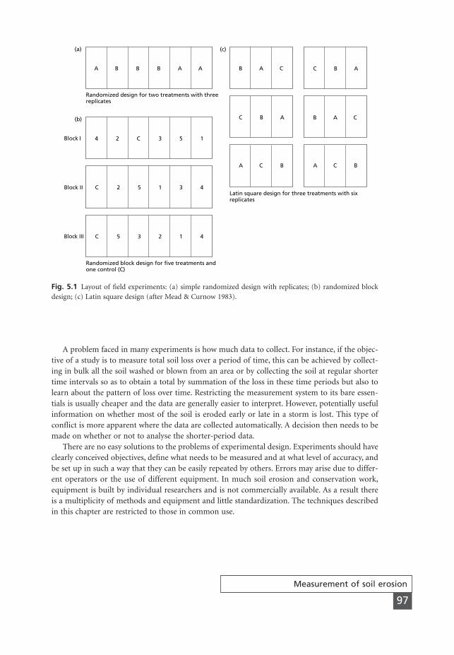
Measurement of soil erosion
97
A problem faced in many experiments is how much data to collect. For instance, if the objec-tive of a study is to measure total soil loss over a period of time, this can be achieved by collect-ing in bulk all the soil washed or blown from an area or by collecting the soil at regular shortertime intervals so as to obtain a total by summation of the loss in these time periods but also tolearn about the pattern of loss over time. Restricting the measurement system to its bare essen-tials is usually cheaper and the data are generally easier to interpret. However, potentially usefulinformation on whether most of the soil is eroded early or late in a storm is lost. This type ofconflict is more apparent where the data are collected automatically. A decision then needs to bemade on whether or not to analyse the shorter-period data.
There are no easy solutions to the problems of experimental design. Experiments should haveclearly conceived objectives, define what needs to be measured and at what level of accuracy, andbe set up in such a way that they can be easily repeated by others. Errors may arise due to differ-ent operators or the use of different equipment. In much soil erosion and conservation work,equipment is built by individual researchers and is not commercially available. As a result thereis a multiplicity of methods and equipment and little standardization. The techniques describedin this chapter are restricted to those in common use.
A B B B A A
C 2 5 1 3 4
C 5 3 2 1 4
4 2 C 3 5 1
B A C
C B A
A C B
C B A
B A C
A C B
(a)
(b)
Block I
Block II
Block III
(c)
Randomized design for two treatments with three replicates
Randomized block design for five treatments and one control (C)
Latin square design for three treatments with six replicates
Fig. 5.1 Layout of field experiments: (a) simple randomized design with replicates; (b) randomized blockdesign; (c) Latin square design (after Mead & Curnow 1983).
MSE05 11/19/04 02:36 PM Page 97
Chapter 5
98
5.2
Field measurements and experiments
Field measurements may be classified into two groups: those designed to determine soil loss fromrelatively small sample areas or erosion plots, often as part of an experiment, and those designedto assess erosion over a larger area, such as a drainage basin.
5.2.1 Erosion plots
Bounded plots
Bounded plots are employed at permanent research or experimental stations to study the factorsaffecting erosion. Each plot is a physically isolated piece of land of known size, slope steepness,slope length and soil type from which both runoff and soil loss are monitored. The number of plots depends upon the purpose of the experiment but usually allows for at least two replicates.
The standard plot is 22 m long and 1.8 m wide, although other plot sizes are sometimes used.The plot edges are made of sheet metal, wood or any material that is stable, does not leak and isnot liable to rust. The edges should extend 150–200 mm above the soil surface and be embeddedin the soil to a sufficient depth so as not to be shifted by alternate wetting-and-drying or freez-ing-and-thawing of the soil. At the downslope end is positioned a collecting trough or gutter,covered with a lid to prevent the direct entry of rainfall, from which sediment and runoff arechannelled into collecting tanks. For large plots or where runoff volumes are very high, the over-flow from a first collecting tank is passed through a divisor, which splits the flow into equal partsand passes one part, as a sample, into a second collecting tank (Fig. 5.2). Examples are the Geibmultislot divisor and the Coshocton wheel. On some plots, prior to passing into the first collect-ing tank, the runoff is channelled through a flume where the discharge is automatically moni-tored. Normally an H-flume is chosen because it is non-silting and unlikely to become blockedwith debris. A further automation is to install an automatic sediment sampler to extract samplesof the runoff at regular time intervals during the storm for later analysis of its sediment concen-tration; the time each sample is taken is also recorded. Rainfall is measured with both standardand autographic gauges adjacent to the plots.
A flocculating agent is added to the mixture of water and sediment collected in each tank. Thesoil settles to the bottom of the tank, and the clear water is then drawn off and measured. Thevolume of soil remaining in the tank is determined and samples of known volume are taken fordrying and weighing. The mean sample weight multiplied by the total volume gives the totalweight of soil in the tank. If all the soil has been collected in the tank, this gives the total soil lossfrom the plot. For tanks below a divisor, the weight of the soil in the tank needs to be adjustedin accordance with the proportion of the total runoff and sediment passing into the tank. Thusfor the layout shown in Fig. 5.2, the total soil loss from the plot is the weight of the soil in thefirst tank plus, assuming one-fifth of the overflow passes through the divisor into the second tank,five times the weight of soil in the second tank. Where automatic sediment sampling occurs, thesediment concentration is determined for each sample. Since the time when each sample wastaken during the storm is known, the data can be integrated over time to give a sediment graph.Full details of the equipment, manufacturing instructions for the divisors and operation oferosion plots are found in Agricultural Handbook No. 224 of the United States Department ofAgriculture (1979) and in Hudson (1993a).
MSE05 11/19/04 02:36 PM Page 98
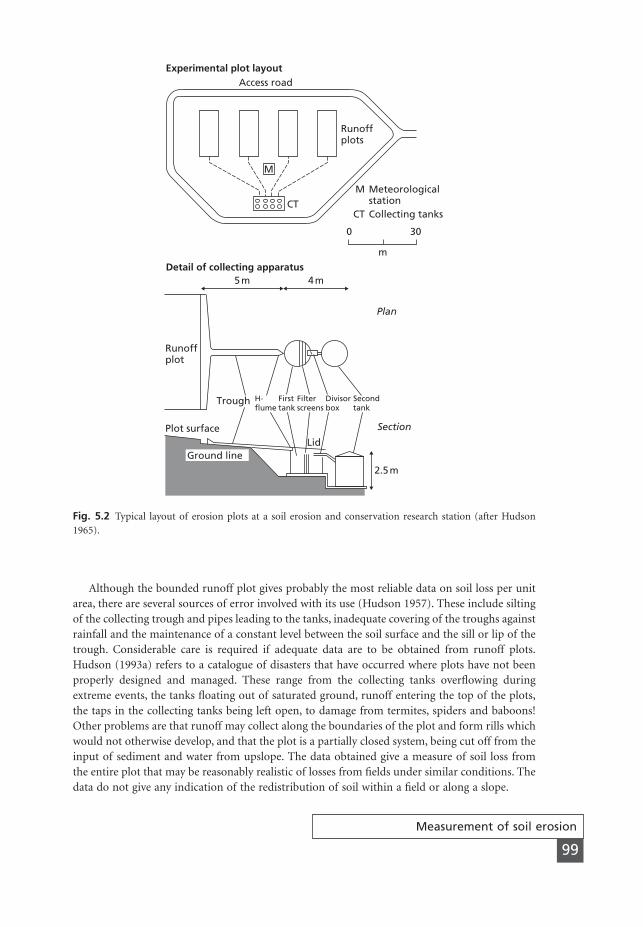
Measurement of soil erosion
99
Although the bounded runoff plot gives probably the most reliable data on soil loss per unitarea, there are several sources of error involved with its use (Hudson 1957). These include siltingof the collecting trough and pipes leading to the tanks, inadequate covering of the troughs againstrainfall and the maintenance of a constant level between the soil surface and the sill or lip of thetrough. Considerable care is required if adequate data are to be obtained from runoff plots.Hudson (1993a) refers to a catalogue of disasters that have occurred where plots have not beenproperly designed and managed. These range from the collecting tanks overflowing duringextreme events, the tanks floating out of saturated ground, runoff entering the top of the plots,the taps in the collecting tanks being left open, to damage from termites, spiders and baboons!Other problems are that runoff may collect along the boundaries of the plot and form rills whichwould not otherwise develop, and that the plot is a partially closed system, being cut off from theinput of sediment and water from upslope. The data obtained give a measure of soil loss fromthe entire plot that may be reasonably realistic of losses from fields under similar conditions. Thedata do not give any indication of the redistribution of soil within a field or along a slope.
Access road
M
0 30
m
5 m 4 m
CT
Runoffplots
Experimental plot layout
Detail of collecting apparatus
Meteorologicalstation
Runoffplot
Plot surface
Plan
Section
Collecting tanks
M
CT
Trough
Ground lineLid
Divisorbox
Secondtank
Filterscreens
Firsttank
H-flume
2.5 m
Fig. 5.2 Typical layout of erosion plots at a soil erosion and conservation research station (after Hudson1965).
MSE05 11/19/04 02:36 PM Page 99
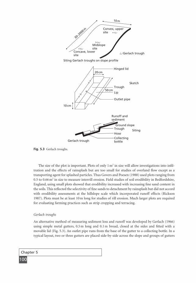
Chapter 5
100
The size of the plot is important. Plots of only 1 m2 in size will allow investigations into infil-tration and the effects of rainsplash but are too small for studies of overland flow except as atransporting agent for splashed particles. Thus Govers and Poesen (1988) used plots ranging from0.5 to 0.66 m2 in size to measure interrill erosion. Field studies of soil erodibility in Bedfordshire,England, using small plots showed that erodibility increased with increasing fine sand content inthe soils. This reflected the selectivity of fine sands to detachment by rainsplash but did not accordwith erodibility assessments at the hillslope scale which incorporated runoff effects (Rickson1987). Plots must be at least 10 m long for studies of rill erosion. Much larger plots are requiredfor evaluating farming practices such as strip cropping and terracing.
Gerlach troughs
An alternative method of measuring sediment loss and runoff was developed by Gerlach (1966)using simple metal gutters, 0.5 m long and 0.1 m broad, closed at the sides and fitted with amovable lid (Fig. 5.3). An outlet pipe runs from the base of the gutter to a collecting bottle. In atypical layout, two or three gutters are placed side-by-side across the slope and groups of gutters
Convex, uppersite
Concave, lowersite Gerlach trough
Hinged lid
SketchTrough
Lip
Outlet pipe
Runoff andsediment
Ground slopeTrough
Hose
Collectingbottle
Siting
Midslopesite
Gerlach trough
10 cm
10 m
20 cm
50 cm
Siting Gerlach troughs on slope profile
30–2
000 m
Fig. 5.3 Gerlach troughs.
MSE05 11/19/04 02:36 PM Page 100
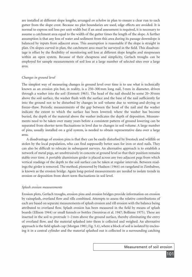
Measurement of soil erosion
101
are installed at different slope lengths, arranged en echelon in plan to ensure a clear run to eachgutter from the slope crest. Because no plot boundaries are used, edge effects are avoided. It isnormal to express soil loss per unit width but if an areal assessment is required, it is necessary toassume a catchment area equal to the width of the gutter times the length of the slope. A furtherassumption is that any loss of water and sediment from this area during its passage downslope isbalanced by inputs from adjacent areas. This assumption is reasonable if the slope is straight inplan. On slopes curved in plan, the catchment area must be surveyed in the field. This disadvan-tage is offset by the flexibility of monitoring soil loss at different slope lengths and steepnesseswithin an open system. Because of their cheapness and simplicity, Gerlach troughs can beemployed for sample measurements of soil loss at a large number of selected sites over a largearea.
Changes in ground level
The simplest way of measuring changes in ground level over time is to use what is technicallyknown as an erosion pin but, in reality, is a 250–300 mm long nail, 5 mm in diameter, driventhrough a washer into the soil (Emmett 1965). The head of the nail should be some 20–30 mmabove the soil surface, the washer flush with the surface and the base of the nail sufficiently farinto the ground not to be disturbed by changes in soil volume due to wetting-and-drying orfreeze–thaw. Periodic measurements of the gap between the head of the nail and the washer indicate the extent to which the surface has been lowered; where the washer has become buried, the depth of the material above the washer indicates the depth of deposition. Measure-ments need to be taken over many years before a consistent pattern of ground lowering can beseparated from shorter-term fluctuations in level due to changes in soil volume. A large numberof pins, usually installed on a grid system, is needed to obtain representative data over a largearea.
A disadvantage of erosion pins is that they can be easily disturbed by livestock and wildlife orstolen by the local population, who can find supposedly better uses for iron or steel nails. Theycan also be difficult to relocate in subsequent surveys. An alternative approach is to establish anetwork of metal pegs, set unobtrusively in concrete at ground level so that their position remainsstable over time. A portable aluminium girder is placed across any two adjacent pegs from whichvertical readings of the depth to the soil surface can be taken at regular intervals. Between read-ings the girder is removed. The method, pioneered by Hudson (1964) on rangeland in Zimbabwe,is known as the erosion bridge. Again long-period measurements are needed to isolate trends inerosion or deposition from short-term fluctuations in soil level.
Splash erosion measurements
Erosion plots, Gerlach troughs, erosion pins and erosion bridges provide information on erosionby rainsplash, overland flow and rills combined. Attempts to assess the relative contributions ofeach are based on separate measurements of splash erosion and rill erosion with the balance beingattributed to overland flow. Splash erosion has been measured in the field by means of splashboards (Ellison 1944) or small funnels or bottles (Sreenivas et al. 1947; Bollinne 1975). These areinserted in the soil to protrude 1–2 mm above the ground surface, thereby eliminating the entryof overland flow, and the material splashed into them is collected and weighed. An alternativeapproach is the field splash cup (Morgan 1981; Fig. 5.4), where a block of soil is isolated by enclos-ing it in a central cylinder and the material splashed out is collected in a surrounding catching
MSE05 11/19/04 02:36 PM Page 101
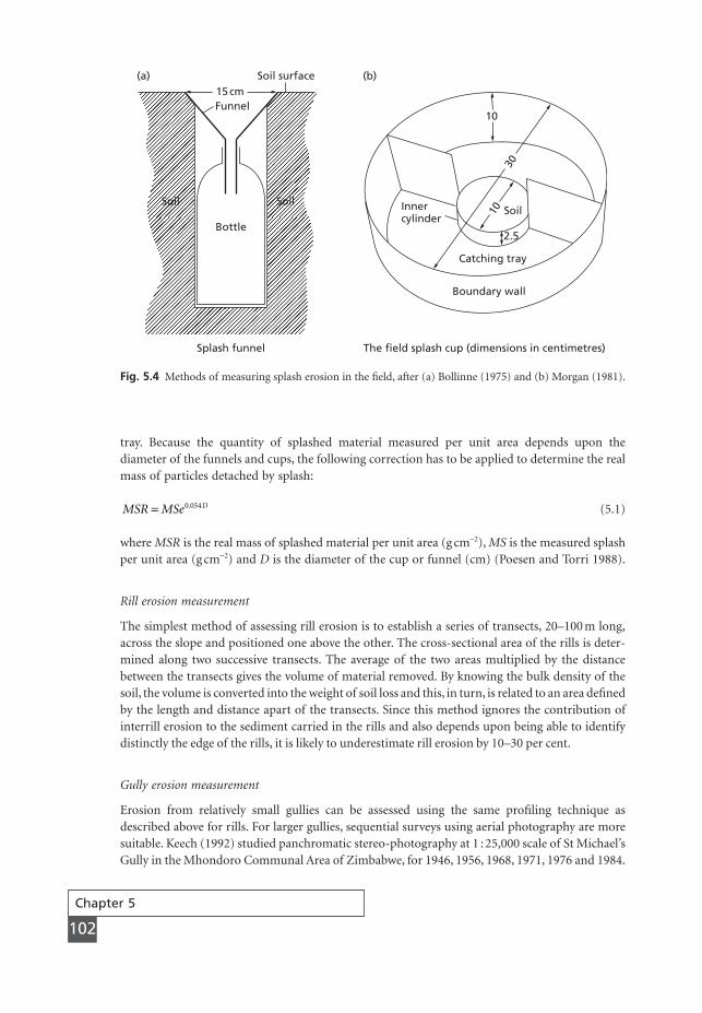
Chapter 5
102
tray. Because the quantity of splashed material measured per unit area depends upon the diameter of the funnels and cups, the following correction has to be applied to determine the realmass of particles detached by splash:
(5.1)
where MSR is the real mass of splashed material per unit area (g cm-2), MS is the measured splashper unit area (g cm-2) and D is the diameter of the cup or funnel (cm) (Poesen and Torri 1988).
Rill erosion measurement
The simplest method of assessing rill erosion is to establish a series of transects, 20–100 m long,across the slope and positioned one above the other. The cross-sectional area of the rills is deter-mined along two successive transects. The average of the two areas multiplied by the distancebetween the transects gives the volume of material removed. By knowing the bulk density of thesoil, the volume is converted into the weight of soil loss and this, in turn, is related to an area definedby the length and distance apart of the transects. Since this method ignores the contribution ofinterrill erosion to the sediment carried in the rills and also depends upon being able to identify distinctly the edge of the rills, it is likely to underestimate rill erosion by 10–30 per cent.
Gully erosion measurement
Erosion from relatively small gullies can be assessed using the same profiling technique asdescribed above for rills. For larger gullies, sequential surveys using aerial photography are moresuitable. Keech (1992) studied panchromatic stereo-photography at 1 : 25,000 scale of St Michael’sGully in the Mhondoro Communal Area of Zimbabwe, for 1946, 1956, 1968, 1971, 1976 and 1984.
MSR MSe D= 0 054.
Soil surface(a) (b)
Funnel
Bottle
Splash funnel The field splash cup (dimensions in centimetres)
Boundary wall
Catching tray
Innercylinder
10
1030
Soil
2.5
Soil Soil
15 cm
Fig. 5.4 Methods of measuring splash erosion in the field, after (a) Bollinne (1975) and (b) Morgan (1981).
MSE05 11/19/04 02:36 PM Page 102
Using a stereoplotter, a stereomodel of the gully was set up for each year of survey using hori-zontal and vertical controls taken from 1 : 50,000 scale topographical maps. Difficulty was expe-rienced in deciding where the up-slope boundary of the gully should be drawn and then ininterpreting that boundary consistently along the periphery of the gully on the different sets ofphotography. Once a working procedure was established, the position of the edge of the gully wasplotted for the different dates. Some 126 points or nodes were then identified along the definedmargin on the 1946 photography, against which changes in position could be measured. Usingthe plotting machine to read off heights, cross-sections of the gully were determined at intervalsdown the gully. From this information, the extent of retreat of the gully headwall and side wallsand the volume of material removed from the gully between different dates were calculated.More recent surveys of gullies use large-scale (1 : 10,000) aerial photography to construct high-resolution digital elevation models (DEMs). Rates of gully erosion are calculated from differencesin elevation between DEMs of different dates (De Rose et al. 1998; Betts et al. 2003). Digitallygenerated DEMs can match the accuracy of traditional analytical photogrammetric techniquesand are much faster to produce (Baily et al. 2003).
5.2.2 Catchments
Sediment yield
The sediment yield of a catchment is obtained from measurements of the quantity of sedimentleaving a catchment along the river over time. Recording stations are established at the exit pointfor the automatic measurement of discharge, using weirs and depth recorders, and suspendedsediment concentrations in the river water. Water samples are taken at set times with speciallydesigned integrated sediment samplers, or the sediment concentration is monitored continuouslyby recording the turbidity of the water. Bucket samples are not recommended because theycontain only the surface water and cannot provide information on the sediment being transportedthroughout the depth and width of the river channel. With measurements made at set times, thereis a need to extrapolate the data to cover the period between samples. The standard approach isto establish a sediment discharge rating curve in which the sediment concentration (C) is relatedto the water discharge (Q) by the equation:
(5.2)
The accuracy of this method is highly dependent on the frequency of sampling. Walling et al.(1992) compared results from regular 7-day, 14-day and 28-day sampling programmes of sus-pended sediment load in the River Exe, Devon, England over a two-year period, with results fromcontinuous sampling using a turbidity recorder. Estimates of the sediment load were found tovary between 10 and 300 per cent of that obtained from continuous monitoring. The likelihoodof underestimation increased as the sampling frequency decreased, since, with longer samplingintervals, the record is likely to include fewer flood events. Monthly sampling for estimatingannual sediment yield of larger catchments, 1000–3000 km2 in size, can result in underestima-tions of 60–80 per cent (Phillips et al. 1999). Of course, it should be recognized that the turbid-ity meter does not give a true record because the measurements are subject to errors associatedwith the influence of the particle size of the sediment load, the magnitude of the sediment con-centration, the presence of organic matter and the need to keep the sensors clear of algae. Despitethese problems, the method is currently the best available to provide estimates of suspended sediment yield, especially if high frequency data are needed. It should be recognized, however,
C aQb=
Measurement of soil erosion
103
MSE05 11/19/04 02:36 PM Page 103
that, because of the need for regular calibration and maintenance, such data come at greater costcompared to using rating curves.
Reservoir surveys
Sedimentation rates in lakes and reservoirs can indicate how much erosion has taken place in acatchment upstream, provided the efficiency of the reservoir as a sediment trap is known. Rappet al. (1972b) used repeated surveys of designated transects across four reservoirs in the Dodomaregion of Tanzania in relation to a set level or benchmark. Using manual soundings of depth froma boat, a contour map was made of the bottom of the reservoir. The volume of the reservoir wasobtained by adding up the partial volumes (V):
(5.3)
where V is the volume of sediment (m3), h is the upper contour interval (m), A is the area of theupper contour (m2) and B is the area of the lower contour interval (m2). To this total, the volumebelow the lowest contour was added, calculated as the product of the area of the lowest contourand the mean depth to that contour from the bottom. The reservoir volume was then comparedwith the initial volume. The reduction in volume represents the volume of sediment accumulatedin the reservoir. Assuming an average dry bulk density of 1.5 Mg m-3, the volume was convertedinto a mass and divided by the area of the catchment upstream to give an erosion value in t ha-1. This was further adjusted by assuming that the sediment in the reservoir represented abouthalf that eroded from the catchment. Dividing the adjusted total by the number of years since thereservoir was built gave a mean annual erosion rate. More rapid reservoir surveys can be madeusing an echo-sounder to obtain depth readings, an electro-distance measuring theodolite or lasertheodolite to fix the position of the sounding, and a digital elevation model (DEM) to producethe contour map (Brabben et al. 1988). Sedimentation rates in farm ponds can be analysed usinga similar methodology (Verstraeten & Poesen 2001).
Potential sources of error are quite high with reservoir surveys, the most important being theestimate of the trap efficiency of the reservoir, which requires knowledge of the frequency andsediment concentration of flows carried over the spillway in times of flood and errors arising incalculating the capacity of the reservoir. Even small errors in the latter may give rise to errors upto two orders of magnitude in determining the volume of deposited material. Care is also requiredto ensure that the source of sediment is from erosion in the contributing catchment. For manysmall reservoirs in south-east Australia, up to 85 per cent of the sediment comes from tramplingof the shoreline by cattle (Lloyd et al. 1998). Compared with data from suspended sediment con-centrations, the data from reservoir surveys incorporate material transported as bed load as wellas suspended sediment.
Tracers
The most commonly used tracer in soil erosion measurement is the radioactive isotope, caesium-137 (137Cs). Caesium-137 was produced in the fall-out of atmospheric testing of nuclear weaponsfrom the 1950s to 1970s. It was distributed globally in the stratosphere and deposited on the earth’ssurface in the rainfall. Regionally, the amount deposited varies with the amount of rain but, withinsmall areas, the deposition is reasonably uniform. The isotope is strongly and quickly adsorbed to clay particles within the soil. By analysing the isotope content of soil cores collected on a grid system varying in density from 10 ¥ 10 to 20 ¥ 20 m, the spatial pattern of isotope loading is
V h A B= +( ) 2
Chapter 5
104
MSE05 11/19/04 02:36 PM Page 104
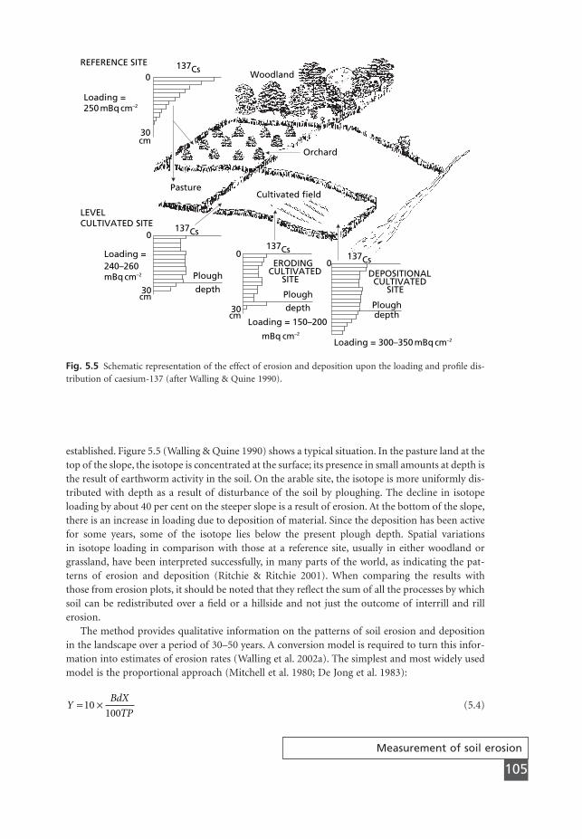
Measurement of soil erosion
105
established. Figure 5.5 (Walling & Quine 1990) shows a typical situation. In the pasture land at thetop of the slope, the isotope is concentrated at the surface; its presence in small amounts at depth isthe result of earthworm activity in the soil. On the arable site, the isotope is more uniformly dis-tributed with depth as a result of disturbance of the soil by ploughing. The decline in isotopeloading by about 40 per cent on the steeper slope is a result of erosion. At the bottom of the slope,there is an increase in loading due to deposition of material. Since the deposition has been activefor some years, some of the isotope lies below the present plough depth. Spatial variations in isotope loading in comparison with those at a reference site, usually in either woodland or grassland, have been interpreted successfully, in many parts of the world, as indicating the pat-terns of erosion and deposition (Ritchie & Ritchie 2001). When comparing the results with those from erosion plots, it should be noted that they reflect the sum of all the processes by whichsoil can be redistributed over a field or a hillside and not just the outcome of interrill and rillerosion.
The method provides qualitative information on the patterns of soil erosion and depositionin the landscape over a period of 30–50 years. A conversion model is required to turn this infor-mation into estimates of erosion rates (Walling et al. 2002a). The simplest and most widely usedmodel is the proportional approach (Mitchell et al. 1980; De Jong et al. 1983):
(5.4)YBdX
TP= ¥10
100
REFERENCE SITE
Loading = 250 mBq cm–2
0
30cm
137Cs
137Cs
137Cs137Cs
0
30cm
Plough
depth
LEVELCULTIVATED SITE
Pasture
Orchard
Cultivated field
Loading = 240–260mBq cm–2
0
30cm
Plough
depth
0
Ploughdepth
Woodland
Loading = 150–200
mBq cm–2
Loading = 300–350 mBq cm–2
ERODINGCULTIVATED
SITEDEPOSITIONALCULTIVATED
SITE
Fig. 5.5 Schematic representation of the effect of erosion and deposition upon the loading and profile dis-tribution of caesium-137 (after Walling & Quine 1990).
MSE05 11/19/04 02:36 PM Page 105
Chapter 5
106
where Y is mean annual soil loss (t ha-1 yr-1), B is the bulk density of the soil (kg m-3), d is thedepth of the plough or cultivated layer (m), T is the time that has elapsed since the start of theaccumulation of 137Cs and P is the ratio of the concentration of 137Cs in the mobilized sedimentto that in the original soil. The term X is the percentage reduction in the total 137Cs inventory relative to the reference value, i.e.
(5.5)
where Aref is the caesium loading at the reference site (Bq m-2) and A is the loading at the samplepoint. For sites of deposition, X is positive and P is the ratio of the concentration of 137Cs in thedeposited sediment to that in the mobilized sediment. The method tends to underestimate erosionrates because it does not take into account the dilution of 137Cs concentration on erosion sitesthrough the incorporation of soil from below the original plough depth.
An alternative approach is to develop a mass balance model based on the accumulation ordepletion of 137Cs through time as a result of erosion and deposition. The mass balance for aneroding site can be described by (Walling & He 1999a):
(5.6)
where A(t) is the 137Cs loading (Bq m-2), t is the time (years) since 137Cs fallout began, I(t) is the annual input of 137Cs from fallout at time t (Bq m-2 yr-1), l is the decay constant for 137Cs (= 0.023 y-1), R is the erosion rate (kg m-2 y-1) and dm is the average plough depth representedas a cumulative mass depth (kg m-2). For an eroding soil,
(5.7)
and for a depositional site,
(5.8)
where R¢ is the deposition rate (kg m-2 yr-1) and Cd (t¢) is the concentration of 137Cs in thedeposited sediment in year t¢ (Bq kg-1).
If, for the situation shown in Fig. 5.5, it is assumed that the data relate to 1990, the 137Cs loadingon the eroding cultivated site is 200 mBq cm-2, the bulk density of the soil is 1.4 Mg m-3 and P isequal to 2.0, a typical value (He & Walling 1996), the erosion rate is calculated at 22.9 t ha-1 yr-1.The proportional method yields 19.4 t ha-1 yr-1. If it is assumed for the depositional site that theloading is 300 mBq cm-2, the loading is distributed uniformly throughout the 25 cm plough depthto give a concentration of 2.5 Bq kg-1 and the conditions are unvarying from year to year, the depo-sition rate is calculated as 7.4 t ha-1 yr-1. Generally, soil erosion rates obtained using caesium-137compare well with measured rates from erosion plots and instrumented catchments(Theocharopoulos et al. 2003; Zhang et al. 2003).
Recent developments of the approach allow for the likelihood that some or all of the 137Csfallout will be removed by erosion before it can be adsorbed to the soil (Walling & He 1999a), as
¢ =( ) -
¢( ) ¢- - ¢( )ÚR
A t A
C t e dt
ref
dt t
t l1963
YdB
p
X t
= - -ÊË
ˆ¯
ÈÎÍ
˘˚˙
-( )10
1 1100
1 1963
dA t
dtI t
R
dA t
m
( )= ( ) - +Ê
ˈ¯ ( )l
XA A
Aref
ref
=-Ê
ËÁˆ¯
¥100
MSE05 11/19/04 02:36 PM Page 106
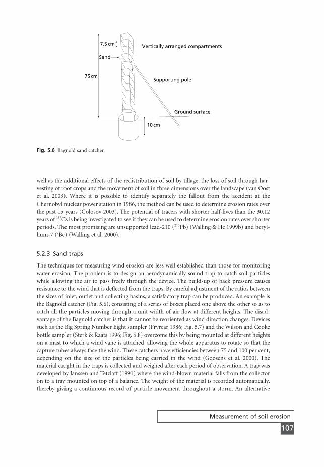
Measurement of soil erosion
107
well as the additional effects of the redistribution of soil by tillage, the loss of soil through har-vesting of root crops and the movement of soil in three dimensions over the landscape (van Oostet al. 2003). Where it is possible to identify separately the fallout from the accident at the Chernobyl nuclear power station in 1986, the method can be used to determine erosion rates overthe past 15 years (Golosov 2003). The potential of tracers with shorter half-lives than the 30.12years of 137Cs is being investigated to see if they can be used to determine erosion rates over shorterperiods. The most promising are unsupported lead-210 (210Pb) (Walling & He 1999b) and beryl-lium-7 (7Be) (Walling et al. 2000).
5.2.3 Sand traps
The techniques for measuring wind erosion are less well established than those for monitoringwater erosion. The problem is to design an aerodynamically sound trap to catch soil particleswhile allowing the air to pass freely through the device. The build-up of back pressure causesresistance to the wind that is deflected from the traps. By careful adjustment of the ratios betweenthe sizes of inlet, outlet and collecting basins, a satisfactory trap can be produced. An example isthe Bagnold catcher (Fig. 5.6), consisting of a series of boxes placed one above the other so as tocatch all the particles moving through a unit width of air flow at different heights. The disad-vantage of the Bagnold catcher is that it cannot be reoriented as wind direction changes. Devicessuch as the Big Spring Number Eight sampler (Fryrear 1986; Fig. 5.7) and the Wilson and Cookebottle sampler (Sterk & Raats 1996; Fig. 5.8) overcome this by being mounted at different heightson a mast to which a wind vane is attached, allowing the whole apparatus to rotate so that thecapture tubes always face the wind. These catchers have efficiencies between 75 and 100 per cent,depending on the size of the particles being carried in the wind (Goosens et al. 2000). The material caught in the traps is collected and weighed after each period of observation. A trap wasdeveloped by Janssen and Tetzlaff (1991) where the wind-blown material falls from the collectoron to a tray mounted on top of a balance. The weight of the material is recorded automatically,thereby giving a continuous record of particle movement throughout a storm. An alternative
75 cm
7.5 cm
10 cm
Ground surface
Supporting pole
Vertically arranged compartments
Sand
Fig. 5.6 Bagnold sand catcher.
MSE05 11/19/04 02:36 PM Page 107
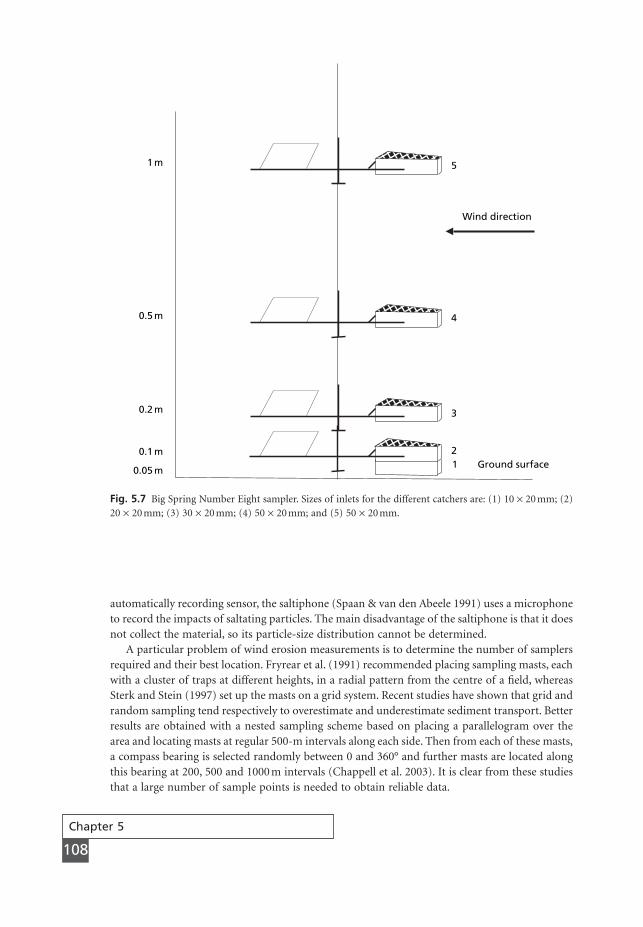
Chapter 5
108
automatically recording sensor, the saltiphone (Spaan & van den Abeele 1991) uses a microphoneto record the impacts of saltating particles. The main disadvantage of the saltiphone is that it doesnot collect the material, so its particle-size distribution cannot be determined.
A particular problem of wind erosion measurements is to determine the number of samplersrequired and their best location. Fryrear et al. (1991) recommended placing sampling masts, eachwith a cluster of traps at different heights, in a radial pattern from the centre of a field, whereasSterk and Stein (1997) set up the masts on a grid system. Recent studies have shown that grid andrandom sampling tend respectively to overestimate and underestimate sediment transport. Betterresults are obtained with a nested sampling scheme based on placing a parallelogram over thearea and locating masts at regular 500-m intervals along each side. Then from each of these masts,a compass bearing is selected randomly between 0 and 360° and further masts are located alongthis bearing at 200, 500 and 1000 m intervals (Chappell et al. 2003). It is clear from these studiesthat a large number of sample points is needed to obtain reliable data.
1 m
0.5 m
0.2 m
0.1 m
0.05 m
5
4
3
21 Ground surface
Wind direction
Fig. 5.7 Big Spring Number Eight sampler. Sizes of inlets for the different catchers are: (1) 10 ¥ 20 mm; (2)20 ¥ 20 mm; (3) 30 ¥ 20 mm; (4) 50 ¥ 20 mm; and (5) 50 ¥ 20 mm.
MSE05 11/19/04 02:36 PM Page 108
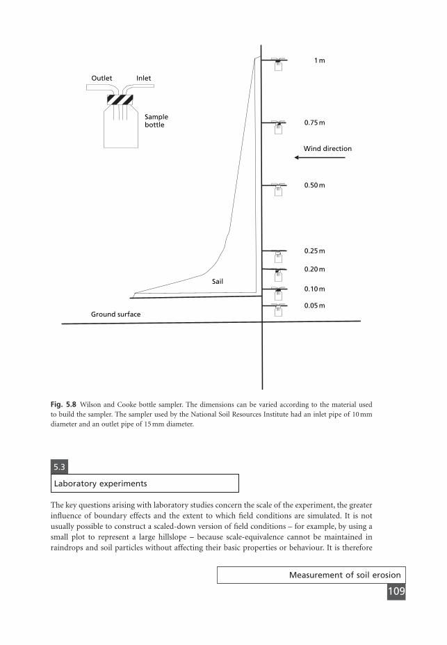
Measurement of soil erosion
109
Outlet Inlet
Samplebottle
Sail
Ground surface
1 m
0.75 m
0.50 m
0.25 m
0.20 m
0.10 m
0.05 m
Wind direction
Fig. 5.8 Wilson and Cooke bottle sampler. The dimensions can be varied according to the material used to build the sampler. The sampler used by the National Soil Resources Institute had an inlet pipe of 10 mmdiameter and an outlet pipe of 15 mm diameter.
5.3
Laboratory experiments
The key questions arising with laboratory studies concern the scale of the experiment, the greaterinfluence of boundary effects and the extent to which field conditions are simulated. It is notusually possible to construct a scaled-down version of field conditions – for example, by using asmall plot to represent a large hillslope – because scale-equivalence cannot be maintained in raindrops and soil particles without affecting their basic properties or behaviour. It is therefore
MSE05 11/19/04 02:36 PM Page 109
preferable to treat laboratory experiments as representing true-to-scale field simulation. Even so,many factors cannot be properly simulated and, unless the laboratory facilities are very large, norcan processes such as rill erosion and the saltation of soil particles by wind.
5.3.1 Rainfall simulation
Many laboratory studies centre on the use of a rainfall simulator, which is designed to produce astorm of known energy, intensity and drop-size characteristics that can be repeated on demand.The most important design requirements of a simulator are that it should reproduce the drop-size distribution, drop velocity at impact and intensity of natural rainfall with a uniform spatialdistribution and that these conditions should be repeatable. The need to reproduce the energy ofthe natural rainfall for the intensity being simulated is generally regarded as less important(Bubenzer 1979).
Rainfall simulators are classified according to the drop-formers used. The most common aretubing tips, either hypodermic needles or capillary tubes (De Ploey et al. 1976) and nozzles (Morinet al. 1967). None accurately recreates all the properties of natural rain (Hall 1970). There is insuf-ficient height in most laboratories for water drops to achieve terminal velocity during fall, so theirkinetic energy is low. To overcome this, water is released from low heights under pressure. Thisresults in too high an intensity and, because the increase in pressure produces small drop sizes,unrealistic drop-size distributions. The intensity can be brought down by reducing the frequencyof rain striking the target area, either by oscillating the spray over the target or by intermittentlyshielding the target from the spray. It should be noted, however, that this only reduces the inten-sity measured as the amount of water applied over a given time period; the instantaneous inten-sity and impact energy of the simulated rain are not reduced. True spatial uniformity is alsovirtually impossible to achieve.
Studies of splash erosion are made in the laboratory by filling containers with soil, weighingthem dry, subjecting them to a simulated rainstorm of pre-selected intensity and measuring theweight loss from the containers on drying. In this way different soils can be compared for theirdetachability. The standard container is the splash cup first used by Ellison (1944), a brass cylin-der 77 mm in diameter and 50 mm deep with a wire mesh base. A thin layer of cotton wool orsponge rubber is placed in the bottom of the cup, which is then filled with the soil, oven dried to a constant weight and weighed. The soil in the cup is brought to saturation prior to rainfallsimulation. The soil level in the cup needs to be a few millimetres below the rim, as otherwise theerosion is accelerated by material washing off the surface during the early part of the storm(Mazurak & Mosher 1968); this effect can be enhanced if the initial raindrop impacts create apitted or rough surface or if the surface is too loosely packed (Kinnell 1974). Towards the end ofthe storm, the splash loss will be reduced because the level of the soil within the cup becomes toolow and splashed particles are intercepted by the rim of the cup (Bisal 1950).
Where several soils are being compared it is important to treat them all the same. Molden-hauer (1965) recommends collecting them from the field under uniform moisture conditions,achieved by flooding the surrounding area with 100 mm of water and covering it with polythenesheet for 48 hours before taking the sample. This gives a condition close to field capacity. Whenthe samples are brought back to the laboratory they should be dried to a constant weight andsplit into 200 g portions. These are poured into the splash cups uniformly, reversing the directionof pouring regularly so that all the large aggregates do not accumulate at one end. Differences inthe moisture content and surface distribution of stones and aggregates are the main reasons forthe high level of variability in measurements of splash erosion in laboratory experiments (Luk1981). Although the soils are free draining, their condition does not represent the field situation
Chapter 5
110
MSE05 11/19/04 02:36 PM Page 110
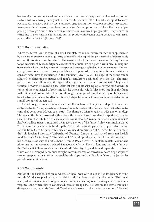
because they are uncompacted and not subject to suction. Attempts to simulate soil suction onsuch a small scale have generally not been successful and it is difficult to achieve repeatable com-paction. Fortunately, a soil in a loose saturated state is at its most erodible, so laboratory experi-ments reproduce the worst conditions for erosion. Further processing of the soil – for example,passing it through 4 mm or finer sieves to remove stones or break up aggregates – may reduce thevariability in the splash measurements but can produce misleading results compared with smallplot studies in the field (Rickson 1987).
5.3.2 Runoff simulation
Where the target is in the form of a small soil plot, the rainfall simulator may be supplementedby a device to supply a known quantity of runoff at the top of the plot, instead of relying solelyon runoff resulting from the rainfall. The set-up at the Experimental Geomorphology Labora-tory, University of Leuven, Belgium, consists of an aluminium and plexiglass flume, 4 m long and0.4 m wide, which is fed by water at its upper end through a cylinder with ten openings. The dis-charge is controlled by a tap through which water is pumped to the cylinder from a container; aconstant water level is maintained in the container (Savat 1975). The slope of the flume can beadjusted to different steepnesses and rainfall simulators positioned over the top. The mainproblem with a small flume of this type is that edge effects are difficult to eliminate. They can bereduced, however, by collecting the sediment and runoff washing off a narrow strip down thecentre of the plot instead of collecting for the whole plot width. The short length of the flumemakes it difficult to simulate rill erosion although the supply of runoff at the top of the slope canbe adjusted to simulate the effect of different slope lengths. Sediment can also be added to therunoff upslope of the test soil.
A much longer combined rainfall and runoff simulator with adjustable slope has been builtat the Centre for Geomorphology in Caen, France, to enable rill erosion to be investigated undercontrolled conditions (Govers et al. 1987). The flume is 20.4 m long, 1.4 m wide and 0.7 m deep.The base of the flume is covered with a 15-cm thick layer of gravel overlain by a perforated plasticsheet on top of which 40 cm thickness of test soil is placed. A rainfall simulator, comprising 644flexible capillary tubes, is mounted 1.7 m above the top of the flume. A fine wire-mesh is placed70 cm below the capillaries to break up the 2.9 mm diameter drops into a drop-size distributionranging from 0.6 to 4.6 mm, with a median volume drop diameter of 2.8 mm. The long flume inthe Soil Erosion Laboratory, University of Toronto, Canada, is constructed from ten flexiblemodules, each 2.45 m long, 0.85 m wide and 0.31 m deep, which can be tilted and combined toproduce slopes of varying profile shape (Bryan & Poesen 1989). A rainfall simulator comprisingnine cone-jet spray nozzles is placed 8 m above the flume. The 6 m long and 2 m wide flume atthe National Soil Resources Institute, Cranfield University, England, is made up of three modules,which can be arranged to produce straight, convex, concave or convexo-concave slope shapes ofvarying steepnesses or to form two straight side slopes and a valley floor. Nine cone-jet nozzlesprovide rainfall simulation.
5.3.3 Wind tunnels
Almost all the basic studies on wind erosion have been carried out in the laboratory in windtunnels. Wind is supplied by a fan that either sucks or blows air through the tunnel. The tunnelis shaped so that air enters through a honeycomb shield, serving as a flow straightener, into a con-vergence zone, where flow is constricted, passes through the test section and leaves through adivergence zone, in which flow is diffused. A mesh screen at the outlet traps most of the sand
Measurement of soil erosion
111
MSE05 11/19/04 02:36 PM Page 111
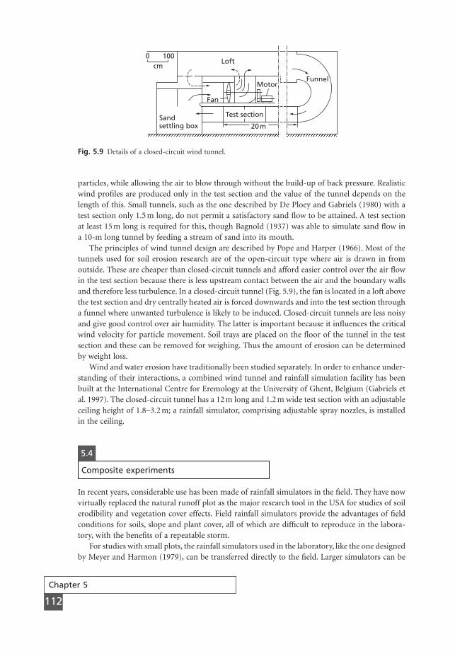
Chapter 5
112
particles, while allowing the air to blow through without the build-up of back pressure. Realisticwind profiles are produced only in the test section and the value of the tunnel depends on thelength of this. Small tunnels, such as the one described by De Ploey and Gabriels (1980) with atest section only 1.5 m long, do not permit a satisfactory sand flow to be attained. A test sectionat least 15 m long is required for this, though Bagnold (1937) was able to simulate sand flow ina 10-m long tunnel by feeding a stream of sand into its mouth.
The principles of wind tunnel design are described by Pope and Harper (1966). Most of thetunnels used for soil erosion research are of the open-circuit type where air is drawn in fromoutside. These are cheaper than closed-circuit tunnels and afford easier control over the air flowin the test section because there is less upstream contact between the air and the boundary wallsand therefore less turbulence. In a closed-circuit tunnel (Fig. 5.9), the fan is located in a loft abovethe test section and dry centrally heated air is forced downwards and into the test section througha funnel where unwanted turbulence is likely to be induced. Closed-circuit tunnels are less noisyand give good control over air humidity. The latter is important because it influences the criticalwind velocity for particle movement. Soil trays are placed on the floor of the tunnel in the testsection and these can be removed for weighing. Thus the amount of erosion can be determinedby weight loss.
Wind and water erosion have traditionally been studied separately. In order to enhance under-standing of their interactions, a combined wind tunnel and rainfall simulation facility has beenbuilt at the International Centre for Eremology at the University of Ghent, Belgium (Gabriels etal. 1997). The closed-circuit tunnel has a 12 m long and 1.2 m wide test section with an adjustableceiling height of 1.8–3.2 m; a rainfall simulator, comprising adjustable spray nozzles, is installedin the ceiling.
0 100Loft
cm
Fan
MotorFunnel
Test sectionSandsettling box 20 m
Fig. 5.9 Details of a closed-circuit wind tunnel.
5.4
Composite experiments
In recent years, considerable use has been made of rainfall simulators in the field. They have nowvirtually replaced the natural runoff plot as the major research tool in the USA for studies of soilerodibility and vegetation cover effects. Field rainfall simulators provide the advantages of fieldconditions for soils, slope and plant cover, all of which are difficult to reproduce in the labora-tory, with the benefits of a repeatable storm.
For studies with small plots, the rainfall simulators used in the laboratory, like the one designedby Meyer and Harmon (1979), can be transferred directly to the field. Larger simulators can be
MSE05 11/19/04 02:36 PM Page 112

Measurement of soil erosion
113
built by joining together modules of the smaller ones. Modules of a simulator built by Bazzoffiet al. (1980) have been combined to form a field simulator capable of covering a standard runoffplot (Zanchi et al. 1981). Alternatively, large-area simulators can be purpose-designed and built.The best example is the rotating-boom simulator (Swanson 1965) in which nozzles are mountedon a series of spray booms positioned radially from a central stem. The nozzles spray water froma height of 3 m and the booms rotate at four revolutions per minute to give a uniform distribu-tion of rain over a circular area large enough to accommodate two plots, 10 ¥ 4.3 m.
A major difficulty with field rainfall simulators is their limited portability, especially in diffi-cult terrain. Several designs for simple, portable simulators have been produced (Imeson 1977;Kamphorst 1987; Cerdà et al. 1997) with the ability to generate rainfall at intensities between 40and 120 mm h-1 with reasonably realistic drop-size distributions. However, their limited waterstorage and low height means that they produce only short duration storms of low energy. Theyalso cover very small plot sizes, often less than 1 m2.
Less use has been made of field wind tunnels partly because, as noted above, small ones, whichwould be the most portable, are of limited value. Since experimental field plots are not used inwind erosion research, there is little demand for large permanently sited tunnels. However, somelarge wind tunnels have been developed for field use (Zingg 1951; Chepil et al. 1955; Bocharov1984; Fryrear 1984).
If a full picture of soil erosion by water over alandscape is to be established, it is necessaryto examine the various sources of sediment,the pathways along which it is moved to thecatchment outlet and the opportunities fordeposition on the way. If separate measure-ments are made of each of these components,they can be used to establish a sedimentbudget.
The selection of measurement sites toestablish the pattern of sediment movementposes a problem of sampling. Since it is onlypossible to take measurements at specificpoints in the landscape, it is important thatthese are representative of the catchment as awhole and not biased towards known placesof high erosion, as otherwise an unrealisticassessment of the sediment budget will beobtained. One approach (Fig. B5.1) is to dividea catchment into sub-basins and set uprecording stations to measure the sedimentyield at the mouth of each. Within each sub-basin, slope profiles are chosen at regularintervals or at random along the mid-slope
Box 5
line, which lies half-way between the mainriver and the divide. Bounded erosion plots orGerlach troughs are installed along eachprofile either randomly or in set positions.Amphlett (1988) recommends that within sucha nested arrangement, the respective samplecatchments should differ in size by an order ofmagnitude. Thus, within a 100 km2 catchment,the first level of sub-catchment should be 10 km2 in size, the next level 1 km2, the next0.1 km2 and so on, down to 10 m2 or even 1 m2
erosion plots. To this basic structure, there is aneed to establish measurement points alongknown pathways of sediment movement suchas tractor wheelings and trackways, to set upnetworks of erosion pins or sediment traps tocollect material in depositional sites, and tomonitor erosion of river banks using eithererosion pins inserted horizontally into thebanks or repeated surveys. Data may also beobtained from sediment surveys in ponds andreservoirs. The information obtained is thenused to estimate the contribution of thedifferent sources to the sediment yield of thecatchment.
Sediment budgets
Continued
MSE05 11/19/04 02:36 PM Page 113
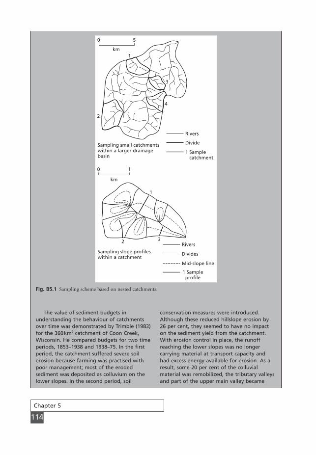
Chapter 5
114
The value of sediment budgets inunderstanding the behaviour of catchmentsover time was demonstrated by Trimble (1983)for the 360km2 catchment of Coon Creek,Wisconsin. He compared budgets for two timeperiods, 1853–1938 and 1938–75. In the firstperiod, the catchment suffered severe soilerosion because farming was practised withpoor management; most of the erodedsediment was deposited as colluvium on thelower slopes. In the second period, soil
conservation measures were introduced.Although these reduced hillslope erosion by26 per cent, they seemed to have no impacton the sediment yield from the catchment.With erosion control in place, the runoffreaching the lower slopes was no longercarrying material at transport capacity andhad excess energy available for erosion. As aresult, some 20 per cent of the colluvialmaterial was remobilized, the tributary valleysand part of the upper main valley became
0 5
1
3
4
2
km
0
km
1
1
2 3
Sampling slope profileswithin a catchment
Sampling small catchmentswithin a larger drainagebasin
Rivers
Rivers
Divide
1 Sample catchment
Divides
Mid-slope line
1 Sampleprofile
Fig. B5.1 Sampling scheme based on nested catchments.
MSE05 11/19/04 02:36 PM Page 114
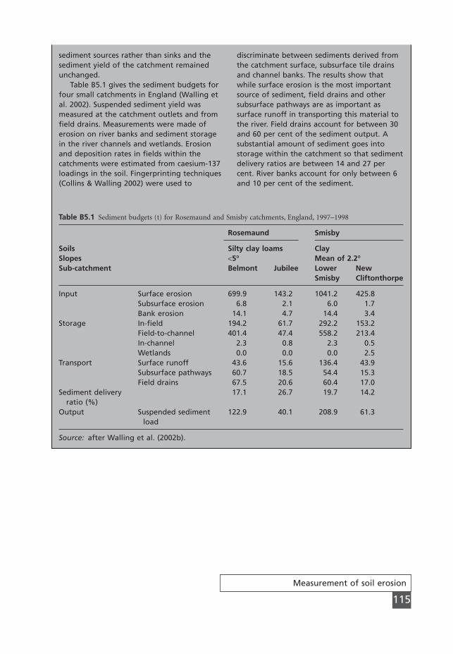
Measurement of soil erosion
115
sediment sources rather than sinks and thesediment yield of the catchment remainedunchanged.
Table B5.1 gives the sediment budgets forfour small catchments in England (Walling etal. 2002). Suspended sediment yield wasmeasured at the catchment outlets and fromfield drains. Measurements were made oferosion on river banks and sediment storagein the river channels and wetlands. Erosionand deposition rates in fields within thecatchments were estimated from caesium-137loadings in the soil. Fingerprinting techniques(Collins & Walling 2002) were used to
discriminate between sediments derived fromthe catchment surface, subsurface tile drainsand channel banks. The results show thatwhile surface erosion is the most importantsource of sediment, field drains and othersubsurface pathways are as important assurface runoff in transporting this material tothe river. Field drains account for between 30and 60 per cent of the sediment output. Asubstantial amount of sediment goes intostorage within the catchment so that sedimentdelivery ratios are between 14 and 27 percent. River banks account for only between 6and 10 per cent of the sediment.
Table B5.1 Sediment budgets (t) for Rosemaund and Smisby catchments, England, 1997–1998
Rosemaund Smisby
Soils Silty clay loams ClaySlopes <5° Mean of 2.2°Sub-catchment Belmont Jubilee Lower New
Smisby Cliftonthorpe
Input Surface erosion 699.9 143.2 1041.2 425.8Subsurface erosion 6.8 2.1 6.0 1.7Bank erosion 14.1 4.7 14.4 3.4
Storage In-field 194.2 61.7 292.2 153.2Field-to-channel 401.4 47.4 558.2 213.4In-channel 2.3 0.8 2.3 0.5Wetlands 0.0 0.0 0.0 2.5
Transport Surface runoff 43.6 15.6 136.4 43.9Subsurface pathways 60.7 18.5 54.4 15.3Field drains 67.5 20.6 60.4 17.0
Sediment delivery 17.1 26.7 19.7 14.2ratio (%)
Output Suspended sediment 122.9 40.1 208.9 61.3load
Source: after Walling et al. (2002b).
MSE05 11/19/04 02:36 PM Page 115
Chapter 6
116
The techniques described in Chapter 5 allow rates of erosion to be determined at different posi-tions in the landscape over various spatial and time scales. However, it is not possible to take mea-surements at every point in the landscape. It also takes time to build up a sufficient data base toensure that the measurements are not biased by an extreme event or a few years of abnormallyhigh rainfall. Long-period measurements are required to study how erosion rates respond tochanges in land use and climate or the use of erosion-control measures. In order to overcomethese deficiencies, models can be used to predict erosion under a wide range of conditions. Theresults of the predictions can then be compared with the measurements to ensure their validity.If the predictions are sufficiently accurate, the method may be used to estimate erosion in otherareas of similar conditions.
Most of the models used in soil erosion studies are of the empirical grey-box type (Table 6.1).They are based on defining the most important factors and, through the use of observation, mea-surement, experiment and statistical techniques, relating them to soil loss. However, as our under-standing of the mechanics of erosion processes grows, the opportunity exists for developingwhite-box and physically based models.
CHAPTER 6
Modelling soilerosion
6.1
Defining objectives
Models are of necessity simplifications of reality. Decisions need to be made on a suitable levelof complexity or simplicity depending on the objective. The starting point for all modelling musttherefore be a clear statement of the objective. This may be prediction or explanation. Managers,planners and policy-makers require relatively simple predictive tools to aid decision-making,albeit about rather complex systems. Researchers seek models that describe how the system func-tions in order to enlighten understanding of the system and how it responds to change. Thischapter is concerned only with predictive models since these are most useful for practical appli-cations but, increasingly, many of these models are developed by researchers and have a soundphysical base reflecting our knowledge of how the erosion system works.
Decisions need to be made on whether prediction should be for a year, a day, a storm or shortperiods within a storm; and whether it should be for a field, a hillslope or a drainage basin. Thesedifferences in temporal and spatial perspectives will influence the processes that need to be
MSE06 11/19/04 02:37 PM Page 116
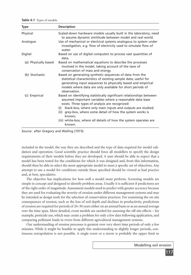
Modelling soil erosion
117
included in the model, the way they are described and the type of data required for model vali-dation and operation. Good scientific practice should force all modellers to specify the designrequirements of their models before they are developed. A user should be able to expect that amodel has been tested for the conditions for which it was designed and, from this information,should then be able to select the most appropriate model to meet a specific set of objectives. Anyattempt to use a model for conditions outside those specified should be viewed as bad practiceand, at best, speculative.
The objective has implications for how well a model must perform. Screening models aresimple in concept and designed to identify problem areas. Usually it is sufficient if predictions areof the right order of magnitude. Assessment models need to predict with greater accuracy becausethey are used for evaluating the severity of erosion under different management systems and maybe intended as design tools for the selection of conservation practices. For examining the on-siteconsequences of erosion, such as the loss of soil depth and declines in productivity, predictionsof erosion are required for periods of 20–30 years either on an annual basis or as an annual averageover the time span. More detailed, event models are needed for assessing the off-site effects – forexample, pesticide use, which may create a problem for only a few days following application, andcomparing pollutant loads in rivers from different agricultural management systems.
Our understanding of erosion processes is greatest over very short time periods of only a fewminutes. While it might be feasible to apply this understanding to slightly longer periods, con-tinuous extrapolation is not possible. A single event or a storm is probably the upper limit to
Table 6.1 Types of models
Type Description
Physical Scaled-down hardware models usually built in the laboratory; need to assume dynamic similitude between model and real world.
Analogue Use of mechanical or electrical systems analogous to system under investigation, e.g. flow of electricity used to simulate flow of water.
Digital Based on use of digital computers to process vast quantities of data.
(a) Physically based Based on mathematical equations to describe the processes involved in the model, taking account of the laws of conservation of mass and energy.
(b) Stochastic Based on generating synthetic sequences of data from the statistical characteristics of existing sample data; useful for generating input sequences to physically based and empirical models where data are only available for short periods of observation.
(c) Empirical Based on identifying statistically significant relationships between assumed important variables where a reasonable data base exists. Three types of analysis are recognized:
(i) black-box, where only main inputs and outputs are studied;(ii) grey-box, where some detail of how the system works is
known;(iii) white-box, where all details of how the system operates are
known.
Source: after Gregory and Walling (1973).
MSE06 11/19/04 02:37 PM Page 117
Chapter 6
118
which relationships established for instantaneous conditions can be applied. Thus longer-termmodelling can only be achieved by summing the predictions for individual storms. The alterna-tive is to develop models empirically using data collected on an annual or mean annual basis. Thescale of operation must also be considered. The detailed requirements for modelling erosion overa large drainage basin differ from those demanded by models of soil loss from a short length ofhillslope or at the point of impact of a single raindrop. Scale influences the number of factorsthat need to be incorporated in the model, those that can be held constant and those that can bedesignated primary factors around which the model must be constructed.
In addition to the area over which the model should operate being defined, the behaviour ofthe model at the boundary of that area needs to be considered. The simplest assumption is thata model applies to a single area of land with a well defined boundary across which there is notransfer of water or sediment. Such an assumption is clearly unrealistic for most hillslope appli-cations, since water and sediment pass downslope from one segment to another and, where theslope is variable in plan, may also move across-slope to concentrate in hollows or areas of flowconvergence. Most erosion models allow for transfer of material across the lower boundary butfew deal with more complicated boundaries, such as the junction between the hillslope and theriver channel. Most soil erosion models also consider the boundaries as fixed in their locationover time, ignoring the possible movement of the lower hillslope boundary upslope as a result ofbank erosion and the gradual lowering of the summit by erosion.
The model should be formulated conceptually, representing it by a flow chart such as thatshown in Fig. 6.1. Viewing the model in this way enables the structure of the system, the logicalorder of transfers of energy and matter through the system, the system variables and the inter-actions between the variables to be defined. It is also a good test of the level of scientific under-standing of the system and the degree to which the model might need to be simplified becauseof insufficient knowledge. A model can be simplified by concentrating on those processes whichhave the greatest influence over the output and ignoring those which have very little effect.Once the processes operating within the model have been identified, they need to be describedmathematically. The methods used can range from simple equations, often expressing a statisti-cal relationship, to complex expressions related to the fundamental physics or mechanics of theprocess. The former are more common in empirical models, whereas the latter provide the foun-dation for physically based models.
It is generally recognized that a good model should satisfy the requirements of reliability, uni-versal applicability, easy use with a minimum of data, comprehensiveness in terms of the factorsand erosion processes included and the ability to take account of changes in climate, land use andconservation practice. Unfortunately, many of the ideal characteristics of models conflict witheach other. Ease of operation can mean that input data are readily available – for example fromtables in an accompanying user’s manual. Such data, however, are at best only guide values andthere may be uncertainty in how well they describe actual conditions.
6.2
Empirical models
The simplest model is a black-box type relating sediment loss to either rainfall or runoff. A typicalrelationship is:
(6.1)Qs aQb=
MSE06 11/19/04 02:37 PM Page 118
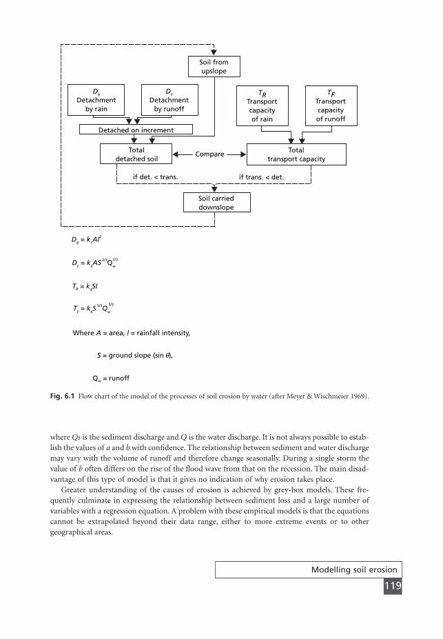
Modelling soil erosion
119
where Qs is the sediment discharge and Q is the water discharge. It is not always possible to estab-lish the values of a and b with confidence. The relationship between sediment and water dischargemay vary with the volume of runoff and therefore change seasonally. During a single storm thevalue of b often differs on the rise of the flood wave from that on the recession. The main disad-vantage of this type of model is that it gives no indication of why erosion takes place.
Greater understanding of the causes of erosion is achieved by grey-box models. These fre-quently culminate in expressing the relationship between sediment loss and a large number ofvariables with a regression equation. A problem with these empirical models is that the equationscannot be extrapolated beyond their data range, either to more extreme events or to other geographical areas.
Soil fromupslope
DR
Detachmentby rain
DF
Detachmentby runoff
TRTransportcapacityof rain
TFTransportcapacityof runoff
Detached on increment
Totaldetached soil
Totaltransport capacity
if trans. < det.if det. < trans.
Soil carrieddownslope
DR = k
1AI2
DF = k
2AS
2/3Qw
TF = k
4S
5/3Qw
2/3
5/3
TR = k3SI
Where A = area, l = rainfall intensity,
S = ground slope (sin q),
Qw = runoff
Compare
Fig. 6.1 Flow chart of the model of the processes of soil erosion by water (after Meyer & Wischmeier 1969).
MSE06 11/19/04 02:37 PM Page 119
Chapter 6
120
6.2.1 Universal Soil Loss Equation
The first attempt to develop a soil loss equation for areas such as hillslopes and fields was that ofZingg (1940), who related erosion to slope steepness and slope length (eqn 3.11). Further devel-opments led to the addition of a climatic factor based on the maximum 30-minute rainfall totalwith a two-year return period (Musgrave 1947), a crop factor, to take account of the protection-effectiveness of different crops (Smith 1958), a conservation factor and a soil erodibility factor.Changing the climatic factor to the rainfall erosivity index (R) ultimately yielded the UniversalSoil Loss Equation (USLE; Wischmeier & Smith 1978). The equation is:
(6.2)
where E is the mean annual soil loss, R is the rainfall erosivity factor, K is the soil erodibility factor,L is the slope length factor, S is the slope steepness factor, C is the crop management factor andP is the erosion-control practice factor. Since K represents mean annual soil loss per unit of R, Ehas the same units as K. Thus, if K is in t ha-1 for one unit of metric R, multiplication by themetric R value will give the value of E in t ha-1. If K is in US tons per acre per unit of AmericanR, multiplication by the American R value yields a value of E in US tons per acre. In both cases,the E value is then adjusted by multiplying by the values of L, S, C and P, which are dimension-less coefficients. The individual factors in the equation are derived as follows.
R. This is the rainfall erosivity index, described in section 4.1.2, based on mean annual EI30. IfE is in foot-tons per acre and I30 is in inches per hour,
(6.3)
R is in American units. If E is in MJ ha-1 and I30 is in mm h-1, R is in metric units.K. This is the soil erodibility index (section 3.2) defined as mean annual soil loss per unit of
R for a standard condition of bare soil, recently tilled up-and-down slope with no conservationpractice and on a slope of 5° and 22 m length. K can be defined for a unit of both American andmetric R. Wherever possible, K should be based on measured values. If the value is obtained fromthe nomograph (Fig. 3.1), it should be remembered that this is an estimated value and will besubject to error.
LS. The factors of slope length (L) and slope steepness (S) can be combined in a single index,which expresses the ratio of soil loss under a given slope steepness and slope length to the soilloss from the standard condition of a 5° slope, 22 m long, for which LS = 1.0. The appropriatevalue can be obtained from nomographs (Wischmeier & Smith 1978) or from the equation:
(6.4)
where x is the slope length (m) and s is the slope gradient in per cent. As seen in section 3.3, thevalue of n should be varied according to the slope steepness.
C. The crop management factor represents the ratio of soil loss under a given crop to thatfrom bare soil. Since soil loss varies with the erosivity and the morphology of the plant cover(section 3.4), it is necessary to take account of changes in these during the year in arriving at anannual value. For arable farming, the year is divided into periods corresponding to different stagesof crop growth. These are defined as: (i) fallow, inversion ploughing to seed-bed establishment;(ii) seed-bed, secondary tillage for formation of the seed-bed to 10 per cent crop cover; (iii) estab-
LSx
s sn
= ÊË
ˆ¯ + +( )
22 130 065 0 045 0 0065 2
.. . .
R EI= 30 100
E R K L S C P= ¥ ¥ ¥ ¥ ¥
MSE06 11/19/04 02:37 PM Page 120

lishment, 10–50 per cent crop cover; (iv) development, 50–75 per cent crop cover; (v) maturity,75 per cent crop cover to harvest; and (vi) residue or stubble, harvest to ploughing or new seeding.For the last period, three options are considered: leaving the residue in the field without seeding;leaving the residue and seeding an off-season crop; and removing the residue and leaving theground bare. For a given crop, separate ratio values are obtained for each period from tables summarizing data collected over many years by the United States Natural Resources Conserva-tion Service at their experimental stations (Wischmeier & Smith 1978). The values vary not onlywith the crop but also, for a single crop, with yield, plant density and the nature of the previouscrop. The individual values for each period are weighted according to the percentage of the meanannual R value falling in that period. The weighted values are then summed to give the annual Cvalue.
The method just described allows C factor values to be determined for the crop rotations and management practices found in the USA. For other countries, detailed information for calculating the C factor in this way does not always exist and it may be more appropriate to useaverage annual values. Table 6.2 gives typical ranges of values for different crops and manage-ment systems.
P. Values for the erosion-control practice factor are obtained from tables of the ratio of soilloss where the practice is applied to the soil loss where it is not. With no erosion-control prac-tice, P = 1.0. Values cover contouring and contour strip-cropping and vary with the slope steep-ness (Table 6.3). Where diversion terracing is adopted, the value for contouring is used for the Pfactor and the LS factor is adjusted for the slope length represented by the horizontal spacingbetween the terraces. This method is not appropriate for bench terracing, for which values of Pfor different types have been established from research in Taiwan (Chan 1981).
As the example in Table 6.4 shows, the equation is normally used to predict mean annual loss.Since it was derived from and tested on data from experimental stations in the USA, which,when combined, represent over 10,000 years of record, it is widely accepted as reliable. Whentested against a data set of 2300 plot years, it gave predictions of mean annual soil loss within ±5 t ha-1 84 per cent of the time (Wischmeier & Smith 1978). The USLE has become the standardtechnique of soil conservation workers. The equation can be rearranged so that, if an acceptablevalue of E is chosen, the slope length (L) required to reduce soil loss to that value can be calcu-lated, all other conditions being unchanged. In this way, appropriate terrace spacings can be determined. Alternatively, the required C value may be predicted and the tables searched to findthe most suitable cropping practice that will give that value.
Although the equation is described as universal, its data base, though extensive, is restrictedto the USA east of the Rocky Mountains, to slopes where cultivation is permissible, normally 0–7°,and to soils with a low content of montmorillonite; it is also deficient in information on the erodibility of sandy soils. Several attempts have been made to apply the equation more widely.Extensive data have been collected on R, K, C and P factor values so that it can be used in WestAfrica (Roose 1975) and India (Singh et al. 1981). Modifications have been made to the R valueand data collected on C factor values so that it can be applied to Bavaria, Germany (Schwertmannet al. 1987), where it has been used in association with erosion surveys to quantify the risk oferosion (Auerswald & Schmidt 1986).
In addition to the limitations of its data base, there are theoretical problems with the equa-tion. Soil erosion cannot be adequately described merely by multiplying together six factor values.There is considerable interdependence between the variables. Some of these are considered. Forinstance, rainfall influences the R and C factors and terracing the L and P factors. Other interac-tions, however, such as the greater significance of slope steepness in areas of intense rainfall(section 3.3) are ignored. The rainfall erosion index is based on studies of drop-size distributions
Modelling soil erosion
121
MSE06 11/19/04 02:37 PM Page 121

Chapter 6
122
of rains, which, as seen in section 3.1.2, may have limited applicability. One important factor towhich soil loss is closely related, namely runoff, is not dealt with explicitly but is incorporatedwithin the R factor.
During the 1970s, the Universal Soil Loss Equation was widely used for estimating sheet andrill erosion in national assessments of soil erosion in the USA. By necessity, the equation wasapplied to conditions beyond its data base – for example, to rangeland and forest land in thewestern USA. As a result of the experience, a number of changes were made that are now incor-porated in the Revised Universal Soil Loss Equation (RUSLE) (Renard et al. 1991). These include:
Table 6.2 C-factor values for the Universal Soil Loss Equation
Practice Average annualC-factor
Bare soil 1.00Forest or dense shrub, high mulch crops 0.001Savanna or prairie grass in good condition 0.01Overgrazed savanna or prairie grass 0.10Maize, sorghum or millet; high productivity; conventional tillage 0.20–0.55Maize, sorghum or millet; low productivity; conventional tillage 0.50–0.90Maize, sorghum or millet; high productivity; chisel ploughing into residue 0.12–0.20Maize, sorghum or millet; low productivity; chisel ploughing into residue 0.30–0.45Maize, sorghum or millet; high productivity; no or minimum tillage 0.02–0.10Cotton 0.40–0.70Meadow grass 0.01–0.025Soya beans 0.20–0.50Wheat 0.10–0.40Rice 0.10–0.20Groundnuts 0.30–0.80Palm trees, coffee, cocoa with cover crops 0.10–0.30Pineapple on contour; residue removed 0.10–0.40Pineapple on contour; with surface residue 0.01Potatoes; rows downslope 0.20–0.50Potatoes; rows across slope 0.10–0.40Cowpeas 0.30–0.40Strawberries; with weed cover 0.27Pomegranate; with weed cover 0.08Pomegranate; clean-weeded 0.56Ethiopian tef 0.25Sugar cane 0.13–0.40Yams 0.40–0.50Pigeon peas 0.60–0.70Mungbean 0.04Chilli 0.33Coffee: after first harvest 0.05Plantains: after establishment 0.05–0.10Papaya 0.21
Source: after Wischmeier and Smith (1978), Roose (1977), Singh et al. (1981), El-Swaify et al.(1982), Hurni (1987), Hashim and Wong (1988).
MSE06 11/19/04 02:37 PM Page 122

Table 6.3 P-factor values for the Universal Soil Loss Equation
Erosion-control practice P-factor value
Contouring: 0–1° slope 0.60*Contouring: 2–5° slope 0.50*Contouring: 6–7° slope 0.60*Contouring: 8–9° slope 0.70*Contouring: 10–11° slope 0.80*Contouring: 12–14° slope 0.90*Level bench terrace 0.14Reverse-slope bench terrace 0.05Outward-sloping bench terrace 0.35Level retention bench terrace 0.01Tied ridging 0.10–0.20
* Use 50% of the value for contour bunds or if contour stripcropping is practised.Source: after Wischmeier and Smith (1978), Roose (1977),Chan (1981a).
Table 6.4 Prediction of soil loss using the Universal Soil Loss Equation
ProblemCalculation of mean annual soil loss on a 100-m long slope of 7° on soils of the RengamSeries under maize cultivation with contour bunds spaced at 20m intervals, near KualaLumpur, Malaysia.
EquationMean annual soil loss = R ¥ K ¥ LS ¥ C ¥ P
Estimating R (Rainfall erosion index)In the absence of locally published maps of R values, three different procedures forestimating R from mean annual precipitation (P) are used.
Method 1Mean annual precipitation (P) = 2695mmFrom Roose (1975), mean annual rainfall erosion index (R) in American units = 0.5 P
= 0.5 ¥ 2695= 1347.5
Conversion to Mgmmha-1 h-1 = 1347.5 ¥ 17.3= 23,311.8
Method 2From Morgan (1974), mean annual erosivity = 9.28 P - 8,838(KE > 25)
= (9.28 ¥ 2695) - 8838= 16,171.6Jm-2
= 161.716Mgha-1
MSE06 11/19/04 02:37 PM Page 123

Table 6.4 Continued
Multiply by I30 (use 75mmh-1; maximum value = 161.716 ¥ 75recommended by Wischmeier and Smith (1978)
= 12,128.7
Method 3From Foster et al. (1981), mean annual EI30 = 0.276 P ¥ I30
(kg.m.mm)(m2 h-1)= 0.276 ¥ 2695 ¥ 75= 55,786.5
Divide by 100 to convert to Mgmmha-1 h-1 = 55.79
Best estimate: discard result from Method 3, which is rather low.Take average value of Methods 1 and 2: = 17,720
Estimating K (Soil erodibility index)From Whitmore and Burnham (1969), the soils have a 43% clay, 8% silt, 9% fine sand and40% coarse sand content; organic content is about 3%.Using the nomograph (Fig. 3.1), gives a first approximation K value = 0.005
Estimating LS (Slope factor)For slope length (l) and slope steepness (s) in metres and percent respectively,
With contour bunds at 20m spacing, l = 20m and s = 12% (approximation of 7°)
Estimating C (Crop management factor)According to Table 6.2, the C value for maize ranges between 0.2 and 0.9, depending onthe productivity. For many tropical farming conditions, C for maize lies between 0.4 and 0.9(Roose 1975), depending on the cover.
During the three-month period from seeding to harvest, the cover is likely to vary from 9to 45 per cent in the first month, from 55 to 93 per cent in the second month, and from 45to 57 per cent in the third month. Therefore, we might assume C values of 0.9, 0.4 and 0.7for the three respective months.
Maize can be planted at any time of year in Malaysia but assume planting after the Aprilrains, allowing growth, ripening and harvesting in June and July, which are the driestmonths. Land is under dense secondary growth prior to planting (assume C = 0.001) andallowed to revert to the same after harvest (C = 0.1).
Of the mean annual precipitation, 32 per cent falls between January and April inclusive, 10per cent in May, 6 per cent in June, 7 per cent in July and 45 per cent between August andDecember. Assuming that erosivity is directly related to precipitation amount, these valuescan be used to describe the distribution of the R factor throughout the year.
From the above information, the following table is constructed.
LS
LS
LS
= ( ) + ¥( ) + ¥( )( )= ¥=
20 22 0 065 0 045 12 0 0065 12
0 95 1 54
0 5 2.. . .
. .
1.46
LS l s s= ( ) + +( )22 0 065 0 045 0 00650 5 2.
. . .
MSE06 11/19/04 02:37 PM Page 124
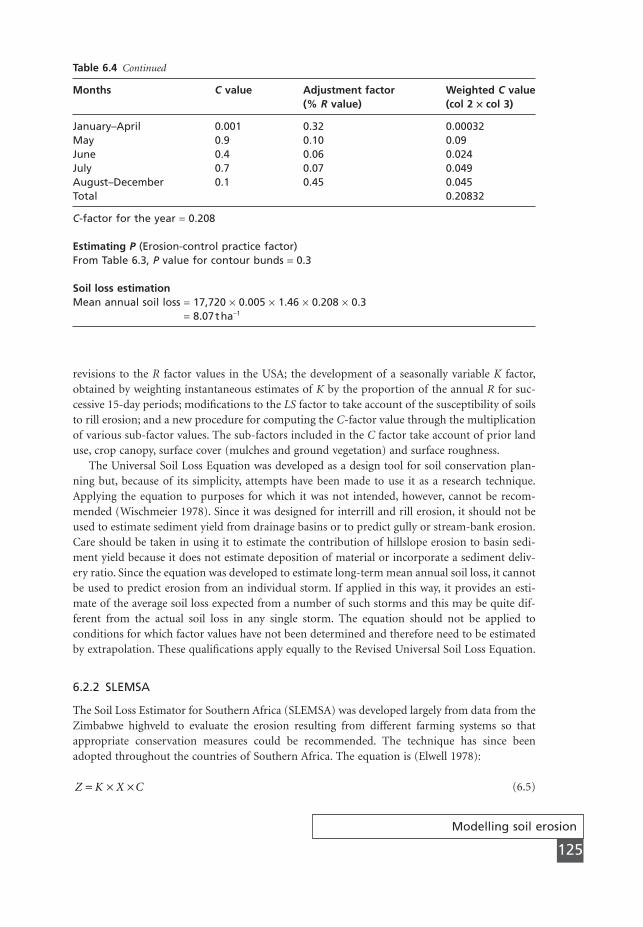
Modelling soil erosion
125
revisions to the R factor values in the USA; the development of a seasonally variable K factor,obtained by weighting instantaneous estimates of K by the proportion of the annual R for suc-cessive 15-day periods; modifications to the LS factor to take account of the susceptibility of soilsto rill erosion; and a new procedure for computing the C-factor value through the multiplicationof various sub-factor values. The sub-factors included in the C factor take account of prior landuse, crop canopy, surface cover (mulches and ground vegetation) and surface roughness.
The Universal Soil Loss Equation was developed as a design tool for soil conservation plan-ning but, because of its simplicity, attempts have been made to use it as a research technique.Applying the equation to purposes for which it was not intended, however, cannot be recom-mended (Wischmeier 1978). Since it was designed for interrill and rill erosion, it should not beused to estimate sediment yield from drainage basins or to predict gully or stream-bank erosion.Care should be taken in using it to estimate the contribution of hillslope erosion to basin sedi-ment yield because it does not estimate deposition of material or incorporate a sediment deliv-ery ratio. Since the equation was developed to estimate long-term mean annual soil loss, it cannotbe used to predict erosion from an individual storm. If applied in this way, it provides an esti-mate of the average soil loss expected from a number of such storms and this may be quite dif-ferent from the actual soil loss in any single storm. The equation should not be applied toconditions for which factor values have not been determined and therefore need to be estimatedby extrapolation. These qualifications apply equally to the Revised Universal Soil Loss Equation.
6.2.2 SLEMSA
The Soil Loss Estimator for Southern Africa (SLEMSA) was developed largely from data from theZimbabwe highveld to evaluate the erosion resulting from different farming systems so thatappropriate conservation measures could be recommended. The technique has since beenadopted throughout the countries of Southern Africa. The equation is (Elwell 1978):
(6.5)Z K X C= ¥ ¥
Table 6.4 Continued
Months C value Adjustment factor Weighted C value(% R value) (col 2 ¥ col 3)
January–April 0.001 0.32 0.00032May 0.9 0.10 0.09June 0.4 0.06 0.024July 0.7 0.07 0.049August–December 0.1 0.45 0.045Total 0.20832
C-factor for the year = 0.208
Estimating P (Erosion-control practice factor)From Table 6.3, P value for contour bunds = 0.3
Soil loss estimationMean annual soil loss = 17,720 ¥ 0.005 ¥ 1.46 ¥ 0.208 ¥ 0.3
= 8.07tha-1
MSE06 11/19/04 02:37 PM Page 125

where Z is mean annual soil loss (t ha-1), K is mean annual soil loss (t ha-1) from a standard fieldplot, 30 m long, 10 m wide, at 2.5° slope for a soil of known erodibility (F) under a weed-free barefallow, X is a dimensionless combined slope length and steepness factor and C is a dimensionlesscrop management factor.
K. The value of K is determined by relating mean annual soil loss to mean annual rainfallenergy (E) using the exponential relationship:
(6.6)
where E is in J m2, and the values of a and b are functions of the soil erodibility factor (F):
(6.7)
(6.8)
X. The topographic factor (X) adjusts the value of soil loss calculated for the standard condi-tion to that for the actual conditions of slope steepness and slope length. The value of X is obtainedfrom:
(6.9)
where L is the slope length (m) and s is the percentage slope.The procedure is modified if contour ridges are used as a conservation measure. In this case,
instead of L and s being defined in the downslope direction, L becomes the maximum length ofthe ridges and s is the across-slope grade (in per cent) of the ridge. If the across-slope grade isless than 1 per cent, the value of X is first determined for a 1 per cent grade and then multipliedby the term Y, defined by:
(6.10)
C. The crop management factor (C) adjusts the value of soil loss for the standard bare soilcondition to that from a cropped field. The value is dependent upon the percentage of the rain-fall energy intercepted by the crop (i). For crops and natural grassland with i < 50 per cent andfor dense pastures and mulches with i ≥ 50 per cent, the following relationship is used:
(6.11)
For crops and natural grasslands when i ≥ 50 per cent, the relationship is:
(6.12)
The value of i is obtained by weighting the percentage crop cover in each ten-day period by thepercentage of the mean annual rainfall energy (E) occurring in that period and summing thevalues.
Guide values for soil erodibility (F) and average percentage crop covers for use with SLEMSAare given in Table 6.5. An example of its use is shown in Table 6.6.
C i= -( )2 3 0 01 30. .
C e i= -( )0 06.
Y s s= +( )0 572 0 428. .
X L s s= ( ) + +( )[ ]0 5 20 76 0 53 0 076 25 65. . . . .
b F= +0 4681 0 7663. .
a F= -2 884 8 2109. .
ln lnK b E a= +
Chapter 6
126
MSE06 11/19/04 02:37 PM Page 126

Table 6.5 Input values for soil erodibility and crop cover for use in SLEMSA
Soil erodibility (F factor)
Soil texture Soil type F value
Light sands 4loamy sandssandy loams
Medium sandy clay loam 5clay loamsandy clay
Heavy clay 6heavy clay
Subtract the following from the F value:1 for light-textured soils consisting mainly of sands and silts1 for restricted vertical permeability within one metre of the surface or for severe soil
crusting1 for ridging up-and-down the slope1 for deterioration in soil structre due to excessive soil loss in the previous year
(>20tha-1) or for poor soil management0.5 for slight to moderate surface crusting or for soil losses of 10–20tha-1 in the previous
year.
Add the following to the F value:2 for deep (>2m) well drained, light-textured soils1 for tillage techniques which encourage maximum retention of water on the surface,
e.g. ridging on the contour1 for tillage techniques which encourage high surface infiltration and maximum water
storage in the profile, e.g. ripping, wheel-track planting1 for first season of no tillage2 for subsequent seasons of no tillage
Crop cover ratings (C)
Crop Average percentage cover
Cotton 40–65Cowpeas 40–55Tobacco 11–54Sorghum 50–70Sunflower 20–59Groundnuts 55–65Velvet beans 46–70Coffee 60–80Maize 42–80Rotational grass 80–98Soya beans 40–65Rice 70–80Weed fallow 100
After Elwell and Wendelaar (1977), Elwell (1978).
MSE06 11/19/04 02:37 PM Page 127

Table 6.6 Prediction of soil loss using SLEMSA
ProblemCalculation of mean annual soil loss on a 100-m long slope of 7° on soils of the RengamSeries under maize cultivation with contour bunds at 20m spacing, near Kuala Lumpur,Malaysia (compare with Table 6.4).
Basic equationSoil loss (Z) = K ¥ X ¥ C
Estimating KMean annual precipitation (P) = 2695mmMean annual rainfall energy (E) (Morgan 1974) = 9.28P - 8838
= (9.28 ¥ 2695) - 8838= 16,172Jm-2
Soil erodibility (F)From Table 6.5, for a sandy clay, F = 5Calculation of K
lnK = blnE + awhere a = 2.884 - 8.1209F
b = 0.4681 + 0.7663FTherefore, a = 2.884 - (8.1209 ¥ 5)
= -37.7205and b = 0.4681 + (0.7663 ¥ 5)
= 4.2996lnK = (4.2996 ¥ 9.6910) - 37.7205
= 3.9469which gives K = 51.78
Estimating XFor unridged landX = (0.76 + 0.53s + 0.0765s2)/25.65where l is slope length (m) and s is slope steepness (%)For contour bunds every 20m, l = 20 and s = 7° or 12%X = (0.76 + (0.53 ¥ 0.12) + (0.0765 ¥ 122)/25.65X = 4.47 ¥ 18.064/25.65X = 3.15
Estimating CCalculation of the proportion of rainfall intercepted by the plant cover (i) by weighting thepercentage crop cover for each cropping season by the proportion of the mean annualrainfall occurring in that season.For the conditions described in Table 6.4 and taking values from Table 6.5
Months % rainfall % cover Value of i (col 2 ¥ col 3)
January–April 0.32 100 32.00May–July 0.23 45 10.35August–December 0.45 90 40.50Total 82.85
C = (2.3 - 0.01i)/30= (2.3 - (0.01 ¥ 82.85))/30= 0.049
Soil loss estimationMean annual soil loss = 51.78 ¥ 3.15 ¥ 0.049
= 7.99tha-1
20
/
MSE06 11/19/04 02:37 PM Page 128

Modelling soil erosion
129
6.2.3 The Morgan, Morgan and Finney method
Morgan et al. (1984) developed a model to predict annual soil loss from field-sized areas on hill-slopes, which, while endeavouring to retain the simplicity of the Universal Soil Loss Equation,encompassed some of the recent advances in understanding of erosion processes. The approachwas revised by Morgan (2001). The model separates the soil erosion process into a water phaseand a sediment phase (Fig. 6.2). The sediment phase is a simplification of the scheme describedby Meyer and Wischmeier (1969; Fig. 6.1). It considers soil erosion to result from the detachmentof soil particles by raindrop impact and runoff and the transport of those particles by overlandflow. The process of transport by rainsplash is ignored. Thus, the sediment phase comprises threepredictive equations, one for the rate of particle detachment by rainsplash, one for the rate ofparticle detachment by runoff and one for the transport capacity of overland flow. The inputs tothese equations of rainfall energy and runoff volume respectively are obtained from the waterphase. The model uses 12 operating functions (Table 6.7) for which 19 input parameters are required (Table 6.8). Typical values for soil parameters are given in Table 6.9, for effectivehydrological depth of the soil in Table 6.10 and for the Et/E0 ratio, interception and the crop management factors in Table 6.11.
The effects of soil conservation practices can be allowed for within the separate phases of themodel. For example, agronomic measures will bring about changes in evapotranspiration, inter-ception and crop management, which will affect respectively the volume of runoff, the rate ofdetachment and the transport capacity.
Table 6.7 Operating functions for the Morgan–Morgan–Finney method of predicting soil loss
Water phase
ER = R ¥ (1 - A)LD = ER ¥ CCDT = ER - LDKE(DT) = DT(11.9 + 8.7 logI)KE(LD) = LD ((15.8 - PH0.5) - 5.87)KE = KE(DT) + KE(LD)Q = R exp(-Rc/Ro)Rc = 1000 MS ¥ BD ¥ EHD(Et/Eo)0.5
Ro = R/Rn
Sediment phase
F = K ¥ KE ¥ 10-3
H = ZQ1.5 sinS(1 - GC) ¥ 10-3
Z = 1/(0.5COH)J = F + ZG = CQ2 sinS ¥ 10-3
ER = effective rainfall (mm)LD = leaf drainage (mm)DT = direct throughfall (mm)KE = kinetic energy of the rainfall (Jm-2)Q = volume of overland flow (mm)F = annual rate of soil particle detachment by raindrop impact (kgm-2)H = annual rate of soil particle detachment by runoff (kgm-2)J = annual rate of total soil particle detachment (kgm-2)G = annual transport capacity of overland flow (kgm-2)
MSE06 11/19/04 02:37 PM Page 129
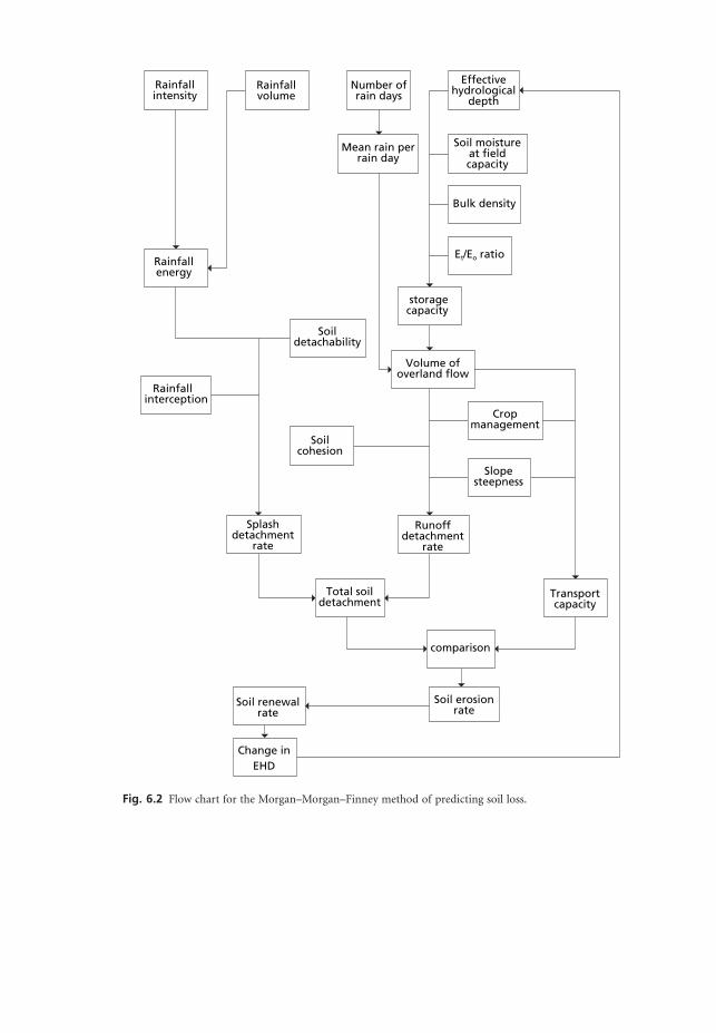
Rainfallintensity
Rainfallvolume
Number ofrain days
Effectivehydrological
depth
Mean rain perrain day
Soil moistureat fieldcapacity
Bulk density
Et/Eo ratio
storagecapacity
Cropmanagement
Slopesteepness
Runoffdetachment
rate
Rainfallenergy
Soildetachability
Rainfallinterception
Soilcohesion
Volume ofoverland flow
Splashdetachment
rate
Total soildetachment
Transportcapacity
comparison
Soil erosionrate
Soil renewalrate
Change inEHD
Fig. 6.2 Flow chart for the Morgan–Morgan–Finney method of predicting soil loss.
MSE06 11/19/04 02:37 PM Page 130

Modelling soil erosion
131
The model compares the predictions of total detachment by rainsplash and runoff with thetransport capacity of the runoff and assigns the lower of the two values as the annual rate of soilloss, thereby denoting whether detachment or transport is the limiting factor. The predictionsobtained by the model are most sensitive to changes in annual rainfall and soil parameters whenerosion is transport-limited and to changes in rainfall interception and annual rainfall whenerosion is detachment-limited. Thus, good information on rainfall and soils is required for suc-cessful prediction. An example of the use of the model is presented in Table 6.12.
Like the Universal Soil Loss Equation, the model cannot be used to predict soil loss from indi-vidual storms or from gully erosion. The model has been used to predict soil loss in Indonesia
Table 6.8 Input parameters to the Morgan–Morgan–Finney method of predicting soil loss
Factor Parameter Definition
Rainfall R Annual or mean annual rainfall (mm)Rn Number of rain days per yearI Typical value for intensity of erosive rain (mmh-1); use 10 for
temperate climates, 25 for tropical climates and 30 for strongly seasonal climates (e.g. Mediterranean type or monsoon)
Soil MS Soil moisture content at field capacity or 1/3 bar tension (wt %)BD Bulk density of the top soil layer (Mgm-3)EHD Effective hydrological depth of soil (m); value depends on
vegetation/crop cover, presence or absence of surface crust, presence of impermeable layer within 0.15m of the surface
K Soil detachability index (gJ-1) defined as the weight of soil detached from the soil mass per unit of rainfall energy
COH Cohesion of the surface soil (kPa) as measured with a torvane under saturated conditions
SD Total soil depth (m) defined as the depth of soil surface to bedrock
W Rate of increase in soil depth by weathering at the rock–soil interface (mmyr-1)
V Rate of increase in effective hydrological layer (mmyr-1) as a result of crop management practices and the natural breakdown of vegetative matter into humus
Landform S Slope steepness (°)Land cover A Proportion (between 0 and 1) of the rainfall intercepted by the
vegetation or crop coverEt/Eo Ratio of actual (Et) to potential (Eo) evapotranspirationC Crop cover management factor; combines the C and P factors of
the Universal Soil Loss EquationCC Percentage canopy cover, expressed as a proportion between 0
and 1GC Percentage ground cover, expressed as a proportion between 0
and 1PH Plant height (m), representing the height from which raindrops
fall from the crop or vegetation cover to the ground surfaceTime N Number of consecutive years for which the model is to operate
MSE06 11/19/04 02:37 PM Page 131

Chapter 6
132
(Besler 1987) and Nepal (Shrestha 1997) and incorporated within a geographical informationsystem for predicting erosion in Mediterranean Europe (De Jong 1994; Paracchini et al. 1997; DeJong et al. 1999). The model can be used to predict soil loss from small catchments by dividingthe catchment into land units of similar soils, slopes and land cover (section 4.2.2) and routingthe annual runoff and sediment production over the land surface from one unit to another. Therunoff for each unit is then calculated as the summation of the runoff generated on that unit andthe runoff flowing into it from upslope; the transport capacity is calculated for the combinedrunoff. Similarly, the total sediment available for transport is the summation of that detached on
Table 6.9 Typical values for soil parameters used in the Morgan–Morgan–Finney method of predicting soil loss
Soil type MS BD K COH
Sand 0.08 1.5 1.2 2Loamy sand – – 0.3 2Sandy loam 0.28 1.2 0.7 2Loam 0.20 1.3 0.8 3Silt – – 1.0 –Silt loam 0.25 1.3 0.9 3Sandy clay loam – – 0.1 3Clay loam 0.40 1.3 0.7 10Silty clay loam – – 0.8 9Sandy clay – – 0.3 –Silty clay 0.30 – 0.5 10Clay 0.45 1.1 0.05 12
Source: summarized in Morgan et al. (1982), Morgan (2001).
Table 6.10 Recommended values for the Effective Hydrological Depth (m) in the Morgan–Morgan–Finneymethod of predicting soil loss
Condition EHD
Bare soil without surface crust; no impermeable barrier in top 0.2m 0.09Bare shallow soils on steep slopes; crusted soils 0.05Row crops (e.g. wheat, barley, maize, beans, rice) 0.12Row crops intercropped with legumes/grasses 0.15Mature forest, dense secondary forest 0.20Rubber, oil palm 0.15Cocoa, coffee 0.12Banana 0.18Savanna/prairie grass 0.14Cultivated grass 0.12Cotton 0.10Groundnut 0.12
Where terracing is used, add 0.01 to EHD to take account of the resulting increase in waterstorage.Source: after Morgan (2001).
MSE06 11/19/04 02:37 PM Page 132
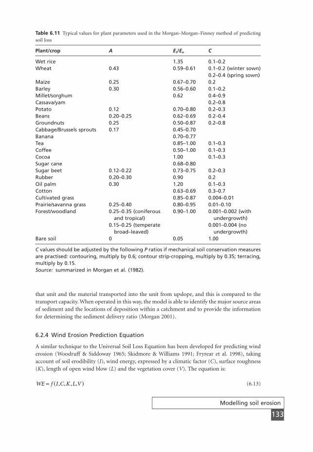
Modelling soil erosion
133
that unit and the material transported into the unit from upslope, and this is compared to thetransport capacity. When operated in this way, the model is able to identify the major source areasof sediment and the locations of deposition within a catchment and to provide the informationfor determining the sediment delivery ratio (Morgan 2001).
6.2.4 Wind Erosion Prediction Equation
A similar technique to the Universal Soil Loss Equation has been developed for predicting winderosion (Woodruff & Siddoway 1965; Skidmore & Williams 1991; Fryrear et al. 1998), takingaccount of soil erodibility (I), wind energy, expressed by a climatic factor (C), surface roughness(K), length of open wind blow (L) and the vegetation cover (V). The equation is:
(6.13)WE f I C K L V= ( ), , , ,
Table 6.11 Typical values for plant parameters used in the Morgan–Morgan–Finney method of predictingsoil loss
Plant/crop A Et/Eo C
Wet rice 1.35 0.1–0.2Wheat 0.43 0.59–0.61 0.1–0.2 (winter sown)
0.2–0.4 (spring sown)Maize 0.25 0.67–0.70 0.2Barley 0.30 0.56–0.60 0.1–0.2Millet/sorghum 0.62 0.4–0.9Cassava/yam 0.2–0.8Potato 0.12 0.70–0.80 0.2–0.3Beans 0.20–0.25 0.62–0.69 0.2–0.4Groundnuts 0.25 0.50–0.87 0.2–0.8Cabbage/Brussels sprouts 0.17 0.45–0.70Banana 0.70–0.77Tea 0.85–1.00 0.1–0.3Coffee 0.50–1.00 0.1–0.3Cocoa 1.00 0.1–0.3Sugar cane 0.68–0.80Sugar beet 0.12–0.22 0.73–0.75 0.2–0.3Rubber 0.20–0.30 0.90 0.2Oil palm 0.30 1.20 0.1–0.3Cotton 0.63–0.69 0.3–0.7Cultivated grass 0.85–0.87 0.004–0.01Prairie/savanna grass 0.25–0.40 0.80–0.95 0.01–0.10Forest/woodland 0.25–0.35 (coniferous 0.90–1.00 0.001–0.002 (with
and tropical) undergrowth)0.15–0.25 (temperate 0.001–0.004 (no
broad–leaved) undergrowth)Bare soil 0 0.05 1.00
C values should be adjusted by the following P ratios if mechanical soil conservation measuresare practised: contouring, multiply by 0.6; contour strip-cropping, multiply by 0.35; terracing,multiply by 0.15.Source: summarized in Morgan et al. (1982).
MSE06 11/19/04 02:37 PM Page 133
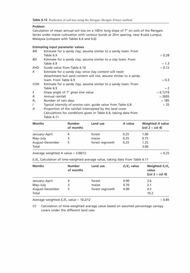
Table 6.12 Prediction of soil loss using the Morgan–Morgan–Finney method
ProblemCalculation of mean annual soil loss on a 100m long slope of 7° on soils of the RengamSeries under maize cultivation with contour bunds at 20m spacing, near Kuala Lumpur,Malaysia (compare with Tables 6.4 and 6.6)
Estimating input parameter valuesMS Estimate for a sandy clay; assume similar to a sandy loam. From
Table 6.9 = 0.28BD Estimate for a sandy clay; assume similar to a clay loam. From
Table 6.9 = 1.3EHD Guide value from Table 6.10 = 0.12K Estimate for a sandy clay; since clay content will resist
detachment but sand content will not, assume similar to a sandyloam. From Table 6.9 = 0.3
COH Estimate for a sandy clay; assume similar to a sandy loam. FromTable 6.9 = 2
S Slope angle of 7° gives sine value = 0.1219R Annual rainfall = 2695Rn Number of rain days = 185I Typical intensity of erosive rain; guide value from Table 6.8 = 25A Proportion of the rainfall intercepted by the land cover.
Calculations for conditions given in Table 6.4, taking data fromTable 6.11
Months Number Land use A value Weighted A valueof months (col 2 ¥ col 4)
January–April 4 forest 0.25 1.00May–July 3 maize 0.25 0.75August–December 5 forest regrowth 0.25 1.25Total 3.00
Average weighted A value = 3.00/12 = 0.25
Et /Eo Calculation of time-weighted average value, taking data from Table 6.11
Months Number Land use Et/Eo value Weighted Et/Eo
of months value(col 2 ¥ col 4)
January–April 4 forest 0.90 3.6May–July 3 maize 0.70 2.1August–December 5 forest regrowth 0.90 4.5Total 10.2
Average weighted Et /Eo value = 10.2/12 = 0.85
CC Calculation of time-weighted average value based on assumed percentage canopycovers under the different land uses
MSE06 11/19/04 02:37 PM Page 134
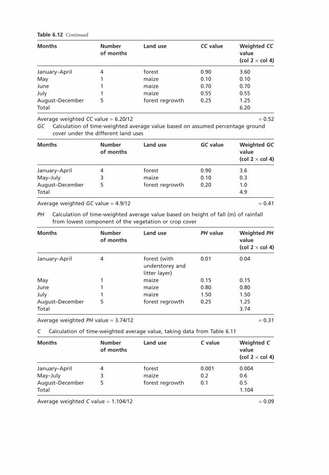
Table 6.12 Continued
Months Number Land use CC value Weighted CCof months value
(col 2 ¥ col 4)
January–April 4 forest 0.90 3.60May 1 maize 0.10 0.10June 1 maize 0.70 0.70July 1 maize 0.55 0.55August–December 5 forest regrowth 0.25 1.25Total 6.20
Average weighted CC value = 6.20/12 = 0.52GC Calculation of time-weighted average value based on assumed percentage ground
cover under the different land uses
Months Number Land use GC value Weighted GCof months value
(col 2 ¥ col 4)
January–April 4 forest 0.90 3.6May–July 3 maize 0.10 0.3August–December 5 forest regrowth 0.20 1.0Total 4.9
Average weighted GC value = 4.9/12 = 0.41
PH Calculation of time-weighted average value based on height of fall (m) of rainfallfrom lowest component of the vegetation or crop cover
Months Number Land use PH value Weighted PHof months value
(col 2 ¥ col 4)
January–April 4 forest (with 0.01 0.04understorey andlitter layer)
May 1 maize 0.15 0.15June 1 maize 0.80 0.80July 1 maize 1.50 1.50August–December 5 forest regrowth 0.25 1.25Total 3.74
Average weighted PH value = 3.74/12 = 0.31
C Calculation of time-weighted average value, taking data from Table 6.11
Months Number Land use C value Weighted Cof months value
(col 2 ¥ col 4)
January–April 4 forest 0.001 0.004May–July 3 maize 0.2 0.6August–December 5 forest regrowth 0.1 0.5Total 1.104
Average weighted C value = 1.104/12 = 0.09
MSE06 11/19/04 02:37 PM Page 135

Table 6.12 Continued
Estimating effective rainfall (ER)From Table 6.7
ER = 2695 ¥ (1 - 0.25)= 2021.25mm
Estimating volumes of leaf drainage (LD) and direct throughfall (DT)From Table 6.7
LD = 2021.25 ¥ 0.52= 1051.05mm
DT = 2021.25 - 1051.05= 970.20mm
Estimating kinetic energy of the effective rainfallFrom Table 6.7
KE(DT) = 970.20 (11.9 + 8.7 log25)= 23,343Jm-2
KE(LD) = 1051.05 ((15.8 ¥ 0.310.5) - 5.87)= 3077Jm-2
KE = 23,343 + 3077= 26,421Jm-2
Estimating volume of overland flowFrom Table 6.7Rc = 1000 ¥ 0.28 ¥ 0.12 ¥ 0.850.5
= 30.98mmRn = 2695/185
= 14.57mmQ = 2695e-30.98/14.97
= 340.1mm
Estimating rate of soil particle detachmentFrom Table 6.7, annual rate of detachment by raindrop impact
F = 0.3 ¥ 26,421 ¥ 10-3
= 7.93kgm-2
From Table 6.7, annual rate of detachment by runoff
Z = 1/(0.5 ¥ 2)= 1
H = 1 ¥ 340.11.5 ¥ 0.1219 ¥ 0.59 ¥ 10-3
= 0.45kgm-2
Total annual rate of detachment
J = 7.93 + 0.45= 8.38kgm-2
Estimating annual transport capacity of overland flow
G = 0.09 ¥ 340.12 ¥ 0.1219 ¥ 10-3
= 1.27kgm-2
Soil loss estimationMean annual soil loss equals the lower of the values of J and G = 1.27kgm-2
Convert to tha-1 = 10 ¥ 1.27 = 12.7tha-1
MSE06 11/19/04 02:37 PM Page 136

Modelling soil erosion
137
where WE is the mean annual wind erosion (t ha-1), I is the mean annual wind erosion for a givensoil (t ha-1) in a level dry bare field at Garden City, Kansas (Table 3.5), C is a dimensionless numberto adjust the value of I for the actual climatic conditions compared with those at Garden City,K is a dimensionless number to adjust I for roughness produced by tillage, L is in m and V is the quantity of vegetative cover expressed as flattened wheat straw equivalent in kg DM ha-1. Theequation allows for interactions between the factors and so it cannot be solved by multiplying thevalues of the various factors together. Factor relationships are rather complex and predictions canonly be obtained by using complex nomographs or specially developed equations applied in a setsequence (Table 6.13).
Table 6.13 Prediction of wind erosion
Basic equation
WE = f(I, C, K, L, V )
Estimating I (soil erodibility index)Values represent the potential annual soil loss (tha-1) for a level bare dry field near GardenCity, Kansas. They have been determined from wind tunnel studies (section 3.2; Table 3.7)and may be estimated by knowing the percentage of dry stable aggregates larger than0.84mm in the soil. The values are adjusted by a term Is to take account of the steepnessof the windward slope (Woodruff & Siddoway 1965).
Estimating C (climatic index)The index takes account of wind erosion as a function of wind velocity and soil moisturecontent. The former is expressed by the mean annual wind velocity (v, ms-1) measured at aheight of 9m and the latter by the Thornthwaite precipitation effectiveness index (P - E).The index is then expressed as a percentage of its value of 2.9 for Garden City Kansas.Thus:
where
in which P is the mean precipitation for month i (inches) and T is the mean temperature formonth i (°F). In application, a minimum value of 18.4 is adopted for mean monthly T - 10and maximum value of 13mm is used for mean monthly precipitation.
Estimating K (ridge roughness index)The roughness of ridges produced by tillage and planting equipment is expressed by aroughness factor (R) calculated from
where H is the ridge height (mm) and I is the distance between the ridges. Values of K areexpressed by:
K = 1 R < 2.27K = 1.125 - 0.153 lnR 2.27 £ R < 89 K = 0.336exp (0.0032R) R ≥ 89
R H I= 4 2
P EP
Ti- =
-ÊË
ˆ¯=Â115
101
1210 9
Cv
P E= ◊
-( )1002 9
3
2.
MSE06 11/19/04 02:37 PM Page 137

Table 6.13 Continued
Estimating L (length of open wind blow)The value of L is calculated as a function of equivalent field length (D) and the distancesheltered by any trees, shelterbelts, field hedges or windbreaks. The equivalent field lengthis calculated from measurements of actual field length (l, m), field width (w, m), fieldorientation expressed as the clockwise angle between field length and north (f, rad), andwind direction clockwise from north (q, rad):
The value of L is the determined from:
where H is the height of the shelterbelt.
Estimating V (vegetation cover)The vegetation cover index depends on standing live biomass, standing dead residue andflattened crop residue. The original work on the effects of vegetation was carried out forflattened wheat straw and so all weights of living or dead vegetative matter need to beconverted into flattened wheat straw equivalents, defined as 254mm tall stalks lying flaton the soil in rows perpendicular to the wind direction, with 254mm row spacing andstalks oriented perpendicular to the wind direction. Values of V for various crops are givenin Woodruff and Siddoway (1965) and for perennial rangeland grasses in Lyles and Allison(1981). For a wide range of crops, an estimate of the flattened wheat straw or small grainequivalent weight of the residue (SGe, kgha-1) can be obtained from:
where Rw is the weight of the standing residue of the crop (kgha-1), d is the average stalkdiameter (cm) and g is the average specific weight of the stalks (Mgm-3) (Lyles & Allison1981).
Applying the equationStep 1: E1 = I . IsStep 2: E2 = E1.KStep 3: E3 = E2.CStep 4: E4 = (F0.3484 + E30.3484 - E20.3484)2.87
where F = E2 {1 - 0.1218(L/Lo)-0.3829 exp(-3.33L/Lo)}Lo = 1.56 ¥ 106 (E2)-1.26 exp(-0.00156E2)
Step 5: E5 = g E4h
where g = 952.5(1-h)
h
Step 6: WE = E5
=+ -( )
10 0537 0 9436 0 000112. . .exp V
SGe Rw d Rw d= + ( ) -0 162 8 708 2711 2
. . g
L D H= -10
Dlw
l cos w sin=
+ -ÊË
ˆ¯ + + -Ê
ˈ¯
p q f p q f2 2
MSE06 11/19/04 02:37 PM Page 138
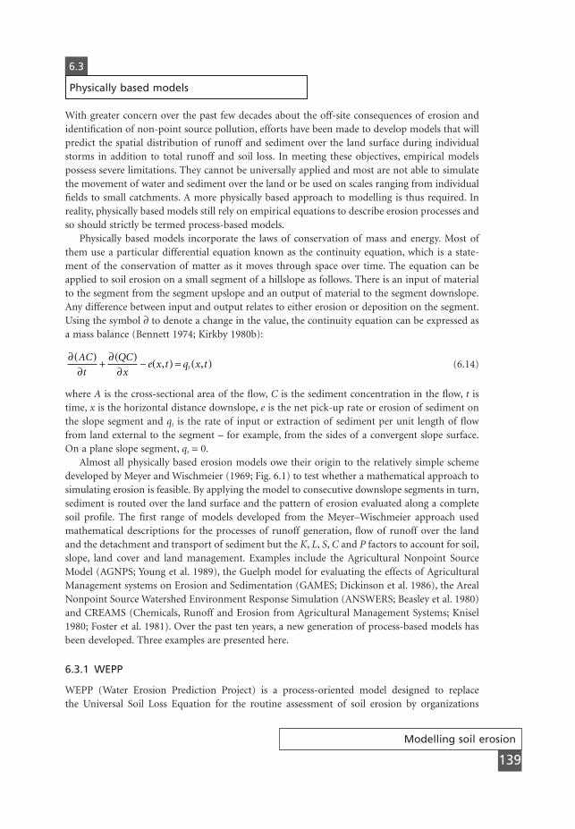
Modelling soil erosion
139
6.3
Physically based models
With greater concern over the past few decades about the off-site consequences of erosion andidentification of non-point source pollution, efforts have been made to develop models that willpredict the spatial distribution of runoff and sediment over the land surface during individualstorms in addition to total runoff and soil loss. In meeting these objectives, empirical modelspossess severe limitations. They cannot be universally applied and most are not able to simulatethe movement of water and sediment over the land or be used on scales ranging from individualfields to small catchments. A more physically based approach to modelling is thus required. Inreality, physically based models still rely on empirical equations to describe erosion processes andso should strictly be termed process-based models.
Physically based models incorporate the laws of conservation of mass and energy. Most ofthem use a particular differential equation known as the continuity equation, which is a state-ment of the conservation of matter as it moves through space over time. The equation can beapplied to soil erosion on a small segment of a hillslope as follows. There is an input of materialto the segment from the segment upslope and an output of material to the segment downslope.Any difference between input and output relates to either erosion or deposition on the segment.Using the symbol ∂ to denote a change in the value, the continuity equation can be expressed asa mass balance (Bennett 1974; Kirkby 1980b):
(6.14)
where A is the cross-sectional area of the flow, C is the sediment concentration in the flow, t istime, x is the horizontal distance downslope, e is the net pick-up rate or erosion of sediment onthe slope segment and qs is the rate of input or extraction of sediment per unit length of flowfrom land external to the segment – for example, from the sides of a convergent slope surface.On a plane slope segment, qs = 0.
Almost all physically based erosion models owe their origin to the relatively simple schemedeveloped by Meyer and Wischmeier (1969; Fig. 6.1) to test whether a mathematical approach tosimulating erosion is feasible. By applying the model to consecutive downslope segments in turn,sediment is routed over the land surface and the pattern of erosion evaluated along a completesoil profile. The first range of models developed from the Meyer–Wischmeier approach usedmathematical descriptions for the processes of runoff generation, flow of runoff over the landand the detachment and transport of sediment but the K, L, S, C and P factors to account for soil,slope, land cover and land management. Examples include the Agricultural Nonpoint SourceModel (AGNPS; Young et al. 1989), the Guelph model for evaluating the effects of AgriculturalManagement systems on Erosion and Sedimentation (GAMES; Dickinson et al. 1986), the ArealNonpoint Source Watershed Environment Response Simulation (ANSWERS; Beasley et al. 1980)and CREAMS (Chemicals, Runoff and Erosion from Agricultural Management Systems; Knisel1980; Foster et al. 1981). Over the past ten years, a new generation of process-based models hasbeen developed. Three examples are presented here.
6.3.1 WEPP
WEPP (Water Erosion Prediction Project) is a process-oriented model designed to replace the Universal Soil Loss Equation for the routine assessment of soil erosion by organizations
∂( )∂
+∂( )
∂- ( ) = ( )AC
t
QC
xe x t q x ts, ,
MSE06 11/19/04 02:37 PM Page 139

involved in soil and water conservation and environmental planning (Nearing et al. 1989b). Theoverall package contains three computer models: a profile version, a watershed version and a gridversion. The profile version estimates soil detachment and deposition along a hillslope profile andthe net total soil loss from the end of the slope. It can be applied to areas up to about 260 ha insize. The watershed and grid versions allow estimates of net soil loss and deposition over smallcatchments. The models take account of climate, soils, topography, management and supportingpractices. They are designed to run on a continuous simulation but can be operated for a singlestorm. A separate model, CLIGEN (Nicks et al. 1995), is used to generate the climatic data onrainfall, temperature, solar radiation and wind speed for any location in the USA for input toWEPP.
The erosion model within WEPP applies the continuity equation for sediment transportdownslope in the form (Foster & Meyer 1972):
(6.15)
where Qs is the sediment load per unit width per unit time, x is the distance downslope, Di is thedelivery rate of particles detached by interrill erosion to rill flow and Df is the rate of detachmentor deposition by rill flow. The interrill erosion rate (Di) is given by:
(6.16)
where Ki is an expression of interrill erodibility of the soil, I is the effective rainfall intensity, Ceexpresses the effect of the plant canopy, Ge expresses the effect of ground cover, Rs is the spacingof rills and w is the width of the rill computed as a function of the flow discharge. The canopyeffect is estimated by:
(6.17)
where F is the fraction of the soil protected by the canopy and PH is the canopy height. Theground cover effect is estimated by:
(6.18)
where gi is the fraction of the interrill surface covered by ground vegetation or crop residue.The rate of detachment of soil particles by rill flow (Df) is given by:
(6.19)
where Dc is the detachment capacity, Qs is the sediment load in the flow and Tc is the sedimentload at transport capacity. Detachment capacity is expressed as:
(6.20)
where Kr is the rill erodibility of the soil, t is the flow shear stress acting on the soil and tc is thecritical flow shear stress for detachment to occur. The transport capacity of the flow is obtainedfrom:
(6.21)Tc kt= t 3 2
D Kc r c= -( )t t
D D Qs Tcf c= -( )1
Ge e gi= -2 5.
Ce Fe PH= - -1 0 34.
D K I CeGe Rs wi i= ( )2
dQs dx D Di f= +
Chapter 6
140
MSE06 11/19/04 02:37 PM Page 140
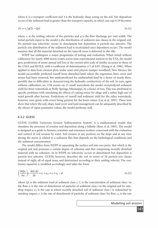
where kt is a transport coefficient and t is the hydraulic shear acting on the soil. Net depositionoccurs if the sediment load is greater than the transport capacity, in which case eqn 6.19 becomes:
(6.22)
where vs is the settling velocity of the particles and q is the flow discharge per unit width. Theinitial particle input to the model is the distribution of sediment-size classes in the original soil.No particle-size selectivity occurs in detachment but deposition is particle-size selective. The particle-size distribution of the sediment load is recalculated once deposition occurs. The modelassumes that all the material detached on the interrill areas is delivered to the rills.
WEPP has undergone a major programme of testing and evaluation. When tested without calibration for nearly 4000 storm events across nine experimental stations in the USA, the modelgave predictions of mean annual soil loss at the erosion plot scale of similar accuracy to those ofthe USLE and RUSLE, with a coefficient of determination (r2) of 0.85 (Zhang et al. 1996). Whenapplied to data from erosion plots under semi-arid pinyon–juniper woodland, New Mexico, themodel successfully predicted runoff from disturbed land, where the vegetation, litter cover andstones had been removed, but underpredicted for undisturbed land by a factor of nearly three,possibly due to difficulties in characterizing the hydraulic conductivity of the soil. In tests, againwithout calibration, on 1194 events on 15 small watersheds the model overpredicted sedimentyield for three watersheds at Holly Springs, Mississippi, by a factor of two. This was attributed tospecific problems with simulating the effects of cutting maize for silage and a rather high rate ofweed growth after harvest. Predictions of runoff and sediment yield for the other watersheds,however, were good, with errors being greatest for the lower values (Liu et al. 1997). These testsshow that where the soil, slope, land cover and land management can be adequately described bythe choice of input parameter values, the model performs well.
6.3.2 GUESS
GUESS (Griffith University Erosion Sedimentation System) is a mathematical model that simulates the processes of erosion and deposition along a hillside (Rose et al. 1983). The modelis designed as a guide to farmers, scientists and extension workers concerned with the evaluationand control of soil erosion by water. Soil erosion at any position on the slope and at any timeduring the storm is related to a sediment flux that depends on the hydrological conditions andthe sediment concentration.
The model differs from WEPP in separating the surface soil into two parts: that which is theoriginal soil and possesses a certain degree of cohesion and that comprising recently detachedmaterial with no cohesion. As in WEPP, no selectivity occurs in detachment but deposition is particle-size selective. GUESS, however, describes the soil in terms of 50 particle-size classesinstead of eight, all of equal mass, and determined according to their settling velocity. The con-tinuity equation is modified accordingly and takes the form:
(6.23)
where Qsi is the sediment load of sediment class i, Ci is the concentration of sediment class i inthe flow, ei is the rate of detachment of particles of sediment class i in the original soil by rain-drop impact, edi is the rate at which recently detached soil of sediment class i is redetached byraindrop impact, ri is the rate of detachment of particles of sediment class i by flow, rdi is the rate
∂∂
ÊËÁ
ˆ¯
+∂( )
∂= + + + -
Qs
x
C h
te e r r di i
i di i di i
D v q Tc Qsf s= -( )
Modelling soil erosion
141
MSE06 11/19/04 02:37 PM Page 141

at which recently detached soil of sediment class i is redetached by the flow, and di is the rate ofdeposition.
The rate of detachment of soil particles of sediment class i by raindrop impact is given by:
(6.24)
where a is the detachability of the soil, Ce is the fraction of the soil surface exposed to raindrops,I is the rainfall intensity and N is the number of particle size classes. The same equation is usedto calculate the rate of redetachment of soil particles by raindrop impact (edi) except that a isreplaced by ad, an expression of redetachability of the soil. The detachment rate of soil particlesby flow is modelled as a function of stream power (W), defined as the product of flow shear stress(t) and flow velocity (v) above a critical value (Wc):
(6.25)
where (1 - H) is the fraction of the original soil surface exposed to runoff, F is the fraction ofexcess stream power which is used in detachment, generally assumed to be � 0.1, and J is theamount of unit stream power necessary to detach a unit mass of soil. For redetachment of soilparticles, the rate is:
(6.26)
where ai is a dimensionless parameter with a value dependent on the depth of flow (usually ≥1but taken as 1 for shallow flow), H is the fraction of the surface soil covered by recently depositedmaterial, s is the submerged sediment density, r is the density of water, h is the depth of flow,Mi is the mass fraction of sediment class i to that of the total mass (M) of material being redetached. The rate of deposition of sediment class i is given by:
(6.27)
where vsi is the fall velocity of particles of sediment class i.Unlike in the WEPP model, not all the sediment detached or redetached by raindrop impact
is contributed to the flow. A limitation is placed so that:
(6.28)
where Crain is the contribution of detachment by raindrop impact to the sediment concentrationin the flow, and H approximates to 0.9. The transport capacity of the flow (Cmax) is representedby (Rose & Hairsine 1988):
(6.29)
The equation is applied either to the overland flow or, if rills are present, by assigning all the flowto the rills and, by dividing by the number of rills, calculating the water discharge and velocityper rill. The sediment flux in the rill can then be multiplied by the number of rills to give thetotal sediment flux for the slope.
CF
v Nsvmax
si
= ÊËÁ
ˆ¯ -ÊË
ˆ¯
r ss rS
C HaI v Nrain si= ( ) ( )S
d v Ci i si i=a
rHF
g h
M
Mdi
i c i= ÊËÁ
ˆ¯ -ÊË
ˆ¯
-ÊË
ˆ¯
a ss r
W W
r H F IJi c= -( ) -( )1 W W
e aC I Ni e=
Chapter 6
142
MSE06 11/19/04 02:37 PM Page 142
While it is possible for the actual sediment concentration (C) in the flow to equal Cmax, it isusually lower than Cmax by an amount depending on the strength of the soil matrix (b). The erodibility parameter (b) can be defined from the relationship:
(6.30)
The model calculates average values of C and Cmax for an event so that b can be evaluated from:
(6.31)
With bare tilled soils, b approximates to 1.0 but where the ground surface is protected by a vegetation cover in close contact with the soil, it can fall to between 0.6 and 0.8 in value (Presbitero et al. 1995). On a heavily consolidated soil, b can be as low as 0.1–0.4 (Hashim et al.1995; Paningbatan et al. 1995). The model needs to be calibrated to determine the values of J, Wc
and b. An extensive testing programme is under way in Australia, the Philippines, Malaysia andThailand.
6.3.3 EUROSEM
EUROSEM (European Soil Erosion Model; Morgan et al. 1998; Fig. 6.3) is an event-based modeldesigned to compute the sediment transport, erosion and deposition over the land surfacethroughout a storm. It can be applied to either individual fields or small catchments. Comparedwith other models, EUROSEM simulates interrill erosion explicitly, including the transport of water and sediment from interrill areas to rills, thereby allowing for deposition of material en route. This is considered more realistic than assigning all or a set proportion of the detachedmaterial to the rills. A more physically based approach to simulating the effect of vegetation orcrop cover is used, taking account of the influence of leaf drainage. Soil conservation measurescan be allowed for by choosing appropriate values of the soil, microtopography and plant cover parameters so as to describe the conditions associated with each practice. Unlike othermodels, however, EUROSEM does not describe the eroded sediment in terms of its particle size.
Equation 6.14 is used as the continuity equation in which the term (e), the net rate of pick-up of sediment, is defined as:
(6.32)
The rate of detachment by raindrop impact (Di) is calculated from:
(6.33)
where k is the detachability of the soil by raindrop impact and h is the depth of surface water.The kinetic energy (KE; J m-2 mm-1) of the rainfall is determined separately for the direct through-fall (DT) and the leaf drainage (LD) using relationships proposed by Brandt (1990):
(6.34)
(6.35)KE LD PH( ) = ¥( ) -15 8 5 870 5. ..
KE DT I( ) = +8 95 8 44. . log
D k KE eih= -. ..1 0 2
e D Di f= +
b =ln
ln
C
Cmax
C Cmax= b
Modelling soil erosion
143
MSE06 11/19/04 02:37 PM Page 143
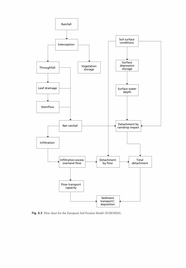
Rainfall
Interception
Throughfall
Leaf drainage
Stemflow
Net rainfall
Vegetationstorage
Soil surfaceconditions
Surfacedepression
storage
Surface waterdepth
Detachment byraindrop impact
Detachmentby flow
Infiltration
Infiltration-excessoverland flow
Flow transportcapacity
Totaldetachment
Sedimenttransport / deposition
Fig. 6.3 Flow chart for the European Soil Erosion Model (EUROSEM).
MSE06 11/19/04 02:37 PM Page 144
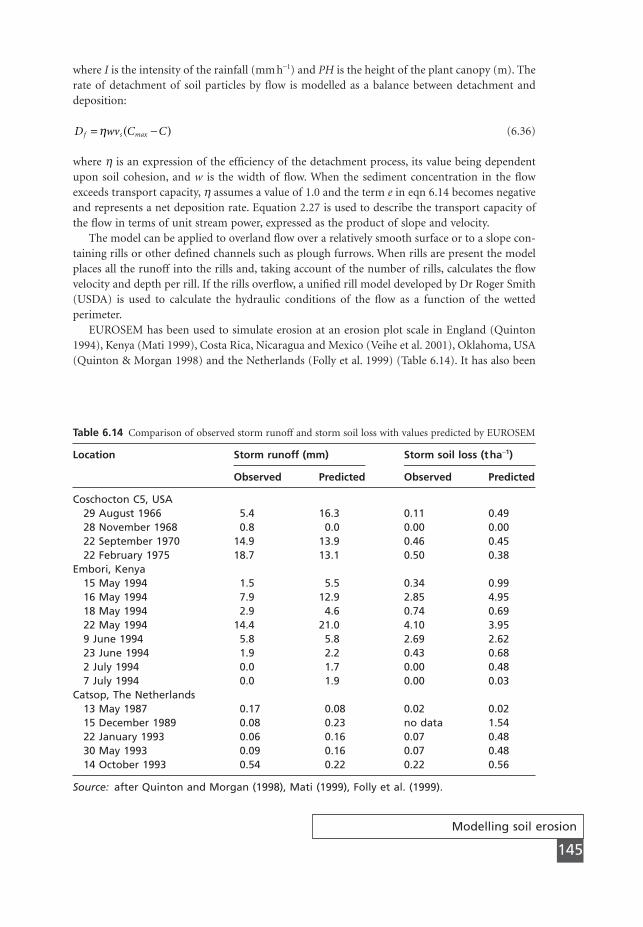
Modelling soil erosion
145
where I is the intensity of the rainfall (mm h-1) and PH is the height of the plant canopy (m). Therate of detachment of soil particles by flow is modelled as a balance between detachment anddeposition:
(6.36)
where h is an expression of the efficiency of the detachment process, its value being dependentupon soil cohesion, and w is the width of flow. When the sediment concentration in the flowexceeds transport capacity, h assumes a value of 1.0 and the term e in eqn 6.14 becomes negativeand represents a net deposition rate. Equation 2.27 is used to describe the transport capacity ofthe flow in terms of unit stream power, expressed as the product of slope and velocity.
The model can be applied to overland flow over a relatively smooth surface or to a slope con-taining rills or other defined channels such as plough furrows. When rills are present the modelplaces all the runoff into the rills and, taking account of the number of rills, calculates the flowvelocity and depth per rill. If the rills overflow, a unified rill model developed by Dr Roger Smith(USDA) is used to calculate the hydraulic conditions of the flow as a function of the wettedperimeter.
EUROSEM has been used to simulate erosion at an erosion plot scale in England (Quinton1994), Kenya (Mati 1999), Costa Rica, Nicaragua and Mexico (Veihe et al. 2001), Oklahoma, USA(Quinton & Morgan 1998) and the Netherlands (Folly et al. 1999) (Table 6.14). It has also been
D wv C Cf s max= -( )h
Table 6.14 Comparison of observed storm runoff and storm soil loss with values predicted by EUROSEM
Location Storm runoff (mm) Storm soil loss (tha-1)
Observed Predicted Observed Predicted
Coschocton C5, USA29 August 1966 5.4 16.3 0.11 0.4928 November 1968 0.8 0.0 0.00 0.0022 September 1970 14.9 13.9 0.46 0.4522 February 1975 18.7 13.1 0.50 0.38
Embori, Kenya15 May 1994 1.5 5.5 0.34 0.9916 May 1994 7.9 12.9 2.85 4.9518 May 1994 2.9 4.6 0.74 0.6922 May 1994 14.4 21.0 4.10 3.959 June 1994 5.8 5.8 2.69 2.6223 June 1994 1.9 2.2 0.43 0.682 July 1994 0.0 1.7 0.00 0.487 July 1994 0.0 1.9 0.00 0.03
Catsop, The Netherlands13 May 1987 0.17 0.08 0.02 0.0215 December 1989 0.08 0.23 no data 1.5422 January 1993 0.06 0.16 0.07 0.4830 May 1993 0.09 0.16 0.07 0.4814 October 1993 0.54 0.22 0.22 0.56
Source: after Quinton and Morgan (1998), Mati (1999), Folly et al. (1999).
MSE06 11/19/04 02:37 PM Page 145
Chapter 6
146
used to evaluate the effectiveness of contour grass strips as an erosion-control measure nearCochabamba, Bolivia (Quinton & Rodriguez 1999) and adopted as the erosion model in an investigation of alternative policies for reducing the losses of nitrogen, phosphorus and soil fromagricultural land in Norway (Vatn et al. 1996).
6.3.4 Wind erosion models
Although considerable research is taking place to develop a physically based wind erosion model,the work is still in the developmental stage. Particular difficulties arise in simulating the highdegree of complexity and randomness of the detachment and transport of soil particles by wind;in representing a three-dimensional sediment transport system as a simpler two-dimensional one;and in describing the physics of the system by mathematical equations that can be solved. Manyof the present models apply only to rather limited conditions such as sediment movement attransport capacity or bare soil. The most comprehensive state-of-the-art model that can simulatethe effects of soil, land cover and tillage is the Wind Erosion Prediction System (WEPS) (Hagen1991), which is a daily simulation model applicable at a field scale. Research is under way to linkWEPS and WEPP into a single process-based model (Fox et al. 2001). Unfortunately, it isextremely difficult to validate wind erosion models because suitable field measurements of erosionare hard to obtain (see section 5.1.3).
6.4
Sensitivity analysis
Sensitivity analysis indicates by how much the output of a model alters in relation to a unit changein the value of one or more of the inputs. It should be carried out on all models to show that themodel behaves rationally and to indicate how accurately values of the inputs need to be measuredor estimated. Rational behaviour is generally judged on whether the level of sensitivity of thefactors in the model matches what is expected in reality and on whether the relationships betweenthe output and the controlling factors accord with what is observed in the field or in laboratoryexperiments. For example, EUROSEM gives rational output with respect to relationships betweensoil loss and slope steepness and the percentage cover of low-growing vegetation but is less satisfactory with tree covers because it underpredicts soil particle detachment by leaf drainage(Morgan 1996).
Sensitivity analysis can be extended to evaluate whether the interaction between factors is cor-rectly simulated and whether a model gives plausible results when operated under extreme con-ditions. It may also be used to identify which processes could be excluded without significant lossof information should a decision be made to simplify a model.
Despite its simplicity of purpose, sensitivity analysis is not straightforward. A choice has to bemade about which sensitivity index to use (Table 6.15). Absolute sensitivity (McCuen 1973) is the simplest. It describes the rate of change in output with respect to a change in the value of input. However, it does not take account of the relative magnitudes of the values. For example,a 10 per cent change in a typical value of saturated hydraulic conductivity might increase the input value by 20–25 mm h-1, whereas a 10 per cent change in the value of Manning’s nmight increase the the input value by 0.001–0.002. To compare these changes, the relative sen-sitivity index, which normalizes the input and output around a base value chosen by the user,
MSE06 11/19/04 02:37 PM Page 146
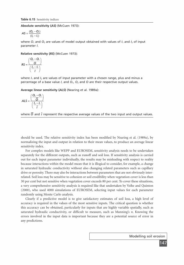
Modelling soil erosion
147
should be used. The relative sensitivity index has been modified by Nearing et al. (1989a), by normalizing the input and output in relation to their mean values, to produce an average linearsensitivity index.
For complex models like WEPP and EUROSEM, sensitivity analysis needs to be undertakenseparately for the different outputs, such as runoff and soil loss. If sensitivity analysis is carriedout for each input parameter individually, the results may be misleading with respect to realitybecause interactions within the model mean that it is illogical to consider, for example, a changein saturated hydraulic conductivity without also changing related parameters such as capillarydrive or porosity. There may also be interactions between parameters that are not obviously inter-related. Soil loss may be sensitive to cohesion or soil erodibility when vegetation cover is less than30 per cent but not sensitive when vegetation cover exceeds 80 per cent. To cover these situations,a very comprehensive sensitivity analysis is required like that undertaken by Veihe and Quinton(2000), who used 4000 simulations of EUROSEM, selecting input values for each parameter randomly using Monte Carlo analysis.
Clearly if a predictive model is to give satisfactory estimates of soil loss, a high level ofaccuracy is required in the values of the most sensitive inputs. The critical question is whetherthis accuracy can be obtained, particularly for inputs that are highly variable spatially, such as saturated hydraulic conductivity, or difficult to measure, such as Manning’s n. Knowing the errors involved in the input data is important because they are a potential source of error in any predictions.
Table 6.15 Sensitivity indices
Absolute sensitivity (AS) (McCuen 1973):
where O1 and O2 are values of model output obtained with values of I1 and I2 of inputparameter I.
Relative sensitivity (RS) (McCuen 1973):
where I1 and I2 are values of input parameter with a chosen range, plus and minus apercentage of a base value I, and O1, O2 and O are their respective output values.
Average linear sensitivity (ALS) (Nearing et al. 1989a):
where and represent the respective average values of the two input and output values.IO
ALS
O OO
I II
=
-ÊË
ˆ¯
-ÊË
ˆ¯
2 1
2 1
RS
O OO
I II
=
-ÊË
ˆ¯
-ÊË
ˆ¯
2 1
2 1
ASO OI I
= -( )-( )
2 1
2 1
MSE06 11/19/04 02:37 PM Page 147
Chapter 6
148
6.5
Model validation
The success of any model must be judged by how well it meets its objectives or requirements.With a predictive model this means deciding on the time and space scale for which predictionsare required and the level of accuracy. When making a judgement on the utility of a model, it isnecessary to distinguish between failures due to misuse, those related to inadequate input dataand those associated with the structure of the model or its operating functions. In the latter case, failure may result from poor conceptualization of the problem, omission of importantfactors or inaccurate representation of a particular element in the model by the operating func-tion or equation employed. The solution is to modify or in some instances completely rethinkthe model.
The accuracy of model predictions is usually tested by comparing predicted with measuredvalues and applying some measure of goodness-of-fit. The data used for validation should, ofcourse, always be different from those used to develop the model. Criteria for validation are byno means clear-cut and need to be set for individual models in relation to their objective. In manycases, a qualitative assessment is all that is required. Thus, Meyer and Wischmeier (1969) judgedthe success of their model by how well it reproduced the patterns of sediment movement foundin the field. For many applications, it may be sufficient to show that a model predicts the correctlocation of erosion and sedimentation.
Where the objective is to predict amounts of soil loss, it is necessary to compare the predic-tions with measured values. This can be achieved by dividing the predicted by the measured valueto give a ratio. Ideally, the ratio should be equal to 1.0 but, since this is rarely the case, its valuehas to be related to some guideline in order to judge whether it is acceptable – for example, theratio might lie between 0.75 and 1.5 in value or, less stringently, between 0.5 and 2.0. The per-centage of predictions that are acceptable can be used as a measure of a model’s success. Althoughthe use of ratios is a simple and effective method of validation, they cannot be applied where non-linear relationships are involved. In this case, the simplest measure is to examine the absolute dif-ferences between predicted and observed values. These types of tests, however, assume that a givenlevel of error is equally important over the full range of values, whereas, for many purposes, higherlevels may be acceptable at very low values of soil loss. A predicted value for mean annual soilloss of 0.02 t ha-1 may be acceptable in relation to a recorded value of 0.002 t ha-1 for evaluatingerosion-control strategies, since both values indicate that there is no on-site erosion problem.However, a predicted value of 200 t ha-1 against a recorded value of 20 t ha-1 would not be accept-able, since it would give a very misleading impression of the severity of the problem.
Many workers use correlation and regression analyses in order to test the strength of associ-ation between predicted and observed values. Experience with the WEPP model indicates thatcoefficients of determination (r2) greater than 0.5 should be deemed acceptable (Zhang et al. 1996)and that the best models are unlikely to give values in excess of 0.76 (Nearing 1998). A high andsignificant value of the correlation coefficient, however, does not imply that a model is perform-ing well, merely that the model is producing results with a degree of precision and with the righttrend. Unless the predicted and observed values have a 1:1 relationship, the model predictions are inaccurate to a certain degree. Ideally, a regression equation for the relationship should havea slope of 1.0 and pass through zero. Statistical tests should be applied to determine whether particular relationships differ significantly from these two conditions. A least-squares regressionapproach assumes that there will be some error in the predicted value but not in the observedvalue. This assumption is certainly questionable because, as seen in Chapter 5, all measurement
MSE06 11/19/04 02:37 PM Page 148
Modelling soil erosion
149
techniques are subject to measurement errors. It is preferable to recognize this and use a reducedmajor axis regression (Kermack & Haldane 1950; Till 1973), which allows for errors in both setsof values. A model can only be as good as the data that are fed into it. If much of the input datacontains errors of 10 per cent or more, it is unrealistic to expect a model to give predictions to accuracies of 5 per cent or less. It is also unreasonable to expect a model to perform better than the natural variability in erosion as indicated by data from replicate erosion plots (Nearing2000).
The efficiency coefficient (CE), proposed by Nash and Sutcliffe (1970), is now increasinglyused as an alternative to the correlation coefficient to express the performance of a model:
(6.37)
where Xobs is the observed value, Xmean is the mean of a set of observed values and Xpred is the pre-dicted value. The efficiency parameter is thus a measure of the variance in the predictions fromthe one-to-one prediction line with the measured values. In a comparative study using 1600 yearsof plot data for 20 locations in the USA, Tiwari et al. (2000) obtained CE values of 0.71, 0.80 and0.72 for WEPP, USLE and RUSLE respectively. The better result with the USLE was attributed tobetter input data. Annual soil loss predictions with the revised Morgan–Morgan–Finney modelgave CE values of 0.58 for runoff and 0.65 for soil loss, although tests on a second data set gaverespective values of 0.94 and 0.84 (Morgan 2001). Generally a CE value greater than 0.5 is con-sidered satisfactory (Quinton 1997) and one should not expect values to exceed 0.7 (Nearing1998).
It is also necessary to know whether a prediction has been arrived at in the right way. Forexample, if soil loss is limited by the detachment rate and the model predicts the right total butas a result of a limitation in transport capacity, it cannot be considered a successful model and itcannot be used for soil conservation, since any strategy based on its predictions will reflect a wrongdiagnosis. It is therefore essential that validation of process-based models be extended to coverall of their constituent modules. Given the very limited measured data available for such valida-tion and the associated measurement errors, De Roo (1996) concludes that, at present, it is virtually impossible to validate a process-based model in any meaningful way. Despite theadvances made in recent years in developing physically based models, a simple empirical modelis often more successful in predicting soil erosion and is usually easier to use.
CEX X X X
X X
obs mean pred obs
obs mean
=-( ) - -( )
-( )ÂÂ
Â2 2
2
The difficulty of obtaining an exact fitbetween predicted and observed values is areflection of uncertainty in model prediction.Uncertainties arise from: errors in the mea-sured values; the high spatial variability ofsome input parameters, which means thatthey cannot be properly represented by asingle value; the need to estimate some
Box 6
parameter values because they cannot beeasily measured; selection of parameter valuesto characterize field conditions, particularlysurface roughness, crusting, stoniness and veg-etation cover; and errors in the model struc-ture or the operating equations, particularlywhere empirical equations are used todescribe physical processes.
Uncertainty in model predictions
Continued
MSE06 11/19/04 02:37 PM Page 149
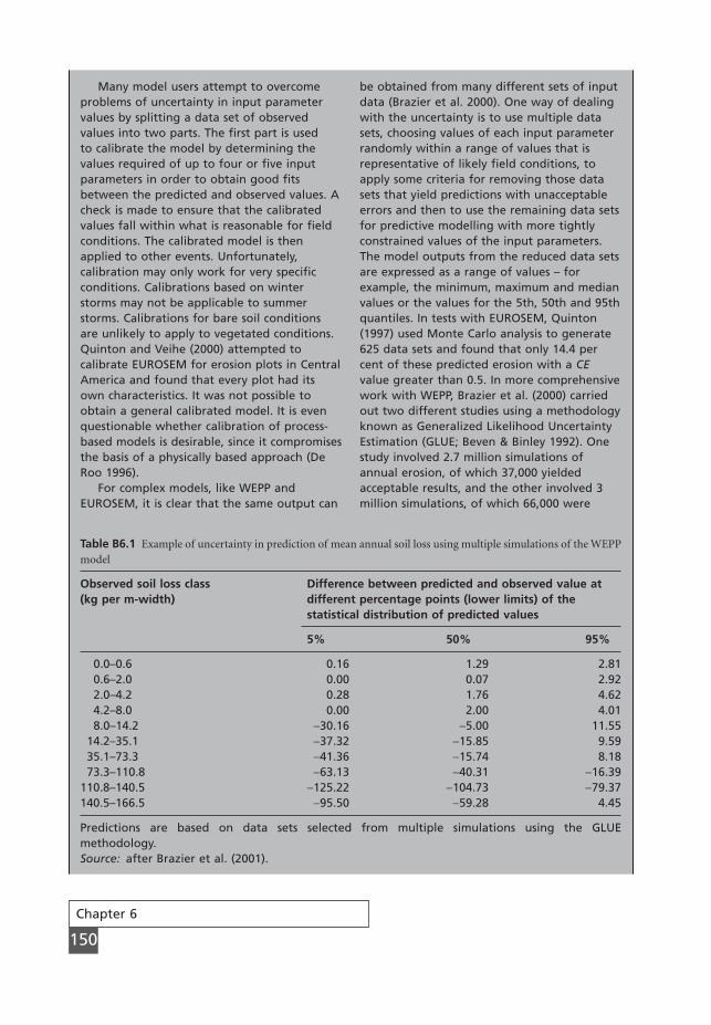
Chapter 6
150
Many model users attempt to overcomeproblems of uncertainty in input parametervalues by splitting a data set of observedvalues into two parts. The first part is used to calibrate the model by determining thevalues required of up to four or five inputparameters in order to obtain good fitsbetween the predicted and observed values. Acheck is made to ensure that the calibratedvalues fall within what is reasonable for fieldconditions. The calibrated model is thenapplied to other events. Unfortunately,calibration may only work for very specificconditions. Calibrations based on winterstorms may not be applicable to summerstorms. Calibrations for bare soil conditionsare unlikely to apply to vegetated conditions.Quinton and Veihe (2000) attempted tocalibrate EUROSEM for erosion plots in CentralAmerica and found that every plot had itsown characteristics. It was not possible toobtain a general calibrated model. It is evenquestionable whether calibration of process-based models is desirable, since it compromisesthe basis of a physically based approach (DeRoo 1996).
For complex models, like WEPP andEUROSEM, it is clear that the same output can
be obtained from many different sets of inputdata (Brazier et al. 2000). One way of dealingwith the uncertainty is to use multiple datasets, choosing values of each input parameterrandomly within a range of values that isrepresentative of likely field conditions, toapply some criteria for removing those datasets that yield predictions with unacceptableerrors and then to use the remaining data setsfor predictive modelling with more tightlyconstrained values of the input parameters.The model outputs from the reduced data setsare expressed as a range of values – forexample, the minimum, maximum and medianvalues or the values for the 5th, 50th and 95thquantiles. In tests with EUROSEM, Quinton(1997) used Monte Carlo analysis to generate625 data sets and found that only 14.4 percent of these predicted erosion with a CEvalue greater than 0.5. In more comprehensivework with WEPP, Brazier et al. (2000) carriedout two different studies using a methodologyknown as Generalized Likelihood UncertaintyEstimation (GLUE; Beven & Binley 1992). Onestudy involved 2.7 million simulations ofannual erosion, of which 37,000 yieldedacceptable results, and the other involved 3million simulations, of which 66,000 were
Table B6.1 Example of uncertainty in prediction of mean annual soil loss using multiple simulations of the WEPPmodel
Observed soil loss class Difference between predicted and observed value at(kg per m-width) different percentage points (lower limits) of the
statistical distribution of predicted values
5% 50% 95%
0.0–0.6 0.16 1.29 2.810.6–2.0 0.00 0.07 2.922.0–4.2 0.28 1.76 4.624.2–8.0 0.00 2.00 4.018.0–14.2 -30.16 -5.00 11.55
14.2–35.1 -37.32 -15.85 9.5935.1–73.3 -41.36 -15.74 8.1873.3–110.8 -63.13 -40.31 -16.39
110.8–140.5 -125.22 -104.73 -79.37140.5–166.5 -95.50 -59.28 4.45
Predictions are based on data sets selected from multiple simulations using the GLUE methodology.Source: after Brazier et al. (2001).
MSE06 11/19/04 02:37 PM Page 150

Modelling soil erosion
151
acceptable. Table B6.1 shows the differencesbetween the values of the 5th, 50th and 95thquantiles of the statistical distribution ofpredicted values from the acceptable data sets and the observed values for differentmagnitudes of annual soil loss. It is clear fromthese studies that model predictions have ahigh level of uncertainty associated with them.The results also confirm the tendency of WEPPto overpredict at low values and underpredictat high values.
Given the large number of simulationsrequired to produce data sets from whichpredictions can be made with reduced levels
of uncertainty, it is unlikely that many modelusers will attempt this type of analysis,particularly when, as shown by Quinton(1997), it may reduce the level of variabilityaround the prediction but will not necessaryresult in a better fit between observed andpredicted values. Reducing the level ofuncertainty associated with model predictionsis vital if models are to become widely used.Modellers need to recognize that most usersdo not want multiple predictions withdifferent levels of uncertainty but wish tooperate with a single predicted value in whichthey can have confidence.
MSE06 11/19/04 02:37 PM Page 151
Chapter 7
152
The aim of soil conservation is to reduce erosion to a level at which the maximum sustainablelevel of agricultural production, grazing or recreational activity can be obtained from an area ofland without unacceptable environmental damage. Since erosion is a natural process, it cannotbe prevented. But it can be reduced to a maximum acceptable level or soil loss tolerance. Thisshould be considered as a performance criterion that erosion-control measures are expected toachieve.
CHAPTER 7
Strategies forerosion control
7.1
Soil loss tolerance
Theoretically, soil erosion should be maintained at a rate that equals or is below the natural rateat which new soil forms. Unfortunately, it is difficult to recognize when this balance exists.Although rates of soil loss can be measured (see Chapter 5), rates of soil formation are so slowthat they cannot be easily determined. According to Buol et al. (1973), rates of soil formationthroughout the world range from 0.01 to 7.7 mm yr-1. The fastest rates are exceptional, however,and the average is about 0.1 mm yr-1 (Zachar 1982).
An alternative approach that avoids the need to measure the rate of new soil formation directlyis to estimate the rate required to match the rate of removal by erosion and solution in areaswhere an equilibrium condition might be presumed to exist. Using data from small watershedsunder forest and grassland, Alexander (1988) found the required rates to be between 0.3 and 2 t ha-1 annually with the majority being below 1 t ha-1 which, assuming a bulk density for the soil of 1.0 Mg m-3, is equivalent to 0.1 mm yr-1. Such a rate, however, may be a rather conserva-tive indicator for the development of an agriculturally productive soil.
Bennett (1939) and Hall et al. (1979) suggest that in soils of medium to moderately coarsetexture on well managed crop land the annual rates of formation of the A horizon can exceed 11 t ha-1. This is because the subsoil can be improved by incorporating it with the top soil duringtillage and by adding fertilizers and organic matter. It is against this background that values forsoil loss tolerance are set so as to maintain an adequate rooting depth and avoid significant reduc-tions in yield while the surface layer of soil is removed by erosion (McCormack & Young 1981).Soil loss tolerance is then defined as the maximum permissible rate of erosion at which soil fer-tility can be maintained over 20–25 years. A mean annual soil loss of 11 t ha-1 is generally accepted
MSE07 11/19/04 02:39 PM Page 152
Strategies for erosion control
153
as appropriate but values as low as 2 t ha-1 are recommended for particularly sensitive areas wheresoils are thin or highly erodible (Hudson 1981). Where soils are deeper than 2 m, the subsoils arecapable of improvement and reductions in crop yield are unlikely to be brought about by erosionover the next 50 years or more, some scientists favour increasing the tolerance to 15–20 t ha-1
(Schertz 1983).These recommendations on soil loss tolerance are based solely on agricultural considerations.
They ignore problems of pollution and sedimentation that arise as plant nutrients and pesticidesleave a field either in solution in the runoff or attached to sediment particles. Particular concernrelates to the removal of nitrogen, phosphorus and organic matter but, in the context of erosion,most attention is given to the removal of phosphorus, which can occur in both soluble and particulate forms. Between 45 and 90 per cent of the annual phosphorus contribution to watercourses is in particulate form (Kronvang 1990; Hasholt 1991; Sibbesen et al. 1994; Sibbesen &Sharpley 1997), with some 18–49 per cent of this being bioavailable, which means that it is poten-tially available for uptake by algae (Sharpley & Smith 1990) and therefore a contributor toeutrophication of water bodies. Although no guidelines exist regarding acceptable rates of par-ticulate phosphorus within runoff, some simple calculations can provide a rough indicator.If it is assumed that a mean annual flow-weighted concentration of soluble phosphorus of10 mg l-1 produces a risk of eutrophication (Sharpley & Smith 1990) and that this represents some20 per cent of the total annual transport of phosphorus, annual rates in excess of 1 kg l-1 wouldbe of concern. Since, very broadly, measured data show that values of mean annual phosphorusconcentrations in kg l-1 relate proportionately to mean annual soil loss values in t ha-1 (Sharpley& Smith 1990; Sibbesen et al. 1994), this would equate to an annual erosion rate of 1 t ha-1, therebysupporting the recommendation made by Moldenhauer and Onstad (1975) that a soil loss tolerance no greater than 1 t ha-1 may be required to reduce the effects of non-point source pollution from agricultural land to acceptable levels.
A pragmatic approach to determining the level of soil loss tolerance is to decide what level ofenvironmental damage is acceptable using the criteria described in Table 4.3 as a guide. For mostpurposes, soil tolerance would be set to equate with the upper limits of damage classes 1, 2 or 3since the damage is unacceptable at higher levels. This approach provides the opportunity to settolerance levels in relation to local conditions and locally set objectives rather than seeking someuniversal value.
7.2
Principles of soil conservation
From the discussion of the mechanics of the detachment and transport of soil particles by rain-splash, runoff and wind (Chapter 2), it follows that the strategies for soil conservation must bebased on: covering the soil to protect it from raindrop impact; increasing the infiltration capac-ity of the soil to reduce runoff; improving the aggregate stability of the soil; and increasing surfaceroughness to reduce the velocity of runoff and wind. The various conservation techniques can bedescribed under the headings of agronomic measures, soil management and mechanical methods.Agronomic measures utilize the role of vegetation to protect the soil against erosion. Soil man-agement is concerned with ways of preparing the soil to promote plant growth and improve itsstructure so that it is more resistant to erosion. Mechanical or physical methods, often involvingengineering structures, depend on manipulating the surface topography – for example, installingterraces or windbreaks – to control the flow of water and air. Agronomic measures combined with
MSE07 11/19/04 02:39 PM Page 153
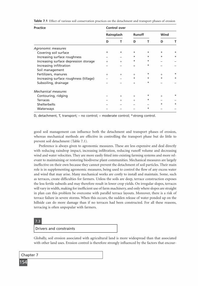
Chapter 7
154
good soil management can influence both the detachment and transport phases of erosion,whereas mechanical methods are effective in controlling the transport phase but do little toprevent soil detachment (Table 7.1).
Preference is always given to agronomic measures. These are less expensive and deal directlywith reducing raindrop impact, increasing infiltration, reducing runoff volume and decreasingwind and water velocities. They are more easily fitted into existing farming systems and more rel-evant to maintaining or restoring biodiverse plant communities. Mechanical measures are largelyineffective on their own because they cannot prevent the detachment of soil particles. Their mainrole is in supplementing agronomic measures, being used to control the flow of any excess waterand wind that may arise. Many mechanical works are costly to install and maintain. Some, suchas terraces, create difficulties for farmers. Unless the soils are deep, terrace construction exposesthe less fertile subsoils and may therefore result in lower crop yields. On irregular slopes, terraceswill vary in width, making for inefficient use of farm machinery, and only where slopes are straightin plan can this problem be overcome with parallel terrace layouts. Moreover, there is a risk ofterrace failure in severe storms. When this occurs, the sudden release of water ponded up on thehillside can do more damage than if no terraces had been constructed. For all these reasons,terracing is often unpopular with farmers.
Table 7.1 Effect of various soil conservation practices on the detachment and transport phases of erosion
Practice Control over
Rainsplash Runoff Wind
D T D T D T
Agronomic measuresCovering soil surface * * * * * *Increasing surface roughness – – * * * *Increasing surface depression storage + + * * – –Increasing infiltration – – + * – –Soil managementFertilizers, manures + + + * + *Increasing surface roughness (tillage) – – * * * *Subsoiling, drainage – – + * – –
Mechanical measuresContouring, ridging – + + * + *Terraces – + + * – –Shelterbelts – – – – * *Waterways – – – * – –
D, detachment, T, transport; – no control; + moderate control; * strong control.
7.3
Drivers and constraints
Globally, soil erosion associated with agricultural land is more widespread than that associatedwith other land uses. Erosion control is therefore strongly influenced by the factors that encour-
MSE07 11/19/04 02:39 PM Page 154
Strategies for erosion control
155
age or discourage farmers from adopting soil conservation. In non-agricultural areas, erosion isimportant wherever it threatens the integrity of a resource – for example, destruction of roads,trackways and footpaths, sedimentation of water bodies or exposure of buried pipelines. Thedriver for erosion control is to protect the resource and prevent liability for environmentaldamage, particularly in societies that adopt the principle of the ‘polluter pays’. Moreover, organi-zations like highways agencies, engineering companies and pipeline companies will install pro-tective measures because they want to retain their reputations for sensitive management of theenvironment.
7.3.1 Perceptions of erosion
The relevance of conservation measures to a farming system depends in part of how farmers andothers perceive the erosion problem and its consequences. Most farmers are aware of the problemand its effects. The notion of the peasant farmer damaging land through ignorance is severelymistaken. The small-scale farmer is as much an experienced and efficient practioner of land hus-bandry as the large-scale commercial farmer, but with a different objective, namely that of sur-vival rather than profit (Hudson 1981). If a farmer destroys land by overcropping or overgrazing,it is because there is no alternative employment from which to make a living. Farmers who workmarginal land because there is no other land available are generally well aware of the damage theycause. Surveys of small-scale farmers in Sierra Leone showed that the majority correctly perceivedan erosion problem on their land and associated it with high rainfall, steep slopes and lack ofvegetation cover (Millington 1987). Studies of large-scale farmers in erosion-prone areas ofOhio revealed that over 40 per cent of them knew they owned land on which erosion was severeenough to affect productivity (Napier 1990). However, since farmers appreciate erosion mainlythrough its effects on yield, sediment accumulation on footslopes and formation of gullies, theyunderestimate its seriousness compared with more scientific assessments based on reductions inthe depth of soil (Stocking & Clark 1999; Holden & Shiferaw 1999).
Most farmers are concerned with the effects of erosion on productivity and on increased costsof seeds for replanting a crop destroyed by erosion, fertilizers to maintain soil fertility, and waterstorage or irrigation facilities to provide additional water for crop growth (Shaxson 1987).Farmers’ decisions, however, tend to be a compromise between preventing long-term soil damageby erosion and maximizing short-term income. Generally, the farmer is not unwilling to changepractices but will do so only if substantial benefits arise and the investment costs can be recov-ered. Where a land user does not perceive such benefits, soil conservation is unlikely to be adopted.For example, where land is cheap and readily available, the incentive is to make a rapid profit andthen move on to new land when the soil becomes unproductive. For the subsistence farmer, aparticular problem is whether or not a new practice increases the risk of crop failure. Taking uphigher yielding crop varieties that may also help to reduce erosion by increasing biomass will notbe an acceptable gamble if, in one year out of ten, the crop yields less than the minimum requiredfor subsistence, even though much higher yields will be obtained in the other nine years (Hudson1981). These pressures invariably mean that, regardless of good intentions, the concept of a farmermanaging the land according to an ethic of land stewardship is an inappropriate base for soil conservation (Hudson 1988).
7.3.2 Land tenure
The arrangements by which tenure is granted to the land user can influence attitudes towards soilconservation. Where farmers own the land, they are more likely to consider the long-term
MSE07 11/19/04 02:39 PM Page 155

Chapter 7
156
consequences of their actions and adopt soil-protection measures unless the need for short-termsurvival dictates otherwise. Tenure systems based on short-term cultivation rights, share-cropping and collectives generally lead to poor management because of uncertainty aboutwhether conservation work carried out on the land will be rewarded. Legal title to the land,however, may be less important than a guaranteed long-term right to use the land, as seen inVietnam and China, where soil conservation is practised even though private ownership of theland is not allowed (Phien & Tu Siem 1996; Li et al. 1998).
The overall size of a farm does not necessarily influence the frequency or type of soil conser-vation measures employed. Hallsworth (1987) cites data from the Nyasa, Rift Valley and WesternProvinces of Kenya that show that 51 per cent of the farmers with holdings of less than 1 ha usefertilizers to maintain productivity, whereas on farms of over 10 ha the figure is still only 68 percent. Equivalent figures for the use of terracing are 24 per cent and 21 per cent respectively. Formulching, however, the figures are 5 and 17 per cent respectively, the lower figure reflecting thedifficulty of supplying mulch material on very small holdings. More important than farm size isthe layout of the farm and, in particular, its degree of fragmentation, since many conservationmeasures, such as terraces, become impractical when the land is held in small and scatteredparcels. Mulching is more difficult because there may be a considerable distance between the stripof land from which the mulch is taken and the strip on which it needs to be applied. Land con-solidation programmes may not improve the erosion status, however, because, as seen in north-ern France, the reorganization of holdings into larger fields means the removal of field boundariesand increases in the length over which surface runoff can flow.
7.3.3 Labour
All soil conservation work implies extra labour. It is needed for the building and maintenance ofterraces and for the growing of additional soil-protective crops either in rotation or by inter-cropping (Table 7.2). The likelihood of any soil conservation measure being adopted depends onwhether the farmer and associated family can meet the increased labour demands (Stocking &Abel 1992). Surveys in northern Thailand showed that while 76 per cent of the farmers believedthat soil conservation would bring about an improvement in yields, 85 per cent said they did nothave the labour resource to implement the measures (Harper & El-Swaify 1988). While it may be
Table 7.2 Examples of labour requirements for soil conservation
Conservation practice Labour(person-days ha-1)
Construction of contour terraces 100–300Construction of bench terraces 200–500Construction of bench terraces with stone side slopes (Inca type) 1000–1800Annual maintenance of terraces 40–60Contour stone bunds 50–60Contour grass barriers 40–45Intercropping an additional crop with maize (extra labour over 150–200maize monoculture)Construction of Katumani-type pits 100–120
Sources: Wenner (1981), Alfaro Moreno (1988), IFAD (1992), Stocking and Abel (1992),Gichangi et al. (1992).
MSE07 11/19/04 02:39 PM Page 156
Strategies for erosion control
157
thought that in countries with high population densities and high rates of unemployment, labour-intensive conservation schemes would be beneficial, this view ignores the fact that farmers maygive a higher priority in their use of labour to other activities, such as marketing their produce,traditional craftwork, house maintenance and off-farm employment. Moreover, a poor small-scalefarmer is often physically unable to put more hours of work into the land because of poor dietand poor health. If the family tries to secure additional sources of income by the young men goingto the towns or to the mines, an inadequate workforce is left behind on the farm, comprisinggrandparents, whose working life is over, young women, whose working time is limited by dutiesof housekeeping and child bearing, and children. In many countries, AIDS and other diseases aresubstantially reducing labour supply on family farms.
The organization of labour within the family is frequently highly specialized by age and sex.Men may do the land clearing and ploughing and women the weeding and collection of fuel wood;men may look after the cash crops and women the food crops. Knowing which groups performwhich tasks is important, so that extension workers can target the most appropriate sector of thelabour force. When soil conservation introduces new tasks, these have to be assigned in accept-able ways without creating stresses elsewhere in the system. Replacing hand-hoeing with oxploughs may enable more land to be cultivated by the men but will result in much more weedingfor the women (Milner & Douglas 1989).
The availability of labour can be improved if farmers have sufficient income to hire additionalworkers but, more often than not, serious constraints exist, particularly at times of land prepa-ration and harvest when the work has to be done in a very short time. Other ways of improvinglabour supply are through communal schemes where farmers and their families come togetherto build terraces, dig the soil or weed the crop for what is, at the same time, a social occasion.
7.3.4 Access to soil conservation
The ability of farmers to adopt soil conservation measures will depend on their access to all appro-priate resources, not just labour. These may vary from knowledge of new systems to an ability toafford the necessary inputs of capital to take them up. Whether or not farmers have the cash topurchase the additional seeds, fertilizer or machinery required to support a more conservation-oriented farming system will clearly affect its uptake; many poor farmers have insufficient security to support loans and would consider the risk of borrowing money too high. Most credit agencies would also view small-scale farmers as unacceptable risks and restrict access tocredit to larger-scale and wealthier land owners.
It is pointless designing a soil conservation programme that requires levels of input to whichthe targeted farmers have no access. However, it should be recognized that many farmers use theirown initiative, technical skill and labour to develop soil conservation measures where they benefitfrom so doing. Between 1948 and 1978, farmers in the Machakos District of Kenya (Tiffen et al.1994) made large investments in terracing, tree planting and hedging as well as improving cultivation techniques in order to grow coffee, cotton, oranges and papaya. Despite a rapidlyincreasing population density of 3 per cent per year, the cash value of farm output per hectarerose tenfold and soil loss was reduced by one-third. Farmers on land holdings of less than 5 ha in western Santa Catarina, Brazil, adopted intercropping of maize and velvet bean (Mucunapruriens) to protect soil because this made the difference between making a small profit or a finan-cial loss (Stocking & Tengberg 1999). In these situations, the aim of the soil conservationist is towork with the farmer to enhance the performance of the measures and optimize their benefits.Where such benefits are not perceived, farmers will even remove conservation work to which they
MSE07 11/19/04 02:39 PM Page 157
Chapter 7
158
already have access, such as terracing installed on food-for-work programmes (Holden & Shiferaw1999).
7.3.5 External factors
The causes of soil erosion rarely relate only to the existing physical and socio-economic condi-tions of a farming system but arise also from its inability to adapt to changing circumstancesbrought about by drought, increases in population, fragmentation or enlargement of farms, eco-nomic pressures to grow cash crops rather than food crops and new technologies. Erosion in muchof Europe reflects the breakdown of farming systems formerly based on a rotation of cereals, rootcrops and grasses, or a combination of tree crops, cereals and pastures. With economic incentivesto grow continuous cereals and roots, all essentially soil-degrading crops, the loss of grass has led to a decline in organic matter and a deterioration in the aggregate stability of the soils. Thepenetration of a cash economy into areas of traditional subsistence farmers and pastoralists frequently marginalizes those sections of the community who do not have sufficient eco-nomic resources to take advantage of the new income opportunities (Franke & Chasin 1981).Pastoralists are often displaced from the better quality land and forced to utilize and thereforeovergraze poorer areas. Small-scale farmers who plant new cash crops, which are often more soil-degrading, lose their food security and in years when the market price for the crop is low are unable to provide the necessary inputs to maintain soil fertility and conservation structures.To obtain money to buy food, they may have to relinquish control of their land and lose theirsecurity of tenure. With more of the land area taken up in cash crops, food crops are in shortsupply and more expensive. Similarly, surplus labour is taken up by the larger-scale farmers,reducing its seasonal availability. As a result, many farmers can no longer adjust their farmingsystem to meet the needs of soil conservation.
If soil erosion as a response to changes in farming systems is to be avoided, soil conservationmust be a dynamic process capable of adjusting to future change. It is insufficient to develop astrategy that merely solves an immediate problem. The need for adaptability in soil conservationsystems is likely to increase because the global impacts on erosion and agriculture expected toarise from climatic change will be far greater than those hitherto associated with changes in landuse.
7.3.6 Technological transfer
Though the principles of soil conservation are transferable, conservation strategies developed inone area will not necessarily work elsewhere. What is feasible on a 100–200 ha farm with a highlevel of mechanization in the Midwest of the USA is unlikely to be applicable to a smallholdingof less than 0.5 ha in the tropics. The non-transferability of soil conservation measures is perhapsbest illustrated by the failure of channel terraces within the small-scale farming systems of Africa.Borrowed from the USA, where they were successfully developed and implemented in the 1930sand 1940s, such terraces formed the nub of soil conservation programmes proposed by the European colonial administrations in much of central and eastern Africa. Since the Crown Landmade available to European settlers was not under pressure, there was little incentive to practisesoil conservation and the colonial governments were forced to support the implementation ofterraces and other structural measures by legal means to ensure that the works were maintainedand appropriate soil management, such as contour ploughing, followed. With the measures beinggenerally effective on the large settler farms, the governments tried to impose them on the landreserved for the local population on which erosion was becoming particularly severe. Despite
MSE07 11/19/04 02:39 PM Page 158
Strategies for erosion control
159
much exhortation and attempts at compulsion, the policy was a failure. The measures were seenas too labour-intensive for the expected economic return, took too much scarce land out of cul-tivation, were not supported by the same system of subsidies and loans that were made availableto the settlers and were regarded as an illustration of what was increasingly seen as the unfairnessof colonial rule (Temple 1972; Wood 1992). Today, there are many examples throughout Africawhere channel terraces and bench terraces implemented by governments, pre- and post-independence, have not worked, whereas indigenous, often highly labour-intensive systems, havebeen successful (Roose 1992; Cheatle & Njoroge 1993; Tiffen et al. 1994).
As long as soil conservation and extension services were promoting technologies modelled on those developed in the USA, indigenous conservation practices were either ignored or dismissed as ineffective. The fact that many were simply good farming practices of soil and water management that also happened to be helpful in reducing erosion was disregarded.Although these included traditional bench terrace systems, like those built by the Incas in Peru,they also encompassed contour bunds to promote infiltration of water and increase soil moisture, mulching to conserve water and soil fertility, burying of weeds and trash to improvefertility and weed control, crop rotation and weed fallows (Critchley et al. 1994; Reij et al. 1996;Tengberg et al. 1998). A characteristic of these indigenous systems is that they are not standard-ized; they vary from area to area and, often, from farm to farm, and their designs do not conformto the technical standards proposed by soil conservation services (Humbert-Droz 1996). Indige-nous systems are not without problems, however. Structural measures require large inputs of labour to construct and maintain. Trash lines and mulching enhance the survival and spreadof insect pests and disease pathogens (Tengberg et al. 1999). Nevertheless, indigenous systemsprovide a base for the soil conservationist to work with the local farmers to improve the localtechnology.
7.3.7 Economic evaluation
A major problem with applying economic analysis to soil conservation is that many aspects, suchas benefits related to minimizing adverse environmental impacts, are difficult to quantify in mon-etary terms. Although this may be of limited importance in a farm budget, it can be vital at aproject scale for deciding on the size of financial incentives given to farmers to promote soil con-servation for the benefit of the community. An analysis directed at the community should takeaccount of the costs of not controlling the erosion, including downstream or downwind sedi-mentation, and the benefits in terms of crop production and employment. However, at this levelthe analysis generally suffers from inadequate information on: how to price labour when muchof it is in the form of unpaid inputs from farmers and their families; how to take account of theeffects of different currency exchange rates where a black currency market exists alongside theofficial exchange; and how to cost the differences between a project with soil conservation andone without when the impact of continuing erosion on productivity cannot be quantified (Bojö1992). Detailed information on the economics of households and their decision-making processescan be difficult to obtain, with many farmers unwilling to provide it or supplying misleading data(Ellis-Jones & Mason 1999).
Different views exist on whether projects should be evaluated in terms of: their net presentvalue (NPV), i.e. the sum of discounted benefits less the sum of discounted costs; their internalrate of return (IRR), i.e. the rate of interest that the project can afford to pay to cover the resourcesrequired; or their benefit–cost ratio, defined as the sum of discounted benefits divided by the dis-counted costs. Decisions on the appropriate discount rate can seriously affect the results of NPVanalysis. Disagreement also exists on whether the evaluation should be made over 10, 20, 30 years
MSE07 11/19/04 02:39 PM Page 159
Chapter 7
160
or longer. Extending the time horizon to 50 years can have a detrimental effect on the outcome,especially if discount rates of 10 per cent or more are used (Bojö 1992).
If the analysis is applied to an individual farmer, costs and benefits can be more easily quantified and yearly cash flows calculated (Hedfors 1983). Benefit–cost ratios to farmers in the Acelhuate Basin, El Salvador, from adopting a system of contour cultivation, contour grass strips and contour ditches to grow maize, sorghum and beans on steep slopes ranged from 1.0 to 2.8, depending on slope steepness and the depth of soil (Wiggins 1981). Greatestreturns were predicted for the gentler-sloping land with deeper soil, whereas benefits were very limited or neutral for farmers working slopes of 25–51° with no top soil and renting the land on annual leases. It is clear that these last farmers have no economic accessibility to soil conservation. At both 5 and 20 per cent discount rates contour grass barriers were found to beuneconomic for farmers in the Cochabamba region, Bolivia, unless they brought about a 20 percent increase in productivity (Ellis-Jones & Mason 1999). Economic analysis of small farms inthe Machakos District of Kenya showed that soil conservation measures gave a return of KSh5per man-day where terracing and some tree- and grass-planting were used, and KSh21 where allthe terrace edges were planted with fodder grasses and fruit trees (Tjernström 1992). Studies in the USA (Ervin & Washburn 1981; Mueller et al. 1985) showed that in the 1970s and early1980s, with the effects of erosion on productivity being masked by higher-yielding crop varietiesand improved soil and water management, the cost of adopting a conservation technique was often higher than any benefit gained. As farmers came under greater economic stress, theyabandoned existing soil conservation practices to reduce costs and avoid bankruptcy (Napier1988). More recent economic analysis based on partial budgets of the additional benefits and costs show that adopting a no-tillage practice with nutrient management can bring about netbenefits to a farmer of US$17.4 per hectare for maize, $7.7 for wheat and $3.6 for soya bean com-pared to conventional tillage (Natural Resources Conservation Service 1999). Obtaining higheryields from the new practice is an important contributor to these benefits. Were the yields toremain the same, there would be a net benefit of $8.9 per hectare for maize and $2.4 for wheatbut a net disbenefit of $7.3 for soya bean. Installing a mixed grass and forest riparian barrier totrap eroded sediment and help reduce off-site water pollution would produce a net disbenefit tothe farmer of $19.8 per hectare, even after allowing for government payments of $34.4 per hectare for enrolling the land under the Conservation Reserve Program and an additional $1.2per hectare for management of the barrier, and after amortizing the establishment costs over tenyears at 8 per cent interest (Natural Resources Conservation Service 1999). The question arisesas to whether further public support should be provided to obtain the additional benefits to riverwater quality.
As the last example shows, soil conservation can have many benefits beyond the farm level.Since these cannot always be easily expressed in monetary terms, alternative methods tocost–benefit analysis need to be used if they are to be taken into account. One approach, multi-criteria analysis, uses cost–benefit for those items that can be properly represented in this way andthen modifies the results by a series of weightings, designed to assess the other costs or benefits.For the Konto River Watershed Development Project, Indonesia, weightings were developed toexpress: the expected income to the local population, particularly the landless; the changes in ratesof runoff and erosion; and the preservation of natural forest (de Graaf 2001). In practice, multi-criteria analysis can be somewhat complex, with difficulties in deciding what the weightingsshould be and how their values should be determined, especially when, unlike measures of erosionand runoff, they cannot be easily expressed numerically. A better approach, which has yet to bewidely used in soil conservation studies, would appear to be cost-effectiveness analysis. Here, theobjectives are decided in advance and expressed as performance criteria. The lowest cost of achiev-
MSE07 11/19/04 02:39 PM Page 160
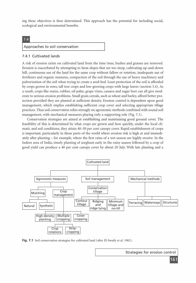
Strategies for erosion control
161
ing these objectives is then determined. This approach has the potential for including social,ecological and environmental benefits.
Cultivated land
Agronomic measures
Mulching Cropmanagement
Soil management
Conservationtillage
Mechanical methods
Terracing Waterways StructuresNatural Synthetic
Contourtillage
Ridgingand
ridge tying
Minimumtillage and
no-till
High-densityplanting
Multiplecropping
Covercropping
Croprotations
Strip-cropping
Fig. 7.1 Soil conservation strategies for cultivated land (after El-Swaify et al. 1982).
7.4
Approaches to soil conservation
7.4.1 Cultivated lands
A risk of erosion exists on cultivated land from the time trees, bushes and grasses are removed.Erosion is exacerbated by attempting to farm slopes that are too steep, cultivating up-and-downhill, continuous use of the land for the same crop without fallow or rotation, inadequate use offertilizers and organic manures, compaction of the soil through the use of heavy machinery andpulverization of the soil when trying to create a seed-bed. Least protection of the soil is affordedby crops grown in rows, tall tree crops and low-growing crops with large leaves (section 3.4). Asa result, crops like maize, rubber, oil palm, grape vines, cassava and sugar beet can all give mod-erate to serious erosion problems. Small grain cereals, such as wheat and barley, afford better pro-tection provided they are planted at sufficient density. Erosion control is dependent upon goodmanagement, which implies establishing sufficient crop cover and selecting appropriate tillagepractices. Thus soil conservation relies strongly on agronomic methods combined with sound soilmanagement, with mechanical measures playing only a supporting role (Fig. 7.1).
Conservation strategies are aimed at establishing and maintaining good ground cover. Thefeasibility of this is determined by what crops are grown and how quickly, under the local cli-matic and soil conditions, they attain 40–50 per cent canopy cover. Rapid establishment of cropsis important, particularly in those parts of the world where erosion risk is high at and immedi-ately after planting – for example, where the first rains of a wet season are highly erosive. In theIndore area of India, timely planting of sorghum early in the rainy season followed by a crop ofgood yield can produce a 40 per cent canopy cover by about 20 July. With late planting and a
MSE07 11/19/04 02:39 PM Page 161
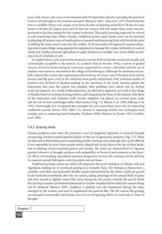
Chapter 7
162
poor yield, 40 per cent cover is not attained until 30 September, thereby extending the period oferosion risk throughout the summer monsoon (Shaxson 1981). Aina et al. (1977) found that thetime to establish 50 per cent canopy cover from the date of planting varied from 38 days for soyabeans to 46 days for pigeon peas and 63 days for cassava. Soil loss under these crops was pro-portional to the time needed for the canopy to develop. Thus quick-growing crops may be viewedas soil-conserving crops. Where climatic conditions permit, early season cover can be providedby planting off-season crops of small grains or mustard and destroying them with herbicide priorto drilling the main season crop into the residue. To be successful, this approach requires adopt-ing conservation tillage, using appropriate equipment to manage the residue, herbicides to controlweeds and, ideally, precision agriculture to apply fertilizers at variable rates across fields accord-ing to local variations in soil.
As implied above, soil conservation measures must be both technically sound and socially andeconomically acceptable to the farmers. In southern Mali in the late 1970s, a system of gradedterraces, diversion drains and grass waterways, supported by contour cultivation, and the use ofmulches and manures, was tested in the village of Fonsébougou. Although the measures success-fully reduced the erosion, the engineering works took up 10–14 per cent of the farm land and theterraces and the grass cover in the waterways were poorly maintained. Only a limited number offarmers were involved in decision-making or the execution of the work. Farmers gained theimpression that once the system was installed, their problems were solved and no further work was required. As a result of this experience, an alternative approach was tried in the villageof Kaniko based on existing farming systems, and integrating the ideas of the farmers with thoseof the researchers and extension staff. Greater emphasis was placed on contour grass strips and the use of trees and hedges rather than terraces (Fig. 7.2; Kleene et al. 1989; Hijkoop et al.1991). Increasingly, it is recognized that strategies for soil conservation must rely on improvingtraditional systems (Roose 1992; Table 7.3), instead of imposing entirely new techniques fromoutside, and on enhancing land husbandry (Hudson 1993b; Hudson & Cheatle 1993; Critchleyet al. 1994).
7.4.2 Grazing lands
Erosion problems arise when the protective cover of rangeland vegetation is removed throughovergrazing. Erosion control depends largely on the use of agronomic measures (Fig. 7.3). Theseare directed at determining and maintaining suitable stocking rates, although this can be difficultif not impossible in areas where people attach cultural and social value to the size of their herds,and at planting erosion-resistant grasses and shrubs. The latter are characterized by vigorousgrowth, tolerance of drought and poor soils, palatability to livestock and resistance to the physi-cal effects of trampling. Specialized measures designed to increase the resistance of the soil maybe required around field gates, watering points and salt boxes.
Traditional grazing systems are often well adapted to the local conditions of climate, soils andvegetation, making use of rotational grazing on a nomadic basis. The Turkana in Kenya have acarefully controlled and reasonably flexible system administered by the elders. Cattle are grazedin the lowlands immediately after the wet season, taking advantage of the annual flush of grass,and then moved to slightly wetter hilly areas during the dry season, towards the end of whichthey are kept around a permanent homestead in riverine woodland from which dry-season foragecan be obtained (Barrow 1989). Sorghum is planted near the homestead during the rains,managed by the women, and used to supplement the pastoral diet. The dry-season hill-grazingsare managed communally and include areas of reserved grazing which are used only in times ofdrought.
MSE07 11/19/04 02:39 PM Page 162
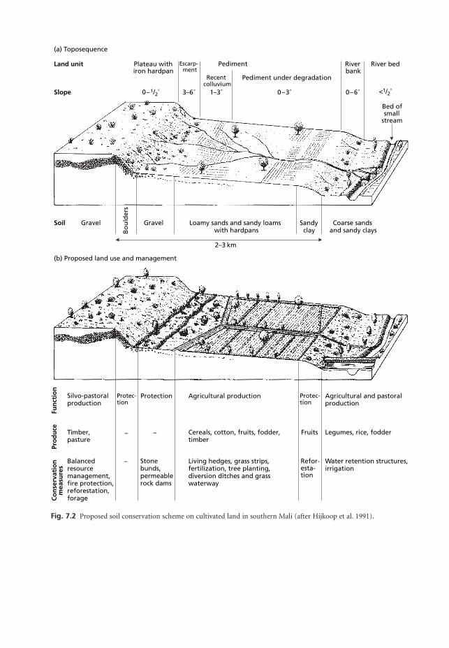
(a) Toposequence
Plateau withiron hardpan
Escarp-ment
Pediment
Recentcolluvium
Pediment under degradation
Riverbank
River bed
Bed ofsmall
stream
0–1/2˚ 3–6˚ 1–3˚ 0–3˚ 0–6˚ <1/2˚
Land unit
Slope
Gravel
Bo
uld
ers
Loamy sands and sandy loamswith hardpans
Gravel Sandyclay
Coarse sandsand sandy clays
Soil
2–3 km
(b) Proposed land use and management
Silvo-pastoralproduction
Timber, pasture
Balancedresourcemanagement,fire protection,reforestation,forage
Fun
ctio
nPr
od
uce
Co
nse
rvat
ion
mea
sure
s
Protec-tion
Protection Agricultural production Protec-tion
Agricultural and pastoralproduction
Cereals, cotton, fruits, fodder, timber
Fruits Legumes, rice, fodder
Stone bunds,permeablerock dams
Living hedges, grass strips,fertilization, tree planting,diversion ditches and grasswaterway
Refor-esta-tion
Water retention structures,irrigation
–
–
–
Fig. 7.2 Proposed soil conservation scheme on cultivated land in southern Mali (after Hijkoop et al. 1991).
MSE07 11/19/04 02:39 PM Page 163

Tab
le 7
.3V
aria
tion
in
tra
diti
onal
an
d pr
opos
ed s
oil c
onse
rvat
ion
sys
tem
s w
ith
clim
ate
in W
est
Afr
ica
Are
aSo
uth
So
ud
ania
nN
ort
h S
ou
dan
ian
Sou
th S
ahel
ian
No
rth
Sah
elia
n
Rai
nfa
ll>1
000
mm
700–
1000
mm
400–
700
mm
150–
400
mm
Co
nse
rvat
ion
ob
ject
ives
Dis
po
se o
f ex
cess
rai
nH
old
rai
n i
n s
itu
wh
ile
Co
nce
ntr
ate
rain
by
Co
nce
ntr
ate
rain
by
wat
er
wh
ile c
on
serv
ing
so
ilco
nse
rvin
g s
oil
wat
er h
arve
stin
gh
arve
stin
g f
rom
a
fro
m a
cat
chm
ent
catc
hm
ent
area
wh
ilear
ea w
hile
co
nse
rvin
gco
nse
rvin
g s
oil
on
so
il o
n c
rop
ped
lan
dcr
op
ped
lan
dSo
ilsFe
rral
itic
Leac
hed
fer
rug
ino
us
+ve
rtis
ols
Leac
hed
fer
rug
ino
us
San
dy
shee
t o
n b
row
n
+b
row
n o
n b
asic
ro
cks
+ve
rtis
ols
+b
row
nsu
b-a
rid
so
ilo
n b
asic
ro
cks
Veg
etat
ion
Tree
sav
ann
aTr
ee s
avan
na
Bu
sh s
avan
na
Step
pe,
bu
shFa
rmin
g s
yste
mY
ams
on
lar
ge
mo
un
ds.
Sup
erfi
cial
till
age.
Cro
pp
ing
on
Sup
erfi
cial
till
age.
Sow
ing
on
th
e fl
at.
Two
M
aize
+ in
terc
rop
pin
gth
e fl
at.
Two
wee
din
gs.
Cro
pp
ing
on
th
e fl
at.
wee
din
gs.
Mill
et o
n
in r
idg
es.
Mill
et +
So
rgh
um
, co
tto
n o
r m
illet
+Tw
o w
eed
ing
s.sa
nd
y so
ils.
Sorg
hu
m o
ng
rou
nd
nu
t +
vari
ou
sso
rgh
um
or
gro
un
d n
ut
+So
rgh
um
or
mill
etcl
ay s
oils
on
lo
w g
rou
nd
.o
n r
idg
es.
cow
pea
s. H
illsl
op
e ru
no
ff
then
gro
un
d n
ut
or
Gra
zin
g o
n h
illsl
op
es.
Inte
rcro
pp
ing
+o
n w
ater
way
s. T
ota
l co
wp
eas.
Mu
lch
ing
,G
ard
ens
in l
ow
-lyi
ng
ag
rofo
rest
ry.
infi
ltra
tio
n o
r ra
in i
n t
he
sto
ne
bu
nd
s, g
rass
or
area
s. R
etre
at fl
oo
din
g.
Dra
inag
e b
etw
een
fiel
d.
Sto
ne
bu
nd
s an
d w
alls
.b
rush
bar
rier
s o
np
lots
.G
rass
, st
on
e o
r b
rush
bar
rier
sco
nto
ur.
Tied
rid
gin
go
n c
on
tou
r.o
n s
and
y so
ils(s
om
etim
es).
Pro
po
sed
mo
der
nA
ffo
rest
atio
n o
f la
teri
teIm
pro
vem
ent
of
gra
ssla
nd
. Im
pro
vem
ent
of
Shru
b f
ora
ge
pla
nti
ng
s in
m
anag
emen
tsc
rees
. G
rass
ed b
uff
erLi
vin
g h
edg
es +
sto
ne
bu
nd
sg
rass
lan
d.
Pou
nd
s fo
rlu
net
tes
or
dit
ches
.st
rip
s. G
ully
o
r g
rass
ed b
uff
er s
trip
s. G
rass
catt
le +
su
pp
lem
enta
ryG
rass
lan
d m
anag
emen
t.re
sto
rati
on
. Pr
ote
ctio
nw
ater
way
s.ir
rig
atio
n o
f g
ard
ens.
Pou
nd
s fo
r ca
ttle
.o
f ri
ce fi
eld
s.St
on
e b
un
ds
pro
tect
edTr
app
ing
ru
no
ff o
nb
y g
rass
. G
ully
h
illsl
op
es.
Sto
ne
bu
nd
s m
anag
emen
t.o
n p
edim
ent.
Sou
rce:
afte
r R
oo
se (
1992
).
MSE07 11/19/04 02:39 PM Page 164
Strategies for erosion control
165
Virtually all traditional grazing systems are under pressure today. First, human populationnumbers, as a result of better health, and livestock numbers, as a result of better veterinary ser-vices, are both increasing. Second, there is a conflict between the individual and family owner-ship of livestock and the communal ownership of the pasture. The individual derives a positiveutility of almost one for every additional animal owned and grazed on communal land but expe-riences a negative utility of only a small fraction of one as a result of ensuing overgrazing. Themaximization of individual benefit at the expense of the community, termed by Hardin (1968)‘the tragedy of the commons’, is one of the biggest challenges facing soil conservationists on range-land. The conflict becomes most marked when incentives for commercial livestock productionare so strong that individuals, usually those owning the larger numbers and better quality stock,break away and take over much of the land, enclosing it by fencing, displacing other members ofthe community and increasing the pressure on the remaining range. Third, the provision of addi-tional watering points, often located without consideration of the traditional movement of stock,has meant that availability of forage rather than water has become the limiting factor on livestocknumbers, creating additional pressure on the land. Fourth, the concentration of people in settle-ments to provide health, education and water more efficiently and to promote cash cropping withirrigation has caused people to abandon their nomadic tradition, with the result that stock arekept all year on pastures close to the homestead. Sometimes new settlement schemes will be sitedon seasonal grazing areas, thereby removing them from the system. Fifth, education of the youthand changed political systems are gradually eroding the authority of the elders.
Grazing can be considered as the removal of biomass from rangeland. The rate of removaldepends upon the number of animals and their daily intake of forage. Soil conservation is there-fore aimed at controlling grazing numbers so that a sufficient vegetation cover is sustained overtime to protect the soil. The loss of vegetation increases the rate of runoff and erosion anddecreases the amount of water in the soil, which, in turn, reduces the amount of vegetationgrowth. In reality, the vegetation–erosion–grazing interaction is more complex because of theneed to consider soil fertility, loss of soil nutrients, production of litter, the palatability and diges-tive value to stock of the different species in the plant community and the ability of the differentspecies to survive under changing grazing, moisture and nutrient conditions. At present, the inter-action is poorly understood. On the one hand, there is considerable evidence that many tropicalrangelands are overstocked. It is suggested by Pratt and Gwynne (1977) that the threshold stock-ing rate on the semi-arid lands of northeast Kenya is about 1 Tropical Livestock Unit (TLU) per25 ha whereas actual stocking rates range from 1 TLU per 4 ha to 1 TLU per 30 ha (Peden 1987).In the Middle Veld of Swaziland, stocking rates are about 1 TLU per 1.3 ha compared with sus-tainable rates of 1 TLU for every 2.5 to 3.5 ha (Nsibandze 1987; Dlamini & Maro 1988). On theother hand, application of a simple grazing model developed by Biot (1990) to the rangelands of Botswana suggests that at a grazing intensity of 1 TLU per 5 ha, the system would remain reasonably stable for the next 2000 years. Clearly with such discrepancy between conventionalwisdom and model predictions, it is difficult to determine the safe level of grazing, particularlywhen short-term fluctuations in climate also need to be considered. Further, there is often a con-flict between designing a strategy that sustains the productivity of the rangeland and maximizeseconomic benefit over the medium to long term, and a strategy that maintains erosion at a muchlower tolerable level to minimize environmental impacts.
7.4.3 Forest lands
Forests provide excellent protection of the topsoil against erosion. They maintain high rates ofevapotranspiration, interception and infiltration and therefore generate only small quantities of
MSE07 11/19/04 02:39 PM Page 165
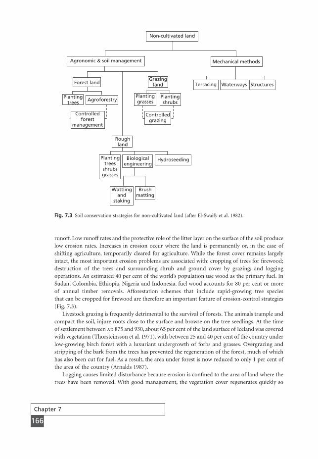
Chapter 7
166
runoff. Low runoff rates and the protective role of the litter layer on the surface of the soil producelow erosion rates. Increases in erosion occur where the land is permanently or, in the case ofshifting agriculture, temporarily cleared for agriculture. While the forest cover remains largelyintact, the most important erosion problems are associated with: cropping of trees for firewood;destruction of the trees and surrounding shrub and ground cover by grazing; and logging operations. An estimated 40 per cent of the world’s population use wood as the primary fuel. InSudan, Colombia, Ethiopia, Nigeria and Indonesia, fuel wood accounts for 80 per cent or moreof annual timber removals. Afforestation schemes that include rapid-growing tree species that can be cropped for firewood are therefore an important feature of erosion-control strategies(Fig. 7.3).
Livestock grazing is frequently detrimental to the survival of forests. The animals trample andcompact the soil, injure roots close to the surface and browse on the tree seedlings. At the timeof settlement between 875 and 930, about 65 per cent of the land surface of Iceland was coveredwith vegetation (Thorsteinsson et al. 1971), with between 25 and 40 per cent of the country underlow-growing birch forest with a luxuriant undergrowth of forbs and grasses. Overgrazing andstripping of the bark from the trees has prevented the regeneration of the forest, much of whichhas also been cut for fuel. As a result, the area under forest is now reduced to only 1 per cent ofthe area of the country (Arnalds 1987).
Logging causes limited disturbance because erosion is confined to the area of land where thetrees have been removed. With good management, the vegetation cover regenerates quickly so
Non-cultivated land
Agronomic & soil management
Forest land
Plantingtrees Agroforestry
Controlledforest
management
Grazingland
Plantinggrasses
Planting shrubs
Controlledgrazing
Roughland
Biologicalengineering
Plantingtrees
shrubsgrasses
Hydroseeding
Mechanical methods
Terracing Waterways Structures
Wattlingand
staking
Brushmatting
Fig. 7.3 Soil conservation strategies for non-cultivated land (after El-Swaify et al. 1982).
MSE07 11/19/04 02:39 PM Page 166
Strategies for erosion control
167
that high erosion rates are restricted to the first and sometimes the second and third years afterfelling. The level of disturbance is related to the method of clearance. Studies of three practicesin Nigeria (Lal 1981) showed that more erosion followed mechanical clearance using crawler trac-tors with tree-pusher and root-rake attachments than manual clearance using chain saws. Leasterosion followed manual clearance with machete and axe. Erosion immediately after clearance isgenerally associated with surface runoff. Another effect of forest removal, however, is the gradualloss of shear strength of the soil following the decay of the root systems (O’Loughlin 1974;O’Loughlin & Watson 1979). This induces a risk of landslides, which is greatest about five yearsafter clearance (Bishop & Stevens 1964; Beschta 1978), although some researchers suggest a slowerdeterioration, with maximum slide hazard being reached 15 years after logging (Rice & Krammes1970).
The main erosion problems in logged areas are associated with skid trails and roads, which arefrequently areas of bare compacted soil. Studies in Pahang, Malaysia, showed that traffic along skid trails and logging roads increased the bulk density of the ultisol soil to 1.5 and 1.6 Mg m-3
respectively, compared to 1.1 Mg m-3 on undisturbed land, with resulting respective decreases inporosity of 62 and 69 per cent (Baharuddin et al. 1996). Erosion rates at log-landings and onhaulage roads on slopes of less than 10° in Sabah, Malaysia, are some three times higher than thosefrom primary rain forest on much steeper slopes (Clarke et al. 2002). As reported by Swanson andDyrness (1975), who measured 2,300,000 t ha-1 on a roadside in western Oregon, USA, annualerosion rates from logging roads can be very high. Roads, tracks and paths can contribute up to half of the total sediment yield in forested catchments (Reid et al. 1981). Cut slopes are particularlyvulnerable, being up to ten times more erodible than fill slopes (Riley 1988). Erosion can be mini-mized by locating roads on ridges and gentle slopes to avoid the need for cut slopes.
Another source of sediment, widely reported from afforestation schemes in Wales (Newson1980; Robinson & Blyth 1982; Murgatroyd & Ternan 1983; Francis & Taylor 1989), occurs wherethe land has to be drained by surface ditches. The ditch banks erode as the channels adjust fromtheir relatively deep and narrow cut-form to a shallower, wide one. The increased runoff fromthe ditches also causes bank erosion in the rivers immediately downstream.
7.4.4 Land clearance
The methods used for clearance of forest for agricultural development not only affect the amountof soil loss that takes place but also influence the subsequent crop yields. The mechanical clear-ance of forest on an alfisol in Nigeria (Lal & Cummings 1979) significantly increased the bulkdensity and decreased the infiltration capacity of the soil compared with removal by slash-and-burn. Bulk densities were increased from 0.9 Mg m-3 on uncleared land to 1.12 Mg m-3 with slash-and-burn and 1.25 Mg m-3 with mechanical clearance. The respective infiltration capacities were112, 52 and 19 mm h-1. Clearance of forest on 30–40° slopes in Malaysia on an ultisol soil reducedthe infiltration capacity from 214 mm h-1 on uncleared land to 149 mm h-1 using slash-and-burnand 43 mm h-1 using crawler tractors with straight blades; the respective bulk densities were 1.06,1.33 and 1.48 Mg m-3 (Jusoff & Majid 1988).
The response of crop yield to different types of land clearance depends on the degree of dis-turbance and the subsequent method of cultivation. Potentially, the situation is worse withmechanical clearance because much of the litter layer is scraped away, removing the immediateprotection of the soil against erosion and the source of organic material. Yet, on an ultisol soil ona 2° slope in northern Thailand, mechanical clearance of the forest by tractor with a tree-pusherblade followed by construction of contour bunds, no-tillage and inclusion of legumes in a
MSE07 11/19/04 02:39 PM Page 167
Chapter 7
168
rotation system led to higher rice yields compared to other treatments (Boonchee et al. 1988). Incontrast, on ultisols in Peru (Seubert et al. 1977) and alfisols in Nigeria (Lal 1981), significantlyhigher yields were obtained using conventional tillage practices or chisel ploughing followingmechanical clearance compared to using no tillage or mulching. The latter techniques initiallyresulted in rather low yields, even when fertilizer was added, because they did not overcome theincreased compaction of the soil.
If disturbance of the surface is kept to a minimum and a system of land management imposedfor eight to ten years after clearance to overcome any increases in compaction of the soil, forestland can be successfully cleared for agriculture. If the land cannot be cropped immediately becausethe disturbance has been too great, the planting of a cover crop will help to restore the soil closeto its original bulk density and infiltration capacity (Hulugalle et al. 1984), after which a range ofmanagement practices, including no tillage, is possible. Once under agricultural use, the appro-priate soil conservation practices for cultivated land must be adopted.
7.4.5 Rough lands
Areas of rough ground remaining in their natural habitats because they are too marginal for otherforms of land use include hilly and mountainous terrain with shallow stony soils and steep slopes,alpine grasslands, arctic tundras and sand dunes. Since they are often areas of spectacular scenery,they attract recreational use. Their marginality, however, means that they are sensitive to any dis-turbance, and their ability to withstand recreational impacts is low. The main problems of landdegradation are associated with footpaths, tracks created by horses, motor cycles and off-roadvehicles, and very intensive use at car parks and camp sites.
Approaches to controlling erosion range from exclusion of people, appropriate in areas ofspecial scientific interest or in nature reserves, to use of erosion-resistant plant species, supportedwhere necessary by drainage to reduce soil moisture content and increase soil strength, and arti-ficial strengthening or reinforcement of footpaths. Although few plants can withstand prolongedand heavy pressure from walkers and horses, studies of footpath erosion in the English Lake Dis-trict show that grasses, including Nardus stricta, Agrostis spp. and Festuca spp. resist tramplingbetter than Calluna heathland (Coleman 1981). One way of comparing the vulnerability of dif-ferent habitats to trampling is to determine the number of passes by individual walkers they canwithstand before the plant cover is reduced from 100 to 50 per cent. Sand dune pasture can with-stand between 1100 and 1800 passes, alpine plant communities less than 60 and arctic tundraonly about eight passes (Liddle 1973). Trampling of a grass cover on a clay soil with a moisturecontent close to field capacity resulted in runoff rising rapidly between 0 and 50 passes, then lev-elling off before rising again between 700 and 900 passes. The rate of soil loss, however, increasedlinearly with increasing number of passes. Since patches of bare ground did not appear until 250passes and even after 900 passes between 25 and 50 per cent of the cover remained, the criticalperiod when increased runoff and erosion are initiated seems to occur before any decrease in thevegetation cover is observed (Quinn et al. 1980).
In addition to being able to survive in the climatic and soil environment, the plant speciesselected for revegetation of rough areas should ideally be local, so as not to introduce new speciesinto the ecological system, and should meet the following criteria: short or prostrate growth form,flexible rather than brittle or rigid stems and leaves, basal or underground growth points, rapidgrowth, ability to withstand burial by soil and rocks and ability to withstand exposure of the rootsystem (Coppin & Richards 1990). Often an ecological succession can be planned involving amixture of species, both grasses and shrubs, to give an initial rapid growth and cover of the groundfollowed by longer-term development of erosion-resistant plants.
MSE07 11/19/04 02:39 PM Page 168
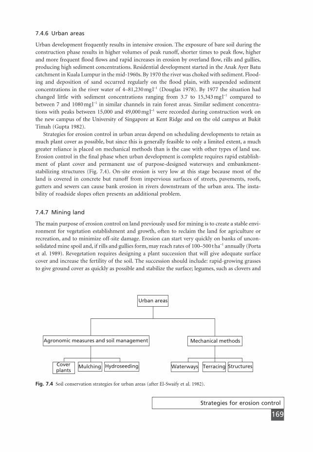
Strategies for erosion control
169
7.4.6 Urban areas
Urban development frequently results in intensive erosion. The exposure of bare soil during theconstruction phase results in higher volumes of peak runoff, shorter times to peak flow, higherand more frequent flood flows and rapid increases in erosion by overland flow, rills and gullies,producing high sediment concentrations. Residential development started in the Anak Ayer Batucatchment in Kuala Lumpur in the mid-1960s. By 1970 the river was choked with sediment. Flood-ing and deposition of sand occurred regularly on the flood plain, with suspended sediment concentrations in the river water of 4–81,230 mg l-1 (Douglas 1978). By 1977 the situation hadchanged little with sediment concentrations ranging from 3.7 to 15,343 mg l-1 compared tobetween 7 and 1080 mg l-1 in similar channels in rain forest areas. Similar sediment concentra-tions with peaks between 15,000 and 49,000 mg l-1 were recorded during construction work onthe new campus of the University of Singapore at Kent Ridge and on the old campus at BukitTimah (Gupta 1982).
Strategies for erosion control in urban areas depend on scheduling developments to retain asmuch plant cover as possible, but since this is generally feasible to only a limited extent, a muchgreater reliance is placed on mechanical methods than is the case with other types of land use.Erosion control in the final phase when urban development is complete requires rapid establish-ment of plant cover and permanent use of purpose-designed waterways and embankment-stabilizing structures (Fig. 7.4). On-site erosion is very low at this stage because most of the land is covered in concrete but runoff from impervious surfaces of streets, pavements, roofs,gutters and sewers can cause bank erosion in rivers downstream of the urban area. The insta-bility of roadside slopes often presents an additional problem.
7.4.7 Mining land
The main purpose of erosion control on land previously used for mining is to create a stable envi-ronment for vegetation establishment and growth, often to reclaim the land for agriculture orrecreation, and to minimize off-site damage. Erosion can start very quickly on banks of uncon-solidated mine spoil and, if rills and gullies form, may reach rates of 100–500 t ha-1 annually (Portaet al. 1989). Revegetation requires designing a plant succession that will give adequate surfacecover and increase the fertility of the soil. The succession should include: rapid-growing grassesto give ground cover as quickly as possible and stabilize the surface; legumes, such as clovers and
Urban areas
Agronomic measures and soil management
Coverplants
Mulching Hydroseeding
Mechanical methods
Waterways Terracing Structures
Fig. 7.4 Soil conservation strategies for urban areas (after El-Swaify et al. 1982).
MSE07 11/19/04 02:39 PM Page 169
Chapter 7
170
vetches, to fix nitrogen; and other grasses and shrubs to provide the long-term cover. Species selec-tion will depend on local soil and climatic condititions but should aim to produce a uniformrather than clumpy pattern of vegetation to avoid concentrations of runoff and localized erosion(section 3.4.2). The ideal condition is difficult to achieve, however, where the soils have low water-retention capacity or are toxic, or where cold, drought or exposure inhibit plant growth.Choosing vegetation that has beneficial effects is important. In order to reduce the costs ofreclamation of spoil mounds from tin mining on the Jos Plateau, Nigeria, the Mine Lands Recla-mation Unit chose Eucalyptus spp., which could be cropped as a source of fuel and pole timber,but these have resulted in significant declines in the base status and pH of the soil (Alexander1990) to the detriment of other plant growth. Among the mechanical measures, terraces andwaterways will be required to control runoff and remove excess water safely from the site, usuallyto silt-traps and soak-aways at the base of the slope, and revegetation may need to be supportedby the use of geotextiles to provide an immediate protection to the soil and prevent erosionwashing or blowing away the seeds. Contour wattling, contour brush-layering or terrace con-struction may be additionally employed to supplement the vegetation for longer-term protectionof the soil.
7.4.8 Pipeline corridors
Restoration work along pipeline rights-of-way is usually directed at re-establishing the ori-ginal vegetation cover or returning the land to agriculture. Erosion can inhibit restoration bywashing out seeds and young plants. In addition, sediment washed off the right-of-way can cause environmental damage on surrounding land and rill and gully erosion can expose the pipe.The potential for erosion is high because in order to install the pipe, the top soil has been removed, temporarily stored and then replaced by spreading it on to land which has been heavily compacted by machinery. Infiltration rates through the compacted layer are low, so thatrunoff is easily generated and the top soil is erodible because it has lost much of its cohesionthrough disturbance. A compromise has to be sought between compacting the top soil suffi-ciently to increase its strength while keeping compaction low enough so that it does not inhibit plant emergence or root development. Bulk densities in excess of 1.3 Mg m-3 on clay soils,1.4 Mg m-3 on silty and loamy and 1.6 Mg m-3 on sandy soils will limit plant growth (Daddow &Warrington 1983).
Similar to the situation described above for restoring mine spoil, a plant succession needs tobe designed based on quick-growing native species, adapted to the local soils and climate, toprovide dense ground cover, and slower-growing shrubs and bushes to reinforce the soil throughthe root network and reduce soil moisture through evapotranspiration. A mixture of species is preferred to create biodiversity and a healthy plant community. A particular problem is timing,since the completion of pipeline installation does not always coincide with optimum periods of the year for reseeding and replanting. Vegetation establishment will be restricted when the temperature falls below that for plant growth or is so high that evaporation reduces the availablesoil moisture. In the period before sufficient vegetation cover is obtained, erosion mats should be placed on the slope to protect the soil and diverter berms used to intercept any surface runoff and carry it off the slope to a safe disposal point. It is important that the berms are designed and installed correctly. Inappropriate construction practices and errors in design are amajor cause of erosion along many pipeline corridors. Common examples of poor practiceinclude the disposal of excess soil on steep sideslopes, where it is vulnerable to gully and pipeerosion, and failure to convey runoff away from the slope, which then becomes gullied (Hann &Morgan 2003).
MSE07 11/19/04 02:39 PM Page 170
Strategies for erosion control
171
7.4.9 Road banks
As indicated in section 7.4.3, road banks on either cut or fill slopes are frequently major sourcesof sediment. Poor disposal of runoff is an important cause of erosion associated with roads.Runoff upslope of the road should be collected in roadside drains or ditches, which are then ledinto culverts under the road, usually discharging into existing valleys. It is common, however, todischarge the runoff collected from several small streams into a single culvert, which means thatthe catchment area of the recipient channel downslope of the road is increased. Where adequateprotection measures are not put in place, the increased runoff can enlarge the channel into a gully(Nyssen et al. 2002), which, over time, will extend back upslope and damage the road. The roadshoulder, the land between the road surface and the side drain, is also vulnerable to erosion, par-ticularly where the road surface is metalled and the shoulder is unprotected (Freer-Hewish 1991;Kamalu 1991).
The methods used for erosion control range from engineering structures such as revetmentsand retaining walls to stabilization of the slope by vegetation. Grasses will protect the slope againsterosion by raindrop impact and runoff, and also trap moving sediment, while shrubs and treeswill increase the strength of the soil through root reinforcement. Trees will also help to supportthe slope by buttressing (section 3.4.4). Vegetation increases the infiltration of water into the soil,but this can cause problems where rainfall amounts and intensities are very high. While the result-ing reduction in runoff will help to control surface erosion, the increased moisture content of thesoil may exacerbate the risk of mass soil failure. Whether this occurs will depend on the extentto which root reinforcement has increased the cohesive strength of the soil and root penetrationacross the potential slide plane has anchored the soil mass to the underlying material. Where soilsaturation is a danger, the vegetation may need to be supported by cut-off drains above the slopeto prevent the influx of surface water, and trench or herringbone rubble drains to aid drainageof the slope itself. In the initial stages, until the vegetation cover is established, wattling, brushlayering or erosion mats may be needed to provide temporary erosion control and stability. Forsurface erosion and for soil failures extending to depths of up to 2 m, vegetation has the advan-tages over engineering structures of being cheaper to install, aesthetically more pleasing and, inthe long-term, self-repairing, with an indefinite life. It will, however, require regular maintenanceand occasional repair. Although they have not yet been adopted as standard practice worldwide,civil and highway engineers are showing increasing interest in both bioengineering, in which veg-etation is used on its own as an engineering material, and biotechnical engineering, in which theengineering properties of vegetation are combined with inert structures. A detailed manual hasbeen developed for Nepal describing the properties of some 13 local grass, 13 shrub, 15 tree andsix clumping bamboo species suitable for bioengineering (Howell 1999).
When considering strategies for erosion control related to roads, it is important to take accountof the location of the road within the landscape and, in particular, the nature of the land use onthe slope above the road bank. In the Himalaya where the road banks are frequently oversteep-ened cut sections of the hillside, seepage from irrigation terraces on the slope above can increaseinstability. Inclusion of forestry, either as agroforestry or as community-managed forests, mayhelp to stabilize both the slope above and the road bank itself and be more satisfactory than anengineering solution. If the forest can provide fodder, fuel and fruits, its long-term managementmay be vested in the individual farmers and the community as a whole.
MSE07 11/19/04 02:39 PM Page 171

Chapter 7
172
Soil conservation design most logically followsa sequence of events (Fig. B7.1) beginningwith a thorough assessment of erosion riskusing the techniques described in Chapter 4.This is followed by the design of a sound land-use plan, based on what the land is bestsuited for under present or proposed eco-nomic and social conditions and what is com-patible with the maintenance ofenvironmental stability.
Land capability classificationBy adopting land capability classification as amethodology for land-use planning a distinc-tion can be made, as seen in section 4.2.1,between areas where erosion is likely to occurthrough mismanagement and areas whereerosion occurs through misuse. In the firstcase, erosion can be reduced to a tolerablelevel by suitable conservation practices but, inthe second case, erosion control is expensiveand difficult, if not impossible. The land islikely to become so degraded that eventuallyit will have to be abandoned. Much moneycan be spent attempting to reclaim landwhere soil degradation has become virtuallyirreversible but the low productivity of theland means that the investment is highly ques-tionable since it can never be repaid.
Defining conservation needsThe ultimate success of soil conservationschemes depends on how well the erosionproblem has been identified, the suitability ofthe conservation measures selected to dealwith the problem and the willingness of thefarmers and others to implement them. Thesefeatures of an erosion-control strategy are justas important as the ability of the engineer todesign the conservation structures required.Correct identification of the major areas oferosion and therefore the main sources of sed-iment is also essential. Too often expensiveconstruction work has been carried out onareas of land that were thought to be impor-tant sources of sediment but in fact were not
Box 7
(Perrens & Trustrum 1984). By contrast,treating a small but carefully targeted area ofland can be very effective. Soil loss in theWuding Valley, China, was reduced by half bytreating 20.5 per cent of the catchment (Jianget al. 1981).
Existing farming systemsThe farming systems already operating in thearea should be analysed to see how well theyprotect the land, particularly at the criticalperiods of the year when erosion risk ishighest. This is best achieved by relating thefarming calendar to the monthly pattern oferosivity. For example, in eastern Thailand(Prinz 1992), erosivity reaches its peak in thefirst half of the wet season when the crops ofkenaf, groundnut and upland rice do not yetprovide adequate cover. On the loamy soils ofnorth-eastern France (Monnier & Boiffin 1986),the danger of erosion under winter-sowncereals is high, even when the soil is coveredand rainfall is relatively low, because of themarked reduction in infiltration rates betweenDecember and March as a result of crusting ofthe soil in the autumn (section 2.1). Studies ofthe farming systems can also provide informa-tion on how the farmers perceive erosion, theconservation measures already adopted andthe social, economic, political and institutionalconstraints on the take-up of further measures.
Selection of conservation strategiesBased on assessments of the severity oferosion and its off-site impacts, a decision canbe made on whether soil conservation mea-sures are required in order to meet a desiredsoil loss tolerance. If so, a further decision isneeded on the performance criteria theyshould achieve. These can be wider thanmeeting a given soil loss tolerance and includeprotection of watersheds and areas of scien-tific or heritage interest. They may also coversocio-economic objectives such as relievingpoverty and producing sustainable rural liveli-
Planning a soil conservation strategy
MSE07 11/19/04 02:39 PM Page 172
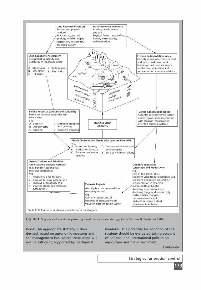
Strategies for erosion control
173
Land Resource Inventory Water Resource InventoryErosion and present Existing development
and usePhysical factors: streamflow,floods, water quality,sedimentation
landusePhysical factors: soilsgeology, rainfall, slope,vegetation, microrelief,drainage pattern
Land Capability AssessmentAssessment Capability andsuitability of landscape units:
A Mountains D Rolling landsE Flat landsB Steeplands
C Hill lands
A
B A
CD
D
C
E
Erosion Sedimentation IndexIdentify source of erosion hazardand fate of sediment, ranklandscape units and elementson the basis of erosion and
Consider socioeconomic factorsand integrate soil conservationwith landuse (conservation-oriented farming systems)
sedimentation sources and sinks
Define Conservation NeedsDefine Potential Landuse and SuitabilityBased on resource capacities andconstraintse.g.A Forestry D Extensive cropping
E Intensive croppingand grazingB Agroforestry
C Grazing
wind erosionsheet erosionsedimentationflooding
landslides
gullies
streambank
MANAGEMENTACTIONS
Match Conservation Needs with Landuse Potential
Assess Options and Priorities
e.g.A Protection forestryB Production forestryC Gully control works
-grazing
Use economic analysis methods(e.g. benefit-cost analysis)to judge alternativese.g.1 Reserve A, B for forestry2 Develop farming system for D3 Improve productivity of C4 Develop cropping and tillage
system for E
D Contour cultivation and
E Zero or minimum tillagestrip-cropping
Quantify Impacts onLandscape and Productivitye.g.Loss of top soil (C, D, E)sediment yield from streambank (D,E)sediment deposition on land (E),sedimentation in reservoir,increased flood heightdeclining crop productivity,declining rangeland productivity,
(Usually but not necessarily inmonetary terms)e.g.Cost of erosion control,benefits of increased yields,value of more irrigation water
water quality changes,decreased water yield,reduced reservoir outputdue to sedimentation
Evaluate Impacts
*A, B, C, D, E refer to landscape units shown in the diagram.
Fig. B7.1 Sequence of events in planning a soil conservation strategy (after Perrens & Trustrum 1984).
hoods. An appropriate strategy is thendevised, based on agronomic measures andsoil management but, where these alone willnot be sufficient, supported by mechanical
measures. The potential for adoption of thestrategy should be evaluated taking accountof national and international policies on agriculture and the environment.
Continued
MSE07 11/19/04 02:39 PM Page 173

Chapter 7
174
Impact assessmentThe next stage is to quantify the impacts ofthe proposed land use and associated conser-vation strategy. Simple environmental impactassessments can be made using the predictivemodels described in Chapter 6. Models havealso been developed for forecasting theimpact of erosion on the productivity of thesoil. Most, such as the Productivity Index (PI)(Larson et al. 1985) and the Erosion Productiv-ity Impact Calculator (EPIC) (Williams et al.1984) are only valid in areas such as the USAand western Europe, where soil fertility is nota limiting factor because nutrients are addedto the soil through fertilizers. At present, themodels can only serve as guides to the likely
impacts because they have not been widelyvalidated owing to a lack of adequate data.To obtain the necessary information onchanges in the nutrient status and physicalproperties of a soil as a result of erosionrequires a minimum period of ten years undernatural conditions. Trying to speed up theprocess by scalping the top soil to differentdepths results in an underestimation of theeffect on nutrient removal by some five to tentimes (Stocking & Peake 1987). Impact analysiscan include economic assessments at thefarmer level, using cost–benefit analysis, aswell as wider assessments taking account ofcosts and benefits that cannot be described inmonetary terms (section 7.3.7).
MSE07 11/19/04 02:39 PM Page 174
Crop and vegetation management
175
Agronomic measures for soil conservation use the protective effect of plant covers to reduceerosion (section 3.4). Because of differences in their density and morphology, plants differ in theirability to protect the soil. Generally, row crops are the least effective and give rise to more seriouserosion problems. This is because of the high percentage of bare ground, particularly in the earlystages of crop growth, and the need to prepare a seed bed. In the design of a conservation strat-egy based on agronomic measures, row crops must be combined with protection-effective crops.Agronomic measures also form an important component of conservation tillage (Chapter 9) andof strategies to control erosion in plantations, forests and non-agricultural areas.
CHAPTER 8
Crop andvegetationmanagement
8.1
Rotation
The simplest way to combine different crops is to grow them consecutively in rotation. The fre-quency with which row crops are grown depends upon the severity of erosion. Where erosionrates are low, they may be grown every other year, but, in very erodible areas, they may be per-missible only once in five or seven years. A high rate of soil loss under the row crop is counter-acted by low rates under the other crops so that, averaged over a six- or seven-year period, theannual erosion rate remains low. The long-term effects of rotation versus continuous monocul-ture can be quite dramatic as shown by data from the experiments carried out at Sanborn Field,Missouri. On 4° slopes with a silt-loam soil, the annual erosion rate under continuous maize was44 t ha-1 compared with 6 t ha-1 from a maize–wheat–clover rotation. After 100 years, land undercontinuous maize had only 44 per cent as much top soil as land kept permanently under grass,whereas the land under the rotation system had 70 per cent (Gantzer et al. 1990).
Suitable crops for use in rotations are legumes and grasses. These provide good ground cover,help to maintain or even improve the organic status of the soil, thereby contributing to soil fertility,and enable a more stable aggregate structure to develop in the soil. The effects are often sufficientto reduce erosion and increase yield during the first year of row-crop cultivation, but they rarelyextend into the second year. For this reason, two continuous years of planting with a row cropshould be avoided. Hudson (1981) showed that a rotation of tobacco–grass–grass–tobacco–grass–grass was more effective in Zimbabwe than one of two consecutive years of tobacco followed byfour years of grass. The respective mean annual soil loss rates were 12 and 15 t ha-1.
MSE08 11/19/04 02:40 PM Page 175

8.1.1 Shifting cultivation
Shifting cultivation is a traditional method of reducing soil erosion in the tropics by rotating thelocation of the fields. An area of forest is cleared by slash-and-burn, the soil loosened by handhoeing and a crop planted. Where two crops a year can be obtained, a second crop is grown afterthe harvest of the first; otherwise the land is left in a weed fallow. The same area may be croppedfor a second year before being allowed to revert to scrub and secondary forest. Typical crops grownare cassava, maize, upland rice and yam. The residual effect of the forest on the organic contentand aggregate stability of the soil generally lasts for the first year of farming so that soil lossremains low. Erosion rates rise rapidly if the land continues to be cropped in subsequent years.Soil loss from land under upland rice in Mindanao, Philippines, averaged 0.38 g m-2 per day on anew clearing but rose to 14.91 g m-2 per day on a clearing in its twelfth year of cultivation (Kellman1969).
The practice of shifting cultivation will maintain soil fertility and reduce erosion to tolerablelevels provided the associated conditions of low crop yields and low ratio of population to landarea remain socially and economically acceptable. The critical factor in the system is the lengthof the fallow period. This is traditionally between 7 and 20 years in West Africa (Okigbo 1977)but increasing population densities and the desire of people to raise their standard of living bychanging from subsistence to cash cropping put pressure on the land, resulting in a reduction andsometimes the elimination of the fallow period. Serious erosion problems are created when thefallow period is reduced and alternative farming practices to the shifting cultivation system arerequired to solve them, using intercropping, mulching and agroforestry.
8.1.2 Row-crop cultivation
Particular problems are associated with maize, which, when grown as a row crop with conven-tional tillage and clean weeding, results in an annual soil loss on 2–5° slopes of between 10 and120 t ha-1, taking data from Zimbabwe (Hudson 1981), Malaysia (Sulaiman et al. 1981) and India(Singh et al. 1979). These rates are well above most soil loss tolerance levels. Where maize is grownin a more traditional manner with cultivation being restricted to ploughing and with no weeding,it presents fewer difficulties but the yields are rather low, often only 1 t ha-1 compared with over5 t ha-1 regularly achieved in the USA. There is an urgent need to find a way of increasing the yieldwithout increasing the erosion.
Soya beans are often used in rotation with maize because of their apparent ability to reducesoil loss by intercepting a high percentage of the rainfall. At 90 per cent canopy cover, soya beansintercept 58 per cent of the rainfall, compared with 40 per cent for maize interplanted with cassavaand only 28 per cent for cassava on its own. Respective annual soil losses are 4.0, 6.9 and 11.0 t ha-1 in the Ibadan area of Nigeria (Aina et al. 1979). However, studies in the Midwest of theUSA indicate that soya beans can result in as much if not more erosion than maize (Laflen &Moldenhauer 1979). The average annual soil loss on a 4° slope with a silt-loam soil over sevenyears was 7.0 t ha-1 for continuous maize, 6.5 t ha-1 for maize following soya beans and 9.6 t ha-1
for soya beans following maize. The main reasons for the increased erosion under soya beans arethat the crop affords less protection than maize in the stage between canopy cover and harvest,and produces less residue after harvest.
In addition to controlling erosion, the inclusion of grasses and legumes in a rotation canincrease yields of the main crop. Yields of maize greater than 5 t ha-1 were obtained at Ibadan fol-lowing a year with the land under Centrosema pubescens, Setaria splendida or Stylosanthes gracilis
Chapter 8
176
MSE08 11/19/04 02:40 PM Page 176
Crop and vegetation management
177
(Okigbo & Lal 1977). Unless the fallow crops can be used for grazing or fodder, however, theyhave no immediate value to the farmer. Thus, crop rotations with grasses and legumes are rarelypractised in the main cereal-growing areas of the world and are unlikely to be acceptable any-where if their inclusion gives no income to the farmer. Under these conditions, an alternativeapproach to erosion control is required based on minimizing the period of bare ground – forexample, by leaving crop residue on the land after harvest and delaying ploughing until the fol-lowing spring, or, where winter cereals are grown, sowing as early as possible to ensure good coverbefore winter temperatures inhibit plant growth. Late sowing of winter cereals was a major causeof soil erosion in the 1980s over much of southern and eastern England (Boardman & Evans1994) and northern France (Monnier & Boiffin 1986).
8.1.3 Grazing land management
Rotation is commonly practised on grazing land, moving the stock from one pasture to anotherin turn, to give time for the grass to recover. Generally, rangelands should not be exploited tomore than 40–50 per cent of the annual production of their most palatable species (Fournier1972; Thorsteinsson 1980a), a condition that is reached when about 10–20 per cent of the annualgrowth of the woody species has been removed. The vegetation should be allowed to regeneratesufficiently to provide a 70 per cent ground cover at times of erosion risk. Grazing has to be verycarefully managed. While overgrazing can lead to deterioration of the rangeland and the onset oferosion, undergrazing can result in the loss of nutritious grasses, many of which regenerate morerapidly when grazed.
Overgrazing of the summer pastures in Iceland led to a decline in the proportion of grasseswithin the plant community from 30 to 12 per cent and rises in the proportions of sedges andrushes from 18 to 26 per cent, and mosses from 15 to 24 per cent (Thorsteinsson 1980a). Theannual yield of woody species on overgrazed land is only 150 kg DM ha-1 compared with 800 kgDM ha-1 on protected land. The plant density is often low with open scars in the vegetation cover.An increase in the numbers of sheep and a decrease in the length of the growing season from 240 to 210 days between 1944 and 1968 created pressure on the better pastures of the Peak District in the UK, leading to a breakdown in the turf mat, soil erosion and a change in swardtype from Agrostis–Festuca to Nardetum (Evans 1977), with a consequent lowering of the sheep-carrying capacity. This change in vegetation type and also that from heather to grassland has beenobserved generally in the UK following overgrazing of upland pastures over periods of five to tenyears (Fenton 1937; Jeffers 1986). Where undergrazing occurs, grassland and heather give way tobirch scrub and woodland over a period of 10–50 years but are also in danger of invasion bybracken, in which case the succession to trees may be delayed and take centuries to occur (Jeffers1986).
Controlled burning, preferably practised on a rotational basis, is essential for the removal ofundesirable species, whereas uncontrolled burning can prevent plants from re-establishing and,by increasing the extent of bare ground, result in serious erosion. Generally, soil loss is highest inthe first year after fire (Shakesby et al. 1993) and returns to background levels within three to fouryears. The absolute increase in erosion may be quite low, however, on soils with a stable granu-lar structure (Kutiel 1994). On other soils, a high soil loss occurs because vaporization and read-sorption of stable organic substances during the burn makes the soil hydrophobic (De Bano etal. 1970), which decreases the infiltration rate, increases the runoff and enhances detachability byraindrop impact (Terry & Shakesby 1993; Doerr et al. 2002). The severity of the effect dependsupon the temperature of the burn. In an experimental study under Mediterranean maquis
MSE08 11/19/04 02:40 PM Page 177
Chapter 8
178
vegetation, annual erosion was five times higher than that of an unburned area following a firewith a mean soil surface temperature of 180°C, but was 50 times higher after a burn with a meansoil surface temperature of 475°C (Giovannini et al. 1988). The higher temperature burn causedthe finer particles in the subsoil to form sand-size cement-like aggregates with low porosity (Giovannini 1994), which encouraged the generation of more runoff. Depending upon the soil,rainfall, temperature of burn and degree of insulation provided by duff (Dimitrakopoulos et al.1994), it takes some three years for the surface soil to be restored to pre-burn condition and someseven to twelve years for the plant community to re-establish following a fire (Naveh 1975;Trabaud & Lepart 1980), which implies that burning every seven to ten years is probably requiredto control invasion of the rangeland by undesirable species.
Prescribed burning modifies the density, stature and composition of brush stands within aplant community but kills only a few species outright. Most brush species sprout vigorously afterfire to the detriment of grasses. Grasses, however, fill the gaps between the brush and reach theirmaximum development in the second and third years following a fire. Thus, fire can be used totopkill and open up mature stands of brush so that a seed bed can be created for the establish-ment of grasses. Once the brush resprouts, however, it has a competitive advantage over the younggrass and needs to be controlled by herbicides until the grass is strong enough to carry fire. Afterthis stage has been reached, burning can be used periodically to control brush and to maintain amore diverse plant community than would occur if the ecological succession were allowed todevelop uninterrupted (Kutiel 1994).
A critical factor in a rotational grazing system is the quality of the poorest rangeland. The tra-ditional sheep-grazing system in Iceland relied on cultivated pastures close to the farm, whichwere grazed in the spring and autumn, and on communal upland pastures, which were grazed inthe summer, while two crops of hay were cut from the cultivated lands for winter feed. Duringthe 1960s the farmers reduced the time that sheep spent in the uplands with the result that onlyone crop of hay was obtained and winter feed had to be imported. However, with imported feed,more stock could be kept during the winter. With increasing sheep numbers, the pressure on thesummer grazings intensified, leading to overgrazing and erosion. The availability of summer pas-tures thus became the limiting factor in sheep production (Thorsteinsson et al. 1971). Avoidingovergrazing and erosion in the uplands through the adoption of appropriate stocking rates wastherefore vital. Government policies were therefore introduced to subsidize environmental pro-jects undertaken by farmers in return for reducing sheep numbers. As a result, the number ofsheep has halved since 1979, bringing about improvements to the quality of the rangeland, bettercarcass weights and economic benefits to the farmers (Arnalds 1999).
There is no universal formula for determining stocking rates and the carrying capacity of pas-tures is usually imprecisely defined. The determination is more difficult in regions with high vari-ability in rainfall from year to year, so that overgrazing is almost inevitable when several years ofdrought follow in succession. The sheep-grazing capacity of the pastures in Iceland was assessedby mapping the vegetation of the country from aerial photography and field survey and classify-ing it into 94 different types (Steindórsson 1980). Based on the average annual production of drymatter, the palatability of the plant species to sheep and limiting the annual removal to 50 percent of the annual growth of the palatable species, the carrying capacity of each type was calcu-lated (Thorsteinsson 1980a, b). In reality, such surveys can only determine an average carryingcapacity. The actual carrying capacity at a given moment will depend upon local soil and vege-tation conditions, variations in climate and the extent to which trees and shrubs are cut for fueland timber. Regular inspection and judgement of the quality of the pastures are thus needed todetermine when stock should be moved from one area to another in a rotation system. The car-rying capacity is also affected by the browsing of wildlife. The migration of wildlife on to a ranch
MSE08 11/19/04 02:40 PM Page 178

Crop and vegetation management
179
in the Narok area of Kenya in the rainy season causes the stocking intensity to rise to 1.23 TLUha-1 compared with a wet-season carrying capacity of 0.9 TLU ha-1. When the wildlife move awayduring the dry season, the stocking rate falls to 0.5 TLU ha-1, which is very close to the dry-seasoncarrying capacity (Mwichabe 1992). Clearly, if the land user is to obtain optimal stocking, wildlifemust be kept out of the pastures.
Rotational grazing and burning are most appropriate for large-scale ranches of 4000 ha ormore since this size allows for greater flexibility in the design of suitable systems with respect tovariability in land quality, water supply, levels of degradation and climate. Figure 8.1 shows exam-ples of rotational grazing systems used in the Arid and Semi-Arid Lands (ASAL) project in Kenya(Pratt & Gwynne 1977; Mututho 1989) to manage communal grazing.
GG
G
G
G
G
G
G
G
G
G
G
G
M-A M M-A M-A M M-A
G
G
G
G
(a)Year 1 Year 2 Year 3 Year 4
Block
I
II
III
IV
J-A M-A S-D J-A M-A S-D J-A M-A S-D J-A M-A S-D
Scheme for a four-block balanced rotational grazing system, as used for the rehabilitation of overgrazed land in Kenya, showing the movement of livestock as each block is grazed in turn (G) for a period of four months. The complete grazing cycle lasts four years, at the end of which the cycle is repeated. In the areas where this system has been used, the wet season lasts from April to September, as shown by the shaded area.
G
G
G
G
G
G
G
G
G
G
G
G
A-JA-J J-SJ-S A-JA-J J-SJ-S A-JA-J J-SJ-S A-JA-J J-SJ-S
G
G G
G G
G G
G
(b) Year 1 Year 2 Year 3 Year 4Block
I
II
III
IV
O-DJ-M A-J J-S O-DJ-M A-J J-S O-DJ-M A-J J-S O-DJ-M A-J J-S
G
G
G
G–––
–––
G
G
G
–––
G
G
G
–––
G
G
G
G
G
G
A variation of the 4-block grazing system. The grazing is still balanced between blocks, but grazing periods last 3 months and rest periods are of different lengths. Provision is included for burning each block once in 4 years, with a full growing season's rest before and after burning, but one of the other rest periods during the cycle does not include part of a growing season. However, under a bimodal rainfall pattern, with rains in April–June and October–December, the latter objection would not arise and there would be more opportunities for burning.
A-JA-J J-SJ-S A-JA-J J-SJ-S A-JA-J J-SJ-S A-JA-J J-SJ-S
(c) Year 1 Year 2 Year 3 Year 4Block
I
II
III
IV
O-DJ-M A-J J-S O-DJ-M A-J J-S O-DJ-M A-J J-S O-DJ-M A-J J-S
G
G–––
–––
G
G
–––
G
–––
G
G
G
A second variant of the 4-block grazing system with longer grazing periods, each of 6-months' duration, which eliminate the short rests which appear in Fig. (b). Two opportunities for burning are shown in each block, though the one that is preceded by a short rest period should only be used in years of favourable rainfall. Alternatively, grass not burnt might be used as reserve grazing.
M M-A M M-A M-A M-A
(d)Year 1 Year 2 Year 3 Year 4
Block
I
II
III
IV
J-A M-A S-D J-A M-A S-D J-A M-A S-D J-A M-A S-D
G
G
G
G
G
G
A balanced 4-block grazing system, in which the grazing applied to each block comprises one period of 4 months andone of 8 months. This is an alternative to Fig. (c), though the second opportunity for burning during the long rest period would seldom be used since it is followed soon after by 8 months grazing.
––––––
–––
–––
G––––––
–––
––––––
–––––––––
Fig. 8.1 Rotational grazing system for semi-arid lands in Kenya (after Pratt & Gwynne 1977; Mututho 1989).
MSE08 11/19/04 02:40 PM Page 179
Chapter 8
180
8.1.4 Forest management
The principles of rotation can be applied to other forms of land use. The timber resources offorests are often exploited commercially by clear-felling patches of land on a rotational basis.Erosion rates are highest in the years immediately following logging but decline in subsequentyears with either regrowth of the natural vegetation or replanting so that, averaged over 12 ormore years, they may be little different from those of undisturbed land. In western Oregon, annualsediment yield from Deer Creek catchment averaged 0.97 t ha-1 for the period 1959–65 beforeroads were constructed in late 1965 for the patch-cutting of 25 per cent of the catchment in late1966 (Beschta 1978). The sediment yield in 1966 increased by 150 per cent but in 1967 it wasonly 40 per cent above the pre-cutting average. Sediment production in subsequent years thenfell to the pre-cutting average until, in 1972, it suddenly increased by 170 per cent because ofseveral mass failures along roadsides in the patch-cut area (section 7.4.3). The 1973 sediment yieldwas again similar to the pre-cutting average. Thus, provided erosion on roadside embankmentsand cuttings can be controlled, an area can recover quickly from the effects of patch-cutting.Clearance of much larger areas can create longer-term problems. In the neighbouring NeedleBranch watershed, annual pre-cutting sediment yield averaged 0.53 t ha-1. Following clearance of82 per cent of the catchment in 1966, sediment yield was 50 per cent above the pre-cutting averagein 1966 and 260 per cent above in 1967, and did not return to pre-cutting levels until 1973.
Forest fires represent an additional hazard once an area has been cut because, as shown byobservations following wildfire in Pine Creek, Boise National Forest, Idaho, the erosion directlyattributable to burning is greater in cut than in uncut areas (Megahan & Molitor 1975). Responsesto fire in terms of hydrophobicity of the soil, generation of runoff and erosion are similar to thosedescribed for burning on rangeland (section 8.1.3). The severity of the burn is important. On theisland of Lesvos, Greece, post-fire erosion in 30 rainfall events between October 1992 and March1993 was: 12.2 t ha-1 following a severe burn that destroyed the litter layer and all but 0–10 percent of the crown canopy; 1.3 t ha-1 following a moderate burn where the litter layer was consumed but 45–60 per cent of the canopy remained; and 0.2 t ha-1 from an unburned area(Dimitrakopoulos & Seilopoulos 2002). Replanting needs to take place quickly after clear fellingbefore the loss of top soil and plant nutrients through erosion reduces the quality of the land. Ifplanting is delayed, it is desirable to establish ground cover using some of the cover crops referredto in section 8.2.
Although with careful management and limiting clearance to small areas at a time patch-cutting may be an acceptable technique, in very erodible areas soil loss may still be too severe topermit its use. In these areas, selective felling, in which only mature trees are removed and theother trees remain to provide a plant cover, is a better conservation practice. The chosen treesshould be removed by directional felling to avoid damage to seedlings, young trees and rivers. Afilter strip, with a minimum width of 20 m, should be maintained on the banks of perennialstreams. Harvesting by tractors fitted with shear blades and using skid trails should be permittedonly on slopes up to 30° (Wan Yusoff 1988).
8.2
Cover crops
Cover crops are grown as a conservation measure either during the off-season or as ground pro-tection under trees. In the USA they are grown as winter annuals and ploughed in to form a greenmanure prior to sowing the main crop. Typical crops used are rye, oats, mustard, hairy vetch,
MSE08 11/19/04 02:40 PM Page 180
Crop and vegetation management
181
sweet clover and lucerne in the north, and Austrian winter peas, crimson clover, crotalaria andlespedeza in the south. To be effective, the cover crop must be quick to establish, provide an earlycanopy cover, be aggressive enough to suppress weeds and possess a deep root system to improvethe macroporosity of the soil. The broadcast sowing of winter rye at a rate of 120–130 kg ha-1 asearly as possible in the autumn is practised to control wind erosion on the sandy soils of thenorthern Netherlands where sugar beet, potatoes and maize are grown (Eppink & Spaan 1989).Early sowing is essential because a good crop cover must be obtained by the end of December,since the climate is too cold for growth in February and March, the period when the soil surfaceis dry and strong winds with low humidity are most common. The crop is spray-killed with her-bicide at a suitable time in the spring, usually before the drilling of sugar beet or before the emer-gence of potatoes and maize. Maintaining a cover crop over winter instead of bare soil is alsobeneficial in reducing the leaching of nitrogen to groundwater.
Ground covers are grown under tree crops to protect the soil from the impact of water dropsfalling from the canopy. They are particularly important with tall crops such as rubber where theheight of fall is sufficient to cause the drops to approach their terminal velocity (section 3.4.1).With bare soil underneath the trees, erosion rates greater than 20 t ha-1 have been recorded underoil palm in Malaysia, even with bench terracing (Lim 1988). The erosion can be reduced to lessthan 0.5 t ha-1 with cover crops, although the harvesting paths still remain vulnerable (Maene et al. 1979). The most common cover crops used are Pueraria phaseoloides, Calapogoniummucunoides and Centrosema pubescens. Although they grow rapidly and retain nutrients in thesoil that would otherwise be removed by leaching, their use can sometimes give problems. First,as the main crop becomes established and ground conditions change from strong, open sunshineto shade, there is a risk that a satisfactory cover will not be attained. Second, the cost of growingthe cover crops may outweigh the benefits an individual farmer receives. Most covers give noincome and this restricts their use on smallholdings where farmers do not have sufficient cashreserves to wait for the tree crop to mature. Research is required to find suitable cover crops, par-ticularly varieties of beans and peas, that the smallholder can grow. Third, ground covers competefor the available moisture and, in dry areas, may adversely affect the growth of the main crop.Studies in rubber plantations in eastern Java show that cover crops may reduce the soil moistureby up to 50 per cent during the dry season compared with clean-weeding (Williams & Joseph1970). An alternative conservation measure is required in these circumstances.
When used in vineyards in the Beaujolais region of France, a permanent grass cover, managedby mowing, reduced erosion to less than 7 per cent of that in vineyards with bare soil. There wasno competition with the vines for moisture during the hot dry summer since the increased infil-tration promoted by the grass limited the water loss by runoff during storms and thereby offsetany potential water deficit (Gril et al. 1989). In the Mosel Valley, Germany, grass reduced the avail-able water in the top 40 cm of soil in the summer when rainfalls were about average but improvedthe moisture status during dry summers, with no significant difference in yield compared withmaintaining a bare tilled soil under vines (Husse 1991).
8.3
Strip-cropping
With strip-cropping, row crops and protection-effective crops are grown in alternating stripsaligned on the contour or perpendicular to the wind (Fig. 8.2a). Erosion is largely limited to therow-crop strips and soil removed from these is trapped within and behind the next strip
MSE08 11/19/04 02:40 PM Page 181
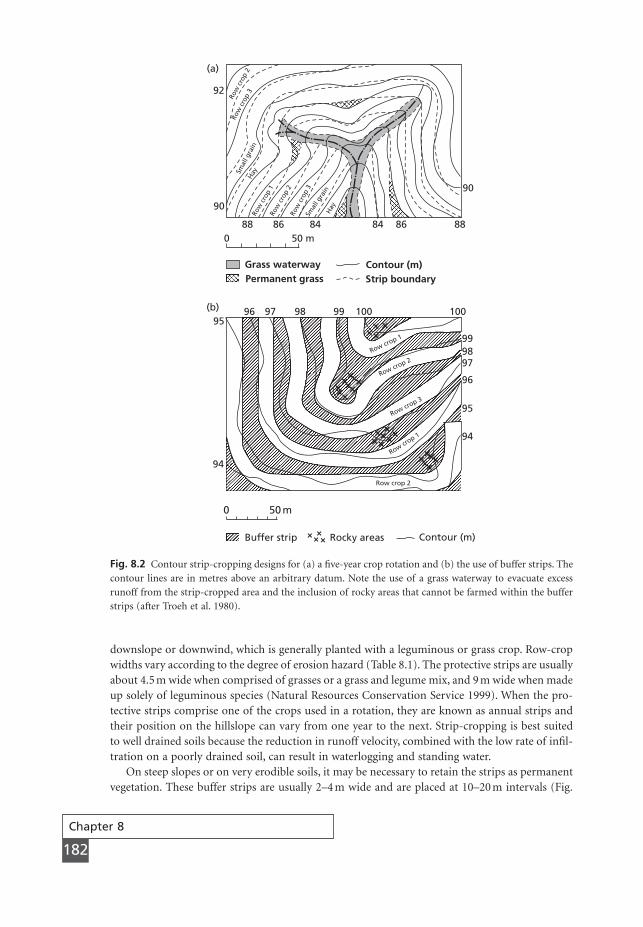
Chapter 8
182
downslope or downwind, which is generally planted with a leguminous or grass crop. Row-cropwidths vary according to the degree of erosion hazard (Table 8.1). The protective strips are usuallyabout 4.5 m wide when comprised of grasses or a grass and legume mix, and 9 m wide when madeup solely of leguminous species (Natural Resources Conservation Service 1999). When the pro-tective strips comprise one of the crops used in a rotation, they are known as annual strips andtheir position on the hillslope can vary from one year to the next. Strip-cropping is best suitedto well drained soils because the reduction in runoff velocity, combined with the low rate of infil-tration on a poorly drained soil, can result in waterlogging and standing water.
On steep slopes or on very erodible soils, it may be necessary to retain the strips as permanentvegetation. These buffer strips are usually 2–4 m wide and are placed at 10–20 m intervals (Fig.
92
90
96 97 98 99 100 100
0 50 m88 86 84 84 86 88
90
Hay
Row crop 2
Row crop 1
Row crop 3
Row crop 2
Row crop 1
Hay
Smal
l gra
in
Smal
l gra
in
Row
cro
p 3
Row
cro
p 3
Row
cro
p 2
Row
cro
p 2
Row
cro
p 1
Grass waterwayPermanent grass
Contour (m)Strip boundary
999897
96
95
94
94
0 50 m
95(b)
(a)
Buffer strip +
+++++++
+++++++++
++++++
++++
+++ Rocky areas Contour (m)
Fig. 8.2 Contour strip-cropping designs for (a) a five-year crop rotation and (b) the use of buffer strips. Thecontour lines are in metres above an arbitrary datum. Note the use of a grass waterway to evacuate excessrunoff from the strip-cropped area and the inclusion of rocky areas that cannot be farmed within the bufferstrips (after Troeh et al. 1980).
MSE08 11/19/04 02:40 PM Page 182
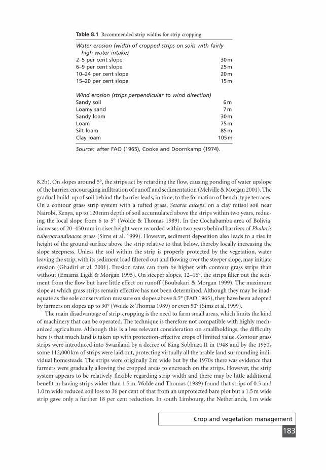
Crop and vegetation management
183
8.2b). On slopes around 5°, the strips act by retarding the flow, causing ponding of water upslopeof the barrier, encouraging infiltration of runoff and sedimentation (Melville & Morgan 2001). Thegradual build-up of soil behind the barrier leads, in time, to the formation of bench-type terraces.On a contour grass strip system with a tufted grass, Setaria anceps, on a clay nitisol soil nearNairobi, Kenya, up to 120 mm depth of soil accumulated above the strips within two years, reduc-ing the local slope from 6 to 5° (Wolde & Thomas 1989). In the Cochabamba area of Bolivia,increases of 20–450 mm in riser height were recorded within two years behind barriers of Phalaristuberoarundinacea grass (Sims et al. 1999). However, sediment deposition also leads to a rise inheight of the ground surface above the strip relative to that below, thereby locally increasing theslope steepness. Unless the soil within the strip is properly protected by the vegetation, waterleaving the strip, with its sediment load filtered out and flowing over the steeper slope, may initiateerosion (Ghadiri et al. 2001). Erosion rates can then be higher with contour grass strips thanwithout (Emama Ligdi & Morgan 1995). On steeper slopes, 12–16°, the strips filter out the sedi-ment from the flow but have little effect on runoff (Boubakari & Morgan 1999). The maximumslope at which grass strips remain effective has not been determined. Although they may be inad-equate as the sole conservation measure on slopes above 8.5° (FAO 1965), they have been adoptedby farmers on slopes up to 30° (Wolde & Thomas 1989) or even 50° (Sims et al. 1999).
The main disadvantage of strip-cropping is the need to farm small areas, which limits the kindof machinery that can be operated. The technique is therefore not compatible with highly mech-anized agriculture. Although this is a less relevant consideration on smallholdings, the difficultyhere is that much land is taken up with protection-effective crops of limited value. Contour grassstrips were introduced into Swaziland by a decree of King Sobhuza II in 1948 and by the 1950ssome 112,000 km of strips were laid out, protecting virtually all the arable land surrounding indi-vidual homesteads. The strips were originally 2 m wide but by the 1970s there was evidence thatfarmers were gradually allowing the cropped areas to encroach on the strips. However, the stripsystem appears to be relatively flexible regarding strip width and there may be little additionalbenefit in having strips wider than 1.5 m. Wolde and Thomas (1989) found that strips of 0.5 and1.0 m wide reduced soil loss to 36 per cent of that from an unprotected bare plot but a 1.5 m widestrip gave only a further 18 per cent reduction. In south Limbourg, the Netherlands, 1 m wide
Table 8.1 Recommended strip widths for strip cropping
Water erosion (width of cropped strips on soils with fairlyhigh water intake)
2–5 per cent slope 30m6–9 per cent slope 25m10–24 per cent slope 20m15–20 per cent slope 15m
Wind erosion (strips perpendicular to wind direction)Sandy soil 6mLoamy sand 7mSandy loam 30mLoam 75mSilt loam 85mClay loam 105m
Source: after FAO (1965), Cooke and Doornkamp (1974).
MSE08 11/19/04 02:40 PM Page 183
strips reduced sediment discharge by 50–60 per cent, 5 m wide strips by 60–90 per cent and 10 mwide strips by 90–99 per cent (van Dijk et al. 1996).
The plants chosen to form permanent buffer strips are usually grasses. They should be peren-nial, quick to establish and able to withstand periods of both flood and drought. They shouldhave deep-rooted systems to reinforce the soil and reduce scouring, a uniform density of topgrowth to provide a filter for sediment and reduce flow velocity; their growth points should beclose to the ground or below the soil so that they are not grazed out and can recover from damageafter fire; and they should either be sterile or propagate very slowly so that they do not becomeweeds in the adjacent cropped strips. Rhizomous species should be avoided since they spread veryrapidly on to surrounding land. Tussocky grasses, such as Kikuyu grass (Pennisetum clandes-tinum), should be avoided because they concentrate the flow (section 3.4.2). Grasses with an erectgrowth habit of interwoven stems which act like a porous filter are more effective in reducingerosion than those with slender creeping rhizomes and a more horizontal growth form (Lakew& Morgan 1996; Melville & Morgan 2001). Suitable species include Napier grass (Pennisetum pur-pureum), Guatemala grass (Tripsacum laxum), Makarikari grass (Panicum coloratum), Canarygrass (Phalaris canariensis), oat grass (Hyparrhenia spp.), wheat grass (Agropyron spp.) and lymegrass (Elymus spp.).
Considerable publicity has been given to vetiver grass (Vetiver zizanioides). Vetiver grass estab-lishes quickly from splits and does not compete with adjacent crops. It is adapted to a wide rangeof climatic and soil conditions with tolerance to both heavy metal and saline toxicity (Pease &Truong 2002). Over an 11-month period on an oxisol under cassava at the Santander de QuilichaoResearch Station, near Cali, Colombia, soil loss was 1.3 t ha-1 with vetiver grass contour barriers,4.0 t ha-1 with Napier grass strips and 8.3 t ha-1 with no conservation measures (Laing 1992). Overa three-year period on the Punjabrao Krishi Vidyapeeth University Farm, Manoli, India, annualsoil loss averaged 3.3 t ha-1 with vetiver grass strips on the contour compared with 11.4 t ha-1 usingacross-slope cultivation for a rotation of green gram–pigeon pea–safflower, pearl millet–safflowerand pearl millet (Bharad & Bathkal 1991). While vetiver grass has the advantage that it is notpalatable to livestock and therefore any strips formed from it are likely to remain undamaged, itprovides no income to the farmer, whereas Napier grass can be cut and fed to cattle. Clearly theideal situation is where the economic value of the grass strips equals or exceeds that lost by takingthe land out of agricultural production.
Strip systems can also be used to provide in-field shelter for wind-sensitive crops and protectthe soil against erosion by wind. In the fens of eastern England, live barley strips are used toprotect onions, sugar beet and carrots from wind damage and to control erosion on the lowlandpeat soils. The barley is sown in February or March, allowing time for it to emerge before themain crop is drilled in mid to late April, the critical period for erosion. Once the main crop hassufficient biomass to perform a protective role, the barley is killed with a selective herbicide. Livebarley meets the design requirements of a plant for infield shelter in having bladed rather thanovate leaf forms to minimize the risk of streamlining in strong winds, rigid leaves to reduce flutterand thereby minimize the ‘wall effect’ (section 3.4.3) and an upright growth habit with at least0.65 kg DM m-3 of uniform biomass in the lowest 5 cm to provide an adequate filter (Morgan1989). The barley strips should be spaced at distances of eight to ten times their height, which isevery 2 m if the barley is 20 cm tall at the time when the risk of erosion is highest.
Barrier strips or buffers can be used to protect water bodies from pollution by sediment andthe chemicals adsorbed to it, particularly phosphorus. For this purpose, grass barriers need to beplaced in critical positions in the landscape, such as: alongside rivers, lakes and reservoirs, wherethey form riparian barriers; on the convexities of hillslopes to reduce runoff velocities and preventthe initiation of rills; and across pathways of water and sediment movement such as unsurfaced
Chapter 8
184
MSE08 11/19/04 02:40 PM Page 184
Crop and vegetation management
185
tracks. Since they need to trap all the sediment, including the fine clay particles, they need to bewider than those described above. Riparian barriers are often 5–10 m wide. A 9-m wide strip isusually sufficient to trap 80 per cent of the sediment (Natural Resources Conservation Service1999). Studies in Denmark indicate that a 12-m wide buffer is sufficient to trap all sediment andparticulate phosphorus transported from surrounding hillslopes and prevent it entering the watercourse (Kronvang et al. 2000). It should be noted that their ability to trap sediment means thatthey are ‘designed to fail’ since they become less effective over time as sediment builds up withinand upslope of the strip. When the sediment accumulates to a depth of about 150 mm, it is rec-ommended that it is removed by tillage and the barrier re-established. Otherwise there is a riskof the runoff being diverted around the barrier. Mowing of the barrier leads to more vigorousgrowth of the grass, making it more effective in nutrient uptake and carbon sequestration.
Forests can be used for riparian barriers with the additional advantages of creating shade for the aquatic environment and a diverse habitat for wildlife. Typically, they comprise three zones: (i) a zone of mixed grass species forming a filter adjacent to agricultural land; (ii) an intermediate zone of managed forest; and (iii) a zone of undisturbed forest alongside the river.The first zone, usually 10 m wide, reduces runoff by 56–72 per cent and the transport of sedimentby 78–83 per cent (Sheridan et al. 1999). Where the surrounding land is pasture and not crop,this zone can be dispensed with. Where the riparian barrier is installed alongside a river on a floodplain that is wider than 100 m, the width of zones (ii) and (iii) combined should be at least 30 m.For narrower flood plains, the combined width should be 13.7 m. For channels without a floodplain, a combined width of 10.7 m is recommended (Natural Resources Conservation Service1999).
8.4
Multiple cropping
The aim of multiple cropping is to increase the production from the land while providing pro-tection of the soil from erosion. The method involves either sequential cropping, growing two ormore crops a year in sequence, or intercropping, growing two or more crops on the same pieceof land at the same time. Many schemes involve a mixture of the two. Multiple cropping has beentraditionally practised in the Caribbean in the kitchen gardens, which, averaging 0.2 ha in size,provide the subsistence component of fruits and vegetables for many families in rural areas. Thosein Grenada combine fruit trees, with banana the most ubiquitous but also including coconut,cocoa, mango and breadfruit, with vegetables, especially root crops such as sweet potatoes andyams. Pigeon peas, groundnuts, dasheen, okra, pepper and tomatoes are also grown. The homegarden thus mimics the natural, multilayered ecosystem (Hoogerbrugge & Fresco 1993). Althoughthe garden has a confused appearance (Fig. 8.3), the organization of the cropped land is system-atic and the better farmers carry out regular weeding, selective application of fertilizers and irrigation (Brierley 1976).
When using sequential cropping, attention must be paid to the order in which the crops aregrown. Lal (1976) found that on a 6° slope near Ibadan, Nigeria, a crop of maize followed by oneof cowpeas with no tillage produced a loss of only 0.2 t ha-1. Growing cowpeas followed by maizebut with tillage gave a soil loss of 6.2 t ha-1. Although it is difficult to isolate the effects of zerotillage, it seems that a maize–cowpeas sequence produces less erosion than a cowpeas–maize onebecause maize is a soil-depleting crop and, when grown second, is planted into an already par-tially exhausted soil. Soil loss is also greater under maize than cowpea (Lal 1977a) and the
MSE08 11/19/04 02:40 PM Page 185
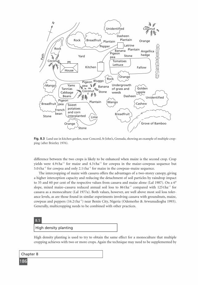
Chapter 8
186
difference between the two crops is likely to be enhanced when maize is the second crop. Cropyields were 4.9 t ha-1 for maize and 4.3 t ha-1 for cowpea in the maize–cowpeas sequence but 5.0 t ha-1 for cowpea and only 2.1 t ha-1 for maize in the cowpeas–maize sequence.
The intercropping of maize with cassava offers the advantages of a two-storey canopy, givinga higher interception capacity and reducing the detachment of soil particles by raindrop impactto 35 and 60 per cent of the respective values from cassava and maize alone (Lal 1987). On a 6°slope, mixed maize–cassava reduced annual soil loss to 86 t ha-1 compared with 125 t ha-1 forcassava as a monoculture (Lal 1977a). Both values, however, are well above most soil loss toler-ance levels, as are those found in similar experiments involving cassava with groundnuts, maize,cowpeas and peppers (16.2 t ha-1) near Benin City, Nigeria (Odemerho & Avwunudiogba 1993).Generally, multicropping needs to be combined with other practices.
N
Rock Breadfruit
Unidentified Coconut
Orange
Yard
HouseKitchen
Coconut
Rock
Path
Mango
Breadfruit
YamsTannias
CabbageBeans
Coconut
Pigeonpea
Pigeonpea
Pigeonpea
Lime
Mango
Breadfruit
Dasheen
Cashew
Unidentified
Goldenapple
Fallow
Orange
DasheenPlantain
PlantainBanana
Banana
Stone
Stone
TomatoesLettuce
LatrinePepper
Plantain
Plantain
Angellicahedge
Rock
Undergrowthof grass andweeds
OrangeStone
Stone
Sweetpotatoesand corninterplanted
Frenchbean
Bluggo
Grove of Bamboo
Fig. 8.3 Land use in kitchen garden, near Concord, St John’s, Grenada, showing an example of multiple crop-ping (after Brierley 1976).
8.5
High density planting
High density planting is used to try to obtain the same effect for a monoculture that multiplecropping achieves with two or more crops. Again the technique may need to be supplemented by
MSE08 11/19/04 02:40 PM Page 186
Crop and vegetation management
187
other practices. Hudson (1981) showed in Zimbabwe that increasing the planting density of maizefrom 25,000 to 37,000 plants per hectare and using a trash mulch at the higher density reducedannual soil loss from 12.3 to 0.7 t ha-1. Respective crop yields were 5 and 10 t ha-1. The arrange-ment of the plants also has an effect. With a plant population of 55,000 plants per hectare, thelowest soil loss from maize in the Doon Valley, northern India, was obtained by increasing thedistance between the rows and increasing the plant density within the rows. Thus changing froma row spacing of 450 mm and a plant spacing of 400 mm to a row spacing of 900 mm and a plantspacing of 200 mm reduced annual soil loss under maize from 22.6 to 13.9 t ha-1 (Bhardwaj et al.1985).
High density planting can be effective even when targeted only on those parts of the landscapethat are most vulnerable to erosion. In a study on the Belgian loess under winter-sown triticale,a second sowing was carried out along the valley floor where runoff concentrates and ephemeralgullies form. This increased the plant density by 50 per cent and resulted in a 42 per cent reduc-tion in erosion (Gyssels et al. 2002). Clearly, the need to make a second sowing would increasecosts but this would not be necessary with modern precision agriculture, where the sowing ratecould be automatically adjusted to position in the field.
8.6
Mulching
Mulching is the covering of the soil with crop residues such as straw, maize stalks, palm frondsor standing stubble. The cover protects the soil from raindrop impact and reduces the velocity ofrunoff and wind. It is most useful as an alternative to cover crops in dry areas where insufficientrain prevents the establishment of a ground cover before the onset of heavy rain or strong winds,or where a cover crop competes for moisture with the main crop. In the semi-humid tropics, theside-effects of a mulch in the forms of lower soil temperatures and increased soil moisture arebeneficial and may increase yields. Elsewhere the effects can be detrimental. In cool climates, thereduction in soil temperature shortens the growing season, while in wet areas, higher soil mois-ture may induce gleying and anaerobic conditions. Crop yields may also be reduced because themulch competes with the main crop for nitrogen as it decomposes.
The effectiveness of mulching in reducing erosion was demonstrated by the field experimentsof Borst and Woodburn (1942), who found that, on a silt-loam soil on a 7° slope, annual soil losswas 24.6 t ha-1 from uncultivated bare land but only 1.1 t ha-1 from land covered with a strawmulch applied at 5 t ha-1. Lal (1976) found that covering an alfisol on a 6° slope with 6 t ha-1 ofstraw mulch resulted in an annual soil loss of 0.2 t ha-1 compared with 23.3 t ha-1 on bare soil.Although such low soil losses are not always achieved, the extent to which a mulch will reduceerosion is generally impressive. A grass mulch at 4 t ha-1 applied to a silt-loam soil on a 4.5° slopenear Dehra Dun, India, reduced annual soil loss under maize to 5.0 t ha-1 compared with 22.4 t ha-1 for maize tilled conventionally up-and-down slope (Khybri 1989). A grass mulch at 15 t ha-1 on a sandy loam soil with a 3° slope near Pakhribas in eastern Nepal gave an annual soilloss under maize of 16.9 t ha-1 compared with 32.8 t ha-1 for the traditional practice of maize plant-ing followed by two hoeings (Sherchan et al. 1990).
Mulches can also be used under tree crops. Using pruned fronds to cover harvesting paths inan oil palm plantation in Johor, Malaysia, reduced annual soil loss to 4.2 t ha-1 from 14.9 t ha-1
recorded on unprotected paths (Maene et al. 1979). A grass mulch applied between rows of youngtea on a 6° slope on an ultisol near Kericho, Kenya, reduced average annual soil loss over three
MSE08 11/19/04 02:40 PM Page 187
Chapter 8
188
years to 0.7 t ha-1 compared with 210.8 t ha-1 for bare hand-tilled soil between the rows (Othieno1978).
Most applications of mulching involve spreading crop residues on the surface of the soil butthis method creates problems in drilling and planting through the mulch, unless specializedequipment is used. An alternative approach is to incorporate the mulch in the soil. Although thisreduces the overall surface cover, the mulch elements help to bind the soil, simulating the effectof plant roots, and increase infiltration rates. Duley and Russel (1943) found that incorporatedcrop residue reduced annual soil loss from 35.7 t ha-1 on a bare soil to 9.9 t ha-1. The effect of incor-porated mulch depends upon the material used. Wheat straw is particularly effective because itproduces a large number of individual mulch elements, resulting in a more uniform pattern ofincorporation, good contact between the mulch and the soil, and sufficient material on the surfaceto form miniature dams, behind which water ponds, and protect the soil against crusting. In con-trast, maize stalks perform badly because their large size means that the surface is sparsely covered,the contact with the soil is poor and the individual elements are easily washed out and trans-ported downslope (Abrahim & Rickson 1989). Overall, incorporated mulches are less effectivethan surface mulches.
When using mulches to control wind erosion, standing stubble is required because of thedanger of spread mulches blowing away. A mulch of 1 t ha-1 of standing wheat stubble or 2 t ha-1
of flattened wheat straw will reduce annual wind erosion rates to a tolerable level of 0.2 t ha-1. Toachieve the same effect with sorghum stubble requires a mulch of 6.7 t ha-1 (Chepil & Woodruff1963). In a review of research carried out in the Sahel, Bielders et al. (1998) showed that 2 t ha-1
of millet stover could reduce soil loss by between 42 and 92 per cent, depending on wind velocities.
There is considerable experimental evidence (Wischmeier 1973; Lal 1977b; Laflen & Colvin1981; Norton et al. 1985; Bekele & Thomas 1992) to show that the rate of soil loss decreases exponentially with an increase in the percentage area covered by a mulch. The mulch factor (MF),defined as the ratio of soil loss with a mulch to that without, is related to the percentage residueor mulch cover (RC) by the expression (Laflen & Colvin 1981):
(8.1)
where a ranges in value from 0.01 to 0.07, depending on the degree of soil disturbance by tillage.For a mouldboard plough, the value is 0.03, and for no tillage, 0.06 (Norton et al. 1985). Husseinand Laflen (1982) found that the exponential relationship applied only to rill erosion and thatthe rate of interrill erosion decreased linearly with increasing residue cover. Since for most soilsthe contribution of interrill erosion to total soil loss is quite small for slope lengths in excess of25 m, eqn 8.1 can be used to obtain mulch factor values that, when multiplied by the C-factorvalues, allow the effects of mulching to be included in the Universal Soil Loss Equation (section6.1.1).
A mulch should cover 70–75 per cent of the soil surface. With straw, an application rate of5 t ha-1 is sufficient to achieve this. A lesser covering will not adequately protect the soil, while agreater covering may delay plant emergence and suppress plant growth. Denser mulches, givingat least 90 per cent cover, are sometimes used under tree crops to control weeds. An estimate ofthe required application rate to control erosion can be made for a preselected set of conditionsusing the Manning equation for flow velocity (eqn 2.18) and the relationship between Manning’sn and mulch rate for straw (Foster et al. 1982):
(8.2)n Mm = 0 071 1 12. . interrill erosion
MF e a RC= - .
MSE08 11/19/04 02:40 PM Page 188

Crop and vegetation management
189
(8.3)
where nm is the value of n due to the mulch and M is the mulch rate (kg m-2) (Table 8.2). Nosimilar procedure exists for determining mulch rates to control wind erosion, but the effective-ness of standing crop residues depends upon the number of standing stalks per unit area andtheir size.
As indicated above, controlling erosion with a mulch poses special problems for the arablefarmer because tillage tools become clogged with the residue, weed control and pest control are
n Mm = 0 105 0 84. . rill erosion
Table 8.2 Estimating the required density of a maize stalk mulch to control water erosion
Estimation is made for the following conditions:Sandy soil, desired maximum flow velocity = 0.75ms-1
Flow depth in small channels = 100mmSlope = 5°
Estimating the required value for total Manning’s n:From the Manning equation:
For simplicity, assume the hydraulic radius (r) is approximated by the depth of flow andthat slope (s) can be represented by the tangent of the slope angle. Thus
Estimating required value for Manning’s n due to mulch (nm):According to Foster et al. (1982):
Taking a value of Manning’s n due to the soil (ns) = 0.02, gives
Estimating required mulch application rate (M):Rearranging eqn 8.3 gives
Note: Theoretically this procedure can be used to determine application rates for othermulches but in practice the relationships between M and nm have not been established. Eqn8.3 cannot therefore be used for wheat straw, soya bean residue, palm fronds or other mulchmaterials.
Mn
M
M
m= ÊË
ˆ¯
= ÊË
ˆ¯
= -
0 0105
0 07670 0105
0 72
1 06
1 06
2
.
.
..
.
.
kgm
n
nm
m
= -( )=
0 843 0 02
0 0767
3 2 3 2 2 3. .
.
n n nm s= -( )3 2 3 2 2 3
n
n
= ¥
=
0 1 0 0870 75
0 0843
0 67 0 5. ..
.
. .
nr s
v=
0 67 0 5. .
MSE08 11/19/04 02:40 PM Page 189
Chapter 8
190
more difficult, planting under the residue is not always successful and crop yields, especially inhumid and semi-humid areas, are sometimes lower. Mulching on its own is not always an appro-priate technique but where it is combined with conservation tillage, many of these problems canbe overcome and it has tremendous potential as a method of erosion control.
Rock fragments on the surface can act in the same way as a mulch. Relationships between rateof erosion and percentage stone cover frequently follow that described by eqn 8.1 (Poesen 1992).Therefore stone mulches might be appropriate for erosion control on non-agricultural areas suchas road banks and construction sites. However, where the stones are embedded in a sealed orcrusted soil, interrill erosion can be enhanced and will increase with percentage stone coverbecause the runoff generated on the impermeable stone elements is unable to infiltrate the sur-rounding soil (Poesen & Ingelmo-Sanchez 1992). On an erodible soil, rock fragments can alsoinduce local turbulence, leading to scouring on the upstream side of the stones and depositionon the downstream side. With small stones or pebbles around 15 mm in size, scouring can causesediment yield to increase as cover increases from zero to 20 per cent but, with further increasesin percentage cover, the protective effect prevails. On covers of 60 per cent and above, scour isalmost impossible. For cobbles around 86 mm in size, however, there is no reduction in sedimentproduction and the soil loss increases exponentially with increasing percentage cover (Bunte &Poesen 1994). Since rock fragments can both decrease and increase erosion according to local cir-cumstances, their use as a mulch to control water erosion cannot be recommended.
A different picture emerges for wind erosion control. Pebble and gravel mulches have beenused in the semi-arid regions of northwest China for over 300 years (Gale et al. 1993) to help topreserve moisture from the limited rainfall and trap wind-blown material. A pebble mulchreduces the rate of wind erosion by 84–96 per cent (Li et al. 2001) and can trap between 1.6 and1.8 times more sediment than the surrounding land. Pebbles of 25 mm diameter are more effec-tive than those of 100 mm diameter, trapping 2.8 times as much, probably because the largerpebbles create more turbulence (Li & Liu 2003). Since the nitrogen and organic content of thedust is two to three times higher than that of the local soil, the accumulated sediment adds to thefertility of the gravel-mulched fields. Over time, the spaces between the pebbles fill with soil andthe surface becomes smoother, thereby reducing the effectiveness of the technique. Tillage,however, will help to return the gravel to the surface.
8.7
Revegetation
Vegetation plays a major role in the process of erosion control on gullied areas, landslides, sanddunes, road embankments, construction sites, mine spoils and pipeline corridors. Rapid revege-tation is also necessary for replanting forest in areas cleared by patch-cutting and for coveringland cleared of forest in favour of agriculture. The first-listed cases represent marginal environ-ments for plant growth where the risk of vegetation failing to re-establish is high. The second-listed cases are less marginal and the objective is to minimize damage during clearance and toestablish cover quickly before the environment has time to deteriorate.
When developing a plan for revegetating an area, a soil test should be carried out to establishpH, nutrient levels, moisture status, salinity levels and the presence of toxic ions, all of which willinfluence the range of species that will grow. Climatic conditions should also be studied, includ-ing the frequency of drought and waterlogging. Topographic influences on the local climate areimportant – for example, differences in temperature and moisture between sunny and shady
MSE08 11/19/04 02:40 PM Page 190
slopes, and frost hollows. Topography also determines the location of dry and wet sites throughits effect on movement of water through the soil. Plant species should be selected for their prop-erties of rapid growth, toughness in respect of diseases and pests, ability to compete with lessdesirable species and adaptability to the local soil and climatic conditions. Wherever possible,native species should be chosen. A study of neighbouring sites often gives a good indication ofwhat species are most likely to survive and thrive. The use of introduced or exotic species shouldnot be ruled out, however, especially where the local environment has deteriorated beyond thatof adjacent sites or where numbers of local species are limited. The revegetation plan should allowfor plant succession to take place naturally. In many cases, the objective is to establish pioneerspecies to give immediate cover and improve the soil, permitting native species to come in andtake over as the colonizing plants decline. Generally, a mix of plant species is required because itis impossible to predict the success of any one species in marginal environments. A monocultureis also more susceptible to disease. The species mix should include grasses, forbs and woodyspecies, both bushes and trees, except where specific requirements make such a mix undesirable,as with certain types of gully reclamation or along pipeline corridors. Detailed coverage of thevarious methods of vegetation establishment can be found in Gray and Leiser (1982) and Coppinand Richards (1990).
8.7.1 Restoration of gullied lands
Revegetation is used in gully erosion control as a method of increasing infiltration and reducingsurface runoff. Provided about 30–35 per cent vegetation cover remains on the land, closing anarea on the gullied loess in the Xingzihe Basin by fencing and prohibiting its use for grazing canlead to a natural increase in cover to 70–90 per cent within three to four years. However, withsupplementary planting of grasses and shrubs, the same effect can be achieved within two years(Tang et al. 1987). Generally, the area around the gullies needs to be treated with grasses, legumes,shrubs and trees or combinations thereof, aided in the early stages by mulching or the use of geo-textiles. Research carried out at the Suide Soil and Water Conservation Experiment Station of theHuang He Conservancy Commission shows that afforestation can reduce runoff in the gulliedloess areas by 65–80 per cent and soil loss by 75–90 per cent. Growing grass reduces runoff by50–60 per cent and soil loss by 60–80 per cent (Gong & Jiang 1977). The planting of trees andherbs on the steep slopes of the gully sides and raising crops on bench terraces on the gentlerslopes of the divides (Fig. 8.4) can stabilize the land and prevent sediment from entering thegullies. By supporting these measures with check dams and reservoirs along the gully beds, thevolume of sediment entering the Huang He from gullies in the Wuding Valley was reduced by 44per cent over the period 1971–8 (Jiang et al. 1981).
In the studies mentioned above, the main objective was to increase infiltration. Achieving thiswill help to reduce gullying when surface processes are involved, but where the gullies are fed bysubsurface pipes or tunnels (section 2.6.1), it is necessary also to promote infiltration in a uniformpattern. Since trees and grasses have different root densities and their root networks extend todifferent depths, their mixture may result in more infiltration under the trees, which may, in turn,feed water into a pipe system. Even if the pipe network has been previously broken up by sub-surface ripping, concentrations of water in the soil may encourage pipes to reform. This is morelikely to occur if tree species with long tap roots are planted. Thus, the best vegetative treatmentfor tunnelled areas is to establish a dense, uniform grass cover. Where conditions are too mar-ginal for grass to grow, shrubs and trees will have to be used but species with a good system oflateral rather than vertical roots should be chosen.
Crop and vegetation management
191
MSE08 11/19/04 02:40 PM Page 191
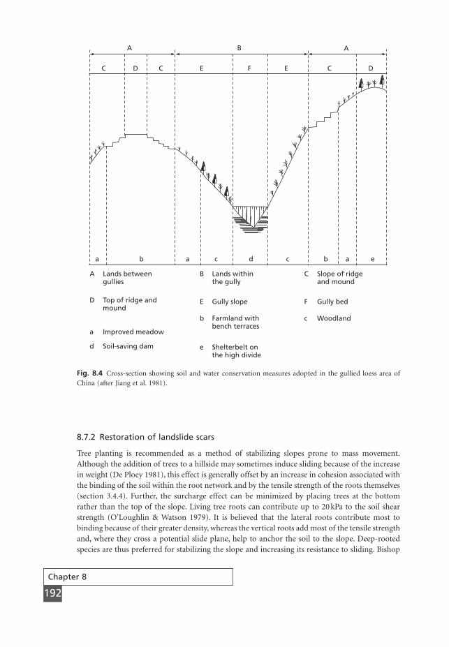
Chapter 8
192
8.7.2 Restoration of landslide scars
Tree planting is recommended as a method of stabilizing slopes prone to mass movement.Although the addition of trees to a hillside may sometimes induce sliding because of the increasein weight (De Ploey 1981), this effect is generally offset by an increase in cohesion associated withthe binding of the soil within the root network and by the tensile strength of the roots themselves(section 3.4.4). Further, the surcharge effect can be minimized by placing trees at the bottomrather than the top of the slope. Living tree roots can contribute up to 20 kPa to the soil shearstrength (O’Loughlin & Watson 1979). It is believed that the lateral roots contribute most tobinding because of their greater density, whereas the vertical roots add most of the tensile strengthand, where they cross a potential slide plane, help to anchor the soil to the slope. Deep-rootedspecies are thus preferred for stabilizing the slope and increasing its resistance to sliding. Bishop
A B
C D C E F E C D
A
a b a c d c b a e
A B C
F
c
E
b
e
D
a
d
Lands betweengullies
Lands withinthe gully
Gully slope
Farmland withbench terraces
Shelterbelt onthe high divide
Top of ridge andmound
Improved meadow
Soil-saving dam
Slope of ridgeand mound
Gully bed
Woodland
Fig. 8.4 Cross-section showing soil and water conservation measures adopted in the gullied loess area ofChina (after Jiang et al. 1981).
MSE08 11/19/04 02:40 PM Page 192
and Stevens (1964) show that large trees can increase the shearing stress required for sliding by2.5 kPa, which is why, as seen in section 7.4.3, their removal can promote landslides. Grass rootscan increase the shear strength of soils by between 0.1 and 11.6 kPa (Lawrance et al. 1996; Preston& Crozier 1999).
Closing an area, particularly from livestock but also from wild animals, will allow vegetationto colonize landslide scars naturally. The rate of recovery, however, is slow. Herbs come in first,followed by grasses, but only after about four years do perennial grasses dominate the cover andshrubs start to appear. After seven years the cover on scars in the Mgeta Valley, Tanzania, was only25 per cent (Lundgren 1978). Recovery of soil slip scars in the Wairarapa hill country, NewZealand, takes 20 years but even then the productivity of the pasture is only 80 per cent of thaton uneroded land. Despite recolonization, the quality of the land deteriorates (Trustrum et al.1984). Tree planting was attempted on the slide scars in the Mgeta Valley but the species used, Acacia mearnssii, Cupressus lusitanica and Eucalyptus maidenni, proved unsuitable. All theCupressus lusitanica seedlings died and the survival of the others was threatened by gully erosion(Lundgren 1978). This example emphasizes the need for careful selection of species in relation to the environmental conditions.
8.7.3 Afforestation
Many countries have afforestation programmes aimed at arresting erosion and regulating floods.Most schemes involve closing the land to other uses. It should be recognized, however, that thesuccess of such schemes depends on the methods used to prepare the land for replanting and thatit takes some years before the all-important litter layer develops on the soil surface. As seen insection 7.4.3, erosion often increases in the early years of reforestation work.
In the Vasad and Kota areas of Gujarat, India, the closing of gullied lands to grazing allowedthe establishment first of a good grass cover of desirable species and then an increase in treenumbers through natural colonization. Afforestation trials were also successfully implemented,with bamboo, teak, sissoo and eucalyptus as the most promising species (Tejwani 1981). The prin-cipal species in forest plantations in Kenya, Cupressus lusitanica, Pinus patula, Pinus radiata andEucalyptus saligna, are selected because of their rapid growth rather than their value in soil andwater conservation (Konuche 1983). Although the pines are generally satisfactory, the cypressresults in a bare forest floor liable to erosion by overland flow unless the stands are pruned andthinned. The role of eucalypts is unclear because of evidence that when planted in wet areas theyresult in a reduction of water supply in springs and rivers (Gosh et al. 1978), yet when grown indrier areas they do not consume large quantities of water (Konuche 1983). Since eucalypts developtheir root systems rapidly and promote infiltration and subsurface drainage, they may inducemass movements when planted on steep slopes with shallow soils (section 3.4.4). This is becauseof the impedance to subsurface water movement at the soil–rock interface and the reduction inthe shear strength of the soil as the moisture content increases to saturation (De Ploey & Cruz1979).
8.7.4 Restoration for pasture
Revegetation of lands for pasture is the major activity of LandgræQsla Ríkisins, the State Soil Conservation Service of Iceland. Work is concentrated on restoration of bare moving sands and gravels using aerial seeding. The land is first fenced to keep out livestock. Elymus arenariusis then planted on the moving dunes in strips at right angles to the erosive winds and fertilizedannually until serious sand movement has been halted. This plant thrives well in drifting sand
Crop and vegetation management
193
MSE08 11/19/04 02:40 PM Page 193
and collects and fixes its own dunes. Once the sand has been stabilized, the Elymus dies out andFestuca rubra, Poa pratensis and Phleum pratensis are aerially seeded. Imported seeds are usedbecause the local climate is too severe to provide a reservoir of locally available seed. Fertilizer isapplied aerially each year for the next two to four years, by which time a reasonable vegetationcover has been obtained. No further work is carried out and, in the absence of continued fertil-izer application, the seeded grasses die out and the vegetation cover becomes poor. Sufficient sta-bility and organic matter have been achieved, however, to allow native vegetation to recolonize.The land remains protected for 30 years (Runólfsson 1978; Arnalds et al. 1987) before beingreturned to the farmer.
In many countries of the world, revegetation is limited not only by the infertility of the soilbut also by lack of water. In addition to supplying fertilizers in the early stages of reclamation, itis necessary to provide water-conserving structures. Mututho (1989) modified a traditional pittingpractice of the WaMatengo people in southern Tanzania to form semi-circular pits, 5–12 m2 inarea, surrounded by a 15–30 cm high bank to trap water on rangeland reclamation schemes inthe Kitui District, Kenya. The sites were excluded from grazing and the pits planted with indige-nous perennial grasses. The pits, however, require considerable inputs of labour for their con-struction. A modified version, known as the Katumani pit, has been developed (Gichangi et al.1992) that is only 1.5–3.0 m2 in area. These pits are also planted with indigenous grasses but, inthe first year after construction, a crop of beans and cowpeas can be obtained to give a short-termincome until the grazing land has been rehabilitated.
8.7.5 Embankment and cut slopes
Rapid establishment of a grass or legume cover is essential on embankment and cut slopes tominimize surface erosion and enhance slope stability. This is commonly achieved by hydroseed-ing a seed and fertilizer mix. Where immediate erosion control is necessary, mulches or geotex-tiles should be used to protect the soil and prevent the seeds from being washed away. A strawmulch, applied at 4 t ha-1 at the time of seeding and fertilizing the soil in the autumn, was foundto reduce erosion to acceptable levels on 45° roadside slopes in western Oregon (Dyrness 1975)and allow the establishment of more than 70 per cent vegetation cover by the end of the follow-ing summer. Maximum cover, mainly rye grass, bent and fescue, was achieved after some threeyears but then lack of nitrogen caused the vegetation to decline to only 10 per cent cover aftereight years. By this time the slope was protected by a dense litter of dead grass. Addition of morefertilizer quickly revived the vegetation, which developed to 90 per cent cover within one year.Most erosion occurred in the first year of the treatment, after which soil loss was virtually zero.An alternative way of establishing cover is to plant natural turf over the slope, as is standard prac-tice in the urban areas of Singapore (Ramaswamy et al. 1981).
Grasses, mainly Cynodon dactylon and Pennisetum clandestinum, are used to control surfaceerosion on 30–65° road banks in eastern Nepal (Howell et al. 1991) but the increased infiltrationthat results enhances the risk of shallow slides (section 7.4.9). In order to reduce the risk, deeper-rooted grasses, such as Eulaliopsis binata, Neyraudia reynaudiana, Saccharum spontaneum andCymbopogon microtheca, are recommended to anchor the soil and root mat to the underlyingweathered material. However, these grasses are clumpy in habit and cause runoff to concentrate.Moreover, their roots do not always adhere well to the coarse debris and pull-out when the mate-rial starts to move. To counteract this and provide deeper stability, plant successions are plannedfor the revegetation work, allowing the grasses to be supported by shrubs and trees. Suitable treespecies include Pinus wallichiana, Pinus roxburghii, Acacia catechu, Dalbergia sissoo and Alnusnepalensis. In order to sustain the grass cover, the forest must remain 50 per cent open, so long-
Chapter 8
194
MSE08 11/19/04 02:40 PM Page 194
term management will be required to prevent the closure of the forest canopy (Howell 1999).Despite the versatility of vegetation for erosion control on road banks, the steepness of manyslopes and the harshness of the environment often mean that vegetative solutions need to be inte-grated with structural work.
8.7.6 Pipeline corridors
Pipeline corridors comprise strips of land, usually 20–40 m wide, extending for many hundredsof kilometres across country. As indicated in section 7.4.8, there is a risk of erosion between thetime the pipe is installed and the regrowth of the vegetation. Severe erosion can hinder the restora-tion work by washing out seeds and young plants. In many situations, the most cost-effectivemethod of combining revegetation and erosion control is to reseed, cover the slope with a surface-laid geotextile and then plant saplings through the geotextile material. Where a suitable localsource is available, a mulch may be used instead of the geotextile, but it is important that at leasta 70 per cent ground cover is maintained throughout the vulnerable period. The success of therestoration work, particularly where the aim is to re-establish the local plant community, can beenhanced by careful management of the top soil during its removal, storage and return (Coppin& Richards 1990) in order to preserve as much of the original soil structure and cohesion as pos-sible and not to damage the seed bank contained in the soil. Since the seed bank contains repre-sentative material of the local plant community, it should be viewed as the foundation forre-establishing the local ecology; reseeding and replanting are used to supplement the seed bank.In dry climates or where revegetation work is carried out prior to the dry season, the seeds andplants must be watered regularly. Water conservation measures, such as pits and lunettes (Hudson1987), can be used to trap and store surface runoff from occasional rain storms. As is the casewith road banks, it is important to plan a plant succession. When deciding which species to usefor reseeding and replanting, emphasis should be given to the colonizing ones in order to estab-lish cover as rapidly as possible. Other species will emerge from the seed bank and by invasionfrom the surrounding land. Once a vegetation cover has been re-established, the plant successionmust be managed in order to ensure that a uniform cover of grasses and shrubs is maintainedand that trees do not take hold, since their roots can damage the pipe.
8.7.7 Sand dune restoration
The first stage in sand dune restoration is to stabilize the moving sand in order to create a suit-able environment for plants to grow. Fences are erected to reduce wind speed, trap sand andenclose the area to keep out livestock and people. The sand surface is fixed using soil stabilizersor geotextiles. The main plants used in stabilizing sand dunes in the coastal areas of Europe and the USA are marram grass (Ammophila arenaria) and American beach grass (Ammophila breviligulata). These have strong extensive root networks in both lateral and vertical directions,which enable them to bind the soil while the grass acts as a sediment trap (Hesp 1979). Theythrive well in moving sand with low nutrient availability. Grasses should be planted as 100–150-mm wide culms rather than seeded because of the risk of the seeds being blown away andthe young plants damaged by sand blasting. Once stabilized, the dunes can be planted with shrubsand trees.
Similar approaches are used to stabilize desert dunes. Within eight years of the establishmentof the fast-growing Tamarix aphylla on sands near the Al-Hasa oasis in Saudi Arabia, the depthof the organic horizon had increased from zero to 10 mm and the calcium carbonate contentdecreased from 30 to 15 per cent (Stevens 1974). The long-term effect of such schemes is not
Crop and vegetation management
195
MSE08 11/19/04 02:40 PM Page 195
Chapter 8
196
clear, however, because, as the trees mature, the soil moisture within the dune is depleted. Sur-vival of the vegetation then depends on the ability of the tree roots to seek out groundwater. Ifthis turns out to be salty, the trees may die and the dunes may be remobilized (Gupta 1979). Gen-erally, where precipitation annually exceeds 250 mm, dunes can be stabilized by vegetation withinfive to ten years. Where annual precipitation is between 100 and 250 mm, vegetational stabiliza-tion is possible but may take 20–30 years; moreover, woody species cannot grow and only shrubsand grasses can be used. Where precipitation is less than 100 mm per year, a vegetation-basedapproach is not feasible except with irrigation over very small areas.
8.7.8 Restoration of recreational areas
Closing the land and replanting with trees, shrubs and grasses is frequently adopted to renovateareas eroded through recreational use. Examples are the Tarn Hows project in the English LakeDistrict (Barrow et al. 1973), the reclamation of gullies in the Box Hill area of the North Downsin southeast England (Streeter 1977), the footpath restoration work of the Three Peaks area ofthe Yorkshire Dales National Park (Rose 1989) and the revegetation of the Heavenly Ski Resortin the Tahoe Basin, California (Morse 1992). In addition to ensuring that the species used forreplanting are compatible with the physical environment and resistant to trampling, plant selec-tion may be influenced by aesthetic considerations so as to enhance landscape quality and by theneed to create varied and interesting wildlife habitats.
8.8
Agroforestry
Trees can be incorporated within a farming system by planting them on land that is not suitablefor crop production. Where trees are deliberately integrated with crops or animals or both toexploit expected positive interactions between the trees and other land uses, the practice is definedas agroforestry (Lundgren & Nair 1985). Trees help to preserve the fertility of the soil throughthe return of organic matter and the fixation of nitrogen. They improve the soil’s structure andhelp to maintain high infiltration rates and greater water-holding capacity. As a result less runoffis generated and erosion is better controlled. Trees are also attractive to the farmer where theyprovide additional needs, especially fuel, fodder and fruits. Multipurpose trees and shrubs arethus fundamental to agroforestry.
Agroforestry is encouraged in many countries as a way of modifying existing farming systemsto promote soil fertility, erosion control and a diversified source of income. Three types of prac-tice may be defined. Agrisilviculture involves the combination of trees and crops. Silvopastoral-ism is the combination of trees and animals. Agrosilvopastoralism combines trees with crops andanimals. Within these systems, trees can be used to supplement existing erosion-control measures– for example, by being added to contour grass strips and terraces – or they can be used to controlerosion direct – for example, in multiple-cropping systems such as kitchen gardens or withcontour-aligned hedgerows in intercropping. Although the latter act as live barriers and trap sed-iment, leading to the formation of terraces over time, as described in section 8.3, an importantfeature of the hedgerows is that they increase infiltration by three to eight times because of theirroot systems (Kiepe 1995) and thereby reduce runoff. Much attention has been given to alley crop-ping systems, in which multipurpose trees are grown as contour hedges separated by strips ofcropland. On a 16° slope at the Butare Research Station, Rwanda, the annual soil loss over four
MSE08 11/19/04 02:40 PM Page 196
Crop and vegetation management
197
years from cassava in an alley cropping system with 5-m wide strips of the leguminous shrub Cal-liandra calothyrsus grown on microterraces was 12.5 t ha-1 compared with 111 t ha-1 for traditionalcultivation of cassava. Mixed cropping of cassava in the alleys with beans, maize and sweet pota-toes, alternating with leguminous cover crops, reduced soil loss to 1 t ha-1 (König 1992). In a rangeof alley systems on an alfisol on a 4° slope near Ibadan, Nigeria, annual soil loss over two yearsfor a maize–cowpea rotation was 1.6 t ha-1 with Leucaena hedges at 4 m spacing, 0.15 t ha-1 withLeucaena hedges at 2 m spacing, 0.88 t ha-1 with Gliricidia hedges at 4 m spacing and 1.7 t ha-1 withGliricidia hedges at 2 m spacing compared with 8.7 t ha-1 with conventional cultivation and 0.025 t ha-1 with no tillage (Lal 1988). Crop yields of the maize were similar in all systems. Studiesin many countries show that agroforestry systems reduce erosion by at least ten times comparedto having no soil conservation measures (Young 1998).
Agroforestry systems require careful selection of both crops and tree species if a beneficial interaction is to be obtained. Indeed, several studies bring into question whether such interac-tion can be achieved. With alley cropping systems at Bellary, India, yields of sorghum, safflowerand Bengal gram were reduced by 16, 53 and 53 per cent respectively when grown between Leucaena leucocephala alleys at 4.5 m spacing (Srivastva & Rama Mohan Rao 1988), mainly as aresult of soil moisture depletion on land close to the hedgerows. Sorghum yields were also reducedwhen grown in combination with Acacia nilotica, Azadirachta indica and Eucalyptus hybrid. Yieldreductions in sorghum and pearl-millet were observed in agrisilvicultural systems near Karnal,northern India (Kumar et al. 1990). Clearly, with these adverse effects, the acceptability of thesystem will depend on whether the grain yields are still sufficient for survival and whether addi-tional income can be obtained from the trees. According to the Natural Resources ConservationService (1999), alleys at 12 m spacing will allow the cropping of maize and soya bean for betweenfive and ten years before yields reduce; alleys at 24 m spacing will allow cropping for 20 years ormore.
The most important tree species are: Leucaena leucocephala, which is a quick-growing foddertree but also provides timber for fuel and pulpwood; Prosopis juliflora and Prosopis chilensis, whichare drought-resistant and provide wood for fuel and poles; Acacia albida, which is well adaptedto sandy soils and produces good fodder; Acacia nilotica; and Sesbandia grandiflora. Alternativesystems, however, which might generate more income, could include fruit trees and more shade-loving crops.
A dense and uniform ground cover of vegeta-tion is the most effective way of controllingerosion. Revegetation using native grasses,trees and shrubs is thus widely recommendedas the most appropriate long-term method ofrestoring gullied land, landslide scars, roadbanks, pipeline rights-of-way, mining spoil anderoded land in recreation areas. When design-ing a revegetation scheme it is important todraw up in advance clear specifications of
Box 8
what is required so that these can beagreed with the contractors who will carry
out the work (Table B8.1).In choosing vegetation species, attention
should be given to:� native species, adapted to local climatic and
soil conditions, to ensure integrity of thelocal ecology;
� the availability of seeds and plants;� species with low fire risk;� species with appropriate engineering prop-
erties for erosion control (Table B8.2);
Selecting vegetation for erosioncontrol
Continued
MSE08 11/19/04 02:40 PM Page 197
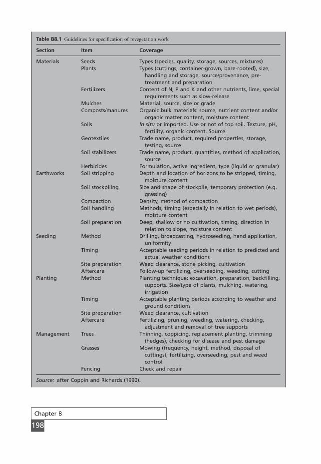
Chapter 8
198
Table B8.1 Guidelines for specification of revegetation work
Section Item Coverage
Materials Seeds Types (species, quality, storage, sources, mixtures)Plants Types (cuttings, container-grown, bare-rooted), size,
handling and storage, source/provenance, pre-treatment and preparation
Fertilizers Content of N, P and K and other nutrients, lime, special requirements such as slow-release
Mulches Material, source, size or gradeComposts/manures Organic bulk materials: source, nutrient content and/or
organic matter content, moisture content Soils In situ or imported. Use or not of top soil. Texture, pH,
fertility, organic content. Source.Geotextiles Trade name, product, required properties, storage,
testing, sourceSoil stabilizers Trade name, product, quantities, method of application,
sourceHerbicides Formulation, active ingredient, type (liquid or granular)
Earthworks Soil stripping Depth and location of horizons to be stripped, timing, moisture content
Soil stockpiling Size and shape of stockpile, temporary protection (e.g. grassing)
Compaction Density, method of compactionSoil handling Methods, timing (especially in relation to wet periods),
moisture contentSoil preparation Deep, shallow or no cultivation, timing, direction in
relation to slope, moisture contentSeeding Method Drilling, broadcasting, hydroseeding, hand application,
uniformityTiming Acceptable seeding periods in relation to predicted and
actual weather conditionsSite preparation Weed clearance, stone picking, cultivationAftercare Follow-up fertilizing, overseeding, weeding, cutting
Planting Method Planting technique: excavation, preparation, backfilling, supports. Size/type of plants, mulching, watering, irrigation
Timing Acceptable planting periods according to weather and ground conditions
Site preparation Weed clearance, cultivationAftercare Fertilizing, pruning, weeding, watering, checking,
adjustment and removal of tree supportsManagement Trees Thinning, coppicing, replacement planting, trimming
(hedges), checking for disease and pest damageGrasses Mowing (frequency, height, method, disposal of
cuttings); fertilizing, overseeding, pest and weed control
Fencing Check and repair
Source: after Coppin and Richards (1990).
MSE08 11/19/04 02:40 PM Page 198

Crop and vegetation management
199
� mixtures of species to create biodiversityand a more healthy plant community;
� mixtures of species with a range of estab-lishment rates, including rapidly establish-ing ‘pioneer’ species to colonize the areaand stabilize the surface and slower estab-
lishing species that will form the maturevegetation cover;
� the required pattern of plant succession,taking account of when particular specieswill establish and when they will die out.
Table B8.2 Desirable properties of plants for control of soil erosion by water
Plant component Required properties
Roots Vigorous development close to the surface to reinforce resistance to erosion, i.e. dense, shallow horizontal root structure
Shoots Dense uniform growth close to soil surface to impart roughness to flow and reduce its velocity; resistant to damage in high flows
Growth cycle Provision of sufficient shoot and root growth to protect the soil when erosion risk is greatest; may need to consider ability to protect the soil when heavy rain occurs after die-back at end of dry or cool season; ability to self-repair by rapid regrowth
Growth habit Uniform growth habit close to the ground to protect the soil from raindrop impact and stresses exerted by running water; avoid clumpy or tussocky species and species with canopies taller than 0.5m unless mixed with otherlow-growing species
Growth rate Rapid establishment, especially for ‘pioneer’ species; low maintenance
MSE08 11/19/04 02:40 PM Page 199
Chapter 9
200
The aim of sound soil management is to maintain the fertility and structure of the soil. Highlyfertile soils result in high crop yields, good plant cover and, therefore, in conditions that mini-mize the erosive effects of raindrops, runoff and wind. Soil fertility and the land husbandry tosupport it can therefore be seen as the key to soil conservation.
CHAPTER 9
Soilmanagement
9.1
Organic content
One way of achieving and maintaining a fertile soil is to apply organic matter. This improves thecohesiveness of the soil, increases its water retention capacity and promotes a stable aggregatestructure (section 3.2). Organic material may be added as green manures, straw or a manure thathas already undergone a high degree of fermentation. The effectiveness of the material varies withthe isohumic factor, which is the quantity of humus produced per unit of organic matter (Table9.1; Kolenbrander 1974). Green manures, which are normally leguminous crops ploughed in, havea high rate of fermentation and yield a rapid increase in soil stability. The increase is short-lived,however, because of a low isohumic factor. Straw decomposes less rapidly and so takes longer toaffect soil stability but has a higher isohumic factor. Previously fermented manures require stilllonger to influence soil stability but their effect is longer lasting because these have a still higherisohumic factor (Fournier 1972).
Ekwue et al. (1993) found that ploughing in groundnut haulm on a range of soil types innorthern Nigeria was more effective than cow dung in immediately reducing soil detachment byraindrop impact. Bonsu (1985) also found that cow dung was not fully effective in the savannaregions of West Africa because the extremely high temperatures bring about volatilization ofnitrogen and desiccation of the manure. It was better to combine cow dung with a straw mulchto increase the protection of the surface soil against erosion and enhance the moisture content ofthe soil. A combined application of cow dung at 5 t ha-1 and wheat straw mulch at 4 t ha-1 gavethe lowest soil loss and the highest yields of grain sorghum compared with a range of other prac-tices. The dung and mulch have to be applied every year because termites attack the straw duringthe dry season. Combined cow dung and maize straw mulch were similarly effective in reducingerosion in the humid tropical region of Ghana.
To increase the resistance of an erodible soil by building up organic matter is a lengthy process.Before any effect on stability is observed, the organic content must be raised above 2 per cent
MSE09 11/19/04 02:42 PM Page 200
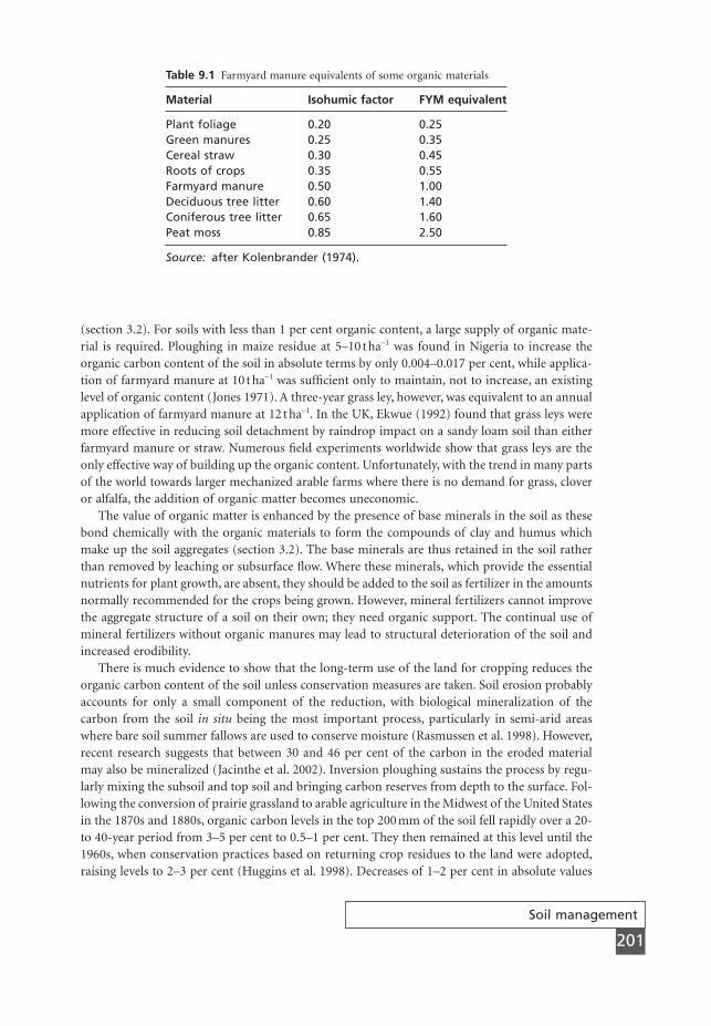
Soil management
201
(section 3.2). For soils with less than 1 per cent organic content, a large supply of organic mate-rial is required. Ploughing in maize residue at 5–10 t ha-1 was found in Nigeria to increase theorganic carbon content of the soil in absolute terms by only 0.004–0.017 per cent, while applica-tion of farmyard manure at 10 t ha-1 was sufficient only to maintain, not to increase, an existinglevel of organic content (Jones 1971). A three-year grass ley, however, was equivalent to an annualapplication of farmyard manure at 12 t ha-1. In the UK, Ekwue (1992) found that grass leys weremore effective in reducing soil detachment by raindrop impact on a sandy loam soil than eitherfarmyard manure or straw. Numerous field experiments worldwide show that grass leys are theonly effective way of building up the organic content. Unfortunately, with the trend in many partsof the world towards larger mechanized arable farms where there is no demand for grass, cloveror alfalfa, the addition of organic matter becomes uneconomic.
The value of organic matter is enhanced by the presence of base minerals in the soil as thesebond chemically with the organic materials to form the compounds of clay and humus whichmake up the soil aggregates (section 3.2). The base minerals are thus retained in the soil ratherthan removed by leaching or subsurface flow. Where these minerals, which provide the essentialnutrients for plant growth, are absent, they should be added to the soil as fertilizer in the amountsnormally recommended for the crops being grown. However, mineral fertilizers cannot improvethe aggregate structure of a soil on their own; they need organic support. The continual use ofmineral fertilizers without organic manures may lead to structural deterioration of the soil andincreased erodibility.
There is much evidence to show that the long-term use of the land for cropping reduces theorganic carbon content of the soil unless conservation measures are taken. Soil erosion probablyaccounts for only a small component of the reduction, with biological mineralization of thecarbon from the soil in situ being the most important process, particularly in semi-arid areaswhere bare soil summer fallows are used to conserve moisture (Rasmussen et al. 1998). However,recent research suggests that between 30 and 46 per cent of the carbon in the eroded materialmay also be mineralized (Jacinthe et al. 2002). Inversion ploughing sustains the process by regu-larly mixing the subsoil and top soil and bringing carbon reserves from depth to the surface. Fol-lowing the conversion of prairie grassland to arable agriculture in the Midwest of the United Statesin the 1870s and 1880s, organic carbon levels in the top 200 mm of the soil fell rapidly over a 20-to 40-year period from 3–5 per cent to 0.5–1 per cent. They then remained at this level until the1960s, when conservation practices based on returning crop residues to the land were adopted,raising levels to 2–3 per cent (Huggins et al. 1998). Decreases of 1–2 per cent in absolute values
Table 9.1 Farmyard manure equivalents of some organic materials
Material Isohumic factor FYM equivalent
Plant foliage 0.20 0.25Green manures 0.25 0.35Cereal straw 0.30 0.45Roots of crops 0.35 0.55Farmyard manure 0.50 1.00Deciduous tree litter 0.60 1.40Coniferous tree litter 0.65 1.60Peat moss 0.85 2.50
Source: after Kolenbrander (1974).
MSE09 11/19/04 02:42 PM Page 201
Chapter 9
202
of organic carbon occurred over 30–70 years after parts of the Great Plains of the USA and Canadawere brought into cultivation (Haas et al. 1957; Martel & Paul 1974).
As indicated in Chapter 1, in addition to the concern over the effects of carbon loss on thefertility of the soil, there is the recognition that the loss is a contributor to carbon dioxide in theatmosphere and may therefore play a part in any global warming (Flach et al. 1997). As a result,much research on soil management today is focused on the potential of using soils to sequestercarbon. Practices such as the elimination of bare fallows, the use of no tillage and return of cropresidues can bring about small increases in organic carbon in soils quite rapidly (Huggins et al.1998; Janzen et al. 1998; McConkey et al. 2003) but the effect is just as quickly lost should thepractices be discontinued. According to Lal (2002), the adoption of conservation tillage has thepotential to sequester carbon at rates of 500–800 kg ha-1 yr-1 in humid temperate areas, 300–500in arid temperate areas, 200–400 in the humid tropics and 100–200 in the arid tropics. Equiva-lent values obtained by the use of cover crops are 400–600, 200–400, 150–300 and 50–150 kgha-1 yr-1 respectively. By far the most effective method of carbon sequestration is to establish apermanent vegetation cover. Five years after establishing grass on a sandy loam soil formerly undercontinuous wheat-fallow cropping at Keeline, Wyoming, soil organic carbon levels in the top soilhad returned to those found on native rangelands (Reeder et al. 1998). A strategy of growing bio-energy crops on the surplus arable land in the United Kingdom would sequester carbon at anannual rate of 3.5 Tg, which is equivalent to 2.2 per cent of the country’s 1990 carbon emission(Smith et al. 2000). Establishing a vegetation cover on the estimated 250 million hectares ofseverely eroded land across the world has the potential to sequester carbon at annual rates of0.42–0.83 Pg (Lal 2002). The rate of sequestration peaks some 10–15 years after soil restorationand net accumulations are usually small after 25 to 30 years. Over this period, however, a com-bination of erosion control and restoration of degraded soils globally could sequester some 50–70 Pg C, which would provide some temporary mitigation to the greenhouse effect on worldclimates, while other policies on carbon emissions are put in place. However, without the inter-national political will to promote erosion control and also prevent the reversion of restored landto agricultural production, soil conservation as a basis for carbon sequestration can remain onlya potential.
9.2
Tillage practices
When managed so as to maintain their fertility, most soils retain their stability and are notadversely affected by standard tillage operations. Indeed, tillage is an essential management technique: it provides a suitable seed bed for plant growth and helps to control weeds. The tillage tools pulled by a tractor are designed to apply an upward force to cut and loosen the compacted soil, sometimes to invert it and mix it, and to smooth and shape its surface. When themoisture content of the soil is below the plastic limit (section 3.2), the soil fails by cracking, withthe soil aggregates sliding over each other but remaining unbroken. The soil ahead of the loos-ening tool moves forwards and upwards over the entire working depth. Soil loosening is effectivewhere the confining stresses resisting upward movement are less than those resisting sidewaysmovement of the soil. Vertical confining stress is obviously zero at the surface and increases withdepth until, at a critical depth, it equals the lateral confining stresses. Below this depth, the soilmoves only forwards and sideways and failure occurs, with a risk of compaction (Godwin & Spoor1977).
MSE09 11/19/04 02:42 PM Page 202
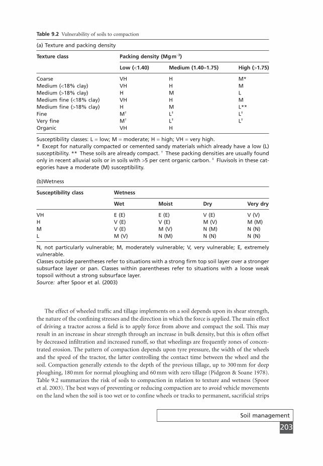
Soil management
203
The effect of wheeled traffic and tillage implements on a soil depends upon its shear strength,the nature of the confining stresses and the direction in which the force is applied. The main effectof driving a tractor across a field is to apply force from above and compact the soil. This mayresult in an increase in shear strength through an increase in bulk density, but this is often offsetby decreased infiltration and increased runoff, so that wheelings are frequently zones of concen-trated erosion. The pattern of compaction depends upon tyre pressure, the width of the wheelsand the speed of the tractor, the latter controlling the contact time between the wheel and thesoil. Compaction generally extends to the depth of the previous tillage, up to 300 mm for deepploughing, 180 mm for normal ploughing and 60 mm with zero tillage (Pidgeon & Soane 1978).Table 9.2 summarizes the risk of soils to compaction in relation to texture and wetness (Spoor et al. 2003). The best ways of preventing or reducing compaction are to avoid vehicle movementson the land when the soil is too wet or to confine wheels or tracks to permanent, sacrificial strips
Table 9.2 Vulnerability of soils to compaction
(a) Texture and packing density
Texture class Packing density (Mgm-3)
Low (<1.40) Medium (1.40–1.75) High (>1.75)
Coarse VH H M*Medium (<18% clay) VH H MMedium (>18% clay) H M LMedium fine (<18% clay) VH H MMedium fine (>18% clay) H M L**Fine M† L‡ L‡
Very fine M† L‡ L‡
Organic VH H
Susceptibility classes: L = low; M = moderate; H = high; VH = very high.* Except for naturally compacted or cemented sandy materials which already have a low (L)susceptibility. ** These soils are already compact. † These packing densities are usually foundonly in recent alluvial soils or in soils with >5 per cent organic carbon. ‡ Fluvisols in these cat-egories have a moderate (M) susceptibility.
(b)Wetness
Susceptibility class Wetness
Wet Moist Dry Very dry
VH E (E) E (E) V (E) V (V)H V (E) V (E) M (V) M (M)M V (E) M (V) N (M) N (N)L M (V) N (M) N (N) N (N)
N, not particularly vulnerable; M, moderately vulnerable; V, very vulnerable; E, extremely vulnerable.Classes outside parentheses refer to situations with a strong firm top soil layer over a strongersubsurface layer or pan. Classes within parentheses refer to situations with a loose weaktopsoil without a strong subsurface layer.Source: after Spoor et al. (2003)
MSE09 11/19/04 02:42 PM Page 203
across a field (Chamen et al. 2003). Since plough pans help to protect a soil from compaction,they should only be broken up where they significantly impede root development, aeration ordrainage (Spoor et al. 2003).
9.2.1 Conventional tillage
Over the years a reasonably standard or conventional system of tillage, involving ploughing, sec-ondary cultivation, with one or more disc harrowings, and planting has been found suitable fora wide range of soils. Ploughing is carried out with the mouldboard plough, although, on stonyland or with soils that do not fall cleanly off mouldboards, the disc plough is often used. Mould-board ploughs invert the plough furrow and lift and move all the soil in the plough layer, usuallyto a depth of 100–200 mm. Secondary cultivation to form the seed bed and remove weeds iscarried out by either disc or tine cultivators. With disc cultivators the soil is broken up by thepassage of saucer-shaped metal discs mounted on axles. The most common tine cultivator is thechisel type, which consists of a series of metal blades mounted on a frame. The blades vary inwidth from narrow, 50 mm, to wide, 75 mm, but can be up to 300 mm wide. Ploughing producesa rough cloddy surface with local variations in height of 120–160 mm. Secondary cultivationreduces the roughness to 30–40 mm, while drilling and rolling decrease it still further (section2.1; Table 2.2). Roughness is also reduced over time by raindrop impact and water and winderosion. Soil loss (SL) by water erosion decreases with increasing roughness (R) according to therelationship (Cogo et al. 1984):
(9.1)
which means that small increases in roughness from a virtually smooth surface can have sub-stantial effects on reducing erosion but much larger increases will be needed to have the sameeffect with an already rough surface. Tillage can often be used successfully to roughen the surfaceto control wind erosion in an emergency, using a chisel to produce ridges and furrows across thepath of the prevailing wind (Woodruff et al. 1957). Ridging was found to decrease wind erosionby between 15 and 26 per cent in experiments carried out in Niger (Bielders et al. 1998).
9.2.2 Contour tillage
Carrying out ploughing, planting and cultivation on the contour can reduce soil loss from slopingland compared with cultivation up-and-down the slope. The effectiveness of contour tillage varieswith the length and steepness of the slope. It is inadequate as the sole conservation measures forlengths greater than 180 m at 1° steepness. The allowable length declines with increasing steep-ness to 30 m at 5.5° and 20 m at 8.5°. Moreover, the technique is only effective during storms oflow rainfall intensity. Protection against more extreme storms is improved by supplementingcontour farming with strip cropping (section 8.3).
On silty and fine sandy soils, erosion may be further reduced by storing water on the surfacerather than allowing it to run off. Limited increases in storage capacity can be obtained by formingridges, usually at a slight grade of about 1 : 400 to the contour, at regular intervals determined byslope steepness. Contour ridging is generally ineffective on its own as a soil conservation measureon slopes steeper than 4.5°. Greater storage of water and more effective erosion control can beachieved by connecting the ridges with cross-ties over the intervening furrows, thereby forminga series of rectangular depressions that fill with water during rain. Because crop damage can occurif the water cannot soak into the soil within 48 h, this practice, known as tied ridging, should only
SL e Rµ -0 5.
Chapter 9
204
MSE09 11/19/04 02:42 PM Page 204
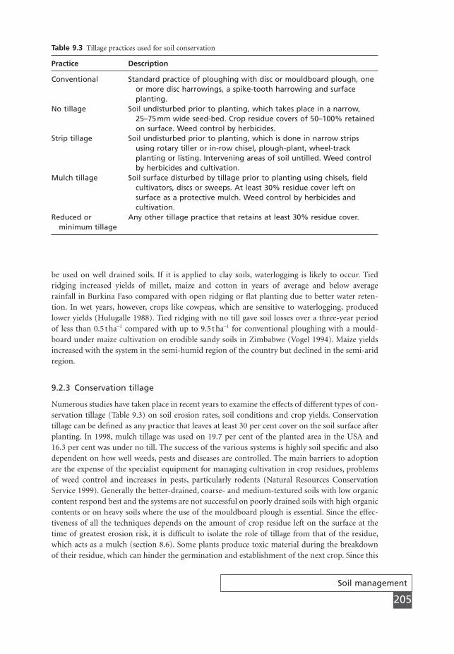
Soil management
205
be used on well drained soils. If it is applied to clay soils, waterlogging is likely to occur. Tiedridging increased yields of millet, maize and cotton in years of average and below average rainfall in Burkina Faso compared with open ridging or flat planting due to better water reten-tion. In wet years, however, crops like cowpeas, which are sensitive to waterlogging, producedlower yields (Hulugalle 1988). Tied ridging with no till gave soil losses over a three-year periodof less than 0.5 t ha-1 compared with up to 9.5 t ha-1 for conventional ploughing with a mould-board under maize cultivation on erodible sandy soils in Zimbabwe (Vogel 1994). Maize yieldsincreased with the system in the semi-humid region of the country but declined in the semi-aridregion.
9.2.3 Conservation tillage
Numerous studies have taken place in recent years to examine the effects of different types of con-servation tillage (Table 9.3) on soil erosion rates, soil conditions and crop yields. Conservationtillage can be defined as any practice that leaves at least 30 per cent cover on the soil surface afterplanting. In 1998, mulch tillage was used on 19.7 per cent of the planted area in the USA and16.3 per cent was under no till. The success of the various systems is highly soil specific and alsodependent on how well weeds, pests and diseases are controlled. The main barriers to adoptionare the expense of the specialist equipment for managing cultivation in crop residues, problemsof weed control and increases in pests, particularly rodents (Natural Resources ConservationService 1999). Generally the better-drained, coarse- and medium-textured soils with low organiccontent respond best and the systems are not successful on poorly drained soils with high organiccontents or on heavy soils where the use of the mouldboard plough is essential. Since the effec-tiveness of all the techniques depends on the amount of crop residue left on the surface at thetime of greatest erosion risk, it is difficult to isolate the role of tillage from that of the residue,which acts as a mulch (section 8.6). Some plants produce toxic material during the breakdownof their residue, which can hinder the germination and establishment of the next crop. Since this
Table 9.3 Tillage practices used for soil conservation
Practice Description
Conventional Standard practice of ploughing with disc or mouldboard plough, oneor more disc harrowings, a spike-tooth harrowing and surfaceplanting.
No tillage Soil undisturbed prior to planting, which takes place in a narrow,25–75mm wide seed-bed. Crop residue covers of 50–100% retainedon surface. Weed control by herbicides.
Strip tillage Soil undisturbed prior to planting, which is done in narrow stripsusing rotary tiller or in-row chisel, plough-plant, wheel-trackplanting or listing. Intervening areas of soil untilled. Weed controlby herbicides and cultivation.
Mulch tillage Soil surface disturbed by tillage prior to planting using chisels, fieldcultivators, discs or sweeps. At least 30% residue cover left onsurface as a protective mulch. Weed control by herbicides andcultivation.
Reduced or Any other tillage practice that retains at least 30% residue cover.minimum tillage
MSE09 11/19/04 02:42 PM Page 205
is a particular problem in monocultures of maize and wheat, conservation tillage is also depen-dent on the use of crop rotations.
No tillage
No tillage describes the system whereby tillage is restricted to that necessary for planting the seed. Drilling takes place directly into the stubble of the previous crop and weeds are controlledby herbicides. Generally between 50 and 100 per cent of the surface remains covered with residue.The technique has been found to increase the percentage of water-stable aggregates in the soilcompared to tine or disc cultivation and ploughing (Aina 1979; Douglas & Goss 1982; Schjøn-ning & Rasmussen 1989; Suwardji & Eberbach 1998; Mrabet et al. 2001). It is not suitable,however, on soils that compact and easily seal because it can lead to lower crop yields and greaterrunoff.
No tillage reduced erosion rates under maize (Bonsu & Obeng 1979) and millet (Bonsu 1981)in Ghana to levels comparable with those achieved by multiple cropping but generally not to thelevels obtained with surface mulching. Moreover, no tillage was not always effective in the firstyear of its operation because of the low percentage crop residues on the surface. At Ibadan,Nigeria, the technique reduced annual soil loss under maize with two crops per year to 0.07 t ha-1, compared with 56 t ha-1 for hoe and cutlass, 8.3 t ha-1 for a mouldboard plough and 9.1 t ha-1 for a mouldboard plough followed by harrowing (Osuji et al. 1980).
No tillage is viewed as the leading technology to control erosion on crop-livestock farms inthe Midwest of the USA based on pig production and the growing of maize, soya bean and wheatin rotation. In a review of various studies of tillage systems, Moldenhauer (1985) showed thatannual soil loss under no till on a range of erodible soils in the Corn Belt was 5–15 per cent ofthat from conventional tillage. No till is also recommended on the ultisol soils of the SouthernPiedmont of the USA, which have become severely eroded after 150 years of continuous crop-ping. As alternatives to the conventional system of growing soya bean with a bare fallow overwinter, the following no tillage systems were studied: soya bean with wheat as a winter cover andusing in-row chisel tillage; soya bean with barley as a winter cover and using fluted coulters; andsoya bean with rye as a green manure and using fluted coulters. The respective mean annual soillosses for the four systems are 26.2, 0.1, 0.1 and 3.4 t ha-1 (Langdale et al. 1992). The use of notillage on silty, crust-prone soils in northern France reduced erosion over two years (1993–4) to0.04 t ha-1 from 0.18 t ha-1 with conventional tillage using a mouldboard plough, but increasedrunoff from 3.2 to 6.1 mm (Martin 1999), resulting in greater risk of erosion and flooding furtherdownslope. There is some evidence, however, to suggest that such an adverse effect might be short-lived. After 16 years of no tillage, the saturated hydraulic conductivity of the surface layer of OxicPaleustalf soils under winter wheat in the Wagga Wagga region of New South Wales was higherthan that under conventional cultivation, an effect attributed to greater biological activity as wit-nessed by the greater earthworm population (Suwardji & Eberbach 1998). Increased earthwormnumbers were also a feature of long-term no tillage on soils ranging from sands to silt loams inGermany (Tebrügge & Düring 1999).
Strip tillage
With strip tillage, the soil is prepared for planting along narrow strips, with the intervening areasleft undisturbed. Typically, up to one-third of the soil is tilled in a single plough–plant operation.When used for maize cultivation on research plots of the University of Science and Technology,Kumasi, Ghana, the technique reduced soil loss from 23 storms totalling 452 mm of rain to
Chapter 9
206
MSE09 11/19/04 02:42 PM Page 206
Soil management
207
0.2 t ha-1 compared with 0.9 t ha-1 with a plough–harrow–plant sequence and 1.4 t ha-1 with tra-ditional tillage using a hoe and cutlass (Baffoe-Bonnie & Quansah 1975). The plough–plantsystem caused least soil compaction, conserved most soil moisture and reduced losses of organicmatter, nitrogen, phosphorus and potassium (Quansah & Baffoe-Bonnie 1981). Plough–plantsystems have not become popular, however, because of problems of weed control and the slowspeed of planting.
Mulch tillage
Difficulties with weed control, operating with large amounts of residue and, in many cases, loweryields have prevented the widespread take-up of stubble-mulch tillage. When tested to reducewater erosion on vertisols in Australia under continuous wheat production, the technique failedto increase the aggregate stability of the soil compared with conventional tillage (Marston & Hird1978) and did not reduce erosion to an acceptable level (Marston & Perrens 1981). Nevertheless,the system has be used successfully to control wind erosion and conserve moisture in drier wheat-growing areas (Fenster & McCalla 1970).
Minimum tillage
Minimum tillage or reduced tillage refers to practices using chiselling or discing to prepare thesoil whilst retaining a 15–25 per cent residue cover. With one disc cultivation prior to plantingon a silty clay soil under continuous wheat production near Pisa, Italy, runoff was increased overthat from conventional tillage. The minimum tilled plots retained moisture and this, in turn,reduced the cracking which plays a major role in promoting high infiltration of water in thesesoils. Despite the higher runoff, annual soil loss was lower under minimum tillage, at 1.6 t ha-1
compared with 4.1 t ha-1 from conventional tillage (Chisci & Zanchi 1981).Chiselling in the autumn to produce a rough surface but retain residue cover, followed by disc
cultivation in the spring to smooth the seed bed and cover the residue, is now widely practisedin maize–soya bean agriculture in the Corn Belt of the USA. It can reduce soil loss by an orderof magnitude over that recorded from conventional tillage (Siemens & Oschwald 1978; Johnson& Moldenhauer 1979). The technique works well when soya bean is planted in the chiselled maizeresidue but is not satisfactory when maize is planted in the chiselled soya bean residue becausethe latter deteriorates very rapidly and by the following spring there is insufficient cover to protectthe soil. Alternative practices for this year of the rotation include growing a winter cover crop, killing it in the spring with a contact herbicide and planting maize in the residue of thecover, or planting maize with no tillage in order to minimize disturbance of the soil. After some20 years of reduced tillage on loess soils in Germany, soil organic carbon was 5 Mg ha-1 higherthan on similar conventionally tilled soils but the technique was found to create problems forfarmers, with the accumulation of crop residues on the surface and infestations of weeds,fungal diseases and pests. Short-term inversion ploughing can be used to ameliorate these prob-lems but its effects are so dramatic that only one year of conventional tillage is sufficient to removeall the benefits of reduced tillage with respect to carbon and organic matter (Stockfisch et al.1999).
As with no tillage, there is concern that by not breaking up the soil, the technique will lead toa less porous surface with a resulting increase in runoff and erosion (Soane & Pidgeon 1975).However, Voorhees and Lindstrom (1984) found that on a silty clay loam, there was no differencein the porosity of the soil to 150 mm depth between no tillage and conventional tillage after fouryears and no difference to a depth of 300 mm after seven years. Kemper and Derpsch (1981)
MSE09 11/19/04 02:42 PM Page 207
Chapter 9
208
suggest that no tillage can be effective in restoring the porosity of oxisols and alfisols where it hasbeen reduced by the development of a plough pan but that it will take ten to twelve years.
9.2.4 Alternatives to conservation tillage
An alternative approach to conservation tillage is to attempt, through careful timing of opera-tions in relation to soil conditions, to use tillage to produce an erosion-resistant surface. Severalfarmers on sandy loam soils in the Midlands of England have adopted the Glassford system ofploughing and pressing the soil to produce a cloddy surface to control wind erosion on landdevoted to sugar beet. When the soil is moist but not wet, a chisel is used to break up the crustand produce ridges and furrows at right angles to the direction of erosive winds. The land in thefurrows is then rolled either in the same operation, by modifying the chisel plough to incorpo-rate a roll press, or as soon as possible in a second operation before the soil dries out. This tillageis preferably carried out in January and the resulting surface of micro hills and valleys remainsstable throughout the spring blowing period even after it has been broken up by drilling, whichis carried out transverse to the press ridges. The Glassford system can thus be practised with stan-dard farm equipment.
Conservation tillage has not proved appropriate for the management of the vertisols. Thesesoils have a high percentage of smectitic clays, which undergo pronounced shrinking when dry,resulting in deep cracks that close only after prolonged wetting. In India, there is a problem ofhow to prepare a good seed bed on these soils, since sowing has to be carried out in the hard drysoil in advance of the rains in order to obtain a good crop cover to protect the soil from erosionin the rainy season. Experiments by ICRISAT showed that by preparing a surface of broad-basedbeds (950 mm wide) and furrows (550 mm wide and graded at 1 : 150) as soon in the rainy seasonas the soil becomes workable, annual soil loss was reduced over a six-year period to 1.2 t ha-1 com-pared with 6.6 t ha-1 with conventional tillage practice (Pathak et al. 1985). Steeper furrow gradesresulted in too much erosion, while gentler grades did not provide sufficient drainage under wetconditions (Kampen et al. 1981). With better moisture control due to surface drainage along thefurrows, crop yields were also increased (El-Swaify et al. 1985). However, the take-up of the tech-nique by farmers is limited because of the need for specialized and costly equipment, namely awheeled tool bar to make the raised bed, and increased labour requirements.
Subsoiling is used to break up impermeable soil layers, such as plough pans, at depth, although,as seen above (Spoor et al. 2003), this should only be done when the pan has an adverse effect ondrainage and crop yield. Deep tillage using a crawler tractor to pull two chisels through groundto open up furrows about 100 mm wide and 500–700 mm deep is a recommended practice tobreak up subsurface pipes and tunnels (Colclough 1965; Crouch 1978). This treatment aids theestablishment of grasses, forbs and legumes and is therefore carried out prior to reseeding theland for pasture. Control of tunnel erosion (section 2.6.1) is dependent upon the success ofthe revegetation in achieving a uniform pattern of infiltration because the effects of the rippingdecline after three to five years (Aldon 1976).
9.3
Drainage
Drainage is used as a soil conservation measure to reduce runoff and therefore erosion on heavyclay soils. Heavy sticky soils with a moisture content above the plastic limit are difficult to manage
MSE09 11/19/04 02:42 PM Page 208
Soil management
209
because they fail compressively during tillage and become smeared (Spoor & Godwin 1979).Erodible soils with more than 20 per cent clay content will benefit from the installation of moledrains and from the break-up of compacted layers at depth by subsoiling. Pipe drainage was foundto be very effective in reducing erosion on clay soils derived from Pliocene marine sediments incentral Italy (Chisci et al. 1978; Zanchi 1989). However, subsurface drains can be importantsources of sediment. On marine clay soils in southern Norway, the suspended sediment concen-trations prior to autumn ploughing range from 0.13 to 0.15 g l-1 in drainage waters and 2.7 to 3.2 g l-1 in surface runoff; after ploughing, the respective values are 3.8–4.3 and 2.2–2.9 g l-1. Inyears with no tillage, concentrations in drainage water never exceed 0.8 g l-1 (Øygarden 1995).
9.4
Soil stabilizers
Improvements in soil structure can be achieved by applying soil conditioners. These may take theform of organic by-products, polyvalent salts and various synthetic polymers. Polyvalent saltssuch as gypsum bring about flocculation of the clay particles, while organic by-products and syn-thetic polymers bind the soil particles into aggregates. Although soil stabilizers are too expensivefor general agricultural use, where the cost is warranted they are helpful on special sites like sanddunes, road cuttings, embankments and stream banks, to provide temporary stability prior to theestablishment of a plant cover.
Gypsum has been used successfully to improve the structure of sodic soils in southeast Aus-tralia (Davidson & Quirk 1961; Rosewell 1970). These soils are particularly susceptible to tunnelerosion. Their high sodium content results in the dispersal of clay minerals when in contact withwater, with consequent structural deterioration. The most effective treatment is to apply gypsumas a cation to replace the sodium. A good drainage system is also necessary to wash out the sodiumfrom the soil. The treatment is extremely expensive over large areas and, unless accompanied byripping to break up the tunnels and the sowing of grass, gives only temporary relief. Gypsum hasalso been used to reduce surface crusting and runoff on red-brown earths in the wheat-growingregion of South Australia where the soils are unstable because of high contents of exchangeablemagnesium (Grierson 1978).
Soil conditioners fall into two groups, those that render the soil hydrophobic and thereforedecrease infiltration and increase runoff, and those that make the soil hydrophilic, increase infil-tration and decrease runoff. Hydrophobic conditioners based on bitumen are generally effectivein controlling erosion for only a few storms and are not always suitable for soil conservation purposes. They can, however, be employed to increase water yield; for example, to supply farmponds (Laing 1978). Asphalt and latex emulsions seal the surface, thereby increasing runoff,but they are effective in stabilizing the soil and preventing erosion until the seal is broken. Whenapplied to agricultural soils, for example, subsequent discing to a depth of 200 mm can partiallydestroy the seal and promote aggregate destruction (Gabriels & De Boodt 1978). This problemcan be alleviated to some extent by incorporating the emulsion in the top 100–200 mm of the soil (Gabriels et al. 1977). The critical factor in this case is the size of the aggregates that are produced: if they are too small, infiltration rates remain low. For effective infiltration withhydrophobic conditioners, the aggregates should be at least 2 mm in size and ideally larger than5 mm (Pla 1977).
Experience with polyacrylamide conditioners that are hydrophilic shows that high infiltrationrates can be obtained regardless of aggregate size. Small plot studies with rainfall simulation
MSE09 11/19/04 02:42 PM Page 209
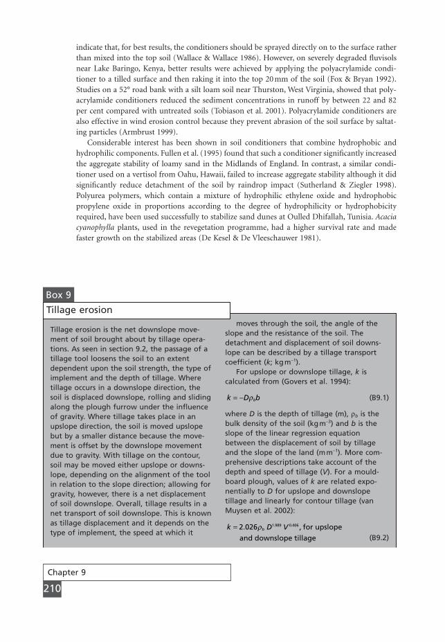
Chapter 9
210
indicate that, for best results, the conditioners should be sprayed directly on to the surface ratherthan mixed into the top soil (Wallace & Wallace 1986). However, on severely degraded fluvisolsnear Lake Baringo, Kenya, better results were achieved by applying the polyacrylamide condi-tioner to a tilled surface and then raking it into the top 20 mm of the soil (Fox & Bryan 1992).Studies on a 52° road bank with a silt loam soil near Thurston, West Virginia, showed that poly-acrylamide conditioners reduced the sediment concentrations in runoff by between 22 and 82per cent compared with untreated soils (Tobiason et al. 2001). Polyacrylamide conditioners arealso effective in wind erosion control because they prevent abrasion of the soil surface by saltat-ing particles (Armbrust 1999).
Considerable interest has been shown in soil conditioners that combine hydrophobic andhydrophilic components. Fullen et al. (1995) found that such a conditioner significantly increasedthe aggregate stability of loamy sand in the Midlands of England. In contrast, a similar condi-tioner used on a vertisol from Oahu, Hawaii, failed to increase aggregate stability although it didsignificantly reduce detachment of the soil by raindrop impact (Sutherland & Ziegler 1998).Polyurea polymers, which contain a mixture of hydrophilic ethylene oxide and hydrophobicpropylene oxide in proportions according to the degree of hydrophilicity or hydrophobicityrequired, have been used successfully to stabilize sand dunes at Oulled Dhifallah, Tunisia. Acaciacyanophylla plants, used in the revegetation programme, had a higher survival rate and madefaster growth on the stabilized areas (De Kesel & De Vleeschauwer 1981).
Tillage erosion is the net downslope move-ment of soil brought about by tillage opera-tions. As seen in section 9.2, the passage of atillage tool loosens the soil to an extentdependent upon the soil strength, the type ofimplement and the depth of tillage. Wheretillage occurs in a downslope direction, thesoil is displaced downslope, rolling and slidingalong the plough furrow under the influenceof gravity. Where tillage takes place in anupslope direction, the soil is moved upslopebut by a smaller distance because the move-ment is offset by the downslope movementdue to gravity. With tillage on the contour,soil may be moved either upslope or downs-lope, depending on the alignment of the toolin relation to the slope direction; allowing forgravity, however, there is a net displacementof soil downslope. Overall, tillage results in anet transport of soil downslope. This is knownas tillage displacement and it depends on thetype of implement, the speed at which it
Box 9
moves through the soil, the angle of theslope and the resistance of the soil. Thedetachment and displacement of soil downs-lope can be described by a tillage transportcoefficient (k; kgm-1).
For upslope or downslope tillage, k iscalculated from (Govers et al. 1994):
(B9.1)
where D is the depth of tillage (m), rb is thebulk density of the soil (kgm-3) and b is theslope of the linear regression equationbetween the displacement of soil by tillageand the slope of the land (mm-1). More com-prehensive descriptions take account of thedepth and speed of tillage (V). For a mould-board plough, values of k are related expo-nentially to D for upslope and downslopetillage and linearly for contour tillage (vanMuysen et al. 2002):
(B9.2)k D Vb= 2 026 1 989 0 406. ,. .r for upslope
and downslope tillage
k D bb= - r
Tillage erosion
MSE09 11/19/04 02:42 PM Page 210
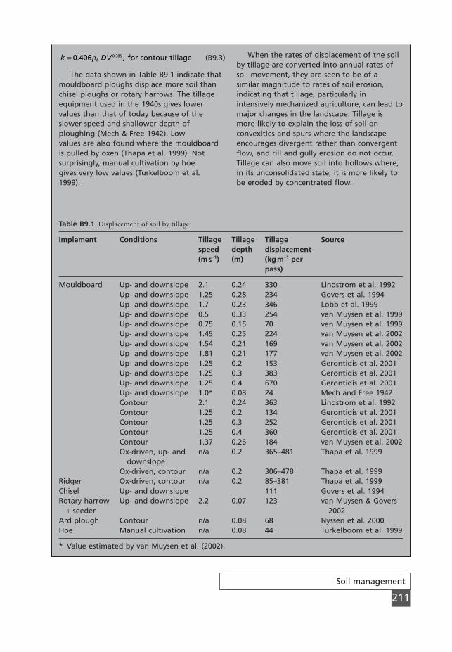
Soil management
211
(B9.3)
The data shown in Table B9.1 indicate thatmouldboard ploughs displace more soil thanchisel ploughs or rotary harrows. The tillageequipment used in the 1940s gives lowervalues than that of today because of theslower speed and shallower depth ofploughing (Mech & Free 1942). Low values are also found where the mouldboardis pulled by oxen (Thapa et al. 1999). Notsurprisingly, manual cultivation by hoe gives very low values (Turkelboom et al. 1999).
k DVb= 0 406 0 385. ,.r for contour tillage When the rates of displacement of the soilby tillage are converted into annual rates ofsoil movement, they are seen to be of asimilar magnitude to rates of soil erosion,indicating that tillage, particularly inintensively mechanized agriculture, can lead tomajor changes in the landscape. Tillage ismore likely to explain the loss of soil onconvexities and spurs where the landscapeencourages divergent rather than convergentflow, and rill and gully erosion do not occur.Tillage can also move soil into hollows where,in its unconsolidated state, it is more likely tobe eroded by concentrated flow.
Table B9.1 Displacement of soil by tillage
Implement Conditions Tillage Tillage Tillage Sourcespeed depth displacement(ms-1) (m) (kgm-1 per
pass)
Mouldboard Up- and downslope 2.1 0.24 330 Lindstrom et al. 1992Up- and downslope 1.25 0.28 234 Govers et al. 1994Up- and downslope 1.7 0.23 346 Lobb et al. 1999Up- and downslope 0.5 0.33 254 van Muysen et al. 1999Up- and downslope 0.75 0.15 70 van Muysen et al. 1999Up- and downslope 1.45 0.25 224 van Muysen et al. 2002Up- and downslope 1.54 0.21 169 van Muysen et al. 2002Up- and downslope 1.81 0.21 177 van Muysen et al. 2002Up- and downslope 1.25 0.2 153 Gerontidis et al. 2001Up- and downslope 1.25 0.3 383 Gerontidis et al. 2001Up- and downslope 1.25 0.4 670 Gerontidis et al. 2001Up- and downslope 1.0* 0.08 24 Mech and Free 1942Contour 2.1 0.24 363 Lindstrom et al. 1992Contour 1.25 0.2 134 Gerontidis et al. 2001Contour 1.25 0.3 252 Gerontidis et al. 2001Contour 1.25 0.4 360 Gerontidis et al. 2001Contour 1.37 0.26 184 van Muysen et al. 2002Ox-driven, up- and n/a 0.2 365–481 Thapa et al. 1999
downslopeOx-driven, contour n/a 0.2 306–478 Thapa et al. 1999
Ridger Ox-driven, contour n/a 0.2 85–381 Thapa et al. 1999Chisel Up- and downslope 111 Govers et al. 1994Rotary harrow Up- and downslope 2.2 0.07 123 van Muysen & Govers
+ seeder 2002Ard plough Contour n/a 0.08 68 Nyssen et al. 2000Hoe Manual cultivation n/a 0.08 44 Turkelboom et al. 1999
* Value estimated by van Muysen et al. (2002).
MSE09 11/19/04 02:42 PM Page 211
Chapter 10
212
Mechanical field practices are used to control the movement of water and wind over the soilsurface. A range of techniques is available and the decision on which to adopt depends on whetherthe objective is to reduce the velocity of runoff and wind, increase the surface water storage capacity or safely dispose of excess water. Mechanical methods are normally employed to supportagronomic measures and soil management.
CHAPTER 10
Mechanicalmethods oferosion control
10.1
Contour bunds
Contour bunds are earth banks, 1.5–2 m wide, thrown across the slope to act as a barrier to runoff,to form a water storage area on their upslope side and to break up a slope into segments shorterin length than is required to generate overland flow. They are suitable for slopes of 1–7° and arefrequently used on smallholdings in the tropics where they form permanent buffers in a strip-cropping system, being planted with grasses or trees. The banks, spaced at 10–20 m intervals, aregenerally hand-constructed. There are no precise specifications for their design and deviations intheir alignment of up to 10 per cent from the contour are permissible. In Wallo Province, Ethiopia,Hurni (1984) found that earth bunds were only effective on slopes up to 6°. An alternative tech-nique on stony soils is to construct stone bunds, 250–300 mm high, set in a shallow trench on thecontour. In order to enhance their ability to filter runoff and trap sediment, smaller stones shouldbe placed on the upslope side and, if possible, gravels upslope of them (Hudson 1987). On steeplysloping land with erodible andosol soils devoted to potatoes and forage oats near Cochabamba,Bolivia, annual erosion from fields with stone bunds ranged from 38 to 124 t ha-1 compared with118 to 164 t ha-1 on land without (Clark et al. 1999).
10.2
Terraces
Terraces are earth embankments constructed across the slope to intercept surface runoff, conveyit to a stable outlet at a non-erosive velocity and shorten slope length. They thus perform similarfunctions to contour bunds. They differ from them by being designed to more stringent specifi-
MSE10 11/19/04 02:43 PM Page 212
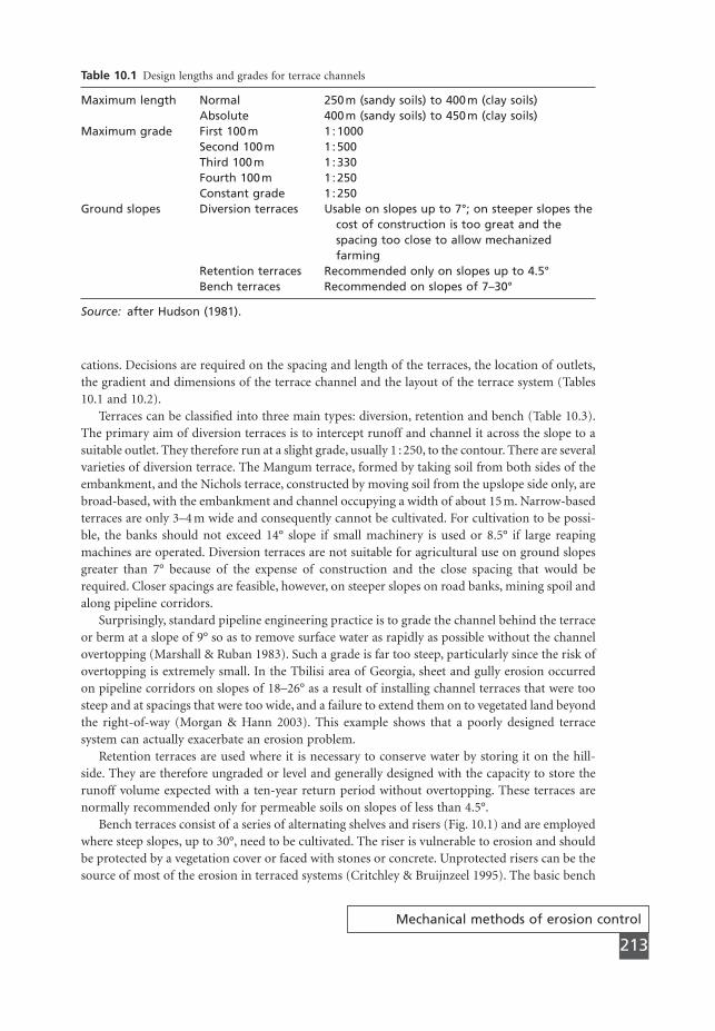
Mechanical methods of erosion control
213
cations. Decisions are required on the spacing and length of the terraces, the location of outlets,the gradient and dimensions of the terrace channel and the layout of the terrace system (Tables10.1 and 10.2).
Terraces can be classified into three main types: diversion, retention and bench (Table 10.3).The primary aim of diversion terraces is to intercept runoff and channel it across the slope to asuitable outlet. They therefore run at a slight grade, usually 1 : 250, to the contour. There are severalvarieties of diversion terrace. The Mangum terrace, formed by taking soil from both sides of theembankment, and the Nichols terrace, constructed by moving soil from the upslope side only, arebroad-based, with the embankment and channel occupying a width of about 15 m. Narrow-basedterraces are only 3–4 m wide and consequently cannot be cultivated. For cultivation to be possi-ble, the banks should not exceed 14° slope if small machinery is used or 8.5° if large reapingmachines are operated. Diversion terraces are not suitable for agricultural use on ground slopesgreater than 7° because of the expense of construction and the close spacing that would berequired. Closer spacings are feasible, however, on steeper slopes on road banks, mining spoil andalong pipeline corridors.
Surprisingly, standard pipeline engineering practice is to grade the channel behind the terraceor berm at a slope of 9° so as to remove surface water as rapidly as possible without the channelovertopping (Marshall & Ruban 1983). Such a grade is far too steep, particularly since the risk ofovertopping is extremely small. In the Tbilisi area of Georgia, sheet and gully erosion occurredon pipeline corridors on slopes of 18–26° as a result of installing channel terraces that were toosteep and at spacings that were too wide, and a failure to extend them on to vegetated land beyondthe right-of-way (Morgan & Hann 2003). This example shows that a poorly designed terracesystem can actually exacerbate an erosion problem.
Retention terraces are used where it is necessary to conserve water by storing it on the hill-side. They are therefore ungraded or level and generally designed with the capacity to store therunoff volume expected with a ten-year return period without overtopping. These terraces arenormally recommended only for permeable soils on slopes of less than 4.5°.
Bench terraces consist of a series of alternating shelves and risers (Fig. 10.1) and are employedwhere steep slopes, up to 30°, need to be cultivated. The riser is vulnerable to erosion and shouldbe protected by a vegetation cover or faced with stones or concrete. Unprotected risers can be thesource of most of the erosion in terraced systems (Critchley & Bruijnzeel 1995). The basic bench
Table 10.1 Design lengths and grades for terrace channels
Maximum length Normal 250m (sandy soils) to 400m (clay soils)Absolute 400m (sandy soils) to 450m (clay soils)
Maximum grade First 100m 1:1000Second 100m 1:500Third 100m 1:330Fourth 100m 1:250Constant grade 1:250
Ground slopes Diversion terraces Usable on slopes up to 7°; on steeper slopes the cost of construction is too great and the spacing too close to allow mechanized farming
Retention terraces Recommended only on slopes up to 4.5°Bench terraces Recommended on slopes of 7–30°
Source: after Hudson (1981).
MSE10 11/19/04 02:43 PM Page 213

Table 10.2 Formulae for determining spacing of terraces
ApproachMany formulae have been developed for determining the difference in height betweentwo successive terraces; this difference in height is known as the vertical interval (VI).
Theoretical or analytical formulaeFor steady state conditions, the runoff (Q) at slope length (x) on a hillside can be expressedas:
Q = (R - i) x cosq
where R is the rainfall intensity, i is the infiltration capacity of the soil and q is the slopeangle.
From the Manning equation of flow velocity:
The hydraulic radius (r) is expressed by:
Therefore:
Rearranging for given values of R and i, say those for the 1-hour rainfall with a 10-yearreturn period, and for a preselected value of v, say the maximum permissible velocity forthe soil (vc; Table 10.6), gives a slope distance xcrit, which can be used as the distancebetween the terraces downslope:
A value of n = 0.01 is recommended for bare soil.For example, if the peak rainfall excess (R - i) on a sandy loam soil is 0.2mms-1, and theselected value for vc is 0.75ms-1, then for a slope of 3°:
A similar approach was used by Mirtskhoulava (2001) to produce the formula:
xv
R i m s ncrit
c
. .=
-( )0 000034 3 32
2 32 1 16
. .
x
x
VI x sin
crit
crit
crit
= ¥¥ ¥
== =
0 75 0 200 0002 0 1904 0 9886
22 55
1 18
5 2 3 2. .. . .
.
.
m
mq
xv n
R i sin coscrit
c=-( )
5 2 3 2
3 4q q
R i x cosvn
sinsin
n-( ) = Ê
ˈ¯
È
ÎÍ
˘
˚˙q
1 2
3 2 5 31 2
rvn
sin= Ê
ˈ¯1 2
3 2
q
Q R i x cosr sin
n= -( ) =q q5 3 1 2
MSE10 11/19/04 02:43 PM Page 214

Table 10.2 Continued
where m is a coefficient describing the roughness related to the soil particles (m = 1.0 forsilts, 1.1 for sands and sandy loams, 1.3 for loamy sands and clay loams and 1.5 for clays),and s = slope (mm-1). This method tends to give wider terrace spacings on low-angledslopes and closer spacings on steep slopes. When the two methods were applied to thedesign of diverter berm spacings on pipeline rights-of-way near Tbilisi, Georgia, they gavevery similar results over slopes ranging from 19 to 26° (Morgan et al. 2003).
Empirical formulae
Ramser method where a = 3 or 4, depending onthe severity of erosion
United States Soil VI(m) = aS + b where a varies from 0.12 in theConservation Service south to 0.24 in the north of
the USA and b varies between 0.3 and 1.2 according to theerodibility of the soil
Zimbabwe where f varies from 3 to 6according to the erodibility ofthe soil
South Africa where a varies from 1.5 for lowrainfall areas to 4 for highrainfall areas and b varies from 1 to 3 according to the erodibility of the soil
Algeria
Israel VI(m) = XS + Y where X varies from 0.25 to 0.3according to the rainfall and Yis 1.5 or 2.0 according to theerodibility of the soil
Kenya
New South Wales, HI (m) = KS-0.5 where K varies from 1.0 to 1.4Australia according to the erodibility of
the soilMarshall et al., Rocky HI (m) = 45 slopes < 5%Mountains, USA (used for HI (m) = 30 slopes 5–10%
spacing of diverter berms HI (m) = 305/S slopes > 10%on pipeline rights of way
Bench terracesAlgeria/Morocco VI (m) = (260S)-0.3 for slopes of 10–25%
VI (m) = (64S)-0.5 for slopes > 25%India VI (m) = 2(D - 0.15) where D is the depth of
productive soil
Taiwan/Jamaica where Wb is the width of theshelf (m) and U is the slopeof the riser (expressed as aratio of horizontal distanceto vertical rise and usuallytaken as 1.0 or 0.75)
VIS.Wb
S.Um( ) =
- ( )100
VIS
m( ) = +( )0 3 24
.
VIS
m( ) = +10
2
VISa
bm( ) = +
VIS f
ft( ) = +2
VISa
m( ) = +ÊË
ˆ¯0 305 2.
MSE10 11/19/04 02:43 PM Page 215

Chapter 10
216
terrace system can be modified according to the nature and value of the crops grown. Two kindsof system are used in Malaysia. Where tree crops are grown, the terraces are widely spaced, theshelves being wide enough for one row of plants, usually rubber or oil palm, and the long, rela-tively gentle riser banks being planted with grass or a ground creeper; this system is sometimesknown as orchard terracing. With more valuable crops such as temperate vegetables grown in thehighlands, the shelves are closely spaced and the steeply sloping risers frequently protected with
Table 10.2 Continued
China where b is the angle of slopeof the riser (normally 70–75°)
Taiwan for inward-sloping benchterraces
Fanya juuKenya VI (m) = aS + b where a = 0.075 and b = 0.6
VI, vertical interval between the terraces; HI, horizontal interval between the terraces; S, slope(per cent).Note: it is recommended that three or more of the formulae be used and that the designspacing be based on a consensus of the results.Source: after Ramser (1945), Lakshmipathy and Narayanswamy (1956), Gichungwa (1970),Sheng (1972b), Bensalem (1977), Charman (1978), Chan (1981b), Fang et al. (1981), Hudson(1981), Marshall and Ruban (1983), Thomas and Biamah (1989), Mirtskhoulava (2001), Morganet al. (2003).
VIWb.S S U
S.Um( ) = ( ) + -( )
- ( )0 1
100.
VIWbS
m( ) =-( )cos cos b
Table 10.3 Types of terraces
Diversion terraces Used to intercept overland flow on a hillside and channel it across slope to a suitable outlet, e.g. grass waterway or soak away to tile drain; built at slight downslope grade from contour.
Mangum type Formed by taking soil from both sides of the embankment.Nichols type Formed by taking soil from upslope side of the embankment only.Broad-based type Bank and channel occupy width of 15m.Narrow-based type Bank and channel occupy width of 3–4m.
Retention terraces Level terraces; used where water must be conserved by storage onthe hillside.
Bench terraces Alternating series of shelves and risers used to cultivate steep slopes. Riser often faced with stones or concrete. Various modifications to permit inward-sloping shelves for greater water storage or protection on very steep slopes or to allow cultivation of tree crops or market-garden crops.
Fanya juu terraces Terraces formed by digging a ditch on the contour and throwing the soil on the upslope side to form a bank. If the soil is thrown downslope, it is called fanya chini.
MSE10 11/19/04 02:43 PM Page 216
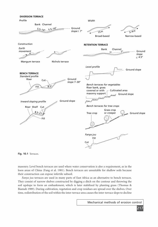
Mechanical methods of erosion control
217
masonry. Level bench terraces are used where water conservation is also a requirement, as in theloess areas of China (Fang et al. 1981). Bench terraces are unsuitable for shallow soils becausetheir construction can expose infertile subsoil.
Fanya juu terraces are used in many parts of East Africa as an alternative to bench terraces.They consist of narrow shelves constructed by digging a ditch on the contour and throwing thesoil upslope to form an embankment, which is later stabilized by planting grass (Thomas &Biamah 1989). During cultivation, vegetation and crop residues are spread over the shelves. Overtime, redistribution of the soil within the inter-terrace area causes the inter-terrace slope to decline
Fill
CutShelfRiser
8.5–21.5°
Ground slopeInward sloping profile
Fill
Cut
8.5°
BENCH TERRACEStandard profile
Riser
Mangum terrace Nichols terrace
Construction
DIVERSION TERRACE
Bank Channel
Profile
Earthmovement
RETENTION TERRACE
5.5–14° 5.5–14° Groundslope 7°≥
Groundslope 7–30°
Width
15 m
Broad-based Narrow-based3–4 m
Bank Channel7° 7° Ground
slope≥ 4.5°
Ground slopeLevel profile
Bench terraces for vegetablesRiser bank, grasscovered or withmasonry support
Cultivated area
Ground slope
Ground slope
Bench terraces for tree crops
Tree cropGrass cropor creeper
Fanya juuFill
Cut
≥
Fig. 10.1 Terraces.
MSE10 11/19/04 02:43 PM Page 217
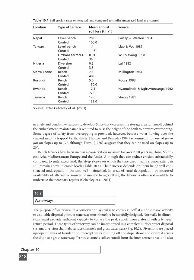
Chapter 10
218
in angle and bench-like features to develop. Since this decreases the storage area for runoff behindthe embankment, maintenance is required to raise the height of the bank to prevent overtopping.Some degree of safety from overtopping is provided, however, because water flowing over theembankment is trapped by the ditch. Thomas and Biamah (1989) recommend the use of fanyajuu on slopes up to 17°, although Hurni (1986) suggests that they can be used on slopes up to26°.
Bench terraces have been used as a conservation measure for over 2000 years in China, South-east Asia, Mediterranean Europe and the Andes. Although they can reduce erosion substantiallycompared to unterraced land, the steep slopes on which they are used means erosion rates canstill remain above tolerable levels (Table 10.4). Their success depends on them being well con-structed and, equally important, well maintained. In areas of rural depopulation or increasedavailability of alternative sources of income to agriculture, the labour is often not available toundertake the necessary repairs (Critchley et al. 2001).
Table 10.4 Soil erosion rates on terraced land compared to similar unterraced land as a control
Location Type of terrace Mean annual Sourcesoil loss (t ha-1)
Nepal Level bench 20.0 Partap & Watson 1994Control 100.0
Taiwan Level bench 1.4 Liao & Wu 1987Control 11.6Orchard terraces 0.01 Wu & Wang 1998Control 36.5
Nigeria Diversion 0.3 Lal 1982Control 3.3
Sierra Leone Bench 7.5 Millington 1984Control 48.0
Burundi Bench 5.0 Roose 1988Control 150.0
Rwanda Bench 12.3 Nyamulinda & Ngiruwonsanga 1992Control 72.0
Jamaica Bench 17.0 Sheng 1981Control 133.0
Source: after Critchley et al. (2001).
10.3
Waterways
The purpose of waterways in a conservation system is to convey runoff at a non-erosive velocityto a suitable disposal point. A waterway must therefore be carefully designed. Normally its dimen-sions must provide sufficient capacity to convey the peak runoff from a storm with a ten-yearreturn period. Three types of waterway can be incorporated in a complete surface water disposalsystem: diversion channels, terrace channels and grass waterways (Fig. 10.2). Diversions are placedupslope of areas of farmland to intercept water running off the slope above and divert it acrossthe slope to a grass waterway. Terrace channels collect runoff from the inter-terrace areas and also
MSE10 11/19/04 02:43 PM Page 218
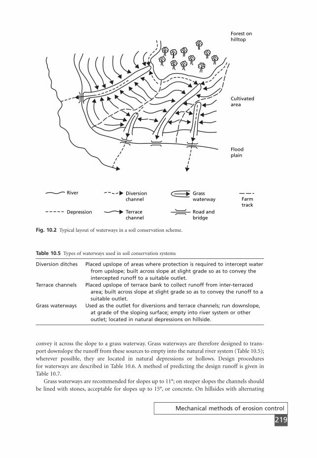
Mechanical methods of erosion control
219
convey it across the slope to a grass waterway. Grass waterways are therefore designed to trans-port downslope the runoff from these sources to empty into the natural river system (Table 10.5);wherever possible, they are located in natural depressions or hollows. Design procedures for waterways are described in Table 10.6. A method of predicting the design runoff is given inTable 10.7.
Grass waterways are recommended for slopes up to 11°; on steeper slopes the channels shouldbe lined with stones, acceptable for slopes up to 15°, or concrete. On hillsides with alternating
River
Depression
Diversionchannel
Terracechannel
Grasswaterway Farm
trackRoad andbridge
Forest onhilltop
Cultivatedarea
Floodplain
Fig. 10.2 Typical layout of waterways in a soil conservation scheme.
Table 10.5 Types of waterways used in soil conservation systems
Diversion ditches Placed upslope of areas where protection is required to intercept waterfrom upslope; built across slope at slight grade so as to convey theintercepted runoff to a suitable outlet.
Terrace channels Placed upslope of terrace bank to collect runoff from inter-terracedarea; built across slope at slight grade so as to convey the runoff to asuitable outlet.
Grass waterways Used as the outlet for diversions and terrace channels; run downslope,at grade of the sloping surface; empty into river system or otheroutlet; located in natural depressions on hillside.
MSE10 11/19/04 02:43 PM Page 219
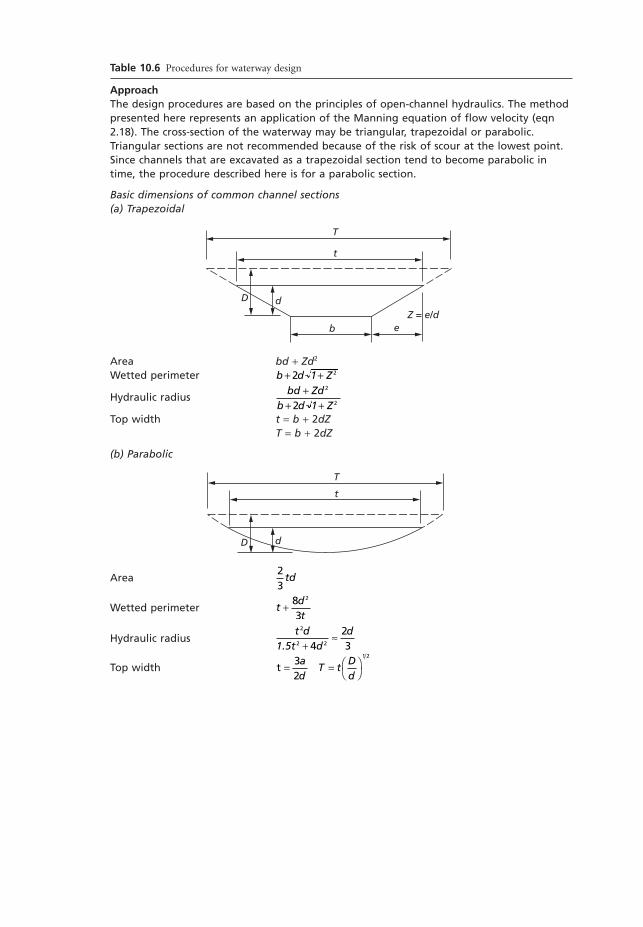
Table 10.6 Procedures for waterway design
ApproachThe design procedures are based on the principles of open-channel hydraulics. The methodpresented here represents an application of the Manning equation of flow velocity (eqn2.18). The cross-section of the waterway may be triangular, trapezoidal or parabolic.Triangular sections are not recommended because of the risk of scour at the lowest point.Since channels that are excavated as a trapezoidal section tend to become parabolic intime, the procedure described here is for a parabolic section.
Basic dimensions of common channel sections(a) Trapezoidal
dD
b
t
T
eZ = e/d
Area bd + Zd2
Wetted perimeter
Hydraulic radius
Top width t = b + 2dZT = b + 2dZ
(b) Parabolic
bd Zdb d 1 Z
++ +
2
22
b d 1 Z+ +2 2
T
D d
t
Area
Wetted perimeter
Hydraulic radius
Top width t = = ÊË
ˆ¯
32
1 2ad
T tDd
t d1.5t d
d2
2 2423+
ª
tdt
+ 83
2
23
td
MSE10 11/19/04 02:43 PM Page 220

Table 10.6 Continued
The waterways used in soil conservation works on agricultural land are normally designedto convey the peak runoff expected with a 10-year return period without causing scour orfill. For other situations, such as construction sites, mining land or pipeline corridors, highermagnitude events may be chosen, particularly if there is a risk of destruction of assets orloss of life should the waterway overtop. The peak runoff can be estimated using themethod shown in Table 10.7.
The design is based on the conditions expected to prevail two years after installation, i.e.after the grass vegetation lining has become established. Although the waterway isvulnerable to erosion in the interim period, providing a stable design for this time wouldresult in overdesign for the rest of its life. It would also lead to an unnecessary reduction inthe area that can be devoted to arable farming.
Designs are based on the concept of a maximum allowable or safe velocity of flow in thechannel. Temple (1991) has shown that the influence of flow duration on the stability ofthe channel is small in the first 100 hours of flow unless the vegetation is destroyed or hasa clumpy growth habit, in which case erosion of the bare areas can undermine thevegetation cover. Since, in these channels flow durations of 100 hours are unlikely, noallowance is made in the channel design for the duration of the flow. The design,therefore, is based on peak flows not exceeding the maximum permitted value.
Design problemDesign a parabolic grass waterway to convey a peak flow of 6m3 s-1 on a 1 per cent slopeover an erodible sandy soil with Bermuda grass vegetation in a good stand cut to a heightof 60mm.
ProcedureDischarge (Q) = 6m3 s-1 (given)Slope (s) = 0.01 (given)Velocity (v)
select a maximum permissible velocity according to the proposed vegetation cover andlocal soil:
= 1.5ms-1
Maximum safe velocities (ms-1) in channels based on covers expected after two seasons
Material Bare Medium grass Very good grasscover cover
Very light silty sand 0.3 0.75 1.5Light loose sand 0.5 0.9 1.5Coarse sand 0.75 1.25 1.7Sandy soil 0.75 1.5 2.0Firm clay loam 1.0 1.7 2.3Stiff clay or stiff gravelly soil 1.5 1.8 2.5Geotextile mat 1.5 2.5 3.5Coarse gravels 1.5 1.8 n/aShale, hardpan, soft rock 1.8 2.1 n/aHand-pitched stone 2.0 n/a n/aHard cemented conglomerates 2.5 n/a n/aRip-rap (D50: 250–400mm) 3.0 n/a n/aBox gabions, grouted stone 5.0 n/a n/aConcrete block systems 6.0 n/a n/a
n/a, not applicable, since a medium or very good grass cover is unlikely to be obtained.Intermediate values may be selected.
MSE10 11/19/04 02:43 PM Page 221
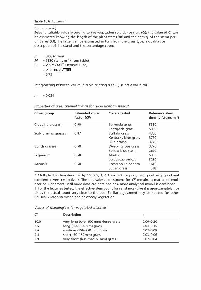
Table 10.6 Continued
Roughness (n)Select a suitable value according to the vegetation retardance class (CI); the value of CI canbe estimated knowing the length of the plant stems (m) and the density of the stems perunit area (M); the latter can be estimated in turn from the grass type, a qualitativedescription of the stand and the percentage cover:
m = 0.06 (given)M = 5380 stems m-2 (from table)CI = (Temple 1982)
== 6.75
Interpolating between values in table relating n to CI, select a value for:
n = 0.034
Properties of grass channel linings for good uniform stands*
Cover group Estimated cover Covers tested Reference stemfactor (CF) density (stems m-2)
Creeping grasses 0.90 Bermuda grass 5380Centipede grass 5380
Sod-forming grasses 0.87 Buffalo grass 4300Kentucky blue grass 3770Blue grama 3770
Bunch grasses 0.50 Weeping love grass 3770Yellow blue stem 2690
Legumes† 0.50 Alfalfa 5380Lespedeza sericea 3230
Annuals 0.50 Common Lespedeza 1610Sudan grass 538
* Multiply the stem densities by 1/3, 2/3, 1, 4/3 and 5/3 for poor, fair, good, very good andexcellent covers respectively. The equivalent adjustment for CF remains a matter of engi-neering judgement until more data are obtained or a more analytical model is developed.† For the legumes tested, the effective stem count for resistance (given) is approximately fivetimes the actual count very close to the bed. Similar adjustment may be needed for otherunusually large-stemmed and/or woody vegetation.
Values of Manning’s n for vegetated channels
CI Description n
10.0 very long (over 600mm) dense grass 0.06–0.207.6 long (250–500mm) grass 0.04–0.155.6 medium (150–250mm) grass 0.03–0.084.4 short (50–150mm) grass 0.03–0.062.9 very short (less than 50mm) grass 0.02–0.04
2 5 0 06 53801 3
. . ¥( )2 5
1 3. m M( )
MSE10 11/19/04 02:43 PM Page 222

Table 10.6 Continued
Calculate the hydraulic radius (r) from the Manning equation:
Calculate the required cross-sectional area (A) of the channel:
Calculate the design depth, which for a parabolic section can be approximated by:
d = 1.5rd = 1.5 ¥ 0.364d = 0.55m
Calculate the top width, which for a parabolic section is expressed by:
Check that the capacity given by the design criteria is adequate. For a parabolic section:
Q = Av = 0.67tdvQ = 0.67 ¥ 10.86 ¥ 0.55 ¥ 1.5Q = 6m3 s-1, which is adequate
Add 20 per cent free board to the design depth:
d = 0.55 + 0.11 = 0.66m
Final design criteria:
depth = 0.66mtop width = 10.86m
Notes1 This procedure can be used for all waterways in a terrace and waterway system. With
terrace channels and diversion channels, however, the slope is not predetermined by theground slope but should be selected from guidelines given in Table 10.1. Terrace channelsare usually unvegetated except with broad-based terraces, where they may be cropped aspart of the inter-terrace area. A value of n = 0.02 should be used for bare soil.
tA
. d
t
t
=
=¥
=
0 674
0 67 0 55
10 86
. .
. m
AQv
A
A
=
=
=
61 54 2
.m
rvns
r
r
= ÊË
ˆ¯
= ¥ÊË
ˆ¯
=
0 5
1 5
0 5
1 51 5 0 034
0 010 364
.
.
.
.. .
.. m
MSE10 11/19/04 02:43 PM Page 223
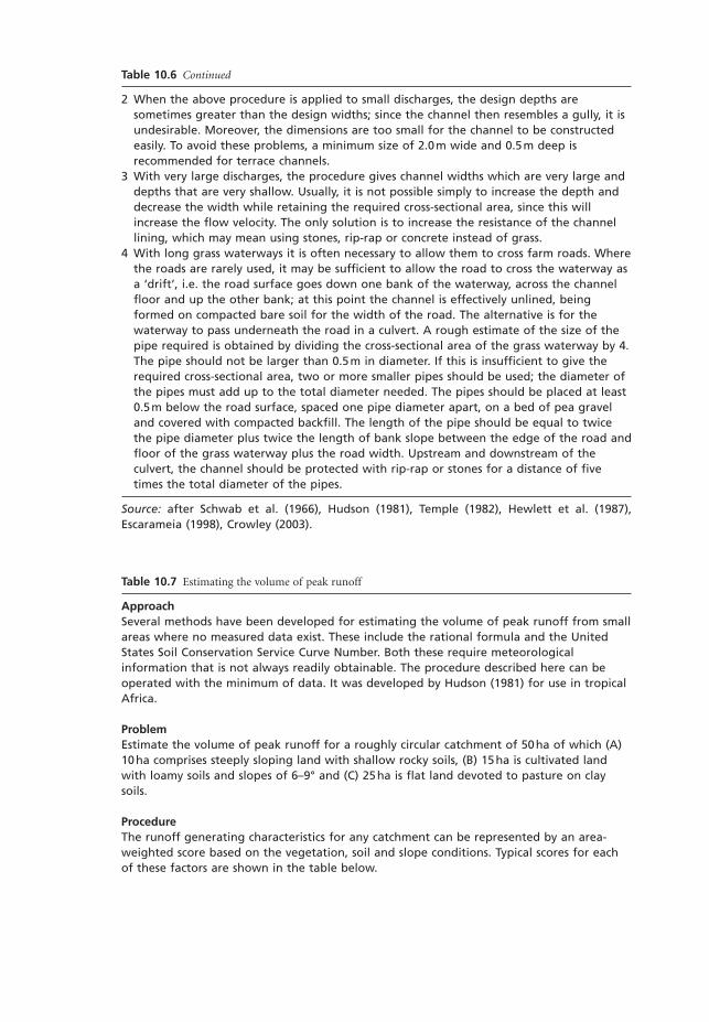
Table 10.6 Continued
2 When the above procedure is applied to small discharges, the design depths aresometimes greater than the design widths; since the channel then resembles a gully, it isundesirable. Moreover, the dimensions are too small for the channel to be constructedeasily. To avoid these problems, a minimum size of 2.0m wide and 0.5m deep isrecommended for terrace channels.
3 With very large discharges, the procedure gives channel widths which are very large anddepths that are very shallow. Usually, it is not possible simply to increase the depth anddecrease the width while retaining the required cross-sectional area, since this willincrease the flow velocity. The only solution is to increase the resistance of the channellining, which may mean using stones, rip-rap or concrete instead of grass.
4 With long grass waterways it is often necessary to allow them to cross farm roads. Wherethe roads are rarely used, it may be sufficient to allow the road to cross the waterway asa ‘drift’, i.e. the road surface goes down one bank of the waterway, across the channelfloor and up the other bank; at this point the channel is effectively unlined, beingformed on compacted bare soil for the width of the road. The alternative is for thewaterway to pass underneath the road in a culvert. A rough estimate of the size of thepipe required is obtained by dividing the cross-sectional area of the grass waterway by 4.The pipe should not be larger than 0.5m in diameter. If this is insufficient to give therequired cross-sectional area, two or more smaller pipes should be used; the diameter ofthe pipes must add up to the total diameter needed. The pipes should be placed at least0.5m below the road surface, spaced one pipe diameter apart, on a bed of pea graveland covered with compacted backfill. The length of the pipe should be equal to twicethe pipe diameter plus twice the length of bank slope between the edge of the road andfloor of the grass waterway plus the road width. Upstream and downstream of theculvert, the channel should be protected with rip-rap or stones for a distance of fivetimes the total diameter of the pipes.
Source: after Schwab et al. (1966), Hudson (1981), Temple (1982), Hewlett et al. (1987),Escarameia (1998), Crowley (2003).
Table 10.7 Estimating the volume of peak runoff
ApproachSeveral methods have been developed for estimating the volume of peak runoff from smallareas where no measured data exist. These include the rational formula and the UnitedStates Soil Conservation Service Curve Number. Both these require meteorologicalinformation that is not always readily obtainable. The procedure described here can beoperated with the minimum of data. It was developed by Hudson (1981) for use in tropicalAfrica.
ProblemEstimate the volume of peak runoff for a roughly circular catchment of 50ha of which (A)10ha comprises steeply sloping land with shallow rocky soils, (B) 15ha is cultivated landwith loamy soils and slopes of 6–9° and (C) 25ha is flat land devoted to pasture on claysoils.
ProcedureThe runoff generating characteristics for any catchment can be represented by an area-weighted score based on the vegetation, soil and slope conditions. Typical scores for eachof these factors are shown in the table below.
MSE10 11/19/04 02:43 PM Page 224
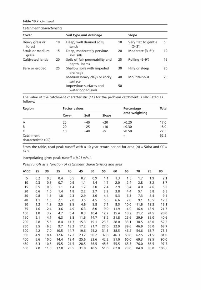
Table 10.7 Continued
Catchment characteristics
Cover Soil type and drainage Slope
Heavy grass or 10 Deep, well drained soils, 10 Very flat to gentle 5forest sands (0–3°)
Scrub or medium 15 Deep, moderately pervious 20 Moderate (3–6°) 10grass soil, silts
Cultivated lands 20 Soils of fair permeability and 25 Rolling (6–9°) 15depth, loams
Bare or eroded 25 Shallow soils with impeded 30 Hilly or steep 20drainage
Medium heavy clays or rocky 40 Mountainous 25surface
Impervious surfaces and 50waterlogged soils
The value of the catchment characteristic (CC) for the problem catchment is calculated asfollows:
Region Factor values Percentage Total
Cover Soil Slopearea weighting
A 25 +40 +20 ¥0.20 17.0B 20 +25 +10 ¥0.30 18.0C 10 +40 +5 ¥0.50 27.5Catchment = 62.5characteristic (CC)
From the table, read peak runoff with a 10-year return period for area (A) = 50ha and CC =62.5.
Interpolating gives peak runoff = 9.25m3 s-1.
Peak runoff as a function of catchment characteristics and area
A\CC 25 30 35 40 45 50 55 60 65 70 75 80
5 0.2 0.3 0.4 0.5 0.7 0.9 1.1 1.3 1.5 1.7 1.9 2.110 0.3 0.5 0.7 0.9 1.1 1.4 1.7 2.0 2.4 2.8 3.2 3.715 0.5 0.8 1.1 1.4 1.7 2.0 2.4 2.9 3.4 4.0 4.6 5.220 0.6 1.0 1.4 1.8 2.2 2.7 3.2 3.8 4.4 5.1 5.8 6.530 0.8 1.3 1.8 2.3 2.9 3.6 4.4 5.3 6.3 7.3 8.4 9.540 1.1 1.5 2.1 2.8 3.5 4.5 5.5 6.6 7.8 9.1 10.5 12.350 1.2 1.8 2.5 3.5 4.6 5.8 7.1 8.5 10.0 11.6 13.3 15.175 1.6 2.4 3.6 4.9 6.3 8.0 9.9 11.9 14.0 16.4 18.9 21.7
100 1.8 3.2 4.7 6.4 8.3 10.4 12.7 15.4 18.2 21.2 24.5 28.0150 2.1 4.1 6.3 8.8 11.6 14.7 18.2 21.8 25.6 29.9 35.0 40.6200 2.8 5.5 8.4 11.7 15.3 19.1 23.3 28.0 33.1 38.5 45.0 52.5250 3.5 6.5 9.7 13.2 17.2 21.7 27.0 32.9 39.6 46.9 55.0 63.7300 4.2 7.0 10.5 14.7 19.6 25.2 31.5 38.5 46.2 54.6 63.7 73.5350 4.9 8.4 12.6 17.2 23.2 30.2 37.8 46.3 53.8 62.5 71.5 81.0400 5.6 10.0 14.4 19.4 25.6 33.6 42.2 51.0 60.0 69.3 79.5 90.0450 6.3 10.5 15.5 21.5 28.5 36.5 45.5 55.5 65.5 76.0 86.5 97.5500 7.0 11.0 17.0 23.5 31.0 40.5 51.0 62.0 73.0 84.0 95.0 106.5
MSE10 11/19/04 02:43 PM Page 225
Chapter 10
226
gentle and steep sections, a grass waterway with drop structures on the steeper slopes should beused. The selection of grasses for planting should take account of the local soil and climatic en-vironment and the need to establish dense cover very rapidly. Commonly used grasses areCynodon dactylon (Bermuda grass), Poa pratensis (Kentucky bluegrass), Bromis inermis (smoothbromegrass) and Pennisetum purpureum (Napier grass). It is recommended, however, to seek localagronomic or ecological advice before making the final selection.
Grass waterways can be replaced in the water disposal system by tile drains. Diversion andterrace channels are graded to a soak-away, normally located in a natural depression, which pro-vides the intake to the drain. The tile system is designed to remove surface water over a periodnot exceeding 48 hours so that crop damage does not occur. Soil loss from tile-outlet terraces ismuch reduced because less than 5 per cent of the sediment delivered to the soak-aways passesinto the drainage system (Laflen et al. 1972). The tile outlet consists of four parts: the inlet tube,the orifice plate, the conducting pipe and the outlet. The inlet tube is usually made of plastic andrises from a pipe below ground to a height 70–100 mm above the adjacent terrace bank; the tubehas holes or slots at regular intervals above ground level and a removable cap to prevent the entryof debris and allow access. The orifice plate is positioned at the base of the tube, where it con-nects with the conducting pipe; it regulates the downward flow of water. The conducting pipe,also of plastic, carries water from one or more inlet tubes to the outlet, which is normally in anatural waterway. The terrace bank adjacent to the inlet must be level to reduce the risk of over-topping by ponded water. Although tile outlets are commonly used in the USA because they takeup less cropland, they are more expensive. On a worldwide basis, grass waterways remain thecheapest and most effective form of terrace outlet.
The main reason why terrace and waterway systems reduce erosion is the way they managethe runoff. The terraces divide the hillside into inter-terrace areas, which should be small enoughin area to generate only small quantities of runoff. The grass waterway reduces the speed of flowbecause of the retardance effects of the vegetation. The arrangement of the waterway networkgives a high tributary (diversion and terrace channels) to main channel (grass waterway) ratioand a catchment that is elongate in shape rather than square or circular; both attributes contribute to a reduction in peak flow.
Table 10.7 Continued
A is the area of the catchment in hectares, CC is the catchment characteristics from theprevious table, and the runoff (m3 s-1) is for a 10-year return period.
Notes:Rainfall intensity: tropical (high) multiply by 1.0
temperate (low) multiply by 0.75Catchment shape: long, narrow multiply by 0.8
square, circular multiply by 1.0broad, short multiply by 1.25
Return period: 2 years multiply by 0.95 years multiply by 0.9510 years multiply by 1.025 years multiply by 1.2550 years multiply by 1.5
MSE10 11/19/04 02:43 PM Page 226
Mechanical methods of erosion control
227
A terrace and waterway system must be designed to give the most efficient layout possible interms of farming operations. This can be achieved by following a systematic design procedureand then making adjustments within certain tolerance limits to take account of local topography.Once a system has been constructed, regular maintenance is required to prevent it from deterio-rating. This includes: cutting the grass in the waterways to maintain it at the height on which thechannel design is based; regular applications of fertilizers to promote grass growth; closure of thewaterways to animals and vehicles, especially when the soil is wet and damage could occur; andregular inspection and repair of breaks in the terrace banks. Although a terrace and waterwaysystem will fail with the occurrence of a storm of much higher magnitude than that for which itis designed, by far the most common cause of failure is inadequate maintenance. Once a failurein vegetation cover occurs, the reduction in flow resistance is immediate and it may take two ormore years for natural recovery to take effect (Temple & Alspach 1992).
10.4
Temporary measures
Temporary measures for erosion control are required on construction sites and also, until a vegetation cover has been established, on road banks and pipeline corridors. Generally, when the catchment area is less than 2 ha, sediment traps such as silt fences are sufficient, but for largerareas it is usually necessary to install a sedimentation pond or basin.
10.4.1 Silt fences
Silt fences are synthetic geotextile meshes attached to vertical posts driven into the ground to forma fence. They are placed across the slope approximately perpendicular to the direction of runoff.Their purpose is not to prevent erosion per se but to trap sediment and prevent it leaving theslope. It is important that the fence is high enough and anchored sufficiently well to support thehydraulic and silting loads. The maximum height of the fence (Hmax; m) is defined by (Rankilor1989):
(10.1)
where P is the precipitation rate of the design storm (m h-1), t is the duration of the storm, L isthe slope length between successive fences (m) and s is slope (m m-1). In order to support thefence, posts should be driven into the ground to a depth (G) that is at least three times Hmax andthe fence should be anchored in a trench that is at least 0.5 Hmax. Posts should be spaced at a dis-tance no greater than 2G. Failure to anchor the fence and install the posts at sufficient depth andwith suitable spacing is the main cause of failure of silt fences. Usually the limiting factor is thedepth to which the posts can be driven. If the design depth is not feasible, the fences must beplaced closer together so as to reduce L and, thereby, reduce Hmax.
10.4.2 Burlap rolls, straw bales
Burlap rolls, also known as bolsters, are tubes of hessian or jute filled with soil or stones that canbe placed across the slope on the contour. Generally, they are not successful. They need to be
HPtL
smax ≥1 4.
MSE10 11/19/04 02:43 PM Page 227
Chapter 10
228
placed in a shallow trench to prevent runoff cutting channels underneath them because theircylindrical shape results in very limited contact with the soil. When used on road banks in Nepal,the hessian rotted rapidly, causing the structure to fail. On pipeline corridors in Georgia, theywere quickly destroyed by cattle. Straw bales arranged as a barrier across the slope are similarlyfragile and since 1992 the United States Environmental Protection Agency has not recognized balebarriers as an appropriate technique for reducing sediment in runoff.
10.4.3 Sedimentation ponds
Sedimentation ponds or basins are used to trap suspended sediment particles contained in runoff and prevent them leaving a site. Since it is almost impossible to contain all the runoffthat may be discharged from a construction site, the aim is to capture the suspended sedimentand then allow the clearer runoff to overflow through a drain to a safe outlet. The required volume of a sedimentation pond (Vmin; m3) is calculated as the larger of the following values(Fifield 1999):
(10.2)
where SAmin is the minimum surface area of the pond, defined as:
(10.3)
where Qout = outflow from the pond (m3 s-1) and vs is settling velocity of the particles (cm s-1).The average depth of the pond must be ≥0.67 m with a minimum outlet depth of 0.61 m.
SAQ
vmin
out
s
=120
V SA
V
min min
min
≥≥ -
0 671
.
or runoff from two-year, 24-h storm up to 252m ha3
10.5
Stabilization structures
Stabilization structures are used to control erosion on steep slopes such as gully sidewalls,embankments and cuttings. Bioengineering techniques, like brush layering and wattling, use livecuttings of quick-rooting plant species, usually willow. They give an immediate reinforcement ofthe soil, as well as providing the basis for long-term slope stability as the cuttings take root andthe vegetation grows.
With brush layering, live willow stakes are laid in lines across the slope on or close to thecontour at 2 m intervals on slopes less than 30° and at 1 m interval on slopes of 30–45°; the methodis not recommended for steeper slopes. The lines to be planted are marked out on the slope,with the first line 0.5 m from the bottom of the slope. Starting from the bottom, a small terrace,400 mm wide, is cut with a 20 per cent fall into the back slope. Cuttings are placed on the terraceat 50 mm intervals, butt ends into the slope with at least one bud and up to one-third of thecutting protruding beyond the edge of the terrace. A 20 mm thick layer of soil is placed on thecuttings and a second layer of cuttings placed on this, staggered with the first layer. The terraceis then backfilled with the material excavated when forming the next terrace upslope and lightlycompacted using foot pressure (Howell 1999).
Wattles, also termed fascines, are cigar-shaped bundles of six to eight live cuttings, each 200–250 mm in diameter, arranged with butt ends alternating, and tied at 300–400 mm intervals
MSE10 11/19/04 02:43 PM Page 228
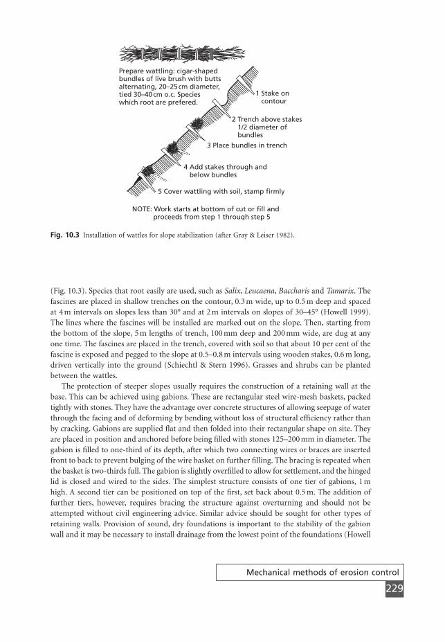
Mechanical methods of erosion control
229
(Fig. 10.3). Species that root easily are used, such as Salix, Leucaena, Baccharis and Tamarix. Thefascines are placed in shallow trenches on the contour, 0.3 m wide, up to 0.5 m deep and spacedat 4 m intervals on slopes less than 30° and at 2 m intervals on slopes of 30–45° (Howell 1999).The lines where the fascines will be installed are marked out on the slope. Then, starting fromthe bottom of the slope, 5 m lengths of trench, 100 mm deep and 200 mm wide, are dug at anyone time. The fascines are placed in the trench, covered with soil so that about 10 per cent of thefascine is exposed and pegged to the slope at 0.5–0.8 m intervals using wooden stakes, 0.6 m long,driven vertically into the ground (Schiechtl & Stern 1996). Grasses and shrubs can be plantedbetween the wattles.
The protection of steeper slopes usually requires the construction of a retaining wall at thebase. This can be achieved using gabions. These are rectangular steel wire-mesh baskets, packedtightly with stones. They have the advantage over concrete structures of allowing seepage of waterthrough the facing and of deforming by bending without loss of structural efficiency rather thanby cracking. Gabions are supplied flat and then folded into their rectangular shape on site. Theyare placed in position and anchored before being filled with stones 125–200 mm in diameter. Thegabion is filled to one-third of its depth, after which two connecting wires or braces are insertedfront to back to prevent bulging of the wire basket on further filling. The bracing is repeated whenthe basket is two-thirds full. The gabion is slightly overfilled to allow for settlement, and the hingedlid is closed and wired to the sides. The simplest structure consists of one tier of gabions, 1 mhigh. A second tier can be positioned on top of the first, set back about 0.5 m. The addition offurther tiers, however, requires bracing the structure against overturning and should not beattempted without civil engineering advice. Similar advice should be sought for other types ofretaining walls. Provision of sound, dry foundations is important to the stability of the gabionwall and it may be necessary to install drainage from the lowest point of the foundations (Howell
Prepare wattling: cigar-shapedbundles of live brush with buttsalternating, 20–25 cm diameter,tied 30–40 cm o.c. Specieswhich root are prefered.
1 Stake on contour
2 Trench above stakes 1/2 diameter of bundles
3 Place bundles in trench
4 Add stakes through and below bundles
5 Cover wattling with soil, stamp firmly
NOTE: Work starts at bottom of cut or fill and proceeds from step 1 through step 5
Fig. 10.3 Installation of wattles for slope stabilization (after Gray & Leiser 1982).
MSE10 11/19/04 02:43 PM Page 229
Chapter 10
230
1999). Soil can be used to fill the spaces between the stones within the gabion, allowing the structure to be seeded or planted with shrubs and trees.
Drainage is used to control surface and seepage water and prevent the build-up of soil water.The principles are to construct a diversion channel to run at grade across the hillslope, upslopeof any area at risk of slide or slump, thereby reducing the amount of water coming into the area.Subsurface drains of 75 mm diameter PVC perforated pipe, wrapped in a filter cloth to preventblockage, can also be installed to intercept subsurface flow. The area itself can be drained by rubbledrains, excavated to a depth of 300 mm and a width of 500 mm and filled with rocks. Safe outletsmust be provided for all components of the drainage system.
10.6
Geotextiles
Geotextile products commercially available for use in erosion control range from open-weavetextile meshes, made from polypropylene, coir or jute, to blankets, containing natural or syntheticfibres that are woven, glued or structurally bound with nets or meshes. They are supplied in rolls,unrolled over the hillslope from the top and anchored with large pins. The natural fibre types arebiodegradable and are designed to be laid over the surface of the slope to give temporary pro-tection against erosion until a vegetation cover is established. The artificial fibre types, whichinclude geowebs and geogrids as well as mats, are buried and designed to give permanent pro-tection to a slope by reinforcing the soil; once a vegetation cover is established, the plant rootsand the fibre act together to increase the cohesion of the soil and the fibre provides a back-upresistance should the vegetation fail.
Surface-laid mats of natural fibres are the most effective in controlling soil detachment byraindrop impact because they provide good surface cover, high water absorption, thick fibres tointercept splashed particles from their point of ejection and a rough surface in which water isponded, thereby further inhibiting the splash action on the soil (Rickson 1995). In contrast, buriedmats of artificial fibres do not effectively control the splash process. Their percentage cover andwater-absorbing capacities are low and problems with backfilling them mean that they tend to befilled with highly erodible unconsolidated material. Despite the ability of natural fibres to holdwater, no significant differences in runoff production were observed in laboratory experimentsbetween an unprotected slope and slopes protected by natural or artificial fibres. However, erosionresulting from the runoff was significantly lower for slopes protected by surface-laid jute matsbecause of the higher roughness imparted to the flow. Although surface-laid mats of coir, wood-chip and artificial fibres also reduced soil loss by runoff, they were less effective than the jutebecause they did not adhere to the soil surface as well. The ability of the mat to drape naturallyover the surface is important, because otherwise surface runoff will pass underneath it and erosionwill occur beneath the mat.
Table 10.8 gives the C-factor values (section 6.2.1) for a range of erosion mats. It should bestressed that these relate to conditions immediately after installation of the geotextile materials.Over time, the natural fibre mats will become less effective as they biodegrade, whereas the per-formance of the artificial fibre mats is likely to remain constant. However, by the time degrada-tion of the mat takes place, the vegetation cover should have established sufficiently to protect theslope, particularly since the mat modifies the soil’s microclimate and improves the conditions forplant growth (Rickson 1995).
MSE10 11/19/04 02:43 PM Page 230

Mechanical methods of erosion control
231
Table 10.8 C-factor values for geotextile erosion mats
Product C-factor value
Woven jute mesh (500gm-2) 0.01–0.07Polypropylene mesh sewn together with wood wool (poplar, pine, aspen) 0.01–0.04
(350–500gm-2)Mesh of nylon polyamide filaments (260gm-2) 0.20–0.25Multiple layered polyethylene mat (450gm-2) 0.20–0.25Polyethylene expanding cellular grid (1780gm-2) 0.50–0.75Woven polypropylene mat (88gm-2) 0.06–0.10Woven coir mat (400–900gm-2) 0.02–0.12Polymeric netting sewn together with straw and coconut fibres 0.01–0.08
(270–550gm-2)Wood fibre hydromulch bonded to photodegradable netting (270gm-2) 0.01Non-woven UV-stabilized blanket and randomly oriented thermally 0.20–0.30welded PVC mono-filaments (1260gm-2)
Values in gm-2 denote mass per area of the material.Source: after Fifield et al. (1989), Fifield and Malnor (1990), Cazzuffi et al. (1991), Krenistkyand Carroll (1994), Rickson (1995), Sutherland and Ziegler (1996), Sutherland et al. (1997),Pazos and Gasca (1998).
10.7
Brush matting
Brush mats can be used as an alternative to geotextiles to provide an immediate cover to the slopeand prevent surface erosion. Since they also provide the basis for the long-term vegetation cover,they are only suitable for sites where the species used is appropriate as the final land cover. Withbrush matting, cuttings of stems and branches of live willow are placed on the slope, butt endsdownslope, at 20–50 stems per running metre, to give a minimum of 80 per cent ground cover(Schiechtl & Stern 1996). The thicker ends of the branches are covered with soil to aid rootingand then fixed with stones or pegs. The whole is covered with soil and the brush fixed to the slopeusing stakes or wires.
10.8
Gully control
Stabilization structures play an important role in gully reclamation and gully erosion control.Small dams, usually 0.4–2.0 m in height, made from locally available materials such as earth,wooden planks, brushwood or loose rock, are built across gullies to trap sediment and therebyreduce channel depth and slope. The structures have a high risk of failure but provide temporarystability and are therefore used in association with agronomic treatment of the surrounding landwhere grasses, trees and shrubs are planted. If the agronomic measures successfully hold the soil and reduce runoff, the dams can be allowed to fall into disrepair. Even though they are
MSE10 11/19/04 02:43 PM Page 231
temporary, the dams have to be carefully designed. They must be provided with a spillway to dealwith overtopping during high flows and installed at a spacing appropriate to the slope of thechannel. Dam spacing should be based on the ‘head-to-toe’ rule, whereby the top of a downstreamdam is level with the lowest elevation of the upstream dam.
The spacing of the dams can be determined from the formula of Heede (1976):
(10.4)
where HE is the dam height, q is the slope angle of the gully floor and K is a constant equal to0.3 for tan q £ 0.2 and 0.5 for tan q > 0.2. The dam height is measured from the crest of the spillway to the gully floor. Based on the costs of construction, loose-rock dams are only eco-nomical for heights up to 0.45 m; single-fence dams are the most economical for dam heights of0.45–0.75 m; and double-fence dams for heights of 0.75–1.7 m (Heede & Mufich 1973). The gullydepths for which these dam heights are recommended are less than 1.2, 1.2–1.5 and 1.5–2.1 mrespectively.
Keying a check dam into the sides and floor of the gully is necessary for stability. This entailsdigging a trench, usually 0.6 m deep and wide, across the channel, but if the channel walls aredeeply cracked and fissured, the trench should be increased in depth to 1.2 or even 1.8 m. Apronsmust be installed on the gully floor downstream of the check dam to prevent flows from under-cutting the structure. Where the slope of the gully is less than 8.5°, the length of the apron shouldbe 1.5 times the height of the structure; for steeper slopes it should be 1.75 times its height. Atthe downstream end of the apron, a loose rock sill about 0.15 m high should be built to create apool to help to absorb the energy of the water falling over the spillway. The spillway should bedesigned to convey peak flows with a given return period, usually 25 years. It is recommendedthat the spillway be trapezoidal in cross-section, with a bottom length (L) that is equal to thebottom width of the gully. A longer spillway is not desirable because water flowing over the spill-way will strike the gully sides, where protection against erosion is less. The depth of the spillway(D) is given by the equation:
(10.5)
and, assuming the spillway sides are sloped at 1 : 1, the top length (Lt) is obtained from (Heede1976):
(10.6)
This approach assumes that the spillways are approximate to a broad-crested weir.Construction of a loose-rock dam (Fig. 10.4) begins by sloping back the tops of the banks. A
trench is then dug across the floor of the gully and into the banks into which the large rocks areplaced to form the toe of the structure. The dam is built upwards from the toe, using flatter rockson the downstream face. Rocks smaller than 100 mm in diameter should not be used because theywill be quickly washed out. A dam made of large rocks will leave large voids in the structurethrough which water jets may flow, weakening the dam. These jets will also carry sedimentthrough the dam instead of allowing it to accumulate on the upstream side. To avoid these effects,the dam should be made with a graded rock structure. An effective composition is 25 per cent of
L L Dt = +
DQ
L= Ê
ˈ¯1 65
2 3
.
spacing =HE
K tan cosq q
Chapter 10
232
MSE10 11/19/04 02:43 PM Page 232
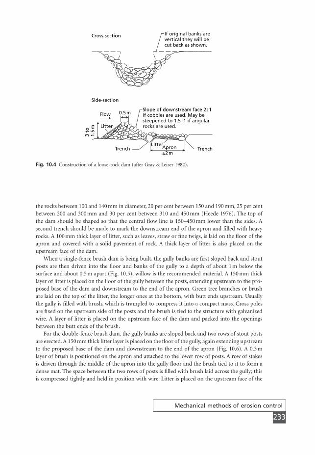
Mechanical methods of erosion control
233
the rocks between 100 and 140 mm in diameter, 20 per cent between 150 and 190 mm, 25 per centbetween 200 and 300 mm and 30 per cent between 310 and 450 mm (Heede 1976). The top ofthe dam should be shaped so that the central flow line is 150–450 mm lower than the sides. Asecond trench should be made to mark the downstream end of the apron and filled with heavyrocks. A 100 mm thick layer of litter, such as leaves, straw or fine twigs, is laid on the floor of theapron and covered with a solid pavement of rock. A thick layer of litter is also placed on theupstream face of the dam.
When a single-fence brush dam is being built, the gully banks are first sloped back and stoutposts are then driven into the floor and banks of the gully to a depth of about 1 m below thesurface and about 0.5 m apart (Fig. 10.5); willow is the recommended material. A 150 mm thicklayer of litter is placed on the floor of the gully between the posts, extending upstream to the pro-posed base of the dam and downstream to the end of the apron. Green tree branches or brushare laid on the top of the litter, the longer ones at the bottom, with butt ends upstream. Usuallythe gully is filled with brush, which is trampled to compress it into a compact mass. Cross polesare fixed on the upstream side of the posts and the brush is tied to the structure with galvanizedwire. A layer of litter is placed on the upstream face of the dam and packed into the openingsbetween the butt ends of the brush.
For the double-fence brush dam, the gully banks are sloped back and two rows of stout postsare erected. A 150 mm thick litter layer is placed on the floor of the gully, again extending upstreamto the proposed base of the dam and downstream to the end of the apron (Fig. 10.6). A 0.3 mlayer of brush is positioned on the apron and attached to the lower row of posts. A row of stakesis driven through the middle of the apron into the gully floor and the brush tied to it to form adense mat. The space between the two rows of posts is filled with brush laid across the gully; thisis compressed tightly and held in position with wire. Litter is placed on the upstream face of the
TrenchTrenchLitterApron
±2 m
0.5 mFlow
3 to
1.5
m Litter
Slope of downstream face 2 : 1if cobbles are used. May besteepened to 1.5 : 1 if angularrocks are used.
Side-section
Cross-section If original banks arevertical they will becut back as shown.
Fig. 10.4 Construction of a loose-rock dam (after Gray & Leiser 1982).
MSE10 11/19/04 02:43 PM Page 233
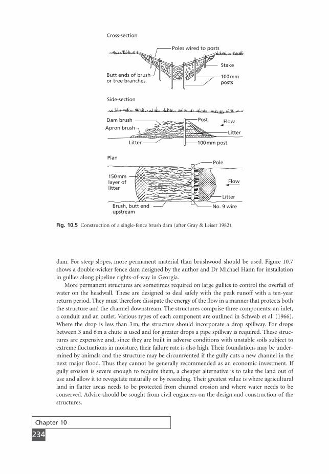
Chapter 10
234
dam. For steep slopes, more permanent material than brushwood should be used. Figure 10.7shows a double-wicker fence dam designed by the author and Dr Michael Hann for installationin gullies along pipeline rights-of-way in Georgia.
More permanent structures are sometimes required on large gullies to control the overfall ofwater on the headwall. These are designed to deal safely with the peak runoff with a ten-yearreturn period. They must therefore dissipate the energy of the flow in a manner that protects boththe structure and the channel downstream. The structures comprise three components: an inlet,a conduit and an outlet. Various types of each component are outlined in Schwab et al. (1966).Where the drop is less than 3 m, the structure should incorporate a drop spillway. For dropsbetween 3 and 6 m a chute is used and for greater drops a pipe spillway is required. These struc-tures are expensive and, since they are built in adverse conditions with unstable soils subject toextreme fluctuations in moisture, their failure rate is also high. Their foundations may be under-mined by animals and the structure may be circumvented if the gully cuts a new channel in thenext major flood. Thus they cannot be generally recommended as an economic investment. Ifgully erosion is severe enough to require them, a cheaper alternative is to take the land out ofuse and allow it to revegetate naturally or by reseeding. Their greatest value is where agriculturalland in flatter areas needs to be protected from channel erosion and where water needs to be conserved. Advice should be sought from civil engineers on the design and construction of thestructures.
Cross-section
Poles wired to posts
Stake
100 mmposts
Butt ends of brushor tree branches
Side-section
Dam brush
Apron brush
150 mmlayer oflitter
Litter
Plan
Post Flow
Flow
Litter
Litter
No. 9 wireBrush, butt endupstream
100 mm post
Pole
Fig. 10.5 Construction of a single-fence brush dam (after Gray & Leiser 1982).
MSE10 11/19/04 02:43 PM Page 234
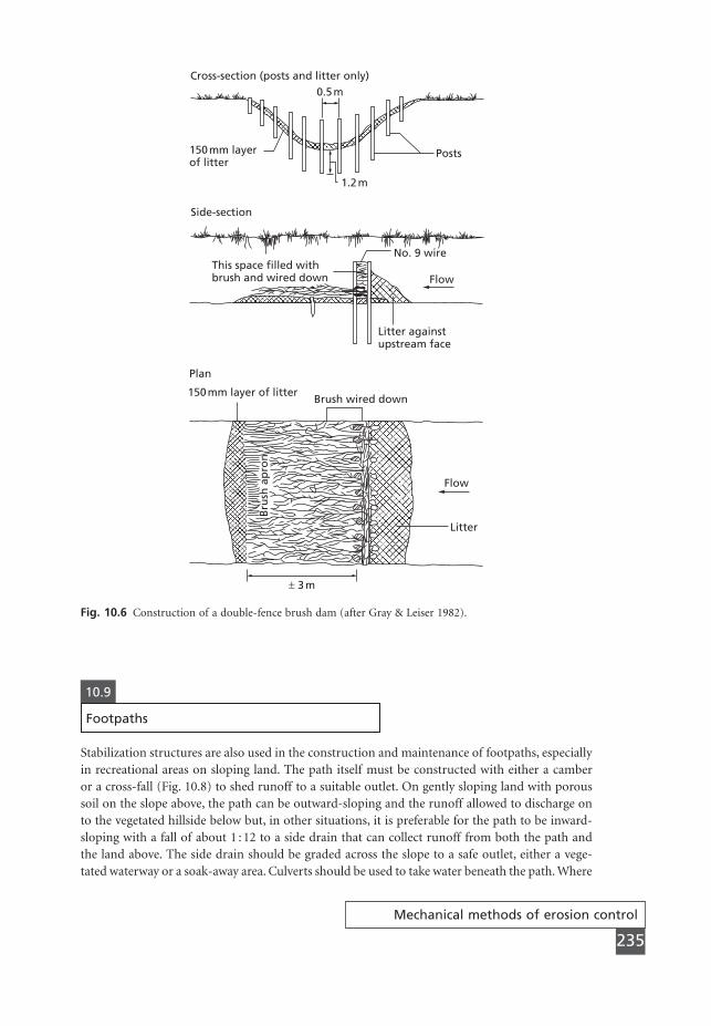
Mechanical methods of erosion control
235
Cross-section (posts and litter only)
Posts150 mm layerof litter
Side-section
This space filled withbrush and wired down
No. 9 wire
Flow
Litter againstupstream face
Plan
150 mm layer of litterBrush wired down
Bru
sh a
pro
n
0.5 m
1.2 m
Flow
Litter
± 3 m
Fig. 10.6 Construction of a double-fence brush dam (after Gray & Leiser 1982).
10.9
Footpaths
Stabilization structures are also used in the construction and maintenance of footpaths, especiallyin recreational areas on sloping land. The path itself must be constructed with either a camberor a cross-fall (Fig. 10.8) to shed runoff to a suitable outlet. On gently sloping land with poroussoil on the slope above, the path can be outward-sloping and the runoff allowed to discharge onto the vegetated hillside below but, in other situations, it is preferable for the path to be inward-sloping with a fall of about 1 : 12 to a side drain that can collect runoff from both the path andthe land above. The side drain should be graded across the slope to a safe outlet, either a vege-tated waterway or a soak-away area. Culverts should be used to take water beneath the path. Where
MSE10 11/19/04 02:43 PM Page 235
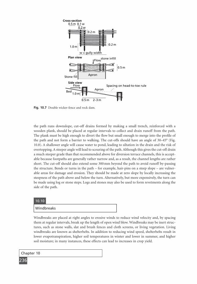
Chapter 10
236
the path runs downslope, cut-off drains formed by making a small trench, reinforced with awooden plank, should be placed at regular intervals to collect and drain runoff from the path.The plank must be high enough to divert the flow but small enough to merge into the profile ofthe path and not form a barrier to walking. The cut-offs should have an angle of 30–45° (Fig.10.8). A shallower angle will cause water to pond, leading to siltation in the drain and the risk ofovertopping. A steeper angle will lead to scouring of the path. Although this gives the cut-off draina much steeper grade than that recommended above for diversion terrace channels, this is accept-able because footpaths are generally rather narrow and, as a result, the channel lengths are rathershort. The cut-off should also extend some 300 mm beyond the path to avoid runoff by-passingthe structure. Bends or turns in the path – for example, hair-pins on a steep slope – are vulner-able areas for damage and erosion. They should be made at zero slope by locally increasing thesteepness of the path above and below the turn. Alternatively, but more expensively, the turn canbe made using log or stone steps. Logs and stones may also be used to form revetments along theside of the path.
0.5 m
0.2 m
0.2 m
w = gully width
1.0 m
0.1 w 0.2 w
Apron
Flow
Stone fill
0.5 m
Cross-section
Plan view
Side view
0.5 m 2–3 m
FlowApron
Bed1.0 m
Spacing on head-to-toe rule
stone infill
Fig. 10.7 Double wicker-fence and rock dam.
10.10
Windbreaks
Windbreaks are placed at right angles to erosive winds to reduce wind velocity and, by spacingthem at regular intervals, break up the length of open wind blow. Windbreaks may be inert struc-tures, such as stone walls, slat and brush fences and cloth screens, or living vegetation. Livingwindbreaks are known as shelterbelts. In addition to reducing wind speed, shelterbelts result inlower evapotranspiration, higher soil temperatures in winter and lower in summer, and highersoil moisture; in many instances, these effects can lead to increases in crop yield.
MSE10 11/19/04 02:43 PM Page 236
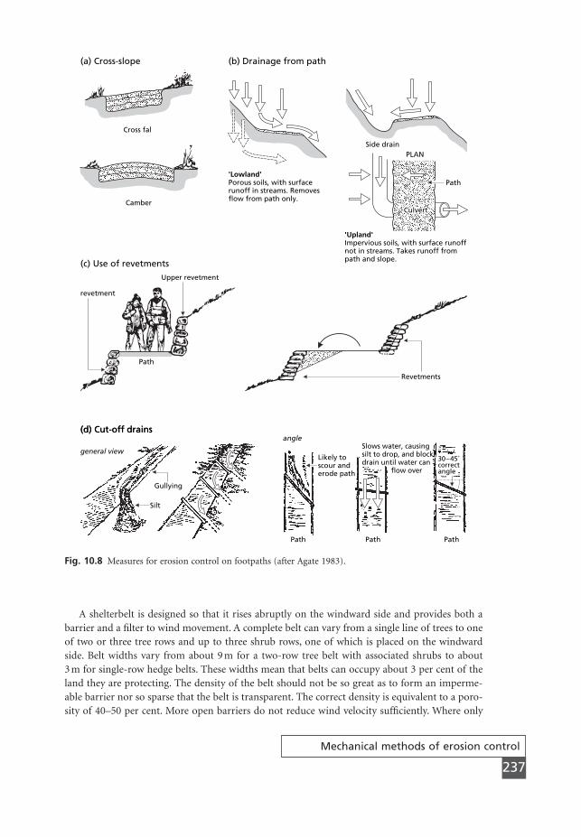
Mechanical methods of erosion control
237
A shelterbelt is designed so that it rises abruptly on the windward side and provides both abarrier and a filter to wind movement. A complete belt can vary from a single line of trees to oneof two or three tree rows and up to three shrub rows, one of which is placed on the windwardside. Belt widths vary from about 9 m for a two-row tree belt with associated shrubs to about 3 m for single-row hedge belts. These widths mean that belts can occupy about 3 per cent of theland they are protecting. The density of the belt should not be so great as to form an imperme-able barrier nor so sparse that the belt is transparent. The correct density is equivalent to a poro-sity of 40–50 per cent. More open barriers do not reduce wind velocity sufficiently. Where only
CulvertCulvert
(d) Cut-off drains
Culvert
(a) Cross-slope
Cross fal
Camber
(b) Drainage from path
'Lowland'Porous soils, with surfacerunoff in streams. Removesflow from path only.
'Upland'Impervious soils, with surface runoff not in streams. Takes runoff from path and slope.
Side drainPLAN
Path
Culvert
(c) Use of revetmentsUpper revetment
revetment
Path
Revetments
(d) Cut-off drains
general view
angle
Gullying
Silt
Likely to scour and erode path
Path Path Path
Slows water, causing silt to drop, and blockdrain until water can flow over
30 – 45˚ correct angle
Fig. 10.8 Measures for erosion control on footpaths (after Agate 1983).
MSE10 11/22/04 11:18 AM Page 237

Chapter 10
238
a single row of trees is used, it is important that the branches and foliage extend to ground levelto give the required level of porosity in the lower metre where most of the sediment movementby saltation takes place (section 2.8). With denser barriers there is a much greater reduction inwind speed initially but, since the velocity increases more rapidly with distance downwind thanis the case for more porous barriers, they are effective for only short distances.
The reduction in wind velocity by a shelterbelt begins at a distance of about five times theheight of the belt upwind and reaches a maximum of about 40 per cent of the original wind velo-city at a distance of about three times the height of the belt downwind. Velocity then increasesagain, returning to the original wind speed at a distance of about 30 times the barrier height (Marshall 1967). Shelterbelts are designed to maintain the wind velocity at about 80 per cent ofthe open wind velocity. Wind tunnel studies by Woodruff and Zingg (1952) showed that tree belts
(d) Cut-off drains (continued)
Height Length
Stone reinforcement
Too high Correct
Uphillview
Too short
300 mm
Stream maydivert
Reinforce with stone
(e) Making a turn
Correct use of path slope Use of steps
Increase slope
Arrows indicatedrainage
Increase slope
DRAINAGE CHANNEL
Correct
Fig. 10.8 Continued
MSE10 11/19/04 02:43 PM Page 238
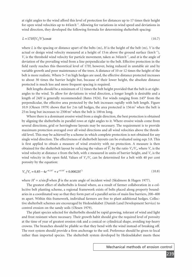
at right angles to the wind afford this level of protection for distances up to 17 times their heightfor open wind velocities up to 44 km h-1. Allowing for variations in wind speed and deviations inwind direction, they developed the following formula for determining shelterbelt spacing:
(10.7)
where L is the spacing or distance apart of the belts (m), H is the height of the belt (m), V is theactual or design wind velocity measured at a height of 15 m above the ground surface (km h-1),Vt is the threshold wind velocity for particle movement, taken as 34 km h-1, and a is the angle ofdeviation of the prevailing wind from a line perpendicular to the belt. Effective protection in thefield rarely reaches this theoretical level of 17H, however, being reduced in unstable air and byvariable growth and poor maintenance of the trees. A distance of 10 or 12 times the height of thebelt is more realistic. Where 5–7 m high hedges are used, the effective distance protected increasesto about 30 times the barrier height but, because of their lower height, the absolute distance protected is much less and more frequent spacing is required.
Belt lengths should be a minimum of 12 times the belt height provided that the belt is at right-angles to the wind. To allow for deviations in wind direction, a longer length is desirable and alength of 24H is generally recommended (Bates 1924). For winds ranging from ±45° from theperpendicular, the effective area protected by the belt increases rapidly with belt length. Figure10.9 (Olesen 1979) shows that for 2 m tall hedges, the area protected is 156 m2 when the belt is25 m long but increases to 2500 m2 when the belt is 100 m long.
Where there is a dominant erosive wind from a single direction, the best protection is obtainedby aligning the shelterbelts in parallel rows at right angles to it. Where erosive winds come fromseveral directions, grid or herringbone layouts may be necessary. The requirement is to providemaximum protection averaged over all wind directions and all wind velocities above the thresh-old level. This may be achieved by a scheme in which complete protection is not obtained for anysingle wind direction. The effectiveness of shelterbelt layouts can be evaluated using eqn 3.8. Thisis first applied to obtain a measure of wind erosivity with no protection. A measure is thenobtained for the shelterbelt layout by reducing the values of t by the ratio Vx/Vo, where Vx is thewind velocity at distance x from the belt, with x measured in units of barrier height, and Vo is thewind velocity in the open field. Values of Vx/Vo can be determined for a belt with 40 per centporosity by the equation:
(10.8)
where H¢ = x/sin b when b is the acute angle of incident wind (Skidmore & Hagen 1977).The greatest effect of shelterbelts is found where, as a result of farmer collaboration in a col-
lective belt planting scheme, a regional framework exists of belts placed along property bound-aries in a coordinated way so that they form part of a parallel series of main line barriers, 200–400m apart. Within this framework, individual farmers are free to plant additional hedges. Collec-tive shelterbelt schemes are encouraged by Hedeselskabet (Danish Land Development Service) tocontrol erosion on the sandy soils (Olesen 1979).
The plant species selected for shelterbelts should be rapid growing, tolerant of wind and lightand frost resistant where necessary. Their growth habit should give the required level of porosityat the time of year of greatest erosion risk and a conical or cylindrical shape, avoiding top-heavycrowns. The branches should be pliable so that they bend with the wind instead of breaking off.The root system should provide a firm anchorage to the soil. Preference should be given to localrather than imported species. The shelterbelt system developed by Hedeselskabet meets these
V V e e Hx oH H= - + +- ¢ - ¢ ¢0 85 4 0 00020 2 0 3 2. .. .
V
L H V Vt= ( )17 cosa
Mechanical methods of erosion control
239
MSE10 11/19/04 02:43 PM Page 239
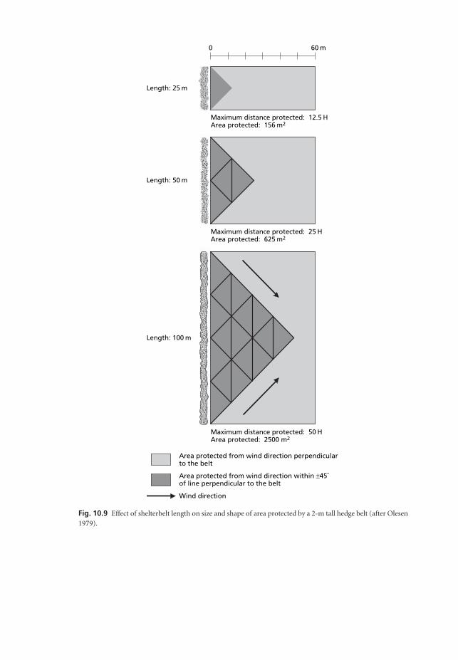
Area protected from wind direction perpendicular to the belt
Area protected from wind direction within ±45˚ of line perpendicular to the belt
Wind direction
0 60 m
Length: 25 m
Length: 50 m
Length: 100 m
Maximum distance protected: 50 H Area protected: 2500 m2
Maximum distance protected: 12.5 HArea protected: 156 m2
Maximum distance protected: 25 H Area protected: 625 m2
Fig. 10.9 Effect of shelterbelt length on size and shape of area protected by a 2-m tall hedge belt (after Olesen1979).
MSE10 11/19/04 02:43 PM Page 240
Mechanical methods of erosion control
241
requirements and, at the same time, provides for an ecological succession to give an effectivebarrier within three to four years and one with a life of 50–80 years. The belts are made up ofthree parallel rows, 1.25–1.5 m apart, each row comprising: nurse trees, such as alders and willows,which are fast-growing and provide the early protection; durable trees, such as oaks, sycamore,elm, maple and rowan, which take longer to grow but provide the long-term protection; andshade-tolerant bushes to provide undergrowth in the lower levels of the belt. The mixture ofspecies provides a belt that is less vulnerable to attack by diseases and pests, visually more attrac-tive and able to give a varied habitat for wildlife. The belt needs to be protected in its early yearsagainst damage by livestock and spray drift. After about five years and then at an interval of everythree to four years, mechanical cutting of the sides of the belt is required to maintain the necessary shape, particularly the sharp rise from the ground on the windward side.
Windbreaks of brushwood or plastic meshes with about 50 per cent porosity are often usedto help to stabilize mobile sand dunes and, thereby, provide a more suitable environment for veg-etation growth. The windbreaks, sometimes termed sand fences, are placed at right angles to thewind (Savage & Woodhouse 1968). Deposition occurs windward of the barrier for a distance of0.4–2.0 times the barrier height and in the lee of the barrier for a distance up to four times theheight. Once the sand has accumulated and almost buried the fence, a second fence is built ontop of the newly formed dune. Further fences are added until the dune is reformed by the windinto a streamlined shape so that air flows over it without loss of transport capacity. Where windvelocities exceed 18 m s-1, double or triple fence systems are used, spaced at intervals of four timesthe barrier height.
1 Using aerial photographs, topographicmaps and reconnaissance field surveys,determine the preliminary positions of thegrass waterways. Locate the waterways inthe natural depressions, hollows ordrainage lines of the ground surface.
2 Locate the main breaks of slope and anybadly eroded or gullied areas. Terracebanks should, wherever possible, belocated to incorporate slope breaks and bepositioned upslope of eroded lands.
3 Determine the spacing or vertical interval(VI) between the terraces. The computedspacings may be varied by 25–30 per centto allow for adjustments in position of theterraces to conform with slope breaks andavoid eroded areas.
4 Determine terrace lengths. Terraces mustbe limited in length to avoid dangerousaccumulations of runoff and large cross-sectional areas to the terrace channels.
Box 10
5 Adjust the positions of the grass water-ways if necessary to avoid excessive terracelengths.
6 Locate paths and farm roads along thedivides between separate terrace andwaterway systems. The use of crest loca-tions minimizes the catchment area con-tributing runoff to the road. Runoff maythen be discharged into the surroundingland without the need for side drains. Crestlocations also dispense with the need forbridges and culverts, avoid breaking up ter-races to allow roads to cross them andkeep vehicles away from grass waterways.
7 Using contour maps and aerial pho-tographs, plan the layout of the system.Locate the grass waterways and diversionchannels on the maps and photographs.Locate the top or key terrace and positionthe others in relation to it in accordancewith the design spacings, lengths and gra-dients and in keeping with the location of
Laying out terraces and waterways
Continued
MSE10 11/19/04 02:43 PM Page 241
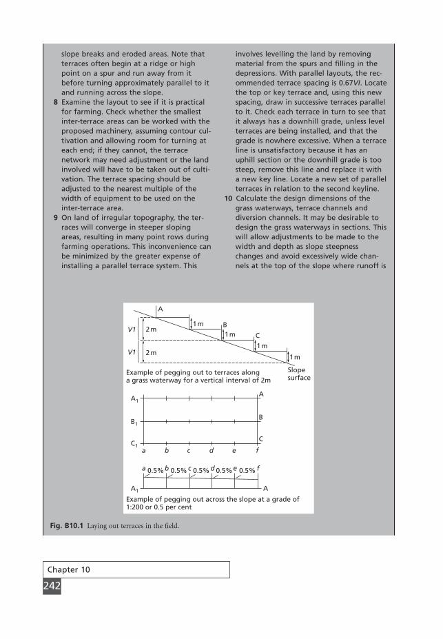
Chapter 10
242
slope breaks and eroded areas. Note thatterraces often begin at a ridge or highpoint on a spur and run away from itbefore turning approximately parallel to itand running across the slope.
8 Examine the layout to see if it is practicalfor farming. Check whether the smallestinter-terrace areas can be worked with theproposed machinery, assuming contour cul-tivation and allowing room for turning ateach end; if they cannot, the terracenetwork may need adjustment or the landinvolved will have to be taken out of culti-vation. The terrace spacing should beadjusted to the nearest multiple of thewidth of equipment to be used on theinter-terrace area.
9 On land of irregular topography, the ter-races will converge in steeper slopingareas, resulting in many point rows duringfarming operations. This inconvenience canbe minimized by the greater expense ofinstalling a parallel terrace system. This
involves levelling the land by removingmaterial from the spurs and filling in thedepressions. With parallel layouts, the rec-ommended terrace spacing is 0.67VI. Locatethe top or key terrace and, using this newspacing, draw in successive terraces parallelto it. Check each terrace in turn to see thatit always has a downhill grade, unless levelterraces are being installed, and that thegrade is nowhere excessive. When a terraceline is unsatisfactory because it has anuphill section or the downhill grade is toosteep, remove this line and replace it witha new key line. Locate a new set of parallelterraces in relation to the second keyline.
10 Calculate the design dimensions of thegrass waterways, terrace channels anddiversion channels. It may be desirable todesign the grass waterways in sections. Thiswill allow adjustments to be made to thewidth and depth as slope steepnesschanges and avoid excessively wide chan-nels at the top of the slope where runoff is
A
B
C2 m
Example of pegging out to terraces alonga grass waterway for a vertical interval of 2m
Example of pegging out across the slope at a grade of1:200 or 0.5 per cent
Slopesurface
2 m
A1
A1 A
B1
C1a b c d e f
a b c d e f
A
B
C
0.5% 0.5% 0.5% 0.5% 0.5%
1 m
1 m
1 m
1 m
V1
V1
{{
Fig. B10.1 Laying out terraces in the field.
MSE10 11/19/04 02:43 PM Page 242

Mechanical methods of erosion control
243
less. When the slope exceeds 11°, stone- orconcrete-lined channels or drop structuresshould be used.
11 Stake out the waterway in the field andconstruct it by excavating soil from thecentre and throwing it to each side to formthe banks; check first, however, that thenatural depression does not already meetthe design depth and top width require-ments. Seed the grass cover along withcompost, fertilizer and mulch.
12 Stake out the position of the diversionchannels and terrace channels along theoutlet or grass waterway to the appropri-ate VI (Fig. B10.1). From these positions,the terraces are pegged out across theslope according to the selected grade. Thevertical intervals should be checked regu-larly. Begin with the diversion channel,
then the top terrace and work downslope.Minor adjustments to the position of theterrace channels can be made within a tol-erance of ±50mm VI. Mark the lines of thechannels with a plough furrow.
13 Construct the diversion channel and thenthe terrace, beginning at the top andworking downslope. This method ofworking is necessary because each terracechannel is designed to convey only therunoff from its inter-terrace area; it cannotcope with runoff from further upslope andso the protection works must be in placeprior to construction. If the top soil is thin,it should be scraped off first, stored andthen returned to the inter-terrace areaafter the terraces are complete.
After Schwab et al. (1966), Troeh et al. (1980),Hudson (1981) and Wenner (1981).
MSE10 11/19/04 02:43 PM Page 243
Chapter 11
244
The ultimate objective of research on soil erosion is to solve erosion problems by adopting suitable protection measures. Suitability implies not just reducing erosion to an acceptable level;the measures must be capable of implementation. The aim of this chapter is to provide a back-ground to some of the issues involved in implementing soil conservation proposals.
CHAPTER 11
Implementation
11.1
Socio-economic setting
As indicated in Chapter 6, soil erosion is frequently a response to the breakdown of farmingsystems. The three major periods in history associated with extensive soil erosion (Dregne 1982)all reflect the inability of existing farming systems to deal with population growth and the inten-sification of agriculture. These periods were: the expansion of agriculture into China, the MiddleEast and the Mediterranean some 1000–3000 years ago; the migration of Europeans to developcolonies some 50–150 years ago; and the expansion in the past 30–50 years of people on to mar-ginal lands in Latin America, Africa and Asia. In all cases, the outcome was land degradation andthe movement of population to new areas. The migrants took with them agricultural practicesthat had worked for hundreds of years in their home areas but that were generally unsuited totheir new environments. Unfortunately, knowledge of this unsuitability was only available fromexperience.
Today, rural depopulation is causing erosion due to the lack of labour to maintain soil con-servation works. Although most pronounced in Mediterranean Europe, it is a trend that willbecome increasingly important worldwide as all countries over the next century experience adecline in the proportion of their population employed in agriculture and a movement of peopleto the towns. The need to supply food for the urban market will also create an increasing strainon many existing farming systems. No longer is it appropriate to view soil erosion solely as aproblem arising from population pressure. In many countries, a declining rural labour force andthe need to increase agricultural production are leading to the amalgamation of holdings,increases in field sizes and wholesale levelling of land to make it easier to work with larger machinery, all trends that lead to increases in erosion.
Unfortunately, the overall take-up of soil conservation remains poor. After six decades ofvoluntary soil conservation programmes in the USA, erosion is still at an unacceptably high level(Swanson et al. 1986). Farmers are unlikely to adopt conservation measures if there is no imme-
MSE11 11/19/04 02:45 PM Page 244
Implementation
245
diate threat to the productivity of their land or if the main justification for their use is to preventpollution and other off-site damage (Napier 1990), unless there are either incentives for theiradoption or meaningful penalties for not using conservation production systems (Napier 1999).These issues bring into question the role that governments can play.
11.2
Political context
Although most governments have some form of soil protection policies that include erosioncontrol, few are translated into effective action because of the lack of political will; soil conser-vation is not a vote-winning concern (Hudson 1981). Yet, under certain conditions, governmentsdo respond quite rapidly. The United States Soil Conservation Service was created as a result ofpolitical pressure from all segments of society who were affected by severe wind erosion duringthe 1930s. Farmers lost their soil and often their farms, exacerbating the effects of the worldwideeconomic depression of the time; national food supplies were threatened; and off-site sedimen-tation created problems for the urban population and the non-agricultural population in ruralareas (Rasmussen 1982). A much earlier but smaller-scale example occurred at the end of thenineteenth century in Iceland, where drifting sand seriously affected the livelihood of farmers inthe southern and north-eastern parts of the country. Under pressure from the Agricultural Societyof Iceland, the Icelandic Parliament (Althing) made available a small grant to bring in Danishspecialists to investigate the problem and gave District Commissions the authority to take action.Without any financial wherewithal or knowledge of the best measures to take, however, this legislation was of little value. Political pressure from farmers continued and in 1907 the Act ofForestry and Prevention of Erosion of Land was passed, effectively marking the foundation of theState Soil Conservation Service of Iceland (Runólfsson 1978, 1987). These examples serve to indicate what can be achieved if the farmers in particular and society in general have sufficientpolitical voice. Since this occurs only when disaster is imminent, the response of governmentsseems to be limited to crisis management.
Within the past 30 years many governments have endeavoured to set up conservation initia-tives but have been constrained by lack of funds and the limited political value of being involvedin conservation work. In Kenya, protection of the environment was formally endorsed by the President in 1977 and a permanent Presidential Commission on Soil Conservation and Afforesta-tion was established in 1980 to develop strategy and policy, ensure coordination between inter-ested bodies and monitor progress. This encouraged external financial and technical assistancesuch as that provided by the Swedish International Development Authority (SIDA) to the NationalSoil and Water Conservation Programme. In many countries, so many organizations are nowinvolved in promoting soil conservation that new political problems have arisen, such as how thework might best be coordinated, how the responsibilities of each organization might be defined,and what should be the role of external organizations vis-à-vis those of the host country.
11.3
New approaches
The past three decades have seen considerable changes in the approaches used to promote andimplement soil conservation. Perhaps the most fundamental has been the move from a top-down
MSE11 11/19/04 02:45 PM Page 245

towards a bottom-up approach of participatory development in which the farming family, notjust the head male, is involved in defining priorities. The job of the technical experts, includingphysical scientists and socio-economists, is to work with the family in producing a site-specificscheme. This approach aims to give farmers ownership of the proposals since they become majordecision-makers throughout the soil conservation process. A key issue is how to provide thatempowerment without reducing the influence and motivation of extension staff. In many cases,soil conservation is no longer promoted directly but is presented by stealth within a backgroundof water conservation, improved soil fertility and overall promotion of wise land use and goodland husbandry (Shaxson 1988). The new approach also depends on recognizing that many tra-ditional agricultural systems involve soundly based soil protection practices (section 7.3.6) andthat more acceptable conservation schemes can be developed by building on these.
Although the results of this new approach are promising, it is too early to know whether theycan be sustained in the long term. Further, the implication that the top-down approach mustalways be unsuccessful cannot be supported. Experience from a number of projects in India,involving different farmers, shows that how farmers perceive the risk and the economic benefitsis more important in the end. Projects where this is not recognized will fail no matter how muchfarmer participation is involved (Singh 1990).
A second area where a change of attitude is taking place is the move from soil conservationprojects to soil conservation programmes. Projects have been favoured by aid agencies and otherdonors because money can be made available for a specific purpose over a finite period and theoutcome monitored. The results can be seen in the number of kilometres of terraces and water-ways constructed. Present-day food-for-work programmes follow a similar philosophy. Once thestructures are in place, however, farmers are likely to remove them if they appear to have nobenefit; for example, if they take up scarce land on a holding that is already too small (Holden &Shiferaw 1999). Since few of these projects have produced sustained conservation benefits, empha-sis is now being placed on developing soil conservation programmes based on integratingresearch, extension, education and training. By having a longer life than the three to five yearstypical of soil conservation projects, soil conservation programmes should provide for greatercontinuity.
A soil conservation programme is based on a general mission statement and encompasses arange of activities targeted on individual farmers, communities and the population in general.Each activity has specific objectives, its performance is monitored and the programme is continually updated and modified. The Swedish Aid programme in Kenya worked with exist-ing government structures to train staff and build the appropriate institutions to liaise withfarmers. An important outcome was the training of soil conservation officers and technical assis-tants to maintain regular contact with and advise farmers through a Training and Visit System.Each technical assistant operated through a contact farmer and between four and eight followerfarmers, visiting on a set day and time once a fortnight to discuss soil conservation, crops, mech-anization, farm management and other issues. Where women’s groups and other self-help groupsexist, they were also used as contacts (Mbegera et al. 1992). The results were mixed because thecontact farmers tended to be those who were already resource-rich and socially well connected,and were also men rather than women. Further, with its emphasis on crop production, very littleattention was given to soil conservation. Since it was not meeting government objectives, the soilconservation programme was forced to develop a separate approach instead of working throughthe mainstream extension programme (Kiara et al. 1996).
Instead of working with contact farmers, the Department of Land Development in Thailandoperates through land development villages, one in each administrative district of the country,where the farmers and government agencies work together to establish land development pro-
Chapter 11
246
MSE11 11/19/04 02:45 PM Page 246
grammes that will prevent land degradation, restore already degraded land and adopt a land usepattern that will increase the income of the farmers (Attaviroj 1996). The emphasis of the pro-gramme is on soil and water conservation. The intention is that the techniques established at thedevelopment villages will be disseminated to neighbouring villages through field days withfarmer-to-farmer contacts. At present, the Thai government is providing all the funding. The testof its success will be its sustainability once funding is reduced or withdrawn entirely.
A third area of reappraisal, arising from the above, is whether soil conservation should beapproached at the level of the individual farmer, the village or some form of administrative dis-trict, or at a watershed. The watershed has the advantage of being the natural geomorphologicalunit for water erosion. The risk of erosion at any point within a watershed can be understood inrelation to its topographic position and the effect this has on local hydrology and sediment pro-duction. The off-site effects of erosion are also more easily appreciated within a watershed thanby the study of an individual field. Emphasis on a watershed, however, can result in too muchreliance on mechanical measures aimed at runoff control and on a top-down approach to erosioncontrol. Moreover, local communities do not always identify with a physical catchment. In largecatchments, they identify with their village and local area so that farmers in the upper reachesmay have little interest in the welfare of those at the lower end (Thomas 1996). The watershedapproach can easily ignore the fact that the success or otherwise of soil conservation depends onthe behaviour of the individual land user. At the most basic level, the effective watershed is afarmer’s field, and with the increasing emphasis on agronomic methods of erosion control thisseems the most appropriate unit at which to operate.
Administrative units are required through which contact can be made with farmers. In theUSA, these take the form of Conservation Districts set up under the 1937 Standard State SoilConservation Districts Enabling Law. The Districts provide the forum through which farmers canapproach the various federal, state and local agencies that provide technical and financial assis-tance for conservation work. They bring together farmers, public-spirited citizens in business,industry and education, and officers of the Natural Resources Conservation Service, establishedin 1994 as the successor to the Soil Conservation Service, with a wider remit to cover soil, water,land and the natural environment. In Kenya, the Soil Conservation Districts are the administra-tive units for the planning and implementation of soil conservation programmes but the participation of farmers is organized within each District through catchment conservation com-mittees responsible for watersheds, typically 200–500 ha in size. The committees comprisefarmers, chiefs and assistant chiefs, as well as the soil conservation officer and technical assistant.All are involved in decision-making to develop a feasible and acceptable land management planfor each farm in the catchment (Kiara 2001). Similar approaches are being used in Burkina Faso(Eger & Bado 1992) and northern Thailand (Oberhauser & Limchoowong 1996).
Within the USA, individual counties and metropolitan areas have the responsibility fordrawing up and managing Erosion and Sediment Control (ESC) programmes to comply with therequirements of the National Pollutants Discharge Elimination System for both point and non-point source pollution under the 1987 Clean Water Act. The ESC programmes must provide guid-ance on best management practices to prevent erosion and control sediment during construction.The most successful bring together environmental conservation groups, the building community,contractors, real estate people and the local government. This group of stakeholders has to decideon the measures that should be adopted to meet the required standards of water quality. Thesecan range from ordinances to control land use and protect regional floodways and flood plainsto the development and implementation of regulations with which construction firms mustcomply or face financial penalties. Education is an important activity of ESC programmes(Mitchell 1998). Training must be provided for the contractors in relation to best practices in soil
Implementation
247
MSE11 11/19/04 02:45 PM Page 247
Chapter 11
248
management, soil handling, landscaping, operation of heavy machinery and other activities con-cerned with ground disturbance. Outreach campaigns educate elected officials, community resi-dents and business leaders about the need for conservation systems with the aim of developinglocal community ownership of their rivers, lakes, wetlands and watersheds. Such ownership isimportant in order to secure sufficient funding to implement the programme, which comes froma mixture of state and local authority taxes, development permits, penalties for non-compliancewith regulations and grants and donations from charities and private companies.
The advantages of involving the local community in erosion control programmes are notlimited to urban areas and construction work. As shown by the Land Care movement in Australia, they also apply to groups of farmers and interested citizens in rural areas. The LandCare approach is essentially a bottom-up, community-led activity. The federal government ofAustralia provides some 21 per cent of the funding to Land Care community projects, the remain-der coming from the farmers themselves, the local community and the state governments. TheLand Care movement now directly influences many state government policies on environmentalprotection, the allocation of funds and the type of institutional support provided (Prior 1996).It plays an increasing role in: identifying problems of natural resource management; extensionwork, publicity and communication; networking; mobilizing local resources, including funding;and the management of natural resources. By taking over more responsibility in these areas fromthe state and federal governments, it is increasing local effectiveness and reducing governmentcosts.
11.4
Responsible bodies
In some countries, soil conservation is the responsibility of a specific agency, which has a clearlydefined mission and an administrative structure with a national core to define policy, and regionaland local sub-divisions for implementation. The boundaries of its remit with respect to otheragencies are also clear. This is generally the situation in countries with a formalized soil conser-vation service. Elsewhere, soil conservation is administered alongside other activities throughadvisory services to farmers. With the present focus on promoting soil conservation as an overallpart of land husbandry, this might be considered a more appropriate model but, as seen abovewith respect to the US Natural Resources Conservation Service, many soil conservation servicesnow have a wider environmental remit.
In many countries, the implementation of soil conservation projects and programmes is theresponsibility of a multiplicity of organizations, including: national and local governments, ofteninvolving several ministries covering agriculture, forestry, public works and the environment; aidagencies, with several overseas governments and international organizations being involved; non-governmental organizations; and private companies. Often the result is ill-defined responsibili-ties, competition between bodies for scarce resources, particularly skilled labour, and confusionon the part of the farmer about whom to contact. In a review of the situation in Java, Indonesia,in the 1980s, McCauley (1988) found six government organizations that included aspects ofsoil conservation in their responsibilities working alongside FAO, UNDP, USAID, the Asian Development Bank, the World Bank and the Dutch government. There was little coordination ofactivities and often competition to work on different aspects within the same watershed project.It was to avoid this type of problem that the Kenyan government set up the Presidential Com-mission on Soil Conservation and Afforestation.
MSE11 11/19/04 02:45 PM Page 248
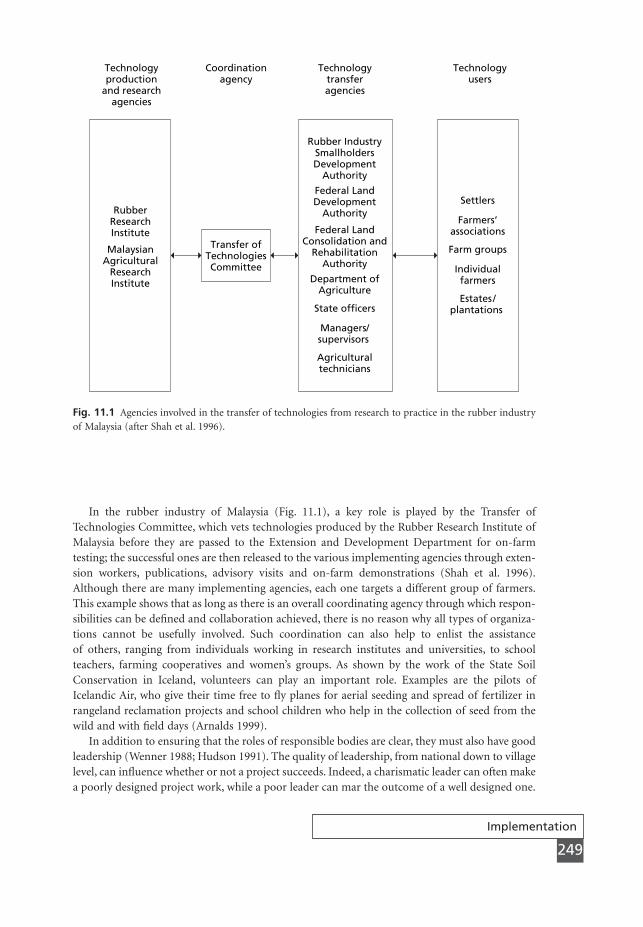
Implementation
249
In the rubber industry of Malaysia (Fig. 11.1), a key role is played by the Transfer ofTechnologies Committee, which vets technologies produced by the Rubber Research Institute ofMalaysia before they are passed to the Extension and Development Department for on-farmtesting; the successful ones are then released to the various implementing agencies through exten-sion workers, publications, advisory visits and on-farm demonstrations (Shah et al. 1996).Although there are many implementing agencies, each one targets a different group of farmers.This example shows that as long as there is an overall coordinating agency through which respon-sibilities can be defined and collaboration achieved, there is no reason why all types of organiza-tions cannot be usefully involved. Such coordination can also help to enlist the assistance of others, ranging from individuals working in research institutes and universities, to school teachers, farming cooperatives and women’s groups. As shown by the work of the State Soil Conservation in Iceland, volunteers can play an important role. Examples are the pilots ofIcelandic Air, who give their time free to fly planes for aerial seeding and spread of fertilizer inrangeland reclamation projects and school children who help in the collection of seed from thewild and with field days (Arnalds 1999).
In addition to ensuring that the roles of responsible bodies are clear, they must also have goodleadership (Wenner 1988; Hudson 1991). The quality of leadership, from national down to villagelevel, can influence whether or not a project succeeds. Indeed, a charismatic leader can often makea poorly designed project work, while a poor leader can mar the outcome of a well designed one.
RubberResearchInstitute
MalaysianAgricultural
ResearchInstitute
Rubber IndustrySmallholdersDevelopment
Authority
Federal LandDevelopment
Authority
Federal LandConsolidation and
RehabilitationAuthority
Department ofAgriculture
State officers
Managers/supervisors
Agriculturaltechnicians
Settlers
Farmers’associations
Farm groups
Individualfarmers
Estates /plantations
Transfer ofTechnologiesCommittee
Technologyproduction
and researchagencies
Technologytransferagencies
Technologyusers
Coordinationagency
Fig. 11.1 Agencies involved in the transfer of technologies from research to practice in the rubber industryof Malaysia (after Shah et al. 1996).
MSE11 11/19/04 02:45 PM Page 249

Chapter 11
250
The training of project managers, junior level managers and field technicians must thereforeinclude organizational, team and personal management as well as the technical aspects of soilconservation. It must also be backed up by a suitable career structure in which promotion is basedon performance and not solely on academic qualifications (Tejwani 1992). A post as a technicalassistant or a field soil conservation officer must not in any way be an inferior position to one inan academic or research environment. The conservation extension and advisory service must bea truly professional organization, staffed by professionals.
International organizations such as the Food and Agriculture Organization of the UnitedNations increasingly view their major role as encouraging national governments to establish con-servation programmes (Sanders 1988). Support is provided in the form of advice, secondment oftrained staff and coordination, bringing together financing agencies, in-country experts and insti-tutions and non-government organizations to work in partnership to produce a long-term con-servation plan (Dent 1996). The FAO also strongly supports regional bodies, like the Asian SoilConservation Network (ASOCON), the International Scheme for the Conservation and Reclamation of African Lands and the Conservation of Lands in Asia and the Pacific (CLASP),which bring together experts from different countries to share experiences with the aim of iden-tifying more effective approaches to soil conservation.
11.5
Requirements for technology
Although, as stated earlier, the broad technology for controlling soil erosion is understood, it mustsatisfy a number of requirements in addition to being scientifically sound. These include (Hudson1991):
� a high and quick financial return;� a reduction in risk;� no loss of existing benefits;� accessibility to the farmer in terms of extra inputs of labour and capital;� social acceptability, particularly in terms of gender issues;� an extension or modification of an existing practice rather than something new.
The farmers must be convinced that the technology will work and there must be sufficient insti-tutional support through the extension services. The technology should be effective on farms aswell as on research stations. Trial farms thus form an important part of soil conservation pro-grammes. In a scheme to introduce new technologies, including agroforestry and social forestry,to shifting cultivators in the uplands of Mindanao, Philippines, participatory programmes wereintroduced on selected farms in target areas. Within each target area, some ten farmers wereselected as programme participants. Conservation measures were introduced on each chosen farmafter discussion with the farmer family about their aspirations and the constraints of the presentfarming systems (Pava et al. 1990). Farmers trained through this programme were later asked toassist in promoting a similar programme run by the Mindanao Baptist Rural Life Center in thePulangi watershed (Cruz 1996).
MSE11 11/19/04 02:45 PM Page 250

Implementation
251
11.6
Legislative instruments
There is considerable disagreement among soil conservation workers on the importance oflegislation. Many early soil and water conservation programmes relied on laws that requiredfarmers to adopt certain techniques and desist from using others. Laws were also passed to restrictactivities on certain types of land; for example, cultivation should not be permitted on slopesabove a certain steepness, or forests in watershed areas should be protected. In some cases, legis-lation appears to work. Contour grass strips were introduced in Swaziland by royal decree andaccepted by almost all farmers (section 8.3). In Iceland, the State Soil Conservation Service hasthe legal power to acquire degraded land from farmers. In reality, however, the Swazi farmersadopted the technology because it seemed to work. The Conservation Service in Iceland has neverused its power because most farmers are only too willing to have the Service help them to restoretheir land. Generally, if legislation is effective it is because the principles behind it have alreadybeen accepted by the population (Hudson 1981).
If legislation is unworkable, the alternative is for farmers to adopt soil conservation volun-tarily. The low extent of farmer uptake, however, suggests that this does not work either,particularly where, as in the USA and Europe, the benefits of conservation are acquired by thecommunity at large rather than the individual farmer. In this situation, the role of governmentis to provide the necessary framework within which soil conservation can be promoted. In manycases, however, government frameworks have been detrimental to soil protection. The failure tocontain erosion in the USA (Napier 1990) and the increasing erosion problem in parts of Europe(Chisci 1986; Boardman 1988) have been attributed to agricultural policies and have led to calls for more environmentally friendly farming. Within this context, the following options areavailable as ways of encouraging farmers to adopt more conservation-oriented measures.
11.6.1 Regulatory instruments
Examples of regulatory instruments include prohibiting arable farming on land classified asunsuitable for arable crops, setting a maximum acceptable rate of erosion and making land usersliable to legal action if the rate is exceeded, and setting minimum requirements on farms for pro-vision of wildlife habitats. As mentioned above, these measures are only effective if they can bemonitored and enforced. Regulations based on rates of erosion would be almost impossible toapply because erosion is costly to measure and there is considerable uncertainty on the levels ofaccuracy that can be obtained. Proving in a court of law that soil loss from an area of land hadexceeded a particular level would be extremely difficult. The regulations would need to be specific about the size of the area involved and the return period of the event. It would also benecessary to prove that the erosion was the result of mismanagement on the part of the land userand not a response to an extreme event.
11.6.2 Advisory work
An effective advisory service is the vital element behind all participatory approaches to soil con-servation. An effective service, however, is costly, which means either a realistic charge must bemade to farmers or the government must defray the expense. In many countries, the farmers areunable to pay and government finance is not available to run a staff of well trained and moti-vated professionals. Even where farmers can pay, they are less likely to seek advice than if the
MSE11 11/19/04 02:45 PM Page 251

service were free. Whatever advice is given, it is clear from much of the evidence presented in sec-tions 7.3 and 11.4 that it will only be taken up if economic benefits ensue to the farmer. Thus, itis often necessary to support advisory work with other financial incentives.
11.6.3 Financial support
Financial support should only be provided if adopting particular soil conservation practicesresults in farming below the economic optimum and there is a benefit beyond the individualfarmer to the local community or to society in general. Incentives should be limited to stimulat-ing the involvement of farmers and not aimed at buying their participation (IFAD 1992). Themost suitable type of financial incentive is likely to be site specific. In some cases, it may consistof the provision of basic tools, such as pickaxes, wheelbarrows, seeds and cuttings; in others itmay include the construction of terraces, the costs of training courses for farmers and the cost of land lost to cultivation by grassing valley floors or introducing contour grass strips or shelterbelts. Incentives may also be set within a broader environmental context; for example,the promotion of winter cover crops to control nitrate leaching. They can also take the form of policies that have an effect on the net income of farmers and land users, or that provide thenecessary enabling conditions for the take-up of better conservation practices (Fig. 11.2; Enters1999).
Cost-sharing programmes between farmer and government were the basis of the early workof the US Soil Conservation Service (Napier 1990). Their disadvantages are that they lead to com-placency that soil conservation is being adequately supported and they require a long-term finan-cial commitment. Moreover, once the incentive is withdrawn, the conservation ceases, a responsethat is typical of many schemes based on financial incentives worldwide (Huszar 1999). Pro-grammes that rely on farmers taking land out of agricultural production suffer from the sameshort-term commitment. Under the 1985 Farm Bill, the United States government establishedthree conservation schemes: the Conservation Reserve Program; Highly Erodible Land Protection, including the Sodbuster and Conservation Compliance; and Wetland Protection.Under the Conservation Reserve Program (CRP), farmers entered a contractual arrangement withthe government to retire highly erodible land for ten years in return for a rent payment. Thosewho violated the contract within that time stood to lose federal farm benefits and were requiredto repay rent with interest. The Sodbuster Provision was designed to prevent new, highly erodi-ble land from being brought into production. Anyone converting such land to crops without anapproved conservation plan would lose all USDA programme benefits, such as price support,loans, disaster payments, federal crop insurance and CRP payments, on all the land they farmed.Under Conservation Compliance, an approved conservation programme was required on all cur-rently cropped erodible land. The Wetland Protection operated through the Swampbuster pro-gramme, removing benefits to anyone who converted wetland into crop production. Between1985 and 1990, nearly 13.7 million hectares of land were enrolled under CRP and conservationplans were approved for some 52.6 million hectares. Although a significant reduction in soilerosion resulted, the cost was extremely high because land owners could negotiate the price atwhich they were prepared to retire the land; in some locations the payments made were 200–300per cent higher than local cash rents (Hoag 1999). Further, the eligibility rules, requiring fields tohave erodible soils over at least two-thirds of their area and to have been cropped for two yearsbetween 1981 and 1985, meant that in Illinois, Iowa and Missouri some 25 per cent of the landclassified as highly erodible was excluded from the scheme (Padgitt 1989). There were also con-cerns about the way the provisions in the programmes were implemented. One study concludedthat some tens of millions of dollars in farm support went to farmers who should have been
Chapter 11
252
MSE11 11/19/04 02:45 PM Page 252
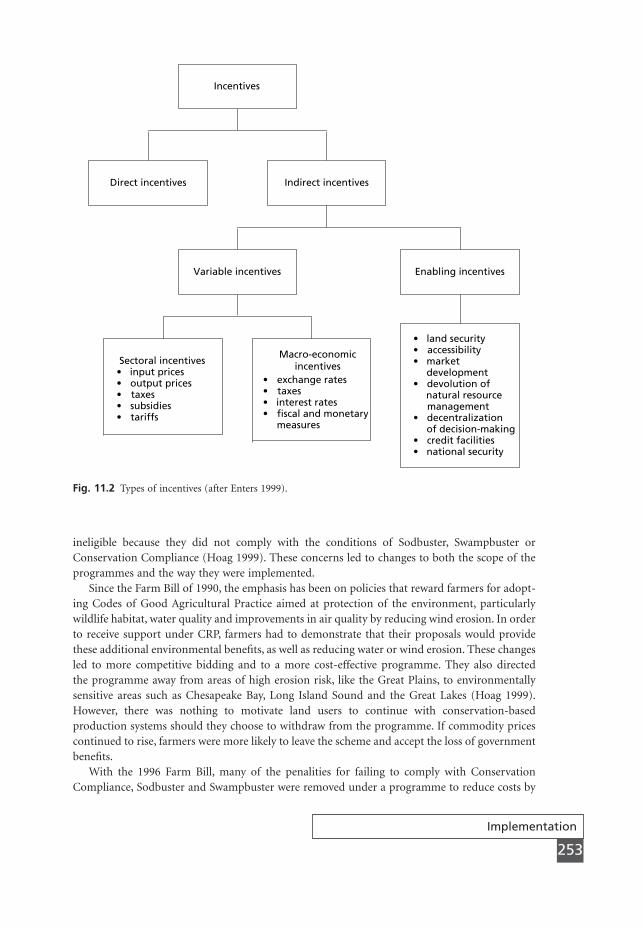
Implementation
253
ineligible because they did not comply with the conditions of Sodbuster, Swampbuster or Conservation Compliance (Hoag 1999). These concerns led to changes to both the scope of theprogrammes and the way they were implemented.
Since the Farm Bill of 1990, the emphasis has been on policies that reward farmers for adopt-ing Codes of Good Agricultural Practice aimed at protection of the environment, particularlywildlife habitat, water quality and improvements in air quality by reducing wind erosion. In orderto receive support under CRP, farmers had to demonstrate that their proposals would providethese additional environmental benefits, as well as reducing water or wind erosion. These changesled to more competitive bidding and to a more cost-effective programme. They also directed the programme away from areas of high erosion risk, like the Great Plains, to environmentallysensitive areas such as Chesapeake Bay, Long Island Sound and the Great Lakes (Hoag 1999).However, there was nothing to motivate land users to continue with conservation-based production systems should they choose to withdraw from the programme. If commodity pricescontinued to rise, farmers were more likely to leave the scheme and accept the loss of governmentbenefits.
With the 1996 Farm Bill, many of the penalities for failing to comply with Conservation Compliance, Sodbuster and Swampbuster were removed under a programme to reduce costs by
Incentives
Direct incentives Indirect incentives
Variable incentives Enabling incentives
Sectoral incentives• input prices• output prices• taxes• subsidies• tariffs
Macro-economicincentives
• land security • accessibility • market development • devolution of natural resource management • decentralization of decision-making • credit facilities • national security
• exchange rates • taxes • interest rates • fiscal and monetary measures
Fig. 11.2 Types of incentives (after Enters 1999).
MSE11 11/19/04 02:45 PM Page 253

Chapter 11
254
phasing out commodity support. The CRP remained, with the statutory upper limit beingincreased to 14 million hectares, but its focus changed to improving water quality rather thansaving soil. As a result, a greater proportion of the funding was directed towards livestock farmers.The 2002 Farm Bill authorized the continuation of CRP through to 2007, with the upper limitfor funding being increased to 15.9 million hectares. In addition, a new programme was introduced for soil erosion and sediment control in the Great Lakes Basin (Natural ResourcesConservation Service 2002). To assist farmers in bidding for funds, the Natural Resources Con-servation Service is promoting the CORE4 programme (Natural Resources Conservation Service1999), established by the Conservation Technology Information Center, as a basis for planning,financing and implementing farm management systems. CORE4 has four aims – better soil,cleaner water, greater profit and brighter future – and four components: conservation tillage(section 9.2.3), crop nutrient management, weed and pest management and conservation buffers(section 8.3).
Experience in the United States and many other countries shows that financial support for soilconservation must be treated with care. Inappropriate support can either destroy the long-termprospects of a soil conservation programme or require a high level of long-term funding thatcannot be sustained. Under certain circumstances, where damage from erosion can be clearlyrelated to inadequate on-site management and to a specific land user, financial costs can bereduced through legislation based on the principle of the ‘polluter pays’. The risk of prosecutionis a major incentive to the land user to prevent erosion because of the associated embarrassmentand inconvenience, in addition to the financial burden (Hannam 1999). In New South Wales,Australia, soil conservation offences are viewed as criminal offences but prosecutions are subjectto strict rules of evidence that must show substantial environmental damage and wilfulness onthe part of the land user. Although penalties can be up to A$110,000 for an offence and the courthas the power to set conditions on land rehabilitation in perpetuity, the high costs involved indeveloping the case mean that prosecution is only used as a last resort.
Land users need to be persuaded that the cost of conservation is preferable to any court set-tlement that might be demanded. This is more likely to apply to land users responsible for pre-venting erosion on mining spoil, industrial land, pipeline corridors and construction sites thanto farmers, where apportioning blame is more difficult. In the future, regular monitoring of theenvironment through remote sensing may make it easier to identify the sources of sediment delivered to rivers and lakes and it may be feasible to hold land users responsible where it can beshown that they have not complied with a Code of Good Agricultural Practice. The Ministries ofAgriculture in many European countries have issued such codes and subsidies are provided forintroducing riparian barriers, planting of trees and taking land out of production through set-aside programmes. Such support is best regarded as payments to land users for ‘environmentalservices’ for the public good (Giger et al. 1999; Enters 2001).
The Land Care Programme of Australia is nowconsidered one of the most successful commu-nity-based soil conservation programmes inthe world. It is a partnership between thefederal government, the various state govern-
Box 11
ments and the local community to combinethe work of the extension services with localskills and energy to address local and regionalproblems of land management. It developedbecause the more traditional approach ofusing extension services to transfer technology
Land Care
MSE11 11/19/04 02:45 PM Page 254

Implementation
255
to farmers and improve land managementpractices was viewed as a failure (Knowles-Jackson 1996).
There are now some 4000 Land Care orsimilar groups throughout Australia. Somedeal only with single issues, such as controllingrabbits or planting trees. The majority,however, are concerned with land use, landdegradation and land rehabilitation on acatchment basis. Land degradation covers soilerosion, salinity, loss of soil structure andquality, decline of native vegetation and lossof water quality. The groups are essentially‘self-starting, autonomous grassroots bodies’in which the members share aspirations, skillsand experiences, seek advice from experts andidentify funds from various state and federalgovernment and private sources to implementtheir proposals (Roberts 1992). Themembership includes representatives of thecommunity, business and government, as wellas farmers. The combination of peer pressure,camaraderie and sharing of work andinformation contributes to communityownership of the problem.
The Commonwealth Government ofAustralia provides funding without interferingwith the autonomy of the Land Care Groups.Funds are provided to support:� a regional and national facilitator to assist
groups and encourage communicationbetween groups and the government;
� Land Care Australia Ltd, a non-profitmaking public company that promotes theinvolvement of society in general and seekssponsorship through donations and grants;
� partial funding of Land Care projectsthrough the National Heritage Trust;
� the Australian Land Care Council, a commu-nity-based advisory body with a remit tofurther links between land care groups, theCommonwealth Government and theNational Heritage Trust.
Land Care groups submit project proposals,prepared according to national guidelines, tothe State Soil Conservation Service. Fundingunder the National Land Care programme isdependent on the benefits likely to accruefrom the proposal to the community at large.
Although the support of the National HeritageTrust is effectively a financial incentive fundedby taxation, the fact that it is partial funding,that the proposals come from local initiativeand that long-term community involvement isanticipated makes Land Care a ‘new genera-tion’ soil conservation programme, distinctfrom more traditional programmes basedsolely on government funding (Nabben 1999).Often the Land Care groups provide, throughtheir own cash, materials and labour, morethan twice the funding received from govern-ment sources. In addition, groups are able tosecure sponsorship from business. For example,Alcoa, a mining company, is helping tosupport six groups, comprising 88 farmingfamilies, to implement farm and catchmentplans in the Avon catchment, Western Australia, working with Agriculture WesternAustralia, which provides the technical exper-tise (Nabben 1999). Rather than expertisebeing presented as recipes by experts, in manyLand Care programmes the group memberswork together with the extension agents todetermine locally relevant topics and developtraining programmes that, through discussion,lead to understanding of the causes of aproblem and the planning of a long-term solu-tion (Marston 1996).
The following are considered keycharacteristics of Land Care groups (Campbell1994; Marston 1996):� they are generally concerned with a broad
range of multidisciplinary issues;� they are based on neighbourhoods or
catchments with contiguous boundaries,rather than merely groups of farmers witha common interest and narrow agenda;
� the impetus for establishing Land Caregroups comes from the community;
� proposals for land use management andconservation are developed through a peer-group framework;
� the momentum and ownership of the pro-gramme is with the community.
An important feature of the Land Care pro-gramme is that the financial support comesmainly in the form of grants rather thancheap credit, loans or subsidies. These can be
Continued
MSE11 11/19/04 02:45 PM Page 255

Chapter 11
256
targeted on programmes that encourage sus-tainable and profitable farming systems. Theytherefore encourage farmers to take the riskof developing such systems without commit-ment to long-term repayment or long-termgovernment support. Studies of the AvonLandcare Programme show that thebenefit–cost ratios (section 7.3.7) at the catch-ment level ranged from 1.7 to 2.3 and at thelevel of the individual farmer from 0.9 to 4.7(Nabben 1999). In addition, the programmebrought about positive sociological changes tothe rural community.
Despite the apparent success of the LandCare programme, there is a concern that
enthusiasm for it will decline. Bradsen (1994)questioned whether the programme wassufficiently funded or had the depth oftechnical rigour to address the issues, yetwould be successful enough to prevent a more effective system of land conservationbeing put in place. However, the changes inattitude brought about by the programme,the fact that many projects appear to beeconomically sustainable and the highmultiplier effect in terms of increased fundingbeyond that supplied by the governmentindicate that the Land Care programme seemsto be beneficial overall and providing valuefor money.
MSE11 11/19/04 02:45 PM Page 256

The way ahead
257
Soil is an important component of the global ecosystem. It is fundamental to life on earth. Yet,when compared to water and air, it is the poor relation in respect of policies designed to promoteacceptable standards of quality and ensure its protection. As seen in Chapter 11, soil erosion hasbeen recognized as a problem for centuries but the success rate in controlling it is poor. It hasgenerally not proved economic for farmers to practise soil conservation and the political will toenforce erosion control has not been there. One reason for this is that from the viewpoint of agri-cultural production, it has not been globally required. Between 1945 and 1990, the rate of loss ofagricultural land through erosion, at 0.1 per cent per year, was more than offset by annualincreases in crop productivity of 1–2 per cent as a result of better farming practices and greateruse of irrigation, pesticides and fertilizers. Against this background, Lomborg (2001) concludesthat extra efforts to reduce erosion cannot be justified. However, this conclusion ignores the extentto which past and present soil conservation works may have helped to reduce the loss of land.Further, an important section of the world’s population is still engaged in low-input agricultureand therefore effectively ‘mining’ the soil resource because that is the only way they can securetheir present livelihood; through poverty, they do not have access to the resources needed to adoptmore sustainable farming practices. There is also the issue of maintaining existing erosion controlmeasures in areas where migration and disease are reducing the size of the rural population. Aglobal analysis of the effects of erosion should also take account of resulting reductions in waterquality and increases in flooding. These are likely to become the main drivers for implementingerosion control measures and the major justification why the costs should be borne by the com-munity rather than the individual land user either through increased taxation or by paying higherprices for food, oil, gas, electricity and road and rail construction. Since, historically, erosion hasincreased whenever farmers have been unable to adjust their management practices to changingcircumstances, there is the added uncertainty of how farmers worldwide will adapt to any changesin climate.
The reasons for failure of many soil conservation projects and programmes are listed in Table12.1 (Hudson 1991). Whether or not existing approaches using participatory methods andworking at the community level (section 11.3) will overcome these remains to be seen. Estab-lishing an enthusiastic and professional extension service, encouraging the involvement of all thestakeholders in the community and improving the institutional framework for implementationwill all undoubtedly help but, in the end, the success of the new approaches will depend onwhether they help farmers and other land users to develop profitable and sustainable ways ofmanaging the land. The willingness of the community to pay that proportion of the profit thatrelates to the environmental benefit may well be critical.
CHAPTER 12
The way ahead
MSE12 11/19/04 02:46 PM Page 257
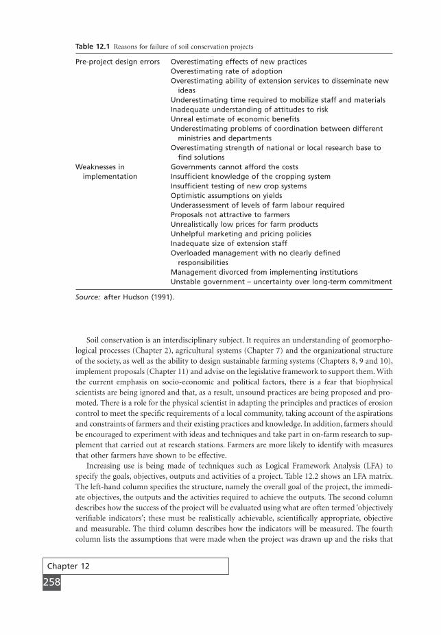
Chapter 12
258
Soil conservation is an interdisciplinary subject. It requires an understanding of geomorpho-logical processes (Chapter 2), agricultural systems (Chapter 7) and the organizational structureof the society, as well as the ability to design sustainable farming systems (Chapters 8, 9 and 10),implement proposals (Chapter 11) and advise on the legislative framework to support them. Withthe current emphasis on socio-economic and political factors, there is a fear that biophysical scientists are being ignored and that, as a result, unsound practices are being proposed and pro-moted. There is a role for the physical scientist in adapting the principles and practices of erosioncontrol to meet the specific requirements of a local community, taking account of the aspirationsand constraints of farmers and their existing practices and knowledge. In addition, farmers shouldbe encouraged to experiment with ideas and techniques and take part in on-farm research to sup-plement that carried out at research stations. Farmers are more likely to identify with measuresthat other farmers have shown to be effective.
Increasing use is being made of techniques such as Logical Framework Analysis (LFA) tospecify the goals, objectives, outputs and activities of a project. Table 12.2 shows an LFA matrix.The left-hand column specifies the structure, namely the overall goal of the project, the immedi-ate objectives, the outputs and the activities required to achieve the outputs. The second columndescribes how the success of the project will be evaluated using what are often termed ‘objectivelyverifiable indicators’; these must be realistically achievable, scientifically appropriate, objectiveand measurable. The third column describes how the indicators will be measured. The fourthcolumn lists the assumptions that were made when the project was drawn up and the risks that
Table 12.1 Reasons for failure of soil conservation projects
Pre-project design errors Overestimating effects of new practicesOverestimating rate of adoptionOverestimating ability of extension services to disseminate new
ideasUnderestimating time required to mobilize staff and materialsInadequate understanding of attitudes to riskUnreal estimate of economic benefitsUnderestimating problems of coordination between different
ministries and departmentsOverestimating strength of national or local research base to
find solutionsWeaknesses in Governments cannot afford the costs
implementation Insufficient knowledge of the cropping systemInsufficient testing of new crop systemsOptimistic assumptions on yieldsUnderassessment of levels of farm labour requiredProposals not attractive to farmersUnrealistically low prices for farm productsUnhelpful marketing and pricing policiesInadequate size of extension staffOverloaded management with no clearly defined
responsibilitiesManagement divorced from implementing institutionsUnstable government – uncertainty over long-term commitment
Source: after Hudson (1991).
MSE12 11/19/04 02:46 PM Page 258

The way ahead
259
Table 12.2 Matrix for logical framework analysis
Project strategy Indicators of Means and sources Assumptions andachievement of verification risks
GoalWhat general purpose What are the relevant What data are What external
will the strategy indicators (social, required to conditions or achieve? economic, verify that the factors are
environmental) to goal has been required to demonstrate that achieved? sustain the the goal has been project?achieved?
ObjectivesWhat are the What are the relevant What data are What conditions
immediate indicators to assess required to are required to objectives that whether the verify that the enable the should be met? objectives have objectives have objectives to What benefits and been met, e.g. been met? What meet the goals, costs are expected? benefit–cost are the methods e.g. project What improvements analysis, standards of data objectives are expected? of service, collection, related to
environmental analysis and erosion control enhancement? presentation? may need to be
consistent with sustainability?
OutputsWhat are the results What types, quality What are the What conditions
of the project? Do and quantity of sources of are required to they deliver the output will be information enable the intended objectives? produced, by whom required to show outputs to
and by when? that the outputs deliver the have been objectives?achieved? How will the data be collected, analysed and presented?
ActivitiesWhat activities must What materials, What are the What conditions
be undertaken to equipment, labour sources of must be met to produce the and services are information to ensure that the intended outputs, needed, over what show that the activities can beby whom and by period and at what resources to carried out as when? cost? implement the planned? What
project have factors might been met? How influence the will the data be achievement of collected, the outputs analysed and which are presented? outside the
control of theprojectmanagement?
MSE12 11/19/04 02:46 PM Page 259
may impede its performance. The top two rows in the matrix help to set the criteria for projectevaluation and the bottom two rows provide the framework for implemention. In many situa-tions, it may be appropriate to construct matrices for all the stakeholder groups involved in aproject, since each will have slightly different objectives and different roles to play. LFA placesmuch greater emphasis on monitoring and post-project evaluation and encourages the use of programme audits to evaluate the success of the project and the performance of the variousstakeholders.
Programme audits should be carried out by an independent organization and cover the performance of the people involved in the project, the project plans and the extent to which,for example, best management practices are being applied (Holbrook & Johns 2002). It is im-portant to decide who and what to audit and then to establish the base-line conditions againstwhich changes in conditions can be measured. The auditing team must decide what data to collectand what questions to ask, using the objectively verifiable indicators as a guide. Audits should be used to identify successes and deficiencies in a project and make recommendations forimprovements in performance. The results of an audit can often lead to changes to design manualsdescribing best management practices and to improvements in administration and training programmes.
Arguably, the weakest part of soil conservation programmes to date has been the lack of aneffective legal framework. Although many countries have a multiplicity of laws relating to landuse planning, forest management, species and habitat protection and water management, manyof which affect erosion indirectly, often they are not effective. Either they are not properly imple-mented or, in some cases, they enhance land degradation by encouraging inappropriate land use.The various global environmental treaties, conventions and strategies, such as Agenda 21 and theConventions on Climatic Change, Biological Diversity and Combating Desertification, areencouraging some governments to review their legislation relating to land degradation (Hannam& Boer 2001). The various Directives related to water, air and the environment issued by the European Union are having a similar effect among the member states. As indicated in Chapter11, most changes with respect to erosion and sedimentation relate to developing Codes of BestManagement Practices, with some financial incentives to encourage their adoption. In contrastto legislation on water quality, there are no legal definitions of acceptable soil quality or accept-able levels of tolerable erosion rates. Partly, this is because these cannot be easily defined or casesof their violation cannot be supported by unequivocal evidence. Enforcement is either throughcross-compliance, which means that land users can receive certain benefits only if they candemonstrate they have adopted specified management practices, or through penalties for envi-ronmental damage on the principle of the ‘polluter pays’; although, as seen in section 11.6.3, thelatter is rarely used. Generally, legislation is seen as providing an enabling role by establishing theinstitutional framework for implementing soil conservation and protection policies and en-couraging the voluntary participation of land users. As yet little attention has been given to in-corporating soil conservation practices into incentives for carbon sequestration and providing the legislation for its use in carbon credit trading.
According to Hannam (2001), an essential requirement for the future is to change public atti-tudes so that they will support the concept of ‘natural rights for soil’, which need to be protected.There are encouraging moves in this direction. Germany and Switzerland have specific Soil Pro-tection Acts within their legislation, the USA has many state and local resource conservation lawsthat have evolved from the 1935 Soil Conservation Act and the 1937 Standard Soil ConservationDistrict Law. Iceland has the 1965 Log um LandgræQslu to combat soil erosion in rangeland. TheEuropean Union is developing a Soils Directive and will expect each of its member states tosupport it by implementing soil strategies. As soil protection rises up the political agenda and
Chapter 12
260
MSE12 11/19/04 02:46 PM Page 260

national governments and communities become more aware of the substantial costs arising fromenvironmental damage associated with erosion, the political will to do something will increase.The Land Care movement in Australia, its counterpart in New Zealand and the community-basedErosion and Sedimentation Control programmes in the USA indicate that local communitygroups, involving all the stakeholders with an interest in soil erosion and resource management,may be the most effective way of implementing policy. Since this takes responsibilities away fromcentral governments, there is the question of whether governments will be prepared to providethe enabling financial support to community groups while allowing them local autonomy andthe ability to function with minimum bureaucracy.
Soil erosion is an integral part of the natural and cultural environment; its rate and spatialand temporal distribution depend on the interaction of physical and human circumstances.Archaeological and historical studies show how the nature of this interaction has changed overtime (section 1.2). Since the 1930s the need for erosion control has been driven largely by con-cerns over food production and security of food supply both for individual countries and for theincreasing world population. Since the 1970s, there has been increasing concern about the envi-ronmental damage caused by erosion. Although much of this damage is associated with sedimentderived from agricultural areas and the chemicals adsorbed to it, problems can also arise fromerosion on road banks, urban land, pipeline corridors and recreational areas (Chapter 7). Thepeople whose activities may contribute to erosion and who may be affected by any damage arenow a much wider group than farmers. Erosion affects whole communities. The next few decadeswill reveal whether the spatial distribution of erosion will alter in relation to changes in climateand the resulting human responses, particularly changes in land cover. Areas that traditionallyhave not experienced erosion problems may well do so in the future.
The way ahead
261
MSE12 11/19/04 02:46 PM Page 261

References
262
Abrahams, A.D., Parsons, A.J. and Hirsch, P.J. 1992. Fieldand laboratory studies of resistance to interrill overlandflow on semi-arid hillslopes, southern Arizona. InParsons, A.J. and Abrahams, A.D. (eds), Overland flow:hydraulics and erosion mechanics. UCL Press, London:1–23.
Abrahams, A.D., Parsons, A.J. and Luk, S.H. 1991. Theeffect of spatial variability in overland flow on thedownslope pattern of soil loss on a semiarid hillslope,southern Arizona. Catena 18: 255–70.
Abrahim, Y.B. and Rickson, R.J. 1989. The effectiveness ofstubble mulching in soil erosion control. In Schwert-mann, U., Rickson, R.J. and Auerswald, K. (eds), Soilerosion protection measures in Europe. Soil TechnologySeries 1: 115–26.
Abtew, W., Gregory, J.M. and Borrelli, J. 1989. Windprofile: estimation of displacement height and aerody-namic roughness. Transactions of the American Societyof Agricultural Engineers 32: 521–7.
Agate, E. 1983. Footpaths. British Trust for ConservationVolunteers, Wallingford.
Aina, P.O., Lal, R. and Taylor, G.S. 1977. Soil and cropmanagement in relation to soil erosion in the rainfor-est of western Nigeria. In Soil erosion: prediction andcontrol. Soil Conservation Society of America SpecialPublication 21: 75–82.
Aina, P.O., Lal, R. and Taylor, G.S. 1979. Effects of vegetalcover on soil erosion on an alfisol. In Lal, R. and Green-land, D.J. (eds), Soil physical properties and crop pro-duction in the tropics. Wiley, London: 501–8.
Al-Awadhi, J.M. and Willetts, B.B. 1999. Sand transportand deposition within arrays of non-erodible cylindri-cal elements. Earth Surface Processes and Landforms 24:423–35.
Alberts, E.E., Moldenhauer, W.C. and Foster, G.R. 1980.Soil aggregates and primary particles transported in rill
and interrill flow. Soil Science Society of America Journal44: 590–5.
Alberts, E.E., Laflen, J.M., Rawls, W.J., Simanton, J.R. andNearing, M.A. 1989. Soil component. In Lane, L.J. andNearing, M.A. (eds), USDA – Water Erosion PredictionProject: hillslope profile model documentation. USDA-ARS National Soil Erosion Research Laboratory ReportNo. 2: 6.1–6.15.
Aldon, E.F. 1976. Soil ripping treatments for runoffand erosion control. In Proceedings of the Federal Inter-Agency Sediment Conference, Denver, Colorado 3:2.24–2.29.
Al-Durrah, M.M. and Bradford, J.M. 1981. New methodsof studying soil detachment due to water drop impact.Soil Science Society of America Journal 45: 949–53.
Al-Durrah, M.M. and Bradford, J.M. 1982. Parameters fordescribing soil detachment due to single water dropimpact. Soil Science Society of America Journal 46:836–40.
Alexander, E.B. 1988. Rates of soil formation: implicationsfor soil loss tolerance. Soil Science 145: 37–45.
Alexander, M.J. 1990. Reclamation after tin mining on the Jos Plateau, Nigeria. Geographical Journal 156: 44–50.
Alfaro Moreno, J. 1988. Farmer income and soil conser-vation in the Peruvian Andes. In Rimwanich, S. (ed.),Land conservation for future generations. Department ofLand Development, Bangkok: 711–26.
Amphlett, M.B. 1988. A nested catchment approach tosediment yield monitoring in the Magat catchment,central Luzon, the Philippines. In Rimwanich, S. (ed.),Land conservation for future generations. Land Devel-opment Department, Bangkok: 283–98.
Anderson, M.G. and Richards, K.S. 1987. Slope stability:geotechnical engineering and geomorphology. Wiley,Chichester.
References
MSERE 11/19/04 02:51 PM Page 262
References
263
André, J.E. and Anderson, H.W. 1961. Variation of soilerodibility with geology, geographic zone, elevationand vegetation type in northern California wildlands.Journal of Geophysical Research 66: 3351–8.
Armbrust, D.V. 1999. Effectiveness of polyacrylamide(PAM) for wind erosion control. Journal of Soil andWater Conservation 54: 557–9.
Armstrong, C.L. and Mitchell, J.K. 1987. Transformationsof rainfall by plant canopy. Transactions of the Ameri-can Society of Agricultural Engineers 30: 688–96.
Arnalds, A. 1987. Ecosystem disturbance in Iceland. Arcticand Alpine Research 19: 508–13.
Arnalds, A. 1999. Incentives for soil conservation inIceland. In Sanders, D.W., Huszar, P.C., Sombatpanit, S.and Enters, T. (eds), Incentives in soil conservation: fromtheory to practice. Oxford and IBH Publishing, NewDelhi: 135–50.
Arnalds, O. 2000. The Iceland ‘rofabard’ soil erosion fea-tures. Earth Surface Processes and Landforms 25: 17–28.
Arnalds, O., Aradóttir, A.L. and Thorsteinsson, I. 1987.The nature and restoration of denuded areas in Iceland.Arctic and Alpine Research 19: 518–25.
Arnalds, O., Thorarinsdottir, E.F., Metusalemsson, S.,Jonsson, A., Gretarsson, E. and Arnason, A. 2001. Soilerosion in Iceland. The Soil Conservation ResearchService and the Agricultural Research Institute, Reyk-javik.
Arnoldus, H.M.J. 1980. An approximation of the rainfallfactor in the Universal Soil Loss Equation. In De Boodt,M. and Gabriels, D. (eds), Assessment of erosion. Wiley,Chichester: 127–32.
Arulanandan, K. and Heinzen, R.T. 1977. Factors influ-encing erosion in dispersive clays and methods of iden-tification. International Association of ScientificHydrology Publication 122: 75–81.
Arulanandan, K., Loganathan, P. and Krone, R.B. 1975.Pore and eroding fluid influences on the surfaceerosion of a soil. Journal of the Geotechnical Engineer-ing Division ASCE 101: 53–66.
Attaviroj, P. 1996. Land development villages and soildoctors: strategies towards better land husbandry inThailand. In Sombatpanit, S., Zöbisch, M.A., Sanders,D.W. and Cook, M.G. (eds), Soil conservation extension:from concepts to adoption. Soil and Water ConservationSociety of Thailand, Bangkok: 153–7.
Auerswald, K. and Schmidt, F. 1986. Atlas der Erosions-gefährdung in Bayern – Karten zum flächenhaftenBodenabtrung durch Regen. GLA-Fachberichte 1, Geol-ogisches Landesamt, Munich.
Babaji, G.A. 1987. Some plant stem properties and over-land flow hydraulics: a laboratory simulation. PhDThesis, Cranfield Institute of Technology.
Bache, D.H. 1986. Momentum transfer to plant canopies:influence of structure and variable drag. Atmosphericenvironment 20: 1369–78.
Baffoe-Bonnie, E. and Quansah, C. 1975. The effect oftillage on soil and water loss. Ghana Journal of Agricul-tural Science 8: 191–5.
Bagnold, R.A. 1937. The transport of sand by wind. Geo-graphical Journal 89: 409–38.
Bagnold, R.A. 1941. The physics of blown sand and desertdunes. Chapman and Hall, London.
Bagnold, R.A. 1951. The movement of a cohesionlessgranular bed by fluid flow over it. British Journal ofApplied Physics 2: 29–34.
Bagnold, R.A. 1979. Sediment transport by wind andwater. Nordic Hydrology 10: 309–22.
Baharuddin, K., Mokhtaruddin, A.M. and Majid, N.M.1996. Effects of logging on soil physical properties inPeninsular Malaysia. Land husbandry 1(1/2): 33–41.
Baily, B., Collier, P., Farres, P., Inkpen, R. and Pearson, A.2003. Comparative assessment of analytical and digitalphotogrammetric methods in the construction ofDEMs of geomorphological forms. Earth SurfaceProcesses and Landforms 28: 307–20.
Barahona, E., Quirantes, J., Guardiola, J.L. and Iriarte, A.1990. Factors affecting the susceptibility of soils tointerrill erosion in south-eastern Spain. In Rubio, J.L.and Rickson, R.J. (eds), Strategies to combat desertifica-tion in Mediterranean Europe. Commission of theEuropean Communities Report EUR 11175 EN/ES:216–27.
Barrow, E.G.C. 1989. The value of traditional knowledgein present-day soil-conservation practice: the exampleof West Pokot and Turkana. In Thomas, D.B., Biamah,E.K., Kilewe, A.M., Lundgren, L. and Mochoge, B.O.(eds), Soil and water conservation in Kenya. Departmentof Agricultural Engineering, University ofNairobi/Swedish International Development Author-ity: 471–85.
Barrow, G., Brotherton, D.I. and Maurice, O.C. 1973. TarnHows experimental restoration project. CountrysideRecreation News Supplement 9: 13–18.
Bates, C.G. 1924. The windbreak as a farm asset. USDAFarmers’ Bulletin 1405.
Bazzoffi, P., Torri, D. and Zanchi, C. 1980. Stima del-l’erodibilità dei suoli mediante simulazione di pioggiain laboratorio. Nota 1: simulatore di pioggia. AnnaliIstituto Sperimentale per lo Studio e la Difesa del Suolo11: 129–40.
Beasley, D.B., Huggins, L.F. and Monke, E.J. 1980.ANSWERS: a model for watershed planning. Transac-tions of the American Society of Agricultural Engineers23: 938–44.
MSERE 11/19/04 02:51 PM Page 263
Begin, Z.B. and Schumm, S.A. 1979. Instability of alluvialvalley floors: a method for its assessment. Transactionsof the American Society of Agricultural Engineers 22:347–50.
Bekele, M.W. and Thomas, D.B. 1992. The influence ofsurface residue on soil loss and runoff. In Hurni, H. andTato, K. (eds), Erosion, conservation and small-scalefarming. Geographica Bernensia, Bern: 439–52.
Bennett, H.H. 1939. Soil conservation. McGraw-Hill, NewYork.
Bennett, J.P. 1974. Concepts of mathematical modeling of sediment yield. Water Resources Research 10: 485–92.
Bensalem, B. 1977. Examples of soil and water conserva-tion practices in North African countries. FAO SoilsBulletin 33: 151–60.
Berry, L. and Ruxton, B.P. 1960. The evolution of HongKong harbour basin. Zeitschrift für Geomorphologie 4:97–115.
Beschta, R.L. 1978. Long-term patterns of sediment pro-duction following road construction and logging in theOregon Coast Range. Water Resources Research 14:1011–16.
Besler, H. 1987. Slope properties, slope processes and soilerosion risk in the tropical rain forest of KalimantanTimur (Indonesian Borneo). Earth Surface Processesand Landforms 12: 195–204.
Betts, H.D., Trustrum, N.A. and DeRose, R.C. 2003. Geo-morphic changes in a complex gully system measuredfrom sequential digital elevation models, and implica-tions for management. Earth Surface Processes andLandforms 28: 1043–58.
Beuselinck, L., Govers, G., Hairsine, P.B., Sander, G.C. andBreynaert M. 2002. The influence of rainfall on sedi-ment transport by overland flow over areas of netdeposition. Journal of Hydrology 257: 145–63.
Beven, K. and Binley, A. 1992. The future of distributedmodels: model calibration and uncertainty prediction.Hydrological Processes 6: 279–98.
Bharad, G.M. and Bathkal, B.C. 1991. Role of vetiver grassin soil and moisture conservation. Vetiver Newsletter 6:15–17.
Bhardwaj, S.P., Khybri, M.L., Ram, S. and Prasad, S.N.1985. Crop geometry – a nonmonetary input for reduc-ing erosion in corn on four percent slope. In El-Swaify,S.A., Moldenhauer, W.C. and Lo, A. (eds), Soil erosionand conservation. Soil Conservation Society ofAmerica, Ankeny, IA: 644–8.
Bielders, C.L., Rajot, J.L. and Koala, S. 1998. Wind erosionresearch in Niger: the experience of ICRISAT andAdvanced Research Organizations. In Sivakumar,M.V.K., Zöbisch, M.A., Koala, S. and Maukonen, T.
References
264
(eds), Wind erosion in Africa and west Asia: problemsand control strategies. ICARDA, Aleppo: 95–123.
Biot, Y. 1990. THEPROM – an erosion productivitymodel. In Boardman, J., Foster, I.D.L. and Dearing, J.A.(eds), Soil erosion on agricultural land. Wiley, Chich-ester: 465–79.
Bisal, F. 1950. Calibration of splash cup for soil erosionstudies. Agricultural Engineering 31: 621–2.
Bishop, D.M. and Stevens, M.E. 1964. Landslides onlogged areas in southeast Alaska. USDA Forest ResearchService Paper NOR-1.
Blong, R.J., Graham, O.P. and Veness, J.A. 1982. The roleof sidewall processes in gully development: some NSWexamples. Earth Surface Processes and Landforms 7:381–5.
Boardman, J. 1988. Public policy and soil erosion inBritain. In Hooke, J.M. (ed), Geomorphology in envi-ronmental planning. Wiley, Chichester: 33–50.
Boardman, J. 1990. Soil erosion on the South Downs: areview. In Boardman, J., Foster, I.D.L. and Dearing, J.A.(eds), Soil erosion on agricultural land. Wiley, Chich-ester: 87–105.
Boardman, J. and Evans, R. 1994. Soil erosion in Britain:a review. In Rickson, R.J. (ed.), Conserving soil resources:European perspectives. CAB International, Wallingford:3–12.
Bocharov, A.P. 1984. A description of devices used in thestudy of wind erosion of soils. Balkema, Rotterdam.
Boiffin, J. 1985. Stage and time-dependency of soil crust-ing in situ. In Callebaut, F., Gabriels, D. and De Boodt,M. (eds), Assessment of surface crusting and sealing.Flanders Research Centre for Soil Erosion and Conser-vation, State University of Gent: 91–8.
Boiffin, J. and Monnier, G. 1985. Infiltration rate asaffected by soil surface crusting caused by rainfall. InCallebaut, F., Gabriels, D. and De Boodt, M. (eds),Assessment of surface crusting and sealing. FlandersResearch Centre for Soil Erosion and Conservation,State University of Gent: 210–17.
Boix-Fayos, C., Calvo-Cases, A., Imeson, A.C. andSoriano-Soto, M.D. 2001. Influence of soil propertieson the aggregation of some Mediterranean soils and theuse of aggregate size and stability as land degradationindicators. Catena 44: 47–67.
Bojö, J. 1992. Cost–benefit analysis of soil and water con-servation projects: a review of 20 empirical studies. InTato, K. and Hurni, H. (eds), Soil conservation for sur-vival. Soil and Water Conservation Society, Ankeny, IA:195–205.
Bollinne, A. 1975. La mesure de l’intensité du splash sursol limoneux. Mise au point d’une technique de terrainet premiers résultats. Pédologie 25: 199–210.
MSERE 11/19/04 02:51 PM Page 264
References
265
Bollinne, A. 1977. La vitesse de l’érosion sous culture enrégion limoneuse. Pédologie 27: 191–206.
Bollinne, A. 1978. Study of the importance of splash andwash on cultivated loamy soils of Hesbaye (Belgium).Earth Surface Processes 3: 71–84.
Bollinne, A., Laurant, A. and Boon, W. 1979. L’érosivitédes précipitations à Florennes. Révision de la carte des isohyètes et de la carte d’érosivité de la Belgique.Bulletin de la Société Géographique de Liège 15: 77–99.
Bonell, M. and Gilmour, D.A. 1978. The development ofoverland flow in a tropical rain forest catchment.Journal of Hydrology 39: 365–82.
Bonsu, M. 1981. Assessment of erosion under differentcultural practices on a savanna soil in the northernregion of Ghana. In Morgan, R.P.C. (ed), Soil conserva-tion: problems and prospects. Wiley, Chichester: 247–53.
Bonsu, M. 1985. Organic residues for less erosion andmore grain in Ghana. In El-Swaify, S.A., Moldenhauer,W.C. and Lo, A. (eds), Soil erosion and conservation.Soil Conservation Society of America, Ankeny, IA: 615–20.
Bonsu, M. and Obeng, H.B. 1979. Effects of cultural practices on soil erosion and maize production in thesemi-deciduous rain forest and forest-savanna tran-sition zones of Ghana. In Lal, R. and Greenland, D.J.(eds), Soil physical properties and crop production in thetropics. Wiley, Chichester: 509–19.
Boon, W. and Savat, J. 1981. A nomogram for the predic-tion of rill erosion. In Morgan, R.P.C. (ed), Soil conser-vation: problems and prospects. Wiley, Chichester:303–19.
Boonchee, S., Peukrai, S. and Chinabutr, N. 1988. Effectsof land development and management on soil conser-vation in northern Thailand. In Rimwanich, S. (ed),Land conservation for future generations. Department ofLand Development, Bangkok: 1101–12.
Borghi, C.E., Giannoni, S.M. and Martinez-Rica, J.P. 1990.Soil removed by voles of the genus Pitymys in theSpanish Pyrenees. Pirineos 136: 3–17.
Borst, H.L. and Woodburn, R. 1942. The effect ofmulching and methods of cultivation on runoff anderosion from Muskingum silt loam. Agricultural Engi-neering 23: 19–22.
Bork, H.R. 1989. The history of soil erosion in southernLower Saxony. Landschaftsgenese und Landschaftsökolo-gie 16: 135–63.
Bork, H.R. and Rohdenburg, H. 1981. Rainfall simulationin south-east Spain. In Morgan, R.P.C. (ed), Soil con-servation: problems and prospects. Wiley, Chichester:293–302.
Bork, H.R., Bork, H., Dalchow, C., Faust, B., Priorr, H.P.and Schatz, T. 1998. Landschaftsentwicklung in Mit-
teleuropa. Wirkungen des Menschen auf die Land-schaften. Klett-Perthes, Gotha.
Boubakari, M. and Morgan, R.P.C. 1999. Contour grassstrips for soil erosion control on steep lands: a labora-tory simulation. Soil Use and Management 15: 21–6.
Bouma, N.A. and Imeson, A.C. 2000. Investigation of rela-tionships between measured field indicators anderosion processes on badland surfaces at Petrer, Spain.Catena 40: 147–71.
Bouyoucos, G.J. 1935. The clay ratio as a criterion of sus-ceptibility of soils to erosion. Journal of the AmericanSociety of Agronomy 27: 738–51.
Bowyer-Bower, T.A.S. 1993. Effects of rainfall intensityand antecedent moisture on the steady-state infiltra-tion rate in a semi-arid region. Soil Use and Manage-ment 9: 69–76.
Brabben, T., Bird, J. and Bolton, P. 1988. Improving thesurvey and computation of reservoir sedimentation.ODU Bulletin 12: 4–7.
Bradford, J.M. and Piest, R.F. 1980. Erosional develop-ment of valley-bottom gullies in the Upper Mid-Western United States. In Coates, D.R. and Vitek, J.D.(eds), Thresholds in geomorphology. Allen and Unwin,London: 75–101.
Bradford, J.M., Truman, C.C. and Huang, C. 1992. Com-parisons of three measures of resistance of soil surfaceseals to raindrop splash. Soil Technology 5: 47–56.
Bradsen, J. 1994. Natural resource conservation in Australia: some fundamental issues. In Napier, T.L.,Camboni, S.M. and El-Swaify, S.A. (eds), Adopting conservation on the farm: an international perspective on the socioeconomics of soil and water conservation.Soil and Water Conservation Society, Ankeny, IA:435–60.
Brandt, C.J. 1989. The size distributions of throughfalldrops under vegetation canopies. Catena 16: 507–24.
Brandt, C.J. 1990. Simulation of the size distribution anderosivity of raindrops and throughfall drops. EarthSurface Processes and Landforms 15: 687–98.
Brazier, R.E., Beven, K.J., Freer, J. and Rowan, J.S. 2000.Equifinality and uncertainty in physically based soilerosion models: application of the GLUE methodologyto WEPP. Earth Surface Processes and Landforms 25:825–45.
Bridges, E.M. and Oldeman, L.R. 2001. Food productionand environmental degradation. In Bridges, E.M.,Hannam, I.D., Oldeman, L.R., Penning de Vries, F.W.T.,Scherr, S.J. and Sombatpanit, S. (eds), Response to landdegradation. Science Publishers, Enfield, NH: 36–43.
Brierley, J.S. 1976. Kitchen gardens in the West Indies witha contemporary study from Grenada. Journal of Tropi-cal Geography 43: 30–40.
MSERE 11/19/04 02:51 PM Page 265
Brown, L.C. and Foster, G.R. 1987. Storm erosivity usingidealized intensity distributions. Transactions of theAmerican Society of Agricultural Engineers 30: 379–86.
Browning, G.M., Norton, R.A., McCall, A.G. and Bell, F.G.1948. Investigation in erosion control and the reclama-tion of eroded land at the Missouri Valley Loess Conser-vation Experiment Station, Clarinda, Iowa. USDATechnical Bulletin 959.
Bruce-Okine, E. and Lal, R. 1975. Soil erodibility as determined by raindrop technique. Soil Science 119:149–57.
Brunori, F., Penzo, M.C. and Torri, D. 1989. Soil shearstrength: its measurement and soil detachability.Catena 16: 59–71.
Brunsden, D. and Prior, D.B. 1984. Slope instability. Wiley,Chichester.
Bryan, R.B. 1968. The development, use and efficiency ofindices of soil erodibility. Geoderma 2: 5–26.
Bryan, R.B. 1979. The influence of slope angle on soilentrainment by sheetwash and rainsplash. EarthSurface Processes 4: 43–58.
Bryan, R.B. and Poesen, J.W.A. 1989. Laboratory experi-ments on the influence of slope length on runoff, per-colation and rill development. Earth Surface Processesand Landforms 14: 211–31.
Bryan, R.B. and Yair, A. 1982. Perspectives on studies ofbadland geomorphology. In Bryan, R. and Yair, A. (eds),Badland geomorphology and piping. Geo Books,Norwich: 1–12.
Bubenzer, G.D. 1979. Rainfall characteristics importantfor simulation. In Proceedings, Rainfall simulator work-shop, Tucson, Arizona. USDA-SEA Agricultural Reviewsand Manuals ARM-W-10: 22–34.
Bubenzer, G.D. and Jones, B.A. 1971. Drop size andimpact velocity effects on the detachment of soil undersimulated rainfall. Transactions of the American Societyof Agricultural Engineers 14: 625–8.
Bunte, K. and Poesen, J. 1994. Effects of rock fragment sizeand cover on overland flow hydraulics, local turbulenceand sediment yield on an erodible soil surface. EarthSurface Processes and Landforms 19: 115–35.
Buol, S.W., Hole, F.D. and McCracken, P.J. 1973. Soilgenesis and classification. Iowa State University Press,Ames, IA.
Buttner, G. and Csillag, F. 1989. Comparative study ofcrop and soil mapping using multitemporal and multispectral SPOT and Landsat Thematic Mapperdata. Remote Sensing of the Environment 29: 241–9.
Cammeraat, L.H. 2002. A review of two strongly con-trasting geomorphological systems within the context
References
266
of scale. Earth Surface Processes and Landforms 27:1201–22.
Campbell, A. 1994. Landcare: community shaping the landand the future. Allen and Unwin, Sydney.
Carson, M.A. and Kirkby, M.J. 1972. Hillslope form andprocess. Cambridge University Press, Cambridge.
Carte, A. 1971. Raindrop spectra in Pretoria. South AfricanGeographical Journal 53: 100–3.
Carter, C.E., Greer, J.D., Braud, H.J. and Floyd, J.M. 1974.Raindrop characteristics in south central United States.Transactions of the American Society of AgriculturalEngineers 17: 1033–7.
Carver, M. and Schreier, H. 1995. Sediment and nutrientbudgets over four spatial scales in the Jhikhu Kholawatershed: implications for land use management. InSchreier, H., Shah, P.B. and Brown, S. (eds), Challengesin mountain resource management in Nepal: processes,trends and dynamics in middle mountain watersheds.ICIMOD/IDRC/UBC, Kathmandu: 163–70.
Cazzuffi, D., Monti, R. and Rimoldi, P. 1991. Geosynthet-ics subjected to different conditions of rain and runoffin erosion control application: a laboratory investiga-tion. In Erosion control: a global perspective. Interna-tional Erosion Control Association, Steamboat Springs,CO: 191–208.
Cerdà, A., Ibáñez, S. and Calvo, A. 1997. Design and oper-ation of a small and portable rainfall simulator forrugged terrain. Soil Technology 11: 163–70.
Cerdan, O., Le Bissonnais, Y., Couturier, A., Bourennane,H. and Souchère, V. 2002a. Rill erosion on cultivatedhillslopes during two extreme rainfall events in Normandy, France. Soil and Tillage Research 67: 99–108.
Cerdan, O., Le Bissonnais, Y., Martin, P. and Lecomte, V.2002b. Sediment concentration in interrill flow: inter-actions between soil surface conditions, vegetation andrainfall. Earth Surface Processes and Landforms 27:193–205.
Cerro, C., Bech, J., Codina, B. and Lorente, J. 1998. Mod-eling rain erosivity using disdrometric techniques. SoilScience Society of America Journal 62: 731–5.
Cervera, M., Clotet, N. and Sala, M. 1990. Runoff and sed-iment production on small badland basins in the UpperLlobregat catchment (submediterranean environ-ment). Internal Report, LUCDEME Project.
Chamen, T., Alakukku, L., Pires, S., Sommer, C., Spoor,G., Tijink, F. and Weisskopf, P. 2003. Prevention strate-gies for field traffic-induced subsoil compaction: areview. Part 2. Equipment and field practices. Soil andTillage Research 73: 161–74.
Chan, C.C. 1981a. Evaluation of soil loss factors on culti-vated slopelands of Taiwan. Food and Fertilizer Tech-nology Center Taipei, Technical Bulletin 55.
MSERE 11/19/04 02:51 PM Page 266
References
267
Chan, C.C. 1981b. Conservation measures in the culti-vated slopes of Taiwan. Food and Fertilizer TechnologyCenter Taipei, Extension Bulletin 137.
Chapman, D.M. 1990. Aeolian sand transport – an opti-mized model. Earth Surface Processes and Landforms 15:751–60.
Chapman, G. 1948. Size of raindrops and their strikingforce at the soil surface in a red pine plantation. Trans-actions of the American Geophysical Union 29: 664–70.
Chappell, A., McTainsh, G., Leys, J. and Strong, G. 2003.Simulations to optimize sampling of aeolian sedimenttransport in space and time for mapping. Earth SurfaceProcesses and Landforms 28: 1223–41.
Charman, P.E.V. 1978. Soils of New South Wales: theircharacterisation, classification and conservation. NSWSoil Conservation Service Technical Handbook 1.
Cheatle, R.J. and Njoroge, S.N.J. 1993. Smallholder adop-tion of some land husbandry practices in Kenya. InHudson, N. and Cheatle, R.J. (eds), Working withfarmers for better land husbandry. IT Publications,Southampton: 130–41.
Chepil, W.S. 1945. Dynamics of wind erosion. III. Trans-port capacity of the wind. Soil Science 60: 475–80.
Chepil, W.S. 1946. Dynamics of wind erosion. VI. Sortingof soil material by wind. Soil Science 61: 331–40.
Chepil, W.S. 1950. Properties of soil which influence winderosion. II. Dry aggregate structure as an index oferodibility. Soil Science 69: 403–14.
Chepil, W.S. 1960. Conversion of relative field erodibilityto annual soil loss by wind. Soil Science Society ofAmerica Proceedings 24: 143–5.
Chepil, W.S., Siddoway, F.H. and Armbrust, D.V. 1964.Wind erodibility of knolly terrain. Journal of Soil andWater Conservation 19: 179–81.
Chepil, W.S. and Woodruff, N.P. 1963. The physics ofwind erosion and its control. Advances in Agronomy 15:211–302.
Chepil, W.S., Woodruff, N.P. and Zingg, A.W. 1955. Fieldstudy of wind erosion in western Texas. USDA Soil Con-servation Service Technical Paper SCS-TP-125.
Chisci, G. 1986. Influence of change in land use and man-agement on the acceleration of land degradation phe-nomena in the Apennines hilly areas. In Chisci, G. andMorgan, R.P.C. (eds), Soil erosion in the European Com-munity: impact of changing agriculture. Balkema, Rot-terdam: 3–18.
Chisci, G., Bazzoffi, P. and Mbagwu, J.S.C. 1989. Com-parison of aggregate stability indices for soil classifica-tion and assessment of soil management practices. SoilTechnology 2: 113–33.
Chisci, G. and Zanchi, C. 1981. The influence of differenttillage systems and different crops on soil losses on hilly
silty-clayey soil. In Morgan, R.P.C. (ed.), Soil conser-vation: problems and prospects. Wiley, Chichester:211–17.
Chisci, G., Zanchi, C. and Biagi, B. 1978. Drenaggio pro-fondo in un suolo limo-argilloso su sedimenti pliocenimarini in funzione di differenti colture. Annali IstitutoSperimentale per lo Studio e la Difesa del Suolo 9:257–72.
Chorley, R.J. 1959. The geomorphic significance ofsome Oxford soils. American Journal of Science 257:503–15.
Clark, R., Durón, G., Quispe, G. and Stocking, M.A. 1999.Boundary bunds or piles of stones? Using farmers’practices in Bolivia to aid soil conservation. MountainResearch and Development 19: 235–40.
Clarke, M.A., Walsh, R.P.D., Sinun, W., Larenus, J. andHanapi, J. 2002. Soil erosion and surface roughnessdynamics in relation to slope angle in primary andlogged tropical rainforest, eastern Sabah. In Rubio, J.L.,Morgan, R.P.C., Asins, S. and Andreu, V. (eds), Soil atthe third millennium. Geoforma Ediciones, Logroño:1471–84.
Cogo, N.P., Moldenhauer, W.C. and Foster, G.R. 1984. Soilloss reductions from conservation tillage practices. SoilScience Society of America Journal 48: 368–73.
Colclough, J.D. 1965. Soil conservation and soil erosioncontrol in Tasmania: tunnel erosion. Tasmanian Journalof Agriculture 36: 7–12.
Coleman, R. 1981. Footpath erosion in the English LakeDistrict. Applied Geography 1: 121–31.
Collins, A.L. and Walling, D.E. 2002. Selecting finger-printproperties for discriminating sediment sources in riverbasins. Journal of Hydrology 261: 218–44.
Combeau, A. and Monnier, G. 1961. A method for thestudy of structural stability: application to tropicalsoils. African Soils 6: 33–52.
Cooke, R.U. and Doornkamp, J.C. 1974. Geomorphologyin environmental management. Oxford UniversityPress, Oxford.
Coote, D.R., Malcolm-McGovern, C.A., Wall, G.J., Dick-inson, W.T. and Rudra, R.P. 1988. Seasonal variation oferodibility indices based on shear strength and aggre-gate stability in some Ontario soils. Canadian Journalof Soil Science 68: 405–16.
Coppin, N.J. and Richards, I.G. 1990. Use of vegetation incivil engineering. CIRIA/Butterworths, London.
Coutinho, M.A. and Tomás, P.P. 1995. Characterisation ofraindrop size distributions at the Vale Formoso Exper-imental Erosion Center. Catena 25: 187–97.
Critchley, W.R.S. and Bruijnzeel, L.A. 1995. Terrace risers:erosion control or sediment source? In Singh, R.B. andHaigh, M.J. (eds), Sustainable reconstruction of highland
MSERE 11/19/04 02:51 PM Page 267
and headwater regions. Oxford and IBH Publishing,New Delhi: 529–41.
Critchley, W.R.S., Reij, C. and Willcocks, T.J. 1994. Indige-nous soil and water conservation: a review of the stateof knowledge and prospects of building on traditions.Land Degradation and Rehabilitation 5: 293–314.
Critchley, W.R.S., Sombatpanit, S. and Medina, S.M. 2001.Uncertain steps? Terraces in the tropics. In Bridges,E.M., Hannam, I.D., Oldeman, L.R., Penning de Vries,F.W.T., Scherr, S.J. and Sombatpanit, S. (eds), Responseto land degradation. Science Publishers, Enfield, NH:325–38.
Crosson, P. 1995. Soil erosion estimates and costs. Science269: 461–4.
Crouch, R.J. 1976. Field tunnel erosion – a review. Journalof the Soil Conservation Service NSW 32: 98–111.
Crouch, R.J. 1978. Variation in the structural stability ofsoil in a tunnel-eroding area. In Emerson, W.W., Bond,R.D. and Dexter, A.R. (eds), Modification of soil struc-ture. Wiley, Chichester: 267–74.
Crouch, R.J. 1990a. Erosion processes and rates for gulliesin granitic soils, Bathurst, New South Wales, Australia.Earth Surface Processes and Landforms 15: 169–73.
Crouch, R.J. 1990b. Rates and mechanisms of discontin-uous gully erosion a red-brown earth catchment, NewSouth Wales, Australia. Earth Surface Processes andLandforms 15: 277–82.
Crouch, R.J., McGarity, J.W. and Storrier, R.R. 1986.Tunnel formation processes in the Riverina area ofNSW, Australia. Earth Surface Processes and Landforms11: 157–68.
Crowley, C.M. 2003. Ten rules of thumb for culvert cross-ings. Erosion Control 10(6): 72–5.
Cruse, R.M. and Larson, W.E. 1977. Effect of soil shearstrength on soil detachment due to raindrop impact.Soil Science Society of America Journal 41: 777–81.
Cruz, E.B. 1996. The adoption of hedgerows as a soil con-servation measure in the Philippines. In Sombatpanit,S., Zöbisch, M.A., Sanders, D.W. and Cook, M.G. (eds),Soil conservation extension: from concepts to adoption.Soil and Water Conservation Society of Thailand,Bangkok: 447–55.
Currence, H.D. and Lovely, W.G. 1970. The analysis ofsurface roughness. Transactions of the American Societyof Agricultural Engineers 13: 710–14.
Daddow, R.L. and Warrington, G.E. 1983. Growth-limit-ing soil bulk densities as influenced by soil texture.WDG Report, WSDG-TN-00005, USDA Forest Service.
Davidson, J.L. and Quirk, J.P. 1961. The influence of dis-solved gypsum on pasture establishment on irrigatedsodic clays. Australian Journal of Agricultural Research12: 100–10.
References
268
De Bano, L.F., Mann, L.D. and Hamilton, D.A. 1970.Translocation of hydrophobic substances into soil byburning organic litter. Soil Science Society of AmericaProceedings 34: 130–3.
Dedkov, A.P. and Mozzherin, V.I. 1996. Erosion and sed-iment yield on the Earth. International Association ofScientific Hydrology Publication 236: 29–33.
De Graaf, J. 2001. The economic appraisal of soil andwater conservation measures. In Bridges, E.M.,Hannam, I.D., Oldeman, L.R., Penning de Vries, F.W.T.,Scherr, S.J. and Sombatpanit, S. (eds), Response to landdegradation. Science Publishers, Enfield, NH: 274–83.
De Jong, E., Begg, C.B.M. and Kachanoski, R.G. 1983.Estimates of soil erosion and deposition for someSaskatchewan soils. Canadian Journal of Soil Science 63:607–17.
De Jong, S.M. 1994. Applications of reflective remotesensing for land degradation studies in a Mediter-ranean environment. Nederlandse Geografische Studies177.
De Jong, S.M., Paracchini, M.L., Bertolo, F., Folving, S.,Megier, J. and De Roo, A.P.J. 1999. Regional assessmentof soil erosion using the distributed model SEMMEDand remotely sensed data. Catena 37: 291–308.
De Kesel, M. and De Vleeschauwer, D. 1981. Sand dunefixation in Tunisia by means of polyurea polyalkyleneoxide (Uresol). In Lal, R. and Russell, E.W. (eds),Tropical agricultural hydrology. Wiley, Chichester:273–81.
De Meis, M.R.M. and De Moura, J.R.S. 1984. Upper Qua-ternary sedimentation and hillslope evolution: south-eastern Brazilian plateau. American Journal of Science284: 241–54.
Dent, F.J. 1996. The FAO land conservation and rehabili-tation scheme. In Sombatpanit, S., Zöbisch, M.A.,Sanders, D.W. and Cook, M.G. (eds), Soil conservationextension: from concepts to adoption. Soil and WaterConservation Society of Thailand, Bangkok: 301–14.
De Ploey, J. 1981. The ambivalent effects of some factorsof erosion. Mémoirs, Institute de Géologie, l’Universitéde Louvain 31: 171–81.
De Ploey, J. 1982. A stemflow equation for grasses andsimilar vegetation. Catena 9: 139–52.
De Ploey, J. 1989a. A model for headcut retreat in rills andgullies. Catena Supplement 14: 81–6.
De Ploey, J. 1989b. Erosional systems and perspectives forerosion control in European loess areas. In Schwert-mann, U., Rickson, R.J. and Auerswald, K. (eds), Soilerosion protection measures in Europe. Soil TechnologySeries 1: 93–102.
De Ploey, J. and Cruz, O. 1979. Landslides in the Serra doMar, Brazil. Catena 6: 111–22.
MSERE 11/19/04 02:51 PM Page 268

References
269
De Ploey, J. and Gabriels, D. 1980. Measuring soil loss andexperimental studies. In Kirkby, M.J. and Morgan,R.P.C. (eds), Soil erosion. Wiley, Chichester: 63–108.
De Ploey, J., Savat, J. and Moeyersons, J. 1976. The differ-ential impact of some soil factors on flow, runoff creepand rainwash. Earth Surface Processes 1: 151–61.
De Roo, A.P.J. 1996. Validation problems of hydrologicand soil-erosion catchment models: examples from aDutch erosion project. In Anderson, M.G. and Brooks,S.M. (eds), Advances in hillslope processes. Wiley, Chich-ester: 669–83.
DeRose, R.C., Gomez, B., Marden, M. and Trustrum, N.A.1998. Gully erosion in Mangatu Forest, New Zealand,estimated from digital elevation models. Earth SurfaceProcesses and Landforms 23: 1045–53.
Dickinson, W.T., Rudra, R.P. and Wall, G.J. 1986. Identifi-cation of soil erosion and fluvial sediment problems.Hydrological Processes 1: 111–24.
Dimitrakopoulos, A.P., Martin, R.E. and Papamichos,N.T. 1994. A simulation model of soil heating duringwildland fires. In Sala, M. and Rubio, J.L. (eds), Soilerosion and degradation as a consequence of forest fires.Geoforma Ediciones, Logroño: 199–206.
Dimitrakopoulos, A.P. and Seilopoulos, D. 2002. Effects ofrainfall and burning intensity on early post-fire soilerosion in a Mediterranean forest of Greece. In Rubio,J.L., Morgan, R.P.C., Asins, S. and Andreu, V. (eds), Soilat the third millennium. Geoforma Ediciones, Logroño:1351–7.
Disrud, L.A. and Krauss, R.K. 1971. Examining theprocess of soil detachment from clods exposed to wind-driven simulated rainfall. Transactions of the AmericanSociety of Agricultural Engineers 14: 90–2.
Dissmeyer, G.E. and Foster, G.R. 1981. Estimating thecover-management factor (C) in the Universal Soil LossEquation for forest conditions. Journal of Soil andWater Conservation 36: 235–40.
Dlamini, P.M. and Maro, P.S. 1988. The economic behav-iour of the farming communities on conservation pro-grammes: Swaziland and the SADCC region. Paperpresented to Second Workshop, Economics of Conser-vation (Swaziland).
Doerr, S.H., Leighton-Boyce, G., Shakesby, R.A. andWalsh, R.P.D. 2002. The role of hydrophobicity in soilerosion processes: evidence from Portuguese forestsoils. In Rubio, J.L., Morgan, R.P.C., Asins, S. andAndreu, V. (eds), Soil at the third milllennium. Geo-forma Ediciones, Logroño: 1311–22.
Doerr, S.H., Shakesby, R.A. and Walsh, R.P.D. 2000. Soilwater repellency: its causes, characteristics and hydro-geomorphological significance. Earth-Science Reviews51: 33–65.
Dolgilevich, M.I., Sofronova, A.A. and Mayevskaya, L.L.1973. Klassifikatsia pochv zapadnoy Sibiri, severnogoKazakhstana po stepeniy podatlivosti k vetrovoy eroziy.Bulletin VNIIA No. 12.
Dong, Z., Liu, X., Li, F., Wang, H. and Zhao, A. 2002.Impact-entrainment relationship in a saltating cloud.Earth Surface Processes and Landforms 27: 641–58.
Dotterweich, M., Schmitt, A., Schmidtchen, G. and Bork,H.R. 2003. Quantifying historical gully erosion innorthern Bavaria. Catena 50: 135–50.
Douglas, I. 1978. The impact of urbanisation on fluvialgeomorphology in the humid tropics. Géo-Eco-Trop 2:239–42.
Douglas, J.T. and Goss, M.J. 1982. Stability and organicmatter content of surface soil aggregates under differ-ent methods of cultivation and in grassland. Soil andTillage Research 2: 155–76.
Downes, R.G. 1946. Tunnelling erosion in north-easternVictoria. Journal of the Council of Scientific and Indus-trial Research 19: 283–92.
Dregne, H.E. 1982. Desertification: man’s abuse ofthe land. Journal of Soil and Water Conservation 33:11–14.
D’Souza, V.P.C. and Morgan, R.P.C. 1976. A laboratorystudy of the effect of slope steepness and curvature onsoil erosion. Journal of Agricultural EngineeringResearch 21: 21–31.
Duley, F.L. and Russel, J.C. 1943. Effect of stubblemulching on soil erosion and runoff. Soil ScienceSociety of America Proceedings 7: 77–81.
Dunne, T. and Aubry, B.F. 1986. Evaluation of Horton’stheory of sheetwash and rill erosion on the basis of fieldexperiments. In Abrahams, A.D. (eds), Hillslopeprocesses. Allen and Unwin, London: 31–53.
Dunne, T. and Black, R.D. 1970. Partial area contributionsto storm runoff in a small New England watershed.Water Resources Research 6: 1296–311.
Dyrness, C.T. 1975. Grass-legume mixtures for erosioncontrol along forest roads in western Oregon. Journalof Soil and Water Conservation 30: 169–73.
Edwards, K. 1993. Soil erosion and conservation in Aus-tralia. In Pimental, D. (ed), World soil erosion and con-servation. Cambridge University Press, Cambridge:147–69.
Edwards, W.M. and Owens, L.B. 1991. Large storm effectson total soil loss. Journal of Soil and Water Conservation46: 75–8.
Eger, H. and Bado, J. 1992. Village-level land managementin the central plateau of Burkina Faso. In Hurni, H. andTato, K. (eds), Erosion, conservation and small-scalefarming. Geographica Bernensia, Bern: 531–40.
Ekwue, E.I. 1990. Effect of organic matter on splash
MSERE 11/19/04 02:51 PM Page 269
detachment and the processes involved. Earth SurfaceProcesses and Landforms 15: 175–81.
Ekwue, E.I. 1992. Effect of organic and fertiliser treat-ments on soil physical properties and erodibility. Soiland Tillage Research 22: 199–209.
Ekwue, E.I., Ohu, J.O. and Wakawa, I.H. 1993. Effects ofincorporating two organic materials at varying levelson splash detachment of some soils from Borno State,Nigeria. Earth Surface Processes and Landforms 18:399–406.
Ellis-Jones, J. and Mason, T. 1999. Livelihood strategiesand assets of small farmers in the evaluation of soil andwater management practices in the temperate Inter-Andean valleys of Bolivia. Mountain Research andDevelopment 19: 221–34.
Ellison, W.D. 1944. Two devices for measuring soilerosion. Agricultural Engineering 25: 53–5.
El-Swaify, S.A. 1994. State of the art for assessing soil andwater conservation needs and technologies. In Napier,T.L., Camboni, S.M. and El-Swaify, S.A. (eds), Adoptingconservation on the farm. An international perspective onthe socioeconomics of soil and water conservation. Soiland Water Conservation Society, Ankeny, IA: 13–27.
El-Swaify, S.A., Dangler, E.W. and Armstrong, C.L. 1982.Soil erosion by water in the tropics. College of TropicalAgriculture and Human Resources, University ofHawaii.
El-Swaify, S.A., Pathak, P., Rego, T.J. and Singh, S. 1985.Soil management for optimized productivity underrainfed conditions in the semi-arid tropics. Advances inSoil Science 1: 1–64.
Elwell, H.A. 1978. Modelling soil losses in SouthernAfrica. Journal of Agricultural Engineering Research 23:111–27.
Elwell, H.A. 1981. A soil loss estimation technique forsouthern Africa. In Morgan, R.P.C. (ed.), Soil conserva-tion: problems and prospects. Wiley, Chichester: 281–92.
Elwell, H.A. and Stocking, M.A. 1976. Vegetal cover toestimate soil erosion hazard in Rhodesia. Geoderma 15:61–70.
Elwell, H.A. and Wendelaar, F.E. 1977. To initiate a vegetalcover data bank for soil loss estimation. Department ofConservation and Extension, Research Bulletin 23.
Emama Ligdi, E. and Morgan, R.P.C. 1995. Contour grassstrips: a laboratory simulation of their role in soilerosion control. Soil Technology 8: 109–17.
Emmett, W.W. 1965. The vigil network: methods of mea-surement and a sample of data collected. InternationalAssociation of Scientific Hydrology Publication 66:89–106.
Emmett, W.W. 1970. The hydraulics of overland flow onhillslopes. USGS Professional Paper 662-A.
References
270
Engman, E.T. 1986. Roughness coefficients for routingsurface runoff. Journal of the Irrigation and DrainageDivision ASCE 112: 39–53.
Enters, T. 1999. Incentives as policy instruments – keyconcepts and definitions. In Sanders, D.W., Huszar,P.C., Sombatpanit, S. and Enters, T. (eds), Incentives insoil conservation: from theory to practice. Oxford andIBH Publishing, New Delhi: 25–40.
Enters, T. 2001. Incentives for soil conservation. InBridges, E.M., Hannam, I.D., Oldeman, L.R., Penningde Vries, F.W.T., Scherr, S.J. and Sombatpanit, S. (eds),Response to land degradation. Science Publishers,Enfield, NH: 351–60.
Environment Agency, 2002. Agriculture and naturalresources: benefits, costs and potential solutions. Envi-ronment Agency, Bristol.
Eppink, L.A.A.J. and Spaan, W.P. 1989. Agricultural winderosion control measures in The Netherlands. In Schw-ertmann, U., Rickson, R.J. and Auerswald, K. (eds), Soilerosion protection measures in Europe. Soil TechnologySeries 1: 1–13.
Ervin, D.E. and Washburn, R. 1981. Profitability of soilconservation practices in Missouri. Journal of Soil andWater Conservation 36: 107–11.
Escarameia, M. 1998. River and channel revetments – adesign manual. Thomas Telford, London.
Evans, A.C. 1948. Studies on the relationships betweenearthworms and soil fertility. II. Some effects ofearthworms and soil structure. Applied Biology 35:1–13.
Evans, R. 1977. Overgrazing and soil erosion on hill pas-tures with particular reference to the Peak District.Journal of the British Grassland Society 32: 65–76.
Evans, R. 1980. Mechanics of water erosion and theirspatial and temporal controls: an empirical viewpoint.In Kirkby, M.J. and Morgan, R.P.C. (eds), Soil erosion.Wiley, Chichester: 109–28.
Evans, R. and Nortcliff, S. 1978. Soil erosion in northNorfolk. Journal of Agricultural Science Cambridge 90:185–92.
Everaert, W. 1991. Empirical relations for the sedimenttransport capacity of interrill flow. Earth SurfaceProcesses and Landforms 16: 513–32.
Eyles, R.J. 1967. Laterite at Kerdau, Pahang, Malaya.Journal of Tropical Geography 25: 18–23.
Fang, Z.S., Zhou, P.H., Liu, Q.D., Liu, B.H., Ren, L.T. andZhang, H.X. 1981. Terraces in the loess plateau ofChina. In Morgan, R.P.C. (ed.), Soil conservation: prob-lems and prospects. Wiley, Chichester: 481–513.
FAO 1965. Soil erosion by water. FAO, Rome.FAO 1976. A framework for land evaluation. FAO Soils
Bulletin 32.
MSERE 11/19/04 02:51 PM Page 270
References
271
Farres, P. 1978. The role of time and aggregate size in thecrusting process. Earth Surface Processes 3: 243–54.
Fenster, C.R. and McCalla, T.M. 1970. Tillage practices inwestern Nebraska with a wheat-fallow rotation.Nebraska Agriculture Station, Lincoln, Bulletin 597.
Fenton, E.W. 1937. The influence of sheep on the vegeta-tion of hill grazings in Scotland. Journal of Ecology 25:424–30.
Fifield, J.S. 1999. Effective sediment and erosion controlfor construction sites. Erosion Control 5(6): 36–40.
Fifield, J.S. and Malnor, L.K. 1990. Erosion control mate-rials vs a semiarid environment. What has been learnedfrom three years of testing? In Erosion control: technol-ogy in transition. International Erosion Control Associ-ation, Steamboat Springs, CO: 233–48.
Fifield, J.S., Malnor, L.K. and Dezman, L.E. 1989. Effec-tiveness of erosion control products on steep slopes tocontrol sediment and to establish dryland grasses. InErosion knows no boundaries. International ErosionControl Association, Steamboat Springs, CO: 45–55.
Finney, H.J. 1984. The effect of crop covers on rainfallcharacteristics and splash detachment. Journal of Agri-cultural Engineering Research 29: 337–43.
Flach, K.W., Barnwell Jr, T.O. and Crosson, P. 1997.Impacts of agriculture on atmospheric carbon dioxide.In Paul, E.A., Paustian, K., Elliott, E.T. and Cole, C.V.(eds), Soil organic matter in temperate agroecosystems:long-term experiments in North America. CRC Press,Boca Raton, FL: 3–13.
Folly, A., Quinton, J.N. and Smith, R.E. 1999. Evaluationof the EUROSEM model using data from the Catsopwatershed, The Netherlands. Catena 37: 507–19.
Foster, G.R. 1982. Modeling the erosion process. In Haan,C.T., Johnson, H.P. and Brakensiek, D.L. (eds), Hydro-logic modeling of small watersheds. American Society ofAgricultural Engineers Monograph 5: 297–380.
Foster, G.R., Johnson, C.B. and Moldenhauer, W.C. 1982.Hydraulics of failure of unanchored corn-stalk andwheat straw mulches for erosion control. Transactionsof the American Society of Agricultural Engineers 25:940–7.
Foster, G.R., Lane, L.J., Nowlin, J.D., Laflen, J.M. andYoung, R.A. 1981. Estimating erosion and sedimentyield on field-sized areas. Transactions of the AmericanSociety of Agricultural Engineers 24: 1253–63.
Foster, G.R. and Meyer, L.D. 1972. A closed-form soilerosion equation for upland areas. In Shen, H.W. (ed.),Sedimentation. Department of Civil Engineer-ing,Colorado State University, Fort Collins: 12.1–12.19.
Foster, R.L. and Martin, G.L. 1969. Effect of unit weightand slope on erosion. Journal of the Irrigation andDrainage Division ASCE 95: 551–61.
Fournier, F. 1960. Climat et érosion: la relation entre l’éro-sion du sol par l’eau et les précipitations atmosphériques.Presses Universitaires de France, Paris.
Fournier, F. 1972. Soil conservation. Nature and Environ-ment Series, Council of Europe.
Fox, D. and Bryan, R.B. 1992. Influence of a polyacry-lamide soil conditioner on runoff generation and soilerosion: field tests in Baringo District, Kenya. Soil Tech-nology 5: 101–19.
Fox, F.A., Flanagan, D.C., Wagner, L.E. and Deer-Ascough,L. 2001. WEPS and WEPP science commonalityproject. In Ascough II, J.C. and Flanagan, D.C. (eds),Proceedings of the ASAE symposium on soil erosionresearch for the 21st century: 376–79.
Francis, I.S. and Taylor, J.A. 1989. The effect of forestrydrainage operations on upland sediment yields: a studyof two peat-covered catchments. Earth Surface Processesand Landforms 14: 73–83.
Franke, R. and Chasin, B.H. 1981. Peasants, peanuts,profits and pastoralists. The Ecologist 11: 156–68.
Fredén, C. and Furuholm, L. 1978. The Säterberget Gullyat Brattforsheden, Värmland. Geologiska Föreningens iStockholm Förhandlingar 100: 231–5.
Free, G.R. 1960. Erosion characteristics of rainfall. Agri-cultural Engineering 41: 447–9, 455.
Freer-Hewish, R.J. 1991. Erosion of road shoulders fromrainfall and runoff. In Erosion control: a global perspec-tive. International Erosion Control Association, Steam-boat Springs, CO: 263–73.
Froehlich, W. and Starkel, L. 1993. The effects ofdeforestation on slope and channel evolution in thetectonically active Darjeeling Himalaya. Earth SurfaceProcesses and Landforms 18: 285–90.
Fryrear, D.W. 1984. Soil ridges-clods and wind erosion.Transactions of the American Society of AgriculturalEngineers 27: 445–8.
Fryrear, D.W. 1986. A field dust sampler. Journal of Soiland Water Conservation 41: 117–20.
Fryrear, D.W., Saleh, A., Bilbro, J.D., Schomberg, H.M.,Stout, J.E. and Zobeck, T.M. 1998. Revised Wind ErosionEquation (RWEQ). Wind Erosion and Water Conserva-tion Research Unit, USDA-ARS, Southern Plains AreaCropping Systems Research Laboratory, Technical Bulletin 1.
Fryrear, D.W., Stout, J.E., Hagen, L.J. and Vories, E.D.1991. Wind erosion: field measurement and analysis.Transactions of the American Society of AgriculturalEngineers 34: 155–60.
Fullen, M.A., Tye, A.M. and Cookson, K.E. 1995. Effectsof ‘Agri-SC’ soil conditioner on soil structure anderodibility: some further observations. Soil Use andManagement 11: 183–5.
MSERE 11/19/04 02:51 PM Page 271
Gabriels, D. 2002. Rain erosivity in Europe. In Rubio, J.L.,Morgan, R.P.C., Asins, S. and Andreu, V. (eds), Man andsoil at the third millennium. Geoforma Ediciones,Logroño: 99–108.
Gabriels, D., Cornelis, W., Pollet, I., van Coillie, T. andOuessar, M. 1997. The ICE wind tunnel for wind andwater erosion studies. Soil Technology 10: 1–8.
Gabriels, D. and De Boodt, M. 1978. Evaluation of soilconditioners for water erosion control and sand stabi-lization. In Emerson, W.W., Bond, R.D. and Dexter,A.R. (eds), Modification of soil structure. Wiley, Chich-ester: 341–8.
Gabriels, D., Maene, L., Lenvain, J. and De Boodt, M. 1977.Possibilities of using soil conditioners for soil erosioncontrol. In Greenland, D.J. and Lal, R. (eds), Soil con-servation and management in the humid tropics. Wiley,London: 99–108.
Gabriels, D., Pauwels, J.M. and De Boodt, M. 1975. Theslope gradient as it affects the amounts and size distri-bution of soil loss material from runoff on silt loamaggregates. Mededelingen Fakulteit Landbouwweten-schappen, Rijksuniversiteit Gent 40: 1333–8.
Gale, W.J., McColl, R.W. and Xie, F. 1993. Sandy fields tra-ditional farming water conservation in China. Journalof Soil and Water Conservation 48: 474–7.
Gantzer, C.J., Anderson, S.H., Thompson, A.L. andBrown, J.R. 1990. Estimating soil erosion after 100 yearsof cropping on Sanborn field. Journal of Soil and WaterConservation 45: 641–4.
George, H. and Jarvis, M.G. 1979. Land for camping andcaravan sites, picnic sites and footpaths. In Jarvis, M.G.and Mackney, D. (eds), Soil survey applications. SoilSurvey of England and Wales Technical Monograph 13:166–83.
Gerlach, T. 1966. Wspólczesby rozwóy stoków w dorzeczu górnego Grajcarka (Beskid Wysoki-KarpatyZachodnie). Prace Geograf. IG PAN 52 (with Frenchsummary).
Gerontidis, S., Kosmas, C., Detsis, B., Marathianou, M.,Zafiriou, Th. and Tsara, M. 2001. The effect of mould-board plough on tillage erosion along a hillslope.Journal of Soil and Water Conservation 56: 147–52.
Ghadiri, H. and Payne D. 1979. Raindrop impact and soilsplash. In Lal, R. and Greenland, D.J. (eds), Soil physi-cal properties and crop production in the tropics. Wiley,Chichester: 95–104.
Ghadiri, H., Rose, C.W. and Hogarth, W.L. 2001. Theinfluence of grass and porous barrier strips on runoffhydrology and sediment transport. Transactions of theAmerican Society of Agricultural Engineers 44: 259–68.
Gichangi, E.M., Jones, R.K., Njarui, D.M., Simpson, J.R.,Mututho, J.M.N. and Kitheka, S.K. 1992. Pitting prac-
References
272
tices for rehabilitating eroded grazing land in the semi-arid tropics of eastern Kenya: a progress report. InHurni, H. and Tato, K. (eds), Erosion, conservation andsmall-scale farming. Geographica Bernensia, Bern:313–27.
Gichungwa, J.K. 1970. Soil conservation in CentralProvince (Kenya). Ministry of Agriculture, Nairobi.
Gifford, G.F. 1976. Applicability of some infiltration for-mulae to rangeland infiltrometer data. Journal ofHydrology 28: 1–11.
Giger, M., Liniger, H.P. and Critchley, W. 1999. Use ofdirect incentives and profitability of soil and water con-servation in eastern and southern Africa. In Sanders,D.W., Huszar, P.C., Sombatpanit, S. and Enters, T.(eds), Incentives in soil conservation: from theory to practice. Oxford and IBH Publishing, New Delhi:247–74.
Gillette, D.A. and Stockton, P.H. 1989. The effect ofnonerodible particles on wind erosion on erodible surfaces. Journal of Geophysical Research 94: 12885–93.
Gilley, J.E., Woolhiser, D.A. and McWhorter, D.B. 1985.Interrill soil erosion. Part II. Testing and use of modelequations. Transactions of the American Society of Agri-cultural Engineers 28: 154–9.
Giovannini, G. 1994. The effect of fire on soil quality. InSala, M. and Rubio, J.L. (eds), Soil erosion and degrada-tion as a consequence of forest fires. Geoforma Ediciones,Logroño: 15–27.
Giovannini, G., Lucchesi, S. and Giachetti, M. 1988.Effects of heating on some physical and chemical para-meters related to soil aggregation and erodibility. SoilScience 146: 255–61.
Glasstetter, M. and Prasuhn, V. 1992. The influence ofearthworm activity on erodibility and soil losses incentral European agricultural soils. In Hurni, H. andTato, K. (eds), Erosion, conservation and small-scalefarming. Geographica Bernensia, Bern: 285–98.
Godwin, R.J. and Spoor, G. 1977. Soil failure with narrowtines. Journal of Agricultural Engineering Research 22:213–28.
Golosov, V. 2003. Application of Chernobyl-derived 137Csfor the assessment of soil redistribution within a culti-vated field. Soil and Tillage Research 69: 85–98.
Gong, S.Y. and Jiang, D.Q. 1977. Soil erosion and itscontrol in small gully watersheds in the rolling loessarea on the middle reaches of the Yellow River. Parissymposium on erosion and soil matter transport in inlandwaters, preprint.
Goosens, D., Offer, Z. and London, G. 2000. Wind tunneland field calibration of five aeolian sand traps. Geo-morphology 35: 233–52.
MSERE 11/19/04 02:51 PM Page 272
References
273
Gosh, R.L., Kaul, O.N. and Subba-Rao, B.K. 1978. Someaspects of water relations and nutrition in Eucalyptusplantations. Indian Forester 104: 517–24.
Govers, G. 1985. Selectivity and transport capacity of thinflows in relation to rill erosion. Catena 12: 35–49.
Govers, G. 1987. Initiation of motion in overland flow.Sedimentology 34: 1157–64.
Govers, G. 1989. Grain velocities in overland flow: a lab-oratory study. Earth Surface Processes and Landforms14: 481–98.
Govers, G. 1990. Empirical relationships for the trans-porting capacity of overland flow. International Associ-ation of Hydrological Sciences Publication 189: 45–63.
Govers, G. 1991. Time-dependency of runoff velocity anderosion: the effect of the initial soil moisture profile.Earth Surface Processes and Landforms 16: 713–29.
Govers, G. 1992. Relationship between discharge, velocityand flow area for rills eroding loose, non-layered mate-rials. Earth Surface Processes and Landforms 17: 515–28.
Govers, G., Everaert, W., Poesen, J., Rauws, G. and DePloey, J. 1987. Susceptibilité d’un sol limoneux à l’éro-sion par rigoles: essais dans le grand canal de Caen. Bul-letin du Centre de Géomorphologie CNRS Caen 33:83–106.
Govers, G. and Poesen, J. 1985. A field-scale study ofsurface sealing and compaction on loam and sandyloam soils. Part I. Spatial variability of soil surfacesealing and crusting. In Callebaut, F., Gabriels, D. andDe Boodt, M. (eds), Assessment of soil surface crustingand sealing. Flanders Research Centre for Soil Erosionand Conservation, State University of Gent: 171–82.
Govers, G. and Poesen, J. 1988. Assessment of the interrilland rill contributions to total soil loss from an uplandfield plot. Geomorphology 1: 343–54.
Govers, G. and Rauws, G. 1986. Transporting capacity ofoverland flow on plane and on irregular beds. EarthSurface Processes and Landforms 11: 515–24.
Govers, G., Vandaele, K., Desmet, P., Poesen, J. and Bunte,K. 1994. The role of tillage in soil redistribution on hill-slopes. European Journal of Soil Science 45: 469–78.
Gray, D.H. and Leiser, A.T. 1982. Biotechnical slope protec-tion and erosion control. Van Nostrand Reinhold, NewYork.
Green, W.H. and Ampt, G.A. 1911. Studies on soil physics.I: The flow of air and water through soils. Journal ofAgricultural Science 4: 1–24.
Greenway, D.R. 1987. Vegetation and slope stability. InAnderson, M.G. and Richards, K.S. (eds), Slope stabil-ity: geotechnical engineering and geomorphology. Wiley,Chichester: 187–230.
Gregory, K.J. and Walling, D.E. 1973. Drainage basin formand process. Edward Arnold, London.
Grierson, I.T. 1978. Gypsum and red-brown earths. InEmerson, W.W., Bond, R.D. and Dexter, A.R. (eds),Modification of soil structure. Wiley, Chichester: 315–24.
Gril, J.J., Canler, J.P. and Carsoulle, J. 1989. The benefitsof permanent grass and mulching for limiting runoffand erosion in vineyards. Experimentations using rain-fall simulations in the Beaujolais. In Schwertmann, U.,Rickson, R.J. and Auerswald, K. (eds), Soil erosion pro-tection measures in Europe. Soil Technology Series 1:157–66.
Grissinger, E.H. 1966. Resistance of selected clay systemsto erosion by water. Water Resources Research 2: 131–8.
Grissinger, E.H. and Asmussen, L.E. 1963. Discussion ofchannel stability in undisturbed cohesive soils by E.M.Flaxman. Journal of the Hydraulics Division ASCE 89:529–64.
Gupta, A. 1982. Observations on the effects of urbaniza-tion on runoff and sediment production in Singapore.Singapore Journal of Tropical Geography 3: 137–46.
Gupta, J.P. 1979. Some observations on the periodic variations in moisture in stabilized and unstabilizeddunes of the Indian desert. Journal of Hydrology 41:153–6.
Guy, B.T. and Dickinson, W.T. 1990. Inception of sedi-ment transport in shallow overland flow. Catena Sup-plement 17: 91–109.
Guy, B.T., Dickinson, W.T., Rudra, R.P. and Wall, G.J.1990. Hydraulics of sediment-laden sheetflow and theinfluence of simulated rainfall. Earth Surface Processesand Landforms 15: 101–18.
Gyssels, G., Poesen, J., Nachtergaele, J. and Govers, G.2002. The impact of sowing density of small grains onrill and ephemeral gully erosion in concentrated flowzones. Soil and Tillage Research 64: 189–201.
Haas, H.J., Evans, C.E. and Miles, E.F. 1957. Nitrogen andcarbon changes in Great Plains soils as influenced bycropping and soil treatments. USDA Technical Bulletin1164.
Hagen, L.J. 1991. A wind erosion prediction system tomeet user needs. Journal of Soil and Water Conservation46: 106–11.
Hall, G.F., Daniels, R.B. and Foss, J.E. 1979. Soil forma-tion and renewal rates in the US. In Symposium ondeterminants of soil loss tolerance. Soil Science Societyof America Annual Meeting, Fort Collins, CO.
Hall, M.J. 1970. A critique of methods of simulating rain-fall. Water Resources Research 6: 1104–14.
Hall, R.L. and Calder, I.R. 1993. Drop size modificationby forest canopies: measurements using a disdrometer.Journal of Geophysical Research 98: 18465–70.
Hallsworth, E.G. 1987. Anatomy, physiology and psychol-ogy of erosion. Wiley, Chichester.
MSERE 11/19/04 02:51 PM Page 273
Hann, M.J. and Morgan, R.P.C. 2003. Prevention ofbiorestoration failures along pipeline rights-of-way. InMoore, H.M., Fox, H.R. and Elliott, S. (eds), Land recla-mation: extending the boundaries. Balkema, Rotterdam:227–33.
Hannam, I. 1999. Soil conservation incentives in NewSouth Wales, Australia. In Sanders, D.W., Huszar, P.C.,Sombatpanit, S. and Enters, T. (eds), Incentives in soilconservation: from theory to practice. Oxford and IBHPublishing, New Delhi: 183–96.
Hannam, I.D. 2001. A global view of the law and policyto manage land degradation. In Bridges, E.M.,Hannam, I.D., Oldeman, L.R., Penning de Vries, F.W.T.,Scherr, S.J. and Sombatpanit, S. (eds), Response to landdegradation. Science Publishers, Enfield, NH: 385–94.
Hannam, I.D. and Boer, B.W. 2001. Land degradation andinternational environmental law. In Bridges, E.M.,Hannam, I.D., Oldeman, L.R., Penning de Vries, F.W.T.,Scherr, S.J. and Sombatpanit, S. (eds), Response to landdegradation. Science Publishers, Enfield, NH: 429–38.
Hannam, I.D. and Hicks, R.W. 1980. Soil conservationand urban land use planning. Journal of the Soil Con-servation Service NSW 36: 134–45.
Hansen, B. 1990. Afstrømning og stoftransport i Rabis ogSyvbaek. NPo-forskning fra Miljøstyrelsen B9.
Hardin, G. 1968. The tragedy of the commons. Science162: 1243–8.
Harper, D.E. and El-Swaify, S.A. 1988. Sustainable agri-cultural development in north Thailand: conservationas a component of success in assistance projects. InMoldenhauer, W.C. and Hudson, N.W. (eds), Conser-vation farming on steep lands. Soil and Water Conser-vation Society, Ankeny, IA: 77–92.
Hashim, G.M., Ciesiolka, C.A.A., Yusoff, W.A., Nafis,A.W., Mispan, M.R., Rose, C.W. and Coughlan, K.J.1995. Soil erosion processes on sloping land in the eastcoast of Peninsular Malaysia. Soil Technology 8: 215–33.
Hashim, G.M. and Wong, N.C. 1988. Erosion from steep land under various plant covers and terrains.In Tay, T.H., Mokhtaruddin, A.M. and Zahari, A.B.(eds), Steepland agriculture in the humid tropics.MARDI/Malaysian Society of Soil Science, KualaLumpur: 424–61.
Hasholt, B. 1991. Influence of erosion on the transport ofsuspended sediment and phosphorus. InternationalAssociation of Hydrological Sciences Publication 203:329–38.
Hazelhoff, L., van Hoof, P., Imeson, A.C. and Kwaad,F.J.P.M. 1981. The exposure of forest soil to erosion byearthworms. Earth Surface Processes and Landforms 6:235–50.
References
274
He, Q. and Walling, D.E. 1996. Interpreting particle sizeeffects in the adsorption of 137Cs and unsupported 210Pbby mineral soils and sediments. Journal of Environmen-tal Radioactivity 30: 117–37.
Hedfors, L. 1983. Evaluation and economic appraisal ofsoil conservation in a pilot area: a summarised report.In Thomas, D.B. and Senga, W.M. (eds), Soil and waterconservation in Kenya. Institute of DevelopmentStudies and Faculty of Agriculture, University ofNairobi, Occasional Paper 42: 257–62.
Heede, B.H. 1975a. Watershed indicators of landformdevelopment. In Hydrology and water resources inArizona and the Southwest, Volume 5. Proceedings, 1975Meeting, Arizona Section, American Water ResourcesAssociation and Hydrology Section of the ArizonaAcademy of Science: 43–6.
Heede, B.H. 1975b. Stages of development of gullies in thewest. In Present and prospective technology for predict-ing sediment yields and sources. USDA-ARS PublicationARS-S-40: 155–61.
Heede, B.H. 1976. Gully development and control: thestatus of our knowledge. USDA Forest Service ResearchPaper RM-169.
Heede, B.H. and Mufich, J.G. 1973. Functional relation-ships and a computer program for structural gullycontrol. Journal of Environmental Management 1:321–44.
Hénin, S.G., Monnier, G. and Combeau, A. 1958.Méthode pour l’étude de la stabilité structurale des sols.Annales Agronomie 9: 73–92.
Herwitz, S.R. 1986. Infiltration-excess caused by stemflowin a cyclone-prone tropical rain forest. Earth SurfaceProcesses and Landforms 11: 401–12.
Hesp, P. 1979. Sand trapping ability of culms of marramgrass (Ammophila arenaria). Journal of the Soil Conser-vation Service NSW 35: 156–60.
Hewlett, H.W.M., Boorman, L.A. and Bramley, M.E.1987. Design of reinforced grass waterways. CIRIAReport 116.
Hijkoop, J., van der Poel, P. and Kaya, B. 1991. Une luttede longue haleine. Aménagements anti-érosifs et gestionde terroir. IER Bamako / KIT Amsterdam.
Hills, R.C. 1970. The determination of the infiltrationcapacity of field soils using the cylinder infiltrometer.British Geomorphological Research Group Technical Bul-letin 5.
Hjulström, F. 1935. Studies of the morphological activityof rivers as illustrated by the River Fyries. Bulletin of theGeological Institute, University of Uppsala 25: 221–527.
Hoag, D. 1999. Soil conservation incentives in the1985–1996 US Farm Bills. In Sanders, D.W., Huszar,
MSERE 11/19/04 02:51 PM Page 274
References
275
P.C., Sombatpanit, S. and Enters, T. (eds), Incentives insoil conservation: from theory to practice. Oxford andIBH Publishing, New Delhi: 165–82.
Holbrook, F. and Johns, J.P. 2002. EPSC goes under themicroscope: an in-depth approach to program audits.Erosion Control 9(6): 42–9.
Holden, S.T. and Shiferaw, B. 1999. Incentives for sus-tainable land management in peasant agriculture in theEthiopian Highlands. In Sanders, D.W., Huszar, P.C.,Sombatpanit, S. and Enters, T. (eds), Incentives in soilconservation: from theory to practice. Oxford and IBHPublishing, New Delhi: 275–94.
Hoogerbrugge, I.D. and Fresco, L.O. 1993. Homegardensystems: agricultural characteristics and challenges.International Institute for Environment and Develop-ment Gatekeeper Series 39.
Hoogmoed, W.B. and Stroosnijder, L. 1984. Crust forma-tion on sandy soils in the Sahel. I. Rainfall and infiltra-tion. Soil and Tillage Research 4: 5–24.
Horton, R.E. 1945. Erosional development of streams andtheir drainage basins: a hydrophysical approach toquantitative morphology. Bulletin of the GeologicalSociety of America 56: 275–370.
Horváth, V. and Erodi, B. 1962. Determination of naturalslope category limits by functional identity of erosionintensity. International Association of Scientific Hydrol-ogy Publication 59: 131–43.
Houze, R.A., Hobbs, P.V., Parsons, D.B. and Herzeg, P.H.1979. Size distribution of precipitation particles infrontal clouds. Journal of Atmospheric Science 36:156–62.
Howell, J. 1999. Roadside bio-engineering. Department ofRoads, HM Government of Nepal, Kathmandu.
Howell, J.H., Clark, J.E., Lawrance, C.J. and Sunwar, I.1991. Vegetation structures for stabilising highway slopes.A manual for Nepal. Department of Roads, HM Gov-ernment of Nepal, Kathmandu.
Huang, C., Bradford, J.M. and Cushman, J.H. 1982. Anumerical study of raindrop impact phenomena: therigid case. Soil Science Society of America Journal 46:14–19.
Hudson, N.W. 1957. The design of field experiments onsoil erosion. Journal of Agricultural EngineeringResearch 2: 56–65.
Hudson, N.W. 1963. Raindrop size distribution in highintensity storms. Rhodesian Journal of AgriculturalResearch 1: 6–11.
Hudson, N.W. 1964. Field measurements of acceleratedsoil erosion in localized areas. Rhodesian AgriculturalJournal 31: 46–8.
Hudson, N.W. 1965. The influence of rainfall on themechanics of soil erosion with particular reference to
Southern Rhodesia. MSc Thesis, University of CapeTown.
Hudson, N.W. 1981. Soil conservation, 2nd edn. Batsford,London.
Hudson, N.W. 1987. Soil and water conservation in semi-arid areas. FAO Soils Bulletin 57.
Hudson, N.W. 1988. Soil conservation strategies for thefuture. In Rimwanich, S. (ed.), Land conservation forfuture generations. Department of Land Development,Bangkok: 117–30.
Hudson, N.W. 1991. Reasons for success and failure of soilconservation projects. FAO Soils Bulletin 64.
Hudson, N.W. 1993a. Field measurement of soil erosionand runoff. FAO Soils Bulletin 68.
Hudson, N.W. 1993b. Land husbandry. Batsford, London.Hudson, N.W. and Cheatle, R.J. 1993. Working with
farmers for better land husbandry. IT Publications,Southampton.
Hudson, N.W. and Jackson, D.C. 1959. Results achievedin the measurement of erosion and runoff in SouthernRhodesia. Proceedings of the Third Inter-African SoilsConference. Dalaba: 575–83.
Huggins, D.R., Buyanovsky, G.A., Wagner, G.H., Brown,J.R., Darmody, R.G., Peck, T.R., Lesoing, G.W., Vanotti,M.B. and Bundy, L.G. 1998. Soil organic C in the tall-grass prairie-derived region of the corn belt: effects oflong-term crop management. Soil and Tillage Research47: 219–34.
Hulugalle, N.R. 1988. Properties of tied ridges in theSudan savannah of the West African semi-arid tropics.In Rimwanich, S. (ed.), Land conservation for futuregenerations. Department of Land Development,Bangkok: 693–709.
Hulugalle, N.R., Lal, R. and Terkuile, C.H.H. 1984. Soilphysical changes and crop root growth following dif-ferent methods of land clearing in western Nigeria. SoilScience 138: 172–9.
Humbert-Droz, B. 1996. Integrating indigenous know-ledge in soil conservation in a watershed developmentprogramme. In Sombatpanit, S., Zöbisch, M.A.,Sanders, D.W. and Cook, M.G. (eds), Soil conserva-tion extension: from concepts to adoption. Soil and Water Conservation Society of Thailand, Bangkok:67–75.
Hurni, H. 1984. Soil conservation research project Ethiopia.Volume 4. Third progress report (Year 1983). Universityof Bern/United Nations University.
Hurni, H. 1986. Guidelines for development agents on soilconservation in Ethiopia. Ministry of Agriculture, AddisAbaba.
Hurni, H. 1987. Erosion–productivity–conservationsystems in Ethiopia. In Pla Sentis, I. (ed.), Soil conser-
MSERE 11/19/04 02:51 PM Page 275
vation and productivity. Sociedad Venezolana de laCiencia del Suelo, Maracay: 654–74.
Hurni, H. 1993. Land degradation, famine and landresource scenarios in Ethiopia. In Pimental, D. (ed.),World soil erosion and conservation. Cambridge Univer-sity Press, Cambridge: 27–61.
Husse, B. 1991. Soil conservation in vineyards. UniversitätTrier Forschungstelle Bodenerosion 10: 89–96.
Hussein, M.H. and Laflen, J.M. 1982. Effects of cropcanopy and residue on rill and interrill soil erosion.Transactions of the American Society of AgriculturalEngineers 25: 1310–15.
Huszar, P.C. 1999. Justification for using soil conservationincentives. In Sanders, D.W., Huszar, P.C., Sombatpanit,S. and Enters, T. (eds), Incentives in soil conservation:from theory to practice. Oxford and IBH Publishing,New Delhi: 57–68.
IFAD 1992. Soil and water conservation in sub-SaharanAfrica. Towards sustainable development by the ruralpoor. Rome.
Imeson, A.C. 1976. Some effects of burrowing animals onslope processes in the Luxembourg Ardennes. Part I.The excavation of animal mounds in experimentalplots. Geografiska Annaler 58-A: 115–25.
Imeson, A.C. 1977. A simple field-portable rainfall simu-lator for difficult terrain. Earth Surface Processes 2:431–6.
Ireland, H.A., Sharpe, C.F.S. and Eargle, D.H. 1939.Principles of gully erosion in the piedmont of SouthCarolina. USDA Technical Bulletin 633, Washington,DC.
Iversen, J.D. 1985. Aeolian threshold: effect of densityratio. In Barndorff-Nielsen, O.E., Møller, J.T., Ras-mussen, K.R. and Willetts, B.B. (eds), Proceedings ofinternational workshop on the physics of blown sand.Memoir No. 8, Department of Theoretical Statistics,University of Aarhus: 67–81.
Jacinthe, P.A., Lal, R. and Kimble, J.M. 2002. Carbondioxide evolution in runoff from simulated rainfall onlong-term no-till and plowed soils in southwesternOhio. Soil and Tillage Research 66: 23–33.
Jackson, S.J. 1984. The role of slope form on soil erosionat different scales as a possible link between soil erosionsurveys and soil erosion models. PhD Thesis, CranfieldInstitute of Technology.
Janssen, W. and Tetzlaff, G. 1991. Constructon and cali-bration of a registrating sediment trap. In Karácsony, J.and Szalai, G. (eds), Proceedings of the internationalwind erosion workshop of CIGR. University of Agricul-tural Sciences, Gödöllo, Hungary.
Janzen, H.H., Campbell, C.A., Izaurralde, R.C., Ellert,B.H., Juma, N., McGill, W.B. and Zentner, R.P. 1998.
References
276
Management effects on soil C storage on the Canadianprairies. Soil and Tillage Research 47: 181–95.
Jayawardena, A.W. and Rezaur, R.B. 2000. Drop size dis-tribution and kinetic energy load of rainstorms inHong Kong. Hydrological Processes 14: 1069–82.
Jeffers, J.N.R. 1986. The role of ecosystem theory inupland land use and management. In Chisci, G. andMorgan, R.P.C. (eds), Soil erosion in the European Com-munity: impact of changing agriculture. Balkema, Rot-terdam: 51–65.
Jensen, J.L. and Sørensen, M. 1986. Estimation of someaeolian saltation transport parameters: a reanalysis ofWilliams’ data. Sedimentology 33: 547–58.
Jiang, D., Qi, L. and Tan, J. 1981. Soil erosion and conser-vation in the Wuding River Valley, China. In Morgan,R.P.C. (ed.), Soil conservation: problems and prospects.Wiley, Chichester: 461–79.
Johnson, C.B. and Moldenhauer, W.C. 1979. Effect ofchisel versus moldboard plowing on soil erosion bywater. Soil Science Society of America Journal 43: 177–9.
Jones, M.J. 1971. The maintenance of soil organic matterunder continuous cultivation at Samaru, Nigeria.Journal of Agricultural Science Cambridge 77: 473–82.
Jones, R.G.B. and Keech, M.A. 1966. Identifying andassessing problem areas in soil erosion surveys usingaerial photographs. Photogrammetric Record 5(27):189–97.
Jusoff, K. and Majid, N.M. 1988. Effects of site prepara-tion methods on soil physical characteristics. InRimwanich, S. (ed.), Land conservation for future gen-erations. Department of Land Development, Bangkok:745–54.
Kamalu, C. 1991. Soil erosion on road shoulders: theeffects of rainfall-runoff interaction. In Erosion control:a global perspective. International Erosion ControlAssociation, Steamboat Springs, CO: 249–62.
Kamalu, C. 1993. Soil erosion on road shoulders. PhDThesis, Cranfield University.
Kampen, J., Hari Krishna, J. and Pathak, P. 1981. Rainyseason cropping on deep vertisols in the semi-aridtropics: effects on hydrology and soil erosion. In Lal, R.and Russell, E.W. (eds), Tropical agricultural hydrology.Wiley, Chichester: 257–71.
Kamphorst, A. 1987. A small rainfall simulator for thedetermination of soil erodibility. Netherlands Journal ofAgricultural Science 35: 407–15.
Keech, M.A. 1969. Mondaro Tribal Trust Land. Determi-nation of trend using air photo analysis. RhodesianAgricultural Journal 66: 3–10.
Keech, M.A. 1992. The photogrammetrical evaluation ofareal and volumetric change in a gully in Zimbabwe. InHurni, H. and Tato, K (eds), Erosion, conservation and
MSERE 11/19/04 02:51 PM Page 276
References
277
small-scale farming. Geographica Bernensia, Bern:51–62.
Kellman, M.C. 1969. Some environmental components ofshifting cultivation in upland Mindanao. Journal ofTropical Geography 28: 40–56.
Kemper, B. and Derpsch, R. 1981. Results of studies madein 1978 and 1979 to control erosion by cover crops andno-tillage techniques in Paraná, Brazil. Soil and TillageResearch 1: 253–68.
Kermack, K.A. and Haldane, J.B.S. 1950. Organic correla-tion and allometry. Biometrika 37: 30–41.
Khybri, M.L. 1989. Mulch effects on soil and water loss inmaize in India. In Moldenhauer, W.C., Hudson, N.W.,Sheng, T.C. and Lee, S.W. (eds), Development of conser-vation farming on hillslopes. Soil and Water Conserva-tion Society, Ankeny, IA: 195–8.
Kiara, J.K. 2001. The catchment approach to soil andwater conservation in Kenya. In Bridges, E.M.,Hannam, I.D., Oldeman, L.R., Penning de Vries, F.W.T.,Scherr, S.J. and Sombatpanit, S. (eds), Response to landdegradation. Science Publishers, Enfield, NH: 370–1.
Kiara, J.K., Skoglund, E. and Eriksson, A. 1996. Develop-ment of soil conservation extension in Kenya. In Som-batpanit, S., Zöbisch, M.A., Sanders, D.W. and Cook,M.G. (eds), Soil conservation extension: from concepts to adoption. Soil and Water Conservation Society ofThailand, Bangkok: 35–45.
Kiepe, P. 1995. No runoff, no soil loss: soil and water con-servation in hedgerow barrier systems. TropicalResource Management Papers 10, Wageningen.
Kinnell, P.I.A. 1974. Splash erosion: some observations onthe splash-cup technique. Soil Science Society ofAmerica Proceedings 38: 657–60.
Kinnell, P.I.A. 1981. Rainfall intensity–kinetic energy rela-tionships for soil loss prediction. Soil Science Society ofAmerica Journal 45: 153–5.
Kinnell, P.I.A. 1987. Rainfall energy in eastern Australia:intensity–kinetic energy relationships for Canberra,ACT. Australian Journal of Soil Research 25: 547–53.
Kinnell, P.I.A. 1990. The mechanics of raindrop-inducedflow transport. Australian Journal of Soil Research 28:497–516.
Kirkby, M.J. 1969a. Infiltration, throughflow and overlandflow. In Chorley, R.J. (ed.), Water, earth and man.Methuen, London: 215–27.
Kirkby, M.J. 1969b. Erosion by water on hillslopes. InChorley, R.J. (ed.), Water, earth and man. Methuen,London: 229–38.
Kirkby, M.J. 1971. Hillslope process–response modelsbased on the continuity equation. In Brunsden, D.(ed.), Slopes: form and process. Institute of British Geo-graphers Special Publication 3: 15–30.
Kirkby, M.J. 1980a. The problem. In Kirkby, M.J. andMorgan, R.P.C. (eds), Soil erosion. Wiley, Chichester:1–16.
Kirkby, M.J. 1980b. Modelling water erosion processes. InKirkby, M.J. and Morgan, R.P.C. (eds), Soil erosion.Wiley, Chichester: 183–216.
Kleene, P., Sanogo, B. and Vierstra, G. 1989. A partir deFonsébougou. Présentation, objectifs et méthodologie du‘Volet Fonsébougou’ (1977–1987). IER, Bamako/IRT,Amsterdam.
Klingebiel, A.A. and Montgomery, P.H. 1966. Land capa-bility classification. USDA Soil Conservation ServiceAgricultural Handbook 210.
Knisel, W.G. 1980. CREAMS: a field scale model for chem-icals, runoff and erosion from agricultural manage-ment systems. USDA Conservation Research Report 26.
Knowles-Jackson, C. 1996. The Landcare movement: itsgrowth in a soil conservation district. In Sombatpanit,S., Zöbisch, M.A., Sanders, D.W. and Cook, M.G. (eds),Soil conservation extension: from concepts to adoption.Soil and Water Conservation Society of Thailand,Bangkok: 293–9.
Kolenbrander, G.J. 1974. Efficiency of organic manure inincreasing soil organic matter content. Transactions,10th International Congress of Soil Science 2: 129–36.
König, D. 1992. The potential of agroforestry methods forerosion control in Rwanda. Soil Technology 5: 167–76.
Konuche, P.K.A. 1983. Effects of forest management prac-tices on soil and water conservation in Kenya forests.In Thomas, D.B. and Senga, W.M. (eds), Soil and waterconservation in Kenya. Institute of DevelopmentStudies and Faculty of Agriculture, University ofNairobi, Occasional Paper 42: 350–9.
Kowal, J.M. and Kassam, A.H. 1976. Energy load andinstantaneous intensity of rainstorms at Samaru,northern Nigeria. Tropical Agriculture 53: 185–97.
Krenitsky, E.C. and Carroll, M.J. 1994. Use of erosioncontrol materials to establish turf. In Sustaining envi-ronmental quality: the erosion control challenge. Inter-national Erosion Control Association, SteamboatSprings, CO: 79–90.
Kronvang, B. 1990. Sediment-associated phosphorustransport from two intensively farmed catchmentareas. In Boardman, J., Foster, I.D.L. and Dearing, J.A.(eds), Soil erosion on agricultural land. Wiley, Chich-ester: 313–30.
Kronvang, B., Laubel, A.R., Larsen, S.E. and Iversen, S.L.2000. Soil erosion and sediment delivery throughbuffer zones in Danish slope units. International Asso-ciation of Scientific Hydrology Publication 263: 67–73.
Kumar, A., Samra, J.S., Singh, N.T. and Batra, L. 1990. Treecanopy–intercrop relationships in an agroforestry
MSERE 11/19/04 02:51 PM Page 277
system. In Proceedings, International symposium onwater erosion, sedimentation and resource conservation.Central Soil and Water Conservation Research andTraining Institute, Dehra Dun: 446–52.
Kutiel, P. 1994. Fire and ecosystem heterogeneity: aMediterranean case study. Earth Surface Processes andLandforms 19: 187–94.
Kutílek, M., Krejca, M., Haverkamp, R., Rendón, L.P. andParlange, J.Y. 1988. On extrapolation of algebraic infil-tration equations. Soil Technology 1: 47–61.
Kwaad, F.J.P.M. 1977. Measurements of rainsplash erosionand the formation of colluvium beneath deciduouswoodland in the Luxembourg Ardennes. Earth SurfaceProcesses 2: 161–73.
Kwaad, F.J.P.M. 1991. Summer and winter regimes ofrunoff generation and soil erosion on cultivated loesssoils (The Netherlands). Earth Surface Processes andLandforms 16: 653–62.
Laflen, J.M. and Colvin, T.S. 1981. Effect of crop residueon soil loss from continuous row cropping. Transac-tions of the American Society of Agricultural Engineers24: 605–9.
Laflen, J.M., Johnson, H.P. and Reeve, R.C. 1972. Soil lossfrom tile-outlet terraces. Journal of Soil and Water Con-servation 27: 74–7.
Laflen, J.M. and Moldenhauer, W.C. 1979. Soil and waterlosses from corn-soybean rotations. Soil Science Societyof America Journal 43: 1213–15.
Laing, D. 1992. From the International Center for Tropi-cal Agriculture (CIAT), Cali, Colombia. VetiverNewsletter 8: 13–15.
Laing, I.A.F. 1978. Soil surface treatment for runoffinducement. In Emerson, W.W., Bond, R.D. and Dexter,A.R. (eds), Modification of soil structure. Wiley, Chich-ester: 249–56.
Lakew, D.T. and Morgan, R.P.C. 1996. Contour grassstrips: a laboratory simulation of their role in erosioncontrol using live grasses. Soil Technology 9: 83–9.
Lakshmipathy, B.M. and Narayanswamy, S. 1956. Benchterracing in the Nilgiris. Journal of Soil and Water Con-servation in India 4: 161–8.
Lal, R. 1976. Soil erosion problems on an alfisol in westernNigeria and their control. IITA Monograph 1.
Lal, R. 1977a. Soil-conserving versus soil-degrading crops and soil management for erosion control. InGreenland, D.J. and Lal, R. (eds), Soil conservation and management in the humid tropics. Wiley, London:81–6.
Lal, R. 1977b. Soil management systems and erosioncontrol. In Greenland, D.J. and Lal, R. (eds), Soil con-servation and management in the humid tropics. Wiley,Chichester: 93–7.
References
278
Lal, R. 1981. Deforestation of tropical rainforest andhydrological problems. In Lal, R. and Russell, E.W.(eds), Tropical agricultural hydrology. Wiley, Chichester:131–40.
Lal, R. 1982. Effect of slope length and terracing on runoffand erosion on a tropical soil. International Associationof Hydrological Sciences Publication 137: 23–31.
Lal, R. 1987. Research achievements towards soil andwater conservation in the tropics: potential and prior-ities. In Pla Sentis, I. (ed.), Soil conservation and pro-ductivity. Sociedad Venezolana de la Ciencia del Suelo,Maracay: 755–87.
Lal, R. 1988. Soil erosion control with alley cropping. InRimwanich, S. (ed.), Land conservation for future gen-erations. Land Development Department, Bangkok:237–45.
Lal, R. 1995. Global soil erosion by water and carbondynamics. In Lal, R., Kimble, J.M., Levine, E. andStewart, B.A. (eds), Soils and global change. CRC/Lewis,Boca Raton, FL: 131–41.
Lal, R. 2002. Soil conservation and restoration tosequester carbon and mitigate the greenhouse effect. InRubio, J.L., Morgan, R.P.C., Asins, S. and Andreu, V.(eds), Man and soil at the third millennium. GeoformaEdiciones, Logroño: 37–51.
Lal, R. and Cummings, D.J. 1979. Clearing a tropicalforest. I. Effects on soil and microclimate. Field CropsResearch 2: 91–107.
Lang, R.D. and McCaffrey, L.A.H. 1984. Ground cover: itseffects on soil loss from grazed runoff plots, Gunnedah.Journal of the Soil Conservation Service NSW 40: 56–61.
Langdale, G.W., Mills, W.C. and Thomas, A.W. 1992. Con-servation tillage development for soil erosion control inthe southern Piedmont. In Hurni, H. and Kebedo Tato(eds), Erosion, conservation and small-scale farming.Geographica Bernensia, Bern: 453–8.
Larson, W.E., Pierce, F.J. and Dowdy, R.H. 1985. Loss inlong-term productivity from soil erosion in the UnitedStates. In El-Swaify, S.A., Moldenhauer, W.C. and Lo, A.(eds), Soil erosion and conservation. Soil ConservationSociety of America, Ankeny, IA: 262–71.
Laurent, A. and Bollinne, A. 1978. Caractérisation despluies en Belgique du point de vue de leur intensité etde leur erosivité. Pédologie 28: 214–32.
Lawrance, C.J., Rickson, R.J. and Clark, J.E. 1996. Theeffect of grass roots on the shear strength of colluvialsoils in Nepal. In Anderson, M.G. and Brooks, S.M.(eds), Advances in hillslope processes. Wiley, Chichester:857–68.
Laws, J.O. and Parsons, D.A. 1943. The relationship ofraindrop size to intensity. Transactions of the AmericanGeophysical Union 24: 452–60.
MSERE 11/19/04 02:51 PM Page 278
References
279
Le Bissonnais, Y. 1990. Experimental study and modellingof soil surface crusting processes. Catena Supplement17: 13–28.
Le Bissonnais, Y., Montier, C., Jamagne, M., Daroussin, J.and King, D. 2002. Mapping erosion risk for cultivatedsoils in France. Catena 46: 207–20.
Leigh, C. 1982. Sediment transport by surface wash andthroughflow at the Pasoh Forest Reserve, Negri Sembi-lan, Peninsular Malaysia. Geografiska Annaler 64-A:171–80.
Lenvain, J.S., Sakala, W.K. and Pauwelyn, P.L.L. 1988. Iso-erodent map of Zambia. Part II. Erosivity predictionand mapping. Soil Technology 1: 251–62.
Leopold, L.B., Wolman, M.G. and Miller, J.P. 1964. Fluvialprocesses in geomorphology. Freeman, San Francisco.
Lettau, K. and Lettau, H.H. 1978. Experimental andmicrometeorological studies of dune migration. InLettau, H.H. and Lettau, K. (eds), Exploring the world’sdriest climates. Institute of Environmental ScienceReport No. 101, Center for Climatic Research, Univer-sity of Wisconson: 110–47.
Li, G., Rozelle, S. and Brandt, L. 1998. Tenure, land rightsand farmer investment incentives in China. AgriculturalEconomics 19: 61–71.
Li, X.Y. and Liu, L.Y. 2003. Effect of gravel mulch onaeolian dust accumulation in the semiarid region ofnorthwest China. Soil and Tillage Research 70: 73–81.
Li, X.Y., Liu, L.Y. and Gong, J.D. 2001. Influence of pebblemulch on soil erosion by wind and trapping capacityfor windblown sediment. Soil and Tillage Research 59:137–42.
Liao, M.C. and Wu, H.L. 1987. Soil conservation on steep-lands in Taiwan. Chinese Soil and Water ConservationSociety, Taipei.
Liddle, M.J. 1973. The effects of trampling and vehicles onnatural vegetation. PhD Thesis, University College ofNorth Wales, Bangor.
Lim, K.H. 1988. A study on soil erosion control undermature oil palm in Malaysia. In Rimwanich, S. (ed.),Land conservation for future generations. Department ofLand Development, Bangkok: 783–95.
Lindstrom, M.J., Nelson, W.W. and Schumacher, T.E.1992. Quantifying tillage erosion rates due to mould-board plowing. Soil and Tillage Research 24: 243–55.
Liu, B.Y., Nearing, M.A., Baffaut, C. and Ascough II, J.C.1997. The WEPP watershed model. III. Comparisons tomeasured data from small watersheds. Transactions ofthe American Society of Agricultural Engineers 40:945–51.
Livingstone, I. and Warren, A. 1996. Aeolian geomorphol-ogy. Addison Wesley Longman, Harlow.
Lloyd, S.D., Bishop, P. and Reinfelds, I. 1998. Shorelineerosion: a cautionary note in using small farm dams todetermine catchment erosion rates. Earth SurfaceProcesses and Landforms 23: 905–12.
Lobb, D.A., Kachanoski, R.G. and Miller, M.H. 1999.Tillage translocation and tillage erosion in the complexlandscapes of south-western Ontario, Canada. Soil andTillage Research 51: 189–209.
Logie, M. 1982. Influence of roughness elements and soilmoisture on the resistance of sand to wind erosion.Catena Supplement 1: 161–73.
Lomborg, B. 2001. The skeptical environmentalist. Mea-suring the real state of the world. Cambridge UniversityPress, Cambridge.
López-Bermúdez, F. and Romero-Diaz, M.A. 1989. Pipingerosion and badland development in south-east Spain.Catena Supplement 14: 59–73.
Low, F.K. 1967. Estimating potential erosion in develop-ing countries. Journal of Soil and Water Conservation22: 147–8.
Lugo-Lopez, M.A. 1969. Prediction of the erosiveness ofPuerto Rican soils on a basis of the percentage of par-ticles of silt and clay when aggregated. Journal of Agri-culture, University of Puerto Rico 53: 187–90.
Luk, S.H. 1981. Variability of rainwash erosion withinsmall sample areas. In Proceedings, Twelfth Binghamp-ton Geomorphology Symposium. Allen and Unwin,London: 243–68.
Lundgren, B. and Nair, P.K.R. 1985. Agroforestry for soilconservation. In El-Swaify, S.A., Moldenhauer, W.C.and Lo, A. (eds), Soil erosion and conservation. Soil Con-servation Society of America, Ankeny, IA: 703–11.
Lundgren, L. 1978. Studies of soil and vegetation devel-opment on fresh landslide scars in the Mgeta Valley,western Uluguru Mountains, Tanzania. GeografiskaAnnaler 60-A: 91–127.
Lundgren, L. and Rapp, A. 1974. A complex landslide withdestructive effects on the water supply of Morogorotown, Tanzania. Geografiska Annaler 56-A: 251–60.
Lvovich, M.I., Karasik, G.Ya., Bratseva, N.L., Medvedeva,G.P. and Maleshko, A.V. 1991. Contemporary intensityof the world land intracontinental erosion. USSRAcademy of Sciences, Moscow.
Lyles, L. and Allison, B.E. 1981. Equivalent wind erosionprotection from selected crop residues. Transactions ofthe American Society of Agricultural Engineers 24:405–9.
Lyles, L., Dickerson, J.D. and Schmeidler, M.F. 1974a. Soildetachment from clods by rainfall: effects of wind,mulch cover and initial soil moisture. Transactions ofthe American Society of Agricultural Engineers 17:697–700.
MSERE 11/19/04 02:51 PM Page 279
Lyles, L., Schrandt, R.L. and Schmeidler, M.F. 1974b. Howaerodynamic roughness elements control sand move-ment. Transactions of the American Society of Agricul-tural Engineers 17: 134–9.
McCauley, D.S. 1988. Overcoming institutional and organizational constraints to watershed managementfor the densely populated island of Java. In Rimwanich,S. (ed.), Land conservation for future generations.Department of Land Development, Bangkok: 1039–60.
McConkey, B.G., Liang, B.C., Campbell, C.A., Curtin, D.,Moulin, A., Brandt, S.A. and Lafond, G.P. 2003. Croprotation and tillage impact on carbon sequestration inCanadian prairie soils. Soil and Tillage Research 74:81–90.
McCormack, D.E. and Young, K.K. 1981. Technical andsocietal implications of soil loss tolerance. In Morgan,R.P.C. (ed.), Soil conservation: problems and prospects.Wiley, Chichester: 365–76.
McCormack, R.J. 1971. The Canada Land Use Inventory:a basis for land use planning. Journal of Soil and WaterConservation 26: 141–6.
McCuen, R.H. 1973. The role of sensitivity analysis inhydrologic modelling. Journal of Hydrology 18: 37–53.
McGregor, J.C. and Mutchler, C.K. 1978. The effect of crop canopy on raindrop size distribution. USDASedimentation Laboratory Annual Report. Oxford MS.
McHugh, M., Harrod, T. and Morgan, R. 2002. The extentof soil erosion in upland England and Wales. EarthSurface Processes and Landforms 27: 99–107.
McIsaac, G.F. 1990. Apparent geographic and atmos-pheric influences on raindrop sizes and rainfall kineticenergy. Journal of Soil and Water Conservation 45:663–6.
Maene, L.M., Thong, K.C., Ong, T.S. and Mokhtaruddin,A.M. 1979. Surface wash under mature oil palm. InPushparajah, E. (ed.), Proceedings, Symposium on waterin Malaysian agriculture. Malaysian Society of SoilScience, Kuala Lumpur: 203–16.
Magrath, W.B. and Arens, P. 1989. The cost of soil erosionon Java: a natural resource accounting approach. Envi-ronment Department Working Paper 18. World BankPolicy Planning and Research Staff, World Bank, Wash-ington, DC.
Marshall, J.K. 1967. The effect of shelter on the produc-tivity of grasslands and field crops. Field Crops Abstracts20: 1–14.
Marshall, J.S. and Palmer, W.M. 1948. Relation of raindrop size to intensity. Journal of Meteorology 5: 165–6.
Marshall, R.G. and Ruban, T.F. 1983. Geotechnical aspectsof pipeline construction in Alberta. Canadian Geotech-nical Journal 20: 1–10.
References
280
Marston, D. 1996. Extending soil conservation fromconcept to action. In Sombatpanit, S., Zöbisch, M.A.,Sanders, D.W. and Cook, M.G. (eds), Soil conservationextension: from concepts to adoption. Soil and WaterConservation Society of Thailand, Bangkok: 27–34.
Marston D. and Hird, C. 1978. Effect of stubble manage-ment on the structure of black cracking clays. InEmerson, W.W., Bond, R.D. and Dexter, A.R. (eds),Modification of soil structure. Wiley, Chichester: 411–17.
Marston, D. and Perrens, S.J. 1981. Effect of stubble onerosion of a black earth soil. In Tingsanchali, T. andEggers, H. (eds), Southeast Asian regional symposium onproblems of soil erosion and sedimentation. Asian Insti-tute of Technology, Bangkok: 289–300.
Martel, Y.A. and Paul, E.A. 1974. Effects of cultivation onthe organic matter of grassland soils as determined byfractionation and radiocarbon dating. CanadianJournal of Soil Science 54: 419–26.
Martin, L. and Morgan, R.P.C. 1980. Soil erosion in mid-Bedfordshire. In Doornkamp, J.C., Gregory, K.J. andBurn, A.S. (eds), Atlas of drought in Britain 1975–76.Institute of British Geographers, London: 47.
Martin, P. 1999. Reducing flood risk from sediment-ladenagricultural runoff using intercrop management tech-niques in northern France. Soil and Tillage Research 52:233–245.
Martin, P., Le Bissonnais, Y., Benkhadra, H., Ligneau, L.and Ouvry, J.F. 1997. Mesures du ruissellement et del’érosion diffuse engendrés par les pratiques culturalesen Pays de Caux (Normandie). Géomorphologie: Relief,Processus, Environment 2: 143–54.
Martínez-Mena, M., Williams, A.G., Ternan, J.L. andFitzjohn, C. 1998. Role of antecedent soil water contenton aggregates stability in a semi-arid environment. Soiland Tillage Research 48: 71-80.
Mason, B.J. and Andrews, J.B. 1960. Drop size distribu-tions from various types of rain. Quarterly Journal ofthe Royal Meteorological Society 86: 346–53.
Mason, B.J. and Ramandham, R. 1953. A photoelectricspectrometer. Quarterly Journal of the Royal Meteoro-logical Society 79: 490–5.
Mathieu, R., King, C. and Le Bissonnais, Y. 1997. Contri-bution of multi-temporal SPOT data to the mappingof a soil erosion index. The case of the loamy plateauxof northern France. Soil Technology 10: 99–110.
Mati, B.M. 1999. Erosion hazard assessment in the UpperEwaso Ng’iro basin of Kenya: application of GIS, USLEand EUROSEM. PhD Thesis, Cranfield University.
Mazurak, A.P. and Mosher, P.N. 1968. Detachment of soilparticles in simulated rainfall. Soil Science Society ofAmerica Proceedings 32: 716–19.
MSERE 11/19/04 02:51 PM Page 280
References
281
Mbegera, M., Eriksson, A. and Njoroge, S.N.J. 1992. Soiland water conservation training and extension: theKenyan experience. In Tato, K and Hurni, H. (eds), Soilconservation for survival. Soil and Water ConservationSociety, Ankeny, IA: 284–95.
Mead, R. and Curnow, R.N. 1983. Statistical methods inagriculture and experimental biology. Chapman andHall, London.
Mech, S.J. and Free, G.R. 1942. Movement of soil duringtillage operations. Agricultural Engineering 23: 379–82.
Megahan, W.F. and Molitor, D.C. 1975. Erosional effectsof wildfire and logging in Idaho. Proceedings, Sympo-sium on watershed management. American Society ofCivil Engineers, St Giles, MI: 423–44.
Mein, R.G. and Larson, C.L. 1973. Modeling infiltrationduring a steady rain. Water Resources Research 9:384–94.
Melville, N. and Morgan, R.P.C. 2001. The influence ofgrass density on effectiveness of contour grass strips forcontrol of soil erosion on low-angle slopes. Soil Use andManagement 17: 278–81.
Merritt, E. 1984. The identification of four stages duringmicrorill development. Earth Surface Processes andLandforms 9: 493–6.
Merten, G.H., Nearing, M.A. and Borges, A.L.O. 2001.Effect of sediment load on soil detachment and depo-sition in rills. Soil Science Society of America Journal 65:861–8.
Merzouk, A. and Blake, G.R. 1991. Indices for the estima-tion of interrill erodibility of Moroccan soils. Catena18: 537–50.
Meyer, L.D. 1965. Mathematical relationships governingsoil erosion by water. Journal of Soil and Water Conser-vation 20: 149–50.
Meyer, L.D. 1981. How rain intensity affects interrillerosion. Transactions of the American Society of Agricul-tural Engineers 24: 1472–5.
Meyer, L.D., Foster, G.R. and Römkens, M.J.M. 1975.Source of soil eroded by water from upland slopes. InPresent and prospective technology for predicting sedi-ment yields and sources. USDA-ARS Publication ARS-S-40: 177–89.
Meyer, L.D. and Harmon, W.C. 1979. Multiple-intensityrainfall simulator for erosion research on rowsideslopes. Transactions of the American Society of Agri-cultural Engineers 22: 100–3.
Meyer, L.D. and Monke, E.J. 1965. Mechanics of soilerosion by rainfall and overland flow. Transactions of the American Society of Agricultural Engineers 8:572–7.
Meyer, L.D. and Wischmeier, W.H. 1969. Mathematicalsimulation of the process of soil erosion by water.
Transactions of the American Society of AgriculturalEngineers 12: 754–8, 762.
Middleton, H.E. 1930. Properties of soils which influencesoil erosion. USDA Technical Bulletin 178.
Mihara, Y. 1951. Raindrops and soil erosion. Bulletin of theNational Institute of Agricultural Science, Series A, 1 (inJapanese).
Miller, W.P. and Sumner, M.E. 1988. Dispersion processesaffecting runoff and erosion in highly weathered soils.In Rimwanich, S. (ed.), Land conservation for futuregenerations. Department of Land Development,Bangkok: 419–27.
Millington, A.C. 1984. Indigenous soil conservationstudies in Sierra Leone. International Association ofHydrological Sciences Publication 144.
Millington, A. 1987. Local farmer perceptions of soilerosion hazards and indigenous soil conservationstrategies in Sierra Leone, West Africa. In Pla Sentis, I.(ed.), Soil conservation and productivity. Sociedad Vene-zolana de la Ciencia del Suolo, Maracay: 675–90.
Milner, C. and Douglas, M.G. 1989. Problems of landdegradation in Commonwealth Africa. CommonwealthSecretariat, London.
Mirtskhoulava, Ts.E. 2001. Soil erosion: forecasting, risk,conservation. Georgian Institute of Water Managementand Engineering Ecology, Tbilisi.
Mitchell, J.K., Bubenzer, G.D., McHenry, J.R. and Ritchie,J.C. 1980. Soil loss estimation from the fallout caesium-137 measurements. In De Boodt, M. and Gabriels,D. (eds), Assessment of erosion. Wiley, Chichester:393–401.
Mitchell, M. 1998. Evaluating the effectiveness of erosioncontrol programs. Erosion Control 5(6): 30–40.
Moeyersons, J. 1983. Measurements of splash-saltationfluxes under oblique rain. Catena Supplement 4: 19–31.
Moeyersons, J. and De Ploey, J. 1976. Quantitative data on splash erosion simulated on unvegetated slopes.Zeitschrift für Geomorphologie Supplementband 25:120–131.
Moldenhauer, W.C. 1965. Procedure for studying soilcharacteristics using disturbed samples and simulatedrainfall. Transactions of the American Society of Agricul-tural Engineers 8: 74–5.
Moldenhauer, W.C. 1985. A comparison of conservationtillage systems for reducing erosion. In D’Itri, F.M.(ed.), A systems approach to conservation tillage. LewisPublishers, Chelsea, MI: 111–20.
Moldenhauer, W.C. and Onstad, C.A. 1975. Achievingspecified soil loss levels. Journal of Soil and Water Con-servation 30: 166–8.
Monnier, G. and Boiffin, J. 1986. Effect of the agriculturaluse of soils on water erosion: the case of cropping
MSERE 11/19/04 02:51 PM Page 281

systems in western Europe. In Chisci, G. and Morgan,R.P.C. (eds), Soil erosion in the European Community:impact of changing agriculture. Balkema, Rotterdam:17–32.
Montgomery, D.R. and Dietrich, W.E. 1994. Landscapedissection and drainage area-slope thresholds. InKirkby, M.J. (ed.), Process models and theoretical geo-morphology. Wiley, Chichester: 221–45.
Moore, I.D., Burch, G.J. and Mackenzie, D.H. 1988. Topo-graphic effects on the distribution of surface soil waterand the location of ephemeral gullies. Transactions ofthe American Society of Agricultural Engineers 34:1098–107.
Morel-Seytoux, H.J. and Khanji, J. 1974. Derivation of anequation of infiltration. Water Resources Research 10:794–800.
Moretti, S. and Rodolfi, G. 2000. A typical ‘calanchi’ land-scape on the eastern Appenine margin (Atri, centralItaly): geomorphological features and evolution.Catena 40: 217–28.
Morgan, R.P.C. 1974. Estimating regional variations insoil erosion hazard in Peninsular Malaysia. MalayanNature Journal 28: 94–106.
Morgan, R.P.C. 1976. The role of climate in the denuda-tion system: a case study from Peninsular Malaysia. InDerbyshire, E. (ed.), Climate and geomorphology. Wiley,London: 317–43.
Morgan, R.P.C. 1980a. Field studies of sediment transportby overland flow. Earth Surface Processes 3: 307–16.
Morgan, R.P.C. 1980b. Soil erosion and conservation inBritain. Progress in Physical Geography 4: 24–47.
Morgan, R.P.C. 1981. Field measurement of splasherosion. International Association of Scientific HydrologyPublication 133: 373–82.
Morgan, R.P.C. 1985a. Assessment of soil erosion risk inEngland and Wales. Soil Use and Management 1:127–31.
Morgan, R.P.C. 1985b. Effect of corn and soybean canopyon soil detachment by rainfall. Transactions of theAmerican Society of Agricultural Engineers 28: 1135–40.
Morgan, R.P.C. 1989. Design of in-field shelter systems forwind erosion control. In Schwertmann, U., Rickson,R.J. and Auerswald, K. (eds), Soil erosion protectionmeasures in Europe. Soil Technology Series 1: 15–23.
Morgan, R.P.C. 1996. Verification of the European SoilErosion Model (EUROSEM) for varying slope and veg-etation conditions. In Anderson, M.G. and Brooks,S.M. (eds), Advances in hillslope processes. Wiley, Chich-ester: 657–68.
Morgan, R.P.C. 2001. A simple approach to soil loss pre-diction: a revised Morgan–Morgan–Finney model.Catena 44: 305–22.
References
282
Morgan, R.P.C. and Finney, H.J. 1987. Drag coefficients ofsingle crop rows and their implications for winderosion control. In Gardiner, V. (ed.), Internationalgeomorphology 1986. Part II. Wiley, Chichester: 449–58.
Morgan, R.P.C. and Hann, M.J. 2003. Design of diverterberms for erosion control and biorestoration alongpipeline rights-of-way. Poster paper presented to LandReclamation 2003, Runcorn.
Morgan, R.P.C., Hann, M.J., Shilston, D., Lee, E.M., Mirt-skhoulava, Ts.E., Nadirashvili, V., Topuria, L., Clarke, J.and Sweeney, M. 2004. Use of terrain analysis as a basisfor erosion risk assessment: a case study from pipelinerights-of-way in Georgia. Paper presented to Interna-tional Conference on Terrain and geohazard challengesfacing onshore oil and gas pipelines. BP/ICE, London.
Morgan, R.P.C., McIntyre, K., Vickers, A.W., Quinton, J.N.and Rickson, R.J. 1997a. A rainfall simulation study ofsoil erosion on rangeland in Swaziland. Soil Technology11: 291–9.
Morgan, R.P.C., Martin, L. and Noble, C.A. 1986. Soilerosion in the United Kingdom: a case study from mid-Bedfordshire. Silsoe College, Occasional Paper 14.
Morgan, R.P.C., Mirtskhoulava, Ts.E., Nadirashvili, V.,Hann, M.J. and Gasca, A.H. 2003. Spacing of berms forerosion control along pipeline rights-of-way. Biosys-tems Engineering 85: 249–59.
Morgan, R.P.C. and Mngomezulu, D. 2003. Thresholdconditions for initiation of valley-side gullies in theMiddle Veld of Swaziland. Catena 50: 401–14.
Morgan, R.P.C., Morgan, D.D.V. and Finney, H.J. 1982.Stability of agricultural ecosystems: documentation ofa simple model for soil erosion assessment. Interna-tional Institute for Applied Systems Analysis Collabora-tive Paper CP-82-50.
Morgan, R.P.C., Morgan, D.D.V. and Finney, H.J. 1984. Apredictive model for the assessment of soil erosion risk.Journal of Agricultural Engineering Research 30: 245–53.
Morgan, R.P.C., Quinton, J.N., Smith, R.E., Govers, G.,Poesen, J.W.A., Auerswald, K., Chischi, G., Torri, D. andStyczen, M.E. 1998. The European Soil Erosion Model(EUROSEM): a dynamic approach for predicting sed-iment transport from fields and small catchments.Earth Surface Processes and Landforms 23: 527–44.
Morgan, R.P.C., Rickson, R.J., McIntyre, K., Brewer, T.R.and Altshul, H.J. 1997b. Soil erosion survey of thecentral part of the Swaziland Middleveld. Soil Technol-ogy 11: 263–89.
Morin, J., Goldberg, D. and Seginer, I. 1967. A rainfall sim-ulator with a rotating disc. Transactions of the AmericanSociety of Agricultural Engineers 10: 74–7, 79.
Morse, G. 1992. Revegetation at Heavenly Ski Resort: past,present and future. In The environment is our future.
MSERE 11/19/04 02:51 PM Page 282
References
283
International Erosion Control Association, SteamboatSprings, CO: 37–42.
Mosley, M.P. 1973. Rainsplash and the convexity ofbadland divides. Zeitschrift für Geomorphologie Supple-mentband 18: 10–25.
Mosley, M.P. 1982. The effect of a New Zealand beechforest canopy on the kinetic energy of water drops andon surface erosion. Earth Surface Processes and Land-forms 7: 103–7.
Moss, A.J., Green, P. and Hutka, J. 1982. Small channels:their formation, nature and significance. Earth SurfaceProcesses and Landforms 7: 401–15.
Moss, A.J. and Walker, P.H. 1978. Particle transport bycontinental water flows in relation to erosion, deposi-tion, soils and human activities. Sedimentary Geology20: 81–139.
Mrabet, R., Saber, N., El-Brahli, A., Lahlou, S. and Bessam,F. 2001. Total particulate organic matter and structuralstability of a Calcixeroll soil under different wheat rota-tions and tillage systems in a semiarid area of Morocco.Soil Tillage Research 57: 225–35.
Mueller, D.H., Klemme, R.M. and Daniel, T.C. 1985.Short- and long-term cost comparisons of conven-tional and conservation tillage systems in corn pro-duction. Journal of Soil and Water Conservation 40:466–70.
Mulligan, K.R. 1988. Velocity profiles measured on thewindward slope of a transverse dune. Earth SurfaceProcesses and Landforms 13: 573–82.
Murdoch, G., Webster, R. and Lawrance, C.J. 1971. A landsystem atlas of Swaziland. Military Vehicle Experimen-tal Establishment, Christchurch.
Murgatroyd, A.L. and Ternan, J.L. 1983. The impact ofafforestation on stream bank erosion and channelform. Earth Surface Processes and Landforms 8: 357–69.
Musgrave, G.W. 1947. The quantitative evaluation offactors in water erosion: a first approximation. Journalof Soil and Water Conservation 2: 133–8.
Musick, H.B. and Gillette, D.A. 1990. Field evaluation ofrelationships between a vegetation structural parame-ter and sheltering against wind erosion. Land Degrada-tion and Rehabilitation 2: 87–94.
Mutchler, C.K. and Young, R.A. 1975. Soil detachment byraindrops. In Present and prospective technology for pre-dicting sediment yields and sources. USDA-ARS Publi-cation ARS-S-40: 113–17.
Mututho, J.M.N. 1989. Some aspects of soil conservationon grazing lands. In Thomas, D.B., Biamah, E.K.,Kilewe, A.M., Lundgren, L. and Mochoge, B.O. (eds),Soil and water conservation in Kenya. Department ofAgricultural Engineering, University of Nairobi/SIDA:315–22.
Mwichabe, S. 1992. The effect of range management onvegetation cover in the Narok area, Kenya. In Hurni, H.and Tato, K. (eds), Erosion, conservation and small-scalefarming. Geographica Bernensia, Bern: 407–13.
Nabben, T. 1999. Funding to community Landcare groupsin Western Australia: a powerful ‘new generation’ of soilconservation incentives. In Sanders, D.W., Huszar, P.C.,Sombatpanit, S. and Enters, T. (eds), Incentives in soilconservation: from theory to practice. Oxford and IBHPublishing, New Delhi: 197–214.
Nachtergaele, J. 2001. A spatial and temporal analysis ofthe characteristics, importance and prediction ofephemeral gully erosion. PhD Thesis, Katholieke Uni-versiteit Leuven.
Nachtergaele, J., Poesen, J., Oostwoud Wijdenes, D. andVandekerckhove, L. 2002. Medium-term evolution of agully developed in a loess-derived soil. Geomorphology46: 223–39.
Napier, T.L. 1988. Socio-economic factors influencing theadoption of soil erosion control practices in the UnitedStates. In Morgan, R.P.C. and Rickson, R.J. (eds),Erosion assessment and modelling. Commission of theEuropean Communities Report EUR 10860 EN:299–327.
Napier, T.L. 1990. The evolution of US soil-conservationpolicy: from voluntary adoption to coercion. In Board-man, J., Foster, I.D.L. and Dearing, J.A. (eds), Soilerosion on agricultural land. Wiley, Chichester: 627–44.
Napier, T.L. 1999. Inadequacies of voluntary soil andwater conservation incentives threaten adoption of reg-ulatory approaches. In Sanders, D.W., Huszar, P.C.,Sombatpanit, S. and Enters, T. (eds), Incentives in soilconservation: from theory into practice. Oxford and IBHPublishing, New Delhi: 151–64.
Nash, J.E. and Sutcliffe, J.V. 1970. River flow forecastingthrough conceptual models. I. Discussion of principles.Journal of Hydrology 10: 282–90.
Nassif, S.H. and Wilson, E.M. 1975. The influence of slopeand rain intensity on runoff and infiltration. Hydrolog-ical Sciences Bulletin 20: 539–53.
Natural Resources Conservation Service 1999. CORE4conservation practices training guide. The common sense approach to natural resources conservation.USDA Natural Resources Conservation Service(http://www.nrcs.usda.gov/technical/ECS/agronomy/core4.pdf).
Natural Resources Conservation Service 2002. Farm Bill 2002: conservation provisions overview. USDANatural Resources Conservation Service (http://www.nrcs.usda.gov/programs/farmbill/2002).
Naveh, Z. 1975. The evolutionary sequence of fire in theMediterranean region. Vegetation 9: 199–06.
MSERE 11/19/04 02:51 PM Page 283
Nearing, M.A. 1998. Why soil erosion models overpredictsmall soil losses and underpredict large soil losses.Catena 32: 15–22.
Nearing, M.A. 2000. Evaluating soil erosion models usingmeasured plot data: accounting for variability in thedata. Earth Surface Processes and Landforms 25:1035–43.
Nearing, M.A., Deer-Ascough, L. and Chaves, H.M.L.1989a. WEPP model sensitivity analysis. In Lane, L.J.and Nearing, M.A. (eds), USDA Water Erosion Predic-tion Project: hillslope model documentation. USDA-ARSNSERL Report 2: 14.1–14.33.
Nearing, M.A., Foster, G.R., Lane, L.J. and Finckner, S.C.1989b. A process-based soil erosion model for USDA-Water Erosion Prediction Project technology. Transac-tions of the American Society of Agricultural Engineers32: 1587–93.
Newson, M. 1980. The erosion of drainage ditches and itseffect on bed-load yields in mid-Wales: reconnaissancecase studies. Earth Surface Processes 3: 275–90.
Nickling, W.G. and McKenna Neuman, C.K. 1995. Devel-opment of deflation lag surfaces. Sedimentology 42:403–14.
Nicks, A.D., Lane, L.J. and Gander, G.A. 1995. Weathergenerator. In Flanagan, D.C. and Nearing, M.A. (eds),USDA-Water Erosion Prediction Project: hillslope profileand watershed model documentation. USDA-ARSNSERL Report 10.
Noble, C.A. and Morgan, R.P.C. 1983. Rainfall intercep-tion and splash detachment with a Brussels sproutsplant: a laboratory simulation. Earth Surface Processesand Landforms 8: 569–77.
Norton, L.D., Cogo, N.P. and Moldenhauer, W.C. 1985.Effectiveness of mulch in controlling erosion. In El-Swaify, S.A., Moldenhauer, W.C. and Lo, A. (eds), Soilerosion and conservation. Soil Conservation Society ofAmerica, Ankeny, IA: 598–606.
Nossin, J.J. 1964. Geomorphology of the surroundings ofKuantan (Eastern Malaya). Geologie en Mijnbouw 43:157–82.
Nsibandze, S.M. 1987. The history of soil conservation inSwaziland. Paper presented at SADCC Seminar,Maputo.
Nyamulinda, V. and Ngiruwonsanga, V. 1992. Lutte anti-érosif et strategies paysannes dan les montagnes duRwanda. Réseau Erosion Bulletin 12: 71–82.
Nyssen, J., Poesen, J., Haile, M., Moeyersons, J. andDeckers, J. 2000. Tillage erosion on slopes with soil con-servation structures in the Ethiopian highlands. Soiland Tillage Research 57: 115–27.
Nyssen, J., Poesen, J., Moeyersons, J., Luyten, E., Veyret-Picot, M., Deckers, J., Haile, M. and Govers, G. 2002.
References
284
Impact of road building on gully erosion risk: a casestudy from the northern Ethiopian Highlands. EarthSurface Processes and Landforms 27: 1267–83.
Oberhauser, U. and Limchoowong, S. 1996. Soil conser-vation by local communities. In Sombatpanit, S.,Zöbisch, M.A., Sanders, D.W. and Cook, M.G. (eds),Soil conservation extension: from concepts to adoption.Soil and Water Conservation Society of Thailand,Bangkok: 59–66.
Odemerho, F.O. 1986. Variation in erosion – slope rela-tionship on cut slopes along a tropical highway. Singa-pore Journal of Tropical Geography 7: 98–107.
Odemerho, F.O. and Avwunudiogba, A. 1993. The effectsof changing cassava management practices on soil loss:a Nigerian example. Geographical Journal 159: 63–9.
Okigbo, B.N. 1977. Farming systems and soil erosion inWest Africa. In Greenland, D.J. and Lal, R. (eds), Soilconservation and management in the humid tropics.Wiley, London: 151–63.
Okigbo, B.N. and Lal, R. 1977. Role of cover crops in soil and water conservation. FAO Soils Bulletin 33:97–108.
Oldeman, L.R. 1994. An international methodology for anassessment of soil degradation, land georeferenced soilsand terrain data base. In The collection and analysis ofland degradation data. FAO-RAPA Publication 1994/3,Bangkok: 35–60.
Olesen, F. 1979. Læplantning. Det Danske Hedeselskab,Viborg.
O’Loughlin, C.L. 1974. A study of tree root strength dete-rioration following clearfelling. Canadian Journal ofForest Research 4: 107–13.
O’Loughlin, C.L. and Watson, A. 1979. Root-woodstrength deterioration in radiata pine after clearfelling.New Zealand Journal of Forestry Science 9: 284–93.
Onaga, K., Shirai, K. and Yoshinaga, A. 1988. Rainfallerosion and how to control its effects on farmland inOkinawa. In Rimwanich, S. (ed.), Land conservation forfuture generations. Department of Land Development,Bangkok: 627–39.
Osuji, G.E. 1989. Raindrop characteristics in the humidtropics. Journal of Environmental Management 28:227–33.
Osuji, G.E., Babalola, O. and Aboaba, F.O. 1980. Rainfallerosivity and tillage practices affecting soil and waterloss on a tropical soil in Nigeria. Journal of Environ-mental Management 10: 207–17.
Othieno, C.O. 1978. An assessment of soil erosion on afield of young tea under different soil managementpractices. In Soil and water conservation in Kenya. Insti-tute of Development Studies, University of Nairobi,Occasional Paper 27: 62–73.
MSERE 11/19/04 02:51 PM Page 284
References
285
Øygarden, L. 1995. Runoff and erosion in small catch-ments. European Society for Soil Conservation Newslet-ter 1/2: 17–20.
Øygarden, L. 2003. Rill and gully development during anextreme winter runoff event in Norway. Catena Sup-plement 50: 217–42.
Padgitt, M. 1989. Soil diversity and the effects of field eli-gibility rules in implementing soil conservation pro-grams targeted to highly erodible land. Journal of Soiland Water Conservation 44: 91–5.
Palmer, R.S. 1964. The influence of a thin water layer onwater-drop impact forces. International Association ofScientific Hydrology Publication 65: 141–8.
Paningbatan, E.P., Ciesiolka, C.A., Coughlan, K.J. andRose, C.W. 1995. Alley cropping for managing soilerosion of hilly lands in The Philippines. Soil Technol-ogy 8: 193–204.
Paracchini, M.L., Minacapilli, M., Bertolo, F. and Folving,S. 1997. Soil erosion modelling and coastal dynamics:a case study from Sicily. In Remote sensing: observationsand interactions. Remote Sensing Society, Nottingham:334–9.
Parsons, A.J., Abrahams, A.D. and Luk, S.H. 1990.Hydraulics of interrill overland flow on a semi-aridhillslope, southern Arizona. Journal of Hydrology 117:255–73.
Partap, T. and Watson, H.R. 1994. Sloping agriculturalland technology (SALT). A regenerative option for sus-tainable mountain farming. ICIMOD Occasional Paper23.
Pathak, P., Miranda, S.M. and El-Swaify, S.A. 1985.Improved rainfed farming for semiarid tropics: impli-cations for soil and water conservation. In El-Swaify,S.A., Moldenhauer, W.C. and Lo, A. (eds), Soil erosionand conservation. Soil and Water Conservation Societyof America, Ankeny, IA: 338–54.
Pava, H.M., Arances, J.B., Magallanes, J.M., Mugot, I.O.,Manubag, J.M. and Sealza, I.S. 1990. Participatoryprocesses to upland development: the MUSUANmodel. MUSUAN Program Monograph Series 2, CentralMindanao University, Bukidnon.
Pazos, A. and Gasca, A.H. 1998. Prueba piloto para controlde erosión. Linea de Flujo Cupiagua XC-TIE IN. Paperpresented to 7th Congress, Sociedad Colombiana deGeotecnía.
Pearce, A.J. 1976. Magnitude and frequency of erosion byHortonian overland flow. Journal of Geology 84: 65–80.
Pease, M. and Truong, P. 2002. Vetiver grass technology: atool against environmental degradation in southernEurope. In Rubio, J.L., Morgan, R.P.C., Asins, S. andAndreu, V. (eds), Soil at the third millennium. GeoformaEdiciones, Logroño: 2167–78.
Peden, D.G. 1987. Livestock and wildlife population distributions in relation to aridity and human popula-tion in Kenya. Journal of Range Management 40: 67–71.
Perrens, S.J. and Trustrum, N.A. 1984. Assessment andevaluation for soil conservation policy. East – West Envi-ronment and Policy Institute, Workshop Report, Hon-olulu, HI.
Petryk, S. and Bosmajian, G. 1975. Analysis of flowthrough vegetation. Journal of the Hydraulics DivisionASCE 101: 871–4.
Phien, T. and Tu Siem, N. 1996. Soil conservation exten-sion in agricultural development in Vietnam. In Som-batpanit, S., Zöbish, M.A., Sanders, D.W. and Cook,M.G. (eds), Soil conservation extension: from concepts toadoption. Soil and Water Conservation Society of Thai-land, Bangkok: 359–63.
Philip, J.R. 1957. The theory of infiltration. I. The infil-tration equation and its solution. Soil Science 83:345–57.
Phillips, J.M., Webb, B.W., Walling, D.E. and Leeks, G.J.L.1999. Estimating the suspended sediment loads ofrivers in the LOIS study area using infrequent samples.Hydrological Processes 13: 1035–50.
Pidgeon, J.D. and Soane, B.D. 1978. Soil structure andstrength relations following tillage, zero tillage andwheel traffic in Scotland. In Emerson, W.W., Bond,R.D. and Dexter, A.R. (eds), Modification of soil struc-ture. Wiley, Chichester: 371–8.
Pihan, J. 1979. Risques climatiques d’érosion hydrique dessols en France. In Vogt, H. and Vogt, Th. (eds), Colloquesur l’érosion agricole des sols en milieu tempéré nonMediterranéen. L’Université Louis Pasteur, Strasbourg:13–18.
Pilgrim, D.H. and Huff, D.D. 1983. Suspended sedimentin rapid subsurface stormflow on a large field plot.Earth Surface Processes and Landforms 8: 451–63.
Pimental, D., Allen, J., Beers, A., Guinand, L., Hawkins, A.,Linder, R., McLaughlin, P., Meer, B., Musonda, D.,Perdue, D., Poisson, S., Salazar, R., Siebert, S. andStoner, K. 1993. Soil erosion and agricultural produc-tivity. In Pimental, D. (ed.), World soil erosion and con-servation. Cambridge University Press, Cambridge:277–92.
Pimental, D., Harvey, C., Resodudarmo, P., Sinclair, K.,Kurtz, D., McNair, M., Crist, S., Spritz, L., Fitton, L., Saf-fouri, R. and Blair, R. 1995. Environmental and eco-nomic costs of soil erosion and conservation benefits.Science 267: 117–23.
Pla, I. 1977. Aggregate size and erosion control on slopingland treated with hydrophobic bitumen emulsion. InGreenland, D.J. and Lal, R. (eds), Soil conservation and
MSERE 11/19/04 02:51 PM Page 285
management in the humid tropics. Wiley, London:109–15.
Poesen, J. 1981. Rainwash experiments on the erodibilityof loose sediments. Earth Surface Processes and Land-forms 6: 285–307.
Poesen, J. 1984. The influence of slope angle on infiltra-tion rate and Hortonian overland flow volume.Zeitschrift für Geomorphologie Supplementband 49:117–31.
Poesen, J. 1985. An improved splash transport model.Zeitschrift für Geomorphologie 29: 193–211.
Poesen, J. 1987. Transport of rock fragments by rill flow:a field study. Catena Supplement 8: 35–54.
Poesen, J. 1989. Conditions for gully formation in theBelgian loam belt and some ways to control them. InSchwertmann, U., Rickson, R.J. and Auerswald, K.(eds), Soil erosion protection measures in Europe. SoilTechnology Series 1: 39–52.
Poesen, J.W.A. 1992. Mechanisms of overland-flow generation and sediment production on loamy andsandy soils with and without rock fragments. InParsons, A.J. and Abrahams, A.D. (eds), Overland flow:hydraulics and erosion mechanics. UCL Press, London:275–305.
Poesen, J. 1993. Gully typology and gully control measuresin the European loess belt. In Wicherek, S. (ed.), Farm-land erosion in temperate plains environment and hills.Elsevier, Amsterdam: 221–39.
Poesen, J. and Ingelmo-Sanchez, F. 1992. Runoff and sed-iment yield from topsoils with different porosity asaffected by rock fragment cover and position. Catena19: 451–74.
Poesen, J., Nachtergaele, J., Verstraeten, G. and Valentin, C. 2003. Gully erosion and environmentalchange: importance and research needs. Catena 50:91–133.
Poesen, J. and Torri, D. 1988. The effect of cup size onsplash detachment and transport measurements. I.Field measurements. Catena Supplement 12: 133–6.
Poesen, J.W., Torri, D. and Bunte, K. 1994. Effects of rockfragments on soil erosion by water at different spatialscales: a review. Catena 23: 141–66.
Pope, A. and Harper, J.J. 1966. Low-speed wind tunneltesting. Wiley, London.
Porta, J., Poch, R.M. and Boixadera, J. 1989. Land evalua-tion and erosion control practices on mined soils in NESpain. In Schwertmann, U., Rickson, R.J. and Auer-swald, K. (eds), Soil erosion protection measures inEurope. Soil Technology Series 1: 189–206.
Pratt, D.T. and Gwynne, M.D. 1977. Rangeland manage-ment and ecology in East Africa. Hodder and Stoughton,London.
References
286
Presbitero, A.L., Escalante, M.C., Rose, C.W., Coughlan,K.J. and Ciesiolka, C.A. 1995. Erodibility evaluationand the effect of land management practices on soilerosion from steep slopes in Leyte, The Philippines. SoilTechnology 8: 205–13.
Preston, N.J. and Crozier, M.J. 1999. Resistance to shallowlandslide failure through root-derived cohesion in EastCoast Hill Country soils, North Island, New Zealand.Earth Surface Processes and Landforms 24: 665–75.
Prinz, D. 1992. Towards an optimal utilisation of the soiland water resources in a semi-humid environment: anexample from Thailand. In Tato, K. and Hurni, H.(eds), Soil conservation for survival. Soil and Water Con-servation Society, Ankeny, IA: 321–31.
Prior, J.C. 1996. From technology transfer to communitydevelopment: the policy implications of the AustralianLandcare movement. In Sombatpanit, S., Zöbisch,M.A., Sanders, D.W. and Cook, M.G. (eds), Soil conser-vation extension: from concepts to adoption. Soil andWater Conservation Society of Thailand, Bangkok:77–86.
Proffitt, A. and Rose, C.W. 1992. Relative contributions tosoil loss by rainfall detachment and runoff entrain-ment. In Hurni, H. and Tato, K. (eds), Erosion, conser-vation and small-scale farming. Geographica Bernensia,Bern: 75–89.
Proffitt, A.P.B., Rose, C.W. and Hairsine, P.B. 1991.Detachment and deposition: experiments with lowslopes and significant water depths. Soil Science Societyof America Journal 55: 325–32.
Quansah, C. 1981. The effect of soil type, slope, rainintensity and their interactions on splash detachmentand transport. Journal of Soil Science 32: 215–24.
Quansah, C. 1982. Laboratory experiments for the statis-tical derivation of equations for soil erosion modellingand soil conservation design. PhD Thesis, CranfieldInstitute of Technology.
Quansah, C. 1985. Rate of soil detachment by overlandflow, with and without rain, and its relationship withdischarge, slope steepness and soil type. In El-Swaify,S.A., Moldenhauer, W.C. and Lo, A. (eds), Soil erosionand conservation. Soil Conservation Society ofAmerica, Ankeny, IA: 406–23.
Quansah, C. and Baffoe-Bonnie, E. 1981. The effect of soilmanagement systems on soil loss, runoff and fertilityerosion in Ghana. In Tingsanchali, T. and Eggers, H.(eds), Southeast Asian regional symposium on problemsof soil erosion and sedimentation. Asian Institute ofTechnology, Bangkok: 207–17.
Quinn, N.W., Morgan, R.P.C. and Smith, A.J. 1980. Sim-ulation of soil erosion induced by human trampling.Journal of Environmental Management 10: 155–65.
MSERE 11/19/04 02:51 PM Page 286
References
287
Quinton, J.N. 1994. The validation of physics-basederosion models with particular reference toEUROSEM. PhD Thesis, Cranfield University.
Quinton, J.N. 1997. Reducing predictive uncertainty inmodel simulations: a comparison of two methodsusing the European Soil Erosion Model (EUROSEM).Catena 30: 101–17.
Quinton, J.N. and Morgan, R.P.C. 1998. EUROSEM: anevaluation with single event data from the C5 Water-shed, Oklahoma, USA. In Boardman, J. and Favis-Mortlock, D. (eds), Modelling soil erosion by water.NATO ASI Series 1, 55: 65–74.
Quinton, J.N. and Rodriguez, F. 1999. Impact of live bar-riers on soil erosion in the Pairuani sub-catchment,Bolivia. Mountain Research and Development 19: 292–9.
Quinton, J.N. and Veihe, A. 2000. Development and appli-cation of soil productivity index for Central America:soil erosion modelling. Individual Partner Final Reportto Commission of European Communities, ResearchContract ERBI 18 CT 960096.
Ramaswamy, S.D., Aziz, M.A. and Narayanan, N. 1981.Some methods of control of erosion on natural slopesin urbanizd areas. In Tingsanchali, T. and Eggers, H.(eds), Southeast Asian regional symposium on problemsof soil erosion and sedimentation. Asian Institute ofTechnology, Bangkok: 327–39.
Ramser, C.E. 1945. Developments in terrace spacing. Agri-cultural Engineering 26: 285–9.
Randall, J.M. 1969. Wind profiles in an orchard planta-tion. Agricultural Meteorology 6: 439–52.
Rankilor, P.R. 1989. The reduction of soil erosion by pre-formed systems. In Soil erosion and its control. JasonConsultants, Geneva: 56–70.
Rapp, A., Axelsson, V., Berry, L. and Murray-Rust, D.H.1972a. Soil erosion and sediment transport in theMorogoro River catchment. Geografiska Annaler 54-A:125–55.
Rapp, A., Murray-Rust, D.H., Christiansson, C. and Berry,L. 1972b. Soil erosion and sedimentation in four catch-ments near Dodoma, Tanzania. Geografiska Annaler 54-A: 255–318.
Rasmussen, K.R., Sørensen, M. and Willetts, B.B. 1985.Measurement of saltation and wind strength onbeaches. In Barndorff-Nielsen, O.E., Møller, J.T., Ras-mussen, K.R. and Willetts, B.B. (eds), Proceedings ofinternational workshop on the physics of blown sand.Memoirs No. 8, Department of Theoretical Statistics,University of Aarhus: 301–25.
Rasmussen, P.E., Albrecht, S.L. and Smiley, R.W. 1998. SoilC and N changes under tillage and cropping systems insemi-arid Pacific Northwest agriculture. Soil and TillageResearch 47: 197–205.
Rasmussen, W.D. 1982. History of soil conservation, insti-tutions and incentives. In Halcrow, H.G., Heady, E.O.and Cotner, M.L. (eds), Soil conservation policies, insti-tutions and incentives. Soil Conservation Society ofAmerica, Ankeny, IA: 3–18.
Rauws, G. 1987. The initiation of rills on plane beds ofnon-cohesive sediments. Catena Supplement 8: 107–18.
Rauws, G. and Govers, G. 1988. Hydraulic and soilmechanical aspects of rill generation on agriculturalsoils. Journal of Soil Science 39: 111–24.
Ree, W.O. 1949. Hydraulic characteristics of vegetation forvegetated waterways. Agricultural Engineering 30:184–7, 189.
Reeder, J.D., Schuman, G.E. and Bowman, R.A. 1998. SoilC and N changes on conservation reserve programlands in the Central Great Plains. Soil and TillageResearch 47: 339–49.
Reid, M., Dunne, T. and Cederholm, C.J. 1981. Applica-tion of sediment budget studies to the evaluation oflogging road impact. New Zealand Journal of Hydrology20: 49–62.
Reij, C., Scoones, I. and Toulmin, C. 1996. Sustaining thesoil. Indigenous soil and water conservation in Africa.Earthscan, London.
Renard, K.G., Foster, G.R., Weesies, G.A. and Porter, J.P.1991. RUSLE: Revised Universal Soil Loss Equation.Journal of Soil and Water Conservation 46: 30–3.
Rice, R.M. and Krammes, J.S. 1970. Mass-wastingprocesses in watershed management. In Proceedings,Symposium on interdisciplinary aspects of watershedmanagement. American Society of Civil Engineers, StGiles, MI: 231–60.
Richter, G. and Negendank, J.F.W. 1977. Soil erosionprocesses and their measurement in the German areaof the Moselle river. Earth Surface Processes 2: 261–78.
Rickson, R.J. 1987. Small plot field studies of soil erodi-bility using a rainfall simulator. In Pla Sentis, I. (ed.),Soil conservation and productivity. Sociedad Venezolanade la Ciencia del Suolo, Maracay: 339–48.
Rickson, R.J. 1995. Simulated vegetation and geotextiles.In Morgan, R.P.C. and Rickson, R.J. (eds), Slope stabi-lization and erosion control: a bioengineering approach.E. and F.N. Spon, London: 95–131.
Riley, S.J. 1988. Soil loss from road batters in the KaruahState Forest, eastern Australia. Soil Technology 1:313–32.
Ripley, E.A. and Redman, R.E. 1976. Grassland. In Mon-teith, J.L. (ed.), Vegetation and the atmosphere. Volume2. Case studies. Academic Press, London: 349–98.
Ritchie, J.C. and Ritchie, C.A. 2001. Bibliography of pub-lications of 137caesium studies related to erosion and
MSERE 11/19/04 02:51 PM Page 287
sediment deposition (http://hydrolab.arsusda.gov/cesium137bib.htm).
Roberts, B. 1992. Landcare Manual. New South WalesUniversity Press, Kensington, NSW.
Robinson, D.A. and Blackman, J.D. 1990. Some costs andconsequences of soil erosion and flooding aroundBrighton and Hove, autumn 1987. In Boardman, J.,Foster, I.D.L. and Dearing, J.A. (eds), Soil erosion onagricultural land. Wiley, Chichester: 369–82.
Robinson, M. and Blyth, K. 1982. The effect of forestrydrainage operations on upland sediment yields: a casestudy. Earth Surface Processes and Landforms 7: 85–90.
Roels, J.M. and Jonker, P.J. 1985. Representativity andaccuracy of measurements of soil loss from runoffplots. Transactions of the American Society of Agricul-tural Engineers 28: 1458–66.
Rogers, N.W. and Selby, M.J. 1980. Mechanisms of shallowtranslational landsliding during summer rainstorms:North Island, New Zealand. Geografiska Annaler 62-A:11–21.
Rogler, H. and Schwertmann, U. 1981. Erosivität derNiederschläge und Isoerodentkarte von Bayern.Zeitschrift für Kulturtechnik und Flurbereiniging 22:99–112.
Roose, E.J. 1967. Dix années de mesure de l’érosion et duruissellement au Sénégal. L’Agronomie Tropicale 22:123–52.
Roose, E.J. 1971. Influence des modifications du milieunaturel sur l’érosion: le bilan hydrique et chimique suiteà la mise en culture sous climat tropical. ORSTOM,Adiopodoumé, Ivory Coast.
Roose, E.J. 1975. Erosion et ruissellement en Afrique del’ouest: vingt années de mesures en petites parcellesexpérimentales. ORSTOM, Adiopodoumé, Ivory Coast.
Roose, E.J. 1976. Contribution à l’étude de l’influence de lamésofaune sur la pédogenèse actuelle. RapportsORSTOM, Abidjan: 2–23.
Roose, E.J. 1977. Application of the Universal Soil LossEquation of Wischmeier and Smith in West Africa. InGreenland, D.J. and Lal, R. (eds), Soil conservation andmanagement in the humid tropics. Wiley, London:177–87.
Roose, E.J. 1988. Soil and water conservation lessons fromsteep-slope farming in French-speaking countries ofAfrica. In Moldenhauer, W.C. and Hudson, N.W. (eds),Conservation farming on steep lands. Soil and WaterConservation Society of America, Ankeny, IA: 207–14.
Roose, E.J. 1992. Traditional and modern strategies forsoil and water conservation in the Sudano-Sahelianareas of western Africa. In Hurni, H. and Tato, K. (eds),Erosion, conservation and small-scale farming. Geo-graphica Bernensia, Bern: 349–65.
References
288
Rose, C.W. and Hairsine, P.B. 1988. Processes of watererosion. In Stefan, W.L., Denmead, Q.T. and White, I.(eds), Flow and transport in the natural environment.Springer-Verlag, Berlin: 312–26.
Rose, C.W., Williams, J.R., Sander, G.C. and Barry, D.A.1983. A mathematical model of soil erosion and depo-sition process. I. Theory for a plane element. SoilScience Society of America Journal 47: 991–5.
Rose, S.J.C. 1989. The Three Peaks Project: tackling foot-path erosion. In Erosion knows no boundaries. Interna-tional Erosion Control Association, Steamboat Springs,CO: 369–78.
Rosewell, C.J. 1970. Investigations into the control ofearth-work tunnelling. Journal of the Soil ConservationService NSW 26: 188–203.
Rosewell, C.J. 1986. Rainfall kinetic energy in eastern Aus-tralia. Journal of Climate and Applied Meteorology 25:1695–701.
Rowntree, K.M. 1983. Rainfall erosivity in Kenya: somepreliminary considerations. In Thomas, D.B. andSenga, W.M. (eds), Soil and water conservation in Kenya.Institute of Development Studies and Faculty of Agri-culture, University of Nairobi Occasional Paper 42:1–19.
Runólfsson, S. 1978. Soil conservation in Iceland. InHoldgate, M.W. and Woodman, M.J. (eds), The break-down and restoration of ecosystems. Plenum, New York:231–40.
Runólfsson, S. 1987. Land reclamation in Iceland. Arcticand Alpine Research 19: 514–17.
Russell, M.A., Walling, D.E. and Hodgkinson, R.A. 2001.Suspended sediment sources in two small lowland agri-cultural catchments in the UK. Journal of Hydrology252: 1–24.
Rutin, J. 1992. Geomorphic activity of rabbits on a coastalsand dune, De Blink Dunes, The Netherlands. EarthSurface Processes and Landforms 17: 85–94.
Salles, C., Poesen, J. and Govers, G. 2000. Statistical andphysical analysis of soil detachment by raindropimpact: rain erosivity indices and threshold energy.Water Resources Research 36: 2721–9.
Sanders, D.W. 1988. Food and Agricultural Organizationactivities in soil conservation. In Moldenhauer, W.C.and Hudson, N.W. (eds), Conservation farming on steeplands. Soil and Water Conservation Society, Ankeny, IA:54–62.
Savage, R.P. and Woodhouse, W.W. 1968. Creation andstabilization of coastal barrier dunes. In Proceed-ings, Coastal engineering conference (London) 1: 671–700.
Savat, J. 1975. Discharge velocities and total erosion of acalcareous loess: a comparison between pluvial and
MSERE 11/19/04 02:51 PM Page 288
References
289
terminal runoff. Revue de Géomorphologie Dynamique24: 113–22.
Savat, J. 1979. Laboratory experiments on erosion anddeposition of loess by laminar sheet flow and turbulentrill flow. In Vogt, H. and Vogt, Th. (ed.), Colloque surl’érosion agricole des sols en milieu tempéré non Mediter-ranéen. L’Université Louis Pasteur, Strasbourg: 139–43.
Savat, J. 1981. Work done by splash: laboratory experi-ments. Earth Surface Processes and Landforms 6:275–83.
Savat, J. 1982. Common and uncommon selectivity in theprocess of fluid transportation: field observations andlaboratory experiments on bare surfaces. Catena Sup-plement 1: 139–60.
Savat, J. and De Ploey, J. 1982. Sheetwash and rill devel-opment by surface flow. In Bryan, R. and Yair, A. (eds),Badland geomorphology and piping. Geo Books,Norwich: 113–26.
Schertz, D.L. 1983. The basis for soil loss tolerance.Journal of Soil and Water Conservation 38: 10–14.
Schiechtl, H.M. and Stern, R. 1996. Ground bioengineer-ing techniques for slope protection and erosion control.Blackwell Science, Oxford.
Schjønning, P. and Rasmussen, K.J. 1989. Long termreduced cultivation. I. Soil strength and stability. Soiland Tillage Research 15: 79–90.
Scholten, T. 1997. Hydrology and erodibility of the soilsand saprolite cover of the Swaziland Middleveld. SoilTechnology 11: 247–62.
Schumm, S.A. 1979. Geomorphic thresholds: the conceptand its applications. Transactions of the Institute ofBritish Geographers New Series 4: 485–515.
Schwab, G.O., Frevert, R.K., Edminster, T.W. and Barnes,K.K. 1966. Soil and water conservation engineering.Wiley, New York.
Schwertmann, U., Vogl, W. and Kainz, M. 1987. Boden-erosion durch Wasser. Ulmer Verlag, Stuttgart.
Scoging, H., Parsons, A.J. and Abrahams, A.D. 1992.Application of a dynamic overland-flow hydraulicmodel to a semi-arid hillslope, Walnut Gulch, Arizona.In Parsons, A.J. and Abrahams, A.D. (eds), Overlandflow: hydraulics and erosion mechanics. UCL Press,London: 105–45.
Scoging, H.M. and Thornes, J.B. 1979. Infiltration char-acteristics in a semi-arid environment. InternationalAssociation of Scientific Hydrology Publication 128:159–68.
Sempere-Torres, D., Salles, C., Creutin, J.D. and Delrieu,G. 1992. Quantification of soil detachment by raindropimpact: performances of classical formulae of kineticenergy in Mediterranean storms. International Associa-tion of Hydrological Sciences Publication 210: 115–24.
Seubert, C.E., Sanchez, P.A. and Valverde, C. 1977. Effectsof land clearing methods on soil properties and soilperformance in the Amazon jungle of Peru. TropicalAgriculture 54: 307–21.
Shah, R.B., Eusof, Z. and Zamnis, M.M. 1996. Soil con-servation extension in Malaysia. In Sombatpanit, S.,Zöbisch, M.A., Sanders, D.W. and Cook, M.G. (eds),Soil conservation extension: from concepts to adoption.Soil and Water Conservation Society of Thailand,Bangkok: 279–91.
Shakesby, R.A., Coelho, C. de A.O., Ferreira, A.D., Terry,J.P. and Walsh, R.P.D. 1993. Wildfire impacts on soilerosion and hydrology in west Mediterranean forest,Portugal. International Journal of Wildland Fire 3:95–110.
Shakesby, R.A. and Whitlow, R. 1991. Perspectives on pre-historic and recent gullying in central Zimbabwe. Geo-Journal 23: 49–58.
Sharpe, C.F.S. 1938. Landslides and related phenomena.Columbia University Press, New York.
Sharpley, A.N. and Smith, S.J. 1990. Phosphorus transportin agricultural runoff: the role of soil erosion. In Boardman, J., Foster, I.D.L. and Dearing, J.A. (eds),Soil erosion on agricultural land. Wiley, Chichester:351–66.
Shaxson, T.F. 1981. Reconciling social and technical needsin conservation work on village farmlands. In Morgan,R.P.C. (ed.), Soil conservation: problems and prospects.Wiley, Chichester: 385–97.
Shaxson, T.F. 1987. Changing approaches to soil conser-vation. In Pla Sentis, I. (ed.), Soil conservation and pro-ductivity. Sociedad Venezolana de la Ciencia del Suolo,Maracay: 11–27.
Shaxson, T.F. 1988. Conserving soil by stealth. In Mold-enhauer, W.C. and Hudson, N.W. (eds), Conservingfarming on steep lands. Soil and Water ConservationSociety, Ankeny, IA: 9–17.
Sheng, T.C. 1972a. A treatment-oriented land capabilityclassification scheme for hilly marginal lands in thehumid tropics. Journal of the Scientific Research CouncilJamaica 3: 93–112.
Sheng, T.C. 1972b. Bench terracing. Journal of the Scien-tific Research Council Jamaica 3: 113–27.
Sheng, T.C. 1981. The need for soil conservation struc-tures for steep cultivated slopes in the humid tropics.In Lal, R. and Russell, E.W. (eds), Tropical agriculturalhydrology. Wiley, Chichester: 357–72.
Sherchan, D.P., Chand, S.P., Thapa, Y.B., Tiwari, T.P. andGurung, G.B. 1990. Soil and nutrient losses in runoffon selected crop husbandry practices on hill slope soilof the eastern Nepal. In Proceedings, International sym-posium on water erosion, sedimentation and resource
MSERE 11/19/04 02:51 PM Page 289
conservation. Central Soil and Water ConservationResearch and Training Institute, Dehra Dun: 188–98.
Sheridan, J.M., Lowrance, R. and Bosch, D.D. 1999. Man-agement effects on runoff and sediment transport inriparian forest buffers. Transactions of the AmericanSociety of Agricultural Engineers 42: 55–64.
Shields, A. 1936. Anwendung der Ähnlichkeitsmechanikund der Turbulenzforschung auf die Geschiebebewe-gung. Mitteilungen der Preussischen Anstalt Wasserbauand Schiffbau 26.
Shrestha, D.P. 1997. Assessment of soil erosion in theNepalese Himalaya: a case study in Likhu Khola Valley,Middle Mountain Region. Land Husbandry 2(1):59–80.
Sibbesen, E., Schjønning, P., Hansen, A.C., Nielsen, J.D.and Heidmann, T. 1994. Surface runoff, erosion andloss of phosphorus relative to soil physical factors asinfluenced by tillage and cropping systems. In Jensen,H.E., Schjønning, P., Mikkelsen, S.A. and Madsen, K.B.(eds), Soil tillage for crop production and protection ofthe environment. ISTRO, Aalborg: 245–50.
Sibbesen, E. and Sharpley, A.N. 1997. Setting and justify-ing upper critical limits for phosphorus in soils. InTunney, H., Carlton, O.T., Brookes, P.C. and Johnston,A.E. (eds), Phosphorus loss from soil to water. CAB Inter-national, Wallingford.
Sidorchuk, A., Märker, M., Moretti, S. and Rodolfi, G.2003. Gully erosion modelling and landscape responsein the Mbuluzi River catchment of Swaziland. Catena50: 507–25.
Siemens, J.C. and Oschwald, W.R. 1978. Corn-soybeantillage systems: erosion control, effects on crop pro-duction, costs. Transactions of the American Society ofAgricultural Engineers 21: 293–302.
Sims, B.G., Rodríguez, F., Eid, M. and Espinoza, T. 1999.Biophysical aspects of vegetative soil and water conser-vation practices in the inter-Andean valleys of Bolivia.Mountain Research and Development 19: 282–91.
Singh, G., Babu, R. and Chandra, S. 1981. Soil loss predic-tion research in India. Central Soil and Water Conser-vation Research and Training Institute Bulletin No.T12/D9, Dehra Dun.
Singh, G., Bhardwaj, S.P. and Singh, B.P. 1979. Effect ofrow cropping of maize and soybean on erosion losses.Indian Journal of Soil Conservation 7: 43–6.
Singh, K. 1990. Enlisting people’s participation in soil andwater conservation programmes: lessons of India’sexperience. In Proceedings, International symposium onwater erosion, sedimentation and resource conservation.Central Soil and Water Conservation Research andTraining Institute, Dehra Dun: 471–81.
Skidmore, E.L. and Hagen, L.J. 1977. Reducing wind
References
290
erosion with barriers. Transactions of the AmericanSociety of Agricultural Engineers 20: 911–15.
Skidmore, E.L. and Williams, J.P. 1991. Modified EPICwind erosion model. In Modeling plant and soil systems.ASA-CSSA-SSSA Agronomy Monograph No. 31,Madison WI: 457–69.
Skidmore, E.L. and Woodruff, N.P. 1968. Wind erosionforces in the United States and their use in predictingsoil loss. USDA Agricultural Research Service Handbook346.
Slattery, M.C. and Bryan, R.B. 1992. Hydraulic conditionsfor rill incision under simulated rainfall: a laboratoryexperiment. Earth Surface Processes and Landforms 17:127–46.
Smalley, I.J. 1970. Cohesion of soil particles and theintrinsic resistance of simple soil systems to winderosion. Journal of Soil Science 21: 154–61.
Smith, D.D. 1958. Factors affecting rainfall erosion andtheir evaluation. International Association of ScientificHydrology Publication 43: 97–107.
Smith, P., Milne, R., Powlson, D.S., Smith, J.U., Falloon, P.and Coleman, K. 2000. Revised estimates of the carbonmitigation potential of UK agricultural land. Soil Useand Management 16: 293–5.
Smithen, A.A. and Schulze, R.E. 1982. The spatial distri-bution in southern Africa of rainfall erosivity for use inthe Universal Soil Loss Equation. Water SA 8: 74–8,165–7.
Soane, B.D. and Pidgeon, J.D. 1975. Tillage requirementin relation to soil physical properties. Soil Science 119:376–84.
Soil Survey of England and Wales 1979. Land use capabil-ity: England and Wales. 1 : 1,000,000 map sheets.
Soil Survey of England and Wales 1983. Soil map ofEngland and Wales. 1 : 250,000 map sheets.
Sørensen, M. 1985. Estimation of some aeolian saltationtransport parameters from transport rate profiles. InBarndorff-Nielsen, O.E., Møller, J.T., Rasmussen, K.R.and Willetts, B.B. (eds), Proceedings on internationalworkshop on the physics of blown sand. Memoirs No. 8,Department of Theoretical Statistics, University ofAarhus: 141–90.
Spaan, W.P. and van den Abeele, G.D. 1991. Wind borneparticle measurements with acoustic sensors. Soil Tech-nology 4: 51–63.
Spoor, G. and Godwin, R.J. 1979. Soil deformation andshear strength characteristics of some clay soils at dif-ferent moisture contents. Journal of Soil Science 30:483–98.
Spoor, G., Tijink, F.G.J. and Weisskopf, P. 2003. Subsoilcompaction: risk, avoidance, identification and allevia-tion. Soil and Tillage Research 73: 175–82.
MSERE 11/19/04 02:51 PM Page 290
References
291
Sreenivas, L., Johnston, J.R. and Hill, H.O. 1947. Somerelationships of vegetation and soil detachment in theerosion process. Soil Science Society of America Pro-ceedings 11: 471–4.
Srivastva, A.K. and Rama Mohan Rao, M.S. 1988. Cropresponses under different agroforestry practices in semiarid black soil region. Indian Journal of Soil Conserva-tion 16: 1–10.
Starkel, L. 1972. The role of catastrophic rainfall in theshaping of the relief of the Lower Himalaya (Darjeel-ing Hills). Geographica Polonica 21: 103–47.
Steindórsson, S. 1980. Flokkun gróQurs í gróQurfélög.Íslenzkar Landbúna arrannsóknir 12: 11–52.
Sterk, G., Jacobs, A.F.G. and van Boxel, J.H. 1998. Theeffect of turbulent flow structures on saltation sandtransport in the atmospheric boundary layer. EarthSurface Processes and Landforms 23: 877–87.
Sterk, G. and Raats, P.A.C. 1996. Comparison of modelsdescribing the vertical distribution of wind-erodedsediment. Soil Science Society of America Journal 60:1914–19.
Sterk, G. and Stein, A. 1997. Mapping wind-blown masstransport modelling in space and time. Soil ScienceSociety of America Journal 61: 232–9.
Stevens, J.H. 1974. Stabilization of eolian sands in SaudiArabia’s Al Hasa oasis. Journal of Soil and Water Con-servation 29: 129–33.
Stockfisch, N., Forstreuter, T. and Ehlers, W. 1999. Plough-ing effects on soil organic matter after twenty years ofconservation tillage in Lower Saxony, Germany. Soiland Tillage Research 52: 91–101.
Stocking, M.A. 1986. The cost of soil erosion in Zimbabwein terms of loss of three major nutrients. FAO Consul-tants Working Paper 3, AGLS, Rome.
Stocking, M. and Abel, N. 1992. Labour costs: a criticalelement in soil conservation. In Tato, K. and Hurni, H.(eds), Soil conservation for survival. Soil and Water Con-servation Society, Ankeny, IA: 206–18.
Stocking, M. and Clark, R. 1999. Soil productivity anderosion: biophysical and farmer-perspective assessmentfor hillslopes. Mountain Research and Development 19:191–202.
Stocking, M.A. and Elwell, H.A. 1973a. Prediction of sub-tropical storm soil losses from field plot studies. Agri-cultural Meteorology 12: 193–201.
Stocking, M.A. and Elwell, H.A. 1973b. Soil erosionhazard in Rhodesia. Rhodesian Agricultural Journal 70:93–101.
Stocking, M.A. and Elwell, H.A. 1976. Rainfall erosivityover Rhodesia. Transactions of the Institute of BritishGeographers New Series 1: 231–45.
Stocking, M. and Peake, L. 1987. Erosion-induced loss in
Q
soil productivity: trends in research and internationalcooperation. In Pla Sentis, I. (ed.), Soil conservation andproductivity. Sociedad Venezolana de la Ciencia delSuolo, Maracay: 399–438.
Stocking, M. and Tengberg, A. 1999. Soil conservation asincentive enough – experiencies from southern Braziland Argentina on identifying sustainable practices. InSanders, D.W., Huszar, P.C., Sombatpanit, S. andEnters, T. (eds), Incentives in soil conservation: fromtheory to practice. Oxford and IBH Publishing, NewDelhi: 69–84.
Strednansky, J. 1977. Kritickérychlosti vetra z hladiskaerodavtelnosti pôd na juznom Slovensku. Vysoká skolapolnohospodárska. Nitra.
Streeter, D.T. 1977. Gully restoration on Box Hill. Coun-tryside Recreation Review 2: 28–40.
Styczen, M. and Høgh-Schmidt, K. 1988. A new descrip-tion of splash erosion in relation to raindrop sizes andvegetation. In Morgan, R.P.C. and Rickson, R.J. (eds),Erosion assessment and modelling. Commission of theEuropean Communities Report No.EUR 10860 EN:147–84.
Styczen, M. and Nielsen, S.A. 1989. A view of soil erosiontheory, process research and model building: possibleinteractions and future developments. Quaderni diScienza del Suolo 2: 27–45.
Sulaiman, W., Maene, L.M. and Mokhtaruddin, A.M.1981. Runoff, soil and nutrient losses from an ultisolunder different legumes. In Tingsanchali, T. and Eggers,H. (eds), Southeast Asian regional symposium on prob-lems of soil erosion and sedimentation. Asian Institute ofTechnology, Bangkok: 275–86.
Sutherland, R.A. and Ziegler, A.D. 1996. Geotextile effec-tiveness in reducing interrill runoff and sediment flux.In Erosion control technology: bringing it home. Interna-tional Erosion Control Association, Steamboat Springs,CO: 393–405.
Sutherland, R.A. and Ziegler, A.D. 1998. The influence ofthe soil conditioner ‘Agri-SC’ on splash detachmentand aggregate stability. Soil and Tillage Research 45:373–87.
Sutherland, R.A., Ziegler, A.D. and Tran, L.T. 1997. Rollederosion control systems and their effect on sedimentredistribution by rainsplash – a laboratory investiga-tion. In Proceedings of Conference 28. InternationalErosion Control Association, Steamboat Springs, CO:427–43.
Suwardji, P. and Eberbach, P.L. 1998. Seasonal changes ofphysical properties of an Oxic Paleustalf (Red Kan-dosol) after 16 years of direct drilling or conventionalcultivation. Soil and Tillage Research 49: 65–77.
Swanson, F.J. and Dyrness, C.T. 1975. Impact of clearcut-
MSERE 11/19/04 02:51 PM Page 291
ting and road construction on soil erosion by landslidesin the West Cascade Range, Oregon. Geology 3: 393–6.
Swanson, L.E., Camboni, S.M. and Napier, T.L. 1986.Barriers to the adoption of soil conservation practiceson farms. In Lovejoy, S.B. and Napier, T.L. (eds),Conserving soil: insights from socioeconomic research.Soil Conservation Society of America, Ankeny, IA:108–20.
Swanson, N.P. 1965. Rotating-boom rainfall simulator.Transactions of the American Society of AgriculturalEngineering 8: 71–2.
Swiechowicz, J. 2002. Linkage of slope wash and sedimentand solute export from a foothill catchment in theCarpathian foothills of south Poland. Earth SurfaceProcesses and Landforms 27: 1389–1413.
Tackett, J.L. and Pearson, R.W. 1965. Some characteristicsof soil crust formed by simulated rainfall. Soil Science99: 407–13.
Talsma, T. 1969. In situ measurement of sorptivity. Aus-tralian Journal of Soil Research 17: 269–76.
Tang, K., Zhou, H., Hou, X. and Liu, Y. 1987. The influ-ence of destruction and reconstruction of vegetationon soil erosion and its control in the loess plateau ofChina. In Pla Sentis, I. (eds), Soil conservation and pro-ductivity. Sociedad Venezolana de la Ciencia del Suelo,Maracay: 963–72.
Tebrügge, F. and Düring, R.A. 1999. Reducing tillageintensity – a review of results from a long-term studyin Germany. Soil and Tillage Research 53: 15–28.
Tejwani, K.G. 1981. Watershed management as a basis forland development and management in India. In Lal, R.and Russell, E.W. (eds), Tropical agricultural hydrology.Wiley, Chichester: 239–55.
Tejwani, K.G. 1992. Training, education and demonstra-tion in soil and water conservation. In Tato, K. andHurni, H. (eds), Soil conservation for survival. Soil andWater Conservation Society, Ankeny, IA: 269–76.
Temple, D.M. 1982. Flow retardance of submerged grasschannel linings. Transactions of the American Society ofAgricultural Engineers 25: 1300–3.
Temple, D.M. 1991. Changes in vegetal flow retardanceduring long-duration flows. Transactions of the Ameri-can Society of Agricultural Engineers 34: 1769–74.
Temple, D.M. and Alspach, D. 1992. Failure and recoveryof a grass-lined channel. Transactions of the AmericanSociety of Agricultural Engineers 35: 171–3.
Temple, P.H. 1972. Soil and water conservation policies inthe Uluguru Mountains, Tanzania. Geografiska Annaler54-A: 110–23.
Temple, P.H. and Rapp, A. 1972. Landslides in the Mgetaarea, western Uluguru Mountains, Tanzania.Geografiska Annaler 54-A: 157–93.
References
292
Tengberg, A., Ellis-Jones, J., Kiome, R.M. and Stocking, M.1998. Applying the concept of agrodiversity to indige-nous soil and water conservation practices in easternKenya. Agriculture, Ecosystems and Environment 70:259–72.
Tengberg, A., Muriithi, L. and Okoba, B. 1999. Land man-agement on semi-arid hillsides in eastern Kenya: learn-ing from farmers’ diverse practices. Mountain Researchand Development 19: 354–63.
Terry, J.P. and Shakesby, R.A. 1993. Soil hydrophobicityeffects on rainsplash: simulated rainfall and photo-graphic evidence. Earth Surface Processes and Land-forms 18: 519–25.
Terwilliger, V.J. 1990. Effects of vegetation on soil slippageby pore pressure modification. Earth Surface Processesand Landforms 15: 553–70.
Thapa, B.B., Cassel, D.K. and Garrity, D.P. 1999. Ridgetillage and contour natural grass barrier strips reducetillage erosion. Soil and Tillage Research 51: 341–56.
Theocharopoulos, S.P., Florou, H., Walling, D.E.,Kalantzakos, H., Christou, M., Tountas, P. and Niko-laou, T. 2003. Soil erosion and deposition rates in a cul-tivated catchment area in central Greece, estimatedusing the 137Cs technique. Soil and Tillage Research 69:153–62.
Thomas, D.B. 1996. Soil conservation extension: con-straints to progress and lessons learned in East Africa.In Sombatpanit, S., Zöbisch, M.A., Sanders, D.W. andCook, M.G. (eds), Soil conservation extension: from con-cepts to adoption. Soil and Water Conservation Societyof Thailand, Bangkok: 245–56.
Thomas, D.B. and Biamah, E.K. 1989. Origin, applicationand design of the fanya juu terrace. In Moldenhauer,W.C., Hudson, N.W., Sheng, T.C. and Lee, S.W. (eds),Development of conservation farming on hillslopes. Soiland Water Conservation Society, Ankeny, IA: 185–94.
Thornes, J.B. 1976. Semi-arid erosion systems: case studiesfrom Spain. London School of Economics Geographi-cal Papers 7.
Thorp, J. 1949. Effect of certain animals that live in soils.Science Monthly 68: 180–91.
Thorsteinsson, I. 1980a. Nyting útaga: beitarþungi. Íslen-zkar Landbúna arrannsóknir 12(2): 113–22.
Thorsteinsson, I. 1980b. Beitagildi gróQurlenda. ÍslenzkarLandbúna arrannsóknir 12(2): 123–5.
Thorsteinsson, I., Ólafsson, G. and van Dyne, G.M. 1971.Range resources of Iceland. Journal of Range Manage-ment 24: 86–93.
Tiffen, M., Mortimore, M. and Gichuki, F. 1994. Morepeople, less erosion. Environmental recovery in Kenya.Wiley, Chichester.
Q
Q
MSERE 11/19/04 02:51 PM Page 292
References
293
Till, R. 1973. The use of linear regression in geomorphol-ogy. Area 5: 303–8.
Tiwari, A.K., Risse, L.M. and Nearing, M.A. 2000. Evalu-ation of WEPP and its comparison with USLE andRUSLE. Transactions of the American Society of Agricul-tural Engineers 43: 1129–35.
Tjernström, R. 1992. Yields from terraced and non-ter-raced fields in the Machakos District of Kenya. In Tato,K. and Hurni, H. (eds), Soil conservation for survival.Soil and Water Conservation Society, Ankeny, IA:251–65.
Tobiason, S., Jenkins, D., Molash, E. and Rush, S. 2001.Polymer use and testing for erosion and sedimentcontrol on construction sites. Erosion Control 8(1):90–101.
Torri, D. and Borselli, L. 1991. Overland flow and soilerosion: some processes and their interactions. CatenaSupplement 19: 129–37.
Torri, D. and Poesen, J. 1988. Incipient motion conditionsfor single rock fragments in simulated rill flow. EarthSurface Processes and Landforms 13: 225–37.
Torri, D. and Poesen, J. 1992. The effect of soil surfaceslope on raindrop detachment. Catena 19: 561–78.
Torri, D., Regüés, D., Pelligrini, S. and Bazzoffi, P. 1999.Within-storm soil surface dynamics and erosive effectsof rainstorms. Catena 38: 131–50.
Torri, D. and Sfalanga, M. 1986. Some problems on soilerosion modelling. In Giorgini, A. and Zingales, F.(eds), Agricultural nonpoint source pollution: modelselection and applications. Elsevier, Amsterdam: 161–71.
Torri, D., Sfalanga, M. and Chisci, G. 1987a. Thresholdconditions for incipient rilling. Catena Supplement 8:97–105.
Torri, D., Sfalanga, M. and Del Sette, M. 1987b. Splashdetachment: runoff depth and soil cohesion. Catena 14:149–55.
Trabaud, L. and Lepart, J. 1980. Diversity and stability ingarrigue ecosystems after fire. Vegetation 43: 49–57.
Tracy, F.C., Renard, K.G. and Fogel, M.M. 1984. Rainfallenergy characteristics for southeastern Arizona. InWater today and tomorrow. Irrigation and DrainageDivision ASCE, New York: 559–66.
Trimble, S.W. 1983. A sediment budget for Coon Creekbasin in the Driftless Area, Wisconsin, 1853–1977.American Journal of Science 283: 454–74.
Troeh, F.R., Hobbs, J.A. and Donohue, R.L. 1980. Soil andwater conservation for productivity and environmentalprotection. Prentice Hall, Englewood Cliffs, NJ.
Truman, C.C., Bradford, J.M. and Ferris, J.E. 1990.Antecedent water content and rainfall energy influenceon soil aggregate breakdown. Soil Science Society ofAmerica Journal 54: 1385–92.
Trustrum, N.A., Thomas, V.J. and Lambert, M.G. 1984.Soil slip erosion as a constraint to hill country pastureproduction. Proceedings of the New Zealand GrasslandAssociation 45: 66–76.
Turkelboom, F., Poesen, J., Ohler, I. and Ongprasert, S.1999. Reassessment of tillage erosion rates by manualtillage on steep slopes in northern Thailand. Soil andTillage Research 51: 245–59.
Uchijima, Z. 1976. Maize and rice. In Monteith, J.L. (ed.),Vegetation and the atmosphere. Volume 2. Case studies.Academic Press, London: 33–64.
United States Department of Agriculture 1979. Fieldmanual for research in agricultural hydrology. USDAAgricultural Handbook 224.
Uri, N.D. and Lewis, J.A. 1998. The dynamics of soilerosion in US agriculture. Science of the Total Environ-ment 218: 45–58.
Usón, A. and Ramos, M.C. 2001. An improved rainfallerosivity index obtained from experimental interrillsoil losses in soils with a Mediterranean climate. Catena43: 293–305.
Van Asch, Th.W.J. 1983. Water erosion on slopes in someland units in a Mediterranean area. Catena Supplement4: 129–40.
Vandaele, K. and Poesen, J. 1995. Spatial and temporalpatterns of soil erosion rates in an agricultural catch-ment, central Belgium. Catena 25: 213–26.
Vandekerckhove, L., Poesen, J., Oostwoud Wijdenes, D.,Nachtergaele, J., Kosmas, C., Roxo, M.J. and deFigueiredo, T. 2000. Thresholds for gully initiation andsedimentation in Mediterranean Europe. Earth SurfaceProcesses and Landforms 25: 1201–20.
Van Dijk, A.I.J.M., Bruijnzeel, L.A. and Rosewell, C.J.2002. Rainfall intensity–kinetic energy relationships:a critical literature review. Journal of Hydrology 261:1–23.
Van Dijk, P.M., Kwaad, F.J.P.M. and Klapwijk, M. 1996.Retention of water and sediment by grass strips. Hydro-logical Processes 10: 1069–80.
Van Muysen, W. and Govers, G. 2002. Soil displacementand tillage erosion during secondary tillage operations:the case of rotary harrow and seeding equipment. Soiland Tillage Research 65: 185–91.
Van Muysen, W., Govers, G., Bergkamp, G., Roxo, M. andPoesen, J. 1999. Measurement and modelling of theeffects of initial soil condition and slope gradient onsoil translocation during tillage. Soil and TillageResearch 51: 303–16.
Van Muysen, W., Govers, G. and Van Oost, K. 2002. Iden-tification of important factors in the process of tillageerosion: the case of mouldboard tillage. Soil and TillageResearch 65: 77–93.
MSERE 11/19/04 02:51 PM Page 293
Van Oost, K., Govers, G. and Van Muysen, W. 2003. Aprocess-based conversion model for caesium-137derived erosion rates on agricultural land: an integratedspatial approach. Earth Surface Processes and Landforms28: 187–207.
Vatn, A., Bakken, L.R., Bleken, M.A., Botterweg, P.,Lundeby, H., Romstad, E., Rørstad, P.K. and Vold, A.1996. Policies for reduced nutrient losses and erosionfrom Norwegian agriculture. Norwegian Journal ofAgricultural Science Supplement 23.
Veihe, A. and Quinton, J. 2000. Sensitivity analysis ofEUROSEM using Monte Carlo simulation. I. Hydro-logical, soil and vegetation parameters. HydrologicalProcesses 14: 915–26.
Veihe, A., Rey, J., Quinton, J.N., Strauss, P., Sancho, F.M.and Somarriba, M. 2001. Modelling of event-based soilerosion in Costa Rica, Nicaragua and Mexico: evalua-tion of the EUROSEM model. Catena 44: 187–203.
Verbyla, D.L. and Richardson, C.A. 1996. Remote sensingclearcut areas within a forested watershed: comparingSPOT HRV Panchromatic, SPOT HRV multispectral,and Landsat Thematic Mapper data. Journal of Soil andWater Conservation 51: 423–7.
Verstraeten, G. and Poesen, J. 1999. The nature of small-scale flooding, muddy floods and retention pond sedi-mentation in central Belgium. Geomorphology 29:275–92.
Verstraeten, G. and Poesen, J. 2001. Modelling the long-term sediment trap efficiency of small ponds. Hydro-logical Processes 15: 2797–819.
Vis, M. 1986. Interception, drop size distributions andrainfall kinetic energy in four Colombian forest ecosys-tems. Earth Surface Processes and Landforms 11:591–603.
Vittorini, S. 1972. The effect of soil erosion in an experi-mental station in the Pliocene clay of the Val d’Era(Tuscany) and its influence on the evolution of theslopes. Acta Geographica Debrecina 10: 71–81.
Vogel, H. 1990. Deterioration of a mountainous agro-ecosystem in the Third World due to emigration ofrural labour. In Messerli, B. and Hurni, H. (eds), Africanmountains and highlands: problems and perspectives.African Mountains Association, Bern: 389–406.
Vogel, H. 1994. Conservation tillage in Zimbabwe. Evalua-tion of several techniques for the development of sustain-able crop production systems in smallholder farming.Geographica Bernensia, African Studies Series A11.
Voorhees, W.B. and Lindstrom, M.J. 1984. Long-termeffects of tillage method on soil tilth independent ofwheel traffic compaction. Soil Science Society of AmericaJournal 48: 152–5.
Voroney, R.P., van Veen, J.A. and Paul, E.A. 1981. Organic
References
294
carbon dynamics in grassland soils. II. Model valida-tion and simulation of the long-term effects of cultiva-tion and rainfall erosion. Canadian Journal of SoilScience 61: 211–24.
Voznesensky, A.S. and Artsruui, A.B. 1940. Laboratoriyametod opretseleniy protivoerozionnoy ustoychivostipochv. In Voprosi protivoerozionnoy ustoychivosti pochv.Izd. Zakavk. NIIVKH, Tbilisi.
Wallace, G.A. and Wallace, A. 1986. Control of soil erosionby polymeric soil conditioners. Soil Science 141: 363–7.
Walling, D.E. 1983. The sediment delivery problem.Journal of Hydrology 69: 209–37.
Walling, D.E. and He, Q. 1999a. Improved models for esti-mating soil erosion rates from cesium-137 measure-ments. Journal of Environmental Quality 28: 611–22.
Walling, D.E. and He, Q. 1999b. Use of fallout lead-210measurements to estimate soil erosion on cultivatedland. Soil Science Society of America Journal 63:1404–12.
Walling, D.E., He, Q. and Appleby, P.G. 2002a. Conversionmodels for use in soil-erosion, soil-redistribution andsedimentation investigations. In Zapata, F. (ed.), Hand-book for the assessment of soil erosion and sedimentationusing environmental radionuclides. Kluwer, Dordrecht:111–64.
Walling, D.E., He, Q. and Blake, W. 2000. Use of 7Be and137Cs measurements to document short- and medium-term rates of water-induced soil erosion on agriculturalland. Water Resources Research 35: 3865–74.
Walling, D.E. and Kleo, A.H.A. 1979. Sediment yield ofrivers in areas of low precipitation: a global view. Inter-national Association of Scientific Hydrology Publication128: 479–93.
Walling, D.E. and Quine, T.A. 1990. Use of caesium-137to investigate patterns and rates of soil erosion onarable fields. In Boardman, J., Foster, I.D.L. andDearing, J.A. (eds), Soil erosion in agricultural land.Wiley, Chichester: 33–53.
Walling, D.E., Russell, M.A., Hodgkinson, R.A. andZhang, Y. 2002b. Establishing sediment budgets for twosmall lowland agricultural catchments in the UK.Catena 47: 323–53.
Walling, D.E. and Webb, B.W. 1983. Patterns of sedimentyield. In Gregory, K.J. (ed.), Background to palæohy-drology. Wiley, Chichester: 69–100.
Walling, D.E., Webb, B.W. and Woodward, J.C. 1992.Some sampling considerations in the design of effec-tive strategies for monitoring sediment-associatedtransport. International Association of Hydrological Sci-ences Publication 210: 279–88.
Wan Yusoff, W.A. 1988. Forest management and conser-vation practices for controlling soil erosion in the
MSERE 11/19/04 02:51 PM Page 294
References
295
natural forest of Peninsular Malaysia. In Rimwanich, S.(ed.), Land conservation for future generations. Depart-ment of Land Development, Bangkok: 869–75.
Wells, N.A. and Andriamihaja, B. 1991. Growth of gullieson laterite in Madagascar: non-intuitive implicationsfor control. In Erosion control: a global perspective.International Erosion Control Association, SteamboatSprings, CO: 379–401.
Wells, N.A., Andriamijaha, B. and Rakotovololona, H.F.S.1991. Patterns of development of lavaka, Madagascar’sunusual gullies. Earth Surface Processes and Landforms16: 189–206.
Wen, D. 1993. Soil erosion and conservation in China. InPimental, D. (ed.), World soil erosion and conservation.Cambridge University Press, Cambridge: 63–85.
Wenner, C.C. 1981. Soil conservation in Kenya. Ministry ofAgriculture, Nairobi.
Wenner, C.C. 1988. The Kenyan model of soil conserva-tion. In Moldenhauer, W.C. and Hudson, N.W. (eds),Conservation farming on steep lands. Soil and WaterConservation Society, Ankeny, IA: 197–206.
Whitlow, R. and Bullock, A. 1986. Rapid gully develop-ment in Mangwende Communal Land. Zimbabwe Agri-cultural Journal 83: 149–60.
Whitmore, T.C. and Burnham, C.P. 1969. The altitudinalsequence of forests and soils on granite near KualaLumpur. Malayan Nature Journal 22: 99–118.
Wiersum, K.F., Budirijanto, P. and Rhomdoni, D. 1979.Influence of forests on erosion. Seminar on the erosionproblem in the Jatiluhur area. Institute of Ecology, Pad-jadjaran University, Bandung, Report 3.
Wiggins, S.L. 1981. The economics of soil conservation inthe Acelhuate River Basin, El Salvador. In Morgan,R.P.C. (ed.), Soil conservation: problems and prospects.Wiley, Chichester: 399–417.
Willetts, B.B. and Rice, M.A. 1985. Inter-saltation colli-sion. In Barndorff-Nielsen, O.E., Møller, J.T., Ras-mussen, K.R. and Willetts, B.B. (eds), Proceedings ofinternational workshop on the physics of blown sand.Memoir No. 8, Department of Theoretical Statistics,University of Aarhus: 83–100.
Willetts, B.B. and Rice, M.A. 1988. Particle dislodgementfrom a flat sand bed by wind. Earth Surface Processesand Landforms 13: 717–28.
Williams, A.R. and Morgan, R.P.C. 1976. Geomorpholog-ical mapping applied to soil erosion evaluation. Journalof Soil and Water Conservation 31: 164–8.
Williams, C.N. and Joseph, K.T. 1970. Climate, soil andcrop production in the humid tropics. Oxford UniversityPress, Kuala Lumpur.
Williams, J.R., Jones, C.A. and Dyke, P.T. 1984. A model-ing approach to determining the relationship between
erosion and soil productivity. Transactions of the Amer-ican Society of Agricultural Engineers 27: 129–44.
Wischmeier, W.H. 1973. Conservation tillage to controlwater erosion. In Proceedings, National conservationtillage conference. Soil Conservation Society of America,Ankeny, IA: 133–41.
Wischmeier, W.H. 1975. Estimating the soil loss equa-tion’s cover and management factor for undisturbedarea. In Present and prospective technology for predictingsediment yields and sources. USDA ARS PublicationARS-S-40: 118–24.
Wischmeier, W.H. 1978. Use and misuse of the UniversalSoil Loss Equation. Journal of Soil and Water Conserva-tion 31: 5–9.
Wischmeier, W.H., Johnson, C.B. and Cross, B.V. 1971. Asoil erodibility nomograph for farmland and construc-tion sites. Journal of Soil and Water Conservation 26:189–93.
Wischmeier, W.H. and Mannering, J.V. 1969. Relation ofsoil properties to its erodibility. Soil Science Society ofAmerica Proceedings 23: 131–7.
Wischmeier, W.H. and Smith, D.D. 1958. Rainfall energyand its relationship to soil loss. Transactions of theAmerican Geophysical Union 39: 285–91.
Wischmeier, W.H. and Smith, D.D. 1978. Predicting rain-fall erosion losses. USDA Agricultural Research ServiceHandbook 537.
Wise, S.M., Thornes, J.B. and Gilman, A. 1982. How oldare the badlands? A case study from southeast Spain. InBryan, R. and Yair, A. (eds), Badland geomorphology andpiping. Geo Books, Norwich: 259–77.
Withers, B. and Vipond, S. 1974. Irrigation: design andpractice. Batsford, London.
WMS Associates 1988. Gully erosion in Swaziland. FinalReport. WMS, Fredericton, NB.
Wolde, F.T. and Thomas, D.B. 1989. The effect of narrowgrass strips in reducing soil loss and runoff in a Kabetenitosol, Kenya. In Thomas, D.B., Biamah, E.K., Kilewe,A.M., Lundgren, L. and Mochoge, B.O. (eds), Soil andwater conservation in Kenya. Department of Agricul-tural Engineering, University of Nairobi/SIDA: 176–94.
Wolfe, S.A. and Nickling, W.G. 1996. Shear stress parti-tioning in sparsely vegetated desert canopies. EarthSurface Processes and Landforms 21: 607–19.
Wolman, M.G. 1967. A cycle of sedimentation anderosion in urban river channels. Geografiska Annaler49-A: 385–95.
Wood, A.P. 1992. Zambia’s soil conservation heritage: areview of policies and attitudes towards soil conserva-tion from colonial times to the present. In Tato, K. andHurni, H. (eds), Soil conservation for survival. Soil andWater Conservation Society, Ankeny, IA: 156–71.
MSERE 11/19/04 02:51 PM Page 295
Woodburn, R. and Kozachyn, J. 1956. A study of relativeerodibility of a group of Mississippi gully soils. Trans-actions of the American Geophysical Union 37: 749–53.
Woodruff, N.P., Chepil, W.S. and Lynch, R.D. 1957. Emer-gency chiseling to control wind erosion. Kansas Agri-cultural Experimental Station Technical Bulletin 90.
Woodruff, N.P. and Siddoway, F.H. 1965. A wind erosionequation. Soil Science Society of America Proceedings 29:602–8.
Woodruff, N.P. and Zingg, A.W. 1952. Wind-tunnelstudies of fundamental problems related to wind-breaks. US Soil Conservation Service Publication SCS-TP-112.
Wright, J.L. and Brown, K.W. 1967. Comparison ofmomentum and energy balance methods of comput-ing vertical transfer within in a crop. Agronomy Journal59: 427–32.
Wu, C.C. and Wang, A.B. 1998. Soil loss and soil conser-vation measures on steep sloping orchards. Advances inGeoEcology 31: 383–7.
Wu, T.H. 1995. Slope stabilization. In Morgan, R.P.C. andRickson, R.J. (eds), Slope stabilization and erosioncontrol: a bioengineering approach. E. and F.N. Spon,London: 221–64.
Yair, A. and Rutin, J. 1981. Some aspects of the regionalvariation in the amount of the available sediment pro-duced by isopods and porcupines, northern Negev,Israel. Earth Surface Processes and Landforms 6: 221–34.
Young, A. 1969. Present rate of land erosion. Nature 224:851–2.
Young, A. 1976. Tropical soils and soil survey. CambridgeUniversity Press, Cambridge.
Young, A. 1998. Land resources: now and for the future.Cambridge University Press, Cambridge.
Young, R.A., Onstad, C.A., Bosch, D.D. and Anderson,W.P. 1989. AGNPS: a nonpoint-source pollution model
References
296
for evaluating agricultural watersheds. Journal of Soiland Water Conservation 44: 168–73.
Zachar, D. 1982. Soil erosion. Elsevier, Amsterdam.Zanchi, C. 1989. Drainage as a soil conservation and soil
stabilizing practice on hilly slopes. In Schwertmann, U.,Rickson, R.J. and Auerswald, K. (eds), Soil protectionmeasures in Europe. Soil Technology Series 1: 73–82.
Zanchi, C., Bazzoffi, P., D’Egidio, G. and Nistri, L. 1981.Field rainfall simulator. In Field excursion guide, Pro-ceedings of the Florence Symposium. International Asso-ciation of Scientific Hydrology: 46–9.
Zanchi, C. and Torri, D. 1980. Evaluation of rainfallenergy in central Italy. In De Boodt, M. and Gabriels,D. (eds), Assessment of erosion. Wiley, London: 133–42.
Zaruba, Q. and Mencl, V. 1969. Landslides and theircontrol. Elsevier, Amsterdam.
Zhang, X.C., Nearing, M.A., Risse, L.M. and McGregor,K.C. 1996. Evaluation of runoff and soil loss predic-tions using natural runoff plot data. Transactions of theAmerican Society of Agricultural Engineers 39: 855–63.
Zhang, X., Zhang, Y., Wen, A. and Feng, M. 2003. Assess-ment of soil losses on cultivated land by using the 137Cstechnique in the upper Yangtze River basin of China.Soil and Tillage Research 69: 99–106.
Zhu, T.X. 2003. Tunnel development over a 12 year periodin a semi-arid catchment of the loess plateau, China.Earth Surface Processes and Landforms 28: 507–25.
Zhu, T.X., Luk, S.H. and Cai, Q.G. 2002. Tunnel erosionand sediment production in the hilly loess region,North China. Journal of Hydrology 257: 78–90.
Zingg, A.W. 1940. Degree and length of land slope as itaffects soil loss in runoff. Agricultural Engineering 21:59–64.
Zingg, A.W. 1951. A portable wind tunnel and dust col-lector developed to evaluate the erodibility of field sur-faces. Agronomy Journal 43: 189–91.
MSERE 11/19/04 02:51 PM Page 296

The authors and publishers gratefully acknowledge the following for permission to reproducecopyright material:
Fig. 1.1 Walling, D.E. and Kleo, A.H.A. 1979. Sediment yield of rivers in areas of low precipita-tion: a global view. In: The Hydrology of Areas of Low Precipitation. International Association ofScientific Hydrology Publication 128: 479–93. Reproduced with permission from IAHS Press,Wallingford, UK.
Fig. 1.2 Walling, D.E. and Webb, B.W. 1983. Patterns of sediment yield. In Gregory, K.J. (ed.),Background to Palaeohydrology. Wiley, Chichester: 69–100. Reproduced with permission fromJohn Wiley & Sons Ltd.
Fig. 1.4 Kirkby, M.J. 1980. The problem. In Kirkby, M.J. and Morgan, R.P.C. (eds), Soil Erosion.Wiley, Chichester: 1–16. Reproduced with permission from John Wiley & Sons Ltd.
Fig. 1.5 Wolman, M.G. 1967. A cycle of sedimentation and erosion in urban river channels.Geografiska Annaler 49A: 385–95. Figure 1, p. 386. Reproduced with permission from BlackwellPublishing Ltd.
Fig. 2.2 Poesen, J. 1985. An improved splash transport model. Zeitschrift für Geomorphologie29: 193–211. Figure 1, p. 196. Reproduced with permission from Gebrüder Borntraeger Verlagsbuchhandlung.
Fig. 2.5 Poesen, J., Nachtergaele, J., Verstraeten, G. and Valentin, C. 2003. Gully erosion and envi-ronmental change: importance and research needs. Catena 50: 91–133. Figure 8. Reproduced withpermission from Elsevier.
Fig. 4.1 Stocking, M.A. and Elwell, H.A. 1976. Rainfall erosivity over Rhodesia. Transactions of theInstitute of British Geographers New Series 1: 231–45. Figure 6, p. 244. Reproduced with permis-sion from Blackwell Publishing Ltd.
Fig. 4.2 Hudson, N.W. 1981. Soil Conservation. Batsford, London (2nd edn). Reproduced withpermission from Chrysalis Books Group.
Fig. 4.7 Morgan, R.P.C. 1980. Soil erosion and conservation in Britain. Progress in Physical Geog-raphy 4: 24–47. Figure 1, p. 36. Reproduced with permission from Arnold Publishers, a memberof the Hodder Headline Group.
Fig. 4.12 Hudson, N.W. 1981. Soil Conservation. Batsford, London (2nd edn). Reproduced withpermission from Chrysalis Books Group.
Fig. 4.14 Morgan, R.P.C. 1985. Assessment of soil erosion risk in England and Wales. Soil Use andManagement 1: 127–31. Figure 1, p. 129. Reproduced with permission from the British Soil ScienceSociety.
Acknowledgements
297
Acknowledgements
MSEACK 11/19/04 02:47 PM Page 297

B4.1 Arnalds, O., Thorarinsdottir, E.F., Metusalemsson, S., Jonsson, A., Gretarsson, E. andArnason, A. 2001. Soil Erosion in Iceland. The Soil Conservation Research Service and the Agri-cultural Research Institute, Iceland. Reproduced with permission from the Agricultural ResearchInstitute of Iceland.
Table 4.1 Arnalds, O., Thorarinsdottir, E.F., Metusalemsson, S., Jonsson, A., Gretarsson, E. andArnason, A. 2001. Soil Erosion in Iceland. The Soil Conservation Research Service and the Agri-cultural Research Institute, Iceland. Reproduced with permission from the Agricultural ResearchInstitute of Iceland.
Fig. 5.4 Morgan, R.P.C. 1981. Field measurement of splash erosion. In: Erosion and SedimentTransport Measurement. International Association of Scientific Hydrology Publication 133: 373–82.Figure 1, p. 375. Reproduced with permission from IAHS Press, Wallingford, UK.
Fig. 5.5 Walling, D.E. and Quine, T.A. 1990. Use of caesium-137 to investigate patterns and ratesof soil erosion on arable fields. In Boardman, J., Foster, I.D.L. and Dearing, J.A. (eds), Soil Erosionin Agricultural Land. Wiley, Chichester: 33–53. Figure 4.2, p. 36. Reproduced with permission fromJohn Wiley & Sons Ltd.
Fig. 6.1 Meyer, L.D. and Wischmeier, W.H. 1969. Mathematical simulation of the process of soilerosion by water. Transactions of the American Society of Agricultural Engineers 12: 754–58, 762.Figure 1, p. 755. Reproduced with permission from the American Society of Agricultural Engi-neers.
Table B6.1 Brazier, R.E., Beven, K.J., Anthony, S.G. and Rowan J.S. 2000. Implications of modeluncertainty for the mapping of hillslope-scale soil erosion prediction. Earth Surface Processes andLandforms 26. Table II, p. 1343. Reproduced with permission from John Wiley & Sons Ltd.
Fig. 8.3 Brierley, J.S. 1976. Kitchen gardens in the West Indies with a contemporary study fromGrenada. Journal of Tropical Geography 43: 30–40. Figure 2, p. 37. Reproduced with permissionfrom Blackwell Publishing Ltd.
Fig. 8.4 Jiang, D., Qi, L. and Tan, J. 1981. Soil erosion and conservation in the Wuding River Valley,China. In Morgan, R.P.C. (ed), Soil Conservation: Problems and Prospects. Wiley, Chichester:461–79. Figure 11, p. 472. Reproduced with permission from John Wiley & Sons Ltd.
Table B8.1 Coppin, N.J. and Richards, I.G. 1990. Use of Vegetation in Civil Engineering. CIRIA/But-terworths, London. Reproduced with permission from CIRIA.
Fig. 10.8 Agate, E. 1983. Footpaths. British Trust for Conservation Volunteers, Wallingford. Repro-duced with permission from the BTCV.
Table 10.1 Hudson, N.W. 1981. Soil Conservation. Batsford, London (2nd edn). Reproduced withpermission from Chrysalis Books Group.
Table 10.6 Temple, D.M. 1982. Flow retardance of submerged grass channel linings. Transactionsof the American Society of Agricultural Engineers 25: 1300–3. Table 1, p. 755. Reproduced with per-mission from the American Society of Agricultural Engineers.
The publishers apologize for any errors or omissions in the above list and would be grateful tobe notified of any corrections that should be incorporated in the next edition or reprint of thisbook.
Acknowledgements
298
MSEACK 11/19/04 02:47 PM Page 298

Index
299
advisory services 248, 250, 251aerial photographs 87, 90, 102, 103, 178, 241afforestation 166, 167, 191, 193aggregate stability 50, 51, 52, 53, 65, 66, 153, 176,
206, 207, 210agroforestry 171, 176, 196–7, 250agronomic measures 129, 153, 154, 161, 162, 173,
175, 212, 231, 247alley cropping 196–7antecedent events 46ants 57armouring 41audits 260
badlands 36Bagnold catcher 107bench terraces 121, 159, 181, 191, 213, 217,
218bioengineering 171, 228biotechnical engineering 171bottom-up approach 246, 248broad bed and furrow 208brush dams 233–4brush layering 170, 171, 228brush matting 231buffer strips 182, 184burlap rolls 227burning 177, 178
see also firebuttressing 171
C factor 120–1, 125, 139, 188, 230caesium-137 104–7, 115carbon emission 1, 10, 202carbon sequestration 202, 260carrying capacity 178
check dams 191, 232clear felling 180CLIGEN 140climatic change 1, 32, 158, 261Codes of Good Agricultural Practice 253, 254cohesion 22, 29, 37, 51, 52, 56, 57, 64, 96, 141,
147, 170, 192, 195, 230colluvium 5, 18, 27, 114commons, tragedy of 165compaction 15, 17, 161, 168, 202, 203Conservation Districts 247Conservation Reserve Program (CRP) 160, 252,
254conservation tillage 162, 175, 190, 202, 205–8,
254construction sites 14, 190, 227, 254contact farmers 246continuity equation 23, 139, 140, 141, 143contour bunds 159, 212contour grass strips 146, 162, 183, 196, 251,
252contour ploughing 9, 158contour ridges 126contour tillage 204, 211contouring 121CORE4 programme 254Coshocton wheel 98cost–benefit analysis 160, 174, 256cost-effectiveness 160costs of soil erosion 1cost-sharing programmes 252cover crops 168, 180–1, 206, 252credit 157crop residue 59, 177, 187, 188, 202, 205, 206crusting 15, 17, 18, 25, 27, 31, 52, 59, 65, 76, 91,
149, 172, 209
Index
MSEINDEX 11/19/04 02:48 PM Page 299
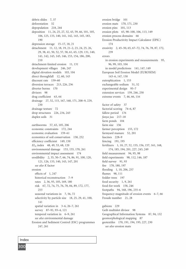
Index
300
debris slides 7, 37deforestation 32depopulation 218, 244deposition 11, 24, 25, 27, 32, 43, 59, 66, 101, 105,
106, 125, 133, 140, 141, 142, 143, 145, 183,190
depression storage 15–17, 18, 21detachment 11, 12, 18, 19, 21–2, 23, 24, 25, 26,
29, 38, 41, 50, 52, 57, 58, 61, 65, 129, 131, 140,141, 142, 143, 145, 146, 153, 154, 186, 200,210
detachment-limited erosion 11, 131development villages 246, 247digital elevation models 103, 104direct throughfall 12, 60, 143discount rate 159–60diversion terraces 213, 226, 236diverter berms 170divisors 98drag coefficient 63, 64drainage 27, 52, 115, 167, 168, 171, 208–9, 229,
230drainage texture 72drop structures 226, 234, 243duplex soils 31
earthworms 57, 65, 105, 206economic constraints 172, 244economic evaluation 159–61economics of soil conservation 158, 252efficiency coefficient 149, 150EI30 index 48, 49, 53, 68, 120environmental damage 153, 155, 170, 261environmental impact assessment 174erodibility 2, 35, 50–7, 66, 74, 86, 91, 100, 120,
121, 126, 133, 140, 143, 147, 201see also K factor
erosioneffects of 1, 247historical reconstruction 7–9rates 2, 36, 93, 105, 169, 180risk 67, 72, 74, 75, 76, 78, 84, 89, 172, 177,
253seasonal variations in 7, 56, 72selectivity by particle size 18, 25, 29, 41, 100,
141spatial variation in 3–6, 26–7, 261survey 87–91, 93–4, 121temporal variation in 6–9, 261see also environmental damage
Erosion and Sediment Control (ESC) programmes247, 261
erosion bridge 101erosion mats 170, 171, 230erosion pins 101, 113erosion plots 65, 98–100, 106, 113, 149erosion process domains 66Erosion Productivity Impact Calculator (EPIC)
174erosivity 2, 45–50, 65, 67–72, 74, 76, 78, 87, 172,
239errors
in erosion experiments and measurements 95,96, 99, 103, 104
in model predictions 141, 147, 149European Soil Erosion Model (EUROSEM)
143–6, 147, 150eutrophication 1, 153exchangeable sodium 51, 52experimental design 95–7extension services 159, 246, 250extreme events 7, 46, 66, 116
factor of safety 37factorial scoring 74–6, 87fallow period 176fanya juu 217–18farm ponds 104farm size 156farmer perception 155, 172farmyard manure 52, 201fascines 228–9fencing 191, 195fertilizers 1, 10, 27, 52, 155, 156, 157, 161, 168,
174, 185, 194, 201, 227, 243, 249field measurement 94, 95, 98field experiments 98, 112, 146, 187field survey 91, 93fire 178, 180, 197flooding 1, 10, 206, 257flumes 98, 111fodder trees 197food security 1, 9, 261food-for-work 158, 246footpaths 94, 168, 196, 235–6frequency-magnitude of erosion events 6–7, 66Froude number 21, 28
gabions 229Geib multislot divisor 98Geographical Information Systems 87, 94, 132geomorphological mapping 87geotextiles 170, 191, 194, 195, 227, 230
see also erosion mats
MSEINDEX 11/19/04 02:48 PM Page 300
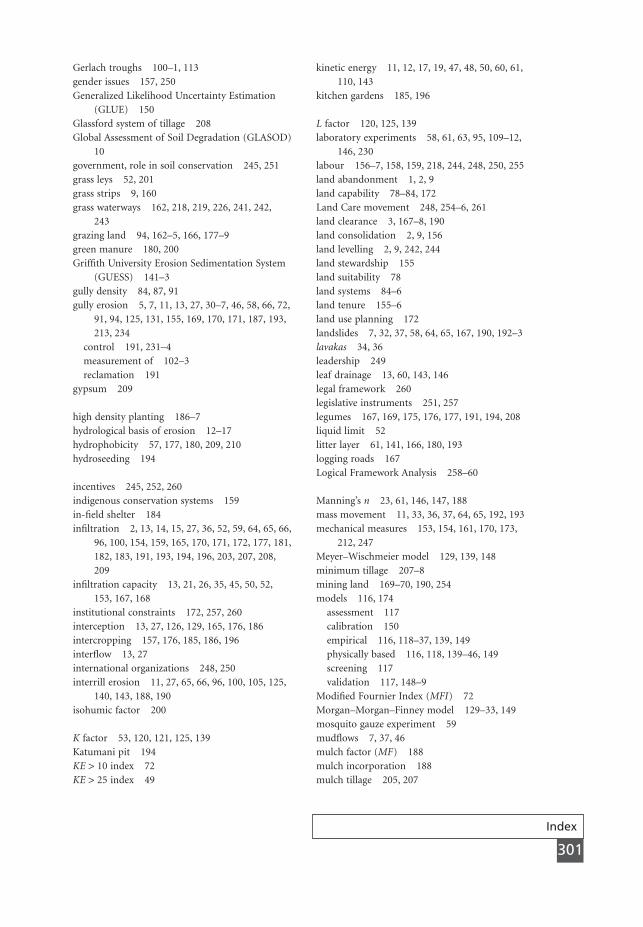
Index
301
Gerlach troughs 100–1, 113gender issues 157, 250Generalized Likelihood Uncertainty Estimation
(GLUE) 150Glassford system of tillage 208Global Assessment of Soil Degradation (GLASOD)
10government, role in soil conservation 245, 251grass leys 52, 201grass strips 9, 160grass waterways 162, 218, 219, 226, 241, 242,
243grazing land 94, 162–5, 166, 177–9green manure 180, 200Griffith University Erosion Sedimentation System
(GUESS) 141–3gully density 84, 87, 91gully erosion 5, 7, 11, 13, 27, 30–7, 46, 58, 66, 72,
91, 94, 125, 131, 155, 169, 170, 171, 187, 193,213, 234
control 191, 231–4measurement of 102–3reclamation 191
gypsum 209
high density planting 186–7hydrological basis of erosion 12–17hydrophobicity 57, 177, 180, 209, 210hydroseeding 194
incentives 245, 252, 260indigenous conservation systems 159in-field shelter 184infiltration 2, 13, 14, 15, 27, 36, 52, 59, 64, 65, 66,
96, 100, 154, 159, 165, 170, 171, 172, 177, 181,182, 183, 191, 193, 194, 196, 203, 207, 208,209
infiltration capacity 13, 21, 26, 35, 45, 50, 52,153, 167, 168
institutional constraints 172, 257, 260interception 13, 27, 126, 129, 165, 176, 186intercropping 157, 176, 185, 186, 196interflow 13, 27international organizations 248, 250interrill erosion 11, 27, 65, 66, 96, 100, 105, 125,
140, 143, 188, 190isohumic factor 200
K factor 53, 120, 121, 125, 139Katumani pit 194KE > 10 index 72KE > 25 index 49
kinetic energy 11, 12, 17, 19, 47, 48, 50, 60, 61,110, 143
kitchen gardens 185, 196
L factor 120, 125, 139laboratory experiments 58, 61, 63, 95, 109–12,
146, 230labour 156–7, 158, 159, 218, 244, 248, 250, 255land abandonment 1, 2, 9land capability 78–84, 172Land Care movement 248, 254–6, 261land clearance 3, 167–8, 190land consolidation 2, 9, 156land levelling 2, 9, 242, 244land stewardship 155land suitability 78land systems 84–6land tenure 155–6land use planning 172landslides 7, 32, 37, 58, 64, 65, 167, 190, 192–3lavakas 34, 36leadership 249leaf drainage 13, 60, 143, 146legal framework 260legislative instruments 251, 257legumes 167, 169, 175, 176, 177, 191, 194, 208liquid limit 52litter layer 61, 141, 166, 180, 193logging roads 167Logical Framework Analysis 258–60
Manning’s n 23, 61, 146, 147, 188mass movement 11, 33, 36, 37, 64, 65, 192, 193mechanical measures 153, 154, 161, 170, 173,
212, 247Meyer–Wischmeier model 129, 139, 148minimum tillage 207–8mining land 169–70, 190, 254models 116, 174
assessment 117calibration 150empirical 116, 118–37, 139, 149physically based 116, 118, 139–46, 149screening 117validation 117, 148–9
Modified Fournier Index (MFI) 72Morgan–Morgan–Finney model 129–33, 149mosquito gauze experiment 59mudflows 7, 37, 46mulch factor (MF) 188mulch incorporation 188mulch tillage 205, 207
MSEINDEX 11/19/04 02:48 PM Page 301

Index
302
mulches and mulching 52, 58, 125, 126, 156, 159,168, 176, 187–90, 191, 194, 195, 200, 205, 206,243
multi-criteria analysis 160multiple cropping 185–6, 196, 206
National Pollutants Discharge Elimination System247
nested catchments 113Normalized Difference Vegetation Index (NDVI)
89no tillage 160, 167, 168, 188, 197, 202, 205, 207,
209
orchard terracing 216organic carbon 52, 201, 202, 207organic matter 51, 53, 65, 153, 194, 196, 200, 207overcropping 155overgrazing 31, 32, 155, 166, 177, 178overland flow 11, 12, 19, 21–7, 28, 45, 46, 58, 59,
61, 63, 66, 72, 100, 101, 129, 142, 145, 169,193, 212
P factor 120, 121, 139p2/P index 72participatory approaches 246, 250, 251, 257patch cutting 178, 190pebble mulch 190phosphorus 27, 146, 153, 184pipeline corridors 85, 170, 190, 191, 195, 197,
213, 227, 228, 254, 261piping 58, 170
see also tunnel erosionpitting 194, 195plane of zero wind velocity (z0) 38, 63plant cover 49, 58, 59–65, 67, 91, 140, 143, 175plant spacing 187plastic limit 51, 202, 208plough pans 204, 208plough-plant 206, 207political constraints 172, 245, 257, 258polluter pays 155, 254, 260population pressure 2, 9, 244pro-forma for field surveys 91productivity 9, 10, 117, 155, 156, 159, 160, 165,
172, 257Productivity Index (PI) 174
R factor 68, 71, 72, 120, 121, 122, 125raindrop impact 16, 17, 21, 22, 24, 26, 27, 29, 52,
56, 59, 60, 65, 129, 141, 142, 143, 153, 154,171, 177, 186, 200, 204, 210
rainfallaggressiveness 72drop-size distribution 47, 60, 61, 110, 113, 121intensity 19, 26, 45, 46, 47, 49, 61, 65, 72, 96,
110, 140, 142, 145, 204simulation 58, 96, 110–11, 112, 113, 209
rainsplash 11, 22, 58, 100, 131rangeland 121, 162, 165, 178recreation 78, 168, 196, 197, 235, 261regulatory instruments 251remote sensing 89, 254replication 95, 96, 98reservoir surveys 104retention terraces 213revegetation 168, 169, 190–1, 193, 194, 195, 196,
210species selection 170, 191, 196, 197–9
Revised Universal Soil Loss Equation (RUSLE)122, 125, 141, 149
Reynolds number 21, 22ridging 204rill erosion 11, 12, 13, 26, 28–30, 35, 36, 45, 46,
56, 59, 66, 72, 87, 91, 94, 100, 101, 102, 105,110, 111, 122, 125, 125, 140, 141, 142, 143,145, 169, 170, 188
riparian barriers 160, 184, 185, 254ripping 191, 208, 209road banks 171, 190, 194, 195, 197, 227, 228,
261rock dams 232–3rock fragments 15, 22, 29, 41, 65, 190rofabarð 93, 94roots, role in erosion control 53, 59, 64, 91, 167,
171, 192, 196, 239rotation 121, 159, 161, 167, 175, 176, 177, 180,
182, 197, 206, 207rotational grazing 162, 178, 179row crops 175, 176–7, 181roughness 16–17, 18, 61, 65, 125, 133, 149, 153,
204runoff generation 15, 65runoff plots 96, 112runoff simulation 111
S factor 120, 125, 139saltation 40, 41, 44, 110, 238sand dunes 57, 168, 190, 193–4, 195–6, 209, 210,
241sand fences 241sand traps 107–8saprolite 5, 34, 35satellite imagery 87, 89, 90
MSEINDEX 11/19/04 02:48 PM Page 302

Index
303
saturated hydraulic conductivity 13, 14, 18, 34,146, 147, 206
scale 65–6, 94, 109, 116, 118, 139, 148sediment
budgets 113–15delivery ratio 6, 115, 125, 133discharge rating curve 103samplers 98, 103sinks 5, 115yield 4, 103, 113, 114, 115, 125, 180
sedimentation 1, 9, 153, 260sedimentation ponds 227, 228seed bank 195selective felling 180selective analysis 146–7sequential cropping 185settling velocity 25, 43, 141shear strength 18, 28, 37, 50, 52, 64, 76, 167, 192,
193, 203shear stress 22, 29, 38, 140, 142shear velocity 22, 23, 25, 28, 38, 40, 41, 52, 63sheet flow see overland flowshelterbelts 236–41, 252Shields number 22, 38shifting cultivation 166, 176silt fences 227silt traps 170slaking 18, 51slope 20, 22, 50, 57–9, 65, 66, 74, 75, 78, 84, 86,
87, 95, 96, 101, 111, 120, 121, 126, 145socio-economic constraints 172, 244, 258sodium adsorption ratio 51soil
concept of soil rights 260failure during tillage 202failure under raindrop impact 18, 52fertility 152, 155, 159initiation of particle movement 42–3moisture 51, 57, 65, 159, 181, 197, 208, 236rates of formation 152texture 14, 18, 50, 203treatment for experiments 110
soil conservationaccess to 157–8defining needs 172on cultivated lands 161–2on forest land 165–7, 180on grazing land 162–5, 177–9, 193–4on mining land 169–70on pipeline corridors 170, 195principles of 153–4programmes 158, 246, 248, 254, 257
projects 246, 248, 257on road banks 171, 194–5on rough land 168strategy 172–4in urban areas 169
Soil Loss Estimator for Southern Africa (SLEMSA)125–6
soil loss tolerance 152–3, 172, 176, 186, 260soil management 153, 158, 161, 173, 200, 212soil stabilizers 195, 209–10splash boards 101splash cups 101, 110splash erosion 13, 17–21, 57, 58, 59, 66, 72, 110
measurement of 101–2splash funnels 101splash pedestals 20, 90stakeholders 247, 257, 260, 261stemflow 13, 61stocking rates 162, 165, 178, 179stone bunds 212stone mulch 190stones 26
see also rock fragmentsstraw bales 228stream power 25, 29, 142, 145strip cropping 100, 121, 181–5, 204, 212strip tillage 206–7stubble-mulch tillage 207subsidies 159, 254subsoiling 208, 209surcharge 64, 192
technology, requirements of 250technology transfer 158–9, 249, 254termites 57, 99, 200terrace failure 154terraces 2, 9, 100, 121, 153, 154, 156, 157, 158,
159, 160, 162, 170, 196, 212–18, 252layouts 213, 227, 241–3spacing 121, 213
thixotropic behaviour 51thresholds, application to erosion 21, 32–4, 38,
46, 239tied ridging 204–5tillage 33, 50, 53, 66, 107, 137, 146, 160, 161, 168,
176, 188, 190, 202–9tillage erosion 210–11tile outlet terraces 226top-down approach 245, 246, 247tracers 104–7traditional conservation systems 162, 246
see also indigenous conservation systems
MSEINDEX 11/19/04 02:48 PM Page 303

Index
304
training 247, 250, 252, 255, 260Training and Visit System 246trampling 11, 58, 104, 162, 168, 196transport 11, 12, 20, 24–6, 38, 41, 50, 58, 63, 129,
153, 154transport capacity 24, 25, 26, 29, 41, 59, 114, 129,
131, 132, 133, 140, 142, 145, 146, 149, 241transport-limited erosion 11, 131treatment-oriented land classification 78tree crops 187tunnel erosion 27, 30, 31, 32, 36, 191, 208, 209turbidity recorder 103
uncertainty, in model predictions 149–51undergrazing 177Universal Soil Loss Equation (USLE) 85, 120–5,
129, 131, 133, 139, 141, 149, 188urban land use 7, 84, 169, 261
vegetation 3, 26, 27, 41, 59, 60, 63, 64, 65, 72, 84,89, 91, 133, 141, 143, 147, 149, 166, 171, 177,197
vetiver grass 184volunteers 249
Water Erosion Prediction Project (WEPP)139–41, 142, 146, 147, 148, 149, 150, 151
water quality 10, 253, 255waterways 170, 218–27wattling 170, 171, 228weathering 11, 16, 17, 30wildlife 101, 178wind, effect on rainfall energy 20wind breaks 2, 153, 236–41wind erosion 38–41, 53, 58, 93, 107, 111, 113,
181, 184, 188, 189, 245, 253control 190, 204, 207, 208, 210measurement of 108
Wind Erosion Prediction Equation 133Wind Erosion Prediction System (WEPS) 146wind erosivity 50wind tunnels 53, 63, 111–12, 113, 238
MSEINDEX 11/19/04 02:48 PM Page 304