software development for settlement and consolidation analysis
TRANSCRIPT
SCHOOL OF GRADUATE STUDIES
DEPARTMENT OF CIVIL ENGINEERING
SOFTWARE DEVELOPMENT FOR CONSOLIDATION
AND SETTLEMENT ANALYSIS
A THESIS SUBMITTED TO THE SCHOOL OF GRADUATE STUDIES OF
ADDIS ABABA UNIVERSITY IN PARTIAL FULFILLMENT OF THE
REQUIREMENTS FOR THE DEGREE OF MASTER OF SCIENCE IN CIVIL
ENGINEERING (GEOTECHNIQUES)
BY: AYENEW YIHUNE
ADVISOR: PROF. ALEMAYEHU TEFERRA
November, 2011 Addis Ababa, Ethiopia
AAiT
Addis Ababa University
Addis Ababa Institute of Technology
��� ��� ��� � �����
��� ��� ������
SCHOOL OF GRADUATE STUDIES
DEPARTMENT OF CIVIL ENGINEERING
SOFTWARE DEVELOPMENT FOR CONSOLIDATION
AND SETTLEMENT ANALYSIS
A THESIS SUBMITTED TO THE SCHOOL OF GRADUATE STUDIES OF
ADDIS ABABA UNIVERSITY IN PARTIAL FULFILLMENT OF THE
REQUIREMENTS FOR THE DEGREE OF MASTER OF SCIENCE IN CIVIL
ENGINEERING (GEOTECHNIQUES)
BY: AYENEW YIHUNE
Approved by board examiners:
1. ______________________________ ________________ ________________
2. ______________________________ ________________ ________________
3. ______________________________ ________________ ________________
4. ______________________________ ________________ ________________
AAiT
Addis Ababa University
Addis Ababa Institute of Technology
��� ��� ��� � �����
��� ��� ������
Advisor Signature Date
External Examiner Signature Date
Internal Examiner Signature Date
Chairman Signature Date
i
Software Development for Consolidation and Settlement Analysis
ACKNOWLEDGEMENT
First of all, I would like to thank God for His help in my life.
I would like to express my thanks and respect to my advisor Professor Alemayehu Teferra for
his effort in guiding me and editing this work. I would like to extend my thanks also for Dr.
Hadush Seged and other staff of Geotechnical Engineering stream for their support and
comment.
I need to say thanks to my family, specially my father, for their continuous follow-up and
assistance. Last but not least, I like to acknowledge Ashu Sintayehu for his help in fulfilling
working material.
ii
Software Development for Consolidation and Settlement Analysis
Table of Contents
Acknowledgment ........................................................................................................................ i
List of Tables ............................................................................................................................. vi
List of Figures ......................................................................................................................... viii
Comments .................................................................................................................................. xi
Abstract .................................................................................................................................... xii
CHAPTER ONE
1. Introduction ............................................................................................................................1
1.1.Background.........................................................................................................................1
1.2.Objective of the Thesis .......................................................................................................2
1.3.Problem Statement..............................................................................................................3
1.4.Organization of the Thesis..................................................................................................3
CHAPTER TWO
2. Literature Review ...................................................................................................................4
2.1.Consolidation Analysis .......................................................................................................4
2.1.1. One dimensional consolidation for saturated soils ...................................................4
2.1.1.1.Solution using Fourier series ...............................................................................5
2.1.1.2.Solution using finite difference method ...............................................................9
2.1.2. One dimensional consolidation for unsaturated soils ............................................10
2.1.2.1.Water phase partial differential equation ...........................................................11
2.1.2.2.Air phase partial differential equation ...............................................................13
2.2.Settlement Analysis ..........................................................................................................15
2.2.1. Immediate settlement .............................................................................................15
2.2.2. Primary settlement .................................................................................................16
iii
Software Development for Consolidation and Settlement Analysis
2.2.2.1.Compression index method ...............................................................................16
2.2.2.2.Average modulus of compressibility method ....................................................16
2.2.2.3.Coefficient of volume compressibility method .................................................16
2.2.3. Secondary settlement .............................................................................................17
2.2.3.1.Constant modulus of compressibility method ...................................................17
2.2.3.2.Variable modulus of compressibility method ....................................................17
CHAPTER THREE
3. Methodology ........................................................................................................................22
3.1.General .............................................................................................................................22
3.2.Consolidation Analysis .....................................................................................................22
3.2.1. Consolidation analysis using Fourier series solution .............................................22
3.2.1.1.Inputs .................................................................................................................23
3.2.1.2.Conditions considered ........................................................................................23
3.2.1.3.Outputs ...............................................................................................................24
3.2.2. Consolidation analysis by finite difference method ..............................................24
3.2.2.1.Saturated soils ....................................................................................................24
3.2.2.2.Unsaturated soils ................................................................................................27
3.3.Settlement Analysis ..........................................................................................................29
3.3.1. Inputs .....................................................................................................................29
3.3.2. Conditions considered ...........................................................................................30
3.3.3. Outputs ...................................................................................................................32
CHAPTER FOUR
4. Application of the Software ................................................................................................33
4.1.General ............................................................................................................................33
4.1.1. File menu ...............................................................................................................34
iv
Software Development for Consolidation and Settlement Analysis
4.1.2. Edit menu ...............................................................................................................34
4.1.3. Define menu ..........................................................................................................34
4.1.4. Result menu ...........................................................................................................35
4.1.5. Help menu ..............................................................................................................35
4.2.Consolidation Analysis by Fourier Series Method ..........................................................36
4.3.Consolidation Analysis by FDM for Saturated Soil ........................................................39
4.3.1. Constant load scenario ...........................................................................................39
4.3.2. Variable load scenario ...........................................................................................43
4.3.3. Abrupt change of load scenario .............................................................................44
4.4.Consolidation Analysis by FDM for Unsaturated Soil ....................................................45
4.5.Settlement Analysis .........................................................................................................48
4.5.1. Rectangular foundation ..........................................................................................48
4.5.2. Circular foundation ................................................................................................54
CHAPTER FIVE
5. Validation of the Software ..................................................................................................58
CHAPTER SIX
6. Conclusion and Recommendation .......................................................................................59
6.1.Conclusion .......................................................................................................................59
6.2.Recommendation .............................................................................................................59
Reference ......................................................................................................................................60
APPENDIX
A. Flowchart .............................................................................................................................61
B. Validation of the Software ..................................................................................................70
B.1. Consolidation Analysis for a Saturated Soil .........................................................71
B.1.1. Result from common calculation methods ............................................................72
v
Software Development for Consolidation and Settlement Analysis
B.1.1.1. Fourier series method ................................................................................72
B.1.1.2. Finite difference method ...........................................................................79
B.1.2. Result from the developed software ......................................................................82
B.1.2.1. Fourier series method ................................................................................83
B.1.2.2. Finite difference method ...........................................................................86
B.2. Consolidation Analysis for an Unsaturated soil ....................................................89
B.2.1. Result from common calculation methods ............................................................90
B.2.1.1. Degree of consolidation for two years ......................................................90
B.2.1.2. Isochrone after one year ............................................................................93
B.2.2. Result from the developed software ......................................................................94
B.2.2.1. Degree of consolidation for two years ......................................................94
B.2.2.2. Isochrone after one year ............................................................................96
B.3. Settlement Analysis ..............................................................................................97
B.3.1. Result from common calculation methods ............................................................98
B.3.1.1. Immediate (elastic) settlement ..................................................................98
B.3.1.2. Final primary settlement .........................................................................100
B.3.1.3. Primary settlement after two years .........................................................112
B.3.1.4. Secondary settlement ..............................................................................114
B.3.2. Result from the developed software ....................................................................116
B.3.2.1. Final settlement .......................................................................................116
B.3.2.2. Settlement after two years .......................................................................119
vi
Software Development for Consolidation and Settlement Analysis
List of Tables
Table B.1 Degree of consolidation for three years for single drainage case ............................72
Table B.2 Degree of consolidation for three years for double drainage case ...........................73
Table B.3 Time for 50% degree of consolidation for single drainage case .............................74
Table B.4 Time for 50% degree of consolidation for double drainage case ............................75
Table B.5 Pore water pressure at different depths for single drainage case ............................76
Table B.6 Pore water pressure at different depths for double drainage case ...........................78
Table B.7 Finite difference calculation table for single drainage case ....................................79
Table B.8 Finite difference calculation table for double drainage case ...................................80
Table B.9 Finite difference calculation table for single drainage case ....................................87
Table B.10 Finite difference calculation table for double drainage case ...................................87
Table B.11 Finite difference calculation table for water phase .................................................91
Table B.12 Finite difference calculation table for air phase ......................................................92
Table B.13 Finite difference calculation table for water phase .................................................94
Table B.14 Finite difference calculation table for air phase ......................................................95
Table B.15 Pressure due to uniform parts ................................................................................101
Table B.16 Pressure due to triangular parts .............................................................................102
Table B.17 Summary of pressure distributions (uniform + triangular) ....................................102
Table B.18 Pressure due to uniform part under point A and B ................................................103
Table B.19 Pressure due to triangular part under point A .......................................................104
Table B.20 Pressure due to triangular part under point B ........................................................104
Table B.21 Summary of pressure distributions (rectangular + triangular) ...............................104
Table B.22 Pressure due to uniform parts ................................................................................105
Table B.23 Pressure due to uniform parts ................................................................................106
vii
Software Development for Consolidation and Settlement Analysis
Table B.24 Pressure due to triangular parts .............................................................................106
Table B.25 Pressure due to triangular parts .............................................................................107
Table B.26 Summary of pressure distributions (uniform + triangular) ....................................107
Table B.27 Degree of consolidation for two years ..................................................................113
Table B.28 Secondary settlement at different locations ..........................................................115
viii
Software Development for Consolidation and Settlement Analysis
List of Figures
Figure 3.1 Initial excess pore water pressure distribution .......................................................24
Figure 3.2 Loads ......................................................................................................................31
Figure 4.1 Main window ..........................................................................................................33
Figure 4.2 Menus .....................................................................................................................34
Figure 4.3 New dialog box .......................................................................................................36
Figure 4.4 Load dialog box ......................................................................................................36
Figure 4.5 Load dialog box ......................................................................................................37
Figure 4.6 Soil Property dialog box .........................................................................................37
Figure 4.7 Consolidation dialog box ........................................................................................38
Figure 4.8 Isochrone dialog box ..............................................................................................39
Figure 4.9 Load dialog box ......................................................................................................40
Figure 4.10 Load dialog box ......................................................................................................40
Figure 4.11 Soil Property dialog box .........................................................................................41
Figure 4.12 Consolidation dialog box ........................................................................................41
Figure 4.13 Isochrone dialog box ..............................................................................................42
Figure 4.14 Export dialog box ...................................................................................................43
Figure 4.15 Load dialog box .....................................................................................................43
Figure 4.16 Load dialog box .....................................................................................................44
Figure 4.17 Load dialog box ......................................................................................................44
Figure 4.18 Load dialog box ......................................................................................................45
Figure 4.19 Load dialog box ......................................................................................................45
Figure 4.20 Soil Property dialog box .........................................................................................46
Figure 4.21 Consolidation dialog box ........................................................................................46
Figure 4.22 Isochrone dialog box ..............................................................................................47
ix
Software Development for Consolidation and Settlement Analysis
Figure 4.23 Structure dialog box ...............................................................................................48
Figure 4.24 Load dialog box ......................................................................................................49
Figure 4.25 Soil Property dialog box .........................................................................................50
Figure 4.26 J’ dialog box ...........................................................................................................50
Figure 4.27 Modulus of Compressibility dialog box .................................................................51
Figure 4.28 Settlement dialog box .............................................................................................51
Figure 4.29 Settlement dialog box .............................................................................................52
Figure 4.30 Pressure Distribution dialog box ............................................................................53
Figure 4.31 Time-Settlement Graph dialog box ........................................................................54
Figure 4.32 Load dialog box ......................................................................................................55
Figure 4.33 Settlement dialog box .............................................................................................56
Figure 4.34 Pressure Distribution dialog box ............................................................................57
Figure B.1 Initial excess pore water pressure distributions .....................................................71
Figure B.2 Isochrone after two years for single drainage case ................................................77
Figure B.3 Isochrone after two years for double drainage case ...............................................78
Figure B.4 Isochrone after two years for single drainage case ................................................81
Figure B.5 Isochrone after two years for double drainage case ...............................................82
Figure B.6 Degree of consolidation for three years for single drainage case ..........................83
Figure B.7 Degree of consolidation for three years for double drainage case .........................83
Figure B.8 Time for 50% degree of consolidation for single drainage case ............................84
Figure B.9 Time for 50% degree of consolidation for double drainage case ..........................84
Figure B.10 Isochrone after two years for single drainage case ................................................85
Figure B.11 Isochrone after two years for double drainage case ...............................................86
Figure B.12 Isochrone after two years for single drainage case ................................................88
Figure B.13 Isochrone after two years for double drainage case ...............................................89
x
Software Development for Consolidation and Settlement Analysis
Figure B.14 Initial excess pore water pressure distributions .....................................................89
Figure B.15 Isochrone after one year for water phase ...............................................................93
Figure B.16 Isochrone after one year for air phase ....................................................................94
Figure B.17 Isochrone after one year for water phase ...............................................................96
Figure B.18 Isochrone after one year for air phase ....................................................................96
Figure B.19 Elevation and plan of an abutment ........................................................................98
Figure B.20 Contact pressure distribution ...............................................................................100
Figure B.21 Contact pressure distribution ...............................................................................101
Figure B.22 Pressure distribution with depth ..........................................................................110
Figure B.23 Approximate initial excess pore water pressure distribution ...............................113
Figure B.24 Settlement at the center ........................................................................................116
Figure B.25 Settlement at the edges ........................................................................................117
Figure B.26 Settlement at the characteristic points .................................................................118
Figure B.27 Settlement at the center ........................................................................................119
Figure B.28 Settlement at the edges ........................................................................................120
Figure B.29 Settlement at the characteristic points .................................................................121
Figure B.30 Pressure distribution under the center ..................................................................122
Figure B.31 Pressure distribution under edge A ......................................................................123
Figure B.32 Pressure distribution under edge B ......................................................................123
Figure B.33 Pressure distribution under characteristic points near edge A .............................124
Figure B.34 Pressure distribution under characteristic points near edge B .............................124
xi
Software Development for Consolidation and Settlement Analysis
COMMENTS
The user is advised to close and restart the software after each analysis to start another
analysis. The user should not select secondary settlement analysis without selecting primary
settlement analysis for the case when the thickness is required to be calculated by the software
(i.e. when the “Large” radio button in the “Soil Property” dialog box of the settlement
analysis part of the software is checked). The term “primary consolidation settlement” is
changed to “primary settlement”. The software may also have other errors.
xii
Software Development for Consolidation and Settlement Analysis
ABSTRACT
Consolidation and settlement analysis is one of the main tasks of a geotechnical engineer.
There are different methods of analyzing consolidation and settlement. In this study, software
for the analysis of consolidation and settlement is developed.
The developed software analyzes one dimensional consolidation for saturated and unsaturated
soils. Consolidation analysis for saturated soils is done by the Fourier series solution and by
finite difference solution of Terzaghi’s one dimensional consolidation equation for saturated
soils. Consolidation analysis for unsaturated soils is done by finite difference method. The
analysis is done for different loadings, scenarios, drainage conditions and soil conditions.
The software analyzes immediate settlement, primary settlement and secondary settlement.
Primary settlement calculation is done by compression index method, average modulus of
compressibility method and coefficient of volume compressibility method. Secondary
settlement calculation is done by constant modulus of compressibility method and variable
modulus of compressibility method. The analysis is done for different loadings, foundation
types, and locations of the foundation, drainage conditions and soil conditions.
The result of consolidation analysis by Fourier series method and finite difference method
give approximately similar result. For the consolidation analysis by finite difference method,
the stability of the calculation is very sensitive to the beta value. The result may not be
reliable for inappropriate beta values. The developed software can be used to analyze
consolidation and settlement simply, quickly and accurately. Comparison of results obtained
from different analysis methods of consolidation and settlement can be also made with the
software. The developed software is also important to study the properties of the results for
different values of input parameters.
1
Software Development for Consolidation and Settlement Analysis
CHAPTER ONE
Introduction
1.1 Background
Now a days, the use of software has become very important in many fields of studies. This
even goes further with the progressive development of computers which enables users to do
their works with easily portable desktops and laptops. The use of software makes many works
which were tedious and even impractical manually to be done within seconds.
In engineering, software application has become common for many purposes. One reason for
this is that many engineering subjects involve large amount of calculations which are time
consuming and at times difficult to tackle. The other reason is the development of numerical
methods including the well known methods like finite difference and finite element.
This study is aimed at developing software for consolidation and settlement analysis, which
play major role in geotechnical engineering.
The basic differential equation for one dimensional consolidation of saturated soils was first
derived by Terzaghi [8] [1] [9]. For unsaturated soils, different contributions have been done
by Biot, Larmour, Hill, Olson, Scott, Blight, Barden, Fredlund and Hasan and other
researchers. Fredlund and Hasan developed two partial differential equations from which pore
air and pore water pressures could be calculated. [2]
Different ways have been suggested to use the above equations for practical purpose. The first
way is solving by using Fourier series. By this method, a solution can be obtained for
Terzaghi’s one dimensional consolidation equation. The problem here is that it is difficult to
compute the sum up to a reasonable accuracy with hand calculation. The problem even goes
further if the series do not converge with few sums. The second method is to use tables which
correlate one value to the other. This method, even if it is less accurate, is easy and workable
method for hand calculation. The third method of solving the equations is to use numerical
methods like finite difference method and finite element method. This method is the most
2
Software Development for Consolidation and Settlement Analysis
powerful method which can be used for various cases. The problem of this method is again
the large amount of calculation work involved.
There are three settlement types. These are immediate settlement, primary settlement and
secondary settlement. Calculation of primary settlement and secondary settlement involves
calculation of pressure distribution under the point at which settlement is to be calculated.
This can be done by using pressure distribution calculation equations. Pressure distribution
calculation using these equations can be done by using the equations directly or by using
tables prepared from these equations. Calculation using the equations directly, and even using
tables prepared from these equations, could be difficult for manual calculation because
pressure distribution calculation involves pressure calculation at different points for a given
depth. And, if primary settlement after a given time is needed, the degree of consolidation
should be first calculated which is part of consolidation analysis. [8]
Tesfahun Redi developed earlier software for consolidation analysis by finite difference
method for saturated soils. The developed software performs consolidation analysis for
different scenarios, initial excess pore water pressure distributions, drainage conditions, for
variable cv case and for multi-layered soils. [3]
1.2 Objective of the Thesis
The general objective of this thesis is to develop software that analyzes consolidation process
and settlement. The specific objectives of the thesis are the following.
� To develop a simple, faster and accurate way of analyzing consolidation process and
settlement.
� To develop an easy way of comparing results obtained by different methods of
consolidation and settlement analysis.
3
Software Development for Consolidation and Settlement Analysis
1.3 Problem Statement
Hand calculations of consolidation process and settlement analysis are laborious and time
consuming. The development of software would enhance the calculation process and would
serve as a tool for the practice.
1.4 Organization of the Thesis
This thesis has five chapters. The first chapter contains a general introduction about the study,
the objective of the study and the problem statement of the study. The second chapter is about
the previous works done regarding consolidation and settlement of soils. In the third chapter,
the methodology of the study is provided. This includes the works done to arrive to the final
result (i.e. the software), the inputs required for the software, the cases considered and the
outputs obtained from the software. In the fourth chapter, the procedures to use the software
are presented. In the fifth chapter, the application of the software is presented. In the sixth
chapter, which is the last chapter, the conclusions made from the study and the
recommendations for further studies are stated.
4
Software Development for Consolidation and Settlement Analysis
CHAPTER TWO
Literature Review
2.1 Consolidation Analysis
The application of loading on a soil layer will cause a change in stress in the soil. This change
in stress will be carried by the soil grains and the pore fluid in the soil. The component carried
by the soil grains is called effective stress and the component carried by the pore fluid is
called pore pressure. In general, the total stress will be carried by the pore fluid initially and as
time progresses the stress will be transferred from pore fluid to the soil structure. This rate of
transfer is influenced by the permeability of the soil. The increase in stress in the pore fluid
will cause the pore fluid to escape from the soil which in turn will cause a volume change in
the soil. This process of escape of pore fluid from the soil due to change in stress in the soil
and transfer of pressure from the pore fluid to the soil structure is called consolidation.
2.1.1 One dimensional consolidation for saturated clay soils
The theory of one dimensional consolidation for saturated clay soils was proposed by
Terzaghi [9]. Assumptions used to derive Terzaghi’s one dimensional consolidation theory
are [1]:
� The clay layer is homogeneous.
� The clay layer is saturated.
� The compression of the soil layer is due to the change in volume only, which in turn,
is due to the squeezing out of water from the void spaces.
� Darcy’s law is valid.
� Deformation of soil occurs only in the direction of the load application.
� The coefficient of consolidation cv is constant during the consolidation.
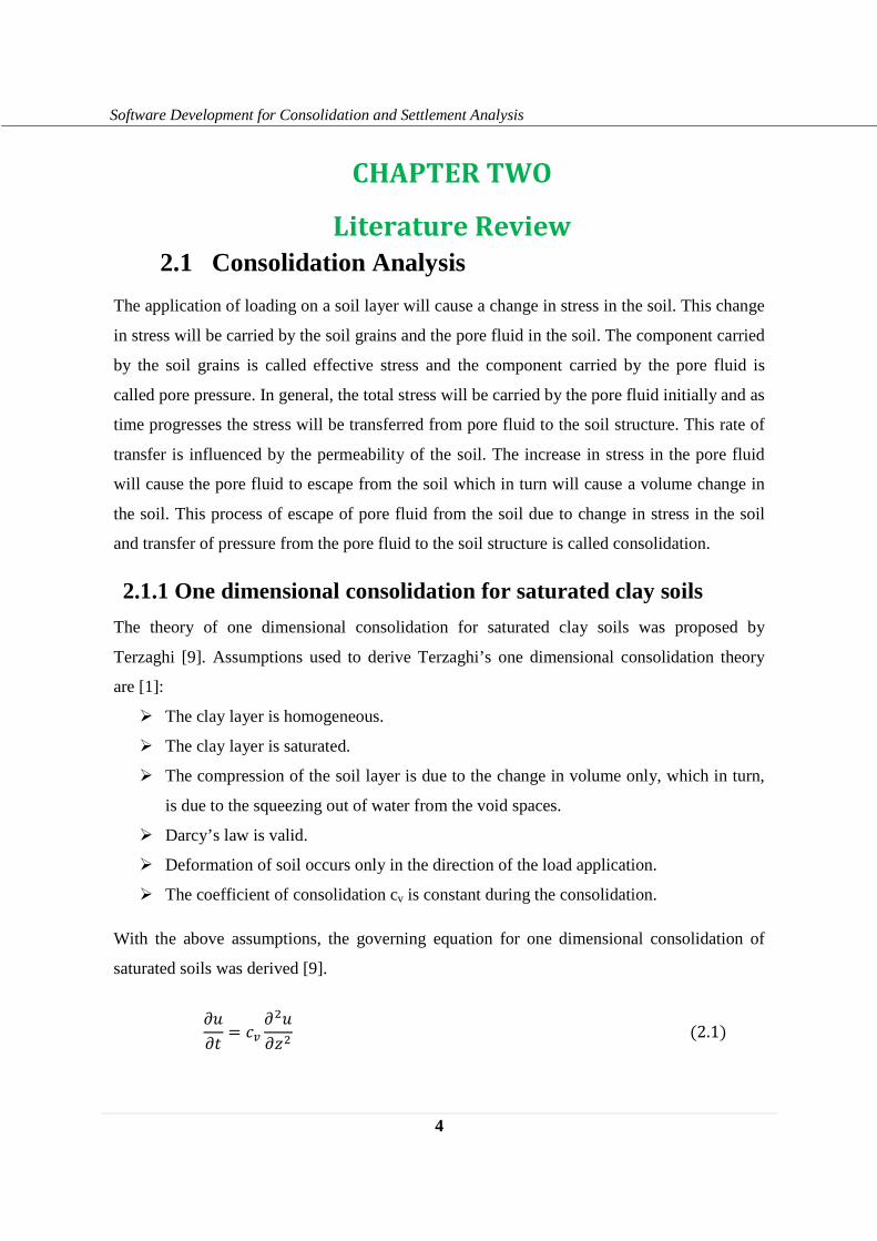
With the above assumptions, the governing equation for one dimensional consolidation of
saturated soils was derived [9].
���� = �� ������ (2.1)
5
Software Development for Consolidation and Settlement Analysis
Where:
� = Pore water pressure
� = Depth
�� = Coefficient of consolidation (�� = � �����⁄ ) � = Permeability
�� = Unit weight of water
�� = Coefficient of volume compressibility
Different ways are attempted to solve Eq. (2.1). A rigorous solution can be obtained by using
Fourier series. A solution can also be obtained using finite difference method.
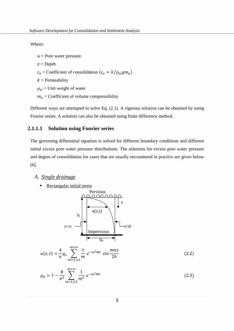
2.1.1.1 Solution using Fourier series
The governing differential equation is solved for different boundary conditions and different
initial excess pore water pressure distributions. The solutions for excess pore water pressure
and degree of consolidation for cases that are usually encountered in practice are given below
[6].
A. Single drainage
� Rectangular initial stress
�(�, �) = 4� �� � 1������ !"#���2ℎ�%&
�%',(,)(2.2)
*+ = 1 − 8�� � 1�� ����� (2.3)�%&�%',(,)
h
Pervious
qo
Impervious
z
u(z,t)
t=0 t=∞
6
Software Development for Consolidation and Settlement Analysis
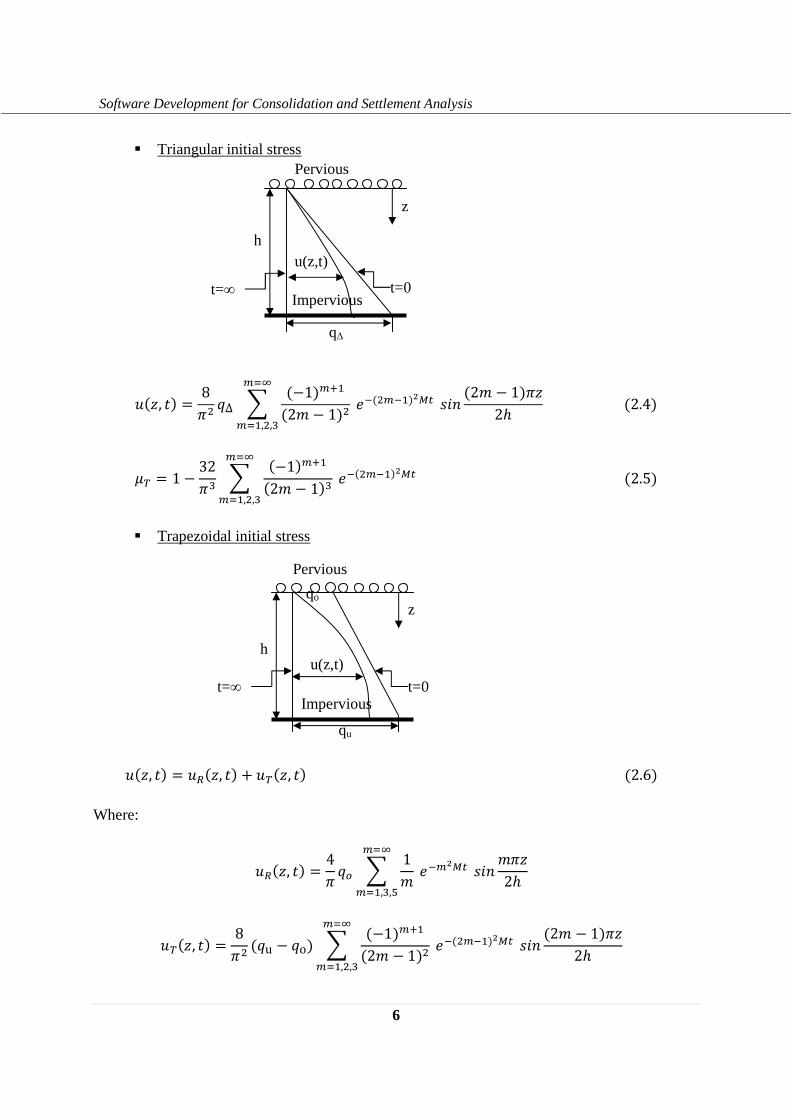
� Triangular initial stress
�(�, �) = 8�� �Δ � (−1)�0'(2� − 1)� ��(���')�� !"# (2� − 1)��2ℎ (2.4)�%&
�%',�,(
*1 = 1 − 32�( � (−1)�0'(2� − 1)( ��(���')�� (2.5)�%&
�%',�,(
� Trapezoidal initial stress
�(�, �) = �+(�, �) + �1(�, �)(2.6) Where:
�+(�, �) = 4� �� � 1������ !"#���2ℎ�%&
�%',(,)
�1(�, �) = 8�� (�u − �o) � (−1)�0'(2� − 1)� ��(���')�� !"# (2� − 1)��2ℎ
�%&�%',�,(
Impervious
h
h
qo
Pervious
Pervious
u(z,t)
qu
Impervious
z
u(z,t)
q∆
z
t=∞
t=∞
t=0
t=0
7
Software Development for Consolidation and Settlement Analysis
*1+7 = 2*+�� + *1(�8 − ��)�8 + �� (2.7) Where:
*+ = 1 − 8�� � 1�� ����� �%&�%',(,)
*1 = 1 − 32�( � (−1)�0'(2� − 1)( ��(���')�� �%&
�%',�,(
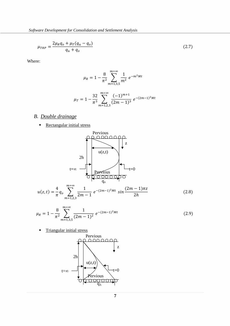
B. Double drainage
� Rectangular initial stress
�(�, �) = 4� �� � 12� − 1��(���')�� !"# (2� − 1)��2ℎ�%&
�%',�,((2.8)
*+ = 1 − 8�� � 1(2� − 1)� ��(���')�� (2.9)�%&�%',(,)
� Triangular initial stress
2h
2h
Pervious
Pervious
qo
Pervious
z
u(z,t)
u(z,t)
q∆
Pervious
z
t=∞
t=∞
t=0
t=0
8
Software Development for Consolidation and Settlement Analysis
�(�, �) = 2� �Δ � (−1)�0'� ����� !"#���2ℎ (2.10)�%&
�%',�,(
*1 = 1 − 8�� � 1�� ����� �%&�%',(,)
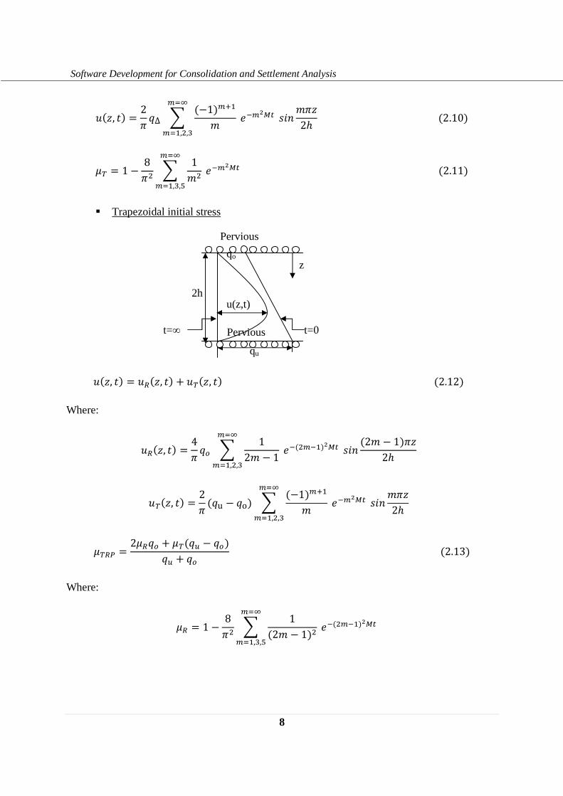
(2.11) � Trapezoidal initial stress
�(�, �) = �+(�, �) + �1(�, �)(2.12) Where:
�+(�, �) = 4� �� � 12� − 1��(���')�� !"# (2� − 1)��2ℎ�%&
�%',�,(
�1(�, �) = 2� (�u − �o) � (−1)�0'� ����� !"#���2ℎ
�%&�%',�,(
*1+7 = 2*+�� + *1(�8 − ��)�8 + �� (2.13) Where:
*+ = 1 − 8�� � 1(2� − 1)� ��(���')�� �%&�%',(,)
2h
qo
Pervious
u(z,t)
qu
Pervious
z
t=∞ t=0
9
Software Development for Consolidation and Settlement Analysis
*1 = 1 − 8�� � 1�� ����� �%&�%',(,)
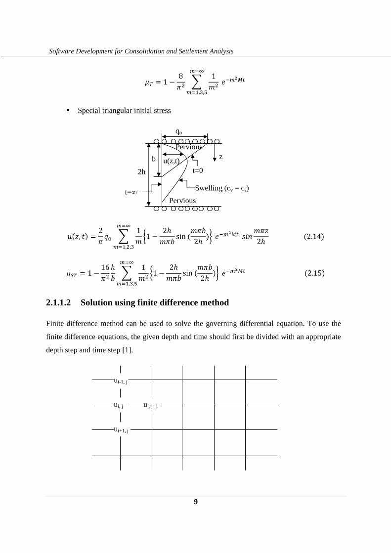
� Special triangular initial stress
�(�, �) = 2� �o � 1�<1 − 2ℎ��= sin(��=2ℎ )A����� !"#���2ℎ (2.14)�%&�%',�,(
*B1 = 1 − 16�� ℎ= � 1�� <1 − 2ℎ��= sin(��=2ℎ )A����� (2.15)�%&�%',(,)
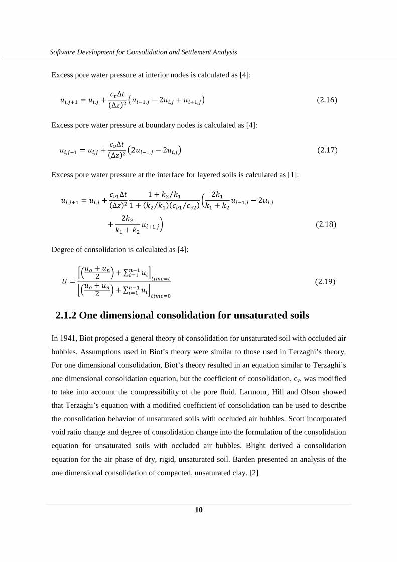
2.1.1.2 Solution using finite difference method
Finite difference method can be used to solve the governing differential equation. To use the
finite difference equations, the given depth and time should first be divided with an appropriate
depth step and time step [1].
b
2h
qo
Pervious
u(z,t)
Pervious
z
ui-1, j
ui, j ui, j+1
ui+1, j
t=∞
t=0
Swelling (cv = cs)
10
Software Development for Consolidation and Settlement Analysis
Excess pore water pressure at interior nodes is calculated as [4]:
�C,D0' = �C,D + ��∆�(∆�)� F�C�',D − 2�C,D + �C0',DG(2.16) Excess pore water pressure at boundary nodes is calculated as [4]:
�C,D0' = �C,D + ��∆�(∆�)� F2�C�',D − 2�C,DG(2.17) Excess pore water pressure at the interface for layered soils is calculated as [1]:
�C,D0' = �C,D + ��'∆�(∆�)� 1 + �� �'⁄1 + (�� �'⁄ )(��' ���⁄ ) H 2�'�' + �� �C�',D − 2�C,D+ 2���' + �� �C0',DI(2.18)
Degree of consolidation is calculated as [4]:
J = KL�� + �M2 N + ∑ �CM�'C%' P C�Q% KL�� + �M2 N + ∑ �CM�'C%' P C�Q%R(2.19)
2.1.2 One dimensional consolidation for unsaturated soils
In 1941, Biot proposed a general theory of consolidation for unsaturated soil with occluded air
bubbles. Assumptions used in Biot’s theory were similar to those used in Terzaghi’s theory.
For one dimensional consolidation, Biot’s theory resulted in an equation similar to Terzaghi’s
one dimensional consolidation equation, but the coefficient of consolidation, cv, was modified
to take into account the compressibility of the pore fluid. Larmour, Hill and Olson showed
that Terzaghi’s equation with a modified coefficient of consolidation can be used to describe
the consolidation behavior of unsaturated soils with occluded air bubbles. Scott incorporated
void ratio change and degree of consolidation change into the formulation of the consolidation
equation for unsaturated soils with occluded air bubbles. Blight derived a consolidation
equation for the air phase of dry, rigid, unsaturated soil. Barden presented an analysis of the
one dimensional consolidation of compacted, unsaturated clay. [2]
11
Software Development for Consolidation and Settlement Analysis
Fredlund and Hasan presented two partial differential equations which could be solved for the
pore air and pore water pressures during the consolidation process of an unsaturated soil. The
air phase was assumed to be continuous. Both equations were solved simultaneously, and the
method is commonly called a two phase flow approach. The formulation by Fredlund and
Hasan was similar in form to the conventional one dimensional Terzaghi’s derivation. The
derivations also demonstrated a smooth transition between the unsaturated and saturated cases.
Similar consolidation equations have also been proposed by Lloret and Alonso. The two
partial differential equations are given below. [2]
2.1.2.1 Water phase partial differential equation
��� ����� = −(�'S� −���) ��T�� + ����� �����U� + 1��� ����U ����U + ����U (2.20)
Where:
�'S� = Coefficient of water volume change with respect to a change in the net
normal stress
��� = Coefficient of water volume change with respect to a change in the matric
suction
�� = Coefficient of permeability with respect to water
�� = Density of water
� = Gravitational acceleration
The above equation is a general form of water phase partial differential equation. The
equation can be simplified for special soil conditions.
A. Saturated condition For saturated condition, �'S� and ��� will be equal to the
coefficient of volume change, ��. The saturated coefficient of permeability is usually
assumed to remain constant during consolidation process. So, the above equation will
take the form of Terzaghi’s equation for saturated soils.
����� = ������������U� (2.21)
12
Software Development for Consolidation and Settlement Analysis
B. Dry soil condition For this condition, the coefficients of water volume change, �'S�
and ���, and the coefficient of permeability with respect to water, �� will go to zero.
Substituting zero value for these parameters, the water phase partial differential
equation will vanish.
C. Special case of unsaturated soils In an unsaturated soil air and water flows can
take place simultaneously during consolidation. The consolidation equation, presented
in Eq. (2.20), for the water phase can be rearranged as follows:
����� = −CW ��T�� + ��� �����U� + ���������U ����U + �X ����U (2.22)
Where:
CW = Interactive constant associated with the water phase partial differential
equation, CW = (1 −��� �'S�⁄ ) (��� �'S�⁄⁄ ) ��� = Coefficient of consolidation with respect to the water phase, ��� =
�� ������⁄
�X = Gravity term constant, �X = 1 ���⁄
If the last two terms are neglected, a simplified form of water phase partial differential
equation can be obtained.
����� = −CW ��T�� + ��� �����U� (2.23) There are many cases where the dissipation of the excess pore air pressure occurs almost
instantaneously. For these cases, the above equation will be further simplified to a form
similar to Terzaghi’s equation.
����� = ��� �����U� (2.24)
13
Software Development for Consolidation and Settlement Analysis
2.1.2.2 Air phase partial differential equation
−Y�'ST − ��T − (1 − Z)#ūT \��T��= ��T ����� − ]T∗(_T `a⁄ )ūT
���T�U� − 1(_T `a⁄ )ūT�]T∗�U ��T�U (2.25)
Where:
�'ST = Coefficient of air volume change with respect to a change in the net normal
stress
��T = Coefficient of air volume change with respect to a change in the matric
suction
Z = Degree of saturation
# = Porosity
]T∗ = Coefficient of transmission for the air phase
_T = Molecular mass of air (��/��cd) ` = Universal gas constant (` = 8.31432e/(�cd. f)) a = Absolute temperature (a = �� + 273.16)(f) �� = Temperature (oC)
ūT = Absolute pore air pressure (ūT = �T + ūT �)(�gh) �T = Gauge pore air pressure (�gh) ūT � = Atmospheric pressure (ūT � = 101�gh)
The above equation is a general form of air phase partial differential equation. The equation
can be simplified for special soil conditions.
A. Saturated condition For saturated condition, �'ST and ��Twill be equal to zero. The
coefficient of transmission, ]T∗ , will approach to zero. So, the air phase partial
differential equation will vanish.
B. Dry soil condition For this condition, the coefficients of volume change with
respect to the matric suction approach zero. The coefficient of transmission, ]T∗, will
change to a constant value of ]i∗. So, the air phase partial differential equation will be:
14
Software Development for Consolidation and Settlement Analysis
−H�'ST − #ūTI��T�� = ]i∗(_T `a⁄ )ūT���T�U� (2.26)
Rearranging the above equation will give an equation of form similar to Terzaghi’s equation.
��T�� = ]i∗(_T `a⁄ ) 1(�'ST ūT + #)���T�U� (2.27)
C. Special case of unsaturated soils For this condition air and water flows can take
place simultaneously during consolidation. The consolidation equation, presented in
Eq. (2.25), for the air phase can be written as:
��T�� = −Cj ����� + ��T ���T�U� + ��T]T∗�]T∗�U ��T�U (2.28)
Where:
Cj = Interactive constant associated with the air phase partial differential equation,
Cj = ��T �'ST⁄1 −��T �'ST⁄ − (1 − Z)#/(ūT�'ST ) ��T = Coefficient of consolidation with respect to the air phase,
��T = ]T∗(_T `a⁄ ) 1ūT�'ST (1 − ��T �'ST⁄ ) − (1 − Z)#
If the variation of ]T∗ with space is neglected, the above equation will be simplified as:
��T�� = −Cj ����� + ��T ���T�U� (2.29) Equation (2.23) and Equation (2.29) are solved simultaneously using finite difference
method [2].
Pore water pressure is calculated as:
��(C,D0') = ��(C,D) + k��'�(1 − lTl�) − l�(1 − lTl�)kTm'T(2.30)
15
Software Development for Consolidation and Settlement Analysis
Pore air pressure is calculated as:
�T(C,D0') = �T(C,D) + kTm'T(1 − lTl�) − lT(1 − lTl�)k��'� (2.31) Where:
k� = ��� n�nU2 kT = ��T o op� �'� = ��(C�',D) − 2��(C,D) + ��(C0',D) m'T = �T(C�',D) − 2�T(C,D) + �T(C0',D)
Pore water pressure and pore air pressure values for the given time step are calculated using
pore water and pore air pressure values of previous time step. To pass to the next time step the
pore water pressure and pore air pressure values for the time step should be calculated.
2.2 Settlement Analysis
Settlement is a vertical movement of structures due to stresses in soils. The total settlement of
a structure is the sum of three components namely; immediate settlement, primary settlement
and secondary settlement. [1]
2.2.1 Immediate settlement
Immediate settlement or elastic settlement is caused by the elastic behavior of soils. It is
calculated from the elastic parameters of the soil. [8]
ZC = �q 1 − *�r s�(2.32)
Where:
ZC= Immediate settlement
� = Contact pressure
* = Poisson’s ratio
16
Software Development for Consolidation and Settlement Analysis
r = Modulus of elasticity
q = Least lateral dimension
s� = Influence factor
2.2.2 Primary settlement
There are different ways of calculating primary settlement. These methods are given below [8]
[4]:
2.2.2.1 Compression index method
Zt = � �u∆vC1 + ��C%MC%'
dc�'R w�w' (2.33) Where:
�u = Compression index
∆vC = Depth step
�� = Initial void ratio
w' = Overburden pressure
w� = w' + ∆w
∆w = Additional pressure due to applied load
2.2.2.2 Average modulus of compressibility method
Zt = xry (2.34) Where:
x = Area of pressure distribution curve
ry = Average modulus of compressibility
2.2.2.3 Coefficient of volume compressibility method
Zt = ��wv(2.35)
17
Software Development for Consolidation and Settlement Analysis
Where:
�� = Coefficient of volume compressibility
w = Stress due to applied additional load
v = Thickness of soil
2.2.3 Secondary settlement
It is a settlement due to plastic deformation of soils. It is a time dependant settlement.
Immediate settlement and primary settlement attain finite values while this is not the case in
secondary settlement. [8]
Two methods of determining secondary settlement are given below:
2.2.3.1 Constant modulus of compressibility method
With this method secondary settlement is calculated as [6]:
Zy = xryy ln(t� t'⁄ )(2.36) Where:
x = Area of pressure distribution curve
ryy = Modulus of compressibility for secondary settlement
t' = Time for completion of primary settlement
t� = Time for which settlement is to be calculated
2.2.3.2 Variable modulus of compressibility method
Secondary settlement by this method is calculated as [6]:
Zy = |ln(t� t'⁄ )}� (2.37) Where:
| = ~� (|' + 4|� + |() |' = d#F1 + (∆� � ⁄ )G
18
Software Development for Consolidation and Settlement Analysis
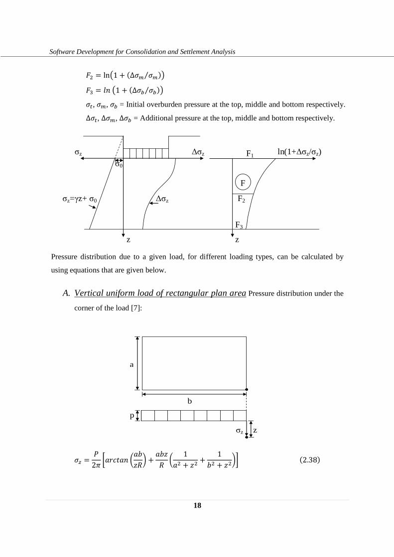
|� = lnF1 3 ∆�� ��⁄ �G |( � d#F1 3 ∆�� ��⁄ �G � , ��, �� = Initial overburden pressure at the top, middle and bottom respectively.
∆� , ∆��, ∆�� = Additional pressure at the top, middle and bottom respectively.
Pressure distribution due to a given load, for different loading types, can be calculated by
using equations that are given below.
A. Vertical uniform load of rectangular plan area Pressure distribution under the
corner of the load [7]:
�� � g2� �h���h# Hh=�`I 3 h=�` H 1h� 3 �� 3 1=� 3 ��I�2.38�
F2
F1
F3
z z
σ0
σz=γz+ σ0 ∆σz
σz ∆σz ln(1+∆σz/σz)
F
p
σz
a
b
z
19
Software Development for Consolidation and Settlement Analysis
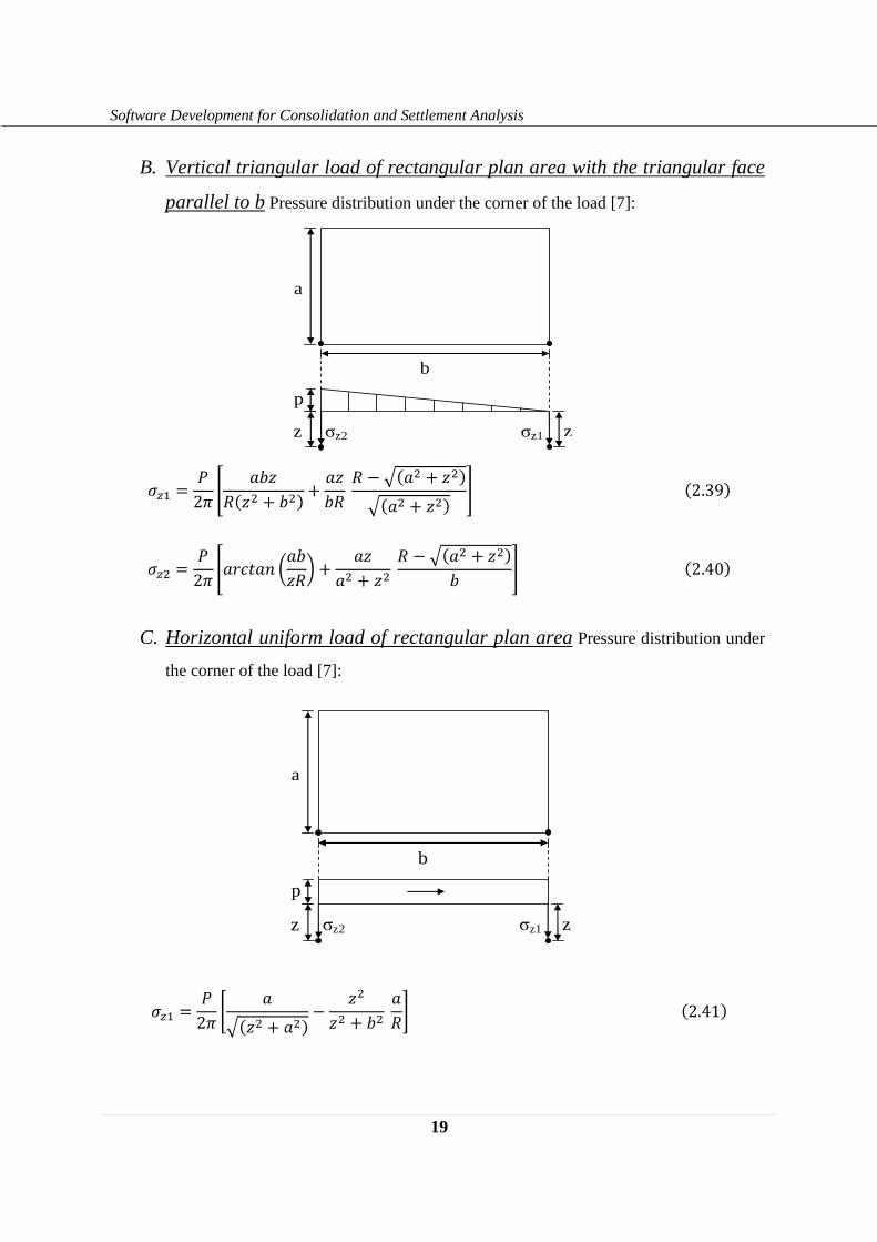
B. Vertical triangular load of rectangular plan area with the triangular face
parallel to b Pressure distribution under the corner of the load [7]:
��' = g2� � h=�`�� 3 =�� 3 h�=` ` , �h� 3 ����h� 3 ��� �2.39�
��� � g2� �h���h# Hh=�`I 3 h�h� 3 �� ` , �h� 3 ���= �2.40� C. Horizontal uniform load of rectangular plan area Pressure distribution under
the corner of the load [7]:
��' � g2� � h��� 3 h�� , ���� 3 =� h̀�2.41�
p
σz1
a
b
z σz2 z
p
σz1
a
b
z σz2 z
20
Software Development for Consolidation and Settlement Analysis
��� = − g2� � h��� 3 h�� , ���� 3 =� h̀� 2.42�
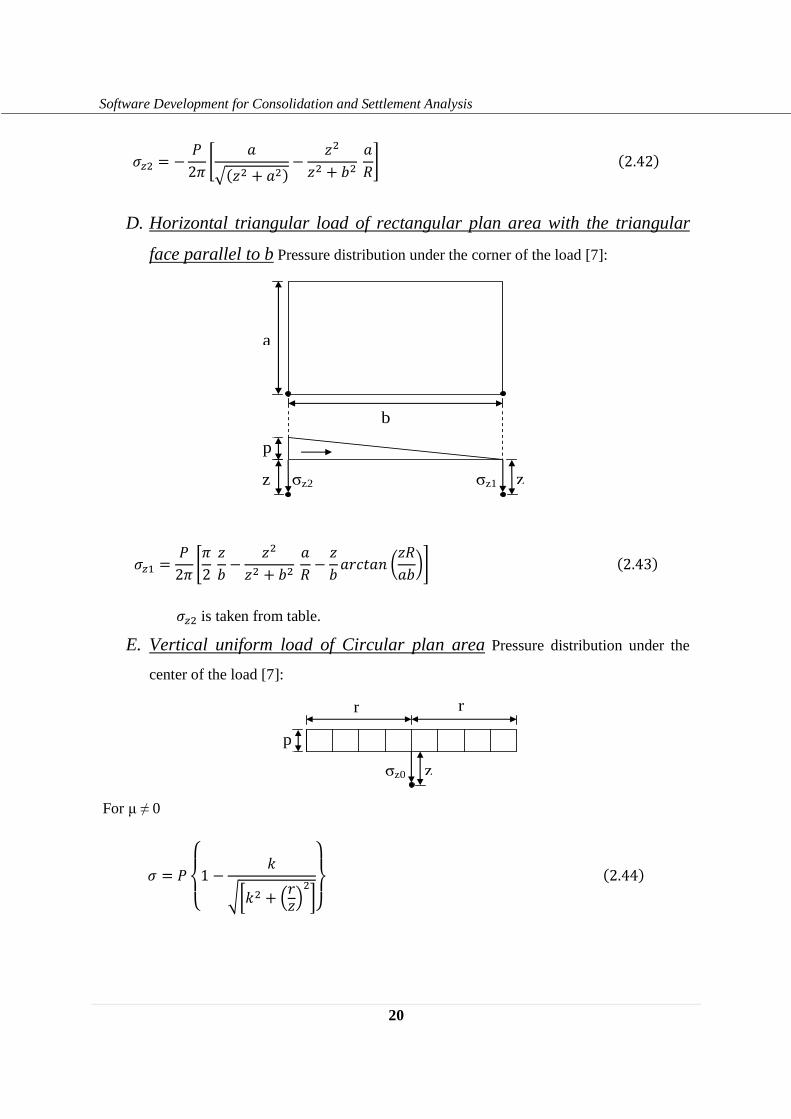
D. Horizontal triangular load of rectangular plan area with the triangular
face parallel to b Pressure distribution under the corner of the load [7]:
��' � g2� ��2�= , ���� 3 =� h̀ , �= h���h# H�h̀=I� 2.43�
��� is taken from table.
E. Vertical uniform load of Circular plan area Pressure distribution under the
center of the load [7]:
For µ ≠ 0
� � g���1 , �
���� 3 L��N�����2.44�
p
σz1
a
b
z σz2 z
p
σz0
r
z
r
21
Software Development for Consolidation and Settlement Analysis
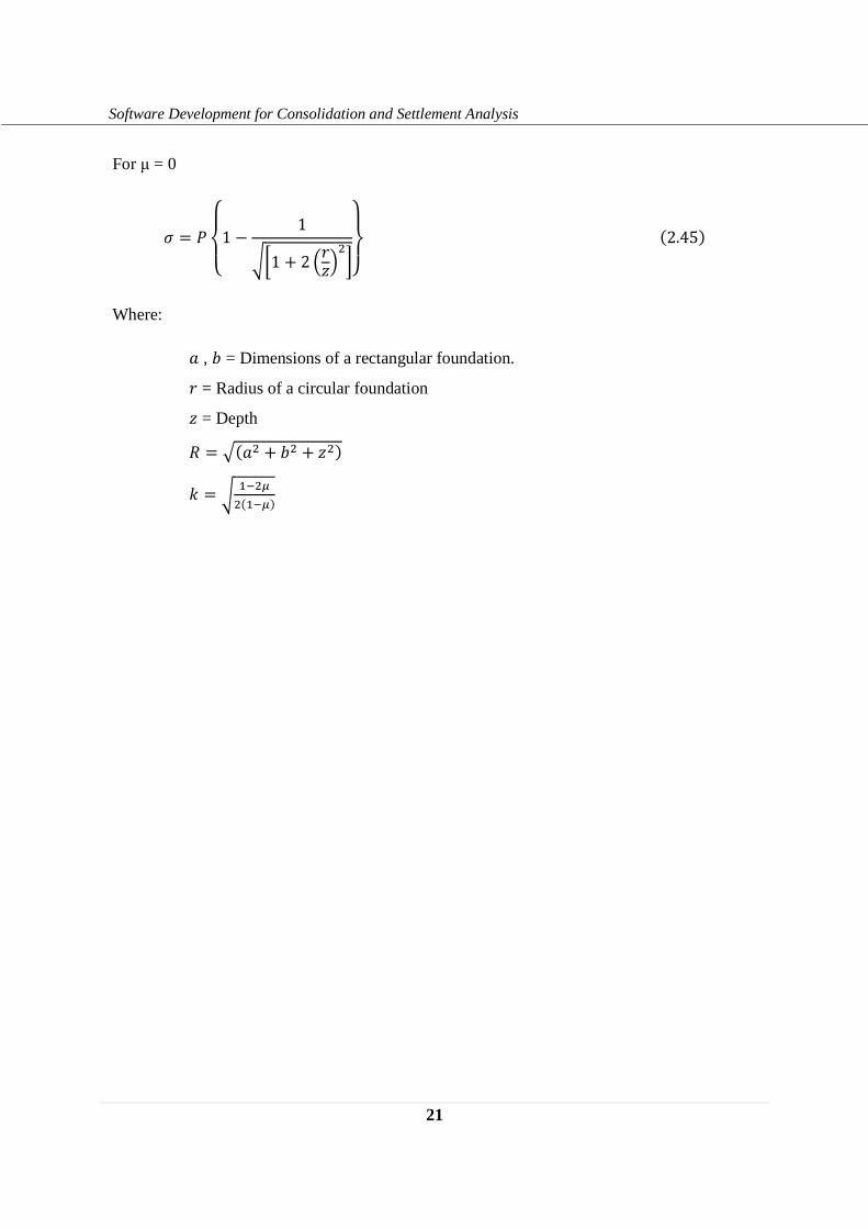
For µ = 0
� = g���1 − 1
��1 + 2 L��N�����(2.45)
Where:
h , = = Dimensions of a rectangular foundation.
� = Radius of a circular foundation
� = Depth
` = �(h� + =� + ��) � = � '����('��)
22
Software Development for Consolidation and Settlement Analysis
CHAPTER THREE
Methodology
3.1 General
As stated in chapter one, the aim of this thesis is to develop software for analysis of
consolidation and settlement. A software is developed using visual basic.net 2008
programming language. Flowchart is first prepared before going to designing the interface of
the software and writing the code. The next work performed is preparing interface, writing the
code and debugging.
The prepared flowchart describes the flow of the work which includes the inputs required, the
way of arriving to the output and the output of the software. The flowchart is presented in the
appendix part of the thesis. The software has a multi-form user interface. These forms
communicate to each other through globally declared variables in a module. Debugging is
done repeatedly during the coding time.
The software performs consolidation and settlement analysis for different loading conditions,
different drainage conditions and different soil conditions. The analyses done by the software
for these conditions are given in the next sections of this chapter.
3.2 Consolidation Analysis
As stated in chapter two, consolidation analysis can be done by using Fourier series solution
of the consolidation equation or by using finite difference solution. The developed software
can analyze consolidation by the two methods.
3.2.1 Consolidation analysis using Fourier series solution
Consolidation analysis using Fourier series solution of consolidation equation is done using
equations (2.2) to (2.15) in chapter two. Inputs required, conditions considered and the
outputs of the software for this case are given below.

23
Software Development for Consolidation and Settlement Analysis
3.2.1.1 Input
Inputs required for this case include initial excess pore water pressure distribution, drainage
condition, thickness of consolidating layer and coefficient of consolidation of the soil. In
addition to this inputs, time, depth and degree of consolidation values may be needed
depending on the required output.
3.2.1.2 Conditions considered
For consolidation analysis using Fourier series solution, one assumes that the soil is saturated.
It is also assumed that soil layer is homogeneous. Single and double drainage conditions are
treated.
Initial excess pore water pressure distribution can be given or it can be calculated from
contact pressure due to given surface loading. The initial excess pore water pressure
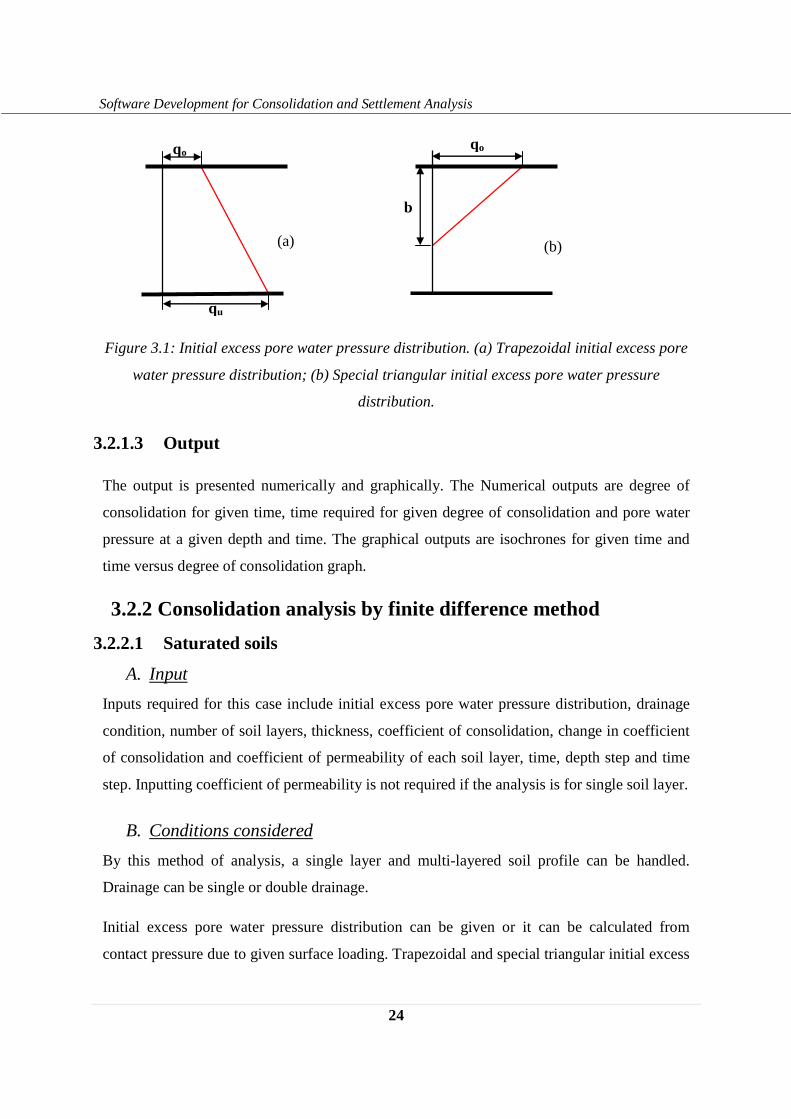
distributions considered are trapezoidal and special triangular (Fig. 3.1). Rectangular and
triangular initial excess pore water pressure distributions can be handled using the trapezoidal
case. Special triangular initial excess pore water pressure distribution is considered for double
drainage only. For initial excess pore water pressure distribution from contact pressure case,
the contact pressures considered are rectangular uniform contact pressure and circular uniform
contact pressure. Here the initial excess pore water pressure distribution is taken as the
calculated pressure distribution by approximating it to a trapezoidal shape. For rectangular
uniform contact pressure case, pressure distributions, in turn initial excess pore water pressure
distributions, under the center and at the characteristic point of the load area are considered
whereas for circular uniform contact pressure case, initial excess pore water pressure
distribution only under the center of the load area is considered.
24
Software Development for Consolidation and Settlement Analysis
Figure 3.1: Initial excess pore water pressure distribution. (a) Trapezoidal initial excess pore
water pressure distribution; (b) Special triangular initial excess pore water pressure
distribution.
3.2.1.3 Output
The output is presented numerically and graphically. The Numerical outputs are degree of
consolidation for given time, time required for given degree of consolidation and pore water
pressure at a given depth and time. The graphical outputs are isochrones for given time and
time versus degree of consolidation graph.
3.2.2 Consolidation analysis by finite difference method
3.2.2.1 Saturated soils
A. Input
Inputs required for this case include initial excess pore water pressure distribution, drainage
condition, number of soil layers, thickness, coefficient of consolidation, change in coefficient
of consolidation and coefficient of permeability of each soil layer, time, depth step and time
step. Inputting coefficient of permeability is not required if the analysis is for single soil layer.
B. Conditions considered
By this method of analysis, a single layer and multi-layered soil profile can be handled.
Drainage can be single or double drainage.
Initial excess pore water pressure distribution can be given or it can be calculated from
contact pressure due to given surface loading. Trapezoidal and special triangular initial excess
qo
b
qo
qu
(a) (b)
25
Software Development for Consolidation and Settlement Analysis
pore water pressure distributions can be given. Rectangular and triangular initial excess pore
water pressures can be handled by the trapezoidal case. For initial excess pore water pressure
from contact pressure case, rectangular uniform contact pressure and circular uniform contact
pressure distributions are considered. Initial excess pore water pressure distributions at the
center and at the characteristic point of the load area are considered for rectangular uniform
contact pressure distribution case whereas initial excess pore water pressure distribution only
at the center is considered for circular uniform contact pressure distribution case.
In addition to the above conditions, this case also includes different load scenarios. These
scenarios are constant load scenario, variable load scenario and abrupt change of load
scenario. For constant load scenario, Eq. (2.16), Eq. (2.17), Eq. (2.18) and Eq. (2.19) are used
to calculate pore water pressure and degree of consolidation. However, for variable load and
abrupt change of load scenarios, these equations are modified as given below [4].
� Variable load scenario
Excess pore water pressure at interior nodes is calculated as:
�C,D0' = ��C,D+�C,D + ����� F�C�',D − 2�C,D + �C0',DG(3.1) Excess pore water pressure at boundary nodes is calculated as:
�C,D0' = ��C,D + �C,D + ����� F2�C�',D − 2�C,DG(3.2) Excess pore water pressure at the interface for layered soils is calculated as:
�C,D0' = ��C,D + �C,D + ��'∆�(∆�)� 1 + �� �'⁄1 + (�� �'⁄ )(��' ���⁄ ) × H 2�'�' + �� �C�',D − 2�C,D + 2���' + �� �C0',DI(3.3)
Where:
- ��C,D = Change in excess pore water pressure per each time step due to the change in
load
26
Software Development for Consolidation and Settlement Analysis
Degree of consolidation is calculated as:
J = KL�� + �M2 N + ∑ �CM�'C%' P KL�� + �M2 N + ∑ �CM�'C%' P�(3.4)
Where:
- KL8�08�� N + ∑ �CM�'C%' P = Term calculated using pore water pressure at time t.
- KL8�08�� N + ∑ �CM�'C%' P� = Term calculated using unconsolidated pressure at time t.
� Abrupt change of load scenario
For calculations at the times different from the time of abrupt change of load, excess pore
water pressure is calculated using equations (2.16), (2.17) and (2.18). For calculations at the
time of abrupt change of load, the following equations are used.
Excess pore water pressure at interior nodes is calculated as:
�C,D0' = ��C,D+�C,D + ����� F�C�',D − 2�C,D + �C0',DG(3.5) Excess pore water pressure at boundary nodes is calculated as:
�C,D0' = ��C,D + �C,D + ����� F2�C�',D − 2�C,DG(3.6) Excess pore water pressure at the interface for layered soils is calculated as:
�C,D0' = ��C,D + �C,D + ��'∆�(∆�)� 1 + �� �'⁄1 + (�� �'⁄ )(��' ���⁄ ) × H 2�'�' + �� �C�',D − 2�C,D + 2���' + �� �C0',DI(3.7)
Where:
- ��C,D = Change in excess pore water pressure due to the abrupt change in load
27
Software Development for Consolidation and Settlement Analysis
Calculation of degree of consolidation will be done by Eq. (3.4).
C. Output
The outputs of this case are given in tabular and graphical form. The outputs obtained in
tabular form are pore water pressure for each depth step and time step and degree of
consolidation for each time step. Graphical outputs are isochrones for given time and time
versus degree of consolidation graph. Isochrones are plotted in two options. One option is
plotting isochrones for each time step up to the given time. The second option is plotting
isochrone for a selected time step in the range of the given time.
3.2.2.2 Unsaturated soils
Consolidation analysis for unsaturated soils includes analysis with respect to both water and
air.
A. Input
Inputs related to the water phase are initial excess pore water pressure distribution, drainage
condition for water, coefficient of permeability with respect to water, density of water,
coefficient of water volume change with respect to change in net normal stress and coefficient
of water volume change with respect to change in matric suction.
Inputs related to the air phase are initial excess pore air pressure distribution, drainage
condition for air, molecular mass of air, coefficient of transmission, coefficient of air volume
change with respect to change in net normal stress and coefficient of air volume change with
respect to change in matric suction.
In addition to the above inputs other inputs required are thickness of soil, degree of saturation,
porosity, temperature, time, depth step and time step.
B. Conditions considered
Consolidation analysis for unsaturated soils by finite difference method is done for only single
soil layer. Single or double drainage can be considered.
28
Software Development for Consolidation and Settlement Analysis
Initial excess pore air and pore water pressure distributions considered in this analysis case
are trapezoidal initial excess pore air and pore water pressure distributions and special
triangular initial excess pore air and pore water pressure distributions. Here also rectangular
and triangular initial excess pore air and pore water pressure distributions can be handled by
the trapezoidal case.
Excess pore water pressure and excess pore air pressure calculation at interior nodes is done
using equations (2.30) and (2.31). For excess pore water pressure and excess pore air pressure
calculation at boundary nodes, equations (2.30) and (2.31) are modified to the following form.
Equation for calculating pore water pressure:
��(C,D0') = ��(C,D) + k��'�(1 − lTl�) − l�(1 − lTl�)kTm'T (3.9) Equation for calculating pore air pressure:
�T(C,D0') = �T(C,D) + kTm'T(1 − lTl�) − lT(1 − lTl�)k��'�(3.8) Where:
k� = ��� n�nU2 kT = ��T o op� �'� = 2��(C�',D) − 2��(C,D) m'T = 2�T(C�',D) − 2�T(C,D)
Degree of consolidation calculation is done using Eq. (2.19) for the air and water phases.
C. Output
The outputs of this case are also obtained in tabular and graphical form. The outputs obtained
in tabular form are pore air pressure and pore water pressure for each depth step and time step
and degree of consolidation for air and water phases for each time step. Graphical outputs are
isochrones for given time and time versus degree of consolidation graph for both phases.
29
Software Development for Consolidation and Settlement Analysis
Isochrones for each time step to the given time or isochrone for a selected time step in the
range of the given time can be obtained.
3.3 Settlement Analysis
Settlement analysis part of the software contains calculation of immediate settlement, primary
settlement and secondary settlement. Immediate settlement is a settlement independent of
time whereas primary settlement and secondary settlement are time dependant settlements.
Primary settlement can be calculated as primary settlement for given time or final primary
settlement. Secondary settlement is calculated for times after the completion of primary
settlement. Time of completion of primary settlement for given loading is an input required
from the user.
Immediate settlement is calculated by using equation (2.32). Final primary settlement is
calculated using equations (2.33), (2.34) or (2.35) depending on the selected calculation
method. Primary settlement for given time is calculated from the final primary settlement and
degree of consolidation. Degree of consolidation is calculated by Fourier series method using
equations (2.3), (2.5), (2.7), (2.9), (2.11) and (2.13). Secondary settlement is calculated using
equations (2.36) and (2.37) depending on the selected calculation method.
3.3.1 Input
Inputs required for settlement analysis part of the software include load, type and dimension
of the footing for which settlement is to be calculated, surcharge above the base of the footing,
thickness of the soil layer, unit weight, influence factor (for immediate settlement calculation),
Poisson’s ratio, modulus of elasticity, modulus of compressibility, compression index, initial
void ratio, coefficient of volume compressibility, parameters related to secondary settlement
(i.e. modulus of compressibility for secondary settlement and }�), coefficient of consolidation,
drainage condition, time for one hundred percent consolidation and time. All the above inputs
are not necessary for any settlement analysis. The inputs required from the user depend on the
type of analysis.
30
Software Development for Consolidation and Settlement Analysis
3.3.2 Conditions considered
The conditions considered depend upon parameters like the type of settlement to be calculated
and point at which the settlement is to be calculated. Generally, settlement analysis is done for
single soil layer. The overburden pressure from the soil above the base of the footing for
which settlement is to be calculated and other loads above the base of the footing are
considered as surcharge. The foundation types considered are rectangular foundation and
circular foundation.
For rectangular foundation, vertical loads and horizontal loads will be accepted by the
software. Vertical loads accepted include point load with eccentricity in both directions, line
load with eccentricity, distributed load with a trapezoidal shape. Any other distribution that
does not comply with the standard flexure formula is not accepted by the software. Horizontal
loads accepted include uniformly distributed load and triangularly distributed load. Fig. 3.2
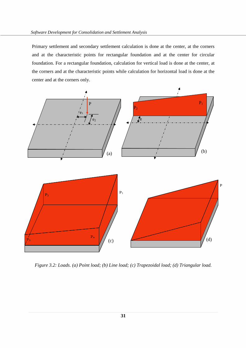
shows some selected loading geometries for vertical and horizontal loads.
For circular foundation case, point load at the center, line load at the centerlines and vertical
uniformly distributed load will be accepted.
Thickness of the settling layer can be given by the user or can be determined by the software.
The thickness determined by the software is taken as the depth from the base of the
foundation to a depth at which the pressure due to the load coming from the foundation
becomes ten percent of the over burden pressure at that depth.
Immediate settlement calculation is carried out for only vertical loading. The given load will
be averaged to uniformly distributed load to use it for immediate settlement calculation.
Immediate settlement calculation is done at the center, at the corners and at the characteristic
points for rectangular foundation and at the center for circular foundation.
31
Software Development for Consolidation and Settlement Analysis
Primary settlement and secondary settlement calculation is done at the center, at the corners
and at the characteristic points for rectangular foundation and at the center for circular
foundation. For a rectangular foundation, calculation for vertical load is done at the center, at
the corners and at the characteristic points while calculation for horizontal load is done at the
center and at the corners only.
Figure 3.2: Loads. (a) Point load; (b) Line load; (c) Trapezoidal load; (d) Triangular load.
P
P1
P3 P4
P2
(a) (b)
(c) (d)
e1
e2
P
e
P1 P2
32
Software Development for Consolidation and Settlement Analysis
3.3.3 Output
The outputs of the settlement analysis are presented numerically and graphically. The
numerical outputs include immediate settlement, final primary settlement, primary settlement
for given time, secondary settlement, final total settlement and total settlement for given time.
Graphical outputs are pressure distribution and time versus total settlement graph.
33
Software Development for Consolidation and Settlement Analysis
CHAPTER FOUR
Application of the Software
In this chapter, the contents of the developed software and the procedures that will be
followed to use the software are presented.
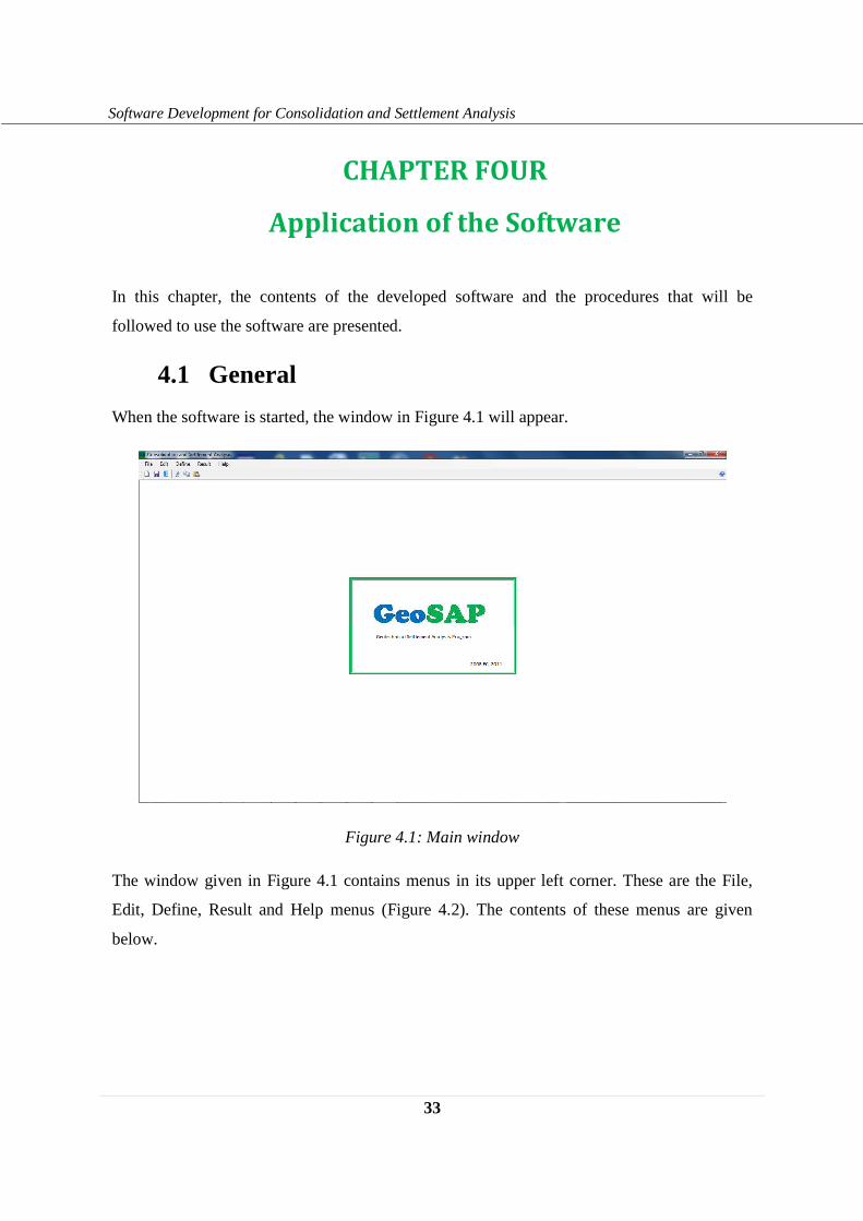
4.1 General
When the software is started, the window in Figure 4.1 will appear.
Figure 4.1: Main window
The window given in Figure 4.1 contains menus in its upper left corner. These are the File,
Edit, Define, Result and Help menus (Figure 4.2). The contents of these menus are given
below.

34
Software Development for Consolidation and Settlement Analysis
Figure 4.2: Menus
4.1.1 File menu
This menu contains the New, Save As and Export commands. The New command lets the
user to select the type of analysis. The Save As command allows the user to save the inputs
used for analysis. The Export command is used to export finite difference calculation table to
excel in the case of consolidation analysis by finite difference method. These commands can
also be accessed by using the shortcut keys given there or by the buttons provided in the
toolbar.
4.1.2 Edit menu
The commands in this menu are the Cut, Copy and Paste commands. These commands are
used to cut, copy and paste a text respectively. These commands can also be accessed by
using the shortcut keys given or by the buttons provided in the toolbar.
4.1.3 Define menu
This menu contains commands used to insert input values. For consolidation analysis, the first
command is the Load command which is used to input parameters related to load. For
settlement analysis, the first command is the Structure and Load command. This is used to
input parameters related to foundation and load. The next command for both consolidation
and settlement analysis is the Soil Property command. This command allows the user to input
parameters related to soil.
35
Software Development for Consolidation and Settlement Analysis
4.1.4 Result menu
The result menu contains commands that provide the user with the results of the analysis. For
consolidation analysis, the commands in this menu are the Consolidation, Isochrones and
Time Vs Degree of Consolidation Graph commands. The Consolidation command is used to
display numerical outputs of consolidation analysis. The Isochrones command and the Time
Vs Degree of Consolidation command are used to display isochrones and time versus degree
of consolidation graph respectively. For settlement analysis, the menu contains the Settlement,
Pressure Distribution and Time Vs Settlement graph commands. The Settlement command is
used to display numerical outputs of settlement analysis. The Pressure Distribution command
and the Time Vs Settlement Graph command are used to display pressure distribution and
time versus settlement graphs respectively.
4.1.5 Help menu
The Help menu contains the GeoSAP Help and About GeoSAP commands. The GeoSAP
Help command can also be accessed by using the shortcut key given or the Help button in the
toolbar.
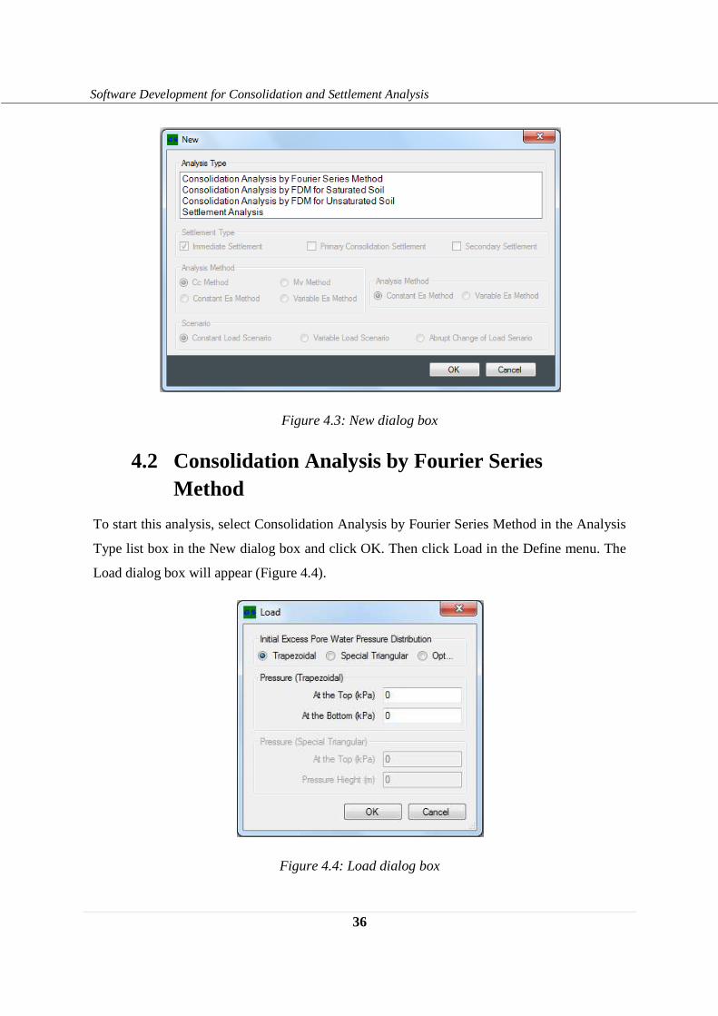
In starting both consolidation and settlement analysis, the first step is to click New in the File
menu to display the New dialog box (Figure 4.3). The New dialog box allows the user to
select the type of analysis to be done.
36
Software Development for Consolidation and Settlement Analysis
Figure 4.3: New dialog box
4.2 Consolidation Analysis by Fourier Series Method
To start this analysis, select Consolidation Analysis by Fourier Series Method in the Analysis
Type list box in the New dialog box and click OK. Then click Load in the Define menu. The
Load dialog box will appear (Figure 4.4).
Figure 4.4: Load dialog box
37
Software Development for Consolidation and Settlement Analysis
In the Initial Excess Pore Water Pressure Distribution group box, select the given initial
excess pore water pressure distribution. If the Trapezoidal or Special Triangular radio button
is selected, give the loads and click OK. If the Opt... radio button is selected, another Load
dialog box will appear (Figure 4.5).
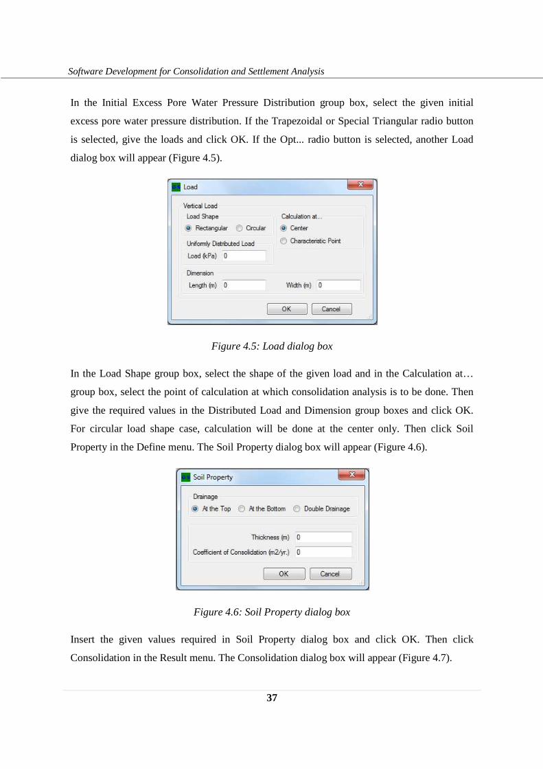
Figure 4.5: Load dialog box
In the Load Shape group box, select the shape of the given load and in the Calculation at…
group box, select the point of calculation at which consolidation analysis is to be done. Then
give the required values in the Distributed Load and Dimension group boxes and click OK.
For circular load shape case, calculation will be done at the center only. Then click Soil
Property in the Define menu. The Soil Property dialog box will appear (Figure 4.6).
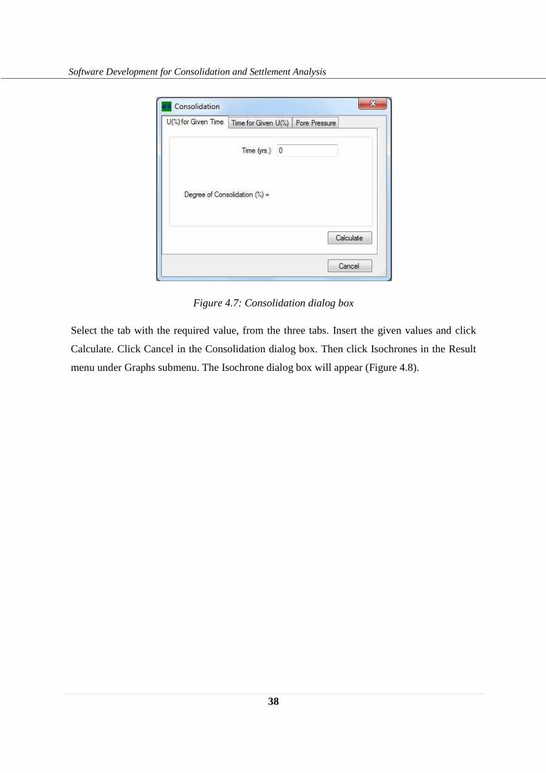
Figure 4.6: Soil Property dialog box
Insert the given values required in Soil Property dialog box and click OK. Then click
Consolidation in the Result menu. The Consolidation dialog box will appear (Figure 4.7).
38
Software Development for Consolidation and Settlement Analysis
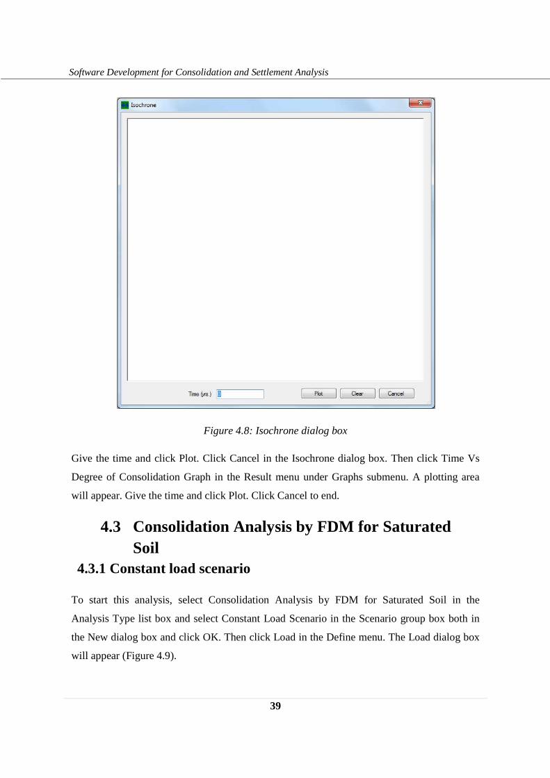
Figure 4.7: Consolidation dialog box
Select the tab with the required value, from the three tabs. Insert the given values and click
Calculate. Click Cancel in the Consolidation dialog box. Then click Isochrones in the Result
menu under Graphs submenu. The Isochrone dialog box will appear (Figure 4.8).
39
Software Development for Consolidation and Settlement Analysis
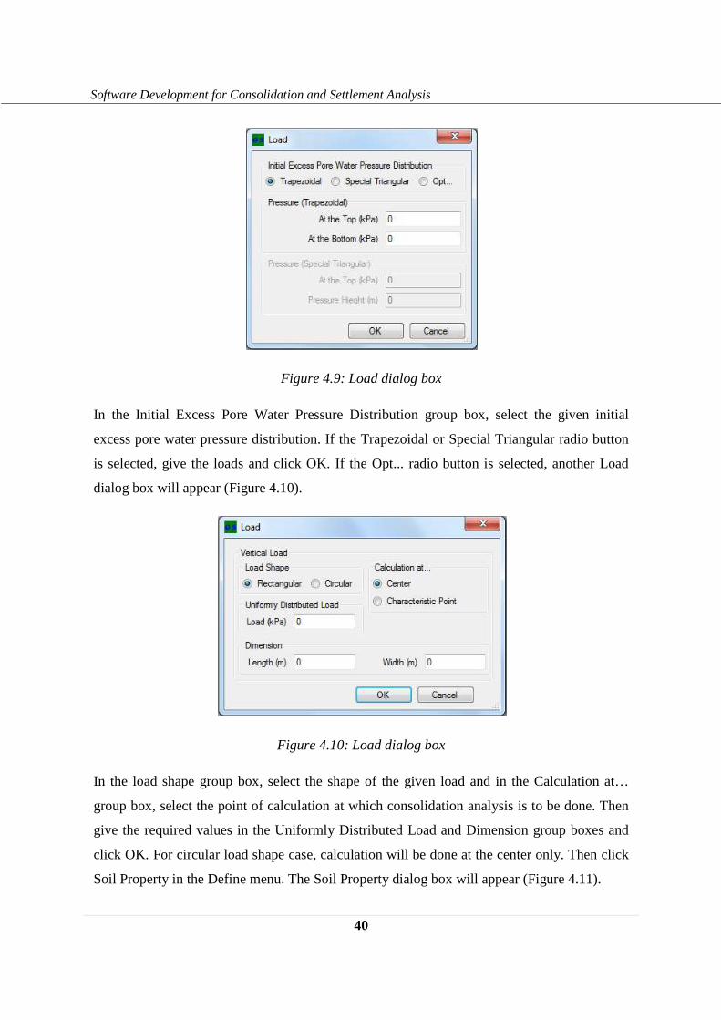
Figure 4.8: Isochrone dialog box
Give the time and click Plot. Click Cancel in the Isochrone dialog box. Then click Time Vs
Degree of Consolidation Graph in the Result menu under Graphs submenu. A plotting area
will appear. Give the time and click Plot. Click Cancel to end.
4.3 Consolidation Analysis by FDM for Saturated Soil
4.3.1 Constant load scenario
To start this analysis, select Consolidation Analysis by FDM for Saturated Soil in the
Analysis Type list box and select Constant Load Scenario in the Scenario group box both in
the New dialog box and click OK. Then click Load in the Define menu. The Load dialog box
will appear (Figure 4.9).
40
Software Development for Consolidation and Settlement Analysis
Figure 4.9: Load dialog box
In the Initial Excess Pore Water Pressure Distribution group box, select the given initial
excess pore water pressure distribution. If the Trapezoidal or Special Triangular radio button
is selected, give the loads and click OK. If the Opt... radio button is selected, another Load
dialog box will appear (Figure 4.10).
Figure 4.10: Load dialog box
In the load shape group box, select the shape of the given load and in the Calculation at…
group box, select the point of calculation at which consolidation analysis is to be done. Then
give the required values in the Uniformly Distributed Load and Dimension group boxes and
click OK. For circular load shape case, calculation will be done at the center only. Then click
Soil Property in the Define menu. The Soil Property dialog box will appear (Figure 4.11).
41
Software Development for Consolidation and Settlement Analysis
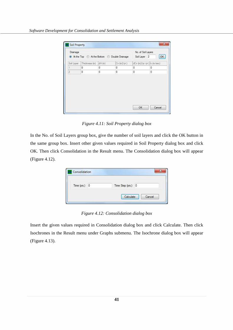
Figure 4.11: Soil Property dialog box
In the No. of Soil Layers group box, give the number of soil layers and click the OK button in
the same group box. Insert other given values required in Soil Property dialog box and click
OK. Then click Consolidation in the Result menu. The Consolidation dialog box will appear
(Figure 4.12).
Figure 4.12: Consolidation dialog box
Insert the given values required in Consolidation dialog box and click Calculate. Then click
Isochrones in the Result menu under Graphs submenu. The Isochrone dialog box will appear
(Figure 4.13).
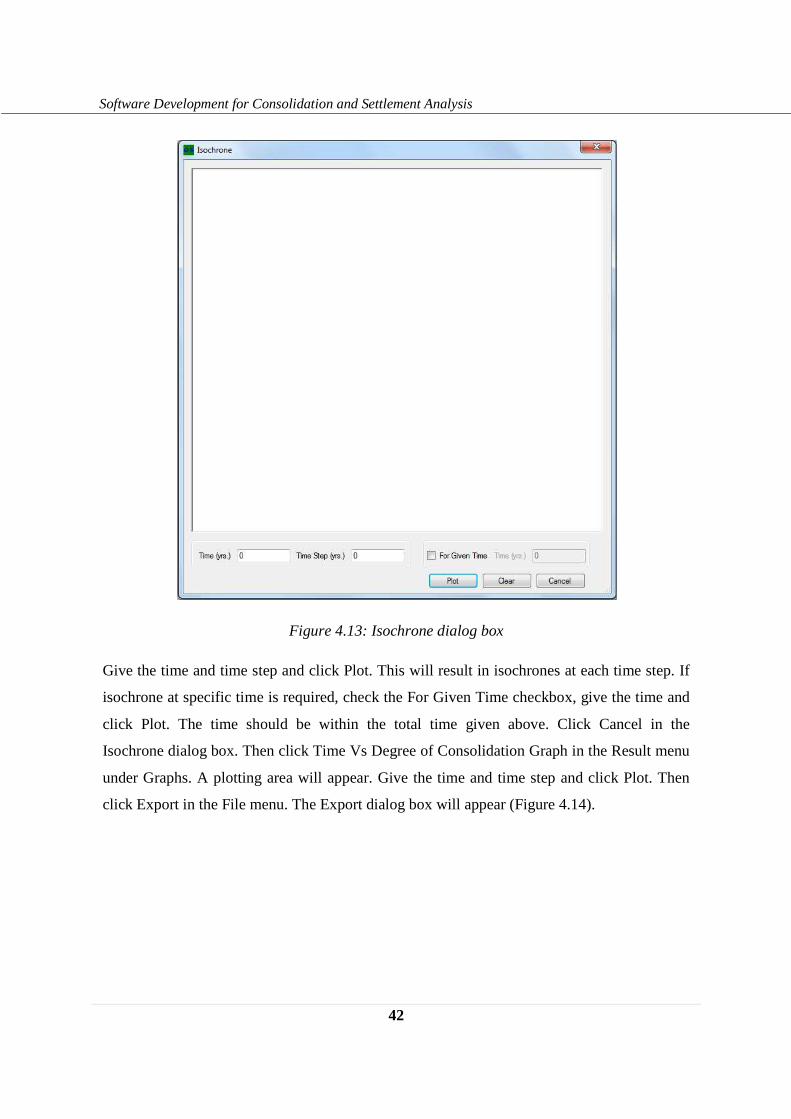
42
Software Development for Consolidation and Settlement Analysis
Figure 4.13: Isochrone dialog box
Give the time and time step and click Plot. This will result in isochrones at each time step. If
isochrone at specific time is required, check the For Given Time checkbox, give the time and
click Plot. The time should be within the total time given above. Click Cancel in the
Isochrone dialog box. Then click Time Vs Degree of Consolidation Graph in the Result menu
under Graphs. A plotting area will appear. Give the time and time step and click Plot. Then
click Export in the File menu. The Export dialog box will appear (Figure 4.14).
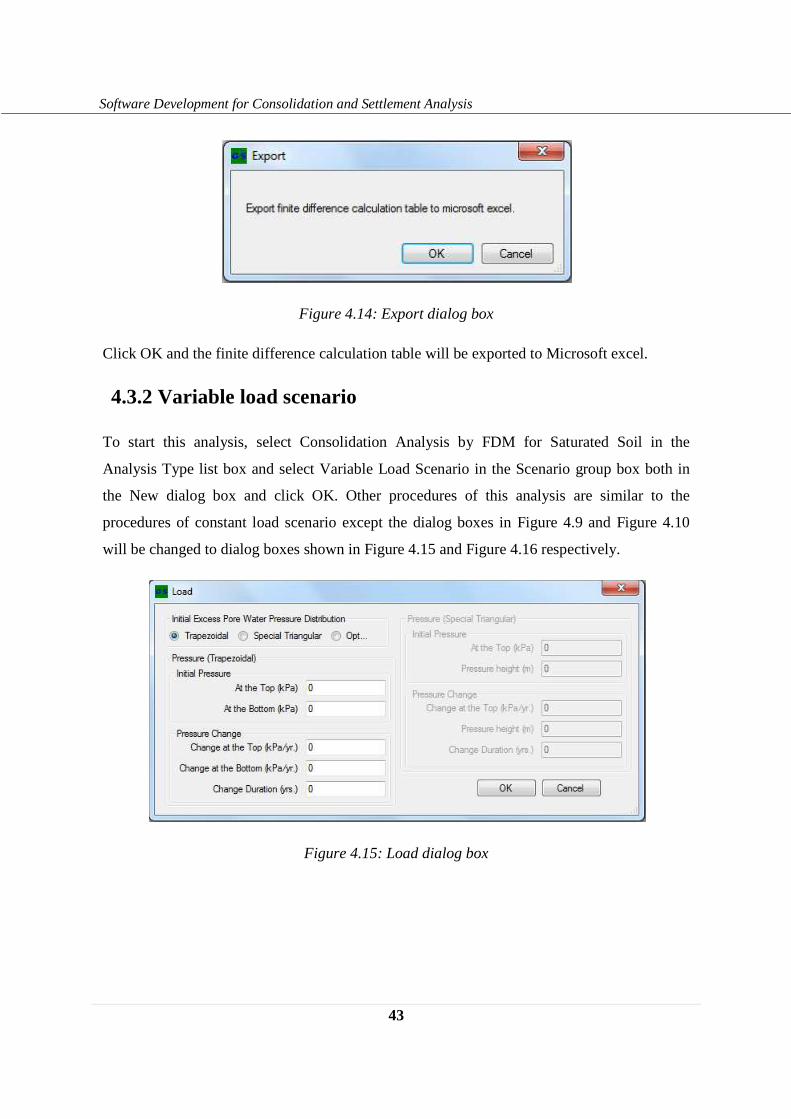
43
Software Development for Consolidation and Settlement Analysis
Figure 4.14: Export dialog box
Click OK and the finite difference calculation table will be exported to Microsoft excel.
4.3.2 Variable load scenario
To start this analysis, select Consolidation Analysis by FDM for Saturated Soil in the
Analysis Type list box and select Variable Load Scenario in the Scenario group box both in
the New dialog box and click OK. Other procedures of this analysis are similar to the
procedures of constant load scenario except the dialog boxes in Figure 4.9 and Figure 4.10
will be changed to dialog boxes shown in Figure 4.15 and Figure 4.16 respectively.
Figure 4.15: Load dialog box
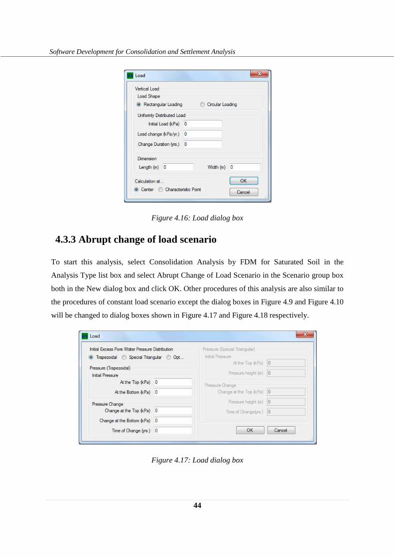
44
Software Development for Consolidation and Settlement Analysis
Figure 4.16: Load dialog box
4.3.3 Abrupt change of load scenario
To start this analysis, select Consolidation Analysis by FDM for Saturated Soil in the
Analysis Type list box and select Abrupt Change of Load Scenario in the Scenario group box
both in the New dialog box and click OK. Other procedures of this analysis are also similar to
the procedures of constant load scenario except the dialog boxes in Figure 4.9 and Figure 4.10
will be changed to dialog boxes shown in Figure 4.17 and Figure 4.18 respectively.
Figure 4.17: Load dialog box
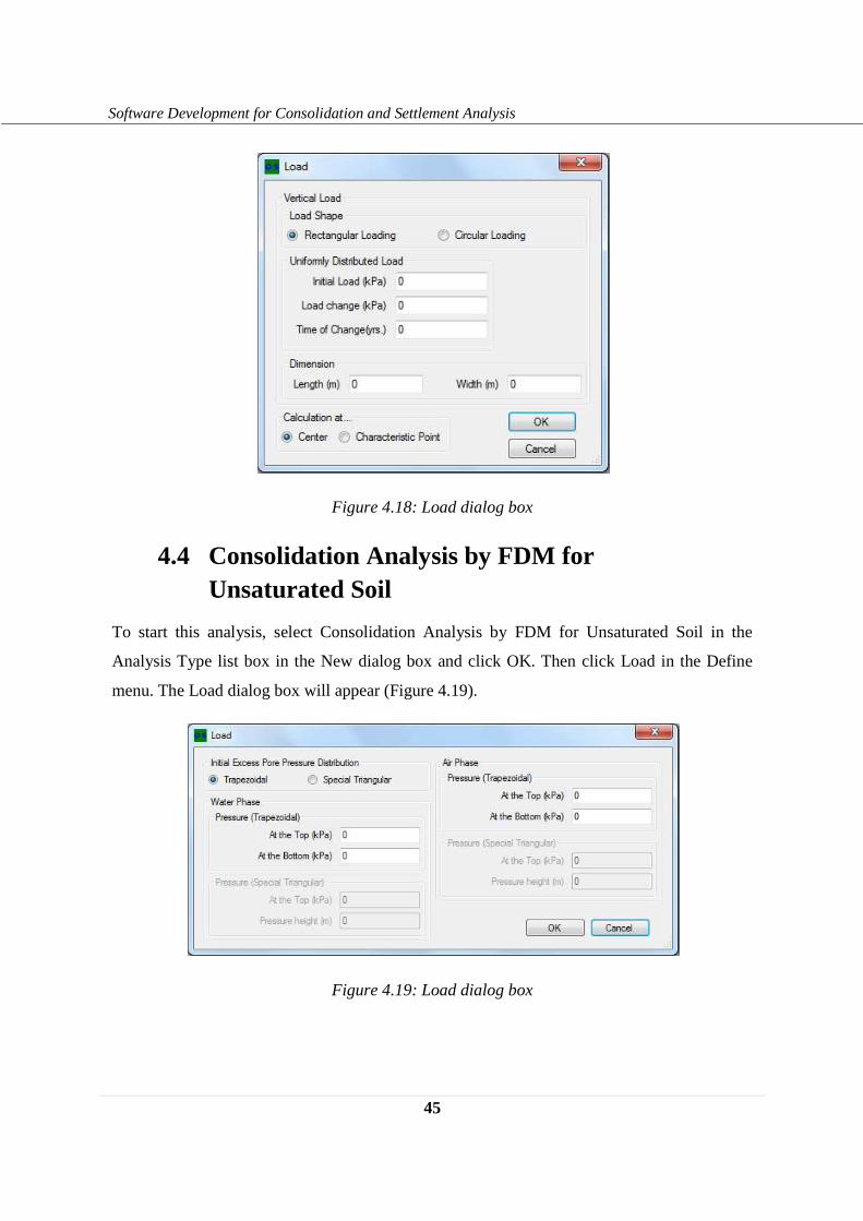
45
Software Development for Consolidation and Settlement Analysis
Figure 4.18: Load dialog box
4.4 Consolidation Analysis by FDM for Unsaturated Soil
To start this analysis, select Consolidation Analysis by FDM for Unsaturated Soil in the
Analysis Type list box in the New dialog box and click OK. Then click Load in the Define
menu. The Load dialog box will appear (Figure 4.19).
Figure 4.19: Load dialog box
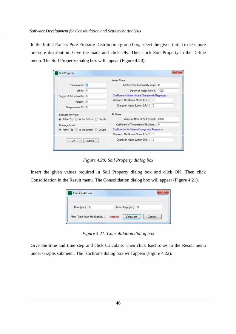
46
Software Development for Consolidation and Settlement Analysis
In the Initial Excess Pore Pressure Distribution group box, select the given initial excess pore
pressure distribution. Give the loads and click OK. Then click Soil Property in the Define
menu. The Soil Property dialog box will appear (Figure 4.20).
Figure 4.20: Soil Property dialog box
Insert the given values required in Soil Property dialog box and click OK. Then click
Consolidation in the Result menu. The Consolidation dialog box will appear (Figure 4.21).
Figure 4.21: Consolidation dialog box
Give the time and time step and click Calculate. Then click Isochrones in the Result menu
under Graphs submenu. The Isochrone dialog box will appear (Figure 4.22).
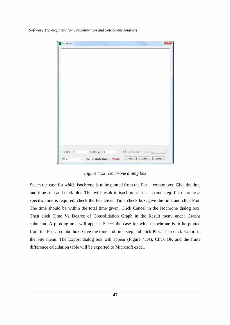
47
Software Development for Consolidation and Settlement Analysis
Figure 4.22: Isochrone dialog box
Select the case for which isochrone is to be plotted from the For… combo box. Give the time
and time step and click plot. This will result in isochrones at each time step. If isochrone at
specific time is required, check the For Given Time check box, give the time and click Plot.
The time should be within the total time given. Click Cancel in the Isochrone dialog box.
Then click Time Vs Degree of Consolidation Graph in the Result menu under Graphs
submenu. A plotting area will appear. Select the case for which isochrone is to be plotted
from the For… combo box. Give the time and time step and click Plot. Then click Export in
the File menu. The Export dialog box will appear (Figure 4.14). Click OK and the finite
difference calculation table will be exported to Microsoft excel.
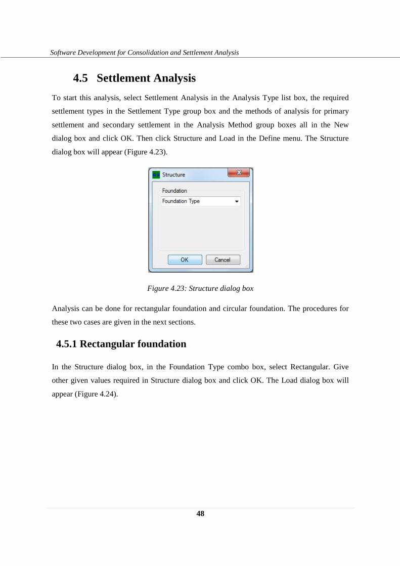
48
Software Development for Consolidation and Settlement Analysis
4.5 Settlement Analysis
To start this analysis, select Settlement Analysis in the Analysis Type list box, the required
settlement types in the Settlement Type group box and the methods of analysis for primary
settlement and secondary settlement in the Analysis Method group boxes all in the New
dialog box and click OK. Then click Structure and Load in the Define menu. The Structure
dialog box will appear (Figure 4.23).
Figure 4.23: Structure dialog box
Analysis can be done for rectangular foundation and circular foundation. The procedures for
these two cases are given in the next sections.
4.5.1 Rectangular foundation
In the Structure dialog box, in the Foundation Type combo box, select Rectangular. Give
other given values required in Structure dialog box and click OK. The Load dialog box will
appear (Figure 4.24).
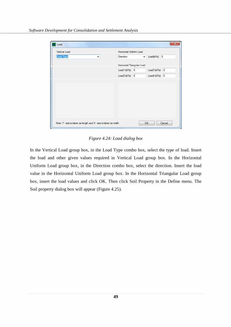
49
Software Development for Consolidation and Settlement Analysis
Figure 4.24: Load dialog box
In the Vertical Load group box, in the Load Type combo box, select the type of load. Insert
the load and other given values required in Vertical Load group box. In the Horizontal
Uniform Load group box, in the Direction combo box, select the direction. Insert the load
value in the Horizontal Uniform Load group box. In the Horizontal Triangular Load group
box, insert the load values and click OK. Then click Soil Property in the Define menu. The
Soil property dialog box will appear (Figure 4.25).
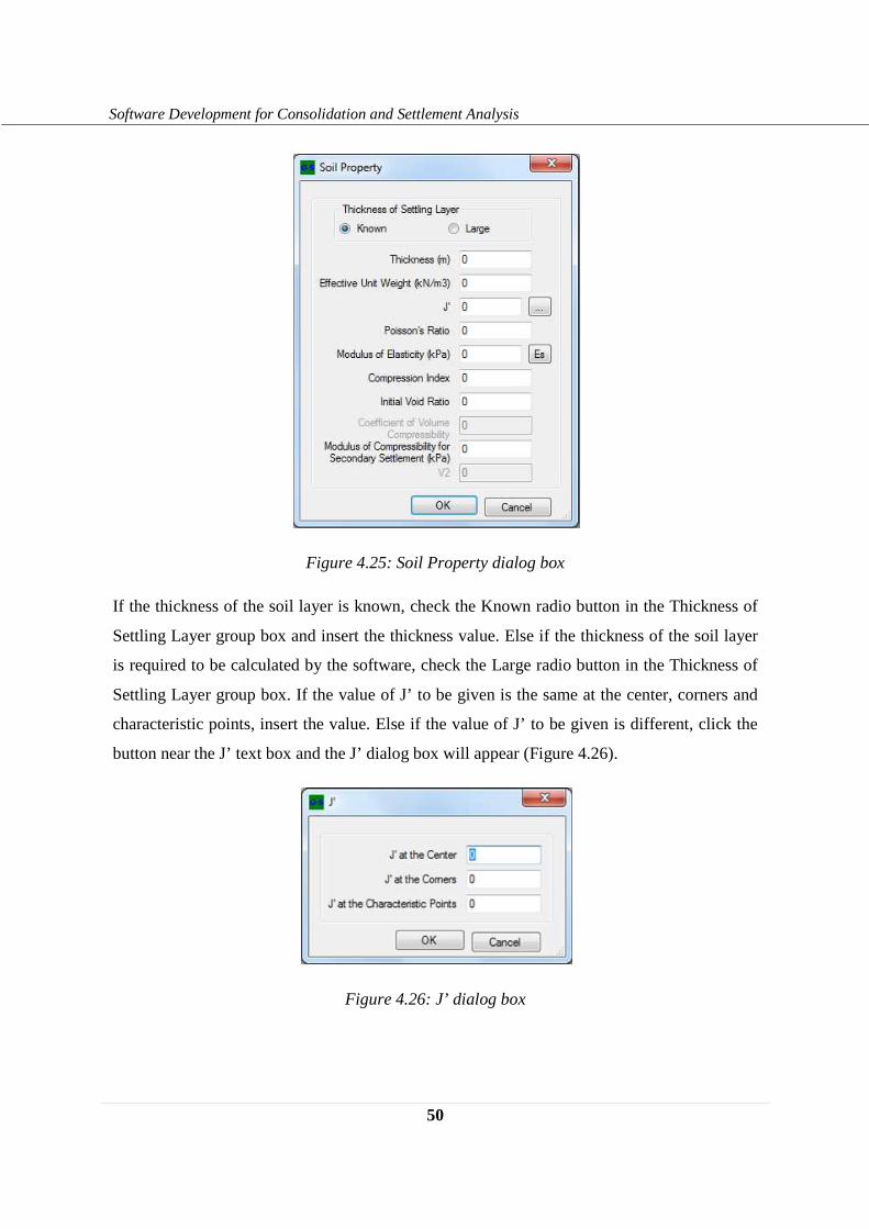
50
Software Development for Consolidation and Settlement Analysis
Figure 4.25: Soil Property dialog box
If the thickness of the soil layer is known, check the Known radio button in the Thickness of
Settling Layer group box and insert the thickness value. Else if the thickness of the soil layer
is required to be calculated by the software, check the Large radio button in the Thickness of
Settling Layer group box. If the value of J’ to be given is the same at the center, corners and
characteristic points, insert the value. Else if the value of J’ to be given is different, click the
button near the J’ text box and the J’ dialog box will appear (Figure 4.26).
Figure 4.26: J’ dialog box
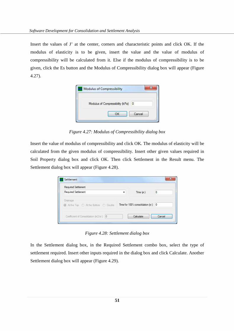
51
Software Development for Consolidation and Settlement Analysis
Insert the values of J’ at the center, corners and characteristic points and click OK. If the
modulus of elasticity is to be given, insert the value and the value of modulus of
compressibility will be calculated from it. Else if the modulus of compressibility is to be
given, click the Es button and the Modulus of Compressibility dialog box will appear (Figure
4.27).
Figure 4.27: Modulus of Compressibility dialog box
Insert the value of modulus of compressibility and click OK. The modulus of elasticity will be
calculated from the given modulus of compressibility. Insert other given values required in
Soil Property dialog box and click OK. Then click Settlement in the Result menu. The
Settlement dialog box will appear (Figure 4.28).
Figure 4.28: Settlement dialog box
In the Settlement dialog box, in the Required Settlement combo box, select the type of
settlement required. Insert other inputs required in the dialog box and click Calculate. Another
Settlement dialog box will appear (Figure 4.29).
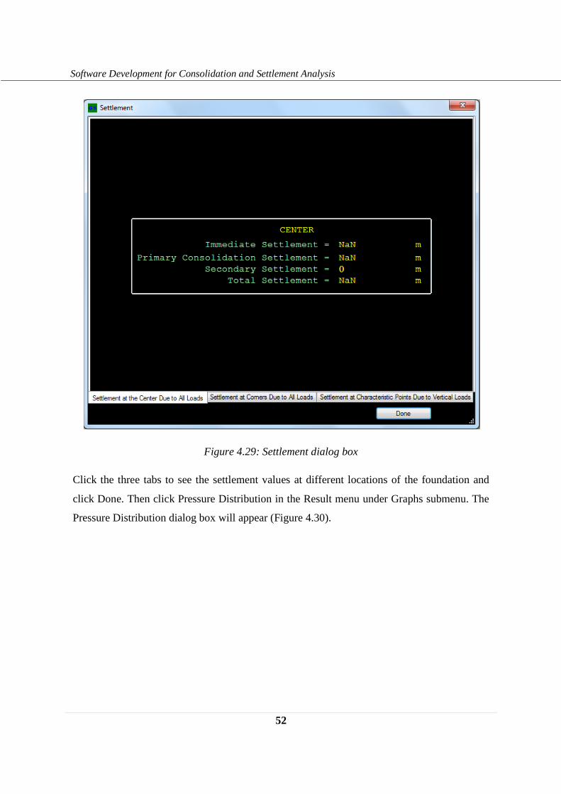
52
Software Development for Consolidation and Settlement Analysis
Figure 4.29: Settlement dialog box
Click the three tabs to see the settlement values at different locations of the foundation and
click Done. Then click Pressure Distribution in the Result menu under Graphs submenu. The
Pressure Distribution dialog box will appear (Figure 4.30).
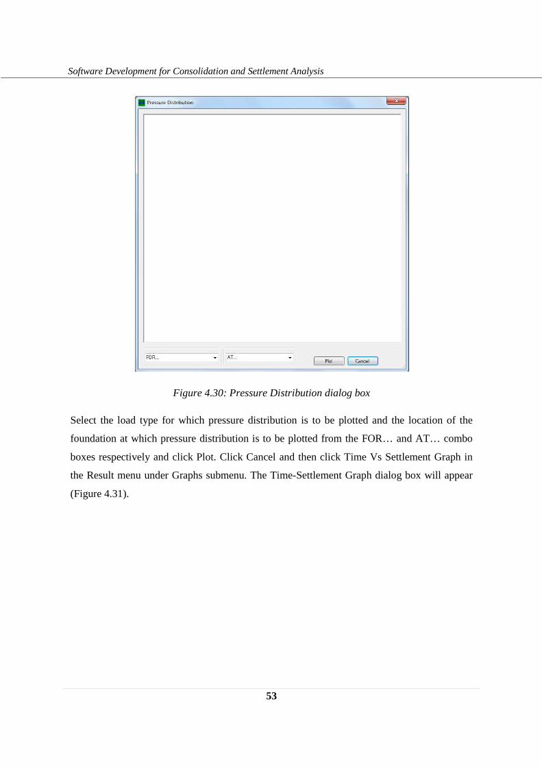
53
Software Development for Consolidation and Settlement Analysis
Figure 4.30: Pressure Distribution dialog box
Select the load type for which pressure distribution is to be plotted and the location of the
foundation at which pressure distribution is to be plotted from the FOR… and AT… combo
boxes respectively and click Plot. Click Cancel and then click Time Vs Settlement Graph in
the Result menu under Graphs submenu. The Time-Settlement Graph dialog box will appear
(Figure 4.31).
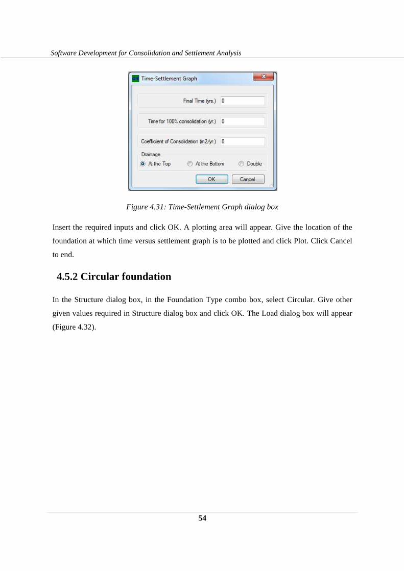
54
Software Development for Consolidation and Settlement Analysis
Figure 4.31: Time-Settlement Graph dialog box
Insert the required inputs and click OK. A plotting area will appear. Give the location of the
foundation at which time versus settlement graph is to be plotted and click Plot. Click Cancel
to end.
4.5.2 Circular foundation
In the Structure dialog box, in the Foundation Type combo box, select Circular. Give other
given values required in Structure dialog box and click OK. The Load dialog box will appear
(Figure 4.32).
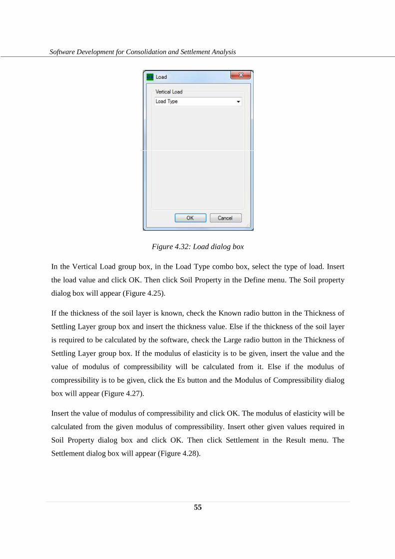
55
Software Development for Consolidation and Settlement Analysis
Figure 4.32: Load dialog box
In the Vertical Load group box, in the Load Type combo box, select the type of load. Insert
the load value and click OK. Then click Soil Property in the Define menu. The Soil property
dialog box will appear (Figure 4.25).
If the thickness of the soil layer is known, check the Known radio button in the Thickness of
Settling Layer group box and insert the thickness value. Else if the thickness of the soil layer
is required to be calculated by the software, check the Large radio button in the Thickness of
Settling Layer group box. If the modulus of elasticity is to be given, insert the value and the
value of modulus of compressibility will be calculated from it. Else if the modulus of
compressibility is to be given, click the Es button and the Modulus of Compressibility dialog
box will appear (Figure 4.27).
Insert the value of modulus of compressibility and click OK. The modulus of elasticity will be
calculated from the given modulus of compressibility. Insert other given values required in
Soil Property dialog box and click OK. Then click Settlement in the Result menu. The
Settlement dialog box will appear (Figure 4.28).
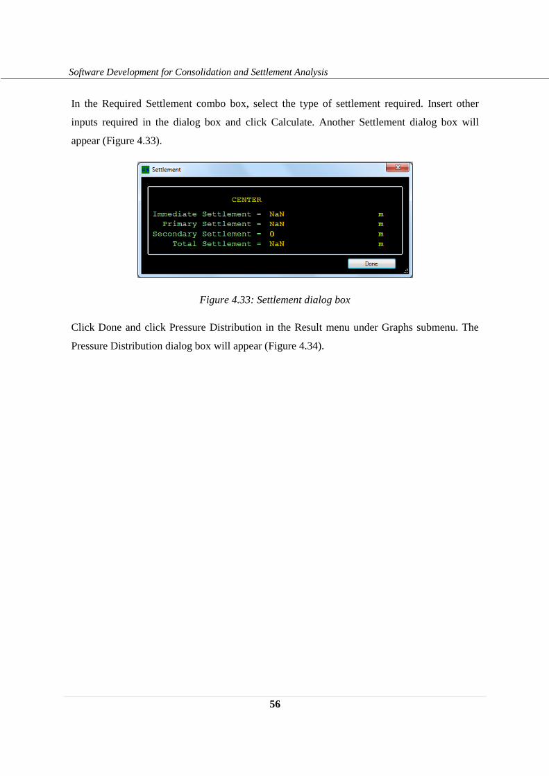
56
Software Development for Consolidation and Settlement Analysis
In the Required Settlement combo box, select the type of settlement required. Insert other
inputs required in the dialog box and click Calculate. Another Settlement dialog box will
appear (Figure 4.33).
Figure 4.33: Settlement dialog box
Click Done and click Pressure Distribution in the Result menu under Graphs submenu. The
Pressure Distribution dialog box will appear (Figure 4.34).
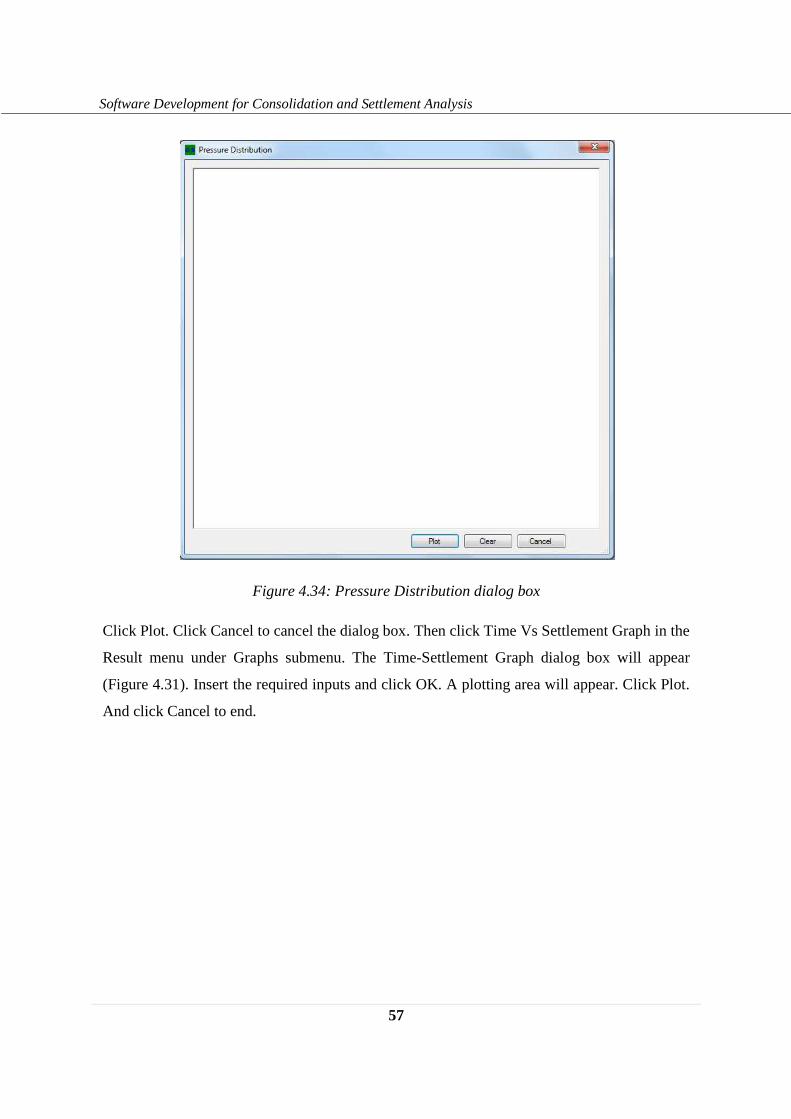
57
Software Development for Consolidation and Settlement Analysis
Figure 4.34: Pressure Distribution dialog box
Click Plot. Click Cancel to cancel the dialog box. Then click Time Vs Settlement Graph in the
Result menu under Graphs submenu. The Time-Settlement Graph dialog box will appear
(Figure 4.31). Insert the required inputs and click OK. A plotting area will appear. Click Plot.
And click Cancel to end.
58
Software Development for Consolidation and Settlement Analysis
CHAPTER FIVE
Validation of the Software
To validate the software developed, examples have been worked out as presented in Appendix
B. From the examples, the following observation is made.
� The result obtained from the common calculation methods and the results of the
software are more or less similar in all analyses.
� The result of consolidation analysis by Fourier series method and finite difference
method give approximately similar result. The value of pore water pressure obtained
from the two methods is more or less the same. And the value of degree of
consolidation from the methods is also similar even if it is not as similar as the pore
water pressure.
� The developed software is simpler, faster and more accurate.
59
Software Development for Consolidation and Settlement Analysis
CHAPTER SIX
Conclusion and Recommendation
6.1 Conclusion
Conclusions from the study include:
1. The result of consolidation analysis by Fourier series method and finite difference
method give approximately similar result.
2. For the consolidation analysis by finite difference method, the stability of the
calculation is very sensitive to the beta value. The result may not be reliable for
inappropriate beta values.
3. The developed software can be used to analyze consolidation and settlement simply,
quickly and accurately. Comparison of results obtained from different analysis
methods of consolidation and settlement can be also made with the software. The
developed software is also important to study the properties of the results for different
values of input parameters.
6.2 Recommendation
There are additional cases to be considered which are important for the practice and open for
further studies. These include settlement analysis for unsaturated soils, consolidation and
settlement analysis for two dimensional and three dimensional consolidation processes.
60
Software Development for Consolidation and Settlement Analysis
References
1. Das, B.M., 2008. Advanced Soil Mechanics. Taylor and Francis. New York.
2. Fredlund, D.G. and H. Rahardjo, 1993. Soil Mechanics for Unsaturated Soils. JOHN
WILEY AND SONS, INC. New York.
3. Redie, T., 2010. Software Development for Consolidation Analysis under Various
Loading Conditions Using Finite Difference Method. Unpublished Thesis. Addis Ababa
Institute of Technology.
4. Seged, H., 2010. Finite Difference Method. Lecture Notes, CENG 6202 Advanced
Computational Methods in Geotechnical Engineering, Addis Ababa Institute of
Technology.
5. Teferra, A., 2008. Principles of Foundation Engineering. AAU – Press. Addis Ababa.
6. Teferra, A., 2010. Theory of Consolidation and Settlement Analysis. Lecture Notes,
CENG 6207 Advanced Soil Mechanics, Addis Ababa Institute of Technology.
7. Teferra, A. and E. Schultze, 1988. Formulae, Charts and Tables in the area of soil
Mechanics and Foundation Engineering. A.A.BALKEMA. Rotterdam.
8. Teferra, A. and M. Leikun, 1999. Soil Mechanics. AAU – Press. Addis Ababa.
9. Terzaghi, K., 1943. Theoretical Soil Mechanics. JOHN WILEY AND SONS, INC. New
York.
61
Software Development for Consolidation and Settlement Analysis
APPENDIX A
Flowchart

62
Software Development for Consolidation and Settlement Analysis
No No
Yes Yes Yes
No
Unsaturated
Saturated
Fourier series
Consolidation Settlement
START
F E
Select settlement types to be calculated D
Stop Stop Stop
C B A
Analysis Type
Method
Finite difference method
Saturation
Immediate Primary Secondary
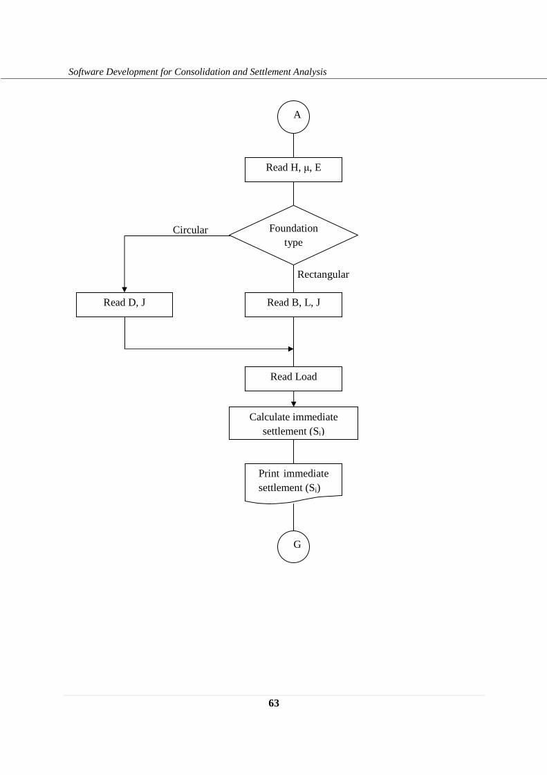
63
Software Development for Consolidation and Settlement Analysis
Circular
Read H, µ, E
Read D, J Read B, L, J
Calculate immediate settlement (Si)
Print immediate settlement (Si)
A
G
Foundation type
Rectangular
Read Load
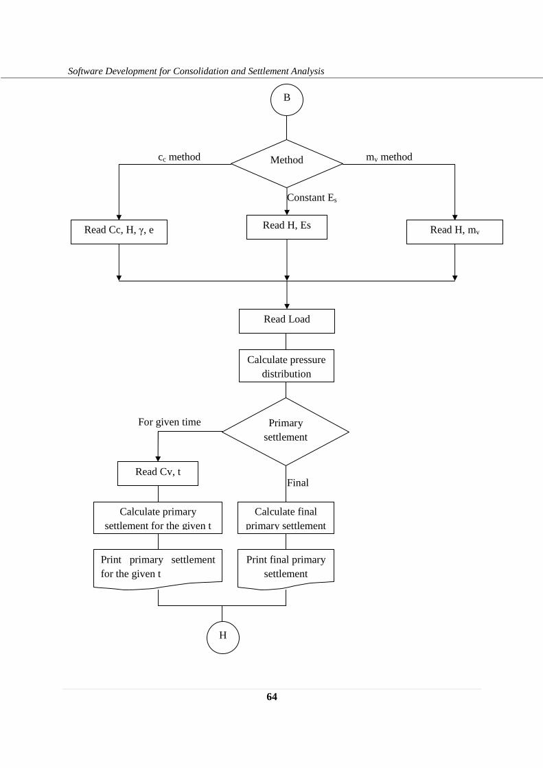
64
Software Development for Consolidation and Settlement Analysis
Final
For given time
cc method mv method
Constant Es
B
Read Cc, H, γ, e Read H, mv Read H, Es
Read Load
Method
Calculate pressure distribution
Calculate final primary settlement
Calculate primary settlement for the given t
Read Cv, t
Print primary settlement for the given t
Print final primary settlement
H
Primary settlement
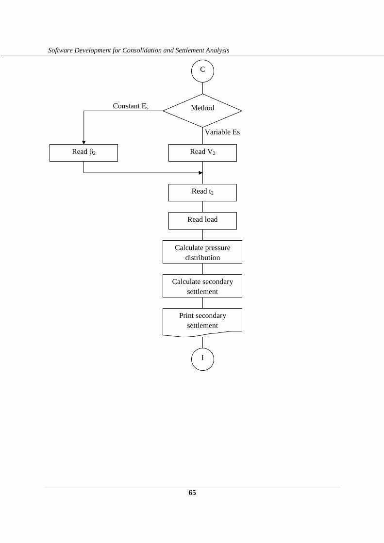
65
Software Development for Consolidation and Settlement Analysis
Variable Es
Constant Es
Read load
Calculate pressure distribution
Calculate secondary settlement
Print secondary settlement
I
C
Read β2 Read V2
Read t2
Method
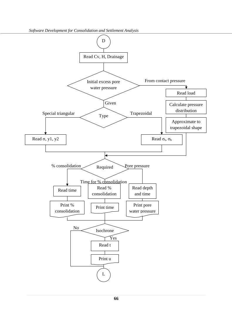
66
Software Development for Consolidation and Settlement Analysis
Yes
No
Pore pressure
Time for % consolidation
% consolidation
Trapezoidal Special triangular
Given
From contact pressure
D
Read Cv, H, Drainage
Read σ, y1, y2 Read σt, σb
Read time Read % consolidation
Read depth and time
Print % consolidation
Print time Print pore water pressure
Read t
Print u
L
Initial excess pore water pressure
Type
Required
Read load
Calculate pressure distribution
Isochrone
Approximate to trapezoidal shape
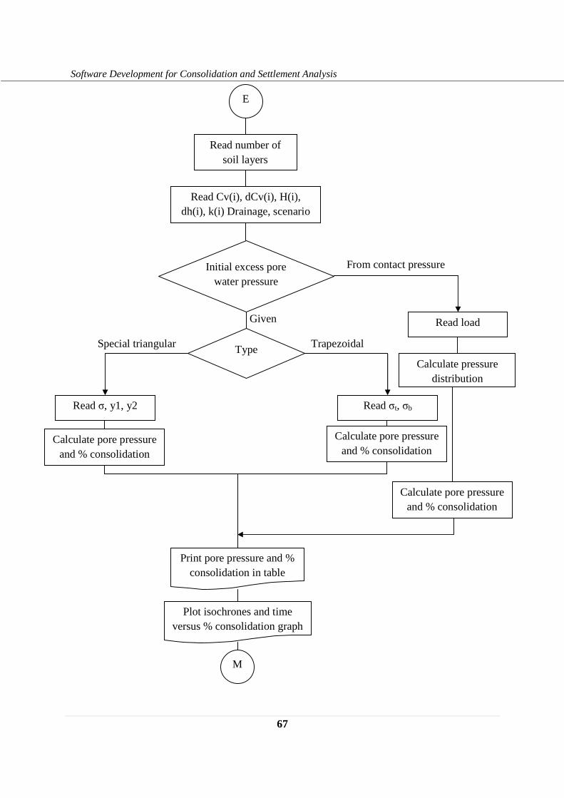
67
Software Development for Consolidation and Settlement Analysis
E
Read Cv(i), dCv(i), H(i), dh(i), k(i) Drainage, scenario
Print pore pressure and % consolidation in table
Plot isochrones and time versus % consolidation graph
M
Read number of soil layers
Trapezoidal Special triangular
Given
From contact pressure
Read σ, y1, y2 Read σt, σb
Initial excess pore water pressure
Type
Read load
Calculate pressure distribution
Calculate pore pressure and % consolidation
Calculate pore pressure and % consolidation
Calculate pore pressure and % consolidation
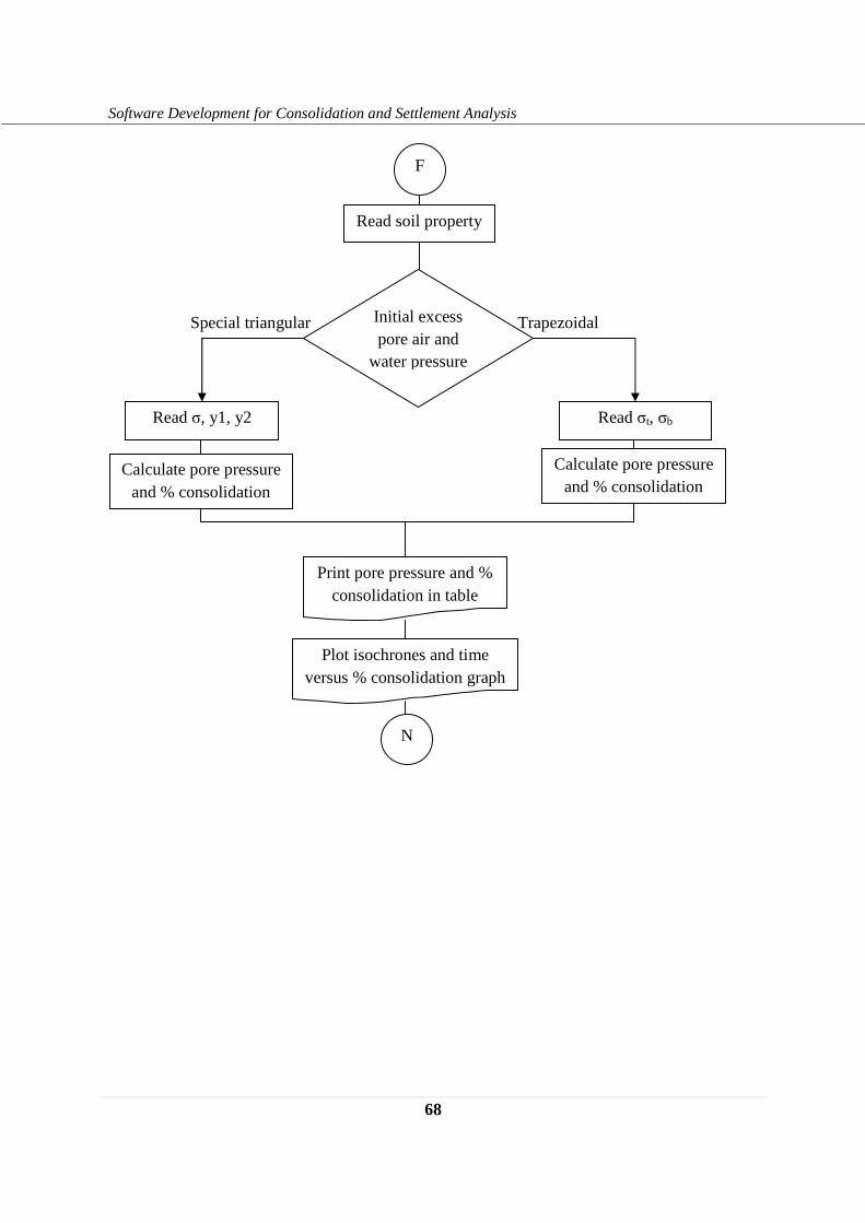
68
Software Development for Consolidation and Settlement Analysis
F
Read soil property
N
Print pore pressure and % consolidation in table
Plot isochrones and time versus % consolidation graph
Trapezoidal Special triangular
Read σ, y1, y2 Read σt, σb
Initial excess pore air and
water pressure
Calculate pore pressure and % consolidation
Calculate pore pressure and % consolidation
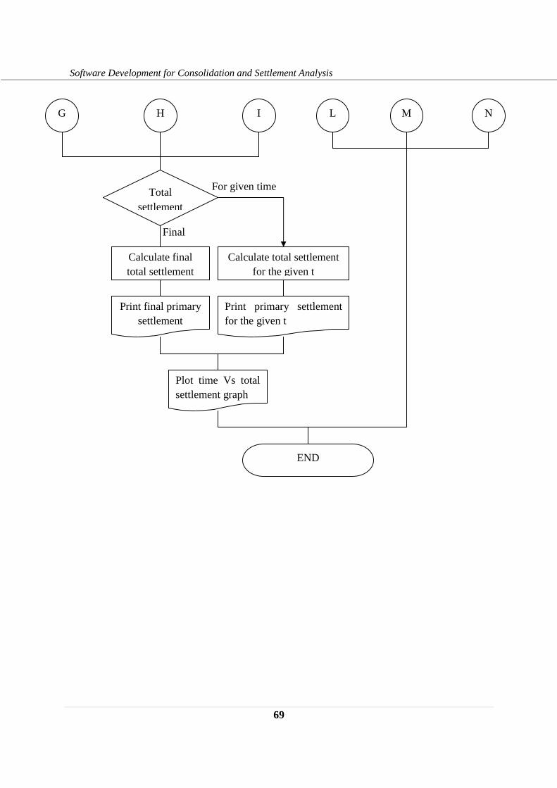
69
Software Development for Consolidation and Settlement Analysis
Final
For given time
G H I L M N
Calculate final total settlement
Print primary settlement for the given t
Print final primary settlement
Calculate total settlement for the given t
Plot time Vs total settlement graph
END
Total settlement
70
Software Development for Consolidation and Settlement Analysis
APPENDIX B
Example Problems
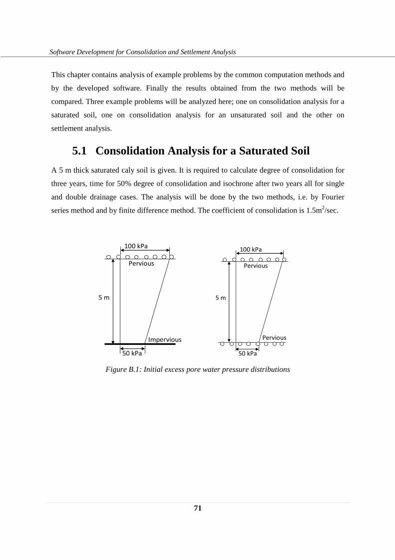
71
Software Development for Consolidation and Settlement Analysis
This chapter contains analysis of example problems by the common computation methods and
by the developed software. Finally the results obtained from the two methods will be
compared. Three example problems will be analyzed here; one on consolidation analysis for a
saturated soil, one on consolidation analysis for an unsaturated soil and the other on
settlement analysis.
5.1 Consolidation Analysis for a Saturated Soil
A 5 m thick saturated caly soil is given. It is required to calculate degree of consolidation for
three years, time for 50% degree of consolidation and isochrone after two years all for single
and double drainage cases. The analysis will be done by the two methods, i.e. by Fourier
series method and by finite difference method. The coefficient of consolidation is 1.5m2/sec.
Figure B.1: Initial excess pore water pressure distributions
50 kPa
100 kPa
Impervious
Pervious
5 m
50 kPa
100 kPa
Pervious
Pervious
5 m
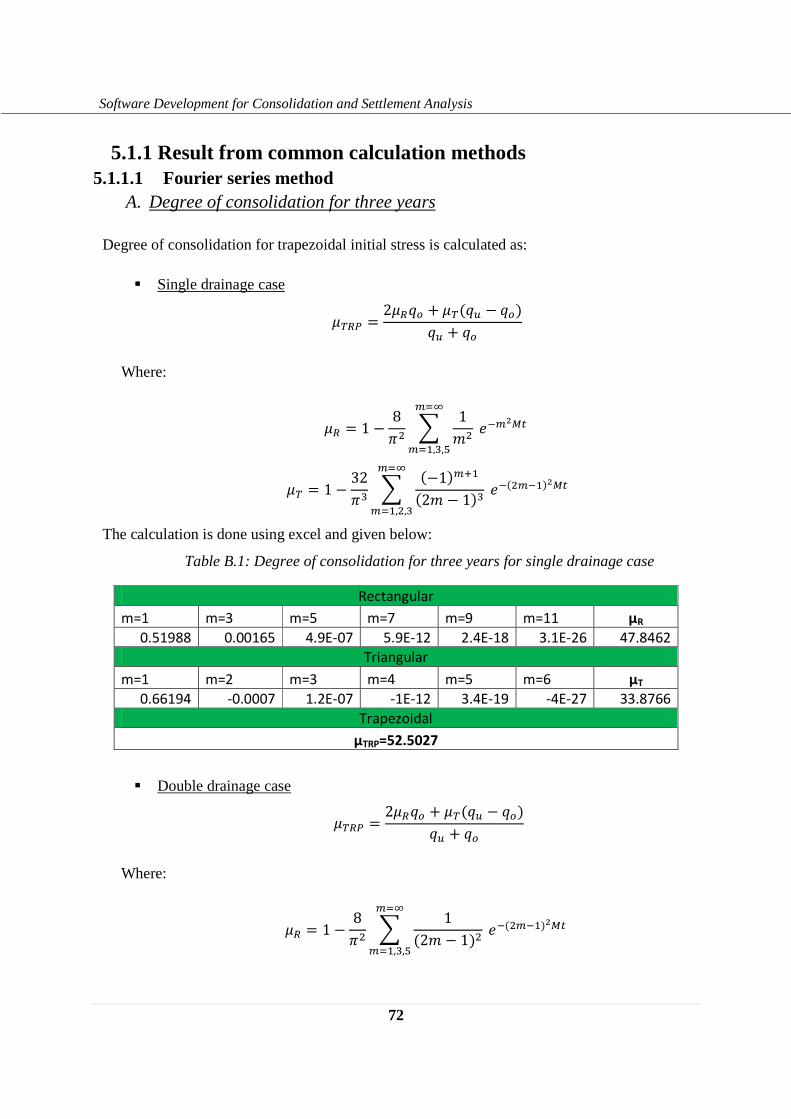
72
Software Development for Consolidation and Settlement Analysis
5.1.1 Result from common calculation methods 5.1.1.1 Fourier series method
A. Degree of consolidation for three years
Degree of consolidation for trapezoidal initial stress is calculated as:
� Single drainage case
*1+7 = 2*+�� + *1(�8 − ��)�8 + �� Where:
*+ = 1 − 8�� � 1�� ����� �%&�%',(,)
*1 = 1 − 32�( � (−1)�0'(2� − 1)( ��(���')�� �%&
�%',�,(
The calculation is done using excel and given below:
Table B.1: Degree of consolidation for three years for single drainage case
Rectangular
m=1 m=3 m=5 m=7 m=9 m=11 μR
0.51988 0.00165 4.9E-07 5.9E-12 2.4E-18 3.1E-26 47.8462
Triangular
m=1 m=2 m=3 m=4 m=5 m=6 μT
0.66194 -0.0007 1.2E-07 -1E-12 3.4E-19 -4E-27 33.8766
Trapezoidal
μTRP=52.5027
� Double drainage case
*1+7 = 2*+�� + *1(�8 − ��)�8 + ��
Where:
*+ = 1 − 8�� � 1(2� − 1)� ��(���')�� �%&�%',(,)
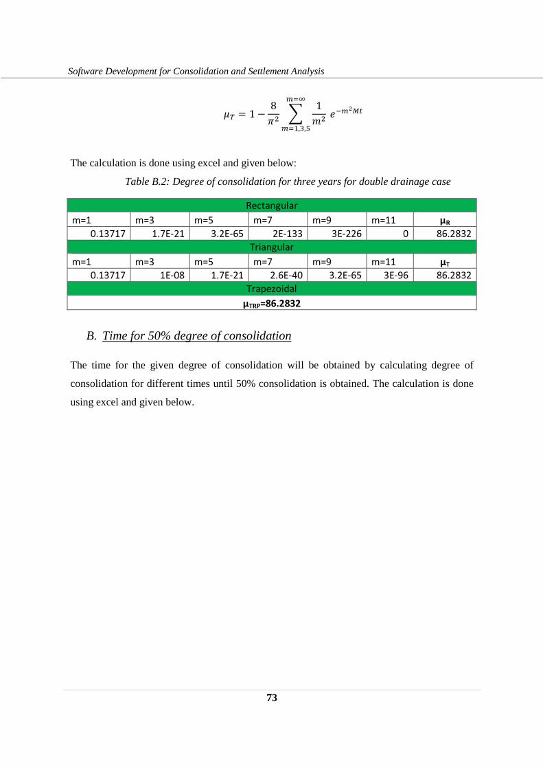
73
Software Development for Consolidation and Settlement Analysis
*1 = 1 − 8�� � 1�� ����� �%&�%',(,)
The calculation is done using excel and given below:
Table B.2: Degree of consolidation for three years for double drainage case
Rectangular
m=1 m=3 m=5 m=7 m=9 m=11 μR
0.13717 1.7E-21 3.2E-65 2E-133 3E-226 0 86.2832
Triangular
m=1 m=3 m=5 m=7 m=9 m=11 μT
0.13717 1E-08 1.7E-21 2.6E-40 3.2E-65 3E-96 86.2832
Trapezoidal
μTRP=86.2832
B. Time for 50% degree of consolidation
The time for the given degree of consolidation will be obtained by calculating degree of
consolidation for different times until 50% consolidation is obtained. The calculation is done
using excel and given below.
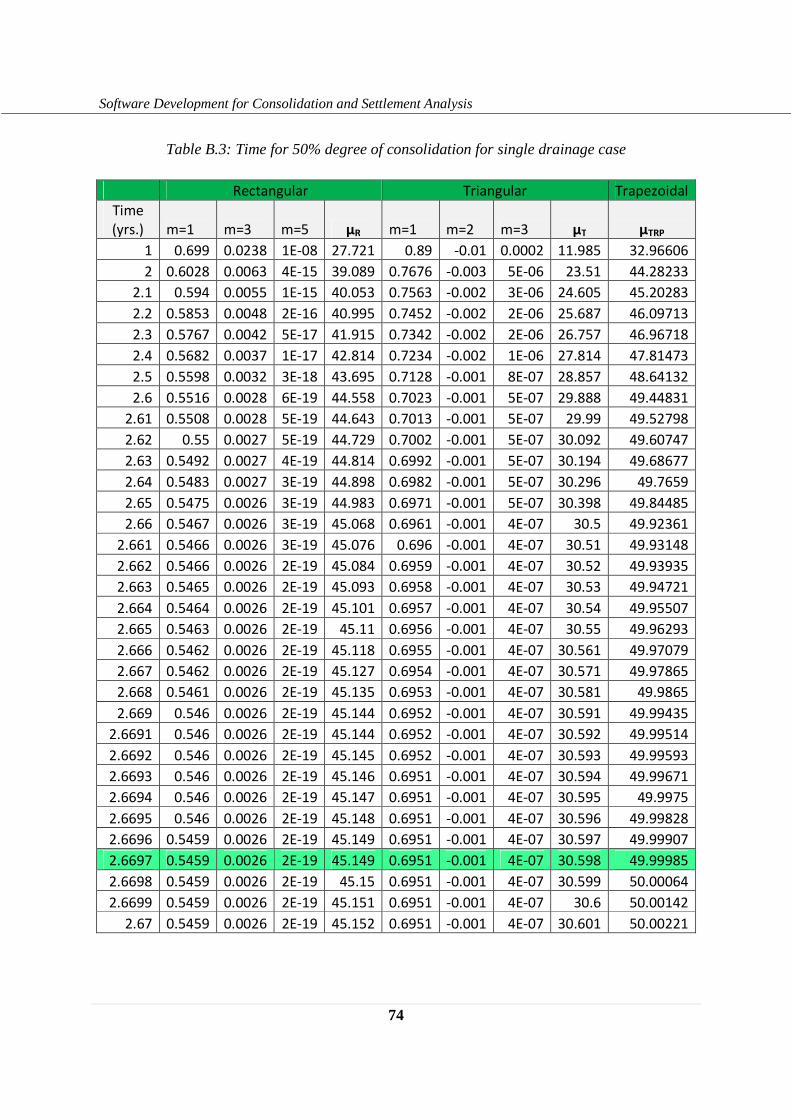
74
Software Development for Consolidation and Settlement Analysis
Table B.3: Time for 50% degree of consolidation for single drainage case
Rectangular Triangular Trapezoidal
Time
(yrs.) m=1 m=3 m=5 μR m=1 m=2 m=3 μT μTRP
1 0.699 0.0238 1E-08 27.721 0.89 -0.01 0.0002 11.985 32.96606
2 0.6028 0.0063 4E-15 39.089 0.7676 -0.003 5E-06 23.51 44.28233
2.1 0.594 0.0055 1E-15 40.053 0.7563 -0.002 3E-06 24.605 45.20283
2.2 0.5853 0.0048 2E-16 40.995 0.7452 -0.002 2E-06 25.687 46.09713
2.3 0.5767 0.0042 5E-17 41.915 0.7342 -0.002 2E-06 26.757 46.96718
2.4 0.5682 0.0037 1E-17 42.814 0.7234 -0.002 1E-06 27.814 47.81473
2.5 0.5598 0.0032 3E-18 43.695 0.7128 -0.001 8E-07 28.857 48.64132
2.6 0.5516 0.0028 6E-19 44.558 0.7023 -0.001 5E-07 29.888 49.44831
2.61 0.5508 0.0028 5E-19 44.643 0.7013 -0.001 5E-07 29.99 49.52798
2.62 0.55 0.0027 5E-19 44.729 0.7002 -0.001 5E-07 30.092 49.60747
2.63 0.5492 0.0027 4E-19 44.814 0.6992 -0.001 5E-07 30.194 49.68677
2.64 0.5483 0.0027 3E-19 44.898 0.6982 -0.001 5E-07 30.296 49.7659
2.65 0.5475 0.0026 3E-19 44.983 0.6971 -0.001 5E-07 30.398 49.84485
2.66 0.5467 0.0026 3E-19 45.068 0.6961 -0.001 4E-07 30.5 49.92361
2.661 0.5466 0.0026 3E-19 45.076 0.696 -0.001 4E-07 30.51 49.93148
2.662 0.5466 0.0026 2E-19 45.084 0.6959 -0.001 4E-07 30.52 49.93935
2.663 0.5465 0.0026 2E-19 45.093 0.6958 -0.001 4E-07 30.53 49.94721
2.664 0.5464 0.0026 2E-19 45.101 0.6957 -0.001 4E-07 30.54 49.95507
2.665 0.5463 0.0026 2E-19 45.11 0.6956 -0.001 4E-07 30.55 49.96293
2.666 0.5462 0.0026 2E-19 45.118 0.6955 -0.001 4E-07 30.561 49.97079
2.667 0.5462 0.0026 2E-19 45.127 0.6954 -0.001 4E-07 30.571 49.97865
2.668 0.5461 0.0026 2E-19 45.135 0.6953 -0.001 4E-07 30.581 49.9865
2.669 0.546 0.0026 2E-19 45.144 0.6952 -0.001 4E-07 30.591 49.99435
2.6691 0.546 0.0026 2E-19 45.144 0.6952 -0.001 4E-07 30.592 49.99514
2.6692 0.546 0.0026 2E-19 45.145 0.6952 -0.001 4E-07 30.593 49.99593
2.6693 0.546 0.0026 2E-19 45.146 0.6951 -0.001 4E-07 30.594 49.99671
2.6694 0.546 0.0026 2E-19 45.147 0.6951 -0.001 4E-07 30.595 49.9975
2.6695 0.546 0.0026 2E-19 45.148 0.6951 -0.001 4E-07 30.596 49.99828
2.6696 0.5459 0.0026 2E-19 45.149 0.6951 -0.001 4E-07 30.597 49.99907
2.6697 0.5459 0.0026 2E-19 45.149 0.6951 -0.001 4E-07 30.598 49.99985
2.6698 0.5459 0.0026 2E-19 45.15 0.6951 -0.001 4E-07 30.599 50.00064
2.6699 0.5459 0.0026 2E-19 45.151 0.6951 -0.001 4E-07 30.6 50.00142
2.67 0.5459 0.0026 2E-19 45.152 0.6951 -0.001 4E-07 30.601 50.00221
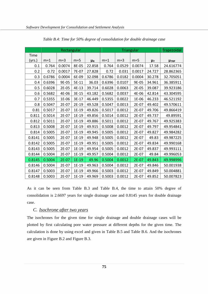
75
Software Development for Consolidation and Settlement Analysis
Table B.4: Time for 50% degree of consolidation for double drainage case
Rectangular Triangular Trapezoidal
Time
(yrs.) m=1 m=3 m=5 μR m=1 m=3 m=5 μT μTRP
0.1 0.764 0.0074 8E-05 22.858 0.764 0.0529 0.0074 17.58 24.616774
0.2 0.72 0.0017 7E-07 27.828 0.72 0.031 0.0017 24.727 28.862365
0.3 0.6786 0.0004 6E-09 32.098 0.6786 0.0182 0.0004 30.278 32.705051
0.4 0.6396 9E-05 5E-11 36.03 0.6396 0.0107 9E-05 34.961 36.385911
0.5 0.6028 2E-05 4E-13 39.714 0.6028 0.0063 2E-05 39.087 39.923186
0.6 0.5682 4E-06 3E-15 43.182 0.5682 0.0037 4E-06 42.814 43.304595
0.7 0.5355 1E-06 3E-17 46.449 0.5355 0.0022 1E-06 46.233 46.521192
0.8 0.5047 2E-07 2E-19 49.528 0.5047 0.0013 2E-07 49.402 49.570611
0.81 0.5017 2E-07 1E-19 49.826 0.5017 0.0012 2E-07 49.706 49.866419
0.811 0.5014 2E-07 1E-19 49.856 0.5014 0.0012 2E-07 49.737 49.89591
0.812 0.5011 2E-07 1E-19 49.886 0.5011 0.0012 2E-07 49.767 49.925383
0.813 0.5008 2E-07 1E-19 49.915 0.5008 0.0012 2E-07 49.797 49.954841
0.814 0.5005 2E-07 1E-19 49.945 0.5005 0.0012 2E-07 49.827 49.984282
0.8141 0.5005 2E-07 1E-19 49.948 0.5005 0.0012 2E-07 49.83 49.987225
0.8142 0.5005 2E-07 1E-19 49.951 0.5005 0.0012 2E-07 49.834 49.990168
0.8143 0.5005 2E-07 1E-19 49.954 0.5005 0.0012 2E-07 49.837 49.993111
0.8144 0.5004 2E-07 1E-19 49.957 0.5004 0.0012 2E-07 49.84 49.996053
0.8145 0.5004 2E-07 1E-19 49.96 0.5004 0.0012 2E-07 49.843 49.998996
0.8146 0.5004 2E-07 1E-19 49.963 0.5004 0.0012 2E-07 49.846 50.001938
0.8147 0.5003 2E-07 1E-19 49.966 0.5003 0.0012 2E-07 49.849 50.004881
0.8148 0.5003 2E-07 1E-19 49.969 0.5003 0.0012 2E-07 49.852 50.007823
As it can be seen from Table B.3 and Table B.4, the time to attain 50% degree of
consolidation is 2.6697 years for single drainage case and 0.8145 years for double drainage
case.
C. Isochrone after two years
The isochrones for the given time for single drainage and double drainage cases will be
plotted by first calculating pore water pressure at different depths for the given time. The
calculation is done by using excel and given in Table B.5 and Table B.6. And the isochrones
are given in Figure B.2 and Figure B.3.
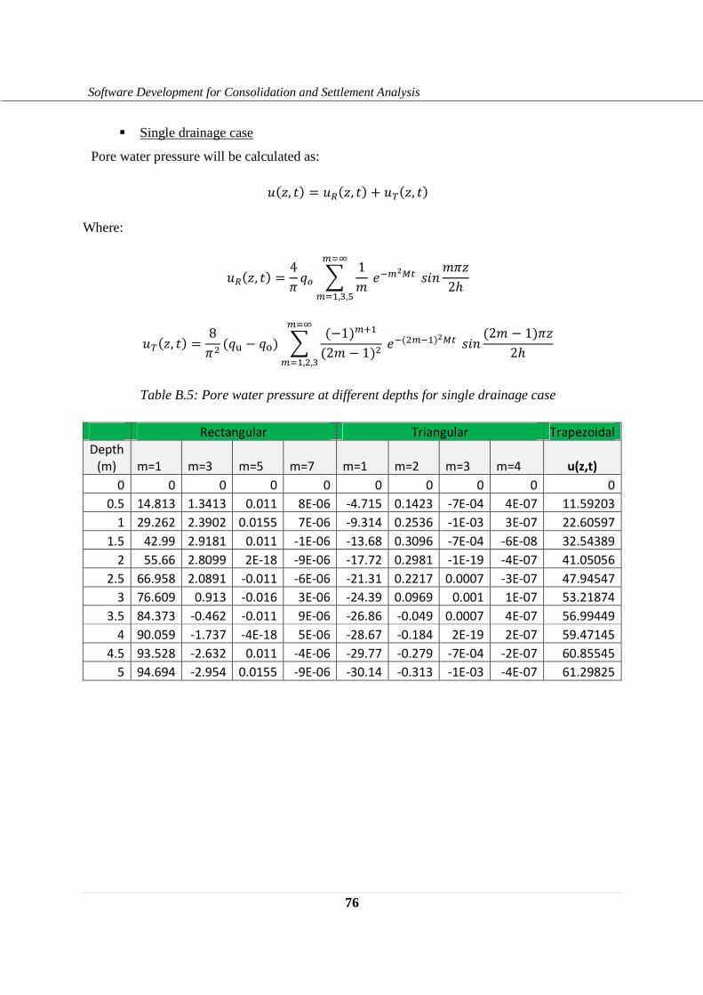
76
Software Development for Consolidation and Settlement Analysis
� Single drainage case
Pore water pressure will be calculated as:
�(�, �) = �+(�, �) + �1(�, �) Where:
�+(�, �) = 4� �� � 1������ !"#���2ℎ�%&
�%',(,)
�1(�, �) = 8�� (�u − �o) � (−1)�0'(2� − 1)� ��(���')�� !"# (2� − 1)��2ℎ
�%&�%',�,(
Table B.5: Pore water pressure at different depths for single drainage case
Rectangular Triangular Trapezoidal
Depth
(m) m=1 m=3 m=5 m=7 m=1 m=2 m=3 m=4 u(z,t)
0 0 0 0 0 0 0 0 0 0
0.5 14.813 1.3413 0.011 8E-06 -4.715 0.1423 -7E-04 4E-07 11.59203
1 29.262 2.3902 0.0155 7E-06 -9.314 0.2536 -1E-03 3E-07 22.60597
1.5 42.99 2.9181 0.011 -1E-06 -13.68 0.3096 -7E-04 -6E-08 32.54389
2 55.66 2.8099 2E-18 -9E-06 -17.72 0.2981 -1E-19 -4E-07 41.05056
2.5 66.958 2.0891 -0.011 -6E-06 -21.31 0.2217 0.0007 -3E-07 47.94547
3 76.609 0.913 -0.016 3E-06 -24.39 0.0969 0.001 1E-07 53.21874
3.5 84.373 -0.462 -0.011 9E-06 -26.86 -0.049 0.0007 4E-07 56.99449
4 90.059 -1.737 -4E-18 5E-06 -28.67 -0.184 2E-19 2E-07 59.47145
4.5 93.528 -2.632 0.011 -4E-06 -29.77 -0.279 -7E-04 -2E-07 60.85545
5 94.694 -2.954 0.0155 -9E-06 -30.14 -0.313 -1E-03 -4E-07 61.29825
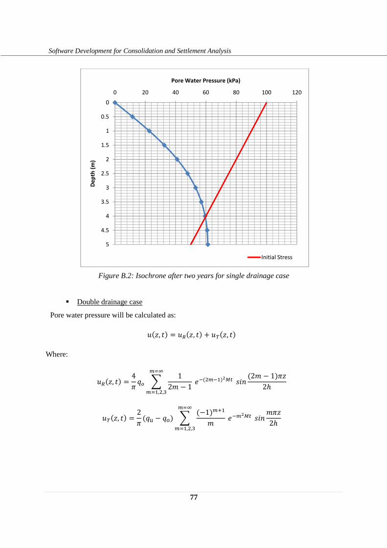
77
Software Development for Consolidation and Settlement Analysis
Figure B.2: Isochrone after two years for single drainage case
� Double drainage case
Pore water pressure will be calculated as:
�(�, �� � �+�, �� 3 �1�, �� Where:
�+�, �� � 4� �� � 12� , 1�����'��� !"# 2� , 1���2$�%&
�%',�,(
�1�, �� � 2� �u , �o� � ,1��0'� ����� !"#���2$
�%&�%',�,(
0
0.5
1
1.5
2
2.5
3
3.5
4
4.5
5
0 20 40 60 80 100 120D
ep
th (
m)
Pore Water Pressure (kPa)
Initial Stress

78
Software Development for Consolidation and Settlement Analysis
Table B.6: Pore water pressure at different depths for double drainage case
Rectangular Triangular Trapezoidal
Depth
(m) m=1 m=2 m=3 m=4 m=1 m=2 m=3 m=4 u(z,t)
0 0 0 0 0 0 0 0 0 0
0.5 12.037 0.0008 4E-12 9E-25 -3.009 0.082 -2E-04 4E-19 9.110658
1 22.897 0.0009 4E-28 -1E-24 -5.724 0.1326 -2E-04 5E-35 17.30578
1.5 31.514 0.0003 -4E-12 4E-25 -7.879 0.1326 -8E-05 -4E-19 23.7687
2 37.047 -6E-04 -9E-28 7E-25 -9.262 0.082 0.0001 -1E-34 27.86713
2.5 38.954 -1E-03 4E-12 -1E-24 -9.739 2E-17 0.0002 4E-19 29.21477
3 37.047 -6E-04 1E-27 7E-25 -9.262 -0.082 0.0001 2E-34 27.70321
3.5 31.514 0.0003 -4E-12 4E-25 -7.879 -0.133 -8E-05 -4E-19 23.50347
4 22.897 0.0009 -2E-27 -1E-24 -5.724 -0.133 -2E-04 -2E-34 17.04055
4.5 12.037 0.0008 4E-12 9E-25 -3.009 -0.082 -2E-04 4E-19 8.946736
5 5E-15 4E-19 2E-27 1E-39 -1E-15 -3E-17 -9E-20 3E-34 3.55E-15
Figure B.3: Isochrone after two years for double drainage case
0
0.5
1
1.5
2
2.5
3
3.5
4
4.5
5
0 20 40 60 80 100 120
De
pth
(m
)
Pore Water Pressure (kPa)
Initial Stress
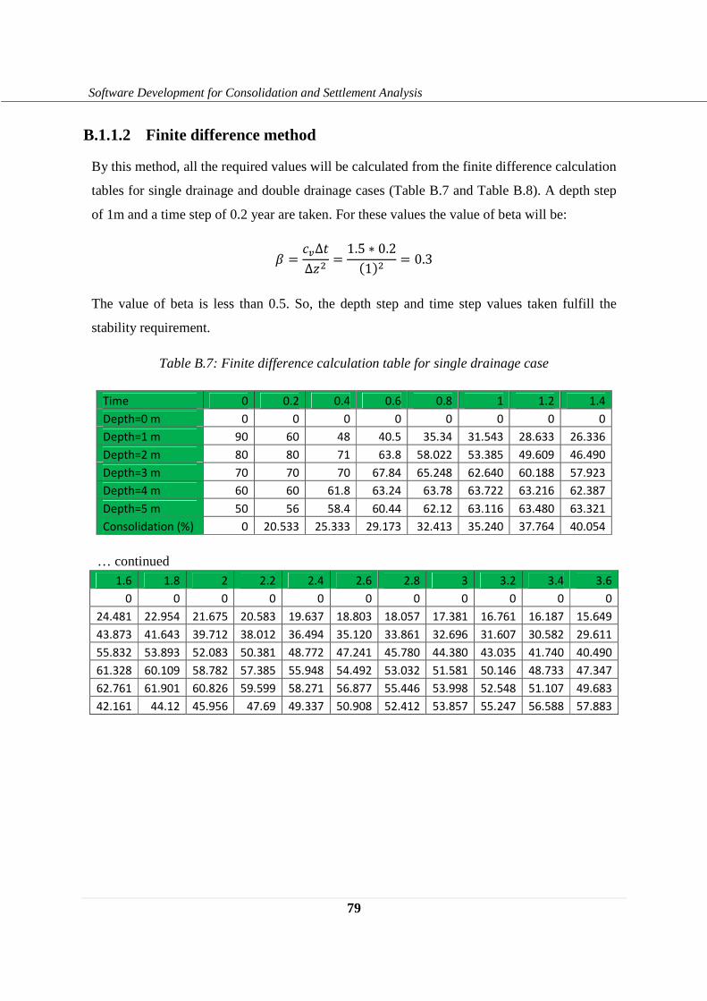
79
Software Development for Consolidation and Settlement Analysis
B.1.1.2 Finite difference method
By this method, all the required values will be calculated from the finite difference calculation
tables for single drainage and double drainage cases (Table B.7 and Table B.8). A depth step
of 1m and a time step of 0.2 year are taken. For these values the value of beta will be:
k = ��∆�∆�� = 1.5 ∗ 0.2(1)� = 0.3
The value of beta is less than 0.5. So, the depth step and time step values taken fulfill the
stability requirement.
Table B.7: Finite difference calculation table for single drainage case
Time 0 0.2 0.4 0.6 0.8 1 1.2 1.4
Depth=0 m 0 0 0 0 0 0 0 0
Depth=1 m 90 60 48 40.5 35.34 31.543 28.633 26.336
Depth=2 m 80 80 71 63.8 58.022 53.385 49.609 46.490
Depth=3 m 70 70 70 67.84 65.248 62.640 60.188 57.923
Depth=4 m 60 60 61.8 63.24 63.78 63.722 63.216 62.387
Depth=5 m 50 56 58.4 60.44 62.12 63.116 63.480 63.321
Consolidation (%) 0 20.533 25.333 29.173 32.413 35.240 37.764 40.054
1.6 1.8 2 2.2 2.4 2.6 2.8 3 3.2 3.4 3.6
0 0 0 0 0 0 0 0 0 0 0
24.481 22.954 21.675 20.583 19.637 18.803 18.057 17.381 16.761 16.187 15.649
43.873 41.643 39.712 38.012 36.494 35.120 33.861 32.696 31.607 30.582 29.611
55.832 53.893 52.083 50.381 48.772 47.241 45.780 44.380 43.035 41.740 40.490
61.328 60.109 58.782 57.385 55.948 54.492 53.032 51.581 50.146 48.733 47.347
62.761 61.901 60.826 59.599 58.271 56.877 55.446 53.998 52.548 51.107 49.683
42.161 44.12 45.956 47.69 49.337 50.908 52.412 53.857 55.247 56.588 57.883
… continued
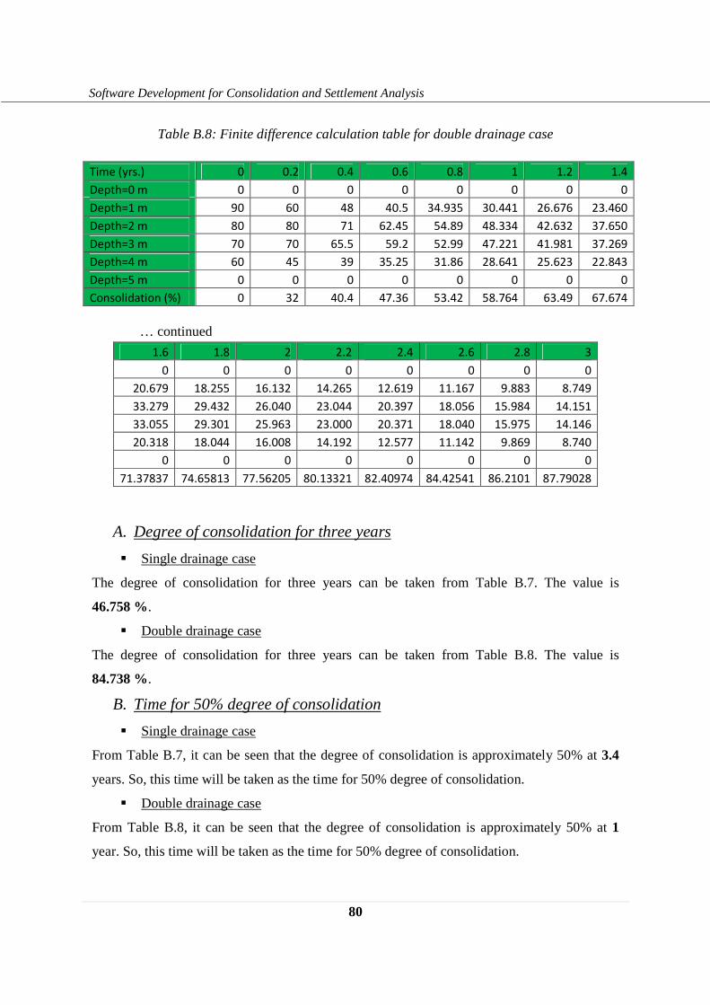
80
Software Development for Consolidation and Settlement Analysis
Table B.8: Finite difference calculation table for double drainage case
Time (yrs.) 0 0.2 0.4 0.6 0.8 1 1.2 1.4
Depth=0 m 0 0 0 0 0 0 0 0
Depth=1 m 90 60 48 40.5 34.935 30.441 26.676 23.460
Depth=2 m 80 80 71 62.45 54.89 48.334 42.632 37.650
Depth=3 m 70 70 65.5 59.2 52.99 47.221 41.981 37.269
Depth=4 m 60 45 39 35.25 31.86 28.641 25.623 22.843
Depth=5 m 0 0 0 0 0 0 0 0
Consolidation (%) 0 32 40.4 47.36 53.42 58.764 63.49 67.674
1.6 1.8 2 2.2 2.4 2.6 2.8 3
0 0 0 0 0 0 0 0
20.679 18.255 16.132 14.265 12.619 11.167 9.883 8.749
33.279 29.432 26.040 23.044 20.397 18.056 15.984 14.151
33.055 29.301 25.963 23.000 20.371 18.040 15.975 14.146
20.318 18.044 16.008 14.192 12.577 11.142 9.869 8.740
0 0 0 0 0 0 0 0
71.37837 74.65813 77.56205 80.13321 82.40974 84.42541 86.2101 87.79028
A. Degree of consolidation for three years
� Single drainage case
The degree of consolidation for three years can be taken from Table B.7. The value is
46.758 %.
� Double drainage case
The degree of consolidation for three years can be taken from Table B.8. The value is
84.738 %.
B. Time for 50% degree of consolidation
� Single drainage case
From Table B.7, it can be seen that the degree of consolidation is approximately 50% at 3.4
years. So, this time will be taken as the time for 50% degree of consolidation.
� Double drainage case
From Table B.8, it can be seen that the degree of consolidation is approximately 50% at 1
year. So, this time will be taken as the time for 50% degree of consolidation.
… continued
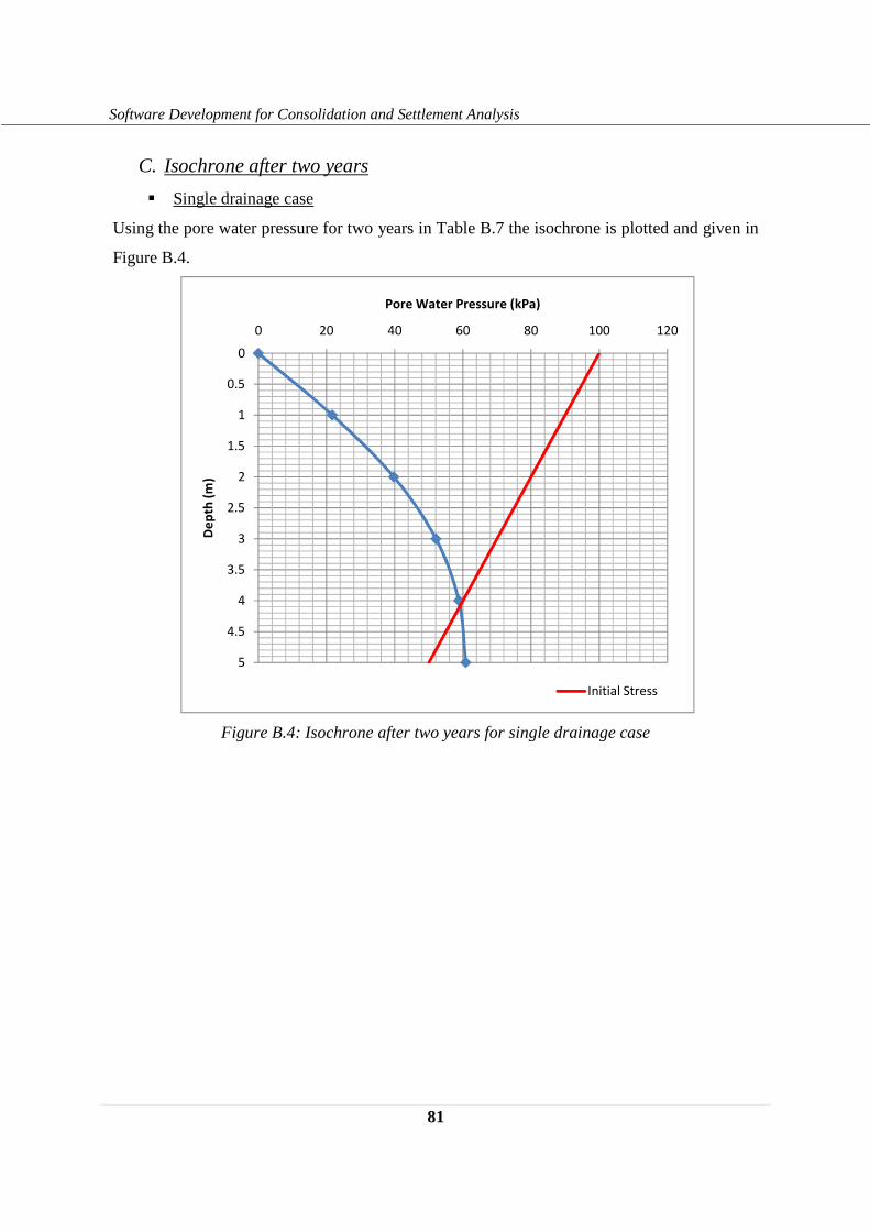
81
Software Development for Consolidation and Settlement Analysis
C. Isochrone after two years
� Single drainage case
Using the pore water pressure for two years in Table B.7 the isochrone is plotted and given in
Figure B.4.
Figure B.4: Isochrone after two years for single drainage case
0
0.5
1
1.5
2
2.5
3
3.5
4
4.5
5
0 20 40 60 80 100 120
De
pth
(m
)
Pore Water Pressure (kPa)
Initial Stress
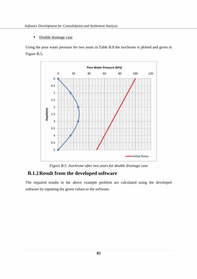
82
Software Development for Consolidation and Settlement Analysis
� Double drainage case
Using the pore water pressure for two years in Table B.8 the isochrone is plotted and given in
Figure B.5.
Figure B.5: Isochrone after two years for double drainage case
B.1.2 Result from the developed software
The required results in the above example problem are calculated using the developed
software by inputting the given values to the software.
0
0.5
1
1.5
2
2.5
3
3.5
4
4.5
5
0 20 40 60 80 100 120
De
pth
(m)
Pore Water Pressure (kPa)
Initial Stress
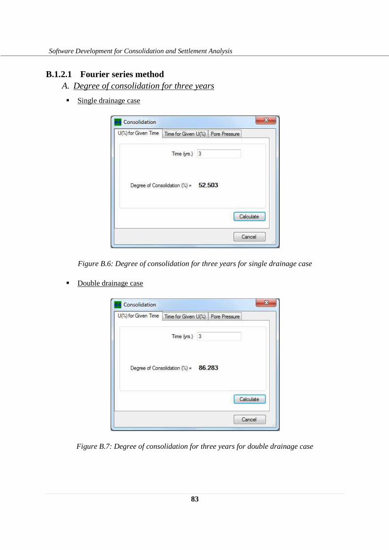
83
Software Development for Consolidation and Settlement Analysis
B.1.2.1 Fourier series method A. Degree of consolidation for three years
� Single drainage case
Figure B.6: Degree of consolidation for three years for single drainage case
� Double drainage case
Figure B.7: Degree of consolidation for three years for double drainage case
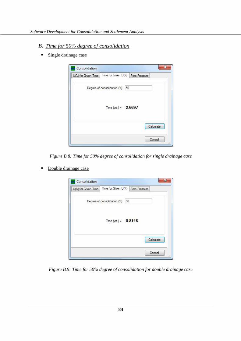
84
Software Development for Consolidation and Settlement Analysis
B. Time for 50% degree of consolidation
� Single drainage case
Figure B.8: Time for 50% degree of consolidation for single drainage case
� Double drainage case
Figure B.9: Time for 50% degree of consolidation for double drainage case
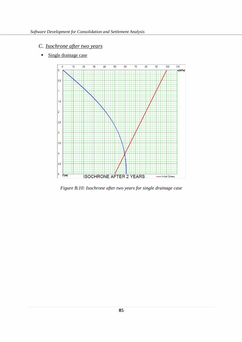
85
Software Development for Consolidation and Settlement Analysis
C. Isochrone after two years
� Single drainage case
Figure B.10: Isochrone after two years for single drainage case
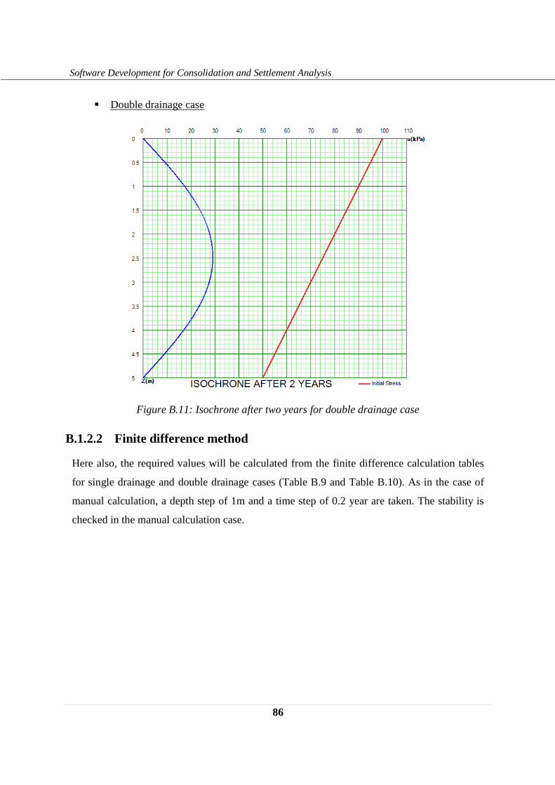
86
Software Development for Consolidation and Settlement Analysis
� Double drainage case
Figure B.11: Isochrone after two years for double drainage case
B.1.2.2 Finite difference method
Here also, the required values will be calculated from the finite difference calculation tables
for single drainage and double drainage cases (Table B.9 and Table B.10). As in the case of
manual calculation, a depth step of 1m and a time step of 0.2 year are taken. The stability is
checked in the manual calculation case.
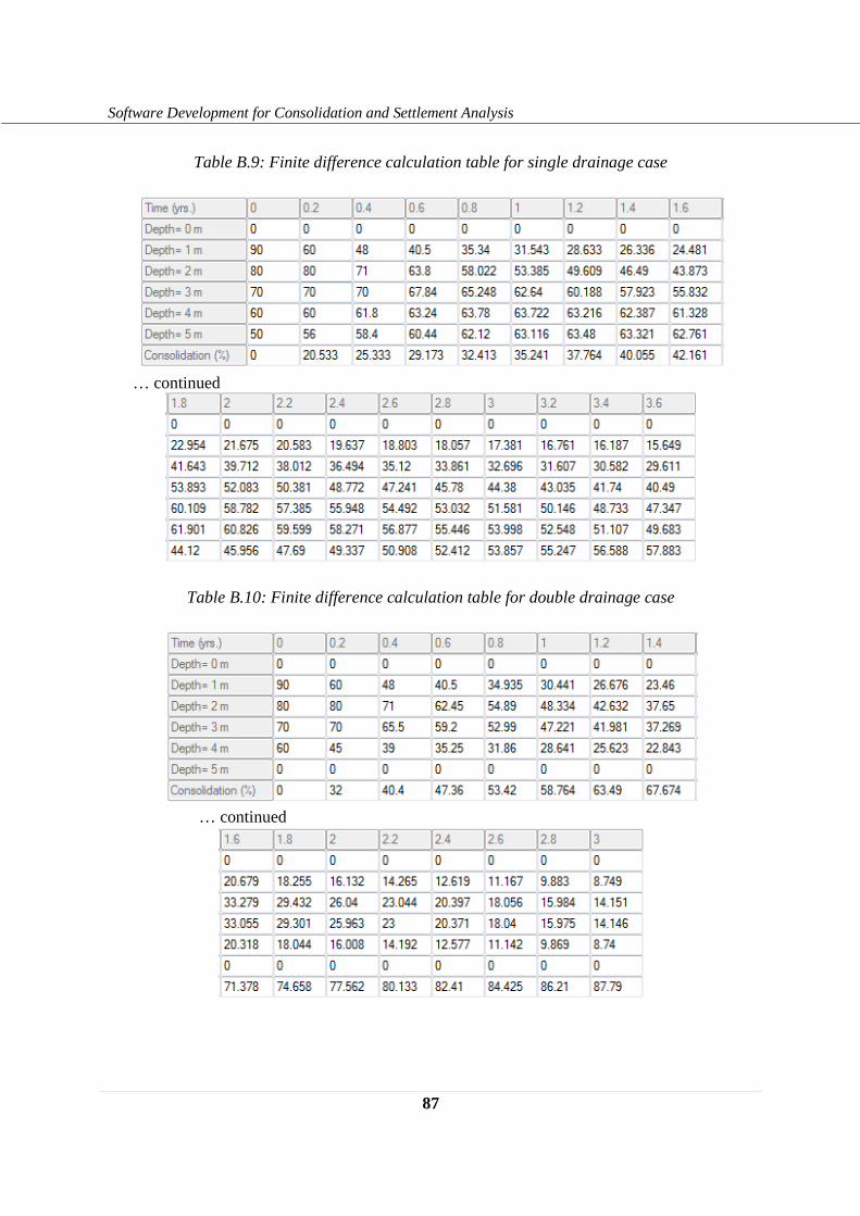
87
Software Development for Consolidation and Settlement Analysis
Table B.9: Finite difference calculation table for single drainage case
Table B.10: Finite difference calculation table for double drainage case
… continued
… continued
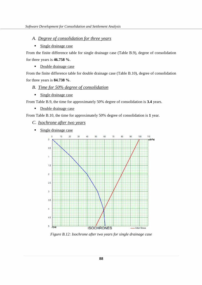
88
Software Development for Consolidation and Settlement Analysis
A. Degree of consolidation for three years
� Single drainage case
From the finite difference table for single drainage case (Table B.9), degree of consolidation
for three years is 46.758 %.
� Double drainage case
From the finite difference table for double drainage case (Table B.10), degree of consolidation
for three years is 84.738 %.
B. Time for 50% degree of consolidation
� Single drainage case
From Table B.9, the time for approximately 50% degree of consolidation is 3.4 years.
� Double drainage case
From Table B.10, the time for approximately 50% degree of consolidation is 1 year.
C. Isochrone after two years
� Single drainage case
Figure B.12: Isochrone after two years for single drainage case
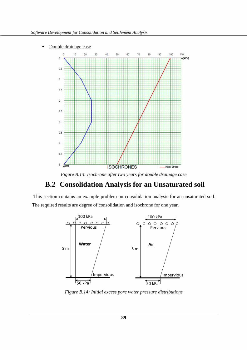
89
Software Development for Consolidation and Settlement Analysis
� Double drainage case
Figure B.13: Isochrone after two years for double drainage case
B.2 Consolidation Analysis for an Unsaturated soil
This section contains an example problem on consolidation analysis for an unsaturated soil.
The required results are degree of consolidation and isochrone for one year.
Figure B.14: Initial excess pore water pressure distributions
50 kPa
100 kPa
Impervious
Pervious
5 m Water
50 kPa
100 kPa
Impervious
Pervious
5 m Air
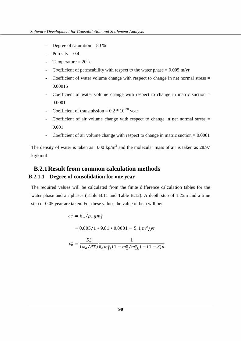
90
Software Development for Consolidation and Settlement Analysis
- Degree of saturation = 80 %
- Porosity = 0.4
- Temperature = 20 0c
- Coefficient of permeability with respect to the water phase = 0.005 m/yr
- Coefficient of water volume change with respect to change in net normal stress =
0.00015
- Coefficient of water volume change with respect to change in matric suction =
0.0001
- Coefficient of transmission = 0.2 * 10-20 year
- Coefficient of air volume change with respect to change in net normal stress =
0.001
- Coefficient of air volume change with respect to change in matric suction = 0.0001
The density of water is taken as 1000 kg/m3 and the molecular mass of air is taken as 28.97
kg/kmol.
B.2.1 Result from common calculation methods B.2.1.1 Degree of consolidation for one year
The required values will be calculated from the finite difference calculation tables for the
water phase and air phases (Table B.11 and Table B.12). A depth step of 1.25m and a time
step of 0.05 year are taken. For these values the value of beta will be:
��� = �� ������⁄ = 0.005 1 ∗ 9.81 ∗ 0.0001⁄ = 5. 1��/U�
��T = ]T∗(_T `a⁄ ) 1ūT�'ST (1 − ��T �'ST⁄ ) − (1 − Z)#
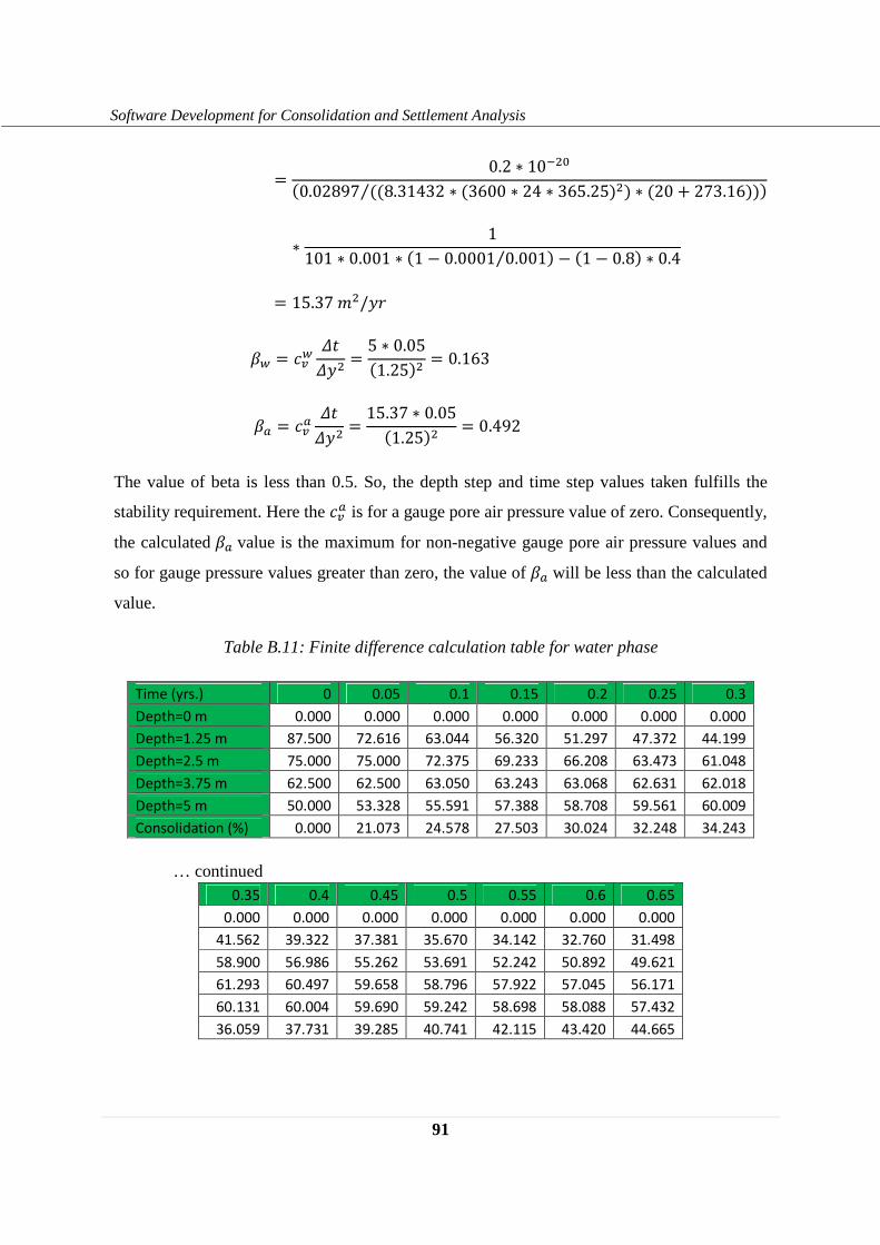
91
Software Development for Consolidation and Settlement Analysis
= 0.2 ∗ 10��R(0.02897 ((8.31432 ∗ (3600 ∗ 24 ∗ 365.25)�) ∗ (20 + 273.16)⁄ ))
∗ 1101 ∗ 0.001 ∗ (1 − 0.0001 0.001⁄ ) − (1 − 0.8) ∗ 0.4= 15.37��/U�
k� = ��� n�nU� = 5 ∗ 0.05(1.25)� = 0.163 kT = ��T n�nU� = 15.37 ∗ 0.05(1.25)� = 0.492
The value of beta is less than 0.5. So, the depth step and time step values taken fulfills the
stability requirement. Here the ��T is for a gauge pore air pressure value of zero. Consequently,
the calculated kT value is the maximum for non-negative gauge pore air pressure values and
so for gauge pressure values greater than zero, the value of kT will be less than the calculated
value.
Table B.11: Finite difference calculation table for water phase
Time (yrs.) 0 0.05 0.1 0.15 0.2 0.25 0.3
Depth=0 m 0.000 0.000 0.000 0.000 0.000 0.000 0.000
Depth=1.25 m 87.500 72.616 63.044 56.320 51.297 47.372 44.199
Depth=2.5 m 75.000 75.000 72.375 69.233 66.208 63.473 61.048
Depth=3.75 m 62.500 62.500 63.050 63.243 63.068 62.631 62.018
Depth=5 m 50.000 53.328 55.591 57.388 58.708 59.561 60.009
Consolidation (%) 0.000 21.073 24.578 27.503 30.024 32.248 34.243
0.35 0.4 0.45 0.5 0.55 0.6 0.65
0.000 0.000 0.000 0.000 0.000 0.000 0.000
41.562 39.322 37.381 35.670 34.142 32.760 31.498
58.900 56.986 55.262 53.691 52.242 50.892 49.621
61.293 60.497 59.658 58.796 57.922 57.045 56.171
60.131 60.004 59.690 59.242 58.698 58.088 57.432
36.059 37.731 39.285 40.741 42.115 43.420 44.665
… continued
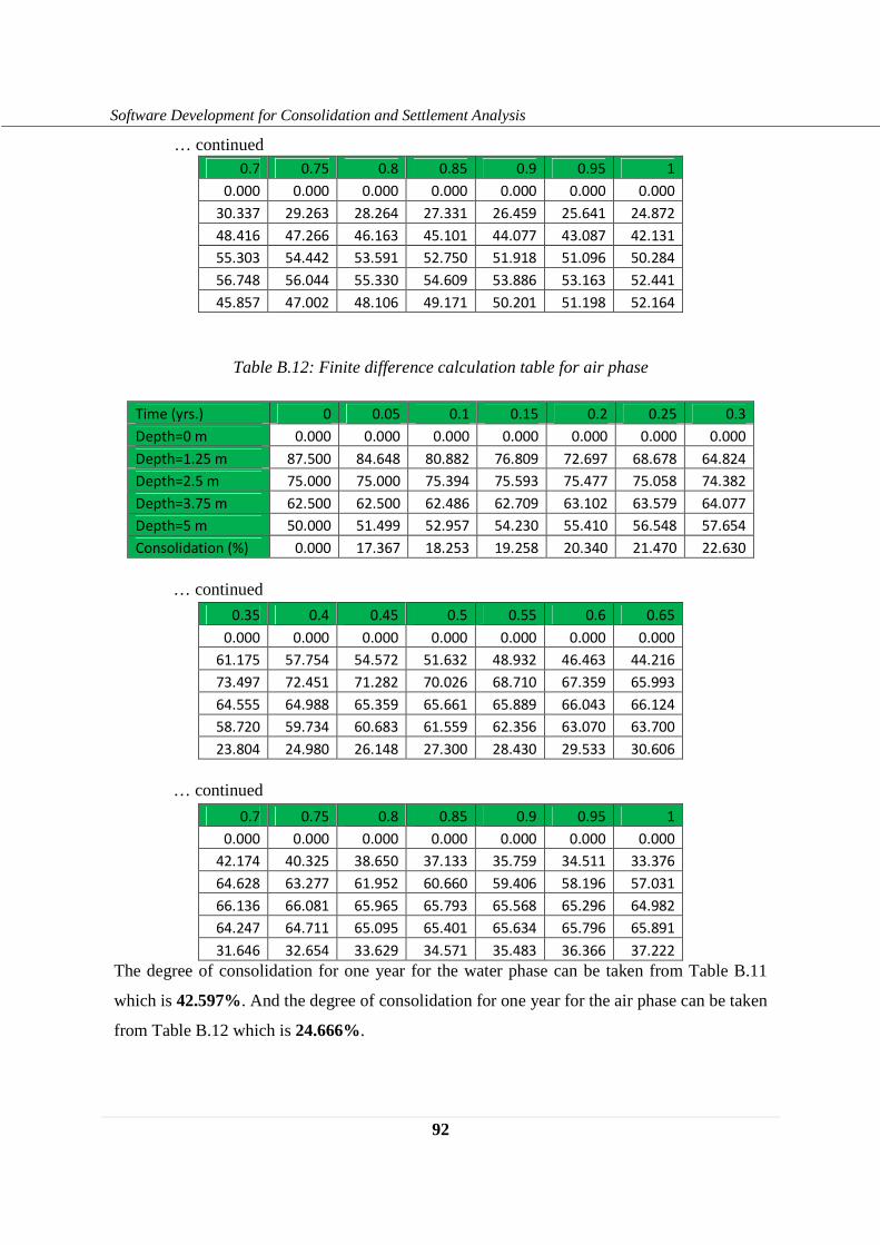
92
Software Development for Consolidation and Settlement Analysis
0.7 0.75 0.8 0.85 0.9 0.95 1
0.000 0.000 0.000 0.000 0.000 0.000 0.000
30.337 29.263 28.264 27.331 26.459 25.641 24.872
48.416 47.266 46.163 45.101 44.077 43.087 42.131
55.303 54.442 53.591 52.750 51.918 51.096 50.284
56.748 56.044 55.330 54.609 53.886 53.163 52.441
45.857 47.002 48.106 49.171 50.201 51.198 52.164
Table B.12: Finite difference calculation table for air phase
Time (yrs.) 0 0.05 0.1 0.15 0.2 0.25 0.3
Depth=0 m 0.000 0.000 0.000 0.000 0.000 0.000 0.000
Depth=1.25 m 87.500 84.648 80.882 76.809 72.697 68.678 64.824
Depth=2.5 m 75.000 75.000 75.394 75.593 75.477 75.058 74.382
Depth=3.75 m 62.500 62.500 62.486 62.709 63.102 63.579 64.077
Depth=5 m 50.000 51.499 52.957 54.230 55.410 56.548 57.654
Consolidation (%) 0.000 17.367 18.253 19.258 20.340 21.470 22.630
0.35 0.4 0.45 0.5 0.55 0.6 0.65
0.000 0.000 0.000 0.000 0.000 0.000 0.000
61.175 57.754 54.572 51.632 48.932 46.463 44.216
73.497 72.451 71.282 70.026 68.710 67.359 65.993
64.555 64.988 65.359 65.661 65.889 66.043 66.124
58.720 59.734 60.683 61.559 62.356 63.070 63.700
23.804 24.980 26.148 27.300 28.430 29.533 30.606
0.7 0.75 0.8 0.85 0.9 0.95 1
0.000 0.000 0.000 0.000 0.000 0.000 0.000
42.174 40.325 38.650 37.133 35.759 34.511 33.376
64.628 63.277 61.952 60.660 59.406 58.196 57.031
66.136 66.081 65.965 65.793 65.568 65.296 64.982
64.247 64.711 65.095 65.401 65.634 65.796 65.891
31.646 32.654 33.629 34.571 35.483 36.366 37.222
The degree of consolidation for one year for the water phase can be taken from Table B.11
which is 42.597%. And the degree of consolidation for one year for the air phase can be taken
from Table B.12 which is 24.666%.
… continued
… continued
… continued
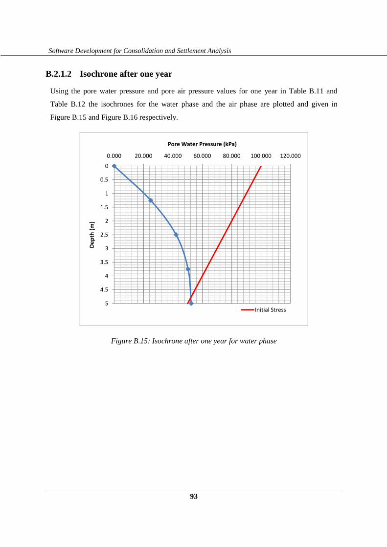
93
Software Development for Consolidation and Settlement Analysis
B.2.1.2 Isochrone after one year
Using the pore water pressure and pore air pressure values for one year in Table B.11 and
Table B.12 the isochrones for the water phase and the air phase are plotted and given in
Figure B.15 and Figure B.16 respectively.
Figure B.15: Isochrone after one year for water phase
0
0.5
1
1.5
2
2.5
3
3.5
4
4.5
5
0.000 20.000 40.000 60.000 80.000 100.000 120.000
De
pth
(m
)
Pore Water Pressure (kPa)
Initial Stress
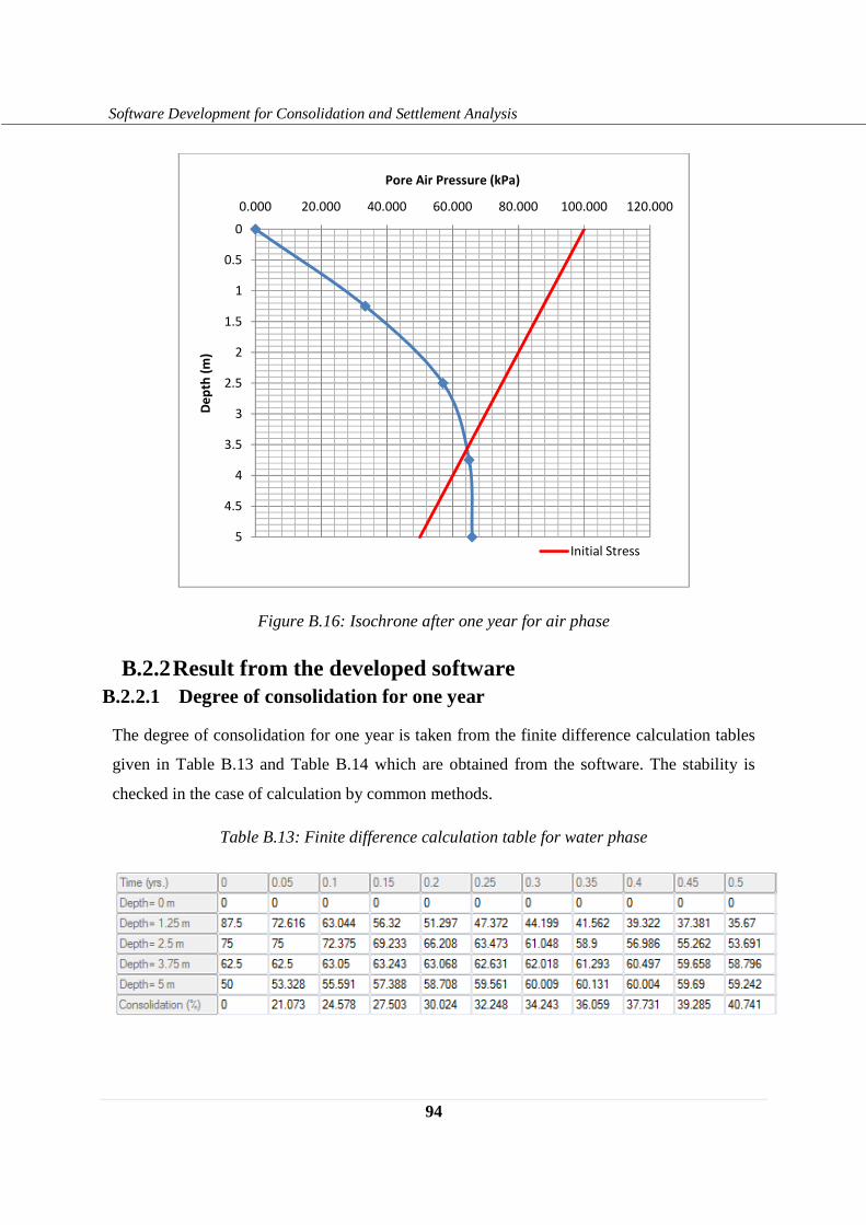
94
Software Development for Consolidation and Settlement Analysis
Figure B.16: Isochrone after one year for air phase
B.2.2 Result from the developed software B.2.2.1 Degree of consolidation for one year
The degree of consolidation for one year is taken from the finite difference calculation tables
given in Table B.13 and Table B.14 which are obtained from the software. The stability is
checked in the case of calculation by common methods.
Table B.13: Finite difference calculation table for water phase
0
0.5
1
1.5
2
2.5
3
3.5
4
4.5
5
0.000 20.000 40.000 60.000 80.000 100.000 120.000D
ep
th (
m)
Pore Air Pressure (kPa)
Initial Stress
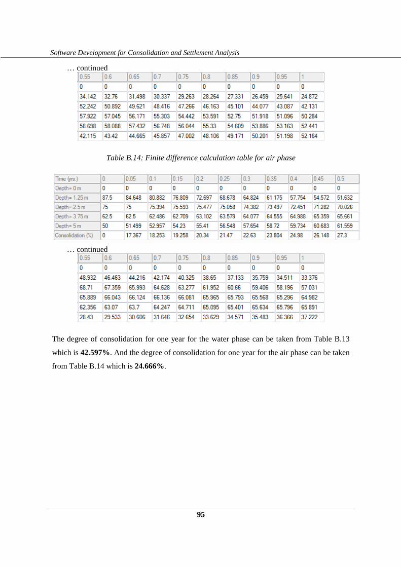
95
Software Development for Consolidation and Settlement Analysis
Table B.14: Finite difference calculation table for air phase
The degree of consolidation for one year for the water phase can be taken from Table B.13
which is 42.597%. And the degree of consolidation for one year for the air phase can be taken
from Table B.14 which is 24.666%.
… continued
… continued
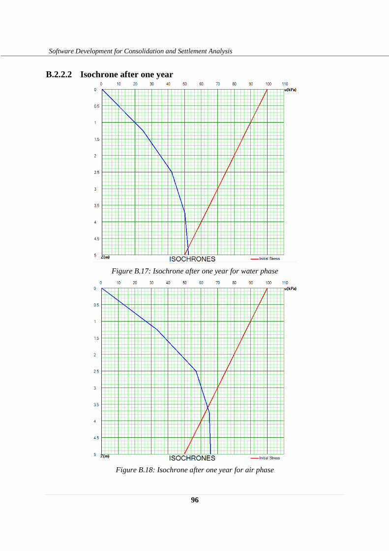
96
Software Development for Consolidation and Settlement Analysis
B.2.2.2 Isochrone after one year
Figure B.17: Isochrone after one year for water phase
Figure B.18: Isochrone after one year for air phase
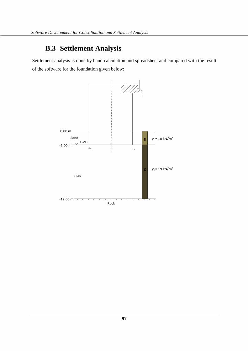
97
Software Development for Consolidation and Settlement Analysis
B.3 Settlement Analysis
Settlement analysis is done by hand calculation and spreadsheet and compared with the result
of the software for the foundation given below:
S
C
GWT
0.00 m
-2.00 m
-12.00 m
A B
Sand
Clay
Rock
γt = 18 kN/m3
γt = 19 kN/m3

98
Software Development for Consolidation and Settlement Analysis
Figure B.19: Elevation and plan of an abutment
The required values are immediate (elastic) settlement, final primary settlement, primary
settlement after two years and secondary settlement after 35 years taking time for completion
of primary consolidation to be 25 years.
B.3.1 Result from common calculation methods B.3.1.1 Immediate (elastic) settlement
The immediate settlement is calculated as:
ZC = �q 1 , *�r s�
Where:
� Z = Immediate settlement
� � = Contact pressure
� * = Poisson’s ratio
� r = Modulus of elasticity
� q = Least lateral dimension
A B
P
a = 8m
b = 4m
e
Y
X
P = 5MN
μ = 0.4
e = 0.3m Es = 30 MPa
Cv = 20*10-4
cm2/sec
V2 = 100
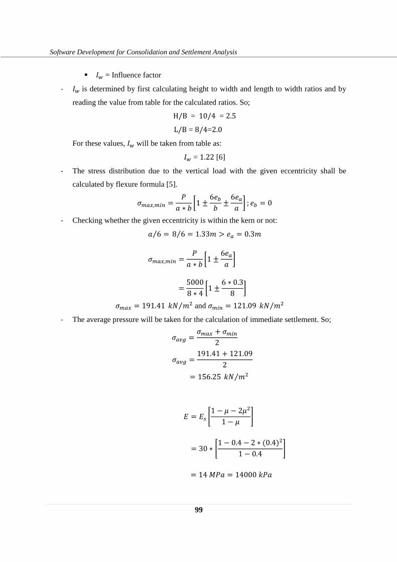
99
Software Development for Consolidation and Settlement Analysis
� s� = Influence factor
- s� is determined by first calculating height to width and length to width ratios and by
reading the value from table for the calculated ratios. So;
H/B = 10/4 = 2.5
L/B = 8/4=2.0
For these values, s� will be taken from table as:
s� = 1.22 [6]
- The stress distribution due to the vertical load with the given eccentricity shall be
calculated by flexure formula [5].
��T�,�CM = gh ∗ = �1 ± 6��= ± 6�Th � ; �� = 0
- Checking whether the given eccentricity is within the kern or not:
h 6 =⁄ 8 6⁄ = 1.33� > �T = 0.3�
��T�,�CM = gh ∗ = �1 ± 6�Th � = 50008 ∗ 4 �1 ± 6 ∗ 0.38 �
��T� = 191.41 �� ��⁄ and ��CM = 121.09 �� ��⁄
- The average pressure will be taken for the calculation of immediate settlement. So;
�T�X = ��T� + ��CM2
�T�X = 191.41 + 121.092
= 156.25 �� ��⁄
r = ry �1 − * − 2*�1 − * �
= 30 ∗ �1 − 0.4 − 2 ∗ (0.4)�1 − 0.4 � = 14�gh = 14000�gh
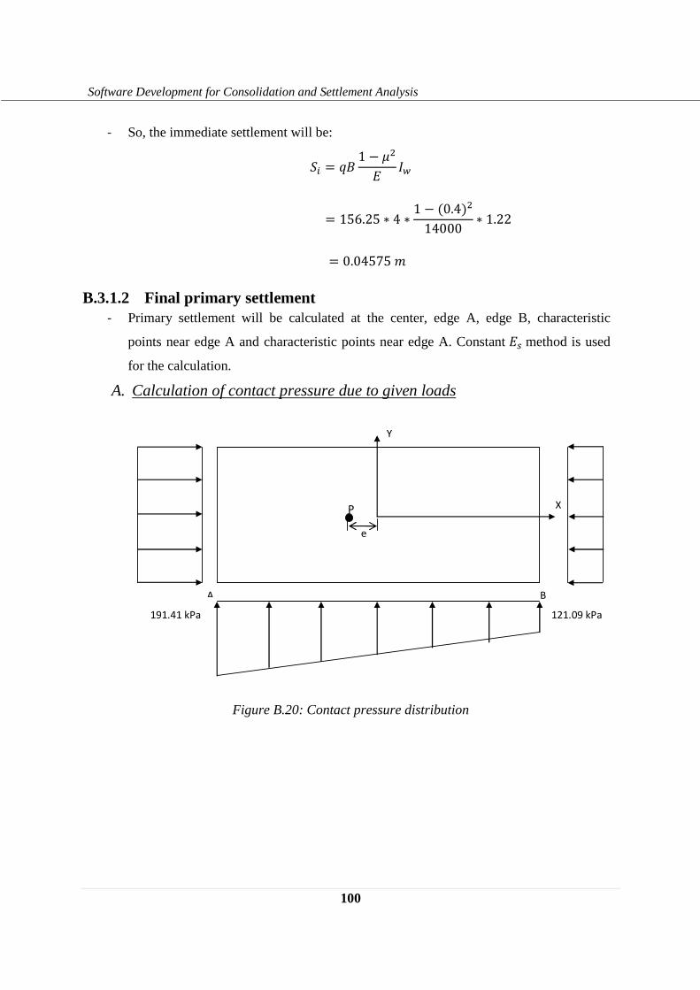
100
Software Development for Consolidation and Settlement Analysis
- So, the immediate settlement will be:
ZC = �q 1 , *�r s�
� 156.25 ∗ 4 ∗ 1 , 0.4��14000 ∗ 1.22
� 0.04575� B.3.1.2 Final primary settlement
- Primary settlement will be calculated at the center, edge A, edge B, characteristic
points near edge A and characteristic points near edge A. Constant ry method is used
for the calculation.
A. Calculation of contact pressure due to given loads
Figure B.20: Contact pressure distribution
Y
X
A B
e
P
121.09 kPa 191.41 kPa
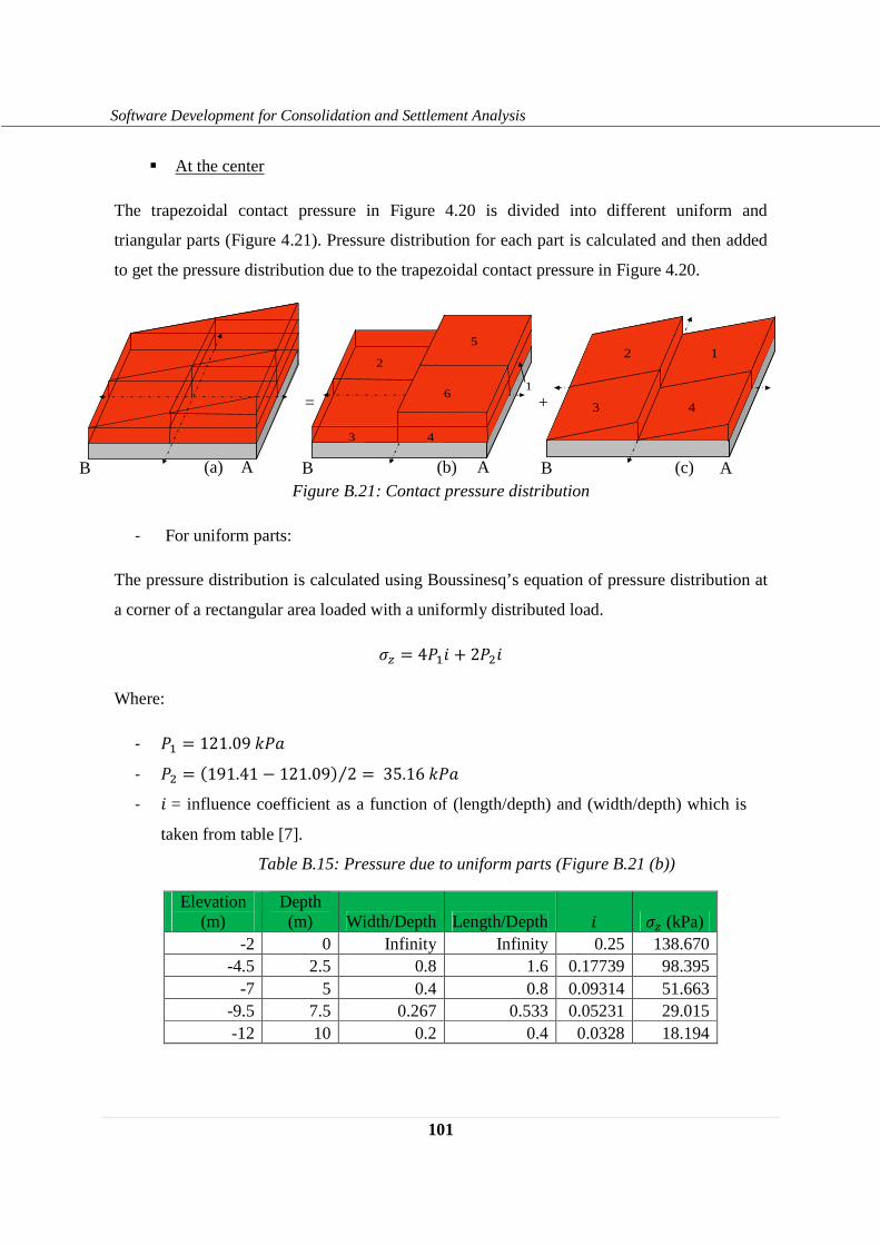
101
Software Development for Consolidation and Settlement Analysis
� At the center
The trapezoidal contact pressure in Figure 4.20 is divided into different uniform and
triangular parts (Figure 4.21). Pressure distribution for each part is calculated and then added
to get the pressure distribution due to the trapezoidal contact pressure in Figure 4.20.
= +
Figure B.21: Contact pressure distribution
- For uniform parts:
The pressure distribution is calculated using Boussinesq’s equation of pressure distribution at
a corner of a rectangular area loaded with a uniformly distributed load.
�� = 4g'" 3 2g�" Where:
- g' � 121.09�gh
- g� � 191.41 , 121.09� 2⁄ � 35.16�gh
- " = influence coefficient as a function of (length/depth) and (width/depth) which is
taken from table [7].
Table B.15: Pressure due to uniform parts (Figure B.21 (b))
Elevation (m)
Depth (m) Width/Depth Length/Depth " �� (kPa)
-2 0 Infinity Infinity 0.25 138.670 -4.5 2.5 0.8 1.6 0.17739 98.395
-7 5 0.4 0.8 0.09314 51.663 -9.5 7.5 0.267 0.533 0.05231 29.015 -12 10 0.2 0.4 0.0328 18.194
2
3 4
1
5
6
4 3
2 1
(a) (b) (c) B A A A B B
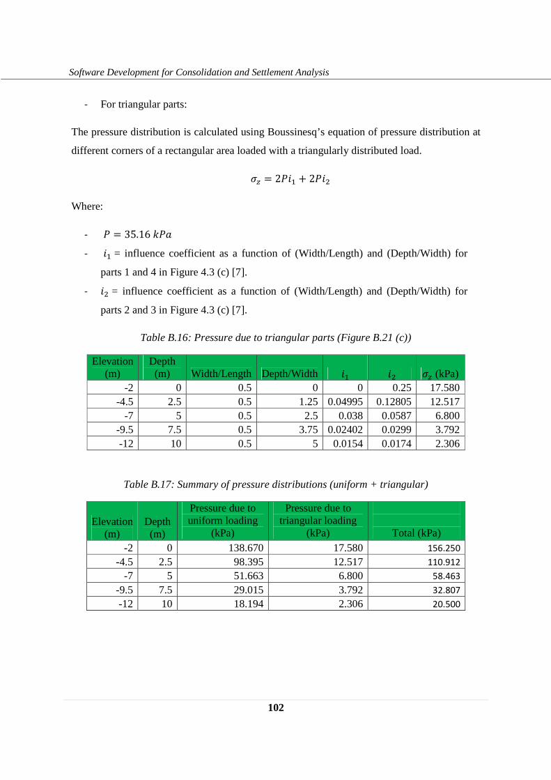
102
Software Development for Consolidation and Settlement Analysis
- For triangular parts:
The pressure distribution is calculated using Boussinesq’s equation of pressure distribution at
different corners of a rectangular area loaded with a triangularly distributed load.
�� = 2g"' + 2g"�
Where:
- g = 35.16�gh
- "' = influence coefficient as a function of (Width/Length) and (Depth/Width) for
parts 1 and 4 in Figure 4.3 (c) [7].
- "� = influence coefficient as a function of (Width/Length) and (Depth/Width) for
parts 2 and 3 in Figure 4.3 (c) [7].
Table B.16: Pressure due to triangular parts (Figure B.21 (c))
Elevation (m)
Depth (m) Width/Length Depth/Width "' "� �� (kPa)
-2 0 0.5 0 0 0.25 17.580 -4.5 2.5 0.5 1.25 0.04995 0.12805 12.517
-7 5 0.5 2.5 0.038 0.0587 6.800 -9.5 7.5 0.5 3.75 0.02402 0.0299 3.792 -12 10 0.5 5 0.0154 0.0174 2.306
Table B.17: Summary of pressure distributions (uniform + triangular)
Elevation (m)
Depth (m)
Pressure due to uniform loading
(kPa)
Pressure due to triangular loading
(kPa)
Total (kPa) -2 0 138.670 17.580 156.250
-4.5 2.5 98.395 12.517 110.912
-7 5 51.663 6.800 58.463
-9.5 7.5 29.015 3.792 32.807
-12 10 18.194 2.306 20.500
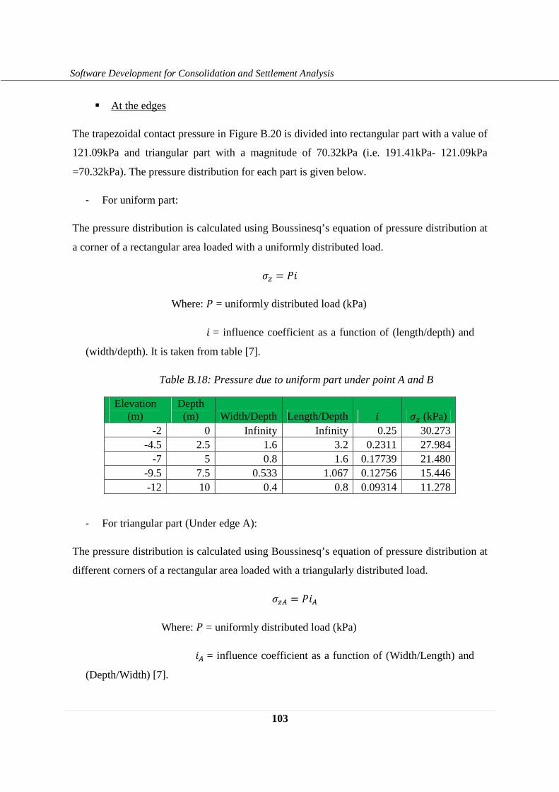
103
Software Development for Consolidation and Settlement Analysis
� At the edges
The trapezoidal contact pressure in Figure B.20 is divided into rectangular part with a value of
121.09kPa and triangular part with a magnitude of 70.32kPa (i.e. 191.41kPa- 121.09kPa
=70.32kPa). The pressure distribution for each part is given below.
- For uniform part:
The pressure distribution is calculated using Boussinesq’s equation of pressure distribution at
a corner of a rectangular area loaded with a uniformly distributed load.
�� = g" Where: g = uniformly distributed load (kPa)
" = influence coefficient as a function of (length/depth) and
(width/depth). It is taken from table [7].
Table B.18: Pressure due to uniform part under point A and B
Elevation (m)
Depth (m) Width/Depth Length/Depth " �� (kPa)
-2 0 Infinity Infinity 0.25 30.273 -4.5 2.5 1.6 3.2 0.2311 27.984
-7 5 0.8 1.6 0.17739 21.480 -9.5 7.5 0.533 1.067 0.12756 15.446 -12 10 0.4 0.8 0.09314 11.278
- For triangular part (Under edge A):
The pressure distribution is calculated using Boussinesq’s equation of pressure distribution at
different corners of a rectangular area loaded with a triangularly distributed load.
�� = g"
Where: g = uniformly distributed load (kPa)
" = influence coefficient as a function of (Width/Length) and
(Depth/Width) [7].
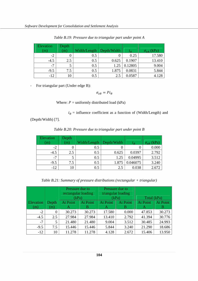
104
Software Development for Consolidation and Settlement Analysis
Table B.19: Pressure due to triangular part under point A
Elevation (m)
Depth (m) Width/Length Depth/Width " �� (kPa)
-2 0 0.5 0 0.25 17.580 -4.5 2.5 0.5 0.625 0.1907 13.410
-7 5 0.5 1.25 0.12805 9.004 -9.5 7.5 0.5 1.875 0.0831 5.844 -12 10 0.5 2.5 0.0587 4.128
- For triangular part (Under edge B):
��¡ = g"¡
Where: g = uniformly distributed load (kPa)
"¡ = influence coefficient as a function of (Width/Length) and
(Depth/Width) [7].
Table B.20: Pressure due to triangular part under point B
Elevation (m)
Depth (m) Width/Length Depth/Width "¡ ��¡ (kPa)
-2 0 0.5 0 0 0.000 -4.5 2.5 0.5 0.625 0.0397 2.792
-7 5 0.5 1.25 0.04995 3.512 -9.5 7.5 0.5 1.875 0.046075 3.240 -12 10 0.5 2.5 0.038 2.672
Table B.21: Summary of pressure distributions (rectangular + triangular)
Elevation (m)
Depth (m)
Pressure due to rectangular loading
(kPa)
Pressure due to triangular loading
(kPa) Total (kPa) At Point
A At Point
B At Point
A At Point
B At Point
A At Point
B -2 0 30.273 30.273 17.580 0.000 47.853 30.273
-4.5 2.5 27.984 27.984 13.410 2.792 41.394 30.776 -7 5 21.480 21.480 9.004 3.512 30.485 24.993
-9.5 7.5 15.446 15.446 5.844 3.240 21.290 18.686 -12 10 11.278 11.278 4.128 2.672 15.406 13.950
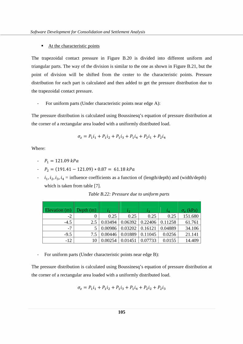
105
Software Development for Consolidation and Settlement Analysis
� At the characteristic points
The trapezoidal contact pressure in Figure B.20 is divided into different uniform and
triangular parts. The way of the division is similar to the one as shown in Figure B.21, but the
point of division will be shifted from the center to the characteristic points. Pressure
distribution for each part is calculated and then added to get the pressure distribution due to
the trapezoidal contact pressure.
- For uniform parts (Under characteristic points near edge A):
The pressure distribution is calculated using Boussinesq’s equation of pressure distribution at
the corner of a rectangular area loaded with a uniformly distributed load.
�� = g'"' + g'"� + g'"( + g'"¢ + g�"' + g�"¢
Where:
- g' = 121.09�gh
- g� = (191.41 − 121.09) ∗ 0.87 = 61.18�gh
- "', "�, "(, "¢ = influence coefficients as a function of (length/depth) and (width/depth)
which is taken from table [7].
Table B.22: Pressure due to uniform parts
Elevation (m) Depth (m) "'
"� "( "¢ �� (kPa)
-2 0 0.25 0.25 0.25 0.25 151.680 -4.5 2.5 0.03494 0.06392 0.22406 0.11258 61.761
-7 5 0.00986 0.03202 0.16121 0.04889 34.106 -9.5 7.5 0.00446 0.01889 0.11045 0.0256 21.141 -12 10 0.00254 0.01451 0.07733 0.0155 14.409
- For uniform parts (Under characteristic points near edge B):
The pressure distribution is calculated using Boussinesq’s equation of pressure distribution at
the corner of a rectangular area loaded with a uniformly distributed load.
�� = g'"' + g'"� + g'"( + g'"¢ + g�"� + g�"(
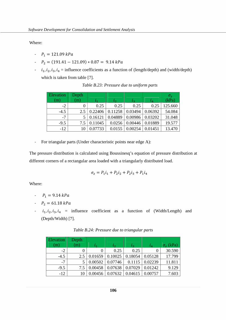
106
Software Development for Consolidation and Settlement Analysis
Where:
- g' = 121.09�gh
- g� = (191.41 − 121.09) ∗ 0.87 = 9.14�gh
- "', "�, "(, "¢ = influence coefficients as a function of (length/depth) and (width/depth)
which is taken from table [7].
Table B.23: Pressure due to uniform parts
Elevation (m)
Depth (m)
"' "�
"( "¢ ��
(kPa) -2 0 0.25 0.25 0.25 0.25 125.660
-4.5 2.5 0.22406 0.11258 0.03494 0.06392 54.084 -7 5 0.16121 0.04889 0.00986 0.03202 31.048
-9.5 7.5 0.11045 0.0256 0.00446 0.01889 19.577 -12 10 0.07733 0.0155 0.00254 0.01451 13.470
- For triangular parts (Under characteristic points near edge A):
The pressure distribution is calculated using Boussinesq’s equation of pressure distribution at
different corners of a rectangular area loaded with a triangularly distributed load.
�� = g'"' + g�"� + g�"( + g'"¢
Where:
- g' = 9.14�gh
- g� = 61.18�gh
- "', "�, "(, "¢ = influence coefficient as a function of (Width/Length) and
(Depth/Width) [7].
Table B.24: Pressure due to triangular parts
Elevation (m)
Depth (m) "'
"� "( "¢ �� (kPa)
-2 0 0 0.25 0.25 0 30.590 -4.5 2.5 0.01659 0.10025 0.18054 0.05128 17.799
-7 5 0.00502 0.07746 0.1115 0.02239 11.811 -9.5 7.5 0.00458 0.07638 0.07029 0.01242 9.129 -12 10 0.00456 0.07632 0.04615 0.00757 7.603
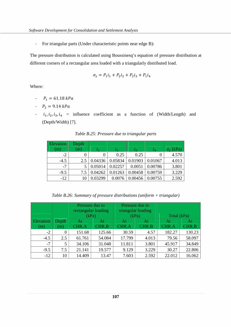
107
Software Development for Consolidation and Settlement Analysis
- For triangular parts (Under characteristic points near edge B):
The pressure distribution is calculated using Boussinesq’s equation of pressure distribution at
different corners of a rectangular area loaded with a triangularly distributed load.
�� = g'"' + g�"� + g�"( + g'"¢
Where:
- g' = 61.18�gh
- g� = 9.14�gh
- "', "�, "(, "¢ = influence coefficient as a function of (Width/Length) and
(Depth/Width) [7].
Table B.25: Pressure due to triangular parts
Elevation (m)
Depth (m) "'
"� "( "¢ �� (kPa)
-2 0 0 0.25 0.25 0 4.570 -4.5 2.5 0.04336 0.05834 0.01903 0.01067 4.013
-7 5 0.05014 0.02257 0.0051 0.00786 3.801 -9.5 7.5 0.04262 0.01263 0.00458 0.00759 3.229 -12 10 0.03299 0.0076 0.00456 0.00755 2.592
Table B.26: Summary of pressure distributions (uniform + triangular)
Elevation
(m) Depth (m)
Pressure due to rectangular loading
(kPa)
Pressure due to triangular loading
(kPa) Total (kPa) At
CHR.A At
CHR.B At
CHR.A At
CHR.B At
CHR.A At
CHR.B -2 0 151.68 125.66 30.59 4.57 182.27 130.23
-4.5 2.5 61.761 54.084 17.799 4.013 79.56 58.097 -7 5 34.106 31.048 11.811 3.801 45.917 34.849
-9.5 7.5 21.141 19.577 9.129 3.229 30.27 22.806 -12 10 14.409 13.47 7.603 2.592 22.012 16.062
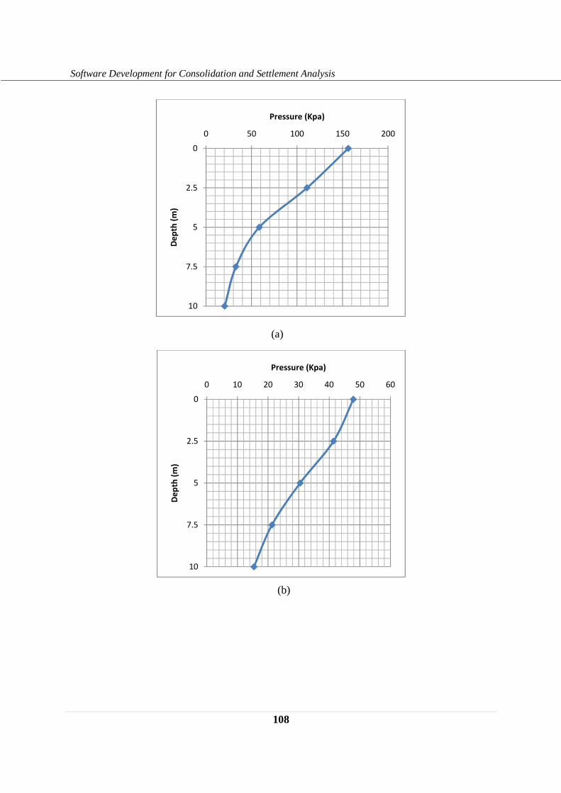
108
Software Development for Consolidation and Settlement Analysis
0
2.5
5
7.5
10
0 50 100 150 200
De
pth
(m
)
Pressure (Kpa)
0
2.5
5
7.5
10
0 10 20 30 40 50 60
De
pth
(m
)
Pressure (Kpa)
(a)
(b)
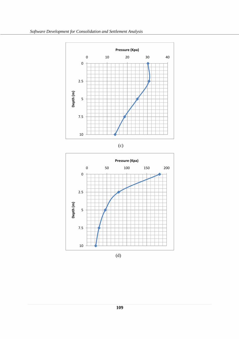
109
Software Development for Consolidation and Settlement Analysis
0
2.5
5
7.5
10
0 10 20 30 40
De
pth
(m
)
Pressure (Kpa)
0
2.5
5
7.5
10
0 50 100 150 200
De
pth
(m
)
Pressure (Kpa)
(c)
(d)
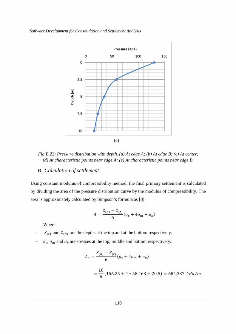
110
Software Development for Consolidation and Settlement Analysis
Fig B.22: Pressure distribution with depth. (a) At edge A; (b) At edge B; (c) At center; (d) At characteristic points near edge A; (e) At characteristic points near edge B.
B. Calculation of settlement
Using constant modulus of compressibility method, the final primary settlement is calculated
by dividing the area of the pressure distribution curve by the modulus of compressibility. The
area is approximately calculated by Simpson’s formula as [8]:
x = £(�) − £( )6 � 3 4�� 3 ��� Where:
- £ � and £�� are the depths at the top and at the bottom respectively.
- � , �� and �� are stresses at the top, middle and bottom respectively.
x¤ � £�� , £ �6 � 3 4�� 3 ��� � 106 156.25 3 4 ∗ 58.463 3 20.5� � 684.337 �gh �⁄
0
2.5
5
7.5
10
0 50 100 150
De
pth
(m
)
Pressure (Kpa)
(e)

111
Software Development for Consolidation and Settlement Analysis
x = £(�) − £( )6 (� + 4�� + ��) = 106 (47.853 + 4 ∗ 30.485 + 15.406) = 308.665 �gh �⁄
x¡ = £(�) − £( )6 (� + 4�� + ��) = 106 (30.273 + 4 ∗ 24.993 + 13.95) = 240.325 �gh �⁄
xu¥ = £(�) − £( )6 (� + 4�� + ��) = 106 (47.853 + 4 ∗ 30.485 + 15.406) = 646.583 �gh �⁄
xu¥¡ = £(�) − £( )6 (� + 4�� + ��) = 106 (30.273 + 4 ∗ 24.993 + 13.95) = 476.147 �gh �⁄
The settlement will be:
Zt¤ = x¤ry = 684.33730000 = 0.0228�
Zt = x ry = 308.66530000 = 0.0103�
Zt¡ = x¡ry = 240.32530000 = 0.0080�
Ztu¥ = xu¥ ry = 646.58330000 = 0.0216�
Ztu¥¡ = xu¥¡ry = 476.14730000 = 0.0159�
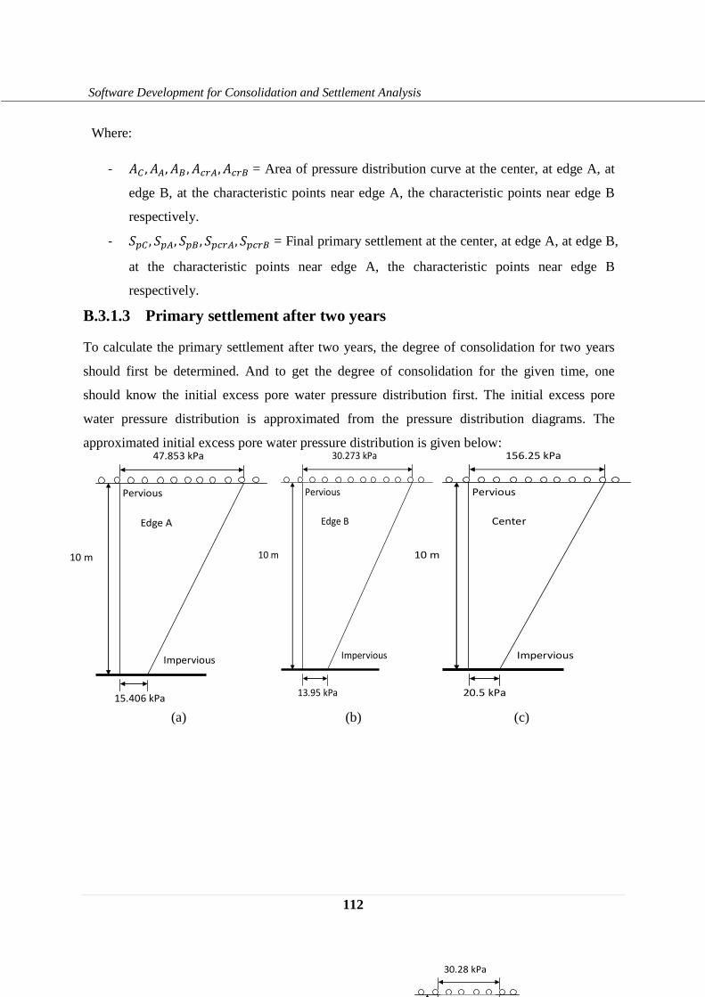
112
Software Development for Consolidation and Settlement Analysis
Where:
- x¤ , x , x¡ , xu¥ , xu¥¡ = Area of pressure distribution curve at the center, at edge A, at
edge B, at the characteristic points near edge A, the characteristic points near edge B
respectively.
- Zt¤ , Zt , Zt¡ , Ztu¥ , Ztu¥¡ = Final primary settlement at the center, at edge A, at edge B,
at the characteristic points near edge A, the characteristic points near edge B
respectively.
B.3.1.3 Primary settlement after two years
To calculate the primary settlement after two years, the degree of consolidation for two years
should first be determined. And to get the degree of consolidation for the given time, one
should know the initial excess pore water pressure distribution first. The initial excess pore
water pressure distribution is approximated from the pressure distribution diagrams. The
approximated initial excess pore water pressure distribution is given below:
30.28 kPa
Pervious
(a) (b) (c)
10 m
Edge A
47.853 kPa
15.406 kPa
Impervious
Pervious
10 m
Edge B
30.273 kPa
13.95 kPa
Impervious
Pervious
10 m
Center
156.25 kPa
20.5 kPa
Impervious
Pervious
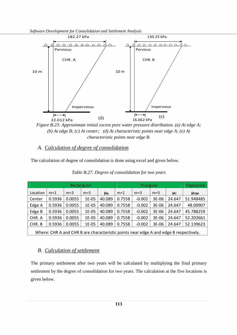
113
Software Development for Consolidation and Settlement Analysis
Figure B.23: Approximate initial excess pore water pressure distribution. (a) At edge A; (b) At edge B; (c) At center; (d) At characteristic points near edge A; (e) At
characteristic points near edge B.
A. Calculation of degree of consolidation
The calculation of degree of consolidation is done using excel and given below.
Table B.27: Degree of consolidation for two years
Rectangular Triangular Trapezoidal
Location m=1 m=3 m=5 μR m=1 m=3 m=5 μT μTRP
Center 0.5936 0.0055 1E-05 40.089 0.7558 -0.002 3E-06 24.647 51.948485
Edge A 0.5936 0.0055 1E-05 40.089 0.7558 -0.002 3E-06 24.647 48.00907
Edge B 0.5936 0.0055 1E-05 40.089 0.7558 -0.002 3E-06 24.647 45.788259
CHR. A 0.5936 0.0055 1E-05 40.089 0.7558 -0.002 3E-06 24.647 52.202661
CHR. B 0.5936 0.0055 1E-05 40.089 0.7558 -0.002 3E-06 24.647 52.139623
Where: CHR A and CHR B are characteristic points near edge A and edge B respectively.
B. Calculation of settlement
The primary settlement after two years will be calculated by multiplying the final primary
settlement by the degree of consolidation for two years. The calculation at the five locations is
given below.
(d) (e)
10 m
CHR. B
130.23 kPa
16.062 kPa
Impervious
Pervious
10 m
CHR. A
182.27 kPa
22.012 kPa
Impervious
Pervious
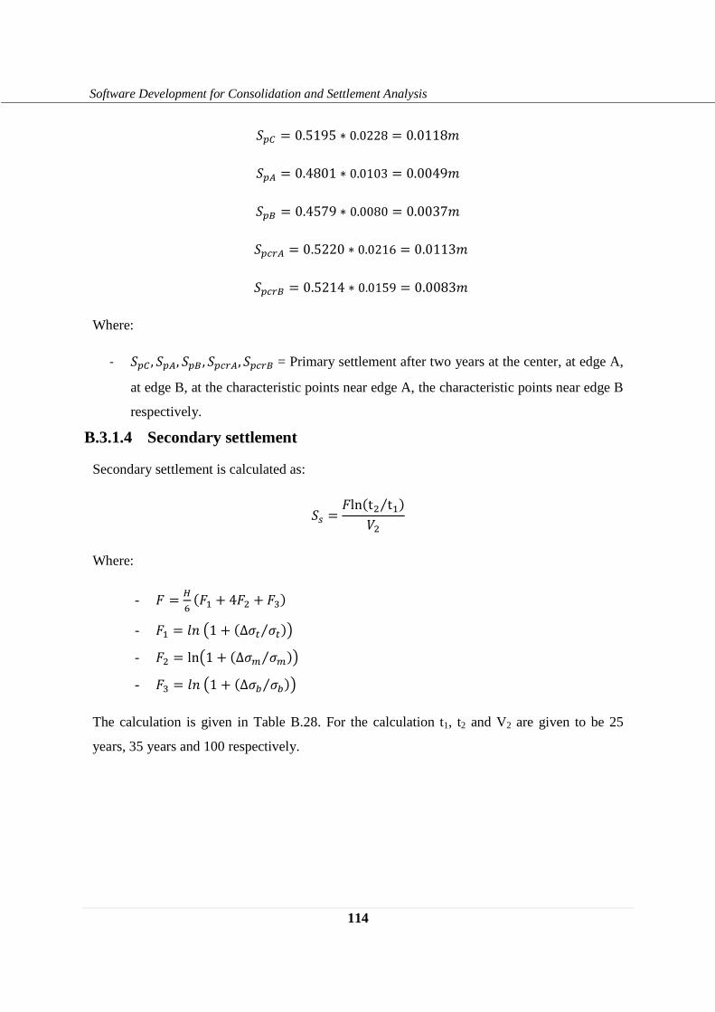
114
Software Development for Consolidation and Settlement Analysis
Zt¤ = 0.5195 ∗ 0.0228 = 0.0118�
Zt = 0.4801 ∗ 0.0103 = 0.0049�
Zt¡ = 0.4579 ∗ 0.0080 = 0.0037�
Ztu¥ = 0.5220 ∗ 0.0216 = 0.0113�
Ztu¥¡ = 0.5214 ∗ 0.0159 = 0.0083�
Where:
- Zt¤ , Zt , Zt¡ , Ztu¥ , Ztu¥¡ = Primary settlement after two years at the center, at edge A,
at edge B, at the characteristic points near edge A, the characteristic points near edge B
respectively.
B.3.1.4 Secondary settlement
Secondary settlement is calculated as:
Zy = |ln(t� t'⁄ )}�
Where:
- | = ~� (|' + 4|� + |() - |' = d#F1 + (∆� � ⁄ )G - |� = lnF1 + (∆�� ��⁄ )G - |( = d#F1 + (∆�� ��⁄ )G
The calculation is given in Table B.28. For the calculation t1, t2 and V2 are given to be 25
years, 35 years and 100 respectively.
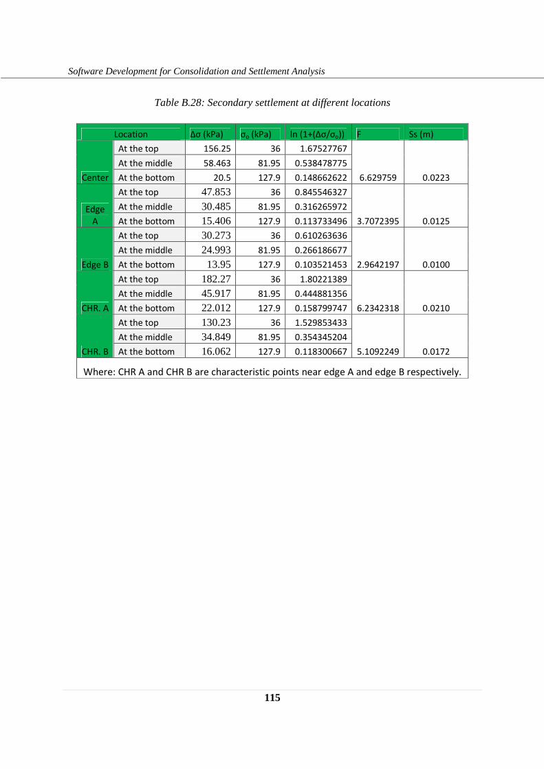
115
Software Development for Consolidation and Settlement Analysis
Table B.28: Secondary settlement at different locations
Location Δσ (kPa) σo (kPa) ln (1+(Δσ/σo)) F Ss (m)
Center
At the top 156.25 36 1.67527767
6.629759 0.0223
At the middle 58.463 81.95 0.538478775
At the bottom 20.5 127.9 0.148662622
Edge
A
At the top 47.853 36 0.845546327
3.7072395 0.0125
At the middle 30.485 81.95 0.316265972
At the bottom 15.406 127.9 0.113733496
Edge B
At the top 30.273 36 0.610263636
2.9642197 0.0100
At the middle 24.993 81.95 0.266186677
At the bottom 13.95 127.9 0.103521453
CHR. A
At the top 182.27 36 1.80221389
6.2342318 0.0210
At the middle 45.917 81.95 0.444881356
At the bottom 22.012 127.9 0.158799747
CHR. B
At the top 130.23 36 1.529853433
5.1092249 0.0172
At the middle 34.849 81.95 0.354345204
At the bottom 16.062 127.9 0.118300667
Where: CHR A and CHR B are characteristic points near edge A and edge B respectively.
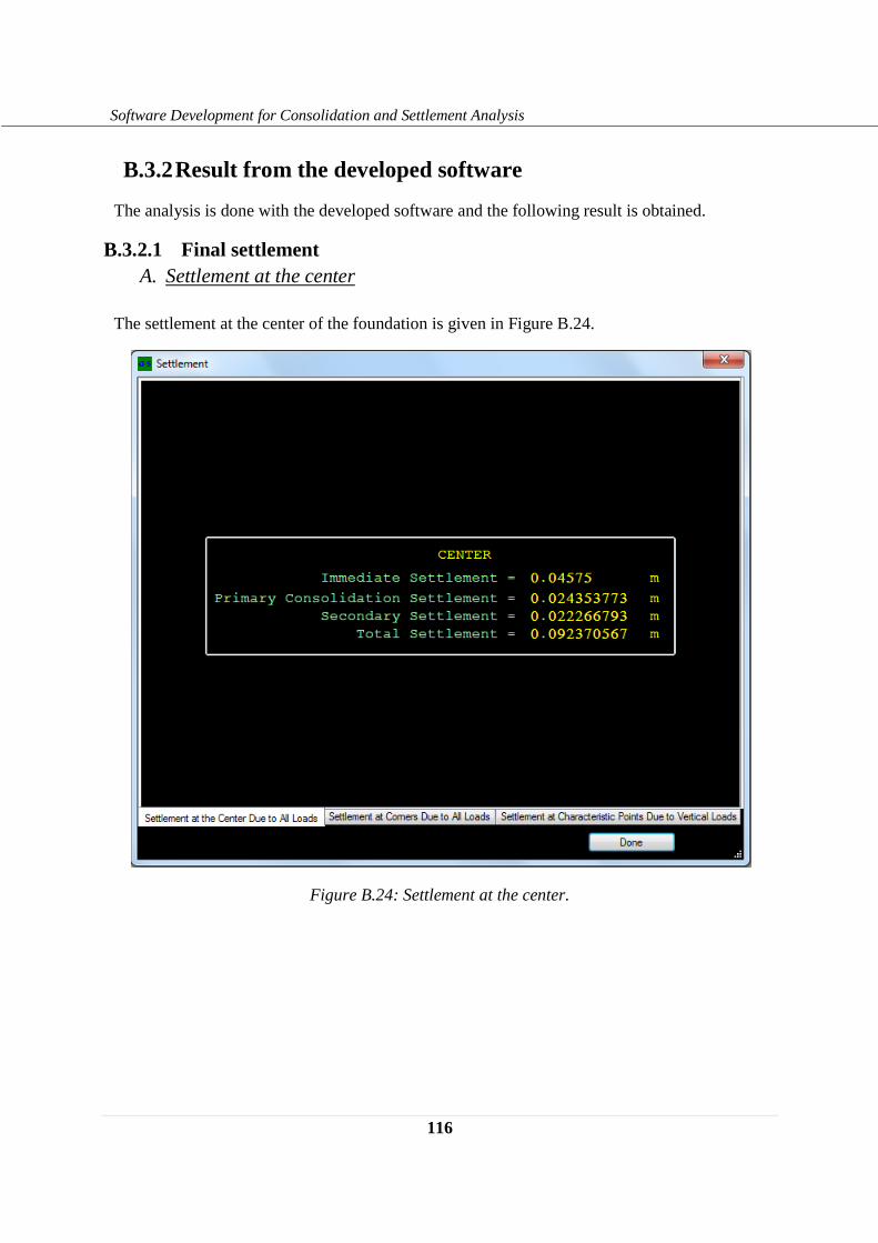
116
Software Development for Consolidation and Settlement Analysis
B.3.2 Result from the developed software
The analysis is done with the developed software and the following result is obtained.
B.3.2.1 Final settlement A. Settlement at the center
The settlement at the center of the foundation is given in Figure B.24.
Figure B.24: Settlement at the center.
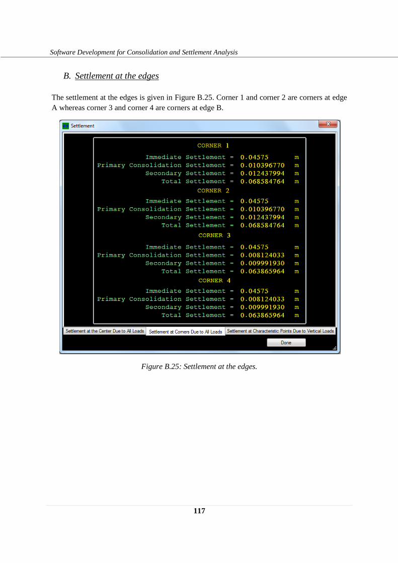
117
Software Development for Consolidation and Settlement Analysis
B. Settlement at the edges
The settlement at the edges is given in Figure B.25. Corner 1 and corner 2 are corners at edge A whereas corner 3 and corner 4 are corners at edge B.
Figure B.25: Settlement at the edges.
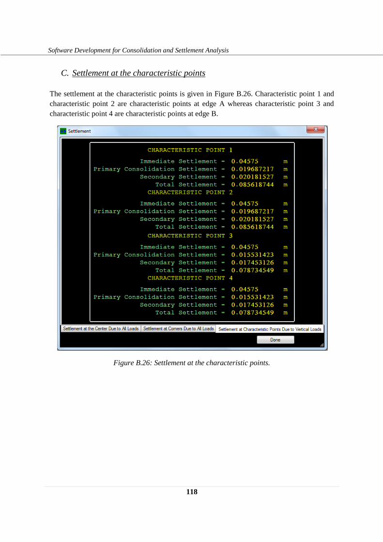
118
Software Development for Consolidation and Settlement Analysis
C. Settlement at the characteristic points
The settlement at the characteristic points is given in Figure B.26. Characteristic point 1 and characteristic point 2 are characteristic points at edge A whereas characteristic point 3 and characteristic point 4 are characteristic points at edge B.
Figure B.26: Settlement at the characteristic points.

119
Software Development for Consolidation and Settlement Analysis
B.3.2.2 Settlement after two years A. Settlement at the center
The settlement at the center of the foundation is given in Figure B.27.
Figure B.27: Settlement at the center.
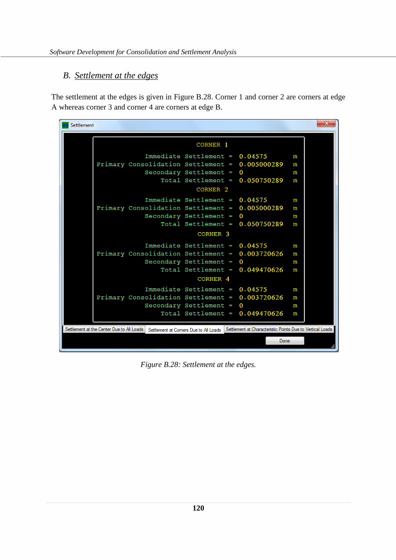
120
Software Development for Consolidation and Settlement Analysis
B. Settlement at the edges
The settlement at the edges is given in Figure B.28. Corner 1 and corner 2 are corners at edge A whereas corner 3 and corner 4 are corners at edge B.
Figure B.28: Settlement at the edges.
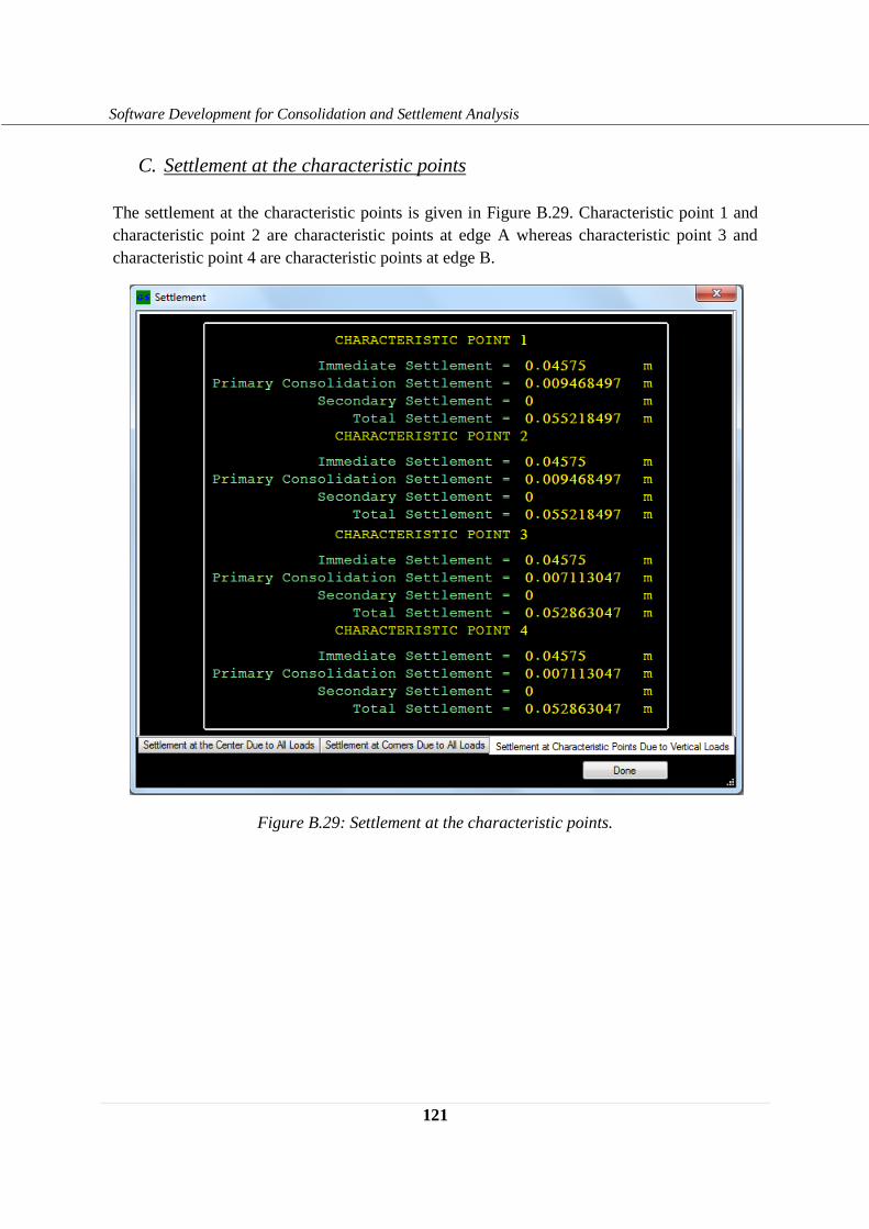
121
Software Development for Consolidation and Settlement Analysis
C. Settlement at the characteristic points
The settlement at the characteristic points is given in Figure B.29. Characteristic point 1 and characteristic point 2 are characteristic points at edge A whereas characteristic point 3 and characteristic point 4 are characteristic points at edge B.
Figure B.29: Settlement at the characteristic points.
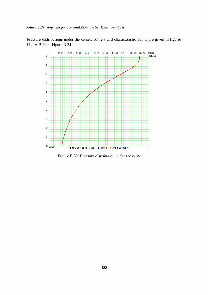
122
Software Development for Consolidation and Settlement Analysis
Pressure distributions under the center, corners and characteristic points are given in figures Figure B.30 to Figure B.34.
Figure B.30: Pressure distribution under the center.
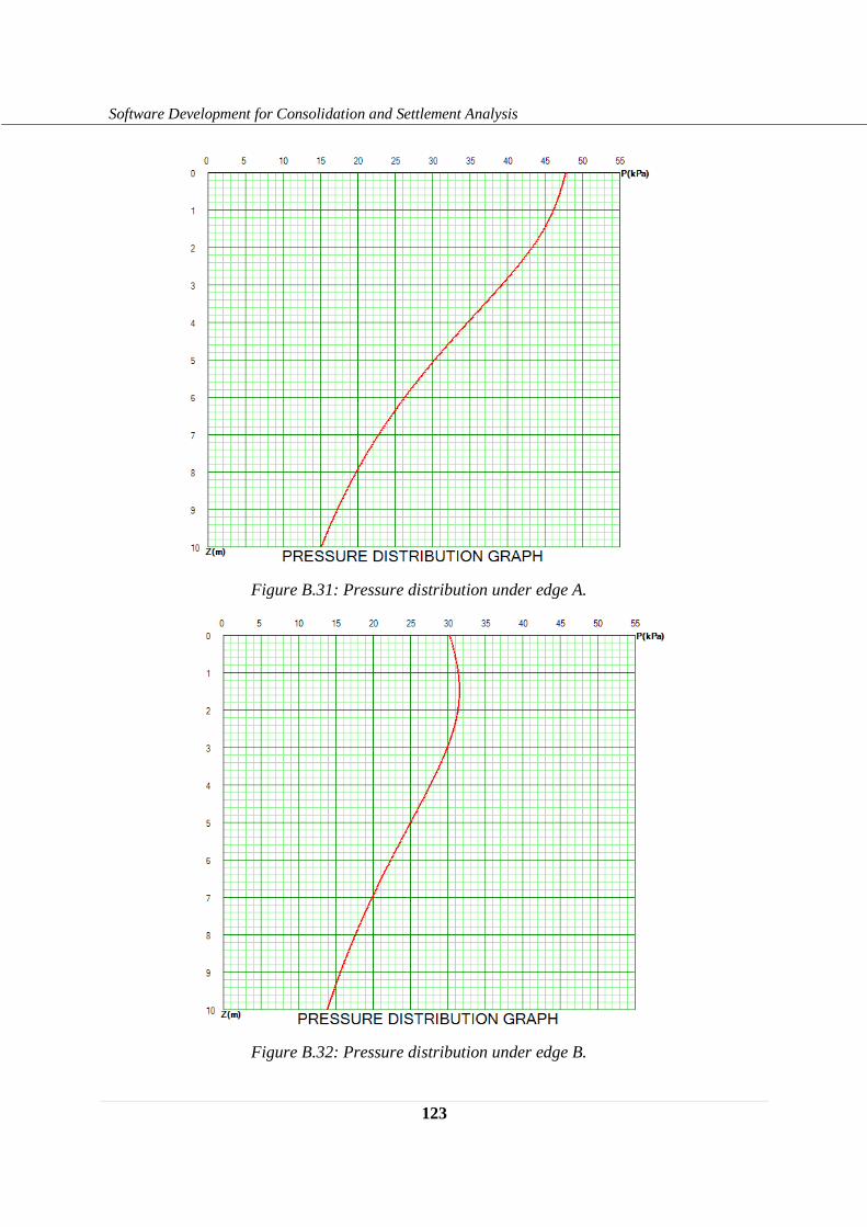
123
Software Development for Consolidation and Settlement Analysis
Figure B.31: Pressure distribution under edge A.
Figure B.32: Pressure distribution under edge B.
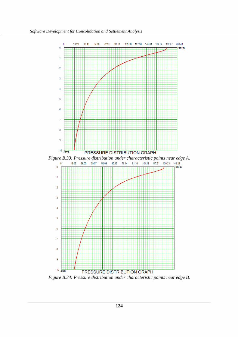
124
Software Development for Consolidation and Settlement Analysis
Figure B.33: Pressure distribution under characteristic points near edge A.
Figure B.34: Pressure distribution under characteristic points near edge B.
Software Development for Consolidation and Settlement Analysis
Declaration
This thesis is my original work and has not been presented for a degree in any other university,
and that all sources of marerial used for the thesis have been duly acknowledged.
Name: Ayenew Yihune
Signature: ______________________
Advisor: Professor Alemayehu Teferra
Signature: ______________________