social mobility, economic growth and socioeconomic
TRANSCRIPT
Centro auspiciado por la Fundación ESRU:
Social Mobility, Economic Growth and Socioeconomic Inequality in an Economy without Informality and with Social Protection Autores:
Florian Chávez-Juárez LNPP - CIDE
Raquel Y. Badillo Salas LNPP - CIDE
Victoria Hernández Sistos LNPP - CIDE Documento de trabajo no.
Centro auspiciado por:
04/2017
Social Mobility, Economic Growth and Socioeconomic Inequality in an Economy without
Informality and with Social Protection1
Florian Chávez-Juárez Raquel Yunoen Badillo Salas
Victoria Hernández Sistos
Julio 2017
Abstract
Mexico is characterised by low economic growth, high income inequality and low intergenerational mobility. These outcomes are likely to be linked to each other. In this study we develop an agent-based model allowing us to study the effects of a radical change in the Mexican Social Security System on inequality, social mobility and economic growth. In particular, we study the effect of moving from the currently implemented dual social security system to a universal system paid through taxes rather than contributions of formal workers. Our model includes traditional elements such as families optimising their utility and firms optimising their profits, but also a series of other processes such as education dependent fertility, assortative mating and search frictions in the labour market. Our baseline model reproduces the actual situation in the Mexican economy quite reasonably and allows us to carry out the simulation of policy changes. The results of this simulation exercise show relatively modest effects in terms of inequality and social mobility. GDP growth is substantially higher under the new policy. This GDP gain is essentially due to an increased proportion of formal firms once the contributions to social security are dropped. Keywords: inequality, social mobility, economic growth, social security, Mexico, agent-based model. JEL-Classification: C63, D63, H20, H52, H55, I24, I30, J20, J62. .
1 This study has been commissioned and partially funded by the Centro de Estudios Espinosa Yglesias (CEEY). We
would like to thank CEEY and in particular Marcelo Delajara for their support, Diana Flores, Lilian Medrano and Gonzalo Ares for their research assistance during the first phase of the project and Cristina Galíndez for her administrative support. The presented results in this study are based on work in progress. All errors are ours.
Contents
1 Introduction 6
2 Literature review and background information 9
2.1 Assortative mating . . . . . . . . . . . . . . . . . . . . . . . . . . . . . . . . . . . . . . . . . . . . . . 9
2.2 Socioeconomic gradient in fertility . . . . . . . . . . . . . . . . . . . . . . . . . . . . . . . . . . . . . 10
2.3 Human capital accumulation . . . . . . . . . . . . . . . . . . . . . . . . . . . . . . . . . . . . . . . . 10
2.4 Social security system and informality . . . . . . . . . . . . . . . . . . . . . . . . . . . . . . . . . . . 11
2.5 Labour market . . . . . . . . . . . . . . . . . . . . . . . . . . . . . . . . . . . . . . . . . . . . . . . . 12
2.6 Capital market and investment by families . . . . . . . . . . . . . . . . . . . . . . . . . . . . . . . . . 13
2.7 The Mexican context . . . . . . . . . . . . . . . . . . . . . . . . . . . . . . . . . . . . . . . . . . . . . 13
2.7.1 The Mexican social security system . . . . . . . . . . . . . . . . . . . . . . . . . . . . . . . . . 13
2.7.2 Tax collection and proposed reforms . . . . . . . . . . . . . . . . . . . . . . . . . . . . . . . . 13
3 The model 15
3.1 The model at a glance . . . . . . . . . . . . . . . . . . . . . . . . . . . . . . . . . . . . . . . . . . . . 15
3.1.1 Key actors and their relationships . . . . . . . . . . . . . . . . . . . . . . . . . . . . . . . . . 15
3.1.2 Time frame and order or processes . . . . . . . . . . . . . . . . . . . . . . . . . . . . . . . . . 16
3.2 Families . . . . . . . . . . . . . . . . . . . . . . . . . . . . . . . . . . . . . . . . . . . . . . . . . . . . 17
3.2.1 Consumption and investment decision . . . . . . . . . . . . . . . . . . . . . . . . . . . . . . . 17
3.2.2 Labour supply . . . . . . . . . . . . . . . . . . . . . . . . . . . . . . . . . . . . . . . . . . . . 18
3.2.3 Procreation . . . . . . . . . . . . . . . . . . . . . . . . . . . . . . . . . . . . . . . . . . . . . . 18
3.3 Firms . . . . . . . . . . . . . . . . . . . . . . . . . . . . . . . . . . . . . . . . . . . . . . . . . . . . . 19
3.4 Government . . . . . . . . . . . . . . . . . . . . . . . . . . . . . . . . . . . . . . . . . . . . . . . . . . 20
3.5 Schools . . . . . . . . . . . . . . . . . . . . . . . . . . . . . . . . . . . . . . . . . . . . . . . . . . . . 20
3.6 Health sector . . . . . . . . . . . . . . . . . . . . . . . . . . . . . . . . . . . . . . . . . . . . . . . . . 21
3.7 Nature . . . . . . . . . . . . . . . . . . . . . . . . . . . . . . . . . . . . . . . . . . . . . . . . . . . . . 21
4 Results 22
4.1 Baseline model . . . . . . . . . . . . . . . . . . . . . . . . . . . . . . . . . . . . . . . . . . . . . . . . 22
4.1.1 Education distribution . . . . . . . . . . . . . . . . . . . . . . . . . . . . . . . . . . . . . . . . 22
4.1.2 Structure of the economy and formality . . . . . . . . . . . . . . . . . . . . . . . . . . . . . . 23
4.1.3 Economic growth . . . . . . . . . . . . . . . . . . . . . . . . . . . . . . . . . . . . . . . . . . . 24
4.1.4 Intergenerational correlations . . . . . . . . . . . . . . . . . . . . . . . . . . . . . . . . . . . . 26
i
CONTENTS CONTENTS
4.1.5 Inequality . . . . . . . . . . . . . . . . . . . . . . . . . . . . . . . . . . . . . . . . . . . . . . . 26
4.2 Changes in the social security system . . . . . . . . . . . . . . . . . . . . . . . . . . . . . . . . . . . . 27
4.2.1 Simulation approach . . . . . . . . . . . . . . . . . . . . . . . . . . . . . . . . . . . . . . . . . 28
4.2.1.1 Expected results . . . . . . . . . . . . . . . . . . . . . . . . . . . . . . . . . . . . . . 29
4.2.2 Effects on the government income . . . . . . . . . . . . . . . . . . . . . . . . . . . . . . . . . 29
4.2.3 Effects on growth and formality . . . . . . . . . . . . . . . . . . . . . . . . . . . . . . . . . . . 31
4.2.4 Effects on inequality . . . . . . . . . . . . . . . . . . . . . . . . . . . . . . . . . . . . . . . . . 32
4.2.5 Effects on social mobility . . . . . . . . . . . . . . . . . . . . . . . . . . . . . . . . . . . . . . 34
5 Conclusion 37
A Overview, Design concepts and Details 43
A.1 Overview . . . . . . . . . . . . . . . . . . . . . . . . . . . . . . . . . . . . . . . . . . . . . . . . . . . 43
A.1.1 Purpose . . . . . . . . . . . . . . . . . . . . . . . . . . . . . . . . . . . . . . . . . . . . . . . . 43
A.1.2 Entities, state variables and scales . . . . . . . . . . . . . . . . . . . . . . . . . . . . . . . . . 43
A.1.3 Process overview and scheduling . . . . . . . . . . . . . . . . . . . . . . . . . . . . . . . . . . 46
A.2 Design Concepts . . . . . . . . . . . . . . . . . . . . . . . . . . . . . . . . . . . . . . . . . . . . . . . 47
A.2.1 Basic principles . . . . . . . . . . . . . . . . . . . . . . . . . . . . . . . . . . . . . . . . . . . . 47
A.2.2 Emergence . . . . . . . . . . . . . . . . . . . . . . . . . . . . . . . . . . . . . . . . . . . . . . 47
A.2.3 Adaptation . . . . . . . . . . . . . . . . . . . . . . . . . . . . . . . . . . . . . . . . . . . . . . 47
A.2.4 Objectives . . . . . . . . . . . . . . . . . . . . . . . . . . . . . . . . . . . . . . . . . . . . . . . 48
A.2.5 Learning . . . . . . . . . . . . . . . . . . . . . . . . . . . . . . . . . . . . . . . . . . . . . . . . 48
A.2.6 Prediction . . . . . . . . . . . . . . . . . . . . . . . . . . . . . . . . . . . . . . . . . . . . . . . 48
A.2.7 Sensing . . . . . . . . . . . . . . . . . . . . . . . . . . . . . . . . . . . . . . . . . . . . . . . . 48
A.2.8 Interaction . . . . . . . . . . . . . . . . . . . . . . . . . . . . . . . . . . . . . . . . . . . . . . 48
A.2.9 Stochasticity . . . . . . . . . . . . . . . . . . . . . . . . . . . . . . . . . . . . . . . . . . . . . 48
A.2.10 Collectives . . . . . . . . . . . . . . . . . . . . . . . . . . . . . . . . . . . . . . . . . . . . . . 49
A.2.11 Observation . . . . . . . . . . . . . . . . . . . . . . . . . . . . . . . . . . . . . . . . . . . . . . 49
A.3 Details . . . . . . . . . . . . . . . . . . . . . . . . . . . . . . . . . . . . . . . . . . . . . . . . . . . . . 49
A.3.1 Initialisation . . . . . . . . . . . . . . . . . . . . . . . . . . . . . . . . . . . . . . . . . . . . . 49
A.3.2 Input . . . . . . . . . . . . . . . . . . . . . . . . . . . . . . . . . . . . . . . . . . . . . . . . . 50
A.3.3 Sub-models . . . . . . . . . . . . . . . . . . . . . . . . . . . . . . . . . . . . . . . . . . . . . . 50
A.3.3.1 Firms, production and labour market . . . . . . . . . . . . . . . . . . . . . . . . . . 50
A.3.3.2 Financial market . . . . . . . . . . . . . . . . . . . . . . . . . . . . . . . . . . . . . . 55
A.3.3.3 Family related processes . . . . . . . . . . . . . . . . . . . . . . . . . . . . . . . . . . 55
A.3.3.4 Government related processes . . . . . . . . . . . . . . . . . . . . . . . . . . . . . . . 60
A.3.3.5 Nature and adaptation processes . . . . . . . . . . . . . . . . . . . . . . . . . . . . . 62
B Calibration 66
B.1 Income . . . . . . . . . . . . . . . . . . . . . . . . . . . . . . . . . . . . . . . . . . . . . . . . . . . . . 67
C Overview of parameters 68
ii
CONTENTS CONTENTS
D Sensitivity analyses 70
E Agent-based modelling approach 72
E.1 What are agent-based models? . . . . . . . . . . . . . . . . . . . . . . . . . . . . . . . . . . . . . . . 72
E.2 Why ABM for this project? . . . . . . . . . . . . . . . . . . . . . . . . . . . . . . . . . . . . . . . . . 73
E.3 Modelling process . . . . . . . . . . . . . . . . . . . . . . . . . . . . . . . . . . . . . . . . . . . . . . . 73
E.4 Technical implementation . . . . . . . . . . . . . . . . . . . . . . . . . . . . . . . . . . . . . . . . . . 74
iii
List of Figures
3.1 Schematical representation of the model . . . . . . . . . . . . . . . . . . . . . . . . . . . . . . . . . . 16
4.1 Distribution of education over time . . . . . . . . . . . . . . . . . . . . . . . . . . . . . . . . . . . . . 23
4.2 Distribution of firm sizes by type of product . . . . . . . . . . . . . . . . . . . . . . . . . . . . . . . . 24
4.3 Relative importance of firm types by number and number of workers . . . . . . . . . . . . . . . . . . 25
4.4 Proportion of formal firms by product type and size of the firm . . . . . . . . . . . . . . . . . . . . . 25
4.5 Average GDP growth rates at constant prices (period 25) over time . . . . . . . . . . . . . . . . . . 25
4.6 Intergenerational correlations . . . . . . . . . . . . . . . . . . . . . . . . . . . . . . . . . . . . . . . . 26
4.7 Government revenue . . . . . . . . . . . . . . . . . . . . . . . . . . . . . . . . . . . . . . . . . . . . . 30
4.8 Government expenditure . . . . . . . . . . . . . . . . . . . . . . . . . . . . . . . . . . . . . . . . . . . 31
4.9 Evolution of GDP as compared to the baseline model . . . . . . . . . . . . . . . . . . . . . . . . . . 31
4.10 Evolution of the proportion of formal firms . . . . . . . . . . . . . . . . . . . . . . . . . . . . . . . . 32
4.11 Effects on income inequality . . . . . . . . . . . . . . . . . . . . . . . . . . . . . . . . . . . . . . . . . 33
4.12 Effects on intergenerational education mobilty . . . . . . . . . . . . . . . . . . . . . . . . . . . . . . . 34
4.13 Inequality of educational opportunities by policy setting . . . . . . . . . . . . . . . . . . . . . . . . . 35
A.1 Product and firm space . . . . . . . . . . . . . . . . . . . . . . . . . . . . . . . . . . . . . . . . . . . 51
A.2 Recovery from health care shock . . . . . . . . . . . . . . . . . . . . . . . . . . . . . . . . . . . . . . 57
A.3 Amount of social security contribution . . . . . . . . . . . . . . . . . . . . . . . . . . . . . . . . . . . 61
A.4 Income tax rate in function of income . . . . . . . . . . . . . . . . . . . . . . . . . . . . . . . . . . . 62
A.5 Expected number of children by education and age . . . . . . . . . . . . . . . . . . . . . . . . . . . . 64
iv
List of Tables
3.1 Types of products/firms in the economy . . . . . . . . . . . . . . . . . . . . . . . . . . . . . . . . . . 19
4.1 InequalityMeaures . . . . . . . . . . . . . . . . . . . . . . . . . . . . . . . . . . . . . . . . . . . . . . 27
4.2 Overview of policy interventions . . . . . . . . . . . . . . . . . . . . . . . . . . . . . . . . . . . . . . 28
4.3 Effects on income inequality . . . . . . . . . . . . . . . . . . . . . . . . . . . . . . . . . . . . . . . . . 33
4.4 Effects on social mobility . . . . . . . . . . . . . . . . . . . . . . . . . . . . . . . . . . . . . . . . . . 35
4.5 Transition matrix by policy scheme . . . . . . . . . . . . . . . . . . . . . . . . . . . . . . . . . . . . . 36
A.1 Main entities . . . . . . . . . . . . . . . . . . . . . . . . . . . . . . . . . . . . . . . . . . . . . . . . . 45
A.2 Overview of processes and scheduling . . . . . . . . . . . . . . . . . . . . . . . . . . . . . . . . . . . . 46
A.4 Price adaptation in the goods and services market . . . . . . . . . . . . . . . . . . . . . . . . . . . . 64
B.1 Calibration methods . . . . . . . . . . . . . . . . . . . . . . . . . . . . . . . . . . . . . . . . . . . . . 66
D.1 Sensitivity analysis . . . . . . . . . . . . . . . . . . . . . . . . . . . . . . . . . . . . . . . . . . . . . . 70
v
Chapter 1
Introduction
Mexico, like most countries in Latin America, is characterised by large economic inequalities and very low social
mobility. In terms of intergenerational correlations in years of education, Latin American Countries display substan-
tially larger values than countries on other continents. Among the Latin American Countries, Mexico is among the
countries with the highest correlations (Hertz et al., 2007). Social mobility is closely linked to economic inequality.
With a few exceptions1, most studies find a negative relationship between social mobility and economic inequality
(Erikson and Goldthorpe, 1991; Ozdural, 1993; Becker and Tomes, 1986; Bjorklund and Jantti, 1997; Corak, 2013;
Torche, 2014; Andrews and Leigh, 2009)
At the same time, Mexico has experienced long periods of very modest economic growth. According to data
from the World Bank the annual growth rate of the GDP per capita in current US$ over the last 10 years was
about 1.3% in Mexico, which is substantially lower than other countries in the region such as Brazil (6.1%), Bolivia
(11.5%) or Chile (5.6%) (World Bank, 2016).
Both phenomena, low growth rates and low social mobility (or high economic inequality), are likely to be related
to each other. For instance, OECD (2015) highlight the negative relationship between income inequality and
economic growth in OECD countries.
The goal of this study is to analyse the relationship between these three phenomena and to see whether changes
in the social security system can help improve the situation. In particular, the main research question is whether a
change in the Social Security System - from the currently dual system with a contributory and a non-contributory
system to a universal system - can reduce inequality, increase social mobility and increase economic growth as a
consequence. The hypothesis is that such a change in the social security system would mainly benefit the poor and
would therefore decrease inequality. Lower inequality should then generate higher social mobility and eventually
higher economic growth.
Answering such a big research question is very challenging and complex, because many socioeconomic processes
play an important role. In this study we aim at providing a first attempt of an answer. We do so by developing
a theoretical model that is grounded in empirical evidence and a wide range of previous work on the topics. The
model must be able to take into account multiple socioeconomic phenomena and adjust sufficiently close to the
actual Mexican situation.
We have two specific goals in this study. First, we aim at producing a model that is sufficiently close to the
Mexican reality and reproduces a series of key statistics appropriately. Second, we perform a simulation exercise of
1Checchi et al. (1996) point to a positive relationship when comparing the US with Southern European Countries.
6
CHAPTER 1. INTRODUCTION
a specific policy proposal aiming at introducing a universal social security system in Mexico.
To achieve these goals, we base our model on the existing literature and as much as possible on empirical
evidence. With regard to the literature, we rely on two main references. On the one hand Anton et al. (2012) who
develop a model for Mexico in which they focus on the firm side and deal with questions of formality, social security
and growth. On the other hand, we follow Chavez-Juarez (2015) for phenomena related to the family investment
in education and social mobility.
The model is built around individuals, families, firms and the government. We use a four sector economy and
adjust the model as much as possible to the Mexican system. The education, tax and current social security systems
are directly modelled according to the Mexican legislation. In addition to rather standard elements such as a utility
maximisation for families and a profit maximisation for firms, we also include processes such as assortative mating,
education dependent fertility and matching frictions in the labour market.
In order to build such a complex model, we use innovative agent-based modelling techniques. These techniques
are particularly well suited for this study for a number of reasons. First, agent-based models allow us to include
the aforementioned sub-processes and mechanisms that are likely to matter for the research question. Second,
agent-based models allow us to model closer to the reality of a particular country. In this study we implement
the Mexican tax and Social security system quite closely to reality. Moreover, we initiate the model with survey
data from the Mexican Family Life Survey (MxFLS). Thirdly, agent-based models allow us to analyse not only a
long-term equilibrium, but also short-run effects of any policy change. These short-run effect can be different from
the long-run outcomes. Understanding these differences is very important in terms of public policy, in particular
in a country where the administration is elected every six years without the possibility of renewal. Hence, reforms
with short-term adverse effects and long-term benefits might be difficult to implement.
While these advantages of agent-based models are key to our study, the technique also comes at some cost. For
instance, we are not able to provide analytical solutions and there is a certain risk for the model to become too
complex. This complexity might then result in a reduced understanding of what is happening in the model. To
avoid creating a black box, we simplify a number of processes, such as the education and health sector for instance.
It is very important to underline the fact that the model we present in this study is a first attempt to approach
the topic and to model the economic situation in Mexico. Many modelling details will require further research in
order to be refined and provide more accurate results. In this respect, we see this study as a first iteration of the
iterative modelling approach described in Chavez-Juarez (2016). This first model answers some question and raises
new ones, which can then be addresses in other studies, both empirically and by adapting the proposed model.
The results of our simulation study shows that the change from the dual to a universal social security system
has only very modest effects on social mobility and inequality. While inequality slightly decreases, we do not find
any change in relatively social mobility. In contrast, we do find some positive effect on absolute intergenerational
social mobility and on economic growth. The effect on absolute social mobility seems to be due to the change in
the social security system, while the effects on GDP growth are more likely to stem from the accompanying tax
reforms. The clearest effect we find is with respect to the proportion of formal firms, which increases sharply after
the change in the social security system. This important change is due to the elimination of the social security
contributions which are with roughly 20% quite high, especially for low wages.
We will start with a short literature review in section 2, followed by the presentation of the core elements of the
model in section 3.1. A complete explanation of the model aiming at increasing its reproducibility is presented in
the form of the Overview, Design concepts and Details (ODD) protocol in Appendix A. The results are presented in
two steps, first we present the baseline model in section 4.1 and then the effects of the change in the social security
7
CHAPTER 1. INTRODUCTION
system in section 4.2. Section 5 then concludes the study by highlighting the most important point and discussing
the future steps to be taken. In addition to the detailed explanation of the model, the appendix also includes
additional information on agent-based models, some sensitivity analyses and an explanation on the calibration of
the model.
8
Chapter 2
Literature review and background
information
The model we develop in this study is very extensive in terms of phenomena and processes we include. As a
consequence, discussing the literature of each of the processes in detail would be beyond the scope of this article.
We therefore focus our literature review on the most important contributions and on articles that directly contribute
to our model. Two references using Mexican data are of particular interest for this study. On the one hand, the
model developed in Chavez-Juarez (2015) uses the same technique as our model and focuses on intergenerational
mobility, investment in education and the family decisions. On the other hand, Anton et al. (2012) focus on the
decisions taken by firms and discuss important issues of the tax and social security system. Hence, these two
references complement each other almost perfectly for the sake of this study and therefore form the starting point
of this model. Both references include an extensive literature review of their respective main issues. In this literature
review we discuss some key elements of these strands of literature, but we are not able to discuss all the details.
We start our literature review by discussing the key processes for social mobility and present them in a chrono-
logical order from the point of view of a child. We start with processes taking place very early in life and then
move to what happens later. Afterwards we will discuss the literature on which the model presented in Anton et
al. (2012) is based on.
2.1 Assortative mating
Important processes for social mobility take place well before birth. The marriage market is characterised by a
non-random mating, where individuals with similar characteristics are more likely to meet. Becker (1973) provides
a theoretical rationale for this phenomenon of assortative mating. Ermisch et al. (2006) use German and British
data and finds that between 40% and 50% of the covariance the income of two generations can be attributed to
assortative mating. Thiessen and Gregg (1980), Wolf and Figueredo (2011) and van Leeuwen et al. (2008) discuss
assortative mating from an evolutionary and biological perspective.
Using data from Mexico, Wendelspiess Chavez Juarez (2015) finds spousal correlations of 0.4 for the IQ and
of 0.65 for years of education. As a consequence, it is likely to have both parents with similar levels of education
and no regression to the mean takes place. Given that high parental education is an important advantage in life,
children have either a double advantage or a double disadvantage. This advantage manifests itself mostly through
9
CHAPTER 2. LITERATURE REVIEW AND BACKGROUND INFORMATION2.2. SOCIOECONOMIC GRADIENT IN FERTILITY
the resulting intergenerational link in education.
2.2 Socioeconomic gradient in fertility
A second important phenomenon for social mobility taking place before or at birth is the education dependent
fertility rate (Chavez-Juarez, 2015). It is well documented that more educated parents tend to have fewer children.
Using data from Mexico, Chavez-Juarez (2015) finds that very little educated women have on average almost
5 children, while university graduates have only 2 children on average. This phenomenon is important for two
reasons. First, families with little educated parents tend to have lower incomes and in addition, they have to
use these resources for more children. As a consequence, the per capita investment in education is likely to be
substantially lower in families with poorly educated parents. According to the model proposed by Chavez-Juarez
(2015), the education dependent fertility account for up to 10% of the intergenerational correlation in education
with the mother.
2.3 Human capital accumulation
The two already discussed phenomena directly matter for the human capital accumulation of the children. Education
is a key element for both economic growth and social mobility. Education directly affects labour productivity and
innovation, two key factors for economic growth. In terms of social mobility, we observe a strong intergenerational
correlation in terms of years of education (Hertz et al., 2007). This transmission starts very early, because at least
some parts of cognitive ability are genetically transmitted from one generation to the next (Bjorklund et al., 2010;
Anger and Heineck, 2010; Black et al., 2009). Parents with higher cognitive abilities tend to have higher incomes
and more education. By transmitting these abilities to the next generation, the children are more likely to have
good outcomes in terms of education and income. Consequently, we end up observing intergenerational correlations
both in education and income. However, educational correlations across generations are not only due to biological
factors. Another very important element is the possibility and willingness of parents to invest in the education
of their children. Most models of social mobility use this process as key explanatory factor. For instance, Maoz
and Moav (1999) include liquidity constraints in their model to explain why low income families invest less in the
education of children. Similar approaches are taken by Galor and Zeira (1993) and Becker and Tomes (1986). This
phenomenon is reinforced by the education dependent fertility discussed in the previous section. Empirically, various
studies have concluded that this economic channel is important in explaining social mobility. Carneiro and Heckman
(2002) find that in the US only about 8% of students have short term credit constraints. However, they argue that
the long term economic conditions of the family appear to matter more for the intergenerational transmission of
education. Alfonso (2009) confirms this relatively more important role of long term economic conditions for four
Latin American Countries. Wendelspiess Chavez Juarez (2015) compares the importance of different transmission
channel in Mexico and finds the economic channel to be the single most important one. He further decomposes
the effect in long- and short-term effects and also finds a relatively more important role of the long-run economic
situation of parents.
All the elements discussed up to this point, namely assortative mating, genetic transmission of cognitive ability
and the income gradient in education investment build the core elements of an agent-based model developed in
Chavez-Juarez (2015). Chavez-Juarez (2015) aimed at analysing the effects of cash transfer programs on educational
mobility. As a consequence, his model does not look at phenomena beyond the human capital accumulation. Given
10
CHAPTER 2. LITERATURE REVIEW AND BACKGROUND INFORMATION2.4. SOCIAL SECURITY SYSTEM AND INFORMALITY
the goal of our project and the particular interest in the social security system and economic growth, the model
proposed by Chavez-Juarez (2015) must be complemented in various ways. We will now discuss these additional
phenomena that are mostly discussed in Anton et al. (2012).
2.4 Social security system and informality
The social security system is essentially absent in Chavez-Juarez (2016). However, it might have various implica-
tions both for social mobility and economic growth. Economic shocks due to urgent medical conditions of family
members or unemployment of the breadwinner for instance, will generally affect poor households more. In partic-
ular, such shocks can negatively affect the education attainment of children if they have to drop out of school for
instance (Woldehanna and Hagos, 2015; Duryea et al., 2007; Bound and Turner, 2011). The importance of such
economic shocks in general is directly linked to the social protection in a given country. A strongly developed
social security system might help reduce the negative consequences of health shock on education. Such a protection
over-proportionally helps families at the lower end of the socio-economic distribution because wealthier families can
more easily cope with shocks even without social protection. Hence, when looking at the link between economic
shocks and social mobility, it is of paramount importance to consider also the social security system.
Looking at the Mexican social security system more closely brings us directly to another important topic discussed
in Anton et al. (2012) that should be added to Chavez-Juarez (2016): informality. In fact, the Mexican social security
system is a dual system, one for formal workers with large benefits and complete coverage (IMSS and ISSSTE )
and one for informal workers with a limited safety net (Seguro popular). The Seguro Popular has a substantially
lower coverage of around 250 medical treatments as compared to the full coverage of the contributory social security
system for the formal workers. As a consequence of this dual system, the social security system itself can be a source
of low social mobility in case low-income families are more likely to operate in the informal market where social
security is lower and therefore economic shocks hit harder.
Of course, the phenomenon of informality is not only linked to the concept of social mobility but also - and
probably even more - to economic growth. For the purpose of our model, the dual economy plays a role in two
processes: firms have to decide whether they operate in the formal or in the informal marked and workers have to
take a similar decision.
Informality has been discussed in very different ways in the literature, by focussing either on firms’ choice,
workers’ choice or a total segmentation of the markets.
Let us first discuss the approach where formality is mainly linked to the firms’ choice. This approach has been
used in Anton et al. (2012) and will also be the starting point for our model. The approach includes three main
channels: regulation entry, credit constraints and tax compliance. For example, in the first channel we find some
influential work such as Djankov et al. (2002) that argues firms face significant entry costs to be able to operate
formally, these costs are in form of registration and licenses fees. In the second channel some authors such as Straub
(2005) argue that some services that improve the productivity of the firms are restricted to the formal sector. This
is because the informal sector does not register their activities and it is difficult for banks to monitor them. Finally,
in the third approach, firms choose formality or informality based on tax compliance. In this approach we find
some authors such as Anton et al. (2012). Firms can be formal with certain cost of entry or informal and illegal
with certain probability to be caught by the authority. Incomplete tax enforcement distorts decisions in allocation
of resources.
In the second approach, we find some authors such Maloney (2004) arguing that informality is a worker decision.
11
CHAPTER 2. LITERATURE REVIEW AND BACKGROUND INFORMATION 2.5. LABOUR MARKET
Some workers prefer informal jobs because they are able to find substitutes for the protection or services offered by
formal institutions or are willing to trade these formal benefits in exchange of other amenities in the informal sector
such as time flexibility, greater independence or less pressure environment. Maloney (2004) argues that informal
workers choose informality because entrepreneurial desire to create their own business or because skills obsolescence.
Finally, a last approach of market segmentation was an idea implemented by Lewis (1954) and after formalised
by Harris and Todaro (1970). Wages in the formal sector are set exogenously and higher than in the informal sector.
For this reason, informal workers are always trying to enter to formal sectors but these formal jobs are restricted
to a limited quantity. The main implication of this model is that wages set above of market equilibria in formal
sector will produce unemployment and less production in both informal and formal sectors. However, this approach
considers a segmentation between the sectors, with low or no possibility of moving from one sector to the other.
As previously mentioned, we will base our model on the first approach, where firms decide whether to operate
formally paying taxes and social security contributions or not. The approach does not include a mechanism for the
labour market, which is of course of paramount importance for the development of our model.
2.5 Labour market
Models with search and matching frictions deal with the labour market and formality at the same time. In this
kind of models, the formal sector suffers of market rigidities: workers and employers meet each other only through
available job offers, while the informal sector is completely competitive, without entry barriers for workers nor
for employers (see Albrecht et al. (2009); Zenou (2008)). The main implication of this assumption is that in the
formal sector, the wage is determined by a bargaining between workers and firms. Albrecht et al. (2009) allows for
heterogeneity in workers’ skills and find that on average formal workers are more productive than their informal-
sector counterparts.
This last approach with a bargaining in at least some of the sectors is another important element for our study.
Social mobility creates a mismatch between ability and education due to the aforementioned mechanisms. This
mismatch is likely to create suboptimal matching in the labour market as well, given that firms generally can only
observe education, but not ability.
The literature has proposed several ways in which firms search and hire workers1. We can broadly group the
approaches into two main focuses. The first refers to a random process, where workers and firms stochastically
meet. In this focus we can find some authors such as Diamond (1982) and Zenou (2008). They argue that the
matching process is similar as if firms were urns and workers were balls. If all workers and firms are ex ante identical
and if only one worker can occupy each work an uncoordinated application process will lead to overcrowding in
some jobs and no applications in others.
The second approach refers to a meeting probability based on heterogeneous characteristics of the workers and
firms. Authors such as Basu et al. (2015) argue that not every worker knows about all market vacancies. They
assume that not all job seekers receive the full set of offers. Instead firm and job seeker meet each other with a
probability that depends on their skill type (high or low), expected job offers and the minimum wage in the economy.
In our context, an additional reason for heterogeneous access to job offers is the social status and social networks.
We will focus on this approach because some heterogeneity of workers might be very important in explaining their
access to the formal labour market.
1Petrongolo and Pissarides (2001) provide a good overview and generalisation of a number of approaches and group them into sixcategories.
12
CHAPTER 2. LITERATURE REVIEW AND BACKGROUND INFORMATION2.6. CAPITAL MARKET AND INVESTMENT BY FAMILIES
2.6 Capital market and investment by families
A last important element that should be added in this study is the capital market and capital ownership. In
seminal contributions such as Becker (1975), Loury (1981) and Galor and Zeira (1993), capital plays a crucial
role in explaining intergenerational persistence of income, wealth and education. Richer families are able to hold
financial assets which affect social mobility in at least three ways. First, as already mentioned before, financial assets
can help reduce the effect of economic shocks and therefore in the absence of a social safety net, richer families
are substantially less vulnerable to shocks than poorer families. Second, families with higher wealth can invest
more in the education of their offspring, which will result in higher earnings in the long run. Finally, capital stocks
generate capital income in addition to labour income. This directly increases the income inequality and therefore
the capabilities to invest in the education of the next generation, even without using the wealth stock itself.
2.7 The Mexican context
In addition to the above general discussion, it is important to understand the Mexican context and to discuss how
the current policy mechanisms might affect social mobility. We first discuss the social security system, focusing on
the health sector and then discuss the tax system along with already proposed reforms.
2.7.1 The Mexican social security system
The Mexican social security system is characterised by a dual system where formal workers have access to a
contributory social security system (IMSS or ISSSTE), while informal workers can only have access to the non-
contributory health system Seguro Popular, which covers substantially less medical conditions. Social security
essentially refers to the provision of health care services and some compensation payments (e.g. maternity leave in
the contributory system). Unemployment insurance is not available.
There are major differences between the contributory and the non-contributory system in terms of financing and
coverage. With respect to financing, in the contributory system workers pay a share of their gross salary, while the
non-contributory system is almost exclusively funded by the federal government through income taxes. Beneficiaries
have to pay only a small fee per family that depends on their economic situation. The fee is very low2 and therefore
we simplify the discussion by assuming that health care is for free.
In terms of coverage the contributory system has full coverage of all medical conditions, while the non-contributory
system is limited to slightly more than 250 medical treatments, including preventive care, general practitioner ser-
vices, specialist services, emergencies and some surgery treatments (Seguro Popular, 2016).
2.7.2 Tax collection and proposed reforms
Mexico has one of the lowest tax collection in the world. According with Campos Vazquez et al. (2014), the Mexican
tax structure has not been effective in reducing the inequality; therefore, the social mobility in Mexico is very low.
In recent years, there have been different proposals of fiscal reforms that could have an effect in social mobility.
Two popular proposal involve an increase of the value added tax and an increase of the income tax for the richest
respectively.
2Families in the first four income deciles are waived from the fee, those in the fifth decile pay the equivalent of 112 USD a year andthe richest families pay a maximum of 615 USD (Secretarıa de Salud, 2016)
13
CHAPTER 2. LITERATURE REVIEW AND BACKGROUND INFORMATION 2.7. THE MEXICAN CONTEXT
With respect to changes in the value-added-tax various proposals have been made. Currently most products are
taxed at 16%, while food and medicines are taxed at a reduced rate which is currently set to 0%. Some proposals
target an increase of the general tax rate of 16% to a higher level (not very popular), while other proposals would
rather generalise VAT to all products by increasing the reduced rate (Anton et al., 2012). Nevertheless, this approach
has been criticised because an increase of the VAT (especially on foods and medicines) could be highly regressive.
Anton et al. (2012) argue that regressivity can be avoided by removing all taxes on formal employment and subsidies
to informal employment. In this way the net income would be bigger and every citizen would have access to universal
social security, regardless of their employment status (formal or informal). Of course, this proposal goes far beyond
a simple tax reform, as it would also completely restructure the social security system. In our policy analysis we
simulate a version of this proposal.
The set of proposals aims at changing the income tax rate for the wealthiest people. According with Campos
Vazquez et al. (2014), the share of total income of the richest 1% of individuals in Mexico is 21.3 %. If we compare
it with other countries, the richest people in Mexico have one of the highest shares of total income Campos Vazquez
et al. (2014). Based on this data, Campos Vazquez et al. (2014) found, the marginal rate of income tax has to be
between 40 and 60%, which is clearly above the current rate. This increase would be reflected in a growth of at least
7% of the direct tax revenues. In a joint article the Economic Commission for Latin America and the Caribbean
and Oxfam recommend increasing the income tax rate for the top earners (CEPAL and OXFAM, 2016).
14
Chapter 3
The model
In this section we describe the cornerstones of our agent-based model and focus on the most relevant aspects. In
addition to this discussion, we present all the details of the model in the Overview, Design concepts and Details
(ODD) protocol in the appendix A (Grimm et al., 2006, 2010; Polhill, 2013). The ODD aims at increasing the
reproducibility of agent-based models and allows the reader to understand the details of the modelling approach.
A general discussion on agent-based models in general is proposed in appendix E.
3.1 The model at a glance
3.1.1 Key actors and their relationships
The goal of our model is to discuss the effects of a universal social security, as opposed to the currently implemented
dual system, on intergenerational social mobility, inequality and economic growth. The working hypothesis is to
find a positive relationship between social mobility and economic growth (Maoz and Moav, 1999), i.e. if social
mobility is low, economic growth is small. We therefore expect a universal social insurance to have a positive effect
on social mobility and consequently on economic growth.
In order to simultaneously study social mobility, inequality and economic growth, we have to model both families
and firms. These two entities build the core of our model, but we also include the government, schools and the
health sector. While the model we propose in this study is completely new and built from scratch, it is inspired by
previous models of the different sub-topics. With respect to social mobility and education, we take many elements
from Chavez-Juarez (2015). In terms of the structure of the economy and the dual social security system, our
model is largely based on ideas presented in Anton et al. (2012). In addition to these two main references, we use
concepts from various fields in economics. For instance, the family decision making process is governed by a utility
maximisation which follows to some extent a Beckerian approach (Becker, 2009).
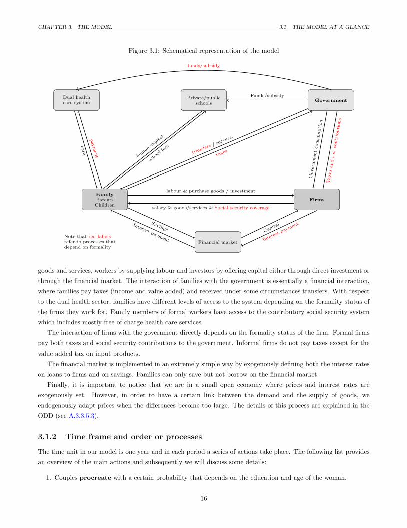
Schematically, we can represent our model as shown in figure 3.1.
Agents are represented in grey boxes; the most important agents are highlighted with bold text. The arrows
between agents refer to processes and/or relationships among agents. Red labels refer to processes and relationships
that depend on the formality status of firms and workers.
Families and firms are the key actors in our model. Families interact with all other agent types, especially
with firms and the government. The relationships with firms are multiple as families are customers by purchasing
15
CHAPTER 3. THE MODEL 3.1. THE MODEL AT A GLANCE
Figure 3.1: Schematical representation of the model
Note that red labelsrefer to processes thatdepend on formality
Firms
GovernmentPrivate/public
schools
Dual healthcare system
Financial market
FamilyParentsChildren
labour & purchase goods / investment
salary & goods/services & Social security coverage
Taxes
and
s.s.
contr
ibuti
ons
Gover
nm
ent
consu
mpti
on
SavingsInterest payment
Capital
Interest
payment
funds/subsidy
Funds/subsidy
care
paym
ent hu
man
capita
l
schoo
l fees
transfe
rs/ ser
vices
taxes
goods and services, workers by supplying labour and investors by offering capital either through direct investment or
through the financial market. The interaction of families with the government is essentially a financial interaction,
where families pay taxes (income and value added) and received under some circumstances transfers. With respect
to the dual health sector, families have different levels of access to the system depending on the formality status of
the firms they work for. Family members of formal workers have access to the contributory social security system
which includes mostly free of charge health care services.
The interaction of firms with the government directly depends on the formality status of the firm. Formal firms
pay both taxes and social security contributions to the government. Informal firms do not pay taxes except for the
value added tax on input products.
The financial market is implemented in an extremely simple way by exogenously defining both the interest rates
on loans to firms and on savings. Families can only save but not borrow on the financial market.
Finally, it is important to notice that we are in a small open economy where prices and interest rates are
exogenously set. However, in order to have a certain link between the demand and the supply of goods, we
endogenously adapt prices when the differences become too large. The details of this process are explained in the
ODD (see A.3.3.5.3).
3.1.2 Time frame and order or processes
The time unit in our model is one year and in each period a series of actions take place. The following list provides
an overview of the main actions and subsequently we will discuss some details:
1. Couples procreate with a certain probability that depends on the education and age of the woman.
16

CHAPTER 3. THE MODEL 3.2. FAMILIES
2. Nature produces health shocks for each individual. The likelihood and intensity of the shocks depend on
individuals’ characteristics.
3. Enrolled children either pass or not the school year.
4. Single individuals mate with a certain probability.
5. Firms optimise their labour and capital structure based on current prices in the market. If this involves
hiring workers, job offers are created and sent to the market.
6. All individuals that are no longer at school and attained the minimum legal age to work compute their
reservation wage and apply to job offers with at least this salary.
7. Firms hire among all the candidates who applied to their offers.
8. Firms adapt their capital and input quantities to the actual outcome of the hiring process and produce
their goods and pay the workers.
9. Families make their consumption, health investment and education investment decisions based
on their disposable income and their utility function.
10. The government receives taxes and spends the money in social security and in government consump-
tion.
Once all these and a few secondary steps are completed, the next period starts. We will now discuss in more
details some of the processes presented in the list. In the interest of clarity, we focus on the most important processes
and present less relevant processes only in the appendix A.
3.2 Families
Families represent the most important agent type in our model, because they are the main consumers, supplier of
the labour force, investors in firms and are directly responsible for key phenomena such as social mobility.
Families take a series of important decision, some of which are modelled through an optimisation process, while
other decisions are implemented in a more passive1 way.
3.2.1 Consumption and investment decision
The decision on how to use the disposable income is probably the most important decision of the family and drives
many of the results of the model. We base this decision on the general idea of the Beckerian approach (Becker,
1973), where families optimise a utility function and no intra-household bargaining takes place. The disposable
income can be used for consumption, savings and investment in both health care and education. We assume the
following Cobb-Douglas utility function:
U(ct, Ht, E[yc], E[mt+1]) = cαct ×H
αht × E[yc]
αy × E[mt+1]αm (3.1)
where ct is the per capita family consumption in period t, Ht is a statistic capturing the average health status
of the family members, E[yc] is the expected income of the children based on the current income structure and
E[mt+1] is the expected disposable income in period t+ 1.
1With ’passive’ we refer to simpler behavioural rules that do not imply an optimisation process.
17
CHAPTER 3. THE MODEL 3.2. FAMILIES
The idea behind this utility function is that families care about consumption, health and education. Health
enters the utility function through the average health stock of the family members. In case all members are in
perfect health and nobody suffered a health shock in this period, Ht is equal to unity and no investment in health
can increase this statistic. In contrast, if at least one of the family members suffered a health shock, Ht can be
influenced by the family through investment in health. As we will discuss later, depending on the health system
the family has access to, the same amount of money translates into more or less health improvements.
Contrary to Chavez-Juarez (2015) who includes the offspring’s years of education in the utility function, we
rather use the expected future income of the children2. Again, we use the average income of all children and
compute the expected values based on the current average incomes by education level.
Finally, we introduce an inter-temporal notion by including the disposable income of the next period in the
utility function. This disposable income is basically the expected income of the next period plus any savings the
family might make in period t.
Note that the education enrolment decisions are only taken at the beginning of a level, for instance once the
child has finished primary education the family optimises over the possible enrolment decisions for lower secondary
education. For each child three options are available: no enrolment, enrolment at a public school or enrolment at
a private school.
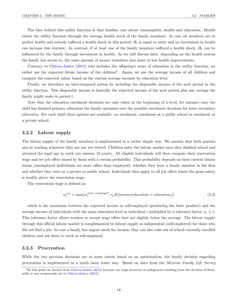
3.2.2 Labour supply
The labour supply of the family members is implemented in a rather simple way. We assume that both parents
aim at working whenever they are not yet retired. Children enter the labour market once they finished school and
attained the legal age to work (we assume 12 years). All eligible individuals will then compute their reservation
wage and see job offers issued by firms with a certain probability. This probability depends on their current labour
status (unemployed individuals see more offers than employed), whether they have a family member in the firm
and whether they were at a private or public school. Individuals then apply to all job offers where the gross salary
is weakly above the reservation wage.
The reservation wage is defined as:
wresi = max(wself−employedi , τLE[income|education = educationi]) (3.2)
which is the maximum between the expected income as self-employed (producing the basic product) and the
average income of individuals with the same education level as individual i multiplied by a tolerance factor τL ≤ 1.
This tolerance factor allows workers to accept wage offers that are slightly below the average. The labour supply
through this official labour market is complemented by labour supply as independent (self-employed) for those who
did not find a job. In case a family has urgent needs for income, they can also take out of school currently enrolled
children and ask them to work as self-employed.
3.2.3 Procreation
While the two previous decisions are to some extent based on an optimisation, the family decision regarding
procreation is implemented in a much more static way. Based on data from the Mexican Family Life Survey
2In this point we deviate from Chavez-Juarez (2015) because our wage structure is endogenous resulting from the decision of firms,while it was exogenously set in Chavez-Juarez (2015).
18
CHAPTER 3. THE MODEL 3.3. FIRMS
(MxFLS) we estimated the likelihood of having a child as a function of the age and education of the woman similar
to the approach used by Chavez-Juarez (2015). In each period we use a stochastic process to simulate whether the
couple will have or not a child. Note that we do not allow for more than one child per period and we ensure a stable
population in the model by multiplying all probabilities by the same factor. This factor endogenously adapts over
time, but does not alter the relationship between the number of children and the education level of the mother.
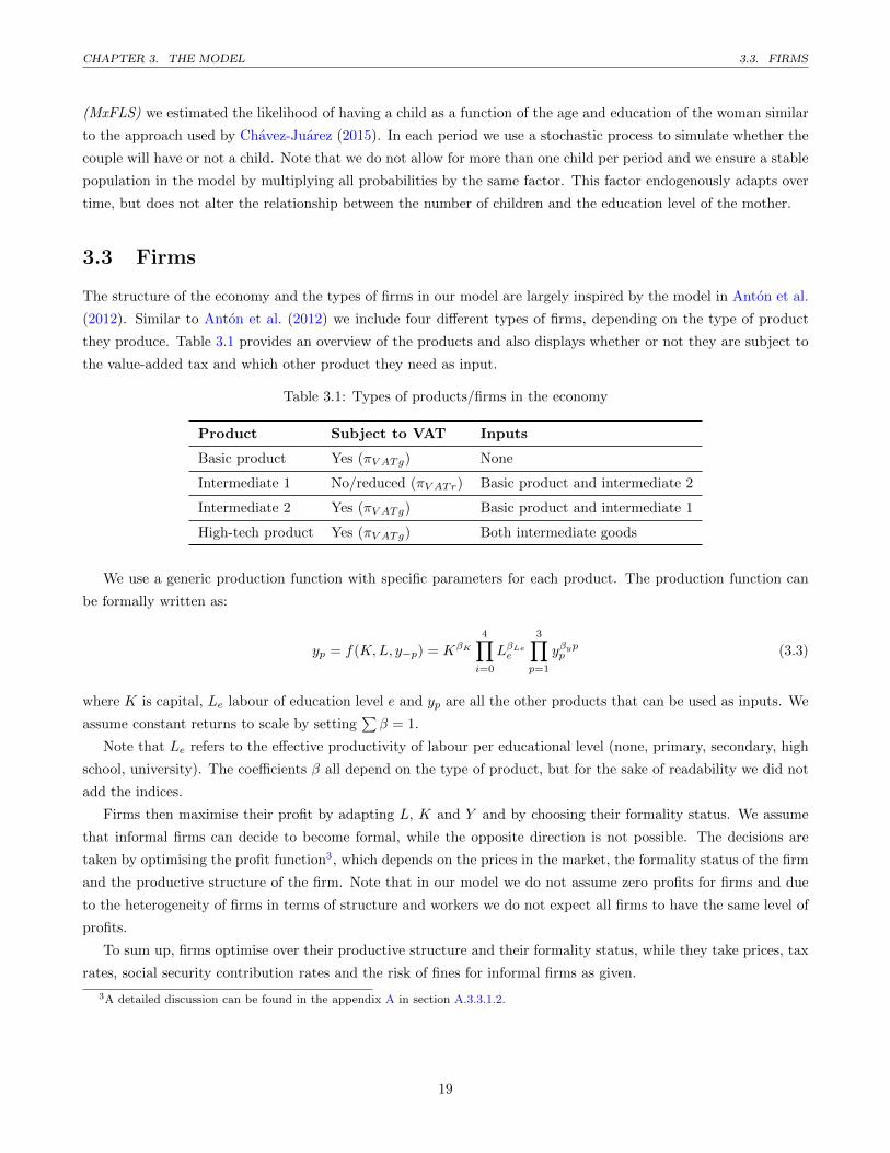
3.3 Firms
The structure of the economy and the types of firms in our model are largely inspired by the model in Anton et al.
(2012). Similar to Anton et al. (2012) we include four different types of firms, depending on the type of product
they produce. Table 3.1 provides an overview of the products and also displays whether or not they are subject to
the value-added tax and which other product they need as input.
Table 3.1: Types of products/firms in the economy
Product Subject to VAT Inputs
Basic product Yes (πV ATg) None
Intermediate 1 No/reduced (πV ATr) Basic product and intermediate 2
Intermediate 2 Yes (πV ATg) Basic product and intermediate 1
High-tech product Yes (πV ATg) Both intermediate goods
We use a generic production function with specific parameters for each product. The production function can
be formally written as:
yp = f(K,L, y−p) = KβK
4∏i=0
LβLee
3∏p=1
yβypp (3.3)
where K is capital, Le labour of education level e and yp are all the other products that can be used as inputs. We
assume constant returns to scale by setting∑β = 1.
Note that Le refers to the effective productivity of labour per educational level (none, primary, secondary, high
school, university). The coefficients β all depend on the type of product, but for the sake of readability we did not
add the indices.
Firms then maximise their profit by adapting L, K and Y and by choosing their formality status. We assume
that informal firms can decide to become formal, while the opposite direction is not possible. The decisions are
taken by optimising the profit function3, which depends on the prices in the market, the formality status of the firm
and the productive structure of the firm. Note that in our model we do not assume zero profits for firms and due
to the heterogeneity of firms in terms of structure and workers we do not expect all firms to have the same level of
profits.
To sum up, firms optimise over their productive structure and their formality status, while they take prices, tax
rates, social security contribution rates and the risk of fines for informal firms as given.
3A detailed discussion can be found in the appendix A in section A.3.3.1.2.
19
CHAPTER 3. THE MODEL 3.4. GOVERNMENT
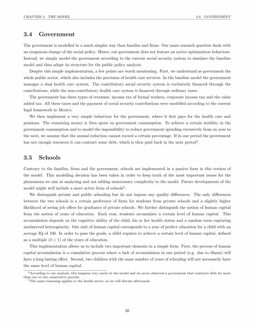
3.4 Government
The government is modelled in a much simpler way than families and firms. Our main research question deals with
an exogenous change of the social policy. Hence, our government does not feature an active optimisation behaviour.
Instead, we simply model the government according to the current social security system to simulate the baseline
model and then adapt its structure for the public policy analysis.
Despite this simple implementation, a few points are worth mentioning. First, we understand as government the
whole public sector, which also includes the provision of health care services. In the baseline model the government
manages a dual health care system. The contributory social security system is exclusively financed through the
contributions, while the non-contributory health care system is financed through ordinary taxes.
The government has three types of revenues: income tax of formal workers, corporate income tax and the value
added tax. All these taxes and the payment of social security contributions were modelled according to the current
legal framework in Mexico.
We then implement a very simple behaviour for the government, where it first pays for the health care and
pensions. The remaining money is then spent on government consumption. To achieve a certain stability in the
government consumption and to model the impossibility to reduce government spending excessively from on year to
the next, we assume that the annual reduction cannot exceed a certain percentage. If in one period the government
has not enough resources it can contract some debt, which is then paid back in the next period4.
3.5 Schools
Contrary to the families, firms and the government, schools are implemented in a passive form in this version of
the model. This modelling decision has been taken in order to keep track of the most important issues for the
phenomena we aim at analysing and not adding unnecessary complexity to the model. Future developments of the
model might well include a more active form of schools5.
We distinguish private and public schooling but do not impose any quality differences. The only differences
between the two schools is a certain preference of firms for students from private schools and a slightly higher
likelihood of seeing job offers for graduates of private schools. We further distinguish the notion of human capital
from the notion of years of education. Each year, students accumulate a certain level of human capital. This
accumulation depends on the cognitive ability of the child, his or her health status and a random term capturing
unobserved heterogeneity. One unit of human capital corresponds to a year of perfect education for a child with an
average IQ of 100. In order to pass the grade, a child requires to achieve a certain level of human capital, defined
as a multiple (δ < 1) of the years of education.
This implementation allows us to include two important elements in a simple form. First, the process of human
capital accumulation is a cumulative process where a lack of accumulation in one period (e.g. due to illness) will
have a long lasting effect. Second, two children with the same number of years of schooling will not necessarily have
the same level of human capital.
4According to our analysis, this happens very rarely in the model and we never observed a government that contracts debt for morethan one or two consecutive periods.
5The same reasoning applies to the health sector, as we will discuss afterwards.
20
CHAPTER 3. THE MODEL 3.6. HEALTH SECTOR
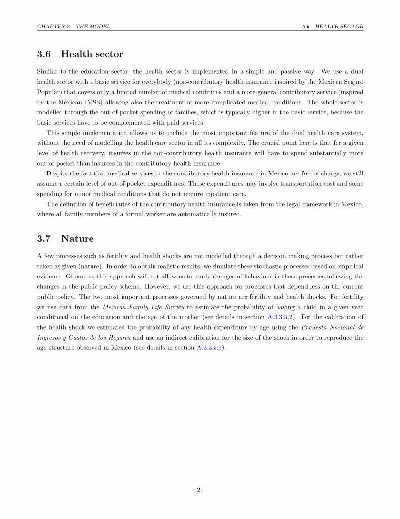
3.6 Health sector
Similar to the education sector, the health sector is implemented in a simple and passive way. We use a dual
health sector with a basic service for everybody (non-contributory health insurance inspired by the Mexican Seguro
Popular) that covers only a limited number of medical conditions and a more general contributory service (inspired
by the Mexican IMSS) allowing also the treatment of more complicated medical conditions. The whole sector is
modelled through the out-of-pocket spending of families, which is typically higher in the basic service, because the
basic services have to be complemented with paid services.
This simple implementation allows us to include the most important feature of the dual health care system,
without the need of modelling the health care sector in all its complexity. The crucial point here is that for a given
level of health recovery, insurees in the non-contributory health insurance will have to spend substantially more
out-of-pocket than insurees in the contributory health insurance.
Despite the fact that medical services in the contributory health insurance in Mexico are free of charge, we still
assume a certain level of out-of-pocket expenditures. These expenditures may involve transportation cost and some
spending for minor medical conditions that do not require inpatient care.
The definition of beneficiaries of the contributory health insurance is taken from the legal framework in Mexico,
where all family members of a formal worker are automatically insured.
3.7 Nature
A few processes such as fertility and health shocks are not modelled through a decision making process but rather
taken as given (nature). In order to obtain realistic results, we simulate these stochastic processes based on empirical
evidence. Of course, this approach will not allow us to study changes of behaviour in these processes following the
changes in the public policy scheme. However, we use this approach for processes that depend less on the current
public policy. The two most important processes governed by nature are fertility and health shocks. For fertility
we use data from the Mexican Family Life Survey to estimate the probability of having a child in a given year
conditional on the education and the age of the mother (see details in section A.3.3.5.2). For the calibration of
the health shock we estimated the probability of any health expenditure by age using the Encuesta Nacional de
Ingresos y Gastos de los Hogares and use an indirect calibration for the size of the shock in order to reproduce the
age structure observed in Mexico (see details in section A.3.3.5.1).
21
Chapter 4
Results
We present the results in two steps, first we discuss the baseline model in section 4.1 which aims at mimicking key
statistics of the Mexican economy. The discussion will focus on the appropriateness of the model in capturing the
main characteristics of the current situation in Mexico.
In section 4.2 we then use the model to simulate a policy change and discuss the results by comparing them to
the baseline outcome.
4.1 Baseline model
The idea is to generate an artificial world that resembles the actual situation in Mexico. Of course, the mere
complexity of the model will not allow us to reproduce all statistics, but we aim at generating a world that
resembles sufficiently well the actual situation in order to run some policy analyses.
We mainly focus on statistics that are directly related to the studied phenomena and put somewhat less weight
on other stylised facts. We simulated the baseline model for 100 different random seeds and ran it for 50 periods.
We generally focus here on the later periods of each run, because the first periods are strongly influenced by the
initial population. For instance, the education distribution of the initial period is simply the education distribution
we found in the data. In contrast, the distribution after 50 periods of the simulation is only the result of the model.
Hence, we can directly use the first periods as stylised facts and compare them to the outcome towards the end of
each simulation run.
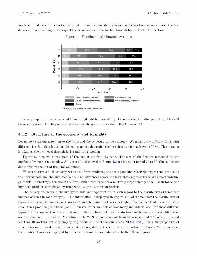
4.1.1 Education distribution
Education is a key element in our model, because it directly links to intergenerational mobility and to the labour
market and eventually to the income distribution. Figure 4.1 shows the education distribution for individuals aged
25 to 40. We focus on this age range to make sure they are no longer enrolled and at the same time sufficiently
young in order to see changes over time in the model.
In general, the years that people go to school increased with time, thus the model produces slightly more
education than what we observe in reality. These changes take essentially place at the extremes of the distribution,
where the share of people without education drops (from 18.8% to 9.1%) and the share of individuals with tertiary
education increases (from 11.7% to 28.2%). Overall, we believe that these changes over time are not necessarily
problematic, because the average education in Mexico is indeed increasing. This applies particularly to the very
22
CHAPTER 4. RESULTS 4.1. BASELINE MODEL
low level of education due to the fact that the number mandatory school years has been increased over the last
decades. Hence, we might also expect the actual distribution to shift towards higher levels of education.
Figure 4.1: Distribution of education over time
9.1 28.6 21.1 13.0 28.2
9.1 26.9 23.2 12.6 28.2
9.8 28.5 21.8 12.4 27.5
8.6 25.2 26.3 13.2 26.7
10.9 20.7 34.8 13.1 20.5
18.8 25.9 33.9 9.7 11.7
0 20 40 60 80 100Percentage
50
40
30
20
10
1
Perio
d (ti
ck)
Considering only individuals aged 25 to 40 years
None or less than primary Primary completed
Lower secondary completed Upper secondary completed
Tertiary
A very important result we would like to highlight is the stability of the distribution after period 20. This will
be very important for the policy analysis as we always introduce the policy in period 25.
4.1.2 Structure of the economy and formality
Let us now turn our attention to the firms and the structure of the economy. We initiate the different firms with
different sizes but then let the model endogenously determine the best firm size for each type of firm. This decision
is taken at the firm level through hiring and firing workers.
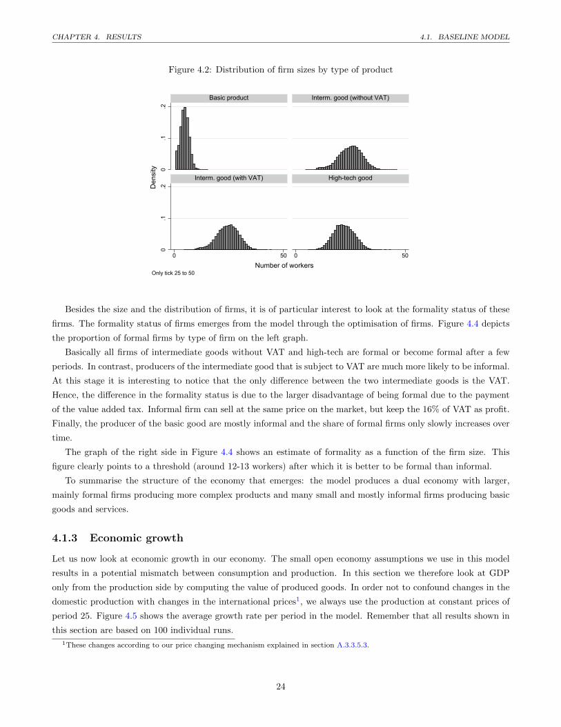
Figure 4.2 displays a histogram of the size of the firms by type. The size of the firms is measured by the
number of workers they employ. All the results displayed in Figure 4.2 are based on period 25 to 50, thus no longer
depending on the initial firm size we impose.
We can observe a dual economy with small firms producing the basic good and relatively bigger firms producing
the intermediate and the high-tech good. The differences across the later three product types are almost indistin-
guishable. Interestingly the size of the firms within each type has a relatively large heterogeneity. For instance, the
high-tech product is produced by firms with 12 up to almost 40 workers.
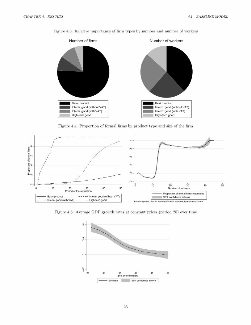
The density estimates in the histogram hide one important result with regard to the distribution of firms: the
number of firms in each category. This information is displayed in Figure 4.3, where we show the distribution of
types of firms by the number of firms (left) and the number of workers (right). We can see that there are many
small firms producing the basic good. However, when we look at how many individuals work for these different
types of firms, we see that the importance of the producers of basic products is much smaller. These differences
are also observed in the data. According to the 2009 economic census from Mexico, around 95% of all firms had
less than 10 workers, but they employ only about 45% of the labour force (INEGI, 2009). Thus, the proportion of
small firms in our model is still somewhat too low, despite the impressive proportion of above 75%. In contrast,
the number of workers employed by these small firms is reasonably close to the official figures.
23
CHAPTER 4. RESULTS 4.1. BASELINE MODEL
Figure 4.2: Distribution of firm sizes by type of product
0.1
.20
.1.2
0 50 0 50
Basic product Interm. good (without VAT)
Interm. good (with VAT) High-tech good
Den
sity
Number of workersOnly tick 25 to 50
Besides the size and the distribution of firms, it is of particular interest to look at the formality status of these
firms. The formality status of firms emerges from the model through the optimisation of firms. Figure 4.4 depicts
the proportion of formal firms by type of firm on the left graph.
Basically all firms of intermediate goods without VAT and high-tech are formal or become formal after a few
periods. In contrast, producers of the intermediate good that is subject to VAT are much more likely to be informal.
At this stage it is interesting to notice that the only difference between the two intermediate goods is the VAT.
Hence, the difference in the formality status is due to the larger disadvantage of being formal due to the payment
of the value added tax. Informal firm can sell at the same price on the market, but keep the 16% of VAT as profit.
Finally, the producer of the basic good are mostly informal and the share of formal firms only slowly increases over
time.
The graph of the right side in Figure 4.4 shows an estimate of formality as a function of the firm size. This
figure clearly points to a threshold (around 12-13 workers) after which it is better to be formal than informal.
To summarise the structure of the economy that emerges: the model produces a dual economy with larger,
mainly formal firms producing more complex products and many small and mostly informal firms producing basic
goods and services.
4.1.3 Economic growth
Let us now look at economic growth in our economy. The small open economy assumptions we use in this model
results in a potential mismatch between consumption and production. In this section we therefore look at GDP
only from the production side by computing the value of produced goods. In order not to confound changes in the
domestic production with changes in the international prices1, we always use the production at constant prices of
period 25. Figure 4.5 shows the average growth rate per period in the model. Remember that all results shown in
this section are based on 100 individual runs.
1These changes according to our price changing mechanism explained in section A.3.3.5.3.
24
CHAPTER 4. RESULTS 4.1. BASELINE MODEL
Figure 4.3: Relative importance of firm types by number and number of workers
Basic productInterm. good (without VAT)Interm. good (with VAT)High-tech good
Number of firms
Basic productInterm. good (without VAT)Interm. good (with VAT)High-tech good
Number of workers
Figure 4.4: Proportion of formal firms by product type and size of the firm
0.2
.4.6
.81
Prop
ortio
n of
form
al fi
rms
0 10 20 30 40 50Period of the simualtion
Basic product Interm. good (without VAT)Interm. good (with VAT) High-tech good
0.2
.4.6
.81
0 10 20 30 40 50Number of workers
Proportion of formal firms (estimate)95% confidence interval
Based on period 25 to 50, Nadaraya-Watson estimator, Epanechnikov kernel
Figure 4.5: Average GDP growth rates at constant prices (period 25) over time
-.005
0.0
05.0
1
25 30 35 40 45 50lpoly smoothing grid
Estimate 95% confidence interval
25
CHAPTER 4. RESULTS 4.1. BASELINE MODEL
Several results can be derived from this figure. First, overall the growth level is very small, attaining a maximum
value of around 1% at period 25. This low growth makes sense because we do not include any technological change
in our model. Second, the growth rates go steadily towards zero and shortly after period 40 the average growth
rate is no longer significantly different from zero.
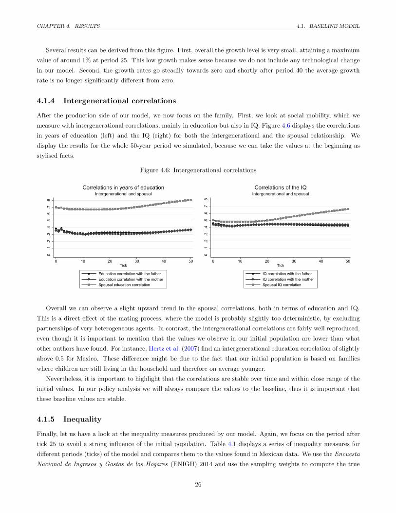
4.1.4 Intergenerational correlations
After the production side of our model, we now focus on the family. First, we look at social mobility, which we
measure with intergenerational correlations, mainly in education but also in IQ. Figure 4.6 displays the correlations
in years of education (left) and the IQ (right) for both the intergenerational and the spousal relationship. We
display the results for the whole 50-year period we simulated, because we can take the values at the beginning as
stylised facts.
Figure 4.6: Intergenerational correlations
0.1
.2.3
.4.5
.6.7
.8
0 10 20 30 40 50Tick
Education correlation with the fatherEducation correlation with the motherSpousal education correlation
Intergenerational and spousalCorrelations in years of education
0.1
.2.3
.4.5
.6.7
.8
0 10 20 30 40 50Tick
IQ correlation with the fatherIQ correlation with the motherSpousal IQ correlation
Intergenerational and spousalCorrelations of the IQ
Overall we can observe a slight upward trend in the spousal correlations, both in terms of education and IQ.
This is a direct effect of the mating process, where the model is probably slightly too deterministic, by excluding
partnerships of very heterogeneous agents. In contrast, the intergenerational correlations are fairly well reproduced,
even though it is important to mention that the values we observe in our initial population are lower than what
other authors have found. For instance, Hertz et al. (2007) find an intergenerational education correlation of slightly
above 0.5 for Mexico. These difference might be due to the fact that our initial population is based on families
where children are still living in the household and therefore on average younger.
Nevertheless, it is important to highlight that the correlations are stable over time and within close range of the
initial values. In our policy analysis we will always compare the values to the baseline, thus it is important that
these baseline values are stable.
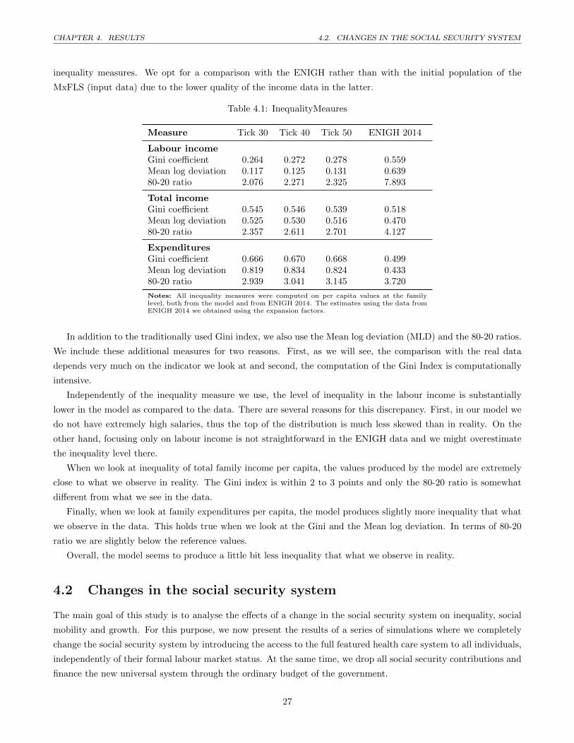
4.1.5 Inequality
Finally, let us have a look at the inequality measures produced by our model. Again, we focus on the period after
tick 25 to avoid a strong influence of the initial population. Table 4.1 displays a series of inequality measures for
different periods (ticks) of the model and compares them to the values found in Mexican data. We use the Encuesta
Nacional de Ingresos y Gastos de los Hogares (ENIGH) 2014 and use the sampling weights to compute the true
26
CHAPTER 4. RESULTS 4.2. CHANGES IN THE SOCIAL SECURITY SYSTEM
inequality measures. We opt for a comparison with the ENIGH rather than with the initial population of the
MxFLS (input data) due to the lower quality of the income data in the latter.
Table 4.1: InequalityMeaures
Measure Tick 30 Tick 40 Tick 50 ENIGH 2014
Labour incomeGini coefficient 0.264 0.272 0.278 0.559Mean log deviation 0.117 0.125 0.131 0.63980-20 ratio 2.076 2.271 2.325 7.893
Total incomeGini coefficient 0.545 0.546 0.539 0.518Mean log deviation 0.525 0.530 0.516 0.47080-20 ratio 2.357 2.611 2.701 4.127
ExpendituresGini coefficient 0.666 0.670 0.668 0.499Mean log deviation 0.819 0.834 0.824 0.43380-20 ratio 2.939 3.041 3.145 3.720
Notes: All inequality measures were computed on per capita values at the familylevel, both from the model and from ENIGH 2014. The estimates using the data fromENIGH 2014 we obtained using the expansion factors.
In addition to the traditionally used Gini index, we also use the Mean log deviation (MLD) and the 80-20 ratios.
We include these additional measures for two reasons. First, as we will see, the comparison with the real data
depends very much on the indicator we look at and second, the computation of the Gini Index is computationally
intensive.
Independently of the inequality measure we use, the level of inequality in the labour income is substantially
lower in the model as compared to the data. There are several reasons for this discrepancy. First, in our model we
do not have extremely high salaries, thus the top of the distribution is much less skewed than in reality. On the
other hand, focusing only on labour income is not straightforward in the ENIGH data and we might overestimate
the inequality level there.
When we look at inequality of total family income per capita, the values produced by the model are extremely
close to what we observe in reality. The Gini index is within 2 to 3 points and only the 80-20 ratio is somewhat
different from what we see in the data.
Finally, when we look at family expenditures per capita, the model produces slightly more inequality that what
we observe in the data. This holds true when we look at the Gini and the Mean log deviation. In terms of 80-20
ratio we are slightly below the reference values.
Overall, the model seems to produce a little bit less inequality that what we observe in reality.
4.2 Changes in the social security system
The main goal of this study is to analyse the effects of a change in the social security system on inequality, social
mobility and growth. For this purpose, we now present the results of a series of simulations where we completely
change the social security system by introducing the access to the full featured health care system to all individuals,
independently of their formal labour market status. At the same time, we drop all social security contributions and
finance the new universal system through the ordinary budget of the government.
27
CHAPTER 4. RESULTS 4.2. CHANGES IN THE SOCIAL SECURITY SYSTEM
As this reform is likely to increase the cost for the government, we simultaneously simulate changes in the tax
structure of the country as discussed in the literature review. We change essentially there parameters of the tax
system:
1. The general value added tax rate (πV ATg, currently 16%)
2. The reduced value added tax rate (πV ATr, currently 0%)
3. The corporate income tax (πCIT , currently 30%)
The argument to modify the CIT is that formal firms have no longer to pay the social security contributions and
therefore a slight increase in the CIT might be cost neutral for them. On the other hand, increasing the VAT is
likely to be the most effective and generalised way to increase tax revenue. We particularly focus on the currently
exempted products with a tax rate of 0%.
In a preliminary analysis we simulated a large number of combinations of the three tax rates. Most of the
analyses schemes reduced the income of the government dramatically. We then limited the number of tax schemes
to the most interesting schemes and increased the number of simulations. The following Table provides a summary
of the interventions.
Table 4.2: Overview of policy interventions
No tax Generalise Increase Gen. VAT + AllBaseline reform VAT VAT increase CIT increased
Setting number 0 1 2 3 4 5
Social security reform no yes yes yes yes yes
Tax reform no no yes yes yes yes
General VAT rate 16% 16% 16% 20% 16% 20%
Reduced VAT rate 0% 0% 16% 16% 16% 20%
Corporate income tax 30% 30% 35% 30% 40% 40%
The baseline model does not include any policy change. We then have five schemes under which the dual system
is changed to a universal system in period 25. This policy measure is identical in all settings and the only differences
is the tax reform to finance this change. In the first setting we do not change the current tax system. This will
allows us to isolate the pure effect of the social security reform. The remaining four settings include increases in
the tax rates. Setting 2 introduced the VAT to products that were previously exempted and slightly increase the
corporate income tax. We call this setting Generalise VAT because we increase the reduced VAT rate from 0% to
the general VAT rate of 16%.
In setting 3 we do not modify the corporate income tax but increase the VAT rate of the products that were
already taxed. Setting 4 includes the generalisation of the VAT rate (similar to setting 2), and a stronger increase
of the corporate income tax. Finally, setting 5 increases all taxes quite strongly.
4.2.1 Simulation approach
In order to evaluate the effect of these different reforms, we simulated each policy reform for 25 different random
seeds. Together with the baseline model in which no policy change takes place, this sums up to a total of 150 runs.
28
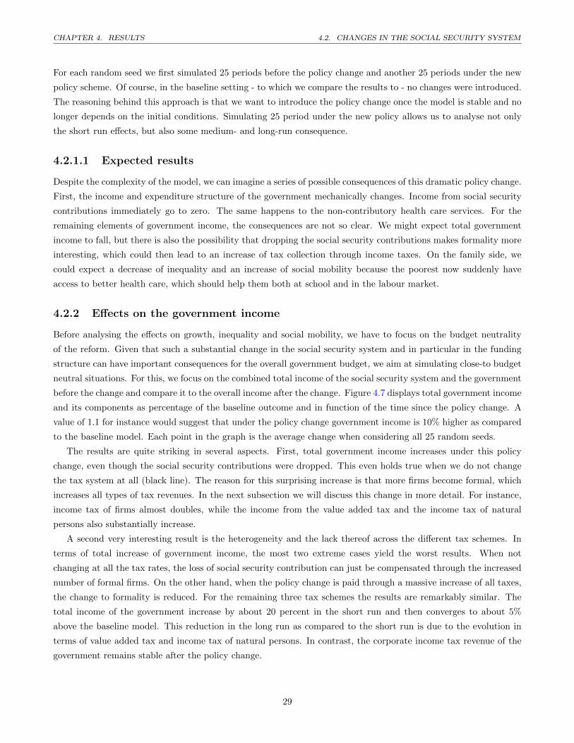
CHAPTER 4. RESULTS 4.2. CHANGES IN THE SOCIAL SECURITY SYSTEM
For each random seed we first simulated 25 periods before the policy change and another 25 periods under the new
policy scheme. Of course, in the baseline setting - to which we compare the results to - no changes were introduced.
The reasoning behind this approach is that we want to introduce the policy change once the model is stable and no
longer depends on the initial conditions. Simulating 25 period under the new policy allows us to analyse not only
the short run effects, but also some medium- and long-run consequence.
4.2.1.1 Expected results
Despite the complexity of the model, we can imagine a series of possible consequences of this dramatic policy change.
First, the income and expenditure structure of the government mechanically changes. Income from social security
contributions immediately go to zero. The same happens to the non-contributory health care services. For the
remaining elements of government income, the consequences are not so clear. We might expect total government
income to fall, but there is also the possibility that dropping the social security contributions makes formality more
interesting, which could then lead to an increase of tax collection through income taxes. On the family side, we
could expect a decrease of inequality and an increase of social mobility because the poorest now suddenly have
access to better health care, which should help them both at school and in the labour market.
4.2.2 Effects on the government income
Before analysing the effects on growth, inequality and social mobility, we have to focus on the budget neutrality
of the reform. Given that such a substantial change in the social security system and in particular in the funding
structure can have important consequences for the overall government budget, we aim at simulating close-to budget
neutral situations. For this, we focus on the combined total income of the social security system and the government
before the change and compare it to the overall income after the change. Figure 4.7 displays total government income
and its components as percentage of the baseline outcome and in function of the time since the policy change. A
value of 1.1 for instance would suggest that under the policy change government income is 10% higher as compared
to the baseline model. Each point in the graph is the average change when considering all 25 random seeds.
The results are quite striking in several aspects. First, total government income increases under this policy
change, even though the social security contributions were dropped. This even holds true when we do not change
the tax system at all (black line). The reason for this surprising increase is that more firms become formal, which
increases all types of tax revenues. In the next subsection we will discuss this change in more detail. For instance,
income tax of firms almost doubles, while the income from the value added tax and the income tax of natural
persons also substantially increase.
A second very interesting result is the heterogeneity and the lack thereof across the different tax schemes. In
terms of total increase of government income, the most two extreme cases yield the worst results. When not
changing at all the tax rates, the loss of social security contribution can just be compensated through the increased
number of formal firms. On the other hand, when the policy change is paid through a massive increase of all taxes,
the change to formality is reduced. For the remaining three tax schemes the results are remarkably similar. The
total income of the government increase by about 20 percent in the short run and then converges to about 5%
above the baseline model. This reduction in the long run as compared to the short run is due to the evolution in
terms of value added tax and income tax of natural persons. In contrast, the corporate income tax revenue of the
government remains stable after the policy change.
29
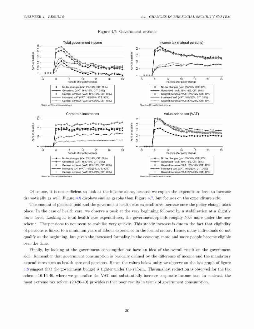
CHAPTER 4. RESULTS 4.2. CHANGES IN THE SOCIAL SECURITY SYSTEM
Figure 4.7: Government revenue
11.
051.
11.
151.
21.
25
As %
of b
asel
ine
-5 0 5 10 15 20 25Periods after policy change
No tax changes (Vat: 0%/16%, CIT: 30%)Generlised (VAT: 16%/16%, CIT: 35%)General increase (VAT: 16%/16%, CIT: 40%)Increased VAT (VAT: 16%/20%, CIT: 30%)General increase (VAT: 20%/20%, CIT: 40%)
Based on 25 runs for each scheme
Total government income
11.
11.
21.
31.
4
As %
of b
asel
ine
-5 0 5 10 15 20 25Periods after policy change
No tax changes (Vat: 0%/16%, CIT: 30%)Generlised (VAT: 16%/16%, CIT: 35%)General increase (VAT: 16%/16%, CIT: 40%)Increased VAT (VAT: 16%/20%, CIT: 30%)General increase (VAT: 20%/20%, CIT: 40%)
Based on 25 runs for each scheme
Income tax (natural persons)1
1.5
22.
5
As %
of b
asel
ine
-5 0 5 10 15 20 25Periods after policy change
No tax changes (Vat: 0%/16%, CIT: 30%)Generlised (VAT: 16%/16%, CIT: 35%)General increase (VAT: 16%/16%, CIT: 40%)Increased VAT (VAT: 16%/20%, CIT: 30%)General increase (VAT: 20%/20%, CIT: 40%)
Based on 25 runs for each scheme
Corporate income tax
11.
21.
41.
61.
82
As %
of b
asel
ine
-5 0 5 10 15 20 25Periods after policy change
No tax changes (Vat: 0%/16%, CIT: 30%)Generlised (VAT: 16%/16%, CIT: 35%)General increase (VAT: 16%/16%, CIT: 40%)Increased VAT (VAT: 16%/20%, CIT: 30%)General increase (VAT: 20%/20%, CIT: 40%)
Based on 25 runs for each scheme
Value-added tax (VAT)
Of course, it is not sufficient to look at the income alone, because we expect the expenditure level to increase
dramatically as well. Figure 4.8 displays similar graphs than Figure 4.7, but focuses on the expenditure side.
The amount of pensions paid and the government health care expenditures increase once the policy change takes
place. In the case of health care, we observe a peek at the very beginning followed by a stabilisation at a slightly
lower level. Looking at total health care expenditures, the government spends roughly 50% more under the new
scheme. The pensions to not seem to stabilise very quickly. This steady increase is due to the fact that eligibility
of pensions is linked to a minimum years of labour experience in the formal sector. Hence, many individuals do not
qualify at the beginning, but given the increased formality in the economy, more and more people become eligible
over the time.
Finally, by looking at the government consumption we have an idea of the overall result on the government
side. Remember that government consumption is basically defined by the difference of income and the mandatory
expenditures such as health care and pensions. Hence the values below unity we observe on the last graph of figure
4.8 suggest that the government budget is tighter under the reform. The smallest reduction is observed for the tax
scheme 16-16-40, where we generalise the VAT and substantially increase corporate income tax. In contrast, the
most extreme tax reform (20-20-40) provides rather poor results in terms of government consumption.
30
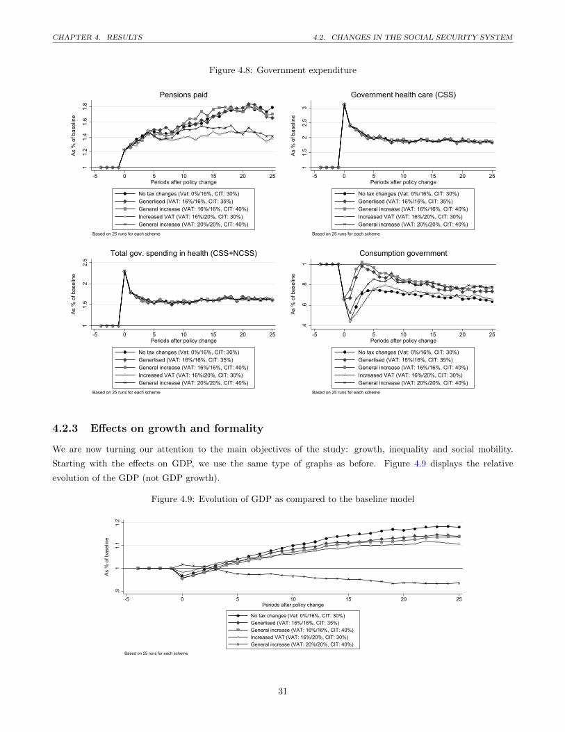
CHAPTER 4. RESULTS 4.2. CHANGES IN THE SOCIAL SECURITY SYSTEM
Figure 4.8: Government expenditure
11.
21.
41.
61.
8
As %
of b
asel
ine
-5 0 5 10 15 20 25Periods after policy change
No tax changes (Vat: 0%/16%, CIT: 30%)Generlised (VAT: 16%/16%, CIT: 35%)General increase (VAT: 16%/16%, CIT: 40%)Increased VAT (VAT: 16%/20%, CIT: 30%)General increase (VAT: 20%/20%, CIT: 40%)
Based on 25 runs for each scheme
Pensions paid
11.
52
2.5
3
As %
of b
asel
ine
-5 0 5 10 15 20 25Periods after policy change
No tax changes (Vat: 0%/16%, CIT: 30%)Generlised (VAT: 16%/16%, CIT: 35%)General increase (VAT: 16%/16%, CIT: 40%)Increased VAT (VAT: 16%/20%, CIT: 30%)General increase (VAT: 20%/20%, CIT: 40%)
Based on 25 runs for each scheme
Government health care (CSS)1
1.5
22.
5
As %
of b
asel
ine
-5 0 5 10 15 20 25Periods after policy change
No tax changes (Vat: 0%/16%, CIT: 30%)Generlised (VAT: 16%/16%, CIT: 35%)General increase (VAT: 16%/16%, CIT: 40%)Increased VAT (VAT: 16%/20%, CIT: 30%)General increase (VAT: 20%/20%, CIT: 40%)
Based on 25 runs for each scheme
Total gov. spending in health (CSS+NCSS)
.4.6
.81
As %
of b
asel
ine
-5 0 5 10 15 20 25Periods after policy change
No tax changes (Vat: 0%/16%, CIT: 30%)Generlised (VAT: 16%/16%, CIT: 35%)General increase (VAT: 16%/16%, CIT: 40%)Increased VAT (VAT: 16%/20%, CIT: 30%)General increase (VAT: 20%/20%, CIT: 40%)
Based on 25 runs for each scheme
Consumption government
4.2.3 Effects on growth and formality
We are now turning our attention to the main objectives of the study: growth, inequality and social mobility.
Starting with the effects on GDP, we use the same type of graphs as before. Figure 4.9 displays the relative
evolution of the GDP (not GDP growth).
Figure 4.9: Evolution of GDP as compared to the baseline model
.91
1.1
1.2
As %
of b
asel
ine
-5 0 5 10 15 20 25Periods after policy change
No tax changes (Vat: 0%/16%, CIT: 30%)Generlised (VAT: 16%/16%, CIT: 35%)General increase (VAT: 16%/16%, CIT: 40%)Increased VAT (VAT: 16%/20%, CIT: 30%)General increase (VAT: 20%/20%, CIT: 40%)
Based on 25 runs for each scheme
31
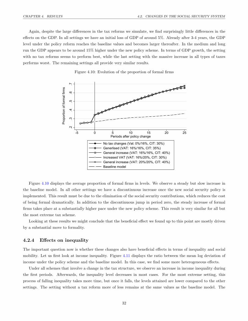
CHAPTER 4. RESULTS 4.2. CHANGES IN THE SOCIAL SECURITY SYSTEM
Again, despite the large differences in the tax reforms we simulate, we find surprisingly little differences in the
effects on the GDP. In all settings we have an initial loss of GDP of around 5%. Already after 3-4 years, the GDP
level under the policy reform reaches the baseline values and becomes larger thereafter. In the medium and long
run the GDP appears to be around 15% higher under the new policy scheme. In terms of GDP growth, the setting
with no tax reforms seems to perform best, while the last setting with the massive increase in all types of taxes
performs worst. The remaining settings all provide very similar results.
Figure 4.10: Evolution of the proportion of formal firms.2
.3.4
.5.6
.7
Prop
ortio
n of
form
al fi
rms
-5 0 5 10 15 20 25Periods after policy change
No tax changes (Vat: 0%/16%, CIT: 30%)Generlised (VAT: 16%/16%, CIT: 35%)General increase (VAT: 16%/16%, CIT: 40%)Increased VAT (VAT: 16%/20%, CIT: 30%)General increase (VAT: 20%/20%, CIT: 40%)Baseline model
Figure 4.10 displays the average proportion of formal firms in levels. We observe a steady but slow increase in
the baseline model. In all other settings we have a discontinuous increase once the new social security policy is
implemented. This result must be due to the elimination of the social security contributions, which reduces the cost
of being formal dramatically. In addition to the discontinuous jump in period zero, the steady increase of formal
firms takes place at a substantially higher pace under the new policy scheme. This result is very similar for all but
the most extreme tax scheme.
Looking at these results we might conclude that the beneficial effect we found up to this point are mostly driven
by a substantial move to formality.
4.2.4 Effects on inequality
The important question now is whether these changes also have beneficial effects in terms of inequality and social
mobility. Let us first look at income inequality. Figure 4.11 displays the ratio between the mean log deviation of
income under the policy scheme and the baseline model. In this case, we find some more heterogeneous effects.
Under all schemes that involve a change in the tax structure, we observe an increase in income inequality during
the first periods. Afterwards, the inequality level decreases in most cases. For the most extreme setting, this
process of falling inequality takes more time, but once it falls, the levels attained are lower compared to the other
settings. The setting without a tax reform more of less remains at the same values as the baseline model. The
32
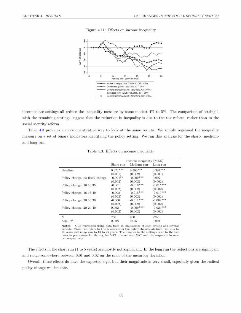
CHAPTER 4. RESULTS 4.2. CHANGES IN THE SOCIAL SECURITY SYSTEM
Figure 4.11: Effects on income inequality
.92
.94
.96
.98
11.
02
As %
of b
asel
ine
-5 0 5 10 15 20 25Periods after policy change
No tax changes (Vat: 0%/16%, CIT: 30%)Generlised (VAT: 16%/16%, CIT: 35%)General increase (VAT: 16%/16%, CIT: 40%)Increased VAT (VAT: 16%/20%, CIT: 30%)General increase (VAT: 20%/20%, CIT: 40%)
intermediate settings all reduce the inequality measure by some modest 4% to 5%. The comparison of setting 1
with the remaining settings suggest that the reduction in inequality is due to the tax reform, rather than to the
social security reform.
Table 4.3 provides a more quantitative way to look at the same results. We simply regressed the inequality
measure on a set of binary indicators identifying the policy setting. We ran this analysis for the short-, medium-
and long-run.
Table 4.3: Effects on income inequality
Income inequality (MLD)Short run Medium run Long run
Baseline 0.371*** 0.386*** 0.387***(0.001) (0.002) (0.001)
Policy change, no fiscal change -0.004** -0.009*** 0.002(0.002) (0.002) (0.002)
Policy change, 16 16 35 -0.001 -0.010*** -0.015***(0.002) (0.002) (0.002)
Policy change, 16 16 40 -0.002 -0.015*** -0.019***(0.002) (0.002) (0.002)
Policy change, 20 16 30 -0.000 -0.011*** -0.009***(0.002) (0.002) (0.002)
Policy change, 20 20 40 0.002 -0.009*** -0.020***(0.002) (0.002) (0.002)
N 750 900 2250Adj. R2 0.008 0.047 0.094
Notes: OLS regression using data from 25 simulations of each setting and severalperiods. Short run refers to 1 to 5 years after the policy change, Medium run to 5 to10 years and Long run to 10 to 25 years. The number in the settings refer to the taxrates in percentage for the regular VAT, the reduced VAT and the corporate incometax respectively
The effects in the short run (1 to 5 years) are mostly not significant. In the long run the reductions are significant
and range somewhere between 0.01 and 0.02 on the scale of the mean log deviation.
Overall, these effects do have the expected sign, but their magnitude is very small, especially given the radical
policy change we simulate.
33
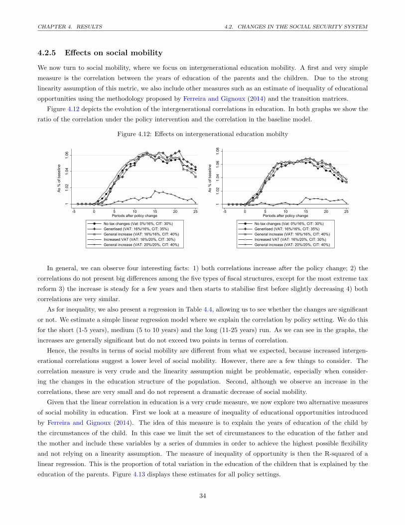
CHAPTER 4. RESULTS 4.2. CHANGES IN THE SOCIAL SECURITY SYSTEM
4.2.5 Effects on social mobility
We now turn to social mobility, where we focus on intergenerational education mobility. A first and very simple
measure is the correlation between the years of education of the parents and the children. Due to the strong
linearity assumption of this metric, we also include other measures such as an estimate of inequality of educational
opportunities using the methodology proposed by Ferreira and Gignoux (2014) and the transition matrices.
Figure 4.12 depicts the evolution of the intergenerational correlations in education. In both graphs we show the
ratio of the correlation under the policy intervention and the correlation in the baseline model.
Figure 4.12: Effects on intergenerational education mobilty
11.
021.
041.
06
As %
of b
asel
ine
-5 0 5 10 15 20 25Periods after policy change
No tax changes (Vat: 0%/16%, CIT: 30%)Generlised (VAT: 16%/16%, CIT: 35%)General increase (VAT: 16%/16%, CIT: 40%)Increased VAT (VAT: 16%/20%, CIT: 30%)General increase (VAT: 20%/20%, CIT: 40%)
11.
021.
041.
061.
08
As %
of b
asel
ine
-5 0 5 10 15 20 25
Periods after policy change
No tax changes (Vat: 0%/16%, CIT: 30%)Generlised (VAT: 16%/16%, CIT: 35%)General increase (VAT: 16%/16%, CIT: 40%)Increased VAT (VAT: 16%/20%, CIT: 30%)General increase (VAT: 20%/20%, CIT: 40%)
In general, we can observe four interesting facts: 1) both correlations increase after the policy change; 2) the
correlations do not present big differences among the five types of fiscal structures, except for the most extreme tax
reform 3) the increase is steady for a few years and then starts to stabilise first before slightly decreasing 4) both
correlations are very similar.
As for inequality, we also present a regression in Table 4.4, allowing us to see whether the changes are significant
or not. We estimate a simple linear regression model where we explain the correlation by policy setting. We do this
for the short (1-5 years), medium (5 to 10 years) and the long (11-25 years) run. As we can see in the graphs, the
increases are generally significant but do not exceed two points in terms of correlation.
Hence, the results in terms of social mobility are different from what we expected, because increased intergen-
erational correlations suggest a lower level of social mobility. However, there are a few things to consider. The
correlation measure is very crude and the linearity assumption might be problematic, especially when consider-
ing the changes in the education structure of the population. Second, although we observe an increase in the
correlations, these are very small and do not represent a dramatic decrease of social mobility.
Given that the linear correlation in education is a very crude measure, we now explore two alternative measures
of social mobility in education. First we look at a measure of inequality of educational opportunities introduced
by Ferreira and Gignoux (2014). The idea of this measure is to explain the years of education of the child by
the circumstances of the child. In this case we limit the set of circumstances to the education of the father and
the mother and include these variables by a series of dummies in order to achieve the highest possible flexibility
and not relying on a linearity assumption. The measure of inequality of opportunity is then the R-squared of a
linear regression. This is the proportion of total variation in the education of the children that is explained by the
education of the parents. Figure 4.13 displays these estimates for all policy settings.
34
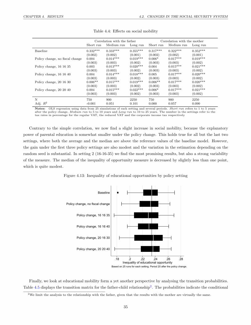
CHAPTER 4. RESULTS 4.2. CHANGES IN THE SOCIAL SECURITY SYSTEM
Table 4.4: Effects on social mobility
Correlation with the father Correlation with the motherShort run Medium run Long run Short run Medium run Long run
Baseline 0.332*** 0.333*** 0.355*** 0.317*** 0.322*** 0.352***(0.002) (0.002) (0.001) (0.002) (0.002) (0.001)
Policy change, no fiscal change 0.004 0.014*** 0.019*** 0.006* 0.017*** 0.019***(0.003) (0.003) (0.002) (0.003) (0.003) (0.002)
Policy change, 16 16 35 0.003 0.013*** 0.020*** 0.004 0.015*** 0.021***(0.003) (0.003) (0.002) (0.003) (0.003) (0.002)
Policy change, 16 16 40 0.004 0.014*** 0.018*** 0.005 0.017*** 0.020***(0.003) (0.003) (0.002) (0.003) (0.003) (0.002)
Policy change, 20 16 30 0.006** 0.015*** 0.019*** 0.006** 0.017*** 0.020***(0.003) (0.003) (0.002) (0.003) (0.003) (0.002)
Policy change, 20 20 40 0.004 0.015*** 0.022*** 0.006* 0.017*** 0.021***(0.003) (0.003) (0.002) (0.003) (0.003) (0.002)
N 750 900 2250 750 900 2250Adj. R2 -0.001 0.051 0.101 0.000 0.057 0.090
Notes: OLS regression using data from 25 simulations of each setting and several periods. Short run refers to 1 to 5 yearsafter the policy change, Medium run to 5 to 10 years and Long run to 10 to 25 years. The number in the settings refer to thetax rates in percentage for the regular VAT, the reduced VAT and the corporate income tax respectively
Contrary to the simple correlation, we now find a slight increase in social mobility, because the explanatory
power of parental education is somewhat smaller under the policy change. This holds true for all but the last two
settings, where both the average and the median are above the reference values of the baseline model. However,
the gain under the first three policy settings are also modest and the variation in the estimation depending on the
random seed is substantial. In setting 2 (16-16-35) we find the most promising results, but also a strong variability
of the measure. The median of the inequality of opportunity measure is decreased by slightly less than one point,
which is quite modest.
Figure 4.13: Inequality of educational opportunities by policy setting
.18 .2 .22 .24 .26 .28Inequality of educational opportunity
Policy change, 20 20 40
Policy change, 20 16 30
Policy change, 16 16 40
Policy change, 16 16 35
Policy change, no fiscal change
Baseline
Based on 25 runs for each setting. Period 20 after the policy change.
Finally, we look at educational mobility form a yet another perspective by analysing the transition probabilities.
Table 4.5 displays the transition matrix for the father-child relationship2. The probabilities indicate the conditional
2We limit the analysis to the relationship with the father, given that the results with the mother are virtually the same.
35
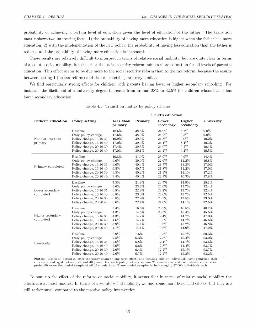
CHAPTER 4. RESULTS 4.2. CHANGES IN THE SOCIAL SECURITY SYSTEM
probability of achieving a certain level of education given the level of education of the father. The transition
matrix shows two interesting facts: 1) the probability of having more education is higher when the father has more
education, 2) with the implementation of the new policy, the probability of having less education than the father is
reduced and the probability of having more education is increased.
These results are relatively difficult to interpret in terms of relative social mobility, but are quite clear in terms
of absolute social mobility. It seems that the social security reform induces more education for all levels of parental
education. This effect seems to be due more to the social security reform than to the tax reform, because the results
between setting 1 (no tax reform) and the other settings are very similar.
We find particularly strong effects for children with parents having lower or higher secondary schooling. For
instance, the likelihood of a university degree increases from around 28% to 32.5% for children whose father has
lower secondary education.
Table 4.5: Transition matrix by policy scheme
Child’s education
Father’s education Policy setting Less thanprimary
Primary Lowersecondary
Highersecondary
University
None or less thanprimary
Baseline 18.6% 38.8% 24.9% 8.7% 9.0%Only policy change 17.6% 38.9% 24.2% 9.5% 9.9%Policy change, 16 16 35 16.9% 39.6% 24.3% 9.0% 10.2%Policy change, 16 16 40 17.0% 39.9% 24.4% 8.4% 10.3%Policy change, 20 16 30 17.4% 39.3% 24.0% 9.2% 10.1%Policy change, 20 20 40 17.0% 39.1% 24.2% 9.2% 10.5%
Primary completed
Baseline 10.8% 41.0% 23.9% 9.9% 14.4%Only policy change 9.6% 39.9% 22.6% 11.2% 16.8%Policy change, 16 16 35 9.6% 40.4% 21.7% 11.3% 17.0%Policy change, 16 16 40 9.5% 40.5% 21.8% 11.2% 17.0%Policy change, 20 16 30 9.5% 40.2% 21.9% 11.1% 17.2%Policy change, 20 20 40 9.4% 40.4% 22.1% 10.3% 17.8%
Lower secondarycompleted
Baseline 7.5% 24.9% 24.7% 14.9% 28.1%Only policy change 6.6% 23.3% 24.0% 13.7% 32.4%Policy change, 16 16 35 6.8% 22.9% 24.2% 13.7% 32.4%Policy change, 16 16 40 6.8% 23.0% 24.0% 13.7% 32.5%Policy change, 20 16 30 6.8% 22.9% 23.9% 13.5% 33.0%Policy change, 20 20 40 6.6% 22.7% 24.0% 14.1% 32.5%
Higher secondarycompleted
Baseline 5.4% 16.6% 20.9% 16.5% 40.7%Only policy change 4.3% 14.5% 20.3% 15.4% 45.5%Policy change, 16 16 35 4.3% 14.7% 19.4% 14.7% 47.0%Policy change, 16 16 40 4.6% 14.7% 19.5% 14.7% 46.6%Policy change, 20 16 30 3.9% 14.4% 19.6% 15.2% 46.8%Policy change, 20 20 40 4.1% 14.1% 19.6% 14.9% 47.2%
University
Baseline 2.9% 7.6% 13.5% 15.7% 60.3%Only policy change 2.5% 6.3% 12.8% 15.4% 63.0%Policy change, 16 16 35 2.6% 6.8% 12.4% 14.7% 63.6%Policy change, 16 16 40 2.6% 6.6% 12.8% 14.4% 63.7%Policy change, 20 16 30 2.6% 6.4% 12.2% 15.1% 63.7%Policy change, 20 20 40 2.6% 6.7% 12.2% 15.3% 63.2%
Notes: Based on period 20 after the policy change (long term effect) and focusing only on individuals having finished theireducation and aged between 25 and 40 years. For each policy setting we ran 25 simulations and computed the transitionprobabilities on the pooled sample of all 25 simulations. These pooled samples include roughly 27’000 individuals each.
To sum up the effect of the reforms on social mobility, it seems that in terms of relative social mobility the
effects are at most modest. In terms of absolute social mobility, we find some more beneficial effects, but they are
still rather small compared to the massive policy intervention.
36
Chapter 5
Conclusion
In this study we developed a rather complex model of the Mexican economy in order to analyse the effects of
changes in the social security system on inequality, social mobility and economic growth. The model uses agent-
base modelling techniques and includes a variety of processes and mechanisms known to matter for at least one of
the aforementioned phenomena. In this regard, we consider for instance assortative mating, education dependent
fertility and matching frictions in the labour market.
The baseline model reproduced the actual statistics for Mexico within a reasonable range. Some values such as
income inequality almost perfectly fit the data, while other statistics such as the intergenerational correlations in
education are somewhat below the values observed in the data. Overall, the model seems to produce an economy
that is reasonably close to the Mexican reality and that allows us to carry out simulations of public policy changes.
Our policy simulation is based on suggested reforms of the social security and the tax system. The major change
in the social security system is to move from the currently implemented dual system to a universal system. In
the current dual system formal workers and their family members have access to a full-fledged contributory social
security system (IMSS or ISSSTE). In contrast, informal workers have only access to a non-contributory social
security system (Seguro Popular) that includes substantially less services. The proposed reform eliminates this
non-contributory social security system and removes all contributions to the contributory system. Moreover, the
new system will be open to all individual independently of their formality status and it will be financed through
the ordinary government budget. For this reason, the proposed reform of the social security system is accompanied
by a tax reform. In this study we consider increases in both the value-added tax and the corporate income tax.
The results of our simulation study suggest that these changes might indeed increase GDP. However, this increase
does not seem to be due to the suggested mechanism going through a reduction of inequality and an increase of social
mobility. These two phenomena change only very little. For instance, income inequality is reduced by a modest
5% and relative intergenerational social mobility does not seem to change. In contrast, absolute intergenerational
mobility in education is positively affected by the policy change, which is of course a beneficial result. According
to our interpretation of the results, the GDP change is essentially due to increased formality. The proportion of
formal firms discontinuously increases upon the policy change and then continues to increase faster than in the
baseline model. This result is due to the elimination of social security contributions, which are especially for low
wages quite high under the current system.
It is important to mention again the fact that the model presented in this study is a first attempt to answer the
research question and to reproduce the Mexican economy appropriately. While we believe that the current version
37
CHAPTER 5. CONCLUSION
of this model largely succeeds, there is a number of limitations that must be mentioned. First, a number of processes
have been implemented in a simplistic way. For instance, schools and the health sector are only implemented in
a passive way. Future developments of the model might want to model these processes with more detail, allows
us to look at more detailed effects of social policies. Second, the calibration and the sensitivity analyses of such a
complex model are difficult and time intensive tasks. The main reason for this is that virtually any parameter can
affect the model in various ways, thus when changing parameters, we must monitor both results that are closely
related to the parameter and parts of the model that are seemingly unrelated.
As a consequence, the model presented in this study must be seen as a first attempt and input for future research.
We see several tasks for future research. As suggested by Chavez-Juarez (2016), agent-based models mostly raise
new questions that can be addressed by empirical analyses. These results can then be included in a revised version
of the model. In our particular case we suggest looking closely at the family behaviour and compare it to the data.
During the development of this model we considered different approaches to model the family behaviour. Eventually,
we used the rather traditional utility maximisation approach. It would therefore be important to validate this choice
through empirical analyses.
In terms of policy analysis, throughout the development of the model, we identified a number of quite complex
processes on the government side. For instance, the contributory social insurance contributions are extremely
complicated to compute, very high for low wages and seems to be highly regressive. It could be interesting to
simulate changes to these mechanisms without the big change of moving to a universal social security.
Another interesting policy change would be the addition of elements to social security. For instance, the current
system does not include unemployment insurance, which would be an important element for social mobility.
38
Bibliography
Albrecht, James, Lucas Navarro, and Susan Vroman, “The Effects of Labour Market Policies in an Economy
with an Informal Sector*,” The Economic Journal, 2009, 119 (539), 1105–1129.
Alfonso, Mariana, “Credit Constraints and the Demand for Higher Education in Latin America,” Inter-American
Development Bank - Education Division - SCL, Working Paper #3 2009.
Andrews, Dan and Andrew Leigh, “More inequality, less social mobility,” Applied Economics Letters, 2009, 16
(15), 1489–1492.
Anger, Silke and Guido Heineck, “Do smart parents raise smart children? The intergenerational transmission
of cognitive abilities,” Journal of Population Economics, 2010, 23, pp. 1255–1282.
Anton, Arturo, Fausto Hernandez, and Santiago Levy Algazi, “The end of informality in Mexico?: fiscal
reform for universal social insurance,” 2012.
Basu, Arnab K., Nancy H. Chau, and Ravi Kanbur, “Contractual Dualism, Market Power and Informality,”
The Economic Journal, 2015, 125 (589), 1534–1573.
Becker, Gary S, “A theory of marriage: Part I,” The Journal of Political Economy, 1973, pp. 813–846.
Becker, Gary S., Human Capital, Columbia University Press, New York, 1975.
Becker, Gary S, Human capital: A theoretical and empirical analysis, with special reference to education, Univer-
sity of Chicago press, 2009.
Becker, Gary S. and Nigel Tomes, “Human Capital and the Rise and Fall of Families,” Journal of Labor
Economics, 1986, 4 (3, Part 2), S1–S39.
Bjorklund, Anders and Markus Jantti, “Intergenerational income mobility in Sweden compared to the United
States,” The American Economic Review, 1997, 87 (5), 1009–1018.
Bjorklund, Anders, Karin Hederos Eriksson, and Markus Jantti, “IQ and Family Background: Are
Associations Strong or Weak?,” The B.E. Journal of Economic Analysis & Policy, 2010, 10 (1).
Black, Sandra E., Paul J. Devereux, and Kjell G. Salvances, “Like Father, Like Son? A Note on the
Intergenerational Transmission of IQ Scores,” Economic Letters, 2009, 105 (1), pp. 138–140.
Bound, John and Sarah Turner, “Chapter 8 - Dropouts and Diplomas: The Divergence in Collegiate Outcomes,”
in Stephen Machin Eric A. Hanushek and Ludger Woessmann, eds., Handbook of The Economics of Education,
Vol. 4, Elsevier, 2011, pp. 573 – 613.
39
BIBLIOGRAPHY BIBLIOGRAPHY
Busso, Matıas, Marıa Victoria Fazio, and Santiago Levy, “(In)Formal and (Un)Productive: The Produc-
tivity Costs of Excessive Informality in Mexico,” IDB Working Paper Series No. IDP-WP-341, August 2012,
Inter-American Development Bank 2012.
Campos Vazquez, Raymundo Miguel, Emmanuel Salavador Chavez Jimenez, and Gerardo Esquivel
Hernandez, “Los Ingresos Altos, la Tributacion Optima y la Recaudacion Posible,” 2014.
Carneiro, Pedro and James J. Heckman, “The Evidence on Credit Constraints in Post-Secondary Schooling,”
The Economic Journal, 2002, 112 (482), 705–734.
CEPAL and OXFAM, “Tributacion para un crecimiento inclusivo,” Technical report published by Comision
Economica para America Latina y el Caribe (CEPAL) and Oxfam. Available at http://www.cepal.org/es/
publicaciones/39949-tributacion-un-crecimiento-inclusivo (November 2016) 2016.
Checchi, Daniele, Andrea Ichino, and Aldo Rustichini, “More Equal but Less Mobile? Education Financing
and Intergenerational Mobility in Italy and in the United States,” CEPR Discussion Papers 1496, C.E.P.R.
Discussion Papers October 1996.
Chavez-Juarez, Florian, “The Effect of Cash Transfer Programs on Educational Mobility-An Agent Based
Approach,” Working Paper, CIDE, mimeo. 2015.
, “On the Role of Agent-based Modeling in the Theory of Development Economics,” Review of Development
Economics, 2016, Online First, Available at http://dx.doi.org/10.1111/rode.12264.
Corak, Miles, “Income inequality, equality of opportunity, and intergenerational mobility,” The Journal of Eco-
nomic Perspectives, 2013, 27 (3), 79–102.
Diamond, Peter A., “Wage Determination and Efficiency in Search Equilibrium,” The Review of Economic
Studies, 1982, 49 (2), 217–227.
Djankov, Simeon, Rafael La Porta, Florencio Lopez de Silanes, and Andrei Shleifer, “The Regulation
of Entry,” The Quarterly Journal of Economics, 2002, 117 (1), 1–37.
Duryea, Suzanne, David Lam, and Deborah Levison, “Effects of economic shocks on children’s employment
and schooling in Brazil,” Journal of development economics, 2007, 84 (1), 188–214.
Erikson, Robert and John H Goldthorpe, The constant flux: A study of class mobility in industrial societies,
Oxford University Press, USA, 1991.
Ermisch, John, Marco Francesconi, and Thomas Siedler, “Intergenerational Mobility and Marital Sorting,”
The Economic Journal, 2006, 116 (513), pp. 659–679.
Ferreira, Francisco H.G. and Jeremie Gignoux, “The Measurement of Educational Inequality: Achievement
and Opportunity,” The World Bank Economics Review, 2014, 28 (2), 210–246.
Galor, Oded and Joseph Zeira, “Income Distribution and Macroeconomics,” The Review of Economic Studies,
1993, 60 (1), 35–52.
Gilbert, Nigel, Agent Based Models, 1st ed., Series: Quantitative Applications in Social Sciences. SAGE Publica-
tions, 2008.
40
BIBLIOGRAPHY BIBLIOGRAPHY
Grimm, Volker, Uta Berger, Donald L. DeAngelis, J. Gary Polhill, Jarl Giske, and Steven F. Rails-
back, “The ODD protocol: A review and first update,” Ecological Modelling, 2010, 221 (23), pp.2760–2768.
, , Finn Bastiansen, Sigrunn Eliassen, Vincent Ginot, Jarl Giske, John Goss-Custard, Tamara
Grand, Simone K. Heinz, Geir Huse, Andreas Huth, Jane U. Jepsen, Christian Jørgensen, Wolf M.
Mooij, Birgit Muller, Guy Peer, Cyril Piou, Steven F. Railsback, Andrew M. Robbins, Martha M.
Robbins, Eva Rossmanith, Nadja Ruger, Espen Strand, Sami Souissi, Richard A. Stillman, Rune
Vabø, Ute Visser, and Donald L. DeAngelis, “A standard protocol for describing individual-based and
agent-based models,” Ecological Modelling, 2006, 198 (1), pp. 115–126.
Grossman, Michael, “On the Concept of Health Capital and the Demand for Health,” Journal of Political
Economy, 1972, 80 (2), pp. 223–255.
Hamill, Lynne and Nigel Gilbert, Agent-Based Modelling in Economics, John Wiley & Sons, 2015.
Harris, John R and Michael P Todaro, “Migration, unemployment and development: a two-sector analysis,”
The American economic review, 1970, pp. 126–142.
Hertz, Tom, Tamara Jayasundera, Patrizio Piraino, Sibel Selcuk, Nicole Smith, and Alina Ve-
rashchagina, “The Inheritance of Educational Inequality: International Comparisons and Fifty-Year Trends,”
The B.E. Journal of Economic Analysis & Policy, 2007, 7 (2), 1–46.
INEGI, “Micro, pequena, mediana y gran empresa : estratificacion de los establecimientos : Censos Economicos
2009,” Instituto Nacional de Estadıstica y Geografıa, Mexico. Available at http://www.inegi.org.mx/est/
contenidos/espanol/proyectos/censos/ce2009/pdf/Mono_Micro_peque_mediana.pdf 2009.
Lewis, W Arthur, “Economic development with unlimited supplies of labour,” The manchester school, 1954, 22
(2), 139–191.
Loury, Glenn C., “Intergenerational transfers and the distritbution of earnings,” Econmetrica, 1981, 49 (4),
843–867.
Maloney, William F, “Informality revisited,” World Development, 2004, 32 (7), 1159–1178.
Maoz, Yishay D and Omer Moav, “Intergenerational mobility and the process of development,” The Economic
Journal, 1999, 109 (458), 677–697.
Miller, John H. and Scott E. Page, Complex Adaptive Systems - An introduction to computational model of
social life, Princeton University Press, 2007.
OECD, “In It Together: Why Less Inequality Benefits All,” OECD Publishing, Paris. Available at http://dx.
doi.org/10.1787/9789264235120-en 2015.
Ozdural, Sanem, “Intergenerational mobility: A comparative study between Turkey and the United States,”
Economics letters, 1993, 43 (2), 221–230.
Petrongolo, Barbara and Christopher A Pissarides, “Looking into the black box: A survey of the matching
function,” Journal of Economic literature, 2001, 39 (2), 390–431.
41
BIBLIOGRAPHY BIBLIOGRAPHY
Polhill, J. Gary, “ODD Updated,” Journal of Artificial Societies and Social Simulation, 2013, 4 (9), Aritcle 9,
http://jasss.soc.surrey.ac.uk/13/4/9.html.
Secretarıa de Salud, “Aviso que establece los niveles de las Cuotas Familiares del Sistema de Proteccion Social
en Salud para el Ejercicio Fiscal 2016,” Diario Oficial de la Federacion, 31 de marzo de 2016, Mexico. Retrieved
from: http://dof.gob.mx/nota_detalle.php?codigo=5431525&fecha=31/03/2016 2016.
Seguro Popular, “Website of the Seguro Popular,” http://www.seguro-popular.gob.mx/ (Accessed in August
2016) 2016.
Straub, Stephane, “Informal sector: the credit market channel,” Journal of Development Economics, 2005, 78
(2), 299–321.
Thiessen, Del and Barbara Gregg, “Human Assortative Mating and Genetic Equilibrium: An Evolutionary
Perspective,” Ethology and Sociobiology, 1980, 1 (2), pp. 111–140.
Torche, Florencia, “Intergenerational Mobility and Inequality: The Latin American Case*,” Annual Review of
Sociology, 2014, 40, 619–642.
van Leeuwen, Marieke, Stephanie van den Berg, and Dorret Boomsma, “A twin-family study of general
IQ,” Learning and Individual Differences, 2008, 18, pp. 76–88.
Wendelspiess Chavez Juarez, Florian, “Intergenerational Transmission of Education: The Relative Importance
of Transmission Channels,” Latin American Economic Review, 2015, 24 (1), pp. 1–44.
Woldehanna, Tassew and Adiam Hagos, “Economic shocks and children’s dropout from primary school:
implications for education policy in Ethiopia,” Africa Education Review, 2015, 12 (1), 28–47.
Wolf, Pedro S.A. and Aurelio Jose Figueredo, “Fecundity, Offspring Longevity, and Assortative Mating:
Parametric Tradeoffs in Sexual and Life History Strategy,” Biodemography and Social Biology, 2011, 57 (2), pp.
171–183.
World Bank, “World Bank Open Data,” Available online: http://data.worldbank.org/. Retrieved August 22,
2016 2016.
Zenou, Yves, “Job search and mobility in developing countries. Theory and policy implications,” Journal of
development economics, 2008, 86 (2), 336–355.
42

Appendix A
Overview, Design concepts and Details
In this appendix we present the Overview, Design concepts and Details protocol proposed by Grimm et al. (2006)
and updated in Grimm et al. (2010). The main purpose of this protocol is to present agent-based model is the
most standardised way possible. This also helps other researchers reproduce the model partially of completely. The
Overview section of the protocol provides a general idea of the model, without going into all the details. In the
Design concepts the model is described through a series of typical characteristics such as emergence, stochasticity
and interaction. Finally, the third part called Details contains all the details of the model and resembles the most
a standard description of an economic model.
A.1 Overview
A.1.1 Purpose
The purpose of this agent-based model is to study the effects of changes in the tax- and social security schemes in
Mexico on economic growth, inequality and intergenerational social mobility. In particular, we aim at studying the
effects of a universal social security as compared to the currently implemented dual system where formal workers
have access to a much completer social security system as opposed to informal workers.
To achieve the goal, the model has to include a variety of processes, actors and phenomena. In particular, we
focus on (investment in) education, the labour market and goods and services market. Additionally, we also include
phenomena related to social mobility such as assortative mating, education dependent fertility, indivisibility of
education, public vs. private schooling, etc. The model is based both on traditional modelling ideas from economic
theory and empirical evidence.
The key agents in the model are families, firms and to a lesser extent the government.
A.1.2 Entities, state variables and scales
The model is composed of four explicitly modelled entities: firms, individuals, families and the government. Other
entities such as the health, education and finance sector are modelled implicitly through methods. They do not
have any kind of state variables.
Table A.1 presents the four main entities along with their state variables. In brackets we indicate the scale or
type of each of the state variables.
43
APPENDIX A. OVERVIEW, DESIGN CONCEPTS AND DETAILS A.1. OVERVIEW
Time frame
The time unit in the model is one year. The reason for this choice is that many important decisions are taken
annually. In particular, each year students either pass a grade or not and parents have to decide whether or not
to send children to the next level. Governments generally also publish their statistics on an annual basis, thus it
makes sense to model the world for this time unit. Furthermore, using a year as unit rather than a longer period
will allow us to analyse the short-, medium- and long run effects of the policy changes.
44
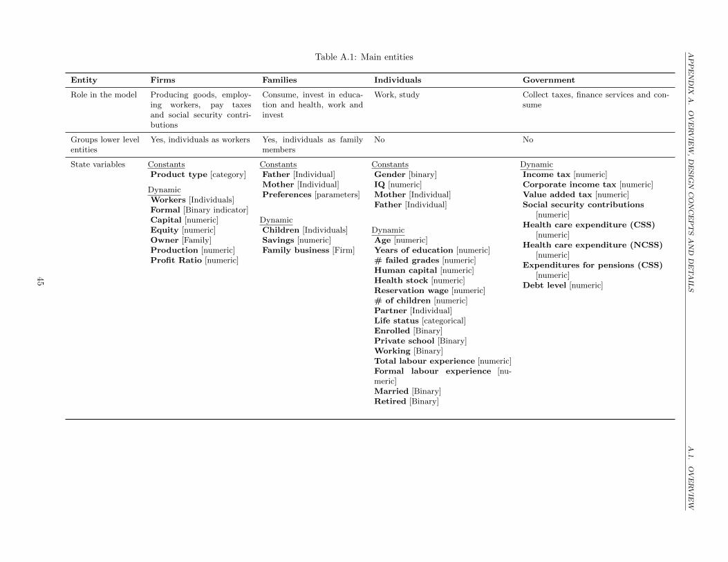
APPENDIX
A.
OVERVIE
W,DESIG
NCONCEPTSAND
DETAIL
SA.1.
OVERVIE
W
Table A.1: Main entities
Entity Firms Families Individuals Government
Role in the model Producing goods, employ-ing workers, pay taxesand social security contri-butions
Consume, invest in educa-tion and health, work andinvest
Work, study Collect taxes, finance services and con-sume
Groups lower levelentities
Yes, individuals as workers Yes, individuals as familymembers
No No
State variables ConstantsProduct type [category]
DynamicWorkers [Individuals]Formal [Binary indicator]Capital [numeric]Equity [numeric]Owner [Family]Production [numeric]Profit Ratio [numeric]
ConstantsFather [Individual]Mother [Individual]Preferences [parameters]
DynamicChildren [Individuals]Savings [numeric]Family business [Firm]
ConstantsGender [binary]IQ [numeric]Mother [Individual]Father [Individual]
DynamicAge [numeric]Years of education [numeric]# failed grades [numeric]Human capital [numeric]Health stock [numeric]Reservation wage [numeric]# of children [numeric]Partner [Individual]Life status [categorical]Enrolled [Binary]Private school [Binary]Working [Binary]Total labour experience [numeric]Formal labour experience [nu-meric]Married [Binary]Retired [Binary]
DynamicIncome tax [numeric]Corporate income tax [numeric]Value added tax [numeric]Social security contributions
[numeric]Health care expenditure (CSS)
[numeric]Health care expenditure (NCSS)
[numeric]Expenditures for pensions (CSS)
[numeric]Debt level [numeric]
45
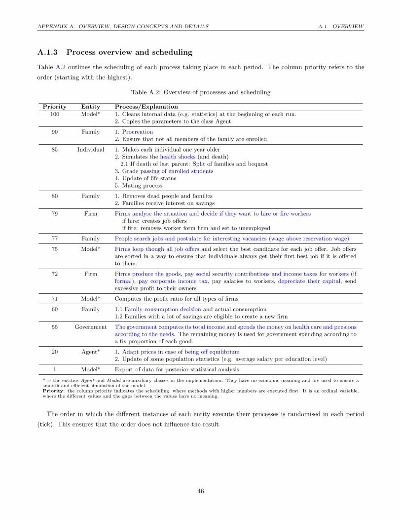
APPENDIX A. OVERVIEW, DESIGN CONCEPTS AND DETAILS A.1. OVERVIEW
A.1.3 Process overview and scheduling
Table A.2 outlines the scheduling of each process taking place in each period. The column priority refers to the
order (starting with the highest).
Table A.2: Overview of processes and scheduling
Priority Entity Process/Explanation
100 Model* 1. Cleans internal data (e.g. statistics) at the beginning of each run.2. Copies the parameters to the class Agent.
90 Family 1. Procreation2. Ensure that not all members of the family are enrolled
85 Individual 1. Makes each individual one year older2. Simulates the health shocks (and death)
2.1 If death of last parent: Split of families and bequest3. Grade passing of enrolled students4. Update of life status5. Mating process
80 Family 1. Removes dead people and families2. Families receive interest on savings
79 Firm Firms analyse the situation and decide if they want to hire or fire workersif hire: creates job offersif fire: removes worker form firm and set to unemployed
77 Family People search jobs and postulate for interesting vacancies (wage above reservation wage)
75 Model* Firms loop though all job offers and select the best candidate for each job offer. Job offersare sorted in a way to ensure that individuals always get their first best job if it is offeredto them.
72 Firm Firms produce the goods, pay social security contributions and income taxes for workers (ifformal), pay corporate income tax, pay salaries to workers, depreciate their capital, sendexcessive profit to their owners
71 Model* Computes the profit ratio for all types of firms
60 Family 1.1 Family consumption decision and actual consumption1.2 Families with a lot of savings are eligible to create a new firm
55 Government The government computes its total income and spends the money on health care and pensionsaccording to the needs. The remaining money is used for government spending according toa fix proportion of each good.
20 Agent* 1. Adapt prices in case of being off equilibrium2. Update of some population statistics (e.g. average salary per education level)
1 Model* Export of data for posterior statistical analysis
* = the entities Agent and Model are auxiliary classes in the implementation. They have no economic meaning and are used to ensure asmooth and efficient simulation of the model.Priority: the column priority indicates the scheduling, where methods with higher numbers are executed first. It is an ordinal variable,where the different values and the gaps between the values have no meaning.
The order in which the different instances of each entity execute their processes is randomised in each period
(tick). This ensures that the order does not influence the result.
46
APPENDIX A. OVERVIEW, DESIGN CONCEPTS AND DETAILS A.2. DESIGN CONCEPTS
A.2 Design Concepts
A.2.1 Basic principles
Families and firms are the key actors in this model, as they take important decisions in each period.
Families use a utility function to decide how much to consume, how much to invest in health, how much to
invest in education and how much money to save to the next period. This optimisation process is influenced by
the economic situation, for instance by the expected future income by education level. Furthermore, the family
indirectly decides on the labour market participation of the children by not letting them to continue at school for
instance. The schooling decision is a direct result of the optimisation process. Once children are out of school, they
aim at incorporating in the labour market, thus there is not voluntary inactivity in this model.
Firms aim at maximising their profits by adjusting their production in terms of capital, labour and inputs.
Depending on the product the firm produces, the marginal utility of the different types of labour is different. We
assume that firms are price takers.
A.2.2 Emergence
In this model, most results emerge from the various interactions between the different players. Only a few results
are directly imposed by the modelling approach. The most important results emerging from the model are:
� distribution of education
� income distribution
� age distribution and the health status of the population
� families (as a result partner search and procreation)
� distribution of firms and their respective production
� wage structure in the economy
� formality of firms
In contrast, a few results are imposed by static processes:
� intergenerational IQ correlation
� spousal correlations in terms of education and IQ
� relationship between maternal education and IQ and the number of children
A.2.3 Adaptation
Families adapt their consumption and investment (in health and education) to their current economic situation and
the education investment to the current economic environment (expected returns to education).
Firms adapt their productive structure to the price structure in the economy and the availability of labour.
The prices of the goods are adapted in case the demand and the supply are substantially different from each other.
This is simply implemented to have a reasonable relationship between supply and demand. The small open economy
assumption does not require supply to be equal to demand.
47

APPENDIX A. OVERVIEW, DESIGN CONCEPTS AND DETAILS A.2. DESIGN CONCEPTS
A.2.4 Objectives
The objective of firms is to maximise their profit, while the objective of families is to maximise the family utility
function. Individuals have no objectives apart from the family level objectives.
A.2.5 Learning
Firms can only observe generally observable characteristics of potential workers (e.g. years of education, experience),
but not their actual level of human capital. Once the worker is employed, the firm has a better understanding of
the human capital.
Families do not directly observe the ability level of their children but can indirectly learn about it by observing
the number of times a student failed to pass a grade.
A.2.6 Prediction
Families and firms do not predict the future over several periods. Instead, they take the current values as a good
estimation of the future periods. In this sense, education decisions are affected by the average wage by education.
Families also predict their income in the next period based on their decisions today (e.g. whether or not the children
continue at school) and taking the income level of the current period as an estimate for the next period.
Firms optimise their productive structure based on the current price level.
A.2.7 Sensing
Families know the health status of each family member and learn about the ability level of children through the
number of failed grades. Firms learn about the actual human capital of workers (as opposed to the generally
observed level of years of education.
A.2.8 Interaction
The only direct interactions between agents take place in the labour market and the marriage market. Both
processes are similar in the sense that agents try to find the best match for their purpose.
In addition to these direct interactions, many indirect interactions through the economy take place. For instance,
families take economy-wide indicators (e.g. wage level per education) into consideration when they decide on the
enrolment of children. These economy-wide values are of course the results of all the interactions in the model.
A.2.9 Stochasticity
The model has a series of stochastic elements. Upon initialisation, the initial population is randomly drawn from a
larger population stemming from the Mexican Family Life Survey. The randomisation is carried out at the family
level in order not to manipulate the actual family structures.
During the simulation, several processes have stochastic elements. In most cases the probabilities depend on
deterministic processes, but the actual choice then takes place using a stochastic process.
Procreation In each period a couple will procreate with a certain probability. This probability
is based on the age and education of the woman.
48

APPENDIX A. OVERVIEW, DESIGN CONCEPTS AND DETAILS A.3. DETAILS
Health shocks In each period, individual face a risks of a health shock. The probability and the
intensity of the shock are stochastic, but depend on the age and previous health
stock of the individual.
Human capital accu-
mulation
For enrolled students the human capital accumulation depends on their IQ, their
health status and a stochastic element.
Mating process The partner mating process is based on a probability of mating with other indi-
viduals that depend on the differences in terms of education and IQ of the two
individuals. The actual partner is then chosen stochastically among all candi-
dates with a positive probability
Labour market Potential workers cannot see all job offers in the market. The probability of seeing
a particular job offer depends on their current labour status, their network and
their type of education (public vs. private).
All stochastic elements can be steered through a unique random seed, allowing us to reproduce the exact same
simulation multiple times and to base any type of policy analysis on the exact same random elements.
A.2.10 Collectives
We have two explicit collectives: firms and families.
Families naturally regroup all family members. Social ties are kept even when children leave their original family
(e.g. for bequests). On the other hand, individuals that are working are regrouped in firms.
A.2.11 Observation
In each period various datasets are exported in a generic text format. These datasets include model-wide statistics
such as income inequality, intergenerational correlations, but also instance-level data on firms, families, individuals
and the government.
In batch simulations (multiple simultaneous simulations) independent datasets for each simulation are exported.
These datasets can then be combined and the different parameter sets can be identified for the policy analysis.
A.3 Details
A.3.1 Initialisation
The simulation is initialised based on actual data from Mexico. We use the Mexican Family Life Survey (MxFLS)
2002 to generate a dataset of 27’455 individuals from 7’020 families. For each family member we have information
on their cognitive ability (an approximation of their IQ), their current education level in years of education, their
role in the family (father, mother, child), their gender, age and for enrolled children the type of school they are
attending (private vs. public).
Unfortunately the Mexican Family Life Survey does not allow us to get usable information on their financial
situation. We therefore randomly draw the initial savings of the families and define families with a certain level of
savings and at least one member with secondary education or more as eligible for having a family business. These
49
APPENDIX A. OVERVIEW, DESIGN CONCEPTS AND DETAILS A.3. DETAILS
firms are then randomly assigned to all eligible families. Workers are allocated randomly to firms according to their
education level.
Apart from the generation of our population, we set some initial values that are needed in the economy. For
instance, the initial prices of the goods were selected based on preliminary results where the prices converged to
certain levels. We took these levels to initialise the model.
The salary paid by education level was estimated using the Mexican Labour Force Survey and we then converted
all to multiples of the annual minimum salary (the monetary unit we use in the model).
The tuition fees for schooling were estimated from various sources of information and we always use the same
values in all simulation in order not to manipulate the outcomes.
Finally, all simulations are always initiated with the actual rates (taxes, social security, etc.) observed in Mexico.
When we simulate policy changes, we always simulate the baseline model for 25 period before starting with the
policy changes.
A.3.2 Input
We do not use inputs during the simulation.
A.3.3 Sub-models
In this last section of the ODD-protocol we present the sub-models. In other words, we describe the various processes
included in this model. We organise this section by type of agent. This ordering is in some cases not very simple
due to the strong interactions between agents.
A.3.3.1 Firms, production and labour market
A.3.3.1.1 Product and firm space
Our model is based on a four-sector economy with both formal and informal and small and big firms. Figure A.1
displays both the firm and the product space of our economy.
In the firm space we have small self-employed individuals which are always informal. For larger firms we then
have a continuum from small to large firms, where the actual firm size is endogenous to the optimisation of the
firms. These firms can be either informal (typically the smaller ones) or formal. The choice between informal and
formal will be made endogenously by the firms and can change over time (e.g. an informal firm becomes formal).
In the product space we have exactly four types of products, similar to the product space in Anton et al. (2012).
The basic product refers to very simple services and products that need no or very limited capital (e.g. taco stand).
The two intermediate products already require some capital for the production and the only difference among them
is that one is subject to VAT while the other is not1. Finally, we have a high-tech product, which can only be
produced by relatively large formal firms!
It is important to mention that the firm size is endogenous and emerges from the optimisation of firms. We do
not impose any size restrictions.
1This is a feature of the current Mexican tax system, where a series of not very sophisticated products is taxed at a reduced VATrate. This reduced rate is currently set to zero.
50
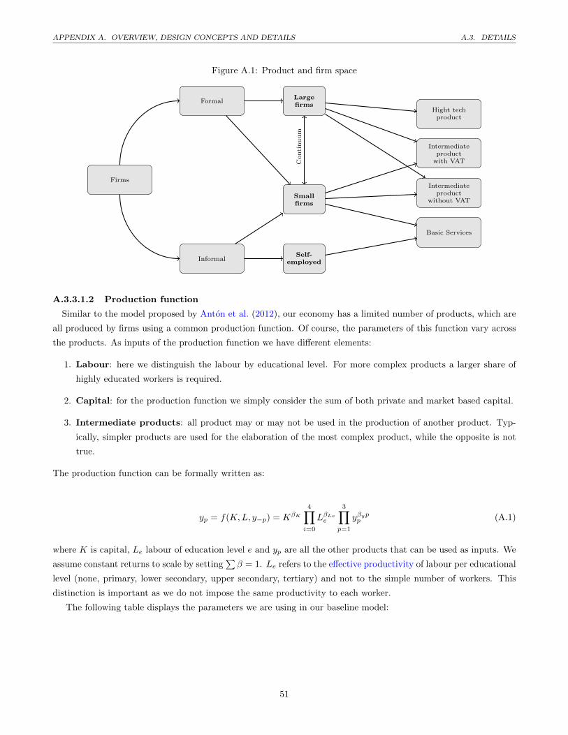
APPENDIX A. OVERVIEW, DESIGN CONCEPTS AND DETAILS A.3. DETAILS
Figure A.1: Product and firm space
Largefirms
Smallfirms
Self-employed
Firms
Formal
Informal
Hight techproduct
Intermediateproduct
with VAT
Intermediateproduct
without VAT
Basic Services
Conti
nuum
A.3.3.1.2 Production function
Similar to the model proposed by Anton et al. (2012), our economy has a limited number of products, which are
all produced by firms using a common production function. Of course, the parameters of this function vary across
the products. As inputs of the production function we have different elements:
1. Labour: here we distinguish the labour by educational level. For more complex products a larger share of
highly educated workers is required.
2. Capital: for the production function we simply consider the sum of both private and market based capital.
3. Intermediate products: all product may or may not be used in the production of another product. Typ-
ically, simpler products are used for the elaboration of the most complex product, while the opposite is not
true.
The production function can be formally written as:
yp = f(K,L, y−p) = KβK
4∏i=0
LβLee
3∏p=1
yβypp (A.1)
where K is capital, Le labour of education level e and yp are all the other products that can be used as inputs. We
assume constant returns to scale by setting∑β = 1. Le refers to the effective productivity of labour per educational
level (none, primary, lower secondary, upper secondary, tertiary) and not to the simple number of workers. This
distinction is important as we do not impose the same productivity to each worker.
The following table displays the parameters we are using in our baseline model:
51
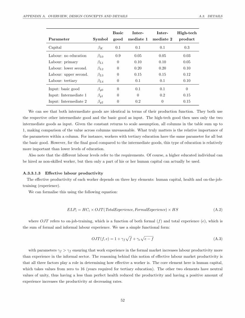
APPENDIX A. OVERVIEW, DESIGN CONCEPTS AND DETAILS A.3. DETAILS
Basic Inter- Inter- High-tech
Parameter Symbol good mediate 1 mediate 2 product
Capital βK 0.1 0.1 0.1 0.3
Labour: no education βL0 0.9 0.05 0.05 0.03
Labour: primary βL1 0 0.10 0.10 0.05
Labour: lower second. βL2 0 0.20 0.20 0.10
Labour: upper second. βL3 0 0.15 0.15 0.12
Labour: tertiary βL4 0 0.1 0.1 0.10
Input: basic good βy0 0 0.1 0.1 0
Input: Intermediate 1 βy1 0 0 0.2 0.15
Input: Intermediate 2 βy2 0 0.2 0 0.15
We can see that both intermediate goods are identical in terms of their production function. They both use
the respective other intermediate good and the basic good as input. The high-tech good then uses only the two
intermediate goods as input. Given the constant returns to scale assumption, all columns in the table sum up to
1, making comparison of the value across columns unreasonable. What truly matters is the relative importance of
the parameters within a column. For instance, workers with tertiary education have the same parameter for all but
the basic good. However, for the final good compared to the intermediate goods, this type of education is relatively
more important than lower levels of education.
Also note that the different labour levels refer to the requirements. Of course, a higher educated individual can
be hired as non-skilled worker, but then only a part of his or her human capital can actually be used.
A.3.3.1.3 Effective labour productivity
The effective productivity of each worker depends on three key elements: human capital, health and on-the-job-
training (experience).
We can formalise this using the following equation:
ELPi = HCi ×OJT (TotalExperience,FormalExperience)×HS (A.2)
where OJT refers to on-job-training, which is a function of both formal (f) and total experience (e), which is
the sum of formal and informal labour experience. We use a simple functional form:
OJT (f, e) = 1 + γf√f + γe
√e− f (A.3)
with parameters γf > γf ensuring that work experience in the formal market increases labour productivity more
than experience in the informal sector. The reasoning behind this notion of effective labour market productivity is
that all three factors play a role in determining how effective a worker is. The core element here is human capital,
which takes values from zero to 16 (years required for tertiary education). The other two elements have neutral
values of unity, thus having a less than perfect health reduced the productivity and having a positive amount of
experience increases the productivity at decreasing rates.
52
APPENDIX A. OVERVIEW, DESIGN CONCEPTS AND DETAILS A.3. DETAILS
A.3.3.1.4 Profit maximisation
A key decision for firms is to have the best possible combination of labour (L), capital (K) and intermediate
products (ypt) in their production function in order to maximise their profits. In our model, the information set firms
can use to decide is limited to their own experience (e.g. no strategic behaviour on expected moves of competitors).
In each period, informal firms also evaluate if it would be beneficial to become formal. For these calculations,
firms consider the market values of the current period as their best guess for the future periods. First, firms compute
the optimal production for different labour force structures
ypt = fp(Kt, Lt, y−p) (A.4)
Technically this optimisation is implemented in a two step procedure. We loop over different possibilities to hire
and fire workers and for each given case we compute the conditionally optimal levels of K and y−p. Each of these
production levels are then multiplied by the price of the product to get the gross income and the profit is computed
using the following equation:
Π =
(1− πCIT )
(yptppt
1 + πV AT− cf (Kt, Lt, ypt)
)if formal
yptppt − ci(Kt, Lt, ypt)− E[Θ] if informal
(A.5)
whereE[Θ] is the expected amount of fine in case the government catches the informal firm:
E[Θ] =∑
w × θp × θm
with∑w being the sum of all wages paid by the firm (e.g. firm size), θp the probability of
getting caught and a parameter for the size of the fine θm. We include the sum of wages to
capture a higher risk for larger firms.
ci(.) and cf (.) are the cost functions for informal and formal firms respectively. They differ in several
ways according to the formality status. Informal firms do not pay the contributory social
security and do not deduce the income tax of their workers. In contrast, formal firms can buy
input goods without paying the value-added tax (they get refunded), but pay the previously
mentioned contributions and taxes.
πCIT is the corporate income tax rate, which if only relevant for formal firms
In section A.3.3.4.2 we provide a detailed discussion on the actual tax schemes in Mexico and how we implement
it in the model. This also includes a discussion on the social security contributions.
Note that firms cannot adjust completely, because at least a part of the capital cannot be destroyed from one
period to the next. We therefore include parameter δcapital capturing how much a firm can reduce the capital stock
from one period to the next. Furthermore, we distinguish equity from market capital. Equity is the capital the
owner family has invested in the firm, while market capital a loans from the financial market. We use a parameter
δleverage to limit the market capital vs. equity ratio. Whenever the firm’s optimal choice is to reduce the capital, it
first reduces the market capital. If this is not possible, the firm reduces equity by sending the excessive money to
the owner. In an equilibrium condition where the optimal capital remains stable, the owner will receive the benefits
53
APPENDIX A. OVERVIEW, DESIGN CONCEPTS AND DETAILS A.3. DETAILS
of the firm in each period.
A.3.3.1.5 Labour market
The labour market is organised in three steps:
1. Firms analyse their current situation and create one or multiple job offers if this increases their expected
benefit for the next period. A job offer consists of a minimum education level and a wage offer. In case firing
workers is beneficial in terms of expected benefit, firms immediately remove the worker from the labour force.
2. Individuals see these job offers with a certain probability and apply if and only if they qualify for the job and
if the offered wage is above their reservation wage.
3. The firm chooses the best candidate among all applicants.
We now explain each of the steps individually.
Step 1 - Firms create job offers
First, firms optimise their labour stucture according to the profit maximisation described in section A.3.3.1.4.
Depending on the result of the optimisation process, the firm dismisses current workers and/or opens a new job
vacancy. At this stage it is important to mention that firms optimise assuming they find an average worker with
the profile they search for. However, firms cannot observe all characteristics of workers and might not find exactly
what they were looking for. Job vacancies are translated into job offers that include information on the minimum
education level and the offered wage. For simplicity, we assume that within a firm workers with the same education
level all earn the same salary. Hence, the proposed salary is simply the salary that is already being paid to other
workers in the firm.
Step 2 - Job seekers apply to interesting jobs (labour supply)
Each job seeker received a given job offer with a certain probability p. This probability varies across individuals
and depends essentially on:
� Labour status: unemployed job seekers have a higher probability than currently employed job seekers (argu-
ment: they have more time to search).
� People with better networks have higher probabilities of receiving the job offer. These networks can be private
(family members working in the same firm), professional (offers of similar firms have higher probabilities) or
educational (graduates of private schools might have higher probabilities).
Hence, the final probability of seeing a job offer depends on all these elements.
p = pbase + punemployment + pnetwork + pprivateSchool (A.6)
Individuals will then apply to all job offers for which they qualify (education weakly above the requested level)
and where their reservation wage (wi) is below the offered wage. The reservation wage is defined as:
wi = max (windependent, µw × E[w|educi]) (A.7)
54
APPENDIX A. OVERVIEW, DESIGN CONCEPTS AND DETAILS A.3. DETAILS
which is essentially what the individual could earn as independent and a fraction of the average wage given the
education level. The parameter µw captures how tolerant an individual is to offers below the current average of
individuals with the same level of education.
Step 3 - Firms choose the best candidate
The final step in the job market is when firms choose among all the candidates. In case of having zero candidates,
the vacancy remains and nobody is hired. Whenever there is a positive number of applicants, the firm chooses the
best candidate according to the following list of priorities:
1. The candidate with the highest level of education
2. if there is a draw: candidate with the largest experience in the formal sector
3. if there is still a draw: candidate with the largest total experience
4. if there is still a draw: candidate with more diploma from private schools
5. if there is still a draw: random
Note that before looping through all firms, we order the job offers starting with the highest offered wage. This
ensures that candidates will always get their first best option (if the firm is interested) and do not have to accept
the first they receive. In case the firm is unable to find a worker for a given position, it increases the salaries of the
concerned education level by 5% for the next period.
A.3.3.1.6 Capital depreciation
Every year (period), the capital of the firm is depreciated by a depreciation factor of δd. Given that the market
capital is what the firm owes the lenders, the depreciation is accounted for on the equity side only. For instance, a
firm with 20 units of equity and 80 units of debt, will have a depreciation of 5 units. Hence, after depreciation, the
equity become 15 units.
A.3.3.2 Financial market
The financial market is implemented in the simplest possible way. We use exogenously set interest rates for both
loans to firms and on savings by families.
A.3.3.3 Family related processes
A.3.3.3.1 Optimisation of allocation of resources
Families optimise behaviour by choosing among current consumption, investment in health and education and
saving money for the next period. There is no possibility to borrow money. The decision is governed by a rather
traditional utility maximising approach based on the strand of literature initiated by Becker (1973). However, due
to the time unit of one year, the decision making process has to be slightly adapted.
Let us define the general utility function as:
U(ct, Ht, E[yc], E[mt+1]) (A.8)
Where:
55
APPENDIX A. OVERVIEW, DESIGN CONCEPTS AND DETAILS A.3. DETAILS
ct is the per capita expenditure for current consumption in period t. This consumption is
further divided into the consumption of the four goods that are produced in the economy.
We will explain the details hereafter.
Ht is the average health stock of all family members. The idea here is that people directly care
about the health status of the family members and therefore aim at maximising this value.
In case all members of the family are in perfect health (Hit = 1), no spending for health
care is required.
E[yc] is the average expected future incomes of the children. This values can be manipulated by
family through investment in education.
E[mt+1] is the expected future disposable income in period t + 1. Here the idea is that instead of
a life-time maximisation, people simply care about what they will have one period ahead.
In our view, this approach does comply with the basic ideas of the traditional economic
models while not relying on the rather unrealistic idea that people plan ahead over the
whole lifespan.
In this version of the study, we use a traditional Cobb-Douglas function:
U(ct, Ht, E[yc], E[mt+1]) = cαct ×H
αht × E[yc]
αy × E[mt+1]αm (A.9)
This functional form allows us to easily decompose the element of current consumption:
cαct =
(3∏p=0
cαcp
pt
)αc
with
3∑p=0
αcp = 1 (A.10)
As a result, we can interpret ct as a measure of expenditure in consumption good. The exact consumption of
the four goods is then governed by the parameters αcp.
Note that we also include a parameter governing the ability of a family to reduce consumption from one period to
the next. It is unreasonable to assume that a family can reduce the consumption by a very large amount. Therefore,
we assume that family tolerate only a loss of τexp and in case of having less disposable income, the family starts
dropping children in out of private schools or even completely out of school and ask them to work as independent.
Numerical optimisation in the ABM model
Similar to the optimisation of the profit function for firms, we solve this optimisation problem partially analitically
and partially numerically. First, we use all the properties of the Cobb-Douglas function to express one optimal
value in function of another optimal value. We then loop over all possible combinations of discrete choices (school
enrollment) and optimise numerically using a Java implementation of the Constrained Optimization BY Linear
Approximation2. Thanks to the loop of discrete choices and the properties of the Cobb-Douglas function, this
numerical optimisation is one-dimensional. This greatly reduces the computation.
A.3.3.3.2 Families starting a business
Whenever family have savings exceeding a certain threshold δbusiness, they are eligible to start a new business
with a certain probability. The process is implemented in a very simple way by looking at the average profit ratios
2The code of this optimisation is available at: https://github.com/cureos/jcobyla
56
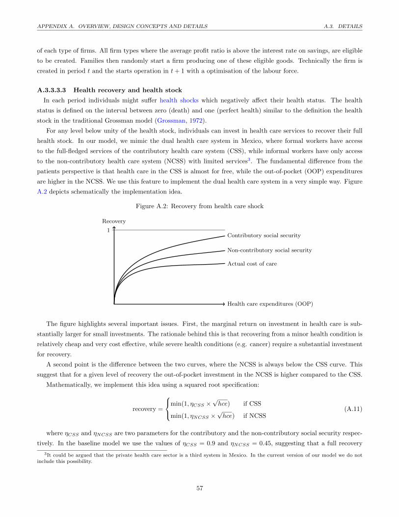
APPENDIX A. OVERVIEW, DESIGN CONCEPTS AND DETAILS A.3. DETAILS
of each type of firms. All firm types where the average profit ratio is above the interest rate on savings, are eligible
to be created. Families then randomly start a firm producing one of these eligible goods. Technically the firm is
created in period t and the starts operation in t+ 1 with a optimisation of the labour force.
A.3.3.3.3 Health recovery and health stock
In each period individuals might suffer health shocks which negatively affect their health status. The health
status is defined on the interval between zero (death) and one (perfect health) similar to the definition the health
stock in the traditional Grossman model (Grossman, 1972).
For any level below unity of the health stock, individuals can invest in health care services to recover their full
health stock. In our model, we mimic the dual health care system in Mexico, where formal workers have access
to the full-fledged services of the contributory health care system (CSS), while informal workers have only access
to the non-contributory health care system (NCSS) with limited services3. The fundamental difference from the
patients perspective is that health care in the CSS is almost for free, while the out-of-pocket (OOP) expenditures
are higher in the NCSS. We use this feature to implement the dual health care system in a very simple way. Figure
A.2 depicts schematically the implementation idea.
Figure A.2: Recovery from health care shock
Recovery
Health care expenditures (OOP)
1Contributory social security
Non-contributory social security
Actual cost of care
The figure highlights several important issues. First, the marginal return on investment in health care is sub-
stantially larger for small investments. The rationale behind this is that recovering from a minor health condition is
relatively cheap and very cost effective, while severe health conditions (e.g. cancer) require a substantial investment
for recovery.
A second point is the difference between the two curves, where the NCSS is always below the CSS curve. This
suggest that for a given level of recovery the out-of-pocket investment in the NCSS is higher compared to the CSS.
Mathematically, we implement this idea using a squared root specification:
recovery =
min(1, ηCSS ×√hce) if CSS
min(1, ηNCSS ×√hce) if NCSS
(A.11)
where ηCSS and ηNCSS are two parameters for the contributory and the non-contributory social security respec-
tively. In the baseline model we use the values of ηCSS = 0.9 and ηNCSS = 0.45, suggesting that a full recovery
3It could be argued that the private health care sector is a third system in Mexico. In the current version of our model we do notinclude this possibility.
57

APPENDIX A. OVERVIEW, DESIGN CONCEPTS AND DETAILS A.3. DETAILS
requires roughly 1.23 annual minimum salaries in the CSS and slightly below 5 annual minimum salaries in the
NCSS.
Finally, we also assume the total cost of care to have a similar functional form. The curve of the actual cost lies
below the out-of-pocket expenditure curves. For a given level of recovery, the horizontal difference between the lines
refers to the cost for the social security system. We assume that the cost of producing a certain level of recovery is
the same in both systems and the only difference is the share of out-of-pocket expenditure.
A.3.3.3.4 Bequest and dissolution of family
A family is conformed with parents and an endogenous number of sons and daughters. When both parents die,
the family is split into single individual families (i.e. each child becomes a new family). Moreover, each of them
receive a bequest, which is equal to a part of savings and equity of the former family. While savings can easily be
split, equity refers to the investment in the family company and can therefore not be split in our model.
In our model, only one child will inherit the family’s company, this assignation is random. This assumption
could yield unequal inheritance for children (e.g. some son receive more (or less) valuable bequests only because
they could not split the company symmetric parts). In order to ensure equality in the process, we use the following
logic:
1. We sum savings and equity together and divide it by the number of children. We then have two scenarios:
2.a If equity is less or equal to the share of each child, we randomly select one child who gets the business plus
any cash from savings to achieve the equal share.
2.b If equity exceeds the equal share, the firm sells equity (e.g. replaces equity by external investment in the firm)
until the equity of the firm equals the equal share. The money obtained from selling equity will be distributed
among the siblings not receiving the business.
A.3.3.3.5 Passing a grade at school
Human capital accumulation is a cumulative process during which each school year adds some human capital to
the already acquired human capital stock. We use this general idea to implement the human capital accumulation
process in our model.
We define 1 unit of HC as being the equivalent of 1 year of perfect (best possible quality) schooling. Hence, we
have by definition
human capital (HCi) ≤ years of schoolingi (A.12)
HC ≤ yearsofschooling by definition.
In each period while being at school, children add a certain level of human capital to their previously acquired
level of human capital:
The process of passing a grade is simulated in various steps:
HCit = HCi,t−1 + min(1,IQ
100∗HSit + εit) (A.13)
58

APPENDIX A. OVERVIEW, DESIGN CONCEPTS AND DETAILS A.3. DETAILS
where IQ refers to the cognitive ability measure and HSit is the health stock of the individual. Therefore, the
expected additional human capital of an average child (IQ=100) in perfect health is equal to unity. The element
εit is a stochastic process which captures some heterogeneity in the human capital accumulation process.
Similar to what happens in the real world, student progress to the next grade only if they pass a certain
threshold. We define this threshold as a fraction of the years of schooling. For instance, to pass the fourth grade,
the accumulated human capital must be at least δ× 4, where we typically have δ ≤ 1. This yields a simple passing
rule:
HCit
≥ δ × g passes grade g
< δ × g has to repeat grade g(A.14)
This implementation is interesting for a number of reasons:
� The human capital accumulation process is cumulative, thus a low accumulation in the past (e.g. due to a
low health stock) will have long lasting effects.
� the requirements to pass grades can change from one level of schooling to another (e.g. δprimary < δsecondary).
The consequence of this would be that children who just passed primary on the threshold, will have a hard
time passing the first grade of the next school level. In the baseline model we use respectively 0.8, 0.85, 0.90
and 0.95 for primary, lower secondary, upper secondary and tertiary education.
In case of not passing the grade, we do not add the full level of human capital to capture the fact that repeating
the grade does not increase knowledge in the same way as continuing with the next grade. In contrast, adding a
part of the acquired human capital rather than nothing captures the fact that even if students did not pass the
grade, they have learned something and the likelihood to pass the grade one year later is substantially higher.
A.3.3.3.6 Mating process - assortative mating
The mating process in our model takes place in three majors steps: selection of candidates, computation of
probabilities and actual selection of partner.
Step 1: Selection of eligible candidates
In a first step, eligible individuals start searching all eligible candidates. Eligibility is based on four criteria:
1. the searcher and the possible candidates are not currently enrolled at school
2. both have currently no partner
3. both are weakly older than the minimum mating age (δminAge = 15)
4. the potential partner must be of the opposite sex
Step 2: compute the mating probability
For all possible candidates the mating probability is computed. This is the crucial step to achieve a certain degree
of assortative mating. We assume the following form:
Pij = max
(0 , 1−
∆IQij
30−
∆educij
6
)(A.15)
59
APPENDIX A. OVERVIEW, DESIGN CONCEPTS AND DETAILS A.3. DETAILS
where ∆IQij = |IQi − IQj | and ∆educ
ij = |eudci − educj | are the absolute values of the difference between the two
individuals in terms of IQ and education.
Note that the probability is equal to zero whenever the IQ-difference exceeds 30 points or the education difference
exceeds 6 years. This implementation is an improved version of the implementation proposed by Chavez-Juarez
(2015). In this version individuals that are more alike have a higher mating probability.
Step 3: Compute overall probability
Before drawing the stochastic element, we then normalise these probabilities by dividing all of them by the sum of
all probabilities and by multiplying by the overall probability of mating.
pnij =Pij∑j Pij
× pmating (A.16)
we then draw a random number from a uniform distribution and select the corresponding partner. Note that
with probability 1− pmating no match takes place. In this case, individual i will start again searching a partner in
the next period.
In case of a positive match, the two individuals leave their family and create a new family.
A.3.3.4 Government related processes
A.3.3.4.1 Government behaviour
The government has a rather simple behaviour, but the different elements are crucial for the model. First, the
government sums up all the incomes from the social security contributions, the value-added tax and the income
taxes and deduces the debt from the last period if there was any. This gives us the total disposable money of
the government. We then deduce the pensions paid to retired workers of the contributory social security system,
assuming 60% of the last salary as a pension payment. We then deduce the cost of health care according to both
systems.
If after these deductions a positive amount of money remains, the government will consume goods and services.
We assume that the government mainly spends on intermediate (20% each) and high-tech (45%) products and only
15% of the spending goes to the basic good. These proportions do not seem to be of much importance for the
stability of the model.
In order to ensure a certain degree of stability, we assume that the government spending cannot be reduced
by more than 30% from one period to the next. Hence, if the government does not have a sufficient amount of
money to spend at least 70% of the last years spending, it has to borrow money. This mechanism is of course very
simplistic, but when we simulate the model is happens only rarely and the results do not depend on it.
A.3.3.4.2 Tax schemes and contributory social security scheme The different tax schemes are directly
inspired and where possible copied from the actual Mexican tax system.
Social security contributions
In reality, the social security contributions are based on a rather complex computation with various categories of
contributions (by concepts). We opted for a simplification of the process that will capture the important elements of
the true system without adding unnecessary complexity to the model. This simplification is particularly important
because our policy simulations will target these contributions and therefore it is important to limit the complexity
60
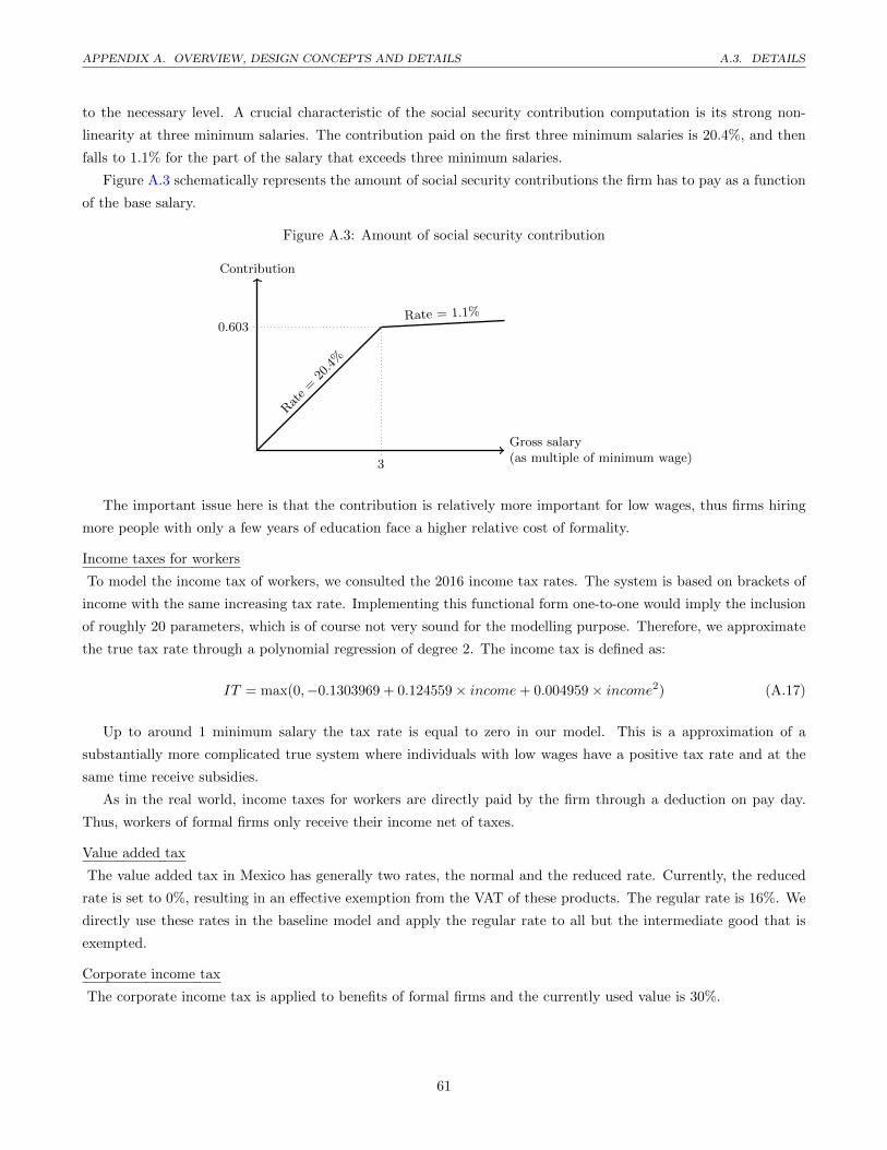
APPENDIX A. OVERVIEW, DESIGN CONCEPTS AND DETAILS A.3. DETAILS
to the necessary level. A crucial characteristic of the social security contribution computation is its strong non-
linearity at three minimum salaries. The contribution paid on the first three minimum salaries is 20.4%, and then
falls to 1.1% for the part of the salary that exceeds three minimum salaries.
Figure A.3 schematically represents the amount of social security contributions the firm has to pay as a function
of the base salary.
Figure A.3: Amount of social security contribution
Contribution
Gross salary(as multiple of minimum wage)
0.603
3
Rat
e=
20.4%
Rate = 1.1%
The important issue here is that the contribution is relatively more important for low wages, thus firms hiring
more people with only a few years of education face a higher relative cost of formality.
Income taxes for workers
To model the income tax of workers, we consulted the 2016 income tax rates. The system is based on brackets of
income with the same increasing tax rate. Implementing this functional form one-to-one would imply the inclusion
of roughly 20 parameters, which is of course not very sound for the modelling purpose. Therefore, we approximate
the true tax rate through a polynomial regression of degree 2. The income tax is defined as:
IT = max(0,−0.1303969 + 0.124559× income+ 0.004959× income2) (A.17)
Up to around 1 minimum salary the tax rate is equal to zero in our model. This is a approximation of a
substantially more complicated true system where individuals with low wages have a positive tax rate and at the
same time receive subsidies.
As in the real world, income taxes for workers are directly paid by the firm through a deduction on pay day.
Thus, workers of formal firms only receive their income net of taxes.
Value added tax
The value added tax in Mexico has generally two rates, the normal and the reduced rate. Currently, the reduced
rate is set to 0%, resulting in an effective exemption from the VAT of these products. The regular rate is 16%. We
directly use these rates in the baseline model and apply the regular rate to all but the intermediate good that is
exempted.
Corporate income tax
The corporate income tax is applied to benefits of formal firms and the currently used value is 30%.
61
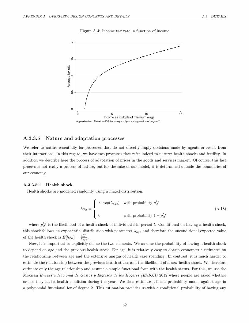
APPENDIX A. OVERVIEW, DESIGN CONCEPTS AND DETAILS A.3. DETAILS
Figure A.4: Income tax rate in function of income
0.0
5.1
.15
.2Av
erag
e ta
x ra
te
0 5 10 15Income as multiple of minimum wage
Approximation of Mexican ISR tax using a polynomial regression of degree 2
A.3.3.5 Nature and adaptation processes
We refer to nature essentially for processes that do not directly imply decisions made by agents or result from
their interactions. In this regard, we have two processes that refer indeed to nature: health shocks and fertility. In
addition we describe here the process of adaptation of prices in the goods and services market. Of course, this last
process is not really a process of nature, but for the sake of our model, it is determined outside the bounderies of
our economy.
A.3.3.5.1 Health shock
Health shocks are modelled randomly using a mixed distribution:
hsit =
∼ exp(λage) with probability phsit
0 with probability 1− phsit
(A.18)
where phsit is the likelihood of a health shock of individual i in period t. Conditional on having a health shock,
this shock follows an exponential distribution with parameter λage and therefore the unconditional expected value
of the health shock is E[hsit] =phsit
λage.
Now, it is important to explicitly define the two elements. We assume the probability of having a health shock
to depend on age and the previous health stock. For age, it is relatively easy to obtain econometric estimates on
the relationship between age and the extensive margin of health care spending. In contrast, it is much harder to
estimate the relationship between the previous health status and the likelihood of a new health shock. We therefore
estimate only the age relationship and assume a simple functional form with the health status. For this, we use the
Mexican Encuesta Nacional de Gastos y Ingresos de los Hogares (ENIGH) 2012 where people are asked whether
or not they had a health condition during the year. We then estimate a linear probability model against age in
a polynomial functional for of degree 2. This estimation provides us with a conditional probability of having any
62
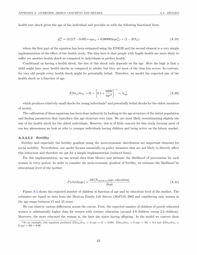
APPENDIX A. OVERVIEW, DESIGN CONCEPTS AND DETAILS A.3. DETAILS
health care shock given the age of the individual and provides us with the following functional form:
phsit = (0.217− 0.002 ∗ ageit + 0.000063age2it) + (1−HSit) (A.19)
where the first part of the equation has been estimated using the ENIGH and the second element is a very simple
implementation of the effect of the health stock. The idea here is that people with fragile health are more likely to
suffer yet another health shock as compared to individuals in perfect health.
Conditional on having a health shock, the size of this shock only depends on the age. Here the logic is that a
child might have more health shocks as compared to adults, but they are most of the time less severe. In contrast,
for very old people every health shock might be potentially lethal. Therefore, we model the expected size of the
health shock as a function of age:
E[hsit|hsit > 0] =
[0.1 +
6000
age2
]−1
= λ−1age (A.20)
which produces relatively small shocks for young individuals4 and potentially lethal shocks for the oldest members
of society.
The calibration of these equations has been done indirectly by looking at the age structure of the initial population
and finding parameters that reproduce this age structure over time. We are most likely overestimating slightly the
size of the health shock for the oldest individuals. However, this is of little concern for this study because most of
our key phenomena we look at refer to younger individuals having children and being active on the labour market.
A.3.3.5.2 Fertility
Fertility and especially the fertility gradient along the socio-economic distribution are important elements for
social mobility. Nevertheless, our model focuses essentially on policy measures that are not likely to directly affect
this behaviour and therefore we opt for a simple implementation (reduced form).
For this implementation, we use actual data from Mexico and estimate the likelihood of procreation for each
woman in every period. In order to consider the socio-economic gradient of fertility, we estimate the likelihood by
educational level of the mother.
P (child|age) =∂E[Nchildren|age, education]
∂age(A.21)
Figure A.5 shows the expected number of children in function of age and by education level of the mother. The
estimates are based on data from the Mexican Family Life Survey (MxFLS) 2002 and considering only women in
the age range between 15 and 45 years.
We can observe various differences across the curves. First, the expected number of children of poorly educated
women is substantially higher than for women with tertiary education (around 4.8 children versus 2.2 children).
Moreover, the more educated the woman is, the later she starts having offspring. In the model we convert these
4As an example, this equation produced E[hsit|hsit > 0, age = 5] = 0.004, E[hsit|hsit > 0, age = 50] = 0.4 and E[hsit|hsit >0, age = 80] = 0.96
63
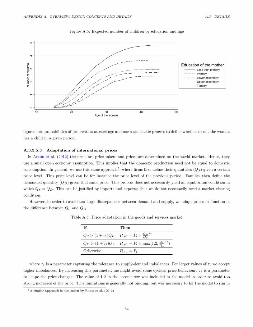
APPENDIX A. OVERVIEW, DESIGN CONCEPTS AND DETAILS A.3. DETAILS
Figure A.5: Expected number of children by education and age0
12
34
5N
umbe
r of c
hild
ren
10 20 30 40 50Age of the woman
Less than primaryPrimaryLower secondaryUpper secondaryTertiary
Education of the mother
figures into probabilities of procreation at each age and use a stochastic process to define whether or not the woman
has a child in a given period.
A.3.3.5.3 Adaptation of international prices
In Anton et al. (2012) the firms are price takers and prices are determined on the world market. Hence, they
use a small open economy assumption. This implies that the domestic production need not be equal to domestic
consumption. In general, we use this same approach5, where firms first define their quantities (QS) given a certain
price level. This price level can be for instance the price level of the previous period. Families then define the
demanded quantity (QD) given that same price. This process does not necessarily yield an equilibrium condition in
which QS = QD. This can be justified by imports and exports; thus we do not necessarily need a market clearing
condition.
However, in order to avoid too large discrepancies between demand and supply, we adapt prices in function of
the difference between QS and QD
Table A.4: Price adaptation in the goods and services market
If Then
QS > (1 + τ1)QD Pt+1 = Pt × QD
QS
τ2
QD > (1 + τ1)QS Pt+1 = Pt ×max(1.2, QD
QS
τ2)
Otherwise Pt+1 = Pt
where τ1 is a parameter capturing the tolerance to supply-demand imbalances. For larger values of τ1 we accept
higher imbalances. By increasing this parameter, me might avoid some cyclical price behaviour. τ2 is a parameter
to shape the price changes. The value of 1.2 in the second row was included in the model in order to avoid too
strong increases of the price. This limitations is generally not binding, but was necessary to for the model to run in
5A similar approach is also taken by Busso et al. (2012)
64
APPENDIX A. OVERVIEW, DESIGN CONCEPTS AND DETAILS A.3. DETAILS
a few situations6. In general, the model results display only very little price changes and we do not expect major
changes in the model results when not allowing prices to change over time.
6Most likely in the current version of the model this condition is no longer necessary, because the problem motivating us to add thiscondition has been solved during the programming process
65

Appendix B
Calibration
An important goal of our approach is to model as close as possible to reality, in this particular case to the Mexican
economy. A crucial element in achieving this goal is the calibration of the model. Calibrating such model is,
however, very complex because many different processes interact. For this first version of the model we used a
mixed approach. Wherever possible, we used Mexican data or the legislation to calibrate parts of the model.
This way of calibration is the first best solution, but unfortunately the data does not allow us to calibrate all
processes in this way. The second best solution is the indirect calibration, where we look at the outcome of the
baseline model and calibrate the model in a way to reproduce the result according to the observed results. For
example, it is impossible to obtain estimates for the severity of health shocks, but we have knowledge about the
age structure of the population. Thus, we calibrate the health shock in a way that the age structure emerging from
the model resembles the actual age structure. Finally, the last calibration method we used is an ad-hoc definition
of some parameters for which we do not have data nor a directly observable result. For all types of calibration, but
especially for the last one, we use sensitivity analyses to see how much the results depend on such ad-hoc values.
Table B.1 provides an overview of the used calibration method for the most important processes in the model.
Table B.1: Calibration methods
Process/value Type of value Calibration strategy
Taxes and contributions
VAT rates Parameters From the Mexican law
Corporate income tax Parameter From the Mexican law
Income tax for natural persons Parameter Parametric approximation of actual tax
scheme
Health
Probability of health shock Parameters Mixed: relationship with age based on data
(ENIGH), while the relationship with previous
health stock was set ad-hoc.
Size of health shock Parameter Indirect based on the resulting age structure
of the population.
Health recovery Parameters Ad-hoc
-continued on next page-
66
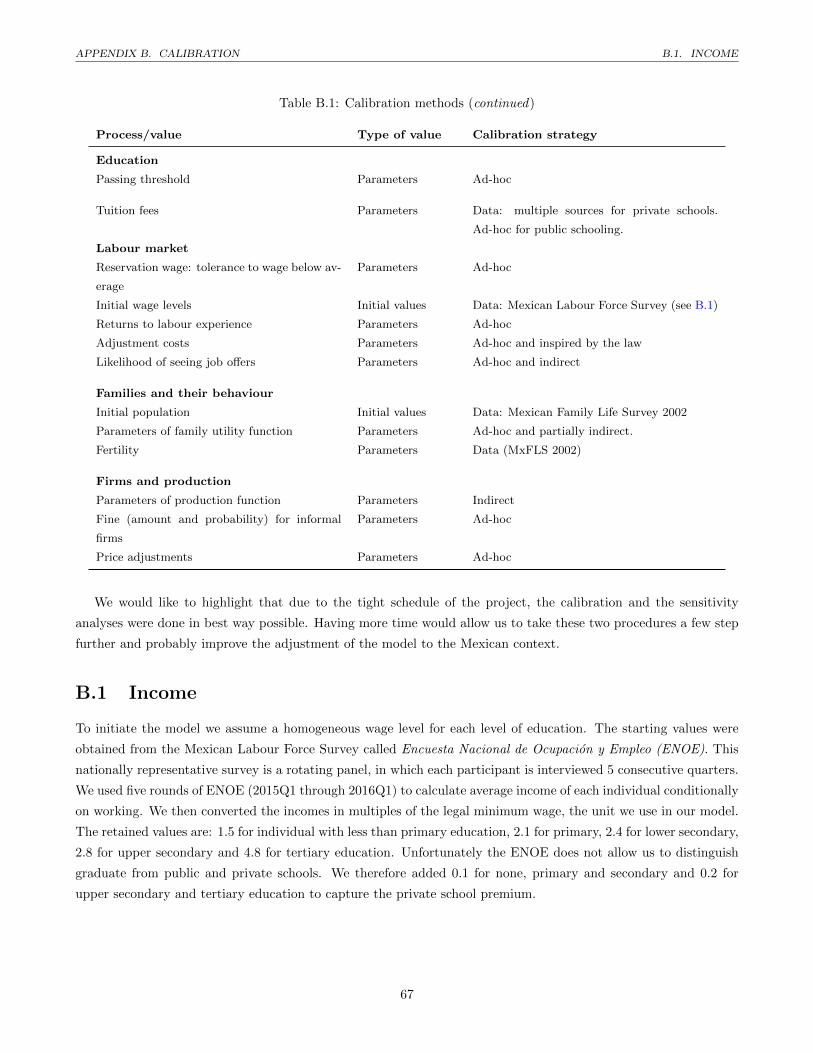
APPENDIX B. CALIBRATION B.1. INCOME
Table B.1: Calibration methods (continued)
Process/value Type of value Calibration strategy
Education
Passing threshold Parameters Ad-hoc
Tuition fees Parameters Data: multiple sources for private schools.
Ad-hoc for public schooling.
Labour market
Reservation wage: tolerance to wage below av-
erage
Parameters Ad-hoc
Initial wage levels Initial values Data: Mexican Labour Force Survey (see B.1)
Returns to labour experience Parameters Ad-hoc
Adjustment costs Parameters Ad-hoc and inspired by the law
Likelihood of seeing job offers Parameters Ad-hoc and indirect
Families and their behaviour
Initial population Initial values Data: Mexican Family Life Survey 2002
Parameters of family utility function Parameters Ad-hoc and partially indirect.
Fertility Parameters Data (MxFLS 2002)
Firms and production
Parameters of production function Parameters Indirect
Fine (amount and probability) for informal
firms
Parameters Ad-hoc
Price adjustments Parameters Ad-hoc
We would like to highlight that due to the tight schedule of the project, the calibration and the sensitivity
analyses were done in best way possible. Having more time would allow us to take these two procedures a few step
further and probably improve the adjustment of the model to the Mexican context.
B.1 Income
To initiate the model we assume a homogeneous wage level for each level of education. The starting values were
obtained from the Mexican Labour Force Survey called Encuesta Nacional de Ocupacion y Empleo (ENOE). This
nationally representative survey is a rotating panel, in which each participant is interviewed 5 consecutive quarters.
We used five rounds of ENOE (2015Q1 through 2016Q1) to calculate average income of each individual conditionally
on working. We then converted the incomes in multiples of the legal minimum wage, the unit we use in our model.
The retained values are: 1.5 for individual with less than primary education, 2.1 for primary, 2.4 for lower secondary,
2.8 for upper secondary and 4.8 for tertiary education. Unfortunately the ENOE does not allow us to distinguish
graduate from public and private schools. We therefore added 0.1 for none, primary and secondary and 0.2 for
upper secondary and tertiary education to capture the private school premium.
67
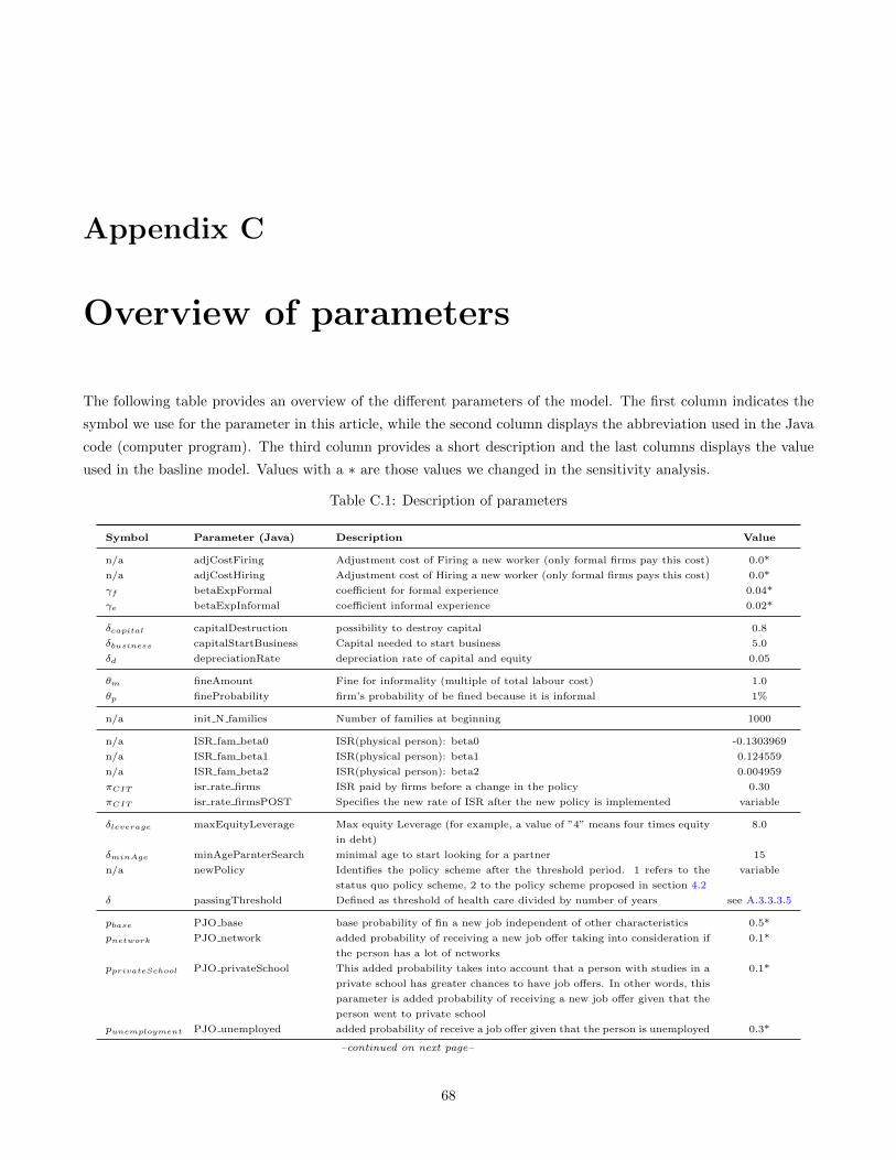
Appendix C
Overview of parameters
The following table provides an overview of the different parameters of the model. The first column indicates the
symbol we use for the parameter in this article, while the second column displays the abbreviation used in the Java
code (computer program). The third column provides a short description and the last columns displays the value
used in the basline model. Values with a ∗ are those values we changed in the sensitivity analysis.
Table C.1: Description of parameters
Symbol Parameter (Java) Description Value
n/a adjCostFiring Adjustment cost of Firing a new worker (only formal firms pay this cost) 0.0*
n/a adjCostHiring Adjustment cost of Hiring a new worker (only formal firms pays this cost) 0.0*
γf betaExpFormal coefficient for formal experience 0.04*
γe betaExpInformal coefficient informal experience 0.02*
δcapital capitalDestruction possibility to destroy capital 0.8
δbusiness capitalStartBusiness Capital needed to start business 5.0
δd depreciationRate depreciation rate of capital and equity 0.05
θm fineAmount Fine for informality (multiple of total labour cost) 1.0
θp fineProbability firm’s probability of be fined because it is informal 1%
n/a init N families Number of families at beginning 1000
n/a ISR fam beta0 ISR(physical person): beta0 -0.1303969
n/a ISR fam beta1 ISR(physical person): beta1 0.124559
n/a ISR fam beta2 ISR(physical person): beta2 0.004959
πCIT isr rate firms ISR paid by firms before a change in the policy 0.30
πCIT isr rate firmsPOST Specifies the new rate of ISR after the new policy is implemented variable
δleverage maxEquityLeverage Max equity Leverage (for example, a value of ”4” means four times equity
in debt)
8.0
δminAge minAgeParnterSearch minimal age to start looking for a partner 15
n/a newPolicy Identifies the policy scheme after the threshold period. 1 refers to the
status quo policy scheme, 2 to the policy scheme proposed in section 4.2
variable
δ passingThreshold Defined as threshold of health care divided by number of years see A.3.3.3.5
pbase PJO base base probability of fin a new job independent of other characteristics 0.5*
pnetwork PJO network added probability of receiving a new job offer taking into consideration if
the person has a lot of networks
0.1*
pprivateSchool PJO privateSchool This added probability takes into account that a person with studies in a
private school has greater chances to have job offers. In other words, this
parameter is added probability of receiving a new job offer given that the
person went to private school
0.1*
punemployment PJO unemployed added probability of receive a job offer given that the person is unemployed 0.3*
–continued on next page–
68
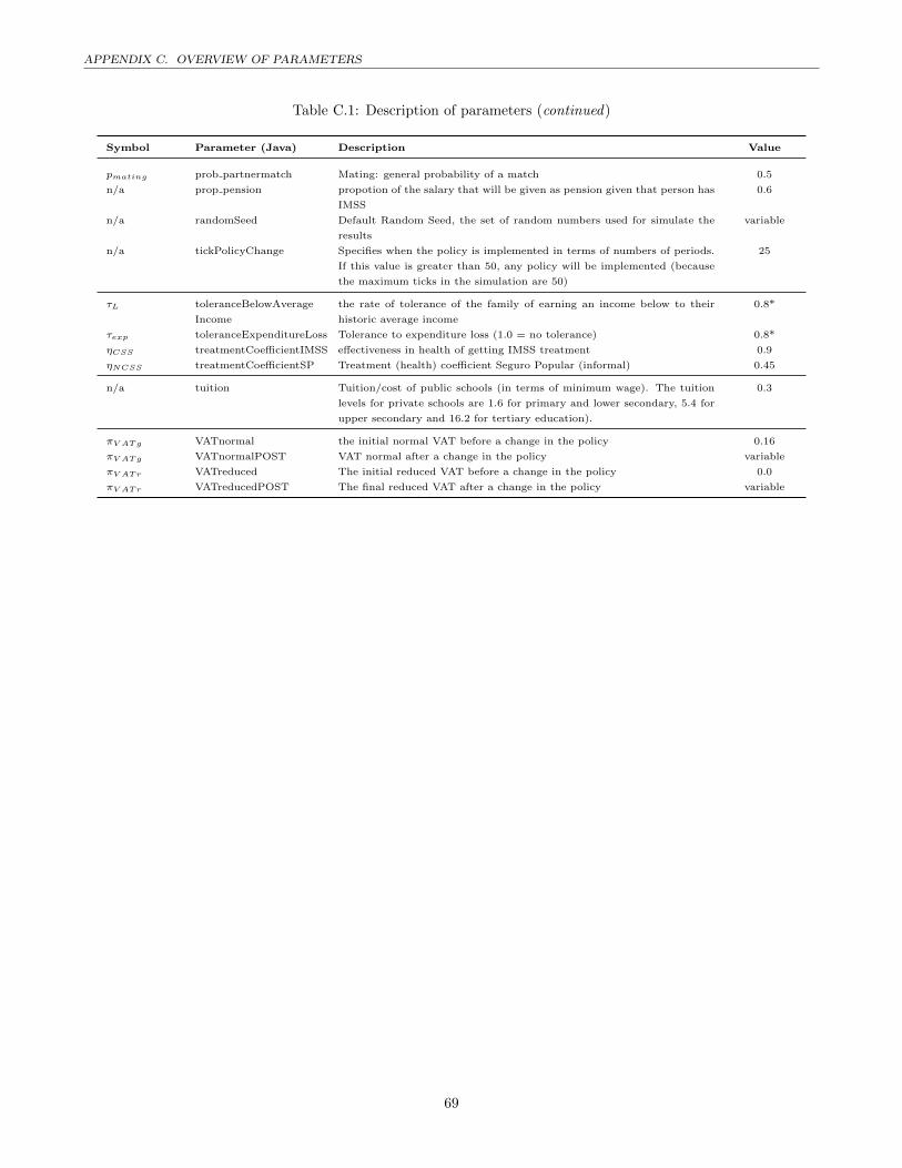
APPENDIX C. OVERVIEW OF PARAMETERS
Table C.1: Description of parameters (continued)
Symbol Parameter (Java) Description Value
pmating prob partnermatch Mating: general probability of a match 0.5
n/a prop pension propotion of the salary that will be given as pension given that person has
IMSS
0.6
n/a randomSeed Default Random Seed, the set of random numbers used for simulate the
results
variable
n/a tickPolicyChange Specifies when the policy is implemented in terms of numbers of periods.
If this value is greater than 50, any policy will be implemented (because
the maximum ticks in the simulation are 50)
25
τL toleranceBelowAverage
Income
the rate of tolerance of the family of earning an income below to their
historic average income
0.8*
τexp toleranceExpenditureLoss Tolerance to expenditure loss (1.0 = no tolerance) 0.8*
ηCSS treatmentCoefficientIMSS effectiveness in health of getting IMSS treatment 0.9
ηNCSS treatmentCoefficientSP Treatment (health) coefficient Seguro Popular (informal) 0.45
n/a tuition Tuition/cost of public schools (in terms of minimum wage). The tuition
levels for private schools are 1.6 for primary and lower secondary, 5.4 for
upper secondary and 16.2 for tertiary education).
0.3
πV ATg VATnormal the initial normal VAT before a change in the policy 0.16
πV ATg VATnormalPOST VAT normal after a change in the policy variable
πV ATr VATreduced The initial reduced VAT before a change in the policy 0.0
πV ATr VATreducedPOST The final reduced VAT after a change in the policy variable
69
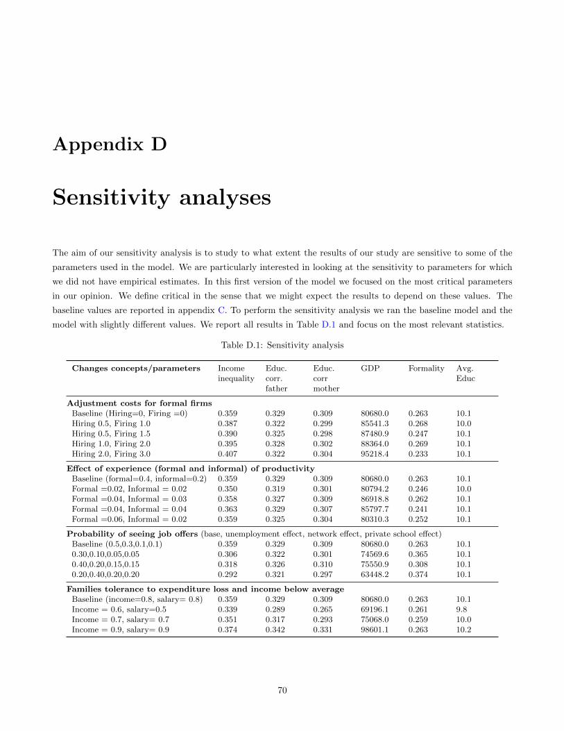
Appendix D
Sensitivity analyses
The aim of our sensitivity analysis is to study to what extent the results of our study are sensitive to some of the
parameters used in the model. We are particularly interested in looking at the sensitivity to parameters for which
we did not have empirical estimates. In this first version of the model we focused on the most critical parameters
in our opinion. We define critical in the sense that we might expect the results to depend on these values. The
baseline values are reported in appendix C. To perform the sensitivity analysis we ran the baseline model and the
model with slightly different values. We report all results in Table D.1 and focus on the most relevant statistics.
Table D.1: Sensitivity analysis
Changes concepts/parameters Incomeinequality
Educ.corr.father
Educ.corrmother
GDP Formality Avg.Educ
Adjustment costs for formal firmsBaseline (Hiring=0, Firing =0) 0.359 0.329 0.309 80680.0 0.263 10.1Hiring 0.5, Firing 1.0 0.387 0.322 0.299 85541.3 0.268 10.0Hiring 0.5, Firing 1.5 0.390 0.325 0.298 87480.9 0.247 10.1Hiring 1.0, Firing 2.0 0.395 0.328 0.302 88364.0 0.269 10.1Hiring 2.0, Firing 3.0 0.407 0.322 0.304 95218.4 0.233 10.1
Effect of experience (formal and informal) of productivityBaseline (formal=0.4, informal=0.2) 0.359 0.329 0.309 80680.0 0.263 10.1Formal =0.02, Informal = 0.02 0.350 0.319 0.301 80794.2 0.246 10.0Formal =0.04, Informal = 0.03 0.358 0.327 0.309 86918.8 0.262 10.1Formal =0.04, Informal = 0.04 0.363 0.329 0.307 85797.7 0.241 10.1Formal =0.06, Informal = 0.02 0.359 0.325 0.304 80310.3 0.252 10.1
Probability of seeing job offers (base, unemployment effect, network effect, private school effect)Baseline (0.5,0.3,0.1,0.1) 0.359 0.329 0.309 80680.0 0.263 10.10.30,0.10,0.05,0.05 0.306 0.322 0.301 74569.6 0.365 10.10.40,0.20,0.15,0.15 0.318 0.326 0.310 75550.9 0.308 10.10.20,0.40,0.20,0.20 0.292 0.321 0.297 63448.2 0.374 10.1
Families tolerance to expenditure loss and income below averageBaseline (income=0.8, salary= 0.8) 0.359 0.329 0.309 80680.0 0.263 10.1Income = 0.6, salary=0.5 0.339 0.289 0.265 69196.1 0.261 9.8Income = 0.7, salary= 0.7 0.351 0.317 0.293 75068.0 0.259 10.0Income = 0.9, salary= 0.9 0.374 0.342 0.331 98601.1 0.263 10.2
70
APPENDIX D. SENSITIVITY ANALYSES
Adjustment costs
In our baseline model we do not include adjustment costs for formal firms (hiring and firing adjustment costs).
As we can see in Table D.1, most key statistics are not sensitive at all to this parameter. The only statistics that
change are income inequality and to some extent GDP. This is an interesting results and opens new questions on
why adjustment costs in the formal sector increase income inequality. In this version of the study we are not able
to respond this question.
Effect of experience
The effect of experience on labour market productivity could also affect a wide range of statistics. We therefore
ran the simulation for a series of values, but do not find any important change in the key statistics. Thus, this
parameter set does not seem to be extremely relevant for the results.
Probability of seeing job offers
The likelihood of seeing job offer depends on many different elements, in particular on the labour market status.
The results suggest that inequality, GDP and the proportion of formal firms are to some extent sensitive to these
parameters. However, we have to highlight the rather extreme changes in this sensitivity analysis.
Tolerance to income and consumption loss
Finally, we look at the two tolerance parameters. On parameters captures how much individuals accept lower wages
than what people with the same education level earn. The second tolerance parameter captures how much loss in
consumption a family accepts from one period to the next. In the baseline model both values are set to 0.8 (80%).
The education correlations are positively related to these two parameters, while the other statistics do not show
much difference. GDP is also somewhat sensitive to these measures, but at this stage it remains unclear through
which mechanisms the tolerance parameters affect GDP.
71
Appendix E
Agent-based modelling approach
A key element of this project is the use of agent-based modelling techniques rather than more traditional modelling
techniques in economics. In this section we briefly introduce the ABM approach and highlight why it might be more
appropriate and promising in achieving the goals of the project. More detailed introductions to agent-based models
can be found in Gilbert (2008) and Miller and Page (2007). A discussion on the usefulness of ABM in development
economics can be found in Chavez-Juarez (2016).
E.1 What are agent-based models?
Agent-based models are typically theoretical models that aim at reproducing real-world phenomena. Such models
have been extensively used in various disciplines of natural science and are becoming more popular among social
scientists. In economics, traditional equilibrium based models can be seen as top-down models, because the be-
haviour of typically representative individuals (micro level) is governed by the equilibrium condition (macro level).
In contrast, agent-based models are bottom-up, where we model the behaviour at the micro level (processes, in-
teractions, etc.) which then sum-up to produce some macro level outcomes that need not necessarily represent an
equilibrium. Hamill and Gilbert (2015) define them in the following concise way:
“An agent-based model is a computer program that creates an artificial world of heterogeneous agents
and enables investigation into how interactions between these agents, and between agents and other
factors such as time and space, add up to form the patterns seen in the real world.”Hamill and Gilbert
(2015).
Let us now have a closer at the notion of agents. Typically, we characterise an agent by characteristics (state
variables) and behavioural rules (processes). Characteristics can be constant (e.g. gender, parental education) or
variable (e.g. years of education, income) over time. At each point in time, an agent is characterised by the set of
these state variables. The second major element of agents are behavioural rules. Behavioural rules describe what
agents do in a given situation. For instance, a behavioural rule can govern the decisions to enrol or not at school.
The behavioural rules are the equivalent to the resulting behaviour after the maximisation of a utility function in
traditional models. These behavioural rules can be very simple (e.g. go to school whenever parents can afford it)
or extremely complicated (e.g. the result of an intertemporal maximisation problem similar to traditional models).
72

APPENDIX E. AGENT-BASED MODELLING APPROACH E.2. WHY ABM FOR THIS PROJECT?
When looking at a single agent, they are very similar to individuals in more traditional models. The important
difference comes when we look at the whole population, because each agent can have different characteristics in each
state variable and also in the behavioural rule. Hence, in agent-based models we do not have a representative agent
or only heterogeneities in a few dimensions. An additional difference is that agent live in an environment, which is
populated by other agents (of different types). Agents then interact with each other and the behaviour/decision of
one agent will depend both on the state variables and the behaviour of other agents.
Another difference to traditional models is the large flexibility in the modelling approach due to the fact that
no analytical solution must be computed. In traditional model it is many times intractable to include multiple
optimisation behaviours and multiple heterogeneities. Given that in agent based model the behaviour is governed
at the micro level and does not have to respect any equilibrium condition, it is virtually costless to add more decisions
and dimensions5. Another advantage of this flexibility is that agent-based models can be built in a modular way,
where in a first version some modules are oversimplified and then developed in subsequent versions of the model.
Finally, agent-based models do not only include heterogeneities in agents’ characteristics and behaviour, but
also in their outcomes. Hence, ABM are a natural way to study phenomena where the distribution of outcomes
(e.g. education, earnings, etc.) are of primary importance.
E.2 Why ABM for this project?
For this project, the agent-based modelling approach seems to be the appropriate method for a number of reasons:
1. the number of processes to be included in the model is large and traditional models would most likely not be
tractable or we would be forced to simplify the model beyond what could be justified.
2. the key outcome of interest is inequality and social mobility. As a consequence, model that heavily rely on
representative agents or a limited number of types are ill suited and agent based models offer the possibility
to study inequality within a generation but also from one generation to the next.
3. one of the goals of the project is to see how different concepts (e.g. social mobility, economic growth) evolve
after a policy change. Agent-based models have an inherent time dimension and it is therefore easy to study
both the short-run and the long run effects of a policy change.
4. Agent-based models allow us to get closer to reality by including both stylised facts and empirical evidence
of the country of analysis. In our particular case, we can model many relevant processes by looking at the
empirical evidence to ensure that these processes resemble what is observed in reality.
5. The possibility to build the model by modules and to oversimplify non-crucial elements in a first version is a
huge advantage. We can therefore focus now on the core elements and include other phenomena in a passive
way. Subsequently, we can then try to make the model more realistic by working on the oversimplified modules
for a second and third version of the model.
E.3 Modelling process
The modelling process is somewhat different to the standard approach. We can simplify the process to the following
steps:
73

APPENDIX E. AGENT-BASED MODELLING APPROACH E.4. TECHNICAL IMPLEMENTATION
1. Identify the different agent types in the model. In our case, we have multiple agent types such as individuals,
families, schools and hospitals.
2. For each agent-type, we identify the processes that must be modelled. For instance, families must decide how
to allocate their resources, whether they want to send the children to school and so forth.
3. For each of the processes we make a literature review and search for empirical evidence. We then analyse
whether it is a crucial process for the study and we have to model it in detail, or if it is of secondary importance
and we can use empirical evidence to make the process more mechanical.
4. For the most important processes we then start to model the behaviour of individuals. For instance, for the
enrolment decision of children we identify the factors that might affect the decision and eventually model the
actual decision.
5. Less important processes (or those that are not of primary interest for the study) which are still crucial for
the model to work can be implemented in a simpler way. For instance, we know that fertility rates in Latin
America are strongly influenced by the education level of the mother. This has direct consequences on social
mobility. Nevertheless, the actual decision process of how many children a couple wants to have is not of
primary interest and also beyond the scope of the study. In order to still have this phenomenon in the model,
we can implement it in a passive way by looking at the empirical evidence and simple reproduce this evidence
through a stochastic process that does not involve any active decision making of the agents.
6. Once each of the active decision making processes is roughly defined, we then look at how the different processes
interact. For instance, in the labour market firms have a process to generate job offers and individuals have to
take a decision on whether or not to accept a job offer. In this step we define how the two processes interact
with each other and what kind of information is revealed to the other agents.
7. Once the full model is conceptualised in this way, we start with the programming of the model and to run
preliminary analyses.
8. Once the model is fully operative, various runs with different settings and different stochastic random seeds
are simulated and then analysed.
E.4 Technical implementation
We implement the model using the Repast Simphony packages in Java. Java has the advantage of cross-platform
compatibility as it is executed on a virtual machine. All the simulations presented in this study were carried out
on Microsoft Windows Workstations at the National Laboratory of Public Policy (LNPP).
74
Index
ABM, 72
Agent-based modelling, 72
Assortative mating, 9, 59
Baseline
inequality, 26
Social mobility, 26
Bequest, 58
Calibration, 66
income, 67
Capital market, 13
Corporate income tax, 61
Distribution
education, 22
Economic growth, 24
Education, 10, 58
Education dependent fertility, 10
Education distribution, 22
Effect
on formality, 31
on growth, 31
on inequality, 32
on social mobility, 34
ENIGH, 26, 62, 63, 66
Family, 17
behaviour, 17
bequest, 58
dissolution, 58
fertility, 63
Fertility, 10, 18, 63
Firms, 19
types, 19
Formality, 11, 23, 31
Future research, 38
GDP, 31
growth, 24
GDP growth, 31
Government, 20
expenditures, 30
income, 29
Growth, 24
growth, 31
Health
recovery, 57
services, 57
Health sector, 21
Human capital, 10, 58
IMSS, 11
Income structure, 67
Income tax
corporate, 61
natural person, 61
Inequality, 26
Inequality of opportunity, 34
Investment
in education, 10
ISSSTE, 11
Job offers, 54
Labour market, 12
Labour supply, 18
Limitations, 38
Mating, 59
Mating probability, 60
Model
75
INDEX INDEX
at a glance, 15
calibration, 66
description, 15
Families, 17
Firms, 19
Government, 20
Health sector, 21
Nature, 21
Overview, 15
overview of processes, 16
Results, 22
Schools, 20
time frame, 16
MxFLS, 19, 27, 49, 63, 67
Nature, 21
ODD, 43
Overview, design concepts and details, 43
Parameters
overview, 68
Partner search, 59
Policy interventions, 28
Policy simulation, 27
price adaptation, 64
Probability
mating, 60
of seeing job offers, 54
Procreation, 18
Product space, 19
Production function, 19
Reservation wage, 54
School
passing grade, 58
Schools, 20
Seguro Popular, 11, 13
Sensitivity analysis, 70
Simualtion approach, 28
Social mobility, 26
Social security system, 11
Software, 74
Supply
labour, 18
Tax
corporate income, 28
value-added, 28, 61
Technical implementation, 74
Time frame, 16
Transition matrix, 35
Value added tax, 61
VAT, 61
Wage
reservation, 54
76