Slippage and the Choice of Market or Limit Orders

in Futures Trading

Scott Brown*, Timothy Koch**, and Eric Powers**1

March, 2007

*University of Puerto Rico

**University of South Carolina

1 The authors particularly wish to thank Scott Barrie for his invaluable assistance in acquiring the brokerage data as well as providing guidance on operations from the perspective of a floor broker, floor trader, and introducing brokerage compliance officer. In addition, we thank Steve Dicke at the Chicago Board of Trade for the time and sales data required for this study. Finally, we thank Esubio Diaz Diaz, Helen Doerpinghaus, Glenn Harrison, Scott Irwin, Eric Johnson, Peter Locke, Stewart Mayhew, and Greg Niehaus for helpful comments.

Slippage and the Choice of Market or Limit Orders

in Futures Trading

Abstract

Retail futures traders face uncertainty regarding the actual price they will obtain when they enter or exit a futures position. Not infrequently, the actual price differs from the expected price. This price ‘surprise,’ known as slippage, may be substantial and varies with factors such as the size of the order, market conditions, and the type of order placed. Using unique data from an introducing brokerage for CBOT futures contracts on wheat, corn, and soybeans, we first quantify the time-to-clear and magnitude of slippage that results from clearing time delays. We then identify factors that affect both time-to-clear and slippage on market orders, in particular, finding that slippage increases with order size, price volatility, and the bid-ask spread. Finally, we analyze individual trader choice between market and limit orders and find that the likelihood of placing limit orders, where regulations require floor brokers to compensate retail traders for the cost of adverse fills, is increasing in price volatility and order size but decreasing in market depth.

1 1

“sometimes the slippage on an execution is so large that you wonder whether

your pit broker was asleep when the stop order was activated. A series of “bad fills” can induce

paranoia in the most rational of minds.”

W. Gallacher, Winner Take All – A Brutally Honest and Irreverent Look at the Motivations and

Methods of Top Traders, 1994, p. 98

I. Introduction

Retail futures traders bear the risk that the price they actually receive will differ from

their expected price at initiation of a trade. Such a price ‘surprise,’ which can be substantial, is

known as slippage. One view is that slippage systematically occurs to the detriment of the party

placing the trade and results from floor brokers taking advantage of uninformed traders. Given

the information asymmetry that exists between retail traders, who possess stale and incomplete

information regarding market conditions, and floor brokers, who observe real-time trading

activity as well as the composition of their order book, the occurrence of systematically

unfavorable slippage is quite plausible.2 An alternative view is that slippage is benign and largely

a by-product of actively-traded markets where floor brokers are sometimes incapable of

immediately filling incoming orders due to heavy trading volume and rapidly fluctuating prices.

Regardless of its source, slippage represents a potentially significant cost to traders. To

assess the frequency and magnitude of slippage, we use a unique sample of over 2,000 Chicago

Board of Trade (CBOT) wheat, corn, and soybean futures order tickets for 69 retail traders – the

data were gathered from an anonymous introducing brokerage and cover a three year time span.

2 A retail trader is an individual who trades for his or her own account or for a clearing firm, but who is not a member of an exchange. Retail traders are not directly involved in the open outcry auction in the pits and thus rely on secondary information. Daigler and Wiley (1999) show that volume generated by off-floor traders contributes to higher return volatility while volume generated by local traders (scalpers) and clearing firms trading on their own account does not. Their interpretation is that off-floor traders are relatively uninformed.

2 2

Among other things, the order tickets report the exact time at which the order was placed with

the introducing brokerage, size of the order, underlying commodity, and price at which the order

was subsequently executed. Using CBOT time and sales transactional data, we estimate the time

at which the order actually cleared and subsequently, the elapsed time for each executed trade.3

Because we know the price at which the order cleared, estimating slippage is straightforward

once the trader’s expected price at the time the order is placed is identified. If futures market

prices satisfy weak-form efficiency and do not contain predictable trends, the most recent prior

transaction price will be a reasonable proxy for a retail trader’s expected price on a market

order.4 For limit orders, expected price is less subjective and should be equal to the limit price

recorded on the actual order. The difference between execution price and expected price provides

our measure of slippage. For a buy order, we calculate slippage as expected price minus actual

price. For a sell order, the relationship is reversed and slippage is calculated as actual price minus

expected price. For each calculation, a positive value represents slippage in the retail trader’s

favor.

Our evidence indicates that, on average, after taking account of bid-ask bounce, slippage on

market orders is not significantly different from zero. For limit orders, execution should only

occur when the market price penetrates the limit price. While floor brokers can certainly err in

executing limit orders, market regulations require the floor broker to cover the cost of adverse

fills. Thus, limit order slippage is bounded from below at zero. While a limited number of limit

orders show positive slippage, the vast majority clear at the limit price and hence have zero

3 As we note in the data section, orders are stamped with both a submission time and an execution time. Introducing Brokerages, however, often stockpile completed orders and stamp them with an execution time all at once during lulls in trading. Thus, the stamped execution time is of little value. 4 Prior research, such as Gray (1979), suggests that predictable trends are not present in futures prices, at least not over the short term (see also Black; 1986, Kuserk and Locke; 1993, Liu, Thompson, and Newbold; 1992, Martell and Trevino; 1990, and Working; 1954, 1967).

3 3

slippage. Thus, the lament of retail traders that “the system” is biased against them is clearly not

supported by the data, either for market orders or for limit orders. However, for market orders,

there is significant cross sectional variation in slippage. For example, slippage on wheat contract

market orders ranges from -2.25¢ to 1.75¢ per bushel. These values equate to a $112.50 loss to a

$87.50 gain per contract relative to the trader’s expected price at the time the order was placed.

In comparison, the half-turn (one-way) commission paid by our retail traders is $14. Thus, the

cost of slippage on market orders is potentially economically important to retail traders.

We next analyze the cross-sectional determinants of market order time-to-clear and find that

it is increasing in order size and bid-ask spread while decreasing in price volatility and market

depth. Clearly, time-to-clear and slippage are closely related as delays in execution go hand-in-

hand with slippage. Our analysis of the absolute value of market order slippage shows that it too

is increasing in order size and bid-ask spread. In contrast to time-to-clear, the absolute value of

slippage is increasing in market volatility.

Traders are certainly not defenseless when conditions indicate that slippage on market orders

is likely. One way for retail traders to control adverse slippage is to simply submit limit orders

rather than market orders.5 When we analyze individual trader choice between market and limit

orders, we find that traders are more likely to submit limit orders for larger orders, when market

volatility is high, and when market depth is low. This suggests that individual traders are

sensitive to the possibility of adverse slippage.

The rest of the paper proceeds as follows. Section II describes the order flow process and

briefly describes existing literature on slippage. Hypotheses regarding factors that should affect

5 One benefit of a limit order is that it is protected from negative slippage. The cost, however, is that the market price might not penetrate the limit price and the order might expire unfilled. In addition, limit orders may incur an adverse selection cost if they are systematically “picked off” by informed traders establishing positions ahead of price movements (Ferguson and Mann; 2001, Manaster and Mann; 1999).

4 4

the magnitude of time-to-clear and slippage are developed in Section III. In section IV we

describe the data and report univariate statistics on time-to-clear and slippage. Cross-sectional

analysis of factors affecting both quantities is reported in section V. Section V also includes a

probit analysis of when retail traders are more likely to submit market as opposed to limit orders.

Finally, we offer conclusions in Section VI.

II. The Order Process and Prior Research.

A. The Order Process

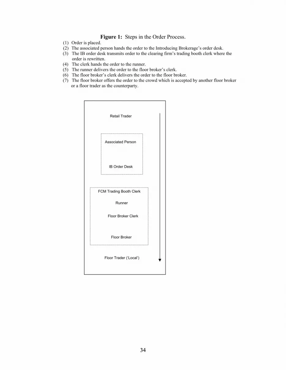
To understand why slippage can occur, one has to understand the order process. The

traditional order process, with a total of seven agents, is displayed in Figure 1. In the traditional

process, a retail order starts with a retail trader phoning the associated person at the introducing

brokerage where the trader maintains an account. The associated person generates a paper ticket

with a time stamp and details of the order. The ticket is then passed to a clerk working the

introducing brokerage’s order desk. Similar orders might be consolidated at the order desk before

the information is transmitted, either by telephone or by computer, to the clearing firm that

represents the introducing brokerage on the floor of the exchange. At the clearing firm’s trading

booth, a paper floor ticket is produced and then reviewed by the trading booth clerk. This ticket

is then either hand-carried by a runner to the floor broker clerk assisting the floor broker, or the

information is “arbed” directly to the floor broker in the pit via hand signals. Finally, the floor

broker clears the order via open outcry against orders held by other floor brokers or against

proprietary trades by floor traders.6

6 Floor traders lease or own seats on the exchange and operate as exchange members. They are scalpers (arbitrageurs), day traders, and position traders who usually trade for their own accounts. Floor traders may affect slippage by bidding or offering at prices within the bid-ask spread.

5 5

Over the last ten years, the CBOT has pushed to automate this process as much as

possible in order to provide better trade execution. Changes have occurred on the floor of the

exchange as well as at introducing brokerages. On the floor of the exchange, floor brokers have

migrated to “electronic clerk” hand-held devices. With these devices, orders can be routed

directly from the trading booth to the floor broker, eliminating the need for a runner as well as a

floor broker clerk and reducing execution time. Additionally, cleared orders can be transmitted

directly to the exchange and back to the trading booth. These devices eliminate the need for

paper floor tickets and significantly speed up the settling-up process.7 Most introducing

brokerages have also implemented web-based electronic order entry software. Rather than

telephoning the introducing brokerage, retail traders can submit orders via computer. These

computer-based orders can then be transmitted directly to floor brokers’ electronic clerk devices.

On August 1, 2006 the CBOT went a step further and initiated side-by-side electronic

trading for its agricultural futures contracts. Now, off exchange traders can routes trades to the

trading floor, or they can submit trades to the e-CBOT® electronic order book. Trades submitted

to e-CBOT® are electronically matched with other e-CBOT® orders. If an e-CBOT® order is not

currently executable, it becomes part of the e-CBOT® order book which is displayed above the

pit on plasma screens and is remotely available to market participants. In addition to being able

to see the electronic order book, floor brokers and traders are able to access it via their hand-held

devices. As of February 2007, approximately 50 percent of agricultural futures contracts cleared

during regular exchange hours are cleared via the e-CBOT® system.

7 Despite the benefits of electronic order routing, many market participants were initially unwilling to adopt the new technology. In response to customer complaints and to improve execution quality, in June 2003, the CBOT mandated that 80 percent of agricultural orders for 8 contracts or less had to be routed electronically. These standards were tightened further in June 2004 to 90 percent of agricultural orders for 10 contracts or less and in June 2005 to 100 percent of agricultural orders for 20 contracts or less. The CBOT also began imposing performance penalties on brokers in 2004 for all agricultural market orders that were not filled in 5 minutes or less.

6 6

During the time frame spanned by our data (May 1999 to March 2002), side-by-side

electronic trading was not available. Electronic order entry was also not available at the

introducing brokerage that provided our data. Thus, the traditional order process was utilized up

to the point where the order was received on the trading floor. According to the brokerage that

supplied our data, the vast majority of orders in our data set were manually processed on the

trading floor in the traditional manner utilizing paper tickets.8

Since the traditional order process was utilized for the majority of orders in our sample,

the speed at which each human agent carries out their assigned tasks ultimately affects the

likelihood and magnitude of slippage. With the exception of the associated person and the floor

broker, all of the agents involved in the order process are paid flat salaries. Thus, while they are

expected to offer fast and efficient service, their incentives for doing so are muted. The

associated person and floor broker, however, earn a commission for each executed contract. In

addition, the floor broker bears the risk of loss on limit orders that are cleared at an adverse price,

while the associated person potentially bears the risk of retail trader insolvency.9 Thus,

incentives for both the associated person and the floor broker to clear trades quickly and

correctly are much stronger than incentives for other participants in the order process.

This multi-stage order clearing process can affect slippage due to potential time delays

between when an order is placed and when it is subsequently filled. One can easily imagine

periods when the various agents are not at the top of their respective games (particularly on

mornings after a televised playoff game for a Chicago sports team), resulting in order delays.

8 According to CBOT staff, in 2000, approximately 30 percent of floor brokers in the agricultural pits utilized electronic clerk hand-held devices and these brokers were responsible for executing approximately 30 percent of agricultural futures orders. By 2002, the percentage of electronically routed agricultural futures orders had increased to 50 percent and by 2003, the percentage had increased to 70 percent. 9 If a retail trader loses more than the amount held as margin with the introducing brokerage and the clearing firm cannot collect the debt, the introducing brokerage must pay the clearing firm and may force the associated person to repay the brokerage. As such, the associated person bears the risk of retail trader insolvency.

7 7

The greater is the time delay, the greater is the range of prices at which an order might be

cleared.

B. Prior Research

Academic research on trading rules routinely incorporates some estimate of trading costs

(see, e.g., Lukac and Brorsen; 1990, Knez and Ready; 1996, or Ready; 2002). Practitioners in

futures markets also emphasize the importance of incorporating trading costs – particularly

slippage – when evaluating trading strategies (see Calhoun; 1989, Crabel; 1990, Radnoty; 1991,

Tharp; 1993, Gallacher; 1994, Kaufman; 1995, Covington Bryce; 1996, and Myers; 1998.) To

date, however, little research exists regarding the frequency and magnitude of slippage across

various markets. Greer, et al. (1992) examine slippage for a small sample of stop orders placed

by a small commodity futures fund in 11 different commodity, currency, and financial contracts.

They determine that slippage, on average, is negative in each commodity, averaging

approximately 0.14% of contract value. This equates to a $38.16 cost to the commodity fund in

addition to traditional transactions costs such as commissions.10

Frino and Oetomo (2005) evaluate slippage on four major financial futures traded on the

Sydney Futures Exchange. They consider only orders that were large enough to require a split fill

in which the order is filled via a sequence of smaller trades at potentially different prices. The

price at which the first leg of the fill occurred becomes their base price and slippage on

subsequent legs is calculated relative to the base price. The primary finding of Frino and Oetomo

is that the magnitude of slippage increases with order size. While there are many similarities

between their research and ours, there are important differences. First, since 1999 the Sydney

10 Greer, et al. analyze stop orders exclusively since stop orders, by definition, provide the retail trader’s expected transaction price. In addition, unlike with limit orders, floor traders do not need to compensate retail traders when slippage costs are incurred.

8 8

Futures Exchange has been strictly an automated electronic trading system. In contrast, the

Chicago Board of Trade during regular trading hours (9:30 am until 1:30 pm CST) was strictly a

traditional open-outcry trading system during the time period of our study.11 Second, we measure

slippage relative to the price prevailing in the market immediately prior to the trade being placed,

not relative to the fill price of the first leg of a split-filled order. Because of this, we are able to

include all trades, not just larger trades.

Kurov (2005) analyzes trading on the Chicago Mercantile Exchange (CME) which has

similar trading architecture to the CBOT. He analyzes 13 months of computerized trade

reconstruction (CTR) data from the Commodities Futures Trading Commission for CME futures

contracts on the S&P 500, NASDAQ 100, Euro, Yen, live cattle, and lean hogs.12 The CTR data

effectively recreates all trading floor activity. While Kurov (2005) does not actually calculate

slippage, he is able to summarize characteristics of all retail trader orders and reports the

estimated time from trading floor time stamp to execution. In addition, Kurov (2005) analyzes

order strategy for retail traders and finds that market volatility and bid-ask spread impact retail

trader choice between market and limit orders. While our dataset is much smaller than Kurov’s,

our work is distinctive in that we are able to track orders from the introducing brokerage through

the time of execution. This provides a more accurate measure of execution time, and also

enables us to get a relatively precise estimate of slippage. In addition, because we have data on

all limit orders submitted by our traders rather than the subset that is actually executed, we are

able to provide a distinctive analysis of retail trader choice between various types of orders.

11 Since 1995, after-hours trading of agricultural futures contracts has occurred on-line from 6:30 pm until 6:00 am. On 1 August, 2006, the CBOT started side-by-side open-outcry and electronic trading of agricultural commodities during regular trading hours. The electronic limit order book is displayed on plasma screens above the actual pit and can be accessed by floor traders using hand-held electronic devices. 12 Our data spans 5/24/1999 to 3/26/2002 while Kurov (2005)’s data spans 6/1/2000 to 6/30/2001. During these time periods, the CBOT and the CME were separate and competing exchanges. In October 2006, however the CBOT and CME agreed to merge, with floor trading to be consolidated at the CBOT location.

9 9

III. Bias in Slippage and Factors Expected to Affect Time-to-Clear and Slippage

A. The Disadvantaged Position of Retail Traders.

Floor traders are privy to a wealth of information including the history of transaction

prices and order quantities, source of those trades, current depth represented by outstanding limit

and stop orders, movements in the cash market, and esoteric items like the noise level in the pit

(Coval and Shumway; 2001). Retail traders, however, are limited to a small subset of this

information. At best, retail traders may have access to real-time tick data.13 If floor brokers and

floor traders take advantage of private information and collude, then market order slippage

should be systematically biased against the retail trader.14 If, as clearing agents contend, the

order process is impartial because collusion is not only illegal, but actively monitored and

enforced, then slippage should be unbiased.

Hypothesis 1: Slippage on market orders will be negative.

B. Motivation of the Floor Broker

Floor broker compensation comes in the form of commissions – the more trades that brokers

clear, the wealthier they become. Thus, floor brokers have ample incentive to provide quick and

13 Real-time tick data are available to retail traders, but are costly at approximately $500 per month. Even real-time tick data are delayed by at least 15 seconds due to data entry and satellite data transmission lag. Alternatively, a retail trader can query the associated person at the introducing brokerage just prior to placing a trade and can also use the internet to obtain free 10-minute delayed prices. 14 Disciplinary action against floor traders is one indication of a tilted playing field. Sarkar and Wu (2000) provide some evidence of bias, showing that prior to the implementation of a “top-step” rule in the CME S&P 500 futures pit, dual traders provided inferior execution of customer trades relative to personal trades. A “top-step” rule prohibits dual traders from making personal trades if they previously made a trade from the top-step of the pit that day.

10 10

accurate trade execution. In addition, floor brokers face the possibility of fines and potential

sanctions (not to mention loss of future order flow) if they are negligent in performing their

duties.

Given floor brokers’ strong incentives, some orders are likely to receive higher precedence.

First, larger orders generate larger commissions. In addition, larger orders are typically submitted

by retail traders with deeper pockets who are likely to account for significant future order flow.

These large order retail traders are also likely to be more sophisticated than the average retail

trader and may be more likely to challenge adverse order fills via the arbitration process.15 For

these reasons, we expect floor brokers to pay greater attention to larger orders. Larger orders,

however, should also be more difficult to fill. As noted by Frino, Oetomo, and Wearing (2004),

larger orders may generate a temporary order imbalance, resulting in longer time-to-clear,

thereby incurring a liquidity cost. Larger orders may also require split fills and may be perceived

to be from more informed traders. Hence, in addition to incurring a liquidity cost, larger orders

may cause a permanent revision in market price.

Because of these countervailing factors, it is not entirely clear what the impact of order size

will be on time-to-clear and slippage. Our expectation is that, on net, there will be a positive

relationship in both instances due to difficulties in filling large orders.

Hypothesis 2a: Market order time-to-clear will be positively related to order size.

Hypothesis 2b: Market order slippage will be positively related to order size.

15 A former compliance officer for a large introducing brokerage who was formerly a floor trader and then a floor broker stated that “small traders simply don’t know their rights and, with the small trades they place, the amount they have to gain is far less than the cost of the hassle of taking the trade to arbitration…large traders on the other hand ‘wield a big stick’ and will take a case to arbitration just to make the floor broker miserable.”

11 11

C. Price Volatility and Market Depth

High price volatility should affect the magnitude of slippage as the increased likelihood of

large and frequent price changes increases the frequency of fills far from the retail trader’s

expected price. Indeed, Greer, et al. (1992) shows that extreme intraday price movements

generate large values of slippage on stop orders. Price volatility, however, may not have an

impact on time-to-clear.

Market depth is likely to have an impact on both time-to-clear and slippage. High market

depth implies that many participants stand willing to be counterparties to incoming orders.16

Depth can be provided by open positions that traders are looking to close out, the limit order

books of floor brokers, and floor traders looking to trade for their own account. Our expectation

is that high market depth, measured as both trading volume and open interest, will lead to shorter

time-to-clear and less slippage. Conversely, floor brokers will have to work harder to clear orders

when market depth is low and time-to-clear and slippage should increase accordingly.17

Prior research has suggested that open interest is a proxy for hedging (uninformed) demand

since speculators (informed) typically don’t carry positions overnight (Bessembinder and Seguin;

1993.) Thus, periods of low open interest and low liquidity may also be periods of high

asymmetric information. If the clearing system contains any bias against retail traders, these may

also be periods where floor brokers are more likely to collude with other floor traders, leading to

longer clearing times and greater slippage.18

16 Kyle (1983) defines market depth as the order flow required to move the futures price one percent. Bessembinder and Seguin (1993) also include open interest as a measure of market depth. While intraday measures of volume are best, most studies use cumulative values at the end of each day. 17 Market depth and price volatility are correlated (Bessembinder and Seguin; 1993) so these statements implicitly assume that volatility is being held constant. 18 Futures floor traders often have direct relationships with specific floor brokers. Thus, while the floor trader is not directly aware of the composition of a floor broker’s deck, the floor broker may signal that he is clearing a large limit order and expects to be clearing a large offsetting order shortly thereafter. The floor broker will then clear the large limit order by trading with the floor trader at different clearing prices with some favorable and some

12 12

Hypothesis 3a: Market order time-to-clear should increase with price volatility.

Hypothesis 3b: Market order slippage should increase with price volatility.

Hypothesis 3c: Market order time-to-clear should decrease with market depth.

Hypothesis 3d: Market order slippage should decrease with market depth.

Similar hypotheses can be stated for limit orders. A fair comparison of time-to-clear between

market orders and limit orders is difficult because our clock on market orders starts when the

order is placed with the introducing brokerage, while our clock for limit orders generally starts

when the order is already in the floor brokers’ deck and the market price penetrates the limit

price. As will be seen later, most limit orders are executed at exactly the limit price, resulting in

no slippage. This is at least partly due to the manner in which we calculate time-to-clear and

slippage for limit orders. It also reflects the fact that floor brokers are “held to the limit” and

must compensate retail traders for fills that occur at worse than the limit price. Thus, we expect

time-to-clear and slippage on limit orders to be less than the corresponding values for market

orders. This outcome, however, is virtually certain and does not warrant separate hypotheses.

IV. Data and Univariate Analysis of Time-to-Clear and Slippage.

A. Data

unfavorable for the floor trader given the prevailing bid-ask spread. The floor broker then clears the offsetting limit order in the deck with the same floor trader at a net profit to the floor trader. This gives the floor trader a profit and increases the likelihood that the floor broker receives full commissions by clearing trades at or better than the limit price. This phenomenon is called ‘dressing up the local’ and gives a floor broker greater assurance of not incurring a loss on a large limit order and being held to the limit. It also generates ‘split fills’ on large limit orders where different parts of the same order are cleared at different prices.

13 13

Our data are drawn from a sample of 16,019 separate orders placed by 69 retail traders between

May 1999 and March 2002 at a particular (anonymous) introducing brokerage.19 The orders

consist of individual paper tickets that record an identifying number, customer number, order

quantity, type of order (market, limit, stop, etc.), date and time that the order was received by the

brokerage, fill price, and the time stamp indicating when the order was recorded filled by the

brokerage. In addition, information on the ticket indicates the commodity, delivery month,

whether it was to sell or buy, whether the order was for futures contracts or options, the strike

price if the order was for options, the limit price if the order was a limit order, and whether the

party placing the order granted the floor broker “discretion”.20

The orders span a wide variety of underlying commodities including Wheat, Corn,

Soybeans, Cocoa, Pork Bellies, Live Cattle, Lean Hogs, Swiss Francs, S&P 500 Minis, etc.

Approximately one-third of the orders are for futures contracts while two-thirds are for options.

To keep our analysis tractable, we exclude options and focus solely on market and limit orders

for futures contracts. We also restrict our analysis to orders for CBOT Wheat, Corn and

Soybeans which are the three most heavily traded CBOT contracts for our traders and account

for about 45 percent of our futures contract orders.21

19 The average trader had 7 years of trading experience, almost $700,000 in reported net worth, opened a margin account with $13,250, and paid $28 in round-turn commissions for each futures position. 20 Discretion enables a floor broker to execute a limit order at a potentially worse price than the limit price specified on the order. When discretion is offered, the number of points the floor broker is authorized to deviate from the limit price is specified. While fills may occur at worse than the original limit price, the added flexibility also enables a floor trader to wait and see whether a fill can be made at better than the limit price, resulting in price improvement. In most instances, discretion will be added to a limit order some time after it was originally submitted, i.e. when the retail trader is worried that the order will not fill. Thus, discretion is used to increase the likelihood that a limit order will be filled. 21 There are a variety of more esoteric order types such as stop orders, fill-or-kill orders, market-on-open orders, and one-cancels-the-other orders. Because these represent a small fraction of the data relative to market and limit orders, they are excluded from our analysis. Orders that were marked void or incomplete (missing key data) are also excluded. While the analysis could be extended to the other commodities, this would require obtaining additional time and sales transaction data from the various exchanges on which these commodities trade.

14 14

During the time period spanned by our sample, CBOT floor trading occurs Monday

through Friday from 9:30 am until 1:30 pm CST. A much less active electronic trading session

occurs from 6:30 pm to 6:00 am. For each contract, the underlying asset is 5,000 bushels of the

applicable commodity. Expiration months are March, May, July, September, and December for

Corn and Wheat; January, March, May, July, August, September, and November for Soybeans.

For each contract, the minimum price tick is ¼ cent which equates to $12.50 per contract.

Margin requirements for hedgers are $750 for Soybean, $850 for Corn, and $1,250 for Wheat.

Margin requirements are approximately $400 greater for traders categorized as speculators.

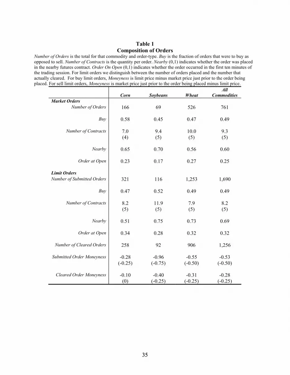
Table 1 provides summary statistics for market and limit orders for CBOT Wheat, Corn

and Soybean contracts. We have a total of 761 market orders and 1,690 limit orders for which we

have adequate data. Orders for Wheat account for 69 percent of market orders and 74 percent of

limit orders. Corn is the next most actively traded contract, accounting for 22 percent of market

orders and 19 percent of limit orders, while Soybeans account for the remainder of both order

types.

Market and limit orders are almost equally divided between buy and sell orders. In

addition, median order sizes are exactly the same at 5 contracts – the mean order size for market

orders is slightly larger at 9.3 contracts versus 8.2 contracts. Larger orders are less likely to be

filled all at once. Approximately 6 percent of our market orders are split fills, while less than 1

percent of the limit orders are split fills (details are not presented in Table 1.) For the split fill

market orders, the average order size is 37 contracts. The majority of orders are in the nearby

contract, i.e. the one that is next to expire. Finally, approximately 30 percent of our orders occur

before or during the first ten minutes of floor-based trading.

15 15

Limit orders that are placed away from the current market price often will not execute.

For our sample of limit orders, 74 percent are eventually executed while 26 percent are not. We

calculate moneyness as the difference between the initial limit price and the market price for the

most recent tick prior to the order being placed. For buy orders, moneyness is calculated as limit

price minus market price, while for sell orders, it is calculated as market price minus limit price.

Thus, in either case, positive moneyness indicates an order that should be immediately

executable while a limit order with negative moneyness will be held in the floor broker’s deck of

orders until the market attains the limit price or the order is cancelled. For all submitted limit

orders, mean (median) moneyness values are -0.53¢ (-0.50¢). Thus, most limit orders are placed

at slightly worse than the current market price. For the subset of cleared limit orders, mean

(median) values of moneyness are -0.28¢ (-0.25¢). One reason why there is so little difference in

initial moneyness values for executed and non-executed limit orders is that limit orders are often

updated. Thus, if the market moves away from the limit price, the retail trader may contact the

introducing brokerage and alter the limit price – updating occurs for approximately 20 percent of

our limit orders.

B. Univariate Statistics on Time-to-Clear and Slippage.

Table 2 reports summary statistics on time-to-clear and slippage. Because we require an

estimate of market price just prior to the order being placed in order to calculate slippage for

market order, we exclude orders that were placed outside the regular trading period of 9:30 am to

1:30 pm. For consistency, this exclusion also applies to limit orders. We also exclude

16 16

observations where the reported clearing price was outside the high-low price range for the

day.22

Remember that we have a precise record of when an order is placed, but an imprecise

record of when an order actually clears. To estimate time-to-clear for market orders, therefore,

we search the CBOT time and sales transactional data for the first occurrence of the recorded

clearing price subsequent to the time when the order was placed. The ensuing time lag is our

minimum estimate of time-to-clear. We also calculate a maximum estimate of time-to-clear

which is equal to the minimum estimate plus the additional time lag until the next reported

CBOT transaction that generates a price change.23 As long as the order cleared in the first

window of opportunity, the actual time-to-clear should lie somewhere in between the minimum

and maximum estimate. Unfortunately, the CBOT time and sales data can be subject to price

gapping when the market is highly volatile. Thus, the data may indicate a price jump from 250¢

per bushel to 251¢ while in reality price transitioned from 250¢ to 250.50¢ to 251¢. This can

occur when price changes are so fast that monitoring external to the pit cannot keep up. While

this is a rare occurrence and will not significantly affect our slippage calculations, it introduces

error into our time-to-clear estimates and may explain some of the outlying time-to-clear

observations.

22 All observations with clearing prices outside the high-low price range for the day have been double-checked for accuracy. Either there was a mistake made in writing the ticket by the introducing brokerage or the order was an “Out-Trade”. Out-Trades arise when there is confusion or miscommunication among participants in the pit. For example, a broker might think he executed a trade for one contract at 210 while the counterparty thought the agreed upon price was 211 – perhaps the market price never dropped below 210.5 on that particular day. Out-Trades, particularly those representing small quantities, are usually informally adjudicated after the close of trade by the two parties involved in the transaction. This ex-post settling up may not be reflected on the actual order ticket. 23 To economize on data entry effort and storage space, the CBOT time and sales data report price and time only when a new futures price occurs on the floor. For example, assume that a new wheat price of $3.00 per bushel was obtained at 10:00 am and that five subsequent trades also occurred at $3.00 per bushel at one minute increments, followed by a trade at $3.01 at 10:06. The CBOT tape will only show the 10:00 trade at $3.00 and the 10:06 trade at $3.01. If our data has a trade placed at 9:59 and cleared at $3.00, we will calculate a minimum time-to-clear of one minute and a maximum time-to-clear of seven minutes.

17 17

For limit orders, time-to-clear is slightly more complicated. First, we limit ourselves to

limit orders that actually cleared. We start the clock when the CBOT time and sales transaction

data first report a price that is equal to the final limit price specified in the order. For minimum

time-to-clear, the clock stops at the first occurrence of a price equal to the price at which the

order clears. In most instances, the order clears at the limit price so the minimum clearing time

is zero. Just as with a market order, the maximum time-to-clear is calculated as minimum time-

to-clear plus the time lag until the next CBOT reported price change.

For market orders as a whole, the average value of minimum time-to-clear is 139 seconds

with a median of 27 seconds. The 5th and 95th percentiles are zero seconds and 379 seconds

respectively.24 For maximum time-to-clear, the average is 182 seconds and the median is 76

seconds. For limit orders, the average minimum time-to-clear is 113 seconds while the median is

zero seconds. The median of zero seconds is not surprising given that our clock starts when the

market hits the limit price and most limit orders are subsequently executed at the limit price.

Mean (median) maximum time-to-clear for limit orders is 148 (19) seconds.

As a time-to-clear benchmark, Kurov (2005) documents mean (median) time-to-clear for

CME market orders in lean hog and live cattle pits of 98.3 (38) seconds and 113.1 (41) seconds

respectively. His time clock begins when the order is receipt stamped on the trading floor, not at

the introducing brokerage. Thus, if similar floor-based delays occur in the CBOT Corn, Soybean,

and Wheat pits, this suggests that our median order takes a maximum of approximately 40

seconds to make it from the associated person taking the order at the introducing brokerage to the

trading floor.

24 For market orders, the correlation between our minimum clearing time calculated with CBOT time and sales data and a clearing time calculated with the actual fill time stamp on the ticket is only about 0.25. The low correlation is consistent with our statement that the fill time stamps are not particularly accurate.

18 18

With delays in clearing comes the possibility of slippage. Calculating slippage is

straightforward. For market orders, we identify the closest previous transaction reported in the

CBOT time and sales transaction data for that commodity. For market buy orders, we then

subtract the clearing price from this pre-submission price. For market sell orders, we subtract the

pre-submission price from the clearing price. Across market orders for all three contracts,

slippage averages only -.110 cents or slightly less than -1/8¢ per contract (to the trader’s

detriment). This is approximately half of the minimum price movement in these contracts.

Indeed, a t-test for whether observed slippage is significantly different from -1/8¢ has a p-value

of 0.45.

While no bid-ask spread is posted, market order slippage of -1/8¢ is likely attributable to

buy orders clearing at the asking price and sell orders clearing at the bid price. Given that the

most recent transaction price utilized in our slippage calculation is equally likely to be at either

the bid or ask – on average it is in the middle – slippage of -1/8¢ is exactly what one would

expect in an unbiased trading environment. Thus, despite the retail trader lament that the trading

process is biased against them – our hypothesis 1 – such complaints are not supported by our

data.

While market order slippage, on average, is not significantly different from what one

would expect from bid-ask bounce, there is a reasonable amount of cross-sectional variation. The

standard deviation of market order slippage is 0.473¢ with a minimum value of -4.5¢ and a

maximum of 5.5¢. With the underlying asset for these contracts being 5,000 bushels of either

wheat, corn or soybeans, these minimum and maximum values correspond to a loss of $225 and

a gain of $250 per contract relative to the trader’s expected price. Given that the one-way

19 19

commission paid by our retail traders is $14, we consider the potential cost of slippage on market

orders to be economically meaningful.

For limit orders, median slippage across all three contracts is zero, indicating that most

are cleared at the limit price. There are no negative values as floor traders are “held to the limit”.

A limited number of positive values with price improvement, however, generate the positive

average limit order slippage value of 0.025¢. Whether price improvement results from deliberate

delay by floor traders in a market that is trending in the retail trader’s favor, or price

improvement reflects the censored result of inadvertent floor trader delay/inattention is unclear.

While there is some variation in limit order slippage - the standard deviation of limit order

slippage is 0.159¢ - it is significantly less than that which is observed for market order slippage.

One way, therefore, that retail traders can protect themselves from adverse slippage is to submit

limit orders rather than market orders. We will explore this in greater detail later in the paper.

C. Regression Analysis of Time-to-Clear and Slippage

To assess whether the factors described in hypotheses 2a through 3d affect cross-

sectional variation in time-to-clear and slippage, we rely on multivariate regressions.

Unfortunately, time-to-clear is bounded from below at zero and is, therefore, not normally

distributed. While slippage is approximately normally distributed, all of our hypotheses concern

the magnitude of slippage, not its signed value. Thus, our slippage analysis focuses on the

absolute value of slippage. Like time-to-clear, this is bounded from below at zero and is not

normally distributed. To account for non-normality, we rely on Generalized Linear Models

(rather than Ordinary Least Squares) with the assumption that error terms follow a gamma

20 20

distribution. This is a reasonably good approximation given the characteristics of our dependent

variables (see Hardin and Hilbe; 2001).

In our analysis, we use three related measures as proxies for market volatility. The first

measure is the range of CBOT reported prices for the ten minutes prior to the placement of the

order. The second measure is the standard deviation of continuously compounded returns per

second over the same ten minute interval. For this measure, we calculate the continuously

compounded return as 1000*log[((pricet + pricet-1)/2)/((pricet-1 + pricet-2)/2)]/(elapsed time). The

price averaging in both the numerator and denominator is done to reduce the impact of bid-ask

bounce on the continuously compounded return. Our third measure is the raw number of reported

price changes reported during the ten minute window. For market depth, we utilize both total

daily trading volume and open interest, recorded in thousands of contracts.

Bid-ask spread is partly a measure of market volatility and partly a measure of market

depth. Following Wang, Michalski, Jordan, and Moriarity (1994), we estimate bid-ask spread

using triplets of prices in the CBOT time and sales data where the middle price in the triplet is

either the high price or the low price of the series. Two examples would be a price series of 210,

210.25, 210, or 210, 209.5, 209.75. For each low-high-low or high-low-high triplet, we estimate

a relative bid-ask spread as 100*abs[(pricet – pricet-1)/((pricet + pricet-1)/2)] where pricet is the

middle price in the triplet. This process eliminates price series that constitute a run-up

(potentially a series of buy-driven transactions) as well as price series that constitute a downturn

(potentially a series of sell-driven transactions). 25

25 Kurov (2005) measures bid-ask spread in the same manner, classifying up-tick trades as ask prices and down-tick trades as bid prices. The difference between consecutive bid and ask prices constitutes his bid-ask spread. He then calculates market volatility as the standard deviation of the last 15 continuously compounded returns based on estimated ask prices. For consistency with our other volatility measures, we measure the standard deviation of returns over the previous 10 minutes rather than relying on the last 15 calculated returns.

21 21

Summary statistics for these independent variables are reported in Table 3, Panel A for

market orders and all executed limit orders. The data reported in Table 3 are for each individual

commodity. Here in the text, we limit ourselves to discussing market orders and limit orders as a

whole. Of our three measures of price volatility, the number of reported price changes is the

easiest to conceptualize.26 Mean (median) values for price change frequency are 21.5 (17) for

market orders and 23.6 (21) for limit orders. Price range and standard deviation of returns show

the same pattern of being larger when limit orders are submitted. Mean (median) price range is

1.15 (1) for market orders and 1.28 (1) for limit orders. The standard deviations of returns range

from 0.14 (0.09) for market orders to 0.15 (0.11) for limit orders.

While time and sales data for the pre-market period appear in the CBOT data, we exclude

it from our calculations. Thus, for the 25 to 30 percent of our orders placed at the opening, there

may be only a few minutes worth of prior market data and our calculated price volatility

measures may be biased. Trading, however, is typically heavier at the opening. Indeed, the mean

and median values for all three measures of price volatility are greatest during the first 10

minutes of trade (results not presented in tables.) Prior research also documents that bid-ask

spreads are greatest at the open (Ferguson and Mann; 2001). Since trading at the open is unique,

in subsequent regression analysis we will generally include a dichotomous variable for trades

placed during the opening ten minutes of trading.

For daily volume and open interest (our proxies for market depth), our mean (median)

values for market orders are 20.3 (16.9) and 85.6 (76.3) thousand contracts respectively. For

limit orders mean (median) values are approximately the same - 19.2 (17.1) thousand contracts

26 While price change frequency is a measure of volatility, it also provides a lower bound on the volume of transactions occurring during the interval. For example, assume that five buy orders at the ask price occur in a row followed by one sell order at the bid price. If bid and ask don’t change during this trade sequence, the CBOT time and sales transaction data will record only two transactions – the first and last ones that generated the price changes.

22 22

for daily volume and 86.5 (76.4) thousand contracts for open interest. Our mean (median)

relative bid-ask spreads are 0.105 (0.094) for market orders and 0.104 (0.096) for limit orders.

Given an average price of approximately 270¢, a relative bid-ask spread of 0.105 represents a

value that is slightly greater than 0.25¢. Note that while the majority of our traders’ orders are in

Wheat, Wheat appears to be the least active pit.

Because of high correlation across many of our independent variables, care must be taken

when including them jointly when estimating regressions. For the subset of market order

observations, Table 3, Panel B presents correlations of the independent variables displayed in

Panel A. As shown in the table, the three measures of market volatility (price range, standard

deviation of returns, and number of price changes) are all highly correlated as are the two

measures of market depth (daily volume and open interest). In addition, bid-ask spread exhibits

substantial correlation with both price range (ρ=.40) and standard deviation of returns (ρ=.45).27

Finally, price change frequency is relatively highly correlated with daily volume (ρ=.33) and

with open interest (ρ=.56).

GLM regression results where market order time-to-clear is the dependent variable are

presented in Table 4. In each specification, dummy variables for Corn and Wheat are included to

control for unobserved differences in each pit’s trading environment. We also exclude outlying

observations where our minimum estimated clearing time is greater than 10 minutes.

As expected, positive coefficient estimates for order size (significant at the five percent

level in specifications 3 and 5 and at the ten percent level in all other specifications) demonstrate

that time-to-clear increases with order size. Our GLM regression is still linear in nature. Thus, a

coefficient estimate of 1.66 in specification 3 indicates that a one standard deviation increase in

27 Mann and Manaster (1996) also document that futures price volatility is positively correlated with bid-ask spread. Part of the relationship between slippage and price volatility is likely attributable to bid-ask bounce.

23 23

order size from 5 contracts to 15 contracts results in a 16.6 second increase in time-to-clear.

Thus, while floor brokers may pay greater attention to larger orders, the difficulty in finding

counterparties actually leads to longer clearing times.28

In addition to order size, specifications 1-4 also demonstrate that price volatility has an

impact. Coefficient estimates for price range, the standard deviation of prices, and price change

frequency are all negative with price range being significant at the ten percent level and standard

deviation of returns being significant at the five percent level. Estimated coefficients for both

open interest and daily volume are negative and statistically significant at the ten percent level.

Results for these two variables are significantly stronger (results not presented in tables) when

none of the price volatility measures are included in the regression. Finally, time-to-clear is

increasing with the estimated bid-ask spread. With one exception, coefficient estimates for bid-

ask spread are significant at the one percent level. As discussed earlier, price volatility measures

calculated during the opening ten minutes of trade might be suspect. When a dummy variable for

orders placed in the opening ten minutes of trading is included in the regressions, however, (not

reported in tables) it is never significant and has minimal impact on other coefficient estimates.

Similarly, excluding orders placed during the opening ten minutes has no significant impact on

time-to-clear regression results.

It is likely that the regression results for price volatility, market depth, and bid-ask spread

all reflect the same underlying phenomenon. Specifically, trades clear more quickly when the

trading pit is more active and each measure is at least partly a proxy for the level of activity at

the time the trade is placed. Further analysis (not displayed in tables) does not reveal any non-

28 Whether an order is executed via a split-fill does not affect these results. Moreover, coefficient estimates for split-fill (not displayed in tables) are not statistically significant.

24 24

linear effects for these independent variables. Thus, there is no evidence of bottlenecks when the

trading pit is particularly active.

Ultimately, we suspect our retail traders should be relatively indifferent if an order takes

60 seconds to clear rather than 30 seconds to clear. With increased clearing time, however, it is

likely that there will be increased slippage. Indeed, the correlation between minimum time-to-

clear and the absolute value of slippage is 0.45 for the sample of market orders analyzed in Table

4. Since slippage is denominated in dollars, we expect it to be a significant concern of our retail

traders. Regression results for market order slippage are presented in Table 5. For consistency,

we also exclude the observations with long clearing times that were excluded in our time-to-clear

analysis.

As with time-to-clear, we find that the absolute value of slippage increases with order

size. For three of the five specifications, coefficient estimates are significant at the five percent

level. The economic magnitude of these estimates, however, is small. The coefficient estimates

of approximately 0.003 indicate that a one standard deviation increase in order size from 5 to 15

contracts generates an increase in slippage of only 0.03 cents which is a $1.50 impact per

contract.

The absolute value of slippage also depends on market conditions. Coefficient estimates

demonstrate that slippage increases with all three measures of price volatility. Here our results

are quite robust with statistical significance at the one percent level for the range of prices, the

standard deviation of returns (one of two specifications), and the log of price change frequency.

While time-to-clear was decreasing in our proxies for market depth, slippage does not seem to

depend on either daily trading volume or open interest. For parsimony, specifications

25 25

incorporating open interest are not included in Table 5. Results for open interest, however, are

quite similar to the results displayed for log daily volume.29

In contrast to the results for daily volume and open interest, bid-ask spread is positively

related to the average value of slippage and estimated coefficients are all statistically significant

at the one percent level. In many respects, this is a simple mechanical relationship that must be

controlled for in the process of evaluating slippage. If transaction prices are bouncing back and

forth between 270 bid, 270.25 ask (for a raw bid-ask spread of 0.25¢ and a relative bid-ask

spread of 0.00093), on average, our retail trader’s expected price will be 270.125. Buy-initiated

orders should clear at 270.25 and sell-initiated orders should clear at 270, in both cases

generating slippage of approximately -0.125¢. Remember that our bid-ask spread variable is

actually 100 times the estimated relative bid-ask spread (i.e. it will be 0.093 rather than 0.00093).

Thus, our coefficient estimates of approximately 3.6 suggest that if the raw spread increases from

0.25¢ to 0.50¢, slippage will increase by approximately 0.033¢. Our suspicion is that noise

biases this coefficient estimate toward zero.

The last item of interest in the slippage regressions is whether the impact differs if the

order was placed during the opening ten minutes of trading. This control variable was never

significantly different from zero when included in the clearing time regressions. Here, however,

order-on-open always has a positive estimated coefficient and is statistically significant at the

one percent level, indicating that slippage is greater, ceteris paribus, at the daily open of trading.

Simply eliminating orders placed during the first ten minutes of trades (not shown in tables) has

no significant effect on other coefficient estimates.

29 In their analysis of slippage on stop orders placed by a single commodity trading fund, Greer et al. (1992) also found that slippage increased with daily price range and with order size. They found no evidence, however, that slippage and market depth are related. Note that Greer et al. (1992) analyze the signed value of slippage, not the absolute value of slippage.

26 26

The picture that emerges from our analysis of time-to-clear and the absolute value of

slippage seems internally consistent. Our evidence consistently shows that both time-to-clear and

the absolute value of slippage increase with order size, demonstrating a decline in trade

execution quality. We also find convincing support for hypotheses 3a-3c regarding the

relationship between trade execution quality and market conditions. We find that both time-to-

clear and the absolute value of slippage increase with our proxies for price volatility with time-

to-clear also decreasing with both proxies for market depth. Hypothesis 3d (slippage and market

depth), however, is not supported empirically.

D. The Choice of Market Versus Limit Orders.

One way for retail traders to minimize the adverse effects of slippage is to simply submit

limit orders instead of market orders. In particular, a trader could submit a marketable limit order.

Indeed, Table 2 documented that slippage on limit orders is minimal relative to slippage on market

orders. Our final analysis assesses whether retail traders respond to the possibility of adverse

slippage by substituting limit orders for market orders when conditions suggest that slippage is

likely. If so, then this will provide empirical evidence to back up our claim that slippage is truly a

concern of retail traders.

Following Kurov (2005), we estimate Probit model regressions where the dependent

variable takes a value of one for market orders and zero for limit orders. The results are presented

in Table 6. Our dependent variables are essentially the same as in our previous analysis of time-to-

27 27

clear and slippage.30 If the factors that are conducive to long time-to-clear and high slippage affect

the choice between market and limit orders, the implication is that retail traders really are

concerned about the possibility of adverse slippage.

Previously, we noted that market order slippage increased with order size. Consistent with

this being a cause for concern for our traders, we find that coefficient estimates for log order size

are negative and statistically significant at the five percent level in three of the five specifications

reported in Table 6 (for the remaining two specifications log order size is significant at the ten

percent level). The coefficient estimates of approximately -0.08 indicate that the probability of a

market order declines by approximately 3 percent when there is a one standard deviation increase

in log order size. Similar results have been documented for equity markets. Harris and Hasbrouck

(1996), for example, report that limit orders on SuperDOT are generally larger than market orders.

Consistent with our earlier results, we also find that market orders are less likely when

market prices are more volatile. This is also consistent with prior research on limit versus market

orders in equity markets (see e.g. Bae, Jang, and Park; 2003, and Ranaldo; 2004). In contrast,

however, Kurov (2005), finds that futures market limit orders are less likely with high price

volatility. Coefficient estimates for both the range of prices and the number of price changes in the

10 minute interval before the trade is placed are negative and significant at the five percent level.

Estimates for the standard deviation of returns, however, are not statistically significant. While

measures of market depth were not significant in our slippage regressions, estimated coefficients

for daily trading volume are positive and statistically significant at the five percent level. Similarly,

coefficient estimates for open interest are also positive (not displayed in tables), but are not

30 For two of our dependent variables, order size and the number of recorded price changes in the prior ten minute interval, we first transform them to their log equivalent. This transformation leads to cleaner results in the non-linear probit regression.

28 28

significantly different from zero. As with order size, these results suggests that retail traders are

concerned about the possibility of adverse slippage.

In our earlier analysis of time-to-clear and slippage, bid-ask spread figured prominently as

an independent variable. In the Probit regressions, however, bid-ask spread is never close to being

significant. Due to its correlation with other independent variables, we opt to leave bid-ask spread

out of our probit analysis. It is unclear why our retail traders appear unconcerned about the

magnitude of the bid-ask spread when it comes to choosing between market and limit orders. One

possibility is that, since bid-ask spread is not published and has to be inferred from the CBOT time

and sales data, it might simply not be present in our retail traders’ information sets at the times that

they place orders.

In our earlier analysis of time-to-clear and slippage, we included order-on-open as a control

variable. Despite the fact that slippage is greater during the opening of the trading session, order-

on-open is not a significant factor in the choice between market and limit orders (results not

presented in tables.) We do, however, include two additional controls. The first is whether the

order is part of a spread trade where a retail trader typically goes long (buys) one contract and short

(sells) another. The two legs of the spread might be the same commodity but with different

expiration dates or the legs might be in different commodities. We also include whether the order

is for the nearby contract. Coefficient estimates for spread are positive and significant at the one

percent level in all five specifications while coefficient estimates for nearby are negative and

significant at the five percent level or better in each specification.

IV Conclusion

29 29

Our paper provides one of the first direct analyses of futures market slippage. Using a unique data

set that documents the trades of 69 retail traders, we track orders from the moment they are

submitted to the introducing brokerage until the time that they clear on the CBOT trading floor. In

doing so, we make three contributions. First, we demonstrate that the common complaint of retail

traders – that “the trading system is systematically biased against them and in favor of

professionals on the floor of the exchange” – does not appear to be true. On average, orders

execute rapidly. The typical time it takes an order to clear is well under two minutes. In addition,

the slippage that results from this time delay is approximately equal to what one would expect

from buying at the ask price and selling at the bid price. Thus, participants on the floor of the

exchange do not appear to be colluding to the detriment of retail traders.

Our second contribution is to show that while slippage is not a problem on average, there is

significant and predictable cross-sectional variation in slippage. Thus, some market conditions are

conducive to long time-to-clear and significant slippage. We find that time-to-clear and slippage

are greater for larger orders and when bid-ask spreads are wide. Similarly, when there is greater

price volatility, both time-to-clear and slippage are greater.

Our final contribution is to document that risk-averse traders are sensitive to the possibility

of large values of slippage. When conditions suggest that slippage is likely, retail traders are more

likely to submit limit orders which, while subject to the possibility that the order does not clear, are

significantly less affected by slippage.

Since the time period spanned by our data, significant changes have occurred at the CBOT.

First, use of electronic order routing to the trading pit has increased substantially. Second, most

introducing brokerages have instituted electronic order placement systems. Finally, the CBOT

instituted side-by-side electronic trading for agricultural commodities on August 1, 2006.

30 30

Presumably, these changes will result in faster clearing times and reduced slippage. Whether this

indeed is the case can certainly be the subject of future research.

31 31

References:

Bae, K., H. Jang, and K. Park, 2003, Traders’ Choice Between Limit and Market Orders: Evidence from NYSE Stocks, Journal of Financial Markets 6, 517-538. Bessembinder, H., and P. Seguin, 1993, Price Volatility, Trading Volume, and Market Depth: Evidence from Futures Markets, Journal of Financial and Quantitative Analysis 28, 21-39. Black, F., 1986, Noise, Journal of Finance, 41, 529-543. Board of Trade, City of Chicago, 2002 CBOT Rulebook, 308-309 Brorson, B. W., 1989, Liquidity Costs and Scalping Returns in the Corn Futures Market, Journal of Futures Markets, 9, 225-236. Calhoun, K., 1989, How to Evaluate a Commodity Trading System, Technical Analysis of Stocks and Commodities, V.7, 12, 458-459. Coval, J., and T. Shumway, 2001, Is Sound Just Noise?, Journal of Finance, 1887-1910 Covington, B., 1996, Considering Risk, Technical Analysis of Stocks and Commodities, V.4,7, 254-255. Daigler, R. and M. Wiley, 1999, The Impact of Trader Type on the Futures Volatility-Volume Relation, Journal of Finance 54, 2297-2316. Easley, D., and M. O’Hara, 1987, Price, Trade Size, and Information in Securities Markets, Journal of Financial Economics 19, 69-90. Ferguson, M., and S.C. Mann, 2001, Execution Costs and Their Intraday Variation in Futures Markets, Journal of Business 74, 125-160. Frino, A., T. Oetomo, and G. Wearin, 2004, The Cost of Executing Large Orders on the Sydney Futures Exchange, Sydney Futures Exchange Market Insights 3, 1-6. Frino, A., and T. Oetomo, 2005, Slippage in Futures Markets: Evidence from the Sydney Futures Exchange, Journal of Futures Markets 25, 1129-1146. Gallacher, W., 1994, Winner Take All – A Brutally Honest and Irreverent Look at the Motivations and Methods of Top Traders, McGraw Hill, New York. Gray, R., 1979, Commentary on a Reexamination of Price Changes in the Commodity Futures Market, International Futures Trading Seminar Proceedings, Chicago Board of Trade, Vol V., 153-154.

32 32

Greer, T, B. W. Brorsen, and S. Liu, 1992, Slippage Costs in Order Execution for a Public Futures Fund, Review of Agricultural Economics 14, 281-288. Hardin, J., and J. Hilbe, 2001, Generalized Linear Models and Extensions, Stata Press, College Station TX. Harris, L., and J. Hasbrouck, 1996, Market Versus Limit Orders: The SuperDOT Evidence on Order Submission Strategy, Journal of Financial and Quantitative Analysis 31, 213-231. Kaufman, P., 1995, Smarter Trading – Improving Performance in Changing Markets, Donnelly & Sons Co. Knez, P., and M. Ready, 1996, Estimating the Profits from Trading Strategies, Review of Financial Studies 9, 1121-1163. Kurov, A., 2005, Execution Quality in Open-Outcry Futures Markets, Journal of Futures Markets 25, 1067-1092. Kuserk, G., and P. Lock, 1993, Scalper Behavior in Futures Markets: an Empirical Examination, Journal of Futures Markets, 13, 409-431. Kyle, A., 1985, Continuous Auctions and Insider Trading, Econometrica 53, 1315-1335. Liu, S., S. Thompson, and P. Newbold, 1992, Impact of Price Adjustment Process and Trading Noise on Return Patterns of Grain Futures, Journal of Futures Markets 12, 575-585. Lukac, L., and B.W. Brorsen, 1990, A Comprehensive Test of Futures Market Disequilibrium, Financial Review 25, 593-622. Manaster, S., and S.C. Mann, 1996, Life in the Pits: Competitive Market Making and Inventory Control, Review of Financial Studies 9, 953-975. Martell, T., and R. Trevino, 1990, The Intraday Behavior of Commodity Futures Prices, Journal of Futures Markets 10, 661-671. Myers, D., 1998, The British Pound Cubed, Technical Analysis of Stocks and Commodities, V. 16, 11, 495-507. Radnoty, C., 1991, Using Spread Orders to Roll Forward, Technical Analysis of Stocks and Commodities V.9, 5, 211-213. Ranaldo, A., 2004, Order Aggressiveness in Limit Order Book Markets, Journal of Financial Markets 7, 53-74. Ready, M., 2002, Profits From Technical Trading Rules, Financial Management, 43-61.

33 33

Sarkar, A., and L. Wu, 2000, Conflicts of Interest and Execution Quality of Futures Floor Traders, Federal Reserve Bank of New York working paper. Tharp, V., 1993, Trade Your Way to Financial Freedom, McGraw Hill, New York. Wang, G.H., R.J. Michalski, J.V. Jordan, and E.J. Moriarity, 1994, An Intraday Analysis of Bid-Ask Spreads and Price Volatility in the S&P 500 index futures market, Journal of Futures Markets, 14, 837-859. Working, H., 1954, Price Effects of Scalping and Day Trading, Proceedings of the Chicago Board of Trade Annual Symposium, 114-139.

34 34

Figure 1: Steps in the Order Process. (1) Order is placed. (2) The associated person hands the order to the Introducing Brokerage’s order desk.

(3) The IB order desk transmits order to the clearing firm’s trading booth clerk where the order is rewritten. (4) The clerk hands the order to the runner. (5) The runner delivers the order to the floor broker’s clerk. (6) The floor broker’s clerk delivers the order to the floor broker. (7) The floor broker offers the order to the crowd which is accepted by another floor broker or a floor trader as the counterparty.

Retail Trader

Associated Person

IB Order Desk

FCM Trading Booth Clerk

Floor Broker Clerk

Floor Broker

Floor Trader (‘Local’)

Runner

35 35

Table 1

Composition of Orders Number of Orders is the total for that commodity and order-type. Buy is the fraction of orders that were to buy as opposed to sell. Number of Contracts is the quantity per order. Nearby (0,1) indicates whether the order was placed in the nearby futures contract. Order On Open (0,1) indicates whether the order occurred in the first ten minutes of the trading session. For limit orders we distinguish between the number of orders placed and the number that actually cleared. For buy limit orders, Moneyness is limit price minus market price just prior to the order being placed. For sell limit orders, Moneyness is market price just prior to the order being placed minus limit price.

Corn

Soybeans Wheat

All Commodities

Market Orders Number of Orders 166 69 526 761

Buy 0.58 0.45 0.47 0.49

Number of Contracts 7.0

(4) 9.4 (5)

10.0 (5)

9.3 (5)

Nearby 0.65 0.70 0.56 0.60

Order at Open 0.23 0.17 0.27 0.25

Limit Orders Number of Submitted Orders 321 116 1,253 1,690

Buy 0.47 0.52 0.49 0.49

Number of Contracts 8.2 (5)

11.9 (5)

7.9 (5)

8.2 (5)

Nearby 0.51 0.75 0.73 0.69

Order at Open 0.34 0.28 0.32 0.32

Number of Cleared Orders 258 92 906 1,256

Submitted Order Moneyness -0.28

(-0.25) -0.96

(-0.75) -0.55

(-0.50) -0.53

(-0.50)

Cleared Order Moneyness -0.10 (0)

-0.40 (-0.25)

-0.31 (-0.25)

-0.28 (-0.25)

36 36

Table 2 Time-to-Clear and Slippage

For market orders, Minimum Time-to-Clear is time of first reported CBOT transaction after the order time where market price equals fill price minus order time. Maximum Time-to-Clear is Minimum Time-to-Clear plus the time lag until the next reported CBOT price change. For limit orders, Minimum Time-to-Clear is time of the first reported CBOT transaction after the order time where market price equals fill price minus time of the first reported CBOT transaction after the order time where market price equals limit price. Maximum Time-to-Clear is Minimum Time-to-Clear plus the time lag until the next reported CBOT price change. Slippage is reported in cents per contract. For buy orders, Slippage is calculated as the trader's expected price minus fill price. For sell orders, Slippage is calculated as fill price minus the trader's expected price. See the text for details on how expected price is calculated for market orders and for limit orders. σ Slippage is the standard deviation of slippage while Observations is the number of observations for which we are able to calculate slippage. In each cell, the upper value is the mean while the lower value (in parentheses) is the median.

Corn Soybeans Wheat All Commodities Market Orders

Minimum Time-to-Clear

103 (9)

265 (11)

133 (44)

139 (27)

Maximum Time-to-

Clear 130 (35)

291 (39)

185 (85)

182 (76)

Slippage -0.007

(0) -0.207 (-0.25)

-0.129 (0)

-0.110 (0)

σ Slippage 0.456 0.564 0.459 0.473

Observations 142 64 480 686

Limit Orders

Minimum Time-to-Clear

60 (0)

134 (0)

127 (0)

113 (0)

Maximum Time-to-

Clear 87

(18) 168 (15)

163 (20)

148 (19)

Slippage 0.037

(0) 0.027

(0) 0.022

(0) 0.025

(0)

σ Slippage 0.207 0.208 0.137 0.159

Observations 225 82 780 1,087

37 37

Table 3, Panel A Price Volatility and Market Depth

For the ten minute window before each order is placed, Price Change Frequency is the number of market price changes, Price Range is the range of market prices, and σ Return is the standard deviation of continuously compounded return. Bid-Ask Spread is determined from the most recent triplet of prices where the middle price is either above or below the two other prices. Daily Volume is the total day’s trading volume in thousands of contracts at the CBOT for that particular contract. Open Interest is the total number of long positions outstanding in thousands of contracts for that particular contract.

Market Limit Corn Soybean Wheat Corn Soybean Wheat Price Change Frequency

25.5 (21)

30.1 (26)

19.3 (16)

25.0 (21)

27.0 (23)

22.3 (19)

Price Range 0.96

(0.75) 1.15

(1.00) 1.20

(1.00) 0.92

(0.75) 1.37

(1.25) 1.36

(1.25) σ Return 0.123

(0.091) 0.082

(0.094) 0.149

(0.093) 0.146

(0.115) 0.089

(0.073) 0.155

(0.112) Bid-Ask Spread 0.117

(0.116) 0.060

(0.052) 0.107

(0.092) 0.116

(0.114) 0.062

(0.052) 0.105

(0.094) Daily Volume 38.8

(36.7) 23.4

(24.4) 14.4

(13.9) 35.7

(32.3) 21.2

(22.5) 15.2

(14.7) Open Interest 169.9

(186.7) 60.0

(70.3) 62.4

(68.8) 177.8

(182.2) 62.4

(69.6) 66.0

(72.2)

Table 3, Panel B Correlation Matrix for Price Volatility and Market Depth

Correlations are calculated for the market order observations that are analyzed in tables 4 and 5. Price

Range σ Return Price

Change Frequency

Bid-Ask Spread

Daily Volume

Open Interest

Price Range 1.00 σ Return 0.58 1.00

Price Change Frequency 0.55 0.40 1.00 Bid-Ask Spread 0.40 0.45 -0.03 1.00 Daily Volume 0.16 0.05 0.33 0.09 1.00 Open Interest -0.01 0.14 0.56 0.03 0.73 1.00

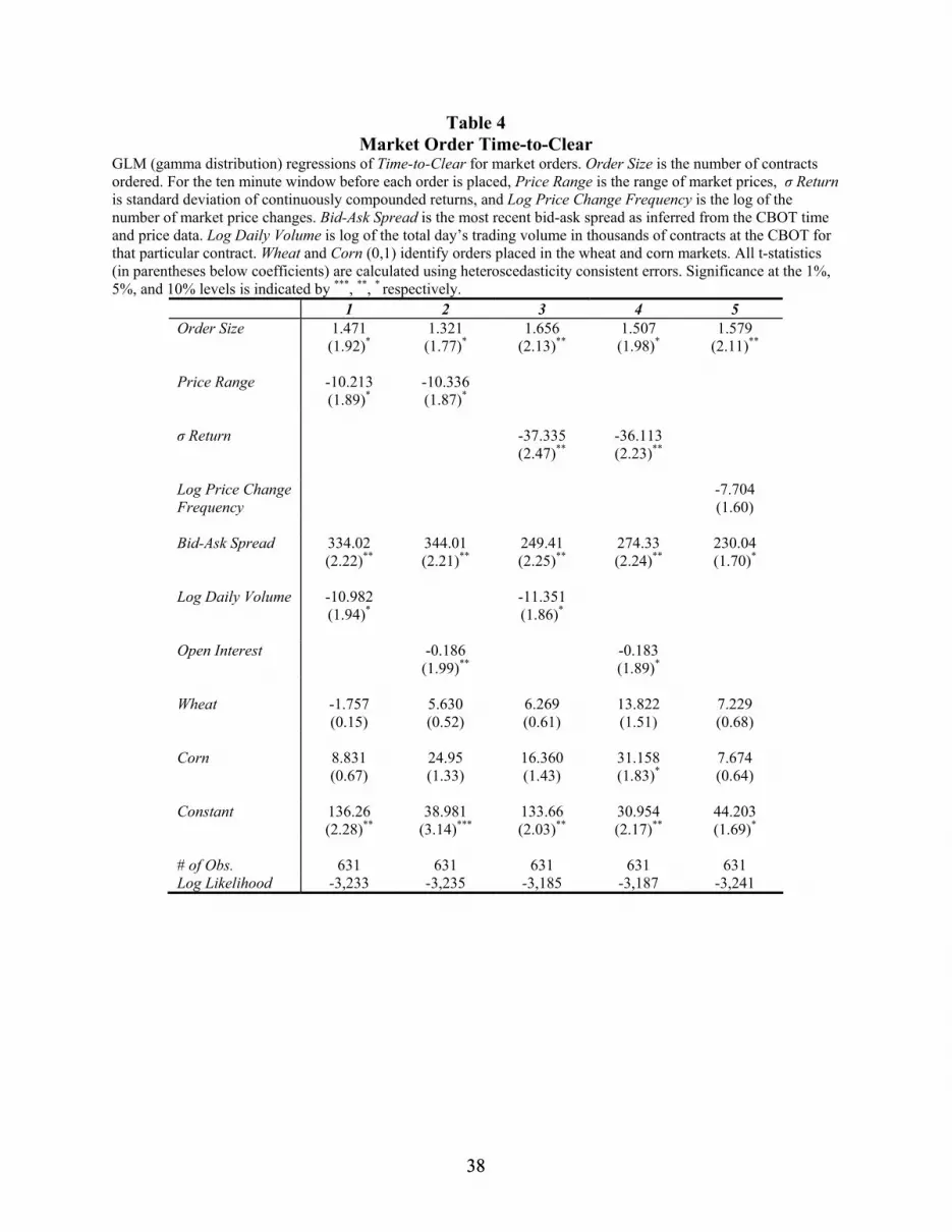
38 38

Table 4 Market Order Time-to-Clear

GLM (gamma distribution) regressions of Time-to-Clear for market orders. Order Size is the number of contracts ordered. For the ten minute window before each order is placed, Price Range is the range of market prices, σ Return is standard deviation of continuously compounded returns, and Log Price Change Frequency is the log of the number of market price changes. Bid-Ask Spread is the most recent bid-ask spread as inferred from the CBOT time and price data. Log Daily Volume is log of the total day’s trading volume in thousands of contracts at the CBOT for that particular contract. Wheat and Corn (0,1) identify orders placed in the wheat and corn markets. All t-statistics (in parentheses below coefficients) are calculated using heteroscedasticity consistent errors. Significance at the 1%, 5%, and 10% levels is indicated by ***, **, * respectively.

1 2 3 4 5 Order Size 1.471

(1.92)* 1.321 (1.77)*

1.656 (2.13)**

1.507 (1.98)*

1.579 (2.11)**

Price Range -10.213

(1.89)* -10.336 (1.87)*

σ Return -37.335

(2.47)** -36.113 (2.23)**

Log Price Change Frequency

-7.704 (1.60)

Bid-Ask Spread 334.02

(2.22)** 344.01 (2.21)**

249.41 (2.25)**

274.33 (2.24)**

230.04 (1.70)*

Log Daily Volume -10.982

(1.94)* -11.351

(1.86)*

Open Interest -0.186 (1.99)**

-0.183 (1.89)*

Wheat -1.757

(0.15) 5.630 (0.52)

6.269 (0.61)

13.822 (1.51)

7.229 (0.68)

Corn 8.831

(0.67) 24.95 (1.33)

16.360 (1.43)

31.158 (1.83)*

7.674 (0.64)

Constant 136.26

(2.28)** 38.981

(3.14)*** 133.66 (2.03)**

30.954 (2.17)**

44.203 (1.69)*

# of Obs. 631 631 631 631 631 Log Likelihood -3,233 -3,235 -3,185 -3,187 -3,241

39 39

Table 5 Magnitude of Market Order Slippage

GLM (gamma distribution) regressions of Absolute Value of Slippage for market orders. Order Size is the number of contracts ordered. For the ten minute window before each order is placed, Price Range is the range of market prices, σ Return is standard deviation of continuously compounded returns, and Log Price Change Frequency is the log of the number of market price changes. Bid-Ask Spread is the most recent bid-ask spread as inferred from the CBOT time and price data. Log Daily Volume is log of the total day’s trading volume in thousands of contracts at the CBOT for that particular contract. Wheat and Corn (0,1) identify orders placed in the wheat and corn markets. All t-statistics (in parentheses below coefficients) are calculated using heteroscedasticity consistent errors. Significance at the 1%, 5%, and 10% levels is indicated by ***, **, * respectively.

1 2 3 4 5 Order Size 0.0027

(1.99)** 0.0027 (1.98)**

0.0022 (1.69)*

0.0023 (1.71) *

0.0029 (2.01)**

Price Range 0.093

(4.20)*** 0.091

(3.88)***

σ Return 0.257

(2.69)*** 0.229

(2.33)**

Log Price Change Frequency

0.059 (6.16)***

Bid-Ask Spread 3.638

(3.86)*** 3.631

(3.92)*** 3.649

(4.13)*** 3.684

(4.04) *** 3.515

(5.01) *** Log Daily Volume 0.0028

(0.15) 0.019

(0.62)

Order on Open 0.108

(3.85)*** 0.108

(3.84)** 0.088

(3.42)*** 0.086

(3.20)*** 0.130

(4.56)***

Wheat -0.145

(2.62)** -0.140 (2.19)**

-0.161 (2.88)***

-0.135 (2.05) **

-0.086 (1.57)

Corn -0.254

(3.62)*** -0.253

(3.62)*** -0.268 (4.05)**

-0.269 (4.07)***

-0.231 (3.73)***

Constant -.047

(0.65) -0.075 (0.35)

0.038 (0.57)

-0.162 (0.46)

-0.148 (1.98)**

# of Obs. 631 631 621 621 631 Log Likelihood 149.16 149.18 137.30 137.93 155.37

40 40

Table 6 Choosing Between Market and Limit Orders

Probit regressions for whether an order is a market (coded 1) or limit order (coded 0). Log Order Size is log of the number of contracts ordered. For the ten minute window before each order is placed, Price Range is the range of market prices, σ Return is standard deviation of continuously compounded returns, and Log Price Change Frequency is the log of the number of market price changes. Daily Volume is the total day’s trading volume in thousands of contracts at the CBOT for that particular contract. Spread (0,1) denotes whether order is a spread. Nearby (0,1) denotes whether the underlying contract is the one closest to expiration. All t-statistics (in parentheses below coefficients) are calculated using heteroscedasticity consistent errors. Significance at the 1%, 5%, and 10% levels is indicated by ***, **, * respectively.

1 2 3 4 5 Log Order Size -0.074

(2.05)** -0.064 (1.77)*

-0.071 (1.96)**

-0.062 (1.69)*

-0.081 (2.23)**

Price Range -0.094

(2.40)** -0.090 (2.27)**

σ Return -0.134

(0.67) -0.173 (0.86)

Log Price Change Frequency

-0.113 (3.07)***

Daily Volume 0.0061

(2.84)*** 0.0061

(2.83)***

Spread 0.575

(7.10)*** 0.568

(6.98)*** 0.583

(7.17)*** 0.574

(7.02)*** 0.582

(7.18)***

Nearby -0.195

(3.09)*** -0.253

(3.86)*** -0.207

(3.26)*** -0.263

(4.01)*** -0.151 (2.27)**

Constant -0.139

(1.50) -0.229 (2.32)**

-0.226 (2.58)***

0.318 (3.37)***

0.054 (0.44)

# of Obs. 2,053 2,053 2,030 2,030 2,053 Log Likelihood -1,280 -1,276 -1,266 -1,262 -1,279