Simultaneous Unsupervised Learning of Disparate Clusterings

Prateek Jain, Raghu Meka and Inderjit S. DhillonDepartment of Computer Sciences, University of Texas

Austin, TX 78712-1188, USA{pjain,raghu,inderjit}@cs.utexas.edu

Abstract

Most clustering algorithms produce a single clustering fora given data set even when the data can be clustered natu-rally in multiple ways. In this paper, we address the difficultproblem of uncovering disparate clusterings from the datain a totally unsupervised manner. We propose two new ap-proaches for this problem. In the first approach we aim tofind good clusterings of the data that are alsodecorrelatedwith one another. To this end, we give a new and tractablecharacterization of decorrelation between clusterings, andpresent an objective function to capture it. We provide aniterative “decorrelated”k-means type algorithm to minimizethis objective function. In the second approach, we modelthe data as a sum of mixtures and associate each mixturewith a clustering. This approach leads us to the problem oflearning a convolution of mixture distributions. Though thelatter problem can be formulated as one of factorial learn-ing [8, 13, 16], the existing formulations and methods do notperform well on many real high-dimensional data sets. Wepropose a new regularized factorial learning framework thatis more suitable for capturing the notion of disparate clus-terings in modern, high-dimensional data sets. The resultingalgorithm does well in uncovering multiple clusterings, andis much improved over existing methods. We evaluate ourmethods on two real-world data sets - a music data set fromthe text mining domain, and a portrait data set from the com-puter vision domain. Our methods achieve a substantiallyhigher accuracy than existing factorial learning as well astraditional clustering algorithms.

1 Introduction

Clustering data into groups based on similarity is often oneof the most important steps in any data analysis application.Currently, most clustering algorithms partition the data intogroups that are disjoint, while other algorithms extend thisapproach to probabilistic or overlapping clustering. How-ever, in many important applications it is necessary to un-cover disparate or alternative clusterings1 in order to reflect

1Throughout this paper, aclusteringwill refer to a set of disjoint clustersof the data.

Figure 1: Images of different persons in different poses.Each row has different persons in the same pose. Eachcolumn has the same person in different poses.

the different groupings inherent in the data. As an exam-ple, consider a set of pictures of different persons in differ-ent poses (see Figure 1). These images can be clustered bythe identity of the person in the picture or by the pose of theperson. Given such a dataset it would be desirable to recovertwo disparate clusterings of the data - one based on the iden-tity of the person and the other based on their pose.

The above problem arises naturally for many otherwidely used datasets, for instance: news articles (can beclustered by the main topic, or by the news source), reviewsof various musical albums (can be clustered by composers, orby other characteristics like genre of the album), and movies(can be clustered based on actors/actresses or genre).

Most existing methods to recover alternative clusteringsuse semi-supervision or side-information about one or moreof the clusterings. Since clustering is generally the first stepin data analysis, such information might not be availablebeforehand. For example, news articles change dynamicallyand it is infeasible to manually label them by topic and thesource. Thus, completely unsupervised techniques to finddisparate clusterings are immensely useful.

In this paper, we present two novel unsupervised ap-

proaches for discovering disparate clusterings in a givendataset. In the first approach we aim to find multiple clus-terings of the data which satisfy two criteria: a) the cluster-ing error of each individual clustering is small and b) differ-ent clusterings have smallcorrelationbetween them. To thisend, we present a new and computationally tractable charac-terization ofcorrelation(or decorrelation) between differentclusterings. We use this characterization to formulate ak-means type objective function which contains error terms foreach individual clustering along with a regularization termcorresponding to the correlation between clusterings. Weprovide a computationally efficientk-means type algorithmfor minimizing this objective function.

In the second approach we model the problem of find-ing disparate clusterings as one of learning the componentdistributions when the given data is sampled from a convolu-tion of mixture distributions. This formulation is appropriatewhen the different clusterings come from independent addi-tive components of the data. The problem of learning a con-volution of mixture distributions is closely related to facto-rial learning [8, 13, 16]. However, the methods of [8, 13, 16]are not suited for recovering multiple clusterings. The prob-lem with applying factorial learning directly is that therearemultiple solutions to the problem of learning a convolutionof mixture distributions. Out of all such possible solutions,the desirable solutions are the ones that give maximally dis-parate clusterings. To address this problem we propose aregularized factorial learning model that intuitively capturesthe notion of decorrelation between clusterings and aims toestimate the parameters of the decorrelated model.

An important aspect of both our approaches is the notionof decorrelation between clusterings. The decorrelation mea-sures that we propose quantify the “orthogonality” betweenthe mean vectors corresponding to different clusterings. Weshow that the characterization of disparity between differentclusterings by the “orthogonality” between the mean vectorsof the respective cluster centers has a well-founded theoreti-cal basis (see Section 3.3.1).

We evaluate our methods on synthetic and real-worlddatasets that have multiple disparate clusterings. We con-sider real-world datasets from two different domains - a mu-sic dataset from the text-mining domain and a portrait datasetfrom the computer vision domain. We compare our meth-ods to two factorial learning algorithms, Co-operative VectorQuantization (CVQ)[8] and Multiple Cause Vector Quanti-zation (MCVQ)[16]. We also compare against traditionalsingle clustering algorithms likek-means and non-negativematrix approximation (NNMA)[15]. On all the datasets,both of our algorithms significantly outperform the factoriallearning as well as the single clustering algorithms. The fac-torial learning methods work reasonably well on a few syn-thetic datasets which exactly satisfy their respective modelassumptions. But they are not robust in the case where model

assumptions are even slightly violated. Because of this, theirperformance is poor on real-world datasets and other syn-thetic datasets. In comparison, our algorithms are more ro-bust and perform significantly better on all the datasets. Forthe music dataset both our algorithms achieve around20%improvement in accuracy over the factorial learning and sin-gle clustering algorithms (k-means and NNMA). Similarly,for the portrait dataset we achieve an improvement of30%over the baseline algorithms.

2 Related Work

Most of the existing work for finding disparate cluster-ings has been in the semi-supervised setting. The semi-supervised clustering problem of finding a clustering con-sistent with a given set of constraints has been extensivelystudied ([21, 23, 2]). This approach has been applied to theproblem of recovering multiple clusterings by providing ap-propriate constraints. Must-link and cannot-link constraintshave been extensively used for semi-supervised clustering([21, 22, 2]). Recently, Davidson et al.[4] proposed an ef-ficient incremental algorithm for must-link and cannot-linkconstraints. An alternative approach to the problem is takenby [1, 10, 11] where it is assumed that a clustering of the datais given and the objective is to find a clustering different fromthe given one. Our work differs from the above approachesin that our methods for discovering the disparate clusteringsare completely unsupervised.

A supervised approach to the related problem of learn-ing hidden two-factor structures from the observed data wassuggested in [20]. Their method, named Separable MixtureModel (SMM), models the data using a bilinear function ofthe factors and can also be used for obtaining two clusteringsof the data. An advantage of our methods over SMM is thatour methods are unsupervised compared to the supervisedapproach of SMM. Also, our model can be extended to morethan two factors, whereas it is unclear how SMM could beextended to a data generated from more than two-factors.

Our second approach (“sum of parts” approach) isclosely related to the factorial learning problem where eachdata point is assumed to be generated by combining multi-ple factors. Ghahramani[8] introduced a novel architecturenamed co-operative vector quantization (CVQ), in which aset of multiple vector quantizers (VQ) combine linearly togenerate the input data. However, a drawback of CVQ is thatit can have multiple solutions. Many of these solutions givepoor results for the problem of discovering disparate cluster-ings, especially on our real-world applications. Also, CVQcan be seen as a special case of our model. Another recentmodel related to factorial learning is multiple cause vectorquantization (MCVQ) (Ross and Zemel[16]). In MCVQ itis assumed that the dimensions of the data can be separatedinto several disjoint factors, which take on values indepen-dently of each other. The factors are then modeled using a

vector quantizer as in CVQ. However, MCVQ also faces thesame drawbacks of CVQ - existence of multiple solutions- which leads to a poor performance for our application ofdiscovering disparate clusterings.

The problem of learning convolutions of distributionsthat forms the basis of our second approach has been con-sidered in the statistics community - see for instance [6],[18], [17]. However, these methods deal with learning con-volutions of simple distributions like binomial, GaussianandPoisson, and do not consider mixtures of distributions. Afundamental problem with learning a convolution of Gaus-sians, as mentioned in [18], is that the problem is not well-defined - there exist many solutions to the learning problem.We face a similar problem in the M-step of our algorithm forlearning the convolution of mixtures of Gaussians, where themaximum likelihood estimation has multiple solutions. Wedeal with this issue by regularizing the solution space in away suitable for the purpose of recovering disparate cluster-ings so that the problem becomes well-posed.

We emphasize that though we state the problem of re-covering disparate clusterings as one of learning independentcomponents from the data, the problem we address is com-pletely different from that of independent component anal-ysis (ICA) [14]. ICA tries to separate a multivariate signalinto independent additive univariate signals, whereas in ourproblem we try to decompose the signal into independentmultivariate signals, each of which may have high correla-tion between its different dimensions.

For our experiments, we also evaluated various simpleextensions ofk-means such as the removal of important fea-tures of the first clustering to uncover the second clustering,and projection of the data onto the space orthogonal to themeans of the first clustering. The later heuristic was moti-vated by principal gene shaving[12]. But, these approachesare ad-hoc and do not perform well in our experiments.

3 Methodology

For simplicity, we present our methods for uncovering twodisparate clusterings from the data; our techniques can begeneralized to uncover more than two clusterings. Wepropose the following approaches:

• Decorrelated-kmeans approach: In this approach we tryto fit each clustering to the entire data, while requir-ing that different clusterings be decorrelated with eachother. To this end, we introduce a novel measure forcorrelation between clusterings. This measure is mo-tivated by the fact that if the representative vectors oftwo clusterings are orthogonal to one another, then thelabellings generated by nearest neighbor assignmentsfor these representative vectors are independent undersome mild conditions (see Section (3.3.1)).

• Sum of parts approach: In this approach we model

the data as a sum of independent components, each ofwhich is a mixture model. We then associate each com-ponent with a clustering. Further, as the distributionof the sum of two independent random variables is theconvolution of the distributions (see [5]), we model theobserved data as being sampled from a convolution oftwo mixtures. Thus, our approach leads us to the prob-lem of learning a convolution of mixtures. Note thatthe individual components uncovered by this approachmay not be good approximations to the data by them-selves, but their sum is. This is in complete contrast tothe first approach where we try to approximate the dataindividually by each component.

3.1 First Approach: Decorrelated-kmeans

Given a set of data pointsZ = {z1, z2, . . . , zn} ⊆ Rm,

we aim to uncover two clusteringsC1 andC2. Specifically,we wish to partition the setZ into k1 groups for the firstclusteringC1 andk2 groups for the second clusteringC2.To achieve this task, we try to finddecorrelatedclusteringseach of which approximates the data as a whole. We proposethe following objective function:

(3.1)

G(µ1...k1, ν1...k2

) =∑

i

∑

z∈C1

i

‖z−µi‖2+∑

j

∑

z∈C2

j

‖z−νj‖2

+ λ∑

i,j

(βTj µi)

2 + λ∑

i,j

(αTi νj)

2,

whereC1i is clusteri of the first clustering,C2

j is clusterj of the second clustering, andλ > 0 is a regularizationparameter. The vectorµi is therepresentativevector ofC1

i ,νj is therepresentativevector ofC2

j , αi is the mean vectorof C1

i andβj is the mean vector ofC2j .

The first two terms of (3.1) correspond to ak-means typeerror term for the clusterings, with a crucial difference beingthat the “representative” vector of a cluster may not be itsmean vector. The last two terms are regularization terms thatmeasure the decorrelation between the two clusterings. Inorder to extend this formulation forT ≥ 2 clusterings, weaddk-means type error terms for each of theT clusterings.Furthermore, we addT × (T − 1)/2 terms corresponding tothe decorrelation between pairs of clusterings.

The decorrelation measure given above is motivatedby the intuition that if the “representative” vectors of twoclusterings are orthogonal to one another, then the labellingsgenerated by nearest neighbor assignments for these vectorsare independent. We provide a theoretical basis for the aboveintuition in Section 3.3.1. Also, an important advantageof the proposed decorrelation measure is that the objectivefunction remains strictly and jointly convex in theµi’s andνj ’s (assuming fixedC1

i ’s andC2j ’s).

To minimize the objective function (3.1), we present

an iterative algorithm which we call Decorrelated-kmeans(Algorithm 1). We fix C1 andC2 to obtainµi’s andνj ’sthat minimize (3.1) and then assign each pointz to C1

i suchthat i = argminl ‖z − µl‖2 and to C2

j such thatj =

argminl ‖z−νl‖2. We initialize one of the clusterings usingk-means withk = k1 and the other clustering randomly.

For computing theµi’s andνj ’s, we need to minimize(3.1). The gradient of the objective function in (3.1) w.r.tµi

is given by:

∂G

∂µi= −2

∑

z∈C1

i

z

+2

∑

j

nij

µi+2λ∑

j

(βTj µi)βj ,

wherenij is the number of points that belong toC1i andC2

j .

Now,(βTj µi)βj = (βjβ

Tj )µi andαi =

(

∑

z∈C1

i

z

)

∑

jnij

. Thus,

∂G

∂µi= −2

∑

j

nijαi + 2∑

j

nijµi + 2λ

∑

j

βjβTj

µi.

Similarly,

∂G

∂νj= −2

∑

i

nijβj + 2∑

i

nijνj + 2λ

(

∑

i

αiαTi

)

νj .

Setting the gradients to zero gives us the following equations:

µi =

I +λ

∑

j nij

∑

j

βjβTj

−1

αi,(3.2)

νj =

(

I +λ

∑

i nij

∑

i

αiαTi

)−1

βj.(3.3)

Since the objective function (3.1) is strictly and jointlyconvex in bothµi’s andνj ’s, the above updates lead to aglobal minima of the objective function (3.1) forfixedC1

andC2.

3.1.1 Computing the updates efficiently:Computing theupdates given by (3.2) and (3.3) requires computing theinverse of anm×m matrix, wherem is the dimensionalityof the data. Thus updating all theµi’s and νj ’s directlywould seem to require O(k1m

3 + k2m3) operations, which

is cubic in the dimensionality of the data. We now givea substantially faster way to compute the updates in timelinear in the dimensionality. Using the Sherman-Morrison-Woodbury formula (see [9]) for the inverse in (3.2), we get

(

I + ξiV V T)−1

= I − ξiV(

I + ξiVT V)−1

V T ,

whereξi = λ∑

jnij

and V = [β1, . . . , βk2]. Using the

eigenvalue decompositionV T V = QΣQT we see that(

I + ξiVT V)−1

= Q (I + ξiΣ)−1

QT .

Algorithm 1 Decorrelated-kmeans (Dec-kmeans)

Input: DataZ = {z1, z2, . . . , zn}k1: Number of clusters in first clustering (C1)k2: Number of clusters in second clustering(C2)λ: regularization parameter

Output: C1, C2: Two different clusterings

1. C1 ← k-means(Z), C2 ← Random assignment2. repeat

2.1. αi ← ComputeMean(C1i ), for all 1 ≤ i ≤ k1

2.2. βj ← ComputeMean(C2j ), for all 1 ≤ j ≤ k2

2.3. Updateµi andνj for all i, j using (3.4), (3.5)

2.4. ∀z, C1i ← C1

i ∪ {z},if i = argminl ‖z − µl‖2.

2.5. ∀z, C2j ← C2

j ∪ {z},if j = argminl ‖z − νl‖2.

4. until convergencereturn C1, C2

SinceV T V is ak2×k2 matrix its eigenvalue decompositioncan be computed in O(k3

2) time. Also, as(I + ξiΣ)−1 is a

diagonal matrix, calculating its inverse requires just O(k2)operations. The updates forµi’s can now be rewritten as,

(3.4) µi =(

I − ξiV Q (I + ξiΣ)−1

QT V T)

αi.

Similarly, the updates forνj ’s can now be written as,

(3.5) νj =(

I − ζjMU (I + ζjΛ)−1

UT MT)

βj ,

whereζj = λ∑

inij

, M = [α1, . . . , αk1], andUΛUT is the

eigenvalue decomposition ofMT M .Using these updates reduces the computational complexityof computing all theµi’s andνj ’s to O(mk2

1 + mk22 + k3

1 +k32). If m > k = max(k1, k2), which is typically the case,

the above bound becomesO(mk2).

3.1.2 Determining λ: The regularization parameterλplays an important role in the Decorrelated-kmeans algo-rithm. It determines the tradeoff between minimizing theindividual clustering error of each clustering (first two termsin (3.1)) and finding decorrelated cluster centers for the dif-ferent clusterings (last two terms in (3.1)). Empirically,we observe that the clustering accuracies are good whenλ ∈ [100, 10000], which is a large range. But, a differentscaling of the data can change this range forλ. Hence, wedetermineλ using a simple heuristic. Note that for small val-ues ofλ, the Decorrelated-kmeans algorithm finds approxi-mately the same clusters for both the clusterings. While for

high value ofλ it tries to find clusterings which are orthog-onal to each other, even though both the clusterings may notfit the data well. Thus, a suitableλ balances out both theobjectives and hence generally there is a sudden change inobjective function value. Based on this intuition we form aheuristic to determineλ: start with a largeλ and find dif-ferent clusterings of the data while decreasingλ, and selecta λ for which the drop in the objective function is the high-est. Note that different variants of the heuristic can be useddepending on the data and domain knowledge. E.g. if thedata is large, then a subset of the data can be used for findingclusterings or if the data is noisy then a more robust measurelike average change in objective function should be preferredover the maximum change measure for selectingλ.

3.2 Second Approach: Sum of Parts

In this section, we describe our “sum of parts” approach.Let Z = {z1, . . . , zn} be the observedm-dimensional datasampled from a random variableZ. We modelZ as a sumX + Y , whereX, Y are independent random variables andare drawn from mixtures of distributions. Specifically,

pX =

k1∑

i=1

aipXi, pY =

k2∑

j=1

bjpYj.

The problem of learning independent components cannow be stated as: Given data sampled according toZ, re-cover the parameters of the probability distributionspXi

, pYj

along with the mixing weightsai, bj .As Z = X + Y , the probability density function ofZ is

the convolution ofpX andpY [5, Section A.4.11]. Thus,(3.6)

pZ(z) = (pX ∗ pY )(z) =

k1∑

i=1

k2∑

j=1

(aibj) · (pXi∗ pYj

)(z) ,

wheref1 ∗ f2(z) =∫

Rm f1(x) · f2(z − x)dx denotes theconvolution off1 andf2.

From (3.6) it follows that when the distributionspXiand

pYjbelong to a family of distributions closed under convolu-

tion, Z can be viewed as a mixture ofk1 × k2 distributions.However, the problem of learning the componentsX andYfrom Z is harder than that of simply learning the parame-ters of a mixture model, as along with learning thek1 × k2

component distributions one must also be able to factor themout. In the following section, we give a generalized Expec-tation Maximization (EM) algorithm for learning the param-eters of the component mixtures when the base distributionsare spherical multi-variate Gaussians. Our techniques canbe extended to more general distributions like non-sphericalGaussians and potentially to other families closed under con-volution.

3.2.1 Learning the convolution of a mixture of Gaus-siansLet the componentsX and Y be mixtures of sphericalGaussians, i.e.,pX =

∑k1

i=1 aiN (µi, σ2) and pY =

∑k2

i=1 biN (νi, σ2). As in our first approach we initialize the

EM algorithm (Algorithm 2) byk-means for the first cluster-ing and a random assignment for the second clustering. Weinitialize µ0

i ’s andν0j ’s to be the means of the first and sec-

ond clusterings respectively. To initializeσ we use a heuris-tic presented in [3],

σ =1√2m

min

(

mini6=j‖µ0

i − µ0j‖, min

i6=j‖ν0

i − ν0j ‖)

.

E-step:

Let ptij(z) denote the conditional probability thatz comes

from the GaussianpXi∗ pYj

given the current parameters.As our main objective is to cluster the data, we use hardassignments in the E-step to ease the computations involved.The E-step in this case will be:(3.7)

pt+1ij (z) =

1, if (i, j) =

argmax(r,s){atrb

ts · N

(

µtr + νt

s, 2(σt)2)

(z)}0, otherwise.

Note that, to uncoverT different clusterings from the data,O(kT ) computational operations are required for each datapoint in the E-step. Ghahramani[8] suggested various ap-proximation methods to reduce the time complexity of thisestimation, and the same can be applied to our setting as well.In our implementation, we use Gibbs sampling for approxi-mating the distribution of labels,pt+1

ij (z), when the parame-ters of the base distributions are fixed.

M-step:

In the M-step, we use the clusterings updated in the E-step (specified bypt+1

ij ’s) to estimate the parameters of thedistributions. Formally, we maximize the log-likelihood:(

µt+11...k1

, νt+11...k2

, σt+1, at+11...k1

, bt+11...k2

)

=

argmaxµ1...k1

,ν1...k2

,σ,

a1...k1,b1...k2

∑

i,j,z

pt+1ij (z) log (aibjN (µi + νj , σ)(z)) .

The mixture weights and varianceσ can be easily computedby differentiating w.r.t.ai’s, bj ’s, σ and setting the deriva-tives to zero. This gives us the following expressions:

at+1i =

1

n

∑

j

∑

z

pt+1ij (z),(3.8)

bt+1j =

1

n

∑

i

∑

z

pt+1ij (z),(3.9)

(σt+1)2 =1

2mn

∑

i,j,z

pt+1ij (z) ‖z − µt

i − νtj‖2.(3.10)

Computing the means to maximize the log-likelihood ismore involved and it reduces to minimizing the followingobjective function:(3.11)

minµ1...k1

,ν1...k2

F (µ1...k1, ν1...k2

) =∑

i,j,z

pt+1ij (z)‖z−µi−νj‖2.

Note that there exist multiple solutions for the above equa-tion; since we can translate the meansµi’s by a fixed vec-tor w and the meansνj ’s by −w to get another set of so-lutions. As discussed in Section 2, the CVQ [8] algorithmalso suffers from the same problem of multiple solutions.Out of all the solutions to (3.11), the solutions which givemaximally disparate clusterings are more desirable. To ob-tain such solutions we regularize theµi’s andνj ’s to havesmall correlation with each other. To this end we introducea regularization term to make theµi’s andνj ’s orthogonalto one another. This correlation measure is similar to themeasure discussed in the previous Decorrelated-kmeans ap-proach (Section 3.1). Formally, we minimize the followingobjective function:

(3.12) F (µ1...k1, ν1...k2

) =∑

i,j,z

pt+1ij (z)‖z − µi − νj‖2

+ λ∑

i,j

(µTi νj)

2,

where λ > 0 is a regularization parameter and can beselected using a heuristic similar to the one described inSection 3.1.2.

Observe that the above objective is not jointly convex inµi andνj but is strictly convex inµi for fixedνj ’s and vice-versa. To minimizeF , we use the block coordinate descentalgorithm ([24]) where we fixνj ’s to minimizeµi and vice-versa. By differentiating (3.12) w.r.t.µi andνj and settingthe derivatives to zero we get,

(

I +λ∑

j νjνTj

∑

j nij

)

µi +

∑

j nijνj∑

j nij= αi,

(

I +λ∑

i µiµTi

∑

i nij

)

νj +

∑

i nijµi∑

i nij= βj ,

wherenij =∑

z pt+1ij (z) is the number of data-points that

belong to clusteri of the first clustering and clusterj of thesecond clustering,αi denotes the mean of all points that areassigned to clusteri in the first clustering andβj denotes themean of points assigned to clusterj in the second clustering,i.e. ,

αi =1

nai

∑

j

∑

z

zpt+1ij (z),(3.13)

βj =1

nbj

∑

i

∑

z

pt+1ij (z).(3.14)

To solve forµi and νj in the above equations we use analternative minimization scheme - we iteratively update theµi andνj as follows:

µi =

(

I +λ∑

j νjνTj

∑

j nij

)−1(

αi −∑

j nijνj∑

j nij

)

(3.15)

νj =

(

I +λ∑

i µiµTi

∑

i nij

)−1(

βj −∑

i nijµi∑

i nij

)

.(3.16)

For initialization we setνj to beβj for eachj. Belowwe prove that this scheme converges to a local minima of(3.12).

LEMMA 3.1. The updates forµi and νj given by(3.15)converge to a local minimum of the regularized objectivefunction given by(3.12).

Proof. As the updates (3.15) minimize the objective functionat each iteration, the updates converge to a fixed point[24].Also, the objective function (3.12) is strictly-convex inµi

for fixedνj ’s and vice-versa. Thus, any fixed point of (3.12)is also a local minimum. It now follows that our updatesconverge to a local minimum of the objective function.�

THEOREM 3.1. Algorithm 2 monotonically decreases theobjective function:

(3.17) F =∑

i,j,z

pt+1ij (z)

‖z − µi − νj‖22σ2

+λ∑

i,j

(µTi νj)

2

Proof. Let Ft be the objective function value at the start oft-th iteration,FE

t be the objective function value after the E-step oft-th iteration andFM

t = Ft+1 be the objective func-tion afterM -step oft-th iteration. The E-step assigns newlabels according to 3.7, which is equivalent to minimizing:

∑

i,j,z

pt+1ij (z)

‖z − µi − νj‖22σ2

,

with µi andνj being fixed.Thus, the first term of the objective function (3.17) is

decreased by the E-step while the second term remains fixed.Hence,Ft ≥ FE

t . Using Lemma 3.1,FEt ≥ FM

t , as onlyµi’s andνj ’s are variables withpij fixed (σ can be absorbedin λ). Thus,Ft ≥ Ft+1. �

3.2.2 Computing the updates efficiently:Using tech-niques similar to Section (3.1.1), the update forµi can bewritten as:(3.18)

µi =(

I − ξiV Q (I + ξiΣ)−1

QT V T)

(

αi −∑

j nijνj∑

j nij

)

,

Algorithm 2 Convolutional-EM (Conv-EM)

Input: DataZ = {z1, z2, . . . , zn}k1: Number of clusters in first clustering (C1)k2: Number of clusters in second clustering(C2)λ: regularization parameter

Output: C1, C2: Two different clusterings

1. C1 ←k-means(Z), C2 ←Random assignment2. µi ←ComputeMean(C1

i ), νj ←ComputeMean(C2j )

3. ai= 1k1

, bj= 1k2

4. repeatE Step:4.1. For eachz, assignpij(z) using (3.7).M Step:

4.2. Assignai, bj andσ using (3.8), (3.9), (3.10).

4.3. Assignαi andβj using (3.13), (3.14).

4.4. νj ← βj

4.5. repeat until convergence

• Updateµi using (3.18).

• Updateνj using (3.19).

5. until convergence6. C1

i = {z|pij(z) = 1, ∀j}, C2j = {z|pij(z) = 1, ∀j}

return C1, C2

where,ξi = λ∑

jnij

andV = [ν1, . . . , νk2] andQΣQT is

the eigenvalue decomposition ofV T V .Similarly, the update forνj can be written as,(3.19)

νj =(

I − ζjMU (I + ζjΛ)−1 UT MT)

(βj −∑

i nijµi∑

i nij),

where,ζj = λ∑

inij

, M = [µ1, . . . , µk1] and MT M =

UΛUT .As in Section (3.1.1), the above updates reduce the

computational complexity of computing all theµi’s andνj ’sfrom O(k1m

3 + k2m3) to O(m(k2

1 + k22)).

3.3 Discussion

3.3.1 Decorrelation measure:Now we motivate thedecorrelation measures used in equations (3.1) and (3.12).For this, we will need the following lemma about multivari-ate Gaussians. In the lemma, letZ ∈ R

m denote a randomvariable with spherical Gaussian distribution. For a subspaceS of R

m let PS : Rm → R

m be the orthogonal projectionoperator onto the subspaceS.

LEMMA 3.2. Let S1, S2 ⊆ Rm be two subspaces such that

S1 ∩ S2 = {0} and letZ1 = PS1(Z), Z2 = PS2

(Z) bethe random variables obtained by projectingZ ontoS1, S2

respectively. Then, the random variablesZ1 and Z2 are

independent if and only if the subspacesS1 and S2 areorthogonal.

Proof. ⇐= If S1 andS2 are orthogonal, then foru1 ∈ S1

andu2 ∈ S2, Pr[Z = u1 + u2] = Pr[Z1 = u1 ∧ Z2 = u2].Further, sinceZ has a spherical Gaussian distribution so doZ1 andZ2. The independence ofZ1 andZ2 follows easilyfrom the above observations.

=⇒ Let the random variablesZ1 andZ2 be indepen-dent. Note that without loss of generality we can assumethat Z has mean0 (as else we can translateZ). Further-more, we can also assume that the support ofZ is con-tained inS1 + S2. This is because,PS1

= PS1◦ PS1+S2

andPS1+S2(Z) is also distributed as a spherical multivari-

ate Gaussian. For the rest of the proof we will suppose thatS1 + S2 = support(Z) = R

m and thatZ has mean0.Using Lemma (3.3) (given below), foru ∈ R

m, we have

Pr[Z = u] = Pr[PS1(Z) = PS1

(u) ∧ PS2(Z) = PS2

(u)].

As Z1 andZ2 are independent the above can be rewrit-ten as

Pr[Z = u] = Pr[PS1(Z) = PS1

(u)]·Pr[PS2(Z) = PS2

(u)].

Now, since the projection of a spherical multivariateGaussian is also a spherical multivariate Guassian, substitut-ing probability density formulaes in the above equation weget the following:

1

(2π)m/2e−

1

2‖u‖2

=1

(2π)m1/2e−

1

2‖u1‖

2 · 1

(2π)m2/2e−

1

2‖u2‖

2

,

where,m1, m2 denote the dimensions ofS1, S2 respectivelyandu1 = PS1

(u), u2 = PS2(u). Noting thatm = m1 + m2

(sinceS1 ∩ S2 = {0}) the above equation can be simplifiedto

‖u‖2 = ‖PS1(u)‖2 + ‖PS2

(u)‖2.As the above equation holds for allu it also holds inparticular foru ∈ S1. Now, foru ∈ S1 we havePS1

(u) = u,thus we get

∀u ∈ S1, PS2(u) = 0.

That is, all the vectors inS1 are projected onto zero byPS2

. Using elementary linear algebra the above conditioncan easily be shown to be equivalent toS1 and S2 beingorthogonal. �

To complete the proof above we need the following Lemma.

LEMMA 3.3. LetS1, S2 be subspaces ofRm such thatS1 ∩S2 = {0}. Then, for allx ∈ S1, andy ∈ S2, there exists auniqueu ∈ S1 + S2 such thatPS1

(u) = x andPS2(u) = y.

Proof. Let x ∈ S1 and y ∈ S2. Also, let P1, P2 be theprojection matrices for the projection operatorsPS1

andPS2

respectively. We first formulate the hypothesis thatS1∩S2 ={0} in terms of the matricesP1, P2 by showing thatI−P1P2

andI − P2P1 are invertible. Suppose on the contrary thatI − P1P2 is not invertible. Then, for some non-zeroz wemust have,(I − P1P2)z = 0, i.e.,z = P1P2z. Recall thatfor a projection matrixP into a subspaceS we always have‖Pu‖ ≤ ‖u‖ with equality if and only ifu ∈ S. Thus, wehave

‖z‖ = ‖P1P2z‖ ≤ ‖P2z‖ ≤ ‖z‖.Therefore,z = P1P2z = P2z, which is possible only ifz ∈ S1 andz ∈ S2. As this contradicts the assumption thatS1 ∩ S2 = {0}, we must haveI − P1P2 to be invertible.Similarly, we can also show thatI − P2P1 is invertible.

Now, to prove the lemma we need to show that thereexists a uniqueu ∈ S1 + S2 such that‘x = P1u andy = P2u’. Since,S1 ∩ S2 = {0}, solving the above systemof equations is equivalent to solving forv ∈ S1, andw ∈ S2

such that

x = P1(v + w), y = P2(v + w).

Manipulating the above equations, we get:

(I − P1P2)v = x− P1y, (I − P2P1)w = y − P2x.

The existence and uniqueness ofv, w follow from the factthatI − P1P2 andI − P2P1 are invertible.

We now give the motivation for our decorrelation mea-sures. Letµ1, . . . , µk1

andν1, . . . , νk2be vectors inRm

such thatµi andνj are orthogonal for alli, j. Let S1 bethe space spanned byµi’s and S2 be the space spannedby νj ’s. Define the “nearest-neighbor” random variables,NN1(Z), NN2(Z) as follows:

NN1(Z) = argmin{‖Z − µi‖ : 1 ≤ i ≤ k1},(3.20)

NN2(Z) = argmin{‖Z − νj‖ : 1 ≤ j ≤ k2}.Then asS1 andS2 are orthogonal to each other, it followsfrom Lemma (3.2) that whenZ is a spherical multivariateGaussian, the random variablesNN1(Z) andNN2(Z) areindependent. Similarly, it can be shown that whenZ is aspherical multivariate Gaussian, the random variablesNN1,andNN2 defined by,

(3.21) (NN1(Z), NN2(Z)) = argmin(i,j)

{‖Z −µi − νj‖},

are independent. Note that in equations (3.1), (3.12) we useinner products involving the mean vectors of different clus-terings as the correlation measure. Thus, minimizing the cor-relation measure ideally leads to the mean vectors of differ-ent clusterings being orthogonal. Also, observe that we usenearest neighbor assignments of the form (3.20), (3.21) inour algorithms in Decorrelated-kmeans and Convolutional-EM. Thus, the decorrelation measures specified in equations(3.1) and (3.12) intuitively correspond to the labellings ofthe clusterings being independent.

−3 −2 −1 0 1 2 3−4

−3

−2

−1

0

1

2

3

Dec−Kmeans Representative Vectors 1Dec−Kmeans Representative Vectors 2Parts Recovered by Conv−EM

Figure 2: Representative vectors obtained by Dec-kmeansand the parts obtained by Conv-EM. The bold line rep-resents the separating hyperplane for the first clustering,while the dotted line represents the separating hyperplanefor the second clustering. Conv-EM produced mean vectors{µ1, µ2, ν1, ν2} and subsequently each of the four parts areobtained byµi + νj (i ∈ {1, 2},j ∈ {1, 2}).

3.3.2 Decorrelated-kmeans vs Convolutional-EM:

Decorrelated-kmeans (Algorithm 1) has a three-fold advan-tage over the “sum of the parts” approach (Algorithm 2):

• Computing the E-step exactly in the “sum of the parts”approach requires O(kT ) computation for each datapoint, whereT is the number of alternative clusterings.On the other hand, in Decorrelated-kmeans, each labelassignment step requires just O(kT ) computations asthe error terms for different clusterings are independentin (3.1). Thus, Decorrelated-kmeans is more scalablethan Convolutional-EM with respect to the number ofalternative clusterings.

• The M-step in the “sum of the parts” approach solvesa non-convex problem and requires an iterative proce-dure to reach a local minimum. In the Decorrelated-kmeans approach, computing the representative vectors(the equivalent of M-step) requires solving a convexproblem and the optimal solution can be written downin closed form. Hence, estimation of representativevectors is more accurate and efficient for Decorrelated-kmeans.

• Decorrelated-kmeans is a discriminative approach,while Convolutional-EM is a generative model basedapproach. Thus, the model assumptions are more strin-gent for the latter approach. This is observed empiri-cally also, where Decorrelated-kmeans works well forall the datasets, but Convolutional-EM suffers on one

of the real-life datasets.

On the flip side, there is no natural interpretation of the“representative” vectors given by Decorrelated-kmeans. Onthe other hand, the means given by Convolutional-EM cannaturally be interpreted as giving a part-based representationof the data. This argument is illustrated by Figure 2. Therepresentative vectors obtained from Decorrelated-kmeanspartition the data into two clusters accurately. But, they don’tgive any intuitive characterization of the data. In contrast,Convolutional-EM is able to recover the four clusters in thedata generated by the addition of two mixtures of Gaussians.

4 Experiments

We now provide experimental results on synthetic as well asreal-world datasets to show the applicability of our meth-ods. For real-world datasets we consider a music datasetfrom the text-mining domain and a portrait dataset from thecomputer-vision domain. We compare our methods againstthe factorial learning algorithms Co-operative Vector Quan-tization (CVQ)[8] and Multiple Cause Vector Quantization(MCVQ)[16]. We also compare against single-clusteringalgorithms such ask-means and NNMA. We will referto the methods of Sections 3.1, 3.2 as Dec-kmeans (forDecorrelated-kmeans) and Conv-EM (for Convolutional-EM) respectively.

We also compare our methods against two simpleheuristics:

1. Feature Removal (FR): In this approach, we first clus-ter the data usingk-means. Then, we remove the co-ordinates that have the mostcorrelationwith the labelsin the obtained clustering. Next, we cluster the dataagain using the remaining features to obtain the alterna-tive clustering. The correlation between a feature andthe labels is taken to be proportional to the total weightof the mean vectors for the feature and inversely pro-portional to the entropy of the particular feature in themean vectors. Formally:

C(i) =

∑

j µij

−∑j

(

µij

∑

lµi

l

logµi

j∑

lµi

l

) ,

whereµij is thei-th dimension of thej-th cluster.

2. Orthogonal Projection (OP): This heuristic is motivatedby principal gene shaving[12]. The heuristic proceedsby projecting the data onto the subspace orthogonal tothe means of the first clustering and uses the projecteddata for computing the second clustering.

(a) Cluster the data using a suitable method of clus-tering.

(b) Let the means of the obtained clustering bem1, . . . , mk. Project the input matrixX onto thespace orthogonal to the one spanned by the meansm1, . . . , mk to getX ′.

(c) Cluster the columns ofX ′ to obtain a newset of labels, and compute the cluster meansm1, . . . , mk.

(d) Repeat steps (b),(c) with meansm1, . . . , mk.

(e) Until convergence, repeat steps (a)-(d).

4.1 Implementation Details: All the methods have beenimplemented in MATLAB. The implementation of MCVQwas obtained from the authors of [16]. Lee and Seung’salgorithm[15] is used for NNMA. Experiments were per-formed on a Linux machine with a 2.4 GHz Pentium IV pro-cessor and 1 GB main memory. For the real-world datasets,we report results in terms of accuracy with the true labels. Asthe number of clusters can be high in the synthetic datasets,we report results in terms of normalized mutual information(NMI) [19]. For all the experiments, accuracy/NMI is aver-aged over 100 runs.

4.2 Synthetic Datasets:For our experiments we generatesynthetic datasets as a sum of independent components.Let X and Y be samples drawn from two independentmixtures of multivariate Gaussians. To evaluate our methodsin various settings, we generate the final datasetZ bycombiningX andY in three different ways. By viewingX andY as thecomponentsof the datasets, and clusteringbased on these components we get two different clusteringsof the data.

1. Concatenated dataset: This dataset is produced bysimply concatenating the features ofX and Y, i.e.,

Z =

[

XY

]

.

2. Partial overlap dataset: In this dataset we allow a fewof the features ofX andY to overlap. Specifically, let

X =

[

X1

X2

]

andY =

[

Y1

Y2

]

, whereX1, X2, Y1 and

Y2 all have the same dimensionality. Then, we form

Z =

X1

X2 + Y1

Y2

.

3. Sum dataset: In this dataset, all of the features ofX andY overlap, i.e.,Z = X + Y.

In our experiments the dimensionality ofX andY was setto 30 and there were3000 data points. We label eachxi

and yj according to the Gaussian from which they weresampled. Thus, eachz is associated with two true-labels.Both our methods produce two disparate clusterings, and

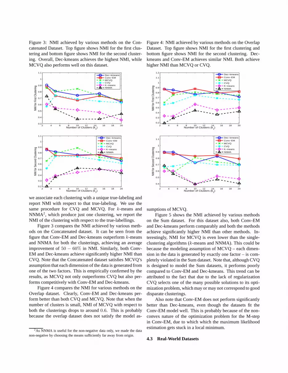
Figure 3: NMI achieved by various methods on the Con-catenated Dataset. Top figure shows NMI for the first clus-tering and bottom figure shows NMI for the second cluster-ing. Overall, Dec-kmeans achieves the highest NMI, whileMCVQ also performs well on this dataset.

2 4 6 8 10 12 14 16 18 200.3

0.4

0.5

0.6

0.7

0.8

0.9

1

1.1

Number of Clusters (k1)

NM

I for

Firs

t Clu

ster

ing

Dec−kmeansConv−EMMCVQCVQK−meansNNMA

2 4 6 8 10 12 14 16 18 200.2

0.3

0.4

0.5

0.6

0.7

0.8

0.9

1

1.1

Number of Clusters (k2)

NM

I for

Sec

ond

Clu

ster

ing

Dec−kmeansConv−EMMCVQCVQK−meansNNMA

we associate each clustering with a unique true-labeling andreport NMI with respect to that true-labeling. We use thesame procedure for CVQ and MCVQ. Fork-means andNNMA2, which produce just one clustering, we report theNMI of the clustering with respect to the true-labellings.

Figure 3 compares the NMI achieved by various meth-ods on the Concatenated dataset. It can be seen from thefigure that Conv-EM and Dec-kmeans outperformk-meansand NNMA for both the clusterings, achieving an averageimprovement of50 − 60% in NMI. Similarly, both Conv-EM and Dec-kmeans achieve significantly higher NMI thanCVQ. Note that the Concatenated dataset satisfies MCVQ’sassumption that each dimension of the data is generated fromone of the two factors. This is empirically confirmed by theresults, as MCVQ not only outperforms CVQ but also per-forms competitively with Conv-EM and Dec-kmeans.

Figure 4 compares the NMI for various methods on theOverlap dataset. Clearly, Conv-EM and Dec-kmeans per-form better than both CVQ and MCVQ. Note that when thenumber of clusters is small, NMI of MCVQ with respect toboth the clusterings drops to around0.6. This is probablybecause the overlap dataset does not satisfy the model as-

2As NNMA is useful for the non-negative data only, we made the datanon-negative by choosing the means sufficiently far away from origin.

Figure 4: NMI achieved by various methods on the OverlapDataset. Top figure shows NMI for the first clustering andbottom figure shows NMI for the second clustering. Dec-kmeans and Conv-EM achieves similar NMI. Both achievehigher NMI than MCVQ or CVQ.

2 4 6 8 10 12 14 16 18 200.2

0.3

0.4

0.5

0.6

0.7

0.8

0.9

1

1.1

1.2

Number of Clusters (k1)

NM

I for

Firs

t Clu

ster

ing

Dec−kmeansConv−EMMCVQCVQK−meansNNMA

2 4 6 8 10 12 14 16 18 20

0.4

0.5

0.6

0.7

0.8

0.9

1

1.1

Number of Clusters (k2)

NM

I for

Sec

ond

Clu

ster

ing

Dec−kmeansConv−EMMCVQCVQK−meansNNMA

sumptions of MCVQ.Figure 5 shows the NMI achieved by various methods

on the Sum dataset. For this dataset also, both Conv-EMand Dec-kmeans perform comparably and both the methodsachieve significantly higher NMI than other methods. In-terestingly, NMI for MCVQ is even lower than the single-clustering algorithms (k-means and NNMA). This could bebecause the modeling assumption of MCVQ – each dimen-sion in the data is generated by exactly one factor – is com-pletely violated in the Sum dataset. Note that, although CVQis designed to model the Sum datasets, it performs poorlycompared to Conv-EM and Dec-kmeans. This trend can beattributed to the fact that due to the lack of regularizationCVQ selects one of the many possible solutions to its opti-mization problem, which may or may not correspond to gooddisparate clusterings.

Also note that Conv-EM does not perform significantlybetter than Dec-kmeans, even though the datasets fit theConv-EM model well. This is probably because of the non-convex nature of the optimization problem for the M-stepin Conv-EM, due to which which the maximum likelihoodestimation gets stuck in a local minimum.

4.3 Real-World Datasets

Figure 5: NMI achieved by various methods on the SumDataset. Top figure shows NMI for the first clustering andbottom figure shows NMI for the second clustering. Dec-kmeans and Conv-EM achieves similar NMI. NMI achievedby MCVQ is very low.

2 4 6 8 10 12 14 16 18 20

0.2

0.4

0.6

0.8

1

1.2

Number of Clusters (k1)

NM

I for

Firs

t Clu

ster

ing

Dec−kmeansConv−EMMCVQCVQK−meansNNMA

2 4 6 8 10 12 14 16 18 20

0.4

0.5

0.6

0.7

0.8

0.9

1

1.1

Number of Clusters (k2)

NM

I for

Sec

ond

Clu

ster

ing

Dec−kmeansConv−EMMCVQCVQK−meansNNMA

4.3.1 Music Dataset:The music dataset is a collection of270 documents, with each document being a review of a clas-sical music piece taken fromamazon.com. Each music pieceis composed by one of Beethoven, Mozart or Mendelssohnand is in one of symphony, sonata or concerto forms. Thus,the documents can be clustered based on the composer orthe genre of the musical piece. For the experiments a term-document matrix was formed with dimensionality258 afterstop word removal and stemming.

Table 1 shows that although all the methods are ableto recover the true clustering for composer, most of thealgorithms perform poorly for the genre based clustering. Inparticular,k-means and NNMA perform very poorly for theclustering based on genre as they produce just one clusteringwhich has high NMI with the clustering based on composers.Note that in this dataset, the sets of features (words) thatdetermine clustering with respect to composer and genrerespectively are almost disjoint. Hence, methods like FeatureRemoval and Orthogonal Projection, which try to identifydisjoint sets of features for the clusterings work fairly well.But, both MCVQ and CVQ algorithm achieve very lowaccuracy as they do not try to finddecorrelatedclusterings.Both our methods outperform the baseline algorithms.

Table 1: Accuracy achieved by various methods on theMusic dataset, which is a collection of text documents. Dec-kmeans performs the best on this dataset. CVQ and MCVQperform very poorly compared to Conv-EM

Method\Type Composer GenreNNMA 1.00 0.40k-means 0.89 0.41Feature Removal 0.97 0.64Orthogonal Projection 0.99 0.66CVQ 0.97 0.57MCVQ 0.91 0.53Conv-EM 1.00 0.65Dec-kmeans 1.00 0.69

4.3.2 Portrait Dataset: The Portrait dataset consists of324 images obtained from Yale Face Dataset B [7]. Eachimage in the dataset is a portrait of one of three people, in oneof three poses in different backgrounds. The dimensionalityof each image is64 × 64. As a first step we reducethe dimensionality of the data to300 by using principalcomponent analysis. As in the music dataset, the currentdataset can be clustered in two natural ways - by the person inthe picture or the pose. Table 2 shows that bothk-means andNNMA perform poorly with respect to both the clusterings.This shows that in the datasets where there is more than onenatural clustering, traditional clustering algorithms could failto find even one good clustering. Hence, it can be beneficialto use alternative clustering methods even if one is interestedin obtaining a single clustering.Our hypothesis is that unlike the music dataset, there are nodominant features for any of the clusterings in this dataset.This hypothesis can be justified by observing the poor ac-curacies of methods like Feature Removal and Orthogo-nal Projection. Conv-EM outperforms baseline algorithmsCVQ and MCVQ significantly, but interestingly Dec-kmeansachieves an even higher accuracy of84% and78% for thetwo clusterings.

5 Conclusions and Future Work

We address the difficult problem of uncovering disparateclusterings from the data in a totally unsupervised setting.We present two novel approaches for the problem - a decor-relatedk-means approach and a sum of parts approach. Inthe first approach, we introduce a new regularization fork-means to uncover decorrelated clusterings. We provide theo-retical justification for using the proposed decorrelationmea-sure. The sum of parts approach leads us to the interestingproblem of learning a convolution of mixture models andwe present a regularized EM algorithm for learning a con-volution of mixtures of spherical Gaussians. We addressthe problem of identifiability for learning a convolution of

Table 2: Accuracy achieved by various methods on the Por-trait dataset, which is a collection of images. Dec-kmeansoutperforms all other methods by a significant margin. Conv-EM achieves better accuracy than all other methods, espe-cially CVQ and MCVQ.

Method\Type Person PoseNNMA 0.51 0.49k-means 0.66 0.56Feature Removal 0.56 0.48Orthogonal Projection 0.66 0.70CVQ 0.53 0.51MCVQ 0.64 0.51Conv-EM 0.69 0.72Dec-kmeans 0.84 0.78

mixtures of Gaussians by using a regularization geared forproviding disparate clusterings. We demonstrate the effec-tiveness and robustness of our algorithms on synthetic andreal-world datasets. On each of these datasets, we signifi-cantly improve upon the accuracy achieved by existing fac-torial learning methods such as CVQ and MCVQ. Our meth-ods also outperform the traditional clustering algorithmslikek-means and NNMA.

For future work, it would be of interest to study the prob-lem of learning a convolution of mixtures for a more generalclass of distributions and look for other settings where learn-ing convolutions of mixtures could be useful. We also planto further investigate the properties of the decorrelationmea-sure, especially for more general distributions of the data. Aproblem that we do not address in this paper is model se-lection - choosing the number of clusters and the numberof clusterings. Good heuristics for choosing these parame-ters would be very useful. Also, a more detailed compari-son of Conv-EM and Dec-kmeans would be useful; it wouldbe interesting to understand the comparable performance ofConv-EM and Dec-kmeans for the synthetic datasets whichfit the convolution model well.

Acknowledgements:This research was supported by NSFgrant CCF-0431257, NSF Career Award ACI-0093404, andNSF-ITR award IIS-0325116.

References

[1] BAE, E. AND BAILEY, J.,COALA: A novel approach for theextraction of an alternate clustering of high quality and highdissimilarity, in ICDM, 2006, pp. 53–62.

[2] B ILENKO , M., BASU, S., AND MOONEY, R.J, Integratingconstraints and metric learning in semi-supervised clustering,in ICML, 2004, pp. 81–88.

[3] B ISHOP, C. M, Neural networks for pattern recognition,Oxford University Press, Oxford, UK, 1996.

[4] I. DAVIDSON, S. S. RAVI , AND M. ESTER, Efficient incre-mental constrained clustering, in KDD, 2007, pp. 240–249.

[5] R. O. DUDA , P. E. HART, AND D. G. STORK, PatternClassification, Wiley-Interscience, November 2000.

[6] W. R. GAFFEY, A consistent estimator of a component ofa convolution, The Annals of Mathematical Statistics, 30(1959), pp. 198–205.

[7] A. GEORGHIADES, P. BELHUMEUR, AND D. KRIEGMAN,From few to many: Illumination cone models for face recog-nition under variable lighting and pose, IEEE Trans. PatternAnal. Mach. Intelligence, 23 (2001), pp. 643–660.

[8] Z. GHAHRAMANI , Factorial learning and the EM algorithm,in NIPS, 1994, pp. 617–624.

[9] G. H. GOLUB AND C. F. VAN LOAN, Matrix Computations,Johns Hopkins Univ. Press, second ed., 1989.

[10] D. GONDEK AND T. HOFMANN, Non-redundant data clus-tering, in ICDM, 2004, pp. 75–82.

[11] D. GONDEK, S. VAITHYANATHAN , AND A. GARG, Cluster-ing with model-level constraints, in SDM, 2005, pp. 126–138.

[12] T. HASTIE, R. TIBSHIRANI , A. EISEN, R. LEVY,L. STAUDT, D. CHAN , AND P. BROWN, Gene shaving asa method for identifying distinct sets of genes with similarex-pression patterns, Genome Biology, (2000).

[13] G. E. HINTON AND R. S. ZEMEL, Autoencoders, minimumdescription length and Helmholtz free energy, in NIPS, 1993,pp. 3–10.

[14] A. HYV ARINEN AND E. OJA, Independent component anal-ysis: algorithms and applications, Neural Networks, 13(2000), pp. 411–430.

[15] D. D. LEE AND H. S. SEUNG, Algorithms for non-negativematrix factorization, in NIPS, 2000, pp. 556–562.

[16] D. A. ROSS ANDR. S. ZEMEL, Learning parts-based repre-sentations of data, JMLR, 7 (2006), pp. 2369–2397.

[17] SAMANIEGO , F. J.AND JONES, L. E., Maximum likelihoodestimation for a class of multinomial distributions arising inrealibility, Journal of the Royal Statistical Society. Series B(Methodological), 43 (1981), pp. 46–52.

[18] SCLOVE, S. L. AND VAN RYZIN , J.,Estimating the parame-ters of a convolution, Journal of the Royal Statistical Society.Series B (Methodological), 31 (1969), pp. 181–191.

[19] A. STREHL AND J. GHOSH, Cluster ensembles — a knowl-edge reuse framework for combining multiple partitions,JMLR, 3 (2002), pp. 583–617.

[20] J. B. TENENBAUM AND W. T. FREEMAN, Separating styleand content with bilinear models, Neural Computation, 12(2000), pp. 1247–1283.

[21] K. WAGSTAFF AND C. CARDIE, Clustering with instance-level constraints, in ICML, 2000, pp. 1103–1110.

[22] K. WAGSTAFF, C. CARDIE, S. ROGERS, AND S. SCHRODL,Constrained k-means clustering with background knowledge,in ICML, 2001, pp. 577–584.

[23] E. P. XING, A. Y. NG, M. I. JORDAN, AND S. RUSSELL,Distance metric learning, with application to clustering withside-information, in NIPS, vol. 15, 2003, pp. 521–528.

[24] W. I. ZANGWILL , Nonlinear Programming: A Unified Ap-proach, Englewood Cliffs: Prentice-Hall, 1969.