Simulation Based Shop Floor Control

by

Young-Jun Sona,*, Sanjay B. Joshib, Richard A. Wyskb, and Jeffrey S. Smithc aDepartment of Systems and Industrial Engineering, The University of Arizona, Tucson, AZ

85721-0020, U.S.A. bDepartment of Industrial and Manufacturing Engineering, Pennsylvania State University,

University Park, PA 16802, U.S.A. cDepartment of Industrial and Systems Engineering, Auburn University, AL 36849-5346, U.S.A.

*Correspondence author Phone: 1-520-626-9530, Fax: 1-520-621-6555, E-mail: son@sie.arizona.edu

Abstract

This paper presents an overview of simulation-based shop floor control. Much of the

work described herein is based on research conducted in the Computer Integrated Manufacturing

(CIM) Lab at The Pennsylvania State University, the Texas A&M Computer Aided

Manufacturing Lab (TAMCAM), Technion in Israel, and the University of Arizona CIM lab over

the past decade. In this approach, a discrete event simulation is used not only as a traditional

analysis and evaluation tool, but also as a task generator that drives shop floor operations in real-

time. To enable this, a special feature of the Arena simulation language was used whereby the

simulation model interacts directly with a shop floor execution system by sending and receiving

messages. This control simulation reads process plans and master production orders from

external databases that are updated by a process planning system and coordinated via an external

business system. The control simulation also interacts with other external programs such as a

planner, a scheduler, and an error detection and recovery function. In this paper, the architecture,

implementation, and the integration of all the components of the proposed simulation-based

control system are described in detail. Finally, extensions to this approach, including automatic

model generation, are described.

Keywords: Shop Floor Control, CIM, Real-time Scheduling, and Simulation

1

1. Introduction Simulation is a commonly used tool to gain insight into the operational behavior of

manufacturing systems. The traditional use of simulation has been limited to planning and design

activities, and several commercial simulation languages have been developed specifically for this

purpose: e.g. Arena, AutoMod, ProModel, etc. Simulation models developed for planning

and design are often aggregate models using statistical distributions to model the stochastic nature

of the environment. These models are used to perform what-if analysis to determine values of

design variables, control strategies and develop estimates of system performance. These models

are usually discarded after the initial plans are finalized.

Several authors have reported the expanded role of simulation to include “real-time”

scheduling as part of intelligent simulation to dynamically select scheduling policies based on

real-time shop floor status [Wu and Wysk, 1989; Harmonosky and Robhon, 1991; Rogers and

Flanagan, 1991; Smith et al., 1996; Drake and Smith, 1996; Jones et al., 1995; Tunali, 1995].

These authors demonstrate that by using the most current system information and by using the

simulation to make predictions about the future, performance can be improved by dynamically

adjusting the scheduling policy and control strategy.

Given that simulation is well suited to capture the complex interactions of a system and

embodies elements of the actual mode of system operation, a natural extension is the use of the

simulation model to actually control the events in a real system. This is the basis of simulation

based shop floor control as first proposed by the Rapid CIM project [Smith et al., 1994]. Using a

simulation model with the proper level of detail and fidelity with real-time capability of

interaction with external events, the same simulation model can be used to provide a common

framework for design, planning and, real time scheduling and control.

This paper presents an overview of our research in simulation based shop floor control

(SBSFC). Section 2 provides a general architecture of SBC. Section 3 describes the system

2

components in the SBSFC system. The complete development cycle along with an overview of

automatic generation of the control simulation is presented in Section 4. Integration of simulation

based control system with scheduling is presented in Section 5. A description of the

implementation detail is presented in Section 6. The Penn State CIM lab and several of the

products manufactured there are described in Section 7. Conclusions and closing remarks are

presented in Section 8.

2. Overview of Simulation Based Control

A shop floor control system (SFCS) is the central part of a computer integrated

manufacturing (CIM) system [Cho, 1993]. The responsibilities of a SFCS fall into three

functional categories: planning, scheduling, and execution [Jones and Saleh, 1990; Joshi et al.,

1990]. In this paper, the function governing “what”, “where”, and “how” is called execution,

whereas a function governing “what”, “when”, and “where” (in the case of alternative resources)

is called decision-making (planning and scheduling). For example, given a “pick an object” task,

the execution function needs to know what needs to be physically done, how the required activity

can be executed (e.g. messaging and coordination) by one or more pieces of equipment

(alternatives). Prior to executing the task, the decision-making function decides when to perform

the task (resolving resource contention) and which piece equipment to use (a given robot among

alternative robots). For a given shop, the execution function is relatively static and depends only

on the physical configuration of the shop; whereas the decision-making function is relatively

dynamic and depends on both the physical configuration of the shop and the production

requirements [Smith and Joshi, 1993; Smith and Joshi, 1995].

In the last decade, simulation models have been used to generate “work to” schedules that

are then used to control the flow of product on a shop floor. More recently, simulation has been

used for system evaluation and then reused as a basis for a real-time system controller. This type

3

of control is referred to as simulation-based shop floor control (SBSFC). This approach has been

illustrated as part of the RapidCIM project [Wysk et al., 1992; Smith et al., 1994] and has been

implemented at the following university labs: 1) The Penn State CIM lab, 2) Texas A&M

Computer Aided Manufacturing (TAMCAM) lab, 3) Technion – Israel Institute of Technology

and 4) University of Arizona CIM lab.

Figure 1 depicts the RapidCIM simulation-based control architecture. The Arena RT

(real-time) simulation package has been used to develop the simulation model that obtains master

production schedules (e.g. part orders) and part process plans from a Microsoft Access 97

database. The database keeps track of part orders and how many parts in each order are finished.

The simulation controls the manufacturing system by sending and receiving messages using

TCP/IP socket-based communication link to a high-level task executor, known as the BigE. The

BigE performs the shop-level execution functions and keeps track of the status of each individual

piece of equipment in the system. The BigE receives instructions (messages) from the simulation

and based on the system status, sends messages to the equipment level controllers. After a task

message is sent from the BigE, both the BigE and the simulation wait for a “completion_ok”

message from the equipment level controller that received the message. Once the BigE receives

the “completion_ok” message, it sends a similar message to the simulation, and the simulation

knows that the current task was completed. The task generator and execution modules

communicate through the task initiation queue (TIQ) and the task completion queue (TCQ). The

simulation uses the TIQ to instruct the BigE to perform specific tasks and receives completion

messages through the TCQ. These queues facilitate the explicit separation of the decision-maker

from the execution module. The separation of the decision-maker and the execution module

makes the system truly “plug and play”. In fact, as long as the decision-maker understands the

physical constraints imposed on the task sequences, any decision-maker can be plugged in to the

execution module according to the current production requirements. Example decision-makers

4

include simulation, a human operator, an expert system, etc [Smith et al., 1994]. Among these

candidates, the following advantages have made simulation popular as part of a decision-maker:

1) easy bookkeeping, 2) easy specification of physical system constraints, 3) built-in ability to

interface with external modules such as databases and external decision procedures, 4) real-time

monitoring and animation, and 5) off-line production prediction or cost estimation.

ARENA: real-time(Task Generator)

Big Executor (Shop Level)

ABBrobot

ProlightIBMrobot

FadalCartracAS/RS

TaskCompletion Queue

DatabasePlanner/Scheduler

TaskInitiation Queue

Eshedrobot

OrdersProcess plans

ShopLevelController

EquipmentLevelControllers

PhysicalEquipment

Figure 1. Simulation-based shop floor control structure

Two general architectures for the decision-making function from the simulation-based

control environment are depicted in Figure 2. For the first architecture, the operating logic for the

controller is directly coded into the simulation model. For the second architecture, an external

scheduler provides input to the simulation (either a work-to schedule for each resource or a

dispatching rule for each decision point). For different architectures or control strategies, the

associated simulations need to be configured differently [Drake et al., 1995]. In this research, the

5

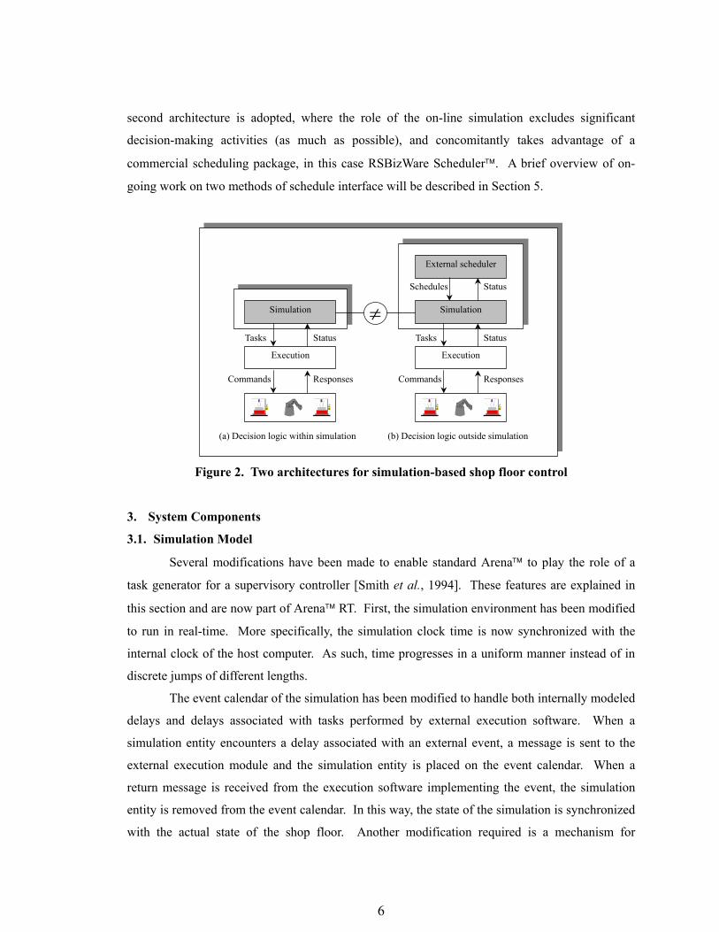
second architecture is adopted, where the role of the on-line simulation excludes significant

decision-making activities (as much as possible), and concomitantly takes advantage of a

commercial scheduling package, in this case RSBizWare Scheduler. A brief overview of on-

going work on two methods of schedule interface will be described in Section 5.

≠StatusTasks

Execution

Simulation

(a) Decision logic within simulation

StatusTasks

StatusSchedules

Execution

Simulation

External scheduler

(b) Decision logic outside simulation

ResponsesCommands ResponsesCommands

Figure 2. Two architectures for simulation-based shop floor control

3. System Components

3.1. Simulation Model

Several modifications have been made to enable standard Arena to play the role of a

task generator for a supervisory controller [Smith et al., 1994]. These features are explained in

this section and are now part of Arena RT. First, the simulation environment has been modified

to run in real-time. More specifically, the simulation clock time is now synchronized with the

internal clock of the host computer. As such, time progresses in a uniform manner instead of in

discrete jumps of different lengths.

The event calendar of the simulation has been modified to handle both internally modeled

delays and delays associated with tasks performed by external execution software. When a

simulation entity encounters a delay associated with an external event, a message is sent to the

external execution module and the simulation entity is placed on the event calendar. When a

return message is received from the execution software implementing the event, the simulation

entity is removed from the event calendar. In this way, the state of the simulation is synchronized

with the actual state of the shop floor. Another modification required is a mechanism for

6

implementing the task initiation queue (TIQ) and the task completion queue (TCQ) (refer to

Section 2). Implementation specifics to facilitate these message queues will be described in

Section 6.

In addition to the modifications made to the simulation software, simulation modeling for

shop-floor control requires much higher level of system detail than when it is used as an analysis

tool. Since the simulation drives physical tasks of equipment in the shop, the simulation model

with low fidelity may cause catastrophic results (e.g. errors, resource collisions, etc.) or system

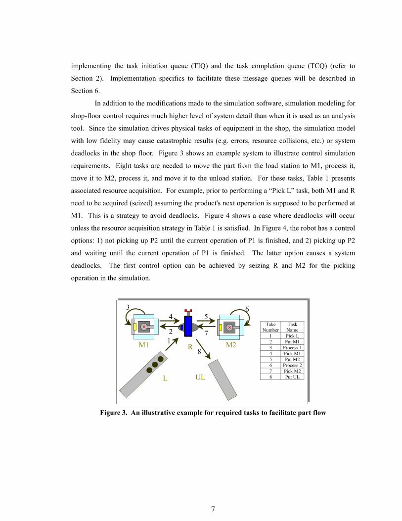
deadlocks in the shop floor. Figure 3 shows an example system to illustrate control simulation

requirements. Eight tasks are needed to move the part from the load station to M1, process it,

move it to M2, process it, and move it to the unload station. For these tasks, Table 1 presents

associated resource acquisition. For example, prior to performing a “Pick L” task, both M1 and R

need to be acquired (seized) assuming the product's next operation is supposed to be performed at

M1. This is a strategy to avoid deadlocks. Figure 4 shows a case where deadlocks will occur

unless the resource acquisition strategy in Table 1 is satisfied. In Figure 4, the robot has a control

options: 1) not picking up P2 until the current operation of P1 is finished, and 2) picking up P2

and waiting until the current operation of P1 is finished. The latter option causes a system

deadlocks. The first control option can be achieved by seizing R and M2 for the picking

operation in the simulation.

8

2

3 4 5

6

71M1 M2R

L UL

Take Number

Task Name

1 Pick L 2 Put M1 3 Process 1 4 Pick M1 5 Put M2 6 Process 2 7 Pick M2 8 Put UL

Figure 3. An illustrative example for required tasks to facilitate part flow

7

Table 1. Resource acquisition for control simulation

Equipment to be seized for each task Task Number Task Name M1 (machine) M2 (machine) R (robot)

1 Pick L √ √ 2 Put M1 √ √ 3 Process 1 √ 4 Pick M1 √ √ 5 Put M2 √ √ 6 Process 2 √ 7 Pick M2 √ 8 Put UL √

M1 M2R

Legend : Operation finished

: Operation currently being done

P2: M1 – M2 P1: M1 – M2 ?

Figure 4. An illustrative example for deadlock avoidance strategy

3.2. Resource Model

In this section, we explore a production resource model that provides a common frame of

reference among the simulation, the execution system (BigE), the process planner, etc. In fact,

this resource model is used as a major input to automatically generate a simulation model and an

execution model (as described in Section 4). A resource model contains a set of definitions and

symbolic descriptions that are required to describe all of the individual resources in a facility as

well as the necessary interactions between these resources. It includes both the physical and

logical information in the facility directed toward the manufacture of the products. Resources (R)

include equipment (E), tools (T), fixtures (F), instruction sets (I), connectivity graph (CG),

locations (L), ports (P), facilitators (FA), which are formally defined as follows:

R = <E, T, F, I, CG, L, P, FA>

A partition of a set A is a collection of disjoint subsets of A whose union is all of A. A = <A1, A2,

8

A3> represents that A is partitioned to A1, A2, and A3.

Methodologies developed in this paper interact with only the equipment (E) and the

connectivity graph (CG). Therefore, discussions in this section focus only on E and CG, and the

other sets will not be further mentioned after this section. Steele et al. (2001) present various

usages of the production resource model.

A manufacturing system is made up of several pieces of equipment (devices). Several

generic types of equipment have been identified. Smith and Joshi (1993) define the types of

equipment (E) as: material processing (MP), material handling (MH), material transport (MT),

and buffer storage (BS). Each piece of equipment in the factory belongs to one of these types.

Formally, the equipment (E) is defined as follows:

E = <MP, MH, MT, BS>, where:

MP = <NMP, PD>,

BS = <ABS, PBS>,

ABS = <SABS, LABS>, and

PBS = <SPBS, LPBS>.

Equipment belonging to the MP set transforms a product in some way. MP is partitioned

into NMP (normal material processors set) and PD (passive devices set). If material processing

equipment requires an equipment level controller, it belongs to the NMP set. Otherwise, it

belongs to the PD set. Equipment belong to the NMP set includes machining centers, inspection

devices, assembly machines, and so on. Equipment belonging to the PD set includes gravity-

based inverters, heat lamps used for drying parts after a painting operation, etc. In this paper, the

MP set refers to the NMP set unless otherwise specified.

Equipment belonging to the MH set includes those pieces of equipment that transfer

products between pieces of equipment; they are robots, human operators, etc. Equipment

belonging to the MT set includes those that move products from one location (as defined below)

to another location; they are AGVs, conveyors, fork trucks, human operators, etc.

Equipment belonging to the BS set includes those pieces of equipment that store products.

General equipment storing products is classified either as ABS or PBS. If the storage equipment

requires an equipment level controller it belongs to ABS set, otherwise, it belongs to PBS set.

Some requirements of ABS equipment level controller include synchronization with MH

equipment, location allocation, capacity control, etc. ABS is partitioned into SABS and LABS.

SABS equipment includes those associated with the system level activities, meaning that products

initiate and terminate their appearance to the production system. LABS equipment is associated

9

with local activities. Equipment belonging to the PBS set stores products and does not need an

equipment level controller. Since no controller exists for this type of equipment, the supervisory

level controller (the simulation model in our case) must make all of the decisions associated with

the equipment. PBS is partitioned into SPBS and LPBS with the same way as in the case of ABS.

A connectivity graph (CG) is a graph showing the connections between the equipment in

the facilities. Each node is associated with a piece of equipment. Arcs are associated with

equipment interactions (e.g. high level tasks). The connectivity graph is formally defined as:

CG = (N, A), where

N = {n1, n2, …, ni} is the set of nodes corresponding to the equipment (E)

A = {aij | i, j ∈ N}.

3.3. Finite State Automata Based Execution Model

This section explores a message-based part state graph (MPSG) that formed the basis of

the BigE and the equipment level controllers in Figure 1. The MPSG presented by Smith and

Joshi (1993) is a formal model of the execution portion of shop floor control that operates in a

distributed control environment. It represents the execution module of a shop floor controller as a

finite state machine. Individual controllers in a distributed environment communicate using a

well-defined protocol (messages) to affect system operation. An MPSG (which mimics the

behavior of the controllers from the part perspective) specifies all possible states that parts can

occupy throughout the system. In comparison with a PLC-based control system, the

computational complexity of an MPSG is extremely low. An MPSG is a modified deterministic

finite automaton (DFA) similar to a Mealy machine [Hopcroft and Ullman, 1979]. Further details

on the MPSG can be found in [Smith, 1992] and [Smith and Joshi, 1993].

Consistent with the type of equipment in the production resource model in Section 3.2,

Smith (1992) developed generic MPSGs for each type of equipment and a supervisory controller

(BigE). Figure 5 shows an example MPSG for MH equipment (e.g. a robot). There are two types

of interactions between the MH equipment and other types (e.g. MP, BS, or MT) of equipment:

synchronous and non-synchronous. When MH equipment puts (loads) a part to MP equipment,

resource synchronization is required (e.g. the MP equipment must open the chuck before the MH

equipment puts the part and the MP equipment must close the chuck before the MH equipment

moves away to a safe position). On the other hand, when an MH equipment picks (or puts) a part

from the passive buffer storage equipment (PBS), no resource synchronization is necessary. As

shown in Figure 5, the process in an MH equipment controller is initiated by a pick request from

10

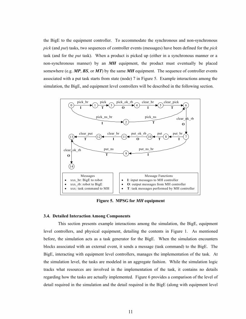
the BigE to the equipment controller. To accommodate the synchronous and non-synchronous

pick (and put) tasks, two sequences of controller events (messages) have been defined for the pick

task (and for the put task). When a product is picked up (either in a synchronous manner or a

non-synchronous manner) by an MH equipment, the product must eventually be placed

somewhere (e.g. MP, BS, or MT) by the same MH equipment. The sequence of controller events

associated with a put task starts from state (node) 7 in Figure 5. Example interactions among the

simulation, the BigE, and equipment level controllers will be described in the following section.

0 1 3 4 5 6

78101112

pick_br pick pick_ok_rb clear_br clear_pick

I T O I T

clear_ok_rbO

put

TOIput_brput_ok_rbclear_br

I

clear_ok_rbO

2pick_ns_br pick_ns

I T

13clear_put

T

9

14

put_ns_brput_nsIT

Messages• xxx_br: BigE to robot• xxx_rb: robot to BigE• xxx: task command to MH

Message Functions• I: input messages to MH controller• O: output messages from MH controller• T: task messages performed by MH controller

Figure 5. MPSG for MH equipment

3.4. Detailed Interaction Among Components

This section presents example interactions among the simulation, the BigE, equipment

level controllers, and physical equipment, detailing the contents in Figure 1. As mentioned

before, the simulation acts as a task generator for the BigE. When the simulation encounters

blocks associated with an external event, it sends a message (task command) to the BigE. The

BigE, interacting with equipment level controllers, manages the implementation of the task. At

the simulation level, the tasks are modeled in an aggregate fashion. While the simulation logic

tracks what resources are involved in the implementation of the task, it contains no details

regarding how the tasks are actually implemented. Figure 6 provides a comparison of the level of

detail required in the simulation and the detail required in the BigE (along with equipment level

11

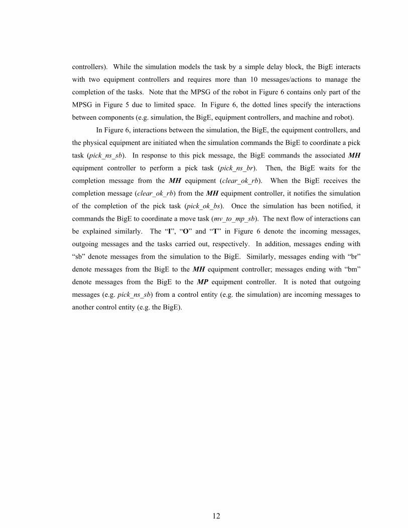
controllers). While the simulation models the task by a simple delay block, the BigE interacts

with two equipment controllers and requires more than 10 messages/actions to manage the

completion of the tasks. Note that the MPSG of the robot in Figure 6 contains only part of the

MPSG in Figure 5 due to limited space. In Figure 6, the dotted lines specify the interactions

between components (e.g. simulation, the BigE, equipment controllers, and machine and robot).

In Figure 6, interactions between the simulation, the BigE, the equipment controllers, and

the physical equipment are initiated when the simulation commands the BigE to coordinate a pick

task (pick_ns_sb). In response to this pick message, the BigE commands the associated MH

equipment controller to perform a pick task (pick_ns_br). Then, the BigE waits for the

completion message from the MH equipment (clear_ok_rb). When the BigE receives the

completion message (clear_ok_rb) from the MH equipment controller, it notifies the simulation

of the completion of the pick task (pick_ok_bs). Once the simulation has been notified, it

commands the BigE to coordinate a move task (mv_to_mp_sb). The next flow of interactions can

be explained similarly. The “I”, “O” and “T” in Figure 6 denote the incoming messages,

outgoing messages and the tasks carried out, respectively. In addition, messages ending with

“sb” denote messages from the simulation to the BigE. Similarly, messages ending with “br”

denote messages from the BigE to the MH equipment controller; messages ending with “bm”

denote messages from the BigE to the MP equipment controller. It is noted that outgoing

messages (e.g. pick_ns_sb) from a control entity (e.g. the simulation) are incoming messages to

another control entity (e.g. the BigE).

12

pick_ns_sb

pick_ns_br

clear_ok_rb

pick_ok_bs

mv_to_mp_s

assign_bm

assign_ok_mb

assign_ok_bs

put_sb

pur_br

pur_ok_rb

grasp_bm

grasp_ok_mb

pick_ns_br

pick_ns

clear_ok_rb

put_br

put

put_ok_rb

assign_bm

assign

assign_ok_mb

grasp_bm

grasp

grasp_ok_mb

Delay(pick_ns_sb)

Delay(mv_to_mp_sb)

Delay(put_sb)

I

I

I

I

I

I

I

O

O

O

O

O

O

I

I

I

I

O

O

O

O

T

T

T

T

Simulation BigE

MH ctrl

MP ctrl

Messages• xxx_sb: simulation to BigE• xxx_bs: BigE to simulation• xxx_br: BigE to robot• xxx_bm: BigE to machine• xxx_mb: machine to bigE• xxx_rb: robot to BigE

Message Functions• I: input messages to the controller• O: output messages from the controller• T: task messages performed by the controller

Figure 6. Interaction among the simulation, the BigE, equipment controllers, and physical

equipment

3.5. Process Plan

The process plan provides the instructions for producing a part. It plays an important role

in shop floor control as it forms a major portion of the specifications required for control. As

13

shown in Figure 1, the Arena RT simulation model obtains part process plans from an external

database. By decoupling product routing from the actual control software it is possible to change

product mix and product flow data without making changes to the control software. Furthermore,

process plans in this research will contain alternative routings. Process plans (and alternative

process plans) are represented using AND/OR graphs [Mettala and Joshi, 1993]. AND/OR

graphs are employed in this research since they provide additional required flexibility over the

traditional process plans represented either by operation charts or by process-routing sheets.

More specifically, AND/OR graphs provide a straightforward mechanism for representing

alternative processing sequences. The controller must be able to serialize, or linearize, the

AND/OR graphs. Further details on process plan representations and the use of process plans for

control can be found in [Wysk et al., 1995] and [Lee et al., 1995].

In this research, the process plan has the following information for every part type: ID

number, operation code, description, resource ID, robot location, NC file name, and port number.

Port numbers are associated with physical locations in the shop; therefore, unique tasks and

operating parameters using the port number, resource ID, and operation code can be created.

4. Rapid System Development

The previous sections presented the operation stage of a simulation-based control system

(SBC). This section describes the development cycle of this type of control system. To reduce

the high cost of control software development and maintenance, research has been conducted on

rapid realization of an SBC for a discrete part manufacturing system [Smith and Joshi, 1993; Son

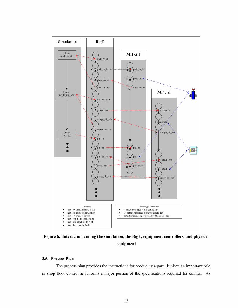
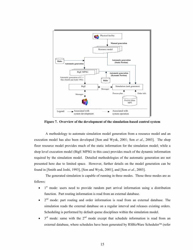
and Wysk, 2001]. Figure 7 illustrates an approach to develop an SBC involving the automatic

generation of an execution model and a simulation model from a resource model. As mentioned

in Section 3.2, the resource model contains information describing all of the individual resources

in a facility as well as the necessary interactions between these resources. A methodology (using

a series of rules) to automate execution model generation from a resource model has been

developed [Smith and Joshi, 1993; Son et al., 2003]. Given an MPSG execution model, Smith

and Joshi (1993) developed software tools for automatically generating essential portion (a set of

C++ files) of the controller (e.g. BigE or equipment level controller).

14

Process plan

Automatic generation(Static Portion)Automatic generation

Manual generation

BigE

Physical facility

Simulation (task generator)

Associated withsystem development

Associated withsystem operation

Resource model

Automatic generation of C++files (Smith and Joshi 1992)

Legend:

Order info.

Rules

Process plansMPS

Messages

Automatic generation(Dynamic Portion)

BigE MPSG

Rules

Messages

Figure 7. Overview of the development of the simulation-based control system

A methodology to automate simulation model generation from a resource model and an

execution model has also been developed [Son and Wysk, 2001; Son et al., 2003]. The shop

floor resource model provides much of the static information for the simulation model; while a

shop level execution model (BigE MPSG in this case) provides much of the dynamic information

required by the simulation model. Detailed methodologies of the automatic generation are not

presented here due to limited space. However, further details on the model generation can be

found in [Smith and Joshi, 1993], [Son and Wysk, 2001], and [Son et al., 2003].

The generated simulation is capable of running in three modes. Those three modes are as

follows:

• 1st mode: users need to provide random part arrival information using a distribution

function. Part routing information is read from an external database.

• 2nd mode: part routing and order information is read from an external database. The

simulation reads the external database on a regular interval and releases existing orders.

Scheduling is performed by default queue disciplines within the simulation model.

• 3rd mode: same with the 2nd mode except that schedule information is read from an

external database, where schedules have been generated by RSBizWare Scheduler (refer

15

to Section 5).

For all three modes, the simulation can be run with (real-time mode) or without (fast mode)

interacting with the shop level execution system.

5. Scheduling Methods

Wu and Wysk (1989) created a multi-pass scheduling framework using a mechanism

controller and a flexible simulator. Multi-pass scheduling algorithms are defined as the

scheduling algorithms that deal with the scheduling problem of selecting the best dispatching rule,

among rules in an alternative space. This multi-pass structure has been applied to the proposed

simulation-based control environment and has been implemented both at the Texas A&M

TAMCAM lab [Drake et al., 1995] and at the Penn State CIM lab [Son et al., 1999].

A multi-pass simulation is composed of two simulations -- a real time simulation and a

preview simulation, which runs in the fast mode. The architecture of the multi-pass simulation

can be seen in Figure 8. Since the real-time simulation has already been described in the previous

sections, this section will focus on inter-simulation interactions and significant parameters for the

multi-pass simulation. Figure 8 describes in detail the “scheduler” block in Figure 1. It should be

noticed that two identical simulation models exist on two different computers. One is used

primarily as a real-time task generator to the shop floor while the other is used for previewing the

system. At each decision point in real-time simulation, a subroutine (implemented using an

“event” block within Arena) in real-time simulation activates a fast mode simulation by sending a

message to see what control policy impacts the current system favorably. Once the look-ahead

manager receives a request, it opens fast-mode Arena and runs the number of alternative models

sequentially. Several simulations are run, and the performances of each alternative are recorded

in the specific file. When this procedure is done in the fast mode simulation, this control policy is

then fed to the real-time simulation for execution of the best control strategy on the system.

Further details on this approach can be found [Drake et al., 1995] and [Son et al., 1999].

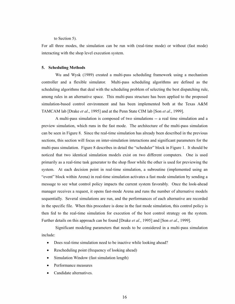
Significant modeling parameters that needs to be considered in a multi-pass simulation

include:

Does real-time simulation need to be inactive while looking ahead? •

•

•

•

•

Rescheduling point (frequency of looking ahead)

Simulation Window (fast simulation length)

Performance measures

Candidate alternatives.

16

The above parameters can be significant and even critical to the overall performance of the

proposed multi-pass simulation mechanism. However, the only way to determine reasonably

appropriate values of each parameter is empirically, i.e. through trial and error. Some of these

concerns have also been discussed in [Wu and Wysk, 1989], [Rogers and Gordon, 1993], and

[Dewan, 1996].

Dynam

ic Link Library

Remote Procedure Call

Database

Statistical Analysis

Best Rule Selection

ARENA: Real-time

"fastmode.bat" file

ARENA: fast-mode

Visual Basic Application

Rule 1Simulation

Rule nSimulation

Processplans

Look-ahead Manager

Operatingpolicy

OrderDetails

Figure 8. Architecture for a simulation-based, real-time scheduling

Work on a simulation-based control system where a work-to schedule for each resource is

provided to the simulation is interesting, yet premature. Because of the different levels of detail

between the scheduler and the controller, it is not trivial to implement the schedules in the

controller as specified by the scheduler. The level of detail between the scheduler and the

controller is different due to the following facts:

• Buffers are not considered in scheduling.

• Material handling is not considered in scheduling.

Schedules generated without considering these two facts must not be provided to the control

simulation. They may cause catastrophic results (e.g. collision) or system deadlocks in the shop

floor. Research is being conducted on this problem, hoping a commercial finite capacity

scheduler called RSBizWare Scheduler will generate schedules and these schedules will be

17

provided to the control simulation.

Two directions of schedule interface with a shop floor control system have been

described in this section. It will be challenging to investigate which method will works better and

under what circumstances.

6. Implementation Details

This section describes implementation details of (a) modifications made to enable

standard Arena to play the role of a task generator for a supervisory controller and (b) interface

with the external database containing process plans and master production schedules.

6.1. Modifications Made in Arena

The event calendar of the simulation has been modified to handle both internally modeled

delays and delays associated with tasks performed by external execution software [Smith et al.,

1994]. Technically, when an entity delay is associated with an external event, the block executes

two threads in parallel. The first thread emulates the delay time using the specified value (e.g.

standard operation time) while the second thread executes the real-time task by sending a

message to the real system to start an activity. The thread then waits for the system to respond

with a task completion message. If the execution thread finishes before the emulation thread, the

emulation thread is terminated and the entity departs the block. If the emulation thread finishes

first, the entity remains suspended in the block until either (a) the execution thread completes, or

(b) the actual task time exceeds a value, in which case the task is terminated with a timeout error

and the entity s sent to the block specified for the case of an error.

Another modification required is a mechanism for implementing the task initiation queue

(TIQ) and the task completion queue (TCQ). To facilitate the TIQ and the TCQ, Arena RT

provides the following functions [Smith et al., 1994]:

• SrIPC_Initialize() - This function initializes the inter-process communications required

for the queues.

• SrIPC_Shutdown() - This function closes the inter-process communications when the

simulation terminates.

• SrIPC_WriteMessage(msg) - This function is used to write the specified text message to

the task initiation queue.

• SrIPC_ReadMessage(msg) - This function is used to read the first message waiting in

the task completion queue.

18

These functions have been developed under Windows 95, 98, 2000 and NT environments.

6.2. Interface with External Database

Process plans and production orders are stored in a database constructed using ‘Microsoft

Access 97’ (refer to Figure 1). In the Arena simulation, an “event” block is used to interface

with the external database. Whenever an entity in the simulation model reaches one of these

blocks, the function “cevent” in the interface code is executed. Four types of events have been

created, and their functions are described below:

• Event 1: this event is triggered by the entity that is periodically created once per minute by

the first submodel of the simulation. It uses an SQL command to read the orders from the

master production database.

• Event 2: this event is executed when an entity representing a new order initially enters the

system. As described in Section 3.5, process plans are represented as AND/OR graphs and

can contain alternative sequences of steps for manufacturing a product. Whenever the

simulation needs to access a process plan for a new product, the associated table is read from

the database and a graph is internally built to keep this AND/OR graph in memory, containing

all the branches (options) in the process plan. Whenever a step in the sequence that makes up

the process plan is completed, this process plan is accessed to determine the next operation to

be performed. Given a current step in the process plan, several options may exist. In the

current implementation, the first option is chosen. However, a planner/scheduler module

could be added to decide which alternative should be executed next. Finally, this event

updates the process plan pointer to point to the next operation.

• Event 3: this event determines the next step in the process plan. It is triggered when an

operation is completed.

• Event 4: this event will delete an order from the database. When all the steps in a process

plan have been completed, this event is used to delete that order from the database.

In Arena 3.01, an event block can be implemented in either Visual C++ or Visual Basic

Application (VBA) embedded in Arena software. In our model, events are implemented in Visual

C++ 6.0.

7. Penn State CIM lab and Products

This section describes example products and facilities at the Penn State CIM lab, where

the proposed simulation-based shop floor control system has been implemented. The purpose of

19

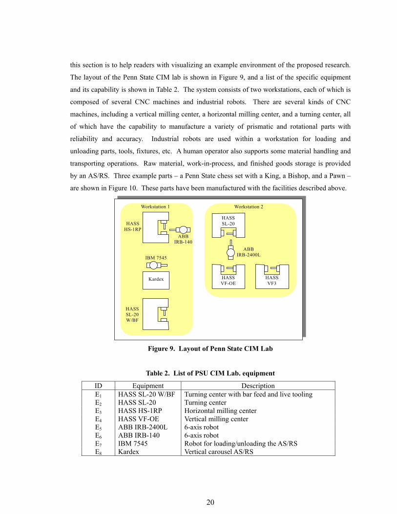
this section is to help readers with visualizing an example environment of the proposed research.

The layout of the Penn State CIM lab is shown in Figure 9, and a list of the specific equipment

and its capability is shown in Table 2. The system consists of two workstations, each of which is

composed of several CNC machines and industrial robots. There are several kinds of CNC

machines, including a vertical milling center, a horizontal milling center, and a turning center, all

of which have the capability to manufacture a variety of prismatic and rotational parts with

reliability and accuracy. Industrial robots are used within a workstation for loading and

unloading parts, tools, fixtures, etc. A human operator also supports some material handling and

transporting operations. Raw material, work-in-process, and finished goods storage is provided

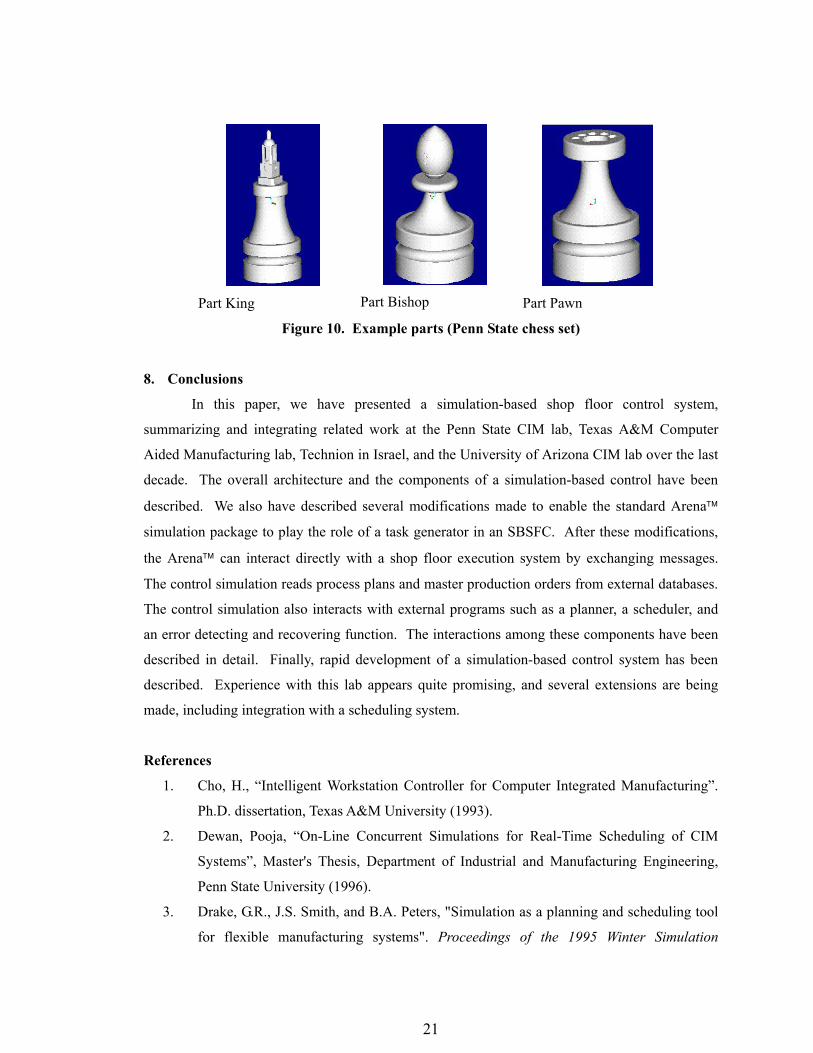
by an AS/RS. Three example parts – a Penn State chess set with a King, a Bishop, and a Pawn –

are shown in Figure 10. These parts have been manufactured with the facilities described above.

Kardex

IBM 7545

ABB IRB-2400L

ABB IRB-140

Workstation 1

HASS SL-20 W/BF

HASS HS-1RP

HASS SL-20

HASS VF-OE

HASS VF3

Workstation 2

Figure 9. Layout of Penn State CIM Lab

Table 2. List of PSU CIM Lab. equipment

ID Equipment Description E1 HASS SL-20 W/BF Turning center with bar feed and live tooling E2 HASS SL-20 Turning center E3 HASS HS-1RP Horizontal milling center E4 HASS VF-OE Vertical milling center E5 ABB IRB-2400L 6-axis robot E6 ABB IRB-140 6-axis robot E7 IBM 7545 Robot for loading/unloading the AS/RS E8 Kardex Vertical carousel AS/RS

20

Part King

Part Bishop

Part Pawn

Figure 10. Example parts (Penn State chess set)

8. Conclusions

In this paper, we have presented a simulation-based shop floor control system,

summarizing and integrating related work at the Penn State CIM lab, Texas A&M Computer

Aided Manufacturing lab, Technion in Israel, and the University of Arizona CIM lab over the last

decade. The overall architecture and the components of a simulation-based control have been

described. We also have described several modifications made to enable the standard Arena

simulation package to play the role of a task generator in an SBSFC. After these modifications,

the Arena can interact directly with a shop floor execution system by exchanging messages.

The control simulation reads process plans and master production orders from external databases.

The control simulation also interacts with external programs such as a planner, a scheduler, and

an error detecting and recovering function. The interactions among these components have been

described in detail. Finally, rapid development of a simulation-based control system has been

described. Experience with this lab appears quite promising, and several extensions are being

made, including integration with a scheduling system.

References

1. Cho, H., “Intelligent Workstation Controller for Computer Integrated Manufacturing”.

Ph.D. dissertation, Texas A&M University (1993).

2. Dewan, Pooja, “On-Line Concurrent Simulations for Real-Time Scheduling of CIM

Systems”, Master's Thesis, Department of Industrial and Manufacturing Engineering,

Penn State University (1996).

3. Drake, G.R., J.S. Smith, and B.A. Peters, "Simulation as a planning and scheduling tool

for flexible manufacturing systems". Proceedings of the 1995 Winter Simulation

21

Conference. pp. 805-812 (1995)

4. Drake, Glenn R. and Jeffrey Smith. 1996. “ Simulation systems for real time planning

scheduling and control”, Proceedings of the 1996 Winter Simulation Conference.

5. Harmononosky, C.M. and S.F. Robohn. 1991, “Real-time scheduling in computer

integrated manufacturing: A review of recent literature”, International Journal of

Computer Integrated Manufacturing, 331-340.

6. Hopcroft, J. E., and J. D. Ullman, Introduction to Automata Theory, Languages, and

Computation, Addison-Wesley Publishing, Reading, MA (1979).

7. Jones, A. T., and A. Saleh, “A Multi-level/Multi-layer Architecture for Intelligent Shop

Floor Control”. International Journal of Computer Integrated Manufacturing, Vol. 3, No.

1, pp. 60 – 70 (1990).

8. Jones, A., Rabelo, L., and Y. Yuchwera. 1995. A hybrid approach for real-time

sequencing and scheduling. International Journal of Computer Integrated,

Manufacturing, 145-154.

9. Joshi, S. B., R. A. Wysk, and A. Jones, “A Scaleable Architecture for CIM Shop Floor

Control”. Proceedings of Cimcon '90, A. Jones Ed., National Institute of Standards and

Technology, pp. 21 – 33 (1990).

10. Lee, S., R.A. Wysk, and J.S. Smith, “Process Planning Interface for a Shop Floor

Control Architecture for Computer Integrated Manufacturing,” International Journal of

Production Research, Vol. 33, No. 9, pp. 2415-2435 (1994).

11. Mettala, E. G., and S. B. Joshi, “A Compact Representation of Alternative Process

Plans/Routing for FMS Control Activities,” International Journal of Design and

Manufacturing, Vol. 3, pp. 91-104 (1993).

12. Rogers, P., and M. Flanagan. 1991. On-line simulation for real-time scheduling of

manufacturing systems, Industrial Engineering, Vol. 23, 37-40.

13. Rogers, P. and R.J. Gordon, "Simulation for real-time decision making in manufacturing

systems". Proceedings of the 1993 Winter Simulation Conference. pp. 866-874 (1993).

14. Smith, J., “A Formal Design and Development Methodology for Shop Floor Control in

Computer Integrated Manufacturing”. Ph.D. dissertation, Penn State University (1992).

15. Smith, J. and S. Joshi., “A Formal Model for Shop Floor Control in Automated

Manufacturing”, Proceedings of the 2nd Industrial Engineering Research Conference,

Los Angeles, CA, 1993.

16. Smith, J., and S. Joshi, “A Shop Floor Controller Class for Computer-integrated

22

Manufacturing”. International Journal of Computer Integrated Manufacturing, Vol. 8,

No. 5, pp. 327 – 339 (1995).

17. Smith, J. S., R. A. Wysk, D. T. Sturrok, S. E. Ramaswamy, G. D. Smith, and S. B. Joshi,

“Discrete Event Simulation for Shop Floor Control”. Proceedings of the 1994 Winter

Simulation Conference, pp. 962-969 (1994).

18. Son, Y., H. Rodriguez-Rivera, and R. A. Wysk, “A Multi-pass Simulation-based, Real-

time Scheduling and Shop Floor Control System”, Transactions of the Society for

Computer Simulation International, 16 (4), 159 – 172 (1999).

19. Son, Y., and R. A. Wysk, “Automatic Simulation Model Generation for Simulation-

based, Real-time Shop Floor Control”, Computers in Industry, 45 (3), 291 – 308 (2001).

20. Son, Y., R. A. Wysk, and A. T. Jones, “Simulation Based Shop Floor Control: Formal

Model, Model Generation, and Control Interface”, IIE Transactions on Design and

Manufacturing, 35 (1), 29 – 48 (2003).

21. Steele, J., Y. Son, and R. A. Wysk, “Resource Modeling for the Integration of the

Manufacturing Enterprise”, Journal of Manufacturing Systems, 19 (6), 407 – 427 (2001).

22. Tunali, S. 1995. Simulation for evaluating machine and AGV scheduling rules in an

FMS environment, Engineering Management Conference, 433-438.

23. Wu, S.D. and R.A. Wysk, "An application of discrete-event simulation to on-line control

and scheduling in flexible manufacturing". International Journal of Production

Research, Vol. 27, No. 9, pp. 1603-1623 (1989).

24. Wysk, R., Joshi, S. B., and Pegden, C.D., ”Rapid Prototyping of Shop Floor Control

Systems for Computer Integrated Manufacturing” ARPA project #8881 (1992).

25. Wysk, R.A., Peters, B.A., and J.S. Smith, “A Formal Process Planning Schema for Shop

Floor Control” Engineering Design and Automation Journal, Vol. 1, No. 1, pp. 3-19

(1994).

26. Wysk, R., and J. Smith, ”A Formal Functional Characterization of Shop Floor Control”

Computers and Industrial Engineering – Special Issue of Manufacturing Systems, Vol.

28, No. 3, pp. 631-644 (1995).

23

Dr. Young-Jun Son is an assistant professor in the Department of Systems and Industrial Engineering at University of Arizona. Dr. Son received his BS degree in Industrial Engineering with honors from POSTECH in Korea in 1996 and his MS and Ph.D. degrees in Industrial and Manufacturing Engineering from Penn State University in 1998 and 2000, respectively. His research work involves distributed and hybrid simulation for analysis and control of automated manufacturing system and integrated supply-chain. Dr. Son was the Rotary International Multi-Year Ambassadorial Scholar in 1996, the Council of Logistics Management Scholar in 1997, and the recipient of the Graham Endowed Fellowship for Engineering at Penn State University in 1999. He was the faculty advisor for the University of Arizona team that was awarded first place in the eighth IIE/Rockwell Software Student Simulation Contest. He is an associate editor of the International Journal of Modeling and Simulation and a professional member of ASME, IEEE, IIE, INFORMS, and SME. Dr. Sanjay Joshi is currently Professor of Industrial and Manufacturing Engineering at Penn State University. He received Ph.D in Industrial Engineering from Purdue University in 1987, MS from SUNY at Buffalo, B.S degree from University of Bombay, India. His research and teaching interests are in the areas of Computer Aided Design and Manufacturing (CAD/CAM) with specific focus on computer aided process planning, control of automated flexible manufacturing systems and Rapid Prototyping and Tooling. He is a recipient of several awards, including Presidential Young Investigator Award from NSF 1991, Outstanding Young Manufacturing Engineer Award from SME 1991, and Outstanding Young Industrial Engineer Award from IIE 1993. He has severed as the Department Editor for Process Planning - IIE Transactions on Design and Manufacturing, and currently serves on the editorial board of Journal of Manufacturing Systems, Journal of Intelligent Manufacturing, and Journal of Engineering Design and Automation, and International Journal of Computer Integrated Manufacturing. Dr. Richard A. Wysk is well-known for his work in computer integrated manufacturing, computer automated manufacturing, computer aided process planning and concurrent engineering. He holds the Leonhard Chair in Engineering at Penn State University. Prior to his current position, he was director of the Institute for Manufacturing Systems and holder of the Royce Wisenbaker Chair in Innovation at Texas A&M. Dr. Wysk also served on the faculty of Virginia Tech and worked in industry as a research analyst for the Caterpillar Tractor Company and as production control manager for General Electric. He is a decorated Vietnam veteran. Dr. Wysk is the author of several textbooks. Honors recognizing his research include the Institute of Industrial Engineers, David F. Baker Distinguished Research Award, and the Society of Manufacturing Engineers Outstanding Young Manufacturing Engineer Award. Dr. Wysk holds Bachelor’s and Master’s degrees in Industrial Engineering and Operations Research from the University of Massachusetts and a Ph.D. in Industrial Engineering from Purdue University. Dr. Jeffrey S. Smith joined Auburn University as an associate professor in the Industrial & Systems Engineering department in September of 1999. Prior to joining Auburn, Dr. Smith was an associate professor in the Industrial Engineering Department at Texas A&M University since 1992. He received the B.S. in Industrial Engineering from Auburn University in 1986 and the M.S. and Ph.D. degrees in Industrial Engineering from Penn State University in 1990 and 1992, respectively. Dr. Smith's teaching and research work involves analysis, design, and control of manufacturing systems, computer simulation, and simulation software development. In addition to his academic positions, Dr. Smith has held industrial positions at Electronic Data Systems and Philip Morris U.S.A. Dr. Smith is an active member of IIE, SME, and INFORMS.

24