Ocean Modelling 28 (2009) 75–87

Contents lists available at ScienceDirect

Ocean Modelling

journal homepage: www.elsevier .com/ locate/ocemod

Simulating morphodynamics with unstructured grids: Description and validationof a modeling system for coastal applications

Xavier Bertin *, Anabela Oliveira, André B. FortunatoEstuaries and Coastal Zones Division, National Laboratory of Civil Engineering, Av. do Brasil, 101, 1700-066 Lisbon, Portugal

a r t i c l e i n f o a b s t r a c t

Article history:Received 18 March 2008Received in revised form 8 September 2008Accepted 5 November 2008Available online 14 November 2008

Keywords:Morphodynamic modelModel assessmentWave–current interactionsSt. Trojan BeachÓbidos Lagoon

1463-5003/$ - see front matter � 2008 Elsevier Ltd. Adoi:10.1016/j.ocemod.2008.11.001

* Corresponding author. Tel.: +351 218443758; faxE-mail address: xbertin@lnec.pt (X. Bertin).

Morphodynamic modeling systems are being subjected to a growing development over the last decadeand increasingly appear as valuable tools for understanding and predicting coastal dynamics and mor-phological changes. The recent improvements of a 2DH unstructured grid morphodynamic modeling sys-tem are presented in this paper and include the implementation of an adaptive morphodynamic timestep, the integration and full coupling of a wave model and the forcing by large scale wave and tide mod-els. This modeling system was first applied to a dissipative wave-dominated beach located on the Frenchcoast, where the availability of field data allowed for a fine calibration and validation of wave-inducedflows and longshore transport, and an assessment of the various sediment transport formulae. The mod-eling system was then applied to a very dynamic Portuguese tidal inlet where numerical tests show thecomputational efficiency of using an adaptive time step. Morphodynamic simulations of this inlet withreal wave and tidal forcings resulted in realistic morphological predictions. The two applications showthat the improved modeling system is able to predict hydrodynamics, transport and morphological evo-lutions in complex coastal environments.

� 2008 Elsevier Ltd. All rights reserved.

1. Introduction

Morphodynamic modeling systems consist of a set of modulesto simulate shallow water flows, wave propagation, sedimenttransport and bottom evolution. These systems have been in exten-sive development over the past 15 years in Europe (de Vriend et al.,1993; Wang et al., 1995; Johnson et al., 1994; de Vriend, 1996;Nicholson et al., 1997; Lesser et al., 2004) and in the US (Hollidayet al., 2002; Kubatko et al., 2006; Long et al., 2008). The increasingvolume of literature on coastal morphodynamic modeling over thepast five years highlights the growing interest of coastal research-ers and engineers in these techniques. Among these recent publica-tions, several were focused on the numerical methods used tosolve the Exner equation (Johnson and Zyserman, 2002; Callaghanet al., 2006; Fortunato and Oliveira, 2007a; Long et al., 2008),others presented and validated new modeling systems (Lesseret al., 2004; Fortunato and Oliveira, 2004; Kubatko et al., 2006;Saied and Tsanis, 2008), while others described applications ofpre-existing modeling systems to complex coastal environments(Sutherland et al., 2004; Grunnet et al., 2004; Jones et al., 2007).

Since the developments of these modeling systems have beenfuelled, to a large extent, by the need to address coastal engineer-ing problems, one would expect successful applications to grow

ll rights reserved.

: +351 218443016.

rapidly, as new and better tools became available. Yet, these appli-cations remain scarce in the literature and do not seem to beincreasing (Cayocca, 2001; Work et al., 2001; Grunnet et al.,2004). This observation suggests that simulating coastal morpho-dynamics remains a challenging task and that increasing thesophistication of the models does not necessarily improve thequality of morphological predictions. Indeed, models comparisonsdo not always recommend the most sophisticated approaches. Forinstance, Grunnet et al. (2004) suggest that the improved represen-tation of physics brought by a fully 3D approach may not outweighits higher computational cost, and that using a 2DH approach mayperform equally well if the final goal is bathymetric evolutionsolely.

This study presents recent developments of the unstructuredgrid morphodynamic modeling system MORSYS2D (Fortunatoand Oliveira, 2004, 2007a). This modeling system aims at simulat-ing hydrodynamics, transport of non-cohesive sediments and mor-phological evolutions in real coastal systems driven by tides,waves, wind and river flows, such as tidal inlets. MORSYS2D wasimproved in the spirit of integrating less sophisticated physics thanother modeling systems, which often implies excessive model tun-ing and large computational resources, but placing greater empha-sis on the forcings and on the representation of the main processes,to perform long-term simulations with a reasonable computationalcost. These recent developments are described in Section 2 and in-clude the implementation of a time-adaptive morphodynamic time

76 X. Bertin et al. / Ocean Modelling 28 (2009) 75–87

step, and the integration of a new wave model and its full couplingwith the tidal model. Section 3 describes the application of the im-proved modeling system to two contrasting sites: (1) a wave-dom-inated dissipative beach, where the availability of detailedhydrodynamics and transport data allows for a fine calibrationand validation of the modeling system; (2) a wave-dominated tidalinlet (according to the classification of Hayes (1975)), where theperformance of the modeling system to provide realistic morpho-logical predictions is assessed. Finally, Section 4 summarizes themain findings of this study and provides some concluding remarks.

2. The morphodynamic modeling system MORSYS2D

2.1. General outline

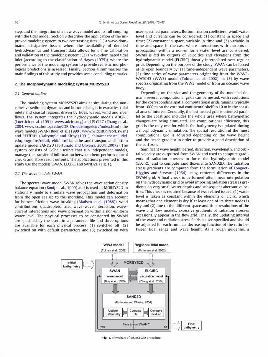
The modeling system MORSYS2D aims at simulating the non-cohesive sediment dynamics and bottom changes in estuaries, tidalinlets and coastal regions, driven by tides, waves, wind and riverflows. The system integrates the hydrodynamic models ADCIRC(Luettich et al. (1991), www.adcirc.org) and ELCIRC (Zhang et al.,2004, www.ccalmr.ogi.edu/CORIE/modeling/elcirc/index.html), thewave models SWAN (Booij et al. (1999), www.wldelft.nl/soft/swan)and REF/DIF1 (Dalrymple and Kirby (1991), chinacat.coastal.udel.edu/programs/refdif/refdif.html) and the sand transport and bottomupdate model SAND2D (Fortunato and Oliveira, 2004, 2007a). Thesystem consists of C-Shell scripts that run independent models,manage the transfer of information between them, perform controlchecks and store result outputs. The applications presented in thisstudy use the models SWAN, ELCIRC and SAND2D (Fig. 1).

2.2. The wave module SWAN

The spectral wave model SWAN solves the wave action densitybalance equation (Booij et al., 1999) and is used in MORSYS2D instationary mode to simulate wave propagation and deformationfrom the open sea up to the shoreline. This model can accountfor bottom friction, wave breaking (Madsen et al. (1988)), windcontributions, quadruplets, triad wave–wave interaction, wave–current interactions and wave propagation within a non-uniformwater level. The physical processes to be considered by SWANare specified by the users in a parameter file and three optionsare available for each physical process: (1) switched off; (2)switched on with default parameters and (3) switched on with

Fig. 1. Flowchart of MO

user-specified parameters. Bottom friction coefficient, wind, waterlevel and currents can be considered: (1) constant in space andtime; (2) constant in space, variable in time and (3) variable intime and space. In the case where interactions with currents orpropagation within a non-uniform water level are considered,SWAN is fed by outputs of velocities and elevations from thehydrodynamic model (ELCIRC) linearly interpolated over regulargrids. Depending on the purpose of the study, SWAN can be forcedat its open boundary by: (1) time-independent wave parameters,(2) time series of wave parameters originating from the WAVE-WATCH3 (WW3) model (Tolman et al., 2002); or (3) by wavespectra originating from the WW3 model or from an oceanic wavebuoy.

Depending on the size and the geometry of the modeled do-main, several computational grids can be nested, with resolutionsfor the corresponding spatial computational grids ranging typicallyfrom 1000 m on the external continental shelf to 10 m in the coast-al area of interest. Generally, the last nested grid is oriented paral-lel to the coast and includes the whole area where bathymetricchanges are being simulated. For computational efficiency, thisgrid is the only one for which the bathymetry is updated duringa morphodynamic simulation. The spatial resolution of the finestcomputational grid is adjusted depending on the wave heightand the beach gradient in order to provide a good description ofthe surf zone.

Significant wave height, period, direction, wavelength, and orbi-tal velocity are outputted from SWAN and used to compute gradi-ents of radiation stresses to force the hydrodynamic model(ELCIRC) and to compute sand fluxes into SAND2D. The radiationstress gradients are computed from the formulation of Longuet-Higgins and Stewart (1964) using centered differences in theSWAN grid. A final check is performed after linear interpolationon the hydrodynamic grid to avoid imposing radiation stresses gra-dients on very small water depths and subsequent aberrant veloc-ities. This check is required because of two related issues: (1) waterlevel is taken as constant within the elements of Elcirc, whichmeans that one element is dry if at least one of its three nodes isdry and (2) due to the different space and time resolutions of thewave and flow models, excessive gradients of radiation stressesoccasionally appear in the flow grid. Finally, the updating intervalof the wave and radiation stress fields is user-specified and shouldbe adjusted for each run as a decreasing function of the ratio be-tween tidal range and wave height. As a rough guideline, a

RSYS2D procedure.

X. Bertin et al. / Ocean Modelling 28 (2009) 75–87 77

1800 s updating interval is used in MORSYS2D for moderate waves(1.5 m) and a moderate tidal range (3 m).

2.3. The hydrodynamic module ELCIRC

ELCIRC was developed as an open source community model at theCenter for Coastal Margin Observation and Prediction (Zhang et al.,2004). ELCIRC solves the fully non-linear, three-dimensional, baro-clinic shallow water equations, coupled to transport equations forsalt and heat. Within MORSYS2SD, a single vertical layer is used,and ELCIRC reverts to a 2D depth-averaged model. Forcings includetides, tidal potential, river flow, wind or waves-induced radiationstresses and solar radiation. A Manning friction law was integrated,with the friction coefficient either constant or variable in space.Although with important implementation differences (e.g. treat-ment of baroclinicity and of tangential velocities), the numericalsolution is inspired from that of UnTRIM (Casulli and Zanolli,1998). The equations are solved with a finite volume technique forvolume conservation and a natural treatment of wetting and drying.The horizontal domain is discretized with a triangular mesh for flex-ibility, and z-coordinates are used in the vertical. A semi-implicittime-stepping algorithm and the Lagrangian treatment of the advec-tive terms ensure stability at large time steps.

The effect of short waves on the hydrodynamics was achievedthrough the forcing by the gradients of wave radiation stresses,which, for depth-averaged models, can be computed through theformulation proposed by Longuet-Higgins and Stewart (1964).Since ELCIRC is used in 2DH mode, the gradients of radiation stres-ses can be regarded as a surface stress ssxy (Blain and Cobb, 2003),which reads:

ssx ¼ �@Sxx

@xþ @Syx

@y

� �ð1Þ

ssy ¼ �@Syy

@yþ @Sxy

@x

� �ð2Þ

where Sxx, Syy, Sxy and Syx are the wave radiation stress terms givenby Longuet-Higgins and Stewart (1964)

Sxx ¼E2

2Cg

Cðcos2 aþ 1Þ � 1

� �ð3Þ

Syy ¼E2

2Cg

Cðsin2 aþ 1Þ � 1

� �ð4Þ

Sxy ¼ Syx ¼ ECg

Csin a cos a ð5Þ

In the previous equations, E ¼ 18 qgH2

rms is the wave energy, a is thewave angle to the x axis, Cg is the wave group velocity, C the wavephase velocity and q is the water density. Wave-induced horizontaldiffusion was also taken into account in the momentum equationsusing an eddy viscosity approach, where the horizontal eddy viscos-ity coefficient mt was computed at each node according to Battjes(1975):

mt ¼ M � Hrms �eb

q

� �13

ð6Þ

In the previous equation (Eq. (6)), M is a dimensionless turbulentparameter set to 1 and eb is the wave energy dissipation coefficientgiven by Thornton and Guza (1983).

2.4. The sand transport and bottom evolution module SAND2D

The bottom update model simulates sand transport due towaves and currents using one of several semi-empirical formulae

and computes the resulting bed changes through the Exner equa-tion (Fortunato and Oliveira, 2004, 2007a). This equation is solvedwith a node-centered finite volume technique based on a triangu-lar unstructured grid, and using a predictor–corrector method:

Dhi ¼ 11� k

rQ i� ð7Þ

where k is the sediment porosity, h is the water depth and Q* is thesediment flux integrated over the morphological time step whichincludes a diffusive term:

Q � ¼ Q þ eð1� kÞ jQ xj@h@x; jQ yj

@h@y

� �ð8Þ

In Eq. (8), e is a user-specified constant to tune the artificial diffu-sion and Q is the sediment flux computed at the center of the ele-ments and integrated in time between steps n and n + 1:

Q ¼Z nþ1

nqðuðtÞ;gðtÞ;hn

;Uorb; :::Þdt ð9Þ

In Eq. (9), q is the instantaneous sand flux, which is a function of thevelocity u, the tidal elevation g and, in the presence of waves, otherparameters like the wave orbital velocity Uorb. Instantaneous sandfluxes are computed using an empirical or a semi-empirical formulaselected within a wide range implemented in MORSYS2D, includ-ing: (1) formulae for currents only (e.g., Ackers and White (1973),Van Rijn (1984), Bhattacharya et al. (2007)); and (2) formulae forwaves and currents (e.g., Bijker (1971), Soulsby-Van Rijn (Soulsby,1997), Bailard and Inman (1981), or the Ackers–White formula(Ackers and White, 1973) adapted to wave environments by Vande Graaff and Van Overeem (1979)). Details on these four latter for-mulations are given in Appendix A.

In earlier versions of the model (Fortunato and Oliveira, 2004),velocities and water levels were fed into SAND2D in the frequencydomain (i.e., through tidal amplitudes and phases, rather than timeseries). While this method was efficient for slowly evolving sys-tems, it also had severe drawbacks. First, using harmonic analysisin wave-driven flows is inadequate. Secondly, its application tovery dynamic coastal systems required the use of morphologicalfactors well below unity (Fortunato and Oliveira, 2007a) to preventlarge Courant numbers and subsequent numerical oscillations. Be-sides being very time-consuming, this method implied using a rep-resentative tide (M2 only), which could be problematic whentrying to reproduce the behavior of a coastal system.

In spite of the predictor–corrector algorithm, the stability of thesolution is limited by the Courant number. Numerical experimentsindicate the model is stable for Courant numbers of up to 10(Fortunato and Oliveira, 2007a). The Courant number can be esti-mated as (Roelvink, 2006):

Cu � bQs

hDxð10Þ

where b is the velocity power in the transport formulae (typicallybetween 3 and 5, depending on the specific formulation).

Maximum values of Cu for a fixed time step vary over more thanthree orders of magnitude within a tidal cycle, thereby imposingthe need for very small time steps. To improve efficiency, an adap-tive time step was implemented, targeting a user-specified con-stant value for Cu (Bertin et al., 2007). The determination of thenext morphological time step is based on two assumptions: (i)the logarithm of an, the maximum Courant number at time n di-vided by the time step, varies linearly in time and (ii) the morpho-logical time step varies slowly from one time step to another. Thefirst assumption was based on observations of Cu during runs witha constant time step. Assumptions (i) and (ii) permit to make a pre-diction of the next Courant number Cun+1, using a log-linearextrapolation (Eqs. (11) and (12)):

78 X. Bertin et al. / Ocean Modelling 28 (2009) 75–87

lnðanþ1Þ � lnðanÞDtnþ1

¼ lnðanÞ � lnðan�1ÞDtn

ð11Þ

According to assumption (ii), Dtn+1 � Dtn, Eq. (12) simplifies to:

anþ1 ¼a2

n

an�1ð12Þ

Then, in order to target a user-specified Courant number Cutarget, thenext morphodynamic time step Dtn+1 can be computed as:

Dtnþ1 ¼ Cutarget �an�1

a2n

ð13Þ

Finally, the last step of the procedure corresponds to the applicationof a relaxation factor and yields the new morphodynamic time stepDt�nþ1:

Dt�nþ1 ¼ d � Dtnþ1 þ ð1� dÞ � Dtn ð14Þ

where d is a relaxation factor which was set to 0.7. The applicationof this relaxation factor enforces approximation (ii) and also pre-vents the extrapolation of a to produce overshoots of the time step.

The implementation of this adaptive procedure leads to timesteps that vary from about 2 min when sand fluxes are maximum(typically around mid-tide and/or for large wave conditions) to45 min when sand fluxes are minimum (around high and low tideand/or when waves are small). Other authors mention using anadaptive time-stepping procedure (Nicholson et al., 1997; Brokeret al., 2003), but the descriptions are not detailed enough to allowfor a comparison with the proposed approach.

3. Application and validation of the morphodynamic modelingsystem

The morphodynamic modeling system was validated at twocontrasting sites: a dissipative wave-dominated beach located in

Fig. 2. General location map of the Iberic Peninsula and France showing the two studiedtidal model of Fortunato et al. (2002) are shown in dashed lines and the output location

the middle of the French Atlantic coast and a very dynamic tidal in-let located in the middle of the Western coast of Portugal (Fig. 2).For the first application, the model was forced by tides and wavesin order to test its ability to reproduce wave deformation, wave-in-duced currents and longshore transport. For the second applica-tion, the model was forced only by tides, to test the performanceof the adaptive time step, and then by tides and waves, to evaluatethe pertinence of morphological predictions.

3.1. Application to a wave-dominated dissipative beach

3.1.1. Model settingIn this section, the morphodynamic modeling system MORSYS2D

was applied to a wave-dominated dissipative beach located withinthe SW part of Oléron Island, in the middle of the French Atlanticcoast (Figs. 2 and 3). A 3-day field measurement campaign, includinga bathymetric survey extending from the dune down to water depthsof 10 m below MSL, tracer experiments and hydrodynamic measure-ments, was conducted on this beach on April 2005, and provided alarge data set of wave parameters, longshore currents and sedimenttransport (Bertin et al., 2008a,b). This beach was also selected be-cause it displayed an almost flat and dissipative morphology duringthe experiments, which induced relatively simple patterns of wave-induced currents (tidal influence is restricted to water level variation(Bertin et al., 2008b)). Another advantage of this site was the localmacrotidal range combined to the deployment of measuring instru-ments within the intertidal zone, which allowed for the record ofcross-shore profiles of wave parameters and wave-induced currents.The model was run from the 4th to the 6th of April 2005 and this per-iod was characterized by a moderate tidal range of 3.5 m and moder-ate WNW swells without local winds producing 0.9–1.3 m cleanwaves at the breaking point.

sites (isobath lines 100 m and 1000 m are shown in bold). Boundaries of the regionals of the WW3 model are marked as crosses.

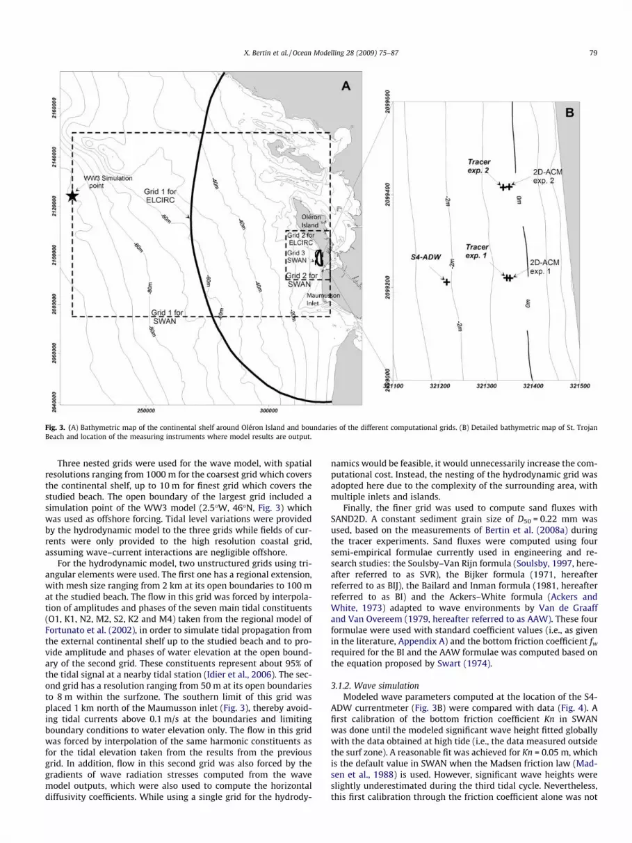
Fig. 3. (A) Bathymetric map of the continental shelf around Oléron Island and boundaries of the different computational grids. (B) Detailed bathymetric map of St. TrojanBeach and location of the measuring instruments where model results are output.

X. Bertin et al. / Ocean Modelling 28 (2009) 75–87 79

Three nested grids were used for the wave model, with spatialresolutions ranging from 1000 m for the coarsest grid which coversthe continental shelf, up to 10 m for finest grid which covers thestudied beach. The open boundary of the largest grid included asimulation point of the WW3 model (2.5�W, 46�N, Fig. 3) whichwas used as offshore forcing. Tidal level variations were providedby the hydrodynamic model to the three grids while fields of cur-rents were only provided to the high resolution coastal grid,assuming wave–current interactions are negligible offshore.

For the hydrodynamic model, two unstructured grids using tri-angular elements were used. The first one has a regional extension,with mesh size ranging from 2 km at its open boundaries to 100 mat the studied beach. The flow in this grid was forced by interpola-tion of amplitudes and phases of the seven main tidal constituents(O1, K1, N2, M2, S2, K2 and M4) taken from the regional model ofFortunato et al. (2002), in order to simulate tidal propagation fromthe external continental shelf up to the studied beach and to pro-vide amplitude and phases of water elevation at the open bound-ary of the second grid. These constituents represent about 95% ofthe tidal signal at a nearby tidal station (Idier et al., 2006). The sec-ond grid has a resolution ranging from 50 m at its open boundariesto 8 m within the surfzone. The southern limit of this grid wasplaced 1 km north of the Maumusson inlet (Fig. 3), thereby avoid-ing tidal currents above 0.1 m/s at the boundaries and limitingboundary conditions to water elevation only. The flow in this gridwas forced by interpolation of the same harmonic constituents asfor the tidal elevation taken from the results from the previousgrid. In addition, flow in this second grid was also forced by thegradients of wave radiation stresses computed from the wavemodel outputs, which were also used to compute the horizontaldiffusivity coefficients. While using a single grid for the hydrody-

namics would be feasible, it would unnecessarily increase the com-putational cost. Instead, the nesting of the hydrodynamic grid wasadopted here due to the complexity of the surrounding area, withmultiple inlets and islands.

Finally, the finer grid was used to compute sand fluxes withSAND2D. A constant sediment grain size of D50 = 0.22 mm wasused, based on the measurements of Bertin et al. (2008a) duringthe tracer experiments. Sand fluxes were computed using foursemi-empirical formulae currently used in engineering and re-search studies: the Soulsby–Van Rijn formula (Soulsby, 1997, here-after referred to as SVR), the Bijker formula (1971, hereafterreferred to as BIJ), the Bailard and Inman formula (1981, hereafterreferred to as BI) and the Ackers–White formula (Ackers andWhite, 1973) adapted to wave environments by Van de Graaffand Van Overeem (1979, hereafter referred to as AAW). These fourformulae were used with standard coefficient values (i.e., as givenin the literature, Appendix A) and the bottom friction coefficient fw

required for the BI and the AAW formulae was computed based onthe equation proposed by Swart (1974).

3.1.2. Wave simulationModeled wave parameters computed at the location of the S4-

ADW currentmeter (Fig. 3B) were compared with data (Fig. 4). Afirst calibration of the bottom friction coefficient Kn in SWANwas done until the modeled significant wave height fitted globallywith the data obtained at high tide (i.e., the data measured outsidethe surf zone). A reasonable fit was achieved for Kn = 0.05 m, whichis the default value in SWAN when the Madsen friction law (Mad-sen et al., 1988) is used. However, significant wave heights wereslightly underestimated during the third tidal cycle. Nevertheless,this first calibration through the friction coefficient alone was not

Fig. 4. Measured and simulated wave parameters at St. Trojan Beach from the 4th to the 6th of April 2005: (A) significant wave height, (B) peak period and (C) wave direction.The dotted line in panel (A) corresponds to model results with default parameters and illustrates the necessity to calibrate the wave model.

80 X. Bertin et al. / Ocean Modelling 28 (2009) 75–87

sufficient to reproduce the cross-shore profile of wave heightswithin the surfzone (Fig. 4A). The default breaking parameter inSWAN (c = 0.73), which corresponds to the ratio between the max-imum possible wave height and the local water depth, appeared tobe inadequate for such a low-gradient beach since the significantwave height was systematically over-predicted within the surfzone. This parameter was thus adjusted to a value of c = 0.55. Thisvalue is in borderline with the 0.6–0.83 range of Battjes and Stive(1985), but led to a fair reproduction of the wave height decaywithin the surfzone (Fig. 4A). This reproduction is very importantfor morphodynamic simulations since the rate of wave height de-cay determines the gradient of radiation stress, thereby controllingthe magnitude and the cross-shore shape of longshore currents.Hence, the calibration of the c breaker parameter may be consid-ered with attention for future modeling works of wave-dominatedenvironments, particularly for low-gradient beaches.

Wave peak periods and directions were very well predictedfrom the first simulations, suggesting the calibrated parametersonly have a negligible influence on wave angle and direction. Over-all, using the WW3 model as offshore forcing resulted in very goodpredictions, which shows the great value of WW3 predictionswhen working in a coastal zone where offshore wave records areunavailable. The good quality of WW3 predictions was already re-ported in several areas (for instance in the Bay of Biscay by Abadieet al. (2006) and Bertin et al. (2008b) and in the Australian GoldCoast by Browne et al. (2007)).

3.1.3. Hydrodynamics simulationModeled longshore currents and water levels were outputted at

the locations of the S4-ADW and 2D-ACM currentmeters and com-pared with data (Fig. 5). A good agreement was observed between

measured and modeled water level (RMSE = 0.06 m, Fig. 5A), whichvalidates the regional tidal model of Fortunato et al. (2002) for off-shore tidal forcing in this area. Water elevation also integrates asetup due to the shore-normal component of the wave radiationstress gradients. To separate the tidal and the wave-induced com-ponents of the elevation, a simulation was performed withoutwaves and the corresponding tidal curve was superimposed onFig. 5A. This figure shows the ability of the model to reproduce thissetup, which is slightly negative backward of the breaking zone(setdown) and reaches up to 0.2 m close to the shoreline. Hence,this good correlation between observed and predicted water depthalso constitutes a first validation of the procedure used to couplethe wave and the hydrodynamic models.

In terms of longshore currents, the calibration was performedthrough the adjustment of a space-constant Manning friction coef-ficient n, until a good correlation was obtained at the location ofthe 2D-ACM currentmeter, which was also the location of sedimenttracer experiment (Fig. 5C). The calibrated value of n = 0.015 m�1/

3 s also leads to a fair prediction of longshore currents in the beachlower part at the location of the S4-ADW currentmeter (Fig. 5B).Although using a simple Manning law to represent bottom frictionat beaches was already used successfully by Smith et al. (1993), itcould appear simplistic compared to other coastal modeling sys-tems, which integrate more sophisticated bed shear stress equa-tions, such as those of Mei (1989), Liu and Dalrymple (1978) orLe Blond and Tang (1974). Nevertheless, these equations weredeveloped for beaches and their validity in tidally-dominated envi-ronments remains to be demonstrated. In particular, the later twoequations result in the absence of bed shear stress when the bot-tom orbital velocity is zero, which would lead to the over-predic-tion of velocities when applied to estuaries and tidal inlets.

Fig. 5. Measured and simulated hydrodynamics at St. Trojan Beach from the 4th to the 6th of April 2005: (A) water depth at the S4-ADW currentmeter, (B) longshore currentat the S4-ADW currentmeter and (C) longshore current at the 2D-ACM currentmeter.

X. Bertin et al. / Ocean Modelling 28 (2009) 75–87 81

Some differences remain between longshore current predic-tions and measurements, particularly at the lower part of thebeach (Fig. 5B). Longshore currents were slightly underestimatedduring the third tidal cycle (Fig. 5B), which could be related tothe underestimation of wave height as reported in the previoussection (Fig. 4A). Then model/data comparison appears weakerfor larger water depths, which can be due to the fact that cur-rents were measured only at 0.4 m from the bottom and donot represent depth-integrated velocities seaward of the break-ing zone, where vertical mixing is weak. Finally, the measuredlongshore current displayed low-frequency fluctuations (0.03–0.003 Hz) that the model was not able to reproduce. This lattervariability is due to the low-frequency modulation of incidentwave energy, which induces fluctuations in current intensity inthe infragravity band. Such fluctuations cannot be representedin our approach since the wave forcing is constant at the timescale of these fluctuations and thus the model only computes‘‘mean currents”.

The overall very good agreement between predicted and ob-served longshore current validates the procedure developed toforce the hydrodynamic model by gradient of wave radiationstresses.

3.1.4. Sand transport predictionsThe fine calibration of hydrodynamics at the St. Trojan Beach al-

lowed for a comparison between the model transport predictionsand tide-integrated values evaluated from tracer experiments. Sed-iment transport was computed over the simulated period using theSVR, the BIJ, the BI and the AAW formulae (Appendix A) and thelongshore component of instantaneous fluxes was outputted atthe location of the 2D-ACM currentmeter, which also coincided

with the location of tracer experiments (Fig. 3B). Sand fluxes werederived from tracer experiments based on the movement of thetracer cloud centroïd between two successive low tides, which pro-vides a local estimation of the total load (i.e. bedload and suspen-sion) integrated over a tidal cycle.

Comparison between instantaneous fluxes obtained from thesefour formulae revealed significant differences, with the BIJ and SVRformulae producing 5–10 times larger fluxes than the BI and AAWformulae (Fig. 6A). Instantaneous fluxes were then integrated overa tidal cycle, to be compared to the transport rates evaluated fromtracer experiments. The same scatter as for instantaneous fluxeswas observed, with the BIJ and SVR formulae producing 5–12 timeslarger sand fluxes than those deduced from tracer experiments.The BI and the AAW formulae gave values in good agreement withtracer results (Figs. 6B and 4C).

Given that the presented formulae were applied as given in theliterature, it can be argued that the observed scattered results arerelated to the intrinsic properties of each formula. The good predic-tive skills of the BI and AAW formulae as well as the one order ofmagnitude overestimations of the BIJ formula are consistent withprevious findings of Bayram et al. (2001), who tested these formu-lae using the field data obtained during Duck Beach experiments(North Carolina, USA).The large errors obtained with the BIJ for-mula could also be explained by the poor performance of this for-mula with fine sands (Camenen and Larroudé, 2003).

Although the results obtained for this particular beach may besite-specific and, for instance, result from the presence of fine sand,they highlight the critical problem that represents the choice of atransport formula when simulating morphological evolutions in areal case study and point out the usefulness of tracer experimentsto evaluate transport predictions.

Fig. 6. (A) Model predictions of instantaneous longshore sand fluxes at the location of the 2D-ACM currentmeter from the 4th to the 6th of April 2005 using the SVR, the BIJ,the BI and the AWM formulae. (B) and (C): comparison of tide-integrated longshore transport at the same location predicted by the model using these formulae and valuesdeduced from tracer experiments.

Fig. 7. Bathymetric map of the continental shelf around the Óbidos Lagoon and boundaries of the different computational grids; the open boundaries of the Grid 1 for SWANare outside the figure limits. Location of the instruments deployed to record wave conditions outside the lagoon and water elevation inside the lagoon at Bico do Corvo (BDC).

82 X. Bertin et al. / Ocean Modelling 28 (2009) 75–87

3.2. Application to a very dynamic tidal inlet

3.2.1. Model settingThe improved modeling system was tested by applying it to the

very dynamic Óbidos Inlet located on the western coast of Portugal(Fig. 7). The combination of a meso-tidal range, a severe wave cli-mate and shallow channels results in high velocities, large sedi-ment fluxes and subsequent very fast morphological changes(Oliveira et al., 2006). Due to these characteristics, this coastal sys-tem is difficult to simulate, but provides an ideal testbed to addressthe numerical stability and the performance of the improved mod-eling system.

The modeling system was forced first by tides alone, using aconstant tide represented by M2 only (producing a 2 m tidalrange outside the lagoon and 1.3 m inside, Fig. 8a) and takingadvantage of previous calibration work (Oliveira et al., 2006).The purpose of this test was to evaluate the performances ofthe adaptive morphodynamic time-stepping procedure in termsof computational time and numerical stability. The initialbathymetry for the simulation was based on two surveys. Thefirst was conducted in June 2000 and covered the whole lagoon.The second was measured in July 2001, after the inlet was relo-cated and the tidal channels dredged, and covered only the lowerlagoon, where the major morphological changes occur (Oliveira

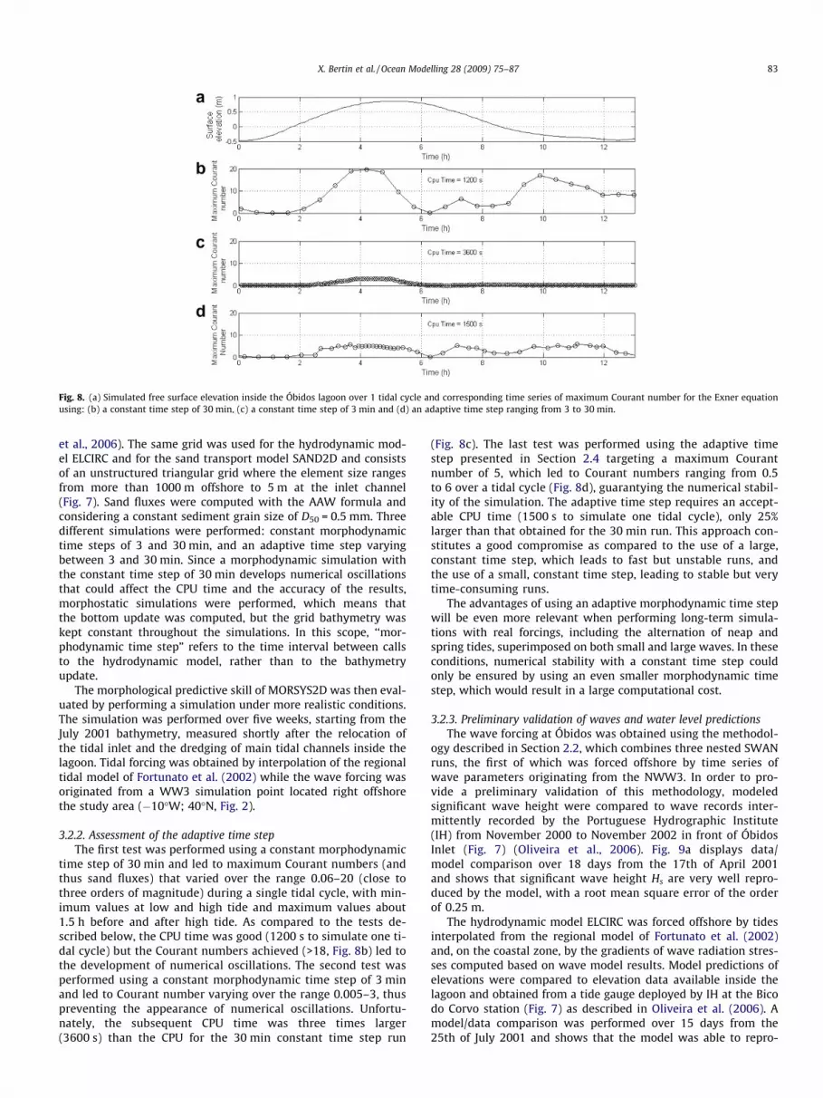
Fig. 8. (a) Simulated free surface elevation inside the Óbidos lagoon over 1 tidal cycle and corresponding time series of maximum Courant number for the Exner equationusing: (b) a constant time step of 30 min, (c) a constant time step of 3 min and (d) an adaptive time step ranging from 3 to 30 min.

X. Bertin et al. / Ocean Modelling 28 (2009) 75–87 83

et al., 2006). The same grid was used for the hydrodynamic mod-el ELCIRC and for the sand transport model SAND2D and consistsof an unstructured triangular grid where the element size rangesfrom more than 1000 m offshore to 5 m at the inlet channel(Fig. 7). Sand fluxes were computed with the AAW formula andconsidering a constant sediment grain size of D50 = 0.5 mm. Threedifferent simulations were performed: constant morphodynamictime steps of 3 and 30 min, and an adaptive time step varyingbetween 3 and 30 min. Since a morphodynamic simulation withthe constant time step of 30 min develops numerical oscillationsthat could affect the CPU time and the accuracy of the results,morphostatic simulations were performed, which means thatthe bottom update was computed, but the grid bathymetry waskept constant throughout the simulations. In this scope, ‘‘mor-phodynamic time step” refers to the time interval between callsto the hydrodynamic model, rather than to the bathymetryupdate.

The morphological predictive skill of MORSYS2D was then eval-uated by performing a simulation under more realistic conditions.The simulation was performed over five weeks, starting from theJuly 2001 bathymetry, measured shortly after the relocation ofthe tidal inlet and the dredging of main tidal channels inside thelagoon. Tidal forcing was obtained by interpolation of the regionaltidal model of Fortunato et al. (2002) while the wave forcing wasoriginated from a WW3 simulation point located right offshorethe study area (�10�W; 40�N, Fig. 2).

3.2.2. Assessment of the adaptive time stepThe first test was performed using a constant morphodynamic

time step of 30 min and led to maximum Courant numbers (andthus sand fluxes) that varied over the range 0.06–20 (close tothree orders of magnitude) during a single tidal cycle, with min-imum values at low and high tide and maximum values about1.5 h before and after high tide. As compared to the tests de-scribed below, the CPU time was good (1200 s to simulate one ti-dal cycle) but the Courant numbers achieved (>18, Fig. 8b) led tothe development of numerical oscillations. The second test wasperformed using a constant morphodynamic time step of 3 minand led to Courant number varying over the range 0.005–3, thuspreventing the appearance of numerical oscillations. Unfortu-nately, the subsequent CPU time was three times larger(3600 s) than the CPU for the 30 min constant time step run

(Fig. 8c). The last test was performed using the adaptive timestep presented in Section 2.4 targeting a maximum Courantnumber of 5, which led to Courant numbers ranging from 0.5to 6 over a tidal cycle (Fig. 8d), guarantying the numerical stabil-ity of the simulation. The adaptive time step requires an accept-able CPU time (1500 s to simulate one tidal cycle), only 25%larger than that obtained for the 30 min run. This approach con-stitutes a good compromise as compared to the use of a large,constant time step, which leads to fast but unstable runs, andthe use of a small, constant time step, leading to stable but verytime-consuming runs.

The advantages of using an adaptive morphodynamic time stepwill be even more relevant when performing long-term simula-tions with real forcings, including the alternation of neap andspring tides, superimposed on both small and large waves. In theseconditions, numerical stability with a constant time step couldonly be ensured by using an even smaller morphodynamic timestep, which would result in a large computational cost.

3.2.3. Preliminary validation of waves and water level predictionsThe wave forcing at Óbidos was obtained using the methodol-

ogy described in Section 2.2, which combines three nested SWANruns, the first of which was forced offshore by time series ofwave parameters originating from the NWW3. In order to pro-vide a preliminary validation of this methodology, modeledsignificant wave height were compared to wave records inter-mittently recorded by the Portuguese Hydrographic Institute(IH) from November 2000 to November 2002 in front of ÓbidosInlet (Fig. 7) (Oliveira et al., 2006). Fig. 9a displays data/model comparison over 18 days from the 17th of April 2001and shows that significant wave height Hs are very well repro-duced by the model, with a root mean square error of the orderof 0.25 m.

The hydrodynamic model ELCIRC was forced offshore by tidesinterpolated from the regional model of Fortunato et al. (2002)and, on the coastal zone, by the gradients of wave radiation stres-ses computed based on wave model results. Model predictions ofelevations were compared to elevation data available inside thelagoon and obtained from a tide gauge deployed by IH at the Bicodo Corvo station (Fig. 7) as described in Oliveira et al. (2006). Amodel/data comparison was performed over 15 days from the25th of July 2001 and shows that the model was able to repro-

Fig. 9. Measured and simulated wave height (a) and surface elevation (b) at Óbidos Inlet, showing the good predictive skills of the modeling system.

84 X. Bertin et al. / Ocean Modelling 28 (2009) 75–87

duce very well the elevations, with root mean square errors of0.065 m.

Fig. 10. Morphological simulation of Óbidos inlet from the 25th of July to the 30thof August 2001, showing the development of a realistic ebb-delta.

3.2.4. Morphodynamic simulationThe initial bathymetry used in this 5 weeks morphodynamic

simulation was measured shortly after the relocation of the tidalinlet and the dredging of the North Channel inside the lagoon,which means that no significant ebb-delta was found in front ofthe inlet at the beginning of the simulation. The predictive skillof the model was thus tested namely by its ability to reproduce arealist ebb-delta. Forcings during the simulated period includedtides ranging from 1.2 to 3 m and short period (Tp = 5–10 s), lowto moderate energy (Hs = 1–2 m) waves coming from the N toNW and inducing a southwestward longshore transport. Fig. 10firstly shows that the model was able to reproduce the develop-ment of a well-shaped and realistic ebb-delta. The channel depthat the inlet increased from 2.5 m below mean sea-level (MSL) to4 m below MSL, and the inlet enlarged from 115 m to 140 m andmigrated about 15 m southward. The enlargement of tidal chan-nels promoted the tidal propagation within the lagoon, whichwas illustrated by an increase of M2 amplitude from 0.4 m at thebeginning of the simulation to 0.5 m after 5 weeks of simulations.This increase in tidal propagation within the lagoon during fairweather conditions is consistent with the observations of Oliveiraet al. (2006), who reported M2 amplitudes exceeding 0.5 m withinthe lagoon in the end of summer 2001. The southward displace-ment of the inlet mouth is also consistent with observations, withindicate that the inlet tends to migrate south after relocations(Fortunato and Oliveira, 2007b). Numerical simulations will haveto be performed over longer periods, to enable the morphologicalpredictions to be compared to several bathymetric surveys. Thiswork is in progress and will be reported on a separate paper.

4. Summary and conclusions

The MORSYS2D modeling system was firstly improved by inte-grating the SWAN spectral wave model (Booij et al., 1999) and forcedoffshore by the WW3 (Tolman et al., 2002) global wave model. Theuse of WW3 data as offshore forcing was shown to be very valuable,particularly in the case where no wave records are available close tothe study area. The comparison with field measurements revealedthat the model of wave dissipation by breaking should be calibrated,which matches the conclusions of Apostos et al. (2008). This calibra-tion is of critical importance since the rate of wave energy decaycontrols the gradients of radiation stresses and thus the magnitudeand cross-shore distribution of longshore currents.

X. Bertin et al. / Ocean Modelling 28 (2009) 75–87 85

The effect of short waves on water circulation was taken intoaccount by including the gradients of wave radiation stress intothe momentum equations of the ELCIRC hydrodynamic model.The horizontal momentum diffusion due to wave breaking wasalso implemented in Elcirc, but data/model comparison at the dis-sipative beach case showed that it only improves slightly thehydrodynamic predictions. A simple Manning friction law wasadopted, which presents the advantage of limiting the calibrationwork and performs well with or without waves. Although our ap-proach could appear simplistic compared to more sophisticatedmodels, it was shown to perform well at a wave-dominatedbeach. Furthermore, model over-calibration subsequent to sophis-ticated physical models for friction or momentum diffusion goesagainst the spirit in which MORSYS2D was developed, whichwas to build a relatively simple and robust modeling system,but being easily applicable to realistic case studies.

The implementation of an adaptive morphodynamic time stepwas shown to result in a good balance between numerical stabilityand computational efficiency. This procedure will be of particularinterest when performing long-term simulations with a real forc-ing (alternation of small and large waves superimposed on springand neap tides), where the numerical stability with a constant timestep could only be ensured by a very small morphodynamic timestep.

Application of the model to two contrasting case studies dem-onstrated its ability to reproduce coastal dynamics. The fine cali-bration of hydrodynamics at the St. Trojan Beach allowed for arealistic comparison between model transport predictions and tra-cer experiments. This comparison revealed a one order of magni-tude scatter from one formula to another and illustrated theproblem that represents the choice of a transport formula whenperforming coastal morphodynamic simulations. An applicationto the Óbidos tidal inlet revealed that the model is able to realisti-cally reproduce the generation of an ebb-delta.

As a general conclusion, the MORSYS2D modeling system wasimproved and is at present capable of simulating waves, tide andwave-induced hydrodynamics, sand transport and morphologicalevolutions of real and complex coastal systems. Longer term mor-phodynamic simulations are being performed and predictions willbe compared to repetitive bathymetric surveys to validate its pre-dictive skills in terms of morphological evolutions.

Acknowledgements

The first author was funded by the European Commissionthrough a Marie Curie postdoctoral fellowship (project IMMATIE-041171). This work was also partially funded by the Fundação paraa Ciência e a Tecnologia, Programa Operacional ‘‘Ciência, Tecnologia,Inovação” and FEDER, project EMERA: Estudo da Embocadura daRia de Aveiro. The authors thank the developing teams of the mod-els ELCIRC and SWAN for making their source codes available, andInstituto Hidrográfico for the Óbidos lagoon data. Finally, theauthors appreciated the comments of two anonymous reviewersas well as those of the associate editor Dr. Julie Pietrzak, whichgreatly improved this manuscript.

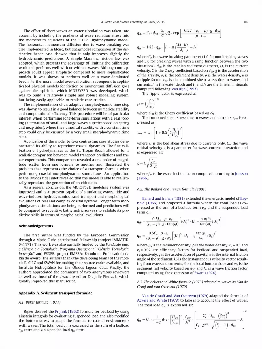
Appendix A. Sediment transport formulae

A.1. Bijker formula (1971)

Bijker derived the Frijlink (1952) formula for bedload by usingEinstein integrals for evaluating suspended load and also modifiedthe bottom stress to adapt the formula to coastal environmentswith waves. The total load qst is expressed as the sum of a bedloadqsb term and a suspended load qss term:

qsb ¼ Cb � d50 �Uc

Cffiffiffigp� exp

�0:27 � ðqs � qÞ � g � d50

l � scw

� �

qss ¼ 1:83 � qsb � I1 � ln33 � h

dc

� �þ I2

� �

where Cb is a wave breaking parameter (1.0 for non breaking wavesand 5.0 for breaking waves with a ramp function between the twosituations), d50 is the median sediment diameter, Uc is the currentvelocity, C is the Chezy coefficient based on d50, g is the accelerationof the gravity, qs is the sediment density, q is the water density, l isa ripple factor, scw is the combined shear stress due to waves andcurrents, h is the water depth and I1 and I2 are the Einstein integralscomputed following Van Rijn (1993).

The ripple factor is expressed as

l ¼ CC90

� �1:5

where C90 is the Chezy coefficient based on d90.The combined shear stress due to waves and currents scw is ex-

pressed as

scw ¼ sc � 1þ 0:5 fUc

Uw

� �2" #

where sc is the bed shear stress due to currents only, Uw the waveorbital velocity. f is a parameter for wave–current interaction andis expressed as:

n ¼ C

ffiffiffiffiffiffiffiffiffifw

2 � g

s

where fw is the wave friction factor computed according to Jonsson(1966).

A.2. The Bailard and Inman formula (1981)

Bailard and Inman (1981) extended the energetic model of Bag-nold (1966) and proposed a formula where the total load is ex-pressed as the sum of a bedload term qsb and the suspended loadterm qss:

qsb ¼0:5f w � q � eb

ðqs � qÞ � g � tanðuÞ ðUtÞ2 � Ut �tanðbÞtanðuÞ ðUtÞ3

� �

qss ¼0:5f w � q � es

ðqs � qÞ � g �wsðUtÞ3 � Ut � es

tanðbÞws

ðUtÞ5� �

where qs is the sediment density, q is the water density, eb = 0.1 andes = 0.02 are efficiency factors for bedload and suspended load,respectively, g is the acceleration of gravity, u is the internal frictionangle of the sediment, Ut is the instantaneous velocity vector result-ing from wave and currents, b is the local bottom slope and ws is thesediment fall velocity based on d50 and fw is a wave friction factorcomputed using the expression of Swart (1974).

A.3. The Ackers and White formula (1973) adapted to waves by Van deGraaf and van Overeem (1979)

Van de Graaff and Van Overeem (1979) adapted the formula ofAckers and White (1973) to take into account the effect of waves.The total load qst is expressed as:

qst ¼ Uc �1

1� pd35 �

Uwc

U�wc

� �n

� Cdgr

Am �Cn

d � Uwc � U�wcUwc

� �n

Cd � gn=2 �ffiffiffiffiffiffiffiffiffiffiffiffiffiffiffiffiffiffiffiffiffiffiffiffiffiffiffiffi

qsq � 1� �

� d35

r � A

2664

3775

m

86 X. Bertin et al. / Ocean Modelling 28 (2009) 75–87

where p is the sediment porosity, d35 the particle diameter ex-ceeded by 65% of the weight, and A, n, m and Cdgr are dimensionlessparameters defined as follows:

n ¼ 1� 0:2432 � lnðdgrÞ

m ¼ 9:66dgrþ 1:34

Cdgr ¼ expð2:86 � lnðdgrÞ � 0:4343 � ½lnðdgrÞ�2 � 8:128Þ

A ¼ 0:23ffiffiffiffiffiffidgr

p þ 0:14

In the main equation, Ucw and U*cw are the current velocity and

shear velocity modified from the original formulation of Ackersand White (1973) to account for waves and currents:

Uwc ¼ Uc �

ffiffiffiffiffiffiffiffiffiffiffiffiffiffiffiffiffiffiffiffiffiffiffiffiffiffiffiffiffiffiffiffiffiffiffiffiffiffiffiffiffiffi1þ 0:5 � n0 � Uw

Uc

� �2s

and

U�wc ¼ U�c �

ffiffiffiffiffiffiffiffiffiffiffiffiffiffiffiffiffiffiffiffiffiffiffiffiffiffiffiffiffiffiffiffiffiffiffiffiffiffiffiffi1þ 0:5 � f � Uw

Uc

� �2s

where

f ¼ 18 � log12 � h

r

� ��

ffiffiffiffiffiffiffiffiffiffiffiffifw

r

� �s

and

f0 ¼ 18 � log10 � h

d35

� ��

ffiffiffiffiffiffiffiffiffiffiffiffiffif 0w2g

� �s

In this two latter equations, h is the water depth, r is the bed rough-ness and fw and f 0w are the wave friction coefficient computedaccording to Swart (1974) and using r and d35 as bed roughness,respectively.

A.4. The Soulsby and Van Rijn formula (Soulsby, 1997)

Soulsby and van Rijn developed a formula to compute sedimenttransport under the combined action of wave and currents. The to-tal load qst is expressed as follows:

qst ¼ As � Uc �

ffiffiffiffiffiffiffiffiffiffiffiffiffiffiffiffiffiffiffiffiffiffiffiffiffiffiffiffiffiffiffiffiffiffiffiffiffiffiffiffiffiffiffiffiffiffiffiU2

c þ0:018

Cd� Uwrms

� �s� Ucr

" #2:4

� ð1� 1:6 � tanðbÞÞ

where Uc is the current velocity, Uwrms is the root mean square waveorbital velocity and b is the local bottom slope, Cd is a drag coeffi-cient, Ucr is the threshold velocity.

As is the sum of a term for bed load Asb and a term for suspendedload Ass:

As ¼ Asb þ Ass

with

Asb ¼0:005 � h � d50

h

� �1:2

qsq � 1� �

� g � d50

� �1:2

and

Asb ¼0:012 � d50 � D�0:6

�

qsq � 1� �

� g � d50

� �1:2

In these two latter equations, h is the water depth, d50 is the meansediment grain size, g is the acceleration of gravity and D* is definedas

D� ¼g � qs

q � 1� �t2

24

35

1=3

� d50

where t is the cinematic viscosity of the water.The drag coefficient Cd in the main equation is defined as:

Cd ¼ 0:40

ln hz0

� �� 1

0@

1A

2

where z0 is the bed roughness length.In the main equation, the threshold current velocity Ucr reads:

Ucr ¼ 0:19 � ðd50Þ0:1 � log4:hd90

� �if 0:1 mm � d50 < 0:5 mm:

And

Ucr ¼ 8:5 � ðd50Þ0:6 � log4 � hd90

� �if 0:5 mm � d50 � 2:0 mm:

References

Abadie, S., Butel, R., Mauriet, S., Morichon, D., Dupuis, H., 2006. Wave climate andlongshore drift on the South Aquitaine coast. Continental Shelf Research 26(16), 1924–1939.

Ackers, P., White, W.R., 1973. Sediment transport: new approach and analysis.Journal of Hydraulics Division 99 (1), 2041–2060.

Apostos, A., Raubenheimer, B., Elgar, S., Guza, R.T., 2008. Testing and calibratingparametric wave transformation models on natural beaches. CoastalEngineering 88 (3), 224–235.

Bagnold, R.A., 1966. An approach to the sediment transport problem from generalphysics. Geological Survey Professional Papers 422-1, Washington, USA.

Bailard, J., Inman, D., 1981. An energetics bedload model for a plane sloping beach:local transport. Journal of Geophysical Research 86 (C), 10938–10954.

Battjes, J., 1975. Modelling of turbulence in the surf zone. In: Symposium onModeling Techniques, ASCE, pp. 1050–1061.

Battjes, J.A., Stive, M.J.F., 1985. Calibration and verification of a dissipation model forrandom breaking waves. Journal of Geophysical Research 90 (C), 9159–9167.

Bayram, A., Larson, M., Miller, H.C., Kraus, N.C., 2001. Crossshore distribution oflongshore sediment transport: comparison between predictive formulas andfield measurements. Coastal Engineering 44, 79–99.

Bertin, X., Fortunato, A., Oliveira, A., 2007. Sensitivity analysis of a morphodynamicmodel applied to a Portuguese tidal inlet. In: Dohmen-Janssen, C.M., Hulsher,S.E. (Eds.), 5th IAHRD Symposium on River, Coastal and EstuarineMorphodynamics (RCEM 2007). Twente University, 17–21 September 2007,pp. 11–17.

Bertin, X., Castelle, B., Anfuso, G., Ferreira, O., 2008a. Improvement of the mixingdepth prediction under conditions of oblique wave breaking. Geo-MarineLetters 28, 65–75.

Bertin, X., Castelle, B., Chaumillon, E., Butel, R., Quique, R., 2008b. Estimation andinter-annual variability of the longshore transport at a high-energy dissipativebeach: the St. Trojan beach, SW Oléron Island, France. Continental ShelfResearch 28, 1316–1332.

Bhattacharya, B., Price, R.K., Solomatine, D.P., 2007. Machine learning approach tomodeling sediment transport. Journal of Hydraulic Engineering 133 (4), 440–450.

Bijker, E.W., 1971. Longshore transport computations. Journal of the Waterways,Harbors and Coastal Engineering Division 97 (4), 687–703.

Blain, C.A., Cobb, M., 2003. Application of a shelf-scale model to wave-inducedcirculation, Part I: Alongshore currents on plane and barred beaches. NRLFormal Report, NRL/FR/7320-03-10,046, Naval Research Laboratory,Department of the Navy, 25pp.

Booij, N., Ris, R., Holthuijsen, L., 1999. A third-generation wave model for coastalregions. 1. Model description and validation. Journal of Geophysical Research104 (C7), 649–666.

Broker, I., Zyserman, J., Madsen, E.O., Mangor, K., Jensen, J., 2003. Morphologicalmodelling: a tool for optimisation of coastal structures. In: Proceedings of theCoastal Engineering Today Conference, Gainesville, Florida, 8–10 October 2003,pp. 1–15.

Browne, M., Castelle, B., Strauss, D., Tomlinson, R., Blumenstein, M., Lane, C., 2007.Near-shore swell estimation from a global wind–wave model: spectral process,

X. Bertin et al. / Ocean Modelling 28 (2009) 75–87 87

linear, and artificial neural network models. Coastal Engineering 54 (5), 445–460.

Callaghan, D.P., Saint-Cast, F., Nielsen, P., Baldock, T.E., 2006. Numerical solutions ofthe sediment conservation law; a review and improved formulation for coastalmorphological modeling. Coastal Engineering 53 (7), 557–571.

Camenen, B., Larroudé, P., 2003. Comparison of sediment transport formulae foracoastal environment. Journal of Coastal Engineering 48 (2), 111–132.

Casulli, V., Zanolli, P., 1998. A three-dimensional semi-implicit algorithm forenvironmental flows on unstructured grids. In: Proceedings of Conference onNumerical Methods for Fluid Dynamics. University of Oxford.

Cayocca, F., 2001. Long-term morphological modeling of a tidal inlet: the ArcachonBasin, France. Coastal Engineering 42 (2), 115–142.

Dalrymple, R.A., Kirby, J.T., 1991. Documentation manual. Combined refraction–diffraction model. REF/DIF 1 version 2.3. CACR Report 91-2, Center for AppliedCoastal Research. Department of Civil Engineering, University of Delaware.

De Vriend, H.J., 1996. Mathematical modelling of meso-tidal barrier island coasts,Part I. Empirical and semi-empirical models. In: Liu, P.L.-F. (Ed.), Advances inCoastal and Ocean Engineering, vol. 2. World Scientific Publishing, Singapore,pp. 115–149.

De Vriend, H.J., Capobianco, M., Chesher, T., de Swart, H.E., Latteux, B., Stive, M.J.F.,1993. Approaches to long-term modelling of coastal morphology: a review.Coastal Engineering 21 (1–3), 225–269.

Fortunato, A.B., Oliveira, A., 2004. A modeling system for tidally driven long-termmorphodynamics. Journal of Hydraulic Research 42 (4), 426–434.

Fortunato, A.B., Oliveira, A., 2007a. Improving the stability of a morphodynamicmodeling system. Journal of Coastal Research, SI 50, 486–490.

Fortunato, A.B., Oliveira, A., 2007b. Case study: improving the stability of the Óbidoslagoon inlet. Journal of Hydraulic Engineering 133 (7), 816–824.

Fortunato, A.B., Pinto, L., Oliveira, A., Ferreira, J.S., 2002. Tidally generated shelfwaves off the Western Iberian Coast. Continental Shelf Research 22 (14), 1935–1950.

Frijlink, H.C., 1952. Discussion des formules de debit solide deKalinske, Einstein etMeyer–Peter and Mueller compte tenue des mesures recentes de transport dansles rivières Néerlandaises. 2nd Journal Hydraulique, Société Hydraulique deFrance, Grenoble, pp. 98–103 (in French).

Grunnet, N.M., Walstra, D.J.R., Ruessink, B.G., 2004. Process-based modelling of ashoreface nourishment. Coastal Engineering 51 (7), 581–607.

Hayes, M.O., 1975. Morphology and sand accumulation in estuaries. In: Cronin, L.E.(Ed.), Estuarine Research, vol. 2. Academic Press, New York, pp. 3–22.

Holliday, B.W., McNair, E.C., Kraus, N.C., 2002. The US Army corps of Engineers’coastal inlets research program. In: Proceedings Dredging’02, ASCE.

Idier, D., Pedreros, R., Oliveros, C., Sottolichio, A., Choppin, L., Bertin, X., 2006.Respective contributions of currents and swell to the sediment mobility in aninternal estuarine platform. Example of the ‘Pertuis Charentais’, France. C.R.Géosciences 338 (10), 718–726.

Johnson, H.K., Zyserman, J.A., 2002. Controlling spatial oscillations in bed levelupdate schemes. Coastal Engineering 46 (2), 109–126.

Johnson, H.K., Brøker, I., Zyserman, J.A., 1994. Identification of some relevantprocesses in coastal morphological modelling. In: Proceedings of the 24thInternational Conference on Coastal Engineering, Kobe, Japan.

Jones, O.P., Petersen, O.S., Kofoed-Hansen, H., 2007. Modelling of complex coastalenvironments: some considerations for best practise. Coastal Engineering 54(10), 717–733.

Jonsson, I.G., 1966. Wave boundary layers and friction factors. In: Proceedings of the10th Coastal Engineering Conference, ASCE, pp. 127–148.

Kubatko, E.J., Westerink, J.J., Dawson, C., 2006. An unstructured gridmorphodynamic model with a discontinuous Galerkin method for bedevolution. Ocean Modelling 15 (1–2), 71–89.

Le Blond, P.H., Tang, C.L., 1974. On energy coupling between waves and rip currents.Journal of Geophysical Research (C79), 811–816.

Lesser, G., Roelvink, J.A., Van Kester, J.A.T.M., Stelling, G.S., 2004. Development andvalidation of a three-dimensional morphological model. Coastal Engineering 51(8–9), 883–915.

Liu, P., Dalrymple, R., 1978. Bottom frictional stresses and longshore currents due towaves with large angle of incidence. Journal of Marine Research 36, 357–375.

Long, W., Kirby, J.T., Shao, Z., 2008. A numerical scheme for morphological bed levelcalculations. Coastal Engineering 55 (2), 167–180.

Longuet-Higgins, M.S., Stewart, R.W., 1964. Radiation stresses in water waves: aphysical discussion, with applications. Deep Sea Research 11, 529–562.

Luettich, R.A., Westerink, J.J., Sheffner, N.W., 1991. ADCIRC: An Advanced Three-Dimensional Model for Shelves, Coasts and Estuaries. Report 1: Theory andMethodology of ADCIRC-2DDI and ADCIRC-3DL.

Madsen, O.S., Poon, Y.-K., Graber, H.C., 1988. Spectral wave attenuation by bottomfriction: theory. In: Proceedings of the 21st International Conference on CoastalEngineering, ASCE, pp. 492–504.

Mei, C.C., 1989. The Applied Dynamics of Ocean Surface Waves. Advanced Series onOcean Engineering, vol. 1. World Scientific, Singapore.

Nicholson, J., Broker, I., Roelvink, J.A., Price, D., Tanguy, J.M., Moreno, L., 1997.Intercomparison of coastal area morphodynamic models. Coastal Engineering31 (1–4), 97–123.

Oliveira, A., Fortunato, A.B., Rego, J.R.L., 2006. Effect of morphological changes onthe hydrodynamics and flushing properties of the Óbidos lagoon (Portugal).Continental Shelf Research 26 (8), 917–942.

Roelvink, J.A., 2006. Coastal morphodynamic evolution techniques. CoastalEngineering 53 (2–3), 277–287.

Saied, U., Tsanis, I.K., 2008. A coastal area morphodynamics model. EnvironmentalModelling and Software 23 (1), 35–49.

Smith, J.M., Larson, M., Kraus, N.C., 1993. Longshore current on a barred beach: fieldmeasurements and calculation. Journal of Geophysical Research (C12), 22717–22731.

Soulsby, R., 1997. Dynamics of marine sands, a manual for practical applications.Thomas Telford, ISBN 0-7277-2584X, HR. Wallingford, England.

Sutherland, J., Walstra, D.J.R., Chesher, T.J., van Rijn, L.C., Southgate, H.N., 2004.Evaluation of coastal area modelling systems at an estuary mouth. CoastalEngineering 51 (8–9), 119–142.

Swart, D.H., 1974. Offshore sediment transport and equilibrium beach profiles. DelftHydraulics Lab Publication 131, Delft, The Netherlands.

Thornton, E.B., Guza, R.T., 1983. Transformation of wave height distribution. Journalof Geophysical Research 88 (C10), 5925–5938.

Tolman, H.L., Balasubramaniyan, B., Burroughs, L.D., Chalikov, D.V., Chao, Y.Y., Chen,H.S., Gerald, V.M., 2002. Development and implementation of wind generatedocean surface wave models at NCEP. Weather and Forecasting 17 (2), 311–333.

Van De Graaff, J., Van Overeem, J., 1979. Evaluation of sediment transport formulaein coastal engineering practice. Coastal Engineering 3 (C), 1–32.

Van Rijn, L.C., 1984. Sediment transport, Part I: Bedload transport. Journal ofHydraulic Engineering ASCE 110, 1431–1456.

Van Rijn, L., 1993. Principles of Sediment Transport in Rivers, Estuaries and CoastalSeas. Aqua Publications, The Netherlands.

Wang, Z.B., Louters, T., de Vriend, H.J., 1995. Morphodynamic modelling for a tidalinlet in the Wadden Sea. Marine Geology 126 (1–4), 289–300.

Work, P.A., Guan, J., Hayter, E.J., Elçi, S., 2001. Mesoscale model for morphologicchange at tidal inlets. Journal of Waterway, Port, Coastal and Ocean Engineering127 (5), 282–289.

Zhang, Y., Baptista, A.M., Myers, E.P., 2004. A cross-scale model for 3D barocliniccirculation in estuary-plume-shelf systems: I. Formulation and skill assessment.Continental Shelf Research 24 (18), 2187–2214.