a shift transformation for fully conservative methods: turbulence simulation on complex,...

Journal of Computational Physics 208 (2005) 704–734

www.elsevier.com/locate/jcp

A shift transformation for fully conservative methods:turbulence simulation on complex, unstructured grids

J.E. Hicken a,*, F.E. Ham b, J. Militzer a, M. Koksal a

a Dalhousie University, Department of Mechanical Engineering, J110 ‘‘C1’’ Building, 5269 Morris St., Halifax, Canada NS B3J 1B6b Center for Turbulence Research, Stanford University, Stanford, CA 94305, USA

Received 6 October 2004; received in revised form 16 February 2005; accepted 3 March 2005

Available online 4 May 2005

Abstract

Operator transformations are presented that allow matrix operators for collocated variables to be transformed into

matrix operators for staggered variables while preserving symmetries. These ‘‘shift’’ transformations permit conserva-

tive, skew-symmetric convective operators and symmetric, positive-definite diffusive operators to be obtained for stag-

gered variables using collocated operators. Shift transformations are not limited to uniform or structured meshes, and

this formulation leads to a generalization of the works of Perot (J. Comput. Phys. 159 (2000) 58) and Verstappen and

Veldman (J. Comput. Phys. 187 (2003) 343). A set of shift operators have been developed for, and applied to, a time-

adaptive Cartesian mesh method with a fractional step algorithm. The resulting numerical scheme conserves mass to

machine error and conserves momentum and energy to second order in time. A mass conserving interpolation is used

for the variables during mesh adaptation; the interpolation conserves momentum and energy to second order in space.

Turbulent channel flow simulations were conducted at Res � 180 using direct numerical simulation (DNS). The DNS

results from the adaptive method compare favourably with spectral DNS results despite the use of a (formally) second-

order accurate scheme.

� 2005 Elsevier Inc. All rights reserved.

Keywords: Direct numerical simulation; Energy-conserving schemes; Stability; Unstructured grids; Staggered mesh; Grid adaptation

1. Introduction

We are interested in the simulation of turbulent, incompressible flows of Newtonian fluids; hence, weconsider the numerical solution of the unsteady, incompressible Navier–Stokes and continuity equations.

The non-dimensional form of these equations is

0021-9991/$ - see front matter � 2005 Elsevier Inc. All rights reserved.

doi:10.1016/j.jcp.2005.03.002

* Corresponding author. Tel.: +1 416 656 0253.

E-mail address: [email protected] (J.E. Hicken).

mailto:[email protected]

J.E. Hicken et al. / Journal of Computational Physics 208 (2005) 704–734 705

ouiot

þ oujuioxj

¼ � opoxi

þ 1

Reo2uioxjoxj

; ð1Þ

oujoxj

¼ 0: ð2Þ

For the purposes of this work, the density is assumed constant and is absorbed in the pressure. The exis-tence and uniqueness of general solutions to (1) and (2) remains an open question; nevertheless, solutions of

the Navier–Stokes and continuity equations have been verified experimentally for several laminar and

unstable flows. Moreover, highly accurate numerical simulations, performed by Kim et al. [12] and others

[17,22], suggest these equations are an excellent model for incompressible turbulence.

Early work on the numerical simulation of turbulence relied on methods using orthogonal functions,

particularly Fourier series, e.g. [12]. These methods, although accurate and fast, are restricted to simple

geometries; thus, during the last decade, many researchers have worked on taking direct numerical simu-

lations (DNS) and large-eddy simulations (LES) beyond spectral methods. Specifically, this paper is con-cerned with the continued development of finite difference/volume methods for turbulence simulation.

Applying finite difference schemes to the simulation of turbulence presents a challenge: reconciling accu-

racy and stability. Upwind schemes are generally stable, because they introduce numerical dissipation.

Numerical dissipation, however, upsets the subtle balance of forces at the smallest scales in the turbulent

flow and introduces errors [15,16]. Conversely, while central difference schemes do not add non-physical

damping, these schemes are often not stable.

One solution to the accuracy-stability problem is to ensure kinetic energy is conserved inviscidly by the

convective terms. Morinishi et al. [16] reviewed existing conservative, second-order finite difference schemesfor structured meshes, and introduced a forth-order conservative discretization. The truncation error for

their strictly conservative scheme is not fourth order on a nonuniform mesh, so they developed a ‘‘nearly

conservative’’ fourth-order scheme which sacrificed conservation for accuracy. Verstappen and Veldman

[22] note that the truncation error is not necessarily the same order as the actual error, and they have devel-

oped a fully conservative scheme for structured Cartesian meshes which is fourth-order despite a lower-

order truncation error.

Perot [18] derived a conservative staggered mesh scheme for unstructured grids, and thus opened the way

for DNS and LES on even more complicated domains (see also [19]). More recently, Mahesh et al. [13] havedeveloped staggered and collocated schemes for complex domains. Their work also suggests that fully con-

servative methods are necessary for accurate LES simulations. Specifically, they argue that strict conserva-

tion is required if the dissipative scales of turbulence are not resolved, since the diffusive terms will not

remove sufficient energy at high Reynolds numbers.

The conservative schemes of [18] and [22] fall into the more general field of mimetic finite difference

methods pioneered by Hyman et al. [7] and Hyman and Shashkov, see [8–10], for example. The extensive

work of Hyman and Shashkov has focused on logically rectangular grids, although the support-operator

method they employ can be applied to more general meshes.The primary aim of this work has been to generalize the methods of Perot [18] and Verstappen and Veld-

man [22]. By considering conservation from an operator perspective, Verstappen and Veldman demon-

strated that the convective operator must be skew-symmetric to guarantee conservation of kinetic

energy. This remark is our starting point for developing a more general, conservative discretization of

the Navier–Stokes and continuity equations.

A secondary goal of this work, and a logical step after considering unstructured meshes, was the devel-

opment of a method suitable for turbulence simulation on adaptive meshes. The adaptive mesh method

presented here builds on the Cartesian grid method of Ham et al. [4] which uses local anisotropicadaptation.

706 J.E. Hicken et al. / Journal of Computational Physics 208 (2005) 704–734

The paper proceeds as follows. Section 2 relates conservation of energy with differential operator sym-

metries. The corresponding discrete operators and their symmetries are then discussed. The shift transfor-

mation is introduced so staggered variables can take advantage of the symmetries of certain collocated

operators. The shift transformation is specialized to an unstructured Cartesian mesh in Section 3. The

Cartesian method uses anisotropic adaptation, and aspects of the adaptive mesh are presented in Section4. Analysis and numerical experiments are used in Section 5 to investigate the accuracy of the method. Sec-

tion 6 presents the results of a DNS of the turbulent channel obtained with present method. The summary

and conclusions can be found in Section 7.

2. Symmetry-preserving discretization

2.1. The governing equations: Skew-symmetry and conservation

The conservative nature of the Navier–Stokes and continuity equations are defining characteristics of

these differential equations which allows them to represent physical flows so well. Together with mass

and momentum conservation, the incompressible form of these equations also conserves kinetic energy

in the absence of viscosity. Energy conservation is not a separate constraint, but rather a consequence of

Eqs. (1) and (2).

Consider the equation governing the global kinetic equation. Let Æ,æ denote the integral scalar product oftwo functions on an open and bounded domain X. For example, the scalar product of two vectors, u and v,is given by

hu; vi ¼Z Z Z

X

u � vdV :

The evolution equation for the global kinetic energy on X can be obtained by differentiating Æu,uæ withrespect to time and using the vector form of (1) [22]

d

dthu; ui ¼ �hðu � $Þu; ui � hu; ðu � $Þui þ 1

Reh$ � $u; ui þ hu;$ � $uið Þ � h$p; ui � hu;$pi: ð3Þ

The differential equation (3) contains several terms involving the convective and gradient operators, ðu � $Þand $, respectively. Assuming boundary terms vanish, or X is periodic, integration by parts reveals that

these operators satisfy [22]

h$p; ui ¼ �hp;$ � ui ð4Þ
and
hðu � $Þv;wi ¼ �hv; ðu � $Þwi: ð5Þ
The first result, Eq. (4), simply states that the adjoint of the divergence operator is the negative gradient
operator. Eq. (5) is an analogous relation between the convective operator and its adjoint. It follows that

the (differential) convective operator is skew-symmetric.

Returning to the kinetic energy equation (3) the importance of these properties becomes clear; they elim-

inate the convective and pressure terms from the equation governing the evolution of global energy. Hence,the energy equation reduces to

o

othu; ui ¼ � 2

Reh$u;$ui: ð6Þ

The skew-symmetries of the convective and divergence operators guarantee global energy conservation inthe absence of viscosity. Moreover, the kinetic energy is monotone decreasing with time when viscosity is


present. The relations (4) and (5) are extremely important and will be revisited when constructing the

appropriate discretization for the continuity and Navier–Stokes equations.

2.2. Energy conservation and discrete operators

On an arbitrary mesh, the finite volume spatial discretizations of the Navier–Stokes and continuity equa-

tions are given by, respectively,

1 Eq

condit

Xdusdt

þ CðuÞus þDus þXGpc ¼ 0s ð7Þ

and

Mus ¼ 0c: ð8Þ
The variable us is an m-column vector of velocities and pc is an n-column vector of pressures. The matrix Xis a diagonal m · m matrix of velocity cell control volumes (CVs). The m · mmatrices CðuÞ andD represent
the convective and diffusive operators, respectively; the u dependence of the convective operator is a remin-

der that this operator is non-linear when applied to us. Finally, the m · n matrix G denotes the gradient

operator and the n · m matrix M is the divergence operator.

A finite volume discretization ensures mass and momentum are conserved; however, unlike the differen-tial equations, energy conservation is not guaranteed by (7) and (8). Following [22], the global discrete en-

ergy is defined as

kusk2 � u�sXus: ð9Þ
An equation for the evolution of iusi2 can be obtained by left-multiplying Eq. (7) by u�s and summing theresulting equation with its conjugate transpose:
d

dtkusk2 ¼ �u�s CðuÞ þ C�ðuÞð Þus � u�s DðuÞ þD�ðuÞð Þus � u�sXGpc � p�cG

�X�us: ð10Þ

The convective and pressure terms vanish in the differential form of the total energy equation because of

their respective operator symmetries. If the analogous terms are to cancel in the discrete energy equation

the following two conditions must be met:

u�s CðuÞ þ C�ðuÞð Þus ¼ 0; ð11Þ

u�sXGpc þ p�cG�X�us ¼ 0: ð12Þ

The first equation is satisfied, for any velocity, if and only if the discrete convective operator is skew-symmetric. Eq. (12) is satisfied if the negative conjugate transpose of the discrete gradient operator is equal

to the divergence operator. Hence,

CðuÞ ¼ �C�ðuÞ ð13Þ
and
�ðXGÞ� ¼ M: ð14Þ
Note, (14) will guarantee (12) only if the velocity field is divergence free (Mus ¼ 0).
The skew-symmetries of the differential operators must be retained when discretizing the equations of

motion if energy, as defined by (9), is to be conserved inviscidly.1 The following subsection will examine

s. (13) and (14) are consequences of the discrete energy definition (9). In general, the energy definition will not produce these

ions. We would like to thank one of the referees for bringing this to our attention.


how the symmetries (13) and (14) constrain the choice of variable arrangement and operator

discretization.

2.3. Constructing discrete operators

For the sake of generality, assume that the underlying mesh is unstructured and the solution domain is

divided into a finite number, n, of non-overlapping volumes. Each volume may have a different number of

faces with area Af and normal nf. Suppose there are m faces on the computational domain.

The discrete variables can be arranged and defined in a variety of ways. The two most common schemes

for the incompressible Navier–Stokes equations are the staggered and collocated arrangements. Fig. 1 illus-

trates the two schemes. The staggered mesh scheme, first proposed by Harlow and Welch [6], stores the

pressure at the cell-centres and a face-normal velocity at the faces. In the collocated arrangement, the pres-

sure and velocities are stored at the cell-centre, and a secondary velocity field is stored at the faces; the col-located velocities are used to satisfy the momentum equation while the face-velocities are used to enforce

mass conservation. The two velocity fields in the collocated arrangement are coupled using an interpolation

method developed by Rhie and Chow [20].

Defining a skew-symmetric convective operator on a collocated mesh is straightforward. Unfortunately,

the gradient operator G used by collocated schemes is not related to the divergence operator via equation

(14). If the two operators were related, as required by energy conservation, the pressure Poisson equation

used to enforce mass conservation would decouple the pressure field into even and odd modes; the result is

the well-known and non-physical checkerboard pressure field [2]. Most collocated methods use a non-conservative pressure gradient term to avoid the decoupling problem.

In contrast, the gradient and divergence operators on a staggered mesh can be related via equation (14)

without decoupling the pressure field; however, a conservative discretization of the convective operator is

difficult to define on unstructured, staggered meshes. This difficulty will be addressed later, when we will

Fig. 1. Variable arrangement for the staggered and collocated schemes. The top two meshes show staggered schemes for a structured

mesh (left) and an unstructured, triangular mesh (right). The lower two meshes show the collocated arrangement for the same

geometries.


show that collocated convective operators can be used to construct suitable staggered convective operators.

For the remainder of this paper, the variables will be assumed to be staggered.

2.3.1. Gradient and divergence operators

Eq. (14) equates the integrated pressure gradient operator, XG, to the negative conjugate transpose ofM, the divergence operator. Hence, specifying one operator determines the other. Since an obvious discret-

ization of the continuity equation is available on staggered meshes, M is defined first and the gradient

operator is allowed to follow. The idea of using one operator to define another is generalized by the sup-

port-operators method discussed in [21], for example.

Integrating the continuity equation (2) over an arbitrary pressure cell k of volume DVk and applying the

divergence theorem yields
Z ZoDV k
ujnj dS ¼Xf2F ðkÞ

Z ZDAf

ujnj dS ¼ 0; ð15Þ

where F(k) is the set of all faces bordering the pressure-cell k and DAf is the set of points on face f. If thediscrete face normal velocities, Uf = uf Æ nf, are located at the centroid of the face then a suitable second-or-

der discretization of (15) is given by

Mus½ �k ¼Xf2F ðkÞ

UfAf ¼ 0: ð16Þ

where Af is the area of face f. As usual, the face normal vector nf points out of the control volume k.

Since �M� ¼ XG the following pressure gradient discretization at face f follows immediately from (16):

XGpc½ �f ¼ ðpc2 � pc1ÞAf ; ð17Þ

The cells c1 and c2 in (17) are adjacent to face f, but their order depends on the nature of the mesh. In general,

the accuracy of the discretization (17) is not second-order; the accuracy will be discussed further in Section 5.

2.3.2. Skew-symmetric convective operator

Let CcðuÞ be an n · n skew-symmetric convective operator on a collocated mesh. The operator CcðuÞ isdefined by its action on an arbitrary pressure-centred variable /c at some cell k:

CcðuÞ/c½ �k ¼Xf2F ðkÞ

ð/c1 þ /c2Þ2

AfUf : ð18Þ

The variable values in the cells adjacent to the face f are denoted by /c1 and /c2 with the convention that the

normal vector points from cell c1 to cell c2, so c1 is cell k for each face in this case. Fig. 2 illustrates the face

normal convention.

The collocated operator CcðuÞ is skew-symmetric provided the face-velocities are mass conserving. To

see this, note that the off-diagonal elements of CcðuÞ are given by

CcðuÞ½ �kj ¼1

2AkjUkj ¼ � 1

2AjkUjk ¼ � CcðuÞ½ �jk ðno sum j; kÞ;

where Akj = Ajk is the area of the face common to cells k and j and Ukj = �Ujk is the face normal velocity

from cell k to cell j. The diagonal term is simply the sum of the off-diagonal elements of row k:

CcðuÞ½ �kk ¼X 1

2AfUf ¼ 0 ðno sum kÞ; ð19Þ

f2F ðkÞ

by virtue of the continuity condition, Eq. (16).

Fig. 2. Face normal and neighbour convention. For cell k the face normal points from cell c1 = k to c2, regardless of which cell k is

identified with. In other words, k represents a permanent labelling of the cells while c1 and c2 can be thought of as temporary.


How does a collocated convective operator help us construct a staggered operator? Suppose the stag-

gered velocities could be averaged, or shifted, to the cell-centres. The collocated operator CcðuÞ could then

be applied to these shifted velocities. Subsequently, the convective flux resulting from the application ofCcðuÞ could be returned to the faces. Therefore, to make use of the collocated operator, two additional

operators are needed: one to move face variables to the cells, and one to move cell variables to the faces.

The operators for moving variables between face and cell are constrained by the skew-symmetry condi-

tion placed on CðuÞ. Let ! and P denote the 3n · m face-to-cell and m · 3n cell-to-face operators, respec-

tively. The 3n rows of the face-to-cell operator and the 3n columns of the cell-to-face operator are needed

because each collocated cell needs three Cartesian velocity components. For simplicity, assume that the ac-

tion of ! on us produces a 3n-vector of velocities such that all the x-component velocities are first, followed

by all of the y-component velocities, and finally all of the z-component velocities. Hence, a staggeredconvective operator will be given by

CðuÞ ¼ PCuðuÞ!;
where the 3n · 3n matrix CuðuÞ is given by
CuðuÞ ¼CcðuÞ 0 0

0 CcðuÞ 0

0 0 CcðuÞ

0B@

1CA:

Conservation of energy demands that

�C�ðuÞ ¼ �!�Cuðu�ÞP� ¼ !�CuðuÞP� ¼ PCuðuÞ! ¼ CðuÞ: ð20Þ
An obvious solution to the constraint (20) would be to choose P* = ! = C giving CðuÞ ¼ C�CuðuÞC. In gen-
eral, a skew-symmetric operator can be constructed using any number of shift operators. Thus, a more gen-

eral convective operator can be defined as

CðuÞ ¼ 1

N

XNi¼1

C�iCuðuÞCi: ð21Þ

The shift operators Ci are further constrained by global momentum conservation. An equation for the evo-

lution of total momentum can be obtained by contracting the discrete momentum equation, Eq. (7), with

the constant m-vector 1s:

d

dtð1�sXusÞ ¼ �1�s ðCðuÞ þDÞus � 1�sXGpc ¼ 0s: ð22Þ

Momentum will be conserved if ðCðuÞ þDÞ�1s ¼ 0s and � G�X1s ¼ M1s ¼ 0c. The latter condition is

guaranteed if mass is conserved by a constant velocity field, i.e. conservation of mass is consistently discret-

ized between cells [22]. The former condition can be separated into the following two conditions:


CðuÞ�1s ¼ 0s and D�1s ¼ 0s [22]. The momentum conservation of the diffusive operator will be addressed

later. The condition for the convective operator can be recast as CðuÞ1s ¼ 0s using the skew-symmetry of

CðuÞ. Now, the constant n-vector 1c lies in the null space of the collocated convective operator, since the

row sum of CcðuÞ is equal to two times the diagonal element; see Eq. (19). If the face-to-cell operators main-

tain the value of a constant it will follow that the staggered convective operator will also conserve momen-tum. That is, if

C1s ¼ 13c;

where 13c is a 3n-vector, then

CðuÞ1s ¼ C�CuðuÞC1s ¼ C�CuðuÞ13c ¼ 0s:

The preceding analysis has shown that the face-to-cell and cell-to-face shift operators are related; further-

more, momentum is conserved provided the face-to-cell operators preserve the value of a constant. Con-

straining the shift operators further is difficult without specializing to a particular type of unstructured

mesh and desired order of accuracy. Several suitable Ci, including the ones adopted for the current work,

are presented in Section 3.

2.3.3. A positive-definite diffusive operator

With the appropriate choice of convective and gradient operators, Eq. (10) reduces to

d

dtkusk2 ¼ �u�s DðuÞ þD�ðuÞð Þus: ð23Þ

To mimic the analogous differential result, Eq. (6), the diffusive terms must be dissipative:

u�s DðuÞ þD�ðuÞð Þus P 0; 8us:
This inequality will be satisfied if D is symmetric and positive semi-definite. Respecting Eq. (23) may be as
important as the inviscid conservation of energy, but constructing a symmetric, positive-definite diffusive

operator to ensure the monotonicity of iusi2 has a large influence on the accuracy of this operator. On

unstructured meshes the accuracy of D may need to take precedence over the properties of the operator.

In this work, however, we have adopted the philosophy of Verstappen and Veldman [22]; namely, that

the symmetries of the convective and diffusive operators are critical to the dynamics of turbulence andshould be respected.

Again, as with the convective operator, a diffusive operator is easily constructed on a collocated mesh.

The diffusive flux is the divergence, M, of a gradient, G, which suggests the finite volume discretization

Dc ¼ � 1

ReMG ¼ 1

ReMX�1M�; ð24Þ

where the Reynolds number has been introduced. The negative sign in (24) arises because of the form of Eq.

(7) where all the operators are on the left-hand side and positive. The collocated diffusive operator (24) is

clearly symmetric and positive-definite. The action of the operator on the variable /c at cell k is

Dc/c½ �k ¼1

Re

Xf2F ðkÞ

ð/c2 � /c1ÞAf

dnf; ð25Þ

where dnf = DVf/Af and DVf = [X]ff is the volume of the velocity cell CV. The length dnf is an approximation

of the distance between the centroids of cell c1 and c2. On general unstructured meshes, the discretization

(25) contains an error term which is O(1), so this operator is unsuitable for many meshes. For the adaptive

Cartesian mesh used in the present study, these low order terms are produced in symmetric pairs whichappear to cancel. This will be discussed further in Section 5.


Of course, a collocated diffusive operator cannot be directly applied to a staggered mesh. Appropriate

face-to-cell and cell-to-face operators are needed to make use of Dc. Fortunately, the shift operators used

for the convective matrix can be reused for the diffusive operator. The general expression for a staggered

diffusive operator is

D ¼ 1

N

XNi¼1

C�iDuCi; ð26Þ

where Du is a 3n · 3n matrix defined by

Du ¼Dc 0 0

0 Dc 0

0 0 Dc

0B@

1CA:

The symmetry and positive-definiteness of the collocated diffusive operator are preserved, because the face-to-cell and cell-to-face operators are the conjugate transpose of each other. Thus, the operatorD will ensure

that the total kinetic energy is monotone decreasing with time.

The momentum conservation properties of D also need to be addressed. Recall that the diffusive oper-

ator will conserve momentum if and only if D�1s ¼ 0s. This requirement can be rewritten as

D1s ¼ 0s; ð27Þ
since the diffusive operator is symmetric. To ensure the convective terms conserve momentum, the shiftoperators have been constructed such that
Ci1s ¼ 13c;

so if the collocated diffusive operator satisfies Dc1c ¼ 0c then Eq. (27) will follow. But the constant vector 1cis clearly in the null space of Dc by construction; see Eq. (25). Thus, the staggered operator D conserves

momentum as required.

3. Specializing to a cartesian grid method

3.1. Unstructured cartesian mesh with anisotropic adaptation

The method presented here was built directly upon the Cartesian method of Ham et al. [4]. Their method

uses anisotropic refinement which provides some control over the local truncation error. Although the ori-

ginal scheme uses collocated variables, the conversion to staggered variables is straightforward. The sim-plicity with which unstructured collocated solvers can be converted to conservative staggered solvers is a

favourable property of the present numerical method.

The shift operators depend on the geometry of the CVs, so a brief review of the mesh used in [4] is nec-

essary before the operators can be defined. The mesh is time-adaptive, so the resulting geometry can be ex-

plained by ‘‘walking-through’’ an example with a few cell refinements. For simplicity, the example is

restricted to two dimensions; the extension to three dimensions is straightforward. Referring to Fig. 3, con-

sider several refinements of the rectangular domain with dimensions of Lx and Ly. The initial domain is

covered by a single coarse cell: Fig. 3(a). Fig. 3(b) shows the domain after one anisotropic refinement inthe y-direction, and Fig. 3(c) is the mesh after several refinements. Each cell refinement is anisotropic

and involves the bisection of the cell in either the x- or y- (or z-) directions. An isotropic refinement is

achieved by two (or three) adaptations in each of the coordinate directions. Each cell is defined uniquely

by its indices (i, j) and refinement levels [li, lj]. For a particular cell, the levels keep track of the number

(a) (c)(b)

Fig. 3. Cartesian adaptive mesh example.


of refinements necessary to get from the global dimensions to the cell�s dimensions. The indices represent

the structured Cartesian indices the cell would have if all cells were refined to its level.

One restriction on the refinement and coarsening algorithms is the number of neighbours permitted ineach direction: four neighbours in three dimensions, two in two dimensions. More precisely, for an arbi-

trary cell C, each neighbour in the xi-direction cannot have an xj- or xk-refinement level which differs from

C�s corresponding level by more than 1, for i 6¼ j 6¼ k. Note that the xi-refinement level of cell C does not

restrict the xi-refinement level of its neighbours in the xi-direction. For example, if cell C has a y-refinement

level of 5 then its east, west, top, and bottom neighbours may have y-refinement levels of 4, 5, or 6, but the

north and south neighbours have no such restriction. For further details on the implementation of the

refinement and coarsening algorithms the reader is directed to the original paper [4].

3.2. Shift operators for unstructured Cartesian meshes

Fig. 4 shows the various geometric dimensions of the unstructured Cartesian staggered mesh. Consider

the velocity cell enclosing face f in this figure. If the normal vector for the velocity cell f is ni,f = 1, then

dnf = xi,c2�xi,c1 and the velocity-cell�s area is

Af ¼ minðDxj;c1;Dxj;c2ÞminðDxk;c1;Dxk;c2Þ;
where i 6¼ j 6¼ k.
Consider only local face-to-cell shifts involving immediate faces of a cell. Even with this restriction, sev-eral possible shift operators are available. One of the more obvious ways to get the velocities from the face

to the cell is to use a face-area weighted average. Such a shift operator is defined by

Cus½ �ik ¼P

f2F ðkÞUfni;f Af

2P

f2F ðkÞAf j ni;f j¼ 1

2DV

� �k

Xf2F ðkÞ

Ufni;f Af ðDxiÞk; i ¼ 1; 2; 3; ð28Þ

where ni,f is the ith component of the outward face normal. Recall that Uf = uf Æ nf, so Uf ni,f defines the ith

Cartesian component of the face velocity. The shift operator (28) is similar to the interpolation used by

Perot [18].

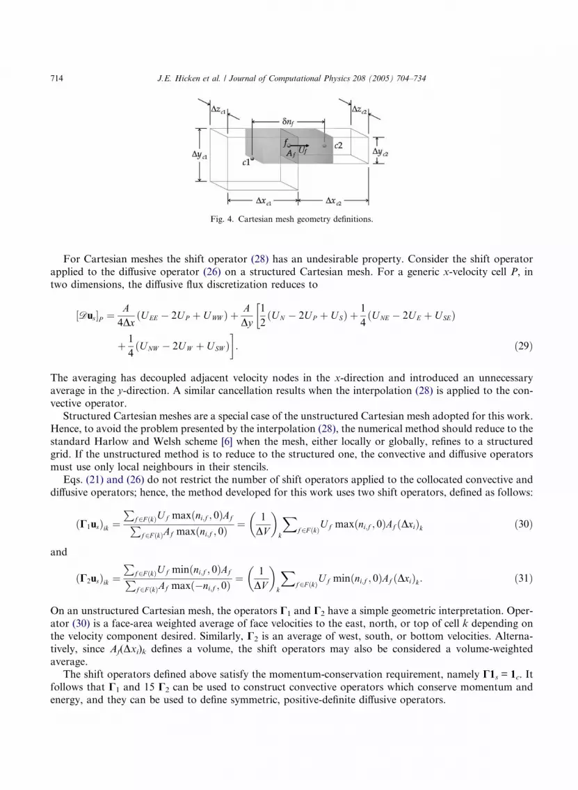
Fig. 4. Cartesian mesh geometry definitions.


For Cartesian meshes the shift operator (28) has an undesirable property. Consider the shift operator

applied to the diffusive operator (26) on a structured Cartesian mesh. For a generic x-velocity cell P, in

two dimensions, the diffusive flux discretization reduces to

Dus½ �P ¼ A4Dx

ðUEE � 2UP þ UWW Þ þADy

1

2ðUN � 2UP þ USÞ þ

1

4ðUNE � 2UE þ USEÞ

�

þ 1

4ðUNW � 2UW þ USW Þ

�: ð29Þ

The averaging has decoupled adjacent velocity nodes in the x-direction and introduced an unnecessary

average in the y-direction. A similar cancellation results when the interpolation (28) is applied to the con-

vective operator.

Structured Cartesian meshes are a special case of the unstructured Cartesian mesh adopted for this work.Hence, to avoid the problem presented by the interpolation (28), the numerical method should reduce to the

standard Harlow and Welsh scheme [6] when the mesh, either locally or globally, refines to a structured

grid. If the unstructured method is to reduce to the structured one, the convective and diffusive operators

must use only local neighbours in their stencils.

Eqs. (21) and (26) do not restrict the number of shift operators applied to the collocated convective and

diffusive operators; hence, the method developed for this work uses two shift operators, defined as follows:

ðC1usÞik ¼P

f2F ðkÞUf maxðni;f ; 0ÞAfPf2F ðkÞAf maxðni;f ; 0Þ

¼ 1

DV

� �k

Xf2F ðkÞ

Uf maxðni;f ; 0ÞAf ðDxiÞk ð30Þ

and

ðC2usÞik ¼P

f2F ðkÞUf minðni;f ; 0ÞAfPf2F ðkÞAf maxð�ni;f ; 0Þ

¼ 1

DV

� �k

Xf2F ðkÞ

Uf minðni;f ; 0ÞAf ðDxiÞk: ð31Þ

On an unstructured Cartesian mesh, the operators C1 and C2 have a simple geometric interpretation. Oper-

ator (30) is a face-area weighted average of face velocities to the east, north, or top of cell k depending onthe velocity component desired. Similarly, C2 is an average of west, south, or bottom velocities. Alterna-

tively, since Af(Dxi)k defines a volume, the shift operators may also be considered a volume-weighted

average.

The shift operators defined above satisfy the momentum-conservation requirement, namely C1s = 1c. It

follows that C1 and 15 C2 can be used to construct convective operators which conserve momentum and

energy, and they can be used to define symmetric, positive-definite diffusive operators.


The convective and diffusive matrix operators used for the present numerical scheme are obtained by

substituting the shift operators C1 and C2 into Eqs. (21) and (26). Specifically,

CðuÞ ¼ 1

2C�

1CuðuÞC1 þ C�2CuðuÞC2

� �ð32Þ

and

D ¼ 1

2C�

1DuC1 þ C�2DuC2

� �: ð33Þ

The gradient operator is identical to the general operator (17) used for arbitrary unstructured meshes.

The convective and diffusive operators, (32) and (33), do not decouple the velocity field into even-odd

modes, in contrast with the operators produced with the interpolation (28).Until now, we have focused on the interpretation of C1 and C2 as face-to-cell operators. Recall,

however, that the conjugate transpose of either matrix is a cell-to-face shift operator. Are the defini-

tions of C1 and C2 consistent with this second interpretation? To answer this question consider an arbi-

trary face f with adjacent cells c1 and c2. The discretization of the convective term at velocity cell f has

the form

CðuÞus½ �f ¼ 1

2C�

1ðCuðuÞC1usÞ þ1

2C�

2ðCuðuÞC2usÞ� �

f

¼ 1

2

Af ðDxf Þc1DV c1

� �DV

dðujuiÞdxj

� �c1

þ 1

2

Af ðDxf Þc2DV c2

� �DV

dðujuiÞdxj

� �c2

¼ 1

2Af ðDxf Þc1

dðujuiÞdxj

��c1

� �þ 1

2Af ðDxf Þc2

dðujuiÞdxj

��c2

� �;

where (Dxf)c1 and (Dxf)c2 are the lengths of c1 and c2, respectively, in the direction of nf. We see that

C�1 and C�

2 scale the cell convective fluxes to account for the difference in volume between the velocity cell

and its adjacent collocated cells. Therefore, the cell-to-face interpretation of the shift operators is appropri-

ate although the accuracy is still uncertain.

3.3. Boundary conditions

No-slip and periodic boundary conditions (BCs) were implemented in the numerical method. The imple-

mentation of the periodic BCs, while requiring careful ‘‘bookkeeping’’, was straightforward. Application of

the no-slip condition was not so clear. Indeed, there are several possible discretizations of this boundary

condition; only two are mentioned here.

The shifting of the convective and diffusive operators suggests a similar strategy for the no-slip BCs.

That is, shift the velocities to the pressure cells, apply the no-slip condition, and return the resulting shearstress to the velocity cells. This implementation, however, does not guarantee a negative source term line-

arization for some velocity cells, e.g. those in Fig. 5. When used for simulations of the turbulent channel,

this BC was found to produce negative wall velocities on the order of �Umax; although, stability did not

seem to be compromised.

Alternatively, the shear stress can be applied directly to the velocity cells without averaging through a

shift operator. Applying the BC directly raises the question of which velocity cells should receive the shear

stress. Clearly, any u- or w-velocity cell adjacent to the wall at y = 0 should be subjected to the no-slip con-

dition. However, restricting the BC to wall-adjacent cells would neglect a viscous stress term in some cells,such as P in Fig. 5. For example, if cell C1 was in the interior of the domain, the viscous stress resulting

from cells to the south would get added to velocity cell P. Hence, because cell C1 has a wall to its south,

Fig. 5. No-slip boundary conditions.


a wall shear stress term should be added to cell P. The shear stresses for cells P and S in the second ap-proach are

sw;P ¼ � Aw;C1=2

ReðDyw;P ÞuP ; ð34Þ

sw;S ¼ �ðAw;C1=2þ Aw;C3

=2ÞReðDyw;SÞ

uS ; ð35Þ

where Dyw,P and Dyw,S are the perpendicular distances from the wall to cells P and S, respectively. Notice

that the wall areas are divided by two; cell S gets a second wall stress term from cell C3 and cell P will get a

viscous stress from its east collocated neighbour C2.

The BCs were implemented using the direct approach, (34), (35), in the final version of the method. This

implementation is absolutely stable, since the boundary source term is linearized using a negative coeffi-

cient. Note that the no-slip BCs reduce to the desired second-order method on a structured mesh.

3.4. Time-integration method

Until now, the analysis has focused exclusively on the spatial discretization of the Navier–Stokes equa-

tions. Convective, gradient, and diffusive operators have been constructed that conserve momentum and

provide for stability through inviscid conservation of energy. Of course, the time derivative in (7) must also

be treated carefully if these properties are to be retained for discrete time integration.

In order to conserve energy and momentum the time advancement must be implicit [18]. The simplestsecond-order time integration scheme, that conserves energy, is the midpoint implicit method. Let Dt bethe time step size between time tn+1 and tn. Hence, the midpoint method applied to (7) gives

Xunþ1s � unsDt

þ Cunþ1 þ un

2

� �unþ1s þ uns

2

� �þD

unþ1s þ uns

2

� ��M� pnþ1

c þ pnc2

� �¼ 0: ð36Þ

The discretization (36) conserves momentum and energy in the absence of viscosity, and it ensures the en-ergy is monotone decreasing if viscosity is non-zero.

The system (36) satisfies our requirements for conservation and could be solved as it stands; see, for

example [5] for its solution on a structured grid. However, most turbulent flows require a small time step

to resolve the fastest scales, and, if the time steps are sufficiently small, the discrete Navier–Stokes equation

can be linearized and decoupled to reduce the computation time without compromising accuracy or con-

servation. Although many authors adopt this approach or variations of it, for example [22,16,1], the work

of Ham et al. [5] suggests that the added expense of solving the fully coupled and non-linear equation may

be justified since the time step can be increased substantially. Obviously, further work is needed in this area.For this work, the discrete Navier–Stokes equations are linearized and decoupled. An appropriate lin-

earization of the convective term, which retains the second-order time accuracy, is given by [4]


Cunþ1 þ un

2

� �unþ1s þ uns

2

� �¼ C

1

2du

� �uns þ CðunÞ 1

2dus þ CðunÞuns þOðDt2Þ;

where dus ¼ unþ1s � uns . A fractional step method [11] was used to decouple the pressure and velocity. The

momentum equations are advanced using the old pressure pn to obtain the first intermediate velocity us.

The effect of the old pressure gradient is subsequently removed from the velocity field to produce ~us.The new velocity, unþ1

s , is obtained by adding the new pressure gradient; since the new velocity is divergence

free, a Poisson equation for the new pressure results. These steps are summarized below in their mathemat-

ical form.

Xdu

Dtþ C

1

2du

� �uns þ CðunÞ 1

2dus þ CðunÞuns þD

1

2dus þ uns

� ��M�pnc ¼ 0; ð37Þ

~us � us ¼ �DtX�1M�pnc ; ð38Þ

MX�1M�pnþ1c ¼ � 1

DtM~us; ð39Þ

unþ1s � ~us ¼ DtX�1M�pnþ1

c ; ð40Þ

where dus ¼ us � uns . This approximate factorization is similar to the collocated fractional step method of

[4]. Eq. (37) was solved using a Jacobi solver, and, as with the collocated version, the residual was reduced

by about six orders of magnitude with approximately 15 iterations. Unlike the collocated version, some

relaxation of Eq. (37) was necessary to obtain convergence: a relaxation constant of 0.8 was sufficient. Fi-

nally, notice that the Laplacian operator in (39) is discretized using a symmetric, positive-definite matrix;

hence, the pressure equation was solved using a diagonally-preconditioned conjugate-gradient method.

A splitting error is associated with using us instead of unþ1s in the momentum equation (37). The error can

be found by adding Eqs. (38) and (40):

unþ1s � us ¼ DtX�1M�ðpnþ1

c � pncÞ ¼ Dt2X�1M� dpcdt

þOðDtÞ� �

: ð41Þ

Hence, despite the linearization and splitting errors, the overall numerical method remains second-order

accurate in time.

The linearization and fractional step errors also affect the discrete energy equation and, therefore, global

energy conservation. The effect of these errors on the energy equation can be shown to be second-order in

time. For example, the convective operator Cðdu=2Þ is not perfectly skew-symmetric because us does not

satisfy the continuity condition; therefore the matrix diagonal does not vanish. However, the differencevelocities used by this operator may be replaced by dun+1 with only a Dt2 penalty, see Eq. (41) – alterna-

tively, the convective operator could be replaced by the skew-symmetric operator Cðdu=2Þ�diagðCðdu=2ÞÞ as in [22].

4. Adaptation

4.1. Adaption criterion

The adaptive mesh was introduced in Section 3. Beginning with a uniform, structured Cartesian mesh,

the mesh is refined and coarsened at each time step using anisotropic bisection or binary agglomeration of


the cells. This subsection presents the criterion used to determine which cells are refined and which are

coarsened.

The adaptation criterion is based on the criterion used by Ham et al. [4]. Their criterion leads to the fol-

lowing target cell sizes:

Dxtarget ¼64c2F yyF zz

F 4xx

� �1=10

; ð42Þ

Dytarget ¼64c2F xxF zz

F 4yy

!1=10

; ð43Þ

Dztarget ¼64c2F xxF yy

F 4zz

� �1=10

; ð44Þ

where

F xixi ¼

ffiffiffiffiffiffiffiffiffiffiffiffiffiffiffiffiffiffiffiffiffiffiffiffiffiffiffiffiffiffiffiffiffiffiffiffiffiffiffiffiffiffiffiffiffiffiffiffiffiffiffiffiffiffiffiffiffiffiffio2uox2i

� �2

þ o2vox2i

� �2

þ o2wox2i

� �2s

ðno sum iÞ: ð45Þ

In [4], the collocated velocities are used in Eq. (45) to find the F xixi . For the present method, the velocities in

(45) are obtained using a face-area weighted average to interpolate the staggered velocities to the cell cen-

tres, specifically, Eq. (28). These interpolated velocities are then used to find the target cell sizes. A criterion

can be derived for the staggered velocities using the Laplacian operator (33), but the appropriate refinement

for individual velocity cells is unclear; how would a single velocity cell refine without altering the cuboid

shape of its adjacent pressure cells? Further work on the adaptation criterion for staggered meshes iswarranted.

The criterion used to derive Eqs. (42)–(44) assumes non-vanishing second derivatives. In the event that

all the variables are locally, or globally, linear in some direction, an appropriate two-dimensional criterion

is adopted. For example, if the flow is locally linear in the z-direction then the target cell sizes become

Dxtarget ¼144c2F yy

F 3xx

� �1=8

; ð46Þ

Dytarget ¼144c2F xx

F 3yy

!1=8

; ð47Þ

Dztarget ¼ Dzcurrent: ð48Þ
Similarly, if the flow is locally linear in two coordinates, say z and y, then we use
Dxtarget ¼24cF xx

� �1=3

; ð49Þ

Dytarget ¼ Dycurrent; ð50Þ

Dztarget ¼ Dzcurrent: ð51Þ


4.2. Adaptation and conservation

When a pressure cell is refined a new face is added which bisects the cell into two new cells. If the

refinement is in the x-direction, for example, the faces in the y- and z-directions are split if necessary.

The addition of a new face and the splitting of old faces requires an interpolation of the velocitiesstored at these faces. Similarly, an interpolation is also needed for some faces during coarsening. Var-

ious interpolations are available, but if mass, momentum, or energy are to be conserved the choices are

severely restricted.

In the Cartesian method of [4], the face velocities are interpolated to conserve mass and the collocated

velocities are interpolated to conserve momentum. In the present staggered method the face velocities are

the only velocities available. Ideally, the face velocities would be interpolated to conserve mass, momentum,

and energy, but this may not be possible in general. Since mass conservation is important for both momen-

tum and energy conservation, the interpolation was constructed to ensure that discrete continuity is notviolated.

Errors may be introduced by the mass conserving interpolation into the other quantities, such as

momentum and energy. Taylor series expansions can be used to show that these errors are second order

in the local grid spacing; the analysis is tedious and straightforward, and, therefore, it is omitted. To

validate the second-order behaviour of the interpolation, the flow in a periodic box with unit dimen-

sions was computed. The initial conditions were constructed using a random, divergence-free velocity

field:

u0 ¼X4i¼1

X4j¼1

X4k¼1

Aijk sinð2ipxÞ sinð2jpyÞ sinð2kpzÞ;

v0 ¼X4i¼1

X4j¼1

X4k¼1

Bijk sinð2ipxÞ sinð2jpyÞ sinð2kpzÞ;

w0 ¼X4i¼1

X4j¼1

X4k¼1

Aijkikcosð2ipxÞ sinð2jpyÞ þ Bijk

jksinð2ipxÞ cosð2jpyÞ

� �cosð2kpzÞ;

where the coefficients Aijk and Bijk were random numbers in the range [�0.1,0.1]. The viscosity was set to

m = 1/2000 initially and subsequently turned off at t = 1.5. The total simulation time was t = 3.0 which pro-

vided an equal sample size for the viscous and inviscid flows. A constant time step was used, and it was

calculated such that the initial CFL number would equal two.

The local kinetic energy of a cell k was defined as

KElocal ¼Xf2F ðkÞ

u2f Af ðDxi;kjni;f jÞ: ð52Þ

Using the above definition, an error measurement for the kinetic energy conservation was constructed as

follows: for each cell that was refined or coarsened, the difference between the local kinetic energy before

and after adaptation was calculated and squared. The squared errors were then summed and divided by the

total number of adaptations; refinement of a cell or coarsening of two cells were each counted as one adap-tation. Finally, a relative error was found by taking the square root of the summed errors and dividing the

result by the total energy before adaptation.

An average cell dimension, Davg, was calculated by summing the volumes of all cells which were adapted;

the volume before adaptation was added for refining cells and the volume after adaptation was added for

10 101

106

105

104

103

102

101

100

∆avg

ε%

slope = 2.7862

least squares fit: slope = 2.786295% confidence interval

Fig. 6. Energy conservation error in the adaptive interpolation.


coarsening cells. The summed volumes were divided by the total number of adaptations, and the cubic root

of the result was taken.

Fig. 6 plots the adaptive interpolation error versus the average adapted cell dimension. A least-squares-

fit shows that the error is approximately second order as predicted. The fit was obtained by transforming

the data to logarithmic space, finding a linear least-squares-fit, and then transforming back. Fig. 6 also

shows the 95% confidence interval for the transformed data.

5. Accuracy

5.1. Error analysis

Traditionally, the truncation error is used to find the accuracy of a method; however, Manteuffel and

White [14] have shown that the truncation error only provides a lower bound for a method�s accuracy.

The resulting lower bound may not reflect the true error. This is the case for the present method.The truncation error for the Navier–Stokes discretization can be found by substituting the analytical

solution into Eq. (7). For the unstructured, staggered Cartesian method the truncation error derivation

is tedious and has been omitted. The truncation error contains, in general, low order terms which suggest

that the method is inconsistent. Practically, however, the low-order terms are paired because of the way the

mesh adapts using bisection, and these paired terms cancel. When the mesh is locally uniform the method

reduces to the standard staggered scheme and becomes second-order accurate. This raises the question:

which errors dominate the solution?

There are two distinct types of low-order terms present in the general form of the truncation error. On aone-dimensional mesh, the first type of error is proportional to DVf(Dxi+1 � Dxi) and is the result of the cell

dimension changing in the x-direction. This error will be referred to as the one-dimensional error and is

analyzed in Appendix A. The second type of error accounts for the remaining low-order terms and is


primarily due to misalignments between the face and cell centroids; such errors will be labelled unstructured

errors.

The analysis in Appendix A shows that the present method is second order on a one-dimensional do-

main; the presence of first order, one-dimensional errors does not result in a first-order scheme. General-

izing this remark to higher dimensions is difficult because of the unstructured errors. The example belowprovides anecdotal evidence that the order of accuracy is also not reflected by the unstructured errors.

Clearly an example does not constitute a proof of the method�s order of accuracy, but it does reveal thenaivety of using the truncation error to deduce the actual error.

On a two- or three-dimensional Cartesian adaptive mesh, changes in cell dimension will usually occur

over surfaces because of the continuous criterion. Therefore, for simplicity, consider a two-part two-dimen-

sional uniform mesh with cell dimensions Dx and Dy for x < x and Dx and Dy/2 for x P x. A portion of this

mesh is shown in Fig. 7 where several u-velocity cells have been labelled. Let DV = DxDyDz and Ai =

DV/Dxi.The individual truncation errors for the cells N and S in Fig. 7 can be shown to be O(1). Instead of the

smaller cells, consider an imaginary cell P created by the agglomeration of N and S, and let uP = (uN + uS)/

2. Approximating uP by the average of the velocities at N and S produces a second order error, but, of more

interest, is the accuracy of the Navier–Stokes discretization at P created by summing the discretizations at

N and S. Each of the terms in the discretization are examined below.

Adding the convective discretizations at N and S yields an approximation for the convective flux at P

over a volume of size DV:

ðCðuÞusÞN þ ðCðuÞusÞS� �

¼ uNE þ uN2

uNE þ uN2

þ uSE þ uS

2

uSE þ uS2

h iAx

2|fflfflfflfflfflfflfflfflfflfflfflfflfflfflfflfflfflfflfflfflfflfflfflfflfflfflfflfflfflfflfflfflfflfflfflfflfflfflfflfflfflfflfflfflfflfflfflfflffl{zfflfflfflfflfflfflfflfflfflfflfflfflfflfflfflfflfflfflfflfflfflfflfflfflfflfflfflfflfflfflfflfflfflfflfflfflfflfflfflfflfflfflfflfflfflfflfflfflffl}convective flux through east face of P

� uN þ uS4

þ uW2

uN þ uS4

þ uW2

h iAx|fflfflfflfflfflfflfflfflfflfflfflfflfflfflfflfflfflfflfflfflfflfflfflfflfflfflfflfflfflfflfflfflffl{zfflfflfflfflfflfflfflfflfflfflfflfflfflfflfflfflfflfflfflfflfflfflfflfflfflfflfflfflfflfflfflfflffl}

convective flux through west face of P

þ vnw þ vne2

uN þ uS8

þ uNNN þ uNN8

þ uN þ uNN4

h iAy|fflfflfflfflfflfflfflfflfflfflfflfflfflfflfflfflfflfflfflfflfflfflfflfflfflfflfflfflfflfflfflfflfflfflfflfflfflfflfflfflfflfflfflfflfflfflfflfflffl{zfflfflfflfflfflfflfflfflfflfflfflfflfflfflfflfflfflfflfflfflfflfflfflfflfflfflfflfflfflfflfflfflfflfflfflfflfflfflfflfflfflfflfflfflfflfflfflfflffl}

convective flux through north face of P

� vsw þ vse2

uN þ uS8

þ uSSS þ uSS8

þ uS þ uSS4

h iAy|fflfflfflfflfflfflfflfflfflfflfflfflfflfflfflfflfflfflfflfflfflfflfflfflfflfflfflfflfflfflfflfflfflfflfflfflfflfflfflfflfflfflfflfflfflffl{zfflfflfflfflfflfflfflfflfflfflfflfflfflfflfflfflfflfflfflfflfflfflfflfflfflfflfflfflfflfflfflfflfflfflfflfflfflfflfflfflfflfflfflfflfflffl}

convective flux through south face of P

þRP ;

where RP denotes the unused terms

Fig. 7. Example of mesh with unstructured type errors.


RP ¼ Ayvnw4

� Ayvne4

� �uN þ uS

4þ uNNN þ uNN

4� uN þ uNN

2

� Ayvsw

4� Ayvse

4

� �uN þ uS

4þ uSSS þ uSS

4� uS þ uSS

2

� 2Ax

16ðuN � uSÞ2:

If we ignore the term RP, summing the convective fluxes at N and S produces a second-order accurate dis-

cretization of the convective flux at P. Moreover, closer inspection of the remaining terms reveals that

RP = O(Dy2A). It follows that
Z Z ZDV P
o

oxjðujuÞdV ¼ ðCðuÞusÞN þ ðCðuÞusÞS

� �þOðDy2AÞ: ð53Þ

Eq. (53) shows that error in convective term is O(Dx), after the flux is divided by DVP.

Next, consider the diffusive flux at P. Combining the diffusive flux at N and S gives

ðDusÞN þ ðDusÞS� �

¼ 1

ReuW þ uNE þ uSE

2

� 2

uN þ uS2

h i Ax

Dx

þ 1

2ReuNN þ uNNN

2

þ uSS þ uSSS

2

� 2

uN þ uS2

h i Ay

Dy

þ 1

2ReuNN � uNð Þ þ uSS � uSð Þ½ � Ay

12Dy

:

The above discretization is a second-order accurate approximation of the diffusive flux at P. Note how the

diffusive fluxes on the north and south faces use an average of two face derivatives; one with a Dy wide

stencil and the other with a Dy/2 wide stencil.Finally, the combined pressure gradient is given by

� ðMusÞN þ ðMusÞS� �

¼ Aypn þ ps

2� pw

�Z Z Z

DV P

opox

dV : ð54Þ

The resulting pressure gradient discretization (54) is also second-order accurate for the cell at P.

For the mesh in Fig. 7, the above analysis has shown that a second-order accurate discretization of the

Navier–Stokes equations can be obtained for the cell P by summing the discretizations at the cells N and S.

Now, if a smooth analytical solution exists then uN and uS must converge to uP as max(Dxi) ! 0.

Specifically,

uN ¼ uP þouoy

� �P

Dy4

þOðDy2Þ

and

uS ¼ uP �ouoy

� �P

Dy4

þOðDy2Þ;

so the error atN and Smust be bounded by O(Dy) on this particular mesh, despite a truncation error of O(1).

In general, the surfaces where the mesh changes from one size to another will neither be aligned with thecoordinate axes nor planar. However, the above argument does demonstrate that the accuracy of the meth-

od cannot be inferred from a truncation error analysis. Numerical experiments were conducted to further

assess the accuracy of the method; these are discussed in the next subsection.


5.2. Tests of numerical accuracy

5.2.1. The convective and diffusive operators on random meshes

The orders of accuracy of the convective term, CðuÞus, and the diffusive term, Dus, were assessed by eval-

uating these terms on random meshes and comparing with analytical solutions. The mesh spacing was effec-tively changed by varying the frequency of the input functions. This approach was used by Perot in [18] for

triangular unstructured meshes.

The input velocities for the convective term were produced from a stream function on a square domain

with dimensions of 100 · 100. The input velocities were

ucðx; yÞ ¼ � sin2pN100

x� �

sin2pN100

y� �

;

vcðx; yÞ ¼ � cos2pN100

x� �

cos2pN100

y� �

:

The parameter N determines the number of modes on the domain and was varied from 1 to 10. For the

diffusive term, the input velocities were

udðx; yÞ ¼ ucðx; yÞ þ sin2pN100

x� �

;

vdðx; yÞ ¼ vcðx; yÞ þ cos2pN100

y� �

:

The random meshes were constructed using a 32 · 32 uniform mesh as an initial mesh and performing arandom refinement process either once or twice. In the refinement process, each cell was randomly refined,

with each direction being refined independently. If two random refinements were used, the maximum pos-

sible ratio between max(Dxi) and min(Dxi) was 4. Fig. 8 shows one possible random mesh. An average mesh

size, Dxavg, was calculated for each random mesh. The relative mesh size was then set equal to the quotient

Fig. 8. Example of a random mesh used to assess the accuracy of the convective and diffusive terms.

10 10 100

10

10

10

relative mesh size(a) (b)

conv

ectiv

e te

rm e

rror

slope = 1

10 10 100

10

10

10

relative mesh sizedi

ffusi

ve te

rm e

rror

slope = 1

Fig. 9. RMS error in the convective term (a), and the diffusive term (b), for three randomly refined meshes.


of the average mesh size and the wave length 100/N; hence the relative mesh size is inversely proportional to

the number of grid points per wave length [18].

The root-mean-square (RMS) errors for the convective and diffusive terms are shown in Fig. 9(a) and

(b), respectively. The results from three randomly adapted meshes are plotted. These results show that

the convective and diffusive terms are first-order accurate for anisotropic Cartesian meshes. First order

accuracy for the diffusive term is perhaps surprising given the O(1) approximation for the gradient used

on some faces; however, as argued in Section 5.1, these low-order terms appear to cancel for anisotropic

Cartesian meshes.For practical problems the mesh adapts in an effort to minimize the error in the solution, so the first-

order accuracy displayed by the convective and diffusive terms on random meshes is an upper bound on

the accuracy. Indeed, when the adaptive criteria were applied to the velocities in this test case, a uni-

form mesh was produced. To assess the accuracy of the adaptive method, a more challenging flow was

studied.

5.3. Lid-driven cavity

The two-dimensional lid-driven cavity flow was also used to evaluate the accuracy of the method.

The error tolerance c, used for the adaptive criterion, was dynamically changed to force the mesh to

a certain size. The adapted mesh was then fixed and not allowed to change. Subsequently, the

numerical method was advanced until a steady solution was obtained. A Reynolds number of 400

was used.

The error for the cavity flow was estimated using the numerical solution of Ghia et al. [3]. The adap-

tive mesh solution was interpolated to the 15 interior points, along the cavity�s vertical mid-line,

reported in [3]. The RMS error between the interpolated solution and the solution of [3] was thencalculated:

erms ¼

ffiffiffiffiffiffiffiffiffiffiffiffiffiffiffiffiffiffiffiffiffiffiffiffiffiffiffiffiffiffiffiffiffiffiffiffiffiffiffiffiffiffiffiffiffi1

15

X15i¼1

ðuGhia � uadaptÞ2vuut :

10 101

103

102

101

slope = 1.7891

slope = 1.7494

(1/N)1/2

εrms

slope = 1slope = 2uniformadaptive

Fig. 10. RMS error for the lid-driven cavity flow.


Fig. 10 shows the RMS error for several adaptive and uniform meshes. Unlike the previous test case, the

accuracy is closer to second-order despite the greater complexity of the flow.

6. Direct numerical simulations of the turbulent channel flow

6.1. Channel flow characteristics and simulation set-up

The channel flow consisted of a rectangular hexahedral with dimensions 2pd · 2d · pd where d is the

channel half-width. Periodic boundary conditions were imposed in the x- and z-directions, and no-slip

boundary conditions were set at y = 0 and y = 2d. The equations of motion were non-dimensionalized using

d and the friction velocity us. The flow was forced in the positive x-direction by a pressure gradient; thepressure gradient was updated dynamically to keep the mass flux constant.

The simulations were performed using a Reynolds number of Reb = 2800 based on the channel half-

width, the kinematic viscosity (m = 1/180), and the bulk velocity Ub:

Ub ¼1

2

Z 2

y¼0

um dyd

;

where um is the time averaged streamwise velocity. The bulk Reynolds number corresponds to a friction

velocity Reynolds number of Res � 180. Many researchers have used this Reynolds number for turbulent

channel simulations, including Kim et al. [12] in their pioneering work. The present results are comparedwith the spectral DNS of Moser et al. [17], since their results are relatively recent and have benefited from

0 0.2 0.4 0.6 0.8 1 1.2 1.4 1.6 1.8 2

5

0

0.5

1

1.5

y/δ

wm

mesh size ≈ 1.0 × 105

mesh size ≈ 1.2 × 105

mesh size ≈ 1.5 × 105

mesh size ≈ 2.0 × 105

Fig. 11. Mean spanwise velocity profile.


more than a decade of research. The DNS statistics reported in [17] were obtained using 128 · 129 · 128

grid points on a 4pd · 2d · 2pd domain.

Simulations were performed with four mesh sizes of approximately 1.0 · 105, 1.2 · 105, 1.5 · 105, and

2.0 · 105 cells based on the number of internal pressure cells. A feedback mechanism was used to adjust

the error tolerance c such that the mesh sizes remained close to the specified number of cells. No other

restrictions were placed on the adaptation criterion; in particular, the mesh was not forced to assume a par-

ticular size near the wall.

A constant time step of 1.25 · 10�3 was adopted for the simulations. This same value was used inthe simulations of Verstappen and Veldman [22]. The time step corresponds to a CFL number of

approximately one; the results of Choi and Moin [1] and Ham et al. [5] suggest that, in channel flow

simulations, the CFL number should not exceed one when fractional step methods are used.

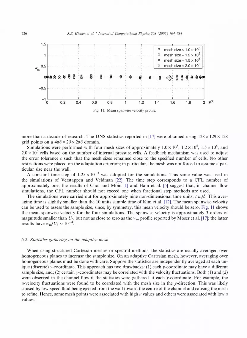
The simulations were carried out for approximately nine non-dimensional time units, t us/d. This aver-aging time is slightly smaller than the 10 units sample time of Kim et al. [12]. The mean spanwise velocity

can be used to assess the sample size, since, by symmetry, this mean velocity should be zero. Fig. 11 shows

the mean spanwise velocity for the four simulations. The spanwise velocity is approximately 3 orders of

magnitude smaller than Ub, but not as close to zero as the wm profile reported by Moser et al. [17]; the latterresults have wm/Ub � 10�4.

6.2. Statistics gathering on the adaptive mesh

When using structured Cartesian meshes or spectral methods, the statistics are usually averaged over

homogeneous planes to increase the sample size. On an adaptive Cartesian mesh, however, averaging over

homogeneous planes must be done with care. Suppose the statistics are independently averaged at each un-

ique (discrete) y-coordinate. This approach has two drawbacks: (1) each y-coordinate may have a differentsample size, and; (2) certain y-coordinates may be correlated with the velocity fluctuations. Both (1) and (2)

were observed in the channel flow if the statistics were gathered at each y-coordinate. For example, the

u-velocity fluctuations were found to be correlated with the mesh size in the y-direction. This was likely

caused by low-speed fluid being ejected from the wall toward the centre of the channel and causing the mesh

to refine. Hence, some mesh points were associated with high u values and others were associated with low u

values.

100

101

102

0

2

4

6

8

10

12

14

16

18

20

y+

um

spectral DNS (Moser et al.)distinct y coordinate statisticsagglomerated statistics

Fig. 12. Agglomerated and raw statistics comparison.


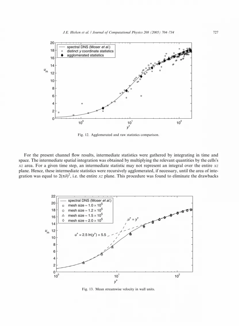
For the present channel flow results, intermediate statistics were gathered by integrating in time andspace. The intermediate spatial integration was obtained by multiplying the relevant quantities by the cells�sxz area. For a given time step, an intermediate statistic may not represent an integral over the entire xz

plane. Hence, these intermediate statistics were recursively agglomerated, if necessary, until the area of inte-

gration was equal to 2(pd)2, i.e. the entire xz plane. This procedure was found to eliminate the drawbacks

100

101

102

0

2

4

6

8

10

12

14

16

18

20

22

y+

um

u+ = y+

u+ = 2.5 ln(y+) + 5.5

spectral DNS (Moser et al.)mesh size ≈ 1.0 × 105

mesh size ≈ 1.2 × 105

mesh size ≈ 1.5 × 105

mesh size ≈ 2.0 × 105

Fig. 13. Mean streamwise velocity in wall units.


discussed above. Fig. 12 compares the distinct y-coordinate statistics with the agglomerated statistics; the

spectral data of [17] is included as a reference.

6.3. Mean and RMS velocity profiles

Mean streamwise profiles are plotted in Fig. 13 together with the spectral data of [17]. Fig. 13 is scaled

using wall units on a log scale. Note that the friction velocity was taken equal to its exact, non-dimensional

value of one; it was not approximated using a discrete wall gradient, since this approach reflects the con-

vergence of us rather than the mean or RMS profiles. The results show that the simulations properly obey

the law of the wall and the log-law. Furthermore, all of the mesh sizes follow the spectral data closely, and

only underestimate the profile slightly. The agglomerated statistics may give the impression that a relatively

coarse, uniform mesh was used; however, recall that the agglomerated statistics are compiled from the raw,

distinct y-coordinate statistics.Using the present method, the finest and coarsest meshes capture the mean profile well using fewer than

2/5 and 1/5, respectively, the number of grid points of the spectral method – the spectral mesh size has been

divided by four to account for the larger domain. To emphasize the significance of this result, note that the

truncation error for a second-order method is accurate for only 1/4 the Nyquist wave number range. Hence,

on a structured mesh, a second-order method would need a mesh approximately 64 times larger than a

spectral mesh to ensure an equally accurate solution. From this perspective, the current method requires

a mesh two orders of magnitude smaller than a uniform mesh.

The rate of solution convergence is difficult to observe with the mean streamwise profile, since all themesh sizes seem to perform equally well. Convergence is more obvious with the streamwise fluctuating

velocity, urms. Fig. 14(a) plots urms for the present simulations and compares these with the results of

[17]. The RMS streamwise velocity improves significantly with mesh refinement. The coarser meshes over-

estimate urms over the entire range, particularly near the wall; see Fig. 14(b). The RMS velocity from the

2.0 · 105 cell simulation follows the spectral profile well, but shows some poor performance close to the wall

where it overestimates the profile more than the next coarser mesh. The source of this discrepancy is not

clear; possible reasons are the sample size, domain size, or boundary conditions. Despite its performance

0 10 200

0.5

1

1.5

2

2.5

3

3.5

y+0 20 40 60 80 100 120 140 160 180

0

0.5

1

1.5

2

2.5

3

3.5

y(a) (b)+

urms


mesh size ≈ 1.2 × 105

mesh size ≈ 1.5 × 105

mesh size ≈ 2.0 × 105

Fig. 14. (a) streamwise RMS fluctuating velocity in wall units: (b) near wall.

0 50 100 1500

0.5

1

1.5

y(a) (b)+

vrms


mesh size ≈ 1.2 × 105

mesh size ≈ 1.5 × 105

mesh size ≈ 2.0 × 105

0 50 100 1500

0.2

0.4

0.6

0.8

1

1.2

1.4

1.6

1.8

2

y+

wrms

Fig. 15. (a) Wall-normal RMS fluctuating velocity and (b) spanwise RMS fluctuating velocity.


near the wall, the finest mesh result compares well with the spectral results considering the accuracy of the

method.

The wall-normal and spanwise fluctuating velocities are plotted in Fig. 15(a) and (b), respectively.

Although both profiles show improvement with refinement, the convergence of wrms is more dramatic thanthat of vrms. Unlike the streamwise fluctuating velocity, the wall-normal and spanwise RMS velocities do

not converge monotonically to the spectral data; for example, the profile of wrms from the coarsest mesh

overestimates the spectral profile while the other mesh sizes underestimate the profile. One possible expla-

nation of this convergence behaviour is the presence of turbulence structures in the simulations with mesh

sizes greater than 1.0 · 105 that are not resolved by the coarsest mesh.

0 20 40 60 80 100 120 140 160 1800

2

4

6

8

10

12

14

16

18

y+

∆ y+

mesh size ≈ 1.0 × 105

mesh size ≈ 1.2 × 105

mesh size ≈ 1.5 × 105

mesh size ≈ 2.0 × 105

smooth, expanding mesh

Fig. 16. Mean wall-normal mesh size.


6.4. Mean mesh size statistics

Since the present method uses a time-adaptive mesh, additional statistics were gathered on the mean cell

dimensions. The dimensions for the u-velocity cells were treated like flow variables and sampled in time and

space. Gathering cell size statistics for all the velocity cells and the pressure cells was deemed unnecessary,since, locally, the dimensions are related by a constant factor of no more than 2. Fig. 16 shows the average

wall-normal cell size, in wall units, as a function of y+. As expected, the mesh is most refined near the wall

and monotone increasing toward the centre of the channel. Surprisingly, perhaps, the finer meshes do not

spread their added degrees of freedom uniformly across the range; rather, the increased resolution tends to

be focused close to the wall and in the log-law region. The smooth, expanding mesh used in Verstappen and

Veldman�s simulations [22], with 64 points in the wall normal direction, is also plotted in Fig. 16. Their

smooth mesh emphasizes the near wall resolution at the expense of the channel centre. The adaptive mesh

results suggest, however, that the wall region may only need to be resolved periodically, and that the meshused in [22] may not be sufficiently fine toward the channel centre. This may explain why the fluctuating

velocities of the present, second order, method compare better with the spectral data than the fourth-order

method of [22].

The mean streamwise and spanwise cell dimensions are plotted in Fig. 17(a) and (b). As the number of

cells increases, the streamwise cell dimension converges to a relatively uniform size of Dx+ � 18, except near

the wall where coarser cells are more frequent. The near wall region is dominated by long, low-speed streaks

aligned with the x-direction, so high streamwise resolution may not be as necessary close to the wall. The

spanwise cell dimension also seems to converge to a relatively uniform size, in this case Dz+ � 9. Unlike thestreamwise dimension, however, the spanwise cell size shows the need for some occasional refinement near

the wall; this is likely caused by the variation of the low speed streaks in the z-direction.

The aim of using an adaptive mesh is to reduce the total number of cells, relative to a structured mesh,

necessary for a given accuracy. Unfortunately, no results for the turbulent channel flow using a structured

Cartesian mesh and second-order method were available for direct comparison. However, the results of

Ham et al. [5] on a smaller domain can be used for an indirect comparison. The second-order results in

[5] are obtained on a 16 · 128 · 32 � 6.5 · 104 mesh with a domain size of pd · 2d · 0.286pd; hence, 106

cells would be needed on the full domain. The present results are in good agreement with 2.0 · 105 cells

0 50 100 1500

2

4

6

8

10

12

14

16

18

y+

∆ z+

0 50 100 1500

10

20

30

40

50

60

70

y(a) (b)+

∆ x+

mesh size ≈ 1.0 × 105

mesh size ≈ 1.2 × 105

mesh size ≈ 1.5 × 105

mesh size ≈ 2.0 × 105

Fig. 17. (a) Mean streamwise and (b) spanwise cell sizes.


on a domain of 2pd · 2d · pd; however, as the RMS velocities show, even this number of cells is slightly

small. Assuming 2.5 · 105 cells would produce excellent agreement with the spectral results, then the pres-

ent method would also need 106 cells on the full domain.

The preceding heuristic analysis suggests that the adaptive mesh does not substantially reduce the num-

ber of cells for turbulent channel simulations compared with structured meshes. The channel flow has twodirections of homogeneity in which a uniform mesh size may be sufficient; indeed, this is implied by the

mean cell size results in the streamwise and spanwise directions. For more general, anisotropic flows we

expect the adaptive mesh will reduce the number of grid points relative to a structured mesh. The channel

flow has also been studied extensively, so the appropriate cell sizes are well documented. This latter point

underlines an important advantage the adaptive mesh has over fixed meshes; in general, the appropriate cell

size will not be known a priori.

7. Conclusions

A shift transformation has been introduced which allows collocated operators to be used for staggered

variables. The transformation preserves the symmetry properties of discrete collocated operators – symmetry

properties that help produce a fully conservative spatial discretization of the Navier–Stokes equations. Var-

ious shift operators can be constructed depending on the mesh used and the stencil size. A set of shift trans-

formations have been successfully applied to an unstructured Cartesian adaptive mesh, and the resulting

convective and diffusive operators do not decouple the solution. A mass conserving interpolation has beenused during mesh adaptation and was shown to conserve momentum and energy to second order in space.

The present method cannot be used to produce a conservative discretization for collocated variables, and

the treatment of the pressure term for these schemes remains an open problem; however, the present meth-

od can be combined with suitable collocated methods to produce a conservative staggered scheme.

Accuracy remains a difficult issue for conservative methods on general unstructured meshes. The present

method has been shown to exhibit second-order convergence when an adaptive mesh is used, and first-order

convergence in general. The accuracy of the Cartesian method benefits from the symmetry of the refine-

ments, and more general unstructured meshes may suffer larger errors due to their irregularity. For thesemeshes, shift operators with larger stencils and higher-order collocated operators may be necessary to

obtain second-order accuracy.

Acknowledgements

This work represents part of a M.A.Sc. thesis produced by the first author, whom was supported by a

Natural Sciences and Engineering Research Council of Canada (NSERC) scholarship; the first authorthanks NSERC for their financial support. The authors wish to thank Dr. Andrew Rau-Chaplin, of Dal-

housie University�s Computer Science Department, for giving them access to his multi-computer cluster.

Finally, the authors thank the referees for their helpful comments and insights.

Appendix A. Errors on a one-dimensional ‘‘Cartesian’’ mesh

Suppose a numerical solution is obtained on a one-dimensional domain of size Lx using an adaptivemesh and the criterion of Section 4.1. Furthermore, suppose the truncation error of the scheme is second

order where adjacent cells are uniform and first order where the mesh changes from one size to another. The

following argument shows that the global error of such a method is second order.

Fig. A.1. Mesh partition into monotonic Fxx intervals.


The global order of accuracy is not obvious, since the number of cells with first-order errors may tend to

infinity. A common argument used for non-uniform meshes assumes that the mesh spacing is a smooth

function of position which implies Dxiþ1 � Dxi ¼ OðDx2i Þ; see, for example [5]. The smooth-mesh argumentcannot be used for the present method, since cell sizes change abruptly. An alternate argument is presented

below. It is based on the following idea: if the number of cells with second-order truncation errors tends to

infinity faster than the number of cells with first-order errors, then the global error will be second order.

Recall from Section 4.1 that, for a one-dimensional problem, the local mesh size satisfies

Dxk 6 Dxtarget ¼24cF xx

� �1=3

: ð49Þ

Assume that the second-order derivative is bounded above and vanishes only at a finite number of loca-

tions. Therefore, the domain can be divided into a finite number of intervals In, n = 1, . . . ,N, such that

Fxx is monotonic on each interval. Fig. A.1 illustrates one possible Fxx and the resulting intervals.

The mesh adapts by successive bisections of existing cells, so each cell k must satisfy Dxk ¼ Lx=2lk for

some lk. Using this restriction and the target cell size (49) yields

lk P1

ln 2ln Lx

F xxðxkÞ24c

� �1=3" #

; ðA:1Þ

lk � 1 61

ln 2ln Lx

F xxðxkÞ24c

� �1=3" #

: ðA:2Þ

It follows from (A.2) that the maximum refinement level on In is bounded above:

maxk2In

lk 6 1þ 1

ln 2ln Lx

maxx2InF xx

24c

� �1=3" #

: ðA:3Þ

For intervals satisfying Fxx 6¼ 0, Eq. (A.1) can be used to find a lower bound for the minimum refinement

level. However, many intervals will have Fxx = 0 at one of their end points. The algorithm does not permit

coarsening beyond the domain, so

mink2In

lk P 0: ðA:4Þ

Fig. A.2. constant Dx subintervals.


Eq. (A.4) does not, necessarily, imply that some cells fail to refine as c ! 0. For a given Fxx(xk) there always

exists a value of c small enough to force another refinement. A possible exception is when a cell exactly

satisfies Fxx = 0. Practically speaking this case should not pose a problem. If necessary, a simple solution

would be to restrict the difference in refinement level to one between adjacent cells.

Using the above results, an upper bound can be found for the difference between maximum and mini-mum refinement levels on each interval In:

Dln ¼ maxk2In

lk �mink2In

lk 6 1þ 1

ln 2ln Lx

maxx2In F xx

24c

� �13

" #: ðA:5Þ

Hence, for a fixed c, each interval In contains a finite number of subintervals Jn,m, m = 1, . . . ,Mn = Dln + 1,

which have constant Dx = Dxm; refer to Fig. A.2. As c ! 0, however, the number of subintervals may tend

to infinity; see Eq. (A.5).

If there are K cells on the mesh in total, the total error will have the form

Error ¼XNn¼1

XMn

m¼1

TmDxmDV m þOXKk¼1

Dx2kDV k

!; ðA:6Þ

where DVm = ADxm is the cell volume. The terms TmDxm are the first-order errors which occur at the inter-

face of two subintervals and include contributions from the 3 faces surrounding the interface. Let Dxn bethe largest cell size on the interval In, so Dxn ¼ Lx=2

lmin . The subinterval containing Dxn must be at the begin-ning or end of In, since Fxx is monotone increasing or decreasing on In. Furthermore, the subinterval adja-

cent to the one containing Dxn must have cells with size Dx 6 Dxn/2, and the next subinterval must have

Dx 6 Dxn/22, and so on. Hence, the global error satisfies

Error 6XNn¼1

Dx2nAXMn

m¼1

T m

2m�1

!þO

XKk¼1

Dx2kDV k

!

6 A~TXNn¼1

Dx2nXMn

m¼1

1

2m�1

!þO

XKk¼1

Dx2kDV k

!; ðA:7Þ

where ~T ¼ maxn

ðmaxm

jTmjÞ. As c ! 0 the number of subintervals on each In may tend to infinity, but the

geometric sum in (A.7) remains bounded by 2. Thus, continuing from (A.7),

Error 6 2A~TXNn¼1

Dx2m þOXKk¼1

Dx2kDV k

!¼ O Dx2

� ; ðA:8Þ

where Dx = maxDxk. The inequality (A.8) shows that the global error on a one-dimensional domain is

indeed second order.

References

[1] H. Choi, P. Moin, Effects of the computational time step on numerical solutions of turbulent flow, J. Comput. Phys. 113 (1994) 1–

4.

[2] J.H. Ferziger, M. Peric, Computational Methods for Fluid Dynamics, Springer, Berlin, 2002.

[3] U. Ghia, K.N. Ghia, C.T. Shin, High-Re solutions for incompressible flow using the Navier–Stokes equations and a multigrid

method, J. Comput. Phys. 48 (1982) 387–411.

[4] F.E. Ham, F.S. Lien, A.B. Strong, A Cartesian grid method with transient anisotropic adaptation, J. Comput. Phys. 179 (2002)

469–494.

[5] F.E. Ham, F.S. Lien, A.B. Strong, A fully conservative second-order finite difference scheme for incompressible flow on

nonuniform grids, J. Comput. Phys. 177 (2002) 117–133.


[6] F.H. Harlow, J.E. Welch, Numerical calculation of time-dependent viscous incompressible flow of fluid with free surface, Phys.

Fluids 8 (12) (1965) 2182–2189.

[7] J.M. Hyman, R.J. Knapp, J.C. Scovel, High order finite volume approximations of differential operators on nonuniform grids,

Physica D 60 (1992) 112–138.

[8] J.M. Hyman, M. Shashkov, Natural discretizations for the divergence, gradient, and curl on logically rectangular grids, Int. J.

Comput. Math. Appl. 33 (1997) 81–104.

[9] J.M. Hyman, M. Shashkov, The orthogonal decomposition theorems for mimetic finite difference methods, SIAM J. Numer.

Anal. 36 (1999) 788–818.

[10] J.M. Hyman, M. Shashkov, Mimetic discretizations for Maxwell�s equations, J. Comput. Phys. 151 (1999) 881–909.

[11] J. Kim, P. Moin, Application of a fractional-step method to incompressible Navier–Stokes equations, J. Comput. Phys. 59 (1985)

308–323.

[12] J. Kim, P. Moin, R. Moser, Turbulence statistics in fully developed channel flow at low Reynolds number, J. Fluid Mech. 177

(1987) 133–166.

[13] K. Mahesh, G. Constantinescu, P. Moin, A numerical method for large-eddy simulation in complex geometries, J. Comput. Phys.

197 (2004) 215–240.

[14] T.A. Manteuffel, B. Andrew, J. White, The numerical solution of second-order boundary value problems on nonuniform meshes,

Math. Comput. 47 (176) (1986) 511–535.

[15] R. Mittal, P. Moin, Suitability of upwind-biased finite difference schemes for large-eddy simulation of turbulent flows, AIAA J. 35

(1997) 1415–1417.

[16] Y. Morinishi, T.S. Lund, O.V. Vasilyev, P. Moin, Fully conservative higher order finite difference schemes for incompressible

flow, J. Comput. Phys. 143 (1998) 90–124.

[17] R.D. Moser, J. Kim, N.N. Mansour, Direct numerical simulation of turbulent channel flow up to Res = 590, Phys. Fluids 11 (4)

(1999) 943–945.

[18] B. Perot, Conservative properties of unstructured staggered mesh schemes, J. Comput. Phys. 159 (2000) 58–89.

[19] B. Perot, R. Nallapati, A moving unstructured staggered mesh method for the simulation of incompressible free-surface flows, J.

Comput. Phys. 184 (2003) 192–214.

[20] C.M. Rhie, W.L. Chow, Numerical study of the turbulent flow past an airfoil with trailing edge separation, AIAA J. 21 (Nov.)

(1983) 1525–1532.

[21] M. Shashkov, S. Steinberg, Support-operator finite-difference algorithms for general elliptic problems, J. Comput. Phys. 118

(1995) 131–151.

[22] R.W.C.P. Verstappen, A.E.P. Veldman, Symmetry-preserving discretization of turbulent flow, J. Comput. Phys. 187 (2003) 343–

368.

a shift transformation for fully conservative methods: turbulence simulation on complex,...

Documents