Simple Alcohols with the Lowest Normal

Boiling Point Using Topological Indices∗

Mikhail Goubko, Oleg MiloserdovInstitute of Control Sciences

of Russian Academy of Sciences, Moscow, Russia

mgoubko@mail.ru, omilos92@gmail.com

(Received October 28, 2014)

Abstract

We find simple saturated alcohols with the given number of carbon atoms andthe minimal normal boiling point. The boiling point is predicted with a weightedsum of the generalized first Zagreb index, the second Zagreb index, the Wiener indexfor vertex-weighted graphs, and a simple index caring for the degree of a carbonatom being incident to the hydroxyl group. To find extremal alcohol moleculeswe characterize chemical trees of order n, which minimize the sum of the secondZagreb index and the generalized first Zagreb index, and also build chemical trees,which minimize the Wiener index over all chemical trees with given vertex weights.

1 Introduction

Consider a collection Ω of admissible molecules (for example, represented with their

structural formulas or chemical graphs), each endowed with k + 1 significant physical

or chemical properties (e.g., normal density, normal boiling point, refraction coefficient,

retention index, or more exotic and problem-specific ones), and let Pi(G), i = 0, ..., k, be

the numeric value of the i-th property of a molecule G ∈ Ω (e.g., the normal boiling point

∗This research is supported by the grant of Russian Foundation for Basic Research, project No 13-07-00389.

arX

iv:1

502.

0122

3v2

[m

ath.

CO

] 2

9 Ju

n 20

15

value). A typical problem of molecular design is the following optimization problem:

P0(G)→ minG∈Ω

(maxG∈Ω

) (1)

Pmini 6 Pi(G) 6 Pmax

i , i = 1, ..., k.

When the functions Pi(·) are only partially known from the experiment, they are re-

placed with predicted figures, relating a chemical graph G ∈ Ω to the predicted value

Pi(G) of the i-th physical or chemical property (i = 0, ..., k) by virtue of numeric charac-

teristics (known as molecular descriptors), which can be calculated on basis of a molecu-

lar structure. A typical quantitative structure-property relation (QSPR) includes several

molecular descriptors, and is presented as

Pi(G) = Pi(I1(G), ..., Im(G)), i = 0, ..., k,

where I1(G), ..., Im(G) are the values of molecular descriptors for the molecular graph G.

The simplest linear regression is just a weighted sum of descriptors:

Pi(G) = α1,iI1(G) + ...+ αm,iIm(G), i = 0, ..., k.

During recent decades a number of topological, geometrical, and quantum-mechanical

molecular descriptors were suggested and studied [13,14,24,25]. Below we limit ourselves

to topological descriptors only (see, for instance, the handbook [1]) to study problem (1)

as a problem of the extremal graph theory [4] .

Exhaustive enumeration of all feasible molecules (the brute force approach) can only

be used to solve this problem when the feasible set is relatively small; for bigger sets

mathematical chemistry suggests a variety of limited search techniques. In numerous

papers lower and upper bounds of dozens topological indices over various feasible sets were

obtained [5–7,18,19,23,26,28–30], and, in many cases, extremal graphs were characterized.

At the same time, the problem (1) of optimization of a composition of indices is still

understudied.

In fact, finding lower and upper bounds of individual indices can be a step towards

solving problem (1), as a linear combination of lower bounds is a lower-bound estimate of

the combination of indices. This estimate can be used in a branch-and-bound algorithm

of limited search. Yet, the quality of the estimate may be considerably poor, resulting in

lack of efficient cuts in a branch-and-bound algorithm.

Anyway, the common shortcoming of an algorithmic approach to index optimization

is that it does not support the analysis of general characteristics of an extremal molecule

(i.e., of a corresponding graph). When available, side information would be of great value

on why a certain graph is optimal or not, what shape the extremal graphs have, etc. Such

information is revealed using analytical tools of discrete optimization.

In this paper we apply recent results in optimization of degree- and distance-based

topological indices to find a simple saturated alcohol with the given molecular weight

and minimal boiling point. We reduce the property minimization problem to that of

minimization of a weighted linear combination of the generalized first Zagreb index, the

second Zagreb index, the vertex-weighted Wiener index, and a simple index caring for

the degree of a carbon atom being incident to the hydroxyl group. Then we characterize

minimizers of this linear combination of indices (see Fig. 5) and of a couple of simpler

regressions (see Fig. 2 and 4).

2 Predicting Boiling Points of Simple Alcohols

The normal boiling point of a liquid is determined by its solvation free energy. The

solvation free energy can be predicted with high accuracy from computer simulations

(see [2,3] for details). The simulation-based approach solves well the “direct problem” of

predicting the solvation free energy for a given molecule, but it does not help solving the

“inverse problem” of finding the molecule having the minimal solvation free energy (and,

consequently, the boiling point). For this reason we predict boiling points of simple sat-

urated alcohols (those having a general formula CnH2n+1OH) with the aid of topological

indices.

Alcohols have relatively high boiling points when compared to related compounds due

to hydrogen bonds involving a highly polarized hydroxyl group, and branched isomers

have lower boiling points than alcohols with the linear structure. Another structural

feature affecting the boiling point is the “oxygen shielding” effect [21], when atoms sur-

rounding the hydroxyl group partially shield it preventing formation of hydrogen bonds

between molecules and, thus, decreasing the boiling point.

We considered several degree-based topological indices (the first Zagreb index M1 [12],

the second Zagreb index M2 [12], Randic index [22] and the others), which are known to

be good metrics of branchiness, and, finally, the generalized first Zagreb index C1 (see

also [9]) has shown the best results:

C1(G) =∑

v∈V (G)

c(dG(v)), (2)

where V (G) is the vertex set of graph G, dG(v) is the degree of the vertex v ∈ V (G)

in graph G, and c(d) is a non-negative function defined for degrees from 1 to 4. It can

alternatively be written as

C1(G) = c(1)n1(G) + c(2)n2(G) + c(3)n3(G) + c(4)n4(G), (3)

where ni(G) is the atoms’ count of degree i = 1, ..., 4 in a molecular graph G, and

c(1), ..., c(4) are regression parameters.

We also employed the classical second Zagreb index [12]

M2(G) =∑

uv∈E(G)

dG(u)dG(v), (4)

where E(G) is the edge set of graph G.

Another index used was the Wiener index, which had been the first topological index

for boiling point prediction [27] due to its high correlation with the molecule’s surface

area. To account for heterogeneity of atoms we allow each pair of vertices u, v ∈ V (G)

to have unique weight µG(u, v) and calculate the pair-weighted Wiener index as

PWWI(G) :=1

2

∑u,v∈V (G)

µG(u, v)dG(u, v), (5)

where dG(u, v) is the distance (the length of the shortest path) between vertices u and v

in G. For example, we can assign different weights to distances between pairs of carbon

atoms and between carbons and the oxygen atom in an alcohol molecule.

Regression tuning has shown the distances between carbon atoms to be irrelevant for

the alcohol boiling point, and only distances to the oxygen matter. All such distances are

accounted with equal weight, so the pair-weighted Wiener index reduces to the distance

of the oxygen atom, which was first used for the alcohol boiling point prediction in [21]:

WIO(G) :=∑

u∈V (G)

dG(u,O). (6)

In [21] a geometrical descriptor has also been suggested to account for oxygen shield-

ing, but we extend the approach by [15] instead, and introduce a simple topological index

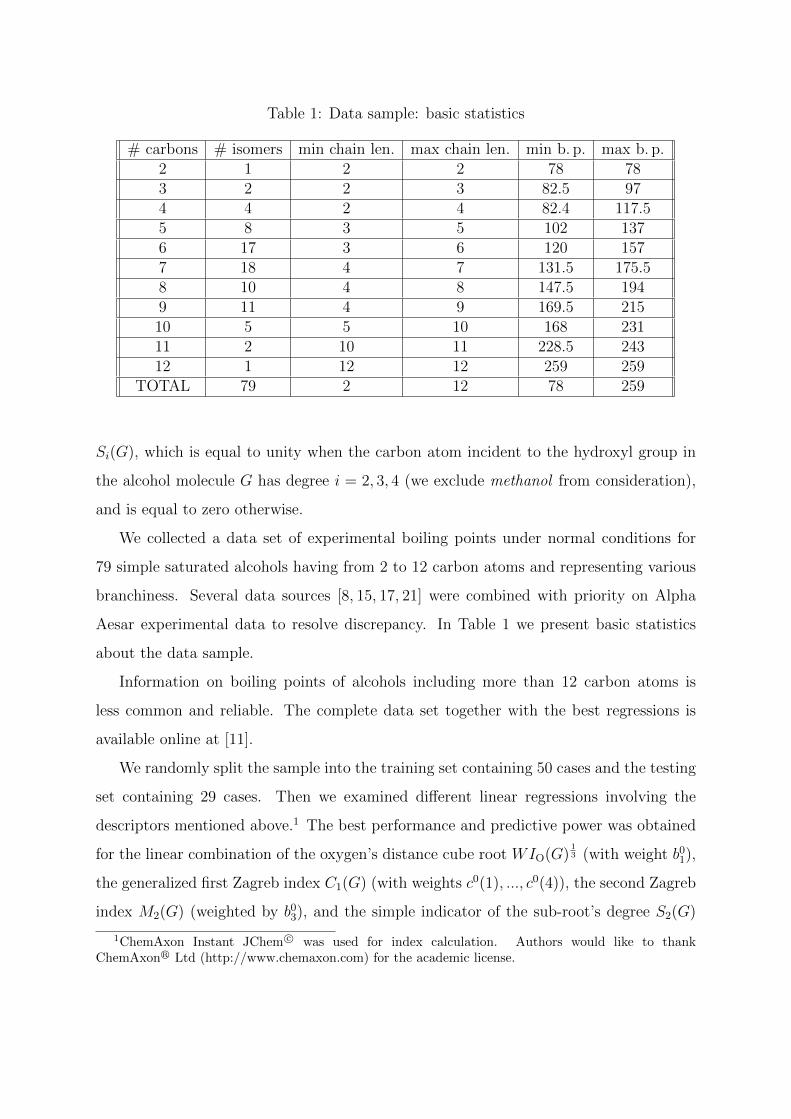
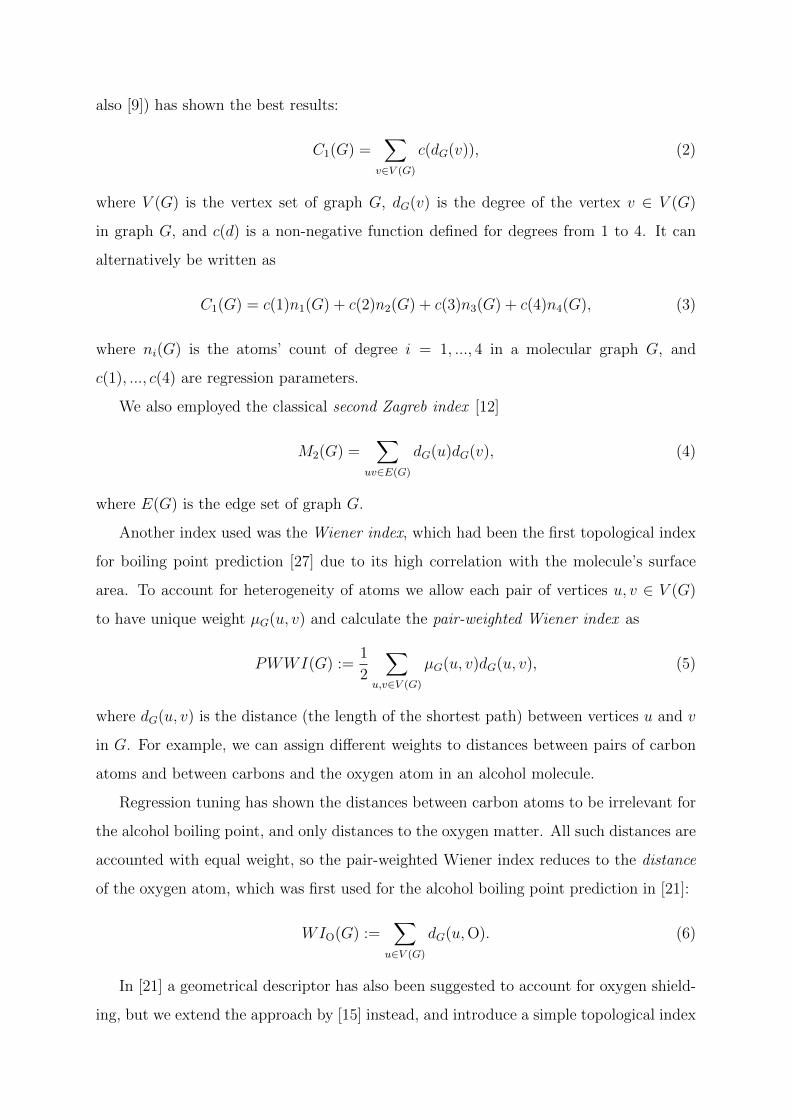
Table 1: Data sample: basic statistics

# carbons # isomers min chain len. max chain len. min b. p. max b. p.2 1 2 2 78 783 2 2 3 82.5 974 4 2 4 82.4 117.55 8 3 5 102 1376 17 3 6 120 1577 18 4 7 131.5 175.58 10 4 8 147.5 1949 11 4 9 169.5 21510 5 5 10 168 23111 2 10 11 228.5 24312 1 12 12 259 259

TOTAL 79 2 12 78 259

Si(G), which is equal to unity when the carbon atom incident to the hydroxyl group in

the alcohol molecule G has degree i = 2, 3, 4 (we exclude methanol from consideration),

and is equal to zero otherwise.

We collected a data set of experimental boiling points under normal conditions for

79 simple saturated alcohols having from 2 to 12 carbon atoms and representing various

branchiness. Several data sources [8, 15, 17, 21] were combined with priority on Alpha

Aesar experimental data to resolve discrepancy. In Table 1 we present basic statistics

about the data sample.

Information on boiling points of alcohols including more than 12 carbon atoms is

less common and reliable. The complete data set together with the best regressions is

available online at [11].

We randomly split the sample into the training set containing 50 cases and the testing

set containing 29 cases. Then we examined different linear regressions involving the

descriptors mentioned above.1 The best performance and predictive power was obtained

for the linear combination of the oxygen’s distance cube root WIO(G)13 (with weight b0

1),

the generalized first Zagreb index C1(G) (with weights c0(1), ..., c0(4)), the second Zagreb

index M2(G) (weighted by b03), and the simple indicator of the sub-root’s degree S2(G)

1ChemAxon Instant JChem c© was used for index calculation. Authors would like to thankChemAxonr Ltd (http://www.chemaxon.com) for the academic license.

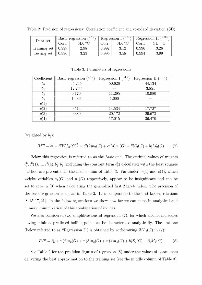
Table 2: Precision of regressions: Correlation coefficient and standard deviation (SD)

Data setBasic regression (“0”) Regression I (“I”) Regression II (“II”)Corr. SD, C Corr. SD, C Corr. SD, C

Training set 0.997 2.98 0.997 3.12 0.996 3.26Testing set 0.996 3.23 0.995 3.58 0.994 3.99

Table 3: Parameters of regressions

Coefficient Basic regression (“0”) Regression I (“I”) Regression II (“II”)b0 35.245 50.626 44.134b1 12.233 − 3.851b2 9.170 11.295 10.980b3 1.486 1.000 −c(1) − − −c(2) 9.514 14.534 17.727c(3) 9.380 20.172 29.673c(4) − 17.015 36.470

(weighted by b02):

BP 0 = b00 + b0

1WIO(G)13 + c0(2)n2(G) + c0(3)n3(G) + b0

2S2(G) + b03M2(G). (7)

Below this regression is referred to as the basic one. The optimal values of weights

b01, c

0(1), ..., c0(4), b02, b

03 (including the constant term b0

0) calculated with the least squares

method are presented in the first column of Table 3. Parameters c(1) and c(4), which

weight variables n1(G) and n4(G) respectively, appear to be insignificant and can be

set to zero in (3) when calculating the generalized first Zagreb index. The precision of

the basic regression is shown in Table 2. It is comparable to the best known relations

[8, 15, 17, 21]. In the following sections we show how far we can come in analytical and

numeric minimization of this combination of indices.

We also considered two simplifications of regression (7), for which alcohol molecules

having minimal predicted boiling point can be characterized analytically. The first one

(below referred to as “Regression I”) is obtained by withdrawing WIO(G) in (7):

BP I = bI0 + cI(2)n2(G) + cI(3)n3(G) + cI(4)n4(G) + bI

2S2(G) + bI3M2(G). (8)

See Table 2 for the precision figures of regression (8) under the values of parameters

delivering the best approximation to the training set (see the middle column of Table 3).

The second simplified regression (referred to as “Regression II” below) is obtained by

withdrawing M2(G) in (7):

BP II = bII0 + bII

1 WIO(G)13 + cII(2)n2(G) + cII(3)n3(G) + cII(4)n4(G) + bII

2 S2(G). (9)

In Table 2 we show its precision under the optimal values of parameters depicted in

the last column of Table 3.

The shortcoming of Regression II is that the term WIO(G)13 appears to be insignificant

after disposal of M2(G), being responsible of approximately 1 per cent of the residual sum

of squares. Nevertheless, we keep this regression for illustration of joint optimization of

C1(G) and of the pair-weighted Wiener index.

3 Minimization of indices and their combinations

In the present paper we find a simple saturated alcohol isomer with n− 1 carbon atoms

having the lowest predicted boiling point. As the regressions introduced in the previous

section are tested only for alcohols containing from 2 to 12 carbon atoms, we restrict our

attention to n 6 14, where we can expect some accuracy of the obtained results.

For n 6 14 admissible sets of all simple saturated alcohol molecules with n−1 carbons

are not too extensive, and allow for the brute-force enumeration. Moreover, we are sure

that no aid of a computer is needed for an organic chemist to draw a molecule being a

good approximation to the boiling point minimizer for all n 6 14. However, our aim is to

show how analytic optimization techniques formalize the professional intuition and help

making general conclusions of verifiable reliability.

Let us characterize chemical trees minimizing indices introduced in the previous sec-

tion and their combinations.

3.1 Degree-based indices

For a simple connected undirected graph G denote with W (G) the set of pendent vertices

(those having degree 1) of the graph G, and with M(G) := V (G)\W (G) the set of internal

vertices (with degree > 1) of G.

Definition 1 A simple connected undirected graph of order n is called a chemical tree

if it has n− 1 edges and its vertex degrees do not exceed 4. Denote with T (n) the set of

all chemical trees of order n. 2

Definition 2 A pendent-rooted chemical tree is a chemical tree, in which one pendent

vertex is distinguished and called a root. A typical pendent-rooted tree is denoted with

Tr, with r being its root. A vertex being incident to the root in Tr is called a sub-root

and is denoted as sub(Tr). Denote with R(n) the set of all pendent-rooted chemical trees

of order n. 2

Clearly, the set Ω(n − 1) of all molecules of simple saturated alcohols having n − 1

carbons coincides with the set R(n) of pendent-rooted chemical trees of order n (with

a root corresponding to the hydroxyl group and the other vertices forming the carbon

skeleton of a molecule).

For a topological index I(·) defined on an admissible set of graphs G introduce the

notation I∗G := minG∈G I(G) and let G∗I := Arg minG∈G I(G) be the set of graphs minimiz-

ing I(·) over G. For example, T ∗M2(n) is the set of chemical trees of order n minimizing

the second Zagreb index M2(·).

Define also the set Ri(n) := T ∈ R(n) : dT (sub(T )) = i of all pendent-rooted trees

with a sub-root having degree i = 2, ..., 4.

We start with the following obvious statement.

Lemma 1 Si(G) achieves its minimum at any pendent-rooted chemical tree with sub-

root’s degree other than i. In other words, R∗Si(n) = R(n)\Ri(n).

Proof is straightforward, as Si(G) = 1 for all G ∈ Ri(n), and Si(G) = 0 otherwise.

Indices C1(G) and M2(G) do not account for heterogeneity of atoms in a molecule,

so we can minimize them over the set T (n) of all chemical trees of order n and then

assign the root to an arbitrary pendent vertex of the index-minimizing tree to obtain a

pendent-rooted tree, which minimizes the index.

Consider an “ad-hoc” degree-based topological index

C(G) := C1(G) + b3M2(G) =∑

v∈V (G)

c(dG(v)) + b3

∑uv∈E(G)

dG(u)dG(v), (10)

where b3 is an arbitrary real constant (we keep notation b3 for compatibility with equations

(7), (8)).

Definition 3 A chemical tree T ∈ T (n) is extremely branched, if its internal vertices

have degree 4, except one vertex having degree 2 when n mod 3 = 0, or one vertex

having degree 3 when n mod 3 = 1. 2

Theorem 1 Assume the following inequalities hold:

c(1) + c(4) + 18b3 < c(2) + c(3), (11)

c(1) + c(3) + 8b3 < 2c(2), (12)

c(2) + c(4) + 8b3 < 2c(3). (13)

If a chemical tree T ∈ T (n) for n > 3 minimizes C(·) over all chemical trees from T (n),

then T is an extremely branched tree. For n 6 17 the inequality (11) can be weakened to

c(1) + c(4) + 17b3 < c(2) + c(3). (14)

Proof We employ the standard argument of index monotonicity with respect to certain

tree transformations. Assume the theorem does not hold, and vertices u, v ∈M(T ) exist

such that u 6= v and dT (u), dT (v) < 4. Four cases are possible.

1. dT (u) = dT (v) = 2. Let v1, v2 ∈ V (T ) be the vertices incident to v in T . Also, let

u1, u2 ∈ V (T ) be the vertices incident to u in T , and u2 lies on the path to the

vertex v in T . Without loss of generality assume that

dT (u1) + dT (u2) > dT (v1) + dT (v2). (15)

Consider a graph T ′ ∈ T (n) obtained from T by replacing the edge u1u with the

edge u1v. It is easy to see that T ′ is a tree. The degree of the vertex u in T ′ is

decreased by one, the degree of vertex v is increased by one, therefore, if u2 6= v,

we have

C(T ′)− C(T ) = c(1) + c(3)− 2c(2) + b3(dT (u1) + dT (v1) + dT (v2)− dT (u2)).

From (15) we obtain C(T ′)−C(T ) 6 c(1) + c(3)− 2c(2) + 2b3dT (u1). Since vertex

degrees 6 4 in a chemical tree, from (12) we have C(T ′) − C(T ) 6 c(1) + c(3) −

2c(2) + 8b3 < 0, which contradicts the assumption that T minimizes C(·).

If u2 = v, in the same manner obtain C(T ′) − C(T ) 6 c(1) + c(3) − 2c(2) + 7b3.

From (12), it is also negative.

2. dT (u) = 2, dT (v) = 3. Let v1, v2, v3 ∈ V (T ) be the vertices incident to v in T .

Also, let u1, u2 ∈ V (T ) be the vertices incident to u in T , and assume u2 lies on the

path to the vertex v in the tree T . Consider a tree T ′ ∈ T (n) obtained from T by

replacing the edge u1u with the edge u1v. By analogy to the previous case, if u2 6= v,

we obtain C(T ′)−C(T ) = c(1) + c(4)− c(2)− c(3) + b3(2dT (u1) +dT (v1) +dT (v2) +

dT (v3) − dT (u2)). Vertex degrees 6 4 in a chemical tree. Moreover, dT (u2) > 2,

since it is an intermediate vertex on the path u, u2, ..., v. Therefore,

C(T ′)− C(T ) 6 c(1) + c(4)− c(2)− c(3) + 18b3,

and, from (11), C(T ′)− C(T ) < 0, which is a contradiction.

To prove the weaker inequality (14) we are enough to prove that C(T ′)−C(T ) < 0

for n 6 17, since dT (u1) = dT (v1) = dT (v2) = dT (v3) = 4, and dT (u2) = 2 is

possible only in a tree of order 18 or more (an example is depicted in Fig. 1a), and

C(T ′)−C(T ) = c(1)+ c(4)− c(2)− c(3)+17b3 for the tree T depicted in Fig. 1b. If

a) b)

u

v

u

v

Figure 1: To the proof of inequality (14)

u2 = v, without loss of generality assume that u = v3. Then C(T ′)−C(T ) = c(1)+

c(4)−c(2)−c(3)+b3(2dT (u1)+dT (v1)+dT (v2)−2) 6 c(1)+c(4)−c(2)−c(3)+14b3.

From (11) (or from (14), if n 6 17), it is negative.

3. The case of dT (v) = 2, dT (u) = 3 is considered in the same manner.

4. dT (u) = dT (v) = 3. Let v1, v2, v3 ∈ V (T ) be the vertices incident to v in T . Also,

let u1, u2, u3 ∈ V (T ) be the vertices incident to u in T , with u1 not laying on a path

to v in T . Without loss of generality assume that

dT (u1) + dT (u2) + dT (u3) > dT (v1) + dT (v2) + dT (v3). (16)

Consider a tree T ′ ∈ T (n) obtained from T by replacing the edge u1u with the edge

u1v. If uv /∈ E(T ), then from (16) and dT (u1) 6 4 we have

C(T ′)−C(T ) = c(2)+c(4)−2c(3)+ b3(dT (u1)+dT (v1)+dT (v2)+dT (v3)−dT (u2)−

−dT (u3)) 6 c(2) + c(4)− 2c(3) + 2b3dT (u1) 6 c(2) + c(4)− 2c(3) + 8b3,

which is less than zero due to (13), and T cannot minimize C(·). If uv ∈ E(T ), in

the same way deduce C(T ′)− C(T ) 6 c(2) + c(4)− 2c(3) + 7b3, which is negative.

The obtained contradictions prove that no more than one internal vertex in T may

have degree less than 4.

As T ∈ T (n) and n > 1, the well-known equity holds:

n1(T ) + 2n2(T ) + 3n3(T ) + 4n4(T ) = 2(n− 1). (17)

On the other hand,

n1(T ) + n2(T ) + n3(T ) + n4(T ) = n. (18)

Assume that n2(T ) = 1, so that n3(T ) = 0. From (18) we have n1(T )+n4(T ) = n−1,

therefore, (17) makes n = 3 + 3n4(T ) and, since n4(T ) ∈ N0, n mod 3 = 0.

In the same manner we show that if n3(T ) = 1 then n mod 3 = 1. If both n2(T ) and

n3(T ) = 0, then n mod 3 = 2, and the proof is complete.

Corollary 1 Under conditions of Theorem 1, any tree T minimizing C(T ) = C1(T ) +

b3M2(T ) over T (n) enjoys the same number ni of vertices of degree i = 1, ..., 4. Therefore,

C1(T ) = C1(T ′) for any pair of trees T, T ′ ∈ T ∗C (n). 2

Corollary 2 Under conditions of Theorem 1 the sets T ∗C (n) for n = 4, ..., 14 are depicted

in Fig. 2. T ∗C (n) contains the sole tree for n < 14 , while T ∗C (14) contains two trees.

Proof From Corollary 1 we learn that only the value of M2(·) may vary within T ∗C (n).

From Theorem 1, for n ∈ 5, 8, 11, 14 an optimal tree is a 4-tree (in which all internal

vertices have degree 4). Each of n1 stem edges (those incident to a pendent vertex) adds

4 to the value of M2, while each of n4 − 1 edges connecting internal vertices adds 16 to

the value of M2. Since n1 and n4 are fixed for fixed n, all 4-trees have the same value of

M2(·) (and, therefore, the same value of C(·)). Consequently, for for n = 5, 8, 11, 14 the

set T ∗C (n) consists of all 4-trees of order n (see Fig. 2).

If T ∈ T ∗C (n), and n ∈ 6, 9, 12, one internal vertex u ∈M(T ) has degree dT (u) = 2,

while all others have degree 4. For n = 6 only one such tree exists depicted in Fig. 2. It

is easy to check that M2(·) is minimized if vertex u is incident to two internal vertices.

Only one such tree exists for n = 9 (see Fig. 2), and the same is true for n = 12.

For n ∈ 4, 7, 10, 13 any tree T ∈ T ∗C (n) has one internal vertex u ∈M(T ) of degree

dT (u) = 3, while all other have degree 4. For n = 4 only one such tree exists depicted in

Fig. 2, and the same is true for n = 7. Again, it is easy to check that, in the context of

M2(·) minimization, vertex u being incident to three internal vertices is strictly preferable

to vertex u being incident to one pendent and two internal vertices, which is, in turn,

preferred to u having two incident pendent vertices. So, optimal trees for n = 10, 13 are

depicted in Fig. 2 (black and white filling of circles is explained below).

The same logic allows continuing the sequence of C(·)-minimizers to n > 14.

4 5 6 7 8 9 10

11 12 13 14

Figure 2: Chemical trees minimizing the “ad-hoc” index C(·) for n = 4, ..., 14 (alcoholmolecules minimizing BP I(·) with possible oxygen positions filled with black)

Therefore, Theorem 1 says that, when conditions (11)-(13) hold, chemical trees min-

imizing C(·) have as many vertices of maximal degree 4 as possible. A similar result can

be proved for the modified Wiener index WIO(·).

3.2 Wiener index

A simple connected undirected graph G is called vertex-weighted if each vertex v ∈ V (G)

is endowed with a non-negaive weight µG(v). With µG we denote the total vertex weight

of the graph G, and WT (n) stands for the set of all vertex-weighted trees of order n.

Klavzar and Gutman [16] defined the Wiener index for vertex-weighted graphs as

VWWI(G) :=1

2

∑u,v∈V (G)

µG(u)µG(v)dG(u, v).

Clearly, VWWI(·) is a special case of the pair-weighted Wiener index PWWI(·)

(defined with formula (5)) for µG(u, v) := µG(u)µG(v). The path-weighted Wiener index

is poorly studied at the moment, but, fortunately, WIO(·), which is the point of our

current interest, can be reduced to the Wiener index for vertex-weighted graphs.

For every alcohol molecule from Ω(n− 1) (or, equivalently, for every pendent-rooted

tree Tr ∈ R(n)) define a vertex-weighted tree T (ε) ∈ WT (n) by assigning the weight

µT (ε)(v) := ε to each vertex v ∈ V (Tr) (a carbon atom) except the root r, and assigning

the weight µT (ε)(r) := 1/ε to the root (the oxygen atom). It is easy to see that under these

weights limε→0 VWWI(T (ε)) = WIO(Tr). Since WIO(·) is integer-valued, minimizers of

VWWI(·) and of WIO(·) coincide for sufficiently small ε.

In [10] the majorization technique suggested by Zhang et al. [29] is used to minimize

VWWI(·) over the set of trees with given vertex weights and degrees. Below we recall

the notation and selected theorems from [10]. We use them to find the extremal vertex

degrees over the set of all trees of order n with fixed vertex weights.

Definition 4 Consider a vertex set V . Let the function µ : V → R+ assign a non-

negative weight µ(v) to each vertex v ∈ V , while the function d : V → N assign a natural

degree d(v). The tuple 〈µ, d〉 is called a generating tuple if the following identity holds:∑v∈V

d(v) = 2(|V | − 1). (19)

Denote with µ :=∑

v∈V µ(v) the total weight of the vertex set V . Let WT (µ) :=

T ∈ WT (|V |) : V (T ) = V, µT (v) = µ(v) for all v ∈ V be the set of trees over the

vertex set V with vertex weights µ(·). For the set WT (µ, d) := T ∈ WT (µ) : dT (v) =

d(v) for all v ∈ V we also require vertices to have degrees d(·). 2

Let V (µ, d) be the domain of functions of a generating tuple 〈µ, d〉. Introduce the

set W (µ, d) := w ∈ V (µ, d) : d(w) = 1 of pendent vertices and the set M(µ, d) :=

V (µ, d)\W (µ, d) of internal vertices.

Definition 5 We will say that in a generating tuple 〈µ, d〉 weights are degree-monotone,

if for any m,m′ ∈M(µ, d) from d(m) < d(m′) it follows that µ(m) 6 µ(m′), and for any

w ∈ W (µ, d) we have µ(w) > 0. 2

For a generating tuple 〈µ, d〉 the generalized Huffman algorithm [10] builds a tree

H ∈ WT (µ, d) as follows.

Setup. Define the vertex set V1 := V (µ, d) and the functions µ1 and d1, which endow

its vertices with weights µ1(v) := µ(v) and degrees d1(v) := d(v), v ∈ V1. We start with

the empty graph H over the vertex set V (µ, d).

Steps i = 1, ..., q − 1. Denote with mi the vertex having the least degree among

the vertices of the least weight in M(µi, di). Let w1, ..., wd(mi)−1 be the vertices having

d(mi)− 1 least weights in W (µi, di). Add to H edges w1mi, ..., wd(mi)−1mi.

Define the set Vi+1 := Vi\w1, ..., wd(mi)−1 and functions µi+1(·), di+1(·), endowing its

elements with weights and degrees as follows:

µi+1(v) := µi(v) for v 6= mi, µi+1(mi) := µi(mi) + µi(w1) + ...+ µi(wd(mi)−1),

di+1(v) := di(v) for v 6= mi, di+1(mi) := 1. (20)

Step q. Consider a vertex mq ∈ M(µq, dq). By construction, |M(µq, dq)| = 1,

|W (µq, dq)| = d(mq). Add to H edges connecting all vertices from W (µq, dq) to mq.

Finally, set µH(v) := µ(v), v ∈ V (H).

Theorem 2 [10] If weights are degree-monotone in a generating tuple 〈µ, d〉, then T ∈

WT ∗VWWI(µ, d) if and only if T ∈ WT (µ, d) and T is a Huffman tree. In other words,

only a Huffman tree minimizes the Wiener index over the set of trees whose vertices have

given weights and degrees. 2

In the present subsection we study how the value of VWWI∗WT (µ, d) changes with

degrees d(·). Our results are analogous to those proved by Zhang et al. [29] for the

“classical” Wiener index. Following [10], we reformulate the problem for directed trees.

Definition 6 A (weighted) directed tree is a weighted connected directed graph with

each vertex except the terminal vertex 2 having the sole outbound arc and the terminal

vertex having no outbound arcs. 2

An arbitrary tree T ∈ WT (n) can be transformed into a directed tree by choosing

an internal vertex t ∈ M(T ), and replacing all its edges with arcs directed towards (a

terminal vertex) t. Let us denote with WD the collection of all directed trees, which can

be obtained in such a way, and let WD(µ, d) stand for all directed trees obtained from

2Typically it is called a root, but we will use an alternative notation to avoid confusion with a rootof a pendent-rooted tree introduced in the previous subsection.

WT (µ, d). Vice versa, in a directed tree from WD(µ, d) replacement of all arcs with

edges makes some tree from WT (µ, d).

If at Step i = 1, ..., q of the generalized Huffman algorithm we add arcs towards the

vertex mi (instead of undirected edges), we obtain a directed Huffman tree with the

terminal vertex mq.

Definition 7 For a vertex v ∈ V (T ) of a directed tree T ∈ WD define its subordinate

group gT (v) ⊆ V (T ) as the set of vertices having the directed path to the vertex v in the

tree T (the vertex v itself belongs to gT (v)). The weight fT (v) of a subordinate group

gT (v) is defined as the total vertex weight of the group: fT (v) :=∑

u∈gT (v) µT (u). 2

Note 1 If all pendent vertices in T have positive weights, then fT (v) > 0 for any v ∈

V (T ). In particular, it is true for any T ∈ WD(µ, d), if weights in 〈µ, d〉 are degree-

monotone.

The Wiener index is defined for directed trees by analogy to the case of undirected

trees: we simply ignore the arcs’ direction when calculating distances. Therefore, a tree

and a corresponding directed tree share the same value of the Wiener index.

The value of the Wiener index for a directed tree Tt ∈ WD(µ) with a terminal vertex

t ∈M(T ) can be written [10] as:

VWWI(Tt) =∑

v∈V (Tt)\t

fTt(v)(µ− fTt(v)) =∑

v∈V (T )\t

χ(fTt(v)), (21)

where χ(x) := x(µ−x), and thus, the problems of Wiener index minimization for vertex-

weighted trees and for weighted directed trees are equivalent.

Definition 8 Every directed tree T is associated with the vector of subordinate groups’

weights f(T ) := (fT (v))v∈V (T )\t, where t is the terminal vertex of T . From equation

(21) we see that the vector f(T ) completely determines the value of VWWI(T ). 2

Definition 9 [20, 29] For the real vector x = (x1, ..., xp), p ∈ N, denote with x↑ =

(x[1], ..., x[p]) the vector where all components of x are arranged in ascending order. 2

Definition 10 [20, 29] A non-negative vector x = (x1, ..., xp), p ∈ N, weakly majorizes

a non-negative vector y = (y1, ..., yp) (which is denoted with x y) if

k∑i=1

x[i] 6k∑

i=1

y[i] for all k = 1, ..., p.

If x↑ 6= y↑, then x is said to strictly weakly majorize y (which is denoted with x y). 2

We will need the following properties of weak majorization.

Lemma 2 [20, 29] Consider a positive number b > 0 and two non-negative vectors

x = (x1, ..., xk, y1, ..., yl) and y = (x1 + b, ..., xk + b, y1− b, ..., yl − b), such that 0 6 k 6 l.

If xi > yi for i = 1, ..., k, then x ≺ y. 2

Lemma 3 [20, 29] If x y and x′ ≺ y′, then (x,x′) ≺ (y,y′), where (x,x′) means

concatenation of vectors x and x′. 2

Lemma 4 [20,29] If χ(x) is a increasing concave function, and (x1, ..., xp) (y1, ..., yp),

then∑p

i=1 χ(xi) 6∑p

i=1 χ(yi), and equality is possible only when (x1, ..., xp)↑

= (y1, ..., yp)↑. 2

The following lemma establishes an important property of directed Huffman trees:

Lemma 5 [10] For any directed Huffman tree H

vm, v′m′ ∈ E(H),m 6= m′, fH(v) < fH(v′)⇒ fH(m) < fH(m′). (22)

Lemma 6 Consider generating tuples 〈µ, d〉 and 〈µ, d′〉 defined on the same vertex set,

and let weights be degree-monotone in 〈µ, d〉. Let the values of degree functions d(·) and

d′(·) differ only for vertices u and v, such that d(u) > d(v) and µ(u) > µ(v), while

d′(u) = d(u)+1, d′(v) = d(v)−1. Then for every directed tree T ∈ WD(µ, d) there exists

such a directed tree T ′ ∈ WD(µ, d′) that f(T ′) f(T ).

Proof By Theorem 2 from [10], such a directed Huffman tree H ∈ WD(µ, d) exists,

that f(H) f(T ).3 Since H ∈ WD(µ, d) and d′(v) = d(v)−1 > 1, we know that d(v) > 2

and v has an incoming arc in H from some vertex v′ ∈ V . Weights are degree-monotone

in 〈µ, d〉, therefore, by construction of a Huffman tree, fH(u) > fH(v) and, thus, without

loss of generality we can assume that u /∈ gH(v).

Assume that v ∈ gH(u). Then a path (v,m1, ...,ml, u) exists in H from the vertex v

to the vertex u, where l > 0. Consider a directed tree T ′ obtained from H by deleting

the arc v′v and adding the arc v′u instead. It is clear that T ′ ∈ WD(µ, d′), and weights

of groups subordinated to vertices v,m1, ...,ml decrease by fH(v′) (which is positive by

Note 1), while weights of the other vertices do not change. Therefore, by Lemma 2,

y := (fT ′(v), fT ′(m1), ..., fT ′(ml)) =

3Please note the different notation in [10] (x w y is used in [10] where we write x y).

= (fH(v)− fH(v′), fH(m1)− fH(v′), ..., fH(ml)− fH(v′))

(fH(v), fH(m1), ..., fH(ml)) =: x.

If one denotes with z the vector of (unchanged) weights of groups subordinated to all

other non-terminal vertices of H, then, by Lemma 3, f(T ′) = (y, z) (x, z) = f(H).

Assume now that v /∈ gH(u). Then there are disjoint paths (u,m1, ...,mk,m) and

(v,m′1, ...,m′l,m) (where k, l > 0) in H from vertices u and v to some vertex m ∈M(H).

If fH(u) > fH(v), then, applying repeatedly formula (22) from Lemma 5, we write

fH(mi) > fH(m′i), i = 1, ...,min[k, l]. It also follows from (22) that k 6 l, since otherwise

fH(ml+1) > fH(m), which is impossible, since ml+1 ∈ gH(m).

Consider a directed tree T ′ ∈ WD(µ, d′) obtained from H by deleting the arc v′v and

adding the arc v′u instead. In the tree T ′ weights of the groups subordinated to the ver-

tices u,m1, ...,mk increase by fH(v′) (i.e., fT ′(u) = fH(u) + fH(v′), fT ′(mi) = fH(mi) +

fH(v′), i = 1, ..., k), weights of the groups subordinated to the vertices v,m′1, ...,m′l de-

crease by fH(v′) (i.e., fT ′(u) = fH(u) − fH(v′), fT ′(m′i) = fH(m′i) − fH(v′), i = 1, ..., l),

weights of all other vertices (including m) do not change. Therefore, by Lemma 2,

y := (fT ′(u), fT ′(m1), ..., fT ′(mk), fT ′(v), fT ′(m′1), ..., fT ′(m′l)) =

= (fH(u) + fH(v′), fH(m1) + fH(v′), ..., fH(mk) + fH(v′),

fH(v)− fH(v′), fH(m′1)− fH(v′), ..., fH(m′l)− fH(v′))

(fH(u), fH(m1), ..., fH(mk), fH(v), fH(m′1), ..., fH(m′l)) =: x.

If z is a vector of (unchanged) weights of groups subordinated to all other non-terminal

vertices of H, then, by Lemma 3, f(T ′) = (y, z) (x, z) = f(H).

By construction of the Huffman tree, the situation of fH(u) = fH(v) is possible only

when d(u) = d(v) and µ(u) = µ(v). In this case we cannot use formula (22) to compare

subordinate groups’ weights of elements of both chains, since all possible alternatives of

k = 0, or l = 0, or any sign of the expression fH(m1) − fH(m′1) in case of k, l > 1 are

possible.

On the other hand, if fH(m1) > fH(m′1), then formula (22) can be used to show that

k 6 l, fH(mi) > fH(m′i), i = 2, ..., k. In case of the opposite inequality, fH(m1) < fH(m′1),

formula (22) says that, by contrast, k > l, fH(mi) < fH(m′i), i = 2, ..., l. Repeating this

argument through the chain, we see that only two alternatives are possible:

• 0 6 p 6 k 6 l, fH(mi) = fH(m′i), i = 1, ..., p, fH(mi) > fH(m′i), i = p+ 1, ..., k. In

this case, as above, we can show that for the directed tree T ′ ∈ WD(µ, d′) obtained

from H by deleting the arc v′v and adding the arc v′u instead, f(T ′) f(H).

• 0 6 p 6 l 6 k, fH(mi) = fH(m′i), i = 1, ..., p, fH(mi) < fH(m′i), i = p + 1, ..., l. In

this case the same inequality is true for the directed tree T ′ ∈ WD(µ, d′) obtained

from H by redirecting to/from vertex v all arcs incident to u, and by redirecting

to/from vertex u all arcs incident to v except the arc v′v.

Therefore, we proved that a tree T ′ ∈ WD(µ, d′) exists such that f(T ′) f(H). As

shown above, f(H) f(T ), so, finally, f(T ′) f(T ).

Definition 11 A directed tree T ∈ WD(µ, d) with a terminal vertex t is called a proper

tree if for all m ∈M(T ), m 6= t, fT (m) 6 µ/2.

Lemma 7 Let a function χ(x) be concave and increasing for x ∈ [0, µ/2]. Consider a pair

of generating tuples, 〈µ, d〉 and 〈µ, d′〉, satisfying conditions of Lemma 6. If T ∈ WD(µ, d)

and T ′ ∈ WD(µ, d′) are directed Huffman trees, then∑v∈V (T ′)\t′

χ(fT ′(v)) <∑

v∈V (T )\t

χ(fT (v)),

where t ∈M(T ) and t′ ∈M(T ′) are terminal vertices of T and T ′ respectively.

Proof From Lemma 6, such a tree T ′′ ∈ WD(µ, d′) exists that f(T ′′) f(T ). Theorem 2

from [10] says that f(T ′) f(T ′′), therefore, f(T ′) f(T ). Denote for short n1 = |V (T )|,

f(T ) = f := (f1, ..., fn1−1), f(T ′) = f ′ := (f ′1, ..., f′n1−1).

It is known (see Lemma 19 in [10]) that each directed Huffman tree with degree-

monotone weights is a proper tree, so, fT (w) 6 µ/2, w ∈M(µ, d)\t, and fT ′(w′) 6 µ/2,

w′ ∈ M(µ, d′)\t′. If a vertex w ∈ V (T ) exists, such that µ(w) > µ/2 (there can be at

most one such vertex in V (T )), then w cannot be an internal vertex in T and a pendent

vertex in T ′, since then conditions of Lemma 6 imply that w = v and µ(u) > µ(w), which

is impossible. Therefore, w is either a terminal vertex both in T and in T ′, or a pendent

vertex both in T and in T ′. In the latter case fT (v) = fT ′(v) = µ(v).

Consequently, fi, f′i 6 µ/2 for i = 1, ..., n1 − 2, and if fn1−1 > µ/2, then fn1−1 =

f ′n1−1 = µ(w).

If fn1−1 6 µ/2, the statement of the lemma follows from Lemma 4.

If fn1−1 > µ/2, we can write∑v∈V (T )\t

χ(fT (v))−∑

v∈V (T ′)\t′

χ(fT ′(v)) =

=

n1−2∑i=1

χ(fi) + χ(fn1−1)−n1−2∑i=1

χ(f ′i)− χ(f ′n1−1) =

n1−2∑i=1

χ(fi)−n1−2∑i=1

χ(f ′i).

Since f ′ f and fn1−1 = f ′n1−1, we have (f ′1, ..., f′n1−2) (f1, ..., fn1−2), and the

statement of the lemma again follows from Lemma 4.

Corollary 3 If generating tuples 〈µ, d〉 and 〈µ, d′〉 satisfy conditions of Lemma 6, then

VWWI∗WT (µ, d′) < VWWI∗WT (µ, d).

Proof Theorem 3 from [10] says that WD∗VWWI(µ, d) consists of all directed Huffman

trees. Consider the directed Huffman trees T ∈ WD∗VWWI(µ, d), T ′ ∈ WD∗VWWI(µ, d′).

Function χ(x) = x(µ − x) in (21) satisfies the conditions of Lemma 7, so, from (21),

VWWI(T ′) < VWWI(T ). Since every proper directed tree from WD(µ, d) has a corre-

sponding tree fromWT (µ, d), and vice versa, we have VWWI∗WT (µ, d) = VWWI∗WD(µ, d),

and the corollary follows immediately.

In the rest of the section we consider a set V consisting of n vertices with weights µ(v),

v ∈ V . The set V can be thought of as a fixed collection of (heterogeneous) atoms used

as building blocks for molecules. All molecules constructed from these building blocks

belong to WT (µ).

We want to use Corollary 3 to show that, similar to Theorem 1, the vertex-weighted

Wiener index is minimized by a tree having as many vertices of the maximum degree

as possible. We cannot apply Corollary 3 to the whole collection WT (µ) of trees with

vertices having fixed weights µ(·) (unless µ(v) ≡ const), as it inevitably contains trees

generated by the tuples with non-degree-monotone weights, for which Corollary 3 is

inapplicable. Therefore, we have to carefully limit a set of admissible trees.

Definition 12 Consider an admissible set M ⊆ WT (µ) and denote with L :=⋂T∈MW (T ) the set of vertices, which are pendent in all trees from M. A generat-

ing tuple 〈µ, d〉 is called extremal forM, if M(µ, d) consists of dn−23e vertices having the

highest weights in V \L (i.e., if u ∈M(µ, d) and v ∈ V \L, then µ(u) > µ(v)), at most one

vertex u ∈ M(µ, d) has degree d(u) < 4 while others having degree 4, and, when exists,

u has the minimal weight in M(µ, d). 2

There can be several extremal tuples for an admissible set, if for some extremal tuple

〈µ, d〉 such vertices w ∈ W (µ, d)\L and m ∈ M(µ, d) exist that µ(w) = µ(m) (swapping

w and m then makes a new extremal tuple). It is clear that weights are degree-monotone

in 〈µ, d〉, and there are only extremely branched trees in WT (µ, d).

Theorem 3 If 〈µ, d〉 is an extremal tuple for an admissible set M⊆WT (µ) of chem-

ical trees with degree-monotone weights, and H ∈ WT (µ, d) is a Huffman tree, then

VWWI(H) 6 VWWI∗M, with equality if and only if M contains H or any other Huff-

man tree generated by the extremal tuple.

Proof Consider a vertex-weighted tree T ∈M. Weights are degree-monotone in T , so,

if dT (u) > dT (v) and d(u) < d(v) for some u, v ∈M(T ), then µ(u) = µ(v). Consequently,

such a tree T ′ ∈ WT (µ) exists that VWWI(T ) = VWWI(T ′), W (T ′) = W (T ), and

from u, v ∈M(T ) and dT ′(u) < dT ′(v) it follows that d(u) 6 d(v) (T ′ is constructed from

T with a permutation of several vertices of equal weight, which does not affect the index

value). So, degrees in the tree T ′ are “compatible” to those in the tuple 〈µ, d〉.

Assume T ′ ∈ WT (µ, d0) for some generating tuple 〈µ, d0〉, and d0(·) 6≡ d(·). Construct

such a sequence 〈µ, d0〉, 〈µ, d1〉, ..., 〈µ, dk〉 of generating tuples with degree-monotone weig-

hts that k > 1, dk(·) ≡ d(·), and each pair 〈µ, di〉, 〈µ, di+1〉 of sequential tuples meets the

requirements of Lemma 6, i = 0, ..., k − 1.

We build the elements of this sequence one by one. For a tuple 〈µ, di〉 define

M+(µ, di) := w ∈ V : di(w) < d(w) and M−(µ, di) := w ∈ V : di(w) > d(w).

Set di+1(ui) = di(ui) + 1 for a vertex ui having the highest weight in M+(µ, di), and

di+1(vi) = di(vi) − 1 for a vertex vi having the least weight in M−(µ, di), while keeping

the degrees of all other vertices.

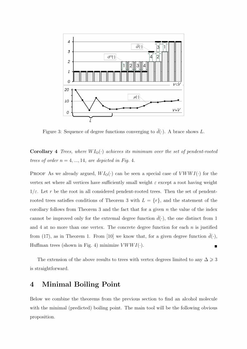
The proof is clear from Fig. 3, where numbers on arrows show steps of trans-

formation of the initial degree function. By Corollary 3, VWWI∗WT (µ, d) < ... <

VWWI∗WT (µ, d0) 6 VWWI(T ′) = VWWI(T ). From Theorem 2 we know that if

T ∈ WT (µ, d), then VWWI(T ) = VWWI∗WT (µ, d) if and only if T is a Huffman tree.

Therefore, for every T ∈ M we have VWWI∗WT (µ, d) 6 VWWI(T ) with equality if

and only if T is a Huffman tree for 〈µ, d〉 or another extremal tuple, and the proof is

complete.

d 0(·)

d (·)

4

4

3

3

2

2

1

1

m(·)

L

v V

v V

Figure 3: Sequence of degree functions converging to d(·). A brace shows L.

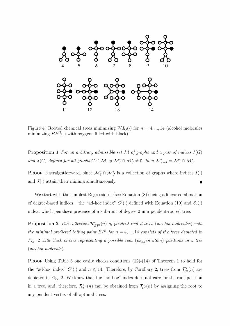
Corollary 4 Trees, where WIO(·) achieves its minimum over the set of pendent-rooted

trees of order n = 4, ..., 14, are depicted in Fig. 4.

Proof As we already argued, WIO(·) can be seen a special case of VWWI(·) for the

vertex set where all vertices have sufficiently small weight ε except a root having weight

1/ε. Let r be the root in all considered pendent-rooted trees. Then the set of pendent-

rooted trees satisfies conditions of Theorem 3 with L = r, and the statement of the

corollary follows from Theorem 3 and the fact that for a given n the value of the index

cannot be improved only for the extremal degree function d(·), the one distinct from 1

and 4 at no more than one vertex. The concrete degree function for each n is justified

from (17), as in Theorem 1. From [10] we know that, for a given degree function d(·),

Huffman trees (shown in Fig. 4) minimize VWWI(·).

The extension of the above results to trees with vertex degrees limited to any ∆ > 3

is straightforward.

4 Minimal Boiling Point

Below we combine the theorems from the previous section to find an alcohol molecule

with the minimal (predicted) boiling point. The main tool will be the following obvious

proposition.

4 5 6 7 8 9 10

11 12 13 14

Figure 4: Rooted chemical trees minimizing WIO(·) for n = 4, ..., 14 (alcohol moleculesminimizing BP II(·) with oxygens filled with black)

Proposition 1 For an arbitrary admissible set M of graphs and a pair of indices I(G)

and J(G) defined for all graphs G ∈M, if M∗I ∩M∗

J 6= ∅, then M∗I+J =M∗

I ∩M∗J .

Proof is straightforward, since M∗I ∩M∗

J is a collection of graphs where indices I(·)

and J(·) attain their minima simultaneously.

We start with the simplest Regression I (see Equation (8)) being a linear combination

of degree-based indices – the “ad-hoc index” CI(·) defined with Equation (10) and S2(·)

index, which penalizes presence of a sub-root of degree 2 in a pendent-rooted tree.

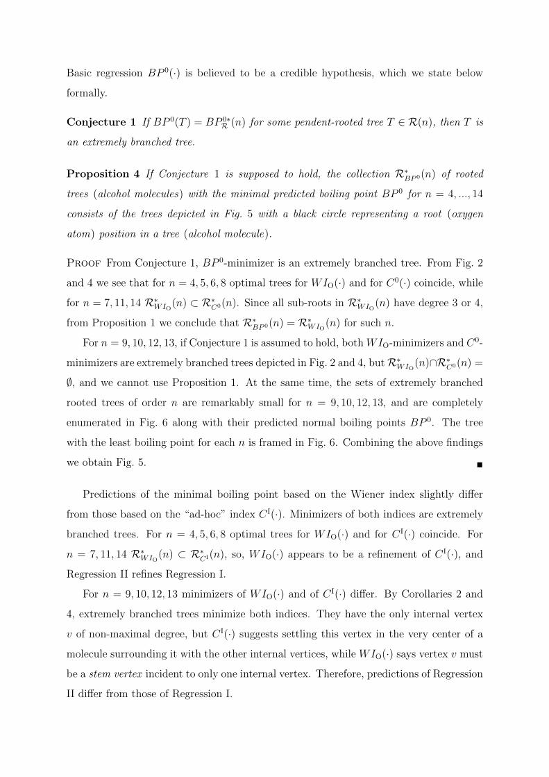
Proposition 2 The collection R∗BP I(n) of pendent-rooted trees (alcohol molecules) with

the minimal predicted boiling point BP I for n = 4, ..., 14 consists of the trees depicted in

Fig. 2 with black circles representing a possible root (oxygen atom) positions in a tree

(alcohol molecule).

Proof Using Table 3 one easily checks conditions (12)-(14) of Theorem 1 to hold for

the “ad-hoc index” CI(·) and n 6 14. Therefore, by Corollary 2, trees from T ∗CI(n) are

depicted in Fig. 2. We know that the “ad-hoc” index does not care for the root position

in a tree, and, therefore, R∗CI(n) can be obtained from T ∗CI(n) by assigning the root to

any pendent vertex of all optimal trees.

From Lemma 1, S2(·) is minimized with pendent-rooted trees whose sub-root has

degree 3 or 4. Each tree in Fig. 2 has a pendent vertex being incident to a vertex of

degree 3 or 4, so, R∗CI(n) ∩ R∗S2(n) 6= ∅, and conditions of Proposition 1 hold for all

n = 4, ..., 14. Therefore, R∗BP I(n) consists of the trees from Fig. 2 with the root assigned

to a pendent vertex incident to a vertex of degree 3 or 4. Possible roots are filled with

black color in Fig. 2.

The similar reasoning can be carried out for Regression II, which is defined with

Equation (9) and adds up from the generalized first Zagreb index CII1 (·), the cube root of

the distance WIO(·) 13 of the oxygen atom in an alcohol molecule, and, again, from S2(·)

index.

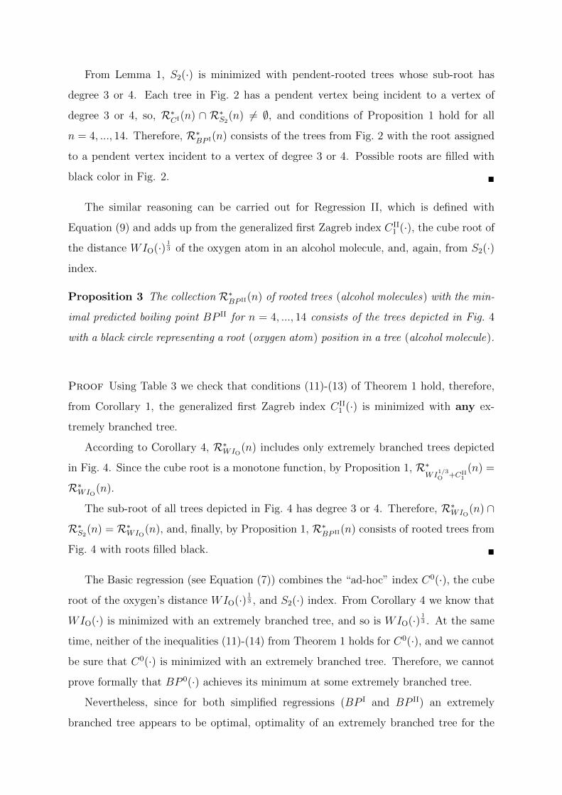
Proposition 3 The collection R∗BP II(n) of rooted trees (alcohol molecules) with the min-

imal predicted boiling point BP II for n = 4, ..., 14 consists of the trees depicted in Fig. 4

with a black circle representing a root (oxygen atom) position in a tree (alcohol molecule).

Proof Using Table 3 we check that conditions (11)-(13) of Theorem 1 hold, therefore,

from Corollary 1, the generalized first Zagreb index CII1 (·) is minimized with any ex-

tremely branched tree.

According to Corollary 4, R∗WIO(n) includes only extremely branched trees depicted

in Fig. 4. Since the cube root is a monotone function, by Proposition 1, R∗WI

1/3O +CII

1

(n) =

R∗WIO(n).

The sub-root of all trees depicted in Fig. 4 has degree 3 or 4. Therefore, R∗WIO(n) ∩

R∗S2(n) = R∗WIO

(n), and, finally, by Proposition 1, R∗BP II(n) consists of rooted trees from

Fig. 4 with roots filled black.

The Basic regression (see Equation (7)) combines the “ad-hoc” index C0(·), the cube

root of the oxygen’s distance WIO(·) 13 , and S2(·) index. From Corollary 4 we know that

WIO(·) is minimized with an extremely branched tree, and so is WIO(·) 13 . At the same

time, neither of the inequalities (11)-(14) from Theorem 1 holds for C0(·), and we cannot

be sure that C0(·) is minimized with an extremely branched tree. Therefore, we cannot

prove formally that BP 0(·) achieves its minimum at some extremely branched tree.

Nevertheless, since for both simplified regressions (BP I and BP II) an extremely

branched tree appears to be optimal, optimality of an extremely branched tree for the

Basic regression BP 0(·) is believed to be a credible hypothesis, which we state below

formally.

Conjecture 1 If BP 0(T ) = BP 0∗R (n) for some pendent-rooted tree T ∈ R(n), then T is

an extremely branched tree.

Proposition 4 If Conjecture 1 is supposed to hold, the collection R∗BP 0(n) of rooted

trees (alcohol molecules) with the minimal predicted boiling point BP 0 for n = 4, ..., 14

consists of the trees depicted in Fig. 5 with a black circle representing a root (oxygen

atom) position in a tree (alcohol molecule).

Proof From Conjecture 1, BP 0-minimizer is an extremely branched tree. From Fig. 2

and 4 we see that for n = 4, 5, 6, 8 optimal trees for WIO(·) and for C0(·) coincide, while

for n = 7, 11, 14 R∗WIO(n) ⊂ R∗C0(n). Since all sub-roots in R∗WIO

(n) have degree 3 or 4,

from Proposition 1 we conclude that R∗BP 0(n) = R∗WIO(n) for such n.

For n = 9, 10, 12, 13, if Conjecture 1 is assumed to hold, both WIO-minimizers and C0-

minimizers are extremely branched trees depicted in Fig. 2 and 4, butR∗WIO(n)∩R∗C0(n) =

∅, and we cannot use Proposition 1. At the same time, the sets of extremely branched

rooted trees of order n are remarkably small for n = 9, 10, 12, 13, and are completely

enumerated in Fig. 6 along with their predicted normal boiling points BP 0. The tree

with the least boiling point for each n is framed in Fig. 6. Combining the above findings

we obtain Fig. 5.

Predictions of the minimal boiling point based on the Wiener index slightly differ

from those based on the “ad-hoc” index CI(·). Minimizers of both indices are extremely

branched trees. For n = 4, 5, 6, 8 optimal trees for WIO(·) and for CI(·) coincide. For

n = 7, 11, 14 R∗WIO(n) ⊂ R∗CI(n), so, WIO(·) appears to be a refinement of CI(·), and

Regression II refines Regression I.

For n = 9, 10, 12, 13 minimizers of WIO(·) and of CI(·) differ. By Corollaries 2 and

4, extremely branched trees minimize both indices. They have the only internal vertex

v of non-maximal degree, but CI(·) suggests settling this vertex in the very center of a

molecule surrounding it with the other internal vertices, while WIO(·) says vertex v must

be a stem vertex incident to only one internal vertex. Therefore, predictions of Regression

II differ from those of Regression I.

4 5 6 7 8 9 10

11 12 13 14

Figure 5: Pendent-rooted chemical trees (alcohol molecules) minimizing BP 0(·) for n =4, ..., 14 with black circles being roots (oxygen atoms)

145.76 146.32 138.48 157.57 159.15 155.20 160.16 156.18 161.11

185.93 186.36 178.29 187.21 187.62 188.02 179.88 180.63 198.34 199.43

n = 12

n = 9 n = 10

n = 13

198.96 199.77 195.71 200.16 196.09 200.93 192.38 201.66 201.66 197.56 197.91 202.72

Figure 6: Extremely branched pendent-rooted trees of order n = 9, 10, 12, 13 and theirBP 0 values (minima are framed)

Basic regression, which contains a weighted linear combination of the Wiener index

and the “ad-hoc” index, represents a sort of intermediate behavior between these extremal

trends (at least for extremely branched trees under Conjecture 1). The weight of the

Wiener index in the regression is not enough to move the minimal tree sufficiently from

the trees depicted in Fig. 2, and Basic regression becomes a yet another refinement of

Regression I.

5 Conclusion

The focus of this paper is development of optimization techniques for combinations of

some well-known and novel topological indices over chemically interesting sets of graphs.

We derived conditions under which an extremely branched tree minimizes the sum of the

second Zagreb index and of the generalized first Zagreb index. We also found minimizers

of the vertex-weighted Wiener index over the set of chemical trees with given vertex

weights.

We enumerated index minimizers for moderate (up to 14) non-hydrogen atom count

in a molecule, and combined them in several regressions of different complexity to forecast

a simple alcohol molecule with the lowest boiling point.

For simpler regressions (Regressions I and II) we managed to obtain a complete an-

alytical characterization of extremal alcohol molecules, while for the most complex (yet

the most precise) “basic” regression we had to limit our attention to extremely branched

trees (see Conjecture 1) and employed the brute-force enumeration to find molecules of

low-boiling alcohols.

Forecasts based on different regressions slightly differ, but they all comply with the

collected experimental data on normal boiling points of simple alcohols.

Finally, let us sketch several promising directions of future research. An obvious

shortcoming of this paper is Conjecture 1, which is explained but is not proven formally.

To justify it, we need to refine sufficiently our optimization techniques, viz, to optimize

jointly the Wiener index and the Zagreb indices.

On the other hand, there is wide space for investigation of popular combinations of

topological indices forecasting important physical and chemical properties of compounds.

References

[1] A. T. Balaban, J. Devillers (Eds.), Topological indices and related descriptors in

QSAR and QSPAR, CRC Press, Boca Raton, 2000.

[2] U. Bren, V. Martınek, J. Florian, Decomposition of the Solvation Free Energies of

Deoxyribonucleoside Triphosphates Using the Free Energy Perturbation Method, J.

Phys. Chem. B 110 (2006), 12782–12788.

[3] U. Bren, D. Janezic, Individual Degrees of Freedom and the Solvation Properties of

Water, J. Chem. Phys. 137 (2012) 024108.

[4] B. Bollobas, Extremal graph Theory , Academic Press, London, 1978.

[5] A. A. Dobrynin, R. Entringer, I. Gutman, Wiener index of trees: theory and appli-

cations, Acta Applicandae Mathematica 66 (2001) 211–249.

[6] M. Fischermann, A. Hoffmann, D. Rautenbach, L. Szekely, L. Volkmann, Wiener

index versus maximum degree in trees, Discrete Applied Mathematics 122 (2002)

127–137.

[7] B. Furtula, I. Gutman, H. Lin, More trees with all degrees odd having extremal

Wiener index, MATCH Commun. Math. Comput. Chem. 70 (2013) 293–296.

[8] R. Garcıa–Domenech, J. Galvez, J. V. de Julian–Ortiz, L. Pogliani, Some new trends

in chemical graph theory, Chem. Rev. 108 (2008) 1127–1169.

[9] M. Goubko, Minimizing degree-based topological indices for trees with given number

of pendent vertices, MATCH Commun. Math. Comput. Chem. 71 (2014) 33–46.

[10] M. Goubko, Minimizing Wiener index for vertex-weighted trees with given weight

and degree sequences, MATCH Commun. Math. Comput. Chem. 73 (2015) ??–??.

[11] http://www.mtas.ru/upload/library/GoubkoMilosOnline14.pdf (last accessed

Oct 30, 2014).

[12] I. Gutman, N. Trinajstic, Graph theory and molecular orbitals. Total π-electron

energy of alternant hydrocarbons, Chem. Phys. Lett. 17 (1972) 535–538.

[13] I. Gutman, B. Furtula (Eds.), Novel molecular structure descriptors — Theory and

Applications I , Univ. Kragujevac, Kragujevac, 2010.

[14] I. Gutman, B. Furtula (Eds.), Novel molecular structure descriptors — Theory and

Applications II , Univ. Kragujevac, Kragujevac, 2010.

[15] D. Janezic, B. Lucic, S. Nikolic, A. Milicevic, N. Trinajstic, Boiling points of alcohols

— a comparative QSPR study, Internet Electronic Journal of Molecular Design 5

(2006), 192–200.

[16] S. Klavzar, I. Gutman, Wiener number of vertex-weighted graphs and a chemical

application, Discrete Appl. Math. 80 (1997) 73–81.

[17] M. Kompany–Zareh, A QSPR study of boiling point of saturated alcohols using

genetic algorithm, Acta chimica slovenica 50 (2003) 259–273.

[18] X. Li, Y. Shi, A survey on the Randic index, MATCH Commun. Math. Comput.

Chem. 59 (2008) 127–156.

[19] H. Lin, Extremal Wiener index of trees with all degrees odd, MATCH Commun.

Math. Comput. Chem. 70 (2013) 287–292.

[20] A. W. Marshall, I. Olkin, Inequalities: theory of majorization and its applications,

mathematics in science and engineering , V. 143, Academic Press, New York, 1979.

[21] P. Penchev, N. Kochev, V. Vandeva, G. Andreev, Prediction of boiling points of

acyclic aliphatic alcohols from their structure, Traveaux Scientifiquesd’Universite de

Plovdiv 35 (2007) 53–57.

[22] M. Randic, On characterization of molecular branching, J. Amer. Chem. Soc. 97

(1975) 6609.

[23] J. Rada, R. Cruz, Vertex-degree-based topological indices over graphs, MATCH

Commun. Math. Comput. Chem. 72 (2014) 603–616.

[24] R. Todeschini, V. Consonni, Handbook of molecular decriptors , Wiley-VCH, Wein-

heim, 2000.

[25] R. Todeschini, V. Consonni, Molecular decriptors for chemoinformatic, Wiley-VCH,

Weinheim, 2009.

[26] H. Wang, The extremal values of the Wiener index of a tree with given degree

sequence, Discrete Appl. Math. 156 (2008) 2647–2654.

[27] H. Wiener, Structrual determination of paraffin boiling points, J. Am. Chem. Soc.

69 (1947) 17–20.

[28] K. Xu, M. Liu, K. C. Das, I. Gutman, B. Furtula, A survey on graphs extremal with

respect to distance-based topological indices, MATCH Commun. Math. Comput.

Chem. 71 (2014) 461–508.

[29] X.-D. Zhang, Q.-Y. Xiang, L.-Q. Xu, R.-Y. Pan, The Wiener index of trees with

given degree sequences, MATCH Commun. Math. Comput. Chem. 60 (2008) 623–

644.

[30] B. Zhou, I. Gutman, Relations between Wiener, hyperWiener and Zagreb indices,

Chem. Phys. Lett. 394 (2004) 93–95.