similarity learning over large collaborative networks
TRANSCRIPT
POUR L'OBTENTION DU GRADE DE DOCTEUR ÈS SCIENCES
acceptée sur proposition du jury:
Prof. K. Aberer, président du juryProf. H. Bourlard, Dr A. Popescu-Belis, directeurs de thèse
Dr S. Bengio, rapporteur Dr J.-C. Chappelier, rapporteur
Prof. A. Krause, rapporteur
Similarity Learning Over Large Collaborative Networks
THÈSE NO 5696 (2013)
ÉCOLE POLYTECHNIQUE FÉDÉRALE DE LAUSANNE
PRÉSENTÉE LE 6 JUIN 2013
À LA FACULTÉ DES SCIENCES ET TECHNIQUES DE L'INGÉNIEURLABORATOIRE DE L'IDIAP
PROGRAMME DOCTORAL EN INFORMATIQUE, COMMUNICATIONS ET INFORMATION
Suisse2013
PAR
Majid YAzDANI


AcknowledgementsI would like to thank my advisers Andrei Popescu-belis and Herve Bourlard, for giving me the
opportunity to work on this interesting topic. I would especially thank Andrei for his support,
help and availability during the past four years.
I also would like to thank Ronan Collobert. I learned many machine learning concepts from
him, and also he has made himself available for research discussions consistently. Many ideas
in this thesis have their roots in these discussions.
I am thankful to my thesis committee - Karl Aberer, Samy Bengio, Jean-Cedric Chappelier, and
Andreas Krause - for being part of my thesis and providing constructive feedbacks to improve
it.
Interaction and discussion with Kate, Afsaneh, Gelareh, Marc, Gokul, Nikos, Darshan, Dinesh,
Tatiana, Marco, Francesco, Nikolae, Leo, Mathew and many other Idiapers, was a great source
of learning. I would like to thank Remi and Kenneth for making ICC a great experience. I thank
Alex, Thomas and CC for making work more enjoyable.
Thanks to Maryam, Hassan and Mehdi who shared generously many good times with me. I
would like to thank Samira for her consistent support and understanding that helped me to
keep high standards alive inside me.
I would like to thank Marjan specially. Her constant encouragement, positive thinking and
kindness over years brought life to my life and shaped my personality, and I am thankful for
that. I also thank my parents who always supported my education, mentally and financially,
and respected my choices.
I would like to thank my lifelong friend Mohsen Hosseini. Interaction with him over the years
played a great role in shaping my critical thinking and research spirit.
I also would like to acknowledge my funding source, the Swiss National Center of Competence
in Research (NCCR) on Interactive Multimodal Information Management (IM2).
iii

AbstractIn this thesis, we propose novel solutions to similarity learning problems on collaborative
networks. Similarity learning is essential for modeling and predicting the evolution of collabo-
rative networks. In addition, similarity learning is used to perform ranking, which is the main
component of recommender systems. Due to the the low cost of developing such collaborative
networks, they grow very quickly, and therefore, our objective is to develop models that scale
well to large networks.
The similarity measures proposed in this thesis make use of the global link structure of the
network and of the attributes of the nodes in a complementary way. We first define a random
walk model, named Visiting Probability (VP), to measure proximity between two nodes in a
graph. VP considers all the paths between two nodes collectively and thus reduces the effect
of potentially unreliable individual links. Moreover, using VP and the structural characteristics
of small-world networks (a frequent type of networks), we design scalable algorithms based on
VP similarity. We then model the link structure of a graph within a similarity learning frame-
work, in which the transformation of nodes to a latent space is trained using a discriminative
model. When trained over VP scores, the model is able to better predict the relations in a
graph in comparison to models learned directly from the network’s links.
Using the VP approach, we explain how to transfer knowledge from a hypertext encyclopedia
to text analysis tasks. We consider the graph of Wikipedia articles with two types of links
between them: hyperlinks and content similarity ones. To transfer the knowledge learned
from the Wikipedia network to text analysis tasks, we propose and test two shared repre-
sentation methods. In the first one, a given text is mapped to the corresponding concepts
in the network. Then, to compute similarity between two texts, VP similarity is applied to
compute the distance between the two sets of nodes. The second method uses the latent
space model for representation, by training a transformation from words to the latent space
over VP scores. We test our proposals on several benchmark tasks: word similarity, docu-
ment similarity / clustering / classification, information retrieval, and learning to rank. The
results are most often competitive compared to state-of-the-art task-specific methods, thus
demonstrating the generality of our proposal. These results also support the hypothesis that
both types of links over Wikipedia are useful, as the improvement is higher when both are used.
In many collaborative networks, different link types can be used in a complementary way.
v
Acknowledgements
Therefore, we propose two joint similarity learning models over the nodes’ attributes, to be
used for link prediction in networks with multiple link types. The first model learns a similarity
metric that consists of two parts: the general part, which is shared between all link types, and
the specific part, which is trained specifically for each type of link. The second model consists
of two layers: the first layer, which is shared between all link types, embeds the objects of the
network into a new space, and then a similarity is learned specifically for each link type in this
new space. Our experiments show that the proposed joint modeling and training frameworks
improve link prediction performance significantly for each link type in comparison to multiple
baselines. The two-layer similarity model outperforms the first one, as expected, due to its
capability of modeling negative correlations among different link types.
Finally, we propose a learning to rank algorithm on network data, which uses both the at-
tributes of the nodes and the structure of the links for learning and inference. Link structure is
used in training through a neighbor-aware ranker which considers both node attributes and
scores of neighbor nodes. The global link structure of the network is used in inference through
an original propagation method called the Iterative Ranking Algorithm. This propagates the
predicted scores in the graph on condition that they are above a given threshold. Thresholding
improves performance, and makes a time-efficient implementation possible, for application
to large scale graphs. The observed improvements are explained considering the structural
properties of small-world networks.
Keywords: Distance Metric Learning, Similarity Learning, Social Network Analysis, Collabora-
tive Network Analysis, Learning to Rank, Link Prediction, Text Semantic Similarity, Random
Walk, Transfer Learning, Classification, Clustering.
vi
RésuméApprentissage de mesures similarité sur des graphes collaboratifs de grande taille
Dans cette thèse, nous proposons de nouvelles solutions au problème de l’apprentissage
automatique de mesures de similarité appliquées aux réseaux ou graphes collaboratifs. L’ap-
prentissage des mesures de similarité est essentiel pour modéliser et prédire l’évolution des
réseaux collaboratifs. De plus, ces mesures sont utilisées pour des tâches de classement qui
sont la composante principale des systèmes de recommandation. Le faible coût de création
de ces réseaux collaboratifs fait qu’ils croissent très vite. C’est pourquoi un de nos objectifs est
de proposer des modèles applicables à des réseaux de grande taille.
Les mesures de similarité proposées dans cette thèse utilisent la structure globale des liens
du graphe et les attributs des nœuds d’une façon complémentaire. Nous définissons d’abord
un modèle de marche aléatoire appelé Probabilité de Visite (VP en anglais) pour mesurer
la proximité de deux nœuds dans un graphe. Le modèle considère l’ensemble des chemins
entre deux nœuds, ce qui réduit l’effet des liens individuels, potentiellement peu fiables. De
plus, partant de la VP et des caractéristiques des réseaux de type “petit monde” (un type
relativement fréquent), nous proposons des algorithmes adaptés aux graphes de grande taille.
Nous modélisons ensuite la structure de liens dans un cadre permettant l’apprentissage discri-
minatif de la similarité, qui projette les nœuds dans un espace latent. Lorsqu’il est entraîné sur
les valeurs de VP, ce modèle fait de meilleurs prédictions sur les liens qu’un modèle entraîné
directement sur les liens du graphe.
Utilisant toujours l’approche VP, nous expliquons comment transférer les informations conte-
nues dans une encyclopédie hypertexte pour les appliquer à des tâches d’analyse de textes.
Nous utilisons le graphe de Wikipedia avec deux types de liens entre articles : les hyperliens
d’origine et des liens construits à partir de la similarité lexicale. Afin de transférer l’information
acquise à partir de Wikipedia vers les tâches d’analyse de texte, nous proposons deux modèles
de représentation. Dans le premier, un texte est mis en correspondance avec les concepts les
plus pertinents du graphe, puis, pour calculer la similarité entre deux textes, nous utilisons
la VP entre les ensembles de concepts. Dans le second modèle, un espace latent sert de re-
présentation commune, et une fonction de transformation entre les mots et l’espace latent
est entraînée avec la VP comme critère. Ces propositions sont testées sur plusieurs tâches :
similarité de mots, similarité de documents, partitionnement de documents, classification de
vii
Acknowledgements
documents, recherche d’information, et apprendre à classer. Les résultats sont le plus souvent
comparables aux meilleurs résultats des méthodes conçues spécifiquement pour chaque
tâche, ce qui démontre la généralité de notre modèle. De plus, les résultats montrent que les
deux types de liens sont utiles.
Les différents types de liens existant dans les graphes collaboratifs peuvent souvent être utili-
sés de manière complémentaire. Nous proposons deux modèles pour l’apprentissage de la
similarité sur les attributs des nœuds, à utiliser pour la prédiction de liens dans les graphes
avec plusieurs types de liens. Le premier modèle apprend une mesure de similarité avec deux
composants : la partie générale, partagée par tous les types de liens, et la partie spécifique,
entraînée de manière séparée sur chaque type. Le second modèle comprend deux couches :
la première (partagée par tous les types de liens) projette les nœuds dans un nouvel espace,
puis une fonction de similarité est entraînée pour chaque type de liens dans cet espace. Nos
expériences montrent que ces modèles améliorent la prédiction de liens pour chaque type.
Le modèle à deux couches est, comme prévu, meilleur que le premier, grâce à sa capacité à
utiliser aussi des corrélations négatives entre types de liens.
Nous proposons, en final, un algorithme pour apprendre à classer les nœuds, qui utilise à la
fois les attributs des nœuds et la structure des liens. Cette dernière est utilisée grâce à une
méthode de propagation originale appelée Algorithme Itératif de Classement. Cette méthode
propage les scores prédits à travers le graphe, à condition qu’ils dépassent un certain seuil.
L’utilisation d’un seul améliore les scores et aboutit à un algorithme rapide pouvant être
appliqué aux graphes de grande taille. Les améliorations observées sont analysées dans la
perspective des propriétés structurelles des graphes du type “petit monde”.
Mots-clés : Apprentissage de distances sur les graphes, Apprentissage de mesures de similarité,
Analyse des réseaux sociaux, Analyse de réseaux collaboratifs, Apprendre à classer, Prédic-
tion de liens, Similarité sémantique de textes, Marche aléatoire, Transfert de l’apprentissage,
Classification, Partitionnement.
viii
ContentsAcknowledgements iii
Abstract (English / Français) v
List of figures xi
List of tables xiv
1 Introduction 1
2 Related work 7
2.1 Distance Metric Learning and Learning to Rank . . . . . . . . . . . . . . . . . . . 8
2.2 Supervised Link Prediction . . . . . . . . . . . . . . . . . . . . . . . . . . . . . . . 9
2.3 Ranking and Distance Based on Link Structure . . . . . . . . . . . . . . . . . . . 10
2.4 Word Semantic Relatedness using Graphs: WordNet and Wikipedia . . . . . . . 11
2.5 Text Semantic Relatedness . . . . . . . . . . . . . . . . . . . . . . . . . . . . . . . . 13
3 Symmetric Random Walk on Large Graphs 17
3.1 Visiting Probability . . . . . . . . . . . . . . . . . . . . . . . . . . . . . . . . . . . . 17
3.1.1 Notations . . . . . . . . . . . . . . . . . . . . . . . . . . . . . . . . . . . . . 18
3.1.2 Definition of Visiting Probability (VP) . . . . . . . . . . . . . . . . . . . . . 18
3.1.3 Importance of a Symmetric Measure: Visiting Probability ‘to’ vs. ‘from’ . 19
3.1.4 Properties of VP . . . . . . . . . . . . . . . . . . . . . . . . . . . . . . . . . . 21
3.1.5 Relation to other Random Walk Models . . . . . . . . . . . . . . . . . . . . 22
3.2 Approximations: Epsilon-Truncated Visiting Probability . . . . . . . . . . . . . . 24
3.2.1 Path Insensitive Epsilon-Truncated Visiting Probability . . . . . . . . . . 25
3.2.2 Path Sensitive Epsilon-Truncated Visiting Probability . . . . . . . . . . . 25
3.2.3 Truncated Visiting Probability Between all Vertices and a Query . . . . . 25
3.3 Fast Computing of Nearest Neighbors of a Query Node . . . . . . . . . . . . . . . 29
3.3.1 Fast K-Nearest Neighbors of a Query Node . . . . . . . . . . . . . . . . . . 30
3.3.2 Community of the Query Node . . . . . . . . . . . . . . . . . . . . . . . . . 31
3.3.3 Experimental Results on Link Prediction . . . . . . . . . . . . . . . . . . . 34
3.4 Learning Embeddings for Latent Space Model of Networks . . . . . . . . . . . . 36
3.4.1 Learning Embeddings . . . . . . . . . . . . . . . . . . . . . . . . . . . . . . 37
3.4.2 Learning From Random Walk Scores . . . . . . . . . . . . . . . . . . . . . 40
ix
Contents
3.4.3 Experimental Results using Latent Space Model . . . . . . . . . . . . . . . 40
4 Transfer Learning from Hypertext Encyclopedia to Text Analysis Tasks 43
4.1 Introduction to Text Similarity . . . . . . . . . . . . . . . . . . . . . . . . . . . . . 44
4.2 Semantic Relatedness: Definitions and Issues . . . . . . . . . . . . . . . . . . . . 44
4.2.1 Nature of Semantic Relations for Words and Texts . . . . . . . . . . . . . . 45
4.2.2 Use of Encyclopedic Knowledge for Semantic Relatedness . . . . . . . . . 46
4.3 Wikipedia as a Network of Concepts . . . . . . . . . . . . . . . . . . . . . . . . . . 46
4.3.1 Concepts = Nodes = Vertices . . . . . . . . . . . . . . . . . . . . . . . . . . 46
4.3.2 Relations = Links = Edges . . . . . . . . . . . . . . . . . . . . . . . . . . . . 47
4.3.3 Properties of the Resulting Network . . . . . . . . . . . . . . . . . . . . . . 48
4.4 Common Representation Space for Transfer Learning . . . . . . . . . . . . . . . 50
4.4.1 Mapping Text Fragments to Concepts in the Network . . . . . . . . . . . . 50
4.4.2 Learning Embeddings to Latent Space . . . . . . . . . . . . . . . . . . . . 54
4.5 Empirical Analyses of VP and Approximations . . . . . . . . . . . . . . . . . . . . 56
4.5.1 Convergence of the path insensitive Epsilon-Truncated VP over Wikipedia 57
4.5.2 Convergence of path sensitive Epsilon-Truncated VP over Wikipedia . . 57
4.5.3 Differences between the Random Walk Model over Content Links and
Direct Lexical Similarity between Articles . . . . . . . . . . . . . . . . . . . 58
4.6 Word Similarity . . . . . . . . . . . . . . . . . . . . . . . . . . . . . . . . . . . . . . 59
4.7 Document Similarity . . . . . . . . . . . . . . . . . . . . . . . . . . . . . . . . . . . 62
4.8 Document Clustering . . . . . . . . . . . . . . . . . . . . . . . . . . . . . . . . . . 64
4.8.1 Setup of Experiment on 20 Newsgroups . . . . . . . . . . . . . . . . . . . . 64
4.8.2 Comparison of VP and Cosine Similarity . . . . . . . . . . . . . . . . . . . 67
4.9 Text Classification . . . . . . . . . . . . . . . . . . . . . . . . . . . . . . . . . . . . . 68
4.9.1 Distance Learning Classifier . . . . . . . . . . . . . . . . . . . . . . . . . . 68
4.9.2 20 Newsgroups Classification . . . . . . . . . . . . . . . . . . . . . . . . . . 69
4.10 Information Retrieval . . . . . . . . . . . . . . . . . . . . . . . . . . . . . . . . . . . 70
4.11 Learning to Rank by Using VP Similarities . . . . . . . . . . . . . . . . . . . . . . 71
4.12 Application to Just-in-Time Retrieval . . . . . . . . . . . . . . . . . . . . . . . . . 73
4.13 Perspectives: Two-Stage Random Walks . . . . . . . . . . . . . . . . . . . . . . . . 74
5 Joint Similarity Learning for Predicting Links in Multi-Link Networks 77
5.1 Motivations . . . . . . . . . . . . . . . . . . . . . . . . . . . . . . . . . . . . . . . . 78
5.2 Joint Similarity for Multiple-Type Link Prediction . . . . . . . . . . . . . . . . . . 78
5.2.1 Similarity Learning Framework . . . . . . . . . . . . . . . . . . . . . . . . . 79
5.2.2 Shared Similarity Model . . . . . . . . . . . . . . . . . . . . . . . . . . . . . 79
5.2.3 Two-layer Similarity . . . . . . . . . . . . . . . . . . . . . . . . . . . . . . . 80
5.2.4 Training the Joint Models . . . . . . . . . . . . . . . . . . . . . . . . . . . . 81
5.2.5 Generalization for Related Problems . . . . . . . . . . . . . . . . . . . . . . 85
5.3 Experimental Results . . . . . . . . . . . . . . . . . . . . . . . . . . . . . . . . . . . 87
5.3.1 Network of TED Talks . . . . . . . . . . . . . . . . . . . . . . . . . . . . . . 87
5.3.2 Network of Amazon Products . . . . . . . . . . . . . . . . . . . . . . . . . . 88
x
Contents
5.3.3 Prediction Performance . . . . . . . . . . . . . . . . . . . . . . . . . . . . . 89
5.3.4 Effect of Low-rank Factorization Dimension . . . . . . . . . . . . . . . . . 93
5.4 Convergence of the Training Shared Similarity Model . . . . . . . . . . . . . . . . 93
5.5 Conclusion . . . . . . . . . . . . . . . . . . . . . . . . . . . . . . . . . . . . . . . . . 94
6 Similarity Learning for Collective Ranking on Networks 97
6.1 Introduction to Ranking on Relational Data . . . . . . . . . . . . . . . . . . . . . 97
6.2 Motivation of the Model . . . . . . . . . . . . . . . . . . . . . . . . . . . . . . . . . 98
6.3 Learning to Rank on a Network . . . . . . . . . . . . . . . . . . . . . . . . . . . . . 99
6.3.1 Neighbors-aware Ranker . . . . . . . . . . . . . . . . . . . . . . . . . . . . 100
6.3.2 Collective Inference . . . . . . . . . . . . . . . . . . . . . . . . . . . . . . . 102
6.3.3 Training the Neighbors-aware Ranker . . . . . . . . . . . . . . . . . . . . . 104
6.4 Experimental Setup and Results . . . . . . . . . . . . . . . . . . . . . . . . . . . . 106
6.4.1 Effect of Threshold . . . . . . . . . . . . . . . . . . . . . . . . . . . . . . . . 108
6.5 Conclusion and Future Perspectives . . . . . . . . . . . . . . . . . . . . . . . . . . 109
7 Conclusion and Perspectives 113
Bibliography 129
Curriculum Vitae 131
xi

List of Figures
3.1 Fast KNN algorithm: schematic representation of the situation in which the VPt
of the node at the position K is larger than the upper bound of all the nodes after
it. The notations are those from Algorithm 5. . . . . . . . . . . . . . . . . . . . . . 30
3.2 Average VP for the top 50 not-linked closest nodes on Cora, CiteSeer, WebKB,
Amazon Products and Wikipedia networks. The VP values decrease rapidly after
the first few nodes. . . . . . . . . . . . . . . . . . . . . . . . . . . . . . . . . . . . . 33
3.3 Two latent space models . . . . . . . . . . . . . . . . . . . . . . . . . . . . . . . . . 38
4.1 Distribution of community sizes for a sample of 1000 nodes (see text for the
definition of a community). For each community size (x-axis) the graphs show
the number of nodes (y-axis) having a community of that size, for each of the two
graphs built from Wikipedia. Both graphs have a tendency towards clustering,
i.e. a non-uniform distribution of links, with an average cluster size of 150–400
for hyperlinks and 7–14 for content links. . . . . . . . . . . . . . . . . . . . . . . . 49
4.2 Average training error for learning embeddings, measured every 1000 iterations,
with and without using regularization. . . . . . . . . . . . . . . . . . . . . . . . . 55
4.3 VPsum(T ) as an “average VP” for content links (a) and hyperlinks (b) over the
Wikipedia graph, depending on T , forα varying from 0.4 to 0.9 (by 0.1, bottom to
top). The shape of the curves indicates the values of T leading to an acceptable
approximation of the exact, non-truncated value: α = 0.8 and T = 10 were
chosen in the subsequent experiments. . . . . . . . . . . . . . . . . . . . . . . . . 57
4.4 Sum of ε-Truncated VP depending on 1/ε for the Wikipedia graph with content
links (a) or hyperlinks (b), for α from 0.6 to 0.9 (bottom to top). The shape of
the curves indicates the values of ε leading to an acceptable approximation
of the non-truncated value: ε= 10−5 and α= 0.8 were chosen for subsequent
experiments. . . . . . . . . . . . . . . . . . . . . . . . . . . . . . . . . . . . . . . . . 58
4.5 Average proportion of identical nodes among K closest neighbors using cosine
similarity vs. average T -truncated VP, for varying sizes K of the neighborhood
and various values ofα (which have little influence on the result). The proportion
decreases for larger neighborhoods, i.e. the two metrics give quite different
results for smaller relatedness values. . . . . . . . . . . . . . . . . . . . . . . . . . 59
xiii
List of Figures
4.6 Spearman rank correlation ρ between automatic and human judgments of word
similarity on the WordSimilarity-353 data set, depending on the weight of con-
tent links in the random walk (the weight of hyperlinks is the complement to
1). The best scores, ρ = 0.70, are reached when content links have more weight
than hyperlinks (0.7–0.8 vs. 0.3–0.2). The result of LSA, ρ = 0.56, is quoted
from Gabrilovich and Markovitch [2007], and is outperformed by other scores in
the literature. . . . . . . . . . . . . . . . . . . . . . . . . . . . . . . . . . . . . . . . 60
4.7 Average frequency of the path lengths contributing to VP on the WordSimilarity-
353 data set, in three configurations (left to right for each integer value): hyper-
links only, equal weights, content links only. . . . . . . . . . . . . . . . . . . . . . 63
4.8 Pearson correlation coefficient r between VP results and human judgments on
document similarity, depending on the weight of the hyperlinks in the combina-
tion (the weight of the content links is the complement to 1). The best score of
r = 0.676 is reached when hyperlinks have less weight than content links, but are
still used. The result of LSA, r = 0.60, is quoted from Lee et al. [2005]. . . . . . . 64
4.9 Frequencies of the path lengths contributing to VP, averaged over the document
similarity data set, in three configurations of the system (left to right for each
integer value): hyperlinks only, content links only, and equal weights for both
types. . . . . . . . . . . . . . . . . . . . . . . . . . . . . . . . . . . . . . . . . . . . . 65
4.10 Values of k-purity (vertical axis) averaged over all documents, for neighbor-
hoods of different sizes k. The horizontal axis indicates the weight w of visiting
probability vs. cosine lexical similarity in the formula: w ×VPComb + (1−w)×LS. 68
5.1 A schematic representation of the two-layer similarity model. Matrix A embeds
the objects in the network to a K -dimensional space. Matrix M i computes the
similarity between objects for link type i . . . . . . . . . . . . . . . . . . . . . . . . 81
6.1 Precision at 10, as a percentage, for the eight rankers listed in the text. The pro-
portion of known prior relations of the query objects in the network is increased
from 0 to 0.7. From left to right, the data sets are WebKB, Cora, and CiteSeer. . . 109
6.2 Recall at 10, as a percentage, for the eight rankers listed in the text. The propor-
tion of known prior relations of the query objects in the network is increased
from 0 to 0.7. From left to right, the data sets are WebKB, Cora, and CiteSeer. . . 110
6.3 Precision at 10, as a percentage, when increasing the threshold c of the IRA from
0.2 to 0.95 on the three data sets. In each graph, the curves correspond to 0.2, 0.4
and 0.8 of prior relations known. . . . . . . . . . . . . . . . . . . . . . . . . . . . . 110
6.4 Recall at 10, as a percentage, when increasing the threshold c of the IRA from 0.2
to 0.95 on the three data sets. In each graph, the curves correspond to 0.2, 0.4
and 0.8 of prior relations known. . . . . . . . . . . . . . . . . . . . . . . . . . . . . 111
6.5 Inference time of the IRA when increasing the threshold c from 0.2 to 0.95 on
the three data sets. In each graph, the curves correspond to 0.2, 0.4 and 0.8 of
prior relations known. . . . . . . . . . . . . . . . . . . . . . . . . . . . . . . . . . . 111
xiv
List of Tables
2.1 Comparison of the present proposal (last line) with previous work cited in this
section, in terms of resources, algorithms, NLP tasks, and data sets. The abbre-
viations for the data sets in the rightmost column are explained in Section 4.6
. The methods are abbreviated as follows: ESA for Explicit Semantic Analy-
sis [Gabrilovich and Markovitch, 2007, 2009], LSA for Latent Semantic Analy-
sis [Deerwester et al., 1990], IC for Information Content [Resnik, 1995, 1999],
PMI-IR pointwise mutual information using data collected by information re-
trieval [Turney, 2001, Mihalcea et al., 2006], and PPR for the Personalized PageR-
ank algorithm [Haveliwala, 2003, Berkhin, 2005]. . . . . . . . . . . . . . . . . . . 15
3.1 Average recall at 50 (in percentage) for 1000 randomly chosen nodes on two
networks: Amazon Products and Wikipedia articles . . . . . . . . . . . . . . . . . 23
3.2 Average recall at 10 (in percentage) for 1000 randomly chosen nodes on two
networks: Facebook and Wikipedia articles . . . . . . . . . . . . . . . . . . . . . . 24
3.3 Number of edges and attributes of the data sets. . . . . . . . . . . . . . . . . . . 35
3.4 Average precision and recall on the Cora network for the link prediction task
described in Section 3.3.3 . . . . . . . . . . . . . . . . . . . . . . . . . . . . . . . . 36
3.5 Average precision and recall on the CiteSeer network for the link prediction task
described in Section 3.3.3 . . . . . . . . . . . . . . . . . . . . . . . . . . . . . . . . 36
3.6 Average precision and recall on the WEBKB network for the link prediction task
described in Section 3.3.3 . . . . . . . . . . . . . . . . . . . . . . . . . . . . . . . . 36
3.7 Precision and recall for the two latent space models trained on networks’ edges:
VP-based community and VP-based K -Nearest Neighbors; the highest scores
are in bold . . . . . . . . . . . . . . . . . . . . . . . . . . . . . . . . . . . . . . . . . 41
4.1 Logical structure of each node in the network resulting from the English Wikipedia. 48
4.2 Accuracy of embeddings learned over four different training sets. The error
(percentage) is computed for 50,000 triples of articles from a separate test set, as
the number of triples that do not respect the ordering of VP similarities. . . . . 56
xv
List of Tables
4.3 A comparison of several word similarity scores, in terms of Spearman rank corre-
lation ρ and Pearson correlation r , on two data sets: WordSimilarity-353 [Finkel-
stein et al., 2002] and M&C [Miller and Charles, 1991]. Our scores for VP appear
in the last line, and are for WordSimilarity-353 in the upper range, though not
above state-of-the-art ones. . . . . . . . . . . . . . . . . . . . . . . . . . . . . . . . 62
4.4 Rand Index (RI), precision, recall and F-score of different clustering methods.
VPComb stands for VP over a combination of content links (weighted 0.6) and
hyperlinks (0.4). Scores in bold are significantly higher than LSA, the one in
italics significantly lower (t-test, p < 0.001). . . . . . . . . . . . . . . . . . . . . . . 66
4.5 Classification accuracy for different sizes of the training set over the 20 News-
groups data set. The accuracy is the average of 10 times run on a randomly
divided data set. ‘DL’ is distance learning classifier, ‘CL’ is the embedding learned
over the content links graph and ‘HL’ the embedding learned over hyperlinks,
‘REG’ stands for regularization of the matrix. The numbers in italics are signifi-
cantly better than the accuracy of the SVM (t-test, p < 0.001) . . . . . . . . . . . 69
4.6 Precision at 10 for different ranking algorithms when training size varies. As
in Table 4.5, ‘RL’ is the ranking learner, ‘CL’ is the embedding learned over the
content links graph and ‘HL’ the embedding learned over hyperlinks, and ‘REG’
stands for regularization of the matrix. . . . . . . . . . . . . . . . . . . . . . . . . 72
4.7 Spearman rank correlation coefficient ρ between automatic and human word
similarity when two-stage random walk is used for VP. In parentheses the re-
spective weights of hyperlinks and content links. The best result, ρ = 0.714 is
found when both hyperlinks and content links are used for the first three stages
(with weights 0.7 vs. 0.3), but only content links are used for latter stages. . . . . 75
4.8 Pearson correlation coefficient r between two-stage VP results and human judg-
ments on document similarity. The best result (0.680) is found when for the
first three stages both hyperlinks (0.8) and content links (0.2) are used, but only
content links are used for latter stages. . . . . . . . . . . . . . . . . . . . . . . . . 75
5.1 Average Mean Average Precision (MAP) for predicting co-purchase links between
Amazon products, when the size of co-purchase training set varies from 30% to
80% of the entire network. The joint model uses both co-purchase and category
links (training set for the latter is always 80% of the network). Bold results are
significantly better (t-test, p < 0.001). . . . . . . . . . . . . . . . . . . . . . . . . . 90
5.2 Average Mean Average Precision (MAP) for predicting category links between
Amazon products, when the size of category training set varies from 30% to
80% of the entire network. The joint model uses both co-purchase and category
links (training set for the former is always 80% of the network). Bold results are
significantly better (t-test, p < 0.001). . . . . . . . . . . . . . . . . . . . . . . . . . 90
xvi
List of Tables
5.3 Average Mean Average Precision (MAP) of content links in TED when the size of
content train set is changed. The joint model uses both content and co-liked
links, the size of co-liked links is 0.8. Bold results are significantly better (t-test,
p < 0.001). . . . . . . . . . . . . . . . . . . . . . . . . . . . . . . . . . . . . . . . . . 92
5.4 Average Mean Average Precision (MAP) of co-liked links in TED when the size of
co-liked train set is changed. The joint model uses both content and co-liked
links, the size of content links is 0.8. Bold results are significantly better (t-test,
p < 0.001). . . . . . . . . . . . . . . . . . . . . . . . . . . . . . . . . . . . . . . . . . 92
5.5 Average Mean Average Precision (MAP) for predicting links between Amazon
products. . . . . . . . . . . . . . . . . . . . . . . . . . . . . . . . . . . . . . . . . . . 93
5.6 Average Mean Average Precision (MAP) for predicting links between TED videos. 94
xvii

1 Introduction
Collaborative online systems make it easy to generate large public networks of data objects.
The cost of creating a new object or a new link between two objects is very small, and is
usually contributed by users. This low cost explains that such collaborative networks grow
very quickly, easily reaching networks of millions of objects based on the collaboration of as
many users. The Web, Wikipedia, social bookmarks, product preference networks, research
articles with citations, and online social networks are examples of such collaborative networks
which shape our daily life.
Moreover, new networks can be inferred from original collaborative ones. For example, con-
sider the network of product preferences in an online store, in which the preference of a
customer for a product is represented by a link, with its strength being coded by the links’
weight. We can infer from this network how much two products are co-preferred and therefore,
the network showing the co-preferred relations between the products in the store can be built
from the original network. Co-authorship is another network of this type. We call this type of
networks collaborative networks as well, because they are inferred directly from collaborative
networks and evolve similarly.
In such collaborative systems, there is usually no central editing authority. Every user acts
autonomously when creating new content. Therefore, not all content in these networks
is equally reliable. The content related to less popular objects is likely to be less reliable.
Conversely, content becomes more and more reliable as it is shaped by the collaboration of
more and more users.
Hence, designing robust methods to perform prediction and analysis of such networked
systems is a valuable focus of interest. Prediction of a system’s evolution can be used to make
recommendations, which can facilitate and also improve the formation of the network.
For example, consider a network with scientific papers and citations. A recommender system
can facilitate the identification of related articles by authors, which is known to be a difficult
and time-consuming task when writing research articles. Moreover, such a system can help
1
Chapter 1. Introduction
authors to find articles that would have been missed otherwise. This can happen for various
reasons such as the low popularity of an article, recency, or lack of knowledge of the authors. In
the latter case, a recommender system would not only facilitate the formation of the network,
but also improve it.
The main component of a recommender system is its ranking functionality. Recommender
systems, given either an implicit or an explicit query, rank all objects, and almost always return
only the top ranked ones. For example, in an online store, a recommender system would
recommend top co-preferred items with respect to a specific item (an implicit query) and
thus help customers to find the most suitable item for their needs and preferences. Besides,
a different recommender system could return top ranked items for a keyword entered by a
customer (explicit query). In both cases, for explicit or implicit queries, the main task is to
rank objects from a network with respect to the query object.
Ranking objects based on a query can be performed by defining a distance measure between
objects and sorting them based on their distance to the query object. Similarly, link for-
mation in social networks is more likely if two nodes have similar social characteristics – a
phenomenon known as homophily in social networks [McPherson et al., 2001]. Therefore, the
problem of ranking, or even more generally the modeling of collaborative networks, can be
transformed into the problem of finding a distance or similarity measure over the networks.
Several sources of information should be considered when building a distance measure over a
collaborative network. The first important source of information is the global link structure of
the network. Collaborative networks typically contain many spurious links, or are incomplete,
making a proximity measure based on local link structure unreliable. Therefore, a robust
proximity measure based on global link structure needs to be designed, in particular so that
it can be applied to large networks. The link structure might consist of multiple link types.
Also, the links can be weighted: for example, in a network of product co-preference, weighted
links indicate how much two products are co-preferred. Therefore, similarity learning over
collaborative networks should be able to consider in a robust way these additional sources of
information.
Another source of information are the attributes of the objects. These can be used to model
the networks’ evolution and consequently the distance between objects. For example, in a
paper/citations network, the similarity of the articles can be modeled by their content words.
Content words can improve the accuracy of the model, especially when the link structure is
not very rich, for example in case of missing citations, low-popularity papers, or either very
new or very old papers.
In addition to the prediction task in collaborative networks, the analysis of the evolution
of a network with respect to node attributes, provides valuable insights that can be used in
designing methods which aim to maximize another utility function. For example, consider
the hypothetical situation in which an online store manager wants to choose a title for her
new product among some different candidate titles. A model that relates the keywords in the
2
title to the likelihood of a sale can guide the manager to optimize the choice of keywords.
In general, the attributes of the nodes are not sufficient to model the network. For instance, let
us consider a product co-preference network in which the products’ attributes are derived
from the title of each product along with category information. The title is a short description
of the product that only makes sense when interpreted by humans and would likely not be
sufficient to model the network. Moreover, feature selection methods are not loss free. For
example in the case of a papers/citations network, if the content of a paper is represented by a
bag of keywords, these cannot grasp the entire content of the paper. Besides, usually some
attributes are missing. For example in the case of online social networks, people tend not to
fill in all the information fields in their profile. Hence, nodes’ attributes and global network
structure (relational attributes) should be used in a complementary way.
The overall contribution of this thesis is two-fold. First, we propose distance learning meth-
ods over large and collaborative networks with high-dimensional features, to be used for
prediction tasks which make use of the global structure of a network and the attributes of its
nodes. Second, we show how to leverage reliable content in these networks to perform text
analysis tasks, improving the state-of-the-art performance in situations when only a small
quantity of labeled data is available. The following sections of this introduction summarize
the achievements corresponding to the diffeent chapters of the thesis.
Symmetric Random Walk on Large Graphs: Approximation
Algorithms and Similarity Learning
This chapter consists of two main parts, in the first part we define a random walk model,
Visiting Probability (VP), to measure proximity between two nodes in a graph. VP considers
all the paths between two nodes collectively and thus reduces the effect of unreliable links. We
define symmetric VP similarity measure and show that using the symmetric VP improves the
prediction performance of the distance.
Moreover, we show how to make use of VP definition and design approximation algorithm
to perform ranking based on VP on large graphs. Besides, we define community of a node
according to VP and bring experimental evidences that the community definition is effective.
Fast algorithms are designed to solve K-nearest neighbors and community identification over
large graphs based on symmetric VP proximity.
A small-world network is a type of graph in which most nodes are not neighbors of one
another, but most nodes can be reached from every other by a small number of hops or
steps. It has been shown that many real-world complex systems can be modeled by small-
world networks including but not limited to neuronal networks, food webs, social networks,
scientific-collaboration networks and World Wide Web. We make use of this structural property
to design fast algorithms on collaborative networks, we use this structural property again in
Chapter 6.
3
Chapter 1. Introduction
In the second part of this chapter, we show that any relation between two nodes in a graph
can be interpreted as the proximity between those two nodes in a latent space. Therefore,
the link structure of a graph can be modeled by a similarity learning framework in which the
transformation of nodes to the latent space is trained using a discriminative model. We show
how to apply this framework to learn the similarity between two nodes based on the node’s
attributes over large graphs. Moreover, we show that similarity learning on attributes from
random walk scores, specifically VP scores here, can model and predict better the relations in
the graph in comparison to learning on the network’s links directly. Therefore, we use both
global network structure (through using VP scores) and node attributes to learn a reliable
similarity measure. At the end we evaluate the effectiveness of the proposed models on link
prediction task on various networks. We show experimentally that if the node attributes are not
predictive enough, ignoring the global link structure for inference can reduce the prediction
performance, we address this issue in Chapter 6.
Transfer Learning from Hypertext Encyclopedia to Text Analysis Tasks
In this chapter, we explain how to transfer knowledge from a hypertext encyclopedia to text
analysis tasks. The VP proximity is used in this chapter to compute semantic relatedness
between words or texts (sets of words), by taking advantage of content-based and link-based
knowledge from hypertext encyclopedias such as Wikipedia.
A network of concepts is first constructed by filtering the encyclopedia’s articles, each concept
corresponding to an article. Two types of weighted links between concepts are considered:
one based on hyperlinks between articles, and another one based on the lexical similarity
between them. A given text is mapped to the corresponding concepts in this network and
then to compute similarity between two texts VP similarity is applied to compute the distance
between sets of nodes.
Moreover, we analyze the convergence of the approximation methods proposed in chapter 3,
over the English Wikipedia data set, and measure various characteristics of the network to
help understanding its usefulness for text analysis tasks.
Finally, to make the algorithm tractable and also make transfer learning possible to other
machine learning tasks and algorithms, we use the latent space model which we explained in
the chapter 3 to train a transformation from words to a latent space over VP scores. Therefore,
we can add one layer to other text analysis tasks which applies this transformation to the
words and insert Wikipedia knowledge to the task.
To evaluate the proposed distance, we apply our method to four important tasks in natural
language processing: word similarity, document similarity, document clustering, and docu-
ment classification, along with a ranking task for information retrieval. The performance of
our method is state-of-the-art or close to it for all the tasks, thus demonstrating the generality
of the method and the accompanying knowledge resource. Moreover, we show that using
4
both hyperlinks and lexical similarity links improves the scores with respect to a method using
only one of them, because hyperlinks bring additional real-world knowledge not captured by
lexical similarity. In Chapter 5 we design algorithms to make use of different link types more
formally.
Additionally, the proposed method is applied to Idiap’s just-in-time information retrieval
system (ACLD), and brings improvement in terms of the relevance of results.
Joint Similarity Learning for Predicting Links in Multi Links Networks
This chapter addresses the problem of link prediction on large multi-link networks (i.e. with
links of multiple types) by proposing two joint similarity learning architectures over the
attributes of the nodes. The first model is a similarity metric that consists of two parts: a
general part, which is shared between all link types, and a specific part, which learns the
similarity for each link type specifically.
The second model consists of two layers: the first one, which is shared between all link types,
embeds the objects of the network into a new space, while the second one learns the similarity
between objects for each link type in this new space. The similarity metrics are optimized
using a large-margin optimization criterion in which connected objects should be closer than
non-connected ones by a certain margin. A stochastic training algorithm is proposed, which
makes the training applicable to large networks with high-dimensional feature spaces.
The models are tested on link prediction for two data sets with two types of links each: TED
talks and Amazon products. The experiments show that jointly modeling of the links given
our frameworks improve link prediction performance significantly for each link type. The
improvement is particularly higher when there are fewer links available from one link type in
the network. Moreover, we show that transfer learning from one link type to another one is
possible using the above frameworks.
At the end, we show how this model can be generalized to similar but different tasks, in-
cluding joint classification and link prediction, and transfer learning between networks with
(approximately) the same set of attributes.
Similarity Learning for Collective Ranking on Networks: Application
to Link Prediction
Traditionally in learning to rank approaches data points are assumed to be independent.
Although this assumption leads to acceptable results in many applications, it is quite ques-
tionable when dealing with network data. Moreover, methods based on the link structure
including methods based on common neighbors and random walk models are ignorant about
the nodes’ attributes in the networks.
5
Chapter 1. Introduction
In this chapter, a method is proposed for learning to rank on network (relational) data, which
makes use of the features of the nodes as well as the existing links between them. First, a
neighbors-aware ranker is trained using a pairwise loss function. Then, collective inference is
performed using a sparse iterative ranking algorithm, which propagates the results of rankers
over the network.
The method is applied to three data sets with papers/citations and webpages/hyperlinks.
The results show that the proposed algorithm, using both link structure and node attributes,
outperforms several other methods: a content-only ranker, a link-only one, an unsupervised
random walk method, a relational topic model, and a method based on the weighted numbers
of common neighbors. In addition, the propagation algorithm improves results even when no
prior link structure is known, and scales efficiently to large networks.
Conclusion and Future Work
In the final chapter, we first summarize the achievements of the previous chapters, mainly in
designing distance learning methods over large collaborative networks with high-dimensional
features, and demonstrating their relevance on a significant number of prediction tasks.
Moreover, we summarize the achievement of leveraging reliable content from these networks
to text analysis tasks, which has improved the state-of-the-art performance in situations when
only a small quantity of labeled data is available.
The focus of this work was on learning a similarity function between two objects. But almost
always in recommender systems a set of top items are shown as a result and therefore, one
should rather aim at an objective function that assigns a score to sets of retrieved objects
as a whole. In preparation for future work, we define formally the concepts of consistency
and diversity, and relate them to the models we presented in this thesis. The main desirable
properties of such a global objective function are: first, it should give a higher score to a set of
items that are related to the query object, and second, it should emphasize either the diversity
or the consistency of the items. For large data sets, finding a set with a maximal score is not
tractable, but we have found that greedy algorithms may help to overcome this problem, and
we foresee further investigations on this topic.
6
2 Related work
The overall focus of this thesis, as presented earlier in the introduction, is two-fold. The first
contribution consists of new distance learning methods over large and collaborative networks
with high-dimensional features, to be used for prediction tasks that use the global network
structure and the node attributes. As mentioned, distance metric learning usually happens in
a ranking framework. Traditionally, distance metric learning and learning to rank methods
were designed for non-relational data sets. In this thesis, we generalize these methods to be
applicable to large relational data sets. We also discuss in this chapter and the following ones,
previous methods which are using only the link structure of a network to infer the distance,
and thus ranking. We show how the methods in this manuscript evolved in comparison to
those methods.
Therefore, the related work corresponding to the first contribution of the thesis falls into
several categories: (1) learning to rank and distance metric learning; (2) link prediction; (3)
distance and ranking based on link structure in networks. In this chapter, we discuss each
category.
Moreover, we show how to leverage reliable content in hypertext encyclopedias (mainly
Wikipedia in this thesis) to achieve better text semantic similarity measures, which are an
essential part of many text analysis tasks. Therefore, related work for this part spans a large
number of domains and approaches, and can be divided mainly into: (1) previous methods for
computing semantic relatedness, including uses of Wikipedia or other networked resources,
for one or more tasks in common with the tasks discussed here; (2) state-of-the-art methods
and scores for each of the targeted tasks. In fact, many combinations of tasks, methods and
resources may share one or more elements with our work. In this chapter, we will focus
on the first type of previous work, while for the other one, performance comparisons with
state-of-the-art methods will be made in each of the application sections of the subsequent
chapters.
7
Chapter 2. Related work
2.1 Distance Metric Learning and Learning to Rank
Many methods for learning to rank have been proposed, with different leaning abilities. We
discuss here some of the main works in this field and show how the proposals in this thesis
relate to them.
Perception Ranking [Crammer and Singer, 2001] is an online algorithm for ordinal classifica-
tion. The algorithm can be employed for ranking as a pointwise method. The main idea is to
learn several parallel perceptron models which make classification between the neighboring
grades. Following a pointwise approach, the ranker is trained based on the grade of each
object, whereas in a pairwise method the ranker is trained on the order (rank) of the pair of
objects. In our work, we always use a pairwise training method, which was shown to be more
effective than pointwise methods [Li, 2011].
IR SVM [Cao et al., 2006] is a pairwise method which formulates the ranking problem as an SVM
classification, and adapts this to the document retrieval problem. The feature selection that
transforms the ranking problem into a classification one – building features for classification
from the query and each target document – is not effective on all data sets. This is especially
problematic for a task such as link prediction, where we have many non-linked examples.
Similarly, SVMRank [Joachims, 2002] is a pairwise ranking algorithm which transforms the
pairwise ranking to SVM binary classification. For SVMRank, batch optimization on large
graphs is not possible considering the number of non-connected pairs. In comparison to
these approaches, we adapt the training algorithm to be applicable to large graphs with high-
dimensional features. Moreover, we generalize the methods in a way that can use the network’s
structural features, and can efficiently model multi edge networks.
Grangier and Bengio [2008] introduce a discriminative model for the retrieval of images from
text queries using a learning procedure optimizing a ranking criterion. The proposed model
addresses the retrieval problem directly and does not rely on an intermediate image annota-
tion, and the training procedure is based on the online learning of kernel-based classifiers,
and therefore is scalable to large data sets.
RankNet [Burges et al., 2005] is a feed forward neural network which is trained by back propa-
gation to learn the scores of each training example. In a similar vein, Bai et al. [2010] perform
supervised training of a nonlinear model over vectors of words, to preserve a pairwise ranking
between documents. Their approach scales well to large data sets with a large number of
words. Similarly, Shaw et al. [2011] train a distance metric by stochastic gradient descent over
a hinge loss function that preserves the network structure. Weston et al. [2011] propose a faster
training algorithm to learn a low-dimensional joint embedding space for both images and
annotations which optimizes precision at the top of the ranked list of annotations for a given
image. We will follow the same general line to build our ranking methods based on similarity
learning, by keeping in mind that the framework should be applicable to large graphs.
A large margin nearest neighbor classifier is built by training a Mahalanobis distance metric by
8
2.2. Supervised Link Prediction
Weinberger et al. [2006]. Similarly, in Section 4.9, we build a distance learning classifier which
learns, given a training set, a similarity measure in a latent space so that for each data point in
the training set, its similarity to data points with the same label (or class) is higher than the
similarity to data points with different labels. We show that prior knowledge leaned from the
Wikipedia network can be successfully transferred to this classifier.
In summary, in comparison to the conventional learning to rank approaches which assume
that data points are independent, we consider dependency between network’s objects by using
neighborhood information as well as object features in the ranker (Chapter 6 and Section 3.4).
In addition, we allow different link-type rankers sharing information among them and model
more accurately the networks’ structure (Chapter 5).
2.2 Supervised Link Prediction
Link prediction can be formulated as a supervised learning task in which the goal is to predict
new link formation. Backstrom and Leskovec [2011] describe the problem of link prediction as
a supervised learning task and illustrate how a method known as supervised random walks
can address the link prediction task. This overcomes one of the main shortcomings of the
link-based previous works by using attribute information to make predictions. However,
this method requires to compute the gradient iteratively in each iteration, which makes the
training inefficient. Supervised random walk (similarly to link-based methods) is not able
to perform ranking when the query object is not part of the network, whereas our pairwise
approaches, trained on the query and target nodes’ attributes, can perform ranking in this
situation.
Similarly, Agarwal et al. [2006] propose a supervised learning method for ranking the objects
in a graph. Their method uses a random walk model and learns the transition probabilities
from the ordered pairs of objects in the training data. A transition probability is learned for
each link, which makes overfitting likely and is not effective for large-scale graphs with many
edges, given that there are many parameters to learn. Similarly to supervised random walk,
this method is not applicable when the query object is not part of the network.
Miller et al. [2009] adopt a generative Bayesian nonparametric approach to simultaneously
infer the number of latent features and to learn which entities have each feature. The method is
difficult to train, and inference for large scale graphs is time-consuming, whereas we consider
designing methods applicable to large networks.
Relational Topic Models (RTM) [Chang, 2009] consider both the documents and the links
between them. For each pair of documents, an RTM models their link as a binary random
variable that is conditioned on their contents. The model can be used to predict links between
documents and is used as one of our baselines (see Section 6.4). The inference and learning
algorithms are based on variational methods. Our proposed method in Chapter 6 outperforms
RTM on the studied networks by a large margin. The neighborhood information is not modeled
9
Chapter 2. Related work
explicitly in RTM in comparison to our method.
Menon and Elkan [2011] propose a link prediction algorithm based on the matrix factorization.
The algorithm essentially is similar to the latent space model which we explain in Section 3.4.
We show in Section 3.4 that learning over random walk scores, instead of networks’ edges,
improve the predictability of the model.
In the case of multi-preference data, also called multiple link type or multi-link networks,
Paccanaro and Hinton [2000] proposed Linear Relational Embeddings in which entities are
embedded in a latent space and relations in this latent space are modeled by linear operations.
This idea has been further improved in the Structured Embeddings (SE) framework proposed
by Bordes et al. [2011]. We follow the same path and investigate further the modeling of multi
preference data in Chapter 5 of this thesis.
In summary, we transform link prediction problem to a ranking problem in which given the
query node, other nodes are ranked based on the likelihood of forming a link with the query.
We will propose methods using the objects’ attributes and the relations between objects in a
network in an effective way to perform ranking, applicable to large networks. In comparison
to supervised generalizations of random walk models [Backstrom and Leskovec, 2011, Agarwal
et al., 2006], our model can be applied even when the query object does not have any known
links in the network. In this case, the performance can be improved by modeling the links
between the rest of the objects in the network, as we propose with the model described in
Chapter 6.
2.3 Ranking and Distance Based on Link Structure
The link prediction task can be formulated as a ranking task of pairs of nodes, using link
structure similarity metrics, for example random walk metrics or metrics using the common
neighborhood. The Adamic and Adar [2001] similarity measure, which is based on com-
mon neighborhood, yields relatively high performance in link prediction [Liben-Nowell and
Kleinberg, 2003].
It is well-known that estimating proximity in networks as the length of shortest path does not
take into account the relative importance of these paths with respect to the overall properties
of the network, such as the number and length of all possible paths between two nodes.
The length of the shortest path is quite sensitive to spurious links. It has been shown that
aggregated measures based on random walks are more effective for link prediction than
individual links and paths [Brand, 2005, Sarkar and Moore, 2007, Liben-Nowell and Kleinberg,
2003].
Two popular random walk measures which are well studied in the previous works are hitting
time, a standard notion in graph theory, and Personalized PageRank (PPR) [Haveliwala, 2003],
surveyed by Berkhin [2005].
10
2.4. Word Semantic Relatedness using Graphs: WordNet and Wikipedia
Hitting time has been used in several studies as a distance measure in graphs, e.g. for di-
mensionality reduction [Saerens et al., 2004] or for collaborative filtering in a recommender
system [Brand, 2005]. Hitting time has also been used for link prediction in social networks
along with other graph-based distances [Liben-Nowell and Kleinberg, 2003], or for semantic
query suggestion using a query/URL bipartite graph [Mei et al., 2008]. A branch-and-bound
approximation algorithm has been proposed to compute a node neighborhood for hitting
time in large graphs [Sarkar and Moore, 2007, Sarkar et al., 2008].
We will develop a random walk model to measure the proximity between two nodes based
on the networks’ link structure in Chapter 3. We explain the relation between the popular
random walk models above and the proposed random walk in Section 3.1.5. Moreover, we
show how to use the definition of our measure to design fast algorithms applicable to large
networks in Sections 3.2, 3.3.1 and 3.3.2.
A shortcoming of the state-of-the-art methods cited above is that they are not trained on
node and edge attributes. Therefore, if the prior link structure around a query node is not
known, then these methods can not perform well in finding similar nodes, e.g. candidates
for linking. For example, in the case of paper citation, unless the paper contains already
many citations, these methods can not perform well. To overcome this problem, we make
a connection between random walk scores and a latent space model learned on the nodes’
attributes in Chapter 3. Moreover, in Chapter 6, our proposed model overcomes this issue by
using nodes’ attributes in addition to the link structure to learn and infer a similarity function.
2.4 Word Semantic Relatedness using Graphs: WordNet and Wikipedia
Many graph-based methods have been applied to NLP problems and were recently surveyed
by Navigli and Lapata [2010] with an application to word sense disambiguation. For instance,
Navigli [2008] defined a method for truncating a graph of WordNet senses built from input
text, while Navigli and Lapata [2010] focused on measures of connectivity and centrality of a
graph built on purpose from the sentences to disambiguate, and are therefore close in spirit to
the ones used to analyze our large Wikipedia-based network in Section 4.3.3.
PageRank has been used for word sense disambiguation over a graph derived from the candi-
date text by Navigli and Lapata [2010]. As for Personalized Page Rank (PPR), the measure has
been used for word sense disambiguation by Agirre and Soroa [2009] over a graph derived from
WordNet, with up to 120,000 nodes and 650,000 edges. PPR has also been used for measuring
lexical relatedness of words in a graph built from WordNet by Hughes and Ramage [2007].
Many other attempts have been made in the past to define word and text similarity distances,
for various applications to language technology. One approach is to construct – manually or
semi-automatically – a taxonomy of word senses or of concepts, with various types of relations,
and to map the text fragments to be compared onto the taxonomy. For instance, WordNet [Fell-
baum, 1998] and Cyc [Lenat, 1995] are two well-known knowledge bases, respectively of word
11
Chapter 2. Related work
senses and concepts, which can be used for overcoming the strong limitations of pure lexical
matching. A thesaurus such as Roget’s can also be used for similar purposes [Jarmasz, 2003,
Jarmasz and Szpakowicz, 2003]. This approach makes use of explicit senses or concepts that
humans can understand and reason about, but the granularity of knowledge representation is
limited by the taxonomy. Building and maintaining these knowledge bases requires a lot of
time and effort from experts. Moreover, they may cover only a fraction of the vocabulary of a
language, and usually include few proper names, conversational words, or technical terms.
Several methods for computing lexical semantic relatedness exploit the paths in semantic
networks or in WordNet, as surveyed by Budanitsky and Hirst [2006, Section 2]. Distance
in the network is one of the obvious criteria for similarity, which can be modulated by the
type of links [Rada et al., 1989] or by local context, when applied to word sense identification
[Leacock and Chodorow, 1998]. Resnik [1995, 1999] improved over distance-based similarity
by defining the information content of a concept as a measure of its specificity, and applied the
measure to word sense disambiguation in short phrases. An information-theoretic definition
of similarity, applicable to any entities that can be framed into a probabilistic model, was
proposed by Lin [1998] and was applied to word and concept similarity. This work and ours
share a similar concern – the quest for a generic similarity or relatedness measure – albeit in
different conceptual frameworks – probabilistic vs. hypertext encyclopedia.
Other approaches make use of unsupervised methods to construct a semantic representation
of words or of documents by analyzing mainly co-occurrence relationships between words
in a corpus (see e.g. Chappelier [2012] for a review). Latent Semantic Analysis [Deerwester
et al., 1990] offers a vector-space representation of words, which is grounded statistically and
is applied to document representation in terms of topics using Probabilistic LSA [Hofmann,
1999] or Latent Dirichlet Allocation [Blei et al., 2003]. These unsupervised methods construct
a low-dimensional feature representation, or concept space, in which words are no longer
supposed to be independent. The methods offer large vocabulary coverage, but the resulting
“concepts” are difficult for humans to interpret [Chang et al., 2009].
Mihalcea et al. [2006] compared several knowledge-based and corpus-based methods (in-
cluding for instance [Leacock and Chodorow, 1998]) and then used word similarity and word
specificity to define one general measure of text semantic similarity. Results of several methods
and combinations are reported in their paper. Because it computes word similarity values
between all word pairs, the proposed measure appears to be suitable mainly for computing
similarity between short fragments – otherwise, the computation becomes quickly intractable.
One of the first methods to use a graph-based approach to compute word relatedness was
proposed by Hughes and Ramage [2007], using Personalized PageRank (PPR) [Haveliwala,
2003] over a graph built from WordNet, with about 400,000 nodes and 5 million links. Their
goal (as ours) was to exploit all possible links between two words in the graph, and not only
the shortest path. They illustrated the merits of this approach on three frequently-used data
sets of word pairs – which will be also used in this thesis, see Section 4.6 – using several
12
2.5. Text Semantic Relatedness
standard correlation metrics as well as an original one, and their scores were close to human
inter-annotator agreement values.
In recent years, Wikipedia has appeared as a promising conceptual network, in which the
relative noise and incompleteness due to its collaborative origin is compensated for by its
large size and a certain redundancy, along with availability and alignment in several languages.
Several large semantic resources were derived from it, such as a relational knowledge base
(DBpedia [Bizer et al., 2009]), two concept networks (BabelNet [Navigli and Ponzetto, 2010]
and WikiNet [Nastase et al., 2010]) and an ontology derived from both Wikipedia and WordNet
(Yago [Suchanek et al., 2008]).
WikiRelate! [Strube and Ponzetto, 2006] is a method for computing semantic relatedness
between two words by using Wikipedia. Each word is mapped to the corresponding Wikipedia
article by using the titles. To compute relatedness, several methods are proposed, namely,
using paths in the Wikipedia category structure, or using the contents of the articles. Our
method, by comparison, also uses the knowledge embedded in the hyperlinks between arti-
cles, along with the entire contents of articles. Recently, the category structure exploited by
WikiRelate! was also applied to computing semantic similarity between words [Ponzetto and
Strube, 2011]. Overall, however, WikiRelate! measures relatedness between two words and is
not applicable to similarity of longer fragments, unlike our method described in Chapter 4.
Another method to compute word similarity was proposed by Milne and Witten [2008a] using
similarity of hyperlinks between Wikipedia pages.
2.5 Text Semantic Relatedness
Several studies have measured relatedness of sentences or entire texts (a summary appears
in Table 2.1 on page 15). In a study by Syed et al. [2008], Wikipedia was used as an ontology
in three different ways to associate keywords or topic names to input documents: either
(1) by cosine similarity retrieval of Wikipedia pages, or (2) by spreading activation through
the Wikipedia categories of these pages, or (3) by spreading activation through the pages
hyperlinked with them. The evaluation was first performed on three articles for which related
Wikipedia pages could be validated by hand, and then on 100 Wikipedia pages, for which the
task was to restore links and categories (similarly to [Milne and Witten, 2008b]). The use of
a private test set makes comparisons with other work uneasy. In another text labeling task,
Coursey et al. [2009] have used the entire English Wikipedia as a graph (5.8 million nodes, 65
million edges) with a version of Personalized PageRank [Haveliwala, 2003] that was initialized
with the Wikipedia pages found to be related to the input text using Wikify! [Mihalcea and
Csomai, 2007]. The method was tested on a random selection of 150 Wikipedia pages, with
the goal of retrieving automatically their manually-assigned categories.
Ramage et al. [2009] have used Personalized PageRank over a WordNet-based graph to detect
paraphrases and textual entailment. They formulated a theoretical assumption similar to ours:
“the stationary distribution of the graph [random] walk forms a ‘semantic signature’ that can
13
Chapter 2. Related work
be compared to another such distribution to get a relatedness score for texts.”
Explicit Semantic Analysis (ESA), proposed by Gabrilovich and Markovitch [2007, 2009], in-
stead of mapping a text to a node or a small group of nodes in a taxonomy, maps the text to
the entire collection of available concepts, by computing the degree of affinity of each concept
to the input text. ESA uses Wikipedia articles as a collection of concepts, and maps texts to this
collection of concepts using a term/document affinity matrix. Similarity is measured in the
new concept space. Unlike our method, ESA does not use the link structure or other structured
knowledge from Wikipedia. Our method, by walking over a content similarity graph, benefits
in addition from a non-linear distance measure according to word co-occurrences.
ESA has been used as a semantic representation (sometimes with modifications) in other
studies of word similarity, such as a cross-lingual experiment with several Wikipedias by
Hassan and Mihalcea [2009], evaluated over translated versions of English data sets (see
Section 4.6 below). In a study by Zesch et al. [2008], concept vectors akin to ESA and path
length were evaluated for WordNet, Wikipedia and the Wiktionary, showing that the Wiktionary
improved over previous methods. ESA also provided semantic representations for a higher-
end application to cross-lingual question answering [Cimiano et al., 2009], and was used by
Yeh et al. [2009], to which we now turn.
Probably the closest antecedent to our study is the WikiWalk approach [Yeh et al., 2009]. A
graph of documents and hyperlinks was constructed from Wikipedia, then the Personalized
PageRank (PPR) [Haveliwala, 2003] was computed for each text fragment, with the teleport
vector being the one resulting from ESA. A dictionary-based initialization of the PPR algorithm
was studied as well. To compute semantic similarity between two texts, Yeh et al. simply
compared their PPR vectors. Their scores for word similarity were slightly higher than those
obtained by ESA [Gabrilovich and Markovitch, 2009], while the scores on document similarity
(Lee data set, see Section 4.7 below) were “well below state of the art, and show that initializing
the random walk with all words in the document does not characterize the documents well.”
By comparison, in our method, we also consider in addition to hyperlinks the effect of word
co-occurrence between article contents, and use a different random walk and initialization
methods.
Mihalcea and Csomai [2007] and Milne and Witten [2008b] discussed enriching a document
with Wikipedia articles. Their methods can be used to add explanatory links to news stories
or educational documents, and more generally to enrich any unstructured text fragment (or
bag-of-words) with structured knowledge from Wikipedia. Both perform disambiguation for
all n-grams, which requires a time-consuming computation of relatedness of all senses to the
context articles. The first method detects linkable phrases and then associates them to the
relevant article, using a probabilistic approach. The second one learns the associations and
then uses the results to search for linkable phrases.
14
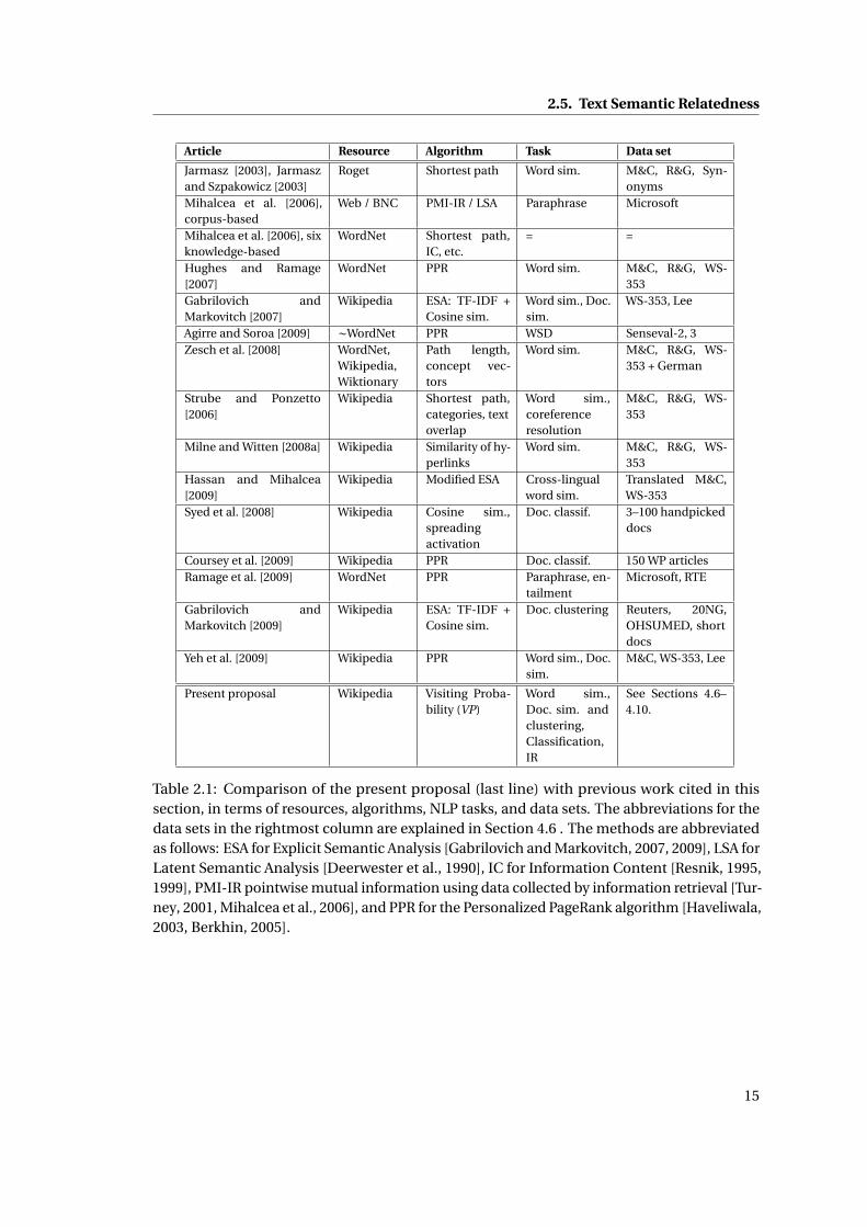
2.5. Text Semantic Relatedness
Article Resource Algorithm Task Data set
Jarmasz [2003], Jarmaszand Szpakowicz [2003]
Roget Shortest path Word sim. M&C, R&G, Syn-onyms
Mihalcea et al. [2006],corpus-based
Web / BNC PMI-IR / LSA Paraphrase Microsoft
Mihalcea et al. [2006], sixknowledge-based
WordNet Shortest path,IC, etc.
= =
Hughes and Ramage[2007]
WordNet PPR Word sim. M&C, R&G, WS-353
Gabrilovich andMarkovitch [2007]
Wikipedia ESA: TF-IDF +Cosine sim.
Word sim., Doc.sim.
WS-353, Lee
Agirre and Soroa [2009] ∼WordNet PPR WSD Senseval-2, 3Zesch et al. [2008] WordNet,
Wikipedia,Wiktionary
Path length,concept vec-tors
Word sim. M&C, R&G, WS-353 + German
Strube and Ponzetto[2006]
Wikipedia Shortest path,categories, textoverlap
Word sim.,coreferenceresolution
M&C, R&G, WS-353
Milne and Witten [2008a] Wikipedia Similarity of hy-perlinks
Word sim. M&C, R&G, WS-353
Hassan and Mihalcea[2009]
Wikipedia Modified ESA Cross-lingualword sim.
Translated M&C,WS-353
Syed et al. [2008] Wikipedia Cosine sim.,spreadingactivation
Doc. classif. 3–100 handpickeddocs
Coursey et al. [2009] Wikipedia PPR Doc. classif. 150 WP articlesRamage et al. [2009] WordNet PPR Paraphrase, en-
tailmentMicrosoft, RTE
Gabrilovich andMarkovitch [2009]
Wikipedia ESA: TF-IDF +Cosine sim.
Doc. clustering Reuters, 20NG,OHSUMED, shortdocs
Yeh et al. [2009] Wikipedia PPR Word sim., Doc.sim.
M&C, WS-353, Lee
Present proposal Wikipedia Visiting Proba-bility (VP)
Word sim.,Doc. sim. andclustering,Classification,IR
See Sections 4.6–4.10.
Table 2.1: Comparison of the present proposal (last line) with previous work cited in thissection, in terms of resources, algorithms, NLP tasks, and data sets. The abbreviations for thedata sets in the rightmost column are explained in Section 4.6 . The methods are abbreviatedas follows: ESA for Explicit Semantic Analysis [Gabrilovich and Markovitch, 2007, 2009], LSA forLatent Semantic Analysis [Deerwester et al., 1990], IC for Information Content [Resnik, 1995,1999], PMI-IR pointwise mutual information using data collected by information retrieval [Tur-ney, 2001, Mihalcea et al., 2006], and PPR for the Personalized PageRank algorithm [Haveliwala,2003, Berkhin, 2005].
15

3 Symmetric Random Walk on LargeGraphs: Approximation Algorithmsand Similarity LearningIn this chapter we define a random walk model, Visiting Probability (VP), to measure proximity
between two nodes in a graph. We show that using a symmetric proximity measure based
on the defined random walk improves the prediction performance of the proximity measure.
Moreover, we show how to apply the definition of VP within approximation algorithms in
order to perform ranking based on VP for large graphs. Besides, we define community of a
node according to VP similarity. Fast algorithms are designed to find the K-nearest neighbors
and identify communities over large graphs using symmetric VP proximity . We demonstrate
the effectiveness of the definitions and algorithms by evaluating them on a link prediction
task over various networks.
In the second part of this chapter, we show that any relation between two nodes in a graph
can be interpreted as the proximity between those two nodes in a latent space. Therefore, the
link structure of a graph can be modeled within a similarity learning framework, in which the
transformation of nodes to the latent space is trained using a discriminative model. We show
how to apply this framework to learn the similarity between two nodes based on the attributes
of the nodes, over large graphs. Moreover, we show that similarity learning on attributes
derived from random walk scores, specifically VP scores here, can model and predict better
the relations in the graph in comparison to learning on the network’s links directly. At the
end, we evaluate again the effectiveness of these models on link prediction task on various
networks.
3.1 Visiting Probability
In this section, we describe our method for computing proximity between two nodes in a
network. The goal is to estimate a distance between two nodes by taking into account the
global connectivity of the network, and without being biased by local properties.
Indeed, the use of individual links and paths, e.g. when estimating proximity as the length of
shortest path, does not take into account their relative importance with respect to the overall
17
Chapter 3. Symmetric Random Walk on Large Graphs
properties of the network, such as the number and length of all possible paths between two
nodes. Moreover, the length of the shortest path is quite sensitive to spurious links. Therefore,
a number of aggregated proximity measures based on random walk have been proposed in
the literature, such as PageRank (including Personalized PageRank) and hitting time. Previous
studied showed that these aggregated measures are more effective for link prediction rather
than individual links and paths [Brand, 2005, Sarkar and Moore, 2007, Liben-Nowell and
Kleinberg, 2003]. Following the same direction our proposal uses a random walk approach,
and defines the proximity of two nodes as the visiting probability (VP), in the long run, of a
random walker going from one node to the other one. We discuss in details the differences
with other popular random walk models and show how using VP enables us to design efficient
algorithm over large graphs.
3.1.1 Notations
Let S = {si |1 ≤ i ≤ n} be the set of n nodes in the network. Assuming that the graph is a directed
weighted multi-link graph, any two nodes si and s j can be connected by one or more directed
and weighted links, which can be of L different types. The structure of links of type l (1 ≤ l ≤ L)
is specified by the (sparse) matrix Al of size n ×n, where Al (i , j ) is the weight of the link of
type l between si and s j . The transition matrix Cl gives the probability of a direct (one step)
transition between nodes si and s j , using only links of type l . This matrix can be built from
the Al matrix as follows:
Cl (i , j ) = Al (i , j )∑nk=1 Al (i ,k)
In the random walk process using all link types (1 ≤ l ≤ L), let the weight wl (∑
l wl = 1) denote
the importance of link type l . Then, the overall transition matrix C which gives the transition
probability Ci , j between any nodes si and s j is C =∑Ll=1 wl Cl .
Moreover, let xi be the normalized real-valued vector of size 1×M representing the feature
vector of node si , where M is the number of possible attributes each node can have in the
graph.
Finally, let~r be the n-dimensional vector which indicates the probabilities of nodes in the
network, i.e. the probability that the random walker starts from each of the nodes, so that∑i~ri = 1.
3.1.2 Definition of Visiting Probability (VP)
Given the nodes si and s j in the network, we compute the probability of visiting s j for the first
time when a random walker starts from si in the network. To compute VP, the following proce-
dure provides a model of the state (node) St of the random walker at step t . The probability of
terminating the procedure successfully, i.e. reaching s j , is the visiting probability of s j from si
18
3.1. Visiting Probability
which is noted VPi j .
Step 0: Position the random walker on the node si . In other words, the initial probability
vector over nodes is: ~r 0i = 1.
Step t : Assuming St−1 is determined, if St−1 = s j then return ‘success’ and finish the proce-
dure. Otherwise, with probability α, choose a value for the next node St according to
the transition matrix C , and with probability 1−α, return ‘fail’. The possibility of ‘failing’,
or absorption probability, introduces a penalty over long paths that makes them less
probable.
In the following we compute the probability of success in the above procedure which is equal
to the VP. We introduce C ′ as being equal to the transition matrix C , except that in row j ,
C ′( j ,k) = 0 for all k. This indicates the fact that when the random walker visits s j for the
first time, it can not exit from it and its probability mass drops to zero in the next step. This
modified transition matrix was defined to account for the definition of visiting probability
as the probability of first visit of s j (a similar idea has been proposed by Sarkar and Moore
[2007]).
To compute the probability of success in the above process, we introduce the probability of
success at step t , p t (success), which is p t (success) =αt (~r 0C ′t ) j . In this formula, (~r 0C ′t ) j is
the j th element of the vector ~r 0C ′t , and C ′t is the power t of matrix C ′. The vector ~r 0C ′t gives
the probability vector at time t , noted ~r t .
Then, the probability of success in the process, i.e. the probability of visiting s j starting from
si , is the sum over all probabilities of success with different lengths:
p(success) =∞∑
t=0p t (success) =
∞∑t=0
αt (~r 0C ′t ) j .
In the following sections, we introduce some properties of VP and afterward according to
those properties we design fast algorithms to compute VP. But first in the following section we
discuss the importance of a symmetric measure for many tasks.
3.1.3 Importance of a Symmetric Measure: Visiting Probability ‘to’ vs. ‘from’
In both directed and undirected graphs VPi j is not symmetric, although proximity (or similar-
ity) should be symmetric. Moreover, we will show experimentally that a symmetric measure
can model and predict the graph structure more accurately.
To compute a symmetric proximity measure between two nodes si and s j , we average between
their visiting probabilities VPi j and VP j i . A larger value of the measure indicates closer
proximity. We can interpret the difference between the two scores VPi j and VP j i in the specific
19
Chapter 3. Symmetric Random Walk on Large Graphs
context of a given network. Let VP:i represent the vector of VP from all nodes to the node si
and VPi : represent the vector of VP from si to all nodes in the network. If sk is a top score node
in VP:i , then there are many high probability paths from sk to si , in comparison to other nodes
in the networks. Depending on the underlying meaning of each link (path) in the network, we
can interpret the difference between VP to and from a node in various ways. To illustrate the
difference between VP to and from, we consider an example from the network of Wikipedia
articles and the hyperlinks between them. Considering the article ‘Anarchism’ in Wikipedia,
the ten closest articles in terms of VP from the article, and respectively to it, were found to be
the following ones:
• Ten closest articles according to their VP to the article: ‘Social Revolutionary Anarchist
Federation’, ’James Koehnline’, ’Toma Bebic’, ’Social insertion’ ,’Robert Graham (his-
torian)’, ’Institute for Anarchist Studies’, ’Ernesto Bonomini’, ’Anarchy in the Age of
Dinosaurs’, ’Bruno Wille’.
• Ten closest articles according to their VP from the article: ’Anarchism’ , ’Situationist
International’, ’Anarchist schools of thought’, ’Issues in anarchism’, ’Individualist anar-
chism’, ’Anarchism and anarcho-capitalism’, ’Anarchism in Spain’, ’History of anarchism’,
’Anarchism and Marxism’, ’Anarchism in the United States’.
The closest articles according to VP from an article tend to be more general topics than closest
articles according to VP to the article. For instance, the first list above includes anarchists
and anarchism communities, while the second one includes more abstract topics related to
anarchism.
The behavior illustrated on this example is expected given the definition of VP. An article that
is close to a target article has more paths to the target article with respect to other articles in
the network, which means that the article is topically more specific with respect to the target
article, as in the above example. This is caused by the definition of hyperlinks in Wikipedia:
article A links to article B if B is needed to explain A, meaning typically that A is more specific
(more detailed). Conversely, an article that is close from an initial article is likely to be a general
and popular article around the topics of the initial article. If we consider the hierarchy between
articles from more general to more specific ones, then articles close to an article are generally
lower in the hierarchy, and article close from an article are higher. Therefore, by using the
average score between VP to and from we can make a more accurate proximity (similarity)
measure that can find articles at similar level in this hierarchy.
In the following section we prove some properties of VP that are used in the algorithms
afterward.
20
3.1. Visiting Probability
3.1.4 Properties of VP
In this section, first we introduce some definitions and then we prove some propositions about
the properties of VP. We remind first that the VP from si to s j by using all paths with length at
most t is given by VPti j which is computed as follows:
VPti j =
t∑p=0
αp (~r 0C ′p ) j where ~r 0i = 1 , C ′(i , :) =
{C (i , :) if i 6= j
0 otherwise
Let’s denote the probability of failing the procedure to compute VP by using at most t steps by
lostti j . In other words, if we consider the traveling of random walker starting from si to s j , the
value of lostti j is the total probability of absorption until step t .
Moreover, we define remti j = 1− (lostt
i j +VPti j ) , which is the probability of not having termi-
nated the procedure until step t . In other words, the probability of returning neither success
nor failure in the first t steps can be computed as:
remti j =
n∑i 6= j
αt (~r 0C ′t )i
This is in fact the probability mass at time t at all nodes except s j , the targeted node. Given
these definitions we formulate the following propositions (to simplify the notations we omit
the indices i j ):
1. VPt+1 ≥ VPt , lostt+1 ≥ lostt , remt+1 ≤ remt
2. remt+1 = remt ×α− (VPt+1 −VPt )
3. VP ≤ VPt + remt ×α︸ ︷︷ ︸uppert
and uppert+1 ≤ uppert
Proofs (given here in condensed form) are derived from the definition of VP:
1. VPt+1 = VPt +αt+1(~r 0C ′t+1) j︸ ︷︷ ︸≥0
⇒ VPt+1 ≥ VPt
lostt+1 = lostt︸︷︷︸probability of failing until t
+ (1−α)∑i 6= j
αt (~r 0C ′t )i︸ ︷︷ ︸probability of failing at t +1
⇒ lostt+1 ≥ lostt
remt+1 = 1− (lostt+1 +VPt+1)≤ 1− (lostt +VPt )︸ ︷︷ ︸according to the above
= remt ⇒ remt+1 ≤ remt
2. remt+1 = P (’not terminated until t ’∧’not failed at (t +1)’)−P (’visiting j at (t +1)’) = remt×α− (VPt+1 −VPt )
21
Chapter 3. Symmetric Random Walk on Large Graphs
3. for any T > t , VPT = VPT−1+α×remT−1−remT = VPT−2+α×remT−2+(α−1)×remT−1−remT = . . . = VPt + remt ×α+ . . .+ (α−1)× remT−2 + (α−1)× remT−1 − remT︸ ︷︷ ︸
≤0
≤
VPt +α× remt︸ ︷︷ ︸upper bound for the value of VP
In summary, we showed that at each step t we can find the upper bound for the final value
of the VP. Moreover, the upper bound and the value of VPt are getting closer as t increases.
We will use these propositions to design fast algorithm to perform ranking and k-nearest
neighbors.
3.1.5 Relation to other Random Walk Models
In this section we discuss the relation between VP and two popular random walk measures
which have been studied extensively and used in many applications: Hitting Time [Aldous
and Fill, 2002, Liben-Nowell and Kleinberg, 2003, Sarkar and Moore, 2007, Sarkar et al., 2008]
and Personalized Page Rank (PPR) or also known as random walk with restart [Haveliwala,
2003, 2002, Tong et al., 2006, Fogaras et al., 2005].
First we define with our own notations the Personalized Page Rank process started from node
si . If~r t represents the probability distribution on all nodes in the graph at step t and~r 0i = 1,
then its value in personalized page rank process is given by:
~r t = (1−α)×~r 0 +α×~r t−1 ×C
and consequently we define PPRti j =~r t
j where~r 0i = 1. In this context~r 0 is also called teleport
vector because at each step with probability 1−α the random walker jumps to this starting
distribution,~r 0.
In cyclic graphs, in the computation of VP, the loops starting from s j and ending to s j do not
have any effect on the final score, unlike the computation of PPR, for which such loops boost
the probability of s j . If some nodes have this type of loops (typically “popular” nodes), then
after using PPR they will have high probability although they might not perceived as being
very close to the initial node si . But if the graph is acyclic, then we can show that the ranking
resulting from VP is equal to the ranking from PPR. More specifically, we can show that in
acyclic graphs, for every nodes si , s j and sk :
VPi j > VPi k ⇔ PPRi j > PPRi k
To prove the above equivalence, we expand PPRti j , and for simplicity we denote PPRi j as PPR j :
PPRtj = (1−α)×~r 0
j +α(1−α)×(~r 0C ) j +α2(1−α)×(~r 0C 2) j +·· ·+αt−1(1−α)(~r 0C t−1) j +αt (~r 0C t ) j
If we consider again the definition of C ′ given earlier, we have (~r 0C ′t ) j ≤ (~r 0C t ) j , because row
22
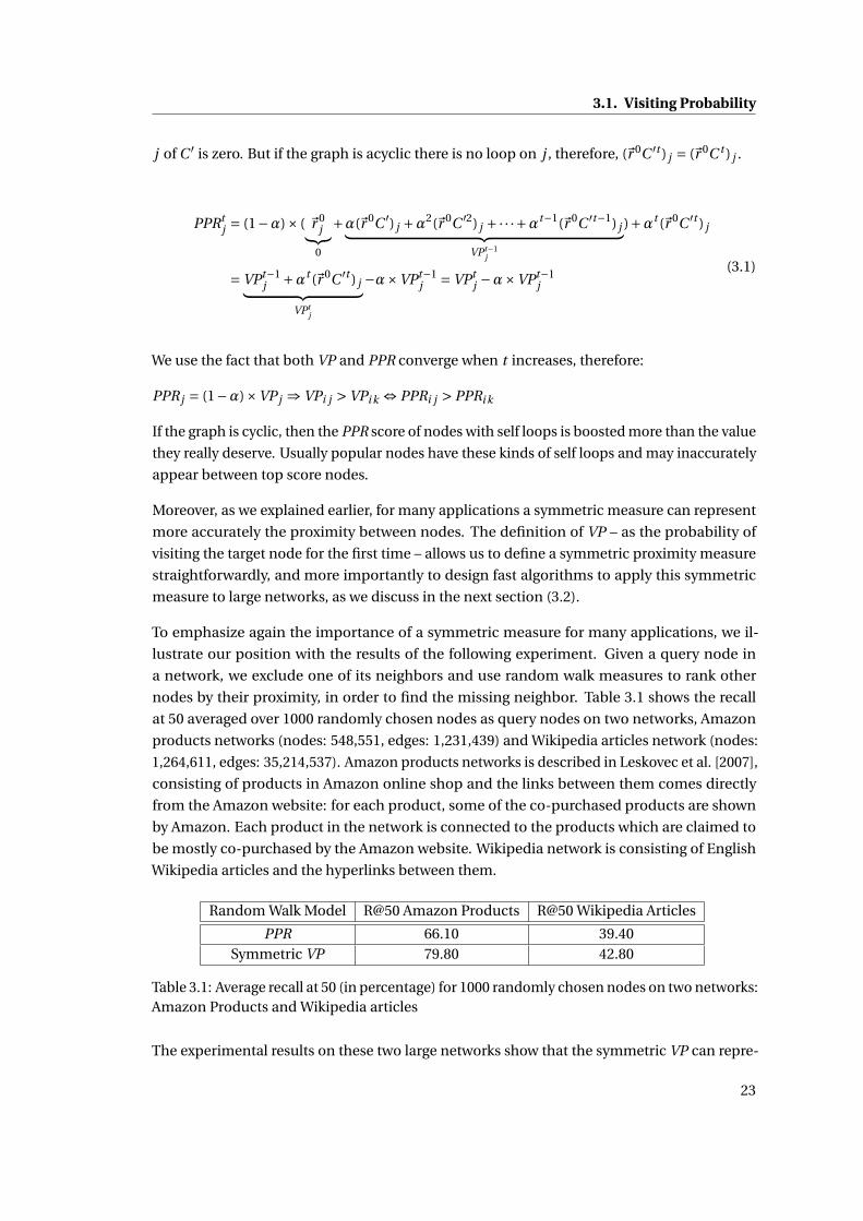
3.1. Visiting Probability
j of C ′ is zero. But if the graph is acyclic there is no loop on j , therefore, (~r 0C ′t ) j = (~r 0C t ) j .
PPRtj = (1−α)× ( ~r 0
j︸︷︷︸0
+α(~r 0C ′) j +α2(~r 0C ′2) j +·· ·+αt−1(~r 0C ′t−1) j︸ ︷︷ ︸VPt−1
j
)+αt (~r 0C ′t ) j
= VPt−1j +αt (~r 0C ′t ) j︸ ︷︷ ︸
VPtj
−α×VPt−1j = VPt
j −α×VPt−1j
(3.1)
We use the fact that both VP and PPR converge when t increases, therefore:
PPR j = (1−α)×VP j ⇒ VPi j > VPi k ⇔ PPRi j > PPRi k
If the graph is cyclic, then the PPR score of nodes with self loops is boosted more than the value
they really deserve. Usually popular nodes have these kinds of self loops and may inaccurately
appear between top score nodes.
Moreover, as we explained earlier, for many applications a symmetric measure can represent
more accurately the proximity between nodes. The definition of VP – as the probability of
visiting the target node for the first time – allows us to define a symmetric proximity measure
straightforwardly, and more importantly to design fast algorithms to apply this symmetric
measure to large networks, as we discuss in the next section (3.2).
To emphasize again the importance of a symmetric measure for many applications, we il-
lustrate our position with the results of the following experiment. Given a query node in
a network, we exclude one of its neighbors and use random walk measures to rank other
nodes by their proximity, in order to find the missing neighbor. Table 3.1 shows the recall
at 50 averaged over 1000 randomly chosen nodes as query nodes on two networks, Amazon
products networks (nodes: 548,551, edges: 1,231,439) and Wikipedia articles network (nodes:
1,264,611, edges: 35,214,537). Amazon products networks is described in Leskovec et al. [2007],
consisting of products in Amazon online shop and the links between them comes directly
from the Amazon website: for each product, some of the co-purchased products are shown
by Amazon. Each product in the network is connected to the products which are claimed to
be mostly co-purchased by the Amazon website. Wikipedia network is consisting of English
Wikipedia articles and the hyperlinks between them.
Random Walk Model R@50 Amazon Products R@50 Wikipedia Articles
PPR 66.10 39.40Symmetric VP 79.80 42.80
Table 3.1: Average recall at 50 (in percentage) for 1000 randomly chosen nodes on two networks:Amazon Products and Wikipedia articles
The experimental results on these two large networks show that the symmetric VP can repre-
23
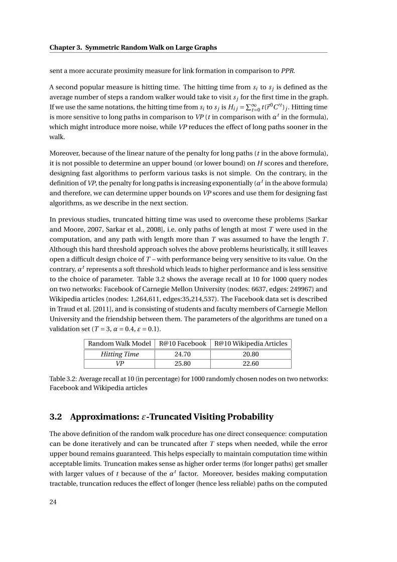
Chapter 3. Symmetric Random Walk on Large Graphs
sent a more accurate proximity measure for link formation in comparison to PPR.
A second popular measure is hitting time. The hitting time from si to s j is defined as the
average number of steps a random walker would take to visit s j for the first time in the graph.
If we use the same notations, the hitting time from si to s j is Hi j =∑∞t=0 t (~r 0C ′t ) j . Hitting time
is more sensitive to long paths in comparison to VP (t in comparison with αt in the formula),
which might introduce more noise, while VP reduces the effect of long paths sooner in the
walk.
Moreover, because of the linear nature of the penalty for long paths (t in the above formula),
it is not possible to determine an upper bound (or lower bound) on H scores and therefore,
designing fast algorithms to perform various tasks is not simple. On the contrary, in the
definition of VP, the penalty for long paths is increasing exponentially (αt in the above formula)
and therefore, we can determine upper bounds on VP scores and use them for designing fast
algorithms, as we describe in the next section.
In previous studies, truncated hitting time was used to overcome these problems [Sarkar
and Moore, 2007, Sarkar et al., 2008], i.e. only paths of length at most T were used in the
computation, and any path with length more than T was assumed to have the length T .
Although this hard threshold approach solves the above problems heuristically, it still leaves
open a difficult design choice of T – with performance being very sensitive to its value. On the
contrary, αt represents a soft threshold which leads to higher performance and is less sensitive
to the choice of parameter. Table 3.2 shows the average recall at 10 for 1000 query nodes
on two networks: Facebook of Carnegie Mellon University (nodes: 6637, edges: 249967) and
Wikipedia articles (nodes: 1,264,611, edges:35,214,537). The Facebook data set is described
in Traud et al. [2011], and is consisting of students and faculty members of Carnegie Mellon
University and the friendship between them. The parameters of the algorithms are tuned on a
validation set (T = 3, α= 0.4, ε= 0.1).
Random Walk Model R@10 Facebook R@10 Wikipedia Articles
Hitting Time 24.70 20.80VP 25.80 22.60
Table 3.2: Average recall at 10 (in percentage) for 1000 randomly chosen nodes on two networks:Facebook and Wikipedia articles
3.2 Approximations: ε-Truncated Visiting Probability
The above definition of the random walk procedure has one direct consequence: computation
can be done iteratively and can be truncated after T steps when needed, while the error
upper bound remains guaranteed. This helps especially to maintain computation time within
acceptable limits. Truncation makes sense as higher order terms (for longer paths) get smaller
with larger values of t because of the αt factor. Moreover, besides making computation
tractable, truncation reduces the effect of longer (hence less reliable) paths on the computed
24
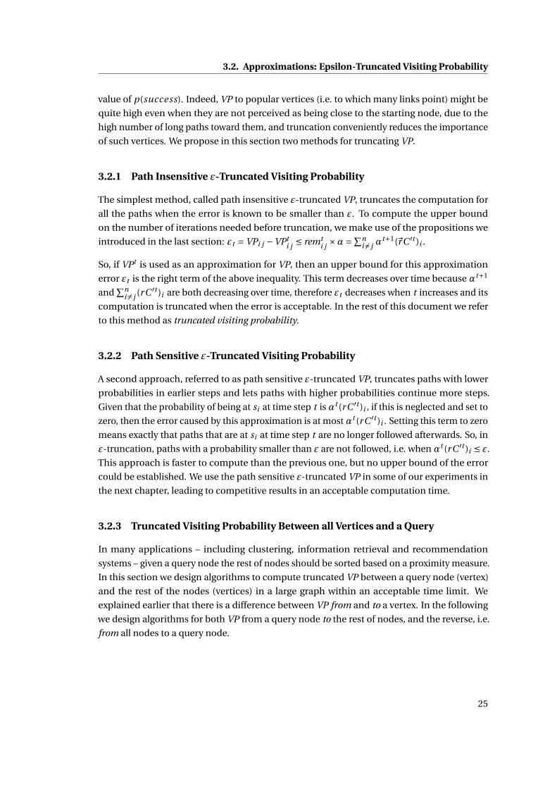
3.2. Approximations: Epsilon-Truncated Visiting Probability
value of p(success). Indeed, VP to popular vertices (i.e. to which many links point) might be
quite high even when they are not perceived as being close to the starting node, due to the
high number of long paths toward them, and truncation conveniently reduces the importance
of such vertices. We propose in this section two methods for truncating VP.
3.2.1 Path Insensitive ε-Truncated Visiting Probability
The simplest method, called path insensitive ε-truncated VP, truncates the computation for
all the paths when the error is known to be smaller than ε. To compute the upper bound
on the number of iterations needed before truncation, we make use of the propositions we
introduced in the last section: εt = VPi j −VPti j ≤ remt
i j ×α=∑ni 6= j α
t+1(~rC ′t )i .
So, if VPt is used as an approximation for VP, then an upper bound for this approximation
error εt is the right term of the above inequality. This term decreases over time because αt+1
and∑n
i 6= j (rC ′t )i are both decreasing over time, therefore εt decreases when t increases and its
computation is truncated when the error is acceptable. In the rest of this document we refer
to this method as truncated visiting probability.
3.2.2 Path Sensitive ε-Truncated Visiting Probability
A second approach, referred to as path sensitive ε-truncated VP, truncates paths with lower
probabilities in earlier steps and lets paths with higher probabilities continue more steps.
Given that the probability of being at si at time step t is αt (rC ′t )i , if this is neglected and set to
zero, then the error caused by this approximation is at mostαt (rC ′t )i . Setting this term to zero
means exactly that paths that are at si at time step t are no longer followed afterwards. So, in
ε-truncation, paths with a probability smaller than ε are not followed, i.e. when αt (rC ′t )i ≤ ε.
This approach is faster to compute than the previous one, but no upper bound of the error
could be established. We use the path sensitive ε-truncated VP in some of our experiments in
the next chapter, leading to competitive results in an acceptable computation time.
3.2.3 Truncated Visiting Probability Between all Vertices and a Query
In many applications – including clustering, information retrieval and recommendation
systems – given a query node the rest of nodes should be sorted based on a proximity measure.
In this section we design algorithms to compute truncated VP between a query node (vertex)
and the rest of the nodes (vertices) in a large graph within an acceptable time limit. We
explained earlier that there is a difference between VP from and to a vertex. In the following
we design algorithms for both VP from a query node to the rest of nodes, and the reverse, i.e.
from all nodes to a query node.
25
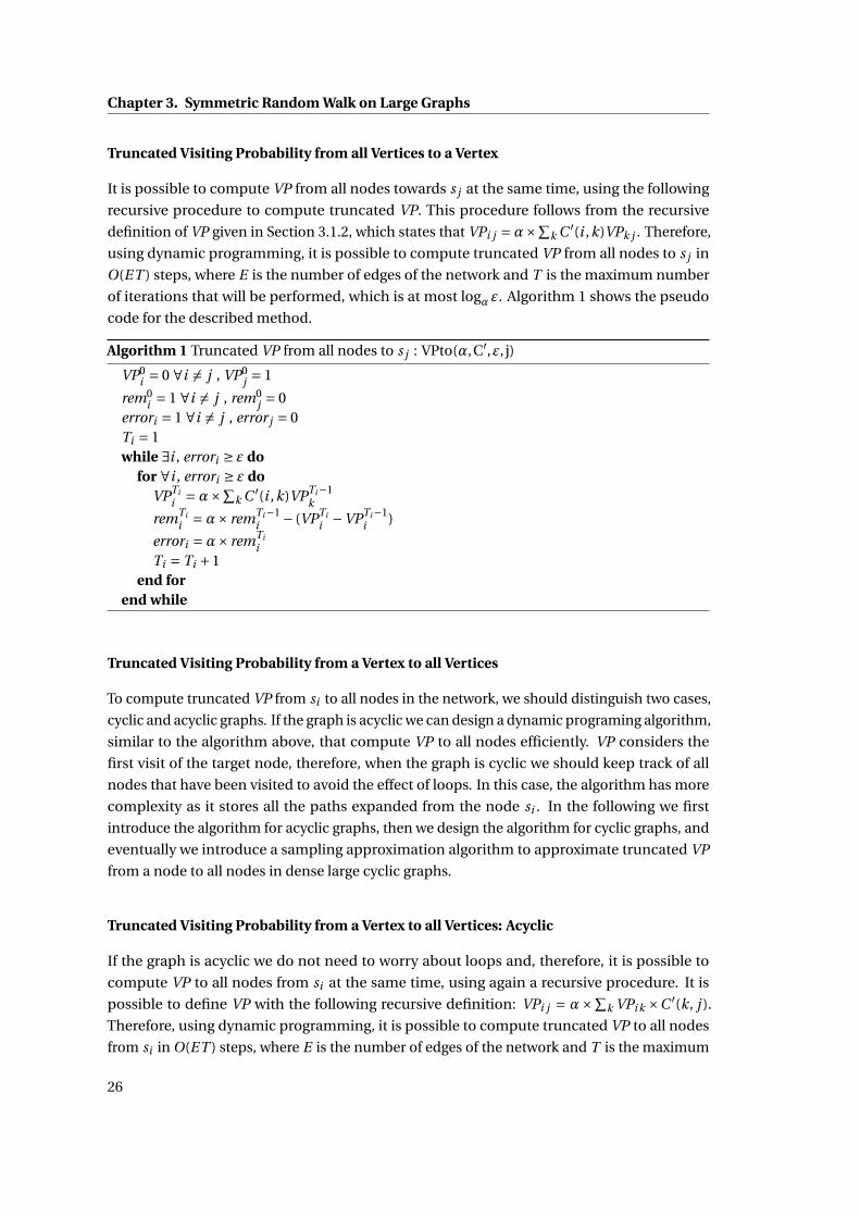
Chapter 3. Symmetric Random Walk on Large Graphs
Truncated Visiting Probability from all Vertices to a Vertex
It is possible to compute VP from all nodes towards s j at the same time, using the following
recursive procedure to compute truncated VP. This procedure follows from the recursive
definition of VP given in Section 3.1.2, which states that VPi j =α×∑k C ′(i ,k)VPk j . Therefore,
using dynamic programming, it is possible to compute truncated VP from all nodes to s j in
O(ET ) steps, where E is the number of edges of the network and T is the maximum number
of iterations that will be performed, which is at most logα ε. Algorithm 1 shows the pseudo
code for the described method.
Algorithm 1 Truncated VP from all nodes to s j : VPto(α,C′,ε, j)
VP0i = 0 ∀i 6= j , VP0
j = 1
rem0i = 1 ∀i 6= j , rem0
j = 0errori = 1 ∀i 6= j , error j = 0Ti = 1while ∃i , errori ≥ ε do
for ∀i , errori ≥ ε doVPTi
i =α×∑k C ′(i ,k)VPTi−1
k
remTi
i =α× remTi−1i − (VPTi
i −VPTi−1i )
errori =α× remTi
iTi = Ti +1
end forend while
Truncated Visiting Probability from a Vertex to all Vertices
To compute truncated VP from si to all nodes in the network, we should distinguish two cases,
cyclic and acyclic graphs. If the graph is acyclic we can design a dynamic programing algorithm,
similar to the algorithm above, that compute VP to all nodes efficiently. VP considers the
first visit of the target node, therefore, when the graph is cyclic we should keep track of all
nodes that have been visited to avoid the effect of loops. In this case, the algorithm has more
complexity as it stores all the paths expanded from the node si . In the following we first
introduce the algorithm for acyclic graphs, then we design the algorithm for cyclic graphs, and
eventually we introduce a sampling approximation algorithm to approximate truncated VP
from a node to all nodes in dense large cyclic graphs.
Truncated Visiting Probability from a Vertex to all Vertices: Acyclic
If the graph is acyclic we do not need to worry about loops and, therefore, it is possible to
compute VP to all nodes from si at the same time, using again a recursive procedure. It is
possible to define VP with the following recursive definition: VPi j = α×∑k VPi k ×C ′(k, j ).
Therefore, using dynamic programming, it is possible to compute truncated VP to all nodes
from si in O(ET ) steps, where E is the number of edges of the network and T is the maximum
26
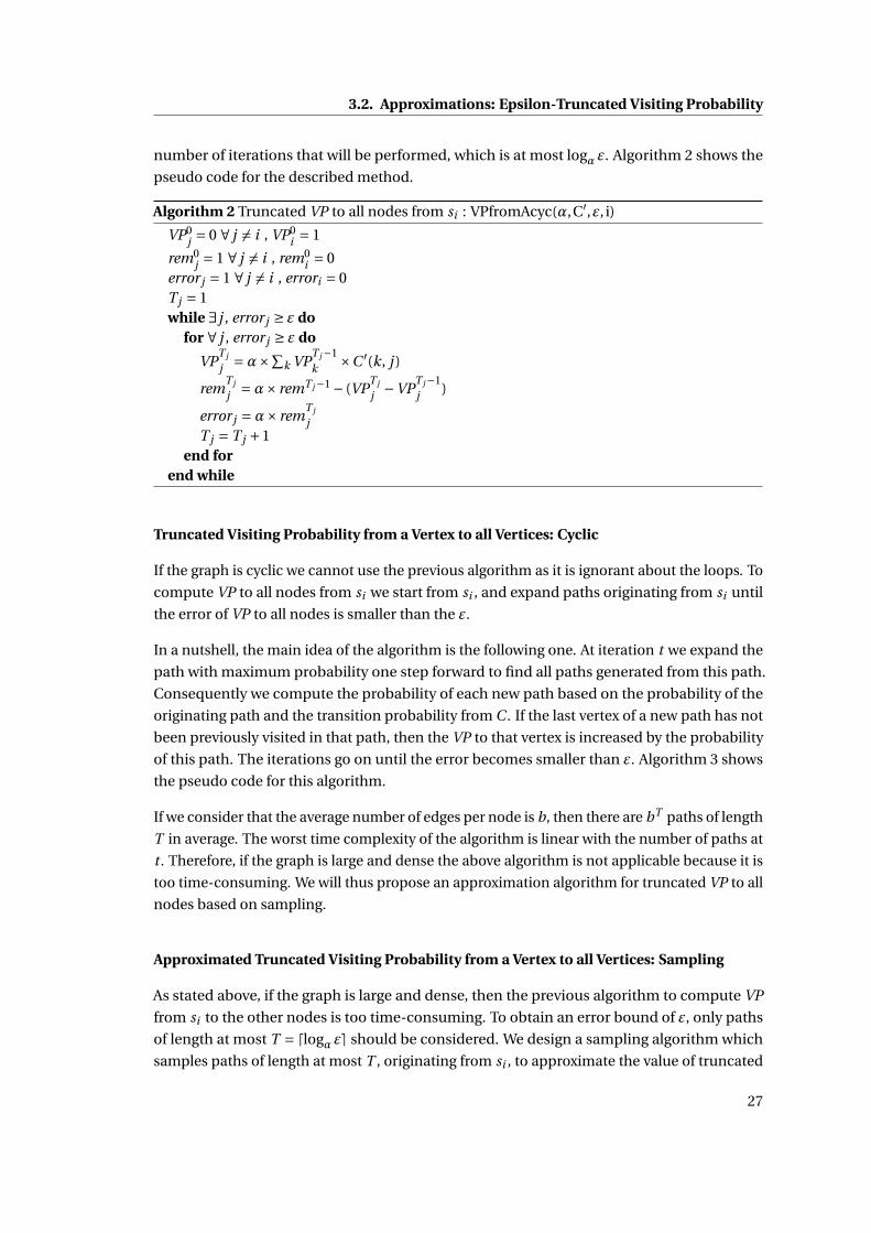
3.2. Approximations: Epsilon-Truncated Visiting Probability
number of iterations that will be performed, which is at most logα ε. Algorithm 2 shows the
pseudo code for the described method.
Algorithm 2 Truncated VP to all nodes from si : VPfromAcyc(α,C′,ε, i)
VP0j = 0 ∀ j 6= i , VP0
i = 1
rem0j = 1 ∀ j 6= i , rem0
i = 0error j = 1 ∀ j 6= i , errori = 0T j = 1while ∃ j , error j ≥ ε do
for ∀ j , error j ≥ ε do
VPT j
j =α×∑k VP
T j−1k ×C ′(k, j )
remT j
j =α× remT j−1 − (VPT j
j −VPT j−1j )
error j =α× remT j
jT j = T j +1
end forend while
Truncated Visiting Probability from a Vertex to all Vertices: Cyclic
If the graph is cyclic we cannot use the previous algorithm as it is ignorant about the loops. To
compute VP to all nodes from si we start from si , and expand paths originating from si until
the error of VP to all nodes is smaller than the ε.
In a nutshell, the main idea of the algorithm is the following one. At iteration t we expand the
path with maximum probability one step forward to find all paths generated from this path.
Consequently we compute the probability of each new path based on the probability of the
originating path and the transition probability from C . If the last vertex of a new path has not
been previously visited in that path, then the VP to that vertex is increased by the probability
of this path. The iterations go on until the error becomes smaller than ε. Algorithm 3 shows
the pseudo code for this algorithm.
If we consider that the average number of edges per node is b, then there are bT paths of length
T in average. The worst time complexity of the algorithm is linear with the number of paths at
t . Therefore, if the graph is large and dense the above algorithm is not applicable because it is
too time-consuming. We will thus propose an approximation algorithm for truncated VP to all
nodes based on sampling.
Approximated Truncated Visiting Probability from a Vertex to all Vertices: Sampling
As stated above, if the graph is large and dense, then the previous algorithm to compute VP
from si to the other nodes is too time-consuming. To obtain an error bound of ε, only paths
of length at most T = dlogα εe should be considered. We design a sampling algorithm which
samples paths of length at most T , originating from si , to approximate the value of truncated
27
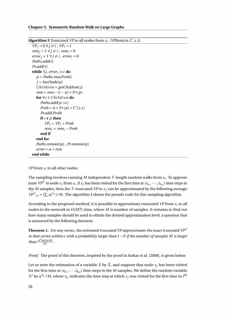
Chapter 3. Symmetric Random Walk on Large Graphs
Algorithm 3 Truncated VP to all nodes from si : VPfrom(α,C′,ε, i)VP j = 0 ∀ j 6= i , VPi = 1rem j = 1 ∀ j 6= i , remi = 0error j = 1 ∀ j 6= i , errori = 0Paths.add(i )Pr.add(1)while ∃ j , error j ≥ ε do
p = Paths.maxProb()j = lastNode(p)C hi ldr en = getChildren( j )rem = rem− (1−α)×Pr (p)for ∀c ∈C hi ldr en do
Paths.add(p->c)Prob =α×Pr (p)×C ′( j ,c)Pr.add(Prob)if c ∉ p then
VPc = VPc +Probremc = remc −Prob
end ifend forPaths.remove(p) , Pr.remove(p)error =α× rem
end while
VP from si to all other nodes.
The sampling involves running M independent T -length random walks from si . To approxi-
mate VPT to node s j from si , if s j has been visited for the first time at {tk1 , · · · , tkm } time steps in
the M samples, then the T -truncated VP to s j can be approximated by the following average:ˆVPT
i j = (∑
l αtkl )/M . The algorithm 4 shows the pseudo code for this sampling algorithm.
According to the proposed method, it is possible to approximate truncated VP from si to all
nodes in the network in O(MT) time, where M is number of samples. It remains to find out
how many samples should be used to obtain the desired approximation level, a question that
is answered by the following theorem.
Theorem 1. For any vertex, the estimated truncated VP approximates the exact truncated VPT
to that vertex within ε with a probability larger than 1−δ if the number of samples M is larger
than α2 ln(2n/δ)2ε2 .
Proof. The proof of this theorem, inspired by the proof in Sarkar et al. [2008], is given below.
Let us note the estimation of a variable X by X , and suppose that node s j has been visited
for the first time at {tk1 , · · · , tkM } time steps in the M samples. We define the random variable
X l by αtkl /M , where tkl indicates the time step at which s j was visited for the first time in l th
28
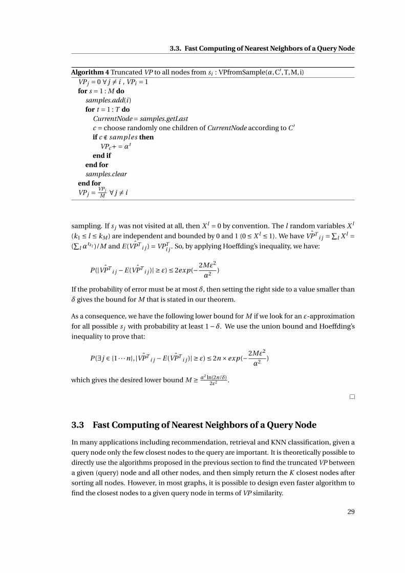
3.3. Fast Computing of Nearest Neighbors of a Query Node
Algorithm 4 Truncated VP to all nodes from si : VPfromSample(α,C′,T,M,i)VP j = 0 ∀ j 6= i , VPi = 1for s = 1 : M do
samples.add(i )for t = 1 : T do
CurrentNode = samples.getLastc = choose randomly one children of CurrentNode according to C ′
if c ∉ samples thenVPc+=αt
end ifend forsamples.clear
end forVP j = VP j
M ∀ j 6= i
sampling. If s j was not visited at all, then X l = 0 by convention. The l random variables X l
(k1 ≤ l ≤ kM ) are independent and bounded by 0 and 1 (0 ≤ X l ≤ 1). We have ˆVPTi j =∑
l X l =(∑
l αtkl )/M and E( ˆVPT
i j ) = VPTi j . So, by applying Hoeffding’s inequality, we have:
P (| ˆVPTi j −E( ˆVPT
i j )| ≥ ε) ≤ 2exp(−2Mε2
α2 )
If the probability of error must be at most δ, then setting the right side to a value smaller than
δ gives the bound for M that is stated in our theorem.
As a consequence, we have the following lower bound for M if we look for an ε-approximation
for all possible s j with probability at least 1−δ. We use the union bound and Hoeffding’s
inequality to prove that:
P (∃ j ∈ {1 · · ·n}, | ˆVPTi j −E( ˆVPT
i j )| ≥ ε) ≤ 2n ×exp(−2Mε2
α2 )
which gives the desired lower bound M ≥ α2 ln(2n/δ)2ε2 .
3.3 Fast Computing of Nearest Neighbors of a Query Node
In many applications including recommendation, retrieval and KNN classification, given a
query node only the few closest nodes to the query are important. It is theoretically possible to
directly use the algorithms proposed in the previous section to find the truncated VP between
a given (query) node and all other nodes, and then simply return the K closest nodes after
sorting all nodes. However, in most graphs, it is possible to design even faster algorithm to
find the closest nodes to a given query node in terms of VP similarity.
29
Chapter 3. Symmetric Random Walk on Large Graphs
3.3.1 Fast K -Nearest Neighbors of a Query Node
We can make use of the propositions we know about VP scores to design a fast K -nearest
neighbors algorithm. We showed that for each t we can determine an upper bound for the
value of VP, and moreover, we showed that the upper bound is converging towards VPt when
t increases. Using these facts, the fast algorithm is intuitively as follows.
Given a query node, at the beginning we have no information about VP between the query
node and any other node in the network. In the next step, we consider all paths of length 1
from and to the query node. After that, we have the VP1 and upper bound for the value of VP
for all nodes in the graph. Still, the difference between the upper bound and VP1 might be
large for many nodes at this step. We sort the nodes by their decreasing VP1 values and pick
the node at position K .
Two scenarios might happen at this stage. First, it may happen that there is no node at any
position after K that has an upper bound larger than the VP1 of the node at position K . In this
case we return the first K nodes and terminate the algorithm, because no node at position
after K can have a larger VP than any node at any position below K , even if we develop paths
of all lengths.
Figure 3.1: Fast KNN algorithm: schematic representation of the situation in which the VPt
of the node at the position K is larger than the upper bound of all the nodes after it. Thenotations are those from Algorithm 5.
Second, there might be nodes at positions after K that have upper bounds larger than VP1
of the node at position K . In this case, we compute the VP2 for these nodes and the node at
position K and sort again the nodes based on these new values. Again, we consider the node at
position K (which might have of course changed after sorting) and repeat the same algorithm,
which will either terminate and return the first K nodes, or will consider again longer paths. In
30
3.3. Fast Computing of Nearest Neighbors of a Query Node
the long run, the recursion will certainly terminate because the upper bounds converge to VPt
eventually. Figure 3.1 shows schematically the situation in which the VPt of the node at the
position K is bigger than the upper bound of the nodes ranked after it.
In the algorithm 5 we give the pseudo code of the algorithm. We will analyze the efficiency of
this algorithm experimentally later in this chapter.
Algorithm 5 KNN for si : KNN(α,C′,ε, i,K)
VP0j = 0 ∀ j 6= i , VP0
i = 1
rem0j = 1 ∀ j 6= i , rem0
i = 0error j = 1 ∀ j 6= i , errori = 0upper j = VP0
j +α× rem0j
T j = 1sorted = sort(VPT )while (∃ j ∈ sorted(K +1 : N ) ,VPT
sorted(K ) ≤ upperT j
j ) ∧ (error j ≥ ε) do
for ∀ j ∈ sorted(K : N ) ,VPTsorted(K ) ≤ upper
T j
j ) ∧ (error j ≥ ε) do
VPT j
j = compute based on VPT j−1
remT j
j =α× remT j−1 − (VPT j
j −VPT j−1j )
error j =α× remT j
j
upper j = VPT j
j +α× remT j
jT j = T j +1
end forsorted = resort(VPT )
end while
3.3.2 Community of the Query Node
In this section, we consider small-world networks and briefly survey the fact that many
networks have been shown to be small-world networks in previous studies. Then, we show
that there is a well-defined community for a query node in a small-world network, and design
a fast algorithm based on VP to perform community identification for a given query node.
A small-world network is a type of graph in which most nodes are not neighbors of one another,
but most nodes can be reached from any other node by a small number of transitions [Watts
and Strogatz, 1998]. In other words, nodes form “local” communities and these communities
are connected together by short paths.
It has been shown that many real-world complex systems can be modeled by small-world net-
works, such as for instance metabolite processing networks [Wagner and Fell, 2001], chemical-
reaction networks [Alon et al., 1999], neural networks [Watts, 2003], food webs [Pimm et al.,
1991], social networks [Carrington et al., 2005], scientific-collaboration networks [Vanraan,
1990] and the entire World Wide Web [Adamic and Huberman, 2000, Barabási and Albert,
1999].
31
Chapter 3. Symmetric Random Walk on Large Graphs
Therefore, if we consider a random walker starting from a query node in a small-world net-
work, only few nodes are likely to be visited in this process, though not necessarily the direct
neighbors of the query node. To justify experimentally this statement, let us consider the
following process. Given a network and a query node, we sort all the nodes in the network
according to their symmetric VP scores. To increase the robustness of our experiment, we
repeat this process for a large number of query nodes and average for each query node the
scores of the nodes in the VP ranking list. Moreover, before averaging, we remove the direct
neighbors of the query node from this ranked list. The final descending ranked list gives us
the average VP scores of each position considering only the nodes that are not directly linked.
For example, the first number is the average VP score of the closest (in terms of VP) not-linked
node to the query node.
Figure 3.2 shows the average VP scores at the top 50 nodes in the ranked list explained
above for the five following networks: Cora (average on all nodes), CiteSeer (average on all
nodes), WebKB (average on all nodes), Amazon Products co-purchased network (average on
1000 nodes chosen randomly), English Wikipedia network (average on 1000 nodes chosen
randomly). The detailed description of the data sets WebKB, CiteSeer and Cora can be found
in Section 3.3.3. It appears that for any query node, there are only very few nodes (3–5) with
high VP, as the curves decrease rapidly. The remaining of nodes are not likely to be visited by a
random walker starting from the query node. Intuitively, by looking at the figures, we can find
the size of the community of a query node, and we formalize below this intuitive concept of
community.
If the nodes are sorted according to their VP as in Figure 3.2, then we can intuitively conclude
that the community boundary is where the VP scores of nodes become negligible. If we
note the ranked list of VP values between si and the rest of (not directly connected) nodes as
VPa1 ,VPa2 , . . . ,VPaN , then the community of the node si , noted Si , can be defined as:
Si = {sa1 , sa2 , . . . sa j } so that
∑ jh=1 VPah∑Nh=1 VPah
≥ Tr, where Tr is a fixed threshold.
Fast Community Identification
We propose now a fast algorithm to identify the community of a given query node. Similar to
the fast K -nearest neighbors algorithm we proposed in Section 3.3.1, we design an algorithm
that finds the community of a node without expanding all paths from and to the query node.
Using the previous propositions about VP, we can show that∑ j
h=1 VPtah∑N
h=1 uppertah
≤∑ j
h=1 VPah∑Nh=1 VPah
for any
given t , because always uppertj is bigger than VP j . Therefore, if at any position j in the ranked
list we have∑ j
h=1 VPtah∑N
h=1 uppertah
≥ Tr, then we know the community of si is until j .
32
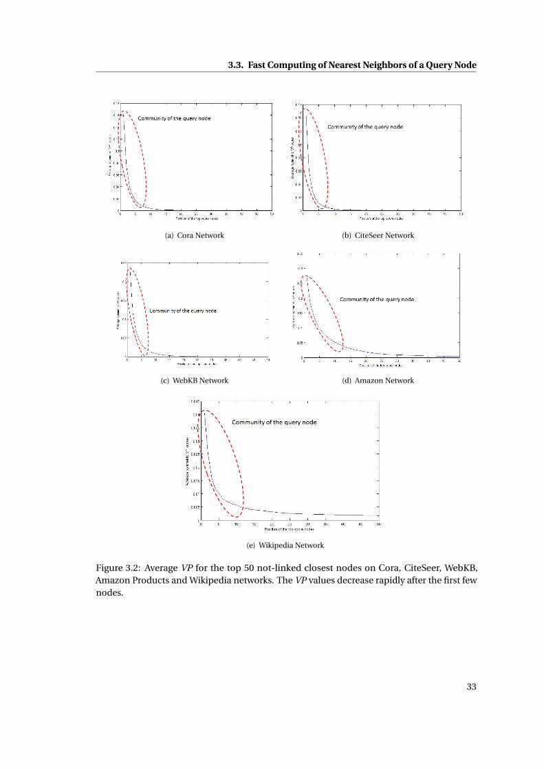
3.3. Fast Computing of Nearest Neighbors of a Query Node
(a) Cora Network (b) CiteSeer Network
(c) WebKB Network (d) Amazon Network
(e) Wikipedia Network
Figure 3.2: Average VP for the top 50 not-linked closest nodes on Cora, CiteSeer, WebKB,Amazon Products and Wikipedia networks. The VP values decrease rapidly after the first fewnodes.
33
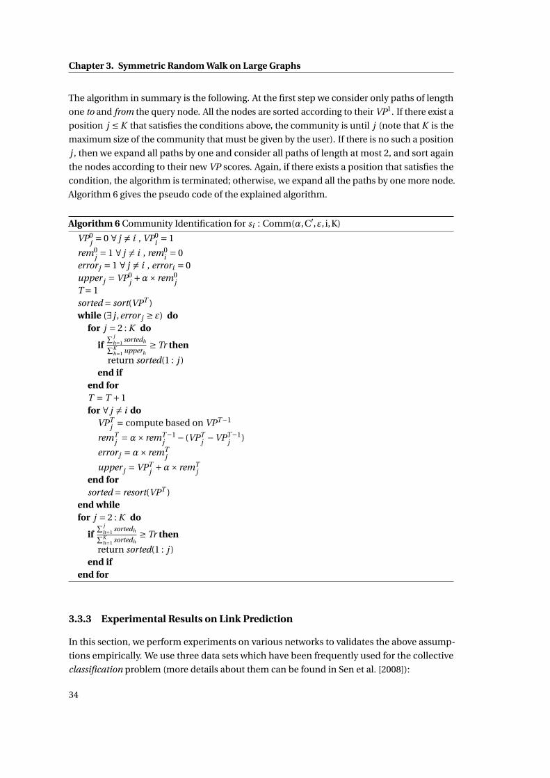
Chapter 3. Symmetric Random Walk on Large Graphs
The algorithm in summary is the following. At the first step we consider only paths of length
one to and from the query node. All the nodes are sorted according to their VP1. If there exist a
position j ≤ K that satisfies the conditions above, the community is until j (note that K is the
maximum size of the community that must be given by the user). If there is no such a position
j , then we expand all paths by one and consider all paths of length at most 2, and sort again
the nodes according to their new VP scores. Again, if there exists a position that satisfies the
condition, the algorithm is terminated; otherwise, we expand all the paths by one more node.
Algorithm 6 gives the pseudo code of the explained algorithm.
Algorithm 6 Community Identification for si : Comm(α,C′,ε, i,K)
VP0j = 0 ∀ j 6= i , VP0
i = 1
rem0j = 1 ∀ j 6= i , rem0
i = 0error j = 1 ∀ j 6= i , errori = 0upper j = VP0
j +α× rem0j
T = 1sorted = sort(VPT )while (∃ j ,error j ≥ ε) do
for j = 2 : K do
if∑ j
h=1 sortedh∑Kh=1 upperh
≥ Tr then
return sorted(1 : j )end if
end forT = T +1for ∀ j 6= i do
VPTj = compute based on VPT−1
remTj =α× remT−1
j − (VPTj −VPT−1
j )
error j =α× remTj
upper j = VPTj +α× remT
jend forsorted = resort(VPT )
end whilefor j = 2 : K do
if∑ j
h=1 sortedh∑Kh=1 sortedh
≥ Tr then
return sorted(1 : j )end if
end for
3.3.3 Experimental Results on Link Prediction
In this section, we perform experiments on various networks to validates the above assump-
tions empirically. We use three data sets which have been frequently used for the collective
classification problem (more details about them can be found in Sen et al. [2008]):
34
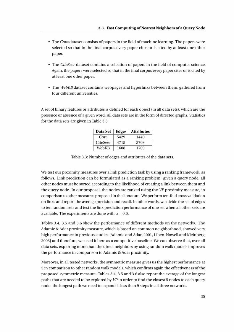
3.3. Fast Computing of Nearest Neighbors of a Query Node
• The Cora dataset consists of papers in the field of machine learning. The papers were
selected so that in the final corpus every paper cites or is cited by at least one other
paper.
• The CiteSeer dataset contains a selection of papers in the field of computer science.
Again, the papers were selected so that in the final corpus every paper cites or is cited by
at least one other paper.
• The WebKB dataset contains webpages and hyperlinks between them, gathered from
four different universities.
A set of binary features or attributes is defined for each object (in all data sets), which are the
presence or absence of a given word. All data sets are in the form of directed graphs. Statistics
for the data sets are given in Table 3.3.
Data Set Edges AttributesCora 5429 1440
CiteSeer 4715 3709WebKB 1608 1709
Table 3.3: Number of edges and attributes of the data sets.
We test our proximity measures over a link prediction task by using a ranking framework, as
follows. Link prediction can be formulated as a ranking problem: given a query node, all
other nodes must be sorted according to the likelihood of creating a link between them and
the query node. In our proposal, the nodes are ranked using the VP proximity measure, in
comparison to other measures proposed in the literature. We perform ten-fold cross validation
on links and report the average precision and recall. In other words, we divide the set of edges
to ten random sets and test the link prediction performance of one set when all other sets are
available. The experiments are done with α= 0.6.
Tables 3.4, 3.5 and 3.6 show the performance of different methods on the networks. The
Adamic & Adar proximity measure, which is based on common neighborhood, showed very
high performance in previous studies [Adamic and Adar, 2001, Liben-Nowell and Kleinberg,
2003] and therefore, we used it here as a competitive baseline. We can observe that, over all
data sets, exploring more than the direct neighbors by using random walk models improves
the performance in comparison to Adamic & Adar proximity.
Moreover, in all tested networks, the symmetric measure gives us the highest performance at
5 in comparison to other random walk models, which confirms again the effectiveness of the
proposed symmetric measure. Tables 3.4, 3.5 and 3.6 also report the average of the longest
paths that are needed to be explored by VP in order to find the closest 5 nodes to each query
node: the longest path we need to expand is less than 9 steps in all three networks.
35
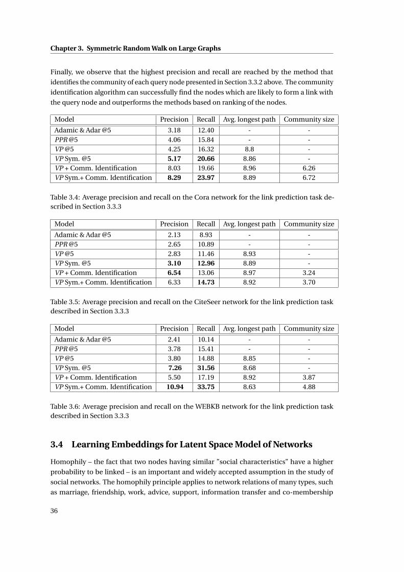
Chapter 3. Symmetric Random Walk on Large Graphs
Finally, we observe that the highest precision and recall are reached by the method that
identifies the community of each query node presented in Section 3.3.2 above. The community
identification algorithm can successfully find the nodes which are likely to form a link with
the query node and outperforms the methods based on ranking of the nodes.
Model Precision Recall Avg. longest path Community size
Adamic & Adar @5 3.18 12.40 - -PPR @5 4.06 15.84 - -VP @5 4.25 16.32 8.8 -VP Sym. @5 5.17 20.66 8.86 -VP + Comm. Identification 8.03 19.66 8.96 6.26VP Sym.+ Comm. Identification 8.29 23.97 8.89 6.72
Table 3.4: Average precision and recall on the Cora network for the link prediction task de-scribed in Section 3.3.3
Model Precision Recall Avg. longest path Community size
Adamic & Adar @5 2.13 8.93 - -PPR @5 2.65 10.89 - -VP @5 2.83 11.46 8.93 -VP Sym. @5 3.10 12.96 8.89 -VP + Comm. Identification 6.54 13.06 8.97 3.24VP Sym.+ Comm. Identification 6.33 14.73 8.92 3.70
Table 3.5: Average precision and recall on the CiteSeer network for the link prediction taskdescribed in Section 3.3.3
Model Precision Recall Avg. longest path Community size
Adamic & Adar @5 2.41 10.14 - -PPR @5 3.78 15.41 - -VP @5 3.80 14.88 8.85 -VP Sym. @5 7.26 31.56 8.68 -VP + Comm. Identification 5.50 17.19 8.92 3.87VP Sym.+ Comm. Identification 10.94 33.75 8.63 4.88
Table 3.6: Average precision and recall on the WEBKB network for the link prediction taskdescribed in Section 3.3.3
3.4 Learning Embeddings for Latent Space Model of Networks
Homophily – the fact that two nodes having similar ”social characteristics” have a higher
probability to be linked – is an important and widely accepted assumption in the study of
social networks. The homophily principle applies to network relations of many types, such
as marriage, friendship, work, advice, support, information transfer and co-membership
36
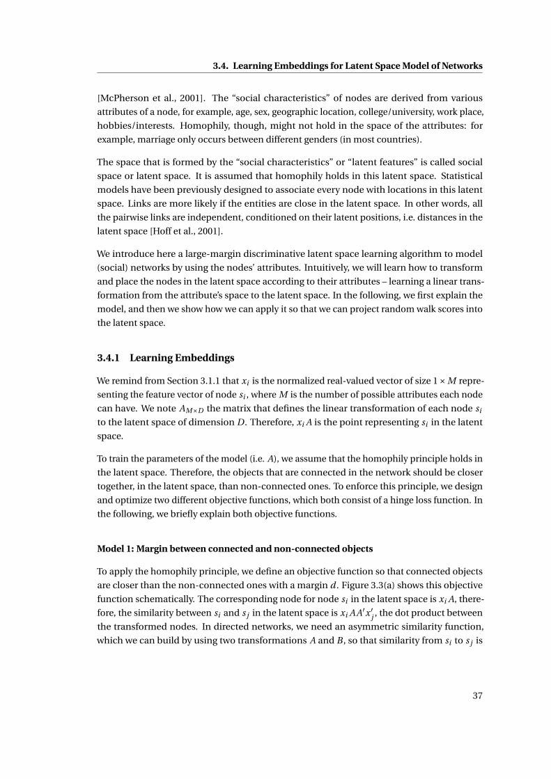
3.4. Learning Embeddings for Latent Space Model of Networks
[McPherson et al., 2001]. The “social characteristics” of nodes are derived from various
attributes of a node, for example, age, sex, geographic location, college/university, work place,
hobbies/interests. Homophily, though, might not hold in the space of the attributes: for
example, marriage only occurs between different genders (in most countries).
The space that is formed by the “social characteristics” or “latent features” is called social
space or latent space. It is assumed that homophily holds in this latent space. Statistical
models have been previously designed to associate every node with locations in this latent
space. Links are more likely if the entities are close in the latent space. In other words, all
the pairwise links are independent, conditioned on their latent positions, i.e. distances in the
latent space [Hoff et al., 2001].
We introduce here a large-margin discriminative latent space learning algorithm to model
(social) networks by using the nodes’ attributes. Intuitively, we will learn how to transform
and place the nodes in the latent space according to their attributes – learning a linear trans-
formation from the attribute’s space to the latent space. In the following, we first explain the
model, and then we show how we can apply it so that we can project random walk scores into
the latent space.
3.4.1 Learning Embeddings
We remind from Section 3.1.1 that xi is the normalized real-valued vector of size 1×M repre-
senting the feature vector of node si , where M is the number of possible attributes each node
can have. We note AM×D the matrix that defines the linear transformation of each node si
to the latent space of dimension D. Therefore, xi A is the point representing si in the latent
space.
To train the parameters of the model (i.e. A), we assume that the homophily principle holds in
the latent space. Therefore, the objects that are connected in the network should be closer
together, in the latent space, than non-connected ones. To enforce this principle, we design
and optimize two different objective functions, which both consist of a hinge loss function. In
the following, we briefly explain both objective functions.
Model 1: Margin between connected and non-connected objects
To apply the homophily principle, we define an objective function so that connected objects
are closer than the non-connected ones with a margin d . Figure 3.3(a) shows this objective
function schematically. The corresponding node for node si in the latent space is xi A, there-
fore, the similarity between si and s j in the latent space is xi A A′x ′j , the dot product between
the transformed nodes. In directed networks, we need an asymmetric similarity function,
which we can build by using two transformations A and B , so that similarity from si to s j is
37
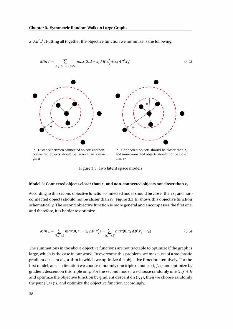
Chapter 3. Symmetric Random Walk on Large Graphs
xi AB ′x ′j . Putting all together the objective function we minimize is the following:
Min L = ∑(i , j )∈E , (i ,z)∉E
max(0,d −xi AB ′x ′j +xi AB ′x ′
z ) (3.2)
(a) Distance between connected objects and non-connected objects should be larger than a mar-gin d
(b) Connected objects should be closer than r1and non-connected objects should not be closerthan r2
Figure 3.3: Two latent space models
Model 2: Connected objects closer than r1 and non-connected objects not closer than r2
According to this second objective function connected nodes should be closer than r1 and non-
connected objects should not be closer than r2. Figure 3.3(b) shows this objective function
schematically. The second objective function is more general and encompasses the first one,
and therefore, it is harder to optimize.
Min L = ∑(i , j )∈E
max(0,r1 −xi AB ′x ′j )+ ∑
(i , j )∉Emax(0, xi AB ′x ′
z − r2) (3.3)
The summations in the above objective functions are not tractable to optimize if the graph is
large, which is the case in our work. To overcome this problem, we make use of a stochastic
gradient descent algorithm in which we optimize the objective function iteratively. For the
first model, at each iteration we choose randomly one triple of nodes (i , j , z) and optimize by
gradient descent on this triple only. For the second model, we choose randomly one (i , j ) ∈ E
and optimize the objective function by gradient descent on (i , j ), then we choose randomly
the pair (i , z) ∉ E and optimize the objective function accordingly.
38
3.4. Learning Embeddings for Latent Space Model of Networks
The gradients of the objective functions at step t are shown below, for the first model:
5Lt (A) = {x ′
i (xz B −x j B) if xi AB ′x ′j −xi AB ′x ′
z < d
0 otherwise
5Lt (B) = {(xz −x j )′xi A if xi AB ′x ′
j −xi AB ′x ′z < d
0 otherwise
and the second model:
5Lt (A) = {
−x ′i (x j B) if (i , j ) ∈ E , xi AB ′x ′
j < r1
x ′i (x j B) if (i , j ) ∉ E , xi AB ′x ′
j > r2
0 otherwise
5Lt (B) = {
−x ′j (xi A) if (i , j ) ∈ E , xi AB ′x ′
j < r1
x ′j (xi A) if (i , j ) ∉ E , xi AB ′x ′
j > r2
0 otherwise
The update of the parameters is done consequently as follows:
At+1 = At −ηt 5Lt (A)
B t+1 = B t −ηt 5Lt (B)
where ηt is the learning rate at the iteration t .
There are many applications for an approach based on latent spaces. First, they speed up
similarity computation, make it independent of graph size, which is useful when a quick result
is needed at query time. Moreover, they can be used for link prediction for new nodes which
are not yet rich in link structure features. Besides, modeling the graph structure based on the
nodes’ attributes gives us valuable insights about how attributes relate to the graph formation
and evolution.
Transfer learning between networks or from a network to another task is challenging. Learning
the latent space on nodes’ attributes makes transfer learning between tasks with (approxi-
mately) same attributes possible, and this is discussed in more detail in Chapter 4.
39
Chapter 3. Symmetric Random Walk on Large Graphs
3.4.2 Learning From Random Walk Scores
We showed how to learn the transformation from features to the latent space on the network’s
connections. There is one implicit assumption in the method we explained above, namely
that all edges in the network are complete and correct. This assumption is almost always
inaccurate, as real-world networks often have spurious and missing links. This assumption is
weaker specially when the network is bigger. Moreover, not all links have the same importance
and, in weighted networks, links may have different weights. Considering the difference
between weights of the links in the process of learning a latent space as explained above is not
straightforward.
To solve these problems, we can use the random walk scores and represent them in a latent
space. These scores consider all paths between two nodes to score their proximity. In this
case we can recognize the missing links, and also the links for which we have less evidence.
Moreover, the weights of the links are reflected in the final random walk scores.
For a given network, let the matrix VP =
VP11 . . . VP1N
· · ·VPN 1 . . . VPN N
gather the symmetric VP
scores between all nodes in the network. The first attempt to learn the latent space from these
scores might be learning all values of VPi j in this matrix by using a transformation to the
latent space. This matrix is very huge, N ×N , and learning on all values is not applicable. We
remember however from Section 3.3.2 that in each row only a few elements are not close to
zero, therefore, not all values in this matrix are valuable for learning.
Hence, we use the same learning algorithm that we explained above, but with one difference:
instead of training on all the network’s edges, we train only on high VP score pairs. The high
score pairs can be found efficiently by the algorithms also explained above, in Sections 3.3.2
and 3.3.1.
3.4.3 Experimental Results using Latent Space Model
In this section, similarly to Section 3.3.3 above, we study the effectiveness of the latent space
model for the link prediction task. As above, we perform ten-fold cross validation on all links
in three different networks. To measure the performance of each method, for a given query we
sort the rest of the nodes based on their similarity in the latent space, and report precision
and recall at 5. The latent space dimension is set to 50.
Table 3.7 shows the average precision and recall for the two latent space models we explained
in the previous section, trained on the networks’ edges and VP scores.
The first important observation is that learning from VP scores improves the performance in
comparison to learning from networks’ edges directly. We discussed the possible reasons in
the previous section, including the fact that the training set is improved because the networks’
40
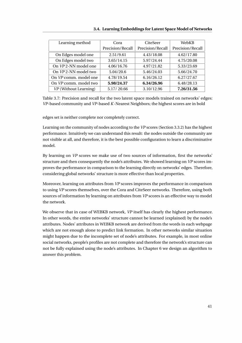
3.4. Learning Embeddings for Latent Space Model of Networks
Learning method Cora CiteSeer WebKBPrecision/Recall Precision/Recall Precision/Recall
On Edges model one 2.51/9.61 4.43/18.08 4.62/17.80On Edges model two 3.65/14.15 5.97/24.44 4.75/20.08
On VP 2-NN model one 4.06/16.76 4.97/21.82 5.33/23.69On VP 2-NN model two 5.04/20.6 5.46/24.03 5.66/24.70
On VP comm. model one 4.78/19.54 6.16/26.12 6.27/27.67On VP comm. model two 5.98/24.37 6.34/26.96 6.48/28.13
VP (Without Learning) 5.17/ 20.66 3.10/12.96 7.26/31.56
Table 3.7: Precision and recall for the two latent space models trained on networks’ edges:VP-based community and VP-based K -Nearest Neighbors; the highest scores are in bold
edges set is neither complete nor completely correct.
Learning on the community of nodes according to the VP scores (Section 3.3.2) has the highest
performance. Intuitively we can understand this result: the nodes outside the community are
not visible at all, and therefore, it is the best possible configuration to learn a discriminative
model.
By learning on VP scores we make use of two sources of information, first the networks’
structure and then consequently the node’s attributes. We showed learning on VP scores im-
proves the performance in comparison to the learning directly on networks’ edges. Therefore,
considering global networks’ structure is more effective than local properties.
Moreover, learning on attributes from VP scores improves the performance in comparison
to using VP scores themselves, over the Cora and CiteSeer networks. Therefore, using both
sources of information by learning on attributes from VP scores is an effective way to model
the network.
We observe that in case of WEBKB network, VP itself has clearly the highest performance.
In other words, the entire networks’ structure cannot be learned (explained) by the node’s
attributes. Nodes’ attributes in WEBKB network are derived from the words in each webpage
which are not enough alone to predict link formation. In other networks similar situation
might happen due to the incomplete set of node’s attributes. For example, in most online
social networks, people’s profiles are not complete and therefore the network’s structure can
not be fully explained using the node’s attributes. In Chapter 6 we design an algorithm to
answer this problem.
41

4 Transfer Learning from HypertextEncyclopedia to Text Analysis Tasks
In this chapter, we apply the techniques we developed in the previous chapter to transfer
knowledge from hypertext encyclopedia towards text analysis tasks. We propose methods for
computing semantic relatedness between words or texts by using knowledge from hypertext
encyclopedias such as Wikipedia. A network of concepts is built by filtering the encyclopedia’s
articles, each concept corresponding to an article. Two types of weighted links between
concepts are considered: one based on the hyperlinks between the texts of the articles, and
another one based on the lexical similarity between them.
To transfer learning from the network of concepts to text analysis tasks we develop two
common representation methods: first, a given text is mapped to the corresponding concepts
in this network and then to compute similarity between two texts VP similarity is applied to
compute the distance between sets of nodes. In other words, the shared representation space
is the set of concepts in the network and every text is represented in this space.
The second method uses the latent space model explained in Chapter 3, Section 3.4, as the
shared representation, and a transformation from words to a latent space is trained over VP
scores. Therefore, to transfer knowledge from the network to any machine learning algorithm,
the given text is transformed using the learned transformation to the latent space.
To evaluate the proposed distance, we apply our method to four important tasks in natural
language processing: word similarity, document similarity, document clustering, and docu-
ment classification, along with a ranking task for information retrieval. The performance of
our method is state-of-the-art or close to it for all the tasks, thus demonstrating the generality
of the method and the accompanying knowledge resource. Moreover, we show that using both
hyperlinks and lexical similarity links improves the scores with respect to a method using only
one of them, because hyperlinks bring additional real-world knowledge not captured by lexical
similarity. Additionally, the proposed method is applied to Idiap’s just-in-time information
retrieval system (ACLD), and brings improvement in terms of the relevance of results.
43
Chapter 4. Transfer Learning from Hypertext Encyclopedia to Text Analysis Tasks
4.1 Introduction to Text Similarity
Estimating the semantic relatedness of two text fragments – such as words, sentences, or entire
documents – is important for many natural language processing or information retrieval
applications. For instance, semantic relatedness has been used for spelling correction [Budan-
itsky and Hirst, 2006], word sense disambiguation [Patwardhan et al., 2003, Kohomban and
Lee, 2005], or coreference resolution [Ponzetto and Strube, 2007]. It has also been shown to
help inducing information extraction patterns [Stevenson and Greenwood, 2005], performing
semantic indexing for information retrieval [Baziz et al., 2005], or assessing topic coherence
[Newman et al., 2010].
Existing measures of semantic relatedness based on lexical overlap, though widely used, are of
little help when text similarity is not based on identical words. Moreover, they assume that
words are independent, which is generally not the case. Other measures, such as PLSA or LDA,
attempt to model in a probabilistic way the relations between words and topics as they occur
in texts, but do not make use of structured knowledge, now available on a large scale, to go
beyond word distribution properties. Therefore, computing text semantic relatedness based
on concepts and their relations, which have linguistic as well as extra-linguistic dimensions,
remains a challenge especially in the general domain and/or over noisy texts.
We propose to compute semantic relatedness between sets of words using the knowledge
enclosed in a large hypertext encyclopedia, with specific reference to the English version of
Wikipedia used in the experimental part. We propose a method to exploit this knowledge for
estimating conceptual relatedness following a statistical approach, by making use of the large-
scale, weakly structured knowledge embodied in the links between concepts. The method
starts by building a network of concepts under the assumption that every encyclopedia
article corresponds to a concept node in the network. Two types of links between nodes are
constructed: one by using the original hyperlinks between articles, and the other one by using
lexical similarity between the articles’ content (Section 4.3).
4.2 Semantic Relatedness: Definitions and Issues
Two samples of language are said to be semantically related if they are about things that are
associated in the world, i.e. bearing some influence one upon the other, or being evoked
together, in speech or thought, more often than other things. Semantic relatedness is a multi-
faceted notion, as it depends on the scale of the language samples (words vs. texts) and on
what exactly counts as a relation. In any case, the adjective ‘semantic’ indicates that we are
concerned with relation between the senses or denotations, and not, e.g., surface forms or
etymology.
44
4.2. Semantic Relatedness: Definitions and Issues
4.2.1 Nature of Semantic Relations for Words and Texts
Semantic relations between words, or rather between their senses, have been well studied
and categorized in linguistics. They include classical relations such as synonymy (identity
of senses, e.g. ‘freedom’ and ‘liberty’), antonymy (opposition of senses such as ‘increase’ vs.
‘decrease’), hypernymy or hyponymy (e.g. ‘vehicle’ and ‘car’ ), and meronymy or holonymy
(part-whole relation such as ‘wheel’ and ‘car’). From this point of view, semantic similarity
is more specific than semantic relatedness. For instance, antonyms are related, but not
similar. Or, following Resnik [1995], ‘car’ and ‘bicycle’ are more similar (as hyponyms of
‘vehicle’) than ‘car’ and ‘gasoline’, though the latter pair may seem more related in the world.
Classical semantic relations are listed in hand-crafted lexical or ontological resources, such as
WordNet [Fellbaum, 1998] or Cyc [Lenat, 1995], or implicitly in Roget’s Thesaurus (as used by
Jarmasz [2003]), or they can be inferred from distributional data as discussed below.
Additional types of lexical relations have been described as ‘non-classical’ by Morris and Hirst
[2004], for instance based on membership in similar classes (e.g. positive qualities), or on
association by location, or due to stereotypes – but these relations do not qualify as similarity
ones, and are generally not listed in lexical resources. Budanitsky and Hirst [2006] point out
that semantic ‘distance’ can be seen as the contrary of either similarity or relatedness. In this
chapter, our use of ‘distance’ will refer to our measure of semantic relatedness as defined
below.
At the sentence level, semantic relatedness can subsume notions such as paraphrase or logical
relations (e.g., entailment or contradiction). More generally, two sentences can be related by a
similarity of topic, a notion that applies to multi-sentence texts as well, even though the notion
of ‘topic’ is difficult to define. Topicality is often expressed in terms of the continuity of themes,
i.e. referents or entities about which something is predicated, which ensures the coherence of
texts. Linguists have analyzed coherence as being maintained by cohesive devices [Hobbs,
1983], which include identity-of-reference, lexical cohesion, and similarity chains based on
classical lexical relations [Halliday and Hasan, 1989].
A key relation between the semantic relatedness of words and their occurrence in texts has
long been exploited by researchers in natural language processing (NLP) under the form of
distributional measures [Mohammad and Hirst, 2005], despite certain limitations pointed out
by Budanitsky and Hirst [2006, Section 6.2]. The assumption that sentences and texts form
coherent units makes it indeed possible to infer word meanings and lexical relations from
distributional similarity [Weeds, 2003], using vector-based models such as Latent Semantic
Analysis [Deerwester et al., 1990], possibly enhanced with syntactic information [Padó and
Lapata, 2007]. In return, the hidden topical parameters that govern the occurrences of words
can be modeled probabilistically (e.g. using PLSA [Hofmann, 1999] or LDA [Blei et al., 2003]),
thus providing measures of text similarity.
45
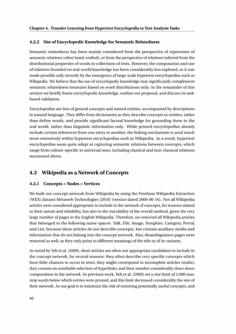
Chapter 4. Transfer Learning from Hypertext Encyclopedia to Text Analysis Tasks
4.2.2 Use of Encyclopedic Knowledge for Semantic Relatedness
Semantic relatedness has been mainly considered from the perspective of repertoires of
semantic relations (often hand-crafted), or from the perspective of relations inferred from the
distributional properties of words in collections of texts. However, the computation and use
of relations founded on real-world knowledge has been considerably less explored, as it was
made possible only recently by the emergence of large-scale hypertext encyclopedias such as
Wikipedia. We believe that the use of encyclopedic knowledge may significantly complement
semantic relatedness measures based on word distributions only: in the remainder of this
section we briefly frame encyclopedic knowledge, outline our proposal, and discuss its task-
based validation.
Encyclopedias are lists of general concepts and named entities, accompanied by descriptions
in natural language. They differ from dictionaries as they describe concepts or entities, rather
than define words, and provide significant factual knowledge for grounding them in the
real world, rather than linguistic information only. While printed encyclopedias already
include certain references from one entry to another, the linking mechanism is used much
more extensively within hypertext encyclopedias such as Wikipedia. As a result, hypertext
encyclopedias seem quite adept at capturing semantic relations between concepts, which
range from culture-specific to universal ones, including classical and non-classical relations
mentioned above.
4.3 Wikipedia as a Network of Concepts
4.3.1 Concepts = Nodes = Vertices
We built our concept network from Wikipedia by using the Freebase Wikipedia Extraction
(WEX) dataset Metaweb Technologies [2010] (version dated 2009-06-16). Not all Wikipedia
articles were considered appropriate to include in the network of concepts, for reasons related
to their nature and reliability, but also to the tractability of the overall method, given the very
large number of pages in the English Wikipedia. Therefore, we removed all Wikipedia articles
that belonged to the following name spaces: Talk, File, Image, Template, Category, Portal,
and List, because these articles do not describe concepts, but contain auxiliary media and
information that do not belong into the concept network. Also, disambiguation pages were
removed as well, as they only point to different meanings of the title or of its variants.
As noted by Yeh et al. [2009], short articles are often not appropriate candidates to include in
the concept network, for several reasons: they often describe very specific concepts which
have little chances to occur in texts; they might correspond to incomplete articles (stubs);
they contain an unreliable selection of hyperlinks; and their number considerably slows down
computation in the network. In previous work, Yeh et al. [2009] set a size limit of 2,000 non-
stop words below which entries were pruned, and this limit decreased considerably the size of
their network. As our goal is to minimize the risk of removing potentially useful concepts, and
46
4.3. Wikipedia as a Network of Concepts
to respect as much as possible the original contents of Wikipedia, we set a cut-off limit of 100
non-stop words, thus pruning only very minor articles. This value is thus much lower than the
value used by Yeh et al. [2009], and is similar to the one used by Gabrilovich and Markovitch
[2009]. Out of an initial set of 4,327,482 articles in WEX, filtering removed about 70% of all
articles based on namespaces and length cut-off, yielding a resulting set of 1,264,611 concepts.
Each concept has a main Wikipedia name, which is the title of the main page describing the
concept. However, in many cases, other words or phrases can be used as well to refer to the
concept. One such type of words can be determined by examining Wikipedia redirects, i.e.
articles that have no content but point the user to a proper article with an alternative title. The
titles of redirect pages were added as secondary titles to the titles of the articles they redirect to.
In addition, for every hyperlink from one article to another, we extracted the corresponding
anchor text and considered it as another possible secondary title for the linked article, thus
capturing a significant part of the terminological variation of concept names (with some noise
due to variability in linking practice). Therefore, each concept has three types of titles (see
summary of data structure in Table 4.1): the original one, the anchor texts of the hyperlinks
targeting it, and the variants provided by redirect pages, each specific title being listed only
once.
4.3.2 Relations = Links = Edges
Relations between concepts can be determined in several ways. In a previous study [Yazdani
and Popescu-Belis, 2010], we considered four types of links between concepts: hyperlinks and
links computed from similarity of content, of category, and of template. While each type of
links captures some form of relatedness, we focus in the present chapter (based on [Yazdani
and Popescu-Belis, 2013]) on the first two types, which are the most complementary. However,
the proposed computational framework is general enough to accommodate more than two
types of links, in particular if an optimal combination can be learned from training data.
The use of hyperlinks between Wikipedia articles embodies the somewhat evident observation
that every hyperlink from the content of an article towards another one indicates a certain
relation between the two articles. These are encyclopedic or pragmatic relations, i.e. between
concepts in the world, and subsume semantic relatedness. In other words, if article A contains
a hyperlink towards article B , then B helps to understand A, and B is considered to be related
to A. Such links represent a substantial amount of human knowledge that is embodied in
the Wikipedia structure. It must be noted that these links are essentially asymmetric, and
we decided to keep them as such, i.e. to list for a given page only its outgoing links and not
the incoming ones. Indeed, observations showed that while the target page of a link helps
understanding the source one, the contrary is not always true or the relation is not specific
enough. For each article, the XML text from WEX was parsed to extract hyperlinks, resulting in
a total of 35,214,537 hyperlinks – a time-consuming operation that required also the ability to
handle instances of ill-formed XML input.
47
Chapter 4. Transfer Learning from Hypertext Encyclopedia to Text Analysis Tasks
The second type of links is based on similarity of lexical content between articles of Wikipedia,
computed from word co-occurrence. If two articles have many words in common, then a
topic-similarity relation holds between them. To capture content similarity, we computed the
lexical similarity between articles as the cosine similarity between the vectors derived from
the articles’ texts, after stopword removal and stemming using Snowball.1 We then linked
every article to its k most similar articles, with a weight according to the normalized lexical
similarity score (for non-zero weights). In the experiments described below, k was set to 10, so
that each node has ten outgoing links to other nodes, based on lexical similarity.2 The value of
k = 10 was chosen to ensure computational tractability, and is slightly lower than the average
number of hyperlinks per concept, which is about 28. As the Wikipedia articles are scattered
in the space of words, tuning k does not seem to bring crucial changes. If k is very small
then the neighborhood contains little information, whereas a large k makes computation
time-consuming.
Concept ID IntegerNames of the concept Name of article in the encyclopedia
Alternative names redirecting to the articleAnchor texts of incoming hyperlinks
Description of the concept TextRelations to other concepts(outgoing links)
Hyperlinks from the description towards otherconcepts (no weights)Lexical similarity links to the ten closest con-cepts (weights from cosine similarity)
Table 4.1: Logical structure of each node in the network resulting from the English Wikipedia.
4.3.3 Properties of the Resulting Network
The processing of the English Wikipedia resulted in a very large network of concepts, each
of them having the logical structure represented in Table 4.1. The network has more than
1.2 million nodes (i.e. vertices), with an average of 28 outgoing hyperlinks per node and 10
outgoing content links per node.
A natural question arising at this point is: how can the structure of the network be character-
ized, apart from putting it to work? It is not possible to visualize the entire network due to its
size, and displaying only a small part, as done for instance by Coursey et al. [2009, Figure 1],
might not be representative of the entire network.3. A number of quantitative parameters
have been proposed in graph theory and social network analysis, and some have for instance
been used to analyze WordNet (and an enhanced version of it) by Navigli and Lapata [2010].
1From the Apache Lucene indexing system available at http://lucene.apache.org/.2Therefore, the outdegree of all nodes is 10, but as the indegree may vary (the number of incoming links), the
graph is not strictly speaking a 10-regular graph.3An example of neighborhood according to our relatedness measure is however shown in Section 4.4.1
48
4.3. Wikipedia as a Network of Concepts
We compute below some well-known parameters for our network, and add a new, more
informative characterization.
A first characteristic of graphs is their degree distribution, i.e. the distribution of the number
of direct neighbors per node. For the original Wikipedia with hyperlinks, a representation [Gr-
ishchenko, 2008] suggests that the distribution follows a power law. A more relevant property
here is the network clustering coefficient, which is the average of clustering coefficients per
node, defined as the size of the immediate neighborhood of the node divided by the maximum
number of links that could connect all pairs of neighbors [Watts and Strogatz, 1998]. For
our hyperlink graph, the value of this coefficient is 0.16, while for the content link graph it is
0.26.4 This shows that the hyperlink graph is less clustered than the content link one, i.e. the
distribution of nodes and links is more homogeneous, and that overall the two graphs have
rather low clustering.5
We propose an ad-hoc measure offering a better illustration of the network’s topology, aimed
at finding out whether the graph is clustered or not – i.e., whether the communities of nodes
based on neighborhoods have a preferred size, or are uniformly distributed. We consider a sam-
ple of 1000 nodes. For each node of the graph, the Personalized PageRank algorithm [Haveli-
wala, 2003] is initialized from that node and run, thus resulting into a proximity coefficient
for each node in the graph to the initial node. This is first done using hyperlinks, and then
using the content links. The community size for the node is computed by sorting all nodes
with respect to their proximity and counting how many nodes contribute to 99% of the mass.
(a) Hyperlink graph (b) Content link graph
Figure 4.1: Distribution of community sizes for a sample of 1000 nodes (see text for thedefinition of a community). For each community size (x-axis) the graphs show the number ofnodes (y-axis) having a community of that size, for each of the two graphs built from Wikipedia.Both graphs have a tendency towards clustering, i.e. a non-uniform distribution of links, withan average cluster size of 150–400 for hyperlinks and 7–14 for content links.
4For the content links, the coefficient was computed regardless of their weights. A recent proposal for computingit for weighted graphs could be applied too [Opsahl and Panzarasa, 2009].
5The observed values, together with the power law degree distribution, suggest that our graph is a scale-freenetwork – characterized by the presence of “hub” nodes – or a small-world network [Watts and Strogatz, 1998].However, it is not clear what impact these properties defined mainly for social networks would have here.
49
Chapter 4. Transfer Learning from Hypertext Encyclopedia to Text Analysis Tasks
The results shown in Figure 4.1 show that the distribution is neither flat nor uniformly de-
creasing, but has a peak, which provides an indication of the average size of clusters. This size
is around 150–400 nodes for the hyperlink graph, without a sharp maximum, showing less
clustering than for content links, for which this average is around 7–14 nodes. The latter value
is partly related to the 10-link limit set for content links, but is not entirely due to it, as the limit
concerns only outgoing links. The use of hyperlinks thus avoids local clusters and extends
considerably the connectivity of the network in comparison to content similarity ones.
4.4 Common Representation Space for Transfer Learning
In order to transfer human knowledge embodied in the Wikipedia network of concepts to-
wards a measure of text similarity in various text analysis tasks, we need to build a shared
representation for text fragments. We propose two shared representation models (i.e. spaces),
which we explain in Sections 4.4.1 and 4.4.2 below.
The network of concepts built from Wikipedia consists of many concepts from human knowl-
edge. Therefore, the set of concepts in the network is rich enough so that it can represent
the content of any text fragment. The first shared representation we develop is the set of
concepts in the network: a given text is simply mapped to the corresponding concepts in this
network. Then, to compute similarity between two texts, VP similarity is applied to compute
the distance between the two sets of nodes (concepts).
The second method uses the latent space model that we explained in Section 3.4 as the shared
representation. In this approach, we assume that there is a latent space in which semantically
similar texts are placed in close positions and semantically unrelated texts are placed farther
away from each other. We showed that each concept in the network (corresponding to a
Wikipedia article) has a text body which explains the concept. We learn a transformation from
words in the title and body to the latent space so that two similar concepts in terms of VP
are in close distance. Therefore, to transfer knowledge from the network to any processing
method that uses feature vectors, texts are transformed using the learned transformation into
the latent space. We now explain each approach in more detail.
4.4.1 Mapping Text Fragments to Concepts in the Network
For mapping, two cases must be considered, according to whether the text matches exactly
the title of a Wikipedia page or not. Exact matching is likely to occur with individual words or
short phrases, but not with entire sentences or longer texts.
If a text fragment consists of a single word or a phrase that matches exactly the title of a
Wikipedia page, then it is simply mapped to that concept. In the case of words or phrases that
may refer to several concepts in Wikipedia, we simply assign to them the same page as the one
assigned by the Wikipedia contributors as the most salient or preferred sense or denotation.
50
4.4. Common Representation Space for Transfer Learning
For instance, ‘mouse’ directs to the page about the animal, which contains an indication that
the ‘mouse_(computing)’ page describes the pointing device, and that other senses are listed
on the ‘mouse_(disambiguation)’ page. So, here, we simply map ‘mouse’ to the animal concept.
However, for other words, no sense or denotation is preferred by the Wikipedia contributors,
e.g. for the word ‘plate’. In such cases, a disambiguation page is associated to that word or
phrase. We chose not to include such pages in our network, as they do not correspond to
individual concepts. So, in order to select the referent page for such words, we simply use the
lexical similarity approach we will now describe.
When a fragment (a word, phrase, sentence, or text) does not match exactly the Wikipedia title
of a vertex in our network, it is mapped to the network by computing its lexical similarity with
the text content of the vertices in the network, using cosine distance over stemmed words,
stopwords being removed. Concept names (principal and secondary ones) are given twice
as much weight as the words found in the description of the concept. The text fragment is
mapped to the k most similar articles according to this similarity score, resulting in a set of at
most k weighted concepts. The weights are normalized, summing up to one, therefore the
text representation in the network is a probability distribution over at most k concepts. Finding
the k closest articles according to lexical similarity can be done efficiently using the Apache
Lucene search engine (see note 1).
For example, consider the following text fragment to be mapped to our network: “Facebook:
you have some serious privacy and security problems.” When this fragment is mapped to the
k = 10 most similar Wikipedia articles, the resulting probability distribution is the following
one: ‘Facebook’ (0.180), ‘Facebook Beacon’ (0.119), ‘Facebook history’ (0.116), ‘Criticism of
Facebook’ (0.116), ‘Facebook features’ (0.116), ‘Privacy’ (0.084), ‘Privacy International’ (0.080),
‘Internet privacy’ (0.080), ‘Privacy policy’ (0.054), ‘Privacy Lost’ (0.054).
This mapping algorithm has an important role in the performance of the final system, in
combination with the network distance (VP). It must however be noted that the effects of
wrong mappings at this stage are countered later on. For instance, when large sets of concepts
related to two text fragments are compared, a few individual mistakes are not likely to alter the
overall relatedness scores. Alternatively, when comparing individual words, wrong mappings
are less likely to occur because the test sets for word similarity described in Section 4.6,
page 60, also consider implicitly the most salient sense of each word, just as described above
for Wikipedia.
VP Between Two Sets of Nodes
After mapping to one or more Wikipedia articles, as just explained, each text is thus represented
by a weighted set of nodes. In order to measure the similarity between two texts after mapping,
we will generalize the definition of VP so that it measures the similarity between two weighted
set of nodes.
51
Chapter 4. Transfer Learning from Hypertext Encyclopedia to Text Analysis Tasks
We first generalize the definition of VP between two nodes given in Section 3.1 to a measure
from a distribution to a node. Given a probability distribution~r over concepts (i.e. a weighted
set of concepts), and a concept s j in the network, we first compute the probability of visiting
s j for the first time when a random walker starts from~r in the network, i.e. from any of the
concepts in~r that have a non-zero probability. To compute visiting probability, the following
procedure provides a model of the state St of the random walker, i.e. the concept in which
the random walker is positioned. Executing the procedure until termination gives the visiting
probability VP.
Step 0: Choose the initial state of the walker with probability P (S0 = si |~r ) = ri . In other
words, position the random walker on any of the concepts of ~r with the probability
stated in~r .
Step t : Assuming St−1 is determined, if St−1 = s j then return ‘success’ and finish the proce-
dure. Otherwise, with probability α, choose a value for the next concept St according to
the transition matrix C , and with probability 1−α, return ‘fail’. The possibility of ‘failing’,
or absorption probability, introduces a penalty over long paths that makes them less
probable.
Similarly we introduce C ′ as being equal to the transition matrix C , except that in row j ,
C ′( j ,k) = 0 for all k. We remind that the transition matrix C , is the linear combination of the
transition matrices of hyperlinks and content links, which they are built from the weights of
links in the network. The possible weights are 0 or 1 for the hyperlink matrix, and actual lexical
similarity scores (or 0) for the content similarity matrix.
The probability of success in the process, i.e. the probability of visiting s j starting from~r , is
the sum over all probabilities of success with different lengths:
p(success) =∞∑
t=0p t (success) =
∞∑t=0
αt (~rC ′t ) j .
Therefore, the computation is the same as before, the only difference here is that~r is resulting
from the mapping algorithm and shows a set of initial concepts instead of one node.
To compute the VP from a weighted set of concepts to another set, i.e. from distribution~r1
to distribution~r2, we construct a virtual node representing~r2 in the network, noted sR (~r2).
We then connect all concepts si to sR (~r2) according to the weights in~r2. We now create the
transition matrix C ′ by adding a new row (numbered nR ) to the transition matrix C with all
elements zero to indicate sR (~r2), then adding a new column with the weights in sR (~r2), and
updating all the other rows of C as follows (Ci j is an element of C ):
52
4.4. Common Representation Space for Transfer Learning
C ′i j =Ci j (1− (~r2)i ) for i , j 6= nR
C ′i nR
= (~r2)i for all i
C ′nR j = 0 for all j .
These modifications to the graph are local and can be done at run time, with the possibility to
undo them for subsequent text fragments to be compared. The algorithm to compute VP is
identical to the section 3.1 and therefore, the same algorithms and properties we explained
there hold for this application here as well.
To compute relatedness between two texts, we average between the visiting probability of~r1
given~r2 (noted VP(~r2,~r1)) and the visiting probability of~r2 given~r1 (noted VP(~r1,~r2)). A larger
value of the measure indicates closer relatedness.
Illustration of Visiting Probability ‘to’ vs. ‘from’ a Text
We showed earlier in Section 3.1.3 the importance of the symmetric VP. Here we illustrate in a
similar way the difference between VP from and to and justify the choice of symmetric VP. To
illustrate the difference between VP to and from a text fragment, we consider the following
example. Though any text fragment could be used, we took the definition of ‘jaguar’ (animal)
from the corresponding Wikipedia article. Although the word ‘jaguar’ is polysemous, the
topic of this particular text fragment is not ambiguous to a human reader. The text was first
mapped to Wikipedia as described above. Then, using VP with equal weights on hyperlinks
and content links, the ten closest concepts (i.e. Wikipedia pages) in terms of VP from the text,
and respectively to it, were found to be the following ones:
• Original text: “The jaguar is a big cat, a feline in the Panthera genus, and is the only
Panthera species found in the Americas. The jaguar is the third-largest feline after the
tiger and the lion, and the largest in the Western Hemisphere.”
• Ten closest concepts according to their VP to the text: ‘John Varty’, ‘European Jaguar’,
‘Congolese Spotted Lion’, ‘Lionhead rabbit’, ‘Panthera leo fossilis’, ‘Tigon’, ‘Panthera
hybrid’, ‘Parc des Félins’, ‘Marozi’, ‘Craig Busch’.
• Ten closest concepts according to their VP from the text: ‘Felidae’, ‘Kodkod’, ‘North
Africa’, ‘Jaguar’, ‘Panthera’, ‘Algeria’, ‘Tiger’, ‘Lion’, ‘Panthera hybrid’, ‘Djémila’.
The closest concepts according to VP from a text tend to be more general than closest concepts
according to VP to the text. For instance, the second list above includes the genus and family
of the jaguar species (Panthera and Felidae), while the first one includes six hybrid or extinct
species related to the jaguar. Concepts close to a text thus bring detailed information related
to the topics of the text, while concepts close from a text are more popular and more general
53
Chapter 4. Transfer Learning from Hypertext Encyclopedia to Text Analysis Tasks
Wikipedia articles. Note also that none of the closest concepts above is related to the Jaguar
car brand, as found by examining each page, including the lesser-known ones (both persons
cited are wildlife film makers and park founders). However, not all concepts are related in an
obvious way (e.g. ‘Algeria’ is likely retrieved through ‘Western Hemisphere’).
The behavior illustrated on this example is expected given the definition of VP. A concept that
is close to a text has more paths in the network towards the text with respect to other concepts
in the network, which means that the concept is quite specific in relation to the topics in the
text, as in the above example. Conversely, a concept that is close from a text (in terms of VP
from a text) is typically related by many paths from the text to the concept, in comparison to
other concepts. This generally means that it is likely that the article is a general and popular
article around the topics of the text. If we consider the hierarchy between concepts from more
general to more specific ones, then concepts close to a text are generally lower in the hierarchy
with respect to the text, and concepts close from a text are generally higher.
4.4.2 Learning Embeddings to Latent Space
The second method we propose to measure text similarity using VP is to learn an embed-
ding (transformation) from words to a latent space using as a criterion the VP scores on the
Wikipedia concept network, following the general approach introduced in Section 3.4 above.
At training time, given a series of samples – that is, pairs of texts with VP values from the first
text to the second one – the goal is to learn a transformation from the space of words to a
latent space, so that the similarity between the latent representation of the texts is as close as
possible to the VP similarity. In other words, the goal is to approximate VP between two texts i
and j by the matrix product xi AB ′x ′j , where xi and x j are the TF-IDF vectors of the two texts
constructed from their words using a fixed dictionary. The size of matrices A and B is n ×m,
with n being the size of the dictionary (number of words) and m the size of the latent space
(akin to the number of topics in topic models). Two different matrices A and B are needed
because VP values are not symmetric in i and j .
In principle, all pairs of Wikipedia articles (i.e., texts) corresponding to nodes in our network
can be used for training, but this set is extremely large (ca. 1.4×10¹²) and moreover, we showed
that the most values are close to zero and are not valuable for training. Therefore, similar
to the section 3.4 we formulate the following constraints for training: (1) training should
focus on neighboring articles (articles with high VP values), and (2) the exact values of VP are
replaced with the ranking of pairs of articles by decreasing VP. We show here that under these
constraints valuable embeddings can be learned.
Let VPtok (i ) be the set of the k closest articles to the article i according to VP similarity. We
define a hinge loss function L as follows, so that the similarity between i and its k closest
54
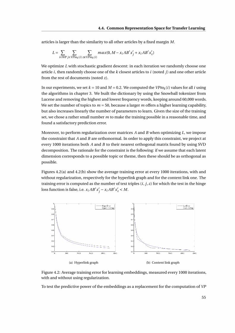
4.4. Common Representation Space for Transfer Learning
articles is larger than the similarity to all other articles by a fixed margin M .
L = ∑i∈WP
∑j∈VPtok (i )
∑z∉VPtok (i )
max(0, M −xi AB ′x ′j +xi AB ′x ′
z )
We optimize L with stochastic gradient descent: in each iteration we randomly choose one
article i , then randomly choose one of the k closest articles to i (noted j ) and one other article
from the rest of documents (noted z).
In our experiments, we set k = 10 and M = 0.2. We computed the VPtok (i ) values for all i using
the algorithms in chapter 3. We built the dictionary by using the Snowball tokenizer from
Lucene and removing the highest and lowest frequency words, keeping around 60,000 words.
We set the number of topics to m = 50, because a larger m offers a higher learning capability,
but also increases linearly the number of parameters to learn. Given the size of the training
set, we chose a rather small number m to make the training possible in a reasonable time, and
found a satisfactory prediction error.
Moreover, to perform regularization over matrices A and B when optimizing L, we impose
the constraint that A and B are orthonormal. In order to apply this constraint, we project at
every 1000 iterations both A and B to their nearest orthogonal matrix found by using SVD
decomposition. The rationale for the constraint is the following: if we assume that each latent
dimension corresponds to a possible topic or theme, then these should be as orthogonal as
possible.
Figures 4.2(a) and 4.2(b) show the average training error at every 1000 iterations, with and
without regularization, respectively for the hyperlink graph and for the content link one. The
training error is computed as the number of text triples (i , j , z) for which the test in the hinge
loss function is false, i.e. xi AB ′x ′j −xi AB ′x ′
z < M .
(a) Hyperlink graph (b) Content link graph
Figure 4.2: Average training error for learning embeddings, measured every 1000 iterations,with and without using regularization.
To test the predictive power of the embeddings as a replacement for the computation of VP
55
Chapter 4. Transfer Learning from Hypertext Encyclopedia to Text Analysis Tasks
at runtime, we excluded 50,000 articles from the training set, and then built 50,000 triples of
articles by choosing randomly, for each of the excluded articles, one article from the k closest
ones and one randomly from the rest of the articles. The test set error, which is the number of
triples from this set that do not respect the order given by VP similarities, is shown in Table 4.2.
Training set for embedding Error (%)Hyperlinks 9.8Hyperlinks with Regularization 13.5Content Links 5.4Content Links with Regularization 5.9
Table 4.2: Accuracy of embeddings learned over four different training sets. The error (per-centage) is computed for 50,000 triples of articles from a separate test set, as the number oftriples that do not respect the ordering of VP similarities.
The two main findings are the following. First, VP over the hyperlinks graph is harder to
learn, which may be due to the fact that hyperlinks are defined by users in a manner that
is not totally predictable. Second, regularization decreases the prediction ability. However,
if regularization traded prediction power for more generality, in other words if it reduced
overfitting to this problem and made the distance more general, then it would still constitute
a useful operation. This will be checked in the experiments in Sections 4.8, 4.9 and 4.11.
Moreover, these experiments will show that the embeddings can be plugged into state-of-the-
art learning algorithms as prior knowledge, improving their performance.
Learning embeddings in comparison to mapping to the concept network has some advantages.
The main one is that it can be applied with a much lower cost at run time. The embedding
approach does not require a fixed number of nodes to project a document on. Moreover, it
can be more easily integrated as prior knowledge to other learning algorithms for NLP, and it
can be applied to very large scale problems.
4.5 Empirical Analyses of VP and Approximations
We now analyze the convergence of the two approximation methods proposed in section 3.2. In
the case of path insensitive ε-truncated approximation lets T shows the maximum path length
that is expanded, when T increases to infinity, the path insensitive ε-truncated approximated
VP converges towards the exact value, but computation time increases linearly with T . In the
case of path sensitive ε-truncation, when ε tends to zero the approximated value converges
towards the real one, but again computation time increases. Therefore, we need to find the
proper values for T and ε as a compromise between the estimated error and the computing
time.
56
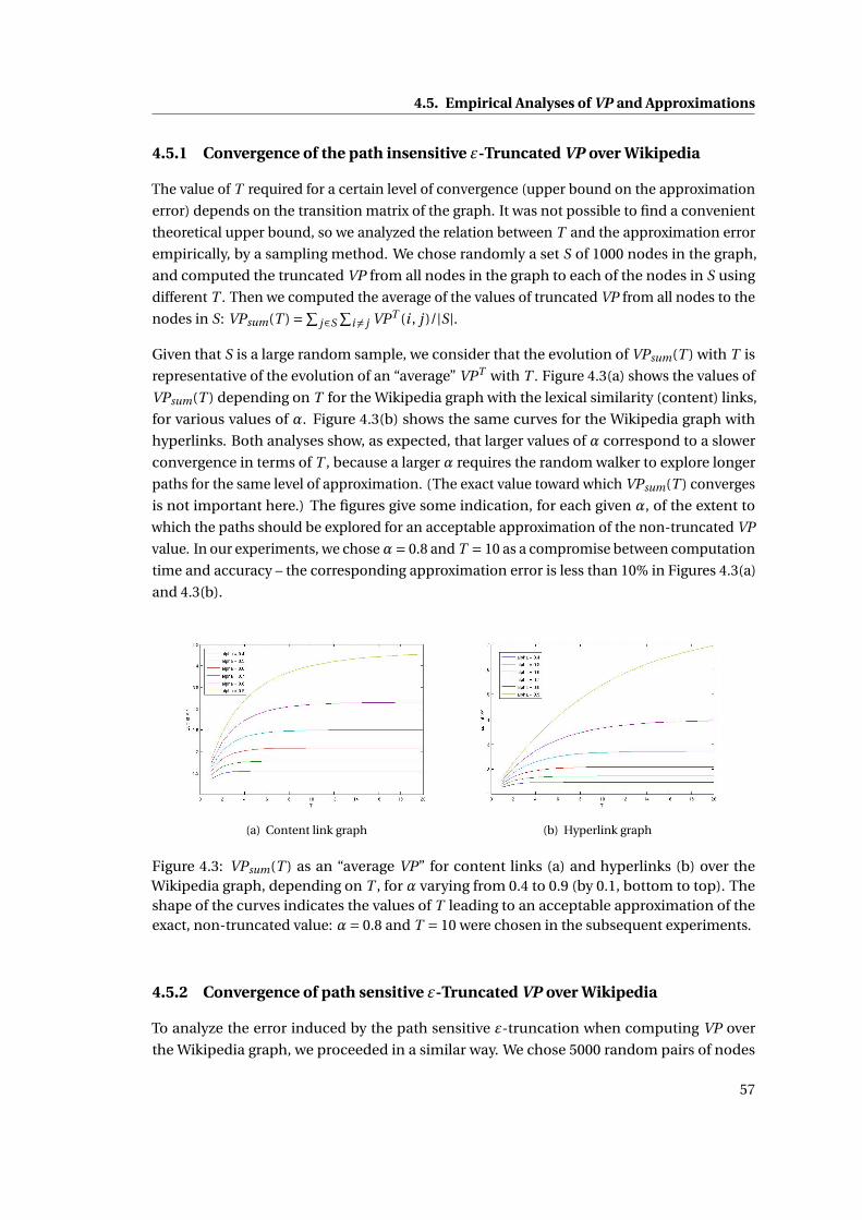
4.5. Empirical Analyses of VP and Approximations
4.5.1 Convergence of the path insensitive ε-Truncated VP over Wikipedia
The value of T required for a certain level of convergence (upper bound on the approximation
error) depends on the transition matrix of the graph. It was not possible to find a convenient
theoretical upper bound, so we analyzed the relation between T and the approximation error
empirically, by a sampling method. We chose randomly a set S of 1000 nodes in the graph,
and computed the truncated VP from all nodes in the graph to each of the nodes in S using
different T . Then we computed the average of the values of truncated VP from all nodes to the
nodes in S: VPsum(T ) =∑j∈S
∑i 6= j VPT (i , j )/|S|.
Given that S is a large random sample, we consider that the evolution of VPsum(T ) with T is
representative of the evolution of an “average” VPT with T . Figure 4.3(a) shows the values of
VPsum(T ) depending on T for the Wikipedia graph with the lexical similarity (content) links,
for various values of α. Figure 4.3(b) shows the same curves for the Wikipedia graph with
hyperlinks. Both analyses show, as expected, that larger values of α correspond to a slower
convergence in terms of T , because a larger α requires the random walker to explore longer
paths for the same level of approximation. (The exact value toward which VPsum(T ) converges
is not important here.) The figures give some indication, for each given α, of the extent to
which the paths should be explored for an acceptable approximation of the non-truncated VP
value. In our experiments, we choseα= 0.8 and T = 10 as a compromise between computation
time and accuracy – the corresponding approximation error is less than 10% in Figures 4.3(a)
and 4.3(b).
(a) Content link graph (b) Hyperlink graph
Figure 4.3: VPsum(T ) as an “average VP” for content links (a) and hyperlinks (b) over theWikipedia graph, depending on T , for α varying from 0.4 to 0.9 (by 0.1, bottom to top). Theshape of the curves indicates the values of T leading to an acceptable approximation of theexact, non-truncated value: α= 0.8 and T = 10 were chosen in the subsequent experiments.
4.5.2 Convergence of path sensitive ε-Truncated VP over Wikipedia
To analyze the error induced by the path sensitive ε-truncation when computing VP over
the Wikipedia graph, we proceeded in a similar way. We chose 5000 random pairs of nodes
57
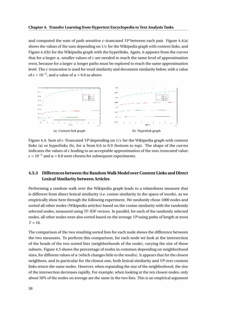
Chapter 4. Transfer Learning from Hypertext Encyclopedia to Text Analysis Tasks
and computed the sum of path sensitive ε-truncated VP between each pair. Figure 4.4(a)
shows the values of the sum depending on 1/ε for the Wikipedia graph with content links, and
Figure 4.4(b) for the Wikipedia graph with the hyperlinks. Again, it appears from the curves
that for a larger α, smaller values of ε are needed to reach the same level of approximation
error, because for a larger α longer paths must be explored to reach the same approximation
level. The ε-truncation is used for word similarity and document similarity below, with a value
of ε= 10−5, and a value of α= 0.8 as above.
(a) Content link graph (b) Hyperlink graph
Figure 4.4: Sum of ε-Truncated VP depending on 1/ε for the Wikipedia graph with contentlinks (a) or hyperlinks (b), for α from 0.6 to 0.9 (bottom to top). The shape of the curvesindicates the values of ε leading to an acceptable approximation of the non-truncated value:ε= 10−5 and α= 0.8 were chosen for subsequent experiments.
4.5.3 Differences between the Random Walk Model over Content Links and DirectLexical Similarity between Articles
Performing a random walk over the Wikipedia graph leads to a relatedness measure that
is different from direct lexical similarity (i.e. cosine similarity in the space of words), as we
empirically show here through the following experiment. We randomly chose 1000 nodes and
sorted all other nodes (Wikipedia articles) based on the cosine similarity with the randomly
selected nodes, measured using TF-IDF vectors. In parallel, for each of the randomly selected
nodes, all other nodes were also sorted based on the average VP using paths of length at most
T = 10.
The comparison of the two resulting sorted lists for each node shows the difference between
the two measures. To perform this comparison, for each node we look at the intersection
of the heads of the two sorted lists (neighborhoods of the node), varying the size of these
subsets. Figure 4.5 shows the percentage of nodes in common depending on neighborhood
sizes, for different values ofα (which changes little to the results). It appears that for the closest
neighbors, and in particular for the closest one, both lexical similarity and VP over content
links return the same nodes. However, when expanding the size of the neighborhood, the size
of the intersection decreases rapidly. For example, when looking at the ten closest nodes, only
about 50% of the nodes on average are the same in the two lists. This is an empirical argument
58
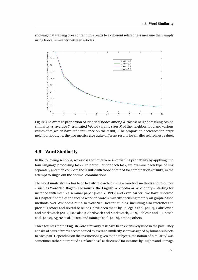
4.6. Word Similarity
showing that walking over content links leads to a different relatedness measure than simply
using lexical similarity between articles.
Figure 4.5: Average proportion of identical nodes among K closest neighbors using cosinesimilarity vs. average T -truncated VP, for varying sizes K of the neighborhood and variousvalues of α (which have little influence on the result). The proportion decreases for largerneighborhoods, i.e. the two metrics give quite different results for smaller relatedness values.
4.6 Word Similarity
In the following sections, we assess the effectiveness of visiting probability by applying it to
four language processing tasks. In particular, for each task, we examine each type of link
separately and then compare the results with those obtained for combinations of links, in the
attempt to single out the optimal combinations.
The word similarity task has been heavily researched using a variety of methods and resources
– such as WordNet, Roget’s Thesaurus, the English Wikipedia or Wiktionary – starting for
instance with Resnik’s seminal paper [Resnik, 1995] and even earlier. We have reviewed
in Chapter 2 some of the recent work on word similarity, focusing mainly on graph-based
methods over Wikipedia but also WordNet. Recent studies, including also references to
previous scores and several baselines, have been made by Bollegala et al. [2007], Gabrilovich
and Markovitch [2007] (see also [Gabrilovich and Markovitch, 2009, Tables 2 and 3]), Zesch
et al. [2008], Agirre et al. [2009], and Ramage et al. [2009], among others.
Three test sets for the English word similarity task have been extensively used in the past. They
consist of pairs of words accompanied by average similarity scores assigned by human subjects
to each pair. Depending on the instructions given to the subjects, the notion of ‘similarity’ was
sometimes rather interpreted as ‘relatedness’, as discussed for instance by Hughes and Ramage
59
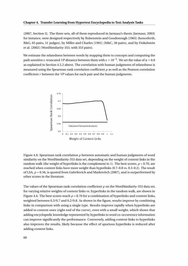
Chapter 4. Transfer Learning from Hypertext Encyclopedia to Text Analysis Tasks
[2007, Section 5]. The three sets, all of them reproduced in Jarmasz’s thesis [Jarmasz, 2003]
for instance, were designed respectively by Rubenstein and Goodenough [1965] (henceforth,
R&G, 65 pairs, 51 judges), by Miller and Charles [1991] (M&C, 30 pairs), and by Finkelstein
et al. [2002] (WordSimilarity-353, with 353 pairs).
We estimate the relatedness between words by mapping them to concepts and computing the
path sensitive ε-truncated VP distance between them with ε= 10−5. We set the value ofα= 0.8
as explained in Section 4.5.2 above. The correlation with human judgments of relatedness is
measured using the Spearman rank correlation coefficient ρ as well as the Pearson correlation
coefficient r between the VP values for each pair and the human judgments.
Figure 4.6: Spearman rank correlation ρ between automatic and human judgments of wordsimilarity on the WordSimilarity-353 data set, depending on the weight of content links in therandom walk (the weight of hyperlinks is the complement to 1). The best scores, ρ = 0.70, arereached when content links have more weight than hyperlinks (0.7–0.8 vs. 0.3–0.2). The resultof LSA, ρ = 0.56, is quoted from Gabrilovich and Markovitch [2007], and is outperformed byother scores in the literature.
The values of the Spearman rank correlation coefficient ρ on the WordSimilarity-353 data set,
for varying relative weights of content links vs. hyperlinks in the random walk, are shown in
Figure 4.6. The best scores reach ρ = 0.70 for a combination of hyperlinks and content links,
weighted between 0.3/0.7 and 0.2/0.8. As shown in the figure, results improve by combining
links in comparison with using a single type. Results improve rapidly when hyperlinks are
added to content ones (right end of the curve), even with a small weight, which shows that
adding encyclopedic knowledge represented by hyperlinks to word co-occurrence information
can improve significantly the performance. Conversely, adding content links to hyperlinks
also improves the results, likely because the effect of spurious hyperlinks is reduced after
adding content links.
60
4.6. Word Similarity
To find out whether the two types of links encode similar relations or not, we examined to
what extent results using VP with hyperlinks only are correlated with results using content
links only. The Spearman rank correlation coefficient between these scores is ρ = 0.71, which
shows that there is some independence between scores.
We also tested our method on the R&G and M&C data sets. The values of the Pearson correla-
tion coefficient r for previous algorithms using lexical resources are given by Jarmasz [2003,
Section 4.3.2], by Gabrilovich and Markovitch [2009, Table 3] and by Agirre et al. [2009, Table 7],
showing again that for word similarity, using lexical resources is very successful, reaching a
correlation of 0.70–0.85 with human judgments. For our own algorithm, correlation r with
human judgments on R&G and M&C is, respectively, 0.38–0.42 and 0.46–0.50, depending on
the combination of links that is used. Lexically-based techniques are thus more successful on
these data sets, for which only the lexical similarity relation is important, while our method,
which considers linguistic as well as extra-linguistic relations, is less efficient.
However, if we examine the Spearman rank correlation ρ on the R&G and M&C data sets,
considering therefore only the ranking between pairs of words and not the exact values of the
relatedness scores, then our method reaches 0.67–0.69. Our scores are thus still lower than
the best lexically-based techniques, which have a ρ between 0.74–0.81 and 0.69–0.86 on R&G
and M&C, but the difference is now smaller. Our method is thus more suitable for capturing
the ranking of the pairs instead of their exact scores, an observation that was also made by
Gabrilovich and Markovitch [2009].
Gabrilovich and Markovitch [2007, Table 4] (see also [Gabrilovich and Markovitch, 2009, Ta-
ble 3]) and Agirre et al. [2009, Table 9] provide the values of the Spearman rank correlation
coefficient ρ of previous methods on the WordSimilarity-353 data set. The best results is
obtained by Explicit Semantic Analysis with ρ = 0.75 and by a system combination of distri-
butional and WordNet-based methods (Agirre et al. [2009]) with ρ = 0.78. Apart from these
methods, the best reported scores on this data are the ones reached by LSA with ρ = 0.56
oly. Our method outperforms this score by a margin that is similar to that of ESA or system
combination [Agirre et al., 2009], though our method does not quite reach their scores.
Some authors have attempted to reproduce the ESA scores: Zesch et al. [2008] reached only
ρ = 0.46, while Ramage et al. [2009] and Hassan and Mihalcea [2009] reported results close
to the original ones [Gabrilovich and Markovitch, 2007, 2009]. A key factor that ensures high
performance seems to be the cleaning procedure applied to concept vectors [Gabrilovich and
Markovitch, 2009, 3.2.3]. Overall, to facilitate comparison of our scores to important scores in
the literature, Table 4.3 provides a synthetic view.
To improve our understanding of the types of links, Figure 4.7 shows the average frequency
of the path lengths traveled for computing path sensitive ε-truncated VP on the word pairs
from WordSimilarity-353, for three different combinations of links. The results show that using
hyperlinks shortens the length of the average path that is used for the computation of VP.
Conversely, by using hyperlinks, the number of paths between words is increasing dramatically
61
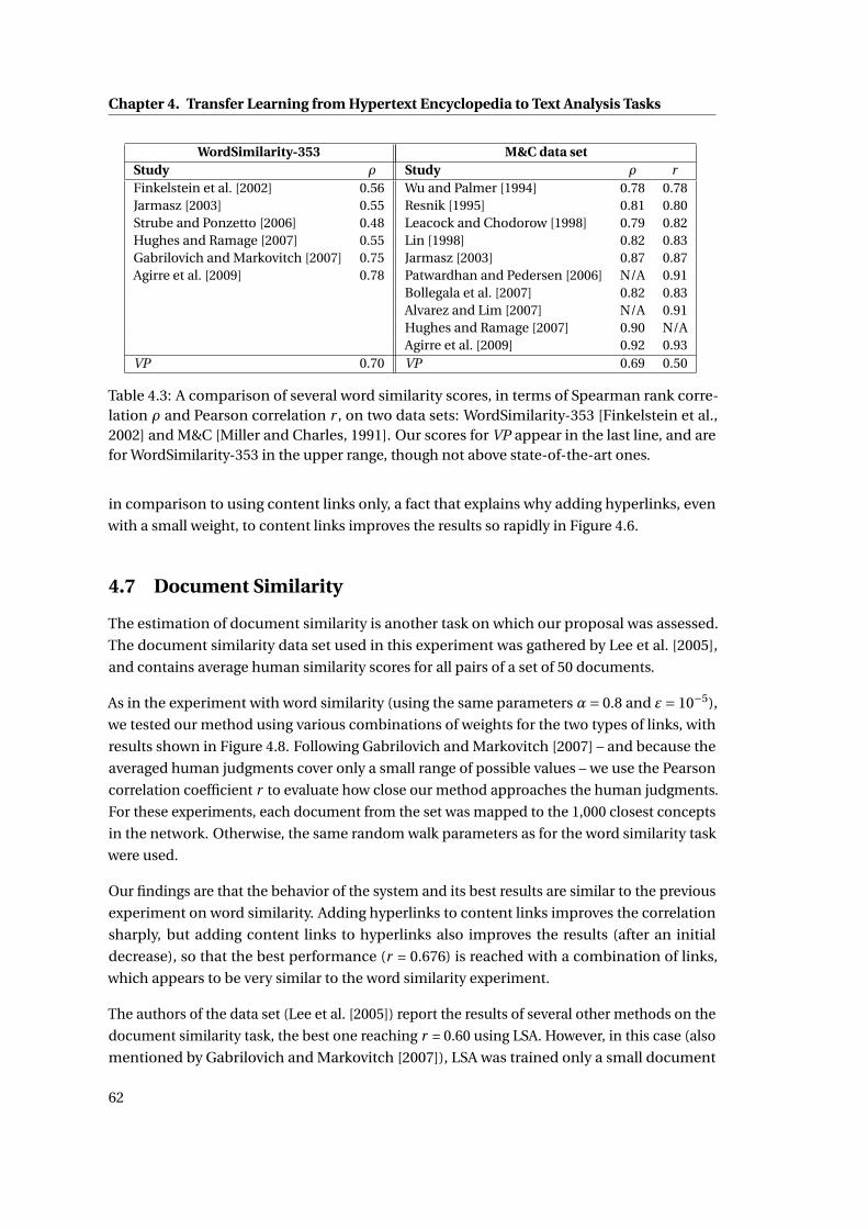
Chapter 4. Transfer Learning from Hypertext Encyclopedia to Text Analysis Tasks
WordSimilarity-353 M&C data setStudy ρ Study ρ rFinkelstein et al. [2002] 0.56 Wu and Palmer [1994] 0.78 0.78Jarmasz [2003] 0.55 Resnik [1995] 0.81 0.80Strube and Ponzetto [2006] 0.48 Leacock and Chodorow [1998] 0.79 0.82Hughes and Ramage [2007] 0.55 Lin [1998] 0.82 0.83Gabrilovich and Markovitch [2007] 0.75 Jarmasz [2003] 0.87 0.87Agirre et al. [2009] 0.78 Patwardhan and Pedersen [2006] N/A 0.91
Bollegala et al. [2007] 0.82 0.83Alvarez and Lim [2007] N/A 0.91Hughes and Ramage [2007] 0.90 N/AAgirre et al. [2009] 0.92 0.93
VP 0.70 VP 0.69 0.50
Table 4.3: A comparison of several word similarity scores, in terms of Spearman rank corre-lation ρ and Pearson correlation r , on two data sets: WordSimilarity-353 [Finkelstein et al.,2002] and M&C [Miller and Charles, 1991]. Our scores for VP appear in the last line, and arefor WordSimilarity-353 in the upper range, though not above state-of-the-art ones.
in comparison to using content links only, a fact that explains why adding hyperlinks, even
with a small weight, to content links improves the results so rapidly in Figure 4.6.
4.7 Document Similarity
The estimation of document similarity is another task on which our proposal was assessed.
The document similarity data set used in this experiment was gathered by Lee et al. [2005],
and contains average human similarity scores for all pairs of a set of 50 documents.
As in the experiment with word similarity (using the same parameters α= 0.8 and ε= 10−5),
we tested our method using various combinations of weights for the two types of links, with
results shown in Figure 4.8. Following Gabrilovich and Markovitch [2007] – and because the
averaged human judgments cover only a small range of possible values – we use the Pearson
correlation coefficient r to evaluate how close our method approaches the human judgments.
For these experiments, each document from the set was mapped to the 1,000 closest concepts
in the network. Otherwise, the same random walk parameters as for the word similarity task
were used.
Our findings are that the behavior of the system and its best results are similar to the previous
experiment on word similarity. Adding hyperlinks to content links improves the correlation
sharply, but adding content links to hyperlinks also improves the results (after an initial
decrease), so that the best performance (r = 0.676) is reached with a combination of links,
which appears to be very similar to the word similarity experiment.
The authors of the data set (Lee et al. [2005]) report the results of several other methods on the
document similarity task, the best one reaching r = 0.60 using LSA. However, in this case (also
mentioned by Gabrilovich and Markovitch [2007]), LSA was trained only a small document
62
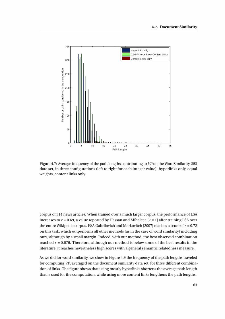
4.7. Document Similarity
Figure 4.7: Average frequency of the path lengths contributing to VP on the WordSimilarity-353data set, in three configurations (left to right for each integer value): hyperlinks only, equalweights, content links only.
corpus of 314 news articles. When trained over a much larger corpus, the performance of LSA
increases to r = 0.69, a value reported by Hassan and Mihalcea [2011] after training LSA over
the entire Wikipedia corpus. ESA Gabrilovich and Markovitch [2007] reaches a score of r = 0.72
on this task, which outperforms all other methods (as in the case of word similarity) including
ours, although by a small margin. Indeed, with our method, the best observed combination
reached r = 0.676. Therefore, although our method is below some of the best results in the
literature, it reaches nevertheless high scores with a general semantic relatedness measure.
As we did for word similarity, we show in Figure 4.9 the frequency of the path lengths traveled
for computing VP, averaged on the document similarity data set, for three different combina-
tion of links. The figure shows that using mostly hyperlinks shortens the average path length
that is used for the computation, while using more content links lengthens the path lengths.
63
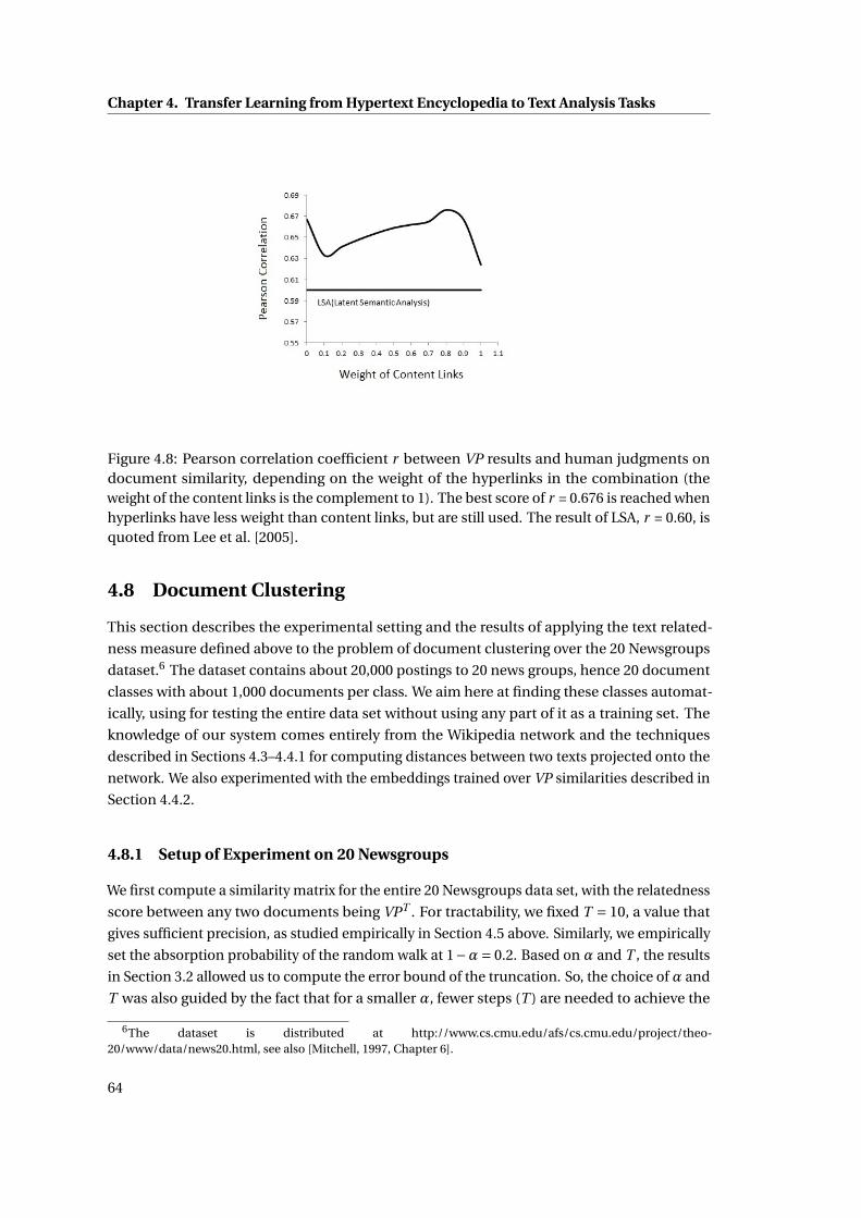
Chapter 4. Transfer Learning from Hypertext Encyclopedia to Text Analysis Tasks
Figure 4.8: Pearson correlation coefficient r between VP results and human judgments ondocument similarity, depending on the weight of the hyperlinks in the combination (theweight of the content links is the complement to 1). The best score of r = 0.676 is reached whenhyperlinks have less weight than content links, but are still used. The result of LSA, r = 0.60, isquoted from Lee et al. [2005].
4.8 Document Clustering
This section describes the experimental setting and the results of applying the text related-
ness measure defined above to the problem of document clustering over the 20 Newsgroups
dataset.6 The dataset contains about 20,000 postings to 20 news groups, hence 20 document
classes with about 1,000 documents per class. We aim here at finding these classes automat-
ically, using for testing the entire data set without using any part of it as a training set. The
knowledge of our system comes entirely from the Wikipedia network and the techniques
described in Sections 4.3–4.4.1 for computing distances between two texts projected onto the
network. We also experimented with the embeddings trained over VP similarities described in
Section 4.4.2.
4.8.1 Setup of Experiment on 20 Newsgroups
We first compute a similarity matrix for the entire 20 Newsgroups data set, with the relatedness
score between any two documents being VPT . For tractability, we fixed T = 10, a value that
gives sufficient precision, as studied empirically in Section 4.5 above. Similarly, we empirically
set the absorption probability of the random walk at 1−α= 0.2. Based on α and T , the results
in Section 3.2 allowed us to compute the error bound of the truncation. So, the choice ofα and
T was also guided by the fact that for a smaller α, fewer steps (T ) are needed to achieve the
6The dataset is distributed at http://www.cs.cmu.edu/afs/cs.cmu.edu/project/theo-20/www/data/news20.html, see also [Mitchell, 1997, Chapter 6].
64
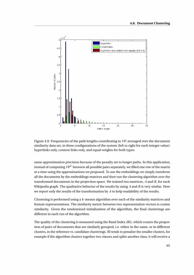
4.8. Document Clustering
Figure 4.9: Frequencies of the path lengths contributing to VP, averaged over the documentsimilarity data set, in three configurations of the system (left to right for each integer value):hyperlinks only, content links only, and equal weights for both types.
same approximation precision because of the penalty set to longer paths. In this application,
instead of computing VPT between all possible pairs separately, we filled one row of the matrix
at a time using the approximations we proposed. To use the embeddings we simply transform
all the documents by the embeddings matrices and then run the clustering algorithm over the
transformed documents in the projection space. We trained two matrices, A and B , for each
Wikipedia graph. The qualitative behavior of the results by using A and B is very similar. Here
we report only the results of the transformation by A to help readability of the results.
Clustering is performed using a k-means algorithm over each of the similarity matrices and
feature representations. The similarity metric between two representation vectors is cosine
similarity. Given the randomized initialization of the algorithm, the final clusterings are
different in each run of the algorithm.
The quality of the clustering is measured using the Rand Index (RI), which counts the propor-
tion of pairs of documents that are similarly grouped, i.e. either in the same, or in different
clusters, in the reference vs. candidate clusterings. RI tends to penalize the smaller clusters, for
example if the algorithm clusters together two classes and splits another class, it will receive a
65
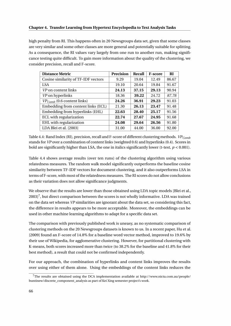
Chapter 4. Transfer Learning from Hypertext Encyclopedia to Text Analysis Tasks
high penalty from RI. This happens often in 20 Newsgroups data set, given that some classes
are very similar and some other classes are more general and potentially suitable for splitting.
As a consequence, the RI values vary largely from one run to another run, making signifi-
cance testing quite difficult. To gain more information about the quality of the clustering, we
consider precision, recall and F-score.
Distance Metric Precision Recall F-score RICosine similarity of TF-IDF vectors 9.29 19.04 12.49 86.67LSA 19.10 20.64 19.84 91.67VP on content links 24.13 37.15 29.13 90.94VP on hyperlinks 18.36 39.22 24.72 87.78VPComb (0.6 content links) 24.26 36.91 29.23 91.03Embedding from content links (ECL) 21.30 26.13 23.47 91.48Embedding from hyperlinks (EHL) 22.63 28.40 25.17 91.56ECL with regularization 22.74 27.67 24.95 91.68EHL with regularization 24.08 29.64 26.56 91.80LDA Blei et al. [2003] 31.00 44.00 36.00 92.00
Table 4.4: Rand Index (RI), precision, recall and F-score of different clustering methods. VPComb
stands for VP over a combination of content links (weighted 0.6) and hyperlinks (0.4). Scores inbold are significantly higher than LSA, the one in italics significantly lower (t-test, p < 0.001).
Table 4.4 shows average results (over ten runs) of the clustering algorithm using various
relatedness measures. The random walk model significantly outperforms the baseline cosine
similarity between TF-IDF vectors for document clustering, and it also outperforms LSA in
terms of F-score, with most of the relatedness measures. The RI scores do not allow conclusions
as their variation does not allow significance judgments.
We observe that the results are lower than those obtained using LDA topic models [Blei et al.,
2003]7, but direct comparison between the scores is not wholly informative. LDA was trained
on the data set whereas VP similarities are ignorant about the data set, so considering this fact,
the difference in results appears to be more acceptable. Moreover, the embeddings can be
used in other machine learning algorithms to adapt for a specific data set.
The comparison with previously published work is uneasy, as no systematic comparison of
clustering methods on the 20 Newsgroups datasets is known to us. In a recent paper, Hu et al.
[2009] found an F-score of 14.8% for a baseline word vector method, improved to 19.6% by
their use of Wikipedia, for agglomerative clustering. However, for partitional clustering with
K-means, both scores increased more than twice (to 38.2% for the baseline and 41.8% for their
best method), a result that could not be confirmed independently.
For our approach, the combination of hyperlinks and content links improves the results
over using either of them alone. Using the embeddings of the content links reduces the
7The results are obtained using the DCA implementation available at http://www.nicta.com.au/people/buntinew/discrete_component_analysis as part of Kei Xing semester project’s work.
66
4.8. Document Clustering
performance in comparison to the computation of the VP values over the graph. On the
contrary, using embeddings of the hyperlinks improves the results in comparison to using the
VP values over the hyperlinks graph.
The embedding learned on VP similarities over the hyperlinks appears to provide a more
general similarity measure, with does not overfit to the Hyperlinks graph of Wikipedia. The
high recall it obtains is related to the larger extension of paths computed with hyperlinks,
which can connect many documents together and attach them to the same class, while the
high precision obtained using content links is due to their tendency to cluster into smaller
neighborhoods.
Although the regularization imposed on the embeddings reduced their predictive power for
the VP similarities, but it improves the performance on this task.
Computation time using embeddings is (as expected) greatly reduced, as computations are
performed in the low-dimensional latent space. Moreover, other unsupervised clustering
algorithms can be applied to the documents transformed by the embeddings, e.g. the state-of-
the-art clustering algorithm proposed by Bordogna and Pasi [2009].
4.8.2 Comparison of VP and Cosine Similarity
To find out in which cases the proposed method improves over a simple cosine similarity
measure, we considered a linear combination of the cosine similarity and VPComb (VP over
content links weighed 0.6 and hyperlinks weighed 0.4), namely w ×VPComb + (1−w)×LS,
and varied the weight w from 0 to 1. Considering the k-nearest neighbors of every document
according to this combined similarity, we define k-purity as the number of documents with
the correct label over the total number of documents k in the computed neighborhood. The
variation of k-purity with w , for several sample values of k, is shown in Figure 4.10.
The best purity appears to be obtained for a combination of the two methods, for all values of k
that were tested. This shows that VPComb brings valuable additional information about docu-
ment relatedness that cannot be found in LS only. Furthermore, when the size of the examined
neighborhood k increases (lower curves in Figure 4.10), the effect of VPComb becomes more
important, i.e. its weight in the optimal combination increases. For very small neighborhoods,
LS is almost sufficient to ensure optimal purity, but for larger ones (k = 10 or 15), VPComb used
alone (w = 1) outperforms LS used alone (w = 0). Their optimal combination leads to scores
that are higher than those obtained for each of them used separately, and, as noted, the weight
of VPComb in the optimal combination increases for larger neighborhoods.
These results can be explained as follows. For very small neighborhoods, the cosine lexical
similarity score with the nearest 1–5 documents is very high, as they have many words in
common, so LS is a good measure of text relatedness. However, when looking at larger
neighborhoods, for which relatedness is less based on identical words, then VPComb becomes
more effective, and LS performs poorly. Therefore, we can predict that VPComb will be most
67
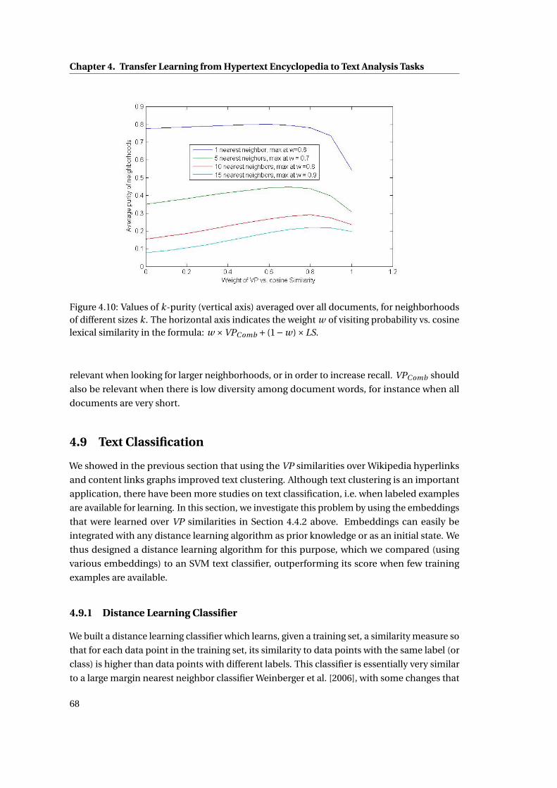
Chapter 4. Transfer Learning from Hypertext Encyclopedia to Text Analysis Tasks
Figure 4.10: Values of k-purity (vertical axis) averaged over all documents, for neighborhoodsof different sizes k. The horizontal axis indicates the weight w of visiting probability vs. cosinelexical similarity in the formula: w ×VPComb + (1−w)×LS.
relevant when looking for larger neighborhoods, or in order to increase recall. VPComb should
also be relevant when there is low diversity among document words, for instance when all
documents are very short.
4.9 Text Classification
We showed in the previous section that using the VP similarities over Wikipedia hyperlinks
and content links graphs improved text clustering. Although text clustering is an important
application, there have been more studies on text classification, i.e. when labeled examples
are available for learning. In this section, we investigate this problem by using the embeddings
that were learned over VP similarities in Section 4.4.2 above. Embeddings can easily be
integrated with any distance learning algorithm as prior knowledge or as an initial state. We
thus designed a distance learning algorithm for this purpose, which we compared (using
various embeddings) to an SVM text classifier, outperforming its score when few training
examples are available.
4.9.1 Distance Learning Classifier
We built a distance learning classifier which learns, given a training set, a similarity measure so
that for each data point in the training set, its similarity to data points with the same label (or
class) is higher than data points with different labels. This classifier is essentially very similar
to a large margin nearest neighbor classifier Weinberger et al. [2006], with some changes that
68
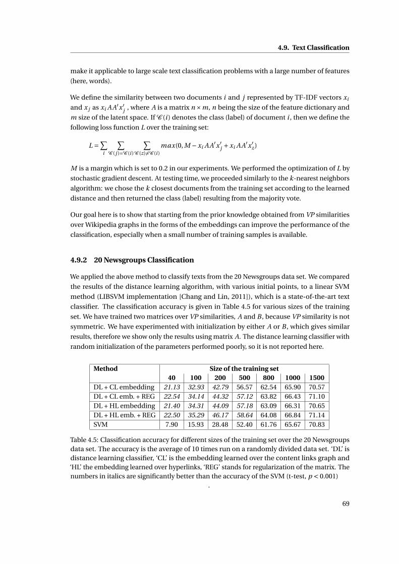
4.9. Text Classification
make it applicable to large scale text classification problems with a large number of features
(here, words).
We define the similarity between two documents i and j represented by TF-IDF vectors xi
and x j as xi A A′x ′j , where A is a matrix n ×m, n being the size of the feature dictionary and
m size of the latent space. If C (i ) denotes the class (label) of document i , then we define the
following loss function L over the training set:
L =∑i
∑C ( j )=C (i )
∑C (z) 6=C (i )
max(0, M −xi A A′x ′j +xi A A′x ′
z )
M is a margin which is set to 0.2 in our experiments. We performed the optimization of L by
stochastic gradient descent. At testing time, we proceeded similarly to the k-nearest neighbors
algorithm: we chose the k closest documents from the training set according to the learned
distance and then returned the class (label) resulting from the majority vote.
Our goal here is to show that starting from the prior knowledge obtained from VP similarities
over Wikipedia graphs in the forms of the embeddings can improve the performance of the
classification, especially when a small number of training samples is available.
4.9.2 20 Newsgroups Classification
We applied the above method to classify texts from the 20 Newsgroups data set. We compared
the results of the distance learning algorithm, with various initial points, to a linear SVM
method (LIBSVM implementation [Chang and Lin, 2011]), which is a state-of-the-art text
classifier. The classification accuracy is given in Table 4.5 for various sizes of the training
set. We have trained two matrices over VP similarities, A and B , because VP similarity is not
symmetric. We have experimented with initialization by either A or B , which gives similar
results, therefore we show only the results using matrix A. The distance learning classifier with
random initialization of the parameters performed poorly, so it is not reported here.
Method Size of the training set40 100 200 500 800 1000 1500
DL + CL embedding 21.13 32.93 42.79 56.57 62.54 65.90 70.57DL + CL emb. + REG 22.54 34.14 44.32 57.12 63.82 66.43 71.10DL + HL embedding 21.40 34.31 44.09 57.18 63.09 66.31 70.65DL + HL emb. + REG 22.50 35.29 46.17 58.64 64.08 66.84 71.14SVM 7.90 15.93 28.48 52.40 61.76 65.67 70.83
Table 4.5: Classification accuracy for different sizes of the training set over the 20 Newsgroupsdata set. The accuracy is the average of 10 times run on a randomly divided data set. ‘DL’ isdistance learning classifier, ‘CL’ is the embedding learned over the content links graph and‘HL’ the embedding learned over hyperlinks, ‘REG’ stands for regularization of the matrix. Thenumbers in italics are significantly better than the accuracy of the SVM (t-test, p < 0.001)
.
69
Chapter 4. Transfer Learning from Hypertext Encyclopedia to Text Analysis Tasks
The first important observation is that, when the training set is small, the distance learning
classifier initialized with the embeddings from VP similarities over Wikipedia graphs out-
performs the baseline SVM classifier significantly. By adding more and more labeled data,
the importance of prior knowledge appears to decrease, presumably because the distance
learning algorithm can infer reliable decisions based only on the training data. A similar effect
was shown for a method based on deep learning by Ranzato and Szummer [2008], with their
method and a TF-IDF/SVM method both reaching 65% accuracy for more than 50 samples
per class (corresponding to 1000 total samples) in the training data.
The second observation is that the orthonormality regularization that we imposed on the
embeddings again improved the performance. The generalization ability was improved at
the price of decreasing slightly the precision in the approximation of the VP values. A third
observation is that the accuracy using hyperlinks was slightly higher than using content links.
4.10 Information Retrieval
In this section, we apply the proposed distance to information retrieval data from TREC-7 and
TREC-8 [Voorhees and Harman, 1999]. The application of our method to a large scale informa-
tion retrieval task requires the computation of VP between a query and the representation of
all the documents in the repository. By using the approximations proposed in Section 3.2, we
can compute T -truncated VP between every query and documents in an acceptable amount
of time. Firstly, we map all documents in the data set to the Wikipedia graph; then, at query
time, each query is mapped to the graph; finally, for each query, VPT is computed to and from
all documents in the data set by using the proposed approximations. In this section, we use
α = 0.8 , T = 10 and a combination of hyperlinks and content links in VP weighted 0.2/0.8,
following observations from previous sections. The time-consuming operation is the first one
– viz., mapping a large collection of documents to the Wikipedia graph – but this is done only
once, before query time.
We used the TREC-7 and TREC-8 Ad-hoc Test Collections.8 The data set includes a repository
of 530,000 documents and two sets of 50 queries. For each query, the data set also provides
relevance judgments for a subset of documents considered to be related to the query, as they
were retrieved by a pool of search methods, a method that is intended to maximize recall.
To study the effect of VP in comparison to lexical similarity and TF-IDF scoring in a single
retrieval operation, we compute for each document and query a linear combination of VPT
with weight w and of lexical similarity with weight 1−w . The weight w thus sets the relative
importance of conceptual relatedness vs. lexical similarity, and will serve to illustrate their
respective contributions. We will refer to this as the Combined similarity. We measure the
IR performance through the average precision of the first 10 returned documents (10 is the
8These are available at http://trec.nist.gov, and we used more specifically the test queries (topics) numbers351–400 and 401–450, with the associated relevance judgments. The documents are available from the LinguisticData Consortium.
70
4.11. Learning to Rank by Using VP Similarities
typical size of the first result page of Web search engines).
We computed all the scores for w = 0 to w = 1 with increments of 0.1, and found out that the
highest score was reached for w = 0.1 for the TREC-7 data set. This optimized value was then
tested over the TREC-8 query set (50 topics), leading to an average precision for Combined of
0.515 , which improves (+15.4 %) over the precision of lexical similarity alone (w = 0), which is
0.446. Egozi et al. [2011] reported precision at 10 on TREC-8 data for various bag-of-words
information retrieval systems (Xapian, Okapi, LM-KL-DIR) along with improved results (up
to 14%) obtained by using a new retrieval algorithm, which integrates ESA [Gabrilovich and
Markovitch, 2009] semantic similarity to the previous systems.9 Here, we reported the mean
average precision at 10, which is the lower bound of precision at 10, but is more informative
than it. Direct comparison between our scores and the scores reported in [Egozi et al., 2011] is
not possible, as they used different base retrieval systems.
We also examined the precision score for every query separately. In particular, we counted the
proportion of queries for which the Combined similarity returned more relevant documents
than lexical similarity alone. Combined similarity outperformed the lexical one on 14 queries,
while the reverse was true for 5 queries only, and the scores were identical on the remaining
31 queries. The average score difference between Combined and lexical similarity is 0.018
(maximum is 1). This value is not significantly above 0 at the usual levels (e.g. p < 0.01), but we
found using a normal distribution that the probability of the true difference being zero, given
the observations, is only p = 0.11. While this does not ensure that the Combined similarity is
“significantly” better than the lexical one, it still provide encouraging evidence for the utility of
VP on the TREC-8 test set.
The precision scores of both methods vary considerably across queries. We therefore examined
separately the “difficult” queries, defined here as the queries on which lexical similarity had
a score of 0.3 or less (meaning it returned between 0 and 3 relevant documents). There are
21 such queries out of 50 on the TREC-8 test set. Over these queries, the Combined similarity
outperforms the lexical one on 7, while the reverse is true for only one, and 13 queries are a
tie. Of course, it might seem unsurprising to see this difference as these queries are “difficult”
for the lexical similarity by definition. However, when examining the 20 queries that are
“difficult” for the Combined similarity, this measure still outperforms the lexical one on 5,
while the reverse is true for only two, and 13 are a tie. These results show that VP provides
complementary information that can improve the results of lexical similarity for IR, especially
for queries on which lexical similarity performs less well.
4.11 Learning to Rank by Using VP Similarities
We have seen in the previous section that the linear combination of the VP and lexical similari-
ties improved only slightly the retrieval results, although VP provides additional information.
9Precision at 10 was improved as follows: for Xapian from 0.472 to 0.478 (+1.3%), for Okapi from 0.488 to 0.522(+7.0%), and for LM-KL-DIR from 0.442 to 0.506 (+14.4%).
71
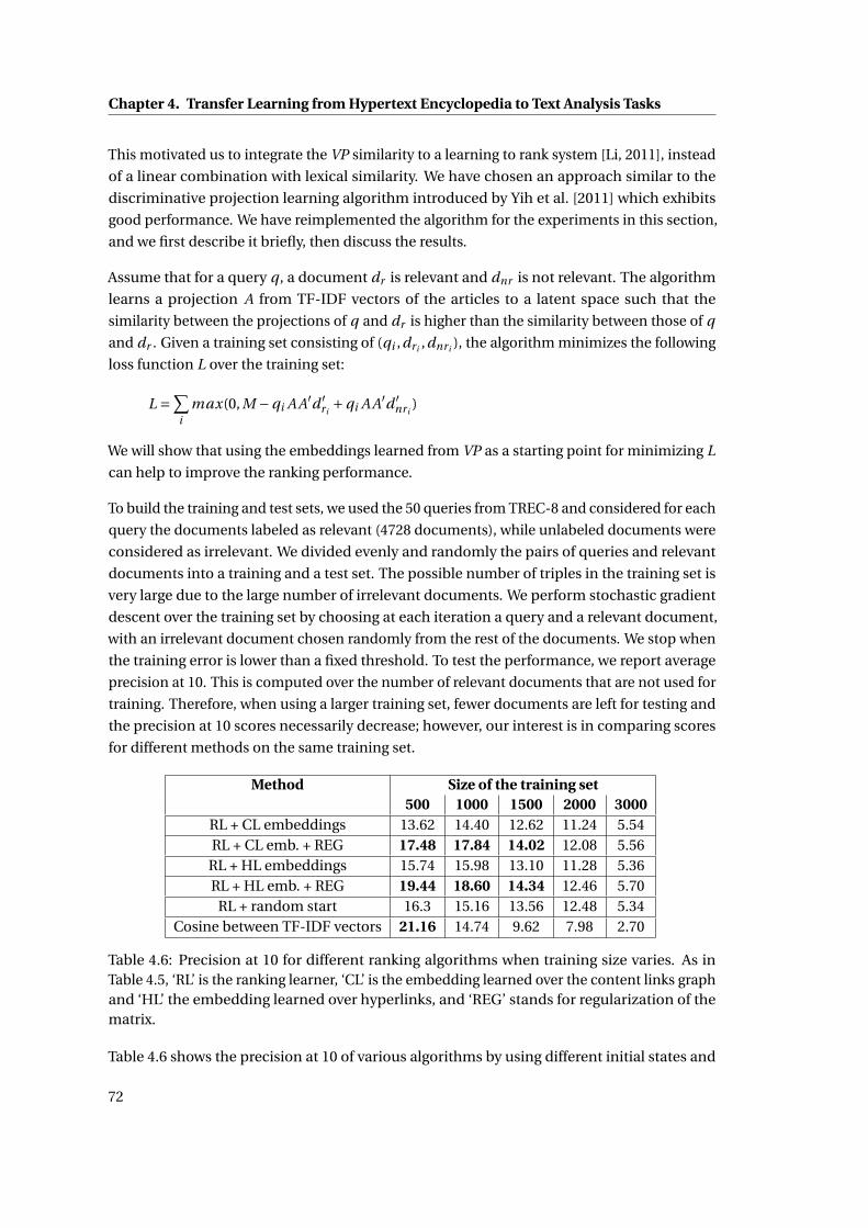
Chapter 4. Transfer Learning from Hypertext Encyclopedia to Text Analysis Tasks
This motivated us to integrate the VP similarity to a learning to rank system [Li, 2011], instead
of a linear combination with lexical similarity. We have chosen an approach similar to the
discriminative projection learning algorithm introduced by Yih et al. [2011] which exhibits
good performance. We have reimplemented the algorithm for the experiments in this section,
and we first describe it briefly, then discuss the results.
Assume that for a query q , a document dr is relevant and dnr is not relevant. The algorithm
learns a projection A from TF-IDF vectors of the articles to a latent space such that the
similarity between the projections of q and dr is higher than the similarity between those of q
and dr . Given a training set consisting of (qi ,dri ,dnri ), the algorithm minimizes the following
loss function L over the training set:
L =∑i
max(0, M −qi A A′d ′ri+qi A A′d ′
nri)
We will show that using the embeddings learned from VP as a starting point for minimizing L
can help to improve the ranking performance.
To build the training and test sets, we used the 50 queries from TREC-8 and considered for each
query the documents labeled as relevant (4728 documents), while unlabeled documents were
considered as irrelevant. We divided evenly and randomly the pairs of queries and relevant
documents into a training and a test set. The possible number of triples in the training set is
very large due to the large number of irrelevant documents. We perform stochastic gradient
descent over the training set by choosing at each iteration a query and a relevant document,
with an irrelevant document chosen randomly from the rest of the documents. We stop when
the training error is lower than a fixed threshold. To test the performance, we report average
precision at 10. This is computed over the number of relevant documents that are not used for
training. Therefore, when using a larger training set, fewer documents are left for testing and
the precision at 10 scores necessarily decrease; however, our interest is in comparing scores
for different methods on the same training set.
Method Size of the training set500 1000 1500 2000 3000
RL + CL embeddings 13.62 14.40 12.62 11.24 5.54RL + CL emb. + REG 17.48 17.84 14.02 12.08 5.56
RL + HL embeddings 15.74 15.98 13.10 11.28 5.36RL + HL emb. + REG 19.44 18.60 14.34 12.46 5.70
RL + random start 16.3 15.16 13.56 12.48 5.34Cosine between TF-IDF vectors 21.16 14.74 9.62 7.98 2.70
Table 4.6: Precision at 10 for different ranking algorithms when training size varies. As inTable 4.5, ‘RL’ is the ranking learner, ‘CL’ is the embedding learned over the content links graphand ‘HL’ the embedding learned over hyperlinks, and ‘REG’ stands for regularization of thematrix.
Table 4.6 shows the precision at 10 of various algorithms by using different initial states and
72
4.12. Application to Just-in-Time Retrieval
different number of training samples. The first observation is that only when the training size
is very small, 10 documents on average for each query, the cosine similarity outperforms the
learning to rank algorithms. Otherwise, the performance of the learning to rank algorithms is
always better than the cosine similarity.
The second result is that when the number of training examples is small, the learning algorithm
initialized with the regularized embeddings outperforms the random initialization. Gradually,
when adding more training examples, it becomes less useful to leverage the prior knowledge,
as the learning algorithm can solve the problem better simply by looking at training samples.
Similarly to the classification experiments, the embeddings learned over the hyperlinks are
more useful than the ones learned over the content links.
4.12 Application to Just-in-Time Retrieval
The Automatic Content Linking Device (ACLD) is a just-in-time document retrieval system
which monitors an ongoing conversation or a monologue and enriches it with potentially
related documents, including multimedia ones, from local repositories or from the Internet
[Popescu-Belis et al., 2008, 2011]. The documents are found using a similarity measure
between documents and the words obtained from automatic speech recognition (ASR). Results
are displayed in real time to meeting participants, or to users watching a recorded lecture or
conversation.
ACLD can be performed over live or recorded lectures, for instance in a computer-assisted
learning environment for individual students. The ACLD enriches the lectures with related
material drawn from various repositories, through a search process that can be guided in real
time by its user.
The goal of our method is to use the proposed semantic similarity to improve the relevance
of the retrieved documents, and to make the mechanism more robust to noise from the
ASR. The goal is to enrich the the conversation with the most related articles from Wikipedia.
Query object is built by using the words obtained from ASR in a given timeframe, stop words
removed. We map the query to the corresponding articles in Wikipedia network using the
method explained in Section 4.4.1. The set of K closest articles based on the symmetric VP
similarity is returned using the algorithms explained in Chapter 3.
We compared the output of semantic similarity search with that of keyword-based search
(see also [Habibi and Popescu-Belis, 2012] for an additional comparison). The ASR transcript
of one AMI meeting (ES2008d) was passed to both search methods, and “evaluation snip-
pets” containing the manual transcript for one-minute excerpts, accompanied by the 8-best
Wikipedia articles found by each method were produced. Overall, 36 snippets were generated.
The manual transcript shown to subjects was enriched with punctuation and speakers’ names,
and the names of the Wikipedia pages were placed on each side of the transcript frame.
73
Chapter 4. Transfer Learning from Hypertext Encyclopedia to Text Analysis Tasks
Subjects were then asked to read each snippet, and decide which of the two document sets
was the most relevant to the discussion taking place, i.e. the most useful as a suggestion to the
participants. They could also answer ‘none’, and could consult the result if necessary. Results
were obtained from 8 subjects, each seeing 9 snippets out of 36. Every snippet was thus seen
by two subjects. The subjects agreed on 23 (64%) snippets and disagreed on 13 (36%).
In fact, the number of true disagreements not including the answer ‘none’ was only 7 out of
36. Over the 23 snippets on which subjects agreed, the result of semantic search was judged
more relevant than that of keyword search for 19 snippets (53% of the total), and the reverse
for 4 snippets only (11%). Alternatively, if one counts the votes cast by subjects in favor of
each system, regardless of agreement, then semantic search received 72% of the votes and
keyword-based only 28%. These numbers show that semantic search quite clearly improves
relevance in comparison to keyword-based one.
The query objects built on words obtained from ASR of a meeting fragment are noisy. This noise
comes mainly from two sources, first noises entered by ASR error and second, the unfocused
nature of the discussions. For example, if a meeting fragment is about reinforcement learning,
we might have words like “enforcement” in the query object which results from ASR error.
Also there might be words about “game design” as it was mentioned as an application of
reinforcement learning. Moreover, the query objects might be consisting of ambiguous words.
In all these cases, when the query is mapped to the corresponding concepts, the effect of noise
– which is less consistent with the majority of the query – reduces. In our hypothetical example
the majority of the mapped concepts are related to reinforcement learning with high weights
(probability) and there are few unrelated concepts with low probabilities. When the random
walk starts the related pages, which have high initial weights or connected through either
type of links to the high weighted pages, get to the top of the list, and unrelated pages drop to
the bottom of the list. Therefore, the second round of denoising of the recommended set is
done by the random walk and therefore, the relevance of the recommended set is improved in
comparison to the keyword based approach.
4.13 Perspectives: Two-Stage Random Walks
In addition to the above experiments, we examined two-stage random walks, in which at
the first stage, the network is built using one set of weights on the links, and in the second
stage using a different set. The hypothesis here is that some links might be more useful when
explored first, while some others might be more useful when explored later, as discussed by
Collins-Thompson and Callan [2005].
For the word similarity task, we focused on ε-truncated two-stage walks in which one combina-
tion of links is used for the first three steps of the random walker, and a different combination
from the fourth to the last steps. The choice of three steps was empirical, by looking at the
average length of single-stage ε-truncated walks. We report the ρ scores of three significant
74
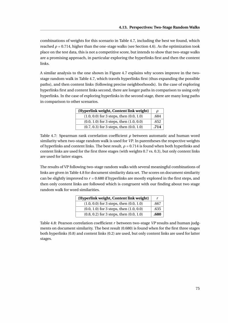
4.13. Perspectives: Two-Stage Random Walks
combinations of weights for this scenario in Table 4.7, including the best we found, which
reached ρ = 0.714, higher than the one-stage walks (see Section 4.6). As the optimization took
place on the test data, this is not a competitive score, but intends to show that two-stage walks
are a promising approach, in particular exploring the hyperlinks first and then the content
links.
A similar analysis to the one shown in Figure 4.7 explains why scores improve in the two-
stage random walk in Table 4.7, which travels hyperlinks first (thus expanding the possible
paths), and then content links (following precise neighborhoods). In the case of exploring
hyperlinks first and content links second, there are longer paths in comparison to using only
hyperlinks. In the case of exploring hyperlinks in the second stage, there are many long paths
in comparison to other scenarios.
(Hyperlink weight, Content link weight) ρ
(1.0, 0.0) for 3 steps, then (0.0, 1.0) .684(0.0, 1.0) for 3 steps, then (1.0, 0.0) .652(0.7, 0.3) for 3 steps, then (0.0, 1.0) .714
Table 4.7: Spearman rank correlation coefficient ρ between automatic and human wordsimilarity when two-stage random walk is used for VP. In parentheses the respective weightsof hyperlinks and content links. The best result, ρ = 0.714 is found when both hyperlinks andcontent links are used for the first three stages (with weights 0.7 vs. 0.3), but only content linksare used for latter stages.
The results of VP following two-stage random walks with several meaningful combinations of
links are given in Table 4.8 for document similarity data set. The scores on document similarity
can be slightly improved to r = 0.680 if hyperlinks are mostly explored in the first steps, and
then only content links are followed which is congruent with our finding about two stage
random walk for word similarities.
(Hyperlink weight, Content link weight) r(1.0, 0.0) for 3 steps, then (0.0, 1.0) .667(0.0, 1.0) for 3 steps, then (1.0, 0.0) .635(0.8, 0.2) for 3 steps, then (0.0, 1.0) .680
Table 4.8: Pearson correlation coefficient r between two-stage VP results and human judg-ments on document similarity. The best result (0.680) is found when for the first three stagesboth hyperlinks (0.8) and content links (0.2) are used, but only content links are used for latterstages.
75

5 Joint Similarity Learning for Predict-ing Links in Multi-Link Networks
In this chapter, we address the problem of link prediction on large networks with links of
multiple types (or in short multi-link networks) by proposing two joint similarity learning
architectures over the nodes’ attributes. The first model is a similarity metric that consists of
two parts: a general part, which is shared between all link types, and a specific part, which
learns the similarity for each link type specifically.
The second model consists of two layers: the first one, which is shared between all link types,
embeds the objects of the network into a new space, while the second one learns the similarity
between objects for each link type in this new space. The similarity metrics are optimized
using a large-margin optimization criterion in which connected objects should be closer than
non-connected ones by a certain margin.
A stochastic training algorithm is proposed, which makes the training applicable to large
networks with high-dimensional feature spaces. The models are tested on link prediction for
two data sets with two types of links each: TED talks (1150 items) and Amazon products (10,000
items). The experiments show that jointly modeling the links in our framework improves link
prediction performance significantly for each link type. The improvement is particularly high
when there are fewer links available from one link type in the network. Moreover, we show that
transfer learning from one link type to another one is possible using the above frameworks.
The chapter is organized as follows. Following an outline of the motivations, we introduce
in Section 5.2 the joint models for multiple-type links, first by defining the shared similarity
model, and then by defining the -layer similarity model. We then describe the large-margin
method for training the similarity functions (5.2.4). We also show how to generalize the
proposed framework to jointly model link prediction and classification in a network (5.2.5).
The experiments described in Section 5.3 on the above-mentioned networks demonstrate the
predictive power of the joint model, in comparison with separate models, as well as with SVM
Rank and cosine similarity.
77
Chapter 5. Joint Similarity Learning for Predicting Links in Multi-Link Networks
5.1 Motivations
The problem of new link prediction in networks is particularly relevant to networks that are
collaboratively built over time, whether they are document-based (such as Wikipedia, or
databases of products or multimedia records) or person-based (social networks such as Face-
book or LinkedIn) or both. In such situations, some nodes become connected over time due to
similarities or affinities that are noticed and validated by users. Predicting such connections is
a functionality which is valuable to speed up network construction, for instance by presenting
these connections as recommendations to users, as discussed in the introduction to this thesis.
However, this is particularly challenging when links are of multiple types. Moreover, accurate
modeling of the connections in the network can be useful to predict the evolution of the
network or even to perform marketing via the network.
We introduce in this chapter two joint link prediction models for networks with multiple link
types. Link prediction is formulated as a learning to rank problem: given a query node, all
other nodes must be sorted according to a score that is related to the likelihood of creating a
link between them and the query node. The proposed link prediction models learn a similarity
metric according to which connected nodes are closer than non-connected nodes.
Two different joint models will be proposed. The shared similarity model consists of two
parts: the general part, which is a shared similarity function between all types of links, and the
specific part, which learns similarity specifically for each type of links. The two-layer similarity
model consists of two layers: in the first layer, objects in the network are embedded into a
new space, while the second layer learns the similarity between objects for each link type
specifically in this new space. The first layer is shared between all link types and can also be
considered as a representation of objects which is common across all link types.
5.2 Joint Similarity for Multiple-Type Link Prediction
Link prediction can be viewed as a ranking problem in which all objects in the network are
ranked based on their similarity score with respect to a query object. A “better” ranking is
one that places objects that are actually linked to the query object at the top of the ranked list.
The score between the two objects in the network can be considered as a similarity metric (or,
conversely, a distance one), and link prediction can be interpreted as a task in which linked
objects should be closer to the query object, in comparison to the non-linked objects.
We model the link structure of a network by learning a similarity measure which, for each
object in the network, assigns larger scores to the objects that are linked to it than to those that
are not. To model N different types of links, we train N different similarity functions, so that
we model the link structure of each type separately. However, in many real-world networks,
links of a certain type are not entirely independent from links of other types. To consider this
dependency, each link-type similarity model shares information with the other models. We
will show in Section 5.3 that the joint modeling increases generalization abilities, hence link
78
5.2. Joint Similarity for Multiple-Type Link Prediction
prediction performance, especially when there are few links from one specific link type.
5.2.1 Similarity Learning Framework
In this section, we build a similarity based ranker to model links in the network. The ranker
returns a score for a given query object q and a target object t by using a similarity function
over their features. If fi (q, t ) represents the ranker for link type i , and xo is the feature vector
of an object o from the network, then we have:
fi (q, t ) = similarityi (xq , xt )
The similarityi function computes a similarity for link type i between objects q and t using
their attributes, following a classical approach for learning to rank methods. Many similarity
functions (or, equivalently, distance metrics) with various learning abilities have been studied
in the literature, for instance RankNet Burges et al. [2005], polynomial semantic indexing Bai
et al. [2009] or structure preserving metric learning Shaw et al. [2011] (see also Chapter 2
above). In this study, we use inspiration from these previous studies and define the similarity
function as follows:
similarityi (xq , xt ) = xq ×Mi ×x ′t
where matrix Mi is a Z × Z matrix, Z being the size of the features, and x ′t is the transpose
of xt . The similarityi function is not necessarily symmetric, which makes it compatible with
networks with directed links. In practice, to make training and storage possible, particularly
when dealing with high-dimensional data such as text in a word vector representation, a
low-rank factorization of M is considered for training Bai et al. [2009], Shaw et al. [2011]. Each
ranker in the above formulation is ignorant about the other link types, therefore we call this
model separate model and it is used in the experiments section as a baseline. We introduce
two models by extending this approach to share information among rankers.
5.2.2 Shared Similarity Model
To introduce joint modeling among rankers, and share information between them, we assume
that each matrix Mi consists of two parts: a general matrix noted G , which is shared between
all rankers, and a specific matrix noted Si , which is learned separately for each link type i .
Hence, Mi =G +Si . The similarity function can thus be formulated as:
si mi l ar i t yi (xq , xt ) = xq × (G +Si )×x ′t = xq ×G ×x ′
t︸ ︷︷ ︸General Similarity
+ xq ×Si ×x ′t︸ ︷︷ ︸
Specific similarity for the type i
The similarity function thus in its turn consists of two parts: first, a general similarity measure
which is shared (and identical) across link types and second, the specific similarity measure
which is adapted to each link type. Matrices G and Si s are the parameters of the similarity
79
Chapter 5. Joint Similarity Learning for Predicting Links in Multi-Link Networks
function which are going to be trained.
Matrix G would represent the correlation between link types. To better explain the role of G
let us consider a network with two link types and extreme hypothetical cases: when the two
link types are independent, and when they are identical. If the two link types are independent,
then the matrix G will be the 0 matrix and the model would be equivalent to the separate
model introduced in the previous section. On the other hand, if the two link types are identical,
then matrix G is identical to the link specific matrices Si . For the other situations between
these two extreme cases, matrix G would be trained to represent the correlation between the
two link types.
However, this model is able to handle dependencies between the link types only if they are
positively correlated. In cases where two link types in the network are negatively correlated,
this correlation would not be modeled by G since having a link of the first type between two
objects prevents us from having the other type of link between them and G would be simply
0. For example consider a network consisting of researchers and two types of collaboration
between them: first intra-institute collaboration and second, inter-institute collaboration.
If there is a link of the first type between two researchers in the network, then the second
link type can not exist between them. This model can not represent this negative correlation
between link types and is equivalent to the separate model on this network.
The above-mentioned problem is the main drawback of our first model. In the following
section we introduce a two-layer similarity model to overcomes this problem.
5.2.3 Two-layer Similarity
The two-layer similarity model consists of two layers: the first layer embeds objects in the
network to a new space, and then the similarity for each link type is learned specifically in this
new space. The first layer which embeds the objects to a new space is the same for all link
types. The first layer can be viewed as a shared representation for objects among all link types.
Figure 5.1 shows schematically the two-layer similarity model.
The matrix AZ×K transforms the objects to a new space with dimension K where Z is the
dimension of objects’ features and matrix Mi is the matrix representing the similarity for the
link type i in the new space. The similarity function can thus be formulated as:
si mi l ar i t yi (xq , xt ) = (xq × A)︸ ︷︷ ︸Shared representation
×(Mi )× (xt × A)′︸ ︷︷ ︸Shared representation
Matrices A and Mi are the parameters of the model which are going to be trained. This
two-layer model overcomes the main problem of the previous model, since it can also model
80
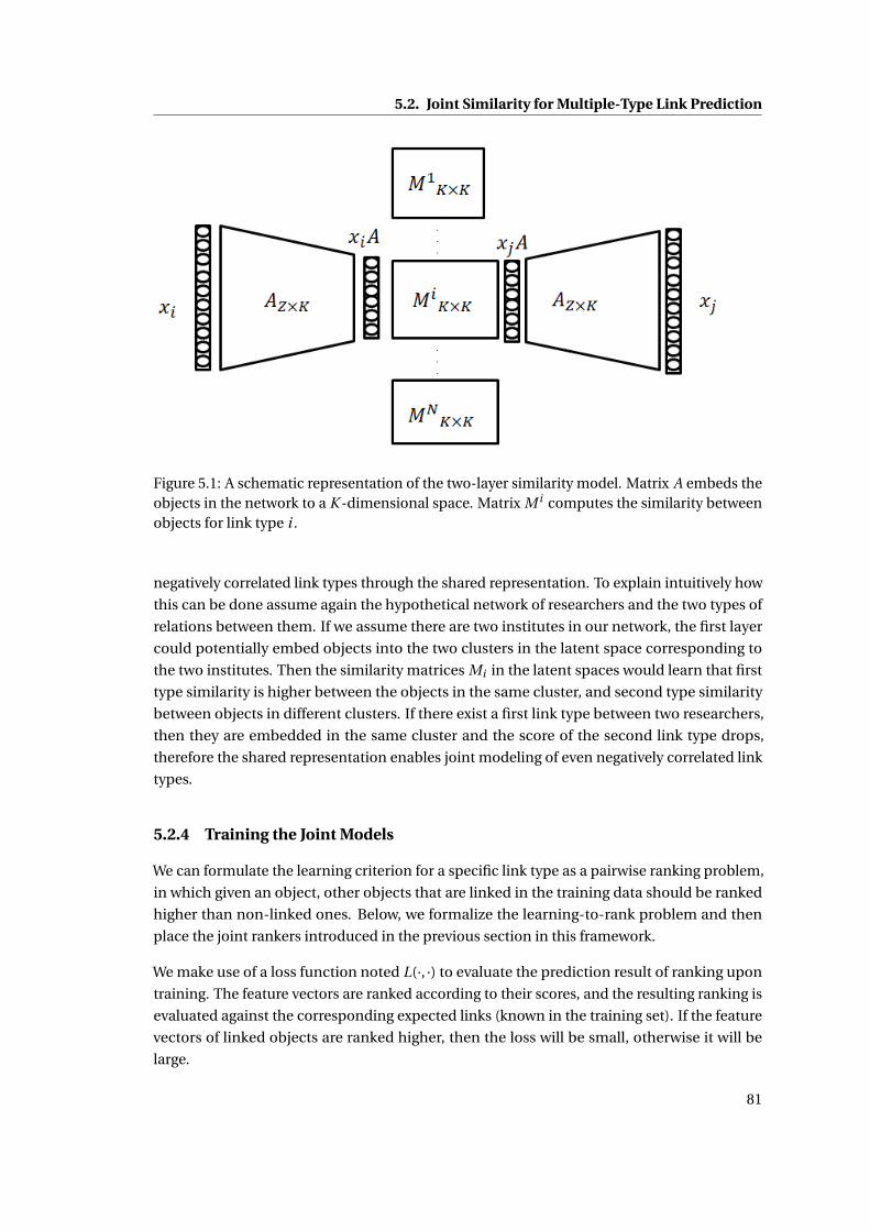
5.2. Joint Similarity for Multiple-Type Link Prediction
Figure 5.1: A schematic representation of the two-layer similarity model. Matrix A embeds theobjects in the network to a K -dimensional space. Matrix M i computes the similarity betweenobjects for link type i .
negatively correlated link types through the shared representation. To explain intuitively how
this can be done assume again the hypothetical network of researchers and the two types of
relations between them. If we assume there are two institutes in our network, the first layer
could potentially embed objects into the two clusters in the latent space corresponding to
the two institutes. Then the similarity matrices Mi in the latent spaces would learn that first
type similarity is higher between the objects in the same cluster, and second type similarity
between objects in different clusters. If there exist a first link type between two researchers,
then they are embedded in the same cluster and the score of the second link type drops,
therefore the shared representation enables joint modeling of even negatively correlated link
types.
5.2.4 Training the Joint Models
We can formulate the learning criterion for a specific link type as a pairwise ranking problem,
in which given an object, other objects that are linked in the training data should be ranked
higher than non-linked ones. Below, we formalize the learning-to-rank problem and then
place the joint rankers introduced in the previous section in this framework.
We make use of a loss function noted L(·, ·) to evaluate the prediction result of ranking upon
training. The feature vectors are ranked according to their scores, and the resulting ranking is
evaluated against the corresponding expected links (known in the training set). If the feature
vectors of linked objects are ranked higher, then the loss will be small, otherwise it will be
large.
81
Chapter 5. Joint Similarity Learning for Predicting Links in Multi-Link Networks
We define here a pairwise hinge loss function L, which attempts to preserve the pairwise order
between objects in the training set by maintaining a margin between the scores of each pair Bai
et al. [2010]. For instance, in a friendship social network, the hinge function (computed only
using feature vectors) aims to preserve the order between the scores of the friend pairs and
the non-friend pairs, scoring all friends higher than all non-friend. Similarly, in the case of
hyperlinked documents, the score of the linked documents pairs should be higher, with a
certain margin, than the score of the non-linked documents.
The goal of training is to approximate the parameters of a similarity function for rankers which
minimizes the pairwise hinge loss function L over the network G with the various types of links
that are given in the training set. Training is performed over the graph G = (V ,E1 ∪E2 ∪ . . .EN ),
where V is the set of vertices (objects) and Ei is the set of edges (links) of type i .
Training the Shared Similarity Model
The empirical risk minimization by using a pairwise hinge loss function over the training set is
as follows. We start from training sets for each link type i :
Traini = {(a,b,c)|(a,b) ∈ Ei ∧ (a,c) ∉ Ei }
The goal is to minimize the loss function L as follows:
Mi nL = λ
2||G||2F + λ
2
∑i||Si ||2F +
∑i∑
(a,b,c)∈Trainimax(0,d − fi (a,b)+ fi (a,c))
(∑
i |Traini |)
The first two terms, the Frobenius norms of matrices G and Si , enforce a regularization on
the parameters and prevent the arbitrary increase of the parameters in the optimization. The
third term of the loss function maintains the order, with a margin d , between the scores of the
connected nodes and the unconnected nodes for link type i .
If we consider the definition of fi from the previous section and the decomposition of Mi
into G and Si , then the subgradients of the loss function with respect to G and to Si are the
following:
5L(G) =λG +∑
i∑
fi (a,b)− fi (a,c)<d x ′a × (xc −xb)∑
i |Traini |
5L(Si ) =λSi +∑
fi (a,b)− fi (a,c)<d x ′a × (xc −xb)
|Traini |
If the training graph G is large, then minimizing the above summation is not tractable. To
overcome this problem we make use of a stochastic gradient descent algorithm in which at
82
5.2. Joint Similarity for Multiple-Type Link Prediction
each iteration we select N samples (a,b,c), one randomly from each Traini set, and perform
gradient descent on each of them. As we are interested in modeling large scale graphs, we will
always make use of this stochastic gradient descent algorithm in the rest of the chapter. The
subgradients of the approximate loss function at iteration t are the following, for an iteration
over one of the samples (a,b,c) ∈ Traini :
5Lt (G) =λG t + {x ′
a(xc −xb) if fi (a,b)− fi (a,c) < d
0 otherwise
5Lt (Si ) =λSit + {
x ′a(xc −xb) if fi (a,b)− fi (a,c) < d
0 otherwise
The update of the parameters is done consequently as follows:
G t+1 =G t −ηt 5Lt (G)
Sit+1 = Si
t −ηt 5Lt (Si )
where ηt is the learning rate at the iteration t .
Analysis of the training algorithm. The first observation is that the time complexity of each
iteration of the stochastic gradient algorithm is O(N 2Z ) where NZ is the average of the number
of non-zero features of the xa , xb and xc . In the textual domain, the number of non-zero
features NZ is usually a couple of hundreds, which is much smaller than the dimension of a
word vector representation of the data, which is usually several hundred thousands (number
of all possible words).
We can follow the same approach that is used to prove the convergence of the PEGASOS
algorithm in Shalev-Shwartz et al. [2011] in order to prove the convergence of the training
algorithm presented above. In fact, we can show that the above algorithm is a special case of
PEGASOS. Prove of the convergence is at the of this chapter in section 5.4.
Low-Rank Factorization. The dimension of G and Si is Z 2 where Z is the number of features
of the data points. In practice, to make training and storage possible, particularly when we are
dealing with high dimension data such as text, a low-rank factorization of G and Si should
be considered. In this case we assume that G = A A′ and Si = Si 1S′i 2 so that A, Si 1 and Si 2
are matrices from Z to a lower dimension. Given that Mi is not necessarily symmetric we
decompose the specific part Si to two lower-rank matrices. Also we change the regularization
on G and Si with the regularization on A, Si 1 and Si 2 in the objective function. The objective
function consisting of the low-rank matrices is not convex any more, but in practice it has
been shown that the low-rank factorization performs well Bai et al. [2009]. The subgradients
83

Chapter 5. Joint Similarity Learning for Predicting Links in Multi-Link Networks
are as following for a given sample (a,b,c) ∈ Traini :
5Lt (A) =λAt +
{x ′
a(xc −xb)At + (xc −xb)′xa At if fi (a,b)− fi (a,c) < d
0 otherwise
5Lt (Si 1) =λS ti 1 +
{x ′
a(xc −xb)S ti 2 if fi (a,b)− fi (a,c) < d
0 otherwise
5Lt (Si 2) =λS ti 2 +
{(xc −xb)′xaS t
i 1 if fi (a,b)− fi (a,c) < d
0 otherwise
Training two-layer Similarity Model
Similarly to the previous section, for the two-layer model the empirical risk minimization
using a pairwise hinge loss function over the training set is as follows. We start from training
sets for each link type i :
Traini = {(a,b,c)|(a,b) ∈ Ei ∧ (a,c) ∉ Ei }
The goal is to minimize the loss function L as follows:
Mi nL = λ
2||A||2F + λ
2
∑i||Mi ||2F +
∑i∑
(a,b,c)∈Trainimax(0,d − fi (a,b)+ fi (a,c))
(∑
i |Traini |)
Again, the first two terms enforce a regularization on the parameters and prevent the arbitrary
increase of the parameters in the optimization. If we consider the definition of fi then the
subgradients of the loss function with respect to A and to Mi are the following:
5L(A) =λA+
∑i
∑fi (a,b)− fi (a,c)<d
(x ′a((xc −xb)A)+ (xc −xb)′(xa A))×Mi∑
i |Traini |
5L(Mi ) =λMi +
∑fi (a,b)− fi (a,c)<d
(xa × A)′((xc −xb)× A)
|Traini |
If the training graph G is large we make use of a stochastic gradient descent algorithm in
which at each iteration we select N samples (a,b,c), one randomly from each Traini set, and
perform gradient descent on each of them. The subgradients of the approximate loss function
84
5.2. Joint Similarity for Multiple-Type Link Prediction
at iteration t are the following, for an iteration over one of the samples (a,b,c) ∈ Traini :
mar g = fi (a,b)− fi (a,c)
5Lt (A) =λAt +
{(x ′
a((xc −xb)At )+ (xc −xb)′(xa At ))×Mit if mar g < d
0 otherwise
5Lt (Mi ) =λMit +
{(xa × At )′((xc −xb)× At ) if mar g < d
0 otherwise
The update of the parameters is done consequently as follows:
At+1 = At −ηt 5Lt (A)
Mit+1 = Mi
t −ηt 5Lt (Mi )
where ηt is the learning rate at the iteration t .
Analysis of the training algorithm. The time complexity of each iteration of the stochastic
gradient algorithm is O(K 2 + NZ ×K ) where NZ is the average of the number of non-zero
features of the xa , xb and xc and K is the size of latent space. The loss function is not convex
in the two-layer similarity model and, therefore, the initialization of the parameter can have a
significant effect on the performance.
5.2.5 Generalization for Related Problems
In this section we show that the above architectures for joint link prediction on multi-networks
can be extended for the similar problems.
Joint Classification and Link Prediction
We show that a joint classification and link prediction task over a network can be reformulated
as a multi-link prediction task, thus enhancing the generality of our proposal. Indeed, in most
real-world networks, objects are labeled with a certain finite label set, and these labels are not
independent from the link structure. For example, in a papers/citations network, it is more
likely that machine learning papers cite other machine learning papers rather than biology
papers. Conversely, a paper which cites many machine learning papers is more likely to be a
machine learning paper rather than a biology paper.
We introduce here a new link type based on the similarity of objects’ labels: every two objects
in the network that have the same label will be connected by such a link. Therefore, the classi-
85
Chapter 5. Joint Similarity Learning for Predicting Links in Multi-Link Networks
fication and the link prediction tasks can be casted to a multi-type link prediction problem, in
which one of the link types is based on the similarity of objects’ labels. Consequently, the goal
of learning for this task is to find similarity functions for which objects with the same labels are
closer than the other objects, and (as above) linked objects are closer than non-linked objects.
For the classification task, i.e. to determine the label of a yet unlabeled object, we consider the
majority label of the closest objects to that object.
The empirical risk minimization for joint classification and link prediction by using a pairwise
hinge loss function over the training set is as follows. To simplify notations, we assume that
there is only one link type i in the network, and we note C (o) the label or class of an object o.
First, the training sets are defined as:
TrainL = {(a,b,c)|(a,b) ∈ E , (a,c) ∉ E } , TrainC = {(a,b,c)|C (b) =C (a),C (c) 6=C (a)}
Then, training is defined as minimizing the loss function L :
Mi nL =λ×Regularization on the parameters+∑
(a,b,c)∈TrainL∪TrainCmax(0,d − fi (a,b)+ fi (a,c))
(|TrainC |+ |TrainL |)Both models introduced above can be used as the similarity model in the above formulation.
In the shared similarity model case we consider a general similarity function which is shared
between classification and link prediction tasks, along with specific similarity functions for
each task separately. In the two-layer model the first layer is the shared representation between
classification and link prediction task, and the second layer shows the specific similarity in
the embedded space. The training algorithm is identical to the case of link prediction on the
multi-type links networks, which was discussed above.
Networks without Attributes
Throughout this chapter, we assumed that the similarity functions are learned over node
attributes. However, in networks where nodes do not have attributes or attributes are not
predictive , the proposed framework can still be applied. For each node, a feature vector is
defined of the size of all nodes in the graph, in which only the element corresponding to the
node has value 1 and the others are set to 0.
In this case, the low rank factorization of the similarity matrix in shared similarity model, or
the first layer in the two-layer model is similar to the existing methods for network matrix
decomposition, such as singular value decomposition or non-negative matrix factorization,
except that our method enforces the large margin criterion and is trained jointly. The empirical
exploration of this case is the topic of future work.
86
5.3. Experimental Results
Inter-Network transfer learning
We show in this chapter that we can transfer the learning from one link type to another
link type through the shared information part. Transferring learning from one network to
another one is another interesting and related problem. Considering two different online
social networks, one based on friendship (such as Facebook) and the second one based on
professional relations (such LinkedIn), the model described here could be applied to share the
learning between the two networks as long as it is possible to build identical feature vectors
for the nodes in both networks. This problem also deserves further investigations.
5.3 Experimental Results
Many real-world networks have multiple types of links. For example, in online social networks,
people have different types of relationships and interactions. In many such networks, espe-
cially those that are collaboratively built, some objects often have fewer links from one link
type. In this section, we consider two networks: TED videos and Amazon products which
are explained. We show that our joint link prediction algorithm improves the link prediction
performance, especially when there are fewer links from one link type.
5.3.1 Network of TED Talks
TED is an online audio-visual broadcasting platform for the TED talks. 1 We consider a
network consisting of nearly 1,200 TED talks, with metadata and transcripts, linked by two
types of links. The first type relate two talks based on the similarity of contents. We derive such
content links from the suggestions of similar talks made by experts from TED. The second type
of links connects two videos if they co-exist in many users favorite lists. Since less popular
talks do not appear in many people’s favorite lists, there are fewer links based on users favorite
lists for such talks, and presumably the links for these talks are not very reliable. Note that
recognizing automatically that two talks have similar contents is difficult, but inference about
the content can be done more easily when two talks co-occur in many people’s favorite lists.
More specifically, the second type of links based on users’ favorite lists is built as follows. Each
talk is represented by a vector in the space of all users, and an element of the vector is 1 if the
talk is in the favorite list of the corresponding user, and 0 otherwise. Given one specific talk,
the rest of the talks can be sorted according to cosine similarity between their vectors and the
initial talk in the space of users. If two talks co-exist in many users’ favorites list, the cosine
similarity between their vectors in the space of users is high. Therefore, to build the second
type of links, we connect each talk with the top k talks based on cosine similarity between
their vectors in the users space. We will call this type of links “co-liked”.
1This data set has been collected by Nikolaos Pappas from Idiap, who has kindly shared it for the work presentedhere. See http://www.ted.com for the original website.
87
Chapter 5. Joint Similarity Learning for Predicting Links in Multi-Link Networks
For example, the TED talk “Lucien Engelen: Crowdsource your health” has two content links
(two recommendations of topically-related talks from TED experts): “Jacqueline Novogratz on
patient capitalism” and “Nicholas Christakis: How social networks predict epidemics”. The
three highest score co-liked talks are: “Marco Tempest: Augmented reality, techno-magic”,
“Aparna Rao: High-tech art (with a sense of humor)” and “Sheikha Al Mayassa: Globalizing the
local, localizing the global”. We can observe that the related videos are about the same topic,
but co-liked videos are much less predictable from the content.
We build a feature vector for each talk from three sources: (1) speaker name, (2) title of the talk,
and (3) talk description as provided by TED (a short text). Each feature vector has a dimension
of 4,771 (based on a filtered vocabulary of 4,771 words), but vectors are very sparse, on average
with only 35 non-zero coefficients.
5.3.2 Network of Amazon Products
We build a network from a subset of Amazon products (described in Leskovec et al. [2007])
with two types of links between them. The first type comes directly from the Amazon website:
for each product, some of the co-purchased products are shown by Amazon. Each product in
the network is connected to the products which are claimed to be mostly co-purchased by the
Amazon website. We call this type of links “co-purchased”.
Each product is assigned to at least one category, often to more. Categories form a hierarchy,
from more general ones to the most detailed ones. We represent each product as a vector in
the space of all categories: if the product is assigned to a category, the corresponding element
is 1, otherwise it is 0. Cosine similarity between category vectors of two products is high if
they are mostly in the same categories from the hierarchy. To build this type of the links, we
connect each product to the k most similar products using cosine similarity between the
category vectors of the products. We call this type of links “category links”.
For example, consider the book “Writers in the Schools: A Guide to Teaching Creative Writing
in the Classroom”. This book is co-purchased with the following other books: “The Magic
Pencil: Teaching Children Creative Writing [. . .]” and “Journal Jumpstarts: Quick Topics and
Tips for Journal Writing”. Two category links are “Reading, Writing, and Learning in ESL (2nd
Edition)” and “Time to Know Them: A Longitudinal Study of Writing and Learning at the
College Level”.
Features of each product in the network come from the title and description of the product. We
use a dictionary of 3,765 words and sampled 10,000 products to build our network of products.
So, our second network is about eight times larger than the first one.
88
5.3. Experimental Results
5.3.3 Prediction Performance
To study the link prediction ability of our models experimentally, we split the objects of each
network into disjoint training and test sets. The training is performed on the objects in the
training set and the links between them, excluding links from these objects to the test set. To
evaluate prediction performance, for each object in the test set, all the objects in the entire
data set (training plus test sets) are ranked by the ranker, and the Mean Average Precision
(MAP) is calculated for the resulting ranked list according to the links in the test set. The final
scores are the average of 5-fold cross validation, with 80% of the data used for training and
20% for testing, in each fold.
We are interested in observing the prediction performance of the joint model when there are
few available links from one link type. To perform such an analysis, we make available to the
joint learner a full training set for one link type (80% of the objects in the network), and a
variable-sized training set for the other link type, varying from a smaller subset (30% of the
nodes) to the full training set (80%) by fixed increments (10%). The test set is always fixed
(20%). We observe the evolution of prediction performance with the size of the training set for
the second type of links.
Table 5.1 shows the average MAP for the objects in the test set for the co-purchased links, in
the Amazon products network, for several models. As explained, the size of the co-purchase
training set varies from 30% to 80% of the entire network, while the training set for category
links is constant (80%). Both ’separate’ and shared similarity model are using low rank factor-
ization of M due to the dimension size of the features, with a latent space of dimension 100.
The size of latent space in two-layer network is set to 100 as well. All matrices are initialized by
random values.
89
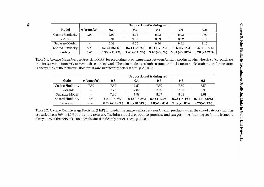
Ch
apter
5.Jo
intSim
ilarityL
earnin
gfo
rP
redictin
gL
inks
inM
ulti-L
ink
Netw
orks
Proportion of training setModel 0 (transfer) 0.3 0.4 0.5 0.6 0.8
Cosine Similarity 8.03 8.03 8.03 8.03 8.03 8.03SVMrank – 8.94 9.06 8.99 8.92 9.11
Separate Model – 8.39 8.53 8.70 8.92 9.13Shared Similarity 8.43 9.16 (+9.1%) 9.21 (+7.9%) 9.31 (+7.0%) 9.56 (+7.1%) 9.59 (+ 5.0%)
two-layer 9.00 9.33 (+11.2%) 9.43 (+10.5%) 9.48 (+8.9%) 9.60 (+8.18%) 9.70 (+7.22%)
Table 5.1: Average Mean Average Precision (MAP) for predicting co-purchase links between Amazon products, when the size of co-purchasetraining set varies from 30% to 80% of the entire network. The joint model uses both co-purchase and category links (training set for the latteris always 80% of the network). Bold results are significantly better (t-test, p < 0.001).
Proportion of training setModel 0 (transfer) 0.3 0.4 0.5 0.6 0.8
Cosine Similarity 7.50 7.50 7.50 7.50 7.50 7.50SVMrank – 7.73 7.82 7.89 7.92 7.92
Separate Model – 7.86 7.99 8.07 8.38 8.61Shared Similarity 7.97 8.31 (+5.7% ) 8.42 (+5.3%) 8.53 (+5.7%) 8.73 (+4.1%) 8.92 (+ 3.6%)
two-layer 8.48 8.79 (+11.8%) 8.8(+10.51%) 8.8(+9.66%) 9.12(+8.8%) 9.25(+7.4%)
Table 5.2: Average Mean Average Precision (MAP) for predicting category links between Amazon products, when the size of category trainingset varies from 30% to 80% of the entire network. The joint model uses both co-purchase and category links (training set for the former isalways 80% of the network). Bold results are significantly better (t-test, p < 0.001).
90
5.3. Experimental Results
The ‘separate’ model shown in Table 5.1 uses only the link type that must be predicted and is
identical to the classical distance learning model that has been used in previous works Bai
et al. [2010], Shaw et al. [2011], Bai et al. [2009]. This model was previously compared with
state-of-the-art link prediction methods and was shown to be effective for link prediction on
networks. The separate model is ignorant about the other link type. The joint models make
use of both link types according to the models described in this chapter. Table 5.1 clearly
shows that the joint models improve the results significantly comparing to the separate model,
SvmRank and Cosine similarity. The separate model is itself superior to the other models
tested in Bai et al. [2010], Shaw et al. [2011], Bai et al. [2009]). SVMrank Joachims [2002],
Herbrich et al. [2000] has shown high performance in ranking; to make it applicable to large
graphs (here, the Amazon products) the optimization was performed on the primal form by
using stochastic gradient descent. Not surprisingly, the two-layer Similarity model has better
performance in comparison to the Shared Similarity model.
Table 5.2 shows similar results, but reversing the link types. In this experiment, we varied the
proportion of category links made available for training, from 30% to 80% of the total number
of objects, and kept the co-purchase links at a constant value (all links over 80% of the nodes
used for training).
The important observation is that when there are few links available for training (columns at
the left of the tables), the improvement of using both link types by the joint ranker is higher,
percentage of the improvement is given in the parenthesis. However, even when the training
set is large, the joint modeling is useful. Moreover, we observe in the extreme case when
there is no training data available (marked “0 (transfer)” in the tables) and the ranker is only
trained on the other link type, still the performance reached through transferring the learning
from the other link type is significantly higher than the ad-hoc similarity metric in baselines
(cosine-similarity). In the two-layer Similarity model we transfer the first layer and use an
orthogonal matrix with all elements one for the second layer. The results confirm that there is
correlation between categorical similarity of the products in Amazon and being co-purchased
by customers, and each of them can help in modeling and predicting of the other one.
Table 5.3 similarly shows the average MAP of the TED dataset for the content links and Table 5.4
shows the average MAP for the co-liked links. The Joint models, specially two-layer model,
significantly improve the link prediction performance for both link types. This shows that
there is a big correlation between relatedness of talks in TED platform and being in the favorite
list of many users.
91
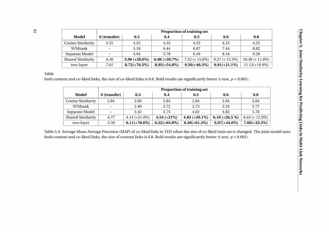
Ch
apter
5.Jo
intSim
ilarityL
earnin
gfo
rP
redictin
gL
inks
inM
ulti-L
ink
Netw
orks
Proportion of training setModel 0 (transfer) 0.3 0.4 0.5 0.6 0.8
Cosine Similarity 4.55 4.55 4.55 4.55 4.55 4.55SVMrank – 5.10 6.44 6.87 7.44 8.02
Separate Model – 4.94 5.78 6.49 8.18 9.28Shared Similarity 6.30 5.96 (+20.6%) 6.98 (+20.7%) 7.52 (+ 15.8%) 9.27 (+ 13.3%) 10.38 (+ 11.8%)
two-layer 7.61 8.72(+76.5%) 8.95(+54.8%) 9.50(+46.3%) 9.91(+21.1%) 11.13(+19.9%)
Table5.3: Average Mean Average Precision (MAP) of content links in TED when the size of content train set is changed. The joint model usesboth content and co-liked links, the size of co-liked links is 0.8. Bold results are significantly better (t-test, p < 0.001).
Proportion of training setModel 0 (transfer) 0.3 0.4 0.5 0.6 0.8
Cosine Similarity 2.84 2.84 2.84 2.84 2.84 2.84SVMrank – 2.40 2.72 2.73 2.33 3.77
Separate Model – 3.42 3.75 4.02 4.82 5.70Shared Similarity 4.77 4.14 (+21.0%) 4.54 (+21%) 4.83 (+20.1%) 6.10 (+26.5 %) 6.44 (+ 12.9%)
two-layer 5.50 6.11(+78.6%) 6.22(+65.8%) 6.49(+61.4%) 6.97(+44.6%) 7.60(+33.3%)
Table 5.4: Average Mean Average Precision (MAP) of co-liked links in TED when the size of co-liked train set is changed. The joint model usesboth content and co-liked links, the size of content links is 0.8. Bold results are significantly better (t-test, p < 0.001).
92
5.4. Convergence of the Training Shared Similarity Model
The joint models have a higher performance than the separate models on both networks that
we experimented with. The difference in the performance of the joint model and separate
model is higher when there are fewer number of links from one link type. In that case, the
denser link type can help more strongly the sparser link type through the shared information
part. But even when there are equal links from different link types, joint modeling through
shared information helps with the generality of the model and improves the link prediction
performance.
5.3.4 Effect of Low-rank Factorization Dimension
We finally study the effect of low-rank factorization on the performance of ranking when the
full training set is available. When the graph is larger, it is possible to train larger dimensions,
but when the network is not large, larger dimensions make over-fitting more likely.
Table 5.5 shows the effect of dimension on link prediction performance for Amazon products.
We observe that the growth of increase in the performance decreases when we increase
the dimension. The time complexity of the algorithm linearly depends with the dimension.
Therefore, for large scale graphs, one should choose a dimension by considering the trade-off
between the time complexity and the performance.
Table 5.6 similarly shows the effect of dimension on the link prediction performance over
the TED talks. Considering the size of network, increasing the dimension decreases the
performance, as it over-fits the training set.
DimensionModel 20 50 100 150
Separate Model (co-purchase) 6.60 8.52 (+29.9%) 9.13 (+7.16%) 9.31(+1.97%)Shared Similarity (co-purchase) 7.29 9.24 (+26.75%) 9.59 (+3.79%) 9.91(+3.34%)
two-layer (co-purchase) 7.29 8.94(+22.63%) 9.70 (+8.50%) 10.11(+4.22%)Separate Model (category) 7.59 8.41 (+10.08%) 8.61 (+2.38%) 8.67(+0.70%)
Shared Similarity (category) 7.96 8.76 (+10.05%) 8.92 (+1.83%) 8.98(+0.67%)two-layer (category) 7.96 8.84(+11.05%) 9.25 (+4.63%) 9.40(+1.62%)
Table 5.5: Average Mean Average Precision (MAP) for predicting links between Amazon prod-ucts.
5.4 Convergence of the Training Shared Similarity Model
To prove the convergence, first we need to establish an upper bound for the norm of the
subgradients at each iteration ||5t (.)||2F <U which can be easily found if the data points are
bounded. For example, if all data points vectors are normalized, then they are bounded, which
is the case in our study.
Theorem 2. Let G = 1T
∑Tt=1 G t and Si = 1
T
∑Tt=1 Si
t be the averages of G and Si so far. Let the
93
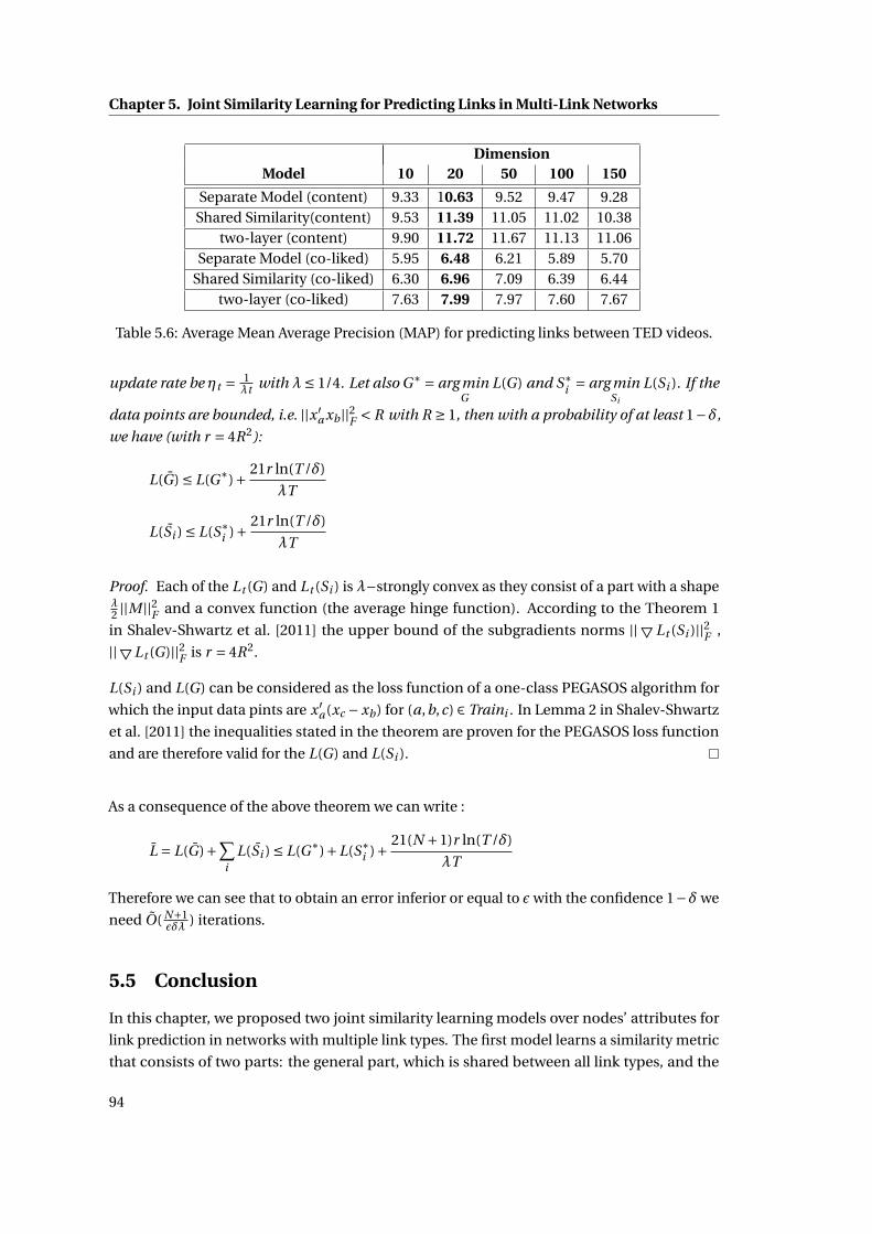
Chapter 5. Joint Similarity Learning for Predicting Links in Multi-Link Networks
DimensionModel 10 20 50 100 150
Separate Model (content) 9.33 10.63 9.52 9.47 9.28Shared Similarity(content) 9.53 11.39 11.05 11.02 10.38
two-layer (content) 9.90 11.72 11.67 11.13 11.06Separate Model (co-liked) 5.95 6.48 6.21 5.89 5.70
Shared Similarity (co-liked) 6.30 6.96 7.09 6.39 6.44two-layer (co-liked) 7.63 7.99 7.97 7.60 7.67
Table 5.6: Average Mean Average Precision (MAP) for predicting links between TED videos.
update rate be ηt = 1λt with λ≤ 1/4. Let also G∗ = arg min
GL(G) and S∗
i = arg minSi
L(Si ). If the
data points are bounded, i.e. ||x ′a xb ||2F < R with R ≥ 1, then with a probability of at least 1−δ,
we have (with r = 4R2):
L(G) ≤ L(G∗)+ 21r ln(T /δ)
λT
L(Si ) ≤ L(S∗i )+ 21r ln(T /δ)
λT
Proof. Each of the Lt (G) and Lt (Si ) is λ−strongly convex as they consist of a part with a shapeλ2 ||M ||2F and a convex function (the average hinge function). According to the Theorem 1
in Shalev-Shwartz et al. [2011] the upper bound of the subgradients norms ||5Lt (Si )||2F ,
||5Lt (G)||2F is r = 4R2.
L(Si ) and L(G) can be considered as the loss function of a one-class PEGASOS algorithm for
which the input data pints are x ′a(xc −xb) for (a,b,c) ∈ Traini . In Lemma 2 in Shalev-Shwartz
et al. [2011] the inequalities stated in the theorem are proven for the PEGASOS loss function
and are therefore valid for the L(G) and L(Si ).
As a consequence of the above theorem we can write :
L = L(G)+∑i
L(Si ) ≤ L(G∗)+L(S∗i )+ 21(N +1)r ln(T /δ)
λT
Therefore we can see that to obtain an error inferior or equal to ε with the confidence 1−δ we
need O( N+1εδλ ) iterations.
5.5 Conclusion
In this chapter, we proposed two joint similarity learning models over nodes’ attributes for
link prediction in networks with multiple link types. The first model learns a similarity metric
that consists of two parts: the general part, which is shared between all link types, and the
94
5.5. Conclusion
specific part, which is trained specifically for each type of link. The second model consists of
two layers: the first layer, which is shared between all link types, embeds the objects of the
network into a new space, and then a similarity is learned specifically for each link type in
this new space. Both models are applicable to large networks with high-dimensional feature
spaces. The experiments show that the proposed joint modeling and training frameworks
improve link prediction performance significantly for each link type in comparison to multiple
baselines. This improvement is higher when there are fewer links available from one link type
in the network. The two-layer similarity model outperforms the first one which is expected
due to its capability of modeling negative correlations among different link types. Moreover,
we illustrated that even if the models are trained completely on one link type and tested on the
other, our models significantly improve the performance in comparison to ad-hoc similarity
metrics.
95

6 Similarity Learning for CollectiveRanking on Networks: Application toLink PredictionThis chapter proposes a method for learning to rank over networks (relational data). The
ranking is performed with respect to a query object which can be part of the network or
outside it. The ranking method makes use of the features of the nodes as well as the existing
links between them. First, a neighbors-aware ranker is trained using a large margin pairwise
loss function. Then, collective inference is performed using an iterative ranking algorithm,
which propagates the results of rankers over the network. By formulating link prediction
as a ranking problem, the method is tested on three networks, with papers/citations and
webpages/hyperlinks. The results show that the proposed algorithm, which uses both link
structure and node attributes, outperforms several other methods: a content-only ranker, a
link-only one, a random walk method, a relational topic model, and a method based on the
weighted number of common neighbors. In addition, the propagation algorithm improves
results even when the query object is not part of the network, and scales efficiently to large
networks.
The chapter is organized as follows. After a brief introduction to the problem (Section 6.1),
we frame the model and put it into perspective in Section 6.2. In Section 6.3 we explain the
collective ranking framework, first by introducing the neighbors-aware ranker and then the
collective inference algorithm. In Section 6.4 we evaluate the proposed method on the three
different data sets, showing that it outperforms several other methods.
6.1 Introduction to Ranking on Relational Data
In network or relational data, the relations between objects are represented by directed or
undirected edges in a network. The ranking problem on network data requires that all objects
in the network are ranked given a query.
Two cases of the ranking problem can occur in network data such as social networks: the
query object itself is an object in the network – i.e. some prior relations with other objects are
known – or the query object is not part of the network.
97
Chapter 6. Similarity Learning for Collective Ranking on Networks
When the query object has already some links in the network, link-based approaches such as
random walk models can be effective, whereas when the query object is not in the network,
these link-based approaches are not applicable, and usually supervised learning over node
attributes are considered.
In both cases, it is possible to exploit the relations between objects in the network to increase
the accuracy of the ranking with respect to a given query. In this work we bridge these two
approaches and make use of attributes and of relations between objects at the same time.
For illustration purposes, let us consider a network formed by scientific papers linked by
citations between them. Given a “query” paper, the goal is to rank all papers in the network
according to a score that reflects the likelihood of being cited by this query paper. If the network
is made of completed papers with optimal citations, then this score should distinguish the
actually cited (respectively not cited) papers. Moreover, the model will also indicate papers that
should have been cited and were not, or, conversely, citations that were spuriously inserted.
But the ranking task is more clearly useful for recommending citations to include in a new
paper (object outside the network) or to extend an existing draft (already in the network). In
both cases, the model computes a ranked list of recommendations for additional citations,
using existing links and object features as well. A similar application is the recommendation
of new connections in social networks.
6.2 Motivation of the Model
Learning to rank can be formulated as a supervised learning task. Suppose that each object,
including the query, can be represented as feature vectors in a given space. Let X be the list of
feature vectors Xi for a list of objects, and let Y be the list of corresponding grades or relevance
scores, for each object, with respect to a given query object q . For example, in the case of a
friendship social network, the grades Yi represent the friendship status (‘friend’ or ‘not friend’)
with the query object (an individual profile) for each member i , and the feature vectors Xi
are derived from the information available from individual profiles of each member i . In
information retrieval terms, the grades Y represent the relevance degree of the objects with
respect to the query.
The goal of the learning to rank task is to automatically learn a function F transforming a
list of feature vectors X into a list of scores with respect to a query q , given the training data
(Xqi , X1,Y1qi ), (Xqi , X2,Y2qi ), . . . , (Xqi , Xm ,Ymqi ) in which Xqi and X j are showing the feature
vectors of the query qi and the object j , and Y j qi shows their corresponding grade.
In all generality, F (q, X ) is a global ranking function, meaning that F assigns scores to the list
of features vectors X for a given set of objects and a query. A global ranking function is able
to consider dependencies between objects as it scores a set of objects instead of each object
alone. However, to make the computation tractable in practice, a local ranking function is
98
6.3. Learning to Rank on a Network
usually considered for applications:
F (q, X ) = [ f (q, X1), f (q, X2), . . . , f (q, Xn)]
The implicit assumption behind using a local ranking function is that the score of each object
is independent from the score of the other objects. In many applications this assumption
yields acceptable results, but in network data this assumption is quite questionable. In a
friendship network, for instance, friendship is more likely if there are more common friends,
and not only if two people have similar profiles. Or, in a citation network, a paper is more
likely to cite another paper if it has already cited several papers that cite the considered paper.
In this chapter, we model the dependency between data objects in the network to solve
the ranking problem more effectively. We make use of a loss function L(·, ·) to evaluate the
prediction result of F (q, X ) upon training. First, the feature vectors X are ranked according
to their scores F (q, X ). Then, the ranking results are evaluated against the corresponding
expected grades Y . If the feature vectors with higher grades are ranked higher, then the loss L
will be small, otherwise it will be large.
However, the minimization of the loss function is difficult as it is not continuous and uses
sorting Li [2011]. Therefore, we consider a surrogate loss function L′ to make the minimization
possible, specifically a pairwise hinge loss function. This function attempts to preserve the
pairwise order between the objects in the training set by maintaining a margin between the
scores of each pair Bai et al. [2010]. For instance, in a friendship social network, the hinge
function aims to preserve the order between the scores of the friend pairs and the non-friend
pairs.
Link prediction can also be formulated as a learning-to-rank problem: given a query node,
all other nodes are sorted according to the likelihood of creating a link between them and
the query node. Link prediction is a binary graded ranking and, in the training phase, if the
linked objects are ranked higher, then the loss will be small, otherwise it will be large. This
formulation has been used in many previous works including Liben-Nowell and Kleinberg
[2003], Adamic and Adar [2001], Backstrom and Leskovec [2011], Shaw et al. [2011], Agarwal
et al. [2006]. In the rest of this chapter we focus on the binary ranking problem for link
prediction, although the framework can be easily generalized for other ranking problems.
6.3 Learning to Rank on a Network
The classification of objects from network data sets has been shown to be successfully ad-
dressed by using collective classification algorithms Jensen et al. [2004], in which a local
classifier is trained to classify each object independently by using at the same time object
features and labels of other objects in its neighborhood. A collective inference algorithm
propagates the results of the local classifiers in the network.
99
Chapter 6. Similarity Learning for Collective Ranking on Networks
For ranking on a network, we draw inspiration from this approach to define a collective ranking
algorithm which consists of three parts:
1. The content-only ranker learns to rank only by using a similarity function on node
attributes, while ignoring relations between nodes. This ranker embodies the approach
which is traditionally used in learning to rank problems.
2. The neighbors-aware ranker learns how to rank according to the information locally
available at each node, coming from the node’s attributes and the neighborhood in-
formation. The size of the neighborhood of which the ranker is aware can vary in
principle; however, in this work, we limit the neighborhood to the direct neighbors, i.e.
one transition away.
3. The collective inference algorithm propagates the results of local rankers over the net-
work. Existing collective inference methods McDowell and K.M. Gupta [2009] are used
as inspiration for an original iterative propagation algorithm, defined below. We will
show that this algorithm is effective for collective ranking and is simpler to implement
and scales better to larger graphs in comparison to other collective inference algorithms.
Moreover, we prove the convergence of the inference algorithm.
In the following subsections we describe the neighbors-aware local ranker, the collective
inference algorithm, and the training process for the ranker.
6.3.1 Neighbors-aware Ranker
The neighbors-aware ranker returns a score given a query, a target node, and the overall graph
structure. The ranker’s score is a function of the neighbors’ scores and of the similarity between
the query and the target node. If we denote the ranker by f , the entire graph by G , the query
and target nodes respectively by q and t , and the features of a node i by xi , then we have:
f (q, t ,G) = si mi l ar i t y(xq , xt )︸ ︷︷ ︸content-only
+αnei g hbor (q, t ,G)︸ ︷︷ ︸neighbors scores
The first part, si mi l ar i t y(xq , xt ), is the content-only ranker which computes the similarity
between q and t based only on their attributes, as proposed by most previous learning to rank
methods. Many content-based rankers with various learning abilities have been studied in the
literature, for instance RankNet Burges et al. [2005], polynomial semantic indexing Bai et al.
[2009] or structure preserving metric learning Shaw et al. [2011]. In this study, we choose a
100
6.3. Learning to Rank on a Network
similar approach and define the similarity function as:
si mi l ar i t y(xq , xt ) = xq ×M ×x ′t
The M matrix is a N ×N matrix, where N is the number of words. In practice, to make the
training and the storage possible, some constraints on M are considered, such as using a
diagonal matrix or performing low-rank factorization Bai et al. [2009], Shaw et al. [2011].
The second part of f , i.e. the neighborhood score, shows how the neighbors of t are scored
with respect to q . If the neighbors of t have high scores, it is more likely that t itself has high
scores. For instance, in a friendship social network, a person q is more likely to be friend with a
person t if they have many common friends. This part of the neighbors-aware ranker takes into
account the dependencies between data objects, and allows us to perform collective ranking
instead of local ranking only. As we are dealing with directed networks here, we consider two
types of neighbors: neighbors from in-links (Ni n(t )) and neighbors from out-links (Nout (t )).
We define the nei g hbor function recursively by using the score function of the neighbors as
follows:
nei g hbor (q, t ,G) = w1
∑n∈Ni n (t ) f (q,n,G)
|Ni n(t )| +w2
∑n∈Nout (t ) f (q,n,G)
|Nout (t )|
The parameters w1 and w2 represent the importance of the in-links neighbors and out-links
neighbors, and are learned during the training along with the parameters of the si mi l ar i t y
function.
Putting all together we have the following formula for the neighbors-aware ranker:
f (q, t ,G) = xq M x ′t +
αw1∑
n∈Ni n (t ) f (q,n,G)
|Ni n(t )| + αw2∑
n∈Nout (t ) f (q,n,G)
|Nout (t )|
According to the above formula, the score of a target node t is defined based on the score of
its neighbors, recursively. Therefore, to compute the score to a target node, the score to its
neighbors should be computed, and to compute the score to the neighbors, the score to the
neighbors of the neighbors should be computed first, and so on. The next sections explains
how these values are estimated.
The α parameter in the definition of the neighbors-aware ranker (we choose α < 1) is the
dampening parameter which decreases the effect of the neighbors’ scores on the target node
score as their distance from the target node increases. For instance, the effect of a neighbor
two transitions away is α times smaller than the effect of the neighbor one transition away.
101
Chapter 6. Similarity Learning for Collective Ranking on Networks
A larger α means that a larger neighborhood is allowed to have an effect on the target node
score, whereas a smaller α achieves the opposite effect. Therefore, α is a hyper-parameter of
the algorithm and is not learned during the training.
6.3.2 Collective Inference
To compute the score for a given query and a target node, we need to know the scores of the
query to the target’s neighbors. To compute this recursive function, we start from an initial
score and iteratively compute the scores.
The score of a node at iteration τ is thus computed based on the score of nodes at iteration
τ−1. More precisely, if f τ(q, t ,G) is the score of node t for the query q at iteration τ, it is
computed as:
f τ(q, t ,G) = xq M x ′t +
αw1∑
n∈Ni n (t ) f τ−1(q,n,G)
|Ni n(t )| + αw2∑
n∈Nout (t ) f τ−1(q,n,G)
|Nout (t )|
There are two cases for the initial scores f 0(q, t ,G): first, if no prior relation is known for the
query in the network, the scores are initialized by the scores of the content-only ranker. Second,
when the query node itself is in the network, they come from the prior known relations, the
initial score is set to 1 if (i , j ) is an edge of the graph G and to 0 otherwise.
To perform the propagation, we propose here a collective inference algorithm, which is
effective for collective ranking, as we will show. The algorithm is easy to implement and scales
well to large graphs in comparison to other collective inference algorithms. We refer to the
algorithm as ‘Iterative Ranking Algorithm’ (IRA) because at each iteration the results of the
neighborhood-aware rankers are propagated one step further in the graph. The pseudocode
for the IRA is given as Algorithm 7 below.
At the first step, the initial score of all nodes with respect to the query is computed according
to the explanation above. Then, scores are normalized and the scores above the threshold
propagate to the neighbors at the next step of the algorithm. This propagation of above-
threshold scores continues until convergence or until the maximum number of iterations is
reached.
The algorithm converges if |w1| < 1 and |w2| < 1, because the effect of long paths decreases
exponentially and eventually vanishes. To ensure the convergence, during the training of the
ranker we impose the constraint that all the parameters (similarity matrix parameters and wi )
must be between zero and one. By imposing this constraint on the parameters we achieve
two goals: (1) we can prove the convergence, and (2) the constraint acts as a regularizer on the
parameters in the loss function minimization and avoids arbitrary growth of the parameters
(see Section 6.3.3).
102
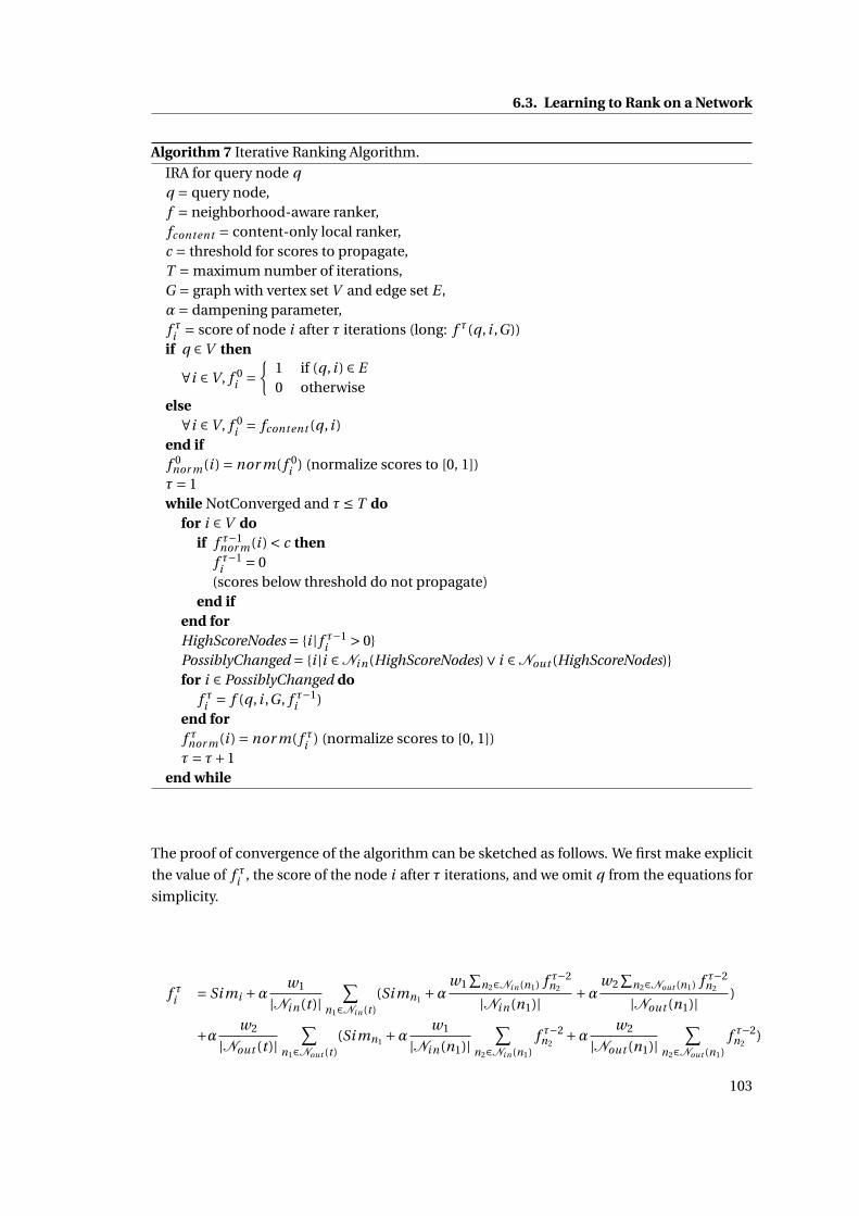
6.3. Learning to Rank on a Network
Algorithm 7 Iterative Ranking Algorithm.
IRA for query node qq = query node,f = neighborhood-aware ranker,fcontent = content-only local ranker,c = threshold for scores to propagate,T = maximum number of iterations,G = graph with vertex set V and edge set E ,α= dampening parameter,f τi = score of node i after τ iterations (long: f τ(q, i ,G))if q ∈V then
∀i ∈V , f 0i =
{1 if (q, i ) ∈ E0 otherwise
else∀i ∈V , f 0
i = fcontent (q, i )end iff 0
nor m(i ) = nor m( f 0i ) (normalize scores to [0, 1])
τ= 1while NotConverged and τ≤ T do
for i ∈V doif f τ−1
nor m(i ) < c thenf τ−1
i = 0(scores below threshold do not propagate)
end ifend forHighScoreNodes = {i | f τ−1
i > 0}PossiblyChanged = {i |i ∈Ni n(HighScoreNodes)∨ i ∈Nout (HighScoreNodes)}for i ∈ PossiblyChanged do
f τi = f (q, i ,G , f τ−1i )
end forf τnor m(i ) = nor m( f τi ) (normalize scores to [0, 1])τ= τ+1
end while
The proof of convergence of the algorithm can be sketched as follows. We first make explicit
the value of f τi , the score of the node i after τ iterations, and we omit q from the equations for
simplicity.
f τi = Si mi +α w1
|Ni n(t )|∑
n1∈Ni n (t )(Si mn1 +α
w1∑
n2∈Ni n (n1) f τ−2n2
|Ni n(n1)| +αw2∑
n2∈Nout (n1) f τ−2n2
|Nout (n1)| )
+α w2
|Nout (t )|∑
n1∈Nout (t )(Si mn1 +α
w1
|Ni n(n1)|∑
n2∈Ni n (n1)f τ−2
n2+α w2
|Nout (n1)|∑
n2∈Nout (n1)f τ−2
n2)
103
Chapter 6. Similarity Learning for Collective Ranking on Networks
If we continue expanding the above equation, the coefficient for the similarity of a node that
is n transitions away is αn × (wa1 · · ·wan ) with ai being either 1 or 2. When increasing n, this
coefficient tends to zero (given that α< 1, w1 < 1, w2 < 1, etc.), which means that the effect of
long paths (including loops) vanishes, and the algorithm converges. One might think that the
thresholding changes this linear algebraic nature of the propagation and then the convergence
can not be guaranteed, but the normalization of the scores and thresholding are used in the
following way considering this issue. In algorithm 7, if the normalized score is higher than the
threshold, the unnormalized score is passed to the next step, and otherwise the score is set to
zero in the next step. In other words, in the above expansion only some terms are expanded
and others are set to zero, which still holds the convergence.
The scores below threshold c will not propagate to the next step of the IRA. There are two main
reasons to add this threshold: the first one is that it prevents the propagation of noise in the
graph, therefore improving performance, as shown in Section 6.4.1. The second reason is to
increase the speed of the collective inference algorithm for larger graphs. In the IRA, in each
iteration, only the score of nodes for which the scores are possibly changed are updated. Only
the scores of the neighbors of nodes with scores higher than the threshold can be changed in
the next iteration. By using a reasonably high threshold, only the scores of very few nodes will
change, despite the size of the graph, and therefore the propagation algorithm is sped up, as
confirmed experimentally in Section 6.4.1. However, in theory, the worst case time complexity
of the algorithm does not change and is still O(N T ).
The above reasons to use threshold in the propagation algorithm are justified, if and only
if, there are only few nodes with high scores in each iteration and there is a long-tail of low
scores nodes. Most real-world networks are small world networks, meaning that nodes form
communities, and these communities are connected by short paths. Therefore, each node is
not connected uniformly to all other nodes in the network, but is usually only connected to a
small number of other nodes in its community. We perform more experimental investigations
in the next sections to validate these assumptions on the networks used as test sets.
6.3.3 Training the Neighbors-aware Ranker
The goal of training is to approximate a local ranker which minimizes a ranking loss function
over the graph G for the queries, target nodes, and associated grades that are given in the
training set. In this section we discuss the training of the binary ranking for link prediction
problem. This can be easily generalized to other ranking problems if needed.
At training time, the graph G = (V ,E) is available, where V is the vertex set and E the edge set,
as in Algorithm 7. We assume that there are two possible grades, ‘connected’ or ‘not connected’,
which are given by the existing edges in the graph. We consider the following training set T
with triples of nodes such as T = {(i , j , z)|(i , j ) ∈ E and(i , z) ∉ E }. The goal of training is to
minimize the empirical risk using a pairwise hinge loss function L over the training set T as
follows:
104
6.3. Learning to Rank on a Network
L = ∑(i , j ,z)∈T
max(0,dmar g − f (i , j ,G)+ f (i , z,G))
so that 0 ≤ wi ≤ 1 and 0 ≤ Mi j ≤ 1
where wi are the parameters of the neighborhood component of f and Mi j are the parameters
of the similarity component of f . We define dmar g as a constant margin that should separate
the examples of two grades (connected vs. not connected). By using the constraint that the
parameters should be bounded, we ensure that the collective inference algorithm converges.
Moreover, the constraint is a regularization on the parameters and prevents the arbitrary
growth of the parameters in the optimization, which is equivalent to the optimization of the
same loss function plus the infinity norm of the parameters.
If the training graph G is large, then minimizing the above summation is not tractable. To
overcome this problem we make use of a stochastic gradient descent algorithm in which at
each iteration we randomly select i , j and z from G and perform gradient descent on them.
To impose the constraint we use gradient projection method.
To perform the training for a given triple (i , j , z), we need to know the score of query i to the
neighbors of j and z. We set the score to the maximum value (1) if there is a link between i and
the neighbor of j in the training graph G , and to the minimum value (0) if there is no such link.
In this case, the optimization is convex and the gradient of the loss function is easy to compute
as the score of the neighbors is constant. We use Ei j = 1 if (i , j ) ∈ E and Ei j = 0 otherwise. The
subgradients of the approximate objective function at time (iteration) τ are the following:
(i , j , z) ∈T
5Lτ(M) = {x ′
i (x j −xz ) if f τ(i , j ,G)− f τ(i , z,G) < d
0 otherwise
dif i n =∑
n∈Ni n ( j ) Ei n
|Ni n ( j )| −∑
n∈Ni n (z) Ei n
|Ni n (z)|
5Lτ(w1) = {dif i n if f τ(i , j ,G)− f τ(i , z,G) < d
0 otherwise
dif out =∑
n∈Nout ( j ) Ei n
|Nout ( j )| −∑
n∈Nout (z) Ei n
|Nout (z)|
5Lτ(w2) = {dif out if f τ(i , j ,G)− f τ(i , z,G) < d
0 otherwise
105
Chapter 6. Similarity Learning for Collective Ranking on Networks
The update of the parameters is done consequently as follows:
Mτ+1 = Mτ−ητ5Lτ(M)
w1τ+1 = w1
τ−ητ5Lτ(w1)
w2τ+1 = w2
τ−ητ5Lτ(w2)
where ητ is the learning rate at the iteration τ.
The dimension of M is N 2 where N is the number of features of the data points. In practice, to
make training and storage possible, particularly when we are dealing with high dimension
data such as text, we perform low-rank factorization of M . In this case we assume that A = AB ′
so that A and B are matrices from N to a lower dimension. Given that M is not necessarily
symmetric, we decompose it into two lower-rank matrices. The objective function consisting
of the low-rank matrices is not convex any more, but in practice it has been shown that the
low-rank factorization performs well Bai et al. [2009]. At each iteration the time complexity of
the stochastic training algorithm is O(Z 2), where Z is the average number of non-zero features
of the objects, which can be much smaller than the dimension N of the features. For example,
for textual data, the feature vectors are very sparse in comparison to the dimension of the
features (i.e. the number of possible words, or vocabulary size).
6.4 Experimental Setup and Results
In this section, we apply the proposed method to Link Prediction problem (connected vs. not
connected) on three network data sets: WEBKB, CiteSeer and Cora which have already been
explained in Section 3.3.3. Given a query, all other objects are ranked according to their score,
and the goal is to get the linked objects at the top of this list.
To build test sets, we randomly exclude some objects from the initial network (about 10%),
and train the algorithm on the remaining network.
We present the performance of the proposed method in terms of precision and recall at 10
for the three data sets. The training set is built by excluding about 10% of the nodes and
their links from the network, meaning that for each query object there is no prior link in the
training network. This scenario corresponds to certain real-world situations, for example
when a new person joins a social network, or a paper is being written and does not cite any
other paper yet. Therefore, the ranking is performed by using two types of information sources
only: first, the features of the query node and of the objects in the network; and second, the
relations between the objects in the network. The second type can be exploited only by using
the neighboorhood-aware ranker and the propagation algorithm described above. This task
is clearly difficult for algorithms based on only the link structure, for example random walk
algorithms or algorithms based on common neighborhood.
106
6.4. Experimental Setup and Results
Another possible real-world situation is when some prior relations of the query object are
known, e.g. a paper with some known citations or a person which already has some relations
in a social network. This will also be explored, by making available some of the relations of the
query object.
To perform a detailed analysis of the performance of the proposed algorithms, their perfor-
mance is analyzed by changing the proportion of the known prior links of the query objects in
the test set, from 0 to 0.7, with 0 meaning that no prior links of the query object are known
(first scenario). This covers therefore the two types of situations described above.
The threshold of the IRA algorithm is set to c = 0.8, which makes the computation fast on the
studied networks, and the effect of this threshold is discussed in the following section through
additional experiments. The similarity matrix M is constrained to be diagonal. The reported
results are the average of 10 different runs for which the test set was chosen randomly at the
start of each run.
Figures 6.1 and 6.2 show respectively the average precision and recall at 10 for the eight algo-
rithms listed below, where the first one corresponds to the full proposal of this chapter, the
second one to its first part only (without propagation), and the other six are previously pro-
posed ones, serving for comparison. Namely, we report the performance of the Personalized
Page Rank random walk Haveliwala [2003], of the Adamic and Adar similarity Liben-Nowell and
Kleinberg [2003], and of a relational topic model, which are the methods that gave especially
high scores in previous studies.
1. Neighbors-aware ranker with IRA.
2. Neighbors-aware ranker without IRA.
3. Content-only ranker.
4. Neighbors-only ranker with IRA.
5. Neighbors-only ranker without IRA.
6. Relational Topic Model (RTM).
7. Personalized Page Rank random walk (RW).
8. Adamic and Adar similarity.
Figures 6.1 and 6.2 show that for all three data sets the ranking performance using the
neighbors-aware ranker with the propagation algorithm ,IRA, is always higher than all the
other algorithms, including the neighbors-aware ranker alone. Therefore, the method pro-
posed in this chapter appears to be effective and competitive.
When the number of known relations of the query objects is increased (right side of the
graphs), the performance of the neighbors-only ranker and the link-based measures get closer
to the rest of the rankers (such as random walk), because the neighborhood and link structure
107
Chapter 6. Similarity Learning for Collective Ranking on Networks
information become available. But when there are few known relations of the query objects in
the network (left side of the graphs), the performance of the neighbors-aware ranker plus IRA,
neighbors-aware ranker alone and even content-only ranker are much higher than link-based
approaches such as random walk model.
Propagation by IRA is shown to be useful even when queries have no known relations at all in
the network (leftmost data points in Figures 6.1 and 6.2). In this case, the IRA propagates the
result of the content-only ranker in the network by exploiting the relations between objects in
the network. For instance, this can increase the score of a node that does not get a high score
from features similarity, but is connected to many nodes with high scores. If we imagine the
scientific papers network again, a low-score paper (according to the content) might get a high
score after propagation because it is cited by many high-score papers. Therefore, modeling
the relations between objects in the network even when there are no known links for the query
object is shown to be helpful.
Neighbors-aware ranker, that uses neighborhood information that is only one transition away,
improves the results significantly for Cora and CiteSeer networks, but does not always improve
the results on WEBKB network. On the other hand, the propagation algorithm, IRA, improves
the performance more on WebKB and Cora network and is less effective on CiteSeer network.
The combination of both neighbors-aware ranker and IRA is a rich model that is able to model
varying-length dependencies if needed, and results in a robust ranking method which is
effective on different networks.
Precision and recall score are not necessarily increasing with the increase of the known links
of the query objects (going from the left to the right side of the figures). This is because for
each query object in the dataset only a fixed number of connected objects (e.g. cited papers)
is available, and by revealing more of them the number of potential correct answers decreases,
i.e. the upper bound of precision at k.
6.4.1 Effect of Threshold
In this section, we analyze experimentally the effect of the threshold c for the propagation of
scores in the IRA algorithm. We report precision and recall at 10 for the three test data sets
while varying the threshold c and the proportion of known links, over the three data sets, in
Figures 6.3 and 6.4.
The first observation is that the performance increases when increasing the threshold. The
main reason is that with a lower threshold, many wrong predictions are propagated in the
graph. Still, when the threshold is close to 1, the performance drops again as the propagation
(which was shown above to be clearly useful) decreases and eventually stops.
The results demonstrate the advantage of the proposed method: the performance increases
when using a high threshold, and in this case only few nodes are updated at each iteration,
therefore the IRA is much faster. The running time, in practice, is nearly constant with respect
108
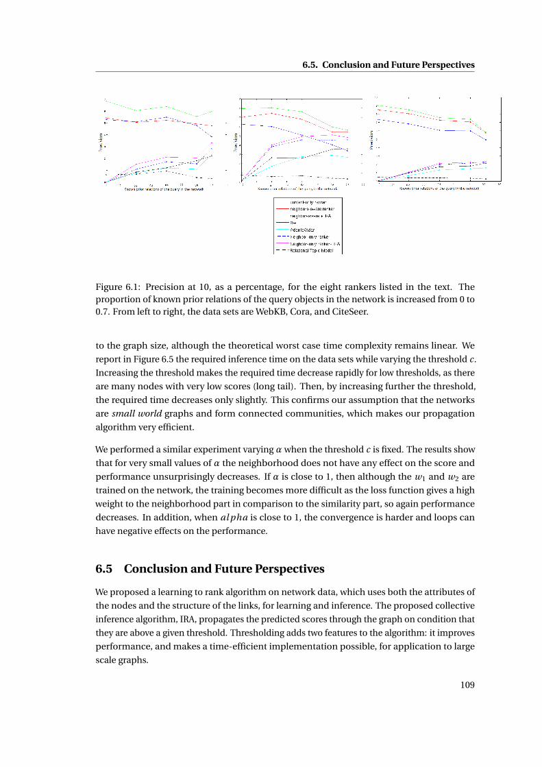
6.5. Conclusion and Future Perspectives
Figure 6.1: Precision at 10, as a percentage, for the eight rankers listed in the text. Theproportion of known prior relations of the query objects in the network is increased from 0 to0.7. From left to right, the data sets are WebKB, Cora, and CiteSeer.
to the graph size, although the theoretical worst case time complexity remains linear. We
report in Figure 6.5 the required inference time on the data sets while varying the threshold c.
Increasing the threshold makes the required time decrease rapidly for low thresholds, as there
are many nodes with very low scores (long tail). Then, by increasing further the threshold,
the required time decreases only slightly. This confirms our assumption that the networks
are small world graphs and form connected communities, which makes our propagation
algorithm very efficient.
We performed a similar experiment varying α when the threshold c is fixed. The results show
that for very small values of α the neighborhood does not have any effect on the score and
performance unsurprisingly decreases. If α is close to 1, then although the w1 and w2 are
trained on the network, the training becomes more difficult as the loss function gives a high
weight to the neighborhood part in comparison to the similarity part, so again performance
decreases. In addition, when al pha is close to 1, the convergence is harder and loops can
have negative effects on the performance.
6.5 Conclusion and Future Perspectives
We proposed a learning to rank algorithm on network data, which uses both the attributes of
the nodes and the structure of the links, for learning and inference. The proposed collective
inference algorithm, IRA, propagates the predicted scores through the graph on condition that
they are above a given threshold. Thresholding adds two features to the algorithm: it improves
performance, and makes a time-efficient implementation possible, for application to large
scale graphs.
109
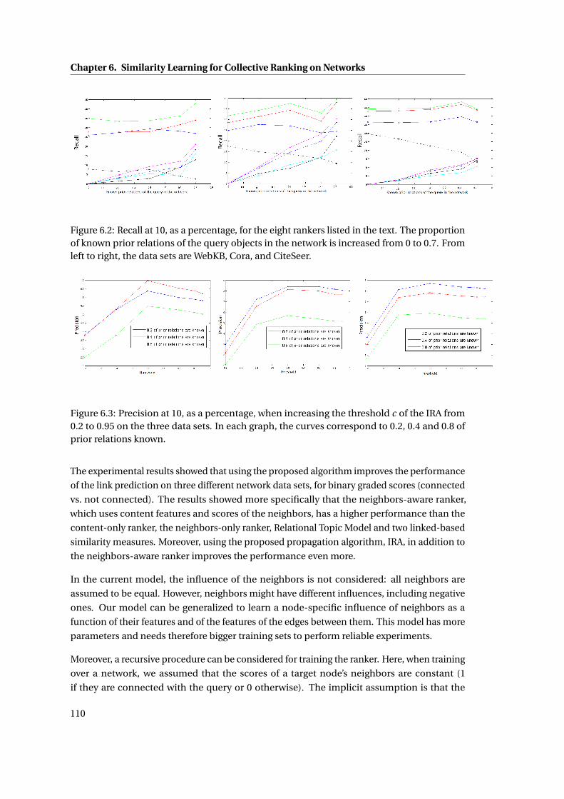
Chapter 6. Similarity Learning for Collective Ranking on Networks
Figure 6.2: Recall at 10, as a percentage, for the eight rankers listed in the text. The proportionof known prior relations of the query objects in the network is increased from 0 to 0.7. Fromleft to right, the data sets are WebKB, Cora, and CiteSeer.
Figure 6.3: Precision at 10, as a percentage, when increasing the threshold c of the IRA from0.2 to 0.95 on the three data sets. In each graph, the curves correspond to 0.2, 0.4 and 0.8 ofprior relations known.
The experimental results showed that using the proposed algorithm improves the performance
of the link prediction on three different network data sets, for binary graded scores (connected
vs. not connected). The results showed more specifically that the neighbors-aware ranker,
which uses content features and scores of the neighbors, has a higher performance than the
content-only ranker, the neighbors-only ranker, Relational Topic Model and two linked-based
similarity measures. Moreover, using the proposed propagation algorithm, IRA, in addition to
the neighbors-aware ranker improves the performance even more.
In the current model, the influence of the neighbors is not considered: all neighbors are
assumed to be equal. However, neighbors might have different influences, including negative
ones. Our model can be generalized to learn a node-specific influence of neighbors as a
function of their features and of the features of the edges between them. This model has more
parameters and needs therefore bigger training sets to perform reliable experiments.
Moreover, a recursive procedure can be considered for training the ranker. Here, when training
over a network, we assumed that the scores of a target node’s neighbors are constant (1
if they are connected with the query or 0 otherwise). The implicit assumption is that the
110
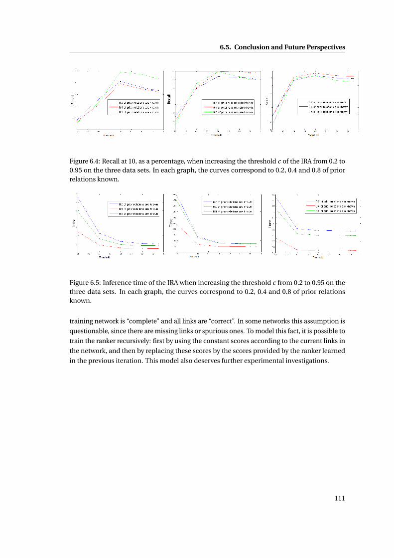
6.5. Conclusion and Future Perspectives
Figure 6.4: Recall at 10, as a percentage, when increasing the threshold c of the IRA from 0.2 to0.95 on the three data sets. In each graph, the curves correspond to 0.2, 0.4 and 0.8 of priorrelations known.
Figure 6.5: Inference time of the IRA when increasing the threshold c from 0.2 to 0.95 on thethree data sets. In each graph, the curves correspond to 0.2, 0.4 and 0.8 of prior relationsknown.
training network is “complete” and all links are “correct”. In some networks this assumption is
questionable, since there are missing links or spurious ones. To model this fact, it is possible to
train the ranker recursively: first by using the constant scores according to the current links in
the network, and then by replacing these scores by the scores provided by the ranker learned
in the previous iteration. This model also deserves further experimental investigations.
111

7 Conclusion and Perspectives
In this thesis, we have proposed novel solutions to similarity learning problems on collabo-
rative networks. As shown throughout the thesis, similarity learning is an essential task for
modeling and predicting the evolution of collaborative networks. Moreover, we showed that
similarity learning is used to perform ranking, which is the main component of recommender
systems. Due to the the low cost of developing such collaborative networks, they grow very
quickly, and therefore, we have aimed for models that scale well to large networks.
Conclusion
Various sources of information can be considered when building a distance measure over a
collaborative network. The first important source of information is the global link structure
of the network. In collaborative networks, there are many spurious and missing links, which
make a proximity measure based on local link structure unreliable. The link structure also
might consist of multiple link types.
In Chapter 3, to answer these requirements, we defined a random walk model, named Visiting
Probability (VP), to measure proximity between two nodes in a graph. VP considers all
the paths between two nodes collectively and thus reduces the effect of unreliable links.
We defined a symmetric VP similarity measure and showed experimentally that using the
symmetric VP improves the prediction performance of the distance. Moreover, we showed
how to use both the VP definition and the structural characteristics of many social networks,
namely the case of small-world networks, to design scalable algorithms based on VP similarity.
We designed approximation algorithms to perform ranking based on VP on large graphs.
Besides, we defined the community of a node according to VP and gave experimental evidence
that this definition was effective. Fast algorithms were designed to solve K-nearest neighbors
and identify the communities over large graphs, based on symmetric VP proximity.
In the second part of Chapter 3, we took advantage of the homophily principle in social net-
works, the fact that two nodes having similar ”social characteristics” have a higher probability
113
Chapter 7. Conclusion and Perspectives
to be linked. We defined a latent space as the space that is formed by the “social characteristics”
or “latent features”, and assumed that homophily holds in this latent space.
Therefore, we showed that the link structure of a graph can be modeled by the proposed
similarity learning framework, in which the transformation of nodes to the latent space is
trained using a discriminative model. We showed how to apply this framework to learn the
similarity between two nodes based on their attributes, over large graphs. Moreover, we
showed that similarity learning on attributes derived from random walk scores, specifically
VP scores, can model and predict better the relations in the graph in comparison to learning
on the network’s links directly. Especially, we showed that training the latent space on the
VP-based communities of nodes resulted in the best prediction performance.
Therefore, we used both global network structure (VP scores) and node attributes to learn
a reliable similarity measure. In the experimental results, we observed that sometimes the
nodes’ attributes were not predictive enough to be able to describe the global link structure of
the network, and the prediction performance dropped when using only the node attributes.
To answer this problem, we designed a learning to rank framework specific to the network
data in Chapter 6.
In Chapter 4, we explained how to transfer knowledge from a hypertext encyclopedia to text
analysis tasks. We have constructed a graph including Wikipedia articles and two different link
structures between them. Our hypothesis was that using both word co-occurrence information
and user-defined hyperlinks between articles could improve the resulting textual distance
for application to a variety of tasks: word similarity; document similarity, clustering, and
classification; information retrieval, and learning to rank.
To transfer learning from the Wikipedia network to text analysis tasks, we proposed and tested
two representation methods. In the first one, a given text is mapped to the corresponding
concepts in the network. Then, to compute similarity between two texts, VP similarity is
applied to compute the distance between the two sets of nodes. In other words, the shared
representation space is the set of concepts in the network and every text is represented in this
space. The second method uses the latent space model explained in Chapter 3 as the shared
representation, by training a transformation from words to the latent space over VP scores.
Therefore, to transfer knowledge from the network to any machine learning algorithms, the
given texts are transformed using this learned transformation. This second approach is easy to
integrate with other machine learning algorithms and also speeds up similarity computation
(testing time) in comparison to the first method.
We tested our proposals on different benchmark tasks: word similarity, document similarity,
clustering, classification, information retrieval and learning to rank, and found that results
were most often competitive compared to state-of-the-art task-specific methods. Our exper-
imental results supported the hypothesis that both types of links over Wikipedia are useful,
as the improvement of performance was higher when both were used together rather than
separately. This sheds light on the fact that in many collaborative networks different link types
114
can be used in a complementary way, and we investigated this problem formally in Chapter 5.
In Chapter 5, we proposed two joint similarity learning models over nodes’ attributes for link
prediction in networks with multiple link types. The first model learns a similarity metric
that consists of two parts: the general part, which is shared between all link types, and the
specific part, which is trained specifically for each type of link. The second model consists of
two layers: the first layer, which is shared between all link types, embeds the objects of the
network into a new space, and then a similarity is learned specifically for each link type in this
new space.
Both models are applicable to large networks with high-dimensional feature spaces. The
experiments showed that the proposed joint modeling and training frameworks improve link
prediction performance significantly for each link type in comparison to multiple baselines.
This improvement is higher when there are fewer links available from one link type in the
network. The two-layer similarity model outperforms the first one, as expected, due to its ca-
pability of modeling negative correlations among different link types. Moreover, we illustrated
that even if the models are trained on only one link type and tested on the other, our models
significantly improve the performance in comparison to ad-hoc similarity metrics.
Finally, in Chapter 6, we proposed a learning to rank algorithm on network data, which uses
both the attributes of the nodes and the structure of the links, for learning and inference.
The global link structure of the network is used in inference by using an original propaga-
tion algorithm named IRA. This algorithm propagates the predicted scores in the graph on
condition that they are above a given threshold. Thresholding improves performance, and
makes a time-efficient implementation possible, for application to large scale graphs. These
improvements were explained considering a structural property of many networks, to be
specific that they are small-word ones.
The experimental results showed that using the IRA algorithm improved the performance of
link prediction on three different network data sets, for binary graded scores (connected vs. not
connected). The results showed more specifically that our neighbors-aware ranker, which uses
content features and scores of the neighbors, has a higher performance than the content-only
ranker, the neighbors-only ranker, Relational Topic Model and two linked-based similarity
measures. Moreover, using the IRA in addition to the neighbors-aware ranker improved the
performance even more.
Overall, we proposed and evaluated distance learning methods over large and collaborative
networks with high-dimensional features, to be used for prediction tasks. These methods
make use of the global structure of a network and the attributes of its nodes. We also showed
how to make use of the correlation between various link types for transfer learning. Moreover,
we showed how to leverage reliable content in these networks to perform text analysis tasks,
improving the state-of-the-art performance.
While we showed the importance of similarity learning in analysis and modeling collaborative
115
Chapter 7. Conclusion and Perspectives
networks, we propose in what follows a perspective on other concepts that can also play role,
which should be the topics of future investigations.
Perspectives on Similarity, Consistency and Diversity in Networks
Recommended sets of items generated by a recommender system are limited, in practice, to a
few items. In this thesis, we almost always followed the assumption that the score assigned to
such a set of items is equal to the sum of the scores of each item, given by its similarity with
the query object. This assumption conforms to the homophily principle, but is in fact stronger
than it. For instance, one exception was presented in Chapter 6, in which we considered the
dependency between linked objects and showed improvement in the prediction performance,
assuming also that there should be consistency between the scores of the linked objects.
Consistency increases the relevance of the recommended set by reducing the value of uncer-
tain objects and increasing the value of coherent objects. This uncertainty is usually due to
the imperfect content analysis techniques or intrinsic noise in the content of the query object.
For example, in a recommender system for multimedia data, this uncertainty can be due to
the imperfection of audio and video content analysis methods. Moreover, the uncertainty can
be due to the intrinsic noise introduced by the unfocused nature of human communication,
for example a video about social network analysis might also mention briefly the application
of social network analysis to neuroscience.
In these cases, if we could also model consistency of the recommended set, then we would be
able to reduce some of the uncertainty in the recommended set. In Chapter 4, Section 4.12, we
showed that performing random walk on the network of objects implicitly solves this problem
for a speech-based recommender system. In the following, we will sketch a formal definition
of consistency based on the models presented in this thesis, to be explored in future work.
In almost all collaborative networks there is a cost for creating a link and therefore, the number
of links per object is limited. For example, the number of products customers can buy from an
online store is limited by their budget. The number of citations in a paper is limited because
authors can not afford reading all papers. Therefore, forming a link between similar objects is
more likely, but it does not imply that each object should necessarily connect to all similar
objects.
Hence, among all similar objects, a diverse set of objects should be chosen for linking, so that
it covers most aspects of the query object. For example, if an article is about the application
of Hidden Markov Models to cryptanalysis, only important papers about Hidden Markov
Models and cryptanalysis should be cited. Diversity thus plays a role in link formation in many
examples, such as Wikipedia, news readers, article citations, consumer products, and music
recommendation. Moreover, in difficult queries like ambiguous ones, diversification of the
recommended set reduces the number of times that the system fails to recommending at least
one relevant item.
116
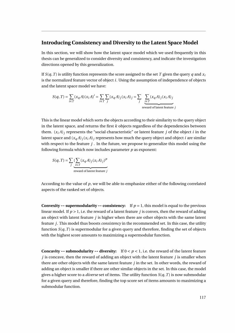
Introducing Consistency and Diversity to the Latent Space Model
In this section, we will show how the latent space model which we used frequently in this
thesis can be generalized to consider diversity and consistency, and indicate the investigation
directions opened by this generalization.
If S(q,T ) is utility function represents the score assigned to the set T given the query q and xi
is the normalized feature vector of object i . Using the assumption of independence of objects
and the latent space model we have:
S(q,T ) = ∑i∈T
(xq A)(xi A)′ = ∑i∈T
∑j
(xq A) j (xi A) j =∑
j
∑i∈T
(xq A) j (xi A) j︸ ︷︷ ︸reward of latent feature j
This is the linear model which sorts the objects according to their similarity to the query object
in the latent space, and returns the first k objects regardless of the dependencies between
them. (xi A) j represents the “social characteristic” or latent feature j of the object i in the
latent space and (xq A) j (xi A) j represents how much the query object and object i are similar
with respect to the feature j . In the future, we propose to generalize this model using the
following formula which now includes parameter p as exponent:
S(q,T ) =∑j
(∑i∈T
(xq A) j (xi A) j )p
︸ ︷︷ ︸reward of latent feature j
According to the value of p, we will be able to emphasize either of the following correlated
aspects of the ranked set of objects.
Convexity ↔ supermodularity ↔ consistency: If p = 1, this model is equal to the previous
linear model. If p > 1, i.e. the reward of a latent feature j is convex, then the reward of adding
an object with latent feature j is higher when there are other objects with the same latent
feature j . This model thus boosts consistency in the recommended set. In this case, the utility
function S(q,T ) is supermodular for a given query and therefore, finding the set of objects
with the highest score amounts to maximizing a supermodular function.
Concavity ↔ submodularity ↔ diversity: If 0 < p < 1, i.e. the reward of the latent feature
j is concave, then the reward of adding an object with the latent feature j is smaller when
there are other objects with the same latent feature j in the set. In other words, the reward of
adding an object is smaller if there are other similar objects in the set. In this case, the model
gives a higher score to a diverse set of items. The utility function S(q,T ) is now submodular
for a given query and therefore, finding the top score set of items amounts to maximizing a
submodular function.
117
Chapter 7. Conclusion and Perspectives
These proposals enrich the latent space model to encompass the concepts of diversity and
consistency. The model still has the main desirable properties for the objective function: first,
it gives a higher score to a set with items that are related to the query object (homophily) and,
second, it emphasizes the diversity or consistency of items depending on the value of p.
There are several questions that must be investigated before putting this model into appli-
cation. First, we need efficient algorithms to train both set of parameters, namely A and p.
Moreover, is p dependent on the query object? It may be the case, indeed, that for some query
objects diversity is more important than consistency, or vice-versa. In this case, can we learn
the value of p depending on the query object? Besides, is p equal for all latent features or
does it change for different features? Again, consistency could be more important for some
features and diversity for other ones. Moreover, is it possible to consider both diversity and
consistency simultaneously for a query object? It may be the case that given a query, a diverse
set of consistent objects is the best recommended set.
Finally, after training these parameters, finding a set with a maximal score is not tractable for
large data sets. In the case of a submodular utility function (with diversity being the target),
efficient greedy algorithms have been proposed for inference on large data sets [Nemhauser
et al., 1978, Minoux, 1978, Krause and Golovin, 2012]. Conversely, if the utility function is
supermodular (consistency being the target), we need to design efficient algorithms to find
the maximal set, or, presumably, approximate it. We foresee further investigations on these
topics to make training and inference possible on large data sets.
118
Bibliography
Lada A. Adamic and Eytan Adar. Friends and neighbors on the web. SOCIAL NETWORKS, 25:
211–230, 2001.
Lada A. Adamic and Bernardo A. Huberman. Power-law distribution of the world wide web.
SCIENCE, 287:2115, 2000.
Alekh Agarwal, Soumen Chakrabarti, and Sunny Aggarwal. Learning to rank networked enti-
ties. In Proceedings of KDD ’06 (12th ACM SIGKDD international conference on Knowledge
discovery and data mining), pages 14–23, 2006.
Eneko Agirre and Aitor Soroa. Personalizing PageRank for word sense disambiguation. In
Proceedings of EACL 2009 (12th Conference of the European Chapter of the Association for
Computational Linguistics), pages 33–41, Athens, Greece, 2009.
Eneko Agirre, Enrique Alfonseca, Keith Hall, Jana Kravalova, Marius Pasca, and Aitor Soroa. A
study on similarity and relatedness using distributional and WordNet-based approaches. In
Proceedings of HLT-NAACL 2009 (Human Language Technologies: the 2009 Annual Confer-
ence of the North American Chapter of the ACL), pages 19–27, Boulder, CO, 2009.
David Aldous and James Allen Fill. Reversible markov chains and random walks on graphs,
2002. URL http://www.stat.berkeley.edu/~aldous/RWG/book.html.
U. Alon, M. G. Surette, N. Barkai, and S. Leibler. Robustness in bacterial chemotaxis. Nature,
397(6715):168–171, 1999.
Marco A. Alvarez and Seung Jin Lim. A graph modeling of semantic similarity between words.
In Proceedings of ICSC 2007 (1st International Conference on Semantic Computing), pages
355–362, Irvine, CA, 2007.
Lars Backstrom and Jure Leskovec. Supervised random walks: Predicting and recommending
links in social networks. In Proceedings of WSDM 2011 (Fourth ACM International Conference
on Web Search and Data Mining), 2011.
Bing Bai, Jason Weston, David Grangier, Ronan Collobert, Kunihiko Sadamasa, Yanjun Qi,
Corinna Cortes, and Mehryar Mohri. Polynomial semantic indexing. In Y. Bengio, D. Schu-
urmans, J. Lafferty, C. K. I. Williams, and A. Culotta, editors, Advances in Neural Information
Processing Systems 22, pages 64–72, 2009.
119
Bibliography
Bing Bai, Jason Weston, David Grangier, Ronan Collobert, Kunihiko Sadamasa, Yanjun Qi,
Olivier Chapelle, and Kilian Weinberger. Learning to rank with (a lot of) word features.
Information Retrieval, 13(3):291–314, 2010.
Albert-László Barabási and Réka Albert. Emergence of Scaling in Random Networks. Science,
286(5439):509–512, 1999.
Mustapha Baziz, Mohand Boughanem, Nathalie Aussenac-Gilles, and Claude Chrisment. Se-
mantic cores for representing documents in IR. In Proceedings of SAC 2005 (ACM Symposium
on Applied Computing), pages 1011–1017, Santa Fe, NM, 2005.
Pavel Berkhin. A survey on PageRank computing. Internet Mathematics, 2(1):73–120, 2005.
C. Bizer, J. Lehmann, G. Kobilarov, S. Auer, C. Becker, R. Cyganiak, and S. Hellmann. DBpedia –
a crystallization point for the web of data. Journal of Web Semantics, 7:154–165, 2009.
David M. Blei, Andrew Y. Ng, and Michael I. Jordan. Latent Dirichlet Allocation. Journal of
Machine Learning Research, 3:993–1022, 2003.
Danushka Bollegala, Yutaka Matsuo, and Mitsuru Ishizuka. Measuring semantic similarity
between words using web search engines. In Proceedings of WWW 2007 (16th International
Conference on World Wide Web), pages 757–766, Banff, Alberta, 2007.
Antoine Bordes, Jason Weston, Ronan Collobert, and Yoshua Bengio. Learning structured
embeddings of knowledge bases. In Proceedings of AAAI 2011 (Twenty-Fifth Conference on
Artificial Intelligence), 2011.
Gloria Bordogna and Gabriella Pasi. Hierarchical-hyperspherical divisive fuzzy C-means (H2D-
FCM) clustering for information retrieval. In Proceedings of WI-IAT 2009 (IEEE/WIC/ACM
International Joint Conference on Web Intelligence and Intelligent Agent Technology), vol-
ume 1, pages 614–621, Milan, Italy, 2009.
Matthew Brand. A random walks perspective on maximizing satisfaction and profit. In
Proceedings of SDM 2005 (SIAM International Conference on Data Mining), pages 12–19,
Newport Beach, CA, 2005.
Alexander Budanitsky and Graeme Hirst. Evaluating WordNet-based measures of semantic
distance. Computational Linguistics, 32(1):13–47, 2006.
Chris Burges, Tal Shaked, Erin Renshaw, Ari Lazier, Matt Deeds, Nicole Hamilton, and Greg
Hullender. Learning to rank using gradient descent. In Proceedings of the 22nd international
conference on Machine learning, ICML ’05, pages 89–96, New York, NY, USA, 2005. ACM.
ISBN 1-59593-180-5. doi: http://doi.acm.org/10.1145/1102351.1102363. URL http://doi.
acm.org/10.1145/1102351.1102363.
Yunbo Cao, Jun Xu, Tie-Yan Liu, Hang Li, Yalou Huang, and Hsiao-Wuen Hon. Adapting ranking
svm to document retrieval. In Proceedings of SIGIR 2006 (29th Annual International ACM
120

Bibliography
SIGIR conference on Research and development in information retrieval), pages 186–193,
2006.
P.J. Carrington, J. Scott, and S. Wasserman. Models and methods in social network analysis.
Cambridge university press, 2005.
Chih-Chung Chang and Chih-Jen Lin. LIBSVM: A library for support vector machines. ACM
Transactions on Intelligent Systems and Technology, 2:article n. 27, 2011.
Jonathan Chang. Relational topic models for document networks. In In Proceedings of AISTATS
2009 (Twelfth International Conference on Artificial Intelligence and Statistics), 2009.
Jonathan Chang, Jordan Boyd-Graber, Sean Gerrish, Chong Wang, and David M. Blei. Reading
tea leaves: How humans interpret topic models. In Y. Bengio, D. Schuurmans, J. Lafferty,
C. K. I. Williams, and A. Culotta, editors, Advances in Neural Information Processing Systems
22, pages 288–296. The MIT Press, Cambridge, MA, 2009.
Jean-Cédric Chappelier. Topic-based generative models for text information access. In Éric
Gaussier and Francois Yvon, editors, Textual Information Access: Statistical Models, pages
129–178. ISTE / Wiley, London, UK, 2012.
P. Cimiano, A. Schultz, S. Sizov, P. Sorg, and S. Staab. Explicit vs. latent concept models for
cross-language information retrieval. In Proceedings of IJCAI 2009 (21st International Joint
Conference on Artificial Intelligence), pages 1513–1518, Pasadena, CA, 2009.
Kevyn Collins-Thompson and Jamie Callan. Query expansion using random walk models. In
Proceedings of CIKM 2005 (14th ACM Conference on Information and Knowledge Manage-
ment), pages 704–711, Bremen, Germany, 2005. ISBN 1-59593-140-6.
Kino Coursey, Rada Mihalcea, and William Moen. Using encyclopedic knowledge for automatic
topic identification. In Proceedings of CoNLL 2009 (13th Conference on Computational
Natural Language Learning), pages 210–218, Boulder, CO, 2009.
Koby Crammer and Yoram Singer. Pranking with ranking. In Advances in Neural Information
Processing Systems 14, pages 641–647. MIT Press, 2001.
Scott Deerwester, Susan T. Dumais, George W. Furnas, Thomas K. Landauer, and Richard
Harshman. Indexing by Latent Semantic Analysis. Journal of the American Society for
Information Science, 41(6):391–407, 1990.
Ofer Egozi, Shaul Markovitch, and Evgeniy Gabrilovich. Concept-based information retrieval
using explicit semantic analysis. ACM Transactions on Information Systems (TOIS), 29(2):
article n. 8, 2011.
Christiane Fellbaum, editor. WordNet: An electronic lexical database. The MIT Press, Cam-
bridge, MA, 1998.
121
Bibliography
Lev Finkelstein, Evgeniy Gabrilovich, Yossi Matias, Ehud Rivlin, Zach Solan, Gadi Wolfman,
and Eytan Ruppin. Placing search in context: The concept revisited. ACM Transactions on
Information Systems (TOIS), 20(1):116–131, 2002.
Daniel Fogaras, Balazs Racz, Karoly Csalogany, and Tamas Sarlos. Towards scaling fully
personalized PageRank: Algorithms, lower bounds, and experiments. Internet Mathematics,
2(3), 2005. URL http://dblp.uni-trier.de/db/journals/im/im2.html.
Evgeniy Gabrilovich and Shaul Markovitch. Computing semantic relatedness using Wikipedia-
based explicit semantic analysis. In Proceedings of IJCAI 2007 (20th International Joint
Conference on Artificial Intelligence), pages 6–12, Hyderabad, India, 2007.
Evgeniy Gabrilovich and Shaul Markovitch. Wikipedia-based semantic interpretation for
natural language processing. Journal of Artificial Intelligence Research, 34:443–498, 2009.
David Grangier and Samy Bengio. A discriminative kernel-based model to rank images from
text queries. IEEE Transactions on Pattern Analysis and Machine Intelligence (TPAMI), 2008.
Victor Grishchenko. Wikipedia as an ant-hill. Web page consulted on April 15, 2012: http://no-
gritzko-here.livejournal.com/22900.html, March 13 2008.
Maryam Habibi and Andrei Popescu-Belis. Using crowdsourcing to compare document
recommendation strategies for conversations. In Proceedings of the ACM Workshop on
Recommendation Utility Evaluation: Beyond RMSE (RUE 2011), pages 15–20, Dublin, 2012.
M.A.K. Halliday and Ruqaiya Hasan. Language, context, and text: aspects of language in a
social-semiotic perspective. Oxford University Press, London, 2nd edition, 1989.
Samer Hassan and Rada Mihalcea. Cross-lingual semantic relatedness using encyclopedic
knowledge. In Proceedings of EMNLP 2009 (Conference on Empirical Methods in Natural
Language Processing), pages 1192–1201, Singapore, 2009.
Samer Hassan and Rada Mihalcea. Semantic relatedness using salient semantic analysis. In
Proceedings of AAAI 2011 (25th AAAI Conference on Artificial Intelligence), pages 884–889,
San Francisco, CA, 2011.
Taher H. Haveliwala. Topic-sensitive PageRank. In Proceedings of WWW 2002 (11th interna-
tional conference on World Wide Web), pages 517–526, 2002.
Taher H. Haveliwala. Topic-sensitive PageRank: A context-sensitive ranking algorithm for web
search. IEEE Transactions on Knowledge and Data Engineering, 15:784–796, 2003. ISSN
1041-4347. doi: http://doi.ieeecomputersociety.org/10.1109/TKDE.2003.1208999.
R. Herbrich, T. Graepel, and K. Obermayer. Large margin rank boundaries for ordinal regres-
sion. In A.J. Smola, P.L. Bartlett, B. Schölkopf, and D. Schuurmans, editors, Advances in
Large Margin Classifiers, pages 115–132, Cambridge, MA, 2000. MIT Press.
122
Bibliography
Jerry Hobbs. Why is discourse coherent? In Fritz Neubauer, editor, Coherence in natural
language texts, pages 29–70. Buske, Hamburg, 1983.
Peter D. Hoff, Adrian E. Raftery, and Mark S. Handcock. Latent space approaches to social
network analysis. JOURNAL OF THE AMERICAN STATISTICAL ASSOCIATION, 97:1090–1098,
2001.
Thomas Hofmann. Probabilistic Latent Semantic Indexing. In Proceedings of SIGIR 1999 (22nd
ACM SIGIR Conference on Research and Development in Information Retrieval), pages 50–57,
Berkeley, CA, 1999.
X. Hu, X. Zhang, C. Lu, EK Park, and X. Zhou. Exploiting Wikipedia as external knowledge
for document clustering. In Proceedings of KDD 2009 (15th ACM SIGKDD International
Conference on Knowledge Discovery and Data Mining), pages 389–396, Paris, France, 2009.
Thad Hughes and Daniel Ramage. Lexical semantic relatedness with random graph walks. In
Proceedings of EMNLP-CoNLL 2007 (Conference on Empirical Methods in Natural Language
Processing and Conference on Computational Natural Language Learning), pages 581–589,
Prague, Czech Republic, 2007.
Mario Jarmasz. Roget’s Thesaurus as a Lexical Resource for Natural Language Processing.
Master’s thesis, University of Ottawa, 2003.
Mario Jarmasz and Stan Szpakowicz. Roget’s thesaurus and semantic similarity. In Proceedings
of RANLP 2003 (Conference on Recent Advances in Natural Language Processing), pages
111–120, Borovetz, Bulgaria, 2003.
David Jensen, Jennifer Neville, and Brian Gallagher. Why collective inference improves re-
lational classification. In Proceedings of KDD 2004 (tenth ACM SIGKDD international
conference on Knowledge discovery and data mining), pages 593–598, 2004.
Thorsten Joachims. Optimizing search engines using clickthrough data. In Proceedings of
KDD 2002 (eighth ACM SIGKDD international conference on Knowledge discovery and data
mining), pages 133–142, 2002.
Upali S. Kohomban and Wee Sun Lee. Learning semantic classes for word sense disambigua-
tion. In Proceedings of ACL 2005 (43rd Annual Meeting of the Association for Computational
Linguistics), pages 34–41, Ann Arbor, MI, 2005.
Andreas Krause and Daniel Golovin. Submodular function maximization. In Tractability:
Practical Approaches to Hard Problems (to appear). Cambridge University Press, 2012.
Claudia Leacock and Martin Chodorow. Combining local context and WordNet similarity for
word sense identification. In Christiane Fellbaum, editor, WordNet: An electronic lexical
database, pages 265–283. The MIT Press, Cambridge, MA, 1998.
123
Bibliography
Michael D. Lee, Brandon Pincombe, and Matthew Welsh. An empirical evaluation of models
of text document similarity. In Proceedings of CogSci 2005 (27th Annual Conference of the
Cognitive Science Society), pages 1254–1259, Stresa, Italy, 2005.
Douglas B. Lenat. CYC: A large-scale investment in knowledge infrastructure. Communications
of the ACM, 38(11):33–38, 1995.
Jure Leskovec, Lada A. Adamic, and Bernardo A. Huberman. The dynamics of viral marketing.
ACM Trans. Web, 1, 2007.
Hang Li. Learning to Rank for Information Retrieval and Natural Language Processing. Syn-
thesis Lectures on Human Language Technology. Morgan and Claypool, San Rafael, CA,
2011.
David Liben-Nowell and Jon Kleinberg. The link prediction problem for social networks. In Pro-
ceedings of CIKM 2003 (12th ACM International Conference on Information and Knowledge
Management), pages 556–559, New Orleans, LA, 2003.
Dekang Lin. An information-theoretic definition of similarity. In Proceedings of ICML 1998
(15th International Conference on Machine Learning), pages 296–304, Madison, WI, 1998.
L.K. McDowell and D.W. Aha K.M. Gupta. Cautious collective classification. Journal of Machine
Learning Research (JMLR), 2009.
Miller McPherson, Lynn Smith-Lovin, and James M. Cook. Birds of a feather: Homophily in
social networks. Annual Review of Sociology, 27:415–444, 2001.
Qiaozhu Mei, Dengyong Zhou, and Kenneth Church. Query suggestion using hitting time. In
Proceeding of CIKM 2008 (17th ACM International Conference on Information and Knowledge
Management), pages 469–478, Napa Valley, CA, 2008.
Aditya Krishna Menon and Charles Elkan. Link prediction via matrix factorization. In Proceed-
ings of ECML PKDD 2011 (2011 European Conference on Machine learning and Knowledge
Discovery in Databases), pages 437–452, 2011.
Metaweb Technologies. Freebase Wikipedia Extraction (WEX).
http://download.freebase.com/wex/, 2010.
Rada Mihalcea and Andras Csomai. Wikify!: Linking documents to encyclopedic knowledge.
In Proceedings of ACM CIKM 2007 (16th ACM Conference on Information and Knowledge
Management), pages 233–242, Lisbon, Portugal, 2007.
Rada Mihalcea, Courtney Corley, and Carlo Strapparava. Corpus-based and knowledge-based
measures of text semantic similarity. In Proceedings of AAAI 2006 (21st National Conference
on Artificial Intelligence), pages 775–782, Boston, MA, 2006.
George A. Miller and Walter G. Charles. Contextual correlates of semantic similarity. Language
and Cognitive Processes, 6(1):1–28, 1991.
124
Bibliography
Kurt Miller, Thomas Griffiths, and Michael Jordan. Nonparametric latent feature models for
link prediction. In Y. Bengio, D. Schuurmans, J. Lafferty, C. K. I. Williams, and A. Culotta,
editors, Advances in Neural Information Processing Systems 22, pages 1276–1284, 2009.
David Milne and Iain H. Witten. An effective, low-cost measure of semantic relatedness
obtained from Wikipedia links. In Proceedings of WIKIAI 2008 (1st AAAI Workshop on
Wikipedia and Artificial Intelligence), pages 25–30, Chicago, IL, 2008a.
David Milne and Iain H. Witten. Learning to link with Wikipedia. In Proceedings of CIKM 2008
(17th ACM Conference on Information and Knowledge Management), pages 509–518, Napa
Valley, CA, 2008b.
Michel Minoux. Accelerated greedy algorithms for maximizing submodular set functions.
In J. Stoer, editor, Optimization Techniques, volume 7 of Lecture Notes in Control and
Information Sciences, pages 234–243. Springer Berlin / Heidelberg, 1978.
Tom M. Mitchell. Machine Learning. McGraw-Hill, New York, NY, 1997.
Saif Mohammad and Graeme Hirst. Distributional measures as proxies for se-
mantic distance: A survey. Available online (consulted on April 15, 2012) at:
http://www.cs.toronto.edu/pub/gh/Mohammad+Hirst-2005.pdf, 2005.
Jane Morris and Graeme Hirst. Non-classical lexical semantic relations. In HLT-NAACL 2004:
Workshop on Computational Lexical Semantics, pages 46–51. Association for Computational
Linguistics, 2004.
V. Nastase, M. Strube, B. Boerschinger, C. Zirn, and A. Elghafari. WikiNet: A very large scale
multi-lingual concept network. In Proceedings of LREC 2010 (7th International Conference
on Language Resources and Evaluation), Valletta, Malta, 2010.
Roberto Navigli. A structural approach to the automatic adjudication of word sense disagree-
ments. Nat. Lang. Eng., 14(4):547–573, 2008.
Roberto Navigli and Mirella Lapata. An experimental study of graph connectivity for unsu-
pervised word sense disambiguation. IEEE Transactions on Pattern Analysis and Machine
Intelligence, 32(4):678–692, 2010.
Roberto Navigli and Simone Paolo Ponzetto. BabelNet: Building a very large multilingual
semantic network. In Proceedings of ACL 2010 (48th Annual Meeting of the Association for
Computational Linguistics), pages 216–225, Uppsala, Sweden, 2010.
G. Nemhauser, L. Wolsey, and M. Fisher. An analysis of the approximations for maximizing
submodular set functions. Mathematical Programming, 1978.
David Newman, Jey Han Lau, Karl Grieser, and Timothy Baldwin. Automatic evaluation of topic
coherence. In Proceedings of HLT-NAACL 2010 (Annual Conference of the North American
Chapter of the Association for Computational Linguistics), pages 100–108, Los Angeles, CA,
2010.
125
Bibliography
Tore Opsahl and Pietro Panzarasa. Clustering in weighted networks. Social Networks, 31(2):
155–163, 2009.
Alberto Paccanaro and Geoffrey E. Hinton. Learning distributed representations of concepts
from relational data. IEEE Transactions on Knowledge and Data Engineering, 13:232–244,
2000.
Sebastian Padó and Mirella Lapata. Dependency-based construction of semantic space
models. Computational Linguistics, 33(2):161–199, 2007.
Siddharth Patwardhan and Ted Pedersen. Using WordNet-based context vectors to estimate
the semantic relatedness of concepts. In Proceedings of the EACL 2006 Workshop on Making
Sense of Sense, pages 1–8, Trento, Italy, 2006.
Siddharth Patwardhan, Satanjeev Banerjee, and Ted Pedersen. Using measures of semantic re-
latedness for word sense disambiguation. In Proceedings of CICLing 2003 (4th International
Conference on Computational Linguistics and Intelligent Text Processing), LNCS 2588, pages
241–257, Mexico City, Mexico, 2003.
Stuart L. Pimm, John H. Lawton, and Joel E. Cohen. Food web patterns and their consequences.
Nature, 350(6320):669–674, 1991. doi: 10.1038/350669a0. URL http://dx.doi.org/10.1038/
350669a0.
Simone Paolo Ponzetto and Michael Strube. Knowledge derived from Wikipedia for computing
semantic relatedness. Journal of Artificial Intelligence Research, 30:181–212, 2007.
Simone Paolo Ponzetto and Michael Strube. Taxonomy induction based on a collaboratively
built knowledge repository. Artificial Intelligence, 175(9-10):1737–1756, 2011.
Andrei Popescu-Belis, Erik Boertjes, Jonathan Kilgour, Peter Poller, Sandro Castronovo, Theresa
Wilson, Alex Jaimes, and Jean Carletta. The AMIDA automatic content linking device: Just-
in-time document retrieval in meetings. In Proceedings of MLMI 2008 (5th International
Workshop on Machine Learning for Multimodal Interaction), pages 272–283. Springer LNCS
5237, 2008.
Andrei Popescu-Belis, Majid Yazdani, Alexandre Nanchen, and Philip N. Garner. A speech-
based just-in-time retrieval system using semantic search. In Proceedings of the 49th Annual
Meeting of the Association for Computational Linguistics: Human Language Technologies,
pages 80–85, 2011.
R. Rada, H. Mili, E. Bicknell, and M. Blettner. Development and application of a metric to
semantic nets. IEEE Transactions on Systems, Man and Cybernetics, 19(1):17–30, 1989.
Daniel Ramage, Anna N. Rafferty, and Christopher D. Manning. Random walks for text
semantic similarity. In Proceedings of TextGraphs-4 (4th Workshop on Graph-based Methods
for Natural Language Processing), pages 23–31, Singapore, 2009.
126
Bibliography
M.A. Ranzato and M. Szummer. Semi-supervised learning of compact document representa-
tions with deep networks. In Proceedings of ICML 2008 (25th International Conference on
Machine Learning), pages 792–799, Helsinki, Finland, 2008.
Philip Resnik. Using information content to evaluate semantic similarity in a taxonomy. In
Proceedings of IJCAI 1995 (14th International Joint Conference on Artificial Intelligence),
pages 448–453, Montreal, 1995.
Philip Resnik. Semantic similarity in a taxonomy: An information-based measure and its
application to problems of ambiguity in natural language. Journal of Artificial Intelligence
Research, 11:95–130, 1999.
Herbert Rubenstein and John B. Goodenough. Contextual correlates of synonymy. Communi-
cations of the ACM, 8(10):627–633, 1965.
Marco Saerens, Francois Fouss, Luh Yen, and Pierre Dupont. The principal components
analysis of a graph, and its relationships to spectral clustering. In Proceedings of ICML 2004
(15th European Conference on Machine Learning ), pages 371–383, 2004.
Purnamrita Sarkar and Andrew Moore. A tractable approach to finding closest truncated-
commute-time neighbors in large graphs. In Proceedings of UAI 2007 (23rd Conference on
Uncertainty in Artificial Intelligence), pages 335–343, Vancouver, BC, 2007.
Purnamrita Sarkar, Andrew W. Moore, and Amit Prakash. Fast incremental proximity search
in large graphs. In Proceedings of ICML 2008 (25th International Conference on Machine
Learning), pages 896–903, Helsinki, Finland, 2008.
Prithviraj Sen, Galileo Mark Namata, Mustafa Bilgic, Lise Getoor, Brian Gallagher, and Tina
Eliassi-Rad. Collective classification in network data. AI Magazine, 29(3):93–106, 2008.
Shai Shalev-Shwartz, Yoram Singer, Nathan Srebro, and Andrew Cotter. Pegasos: primal
estimated sub-gradient solver for svm. Math. Program., 127(1):3–30, 2011.
Blake Shaw, Bert Huang, and Tony Jebara. Learning a distance metric from a network. In
J. Shawe-Taylor, R.S. Zemel, P. Bartlett, F.C.N. Pereira, and K.Q. Weinberger, editors, Advances
in Neural Information Processing Systems 24, pages 1899–1907, 2011.
M. Stevenson and M. Greenwood. A semantic approach to IE pattern induction. In Proceedings
of ACL 2005 (43rd Annual Meeting of the Association for Computational Linguistics), pages
379–386, Ann Arbor, MI, 2005.
Michael Strube and Simone Paolo Ponzetto. WikiRelate! Computing semantic relatedness
using Wikipedia. In Proceedings of AAAI 2006 (21st National Conference on Artificial Intelli-
gence), pages 1419–1424, Boston, MA, 2006.
F.M. Suchanek, G. Kasneci, and G. Weikum. Yago: A large ontology from Wikipedia and
WordNet. Journal of Web Semantics, 6:203–217, 2008.
127
Bibliography
Zareen S. Syed, Tim Finin, and Anupam Joshi. Wikipedia as an ontology for describing
documents. In Proceedings of the Second International Conference on Weblogs and Social
Media, pages 136–144, Seattle, WA, 2008.
Hanghang Tong, Christos Faloutsos, and Jia-Yu Pan. Fast random walk with restart and its
applications. In Proceedings of the ICDM 2006 (Sixth International Conference on Data
Mining), pages 613–622, 2006.
Amanda L. Traud, Eric D. Kelsic, Peter J. Mucha, and Mason A. Porter. Comparing community
structure to characteristics in online collegiate social networks. SIAM Rev., 53(3):526–543,
2011.
Peter F. Turney. Mining the web for synonyms: PMI-IR versus LSA on TOEFL. In Proceedings
of ECML 2001 (12th European Conference on Machine Learning), pages 491–502, Freiburg,
Germany, 2001.
A. F. J. Vanraan. Fractal dimension of co-citations. Nature, 347(6294):626, 1990. doi: 10.1038/
347626a0. URL http://dx.doi.org/10.1038/347626a0.
Ellen M. Voorhees and Donna Harman. Overview of the Eighth Text REtrieval Conference
(TREC-8). In Proceedings of TREC-8, pages 1–24, Gaithersburg, MD, 1999.
Andreas Wagner and David A. Fell. The small world inside large metabolic networks. Proceed-
ings of the Royal Society of London. Series B: Biological Sciences, 268(1478):1803–1810, 2001.
ISSN 0962-8452. URL http://dx.doi.org/10.1098/rspb.2001.1711.
Duncan J. Watts. Small worlds: the dynamics of networks between order and randomness.
Princeton university press, 2003.
Duncan J. Watts and Steven H. Strogatz. Collective dynamics of ‘small-world’ networks. Nature,
393(6684):440–442, 1998.
Julie E. Weeds. Measures and applications of lexical distributional similarity. PhD thesis,
University of Sussex, 2003.
Kilian Weinberger, John Blitzer, and Lawrence Saul. Distance metric learning for large margin
nearest neighbor classification. In Y. Weiss, B. Schölkopf, and J. Platt, editors, Advances in
Neural Information Processing Systems 18, pages 1473–1480. The MIT Press, Cambridge, MA,
2006.
Jason Weston, Samy Bengio, and Nicolas Usunier. WSABIE: Scaling Up to Large Vocabulary
Image Annotation. In Proceedings of IJCAI 2011 (22nd International Joint Conference on
Artificial Intelligence), pages 2764–2770, 2011.
Zhibiao Wu and Martha Palmer. Verb semantics and lexical selection. In Proceedings of ACL
1994 (32nd Annual Meeting of Association for Computational Linguistics), pages 133–138,
Las Cruces, NM, 1994.
128
Bibliography
Majid Yazdani and Andrei Popescu-Belis. A random walk framework to compute textual
semantic similarity: a unified model for three benchmark tasks. In Proceedings of IEEE
ICSC 2010 (4th IEEE International Conference on Semantic Computing), pages 424–429,
Pittsburgh, PA, 2010.
Majid Yazdani and Andrei Popescu-Belis. Computing text semantic relatedness using the
contents and links of a hypertext encyclopedia. Artificial Intelligence, 194:176–202, 2013.
Eric Yeh, Daniel Ramage, Christopher D. Manning, Eneko Agirre, and Aitor Soroa. WikiWalk:
random walks on Wikipedia for semantic relatedness. In Proceedings of TextGraphs-4
(4th Workshop on Graph-based Methods for Natural Language Processing), pages 41–49,
Singapore, 2009.
Wen-Tau Yih, Kristina Toutanova, John C. Platt, and Christopher Meek. Learning discriminative
projections for text similarity measures. In Proceedings of CoNLL 2011 (15th Conference on
Computational Natural Language Learning), pages 247–256, Portland, OR, 2011.
Torsten Zesch, Christof Müller, and Iryna Gurevych. Using Wiktionary for computing semantic
relatedness. In Proceedings of AAAI 2008 (23rd National Conference on Artificial Intelligence),
volume 2, pages 861–866, Chicago, IL, 2008.
129

Majid Yazdani
Idiap Research InstituteCentre du ParcRue Marconi 19CH - 1920 MartignySwitzerlandmajid.yazdani@epfl/idiap.ch
http://majid.yazdani.me/
Research Interest and Expertise
Algorithmic and Statistical Machine Learning applied to Large (Social) Network Analysis, Natural LanguageProcessing, Computational Finance and System design.
EDUCATION
PhD, Computer ScienceEPFL/Idiap Research Institute, Switzerland. 2009 - 2013Course work: 5.77/6Thesis :Similarity Learning Over Large Collaborative Networks [.pdf],Advisers: Prof.Herve Bourlard and Dr.Andrei Popescu-BelisCommittee: Dr.Samy Bengio, Dr.Jean-Cdric Chappelier, Prof.Andreas Krause
Bachelor of Science, Computer EngineeringSharif University of Technology, Tehran, Iran. 2003- 2008Thesis :Website classification using Extended Hidden Markov Model (19.75/20)
Work ExperiencesPostdoctoral Researcher, Idiap research Institute , Martigny, Switzerland March 2013- nowBuilding a matlab toolbox for “Learning on large networked data”
Research Assistant, Idiap research Institute and EPFL, Martigny, Switzerland 2009- February 2013
Research Assistant : Web Intelligence laboratory , Sharif University of Technology 2007-2008
ReportsMajid Yazdani, Andrei Popescu-Belis. Joint Similarity Learning for Predicting Links in Networks withMultiple-type Links. Idiap-RR Idiap-Internal-RR-64-2012, under preparation , 2013.[.pdf]
PUBLICATIONS (Chronological)Hassan Ghasemzadeh Mohammadi, Pierre-Emmanuel Gaillardon, Majid Yazdani, Giovanni De Micheli.A Fast TCAD-based Methodology for Variation Analysis of Emerging Nano-Devices. IEEE InternationalSymposium on Defect and Fault Tolerance in VLSI and Nanotechnology Systems, 2013. [.pdf]
Majid Yazdani, Ronan Collobert, Andrei Popescu-Belis. Learning to Rank on Network Data. Miningand Learning with Graphs , 2013.[.pdf]
131
M. Yazdanip. 2
Majid Yazdani and Andrei Popescu-Belis. Computing text semantic relatedness using the contents andlinks of a hypertext encyclopedia, will appear in proceedings of IJCAI: 23rd International Joint Conferenceof Artificial Intelligence , (2013).[.pdf]
Majid Yazdani and Andrei Popescu-Belis. Computing text semantic relatedness using the contents andlinks of a hypertext encyclopedia, Artificial Intelligence Journal194 (2013), 176–202.[.pdf]
Majid Yazdani and Andrei Popescu-Belis. Using a wikipedia-based semantic relatedness measure for doc-ument clustering. In Proceedings of TextGraphs-6: Graph-based Methods for Natural Language Processing,pages 29–36, Portland, Oregon, 2011. Association for Computational Linguistics.[.pdf]
Andrei Popescu-Belis, Majid Yazdani, Alexandre Nanchen, and Philip N. Garner. A speech-based just-in-time retrieval system using semantic search. In Proceedings of ACL Systems Demonstrations (the 49thAnnual Meeting of the Association for Computational Linguistics: Human Language Technologies) , pages80–85, 2011.[.pdf]
Andrei Popescu-Belis, Majid Yazdani, Alexandre Nanchen, and Philip N. Garner. A just-in-timedocument retrieval system for dialogues or monologues. In Proceedings of SIGDIAL, 2011.[.pdf]
Majid Yazdani and Andrei Popescu-Belis. A random walk framework to compute textual semanticsimilarity: A unified model for three benchmark tasks. In Proceedings of ICSC ’10 (the 2010 IEEE FourthInternational Conference on Semantic Computing), pages 424–429, Washington, DC, USA, 2010. [.pdf]
Majid Yazdani, Milad Eftekhar, and Hassan Abolhassani. Tree-based method for classifying websitesusing extended hidden markov models. In Proceedings of PAKDD ’09 (the 13th Pacific-Asia Conference onAdvances in Knowledge Discovery and Data Mining), pages 780–787, 2009. [.pdf]
Teaching Experiences
• Co-Supervised a Master Project on “topic modeling vs. semi-structured knowledge sources”: EPFL,Switzerland, 2012
• Teaching Assistant : Computer Simulation Fall 2007, Mathematics Department, Sharif University oftechnology
SKILLS
• Machine learning methods: Neural Networks, Kernel Machines, Boosting , Probabilistic GraphicalModels (e.g. HMM, CRF)
• Programming Languages: Proficient in java , MATLAB, R, C , Python, C++ , Lua, Prolog , Verilog, Motorolla 68000 assembly language, JSP , PHP, Django
• Simulation & Synthesis Environments: PGen (Parser Generator), Boson Network Designer, FPGAapplication software: QUARTUS II, NS2
• Data Base Management system: PostgreSQL, MySQL, MongoDB
• Languages : Persian (Mother tongue) , English (fluent) , Arabic (familiar/reading) , French (beginner)
Coursework
• EPFL: Machine Learning , Learning and Geometry , Statistical Sequence Processing, ProbabilisticGraphical models, Computational linguistics , Advanced algorithms , Link Mining and Dynamic Net-work Analysis
• Sharif University of Technology : Computational Logic, AI Planning , Data Mining, CompilerDesign , Artificial Intelligence, Computer Simulation, Advanced Information retrieval, Probability andstatistics, Algorithm design
132
M. Yazdanip. 3
Micellaneous
• Human-Intelligence routing of questions in web: Human acquaintance network forms a small-worldnetwork, which can be used to find the community of experts for any question. BulbMeBack.com isan on-demand social network forming for each specific question to find the experts by using humanintelligence routing of the questions.
• Online Planning under Uncertainty Trading Algorithm: The online algorithm maximizes the profitgiven the current portfolio and uncertain assumptions about the market. The algorithm has beenrunning since 2011 on live data and showed promising results.
• One year studying chemistry at last year of high school, resulting in entrance to national Young ScholarsClub and silver medal in national chemistry olympiad.
133