signal n systems

CHAPTER 2

DISCRETE-TIME SIGNALS AND SYSTEMS

INTRODUCTION.

As shown in the previous chapter, the signals are the sources of the measurement information. Generally, the systems that are dealt with in practical situations evolve in time with continuity. Due to this property, they can be mathematically represented by functions of the independent variable time that belongs to the set of the real numbers. For this reason, these functions are generally referred to as belonging to the continuous timedomain, and the signals are called continuous-time signals.

On the other hand, situations exist where the signals do not evolve with continuity in their appertaining domain. This is the typical case of the signals that represent quantities in the quantum mechanics, and it is also the more simple case of the periodic signals when they are represented in the frequency domain. The Fourier theory shows that, in this case, the signal is defined, in the frequency domain, only for discrete values of the independent variable frequency.

When the independent variable is time and the signal is defined only for discrete values of the independent variable, the signal is defined as belonging to the discrete timedomain and is synthetically called a discrete-time signal. When the independent variable takes only discrete values, it sweeps over its axis by quanta; therefore it can be represented only by integer numbers, that represent actually the serial number of the quantum. For this reason, the independent variable of the mathematical object that represents a discrete-time signal belongs to the set of the integer numbers; the mathematical object is called a sequence.

An example of discrete-time signal is provided by a signal obtained by sampling a continuous-time signal with a constant sampling period. Usually, most discrete-time signals are obtained by sampling continuous-time signals. Anyway, for the sake of generality, a discrete-time signal can be seen as generated by a process defined in the discrete time domain.

For this reason, the discrete-time signals will be analysed by their own, without referring to their possible origin in a sampling operation. In this way the properties of the discrete-time signals can be fully perceived, and the mathematical tools can be defined that are required to provide an answer to the fundamental question of the digital signal processing theory: how and with which changes the information associated to a continuous-time signal is transferred to a discrete-time signal by sampling the continuous-time signal?

6 Chapter 2

THE SEQUENCES.

Definition.

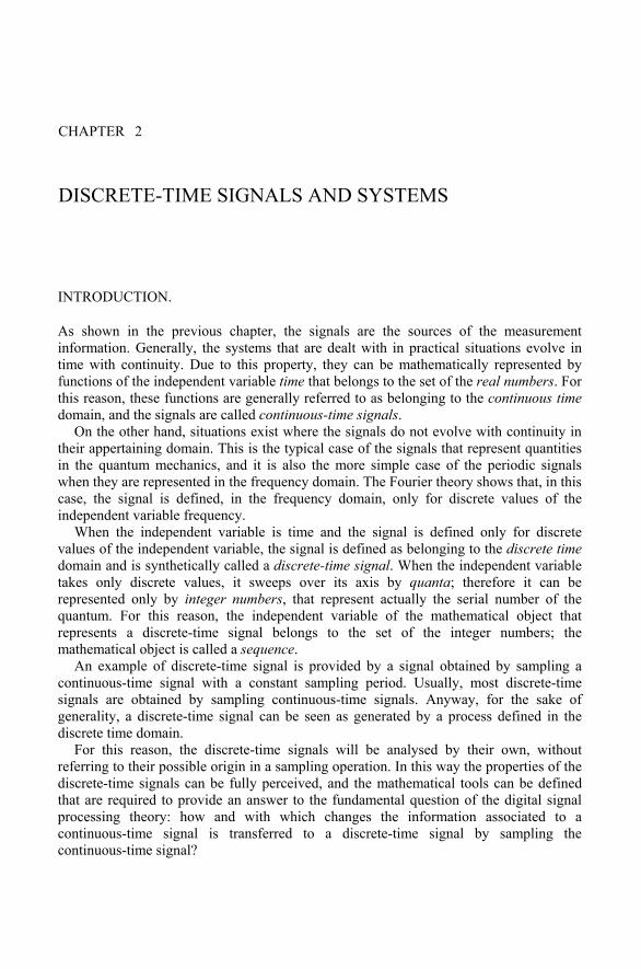
A discrete-time signal is mathematically represented by a sequence of values x:

( ){ } ∞≤≤∞−= nnxx , (2.1)

The n-th value x(n) in the sequence is also called the n-th sample of the sequence. As already stated, the independent variable n belongs to the set of the integer numbers;

this means that {x(n)} is mathematically defined only for integer values of n, and is not defined for non-integer1 values of n.

Fig. 2.1 shows an example of graphical representation of a sequence.

7-10 -9 -8 -7 -6 -5 -4 -3 -2 -1 0 1 2 3 4 5 6 8 9 10 11 12

x(0)

x(1)

x(2)

x(-1)

x(-2)

n

x(n)

Figure 2.1. Graphical representation of a sequence

Sometimes, when the whole sequence cannot be confused with its own samples, the notation in (2.1) is uselessly complex, and therefore the whole sequence is referred to as x(n).

1 It is a common mistake stating that x(n) = 0 for non-integer values of n. This is absolutely incorrect, since a

sequence cannot be mathematically defined for non-integer values of its independent variable n.

Discrete-time signals and systems 7

Particular sequences.

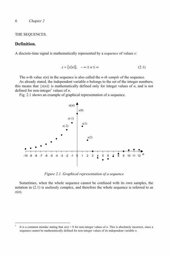
Some sequences play a very important role in the analysis of the discrete-time signals. The most important is the unit sample sequence, which is mathematically defined as:

( )=≠

=δ0,10,0

nn

n (2.2)

and is graphically represented in Fig. 2.2.

0

1

-10 -5 0 5 10

n

δ(n )

Figure 2.2. Unit sample sequence

This sequence is important because it plays, in the analysis of the discrete-time signals and systems, a similar role as that played by the Dirac impulse in the analysis of the continuous-time signals and systems. For this reason, the unit sample sequence is often, though not properly, called discrete-time impulse, or impulse sequence. It is worth while

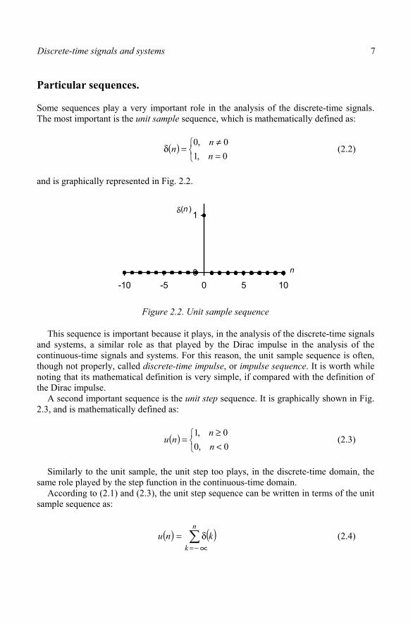
the Dirac impulse. A second important sequence is the unit step sequence. It is graphically shown in Fig.

2.3, and is mathematically defined as:

( )<≥

=0,00,1

nn

nu (2.3)

Similarly to the unit sample, the unit step too plays, in the discrete-time domain, the same role played by the step function in the continuous-time domain.

According to (2.1) and (2.3), the unit step sequence can be written in terms of the unit sample sequence as:

( ) ( )δ=n

knu (2.4)

noting that its mathematical definition is very simple, if compared with the definition of

k =− ∝

8 Chapter 2

0

1

-10 -5 0 5 10 15

n

u(n)

Figure 2.3. Unit step sequence

This can be proved by recalling that, due to (2.2), the elements in the sum (2.4) are

sum (2.4) are zero, and therefore u(n) = 0 for n < 0. For n ≥ 0 only one non-zero term

proved.The inverse relationship, linking the unit sample sequence to the unit step sequence,

can be readily written as:

δ(n) = u(n) - u(n-1) (2.5)

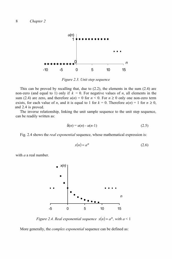
Fig. 2.4 shows the real exponential sequence, whose mathematical expression is:

( ) nanx = (2.6)

with a a real number.

-5 0 5 10 15

n

x(n)

Figure 2.4. Real exponential sequence

More generally, the complex exponential sequence can be defined as:

non-zero (and equal to 1) only if k = 0. For negative values of n, all elements in the

exists, for each value of n, and it is equal to 1 for k = 0. Therefore u(n) = 1 for n ≥ 0, and 2.4 is

( ) nanx = , with a < 1


( ) ( )njenx 0ω+σ= (2.7)

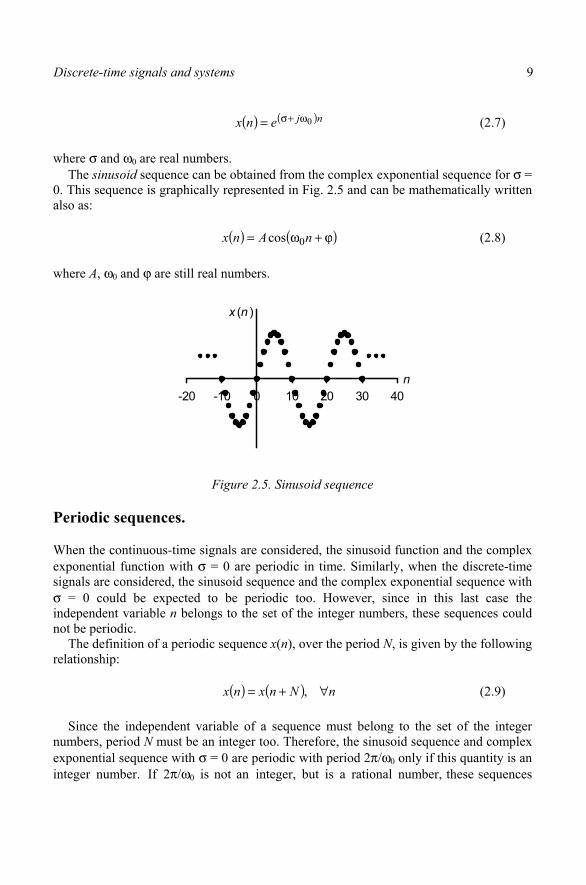
where σ and ω0 are real numbers. The sinusoid sequence can be obtained from the complex exponential sequence for σ =

0. This sequence is graphically represented in Fig. 2.5 and can be mathematically written also as:

( ) ( )ϕ+ω= nAnx 0cos (2.8)

where A, ω0 and ϕ are still real numbers.

-20 -10 0 10 20 30 40n

x (n )

Figure 2.5. Sinusoid sequence

Periodic sequences.

When the continuous-time signals are considered, the sinusoid function and the complex exponential function with σ = 0 are periodic in time. Similarly, when the discrete-time signals are considered, the sinusoid sequence and the complex exponential sequence with σ = 0 could be expected to be periodic too. However, since in this last case the independent variable n belongs to the set of the integer numbers, these sequences could not be periodic.

The definition of a periodic sequence x(n), over the period N, is given by the following relationship:

( ) ( ) nNnxnx ∀+= , (2.9)

Since the independent variable of a sequence must belong to the set of the integer numbers, period N must be an integer too. Therefore, the sinusoid sequence and complex exponential sequence with σ = 0 are periodic with period 2π/ω0 only if this quantity is an integer number. If 2π/ω0 is not an integer, but is a rational number, these sequences

10 Chapter 2

still periodic, but their period will be an integer multiple of 2π/ω0. If 2π/ω0 is neither a rational number, these sequences are not periodic.

This property of the periodic sequences is very important, because it explains how the information associated to a continuous-time periodic signal can be modified after the signal itself has been sampled.

Let s(t) be a sinusoidal, continuous-time signal, with period T. This signal is described by the following equation:

( ) ϕ+π= tT

Ats 2sin (2.10)

Let s(t) be sampled with Ts sampling period, so that:

integeran ,s NNTT = (2.11)

s

( ) ϕ+π=T

kTAkTs ss 2sin ,

that, taking into account (2.11), leads to the following sequence:

( ) ϕ+π= kN

Aks 2sinˆ (2.12)

It can be readily checked that, in (2.12), Nπ=ω 2

0 and therefore, having supposed N an integer, the sequence in (2.12) is periodic with period N. It can be hence concluded that the sequence obtained by sampling the periodic signal s(t) is still periodic and the relationship between the period of the continuous-time signal and that of the discrete-time signal is given by: T = NTs.

On the other hand, signal (2.10) could have been sampled with a sampling period 'sT

so that: 'smTT = with m a real number. In this case (2.12) would have become:

( ) ϕ+π= km

Aks 2sinˆ

and, not being m an integer or a rational number, this sequence is not periodic. It can be concluded that the sampling operation, in this case, has changed the information associated with the continuous-time signal, because a non-periodic sequence has been obtained from a periodic signal. As it will be shown in the next chapter, condition (2.11)

are

Eq. (2.10), evaluated at each sampling time kT , provides:


is one of the conditions that must be satisfied in order to sample a periodic signal correctly.

Coming back to the sinusoid and complex exponential sequences, the ω0 parameter is called the angular frequency (and

πω=2

00f the frequency) of the sequences, no matter

whether they are periodic or not.

Operations between sequences.

The sum and product operations can be defined for the sequences. In particular, the sum of two sequences, x and y, is a sequence whose samples are obtained as the sum of the corresponding samples of the two sequences. From the mathematical point of view, it is:

x + y = {x(n) + y(n)} (2.13)

Similarly, the product of two sequences is defined as a sequence whose samples are obtained as the product of the corresponding samples of the two sequences. From the mathematical point of view, it is:

x · y = {x(n) · y(n)} (2.14)

It can be easily proven that the sum and product operations between sequences satisfy the commutative and associative properties, and the product satisfies also the distributive property with respect to the sum.

The product of a sequence x by a number a is defined as the sequence whose samples are those of sequence x, each multiplied by a. It is:

x · a = {a · x(n)} (2.15)

At last, the shift operation is defined as the operation that, starting from a sequence x,provides its replica, shifted along the n axis by a given integer quantity n0; from the mathematical point of view, this can be written as:

y(n) = x(n - n0) (2.16)

When n0 > 0 the original sequence is shifted on the right, over the n axis, whilst when n0 < 0 it is shifted on the left.

If shifted versions of the unit sample sequence are employed, any sequence can be expressed in terms of the unit sample sequence. Given a sequence x(n), it is indeed possible to write:

12 Chapter 2

( ) ( ) ( )+∞

−∞=−δ=

kknkxnx (2.17)

The above relationship can be readily proven by considering that the shifted unit sample sequence δ(n-k) is non zero (and equal to 1) only for n - k = 0, and hence for n = k. Therefore, the sum at the right-hand side of (2.17) has only one non-zero term, for n = k, whose value is equal to sample x(n), ∀n. Eq. (2.17) is then proven.

THE DISCRETE-TIME SYSTEMS.

Definition.

A system, whichever is the domain it belongs to, is mathematically defined as a unique transformation that maps an input quantity x into an output quantity y. In the discrete time domain, the system’s input and output quantities are sequences, which means that a discrete-time system transforms the input sequence x(n) into the output sequence y(n)univocally. As a matter of fact, a discrete-time transformation can be seen as an algorithm that processes the samples of the input sequence in order to provide the samples of the output sequence.

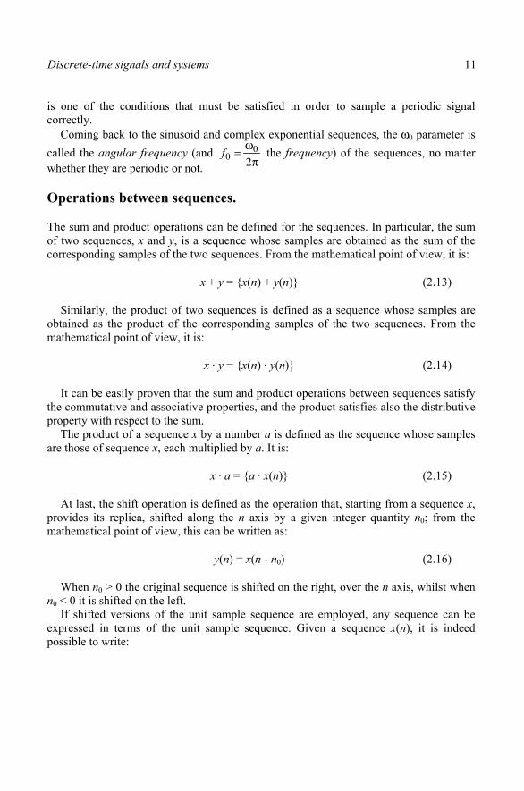
From the mathematical point of view, a transformation is expressed as:

( ) ( )[ ]nxny T=

and is graphically represented as shown in Fig. 2.6.

T[ ] x(n) y(n)

Figure 2.6. Graphical representation of a system and related transformation

The output sequence y(n) is also called the response of system T to the input sequence x(n).

The analysis of a generic system and its related transformation is generally quite complex, unless suitable constraints are introduced that limit the freedom degrees of the system itself, by defining suitable classes of transformations. The most important class is that of the linear systems, to which the overwhelming majority of the algorithms employed in the measurement field belongs.


The linear systems.

The linear systems can be mathematically defined by means of the superposition principle. Given the two input sequences x1(n) and x2(n), let y1(n) and y2(n) be the responses of a system T to the given input sequences respectively, so that:

( ) ( )[ ]nxny 11 T= and ( ) ( )[ ]nxny 22 T=

According to the superposition principle, system T is linear if and only if:

( ) ( )[ ] ( )[ ] ( )[ ] ( ) ( )nbynaynxbnxanbxnax 212121 TTT +=+=+ (2.18)

where a and b are arbitrary constants. Since, according to (2.17), any sequence can be written in terms of the unit sample

sequence, the response of a system can be written as:

( ) ( ) ( )−δ=+∞

−∞=kknkxny T (2.19)

If system T is linear, (2.18) applies and (2.19) can be written as:

( ) ( ) ( )[ ]+∞

−∞=−δ=

kknkxny T (2.20)

Let hk(n) be the system response to the shifted unit sample sequence δ (n - k); (2.20) can be written as:

( ) ( ) ( )+∞

−∞==

kk nhkxny (2.21)

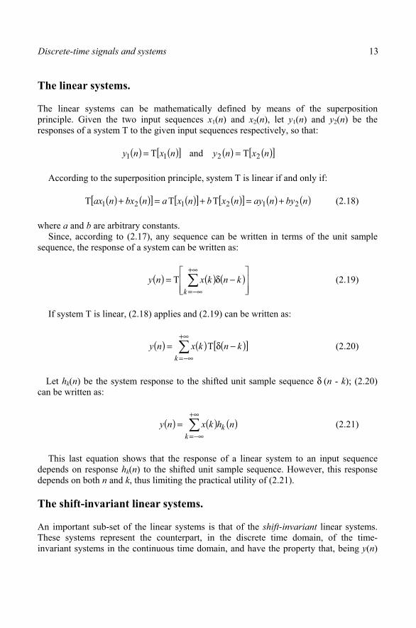
This last equation shows that the response of a linear system to an input sequence depends on response hk(n) to the shifted unit sample sequence. However, this response depends on both n and k, thus limiting the practical utility of (2.21).

The shift-invariant linear systems.

An important sub-set of the linear systems is that of the shift-invariant linear systems. These systems represent the counterpart, in the discrete time domain, of the time-invariant systems in the continuous time domain, and have the property that, being y(n)

14 Chapter 2

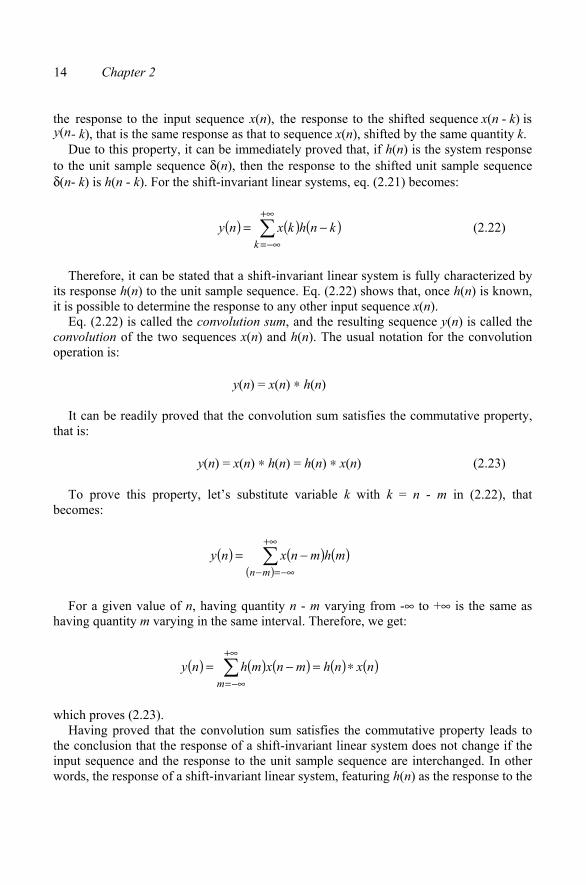
the response to the input sequence x(n), the response to the shifted sequence x(n - k) is y(n- k), that is the same response as that to sequence x(n), shifted by the same quantity k.

Due to this property, it can be immediately proved that, if h(n) is the system response to the unit sample sequence δ(n), then the response to the shifted unit sample sequence δ(n- k) is h(n - k). For the shift-invariant linear systems, eq. (2.21) becomes:

( ) ( ) ( )+∞

−∞=−=

kknhkxny (2.22)

Therefore, it can be stated that a shift-invariant linear system is fully characterized by its response h(n) to the unit sample sequence. Eq. (2.22) shows that, once h(n) is known, it is possible to determine the response to any other input sequence x(n).

Eq. (2.22) is called the convolution sum, and the resulting sequence y(n) is called the convolution of the two sequences x(n) and h(n). The usual notation for the convolution operation is:

y(n) = x(n) ∗ h(n)

It can be readily proved that the convolution sum satisfies the commutative property, that is:

y(n) = x(n) ∗ h(n) = h(n) ∗ x(n) (2.23)

To prove this property, let’s substitute variable k with k = n - m in (2.22), that becomes:

( ) ( ) ( )( )

+∞

−∞=−−=

mnmhmnxny

For a given value of n, having quantity n - m varying from -∞ to +∞ is the same as having quantity m varying in the same interval. Therefore, we get:

( ) ( ) ( ) ( ) ( )+∞

−∞=∗=−=

mnxnhmnxmhny

which proves (2.23). Having proved that the convolution sum satisfies the commutative property leads to

the conclusion that the response of a shift-invariant linear system does not change if the input sequence and the response to the unit sample sequence are interchanged. In other words, the response of a shift-invariant linear system, featuring h(n) as the response to the


unit sample sequence, to sequence x(n) is the same as that of a system, featuring x(n) as the response to the unit sample sequence, to sequence h(n).

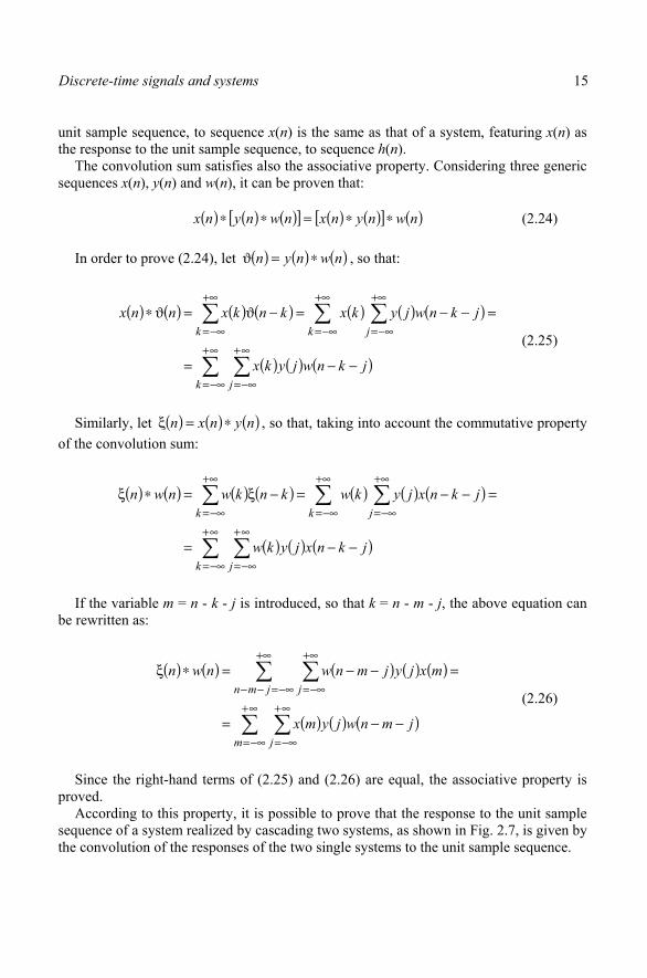
The convolution sum satisfies also the associative property. Considering three generic sequences x(n), y(n) and w(n), it can be proven that:

( ) ( ) ( )[ ] ( ) ( )[ ] ( )nwnynxnwnynx ∗∗=∗∗ (2.24)

In order to prove (2.24), let ( ) ( ) ( )nwnyn ∗=ϑ , so that:

( ) ( ) ( ) ( ) ( ) ( ) ( )

( ) ( ) ( )∞+

−∞=

∞+

−∞=

+∞

−∞=

+∞

−∞=

+∞

−∞=

−−=

=−−=−ϑ=ϑ∗

k j

k jk

jknwjykx

jknwjykxknkxnnx

(2.25)

Similarly, let ( ) ( ) ( )nynxn ∗=ξ , so that, taking into account the commutative property of the convolution sum:

( ) ( ) ( ) ( ) ( ) ( ) ( )

( ) ( ) ( )∞+

−∞=

∞+

−∞=

+∞

−∞=

+∞

−∞=

+∞

−∞=

−−=

=−−=−ξ=∗ξ

k j

k jk

jknxjykw

jknxjykwknkwnwn

If the variable m = n - k - j is introduced, so that k = n - m - j, the above equation can be rewritten as:

( ) ( ) ( ) ( ) ( )

( ) ( ) ( )∞+

−∞=

∞+

−∞=

+∞

−∞=−−

+∞

−∞=

−−=

=−−=∗ξ

m j

jmn j

jmnwjymx

mxjyjmnwnwn

(2.26)

Since the right-hand terms of (2.25) and (2.26) are equal, the associative property is proved.

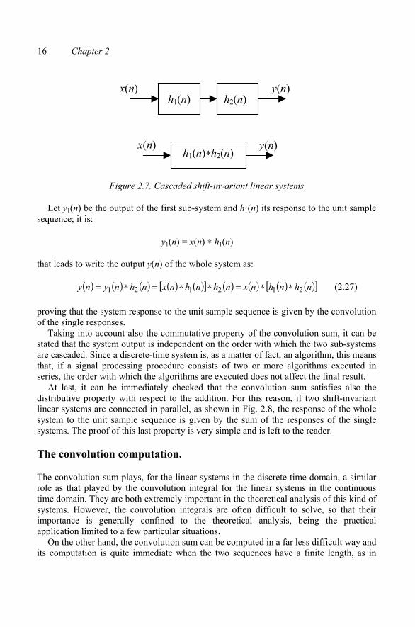
According to this property, it is possible to prove that the response to the unit sample sequence of a system realized by cascading two systems, as shown in Fig. 2.7, is given by the convolution of the responses of the two single systems to the unit sample sequence.

16 Chapter 2

h1(n) h2(n)

h1(n)*h2(n)

x(n)

x(n)

y(n)

y(n)

Figure 2.7. Cascaded shift-invariant linear systems

Let y1(n) be the output of the first sub-system and h1(n) its response to the unit sample sequence; it is:

y1(n) = x(n) ∗ h1(n)

that leads to write the output y(n) of the whole system as:

( ) ( ) ( ) ( ) ( )[ ] ( ) ( ) ( ) ( )[ ]nhnhnxnhnhnxnhnyny 212121 ∗∗=∗∗=∗= (2.27)

proving that the system response to the unit sample sequence is given by the convolution of the single responses.

Taking into account also the commutative property of the convolution sum, it can be stated that the system output is independent on the order with which the two sub-systems are cascaded. Since a discrete-time system is, as a matter of fact, an algorithm, this means that, if a signal processing procedure consists of two or more algorithms executed in series, the order with which the algorithms are executed does not affect the final result.

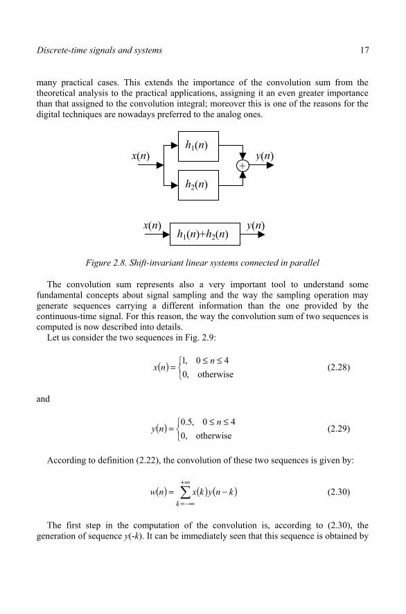
At last, it can be immediately checked that the convolution sum satisfies also the distributive property with respect to the addition. For this reason, if two shift-invariant linear systems are connected in parallel, as shown in Fig. 2.8, the response of the whole system to the unit sample sequence is given by the sum of the responses of the single systems. The proof of this last property is very simple and is left to the reader.

The convolution computation.

The convolution sum plays, for the linear systems in the discrete time domain, a similar role as that played by the convolution integral for the linear systems in the continuous time domain. They are both extremely important in the theoretical analysis of this kind of systems. However, the convolution integrals are often difficult to solve, so that their importance is generally confined to the theoretical analysis, being the practical application limited to a few particular situations.

On the other hand, the convolution sum can be computed in a far less difficult way and its computation is quite immediate when the two sequences have a finite length, as in


many practical cases. This extends the importance of the convolution sum from the theoretical analysis to the practical applications, assigning it an even greater importance than that assigned to the convolution integral; moreover this is one of the reasons for the digital techniques are nowadays preferred to the analog ones.

h1(n)

h2(n)+

x(n) y(n)

h1(n)+h2(n)x(n) y(n)

Figure 2.8. Shift-invariant linear systems connected in parallel

The convolution sum represents also a very important tool to understand some fundamental concepts about signal sampling and the way the sampling operation may generate sequences carrying a different information than the one provided by the continuous-time signal. For this reason, the way the convolution sum of two sequences is computed is now described into details.

Let us consider the two sequences in Fig. 2.9:

( ) ≤≤=

otherwise,040,1 n

nx (2.28)

and

( ) ≤≤=

otherwise,040,5.0 n

ny (2.29)

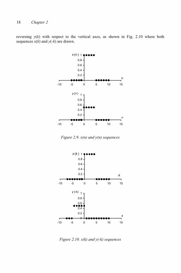
According to definition (2.22), the convolution of these two sequences is given by:

( ) ( ) ( )+∞

−∞=−=

kknykxnw (2.30)

The first step in the computation of the convolution is, according to (2.30), the generation of sequence y(-k). It can be immediately seen that this sequence is obtained by

18 Chapter 2

reversing y(k) with respect to the vertical axes, as shown in Fig. 2.10 where both sequences x(k) and y(-k) are drawn.

0

0.2

0.4

0.6

0.8

1

-10 -5 0 5 10 15

n

x (n )

0

0.2

0.4

0.6

0.8

1

-10 -5 0 5 10 15

n

y (n )

Figure 2.9. x(n) and y(n) sequences

0

0.2

0.4

0.6

0.8

1

-10 -5 0 5 10 15

k

x (k )

0

0.2

0.4

0.6

0.8

1

-10 -5 0 5 10 15

k

y (-k)

Figure 2.10. x(k) and y(-k) sequences


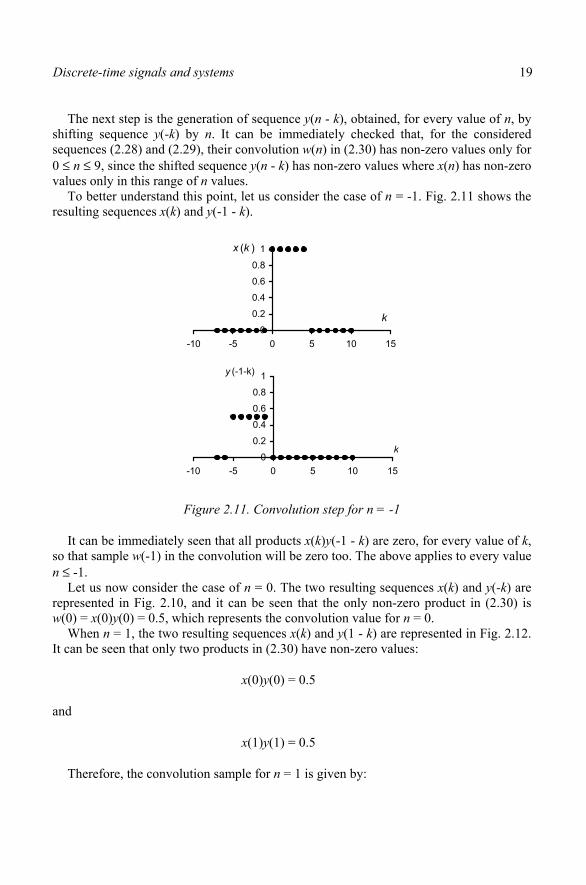
The next step is the generation of sequence y(n - k), obtained, for every value of n, by shifting sequence y(-k) by n. It can be immediately checked that, for the considered sequences (2.28) and (2.29), their convolution w(n) in (2.30) has non-zero values only for 0 ≤ n ≤ 9, since the shifted sequence y(n - k) has non-zero values where x(n) has non-zero values only in this range of n values.

To better understand this point, let us consider the case of n = -1. Fig. 2.11 shows the resulting sequences x(k) and y(-1 - k).

0

0.2

0.4

0.6

0.8

1

-10 -5 0 5 10 15

k

x (k )

0

0.2

0.4

0.6

0.8

1

-10 -5 0 5 10 15

k

y (-1-k)

Figure 2.11. Convolution step for n = -1

It can be immediately seen that all products x(k)y(-1 - k) are zero, for every value of k,so that sample w(-1) in the convolution will be zero too. The above applies to every value n ≤ -1.

Let us now consider the case of n = 0. The two resulting sequences x(k) and y(-k) are represented in Fig. 2.10, and it can be seen that the only non-zero product in (2.30) is w(0) = x(0)y(0) = 0.5, which represents the convolution value for n = 0.

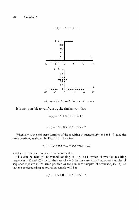
When n = 1, the two resulting sequences x(k) and y(1 - k) are represented in Fig. 2.12. It can be seen that only two products in (2.30) have non-zero values:

x(0)y(0) = 0.5

and

x(1)y(1) = 0.5

Therefore, the convolution sample for n = 1 is given by:

20 Chapter 2

w(1) = 0.5 + 0.5 = 1

0

0.2

0.4

0.6

0.8

1

-10 -5 0 5 10 15

k

x (k )

0

0.2

0.4

0.6

0.8

1

-10 -5 0 5 10 15

k

y (1-k)

Figure 2.12. Convolution step for n = 1

It is then possible to verify, in a quite similar way, that:

w(2) = 0.5 + 0.5 + 0.5 = 1.5

w(3) = 0.5 + 0.5 +0.5 + 0.5 = 2

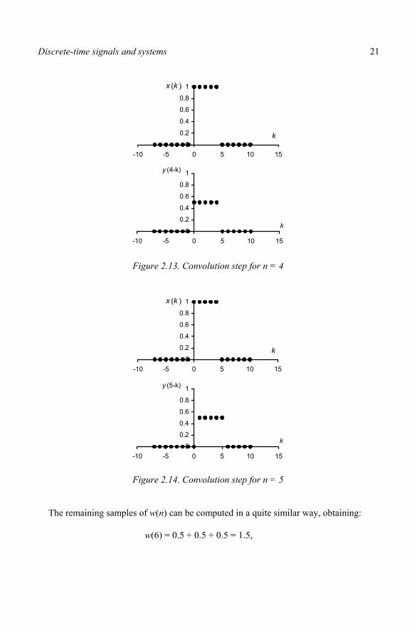
When n = 4, the non-zero samples of the resulting sequences x(k) and y(4 - k) take the same position, as shown by Fig. 2.13. Therefore:

w(4) = 0.5 + 0.5 +0.5 + 0.5 + 0.5 = 2.5

and the convolution reaches its maximum value. This can be readily understood looking at Fig. 2.14, which shows the resulting

sequences x(k) and y(5 - k) for the case of n = 5. In this case, only 4 non-zero samples of sequence x(k) are in the same position as the non-zero samples of sequence y(5 - k), so that the corresponding convolution sample will be:

w(5) = 0.5 + 0.5 + 0.5 + 0.5 = 2.


0

0.2

0.4

0.6

0.8

1

-10 -5 0 5 10 15

k

x (k )

0

0.2

0.4

0.6

0.8

1

-10 -5 0 5 10 15

k

y (4-k)


0

0.2

0.4

0.6

0.8

1

-10 -5 0 5 10 15

k

x (k )

0

0.2

0.4

0.6

0.8

1

-10 -5 0 5 10 15

k

y (5-k)


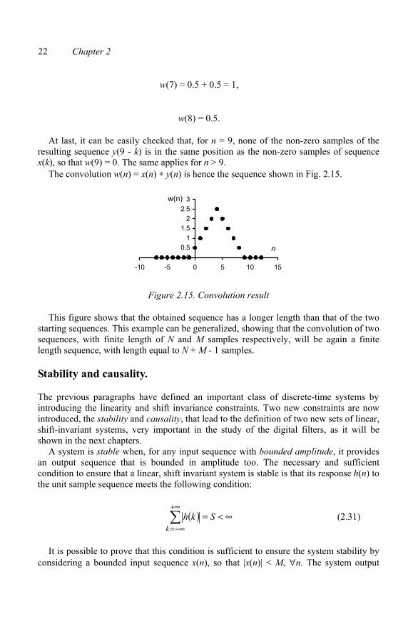
The remaining samples of w(n) can be computed in a quite similar way, obtaining:

w(6) = 0.5 + 0.5 + 0.5 = 1.5,

22 Chapter 2

w(7) = 0.5 + 0.5 = 1,

w(8) = 0.5.

At last, it can be easily checked that, for n = 9, none of the non-zero samples of the resulting sequence y(9 - k) is in the same position as the non-zero samples of sequence x(k), so that w(9) = 0. The same applies for n > 9.

The convolution w(n) = x(n) ∗ y(n) is hence the sequence shown in Fig. 2.15.

00.5

11.5

22.5

3

-10 -5 0 5 10 15

n

w(n)

Figure 2.15. Convolution result

This figure shows that the obtained sequence has a longer length than that of the two starting sequences. This example can be generalized, showing that the convolution of two sequences, with finite length of N and M samples respectively, will be again a finite length sequence, with length equal to N + M - 1 samples.

Stability and causality.

introducing the linearity and shift invariance constraints. Two new constraints are now introduced, the stability and causality, that lead to the definition of two new sets of linear, shift-invariant systems, very important in the study of the digital filters, as it will be shown in the next chapters.

A system is stable when, for any input sequence with bounded amplitude, it provides an output sequence that is bounded in amplitude too. The necessary and sufficient condition to ensure that a linear, shift invariant system is stable is that its response h(n) to the unit sample sequence meets the following condition:

( ) ∞<=+∞

−∞=Skh

k (2.31)

It is possible to prove that this condition is sufficient to ensure the system stability by considering a bounded input sequence x(n), so that |x(n)| < M, ∀n. The system output

The previous paragraphs have defined an important class of discrete-time systems by


sequence can be obtained by applying (2.22); supposing that condition (2.31) is also satisfied, it can be written:

( ) ( ) ( ) ( ) ∞<≤−=+∞

−∞=

+∞

−∞= kkkhMknxkhny

thus proving that the output sequence is also bounded in amplitude. It can be now proved that condition (2.31) is necessary to ensure stability by proving

that, if S = ∞, an input sequence can be found with bounded amplitude that gives rise to an output sequence with unbounded amplitude. Let us consider a linear, shift-invariant system characterized by a response h(n) to the unit sample sequence, and let us consider an input sequence:

( )( )( ) ( )

( ) =

≠−−

=∗

0,0

0,

nh

nhnhnh

nx

where h*(n) is the complex conjugate of h(n). x(n) is bounded because of the way it has been defined. If the output sequence y(n) is now evaluated by applying (2.22), its value for n = 0 is given by:

( ) ( ) ( ) ( ) ( )( )

( )( ) ( ) Skhkh

khkh

khkhkhkxykkkk

====−=+∞

−∞=

+∞

−∞=

+∞

−∞=

+∞

−∞=

2*0

Therefore, if S = ∞, the output sequence is unbounded even in the presence of a bounded input sequence. This proves that condition (2.31) is a necessary condition too.

A system is causal when its output y(n), for every n = n0, depends on the input samples for n ≤ n0 only. For this reason, if x1(n) and x2(n) are two input sequences to a causal system, taken in such a way that x1(n) = x2(n) for n < n0, then the system’s output sequences y1(n) and y2(n) will feature y1(n) = y2(n) for n < n0.

A linear, shift-invariant, causal system has the property that its response to the unit sample sequence is zero for n < 0. This can be proved by considering the system output, evaluated in n = n0, in terms of (2.22) where the commutative property of the convolution has been considered too:

( ) ( ) ( )+∞

−∞=−=

kknxkhny 00 (2.32)

24 Chapter 2

In (2.32) the samples of x(n) for n > n0 are obtained when k < 0. In order to prevent 0

it must be h(k) = 0 for k < 0, as stated. For this reason a sequence with zero samples for n < 0 is called causal. This is

somehow justified by the fact that this sequence could be the response of a linear, shift-invariant, causal system to the unit sample sequence.

An example of linear, shift-invariant, causal and stable system is a system whose response to the unit sample sequence is:

h(n) = anu(n)

Due to the presence of the unit step sequence u(n), h(n) = 0 for n < 0, so that the system is causal. In order to ensure the system stability, (2.31) must be verified, which means that the following quantity:

( )+∞

=

+∞

−∞===

0k

k

kakhS (2.33)

must be finite. It can be noted that the quantity in the right-hand side of (2.33) is a geometrical series

that converges to the finite quantity:

aS

−=

11

for |a| < 1, otherwise the series diverges to infinite. Therefore, the system is stable only if |a| < 1.

FREQUENCY-DOMAIN REPRESENTATION OF THE DISCRETE-TIME SIGNALS AND SYSTEMS.

The frequency response of the linear, shift-invariant systems.

In the previous sections it has been shown how a linear, shift-invariant system can be fully characterized by its response to the unit sample sequence. This property of the discrete-time systems is the counterpart, in the discrete time, of the property of the continuous-time linear, time-invariant systems to be fully characterized by their impulse response.

Another fundamental properties of these continuous-time systems is that their steady-state response to a sinusoidal input is still a sinewave, with the same frequency as the input sinewave, with amplitude and phase determined by the system. It is because of this

these samples to contribute to the sum in (2.32), and hence to the determination of y(n ),


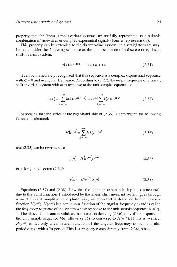
property that the linear, time-invariant systems are usefully represented as a suitable combination of sinewaves or complex exponential signals (Fourier representation).

This property can be extended to the discrete-time systems in a straightforward way. Let us consider the following sequence as the input sequence of a discrete-time, linear, shift-invariant system:

( ) +∞<<∞−= ω nenx nj , (2.34)

It can be immediately recognized that this sequence is a complex exponential sequence with σ = 0 and ω angular frequency. According to (2.22), the output sequence of a linear, shift-invariant system with h(n) response to the unit sample sequence is:

( ) ( ) ( ) ( ) ω−ω+∞

−∞=

−ω == kjnj

k

knj ekheekhny (2.35)

Supposing that the series at the right-hand side of (2.35) is convergent, the following function is obtained:

( ) ( ) ω−ω = kjj ekheH (2.36)

and (2.35) can be rewritten as:

( ) ( ) njj eeHny ωω= (2.37)

or, taking into account (2.34):

( ) ( ) ( )nxeHny jω= (2.38)

Equations (2.37) and (2.38) show that the complex exponential input sequence x(n),due to the transformation T introduced by the linear, shift-invariant system, goes through a variation in its amplitude and phase only, variation that is described by the complex function H(e jω). H (e jω) is a continuous function of the angular frequency ω and is called the frequency response of the system whose response to the unit sample sequence is h(n).

The above conclusion is valid, as mentioned in deriving (2.36), only if the response to the unit sample sequence h(n) allows (2.36) to converge to H (e jω). If this is verified, H (e jω) is not only a continuous function of the angular frequency ω, but it is also periodic in ω with a 2π period. This last property comes directly from (2.36), since:

+∞

−∞=k

+∞

−∞=k

26 Chapter 2

( ) kjkj ee ωπ+ω =2

The fact that H(e jω) takes the same values for any ω = ω0 and ω = ω0 + 2π means that the discrete-time system provides the same response to complex exponential sequences with these two angular frequency values. This is totally justified by the fact that the two complex exponential sequences do not differ.

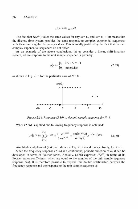
As an example of the above conclusions, let us consider a linear, shift-invariant system, whose response to the unit sample sequence is given by:

( ) −≤≤=

otherwise,010,1 Nn

nh (2.39)

as shown in Fig. 2.16 for the particular case of N = 8.

0

1

-10 -5 0 5 10 15

n

h (n )

Figure 2.16. Response (2.39) to the unit sample sequence for N=8

When (2.36) is applied, the following frequency response is obtained:

( ) ( )( )

( ) 211

0 2sin2sin

11 ω−−

ω−

ω−−

=

ω−ωω

ω=−

−== Njj

NjN

k

kjj eNe

eeeH (2.40)

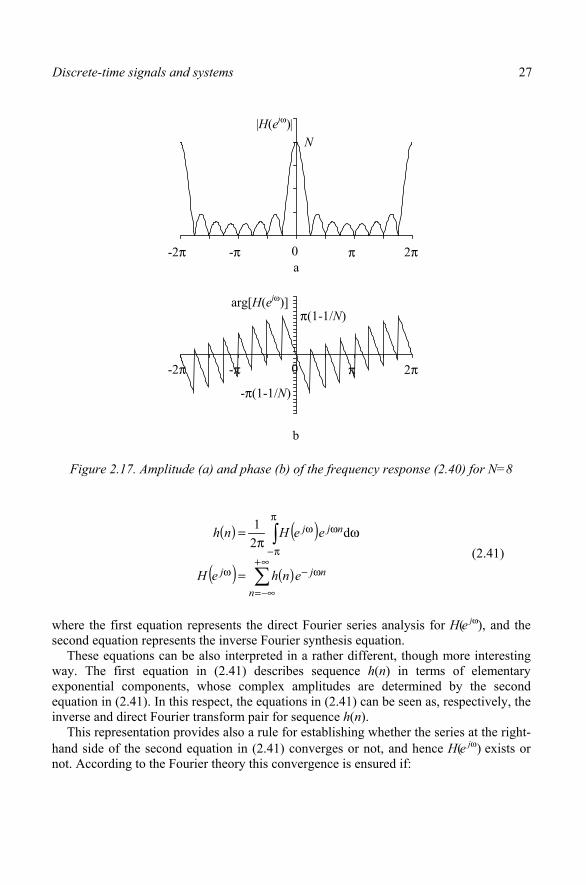
Amplitude and phase of (2.40) are shown in Fig. 2.17 a and b respectively, for N = 8. Since the frequency response (2.36) is a continuous, periodic function of ω, it can be

developed in terms of Fourier series. Actually, (2.36) expresses H(e jω) in terms of its Fourier series coefficients, which are equal to the samples of the unit sample sequence response h(n). It is therefore possible to express this double relationship between the frequency response and the response to the unit sample sequence as:


a

b

|H(ejω)N

-2π -π 0 π 2π

-2π -π 0 π 2π

arg[H(ejω)]π(1-1/N)

-π(1-1/N)

Figure 2.17. Amplitude (a) and phase (b) of the frequency response (2.40) for N=8

( ) ( )

( ) ( )∞+

−∞=

ω−ω

π

π−

ωω

=

ωπ

=

n

njj

njj

enheH

eeHnh d21

(2.41)

where the first equation represents the direct Fourier series analysis for H(e jω), and the second equation represents the inverse Fourier synthesis equation.

These equations can be also interpreted in a rather different, though more interesting

exponential components, whose complex amplitudes are determined by the second equation in (2.41). In this respect, the equations in (2.41) can be seen as, respectively, the inverse and direct Fourier transform pair for sequence h(n).

This representation provides also a rule for establishing whether the series at the right-hand side of the second equation in (2.41) converges or not, and hence H(e jω) exists or not. According to the Fourier theory this convergence is ensured if:

|

way. The first equation in (2.41) describes sequence h(n) in terms of elementary

28 Chapter 2

( ) ∞<+∞

−∞=nnh ,

that is if h(n) is absolutely summable and the series is absolutely convergent. In this situation, (2.36) or the second equation in (2.41), converges to a continuous function of ω. Taking into account (2.31), this leads to the conclusion that it is always possible to define the frequency response of stable systems.

It can be also proved that, since:

( ) ( )2

2 ≤nn

nhnh ,

if h(n) is absolutely summable, it will be also:

( ) ∞<+∞

−∞=nnh 2

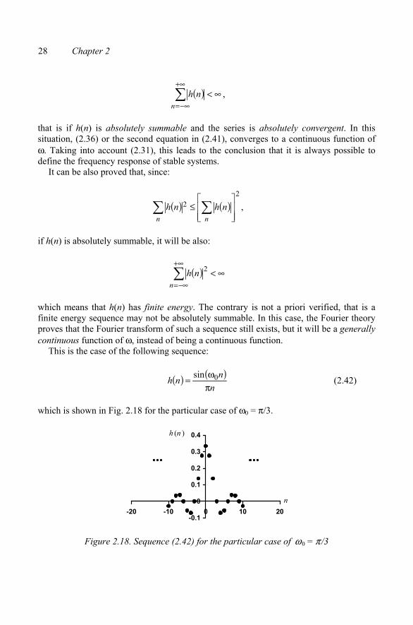
which means that h(n) has finite energy. The contrary is not a priori verified, that is a finite energy sequence may not be absolutely summable. In this case, the Fourier theory proves that the Fourier transform of such a sequence still exists, but it will be a generally continuous function of ω, instead of being a continuous function.

This is the case of the following sequence:

( ) ( )n

nnhπω= 0sin (2.42)

which is shown in Fig. 2.18 for the particular case of ω0 = π/3.

-0.1

0

0.1

0.2

0.3

0.4

-20 -10 0 10 20n

h (n )

Figure 2.18. Sequence (2.42) for the particular case of ω 0 = π /3


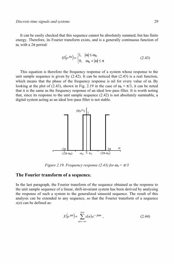
It can be easily checked that this sequence cannot be absolutely summed, but has finite energy. Therefore, its Fourier transform exists, and is a generally continuous function of ω, with a 2π period:

( )π≤ω<ω

ω≤ω=ω

0

0,0,1jeH (2.43)

This equation is therefore the frequency response of a system whose response to the unit sample sequence is given by (2.42). It can be noticed that (2.43) is a real function, which means that the phase of the frequency response is nil for every value of ω. By looking at the plot of (2.43), shown in Fig. 2.19 in the case of ω0 = π/3, it can be noted that it is the same as the frequency response of an ideal low-pass filter. It is worth noting that, since its response to the unit sample sequence (2.42) is not absolutely summable, a digital system acting as an ideal low-pass filter is not stable.

|H(ejω)|

-2π-(2π-ω0) -ω0 0 ω0 (2π-ω0)

2π ω

1

Figure 2.19. Frequency response (2.43) for ω 0 = π /3

The Fourier transform of a sequence.

In the last paragraph, the Fourier transform of the sequence obtained as the response to the unit sample sequence of a linear, shift-invariant system has been derived by analysing the response of such a system to the generalized sinusoid sequence. The result of this analysis can be extended to any sequence, so that the Fourier transform of a sequence x(n) can be defined as:

( ) ( )+∞

−∞=

ω−ω =n

njj enxeX , (2.44)

30 Chapter 2

provided that (2.44) is convergent. The rules to establish whether (2.44) converges to X(ejω) or not are, of course, the same as those seen for (2.36).

If (2.44) converges, then, similarly to (2.36), it converges to a continuous, or generally continuous function of ω, periodic in ω with a 2π period. This conclusion is very important, because it shows that any sequence, provided it has a Fourier transform, has a periodic Fourier transform, with a 2π period in ω. This outlines, as it will be shown into details in the following chapter, a first important source of modification of the information associated to a signal, when moving from the continuous time domain to the discrete time domain after a sampling operation. Every sequence obtained by sampling a continuous-time signal will show a periodic spectrum (Fourier transform) with a 2πperiod in ω, no matter on how the spectrum of the continuous-time signal is. If we consider that the continuous-time signals that are generally dealt with in practical situations have a non-periodic spectrum, the significance of the modifications to which the information associated to a signal is subjected because of the sampling operation is quite evident.

Similarly to what was done for the Fourier transform of h(n), it is possible to define the inverse Fourier transform of X(ejω) as:

( ) ( )π

π−

ωω ωπ

= d21 njj eeXnx (2.45)

Having defined the Fourier transform of a sequence, it is possible to determine the Fourier transform of the output y(n) of a linear, shift-invariant system, with input sequence x(n) and h(n) response to the unit sample sequence.

Applying (2.44) to (2.22) we get:

( ) ( ) ( )+∞

−∞=

ω−+∞

−∞=

ω −=n

nj

k

j ekxknheY (2.46)

If m = n - k is taken, (2.46) becomes:

( ) ( ) ( ) ( )

( ) ( )∞+

−∞=

ω−∞+

−∞=

ω−

+∞

−∞=

+ω−+∞

−∞=

ω

=

==

k

kj

m

mj

m

kmj

k

j

ekxemh

ekxmheY

which, taking into account (2.44), leads to write:

( ) ( ) ( )ωωω ⋅= jjj eXeHeY (2.47)


Eq. (2.47) shows that, similarly to the continuous-time, linear, time-invariant systems, the Fourier transform of the output sequence of a discrete-time, linear, shift-invariant system is given by the product of the Fourier transform of the input sequence by the frequency response, given by the Fourier transform of the response to the unit sample sequence.

If (2.22) is considered, (2.47) shows that the convolution between two sequences in the discrete time domain is changed into the product between the Fourier transforms of the two sequences in the ω domain. It is also possible to prove that the product between two sequences in the discrete time domain is changed into the convolution between the Fourier transforms of the two sequences in the ω domain.

Symmetry properties of the Fourier transform.

Similarly to the Fourier transform of the continuous-time functions, the Fourier transform of the sequences satisfies some very useful properties of symmetry that come mainly from the property of any sequence to be decomposed into the sum of a conjugate symmetric sequence and a conjugate antisymmetric sequence. In this section, the most significant properties will be shortly recalled, without entering into the mathematical details of the proofs, that are well known from the Fourier theory.

A sequence of complex samples xcs(n) is called conjugate symmetric when the following relationship applies:

( ) ( )nxnx −= ∗cscs

where the superscript * stands for complex conjugate. Similarly, a sequence of complex samples xca(n) is called conjugate antisymmetric when the following relationship applies:

( ) ( )nxnx −−= ∗caca

It can be proved that any sequence x(n) can be written as:

x(n) = xcs(n) + xca(n) (2.48)

where :

( ) ( ) ( )[ ]nxnxnx −+= ∗21

cs (2.49)

and :

( ) ( ) ( )[ ]nxnxnx −−= ∗21

ca (2.50)

32 Chapter 2

A real conjugate symmetric sequence, that is a sequence for which xcs(n) = xcs(-n)applies, is called an even sequence. Similarly, a real conjugate antisymmetric sequence, that is a sequence for which xca(n) = -xca(-n) applies, is called an odd sequence.

As for the Fourier transform, the same properties as those valid for the continuous-time functions still apply, so that it can be decomposed as:

( ) ( ) ( )ωωω += jjj eXeXeX cacs (2.51)

where:

( ) ( ) ( )[ ]ω−∗ωω += jjj eXeXeX21

cs (2.52)

and:

( ) ( ) ( )[ ]ω−∗ωω −= jjj eXeXeX21

ca (2.53)

If x(n) is a real sequence, then its Fourier transform is a conjugate symmetric function, that is:

( ) ( )ω−∗ω = jj eXeX (2.54)

If x(n) is an even sequence, then its Fourier transform is a real function.

http://www.springer.com/978-0-387-24966-7

signal n systems

Documents