signal based fault detection and diagnosis for rotating electrical machines: issues and solutions

Signal Based Fault Detection andDiagnosis for rotating electricalmachines: Issues and Solutions

Andrea Giantomassi1, Francesco Ferracuti1, Sabrina Iarlori1, GianlucaIppoliti1 and Sauro Longhi1

AbstractComplex systems are found in almost all field of contemporary science, andare associated with a wide variety of financial, physical, biological, informa-tion and social systems. Complex systems modelling could be addressed bysignal based procedures, which are able to learn the complex system dy-namics from data provided by sensors, which are installed on the system inorder to monitor its physical variables. The aim of diagnosis is to detect ifthe electrical machine is healthy or a change is occurring due to abnormalevents and, in addition, the probable causes of the abnormal events. Diagno-sis is addressed developing machine learning procedures in order to classifythe probable causes of deviations from system normal events. This chapterpresents two Fault Detection and Diagnosis solutions for rotating electri-cal machines by signal based approaches. The first one uses current signatureanalysis techniques based on Kernel Density Estimation and Kullback-Lieblerdivergence. The second one presents a vibration signature analysis techniquesbased on Multi-Scale Principal Component Analysis. Several simulations andexperimentations on real electric motors are carried out in order to verify theeffectiveness of the proposed solutions. The results show that the proposedsignal based diagnosis procedures are able to detect and diagnose differentelectric motor faults and defects, improving the reliability of electrical ma-chines. Fault Detection and Diagnosis algorithms could be used not only withthe fault diagnosis purpose but also in a Quality Control scenario. In fact,they can be integrated in test benches at the end or in the middle of theproduction line in order to test the machines quality. When the electric mo-tors reaches the test benches, the Fault Detection and Diagnosis proceduresacquire sensors measurements and detect if the motor is healthy or faulty, inthis last case further inspections can diagnose the fault type.

Dipartimento di Ingegneria dell’Informazione, Universita Politecnica delle Marche, ViaBrecce Bianche, 60131 Ancona, Italy. e-mail: a.giantomassi,f.ferracuti,s.iarlori,

gianluca.ippoliti,[email protected]

1

2 A. Giantomassi and F. Ferracuti and S. Iarlori and G. Ippoliti and S. Longhi

1 Introduction

Mathematical process models describe the relationship between input sig-nals u(k) and output signals y(k) and are fundamental for model-based faultdetection. In many cases the process models are not known at all or someparameters are unknown. Further, the models have to be rather precise inorder to express deviations as results of process faults. Therefore, process-identification methods have to be applied frequently before applying anymodel-based fault detection method as stated in Giantomassi (2012). Butalso the identification method itself may be a source to gain information on,e.g. process parameters which change under the influence of faults. First pub-lications known on fault detection with identification methods are found inIsermann (1984) and Filbert and Metzger (1982).

For dynamic processes the input signals may be the normal operatingsignal or may be artificial introduced for testing. A considerable advantageof identification methods is that with only one input and one output signalseveral parameters can be estimated, which give a detailed picture on internalprocess quantities. The generated features for fault detection are then impulseresponse values in the case of correlation methods or parameter estimates (seeIsermann (2006)).

On-line process monitoring with fault detection and diagnosis can providerange of processes, as stated in Cheng et al. (2008), Giantomassi et al. (2011)and Ferracuti et al. (2010, 2011). A large number of applications have beenreviewed, e.g. Isermann and Balle (1997) and Patton et al. (2000). Venkata-subramanian et al. (2000a,b,c) published an article series reviewing moni-toring methods with particular attention in the field of chemical processes.They classified the Fault Detection and Diagnosis methods as model-based,signal-based and knowledge-based. Signal-based approaches to FDI (FaultDetection and Isolation) in large-scale process plants, are consolidated andwell studied because for these processes the development of model-based FDImethods require considerable and eventually too high effort, and moreoverbecause large amount of data are collected, as stated in Chiang et al. (2000)and Isermann (2006).

Fault Detection and Diagnosis (FDD) in industrial applications regardtwo important aspects: the FDD for the production plant and for the sys-tems that work for the plant; among these induction motors are the mostimportant electrical machineries in many industrial applications. Consider-ing that, electric motors account about 65% of energy use. In the field ofoperation efficiency, the monitoring activity of rotating electrical machinesfor fault detection and diagnosis is depth investigated, by for example: Ben-loucif and Balaska (2006); Ran and Penman (2008); Singh and Ahmed (2004);Taniguchi et al. (1999); Tavner (2008); Verucchi and Acosta (2008). Vibra-tion analysis is widely accepted as a tool to detect faults of a machine asit is nondestructive, reliable and it permits continuous monitoring withoutstopping the machine (see Ciandrini et al. (2010); Gani and Salami (2002);

Signal Based Fault Detection and Diagnosis for rotating electrical machines 3

Hua et al. (2009); Immovilli et al. (2010); Shuting et al. (2002); Zhaoxia et al.(2009)). In particular analysing the vibration power spectrum it is possibleto detect different faults that arise in rotating machines. In traditional Ma-chine Vibration Signature Analysis (MVSA), the Fourier transform is usedto determine the vibration power spectrum, and the signature at differentfrequencies are identified and compared with healthy measurement to detectfaults in the machine, as in Lachouri et al. (2008). The short coming of thisapproach is that the Fourier analysis is limited to stationary signals whilevibrations are not stationary by nature.

The use of Soft Computing methods is considered an important extensionto the quantitative model-based approach (Patton et al. (2000)), it allowsto improve residual generation in FDD when process signals show complexbehaviours. Multi-Scale Principal Component Analysis (MSPCA) deals withprocesses that operate at different scales: events occurring at different local-izations in time and frequency, stochastic processes and variables measuredat different sampling rate, as reported in Bakshi (1998) and Li et al. (2000).In PCA, well treated in Jolliffe (2002) and Jackson (2003), the correlationamong sensors is used to transform the multivariate space into a subspacewhich preserves maximum variance of the original space. On the other hand,wavelets capture correlation within a sensor. MSPCA is a way to combinethese two techniques, to extract maximum information from multivariatesensor data (Misra et al. (2002)).

Rotating electrical machines are well known systems with accurate analyt-ical models and extensive results in literature. Failure surveys, as Thomsonand Fenger (2001), report that failures, in induction motors, are: stator re-lated (38%), rotor related (10%), bearing related (40%) and others (12%).Fast and accurate diagnosis of incipient faults allows actions to protect thepower system, the process leaded by the machine and the machine itself.

FDD techniques based on MVSA have received great attention in litera-ture because by vibrations it is possible to identify directly mechanical faultsregarding rotating electrical machines. In recent years, many methodologieshave been developed to detect and diagnose mechanical faults of electricalmachines by current measurements. In this context Motor Current SignatureAnalysis (MCSA) monitoring strategies involve detection and identificationof current signature patterns that are indicative of normal and abnormalmotor conditions. However, the motor current is influenced by many factorssuch as electric supply, static and dynamic load conditions, noise, motor ge-ometry, and fault conditions. In Chilengue et al. (2011) an artificial immunesystem approach is investigated for detection and diagnosis of faults in thestator and rotor circuits of induction machines. The technique measures thestator currents to compute its representation before and after a fault condi-tion. These patterns are employed to construct a characteristic image of themachine operating condition. Moreover MCSA procedures are used to detectand diagnose not only classic motor faults (i.e. rotor eccentricity), but alsogear faults (i.e. tooth spall), as presented in Feki et al. (2013). Fault Toler-


ant Control (FTC) as well as robust control systems have been applied inelectric drive systems Ciabattoni et al. (2011a, 2014, 2011b). In Abdelmadjidet al. (2013) a FTC procedure is proposed for stator winding fault of induc-tion motor. It consists of an algorithm which can detect the appearance ofa fault in closed loop and switches itself between a nominal control strategyfor healthy condition and a robust control for faulty condition. Samsi et al.(2009) validated a technique, called Symbolic Dynamic Filtering (SDF), forearly detection of stator voltage imbalance in three-phase induction motors,that involves Wavelet Transform (WT) of current signals. In Baccarini et al.(2010) a sensor-less approach has been proposed to detect one broken ro-tor bar in induction motor. This method is not affected by load and otherasymmetries. The technique estimates stator and rotor flux and analyses thedifferences obtained in torque. A new saturation model that explains the ex-perimental data is investigates in Pedra et al. (2009). The model has threedifferent saturation effects, which have been characterized in four inductionmotors.

As possible solutions of the FDI problem for electrical machines, two dif-ferent approaches are proposed: the first one used vibration signals, providedby accelerometer sensors placed on the machine, and the second one usedcurrent signals provided by inverters.

In the first solution, based on current signals analysis of rotating electricalmachines, different algorithms are applied for FDD: PCA is used to reduce thethree-phase currents space in two dimensions. Then, Kernel Density Estima-tion (KDE) is adopted to estimate the probability density function (PDF)of healthy and of each faulty motor, which will give typical patterns thatcan be used to identify each fault (see Ferracuti et al. (2013a)). Kullback-Leibler (K-L) divergence is used as a distance measure between classifiedstatistic signatures obtained by KDE. K-L allows to identify the dissimilaritybetween two determined probability distributions (that can also be multidi-mensional): one is related to the modeled signatures and the other is relatedto the acquired data samples. By K-L divergence, the classification of eachmotor condition is performed.

In the second approach, based on vibration analysis of rotating electricalmachines, MSPCA is applied for fault detection and diagnosis (Ferracuti et al.(2013b); Lachouri et al. (2008); Misra et al. (2002)). Fault identification isevaluated calculating the contributions of each variable in the principal com-ponent subspace and in the residual space. KDE, which allows to estimate thePDF of random variables is introduced, in Odiowei and Cao (2010), to im-prove the fault detection and isolation capabilities. The contributions PDFsare estimated by KDE, the thresholds are computed for each sensor signal inorder to improve fault detection. Faults are classified using the contributionsinformation by Linear Discriminant Analysis (LDA).

The proposed data-driven algorithms for FDD based on MVSA and MCSAare tested by several simulations and experimentations in order to verify theeffectiveness of the proposed methodologies.


The chapter will be organized in the following sections. In Section 2 al-gorithms for fault detection and isolation based on Motor Current SignatureAnalysis will be discussed, with specific focus on Quality Control scenario.Results on experimental tests on real motors will be reported in Section 3.Algorithm for fault detection and isolation based on vibration signals will bedescribed in Section 4. Results on experimental tests of real motors will be re-ported in Section 5. Comments on the performance of the proposed solutionswill be reported in Section 6.


2 Electric Motor FDD by MCSA in Quality Control

scenario

In industry, QC is a collection of methods that are able to improve the qualityand efficiency in processes, productions and in many others industry aspects.In 1924, Walter Shewhart designed the first control chart and gave a ratio-nale for its use in process monitoring and control (Stuart et al. (1995)). Themain concept of QC is the “proactiveness”, in order to ensure the productquality, monitoring processes and related signals to detect when they “go outof control”. In the last years, manufacturing industries are reversing manyattentions and efforts for the introduction of QC in the production lines andwith large volumes of low-tech products are concentrating many investiga-tions on the efficient introduction of QC in their production lines.

One of the major problems, in which these manufacturing industries areinvolved, is the customers satisfaction, because they usually purchase lots ofproducts with some unwanted defective component. In order to satisfy cus-tomers, manufacturing industries carry out some spot checks at the end ofproduction lines. This method does not ensure the quality of products andtotal defective products removal. A desirable QC solution for these manu-facturing industries should be minimally invasive, effective and with a lowpayback period. In addition, the testing could be made systematic using alow-cost system base on a reduced set of sensors integrated in the test bench.

The proposed FDD system acquires sensors measurements and detects de-fective products. Moreover, by isolating and identifying the defective type,the FDD procedure helps to estimate in which subprocess the defect is intro-duced and allows to remove the defective products, improving the processesquality. The tests, performed at the end of production lines, allow to improvethe quality of processes as a proactive measures for the QC methodology.

2.1 Recalled Results

In this section authors present the algorithms used to develop the FDD pro-cedure. It extracts patterns by current signals using PCA and KDE. ThenK-L divergence compares these patterns to extract the motor health index.

2.1.1 Principal Component Analysis

PCA is a dimensionality reduction technique that produces a lower dimen-sional representation in a way that preserves the correlation structure be-tween the process variables capturing the variability in the data (Jolliffe(2002)). In other words, PCA rotates the original coordinate system along


the direction of maximum variance. Considering a data matrix X ∈ RN×m

of N sample rows and m variable columns that are normalized to zero mean,with mean values vector µ, the matrix X can be decomposed as follows:

X = X + X, (1)

where X is the projection on the Principal Component Subspace (PCS) Sp,

and X, the residual matrix, is the projection on the Residual Subspace (RS)Sr (see Misra et al. (2002)). Defining the loading matrix P , whose columnsare the right singular vectors of X, and selecting the columns of the loadingmatrix P ∈ R

m×p, which correspond to the loading vector associated withthe first p singular values, it follows that:

X = XPP T ∈ Sp. (2)

The residuals matrix X, is the difference between the data matrix X and itsprojection into the first p principal components retained in the PCA model:

X = X(I − PP T ) ∈ Sr, (3)

therefore the residual matrix captures the variations in the observations spacespanned by the loading vectors associated with the r = m−p smallest singularvalues. The projections of the observations in X into the lower-dimensionalspace are contained in the score matrix:

T = XP ∈ RN×p. (4)

PCA is here applied to the currents of three-phase induction motor in or-der to reduce the inputs space from the three original dimensions to twobecause the currents are highly correlated. Indeed for healthy motor, withthree-phase without neutral connection, ideal conditions for the motor and abalanced voltage supply, the stator currents are given by Eq. (5), where ia, iband ic denote the three stator currents, Imax their maximum value, f theirfrequency, φ their phase angle and t the time. Then it is known that eachstator current is given by the combination of the others:

ia(t) = Imaxsin(2πft− φ)

ib(t) = Imaxsin(2πft− 2π/3− φ)

ic(t) = Imaxsin(2πft− 4π/3− φ).

(5)

The PCA transform (4), applied to the signals in Eq. (5), makes the smallestsingular values equal to zero. This implies that the information of the princi-pal component, captured by the smallest singular values, is null then the lastprincipal component could be deleted and the original space reduced fromthree to two without losing information. This is justified by the fact that inEq. (5), each stator current is perfectly correlated to the sum of the others.


Adding Gaussian white noise, with standard deviation σ, to the stator cur-rent signals (Eq. 5), the smallest singular values will not be equal to zero,but it will depend by the ratio between Imax and σ.

2.1.2 Kernel Density Estimation

Given N independent and identically distributed (i.i.d.) random vectorsX = [X1, . . . ,XN ], where Xi = [Xi1, . . . , Xid], whose distribution func-tion F (x) = P [X ≤ x] is absolutely continuous with unknown PDF f(x).The estimated density at x is given by Parzen (1962):

f(x) =1

N

N∑

i=1

1

|H|dK(

x−Xi

|H|d)

. (6)

In the present study a two-dimensional Gaussian kernel function is used so dis 2 and a further simplification, which follows from the restriction of kernelbandwidth H =

h2I : h > 0

, leads to the single bandwidth estimator sothe estimated density f(x) becomes:

f(x) =1

N

N∑

i=1

1

(2πh2)1/2

e−‖x−Xi‖2

2h2 . (7)

where x ∈ Rd whose size ngrid is the points number in which the PDF is

estimated, accordingly to Wand and Jones (1994a). It is well known that thevalue of the bandwidth h and the shape of the kernel function are of criticalimportance as stated in Mugdadi and Ahmad (2004). In many computational-intelligence methods that employ KDE, the issue is to find the appropri-ate bandwidth h (see for example Comaniciu (2003); Mugdadi and Ahmad(2004); Sheather (2004)). In the present work the Asymptotic Mean Inte-grated Squared Error (AMISE) with plug-in bandwidth selection procedureis used to choose automatically the bandwidth h (treated in Wand and Jones(1994b)). In the proposed algorithm, KDE is used to model a specific pat-tern for each motor condition, indeed the features of the current signals aremapped in the two-dimensional principal components space, representing spe-cific signatures of the motor conditions.

2.1.3 Kullback-Leibler Divergence

Given two continuous PDFs f1(x) and f2(x), a measure of “divergence”or “distance” between f1(x) versus f2(x) is given in Kullback and Leibler(1951), as:

I1:2(X) =

∫

Rd

f1(x) logf1(x)

f2(x)dx, (8)


and between f2(x) versus f1(x) is given by:

I2:1(X) =

∫

Rd

f2(x) logf2(x)

f1(x)dx. (9)

Therefore the K-L divergence between f1(x) and f2(x) is:

J(f1; f2) = I1:2(X) + I2:1(X) =

=

∫

Rd

(f1(x)− f2(x)) logf1(x)

f2(x)dx.

(10)

The above equation is known as the symmetric K-L divergence, which repre-sents a non negative measure between two PDFs. In the present work d is 2and a discrete form of K-L divergence is adopted:

J(f1; f2) =

ngrid∑

i=1

d∑

j=1

(f1(xij)− f2(xij)) logf1(xij)

f2(xij). (11)

The K-L divergence allows to define a fault index: if fΩ is the PDF in thePCs space estimated by KDE of the oncoming current measurements, thepresent motor condition is that which minimizes the K-L divergence betweenfΩ and fi that is the i-th PDF related to each modelled motor condition:

c = argmini

J(fΩ ; fi), (12)

where c is the classification output.

2.2 Developed Algorithm

The developed FDD procedure based on KDE consists of two stages: trainingand FDD monitoring. In the first, a KDE model is computed for each motorcondition, in order to have one KDE model in the case of healthy motor andone for each faulty case. The training steps are summarized below:

T1. Stator current signals for each motor condition are acquired;T2. Data are normalized;T3. PCA transform (4) is applied to stator current signals, which are projected

into the two-dimensional principal components space;T4. The matrices P and µ are stored;T5. KDE is performed on the lower-dimensional principal components space

(4) using a grid of ngrid points and a bandwidth h for the Gaussian kernelfunction (7);

T6. PDFs are estimated by KDE (7) and stored.


In diagnosis step, the models previously obtained are compared with thenew data and a fault statistical index is calculated. The diagnosis steps aresummarized below:

D1. Stator current signals are acquired;D2. Data are normalized;D3. The matrices P and µ, previously computed (T3), are applied to signals;D4. KDE is performed on the lower-dimensional principal components space

(4) using the same points grid ngrid and bandwidth h used in the trainingstep (T5);

D5. Symmetric K-L divergence (11) is computed between the estimated PDFby KDE (7) using the acquired current signals, and those stored in thetraining step (one for each condition) (T6);

D6. Diagnosis is evaluated using Eq. (12).

Faults are identified using the Eq. (12) where fΩ is the PDF, estimated byKDE, in the PCs space of the oncoming current measurements and fi is thei− th PDF related to each modelled motor condition. K-L divergence is usedas an input for fault decision algorithm allowing to take decision automati-cally on the operating state and condition of the machine and detecting anyabnormal operating condition.

The next Section introduces the FDD experimental results of inductionmotors in order to show the proposed method performance.


3 Electric Motor FDD by MCSA: Results

In order to verify the effectiveness of the proposed methodology several sim-ulations are carried out using one benchmark and some experimentations us-ing real asynchronous motors. The benchmark uses a Time Stepping CoupledFinite Element-State Space modelling (FEM) approach to generate currentsignals for induction motors as described in Bangura et al. (2003). The sim-ulation dataset consists of twenty-one different motor conditions, which are:one healthy condition, ten broken bars conditions and ten broken connectorsconditions. Twenty time series are generated for each motor condition. Eachsignal consists of 1500 samples. The dataset can be download from UCR timeseries data mining archive in Keogh (2013). The characteristics of the three-phase induction motors are: input voltage 208 V , frequency 60 Hz, numberof rotor bars 34, pole number 2 and power 1.2 hp. The sample rate is 33.3kHz and the processed data, for each test, are related to 0.3 s of acquisi-tion. White noise with standard deviation σ = 0.2 is added to the simulatedcurrent signals. The results are the average of 200 Monte Carlo simulationswhere the training and testing data sets are randomly changed.

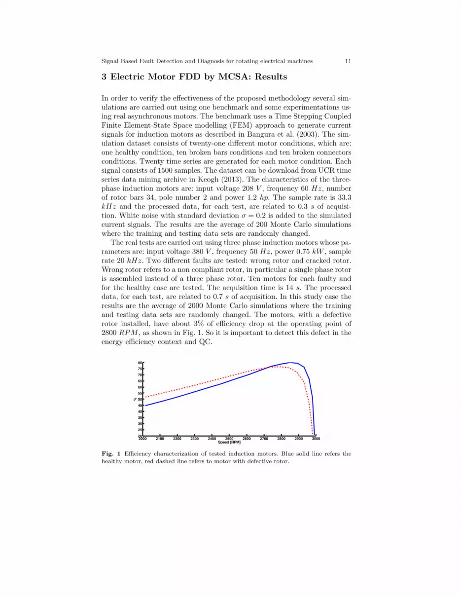
The real tests are carried out using three phase induction motors whose pa-rameters are: input voltage 380 V , frequency 50 Hz, power 0.75 kW , samplerate 20 kHz. Two different faults are tested: wrong rotor and cracked rotor.Wrong rotor refers to a non compliant rotor, in particular a single phase rotoris assembled instead of a three phase rotor. Ten motors for each faulty andfor the healthy case are tested. The acquisition time is 14 s. The processeddata, for each test, are related to 0.7 s of acquisition. In this study case theresults are the average of 2000 Monte Carlo simulations where the trainingand testing data sets are randomly changed. The motors, with a defectiverotor installed, have about 3% of efficiency drop at the operating point of2800 RPM , as shown in Fig. 1. So it is important to detect this defect in theenergy efficiency context and QC.

2000 2100 2200 2300 2400 2500 2600 2700 2800 2900 300020

25

30

35

40

45

50

55

60

65

70

75

80

%

Speed [RPM]

Fig. 1 Efficiency characterization of tested induction motors. Blue solid line refers thehealthy motor, red dashed line refers to motor with defective rotor.


3.1 Results and Discussion

The proposed approach processes three-phase stator currents in order to per-form defects detection and diagnosis as described in section 2.2. The followingtwo subsections show the results related to the two cases described previously.Figs. 2, 3, 4 and 5 show the simulation and experimentation results. The clas-sification accuracy is considered as an index to evaluate the performance ofthe proposed algorithm as shown in Tables 1 and 2. This index is obtainedusing the K-L distances probability distributions of each class, approximatedas normal distributions and estimated by Monte Carlo trials. The simulationsare carried out changing ngrid, the points number in which the PDF is esti-mated, and the current signals acquisition time in steady-state. Figs. 3 and 5show the K-L distances for all Monte Carlo trials. On each vertical line, thecentral dot is the mean and the horizontal edges are the 4 times standarddeviation. The figures show the results with ngrid = 64 × 64 points and theacquisition time, for the benchmark and real motors, equals to 0.3 s and 0.7 srespectively. This algorithm parameters setting guarantees better results forthese cases taking into account the classification accuracy and the processingtime. In the real motor the algorithm takes about 2.5 s for the classificationoutput (Eq. 12): about 1 s to acquire the current signals, of which 0.25 s intransient state and 0.7 s in steady-state, and about 1.45 s to evaluate thePDF and the classification output (Eq. 12). Setting ngrid = 32 × 32 points,the processing time is reduced to 1.5 s but decreasing the classification accu-racy as shown in Tables 1 and 2. The tests are performed for both cases usingthe asymmetric K-L divergence (Eq. 9). The results, related to the symmet-ric K-L divergence and described in the next subsections, are comparable tothose achieved with the asymmetric K-L divergence.

3.1.1 Broken Rotor Bars and Connectors Diagnosis

Figs. 2(a), 2(b) and 2(c) represent the pattern of the healthy motor, onebroken bar and one broken connector conditions, respectively; these figuresshow how the PDFs, estimated by KDE in the principal components space,are used as the specific patterns for the motor conditions. The simulationresults, given in Figs. 3(a), 3(b) and 3(c), show the faults diagnosis for brokenrotor bars and connectors, setting ngrid = 64 × 64 and the current signalsacquisition time in steady-state condition equals to 0.3 s. Fig. 3(a) shows theK-L divergence among the PDFs, estimated by KDE, of all motor conditions(i.e. healthy, from one to ten broken rotor bars and from one to ten brokenconnectors) and the PDF estimated by KDE from stator current signals ofhealthy motor. The results show as the minimum K-L distance is exactlythe healthy condition. Fig. 3(b) shows the K-L divergence among all PDFsand the PDF estimated from stator current signals affected by one brokenrotor bar. In this case the graph shows as the minimum K-L distance is


exactly the broken bar condition. The last graph, Fig. 3(c), shows the onebroken connector diagnosis. Even in this case the K-L divergence detects andidentifies the fault, that is one broken connector. By Monte Carlo simulations,all fault types are diagnosed with 100% accuracy hence the K-L divergencefigures for the others fault types are not reported. Moreover the classificationaccuracy is 100% with acquisition time above 0.3 s for each fault type, whilebelow 0.3 s, the classification accuracy decreases as shown in Table 1.

Table 1 Classification accuracy in the case of finite element motor, changing ngrid, thepoints number in which the PDF is estimated, and the current signals acquisition timein steady-state. Label H means healthy motor, labels 1-10B mean broken bars with the

relative number, labels 1-10C mean broken connectors with relative number.

ngrid 128× 128 64× 64 32× 32

Acquisition0.3 0.15 0.3 0.15 0.3 0.15

time (s)

%

H 100 100 100 100 100 1001B 100 100 100 100 100 1002B 100 100 100 100 100 100

3B 100 100 100 100 100 99.934B 100 100 100 100 100 99.895B 100 100 100 99.96 100 99.706B 100 100 100 100 100 99.877B 100 99.98 100 99.94 100 98.19

8B 99.82 95.34 99.89 95.97 99.55 91.419B 100 99.74 100 99.53 100 98.5610B 100 99.43 100 99.32 99.99 99.43

1C 100 100 100 100 100 99.992C 99.98 96.89 99.88 95.99 99.56 91.013C 99.88 91.71 99.72 95.74 98.48 93.75

4C 99.79 97.61 99.84 98.10 99.93 96.875C 99.98 98.96 99.99 98.49 99.96 96.376C 100 100 100 100 100 99.98

7C 100 100 100 100 100 99.948C 100 100 100 100 100 99.889C 100 99.99 100 100 100 99.4710C 100 99.89 100 99.77 100 96.95

Mean 99.97 99.03 99.97 99.18 99.88 98.15

3.1.2 Real Induction Motors Diagnosis

The Figs. 4(a), 4(b) and 4(c) represent the patterns of three real motors con-ditions: healthy, cracked and wrong rotor; these figures show as the PDFs,


(a)

(b)

(c)

Fig. 2 Interpolated PDFs of finite element motor in the two-dimensional principal com-ponents space estimated by KDE. (a) Healthy motor. (b) Motor with one broken bar. (c)Motor with one broken connector.

estimated by KDE in the principal components space, are distinct and there-fore can be used as a specific pattern for each motor condition. Experimental


(a)

(b)

(c)

Fig. 3 K-L divergence in the case of finite element motor. The blue dots are the mean, theblue bars are the four times standard deviation and the red asterisks are the classificationoutput. Label H means healthy motor, labels 1-10B mean broken bars with the relativenumber, labels 1-10C mean broken connectors with relative number. (a) Healthy motor.(b) Motor with one broken bar. (c) Motor with one broken connector.

results given in Figs. 5(a), 5(b) and 5(c) show the fault diagnosis for crackedand wrong rotors, setting ngrid = 64 × 64 and the current signals acquisi-tion time in steady-state equals to 0.7 s. Fig. 5(a) shows the K-L divergenceamong the PDFs, estimated by KDE, of all motor conditions (i.e. healthy,


cracked and wrong rotors) and the PDF estimated by KDE from stator cur-rent signals of healthy motor. The results show as the minimum K-L distanceis exactly the healthy condition. Fig. 5(b) shows the K-L divergence amongall PDFs and the PDF estimated from stator current signals where crackedrotors are diagnosed. In this case the graph shows as the minimum K-L dis-tance is exactly the cracked rotor condition. The last graph, Fig. 5(c), showsthe wrong rotor diagnosis. Even in this case the K-L divergence detects andidentifies the fault. By Monte Carlo simulations, all fault types are diagnosedwith accuracy reported in Table 2. It can be noticed how the classificationaccuracy in the case of healthy motor is always 100%, therefore the algorithmis able to detect if motors are healthy or if there are some faults or defects.In Figs. 5(b) and 5(c) the blue lines of motors with cracked and wrong rotorare never overlapped to the blue lines of healthy motors so, in these tests, thealgorithm never confuses the cases of healthy motors from those not healthy.

Table 2 Classification accuracy in the case of real motors, changing ngrid, the pointsnumber in which the PDF is estimated, and the current signals acquisition time in steady-

state. Motor conditions are: healthy, motor with cracked rotor and motor with wrongrotor.

ngrid 128× 128 64× 64 32× 32

Acquisition0.7 0.5 0.3 0.7 0.5 0.3 0.7 0.5 0.3

time (s)

%

Healthy 100 100 100 100 100 100 100 100 100

Cracked rotor 98.82 95.08 77.08 99.00 94.74 86.54 98.29 94.02 81.45Wrong Rotor 98.97 99.47 99.49 99.18 99.36 98.56 99.85 99.41 99.21

Mean 99.26 98.18 92.19 99.39 98.03 95.03 99.38 97.81 93.55

The next Section describes the well-known MSPCA algorithm for faultdetection and isolation based on vibration signals.


(a)

(b)

(c)

Fig. 4 Interpolated PDFs of real motors in the two-dimensional principal components

space estimated by KDE. (a) Healthy motor. (b) Motor with cracked rotor. (c) Motor withwrong rotor.

4 Electric Motor FDD by MVSA

In electric motors, faults and defects are often correlated to the vibrationsignals, which can be processed to model the motors behaviour by patternsthat represent the normal and abnormal motor conditions. Vibration analysisis widely accepted as a tool to detect faults of a rotating machine as it is reli-


(a) (b)

(c)

Fig. 5 K-L divergence in the case of real motors. The blue dots are the mean, the blue barsare the four times standard deviation and the red asterisks are the classification output.(a) Healthy motor. (b) Motor with cracked rotor. (c) Motor with wrong rotor.

able, not destructive and it permits continuous monitoring without stoppingthe machine. A brief literature review is given by: Fan and Zheng (2007);Immovilli et al. (2010); Sawalhi and Randall (2008a,b); Tran et al. (2009);Yang and Kim (2006). In particular, it is possible to detect different faultsby analysing the vibration power spectrum. Most common faults are unbal-ance and misalignment. Unbalance may be caused by poor balancing, shaft


inflection (i.e. thermal expansion) and rotor distortion by magnetic forces (awell known problem in high power electrical machines). Misalignment maybe caused by misaligned couplings, misaligned bearings or crooked shaft.

In order to model the vibration signals, MSPCA is taken into account,as presented in Bakshi (1998). MSPCA deals with processes that operate atdifferent scales, and have contributions from:

• events occurring at different localizations in time and frequency;• stochastic processes whose energy or power spectrum changes with time

and/or frequency;• variables measured at different sampling rate or containing missing data.

MSPCA transforms the process data information at different scales by WT.The information of each different scales is captured by PCA modelling. Thesepatterns, which represent the process conditions, can be used to identify eachfault and defect.

To detect the defects a KDE algorithm is used on the PCA residuals, andthe thresholds are computed for each sensors signal. It allows to identify if, foreach wavelet scale, the signals are involved in the fault or not. When Gaus-sian assumption is not recognized, KDE method is a robust methodologyto estimate numerically the PDF, by Odiowei and Cao (2010). Fault isola-tion is carried out by contribution plots, which is based on quantifying thecontribution of each process variable to the individual scores of the PCA rep-resentation. Diagnosis can be performed using the contribution plots becausethey represent the signatures of the rotating electrical machines conditions.The contributions are the inputs of LDA classifier, which is a supervised ma-chine learning algorithm used here to diagnose each motor defect. Severalsimulations are carried out by a benchmark provided by the Case WesternReserve University Bearing Data Center (2014).

4.1 Recalled Results

In this section authors present the algorithms used to develop the fault anddefect diagnosis procedure. It extracts patterns by vibration signals usingMSPCA and PCA contributions are used to diagnose each motor fault.

4.1.1 Principal Component Analysis

PCA is introduced in the section 2.1.1, here an improved PCA fault detectionindex is described. A deviation of the new data sample X from the normalcorrelation could change the projections onto the subspaces, either Sp or Sr.

Consequently, the magnitude of either X or X could increase over the valuesobtained with normal data. The Square Prediction Error (SPE) is a statistic


that measures lack of fit of a model to data. The SPE statistic indicatesthe difference, or residual, between a sample and its projection into the pcomponents retained in the model. The exact description of the distributionof SPE is given in Jackson (2003):

SPE ≡∥

∥

∥X

∥

∥

∥

2

=∥

∥X(I − PP T )∥

∥

2. (13)

The process is considered faultless if:

SPE ≤ δ2 (14)

where δ2 is a confidence limit for SPE. A confidence limit expression for SPE,when x follows a normal distribution, is developed in Jackson and Mudholkar(1979); Misra et al. (2002) and Rodriguez et al. (2006). The fault detectabilityconditions is given in Dunia and Joe Qin (1998) and recalled in the following.Defining:

X = X∗ + fΞ, (15)

where the sample vector for normal operating conditions is denoted by X∗,f represents the magnitude of the fault and Ξ is a fault direction vector.Necessary and sufficient conditions for detectability are:

• Ξ = (I − PP T )Ξ 6= 0, with Ξ the projection of Ξ on the residualsubspace;

•∣

∣

∣f∣

∣

∣=

∣

∣(I − PP T )f∣

∣ > 2δ, with f the projection of f on the residual

subspace.

The drawbacks of SPE index for fault detection are mainly two: the firstis related to the assumption of normal distribution to estimate the thresholdof this index, the second is that the SPE is a weighted sum, with unitarycoefficients, of quadratic residues Xi. To improve the fault detection, thesetwo drawbacks are faced assuming that the process is considered faultless if,for each i:

X2i ≤ δi i = 1, . . . ,m, (16)

where δi is a confidence limit for X2i . To estimate the confidence limit δi,

even when the normality assumption of X2i is not valid, the solution is to

estimate the PDF directly from X2i through a non parametric approach. In

Yu (2011a,b) and Odiowei and Cao (2010), KDE is considered because it is awell established non parametric approach to estimate the PDF of statisticalsignals and evaluate the control limits. Assume y is a random variable andits density function is denoted by p(y). This means that:

P (y < k) =

∫ k

−∞p(y)dy. (17)


Hence, by knowing p(y), an appropriate control limit can be determined fora specific confidence bound α, using Eq. (17). Replacing p(y), in Eq. (17),with the estimation of the probability density function of X2

i , called p(Xi)2,

the control limits will be estimated by:

∫ δi−∞ p(X2

i )dX2i = α. (18)

Fault isolation and diagnosis are performed by the PCA contributions: defin-ing the new observation vector xj ∈ R

m, the total contribution of the ith

process variable Xi is

CONTi =∑Nj=1 x

2ij i = 1, . . . ,m. (19)

4.1.2 Wavelet Transform

The Wavelet Transform (WT) is defined as the integral of the signal f(t)multiplied by scaled, shifted version of basic wavelet function φ(t), that is areal valued function whose Fourier transform satisfies the admissibility cri-teria stated in Li et al. (1999). Then the wavelet transformation c(·, ·) of asignal f(t) is defined as:

c(a, b) =∫

Rf(t) 1√

aφ(

t−ba

)

dt

a ∈ R+ − 0

b ∈ R,

(20)

where a is the so-called scaling parameter, b is the time localization param-eter. Both a and b can be continuous or discrete variables. Multiplying eachcoefficient by an appropriately scaled and shifted wavelet it yields the con-stituent wavelets of the original signal. For signals of finite energy, continuouswavelets synthesis provides the reconstruction formula:

f(t) =1

Kφ

∫

R

∫

R+

c(a, b)1√aφ

(

t− b

a

)

da

a2db (21)

where:

Kψ =

∫ +∞

−∞

| ψ(ξ) || ξ | dξ (22)

denotes a (Wavelet specific) normalization parameter in which φ is the Fouriertransform of φ. Mother wavelets must satisfy the following properties:

∫ +∞−∞ |φ(t)|dt <∞,

∫ +∞−∞ |φ(t)|2dt = 1,

∫ +∞−∞ φ(t)dt = 0. (23)

To avoid intractable computations when operating at every scale of the Con-tinuous WT (CWT), scales and positions can be chosen on a power of two,i.e. dyadic scales and positions. The Discrete WT (DWT) analysis is more


efficient and just as accurate, as reported in Li et al. (1999) and Daubechies(1988). In this scheme a and b are given by:

a = aj0, b = b0aj0k, (j, k) ∈ Z

2, Z := 0,±1,±2, · · · . (24)

The variables a0 and b0 are fixed constants that are set, as in Daubechies(1988), to: a0 = 2 and b0 = 1. The discrete wavelet analysis can be describedmathematically as:

c(a, b) = c(j, k) =∑

n∈Z+ f(n)φj,k(n),a = 2j , b = 2jk,j ∈ Z, k ∈ Z,

(25)

considering the simplified notation f(n) = f(n · tc), n ∈ Z+ and tc the

sampling time, the discretization of continuous time signal f(t) is considered.The inverse transform, also called discrete synthesis, is defined as:

f(n) =∑

j∈Z

∑

k∈Z

c(j, k)φj,k(n). (26)

In Mallat (1989), a signal is decomposed into various scales with different timeand frequency resolutions, this algorithm is known as the multi-resolutionsignal decomposition. Defining:

φj,k(n) = 2−j/2φ(

2−jn− k)

,ψj,k(n) = 2−j/2ψ

(

2−jn− k)

,Vj = span φj,k, k ∈ Z ,Wj = span ψj,k, k ∈ Z ,

(j, k) ∈ Z2 (27)

the wavelet function φj,k, is the orthonormal basis of Vj and the orthogo-nal wavelet ψj,k, called scaling function, is the orthonormal basis of Wj . InDaubechies (1988) is shown that:

Vj⊥Wj ,Vm =Wm+1 ⊕ Vm+1.

Vm,Wm ⊂ L2(R) (28)

Defining f(n) = f as element of V0 =W1 ⊕V1, f can be decomposed into itscomponents along V1 and W1:

f = P1f +Q1f. (29)

with Pj the orthogonal projection onto Vj and Qj the orthogonal projectiononto Wj . Defining j ≥ 1 and f(n) = c0n, it results:


f(n) =∑

k∈Zc1kφ1,k(n) +

∑

k∈Zd1kψ1,k(n),

c1k =∑

n∈Zh(n− 2k)c0n,

d1k =∑

n∈Zg(n− 2k)c0n,

h(n− 2k) = 〈φ1,k(n), φ0,n(n)〉 ,g(n− 2k) = 〈ψ1,k(n), ψ0,n(n)〉 ,

k, n ∈ Z2.

(30)

where the terms g and h are high-pass and low-pass filter coefficients derivedfrom the bases ψ and φ. Considering a dataset of N (n = 1, . . . , N) samples,and introducing a vector notation, c1k and d1k can be rewrite as Daubechies(1988):

c1 = Hc0,d1 = Gc0,

(31)

with

H =

h(0) h(1) · · · h(N)h(−2) h(−1) · · · h(N − 2)

...... · · ·

...h(−2k) h(1− 2k) · · · h(N − 2k)

, (32)

G =

g(0) g(1) · · · g(N)g(−2) g(−1) · · · g(N − 2)

...... · · ·

...g(−2k) g(1− 2k) · · · g(N − 2k)

. (33)

The procedure can be iterated obtaining:

cj = Hcj−1,dj = Gdj−1.

(34)

Then:cj = Hjc

0,dj = Gjd

0,(35)

where Hj is obtained by applying the H filter j times, and Gj is obtained byapplying the H filter j−1 times and the G filter once. Hence any signal maybe decomposed into its contributions in different regions of the time-frequencyspace by projection on the corresponding wavelet basis function. The lowestfrequency content of the signal is represented on a set of scaling functions.The number of wavelet and scaling function coefficients decreases dyadicallyat coarser scales due to the dyadic discretization of the dilation and trans-lation parameters. The algorithms for computing the wavelet decompositionare based on representing the projection of the signal on the correspond-ing basis function as a filtering operation (Mallat (1989)). Convolution withthe filter H represents projection on the scaling function, and convolutionwith the filter G represents projection on a wavelet. Thus, the signal f(n) isdecomposed at different scales, the detail scale matrices and approximation


scale matrices. Defining L the decomposition levels, the approximation scaleAL and the detail scales Dj , j = 1, ..., L are the composition of cj and dj

for every m variables of the data matrix X:

Aj = [cj1, cj2, . . . , c

jm],

Dj = [dj1,dj2, . . . ,d

jm].

j = 1, ..., L (36)

To select the wavelet decomposition level L, it is considered the minimumnumber of decomposition levels, and used to obtain an approximation signalAL so that the upper limit of its associated frequency band is under thefundamental frequency f , is described by the following condition Antonino-Daviu et al. (2006); Bouzida et al. (2011):

2−(L+1)fs < f. (37)

where fs is the sampling frequency of the signals and f is the fundamentalfrequency of the machine. From this condition, the decomposition level of theapproximation signal is the integer L given by:

L = ⌊log2(fs/f)− 1⌋. (38)

4.2 MSPCA Formulation

WT and PCA can be combined to extract maximum information from mul-tivariate sensor data. MSPCA can be used as a tool for fault detection anddiagnosis by means of statistical indexes. In particular, faults are detectedby using Eqs. 16 and 18 and the isolation is conducted by the contributionsmethod (Eq. 19). In this way it is possible to detect which sensor is mostaffected by fault (see Misra et al. (2002)). Two fundamental theorems ex-ist for the MSPCA formulation, they assess that PCA principles remainsunchanged under the Wavelet transformation. These theorems are useful toapply MSPCA methodology, as stated in Bakshi (1998).

Theorem 4.1 Let W =[

H ′L,G

′L,G

′L−1, · · · ,G′

1

]′ ∈ RN×N the orthonor-

mal matrix representing the orthonormal wavelet transformation operatorcontaining the filter coefficients, the principal component loadings obtainedby the PCA of X and WX are identical, whereas the principal componentscores of WX are the wavelet transform of the scores of X.

Theorem 4.2 MSPCA reduces to conventional PCA if neither the principalcomponents nor the wavelet coefficients at any scale are eliminated.

The developed FDD MSPCA based procedure consists of two stages: first,the training step, the faultless data are processed and a model of this data isbuilt. MSPCA training step are summarized below:


T1. Data are preprocessed;T2. The Wavelet analysis is used, to refine the data, with a level of detail L

which is chosen by Eq. (38);T3. Normalize mean and standard deviation of detail and approximation ma-

trices and apply PCA to the approximation matrix AL, of order L, andto the L detail matrices Dj , where j = 1, ...L;

T4. The PCA transformation matrix P and the signal covariance matrix S

are computed for each approximation and detail matrices;T5. The Xi signals (Eq. 13) are computed, for each wavelet matrix;T6. The δi thresholds are computed, for each detail matrix and for the ap-

proximation matrix of order L, using the KDE algorithm (Eq. 18) and aconfidence bound α;

In the second phase, the diagnosis step, the model previously obtained is on-line compared with the new data and a statistical index of failure is calculated.MSPCA diagnosis step are summarized below:

D1. The previous steps, except the threshold computation step (T6), are re-peated for each new dataset, the data are standardized as in the trainingstep (T3) and the PCA and Xi signals are computed using the P and S

matrices, obtained in the training step;D2. If any of the Xi signals is over the thresholds δi, the fault is detected and

the isolation is performed by the∥

∥

∥Xi

∥

∥

∥contributions, else the next data

set is analysed (return to (D1));

D3. Compute all the residual contributions∥

∥

∥Xi

∥

∥

∥, for each sensor, for all details

and approximation matrices and isolate and diagnose the fault type.

The next Section introduces the FDD experimental results in order to showthe MSPCA algorithm performance. Test are carried out on real inductionmotors with different fault severity.

5 Electric Motor FDD by MVSA: Results

The diagnosis algorithm has been tested on the vibration signals provided bythe Case Western Reserve University Bearing Data Center (2014). Experi-ments were conducted using a 2 hp Reliance Electric motor, and accelerationdata was measured at locations near to and remote from the motor bearings.Motor bearings were seeded with faults using electro-discharge machining(EDM). Faults ranging from 0.007 inches in diameter to 0.040 inches in di-ameter were introduced separately at the inner raceway, rolling element (i.e.ball) and outer raceway. Faulted bearings were reinstalled into the test motorand vibration data was recorded for motor loads of 0 to 3 horsepower (motorspeeds of 1797 to 1720 RPM). Accelerometers were placed at the 12 o’clockposition at both the drive end and fan end of the motor housing. Digital data


was collected at 12000 samples per second. Experiments were conducted forboth fan and drive end bearings with outer raceway faults located at 3 o’clock(directly in the load zone), at 6 o’clock (orthogonal to the load zone), and at12 o’clock.

5.1 Results and Discussion

The proposed approach described in section 4.2 has been tested using aDaubechies mother wavelet of order 15, defined db15 mother wavelet (de-fined kernel φ in section 4.1.2). The motor rotation frequency is 30 Hz andthe sampling frequency is 12 kHz, so applying Eq. (38), the level of detailobtained is L = 7. The dimension of Principal Components subspace p chosenby the Kaiser’s rule, treated in Jolliffe (2002).

Incoming batch data samples are then fed into the MSPCA model and thePCA residual contributions are computed for the matrices Dj , j = 1, . . . , L,AL. In the following, these matrices are defined scale matrices, and they arecompared with the respective thresholds. When, at any scale, the numberof residual contribution samples over the thresholds is greater than n · α · γ,where α is the significance level used for the threshold δi calculation (statedin section 4.2), n is the sample number of batch data and γ is a correctiveindex (fixed equal to 2), a fault is detected and the motor is considered faulty.

Once a fault is detected, the isolation and diagnosis tests are performed.At this step the PCA contributions are computed for each scale matrix. Faultisolation allows to detect which sensors are involved in the fault. By usingseveral scales for the DWT analysis, it is possible to cluster the residualcontributions of each scale and define a unique signature of the motor fault,as in the classical MVSA approach. More in detail, the signature of each faultis given by the contributions of each variable for each scale. The results arethe average of 1000 Monte Carlo simulations where the training and testingdata sets are randomly changed.

Figs. 6 and 7 show the residuals of the first accelerometer (i.e. placed at thedrive end) for drive end bearing faults estimated by Eq. (16). The thresholds,drawn in dashed red line, are estimated by KDE (Eq. 18). While Fig. 6(a)shows the residuals for healthy motor, Fig. 6(b) and 6(c) show the residualsof rolling element and inner raceway faults respectively at the detail scales D1

and D4, which are, among all scales, the more representatives of the faults.Figs. 7(a), 7(b) and 7(c) show the residuals of outer raceway faults located

at 3, 6, 12 o’clock respectively at the detail scales D1, D2 and D4, which are,among all scales, the more representatives of the faults. It can be noticedhow the amplitude of residuals is related to the fault type and so they canbe exploited as signatures of the rotating electrical machine conditions.

Figs. 8 and 9 show the contributions plot of each accelerometer at differentscales for drive end bearing faults, particularly Figs. 8(a), 8(b) and 8(c) show


0 200 400 600 800 1000 1200 1400 1600 1800 20000

0.05

0.1

0.15

0.2

0.25

0.3

0.35

0.4

sample

D2

mat

rix

resi

du

al(a)

0 500 1000 1500 2000 2500 3000 3500 40000

10

20

30

40

50

sample

D1

mat

rix

resi

du

al

(b)

0 100 200 300 400 5000

0.01

0.02

0.03

0.04

0.05

0.06

0.07

sample

D4

mat

rix

resi

du

al

(c)

Fig. 6 Residuals of the accelerometer placed at the drive end. (a) Healthy motor at D2

detail scale. (b) Rolling element fault of drive end bearing at D1 detail scale. (c) Innerraceway fault of drive end bearing at D4 detail scale.

the contribution plot of healthy motor, rolling element and inner racewayfaults while Figs. 9(a), 9(b) and 9(c) show the contribution plot of outerraceway faults located at 3, 6, 12 o’clock respectively.

The contribution plots represent the signatures of the electric motor con-ditions. So a supervised machine learning algorithm, with the PCA contri-butions as inputs, can be used to diagnose each motor fault. The Figs. 8 and9 show that the identified signatures by PCA contributions are unique foreach considered fault. The accelerometers are involved in these signaturesat different scales with different amplitudes. As shown by Figs. 8 and 9, all


0 200 400 600 800 1000 1200 1400 1600 1800 20000

200

400

600

800

1000

1200

1400

1600

sample

D2

mat

rix

resi

du

al(a)

0 200 400 600 800 1000 1200 1400 1600 1800 20000

100

200

300

400

500

600

700

800

sample

D2

mat

rix

resi

du

al

(b)

0 500 1000 1500 2000 2500 3000 3500 40000

100

200

300

400

sample

D1

mat

rix

resi

du

al

(c)

Fig. 7 Residuals of the accelerometer placed at the drive end. (a) Outer raceway fault

located at 3 o’clock of drive end bearing at D1 detail scale. (b) Outer raceway fault locatedat 6 o’clock of drive end bearing at D2 detail scale. (c) Outer raceway fault located at 12o’clock of drive end bearing at D2 detail scale.

faults affect the accelerometer placed at the drive end. This points out thatthe contributions plot can be used to identify the sensor more affected by thefaults. Particularly, the fault isolation is performed computing the averagecontribution value of all scales: the sensor affected by the fault is that onewith the highest average contribution value. As shown in Figs. 8 and 9 thesensor more affected by the faults is the accelerometer placed at the driveend. The fault diagnosis is performed using the contribution plots becausethey represent the signatures of the electric motor conditions and are unique


(a)

A6D6

D5D4

D3D2

D1

Acc. Drive End

Acc. Fan End

0

2

4

Mat

rix

con

trib

uti

on

(b)

A6D6

D5D4

D3D2

D1

Acc. Drive End

Acc. Fan End

0

5

10

15

Mat

rix

con

trib

uti

on

(c)

Fig. 8 Contributions plot (a) Healthy motor. (b) Rolling element fault of drive end bear-ing. (c) Inner raceway fault of drive end bearing.

for each fault as shown in Figs. 8 and 9. Outer raceway fault located at 6o’clock and outer raceway fault located at 12 o’clock of drive end bearing af-fect the contributions at the same scales (Figs. 9(b), 9(c)), but contributionsamplitudes are different so they can be used to diagnose the faults.

In order to diagnose each motor fault LDA is used, which searches fora linear transformation that maximizes class separability in a reduced di-mensional space. LDA is proposed in Fisher (1936) for solving binary classproblems. It is further extended to multi-class cases in Rao (1948). In gen-eral, LDA aims to find a subspace that minimizes the within-class scatterand maximizes the between-class scatter simultaneously. PCA contributionsare used as features input to the LDA algorithm. Tables 3, 4 and 5 show theclassification accuracy. The results are the average classification accuracy ofeach motor conditions (i.e. healthy motor, rolling element fault, inner race-way fault, outer raceway fault located at 3, 6 and 12 o’clock) and of 4 motorloads: from 0 to 3 horsepower (motor speeds of 1797 to 1720 RPM). Table3 show the classification accuracy at different wavelet decomposition level L


(a)

A6D6

D5D4

D3D2

D1

Acc. Drive End

Acc. Fan End

0

50

100M

atri

x co

ntr

ibu

tio

n

(b)

A6D6

D5D4

D3D2

D1

Acc. Drive End

Acc. Fan End

0

5

10

15

Mat

rix

con

trib

uti

on

(c)

Fig. 9 Contributions plot (a) Outer raceway fault located at 3 o’clock of drive end bearing.(b) Outer raceway fault located at 6 o’clock of drive end bearing. (c) Outer raceway faultlocated at 12 o’clock of drive end bearing.

and acquisition time of faults occurred at drive end bearing with fault diam-eter of 0.007 inches. The classification accuracy is over 99% for each level Land acquisition time, so a low wavelet decomposition level and acquisitiontime can be chosen to diagnose effectively this faults.

Table 4 show the classification accuracy at different wavelet decompositionlevel L and acquisition time of faults occurred at drive end bearing with faultdiameter of 0.021 inches. The classification accuracy is over 99% for each levelL and acquisition time higher 0.3 s, so a low wavelet decomposition level andacquisition time of 0.3 s can be chosen to diagnose effectively this faults.Table 5 show the classification accuracy at different wavelet decompositionlevel L and acquisition time of faults occurred at fan end bearing with faultdiameter of 0.007 inches. The classification accuracy is over 98% for levelL = 3 and acquisition time higher 0.5 s, so a wavelet decomposition level of 3and acquisition time of 0.3 s can be chosen to diagnose effectively this faults.


Table 3 Mean classification accuracy of drive end bearing faults with fault diameter of0.007 inches.

Acquisition time s

0.1 0.2 0.3 0.5 0.7

%

L

1 99.23 99.96 99.98 100 1002 99.40 99.85 99.99 100 1003 99.55 99.95 100 99.99 1004 99.67 99.98 100 100 100

5 99.47 99.95 100 100 1006 99.29 99.85 99.99 100 100

Table 4 Mean classification accuracy of drive end bearing faults with fault diameter of0.021 inches.

Acquisition time s

0.1 0.2 0.3 0.5 0.7

%

L

1 92.66 97.73 99.19 99.91 99.962 94.76 98.36 99.51 99.75 99.883 95.10 98.87 99.73 99.98 99.994 94.64 98.39 99.21 99.81 99.975 95.00 98.54 99.50 99.79 99.966 94.38 98.25 99.35 99.83 99.88

Table 5 Mean classification accuracy of fan end bearing faults with fault diameter of

0.007 inches.

Acquisition time s

0.1 0.2 0.3 0.5 0.7

%

L

1 73.61 82.50 89.43 93.04 94.31

2 74.76 84.11 90.44 95.02 95.153 83.08 92.54 94.82 98.49 98.604 84.41 91.62 95.37 99.22 99.285 84.41 90.73 95.56 98.90 98.766 84.41 93.14 96.76 99.39 99.31

6 Summary and Conclusions

This chapter addresses the modelling and diagnosis issues of rotating elec-trical machines by signal based solutions. With particular attention to realsystems, two case studies related to rotating electrical machines are discussed.


First FDD solution uses the PCA in order to reduce the currents space intwo dimensions. The PDF of PCA-transformed signals is estimated by KDE.PDFs are the models that can be used to identify each fault. Diagnosis hasbeen carried out using the K-L divergence, which measures the difference be-tween two probability distributions. This divergence is used as a distance mea-sure between classified statistic signatures obtained by KDE. Second FDDsolution uses MSPCA, KDE and PCA contributions to identify and diagnosethe faults. Several experimentations on real motors are carried out in order toverify the effectiveness of the proposed methodologies. First solution, basedon current signals, has been tested on a motor modelled by FEM and realinduction motors in order to diagnose broken rotor bars, broken connector,cracked and wrong rotor. Second solution, based on vibration signals, hasbeen tested on a real induction motors in order to diagnose bearings faults:inner raceway, rolling element (i.e. ball) and outer raceway faults with differ-ent fault diameter (i.e 0.007 and 0.021 inches). Results show that the signalbased solutions are able to model the faults dynamics and diagnose the motorconditions (i.e healthy and faulty) and identify the fault type.

References

Abdelmadjid, G., Mohamed, B. S., Mohamed, T., Ahmed, S., and Youcef,M. (2013). An improved stator winding fault tolerance architecture forvector control of induction motor: Theory and experiment. Electric PowerSystems Research, 104(0):129 – 137.

Antonino-Daviu, J., Riera-Guasp, M., Roger-Folch, J., Martınez-Gimenez, F.,and Peris, A. (2006). Application and optimization of the discrete wavelettransform for the detection of broken rotor bars in induction machines.Applied and Computational Harmonic Analysis, 21(2):268–279.

Baccarini, L. M. R., Tavares, J. P. B., de Menezes, B. R., and Caminhas,W. M. (2010). Sliding mode observer for on-line broken rotor bar detection.Electric Power Systems Research, 80(9):1089 – 1095.

Bakshi, B. R. (1998). Multiscale PCA with application to multivariate sta-tistical process monitoring. AIChE Journal, 44(7):1596–1610.

Bangura, J., Povinelli, R., Demerdash, N. A. O., and Brown, R. (2003). Diag-nostics of eccentricities and bar/end-ring connector breakages in polyphaseinduction motors through a combination of time-series data mining andtime-stepping coupled FE-state-space techniques. IEEE Transactions onIndustry Applications, 39(4):1005–1013.

Benloucif, M. and Balaska, H. (2006). Robust fault detection for an inductionmachine. In Automation Congress, 2006. WAC ’06. World, pages 1–6,Budapest.

Bouzida, A., Touhami, O., Ibtiouen, R., Belouchrani, A., Fadel, M., and Rez-zoug, A. (2011). Fault diagnosis in industrial induction machines through


discrete wavelet transform. IEEE Transactions on Industrial Electronics,58(9):4385–4395.

Case Western Reserve University Bearing Data Center (2014). Bearing DataCenter.

Cheng, H., Nikus, M., and Jamsa-Jounela, S. L. (2008). Evaluation of PCAmethods with improved fault isolation capabilities on a paper machinesimulator. Chemometrics and Intelligent Laboratory Systems, 92(2):186–199.

Chiang, L. H., Russell, E. L., and Braatz, R. D. (2000). Fault diagnosis inchemical processes using Fischer discriminant analysis, discriminant par-tial least squares, and principal component analysis. Chemometrics andIntelligent Laboratory Systems, 50(2):243–252.

Chilengue, Z., Dente, J., and Branco, P. C. (2011). An artificial immunesystem approach for fault detection in the stator and rotor circuits of in-duction machines. Electric Power Systems Research, 81(1):158 – 169.

Ciabattoni, L., Corradini, M., Grisostomi, M., Ippoliti, G., Longhi, S., andOrlando, G. (2011a). Adaptive extended kalman filter for robust sensorlesscontrol of pmsm drives. In Proceedings of the IEEE Conference on Decisionand Control, pages 934–939.

Ciabattoni, L., Corradini, M., Grisostomi, M., Ippoliti, G., Longhi, S., andOrlando, G. (2014). A discrete-time vs controller based on rbf neuralnetworks for pmsm drives. Asian Journal of Control, 16(2):396–408.

Ciabattoni, L., Grisostomi, M., Ippoliti, G., and Longhi, S. (2011b). Esti-mation of rotor position and speed for sensorless dsp-based pmsm drives.In 2011 19th Mediterranean Conference on Control and Automation, MED2011, pages 1421–1426.

Ciandrini, C., Gallieri, M., Giantomassi, A., Ippoliti, G., and Longhi, S.(2010). Fault detection and prognosis methods for a monitoring system ofrotating electrical machines. In Industrial Electronics (ISIE), 2010 IEEEInternational Symposium on, pages 2085–2090.

Comaniciu, D. (2003). An algorithm for data-driven bandwidth selec-tion. IEEE Transactions on Pattern Analysis and Machine Intelligence,25(2):281–288.

Daubechies, I. (1988). Orthonormal bases of compactly supported wavelets.Communications on Pure and Applied Mathematics, 41(7):909–996.

Dunia, R. and Joe Qin, S. (1998). Joint diagnosis of process and sensorfaults using principal component analysis. Control Engineering Practice,6(4):457–469.

Fan, Y. and Zheng, G. (2007). Research of high-resolution vibration signaldetection technique and application to mechanical fault diagnosis. Me-chanical Systems and Signal Processing, 21(2):678 – 687.

Feki, N., Clerc, G., and Velex, P. (2013). Gear and motor fault modelingand detection based on motor current analysis. Electric Power SystemsResearch, 95(0):28 – 37.


Ferracuti, F., Giantomassi, A., Iarlori, S., Ippoliti, G., and Longhi, S. (2013a).Induction motor fault detection and diagnosis using KDE and Kullback-Leibler divergence. In Industrial Electronics Society, IECON 2013 - 39thAnnual Conference of the IEEE, pages 2923–2928.

Ferracuti, F., Giantomassi, A., Ippoliti, G., and Longhi, S. (2010). Multi-scalePCA based fault diagnosis for rotating electrical machines. In EuropeanWorkshop on Advanced Control and Diagnosis, 8th ACD, pages 296 – 301,Ferrara, Italy.

Ferracuti, F., Giantomassi, A., and Longhi, S. (2013b). MSPCA with KDEthresholding to support QC in electrical motors production line. In Man-ufacturing Modelling, Management, and Control, volume 7, pages 1542 –1547.

Ferracuti, F., Giantomassi, A., Longhi, S., and Bergantino, N. (2011). Multi-scale PCA based fault diagnosis on a paper mill plant. In Emerging Tech-nologies Factory Automation (ETFA), 2011 IEEE 16th Conference on,pages 1–8.

Filbert, D. and Metzger, L. (1982). Quality test of systems by parameterestimation. In Proceedings of 9th IMEKO congress, Berlin, Germany.

Fisher, R. A. (1936). The use of multiple measurements in taxonomic prob-lems. Annals of Eugenics, 7(2):179–188.

Gani, A. and Salami, M. (2002). Vibration faults simulation system (VFSS):a system for teaching and training on fault detection and diagnosis. InResearch and Development, 2002. SCOReD 2002. Student Conference on,pages 15–18.

Giantomassi, A. (2012). Modeling estimation and identification of complexsystem dynamics. LAP Lambert Academic Publishing.

Giantomassi, A., Ferracuti, F., Benini, A., Longhi, S., Ippoliti, G., andPetrucci, A. (2011). Hidden Markov model for health estimation and prog-nosis of turbofan engines. In ASME 2011 International Design EngineeringTechnical Conferences & Computers and Information in Engineering Con-ference, pages 1–6.

Hua, L., Zhanfeng, L., and Zhaowei (2009). Time frequency distribution forvibration signal analysis with application to turbo-generator fault diagno-sis. In Control and Decision Conference, 2009. CCDC ’09. Chinese, pages5492 – 5495, Guilin.

Immovilli, F., Bellini, A., Rubini, R., and Tassoni, C. (2010). Diagnosis ofbearing faults in induction machines by vibration or current signals: A crit-ical comparison. IEEE Transactions on Industry Applications, 46(4):1350–1359.

Isermann, R. (1984). Process fault detection on modeling and estimationmethods?a survey. Automatica, 20(4):387–404.

Isermann, R. (2006). Fault-diagnosis dystems. Springer-Verlag, Berlin.Isermann, R. and Balle, P. (1997). Trends in the application of model-basedfault detection and diagnosis of technical processes. Control EngineeringPractice, 5(5):709–719.


Jackson, J. E. (2003). A User’s Guide to Principal Components, volume 587.Wiley-Interscience, New York.

Jackson, J. E. and Mudholkar, G. S. (1979). Control procedures for residualsassociated with principal component analysis. Technometrics, 21(3):341–349.

Jolliffe, I. T. (2002). Principal Component Analysis. Springer, Berlin.Keogh, E. (2013). UCR time series data mining archive.Kullback, S. and Leibler, R. A. (1951). On information and sufficiency. Annalsof Mathematical Statistics, 22(1):79–86.

Lachouri, A., Baiche, K., Djeghader, R., Doghmane, N., and Ouhtati, S.(2008). Analyze and fault diagnosis by Multi-scale PCA. In Informa-tion and Communication Technologies: From Theory to Applications, 2008.ICTTA 2008. 3rd International Conference on, pages 1–6.

Li, W., Yue, H. H., Valle-Cervantes, S., and Qin, S. J. (2000). Recursive PCAfor adaptive process monitoring. Journal of process control, 10(5):471–486.

Li, X., Dong, S., and Yuan, Z. (1999). Discrete wavelet transform for toolbreakage monitoring. International Journal of Machine Tools and Manu-facture, 99(12):1944–1955.

Mallat, S. G. (1989). A theory for multiresolution signal decomposition:the wavelet representation. IEEE Transactions on Pattern Analysis andMachine Intelligence, 11(7):674–693.

Misra, M., Yue, H., Qin, S., and Ling, C. (2002). Multivariate process mon-itoring and fault diagnosis by multi-scale PCA. Computers & ChemicalEngineering, 26(9):1281–1293.

Mugdadi, A. and Ahmad, I. A. (2004). A bandwidth selection for kernel den-sity estimation of functions of random variables. Computational Statistics& Data Analysis, 47(1):49 – 62.

Odiowei, P.-E. and Cao, Y. (2010). Nonlinear dynamic process monitor-ing using canonical variate analysis and kernel density estimations. IEEETransactions on Industrial Informatics, 6(1):36 –45.

Parzen, E. (1962). On estimation of a probability density function and mode.The Annals of Mathematical Statistics, 33(3):1065–1076.

Patton, R., Uppal, F., and Lopez-Toribio, C. (2000). Soft computing ap-proaches to fault diagnosis for dynamic systems: a survey. In 4th IFACSymposium on Fault Detection supervision and Safety for Technical Pro-cesses, pages 298–311, Budapest, Hungary.

Pedra, J., Candela, I., and Barrera, A. (2009). Saturation model for squirrel-cage induction motors. Electric Power Systems Research, 79(7):1054 –1061.

Ran, L. and Penman, J. (2008). Condition Monitoring of Rotating ElectricalMachines, volume 56. Institution of Engineering and Technology, London,United Kingdom.

Rao, C. R. (1948). The utilization of multiple measurements in problems ofbiological classification. Journal of the Royal Statistical Society - Series B,10(2):159–203.


Rodriguez, P., Belahcen, A., and Arkkio, A. (2006). Signatures of electricalfaults in the force distribution and vibration pattern of induction motors.Electric Power Applications, IEE Proceedings -, 153(4):523 –529.

Samsi, R., Ray, A., and Mayer, J. (2009). Early detection of stator volt-age imbalance in three-phase induction motors. Electric Power SystemsResearch, 79(1):239 – 245.

Sawalhi, N. and Randall, R. (2008a). Simulating gear and bearing interactionsin the presence of faults: Part I. the combined gear bearing dynamic modeland the simulation of localised bearing faults. Mechanical Systems andSignal Processing, 22(8):1924 – 1951.

Sawalhi, N. and Randall, R. (2008b). Simulating gear and bearing interac-tions in the presence of faults: Part II. simulation of the vibrations producedby extended bearing faults. Mechanical Systems and Signal Processing,22(8):1952 – 1966.

Sheather, S. J. (2004). Density estimation. Statistical Science, pages 588–597.Shuting, W., Heming, L., and Yonggang, L. (2002). Adaptive radial basisfunction network and its application in turbine-generator vibration fault di-agnosis. In Power System Technology, 2002. Proceedings. PowerCon 2002.International Conference on, volume 3, pages 1607–1610.

Singh, G. and Ahmed, S. A. K. S. (2004). Vibration signal analysis usingwavelet transform for isolation and identification of electrical faults in in-duction machine. Electric Power Systems Research, 68(2):119–136.

Stuart, M., Mullins, E., and Drew, E. (1995). Statistical quality control andimprovement. European Journal of Operational Research, 88(2):203–214.

Taniguchi, S., Akhmetov, D., and Dote, Y. (1999). Fault detection of ro-tating machine parts using novel fuzzy neural network. In Systems, Man,and Cybernetics, 1999. IEEE SMC’99 Conference Proceedings. 1999 IEEEInternational Conference on, volume 1, pages 365–369, Tokyo.

Tavner, P. (2008). Review of condition monitoring of rotating electrical ma-chines. IET Electric Power Applications, 2(4):215–247.

Thomson, W. and Fenger, M. (2001). Current signature analysis to detectinduction motor faults. Industry Applications Magazine, IEEE, 7(4):26–34.

Tran, V. T., Yang, B.-S., Oh, M.-S., and Tan, A. C. C. (2009). Fault diag-nosis of induction motor based on decision trees and adaptive neuro-fuzzyinference. Expert Systems with Applications, 36(2, Part 1):1840 – 1849.

Venkatasubramanian, V., Rengaswamy, R., Yin, K., and Kavuri, S. N.(2000a). A review of process fault detection and diagnosis part I: quantita-tive model-based methods. Computers & Chemical Engineering, 27(3):293–311.

Venkatasubramanian, V., Rengaswamy, R., Yin, K., and Kavuri, S. N.(2000b). A review of process fault detection and diagnosis part II: quali-tative models and search strategies. Computers & Chemical Engineering,27(3):313–326.

Venkatasubramanian, V., Rengaswamy, R., Yin, K., and Kavuri, S. N.(2000c). A review of process fault detection and diagnosis part III: process


history based methods. Computers & Chemical Engineering, 27(3):327–346.

Verucchi, C. J. and Acosta, G. G. (2008). Fault Detection and DiagnosisTechniques in Induction Electrical Machines. IEEE Transactions LatinAmerica, 5(1):41–49.

Wand, M. P. and Jones, M. C. (1994a). Kernel Smoothing. Chapman andHall CRC.

Wand, M. P. and Jones, M. C. (1994b). Multivariate plug-in bandwidthselection. Computational Statistics, 9:97–116.

Yang, B.-S. and Kim, K. J. (2006). Application of Dempster-Shafer theoryin fault diagnosis of induction motors using vibration and current signals.Mechanical Systems and Signal Processing, 20(2):403 – 420.

Yu, J. (2011a). Bearing performance degradation assessment using localitypreserving projections. Expert Systems with Applications, 38(6):7440 –7450.

Yu, J. (2011b). Bearing performance degradation assessment using localitypreserving projections and Gaussian mixture models. Mechanical Systemsand Signal Processing, 25(7):2573 – 2588.

Zhaoxia, W., Fen, L., Shujuan, Y., and Bin, W. (2009). Motor fault di-agnosis based on the vibration signal testing and analysis. In IntelligentInformation Technology Application, 2009. IITA 2009. Third InternationalSymposium on, volume 2, pages 433–436, Nanchang.

signal based fault detection and diagnosis for rotating electrical machines: issues and solutions

Documents