Should I stay or should I go?

Foreign direct investment, employment protection and domestic anchorage

Gerda Dewit

National University of Ireland Maynooth

Holger Görg

Kiel Institute for the World Economy, University of Kiel, and CEPR

Catia Montagna

University of Dundee and GEP University of Nottingham

Abstract

This paper examines theoretically and empirically how employment protection legislation affects location decisions of multinationals. We depart from the “conventional wisdom” by examining not only the effect of protection on inward foreign direct investment (FDI), but also a country’s ability to “anchor” potential outward investment. Based on our simple theoretical framework, we estimate an empirical model, using data on bilateral FDI and employment protection indices for OECD countries, and controlling for other labour market institutions and investment costs. We find that, while an “unfavourable” employment protection differential between a domestic and a foreign location is inimical to FDI, a high domestic level of employment protection tends to discourage outward FDI. The results are in line with our conjecture that strict employment protection in the firm’s home country makes firms reluctant to relocate abroad and keeps them “anchored” at home. JEL no. F23, J80, D80 Keywords: foreign direct investment, employment protection, domestic anchorage, uncertainty

Acknowledgements: We are grateful to Dana Hajkova and Daniel Mirza for help with the OECD data and to David Greenaway, Dermot Leahy, Hassan Molana and an anonymous referee for helpful comments. We also gratefully acknowledge financial support from The Leverhulme Trust under Programme Grant F114/BF and the European Commission under Grant No. SERD-2002-00077.

1. INTRODUCTION The increasing degree of economic integration and the liberalisation of foreign direct

investment (FDI) policies worldwide have brought the determinants of the location of

economic activity to the forefront of debates in policy circles and the popular press.

Governments’ concerns focus increasingly on their ability to attract and/or retain industries,

an issue whose relevance is mirrored by the discussion in the recent article “Another week,

another firm quits the UK” published in the British newspaper The Observer.1

The aim of this paper is to shed some light on the potentially complex effects of labour

market flexibility (or the lack of it) on the location of economic activity.

Labour market laws and institutions are commonly regarded as crucial in determining

the relative attractiveness of locations to internationally mobile firms, particularly if (as in the

case of employment protection measures and redundancy payments) they affect the flexibility

with which firms can adjust output and employment to evolving economic conditions. As a

result, governments increasingly see labour market regulations as viable policy instruments in

trying to influence the location decision of footloose firms. These measures, however, give

rise to a policy trade-off for governments. On the one hand, by restricting firms’ exit options,

employment protection laws may deter inward FDI (e.g. Görg, 2005, and Haaland et al.,

2003). This effect is reflected in the commonly held view that the substantial differences that

exist between economies (even within the European Union) in labour market restrictions

represent a source of unfair ‘competitive advantage’ for those locations with lower costs of

employment adjustments. On the other hand, this type of labour market rigidities may help

governments in locking in (domestic and foreign) firms, thus reducing outward investment

aimed at substituting foreign for domestic employment.

Although a substantial amount of work exists on the impact of employment legislation

on employment,2 little research has been done on the relationship between the former and the

location of industry. Moreover, to our knowledge, the limited body of articles that addresses

this relationship fails to capture the complexity of the effects of employment protection on

industry location because it focuses on the role of employment protection in undermining a

location’s ability to attract new footloose industries, without considering its role in

discouraging firms’ (re)location abroad. Haaland and Wooton (2002) and Haaland et al 1 This quotes a chairman of a regional development agency in the UK as saying that “The big market now is in the retention of the investment business that is here”. The Observer, “Another week, another firm quits the UK”, by Oliver Morgan, 1 June 2003.

1

(2003) provide theoretical analyses that formalise the detrimental effect of employment

protection on inward FDI. This result is supported empirically by Görg (2005) who finds that

host countries’ firing costs are negatively related to inward FDI from the US, Nicoletti et al

(2003) who find that employment protection reduces FDI in OECD countries, and Javorcik

and Spatareanu (2005) who find that labour market flexibility is positively associated with

inward FDI in some Western and Eastern European countries. Dewit et al (2003) argue that

the relationship between labour market flexibility and FDI is more subtle. Their analysis

suggests that employment protection may not necessarily hinder a country’s ability to retain

(and under certain conditions even attract) economic activity; since inflexibility implies

commitment power, firms may prefer an inflexible location over a flexible one, even in an

uncertain environment.

In this paper we enrich the existing literature by arguing that employment protection

also has a ‘domestic anchorage’ effect because it affects a country’s ability to retain their

existing industrial base. Allowing for this effect has implications for the specification of

empirical models of FDI which have not been taken into account in the literature to-date.

We use a simple theoretical model to examine how employment protection regulations

affect the location and relocation decisions of a monopolist when alternative locations

characterised by different degrees of employment protection are possible. We then test

empirically the predictions of the model using panel data on bilateral FDI stocks and

employment protection indices for OECD countries. The data also allow us to control for

other aspects of labour market institutions, in particular the degree of unionisation of the

labour market, the wage bargaining system, and investment costs. Our empirical analysis

supports our conjecture that employment protection laws are likely to have different effects on

firms’ location decisions: whilst an ‘unfavourable’ employment protection differential

between a domestic and a foreign location is inimical to inward FDI, a high domestic level of

employment protection tends to discourage outward FDI. In other words, lay-off costs in

their home country makes firms reluctant to relocate abroad and keeps them ‘anchored’ at

home.

The rest of the paper is organised as follows. A simple theoretical model is developed

in Section 2. The empirical analysis is carried out in Section 3 and Section 4 concludes the

paper.

2 Hiring and firing restrictions are typically not found to have a decisive role on overall rates of unemployment (e.g. Nickell 1998, Nickell et al, 2001), but are shown to reduce job reallocation rates and employment variation over the business cycle – e.g. Bentolila and Bertola (1990), Garibaldi et al. (1997).

2

2. THEORETICAL FRAMEWORK In this section we explore theoretically how differences in employment protection regulations

between countries affect the location and relocation decisions of a firm operating in an

uncertain environment when alternative locations are possible. To this end, we develop a

simple two-period four-stage model that allows for the endogenous determination of both the

initial location and the potential relocation choice of a monopolist choosing between two

countries characterised by different levels of employment protection3. Since the purpose of

this model is not to offer a fully developed theory of FDI in the presence of employment

protection, we omit from the theoretical analysis all other factors (e.g. market size) that might

affect FDI decisions.

We focus on the location decision of a monopolist over two periods (t=1,2). In period

one, the monopolist chooses the initial location for its investment between two countries

which we shall refer to as ‘home’ (h) and ‘foreign’ (f). These locations are assumed to

represent an integrated market4. In period two, the firm will decide whether to remain in the

initial location or to relocate.

The firm knows period-one demand but faces uncertainty about future demand; this

uncertainty is resolved at the start of period two. Demand in period one (t=1) is given by

. To keep matters simple, we assume that there are only two possible states for

period-two demand: with a given probability ρ, demand in t=2 is the same as in t=1; with the

complementary probability 1

11 bqap −=

ρ− , second-period demand will boom, i.e., ε+−= 22 bqap

with 0>ε (note that ε is not a random variable but simply a constant parameter,

representing a positive demand shock). As will become clear, in our model a firm that

initially located in home will not want to relocate to foreign if period-two demand falls;

hence, to keep our analysis as concise as possible we do not focus on this case in the main

3 The monopoly assumption is similar to the one in the model by Haaland et al (2003). We make this assumption for simplicity as the main purpose of the model is to motivate our empirical analysis. For a theoretical analysis of the ‘attraction versus retention’ effects of employment protection in strategic settings, see Dewit et al (2003). 4 These assumptions allow us to focus on the effect of employment protection on location choice, while abstracting from other location determinants, such as market access and other aspects of labour market institutions whose importance for firms’ location decisions is well understood. See, for instance, Markusen (2002) and Leahy and Montagna (2000a).

3

body of the paper but we allow for the possibility of a negative demand shock in an extended

version of the model in the Appendix5.

Since future demand is uncertain, the firm values flexibility. However, flexibility may

be hindered by employment protection regulations. We shall assume that the two countries

differ in labour market institutions, with country h having tighter employment protection

regulations in place than country f.

The firm’s costs depend on where its production takes place. The marginal costs of

production in the two locations are constant and denoted by and hc fc . When setting up a

plant, a fixed cost of hΦ and fΦ , respectively, is incurred. Differences in fixed cost may,

among other things, reflect the fact that when locating abroad a firm will typically incur

additional FDI costs. Thus, it is plausible to assume that the fixed cost in f will be higher

than in h – i.e. f hΦΦ > , with the difference ( f hΦ −Φ ) reflecting the cost of FDI6. In the

presence of employment protection in the production location, redundancy payments will be

incurred when a firm’s production level in period two drops below the level in the previous

period. In other words, employment protection costs are given by if

(i=h,f), where the subscripts refer to the time period and

1 2( )i i iq q−λ 1 2i iq q>

iλ is a constant denoting the degree

of employment protection in country i. For simplicity, we shall assume that the employment

protection differential between h and f is h f hλ λ λ− = , i.e. 0fλ = .

The firm’s decision sequence is as follows. In period one, the firm chooses a location

(stage 1) and subsequently determines its production level (stage 2). In period two, when

uncertainty is resolved, the firm considers whether is should relocate (stage 3) and then

chooses its output level for that period (stage 4). The firm’s location and relocation choices

give rise to four possible intertemporal location patterns: the firm initially produces in ‘home’

and either stays there ( ) or relocates to ‘foreign’ ( ), or, the firm initially produces in

‘foreign’ and either stays there in the next period (

1 2,h h 1 2,h f

1 2,f f ) or relocates to ‘home’ ( 1 2,f h );

subscripts 1 and 2 respectively refer to the production location in period 1 and 2.

In order to investigate how employment protection affects a firm’s possible relocation,

the candidate equilibrium of special interest is ( ), in which the firm relocates to the 1 2,h f

hf

5 As shown in the Appendix, the qualitative conclusions from our analysis remain unaltered. The only difference is that, with the possibility of a negative demand shock in period two, the attractiveness of home as the firm’s initial location is further reduced. 6 Clearly, the two countries could be taken to represent two generic locations considered by a firm with headquarters in a third country. In this instance, > ΦΦ simply captures that the FDI costs for country f are higher than those for country h.

4

region without employment protection, after having chosen the region with employment

protection as its initial production location. It is this equilibrium which we will focus on

henceforth.7 In particular, we want to examine the conditions under which ( ) is an

equilibrium.

1 2,h f

The first condition, which will be discussed in subsection 2.1, requires that the firm’s

second-period profits need to be higher when relocating to ‘foreign’ than when staying in

‘home’, given that the firm chooses to locate in ‘home’ in period one, i.e.,

2 1 2 2 1 2( , ) ( , )h f h hπ π> . Naturally, given that relocation is costly, especially when it involves

redundancy payments, if the firm was to know with certainty in t=1 that it would wish to

relocate in t=2, it would have chosen ‘foreign’ instead of ‘home’ as its initial location.

Therefore, relocation to ‘foreign’ is probabilistic in our model. So, when the firm decides to

locate in ‘home’ in period one –in spite of the fact that it may relocate to ‘foreign’ in period

two− it does so because its expected profits from choosing ‘home’ as its initial location

exceed its expected profits from choosing ‘foreign’ as its initial location. In other words, the

second condition for ( ) to emerge as an equilibrium, which will be discussed in

subsection 2.2., is

1 2,h f

( ) E1 1( )E h fπ π> .

2.1. Period two: the relocation decision

Backward induction requires us to look at the firm’s decisions in period two first. Should the

firm decide to relocate, it will incur the redundancy cost of laying-off workers in the original

location and then the fixed set-up cost in the new location. As discussed above, for relocation

to occur, the condition 2 1 2 2 1 2( , ) ( , )h f h hπ π> must hold. The profit function 2 1( , 2 )h fπ is

given by: fhhff qqcpfh Φ−−−= 122212 )(),( λπ , (1)

where represents operating profits from producing in ‘foreign’ in period two and

reflects the exit costs (in the form of redundancy payments) associated with closing

down production in ‘home’ ( ). Note that has been chosen optimally in period one;

so, given , period-two exit costs associated with leaving the ‘home’ location increase in the

employment protection parameter,

ff qcp 22 )( −

1hq

1h hqλ

02 =hq 1hq

hλ . The optimal second-period output produced after

7 Given the cost function, a firm will not operate from multiple production locations at the same time. With alternative cost functions, partial relocation may occur, but the main message – employment protection makes relocation less likely− will be preserved.

5

relocation to ‘foreign’ is obtained by maximising expression (1) with respect to . This

implies and yields for the two possible states of period-two demand:

fq2

0/),( 2212 =∂∂ fqfhπ

2/)( bca f−

ε+− 2/)( bca f

ff qcp 22 )( −

2 2 2) ( )h hp c q Iπ = − −

=fq2 (2a) 22 bqapif −=

(2b) ε+−= 22 bqapif

Clearly, the larger the positive demand shock, the higher the output level and hence the

operating profit .

The alternative to relocating to ‘foreign’ is staying at ‘home’. Profits from

maintaining production at ‘home’ in t=2 are given by:

2 1 1 2( , ( )h h hh h q q−λ (3)

where I is an indicator variable with 1=I if and 1hq q> 2

h 0=I otherwise. Note that the fixed

costs associated with setting up a plant in ‘home’ have already been paid in t=1 and hence do

not appear in expression (3). The first-order condition that determines the optimal second-

period production level in the “staying-at-home alternative” is ,

which implies for the two possible states of period-two demand:

1 2( , )h h 2 1 2 2( , 0h hπ ) / hq∂ ∂ =

=hq2 (4a) 22 bqapif −=2/)( bIca hh +− λ

λε ++− )( Ica hh

0=I

(4b) ε+−= 22 2/ bqapifb

Note that, whether or 1=I , can only be determined after the optimal first-period output

in ‘home’ ( ) has been calculated (see section 2.2). hq1

2 2 1 2) ( , )h h

From comparing expressions (1) and (3), it is obvious that the relocation condition,

2 1( ,h fπ π> , can be met only if second-period operating profits in ‘foreign’ exceed

those attainable in ‘home’ – that is if 2 2 2( ) ( 2)f f h hp c q p c q− > − . Hence, relocation requires

f hc < c .

When demand in t=2 is the same as in the previous period, the firm will a fortiori

choose the same location as in t=1. However, when demand in period two is booming, the

firm may consider relocation. Given f hc c< and because maximised profits are convex in

output, a positive demand shock in period two will widen the difference between operating

profits attainable in ‘foreign’ and those attainable in ‘home’8.

8 For the same reasons, a negative demand shock in period two will narrow the difference between operating profits attainable in ‘foreign’ and those attainable in ‘home’ and hence makes the ‘foreign’ location even less attractive in period two than in period one. Therefore, relocation will not occur when demand in period two falls (see Appendix).

6

So, if such a positive demand shock occurs in period two, how large does it need to be

to ensure that the firm will choose to relocate from ‘home’ to ‘foreign’? Using expressions

(1), (2b), (3) and (4b), the relocation condition 2 1 2 2 1 2( , ) ( , )h f h hπ π> can be written as:

hhffhhhhf

qIb

cIcb

Icaca1

22

)1(2

)(4

)()( λλελ−+Φ>

−−+

+−−− (5)

Expression (5) indicates that, if the second-period demand shock (ε ) is sufficiently high and

provided that is positive (which it is, as it will be shown in section 2.2 that

), the difference in operating profit between the two locations, given by the left-hand-

side of the expression, will exceed the total costs incurred from relocating to ‘foreign’ –

represented by the right-hand-side of the expression. So, in our model, relocation may occur

even if the level of employment protection does not change in period two

fhh cIc −− λ

1hq

0=I

9. However, what is

important is that, given , a high level of employment protection in ‘home’ may hinder

relocation. A higher level of employment protection in ‘home’, by raising the exit costs

associated with closing down production there, implies that a higher demand shock in period

two is required for relocation to ‘foreign’ to occur. Finally, although employment protection

levels tend to be stable over time because they can only change via legislation, note that if

employment protection in h were to fall in period 2, then relocation to f would be more likely.

In sum, other things equal, relocation will be more likely to occur (i) the larger is the

positive demand shock (ε ), (ii) the lower is fΦ (which partly reflects the cost of FDI) and

(iii) the lower is the level of employment protection in ‘home’ ( hλ ), that determines the exit

costs associated with relocation. Other things equal, a positive level of employment protection

in ‘home’ may discourage relocation and effectively serve as a ‘domestic anchorage’ device,

thus hindering outward FDI. The anchorage effect of employment protection will also be

conceivably stronger the higher are the FDI costs, i.e. a firm may be even more reluctant to

face the occurance of the severance costs associated with relocation in the presence of high

capital mobility barriers. Naturally, the possibility of relocation begs the question of whether

the firm, knowing that it may prefer to produce in ‘foreign’ in the second period, will want to

produce in ‘home’ in the first period. We shall turn to this issue in the next subsection.

9 In fact, changes in parameters other than those related to period-two demand may cause relocation to ‘foreign’ in period two. For instance, one could consider uncertainty on the cost side. If the marginal cost of production in ‘foreign’ fell in period two with a given probability, then – for a large enough cost reduction − relocation from ‘home’ to ‘foreign’ would be a possibility.

7

2.2. Period one: The initial location decision

In order to choose ‘home’ as its initial location, the firm’s expected profit from doing so must

exceed its expected profit from producing in ‘foreign’ – that is: 1( ) ( )E h E f1π π> . Note that,

if the firm chooses home as its initial location, despite the ‘home’ country’s higher marginal

production cost, it must be the case that h fΦ < Φ

)( 1hE

(which will typically be the case if the cost

of FDI is positive). However, in order to determine a sufficient condition for choosing

‘home’ in period one, we need to calculate π and )( 1fEπ .

Let us first determine the firm’s expected profits from choosing ‘home’ as its initial

location ( 1( )E hπ ). We have 11 1( ) hE h E 1

2hπ π π= + with 1

1 1 1( )h h h hp c qπ = − −

2 1 22(1 )h h f

Φ . Assume that

condition (5) is met. Then, the firm that produces in ‘home’ in period one will relocate to

‘foreign’ if the positive demand shock in period two occurs. Hence, the firm’s expected

period-two profits, given that it produces in ‘home’ in t=1 and will relocate to ‘foreign’ in

t=2, if demand booms in period two are 1 12 2h hEπ ρπ ρ π= + − . The firm’s optimal

period-one output is obtained by maximising total expected profit with respect to , or

, implying:

1hq

1 1/ 0hdq =( )dE hπ

1(1 )

2

h hh a c Iq

b

hρ λ ρλ− − − −= . (6)

From expressions (4a) and (6), it is clear that , which implies that no redundancy costs

will be incurred ( ) when the firm remains at ‘home’ in period two. Hence, expressions

(4a) and (6) become respectively:

hh qq 21 <

0=I

bcaq

hh

22−

= and 1(1 )

2

h hh a cq

bρ λ− − −

= . (7)

It is clear from the expression for in (7) that period-one production in ‘home’ is smaller

the higher the degree of employment protection. Intuitively, if a firm chooses a location with a

high degree of employment protection as its initial location, the initial size of its production

plant is likely to be small, as with high

1hq

hλ , the initial production level is kept relatively low in

order to limit future exit costs in the possible case of future relocation.

We now derive an expression for the firm’s expected profits when it chooses ‘foreign’

as its initial location. Total expected profit from producing in ‘foreign’ is 1

1 1( ) 12

f fE f Eπ π π= + with 11 1 1( )f f fp c qπ = − −Φ f . If demand in period two is the same as in

period one, the firm will stay in ‘foreign’ in the next period and will a fortiori do so when

there is a boom in period-two demand, since its operating profits in ‘foreign’ will be larger

8

than in ‘home’ given the lower marginal cost of production in ‘foreign’. Given that the initial

production location is ‘foreign’, period-two profits when producing in ‘foreign’ are

2 1 2 2 2( , ) ( )f ff f p c qπ = −

2 1 2 2( , ) / 0ff f qπ∂ ∂

( ) / 2fa c− (

. Hence, the firm’s optimal second-period production level (implied

by ) when demand in period two is the same as in period one, is

, while it is if a demand boom occurs. Hence, expected profits in

period two from producing in ‘foreign’, given that the initial location is ‘foreign’, are

=

) / 2fa c ε− +

bca f

4()ρ +−

bca f

f 1(4

)( 2

21 ρ −+

−=Eπ ) 2ε .

Since there is no employment protection in ‘foreign’, the firm’s optimal period-one

output, obtained by maximising total expected profit with respect to 1fq , is simply given by:

1 2

ff a cq

b−

= (8)

Using expressions (2b), (7) and (8) as well as the expressions for expected profits, the

condition for the firm choosing ‘home’ as its initial location ( 1( ) ( )E h E f1π π> ) becomes:

2 2( )f ha c⎡ ⎤− − −−⎢ ⎥

⎣ ⎦

2 2( ) ( ) [( ) (1 ) ]4 4

f h ha c a c a cb b

ρ λ− − − − −−h fρΦ < Φ

Φ

(9)

So, the firm will – in spite of the possibility that it will relocate to ‘foreign’ in period two −

choose to produce in ‘home’ in period one, if the fixed cost associated with setting up a plant

in ‘home’ is sufficiently low. The right-hand-side of expression (9) specifies the maximum

value for , which we will denote by h hΦ . Other things equal, hΦ increases in fΦ , which

reflects the cost of FDI – i.e., the more costly it is to set up a plant in f and the more likely will

the firm choose to locate in h in period one. Ceteris paribus, hΦ also decreases in hλ ,

implying that at tighter employment protection regulations, the value of consistent with

the firm choosing ‘home’ as its initial production location will fall. In other words, a region

or country with relatively high employment protection will be less attractive, other things

equal, as an initial production location than a country with more flexible labour markets.

hΦ

10

To summarise, our simple theoretical model predicts that (i) firms are less likely to

locate in countries with a high degree of employment protection; (ii) firms that do locate in

countries with a high degree of employment protection will keep their plant, at least initially,

relatively small and (iii) firms located in countries with a high degree of employment

10 Of course, if the firm expected that the employment protection level in h were to fall in period two, then this would increase the attractiveness of h in period one as the firm’s initial location.

9

protection are less likely to relocate than those located in countries with a low degree of

employment protection. A country with a higher employment protection will therefore be less

attractive to inward FDI; once location has occurred, however, a high level of employment

protection will make relocation less likely, thus acting as an ‘anchor’ for the domestic

industry. Clearly, the sensitivity of investment flows to employment protection will also

depend on the extent of capital market integration, i.e. on the cost of FDI, captured here by the

difference between the fixed set-up costs in the two locations. At a high FDI cost, a high

employment protection differential in favour of f will be both less discouraging of location in

h, and less encouraging relocation to f, thus strenghtening the ‘anchoring’ effect of

employment protection legislation.

3. EMPIRICAL ANALYSIS In this section we estimate an empirical model of the determinants of outward FDI from

‘home’ country h to partner country f using panel data for OECD countries in order to provide

empirical evidence related to the theoretical findings. While the theoretical discussion does

not yield an empirically estimable reduced form equation it nevertheless gives clear guidance

on how employment protection may impact on outward investment.

Inspired by the theoretical discussion we propose the following empirical

specification:

1 2 3 4 5ln( ) ( ) ( * ) [( )* ]hft ht ft ht ht hft ft ht hft hft t hftFDI Xα γ λ γ λ λ γ λ δ γ λ λ δ γ δ β ε= + + − + + − + + + (5)

where λht is a measure of employment protection (EP) in home country h at time t, (λft – λht)

is the difference in employment protection between host and home country and δhft measures

FDI costs between h and f. Other things equal, our theoretical analysis points to a negative

relationship between (λft – λht) and the home country’s outward investment, i.e. γ2 is expected

to be negative. The coefficient γ1 captures the ‘domestic anchorage’ effect described in the

model and is also expected to be negative. The theory also suggests that FDI and its

sensitivity to employment protection may depend on the level of investment costs. In order to

capture this effect, we include interaction terms of our employment protection variables with

a measure of investment cost, multiplying λht and (λft - λht) by δ. Furthermore, δ is included

on its own to control for differences in levels of investment costs.

The vector X captures a number of additional covariates that have been identified in the

literature as potentially affecting the location of FDI. These are:

10

• the level of partner country GDP, to control for the market size of the host economy

(see Culem, 1988).

• the level of home country GDP, to control for the size of the home country, which

determines the supply of FDI (Blonigen, 1997).

• the average wage in the partner country, to control for differences in labour costs

across countries (see Wheeler and Mody, 1992).

• measures of union density and wage coordination in the partner country, to control for

differences in unionisation and the wage bargaining structure – institutional features of

labour markets that, as suggested by the theoretical literature (e.g. Leahy and

Montagna, 2000a), may influence firms’ location decision.

The dependent variable is measured as real outward FDI stocks in USD dollars; the

data are taken from the OECD’s International Investment Statistics Yearbook. Stock data are,

in our view preferable to flows as the latter are short run measures which tend to fluctuate

heavily, while the employment protection measures are likely to adjust only in the medium or

long run. Hence, differences in FDI stocks across countries may be more likely than

differences in flows to reflect inter-country employment protection differentials.11

The level of employment protection is difficult to measure as it includes a variety of

components. We follow Görg (2005) and proxy the tightness of EP using an index of hiring

and firing restrictions in a country. The index itself is constructed from extensive surveys of

managers in 59 countries conducted by the World Economic Forum. In 1999, the Global

Competitiveness Report reported that around 4,000 managers participated. In the survey,

participants are asked to give a score between 0 and 100 in response to a number of questions

describing the overall business climate and competitiveness of the country in which the firm

operates. The particular question for the index used here is: “Hiring and firing practices are

too restricted by government or are flexible enough”. We transformed this index so that the

lower the index the more business friendly respondents judge these practices to be and, hence,

the lower is employment protection. The index is available to us from 1986 to 1995.12 We

also provide a robustness check using a different index obtained from the OECD.

The cost of investment (δ) is a measure of the cost of capital for investments from

home to partner country. It is defined as the required pre-tax rate of return based on the

11 An important shortcoming of the data for the dependent variable is that it does not allow us to distinguish new locations and relocations. Unfortunately we do not have data available that would enable such a distinction. 12 Critics may argue that such an index is likely to be subjective. However, the perception of the managers of the firm as to the ‘desirability’ of a location are likely to play a crucial role in determining their decision.

11

approach developed in King and Fullerton (1984)13. The investment cost variable is also an

index between 0 and 100, going from least to highest cost, as is the index for the degree of

wage coordination in the partner country. The union density variable is defined as a country’s

share of workers that are unionised.14 All of these variables, as well as the GDP data are

taken from the OECD, while data on average wages per country are utilised from the UNIDO

Industrial Statistics database.15

While the OECD FDI data are in principle available to us from 1980 to 2000, the

employment protection index is only available for the period 1986-1995, thus constraining the

time dimension of our empirical analysis to this period.

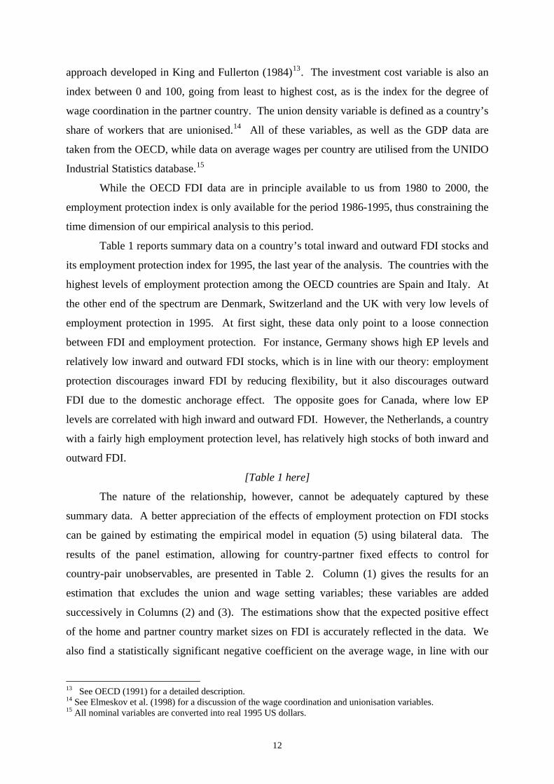
Table 1 reports summary data on a country’s total inward and outward FDI stocks and

its employment protection index for 1995, the last year of the analysis. The countries with the

highest levels of employment protection among the OECD countries are Spain and Italy. At

the other end of the spectrum are Denmark, Switzerland and the UK with very low levels of

employment protection in 1995. At first sight, these data only point to a loose connection

between FDI and employment protection. For instance, Germany shows high EP levels and

relatively low inward and outward FDI stocks, which is in line with our theory: employment

protection discourages inward FDI by reducing flexibility, but it also discourages outward

FDI due to the domestic anchorage effect. The opposite goes for Canada, where low EP

levels are correlated with high inward and outward FDI. However, the Netherlands, a country

with a fairly high employment protection level, has relatively high stocks of both inward and

outward FDI.

[Table 1 here]

The nature of the relationship, however, cannot be adequately captured by these

summary data. A better appreciation of the effects of employment protection on FDI stocks

can be gained by estimating the empirical model in equation (5) using bilateral data. The

results of the panel estimation, allowing for country-partner fixed effects to control for

country-pair unobservables, are presented in Table 2. Column (1) gives the results for an

estimation that excludes the union and wage setting variables; these variables are added

successively in Columns (2) and (3). The estimations show that the expected positive effect

of the home and partner country market sizes on FDI is accurately reflected in the data. We

also find a statistically significant negative coefficient on the average wage, in line with our

13 See OECD (1991) for a detailed description. 14 See Elmeskov et al. (1998) for a discussion of the wage coordination and unionisation variables. 15 All nominal variables are converted into real 1995 US dollars.

12

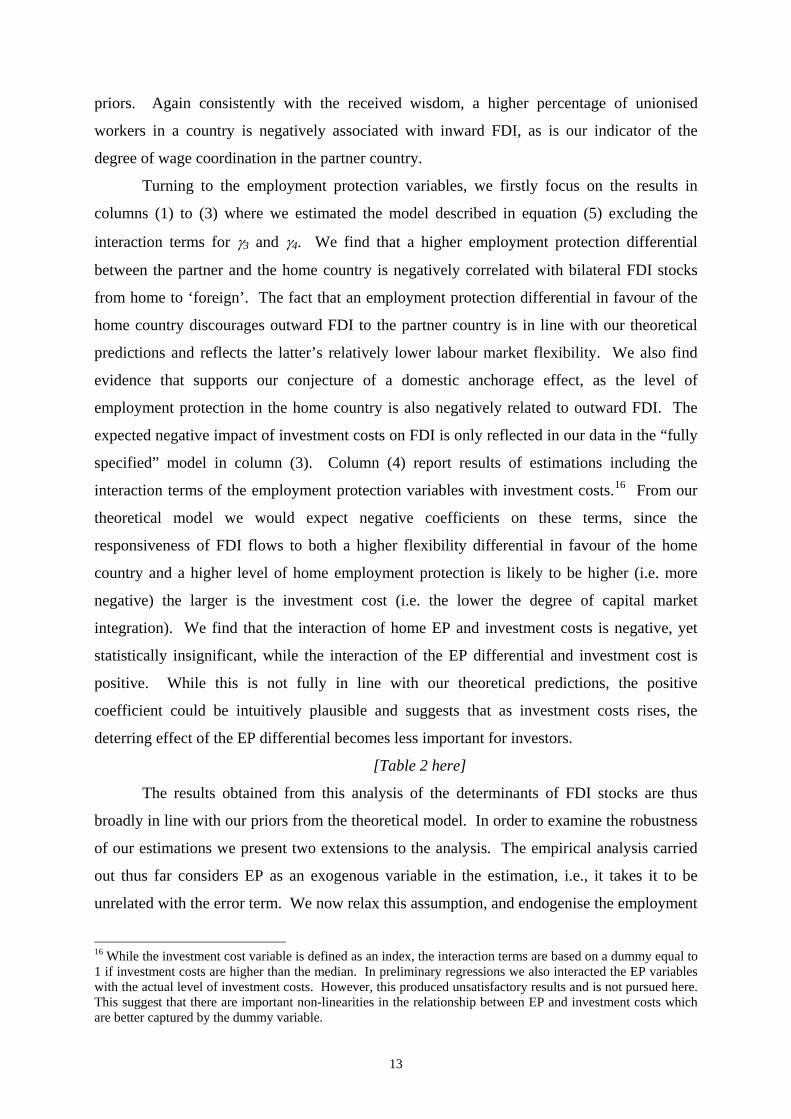
priors. Again consistently with the received wisdom, a higher percentage of unionised

workers in a country is negatively associated with inward FDI, as is our indicator of the

degree of wage coordination in the partner country.

Turning to the employment protection variables, we firstly focus on the results in

columns (1) to (3) where we estimated the model described in equation (5) excluding the

interaction terms for γ3 and γ4. We find that a higher employment protection differential

between the partner and the home country is negatively correlated with bilateral FDI stocks

from home to ‘foreign’. The fact that an employment protection differential in favour of the

home country discourages outward FDI to the partner country is in line with our theoretical

predictions and reflects the latter’s relatively lower labour market flexibility. We also find

evidence that supports our conjecture of a domestic anchorage effect, as the level of

employment protection in the home country is also negatively related to outward FDI. The

expected negative impact of investment costs on FDI is only reflected in our data in the “fully

specified” model in column (3). Column (4) report results of estimations including the

interaction terms of the employment protection variables with investment costs.16 From our

theoretical model we would expect negative coefficients on these terms, since the

responsiveness of FDI flows to both a higher flexibility differential in favour of the home

country and a higher level of home employment protection is likely to be higher (i.e. more

negative) the larger is the investment cost (i.e. the lower the degree of capital market

integration). We find that the interaction of home EP and investment costs is negative, yet

statistically insignificant, while the interaction of the EP differential and investment cost is

positive. While this is not fully in line with our theoretical predictions, the positive

coefficient could be intuitively plausible and suggests that as investment costs rises, the

deterring effect of the EP differential becomes less important for investors.

[Table 2 here]

The results obtained from this analysis of the determinants of FDI stocks are thus

broadly in line with our priors from the theoretical model. In order to examine the robustness

of our estimations we present two extensions to the analysis. The empirical analysis carried

out thus far considers EP as an exogenous variable in the estimation, i.e., it takes it to be

unrelated with the error term. We now relax this assumption, and endogenise the employment

16 While the investment cost variable is defined as an index, the interaction terms are based on a dummy equal to 1 if investment costs are higher than the median. In preliminary regressions we also interacted the EP variables with the actual level of investment costs. However, this produced unsatisfactory results and is not pursued here. This suggest that there are important non-linearities in the relationship between EP and investment costs which are better captured by the dummy variable.

13

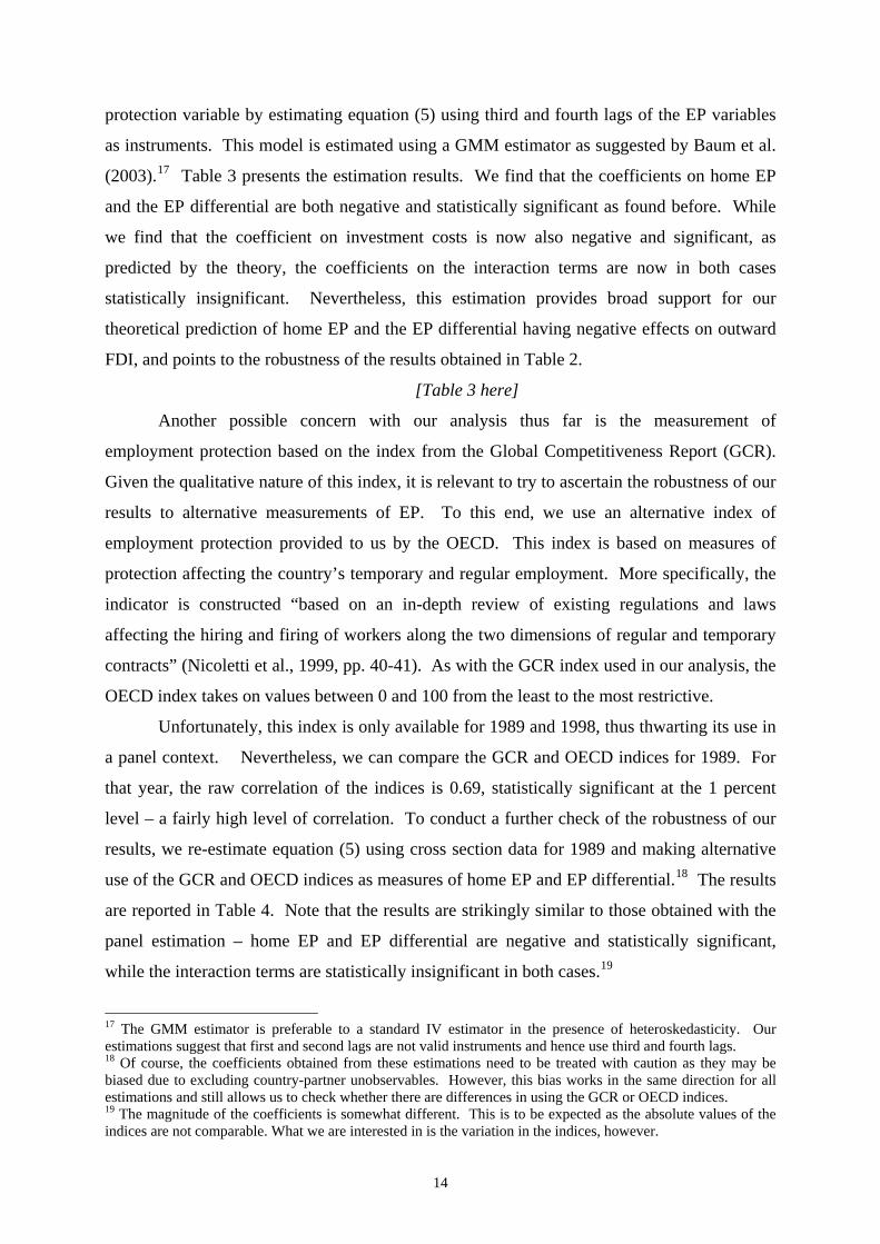
protection variable by estimating equation (5) using third and fourth lags of the EP variables

as instruments. This model is estimated using a GMM estimator as suggested by Baum et al.

(2003).17 Table 3 presents the estimation results. We find that the coefficients on home EP

and the EP differential are both negative and statistically significant as found before. While

we find that the coefficient on investment costs is now also negative and significant, as

predicted by the theory, the coefficients on the interaction terms are now in both cases

statistically insignificant. Nevertheless, this estimation provides broad support for our

theoretical prediction of home EP and the EP differential having negative effects on outward

FDI, and points to the robustness of the results obtained in Table 2.

[Table 3 here]

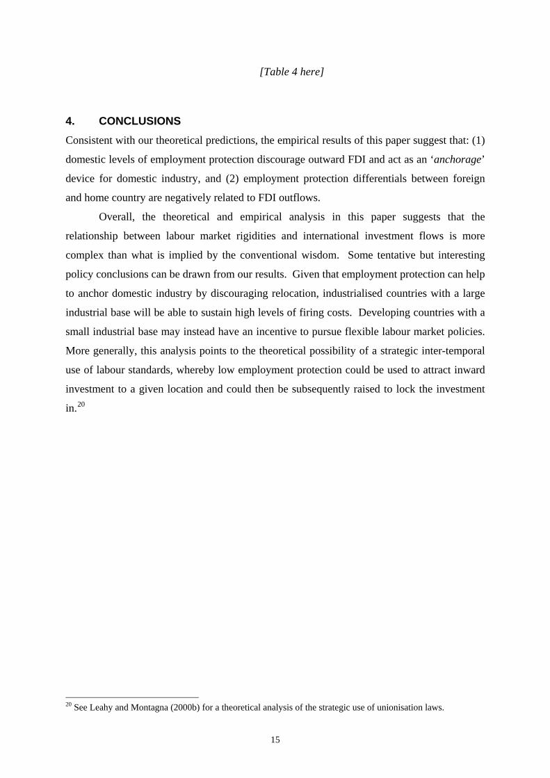
Another possible concern with our analysis thus far is the measurement of

employment protection based on the index from the Global Competitiveness Report (GCR).

Given the qualitative nature of this index, it is relevant to try to ascertain the robustness of our

results to alternative measurements of EP. To this end, we use an alternative index of

employment protection provided to us by the OECD. This index is based on measures of

protection affecting the country’s temporary and regular employment. More specifically, the

indicator is constructed “based on an in-depth review of existing regulations and laws

affecting the hiring and firing of workers along the two dimensions of regular and temporary

contracts” (Nicoletti et al., 1999, pp. 40-41). As with the GCR index used in our analysis, the

OECD index takes on values between 0 and 100 from the least to the most restrictive.

Unfortunately, this index is only available for 1989 and 1998, thus thwarting its use in

a panel context. Nevertheless, we can compare the GCR and OECD indices for 1989. For

that year, the raw correlation of the indices is 0.69, statistically significant at the 1 percent

level – a fairly high level of correlation. To conduct a further check of the robustness of our

results, we re-estimate equation (5) using cross section data for 1989 and making alternative

use of the GCR and OECD indices as measures of home EP and EP differential.18 The results

are reported in Table 4. Note that the results are strikingly similar to those obtained with the

panel estimation – home EP and EP differential are negative and statistically significant,

while the interaction terms are statistically insignificant in both cases.19

17 The GMM estimator is preferable to a standard IV estimator in the presence of heteroskedasticity. Our estimations suggest that first and second lags are not valid instruments and hence use third and fourth lags. 18 Of course, the coefficients obtained from these estimations need to be treated with caution as they may be biased due to excluding country-partner unobservables. However, this bias works in the same direction for all estimations and still allows us to check whether there are differences in using the GCR or OECD indices. 19 The magnitude of the coefficients is somewhat different. This is to be expected as the absolute values of the indices are not comparable. What we are interested in is the variation in the indices, however.

14

[Table 4 here]

4. CONCLUSIONS Consistent with our theoretical predictions, the empirical results of this paper suggest that: (1)

domestic levels of employment protection discourage outward FDI and act as an ‘anchorage’

device for domestic industry, and (2) employment protection differentials between foreign

and home country are negatively related to FDI outflows.

Overall, the theoretical and empirical analysis in this paper suggests that the

relationship between labour market rigidities and international investment flows is more

complex than what is implied by the conventional wisdom. Some tentative but interesting

policy conclusions can be drawn from our results. Given that employment protection can help

to anchor domestic industry by discouraging relocation, industrialised countries with a large

industrial base will be able to sustain high levels of firing costs. Developing countries with a

small industrial base may instead have an incentive to pursue flexible labour market policies.

More generally, this analysis points to the theoretical possibility of a strategic inter-temporal

use of labour standards, whereby low employment protection could be used to attract inward

investment to a given location and could then be subsequently raised to lock the investment

in.20

20 See Leahy and Montagna (2000b) for a theoretical analysis of the strategic use of unionisation laws.

15

References

Barrell, R., and N. Pain (1999). Trade restraints and Japanese direct investment inflows.

European Economic Review 43: 29-45.

Baum, C.F., M.E. Schaffer, and S. Stillman (2003). Instrumental variables and GMM:

Estimation and testing, Working Paper No. 545, Boston College.

Bentolilla S., and G. Bertola (1990). Firing Costs and Labour Demand: How Bad is

Eurosclerosis? Review of Economic Studies, 57: 381-402.

Blonigen, B. A. (1997). Firm-specific Assets and the Link between Exchange Rates and

Foreign Direct Investment. American Economic Review 87: 447-465.

Culem, C. G. (1988). The Locational Determinants of Direct Investments among

Industrialised Countries. European Economic Review 32: 885-904.

Dewit, G., D. Leahy, and C. Montagna (2003). Employment Protection and Globalisation in

Dynamic Oligopoly. CEPR Discussion Paper 3871.

Elmeskov, J., J. Martin, and S. Scarpetta (1998). Key lessons for labour market reforms:

Evidence from OECD countries’ experiences. Swedish Economic Policy Review 5: 205-

252.

Flamm, K. (1984). The volatility of offshore investment. Journal of Development Economics

16: 231-248.

Garibaldi, P., J. Konings, and C. Pissaridis (1997). Gross Job Reallocation and Labour Market

Policy, in D. Snower and G. de la Dehesa (eds.), Unemployment Policy: Government

Options for the Labour Market, Cambridge: Cambridge University Press.

Görg, H. (2005). Fancy a stay at the Hotel California? The role of easy entry and exit for FDI.

Kyklos 58: 519-536.

Haaland, J.I. and I. Wooton (2002). Multinational investment, industry risk and policy

competition. CEPR Discussion Paper 3152.

Haaland, J.I., I. Wooton and G. Faggio (2003). Multinational firms: Easy come, easy go?.

FinanzArchiv 59: 3-26.

Hamermesh, D. (1996). Labor Demand. Princeton: Princeton University Press.

16

Javorcik, B. S., and M. Spatareanu (2005). Do foreign investors care about labor market

regulations? Review of World Economics 141: 375-403.

King, M.A., and D. Fullerton (1984). The taxation of income from capital. Chicago:

University of Chicago Press.

Leahy, D. and C. Montagna (2000a). Unionisation, Rent Extraction and FDI: Challenging

Conventional Wisdom?. Economic Journal 100: 80-92.

Leahy, D. and C. Montagna (2000b). Temporary social dumping, union legalisation and FDI:

A note on the strategic use of standards. Journal of International Trade and Economic

Development 9: 243-259.

Markusen, J.R. (2002). Multinational firms and the theory of international trade. Cambridge,

MA: MIT Press.

Nickell, S. (1998). Unemployment, Questions and some Answers. Economic Journal 108:

802-816.

Nickell, S., L. Nunziata, and G. Quintini (2001). The Beveridge Curve, Unemployment and

Wages in the OECD from the 1960s to the 1990s. CEP Discussion Paper 502, London

School of Economics.

Nicoletti, G., S. Scarpetta, and O. Boylaud (1999). Summary indicators of product market

regulation with an extension to employment protection legislation. OECD Economics

Department Working Paper No. 226.

Nicoletti, G., S. Golub, D. Hajkova, D. Mirza and K-Y. Yoo (2003). Policies and international

integration: Influences on trade and foreign direct investment. OECD Economics

Department Working Paper No. 359.

OECD (1991). Taxing profits in a global economy. Paris: OECD.

Wheeler, D., and A. Mody (1992). International investment location decisions: The case of

U.S. firms. Journal of International Economics 33: 57-76.

17

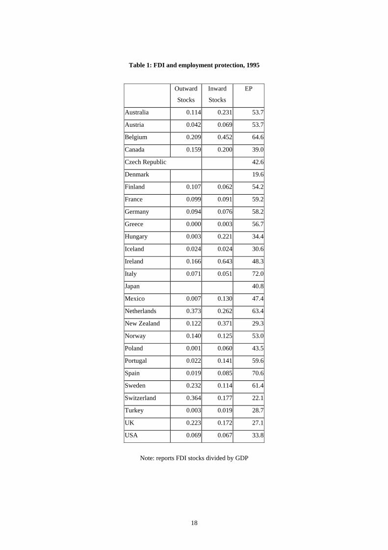
Table 1: FDI and employment protection, 1995

Outward

Stocks

Inward

Stocks

EP

Australia 0.114 0.231 53.7

Austria 0.042 0.069 53.7

Belgium 0.209 0.452 64.6

Canada 0.159 0.200 39.0

Czech Republic 42.6

Denmark 19.6

Finland 0.107 0.062 54.2

France 0.099 0.091 59.2

Germany 0.094 0.076 58.2

Greece 0.000 0.003 56.7

Hungary 0.003 0.221 34.4

Iceland 0.024 0.024 30.6

Ireland 0.166 0.643 48.3

Italy 0.071 0.051 72.0

Japan 40.8

Mexico 0.007 0.130 47.4

Netherlands 0.373 0.262 63.4

New Zealand 0.122 0.371 29.3

Norway 0.140 0.125 53.0

Poland 0.001 0.060 43.5

Portugal 0.022 0.141 59.6

Spain 0.019 0.085 70.6

Sweden 0.232 0.114 61.4

Switzerland 0.364 0.177 22.1

Turkey 0.003 0.019 28.7

UK 0.223 0.172 27.1

USA 0.069 0.067 33.8

Note: reports FDI stocks divided by GDP

18

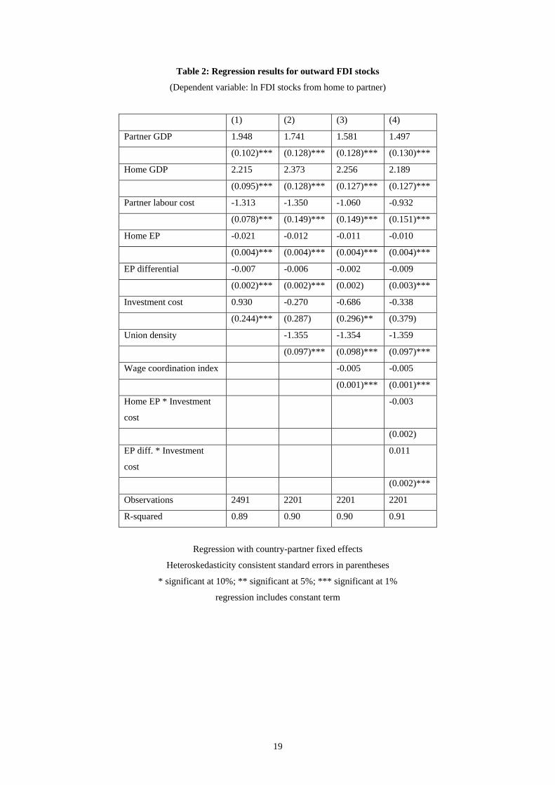
Table 2: Regression results for outward FDI stocks

(Dependent variable: ln FDI stocks from home to partner)

(1) (2) (3) (4)

Partner GDP 1.948 1.741 1.581 1.497

(0.102)*** (0.128)*** (0.128)*** (0.130)***

Home GDP 2.215 2.373 2.256 2.189

(0.095)*** (0.128)*** (0.127)*** (0.127)***

Partner labour cost -1.313 -1.350 -1.060 -0.932

(0.078)*** (0.149)*** (0.149)*** (0.151)***

Home EP -0.021 -0.012 -0.011 -0.010

(0.004)*** (0.004)*** (0.004)*** (0.004)***

EP differential -0.007 -0.006 -0.002 -0.009

(0.002)*** (0.002)*** (0.002) (0.003)***

Investment cost 0.930 -0.270 -0.686 -0.338

(0.244)*** (0.287) (0.296)** (0.379)

Union density -1.355 -1.354 -1.359

(0.097)*** (0.098)*** (0.097)***

Wage coordination index -0.005 -0.005

(0.001)*** (0.001)***

Home EP * Investment

cost

-0.003

(0.002)

EP diff. * Investment

cost

0.011

(0.002)***

Observations 2491 2201 2201 2201

R-squared 0.89 0.90 0.90 0.91

Regression with country-partner fixed effects

Heteroskedasticity consistent standard errors in parentheses

* significant at 10%; ** significant at 5%; *** significant at 1%

regression includes constant term

19

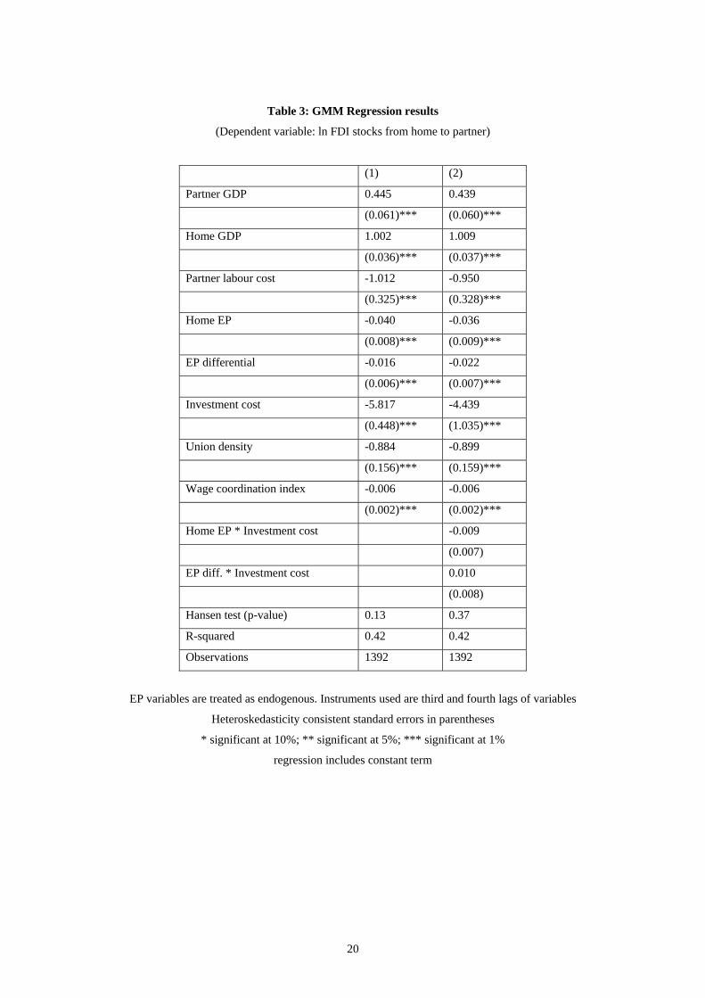
Table 3: GMM Regression results

(Dependent variable: ln FDI stocks from home to partner)

(1) (2)

Partner GDP 0.445 0.439

(0.061)*** (0.060)***

Home GDP 1.002 1.009

(0.036)*** (0.037)***

Partner labour cost -1.012 -0.950

(0.325)*** (0.328)***

Home EP -0.040 -0.036

(0.008)*** (0.009)***

EP differential -0.016 -0.022

(0.006)*** (0.007)***

Investment cost -5.817 -4.439

(0.448)*** (1.035)***

Union density -0.884 -0.899

(0.156)*** (0.159)***

Wage coordination index -0.006 -0.006

(0.002)*** (0.002)***

Home EP * Investment cost -0.009

(0.007)

EP diff. * Investment cost 0.010

(0.008)

Hansen test (p-value) 0.13 0.37

R-squared 0.42 0.42

Observations 1392 1392

EP variables are treated as endogenous. Instruments used are third and fourth lags of variables

Heteroskedasticity consistent standard errors in parentheses

* significant at 10%; ** significant at 5%; *** significant at 1%

regression includes constant term

20

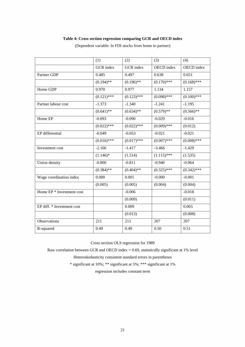
Table 4: Cross section regression comparing GCR and OECD index

(Dependent variable: ln FDI stocks from home to partner)

(1) (2) (3) (4)

GCR index GCR index OECD index OECD index

Partner GDP 0.485 0.497 0.638 0.651

(0.194)** (0.196)** (0.170)*** (0.168)***

Home GDP 0.970 0.977 1.134 1.157

(0.121)*** (0.123)*** (0.098)*** (0.100)***

Partner labour cost -1.373 -1.340 -1.241 -1.195

(0.641)** (0.634)** (0.579)** (0.566)**

Home EP -0.093 -0.090 -0.029 -0.016

(0.022)*** (0.022)*** (0.009)*** (0.012)

EP differential -0.049 -0.053 -0.021 -0.021

(0.016)*** (0.017)*** (0.007)*** (0.008)***

Investment cost -2.166 -1.417 -3.466 -1.429

(1.146)* (1.514) (1.115)*** (1.535)

Union density -0.800 -0.811 -0.940 -0.964

(0.384)** (0.404)** (0.325)*** (0.342)***

Wage coordination index 0.000 0.001 -0.000 -0.001

(0.005) (0.005) (0.004) (0.004)

Home EP * Investment cost -0.006 -0.018

(0.009) (0.011)

EP diff. * Investment cost 0.009 0.003

(0.013) (0.008)

Observations 211 211 207 207

R-squared 0.49 0.49 0.50 0.51

Cross section OLS regression for 1989

Raw correlation between GCR and OECD index = 0.69, statistically significant at 1% level

Heteroskedasticity consistent standard errors in parentheses

* significant at 10%; ** significant at 5%; *** significant at 1%

regression includes constant term

21

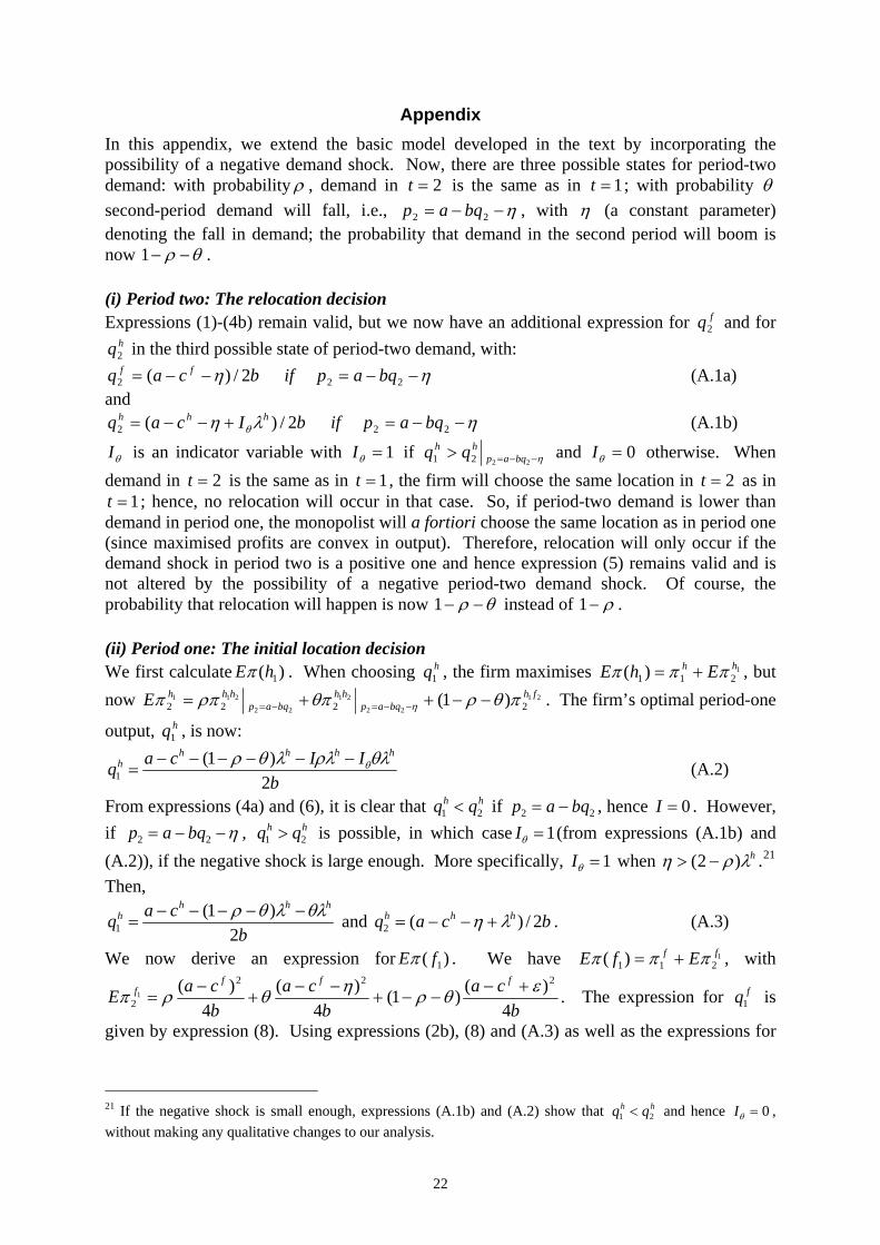
Appendix In this appendix, we extend the basic model developed in the text by incorporating the possibility of a negative demand shock. Now, there are three possible states for period-two demand: with probability ρ , demand in 2=t is the same as in 1=t ; with probability θ second-period demand will fall, i.e., η−−= 2bq2 ap , with η (a constant parameter) denoting the fall in demand; the probability that demand in the second period will boom is now θρ −−1 . (i) Period two: The relocation decision Expressions (1)-(4b) remain valid, but we now have an additional expression for and for

in the third possible state of period-two demand, with:

fq2hq2

ηη −−=−−= 222 2/)( bqapifbcaq ff (A.1a) and

ηλη θ −−=+−−= 222 2/)( bqapifbIcaq hhh (A.1b)

θI is an indicator variable with 1=θI if η−−=>2221 bqap

hh qq and 0=θI otherwise. When demand in is the same as in 2=t 1=t , the firm will choose the same location in as in

; hence, no relocation will occur in that case. So, if period-two demand is lower than demand in period one, the monopolist will a fortiori choose the same location as in period one (since maximised profits are convex in output). Therefore, relocation will only occur if the demand shock in period two is a positive one and hence expression (5) remains valid and is not altered by the possibility of a negative period-two demand shock. Of course, the probability that relocation will happen is now

2=t1=t

θρ −−1 instead of ρ−1 . (ii) Period one: The initial location decision We first calculate )( 1hEπ . When choosing , the firm maximises , but now

hq11

211 )( hh EhE πππ +=21

22

21

22

2112222 )1(+ fh

bqaphh

bqaphhhE πθρθπρππ η −−+= −−=−= . The firm’s optimal period-one

output, , is now: hq1

bIIcaq

hhhhh

2)1(

1θλρλλθρ θ−−−−−−

= (A.2)

From expressions (4a) and (6), it is clear that if hh qq 21 < 22 bqap −= , hence . However, if

0=Iη−−= 22 bqap , is possible, in which casehh qq 21 > 1=θI (from expressions (A.1b) and

(A.2)), if the negative shock is large enough. More specifically, 1=θI when .hλρ)2 −η (> 21 Then,

bcaq

hhhh

2)1(

1θλλθρ −−−−−

= and . (A.3) bcaq hhh 2/)(2 λη +−−=

We now derive an expression for )( 1fEπ . We have , with 1211)( ff EfE πππ +=

bca

bca

bcaE

ffff

4)()1 θρ −−(

4)(

4)( 222

21

εηθρπ +−+

−−+

−=

. The expression for is

given by expression (8). Using expressions (2b), (8) and (A.3) as well as the expressions for

fq1

hh qq 21 < 021 If the negative shock is small enough, expressions (A.1b) and (A.2) show that and hence =θI ,

without making any qualitative changes to our analysis.

22

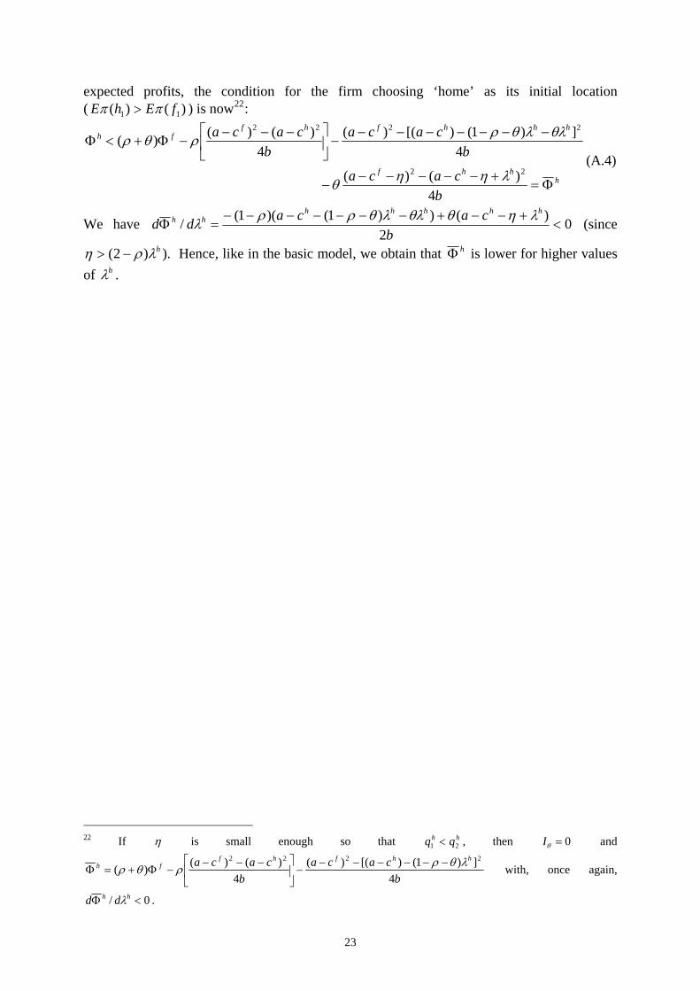
expected profits, the condition for the firm choosing ‘home’ as its initial location ( )()( 11 fEhE ππ > ) is now22:

hhhf

hhhfhffh −Φ+<Φ

)( θρ

bcaca

bcaca

bcaca

Φ=+−−−−−

−

−−−−−−−−⎥

⎦

⎤⎢⎣

⎡ −−−

4)()(

4])1()[()(

4)()(

22

2222

ληηθ

θλλθρρ(A.4)

We have 02

)())1()(1(/ <+−−+−−−−−−−

=Φb

cacaddhhhhh

hh ληθθλλθρρλ (since

). Hence, like in the basic model, we obtain that hλρη )2( −> hΦ is lower for higher values of . hλ

22 If η is small enough so that q , then and hh q21 < 0=θI

23

bcaca

bcaca hhfhf

fh

4])1()[()(

4)()()(

2222 λθρρθρ −−−−−−−⎥

⎦

⎤⎢⎣

⎡ −−−−Φ+=Φ with, once again,

0/ <Φ hh dd λ .