ship speed-power performance assessment

Ship Speed-Power Performance Assessment

Henk J.J. van den Boom1 (Membership; V), Thijs W.F. Hasselaar1 (Membership; V) 1MARIN, Trials & Monitoring department

The speed/power characteristics of ships have always been at the core of ship design. To prove contractually agreed values, speed trials are conducted by the yard prior to delivery of the ship to the owner. In the past schedule integrity of the vessel was often the most important factor for the speed requirement. Today, owners and operators are keen to reduce fuel consumption to decrease operational costs. So far a variety of methods for conducting and analyzing speed/power trials have been used by shipyards. With the assistance of the Sea Trial Analysis-Joint Industry Project, ITTC developed guidelines for the execution and analysis of speed/power trials compliant with IMO EEDI. The need to reduce fuel costs and exhaust gas emissions including the upcoming environmental regulations such as EEOI by IMO urge for reliable monitoring of ship performance in service conditions. This requires accurate information of the speed through water. Although the speed log is one of the oldest instruments on board it is not considered the most reliable one. Results of an extensive monitoring campaign on board a 1800 TEU container vessel equipped with six speed logs within SPA-JIP will be presented. The state of art of performance monitoring will be presented.

KEY WORDS: Delivery Trials; Speed Trials; Speed Through Water; Speed Log; Performance Monitoring; EEDI speed; STAIMO; Direct Power Method. NOMENCLATURE CFD Computational Fluid Dynamics EEDI Energy Efficiency Design Index EEOI Energy Efficiency Operational Index MCR Main engine’s Maximum Continuous Rating PI Performance Index RANS Reynolds Averaged Navier Stokes RPM Rotations Per Minute SOG Speed Over Ground SPA Service Performance Analysis STA-JIP Sea Trial Analysis – Joint Industry Project STW Speed Through Water INTRODUCTION As long as ships have been designed and build, their speed/power performance has been a dominant driver. Sailing vessels were subjected to races to compare their mutual speed in the given wind conditions or tried to set a new record time for ocean crossings. With the arrival of the steam turbine, new ships were subject to a speed trial over a selected stretch of water clearly marked over a distance of 1 nautical mile. Over this “measured mile” it was only required to clock the required time to derive the speed of the vessel. With the availability of GPS the need for pre-defined trial tracks has disappeared and speed/power trials are conducted worldwide. Although the speed-power relation is based on the speed through water, during trials use is made by the speed over ground which is accurately derived from the speed run end positions given by GPS. By conducting trial runs over reciprocal courses the speed through water can be derived by averaging the measured speed over ground of each run.

The relevance of speed/power trials is increasing in time. The ship yard is nowadays responsible for the design of the vessel including the model tests, engineering, construction, outfitting and delivery. Many ship owners leave the responsibility of the delivery trials including speed-power trials with the yard. This implies that the yard itself has to prove that the vessel meets the regulatory and contractual requirements on speed/power performance. It is evident that in this situation reliable, transparent and accurate procedures are required. As the conditions encountered during the trials often deviate from the contract conditions, corrections are applied during the analysis and reporting of the trial results. In the past, institutions such as British Ship Research Association (BSRA), Netherlands Ship Model Basin (NSMB), Society of Naval Architecture and Marine Engineers (SNAME) and International Towing Tank Conference (ITTC) published methods for conducting and analysis of Speed/Power trials. Ship yards “randomly” choose a method and developed their own ‘yard standard’. In 2002, The International Standard Organization published ISO 15016, describing a method to analyze speed trial data. The standard is however not specific; the user may select any added wind or wave resistance calculation method, and the method to reduce the added resistance from the measured shaft power gives room to own interpretation. As a result, when speed & power trials are done in rough conditions, correction methods can be selected such that on paper the ship performs better than it would do in reality in calm water. This has lead to several ship owners taken delivery of ships which were unable to meet their contract performance in service and burning significantly more fuel than anticipated. In some cases the ‘sea margin’ of 15% on power, was already consumed by the new ship in calm water.

This was reason for Shell, P&O-Nedlloyd and MARIN to initiate the Sea Trial Analysis-Joint Industry Project (STA-JIP) in 2004. STA aimed at a transparent, practical and reliable best practice for conducting and analyzing Speed & Power trials utilizing present day knowledge and methods for modern ships.

SNAME Maritime Convention 2014, October 2014 Houston, Texas 2

The Speed & Power trial analysis and reporting should be completed on board within one hour after completing the speed runs. Only in this way additional tests can be initiated when un-satisfactory results are obtained. Today, the delivery speed-power trials is not only relevant for the contractual agreements between yard and owner, but also for the Energy Efficiency Design Index (EEDI). The EEDI is calculated by the shaft power divided by the speed and displacement at full laden conditions and 75% MCR. An unambiguous way to measure, correct and calculate this speed and power is crucial to avoid conflicts between ship yard and owner and EEDI verifier when the calculated EEDI is close to the EEDI threshold for the ship under consideration. Over the last few years STA-Group closely worked together with the International Towing Tank Conference in the development of the ITTC Guidelines for Speed & Power Trials which have been approved by MEPC and accepted for EEDI. In the next section these new Guidelines are discussed in detail. The speed-power relation derived from the delivery trials are not only relevant for the new building contract and for EEDI, but are also a starting point for the performance monitoring of the vessel over its entire service life. The drivers for continuous monitoring of speed and power are obvious; high fuel costs, marginal freight rates and an increasing number of regulations to reduce exhaust gases and improve the regional air quality. The operational profile of a vessel can deviate substantially from the contractual conditions for which the vessel was designed due to slow steaming, fouling, draft deviations, weather etc. By optimizing the vessel for the actual trade, large gains in fuel performance can be obtained. Accurate measurement of the performance is however, far from straightforward. Unlike in speed trials, the speed through water of a trading vessel has to be derived over a single course using a speed log. Although one of the oldest instruments on board, the speed log is not considered as the most reliable one (Munk 2006; Babbedge 1976; Dinham-Peren & Dand 2010; Logan et al. 1980; Muntean 2011; Pedersen & Larsen 2009). Furthermore, the vessel conditions (draft, trim, marine growth) are continuously changing as well as the environmental conditions (wind, waves, shallow water). This normally results in a large spreading of speed/power data points. Therefore special filtering and analysis techniques as well as a better understanding of the accuracy of speed logs is required. In Section 3 these aspects a discussed in detail. SPEED/POWER TRIALS General Principles Speed/Power trials are conducted to establish the vessel speed at a defined shaft power at a specified draught and trim under so called “ideal conditions”: in deep water, no wind, no current and no waves. To establish the speed/power relationship the vessel

has to be in the specified draught and trim condition. By determining the speed and power at different engine power settings and correcting these for the non-ideal conditions, the speed-power relation for the ship in trial draught and trim can be established. The preparation and conduct of the speed/power trials is an important factor in the accuracy of the performance determination. The basic approach is to achieve steady conditions for which the current can be eliminated and the additional resistance caused by wind, waves, viscosity and density of the sea water and the water depth can be corrected for with reliable methods. As such correction methods are restricted in their application, limits as to the minimum water depth, wind speed, wave height and heading with respect to the waves have to be observed. A detailed description of the requirements can be found in (ITTC 2012a). The shaft power can be derived using a shaft torque and RPM meter. Shaft torque is defined as 𝑄 = 𝐺𝐽

𝐷∗ 4𝜖 Eq. 1

Where G is the shear modulus of the shaft, J the moment of inertia of the shaft, 𝜖 the relative strain of the strain gauge and D the diameter of the shaft. The largest uncertainty in the estimation of shaft power is the shear modulus (G-value), which relates the elastic deformation of the shaft in relation to the applied torque. It cannot be measured directly. Ledbetter investigated the variation in G-modulus on 20 random samples of steel 304. He concluded a 1% variation in G-modulus, and that the larger spread often found in literature is primarily introduced by measurement uncertainties in the estimation of G (Ledbetter et al. 1980; Ledbetter 1980). A reduction in uncertainty requires a measured value of G with an uncertainty estimate. It is assumed that the G-modulus of the shaft material is specified accurately based on sample tests. If the G-modulus is not specified with sample data, a conservative default value of 82,649 N/mm2 for regular shaft steel shall be applied. To derive the speed through water with an accuracy in the order of 0.05kn or better double runs must be executed, i.,e. each run is repeated by a run in the opposite direction, performed with the same engine setting. The speed is determined by calculating the distance from end positions of runs using a Differential GPS over a run duration of 10 minutes. This period is determined to calculate the speed over ground with the required accuracy and to encounter sufficient waves to match the sea spectrum measurements. By averaging the results over the counter runs the current is eliminated from the equation. The current normally varies in time and therefore multiple double runs for the same power setting are required. The results have to be averaged with the “Mean of Means”-method utilizing Pascal’s triangle. If the speed on each run is noted 𝑉1,𝑉2, . .𝑉𝑛 , the mean speed 𝑉𝑚 is found as follows: • For one double run: 𝑉𝑚 = 𝑉1+𝑉2

2

• For two double runs, executed directly after each other:

𝑉𝑚 = (𝑉1+3∙𝑉2+3∙𝑉3+𝑉4)8


This method of weighting assumes that the variations of current speed in time are linear (one double run) or quadratic (two double runs) (Kerwin & Hadler 2010). The following trial schedule is required for a first-of-series ship: • Two Double Runs at the same power setting around the

Contract Power • Two Double Runs at the same power setting around EEDI

Power (75% MCR) • One Double Run for at least one other power setting between

65% and 100% MCR In case of strong current variations (>0.3kn within one double run) or limiting wave conditions, an additional double run shall be conducted. Provided that the trial results of the first-of-series vessel are acceptable, for the second and following vessel from a series of sister ships (same dimensions, geometry, propulsor, delivered from the same yard), can be subjected to a limited trial program: • One Double Run at the same power setting around the

Contract Power • One Double Run at the same power setting around EEDI

Power (75% MCR) • One Double Run at one other power setting between 65% and

100% MCR As delivery trials cannot wait for ideal conditions the measured trial data has to be corrected for wind, waves, water viscosity and water depth. For this purpose the “Direct Power Method” is the most transparent and unambiguous procedure. In this method the added resistance encountered during the speed run is approximated and used to predict the additional power required to maintain the speed. All power deviations are subsequently summed including the power deviation due to a different loading of the propeller, obtained from load variation model tests. Per set of measurements for one engine setting, after power correction, the speed through water and average power is determined using the “mean of means” of the corrected speed and power points.

The measured delivered power is:

𝑃DM = 𝑃SM ∙ 𝜂s Eq. 2

PSM: Shaft power measured for each run ηS: Shaft transmission efficiency (0.99 for conventional shaft) The corrected delivered power is calculated as following:

𝑃DC = 𝑃DM − Δ𝑅∙𝑉SM𝜂D0

∙ �1 − 𝑃DM𝑃DC

∙ 𝜉𝑝� Eq. 3

Where ΔR: Resistance increase due to wind, waves and temperature

deviations. VSM: Ship speed measured, obtained from means of means from

double run

ηD0: Propulsion efficiency coefficient in ideal condition, from model test.

ξp: Constant derived from load variation model test. Which is solved iteratively with respect to 𝑃𝐷𝐶 For shallow water a speed correction is applied. Small deviations in displacement are corrected for according using the Admiralty constant (See (ITTC 2012b)). The propeller loading during the trials is also taken into account in the rate of rotation of the propeller shaft. The corrected shaft rate nC is:

𝑛C = 𝑛M𝜉𝑛∙

𝑃DM−𝑃DC𝑃DC

+𝜉𝑣∙Δ𝑉𝑉SM

+1 Eq. 4

Where nM: Measured propeller frequency of revolution, VSM: Measured ship speed, obtained by means of means from

double run 𝜉𝑛 , 𝜉𝑣: Overload factors derived from load variation model test Δ𝑉: Speed correction due to shallow water If load variation tests are not available, the overload factors ξp, ξn and ξv may be obtained from statistical values from sufficient load variation tests for this specific ship type, size and propulsor. If these cannot be provided, the overload factors may be derived by ITTC Procedure 7.5-02-03-01.4 (ITTC 2011). Wind Correction The wind drag on ships increases quadratic with the relative wind speed and can be calculated by: 𝑅𝐴𝐴 = 1

2𝜌𝐴𝐴𝑇𝐶𝑋(𝛿𝑊𝑅)𝑉𝑊𝑅

2 Eq. 5 Where AT: Area of maximum transverse section exposed to the wind CX: Wind resistance coefficient as function of the relative wind

direction 𝛿𝑊𝑅 VWR: Relative wind speed ρA: Mass density of air Wind load coefficients are usually normalized to the wind speed 10m above the water surface. As anemometers are often located higher from the water surface, the wind speed from the anemometer must be corrected for the boundary layer velocity profile of the ocean. When the anemometer is e.g. located 50m above water the correction to 10m reference height results in a reduction of 21% in wind speed consequently 46% in wind load. Wind speed read from the anemometer on top of the wheelhouse should be treated with care, as the wheelhouse normally generates over-speed at the anemometer location. For some directions the anemometer may be shielded by masts, funnels or cargo (Moat et al. 2004). To minimize these effects the wind


vector is averaged over the results of the two counter runs in one double run. Wind drag coefficients for ships have been published by many authors in the past (e.g. (Blendermann 1996; Fujiwara et al. 2005). Many databases are outdated due to the increase in vessel size and change in geometry. Careful selection of the wind drag coefficients for a geosimilar vessel as tested is therefore important. Wind drag coefficients for modern ship geometries can be obtained from wind tunnel measurements or Large eddy simulation-RANS CFD. For containerships it is crucial to distinguish the wind drag in ballast condition without containers on deck but taking into account the lashing bridges (which are exposed to wind during trials) and the design draught case where the vessel is loaded with containers. The wind resistance of the loaded vessel is normally lower than at ballast draught as the full container pack provides a better flow shape than the wheelhouse and lashing bridges. STA-JIP conducted CFD analysis for four modern ship types to correlate with wind tunnel data to arrive at a solid understanding of wind drag of ships and to establish new sets for wind drag correction alongside existing data sets.

Fig. 1: Modern ship types used to compute wind drag coefficients using RANS CFD for STA. Wave Correction Even within the trial limits for wave height, the added resistance due to waves can be a substantial part of the required shaft power. Model test results in regular and irregular head waves for some ten ships in full load and ballast and at different speeds, were compared by the STA-JIP group against the predictions by several published methods used in ISO15016 (ISO15016 2002) and widely used wave correction methods using the ship specific geometry and the measured wave spectra. The spread in the results and deviations from model tests were large, up to factor 10 (van den Boom et al. 2008). In order to make the speed trial analysis method more uniform and unambiguous it was decided by STA-JIP that a new and more reliable method for trial wave corrections was required. A method was developed that is practical in use with limited required input; many yards today refuse to deliver the body plan to the ship owner and the encountered wave spectrum is normally not measured.

The added resistance in waves originates from two sources; firstly the reflection of short waves on the hull and secondly the wave induced ship motions; i.e. heave and pitch. The first component is dominant in short waves; the second component contributes if the wave lengths are similar to the ship length. STA uses for this purpose two different added wave resistance methods; STAwave-1 for reflecting irregular head waves and STAwave-2 for head waves in which the vessel is pitching and heaving. STAwave-1 method is based on the fact that for today’s large ships the head waves encountered in trial conditions are normally short compared to ship length and speed. The added resistance due to the reflection of those short head waves is only dependent on the shape of the waterline in the bow region. The ship displacement, draught, trim and speed play a secondary role. The dominating reflection part in added resistance is a component of the second order wave (drift) forces which can be analytically found from integration over the waterline geometry (Pinkster 1981). For ship shapes in head waves this analytical expressing is for practical sake approximated to:

2116aw s

BWL

BR gH BL

ρ= Eq. 6

Where: 𝐵: Vessel beam on the waterline[m] 𝐿𝐵𝑊𝐿 : Length of bow section [m], as defined in Fig. 2 𝐻𝑆: Significant wave height [m]

Fig. 2: Definition of length of bow section The above expression is in particular practical for speed/power trials because very few input parameters are necessary. No other ship particulars such as parametric coefficients or bluntness factors nor ship speed or wave spectrum are required. It is assumed that the asymptotic short wave value of the transfer function extents over the complete range of wave frequencies and thus that the vessel is not heaving and pitching, which can easily be checked during trials. For small and medium sized vessels or in case long swells are encountered during the trials, the vessel will heave and pitch and those motions will contribute to the overall resistance. For this purpose STAwave-2 was developed. This is an empirical statistical method utilizing sea keeping model test results of some two hundred ships. The transfer function of the added resistance in head waves is parameterized to a function of seven input quantities resembling ship geometry, ship speed, and wave spectrum. A Pierson-Moskowitz spectrum shape is assumed in this method. Both significant wave height and mean period are


required as input for this wave correction method. A detailed description of the method is included in (ITTC 2012b). Both STAwave methods were validated with dedicated model tests for an Aframax tanker and an 2800TEU containership at scale 1:40 in the MARIN Seakeeping and Maneuvering Basin. Both STAwave-1 and STAwave-2 show an acceptable agreement with the model test results (Fig 3) and are far more reliable than the methods described in (ISO15016 2002). As reliable wave corrections can only be made for head waves (and the added resistance in following waves is negligible for normal trial conditions), it is required to conduct speed runs in head waves and following waves. For wave directions within the +/- 45 degrees bow sector, STAwave for head waves is applied.

Fig 3: Added resistance in irregular waves computed by STAwave 1 & 2 compared with results of large model tests for two vessels at different speeds, wave/ship lengths and loading conditions In any case the wave corrections can be conducted with the transfer functions of added resistance derived from full seakeeping tests. If use is made of model test results the wave spectrum encountered during the trials shall be measured. As none of the correction methods for waves are perfect, strict limits as to the allowable wave height have to be observed for speed/power trials. Especially in high sea states the relative error in the added wave resistance methods becomes large, and the run duration of 10 minutes too short to encounter statically sufficient waves over a single run. If wave heights are derived by visual observation the allowable wave height is further limited as the uncertainty in wave parameters is large in this case. Visual observation also require that the trials are conducted in daylight. Fig. 4 shows the limits for both methods (ITTC 2012a).

Fig. 4: Limits for wave height during Speed & Power trials Correction for Water Depth The ship speed/power relation is strongly affected by shallow water. The dominant parameters for the shallower effect are the draught/water depth ratio and the Froude number based on water depth. With the arrival of 400 m container ships capable of 24 knots even the range of moderate water depths 25- 50 m has to be considered shallow water, as the large displacement and high speed affects the ship’s resistance in these water depths. For this reason trials with such vessels in areas with such water depth e.g. offshore China, are corrected for water depth. Traditionally the method of Lackenby (Lackenby 1961) is used for this correction. Lackenby used the model tests conducted by Schlichting (Schlichting 1934). Recent research by Raven (Raven 1992) has shown that Lackenby is far too conservative and over predicts the effect of shallow water up to 100%. This is explained by the fact the model tests were conducted in a shallow water basin with limited tank width. These horizontal restrictions strongly affected the speed/power of the models in shallow water. Furthermore Schlichting only tested 3 old fashioned navy vessels. Lackenby’s method is therefore not only over-conservative but also not applicable to present day ship types. Although ITTC is still allowing the use of Lackenby, a new method has been developed and is currently under verification and validation by STA-Group. It is expected the method proposed by Raven will be approved and accepted in the ITTC Guidelines in the near future. Conversion from Ballast Draught to Design Draught Ship types such as container ships and dry cargo vessels cannot be trialled on their design draught and trim during delivery trials due to the lack of cargo. Results of speed trials have to be converted to the contractual design draught and trim conditions. This conversion is then based on the difference of calm water model test results for the trial condition and the design condition. This has proven to be one of the largest source of deviations and discrepancies in the results of delivery speed trials (Ligtelijn et al. 2004). Model test results are always extrapolated to full scale on the basis of scaling laws to which a ‘correlation allowances’ (CA) is

0

50

100

150

200

250

11kn 11kn 15kn 15kn 11kn 11kn 11kn 11kn 17kn 17kn 23kn 23kn 17kn 17kn 23kn 23kn

2.78 1.93 2.65 2.1 2.67 2.06 2.81 2.28 3.53 2.62 3.31 2.61 3.36 2.5 3.17 2.42

ballast loaded ballast loaded

tanker Container Ship

Add

ed W

ave

Resi

stan

ce [k

N]

Stawave-1Model TestStawave-2

Vs =

λ/Lpp =

0.0

0.5

1.0

1.5

2.0

2.5

3.0

3.5

4.0

4.5

5.0

0 100 200 300 400 500

Hs l

imit

Lpp [m]

Limit with measured wave spectrum

Limit with observed Wave Height & Period


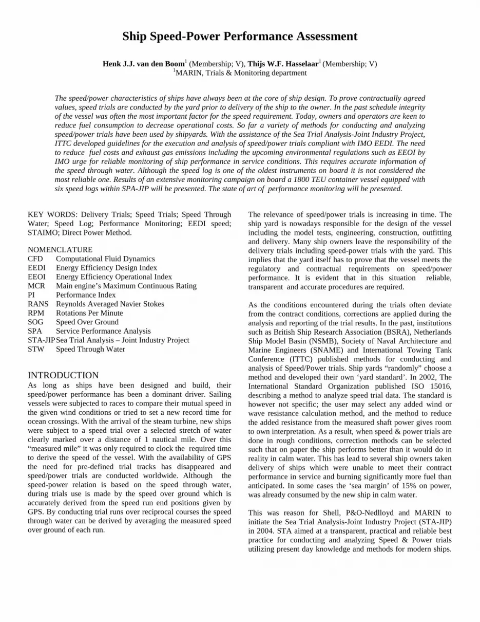
added. These statistical correlation allowances relate the scaled-up model test power with the actual power derived at the actual speed/power trials with that vessel. For a model basin with a sufficient large trial data base for the specific ship type and size, this practice has proven over the years to deliver power predictions with acceptable accuracy. The model test prediction accuracy is thus dependent on the experience of the model basin i.e. the availability of accurate Speed & Power trial data. For several ship types, trial data at design draught is scarce. In particular for relative new ship types, modern speeds and recent sizes such data is often missing. The STA-JIP conducted dedicated Speed & Power trials on, amongst others, three container vessels in the range of 6000 to 14000 TEU at design draught/trim and compared those data with the results of the original delivery trials (Fig. 5) which were also measured and analysed according to STA. For two vessels deviations above 10% in shaft power were found. At a fuel consumption of 240 tons/day this means an excess fuel consumption of 24 tons/day over the life time of the vessel. For this reason STA-JIP has formulated strict guidelines for this ballast draught-design draught conversion of Speed & Power trial results as well as for the extrapolation of model test results towards full scale. Such guidelines were completely lacking in all previous Speed & Power Trial methods.

Fig. 5: 14000 TEU MSC Savona subjected by STA-Group to speed/power trials in both ballast draught and design draught (Courtesy: Claus Peter Offen). STAIMO-Software As part of the co-operation with ITTC to develop the Guidelines for Speed & Power trials, the STA-Group also implemented these Guidelines in a software package called STAIMO. This software not only provides a full analysis of the measured data but also produces the trial report. To avoid a proliferation of different software versions of the ITTC analysis method, STAIMO is released by STA-Group as freeware. It can be downloaded from www.staimo.org. Each STAIMO produced report has a unique number allowing an authenticity check to be made via the website.

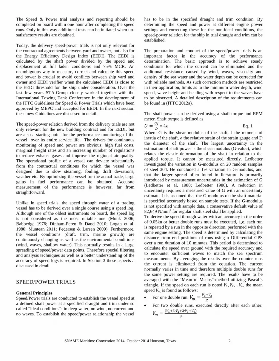
Fig. 6 shows a basic flow diagram of the analysis steps as used in STAIMO.

Fig. 6: Flow diagram of calculation steps in STAIMO software The STA-Group presently consists of 38 members and continues to support STAIMO and to conduct further R&D in this field. PERFORMANCE IN SERVICE The need to reduce fuel costs and exhaust gas emissions including the upcoming EEOI regulations by IMO urge for reliable monitoring of ship performance in service conditions. Telfer was one of the first to discuss the issue in 1926 and introduced a method to measure ship speed from a simple measure of propeller rate of rotation and power (Telfer 1926). Since then, many researchers have investigated ways to accurately monitor the performance of a ship in service. The problems introduced with manual data logging (data uncertainty, reliability, limited data points per day and incomplete datasets), can mostly be overcome with modern technology. This does however not directly result in unambiguous, reliable and accurate performance indicators. The highly unsteady marine environment and constantly varying ship performance makes the definition of the performance of a ship in service a challenging task. Ship performance analysis should therefore not only focus on the correction methods to transfer in-service performance data to conditions which can be compared, but also on the quality and reliability of input parameters such as, ship speed, wind speed and wave height. Many references can be found in technical literature describing approaches to ship performance analysis. Detailed theoretical foundations can be found in (SNAME 1989; Carlton 1994) as well as numerous technical papers. The purpose of this section is therefore not to discuss another analysis approach in detail, but focuses on the quality of data that forms the basis for performance monitoring. Speed Through Water Measurement Ship performance monitoring relies on an accurate speed through water measurement. While during delivery speed trials

Added resistance calculation

Correction of power using Direct Power

Method

Extrapolation to reference

conditions (e.g. full laden draft)

Inputdata

Calculation of mean speed &

power

Report

wind distortion correction

http://www.staimo.org/


counter runs can be executed to account for ocean currents, for a ship in service this is not possible. As a consequence other means to determine speed through water (STW), such as the speed log must be used. When the signal from the speed log is related to shaft power, it is assumed that the propeller inflow speed, and therefore absorbed power, is directly related to the speed through water measured by the speed log in the bow of the ship. The propeller inflow speed varies as a consequence of, hull roughness, drift, rudder action etc. The speed log, installed in the bow of the ship, is furthermore affected by eddies, stratified currents, ship motion, changes in boundary layer due to trim etc. The relationship between propeller inflow velocity and the velocity measured by a speed log is therefore not constant. Speed logs have therefore become notorious for their seemingly large uncertainty, regardless their high instrumentation accuracy, mandated by IMO to be better than 2% of the measured speed (IMO 1995). To overcome the problems experienced with a speed log many researchers have proposed the use of the propeller as a speed indicator. Propeller as a speed indicator Using a torque and RPM sensor the propeller can be used to determine ship speed. Telfer (Telfer 1926) was probably one of the first to introduce this method in 1926 which can be described as following: 1. Measure the propeller absorbed shaft torque and revolutions 2. Calculate the torque coefficient KQ and intersect KQ-J curve

from the propeller open water diagram (obtained either from dedicated trials (Garg 1972) or from model tests)

3. Read the corresponding advance coefficient J and consequently the flow experienced by the propeller (often referred to as ‘advance speed’)

4. Using an assumed wake fraction, the advance speed can be converted in a measure of the ship speed through water, expressed in this paper as Vprop.

The methods relies on the availability of a known and constant wake fraction. For ships sailing at two distinct loading conditions the wake can be determined by comparing the advance speed determined from 𝐽 = 𝑉𝑎

𝑁𝐷 with the speed VS

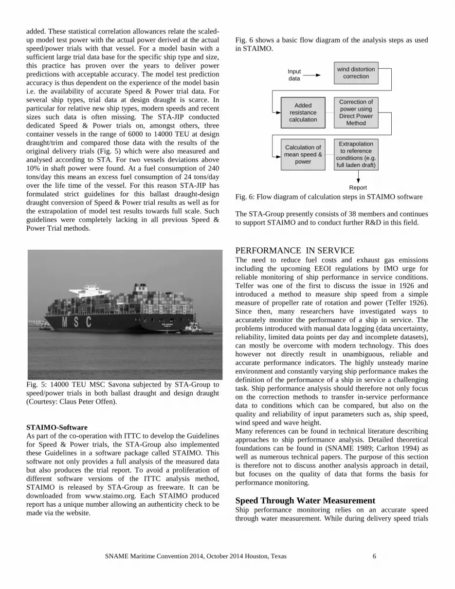
measured by the speed log. The relative difference between Va and VS relates to the wake fraction. Small changes in draft and trim may however have large effects on the wake, depending on hull shape. More importantly, the wake fraction increases as the ship’s hull roughens and fouls, and propeller characteristics change as the propeller roughness increases. The rate of increase in wake cannot be predicted and should be monitored over time to account for changes. The monitoring can be done in two ways: 1. Using the speed over ground and assuming that the

difference between speed through water and speed over ground can be averaged over time. This assumption is however dependent on trading route and requires a large dataset to identify trends. Fig. 7 shows the difference between SOG and STW for a container ship trading between Africa and Asia. The typically large scatter makes

trend identification difficult, particularly as seasonal weather conditions affect the surface current and variations in loading conditions affect the wake fraction

Fig. 7: Relative difference between propeller speed and speed over ground over a period of 1 year

2. Using the speed log by periodically ‘measuring’ the

effective wake fraction directly; the difference between Vprop and STW from a speed log relates to changes in the effective wake.

Apart from the wake fraction, the change in propeller characteristics due to roughness also affect the estimated STW. Propeller roughness reduces propeller efficiency. As a consequence Vprop will indicate a lower ship speed than is indicated on the speed log. This expresses in an overestimation of the power loss of the ship. Methods are available to account for changes in propeller roughness (e.g. (Wan et al. 2003; Townsin et al. 1985)) but this requires periodical propeller inspections and introduces large uncertainties. Water speed log A more direct way to determine ship speed, especially for ships sailing on different loading conditions, is to use the speed log. Speed logs give a more accurate figure of the actual speed through water experienced by the hull, and those that measure outside the boundary layer of the hull are in principle unaffected by hull fouling and draft or trim variations. Doppler speed logs measure outside the boundary layer, while most types of Electro Magnetic (EM) or Acoustic Correlation (AC) logs measure close to the hull and are affected by trim, draft and hull roughness. They are for this reason less suitable for long-time performance monitoring. To assess the accuracy of speed logs under various conditions an extensive monitoring campaign was setup in 2009 to investigate the uncertainties in speed through water measurements as part of a large joint industry project SPA-TOO. An 1800TEU container ship of VROON shipping was equipped with 6 speed logs, distributed along the hull (Fig. 8) and monitored using a dedicated performance monitoring system.

0.7

0.8

0.9

1

1.1

1.2

1.3

Jan-11 Feb-11 Apr-11 Jun-11 Jul-11 Sep-11 Nov-11 Dec-11

Vpro

p /

SOG

[-]

Date


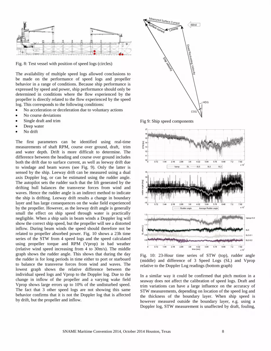
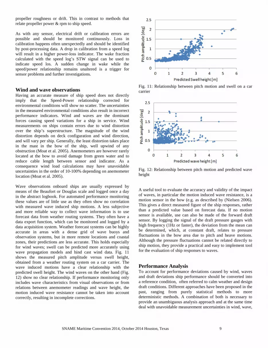
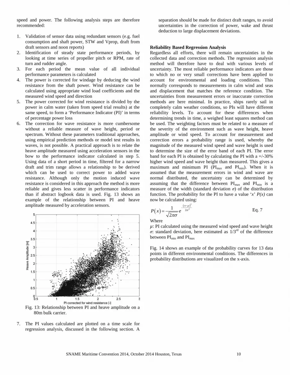
Fig. 8: Test vessel with position of speed logs (circles) The availability of multiple speed logs allowed conclusions to be made on the performance of speed logs and propeller behavior in a range of conditions. Because ship performance is expressed by speed and power, ship performance should only be determined in conditions where the flow experienced by the propeller is directly related to the flow experienced by the speed log. This corresponds to the following conditions: • No acceleration or deceleration due to voluntary actions • No course deviations • Single draft and trim • Deep water • No drift The first parameters can be identified using real-time measurements of shaft RPM, course over ground, draft, trim and water depth. Drift is more difficult to determine. The difference between the heading and course over ground includes both the drift due to surface current, as well as leeway drift due to windage and beam waves (see Fig. 9). Only the latter is sensed by the ship. Leeway drift can be measured using a dual axis Doppler log, or can be estimated using the rudder angle. The autopilot sets the rudder such that the lift generated by the drifting hull balances the transverse forces from wind and waves. Hence the rudder angle is an indirect method to indicate the ship is drifting. Leeway drift results a change in boundary layer and has large consequences on the wake field experienced by the propeller. However, as the leeway drift angle is generally small the effect on ship speed through water is practically negligible. When a ship sails in beam winds a Doppler log will show the correct ship speed, but the propeller will see a distorted inflow. During beam winds the speed should therefore not be related to propeller absorbed power. Fig. 10 shows a 23h time series of the STW from 4 speed logs and the speed calculated using propeller torque and RPM (Vprop) in bad weather (relative wind speed increasing from 4 to 30m/s). The middle graph shows the rudder angle. This shows that during the day the rudder is for long periods in time either to port or starboard to balance the transverse forces from wind and waves. The lowest graph shows the relative difference between the individual speed logs and Vprop to the Doppler log. Due to the change in inflow of the propeller and a varying wake field Vprop shows large errors up to 10% of the undisturbed speed. The fact that 3 other speed logs are not showing this same behavior confirms that it is not the Doppler log that is affected by drift, but the propeller and inflow.

Fig 9: Ship speed components

Fig. 10: 23-Hour time series of STW (top), rudder angle (middle) and difference of 3 Speed Logs (SL) and Vprop relative to the Doppler Log readings (bottom graph) In a similar way it could be confirmed that pitch motion in a seaway does not affect the calibration of speed logs. Draft and trim variations can have a large influence on the accuracy of STW measurements, depending on location of the speed log and the thickness of the boundary layer. When ship speed is however measured outside the boundary layer, e.g. using a Doppler log, STW measurement is unaffected by draft, fouling,


propeller roughness or drift. This in contrast to methods that relate propeller power & rpm to ship speed. As with any sensor, electrical drift or calibration errors are possible and should be monitored continuously. Loss in calibration happens often unexpectedly and should be identified by post-processing data. A drop in calibration from a speed log will result in a higher power-loss indicator. The wake fraction calculated with the speed log’s STW signal can be used to indicate speed los. A sudden change in wake while the speed/power relationship remains unaltered is a trigger for sensor problems and further investigations. Wind and wave observations Having an accurate measure of ship speed does not directly imply that the Speed-Power relationship corrected for environmental conditions will show no scatter. The uncertainties in the measured environmental conditions also result in incorrect performance indicators. Wind and waves are the dominant forces causing speed variations for a ship in service. Wind measurements on ships contain errors due to wind distortion over the ship’s superstructure. The magnitude of the wind distortion depends on deck configuration and wind direction, and will vary per ship. Generally, the least distortion takes place in the mast in the bow of the ship, well upwind of any obstruction (Moat et al. 2005). Anemometers are however rarely located at the bow to avoid damage from green water and to reduce cable length between sensor and indicator. As a consequence wind load calculations may have unavoidable uncertainties in the order of 10-100% depending on anemometer location (Moat et al. 2005). Wave observations onboard ships are usually expressed by means of the Beaufort or Douglas scale and logged once a day in the abstract logbook. For automated performance monitoring these values are of little use as they often show no correlation with measured wave induced ship motions. A less subjective and more reliable way to collect wave information is to use forecast data from weather routing systems. They often have a data export function, which can be monitored and logged by a data acquisition system. Weather forecast systems can be highly accurate in areas with a dense grid of wave buoys and observation systems, but in more remote locations and coastal zones, their predictions are less accurate. This holds especially for wind waves; swell can be predicted more accurately using wave propagation models and hind cast wind data. Fig. 11 shows the measured pitch amplitude versus swell height, obtained from a weather routing system on a car carrier. The wave induced motions have a clear relationship with the predicted swell height. The wind waves on the other hand (Fig. 12) show no clear relationship. If performance monitoring only includes wave characteristics from visual observations or from relations between anemometer readings and wave height, the motion induced wave resistance cannot be taken into account correctly, resulting in incomplete corrections.

Fig. 11: Relationship between pitch motion and swell on a car carrier

Fig. 12: Relationship between pitch motion and predicted wave height A useful tool to evaluate the accuracy and validity of the impact of waves, in particular the motion induced wave resistance, is a motion sensor in the bow (e.g. as described by (Nielsen 2006). This gives a direct measured figure of the ship responses, rather than a predicted value based on forecast data. If no motion sensor is available, use can also be made of the forward draft sensor. By logging the signal of the draft pressure gauges with high frequency (1Hz or faster), the deviation from the mean can be determined, which, at constant draft, relates to pressure fluctuations in the bow area due to pitch and heave motions. Although the pressure fluctuations cannot be related directly to ship motion, they provide a practical and easy to implement tool for the evaluation of ship responses to waves. Performance Analysis To account for performance deviations caused by wind, waves and draft deviations ship performance should be converted into a reference condition, often referred to calm weather and design draft conditions. Different approaches have been proposed in the past, ranging from purely statistical methods to more deterministic methods. A combination of both is necessary to provide an unambiguous analysis approach and at the same time deal with unavoidable measurement uncertainties in wind, wave,


speed and power. The following analysis steps are therefore recommended: 1. Validation of sensor data using redundant sensors (e.g. fuel

consumption and shaft power, STW and Vprop, draft from draft sensors and noon reports)

2. Identification of steady state performance periods, by looking at time series of propeller pitch or RPM, rate of turn and rudder angle.

3. For each period the mean value of all individual performance parameters is calculated

4. The power is corrected for windage by deducing the wind resistance from the shaft power. Wind resistance can be calculated using appropriate wind load coefficients and the measured wind speed and direction

5. The power corrected for wind resistance is divided by the power in calm water (taken from speed trial results) at the same speed, to form a ‘Performance Indicator (PI)’ in terms of percentage power loss

6. The correction for wave resistance is more cumbersome without a reliable measure of wave height, period or spectrum. Without these parameters traditional approaches, using empirical prediction methods or model test results in waves, is not possible. A practical approach is to relate the heave amplitude measured using acceleration sensors in the bow to the performance indicator calculated in step 5. Using data of a short period in time, filtered for a narrow draft and trim range allows a relationship to be derived which can be used to correct power to added wave resistance. Although only the motion induced wave resistance is considered in this approach the method is more reliable and gives less scatter in performance indicators than if abstract logbook data is used. Fig. 13 shows an example of the relationship between PI and heave amplitude measured by acceleration sensors.

Fig. 13: Relationship between PI and heave amplitude on a

80m bulk carrier.

7. The PI values calculated are plotted on a time scale for regression analysis, discussed in the following section. A

separation should be made for distinct draft ranges, to avoid uncertainties in the correction of power, wake and thrust deduction to large displacement deviations.

Reliability Based Regression Analysis Regardless all efforts, there will remain uncertainties in the collected data and correction methods. The regression analysis method will therefore have to deal with various levels of uncertainty. The most reliable performance indicators are those to which no or very small corrections have been applied to account for environmental and loading conditions. This normally corresponds to measurements in calm wind and seas and displacement that matches the reference condition. The uncertainties from measurement errors or inaccurate correction methods are here minimal. In practice, ships rarely sail in completely calm weather conditions, so PIs will have different reliability levels. To account for these differences when determining trends in time, a weighed least squares method can be used. The weighting factors must be related to a measure of the severity of the environment such as wave height, heave amplitude or wind speed. To account for measurement and correction errors a probability range is used, whereby the magnitude of the measured wind speed and wave height is used to determine the size of the error band of each PI. The error band for each PI is obtained by calculating the PI with a +/-30% higher wind speed and wave height than measured. This gives a maximum and minimum PI (PImax and PImin). When it is assumed that the measurement errors in wind and wave are normal distributed, the uncertainty can be determined by assuming that the difference between PImax and PImin is a measure of the width (standard deviation σ) of the distribution function. The probability for the PI to have a value ‘x’ P(x) can now be calculated using:

( )( )2

2212

x

P x eµσ

πσ

−−

= Eq. 7

Where µ: PI calculated using the measured wind speed and wave height σ: standard deviation, here estimated as 1/3rd of the difference between PImin and PImax Fig. 14 shows an example of the probability curves for 13 data points in different environmental conditions. The differences in probability distributions are visualized on the x-axis.


Fig.14: Performance Index values with different probability ranges Using the probability distributions, the mean PI can be found that results in the highest combined probability for all data points. The size of the bandwidth of the error bands, in this case selected as 30% of the measured wind and wave height, is hereby not crucial as the probability distribution remains unaltered. This way of regression analysis provides more reliable trend lines by giving more weight to ‘good weather’ data, without the need for extensive filtering, which may result in too few data points for reliable regression analysis. Typically the number of data points is not distributed evenly over time; days in port result in no data points, while days sailing in fair weather result in many valid data points. To avoid ill-defined trend analysis, the weighted least squares PI described above should be calculated over a period of one month. Trend analysis should be performed over the monthly averages. This avoids that days with few data points get less weight in the identification of trends over time as months with many data points. Fig. 15 shows an example of corrected performance indicators (light blue points) and the monthly weighted average data points.

Fig.15: Time series of PI and weighted monthly mean

Interpretation of Performance Indicators The probability based regression analysis provides a way to interpret scatter in the PI ‘Power Loss’ after it has been corrected to environmental conditions to best knowledge and data quality and divided in draft ranges. One final check is however necessary to validate long-term trends in the PI. The effective wake fraction and PI should show similar trends when fouling or hull roughness develops when analysed over time. The wake is less affected by environmental conditions than the PI ‘Power loss’, and cross-correlation provides therefore a quick way to evaluate the effectiveness of the probability based regression analysis. The separate analysis of different draft and trim conditions (which have a unique wake fraction, thrust deduction and reference curve) is hereby important. CONCLUSIONS The ITTC Guidelines for Speed/Power Trials 2014 have set a new international standard for the conduct and analysis of speed trials. With this standard a worldwide level playing field has been achieved. The EEDI is a starting point in the reduction of CO2 exhaust by ships. Regional measures to improve the air quality as well as the rising fuel costs, urge ship owners and operators to improve the performance of their ships. For this purpose continuous monitoring of performance data is essential. Speed through water from a speed log and power can accurately be related under no-drift conditions using a Doppler log, providing a more reliable speed indicator than STW estimations from propeller characteristics. Performance analysis follows by defining periods of steady state performance, and applying deterministic and statistic methods to deal with variations in environmental conditions and uncertainties in measured ship performance.

Bad weather, large uncertainty

Good weather, low uncertainty


REFERENCES Babbedge, M.P., 1976. A statistical method of correcting log

speeds. Trans. RINA 1977, pp.pp.121–124. Blendermann, W., 1996. Wind loading of ships - Collected data

from wind tunnel tests in uniform flow, Institut fur schiffbau der universitat Hamburg.

Van den Boom, H.J.J., Hout, I.E. Van Der & Flikkema, M.B., 2008. Speed-Power Performance of Ships during Trials and in Service. In SNAME ship performance conference.

Carlton, J.S., 1994. Marine propellers and Propulsion, Butterworth Heinemann.

Dinham-Peren, T.A. & Dand, I.W., 2010. The need for full scale measurements. In William Froude Conference; Advances in Theoretical and Applied Hydrodynamics. Portsmouth, UK.

Fujiwara, T., Ueno, M. & Ikeda, Y., 2005. A new Estimation Method of Wind Forces and Moments acting on Ships on the basis of Physical Component Models. Journal of the Japan Society of Naval Architects and Ocean Engineers, 2.

Garg, B.R., 1972. The service performance of ships with special reference to tankers. Newcastle upon Tyne: Newcastle University.

IMO, 1995. Resolution A.824(10) Performance standards for devices to indicate speed and distance,

ISO15016, 2002. Ships and marine technology - Guidelines for the assessment of speed and power performance by analysis of speed trial data.

ITTC, 2011. 1978 ITTC Performance Prediction Method, Available at: http://ittc.sname.org/CD 2011/pdf Procedures 2011/7.5-02-03-01.4.pdf.

ITTC, 2012a. Recommended procedures and Guidelines - Speed and power trials Part 1: Preparation and Conduct,

ITTC, 2012b. Recommended procedures and guidelines - Speed and Power Trials, Part 2: Analysis of Speed/Power Trial data, ITTC.

Kerwin, J.E. & Hadler, J.., 2010. The Principles of Naval Architectuer Series: propulsion J. R. Paulling, ed., SNAME.

Lackenby, H., 1961. Note on the effect of shallow water on ship resistance, London: British shipbuilding research association BSRA.

Ledbetter, H.M., 1980. Sound velocities and elastic constants of steels 304, 310, and 316. Journal of Material Science and Technology, 14(12), pp.595–596.

Ledbetter, H.M., Frederick, N.V. & Austin, M.W., 1980. Elastic-constant variability in stainless steel 304. J. Appl. Physics, 51, pp.305–309.

Ligtelijn, J.T., Wijngaarden, H.C.J. van & Verkuyl, J.B., 2004. Correlation of cavitation; comparison of full-scale data with results of model tests and computations. In SNAME annual meeting. Washington D.C. USA.

Logan, K.P., Reid, R.E. & Williams, V.E., 1980. Considerations in establishing a speed performance monitoring system for merchant ships - Part 1. Techniques based on propeller relationships - Part 2. In New York city: SNAME, pp. pp93–135.

Moat, B.I. et al., 2005. The effect of ship shape and anemometer location on wind speed measurements obtained from ships. In 4th International Conference on Marine Computational Fluid Dynamics. University of Southampton, UK, pp. 133–139.

Moat, B.I., Yelland, M.J. & Molland, A.F., 2004. Possible biases in wind speed measurements from merchant ships. In 5th International Colloquium on Bluff Body Aerodynamics and Applications. Ottawa, Canada, pp. 537–540.

Munk, T., 2006. Evaluating Hull coatings for precise impact on vessel performance. In Florida USA.

Muntean, T., 2011. Propeller efficiency at full scale - Measurement system and mathematical model design. Eindhoven University.

Nielsen, U.D., 2006. Estimations of on-site directional wave spectra from measured ship responses. Marine Structures, 19, pp.33–69.

Pedersen, B.P. & Larsen, J., 2009. Modeling of Ship Propulsion Performance. In World Maritime Technology Conference WMTC2009. Mumbai, India: The Institute of Marine Engineers.

Pinkster, J.A., 1981. Second Order Wave Drift Forces. Delft University, the Netherlands.

Raven, H.C., 1992. A practical nonlinear method for calculating ship wavemaking and wave resistance’. In 19th Symposium on Naval Hydrodynamics. Seoul, Korea.

Schlichting, O., 1934. Shiffswiderstand auf beschrankter Wassertiefe; Widerstand von Seeschiffen auf flachem Wasser (Resistance in restricted depths of water; the resistance of sea going ships in shallow water). Jb. Shiffbautech. Ges., 35, p.127.

SNAME, 1989. Principles of Naval Architecture Vol 3 Second Rev. E. V Lewis, ed., SNAME.

Telfer, E. V, 1926. The practical analysis of merchant ship trials and service performance. trans NECIES 1926-1927, 43.

Townsin, R.L. et al., 1985. Rough propeller penalties. SNAME transactions 1985, 93, pp.165–187.

Wan, B., Nishikawa, E. & M., U., 2003. A study of on-board monitoring and analysis system of ship propulsion performance - an estimation method of propeller performance with surface roughness effects - (in Japanese). J. Kansai Soc. Naval Architecture of Japan, No. 239 Ma, pp.pp. 55–60.

ship speed-power performance assessment

Documents