separation of indium and other metal values in flash smelter

i

SEPARATION OF INDIUM AND OTHER METAL VALUES IN FLASH SMELTER

ELECTROSTATIC PRECIPITATOR DUST USING HYDROMETALLURGICAL LEACHING

METHODS

By:

Michael Caplan

ii

A thesis submitted to the Faculty and the Board of Trustees of the Colorado School of Mines in

partial fulfillment of the requirements for the degree of Master of Science (Metallurgical and Materials

Engineering)

Golden, Colorado

Date: ____________________

Signed: ______________________

Michael Caplan

Signed: ______________________

Dr. Corby Anderson

Faculty Advisor

Golden, Colorado

Date: ____________________

Signed: _____________________

Dr. Angus Rockett

Professor and Department Head

Department of Metallurgical and Materials Engineering

iii

ABSTRACT

Indium is designated as a critical mineral by the U.S. Department of Energy commonly used in

electronic displays, lead free solders, and photovoltaic panels. Currently, the U.S. is essentially 100%

dependent on imports for its refined indium supply. Because of this, efforts to produce refined indium

domestically are being pursued. This document describes efforts to improve the capability of Rio Tinto

Kennecott Copper, a primary copper producer located in Utah, to produce indium. Two main categories

of efforts are included: 1) improvements to the grade of indium in their concentrator’s main output stream

and 2) separation of indium from other metal values in their Flash Smelter Electrostatic Precipitator Dust,

as well as separation of copper from containments bismuth and arsenic, using a variety of

hydrometallurgical leaching methods. Specifically, they are leaching with sulfuric acid at atmospheric

pressure and in pressurized conditions, leaching with water, leaching with sulfurous acid, leaching with

sodium hydroxide, and sequential leaching with a variety of lixiviants. It was determined that, due to the

nature of indium deportment in the ore body, it is not feasible to increase the grade of indium in the

Kennecott concentrator. Also, it was determined that of the lixiviants used, none transferred a satisfactory

amount of indium to the leachate within the constraints of the conditions tested, but water did provide a

separation between indium and copper, and separations between copper and both bismuth and arsenic.

iv

TABLE OF CONTENTS

ABSTRACT ................................................................................................................................................. iii

TABLE OF CONTENTS ............................................................................................................................. iv

LIST OF FIGURES ..................................................................................................................................... xi

LIST OF TABLES ..................................................................................................................................... xiv

LIST OF EQUATIONS ............................................................................................................................ xvii

ACKNOWLEDGEMENTS ....................................................................................................................... xix

Chapter 1. INTRODUCTION ................................................................................................................ 1

1.1 Critical Minerals ........................................................................................................................... 2

1.2 Criticality of Indium ..................................................................................................................... 2

1.3 Internal Rio Tinto Kennecott Indium Characterization ................................................................ 4

1.4 Contents of Work .......................................................................................................................... 5

Chapter 2. LITERATURE REVIEW ..................................................................................................... 6

2.1 Discovery of Indium ..................................................................................................................... 6

2.2 Properties of Indium ..................................................................................................................... 6

2.3 Applications of Indium ................................................................................................................. 7

2.4 Indium Geology and Mineralogy .................................................................................................. 8

2.4.1 Indium Substitution Mechanisms .......................................................................................... 9

2.4.2 Indium Metallogeny ............................................................................................................ 10

2.5 Global Indium Production ........................................................................................................... 10

2.6 United States Indium Sources ..................................................................................................... 11

2.6 Indium Recovery Methodology .................................................................................................. 12

2.6.1 Nippon Indium Recovery Method ...................................................................................... 14

2.6.2 Nippon Method without Solvent Extraction ....................................................................... 14

2.6.3 Indium Recovery from Zinc Ferrite Leachate ..................................................................... 16

2.6.4 Recovery from Zinc Ferrite Leachate with D2EHPA ......................................................... 16

v

2.6.5 Solvent Extraction with LIX 973N ..................................................................................... 18

2.6.6 Recovery from End-of-Life Flat Panel Displays ................................................................ 19

2.6.7 Factors Affecting Leaching of Indium from Byproducts .................................................... 19

2.6.8 Indium Bioleaching from Sphalerite Tailings ..................................................................... 21

2.6.9 Indium Recovery from Lead Smelting Dust ....................................................................... 21

2.6.10 Recovery of Indium from Zinc Flue Dusts ......................................................................... 24

2.6.11 Recovery of Indium from Copper Flue Dusts ..................................................................... 24

2.6.12 Recovery of Indium from Combined Copper and Zinc Flue Dusts .................................... 24

Chapter 3. CHARACTERIZATION OF COPPERTON CONCENTRATOR SAMPLES .................. 26

3.1 Copperton Concentrator .............................................................................................................. 26

3.2 Sample Preparation ..................................................................................................................... 26

3.3 ICP-MS Data ............................................................................................................................... 30

3.4 Automated Mineralogy of Concentrator Samples ....................................................................... 32

3.5 Indium in the RTKC Ore Body ................................................................................................... 35

Chapter 4. CHARACTERIZATION OF FLASH SMELTER ESP DUST .......................................... 36

4.1 Trouba ICP-MS Data and Elements of Interest .......................................................................... 36

4.2 Generation of Flash Smelter ESP Dust ....................................................................................... 37

4.3 Sample Preparation ..................................................................................................................... 38

4.4 ICP-MS data ................................................................................................................................ 39

4.5 Automated Mineralogy of Bulk FS-ESP Dust ............................................................................ 40

Chapter 5. HYDROMETALLURGICAL LEACHING ....................................................................... 42

5.1 Leaching Overview ..................................................................................................................... 42

5.2 Lixiviants .................................................................................................................................... 43

5.3 Methods of Hydrometallurgical Leaching .................................................................................. 43

Chapter 6. POURBAIX DIAGRAMS .................................................................................................. 45

6.1 Indium Pourbaix Diagram ........................................................................................................... 45

6.2 Cadmium Pourbaix Diagram ...................................................................................................... 46

vi

6.3 Bismuth Pourbaix Diagram ......................................................................................................... 48

6.4 Arsenic Pourbaix Diagram .......................................................................................................... 49

6.5 Copper Pourbaix Diagram .......................................................................................................... 50

6.6 Theoretical Regions of Separation .............................................................................................. 51

Chapter 7. SULFURIC ACID LEACHING ......................................................................................... 54

7.1 Testing Conditions ...................................................................................................................... 54

7.2 Sulfuric Acid Leaching Procedure .............................................................................................. 54

7.3 Preparation of Sulfuric Acid Leachate Samples for Analysis ..................................................... 55

7.3.1 ICP-MS Preparation ............................................................................................................ 55

7.3.2 AAS Preparation ................................................................................................................. 55

7.4 Sulfuric Acid AAS and ICP-MS Data ........................................................................................ 55

7.4.1 Sulfuric Acid Leachate Recovery ....................................................................................... 56

7.5 Sulfuric Acid Leach Residue Mass ............................................................................................. 57

7.6 Sulfuric Acid Consumption ........................................................................................................ 58

7.6.1 Free Acid Titration Procedure ............................................................................................. 58

7.6.2 Sulfuric Acid Consumption Data ........................................................................................ 58

7.7 Sulfuric Acid pH and Eh Data .................................................................................................... 59

7.8 Sulfuric Acid Statistical Analysis ............................................................................................... 60

7.8.1 Analysis of Copper Recovery ............................................................................................. 61

7.8.2 Analysis of Indium Recovery ............................................................................................. 64

7.8.3 Analysis of Cadmium Recovery ......................................................................................... 66

7.8.4 Analysis of Bismuth Recovery ........................................................................................... 67

7.8.5 Analysis of Arsenic Recovery ............................................................................................. 69

7.9 Sulfuric Acid Leaching Discussion ............................................................................................. 71

Chapter 8. SULFUROUS ACID LEACHING ..................................................................................... 72


8.2 Sulfurous Acid Leaching Procedure ........................................................................................... 72

vii

8.3 Preparation of Sulfuric Acid Leachate Samples for Analysis ..................................................... 72

8.4 Sulfurous Acid AAS and ICP-MS Data ...................................................................................... 73

8.4.1 Sulfurous Acid Leachate Recovery ..................................................................................... 73

8.5 Sulfurous Acid Leach Residue Mass .......................................................................................... 74

8.6 Sulfurous Acid Consumption ...................................................................................................... 74

8.6.1 Free Acid Titration Procedure ............................................................................................. 74

8.6.2 Sulfurous Acid Consumption Data ..................................................................................... 75

8.7 Sulfurous Acid pH and Eh Data .................................................................................................. 76

8.8 Sulfurous Acid Statistical Analysis ............................................................................................. 76






8.9 Sulfurous Acid Leaching Discussion .......................................................................................... 84

Chapter 9. ALKALINE LEACHING ................................................................................................... 86


9.2 Caustic Leaching Procedure........................................................................................................ 86

9.3 Preparation of Caustic Leachate Samples for Analysis .............................................................. 86

9.4 Caustic AAS and ICP-MS Data .................................................................................................. 87

9.4.1 Caustic Leachate Recovery ................................................................................................. 87

9.5 Caustic Leach Residue Mass....................................................................................................... 88

9.6 Sodium Hydroxide Consumption................................................................................................ 89

9.6.1 Free Base Titration Procedure ............................................................................................. 89

9.6.2 Sodium Hydroxide Consumption Data ............................................................................... 89

9.7 Caustic pH and Eh Data .............................................................................................................. 90

9.8 Caustic Statistical Analysis ......................................................................................................... 91

viii






9.9 Caustic Leaching Discussion .................................................................................................... 100

Chapter 10. WATER LEACHING ....................................................................................................... 101

10.1 Testing Conditions .................................................................................................................... 101

10.2 Water Leaching Procedure ........................................................................................................ 101

10.3 Preparation of Water Leachate Samples for Analysis ............................................................... 101

10.4 Water AAS and ICP-MS Data .................................................................................................. 101

10.4.1 Water Leachate Recovery ................................................................................................. 102

10.5 Water Leach Residue Mass ....................................................................................................... 103

10.6 Water pH and Eh Data .............................................................................................................. 103

10.7 Water Statistical Analysis ......................................................................................................... 104

10.7.1 Analysis of Copper Recovery ........................................................................................... 104

10.7.2 Analysis of Indium Recovery ........................................................................................... 105

10.7.3 Analysis of Cadmium Recovery ....................................................................................... 106

10.7.4 Analysis of Bismuth Recovery ......................................................................................... 107

10.7.5 Analysis of Arsenic Recovery ........................................................................................... 108

10.8 Water Leaching Discussion ...................................................................................................... 109

Chapter 11. PRESSURIZED SULFURIC ACID LEACHING ............................................................ 111

11.1 Testing Conditions .................................................................................................................... 111

10.2 Pressurized Sulfuric Acid Leaching Procedure......................................................................... 111

11.3 Preparation of Pressurized Sulfuric Acid Leachate Samples for Analysis ............................... 112

11.4 Pressurized Sulfuric Acid AAS and ICP-MS Data ................................................................... 112

11.4.1 Pressurized Sulfuric Acid Leachate Recovery .................................................................. 113

ix

11.5 Pressurized Sulfuric Acid Leach Residue Mass........................................................................ 114

11.6 Sulfuric Acid Consumption ...................................................................................................... 115

11.6.1 Free Acid Titration Procedure ........................................................................................... 115

11.6.2 Sulfuric Acid Consumption Data ...................................................................................... 115

11.7 Pressurized Sulfuric Acid pH and Eh Data ............................................................................... 116

11.8 Pressurized Sulfuric Acid Statistical Analysis .......................................................................... 116






11.9 Pressurized Sulfuric Acid Leaching Discussion ....................................................................... 124

Chapter 12. SEQUENTIAL LEACHING ............................................................................................ 126

12.1 Sequential Leaching Test Conditions ....................................................................................... 126

12.2 Sequential Leaching Procedure ................................................................................................. 127

12.3 Sequential Leaching ICP-MS Data ........................................................................................... 127

12.3.1 Sequential Leachate Recovery .......................................................................................... 128

12.4 Sequential Leaching Residue Mass ........................................................................................... 130

12.5 Sulfuric Acid Consumption ...................................................................................................... 131

12.6 Sequential Leaching pH and Eh Data ....................................................................................... 132

12.7 Sequential Leaching Statistical Analysis .................................................................................. 133






12.8 Sequential Leaching Discussion ............................................................................................... 150

x

Chapter 13. ECONOMIC ANALYSIS ................................................................................................. 152

13.1 Model Assumptions .................................................................................................................. 152

13.1.1 Operation Assumptions ..................................................................................................... 152

13.1.2 FS-ESP Dust Generation and Value Assumptions ............................................................ 153

14.1.3 Elemental Value Assumptions .......................................................................................... 153

13.1.4 Assumptions for Leach Conditions. .................................................................................. 153

13.1.6 Consumables Operating Cost Assumptions ...................................................................... 154

13.1.7 Employee Number, Wage, and Salary Assumptions ........................................................ 154

13.1.8 Model Discount Rate ........................................................................................................ 154

13.1.9 Model Timeline ................................................................................................................. 154

13.2 Leaching Tanks ......................................................................................................................... 155

13.3 Model Capital Expenditures (CAPEX) ..................................................................................... 155

13.4 Model Recoveries to Leachate .................................................................................................. 155

13.5 Water Leaching Model Output ................................................................................................. 156

13.6 Sequential Water Leaching Model Output. ............................................................................... 157

13.7 Model Comparisons and Conclusions ....................................................................................... 157

Chapter 14. OVERALL LEACHING CONCLUSIONS AND PROPOSALS .................................... 159

14.1 Water Leaching Proposals ........................................................................................................ 160

14.2 Sequential Water Leaching Proposals ....................................................................................... 161

REFERENCES ......................................................................................................................................... 164

APPENDICES .......................................................................................................................................... 170

Appendix A: Additional Pourbaix Diagrams .................................................................................. 170

Appendix B: Additional Statistical Figures and Tables ................................................................. 175

Appendix C: Additional Economic Model Information ................................................................. 224

Appendix D: Recovery Calculations .............................................................................................. 225

Appendix E: Permissions for Reuse ............................................................................................... 228

xi

LIST OF FIGURES

Figure 1.1: Average concentrations of gallium, germanium, and indium in areas of RTKC mine [6]. .... 4

Figure 1.2: Indium concentrations for concentrator samples [6]. “Conc” in this figure means batch

concentrate. ............................................................................................................................ 5

Figure 2.1: United States and global indium use compared. ..................................................................... 8

Figure 2.2: Deposits known to contain indium [7]. ................................................................................ 10

Figure 2.3: Breakdown of U.S. indium import sources for 2013-2016 and 2015-2018 [21, 22]. ........... 12

Figure 2.4: Flowsheet of an indium recovery process developed by Nippon Mining and Metals.

Copyright 1995 by The Minerals, Metals & Materials Society. Used with Permission. [23].

.............................................................................................................................................. 13

Figure 2.5: Flowsheet of an indium recovery process previously used by Nippon Mining and Metals.


.............................................................................................................................................. 15

Figure 2.6: Proposed D2EHPA solvent extraction flowsheet [25]. ........................................................ 17

Figure 2.7: Flowsheet for extraction of and separation of indium and copper from zinc reductive leach

residues [27]. ........................................................................................................................ 17

Figure 2.8: D2EHPA flowsheet used by the Chinese Central South University [26]. ............................ 18

Figure 2.9: Data showing the effect apparent particle size on indium recovery via leaching [29]. ........ 19

Figure 2.10: Data showing the effect of temperature on indium recovery via leaching [29]. .................. 20

Figure 2.11: Data showing the effect of H2SO4 concentration on indium recovery via leaching [29] ..... 21

Figure 2.12: Flowsheet for recovery of indium from lead smelter dust via pressure and

atmospheric leaching [32]. ................................................................................................... 22

Figure 2.13: Flowsheet for indium recovery from lead smelting dust [31]. ............................................. 23

Figure 2.14: Flowsheet for indium recovery from copper smelter dust using reducing pressure leaching

[36]. ...................................................................................................................................... 25

Figure 3.1: Gibbs energy minimization simulation for simulated bulk concentrate. .............................. 28

Figure 3.2: Gibbs energy minimization simulation for simulated batch concentrate ............................. 29

Figure 3.3: Gibbs energy minimization for simulated molybdenum concentrate. .................................. 29

Figure 4.1: Generalized depiction of a flash smelting furnace [37, 38]. ................................................. 37

Figure 4.2: RTKC flash smelting and converting flowsheet [41]. .......................................................... 38

Figure 4.3: AMICS image of bulk FS-ESP dust. .................................................................................... 40

Figure 6.1: Indium Eh - pH diagram [46]. .............................................................................................. 46

Figure 6.2: Cadmium Eh – pH diagram [46]. ......................................................................................... 47

Figure 6.3: Bismuth Eh - pH diagram [46]. ............................................................................................ 48

xii

Figure 6.4: Arsenic Eh - pH diagram [46]. ............................................................................................. 49

Figure 6.5: Copper Eh - pH diagram [46]. .............................................................................................. 50

Figure 6.6: Copper and indium Pourbaix diagram overlay. .................................................................... 51

Figure 6.7: Copper and cadmium Pourbaix diagram overlay. ................................................................ 52

Figure 6.8: Copper and arsenic Pourbaix diagram overlay. .................................................................... 52

Figure 6.9: Copper and bismuth Pourbaix diagram overlay. .................................................................. 53

Figure 7.1: Half-normal plot for sulfuric acid copper effects. ................................................................ 61

Figure 7.2: Sulfuric acid copper Pareto chart. ........................................................................................ 62

Figure 7.3: Sulfuric acid copper recovery response surface, low acid condition. ................................... 63

Figure 7.4: Sulfuric acid copper recover response curve, high acid condition. ...................................... 63

Figure 7.5: Sulfuric acid indium recovery response curve, low acid condition. ..................................... 65

Figure 7.6: Sulfuric acid indium recovery response curve, high acid condition. .................................... 65

Figure 7.7: Sulfuric acid cadmium recovery response curve, low temperature condition. ..................... 66

Figure 7.8: Sulfuric acid cadmium response surface, high temperature condition. ................................ 67

Figure 7.9: Sulfuric acid bismuth recovery response surface, low acid condition. ................................. 68

Figure 7.10: Sulfuric acid bismuth recovery response curve, high acid condition. .................................. 69

Figure 7.11: Sulfuric acid arsenic recovery response surface, low acid condition. .................................. 70

Figure 7.12: Sulfuric acid arsenic recovery response surface, high acid condition. ................................. 70

Figure 8.1: Sulfurous acid copper recovery response surface, low acid condition. ................................ 77

Figure 8.2: Sulfurous acid copper recovery response surface, high acid condition. ............................... 78

Figure 8.3: Sulfurous acid indium recovery response surface. ............................................................... 79

Figure 8.4: Sulfurous acid cadmium recovery response surface, low acid condition. ............................ 80

Figure 8.5: Sulfurous acid cadmium recovery response surface, high acid condition. ........................... 81

Figure 8.6: Sulfurous acid bismuth recovery response curve, low acid condition. ................................. 82

Figure 8.7: Sulfurous acid bismuth recovery response surface, high acid condition. ............................. 82

Figure 8.8: Sulfurous acid arsenic recovery response surface, low acid condition. ............................... 83

Figure 8.9: Sulfurous acid arsenic recovery response surface, high acid condition. .............................. 84

Figure 9.1: Caustic leaching copper recovery response surface, low alkalinity condition. .................... 92

Figure 9.2: Caustic leaching copper recovery response surface, high alkalinity condition. ................... 93

Figure 9.3: Caustic leaching indium recovery response surface, low temperature condition. ................ 94

Figure 9.4: Caustic leaching indium recovery response surface, high temperature condition. ............... 94

Figure 9.5: Caustic leaching cadmium recovery response curve, low temperature condition. ............... 95

Figure 9.6: Caustic leaching cadmium recovery response surface, high temperature condition. ........... 96

Figure 9.7: Caustic leaching bismuth recovery response surface, low temperature condition. .............. 97

xiii

Figure 9.8: Caustic leaching bismuth recovery response surface, high temperature condition. ............. 98

Figure 9.9: Caustic leaching arsenic recovery response surface, low temperature condition. ................ 99

Figure 9.10: Caustic leaching arsenic recovery response surface, high temperature condition. ............... 99

Figure 10.1: Water leaching copper recovery response curve. ............................................................... 105

Figure 10.2: Water leaching indium recovery response surface. ............................................................ 106

Figure 10.3: Water leaching cadmium recovery response surface. ........................................................ 107

Figure 10.4: Water leaching bismuth recovery response surface. .......................................................... 108

Figure 10.5: Water leaching arsenic recovery response surface. ............................................................ 109

Figure 11.1: Pressurized sulfuric acid copper recovery response curve. ................................................ 117

Figure 11.2: Pressurized sulfuric acid indium recovery response curve, low temperature condition. .... 118

Figure 11.3: Pressurized sulfuric acid indium recovery response surface, high temperature condition. 119

Figure 11.4: Pressurized sulfuric acid cadmium recovery response surface, short time condition. ....... 121

Figure 11.5: Pressurized sulfuric acid cadmium recovery response surface, long time condition. ........ 121

Figure 11.6: Pressurized sulfuric bismuth recovery response surface. ................................................... 122

Figure 11.7: Pressurized sulfuric acid arsenic recovery response surface. ............................................. 124

Figure 12.1: Water sequential copper recovery response surface. .......................................................... 134

Figure 12.2: Sulfurous acid sequential copper recovery response surface, low acid condition. ............. 135

Figure 12.3: Sulfurous acid sequential copper recovery response surface, high acid condition. ............ 136

Figure 12.4: Water sequential indium recovery response surface, low acid condition. .......................... 137

Figure 12.5: Water sequential indium recovery response surface, high acid condition. ......................... 138

Figure 12.6: Sulfurous acid sequential indium recovery response surface, low acid condition. ............ 139

Figure 12.7: Sulfurous acid sequential indium recovery response surface, high acid condition. ........... 140

Figure 12.8: Water sequential cadmium recovery response surface, low acid condition. ...................... 141

Figure 12.9: Water sequential cadmium recovery response surface, high acid condition. ..................... 142

Figure 12.10: Sulfurous acid sequential cadmium recovery response surface, low acid condition. ......... 143

Figure 12.11: Sulfurous acid sequential cadmium recovery response surface, high acid condition. ........ 144

Figure 12.12: Water sequential bismuth recovery response surface, low acid condition. ........................ 145

Figure 12.13: Water sequential bismuth recovery response surface, high acid condition. ....................... 146

Figure 12.14: Sulfurous acid sequential bismuth recovery response surface, low acid condition. ........... 147

Figure 12.15: Sulfurous acid sequential bismuth recovery response surface, high acid condition. .......... 147

Figure 12.16: Water sequential arsenic recovery response surface. ......................................................... 149

Figure 12.17: Sulfurous acid sequential arsenic recovery response surface. ............................................ 150

Figure 14.1: Potential flowsheet for water leaching. .............................................................................. 161

Figure 14.2: Sequential water leaching proposed flowsheet. .................................................................. 163

xiv

LIST OF TABLES

Table 1.1: DOE critical elements list and associated score [1]. ................................................................ 3

Table 2.1: List of indium minerals [7]. ..................................................................................................... 9

Table 2.2: Global Indium Refinery Production; units are metric tons of indium [21, 22]. ..................... 11

Table 2.3: U.S. indium import and consumption. Data is in metric tons [21, 22]. ................................. 11

Table 3.1: ICP-MS analysis for concentrator samples. ........................................................................... 31

Table 3.2: AMICS phase data for October 2018 concentrator samples. ................................................. 33

Table 3.3: AMICS phase data for January 2019 concentrator samples. ................................................. 34

Table 3.4: AMICS phase data for waste rock samples. .......................................................................... 35

Table 4.1: Average FS-ESP dust elemental composition data generated by Joseph Trouba. ................. 36

Table 4.2: ICP-MS data for FS-ESP dust samples. All values are in ppm. ............................................ 39

Table 4.3: AMICS color key ................................................................................................................... 40

Table 4.4: AMICS phase composition of bulk FS-ESP dust. ................................................................. 41

Table 4.5: AMICS elemental l composition of bulk FS-ESP dust. ......................................................... 41

Table 5.1: Categories of lixiviants and examples [42]. ........................................................................... 43

Table 7.1: Test conditions for sulfuric acid leach trials. ......................................................................... 54

Table 7.2: AAS and ICP-MS data output for sulfuric acid leach test leachates. .................................... 56

Table 7.3: Elemental Recoveries (%) for sulfuric acid leaching tests. ................................................... 56

Table 7.4: Sulfuric acid leach sample, residue and dissolved masses. ................................................... 57

Table 7.5: Sulfuric acid concentrations before and after leach tests from Table 7.1. ............................. 59

Table 7.6: Sulfuric acid leach pH and Eh data. ....................................................................................... 60

Table 7.7: Sulfuric acid copper recovery ANOVA. ................................................................................ 62

Table 7.8: Sulfuric acid leach indium ANOVA. ..................................................................................... 64

Table 7.9: Sulfuric acid leach cadmium ANOVA. ................................................................................. 66

Table 7.10: Sulfuric acid leach bismuth ANOVA. ................................................................................... 67

Table 7.11: Sulfuric acid leach arsenic ANOVA. ..................................................................................... 69

Table 8.1: Test conditions for sulfurous acid leach trials. ...................................................................... 72

Table 8.2: AAS and ICP-MS data output for sulfurous acid leach test leachates. .................................. 73

Table 8.3: Elemental recoveries (%) for sulfurous acid leaching tests. .................................................. 73

Table 8.4: Sulfurous acid leach sample, residue and dissolved masses. ................................................. 74

Table 8.5: Sulfurous acid concentrations before and after leach tests from Table 8.1. .......................... 75

Table 8.6: Sulfurous acid leach pH and Eh data. .................................................................................... 76

Table 8.7: Sulfurous acid leach copper ANOVA. ................................................................................... 77

Table 8.8: Sulfurous acid leach indium ANOVA. .................................................................................. 79

file:///C:/Users/test/Downloads/MCaplan%20Masters%20Thesis%20Format%20copy_r4.docx%23_Toc70261317

xv

Table 8.9: Sulfurous acid leach cadmium recovery. ............................................................................... 80

Table 8.10: Sulfurous acid leach bismuth ANOVA.................................................................................. 81

Table 8.11: Sulfurous acid leach arsenic ANOVA. .................................................................................. 83

Table 9.1: Test conditions for caustic leach trials. .................................................................................. 86

Table 9.2: AAS amd ICP-MS data output for caustic leach test leachates. ............................................ 87

Table 9.3: Elemental recoveries (%) for caustic leaching tests. ............................................................. 87

Table 9.4: Caustic leach sample, residue, and dissolved masses. ........................................................... 88

Table 9.5: Sodium hydroxide concentrations before and after leach tests from Table 9.1. .................... 90

Table 9.6: Caustic Leach pH and Eh data. .............................................................................................. 90

Table 9.7: Caustic leach copper ANOVA. .............................................................................................. 92

Table 9.8: Caustic leach indium ANOVA. ............................................................................................. 93

Table 9.9: Caustic leach cadmium ANOVA. .......................................................................................... 95

Table 9.10: Caustic leach bismuth ANOVA. ............................................................................................ 96

Table 9.11: Caustic leach arsenic ANOVA. ............................................................................................. 98

Table 10.1: Test conditions for water leach trials. .................................................................................. 101

Table 10.2: AAS and ICP-MS data output for water leach test residues. ............................................... 102

Table 10.3: Elemental recoveries (%) for water leaching trials. ............................................................. 102

Table 10.4: Water leach sample, residue, and dissolved masses. ........................................................... 103

Table 10.5: Water leach Eh and pH data. ............................................................................................... 103

Table 10.6: Water leach copper ANOVA. .............................................................................................. 104

Table 10.7: Water leach indium ANOVA. ............................................................................................. 105

Table 10.8: Water leach cadmium ANOVA. .......................................................................................... 106

Table 10.9: Water leach bismuth ANOVA. ............................................................................................ 107

Table 10.10: Water leach arsenic ANOVA. ............................................................................................. 108

Table 11.1: Test conditions for pressurized sulfuric acid leach trials. .................................................... 111

Table 11.2: AAS and ICP-Ms data output for pressurized sulfuric acid leach test leachates. ................ 113

Table 11.3: Elemental recoveries (%) for pressurized sulfuric acid leaching tests. ................................ 113

Table 11.4: Pressurized sulfuric acid leach sample, residue, and dissolved masses. .............................. 114

Table 11.5: Sulfuric acid concentrations before and after leach tests from Table 11.1. ......................... 115

Table 11.6: Pressurized sulfuric acid leach pH and Eh data. .................................................................. 116

Table 11.7: Pressurized sulfuric acid leach copper ANOVA. ................................................................ 117

Table 11.8: Pressurized sulfuric acid leach indium ANOVA. ................................................................ 118

Table 11.9: Pressurized sulfuric acid leach cadmium ANOVA.............................................................. 120

Table 11.10: Pressurized sulfuric acid leach bismuth ANOVA. .............................................................. 121

xvi

Table 11.11: Pressurized Sulfuric acid leach arsenic ANOVA. ............................................................... 123

Table 12.1: Sequential leaching test conditions.*only applicable to sulfurous acid – sulfuric acid ....... 126

Table 12.2: ICP-MS composition data for water – sulfuric acid leachates, all data is in ppm. .............. 128

Table 12.3: ICP-MS composition data for sulfurous acid - sulfuric acid leachates, all data is in ppm.. 128

Table 12.4: Elemental recoveries (%) for water – sulfuric acid sequential leaching trials. .................... 129

Table 12.5: Elemental recoveries (%) for sulfurous acid - sulfuric acid sequential leaching trials. ....... 129

Table 12.6: Water - sulfuric acid leach sample, residue, and dissolved mases. ...................................... 130

Table 12.7: Sulfurous acid - sulfuric acid leach sample, residue, and dissolved masses. ....................... 131

Table 12.8: Sulfuric acid concentrations before and after water – sulfuric acid leach tests. .................. 132

Table 12.9: Sulfuric acid concentrations before and after sulfurous acid - sulfuric acid leach tests. ..... 132

Table 12.10: Water - sulfuric acid Eh and pH data. .................................................................................. 133

Table 12.11: Sulfuric acid - sulfuric acid Eh and pH data. ....................................................................... 133

Table 12.12: Water sequential leach copper ANOVA. ............................................................................. 134

Table 12.13: Sulfurous acid sequential leach copper ANOVA. ............................................................... 135

Table 12.14: Water sequential leach Indium ANOVA. ............................................................................ 136

Table 12.15: Sulfurous acid sequential leach indium ANOVA. ............................................................... 138

Table 12.16: Water sequential leach cadmium ANOVA. ......................................................................... 141

Table 12.17: Sulfurous acid sequential leach cadmium ANOVA. ........................................................... 143

Table 12.18: Water sequential leach bismuth ANOVA. ........................................................................... 144

Table 12.19: Sulfurous acid sequential leach bismuth ANOVA. ............................................................. 146

Table 12.20: Water sequential leach arsenic ANOVA. ............................................................................ 148

Table 12.21: Sulfurous acid sequential leach arsenic ANOVA. ............................................................... 149

Table 13.1: FS-ESP dust production. ...................................................................................................... 153

Table 13.2: Pricing data for each element. .............................................................................................. 153

Table 13.3: Consumables pricing [49, 50, 51]. ....................................................................................... 154

Table 13.4: Employee type, number, and wage information [52, 53]..................................................... 154

Table 13.5: Water leaching model recoveries. ........................................................................................ 155

Table 13.6: Sulfuric acid leaching model recoveries. ............................................................................. 156

Table 13.7: Water leaching model output, USD per annum. .................................................................. 156

Table 13.8: Sequential water leaching model output, USD per annum. ................................................. 157

xvii

LIST OF EQUATIONS

Equation 2.1: Indium standard electrode potentials (relative to SHE). ..................................................... 6

Equation 2.2: Coupled In substation in sphalerite .................................................................................... 9

Equation 6.1: Upper limit for water stability. ......................................................................................... 45

Equation 6.2: Lower limit for water stability. ......................................................................................... 45

Equation 7.1: Determination of free H2SO4 in g/L. ................................................................................ 59

Equation 7.2: Determination of initial sulfuric acid concentration. ........................................................ 59

Equation 7.3: pH determination from proton concentration. .................................................................. 60

Equation 7.4: Determination of proton concentration from sulfuric acid. .............................................. 60

Equation 7.5: Bonferroni limit inequality [48]. ...................................................................................... 61

Equation 7.6: T Score equation. .............................................................................................................. 62

Equation 7.7: Sulfuric acid: ANOVA based Cu recovery equation. ....................................................... 64

Equation 7.8: Sulfuric acid: ANOVA based In recovery equation. ........................................................ 65

Equation 7.9: Sulfuric acid: ANOVA based Cd recovery equation. ....................................................... 67

Equation 7.10: Sulfuric acid: ANOVA based Bi recovery equation......................................................... 69

Equation 8.1: Determination of free H2SO3 in g/L. ................................................................................ 76

Equation 8.2: Determination of initial sulfurous acid concentration. ..................................................... 76

Equation 8.3: Determination of proton concentration from sulfurous acid. ........................................... 77

Equation 8.4: Sulfurous acid: ANOVA based Cu recovery equation. .................................................... 79

Equation 8.5: Sulfurous acid: ANOVA based In recovery equation. ..................................................... 80

Equation 8.6: Sulfurous acid: ANOVA based Bi recovery equation. ..................................................... 84

Equation 9.1: Determination of free NaOH in g/L. ................................................................................ 91

Equation 9.2: Determination of initial sodium hydroxide concentration. ............................................... 91

Equation 9.3: pH determination from OH- concentration. ...................................................................... 92

Equation 9.4: Determination of OH- concentration from NaOH. ........................................................... 92

Equation 9.5: Caustic: ANOVA mased Cu recovery equation. .............................................................. 94

Equation 9.6: Caustic: ANOVA based In recovery equation. ................................................................ 96

Equation 9.7: Caustic: ANOVA based Cd recovery equation. ............................................................... 98

Equation 9.8: Caustic: ANOVA based Bi recovery equation. ................................................................ 99

Equation 9.9: Caustic ANOVA based As recovery equation. .............................................................. 101

Equation 10.1: Water: ANOVA based Cd recovery equation. ............................................................... 109

Equation 10.2: Water: ANOVA based As recovery equation. ................................................................ 112

Equation 11.1: Pressurized sulfuric acid: ANOVA based Cu recovery equation. ................................. 120

Equation 11.2: Pressurized sulfuric acid: ANOVA based In recovery equation. .................................. 121

xviii

Equation 11.3: Pressurized sulfuric acid: ANOVA based Cd recovery equation. ................................. 123

Equation 11.4: Pressurized sulfuric acid: ANOVA based Bi recovery equation. .................................. 125

Equation 11.5: Pressurized sulfuric acid: ANOVA based As recovery equation. ................................. 126

Equation 12.1: Sequential water: ANOVA based Cu recovery equation. ............................................. 137

Equation 12.2: Sequential water: ANOVA based In recovery equation. ............................................... 140

Equation 12.3: Sequential sulfurous acid: ANOVA based In recovery equation. ................................. 142

Equation 12.4: Sequential water: ANOVA based Cd recovery equation. ............................................. 144

Equation 12.5: Sequential sulfurous acid: ANOVA based Cd recovery equation. ................................ 146

Equation 12.6: Sequential water: ANOVA based As recovery equation. .............................................. 151

Equation 12.7: Sequential sulfurous acid: ANOVA based As recovery equation. ................................ 153

xix

ACKNOWLEDGEMENTS

I would like to thank the Critical Materials Institute and Rio Tinto Kennecott for sponsoring this

research and for providing samples.

The assistance and guidance of my faculty advisor Dr. Corby Anderson, as well as the rest of my

thesis committee, being Dr. Patrick Taylor, Erik Spiller, and Dr. Shijie Wang, was of immense

importance to the completion of this work.

I would also like to thank Eagle Engineering for providing insight and automated mineralogy, my

friends and colleagues at KIEM, and Michael Knight for providing equipment.

1

CHAPTER 1. INTRODUCTION

Indium, commonly used in electronic displays via indium tin oxide (ITO), photovoltaics, and

lead-free solders is, as defined by the Department of Energy (DOE), a critical element. This means that

United States supply of indium is not necessarily secure and a supply disruption would result in an

unacceptable hindrance to United States clean energy. Currently, the U.S. imports virtually 100% of its

indium. Because of this, domestic sources are currently being pursued. This research represents one such

effort.

Primary indium producers worldwide produce it as a byproduct, generally of zinc. This is because

indium is commonly associated with zinc. While there are a number of zinc mines and refiners within the

United States, none currently produce refined indium. All non-zinc based indium producers produce

copper as their primary product. This is due to copper and zinc bearing minerals often co-existing in the

same ore bodies.

RioTino Kennecott Copper (RTKC) is a primary producer of copper located near Salt Lake City,

Utah. The Bingham Canyon Mine at RTKC is a sulfide ore body known to contain indium as determined

by an internal RTKC effort. This makes it a good candidate for domestic indium by-production. RTKC

ore and a number of mid-stream products were analyzed for indium content. It was determined that the

flash smelter electrostatic precipitator dust (FS-ESP dust) was the best candidate for indium separation.

The majority of indium produced is done so using hydrometallurgical means, although it is

common for the mid-stream and waste products indium is recovered from to be generated using

pyrometallurgical methods. This meant that there existed a basis of literature on hydrometallurgical

recovery of indium from various mid-stream and waste products to base research on.

This research aims to develop a hydrometallurgical leaching method to separate indium from the

FS-ESP dust. To do this, an understanding of elemental criticality as defined by the DOE, indium

applications, indium mineralogy and indium processing is necessary. Contained herein, are the above, as

well as the leaching methods developed. A hydrometallurgical method to separate indium from the FS-

ESP was not developed, that said a hydrometallurgical methods for separating the indium in the FS-ESP

dust from copper were developed. This method utilizes water leaching to preferentially dissolve the

copper present in the dust while leaving the indium as a solid in the leach residue.

2

1.1 Critical Minerals

The National Academy of Sciences (NAS) defines a critical mineral as one which is subject to

both “supply risk” and an important “impact resulting from a supply disruption”. A “supply risk” is

defined as the potential for a disruption in the political, logistical, or production chains of a mineral to

result in a reduction of availability for that mineral for a given economy, in this case the economy of the

United States. An important “impact resulting from a supply disruption” would be any impact that

substantially hinders or stops economic production for a given key industry [1].

The DOE modified this definition to generate a list of critical elements for the development and

continuation of U.S. clean energy. “Supply risk” is determined by basic availability, demand of

competing technology, political, regulatory and social factors, co-dependence on other markets, and

producer diversity. The “impact of a supply disruption” has been changed to “importance to clean

energy”, i.e. the key industry is clean energy. The “importance to clean energy” is determined by clean

energy demand and substitutability limitations [1].

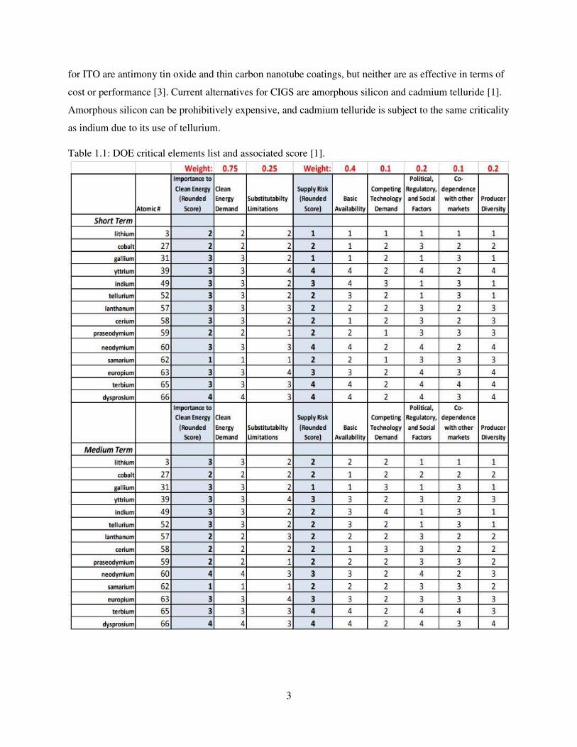
The DOE’s list of critical elements, as well as their criticality scores as defined by the DOE is

shown below in Table 1.1. The criticality score for each mineral is determined by the level of “supply

risk” and “importance to clean energy” for each element. Each category is scored 1 to 4, with 4 being the

highest.

1.2 Criticality of Indium

Indium is a metallic element used in electronics, solders, coatings, photovoltaics, etc., and is one

of the critical elements shown in Table 1.1 [2, 3, 4]. The supply risk necessary to be considered critical is

caused in part by indium’s status as a byproduct of zinc. Because of this, all factors that affect zinc

production in indium producing countries, such as China, Canada and Korea, also affect indium

production [1]. This means that indium supply may be affected by factors beyond the purview of the

global indium market. Additionally, the U.S. is completely dependent on imports for its refined indium

supply. It should be noted that medium term supply risk is lower than short term supply risk as time

allows for increased production from ally countries, production from alternative sources, such as recycled

ITO coatings, and the development of domestic sources.

The importance to clean energy is due to indium’s use in copper-indium-gallium-diselendie

(CIGS) and indium tin oxide (ITO), both of which are used in photovoltaics [1, 3]. This is especially true

in the case of CIGS as it shows potential for improved efficiency relative to other options. A lack of

viable alternatives compounds the importance to clean energy that indium possesses. Current alternatives

3

for ITO are antimony tin oxide and thin carbon nanotube coatings, but neither are as effective in terms of

cost or performance [3]. Current alternatives for CIGS are amorphous silicon and cadmium telluride [1].

Amorphous silicon can be prohibitively expensive, and cadmium telluride is subject to the same criticality

as indium due to its use of tellurium.

Table 1.1: DOE critical elements list and associated score [1].

4

1.3 Internal Rio Tinto Kennecott Indium Characterization

Rio Tinto Kennecott Copper (RTKC) is a primary copper producer located near Salt Lake City,

Utah wholly owned by Rio Tinto. RTKC operates the Brigham Canyon mine, one of the largest open pit

mines on Earth. RTKC accounts for approximately 10% of annual U.S. copper production, processes

approximately 150,000 tons of ore per day and has refined over 20 million tons of copper since 1982. The

mine is a porphyry copper deposit containing large amounts of sulfides. In addition to copper, RTKC also

produces gold, silver, molybdenum, rhenium, and sulfuric acid [5].

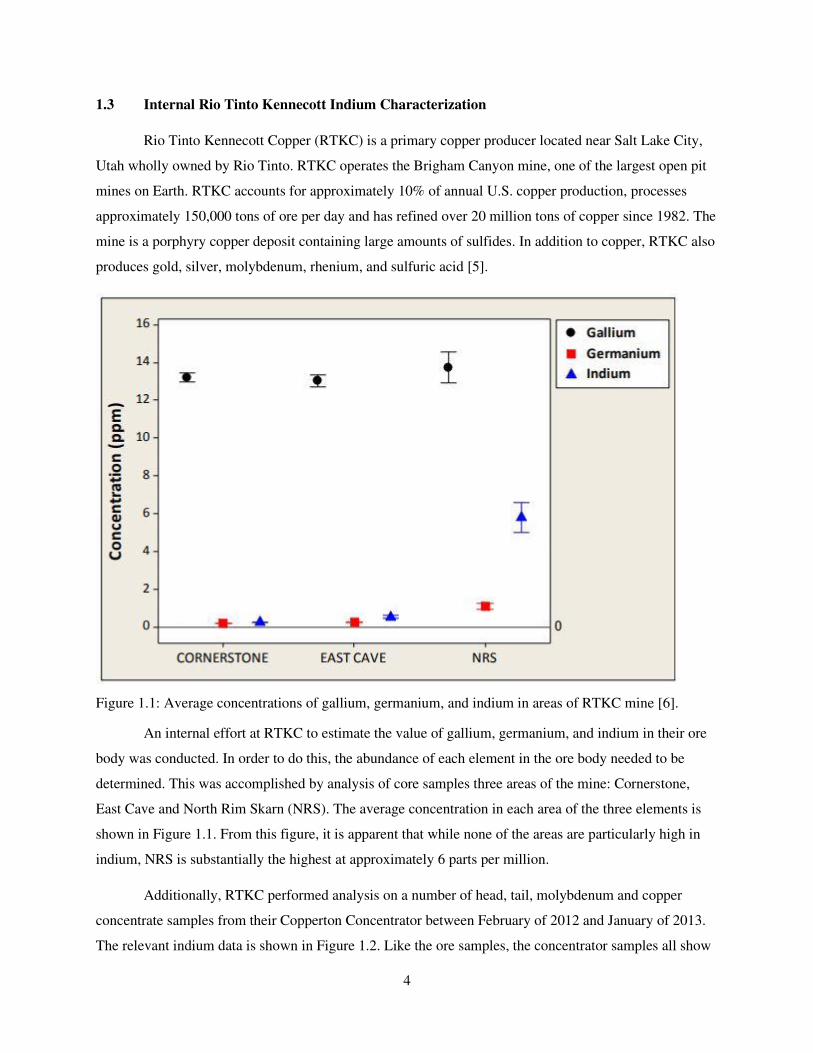
Figure 1.1: Average concentrations of gallium, germanium, and indium in areas of RTKC mine [6].

An internal effort at RTKC to estimate the value of gallium, germanium, and indium in their ore

body was conducted. In order to do this, the abundance of each element in the ore body needed to be

determined. This was accomplished by analysis of core samples three areas of the mine: Cornerstone,

East Cave and North Rim Skarn (NRS). The average concentration in each area of the three elements is

shown in Figure 1.1. From this figure, it is apparent that while none of the areas are particularly high in

indium, NRS is substantially the highest at approximately 6 parts per million.

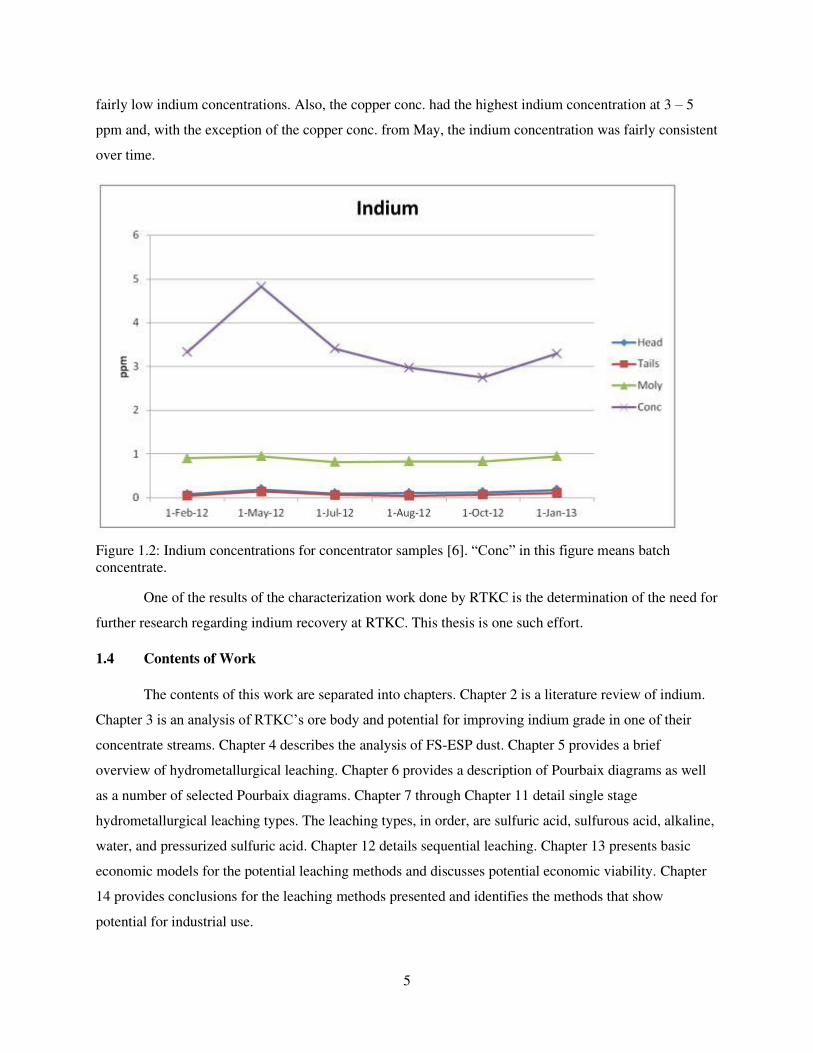
Additionally, RTKC performed analysis on a number of head, tail, molybdenum and copper

concentrate samples from their Copperton Concentrator between February of 2012 and January of 2013.

The relevant indium data is shown in Figure 1.2. Like the ore samples, the concentrator samples all show

5

fairly low indium concentrations. Also, the copper conc. had the highest indium concentration at 3 – 5

ppm and, with the exception of the copper conc. from May, the indium concentration was fairly consistent

over time.

Figure 1.2: Indium concentrations for concentrator samples [6]. “Conc” in this figure means batch

concentrate.

One of the results of the characterization work done by RTKC is the determination of the need for

further research regarding indium recovery at RTKC. This thesis is one such effort.

1.4 Contents of Work

The contents of this work are separated into chapters. Chapter 2 is a literature review of indium.

Chapter 3 is an analysis of RTKC’s ore body and potential for improving indium grade in one of their

concentrate streams. Chapter 4 describes the analysis of FS-ESP dust. Chapter 5 provides a brief

overview of hydrometallurgical leaching. Chapter 6 provides a description of Pourbaix diagrams as well

as a number of selected Pourbaix diagrams. Chapter 7 through Chapter 11 detail single stage

hydrometallurgical leaching types. The leaching types, in order, are sulfuric acid, sulfurous acid, alkaline,

water, and pressurized sulfuric acid. Chapter 12 details sequential leaching. Chapter 13 presents basic

economic models for the potential leaching methods and discusses potential economic viability. Chapter

14 provides conclusions for the leaching methods presented and identifies the methods that show

potential for industrial use.

6

CHAPTER 2. LITERATURE REVIEW

2.1 Discovery of Indium

In 1863, Ferdinand Reich and Hieronymus Theodor Richter were studying thallium in zinc ore

[7]. Specifically, it was sphalerite ore from the Freiberg polymetallic deposit. While using spectroscopy to

analyze thallium, rather than finding the expected thallium spectrum, they instead found a previously

undiscovered indigo blue spectrum. This led them to the conclusion they discovered a new element. Reich

and Richter named the element indium after the color of its spectrum. After additional work, Reich and

Richter concluded that sphalerite was the mineralogical host for indium. Four years after its discovery,

indium was displayed to the world for the first time in the form of a 0.5 kilogram ingot at the 1867 Paris

World Exhibition [7].

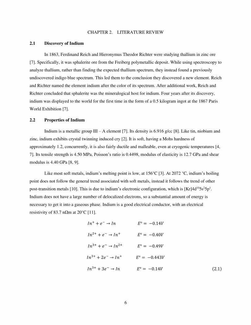
2.2 Properties of Indium

Indium is a metallic group III – A element [7]. Its density is 6.916 g/cc [8]. Like tin, niobium and

zinc, indium exhibits crystal twinning induced cry [2]. It is soft, having a Mohs hardness of

approximately 1.2, concurrently, it is also fairly ductile and malleable, even at cryogenic temperatures [4,

7]. Its tensile strength is 4.50 MPa, Poisson’s ratio is 0.4498, modulus of elasticity is 12.7 GPa and shear

modulus is 4.40 GPa [8, 9].

Like most soft metals, indium’s melting point is low, at 156°C [3]. At 2072 °C, indium’s boiling

point does not follow the general trend associated with soft metals, instead it follows the trend of other

post-transition metals [10]. This is due to indium’s electronic configuration, which is [Kr]4d105s25p1.

Indium does not have a large number of delocalized electrons, so a substantial amount of energy is

necessary to get it into a gaseous phase. Indium is a good electrical conductor, with an electrical

resistivity of 83.7 nΩm at 20°C [11]. 𝐼𝑛+ + 𝑒− → 𝐼𝑛 𝐸° = −0.14𝑉 𝐼𝑛2+ + 𝑒− → 𝐼𝑛+ 𝐸° = −0.40𝑉 𝐼𝑛3+ + 𝑒− → 𝐼𝑛2+ 𝐸° = −0.49𝑉 𝐼𝑛3+ + 2𝑒− → 𝐼𝑛+ 𝐸° = −0.443𝑉 𝐼𝑛3+ + 3𝑒− → 𝐼𝑛 𝐸° = −0.14𝑉 (2.1)

7

In compounds, indium is generally an electron donor. It most often donates three electrons and

becomes In3+, though compounds exist where indium only donates a single electron, and instead becomes

In+ such as in Indium (I) bromide [12]. Shown above in Equation 2.1 are various standard electrode

potentials (relative to SHE) for indium [13, 14]:

In aqueous solutions, indium is known to be amphoteric. As indium3+ the solution tends basic,

while as indium+, the solution tends acidic [10]. Metallic indium is not water soluble but is able to be

dissolved by most inorganic acids. Indium3+ has lowest theoretical solubility between pH 5.5 – 8.5 and

has increased solubility as pH increases or decreases [15].

2.3 Applications of Indium

The primary application of indium is as a component element in thin film coatings found in liquid

crystal displays (LCD’s) in the form of indium tin oxide (ITO) [2]. ITO is used because it is reasonably

mechanically robust, thermally reflective, electrically conductive and optically transparent to the visible

spectrum [4, 16]. These properties make ITO well suited to the application. Over the past 15 years, this

application has accounted for 60% - 70% of global indium use [3, 4, 17].

The second most prevalent global use of indium, at approximately 10%, is as an alloying element,

primarily in low melting point alloys, but also in gold and palladium dental implants and in nuclear

control rods [3, 4]. The most common type of low melting point alloy that contains indium is lead-free

solder. Due to its low melting point, indium can be used as a substitute for lead [3]. This provides a key

benefit in that is allows for the removal of a toxic element in solders [3, 4]. Additionally, indium

containing solders generally have improved thermal fatigue properties compared to lead based solders [3].

In nuclear control rods, indium containing alloys can be used as a substitute for mercury, thus, allowing

for the removal of a toxic element and improved performance [3].

Another key application of indium is as a component element in semiconductors; this accounts

for approximately 9% of global indium use [3]. Indium arsenide, indium antimonite and indium

phosphide are often used for substrate materials in semiconductors [1, 3]. Additionally, indium-gallium-

arsenide is used in semiconductor epitaxial layers [3].

Other applications of indium include use in photovoltaic solar cells, transparent heat reflectors,

fire sprinkler systems, as a coating on metallic components, etc. [1]. Of these, its use in photovoltaic solar

cells is most likely to increase. Currently, the types of solar cells that utilize indium are fairly new and

represent a small share of the solar market [1]. That being said, these types of cells are very promising,

and are expected to increase in market share in the coming years.

8

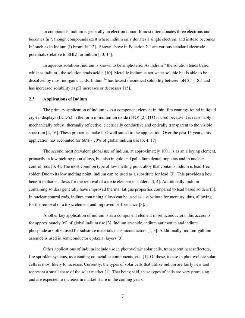
Figure 2.1: United States and global indium use compared.

Indium use in the United States differs somewhat from the rest of the globe. Approximately 49%

of indium used is for ITO film, 33% in low melting point alloys and 14% in electrical components and

semiconductors [2]. A comparison of United States and global indium use can be seen above in Figure

2.1.

2.4 Indium Geology and Mineralogy

The concentration of indium within the Earth’s crust is not well agreed upon. Sources give

numbers as low as 0.05 ppm and as high as 0.24 ppm [4, 7]. For perspective, the approximate

concentration of silver in the Earth’s crust is 0.1 parts per million [2]. Indium is a chalcophile and

generally occurs with base metals like copper, silver, cadmium, tin, lead, bismuth, and zinc [7].

The highest concentrations of indium in rock occur in Tadjik argillite (200 – 5700 ppb), eastern

Kazakhstan granite (530 ppb), German rhyolite (40 – 640 ppb) and granite (20 – 260 ppb), Russian

granite (30 – 210 ppb), Yakutiya monzonite (130 ppb), etc. [7].

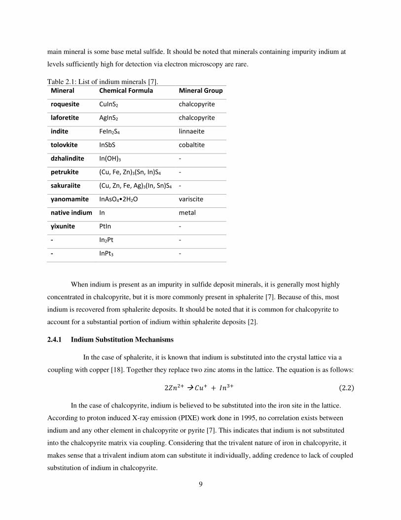
Indium is known to form twelve distinct mineral phases; they are shown below in Table 2.1.

These minerals are fairly rare, and rather than form its own mineral, indium tends to present itself as a

substitutional or interstitial inclusion in some other mineral [7]. Most commonly, this mineral is some

zinc based sulfide, such as sphalerite or wurtzite [2]. Other minerals known to contain indium in solid

solution are chalcopyrite, stannite and cassiterite [7]. Generally, when found as an impurity element the

0%

10%

20%

30%

40%

50%

60%

70%

ITO Film Alloying Element Semiconductors Other

United States vs Global Indium Use

United States Global

9

main mineral is some base metal sulfide. It should be noted that minerals containing impurity indium at

levels sufficiently high for detection via electron microscopy are rare.

Table 2.1: List of indium minerals [7].

Mineral Chemical Formula Mineral Group

roquesite CuInS2 chalcopyrite

laforetite AgInS2 chalcopyrite

indite FeIn2S4 linnaeite

tolovkite InSbS cobaltite

dzhalindite In(OH)3 -

petrukite (Cu, Fe, Zn)3(Sn, In)S4 -

sakuraiite (Cu, Zn, Fe, Ag)3(In, Sn)S4 -

yanomamite InAsO4•2H2O variscite

native indium In metal

yixunite PtIn -

- In2Pt -

- InPt3 -

When indium is present as an impurity in sulfide deposit minerals, it is generally most highly

concentrated in chalcopyrite, but it is more commonly present in sphalerite [7]. Because of this, most

indium is recovered from sphalerite deposits. It should be noted that it is common for chalcopyrite to

account for a substantial portion of indium within sphalerite deposits [2].

2.4.1 Indium Substitution Mechanisms

In the case of sphalerite, it is known that indium is substituted into the crystal lattice via a

coupling with copper [18]. Together they replace two zinc atoms in the lattice. The equation is as follows: 2𝑍𝑛2+ → 𝐶𝑢+ + 𝐼𝑛3+ (2.2)

In the case of chalcopyrite, indium is believed to be substituted into the iron site in the lattice.

According to proton induced X-ray emission (PIXE) work done in 1995, no correlation exists between

indium and any other element in chalcopyrite or pyrite [7]. This indicates that indium is not substituted

into the chalcopyrite matrix via coupling. Considering that the trivalent nature of iron in chalcopyrite, it

makes sense that a trivalent indium atom can substitute it individually, adding credence to lack of coupled

substitution of indium in chalcopyrite.

10

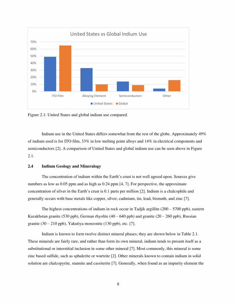
2.4.2 Indium Metallogeny

Indium is known to occur in a fairly large number of deposit types across the globe. For example,

indium occurs in porphyry copper deposits, epithermal-gold deposits, polymetallic base metal deposits,

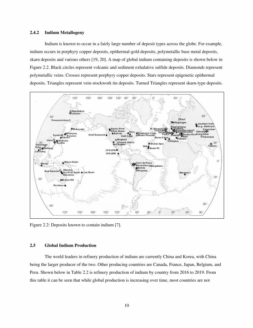
skarn deposits and various others [19, 20]. A map of global indium containing deposits is shown below in

Figure 2.2. Black circles represent volcanic and sediment exhalative sulfide deposits. Diamonds represent

polymetallic veins. Crosses represent porphyry copper deposits. Stars represent epigenetic epithermal

deposits. Triangles represent vein-stockwork tin deposits. Turned Triangles represent skarn-type deposits.

Figure 2.2: Deposits known to contain indium [7].

2.5 Global Indium Production

The world leaders in refinery production of indium are currently China and Korea, with China

being the larger producer of the two. Other producing countries are Canada, France, Japan, Belgium, and

Peru. Shown below in Table 2.2 is refinery production of indium by country from 2016 to 2019. From

this table it can be seen that while global production is increasing over time, most countries are not

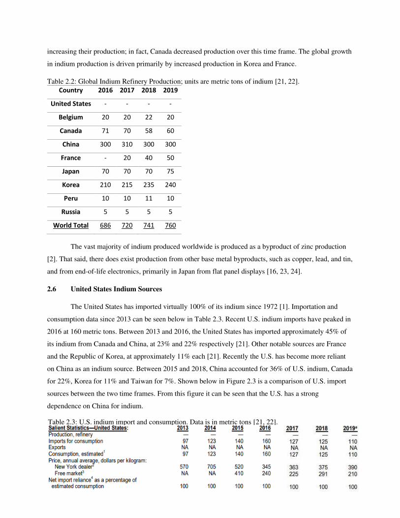
11

increasing their production; in fact, Canada decreased production over this time frame. The global growth

in indium production is driven primarily by increased production in Korea and France.

Table 2.2: Global Indium Refinery Production; units are metric tons of indium [21, 22].

Country 2016 2017 2018 2019

United States - - - -

Belgium 20 20 22 20

Canada 71 70 58 60

China 300 310 300 300

France - 20 40 50

Japan 70 70 70 75

Korea 210 215 235 240

Peru 10 10 11 10

Russia 5 5 5 5

World Total 686 720 741 760

The vast majority of indium produced worldwide is produced as a byproduct of zinc production

[2]. That said, there does exist production from other base metal byproducts, such as copper, lead, and tin,

and from end-of-life electronics, primarily in Japan from flat panel displays [16, 23, 24].

2.6 United States Indium Sources

The United States has imported virtually 100% of its indium since 1972 [1]. Importation and

consumption data since 2013 can be seen below in Table 2.3. Recent U.S. indium imports have peaked in

2016 at 160 metric tons. Between 2013 and 2016, the United States has imported approximately 45% of

its indium from Canada and China, at 23% and 22% respectively [21]. Other notable sources are France

and the Republic of Korea, at approximately 11% each [21]. Recently the U.S. has become more reliant

on China as an indium source. Between 2015 and 2018, China accounted for 36% of U.S. indium, Canada

for 22%, Korea for 11% and Taiwan for 7%. Shown below in Figure 2.3 is a comparison of U.S. import

sources between the two time frames. From this figure it can be seen that the U.S. has a strong

dependence on China for indium.

Table 2.3: U.S. indium import and consumption. Data is in metric tons [21, 22].

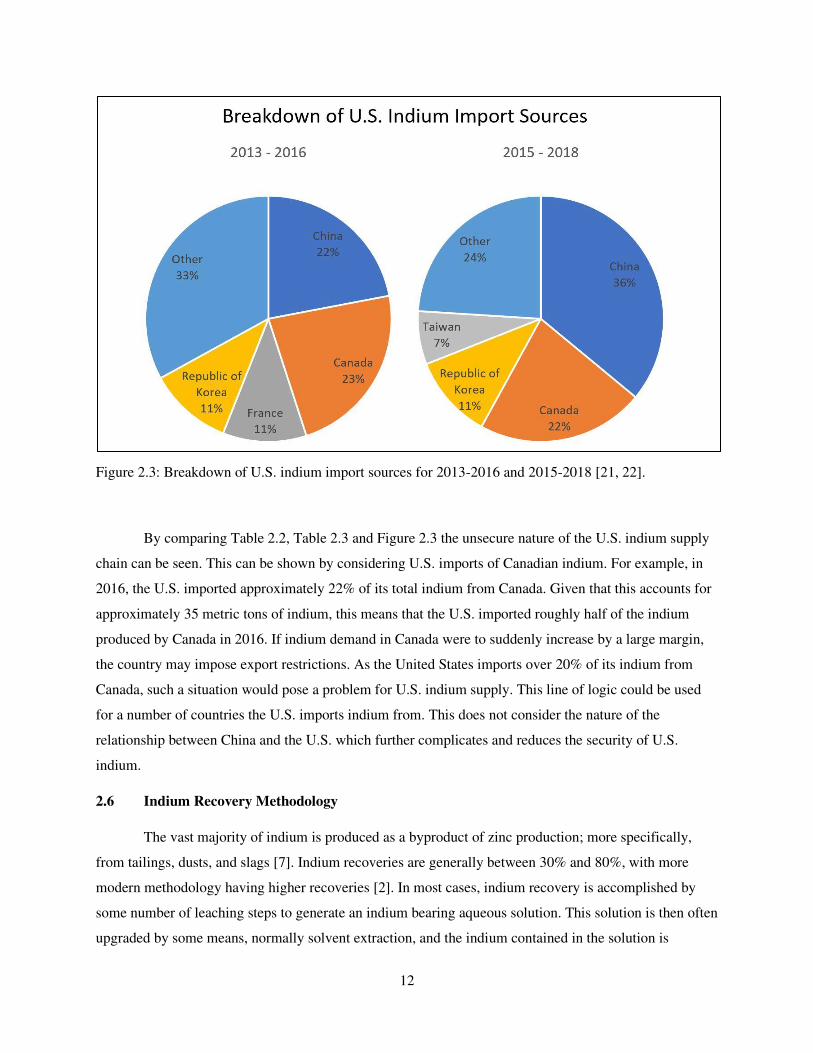
12

Figure 2.3: Breakdown of U.S. indium import sources for 2013-2016 and 2015-2018 [21, 22].

By comparing Table 2.2, Table 2.3 and Figure 2.3 the unsecure nature of the U.S. indium supply

chain can be seen. This can be shown by considering U.S. imports of Canadian indium. For example, in

2016, the U.S. imported approximately 22% of its total indium from Canada. Given that this accounts for

approximately 35 metric tons of indium, this means that the U.S. imported roughly half of the indium

produced by Canada in 2016. If indium demand in Canada were to suddenly increase by a large margin,

the country may impose export restrictions. As the United States imports over 20% of its indium from

Canada, such a situation would pose a problem for U.S. indium supply. This line of logic could be used

for a number of countries the U.S. imports indium from. This does not consider the nature of the

relationship between China and the U.S. which further complicates and reduces the security of U.S.

indium.

2.6 Indium Recovery Methodology

The vast majority of indium is produced as a byproduct of zinc production; more specifically,

from tailings, dusts, and slags [7]. Indium recoveries are generally between 30% and 80%, with more

modern methodology having higher recoveries [2]. In most cases, indium recovery is accomplished by

some number of leaching steps to generate an indium bearing aqueous solution. This solution is then often

upgraded by some means, normally solvent extraction, and the indium contained in the solution is

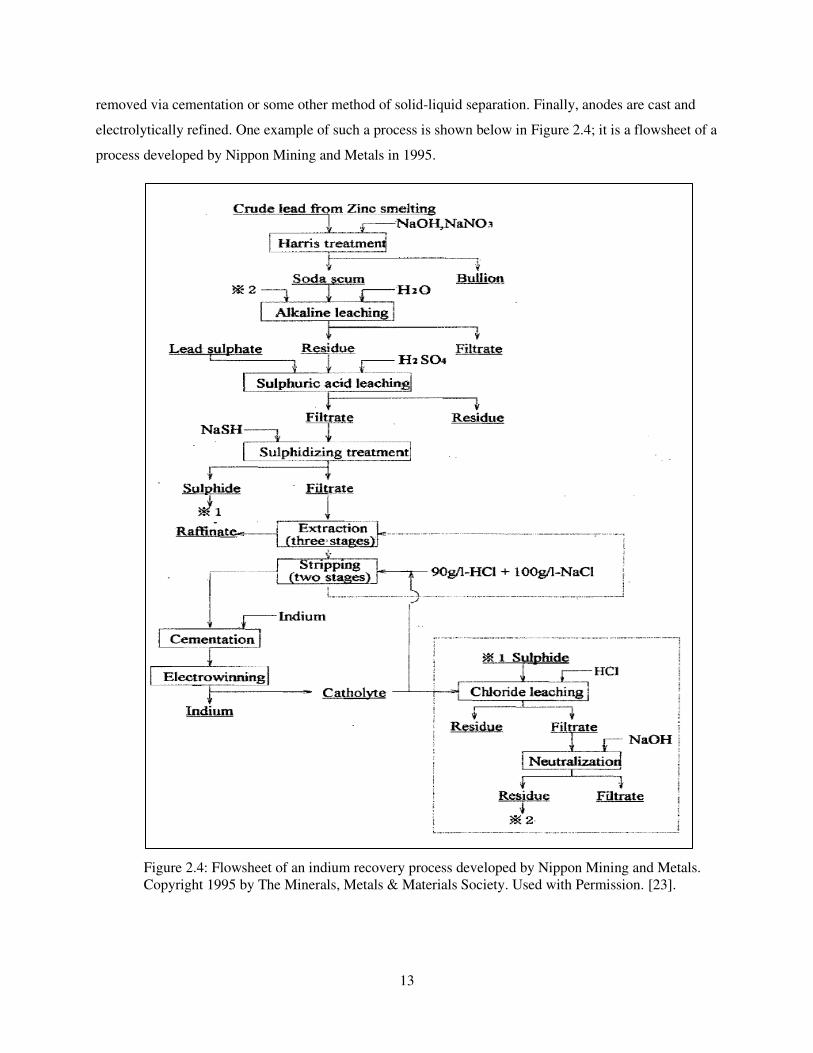
13

removed via cementation or some other method of solid-liquid separation. Finally, anodes are cast and

electrolytically refined. One example of such a process is shown below in Figure 2.4; it is a flowsheet of a

process developed by Nippon Mining and Metals in 1995.

Figure 2.4: Flowsheet of an indium recovery process developed by Nippon Mining and Metals.


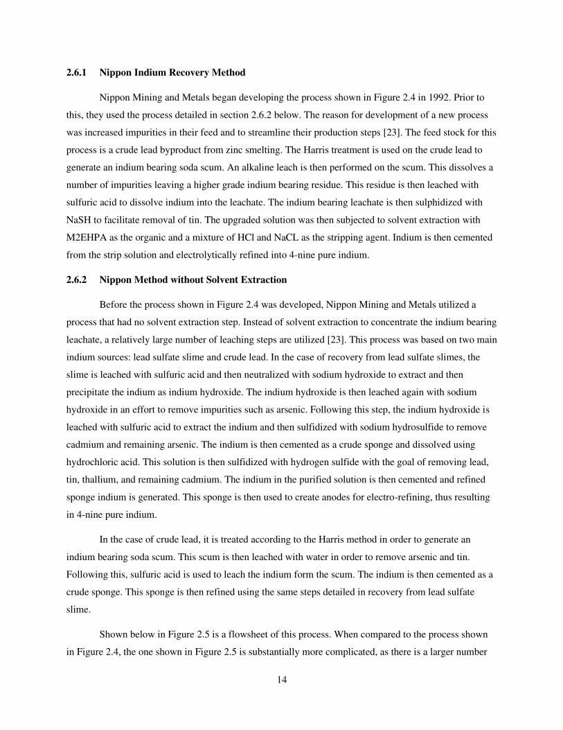
14

2.6.1 Nippon Indium Recovery Method

Nippon Mining and Metals began developing the process shown in Figure 2.4 in 1992. Prior to

this, they used the process detailed in section 2.6.2 below. The reason for development of a new process

was increased impurities in their feed and to streamline their production steps [23]. The feed stock for this

process is a crude lead byproduct from zinc smelting. The Harris treatment is used on the crude lead to

generate an indium bearing soda scum. An alkaline leach is then performed on the scum. This dissolves a

number of impurities leaving a higher grade indium bearing residue. This residue is then leached with

sulfuric acid to dissolve indium into the leachate. The indium bearing leachate is then sulphidized with

NaSH to facilitate removal of tin. The upgraded solution was then subjected to solvent extraction with

M2EHPA as the organic and a mixture of HCl and NaCL as the stripping agent. Indium is then cemented

from the strip solution and electrolytically refined into 4-nine pure indium.

2.6.2 Nippon Method without Solvent Extraction

Before the process shown in Figure 2.4 was developed, Nippon Mining and Metals utilized a

process that had no solvent extraction step. Instead of solvent extraction to concentrate the indium bearing

leachate, a relatively large number of leaching steps are utilized [23]. This process was based on two main

indium sources: lead sulfate slime and crude lead. In the case of recovery from lead sulfate slimes, the

slime is leached with sulfuric acid and then neutralized with sodium hydroxide to extract and then

precipitate the indium as indium hydroxide. The indium hydroxide is then leached again with sodium

hydroxide in an effort to remove impurities such as arsenic. Following this step, the indium hydroxide is

leached with sulfuric acid to extract the indium and then sulfidized with sodium hydrosulfide to remove

cadmium and remaining arsenic. The indium is then cemented as a crude sponge and dissolved using

hydrochloric acid. This solution is then sulfidized with hydrogen sulfide with the goal of removing lead,

tin, thallium, and remaining cadmium. The indium in the purified solution is then cemented and refined

sponge indium is generated. This sponge is then used to create anodes for electro-refining, thus resulting

in 4-nine pure indium.

In the case of crude lead, it is treated according to the Harris method in order to generate an

indium bearing soda scum. This scum is then leached with water in order to remove arsenic and tin.

Following this, sulfuric acid is used to leach the indium form the scum. The indium is then cemented as a

crude sponge. This sponge is then refined using the same steps detailed in recovery from lead sulfate

slime.

Shown below in Figure 2.5 is a flowsheet of this process. When compared to the process shown

in Figure 2.4, the one shown in Figure 2.5 is substantially more complicated, as there is a larger number

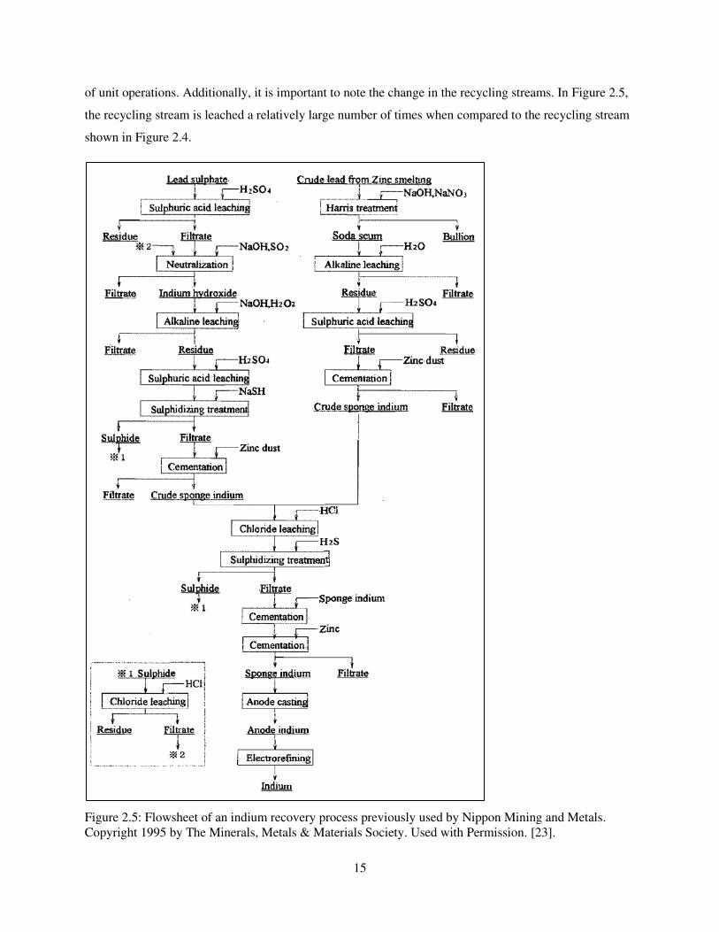
15

of unit operations. Additionally, it is important to note the change in the recycling streams. In Figure 2.5,

the recycling stream is leached a relatively large number of times when compared to the recycling stream

shown in Figure 2.4.

Figure 2.5: Flowsheet of an indium recovery process previously used by Nippon Mining and Metals.


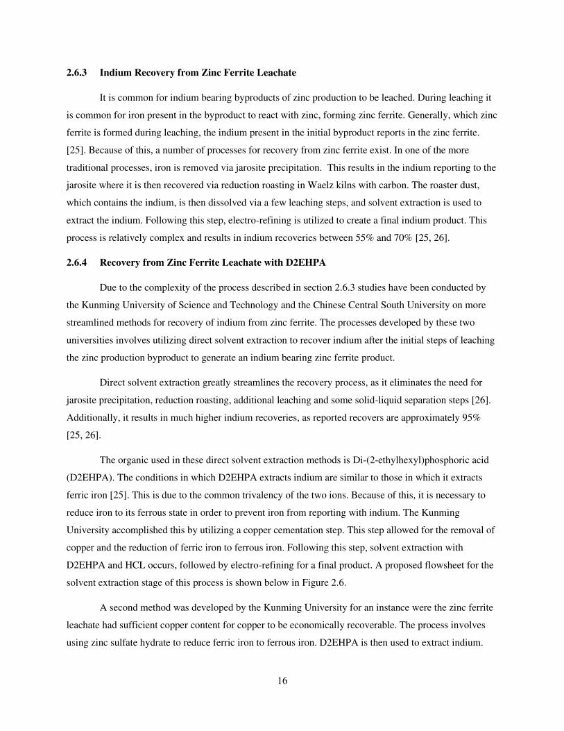
16

2.6.3 Indium Recovery from Zinc Ferrite Leachate

It is common for indium bearing byproducts of zinc production to be leached. During leaching it

is common for iron present in the byproduct to react with zinc, forming zinc ferrite. Generally, which zinc

ferrite is formed during leaching, the indium present in the initial byproduct reports in the zinc ferrite.

[25]. Because of this, a number of processes for recovery from zinc ferrite exist. In one of the more

traditional processes, iron is removed via jarosite precipitation. This results in the indium reporting to the

jarosite where it is then recovered via reduction roasting in Waelz kilns with carbon. The roaster dust,

which contains the indium, is then dissolved via a few leaching steps, and solvent extraction is used to

extract the indium. Following this step, electro-refining is utilized to create a final indium product. This

process is relatively complex and results in indium recoveries between 55% and 70% [25, 26].

2.6.4 Recovery from Zinc Ferrite Leachate with D2EHPA

Due to the complexity of the process described in section 2.6.3 studies have been conducted by

the Kunming University of Science and Technology and the Chinese Central South University on more

streamlined methods for recovery of indium from zinc ferrite. The processes developed by these two

universities involves utilizing direct solvent extraction to recover indium after the initial steps of leaching

the zinc production byproduct to generate an indium bearing zinc ferrite product.

Direct solvent extraction greatly streamlines the recovery process, as it eliminates the need for

jarosite precipitation, reduction roasting, additional leaching and some solid-liquid separation steps [26].

Additionally, it results in much higher indium recoveries, as reported recovers are approximately 95%

[25, 26].

The organic used in these direct solvent extraction methods is Di-(2-ethylhexyl)phosphoric acid

(D2EHPA). The conditions in which D2EHPA extracts indium are similar to those in which it extracts

ferric iron [25]. This is due to the common trivalency of the two ions. Because of this, it is necessary to

reduce iron to its ferrous state in order to prevent iron from reporting with indium. The Kunming

University accomplished this by utilizing a copper cementation step. This step allowed for the removal of

copper and the reduction of ferric iron to ferrous iron. Following this step, solvent extraction with

D2EHPA and HCL occurs, followed by electro-refining for a final product. A proposed flowsheet for the

solvent extraction stage of this process is shown below in Figure 2.6.

A second method was developed by the Kunming University for an instance were the zinc ferrite

leachate had sufficient copper content for copper to be economically recoverable. The process involves

using zinc sulfate hydrate to reduce ferric iron to ferrous iron. D2EHPA is then used to extract indium.

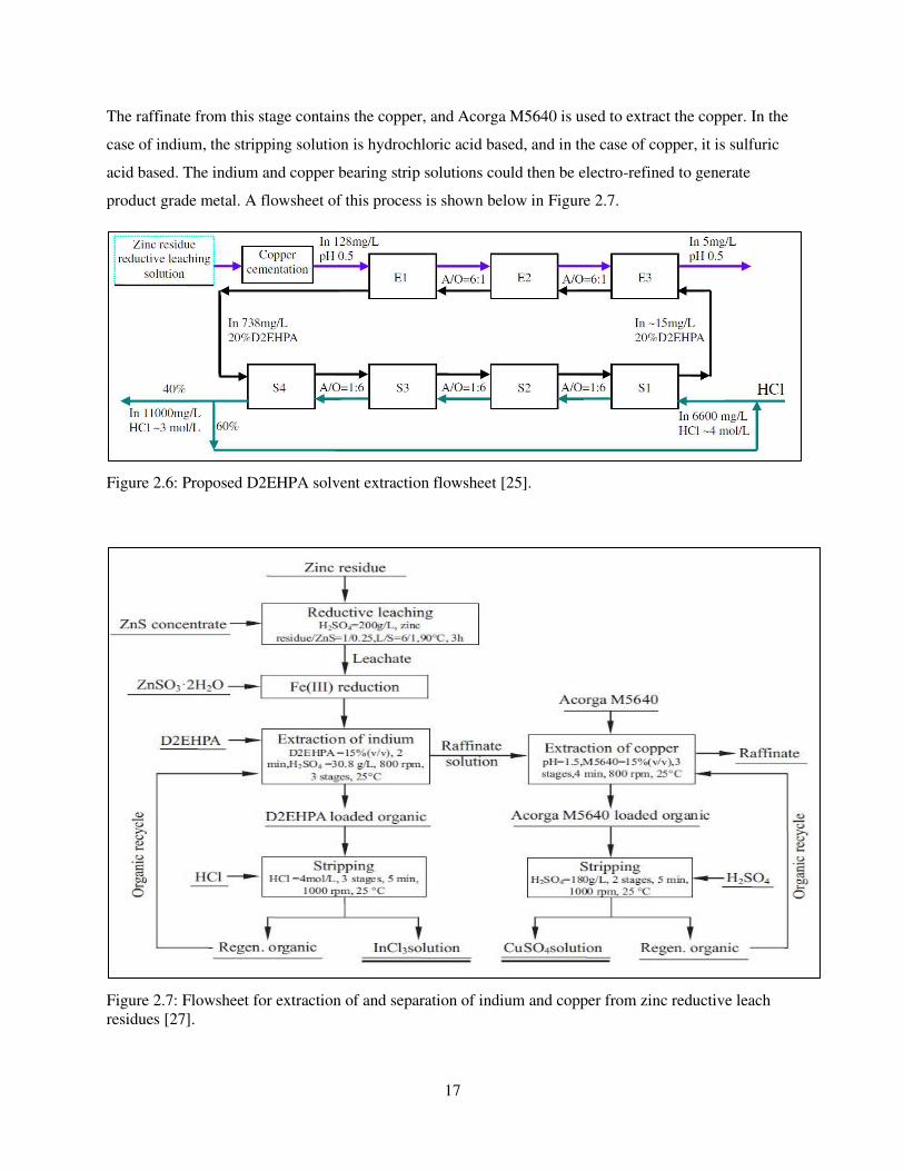
17

The raffinate from this stage contains the copper, and Acorga M5640 is used to extract the copper. In the

case of indium, the stripping solution is hydrochloric acid based, and in the case of copper, it is sulfuric

acid based. The indium and copper bearing strip solutions could then be electro-refined to generate

product grade metal. A flowsheet of this process is shown below in Figure 2.7.

Figure 2.6: Proposed D2EHPA solvent extraction flowsheet [25].

Figure 2.7: Flowsheet for extraction of and separation of indium and copper from zinc reductive leach

residues [27].

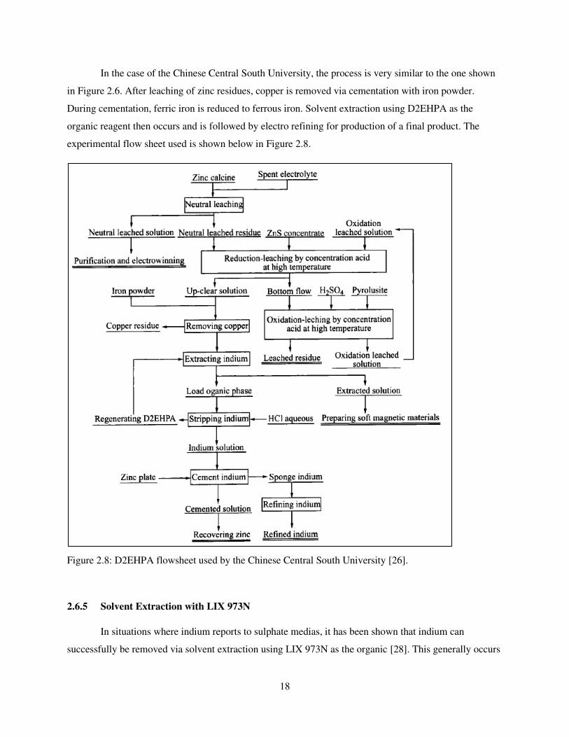
18

In the case of the Chinese Central South University, the process is very similar to the one shown

in Figure 2.6. After leaching of zinc residues, copper is removed via cementation with iron powder.

During cementation, ferric iron is reduced to ferrous iron. Solvent extraction using D2EHPA as the

organic reagent then occurs and is followed by electro refining for production of a final product. The

experimental flow sheet used is shown below in Figure 2.8.

Figure 2.8: D2EHPA flowsheet used by the Chinese Central South University [26].

2.6.5 Solvent Extraction with LIX 973N

In situations where indium reports to sulphate medias, it has been shown that indium can

successfully be removed via solvent extraction using LIX 973N as the organic [28]. This generally occurs

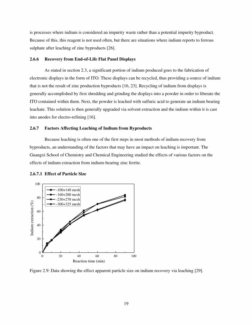
19

is processes where indium is considered an impurity waste rather than a potential impurity byproduct.

Because of this, this reagent is not used often, but there are situations where indium reports to ferrous

sulphate after leaching of zinc byproducts [26].

2.6.6 Recovery from End-of-Life Flat Panel Displays

As stated in section 2.3, a significant portion of indium produced goes to the fabrication of

electronic displays in the form of ITO. These displays can be recycled, thus providing a source of indium

that is not the result of zinc production byproducts [16, 23]. Recycling of indium from displays is

generally accomplished by first shredding and grinding the displays into a powder in order to liberate the

ITO contained within them. Next, the powder is leached with sulfuric acid to generate an indium bearing

leachate. This solution is then generally upgraded via solvent extraction and the indium within it is cast

into anodes for electro-refining [16].

2.6.7 Factors Affecting Leaching of Indium from Byproducts

Because leaching is often one of the first steps in most methods of indium recovery from

byproducts, an understanding of the factors that may have an impact on leaching is important. The

Guangxi School of Chemistry and Chemical Engineering studied the effects of various factors on the

effects of indium extraction from indium-bearing zinc ferrite.

2.6.7.1 Effect of Particle Size

Figure 2.9: Data showing the effect apparent particle size on indium recovery via leaching [29].

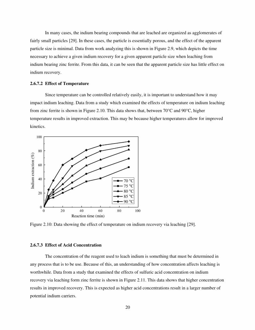
20

In many cases, the indium bearing compounds that are leached are organized as agglomerates of

fairly small particles [29]. In these cases, the particle is essentially porous, and the effect of the apparent

particle size is minimal. Data from work analyzing this is shown in Figure 2.9, which depicts the time

necessary to achieve a given indium recovery for a given apparent particle size when leaching from

indium bearing zinc ferrite. From this data, it can be seen that the apparent particle size has little effect on

indium recovery.

2.6.7.2 Effect of Temperature

Since temperature can be controlled relatively easily, it is important to understand how it may

impact indium leaching. Data from a study which examined the effects of temperature on indium leaching

from zinc ferrite is shown in Figure 2.10. This data shows that, between 70°C and 90°C, higher

temperature results in improved extraction. This may be because higher temperatures allow for improved

kinetics.

Figure 2.10: Data showing the effect of temperature on indium recovery via leaching [29].

2.6.7.3 Effect of Acid Concentration

The concentration of the reagent used to leach indium is something that must be determined in

any process that is to be use. Because of this, an understanding of how concentration affects leaching is

worthwhile. Data from a study that examined the effects of sulfuric acid concentration on indium

recovery via leaching form zinc ferrite is shown in Figure 2.11. This data shows that higher concentration

results in improved recovery. This is expected as higher acid concentrations result in a larger number of

potential indium carriers.

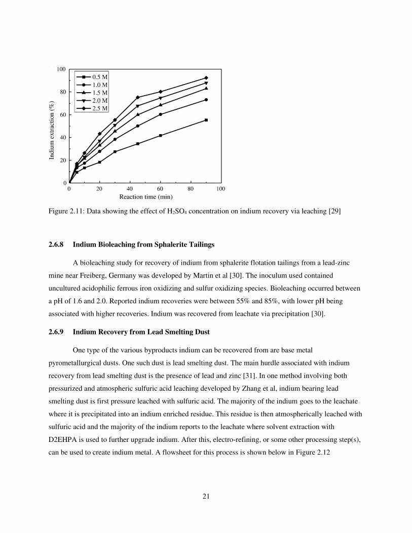
21

Figure 2.11: Data showing the effect of H2SO4 concentration on indium recovery via leaching [29]

2.6.8 Indium Bioleaching from Sphalerite Tailings

A bioleaching study for recovery of indium from sphalerite flotation tailings from a lead-zinc

mine near Freiberg, Germany was developed by Martin et al [30]. The inoculum used contained

uncultured acidophilic ferrous iron oxidizing and sulfur oxidizing species. Bioleaching occurred between

a pH of 1.6 and 2.0. Reported indium recoveries were between 55% and 85%, with lower pH being

associated with higher recoveries. Indium was recovered from leachate via precipitation [30].

2.6.9 Indium Recovery from Lead Smelting Dust

One type of the various byproducts indium can be recovered from are base metal

pyrometallurgical dusts. One such dust is lead smelting dust. The main hurdle associated with indium

recovery from lead smelting dust is the presence of lead and zinc [31]. In one method involving both

pressurized and atmospheric sulfuric acid leaching developed by Zhang et al, indium bearing lead

smelting dust is first pressure leached with sulfuric acid. The majority of the indium goes to the leachate

where it is precipitated into an indium enriched residue. This residue is then atmospherically leached with

sulfuric acid and the majority of the indium reports to the leachate where solvent extraction with

D2EHPA is used to further upgrade indium. After this, electro-refining, or some other processing step(s),

can be used to create indium metal. A flowsheet for this process is shown below in Figure 2.12

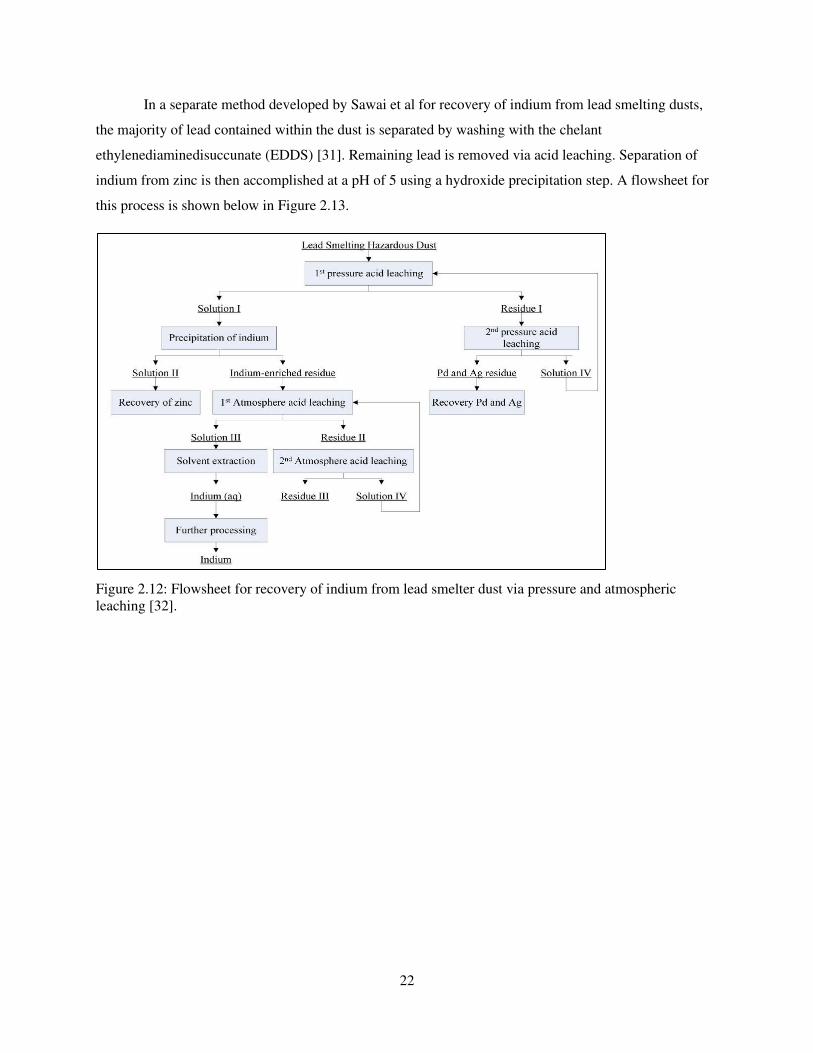
22

In a separate method developed by Sawai et al for recovery of indium from lead smelting dusts,

the majority of lead contained within the dust is separated by washing with the chelant

ethylenediaminedisuccunate (EDDS) [31]. Remaining lead is removed via acid leaching. Separation of

indium from zinc is then accomplished at a pH of 5 using a hydroxide precipitation step. A flowsheet for

this process is shown below in Figure 2.13.

Figure 2.12: Flowsheet for recovery of indium from lead smelter dust via pressure and atmospheric

leaching [32].

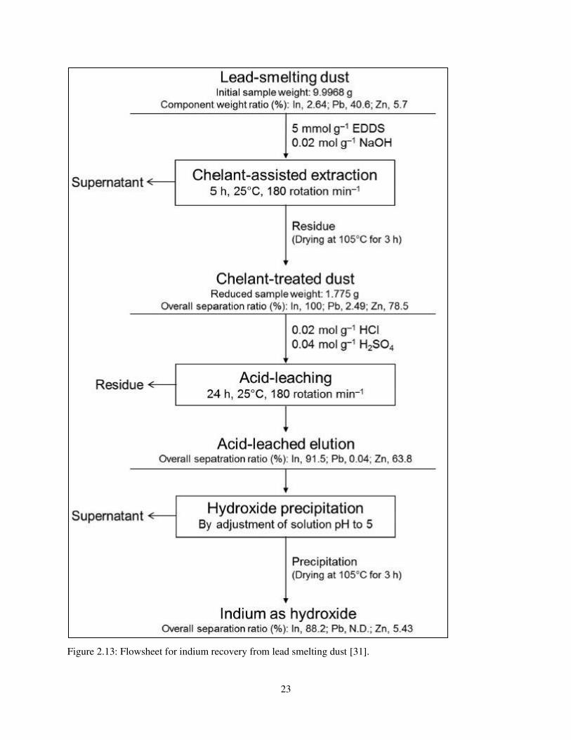
23

Figure 2.13: Flowsheet for indium recovery from lead smelting dust [31].

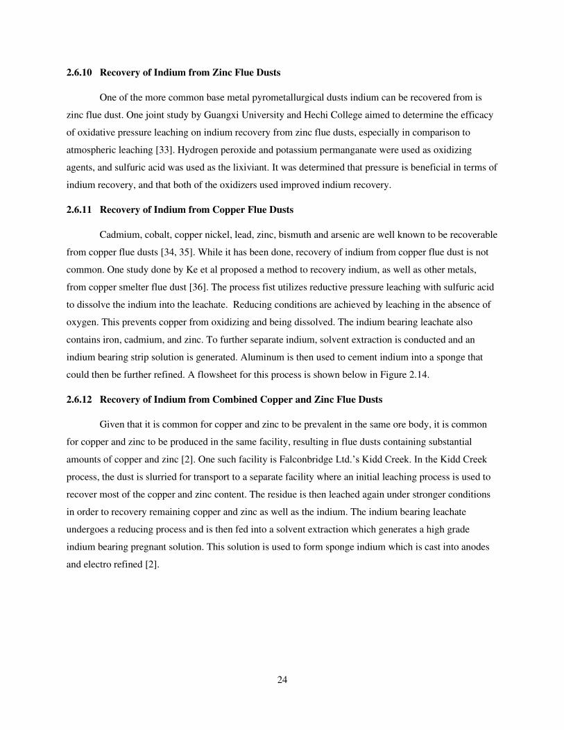
24

2.6.10 Recovery of Indium from Zinc Flue Dusts

One of the more common base metal pyrometallurgical dusts indium can be recovered from is

zinc flue dust. One joint study by Guangxi University and Hechi College aimed to determine the efficacy

of oxidative pressure leaching on indium recovery from zinc flue dusts, especially in comparison to

atmospheric leaching [33]. Hydrogen peroxide and potassium permanganate were used as oxidizing

agents, and sulfuric acid was used as the lixiviant. It was determined that pressure is beneficial in terms of

indium recovery, and that both of the oxidizers used improved indium recovery.

2.6.11 Recovery of Indium from Copper Flue Dusts

Cadmium, cobalt, copper nickel, lead, zinc, bismuth and arsenic are well known to be recoverable

from copper flue dusts [34, 35]. While it has been done, recovery of indium from copper flue dust is not

common. One study done by Ke et al proposed a method to recovery indium, as well as other metals,

from copper smelter flue dust [36]. The process fist utilizes reductive pressure leaching with sulfuric acid

to dissolve the indium into the leachate. Reducing conditions are achieved by leaching in the absence of

oxygen. This prevents copper from oxidizing and being dissolved. The indium bearing leachate also

contains iron, cadmium, and zinc. To further separate indium, solvent extraction is conducted and an

indium bearing strip solution is generated. Aluminum is then used to cement indium into a sponge that

could then be further refined. A flowsheet for this process is shown below in Figure 2.14.

2.6.12 Recovery of Indium from Combined Copper and Zinc Flue Dusts

Given that it is common for copper and zinc to be prevalent in the same ore body, it is common

for copper and zinc to be produced in the same facility, resulting in flue dusts containing substantial

amounts of copper and zinc [2]. One such facility is Falconbridge Ltd.’s Kidd Creek. In the Kidd Creek

process, the dust is slurried for transport to a separate facility where an initial leaching process is used to

recover most of the copper and zinc content. The residue is then leached again under stronger conditions

in order to recovery remaining copper and zinc as well as the indium. The indium bearing leachate

undergoes a reducing process and is then fed into a solvent extraction which generates a high grade

indium bearing pregnant solution. This solution is used to form sponge indium which is cast into anodes

and electro refined [2].

25

Figure 2.14: Flowsheet for indium recovery from copper smelter dust using reducing pressure leaching

[36].

26

CHAPTER 3. CHARACTERIZATION OF COPPERTON CONCENTRATOR SAMPLES

One of the early goals of this project was to improve the grade of indium in one of the Copperton

concentrator concentrate streams. Early upgrading of indium enables easier upgrading and separations

further downstream where indium would ultimately be recovered.

Several types of concentrator samples were obtained for analysis: Feed (also referred to as

“head”), various types of tailings, bulk concentrate, batch concentrate, moly concentrate, and waste rock.

3.1 Copperton Concentrator

The Copperton concentrator at RTKC is a facility in which ore is crushed, ground, slurried, and

fed into a series of flotation cells. The goal of this process is to upgrade the copper and molybdenum

content in concentrate streams so that further processing and upgrading is possible. Currently, RTKC

generates a “bulk” concentrate which is upgraded in copper and molybdenum. From this “bulk”

concentrate, a “batch” concentrate and “moly” concentrate are generated. The purpose of this “batch” and

“moly” separation is to further upgrade molybdenum which is in the “moly” concentrate. The copper

reports to the “batch” concentrate.

3.2 Sample Preparation

All Copperton concentrator samples were to be analyzed using inductively coupled plasma –

mass spectroscopy (ICP-MS). In order for this to occur, the samples must be dissolved into an aqueous

solution. Early attempts at dissolution involved using nitric acid and aqua regia; both were unsuccessful.

Later, and successful attempts at dissolution involved heating, in the presence of a fluxer, the samples to

the point of melting, and then dissolving using nitric acid (in some cases, also hydrofluoric acid), or this

process after roasting of the samples.

The methodology involving nitric acid is to take a 0.5 g sample and add to it, 20 mL of

concentrated nitric acid. To this, approximately 30 mL of deionized (DI) water was added. This mixture is

placed on a hot plate set to approx. 90°C and agitated with a magnetic stir bar. This mixture is left on the

hot plate for up to 24 hours, and DI water periodically added to keep total volume between 45 mL and 60

mL. As stated, this method was not successful for any of the sample types.

The methodology involving aqua regia is essentially the same as the one described for nitric acid.

The only difference is instead of 20 mL of concentrated nitric acid, a solution containing 15 mL of

concentrated nitric acid and 5 mL of concentrated hydrochloric acid is used. As stated, this method was

not successful for any of the sample types.

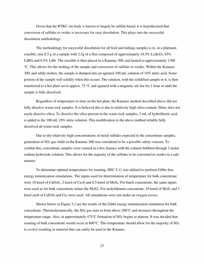
27

Given that the RTKC ore body is known to largely be sulfide based, it is hypothesized that

conversion of sulfides to oxides is necessary for easy dissolution. This plays into the successful

dissolution methodology.

The methodology for successful dissolution for all feed and tailings samples is to, in a platinum

crucible, mix 0.5 g of a sample with 2.5g of a flux composed of approximately 34.5% Li2B4O7, 65%

LiBO2 and 0.5% LiBr. The crucible is then placed in a Katanax 300, and heated to approximately 1100

°C. This allows for the melting of the sample and conversion of sulfides to oxides. Within the Katanax

300, and while molten, the sample is dumped into an agitated 100 mL solution of 10% nitric acid. Some

portion of the sample will solidify when this occurs. The solution, with the solidified sample in it, is then

transferred to a hot plate set to approx. 75 °C and agitated with a magnetic stir bar for 1 hour or until the

sample is fully dissolved.

Regardless of temperature or time on the hot plate, the Katanax method described above did not

fully dissolve waste rock samples. It is believed this is due to relatively high silica content. Nitric does not

easily dissolve silica. To dissolve the silica present in the waste rock samples, 3 mL of hydrofluoric acid

is added to the 100 mL 10% nitric solution. This modification to the above method reliably fully

dissolved all waste rock samples.

Due to the relatively high concentrations of metal sulfides expected in the concentrate samples,

generation of SO2 gas while in the Katanax 300 was considered to be a possible safety concern. To

combat this, concentrate samples were roasted in a box furnace with the exhaust bubbled through 2 molar

sodium hydroxide solution. This allows for the majority of the sulfides to be converted to oxides in a safe

manner.

To determine optimal temperatures for roasting, HSC 5.11 was utilized to perform Gibbs free

energy minimization simulations. The inputs used for determination of temperature for bulk concentrate

were 10 kmol of CuFeS2, 2 kmol of Cu2S and 0.5 kmol of MoS2. For batch concentrate, the same inputs

were used as for bulk concentrate minus the MoS2. For molybdenum concentrate, 10 kmol of MoS2 and 1

kmol each of CuFeS2 and Cu2 were used. All simulations were run under an oxygen excess.

Shown below in Figure 3.1 are the results of the Gibbs energy minimization simulation for bulk

concentrate. Thermodynamically, the SO2 gas stars to form above 200°C and increases throughout the

temperature range. Also, at approximately 475°C formation of SO2 begins to plateau. It was decided that

roasting of bulk concentrate would occur at 600°C. This temperature should allow for the majority of SO2

to evolve resulting in material that can safely be used in the Katanax.

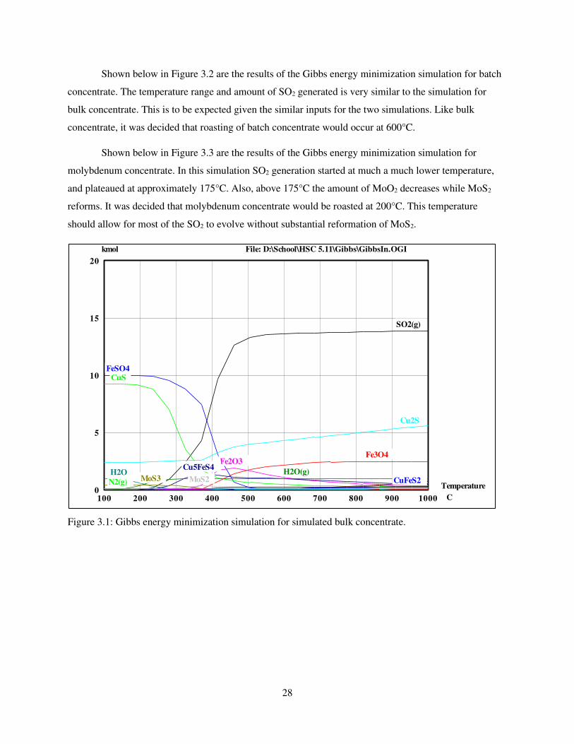
28

Shown below in Figure 3.2 are the results of the Gibbs energy minimization simulation for batch

concentrate. The temperature range and amount of SO2 generated is very similar to the simulation for

bulk concentrate. This is to be expected given the similar inputs for the two simulations. Like bulk

concentrate, it was decided that roasting of batch concentrate would occur at 600°C.

Shown below in Figure 3.3 are the results of the Gibbs energy minimization simulation for

molybdenum concentrate. In this simulation SO2 generation started at much a much lower temperature,

and plateaued at approximately 175°C. Also, above 175°C the amount of MoO2 decreases while MoS2

reforms. It was decided that molybdenum concentrate would be roasted at 200°C. This temperature

should allow for most of the SO2 to evolve without substantial reformation of MoS2.

Figure 3.1: Gibbs energy minimization simulation for simulated bulk concentrate.

100 200 300 400 500 600 700 800 900 10000

5

10

15

20

File: D:\School\HSC 5.11\Gibbs\GibbsIn.OGI

C

kmol

Temperature

SO2(g)

FeSO4CuS

Cu2S

Fe3O4Fe2O3

Cu5FeS4H2O(g)H2O

FeOFeSMoS3 MoS2 MoO2CuFeS2N2(g)

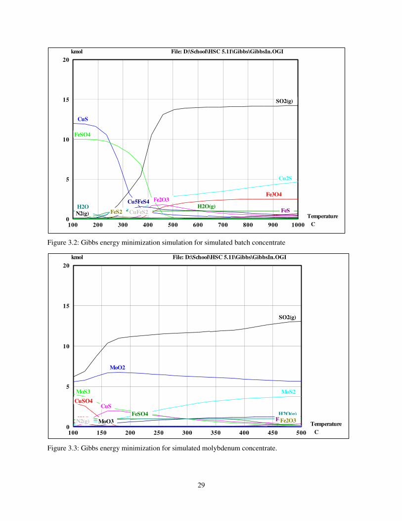
29

Figure 3.2: Gibbs energy minimization simulation for simulated batch concentrate

Figure 3.3: Gibbs energy minimization for simulated molybdenum concentrate.

100 200 300 400 500 600 700 800 900 10000

5

10

15

20


C

kmol

Temperature

SO2(g)

CuS

FeSO4

Cu2S

Fe3O4Fe2O3Cu5FeS4

H2O(g)H2OFeOFeSFeS2 CuFeS2N2(g)

100 150 200 250 300 350 400 450 5000

5

10

15

20


C

kmol

Temperature

SO2(g)

MoO2

MoS3 MoS2

CuSO4CuS

Cu2SFeSO4 H2O(g)H2O FeMoO4Fe2O3N2(g) MoO3

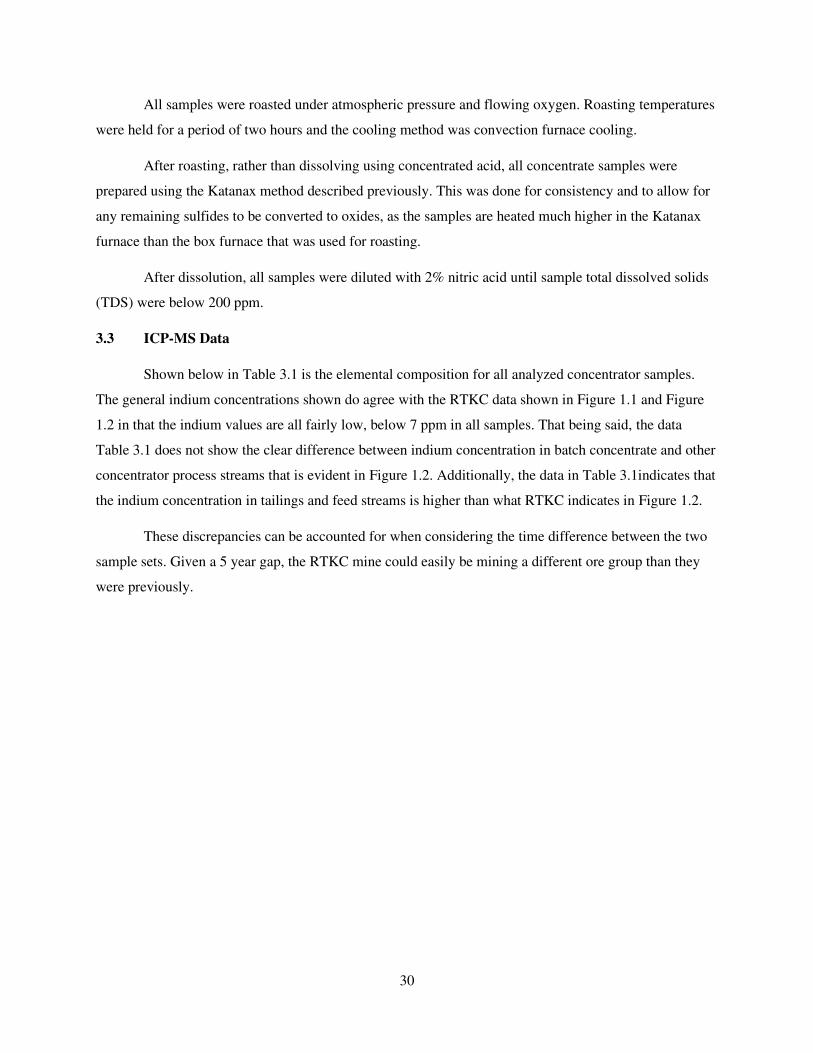
30

All samples were roasted under atmospheric pressure and flowing oxygen. Roasting temperatures

were held for a period of two hours and the cooling method was convection furnace cooling.

After roasting, rather than dissolving using concentrated acid, all concentrate samples were

prepared using the Katanax method described previously. This was done for consistency and to allow for

any remaining sulfides to be converted to oxides, as the samples are heated much higher in the Katanax

furnace than the box furnace that was used for roasting.

After dissolution, all samples were diluted with 2% nitric acid until sample total dissolved solids

(TDS) were below 200 ppm.

3.3 ICP-MS Data

Shown below in Table 3.1 is the elemental composition for all analyzed concentrator samples.

The general indium concentrations shown do agree with the RTKC data shown in Figure 1.1 and Figure

1.2 in that the indium values are all fairly low, below 7 ppm in all samples. That being said, the data

Table 3.1 does not show the clear difference between indium concentration in batch concentrate and other

concentrator process streams that is evident in Figure 1.2. Additionally, the data in Table 3.1indicates that

the indium concentration in tailings and feed streams is higher than what RTKC indicates in Figure 1.2.

These discrepancies can be accounted for when considering the time difference between the two

sample sets. Given a 5 year gap, the RTKC mine could easily be mining a different ore group than they

were previously.

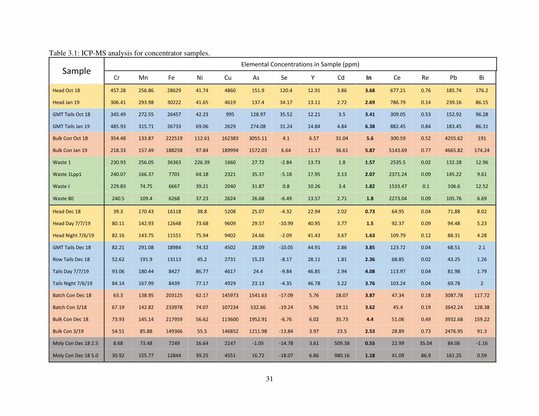
31

Table 3.1: ICP-MS analysis for concentrator samples.

Sample

Elemental Concentrations in Sample (ppm)

Cr Mn Fe Ni Cu As Se Y Cd In Ce Re Pb Bi

Head Oct 18 457.28 256.86 28629 41.74 4860 151.9 120.4 12.91 3.86 3.68 677.21 0.76 185.74 176.2

Head Jan 19 306.41 293.98 30222 41.65 4619 137.4 34.17 13.11 2.72 2.69 786.79 0.14 239.16 86.15

GMT Tails Oct 18 345.49 272.55 26457 42.23 995 128.97 35.52 12.21 3.5 3.41 309.05 0.53 152.92 96.28

GMT Tails Jan 19 485.93 315.71 26733 69.06 2629 274.08 31.24 14.84 4.84 6.38 882.45 0.84 183.45 86.31

Bulk Con Oct 18 354.48 133.87 222519 112.61 162383 3055.11 4.1 6.57 31.04 5.6 300.59 0.52 4255.62 191

Bulk Con Jan 19 218.33 157.49 188258 97.84 189994 1572.03 6.64 11.17 36.61 5.87 5143.69 0.77 4665.82 174.24

Waste 1 230.93 256.05 36363 226.39 1660 27.72 -2.84 13.73 1.8 1.57 2535.5 0.02 132.28 12.96

Waste 1Lpp1 240.07 166.37 7701 64.18 2321 35.37 -5.18 17.95 3.13 2.07 2371.24 0.09 145.22 9.61

Waste J 229.83 74.75 6667 39.21 2040 31.87 0.8 10.26 3.4 1.82 1533.47 0.1 106.6 12.52

Waste 80 240.5 109.4 6268 37.23 2624 26.68 -6.49 13.57 2.71 1.8 2273.04 0.09 105.76 6.69

Head Dec 18 39.3 170.43 16118 38.8 5208 25.07 -4.32 22.94 2.02 0.73 64.95 0.04 71.88 8.02

Head Day 7/7/19 80.11 142.93 12648 73.68 9609 29.57 -10.99 40.95 3.77 1.5 92.37 0.09 94.48 5.23

Head Night 7/6/19 82.16 143.75 11551 75.94 9402 24.66 -2.09 41.43 3.67 1.63 109.79 0.12 88.31 4.28

GMT Tails Dec 18 82.21 291.08 18984 74.32 4502 28.09 -10.05 44.91 2.86 3.85 123.72 0.04 68.51 2.1

Row Tails Dec 18 52.62 191.9 13113 45.2 2731 15.23 -8.17 28.11 1.81 2.36 68.85 0.02 43.25 1.26

Tails Day 7/7/19 93.06 180.44 8427 86.77 4617 24.4 -9.84 46.85 2.94 4.08 113.97 0.04 81.98 1.79

Tails Night 7/6/19 84.14 167.99 8439 77.17 4929 23.13 -4.35 46.78 3.22 3.76 103.24 0.04 69.78 2

Batch Con Dec 18 63.3 138.95 203125 62.17 145973 1541.63 -17.09 5.76 18.07 3.87 47.34 0.18 3087.78 117.72

Batch Con 3/18 67.19 142.82 233978 74.07 107234 532.66 -19.24 5.96 19.11 3.62 45.4 0.19 3642.24 128.38

Bulk Con Dec 18 73.93 145.14 217959 56.62 113600 1952.91 -6.76 6.02 35.73 4.4 51.06 0.49 3932.68 159.22

Bulk Con 3/19 54.51 85.88 149366 55.5 146852 1211.98 -13.84 3.97 23.5 2.53 28.89 0.73 2476.95 91.3

Moly Con Dec 18 2.5 8.68 73.48 7249 16.64 2147 -1.05 -14.78 3.61 509.38 0.55 22.99 35.04 84.06 -1.16

Moly Con Dec 18 5.0 30.92 155.77 12844 39.25 4551 16.72 -18.07 6.86 980.16 1.18 41.09 86.9 161.25 0.59

32

3.4 Automated Mineralogy of Concentrator Samples

As stated in Chapter 2, indium is commonly associated with base metals, such as copper and zinc.

In addition to the ICP-MS analysis discussed previously, automated mineralogy (AMICS) was done by

Eagle Engineering in hopes of revealing such an association in the RTKC ore body.

Shown in Table 3.2 is the AMICS phase data for the October 2018 concentrator samples. It

should be noted that the “Con” designation indicates bulk concentrate. The only difference between the

sample labeled “Con” and “Con R” is that the “R” indicates the sample was roasted as described in

section 3.2. Shown in Table 3.3 is the same for the January 2019 concentrator samples, and in Table 3.4,

is the same for the waste rock samples.

From the data shown in Table 3.2, Table 3.3 and Table 3.4 it can be seen that the phase

composition of the concentrator samples is to be expected of a sulfide based copper deposit. Additionally,

it can be seen that the Copperton concentrator is successfully upgrading both copper and molybdenum in

the bulk concentrate stream, and that relatively little amounts of copper and molybdenum make it to the

waste rock.

Generally, the indium levels shown in Table 3.1 are below the detection limits of AMICS and

will not show up on automated mineralogy scans. That being said, if the indium is concentrated in certain

minerals to levels of 5 wt. % or higher, then the indium would show up on the scan.

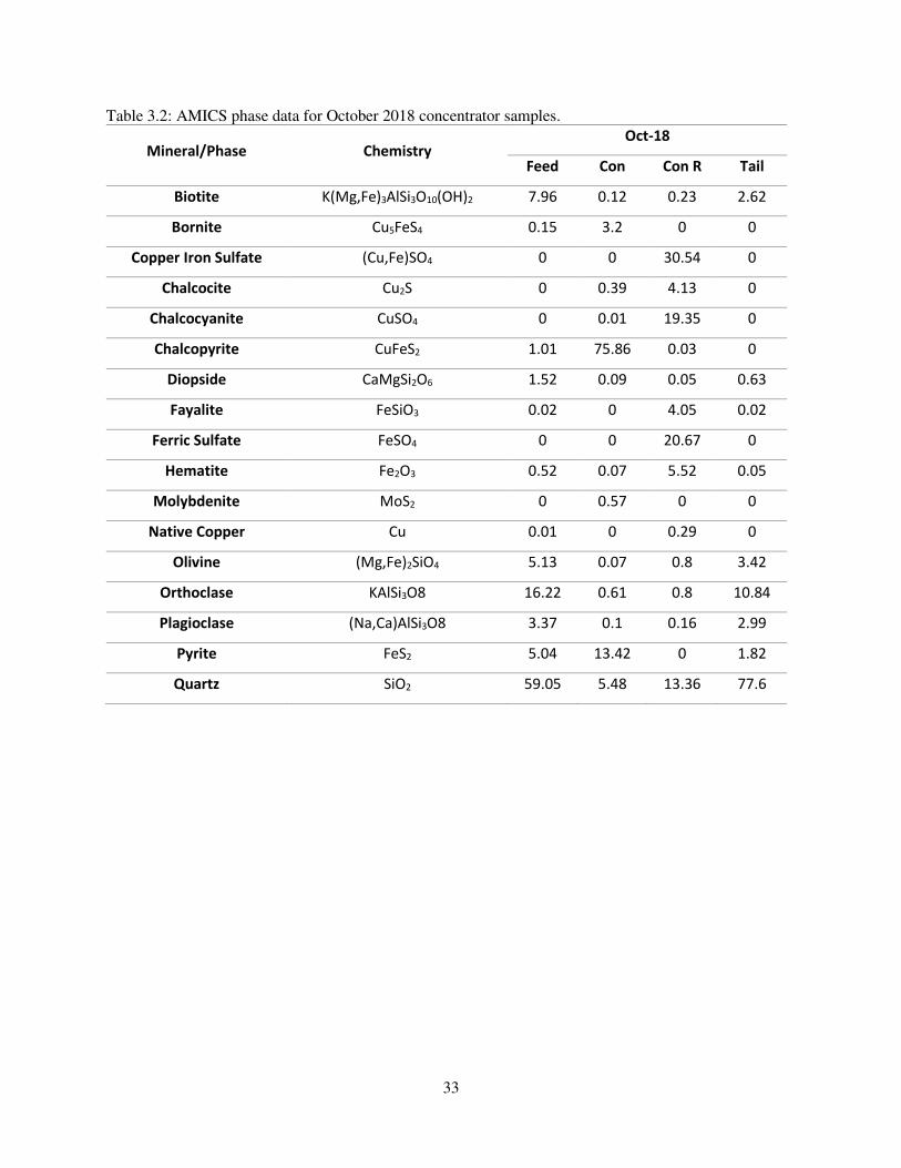
33

Table 3.2: AMICS phase data for October 2018 concentrator samples.

Mineral/Phase Chemistry Oct-18

Feed Con Con R Tail

Biotite K(Mg,Fe)3AlSi3O10(OH)2 7.96 0.12 0.23 2.62

Bornite Cu5FeS4 0.15 3.2 0 0

Copper Iron Sulfate (Cu,Fe)SO4 0 0 30.54 0

Chalcocite Cu2S 0 0.39 4.13 0

Chalcocyanite CuSO4 0 0.01 19.35 0

Chalcopyrite CuFeS2 1.01 75.86 0.03 0

Diopside CaMgSi2O6 1.52 0.09 0.05 0.63

Fayalite FeSiO3 0.02 0 4.05 0.02

Ferric Sulfate FeSO4 0 0 20.67 0

Hematite Fe2O3 0.52 0.07 5.52 0.05

Molybdenite MoS2 0 0.57 0 0

Native Copper Cu 0.01 0 0.29 0

Olivine (Mg,Fe)2SiO4 5.13 0.07 0.8 3.42

Orthoclase KAlSi3O8 16.22 0.61 0.8 10.84

Plagioclase (Na,Ca)AlSi3O8 3.37 0.1 0.16 2.99

Pyrite FeS2 5.04 13.42 0 1.82

Quartz SiO2 59.05 5.48 13.36 77.6

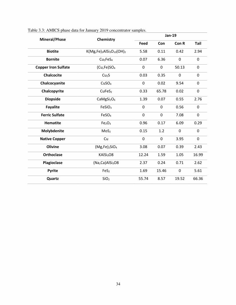
34

Table 3.3: AMICS phase data for January 2019 concentrator samples.

Mineral/Phase Chemistry Jan-19

Feed Con Con R Tail

Biotite K(Mg,Fe)3AlSi3O10(OH)2 5.58 0.11 0.42 2.94

Bornite Cu5FeS4 0.07 6.36 0 0

Copper Iron Sulfate (Cu,Fe)SO4 0 0 50.13 0

Chalcocite Cu2S 0.03 0.35 0 0

Chalcocyanite CuSO4 0 0.02 9.54 0

Chalcopyrite CuFeS2 0.33 65.78 0.02 0

Diopside CaMgSi2O6 1.39 0.07 0.55 2.76

Fayalite FeSiO3 0 0 0.56 0

Ferric Sulfate FeSO4 0 0 7.08 0

Hematite Fe2O3 0.96 0.17 6.09 0.29

Molybdenite MoS2 0.15 1.2 0 0

Native Copper Cu 0 0 3.95 0

Olivine (Mg,Fe)2SiO4 3.08 0.07 0.39 2.43

Orthoclase KAlSi3O8 12.24 1.59 1.05 16.99

Plagioclase (Na,Ca)AlSi3O8 2.37 0.24 0.71 2.62

Pyrite FeS2 1.69 15.46 0 5.61

Quartz SiO2 55.74 8.57 19.52 66.36

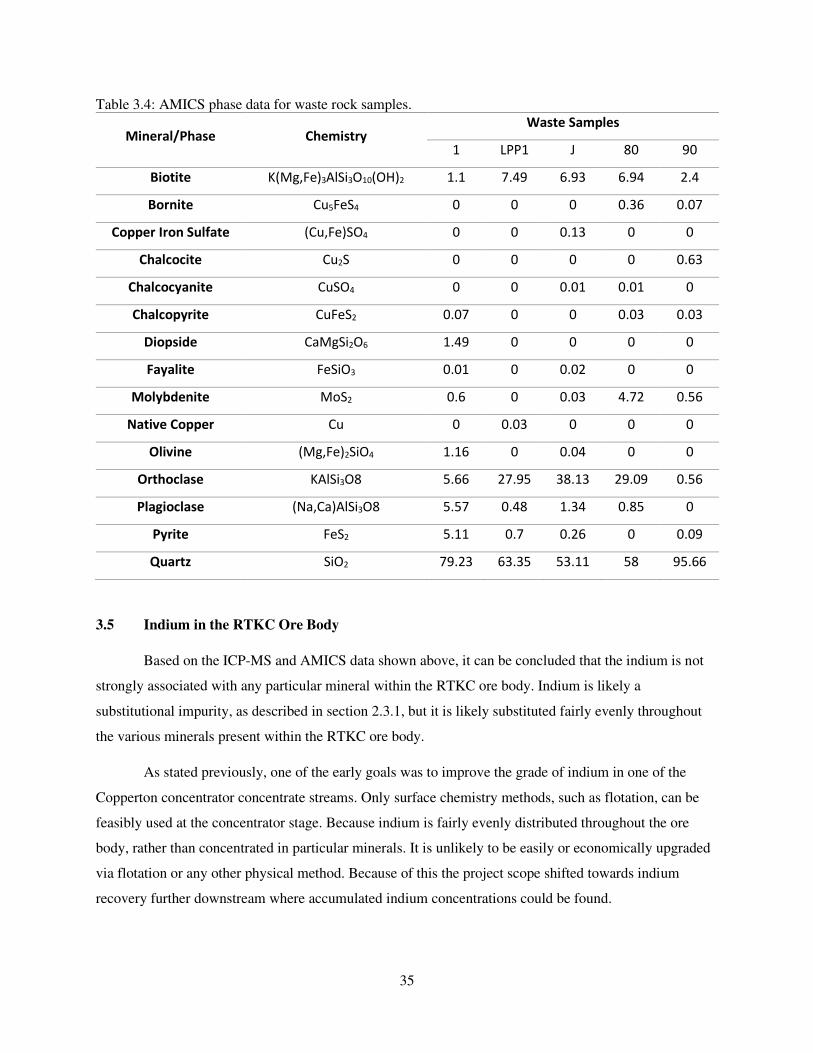
35

Table 3.4: AMICS phase data for waste rock samples.

Mineral/Phase Chemistry Waste Samples

1 LPP1 J 80 90

Biotite K(Mg,Fe)3AlSi3O10(OH)2 1.1 7.49 6.93 6.94 2.4

Bornite Cu5FeS4 0 0 0 0.36 0.07

Copper Iron Sulfate (Cu,Fe)SO4 0 0 0.13 0 0

Chalcocite Cu2S 0 0 0 0 0.63

Chalcocyanite CuSO4 0 0 0.01 0.01 0

Chalcopyrite CuFeS2 0.07 0 0 0.03 0.03

Diopside CaMgSi2O6 1.49 0 0 0 0

Fayalite FeSiO3 0.01 0 0.02 0 0

Molybdenite MoS2 0.6 0 0.03 4.72 0.56

Native Copper Cu 0 0.03 0 0 0

Olivine (Mg,Fe)2SiO4 1.16 0 0.04 0 0

Orthoclase KAlSi3O8 5.66 27.95 38.13 29.09 0.56

Plagioclase (Na,Ca)AlSi3O8 5.57 0.48 1.34 0.85 0

Pyrite FeS2 5.11 0.7 0.26 0 0.09

Quartz SiO2 79.23 63.35 53.11 58 95.66

3.5 Indium in the RTKC Ore Body

Based on the ICP-MS and AMICS data shown above, it can be concluded that the indium is not

strongly associated with any particular mineral within the RTKC ore body. Indium is likely a

substitutional impurity, as described in section 2.3.1, but it is likely substituted fairly evenly throughout

the various minerals present within the RTKC ore body.

As stated previously, one of the early goals was to improve the grade of indium in one of the

Copperton concentrator concentrate streams. Only surface chemistry methods, such as flotation, can be

feasibly used at the concentrator stage. Because indium is fairly evenly distributed throughout the ore

body, rather than concentrated in particular minerals. It is unlikely to be easily or economically upgraded

via flotation or any other physical method. Because of this the project scope shifted towards indium

recovery further downstream where accumulated indium concentrations could be found.

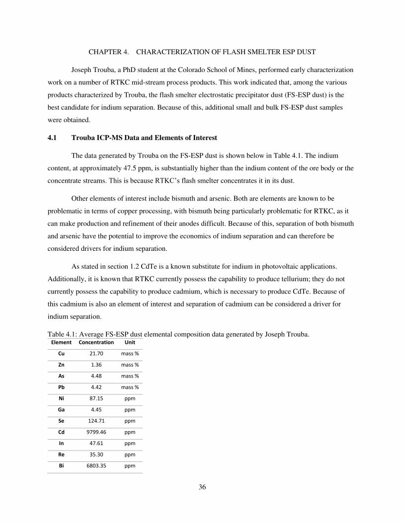
36

CHAPTER 4. CHARACTERIZATION OF FLASH SMELTER ESP DUST

Joseph Trouba, a PhD student at the Colorado School of Mines, performed early characterization

work on a number of RTKC mid-stream process products. This work indicated that, among the various

products characterized by Trouba, the flash smelter electrostatic precipitator dust (FS-ESP dust) is the

best candidate for indium separation. Because of this, additional small and bulk FS-ESP dust samples

were obtained.

4.1 Trouba ICP-MS Data and Elements of Interest

The data generated by Trouba on the FS-ESP dust is shown below in Table 4.1. The indium

content, at approximately 47.5 ppm, is substantially higher than the indium content of the ore body or the

concentrate streams. This is because RTKC’s flash smelter concentrates it in its dust.

Other elements of interest include bismuth and arsenic. Both are elements are known to be

problematic in terms of copper processing, with bismuth being particularly problematic for RTKC, as it

can make production and refinement of their anodes difficult. Because of this, separation of both bismuth

and arsenic have the potential to improve the economics of indium separation and can therefore be

considered drivers for indium separation.

As stated in section 1.2 CdTe is a known substitute for indium in photovoltaic applications.

Additionally, it is known that RTKC currently possess the capability to produce tellurium; they do not

currently possess the capability to produce cadmium, which is necessary to produce CdTe. Because of

this cadmium is also an element of interest and separation of cadmium can be considered a driver for

indium separation.

Table 4.1: Average FS-ESP dust elemental composition data generated by Joseph Trouba. Element Concentration Unit

Cu 21.70 mass %

Zn 1.36 mass %

As 4.48 mass %

Pb 4.42 mass %

Ni 87.15 ppm

Ga 4.45 ppm

Se 124.71 ppm

Cd 9799.46 ppm

In 47.61 ppm

Re 35.30 ppm

Bi 6803.35 ppm

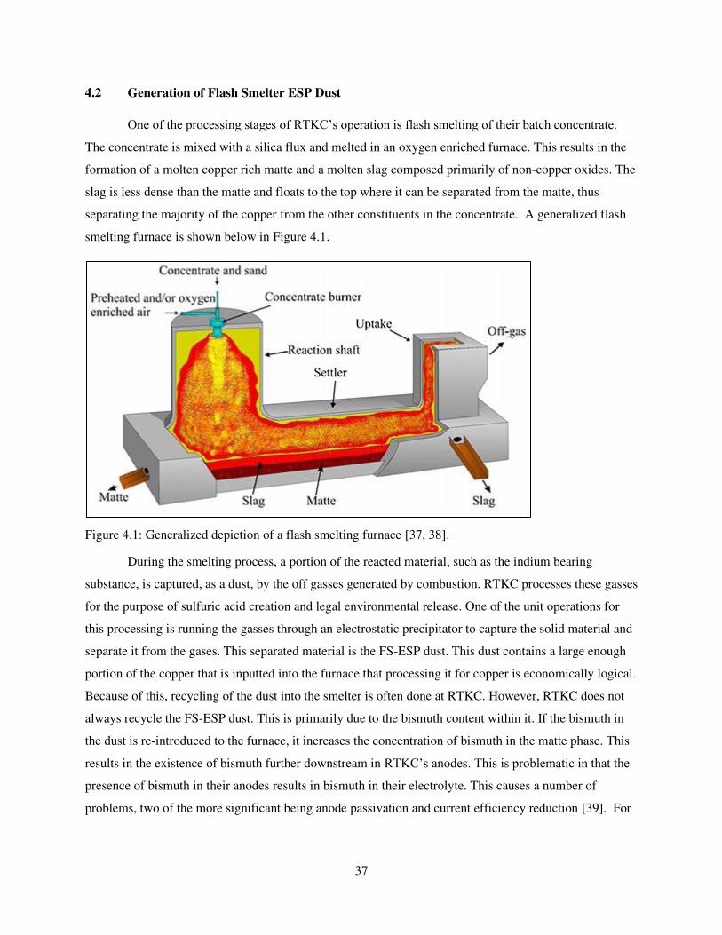
37

4.2 Generation of Flash Smelter ESP Dust

One of the processing stages of RTKC’s operation is flash smelting of their batch concentrate.

The concentrate is mixed with a silica flux and melted in an oxygen enriched furnace. This results in the

formation of a molten copper rich matte and a molten slag composed primarily of non-copper oxides. The

slag is less dense than the matte and floats to the top where it can be separated from the matte, thus

separating the majority of the copper from the other constituents in the concentrate. A generalized flash

smelting furnace is shown below in Figure 4.1.

Figure 4.1: Generalized depiction of a flash smelting furnace [37, 38].

During the smelting process, a portion of the reacted material, such as the indium bearing

substance, is captured, as a dust, by the off gasses generated by combustion. RTKC processes these gasses

for the purpose of sulfuric acid creation and legal environmental release. One of the unit operations for

this processing is running the gasses through an electrostatic precipitator to capture the solid material and

separate it from the gases. This separated material is the FS-ESP dust. This dust contains a large enough

portion of the copper that is inputted into the furnace that processing it for copper is economically logical.

Because of this, recycling of the dust into the smelter is often done at RTKC. However, RTKC does not

always recycle the FS-ESP dust. This is primarily due to the bismuth content within it. If the bismuth in

the dust is re-introduced to the furnace, it increases the concentration of bismuth in the matte phase. This

results in the existence of bismuth further downstream in RTKC’s anodes. This is problematic in that the

presence of bismuth in their anodes results in bismuth in their electrolyte. This causes a number of

problems, two of the more significant being anode passivation and current efficiency reduction [39]. For

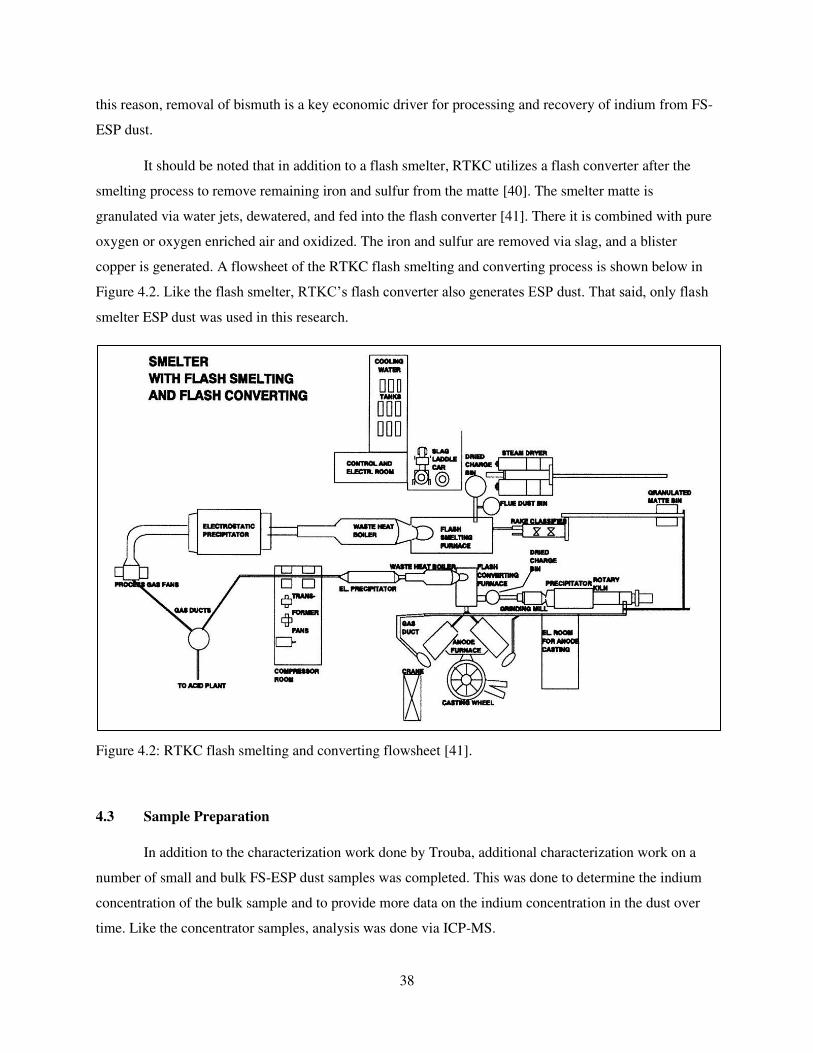
38

this reason, removal of bismuth is a key economic driver for processing and recovery of indium from FS-

ESP dust.

It should be noted that in addition to a flash smelter, RTKC utilizes a flash converter after the

smelting process to remove remaining iron and sulfur from the matte [40]. The smelter matte is

granulated via water jets, dewatered, and fed into the flash converter [41]. There it is combined with pure

oxygen or oxygen enriched air and oxidized. The iron and sulfur are removed via slag, and a blister

copper is generated. A flowsheet of the RTKC flash smelting and converting process is shown below in

Figure 4.2. Like the flash smelter, RTKC’s flash converter also generates ESP dust. That said, only flash

smelter ESP dust was used in this research.

Figure 4.2: RTKC flash smelting and converting flowsheet [41].

4.3 Sample Preparation

In addition to the characterization work done by Trouba, additional characterization work on a

number of small and bulk FS-ESP dust samples was completed. This was done to determine the indium

concentration of the bulk sample and to provide more data on the indium concentration in the dust over

time. Like the concentrator samples, analysis was done via ICP-MS.

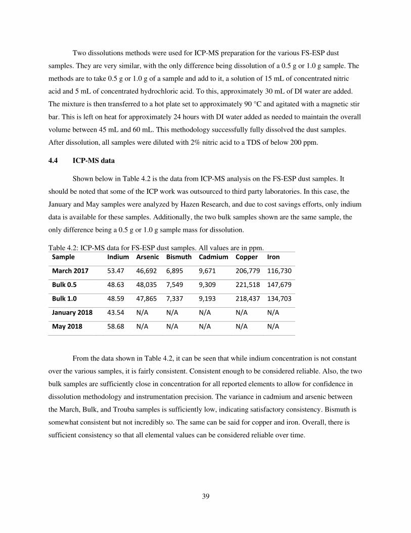
39

Two dissolutions methods were used for ICP-MS preparation for the various FS-ESP dust

samples. They are very similar, with the only difference being dissolution of a 0.5 g or 1.0 g sample. The

methods are to take 0.5 g or 1.0 g of a sample and add to it, a solution of 15 mL of concentrated nitric

acid and 5 mL of concentrated hydrochloric acid. To this, approximately 30 mL of DI water are added.

The mixture is then transferred to a hot plate set to approximately 90 °C and agitated with a magnetic stir

bar. This is left on heat for approximately 24 hours with DI water added as needed to maintain the overall

volume between 45 mL and 60 mL. This methodology successfully fully dissolved the dust samples.

After dissolution, all samples were diluted with 2% nitric acid to a TDS of below 200 ppm.

4.4 ICP-MS data

Shown below in Table 4.2 is the data from ICP-MS analysis on the FS-ESP dust samples. It

should be noted that some of the ICP work was outsourced to third party laboratories. In this case, the

January and May samples were analyzed by Hazen Research, and due to cost savings efforts, only indium

data is available for these samples. Additionally, the two bulk samples shown are the same sample, the

only difference being a 0.5 g or 1.0 g sample mass for dissolution.

Table 4.2: ICP-MS data for FS-ESP dust samples. All values are in ppm.

Sample Indium Arsenic Bismuth Cadmium Copper Iron

March 2017 53.47 46,692 6,895 9,671 206,779 116,730

Bulk 0.5 48.63 48,035 7,549 9,309 221,518 147,679

Bulk 1.0 48.59 47,865 7,337 9,193 218,437 134,703

January 2018 43.54 N/A N/A N/A N/A N/A

May 2018 58.68 N/A N/A N/A N/A N/A

From the data shown in Table 4.2, it can be seen that while indium concentration is not constant

over the various samples, it is fairly consistent. Consistent enough to be considered reliable. Also, the two

bulk samples are sufficiently close in concentration for all reported elements to allow for confidence in

dissolution methodology and instrumentation precision. The variance in cadmium and arsenic between

the March, Bulk, and Trouba samples is sufficiently low, indicating satisfactory consistency. Bismuth is

somewhat consistent but not incredibly so. The same can be said for copper and iron. Overall, there is

sufficient consistency so that all elemental values can be considered reliable over time.

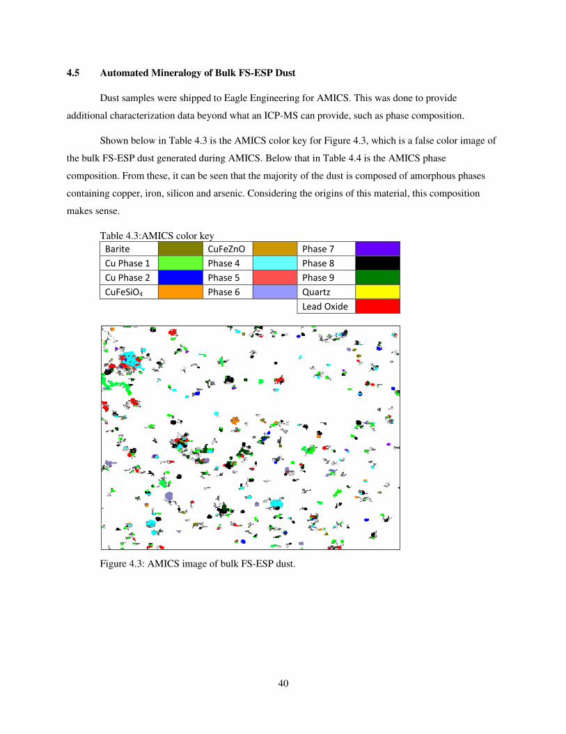
40

4.5 Automated Mineralogy of Bulk FS-ESP Dust

Dust samples were shipped to Eagle Engineering for AMICS. This was done to provide

additional characterization data beyond what an ICP-MS can provide, such as phase composition.

Shown below in Table 4.3 is the AMICS color key for Figure 4.3, which is a false color image of

the bulk FS-ESP dust generated during AMICS. Below that in Table 4.4 is the AMICS phase

composition. From these, it can be seen that the majority of the dust is composed of amorphous phases

containing copper, iron, silicon and arsenic. Considering the origins of this material, this composition

makes sense.

Table 4.3:AMICS color key

Barite CuFeZnO Phase 7

Cu Phase 1 Phase 4 Phase 8

Cu Phase 2 Phase 5 Phase 9

CuFeSiO4 Phase 6 Quartz

Lead Oxide

Figure 4.3: AMICS image of bulk FS-ESP dust.

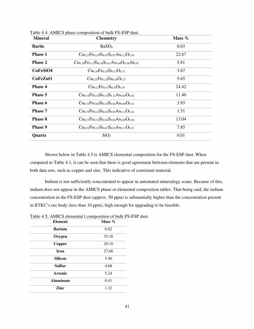
41

Table 4.4: AMICS phase composition of bulk FS-ESP dust.

Mineral Chemistry Mass %

Barite BaSO4 0.03

Phase 1 Cu0.23Fe0.24Si0.03S0.07As0.12O0.30 22.67

Phase 2 Cu0.19Fe0.12Si0.18S0.01As0.04O0.38Al0.07 5.81

CuFeSiO4 Cu0.30Fe0.26Si0.13O0.31 3.67

CuFeZnO Cu0.25Fe0.22Zn0.26O0.27 5.65

Phase 4 Cu0.22Fe0.47S0.02O0.29 24.42






Quartz SiO2 0.01

Shown below in Table 4.5 is AMICS elemental composition for the FS-ESP dust. When

compared to Table 4.1, it can be seen that there is good agreement between elements that are present in

both data sets, such as copper and zinc. This indicative of consistent material.

Indium is not sufficiently concentrated to appear in automated mineralogy scans. Because of this,

indium does not appear in the AMICS phase or elemental composition tables. That being said, the indium

concentration in the FS-ESP dust (approx. 50 ppm) is substantially higher than the concentration present

in RTKC’s ore body (less than 10 ppm), high enough for upgrading to be feasible.

Table 4.5: AMICS elemental l composition of bulk FS-ESP dust. Element Mass %

Barium 0.02

Oxygen 35.16

Copper 20.10

Iron 27.66

Silicon 5.40

Sulfur 4.68

Arsenic 5.24

Aluminum 0.41

Zinc 1.32

42

CHAPTER 5. HYDROMETALLURGICAL LEACHING

As stated in Chapter 3, the indium content of the FS-ESP dust is not sufficiently high to appear in

automated mineralogy scans. Like the concentrator samples (as described in Chapter 3), physical methods

of separation are not likely to be easily or economically utilized for indium recovery. Unlike the

concentrator samples however, the dust is a mid-stream product in which methods other than physical

may be feasible.

The most common separation method, according to literature, used for recovery of indium from

base metal smelting dusts is leaching. Leaching methodology will be the primary separation technique

used in this dissertation.

5.1 Leaching Overview

Leaching is often the first stage of a hydrometallurgical process [42]. In it, some aqueous reagent,

generally called a lixiviant or leachant, is used to selectively recover a desired substance from a mixture

containing that substance. The desired substance, commonly a metal, is transferred from the solid to

aqueous phase where it can be upgraded and recovered with downstream processes. This process is

commonly used in recovery of copper, nickel, gold, zinc, uranium, molybdenum, tungsten, etc. The

aqueous solution generated during leaching is known as leachate, and the remaining solids are commonly

referred to as residue. Generally, the primary goals of leaching are the transfer of the desired substance to

the aqueous phase and the separation of substances.

The transfer of the desired substance to the aqueous phase (recovery) is important because most

hydrometallurgical processes that would occur after leaching require that the desired substance be

aqueous. If the substance is not aqueous, hydrometallurgical recovery in downstream processes is often

not feasible.

Separation, or selectivity, is the ability or tendency of a leaching process to transfer one substance

or set of substances from the group of substances that make up the starting solid. It allows for the

separation of one or more substances from the other substances. This is beneficial in many ways and

scenarios. Generally, it allows for the easier upgrading of the desired substance in downstream processes,

but also, in specific cases, it allows for the removal of specific, problematic, substances in otherwise

problematic substance groups. An example may be removing some hazardous substance from a collection

of otherwise nonhazardous waste.

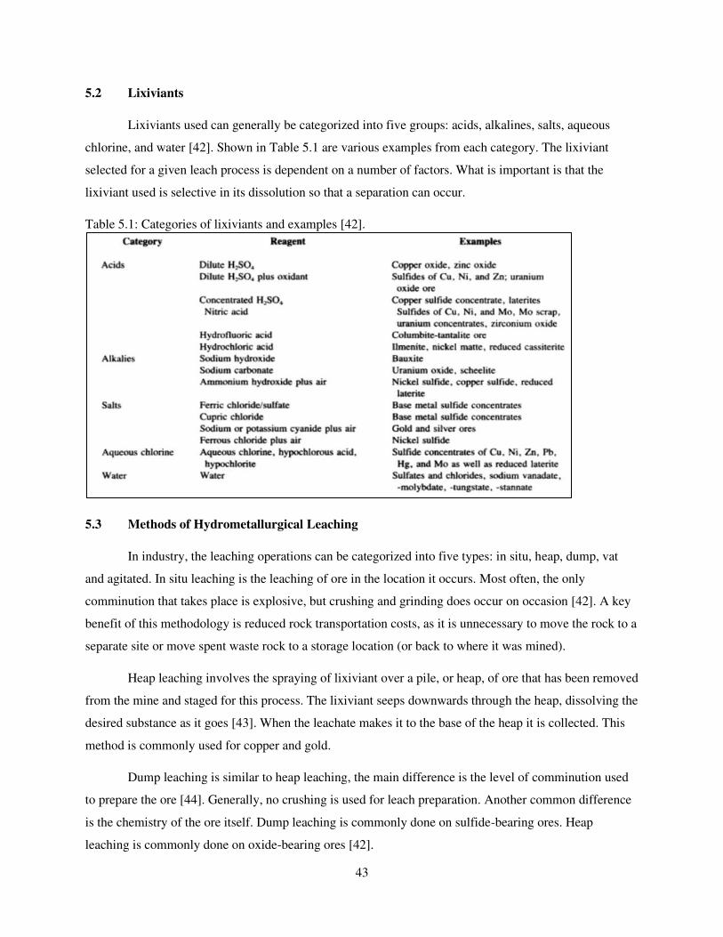
43

5.2 Lixiviants

Lixiviants used can generally be categorized into five groups: acids, alkalines, salts, aqueous

chlorine, and water [42]. Shown in Table 5.1 are various examples from each category. The lixiviant

selected for a given leach process is dependent on a number of factors. What is important is that the

lixiviant used is selective in its dissolution so that a separation can occur.

Table 5.1: Categories of lixiviants and examples [42].

5.3 Methods of Hydrometallurgical Leaching

In industry, the leaching operations can be categorized into five types: in situ, heap, dump, vat

and agitated. In situ leaching is the leaching of ore in the location it occurs. Most often, the only

comminution that takes place is explosive, but crushing and grinding does occur on occasion [42]. A key

benefit of this methodology is reduced rock transportation costs, as it is unnecessary to move the rock to a

separate site or move spent waste rock to a storage location (or back to where it was mined).

Heap leaching involves the spraying of lixiviant over a pile, or heap, of ore that has been removed

from the mine and staged for this process. The lixiviant seeps downwards through the heap, dissolving the

desired substance as it goes [43]. When the leachate makes it to the base of the heap it is collected. This

method is commonly used for copper and gold.

Dump leaching is similar to heap leaching, the main difference is the level of comminution used

to prepare the ore [44]. Generally, no crushing is used for leach preparation. Another common difference

is the chemistry of the ore itself. Dump leaching is commonly done on sulfide-bearing ores. Heap

leaching is commonly done on oxide-bearing ores [42].

44

Vat leaching involves completely or mostly submerging comminuted ore in lixiviant. This

method is known for excellent contact between the lixiviant and the ore being leached. In vat leaching,

the ore is commonly stationary, with the lixiviant being introduced and removed in stages [42]. This can

be done in a continuous or batch process and either pressurized or non-pressurized.

Agitated leaching is generally done in situations where interaction between particles of ore and

lixiviant is not possible without some physical force causing movement of ore particles. Generally, the

ore particles are suspended in the lixiviant by either an impeller or gasses being bubbled through the

solution [42]. This can be either a batch or continuous process and either pressurized or non-pressurized.

In this research, all leach tests are batch agitated leach tests.

45

CHAPTER 6. POURBAIX DIAGRAMS

A Pourbaix diagram, also referred to as Eh – pH diagrams, are diagrams that show the regions of

electro-potential and acidity/alkalinity where particular phases are thermodynamically stable. These

diagrams provide the ability to predict what conditions are likely cause a soluble or aqueous phase to

form. Therefore, they are useful in predicting which leaching conditions are likely to cause a given

substance to transfer to the aqueous phase during leaching and what conditions may result in any desired

separations. It should be noted that these diagrams do not consider the effect of kinetics and therefore

only indicate the equilibrium state of a given system. They do not indicate the potential to form any

metastable phases or the time necessary for equilibrium to occur [45].

Generation of an Eh – pH diagram requires knowledge of the Gibbs free energy associated with

all possible phases of a given system. Thermodynamic data often varies among databases, because of this

Eh – pH diagrams generated from different databases often conflict.

Other than Eh and pH, variables that affect a Pourbaix diagram are temperature, pressure, and

concentrations of the involved species. Generally, these variables are kept at 25 °C, atmospheric pressure

and molalites of around 10-6.

The stability of water is an important factor in many industrial processes and often provides the

practical upper and lower bounds for many process variables. On the Pourbaix diagrams contained herein,

the upper and lower limits of water stability are indicated by diagonal dashed lines. The upper limit is

represented by Equation 6.1 and the lower limit is represented by Equation 6.2. 2𝐻2𝑂 → 𝑂2 + 4𝐻+ + 4𝑒− (6.1) 2𝐻2𝑂 + 2𝑒− → 𝐻2 + 2𝑂𝐻− (6.2)

All Eh – pH diagrams presented in this section were generated using Materials Project Pourbaix

Diagram software, StabCal, and/or the Atlas of Electrochemical Equilibria in Aqueous Solutions. Unless

otherwise stated, the temperature associated with all Eh – pH diagrams is 25 °C, the pressure is 1 atm and

the molality is 0.000001.

6.1 Indium Pourbaix Diagram

Shown below in Figure 6.1 is an Eh – pH diagram for indium. It can be seen that in strongly

reducing conditions, metallic indium is the dominant phase across the entire pH range. In moderate pH

ranges of 4.5 to 12, insoluble In2O3 forms in non-reducing conditions. Increasing alkalinity or acidity in

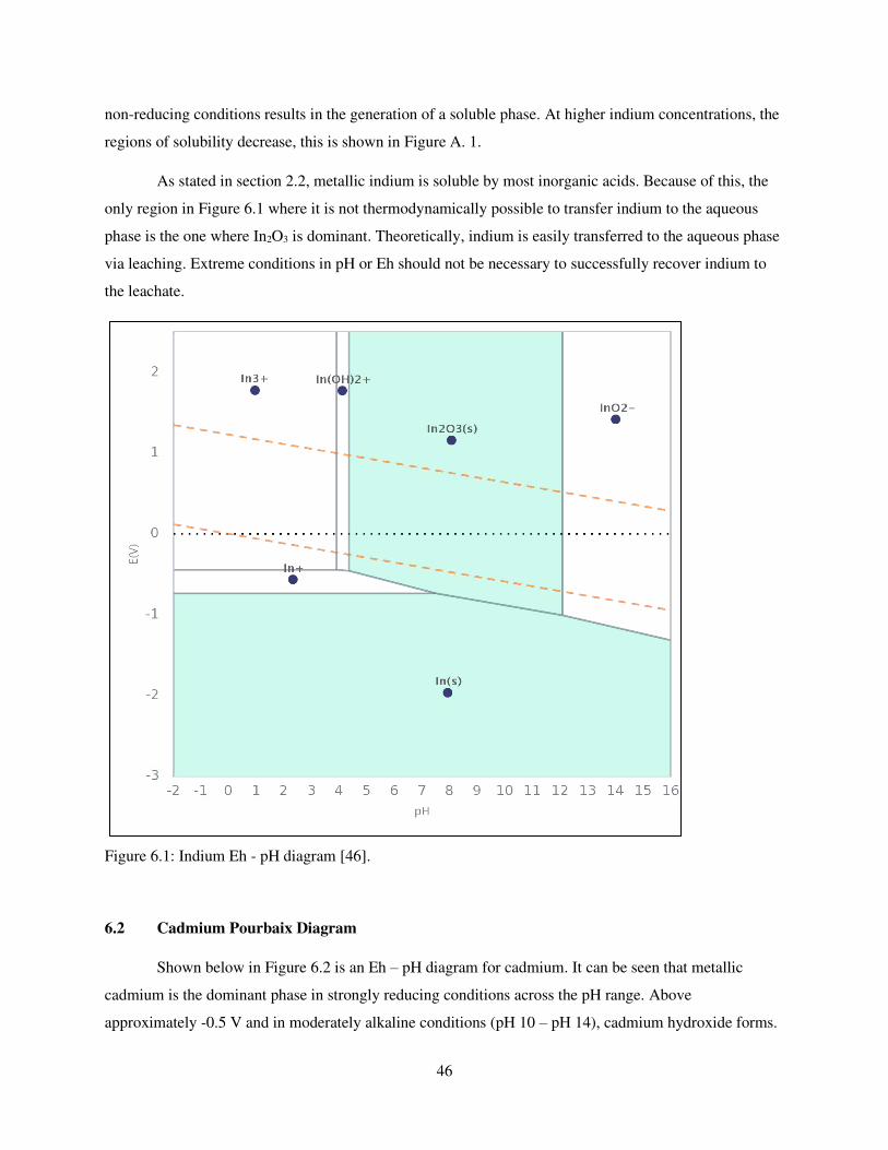
46

non-reducing conditions results in the generation of a soluble phase. At higher indium concentrations, the

regions of solubility decrease, this is shown in Figure A. 1.

As stated in section 2.2, metallic indium is soluble by most inorganic acids. Because of this, the

only region in Figure 6.1 where it is not thermodynamically possible to transfer indium to the aqueous

phase is the one where In2O3 is dominant. Theoretically, indium is easily transferred to the aqueous phase

via leaching. Extreme conditions in pH or Eh should not be necessary to successfully recover indium to

the leachate.

Figure 6.1: Indium Eh - pH diagram [46].

6.2 Cadmium Pourbaix Diagram

Shown below in Figure 6.2 is an Eh – pH diagram for cadmium. It can be seen that metallic

cadmium is the dominant phase in strongly reducing conditions across the pH range. Above

approximately -0.5 V and in moderately alkaline conditions (pH 10 – pH 14), cadmium hydroxide forms.

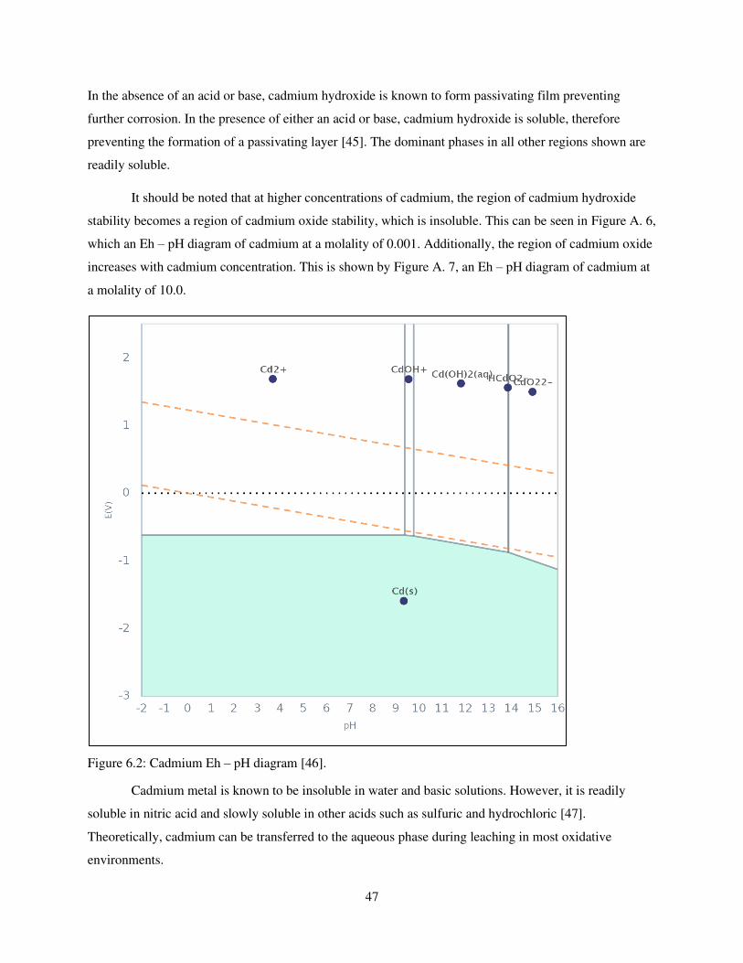
47

In the absence of an acid or base, cadmium hydroxide is known to form passivating film preventing

further corrosion. In the presence of either an acid or base, cadmium hydroxide is soluble, therefore

preventing the formation of a passivating layer [45]. The dominant phases in all other regions shown are

readily soluble.

It should be noted that at higher concentrations of cadmium, the region of cadmium hydroxide

stability becomes a region of cadmium oxide stability, which is insoluble. This can be seen in Figure A. 6,

which an Eh – pH diagram of cadmium at a molality of 0.001. Additionally, the region of cadmium oxide

increases with cadmium concentration. This is shown by Figure A. 7, an Eh – pH diagram of cadmium at

a molality of 10.0.

Figure 6.2: Cadmium Eh – pH diagram [46].

Cadmium metal is known to be insoluble in water and basic solutions. However, it is readily

soluble in nitric acid and slowly soluble in other acids such as sulfuric and hydrochloric [47].

Theoretically, cadmium can be transferred to the aqueous phase during leaching in most oxidative

environments.

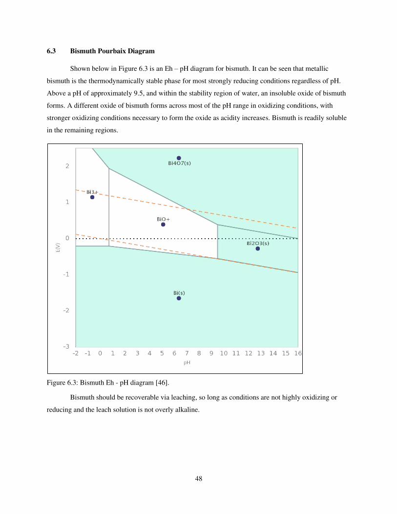
48

6.3 Bismuth Pourbaix Diagram

Shown below in Figure 6.3 is an Eh – pH diagram for bismuth. It can be seen that metallic

bismuth is the thermodynamically stable phase for most strongly reducing conditions regardless of pH.

Above a pH of approximately 9.5, and within the stability region of water, an insoluble oxide of bismuth

forms. A different oxide of bismuth forms across most of the pH range in oxidizing conditions, with

stronger oxidizing conditions necessary to form the oxide as acidity increases. Bismuth is readily soluble

in the remaining regions.

Figure 6.3: Bismuth Eh - pH diagram [46].

Bismuth should be recoverable via leaching, so long as conditions are not highly oxidizing or

reducing and the leach solution is not overly alkaline.

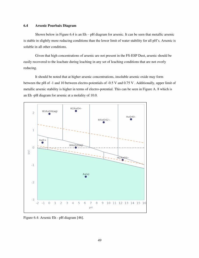
49

6.4 Arsenic Pourbaix Diagram

Shown below in Figure 6.4 is an Eh – pH diagram for arsenic. It can be seen that metallic arsenic

is stable in slightly more reducing conditions than the lower limit of water stability for all pH’s. Arsenic is

soluble in all other conditions.

Given that high concentrations of arsenic are not present in the FS-ESP Dust, arsenic should be

easily recovered to the leachate during leaching in any set of leaching conditions that are not overly

reducing.

It should be noted that at higher arsenic concentrations, insoluble arsenic oxide may form

between the pH of -1 and 10 between electro-potentials of -0.5 V and 0.75 V . Additionally, upper limit of

metallic arsenic stability is higher in terms of electro-potential. This can be seen in Figure A. 8 which is

an Eh -pH diagram for arsenic at a molality of 10.0.

Figure 6.4: Arsenic Eh - pH diagram [46].

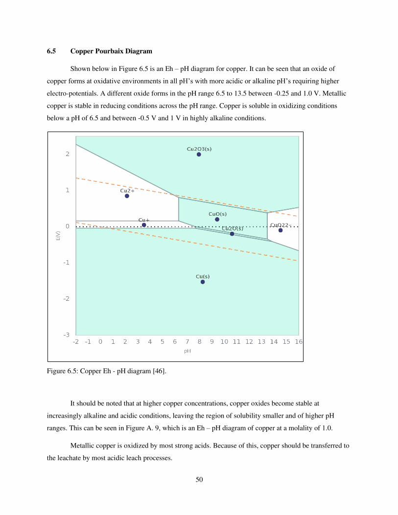
50

6.5 Copper Pourbaix Diagram

Shown below in Figure 6.5 is an Eh – pH diagram for copper. It can be seen that an oxide of

copper forms at oxidative environments in all pH’s with more acidic or alkaline pH’s requiring higher

electro-potentials. A different oxide forms in the pH range 6.5 to 13.5 between -0.25 and 1.0 V. Metallic

copper is stable in reducing conditions across the pH range. Copper is soluble in oxidizing conditions

below a pH of 6.5 and between -0.5 V and 1 V in highly alkaline conditions.

Figure 6.5: Copper Eh - pH diagram [46].

It should be noted that at higher copper concentrations, copper oxides become stable at

increasingly alkaline and acidic conditions, leaving the region of solubility smaller and of higher pH

ranges. This can be seen in Figure A. 9, which is an Eh – pH diagram of copper at a molality of 1.0.

Metallic copper is oxidized by most strong acids. Because of this, copper should be transferred to

the leachate by most acidic leach processes.

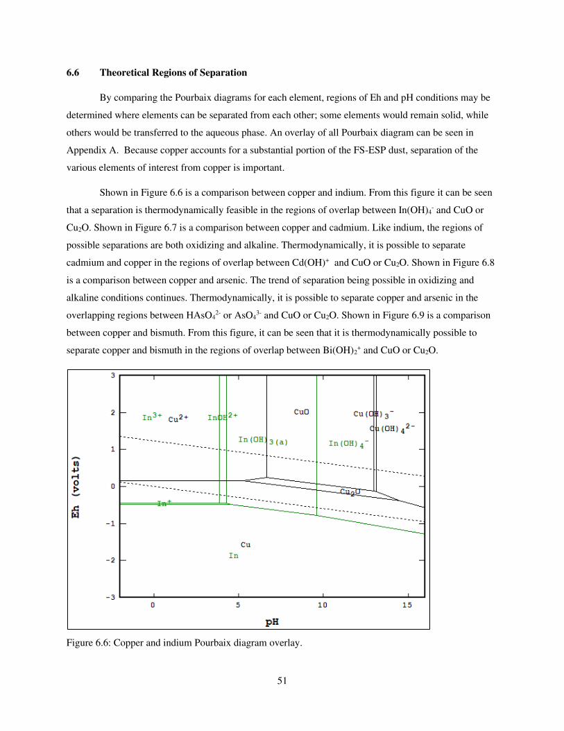
51

6.6 Theoretical Regions of Separation

By comparing the Pourbaix diagrams for each element, regions of Eh and pH conditions may be

determined where elements can be separated from each other; some elements would remain solid, while

others would be transferred to the aqueous phase. An overlay of all Pourbaix diagram can be seen in

Appendix A. Because copper accounts for a substantial portion of the FS-ESP dust, separation of the

various elements of interest from copper is important.

Shown in Figure 6.6 is a comparison between copper and indium. From this figure it can be seen

that a separation is thermodynamically feasible in the regions of overlap between In(OH)4- and CuO or

Cu2O. Shown in Figure 6.7 is a comparison between copper and cadmium. Like indium, the regions of

possible separations are both oxidizing and alkaline. Thermodynamically, it is possible to separate

cadmium and copper in the regions of overlap between Cd(OH)+ and CuO or Cu2O. Shown in Figure 6.8

is a comparison between copper and arsenic. The trend of separation being possible in oxidizing and

alkaline conditions continues. Thermodynamically, it is possible to separate copper and arsenic in the

overlapping regions between HAsO42- or AsO4

3- and CuO or Cu2O. Shown in Figure 6.9 is a comparison

between copper and bismuth. From this figure, it can be seen that it is thermodynamically possible to

separate copper and bismuth in the regions of overlap between Bi(OH)2+ and CuO or Cu2O.

Figure 6.6: Copper and indium Pourbaix diagram overlay.

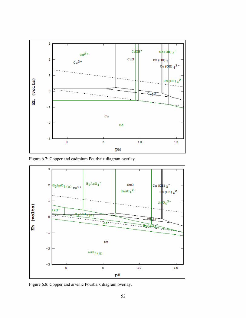
52

Figure 6.7: Copper and cadmium Pourbaix diagram overlay.

Figure 6.8: Copper and arsenic Pourbaix diagram overlay.

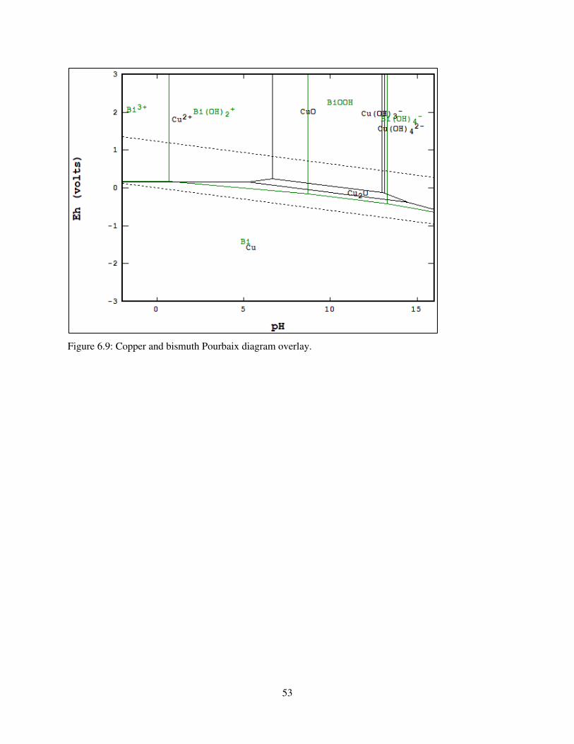
53

Figure 6.9: Copper and bismuth Pourbaix diagram overlay.

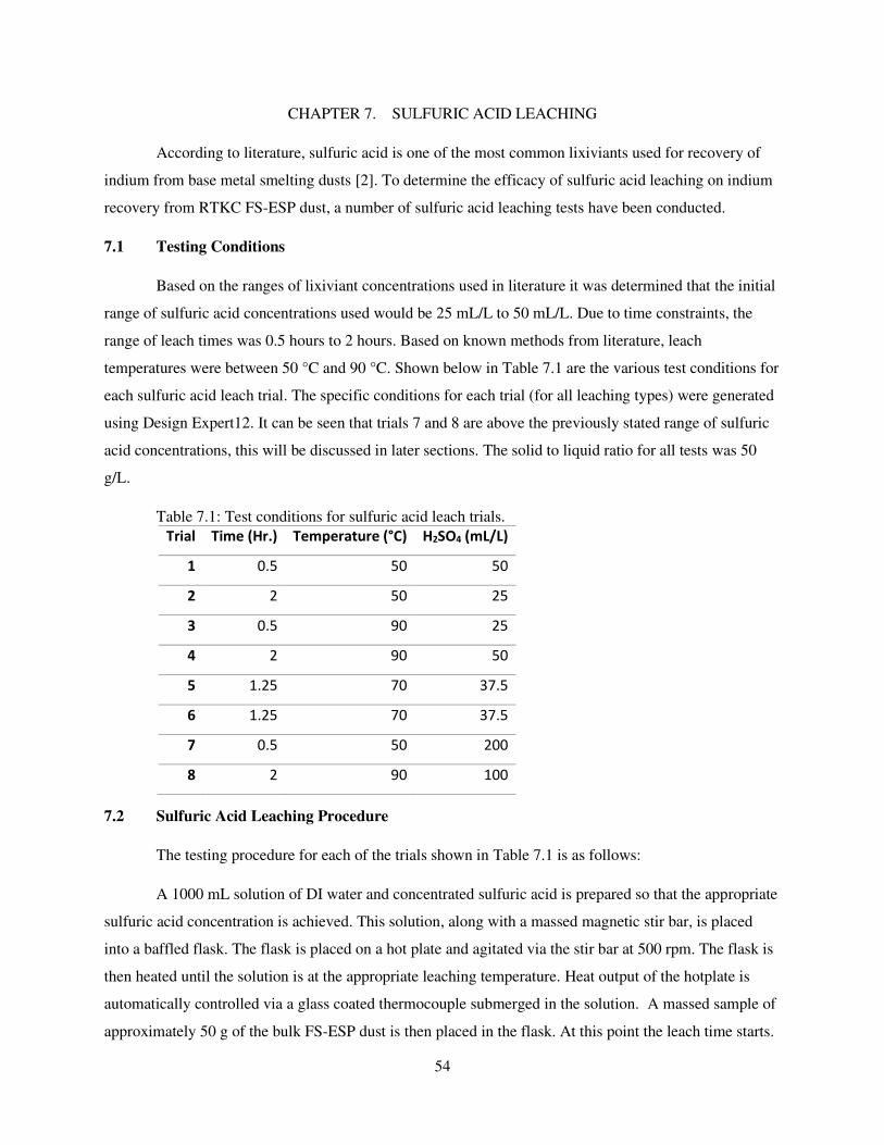
54

CHAPTER 7. SULFURIC ACID LEACHING

According to literature, sulfuric acid is one of the most common lixiviants used for recovery of

indium from base metal smelting dusts [2]. To determine the efficacy of sulfuric acid leaching on indium

recovery from RTKC FS-ESP dust, a number of sulfuric acid leaching tests have been conducted.

7.1 Testing Conditions

Based on the ranges of lixiviant concentrations used in literature it was determined that the initial

range of sulfuric acid concentrations used would be 25 mL/L to 50 mL/L. Due to time constraints, the

range of leach times was 0.5 hours to 2 hours. Based on known methods from literature, leach

temperatures were between 50 °C and 90 °C. Shown below in Table 7.1 are the various test conditions for

each sulfuric acid leach trial. The specific conditions for each trial (for all leaching types) were generated

using Design Expert12. It can be seen that trials 7 and 8 are above the previously stated range of sulfuric

acid concentrations, this will be discussed in later sections. The solid to liquid ratio for all tests was 50

g/L.

Table 7.1: Test conditions for sulfuric acid leach trials.

Trial Time (Hr.) Temperature (°C) H2SO4 (mL/L)

1 0.5 50 50

2 2 50 25

3 0.5 90 25

4 2 90 50

5 1.25 70 37.5

6 1.25 70 37.5

7 0.5 50 200

8 2 90 100

7.2 Sulfuric Acid Leaching Procedure

The testing procedure for each of the trials shown in Table 7.1 is as follows:

A 1000 mL solution of DI water and concentrated sulfuric acid is prepared so that the appropriate

sulfuric acid concentration is achieved. This solution, along with a massed magnetic stir bar, is placed

into a baffled flask. The flask is placed on a hot plate and agitated via the stir bar at 500 rpm. The flask is

then heated until the solution is at the appropriate leaching temperature. Heat output of the hotplate is

automatically controlled via a glass coated thermocouple submerged in the solution. A massed sample of

approximately 50 g of the bulk FS-ESP dust is then placed in the flask. At this point the leach time starts.

55

Upon the completion of the leach time, the flask is removed from the hot plate and the remaining solids

separated from the liquids via a massed filter. Once solid – liquid separation is concluded, the leachate is

stored and the residue is allowed to dry and then stored.

7.3 Preparation of Sulfuric Acid Leachate Samples for Analysis

All leachates from sulfuric acid leach testing were analyzed using ICP-MS and atomic absorption

spectroscopy (AAS). The methods used to prepare the samples for analysis is described.

7.3.1 ICP-MS Preparation

Given that the leachates are already aqueous, the only preparation necessary for ICP-MS analysis

is dilution so that the TDS is below the upper limit specified by the ICP-MS machine used. In most cases,

this is a dilution with 2% nitric acid to a TDS below 200 ppm. That being said, some leachate samples

were sent out for third party analysis, in which case the leachates were sent out with no dilution. The

party doing the analysis performed their own preparation according to their own procedures.

7.3.2 AAS Preparation

Like preparation for ICP-MS, the only preparation necessary for analysis is dilution. Unlike ICP-

MS, the dilution is not to a TDS below the upper limit set by the ICP-MS machine. It is so that the

element being analyzed is of a concentration that is within the range set by the standards used for

calibration of the AAS machine.

In this case, the element being analyzed is copper, and the range of Cu concentrations used in

calibration standards is 5 ppm Cu to 100 ppm Cu. Given the copper concentration in the FS-ESP dust is

approximately 21.70% or 217,000 ppm, 100% copper recovery to the leachate would give a copper

concentration in the leachate of approximately 11,000 ppm. A 110X dilution of leachate containing

11,000 ppm copper would result in the diluted solution having 100 ppm copper, the upper limit set by the

calibration standards. Because of this, a 110X dilution with 2% hydrochloric acid was used for

preparation of leachate for AAS analysis.

7.4 Sulfuric Acid AAS and ICP-MS Data

Shown below in Table 7.2 is the AAS and ICP-MS data for the leachates generated from the trials

shown in Table 7.1. The “readout” value is the value the machine detected in the diluted sample. The

“actual” value is the calculated concentration in the undiluted leachate based on the dilution factor. It

should be noted that ICP-MS dilution factors and readout values for trials 7 and 8 are not available. This

is because ICP-MS analysis of these leachates was conducted by SGS.

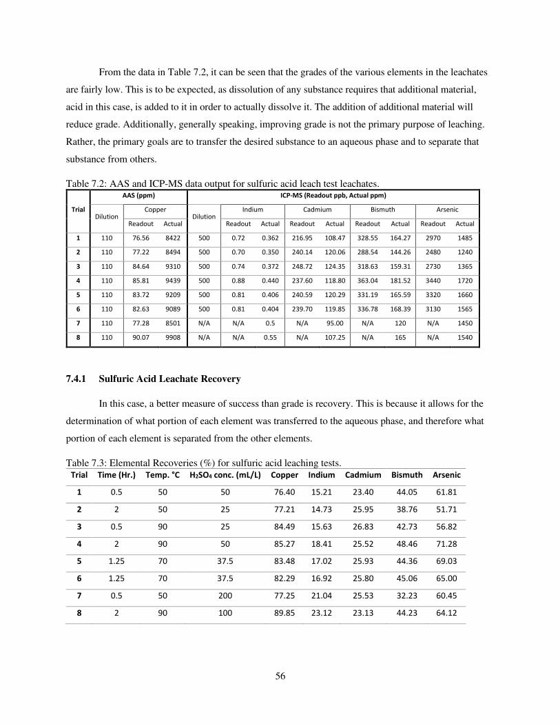
56

From the data in Table 7.2, it can be seen that the grades of the various elements in the leachates

are fairly low. This is to be expected, as dissolution of any substance requires that additional material,

acid in this case, is added to it in order to actually dissolve it. The addition of additional material will

reduce grade. Additionally, generally speaking, improving grade is not the primary purpose of leaching.

Rather, the primary goals are to transfer the desired substance to an aqueous phase and to separate that

substance from others.

Table 7.2: AAS and ICP-MS data output for sulfuric acid leach test leachates.

Trial

AAS (ppm) ICP-MS (Readout ppb, Actual ppm)

Dilution Copper

Dilution Indium Cadmium Bismuth Arsenic

Readout Actual Readout Actual Readout Actual Readout Actual Readout Actual

1 110 76.56 8422 500 0.72 0.362 216.95 108.47 328.55 164.27 2970 1485

2 110 77.22 8494 500 0.70 0.350 240.14 120.06 288.54 144.26 2480 1240

3 110 84.64 9310 500 0.74 0.372 248.72 124.35 318.63 159.31 2730 1365

4 110 85.81 9439 500 0.88 0.440 237.60 118.80 363.04 181.52 3440 1720

5 110 83.72 9209 500 0.81 0.406 240.59 120.29 331.19 165.59 3320 1660

6 110 82.63 9089 500 0.81 0.404 239.70 119.85 336.78 168.39 3130 1565

7 110 77.28 8501 N/A N/A 0.5 N/A 95.00 N/A 120 N/A 1450

8 110 90.07 9908 N/A N/A 0.55 N/A 107.25 N/A 165 N/A 1540

7.4.1 Sulfuric Acid Leachate Recovery

In this case, a better measure of success than grade is recovery. This is because it allows for the

determination of what portion of each element was transferred to the aqueous phase, and therefore what

portion of each element is separated from the other elements.

Table 7.3: Elemental Recoveries (%) for sulfuric acid leaching tests.

Trial Time (Hr.) Temp. °C H2SO4 conc. (mL/L) Copper Indium Cadmium Bismuth Arsenic

1 0.5 50 50 76.40 15.21 23.40 44.05 61.81

2 2 50 25 77.21 14.73 25.95 38.76 51.71

3 0.5 90 25 84.49 15.63 26.83 42.73 56.82

4 2 90 50 85.27 18.41 25.52 48.46 71.28

5 1.25 70 37.5 83.48 17.02 25.93 44.36 69.03

6 1.25 70 37.5 82.29 16.92 25.80 45.06 65.00

7 0.5 50 200 77.25 21.04 25.53 32.23 60.45

8 2 90 100 89.85 23.12 23.13 44.23 64.12

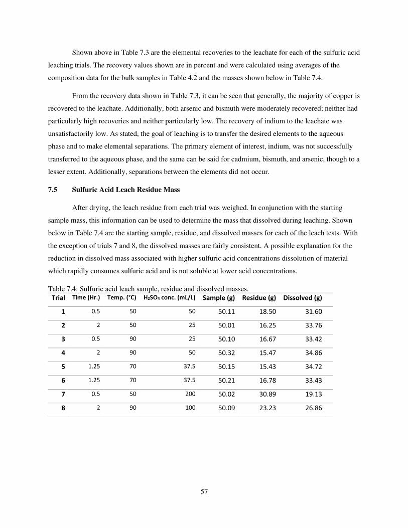
57

Shown above in Table 7.3 are the elemental recoveries to the leachate for each of the sulfuric acid

leaching trials. The recovery values shown are in percent and were calculated using averages of the

composition data for the bulk samples in Table 4.2 and the masses shown below in Table 7.4.

From the recovery data shown in Table 7.3, it can be seen that generally, the majority of copper is

recovered to the leachate. Additionally, both arsenic and bismuth were moderately recovered; neither had

particularly high recoveries and neither particularly low. The recovery of indium to the leachate was

unsatisfactorily low. As stated, the goal of leaching is to transfer the desired elements to the aqueous

phase and to make elemental separations. The primary element of interest, indium, was not successfully

transferred to the aqueous phase, and the same can be said for cadmium, bismuth, and arsenic, though to a

lesser extent. Additionally, separations between the elements did not occur.

7.5 Sulfuric Acid Leach Residue Mass

After drying, the leach residue from each trial was weighed. In conjunction with the starting

sample mass, this information can be used to determine the mass that dissolved during leaching. Shown

below in Table 7.4 are the starting sample, residue, and dissolved masses for each of the leach tests. With

the exception of trials 7 and 8, the dissolved masses are fairly consistent. A possible explanation for the

reduction in dissolved mass associated with higher sulfuric acid concentrations dissolution of material

which rapidly consumes sulfuric acid and is not soluble at lower acid concentrations.

Table 7.4: Sulfuric acid leach sample, residue and dissolved masses.

Trial Time (Hr.) Temp. (°C) H2SO4 conc. (mL/L) Sample (g) Residue (g) Dissolved (g)

1 0.5 50 50 50.11 18.50 31.60

2 2 50 25 50.01 16.25 33.76

3 0.5 90 25 50.10 16.67 33.42

4 2 90 50 50.32 15.47 34.86

5 1.25 70 37.5 50.15 15.43 34.72

6 1.25 70 37.5 50.21 16.78 33.43

7 0.5 50 200 50.02 30.89 19.13

8 2 90 100 50.09 23.23 26.86

58

7.6 Sulfuric Acid Consumption

Determination of sulfuric acid consumption for each leach test allows for a better understanding

of how much acid is necessary for optimal leaching, what substances require higher free acid, what the

rate of acid consumption over time is, etc.

7.6.1 Free Acid Titration Procedure

The procedure for determining free acid via titration is to dilute a 5 mL sample of leachate with

approximately 45 mL of DI water. To this, approximately 5 mL of 20 wt. % sodium thiosulfate and 1 mL

of 0.5g/L methyl orange. The sodium thiosulfate prevents interference from iron and the methyl orange is

the color changing indicator. This solution is then titrated with 1.0 N sodium carbonate. The end point is a

yellow/orange solution. Free sulfuric acid concentration in g/L is then determined by Equation 7.1.

𝐹𝑟𝑒𝑒 𝐻2𝑆𝑂4 = (𝑡𝑖𝑡𝑟𝑎𝑛𝑡 𝑛𝑜𝑟𝑚𝑎𝑙𝑖𝑡𝑦)(𝑚𝐿 𝑡𝑖𝑡𝑟𝑎𝑛𝑡)(49)(𝑚𝐿 𝑠𝑎𝑚𝑝𝑙𝑒) (7.1)

𝑡𝑖𝑡𝑟𝑎𝑡 𝑛𝑜𝑚𝑎𝑙𝑖𝑡𝑦 ≈ 1.0 𝑁 𝑚𝐿 𝑠𝑎𝑚𝑝𝑙𝑒 ≈ 5.0 𝑚𝐿

7.6.2 Sulfuric Acid Consumption Data

Using free H2SO4 data generated from titration and Equation 7.1 the ending sulfuric acid molarity

was calculated. The starting molarity was calculated using the mass of sulfuric acid added to the starting

leach solutions and Equation 7.2. Shown in Table 7.5 are the starting and ending sulfuric acid molarities

for each trial in Table 7.1.

𝑀𝑖 = 𝑔 𝐻2𝑆𝑂4𝑉(𝐻2𝑆𝑂4 𝑚𝑜𝑙𝑎𝑟 𝑚𝑎𝑠𝑠) (7.2)

𝑀𝑖 = 𝑖𝑛𝑖𝑡𝑖𝑎𝑙 𝑚𝑜𝑙𝑎𝑟𝑖𝑡𝑦 𝑉 = 𝑣𝑜𝑙𝑢𝑚𝑒 𝐻2𝑆𝑂4 𝑚𝑜𝑙𝑎𝑟 𝑚𝑎𝑠𝑠 = 98.079 𝑔𝑚𝑜𝑙 It can be seen from Table 7.5 that the ending sulfuric acid concentration does not vary greatly

based on the starting concentration. It is possible this is due to the majority of the acid being consumed by

the copper contained in the dust, and by the time sufficient copper has been dissolved to allow for

dissolution of indium, the conditions are no longer sufficiently acidic to dissolve the majority of the

indium. To test this theory two additional trials were conducted, trials 7 and 8. As shown in Table 7.3,

both trials 7 and 8 showed additional recoveries relative to the other trials, giving some credence to this

hypothesis.

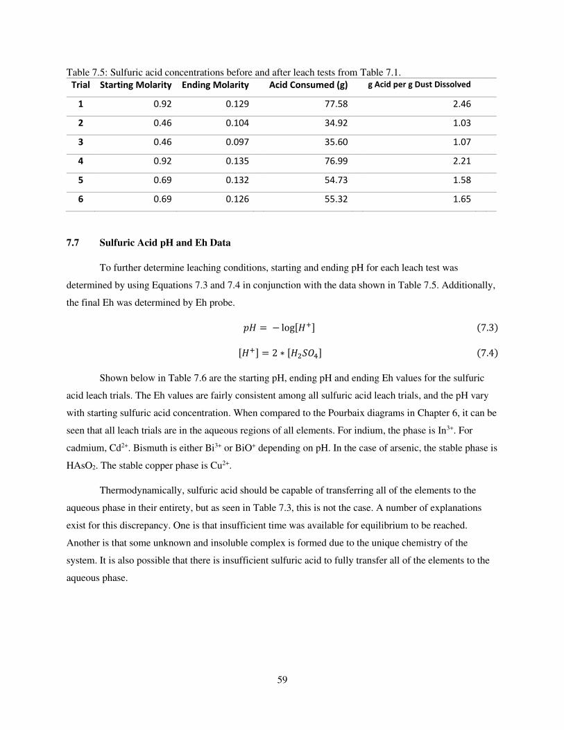
59

Table 7.5: Sulfuric acid concentrations before and after leach tests from Table 7.1.

Trial Starting Molarity Ending Molarity Acid Consumed (g) g Acid per g Dust Dissolved

1 0.92 0.129 77.58 2.46

2 0.46 0.104 34.92 1.03

3 0.46 0.097 35.60 1.07

4 0.92 0.135 76.99 2.21

5 0.69 0.132 54.73 1.58

6 0.69 0.126 55.32 1.65

7.7 Sulfuric Acid pH and Eh Data

To further determine leaching conditions, starting and ending pH for each leach test was

determined by using Equations 7.3 and 7.4 in conjunction with the data shown in Table 7.5. Additionally,

the final Eh was determined by Eh probe. 𝑝𝐻 = − log[𝐻+] (7.3) [𝐻+] = 2 ∗ [𝐻2𝑆𝑂4] (7.4)

Shown below in Table 7.6 are the starting pH, ending pH and ending Eh values for the sulfuric

acid leach trials. The Eh values are fairly consistent among all sulfuric acid leach trials, and the pH vary

with starting sulfuric acid concentration. When compared to the Pourbaix diagrams in Chapter 6, it can be

seen that all leach trials are in the aqueous regions of all elements. For indium, the phase is In3+. For

cadmium, Cd2+. Bismuth is either Bi3+ or BiO+ depending on pH. In the case of arsenic, the stable phase is

HAsO2. The stable copper phase is Cu2+.

Thermodynamically, sulfuric acid should be capable of transferring all of the elements to the

aqueous phase in their entirety, but as seen in Table 7.3, this is not the case. A number of explanations

exist for this discrepancy. One is that insufficient time was available for equilibrium to be reached.

Another is that some unknown and insoluble complex is formed due to the unique chemistry of the

system. It is also possible that there is insufficient sulfuric acid to fully transfer all of the elements to the

aqueous phase.

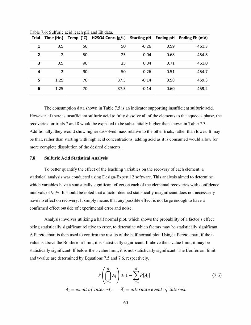
60

Table 7.6: Sulfuric acid leach pH and Eh data.

Trial Time (Hr.) Temp. (°C) H2SO4 Conc. (g/L) Starting pH Ending pH Ending Eh (mV)

1 0.5 50 50 -0.26 0.59 461.3

2 2 50 25 0.04 0.68 454.8

3 0.5 90 25 0.04 0.71 451.0

4 2 90 50 -0.26 0.51 454.7

5 1.25 70 37.5 -0.14 0.58 459.3

6 1.25 70 37.5 -0.14 0.60 459.2

The consumption data shown in Table 7.5 is an indicator supporting insufficient sulfuric acid.

However, if there is insufficient sulfuric acid to fully dissolve all of the elements to the aqueous phase, the

recoveries for trials 7 and 8 would be expected to be substantially higher than shown in Table 7.3.

Additionally, they would show higher dissolved mass relative to the other trials, rather than lower. It may

be that, rather than starting with high acid concentrations, adding acid as it is consumed would allow for

more complete dissolution of the desired elements.

7.8 Sulfuric Acid Statistical Analysis

To better quantify the effect of the leaching variables on the recovery of each element, a

statistical analysis was conducted using Design-Expert 12 software. This analysis aimed to determine

which variables have a statistically significant effect on each of the elemental recoveries with confidence

intervals of 95%. It should be noted that a factor deemed statistically insignificant does not necessarily

have no effect on recovery. It simply means that any possible effect is not large enough to have a

confirmed effect outside of experimental error and noise.

Analysis involves utilizing a half normal plot, which shows the probability of a factor’s effect

being statistically significant relative to error, to determine which factors may be statistically significant.

A Pareto chart is then used to confirm the results of the half normal plot. Using a Pareto chart, if the t-

value is above the Bonferroni limit, it is statistically significant. If above the t-value limit, it may be

statistically significant. If below the t-value limit, it is not statistically significant. The Bonferroni limit

and t-value are determined by Equations 7.5 and 7.6, respectively.

𝑃 (⋂ 𝐴𝑖𝑔𝑖=1 ) ≥ 1 − ∑ 𝑃[�̅�𝑖]𝑔

𝑖=1 (7.5)

𝐴𝑖 = 𝑒𝑣𝑒𝑛𝑡 𝑜𝑓 𝑖𝑛𝑡𝑒𝑟𝑒𝑠𝑡, 𝐴�̅� = 𝑎𝑙𝑡𝑒𝑟𝑛𝑎𝑡𝑒 𝑒𝑣𝑒𝑛𝑡 𝑜𝑓 𝑖𝑛𝑡𝑒𝑟𝑒𝑠𝑡

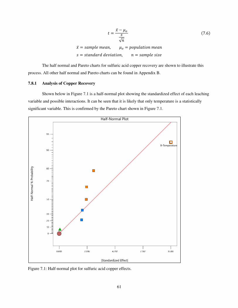
61

𝑡 = �̅� − 𝜇𝑜𝑠√𝑛 (7.6)

�̅� = 𝑠𝑎𝑚𝑝𝑙𝑒 𝑚𝑒𝑎𝑛, 𝜇𝑜 = 𝑝𝑜𝑝𝑢𝑙𝑎𝑡𝑖𝑜𝑛 𝑚𝑒𝑎𝑛 𝑠 = 𝑠𝑡𝑎𝑛𝑑𝑎𝑟𝑑 𝑑𝑒𝑣𝑖𝑎𝑡𝑖𝑜𝑛, 𝑛 = 𝑠𝑎𝑚𝑝𝑙𝑒 𝑠𝑖𝑧𝑒

The half normal and Pareto charts for sulfuric acid copper recovery are shown to illustrate this

process. All other half normal and Pareto charts can be found in Appendix B.

7.8.1 Analysis of Copper Recovery

Shown below in Figure 7.1 is a half-normal plot showing the standardized effect of each leaching

variable and possible interactions. It can be seen that it is likely that only temperature is a statistically

significant variable. This is confirmed by the Pareto chart shown in Figure 7.1.

Figure 7.1: Half-normal plot for sulfuric acid copper effects.

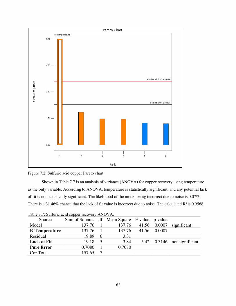
62

Figure 7.2: Sulfuric acid copper Pareto chart.

Shown in Table 7.7 is an analysis of variance (ANOVA) for copper recovery using temperature

as the only variable. According to ANOVA, temperature is statistically significant, and any potential lack

of fit is not statistically significant. The likelihood of the model being incorrect due to noise is 0.07%.

There is a 31.46% chance that the lack of fit value is incorrect due to noise. The calculated R2 is 0.9568.

Table 7.7: Sulfuric acid copper recovery ANOVA.

Source Sum of Squares df Mean Square F-value p-value

Model 137.76 1 137.76 41.56 0.0007 significant

B-Temperature 137.76 1 137.76 41.56 0.0007

Residual 19.89 6 3.31

Lack of Fit 19.18 5 3.84 5.42 0.3146 not significant

Pure Error 0.7080 1 0.7080

Cor Total 157.65 7

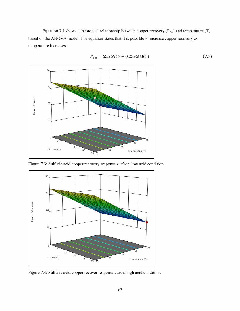
63

Equation 7.7 shows a theoretical relationship between copper recovery (RCu) and temperature (T)

based on the ANOVA model. The equation states that it is possible to increase copper recovery as

temperature increases. 𝑅𝐶𝑢 = 65.25917 + 0.239583(𝑇) (7.7)

Figure 7.3: Sulfuric acid copper recovery response surface, low acid condition.

Figure 7.4: Sulfuric acid copper recover response curve, high acid condition.

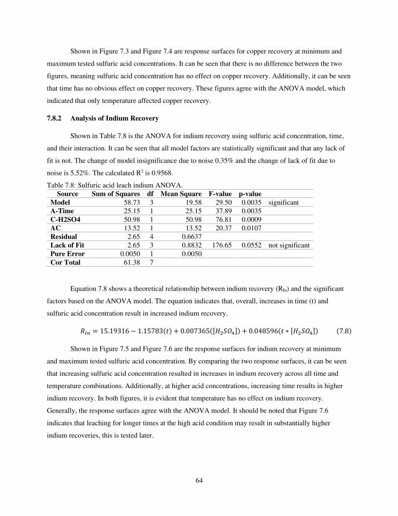
64

Shown in Figure 7.3 and Figure 7.4 are response surfaces for copper recovery at minimum and

maximum tested sulfuric acid concentrations. It can be seen that there is no difference between the two

figures, meaning sulfuric acid concentration has no effect on copper recovery. Additionally, it can be seen

that time has no obvious effect on copper recovery. These figures agree with the ANOVA model, which

indicated that only temperature affected copper recovery.

7.8.2 Analysis of Indium Recovery

Shown in Table 7.8 is the ANOVA for indium recovery using sulfuric acid concentration, time,

and their interaction. It can be seen that all model factors are statistically significant and that any lack of

fit is not. The change of model insignificance due to noise 0.35% and the change of lack of fit due to

noise is 5.52%. The calculated R2 is 0.9568.

Table 7.8: Sulfuric acid leach indium ANOVA.



A-Time 25.15 1 25.15 37.89 0.0035

C-H2SO4 50.98 1 50.98 76.81 0.0009

AC 13.52 1 13.52 20.37 0.0107

Residual 2.65 4 0.6637


Pure Error 0.0050 1 0.0050

Cor Total 61.38 7

Equation 7.8 shows a theoretical relationship between indium recovery (RIn) and the significant

factors based on the ANOVA model. The equation indicates that, overall, increases in time (t) and

sulfuric acid concentration result in increased indium recovery. 𝑅𝐼𝑛 = 15.19316 − 1.15783(𝑡) + 0.007365([𝐻2𝑆𝑂4]) + 0.048596(𝑡 ∗ [𝐻2𝑆𝑂4]) (7.8)

Shown in Figure 7.5 and Figure 7.6 are the response surfaces for indium recovery at minimum

and maximum tested sulfuric acid concentration. By comparing the two response surfaces, it can be seen

that increasing sulfuric acid concentration resulted in increases in indium recovery across all time and

temperature combinations. Additionally, at higher acid concentrations, increasing time results in higher

indium recovery. In both figures, it is evident that temperature has no effect on indium recovery.

Generally, the response surfaces agree with the ANOVA model. It should be noted that Figure 7.6

indicates that leaching for longer times at the high acid condition may result in substantially higher

indium recoveries, this is tested later.

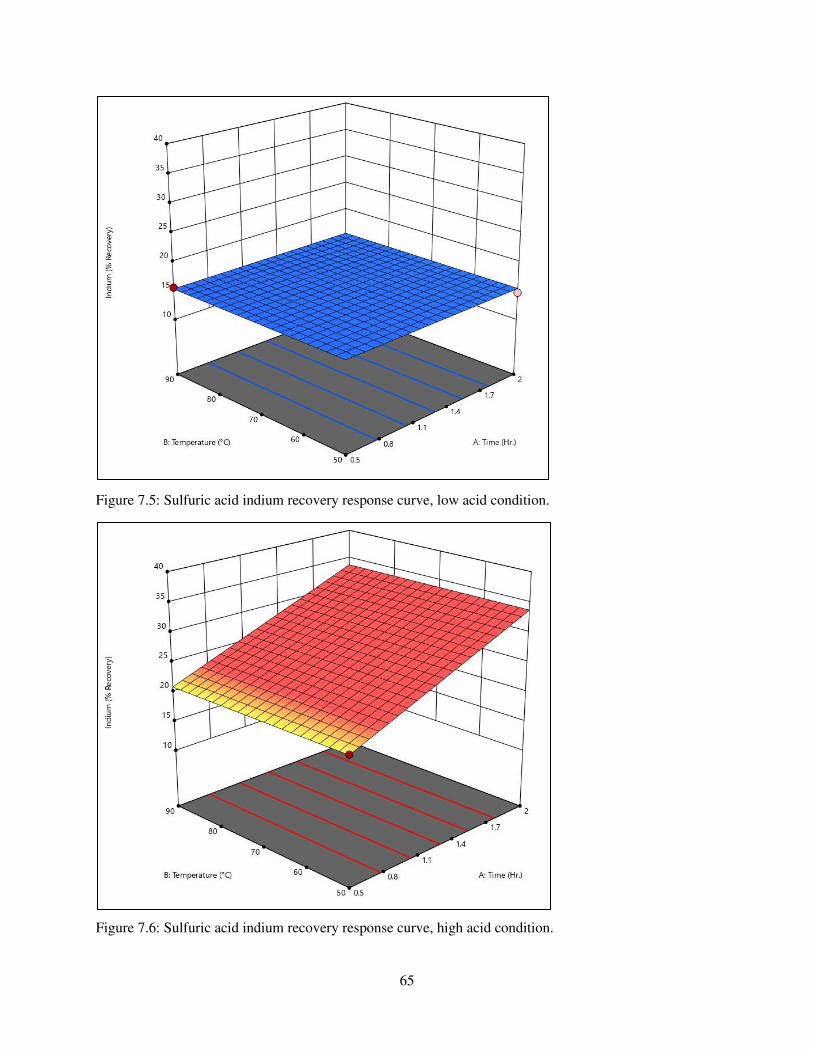
65

Figure 7.5: Sulfuric acid indium recovery response curve, low acid condition.

Figure 7.6: Sulfuric acid indium recovery response curve, high acid condition.

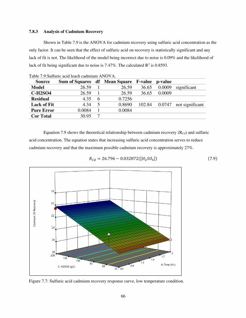
66

7.8.3 Analysis of Cadmium Recovery

Shown in Table 7.9 is the ANOVA for cadmium recovery using sulfuric acid concentration as the

only factor. It can be seen that the effect of sulfuric acid on recovery is statistically significant and any

lack of fit is not. The likelihood of the model being incorrect due to noise is 0.09% and the likelihood of

lack of fit being significant due to noise is 7.47%. The calculated R2 is 0.8593.

Table 7.9:Sulfuric acid leach cadmium ANOVA.



C-H2SO4 26.59 1 26.59 36.65 0.0009

Residual 4.35 6 0.7256


Pure Error 0.0084 1 0.0084

Cor Total 30.95 7

Equation 7.9 shows the theoretical relationship between cadmium recovery (RCd) and sulfuric

acid concentration. The equation states that increasing sulfuric acid concentration serves to reduce

cadmium recovery and that the maximum possible cadmium recovery is approximately 27%. 𝑅𝐶𝑑 = 26.796 − 0.032872([𝐻2𝑆𝑂4]) (7.9)

Figure 7.7: Sulfuric acid cadmium recovery response curve, low temperature condition.

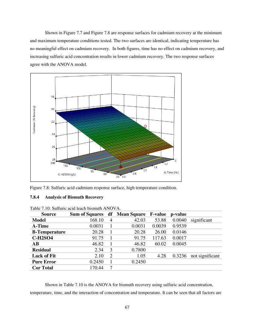
67

Shown in Figure 7.7 and Figure 7.8 are response surfaces for cadmium recovery at the minimum

and maximum temperature conditions tested. The two surfaces are identical, indicating temperature has

no meaningful effect on cadmium recovery. In both figures, time has no effect on cadmium recovery, and

increasing sulfuric acid concentration results in lower cadmium recovery. The two response surfaces

agree with the ANOVA model.

Figure 7.8: Sulfuric acid cadmium response surface, high temperature condition.

7.8.4 Analysis of Bismuth Recovery

Table 7.10: Sulfuric acid leach bismuth ANOVA.



A-Time 0.0031 1 0.0031 0.0039 0.9539

B-Temperature 20.28 1 20.28 26.00 0.0146

C-H2SO4 91.75 1 91.75 117.63 0.0017

AB 46.82 1 46.82 60.02 0.0045

Residual 2.34 3 0.7800


Pure Error 0.2450 1 0.2450

Cor Total 170.44 7

Shown in Table 7.10 is the ANOVA for bismuth recovery using sulfuric acid concentration,

temperature, time, and the interaction of concentration and temperature. It can be seen that all factors are

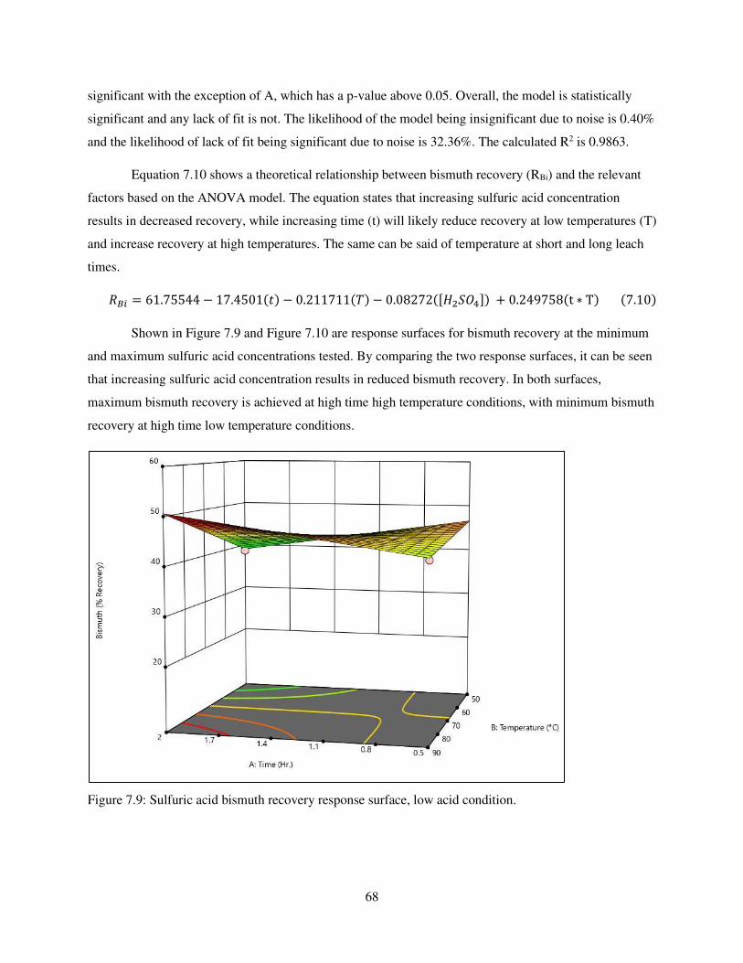
68

significant with the exception of A, which has a p-value above 0.05. Overall, the model is statistically

significant and any lack of fit is not. The likelihood of the model being insignificant due to noise is 0.40%

and the likelihood of lack of fit being significant due to noise is 32.36%. The calculated R2 is 0.9863.

Equation 7.10 shows a theoretical relationship between bismuth recovery (RBi) and the relevant

factors based on the ANOVA model. The equation states that increasing sulfuric acid concentration

results in decreased recovery, while increasing time (t) will likely reduce recovery at low temperatures (T)

and increase recovery at high temperatures. The same can be said of temperature at short and long leach

times. 𝑅𝐵𝑖 = 61.75544 − 17.4501(𝑡) − 0.211711(𝑇) − 0.08272([𝐻2𝑆𝑂4]) + 0.249758(t ∗ T) (7.10)

Shown in Figure 7.9 and Figure 7.10 are response surfaces for bismuth recovery at the minimum

and maximum sulfuric acid concentrations tested. By comparing the two response surfaces, it can be seen

that increasing sulfuric acid concentration results in reduced bismuth recovery. In both surfaces,

maximum bismuth recovery is achieved at high time high temperature conditions, with minimum bismuth

recovery at high time low temperature conditions.

Figure 7.9: Sulfuric acid bismuth recovery response surface, low acid condition.

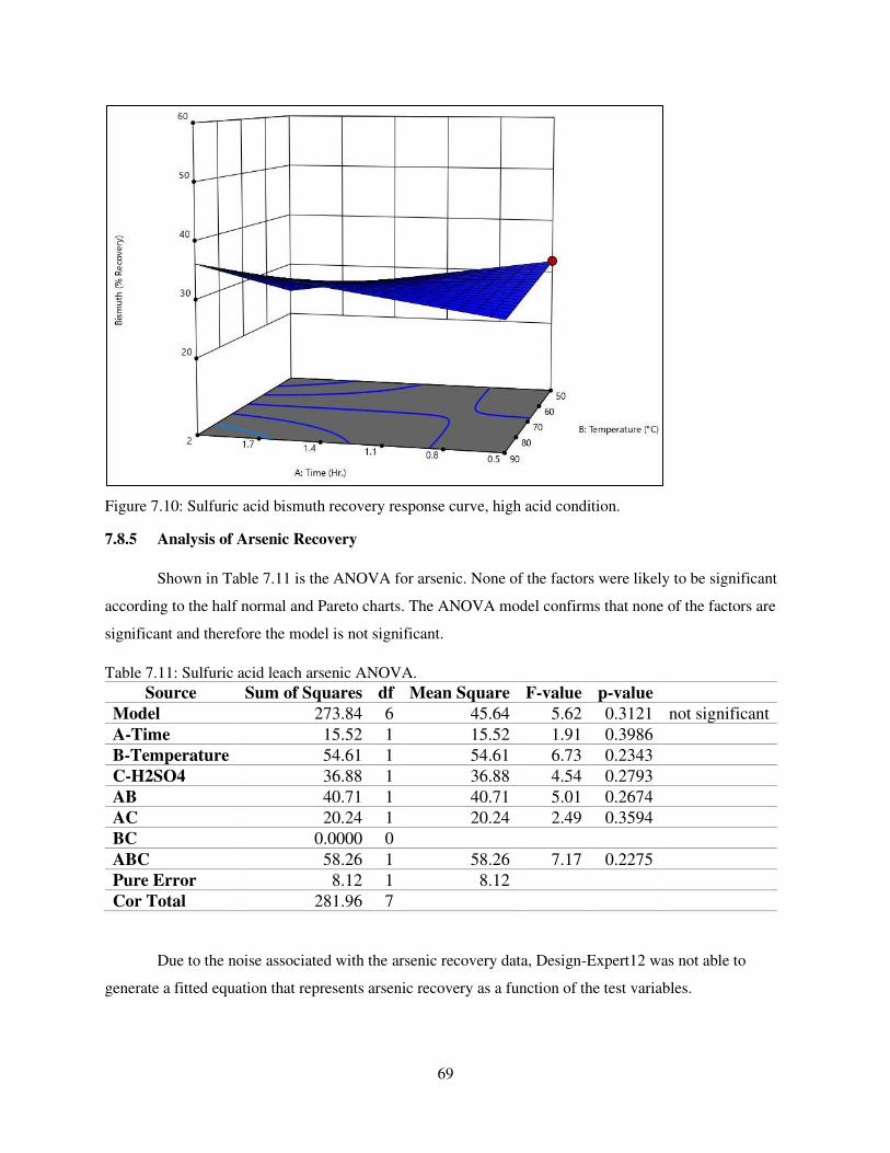
69

Figure 7.10: Sulfuric acid bismuth recovery response curve, high acid condition.

7.8.5 Analysis of Arsenic Recovery

Shown in Table 7.11 is the ANOVA for arsenic. None of the factors were likely to be significant

according to the half normal and Pareto charts. The ANOVA model confirms that none of the factors are

significant and therefore the model is not significant.

Table 7.11: Sulfuric acid leach arsenic ANOVA.


Model 273.84 6 45.64 5.62 0.3121 not significant

A-Time 15.52 1 15.52 1.91 0.3986

B-Temperature 54.61 1 54.61 6.73 0.2343

C-H2SO4 36.88 1 36.88 4.54 0.2793

AB 40.71 1 40.71 5.01 0.2674

AC 20.24 1 20.24 2.49 0.3594

BC 0.0000 0

ABC 58.26 1 58.26 7.17 0.2275

Pure Error 8.12 1 8.12

Cor Total 281.96 7

Due to the noise associated with the arsenic recovery data, Design-Expert12 was not able to

generate a fitted equation that represents arsenic recovery as a function of the test variables.

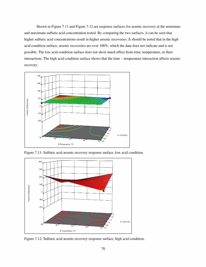
70

Shown in Figure 7.11 and Figure 7.12 are response surfaces for arsenic recovery at the minimum

and maximum sulfuric acid concentration tested. By comparing the two surfaces, it can be seen that

higher sulfuric acid concentrations result in higher arsenic recoveries. It should be noted that in the high

acid condition surface, arsenic recoveries are over 100%, which the data does not indicate and is not

possible. The low acid condition surface does not show much effect from time, temperature, or their

interactions. The high acid condition surface shows that the time – temperature interaction affects arsenic

recovery.

Figure 7.11: Sulfuric acid arsenic recovery response surface, low acid condition.

Figure 7.12: Sulfuric acid arsenic recovery response surface, high acid condition.

71

7.9 Sulfuric Acid Leaching Discussion

Overall, sulfuric acid leaching does not satisfactorily transfer the desired elements to the aqueous

phase. That said, theoretically, sulfuric acid should easily dissolve all elements of interest. Furthermore,

according to literature, several have had success utilizing sulfuric acid to transfer the desired elements to

the aqueous phase. This indicates the existence of some ameliorable hurdle that prevents further

dissolution of the desired elements. One hypothesis is that there is not sufficient sulfuric acid present to

fully dissolve the desired elements, this is supported by the starting and ending concentrations of sulfuric

acid shown in Table 7.5.

The recovery of each element of interest was impacted differently by each test variable and their

interactions. The most common factor that had an impact on recovery was sulfuric acid concentration,

with temperature being the second most common. Time only had a statistically significant effect on the

recovery of indium. Interestingly, the interaction of time and sulfuric acid concentration also had a

statistically significant effect on indium recovery, indicating that additional time is necessary to take

advantage of any benefits associated with higher sulfuric acid recovery.

Based on the equations generated using the ANOVA models, it appears as though indium

recovery can be increased by leaching for times longer than those leached during experimentation, while

cadmium recovery cannot be increased beyond recoveries shown. At a sulfuric acid concentration of 100

mL/L, approximately 90% of the indium would be recovered after 20 hours of leaching at 75 °C. It should

be noted that this was not tested. Also, such conditions would, theoretically, also recover approximately

83% Cu, 23% Cd, 63% Bi, and an unknown amount of arsenic.

Generally, it seems that elemental recoveries can be optimized by primarily modulating sulfuric

acid concentration and temperature. This makes since as higher acid concentration allows for more acid

available for dissolution and higher temperature allows for improved kinetics which should reduce the

time necessary for the reactions to occur.

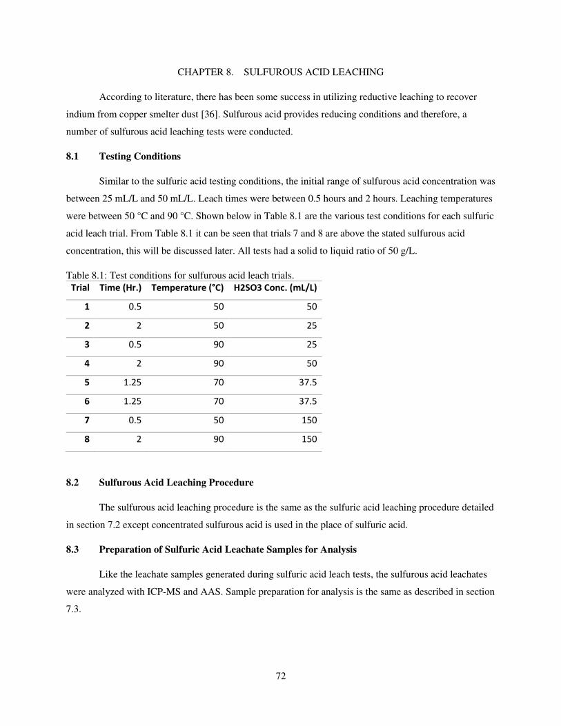
72

CHAPTER 8. SULFUROUS ACID LEACHING

According to literature, there has been some success in utilizing reductive leaching to recover

indium from copper smelter dust [36]. Sulfurous acid provides reducing conditions and therefore, a

number of sulfurous acid leaching tests were conducted.


Similar to the sulfuric acid testing conditions, the initial range of sulfurous acid concentration was

between 25 mL/L and 50 mL/L. Leach times were between 0.5 hours and 2 hours. Leaching temperatures

were between 50 °C and 90 °C. Shown below in Table 8.1 are the various test conditions for each sulfuric

acid leach trial. From Table 8.1 it can be seen that trials 7 and 8 are above the stated sulfurous acid

concentration, this will be discussed later. All tests had a solid to liquid ratio of 50 g/L.

Table 8.1: Test conditions for sulfurous acid leach trials.

Trial Time (Hr.) Temperature (°C) H2SO3 Conc. (mL/L)

1 0.5 50 50

2 2 50 25

3 0.5 90 25

4 2 90 50

5 1.25 70 37.5

6 1.25 70 37.5

7 0.5 50 150

8 2 90 150

8.2 Sulfurous Acid Leaching Procedure

The sulfurous acid leaching procedure is the same as the sulfuric acid leaching procedure detailed

in section 7.2 except concentrated sulfurous acid is used in the place of sulfuric acid.

8.3 Preparation of Sulfuric Acid Leachate Samples for Analysis

Like the leachate samples generated during sulfuric acid leach tests, the sulfurous acid leachates

were analyzed with ICP-MS and AAS. Sample preparation for analysis is the same as described in section

7.3.

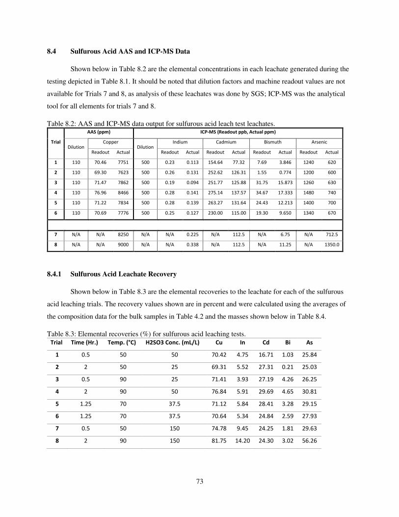
73

8.4 Sulfurous Acid AAS and ICP-MS Data

Shown below in Table 8.2 are the elemental concentrations in each leachate generated during the

testing depicted in Table 8.1. It should be noted that dilution factors and machine readout values are not

available for Trials 7 and 8, as analysis of these leachates was done by SGS; ICP-MS was the analytical

tool for all elements for trials 7 and 8.

Table 8.2: AAS and ICP-MS data output for sulfurous acid leach test leachates.

Trial


Dilution Copper



1 110 70.46 7751 500 0.23 0.113 154.64 77.32 7.69 3.846 1240 620

2 110 69.30 7623 500 0.26 0.131 252.62 126.31 1.55 0.774 1200 600

3 110 71.47 7862 500 0.19 0.094 251.77 125.88 31.75 15.873 1260 630

4 110 76.96 8466 500 0.28 0.141 275.14 137.57 34.67 17.333 1480 740

5 110 71.22 7834 500 0.28 0.139 263.27 131.64 24.43 12.213 1400 700

6 110 70.69 7776 500 0.25 0.127 230.00 115.00 19.30 9.650 1340 670

7 N/A N/A 8250 N/A N/A 0.225 N/A 112.5 N/A 6.75 N/A 712.5

8 N/A N/A 9000 N/A N/A 0.338 N/A 112.5 N/A 11.25 N/A 1350.0

8.4.1 Sulfurous Acid Leachate Recovery

Shown below in Table 8.3 are the elemental recoveries to the leachate for each of the sulfurous

acid leaching trials. The recovery values shown are in percent and were calculated using the averages of

the composition data for the bulk samples in Table 4.2 and the masses shown below in Table 8.4.

Table 8.3: Elemental recoveries (%) for sulfurous acid leaching tests.

Trial Time (Hr.) Temp. (°C) H2SO3 Conc. (mL/L) Cu In Cd Bi As

1 0.5 50 50 70.42 4.75 16.71 1.03 25.84

2 2 50 25 69.31 5.52 27.31 0.21 25.03

3 0.5 90 25 71.41 3.93 27.19 4.26 26.25

4 2 90 50 76.84 5.91 29.69 4.65 30.81

5 1.25 70 37.5 71.12 5.84 28.41 3.28 29.15

6 1.25 70 37.5 70.64 5.34 24.84 2.59 27.93

7 0.5 50 150 74.78 9.45 24.25 1.81 29.63

8 2 90 150 81.75 14.20 24.30 3.02 56.26

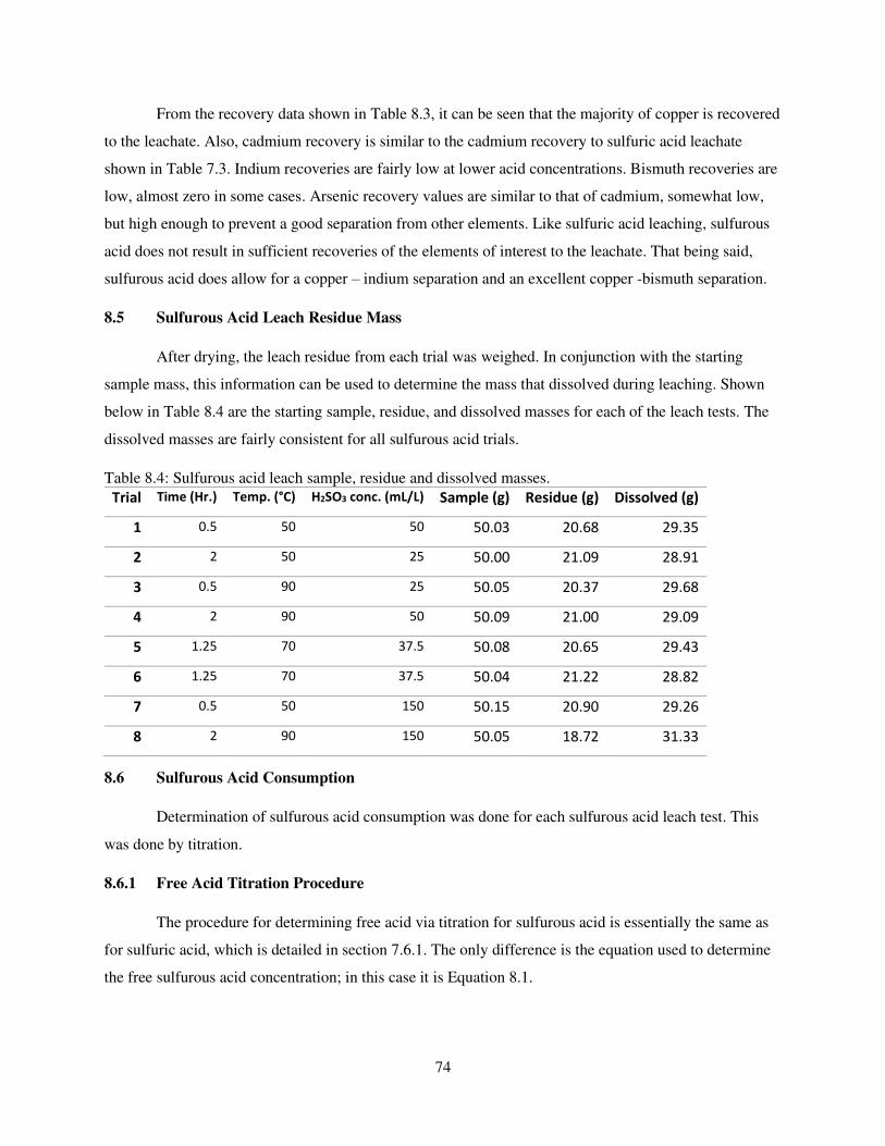
74

From the recovery data shown in Table 8.3, it can be seen that the majority of copper is recovered

to the leachate. Also, cadmium recovery is similar to the cadmium recovery to sulfuric acid leachate

shown in Table 7.3. Indium recoveries are fairly low at lower acid concentrations. Bismuth recoveries are

low, almost zero in some cases. Arsenic recovery values are similar to that of cadmium, somewhat low,

but high enough to prevent a good separation from other elements. Like sulfuric acid leaching, sulfurous

acid does not result in sufficient recoveries of the elements of interest to the leachate. That being said,

sulfurous acid does allow for a copper – indium separation and an excellent copper -bismuth separation.

8.5 Sulfurous Acid Leach Residue Mass

After drying, the leach residue from each trial was weighed. In conjunction with the starting

sample mass, this information can be used to determine the mass that dissolved during leaching. Shown

below in Table 8.4 are the starting sample, residue, and dissolved masses for each of the leach tests. The

dissolved masses are fairly consistent for all sulfurous acid trials.

Table 8.4: Sulfurous acid leach sample, residue and dissolved masses.

Trial Time (Hr.) Temp. (°C) H2SO3 conc. (mL/L) Sample (g) Residue (g) Dissolved (g)

1 0.5 50 50 50.03 20.68 29.35

2 2 50 25 50.00 21.09 28.91

3 0.5 90 25 50.05 20.37 29.68

4 2 90 50 50.09 21.00 29.09

5 1.25 70 37.5 50.08 20.65 29.43

6 1.25 70 37.5 50.04 21.22 28.82

7 0.5 50 150 50.15 20.90 29.26

8 2 90 150 50.05 18.72 31.33

8.6 Sulfurous Acid Consumption

Determination of sulfurous acid consumption was done for each sulfurous acid leach test. This

was done by titration.


The procedure for determining free acid via titration for sulfurous acid is essentially the same as

for sulfuric acid, which is detailed in section 7.6.1. The only difference is the equation used to determine

the free sulfurous acid concentration; in this case it is Equation 8.1.

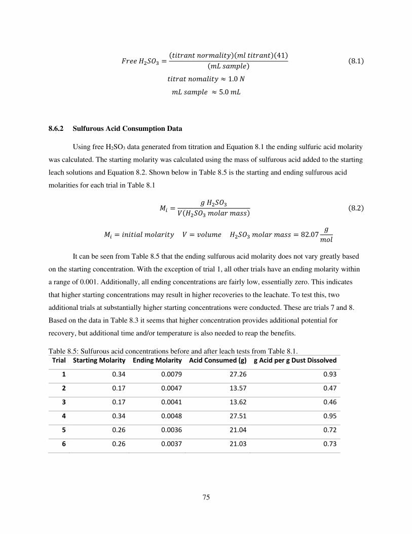
75

𝐹𝑟𝑒𝑒 𝐻2𝑆𝑂3 = (𝑡𝑖𝑡𝑟𝑎𝑛𝑡 𝑛𝑜𝑟𝑚𝑎𝑙𝑖𝑡𝑦)(𝑚𝑙 𝑡𝑖𝑡𝑟𝑎𝑛𝑡)(41)(𝑚𝐿 𝑠𝑎𝑚𝑝𝑙𝑒) (8.1) 𝑡𝑖𝑡𝑟𝑎𝑡 𝑛𝑜𝑚𝑎𝑙𝑖𝑡𝑦 ≈ 1.0 𝑁 𝑚𝐿 𝑠𝑎𝑚𝑝𝑙𝑒 ≈ 5.0 𝑚𝐿

8.6.2 Sulfurous Acid Consumption Data


was calculated. The starting molarity was calculated using the mass of sulfurous acid added to the starting

leach solutions and Equation 8.2. Shown below in Table 8.5 is the starting and ending sulfurous acid

molarities for each trial in Table 8.1

𝑀𝑖 = 𝑔 𝐻2𝑆𝑂3𝑉(𝐻2𝑆𝑂3 𝑚𝑜𝑙𝑎𝑟 𝑚𝑎𝑠𝑠) (8.2)

𝑀𝑖 = 𝑖𝑛𝑖𝑡𝑖𝑎𝑙 𝑚𝑜𝑙𝑎𝑟𝑖𝑡𝑦 𝑉 = 𝑣𝑜𝑙𝑢𝑚𝑒 𝐻2𝑆𝑂3 𝑚𝑜𝑙𝑎𝑟 𝑚𝑎𝑠𝑠 = 82.07 𝑔𝑚𝑜𝑙 It can be seen from Table 8.5 that the ending sulfurous acid molarity does not vary greatly based

on the starting concentration. With the exception of trial 1, all other trials have an ending molarity within

a range of 0.001. Additionally, all ending concentrations are fairly low, essentially zero. This indicates

that higher starting concentrations may result in higher recoveries to the leachate. To test this, two

additional trials at substantially higher starting concentrations were conducted. These are trials 7 and 8.

Based on the data in Table 8.3 it seems that higher concentration provides additional potential for

recovery, but additional time and/or temperature is also needed to reap the benefits.

Table 8.5: Sulfurous acid concentrations before and after leach tests from Table 8.1.

Trial Starting Molarity Ending Molarity Acid Consumed (g) g Acid per g Dust Dissolved

1 0.34 0.0079 27.26 0.93

2 0.17 0.0047 13.57 0.47

3 0.17 0.0041 13.62 0.46

4 0.34 0.0048 27.51 0.95

5 0.26 0.0036 21.04 0.72

6 0.26 0.0037 21.03 0.73

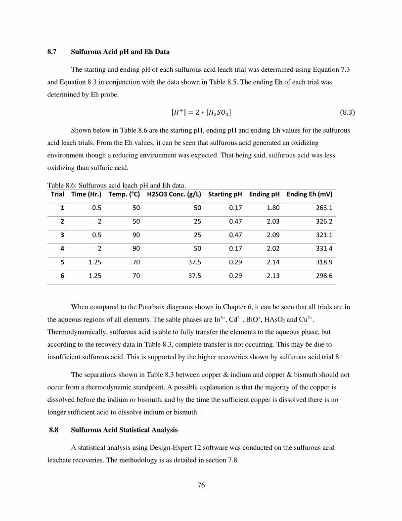
76

8.7 Sulfurous Acid pH and Eh Data

The starting and ending pH of each sulfurous acid leach trial was determined using Equation 7.3

and Equation 8.3 in conjunction with the data shown in Table 8.5. The ending Eh of each trial was

determined by Eh probe. [𝐻+] = 2 ∗ [𝐻2𝑆𝑂3] (8.3)

Shown below in Table 8.6 are the starting pH, ending pH and ending Eh values for the sulfurous

acid leach trials. From the Eh values, it can be seen that sulfurous acid generated an oxidizing

environment though a reducing environment was expected. That being said, sulfurous acid was less

oxidizing than sulfuric acid.

Table 8.6: Sulfurous acid leach pH and Eh data.

Trial Time (Hr.) Temp. (°C) H2SO3 Conc. (g/L) Starting pH Ending pH Ending Eh (mV)

1 0.5 50 50 0.17 1.80 263.1

2 2 50 25 0.47 2.03 326.2

3 0.5 90 25 0.47 2.09 321.1

4 2 90 50 0.17 2.02 331.4

5 1.25 70 37.5 0.29 2.14 318.9

6 1.25 70 37.5 0.29 2.13 298.6

When compared to the Pourbaix diagrams shown in Chapter 6, it can be seen that all trials are in

the aqueous regions of all elements. The sable phases are In3+, Cd2+, BiO+, HAsO2 and Cu2+.

Thermodynamically, sulfurous acid is able to fully transfer the elements to the aqueous phase, but

according to the recovery data in Table 8.3, complete transfer is not occurring. This may be due to

insufficient sulfurous acid. This is supported by the higher recoveries shown by sulfurous acid trial 8.

The separations shown in Table 8.3 between copper & indium and copper & bismuth should not

occur from a thermodynamic standpoint. A possible explanation is that the majority of the copper is

dissolved before the indium or bismuth, and by the time the sufficient copper is dissolved there is no

longer sufficient acid to dissolve indium or bismuth.

8.8 Sulfurous Acid Statistical Analysis

A statistical analysis using Design-Expert 12 software was conducted on the sulfurous acid

leachate recoveries. The methodology is as detailed in section 7.8.

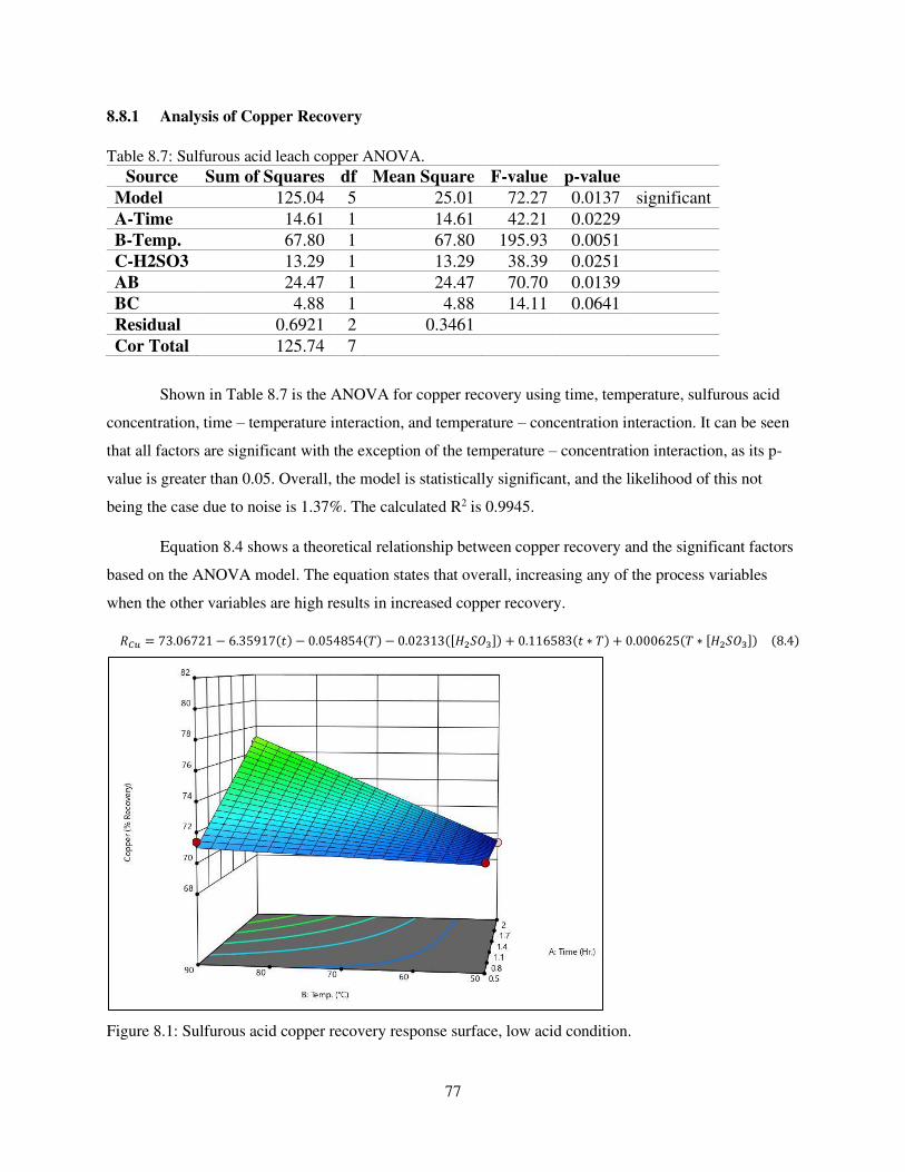
77


Table 8.7: Sulfurous acid leach copper ANOVA.



A-Time 14.61 1 14.61 42.21 0.0229

B-Temp. 67.80 1 67.80 195.93 0.0051

C-H2SO3 13.29 1 13.29 38.39 0.0251

AB 24.47 1 24.47 70.70 0.0139

BC 4.88 1 4.88 14.11 0.0641

Residual 0.6921 2 0.3461

Cor Total 125.74 7

Shown in Table 8.7 is the ANOVA for copper recovery using time, temperature, sulfurous acid

concentration, time – temperature interaction, and temperature – concentration interaction. It can be seen

that all factors are significant with the exception of the temperature – concentration interaction, as its p-

value is greater than 0.05. Overall, the model is statistically significant, and the likelihood of this not

being the case due to noise is 1.37%. The calculated R2 is 0.9945.

Equation 8.4 shows a theoretical relationship between copper recovery and the significant factors

based on the ANOVA model. The equation states that overall, increasing any of the process variables

when the other variables are high results in increased copper recovery. 𝑅𝐶𝑢 = 73.06721 − 6.35917(𝑡) − 0.054854(𝑇) − 0.02313([𝐻2𝑆𝑂3]) + 0.116583(𝑡 ∗ 𝑇) + 0.000625(𝑇 ∗ [𝐻2𝑆𝑂3]) (8.4)

Figure 8.1: Sulfurous acid copper recovery response surface, low acid condition.

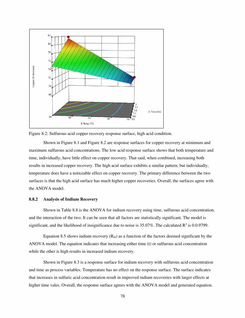
78

Figure 8.2: Sulfurous acid copper recovery response surface, high acid condition.

Shown in Figure 8.1 and Figure 8.2 are response surfaces for copper recovery at minimum and

maximum sulfurous acid concentrations. The low acid response surface shows that both temperature and

time, individually, have little effect on copper recovery. That said, when combined, increasing both

results in increased copper recovery. The high acid surface exhibits a similar pattern, but individually,

temperature does have a noticeable effect on copper recovery. The primary difference between the two

surfaces is that the high acid surface has much higher copper recoveries. Overall, the surfaces agree with

the ANOVA model.


Shown in Table 8.8 is the ANOVA for indium recovery using time, sulfurous acid concentration,

and the interaction of the two. It can be seen that all factors are statistically significant. The model is

significant, and the likelihood of insignificance due to noise is 35.07%. The calculated R2 is 0.0.9799.

Equation 8.5 shows indium recovery (RIn) as a function of the factors deemed significant by the

ANOVA model. The equation indicates that increasing either time (t) or sulfurous acid concentration

while the other is high results in increased indium recovery.

Shown in Figure 8.3 is a response surface for indium recovery with sulfurous acid concentration

and time as process variables. Temperature has no effect on the response surface. The surface indicates

that increases in sulfuric acid concentration result in improved indium recoveries with larger effects at

higher time vales. Overall, the response surface agrees with the ANOVA model and generated equation.

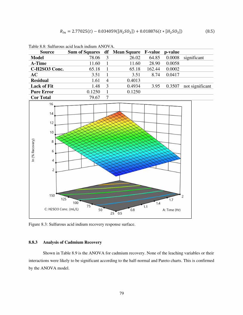
79

𝑅𝐼𝑛 = 2.77025(𝑡) − 0.034059([𝐻2𝑆𝑂3]) + 0.018876(𝑡 ∗ [𝐻2𝑆𝑂3]) (8.5)

Table 8.8: Sulfurous acid leach indium ANOVA.



A-Time 11.60 1 11.60 28.90 0.0058

C-H2SO3 Conc. 65.18 1 65.18 162.44 0.0002

AC 3.51 1 3.51 8.74 0.0417

Residual 1.61 4 0.4013


Pure Error 0.1250 1 0.1250

Cor Total 79.67 7

Figure 8.3: Sulfurous acid indium recovery response surface.


Shown in Table 8.9 is the ANOVA for cadmium recovery. None of the leaching variables or their

interactions were likely to be significant according to the half-normal and Pareto charts. This is confirmed

by the ANOVA model.

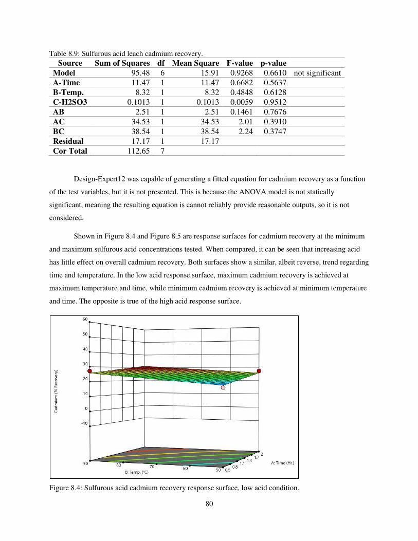
80

Table 8.9: Sulfurous acid leach cadmium recovery.



A-Time 11.47 1 11.47 0.6682 0.5637

B-Temp. 8.32 1 8.32 0.4848 0.6128

C-H2SO3 0.1013 1 0.1013 0.0059 0.9512

AB 2.51 1 2.51 0.1461 0.7676

AC 34.53 1 34.53 2.01 0.3910

BC 38.54 1 38.54 2.24 0.3747

Residual 17.17 1 17.17

Cor Total 112.65 7

Design-Expert12 was capable of generating a fitted equation for cadmium recovery as a function

of the test variables, but it is not presented. This is because the ANOVA model is not statically

significant, meaning the resulting equation is cannot reliably provide reasonable outputs, so it is not

considered.

Shown in Figure 8.4 and Figure 8.5 are response surfaces for cadmium recovery at the minimum

and maximum sulfurous acid concentrations tested. When compared, it can be seen that increasing acid

has little effect on overall cadmium recovery. Both surfaces show a similar, albeit reverse, trend regarding

time and temperature. In the low acid response surface, maximum cadmium recovery is achieved at

maximum temperature and time, while minimum cadmium recovery is achieved at minimum temperature

and time. The opposite is true of the high acid response surface.

Figure 8.4: Sulfurous acid cadmium recovery response surface, low acid condition.

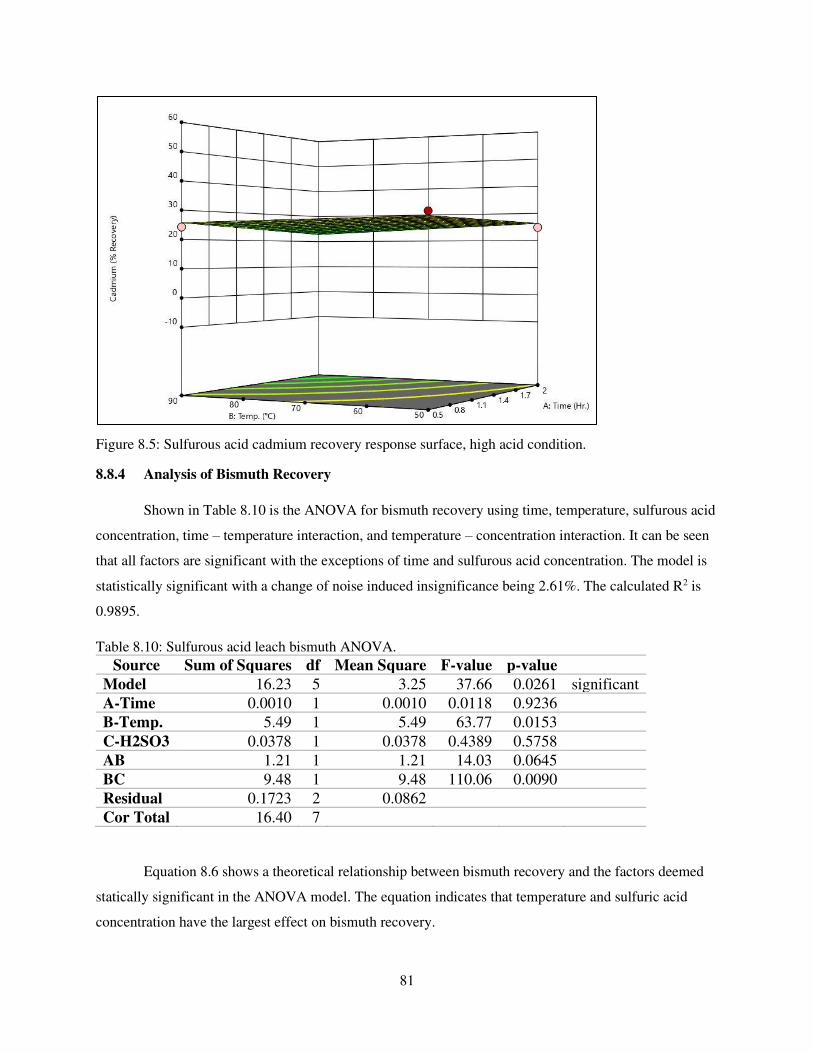
81

Figure 8.5: Sulfurous acid cadmium recovery response surface, high acid condition.


Shown in Table 8.10 is the ANOVA for bismuth recovery using time, temperature, sulfurous acid

concentration, time – temperature interaction, and temperature – concentration interaction. It can be seen

that all factors are significant with the exceptions of time and sulfurous acid concentration. The model is

statistically significant with a change of noise induced insignificance being 2.61%. The calculated R2 is

0.9895.

Table 8.10: Sulfurous acid leach bismuth ANOVA.



A-Time 0.0010 1 0.0010 0.0118 0.9236

B-Temp. 5.49 1 5.49 63.77 0.0153

C-H2SO3 0.0378 1 0.0378 0.4389 0.5758

AB 1.21 1 1.21 14.03 0.0645

BC 9.48 1 9.48 110.06 0.0090

Residual 0.1723 2 0.0862

Cor Total 16.40 7

Equation 8.6 shows a theoretical relationship between bismuth recovery and the factors deemed

statically significant in the ANOVA model. The equation indicates that temperature and sulfuric acid

concentration have the largest effect on bismuth recovery.

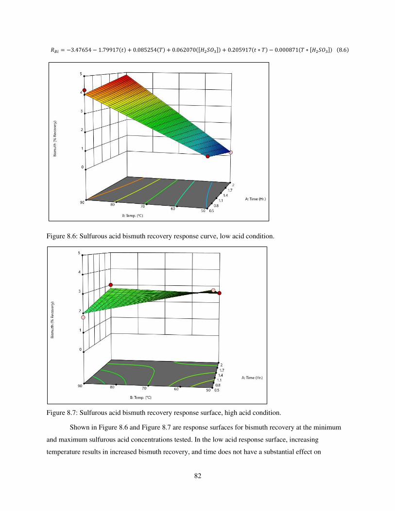
82

𝑅𝐵𝑖 = −3.47654 − 1.79917(𝑡) + 0.085254(𝑇) + 0.062070([𝐻2𝑆𝑂3]) + 0.205917(𝑡 ∗ 𝑇) − 0.000871(𝑇 ∗ [𝐻2𝑆𝑂3]) (8.6)

Figure 8.6: Sulfurous acid bismuth recovery response curve, low acid condition.

Figure 8.7: Sulfurous acid bismuth recovery response surface, high acid condition.


and maximum sulfurous acid concentrations tested. In the low acid response surface, increasing

temperature results in increased bismuth recovery, and time does not have a substantial effect on

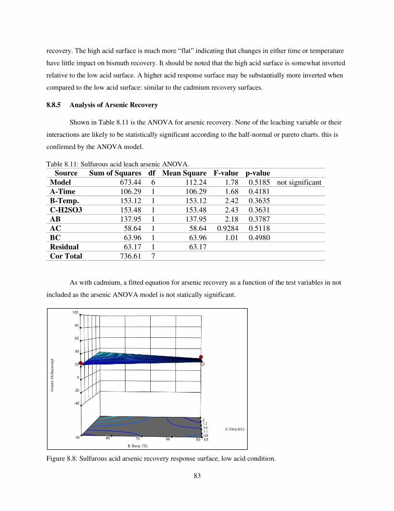
83

recovery. The high acid surface is much more “flat” indicating that changes in either time or temperature

have little impact on bismuth recovery. It should be noted that the high acid surface is somewhat inverted

relative to the low acid surface. A higher acid response surface may be substantially more inverted when

compared to the low acid surface: similar to the cadmium recovery surfaces.


Shown in Table 8.11 is the ANOVA for arsenic recovery. None of the leaching variable or their

interactions are likely to be statistically significant according to the half-normal or pareto charts. this is

confirmed by the ANOVA model.

Table 8.11: Sulfurous acid leach arsenic ANOVA.



A-Time 106.29 1 106.29 1.68 0.4181

B-Temp. 153.12 1 153.12 2.42 0.3635

C-H2SO3 153.48 1 153.48 2.43 0.3631

AB 137.95 1 137.95 2.18 0.3787

AC 58.64 1 58.64 0.9284 0.5118

BC 63.96 1 63.96 1.01 0.4980

Residual 63.17 1 63.17

Cor Total 736.61 7

As with cadmium, a fitted equation for arsenic recovery as a function of the test variables in not

included as the arsenic ANOVA model is not statically significant.

Figure 8.8: Sulfurous acid arsenic recovery response surface, low acid condition.

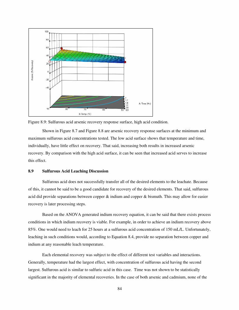
84

Figure 8.9: Sulfurous acid arsenic recovery response surface, high acid condition.

Shown in Figure 8.7 and Figure 8.8 are arsenic recovery response surfaces at the minimum and

maximum sulfurous acid concentrations tested. The low acid surface shows that temperature and time,

individually, have little effect on recovery. That said, increasing both results in increased arsenic

recovery. By comparison with the high acid surface, it can be seen that increased acid serves to increase

this effect.

8.9 Sulfurous Acid Leaching Discussion

Sulfurous acid does not successfully transfer all of the desired elements to the leachate. Because

of this, it cannot be said to be a good candidate for recovery of the desired elements. That said, sulfurous

acid did provide separations between copper & indium and copper & bismuth. This may allow for easier

recovery is later processing steps.

Based on the ANOVA generated indium recovery equation, it can be said that there exists process

conditions in which indium recovery is viable. For example, in order to achieve an indium recovery above

85%. One would need to leach for 25 hours at a sulfurous acid concentration of 150 mL/L. Unfortunately,

leaching in such conditions would, according to Equation 8.4, provide no separation between copper and

indium at any reasonable leach temperature.

Each elemental recovery was subject to the effect of different test variables and interactions.

Generally, temperature had the largest effect, with concentration of sulfurous acid having the second

largest. Sulfurous acid is similar to sulfuric acid in this case. Time was not shown to be statistically

significant in the majority of elemental recoveries. In the case of both arsenic and cadmium, none of the

85

factors were determined to be statistically significant, indicating that not much can be done in terms of

variable manipulation to modulate the recoveries of those two elements.

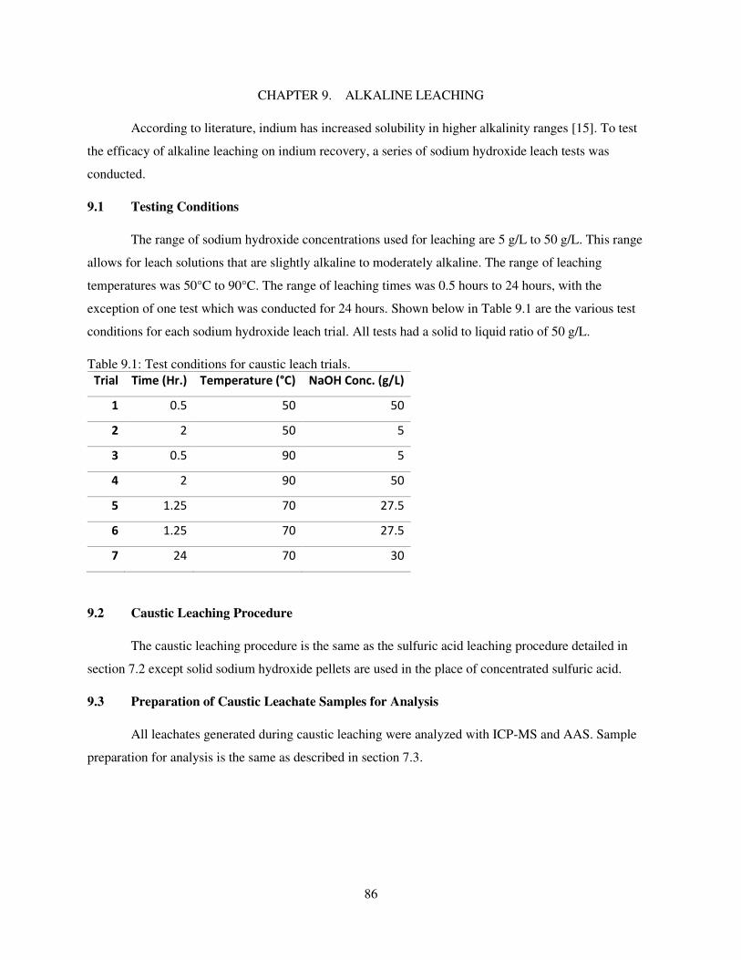
86

CHAPTER 9. ALKALINE LEACHING

According to literature, indium has increased solubility in higher alkalinity ranges [15]. To test

the efficacy of alkaline leaching on indium recovery, a series of sodium hydroxide leach tests was

conducted.


The range of sodium hydroxide concentrations used for leaching are 5 g/L to 50 g/L. This range

allows for leach solutions that are slightly alkaline to moderately alkaline. The range of leaching

temperatures was 50°C to 90°C. The range of leaching times was 0.5 hours to 24 hours, with the

exception of one test which was conducted for 24 hours. Shown below in Table 9.1 are the various test

conditions for each sodium hydroxide leach trial. All tests had a solid to liquid ratio of 50 g/L.

Table 9.1: Test conditions for caustic leach trials.

Trial Time (Hr.) Temperature (°C) NaOH Conc. (g/L)

1 0.5 50 50

2 2 50 5

3 0.5 90 5

4 2 90 50

5 1.25 70 27.5

6 1.25 70 27.5

7 24 70 30

9.2 Caustic Leaching Procedure

The caustic leaching procedure is the same as the sulfuric acid leaching procedure detailed in

section 7.2 except solid sodium hydroxide pellets are used in the place of concentrated sulfuric acid.

9.3 Preparation of Caustic Leachate Samples for Analysis

All leachates generated during caustic leaching were analyzed with ICP-MS and AAS. Sample

preparation for analysis is the same as described in section 7.3.

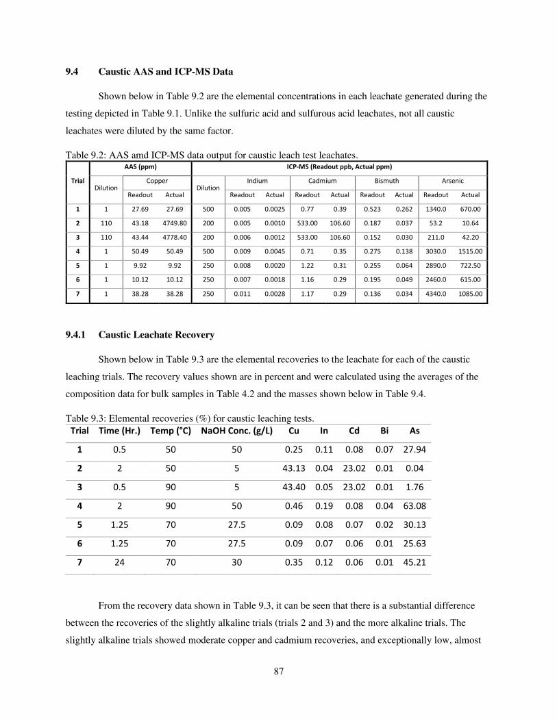
87

9.4 Caustic AAS and ICP-MS Data

Shown below in Table 9.2 are the elemental concentrations in each leachate generated during the

testing depicted in Table 9.1. Unlike the sulfuric acid and sulfurous acid leachates, not all caustic

leachates were diluted by the same factor.

Table 9.2: AAS amd ICP-MS data output for caustic leach test leachates.

Trial


Dilution Copper



1 1 27.69 27.69 500 0.005 0.0025 0.77 0.39 0.523 0.262 1340.0 670.00

2 110 43.18 4749.80 200 0.005 0.0010 533.00 106.60 0.187 0.037 53.2 10.64

3 110 43.44 4778.40 200 0.006 0.0012 533.00 106.60 0.152 0.030 211.0 42.20

4 1 50.49 50.49 500 0.009 0.0045 0.71 0.35 0.275 0.138 3030.0 1515.00

5 1 9.92 9.92 250 0.008 0.0020 1.22 0.31 0.255 0.064 2890.0 722.50

6 1 10.12 10.12 250 0.007 0.0018 1.16 0.29 0.195 0.049 2460.0 615.00

7 1 38.28 38.28 250 0.011 0.0028 1.17 0.29 0.136 0.034 4340.0 1085.00

9.4.1 Caustic Leachate Recovery

Shown below in Table 9.3 are the elemental recoveries to the leachate for each of the caustic

leaching trials. The recovery values shown are in percent and were calculated using the averages of the

composition data for bulk samples in Table 4.2 and the masses shown below in Table 9.4.

Table 9.3: Elemental recoveries (%) for caustic leaching tests.

Trial Time (Hr.) Temp (°C) NaOH Conc. (g/L) Cu In Cd Bi As

1 0.5 50 50 0.25 0.11 0.08 0.07 27.94

2 2 50 5 43.13 0.04 23.02 0.01 0.04

3 0.5 90 5 43.40 0.05 23.02 0.01 1.76

4 2 90 50 0.46 0.19 0.08 0.04 63.08

5 1.25 70 27.5 0.09 0.08 0.07 0.02 30.13

6 1.25 70 27.5 0.09 0.07 0.06 0.01 25.63

7 24 70 30 0.35 0.12 0.06 0.01 45.21

From the recovery data shown in Table 9.3, it can be seen that there is a substantial difference

between the recoveries of the slightly alkaline trials (trials 2 and 3) and the more alkaline trials. The

slightly alkaline trials showed moderate copper and cadmium recoveries, and exceptionally low, almost

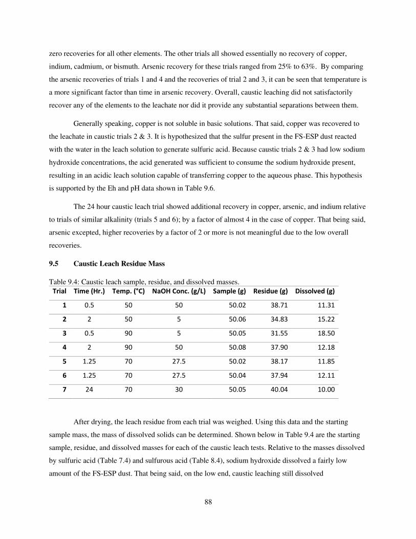
88

zero recoveries for all other elements. The other trials all showed essentially no recovery of copper,

indium, cadmium, or bismuth. Arsenic recovery for these trials ranged from 25% to 63%. By comparing

the arsenic recoveries of trials 1 and 4 and the recoveries of trial 2 and 3, it can be seen that temperature is

a more significant factor than time in arsenic recovery. Overall, caustic leaching did not satisfactorily

recover any of the elements to the leachate nor did it provide any substantial separations between them.

Generally speaking, copper is not soluble in basic solutions. That said, copper was recovered to

the leachate in caustic trials 2 & 3. It is hypothesized that the sulfur present in the FS-ESP dust reacted

with the water in the leach solution to generate sulfuric acid. Because caustic trials 2 & 3 had low sodium

hydroxide concentrations, the acid generated was sufficient to consume the sodium hydroxide present,

resulting in an acidic leach solution capable of transferring copper to the aqueous phase. This hypothesis

is supported by the Eh and pH data shown in Table 9.6.

The 24 hour caustic leach trial showed additional recovery in copper, arsenic, and indium relative

to trials of similar alkalinity (trials 5 and 6); by a factor of almost 4 in the case of copper. That being said,

arsenic excepted, higher recoveries by a factor of 2 or more is not meaningful due to the low overall

recoveries.

9.5 Caustic Leach Residue Mass

Table 9.4: Caustic leach sample, residue, and dissolved masses.

Trial Time (Hr.) Temp. (°C) NaOH Conc. (g/L) Sample (g) Residue (g) Dissolved (g)

1 0.5 50 50 50.02 38.71 11.31

2 2 50 5 50.06 34.83 15.22

3 0.5 90 5 50.05 31.55 18.50

4 2 90 50 50.08 37.90 12.18

5 1.25 70 27.5 50.02 38.17 11.85

6 1.25 70 27.5 50.04 37.94 12.11

7 24 70 30 50.05 40.04 10.00

After drying, the leach residue from each trial was weighed. Using this data and the starting

sample mass, the mass of dissolved solids can be determined. Shown below in Table 9.4 are the starting

sample, residue, and dissolved masses for each of the caustic leach tests. Relative to the masses dissolved

by sulfuric acid (Table 7.4) and sulfurous acid (Table 8.4), sodium hydroxide dissolved a fairly low

amount of the FS-ESP dust. That being said, on the low end, caustic leaching still dissolved

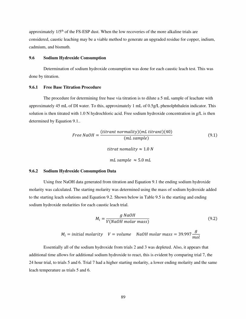
89

approximately 1/5th of the FS-ESP dust. When the low recoveries of the more alkaline trials are

considered, caustic leaching may be a viable method to generate an upgraded residue for copper, indium,

cadmium, and bismuth.

9.6 Sodium Hydroxide Consumption

Determination of sodium hydroxide consumption was done for each caustic leach test. This was

done by titration.

9.6.1 Free Base Titration Procedure

The procedure for determining free base via titration is to dilute a 5 mL sample of leachate with

approximately 45 mL of DI water. To this, approximately 1 mL of 0.5g/L phenolphthalein indicator. This

solution is then titrated with 1.0 N hydrochloric acid. Free sodium hydroxide concentration in g/L is then

determined by Equation 9.1..

𝐹𝑟𝑒𝑒 𝑁𝑎𝑂𝐻 = (𝑡𝑖𝑡𝑟𝑎𝑛𝑡 𝑛𝑜𝑟𝑚𝑎𝑙𝑖𝑡𝑦)(𝑚𝐿 𝑡𝑖𝑡𝑟𝑎𝑛𝑡)(40)(𝑚𝐿 𝑠𝑎𝑚𝑝𝑙𝑒) (9.1)

𝑡𝑖𝑡𝑟𝑎𝑡 𝑛𝑜𝑚𝑎𝑙𝑖𝑡𝑦 ≈ 1.0 𝑁 𝑚𝐿 𝑠𝑎𝑚𝑝𝑙𝑒 ≈ 5.0 𝑚𝐿

9.6.2 Sodium Hydroxide Consumption Data

Using free NaOH data generated from titration and Equation 9.1 the ending sodium hydroxide

molarity was calculated. The starting molarity was determined using the mass of sodium hydroxide added

to the starting leach solutions and Equation 9.2. Shown below in Table 9.5 is the starting and ending

sodium hydroxide molarities for each caustic leach trial.

𝑀𝑖 = 𝑔 𝑁𝑎𝑂𝐻𝑉(𝑁𝑎𝑂𝐻 𝑚𝑜𝑙𝑎𝑟 𝑚𝑎𝑠𝑠) (9.2)

𝑀𝑖 = 𝑖𝑛𝑖𝑡𝑖𝑎𝑙 𝑚𝑜𝑙𝑎𝑟𝑖𝑡𝑦 𝑉 = 𝑣𝑜𝑙𝑢𝑚𝑒 𝑁𝑎𝑂𝐻 𝑚𝑜𝑙𝑎𝑟 𝑚𝑎𝑠𝑠 = 39.997 𝑔𝑚𝑜𝑙 Essentially all of the sodium hydroxide from trials 2 and 3 was depleted. Also, it appears that

additional time allows for additional sodium hydroxide to react, this is evident by comparing trial 7, the

24 hour trial, to trials 5 and 6. Trial 7 had a higher starting molarity, a lower ending molarity and the same

leach temperature as trials 5 and 6.

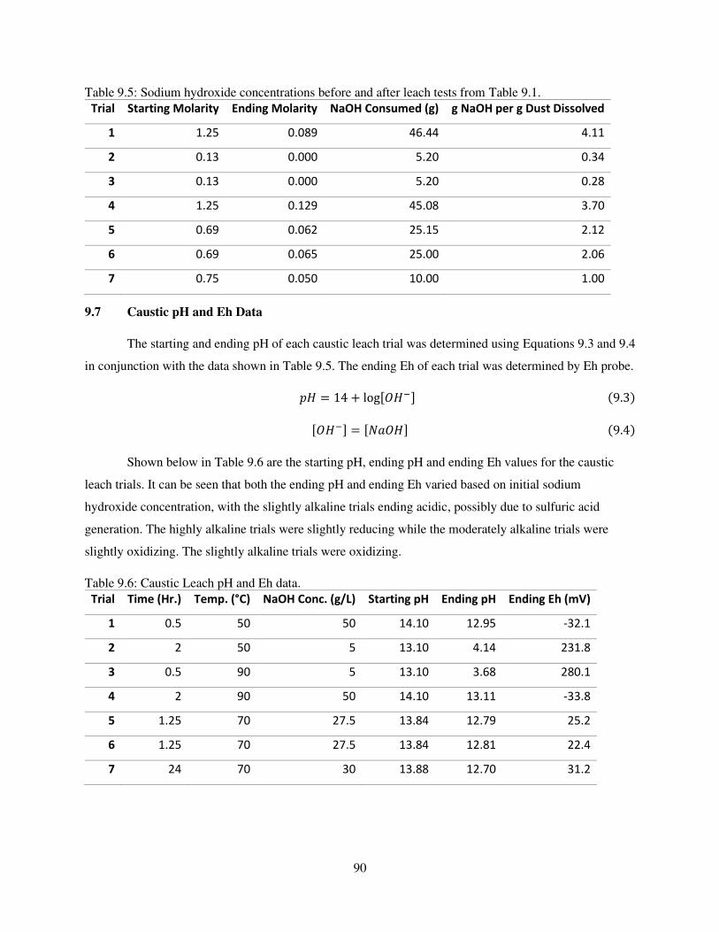
90

Table 9.5: Sodium hydroxide concentrations before and after leach tests from Table 9.1.

Trial Starting Molarity Ending Molarity NaOH Consumed (g) g NaOH per g Dust Dissolved

1 1.25 0.089 46.44 4.11

2 0.13 0.000 5.20 0.34

3 0.13 0.000 5.20 0.28

4 1.25 0.129 45.08 3.70

5 0.69 0.062 25.15 2.12

6 0.69 0.065 25.00 2.06

7 0.75 0.050 10.00 1.00

9.7 Caustic pH and Eh Data

The starting and ending pH of each caustic leach trial was determined using Equations 9.3 and 9.4

in conjunction with the data shown in Table 9.5. The ending Eh of each trial was determined by Eh probe. 𝑝𝐻 = 14 + log[𝑂𝐻−] (9.3) [𝑂𝐻−] = [𝑁𝑎𝑂𝐻] (9.4)

Shown below in Table 9.6 are the starting pH, ending pH and ending Eh values for the caustic

leach trials. It can be seen that both the ending pH and ending Eh varied based on initial sodium

hydroxide concentration, with the slightly alkaline trials ending acidic, possibly due to sulfuric acid

generation. The highly alkaline trials were slightly reducing while the moderately alkaline trials were

slightly oxidizing. The slightly alkaline trials were oxidizing.

Table 9.6: Caustic Leach pH and Eh data.

Trial Time (Hr.) Temp. (°C) NaOH Conc. (g/L) Starting pH Ending pH Ending Eh (mV)

1 0.5 50 50 14.10 12.95 -32.1

2 2 50 5 13.10 4.14 231.8

3 0.5 90 5 13.10 3.68 280.1

4 2 90 50 14.10 13.11 -33.8

5 1.25 70 27.5 13.84 12.79 25.2

6 1.25 70 27.5 13.84 12.81 22.4

7 24 70 30 13.88 12.70 31.2

91

When compared to the Pourbaix diagrams shown in Chapter 6, it can be seen that the caustic

leach trials are not in aqueous regions for all elements or trials. In the case of indium, the moderate and

highly alkaline trials are in the region of InO2-, which is aqueous. The slightly alkaline trials are in the In3+

and In(OH)2+ regions, both of which are aqueous. Thermodynamically, all caustic trials should transfer

indium to the aqueous phase, but none of them do. This may be due to equilibrium not being reached or

the formation of an insoluble complex.

Regarding cadmium, the moderately and highly alkaline trials are in the aqueous Cd(OH)2 region

and the slightly alkaline trials are in the Cd2+ region, which is also aqueous. Like indium, thermodynamics

indicates that all caustic leach trials should transfer cadmium to the aqueous phase. Interestingly, only the

slightly alkaline trials do so. It may be that the cadmium hydroxide is forming a passivating film, though

this should not occur due to the presence of sodium hydroxide.

The bismuth phase that is stable in the moderately and highly alkaline trials in Bi2O3, which is

insoluble. The stable bismuth phase for the slightly alkaline trials is soluble BiO+. Thermodynamically,

the moderate and highly alkaline trials should not dissolve bismuth and they do not. However, the slightly

alkaline trials should and they also do not. This may be explained by the formation of some insoluble

complex or equilibrium not being reached.

For the moderately and highly alkaline trials, the stable arsenic phase is AsO43-, which as

aqueous. For the slightly alkaline trials, the stable phase is aqueous HAsO22. All caustic trials

theoretically transfer arsenic to the aqueous phase, but only the moderately and highly alkaline trials

actually do so.

In the case of copper, the stable phase for the moderately and highly alkaline trials is insoluble

CuO. For the slightly alkaline trials, the stable phase is Cu2+, which is soluble. Thermodynamically, only

the slightly alkaline trials should transfer copper to the aqueous phase and this is what occurred.

9.8 Caustic Statistical Analysis

A statistical analysis using Design-Expert 12 software was conducted on the caustic leachate

recoveries. The methodology is as detailed in section 7.8.


Shown in Table 9.7 is the ANOVA for copper recovery using only sodium hydroxide

concentration. It should be noted that the effect of sodium hydroxide concentration on copper recovery to

the leachate is statistically significant. The likelihood of this being inaccurate due to noise is 2.67%. The

calculated R2 is 0.7454.

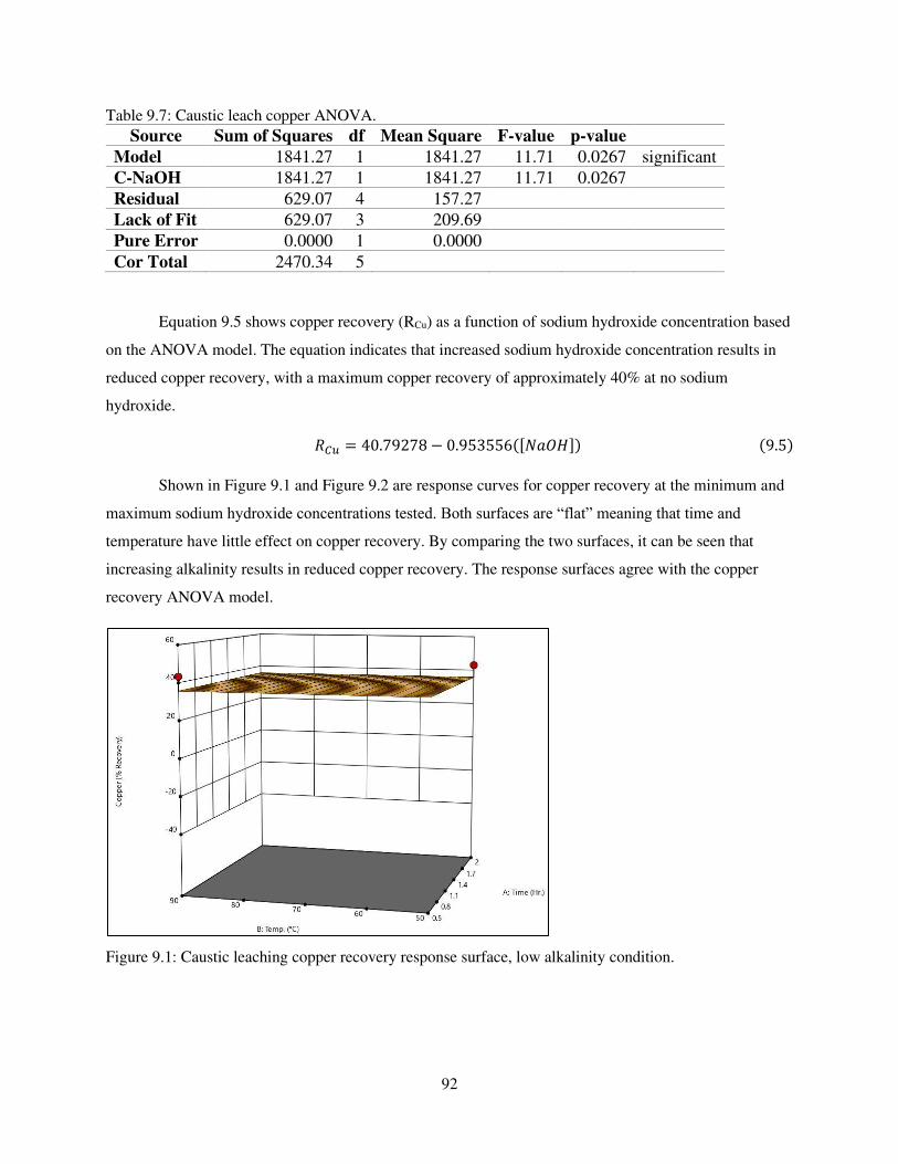
92

Table 9.7: Caustic leach copper ANOVA.



C-NaOH 1841.27 1 1841.27 11.71 0.0267

Residual 629.07 4 157.27

Lack of Fit 629.07 3 209.69

Pure Error 0.0000 1 0.0000

Cor Total 2470.34 5

Equation 9.5 shows copper recovery (RCu) as a function of sodium hydroxide concentration based

on the ANOVA model. The equation indicates that increased sodium hydroxide concentration results in

reduced copper recovery, with a maximum copper recovery of approximately 40% at no sodium

hydroxide. 𝑅𝐶𝑢 = 40.79278 − 0.953556([𝑁𝑎𝑂𝐻]) (9.5)

Shown in Figure 9.1 and Figure 9.2 are response curves for copper recovery at the minimum and

maximum sodium hydroxide concentrations tested. Both surfaces are “flat” meaning that time and

temperature have little effect on copper recovery. By comparing the two surfaces, it can be seen that

increasing alkalinity results in reduced copper recovery. The response surfaces agree with the copper

recovery ANOVA model.

Figure 9.1: Caustic leaching copper recovery response surface, low alkalinity condition.

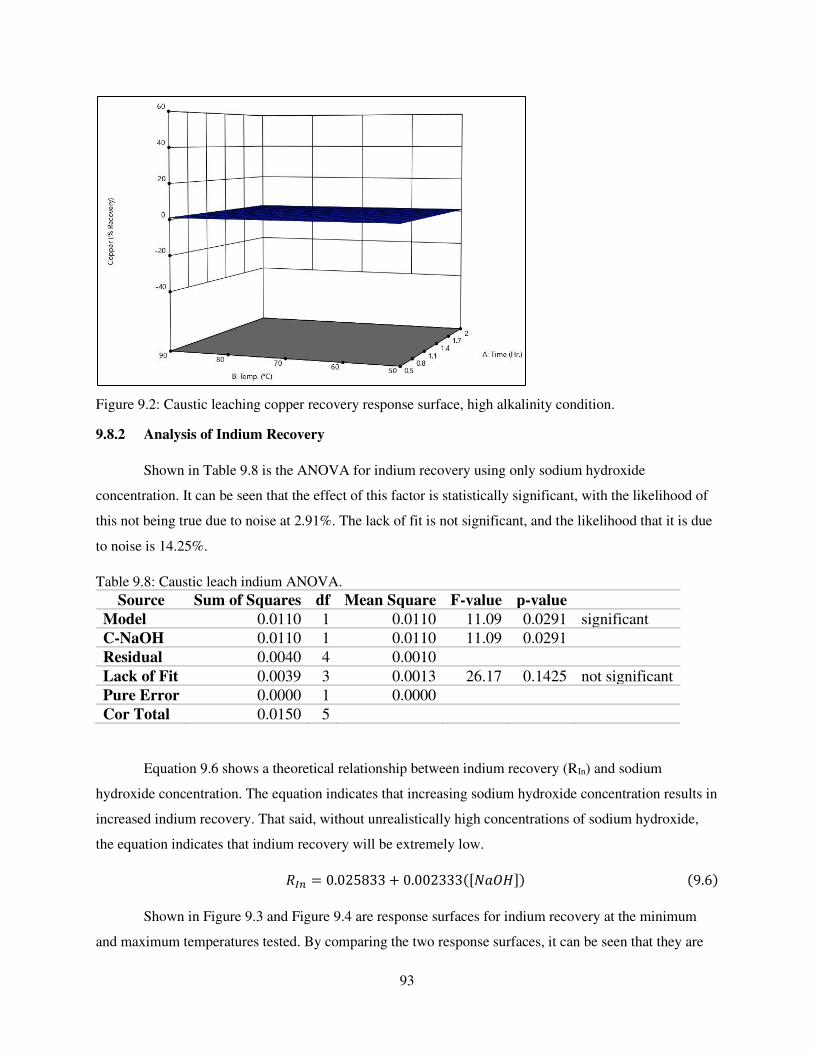
93

Figure 9.2: Caustic leaching copper recovery response surface, high alkalinity condition.


Shown in Table 9.8 is the ANOVA for indium recovery using only sodium hydroxide

concentration. It can be seen that the effect of this factor is statistically significant, with the likelihood of

this not being true due to noise at 2.91%. The lack of fit is not significant, and the likelihood that it is due

to noise is 14.25%.

Table 9.8: Caustic leach indium ANOVA.



C-NaOH 0.0110 1 0.0110 11.09 0.0291

Residual 0.0040 4 0.0010


Pure Error 0.0000 1 0.0000

Cor Total 0.0150 5

Equation 9.6 shows a theoretical relationship between indium recovery (RIn) and sodium

hydroxide concentration. The equation indicates that increasing sodium hydroxide concentration results in

increased indium recovery. That said, without unrealistically high concentrations of sodium hydroxide,

the equation indicates that indium recovery will be extremely low. 𝑅𝐼𝑛 = 0.025833 + 0.002333([𝑁𝑎𝑂𝐻]) (9.6)

Shown in Figure 9.3 and Figure 9.4 are response surfaces for indium recovery at the minimum

and maximum temperatures tested. By comparing the two response surfaces, it can be seen that they are

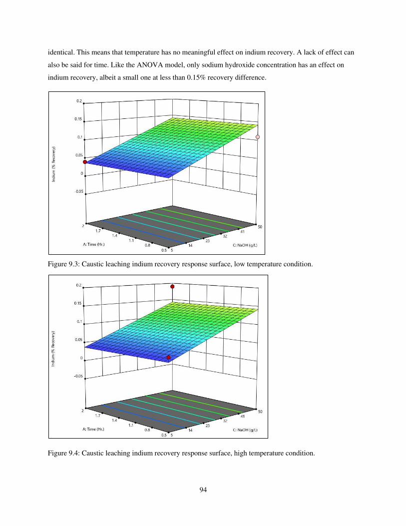
94

identical. This means that temperature has no meaningful effect on indium recovery. A lack of effect can

also be said for time. Like the ANOVA model, only sodium hydroxide concentration has an effect on

indium recovery, albeit a small one at less than 0.15% recovery difference.

Figure 9.3: Caustic leaching indium recovery response surface, low temperature condition.

Figure 9.4: Caustic leaching indium recovery response surface, high temperature condition.

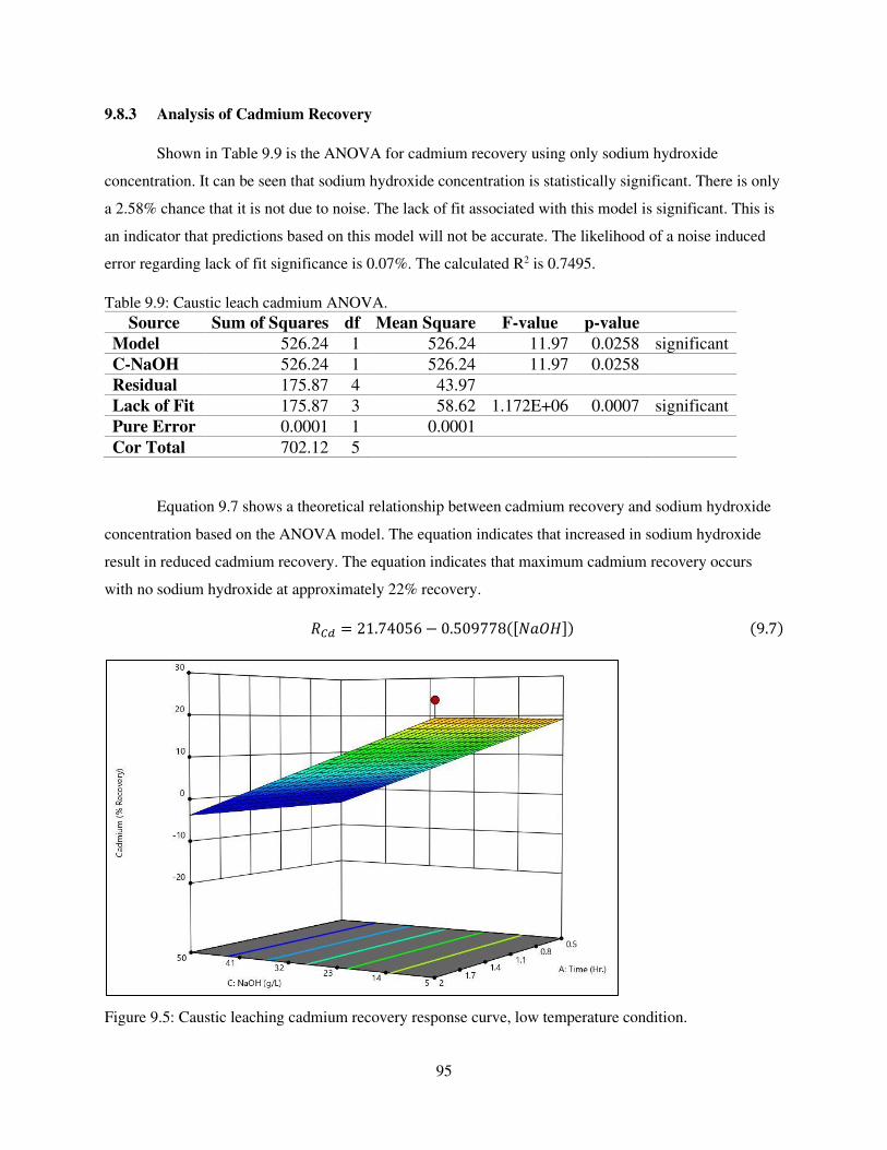
95


Shown in Table 9.9 is the ANOVA for cadmium recovery using only sodium hydroxide

concentration. It can be seen that sodium hydroxide concentration is statistically significant. There is only

a 2.58% chance that it is not due to noise. The lack of fit associated with this model is significant. This is

an indicator that predictions based on this model will not be accurate. The likelihood of a noise induced

error regarding lack of fit significance is 0.07%. The calculated R2 is 0.7495.

Table 9.9: Caustic leach cadmium ANOVA.



C-NaOH 526.24 1 526.24 11.97 0.0258

Residual 175.87 4 43.97

Lack of Fit 175.87 3 58.62 1.172E+06 0.0007 significant

Pure Error 0.0001 1 0.0001

Cor Total 702.12 5

Equation 9.7 shows a theoretical relationship between cadmium recovery and sodium hydroxide

concentration based on the ANOVA model. The equation indicates that increased in sodium hydroxide

result in reduced cadmium recovery. The equation indicates that maximum cadmium recovery occurs

with no sodium hydroxide at approximately 22% recovery. 𝑅𝐶𝑑 = 21.74056 − 0.509778([𝑁𝑎𝑂𝐻]) (9.7)

Figure 9.5: Caustic leaching cadmium recovery response curve, low temperature condition.

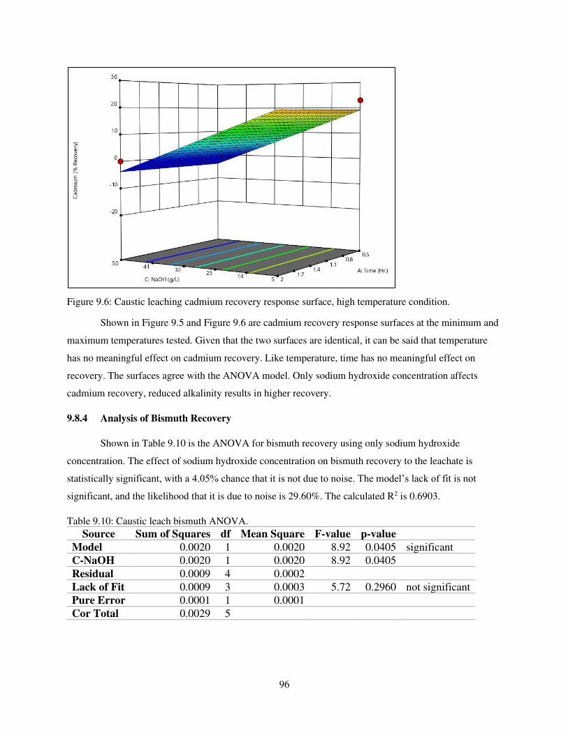
96

Figure 9.6: Caustic leaching cadmium recovery response surface, high temperature condition.

Shown in Figure 9.5 and Figure 9.6 are cadmium recovery response surfaces at the minimum and

maximum temperatures tested. Given that the two surfaces are identical, it can be said that temperature

has no meaningful effect on cadmium recovery. Like temperature, time has no meaningful effect on

recovery. The surfaces agree with the ANOVA model. Only sodium hydroxide concentration affects

cadmium recovery, reduced alkalinity results in higher recovery.


Shown in Table 9.10 is the ANOVA for bismuth recovery using only sodium hydroxide

concentration. The effect of sodium hydroxide concentration on bismuth recovery to the leachate is

statistically significant, with a 4.05% chance that it is not due to noise. The model’s lack of fit is not

significant, and the likelihood that it is due to noise is 29.60%. The calculated R2 is 0.6903.

Table 9.10: Caustic leach bismuth ANOVA.



C-NaOH 0.0020 1 0.0020 8.92 0.0405

Residual 0.0009 4 0.0002


Pure Error 0.0001 1 0.0001

Cor Total 0.0029 5

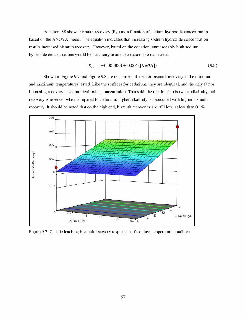
97

Equation 9.8 shows bismuth recovery (RBi) as a function of sodium hydroxide concentration

based on the ANOVA model. The equation indicates that increasing sodium hydroxide concentration

results increased bismuth recovery. However, based on the equation, unreasonably high sodium

hydroxide concentrations would be necessary to achieve reasonable recoveries. 𝑅𝐵𝐼 = −0.000833 + 0.001([𝑁𝑎𝑂𝐻]) (9.8)


and maximum temperatures tested. Like the surfaces for cadmium, they are identical, and the only factor

impacting recovery is sodium hydroxide concentration. That said, the relationship between alkalinity and

recovery is reversed when compared to cadmium; higher alkalinity is associated with higher bismuth

recovery. It should be noted that on the high end, bismuth recoveries are still low, at less than 0.1%.

Figure 9.7: Caustic leaching bismuth recovery response surface, low temperature condition.

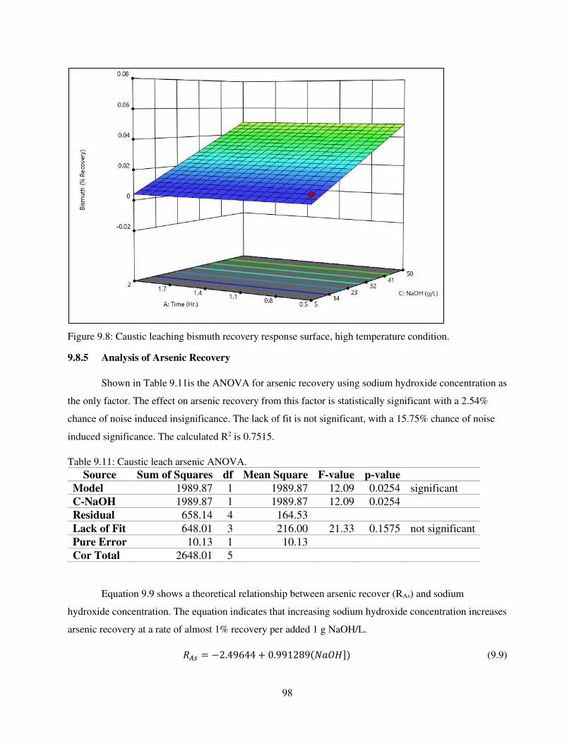
98

Figure 9.8: Caustic leaching bismuth recovery response surface, high temperature condition.


Shown in Table 9.11is the ANOVA for arsenic recovery using sodium hydroxide concentration as

the only factor. The effect on arsenic recovery from this factor is statistically significant with a 2.54%

chance of noise induced insignificance. The lack of fit is not significant, with a 15.75% chance of noise

induced significance. The calculated R2 is 0.7515.

Table 9.11: Caustic leach arsenic ANOVA.



C-NaOH 1989.87 1 1989.87 12.09 0.0254

Residual 658.14 4 164.53


Pure Error 10.13 1 10.13

Cor Total 2648.01 5

Equation 9.9 shows a theoretical relationship between arsenic recover (RAs) and sodium

hydroxide concentration. The equation indicates that increasing sodium hydroxide concentration increases

arsenic recovery at a rate of almost 1% recovery per added 1 g NaOH/L. 𝑅𝐴𝑠 = −2.49644 + 0.991289(𝑁𝑎𝑂𝐻]) (9.9)

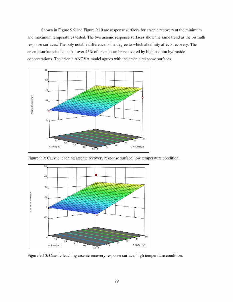
99

Shown in Figure 9.9 and Figure 9.10 are response surfaces for arsenic recovery at the minimum

and maximum temperatures tested. The two arsenic response surfaces show the same trend as the bismuth

response surfaces. The only notable difference is the degree to which alkalinity affects recovery. The

arsenic surfaces indicate that over 45% of arsenic can be recovered by high sodium hydroxide

concentrations. The arsenic ANOVA model agrees with the arsenic response surfaces.

Figure 9.9: Caustic leaching arsenic recovery response surface, low temperature condition.

Figure 9.10: Caustic leaching arsenic recovery response surface, high temperature condition.

100

9.9 Caustic Leaching Discussion

Overall, sodium hydroxide did not consistently transfer any of the elements of interest to the

aqueous phase during leaching. The trials having higher caustic concentration showed to have higher

arsenic recovery, and virtually no recovery for the other elements of interest. This is an indicator that

caustic leaching may provide a good separation between arsenic and the other elements at sodium

hydroxide concentrations above 50 g/L, but this needs to be confirmed.

Only the slightly alkaline trials (2 & 3) were capable of leaching non-near zero amounts of

copper. The other, and substantially more alkaline, trials were not capable of leaching copper.

Thermodynamically, one would expect sodium hydroxide to be incapable of leaching copper based on the

copper Pourbaix diagrams. It is hypothesized that the sulfur in the dust reacted with the water when

leached to generate sulfuric acid. This is supported by the pH data associated with caustic trials 2 & 3,

which show that the leach solution ends substantially more acidic than it starts. The acid neutralized the

small amount of sodium hydroxide, leaving the remaining acid to dissolve copper. It is believed that the

other trials also generated sulfuric acid, but the generated acid was consumed by the NaOH with no

excess acid, thus the lack of large pH shifts and copper dissolution.

For all elemental recoveries, the concentration of sodium hydroxide is the only test variable that

proved to be statistically significant. This indicates that the effects caustic leaching may be achieved

without high temperatures or long leach times, improving the costs and throughput rate of caustic

leaching.

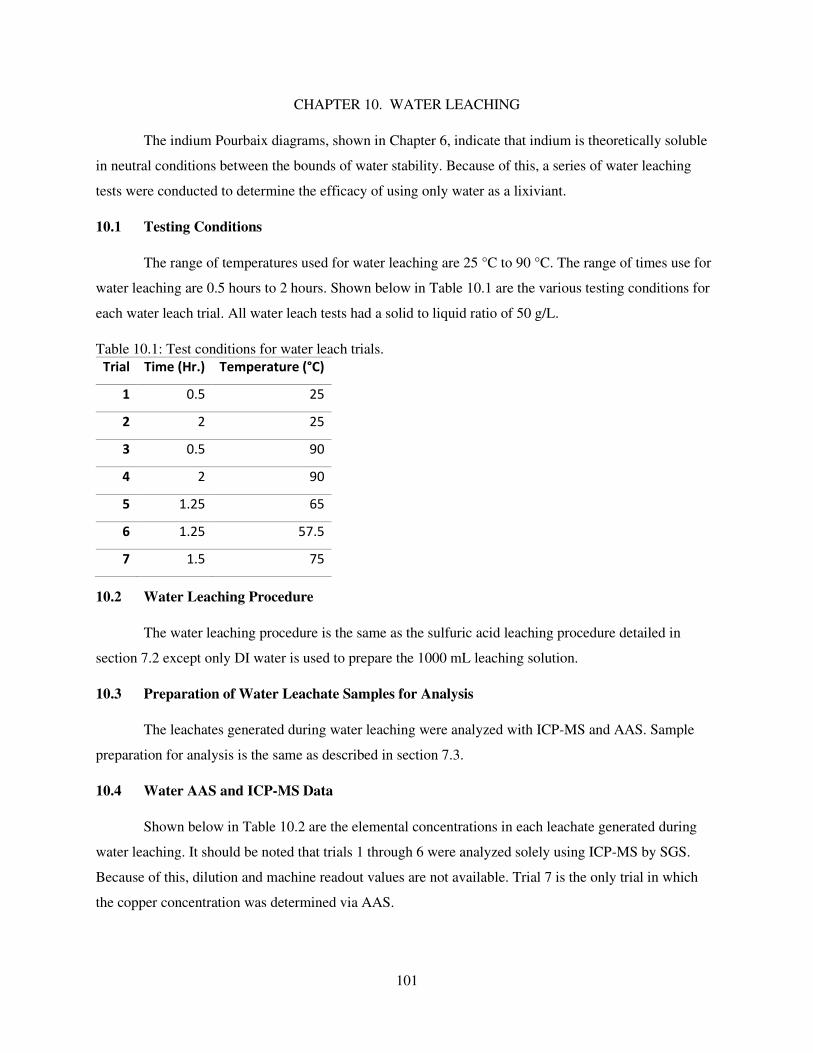
101

CHAPTER 10. WATER LEACHING

The indium Pourbaix diagrams, shown in Chapter 6, indicate that indium is theoretically soluble

in neutral conditions between the bounds of water stability. Because of this, a series of water leaching

tests were conducted to determine the efficacy of using only water as a lixiviant.


The range of temperatures used for water leaching are 25 °C to 90 °C. The range of times use for

water leaching are 0.5 hours to 2 hours. Shown below in Table 10.1 are the various testing conditions for

each water leach trial. All water leach tests had a solid to liquid ratio of 50 g/L.

Table 10.1: Test conditions for water leach trials.

Trial Time (Hr.) Temperature (°C)

1 0.5 25

2 2 25

3 0.5 90

4 2 90

5 1.25 65

6 1.25 57.5

7 1.5 75

10.2 Water Leaching Procedure

The water leaching procedure is the same as the sulfuric acid leaching procedure detailed in

section 7.2 except only DI water is used to prepare the 1000 mL leaching solution.

10.3 Preparation of Water Leachate Samples for Analysis

The leachates generated during water leaching were analyzed with ICP-MS and AAS. Sample

preparation for analysis is the same as described in section 7.3.

10.4 Water AAS and ICP-MS Data

Shown below in Table 10.2 are the elemental concentrations in each leachate generated during

water leaching. It should be noted that trials 1 through 6 were analyzed solely using ICP-MS by SGS.

Because of this, dilution and machine readout values are not available. Trial 7 is the only trial in which

the copper concentration was determined via AAS.

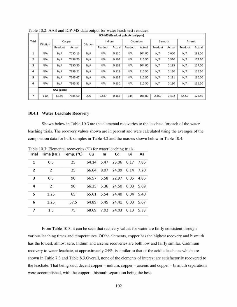
102

Table 10.2: AAS and ICP-MS data output for water leach test residues.

Trial

ICP-MS (Readout ppb, Actual ppm)

Dilution Copper



1 N/A N/A 7055.16 N/A N/A 0.130 N/A 104.00 N/A 0.650 N/A 188.50

2 N/A N/A 7456.70 N/A N/A 0.195 N/A 110.50 N/A 0.520 N/A 175.50

3 N/A N/A 7350.30 N/A N/A 0.133 N/A 104.00 N/A 0.195 N/A 117.00

4 N/A N/A 7299.21 N/A N/A 0.128 N/A 110.50 N/A 0.130 N/A 136.50

5 N/A N/A 7245.67 N/A N/A 0.132 N/A 110.50 N/A 0.131 N/A 130.00

6 N/A N/A 7165.35 N/A N/A 0.130 N/A 110.50 N/A 0.130 N/A 136.50

AAS (ppm)

7 110 68.96 7585.60 200 0.837 0.167 544 108.80 2.460 0.492 642.0 128.40

10.4.1 Water Leachate Recovery

Shown below in Table 10.3 are the elemental recoveries to the leachate for each of the water

leaching trials. The recovery values shown are in percent and were calculated using the averages of the

composition data for bulk samples in Table 4.2 and the masses shown below in Table 10.4.

Table 10.3: Elemental recoveries (%) for water leaching trials.

Trial Time (Hr.) Temp. (°C) Cu In Cd Bi As

1 0.5 25 64.14 5.47 23.06 0.17 7.86

2 2 25 66.64 8.07 24.09 0.14 7.20

3 0.5 90 66.57 5.58 22.97 0.05 4.86

4 2 90 66.35 5.36 24.50 0.03 5.69

5 1.25 65 65.61 5.54 24.40 0.04 5.40

6 1.25 57.5 64.89 5.45 24.41 0.03 5.67

7 1.5 75 68.69 7.02 24.03 0.13 5.33

From Table 10.3, it can be seen that recovery values for water are fairly consistent through

various leaching times and temperatures. Of the elements, copper has the highest recovery and bismuth

has the lowest, almost zero. Indium and arsenic recoveries are both low and fairly similar. Cadmium

recovery to water leachate, at approximately 24%, is similar to that of the acidic leachates which are

shown in Table 7.3 and Table 8.3.Overall, none of the elements of interest are satisfactorily recovered to

the leachate. That being said, decent copper – indium, copper – arsenic and copper – bismuth separations

were accomplished, with the copper – bismuth separation being the best.

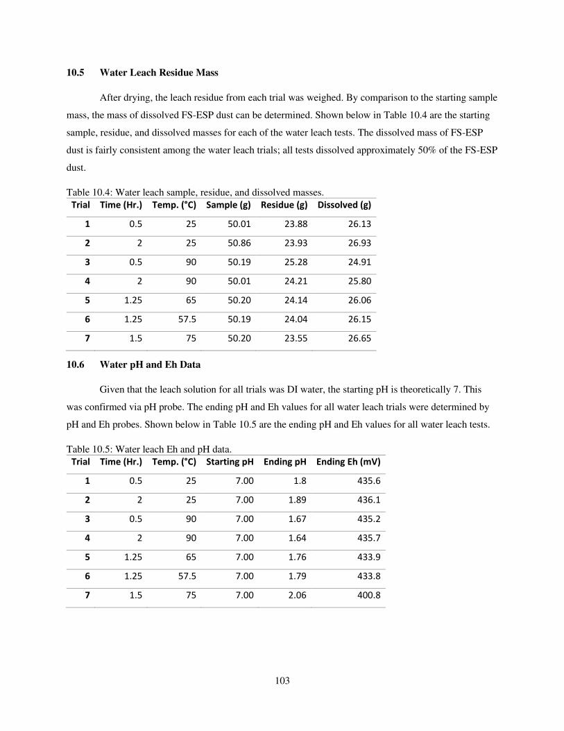
103

10.5 Water Leach Residue Mass

After drying, the leach residue from each trial was weighed. By comparison to the starting sample

mass, the mass of dissolved FS-ESP dust can be determined. Shown below in Table 10.4 are the starting

sample, residue, and dissolved masses for each of the water leach tests. The dissolved mass of FS-ESP

dust is fairly consistent among the water leach trials; all tests dissolved approximately 50% of the FS-ESP

dust.

Table 10.4: Water leach sample, residue, and dissolved masses.

Trial Time (Hr.) Temp. (°C) Sample (g) Residue (g) Dissolved (g)

1 0.5 25 50.01 23.88 26.13

2 2 25 50.86 23.93 26.93

3 0.5 90 50.19 25.28 24.91

4 2 90 50.01 24.21 25.80

5 1.25 65 50.20 24.14 26.06

6 1.25 57.5 50.19 24.04 26.15

7 1.5 75 50.20 23.55 26.65

10.6 Water pH and Eh Data

Given that the leach solution for all trials was DI water, the starting pH is theoretically 7. This

was confirmed via pH probe. The ending pH and Eh values for all water leach trials were determined by

pH and Eh probes. Shown below in Table 10.5 are the ending pH and Eh values for all water leach tests.

Table 10.5: Water leach Eh and pH data.

Trial Time (Hr.) Temp. (°C) Starting pH Ending pH Ending Eh (mV)

1 0.5 25 7.00 1.8 435.6

2 2 25 7.00 1.89 436.1

3 0.5 90 7.00 1.67 435.2

4 2 90 7.00 1.64 435.7

5 1.25 65 7.00 1.76 433.9

6 1.25 57.5 7.00 1.79 433.8

7 1.5 75 7.00 2.06 400.8

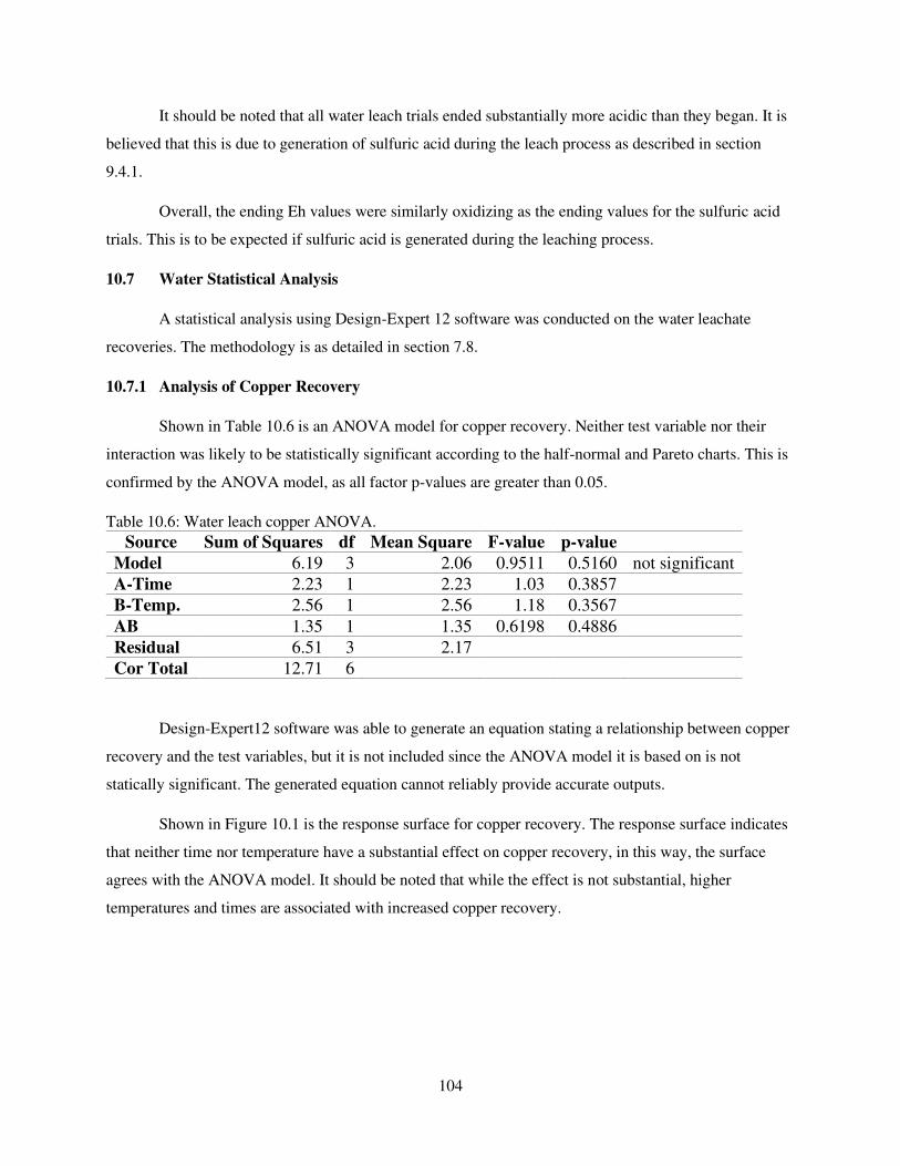
104

It should be noted that all water leach trials ended substantially more acidic than they began. It is

believed that this is due to generation of sulfuric acid during the leach process as described in section

9.4.1.

Overall, the ending Eh values were similarly oxidizing as the ending values for the sulfuric acid

trials. This is to be expected if sulfuric acid is generated during the leaching process.

10.7 Water Statistical Analysis

A statistical analysis using Design-Expert 12 software was conducted on the water leachate

recoveries. The methodology is as detailed in section 7.8.


Shown in Table 10.6 is an ANOVA model for copper recovery. Neither test variable nor their

interaction was likely to be statistically significant according to the half-normal and Pareto charts. This is

confirmed by the ANOVA model, as all factor p-values are greater than 0.05.

Table 10.6: Water leach copper ANOVA.



A-Time 2.23 1 2.23 1.03 0.3857

B-Temp. 2.56 1 2.56 1.18 0.3567

AB 1.35 1 1.35 0.6198 0.4886

Residual 6.51 3 2.17

Cor Total 12.71 6

Design-Expert12 software was able to generate an equation stating a relationship between copper

recovery and the test variables, but it is not included since the ANOVA model it is based on is not

statically significant. The generated equation cannot reliably provide accurate outputs.

Shown in Figure 10.1 is the response surface for copper recovery. The response surface indicates

that neither time nor temperature have a substantial effect on copper recovery, in this way, the surface

agrees with the ANOVA model. It should be noted that while the effect is not substantial, higher

temperatures and times are associated with increased copper recovery.

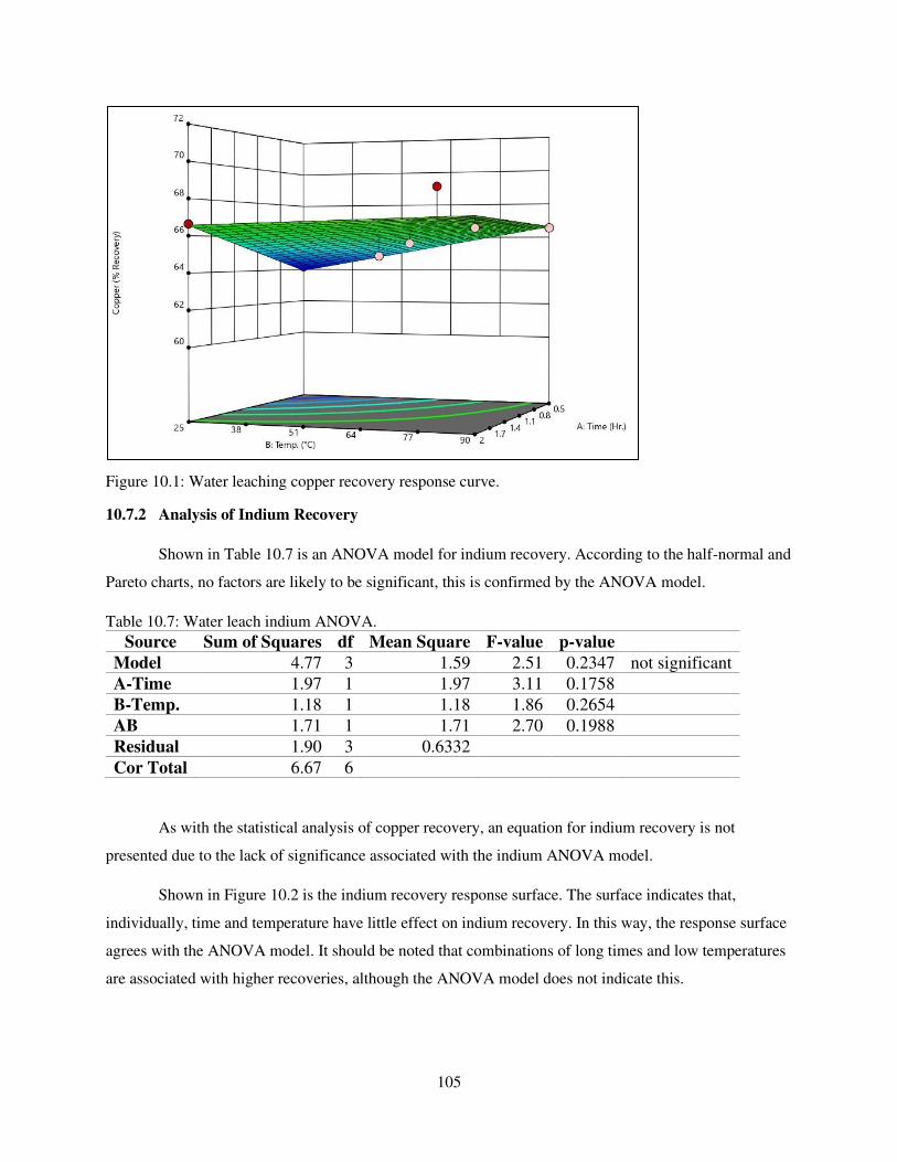
105

Figure 10.1: Water leaching copper recovery response curve.


Shown in Table 10.7 is an ANOVA model for indium recovery. According to the half-normal and

Pareto charts, no factors are likely to be significant, this is confirmed by the ANOVA model.

Table 10.7: Water leach indium ANOVA.



A-Time 1.97 1 1.97 3.11 0.1758

B-Temp. 1.18 1 1.18 1.86 0.2654

AB 1.71 1 1.71 2.70 0.1988

Residual 1.90 3 0.6332

Cor Total 6.67 6

As with the statistical analysis of copper recovery, an equation for indium recovery is not

presented due to the lack of significance associated with the indium ANOVA model.

Shown in Figure 10.2 is the indium recovery response surface. The surface indicates that,

individually, time and temperature have little effect on indium recovery. In this way, the response surface

agrees with the ANOVA model. It should be noted that combinations of long times and low temperatures

are associated with higher recoveries, although the ANOVA model does not indicate this.

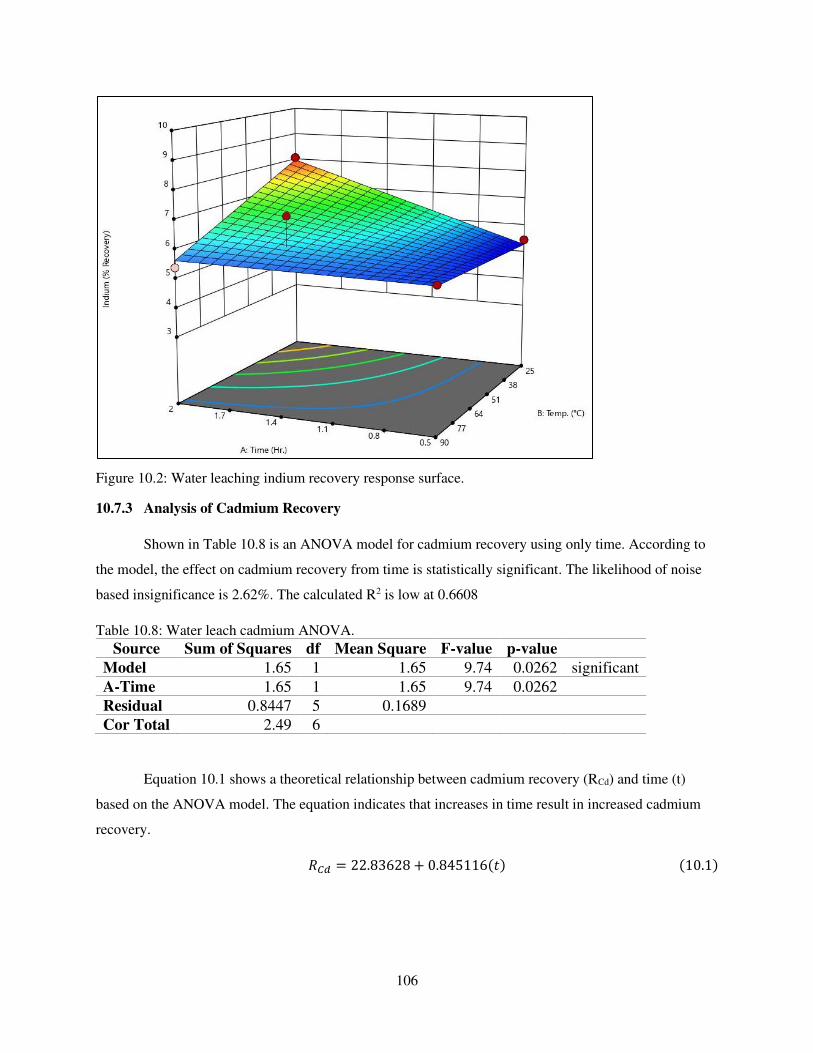
106

Figure 10.2: Water leaching indium recovery response surface.


Shown in Table 10.8 is an ANOVA model for cadmium recovery using only time. According to

the model, the effect on cadmium recovery from time is statistically significant. The likelihood of noise

based insignificance is 2.62%. The calculated R2 is low at 0.6608

Table 10.8: Water leach cadmium ANOVA.



A-Time 1.65 1 1.65 9.74 0.0262

Residual 0.8447 5 0.1689

Cor Total 2.49 6

Equation 10.1 shows a theoretical relationship between cadmium recovery (RCd) and time (t)

based on the ANOVA model. The equation indicates that increases in time result in increased cadmium

recovery. 𝑅𝐶𝑑 = 22.83628 + 0.845116(𝑡) (10.1)

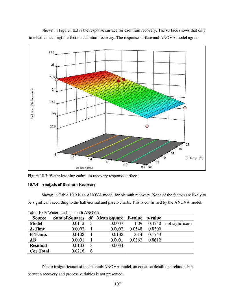
107

Shown in Figure 10.3 is the response surface for cadmium recovery. The surface shows that only

time had a meaningful effect on cadmium recovery. The response surface and ANOVA model agree.

Figure 10.3: Water leaching cadmium recovery response surface.


Shown in Table 10.9 is an ANOVA model for bismuth recovery. None of the factors are likely to

be significant according to the half-normal and pareto charts. This is confirmed by the ANOVA model.

Table 10.9: Water leach bismuth ANOVA.



A-Time 0.0002 1 0.0002 0.0548 0.8300

B-Temp. 0.0108 1 0.0108 3.14 0.1743

AB 0.0001 1 0.0001 0.0362 0.8612

Residual 0.0103 3 0.0034

Cor Total 0.0216 6

Due to insignificance of the bismuth ANOVA model, an equation detailing a relationship

between recovery and process variables is not presented.

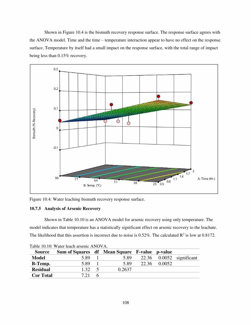
108

Shown in Figure 10.4 is the bismuth recovery response surface. The response surface agrees with

the ANOVA model. Time and the time – temperature interaction appear to have no effect on the response

surface. Temperature by itself had a small impact on the response surface, with the total range of impact

being less than 0.15% recovery.

Figure 10.4: Water leaching bismuth recovery response surface.


Shown in Table 10.10 is an ANOVA model for arsenic recovery using only temperature. The

model indicates that temperature has a statistically significant effect on arsenic recovery to the leachate.

The likelihood that this assertion is incorrect due to noise is 0.52%. The calculated R2 is low at 0.8172.

Table 10.10: Water leach arsenic ANOVA.



B-Temp. 5.89 1 5.89 22.36 0.0052

Residual 1.32 5 0.2637

Cor Total 7.21 6

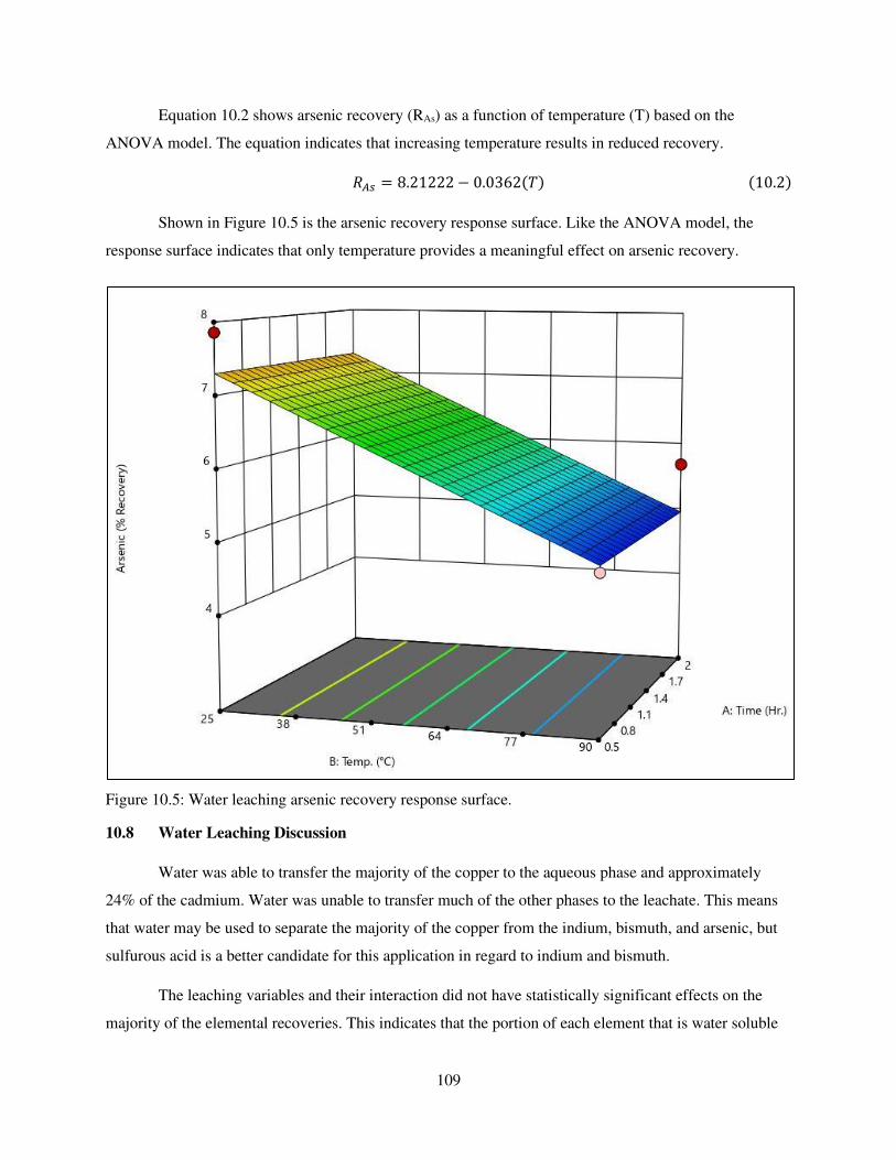
109

Equation 10.2 shows arsenic recovery (RAs) as a function of temperature (T) based on the

ANOVA model. The equation indicates that increasing temperature results in reduced recovery. 𝑅𝐴𝑠 = 8.21222 − 0.0362(𝑇) (10.2)

Shown in Figure 10.5 is the arsenic recovery response surface. Like the ANOVA model, the

response surface indicates that only temperature provides a meaningful effect on arsenic recovery.

Figure 10.5: Water leaching arsenic recovery response surface.

10.8 Water Leaching Discussion

Water was able to transfer the majority of the copper to the aqueous phase and approximately

24% of the cadmium. Water was unable to transfer much of the other phases to the leachate. This means

that water may be used to separate the majority of the copper from the indium, bismuth, and arsenic, but

sulfurous acid is a better candidate for this application in regard to indium and bismuth.

The leaching variables and their interaction did not have statistically significant effects on the

majority of the elemental recoveries. This indicates that the portion of each element that is water soluble

110

will not change much with time or temperature, so there is no reason to increase costs associated with

water leaching by utilizing high temperatures or long leaching times. That said, in the case of cadmium,

time did have a statistically significant effect, and according to Equation 10.1, it may be possible to

increase cadmium recovery to over 80% by leaching for over 72 hours.

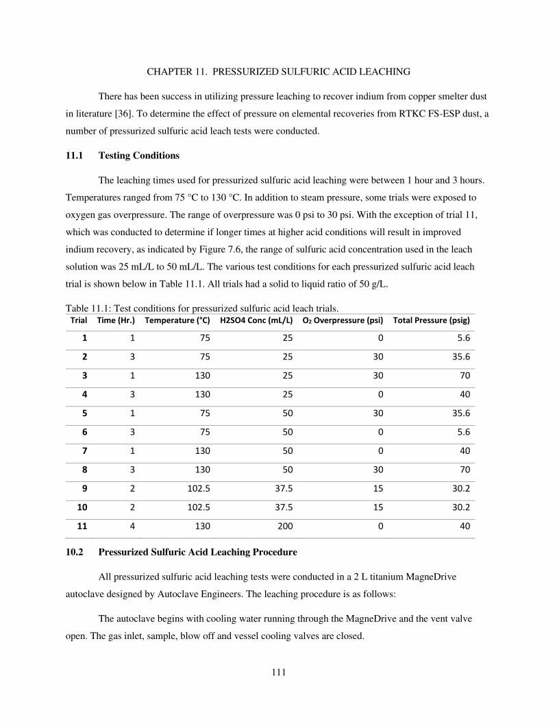
111

CHAPTER 11. PRESSURIZED SULFURIC ACID LEACHING

There has been success in utilizing pressure leaching to recover indium from copper smelter dust

in literature [36]. To determine the effect of pressure on elemental recoveries from RTKC FS-ESP dust, a

number of pressurized sulfuric acid leach tests were conducted.


The leaching times used for pressurized sulfuric acid leaching were between 1 hour and 3 hours.

Temperatures ranged from 75 °C to 130 °C. In addition to steam pressure, some trials were exposed to

oxygen gas overpressure. The range of overpressure was 0 psi to 30 psi. With the exception of trial 11,

which was conducted to determine if longer times at higher acid conditions will result in improved

indium recovery, as indicated by Figure 7.6, the range of sulfuric acid concentration used in the leach

solution was 25 mL/L to 50 mL/L. The various test conditions for each pressurized sulfuric acid leach

trial is shown below in Table 11.1. All trials had a solid to liquid ratio of 50 g/L.

Table 11.1: Test conditions for pressurized sulfuric acid leach trials.

Trial Time (Hr.) Temperature (°C) H2SO4 Conc (mL/L) O2 Overpressure (psi) Total Pressure (psig)

1 1 75 25 0 5.6

2 3 75 25 30 35.6

3 1 130 25 30 70

4 3 130 25 0 40

5 1 75 50 30 35.6

6 3 75 50 0 5.6

7 1 130 50 0 40

8 3 130 50 30 70

9 2 102.5 37.5 15 30.2

10 2 102.5 37.5 15 30.2

11 4 130 200 0 40

10.2 Pressurized Sulfuric Acid Leaching Procedure

All pressurized sulfuric acid leaching tests were conducted in a 2 L titanium MagneDrive

autoclave designed by Autoclave Engineers. The leaching procedure is as follows:

The autoclave begins with cooling water running through the MagneDrive and the vent valve

open. The gas inlet, sample, blow off and vessel cooling valves are closed.

112

A 1000 mL solution of DI water and concentrated sulfuric acid is prepared so that the appropriate

sulfuric acid concentration is achieved. This solution is placed into the autoclave reaction vessel. The

vessel is then raised and sealed. At this point the vent valve is closed and the MagneDrive agitator is

turned on. The heating element is attached to the autoclave reaction vessel and set to heat the reaction

vessel to the leaching temperature or, in the event the leaching temperature is above 100 °C, to 90 °C.

Once the appropriate temperature is reached, the heater is turned off, the MagneDrive agitator is

turned off and the vent valve is opened. The reaction vessel is then unsealed and lowered. A massed

sample of approximately 50 g of the bulk FS-ESP dust is then placed into the reaction vessel. The

reaction vessel is then raised and closed, and the MagneDrive agitator turned on and the vent closed. The

heater is then turned on and set to heat the reaction vessel to the leaching temperature. At this point blast

shields should be put up. Once the leaching temperature is achieved, the leaching time starts. If the trial

calls for O2 overpressure, the overpressure is introduced after the leaching temperature is achieved and

before leaching time starts.

Upon completion of leaching time, the heater is turned off and the reaction vessel cooling valve is

opened. Once the vessel temperature is below 85 °C, the vent valve is slowly opened to release pressure

in the reaction vessel. Once all excess pressure is released, and the temperature has been sufficiently

lowered to the point of operator comfort, the blast shields are removed, the MagneDrive is turned off and

the vessel unsealed and lowered. The reaction vessel is then removed from the autoclave and the contents

poured over a filter to separate the remaining solids from the leachate. Once solid – liquid separation is

concluded, the leachate is stored and the residue is allowed to dry and then stored.

11.3 Preparation of Pressurized Sulfuric Acid Leachate Samples for Analysis

All leachates from pressurized sulfuric acid leach testing were analyzed via ICP-MS and AAS.

All ICP-MS analysis was performed by Hazen Research and therefore, the leachate samples were

prepared by Hazen Research. AAS sample preparation is as described in section 7.3.2.

11.4 Pressurized Sulfuric Acid AAS and ICP-MS Data

Shown below in Table 11.2 are the elemental concentrations in each leachate generated during

the testing depicted in Table 11.1.

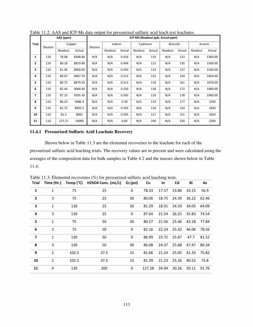
113

Table 11.2: AAS and ICP-Ms data output for pressurized sulfuric acid leach test leachates.

Trial


Dilution Copper



1 110 78.08 8588.80 N/A N/A 0.416 N/A 110 N/A 123 N/A 1360.00

2 110 80.18 8819.80 N/A N/A 0.446 N/A 113 N/A 135 N/A 1500.00

3 110 81.46 8960.60 N/A N/A 0.450 N/A 114 N/A 127 N/A 1540.00

4 110 88.07 9687.70 N/A N/A 0.514 N/A 122 N/A 134 N/A 1820.00

5 110 80.72 8879.20 N/A N/A 0.513 N/A 118 N/A 161 N/A 1870.00

6 110 82.44 9068.40 N/A N/A 0.530 N/A 118 N/A 172 N/A 1890.00

7 110 87.23 9595.30 N/A N/A 0.565 N/A 120 N/A 178 N/A 1960.00

8 110 86.24 9486.4 N/A N/A 0.58 N/A 119 N/A 177 N/A 1930

9 110 81.75 8992.5 N/A N/A 0.505 N/A 116 N/A 154 N/A 1820

10 110 81.5 8965 N/A N/A 0.505 N/A 117 N/A 151 N/A 1820

11 110 127.27 14000 N/A N/A 0.83 N/A 140 N/A 220 N/A 2200

11.4.1 Pressurized Sulfuric Acid Leachate Recovery

Shown below in Table 11.3 are the elemental recoveries to the leachate for each of the

pressurized sulfuric acid leaching trials. The recovery values are in percent and were calculated using the

averages of the composition data for bulk samples in Table 4.2 and the masses shown below in Table

11.4.

Table 11.3: Elemental recoveries (%) for pressurized sulfuric acid leaching tests.

Trial Time (Hr.) Temp (°C) H2SO4 Conc. (mL/L) O2 (psi) Cu In Cd Bi As

1 1 75 25 0 78.33 17.57 23.86 33.15 56.9

2 3 75 25 30 80.06 18.75 24.39 36.22 62.46

3 1 130 25 30 81.29 18.91 24.59 34.05 64.09

4 3 130 25 0 87.64 21.54 26.25 35.83 74.54

5 1 75 50 30 80.57 21.56 25.46 43.18 77.84

6 3 75 50 0 82.16 22.24 25.42 46.06 78.56

7 1 130 50 0 86.99 23.72 25.87 47.7 81.52

8 3 130 50 30 86.08 24.37 25.68 47.47 80.34

9 2 102.5 37.5 15 81.66 21.24 25.05 41.33 75.82

10 2 102.5 37.5 15 81.39 21.23 25.26 40.52 75.8

11 4 130 200 0 127.28 34.94 30.26 59.11 91.76

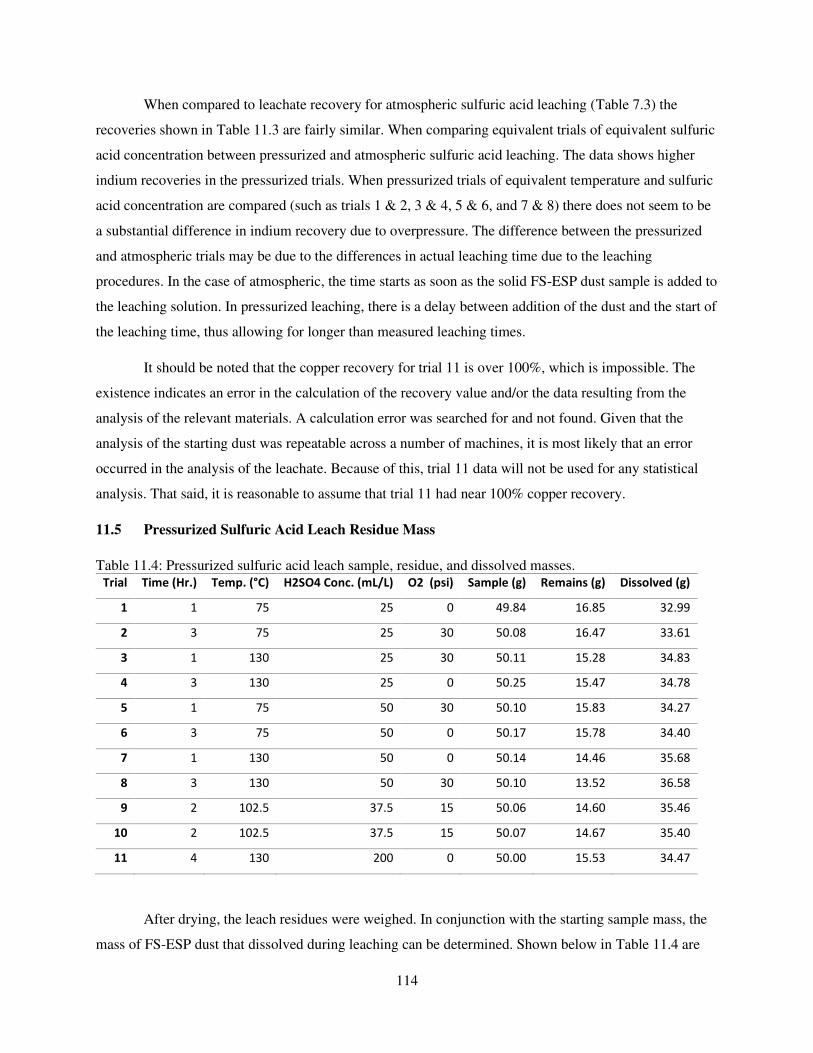
114

When compared to leachate recovery for atmospheric sulfuric acid leaching (Table 7.3) the

recoveries shown in Table 11.3 are fairly similar. When comparing equivalent trials of equivalent sulfuric

acid concentration between pressurized and atmospheric sulfuric acid leaching. The data shows higher

indium recoveries in the pressurized trials. When pressurized trials of equivalent temperature and sulfuric

acid concentration are compared (such as trials 1 & 2, 3 & 4, 5 & 6, and 7 & 8) there does not seem to be

a substantial difference in indium recovery due to overpressure. The difference between the pressurized

and atmospheric trials may be due to the differences in actual leaching time due to the leaching

procedures. In the case of atmospheric, the time starts as soon as the solid FS-ESP dust sample is added to

the leaching solution. In pressurized leaching, there is a delay between addition of the dust and the start of

the leaching time, thus allowing for longer than measured leaching times.

It should be noted that the copper recovery for trial 11 is over 100%, which is impossible. The

existence indicates an error in the calculation of the recovery value and/or the data resulting from the

analysis of the relevant materials. A calculation error was searched for and not found. Given that the

analysis of the starting dust was repeatable across a number of machines, it is most likely that an error

occurred in the analysis of the leachate. Because of this, trial 11 data will not be used for any statistical

analysis. That said, it is reasonable to assume that trial 11 had near 100% copper recovery.

11.5 Pressurized Sulfuric Acid Leach Residue Mass

Table 11.4: Pressurized sulfuric acid leach sample, residue, and dissolved masses. Trial Time (Hr.) Temp. (°C) H2SO4 Conc. (mL/L) O2 (psi) Sample (g) Remains (g) Dissolved (g)

1 1 75 25 0 49.84 16.85 32.99

2 3 75 25 30 50.08 16.47 33.61

3 1 130 25 30 50.11 15.28 34.83

4 3 130 25 0 50.25 15.47 34.78

5 1 75 50 30 50.10 15.83 34.27

6 3 75 50 0 50.17 15.78 34.40

7 1 130 50 0 50.14 14.46 35.68

8 3 130 50 30 50.10 13.52 36.58

9 2 102.5 37.5 15 50.06 14.60 35.46

10 2 102.5 37.5 15 50.07 14.67 35.40

11 4 130 200 0 50.00 15.53 34.47

After drying, the leach residues were weighed. In conjunction with the starting sample mass, the

mass of FS-ESP dust that dissolved during leaching can be determined. Shown below in Table 11.4 are

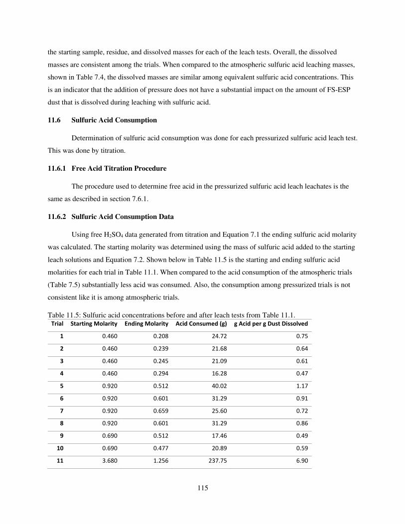
115

the starting sample, residue, and dissolved masses for each of the leach tests. Overall, the dissolved

masses are consistent among the trials. When compared to the atmospheric sulfuric acid leaching masses,

shown in Table 7.4, the dissolved masses are similar among equivalent sulfuric acid concentrations. This

is an indicator that the addition of pressure does not have a substantial impact on the amount of FS-ESP

dust that is dissolved during leaching with sulfuric acid.


Determination of sulfuric acid consumption was done for each pressurized sulfuric acid leach test.

This was done by titration.


The procedure used to determine free acid in the pressurized sulfuric acid leach leachates is the

same as described in section 7.6.1.

11.6.2 Sulfuric Acid Consumption Data


was calculated. The starting molarity was determined using the mass of sulfuric acid added to the starting

leach solutions and Equation 7.2. Shown below in Table 11.5 is the starting and ending sulfuric acid

molarities for each trial in Table 11.1. When compared to the acid consumption of the atmospheric trials

(Table 7.5) substantially less acid was consumed. Also, the consumption among pressurized trials is not

consistent like it is among atmospheric trials.

Table 11.5: Sulfuric acid concentrations before and after leach tests from Table 11.1. Trial Starting Molarity Ending Molarity Acid Consumed (g) g Acid per g Dust Dissolved

1 0.460 0.208 24.72 0.75

2 0.460 0.239 21.68 0.64

3 0.460 0.245 21.09 0.61

4 0.460 0.294 16.28 0.47

5 0.920 0.512 40.02 1.17

6 0.920 0.601 31.29 0.91

7 0.920 0.659 25.60 0.72

8 0.920 0.601 31.29 0.86

9 0.690 0.512 17.46 0.49

10 0.690 0.477 20.89 0.59

11 3.680 1.256 237.75 6.90

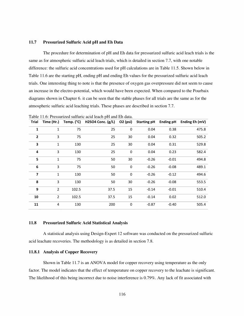
116

11.7 Pressurized Sulfuric Acid pH and Eh Data

The procedure for determination of pH and Eh data for pressurized sulfuric acid leach trials is the

same as for atmospheric sulfuric acid leach trials, which is detailed in section 7.7, with one notable

difference: the sulfuric acid concentrations used for pH calculations are in Table 11.5. Shown below in

Table 11.6 are the starting pH, ending pH and ending Eh values for the pressurized sulfuric acid leach

trials. One interesting thing to note is that the presence of oxygen gas overpressure did not seem to cause

an increase in the electro-potential, which would have been expected. When compared to the Pourbaix

diagrams shown in Chapter 6. it can be seen that the stable phases for all trials are the same as for the

atmospheric sulfuric acid leaching trials. These phases are described in section 7.7.

Table 11.6: Pressurized sulfuric acid leach pH and Eh data.

Trial Time (Hr.) Temp. (°C) H2SO4 Conc. (g/L) O2 (psi) Starting pH Ending pH Ending Eh (mV)

1 1 75 25 0 0.04 0.38 475.8

2 3 75 25 30 0.04 0.32 505.2

3 1 130 25 30 0.04 0.31 529.8

4 3 130 25 0 0.04 0.23 582.4

5 1 75 50 30 -0.26 -0.01 494.8

6 3 75 50 0 -0.26 -0.08 489.1

7 1 130 50 0 -0.26 -0.12 494.6

8 3 130 50 30 -0.26 -0.08 553.5

9 2 102.5 37.5 15 -0.14 -0.01 510.4

10 2 102.5 37.5 15 -0.14 0.02 512.0

11 4 130 200 0 -0.87 -0.40 505.4

11.8 Pressurized Sulfuric Acid Statistical Analysis

A statistical analysis using Design-Expert 12 software was conducted on the pressurized sulfuric

acid leachate recoveries. The methodology is as detailed in section 7.8.


Shown in Table 11.7 is an ANOVA model for copper recovery using temperature as the only

factor. The model indicates that the effect of temperature on copper recovery to the leachate is significant.

The likelihood of this being incorrect due to noise interference is 0.79%. Any lack of fit associated with

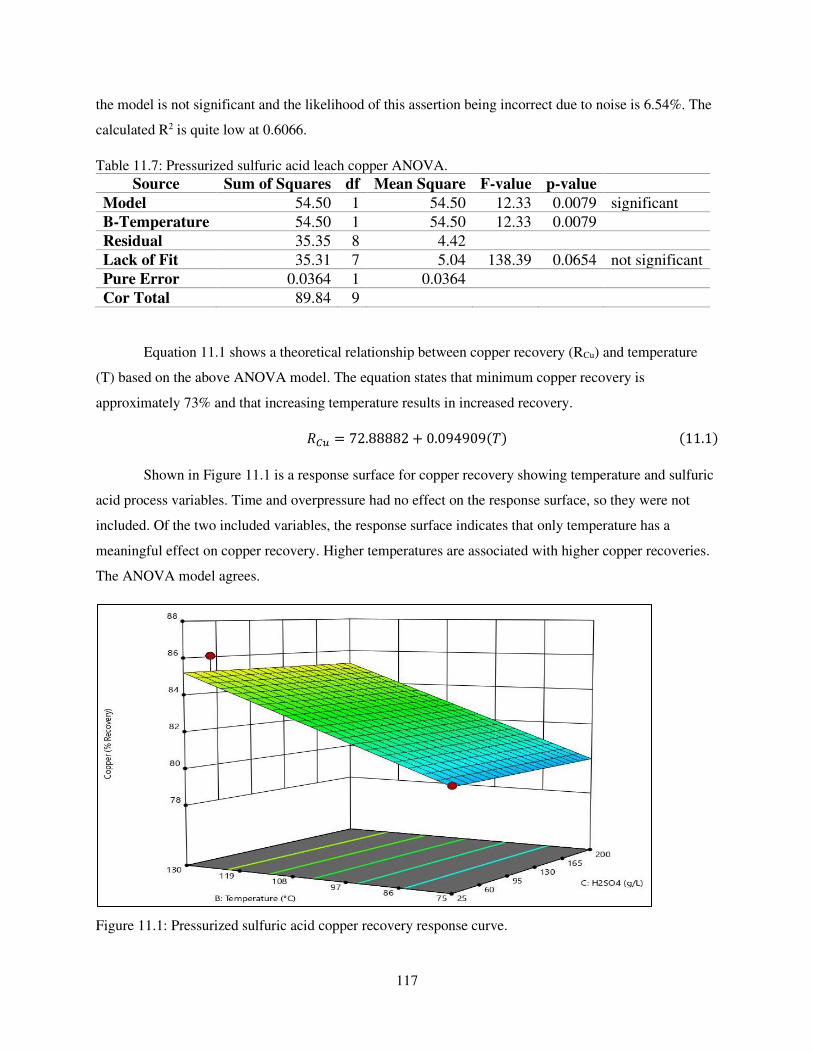
117

the model is not significant and the likelihood of this assertion being incorrect due to noise is 6.54%. The

calculated R2 is quite low at 0.6066.

Table 11.7: Pressurized sulfuric acid leach copper ANOVA.



B-Temperature 54.50 1 54.50 12.33 0.0079

Residual 35.35 8 4.42


Pure Error 0.0364 1 0.0364

Cor Total 89.84 9

Equation 11.1 shows a theoretical relationship between copper recovery (RCu) and temperature

(T) based on the above ANOVA model. The equation states that minimum copper recovery is

approximately 73% and that increasing temperature results in increased recovery. 𝑅𝐶𝑢 = 72.88882 + 0.094909(𝑇) (11.1)

Shown in Figure 11.1 is a response surface for copper recovery showing temperature and sulfuric

acid process variables. Time and overpressure had no effect on the response surface, so they were not

included. Of the two included variables, the response surface indicates that only temperature has a

meaningful effect on copper recovery. Higher temperatures are associated with higher copper recoveries.

The ANOVA model agrees.

Figure 11.1: Pressurized sulfuric acid copper recovery response curve.

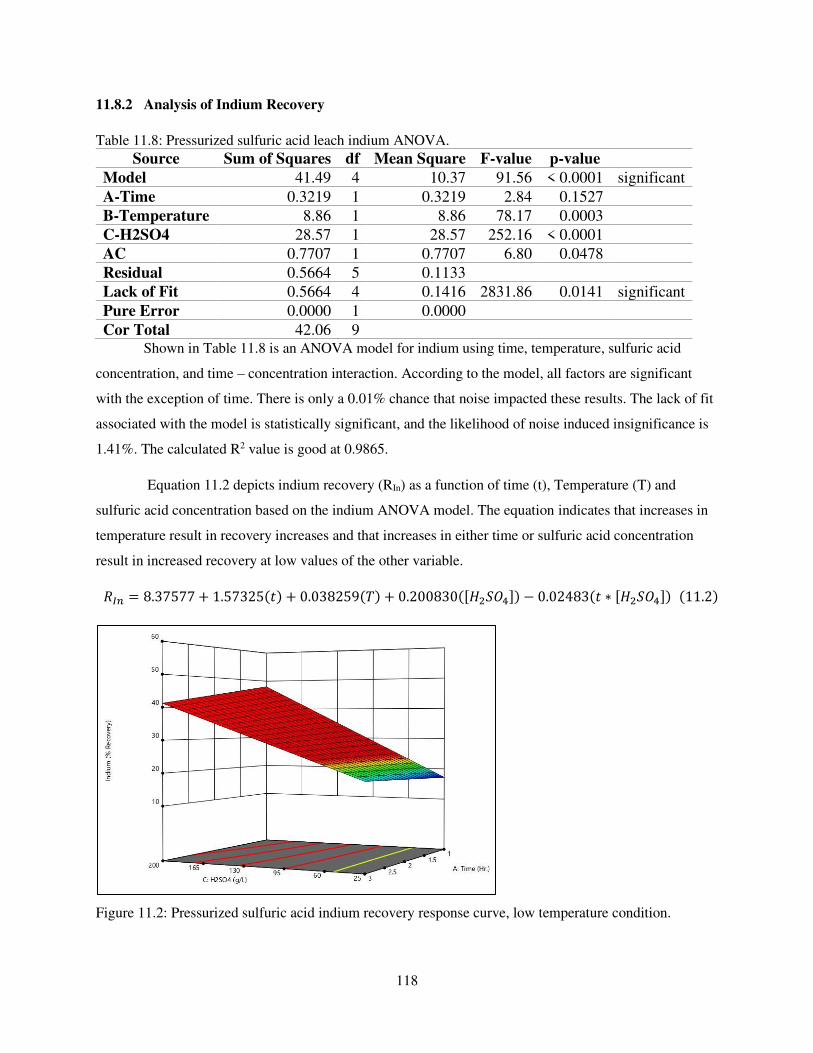
118


Table 11.8: Pressurized sulfuric acid leach indium ANOVA.


Model 41.49 4 10.37 91.56 < 0.0001 significant

A-Time 0.3219 1 0.3219 2.84 0.1527

B-Temperature 8.86 1 8.86 78.17 0.0003

C-H2SO4 28.57 1 28.57 252.16 < 0.0001

AC 0.7707 1 0.7707 6.80 0.0478

Residual 0.5664 5 0.1133

Lack of Fit 0.5664 4 0.1416 2831.86 0.0141 significant

Pure Error 0.0000 1 0.0000

Cor Total 42.06 9

Shown in Table 11.8 is an ANOVA model for indium using time, temperature, sulfuric acid

concentration, and time – concentration interaction. According to the model, all factors are significant

with the exception of time. There is only a 0.01% chance that noise impacted these results. The lack of fit

associated with the model is statistically significant, and the likelihood of noise induced insignificance is

1.41%. The calculated R2 value is good at 0.9865.

Equation 11.2 depicts indium recovery (RIn) as a function of time (t), Temperature (T) and

sulfuric acid concentration based on the indium ANOVA model. The equation indicates that increases in

temperature result in recovery increases and that increases in either time or sulfuric acid concentration

result in increased recovery at low values of the other variable. 𝑅𝐼𝑛 = 8.37577 + 1.57325(𝑡) + 0.038259(𝑇) + 0.200830([𝐻2𝑆𝑂4]) − 0.02483(𝑡 ∗ [𝐻2𝑆𝑂4]) (11.2)

Figure 11.2: Pressurized sulfuric acid indium recovery response curve, low temperature condition.

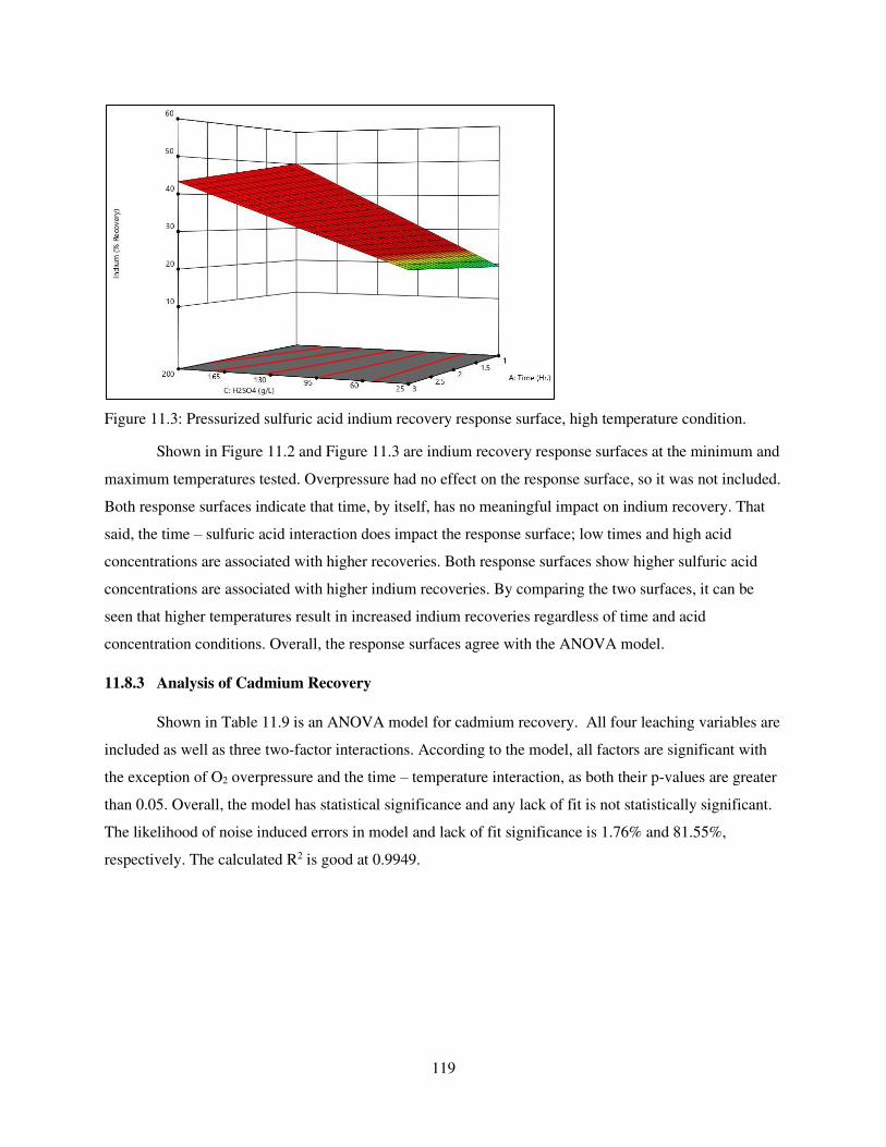
119

Figure 11.3: Pressurized sulfuric acid indium recovery response surface, high temperature condition.

Shown in Figure 11.2 and Figure 11.3 are indium recovery response surfaces at the minimum and

maximum temperatures tested. Overpressure had no effect on the response surface, so it was not included.

Both response surfaces indicate that time, by itself, has no meaningful impact on indium recovery. That

said, the time – sulfuric acid interaction does impact the response surface; low times and high acid

concentrations are associated with higher recoveries. Both response surfaces show higher sulfuric acid

concentrations are associated with higher indium recoveries. By comparing the two surfaces, it can be

seen that higher temperatures result in increased indium recoveries regardless of time and acid

concentration conditions. Overall, the response surfaces agree with the ANOVA model.


Shown in Table 11.9 is an ANOVA model for cadmium recovery. All four leaching variables are

included as well as three two-factor interactions. According to the model, all factors are significant with

the exception of O2 overpressure and the time – temperature interaction, as both their p-values are greater

than 0.05. Overall, the model has statistical significance and any lack of fit is not statistically significant.

The likelihood of noise induced errors in model and lack of fit significance is 1.76% and 81.55%,

respectively. The calculated R2 is good at 0.9949.

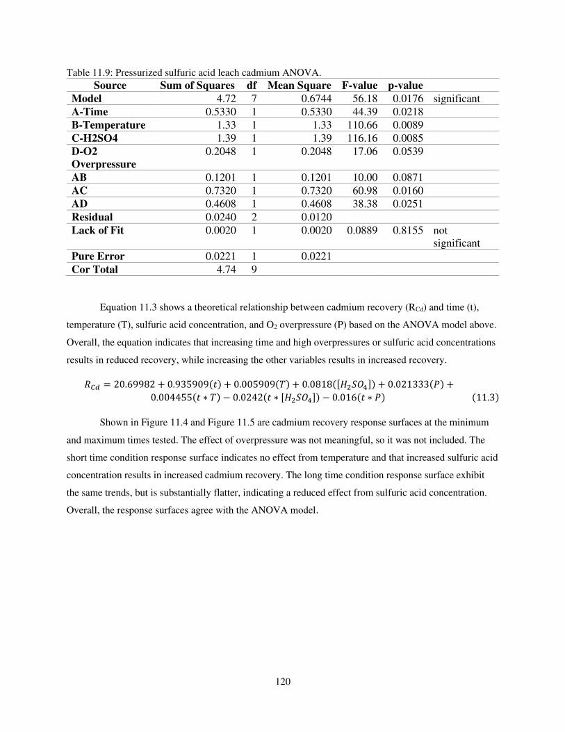
120

Table 11.9: Pressurized sulfuric acid leach cadmium ANOVA.



A-Time 0.5330 1 0.5330 44.39 0.0218

B-Temperature 1.33 1 1.33 110.66 0.0089

C-H2SO4 1.39 1 1.39 116.16 0.0085

D-O2

Overpressure

0.2048 1 0.2048 17.06 0.0539

AB 0.1201 1 0.1201 10.00 0.0871

AC 0.7320 1 0.7320 60.98 0.0160

AD 0.4608 1 0.4608 38.38 0.0251

Residual 0.0240 2 0.0120

Lack of Fit 0.0020 1 0.0020 0.0889 0.8155 not

significant

Pure Error 0.0221 1 0.0221

Cor Total 4.74 9

Equation 11.3 shows a theoretical relationship between cadmium recovery (RCd) and time (t),

temperature (T), sulfuric acid concentration, and O2 overpressure (P) based on the ANOVA model above.

Overall, the equation indicates that increasing time and high overpressures or sulfuric acid concentrations

results in reduced recovery, while increasing the other variables results in increased recovery. 𝑅𝐶𝑑 = 20.69982 + 0.935909(𝑡) + 0.005909(𝑇) + 0.0818([𝐻2𝑆𝑂4]) + 0.021333(𝑃) +0.004455(𝑡 ∗ 𝑇) − 0.0242(𝑡 ∗ [𝐻2𝑆𝑂4]) − 0.016(𝑡 ∗ 𝑃) (11.3)

Shown in Figure 11.4 and Figure 11.5 are cadmium recovery response surfaces at the minimum

and maximum times tested. The effect of overpressure was not meaningful, so it was not included. The

short time condition response surface indicates no effect from temperature and that increased sulfuric acid

concentration results in increased cadmium recovery. The long time condition response surface exhibit

the same trends, but is substantially flatter, indicating a reduced effect from sulfuric acid concentration.

Overall, the response surfaces agree with the ANOVA model.

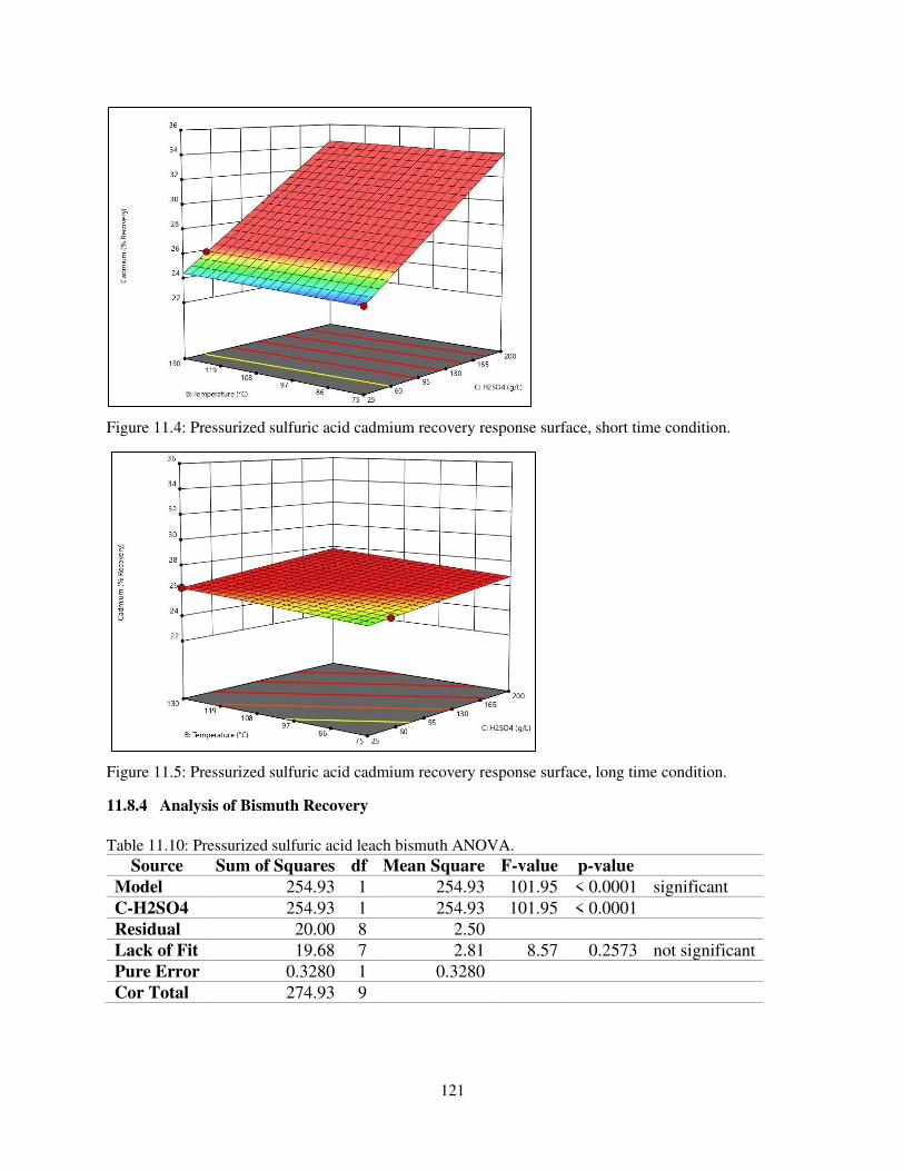
121

Figure 11.4: Pressurized sulfuric acid cadmium recovery response surface, short time condition.

Figure 11.5: Pressurized sulfuric acid cadmium recovery response surface, long time condition.


Table 11.10: Pressurized sulfuric acid leach bismuth ANOVA.


Model 254.93 1 254.93 101.95 < 0.0001 significant

C-H2SO4 254.93 1 254.93 101.95 < 0.0001

Residual 20.00 8 2.50


Pure Error 0.3280 1 0.3280

Cor Total 274.93 9

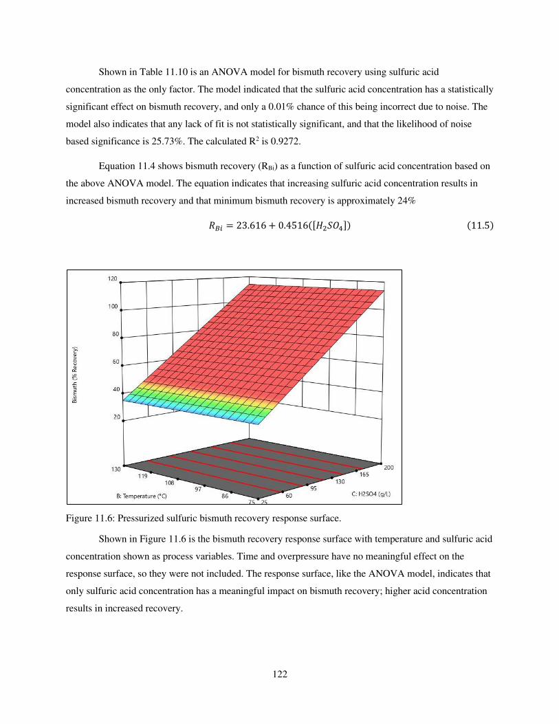
122

Shown in Table 11.10 is an ANOVA model for bismuth recovery using sulfuric acid

concentration as the only factor. The model indicated that the sulfuric acid concentration has a statistically

significant effect on bismuth recovery, and only a 0.01% chance of this being incorrect due to noise. The

model also indicates that any lack of fit is not statistically significant, and that the likelihood of noise

based significance is 25.73%. The calculated R2 is 0.9272.

Equation 11.4 shows bismuth recovery (RBi) as a function of sulfuric acid concentration based on

the above ANOVA model. The equation indicates that increasing sulfuric acid concentration results in

increased bismuth recovery and that minimum bismuth recovery is approximately 24% 𝑅𝐵𝑖 = 23.616 + 0.4516([𝐻2𝑆𝑂4]) (11.5)

Figure 11.6: Pressurized sulfuric bismuth recovery response surface.

Shown in Figure 11.6 is the bismuth recovery response surface with temperature and sulfuric acid

concentration shown as process variables. Time and overpressure have no meaningful effect on the

response surface, so they were not included. The response surface, like the ANOVA model, indicates that

only sulfuric acid concentration has a meaningful impact on bismuth recovery; higher acid concentration

results in increased recovery.

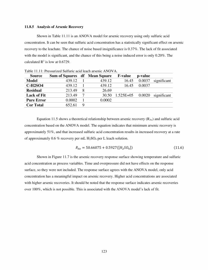
123


Shown in Table 11.11 is an ANOVA model for arsenic recovery using only sulfuric acid

concentration. It can be seen that sulfuric acid concentration has a statistically significant effect on arsenic

recovery to the leachate. The chance of noise based insignificance is 0.37%. The lack of fit associated

with the model is significant, and the chance of this being a noise induced error is only 0.20%. The

calculated R2 is low at 0.6729.

Table 11.11: Pressurized Sulfuric acid leach arsenic ANOVA.



C-H2SO4 439.12 1 439.12 16.45 0.0037

Residual 213.49 8 26.69


Pure Error 0.0002 1 0.0002

Cor Total 652.61 9

Equation 11.5 shows a theoretical relationship between arsenic recovery (RAs) and sulfuric acid

concentration based on the ANOVA model. The equation indicates that minimum arsenic recovery is

approximately 51%, and that increased sulfuric acid concentration results in increased recovery at a rate

of approximately 0.6 % recovery per mL H2SO4 per L leach solution. 𝑅𝐴𝑠 = 50.66075 + 0.5927([𝐻2𝑆𝑂4]) (11.6)

Shown in Figure 11.7 is the arsenic recovery response surface showing temperature and sulfuric

acid concentration as process variables. Time and overpressure did not have effects on the response

surface, so they were not included. The response surface agrees with the ANOVA model, only acid

concentration has a meaningful impact on arsenic recovery. Higher acid concentrations are associated

with higher arsenic recoveries. It should be noted that the response surface indicates arsenic recoveries

over 100%, which is not possible. This is associated with the ANOVA model’s lack of fit.

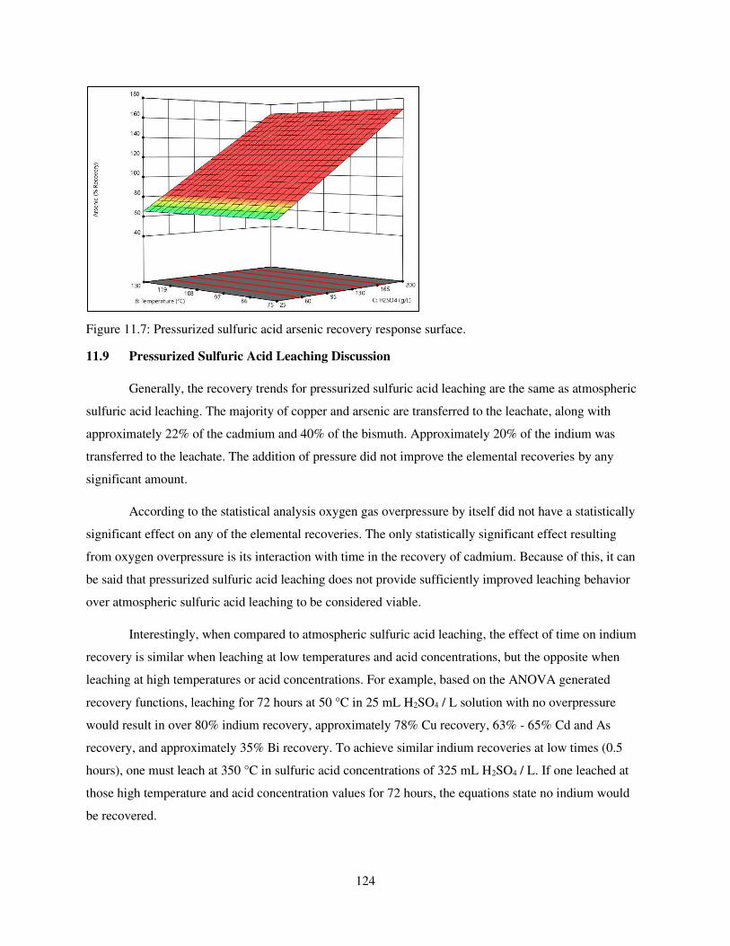
124

Figure 11.7: Pressurized sulfuric acid arsenic recovery response surface.

11.9 Pressurized Sulfuric Acid Leaching Discussion

Generally, the recovery trends for pressurized sulfuric acid leaching are the same as atmospheric

sulfuric acid leaching. The majority of copper and arsenic are transferred to the leachate, along with

approximately 22% of the cadmium and 40% of the bismuth. Approximately 20% of the indium was

transferred to the leachate. The addition of pressure did not improve the elemental recoveries by any

significant amount.

According to the statistical analysis oxygen gas overpressure by itself did not have a statistically

significant effect on any of the elemental recoveries. The only statistically significant effect resulting

from oxygen overpressure is its interaction with time in the recovery of cadmium. Because of this, it can

be said that pressurized sulfuric acid leaching does not provide sufficiently improved leaching behavior

over atmospheric sulfuric acid leaching to be considered viable.

Interestingly, when compared to atmospheric sulfuric acid leaching, the effect of time on indium

recovery is similar when leaching at low temperatures and acid concentrations, but the opposite when

leaching at high temperatures or acid concentrations. For example, based on the ANOVA generated

recovery functions, leaching for 72 hours at 50 °C in 25 mL H2SO4 / L solution with no overpressure

would result in over 80% indium recovery, approximately 78% Cu recovery, 63% - 65% Cd and As

recovery, and approximately 35% Bi recovery. To achieve similar indium recoveries at low times (0.5

hours), one must leach at 350 °C in sulfuric acid concentrations of 325 mL H2SO4 / L. If one leached at

those high temperature and acid concentration values for 72 hours, the equations state no indium would

be recovered.

125

While pressurized sulfuric acid leaching did provide the highest indium recovery values seen of

the leaching methods presented thus far (over 35% in trial 11), the recoveries are not high enough to

justify the lack of separations. Also, on an industrial scale, the increase in cost due to pressurization,

longer times, and longer temperatures may not be worth it.

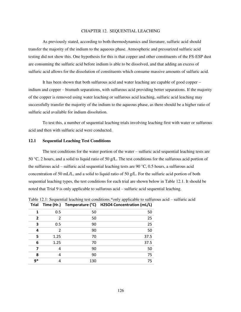
126

CHAPTER 12. SEQUENTIAL LEACHING

As previously stated, according to both thermodynamics and literature, sulfuric acid should

transfer the majority of the indium to the aqueous phase. Atmospheric and pressurized sulfuric acid

testing did not show this. One hypothesis for this is that copper and other constituents of the FS-ESP dust

are consuming the sulfuric acid before indium is able to be dissolved, and that adding an excess of

sulfuric acid allows for the dissolution of constituents which consume massive amounts of sulfuric acid.

It has been shown that both sulfurous acid and water leaching are capable of good copper –

indium and copper – bismuth separations, with sulfurous acid providing better separations. If the majority

of the copper is removed using water leaching or sulfurous acid leaching, sulfuric acid leaching may

successfully transfer the majority of the indium to the aqueous phase, as there should be a higher ratio of

sulfuric acid available for indium dissolution.

To test this, a number of sequential leaching trials involving leaching first with water or sulfurous

acid and then with sulfuric acid were conducted.

12.1 Sequential Leaching Test Conditions

The test conditions for the water portion of the water – sulfuric acid sequential leaching tests are

50 °C, 2 hours, and a solid to liquid ratio of 50 g/L. The test conditions for the sulfurous acid portion of

the sulfurous acid – sulfuric acid sequential leaching tests are 90 °C, 0.5 hours, a sulfurous acid

concentration of 50 mL/L, and a solid to liquid ratio of 50 g/L. For the sulfuric acid portion of both

sequential leaching types, the test conditions for each trial are shown below in Table 12.1. It should be

noted that Trial 9 is only applicable to sulfurous acid – sulfuric acid sequential leaching.

Table 12.1: Sequential leaching test conditions.*only applicable to sulfurous acid – sulfuric acid

Trial Time (Hr.) Temperature (°C) H2SO4 Concentration (mL/L)

1 0.5 50 50

2 2 50 25

3 0.5 90 25

4 2 90 50

5 1.25 70 37.5

6 1.25 70 37.5

7 4 90 50

8 4 90 75

9* 4 130 75

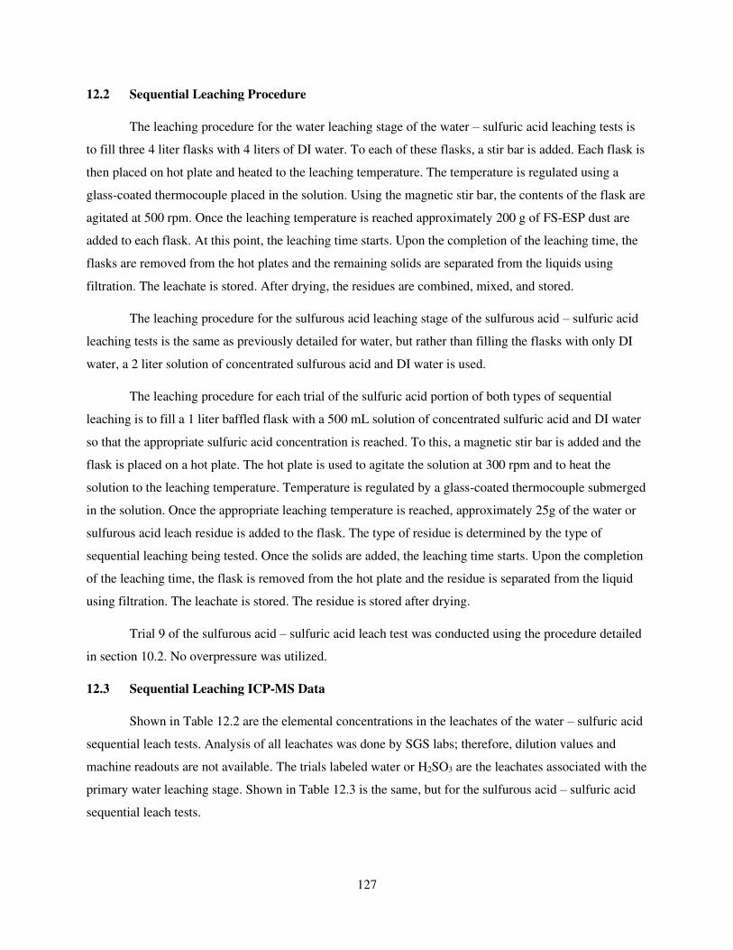
127

12.2 Sequential Leaching Procedure

The leaching procedure for the water leaching stage of the water – sulfuric acid leaching tests is

to fill three 4 liter flasks with 4 liters of DI water. To each of these flasks, a stir bar is added. Each flask is

then placed on hot plate and heated to the leaching temperature. The temperature is regulated using a

glass-coated thermocouple placed in the solution. Using the magnetic stir bar, the contents of the flask are

agitated at 500 rpm. Once the leaching temperature is reached approximately 200 g of FS-ESP dust are

added to each flask. At this point, the leaching time starts. Upon the completion of the leaching time, the

flasks are removed from the hot plates and the remaining solids are separated from the liquids using

filtration. The leachate is stored. After drying, the residues are combined, mixed, and stored.

The leaching procedure for the sulfurous acid leaching stage of the sulfurous acid – sulfuric acid

leaching tests is the same as previously detailed for water, but rather than filling the flasks with only DI

water, a 2 liter solution of concentrated sulfurous acid and DI water is used.

The leaching procedure for each trial of the sulfuric acid portion of both types of sequential

leaching is to fill a 1 liter baffled flask with a 500 mL solution of concentrated sulfuric acid and DI water

so that the appropriate sulfuric acid concentration is reached. To this, a magnetic stir bar is added and the

flask is placed on a hot plate. The hot plate is used to agitate the solution at 300 rpm and to heat the

solution to the leaching temperature. Temperature is regulated by a glass-coated thermocouple submerged

in the solution. Once the appropriate leaching temperature is reached, approximately 25g of the water or

sulfurous acid leach residue is added to the flask. The type of residue is determined by the type of

sequential leaching being tested. Once the solids are added, the leaching time starts. Upon the completion

of the leaching time, the flask is removed from the hot plate and the residue is separated from the liquid

using filtration. The leachate is stored. The residue is stored after drying.

Trial 9 of the sulfurous acid – sulfuric acid leach test was conducted using the procedure detailed

in section 10.2. No overpressure was utilized.

12.3 Sequential Leaching ICP-MS Data

Shown in Table 12.2 are the elemental concentrations in the leachates of the water – sulfuric acid

sequential leach tests. Analysis of all leachates was done by SGS labs; therefore, dilution values and

machine readouts are not available. The trials labeled water or H2SO3 are the leachates associated with the

primary water leaching stage. Shown in Table 12.3 is the same, but for the sulfurous acid – sulfuric acid

sequential leach tests.

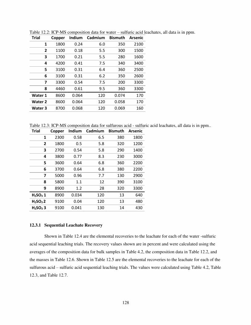
128

Table 12.2: ICP-MS composition data for water – sulfuric acid leachates, all data is in ppm.

Trial Copper Indium Cadmium Bismuth Arsenic

1 1800 0.24 6.0 350 2100

2 1100 0.18 5.5 300 1500

3 1700 0.21 5.5 280 1600

4 4200 0.41 7.5 340 3400

5 3100 0.31 6.4 360 2500

6 3100 0.31 6.2 350 2600

7 3300 0.54 7.5 200 3300

8 4460 0.61 9.5 360 3300

Water 1 8600 0.064 120 0.074 170

Water 2 8600 0.064 120 0.058 170

Water 3 8700 0.068 120 0.069 160

Table 12.3: ICP-MS composition data for sulfurous acid - sulfuric acid leachates, all data is in ppm..

Trial Copper Indium Cadmium Bismuth Arsenic

1 2300 0.58 6.5 380 1800

2 1800 0.5 5.8 320 1200

3 2700 0.54 5.8 290 1400

4 3800 0.77 8.3 230 3000

5 3600 0.64 6.8 360 2200

6 3700 0.64 6.8 380 2200

7 5000 0.96 7.7 130 2900

8 5800 1.1 12 390 3100

9 8900 1.2 28 320 3300

H2SO3 1 8900 0.034 120 13 640

H2SO3 2 9100 0.04 120 13 480

H2SO3 3 9100 0.041 130 14 430

12.3.1 Sequential Leachate Recovery

Shown in Table 12.4 are the elemental recoveries to the leachate for each of the water -sulfuric

acid sequential leaching trials. The recovery values shown are in percent and were calculated using the

averages of the composition data for bulk samples in Table 4.2, the composition data in Table 12.2, and

the masses in Table 12.6. Shown in Table 12.5 are the elemental recoveries to the leachate for each of the

sulfurous acid – sulfuric acid sequential leaching trials. The values were calculated using Table 4.2, Table

12.3, and Table 12.7.

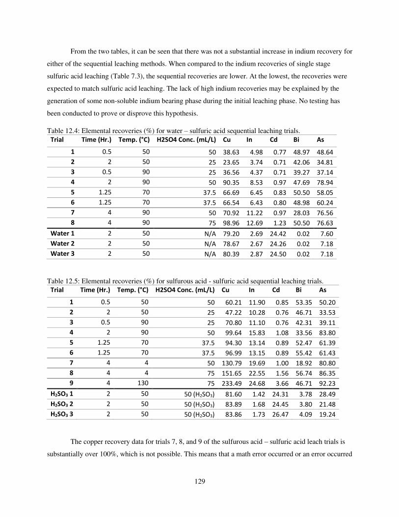
129

From the two tables, it can be seen that there was not a substantial increase in indium recovery for

either of the sequential leaching methods. When compared to the indium recoveries of single stage

sulfuric acid leaching (Table 7.3), the sequential recoveries are lower. At the lowest, the recoveries were

expected to match sulfuric acid leaching. The lack of high indium recoveries may be explained by the

generation of some non-soluble indium bearing phase during the initial leaching phase. No testing has

been conducted to prove or disprove this hypothesis.

Table 12.4: Elemental recoveries (%) for water – sulfuric acid sequential leaching trials.


1 0.5 50 50 38.63 4.98 0.77 48.97 48.64

2 2 50 25 23.65 3.74 0.71 42.06 34.81

3 0.5 90 25 36.56 4.37 0.71 39.27 37.14

4 2 90 50 90.35 8.53 0.97 47.69 78.94

5 1.25 70 37.5 66.69 6.45 0.83 50.50 58.05

6 1.25 70 37.5 66.54 6.43 0.80 48.98 60.24

7 4 90 50 70.92 11.22 0.97 28.03 76.56

8 4 90 75 98.96 12.69 1.23 50.50 76.63

Water 1 2 50 N/A 79.20 2.69 24.42 0.02 7.60

Water 2 2 50 N/A 78.67 2.67 24.26 0.02 7.18

Water 3 2 50 N/A 80.39 2.87 24.50 0.02 7.18

Table 12.5: Elemental recoveries (%) for sulfurous acid - sulfuric acid sequential leaching trials.


1 0.5 50 50 60.21 11.90 0.85 53.35 50.20

2 2 50 25 47.22 10.28 0.76 46.71 33.53

3 0.5 90 25 70.80 11.10 0.76 42.31 39.11

4 2 90 50 99.64 15.83 1.08 33.56 83.80

5 1.25 70 37.5 94.30 13.14 0.89 52.47 61.39

6 1.25 70 37.5 96.99 13.15 0.89 55.42 61.43

7 4 4 50 130.79 19.69 1.00 18.92 80.80

8 4 4 75 151.65 22.55 1.56 56.74 86.35

9 4 130 75 233.49 24.68 3.66 46.71 92.23

H2SO3 1 2 50 50 (H2SO3) 81.60 1.42 24.31 3.78 28.49

H2SO3 2 2 50 50 (H2SO3) 83.89 1.68 24.45 3.80 21.48

H2SO3 3 2 50 50 (H2SO3) 83.86 1.73 26.47 4.09 19.24

The copper recovery data for trials 7, 8, and 9 of the sulfurous acid – sulfuric acid leach trials is

substantially over 100%, which is not possible. This means that a math error occurred or an error occurred

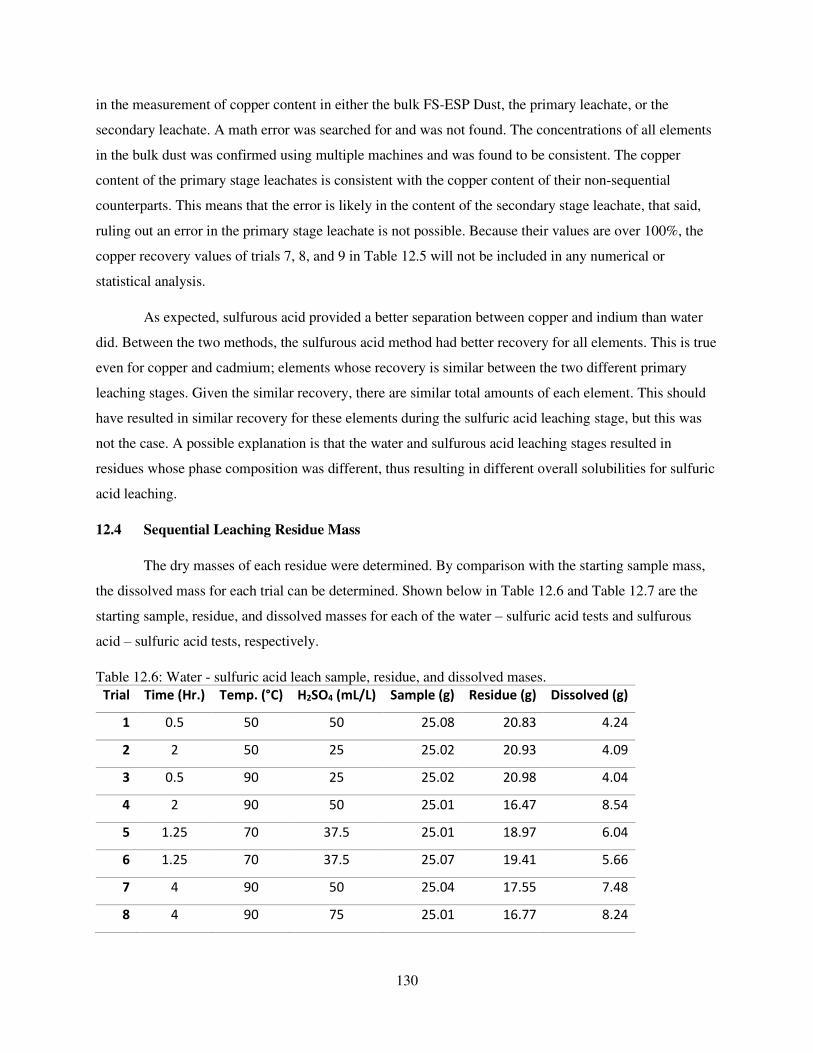
130

in the measurement of copper content in either the bulk FS-ESP Dust, the primary leachate, or the

secondary leachate. A math error was searched for and was not found. The concentrations of all elements

in the bulk dust was confirmed using multiple machines and was found to be consistent. The copper

content of the primary stage leachates is consistent with the copper content of their non-sequential

counterparts. This means that the error is likely in the content of the secondary stage leachate, that said,

ruling out an error in the primary stage leachate is not possible. Because their values are over 100%, the

copper recovery values of trials 7, 8, and 9 in Table 12.5 will not be included in any numerical or

statistical analysis.

As expected, sulfurous acid provided a better separation between copper and indium than water

did. Between the two methods, the sulfurous acid method had better recovery for all elements. This is true

even for copper and cadmium; elements whose recovery is similar between the two different primary

leaching stages. Given the similar recovery, there are similar total amounts of each element. This should

have resulted in similar recovery for these elements during the sulfuric acid leaching stage, but this was

not the case. A possible explanation is that the water and sulfurous acid leaching stages resulted in

residues whose phase composition was different, thus resulting in different overall solubilities for sulfuric

acid leaching.

12.4 Sequential Leaching Residue Mass

The dry masses of each residue were determined. By comparison with the starting sample mass,

the dissolved mass for each trial can be determined. Shown below in Table 12.6 and Table 12.7 are the

starting sample, residue, and dissolved masses for each of the water – sulfuric acid tests and sulfurous

acid – sulfuric acid tests, respectively.

Table 12.6: Water - sulfuric acid leach sample, residue, and dissolved mases.

Trial Time (Hr.) Temp. (°C) H2SO4 (mL/L) Sample (g) Residue (g) Dissolved (g)

1 0.5 50 50 25.08 20.83 4.24

2 2 50 25 25.02 20.93 4.09

3 0.5 90 25 25.02 20.98 4.04

4 2 90 50 25.01 16.47 8.54

5 1.25 70 37.5 25.01 18.97 6.04

6 1.25 70 37.5 25.07 19.41 5.66

7 4 90 50 25.04 17.55 7.48

8 4 90 75 25.01 16.77 8.24

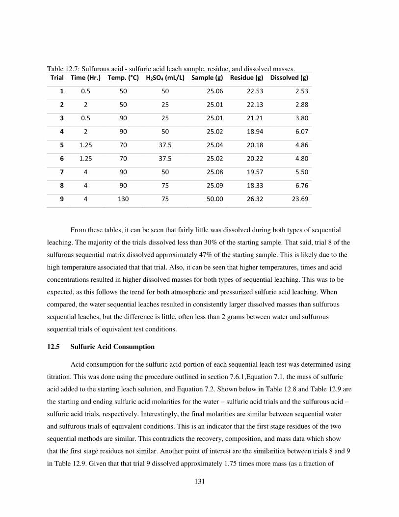
131

Table 12.7: Sulfurous acid - sulfuric acid leach sample, residue, and dissolved masses.

Trial Time (Hr.) Temp. (°C) H2SO4 (mL/L) Sample (g) Residue (g) Dissolved (g)

1 0.5 50 50 25.06 22.53 2.53

2 2 50 25 25.01 22.13 2.88

3 0.5 90 25 25.01 21.21 3.80

4 2 90 50 25.02 18.94 6.07

5 1.25 70 37.5 25.04 20.18 4.86

6 1.25 70 37.5 25.02 20.22 4.80

7 4 90 50 25.08 19.57 5.50

8 4 90 75 25.09 18.33 6.76

9 4 130 75 50.00 26.32 23.69

From these tables, it can be seen that fairly little was dissolved during both types of sequential

leaching. The majority of the trials dissolved less than 30% of the starting sample. That said, trial 8 of the

sulfurous sequential matrix dissolved approximately 47% of the starting sample. This is likely due to the

high temperature associated that that trial. Also, it can be seen that higher temperatures, times and acid

concentrations resulted in higher dissolved masses for both types of sequential leaching. This was to be

expected, as this follows the trend for both atmospheric and pressurized sulfuric acid leaching. When

compared, the water sequential leaches resulted in consistently larger dissolved masses than sulfurous

sequential leaches, but the difference is little, often less than 2 grams between water and sulfurous

sequential trials of equivalent test conditions.


Acid consumption for the sulfuric acid portion of each sequential leach test was determined using

titration. This was done using the procedure outlined in section 7.6.1,Equation 7.1, the mass of sulfuric

acid added to the starting leach solution, and Equation 7.2. Shown below in Table 12.8 and Table 12.9 are

the starting and ending sulfuric acid molarities for the water – sulfuric acid trials and the sulfurous acid –

sulfuric acid trials, respectively. Interestingly, the final molarities are similar between sequential water

and sulfurous trials of equivalent conditions. This is an indicator that the first stage residues of the two

sequential methods are similar. This contradicts the recovery, composition, and mass data which show

that the first stage residues not similar. Another point of interest are the similarities between trials 8 and 9

in Table 12.9. Given that that trial 9 dissolved approximately 1.75 times more mass (as a fraction of

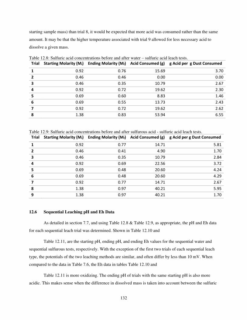
132

starting sample mass) than trial 8, it would be expected that more acid was consumed rather than the same

amount. It may be that the higher temperature associated with trial 9 allowed for less necessary acid to

dissolve a given mass.

Table 12.8: Sulfuric acid concentrations before and after water – sulfuric acid leach tests.

Trial Starting Molarity (Mi) Ending Molarity (Mf) Acid Consumed (g) g Acid per g Dust Consumed

1 0.92 0.76 15.69 3.70

2 0.46 0.46 0.00 0.00

3 0.46 0.35 10.79 2.67

4 0.92 0.72 19.62 2.30

5 0.69 0.60 8.83 1.46

6 0.69 0.55 13.73 2.43

7 0.92 0.72 19.62 2.62

8 1.38 0.83 53.94 6.55

Table 12.9: Sulfuric acid concentrations before and after sulfurous acid - sulfuric acid leach tests.

Trial Starting Molarity (Mi) Ending Molarity (Mf) Acid Consumed (g) g Acid per g Dust Consumed

1 0.92 0.77 14.71 5.81

2 0.46 0.41 4.90 1.70

3 0.46 0.35 10.79 2.84

4 0.92 0.69 22.56 3.72

5 0.69 0.48 20.60 4.24

6 0.69 0.48 20.60 4.29

7 0.92 0.77 14.71 2.67

8 1.38 0.97 40.21 5.95

9 1.38 0.97 40.21 1.70

12.6 Sequential Leaching pH and Eh Data

As detailed in section 7.7, and using Table 12.8 & Table 12.9, as appropriate, the pH and Eh data

for each sequential leach trial was determined. Shown in Table 12.10 and

Table 12.11, are the starting pH, ending pH, and ending Eh values for the sequential water and

sequential sulfurous tests, respectively. With the exception of the first two trials of each sequential leach

type, the potentials of the two leaching methods are similar, and often differ by less than 10 mV. When

compared to the data in Table 7.6, the Eh data in tables Table 12.10 and

Table 12.11 is more oxidizing. The ending pH of trials with the same starting pH is also more

acidic. This makes sense when the difference in dissolved mass is taken into account between the sulfuric

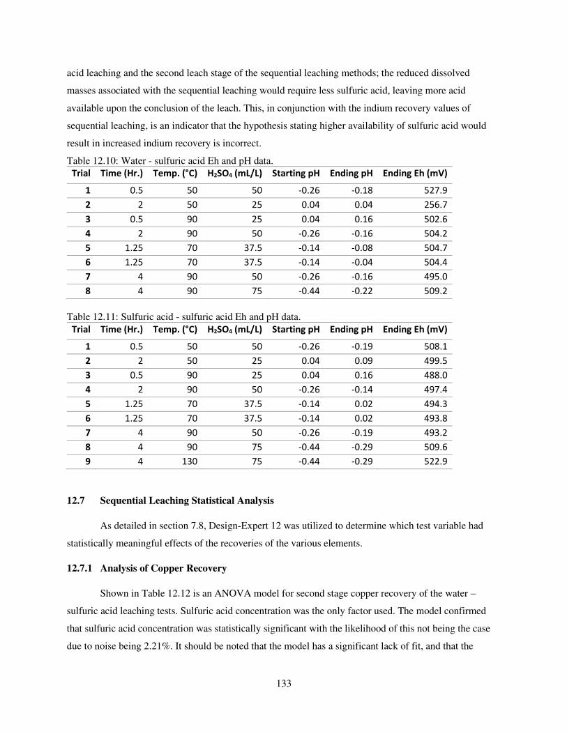
133

acid leaching and the second leach stage of the sequential leaching methods; the reduced dissolved

masses associated with the sequential leaching would require less sulfuric acid, leaving more acid

available upon the conclusion of the leach. This, in conjunction with the indium recovery values of

sequential leaching, is an indicator that the hypothesis stating higher availability of sulfuric acid would

result in increased indium recovery is incorrect.

Table 12.10: Water - sulfuric acid Eh and pH data.

Trial Time (Hr.) Temp. (°C) H2SO4 (mL/L) Starting pH Ending pH Ending Eh (mV)

1 0.5 50 50 -0.26 -0.18 527.9

2 2 50 25 0.04 0.04 256.7

3 0.5 90 25 0.04 0.16 502.6

4 2 90 50 -0.26 -0.16 504.2

5 1.25 70 37.5 -0.14 -0.08 504.7

6 1.25 70 37.5 -0.14 -0.04 504.4

7 4 90 50 -0.26 -0.16 495.0

8 4 90 75 -0.44 -0.22 509.2

Table 12.11: Sulfuric acid - sulfuric acid Eh and pH data.

Trial Time (Hr.) Temp. (°C) H2SO4 (mL/L) Starting pH Ending pH Ending Eh (mV)

1 0.5 50 50 -0.26 -0.19 508.1

2 2 50 25 0.04 0.09 499.5

3 0.5 90 25 0.04 0.16 488.0

4 2 90 50 -0.26 -0.14 497.4

5 1.25 70 37.5 -0.14 0.02 494.3

6 1.25 70 37.5 -0.14 0.02 493.8

7 4 90 50 -0.26 -0.19 493.2

8 4 90 75 -0.44 -0.29 509.6

9 4 130 75 -0.44 -0.29 522.9

12.7 Sequential Leaching Statistical Analysis

As detailed in section 7.8, Design-Expert 12 was utilized to determine which test variable had

statistically meaningful effects of the recoveries of the various elements.


Shown in Table 12.12 is an ANOVA model for second stage copper recovery of the water –

sulfuric acid leaching tests. Sulfuric acid concentration was the only factor used. The model confirmed

that sulfuric acid concentration was statistically significant with the likelihood of this not being the case

due to noise being 2.21%. It should be noted that the model has a significant lack of fit, and that the

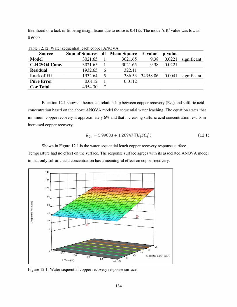
134

likelihood of a lack of fit being insignificant due to noise is 0.41%. The model’s R2 value was low at

0.6099.

Table 12.12: Water sequential leach copper ANOVA.



C-H2SO4 Conc. 3021.65 1 3021.65 9.38 0.0221

Residual 1932.65 6 322.11


Pure Error 0.0112 1 0.0112

Cor Total 4954.30 7

Equation 12.1 shows a theoretical relationship between copper recovery (RCu) and sulfuric acid

concentration based on the above ANOVA model for sequential water leaching. The equation states that

minimum copper recovery is approximately 6% and that increasing sulfuric acid concentration results in

increased copper recovery. 𝑅𝐶𝑢 = 5.99833 + 1.26947([𝐻2𝑆𝑂4]) (12.1)

Shown in Figure 12.1 is the water sequential leach copper recovery response surface.

Temperature had no effect on the surface. The response surface agrees with its associated ANOVA model

in that only sulfuric acid concentration has a meaningful effect on copper recovery.

Figure 12.1: Water sequential copper recovery response surface.

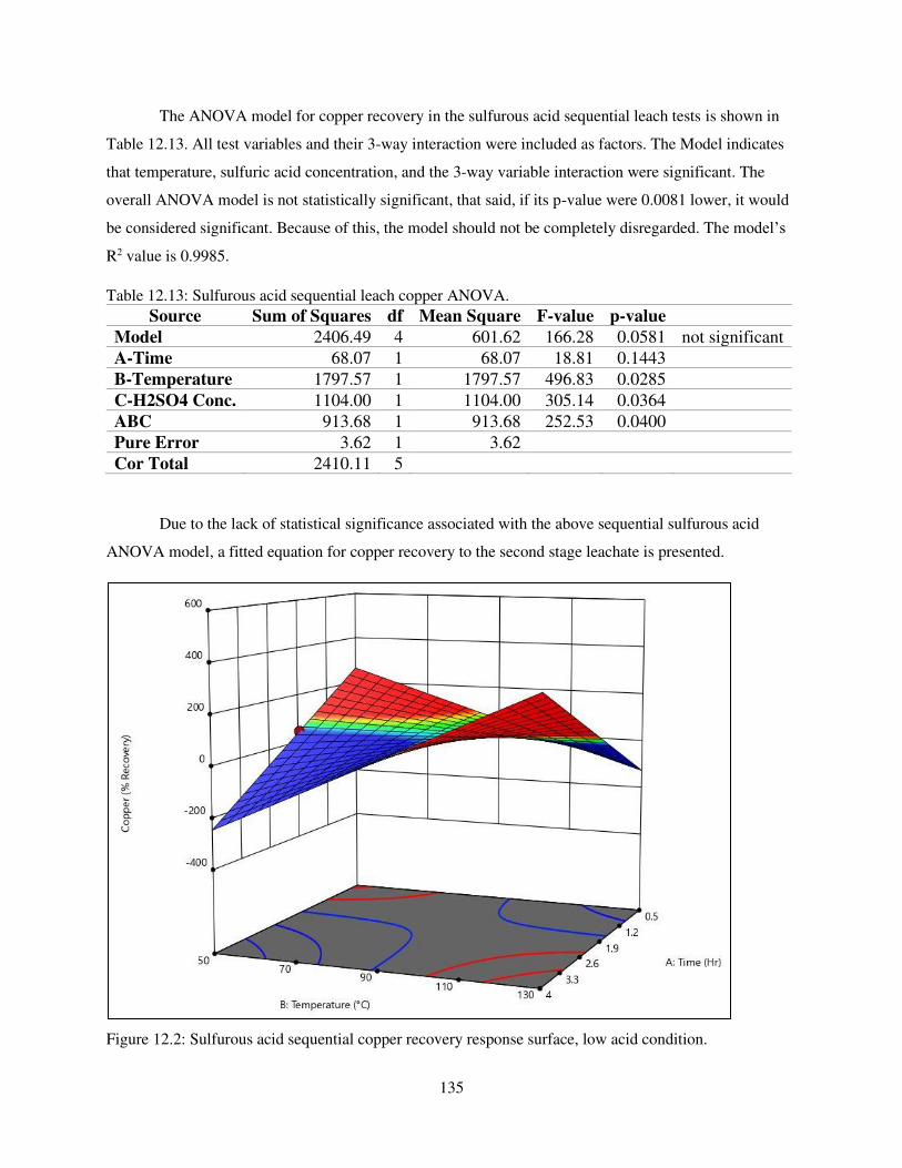
135

The ANOVA model for copper recovery in the sulfurous acid sequential leach tests is shown in

Table 12.13. All test variables and their 3-way interaction were included as factors. The Model indicates

that temperature, sulfuric acid concentration, and the 3-way variable interaction were significant. The

overall ANOVA model is not statistically significant, that said, if its p-value were 0.0081 lower, it would

be considered significant. Because of this, the model should not be completely disregarded. The model’s

R2 value is 0.9985.

Table 12.13: Sulfurous acid sequential leach copper ANOVA.



A-Time 68.07 1 68.07 18.81 0.1443

B-Temperature 1797.57 1 1797.57 496.83 0.0285

C-H2SO4 Conc. 1104.00 1 1104.00 305.14 0.0364

ABC 913.68 1 913.68 252.53 0.0400


Cor Total 2410.11 5

Due to the lack of statistical significance associated with the above sequential sulfurous acid

ANOVA model, a fitted equation for copper recovery to the second stage leachate is presented.

Figure 12.2: Sulfurous acid sequential copper recovery response surface, low acid condition.

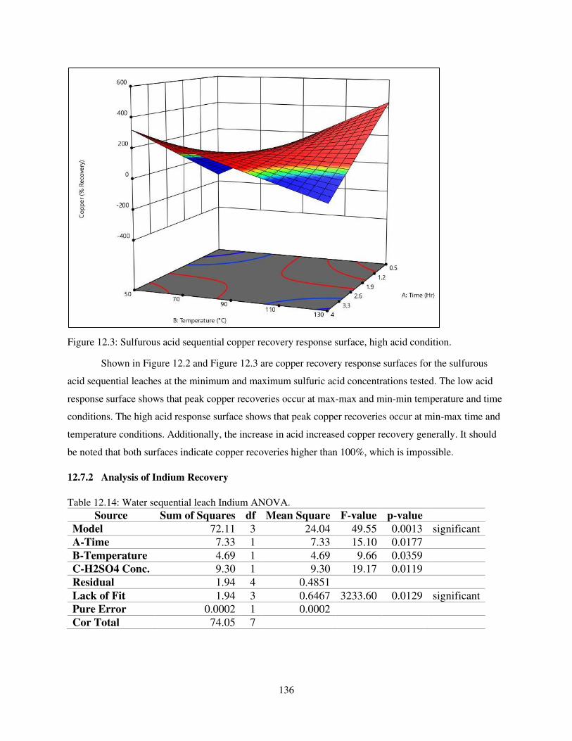
136

Figure 12.3: Sulfurous acid sequential copper recovery response surface, high acid condition.

Shown in Figure 12.2 and Figure 12.3 are copper recovery response surfaces for the sulfurous

acid sequential leaches at the minimum and maximum sulfuric acid concentrations tested. The low acid

response surface shows that peak copper recoveries occur at max-max and min-min temperature and time

conditions. The high acid response surface shows that peak copper recoveries occur at min-max time and

temperature conditions. Additionally, the increase in acid increased copper recovery generally. It should

be noted that both surfaces indicate copper recoveries higher than 100%, which is impossible.


Table 12.14: Water sequential leach Indium ANOVA.



A-Time 7.33 1 7.33 15.10 0.0177

B-Temperature 4.69 1 4.69 9.66 0.0359

C-H2SO4 Conc. 9.30 1 9.30 19.17 0.0119

Residual 1.94 4 0.4851


Pure Error 0.0002 1 0.0002

Cor Total 74.05 7

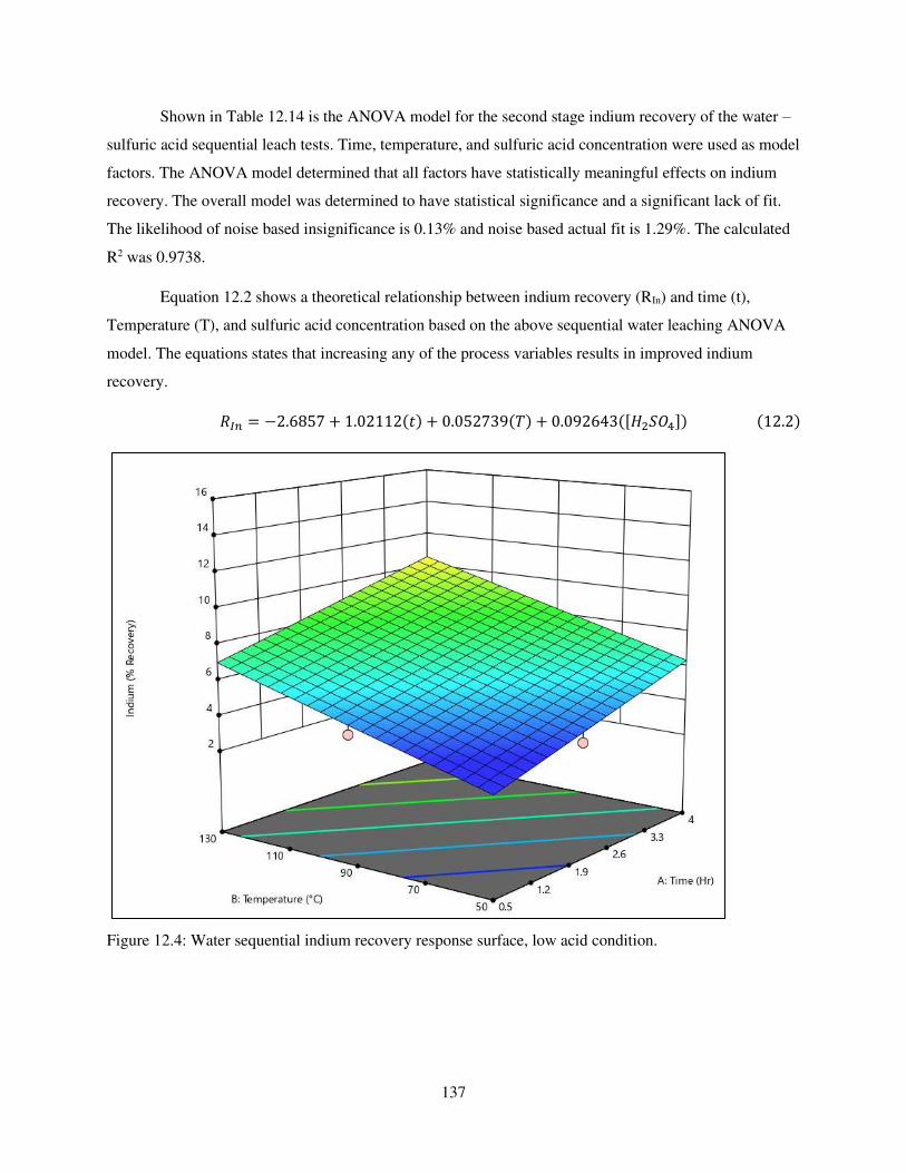
137

Shown in Table 12.14 is the ANOVA model for the second stage indium recovery of the water –

sulfuric acid sequential leach tests. Time, temperature, and sulfuric acid concentration were used as model

factors. The ANOVA model determined that all factors have statistically meaningful effects on indium

recovery. The overall model was determined to have statistical significance and a significant lack of fit.

The likelihood of noise based insignificance is 0.13% and noise based actual fit is 1.29%. The calculated

R2 was 0.9738.

Equation 12.2 shows a theoretical relationship between indium recovery (RIn) and time (t),

Temperature (T), and sulfuric acid concentration based on the above sequential water leaching ANOVA

model. The equations states that increasing any of the process variables results in improved indium

recovery. 𝑅𝐼𝑛 = −2.6857 + 1.02112(𝑡) + 0.052739(𝑇) + 0.092643([𝐻2𝑆𝑂4]) (12.2)

Figure 12.4: Water sequential indium recovery response surface, low acid condition.

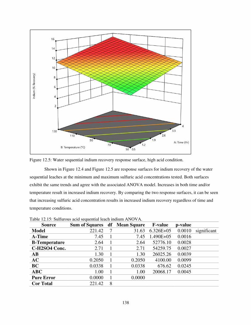
138

Figure 12.5: Water sequential indium recovery response surface, high acid condition.

Shown in Figure 12.4 and Figure 12.5 are response surfaces for indium recovery of the water

sequential leaches at the minimum and maximum sulfuric acid concentrations tested. Both surfaces

exhibit the same trends and agree with the associated ANOVA model. Increases in both time and/or

temperature result in increased indium recovery. By comparing the two response surfaces, it can be seen

that increasing sulfuric acid concentration results in increased indium recovery regardless of time and

temperature conditions.

Table 12.15: Sulfurous acid sequential leach indium ANOVA.


Model 221.42 7 31.63 6.326E+05 0.0010 significant

A-Time 7.45 1 7.45 1.490E+05 0.0016

B-Temperature 2.64 1 2.64 52776.10 0.0028

C-H2SO4 Conc. 2.71 1 2.71 54259.75 0.0027

AB 1.30 1 1.30 26025.26 0.0039

AC 0.2050 1 0.2050 4100.00 0.0099

BC 0.0338 1 0.0338 676.62 0.0245

ABC 1.00 1 1.00 20068.17 0.0045

Pure Error 0.0000 1 0.0000

Cor Total 221.42 8

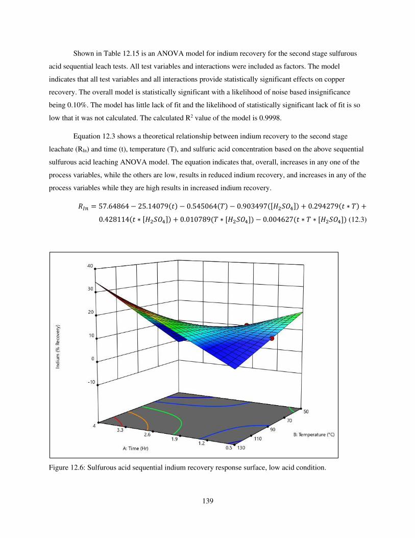
139

Shown in Table 12.15 is an ANOVA model for indium recovery for the second stage sulfurous

acid sequential leach tests. All test variables and interactions were included as factors. The model

indicates that all test variables and all interactions provide statistically significant effects on copper

recovery. The overall model is statistically significant with a likelihood of noise based insignificance

being 0.10%. The model has little lack of fit and the likelihood of statistically significant lack of fit is so

low that it was not calculated. The calculated R2 value of the model is 0.9998.

Equation 12.3 shows a theoretical relationship between indium recovery to the second stage

leachate (RIn) and time (t), temperature (T), and sulfuric acid concentration based on the above sequential

sulfurous acid leaching ANOVA model. The equation indicates that, overall, increases in any one of the

process variables, while the others are low, results in reduced indium recovery, and increases in any of the

process variables while they are high results in increased indium recovery. 𝑅𝐼𝑛 = 57.64864 − 25.14079(𝑡) − 0.545064(𝑇) − 0.903497([𝐻2𝑆𝑂4]) + 0.294279(𝑡 ∗ 𝑇) +0.428114(𝑡 ∗ [𝐻2𝑆𝑂4]) + 0.010789(𝑇 ∗ [𝐻2𝑆𝑂4]) − 0.004627(𝑡 ∗ 𝑇 ∗ [𝐻2𝑆𝑂4]) (12.3)

Figure 12.6: Sulfurous acid sequential indium recovery response surface, low acid condition.

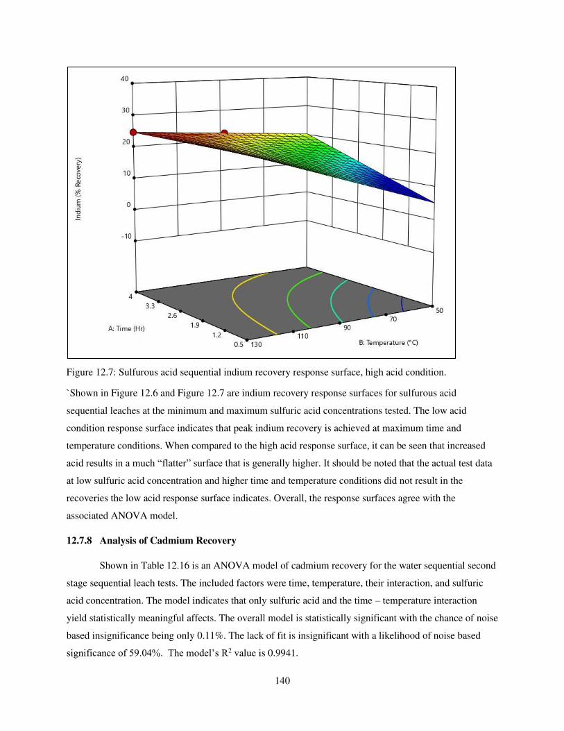
140

Figure 12.7: Sulfurous acid sequential indium recovery response surface, high acid condition.

`Shown in Figure 12.6 and Figure 12.7 are indium recovery response surfaces for sulfurous acid

sequential leaches at the minimum and maximum sulfuric acid concentrations tested. The low acid

condition response surface indicates that peak indium recovery is achieved at maximum time and

temperature conditions. When compared to the high acid response surface, it can be seen that increased

acid results in a much “flatter” surface that is generally higher. It should be noted that the actual test data

at low sulfuric acid concentration and higher time and temperature conditions did not result in the

recoveries the low acid response surface indicates. Overall, the response surfaces agree with the

associated ANOVA model.


Shown in Table 12.16 is an ANOVA model of cadmium recovery for the water sequential second

stage sequential leach tests. The included factors were time, temperature, their interaction, and sulfuric

acid concentration. The model indicates that only sulfuric acid and the time – temperature interaction

yield statistically meaningful affects. The overall model is statistically significant with the chance of noise

based insignificance being only 0.11%. The lack of fit is insignificant with a likelihood of noise based

significance of 59.04%. The model’s R2 value is 0.9941.

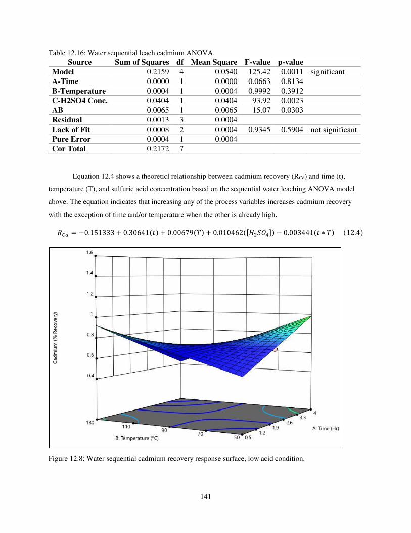
141

Table 12.16: Water sequential leach cadmium ANOVA.



A-Time 0.0000 1 0.0000 0.0663 0.8134

B-Temperature 0.0004 1 0.0004 0.9992 0.3912

C-H2SO4 Conc. 0.0404 1 0.0404 93.92 0.0023

AB 0.0065 1 0.0065 15.07 0.0303

Residual 0.0013 3 0.0004


Pure Error 0.0004 1 0.0004

Cor Total 0.2172 7

Equation 12.4 shows a theoreticl relationship between cadmium recovery (RCd) and time (t),

temperature (T), and sulfuric acid concentration based on the sequential water leaching ANOVA model

above. The equation indicates that increasing any of the process variables increases cadmium recovery

with the exception of time and/or temperature when the other is already high. 𝑅𝐶𝑑 = −0.151333 + 0.30641(𝑡) + 0.00679(𝑇) + 0.010462([𝐻2𝑆𝑂4]) − 0.003441(𝑡 ∗ 𝑇) (12.4)

Figure 12.8: Water sequential cadmium recovery response surface, low acid condition.

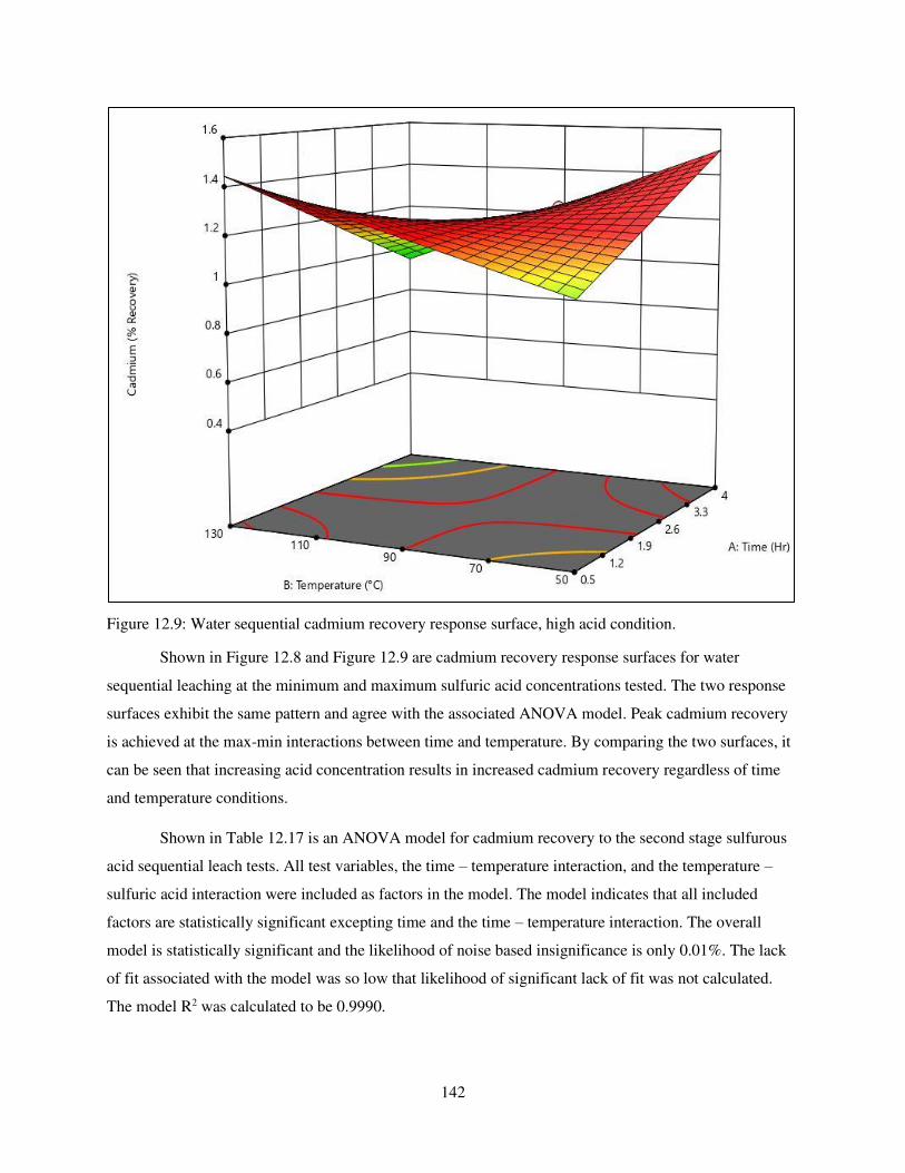
142

Figure 12.9: Water sequential cadmium recovery response surface, high acid condition.

Shown in Figure 12.8 and Figure 12.9 are cadmium recovery response surfaces for water

sequential leaching at the minimum and maximum sulfuric acid concentrations tested. The two response

surfaces exhibit the same pattern and agree with the associated ANOVA model. Peak cadmium recovery

is achieved at the max-min interactions between time and temperature. By comparing the two surfaces, it

can be seen that increasing acid concentration results in increased cadmium recovery regardless of time

and temperature conditions.

Shown in Table 12.17 is an ANOVA model for cadmium recovery to the second stage sulfurous

acid sequential leach tests. All test variables, the time – temperature interaction, and the temperature –

sulfuric acid interaction were included as factors in the model. The model indicates that all included

factors are statistically significant excepting time and the time – temperature interaction. The overall

model is statistically significant and the likelihood of noise based insignificance is only 0.01%. The lack

of fit associated with the model was so low that likelihood of significant lack of fit was not calculated.

The model R2 was calculated to be 0.9990.

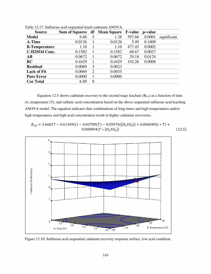
143

Table 12.17: Sulfurous acid sequential leach cadmium ANOVA.



A-Time 0.0126 1 0.0126 5.49 0.1009

B-Temperature 1.10 1 1.10 477.45 0.0002

C-H2SO4 Conc. 0.1582 1 0.1582 68.67 0.0037

AB 0.0672 1 0.0672 29.18 0.0124

BC 0.4429 1 0.4429 192.26 0.0008

Residual 0.0069 3 0.0023

Lack of Fit 0.0069 2 0.0035

Pure Error 0.0000 1 0.0000

Cor Total 6.89 8

Equation 12.5 shows cadmium recovery to the second stage leachate (RCd) as a function of time

(t), temperature (T), and sulfuric acid concentration based on the above sequential sulfurous acid leaching

ANOVA model. The equation indicates that combinations of long times and high temperatures and/or

high temperatures and high acid concentration result in higher cadmium recoveries. 𝑅𝐶𝑑 = 3.66017 − 0.61349(𝑡) − 0.03789(𝑇) − 0.05976([𝐻2𝑆𝑂4]) + 0.006049(𝑡 ∗ 𝑇) +0.000894(𝑇 ∗ [𝐻2𝑆𝑂4]) (12.5)

Figure 12.10: Sulfurous acid sequential cadmium recovery response surface, low acid condition.

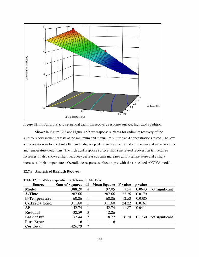
144

Figure 12.11: Sulfurous acid sequential cadmium recovery response surface, high acid condition.

Shown in Figure 12.8 and Figure 12.9 are response surfaces for cadmium recovery of the

sulfurous acid sequential tests at the minimum and maximum sulfuric acid concentrations tested. The low

acid condition surface is fairly flat, and indicates peak recovery is achieved at min-min and max-max time

and temperature conditions. The high acid response surface shows increased recovery as temperature

increases. It also shows a slight recovery decrease as time increases at low temperature and a slight

increase at high temperatures. Overall, the response surfaces agree with the associated ANOVA model.


Table 12.18: Water sequential leach bismuth ANOVA.



A-Time 287.66 1 287.66 22.36 0.0179

B-Temperature 160.86 1 160.86 12.50 0.0385

C-H2SO4 Conc. 311.60 1 311.60 24.22 0.0161

AB 152.74 1 152.74 11.87 0.0411

Residual 38.59 3 12.86



Cor Total 426.79 7

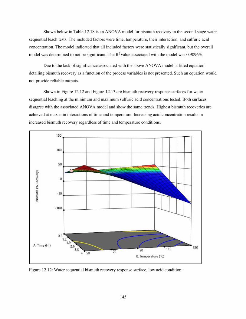
145

Shown below in Table 12.18 is an ANOVA model for bismuth recovery in the second stage water

sequential leach tests. The included factors were time, temperature, their interaction, and sulfuric acid

concentration. The model indicated that all included factors were statistically significant, but the overall

model was determined to not be significant. The R2 value associated with the model was 0.9096%.

Due to the lack of significance associated with the above ANOVA model, a fitted equation

detailing bismuth recovery as a function of the process variables is not presented. Such an equation would

not provide reliable outputs.

Shown in Figure 12.12 and Figure 12.13 are bismuth recovery response surfaces for water

sequential leaching at the minimum and maximum sulfuric acid concentrations tested. Both surfaces

disagree with the associated ANOVA model and show the same trends. Highest bismuth recoveries are

achieved at max-min interactions of time and temperature. Increasing acid concentration results in

increased bismuth recovery regardless of time and temperature conditions.

Figure 12.12: Water sequential bismuth recovery response surface, low acid condition.

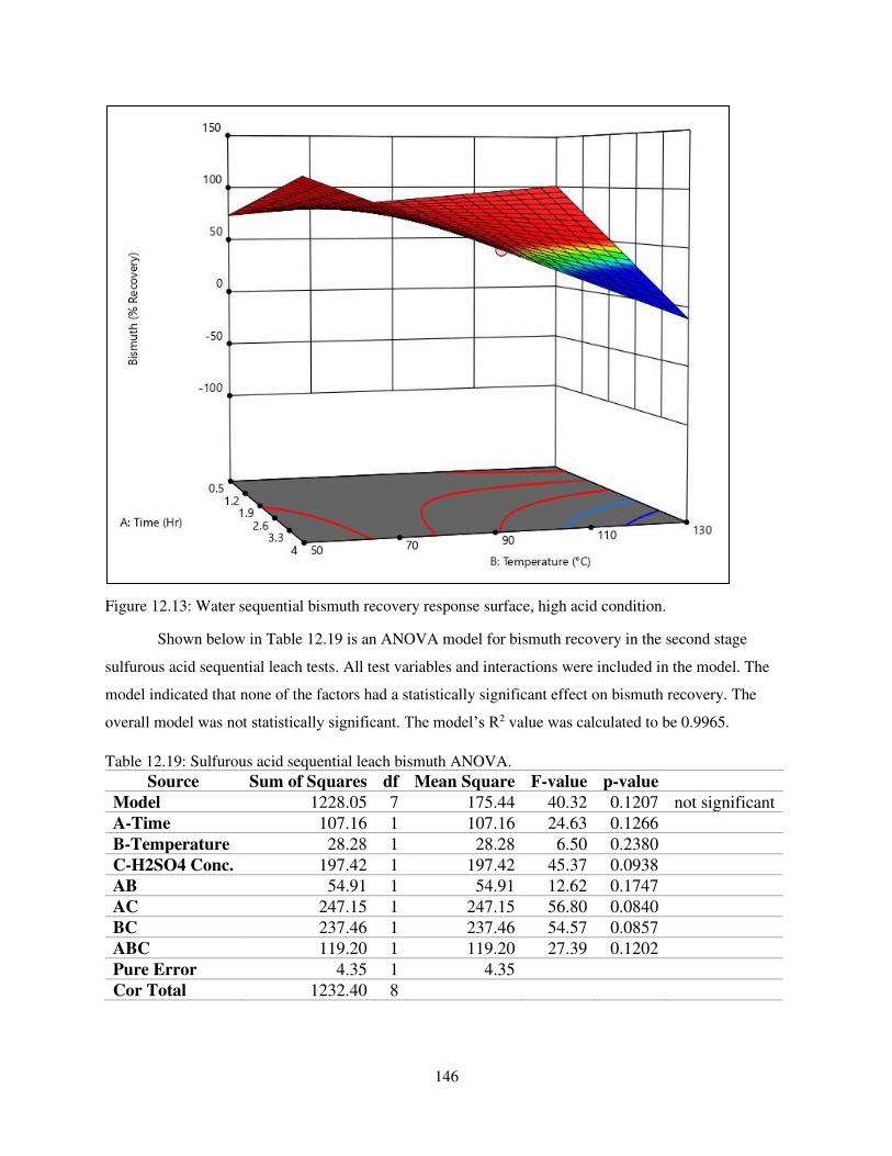
146

Figure 12.13: Water sequential bismuth recovery response surface, high acid condition.

Shown below in Table 12.19 is an ANOVA model for bismuth recovery in the second stage

sulfurous acid sequential leach tests. All test variables and interactions were included in the model. The

model indicated that none of the factors had a statistically significant effect on bismuth recovery. The

overall model was not statistically significant. The model’s R2 value was calculated to be 0.9965.

Table 12.19: Sulfurous acid sequential leach bismuth ANOVA.



A-Time 107.16 1 107.16 24.63 0.1266

B-Temperature 28.28 1 28.28 6.50 0.2380

C-H2SO4 Conc. 197.42 1 197.42 45.37 0.0938

AB 54.91 1 54.91 12.62 0.1747

AC 247.15 1 247.15 56.80 0.0840

BC 237.46 1 237.46 54.57 0.0857

ABC 119.20 1 119.20 27.39 0.1202


Cor Total 1232.40 8

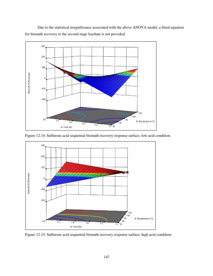
147

Due to the statistical insignificance associated with the above ANOVA model, a fitted equation

for bismuth recovery to the second stage leachate is not provided.

Figure 12.14: Sulfurous acid sequential bismuth recovery response surface, low acid condition.

Figure 12.15: Sulfurous acid sequential bismuth recovery response surface, high acid condition.

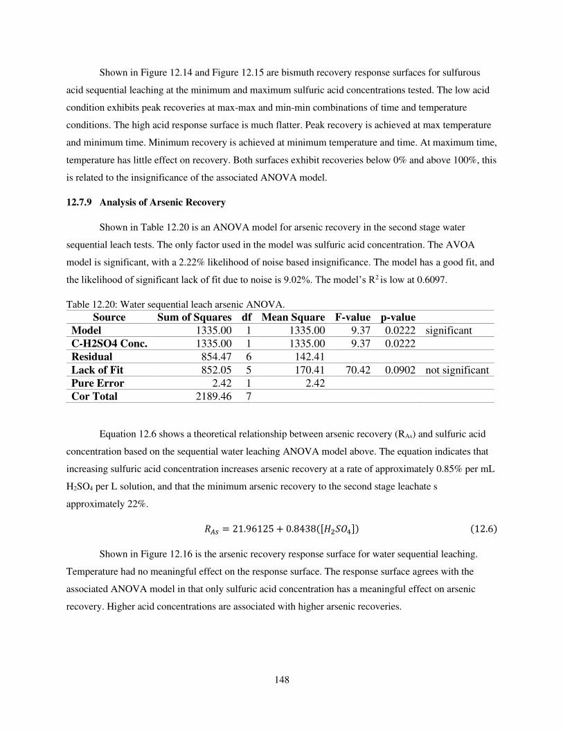
148

Shown in Figure 12.14 and Figure 12.15 are bismuth recovery response surfaces for sulfurous

acid sequential leaching at the minimum and maximum sulfuric acid concentrations tested. The low acid

condition exhibits peak recoveries at max-max and min-min combinations of time and temperature

conditions. The high acid response surface is much flatter. Peak recovery is achieved at max temperature

and minimum time. Minimum recovery is achieved at minimum temperature and time. At maximum time,

temperature has little effect on recovery. Both surfaces exhibit recoveries below 0% and above 100%, this

is related to the insignificance of the associated ANOVA model.


Shown in Table 12.20 is an ANOVA model for arsenic recovery in the second stage water

sequential leach tests. The only factor used in the model was sulfuric acid concentration. The AVOA

model is significant, with a 2.22% likelihood of noise based insignificance. The model has a good fit, and

the likelihood of significant lack of fit due to noise is 9.02%. The model’s R2 is low at 0.6097.

Table 12.20: Water sequential leach arsenic ANOVA.



C-H2SO4 Conc. 1335.00 1 1335.00 9.37 0.0222

Residual 854.47 6 142.41



Cor Total 2189.46 7

Equation 12.6 shows a theoretical relationship between arsenic recovery (RAs) and sulfuric acid

concentration based on the sequential water leaching ANOVA model above. The equation indicates that

increasing sulfuric acid concentration increases arsenic recovery at a rate of approximately 0.85% per mL

H2SO4 per L solution, and that the minimum arsenic recovery to the second stage leachate s

approximately 22%. 𝑅𝐴𝑠 = 21.96125 + 0.8438([𝐻2𝑆𝑂4]) (12.6)

Shown in Figure 12.16 is the arsenic recovery response surface for water sequential leaching.

Temperature had no meaningful effect on the response surface. The response surface agrees with the

associated ANOVA model in that only sulfuric acid concentration has a meaningful effect on arsenic

recovery. Higher acid concentrations are associated with higher arsenic recoveries.

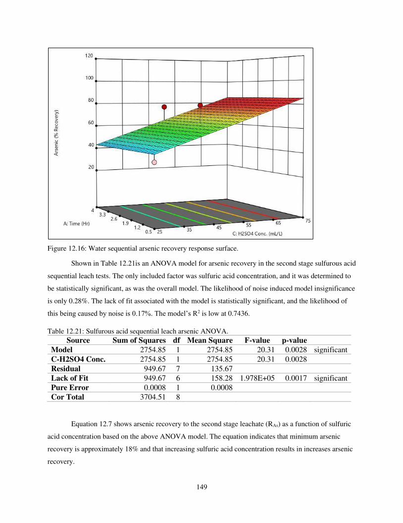
149

Figure 12.16: Water sequential arsenic recovery response surface.

Shown in Table 12.21is an ANOVA model for arsenic recovery in the second stage sulfurous acid

sequential leach tests. The only included factor was sulfuric acid concentration, and it was determined to

be statistically significant, as was the overall model. The likelihood of noise induced model insignificance

is only 0.28%. The lack of fit associated with the model is statistically significant, and the likelihood of

this being caused by noise is 0.17%. The model’s R2 is low at 0.7436.

Table 12.21: Sulfurous acid sequential leach arsenic ANOVA.



C-H2SO4 Conc. 2754.85 1 2754.85 20.31 0.0028

Residual 949.67 7 135.67


Pure Error 0.0008 1 0.0008

Cor Total 3704.51 8

Equation 12.7 shows arsenic recovery to the second stage leachate (RAs) as a function of sulfuric

acid concentration based on the above ANOVA model. The equation indicates that minimum arsenic

recovery is approximately 18% and that increasing sulfuric acid concentration results in increases arsenic

recovery.

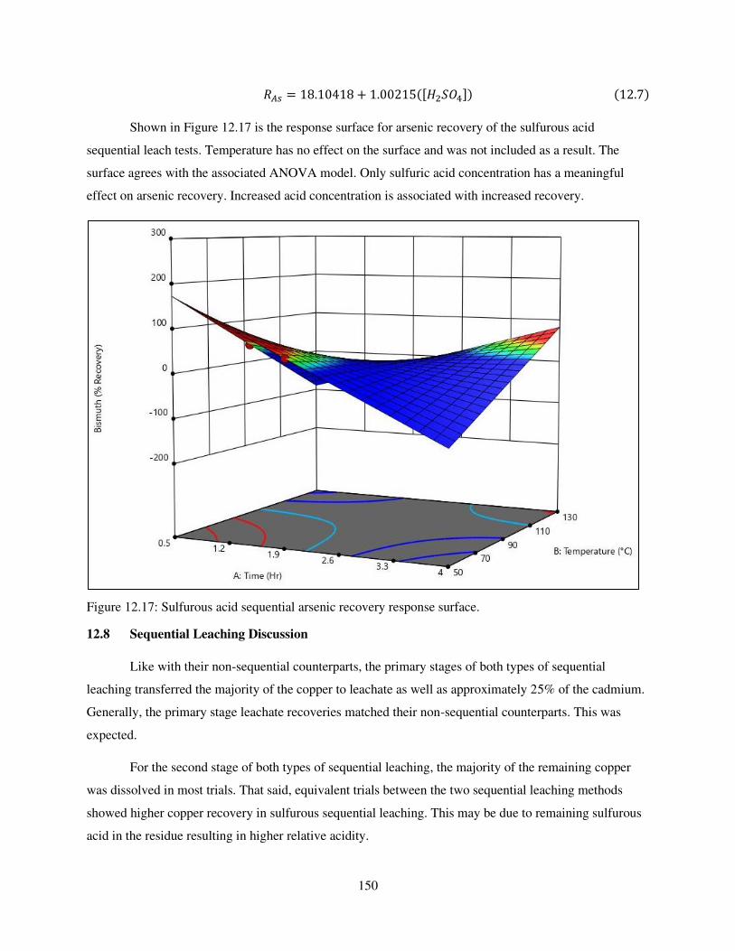
150

𝑅𝐴𝑠 = 18.10418 + 1.00215([𝐻2𝑆𝑂4]) (12.7)

Shown in Figure 12.17 is the response surface for arsenic recovery of the sulfurous acid

sequential leach tests. Temperature has no effect on the surface and was not included as a result. The

surface agrees with the associated ANOVA model. Only sulfuric acid concentration has a meaningful

effect on arsenic recovery. Increased acid concentration is associated with increased recovery.

Figure 12.17: Sulfurous acid sequential arsenic recovery response surface.

12.8 Sequential Leaching Discussion

Like with their non-sequential counterparts, the primary stages of both types of sequential

leaching transferred the majority of the copper to leachate as well as approximately 25% of the cadmium.

Generally, the primary stage leachate recoveries matched their non-sequential counterparts. This was

expected.

For the second stage of both types of sequential leaching, the majority of the remaining copper

was dissolved in most trials. That said, equivalent trials between the two sequential leaching methods

showed higher copper recovery in sulfurous sequential leaching. This may be due to remaining sulfurous

acid in the residue resulting in higher relative acidity.

151

The sulfuric acid leachates of the sequential tests dissolved less indium than their single stage

counterparts of equivalent conditions. This was not expected, especially considering the indium grade in

the residue after primary leaching is higher than the starting FS-ESP Dust. When compared to each other,

sulfurous acid sequential leaching recovered more indium than water sequential leaching, but neither

recovered enough to be considered satisfactory. That said, based on the response surfaces and the

ANOVA model, longer leaching times at higher temperatures may result in higher indium recoveries. For

example, leaching for 28 hours at 75 °C and 75 mL/L H2SO4 would theoretically recover approximately

95% of the remaining indium to the second stage leachate for sequential sulfurous acid leaching,

according to Equation 12.3. In the case of sequential water leaching, the same indium recovery can be

achieved at the same temperature and acid conditions by leaching for 85 hours.

In both types of sequential leaching, the sulfuric acid stage recovered little cadmium, often less

than 1%. This is an indicator that only approximately 25% of the cadmium is of a soluble phase, with the

potential for the remaining cadmium being part of some insoluble complex. The recovery equations

generated using the ANOVA models indicate that in both types of sequential leaching, higher cadmium

recoveries are not feasible.

Regarding bismuth, the two sequential methods exhibited similar recoveries across their

equivalent trials. As for arsenic, the sulfuric acid stage of the sulfurous sequential trials recovered higher

amounts of arsenic than their water sequential counterparts. This is likely due to higher arsenic recovery

from the primary sulfurous acid leaches when compared to primary water leaches. There was less arsenic

in the primary sulfurous acid residues than the primary water residues, so given equivalent sulfuric acid

concentrations, and similar masses of dissolved arsenic, a higher portion of the sulfurous acid residue

arsenic was dissolved in the second stage leaches.

152

CHAPTER 13. ECONOMIC ANALYSIS

Based on the recoveries and separations generated by the leaching methods, water and sequential

water leaching show the most promise. This is further discussed in Chapter 14. In order to gain an

understanding of how practical each leaching method is, a basic economic model was generated for each

method. It should be noted that a number of assumptions had to be made in order to create said models.

These assumptions are not completely accurate and affect the outputs of the model. Additionally, the

models are not for complete processes; they are only for the leaching stages of a complete process which

would have additional costs associated with other processing stages. Because of this, model outputs are

labeled as values generated or lost rather than profit or loss. Also, model outputs should not be considered

final process cash flows or values, as whatever overall recovery process the leaching models are a part of

would have a significant effect of overall process cash flows and economic viability. All model outputs

can only be used for conclusions and insights on the leaching stage of what the overall process would be.

13.1 Model Assumptions

As with all economic models, a number of assumptions are necessary. By their nature, many

assumptions are not completely accurate, but are likely close enough to provide a reasonable

approximation of reality. The most significant assumption is that market prices will remain constant over

time, something that is likely not true. That said, predicting future market trends and prices is beyond the

ability and scope of this research. Another important assumption is that many of the model inputs, such as

operating days per year and operating hours in a day are accurate and not subject to potential changes.

Given that these two inputs often change based on market conditions, this assumption is likely incorrect.

That said, predicting such changes requires the ability to predict future market trends and prices which is

beyond the ability and scope of this research.

A large portion of model inputs are assumed based on available sources and knowledge. A non-

exhaustive list of such inputs follows:

13.1.1 Operation Assumptions

The model assumes that each year, RTKC is producing 320 days of the 365. This is based on

industry standard for industrial production facilities. It allows for any downtime that may occur, such as

holiday closures, repair and maintenance operations, facility upgrades, etc. It is also assumed that each

day, 20 hours of the 24 are in operation. In reality, RTKC is likely in operation for closer to 24 hours.

That said, assuming only 20 hours of operation a day allows for some shift changes, employee breaks, and

some built in model conservatism, as it necessitates reduced production and increased downtime.

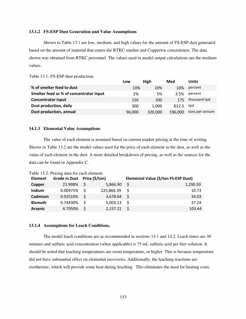
153

13.1.2 FS-ESP Dust Generation and Value Assumptions

Shown in Table 13.1 are low, medium, and high values for the amount of FS-ESP dust generated

based on the amount of material that enters the RTKC smelter and Copperton concentrator. The data

shown was obtained from RTKC personnel. The values used in model output calculations are the medium

values.

Table 13.1: FS-ESP dust production. Low High Med Units

% of smelter feed to dust 10% 10% 10% percent

Smelter feed as % of concentrator input 2% 5% 3.5% percent

Concentrator input 150 200 175 thousand tpd

Dust production, daily 300 1,000 612.5 tpd

Dust production, annual 96,000 320,000 196,000 tons per annum

14.1.3 Elemental Value Assumptions

The value of each element is assumed based on current market pricing at the time of writing.

Shown in Table 13.2 are the model values used for the price of each element in the dust, as well as the

value of each element in the dust. A more detailed breakdown of pricing, as well as the sources for the

data can be found in Appendix C.

Table 13.2: Pricing data for each element.

Element Grade in Dust Price ($/ton) Elemental Value ($/ton FS-ESP Dust)

Copper 21.998% $ 5,866.90 $ 1,290.59

Indium 0.00475% $ 225,866.39 $ 10.73

Cadmium 0.92510% $ 3,678.64 $ 34.03

Bismuth 0.74430% $ 5,003.13 $ 37.24

Arsenic 4.7950% $ 2,157.21 $ 103.44

13.1.4 Assumptions for Leach Conditions.

The model leach conditions are as recommended in sections 14.1 and 14.2. Leach times are 30

minutes and sulfuric acid concentration (when applicable) is 75 mL sulfuric acid per liter solution. It

should be noted that leaching temperatures are room temperature, or higher. This is because temperature

did not have substantial effect on elemental recoveries. Additionally, the leaching reactions are

exothermic, which will provide some heat during leaching. This eliminates the need for heating costs.

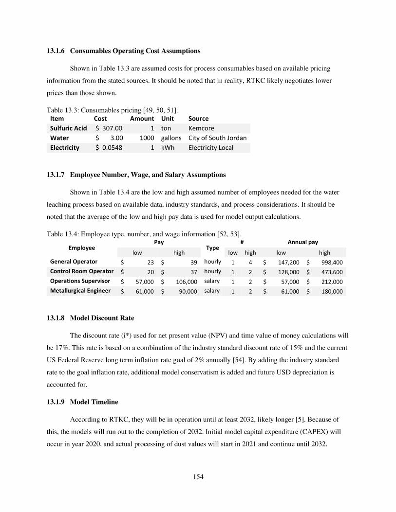
154

13.1.6 Consumables Operating Cost Assumptions

Shown in Table 13.3 are assumed costs for process consumables based on available pricing

information from the stated sources. It should be noted that in reality, RTKC likely negotiates lower

prices than those shown.

Table 13.3: Consumables pricing [49, 50, 51].

Item Cost Amount Unit Source

Sulfuric Acid $ 307.00 1 ton Kemcore

Water $ 3.00 1000 gallons City of South Jordan

Electricity $ 0.0548 1 kWh Electricity Local

13.1.7 Employee Number, Wage, and Salary Assumptions

Shown in Table 13.4 are the low and high assumed number of employees needed for the water

leaching process based on available data, industry standards, and process considerations. It should be

noted that the average of the low and high pay data is used for model output calculations.

Table 13.4: Employee type, number, and wage information [52, 53].

Employee Pay

Type # Annual pay

low high low high low high

General Operator $ 23 $ 39 hourly 1 4 $ 147,200 $ 998,400

Control Room Operator $ 20 $ 37 hourly 1 2 $ 128,000 $ 473,600

Operations Supervisor $ 57,000 $ 106,000 salary 1 2 $ 57,000 $ 212,000

Metallurgical Engineer $ 61,000 $ 90,000 salary 1 2 $ 61,000 $ 180,000

13.1.8 Model Discount Rate

The discount rate (i*) used for net present value (NPV) and time value of money calculations will

be 17%. This rate is based on a combination of the industry standard discount rate of 15% and the current

US Federal Reserve long term inflation rate goal of 2% annually [54]. By adding the industry standard

rate to the goal inflation rate, additional model conservatism is added and future USD depreciation is

accounted for.

13.1.9 Model Timeline

According to RTKC, they will be in operation until at least 2032, likely longer [5]. Because of

this, the models will run out to the completion of 2032. Initial model capital expenditure (CAPEX) will

occur in year 2020, and actual processing of dust values will start in 2021 and continue until 2032.

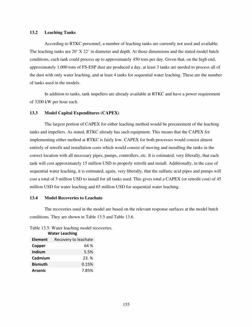
155

13.2 Leaching Tanks

According to RTKC personnel, a number of leaching tanks are currently not used and available.

The leaching tanks are 20’ X 22’ in diameter and depth. At those dimensions and the stated model batch

conditions, each tank could process up to approximately 450 tons per day. Given that, on the high end,

approximately 1,000 tons of FS-ESP dust are produced a day, at least 3 tanks are needed to process all of

the dust with only water leaching, and at least 4 tanks for sequential water leaching. These are the number

of tanks used in the models.

In addition to tanks, tank impellers are already available at RTKC and have a power requirement

of 3200 kW per hour each.

13.3 Model Capital Expenditures (CAPEX)

The largest portion of CAPEX for either leaching method would be procurement of the leaching

tanks and impellers. As stated, RTKC already has such equipment. This means that the CAPEX for

implementing either method at RTKC is fairly low. CAPEX for both processes would consist almost

entirely of retrofit and installation costs which would consist of moving and installing the tanks in the

correct location with all necessary pipes, pumps, controllers, etc. It is estimated, very liberally, that each

tank will cost approximately 15 million USD to properly retrofit and install. Additionally, in the case of

sequential water leaching, it is estimated, again, very liberally, that the sulfuric acid pipes and pumps will

cost a total of 5 million USD to install for all tanks used. This gives total a CAPEX (or retrofit cost) of 45

million USD for water leaching and 65 million USD for sequential water leaching.

13.4 Model Recoveries to Leachate

The recoveries used in the model are based on the relevant response surfaces at the model batch

conditions. They are shown in Table 13.5 and Table 13.6.

Table 13.5: Water leaching model recoveries.

Water Leaching

Element Recovery to leachate

Copper 64 %

Indium 5.5%

Cadmium 23. %

Bismuth 0.15%

Arsenic 7.85%

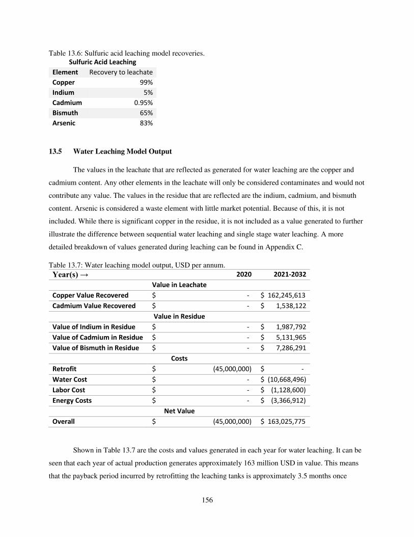
156

Table 13.6: Sulfuric acid leaching model recoveries.

Sulfuric Acid Leaching

Element Recovery to leachate

Copper 99%

Indium 5%

Cadmium 0.95%

Bismuth 65%

Arsenic 83%

13.5 Water Leaching Model Output

The values in the leachate that are reflected as generated for water leaching are the copper and

cadmium content. Any other elements in the leachate will only be considered contaminates and would not

contribute any value. The values in the residue that are reflected are the indium, cadmium, and bismuth

content. Arsenic is considered a waste element with little market potential. Because of this, it is not

included. While there is significant copper in the residue, it is not included as a value generated to further

illustrate the difference between sequential water leaching and single stage water leaching. A more

detailed breakdown of values generated during leaching can be found in Appendix C.

Table 13.7: Water leaching model output, USD per annum.

Year(s) → 2020 2021-2032

Value in Leachate

Copper Value Recovered $ - $ 162,245,613

Cadmium Value Recovered $ - $ 1,538,122

Value in Residue

Value of Indium in Residue $ - $ 1,987,792

Value of Cadmium in Residue $ - $ 5,131,965

Value of Bismuth in Residue $ - $ 7,286,291

Costs

Retrofit $ (45,000,000) $ -

Water Cost $ - $ (10,668,496)

Labor Cost $ - $ (1,128,600)

Energy Costs $ - $ (3,366,912)

Net Value

Overall $ (45,000,000) $ 163,025,775

Shown in Table 13.7 are the costs and values generated in each year for water leaching. It can be

seen that each year of actual production generates approximately 163 million USD in value. This means

that the payback period incurred by retrofitting the leaching tanks is approximately 3.5 months once

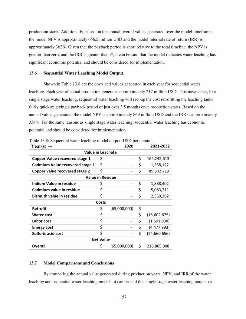
157

production starts. Additionally, based on the annual overall values generated over the model timeframe,

the model NPV is approximately 656.5 million USD and the model internal rate of return (IRR) is

approximately 362%. Given that the payback period is short relative to the total timeline, the NPV is

greater than zero, and the IRR is greater than i*, it can be said that the model indicates water leaching has

significant economic potential and should be considered for implementation.

13.6 Sequential Water Leaching Model Output.

Shown in Table 13.8 are the costs and values generated in each year for sequential water

leaching. Each year of actual production generates approximately 217 million USD. This means that, like

single stage water leaching, sequential water leaching will recoup the cost retrofitting the leaching tanks

fairly quickly; giving a payback period of just over 3.5 months once production starts. Based on the

annual values generated, the model NPV is approximately 869 million USD and the IRR is approximately

334%. For the same reasons as single stage water leaching, sequential water leaching has economic

potential and should be considered for implementation.

Table 13.8: Sequential water leaching model output, USD per annum.

Year(s) → 2020 2021-2032

Value in Leachate

Copper Value recovered stage 1 $ - $ 162,245,613

Cadmium Value recovered stage 1 $ - $ 1,538,122

Copper value recovered stage 2 $ - $ 89,802,719

Value in Residue

Indium Value in residue $ - $ 1,888,402

Cadmium value in residue $ - $ 5,083,211

Bismuth value in residue $ - $ 2,550,202

Costs

Retrofit $ (65,000,000) $ -

Water cost $ - $ (15,602,675)

Labor cost $ - $ (1,501,038)

Energy cost $ - $ (4,477,993)

Sulfuric acid cost $ - $ (24,660,656)

Net Value

Overall $ (65,000,000) $ 216,865,908

13.7 Model Comparisons and Conclusions

By comparing the annual value generated during production years, NPV, and IRR of the water

leaching and sequential water leaching models, it can be said that single stage water leaching may have

158

superior economic potential between the two. This is due to the cost of sulfuric acid associated with

sequential water leaching. While sequential water leaching has substantially higher annual value

generated and NPV, it is only deceptively higher. The single stage water leaching model does not

consider the copper in the residue as a value generated. In reality, it would be processed and therefore is a

value generated. Despite the lack of residue copper being considered in the single stage water leaching

model, it still provided a higher IRR than sequential water leaching. This indicates that it is a better return

on investment. If the copper in the residue were to be incorporated, the IRR and NPV values for single

stage water leaching would be substantially higher, at 564% and 1.04 billion USD.

That said, it should be noted that those higher IRR and NPV values do not consider the cost of

actually processing and recovering the copper in the residue, while the IRR and NPV values associated

with sequential water leaching partially do, as they consider the cost of making the copper aqueous. This

illustrates the substantial impacts the overall recovery process has on final cashflows that reflect a final

marketable product, of which elements in leachate and leach residue are not.

159

CHAPTER 14. OVERALL LEACHING CONCLUSIONS AND PROPOSALS

None of the leaching methods used transferred enough of the indium to the aqueous phase to be

considered satisfactory under the conditions tested. Because of this, the leaching methods used cannot be

described as capable of preparing indium for later recovery via hydrometallurgical methodology without

further research and/or modification. That said, several of the response surfaces indicate that

combinations of time, temperature, and/or lixiviant concentration above and beyond conditions tested

may result in higher indium recoveries. For example, in the case of sulfuric acid, Figure 7.6 indicates that

higher acid concentrations and longer times may improve indium recovery. It should be noted that the

pressurized sulfuric acid response surfaces, which include higher temperatures, do not indicate that

increasing temperature will improve indium recovery. They do, however, indicate that higher acid

concentrations would improve indium recovery. For sulfurous acid, the ANOVA models shows that

higher acid concentrations and temperatures may improve indium recovery. Furthermore, the ANOVA

based recovery equations also indicate that atmospheric and pressurized sulfuric acid leaching are capable

of leaching satisfactory (above 85%) levels of indium in reasonable processing conditions; with the

primary change in processing conditions beyond conditions tested being longer leaching times. For

example, Equation 7.8 indicates that leaching for 20 hours, while keeping other processing variables

within ranges tested, would recovery approximately 90% of the indium. That said, there is not strong

confidence that this would actually occur if tested. This is because longer leaching times being necessary

for sufficient recovery indicate that there is some sort of kinetic limiter in the leaching process.

Theoretically, increasing temperature and pressure should alleviate this problem. However, when sulfuric

acid was used to leach indium at higher temperatures and pressures, obvious increases in indium recovery

were not measured. This is an indicator that longer leach times may not have the effect described in

Equation 11.2

Other than sodium hydroxide, all lixiviants used were shown to be capable of transferring the

majority of the copper present in the dust to the aqueous state. In the cases of sulfurous acid and water, as

well as their sequential counterparts, where low, below 9%, indium transfer occurred, an excellent copper

– indium separation occurred. Because of this, these lixiviants may be used to remove the majority of the

copper from the dust where it can be processed and recovered via other methods, while the dust can be

further processed for its indium content, perhaps pyrometallurgically.

Both sulfurous acid and water also failed to transfer bismuth to the aqueous phase in any

meaningful amount. This means that both lixiviants are capable of recovering copper while leaving

bismuth, a known problematic element, behind. This aspect of both lixiviants may be considered an

160

economic driver as the lack of bismuth allows for less problematic, and costly, electro-processing further

downstream.

Of the lixiviants used, sulfuric acid, pressurized and atmospheric, transferred the highest amounts

of arsenic to the aqueous phase at between approximately 50% and 90%. Sulfurous acid and sodium

hydroxide transferred the second highest amounts at between approximately 25% and 60%. Water

transferred the least at less than 10%. This means that water is capable of a copper – arsenic separation.

Given that arsenic, like bismuth, is a known problematic element during copper production, this

separation can be considered an economic driver.

Excluding mid and high alkalinity trials, cadmium recovery was fairly consistent among all the

lixiviants used at between approximately 22% to 27% transfer to the aqueous phase. None of the

lixiviants were capable of reaching 30% recovery, and none of the ANOVA models or response surfaces

indicate that satisfactory levels of recovery are possible in reasonable processing conditions. Because of

this, none of the lixiviants were shown to be capable of transferring large fractions of cadmium to the

aqueous phase and none of the lixiviants are capable of meaningful separations between cadmium and

any of the other elements of interest. One notable exception is a potential for separation between

cadmium and arsenic when leaching with sodium hydroxide under highly alkaline conditions.

Based on the recoveries shown by the lixiviants used, and the separations they achieved. Water is

likely the most viable candidate for initial hydrometallurgical dust processing when leaching within the

parameters tested. It will allow for the majority of the copper initially present in the dust to be processed

essentially free of bismuth and with substantially reduced arsenic. Additionally, the indium remaining in

the dust after leaching can be processed and recovered without further impacting the copper recovery

processes. Sequential water leaching may be used to transfer additional copper relative to non-sequential

water leaching, but the cost associated with the increased indium transfer, an additional processing step,

and sulfuric acid may prove sequential water leaching to be illogical economically speaking.

14.1 Water Leaching Proposals

As stated, water is a viable candidate as a lixiviant for initial hydrometallurgical dust processing.

In testing, it delivered good separations between copper and indium, copper and bismuth, and copper and

arsenic. The majority of the copper reported to the leachate, while the vast majority of the other stated

elements remained in the residue. This indicates that water can be used to separate indium from RTKC’s

primary product and provide bismuth and arsenic free downstream copper processing.

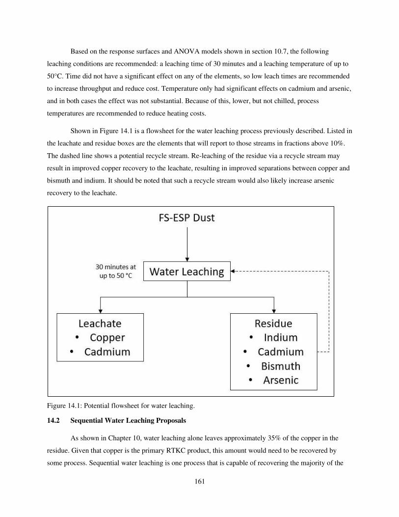
161

Based on the response surfaces and ANOVA models shown in section 10.7, the following

leaching conditions are recommended: a leaching time of 30 minutes and a leaching temperature of up to

50°C. Time did not have a significant effect on any of the elements, so low leach times are recommended

to increase throughput and reduce cost. Temperature only had significant effects on cadmium and arsenic,

and in both cases the effect was not substantial. Because of this, lower, but not chilled, process

temperatures are recommended to reduce heating costs.

Shown in Figure 14.1 is a flowsheet for the water leaching process previously described. Listed in

the leachate and residue boxes are the elements that will report to those streams in fractions above 10%.

The dashed line shows a potential recycle stream. Re-leaching of the residue via a recycle stream may

result in improved copper recovery to the leachate, resulting in improved separations between copper and

bismuth and indium. It should be noted that such a recycle stream would also likely increase arsenic

recovery to the leachate.

Figure 14.1: Potential flowsheet for water leaching.

14.2 Sequential Water Leaching Proposals

As shown in Chapter 10, water leaching alone leaves approximately 35% of the copper in the

residue. Given that copper is the primary RTKC product, this amount would need to be recovered by

some process. Sequential water leaching is one process that is capable of recovering the majority of the

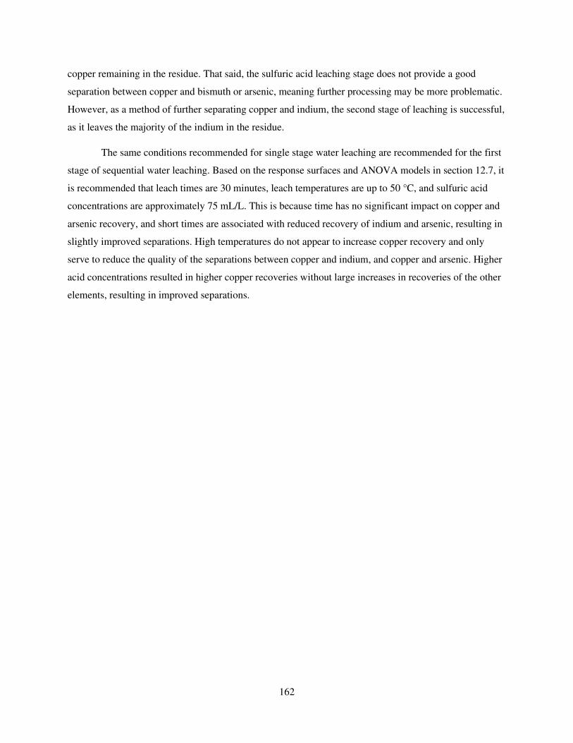
162

copper remaining in the residue. That said, the sulfuric acid leaching stage does not provide a good

separation between copper and bismuth or arsenic, meaning further processing may be more problematic.

However, as a method of further separating copper and indium, the second stage of leaching is successful,

as it leaves the majority of the indium in the residue.

The same conditions recommended for single stage water leaching are recommended for the first

stage of sequential water leaching. Based on the response surfaces and ANOVA models in section 12.7, it

is recommended that leach times are 30 minutes, leach temperatures are up to 50 °C, and sulfuric acid

concentrations are approximately 75 mL/L. This is because time has no significant impact on copper and

arsenic recovery, and short times are associated with reduced recovery of indium and arsenic, resulting in

slightly improved separations. High temperatures do not appear to increase copper recovery and only

serve to reduce the quality of the separations between copper and indium, and copper and arsenic. Higher

acid concentrations resulted in higher copper recoveries without large increases in recoveries of the other

elements, resulting in improved separations.

163

Figure 14.2: Sequential water leaching proposed flowsheet.

Shown in Figure 14.2 is a proposed flowsheet for sequential water leaching showing the percent

of each element that reports to each leachate and residue. The percent’s are based on the response surfaces

and are approximate. The dashed lines show potential recycle streams which may increase recoveries to

the leachate. If implemented, the fractions of each element listed would be different.

164

REFERENCES

[1] U.S. Department of Energy, "Critical Materials Strategy," U.S. Department of Energy, Washington

D.C., 2010.

[2] A. M. Alfantazi and R. R. Moskalyk, "Processing of indium:a review," Minerals Engineering, vol.

16, pp. 687 - 694, 2003.

[3] W. C. Pat Shanks III, B. E. Kimball, A. C. Tolcin and D. E. Guberman, "Germanium and Indium,"

in Critical mineral resources of the United States - Economic and Enviornmental Geology and

Prospects for Future Supply, Reston, U.S. Geological Survey, 2017, pp. I1-I27.

[4] J. D. Jorgenson and M. W. George, "Mineral Commodity Profile Indium," U.S. Geological Survey,

Reston, 2005.

[5] Rio Tinto Kennecott, "riotintokennecott.com," Rio Tinto Kennecott, 2021. [Online]. [Accessed 18

05 2020].

[6] Rio Tinto Kennecott Utah Copper, "Internal memo Progress Report 13 June (Project Center No.

16426)," 2013.

[7] U. Schwarz-Schampera and P. M. Herzig, Indium Geology, Mineralogy, and Economics, New

York: Springer, 2002.

[8] AZO Materials, "Indium (In) - Properties, Applications," AZO Materials, Manchester, 2013.

[9] J. A. A. Smith, "Indium and Indium Coumpounds," Kirk-Othmer Encycopedia of Chemical

Technology, vol. 11, pp. 581-584.

[10] N. N. Greenwood and A. Earnshaw, Chemistry of the Elements, Burlington: Elsevier, 1997.

[11] Wolfram Research, Inc., "Technical data for Indium," Wolfram, Champaign, 2020.

[12] A. M. Guloy and J. D. Corbett, "Synthesis, Structure, and Bonding of Two Lanthanum Indium

Germanides with Novel Structures and Properties," Inorganic Chemistry, vol. 35, no. 9, pp. 2616-

2622, 1996.

165

[13] CRC Press, CRC Handbook of Chemistry and Physics 97th Edition, New York: CRC Press, 216.

[14] Y. Chunh and C.-W. Lee, "Electrochemical behaviors of Indium," Journal of Electrochemical

Science and Technology, vol. 3, no. 1, pp. 1-13, 2012.

[15] L. H. Thanh and J.-C. Liu, "Flotation Separation of Soluble and Colloidal Indium from Aqueous

Solution," Industrial & Engineering Chemistry Research, vol. 53, pp. 1242-1248, 2014.

[16] L. Rocchetti, A. Amato, V. Fonti, S. Ubaldini, I. D. Michelis, B. Kopacek, F. Veglio and F.

Beolchini, "Cross-current lecahing of indium from end-of-life LCD panels," Waste Management,

vol. 42, pp. 180-187, 2015.

[17] G. Phipps, C. Mikolajczak and T. Guckes, "Indium and Gallium: long-term supply," renewable

energy focus, pp. 56-59, 2008.

[18] N. J. Cook, C. L. Ciobanu and T. Williams, "The mineralogy and mineral chemistry of indium in

sulphide deposits and implications for mineral processing," Hydrometallurgy, vol. 108, pp. 226-

228, 2011.

[19] T. Werner, G. M. Mudd and S. M. Jowitt, "The world's by-product and critical metal resources part

III: A global assessment of indium," Ore Geology Reviews, vol. 86, pp. 939-956, 2017.

[20] Z. Qian, Z. Xinzhi, P. Jiayong and S. Shuxun, "Geochemical Enrichment and Mineralization of

Indium," Chinese Journal of Geochemistry, vol. 17, no. 3, pp. 221-225, 1998.

[21] C. S. Anderson, "Indium," in U.S. geological Survey, Mineral Commodity Summaries, January

2018, U.S. Geological Survey, 2018, pp. 78-79.

[22] C. S. Anderson, "Indium," in Mineral Commodity Summaries 2020, U.S. Geological Survey, 2020,

pp. 78-79.

[23] K. Asai, H. Okamoto, J. Hino and T. Kawabata, "Development of indium recovery process using

solvent extraction," Co-products and Minor Elements in Non-Ferrous Smelting, pp. 131-142, 1995.

[24] A. Paiva, "Recovery of Indium from Aqueous Solutions by Solvent Extraction," Separation Science

and Technology, vol. 36, no. 7, pp. 1395-1419, 2001.

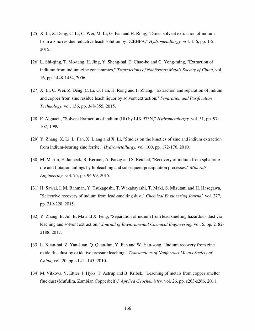
166

[25] X. Li, Z. Deng, C. Li, C. Wei, M. Li, G. Fan and H. Rong, "Direct solvent extraction of indium

from a zinc residue reductive leach solution by D2EHPA," Hydrometallurgy, vol. 156, pp. 1-5,

2015.

[26] L. Shi-qing, T. Mo-tang, H. Jing, Y. Sheng-hai, T. Chao-bo and C. Yong-ming, "Extraction of

indiumn from indium-zinc concentrates," Transactions of Nonferrous Metals Society of China, vol.

16, pp. 1448-1454, 2006.

[27] X. Li, C. Wei, Z. Deng, C. Li, G. Fan, H. Rong and F. Zhang, "Extraction and separation of indium

and copper from zinc residue leach liquor by solvent extraction," Separation and Purification

Technology, vol. 156, pp. 348-355, 2015.

[28] F. Alguacil, "Solvent Extraction of indium (III) by LIX 973N," Hydrometallurgy, vol. 51, pp. 97-

102, 1999.

[29] Y. Zhang, X. Li, L. Pan, X. Liang and X. Li, "Studies on the kinetics of zinc and indium extraction

from indium-bearing zinc ferrite," Hydrometallurgy, vol. 100, pp. 172-176, 2010.

[30] M. Martin, E. Janneck, R. Kermer, A. Patzig and S. Reichel, "Recovery of indium from sphalerite

ore and flotation tailings by bioleaching and subsequent precipitation processes," Minerals

Engineering, vol. 75, pp. 94-99, 2015.

[31] H. Sawai, I. M. Rahman, Y. Tsukagoshi, T. Wakabayashi, T. Maki, S. Mizutani and H. Hasegawa,

"Selectrive recovery of indium from lead-smelting dust," Chemical Engineering Journal, vol. 277,

pp. 219-228, 2015.

[32] Y. Zhang, B. Jin, B. Ma and X. Feng, "Separation of indium from lead smelting hazardous dust via

leaching and solvent extraction," Journal of Enviornmental Chemical Engineering, vol. 5, pp. 2182-

2188, 2017.

[33] L. Xuan-hai, Z. Yan-Juan, Q. Quan-lun, Y. Jian and W. Yan-song, "Indium recovery from zinc

oxide flue dust by oxidative pressure leaching," Transactions of Nonferrous Metals Society of

China, vol. 20, pp. s141-s145, 2010.

[34] M. Vitkova, V. Ettler, J. Hyks, T. Astrup and B. Kribek, "Leaching of metals from copper smelter

flue dust (Mufulira, Zambian Copperbelt)," Applied Geochemistry, vol. 26, pp. s263-s266, 2011.

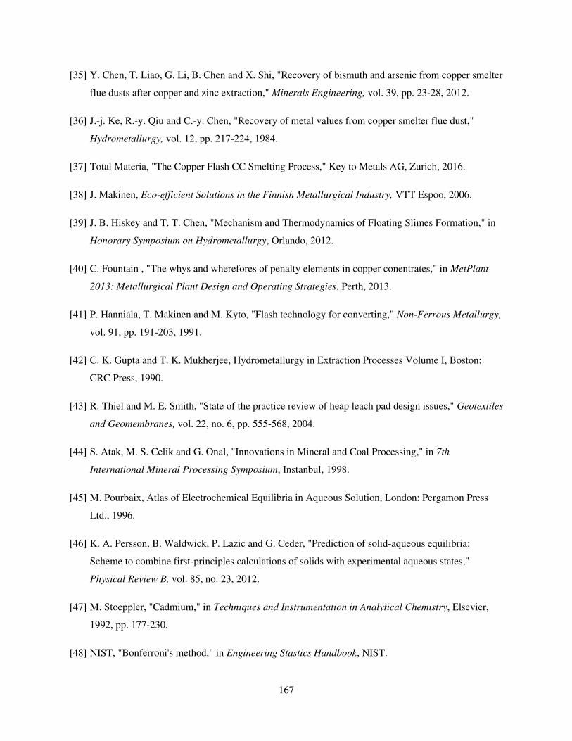
167

[35] Y. Chen, T. Liao, G. Li, B. Chen and X. Shi, "Recovery of bismuth and arsenic from copper smelter

flue dusts after copper and zinc extraction," Minerals Engineering, vol. 39, pp. 23-28, 2012.

[36] J.-j. Ke, R.-y. Qiu and C.-y. Chen, "Recovery of metal values from copper smelter flue dust,"

Hydrometallurgy, vol. 12, pp. 217-224, 1984.

[37] Total Materia, "The Copper Flash CC Smelting Process," Key to Metals AG, Zurich, 2016.

[38] J. Makinen, Eco-efficient Solutions in the Finnish Metallurgical Industry, VTT Espoo, 2006.

[39] J. B. Hiskey and T. T. Chen, "Mechanism and Thermodynamics of Floating Slimes Formation," in

Honorary Symposium on Hydrometallurgy, Orlando, 2012.

[40] C. Fountain , "The whys and wherefores of penalty elements in copper conentrates," in MetPlant

2013: Metallurgical Plant Design and Operating Strategies, Perth, 2013.

[41] P. Hanniala, T. Makinen and M. Kyto, "Flash technology for converting," Non-Ferrous Metallurgy,

vol. 91, pp. 191-203, 1991.

[42] C. K. Gupta and T. K. Mukherjee, Hydrometallurgy in Extraction Processes Volume I, Boston:

CRC Press, 1990.

[43] R. Thiel and M. E. Smith, "State of the practice review of heap leach pad design issues," Geotextiles

and Geomembranes, vol. 22, no. 6, pp. 555-568, 2004.

[44] S. Atak, M. S. Celik and G. Onal, "Innovations in Mineral and Coal Processing," in 7th

International Mineral Processing Symposium, Instanbul, 1998.

[45] M. Pourbaix, Atlas of Electrochemical Equilibria in Aqueous Solution, London: Pergamon Press

Ltd., 1996.

[46] K. A. Persson, B. Waldwick, P. Lazic and G. Ceder, "Prediction of solid-aqueous equilibria:

Scheme to combine first-principles calculations of solids with experimental aqueous states,"

Physical Review B, vol. 85, no. 23, 2012.

[47] M. Stoeppler, "Cadmium," in Techniques and Instrumentation in Analytical Chemistry, Elsevier,

1992, pp. 177-230.

[48] NIST, "Bonferroni's method," in Engineering Stastics Handbook, NIST.

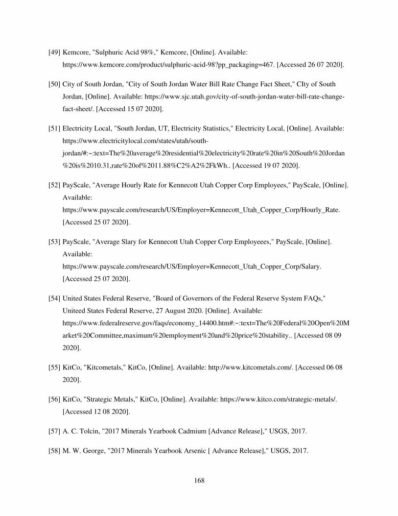
168

[49] Kemcore, "Sulphuric Acid 98%," Kemcore, [Online]. Available:

https://www.kemcore.com/product/sulphuric-acid-98?pp_packaging=467. [Accessed 26 07 2020].

[50] City of South Jordan, "City of South Jordan Water Bill Rate Change Fact Sheet," CIty of South

Jordan, [Online]. Available: https://www.sjc.utah.gov/city-of-south-jordan-water-bill-rate-change-

fact-sheet/. [Accessed 15 07 2020].

[51] Electricity Local, "South Jordan, UT, Electricity Statistics," Electricity Local, [Online]. Available:

https://www.electricitylocal.com/states/utah/south-

jordan/#:~:text=The%20average%20residential%20electricity%20rate%20in%20South%20Jordan

%20is%2010.31,rate%20of%2011.88%C2%A2%2FkWh.. [Accessed 19 07 2020].

[52] PayScale, "Average Hourly Rate for Kennecott Utah Copper Corp Employees," PayScale, [Online].

Available:

https://www.payscale.com/research/US/Employer=Kennecott_Utah_Copper_Corp/Hourly_Rate.

[Accessed 25 07 2020].

[53] PayScale, "Average Slary for Kennecott Utah Copper Corp Employeees," PayScale, [Online].

Available:

https://www.payscale.com/research/US/Employer=Kennecott_Utah_Copper_Corp/Salary.

[Accessed 25 07 2020].

[54] United States Federal Reserve, "Board of Governors of the Federal Reserve System FAQs,"

Uniteed States Federal Reserve, 27 August 2020. [Online]. Available:

https://www.federalreserve.gov/faqs/economy_14400.htm#:~:text=The%20Federal%20Open%20M

arket%20Committee,maximum%20employment%20and%20price%20stability.. [Accessed 08 09

2020].

[55] KitCo, "Kitcometals," KitCo, [Online]. Available: http://www.kitcometals.com/. [Accessed 06 08

2020].

[56] KitCo, "Strategic Metals," KitCo, [Online]. Available: https://www.kitco.com/strategic-metals/.

[Accessed 12 08 2020].

[57] A. C. Tolcin, "2017 Minerals Yearbook Cadmium [Advance Release]," USGS, 2017.

[58] M. W. George, "2017 Minerals Yearbook Arsenic [ Advance Release]," USGS, 2017.

169

[59] SMM, "Bismuth Selenium Tellurium," SMM, [Online]. Available:

https://price.metal.com/Bismuth-Selenium-Tellurium. [Accessed 23 07 2020].

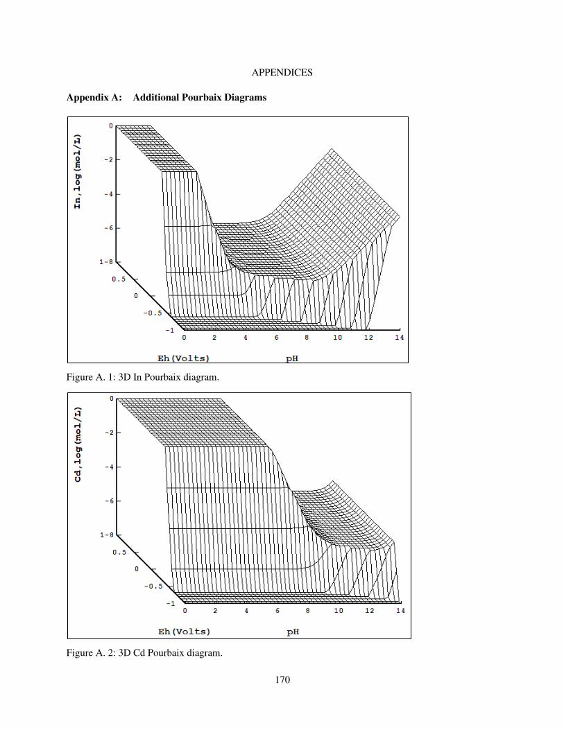
170

APPENDICES

Appendix A: Additional Pourbaix Diagrams

Figure A. 1: 3D In Pourbaix diagram.

Figure A. 2: 3D Cd Pourbaix diagram.

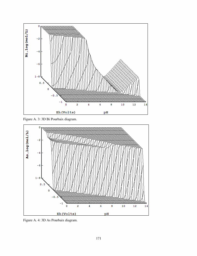
171

Figure A. 3: 3D Bi Pourbaix diagram.

Figure A. 4: 3D As Pourbaix diagram.

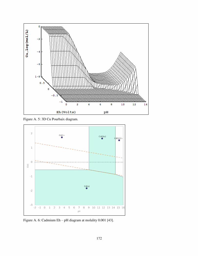
172

Figure A. 5: 3D Cu Pourbaix diagram.

Figure A. 6: Cadmium Eh – pH diagram at molality 0.001 [43].

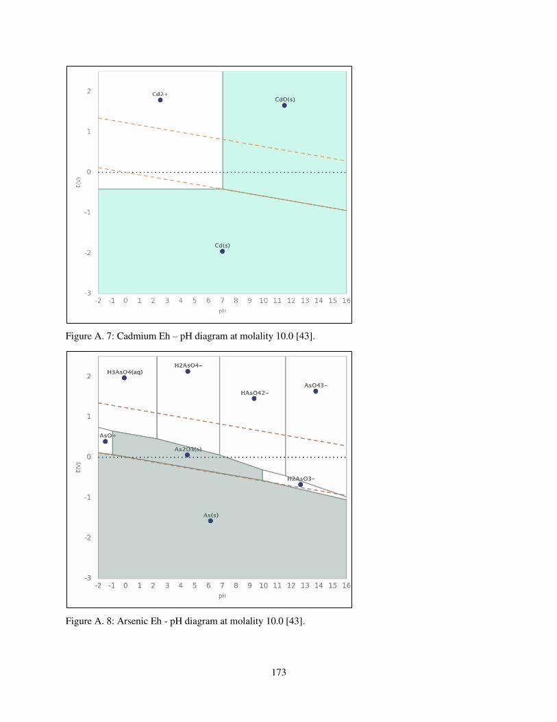
173

Figure A. 7: Cadmium Eh – pH diagram at molality 10.0 [43].

Figure A. 8: Arsenic Eh - pH diagram at molality 10.0 [43].

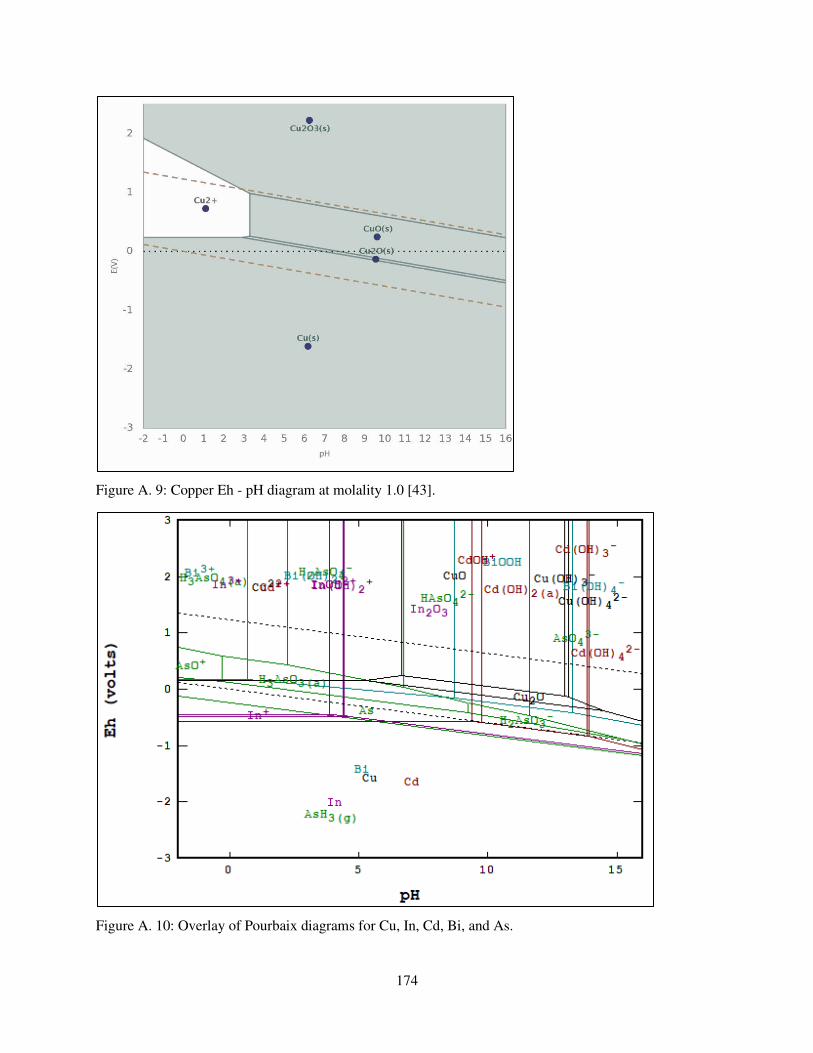
174

Figure A. 9: Copper Eh - pH diagram at molality 1.0 [43].

Figure A. 10: Overlay of Pourbaix diagrams for Cu, In, Cd, Bi, and As.

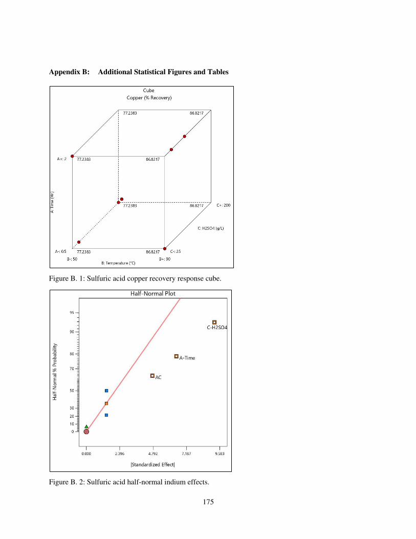
175

Appendix B: Additional Statistical Figures and Tables

Figure B. 1: Sulfuric acid copper recovery response cube.

Figure B. 2: Sulfuric acid half-normal indium effects.

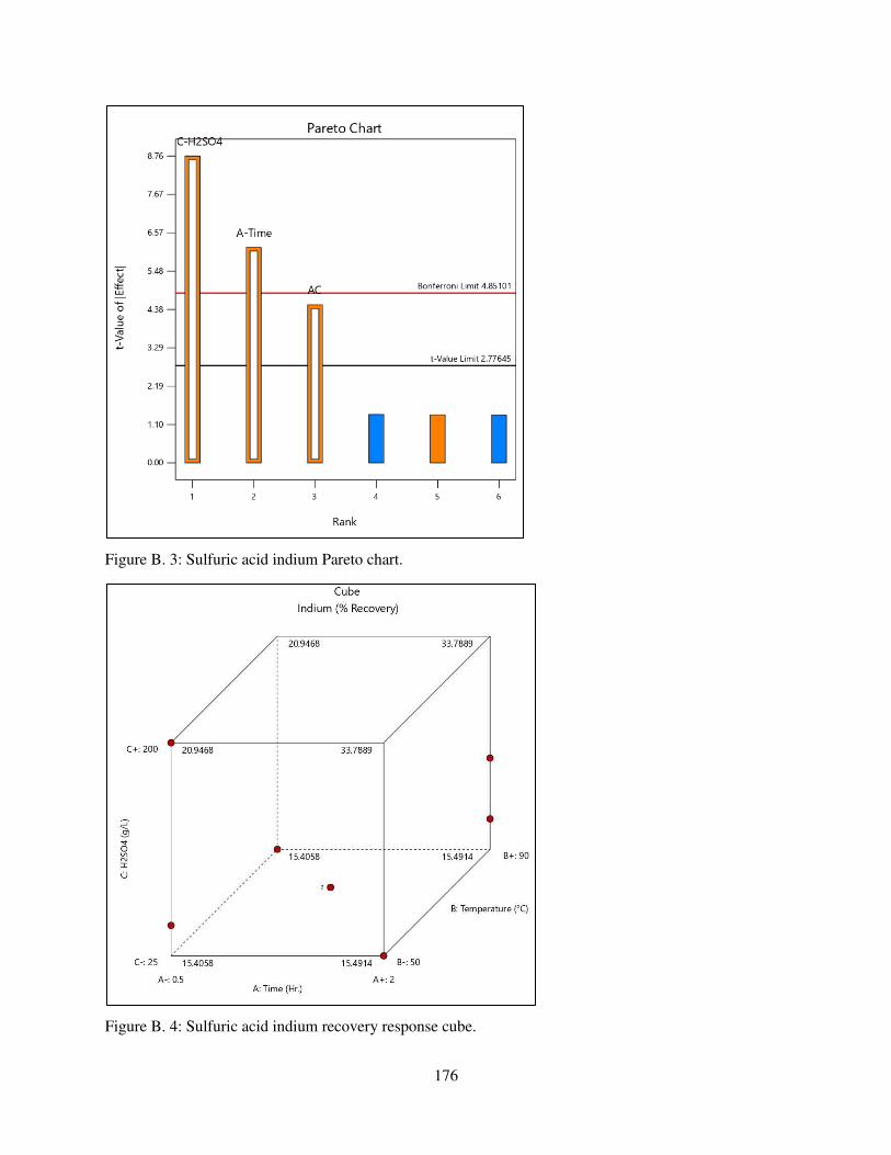
176

Figure B. 3: Sulfuric acid indium Pareto chart.

Figure B. 4: Sulfuric acid indium recovery response cube.

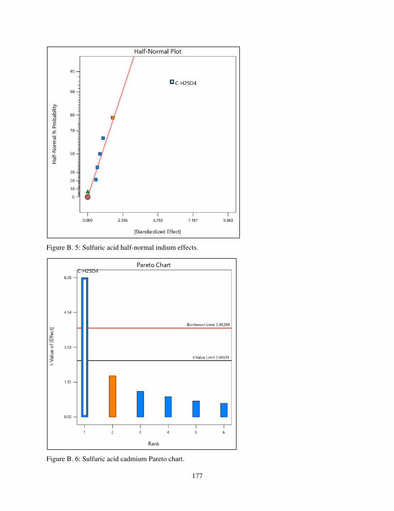
177

Figure B. 5: Sulfuric acid half-normal indium effects.

Figure B. 6: Sulfuric acid cadmium Pareto chart.

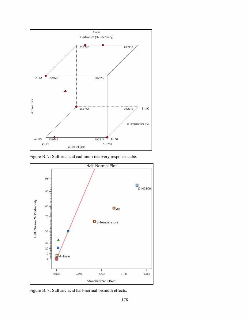
178

Figure B. 7: Sulfuric acid cadmium recovery response cube.

Figure B. 8: Sulfuric acid half-normal bismuth effects.

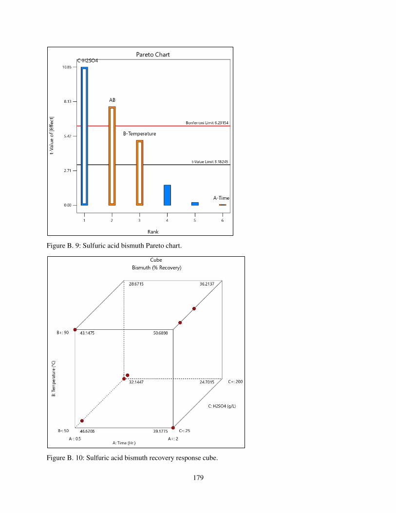
179

Figure B. 9: Sulfuric acid bismuth Pareto chart.

Figure B. 10: Sulfuric acid bismuth recovery response cube.

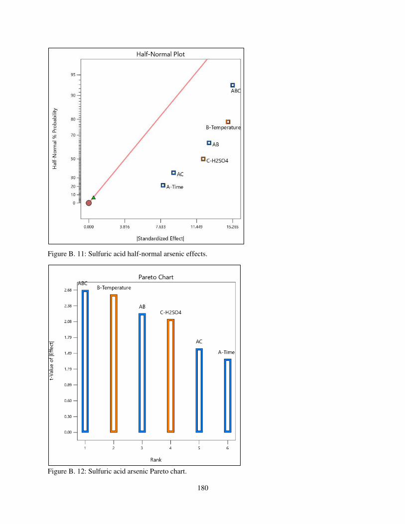
180

Figure B. 11: Sulfuric acid half-normal arsenic effects.

Figure B. 12: Sulfuric acid arsenic Pareto chart.

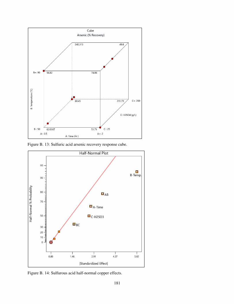
181

Figure B. 13: Sulfuric acid arsenic recovery response cube.

Figure B. 14: Sulfurous acid half-normal copper effects.

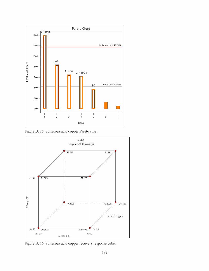
182

Figure B. 15: Sulfurous acid copper Pareto chart.

Figure B. 16: Sulfurous acid copper recovery response cube.

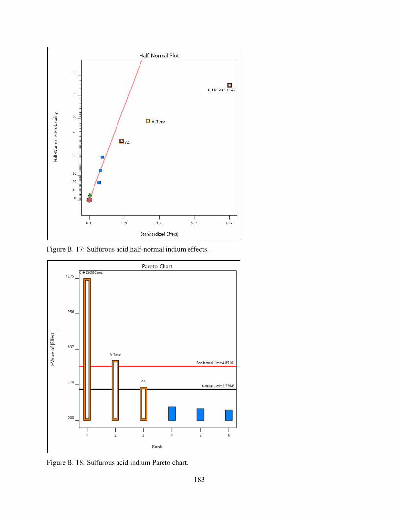
183

Figure B. 17: Sulfurous acid half-normal indium effects.

Figure B. 18: Sulfurous acid indium Pareto chart.

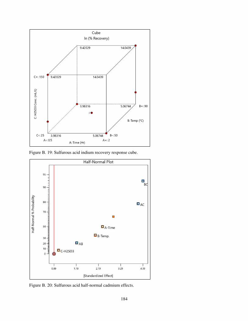
184

Figure B. 19: Sulfurous acid indium recovery response cube.

Figure B. 20: Sulfurous acid half-normal cadmium effects.

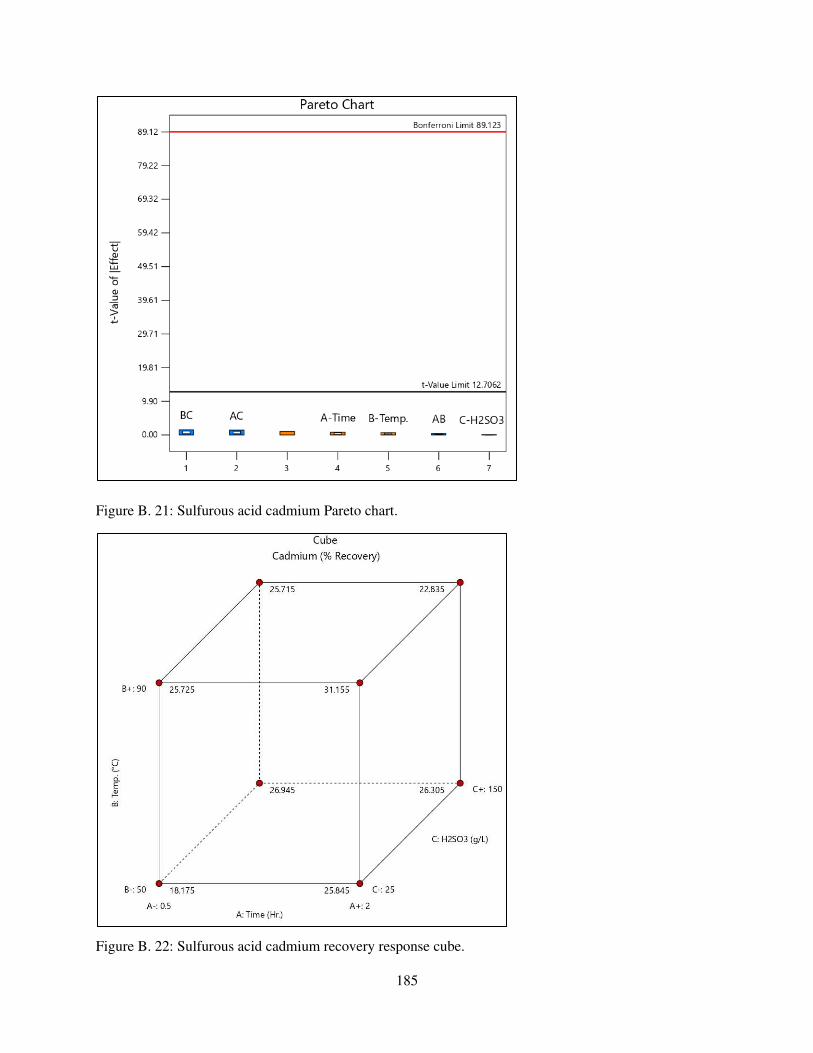
185

Figure B. 21: Sulfurous acid cadmium Pareto chart.

Figure B. 22: Sulfurous acid cadmium recovery response cube.

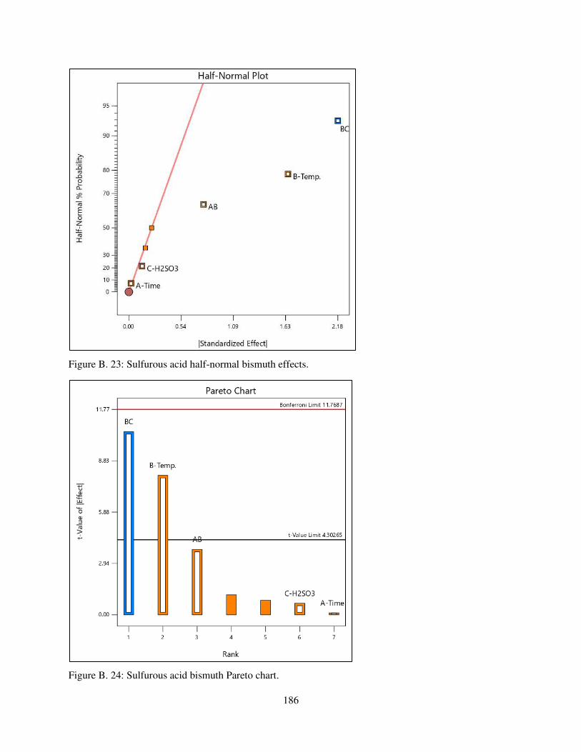
186

Figure B. 23: Sulfurous acid half-normal bismuth effects.

Figure B. 24: Sulfurous acid bismuth Pareto chart.

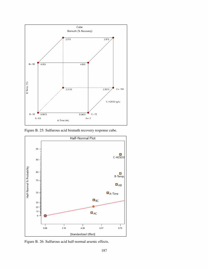
187

Figure B. 25: Sulfurous acid bismuth recovery response cube.

Figure B. 26: Sulfurous acid half-normal arsenic effects.

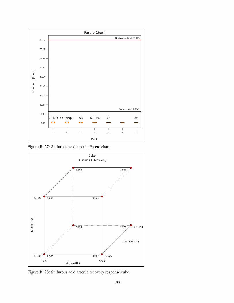
188

Figure B. 27: Sulfurous acid arsenic Pareto chart.

Figure B. 28: Sulfurous acid arsenic recovery response cube.

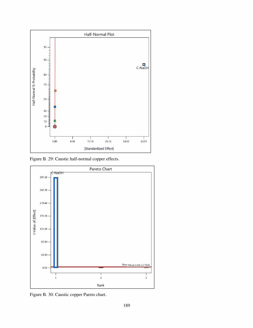
189

Figure B. 29: Caustic half-normal copper effects.

Figure B. 30: Caustic copper Pareto chart.

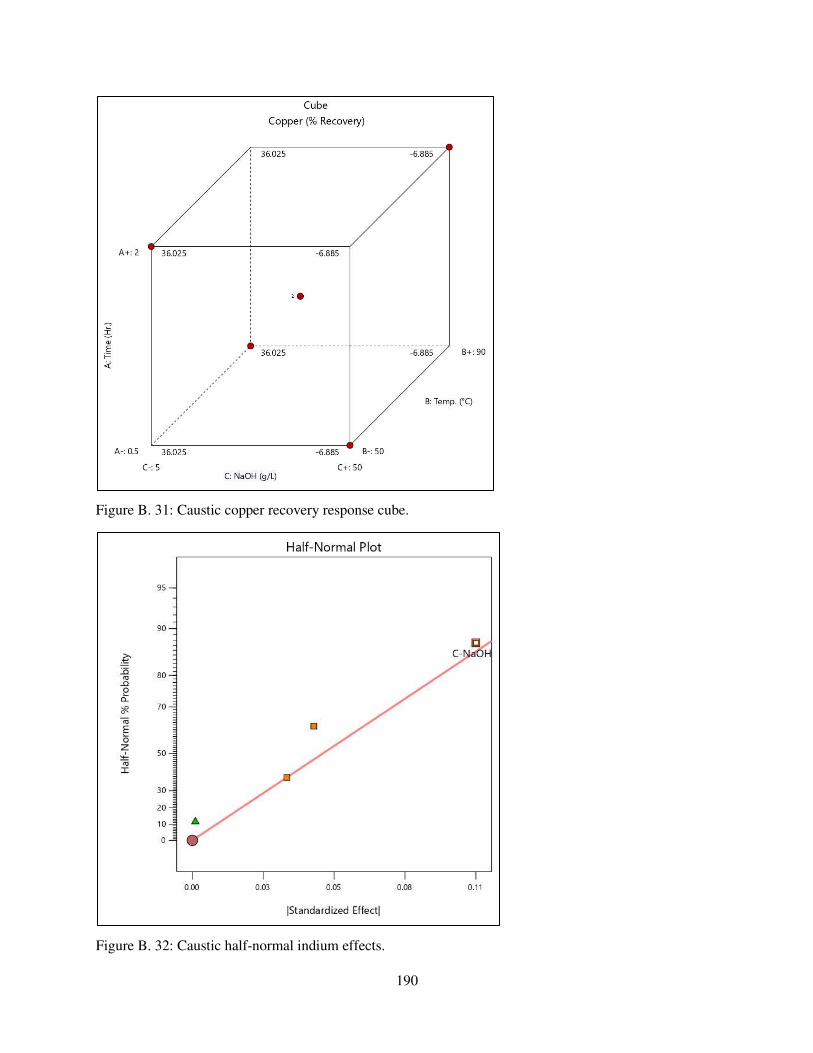
190

Figure B. 31: Caustic copper recovery response cube.

Figure B. 32: Caustic half-normal indium effects.

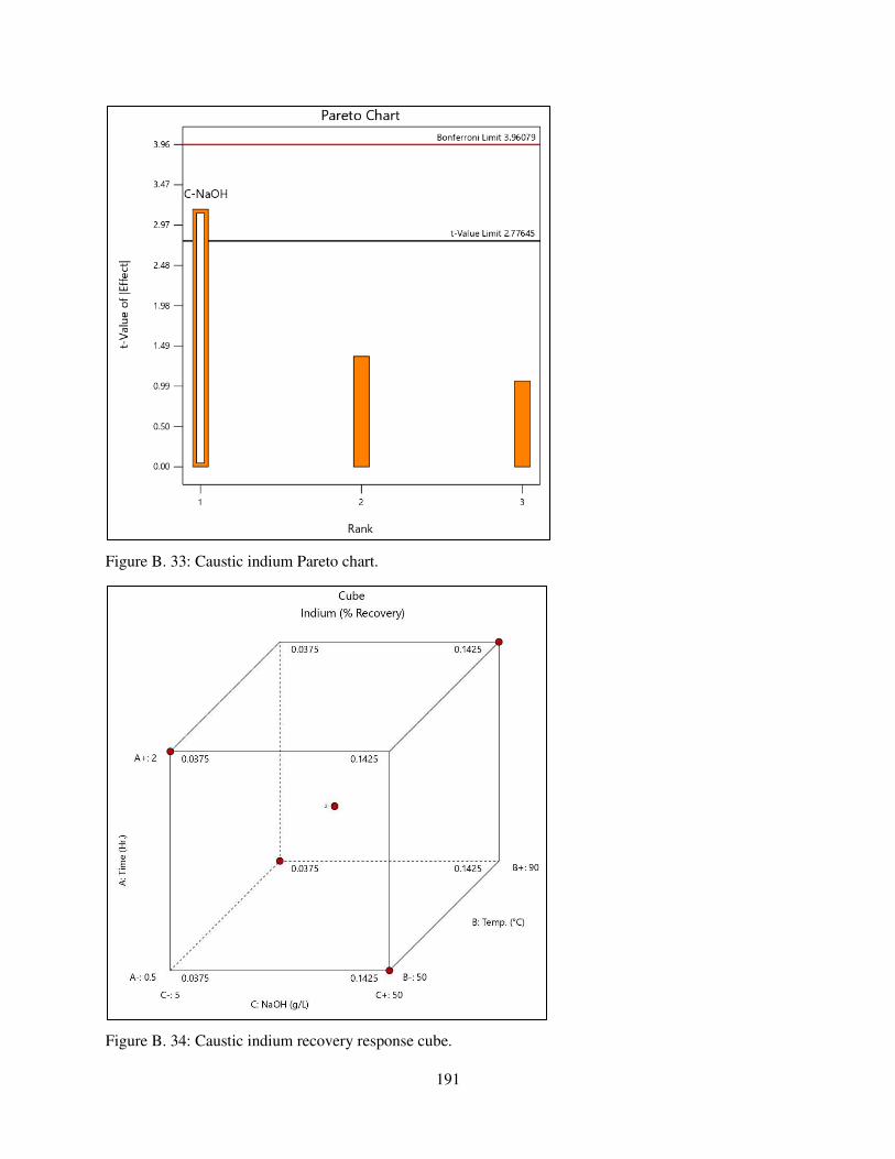
191

Figure B. 33: Caustic indium Pareto chart.

Figure B. 34: Caustic indium recovery response cube.

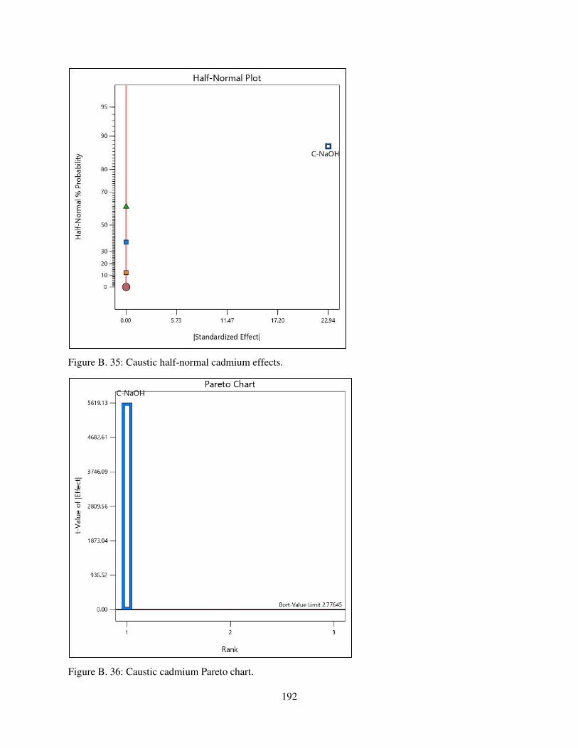
192

Figure B. 35: Caustic half-normal cadmium effects.

Figure B. 36: Caustic cadmium Pareto chart.

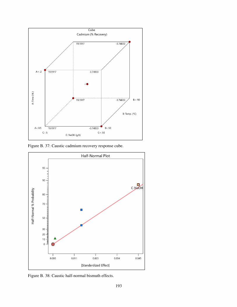
193

Figure B. 37: Caustic cadmium recovery response cube.

Figure B. 38: Caustic half-normal bismuth effects.

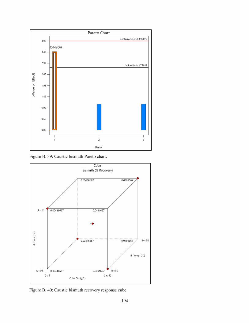
194

Figure B. 39: Caustic bismuth Pareto chart.

Figure B. 40: Caustic bismuth recovery response cube.

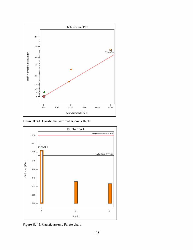
195

Figure B. 41: Caustic half-normal arsenic effects.

Figure B. 42: Caustic arsenic Pareto chart.

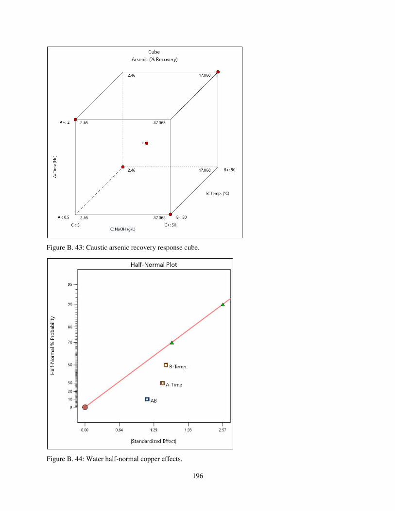
196

Figure B. 43: Caustic arsenic recovery response cube.

Figure B. 44: Water half-normal copper effects.

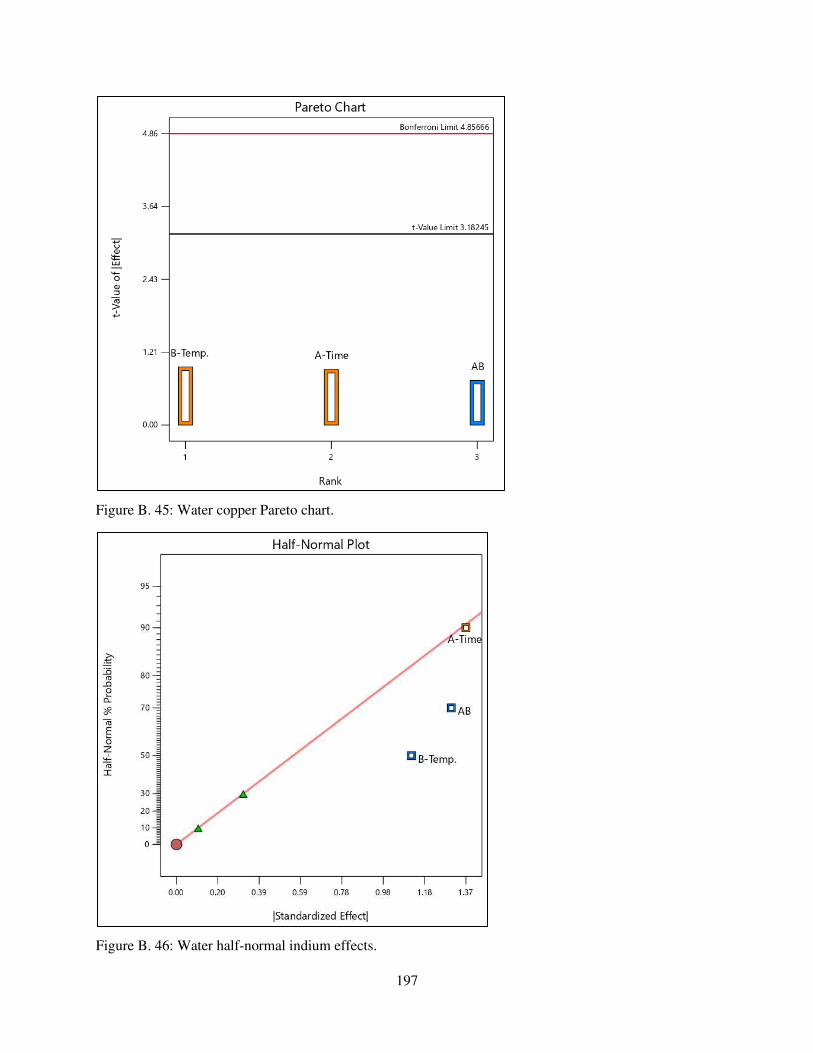
197

Figure B. 45: Water copper Pareto chart.

Figure B. 46: Water half-normal indium effects.

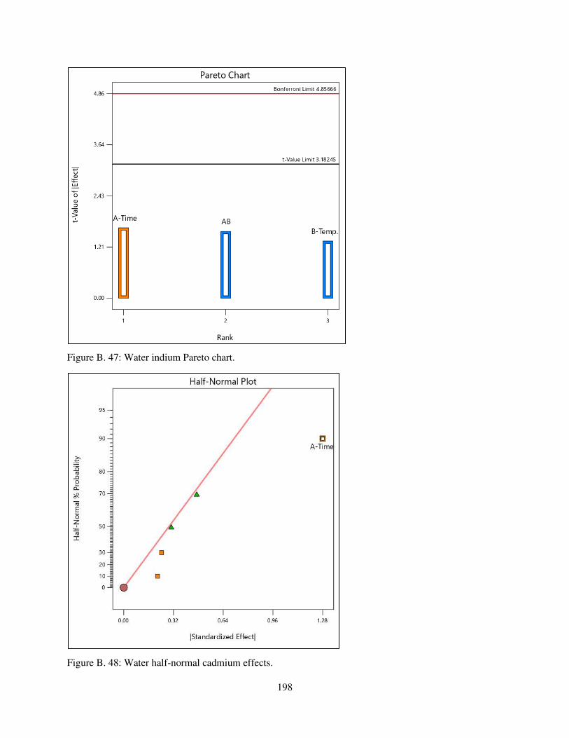
198

Figure B. 47: Water indium Pareto chart.

Figure B. 48: Water half-normal cadmium effects.

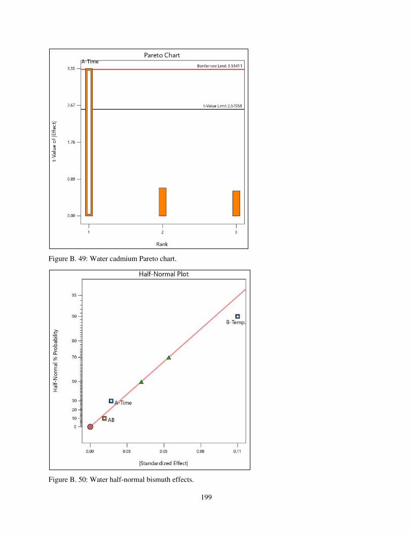
199

Figure B. 49: Water cadmium Pareto chart.

Figure B. 50: Water half-normal bismuth effects.

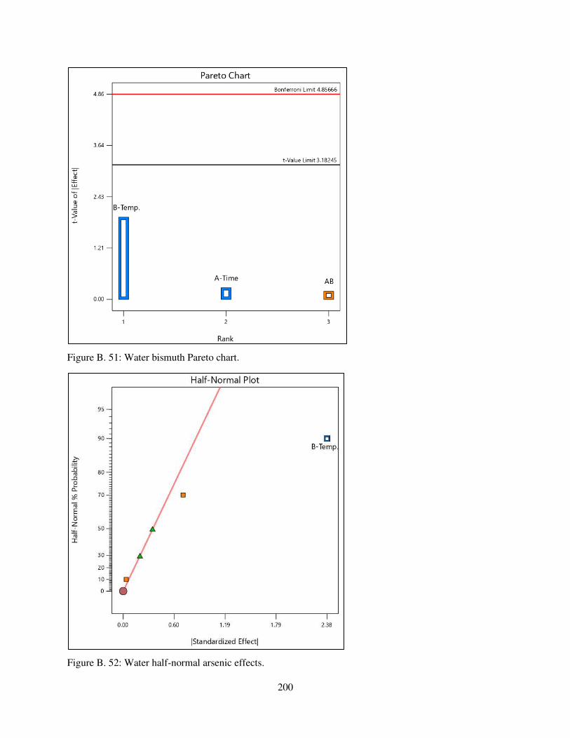
200

Figure B. 51: Water bismuth Pareto chart.

Figure B. 52: Water half-normal arsenic effects.

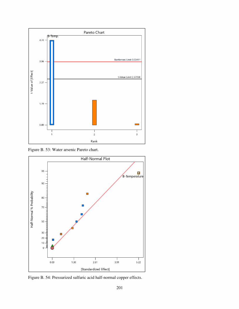
201

Figure B. 53: Water arsenic Pareto chart.

Figure B. 54: Pressurized sulfuric acid half-normal copper effects.

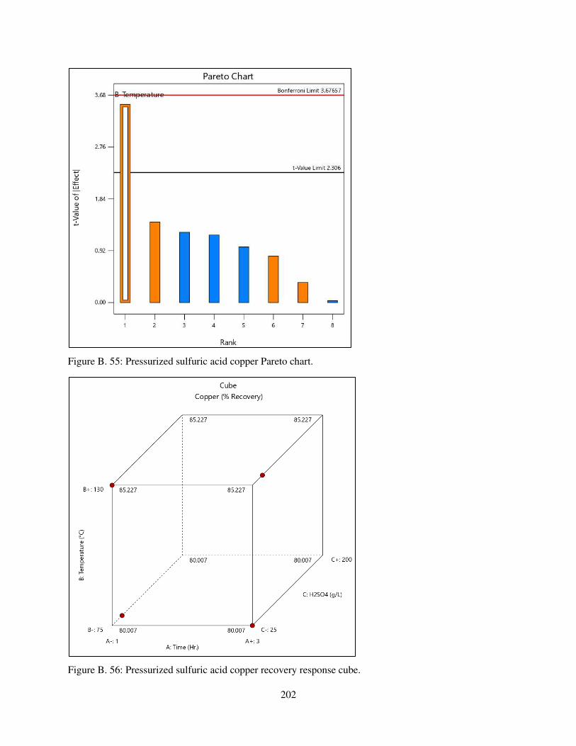
202

Figure B. 55: Pressurized sulfuric acid copper Pareto chart.

Figure B. 56: Pressurized sulfuric acid copper recovery response cube.

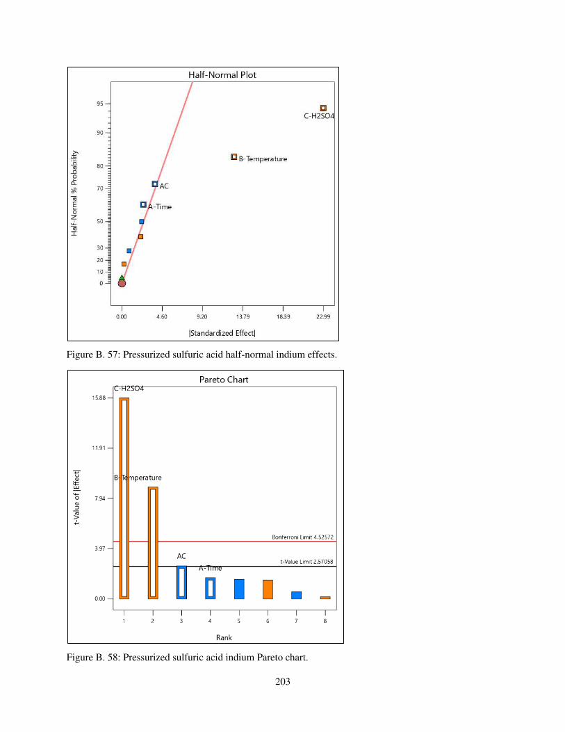
203

Figure B. 57: Pressurized sulfuric acid half-normal indium effects.

Figure B. 58: Pressurized sulfuric acid indium Pareto chart.

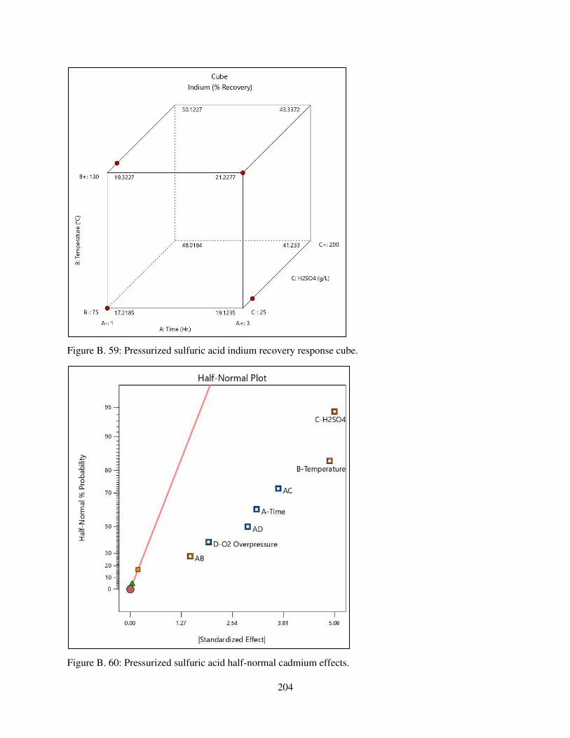
204

Figure B. 59: Pressurized sulfuric acid indium recovery response cube.

Figure B. 60: Pressurized sulfuric acid half-normal cadmium effects.

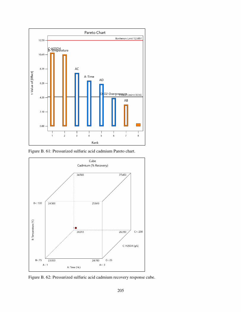
205

Figure B. 61: Pressurized sulfuric acid cadmium Pareto chart.

Figure B. 62: Pressurized sulfuric acid cadmium recovery response cube.

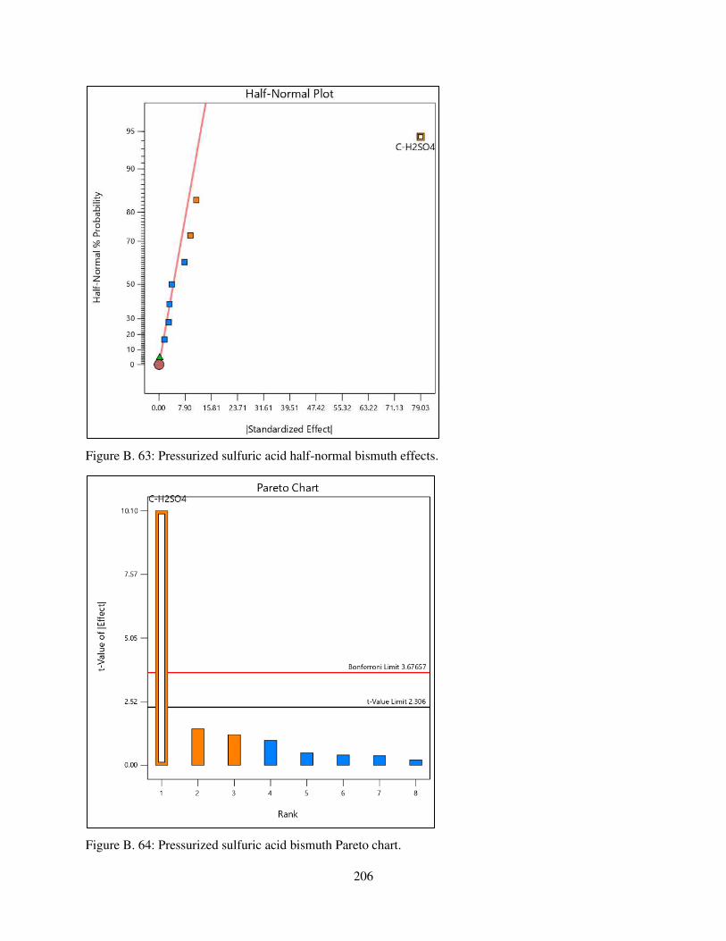
206

Figure B. 63: Pressurized sulfuric acid half-normal bismuth effects.

Figure B. 64: Pressurized sulfuric acid bismuth Pareto chart.

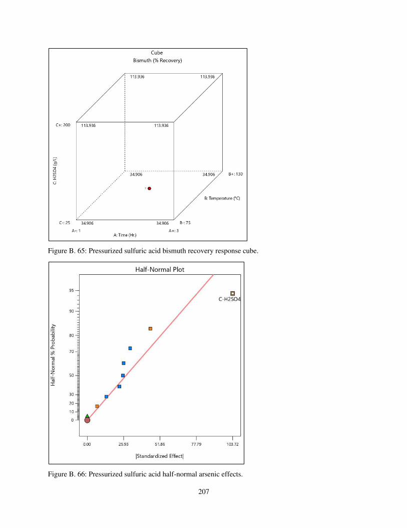
207

Figure B. 65: Pressurized sulfuric acid bismuth recovery response cube.

Figure B. 66: Pressurized sulfuric acid half-normal arsenic effects.

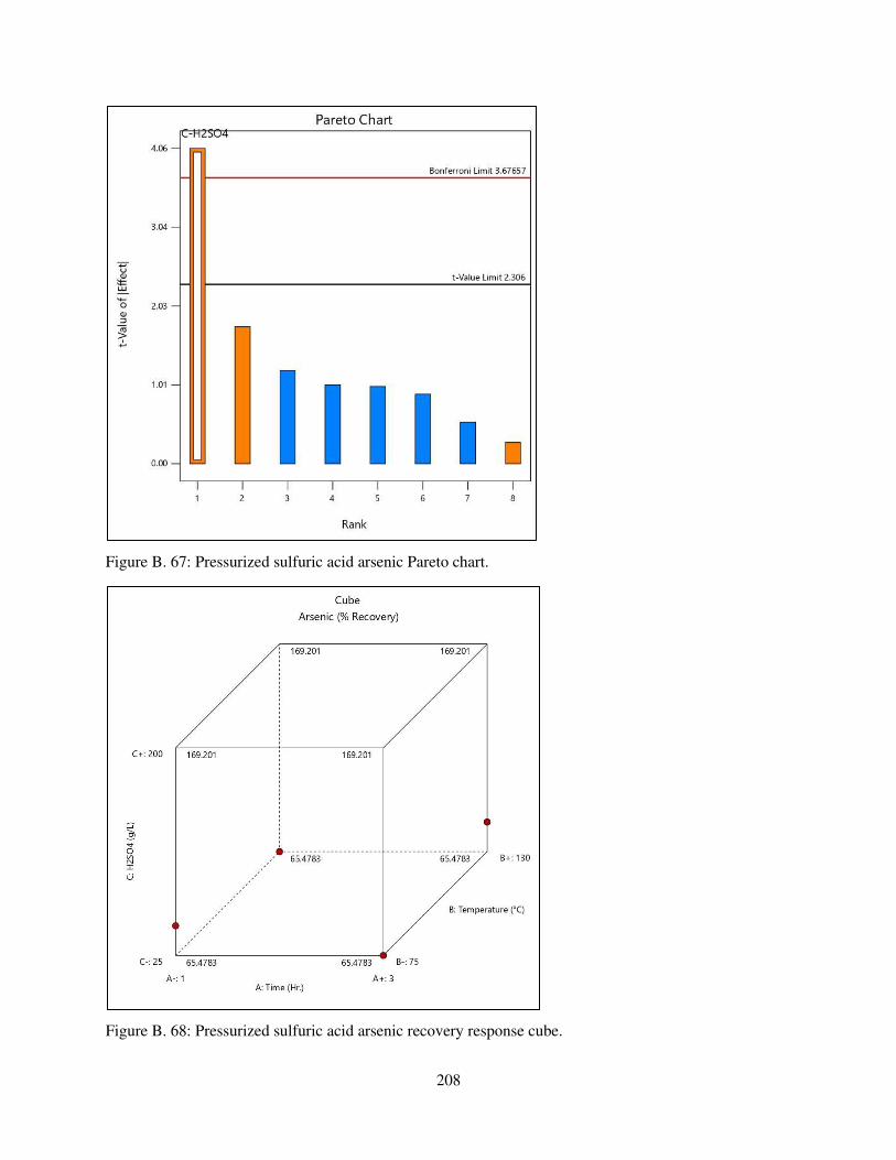
208

Figure B. 67: Pressurized sulfuric acid arsenic Pareto chart.

Figure B. 68: Pressurized sulfuric acid arsenic recovery response cube.

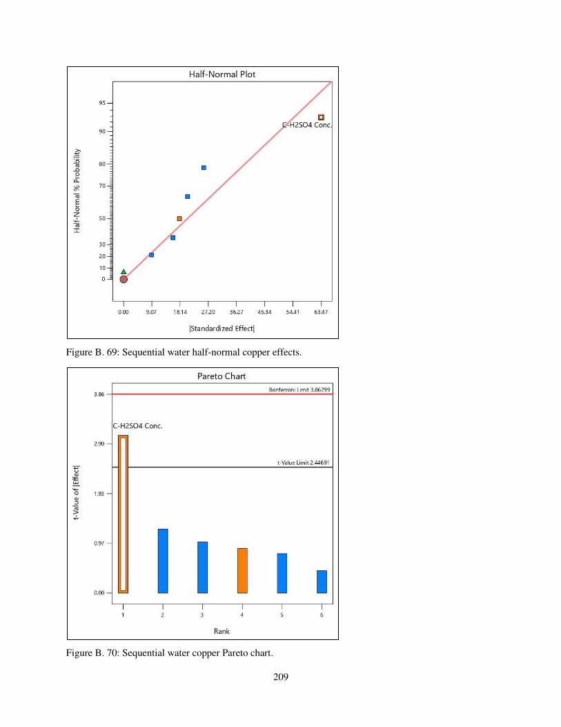
209

Figure B. 69: Sequential water half-normal copper effects.

Figure B. 70: Sequential water copper Pareto chart.

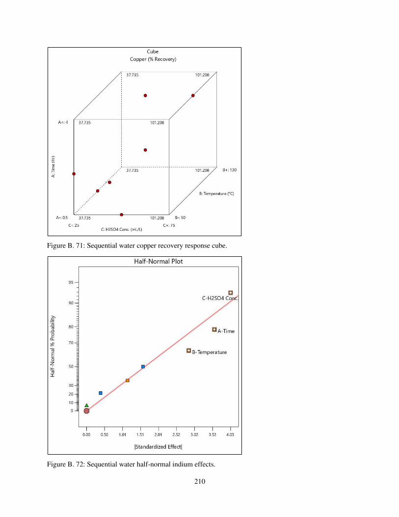
210

Figure B. 71: Sequential water copper recovery response cube.

Figure B. 72: Sequential water half-normal indium effects.

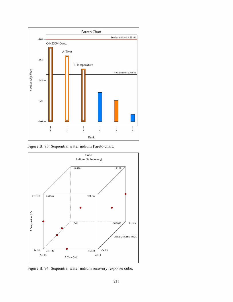
211

Figure B. 73: Sequential water indium Pareto chart.

Figure B. 74: Sequential water indium recovery response cube.

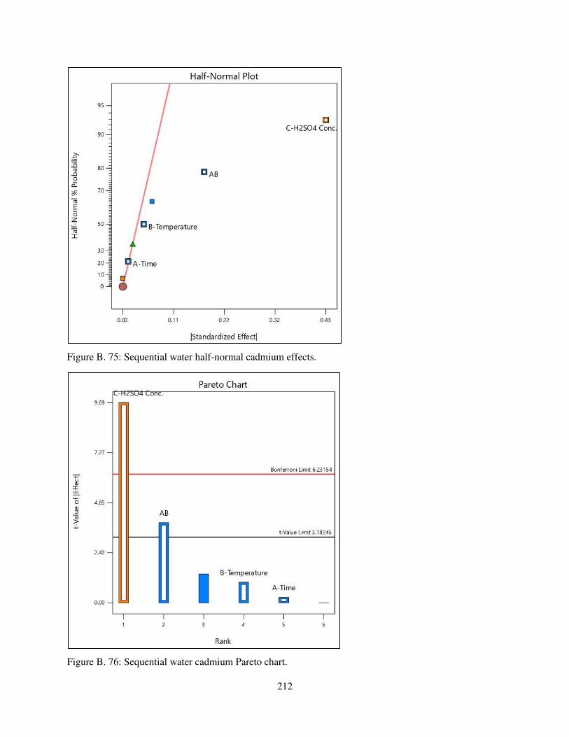
212

Figure B. 75: Sequential water half-normal cadmium effects.

Figure B. 76: Sequential water cadmium Pareto chart.

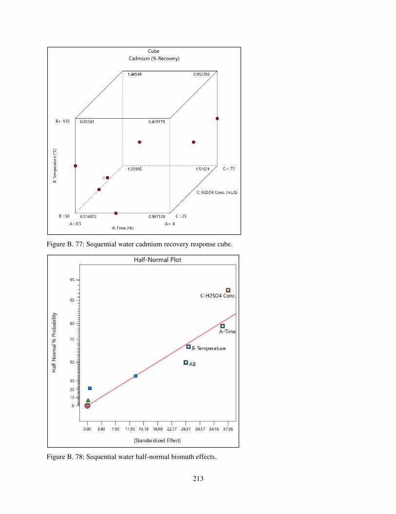
213

Figure B. 77: Sequential water cadmium recovery response cube.

Figure B. 78: Sequential water half-normal bismuth effects.

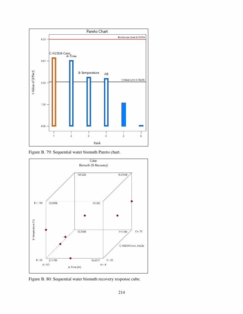
214

Figure B. 79: Sequential water bismuth Pareto chart.

Figure B. 80: Sequential water bismuth recovery response cube.

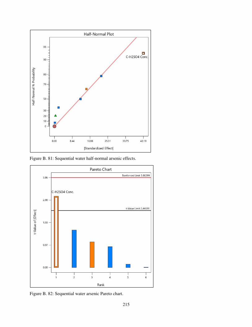
215

Figure B. 81: Sequential water half-normal arsenic effects.

Figure B. 82: Sequential water arsenic Pareto chart.

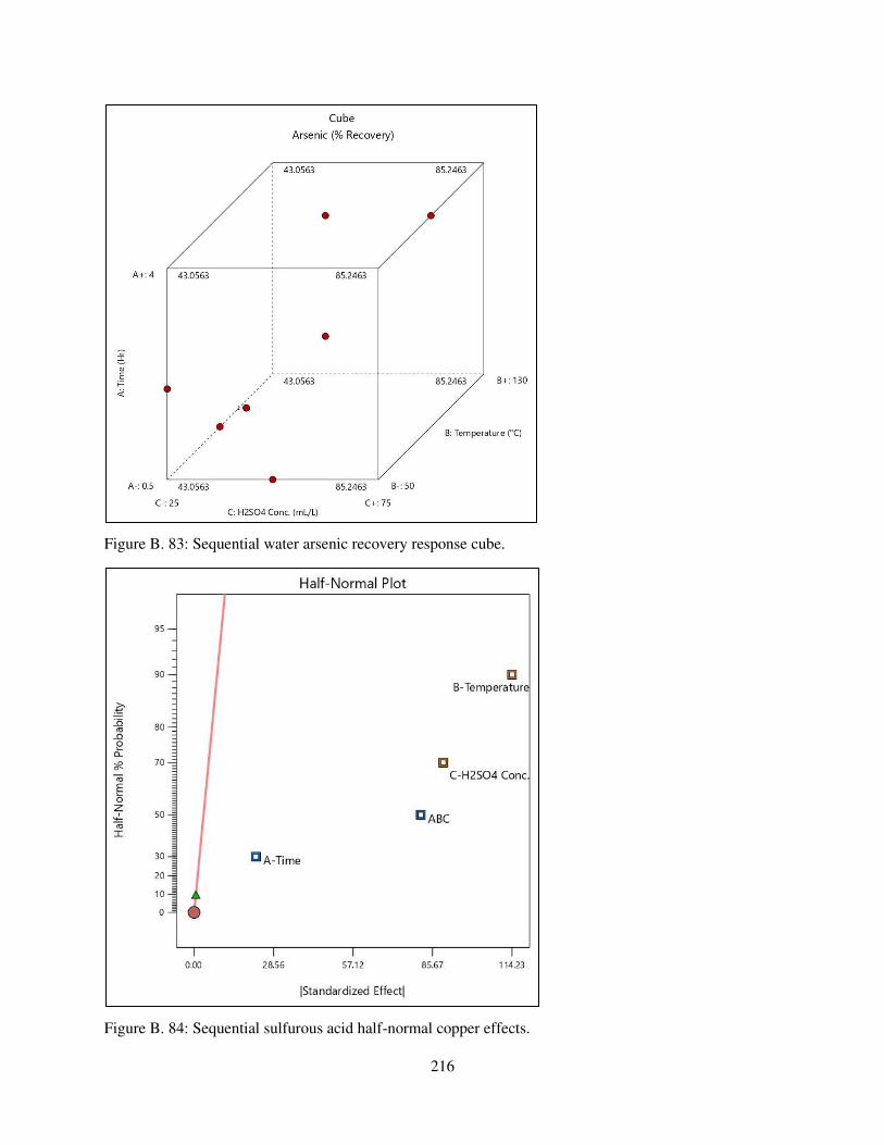
216

Figure B. 83: Sequential water arsenic recovery response cube.

Figure B. 84: Sequential sulfurous acid half-normal copper effects.

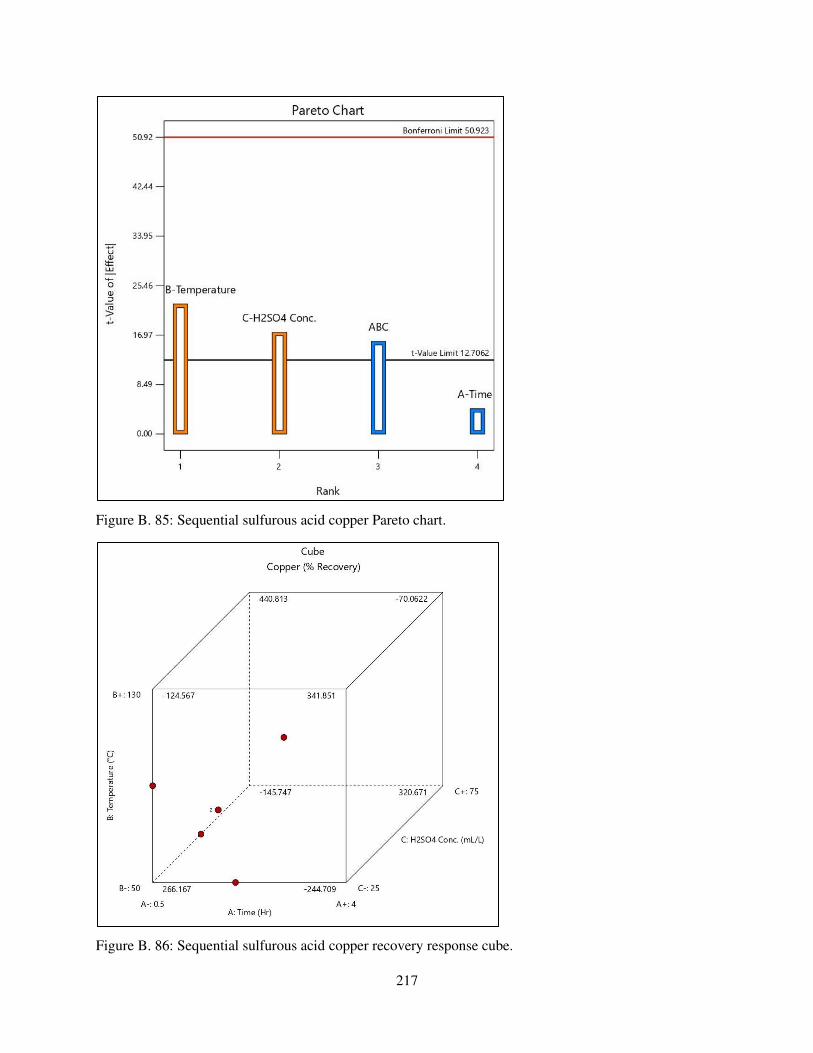
217

Figure B. 85: Sequential sulfurous acid copper Pareto chart.

Figure B. 86: Sequential sulfurous acid copper recovery response cube.

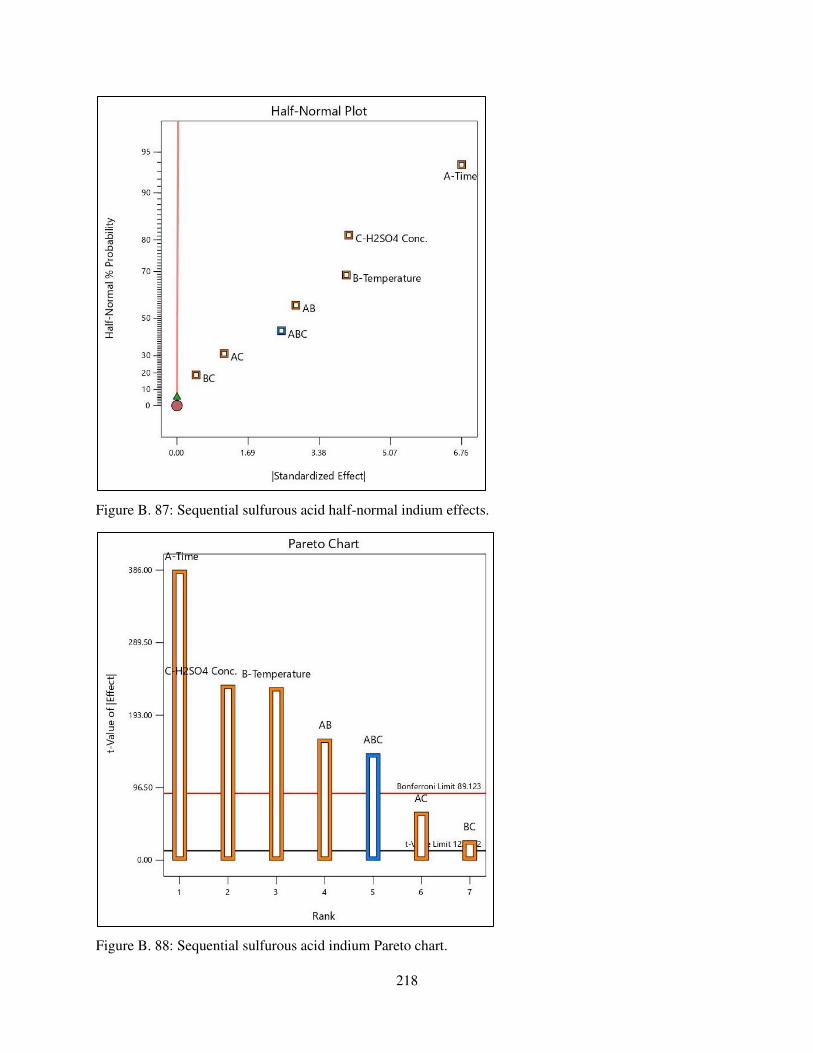
218

Figure B. 87: Sequential sulfurous acid half-normal indium effects.

Figure B. 88: Sequential sulfurous acid indium Pareto chart.

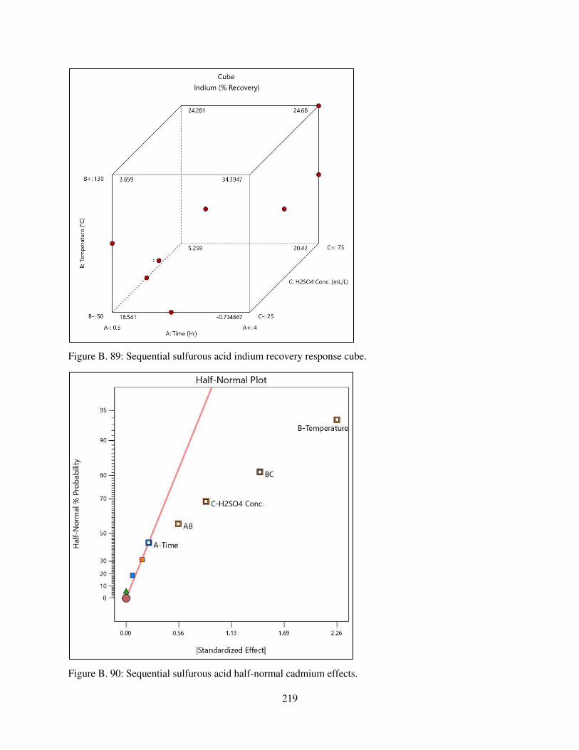
219

Figure B. 89: Sequential sulfurous acid indium recovery response cube.

Figure B. 90: Sequential sulfurous acid half-normal cadmium effects.

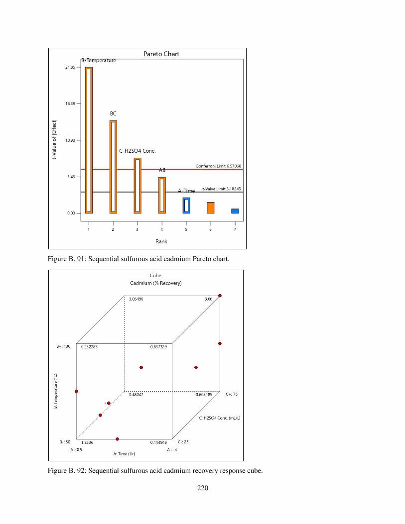
220

Figure B. 91: Sequential sulfurous acid cadmium Pareto chart.

Figure B. 92: Sequential sulfurous acid cadmium recovery response cube.

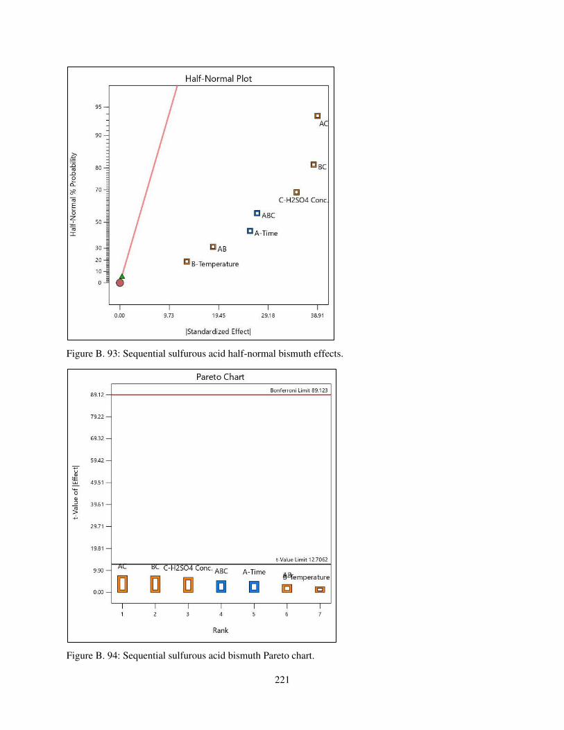
221

Figure B. 93: Sequential sulfurous acid half-normal bismuth effects.

Figure B. 94: Sequential sulfurous acid bismuth Pareto chart.

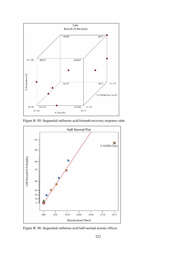
222

Figure B. 95: Sequential sulfurous acid bismuth recovery response cube.

Figure B. 96: Sequential sulfurous acid half-normal arsenic effects.

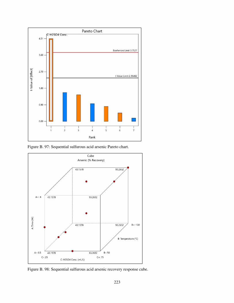
223

Figure B. 97: Sequential sulfurous acid arsenic Pareto chart.

Figure B. 98: Sequential sulfurous acid arsenic recovery response cube.

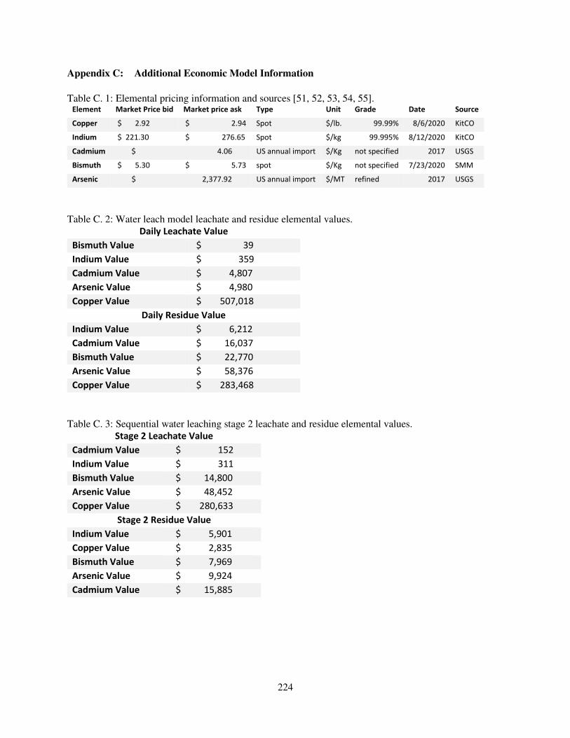
224

Appendix C: Additional Economic Model Information

Table C. 1: Elemental pricing information and sources [51, 52, 53, 54, 55]. Element Market Price bid Market price ask Type Unit Grade Date Source

Copper $ 2.92 $ 2.94 Spot $/lb. 99.99% 8/6/2020 KitCO

Indium $ 221.30 $ 276.65 Spot $/kg 99.995% 8/12/2020 KitCO

Cadmium $ 4.06 US annual import $/Kg not specified 2017 USGS

Bismuth $ 5.30 $ 5.73 spot $/Kg not specified 7/23/2020 SMM

Arsenic $ 2,377.92 US annual import $/MT refined 2017 USGS

Table C. 2: Water leach model leachate and residue elemental values.

Daily Leachate Value

Bismuth Value $ 39

Indium Value $ 359

Cadmium Value $ 4,807

Arsenic Value $ 4,980

Copper Value $ 507,018

Daily Residue Value

Indium Value $ 6,212


Bismuth Value $ 22,770



Table C. 3: Sequential water leaching stage 2 leachate and residue elemental values.

Stage 2 Leachate Value

Cadmium Value $ 152

Indium Value $ 311




Stage 2 Residue Value

Indium Value $ 5,901





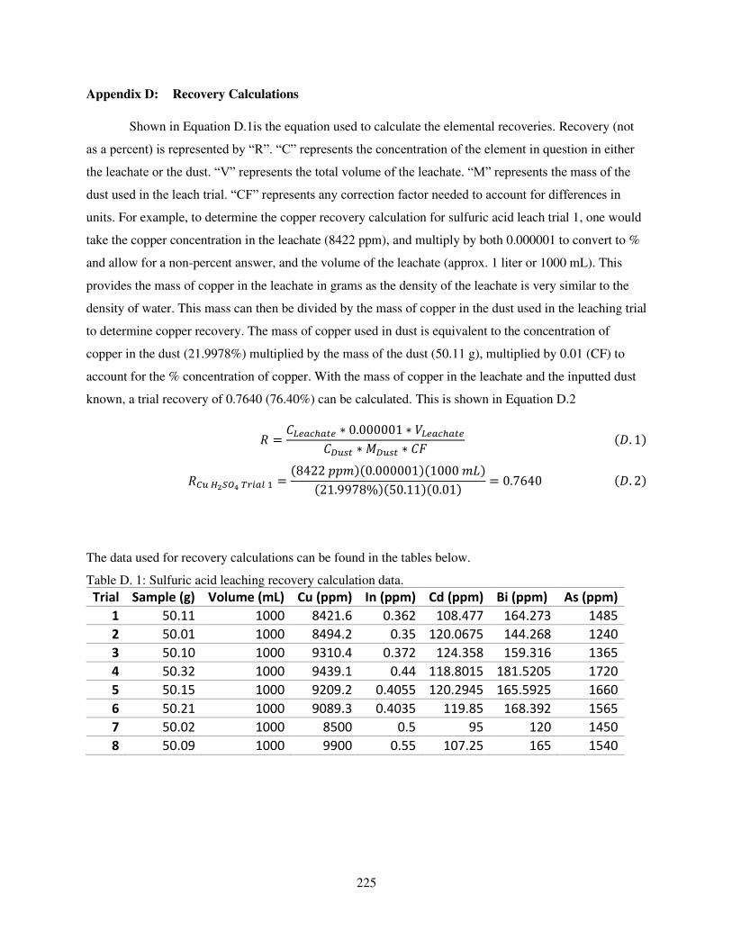
225

Appendix D: Recovery Calculations

Shown in Equation D.1is the equation used to calculate the elemental recoveries. Recovery (not

as a percent) is represented by “R”. “C” represents the concentration of the element in question in either

the leachate or the dust. “V” represents the total volume of the leachate. “M” represents the mass of the

dust used in the leach trial. “CF” represents any correction factor needed to account for differences in

units. For example, to determine the copper recovery calculation for sulfuric acid leach trial 1, one would

take the copper concentration in the leachate (8422 ppm), and multiply by both 0.000001 to convert to %

and allow for a non-percent answer, and the volume of the leachate (approx. 1 liter or 1000 mL). This

provides the mass of copper in the leachate in grams as the density of the leachate is very similar to the

density of water. This mass can then be divided by the mass of copper in the dust used in the leaching trial

to determine copper recovery. The mass of copper used in dust is equivalent to the concentration of

copper in the dust (21.9978%) multiplied by the mass of the dust (50.11 g), multiplied by 0.01 (CF) to

account for the % concentration of copper. With the mass of copper in the leachate and the inputted dust

known, a trial recovery of 0.7640 (76.40%) can be calculated. This is shown in Equation D.2

𝑅 = 𝐶𝐿𝑒𝑎𝑐ℎ𝑎𝑡𝑒 ∗ 0.000001 ∗ 𝑉𝐿𝑒𝑎𝑐ℎ𝑎𝑡𝑒𝐶𝐷𝑢𝑠𝑡 ∗ 𝑀𝐷𝑢𝑠𝑡 ∗ 𝐶𝐹 (𝐷. 1)

𝑅𝐶𝑢 𝐻2𝑆𝑂4 𝑇𝑟𝑖𝑎𝑙 1 = (8422 𝑝𝑝𝑚)(0.000001)(1000 𝑚𝐿)(21.9978%)(50.11)(0.01) = 0.7640 (𝐷. 2)

The data used for recovery calculations can be found in the tables below.

Table D. 1: Sulfuric acid leaching recovery calculation data.

Trial Sample (g) Volume (mL) Cu (ppm) In (ppm) Cd (ppm) Bi (ppm) As (ppm)

1 50.11 1000 8421.6 0.362 108.477 164.273 1485

2 50.01 1000 8494.2 0.35 120.0675 144.268 1240

3 50.10 1000 9310.4 0.372 124.358 159.316 1365

4 50.32 1000 9439.1 0.44 118.8015 181.5205 1720

5 50.15 1000 9209.2 0.4055 120.2945 165.5925 1660

6 50.21 1000 9089.3 0.4035 119.85 168.392 1565

7 50.02 1000 8500 0.5 95 120 1450

8 50.09 1000 9900 0.55 107.25 165 1540

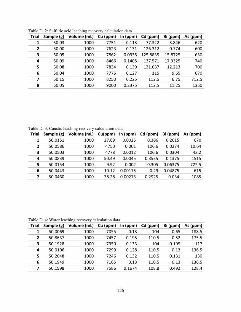
226

Table D. 2: Sulfuric acid leaching recovery calculation data.


1 50.03 1000 7751 0.113 77.322 3.846 620

2 50.00 1000 7623 0.131 126.312 0.774 600

3 50.05 1000 7862 0.0935 125.8835 15.8725 630

4 50.09 1000 8466 0.1405 137.571 17.3325 740

5 50.08 1000 7834 0.139 131.637 12.213 700

6 50.04 1000 7776 0.127 115 9.65 670

7 50.15 1000 8250 0.225 112.5 6.75 712.5

8 50.05 1000 9000 0.3375 112.5 11.25 1350

Table D. 3: Caustic leaching recovery calculation data.

Trial Sample (g) Volume (mL) Cu(ppm) In (ppm) Cd (ppm) Bi (ppm) As (ppm)

1 50.0151 1000 27.69 0.0025 0.386 0.2615 670

2 50.0586 1000 4750 0.001 106.6 0.0374 10.64

3 50.0503 1000 4778 0.0012 106.6 0.0304 42.2

4 50.0839 1000 50.49 0.0045 0.3535 0.1375 1515

5 50.0154 1000 9.92 0.002 0.305 0.06375 722.5

6 50.0443 1000 10.12 0.00175 0.29 0.04875 615

7 50.0460 1000 38.28 0.00275 0.2925 0.034 1085

Table D. 4: Water leaching recovery calculation data.


1 50.0069 1000 7055 0.13 104 0.65 188.5

2 50.8637 1000 7457 0.195 110.5 0.52 175.5

3 50.1928 1000 7350 0.133 104 0.195 117

4 50.0106 1000 7299 0.128 110.5 0.13 136.5

5 50.2048 1000 7246 0.132 110.5 0.131 130

6 50.1949 1000 7165 0.13 110.5 0.13 136.5

7 50.1998 1000 7586 0.1674 108.8 0.492 128.4

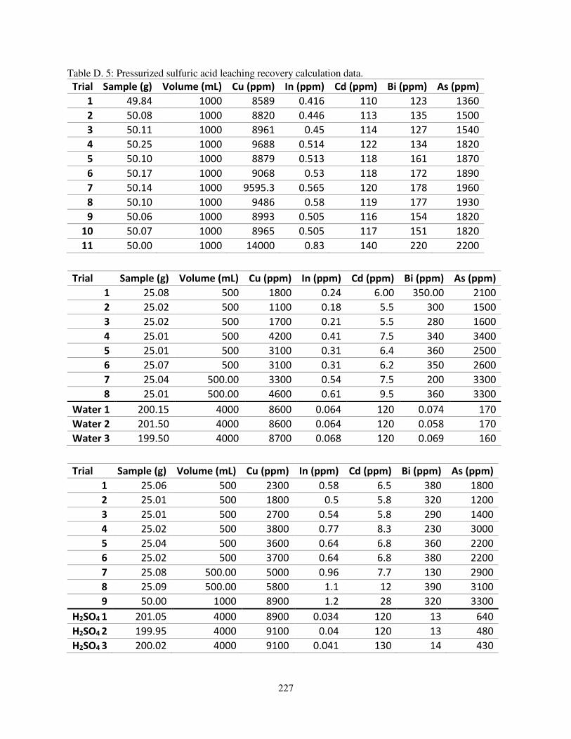
227

Table D. 5: Pressurized sulfuric acid leaching recovery calculation data.


1 49.84 1000 8589 0.416 110 123 1360

2 50.08 1000 8820 0.446 113 135 1500

3 50.11 1000 8961 0.45 114 127 1540

4 50.25 1000 9688 0.514 122 134 1820

5 50.10 1000 8879 0.513 118 161 1870

6 50.17 1000 9068 0.53 118 172 1890

7 50.14 1000 9595.3 0.565 120 178 1960

8 50.10 1000 9486 0.58 119 177 1930

9 50.06 1000 8993 0.505 116 154 1820

10 50.07 1000 8965 0.505 117 151 1820

11 50.00 1000 14000 0.83 140 220 2200


1 25.08 500 1800 0.24 6.00 350.00 2100

2 25.02 500 1100 0.18 5.5 300 1500

3 25.02 500 1700 0.21 5.5 280 1600

4 25.01 500 4200 0.41 7.5 340 3400

5 25.01 500 3100 0.31 6.4 360 2500

6 25.07 500 3100 0.31 6.2 350 2600

7 25.04 500.00 3300 0.54 7.5 200 3300

8 25.01 500.00 4600 0.61 9.5 360 3300

Water 1 200.15 4000 8600 0.064 120 0.074 170

Water 2 201.50 4000 8600 0.064 120 0.058 170

Water 3 199.50 4000 8700 0.068 120 0.069 160


1 25.06 500 2300 0.58 6.5 380 1800

2 25.01 500 1800 0.5 5.8 320 1200

3 25.01 500 2700 0.54 5.8 290 1400

4 25.02 500 3800 0.77 8.3 230 3000

5 25.04 500 3600 0.64 6.8 360 2200

6 25.02 500 3700 0.64 6.8 380 2200

7 25.08 500.00 5000 0.96 7.7 130 2900

8 25.09 500.00 5800 1.1 12 390 3100

9 50.00 1000 8900 1.2 28 320 3300

H2SO4 1 201.05 4000 8900 0.034 120 13 640

H2SO4 2 199.95 4000 9100 0.04 120 13 480

H2SO4 3 200.02 4000 9100 0.041 130 14 430

228

Appendix E: Permissions for Reuse

separation of indium and other metal values in flash smelter

Documents