The University of Chicago

Separating Intrinsic and Environmental Contributions to Growth and Their PopulationConsequences.Author(s): Andrew O. Shelton, William H. Satterthwaite, Michael P. Beakes, Stephan B. Munch,Susan M. Sogard, and Marc MangelSource: The American Naturalist, Vol. 181, No. 6 (June 2013), pp. 799-814Published by: The University of Chicago Press for The American Society of NaturalistsStable URL: http://www.jstor.org/stable/10.1086/670198 .

Accessed: 14/05/2013 12:46

Your use of the JSTOR archive indicates your acceptance of the Terms & Conditions of Use, available at .http://www.jstor.org/page/info/about/policies/terms.jsp

.JSTOR is a not-for-profit service that helps scholars, researchers, and students discover, use, and build upon a wide range ofcontent in a trusted digital archive. We use information technology and tools to increase productivity and facilitate new formsof scholarship. For more information about JSTOR, please contact support@jstor.org.

.

The University of Chicago Press, The American Society of Naturalists, The University of Chicago arecollaborating with JSTOR to digitize, preserve and extend access to The American Naturalist.

http://www.jstor.org

This content downloaded from 161.55.228.44 on Tue, 14 May 2013 12:46:17 PMAll use subject to JSTOR Terms and Conditions

vol. 181, no. 6 the american naturalist june 2013

Separating Intrinsic and Environmental Contributions to

Growth and Their Population Consequences

Andrew O. Shelton,1,2,* William H. Satterthwaite,2,3 Michael P. Beakes,4 Stephan B. Munch,3

Susan M. Sogard,3 and Marc Mangel2,5

1. Conservation Biology Division, Northwest Fisheries Science Center, National Marine Fisheries Service, National Oceanographic andAtmospheric Administration, Seattle, Washington 98112; 2. Center for Stock Assessment Research, University of California, Santa Cruz,Santa Cruz, California 95064; 3. Fisheries Ecology Division, Southwest Fisheries Science Center, National Marine Fisheries Service,National Oceanographic and Atmospheric Administration, Santa Cruz, California 95060; 4. Earth to Oceans Research Group, SimonFraser University, 8888 University Drive, Burnaby, British Columbia V5A 1S6, Canada; 5. Department of Applied Mathematics andStatistics, Jack Baskin School of Engineering, University of California, Santa Cruz, Santa Cruz, California 95064; and Department ofBiology, University of Bergen, Bergen, Norway NO-5020

Submitted July 18, 2012; Accepted November 9, 2012; Electronically published April 15, 2013

Online enhancement: appendix, zip file. Dryad data: http://dx.doi.org/10.5061/dryad.cj36j.

abstract: Among-individual heterogeneity in growth is a com-monly observed phenomenon that has clear consequences for pop-ulation and community dynamics yet has proved difficult to quantifyin practice. In particular, observed among-individual variation ingrowth can be difficult to link to any given mechanism. Here, wedevelop a Bayesian state-space framework for modeling growth thatbridges the complexity of bioenergetic models and the statisticalsimplicity of phenomenological growth models. The model allowsfor intrinsic individual variation in traits, a shared environment,process stochasticity, and measurement error. We apply the modelto two populations of steelhead trout (Oncorhynchus mykiss) grownunder common but temporally varying food conditions. Models al-lowing for individual variation match available data better than mod-els that assume a single shared trait for all individuals. Estimatedindividual variation translated into a roughly twofold range in re-alized growth rates within populations. Comparisons between pop-ulations showed strong differences in trait means, trait variability,and responses to a shared environment. Together, individual- andpopulation-level variation have substantial implications for variationin size and growth rates among and within populations. State-dependent life-history models predict that this variation can lead todifferences in individual life-history expression, lifetime reproductiveoutput, and population life-history diversity.

Keywords: individual heterogeneity, von Bertalanffy, bioenergetics,Bayesian state space, Oncorhynchus mykiss.

Introduction

The expression of among-individual variation results froma complex interaction among genetic variation, phenotypic

* Corresponding author; e-mail: ole.shelton@noaa.gov.

Am. Nat. 2013. Vol. 181, pp. 799–814. � 2013 by The University of Chicago.

0003-0147/2013/18106-53990$15.00. All rights reserved.

DOI: 10.1086/670198

plasticity, population structure, and environmental con-ditions. An important goal of both ecology and evolu-tionary biology is documenting the presence of individualvariation, the mechanisms underlying its maintenance,and its consequences for populations and communities.Both theory and empirical results suggest that the presenceof persistent individual variation can have significant con-sequences for populations (Pfister and Stevens 2003; Vin-denes et al. 2008; Zuidema et al. 2009; Kendall et al. 2011)as well as for communities (Bolnick et al. 2011). Fur-thermore, individual physiology and behavior mediate re-sponses to environmental change (whether natural or an-thropogenic). Thus, an understanding of individualheterogeneity is important for predicting the persistenceof populations in the face of environmental change.

Somatic growth is an important but variable componentof life histories. Persistent individual differences in growthare well documented for a range of taxa (plants: Harper1977; Clark et al. 2007; mammals: Tinker et al. 2008; algaeand invertebrates: Pfister and Stevens 2002). Because sur-vival, maturity, reproductive success, and other vital ratesare frequently related to an individual’s size, variation insomatic growth has implications for both individual fitnessand population dynamics (Kendall and Fox 2002). Thelink between size and vital rates has motivated the wide-spread use of structured population models (e.g., matrixmodels; Caswell 2001), but these models generally assumethat individuals of a given size or state are equivalent (butsee Parma and Deriso 1990; Pfister and Wang 2005; Coul-son et al. 2006; Kendall et al. 2011; Jansen et al. 2012).Thus, the implications for incorporating individual vari-ation in growth for population processes are largely unex-plored (Pfister and Stevens 2003).

This content downloaded from 161.55.228.44 on Tue, 14 May 2013 12:46:17 PMAll use subject to JSTOR Terms and Conditions

800 The American Naturalist

Among-individual variation in somatic growth can arisefrom a variety of processes. For example, individualswithin a population can vary in metabolic rates (von Ber-talanffy 1938, 1957; Beverton and Holt 1959; Metcalfe etal. 1995) or behavioral traits (e.g., aggressiveness or ter-ritoriality; Magnuson 1962; Biro and Stamps 2010). Re-alized growth for an individual arises as a function of (1)an individual’s phenotypic traits, (2) the environmentalconditions shared by the entire population, and (3) sto-chasticity (Kruuk 2004). Stochasticity encompasses a rangeof unmeasured random processes affecting individualgrowth that could include (1) fluctuations in food capturedby an individual, (2) variable responses to fluctuations intemperature, or (3) factors not directly linked to growth(e.g., predation avoidance). Methods that seek to docu-ment and understand individual variation must accountfor these distinct factors. This goal has proven elusive inpractice (e.g., Knape et al. 2011).

There is a well-developed and sophisticated body oftheory describing the physiology of growth (Kitchell 1977;Kooijman 2000), but often it is difficult to match thistheory to available data and to estimate all the parametersfrom size trajectories alone (Fujiwara et al. 2005); thereare usually too many free parameters and unobservedstates to be estimable from available data. At the otherextreme, there are growth models for which parametersare easy to estimate (e.g., von Bertalanffy growth) but thatdescribe patterns in growth that may be difficult to linkto underlying biological mechanisms. Thus, an unsolvedquestion is how to represent individual variation efficientlyin growth models. Recent analyses suggest that althoughindividuals may vary across a wide suite of traits, geneticcorrelations among traits constrain the effective numberof traits to a much smaller number (Kirkpatrick 2009).This observation motivates the development of low-dimensional summaries of among-individual variationthat can be potentially connected to evolutionary models.

Here, we develop and apply a parametric Bayesian state-space framework for jointly estimating among-individual,environmental, and stochastic variation from observed timeseries. We strike a compromise between the simple but diffi-cult-to-interpret growth models and the biologically so-phisticated but statistically unidentifiable full bioenergeticmodels. We then describe a rearing experiment conductedwith two California steelhead (Oncorhyncus mykiss) popu-lations under common conditions and apply our statisticalmethods to estimate parameters for each population. Wecompare patterns of among-individual and between-pop-ulation variation. We then use a state-dependent model ofsteelhead life history developed by Satterthwaite et al. (2009)to predict the optimal life-history strategies and expectedlifetime output associated with projected growth trajectories.This allows us to quantify the predicted effect of individual

growth rate variability and stochasticity on the diversity oflife-history pathways observed in populations. Furthermore,it provides a method for understanding the fitness conse-quences of individual variation under a range of environ-mental conditions.

Methods

Growth Model

We use as our starting point a general model of somaticgrowth, where the rate of growth of an individual of lengthx is

dxp q � kx. (1)

dt

Equation (1) is known as the specialized von Bertalanffygrowth function (VBGF; von Bertalanffy 1957; Pauly 1981;Essington et al. 2001). Biologically, the parameter q containsprocesses contributing to energetic gains (anabolism; e.g.,consumption rates linked to the quality of the environ-ment), while the parameter k represents processes pertainingto energetic costs (catabolism; e.g., metabolic rates and as-sociated behavioral traits). The VBGF arises from bioener-getic principles and is based on specific but reasonable as-sumptions about how growth rate scales with individual size(Essington et al. 2001; Mangel 2006). Descriptions of thederivation of the VBGF from bioenergetic principles andadditional assumptions of the VBGF can be found elsewhere(e.g., von Bertalanffy 1938, 1957; Beverton and Holt 1959;Essington et al. 2001; Mangel 2006), and we refer readersto those references for a complete discussion.

Equation (1) describes the growth process of an indi-vidual. However, almost all applications of the VBGF in-volve fitting an integrated form of equation (1) to pop-ulation-level data and interpreting estimated parametersas the values for an average individual in the population.As noted by many investigators (Sainsbury 1980; Wang1998; Eveson et al. 2007), this interpretation is valid onlyif there is no heterogeneity among individuals; estimatingparameters by ignoring individual variation will yield bi-ased parameter estimates. Thus, two key questions are Isthere biological evidence of among-individual variation,and How can we estimate its magnitude in the face of avariable environment and stochastic variation?

We develop a general model derived from equation (1)and apply it to steelhead trout. While we motivate andframe our analysis in the context of salmonid fish, ourapproach is applicable to a wide range of species. Forsalmonids, detailed studies of physiology show individualvariation in physiological rates (Paszkowski and Olla 1985;Metcalfe et al. 1995; Gilmour et al. 2005; Burton et al.2011) that can drive differences in activity, determine be-havioral dominance hierarchies, and result in variation in

This content downloaded from 161.55.228.44 on Tue, 14 May 2013 12:46:17 PMAll use subject to JSTOR Terms and Conditions

Individual Variation in Growth 801

growth (Martin-Smith and Armstrong 2002; Morinvilleand Rasmussen 2003). However, the link between indi-vidual variation in traits and realized growth in a tem-porally variable environment is largely undescribed(Burton et al. 2011). We integrate equation (1) to obtain

qi�k �ki i( )x (t) p x (t � 1)e � 1 � e , (2)i i k i

and we include the subscript i to make explicit that theparameters are tied to individuals.

Thus, we assume that there is fixed individual variationin the gain and cost parameters. Because qi is related to theamount of resources available to an individual, it is relatedto both the shared environment and the behavioral traitsof that individual. The relationship between physiology, theenvironment, and growth reflects complicated trade-offsthat vary as a result of differences in behavior and life his-tory. We adopt a flexible form for relating qi and ki proposedby Snover et al. (2005, 2006). We let gt denote the sharedenvironment at time t and w be a parameter that determinesthe degree to which q depends on environmental versusmetabolic and behavioral factors; then

wq p gk , (3)i, t t i

and qi, t represents the growth conditions for an individual,given its traits and a shared environment at time t. Notethat w is a population-level parameter; all individuals areassumed to have a shared link between behavior and theenvironment. Snover et al. (2005) explain why 0 ≤ w ≤

. If , then ki and qi are independent, and individual1 w p 0activity has no effect on an individual’s success at obtainingresources from the environment. Therefore, when w p

, individuals with high ki have slower growth. At the other0extreme, , individuals with high ki always have in-w p 1creased access to resources and therefore experience fasterlength-specific growth. For intermediate values of w, therelative growth rate for individuals with different ki willchange with an individual’s length. For , the0 ! w ! 1value of k that has the highest growth rate at a given lengthdepends on the shared environment, gt (fig. A1, availableonline). Thus, this model can qualitatively match the em-pirical observation that the relative success of individualswith different traits varies with the quality of the envi-ronment (Alvarez and Nicieza 2005; Burton et al. 2011).

Combining equations (2) and (3) gives

�k w�1 �ki ix (t � 1) p x (t)e � gk (1 � e ), (4)i i t i

and after n intervals (nominally days), the length of anindividual is

n�1

�k n w�1 �k �k ji i ix (t � n) p x (t)e � k (1 � e ) g e . (5)�i i i t�jjp0

Equation (5) is a deterministic model for individual

growth in a time-varying environment. We also expectstochastic processes to contribute to growth. To accountfor stochasticity, we assume that the environment the in-dividual experiences is a random variable, , and can begt

approximated by a normal density, . Note2g ∼ N(g , j )t t

that gt can, in theory, take on negative values and producenegative growth (shrinking). In this stochastic framework,length is a random variable (denoted by capital letters;Xi(t)) and individuals are measured with error, so we letYi(t) denote observed length. If the interval between ob-servations is nw (for intervals) and thew p 1, 2, … , Wmean environment between measurement intervals can beapproximated by a single constant, gw, then the full time-series model that incorporates process stochasticity andmeasurement error is

�k ni wX (t) p x (t � n )ei i w

n �1w

w�1 �k �k ji i� k (1 � e )g e � z , (6a)�i w tjp0

where

n �1w

2 w�1 �k 2 �2k ji iz ∼ N 0, j [k (1 � e )] e ,�t i( )jp0

and

Y (t) p X (t) � z , (6b)i i obs

where (also see the appendix, available on-2z ∼ N(0, t )obs

line). Equations (6a) and (6b) constitute an individual time-series model where fixed individual traits, a shared envi-ronment, and stochastic variation are all incorporated(Prado and West 2010). Note that both the expected valueand the variance of an individual’s length depend on anindividual’s trait, ki. This model matches the structure ofmany data sets where uniquely marked individuals livingin a shared but variable environment are observed repeat-edly over time.

We note that this is far from the only possible model thatcould be derived and that a variety of alternative structuresfor modeling growth are reasonable. For example, variousapproaches with stochastic differential equations have beendeveloped (e.g., Fujiwara et al. 2005; Gudmundsson 2005;Lv and Pitchford 2007). The model presented here has dis-tinct advantages for parameter estimation (see below). Inthe sections that follow, we describe a rearing experimenton steelhead trout and then apply our model to estimateparameters from the steelhead data.

Study Species and Rearing Experiment

We apply the time-series model to a rearing experimenton California steelhead (Oncorhynchus mykiss; see Beakes

This content downloaded from 161.55.228.44 on Tue, 14 May 2013 12:46:17 PMAll use subject to JSTOR Terms and Conditions

802 The American Naturalist

et al. 2010 and the appendix for the details of the exper-iment). Age-0 steelhead from two populations were raisedin aquarium tanks at the National Marine Fisheries ServiceLaboratory in Santa Cruz, California. The first populationderives from a conservation hatchery on a small coastalstream, Scott Creek (denoted CCC, for central Californiacoast). The CCC population derives from a lineage of pre-dominantly wild fish (Hayes et al. 2004). The second stockcomes from a production hatchery, Coleman National FishHatchery, on Battle Creek, a tributary to the SacramentoRiver (denoted NCCV, for northern California CentralValley). Steelhead broodstock for Coleman hatchery derivepredominantly from hatchery origin (Campton et al. 2004;USFWS 2011). Thus, while the populations derive fromdistinct rivers in different parts of California, the contrastbetween the CCC and NCCV populations also incorpo-rates a comparison between fish of predominantly wildand predominantly hatchery backgrounds.

Fish were grown in cylindrical tanks (490 L), with 20fish per tank and eight tanks of each stock (initial length∼40 mm), and raised on a diet supporting moderate butrestricted growth, except for a period in which an ad lib.ration was available (hereafter “low” and “high” rations,respectively). Tanks were assigned to one of four feedingtreatments, with two replicate tanks per treatment. In July,all tanks were placed on low rations distributed four daysa week. The fish were kept on low rations, except duringthe treatment period, when one of the four treatmentgroups received eight continuous weeks of high rationsdaily (see fig. 1). Thus, all treatment groups received iden-tical amounts of time at each ration level and experiencedequivalent cumulative food per unit body mass over thecourse of the year, although the timing of food availabilityvaried. The length of each individual was observed ap-proximately every 4 weeks for a 10-month period. Weincluded 100 CCC and 138 NCCV individuals in our anal-ysis (see appendix).

Parameter Estimation

We were interested in estimating the joint posterior dis-tribution of the parameters and unobserved, latent statesfor each individual (the length of individuals at each dayof interest) by using Bayesian hierarchical methods (Cres-sie and Wikle 2011; appendix). We estimated parametersfor each population independently, but within populationswe estimated parameters for individuals in all treatmentssimultaneously. We estimated three shared environmentalstates for each population: gS, gL, and gH, correspondingto the first month of the experiment and the low- andhigh-ration treatments, respectively. We used a separateparameter for the first month because introducing fish intoa novel environment should affect growth in addition to

the ration treatment. We estimated the length of each in-dividual on each day it was measured and on the dayswhen feeding treatments were changed (17 and 18 daysfor CCC and NCCV, respectively). We initially investigatedthe potential for tank-specific blocking effects, but therewere no evident differences between tanks within a treat-ment, so we combined tanks into one analysis (fig. A4,available online). We did not attempt to estimate the mea-surement error but treated t2 as fixed (see below).

Preliminary analyses showed that w and the g’s wereonly weakly identifiable. To improve estimation, we per-formed all of our analyses conditioned on values of w. Weestimated parameters for a range of values of w (from 0.1to 1.0, in increments of 0.1) to investigate the effects ofchanging the relationship between individual traits and theenvironment. Models with (the classic von Ber-w p 0talanffy model) failed to converge in most cases; we donot discuss further.w p 0

We considered two model structures for individual var-iation in k. In the first, we estimated a single, shared k forall individuals, so for this model we estimated {k, gS, gL,gH, j2} (hereafter the single-k model). In the second, weestimated a ki for each individual and assumed that thesimilarity among individuals in a population was hierar-chical (hereafter the hierarchical-k model); we modeledeach ki as a random sample from a shared normal distri-bution, , where mk and are the mean and2 2k ∼ N(m , r ) rk k k

variance of k, respectively. Thus, for I individuals we es-timated {k1, k2, ..., kI, mk, , gS, gL, gH, j2}. For all param-2rk

eters we used diffuse prior distributions (summarized intable A1, available online).

Incorporating measurement error is an important con-sideration in ecological models (Clark 2007). Steelheadmeasurements of length were relatively precise, but noempirical estimates of measurement error were made dur-ing the experiment (Beakes et al. 2010). Therefore, wefitted models assuming two values of measurement error( or 4 mm2) to understand the consequences of2t p 1including measurement error for other parameters.

We estimated the posterior distribution of parametersand latent states by using a mix of Gibbs and MetropolisMarkov chain Monte Carlo (MCMC) algorithms to sampleparameters (Gelman et al. 2004) and used standard tech-niques to assess model convergence and diagnostics (seethe appendix). All results represent 4,500 samples fromthe posterior distribution. We performed all analyses in R(ver. 2.13.1; R Development Core Team 2011).

To compare the single-k and hierarchical-k models, weused posterior predictive loss (Gelfand and Ghosh 1998;Clark and Bjørnstad 2004). Predictive loss identifies themodel, m, that provides a balance between a goodness-of-fit term, Gm, and model complexity term, Pm. The preferred

This content downloaded from 161.55.228.44 on Tue, 14 May 2013 12:46:17 PMAll use subject to JSTOR Terms and Conditions

Individual Variation in Growth 803

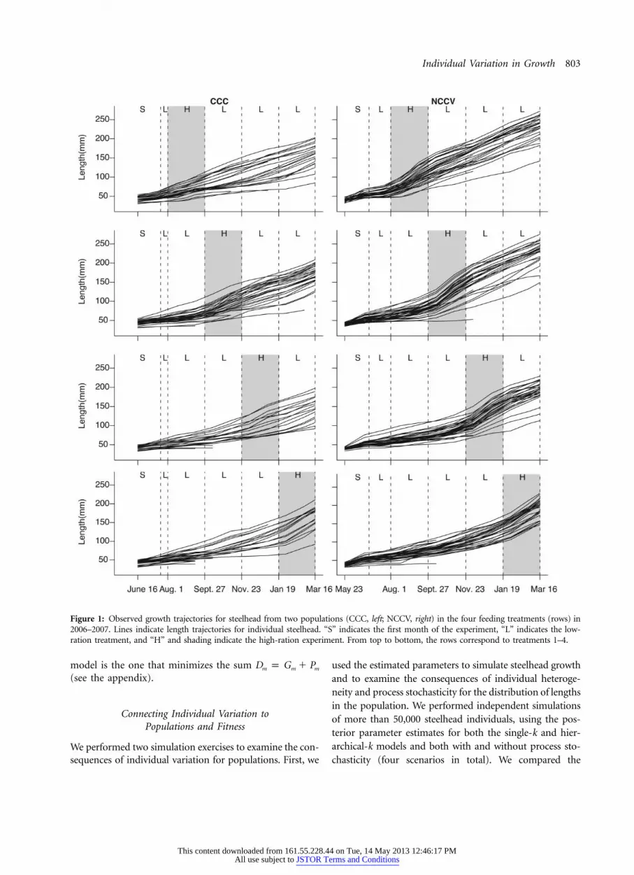
Figure 1: Observed growth trajectories for steelhead from two populations (CCC, left; NCCV, right) in the four feeding treatments (rows) in2006–2007. Lines indicate length trajectories for individual steelhead. “S” indicates the first month of the experiment, “L” indicates the low-ration treatment, and “H” and shading indicate the high-ration experiment. From top to bottom, the rows correspond to treatments 1–4.

model is the one that minimizes the sum D p G � Pm m m

(see the appendix).

Connecting Individual Variation toPopulations and Fitness

We performed two simulation exercises to examine the con-sequences of individual variation for populations. First, we

used the estimated parameters to simulate steelhead growthand to examine the consequences of individual heteroge-neity and process stochasticity for the distribution of lengthsin the population. We performed independent simulationsof more than 50,000 steelhead individuals, using the pos-terior parameter estimates for both the single-k and hier-archical-k models and both with and without process sto-chasticity (four scenarios in total). We compared the

This content downloaded from 161.55.228.44 on Tue, 14 May 2013 12:46:17 PMAll use subject to JSTOR Terms and Conditions

804 The American Naturalist

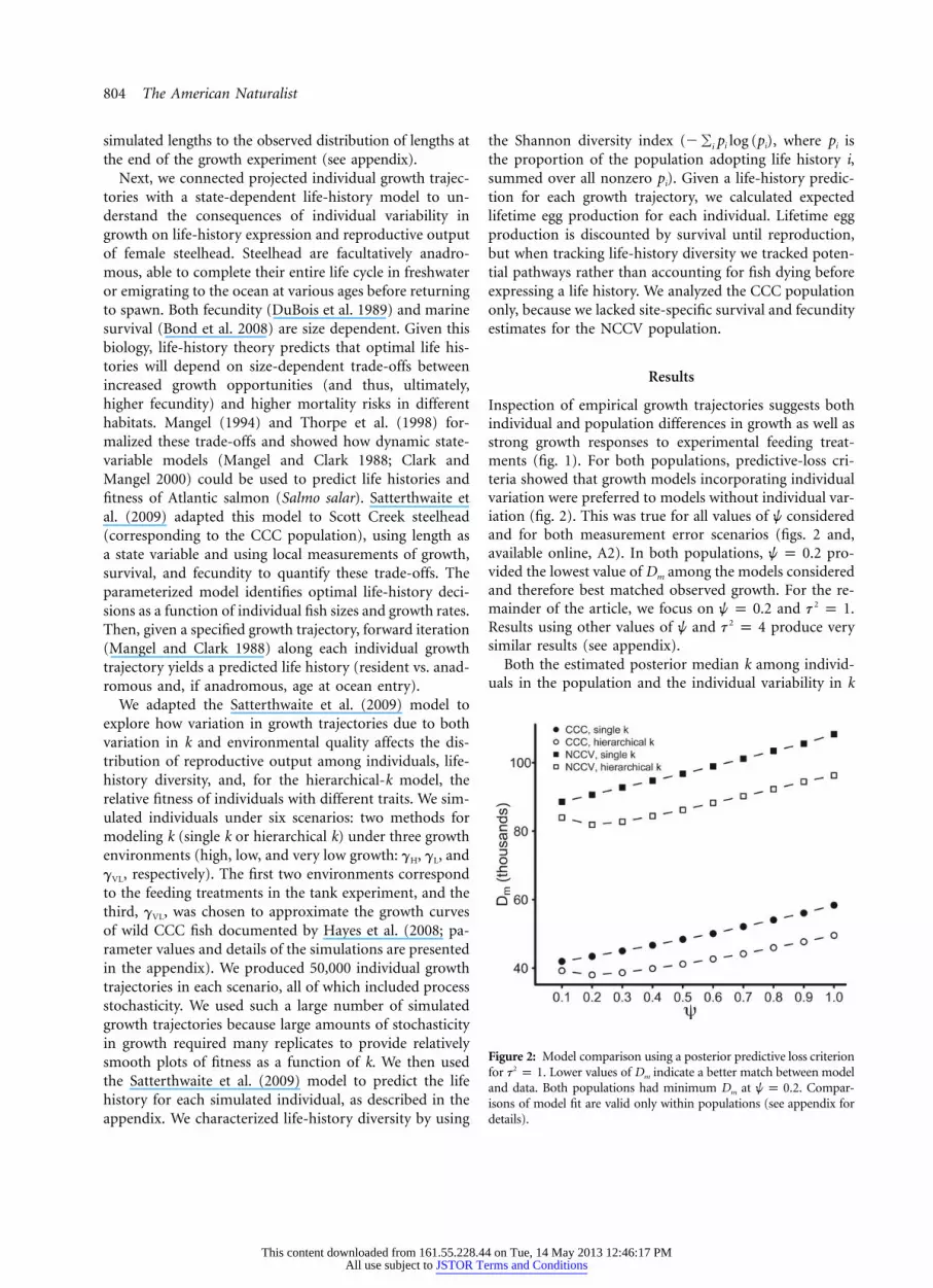
Figure 2: Model comparison using a posterior predictive loss criterionfor . Lower values of Dm indicate a better match between model2t p 1and data. Both populations had minimum Dm at . Compar-w p 0.2isons of model fit are valid only within populations (see appendix fordetails).

simulated lengths to the observed distribution of lengths atthe end of the growth experiment (see appendix).

Next, we connected projected individual growth trajec-tories with a state-dependent life-history model to un-derstand the consequences of individual variability ingrowth on life-history expression and reproductive outputof female steelhead. Steelhead are facultatively anadro-mous, able to complete their entire life cycle in freshwateror emigrating to the ocean at various ages before returningto spawn. Both fecundity (DuBois et al. 1989) and marinesurvival (Bond et al. 2008) are size dependent. Given thisbiology, life-history theory predicts that optimal life his-tories will depend on size-dependent trade-offs betweenincreased growth opportunities (and thus, ultimately,higher fecundity) and higher mortality risks in differenthabitats. Mangel (1994) and Thorpe et al. (1998) for-malized these trade-offs and showed how dynamic state-variable models (Mangel and Clark 1988; Clark andMangel 2000) could be used to predict life histories andfitness of Atlantic salmon (Salmo salar). Satterthwaite etal. (2009) adapted this model to Scott Creek steelhead(corresponding to the CCC population), using length asa state variable and using local measurements of growth,survival, and fecundity to quantify these trade-offs. Theparameterized model identifies optimal life-history deci-sions as a function of individual fish sizes and growth rates.Then, given a specified growth trajectory, forward iteration(Mangel and Clark 1988) along each individual growthtrajectory yields a predicted life history (resident vs. anad-romous and, if anadromous, age at ocean entry).

We adapted the Satterthwaite et al. (2009) model toexplore how variation in growth trajectories due to bothvariation in k and environmental quality affects the dis-tribution of reproductive output among individuals, life-history diversity, and, for the hierarchical-k model, therelative fitness of individuals with different traits. We sim-ulated individuals under six scenarios: two methods formodeling k (single k or hierarchical k) under three growthenvironments (high, low, and very low growth: gH, gL, andgVL, respectively). The first two environments correspondto the feeding treatments in the tank experiment, and thethird, gVL, was chosen to approximate the growth curvesof wild CCC fish documented by Hayes et al. (2008; pa-rameter values and details of the simulations are presentedin the appendix). We produced 50,000 individual growthtrajectories in each scenario, all of which included processstochasticity. We used such a large number of simulatedgrowth trajectories because large amounts of stochasticityin growth required many replicates to provide relativelysmooth plots of fitness as a function of k. We then usedthe Satterthwaite et al. (2009) model to predict the lifehistory for each simulated individual, as described in theappendix. We characterized life-history diversity by using

the Shannon diversity index ( , where pi is�� p log (p )i ii

the proportion of the population adopting life history i,summed over all nonzero pi). Given a life-history predic-tion for each growth trajectory, we calculated expectedlifetime egg production for each individual. Lifetime eggproduction is discounted by survival until reproduction,but when tracking life-history diversity we tracked poten-tial pathways rather than accounting for fish dying beforeexpressing a life history. We analyzed the CCC populationonly, because we lacked site-specific survival and fecundityestimates for the NCCV population.

Results

Inspection of empirical growth trajectories suggests bothindividual and population differences in growth as well asstrong growth responses to experimental feeding treat-ments (fig. 1). For both populations, predictive-loss cri-teria showed that growth models incorporating individualvariation were preferred to models without individual var-iation (fig. 2). This was true for all values of w consideredand for both measurement error scenarios (figs. 2 and,available online, A2). In both populations, pro-w p 0.2vided the lowest value of Dm among the models consideredand therefore best matched observed growth. For the re-mainder of the article, we focus on and .2w p 0.2 t p 1Results using other values of w and produce very2t p 4similar results (see appendix).

Both the estimated posterior median k among individ-uals in the population and the individual variability in k

This content downloaded from 161.55.228.44 on Tue, 14 May 2013 12:46:17 PMAll use subject to JSTOR Terms and Conditions

Individual Variation in Growth 805

0

0.00

02

0.00

04

0.00

06

0

5

10

15

20

25

30

Freq

uenc

y

CCC

k

0

0.00

01

0.00

02

0.00

03

0

5

10

15

20

25

30

35

k

NCCV

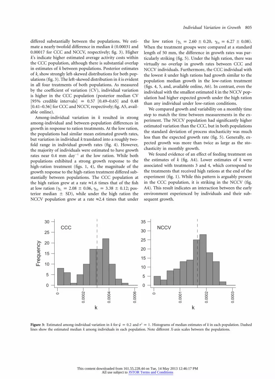
Figure 3: Estimated among-individual variation in k for and . Histograms of median estimates of k in each population. Dashed2w p 0.2 t p 1lines show the estimated median k among individuals in each population. Note different X-axis scales between the populations.

differed substantially between the populations. We esti-mate a nearly twofold difference in median k (0.00031 and0.00017 for CCC and NCCV, respectively; fig. 3). Higherk’s indicate higher estimated average activity costs withinthe CCC population, although there is substantial overlapin estimates of k between populations. Posterior estimatesof ki show strongly left-skewed distributions for both pop-ulations (fig. 3). The left-skewed distribution in k is evidentin all four treatments of both populations. As measuredby the coefficient of variation (CV), individual variationis higher in the CCC population (posterior median CV[95% credible intervals] p 0.57 [0.49–0.65] and 0.48[0.41–0.56] for CCC and NCCV, respectively; fig. A5, avail-able online).

Among-individual variation in k resulted in strongamong-individual and between-population differences ingrowth in response to ration treatments. At the low ration,the populations had similar mean estimated growth rates,but variation in individual k translated into a roughly two-fold range in individual growth rates (fig. 4). However,the majority of individuals were estimated to have growthrates near 0.4 mm day�1 at the low ration. While bothpopulations exhibited a strong growth response to thehigh-ration treatment (figs. 1, 4), the magnitude of thegrowth response to the high-ration treatment differed sub-stantially between populations. The CCC population atthe high ration grew at a rate ≈1.6 times that of the fishat low ration ( , ; pos-g p 2.08 � 0.06 g p 3.38 � 0.12L H

terior median � SD), while under the high ration theNCCV population grew at a rate ≈2.4 times that under

the low ration ( , ).g p 2.60 � 0.20 g p 6.27 � 0.08L H

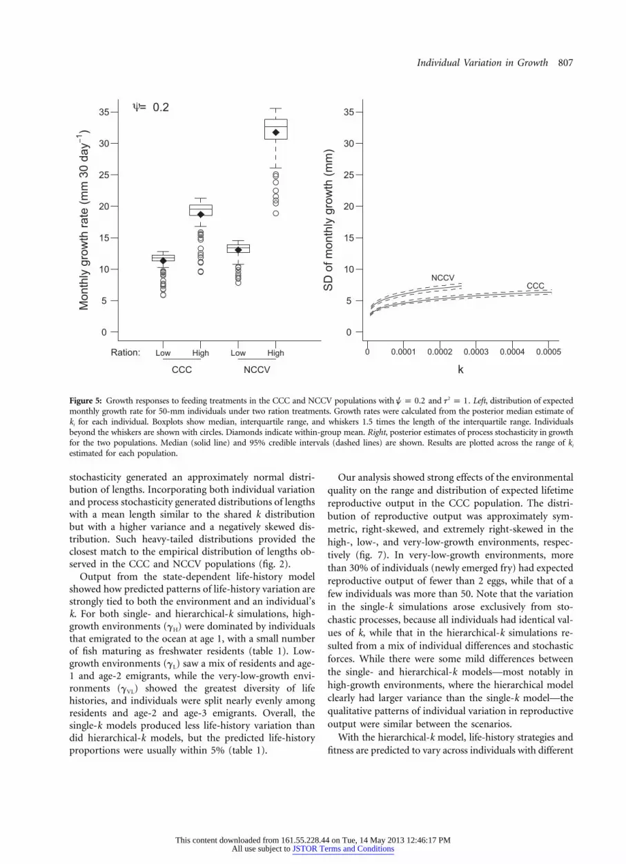
When the treatment groups were compared at a standardlength of 50 mm, the difference in growth rates was par-ticularly striking (fig. 5). Under the high ration, there wasvirtually no overlap in growth rates between CCC andNCCV individuals. Furthermore, the CCC individual withthe lowest k under high rations had growth similar to thepopulation median growth in the low-ration treatment(figs. 4, 5, and, available online, A6). In contrast, even theindividual with the smallest estimated k in the NCCV pop-ulation had higher expected growth under the high rationthan any individual under low-ration conditions.

We compared growth and variability on a monthly timestep to match the time between measurements in the ex-periment. The NCCV population had significantly higherestimated variation than the CCC, but in both populationsthe standard deviation of process stochasticity was muchless than the expected growth rate (fig. 5). Generally, ex-pected growth was more than twice as large as the sto-chasticity in monthly growth.

We found evidence of an effect of feeding treatment onthe estimates of k (fig. A4). Lower estimates of k wereassociated with treatments 3 and 4, which correspond tothe treatments that received high rations at the end of theexperiment (fig. 1). While this pattern is arguably presentin the CCC population, it is striking in the NCCV (fig.A4). This result indicates an interaction between the earlyenvironment experienced by individuals and their sub-sequent growth.

This content downloaded from 161.55.228.44 on Tue, 14 May 2013 12:46:17 PMAll use subject to JSTOR Terms and Conditions

806 The American Naturalist

50 100 150 200 250

0.0

0.2

0.4

0.6

0.8

1.0

1.2

Dai

ly g

row

th ra

te (m

m d

ay1 )

CCC: Low Ration

50 100 150 200 250

CCC: High Ration

50 100 150 200 250

0.0

0.2

0.4

0.6

0.8

1.0

1.2

Length (mm)

Dai

ly g

row

th ra

te (m

m d

ay1 )

NCCV: Low Ration

50 100 150 200 250Length (mm)

NCCV: High Ration

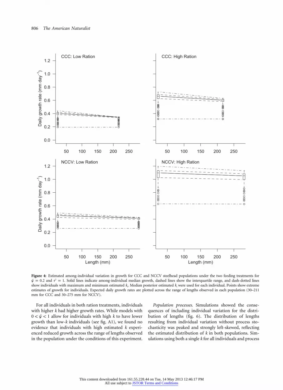
Figure 4: Estimated among-individual variation in growth for CCC and NCCV steelhead populations under the two feeding treatments forand . Solid lines indicate among-individual median growth, dashed lines show the interquartile range, and dash-dotted lines2w p 0.2 t p 1

show individuals with maximum and minimum estimated ki. Median posterior estimated ki were used for each individual. Points show extremeestimates of growth for individuals. Expected daily growth rates are plotted across the range of lengths observed in each population (30–211mm for CCC and 30–275 mm for NCCV).

For all individuals in both ration treatments, individualswith higher k had higher growth rates. While models with

allow for individuals with high k to have lower0 ! w ! 1growth than low-k individuals (see fig. A1), we found noevidence that individuals with high estimated k experi-enced reduced growth across the range of lengths observedin the population under the conditions of this experiment.

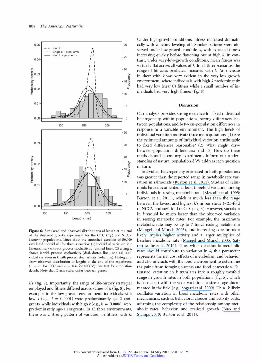
Population processes. Simulations showed the conse-quences of including individual variation for the distri-bution of lengths (fig. 6). The distribution of lengthsresulting from individual variation without process sto-chasticity was peaked and strongly left-skewed, reflectingthe estimated distribution of k in both populations. Sim-ulations using both a single k for all individuals and process

This content downloaded from 161.55.228.44 on Tue, 14 May 2013 12:46:17 PMAll use subject to JSTOR Terms and Conditions

Individual Variation in Growth 807

Low High Low High

CCC NCCV

Ration:

0

5

10

15

20

25

30

35

Mon

thly

gro

wth

rate

(mm

30

day

1 )

= 0.2

0 0.0001 0.0002 0.0003 0.0004 0.0005

0

5

10

15

20

25

30

35

NCCVCCC

k

SD

of m

onth

ly g

row

th (m

m)

Figure 5: Growth responses to feeding treatments in the CCC and NCCV populations with and . Left, distribution of expected2w p 0.2 t p 1monthly growth rate for 50-mm individuals under two ration treatments. Growth rates were calculated from the posterior median estimate ofki for each individual. Boxplots show median, interquartile range, and whiskers 1.5 times the length of the interquartile range. Individualsbeyond the whiskers are shown with circles. Diamonds indicate within-group mean. Right, posterior estimates of process stochasticity in growthfor the two populations. Median (solid line) and 95% credible intervals (dashed lines) are shown. Results are plotted across the range of ki

estimated for each population.

stochasticity generated an approximately normal distri-bution of lengths. Incorporating both individual variationand process stochasticity generated distributions of lengthswith a mean length similar to the shared k distributionbut with a higher variance and a negatively skewed dis-tribution. Such heavy-tailed distributions provided theclosest match to the empirical distribution of lengths ob-served in the CCC and NCCV populations (fig. 2).

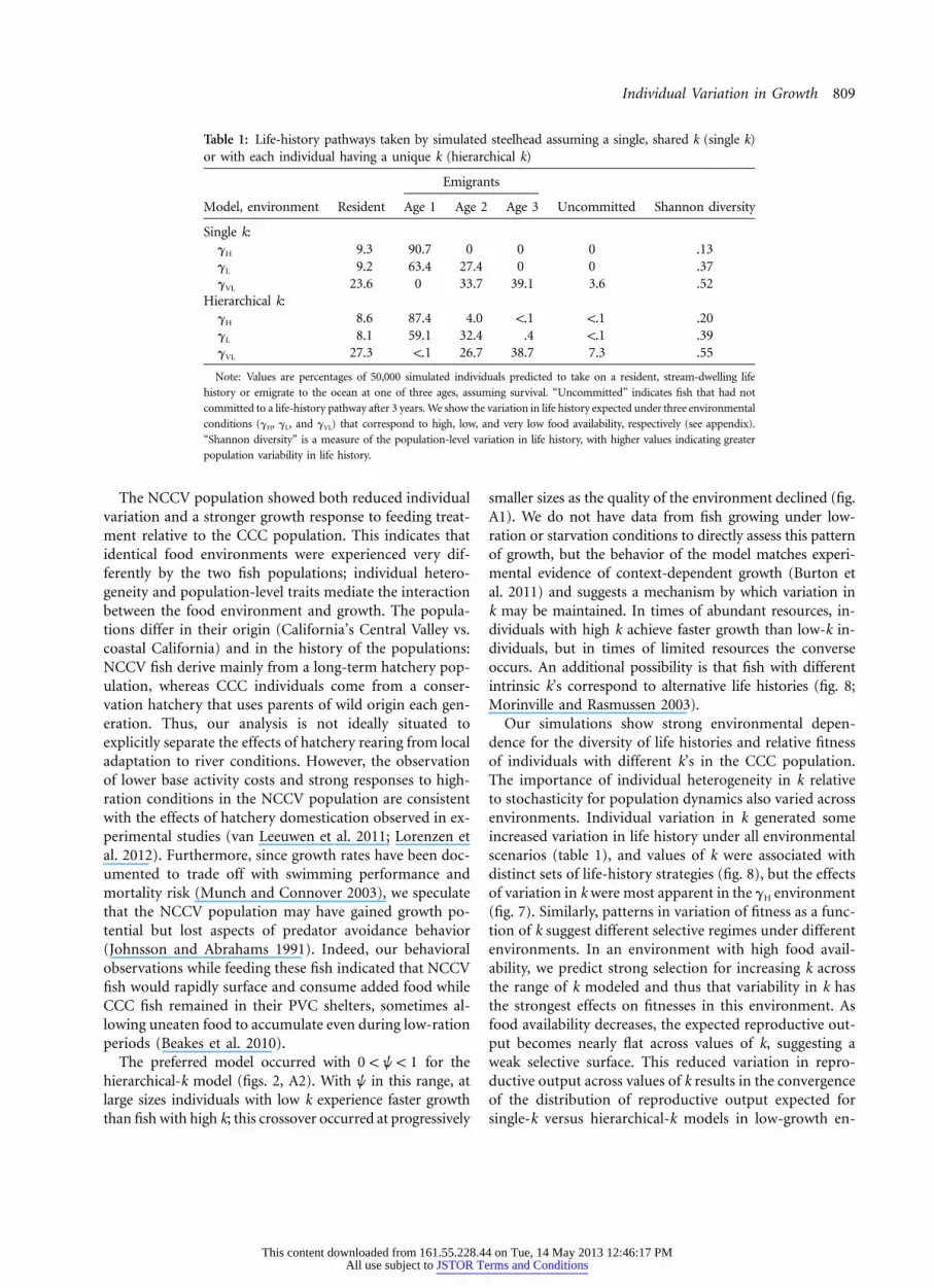
Output from the state-dependent life-history modelshowed how predicted patterns of life-history variation arestrongly tied to both the environment and an individual’sk. For both single- and hierarchical-k simulations, high-growth environments (gH) were dominated by individualsthat emigrated to the ocean at age 1, with a small numberof fish maturing as freshwater residents (table 1). Low-growth environments (gL) saw a mix of residents and age-1 and age-2 emigrants, while the very-low-growth envi-ronments (gVL) showed the greatest diversity of lifehistories, and individuals were split nearly evenly amongresidents and age-2 and age-3 emigrants. Overall, thesingle-k models produced less life-history variation thandid hierarchical-k models, but the predicted life-historyproportions were usually within 5% (table 1).

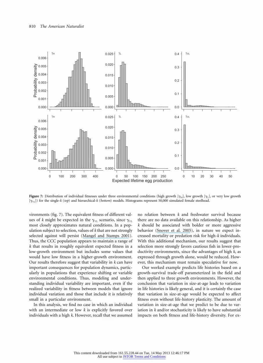
Our analysis showed strong effects of the environmentalquality on the range and distribution of expected lifetimereproductive output in the CCC population. The distri-bution of reproductive output was approximately sym-metric, right-skewed, and extremely right-skewed in thehigh-, low-, and very-low-growth environments, respec-tively (fig. 7). In very-low-growth environments, morethan 30% of individuals (newly emerged fry) had expectedreproductive output of fewer than 2 eggs, while that of afew individuals was more than 50. Note that the variationin the single-k simulations arose exclusively from sto-chastic processes, because all individuals had identical val-ues of k, while that in the hierarchical-k simulations re-sulted from a mix of individual differences and stochasticforces. While there were some mild differences betweenthe single- and hierarchical-k models—most notably inhigh-growth environments, where the hierarchical modelclearly had larger variance than the single-k model—thequalitative patterns of individual variation in reproductiveoutput were similar between the scenarios.

With the hierarchical-k model, life-history strategies andfitness are predicted to vary across individuals with different

This content downloaded from 161.55.228.44 on Tue, 14 May 2013 12:46:17 PMAll use subject to JSTOR Terms and Conditions

808 The American Naturalist

Figure 6: Simulated and observed distributions of length at the endof the steelhead growth experiment for the CCC (top) and NCCV(bottom) populations. Lines show the smoothed densities of 50,000simulated individuals for three scenarios: (1) individual variation in k(hierarchical) without process stochasticity (dashed line), (2) a single,shared k with process stochasticity (dash-dotted line), and (3) indi-vidual variation in k with process stochasticity (solid line). Histogramsshow observed distribution of lengths at the end of the experiment( for CCC and for NCCV). See text for simulationn p 75 n p 106details. Note that X-axis scales differ between panels.

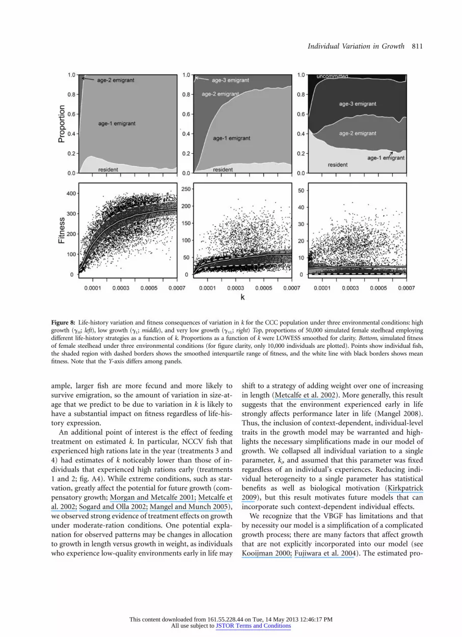
k’s (fig. 8). Importantly, the range of life-history strategiesemployed and fitness differed across values of k (fig. 8). Forexample, in the low-growth environment, individuals withlow k (e.g., ) were predominantly age-2 emi-k p 0.0001grants, while individuals with high k (e.g., ) werek p 0.0006predominantly age-1 emigrants. In all three environments,there was a strong pattern of variation in fitness with k.

Under high-growth conditions, fitness increased dramati-cally with k before leveling off. Similar patterns were ob-served under low-growth conditions, with expected fitnessincreasing quickly before flattening out at high k. In con-trast, under very-low-growth conditions, mean fitness wasvirtually flat across all values of k. In all three scenarios, therange of fitnesses predicted increased with k. An increasein skew with k was very evident in the very-low-growthenvironment, where individuals with high k predominantlyhad very low (near 0) fitness while a small number of in-dividuals had very high fitness (fig. 8).

Discussion

Our analysis provides strong evidence for fixed individualheterogeneity within populations, strong differences be-tween populations, and between-population differences inresponse to a variable environment. The high levels ofindividual variation motivate three main questions: (1) Arethe estimated amounts of individual variation attributableto fixed differences reasonable? (2) What might drivebetween-population differences? and (3) How do thesemethods and laboratory experiments inform our under-standing of natural populations? We address each questionin turn.

Individual heterogeneity estimated in both populationswas greater than the reported range in metabolic rate var-iation in salmonids (Burton et al. 2011). Studies of salm-onids have documented at least threefold variation amongindividuals in resting metabolic rate (Metcalfe et al. 1995;Burton et al. 2011), which is much less than the rangebetween the lowest and highest k’s in our study (≈25-foldin NCCV and ≈60-fold in CCC; fig. 3). However, variationin k should be much larger than the observed variationin resting metabolic rates. For example, the maximummetabolic rate may be up to 7 times resting metabolism(Mangel and Munch 2005), and increasing consumptionlikely implies higher activity and a larger multiplier ofbaseline metabolic rate (Mangel and Munch 2005; Sat-terthwaite et al. 2010). Thus, while variation in metabolicrates should contribute to variation in k, this parameterrepresents the net cost effects of metabolism and behaviorand also interacts with the food environment to determinethe gains from foraging success and food conversion. Es-timated variation in k translates into a roughly twofoldrange in growth rates in both populations (fig. 5), whichis consistent with the wide variation in size-at-age docu-mented in the field (e.g., Sogard et al. 2009). Thus, k likelyconflates variation in basal metabolic rates with othermechanisms, such as behavioral choices and activity costs,affirming the complexity of the relationship among met-abolic rates, behavior, and realized growth (Biro andStamps 2010; Burton et al. 2011).

This content downloaded from 161.55.228.44 on Tue, 14 May 2013 12:46:17 PMAll use subject to JSTOR Terms and Conditions

Individual Variation in Growth 809

Table 1: Life-history pathways taken by simulated steelhead assuming a single, shared k (single k)or with each individual having a unique k (hierarchical k)

Emigrants

Model, environment Resident Age 1 Age 2 Age 3 Uncommitted Shannon diversity

Single k:gH 9.3 90.7 0 0 0 .13gL 9.2 63.4 27.4 0 0 .37gVL 23.6 0 33.7 39.1 3.6 .52

Hierarchical k:gH 8.6 87.4 4.0 !.1 !.1 .20gL 8.1 59.1 32.4 .4 !.1 .39gVL 27.3 !.1 26.7 38.7 7.3 .55

Note: Values are percentages of 50,000 simulated individuals predicted to take on a resident, stream-dwelling life

history or emigrate to the ocean at one of three ages, assuming survival. “Uncommitted” indicates fish that had not

committed to a life-history pathway after 3 years. We show the variation in life history expected under three environmental

conditions (gH, gL, and gVL) that correspond to high, low, and very low food availability, respectively (see appendix).

“Shannon diversity” is a measure of the population-level variation in life history, with higher values indicating greater

population variability in life history.

The NCCV population showed both reduced individualvariation and a stronger growth response to feeding treat-ment relative to the CCC population. This indicates thatidentical food environments were experienced very dif-ferently by the two fish populations; individual hetero-geneity and population-level traits mediate the interactionbetween the food environment and growth. The popula-tions differ in their origin (California’s Central Valley vs.coastal California) and in the history of the populations:NCCV fish derive mainly from a long-term hatchery pop-ulation, whereas CCC individuals come from a conser-vation hatchery that uses parents of wild origin each gen-eration. Thus, our analysis is not ideally situated toexplicitly separate the effects of hatchery rearing from localadaptation to river conditions. However, the observationof lower base activity costs and strong responses to high-ration conditions in the NCCV population are consistentwith the effects of hatchery domestication observed in ex-perimental studies (van Leeuwen et al. 2011; Lorenzen etal. 2012). Furthermore, since growth rates have been doc-umented to trade off with swimming performance andmortality risk (Munch and Connover 2003), we speculatethat the NCCV population may have gained growth po-tential but lost aspects of predator avoidance behavior(Johnsson and Abrahams 1991). Indeed, our behavioralobservations while feeding these fish indicated that NCCVfish would rapidly surface and consume added food whileCCC fish remained in their PVC shelters, sometimes al-lowing uneaten food to accumulate even during low-rationperiods (Beakes et al. 2010).

The preferred model occurred with for the0 ! w ! 1hierarchical-k model (figs. 2, A2). With w in this range, atlarge sizes individuals with low k experience faster growththan fish with high k; this crossover occurred at progressively

smaller sizes as the quality of the environment declined (fig.A1). We do not have data from fish growing under low-ration or starvation conditions to directly assess this patternof growth, but the behavior of the model matches experi-mental evidence of context-dependent growth (Burton etal. 2011) and suggests a mechanism by which variation ink may be maintained. In times of abundant resources, in-dividuals with high k achieve faster growth than low-k in-dividuals, but in times of limited resources the converseoccurs. An additional possibility is that fish with differentintrinsic k’s correspond to alternative life histories (fig. 8;Morinville and Rasmussen 2003).

Our simulations show strong environmental depen-dence for the diversity of life histories and relative fitnessof individuals with different k’s in the CCC population.The importance of individual heterogeneity in k relativeto stochasticity for population dynamics also varied acrossenvironments. Individual variation in k generated someincreased variation in life history under all environmentalscenarios (table 1), and values of k were associated withdistinct sets of life-history strategies (fig. 8), but the effectsof variation in k were most apparent in the gH environment(fig. 7). Similarly, patterns in variation of fitness as a func-tion of k suggest different selective regimes under differentenvironments. In an environment with high food avail-ability, we predict strong selection for increasing k acrossthe range of k modeled and thus that variability in k hasthe strongest effects on fitnesses in this environment. Asfood availability decreases, the expected reproductive out-put becomes nearly flat across values of k, suggesting aweak selective surface. This reduced variation in repro-ductive output across values of k results in the convergenceof the distribution of reproductive output expected forsingle-k versus hierarchical-k models in low-growth en-

This content downloaded from 161.55.228.44 on Tue, 14 May 2013 12:46:17 PMAll use subject to JSTOR Terms and Conditions

810 The American Naturalist

0.000

0.001

0.002

0.003

0.004

0.005

0.006

Pro

babi

lity

dens

ity

H

0.000

0.005

0.010

0.015

0.020

0.025 L

0.0

0.1

0.2

0.3

0.4 VL

0 100 200 300 400

0.000

0.001

0.002

0.003

0.004

0.005

0.006

Pro

babi

lity

dens

ity

H

0 50 100 150 200 250

0.000

0.005

0.010

0.015

0.020

0.025

Expected lifetime egg production

L

0 10 20 30 40 50

0.0

0.1

0.2

0.3

0.4 VL

Figure 7: Distribution of individual fitnesses under three environmental conditions (high growth [gH], low growth [gL], or very low growth[gVL]) for the single-k (top) and hierarchical-k (bottom) models. Histograms represent 50,000 simulated female steelhead.

vironments (fig. 7). The equivalent fitness of different val-ues of k might be expected in the gVL scenario, since gVL

most closely approximates natural conditions. In a pop-ulation subject to selection, values of k that are not stronglyselected against will persist (Mangel and Stamps 2001).Thus, the CCC population appears to maintain a range ofk that results in roughly equivalent expected fitness in alow-growth environment but includes some values thatwould have low fitness in a higher-growth environment.Our results therefore suggest that variability in k can haveimportant consequences for population dynamics, partic-ularly in populations that experience shifting or variableenvironmental conditions. Thus, modeling and under-standing individual variability are important, even if therealized variability in fitness between models that ignoreindividual variation and those that include it is relativelysmall in a particular environment.

In this analysis, we find no case in which an individualwith an intermediate or low k is explicitly favored overindividuals with a high k. However, recall that we assumed

no relation between k and freshwater survival becausethere are no data available on this relationship. As higherk should be associated with bolder or more aggressivebehavior (Snover et al. 2005), in nature we expect in-creased mortality or predation risk for high-k individuals.With this additional mechanism, our results suggest thatselection more strongly favors cautious fish in lower-pro-ductivity environments, since the advantages of high k, asexpressed through growth alone, would be reduced. How-ever, this mechanism must remain speculative for now.

Our worked example predicts life histories based on agrowth-survival trade-off parameterized in the field andthen applied to three growth environments. However, theconclusion that variation in size-at-age leads to variationin life histories is likely general, and it is certainly the casethat variation in size-at-age would be expected to affectfitness even without life-history plasticity. The amount ofvariation in size-at-age that we predict to be due to var-iation in k and/or stochasticity is likely to have substantialimpacts on both fitness and life-history diversity. For ex-

This content downloaded from 161.55.228.44 on Tue, 14 May 2013 12:46:17 PMAll use subject to JSTOR Terms and Conditions

Individual Variation in Growth 811

Figure 8: Life-history variation and fitness consequences of variation in k for the CCC population under three environmental conditions: highgrowth (gH; left), low growth (gL; middle), and very low growth (gVL; right) Top, proportions of 50,000 simulated female steelhead employingdifferent life-history strategies as a function of k. Proportions as a function of k were LOWESS smoothed for clarity. Bottom, simulated fitnessof female steelhead under three environmental conditions (for figure clarity, only 10,000 individuals are plotted). Points show individual fish,the shaded region with dashed borders shows the smoothed interquartile range of fitness, and the white line with black borders shows meanfitness. Note that the Y-axis differs among panels.

ample, larger fish are more fecund and more likely tosurvive emigration, so the amount of variation in size-at-age that we predict to be due to variation in k is likely tohave a substantial impact on fitness regardless of life-his-tory expression.

An additional point of interest is the effect of feedingtreatment on estimated k. In particular, NCCV fish thatexperienced high rations late in the year (treatments 3 and4) had estimates of k noticeably lower than those of in-dividuals that experienced high rations early (treatments1 and 2; fig. A4). While extreme conditions, such as star-vation, greatly affect the potential for future growth (com-pensatory growth; Morgan and Metcalfe 2001; Metcalfe etal. 2002; Sogard and Olla 2002; Mangel and Munch 2005),we observed strong evidence of treatment effects on growthunder moderate-ration conditions. One potential expla-nation for observed patterns may be changes in allocationto growth in length versus growth in weight, as individualswho experience low-quality environments early in life may

shift to a strategy of adding weight over one of increasingin length (Metcalfe et al. 2002). More generally, this resultsuggests that the environment experienced early in lifestrongly affects performance later in life (Mangel 2008).Thus, the inclusion of context-dependent, individual-leveltraits in the growth model may be warranted and high-lights the necessary simplifications made in our model ofgrowth. We collapsed all individual variation to a singleparameter, ki, and assumed that this parameter was fixedregardless of an individual’s experiences. Reducing indi-vidual heterogeneity to a single parameter has statisticalbenefits as well as biological motivation (Kirkpatrick2009), but this result motivates future models that canincorporate such context-dependent individual effects.

We recognize that the VBGF has limitations and thatby necessity our model is a simplification of a complicatedgrowth process; there are many factors that affect growththat are not explicitly incorporated into our model (seeKooijman 2000; Fujiwara et al. 2004). The estimated pro-

This content downloaded from 161.55.228.44 on Tue, 14 May 2013 12:46:17 PMAll use subject to JSTOR Terms and Conditions

812 The American Naturalist

cess stochasticity, j2, absorbs both truly random processesthat affect growth and uncertainty that arises from modelmisspecification. Examples of potential misspecificationinclude the assumption that the range of temperaturesexperienced during the experiment does not affect growthand that the quality of the environment can be describedby constant parameters linked to feeding treatments (gH

and gL). In light of the extensive literature on temperatureeffects on growth and size-dependent consumption rates(e.g., Railsback and Rose 1999), neither of these assump-tions is strictly true. However, our estimates of processstochasticity are reasonably low (fig. 5), suggesting thatour model matches the available data well and that theconsequences of misspecification are relatively minor. Fur-thermore, such assumptions are necessary to ensure thatthe statistical model can be estimated.

A reasonable question is how state-space methods likethe one outlined here to might be applied to studyingsomatic growth in natural populations. Generally, usingtime-series models for the growth of individuals has in-herent appeal. Most notably, it avoids the many biases thatarise from ignoring the time-series structure of growth data(see Fujiwara et al. 2005; Clark et al. 2007; Eveson et al.2007). In practical terms, this type of analysis providesseveral avenues for integrating data from captive and nat-ural populations. First, the estimates of individual varia-tion in terms of CV(k) from captive populations can beused as reasonable prior information for individual vari-ation in natural populations. Second, the Bayesian frame-work provides the potential for the direct incorporationof auxiliary prior information. In our example, we knewthe timing and abundance of food because it was exper-imentally controlled. In natural populations, informationabout food availability is sparse. However, surveys of theabundance of food resources (e.g., insect abundance, inthe case of riverine salmonids) are available in some in-stances and could be incorporated as a covariate to informestimation of g. More generally, expressing and estimatingg as a function of measurable proxy environmental var-iables instead of as free parameters could enable this typeof model to be fitted to natural population data.

Finally, the estimated distribution of k is of interest formodeling individual variation in k in natural populations.In the absence of information, other authors have usedgamma (e.g., Snover et al. 2005, 2006), normal (e.g., Pillinget al. 2002; Eveson et al. 2007), or lognormal density todescribe individual variation in k. Our results show astrongly left-skewed distribution for k (fig. 3), which noneof those distributions can accommodate. The empiricaldistribution of k generates left-skewed distributions oflength-at-age (fig. 6). While there are certainly other pro-cess that can generate skewed distributions in length-at-age (e.g., size-dependent mortality; Carlson et al. 2010),

the observation of skewed distributions in length-at-agein many fish species may be at least partially attributableto individual variation (e.g., Pfister and Stevens 2002; Fu-jiwara et al. 2004). Clearly, additional research is neededto understand the interaction between individual variationin growth and observed patterns of size in naturalpopulations.

Acknowledgments

This work was supported by the Center for Stock Assess-ment Research, a partnership between the Fisheries Ecol-ogy Division, National Oceanographic and AtmosphericAdministration Fisheries, Santa Cruz, California, and theUniversity of California, Santa Cruz, and by National Sci-ence Foundation grant EF-0924195 to M.M. We thank S.Vincenzi, A. Winship, P. Zuidema, and an anonymousreviewer for comments on the manuscript.

Literature Cited

Alvarez, D., and A. G. Nicieza. 2005. Is metabolic rate a reliablepredictor of growth and survival of brown trout (Salmo trutta) inthe wild? Canadian Journal of Fisheries and Aquatic Sciences 62:643–649.

Beakes, M. P., W. H. Satterthwaite, E. M. Collins, D. R. Swank, J. E.Merz, R. G. Titus, S. M. Sogard, and M. Mangel. 2010. Smolttransformation in two California populations of steelhead: effectsof temporal variability in growth. Transactions of the AmericanFisheries Society 139:1263–1275.

Beverton, R. J. H., and S. J. Holt. 1959. A review of the lifespansand mortality rates of fish in nature and their relation to growthand other physiological characteristics. Pages 142–180 in G. E. W.Wolstenholme and M. O’Connor, eds. The lifespan of animals.CIBA Foundation Colloquia on Ageing 5. Little, Brown, Boston.

Biro, P. A., and J. A. Stamps. 2010. Do consistent individual differ-ences in metabolic rate promote consistent individual differencesin behavior? Trends in Ecology and Evolution 25:653–659.

Bolnick, D. I., P. Amarasekare, M. S. Araujo, R. Burger, J. M. Levine,M. Novak, V. H. W. Rudolf, S. J. Schreiber, M. C. Urban, and D.A. Vasseur. 2011. Why intraspecific trait variation matters in com-munity ecology. Trends in Ecology and Evolution 26:183–192.

Bond, M. H., S. A. Hayes, C. V. Hanson, and R. B. MacFarlane. 2008.Marine survival of steelhead (Oncorhynchus mykiss) enhanced bya seasonally closed estuary. Canadian Journal of Fisheries andAquatic Sciences 65:2242–2252.

Burton, T., S. S. Killen, J. D. Armstrong, and N. B. Metcalfe. 2011.What causes intraspecific variation in resting metabolic rate andwhat are its ecological consequences? Proceedings of the RoyalSociety B: Biological Sciences 278:3465–3473.

Campton, D., B. Ardren, S. Hamelberg, K. Niemela, and B. Null.2004. Supplementation of steelhead in Battle Creek, California:history, strategy, objectives, biological uncertainties, and a pro-posed genetic monitoring and evaluation plan. US Fish and Wild-

This content downloaded from 161.55.228.44 on Tue, 14 May 2013 12:46:17 PMAll use subject to JSTOR Terms and Conditions

Individual Variation in Growth 813

life Service, Longview, WA. http://www.fws.gov/redbluff/getReport.aspx?idp44.

Carlson, S., A. Kottas, and M. Mangel. 2010. Bayesian analysis ofsize-dependent over-winter mortality from size-frequency distri-butions. Ecology 91:1016–1024.

Caswell, H. 2001. Matrix population models: construction, analysis,and interpretation. 2nd ed. Sinauer, Sunderland, MA.

Clark, C. W., and M. Mangel. 2000. Dynamic state variable modelsin ecology: methods and applications. Oxford University Press,Oxford.

Clark, J. S. 2007. Models for ecological data. Princeton UniversityPress, Princeton, NJ.

Clark, J. S., and O. N. Bjørnstad. 2004. Population time series: pro-cess, variability, observation errors, missing values, lags, and hid-den states. Ecology 85:3140–3150.

Clark, J. S., M. Wolosin, M. Dietze, I. Ibanez, S. LaDeau, M. Welsh,and B. Kloeppel. 2007. Tree growth inference and prediction fromdiameter censuses and ring widths. Ecological Applications 17:1942–1953.

Coulson, T., T. G. Benton, P. Lundberg, S. R. X. Dall, B. E. Kendall,and J.-M. Gaillard. 2006. Estimating individual contributions topopulation growth: evolutionary fitness in ecological time. Pro-ceedings of the Royal Society B: Biological Sciences 273:547–556.

Cressie, N., and C. K. Wikle. 2011. Statistics for spatio-temporal data.Wiley, Hoboken, NJ.

DuBois, R. B., S. D. Plaster, and P. W. Rasmussen. 1989. Fecundityof spring- and fall-run steelhead from two western Lake Superiortributaries. Transactions of the American Fisheries Society 118:311–316.

Essington, T. E., J. F. Kitchell, and C. J. Walters. 2001. The vonBertalanffy growth function, bioenergetics, and the consumptionrates of fish. Canadian Journal of Fisheries and Aquatic Sciences58:2129–2138.

Eveson, J. P., T. Polacheck, and G. M. Laslett. 2007. Consequencesof assuming an incorrect error structure in von Bertalanffy growthmodels: a simulation study. Canadian Journal of Fisheries andAquatic Sciences 64:602–617.

Fujiwara, M., B. E. Kendall, and R. M. Nisbet. 2004. Growth auto-correlation and animal size variation. Ecology Letters 7:106–113.

Fujiwara, M., B. E. Kendall, R. M. Nisbet, and W. A. Bennett. 2005.Analysis of size trajectory data using an energetic-based growthmodel. Ecology 86:1441–1451.

Gelfand, A. E., and S. K. Ghosh. 1998. Model choice: a minimumposterior predictive loss approach. Biometrika 85:1–11.

Gelman, A., J. B. Carlin, H. S. Stern, and D. B. Rubin. 2004. Bayesiandata analysis. 2nd ed. Chapman & Hall, London.

Gilmour, K. M., J. D. DiBattista, and J. B. Thomas. 2005. Physio-logical causes and consequences of social status in salmonid fish.Integrative and Comparative Biology 45:263–273.

Gudmundsson, G. 2005. Stochastic growth. Canadian Journal ofFisheries and Aquatic Sciences 62:1746–1755.

Harper, J. L. 1977. Population biology of plants. Academic Press,London.

Hayes, S. A., M. H. Bond, C. V. Hanson, E. V. Freund, J. J. Smith,E. C. Anderson, A. J. Ammann, and R. B. MacFarlane. 2008. Steel-head growth in a small central California watershed: upstream andestuarine rearing patterns. Transactions of the American FisheriesSociety 137:114–128.

Hayes, S. A., M. H. Bond, C. V. Hanson, and R. B. MacFarlane. 2004.Interactions between endangered wild and hatchery salmonids; can

the pitfalls of artificial propagation be avoided in small coastalstreams? Journal of Fish Biology. 65(suppl. s1):101–121.

Jansen, M., P. A. Zuidema, N. P. R. Anten, and M. Martınez-Ramos.2012. Strong persistent growth differences govern individual per-formance and population dynamics in a tropical forest understoreypalm. Journal of Ecology 100:1224–1232. doi:10.1111/j.1365-2745.2012.02001.x.

Johnsson, J. I., and M. V. Abrahams. 1991. Interbreeding with do-mestic strain increases foraging under threat of predation in ju-venile steelhead trout: an experimental study. Canadian Journalof Fisheries and Aquatic Sciences 48:243–247.

Kendall, B. E., and G. A. Fox. 2002. Variation among individuals andreduced demographic stochasticity. Conservation Biology 16:109–116.

Kendall, B. E., G. A. Fox, M. Fujiwara, and T. M. Nogeire. 2011.Demographic heterogeneity, cohort selection, and populationgrowth. Ecology 92:1985–1993.

Kirkpatrick, M. 2009. Patterns of quantitative genetic variation inmultiple dimensions. Genetica 136:271–284.

Kitchell, J. F., D. J. Stewart, and D. Weininger. 1977. Applications ofa bioenergetics model to yellow perch (Perca flaescens) and walleye(Stizostedion vitreum vitreum). Journal of the Fisheries ResearchBoard of Canada 34:1922–1935.

Knape, J., N. Jonzen, M. Skold, J. Kikkawa, and H. McCallum. 2011.Individual heterogeneity and senescence in silvereyes on HeronIsland. Ecology 92:813–820.

Kooijman, S. A. L. M. 2000. Dynamic energy and mass budgets inbiological systems. 2nd ed. Cambridge University Press, Cam-bridge.

Kruuk, L. E. B. 2004. Estimating genetic parameters in natural pop-ulations using the “animal model”. Philosophical Transactions ofthe Royal Society B: Biological Sciences 359:873–890.

Lorenzen, K., M. C. M. Beveridge, and M. Mangel. 2012. Culturedfish: integrative biology and management of domestication andinteractions with wild fish. Biological Reviews 87:639–660. doi:10.1111/j.1469-185X.2011.00215.x.

Lv, Q., and J. W. Pitchford. 2007. Stochastic von Bertalanffy models,with applications to fish recruitment. Journal of Theoretical Bi-ology 244:640–655.

Magnuson, J. J. 1962. An analysis of aggressive behavior, growth, andcompetition for food and space in medaka (Oryzias latipes (Pisces,Cyprinodontidae)). Canadian Journal of Zoology 40:313–363.

Mangel, M. 1994. Climate change and salmonid life history variation.Deep Sea Research Part II: Topical Studies in Oceanography 41:75–106.

———. 2006. The theoretical biologist’s toolbox. Cambridge Uni-versity Press, Cambridge.

———. 2008. Environment, damage and senescence: modeling thelife history consequences of variable stress and caloric intake. Func-tional Ecology 22:422–430.

Mangel, M., and C. W. Clark. 1988. Dynamic modeling in behavioralecology. Princeton University Press, Princeton, NJ.

Mangel, M., and S. B. Munch. 2005. A life-history perspective onshort- and long-term consequences of compensatory growth.American Naturalist 166:E155–E176.

Mangel, M., and J. Stamps. 2001. Trade-offs between growth andmortality and the maintenance of individual variation in growth.Evolutionary Ecology Research 3:583–593.

Martin-Smith, K. M., and J. D. Armstrong. 2002. Growth rates of

This content downloaded from 161.55.228.44 on Tue, 14 May 2013 12:46:17 PMAll use subject to JSTOR Terms and Conditions

814 The American Naturalist

wild stream-dwelling Atlantic salmon correlate with activity andsex but not dominance. Journal of Animal Ecology 71:413–423.

Metcalfe, N. B., C. D. Bull, and M. Mangel. 2002. Seasonal variationin catch-up growth reveals state-dependent somatic allocations insalmon. Evolutionary Ecology Research 4:871–881.

Metcalfe, N. B., A. C. Taylor, and J. E. Thorpe. 1995. Metabolic rate,social status and life-history strategies in Atlantic salmon. AnimalBehavior 49:431–436.

Morgan, I. J., and N. B. Metcalfe. 2001. Deferred costs of compen-satory growth after autumnal food shortage in juvenile salmon.Proceedings of the Royal Society B: Biological Sciences 268:295–301.

Morinville, G. R., and J. B. Rasmussen. 2003. Early juvenile bio-energetic differences between anadromous and resident brooktrout (Salvelinus fontinalis). Canadian Journal of Fisheries andAquatic Sciences 60:401–410.

Munch, S. B., and D. O. Conover. 2003. Rapid growth results inincreased susceptibility to predation in Menidia menidia. Evolution57:2119–2127.

Parma, A. M., and R. B. Deriso. 1990. Dynamics of age and sizecomposition in a population subject to size-selective mortality:effects of phenotypic variability in growth. Canadian Journal ofFisheries and Aquatic Sciences 47:274–289.

Paszkowski, C. A., and B. L. Olla. 1985. Social interaction of cohosalmon (Oncorhynchus kisutch) smolts in seawater. Canadian Jour-nal of Zoology 63:2401–2407.

Pauly, D. 1981. The relationship between gill surface area and growthperformance in fish: a generalization of von Bertalanffy’s theoryof growth. Meeresforschung 28:251–282.

Pfister, C. A., and F. R. Stevens. 2002. Genesis of size variability inplants and animals. Ecology 83:59–72.

———. 2003. Individual variation and environmental stochasticity:implications for matrix model predictions. Ecology 84:496–510.

Pfister, C. A., and M. Wang. 2005. Beyond size: matrix projectionmodels for populations where size is an incomplete descriptor.Ecology 86:2673–2683.

Pilling, G. M., G. P. Kirkwood, and S. G. Walker. 2002. An improvedmethod for estimating individual growth variability in fish, andthe correlation between von Bertalanffy growth parameters. Ca-nadian Journal of Fisheries and Aquatic Sciences 59:424–432.

Prado, R., and M. West. 2010. Time series: modeling, computation,and inference. CRC, Boca Raton, FL.

R Development Core Team. 2011. R: a language and environmentfor statistical computing. R Foundation for Statistical Computing,Vienna, Austria. http://www.R-project.org.

Railsback, S. F., and K. A. Rose. 1999. Bioenergetics modeling ofstream trout growth: temperature and food consumption effects.Transactions of the American Fisheries Society 128:241–256.

Sainsbury, K. J. 1980. Effect of individual variability on the vonBertalanffy growth equation. Canadian Journal of Fisheries andAquatic Sciences 37:241–247.

Satterthwaite, W. H., M. P. Beakes, E. M. Collins, D. R. Swank, J. E.Merz, R. G. Titus, S. M. Sogard, and M. Mangel. 2009. Steelheadlife history on California’s central coast: insights from a state-dependent model. Transactions of the American Fisheries Society138:532–548.

———. 2010. State-dependent life history models in a changing (andregulated) environment: steelhead in the California Central Valley.Evolutionary Applications 3:221–243.

Snover, M. L., G. M. Watters, and M. Mangel. 2005. Interacting effectsof behavior and oceanography on growth in salmonids with ex-amples for coho salmon (Oncorhynchus kisutch). Canadian Journalof Fisheries and Aquatic Sciences 62:1219–1230.

———. 2006. Top-down and bottom-up control of life history strat-egies in coho salmon (Oncorhynchus kisutch). American Naturalist167:E140–E157.

Sogard, S. M., and B. L. Olla. 2002. Contrasts in the capacity andunderlying mechanisms for compensatory growth in two pelagicmarine fishes. Marine Ecology Progress Series 243:165–177.

Sogard, S. M., T. H. Williams, and H. Fish. 2009. Seasonal patternsof abundance, growth and site fidelity of juvenile steelhead in asmall coastal California stream. Transactions of the American Fish-eries Society 138:549–563.

Thorpe, J. E., M. Mangel, N. B. Metcalfe, and F. A. Huntingford.1998. Modelling the proximate basis of salmonid life history var-iation, with application to Atlantic salmon, Salmo salar L. Evo-lutionary Ecology 12:581–599.

Tinker, M. T., G. Bentall, and J. A. Estes. 2008. Food limitation leadsto behavioral diversification and dietary specialization in sea otters.Proceedings of the National Academy of Sciences of the USA 105:560–565.

USFWS (US Fish and Wildlife Service). 2011. Biological assessmentof artificial propagation at Coleman National Fish Hatchery andLivingston Stone National Fish Hatchery: program description andincidental take of Chinook salmon and steelhead. USFWS RedBluff Fish and Wildlife Office, Red Bluff, CA and USFWS ColemanNational Fish Hatchery Complex, Anderson, CA. http://www.battle-creek.net/docs/coleman/2011_Biological_Assessment.pdf.

van Leeuwen, T. E., J. S. Rosenfeld, and J. G. Richards. 2011. Adaptivetrade-offs in juvenile salmonid metabolism associated with habitatpartitioning between coho salmon and steelhead trout in coastalstreams. Journal of Animal Ecology 80:1012–1023.

Vindenes, Y., S. Engen, and B.-E. Sæther. 2008. Individual hetero-geneity in vital parameters and demographic stochasticity. Amer-ican Naturalist 171:455–467.

von Bertalanffy, L. 1938. A quantitative theory of organic growth(inquiries on growth laws. II). Human Biology 10:181–213.

———. 1957. Quantitative laws in metabolism and growth. Quar-terly Review of Biology 32:217–231.

Wang, Y.-G. 1998. Effect of individual variability on estimation ofpopulation parameters from length-frequency data. CanadianJournal of Fisheries and Aquatic Sciences 55:2393–2401.

Zuidema, P. A., R. J. W. Brienen, H. J. During, and B. Guneralp.2009. Do persistently fast-growing juveniles contribute dispro-portionately to population growth? a new analysis tool for matrixmodels and its application to rainforest trees. American Naturalist174:709–719.

Associate Editor: Benjamin M. BolkerEditor: Mark A. McPeek

This content downloaded from 161.55.228.44 on Tue, 14 May 2013 12:46:17 PMAll use subject to JSTOR Terms and Conditions