sensitivity analysis for incomplete continuous data

Test (2011) 20:589–606DOI 10.1007/s11749-010-0219-x

O R I G I NA L PA P E R

Sensitivity analysis for incomplete continuous data

Frederico Z. Poleto · Geert Molenberghs ·Carlos Daniel Paulino · Julio M. Singer

Received: 23 July 2010 / Accepted: 11 October 2010 / Published online: 6 November 2010© Sociedad de Estadística e Investigación Operativa 2010

Abstract Models for missing data are necessarily based on untestable assumptionswhose effect on the conclusions are usually assessed via sensitivity analysis. To avoidthe usual normality assumption and/or hard-to-interpret sensitivity parameters pro-posed by many authors for such purposes, we consider a simple approach for esti-mating means, standard deviations and correlations. We do not make distributionalassumptions and adopt a pattern-mixture model parameterization which has easily

Communicated by Domingo Morales.

The authors would like to thank the following institutions for financial support: Frederico Z. Poletoand Julio M. Singer, from Coordenação de Aperfeiçoamento de Pessoal de Nível Superior (CAPES),Brazil, Fundação de Amparo à Pesquisa do Estado de São Paulo (FAPESP), Brazil, and ConselhoNacional de Desenvolvimento Científico e Tecnológico (CNPq), Brazil; Geert Molenberghs, fromthe IAP research Network P6/03 of the Belgian Government (Belgian Science Policy); Carlos DanielPaulino, from Fundação para a Ciência e Tecnologia (FCT) through the research centreCEAUL-FCUL, Portugal.

F.Z. Poleto (�) · J.M. SingerInstituto de Matemática e Estatística, Universidade de São Paulo, Caixa Postal 66281, São Paulo, SP,05314-970, Brazile-mail: [email protected]

J.M. Singere-mail: [email protected]

G. MolenberghsI-BioStat, Universiteit Hasselt, 3590 Diepenbeek, Belgiume-mail: [email protected]

G. MolenberghsKatholieke Universiteit Leuven, 3000 Leuven, Belgium

C.D. PaulinoInstituto Superior Técnico, Universidade Técnica de Lisboa (and CEAUL-FCUL), Av. Rovisco Pais,Lisboa, 1049-001, Portugale-mail: [email protected]

mailto:[email protected]




590 F.Z. Poleto et al.

interpreted sensitivity parameters. We use the so-called estimated ignorance and un-certainty intervals to summarize the results and illustrate the proposal with a practicalexample. We present results for both the univariate and the multivariate cases.

Keywords Identifiability · Ignorance interval · Missing data · Pattern-mixturemodel · Uncertainty interval

Mathematics Subject Classification (2000) 62F10 · 62F03

1 Introduction

In nearly all problems with missing data, untestable assumptions, such as missing atrandom (MAR), following the terminology of Rubin (1976), are required to identifyappropriate statistical models. Such assumptions are usually questionable and statis-ticians commonly address the problem via sensitivity analyses. Specifically for con-tinuous data, Rubin (1977), Little (1994), Little and Wang (1996) and Daniels andHogan (2000) propose sensitivity analyses under assumptions of normality, whileRotnitzky et al. (1998), Scharfstein et al. (1999) and Rotnitzky et al. (2001) use in-verse probability weighted (IPW) methods in the context of semi-parametric modelsfor similar purposes. Reviews of some of these and other approaches are presentedin Daniels and Hogan (2007, Chaps. 9 and 10), Molenberghs and Kenward (2007,Chaps. 19–25) and Fitzmaurice et al. (2008, Chaps. 18, 20 and 22).

Although such methodological developments are useful in many situations, thereare cases where they may be difficult to apply. To avoid such difficulties, we de-rive a simple approach useful for estimating means, standard deviations and cor-relations. We adopt a pattern-mixture model parameterization (Glynn et al. 1986;Little and Rubin 2002) and employ non-identifiable means, standard deviations, andcorrelations, or functions thereof, as sensitivity parameters. This strategy is similar tothe one adopted by Daniels and Hogan (2000), although we do not assume any para-metric distribution for the outcomes. We believe that, in many applications, it maybe easier to elicit information on these sensitivity parameters than on the selection-bias functions used by Rotnitzky and colleagues. Instead of IPW methods, we simplyestimate the identifiable parameters by their sample analogues.

In Sect. 2, we present the data on American colleges that will be used to illustratethe methods described in the remainder of the paper. We introduce the ideas in a uni-variate setup in Sect. 3 and consider a multivariate extension in Sect. 4. We evaluatethe uncertainty intervals employed in our inferences in Sect. 5.

2 The American colleges data

The US News & World Report’s Guide to America’s Best Colleges 1995 collecteddata on more than 30 variables encompassing characteristics such as admission, costs,infrastructure, and performance of students on 1,302 American colleges and univer-sities. Allison (2001) considered the estimation of means, standard deviations and

Sensitivity analysis for incomplete continuous data 591

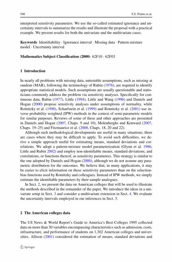
Table 1 Descriptive statistics for CSAT

Collegeadministration

CSAT observed CSAT missing

Count (%) Mean SD Count (%) Mean SD

public 251 (0.53) 945.3 107.5 219 (0.47) ? ?

private 528 (0.63) 978.8 129.2 304 (0.37) ? ?

Note: ? denotes non-observed values, and SD, standard deviation

correlations for seven such variables under MAR and normality assumptions usingthe EM algorithm. For the sake of our exposition, it suffices to focus only on fiveof them, namely, GRADRAT (ratio between the number of graduating seniors andthe number of enrolled students four years earlier ×100), CSAT (combined averagescores on verbal and math sections of the Scholastic Assessment Test), ACT (meanAmerican College Testing scores), RMBRD (total annual costs for room and board,in thousands of dollars) and an indicator of public versus private colleges. One collegehad a GRADRAT equal to 118 and, therefore, the corresponding value was deletedand considered missing. The public-private college administration indicator was theonly variable without missing values; the other four variables were observed simulta-neously only for 23% of the colleges and each variable had from 8% to 45% missingvalues. We are interested in two questions: (i) do the public and private colleges havedifferent means and standard deviations of CSAT? and (ii) are GRADRAT, CSAT,ACT and RMBRD mutually linearly correlated? Descriptive statistics are displayedin Tables 1 and 2. Because all American colleges matching the criteria adopted in thestudy were surveyed, the data make up the entire study population and therefore, stan-dard errors and confidence and uncertainty intervals will be computed and discussedmerely for illustrative purposes.

3 Univariate case

Let Yi denote the measurement on the ith study unit and Ri be an indicator variabletaking on the value 1 if Yi is observed and 0, otherwise, i = 1, . . . , n. In the pattern-mixture model framework, the joint distribution (Yi,Ri) is factored as the product ofthe marginal distribution of Ri and the conditional distribution of Yi given Ri . As ourinterest lies only in moments of Yi , we use the pattern-mixture model approach andconditional expectation properties to write

μ = E(Yi) = E[E(Yi |Ri)

] = γ1μ(1) + γ0μ(0), (1)

σ 2 = Var(Yi) = E[Var(Yi |Ri)

] + Var[E(Yi |Ri)

]

= γ1σ2(1) + γ0σ

2(0) + γ1(μ(1) − μ)2 + γ0(μ(0) − μ)2, (2)

where γr = P(Ri = r), μ(r) = E(Yi |Ri = r) and σ 2(r) = Var(Yi |Ri = r), for r = 0,1.

We can estimate γ1 (γ0 = 1 − γ1), μ(1) and σ(1) by their sample counterparts, i.e.,the proportion of observed units, γ1, and the sample mean and standard deviation of


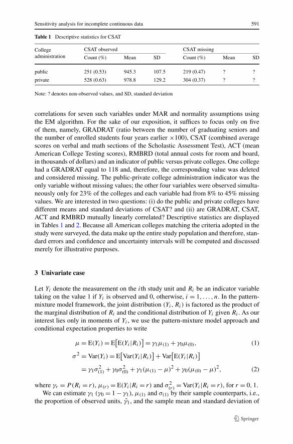
Table 2 Descriptive statistics for GRADRAT (G), CSAT (C), ACT (A) and RMBRD (R)

Resp.pattern Counts(%)

GRADRAT CSAT ACT RMBRD

G C A R Mean SD Mean SD Mean SD Mean SD

o o o o 296 (0.23) 62.6 19.0 988.9 120.4 22.90 2.74 4.25 0.99

o o o m 158 (0.12) 58.0 17.0 961.5 110.6 22.30 2.53 ? ?

o o m o 158 (0.12) 64.6 18.2 976.7 134.7 ? ? 4.73 1.19

o m o o 123 (0.09) 53.0 14.5 ? ? 21.39 1.91 3.25 0.78

m o o o 17 (0.01) ? ? 879.6 98.1 20.76 2.41 3.96 1.14

o o m m 119 (0.09) 62.7 19.1 949.9 124.9 ? ? ? ?

o m m o 157 (0.12) 64.8 20.8 ? ? ? ? 4.27 1.26

o m o m 82 (0.06) 51.9 16.7 ? ? 21.12 1.98 ? ?

m m o o 11 (0.01) ? ? ? ? 20.82 2.27 3.22 0.85

m o m o 5 (0.00) ? ? 871.4 96.1 ? ? 3.50 1.49

m o o m 17 (0.01) ? ? 880.9 109.6 20.47 2.83 ? ?

o m m m 110 (0.08) 57.4 19.5 ? ? ? ? ? ?

m o m m 9 (0.01) ? ? 865.9 56.8 ? ? ? ?

m m o m 10 (0.01) ? ? ? ? 19.90 1.37 ? ?

m m m o 16 (0.01) ? ? ? ? ? ? 3.20 1.14

m m m m 14 (0.01) ? ? ? ? ? ? ? ?

Available statistics 60.4 18.8 968.0 123.6 22.12 2.58 4.15 1.17

Case counts 1203 779 714 783

Analysis (%) (0.92) (0.60) (0.55) (0.60)

Resp.pattern Counts(%)

Correlations

G C A R G × C G × A G × R C × A C × R A × R

o o o o 296 (0.23) 0.56 0.58 0.43 0.92 0.45 0.47

o o o m 158 (0.12) 0.56 0.54 ? 0.87 ? ?

o o m o 158 (0.12) 0.72 ? 0.50 ? 0.53 ?

o m o o 123 (0.09) ? 0.47 0.26 ? ? 0.39

m o o o 17 (0.01) ? ? ? 0.83 −0.29 −0.27

o o m m 119 (0.09) 0.55 ? ? ? ? ?

o m m o 157 (0.12) ? ? 0.58 ? ? ?

o m o m 82 (0.06) ? 0.36 ? ? ? ?

m m o o 11 (0.01) ? ? ? ? ? −0.15

m o m o 5 (0.00) ? ? ? ? 0.02 ?

m o o m 17 (0.01) ? ? ? 0.93 ? ?

o m m m 110 (0.08) ? ? ? ? ? ?

m o m m 9 (0.01) ? ? ? ? ? ?

m m o m 10 (0.01) ? ? ? ? ? ?

m m m o 16 (0.01) ? ? ? ? ? ?

m m m m 14 (0.01) ? ? ? ? ? ?

Available statistics 0.59 0.56 0.50 0.91 0.44 0.47

Case counts 731 659 734 488 476 447

Analysis (%) (0.56) (0.51) (0.56) (0.37) (0.37) (0.34)

Note: ? denotes non-observed values, SD, standard deviation, o, observed, and m, missing


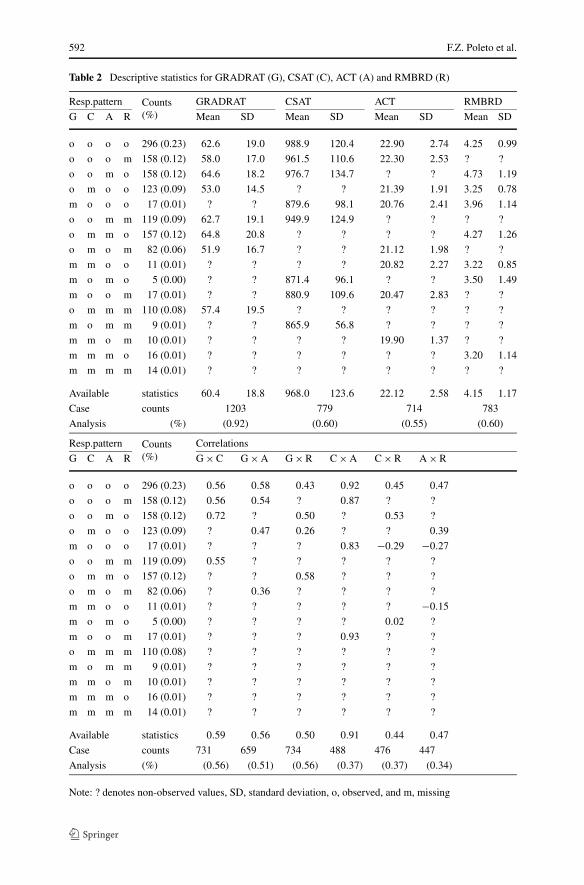
the observed measurements, μ(1) and σ(1). However, as ω = μ(0) or ω = (μ(0), σ(0))

is also needed to estimate μ or σ , respectively, and both μ(0) and σ(0) are not iden-tified from the observed data, it is useful to recall that the statistical uncertainty is acombination of statistical imprecision and statistical ignorance (Molenberghs et al.2001; Kenward et al. 2001). Statistical imprecision is caused by not observing theentire population while statistical ignorance is due to deficiencies in the observationprocess; e.g., when some responses are missing, misclassified, and/or measured witherror. When the sample size tends to infinity, the magnitude of statistical imprecisiondecreases to zero, but that of statistical ignorance may not change. In our case, sta-tistical ignorance is related to the mean and standard deviation of the non-observedunits. Setting a value ωS for ω, we may compute γ1, μ(1) and σ(1) and using (1) and(2), obtain an unbiased estimate μ(ωS) of μ(ωS) and a consistent estimate σ (ωS) ofσ(ωS). As this holds for any ωS , we may perform a sensitivity analysis, obtaining es-timates and confidence regions for the target over a set Ωω that is expected to containthe true value of the sensitivity parameter ω. The range of estimates provides a Hon-estly Estimated Ignorance Region (HEIR) and the union of 100(1 − α)% confidenceregions obtained for different values of ω provides a 100(1 − α)% Estimated Uncer-tainty Region (EURO). In the same way that standard errors and confidence regionsquantify statistical imprecision, ignorance regions measure statistical ignorance anduncertainty regions assess statistical uncertainty.

Vansteelandt et al. (2006) consider a formal approach to the problem and provideappropriate definitions of consistency and coverage for these regions. They show howto construct EUROs with uncertainty level 100(1 − α)% for a scalar parameter π ac-cording to the different definitions of uncertainty regions: (i) strong EUROs coverπ(ω) simultaneously for all ω ∈ Ωω with at least 100(1 −α)% probability, (ii) point-wise EUROs cover π(ω) uniformly over ω ∈ Ωω with at least 100(1 − α)% proba-bility, and (iii) weak EUROs have an expected overlap with the ignorance region ofat least 100(1 − α)% probability. Strong EUROs are conservative pointwise EUROs,which in turn, are conservative weak EUROs. The choice among the three versionsof EUROs depends on which is the more appropriate definition for the uncertaintyregion and on the desired degree of conservativeness. We summarize the algorithmsto construct the three EUROs in Appendix A.

For categorical missing data, the set Ωω may cover an in-depth grid of the wholeparameter space of ω, but for continuous data, this strategy is clearly not feasible; forinstance, note from (1) that μ(μ(0)) −→ ∞ as μ(0) −→ ∞ irrespectively of 0 < γ1 <

1 and μ(1). Therefore, as it is not possible to perform the analysis without a carefulevaluation of Ωω, the data analyst shall look for alternative parameterizations for thesensitivity parameters and select the one for which the elicitation task is more easilyaccomplished. For example, in lieu of using μ(0) as sensitivity parameter, one mayprefer to use α, β , or p, where μ(0) = α + μ(1), μ(0) = βμ(1), chiefly for positivevariables, and μ(0) = F−1

(1) (p), the pth quantile of the theoretical distribution of theobserved units. The variance of the estimator of μ depends upon which sensitivityparameter is used, e.g., for the first three cases, we have

Var[μ(μ(0))

] = γ1σ2(1)

n+ γ1(1 − γ1)(μ(1) − μ(0))

2

n, (3)


Var[μ(α)

] = σ 2(1)E

(1

n1

)+ γ1(1 − γ1)α

2

n, (4)

Var[μ(β)

] = σ 2(1)

[β2E

(1

n1

)+ 2β(1 − β)

n+ γ1(1 − β)2

n

]

+ γ1(1 − γ1)μ2(1)(1 − β)2

n, (5)

where n1 = ∑ni=1 Ri denotes the number of observed units.

Since no sensible analysis can be accomplished if all outcomes are missing, i.e.,if n1 = 0, we could have computed (3)–(5) assuming that n1 follows a positive bino-mial distribution (Stephan 1945) instead of a binomial distribution with parametersn and γ1. However, the changes required for such purposes generate cumbersomeformulae and improve accuracy only when nγ1 is small. Simple approximations forthe first negative moment of the positive binomial distribution are discussed, for ex-ample, by Grab and Savage (1954) and Mendenhall and Lehman (1960). We adoptE(1/n1) ∼= 1/(nγ1 + 1 − γ1) in practice; this is usually accurate to at least two dec-imal places if nγ1 > 10 (Grab and Savage 1954). Nevertheless, comparing (3)–(5)is easier when using the cruder approximation 1/nγ1 in which case the followingrelationships hold for large n:

Var[μ(μ(0))

]< Var

[μ(α)

] ≤ Var[μ(β)

], if β ≤ β1 or β ≥ 1, (6)

Var[μ(μ(0))

] ≤ Var[μ(β)

]< Var

[μ(α)

], if β1 < β ≤ β2 or β3 ≤ β < 1, (7)

Var[μ(β)

]< Var

[μ(μ(0))

]< Var

[μ(α)

], if β2 < β < β3, (8)

where β1 = (−1 − γ1)/(1 − γ1), β2 = (−γ 41 − γ1)/(1 − γ1) and β3 = (γ 4

1 − γ1)/

(1 − γ1). As β1 < β2 < β3 < 0 and β will generally be positive, (8) will hardly occurin practice.

Using expressions for the asymptotic variances and covariances of order statistics(Sen et al. 2009, p. 223), we obtain

Var[μ(p)

] ∼=γ1σ

2(1)

n+ p(1 − p)

{f(1)[F−1(1) (p)]}2

[γ1 − 2

n+ E

(1

n1

)]

+ γ1(1 − γ1)[μ(1) − F−1(1) (p)]2

n+ 2

n

[E

(1

n1

)− 1

n

]

×{

k∑

j=1

pj (1 − p)

f(1)[F−1(1) (pj )]f(1)[F−1

(1) (p)]

+n1∑

j=k+1

p(1 − pj )

f(1)[F−1(1) (p)]f(1)[F−1

(1) (pj )]

}

, (9)

where f(1) denotes the density of the observed units, pk < p < pk+1 and pj =j/n1 +o(n

−1/21 ), j = 1, . . . , n1, such that 0 < p1 < p2 < · · · < pn1 < 1, e.g., pj may


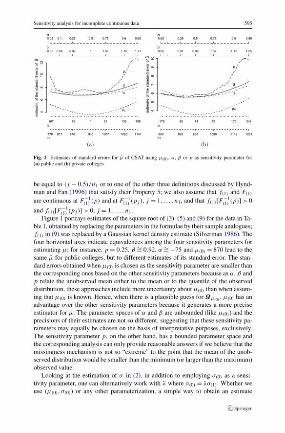
Fig. 1 Estimates of standard errors for μ of CSAT using μ(0) , α, β or p as sensitivity parameter for(a) public and (b) private colleges

be equal to (j − 0.5)/n1 or to one of the other three definitions discussed by Hynd-man and Fan (1996) that satisfy their Property 5; we also assume that f(1) and F(1)

are continuous at F−1(1) (p) and at F−1

(1) (pj ), j = 1, . . . , n1, and that f(1)[F−1(1) (p)] > 0

and f(1)[F−1(1) (pj )] > 0, j = 1, . . . , n1.

Figure 1 portrays estimates of the square root of (3)–(5) and (9) for the data in Ta-ble 1, obtained by replacing the parameters in the formulae by their sample analogues;f(1) in (9) was replaced by a Gaussian kernel density estimate (Silverman 1986). Thefour horizontal axes indicate equivalences among the four sensitivity parameters forestimating μ; for instance, p = 0.25, β ∼= 0.92, α ∼= −75 and μ(0) = 870 lead to thesame μ for public colleges, but to different estimates of its standard error. The stan-dard errors obtained when μ(0) is chosen as the sensitivity parameter are smaller thanthe corresponding ones based on the other sensitivity parameters because as α, β andp relate the unobserved mean either to the mean or to the quantile of the observeddistribution, these approaches include more uncertainty about μ(0) than when assum-ing that μ(0) is known. Hence, when there is a plausible guess for Ωμ(0)

, μ(0) has anadvantage over the other sensitivity parameters because it generates a more preciseestimator for μ. The parameter spaces of α and β are unbounded (like μ(0)) and theprecisions of their estimates are not so different, suggesting that these sensitivity pa-rameters may equally be chosen on the basis of interpretative purposes, exclusively.The sensitivity parameter p, on the other hand, has a bounded parameter space andthe corresponding analysis can only provide reasonable answers if we believe that themissingness mechanism is not so “extreme” to the point that the mean of the unob-served distribution would be smaller than the minimum (or larger than the maximum)observed value.

Looking at the estimation of σ in (2), in addition to employing σ(0) as a sensi-tivity parameter, one can alternatively work with λ where σ(0) = λσ(1). Whether weuse (μ(0), σ(0)) or any other parameterization, a simple way to obtain an estimate


of the variance of σ is to employ the non-parametric bootstrap1 (Efron and Gong1983). As in the previous discussion, it is expected that Var[σ (σ(0))] < Var[σ (λ)]when σ (σ(0)) = σ (λ), for any of the other parameterizations employed for μ(0). Forexample, setting σ0 = 134.3 or λ = 1.25 for public colleges, both with μ(0) = 870,α ∼= −75, β ∼= 0.92 or p = 0.25, we obtain the same estimate for σ (126.4), but theestimates of the standard errors of σ are 2.6, 5.5, 2.3, 5.2, 2.3, 5.1, 2.9, 5.8, respec-tively, when employing (μ(0), σ0), (μ(0), λ), . . . , (p,λ). Although we do not have anexplanation for why the standard errors obtained employing μ(0) are slightly largerthan the corresponding ones obtained using α and β , the main conclusion here is thatthe parameterization for the sensitivity parameter of μ(0) seems to have less impactover the standard error of σ than the parameterization of σ(0).

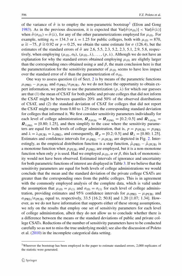
One way to assess question (i) of Sect. 2 is by means of the parametric functionsμ(PRI) − μ(PUB) and σ(PRI)/σ(PUB). As we do not have the opportunity to obtain ex-pert information, we prefer to use the parameterization (p,λ) for which our guessesare that (1) the mean of CSAT for both public and private colleges that did not informthe CSAT might be between quantiles 20% and 50% of the observed distributionsof CSAT, and (2) the standard deviation of CSAT for colleges that did not reportthe CSAT might range from 0.80 to 1.25 times the corresponding standard deviationfor colleges that informed it. We first consider sensitivity parameters individually foreach level of college administration, Ωp(PUB)

= Ωp(PRI) = [0.2;0.5] and Ωλ(PUB)=

Ωλ(PRI) = [0.80;1.25], and then simplify to the case where the sensitivity parame-ters are equal for both levels of college administration, that is, p = p(PUB) = p(PRI)and λ = λ(PUB) = λ(PRI), and consequently, Ωp = [0.2;0.5] and Ωλ = [0.80;1.25].Estimates and confidence intervals for μ(PRI) − μ(PUB) are depicted in Fig. 2. Inter-estingly, as the empirical distribution function is a step function, μ(PRI) − μ(PUB) isa monotone function when p(PUB) and p(PRI) are employed, but it is a non-monotonefunction when only p is used. Had we employed μ(0), α or β , this lack of monotonic-ity would not have been observed. Estimated intervals of ignorance and uncertaintyfor both parametric functions of interest are displayed in Table 3. If we believe that thesensitivity parameters are equal for both levels of college administrations we wouldconclude that the mean and the standard deviation of the private college CSATs aregreater than the corresponding ones from the public colleges. This is in agreementwith the commonly employed analysis of the complete data, which is valid underthe assumption that μ(0) = μ(1) and σ(0) = σ(1) for each level of college adminis-tration, providing estimates and 95% confidence intervals for μ(PRI) − μ(PUB) andσ(PRI)/σ(PUB) equal to, respectively, 33.5 [16.2; 50.8] and 1.20 [1.07; 1.34]. How-ever, as we do not have information that supports either of these strong assumptions,we rely on the results that employ one set of sensitivity parameters for each levelof college administration, albeit they do not allow us to conclude whether there isa difference between the means or the standard deviations of public and private col-lege CSATs. Reductions of the number of sensitivity parameters have to be conductedcarefully so as not to miss the true underlying model; see also the discussion of Poletoet al. (2010) in the incomplete categorical data setting.

1Wherever the bootstrap has been employed in the paper to estimate standard errors, 2,000 replicates ofthe statistic were generated.


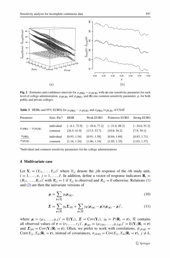
Fig. 2 Estimates and confidence intervals for μ(PRI) −μ(PUB) with (a) one sensitivity parameter for eachlevel of college administration, p(PUB) and p(PRI), and (b) one common sensitivity parameter, p, for bothpublic and private colleges

Table 3 HEIRs and 95% EUROs for μ(PRI) − μ(PUB) and σ(PRI)/σ(PUB) of CSAT

Parameter Sens. Par.a HEIR Weak EURO Pointwise EURO Strong EURO

μ(PRI) − μ(PUB)individual [−6.1; 72.9] [−10.4; 77.2] [−21.6; 88.2] [−24.6; 91.2]

common [26.5; 41.0] [13.5; 53.7] [10.8; 56.2] [7.9; 59.1]

σ(PRI)

σ(PUB)

individual [0.93; 1.54] [0.91; 1.58] [0.84; 1.69] [0.83; 1.71]

common [1.16; 1.24] [1.06; 1.34] [1.05; 1.35] [1.03; 1.37]

aIndividual and common sensitivity parameters for the college administrations

4 Multivariate case

Let Yi = (Yi1, . . . , YiJ )′ where Yij denote the j th response of the ith study unit,i = 1, . . . , n, j = 1, . . . , J . In addition, define a vector of response indicators Ri =(Ri1, . . . ,RiJ )′ with Rij = 1 if Yij is observed and Rij = 0 otherwise. Relations (1)and (2) are then the univariate versions of

μ =∑

r∈Rγrμ(r), (10)

Σ =∑

r∈RγrΣ (r) +

∑

r∈Rγr(μ(r) − μ)(μ(r) − μ)′, (11)

where μ = (μ1, . . . ,μJ )′ = E(Yi ), Σ = Cov(Yi ), γr = P(Ri = r), R containsall observed values of r = (r1, . . . , rJ )′, μ(r) = (μ1(r), . . . ,μJ(r))

′ = E(Yi |Ri = r)and Σ (r) = Cov(Yi |Ri = r). Often, we prefer to work with correlations, ψjk(r) =Corr(Yij , Yik|Ri = r), instead of covariances, σjk(r) = Cov(Yij , Yik|Ri = r), j = k,


and therefore we let Σ (r) = Dσ (r)Ψ (r)Dσ (r) , where Dσ (r) denotes a diagonal matrixwith the elements of σ (r) along the main diagonal, σ (r) = (σj (r), j = 1, . . . , J )′,σ 2

j (r) = Var(Yij |Ri = r) and Ψ (r) = Corr(Yi |Ri = r); the corresponding definitionsfor the unconditional variances, covariances and correlations follow analogously.

In the tetravariate version of Table 2, there are 16 missingness patterns and 136non-identifiable parameters for estimating μ and Σ using (10) and (11); among thesesensitivity parameters, there are 32 means, 32 standard deviations and 72 correla-tions, as indicated by the non-observed values in Table 2. For J = 10 variables sub-ject to missingness, there are 2J = 1,024 potential missingness patterns that generate44,800 non-identifiable parameters: J × 2J−1 = 5,120 means, 5,120 standard devia-tions and

∑J−1j=0

(Jj

)[(J2

) − (j2

)] = 34,560 correlations. The challenge here is not onlythat the number of sensitivity parameters increases exponentially depending on themissingness patterns and on the number of variables, but also that there are addi-tional options for the parameterization. For instance, in the tetravariate case, insteadof using μ1(0,r2,r3,r4), r2, r3, r4 = 0,1, as sensitivity parameters to estimate μ1, wemay prefer to employ functions of these parameters along with the identifiable ones,namely, μ1(1,r2,r3,r4), r2, r3, r4 = 0,1, or yet to use other options, such as quantilesof the distribution of Yi1 conditionally on Ri = (1, r2, r3, r4), for some values ofr2, r3, r4. Another alternative is to use all available data for the j th variable, that is,the mean μj(1) or the quantile of the distribution of Yij conditionally on Rij = 1,Fj(1), e.g., μ1(0,r2,r3,r4) = α1(0,r2,r3,r4) + μ1(1), μ1(0,r2,r3,r4) = β1(0,r2,r3,r4)μ1(1), orμ1(0,r2,r3,r4) = F−1

j (1)(p1(0,r2,r3,r4)). Analogously, and like in the previous section,there is also the possibility to consider reparameterizations of the form σ1(0,r2,r3,r4) =λ1(0,r2,r3,r4)σ1(1), where σ 2

j (1) = Var(Yij |Rij = 1).The lower (upper) bounds of the ignorance interval for each parametric function

of interest may be obtained by minimizing (maximizing) the corresponding func-tion over the appropriate sensitivity parameters. In the tetravariate case, for example,when the target is the mean μj , the optimizations are carried over only the eightnon-identifiable means of {μj(r)} and, for standard deviations, it may be performedover the eight non-identifiable means of {μj(r)} and eight non-identifiable standarddeviations of {σj(r)} (16 sensitivity parameters). For each correlation, the number ofsensitivity parameters to be handled in the optimization increases to 44 (16 means,16 standard deviations and 12 correlations). So, in practice, all the 136 sensitivity pa-rameters would only be used simultaneously if the target were some specific functionof (μ,σ ,Ψ ).

Because of the large number of alternative parameterizations that may be com-bined for a set of variables, we computed the variance of μ only for the case wherethe sensitivity parameters are the non-identifiable elements in μ(r). In Appendix B,this result as well as (10) and (11) are expressed in matrix formulation useful forcomputational implementation. Considering other parameterizations for the sensitiv-ity parameters, we appeal to the non-parametric bootstrap to obtain estimates for thestandard errors of μ, σ , Ψ and functions thereof.

To evaluate question (ii) of Sect. 2, our conjectures about the non-identifiable pa-rameters are that (1) the non-observed means of GRADRAT and of the other vari-ables might range, respectively, between the 30%–50% and 20%–50% quantiles ofthe corresponding observed distributions, (2) the non-observed standard deviations


Table 4 HEIRs and 95% EUROs for means, standard deviations (SDs) and correlations ofGRADRAT (G), CSAT (C), ACT (A) and RMBRD (R)

Variable Parameter HEIR Weak EURO Pointwise EURO Strong EURO

GRADRATMean [59.6;60.3] [58.8;61.1] [58.7;61.2] [58.5;61.4]SD [18.7;19.3] [18.3;19.7] [18.1;19.9] [18.0;20.0]

CSATMean [926.7;963.6] [924.4;965.8] [918.9;971.1] [917.4;972.5]SD [114.7;146.0] [112.8;148.3] [108.7;153.3] [107.6;154.7]

ACTMean [21.16;22.07] [21.17;22.06] [21.08;22.15] [21.06;22.16]SD [2.43;2.95] [2.38;3.01] [2.31;3.10] [2.28;3.13]

RMBRDMean [3.75;4.09] [3.73;4.11] [3.69;4.15] [3.68;4.17]SD [1.09;1.38] [1.08;1.40] [1.04;1.44] [1.03;1.46]

G × C Corr. [0.37;0.69] [0.38;0.69] [0.35;0.71] [0.34;0.72]G × A Corr. [0.31;0.66] [0.31;0.66] [0.28;0.69] [0.28;0.69]G × R Corr. [0.24;0.52] [0.24;0.52] [0.22;0.55] [0.21;0.55]C × A Corr. [0.59;0.95] [0.60;0.95] [0.57;0.97] [0.57;0.97]C × R Corr. [0.11;0.55] [0.12;0.54] [0.08;0.57] [0.07;0.58]A × R Corr. [0.05;0.46] [0.06;0.46] [0.02;0.49] [0.02;0.50]

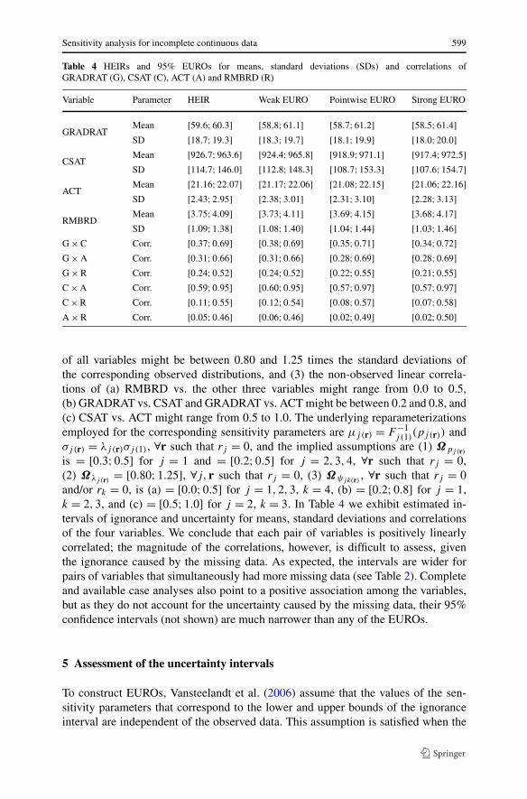
of all variables might be between 0.80 and 1.25 times the standard deviations ofthe corresponding observed distributions, and (3) the non-observed linear correla-tions of (a) RMBRD vs. the other three variables might range from 0.0 to 0.5,(b) GRADRAT vs. CSAT and GRADRAT vs. ACT might be between 0.2 and 0.8, and(c) CSAT vs. ACT might range from 0.5 to 1.0. The underlying reparameterizationsemployed for the corresponding sensitivity parameters are μj(r) = F−1

j (1)(pj (r)) andσj(r) = λj(r)σj (1), ∀r such that rj = 0, and the implied assumptions are (1) Ωpj(r)

is = [0.3;0.5] for j = 1 and = [0.2;0.5] for j = 2,3,4, ∀r such that rj = 0,(2) Ωλj(r) = [0.80;1.25], ∀j, r such that rj = 0, (3) Ωψjk(r) , ∀r such that rj = 0and/or rk = 0, is (a) = [0.0;0.5] for j = 1,2,3, k = 4, (b) = [0.2;0.8] for j = 1,k = 2,3, and (c) = [0.5;1.0] for j = 2, k = 3. In Table 4 we exhibit estimated in-tervals of ignorance and uncertainty for means, standard deviations and correlationsof the four variables. We conclude that each pair of variables is positively linearlycorrelated; the magnitude of the correlations, however, is difficult to assess, giventhe ignorance caused by the missing data. As expected, the intervals are wider forpairs of variables that simultaneously had more missing data (see Table 2). Completeand available case analyses also point to a positive association among the variables,but as they do not account for the uncertainty caused by the missing data, their 95%confidence intervals (not shown) are much narrower than any of the EUROs.

5 Assessment of the uncertainty intervals

To construct EUROs, Vansteelandt et al. (2006) assume that the values of the sen-sitivity parameters that correspond to the lower and upper bounds of the ignoranceinterval are independent of the observed data. This assumption is satisfied when the


target is the mean, but it may fail for standard deviations and correlations. Con-sider, for example, the target σ in the univariate setting of Sect. 3, and assume thatΩσ(0)

= [σL(0);σU

(0)] and Ωμ(0)= [μL

(0);μU(0)] are specified. After replacing the identi-

fiable parameters in (2) by their sample counterparts, we note that σL(0) and σU

(0) are thevalues of σ(0) in the set Ωσ(0)

that, respectively, minimize and maximize σ (μ(0), σ(0))

irrespectively of the data and of μ(0). However, as

arg minμ(0)∈Ωμ(0)

σ (μ(0), σ(0)) =

⎧⎪⎨

⎪⎩

μL(0), if μ(1) < μL

(0),

μU(0), if μ(1) > μU

(0),

μ(1), otherwise,

arg maxμ(0)∈Ωμ(0)

σ (μ(0), σ(0)) ={

μU(0), if (μ(1) − μU

(0))2 > (μ(1) − μL

(0))2,

μL(0), otherwise

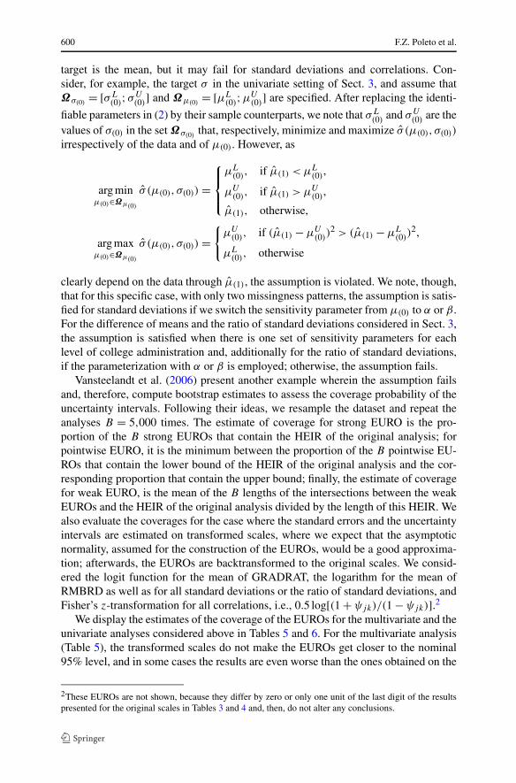
clearly depend on the data through μ(1), the assumption is violated. We note, though,that for this specific case, with only two missingness patterns, the assumption is satis-fied for standard deviations if we switch the sensitivity parameter from μ(0) to α or β .For the difference of means and the ratio of standard deviations considered in Sect. 3,the assumption is satisfied when there is one set of sensitivity parameters for eachlevel of college administration and, additionally for the ratio of standard deviations,if the parameterization with α or β is employed; otherwise, the assumption fails.

Vansteelandt et al. (2006) present another example wherein the assumption failsand, therefore, compute bootstrap estimates to assess the coverage probability of theuncertainty intervals. Following their ideas, we resample the dataset and repeat theanalyses B = 5,000 times. The estimate of coverage for strong EURO is the pro-portion of the B strong EUROs that contain the HEIR of the original analysis; forpointwise EURO, it is the minimum between the proportion of the B pointwise EU-ROs that contain the lower bound of the HEIR of the original analysis and the cor-responding proportion that contain the upper bound; finally, the estimate of coveragefor weak EURO, is the mean of the B lengths of the intersections between the weakEUROs and the HEIR of the original analysis divided by the length of this HEIR. Wealso evaluate the coverages for the case where the standard errors and the uncertaintyintervals are estimated on transformed scales, where we expect that the asymptoticnormality, assumed for the construction of the EUROs, would be a good approxima-tion; afterwards, the EUROs are backtransformed to the original scales. We consid-ered the logit function for the mean of GRADRAT, the logarithm for the mean ofRMBRD as well as for all standard deviations or the ratio of standard deviations, andFisher’s z-transformation for all correlations, i.e., 0.5 log[(1 + ψjk)/(1 − ψjk)].2

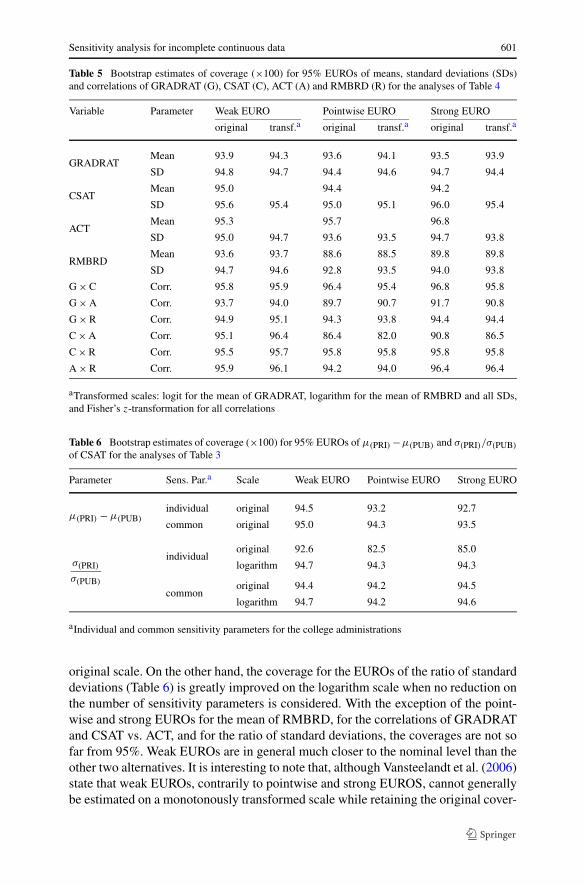
We display the estimates of the coverage of the EUROs for the multivariate and theunivariate analyses considered above in Tables 5 and 6. For the multivariate analysis(Table 5), the transformed scales do not make the EUROs get closer to the nominal95% level, and in some cases the results are even worse than the ones obtained on the

2These EUROs are not shown, because they differ by zero or only one unit of the last digit of the resultspresented for the original scales in Tables 3 and 4 and, then, do not alter any conclusions.


Table 5 Bootstrap estimates of coverage (×100) for 95% EUROs of means, standard deviations (SDs)and correlations of GRADRAT (G), CSAT (C), ACT (A) and RMBRD (R) for the analyses of Table 4

Variable Parameter Weak EURO Pointwise EURO Strong EURO

original transf.a original transf.a original transf.a

GRADRATMean 93.9 94.3 93.6 94.1 93.5 93.9

SD 94.8 94.7 94.4 94.6 94.7 94.4

CSATMean 95.0 94.4 94.2

SD 95.6 95.4 95.0 95.1 96.0 95.4

ACTMean 95.3 95.7 96.8

SD 95.0 94.7 93.6 93.5 94.7 93.8

RMBRDMean 93.6 93.7 88.6 88.5 89.8 89.8

SD 94.7 94.6 92.8 93.5 94.0 93.8

G × C Corr. 95.8 95.9 96.4 95.4 96.8 95.8

G × A Corr. 93.7 94.0 89.7 90.7 91.7 90.8

G × R Corr. 94.9 95.1 94.3 93.8 94.4 94.4

C × A Corr. 95.1 96.4 86.4 82.0 90.8 86.5

C × R Corr. 95.5 95.7 95.8 95.8 95.8 95.8

A × R Corr. 95.9 96.1 94.2 94.0 96.4 96.4

aTransformed scales: logit for the mean of GRADRAT, logarithm for the mean of RMBRD and all SDs,and Fisher’s z-transformation for all correlations

Table 6 Bootstrap estimates of coverage (×100) for 95% EUROs of μ(PRI) −μ(PUB) and σ(PRI)/σ(PUB)

of CSAT for the analyses of Table 3

Parameter Sens. Par.a Scale Weak EURO Pointwise EURO Strong EURO

μ(PRI) − μ(PUB)individual original 94.5 93.2 92.7

common original 95.0 94.3 93.5

σ(PRI)

σ(PUB)

individualoriginal 92.6 82.5 85.0

logarithm 94.7 94.3 94.3

commonoriginal 94.4 94.2 94.5

logarithm 94.7 94.2 94.6

aIndividual and common sensitivity parameters for the college administrations

original scale. On the other hand, the coverage for the EUROs of the ratio of standarddeviations (Table 6) is greatly improved on the logarithm scale when no reduction onthe number of sensitivity parameters is considered. With the exception of the point-wise and strong EUROs for the mean of RMBRD, for the correlations of GRADRATand CSAT vs. ACT, and for the ratio of standard deviations, the coverages are not sofar from 95%. Weak EUROs are in general much closer to the nominal level than theother two alternatives. It is interesting to note that, although Vansteelandt et al. (2006)state that weak EUROs, contrarily to pointwise and strong EUROS, cannot generallybe estimated on a monotonously transformed scale while retaining the original cover-


Table 7 Bootstrap estimates of coverage (×100) for 95% EUROs of μ(PRI) −μ(PUB) and σ(PRI)/σ(PUB)

of CSAT

Parameter Sens. Par.a Scale Weak EURO Pointwise EURO Strong EURO

μ(0) original 95.0 95.1 95.3

μ(PRI) − μ(PUB)α original 95.0 94.6 94.9

β original 95.0 94.6 94.8

p original 94.5 93.2 92.7

(μ(0), σ(0))original 93.7 83.1 84.8

logarithm 94.9 94.4 94.8

(μ(0), λ)original 92.9 82.7 85.1

logarithm 94.8 94.6 94.7

(α,σ(0))original 93.7 81.5 84.2

logarithm 94.8 94.1 94.2

(α,λ)original 92.9 82.6 84.7

σ(PRI)

σ(PUB)

logarithm 94.8 94.5 94.6

(β,σ(0))original 93.7 81.5 84.1

logarithm 94.8 94.1 94.2

(β,λ)original 92.9 82.7 84.7

logarithm 94.8 94.6 94.6

(p,σ(0))original 93.2 81.4 83.7

logarithm 94.5 94.2 93.7

(p,λ)original 92.6 82.5 85.0

logarithm 94.7 94.3 94.3

aOne of these sensitivity parameters for each level of college administration

age level, for the current analyses, the coverages of the weak EUROs are, in general,closer to the nominal level in the cases for which the transformed scale also improvethe coverage of the strong and/or the pointwise EUROs.

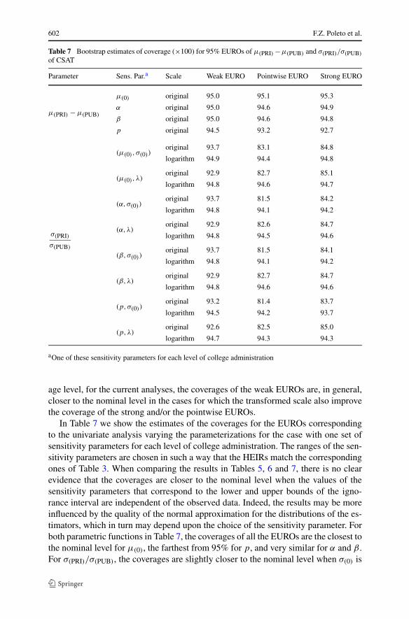
In Table 7 we show the estimates of the coverages for the EUROs correspondingto the univariate analysis varying the parameterizations for the case with one set ofsensitivity parameters for each level of college administration. The ranges of the sen-sitivity parameters are chosen in such a way that the HEIRs match the correspondingones of Table 3. When comparing the results in Tables 5, 6 and 7, there is no clearevidence that the coverages are closer to the nominal level when the values of thesensitivity parameters that correspond to the lower and upper bounds of the igno-rance interval are independent of the observed data. Indeed, the results may be moreinfluenced by the quality of the normal approximation for the distributions of the es-timators, which in turn may depend upon the choice of the sensitivity parameter. Forboth parametric functions in Table 7, the coverages of all the EUROs are the closest tothe nominal level for μ(0), the farthest from 95% for p, and very similar for α and β .For σ(PRI)/σ(PUB), the coverages are slightly closer to the nominal level when σ(0) is


chosen in lieu of λ, for weak EUROs when either μ(0), α, β or p is employed, andalso for the pointwise EURO obtained under the original scale with μ(0); the roles ofσ(0) and λ are reversed for all strong EUROs and the other pointwise EUROs.

6 Discussion

Selection models and pattern-mixture models are likely the most common frame-works for incomplete data modelling. In the univariate case, Scharfstein et al. (2003)showed that the assumption

logitP(Ri = 0|Yi = y) = constant + q(y) (12)

where q is the so-called selection-bias function, under the selection model is equiva-lent to the restriction

f(0)(y) = f(1)(y)exp[q(y)]

∫ ∞−∞ exp[q(s)]f(1)(s) ds

, ∀y, (13)

under the pattern-mixture model. Beyond the direct interpretation of these expres-sions, they also noted that, if q(y) = δ log(y), for example, it follows from (12) thatexp(δ) is the odds ratio of missingness between subjects who differ by one unit oflog(y); from (13), we may conclude that δ > 0 (< 0) indicates that the distributionof Yi for the missing outcomes is more (less) heavily weighted towards large valuesof Yi than the distribution of Yi for the observed outcomes. These insights are funda-mental to carry out a sensitivity analysis. Nevertheless, the functional form of q(y)

as well as the range of values to be considered for δ are hard to assess.When the target of inference is the mean, the standard deviation, the correlation or

some function thereof, we may employ their non-identifiable counterparts as sensitiv-ity parameters. These sensitivity parameters are easier to elicit than the selection-biasfunctions because the former are directly related to the parameters of interest. How-ever, there are connections between both strategies; for example, for a specified q(y),we can use (13) to compute the corresponding results for μ(0), α, β , p, σ(0), and λ

considered in Sect. 3.Some of these ideas on parameterization were considered previously in the liter-

ature. For instance, Rubin (1977) uses (1) to develop a Bayesian solution assumingnormality and Daniels and Hogan (2000) consider a pattern-mixture model of multi-variate normal distributions wherein the model identification is accomplished throughb(d) = μ(d) −μ(d+1) and C(d) = Σ

1/2(d) Σ

−1/2(d+1), d = 1, . . . , J , where d = 1 +∑J

j=1 rjis the drop-out indicator and b(d) and C(d) are, respectively, pre-specified vectors andmatrices. We extend these results by dropping the normality assumption and allowinga greater flexibility for the identification of the model. First, we not only consider ab-solute differences of means of missingness patterns but also relative differences andthe possibility of relating non-observed means to quantiles of observed distributions.Second, we replace the hard-to-elicit functions of covariance matrices by relative dif-ferences of standard deviations and by correlations. Third, in the multivariate case,we show that a non-identifiable mean (or standard deviation) may be related to an


identifiable one not only in cases with a single specific missingness pattern but alsoin cases with sets of missingness patterns wherein the corresponding variable is ob-served. With these alternatives, it is easier to extract information from experts or fromhistorical data and, consequently, to produce meaningful and more plausible sensitiv-ity analyses. When the interest lies only in functions of the means, an advantage ofour approach is that we do not need to specify ranges for the sensitivity parametersof standard deviations (and correlations), in contrast to Daniels and Hogan (2000)who have to identify the adopted multivariate normal distributions and, as a conse-quence, show that their posterior standard deviations of the functions of the meansare influenced by the choice of these sensitivity parameters. However, a drawback ofour approach is that there is no way to set the sensitivity parameters to a value thatcorresponds to the MAR assumption.

Acknowledgement The authors are grateful to an associate editor and a referee for their enlighteningand constructive comments.

Appendix A: Estimated uncertainty regions

For a scalar parameter π of interest, the HEIR obtained by setting ω equal to ωl andωu is denoted by ir(π,Ωω) = [π(ωl ), π(ωu)] = [πl , πu]. Vansteelandt et al. (2006)provided algorithms for constructing the three versions of EUROs defined in Sect. 3,all with the usual form [πl − cα∗/2 se(πl), πu + cα∗/2 se(πu)], where πl and πu areobtained from consistent and asymptotically normal estimators of πl and πu, andse(πl) and se(πu) are obtained from consistent estimators of the standard errors of πl

and πu. For strong EUROs, the critical value cα∗/2 is the 100(1 − α/2)% percentileof the standard normal distribution. For pointwise EUROs, cα∗/2 is the solution of

min

[Φ(cα∗/2) − Φ

(−cα∗/2 − πu − πl

se(πu)

),Φ

(cα∗/2 + πu − πl

se(πl)

)− Φ(−cα∗/2)

]

= 1 − α,

where Φ denotes the standard normal cumulative distribution function. For weakEUROs, cα∗/2 is the solution of

α = se(πl) + se(πu)

πu − πl

∫ +∞

0zϕ(z + cα∗/2) dz + ε,

where ϕ is the standard normal density function and ε is the correction term

ε =∫ +∞

(πu−πl )/se(πu)

ϕ(z + cα∗/2) dz − se(πu)

πu − πl

∫ +∞

(πu−πl )/se(πu)

zϕ(z + cα∗/2) dz

+∫ +∞

(πu−πl )/se(πl )

ϕ(z + cα∗/2) dz − se(πl)

πu − πl

∫ +∞

(πu−πl )/se(πl )

zϕ(z + cα∗/2) dz

that may be set equal to zero unless the sample size is small and/or there is littleignorance about π . When there is much ignorance about π and the sample size islarge, pointwise EUROs approach strong EUROs.


Appendix B: Matrix expressions

With some algebra, (10) and (11) may be conveniently rewritten as

μ = γ ′∗μ(∗),

Σ = γ ′∗Σ (∗)(1P ⊗ IJ ) + γ ′∗S(∗)(1P ⊗ IJ ),

where γ ∗ = γ ⊗ IJ , γ = (γr, r ∈ R)′, ⊗ denotes the Kronecker product, IJ rep-resents an identity matrix of order J , μ(∗) = (μ′

r, r ∈ R)′, Σ (∗) and S(∗) are blockdiagonal matrices with blocks Σ (r) and S(r) = (μ(r) − μ)(μ(r) − μ)′, r ∈ R, respec-tively, 1P denotes a P × 1 vector with all elements equal to 1 and P represents thenumber of missingness patterns, i.e., the cardinality of R. When employing the non-identifiable components of μ(r), stacked in the vector μNI, as sensitivity parameters,the covariance matrix of μ is specified as

Cov[μ

(μNI)] = 1

nγ ′∗ΣI

(∗)(1P ⊗ IJ ) + 1

nμ′

D

[(Dγ − γ γ ′) ⊗ (

1J 1′J

)]μD,

where μD = (Dμr , r ∈ R)′ and ΣI(∗) is obtained from Σ (∗) by replacing the non-

identifiable parameters by 0.

References

Allison PD (2001) Missing data. Sage, Thousand OaksDaniels MJ, Hogan JW (2000) Reparameterizing the pattern mixture model for sensitivity analyses under

informative dropout. Biometrics 56:1241–1248Daniels MJ, Hogan JW (2007) Missing data in longitudinal studies: strategies for Bayesian modeling and

sensitivity analysis. Chapman & Hall, LondonEfron B, Gong G (1983) A leisure look at the bootstrap, the jackknife and cross-validation. Am Stat 37:36–

48Fitzmaurice G, Davidian M, Verbeke G, Molenberghs G (2008) Longitudinal data analysis. Chapman &

Hall, Boca RatonGlynn RJ, Laird NM, Rubin DB (1986) Selection modeling versus mixture modeling with nonignorable

nonresponse (with discussion). In: Wainer H (ed) Drawing inferences from self-selected samples.Erlbaum, Mahwah, pp 115–151

Grab EL, Savage IR (1954) Tables of the expected value of 1/X for positive Bernoulli and Poisson vari-ables. J Am Stat Assoc 49:169–177

Hyndman RJ, Fan Y (1996) Sample quantiles in statistical packages. Am Stat 50:361–365Kenward MG, Goetghebeur E, Molenberghs G (2001) Sensitivity analysis for incomplete categorical data.

Stat Model 1:31–48Little RJA (1994) A class of pattern-mixture models for normal incomplete data. Biometrika 81:471–483Little RJA, Rubin DB (2002) Statistical analysis with missing data, 2nd edn. Wiley, New YorkLittle RJA, Wang YX (1996) Pattern-mixture models for multivariate incomplete data with covariates.

Biometrics 52:98–111Mendenhall W, Lehman JEH (1960) An approximation to the negative moments of the positive binomial

useful in life testing. Technometrics 2:227–242Molenberghs G, Kenward MG (2007) Missing data in clinical studies. Wiley, New YorkMolenberghs G, Kenward MG, Goetghebeur E (2001) Sensitivity analysis for incomplete contingency

tables: the Slovenian plebiscite case. Appl Stat 50:15–29Poleto FZ, Paulino CD, Molenberghs G, Singer JM (2010) Inferential implications of over-para-

meterization: a case study in incomplete categorical data. Tech rep, RT-MAE-2010-04, Instituto deMatemática e Estatística, Universidade de São Paulo


Rotnitzky A, Robins JM, Scharfstein DO (1998) Semiparametric regression for repeated outcomes withnonignorable nonresponse. J Amer Stat Assoc 93:1321–1339

Rotnitzky A, Scharfstein D, Su TL, Robins JM (2001) Methods for conducting sensitivity analysis of trialswith potentially nonignorable competing causes of censoring. Biometrics 57:103–113

Rubin DB (1976) Inference and missing data. Biometrika 63:581–592Rubin DB (1977) Formalizing subjective notions about the effect of nonrespondents in sample surveys.

J Am Stat Assoc 72:538–543Scharfstein DO, Rotnitzky A, Robins JM (1999) Adjusting for nonignorable drop-out using semiparamet-

ric nonresponse models (with discussion). J Am Stat Assoc 94:1096–1146Scharfstein DO, Daniels MJ, Robins JM (2003) Incorporating prior beliefs about selection bias into the

analysis of randomized trials with missing outcomes. Biostatistics 4:495–512Sen PK, Singer JM, Pedroso de Lima AC (2009) From finite sample to asymptotic methods in statistics.

Cambridge University Press, CambridgeSilverman BW (1986) Density estimation, 2nd edn. Chapman & Hall, LondonStephan FF (1945) The expected value and variance of the reciprocal and other negative powers of a

positive Bernoullian variate. Ann Math Stat 16:50–61Vansteelandt S, Goetghebeur E, Kenward MG, Molenberghs G (2006) Ignorance and uncertainty regions

as inferential tools in a sensitivity analysis. Stat Sin 16:953–979

sensitivity analysis for incomplete continuous data

Documents