let continuous outcome variables remain continuous

Hindawi Publishing CorporationComputational and Mathematical Methods in MedicineVolume 2012, Article ID 639124, 12 pagesdoi:10.1155/2012/639124

Research Article

Let Continuous Outcome Variables Remain Continuous

Enayatollah Bakhshi,1 Brian McArdle,2 Kazem Mohammad,3

Behjat Seifi,4 and Akbar Biglarian1

1 Department of Statistics and Computer, University of Social Welfare and Rehabilitation Sciences, Tehran 1985713834, Iran2 Department of Statistics, The University of Auckland, Private Bag 92010, Auckland, New Zealand3 Department of Biostatistics, School of Public Health and Institute of Public Health Research,Tehran University of Medical Sciences, Tehran, Iran

4 Department of Physiology, School of Medicine, Tehran University of Medical Sciences, Tehran, Iran

Correspondence should be addressed to Enayatollah Bakhshi, [email protected]

Received 8 November 2011; Revised 21 February 2012; Accepted 29 February 2012

Academic Editor: Alberto Guillen

Copyright © 2012 Enayatollah Bakhshi et al. This is an open access article distributed under the Creative Commons AttributionLicense, which permits unrestricted use, distribution, and reproduction in any medium, provided the original work is properlycited.

The complementary log-log is an alternative to logistic model. In many areas of research, the outcome data are continuous. Weaim to provide a procedure that allows the researcher to estimate the coefficients of the complementary log-log model withoutdichotomizing and without loss of information. We show that the sample size required for a specific power of the proposedapproach is substantially smaller than the dichotomizing method. We find that estimators derived from proposed method areconsistently more efficient than dichotomizing method. To illustrate the use of proposed method, we employ the data arising fromthe NHSI.

1. Introduction

Recently, logistic regression has become a popular tool inbiomedical studies. The parameter in logistic regression hasthe interpretation of log odds ratio, which is easy for peoplesuch as physicians to understand. Probit and complementarylog-log are alternatives to logistic model. For a covariate Xand a binary response variable Y , let π(X) = P(Y = 1 | X =x). A related model to the complementary log-log link is thelog-log link. For it, π(x) approaches 0 sharply but approaches1 slowly. When the complementary log-log model holds forthe probability of a success, the log-log model holds for theprobability of a failure [1].

These models use a categorical (dichotomous or polyto-mous) outcome variable. In many areas of research, the out-come data are continuous. Many researchers have no hesi-tation in dichotomizing a continuous variable, but thispractice does not make use of within-category information.Several investigators have noted the disadvantages of dicho-tomizing both independent and outcome variables [2–10].Ragland [11] showed that the magnitude of odds ratio andstatistical power depend on the cutpoint used to dichotomize

the response variable. From a clinical point of view, binaryoutcomes may be preferred for some reasons such as (1) set-ting diagnostic criteria for disease, (2) offering a simplerinterpretation of common effect measures from statisticalmodels such as odds ratios and relative risks. However, alladvantages come at the lost information. From a statisticalpoint of view, this loss of information means more sampleswhich are required to attain prespecified powers.

Moser and Coombs [12] provided a closed-form rela-tionship that allows a direct comparison between the logisticand linear regression coefficients. They also provided a pro-cedure that allows the researcher to analyze the original con-tinuous outcome without dichotomizing. To date, a methodthat applies the complementary log-log model withoutdichotomizing and without loss of information has not beenavailable.

We aim to (a) provide a method that allows the researcherto estimate the coefficients of the complementary log-logmodel without dichotomizing and without loss of informa-tion, (b) show that the coefficient of the complementary log-log model can be interpreted in terms of the regression coef-ficients, (c) demonstrate that the coefficient estimates from

mailto:[email protected]

2 Computational and Mathematical Methods in Medicine

this method have smaller variances and shorter confidenceintervals than the dichotomizing method.

2. Methods

2.1. Model. Let y1, y2, . . . , yn be n independent observationson y, and let x1, x2, . . . , xp−1 be p − 1 predictor variablesthought to be related to the response variable y. The multiplelinear regression model for the ith observation can be expres-sed as

yi = β0 + β1xi1 + β2xi2

+ · · · + βp−1xip−1 + Ei i = 1, 2, . . . ,n,(1)

or

yi = xiβ + Ei i = 1, 2, . . . ,n, (2)

where

xi =(

1, xi1, xi2, . . . , xip−1

). (3)

To complete the model, we make the following assumptions:

(1) E(Ei) = 0 for i = 1, 2, . . . ,n,

(2) var(Ei) = σ2 for i = 1, 2, . . . ,n,

(3) the independent Ei follows an extreme value distribu-tion for i = 1, 2, . . . ,n.

Writing the model for each of the n observations, inmatrix form, we have

⎡⎢⎢⎢⎢⎢⎢⎢⎢⎢⎣

y1

y2

.

.

yn

⎤⎥⎥⎥⎥⎥⎥⎥⎥⎥⎦

=

⎡⎢⎢⎢⎢⎢⎢⎢⎢⎢⎣

1x11 x12 . . . x1p−1

1x21 x22 . . . x2p−1

.

.

1xn1 xn2 . . . xnp−1

⎤⎥⎥⎥⎥⎥⎥⎥⎥⎥⎦

⎡⎢⎢⎢⎢⎢⎢⎢⎢⎢⎣

β0

β1

.

.

βp−1

⎤⎥⎥⎥⎥⎥⎥⎥⎥⎥⎦

+

⎡⎢⎢⎢⎢⎢⎢⎢⎢⎢⎣

E1

E2

.

.

En

⎤⎥⎥⎥⎥⎥⎥⎥⎥⎥⎦

, (4)

or

y = Xβ + E. (5)

The preceding three assumptions on Ei and yi can beexpressed in terms of this model:

(1) E(E) = 0,

(2) cov(E) = σ2I ,

(3) the Ei is extreme value (0, σ2) for i = 1, 2, . . . ,n.

2.2. (Largest) Extreme Value Distribution. The PDF and CDFof the extreme value distribution are given by

f(y | xβ, σ

) = π

σ√

6

× exp

(− y − xβ− kσ

σ× π√

6

− exp

(y − xβ − kσ

σ× π√

6

))

−∞〈x〈∞, σ〉0,

P(y ≤ c

) = exp

(− exp

(− c − xβ + kσ

σ× π√

6

))

−∞〈x〈∞, σ〉, k ≈ 0.45.

(6)

It is easy to check that

ωj = lnπ1

lnπ2= ln

(p(y ≤ c | x))

ln(p(y ≤ c | x(−1, j)

))

= − exp(−((c − x′β + kσ

)/σ)× π/

√6)

− exp(−((

c − x′(−1, j)β + kσ)/σ)× π/

√6)

= exp

(π√6· βj

σ

)=⇒ π1 = π2

exp((π/√

6)·(βj /σ)),

(7)

where

x =(

1, x1, . . . , xj , . . . , xp−1

),

x(−1, j) =(

1, x1, . . . , xj − 1, . . . , xp−1

),

β =(β0, β1, . . . ,βj , . . . ,βp−1

)′.

(8)

To return to a random sample of observations (y1, y2, . . . ,yn), we conclude that the PDF and CDF of each independentyi are given by (6), and the corresponding equality (7) isgiven by

ln π1

ln π2= exp

(π

σ√

6β j

), (9)

where the estimate β j is the ( j + 1)th element of vector β =(β0, β1, . . . , β j , . . . , βp−1)

′. It is readily shown that the results

also hold true for the smallest extreme value distribution(Appendix A).

Computational and Mathematical Methods in Medicine 3

2.3. The Proposed Confidence Intervals. Let

β =(β0, β1, . . . , β j , . . . , βp−1

)′

= (X ′X)−1X ′Y j = 0, . . . , p − 1,

σ2 =Y ′(In − X(X ′X)−1X ′

)Y

(n− p

) .

(10)

According to the preceding three assumptions on Ei and yi,we obtain

E(β)= E

[(X ′X)−1X ′Y

]

= (X ′X)−1X ′EY = (X ′X)−1X ′Xβ = β,

E(σ2) = 1

n− pE(Y ′(In − X(X ′X)−1X ′

)Y)

= 1n− p

{tr[(In − X(X ′X)−1X ′

)σ2I]

+E(Y ′)[In − X(X ′X)−1X ′

]E(Y)

}

= 1n− p

{σ2 tr

[In − X(X ′X)−1X ′

]

+β′X ′[In − X(X ′X)−1X ′

]Xβ}

= 1n− p

{σ2[n− tr

(X(X ′X)−1X ′

)]

+β′X ′Xβ − β′X ′X(X ′X)−1X ′Xβ}

= 1n− p

{σ2[n− tr

(X(X ′X)−1X ′

)]

+β′X ′Xβ − β′X ′Xβ}

= 1n− p

σ2[n− tr(IP)] = 1n− p

σ2(n− p) = σ2.

(11)

Therefore, β and σ2 are unbiased estimators of β and σ2.We have assumed that Ei is distributed as an extreme

value, and we use the approximation of the extreme valuedistribution of the errors Ei by the normal distribution. For

normally distributed observations, β j /(σ√δj) follows a non-

central t distribution with n− p degree of freedom and non-

centrality parameter −∞ < βj/(σ√δj) <∞,

1− α = P

⎧⎪⎨⎪⎩t1−(α/2)

⎡⎢⎣n− p,

βj(σ√δj)

⎤⎥⎦

<βj(

σ√δj) < tα/2

⎡⎢⎣n− p,

βj(σ√δj)

⎤⎥⎦

⎫⎪⎬⎪⎭,

(12)

where tα/2[r, s] represents the 100(1− (α/2)) percentile pointof a noncentral t distribution with r degrees of freedom andnoncentrality parameter −∞ < s < ∞, and δj is the ( j + 1)stdiagonal element of (X ′X)−1. We use the approximation ofthe percentiles of the noncentral t distribution by the stand-ard normal percentiles [13], then

1− α = P

⎧⎪⎪⎪⎪⎪⎪⎪⎨⎪⎪⎪⎪⎪⎪⎪⎩

βj/(σ√δj)− zα/2

[1 +

(β2j /(σ2δj

)− z2

α/2

)/2(n− p

)]1/2

1− (z2α/2/2

(n− p

)) <

βj(σ√δj) <

βj/(σ√δj)

+ zα/2[

1 +((

β2j /(σ2δj

)− z2

α/2

)/2(n− p

))]1/2

1− (z2α/2/2

(n− p

))

⎫⎪⎪⎪⎪⎪⎪⎪⎬⎪⎪⎪⎪⎪⎪⎪⎭

,

(βj

σ

)U

=⎧⎪⎨⎪⎩β j

σ

[1− z2

α/2

2(n− p

)]

+ zα/2

⎡⎣δj

⎛⎝1 +

⎛⎝(β2j /σ

2δj)− z2

α/2

2(n− p

)⎞⎠⎞⎠⎤⎦

1/2⎫⎪⎬⎪⎭,

(βj

σ

)L

=⎧⎪⎨⎪⎩β j

σ

[1− z2

α/2

2(n− p

)]− zα/2

⎡⎣δj

⎛⎝1 +

⎛⎝(β2j /σ

2δj)− z2

α/2

2(n− p

)⎞⎠⎞⎠⎤⎦

1/2⎫⎪⎬⎪⎭,

(13)

Thus, we obtain an approximate 100(1 − α) percent confi-dence interval for ωj

⎧⎨⎩exp

⎡⎣ π√

6

(βj

σ

)L⎤⎦, exp

⎡⎣ π√

6

(βj

σ

)U⎤⎦⎫⎬⎭. (14)

3. Comparison of the Two Methods

Let Yi be a continuous outcome variable. For fixed value ofC, we define Y∗i such that

Y∗i =⎧⎨⎩

1 if Yi ≥ C,

0 if Yi < C.(15)


Suppose that Y∗1 , . . . ,Y∗n form a random sample of observa-tions, and we fit a complementary log-log model

πi1 = P(Y∗i = 1 | xi

) = exp(− exp(xiθ)

),

πi2 = P(Y∗i = 1 | x(−1,i)

) = exp(− exp

(x(−1,i)θ

)),

(16)

where xi = (1, xi1, . . . , xi,p−1)′ is the P×1 vector of covariatesfor the ith observation, and θ = (θ0, . . . , θp−1)′ is the P ×1 vector of unknown parameters. The dichotomized ω∗jparameter corresponding to the effect θj is

ω∗j =ln(π1)ln(π2)

= ln(P(Y∗ = 1 | x))

ln(P(Y∗ = 1 | x(−1, j)

))

=(exp(xθ)

)(

exp(x(−1, j)θ

))

= exp(θj)

j = 0, . . . , p − 1.

(17)

In general, maximum likelihood estimation (MLE) can be

used to estimate the parameter θ = (θ0, . . . , θp−1). Let θ =(θ0, . . . , θp−1)

′be the P×1 ML estimate of θ, and let COV(θ)

be the P×P covariance matrix of θ. Using COV(θ) from (23),one can construct confidence intervals. This matrix has as itsdiagonal the estimated variances of each of the ML estimates.The ( j + 1)th diagonal element is given by σ2

θ j. Therefore,

ω∗j = exp(θ j)

, (18)

and for large samples, (θLj , θUj ) = (θ j − zα/2σθ j , θ j + zα/2σθ j )

is a 100(1 − α) percent confidence interval for the true θj .

Then (exp(θLj ), exp(θUj )) is a 100(1 − α) percent confidenceinterval for the true ω∗j .

We now compare the ωj from (7) with the ω∗j from (17)

ωj = ln(π1)ln(π2)

ω∗j =ln(π1)ln(π2)

=⇒ ω∗j = ωj

=⇒ exp

(π√6· βj

σ

)= exp

(θj)

=⇒ π√6· βj

σ= θj ∀βj , θj , σ.

(19)

This show that the coefficient of the complementary log-log model, θj , can be interpreted in terms of the regressioncoefficients, βj . Note that β are related to the responsesthrough the general linear regression model

yi = xiβ + Ei i = 1, . . . ,n, (20)

where the independent Ei are distributed as an extreme valuewith mean 0 and variance σ2 > 0.

4. Covariance Matrix of ModelParameter Estimators

4.1. Derivation of var(ω∗j ) for Large n. The informationmatrix of generalized linear models has the form

∫ =X ′WX [1], where W is the diagonal matrix with diagonalelements wi = (∂μi/∂ηi)

2/(var(yi)), y is response variablewith independent observations (y1, . . . yn), and xi j denotethe value of predictor j,

μi = E(yi), ηi = g

(μi) =

∑

j

θ jxi j , j = 0, 1, . . . , p − 1.

(21)

The covariance matrix of θ is estimated by (X ′WX)−1

.Maximum likelihood estimation for the complementary

log-log model is a special case of the generalized linearmodels. Let

μi = πi = exp

⎛⎝− exp

⎛⎝∑

j

θ jxi j

⎞⎠⎞⎠

=⇒ πi = exp(− exp

(ηi))

,

∂μi∂ηi

= (− exp(ηi))′ exp

(− exp(ηi)) = πi lnπi,

wi = (πI lnπi)2

πi(1− πi)= πi(lnπi)

2

1− πi,

(22)

then

X ′WX =

⎡⎢⎢⎢⎢⎢⎢⎢⎢⎢⎢⎢⎢⎢⎢⎣

n∑

i=1

πi(lnπi)2

1− πi

n∑

i=1

xi1πi(lnπi)

2

1− πi· · ·

n∑

i=1

xi,p−1πi(lnπi)

2

1− πin∑

i=1

xi1πi(lnπi)

2

1− πi

n∑

i=1

x2i1πi(lnπi)

2

1− πi· · ·

n∑

i=1

x1xi,p−1πi(lnπi)

2

1− πi...

...n∑

i=1

xi,p−1πi(lnπi)

2

1− πi

n∑

i=1

x1ixi,p−1πi(lnπi)

2

1− πi· · ·

n∑

i=1

x2i,p−1

πi(lnπi)2

1− πi

⎤⎥⎥⎥⎥⎥⎥⎥⎥⎥⎥⎥⎥⎥⎥⎦

. (23)


It is readily shown that the results hold true for the largestextreme value distribution (Appendix A).

In large samples, var(θ j) approaches σ2θj|θ=θ [14] which

equals the ( j + 1)th diagonal element of (X ′WX)−1.

By applying the delta method, let f (θ j) = exp(θ j), then

var(ω∗j)−→ var

(exp

(θ j))= var

(f(θ j))

=⎛⎝∂ f

(θ j)

∂θ j

∣∣∣θ j=θj

⎞⎠

2(var(θ j))

=(

exp(θj))2 × σ2

θ j.

(24)

4.2. Derivation of var(ω j) for Large n. In large samples, from(10) σ2 → σ2 [15]. Therefore,

var(ω j

)= var

⎛⎝exp

⎛⎝ πβj

σ√

6

⎞⎠⎞⎠ −→ var

⎛⎝exp

⎛⎝ πβj

σ√

6

⎞⎠⎞⎠. (25)

In addition, var(β j) = σ2δj .

By applying the delta method, let g(β j) = exp(πβj/(σ√

6)), then

var(ω j

)−→ var

⎛⎝exp

⎛⎝ πβj

σ√

6

⎞⎠⎞⎠

= var(g(β j

))

=⎛⎝∂g

(β j

)

∂β j

∣∣∣β j=βj

⎞⎠

2

× var(β j

)

=(

π

σ√

6exp

(πβj

σ√

6

))2

σ2δj

= π2√

6δj

(exp

πβj

σ√

6

)2

.

(26)

5. Sample Sizes Saving

5.1. The Power for the Dichotomized Method. In large sam-ples, σθ j converges to σθj almost surely [14]. Therefore, for

a given value of ωj = exp θj (i.e., lnωj = θj), the power isgiven by

p(ωj

)= p

{rejection of ωj = 1 | ωj /= 1

}

= p{

exp(θLj)> 1 | θj

}+ p

{exp

(θUj)< 1 | θj

}

= p{θ j > zα/2σθj | θj

}+ p

{θ j < −zα/2σθj | θj

}

= p

⎧⎨⎩Z >

zα/2σθj − lnωj

σθj

⎫⎬⎭

+ p

⎧⎨⎩Z <

−zα/2σθj − lnωj

σθj

⎫⎬⎭

= p

⎧⎨⎩Z > zα/2 −

lnωj

σθj

⎫⎬⎭ + p

⎧⎨⎩Z < −zα/2 −

lnωj

σθj

⎫⎬⎭

= P{Z > z•1

}+ P

{Z < −z•2

},

(27)

where

⎧⎪⎪⎪⎪⎨⎪⎪⎪⎪⎩

z•1 = zα/2 −lnωj

σθj

z•2 = zα/2 +lnωj

σθj

⎫⎪⎪⎪⎪⎬⎪⎪⎪⎪⎭. (28)

5.2. The Power for the Proposed Method. In large samples, σconverges to σ almost surely [15]. Therefore, for a given valueof ωj = exp(πβj/σ

√6) (i.e., βj = σ(lnωj

√6/π)), the power

is given by

p(ωj

)= p

⎧⎨⎩exp

⎛⎝ π√

6

(βj

σ

)L⎞⎠ > 1 | ωj

⎫⎬⎭

+ p

⎧⎨⎩exp

⎛⎝ π√

6

(βj

σ

)U⎞⎠ < 1 | ωj

⎫⎬⎭

= P

{βLJ > zα/2σ

√δj | βj =

σ lnωj√

6

π

}

+ P

{βUJ < −zα/2σ

√δj | βj =

σ lnωj√

6

π

}

= p

⎧⎪⎨⎪⎩Z >

zα/2σ√δj −

(σ lnωj

√6/π

)

σ√δj

⎫⎪⎬⎪⎭

+ p

⎧⎪⎨⎪⎩Z <

−zα/2σ√δj −

(σ lnωj

√6/π

)

σ√δj

⎫⎪⎬⎪⎭


= p

⎧⎪⎨⎪⎩Z > zα/2 −

lnωj√

6

π√δj

⎫⎪⎬⎪⎭

+ p

⎧⎪⎨⎪⎩Z < −zα/2 −

lnωj√

6

π√δj

⎫⎪⎬⎪⎭

= p{Z > z1} + p{Z < −z2},

(29)

where⎧⎪⎪⎪⎪⎪⎨⎪⎪⎪⎪⎪⎩

z1 = zα/2 −lnωj

√6

π√δj

z2 = zα/2 +lnωj

√6

π√δj

⎫⎪⎪⎪⎪⎪⎬⎪⎪⎪⎪⎪⎭. (30)

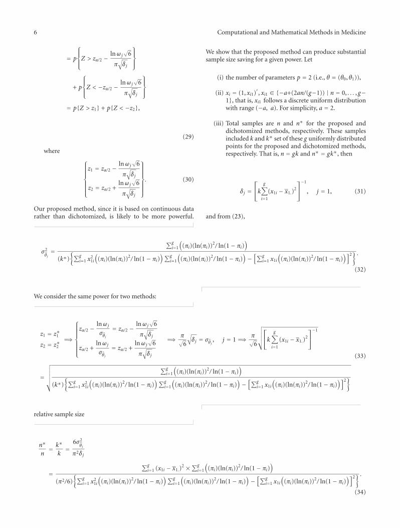
Our proposed method, since it is based on continuous datarather than dichotomized, is likely to be more powerful.

We show that the proposed method can produce substantialsample size saving for a given power. Let

(i) the number of parameters p = 2 (i.e., θ = (θ0, θ1)),

(ii) xi = (1, xi1)′, xi1 ∈ {−a+(2an/(g−1)) | n = 0, . . . , g−1}, that is, xi1 follows a discrete uniform distributionwith range (−a, a). For simplicity, a = 2.

(iii) Total samples are n and n∗ for the proposed anddichotomized methods, respectively. These samplesincluded k and k∗ set of these g uniformly distributedpoints for the proposed and dichotomized methods,respectively. That is, n = gk and n∗ = gk∗, then

δj =⎡⎣k

g∑

i=1

(x1i − x1.)2

⎤⎦−1

, j = 1, (31)

and from (23),

σ2θ j=

∑gi=1

((πi)(ln(πi))2/ ln(1− πi)

)

(k∗){∑g

i=1 x21i


)∑gi=1


)−[∑g

i=1 x1i


)]2} .

(32)

We consider the same power for two methods:

z1 = z∗1z2 = z∗2

=⇒

⎧⎪⎪⎪⎪⎪⎨⎪⎪⎪⎪⎪⎩

zα/2 −lnωj

σθj= zα/2 −

lnωj√

6

π√δj

zα/2 +lnωj

σθj= zα/2 +

lnωj√

6

π√δj

=⇒ π√6

√δj = σθj , j = 1 =⇒ π√

6

√√√√√⎡⎣k

g∑

i=1

(x1i − x1.)2

⎤⎦−1

=

√√√√√√

∑gi=1


)

(k∗){∑g

i=1 x21i


)∑gi=1


)−[∑g

i=1 x1i


)]2}

(33)

relative sample size

n∗

n= k∗

k=

6σ2θ j

π2δj

=∑g

i=1 (x1i − x1.)2 ×∑g

i=1


)

(π2/6){∑g

i=1 x21i


)∑gi=1


)−[∑g

i=1 x1i


)]2} .

(34)


Table 1: Relative sample sizes required to attain any power for the dichotomizing method versus the proposed method.

ω∗ = exp(θ)Average proportion of successes (π)

0.1 0.2 0.3 0.4 0.5

0.25 23.7166 9.5092 7.4954 7.1996 6.8575

0.50 10.6719 5.4176 3.4215 2.5209 2.1784

0.75 7.7088 3.8713 2.5171 1.9380 1.5841

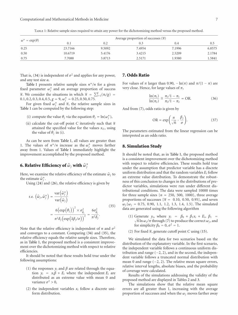
That is, (34) is independent of σ2 and applies for any power,and any test size α.

Table 1 presents relative sample sizes n∗/n for a givenfixed parameter ω∗j and an average proportion of success

π. We consider the situations in which π = ∑gi=1(πi/g) =

0.1, 0.2, 0.3, 0.4, 0.5, g = 9, ω∗j = 0.25, 0.50, 0.75.For given fixed ω∗j and π, the relative sample sizes in

Table 1 can be computed by the following step:

(i) compute the value θj via the equation θj = ln(ω∗j ),

(ii) calculate the cut-off point C iteratively such that πattained the specified value for the values xi1, usingthe value of θj in (i).

As can be seen from Table 1, all values are greater than1. The values of n∗/n increase as the ω∗j moves fartheraway from 1. Values of Table 1 immediately highlight theimprovement accomplished by the proposed method.

6. Relative Efficiency of ω j with ω∗j

Here, we examine the relative efficiency of the estimate ω j tothe estimate ω∗j .

Using (24) and (26), the relative efficiency is given by

r.e.(ω j , ω∗j

)=

var(ω∗j)

var(ω j

)

=6(

exp(θj))2 × σ2

θ j

π2δj(

exp(λβj/σ

))2 =6σ2

θ j

π2δj.

(35)

Note that the relative efficiency is independent of n and σ2

and converges to a constant. Comparing (34) and (35), therelative efficiency equals the relative sample sizes. Therefore,as in Table 1, the proposed method is a consistent improve-ment over the dichotomizing method with respect to relativeefficiencies.

It should be noted that these results hold true under thefollowing assumptions:

(1) the responses yi and β are related through the equa-tion yi = xiβ + Ei where the independent Ei aredistributed as an extreme value with mean 0 andvariance σ2 > 0,

(2) the independent variables xi follow a discrete uni-form distribution.

7. Odds Ratio

For values of π larger than 0.90, − ln(π) and π/(1 − π) arevery close. Hence, for large values of π,

ln(π1)ln(π2)

∼= π1/1− π1

π2/1− π2= OR. (36)

And from (7), odds ratio is given by

OR = exp

(π√6· βj

σ

). (37)

The parameters estimated from the linear regression can beinterpreted as an odds ratio.

8. Simulation Study

It should be noted that, as in Table 1, the proposed methodis a consistent improvement over the dichotomizing methodwith respect to relative efficiencies. These results hold trueunder the assumption that predictor variable has a discreteuniform distribution and that the random variables Ei followan extreme value distribution. To demonstrate the robust-ness of this conclusion to changes in the distributions of pre-dictor variables, simulations were run under different dis-tributional conditions. The data were sampled 10000 timesfor three sample sizes {n = 250, 500, 1000}, three averageproportions of successes {π = 0.10, 0.50, 0.95}, and sevenωj{ωj = 0.75, 0.90, 1.1, 1.2, 1.3, 1.4, 1.5}. The simulateddata are generated using the following algorithm

(1) Generate yi, where yi = β0 + β1xi + Ei, β1 =√6 lnωj/π through (7) to produce the correctωj , and

for simplicity β0 = 0, σ2 = 1.

(2) For fixed π, generate cutoff point C using (15).

We simulated the data for two scenarios based on thedistribution of the explanatory variable. In the first scenario,the independent variable follows a continuous uniform dis-tribution and range (−2, 2), and in the second, the indepen-dent variable follows a truncated normal distribution withmean 0 and range (−2, 2). The relative mean square errors,relative interval lengths, absolute biases, and the probabilityof coverage were calculated.

Results of the simulations addressing the validity of theproposed method are displayed in Tables 2 and 3.

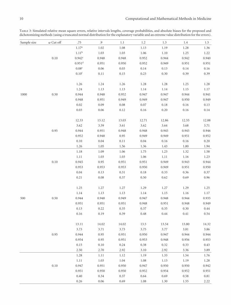
The simulations show that the relative mean squareerrors are all greater than 1, increasing with the averageproportion of successes and when the ωj moves farther away


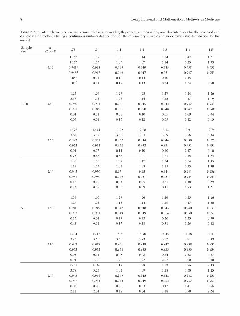
Table 2: Simulated relative mean square errors, relative intervals lengths, coverage probabilities, and absolute biases for the proposed anddichotomizing methods (using a continuous uniform distribution for the explanatory variable and an extreme value distribution for theerrors).

Samplesize

ωCut off

.75 .9 1.1 1.2 1.3 1.4 1.5

1.15a 1.07 1.09 1.14 1.24 1.47 1.71

1.10b 1.03 1.03 1.07 1.14 1.23 1.35

0.10 0.943c 0.948 0.949 0.949 0.945 0.938 0.933

0.948d 0.947 0.949 0.947 0.951 0.947 0.953

0.05e 0.04 0.12 0.14 0.10 0.15 0.11

0.07f 0.01 0.17 0.13 0.24 0.34 0.58

1.23 1.26 1.27 1.28 1.27 1.24 1.26

2.16 1.13 1.23 1.14 1.15 1.17 1.19

1000 0.50 0.940 0.951 0.951 0.945 0.942 0.937 0.934

0.951 0.949 0.951 0.950 0.948 0.947 0.948

0.04 0.01 0.08 0.10 0.05 0.09 0.04

0.05 0.04 0.15 0.12 0.09 0.12 0.13

12.75 12.44 13.22 12.68 13.14 12.91 12.79

3.67 3.57 3.58 3.63 3.69 3.76 3.84

0.95 0.943 0.951 0.952 0.944 0.944 0.938 0.929

0.952 0.954 0.952 0.952 0.951 0.951 0.951

0.04 0.07 0.11 0.10 0.10 0.17 0.10

0.75 0.68 0.86 1.01 1.21 1.45 1.24

1.30 1.08 1.07 1.17 1.24 1.54 1.95

1.16 1.03 1.04 1.08 1.15 1.25 1.39

0.10 0.942 0.950 0.951 0.95 0.944 0.941 0.936

0.951 0.950 0.949 0.951 0.954 0.954 0.953

0.12 0.07 0.24 0.25 0.21 0.18 0.29

0.23 0.08 0.33 0.39 0.41 0.73 1.21

1.35 1.10 1.27 1.26 1.26 1.25 1.26

1.26 1.03 1.13 1.14 1.16 1.17 1.20

500 0.50 0.940 0.949 0.947 0.948 0.943 0.940 0.933

0.952 0.951 0.949 0.949 0.954 0.950 0.951

0.23 0.34 0.27 0.23 0.26 0.25 0.38

0.48 0.11 0.17 0.18 0.31 0.26 0.42

13.04 13.17 13.8 13.90 14.45 14.48 14.47

3.72 3.65 3.68 3.73 3.82 3.91 3.99

0.95 0.942 0.947 0.951 0.949 0.947 0.938 0.935

0.953 0.952 0.954 0.955 0.955 0.953 0.954

0.05 0.11 0.08 0.08 0.24 0.32 0.27

0.94 1.38 1.78 1.92 2.52 3.00 2.90

13.41 14.46 1.12 1.28 1.52 1.96 2.33

3.78 3.73 1.04 1.09 1.18 1.30 1.45

0.10 0.942 0.949 0.949 0.945 0.942 0.942 0.933

0.957 0.954 0.948 0.949 0.952 0.957 0.953

0.02 0.20 0.38 0.33 0.42 0.41 0.66

2.11 2.74 0.42 0.84 1.18 1.78 2.24


Table 2: Continued.

Samplesize

ωCut off

.75 .9 1.1 1.2 1.3 1.4 1.5

1.27 1.25 1.32 1.28 1.30 1.30 1.29

1.16 1.13 1.13 1.14 1.16 1.18 1.20

250 0.50 0.941 0.948 0.952 0.947 0.945 0.943 0.933

0.951 0.951 0.951 0.950 0.951 0.951 0.951

0.12 0.13 0.35 0.44 0.41 0.53 0.55

0.11 0.22 0.39 0.47 0.51 0.74 0.59

12.98 14.6 15.64 15.46 17.05 16.89 18.33

3.75 3.72 3.82 3.88 4.01 4.12 4.29

0.95 0.945 0.955 0.946 0.948 0.940 0.937 0.932

0.959 0.955 0.955 0.959 0.958 0.957 0.952

0.02 0.16 0.39 0.22 0.46 0.47 0.51

1.22 2.75 3.97 3.98 4.99 5.19 6.19

a: Relative mean square errors, b: Relative intervals lengths, c: Coverage probability (proposed), d: Coverage probability (dichotomized), e: % bias (proposed),f: % bias (dichotomized).

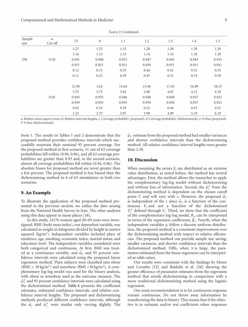
from 1. The results in Tables 1 and 2 demonstrate that theproposed method provides confidence intervals which suc-cessfully maintain their nominal 95 percent coverage. Forthe proposed method in first scenario, 51 out of 63 coverageprobabilities fell within (0.94, 0.96), and all 63 coverage pro-babilities are greater than 0.93 and, in the second scenario,almost all coverage probabilities fell within (0.94, 0.96). Theabsolute biases for proposed method are never greater thana few percent. The proposed method is less biased than thedichotomizing method in 6 of 63 simulations in both twoscenarios.

9. An Example

To illustrate the application of the proposed method pre-sented in the previous section, we utilize the data arisingfrom the National Health Survey in Iran. The other analysesusing this data appear in many places [16].

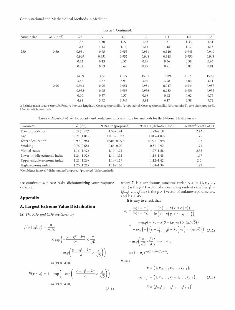
In this study, 14176 women aged 20–69 years were inves-tigated. BMI (body mass index), our dependent variable, wascalculated as weight in kilograms divided by height in meterssquared (kg/m2). Independent variables included place ofresidence, age, smoking, economic index, marital status, andeducation level. The independent variables considered wereboth categorical and continuous. At first, BMI was treat-ed as a continuous variable, and ω j and 95 percent con-fidence intervals were calculated using the proposed linearregression method. Then subjects were classified into obese(BMI ≥ 30 kg/m2) and nonobese (BMI <30 kg/m2). A com-plementary log-log model was used for the binary analysis,with obese or nonobese used as the outcome measure. Theω∗j and 95 percent confidence intervals were calculated usingthe dichotomized method. Table 4 presents the coefficientestimates, estimated confidence intervals, and relative con-fidence interval lengths. The proposed and dichotomizingmethods produced different confidence intervals, althoughthe ω j and ω∗j were similar only varying slightly. The

ω j estimate from the proposed method had smaller variancesand shorter confidence intervals than the dichotomizingmethod. All relative confidence interval lengths were greaterthan 2.58.

10. Discussion

When assuming the errors Ei are distributed as an extremevalue distribution, as noted before, the method has severaladvantages. First, the method allows the researcher to applythe complementary log-log model without dichotomizingand without loss of information. Second, the ω∗j from thedichotomizing method is dependent on the chosen cutoffpoint C and will vary with c. However, the proposed ω j

is independent of the c since ω j is a function of the con-tinuous Yi and not a function of the dichotomizedY∗i defined through C. Third, we show that the coefficientof the complementary log-log model, θj , can be interpretedin terms of the regression coefficients, βj . Fourth, when theindependent variables xi follow a discrete uniform distribu-tion, the proposed method is a consistent improvement overthe dichotomizing method with respect to relative efficien-cies. The proposed method can provide sample size saving,smaller variances, and shorter confidence intervals than thedichotomized method. Fifth, when π is large, the para-meters estimated from the linear regression can be interpret-ed as odds ratios.

Our results were consistent with the findings by Moserand Coombs [12] and Bakhshi et al. [16] showing thegreater efficiency of parameter estimates from the regressionmethod that avoids dichotomizing in comparison with amore traditional dichotomizing method using the logisticregression.

Our main recommendation is to let continuous responseremain continuous. Do not throw away information bytransforming the data to binary. This means that if the objec-tive is to estimate and/or test coefficients when responses


Table 3: Simulated relative mean square errors, relative intervals lengths, coverage probabilities, and absolute biases for the proposed anddichotomizing methods (using a truncated normal distribution for the explanatory variable and an extreme value distribution for the errors).

Sample size ω Cut off .75 .9 1.1 1.2 1.3 1.4 1.5

1.17a 1.02 1.08 1.13 1.19 1.28 1.36

1.11b 1.03 1.03 1.06 1.10 1.25 1.22

0.10 0.942c 0.948 0.948 0.952 0.944 0.942 0.940

0.951d 0.951 0.950 0.952 0.949 0.951 0.951

0.08e 0.06 0.03 0.14 0.13 0.14 0.16

0.10f 0.11 0.15 0.23 0.30 0.39 0.39

1.26 1.24 1.26 1.28 1.28 1.25 1.28

1.24 1.13 1.13 1.14 1.14 1.15 1.17

1000 0.50 0.944 0.948 0.952 0.947 0.947 0.944 0.941

0.948 0.951 0.949 0.949 0.947 0.950 0.949

0.02 0.09 0.08 0.07 0.18 0.16 0.13

0.03 0.06 0.12 0.16 0.20 0.16 0.14

12.33 13.12 13.03 12.71 12.86 12.55 12.88

3.62 3.59 3.61 3.62 3.64 3.68 3.71

0.95 0.944 0.951 0.948 0.948 0.945 0.945 0.946

0.952 0.948 0.95 0.949 0.949 0.951 0.952

0.10 0.04 0.11 0.04 0.16 0.16 0.20

1.26 1.05 1.56 1.36 1.43 1.80 1.94

1.18 1.09 1.06 1.75 1.23 1.32 1.58

1.11 1.03 1.03 1.06 1.11 1.16 1.23

0.10 0.945 0.95 0.951 0.951 0.949 0.943 0.944

0.953 0.953 0.953 0.950 0.949 0.951 0.950

0.04 0.13 0.31 0.18 0.33 0.36 0.37

0.21 0.08 0.37 0.50 0.62 0.69 0.96

1.25 1.27 1.27 1.29 1.27 1.29 1.25

1.14 1.13 1.13 1.14 1.15 1.16 1.17

500 0.50 0.944 0.948 0.949 0.947 0.948 0.944 0.935

0.951 0.951 0.951 0.948 0.951 0.948 0.949

0.13 0.22 0.35 0.37 0.35 0.30 0.44

0.16 0.19 0.39 0.48 0.44 0.41 0.54

13.11 14.02 14.02 13.5 13.54 13.80 14.32

3.73 3.71 3.73 3.75 3.77 3.81 3.86

0.95 0.944 0.95 0.951 0.950 0.947 0.944 0.944

0.954 0.95 0.951 0.953 0.948 0.956 0.953

0.15 0.10 0.24 0.38 0.32 0.33 0.43

2.50 2.70 2.92 3.10 2.92 3.36 3.89

1.28 1.11 1.12 1.19 1.33 1.54 1.76

1.11 1.03 1.04 1.08 1.13 1.19 1.28

0.10 0.947 0.951 0.950 0.947 0.950 0.950 0.942

0.951 0.950 0.950 0.952 0.954 0.952 0.951

0.40 0.34 0.37 0.64 0.69 0.58 0.81

0.26 0.06 0.69 1.08 1.30 1.55 2.22


Table 3: Continued.

Sample size ω Cut off .75 .9 1.1 1.2 1.3 1.4 1.5

1.32 1.30 1.27 1.33 1.31 1.33 1.31

1.15 1.13 1.13 1.14 1.18 1.17 1.18

250 0.50 0.951 0.95 0.953 0.951 0.940 0.945 0.940

0.949 0.951 0.952 0.948 0.948 0.950 0.948

0.22 0.43 0.57 0.69 0.66 0.58 0.66

0.38 0.53 0.64 0.89 0.91 0.82 0.91

14.09 14.51 16.27 15.91 15.89 15.73 15.60

3.86 3.87 3.93 3.92 3.98 4.04 4.11

0.95 0.943 0.95 0.951 0.951 0.947 0.944 0.937

0.953 0.95 0.953 0.956 0.953 0.956 0.952

0.30 0.37 0.57 0.68 0.42 0.62 0.75

4.98 5.52 6.547 5.91 6.17 6.88 7.72

a: Relative mean square errors, b: Relative intervals lengths, c: Coverage probability (proposed), d: Coverage probability (dichotomized), e: % bias (proposed),f: % bias (dichotomized).

Table 4: Adjusted ω∗j , ω j for obesity and confidence intervals using two methods for the National Health Survey.

Covariates ω j(ω∗j ) 95% CIa (proposed) 95% CI (dichotomized) Relativeb length of CI

Place of residence 1.65 (1.97)c 1.58–1.74 1.79–2.18 2.43

Age 1.021 (1.019) 1.018–1.022 1.015–1.022 1.75

Years of education 0.99 (0.98) 0.985–0.997 0.971–0.994 1.92

Smoking 0.76 (0.68) 0.66–0.90 0.51–0.92 1.71

Marital status 1.16 (1.42) 1.10–1.22 1.27–1.58 2.58

Lower-middle economy index 1.24 (1.32) 1.14–1.32 1.18–1.48 1.67

Upper-middle economy index 1.21 (1.26) 1.14–1.29 1.12–1.42 2.0

High economy index 1.20 (1.21) 1.11–1.30 1.08–1.36 1.47aConfidence interval, bdichotomized/proposed, cproposed (dichotomized).

are continuous, please resist dichotomizing your responsevariable.

Appendix

A. Largest Extreme Value Distribution

(a) The PDF and CDF are Given by

f(y | xβ, σ

) = π

σ√

6

× exp

(− y − xβ − kσ

σ× π√

6

− exp

(y − xβ− kσ

σ× π√

6

))

−∞〈x〈∞, σ〉0,

P(y ≤ c

) = 1− exp

(− exp

(− c − xβ− kσ

σ× π√

6

))

−∞〈x〈∞, σ〉0,(A.1)

where Y is a continuous outcome variable, x = (1, x1, . . . ,xp−1) is the p×1 vector of known independent variables, β =(β0,β1, . . . ,βp−1) is the p× 1 vector of unknown parameters,and k ≈ 0.45.

It is easy to check that

ωj = ln(1− π1)ln(1− π2)

= ln(1− p

(y ≤ c | x))

ln(

1− p(y ≤ c | x(−1, j)

))

= − exp(−((c − x′β − kσ

)/σ)× (π/√6

))

− exp(−((

c − x′(−1, j)β − kσ)/σ)× (π/√6

))

= exp

(π√6· βj

σ

)=⇒ 1− π1

= (1− π2)exp((π/√

6)·(βj /σ)),

(A.2)

where

x =(

1, x1, . . . , xj , . . . , xp−1

),

x(−1, j) =(

1, x1, . . . , xj − 1, . . . , xp−1

),

β =(β0,β1, . . . ,βj , . . . ,βp−1

)′.

(A.3)


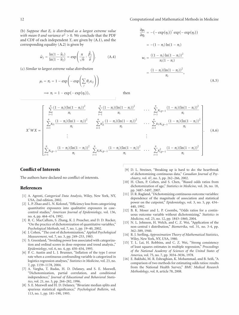
(b) Suppose that Ei is distributed as a largest extreme valuewith mean 0 and variance σ2 > 0. We conclude that the PDFand CDF of each independent Yi are given by (A.1), and thecorresponding equality (A.2) is given by

ω j = ln(1− π1)ln(1− π2)

= exp

⎛⎝ π√

6· β j

σ

⎞⎠. (A.4)

(c) Similar to largest extreme value distribution

μi = πi = 1− exp

⎛⎝− exp

⎛⎝∑

j

θ jxi j

⎞⎠⎞⎠

=⇒ πi = 1− exp(− exp

(ηi))

,

∂μi∂ηi

= −(− exp(ηi))′ exp

(− exp(ηi))

= −(1− πi) ln(1− πi)

wi = ((1− πi) ln(1− πi))2

πi(1− πi)

= (1− πi)(ln(1− πi))2

πi,

(A.5)

then

X ′WX =

⎡⎢⎢⎢⎢⎢⎢⎢⎢⎢⎢⎢⎢⎢⎢⎢⎢⎢⎢⎢⎣

n∑

i=1

(1− πi)(ln(1− πi))2

πi

n∑

i=1

(1− πi)(ln(1− πi))2

πi· · ·

n∑

i=1

xi,p−1(1− πi)(ln(1− πi))2

πi

n∑

i=1

xi1(1− πi)(ln(1− πi))2

πi

n∑

i=1

x2i1

(1− πi)(ln(1− πi))2

πi· · ·

n∑

i=1

x1xi,p−1(1− πi)(ln(1− πi))2

πi

......

n∑

i=1

xi,p−1(1− πi)(ln(1− πi))2

πi

n∑

i=1

xixi,p−1(1− πi)(ln(1− πi))2

πi· · ·

n∑

i=1

x2i,p−1

(1− πi)(ln(1− πi))2

πi

⎤⎥⎥⎥⎥⎥⎥⎥⎥⎥⎥⎥⎥⎥⎥⎥⎥⎥⎥⎥⎦

. (A.6)

Conflict of Interests

The authors have declared no conflict of interests.

References

[1] A. Agresti, Categorical Data Analysis, Wiley, New York, NY,USA, 2nd edition, 2002.

[2] L. P. Zhao and L. N. Kolonel, “Efficiency loss from categorizingquantitative exposures into qualitative exposures in case-control studies,” American Journal of Epidemiology, vol. 136,no. 4, pp. 464–474, 1992.

[3] R. C. MacCallum, S. Zhang, K. J. Preacher, and D. D. Rucker,“On the practice of dichotomization of quantitative variables,”Psychological Methods, vol. 7, no. 1, pp. 19–40, 2002.

[4] J. Cohen, “The cost of dichotomization,” Applied PsychologicalMeasurement, vol. 7, no. 3, pp. 249–253, 1983.

[5] S. Greenland, “Avoiding power loss associated with categoriza-tion and ordinal scores in dose-response and trend analysis.,”Epidemiology, vol. 6, no. 4, pp. 450–454, 1995.

[6] P. C. Austin and L. J. Brunner, “Inflation of the type I errorrate when a continuous confounding variable is categorized inlogistics regression analyses,” Statistics in Medicine, vol. 23, no.7, pp. 1159–1178, 2004.

[7] A. Vargha, T. Rudas, H. D. Delaney, and S. E. Maxwell,“Dichotomization, partial correlation, and conditionalindependence,” Journal of Educational and Behavioral Statis-tics, vol. 21, no. 3, pp. 264–282, 1996.

[8] S. E. Maxwell and H. D. Delaney, “Bivariate median splits andspurious statistical significance,” Psychological Bulletin, vol.113, no. 1, pp. 181–190, 1993.

[9] D. L. Streiner, “Breaking up is hard to do: the heartbreakof dichotomizing continuous data,” Canadian Journal of Psy-chiatry, vol. 47, no. 3, pp. 262–266, 2002.

[10] H. Chen, P. Cohen, and S. Chen, “Biased odds ratios fromdichotomization of age,” Statistics in Medicine, vol. 26, no. 18,pp. 3487–3497, 2007.

[11] D. R. Ragland, “Dichotomizing continuous outcome variables:dependence of the magnitude of association and statisticalpower on the cutpoint,” Epidemiology, vol. 3, no. 5, pp. 434–440, 1992.

[12] B. K. Moser and L. P. Coombs, “Odds ratios for a contin-uous outcome variable without dichotomizing,” Statistics inMedicine, vol. 23, no. 12, pp. 1843–1860, 2004.

[13] N. L. Johnson, H. Welch, and C. Z. Wei, “Application of thenon-central t distribution,” Biometrika, vol. 31, no. 3-4, pp.362–389, 1940.

[14] R. J. Serfling, Approximation Theory of Mathematical Statistics,Wiley, New York, NY, USA, 1980.

[15] T. L. Lai, H. Robbins, and C. Z. Wei, “Strong consistencyof least squares estimates in multiple regression,” Proceedingsof the National Academy of Sciences of the United States ofAmerica, vol. 75, no. 7, pp. 3034–3036, 1978.

[16] E. Bakhshi, M. R. Eshraghian, K. Mohammad, and B. Seifi, “Acomparison of two methods for estimating odds ratios: resultsfrom the National Health Survey,” BMC Medical ResearchMethodology, vol. 8, article 78, 2008.

let continuous outcome variables remain continuous

Documents