self-similarity parameter estimation and reproduction property for non-gaussian hermite processes
TRANSCRIPT

Self-similarity parameter estimation and reproduction
property for non-Gaussian Hermite processes
Alexandra Chronopoulou, Ciprian Tudor, Frederi Viens
To cite this version:
Alexandra Chronopoulou, Ciprian Tudor, Frederi Viens. Self-similarity parameter estimationand reproduction property for non-Gaussian Hermite processes. 2008. <hal-00294038v1>
HAL Id: hal-00294038
https://hal.archives-ouvertes.fr/hal-00294038v1
Submitted on 8 Jul 2008 (v1), last revised 18 Jan 2010 (v2)
HAL is a multi-disciplinary open accessarchive for the deposit and dissemination of sci-entific research documents, whether they are pub-lished or not. The documents may come fromteaching and research institutions in France orabroad, or from public or private research centers.
L’archive ouverte pluridisciplinaire HAL, estdestinee au depot et a la diffusion de documentsscientifiques de niveau recherche, publies ou non,emanant des etablissements d’enseignement et derecherche francais ou etrangers, des laboratoirespublics ou prives.

Self-similarity parameter estimation and reproduction property for
non-Gaussian Hermite processes
Alexandra Chronopoulou1 Ciprian A. Tudor2 Frederi G. Viens1,∗
1 Department of Statistics, Purdue University,
150 N. University St., West Lafayette, IN 47907-2067, USA.
[email protected] [email protected] ∗
2SAMOS-MATISSE, Centre d’Economie de La Sorbonne,
Universite de Paris 1 Pantheon-Sorbonne ,
90, rue de Tolbiac, 75634, Paris, France.
July 8, 2008
Abstract
We consider the class of all the Hermite processes (Z(q,H)t )t∈[0,1] of order q ∈ N
∗ and with Hurst
parameter H ∈ ( 12, 1). The process Z(q,H) is H-selfsimilar, it has stationary increments and it exhibits
long-range dependence identical to that of fractional Brownian motion (fBm). For q = 1, Z(1,H) is fBm,which is Gaussian; for q = 2, Z(2,H) is the Rosenblatt process, which lives in the second Wiener chaos;for any q > 2, Z(q,H) is a process in the qth Wiener chaos. We study the variations of Z(q,H) for any q,by using multiple Wiener -Ito stochastic integrals and Malliavin calculus.
We prove a reproduction property for this class of processes in the sense that the terms appearing inthe chaotic decomposition of their variations give rise to other Hermite processes of different orders andwith different Hurst parameters. We apply our results to construct a strongly consistent estimator forthe self-similarity parameter H from discrete observations of Z(q,H); the asymptotics of this estimator,after appropriate normalization, are proved to be distributed like a Rosenblatt random variable (valueat time 1 of a Rosenblatt process).with self-similarity parameter 1 + 2(H − 1)/q.
2000 AMS Classification Numbers: Primary: 60G18; Secondary 60F05, 60H05, 62F12.
Key words: multiple Wiener integral, Hermite process, fractional Brownian motion, non-centrallimit theorem, quadratic variation, self-similarity, Malliavin calculus, parameter estimation.
1 Introduction
1.1 Background and motivation
The variations of a stochastic process play a crucial role in its probabilistic and statistical analysis. Bestknown is the quadratic variation of a semimartingale, which is crucial for its Ito formula; quadratic varia-tion also has a direct utility in practice, in estimating unknown parameters, such as volatility in financialmodels, in the so-called “historical” context. For self-similar stochastic processes, the study of their varia-tions constitutes a fundamental tool to construct good estimators of their self-similarity parameters. Theseprocesses are well suited to model various phenomena where long memory is an important factor (internettraffic, hydrology, econometrics, among others). The most important modeling task is then to determine orestimate the self-similarity parameter, because it is also typically responsible for the process’s long memoryand its regularity properties. Estimating this parameter is thus an important research direction in theory
∗Corresponding author ; research partially supported by NSF grant DMS 0606615.
1

and practice. Several approaches, such as wavelets, variations, maximum likelihood methods, have beenproposed. We refer to the monograph [1] for a complete exposition.
The family of Gaussian processes known as fractional Brownian motion (fBm) is particularly in-teresting, and most popular among self-similar processes, because of fBm’s stationary increments, its clearsimilarities and differences with standard Brownian motion, and the fact that its self-similarity parameterH , known as the Hurst parameter, is also immediately interpreted as both the memory length parameter(the correlation of unit length increments which are n time units apart decays slowly at the speed n2H−2)and the regularity parameter (fBm is α-Holder continuous on any bounded time interval for any α < H).
Soon after fBm’s inception, the study of its variations began in the 1970’s and 1980’s; of interestto us in the present article are several such studies of variations which uncovered a generalization of fBmto non-Gaussian processes known as the Rosenblatt process and other Hermite processes: [2], [5], [7], [20]or [21]. We briefly recall some relevant basic facts. We consider (BH
t )t∈[0,1] a fractional Brownian motionwith Hurst parameter H ∈ (0, 1). As such, BH is the continuous centered Gaussian process with covariancefunction
RH(t, s) = E [BtBs] =1
2
(
s2H + t2H − |t − s|2H)
, s, t ∈ [0, 1].
Equivalently, B0 = 0 and E[
(Bs − Bt)2]
= |t − s|2H. It is the only continuous Gaussian process H which is
self-similar with stationary increments. Consider the regular partition of the interval [0, 1] as 0 = t0 < t1 <. . . < tN = 1 with ti = i
N , and define the following q-variations
v(q)N =
N−1∑
i=0
Hq
BHti+1
− BHti
(
E
[
(
BHti+1
− BHti
)2])
12
=
N−1∑
i=0
Hq
(
(ti+1 − ti)−H(
BHti+1
− BHti
))
(1)
for any integer q ≥ 2, where Hq is the Hermite polynomial of degree q. Then it follows from the abovereferences that:
• for 0 ≤ H ≤ 1 − 12q the limit in distribution of N− 1
2 v(q)N is a centered Gaussian random variable,
• for 1 − 12q < H < 1 the limit of N q(1−H)−1v
(q)N is a Hermite random variable of order q with self-
similarity parameter q(H − 1) + 1.
This latter random variable is non-Gaussian; it equals the value at time 1 of a Hermite process,which is a stochastic process in the qth Wiener chaos with the same covariance structure as fBm; as such,the Hermite process has stationary increments and shares the same self-similarity, regularity, and longmemory properties as fBm; see Definition 1.
Because of a natural coupling, the last limit above also holds in L2(Ω) (see [14]). In the criticalcase H = 1 − 1
2q the limit is still Gaussian but the normalization involves a logarithm. These results are
widely applied to estimation problems; to avoid the barrier H = 34 that occurs in the case q = 2, one can use
“higher-order filters”, which means that the increments of the fBm are replaced by higher-order increments,such as discrete versions of higher-order derivatives, in order to obtain a Gaussian limit for any H (see [9],[8], [4]).
Nonetheless, the appearance of Hermite random variables in the above non-central limit theoremsbegs the study of Hermite processes as such. Their practical aspects are striking: they provide a wide classof processes from which to model long memory, self-similarity, and Holder-regularity, allowing significantdeviation from fBm and other Gaussian processes, without having to invoke non-linear stochastic differentialequations based on fBm, thereby avoiding the notorious issues associated with such equations (see [15]). Justas in the case of fBm, the estimation of the Hermite process’s parameter H is crucial for proper modeling;to our knowledge it has not been treated in the literature. We choose to tackle this issue by using variationsmethods, to find out how the above central and non-central limit theorems fit into a larger picture.
2

A note regarding the usage of the letter q: in the known results above, this letter was used to discussthe q-th variations (in the sense Hermite polynomials) for fBm data; in this article, in contrast to theseclassical works, we will use data from a Hermite process of order q, and will only consider its quadraticvariation. The historical motivation in the above non-central limit theorem explains this coincidence ofnotation.
Lastly, we mention that various very recent and interesting results, which are beyond the scopeof this article, have been proven for weighted power variations of stochastic processes such as fractionalBrownian motion (see [11], [14], [13]), fractional Brownian sheets (see [18]), iterated Brownian motion (see[12]) or the solution of the stochastic heat equation (see [19] or [3]).
1.2 Main results: summary and discussion
In this article, we show results that are interesting from a theoretical viewpoint, such as the reproducingproperties (the variations of Hermite processes give birth to other Hermite processes); and we provide anapplication to parameter estimation, in which care is taken to show that the estimators can be evaluatedpractically.
Let Z(q,H) be a Hermite process of order q ∈ N∗ with self-similarity parameter H ∈ (12 , 1) (see
Definition 1 further below). Define the centered quadratic variation statistic
VN :=1
N
N−1∑
i=0
(
Z(q,H)i+1
N
− Z(q,H)iN
)2
E
[
(
Z(q,H)i+1
N
− Z(q,H)i
N
)2] − 1
.
Also define some constants which will recur throughout this article:
d(H) : =(2(2H − 1))
1/2
(H + 1)H1/2, (2)
H ′ : = 1 +(H − 1)
q.
1.2.1 Convergence of VN
We prove that, under suitable normalization, the sequence VNN∈Nconverges in L2(Ω) to a Rosenblatt
random variable.
Theorem 1 Let H ∈ (1/2, 1) and q ∈ N r 0, 1. Let Z(q,H) be a Hermite process of order q and self-similarity parameter H (see Definition 1). Define
c = (q!)−1 (4H ′ − 3)1/2(4H ′ − 2)1/2
2d(H)2(H ′(2H ′ − 1))q−1.
Then cN (2−2H)/qVN converges in L2 (Ω) to a standard Rosenblatt random variable with parameter H ′′ :=2(H−1)
q + 1, which is the value at time 1 of a Hermite process of order 2 and self-similarity parameter H ′′.
The Rosenblatt random variable is a double integral with respect to the same Wiener process usedto define the Hermite process; it is thus an element of the second Wiener chaos. In reference to (1) and theresults described thereafter [q = 2 in (1) means normal convergence of normalized quadratic variation forH ≤ 3/4 for fBm data], our Theorem 1 shows that fBm is the only Hermite process for which there existsa range for the parameter H allowing normal convergence of the quadratic variation, while for all otherHermite processes, convergence to a second chaos (Rosenblatt) random variable is universal for all H .
Our proofs are based on chaos expansion into multiple Wiener integrals and Malliavin calculus.
The main line of the proof is as follows: since the variable Z(q,H)t is an element of the qth Wiener chaos,
the product formula for multiple integrals implies that the statistics VN can be decomposed into a sum of
3

multiple integrals from the order 2 to the order 2q. The dominant term in this decomposition, which givesthe final renormalization order N (2−2H)/q, is the term which is a double Wiener integral, and one proves italways converges to a Rosenblatt random variable; all other terms are of much lower orders, which is whythe only remaining term, after renormalization, converges to a second chaos random variable. The differencewith the fBm case comes from the limit of the term of order 2, which in that case is sometimes Gaussianand sometimes Rosenblatt-distributed, depending on the value of H (see [23] for instance).
1.2.2 Convergence of each term in the chaos decomposition of VN : reproduction property
We also study the limits of the other terms in the decomposition of VN , those of order higher than 2,which we can call Tk : 2, 4, · · · , 2q, and we obtain interesting facts: for every k = 2, 4, · · · , 2(q − 1), thenormalization of the kth Wiener chaos term Tk of VN has a limit which is a Hermite random variable oforder k. We call this the reproduction property for Hermite processes, because from one Hermite process oforder q, one can reconstruct other Hermite processes of all even orders from 2 to 2 (q − 1). As an exceptionto this rule, the normalized term of highest order 2q follows a dichotomy: it converges to a Hermite r.v. oforder 2q if H > 3/4, but converges to Gaussian limit if H ∈ (1/2, 3/4] (the lower half of this dichotomy hasbeen noticed for q = 2 in [23]).
Let us compare this more detailed reproduction and dichotomy phenomenon with the basic resultof Theorem 1 described in Section 1.2.1. If q ≥ 2 (non-Gaussian data case), T2 always converges to aRosenblatt r.v., and is in fact responsible for the global behavior of the entire VN , while T2q convergesinstead to a Gaussian limit iff H ≤ 3/4. But if q = 1 (case of fBm data), there is no distinction between T2
and T2q because they coincide with VN itself; in order for the fBm case’s classical dichotomy around H = 3/4to be consistent with our results for q ≥ 2, one sees that for fBm, the quadratic variation VN , which is inthe second Wiener chaos term, has nevertheless to be interpreted as “T2q” rather than “T2”.
Specifically, we have the following detailed result.
Theorem 2 Let Z(q,H) be a Hermite process with q ≥ 2, as in the previous theorem. Consider the Wienerchaos expansion of VN : we write
VN =
q∑
n=1
c2nT2n
where c2q−2k = k!(
qk
)2and T2n is a multiple Wiener integral of order 2n.
• For every H ∈ (1/2, 1) and for every k = 1, . . . , q− 1 the expression (zk,H)−1
N (2−2H)k/qT2k convergesin L2 (Ω) to Zr,K , a Hermite random variable of order r = 2k with self-similarity parameter K =2k(H ′ − 1) + 1, where zk,H is the constant defined by
zq−k,H = d(H)2 [H ′(2H ′ − 1)]k((H ′ − 1)k + 1)
−1(2(H ′ − 1) + 1)
−1.
• For every H ∈ (1/2, 3/4), with k = q, we have convergence in law of x−1/21,H
√NT2q to a standard nor-
mal distribution, with x1,H =(
∑q−1l=1 b2,H,l + 1 + (1/2)
∑∞k=1
(
2k2H − (k + 1)2H − (k − 1)2H)2)
where
b2,H,k = (q!)2(Cqk)22d(H)4a(H ′)2q
(
1 + 1/2∑∞
k=1
(
2k2H − (k + 1)2H − (k − 1)2H)2)
.
• For every H ∈ (3/4, 1), with k = q, we have convergence of x−1/22,H N2−2HT2q in L2(Ω) to Z2q,2H−1, a
Hermite r.v. of order 2q with parameter 2H − 1; here x2,H = (∑q−1
l=1 b1,H,l + H2(2H − 1)/(4H − 3))
and b1,H,l = (q!)2(Cql )22d(H)4a(H ′)2q
∫ 1
0 (1 − x)x4H−4dx.
• For H = 3/4, with k = q, we have convergence in law of√
N/ logNx−1/23,H T2q to a standard normal
distribution, with x3,H = (∑q−1
l=1 b3,H,l + 9/16) and b3,H,l = (q!)2(Cql )22d(H)4a(H ′)2q(1/2).
4

Some of the aspects of this theorem had been discovered in the case of q = 2 (Rosenblatt process) in[23]. In that paper, the existence of a higher-order chaos term with normal convergence had been exhibitedfor the Rosenblatt process with H < 3/4, while the case of H ≥ 3/4 had not been studied. The entirespectrum of convergences in Theorem 2 was not apparent in [23], however, because it was unclear whetherthe term T2’s convergence to a Rosenblatt r.v. was due to the fact that we were dealing with input comingfrom a Rosenblatt process, or whether it was a more general function of the structure of the second Wienerchaos. Here we see that the second alternative is true. In addition one can say that the case of q ∈ 1, 2alone was insufficient to understand the origins of the dichotomies, or lack thereof, around H = 3/4.
The paper [23] had exhibited a remarkable structure of the Rosenblatt data when H < 3/4. In thatcase, as we see in Theorem 2, there are only two terms in the expansion of VN , T2 and T4; moreover, and thisis the remarkable feature, the proper normalization of the term T2 converges in L2 (Ω) to none other thanthe Rosenblatt process at time 1. Since this value is part of the observed data, one can subtract it to takeadvantage of the Gaussian limit of the renormalized T4; an application to parameter estimation with normalasymptotics was included in [23] for H ≤ 3/4. In Theorem 2 above, if q ≥ 3, even if H ≤ 3/4, by whicha Gaussian limit can be constructed from the renormalized T2q, we still have at least two other terms inthe sequence T2, T4, · · ·T2q−2, and all but at most one of these will converge in L2 (Ω) to Hermite processeswith different orders, all different from q, which implies that they are not directly observed. This meansthat our Theorem 2 proves that the operation performed with Rosenblatt data, subtracting an observedquantity to isolate T2q and its Gaussian asymptotics, is not possible for any Hermite process with q ≥ 3.If one resorts to the artificial assumption that we observe all the Hermite processes associated with a fixedWiener process (coupling these processes via Definition 1), then one may perform a sequence of subtractionsand compensations to isolate T2q, generalizing the compensation operation done in one step in [23] for theRosenblatt data. It seems unlikely to us that this assumption may be available in any realistic modelingsituation; we do not comment further on such an extension.
1.2.3 Statistical estimation of H
The last aspect of this paper applies Theorem 1 to estimating the parameter H . Let SN be the empiricalmean of the individual squared increments
SN =1
N
N−1∑
i=0
(
Z(q,H)i+1
N
− Z(q,H)iN
)2
and letHN = − (log SN ) / (2 log N) .
We show that HN is a strongly consistent estimator of H , and we show asymptotic Rosenblatt distribution for
N2(1−H)/q(
H − H)
log N . The fact that this estimator fails to be asymptotically normal is not a problem
in itself. What is more problematic is the fact that if one tries to check one’s assumptions on the data bycomparing the asymptotics of H with a Rosenblatt distribution, one has to know something about the speedof the normalization factor N2(1−H)/q. Here, we prove in addition that one may replace H in this factor byHN , so that the asymptotic properties of HN can actually be checked.
Theorem 3 The estimator HN is strongly consistent, i.e. limN→∞ HN = H almost surely. Moreover thereexists a standard Rosenblatt random variable R with self-similarity parameter 1 + 2(H − 1)/q such that
limN→∞
E[∣
∣
∣2N2(1−HN)/q(
H − HN
)
log N − q!c1/21,H,qR
∣
∣
∣
]
= 0,
where, with a (H ′) :=(
1 + H−1q
)(
1 + 2H−1q
)
, c1,H,q := 2(∫ 1
0 (1 − x)x(2H′−2)(2q−2k)dx)a(H ′)2q−2(2q −2k)!d(H)2.
Replacing the constant c1,H,q by its value in terms of HN instead of H also leads to the aboveconvergence. However, numerical results illustrating model validation based on the above theorem are beyond
5

the scope of this article; moreover such applications would be much more sensitive to the convergence speedthan to the actual constants; therefore we omit the proof of this further improvement by which one mayreplace c1,H,q by c1,HN ,q in Theorem 3.
1.3 Structure of the article
The structure of the remainder of this article is as follows. The above three theorems are proved in severalsteps; each intermediate result is labeled as its own proposition or theorem, with its own proof, the abovethree theorems being a summary of what these intermediate results achieve. Section 2 presents the resultson multiplication in the Wiener chaos that will be needed for our proofs of the above three theorems. Italso defines the class of Hermite processes. Section 3 is devoted to proving Theorem 1, by first finding thenormalization function needed to make the mean square of VN converge to 1, and then showing the asymptoticRosenblatt distribution of the properly normalized VN . Section 4 calculates the asymptotics of all the non-leading terms in the chaos expansion of V 2
N ; for all terms of orders 4 to 2q−2, calculations similar to Section 3ensue. The case of the term of highest order 2q is similar when H > 3/4, but is more delicate when H ≤ 3/4:the use of a new characterization of normal convergence in [16], based on a Malliavin derivative calculation,is required. Section 5 proves Theorem 3 by first showing that 2N2(1−H)/q(H−HN) log N converges in L2 (Ω)to a Rosenblatt random variable and then showing that one may replace H by HN in the power of N if oneis content with L1 (Ω)-convergence. This restriction to L1-convergence is only illusory, since a final theoremin this section explains how to obtain these and all convergences in this paper in any Lp (Ω).
2 Preliminaries
2.1 Multiplication in Wiener Chaos
Let (Wt)t∈[0,1] be a classical Wiener process on a standard Wiener space (Ω,F ,P). If f ∈ L2([0, 1]n) withn ≥ 1 integer, we introduce the multiple Wiener-Ito integral of f with respect to W . We refer to [15] for adetailed exposition of the construction and the properties of multiple Wiener-Ito integrals.
Let f ∈ S, i.e. f is an elementary function, meaning that
f =∑
i1,...,im
ci1,...im1Aii
×...×Aim
where the coefficients satisfy ci1,...im= 0 if two indices ik and il are equal and the sets Ai ∈ B([0, 1]) are
disjoints. For a such step function f we define
In(f) =∑
i1,...,im
ci1,...imW (Ai1 ) . . .W (Aim
)
where we put W ([a, b]) = Wb − Wa. It can be seen that the application In constructed above from S toL2(Ω) is an isometry on S , i.e.
E [In(f)Im(g)] = n!〈f, g〉L2([0,1]n) if m = n (3)
andE [In(f)Im(g)] = 0 if m 6= n.
It also holds thatIn(f) = In
(
f)
where f denotes the symmetrization of f defined by f(x1, . . . , xx) = 1n!
∑
σ∈Snf(xσ(1), . . . , xσ(n)).
Since the set S is dense in L2([0, 1]n) the mapping In can be extended to an isometry from L2([0, 1]n)to L2(Ω) and the above properties hold true for this extension. Note also that In can be viewed as an iteratedstochastic integral
In(f) = n!
∫ 1
0
∫ tn
0
. . .
∫ t2
0
f(tt1 , . . . , tn)dWt1 . . . dWtn;
6

here the integrals are of Ito type; this formula is easy to show for elementary f ’s, and follows for generalf ∈ L2([0, 1]n) by a density argument.
The product for two multiple integrals can be expanded into a sum of multiple integrals (see [15]):if f ∈ L2([0, 1]n) and g ∈ L2([0, 1])m then it holds that
In(f)Im(g) =
m∧n∑
l=0
l!ClmCl
nIm+n−2l(f ⊗l g) (4)
where the contraction f ⊗l g belongs to L2([0, 1]m+n−2l) for l = 0, 1, . . . , m ∧ n and it is given by
(f ⊗l g)(s1, . . . , sn−l, t1, . . . , tm−l)
=
∫
[0,1]lf(s1, . . . , sn−l, u1, . . . , ul)g(t1, . . . , tm−l, u1, . . . , ul)du1 . . . dul. (5)
2.2 The Hermite process
The fractional Brownian process (BHt )t∈[0,1] with Hurst parameter H ∈ (0, 1) can be written as
BHt =
∫ t
0
KH(t, s)dWs, t ∈ [0, 1]
where (Wt, t ∈ [0, T ]) is a standard Wiener process, the kernel KH (t, s) has the expression cHs1/2−H∫ t
s(u−
s)H−3/2uH−1/2du where t > s and cH =(
H(2H−1)β(2−2H,H−1/2)
)1/2
and β(·, ·) is the Beta function. For t > s,
the kernel’s derivative is ∂KH
∂t (t, s) = cH
(
st
)1/2−H(t − s)H−3/2. Fortunately we will not need to use these
expressions explicitly, since they will be involved below only in integrals whose expressions are known.
We will denote by (Z(q,H)t )t∈[0,1] the Hermite process with self-similarity parameter H ∈ (1/2, 1).
Here q ≥ 1 is an integer. The Hermite process can be defined in two ways: as a multiple integral with respectto the standard Wiener process (Wt)t∈[0,1]; or as a multiple integral with respect to a fractional Brownianmotion with suitable Hurst parameter (see Remark 1 below). We adopt the first approach throughout thepaper. We refer to [14] or [22] for the following integral representation of Hermite processes.
Definition 1 The Hermite process (Z(q,H)t )t∈[0,1] of order q ≥ 1 and with self-similarity parameter H ∈
(12 , 1) is given by
Z(q,H)t = d(H)
∫ t
0
. . .
∫ t
0
dWy1. . . dWyq
(
∫ t
y1∨...∨yq
∂1KH′
(u, y1) . . . ∂1KH′
(u, yq)du
)
, t ∈ [0, 1] (6)
where KH′
is the usual kernel of the fractional Brownian motion and
H ′ = 1 +H − 1
q⇐⇒ (2H ′ − 2)q = 2H − 2. (7)
Of fundamental importance is the fact that the covariance of Z(q,H) is identical to that of fBm,namely
E[
Z(q,H)s Z
(q,H)t
]
=1
2(t2H + s2H − |t − s|2H).
The constant d(H), given in (2) on page 3, is chosen to avoid any additional multiplicative constants. Westress that Z(q,H) is far from Gaussian for q > 1, since it is formed of multiple Wiener integrals of order q.
7

Remark 1 Let B be a fractional Brownian motion with Hurst parameter H ′ given by (7) and denote by
IBH′
q the multiple integral of order q with respect to this process. The Hermite process can also be defined as
Z(q,H)t = c(H)IBH′
q (µt) , t ∈ [0, 1] (8)
where µt denotes the uniform measure on the diagonal Dt of [0, t]q. More details can be found in [14].
The basic properties of the Hermite process are listed below:
• the Hermite process Z(q) is H-self-similar and it has stationary increments.
• the mean square of the increment is given by
E
[
∣
∣
∣Z
(q,H)t − Z(q,H)
s
∣
∣
∣
2]
= |t − s|2H ; (9)
as a consequence, it follows will little extra effort from Kolmogorov’s continuity criterion that Z(q,H)
has Holder-continuous paths of any exponent δ < H .
• it exhibits long-range dependence in the sense that∑
n≥1 E[
Z(q,H)1 (Z
(q,H)n+1 − Z
(q,H)n )
]
= ∞. In fact,
the summand in this series is of order n2H−2. This property is identical to that of fBm since theprocesses share the same covariance structure, and the property is well-known for fBm with H > 1/2.
• for q = 1, Z(1,H) is standard fBm with Hurst parameter H , while for q ≥ 2 the Hermite process is notGaussian. In the case q = 2 this stochastic process is known as the Rosenblatt process.
3 Variations of the Hermite process
Recall the centered quadratic variation statistic VN given in the introduction:
VN =1
N
N−1∑
i=0
(
Z(q,H)i+1
N
− Z(q,H)i
N
)2
E
[
(
Z(q,H)i+1
N
− Z(q,H)iN
)2] − 1
. (10)
Since E(
Z(q,H)i+1
N
− Z(q,H)iN
)2
= N−2H by (9), we can write
VN = N2H−1N−1∑
i=0
[
(
Z(q,H)i+1
N
− Z(q,H)iN
)2
− N−2H
]
.
Let Ii := [ iN , i+1
N ], i = 0, . . . , N − 1. In preparation for calculating the variance of VN we will find an explicitexpansion of VN in Wiener chaos. We have
Z(q,H)i+1
N
− Z(q,H)iN
= Iq (fi,N )
where we used the notation
fi,N (y1, . . . , yq) = 1[0, i+1
N](y1 ∨ . . . ∨ yq)d(H)
∫i+1
N
y1∨...∨yq
∂1KH′
(u, y1) . . . ∂1KH′
(u, yq)du
−1[0, iN
](y1 ∨ . . . ∨ yq)d(H)
∫ iN
y1∨...∨yq
∂1KH′
(u, y1) . . . ∂1KH′
(u, yq)du.
8

Using the product formula for multiple integrals (4), we obtain
Iq(fi,N )Iq(fi,N ) =
q∑
l=0
l!(Clq)
2I2q−2l (fi,N ⊗l fi,N )
where the f ⊗l g denotes the l-contraction of the functions f and g given by (5). Let us compute thesecontractions; for l = q we have
(fi,N ⊗q fi,N ) = q!〈fi,N , fi,N 〉L2([0,1])⊗q = E
[
(
Z(q,H)i+1
N
− Z(q,H)i
N
)2]
= N−2H .
Throughout the paper the notation ∂1K(t, s) will be used for ∂1KH′
(t, s). For l = 0 we have
(fi,N ⊗0 fi,N )(y1, . . . yq, z1, . . . , zq) = (fi,N ⊗ fi,N)(y1, . . . yq, z1, . . . , zq)
= fi,N (y1, . . . , yq)fi,N (z1, . . . , zq)
while for 1 ≤ k ≤ q − 1
(fi,N ⊗k fi,N )(y1, . . . yq−k, z1, . . . , zq−k) = d(H)2∫
[0,1]kdα1 . . . dαk
×(
1[0, i+1
N]q−k (yi)1[0, i+1
N]k(αi)
∫i+1
N
y1∨...yq−k∨α1...∨αk
du∂1K(u, y1) . . . ∂1K(u, yq−k)∂1K(u, α1) . . . ∂1K(u, αk)
− 1[0, iN
]q−k(yi)1[0, iN
]k(αi)
∫ iN
y1∨...yq−k∨α1...∨αk
du∂1K(u, y1) . . . ∂1K(u, yq−k)∂1K(u, α1) . . . ∂1K(u, αk)
)
×(
1[0, i+1
N]q−k (zi)1[0, i+1
N]k(αi)
∫i+1
N
z1∨...zq−k∨α1...∨αk
dv∂1K(v, z1) . . . ∂1K(v, zq−k)∂1K(v, α1) . . . ∂1K(v, αk)
− 1[0, iN
]q−k(yi)1[0, iN
]k(αi)
∫ iN
z1∨...zq−k∨α1...∨αk
dv∂1K(v, z1) . . . ∂1K(v, zq−k)∂1K(v, α1) . . . ∂1K(v, αk)
)
and by interchanging the order of the integration we get
(fi,N ⊗k fi,N )(y1, . . . yq−k, z1, . . . , zq−k)
= d(H)2
1[0, i+1
N]q−k(yi)1[0, i+1
N]q−k(zi)
∫i+1
N
y1∨...yq−k
du∂1K(u, y1) . . . ∂1K(u, yq−k)
∫i+1
N
z1∨...zq−k
dv∂1K(v, z1) . . . ∂1K(v, zq−k)
(∫ u∧v
0
∂1K(u, α)∂1K(v, α)dα
)k
−1[0, i+1
N]q−k(yi)1[0, i
N]q−k(zi)
∫i+1
N
y1∨...yq−k
du∂1K(u, y1) . . . ∂1K(u, yq−k)
∫ iN
z1∨...zq−k
dv∂1K(v, z1) . . . ∂1K(v, zq−k)
(∫ u∧v
0
∂1K(u, α)∂1K(v, α)dα
)k
−1[0, iN
]q−k(yi)1[0, i+1
N]q−k(zi)
∫ iN
y1∨...yq−k
du∂1K(u, y1) . . . ∂1K(u, yq−k)
∫i+1
N
z1∨...zq−k
dv∂1K(v, z1) . . . ∂1K(v, zq−k)
(∫ u∧v
0
∂1K(u, α)∂1K(v, α)dα
)k
+1[0, iN
]q−k(yi)1[0, iN
]q−k(zi)
∫ iN
y1∨...yq−k
du∂1K(u, y1) . . . ∂1K(u, yq−k)
∫ iN
z1∨...zq−k
dv∂1K(v, z1) . . . ∂1K(v, zq−k)
(∫ u∧v
0
∂1K(u, α)∂1K(v, α)dα
)k
9

and since∫ u∧v
0
∂1K(u, α)∂1K(v, α)dα = a(H ′)|u − v|2H′−2
with a(H ′) = H ′(2H ′ − 1) we obtain
(fi,N ⊗k fi,N )(y1, . . . yq−k, z1, . . . , zq−k)
= d(H)2a(H ′)k
1[0, i+1
N]q−k(yi)1[0, i+1
N]q−k(zi)
∫i+1
N
y1∨...yq−k
du∂1K(u, y1) . . . ∂1K(u, yq−k)
∫i+1
N
z1∨...zq−k
dv∂1K(v, z1) . . . ∂1K(v, zq−k)|u − v|(2H′−2)k
−1[0, i+1
N]q−k(yi)1[0, i
N]q−k(zi)
∫i+1
N
y1∨...yq−k
du∂1K(u, y1) . . . ∂1K(u, yq−k)
∫ iN
z1∨...zq−k
dv∂1K(v, z1) . . . ∂1K(v, zq−k)|u − v|(2H′−2)k
−1[0, iN
]q−k(yi)1[0, i+1
N]q−k(zi)
∫ iN
y1∨...yq−k
du∂1K(u, y1) . . . ∂1K(u, yq−k)
∫i+1
N
z1∨...zq−k
dv∂1K(v, z1) . . . ∂1K(v, zq−k)|u − v|(2H′−2)k
+1[0, iN
]q−k(yi)1[0, iN
]q−k(zi)
∫ iN
y1∨...yq−k
du∂1K(u, y1) . . . ∂1K(u, yq−k)
∫ iN
z1∨...zq−k
dv∂1K(v, z1) . . . ∂1K(v, zq−k)|u − v|(2H′−2)k
(11)
As a consequence, we can write
VN = T2q + c2q−2T2q−2 + . . . + c4T4 + c2T2 (12)
where
c2q−2k := k!
(
q
k
)2
(13)
are the combinatorial constants from the product formula for 0 ≤ k ≤ q − 1, and
T2q−2k := N2H−1I2q−2k
(
N−1∑
i=0
fi,N ⊗k fi,N
)
. (14)
where the integrands in the last formula above are given explicitly in (11). This Wiener chaos decompositionof VN allows us to find VN ’s precise order of magnitude via its variance’s asymptotics.
Proposition 1 With
c1,H =4d(H)4(H ′(2H ′ − 1))2q−2
(4H ′ − 3)(4H ′ − 2), (15)
it holds thatlim
N→∞E[
c−11,HN (2−2H′)2c−2
2 V 2N
]
= 1.
Proof. We only need to estimate the L2 (Ω) norm of each term appearing in the chaos decomposition(12) of VN , since these terms are orthogonal in L2 (Ω).
10

We can write, for 0 ≤ k ≤ q − 1,
E[
T 22q−2k
]
= N4H−2(2q − 2k)!
∥
∥
∥
∥
∥
(
N−1∑
i=0
fi,N ⊗k fi,N
)s∥∥
∥
∥
∥
2
L2([0,1]2q−2k)
= N4H−2(2q − 2k)!
N−1∑
i,j=0
〈fi,N ⊗kfi,N , fj,N ⊗kfj,N 〉L2([0,1]2q−2k)
where (g)s = g and fi,N⊗kfi,N denotes the symmetrization of the function fi,N ⊗k fi,N . We will consider
first the term T2 obtained for k = q − 1. In this case, the kernel∑N−1
i=0 fi,N ⊗q−1 fi,N is symmetric and wecan avoid its symmetrization. Therefore
E[
T 22
]
= 2! N4H−2‖N−1∑
i=0
fi,N ⊗q−1 fi,N‖2L2([0,1]2)
= 2! N4H−2N−1∑
i,j=0
〈fi,N ⊗q−1 fi,N , fj,N ⊗q−1 fj,N 〉L2([0,1]2).
We compute now the scalar product in the above expression. By using Fubini theorem, we end up with thefollowing easier expression
〈fi,N ⊗q−1 fi,N , fj,N ⊗q−1 fj,N〉L2([0,1]2)
= a(H ′)2qd(H)4∫
Ii
∫
Ii
∫
Ij
∫
Ij
|u − v|(2H′−2)(q−1)|u′ − v′|(2H′−2)(q−1)|u − u′|2H′−2|v − v′|2H′−2dv′du′dvdu
Using the change of variables
y = (u − i
N)N
and similarly for the other variables, we now obtain
E[
T 22
]
= 2d(H)4(H ′(2H ′ − 1))2qN4H−2N−4N−(2H′−2)2qN−1∑
i,j=0
∫ 1
0
∫ 1
0
∫ 1
0
∫ 1
0
dydzdy′dz′
×|y − z|(2H′−2)(q−1)|y′ − z′|(2H′−2)(q−1)|y − y′ + i − j|(2H′−2)|z − z′ + i − j|(2H′−2)
This can be viewed as the sum of a diagonal part (i = j) and a non-diagonal part (i 6= j), wherethe non-diagonal part is dominant, as the reader will readily check. Therefore, the behavior of E
[
T 22
]
willbe given by
E[
T ′22
]
: = 2!d(H)4(H ′(2H ′ − 1))2qN−22∑
i>j
∫ 1
0
∫ 1
0
∫ 1
0
∫ 1
0
dydzdy′dz′
×|y − z|(2H′−2)(q−1)|y′ − z′|(2H′−2)(q−1)|y − y′ + i − j|(2H′−2)|z − z′ + i − j|(2H′−2)
= 2!d(H)4(H ′(2H ′ − 1))2qN−22
N−1∑
i=0
N−i+1∑
ℓ=0
∫ 1
0
∫ 1
0
∫ 1
0
∫ 1
0
dydzdy′dz′
×|y − z|(2H′−2)(q−1)|y′ − z′|(2H′−2)(q−1)|y − y′ + ℓ − 1|(2H′−2)|z − z′ + ℓ − 1|(2H′−2)
= 2!d(H)4(H ′(2H ′ − 1))2qN−22N−1∑
ℓ=0
(N − ℓ + 1)
∫ 1
0
∫ 1
0
∫ 1
0
∫ 1
0
dydzdy′dz′
×|y − z|(2H′−2)(q−1)|y′ − z′|(2H′−2)(q−1)|y − y′ + ℓ − 1|(2H′−2)|z − z′ + ℓ − 1|(2H′−2)
11

As in [23] note that
1
N2
N−1∑
ℓ=0
(N − ℓ + 1)|y − y′ + ℓ − 1|(2H′−2)|z − z′ + ℓ − 1|(2H′−2)
= N2(2H′−2) 1
N
N−1∑
ℓ=0
(1 − ℓ − 1
N)|y − y′
N+
ℓ − 1
N|2H′−2|z − z′
N+
ℓ − 1
N|2H′−2
Using a Riemann sum approximation argument we conclude that
E[
T′22
]
∼ 4d(H)4(H ′(2H ′ − 1))2q−2
(4H ′ − 3)(4H ′ − 2)N2(2H′−2)
Therefore, it follows that
E[
c−11,HN (2−2H′)(2)T 2
2
]
→N→∞ 1. (16)
with c1,H as in (15).
Let us study now the terms T4, · · · , T2q given by (14). Here the function∑N−1
i=0 fi,N ⊗k fi,N is nolonger symmetric but we will show that the behavior of its L2 norm is dominated by E
[
T 22
]
. Since for anysquare integrable function g one has ‖g‖L2 ≤ ‖g‖L2, we have for k = 0, . . . , q − 2
E[
T 22q−2k
]
= (2q − 2k)!N4H−2‖N−1∑
i=0
fi,N⊗kfi,N‖2L2([0,1]2q−2k)
≤ (2q − 2k)!N4H−2‖N−1∑
i=0
fi,N ⊗k fi,N‖2L2([0,1]2q−2k)
= (2q − 2k)!N4H−2N−1∑
i,j=0
〈fi,N ⊗k fi,N , fj,N ⊗k fj,N〉L2([0,1]2q−2k); (17)
proceeding as above we can write
E[
T 22q−2k
]
≤ (2q − 2k)!(H ′(2H ′ − 1))2qd(H)4N4H−2N−1∑
i,j=0
∫
Ii
∫
Ii
dy1dz1
∫
Ij
∫
Ij
dy′1dz′1
×|y1 − z1|(2H′−2)k|y′1 − z′1|(2H′−2)k|y1 − y′
1|(2H′−2)(q−k)|z1 − z′1|(2H′−2)(q−k)
and using a change of variables as before,
E[
T 22q−2k
]
≤ (2q − 2k)!(H ′(2H ′ − 1))2qd(H)4N4H−2N−4N−(2H′−2)2qN−1∑
i,j=0
∫ 1
0
∫ 1
0
∫ 1
0
∫ 1
0
dydzdy′dz′
×|y − z|(2H′−2)k|y′ − z′|(2H′−2)k|y − y′ + i − j|(2H′−2)(q−k)|z − z′ + i − j|(2H′−2)(q−k)
= (2q − 2k)!a(H ′)2qd(H)4N (2H′−2)(2q−2k) 1
N2
N−1∑
ℓ=0
(
1 − ℓ
N
)∫ 1
0
∫ 1
0
∫ 1
0
∫ 1
0
dydzdy′dz′
×|y − z|(2H′−2)k|y′ − z′|(2H′−2)k
∣
∣
∣
∣
y − y′
N+
ℓ − 1
N
∣
∣
∣
∣
(2H′−2)(q−k) ∣∣
∣
∣
z − z′
N+
ℓ − 1
N
∣
∣
∣
∣
(2H′−2)(q−k)
. (18)
Since off a diagonal term (again of lower order), the terms z−z′
N are dominated by ℓN for large ℓ, N it follows
that, for 1 ≤ k ≤ q − 1
E[
c−11,H,qN
(2−2H′)(2q−2k)T 22q−2k
]
=N→∞ O(1) (19)
12

where
c1,H,q = 2(
∫ 1
0
(1 − x)x(2H′−2)(2q−2k)dx)(2q − 2k)!d(H)2a(H ′)2q. (20)
The term T2q (case k = 0) has similar asymptotics for H > 34 , while for H ∈ (1
2 , 34 ) it has to be renormalized
by N ; we omit the details here, which are contained in other proofs in this paper, especially those fromSection 4; in any even, T2q is dominated by T2 in all cases.
It is now clear that the dominant term in the decomposition of VN is the second chaos term. Morespecifically we have for any k ≤ q − 2,
E[
N2(2−2H′)T 22q−2k
]
= O(
N−2(2−2H′)2(q−k−1))
. (21)
Combining this with the orthogonality of chaos integrals, we immediately get that, up to terms that tend to0, N2−2H′
VN and N2−2H′
T2 have the same norm in L2 (Ω). This finishes the proof of the proposition.
Summarizing the spirit of the above proof, to understand the behavior of the renormalized sequenceVN it suffices to study the limit of the term
I2
(
N2H−1N (2−2H′)N−1∑
i=0
fi,N ⊗q−1 fi,N
)
(22)
with
(fi,N ⊗q−1 fi,N )(y, z)
= d(H)2a(H ′)q−1
(
1[0, iN
](y ∨ z)
∫
Ii
∫
Ii
dvdu∂1K(u, y)∂1K(v, z)|u − v|(2H′−2)(q−1)
+1[0, iN
](y)1Ii(z)
∫
Ii
∫i+1
N
z
dvdu∂1K(u, y)∂1K(v, z)|u − v|(2H′−2)(q−1)
+1Ii(y)1[0, i
N](z)
∫i+1
N
y
∫
Ii
dvdu∂1K(u, y)∂1K(v, z)|u − v|(2H′−2)(q−1)
+1Ii(y)1Ii
(z)
∫i+1
N
y
∫i+1
N
z
dvdu∂1K(u, y)∂1K(v, z)|u − v|(2H′−2)(q−1)
)
. (23)
We will see in the proof of the next theorem that, of the contribution of the four terms on the right-handside of (23), only the first one does not tend to 0 in L2 (Ω). Hence the following notation will be useful:fN2 will denote the integrand of the contribution to (22) corresponding to that first term, and r2 will be the
remainder of the integrand in (22). In other words,
fN2 + r2 = N2H−1N (2−2H′)
N−1∑
i=0
fi,N ⊗q−1 fi,N (24)
and
fN2 (y, z) : = N2H−1N (2−2H′)d(H)2a(H ′)q−1
N−1∑
i=0
1[0, iN
](y ∨ z)
∫
Ii
∫
Ii
dvdu∂1K(u, y)∂1K(v, z)|u − v|(2H′−2)(q−1). (25)
Theorem 4 The sequence given by (22) converges in L2 (Ω) as N → ∞ to the constant d(H)2a(H ′)q−1 times
a standard Rosenblatt random variable Z(2,2H′−1)1 with self-similarity parameter 2H ′−1 where H ′ = 1+ H−1
q .
Consequently, we also have that c−1/21,H N (2−2H′)c−1
2 VN converges in L2 (Ω) as N → ∞ to the same Rosenblattrandom variable.
13

Proof: The first statement of the theorem is that N2−2H′
T2 converges to
d(H)2a(H ′)q−1Z(2,2H′−1)1
in L2(Ω). From (22) it follows that T2 is a second-chaos random variable, with kernel
N2H−1N−1∑
i=0
(fi,N ⊗q−1 fi,N )
(see expression in (23)), so we only need to prove this kernel converges in L2(
[0, 1]2)
.The first step is to prove that r2(y, z) defined in (24) converges to zero in L2([0, 1]2) as N → ∞.
The crucial fact is that the intervals Ii which are disjoints, appear in the expression of this term and thisimplies that the non-diagonal terms vanish when we take the square norm of the sum. Indeed,
‖r2‖2L2([0,1]2)
= N4H−2N2(2−2H′)N−1∑
i=0
∫ 1
0
∫ 1
0
dydz
1[0, iN
](y)1Ii(z)
(
∫
Ii
∫i+1
N
z
dvdu∂1K(u, y)∂1K(v, z)|u − v|(2H′−2)(q−1)
)2
+1Ii(y)1[0, i
N](z)
(
∫i+1
N
y
∫
Ii
dvdu∂1K(u, y)∂1K(v, z)|u − v|(2H′−2)(q−1)
)2
+1Ii(y)1Ii
(z)
(
∫i+1
N
y
∫i+1
N
z
dvdu∂1K(u, y)∂1K(v, z)|u − v|(2H′−2)(q−1)
)2
≤ N4H−2N2(2H′−2)
∫
Ii
∫
Ii
∫
Ii
∫
Ii
dudvdu′dv′
|u − v|(2H′−2)(q−1)|u′ − v′|(2H′−2)(q−1)|u − u′|2H′−2|v − v′|2H′−2.
It follows from the calculations done to estimate E[
T 22
]
in the proof of Proposition 1, that this term convergesto zero as N goes to infinity; in fact it can easily be seen that the norm in L2 of r2 corresponds to the diagonalpart in the evaluation in E
[
T 22
]
which is clearly dominated by the non-diagonal part, so this result comesas no surprise.
This shows N (2−2H′)T2 is the sum of I2
(
fN2
)
and a term which goes to 0 in L2 (Ω). To conclude,we proceed in the following way: we show that for every y, z ∈ [0, 1] the sequence fN
2 (y, z) converges to thekernel of the Rosenblatt random variable with desired self-similarity parameter, immediately implying thatthe sequence (fi,N ⊗q−1 fi,N )(y, z) converges to the same kernel. Indeed, we have by definition
fN2 (y, z) = (H ′(2H ′ − 1))(q−1)d(H)2N2H−1N2−2H′
×1[0, iN
](y ∨ z)N−1∑
i=0
∫
Ii
∫
Ii
|u − v|(2H′−2)(q−1)∂1KH′
(u, y)∂1KH′
(v, z)
14

and it is asymptotically equivalent to (in the sense that it has the same limit as)
N2H−1N2−2H′
d(H)2(H ′(2H ′ − 1))(q−1)N−1∑
i=0
∫
Ii
∫
Ii
|u − v|(2H′−2)(q−1)
×∂1KH′
(i/N, y)∂1KH′
(i/N, z)dudv
= (H ′(2H ′ − 1))(q−1)d(H)2N2H−1N2−2H′
N−1∑
i=0
∂1KH′
(i/N, y)∂1KH′
(i/N, z)1y∨z<i/N
×∫
Ii
∫
Ii
|u − v|(2H′−2)(q−1)dudv
= (H ′(2H ′ − 1))(q−1)[((2H ′ − 2)(q − 1) + 1)((H ′ − 1)(q − 1) + 1)]−1
×N2H−1N (2−2H′)N (2−2H′)(q−1)+2N−1∑
i=0
∂1KH′
(i/N, y)∂1KH′
(i/N, z)1y∨z<i/N
= (H ′(2H ′ − 1))(q−1)[((2H ′ − 2)(q − 1) + 1)((H ′ − 1)(q − 1) + 1)]−1
×N−1N−1∑
i=0
∂1KH′
(i/N, y)∂1KH′
(i/N, z)1y∨z<i/N
which is a Riemann sum that converges pointwise on [0, 1]2 to the kernel of the Rosenblatt process at time 1.To obtain the convergence in L2
(
[0, 1]2)
it is enough to show for example that the sequence (fi,N ⊗q−1fi,N )N
is Cauchy in the space L2([0, 1]2); this technical property follows from the proof of Theorem 8 in [23], towhich the reader is referred.
In order to show that the full scaled variation c−1/21,H N (2−2H
′)c−1
2 VN converges in L2(Ω) to the sameRosenblatt random variable as the normalized version of the quantity in (22), it is sufficient to show that,after normalization by N2−2H′
, each of the remaining terms in the chaos expansion (12) of VN , converge to
zero in L2(Ω), i.e. that N (2−2H′)T2q−2k converge to zero in L2(Ω), for all 1 ≤ k < q − 1. From (21) we have
E[
N2(2−2H′)T 22q−2k
]
= O(
N−2(2−2H′)2(q−k−1))
which is all that is needed, concluding the proof of the theorem.
4 Reproduction property for the Hermite process
We now study the limits of the other terms in the chaos expansion (12) of VN . We will consider first theconvergence of the term of greatest order T2q in this expansion. The behavior of T2q is interesting becauseit differs from the behavior of the all other terms: its suitable normalization possesses a Gaussian limitif H ∈ (1/2, 3/4]. Therefore it inherits, in some sense, the properties of the quadratic variations for thefractional Brownian motion (results in [23]).
We have
T2q = N2H−1I2q
(
N−1∑
i=0
fi,N ⊗ fi,N
)
and
E[
T 22q
]
= N4H−2(2q)!
N−1∑
i,j=0
〈fi,N ⊗fi,N , fj,N⊗fj,N〉L2[0,1]2q
We will use the following combinatorial formula: if f, g are two symmetric functions in L2([0, 1]q), then
(2q)!〈f⊗f, g⊗g〉L2([0,1]2q)
= (q!)2〈f ⊗ f, g ⊗ g〉L2([0,1]2q) +
q−1∑
k=1
(
q
k
)2
(q!)2〈f ⊗k g, g ⊗k f〉L2([0,1]2q−2k)
15

to obtain
E[
T 22q
]
= N4H−2(q!)2N−1∑
i,j=0
〈fi,N , fj,N 〉2L2([0,1]q)
+N4H−2(q!)2N−1∑
i,j=0
q−1∑
k=1
(
q
k
)2
〈fi,N ⊗k fj,N , fj,N ⊗k fi,N 〉L2([0,1]2q−2k).
First note that
E[(
Z(q,H)i+1
N
− Z(q,H)i
N
)(
Z(q,H)j+1
N
− Z(q,H)jN
)]
= E [Iq(fi,N )Iq(fj,N )] = q!〈fi,N , fj,N〉L2([0,1]q)
and so the covariance structure of Z(q,H) implies
(q!)2N−1∑
i,j=0
〈fi,N , fj,N〉2L2([0,1]q) =1
4
N−1∑
i,j=0
[
(
i − j + 1
N
)2H
+
(
i − j − 1
N
)2H
− 2
(
i − j
N
)2H]2
. (26)
Secondly, the square norm of the contraction fi,N ⊗k fj,N has been computed before (actually its expressionis obtained in the lines from formula (17) to formula (18)). By a simple polarization, we obtain
N2H−1N−1∑
i,j=0
〈fi,N ⊗k fj,N , fj,N ⊗k fi,N 〉L2([0,1]2q−2k)
= d(H)4a(H ′)2qN4H−2N (2H′−2)2qN−1∑
i,j=0
∫ 1
0
∫ 1
0
∫ 1
0
∫ 1
0
dydzdy′dz′
|y − z + i − j|(2H′−2)k|y′ − z′ + i − j|(2H′−2)k|y − y′ + i − j|(2H′−2)(q−k)|z − z′ + i − j|(2H′−2)(q−k)
and as in the proof of Proposition 1, we can find that if H > 34 this term has to renormalized by
b1,H,kN (2−2H′)2q = bH,kN4−4H
where b1,H,k = (q!)2(Cqk)22d(H)4a(H ′)2q
∫ 1
0(1 − x)x4H−4dx. If H ∈ (1
2 , 34 ), then, the same quantity will be
renormalized byb2,H,kN
where b2,H,k = (q!)2(Cqk)22d(H)4a(H ′)2q
(
1 + 1/2∑∞
k=1
(
2k2H − (k + 1)2H − (k − 1)2H)2)
while for H = 34
the renormalization is of order b3,H,kN(log N)−1 with b3,H,k = (q!)2(Cqk)22d(H)4a(H ′)2q.
As a consequence, we find a sum whose behavior is well-known (it is the same as the mean squareof the quadratic variations of the fractional Brownian motion, see e.g. [23]) and we get, for large N
E[
T 22q
]
∼ 1
Nx1,H , if H ∈ (
1
2,3
4)
E[
T 22q
]
∼ N4H−4x2,H , if H ∈ (3
4, 1)
E[
T 22q
]
∼ log N
Nx3,H , if H =
3
4
where x1,H =(
∑q−1l=1 1/b2,H,l + 1 + (1/2)
∑∞k=1
(
2k2H − (k + 1)2H − (k − 1)2H)2)
, x2,H = (∑q−1
l=1 1/b1,H,l +
H2(2H − 1)/(4H − 3)) and x3,H = (∑q−1
l=1 1/b3,H,l + 9/16).
The fact that the normalizing factor for T2q when H < 3/4 is N−1/2 (in particular does not dependon H) is a tell-tale sign that normal convergence may occur. The next step is then indeed to show thatN−1/2T2q converges to a normal law if H ≤ 3/4. We recall the following result (see Theorem 4 in [16], seealso [17]).
16

Proposition 2 Let FN = In(fN ) be a sequence of square integrable random variables in the n-th Wienerchaos such that E
[
F 2N
]
→ 1 as N → ∞. Then the following are equivalent:
i) The sequence (FN )N≥0 converges to the normal law N(0, 1).
ii) limN→∞ ‖DFN‖2L2[0,1] = n in L2(Ω), where D is the Malliavin derivative w.r.t. the underlying Wiener
process W .
Criterion (ii) is due to [16]; we refer to it as the Nualart–Ortiz-Latorre criterion.
Theorem 5
a) Suppose that H ∈ (12 , 3
4 ) and let FN := x−1/21,H
√NT2q. Then, as N → ∞, then sequence FN convergence
to the standard normal distribution N(0, 1).
b) Suppose H = 34 and set GN :=
√
Nlog N x
−1/23,H T2q. Then, as N → ∞, then sequence GN convergence to
the standard normal distribution N(0, 1).
Proof: From the computations preceding Proposition 2, Condition (i) in Proposition 2 has alreadybeen established: lim
N→∞E[
F 2N
]
= 1.It remains to check that Condition (ii) in Proposition 2 is satisfied.We calculate the Malliavin derivative of FN . It holds that, for every r ∈ [0, 1],
DrFN = x−1/21,H
√NN2H−1(2q)I2q−1
(
N−1∑
i=0
(fi,N ⊗ fi,N )(·, r))
and
‖DFN‖2L2[0,1] =
∫ 1
0
|DrFN |2dr = x−11,HN4q2N4H−2
·∫ 1
0
dr
2q−1∑
k=0
k!(Ck2q−1)
2N−1∑
i,j=0
I2(2q−1)−2k ((fi,N ⊗ fi,N )(·, r) ⊗k (fj,N ⊗ fj,N)(·, r)) .(27)
First we note that:
limN→∞
E[
‖DFN‖2L2[0,1]
]
= limN→∞
E
[∫ 1
0
|DrFN |2dr
]
= 2q.
Indeed, this follows easily because for a random variable G in the nth Wiener chaos, we have
nE[
G2]
=
∫ 1
0
|DrG|2dr.
To complete the proof of (ii), we only need to show that ‖DFN‖2L2[0,1] converges in L2 (Ω) to its
mean. Since its mean is the term of order 0, corresponding to k = 2q − 1 in the expansion (27), our task isonly to show that for all k = 0, 1, · · · , 2q − 2,
N4H−1
∫ 1
0
dr
N−1∑
i,j=0
I2(2q−1)−2k ((fi,N ⊗ fi,N )(·, r) ⊗k (fj,N ⊗ fj,N )(·, r))
converges to 0 in L2 (Ω). Now fix k. To simplify the notation let p = 2 (2q − 1)−2k, and for each i = 1, · · · , N ,
17

let fi,N ⊗ fi,N = f⊗2i,N = φi. We want the convergence to 0 as N → ∞ of
∆N : = N8H−2
∫ 1
0
∫ 1
0
drdr′N−1∑
i,j,i′,j′=0
E[
Ip
[
φi(·, r) ⊗k φj(·, r)]
Ip
[
φi′(·, r′) ⊗k φj′(·, r′)]]
(28)
= p!N8H−2
∫ 1
0
∫ 1
0
drdr′N−1∑
i,j,i′,j′=0
⟨
φi(·, r) ⊗k φj(·, r) ; φi′(·, r′) ⊗k φj′ (·, r′)⟩
L2([0,1]p)
= p!N8H−2N−1∑
i,j,i′,j′=0
⟨(∫ 1
0
drφi(·, r) ⊗k φj(·, r))
;
(∫ 1
0
dr′φi′(·, r′) ⊗k φj′(·, r′))⟩
L2([0,1]p)
= p!N8H−2N−1∑
i,j,i′,j′=0
⟨
φi ⊗k+1 φj ; φi′ ⊗k+1 φj′⟩
L2([0,1]p)(29)
for all k = 0, 1, · · · , 2q − 2.We are faced with the problem of calculating the quantity
Ai,j,i′,j′ (ℓ, N) :=⟨
f⊗2i,N ⊗ℓ f⊗2
j,N ; f⊗2i′,N ⊗ℓ f⊗2
j′,N
⟩
L2([0,1]p)
for all k +1 =: ℓ = 1, · · · , 2q− 1; we may not use the formulas, such as 〈fi,N ⊗k fi,N ; fj,N ⊗k fj,N 〉, obtainedin the previous section, directly for our purposes. Instead, we separate the cases ℓ ≤ q and ℓ > q, beginningwith the first one, to write
(
f⊗2i,N ⊗ℓ f⊗2
j,N
)
(x1, · · ·x2q−ℓ, y1, · · · y2q−ℓ)
=
∫
[0,1]ℓfi,N (x1, · · · , xq) fi,N (xq+1, · · · , x2q−ℓ, r1, · · · , rℓ)
fj,N (y1, · · · , yq) fj,N (yq+1, · · · , y2q−ℓ, r1, · · · , rℓ) dr1 · · · drℓ
= (fi,N ⊗ fj,N) (x1, · · · , xq, y1, · · · , yq) · (fi,N ⊗ℓ fj,N ) (xq+1, · · · , x2q−ℓ, yq+1, · · · , y2q−ℓ) .
This immediately yields
Ai,j,i′,j′ (ℓ, N) = 〈fi,N ; fi′,N〉 〈fj,N ; fj′,N 〉 〈fi,N ⊗ℓ fj,N ; fi′,N ⊗ℓ fj′,N 〉 . (30)
The first two terms in this product are given by the covariance structure of fractional Brownianmotion (we already used this fact for instance in (26)):
〈fi,N ; fi′,N〉 =1
2 q!
[
(
i − i′ + 1
N
)2H
+
(
i − i′ − 1
N
)2H
− 2
(
i − i′
N
)2H]
.
If we ignore all the terms in the sum in (29) such that |i − j| ≤ 1 (for this “tridiagonal”, the reader willcheck that these terms sum up to a quantity of a lower order than the remainder of the sum), we then havethat up to a constant c = c (q, H),
|〈fi,N ; fi′,N 〉| ≤ c1
N2
∣
∣
∣
∣
i − i′
N
∣
∣
∣
∣
2H−2
. (31)
The calculation of the last term in the product (30) is not as easy; however, we may use calculations madein the previous section nonetheless. In particular, an expression for the quantity 〈fi,N ⊗k fi,N ; fj,N ⊗k fj,N 〉was derived from line (17) to line (18); this expression can be transformed via polarization into the followingformula:
〈fi,N ⊗ℓ fj,N ; fi′,N ⊗ℓ fj′,N 〉
= N−4+2q(2−2H′)∫
[0,1]4dydy′dzdz′
[
|y − y′ + i − i′|q−ℓ |z − z′ + j − j′|q−ℓ
· |y − z + i − j|ℓ |y′ − z′ + i′ − j′|ℓ]−(2−2H′)
. (32)
18
Again ignoring the indices such that
m := min (|i − j| , |i − i′| , |j − j′| , |i′ − j′|) ≤ 1,
the expression in (32) is easily bounded above, as follows
|〈fi,N ⊗ℓ fj,N ; fi′,N ⊗ℓ fj′,N 〉| ≤ c
[
∣
∣
∣
∣
i − j
N
∣
∣
∣
∣
ℓ ∣∣
∣
∣
i′ − j′
N
∣
∣
∣
∣
ℓ ∣∣
∣
∣
i − i′
N
∣
∣
∣
∣
q−ℓ ∣∣
∣
∣
j − j′
N
∣
∣
∣
∣
q−ℓ]−(2−2H′)
N−4. (33)
Using (31) and (33), ∆N , via the expression in (29), is now bounded above as
|∆N | ≤ N8H−2N−1∑
i,j,i′,j′=0
∣
∣
∣
⟨
φi ⊗k+1 φj ; φi′ ⊗k+1 φj′⟩
L2([0,1]p)
∣
∣
∣
≤ (c + ON (1))N8H−10∑
i,j,i′,j′=0,··· ,N−1;m≥2
[∣
∣
∣
∣
i − i′
N
∣
∣
∣
∣
∣
∣
∣
∣
j − j′
N
∣
∣
∣
∣
]2H−2
·[
∣
∣
∣
∣
i − j
N
∣
∣
∣
∣
ℓ ∣∣
∣
∣
i′ − j′
N
∣
∣
∣
∣
ℓ ∣∣
∣
∣
i − i′
N
∣
∣
∣
∣
q−ℓ ∣∣
∣
∣
j − j′
N
∣
∣
∣
∣
q−ℓ]−(2−2H′)
= (c + ON (1))N8H−6 1
N4
∑
i,j,i′,j′=0,··· ,N−1;m≥2
[∣
∣
∣
∣
i − i′
N
∣
∣
∣
∣
∣
∣
∣
∣
j − j′
N
∣
∣
∣
∣
]−(2−2H)−(q−ℓ)(2−2H′)
·[∣
∣
∣
∣
i − j
N
∣
∣
∣
∣
∣
∣
∣
∣
i′ − j′
N
∣
∣
∣
∣
]−ℓ(2−2H′).
The quadruple sum in the last expression above cannot be compared directly to a Riemann sum, because thefirst negative power that appears therein is less than −1. However, we can still easily evaluate the behaviorof this sum. Introducing the variables m = i − i′, µ = i − j, ν = i′ − j′and n = j − j′and the powersα = (2 − 2H) + (q − ℓ) (2 − 2H ′) and β = ℓ (2 − 2H ′), note that α > 1 and β < 1. The above sum, timesthe factor N−4, is now bounded above by
1
N2
∑
µ,m∈−N,··· ,N−0
∣
∣
∣
µ
N
∣
∣
∣
−α ∣∣
∣
m
N
∣
∣
∣
−α 1
N2
∑
ν∈−N,··· ,N−0
∣
∣
∣
ν
N
∣
∣
∣
−β ∣∣
∣
n
N
∣
∣
∣
−β
≤ c (β)N−2+2α∑
µ,m∈−N,··· ,N−0
|µ|−α |m|−α
≤ c (α, β)N2α−2.
We have proved that ∆N in (28), which we only need to prove converges to 0, is bounded as
|∆N | ≤ N8H−6+2α−2
= N−2ℓ(2−2H′).
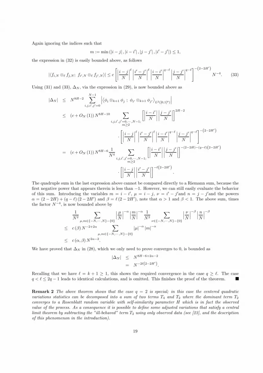
Recalling that we have ℓ = k + 1 ≥ 1, this shows the required convergence in the case q ≥ ℓ. The caseq < ℓ ≤ 2q − 1 leads to identical calculations, and is omitted. This finishes the proof of the theorem.
Remark 2 The above theorem shows that the case q = 2 is special; in this case the centered quadraticvariations statistics can be decomposed into a sum of two terms T4 and T2 where the dominant term T2
converges to a Rosenblatt random variable with self-similarity parameter H which is in fact the observedvalue of the process. As a consequence it is possible to define some adjusted variations that satisfy a centrallimit theorem by subtracting the ”ill-behaved” term T2 using only observed data (see [23], and the descriptionof this phenomenon in the introduction).
19

It is possible to give the limits of the remaining terms T2q−2 to T2 appearing in the decompositionof the statistic VN . All these renormalized terms converge to Hermite random variables of the same order astheir indices (we have already proved this property in detail for T2 in the previous section). This is a kindof “reproduction” of the Hermite processes through their variations.
Theorem 6
• For every H ∈ (12 , 1) and for every k = 1, . . . , q − 2 we have
limN→∞
N (2−2H′)(q−k)T2q−2k = zk,HZ(2q−2k,(2q−2k)(H′−1)+1), in L2(Ω) (34)
where Z(2q−2k,(2q−2k)(H′−1)+1) denotes a Hermite random variable with self-similarity order (2q −2k)(H ′ − 1) + 1 and zk,H = d(H)2a(H ′)k ((H ′ − 1)k + 1)
−1(2(H ′ − 1) + 1)
−1.
• Moreover, if H ∈ (34 , 1) then
limN→∞
N2−2Hx−1/22,H T2q = Z(2q,2H−1), in L2(Ω). (35)
Proof: Recall that, for k = 1 to 2q − 2 we have T2k = N2H−1I2q−2k
(
∑N−1i=0 fi,N ⊗k fi,N
)
with
fi,N ⊗k fi,N given by (11). The first step of the proof is to observe that the limit of N (2H′−2)(q−k)T2q−2k isgiven by
N (2H′−2)(q−k)N2H−1I2q−2k(fN2q−2k)
with
fN2q−2k(y1, . . . , yq−k, z1, . . . , zq−k) = d(H)2a(H ′)k
N−1∑
i=0
1[0, iN
](yi)1[0, iN
](zi)
∫
Ii
∫
Ii
∂1K(u, y1) . . . ∂1K(u, yq−k)∂1K(v, z1) . . . ∂1K(v, zq−k)|u − v|(2H′−2)kdvdu.
The argument leading to the above fact is the same as in Theorem 4: a remainder term r2q−2k, which isdefined by T2q−2k minus I2(f
N2q−2k) converges to zero similarly to the term r2 in the proof of Theorem 4
because of the appearance of the indicator functions 1Ii(yi) or 1Ii
(zi) in each of the terms that form thisremainder.
The second step of the proof is to replace ∂1K(u, yi) by ∂1K( iN , yi) and ∂1K(v, zi) by ∂1K( i
N , zi)on the interval Ii inside the integrals du and dv. The rest of the proof can be argued as in the proof ofTheorem 4. The term N (2−2H′)(q−k)fN
2q−2k will have the same limit as
N (2−2H′)(q−k)N2H−1d(H)2a(H ′)kN−1∑
i=0
1[0, iN
](yi)1[0, iN
](zi)
∂1K(i
N, y1) . . . ∂1K(
i
N, yq−k)∂1K(
i
N, z1) . . . ∂1K(
i
N, zq−k)
∫
Ii
∫
Ii
|u − v|(2−2H′)kdvdu
= d(H)2a(H ′)k ((H ′ − 1)k + 1)−1
(2(H ′ − 1) + 1)−1
N (2−2H′)(q−k)N2H−1N (2−2H′)k+2
N−1∑
i=0
1[0, iN
](yi)1[0, iN
](zi)∂1K(i
N, y1) . . . ∂1K(
i
N, yq−k)∂1K(
i
N, z1) . . . ∂1K(
i
N, zq−k)
= zk,H1
N
N−1∑
i=0
1[0, iN
](yi)1[0, iN
](zi)∂1K(i
N, y1) . . . ∂1K(
i
N, yq−k)∂1K(
i
N, z1) . . . ∂1K(
i
N, zq−k).
20

Now, the last sum is a Riemann sum that converges pointwise and in L2([0, 1]2q−2k) (because the sequencefN2q−2k is a Cauchy sequence in this space) to zk,HL1 where
L1(y1, . . . , yq−k, z1, . . . , zq−k) =
∫ 1
y1∨zq−k
∂1K(u, y1) . . . ∂1K(u, yq−k)∂1K(u, z1) . . . ∂1K(u, zq−k)du
which is the kernel of the Hermite random variable of order 2q − 2k with self-similarity parameter (2q −2k)(H ′ − 1) + 1. The case H ∈ (3
4 , 1) and k = 0 follows analogously.
5 Consistent estimation of H and its asymptotics
In this section, we drop the notational dependence of Z(H,q) on H . Theorem 4 can be immediately appliedto the statistical estimation of H . We note that with VN in (10) and SN defined by
SN =1
N
N−1∑
i=0
(
Z(q)i+1
N
− Z(q)i
N
)2
, (36)
we have1 + VN = N2HSN (37)
andE [SN ] = N−2H .
so that
H = − logE [SN ]
2 logN.
To form an estimator of H , since Theorem 4 implies that SN evidently concentrates around its mean, wewill use SN in the role of an empirical mean, instead of its true mean; in other words we let
H = HN = − log SN
2 log N.
We immediately get from (37) that
log (1 + VN ) = 2H log N + log SN
= 2(
H − H)
log N. (38)
The first observation is that HN is strongly consistent for the Hurst parameter.
Proposition 3 We have that HN converges to H almost surely as N → ∞.
Proof: Let us prove that VN converges to zero almost surely as N → ∞. We know that VN
converges to 0 in L2(Ω) as N → ∞ and an estimation for its variance is given by the formula (16). On theother hand this sequence is stationary because the increments of the Hermite process are stationary. We cantherefore apply a standard argument to obtain the almost sure convergence for discrete stationary sequenceunder condition (16). This argument follows from Theorem 6.2, page 492 in [6] and it can be used exactlyas in the proof of Proposition 1 in [4]. A direct elementary proof using the Borel-Cantelli lemma is almostas easy. The almost sure convergence of H to H is then obtained immediately via (38).
Owing to the fact that VN is of small magnitude (it converges to zero almost surely by the last propo-
sition’s proof), log (1 + VN ) can be confused with VN . It then stands to reason that(
H − H)
N2−2H′
log N
is asymptotically Rosenblatt-distributed since the same holds for VN by Theorem 4. Just as in that theorem,more is true: as we now show, the convergence to a Rosenblatt random variable occurs in L2 (Ω).
21

Proposition 4 There is a standard Rosenblatt random variable R with self-similarity parameter 2H ′ − 1such that
limN→∞
E
[
∣
∣
∣2N2−2H′(
H − H)
log N − c2c1/21,H,qR
∣
∣
∣
2]
= 0
Proof: To simplify the notation, we denote c2c1/21,H,q by c in this proof. Theorem 4 signifies that a
standard Rosenblatt r.v. R with parameter 2H ′ − 1 exists such that
limN→∞
E
[
∣
∣
∣N2−2H′
VN − cR∣
∣
∣
2]
= 0.
From (38) we immediately get
E
[
∣
∣
∣2N2−2H′(
H − H)
log N − cR∣
∣
∣
2]
= E
[
∣
∣
∣N2−2H′
log (1 + VN ) − cR∣
∣
∣
2]
≤ 2E
[
∣
∣
∣N2−2H′
VN − cR∣
∣
∣
2]
+ 2N4−4H′
E[
|VN − log (1 + VN )|2]
.
Therefore, we only need to show that E[
|VN − log (1 + VN )|2]
= o(
N4H′−4)
.
Consider the function f (x) = | log (1 + x) |, defined for x > −1. We have for x > −1/2, |f (x)| ≤2 |x|. We can write
E[
|VN − log (1 + VN )|2]
≤ 2 E[
|VN |2]
+ 2 E[
|log (1 + VN )|2]
= 2 E[
|VN |2]
+ 2 E[
1VN > −1
2
|log (1 + VN )|2]
+2 E[
1VN < −1
2
|log (1 + VN )|2]
≤ 2 E[
|VN |2]
+ 4 E[
1VN > −1
2
|VN |2]
+ 2 E[
1VN < −1
2
|log (1 + VN )|2]
= 6E[
|VN |2]
+ 2 E[
1VN < −1
2
|log (1 + VN )|2]
: = A + B
The term A is bounded above and this is immediately dealt with using the following lemma.
Lemma 1 For every n ≥ 2, there is a constant cn such that E[
|VN |2n]
≤ cn N (4H′−4)n.
Proof: In the proof of Proposition 1 we calculated the L2 norm of the terms appearing in thedecomposition of VN , where VN is a sum of multiple integrals. Therefore, from Proposition 5.1 of [10] weimmediately get an estimate for any event moment of each term. Indeed, for k = q − 1
E[
T 2n2
]
≤ 1 · 3 · 5 · · · (4n − 1)(
c21,H N4H′−4
)n= cnN (4H′−4)n
and for 1 ≤ k < q − 1
E[
T 2n2q−2k
]
≤ 1 · 3 · 5 · · · (2(2q − 2k)n)(
c21,q,H N (2q−2k)(2H′−2)
)n
= cq,nN (2q−2k)(2H′−2)n
The dominant term is again the T2 term and the result follows immediately.
22

For the term B, we write 1VN <−1/2 as 1VN <−1/21SN <2−1N−2H . Now using Holder’s inequality, wewrite
B ≤ P1/p [VN < −1/2]E1/p′[
1SN <2−1N−2H |log (1 + VN )|2p′]
. (39)
To deal with the expectation term, recall that log (1 + VN ) = 2H log N + log SN , and thus
E[
1SN <2−1N−2H |log (1 + VN )|2p′]
≤ cp (2H log N)2p′
+ cpE
[
1SN <2−1N−2H
(
log1
SN
)2p′]
. (40)
We estimate the last expectation by returning to the definition of SN in (36). First note that with f (x) =
10<x<2−1N−2H log2p′
(1/x), and g (x) = 10<x<1 log2p′
(1/x), we have f (x) ≤ g (x) and g (x) is convex. Henceusing Jensen’s inequality on the empirical average defining SN ,
E[
1SN <2−1N−2H |log SN |2p′]
≤ E [g (SN )] = E
[
g
(
1
N
N−1∑
i=0
(
Z(q)i+1
N
− Z(q)iN
)2)]
≤ 1
N
N−1∑
i=0
E
[
g
(
(
Z(q)i+1
N
− Z(q)i
N
)2)]
. (41)
Next we can bound g (x) by cα,px−α for any α ∈ (0, 1) and a constant cα,p large enough. Moreover by
scaling, Z(q)i+1
N
−Z(q)i
N
has the same law as N−HZ where Z is has the law of the Hermite process Z(q) at time
1. Hence
E
[
g
(
(
Z(q)i+1
N
− Z(q)iN
)2)]
≤ cα,pE
[
(
Z(q)i+1
N
− Z(q)iN
)−2α]
= cα,pN2αHE
[
|Z|−2α]
= c′α,pN2αH (42)
where c′α,p is another constant depending only on α and p, which is finite as long as α < 1/2, because Z hasa bounded density at the origin. Combining (40), (41), and (42), we get
E[
1SN <2−1N−2H |log (1 + VN )|2p′]
≤ cp (2H log N)2p′
+ cpc′α,pN
2αH . (43)
To finish controlling B, we only need to evaluate the tail behavior of VN , as in
P [VN < −1/2] = P[
cN2−2H′
VN < −2−1cN2−2H′]
= P[
cN2−2H′
VN − R + R < −2−1cN2−2H′]
.
To lighten the notation we let UN = cN2−2H′
VN − R and xN = 2−1cN2−2H′
. Thus
P [VN < −1/2] ≤ P [UN < −xN/2] + P [R < −xN/2]
≤ P [|UN | > xN/2] + P [|R| > xN/2]
≤ E[
|UN |4]
2c−1N−(8−8H′) + exp(
−c′N2−2H′)
.
Asymptotically the last term is negligible compared to the second-to-last one. Moreover by Lemma 1,
E[
|UN |4]
is bounded. Therefore, for some constant c′′ and N large,
P [VN < −1/2] ≤ c′′N−(8−8H′).
23

Combining this with (39) and (43), we get for large N ,
B ≤ c′′′N−(8−8H′) 1p+2αH 1
p
′
.
By choosing α close enough to 0, we guarantee that B = o(
N4H′−4)
, which finishes the proof of the
proposition.
A difficulty arises when applying the above proposition for model validation when checking theasymptotic distribution of the estimator H : the normalization constant N2−2H′
log N depends on H . Whileit is not always obvious that one may replace this instance of H ′ by its estimator, in our situation, becauseof the L2 (Ω) convergences, this is legitimate, as the following theorem shows.
Theorem 7 Let H ′ = 1 + (H − 1)/q. There is a standard Rosenblatt random variable R with self-similarityparameter 2H ′ − 1 such that
limN→∞
E[∣
∣
∣2N2−2H′(
H − H)
log N − c2c1/21,H,qR
∣
∣
∣
]
= 0.
Proof: By the previous proposition, it is sufficient to prove that
limN→∞
E[∣
∣
∣
(
N2−2H′ − N2−2H′)(
H − H)
log N∣
∣
∣
]
= 0.
We decompose the probability space depending on whether H is far or not from its mean. For a fixed valueε > 0 which will be chosen later, it is most convenient to define the event
D =
H > qε/2 + 2H − 1
.
We have
E[∣
∣
∣
(
N2−2H′ − N2−2H′)(
H − H)
log N∣
∣
∣
]
= E[
1D
∣
∣
∣
(
N2−2H′ − N2−2H′)(
H − H)
log N∣
∣
∣
]
+E[
1Dc
∣
∣
∣
(
N2−2H′ − N2−2H′)(
H − H)
log N∣
∣
∣
]
= : A + B.
We study A first. Let us introduce the shorthand notation x = max(
2 − 2H ′, 2 − 2H ′)
and y =
min(
2 − 2H ′, 2 − 2H ′)
. We may write
∣
∣
∣N2−2H′ − N2−2H′∣
∣
∣ = ex log N − ey log N
= ey log N(
e(x−y) log N − 1)
≤ Ny (log N) (x − y)Nx−y
= 2 (log N)Nx∣
∣
∣H ′ − H ′∣
∣
∣
= 2q−1 (log N)Nx∣
∣
∣H − H∣
∣
∣ .
Thus
A ≤ 2q−1 E
[
1DNx∣
∣
∣H − H
∣
∣
∣
2
log2 N
]
= 2q−1 E
[
Nx−(4−4H′)1DN4−4H′∣
∣
∣H − H∣
∣
∣
2
log2 N
]
.
24

Now choose ε ∈ (0, 2− 2H ′). In this case, if ω ∈ D, and x = 2− 2H ′, we get x− (4 − 4H ′) = −x < −ε. Onthe other hand, for ω ∈ D and x = 2 − 2H ′, we get x − (4 − 4H ′) = 2 − 2H ′ − (4 − 4H ′) < −ε as well. Inconclusion, on D,
x − (4 − 4H ′) < −ε,
which implies immediately
A ≤ N−ε2q−1E
[
N4−4H′∣
∣
∣H − H
∣
∣
∣
2
log2 N
]
;
this prove that A tends to 0 as N → ∞, since the last expectation above is bounded (converges to a constant)by Proposition 4.
Now we may study B. We are now operating with ω ∈ Dc. In other words,
H − H > 1 − H − qε/2.
Still using ε < 2−2H ′, this implies that H > H . Consequently, it is not inefficient to bound∣
∣
∣N2−2H′ − N2−2H′∣
∣
∣
above by N2−2H′
. In the same fashion, we bound∣
∣
∣H − H∣
∣
∣ above by H . Hence we have, using Holder’s
inequality with the powers 2q and p−1 + (2q)−1 = 1.
B ≤ H log N E[
1DcN2−2H′]
(44)
≤ H log N P1/p [Dc] E1/(2q)[
N(2−2H′)2q]
.
From Proposition 4, by Chebyshev’s inequality, we have
P1/p [Dc] ≤E1/p
[
∣
∣
∣H − H∣
∣
∣
2]
(1 − H − qε/2)2/p
≤ cq,HN−(4−4H′)/p (45)
for some constant cq,H depending only on q and H . Dealing with the other term in the upper bound for B
is a little less obvious. We must return to the definition of H. By (38) we have
1 + VN = N2(H−H) = N2q(H′−H′)
= N2q(2−2H′)N−2q(2−2H′).
Therefore,
E1/(2q)[
N(2−2H′)2q]
≤ N2−2H′
E1/(2q) [1 + VN ]
≤ 2N2−2H′
. (46)
Plugging (45) and (46) back into (44), we get
B ≤ 2Hcq,H (log N)N−(4−4H′)(2/p−1).
Given that 2q ≥ 4 and p is conjugate to 2q, we have p ≤ 4/3 so that 2/p − 1 ≥ 1/2 > 0, which proves thatB goes to 0 as N → ∞. This finishes the proof of the theorem.
Finally we state the extension of our results to Lp (Ω)-convergence.
Theorem 8 The convergence in Theorem 7 holds in any Lp (Ω). In fact, the L2 (Ω)-convergences in allother results in this paper can be replaced by Lp (Ω)-convergences.
25

Sketch of proof. We only give the outline of the proof. Lemma 1 works because, in analogy tothe Gaussian case, random variables in a fixed Wiener chaos of order p have moments of all orders, and therelations between the various moments are given by equalities using a set of constants which depend only onp. This Lemma can be used immediately to prove the extension of Proposition 1 that
E[
V 2pN
]
≃ cpNp(4H′−4).
Proving a new version of Theorem 4 with Lp (Ω)-convergence can base itself on the above result, and requires acareful reevaluation of the various terms involved. Proposition 4 can then be extended to Lp (Ω)-convergencethanks to the new Lp (Ω) versions of Theorem 4 and Proposition 1, and Theorem 7 follows easily from thisnew version of Proposition 1.
References
[1] J. Beran (1994): Statistics for Long-Memory Processes. Chapman and Hall.
[2] P. Breuer and P. Major (1983): Central limit theorems for nonlinear functionals of Gaussian fields. J.Multivariate Analysis, 13 (3), 425-441.
[3] K. Burdzy and J. Swanson (2008): Variation for the solution to the stochastic heat equation II. Preprint.
[4] J.F. Coeurjolly (2001): Estimating the parameters of a fractional Brownian motion by discrte variationsof its sample paths. Statistical Inference for Stochastic Processes , 4, 199-227.
[5] R.L. Dobrushin and P. Major (1979): Non-central limit theorems for non-linear functionals of Gaussianfields. Z. Wahrscheinlichkeitstheorie verw. Gebiete, 50, 27-52.
[6] J.L. Doob (1953): Stochastic Processes. Wiley Classics Library.
[7] L. Giraitis and D. Surgailis (1985): CLT and other limit theorems for functionals of Gaussian processes.Z. Wahrsch. verw. Gebiete 70, 191-212.
[8] X. Guyon and J. Leon (1989): Convergence en loi des H-variations d’un processus gaussien stationnairesur R. Annales IHP , 25, 265-282.
[9] G. Lang and J. Istas (1997): Quadratic variations and estimators of the Holder index of a Gaussianprocess. Annales IHP , 33, 407-436.
[10] P. Major (2005): Tail behavior of multiple random integrals and U -statistics. Probability Surveys.
[11] I. Nourdin (2007): Asymptotic behavior of certain weighted quadratic variations and cubic varitionsof fractional Brownian motion. The Annals of Probability, to appear.
[12] I. Nourdin and G. Peccati (2007): Weighted power variations of iterated Brownian motion. Preprint.
[13] I. Nourdin and A. Reveillac (2008): Asymptotic behavior of weighted quadratic variations of fractionalBrownian motion: the critical case H = 1/4. Preprint.
[14] I. Nourdin, D. Nualart and C.A. Tudor (2007): Central and non-central limit theorems for weightedower variations of fractional Brownian motion. Preprint.
[15] D. Nualart (2006): Malliavin Calculus and Related Topics. Second Edition. Springer.
[16] D. Nualart and S. Ortiz-Latorre (2006): Central limit theorems for multiple stochastic integrals andMalliavin calculus. Preprint, to appear in Stochastic Processes and their Applications.
26

[17] D. Nualart and G. Peccati (2005): Central limit theorems for sequences of multiple stochastic integrals.The Annals of Probability, 33 (1), 173-193.
[18] A. Reveillac (2008): Convergence of finite-dimensional laws of the weighted quadratic variations processfor some fractional Brownian sheets. Preprint.
[19] J. Swanson (2007): Variations of the solution to a stochastic heat equation. Annals of Probability, 35(6),2122–2159.
[20] M. Taqqu (1975): Weak convergence to the fractional Brownian motion and to the Rosenblatt process.Z. Wahrscheinlichkeitstheorie verw. Gebiete, 31, 287-302.
[21] M. Taqqu (1979): Convergence of integrated processes of arbitrary Hermite rank. Z. Wahrscheinlichkeit-stheorie verw. Gebiete, 50, 53-83.
[22] C.A. Tudor (2008): Analysis of the Rosenblatt process. ESAIM Probability and Statistics , 12, 230-257.
[23] C.A. Tudor and F. Viens (2007): Variations and estimators for the self-similarity order through Malliavin calculus. Submitted, preprint available athttp://arxiv.org/PS cache/arxiv/pdf/0709/0709.3896v2.pdf.
27