Self-consistent Seeding of the Interchange Instability in

Dipolarization Fronts

Giovanni Lapenta (1), Lapo Bettarini (2)

1) Centrum voor Plasma-Astrofysica,

Departement Wiskunde, Katholieke Universiteit Leuven,

Celestijnenlaan 200B, 3001 Leuven, Belgium (EU)

2) Royal Observatory of Belgium, Ringlaan 3, 1180 Brussels, Belgium (EU)

(Dated: May 4, 2011)

Abstract

We report a 3D magnetohydrodynamics simulation that studies the formation of dipolarization

fronts during magnetotail reconnection. The crucial new feature uncovered in the present 3D sim-

ulation is that the process of reconnection produces flux ropes developing within the reconnection

region. These flux ropes are unstable to the kink mode and introduce a spontaneous structure

in the dawn-dusk direction. The dipolarization fronts forming downstream of reconnection are

strongly affected by the kinking ropes. At the fronts, a density gradient is present with opposite

direction to that of the acceleration field and leads to an interchange instability. We present ev-

idence for a causal link where the perturbations of the kinking flux ropes with their natural and

well defined scales drive and select the scales for the interchange mode in the dipolarization fronts.

The results of the simulation are validated against measured structures observed by the Themis

mission.

1

arX

iv:1

105.

0485

v1 [

astr

o-ph

.EP]

3 M

ay 2

011

I. INTRODUCTION

Reconnection in the Earth magnetotail is a key step in the processes known as substorms.

Reconnection converts magnetic energy stored in the magnetic field of the tail and converts

it into heating and plasma flow away from the reconnection site, tailward and Earthward.

The Earthward flow is accompanied by a dipolarization front, a front of increased vertical

(North-South directed) magnetic field that moves towards the Earth and restores in part

a less stretched and more dipole-like magnetic field in the night side of the Earth, thereby

acquiring the name of dipolarization front [10]. Previous works have investigated the role of

the interchange instability in perturbing the dipolarization front [7, and references therein].

A dipolarization front acts similarly to a snowplow. As the dipolarization front moves,

the vertical magnetic field and the density pile up ahead of it. The curvature of the field

lines and the braking of the front by the momentum exchange with the yet unperturbed

plasma leads to an effective acceleration pointing contrary to the dipolarization front speed.

Such configuration is unstable to interchange modes: the higher density region is ahead of

the front and the density gradient is therefore opposite to the direction of the acceleration.

Several papers have observed this effect [3, 5, 10–14].

Recently, an attempt has been made to match the observed scale of the perturbation

of the front with simulations. The published simulations by Guzdar et al. [7] are 2D and

focus only on the interchange mode, without modeling the full front and its origin from

reconnection. By choosing the initial wavelength of the seed, one can control the scale of the

evolved structure and reproduce the observed features. In 2D macroscopic (MHD) studies

the choice of the initial seed is key because the interchange instability is equally growing in all

wavelengths [7]. In kinetic studies, the finite Larmor radius effect favors the growth rate of

smaller wavelength (too small to be of relevance to the observation) [11]. On the macroscopic

scales of the observed structures, MHD models are appropriate and the independence of the

growth rate on the wavelength of the modes means that other macroscopic driving forces

determine which scales dominate. In 2D studies where only the interchange mode is present,

the only way to force the interchange instability is by design.

To avoid the artificial driving due to the selection of the initial seed, a full 3D simulation

is needed. We report here a 3D simulation where the dipolarization front and the inter-

change instability are self-consistently developing out of a reconnection site. We start the

2

system and the reconnection process without seeding any structure along the direction of

the interchange instability. In doing so we let the system develop naturally and form its own

desired structures.

As in 2D, the reconnection process in 3D develops a diffusion layer where the plasma and

magnetic field decouple and the filed lines reconnect. In the outflow from the reconnection

region two regions form where the exhaust from the reconnection region piles up forming

dipolarization fronts. Also, as in 2D, the diffusion layer has initially the structure of a Sweet-

Parker layer that quickly becomes unstable to the secondary plasmoid instability [8, 9].

After that, the progress in 3D becomes radically different from 2D. In 3D, the plasmoid

instability leads to the formation of flux ropes ejected with the plasma from the diffusion

region and moving towards the dipolarization front. Each flux rope, however, is unstable

naturally to the kink instability, a well known instability that has a well defined natural

maximum mode of growth identified by the linear mode properties. In our simulations we

show that indeed this mode grows to very large amplitudes. Flux ropes become so distorted

as to touch directly the dipolarization fronts, providing a driving to the interchange mode.

The dipolarization fronts are naturally unstable to such mode, but the perturbation from

the kinking flux rope feeds the interchange instability and determines its dominant mode.

The results of our simulation predict specific scales for the warping. A direct comparison

is possible with observation from the THEMIS mission that can be interpreted as successive

crossing of warped fronts. The natural and spontaneous scales developed in our simulations

indeed are of the right order to be compatible with the observed scales.

II. MACROSCOPIC SIMULATION OF RECONNECTION THE EARTH MAG-

NETOTAIL

We solve the complete set of compressional visco-resistive MHD equations with uni-

form viscosity and resistivity parametrized by the global Lundquist number, S, and kinetic

Reynolds number, RM , both set to 104. We use the conventional geomagnetic coordinate

system with x in the Sun-Earth direction, y in the dawn-dusk direction and z in the north

south direction. The boundary conditions are periodic in x and y and reflecting (“perfect

conductor”) in z.

The initial configuration has the main field component reversed, Bx(z) = B0 tanh(z/L),

3

over a characteristic length scale L, while the other components are zero. Reconnection is

initiated with a perturbation of the classic GEM-type, repeated identically in every vertical

plane, independent of y.

The system is modeled with FLIP3D-MHD [2], a Lagrangian Eulerian code based on

discretizing the fluid into computational units acting as Lagrangian markers but used to

compute the operators on a uniform grid. The simulation reported here used 360 (in x) x

60 (in y) x 120 (in z) Lagrangian markers arrayed initially in a 3 x 3 x 3 uniform formation

in each cell of a uniform grid.

The simulation is conducted in dimensionless units, with space normalized to the initial

thickness L and time to the Alfven time τA = vA/L. The computational box has size

Lx/L = 60, Ly/L = 10 and Lz/L = 10. In comparing with observations, the results can

then be rescaled according to physical units for a chosen observed magnetotail thickness.

For example, Guzdar et al. [7] report a initial magnetotail thickness L=0.2RE but different

thicknesses apply to different conditions of the magnetotail.

III. MODES OF INTEREST

The evolution displays a sequence of 4 instabilities: tearing, secondary plasmoid, kink

and finally interchange instability. Let us follow the evolution.

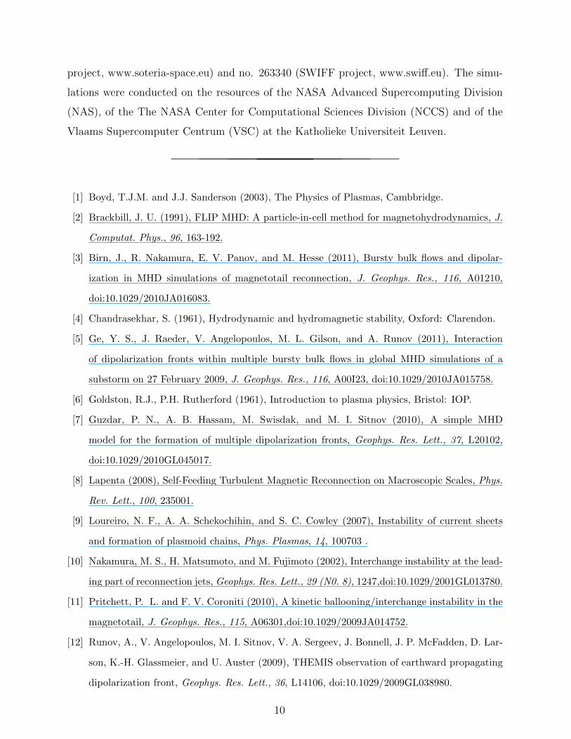
Figure 1 shows the typical configuration of a reconnection layer forming in response to the

initial perturbation localized in the center of the simulation box. From the reconnection layer

two jets of plasma exit along the x axis, tailward and Earthward and form the dipolarization

fronts: the areas of curved field lines that resemble dipole-like magnetic field lines. Ahead

of the front the plasma piles up, a typical observed feature of dipolarization fronts [15, and

references therein]. In Fig. 1 these two regions are visible as areas of increased density

(yellow in the color version and light in the grayscale version).

Given the resistivity set for the present simulation, the SP theory leads to a layer of aspect

ratio ∆/δ = S1/2 = 100, being ∆ and δ the length and the width of the layer respectively.

Previous 2D investigations of the same configuration considered here have shown that when

the aspect ratio exceeds a theoretical limit (estimated close to 100) a secondary plasmoid

instability develops [8, 9]. In the new regime, the process of reconnection proceeds faster

and at a rate independent of resistivity. The present 3D simulation is perturbed uniformly

4

in the dawn-dusk direction y and in absence of any other perturbations the same process

develops in each plane and the SP layer becomes unstable leading to plasmoids that in 3D

assume the form of flux ropes surrounding current filaments.

For the present investigation the focus is on what happens next. These current filaments

have a predominantly azimuthal field, with a small axial component. Therefore, recalling

the properties of the kink instability [1, page 118], these filaments are violently unstable to

the ideal kink instability.

Figure 2 provides a view of the evolution of the kink instability seen in a xy plane cut at

z = 0, the midplane of the simulation box.

The kink instability develops out of the numerical noise with no prescribed perturbation

in the y direction artificially introduced. The noise comes from the truncation error intrinsic

to any finite floating point precision in a computer simulation. The present code uses

double precision real numbers. This explains the very ordered initial phase of the SP layer

formation and its subsequent destabilization by plasmoids. No structure at all is present in

y in the initial setup. At first, as the simulation progresses, correctly, the double precision

FLIP-MHD code retains perfectly the initial symmetry along y, because there is no physical

instability that can lead to structure along y.

However, as soon as the flux ropes are formed and the stability conditions for the kink

instability is exceeded, the very small but present noise from the floating point error seeds

the instability breaking the symmetry in y and leading to the kinked rope shown in Fig. 2.

A dominant mode emerges.

The evolution of the flux rope is confined within the reconnection region and forms

essentially a narrow band with limited span in the vertical (z) direction: the flux rope is

confined within the reconnecting layer and can be displaced only in the x and y plane. The

displacement is then written as

ξ(x, y, z, t) = ξ(x, z)e−iωt−i2πny/Ly (1)

in terms of eigenfunctions with harmonic dependence in y, being i the imaginary constant.

Inspection of Fig. 2 immediately confirms that the dominant mode has n = 4.

The progress of the kink instability leads to a progressive widening of horizontal span

of the reconnection region along the x axis affected by the kinked rope. Eventually, the

rope starts to come into contact with the dipolarization fronts. Up to this moment the

5

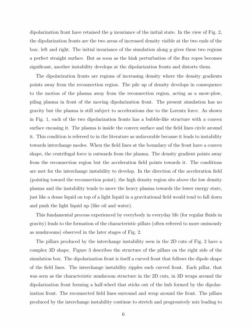
dipolarization front have retained the y invariance of the initial state. In the view of Fig. 2,

the dipolarization fronts are the two areas of increased density visible at the two ends of the

box: left and right. The initial invariance of the simulation along y gives these two regions

a perfect straight surface. But as soon as the kink perturbation of the flux ropes becomes

significant, another instability develops at the dipolarization fronts and distorts them.

The dipolarization fronts are regions of increasing density where the density gradients

points away from the reconnection region. The pile up of density develops in consequence

to the motion of the plasma away from the reconnection region, acting as a snow-plow,

piling plasma in front of the moving dipolarization front. The present simulation has no

gravity but the plasma is still subject to accelerations due to the Lorentz force. As shown

in Fig. 1, each of the two dipolarization fronts has a bubble-like structure with a convex

surface encasing it. The plasma is inside the convex surface and the field lines circle around

it. This condition is refereed to in the literature as unfavorable because it leads to instability

towards interchange modes. When the field lines at the boundary of the front have a convex

shape, the centrifugal force is outwards from the plasma. The density gradient points away

from the reconnection region but the acceleration field points towards it. The conditions

are met for the interchange instability to develop. In the direction of the acceleration field

(pointing toward the reconnection point), the high density region sits above the low density

plasma and the instability tends to move the heavy plasma towards the lower energy state,

just like a dense liquid on top of a light liquid in a gravitational field would tend to fall down

and push the light liquid up (like oil and water).

This fundamental process experienced by everybody in everyday life (for regular fluids in

gravity) leads to the formation of the characteristic pillars (often referred to more ominously

as mushrooms) observed in the later stages of Fig. 2.

The pillars produced by the interchange instability seen in the 2D cuts of Fig. 2 have a

complex 3D shape. Figure 3 describes the structure of the pillars on the right side of the

simulation box. The dipolarization front is itself a curved front that follows the dipole shape

of the field lines. The interchange instability ripples such curved front. Each pillar, that

was seen as the characteristic mushroom structure in the 2D cuts, in 3D wraps around the

dipolarization front forming a half-wheel that sticks out of the hub formed by the dipolar-

ization front. The reconnected field lines surround and wrap around the front. The pillars

produced by the interchange instability continue to stretch and progressively mix leading to

6

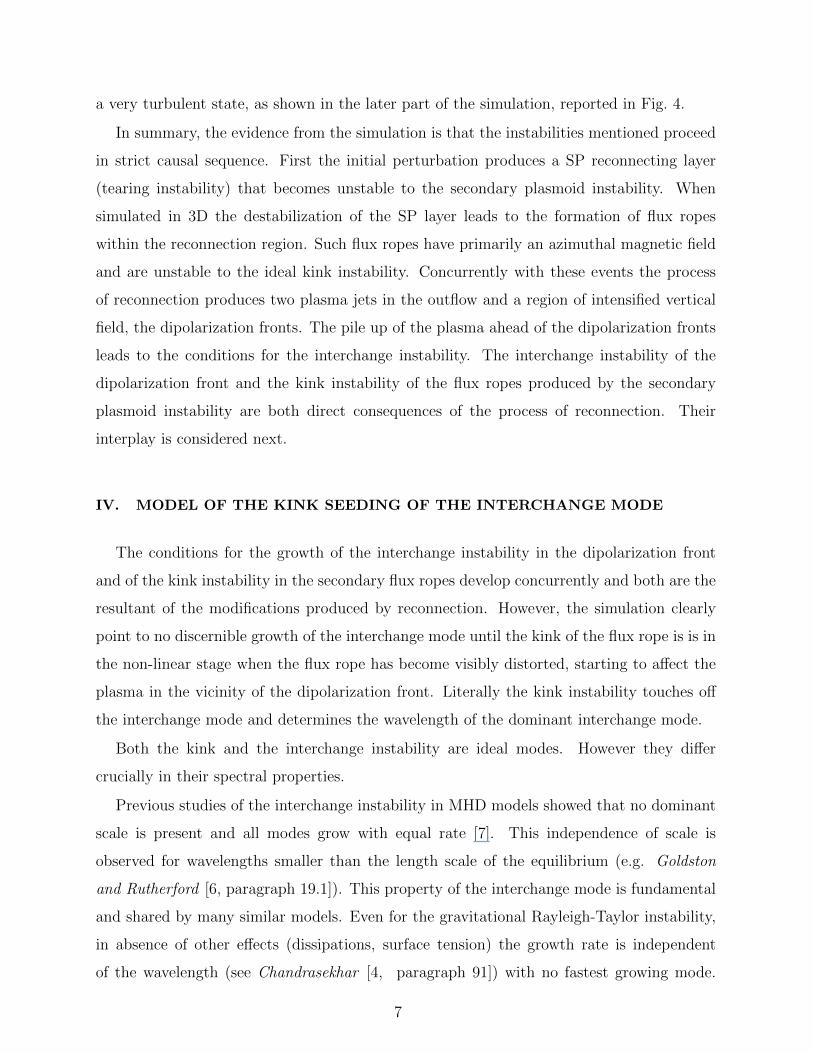
a very turbulent state, as shown in the later part of the simulation, reported in Fig. 4.

In summary, the evidence from the simulation is that the instabilities mentioned proceed

in strict causal sequence. First the initial perturbation produces a SP reconnecting layer

(tearing instability) that becomes unstable to the secondary plasmoid instability. When

simulated in 3D the destabilization of the SP layer leads to the formation of flux ropes

within the reconnection region. Such flux ropes have primarily an azimuthal magnetic field

and are unstable to the ideal kink instability. Concurrently with these events the process

of reconnection produces two plasma jets in the outflow and a region of intensified vertical

field, the dipolarization fronts. The pile up of the plasma ahead of the dipolarization fronts

leads to the conditions for the interchange instability. The interchange instability of the

dipolarization front and the kink instability of the flux ropes produced by the secondary

plasmoid instability are both direct consequences of the process of reconnection. Their

interplay is considered next.

IV. MODEL OF THE KINK SEEDING OF THE INTERCHANGE MODE

The conditions for the growth of the interchange instability in the dipolarization front

and of the kink instability in the secondary flux ropes develop concurrently and both are the

resultant of the modifications produced by reconnection. However, the simulation clearly

point to no discernible growth of the interchange mode until the kink of the flux rope is is in

the non-linear stage when the flux rope has become visibly distorted, starting to affect the

plasma in the vicinity of the dipolarization front. Literally the kink instability touches off

the interchange mode and determines the wavelength of the dominant interchange mode.

Both the kink and the interchange instability are ideal modes. However they differ

crucially in their spectral properties.

Previous studies of the interchange instability in MHD models showed that no dominant

scale is present and all modes grow with equal rate [7]. This independence of scale is

observed for wavelengths smaller than the length scale of the equilibrium (e.g. Goldston

and Rutherford [6, paragraph 19.1]). This property of the interchange mode is fundamental

and shared by many similar models. Even for the gravitational Rayleigh-Taylor instability,

in absence of other effects (dissipations, surface tension) the growth rate is independent

of the wavelength (see Chandrasekhar [4, paragraph 91]) with no fastest growing mode.

7

This leaves the interchange mode scale neutral, the actual observed scale must therefore be

determined by the driving force. If all modes that are excited by the forcing grow with the

same rate, it is the intensity of the driving that determines the dominant scales.

The kink instability is, instead, characterized by a well defined fastest growing mode.

In the most classical case of a cylindrical flux rope within a concentric cylindrical wall

or in vacuum, the well known Kruskal-Shafranov (KS) stability criterion applies: q(a) =

2πaBz(a)/LBθ(a) > 1 (for a flux rope of radius a, periodic length L), where q is hte so-

called safety factor [1, page 118]. However, the case under investigation does not correspond

to the classical cases of kink of a cylindrical flux rope and the KS limit is only indicative.

Two main differences are evident. First, the flux rope is confined within the reconnection

region that is a relatively narrow band in the z direction. The initial size of this region

is equal to the SP layer formed during laminar reconnection. With the evolution of the

secondary islands, the region broadens but is still confined by the stronger lobe magnetic

field. This confinement in the z direction allows the flux ropes to kink only in the x − y

plane and invalidates the usual assumption of cylindrical symmetry of the initial state.

Second, just like for the secondary plasmoid instability responsible for the breakup of

the SP layer and the transition to turbulent reconnection, the presence of flow changes the

stability properties quantitatively if not qualitatively [9]. The flow can stabilize or destabilize

the system as shown in other similar circumstances [4].

For these reasons, we cannot directly compare the instability observed in the simulation

with a simple analytical expression for a reference theoretical kink mode. But the simulation

indicates a strong predominance for the mode n = 4. The kinking rope fits four times the

domain forming four full sinusoidal oscillations. This has the important implication that the

size of the computational box in the dawn-dusk (y) direction is much more than sufficient

to capture the fastest growing mode, giving us confidence to be resolving the largest scales

of interest.

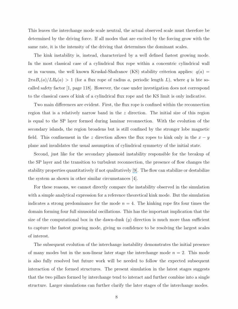
The subsequent evolution of the interchange instability demonstrates the initial presence

of many modes but in the non-linear later stage the interchange mode n = 2. This mode

is also fully resolved but future work will be needed to follow the expected subsequent

interaction of the formed structures. The present simulation in the latest stages suggests

that the two pillars formed by interchange tend to interact and further combine into a single

structure. Larger simulations can further clarify the later stages of the interchange modes.

8

How does this compare with the real magnetotail of the Earth? The observations front

the P4 satellite of the THEMIS mission on Feb 15 2008 reported by Guzdar et al. [7] show a

recurring crossing of the dipolarization from that can be explained assuming that the front

itself becomes warped and distorted as a consequence of the interchange instability discussed

above. The reported observed scale of such warping is in the range 1-3 RE confirmed also

by previous investigations [10].

The results presented here show a natural and spontaneous emergence of a dominant

scale. As noted above the dominant kink and interchange have dominant modes 4 and 2,

respectively. The expected length scale of the interchange structures is therefore Ly/2 = 5L.

To obtain physical dimensions, we need to choose the normalization length L, equal to the

reference initial current sheet thickness. Guzdar et al. [7] suggest L=0.2RE which leads to

a scale of 0.5RE for the kink mode and 1.0RE for the interchange mode. This value is only

indicative as the magnetotail thickness varies over a wide range. But the agreement with

the observations is evident.

The predicted scale is not determined by the box dimensions. The observed features fit 2

to 4 times the simulations box. This is a clear indication that the scale is determined by the

configuration of the initial equilibrium and not by the box size. A key consequence is that

this result confirms and extends the conclusions of Guzdar et al. [7] in a crucial point: in the

present case the scales result naturally from the internal nature of the processes developing.

Instead, the scales reported by Guzdar et al. [7] were intentionally seeded by a suitable

choice of the initial perturbation of the front selected by the researchers.

Future work should investigate via linear theory the conditions of the stability of a flux

rope confined within a magnetic field reversal and embedded in a flow pattern representative

of the flow present near the reconnection point. This flow has been suggested [8, 9] to be a

key aspect of the faster turbulent reconnection phase and should be included in a complete

model of the evolution.

ACKNOWLEDGMENTS

The present work is supported in part by the NASA MMS mission, by the Onderzoek-

fonds KU Leuven (Research Fund KU Leuven) and by the European Commission’s Seventh

Framework Programme (FP7/2007-2013) under the grant agreement no. 218816 (SOTERIA

9

project, www.soteria-space.eu) and no. 263340 (SWIFF project, www.swiff.eu). The simu-

lations were conducted on the resources of the NASA Advanced Supercomputing Division

(NAS), of the The NASA Center for Computational Sciences Division (NCCS) and of the

Vlaams Supercomputer Centrum (VSC) at the Katholieke Universiteit Leuven.

[1] Boyd, T.J.M. and J.J. Sanderson (2003), The Physics of Plasmas, Cambbridge.

[2] Brackbill, J. U. (1991), FLIP MHD: A particle-in-cell method for magnetohydrodynamics, J.

Computat. Phys., 96, 163-192.

[3] Birn, J., R. Nakamura, E. V. Panov, and M. Hesse (2011), Bursty bulk flows and dipolar-

ization in MHD simulations of magnetotail reconnection, J. Geophys. Res., 116, A01210,

doi:10.1029/2010JA016083.

[4] Chandrasekhar, S. (1961), Hydrodynamic and hydromagnetic stability, Oxford: Clarendon.

[5] Ge, Y. S., J. Raeder, V. Angelopoulos, M. L. Gilson, and A. Runov (2011), Interaction

of dipolarization fronts within multiple bursty bulk flows in global MHD simulations of a

substorm on 27 February 2009, J. Geophys. Res., 116, A00I23, doi:10.1029/2010JA015758.

[6] Goldston, R.J., P.H. Rutherford (1961), Introduction to plasma physics, Bristol: IOP.

[7] Guzdar, P. N., A. B. Hassam, M. Swisdak, and M. I. Sitnov (2010), A simple MHD

model for the formation of multiple dipolarization fronts, Geophys. Res. Lett., 37, L20102,

doi:10.1029/2010GL045017.

[8] Lapenta (2008), Self-Feeding Turbulent Magnetic Reconnection on Macroscopic Scales, Phys.

Rev. Lett., 100, 235001.

[9] Loureiro, N. F., A. A. Schekochihin, and S. C. Cowley (2007), Instability of current sheets

and formation of plasmoid chains, Phys. Plasmas, 14, 100703 .

[10] Nakamura, M. S., H. Matsumoto, and M. Fujimoto (2002), Interchange instability at the lead-

ing part of reconnection jets, Geophys. Res. Lett., 29 (N0. 8), 1247,doi:10.1029/2001GL013780.

[11] Pritchett, P. L. and F. V. Coroniti (2010), A kinetic ballooning/interchange instability in the

magnetotail, J. Geophys. Res., 115, A06301,doi:10.1029/2009JA014752.

[12] Runov, A., V. Angelopoulos, M. I. Sitnov, V. A. Sergeev, J. Bonnell, J. P. McFadden, D. Lar-

son, K.-H. Glassmeier, and U. Auster (2009), THEMIS observation of earthward propagating

dipolarization front, Geophys. Res. Lett., 36, L14106, doi:10.1029/2009GL038980.

10

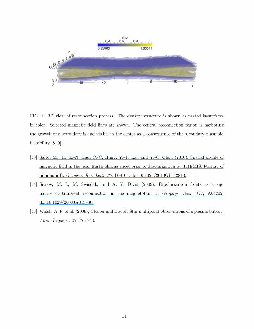
FIG. 1. 3D view of reconnection process. The density structure is shown as nested isosurfaces

in color. Selected magnetic field lines are shown. The central reconnection region is harboring

the growth of a secondary island visible in the center as a consequence of the secondary plasmoid

instability [8, 9].

[13] Saito, M. H., L.-N. Hau, C.-C. Hung, Y.-T. Lai, and Y.-C. Chou (2010), Spatial profile of

magnetic field in the near-Earth plasma sheet prior to dipolarization by THEMIS: Feature of

minimum B, Geophys. Res. Lett., 37, L08106, doi:10.1029/2010GL042813.

[14] Sitnov, M. I., M. Swisdak, and A. V. Divin (2009), Dipolarization fronts as a sig-

nature of transient reconnection in the magnetotail, J. Geophys. Res., 114, A04202,

doi:10.1029/2008JA013980.

[15] Walsh, A. P. et al. (2009), Cluster and Double Star multipoint observations of a plasma bubble,

Ann. Geophys., 27, 725-743.

11

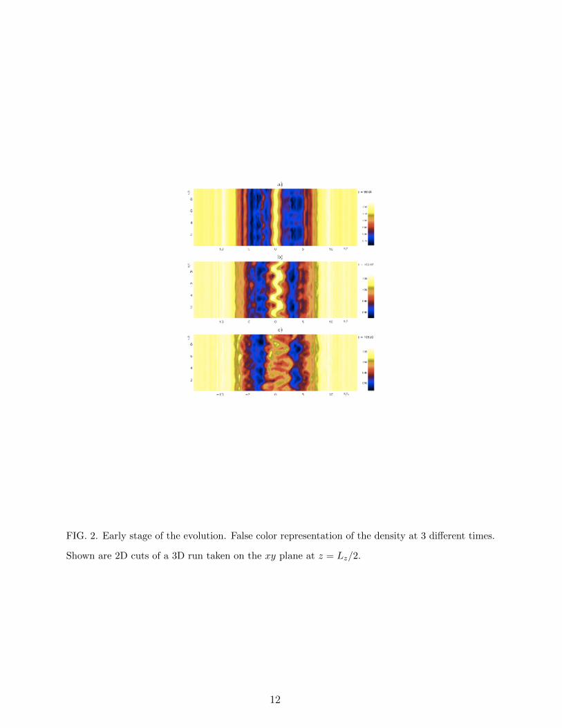
FIG. 2. Early stage of the evolution. False color representation of the density at 3 different times.

Shown are 2D cuts of a 3D run taken on the xy plane at z = Lz/2.

12

FIG. 3. 3D visualization of the isosurface of density at value 1. Shown is only the right half of

the domain in x at time t/τA = 126.03 (the same shown in the 2D cut of Fig. 4). The surface is

colored based on the value of Bx. Field lines are superimposed with their color chosen based on

the local intensity of the magnetic field |B|.

13

FIG. 4. Late stage of the evolution. Contour and false color representation of the density at 2

different times. Shown are 2D cuts of a 3D run taken on the xy plane at z = Lz/2.

14