selection of probability distributions in characterizing risk of extreme events

R W Analysis, Vol. 14, No. 5, 1994

Selection of Probability Distributions in Characterizing Risk of Extreme Events

James H. Lambed,’ Nicholas C. Matalas? Con Way Ling,’ Yacov Y. Haimes,’ and Duan Lil

Received December 30, 1993

1. INTRODUCTION

Use of probability distributions by regulatory agencies often focuses on the extreme events and scenarios that correspond to the tail of probability distributions. This paper makes the case that assessment of the tail of the distribution can and often should be performed separately from assessment of the central values. Factors to consider when developing distributions that account for tail behavior include (a) the availability of data, @) characteristics of the tail of the distribution, and (c) the value of additional information in assessment. The integration of these elements will improve the modeling of extreme events by the tail of distributions, thereby providing policy makers with critical information on the risk of extreme events. Two examples provide insight into the theme of the paper. The first demonstrates the need for a parallel analysis that separates the extreme events from the central values. The second shows a link between the selection of the tail distribution and a decision criterion. In addition, the phenomenon of breaking records in time- series data gives insight to the information that characterizes extreme values. One methodology for treating risk of extreme events explicitly adopts the conditional expected value as a measure of risk. Theoretical results concerning this measure are given to clarify some of the concepts of the risk of extreme events.

KEY WORDS: Extreme events; probabilitydistributions; data availability; distribution tail.

An improved understanding of the risk of extreme events will prove to be essential and critical to future regulatory decision making involving probability distributions. Our purpose is to review some concepts from the risk of extreme events that may be used in the selection of input probability distributions, for example, in Monte Carlo simulation of health and ecosystem risk parameters.

Center for Risk Management of Engineering Systems, University of Virginia, Charlottesville, Virginia.

* U.S. Geological Survey, Reston, Virginia.

1.1. Relevance of Risk of Extreme Events to Selection of Probability Distributions

To suggest some theoretically sound and defensible foundations for regulatory agency guidelines for the selection of probability distributions is the ultimate aim of this paper. Guidelines for distribution selection should be conducive to having meaningful decision criteria, accurate assessments of risk in regulatory problems, and reproduc- ible and persuasive analyses. Since these risk evaluations are often tied to highly infrequent or low-probability catastrophic events, it is imperative that the guidelines consider and build on the statistics of extreme events in the selection of probability distributions. The selection of probability distributions in characterizing the risk of extreme events serves as the focus of this paper.

731 02724332/94/1MXH)731507.CQ/l 0 1994 Society for Risk Analysis

Lambert, Matalas, Ling, Haimes, and Li 732

1.2.

ods,

Observations on the State of the Art in Regulatory Risk Assessment

Many existing environmental risk assessment meth- such as the EPA’s Hazard Ranking Rule, rely on

measures of central tendency of an uncertain or variable parameter to develop an understanding of potential risks. Point estimates of central tendency, such as the expected value, are often easier to calculate and defend than entire distribution estimates, especially in a framework of very limited information. Traditional methods may depend on these point estimates in part because of the lack of data and experience associated with the problem. The inabil- ity of point estimates of central tendency to characterize the impact of extreme events can limit the effectiveness of these models. As the knowledge and experience bases grow, models that better incorporate the uncertainty and variability of the extremes of nature need to be devel- oped. Cognizant of this fact, EPA has indicated its limited acceptance of probabilistic or Monte Carlo simulations as long as the input distributions are credible;(29) a simulation can often capture the shape of the entire output distribution including a rough estimate of the tail. The development of theoretically sound guidelines for distribution selection can facilitate the choice of credible distributions, particularly in the region of the tails.

There is abundant literature reviewing the methods of approximating probability distributions from empirical data. Goodness-of-fit tests determine whether hy- pothesized distributions should be rejected as represen- tations of empirical data. Approaches such as the method of moments and maximum-likelihood estimation are used to estimate distribution parameters. The caveat in directly applying the accepted methods to environmental scenarios is that most deal with selecting the best matches for the “entire” distribution. The problem is that environmental assessments and decisions typically address worst-case scenarios on the tails of distributions. The differences in the tails of distributions can be very significant even if the parameters that characterize the central tendency of the distribution are similar. Lipton and Shadm) show that a Normal and a uniform distribution which have expected values within 1% can differ by up to 34% on the tails. The possibility of significant misrepresentation of potentially the most relevant portion of the distribution, the tails, highlights the importance of bringing the consideration of extreme events into the selection of probability distributions.

Most often environmental regulations focus on extreme events as represented by the tail of a probability

distribution of risk, meaning that more time and effort should be spent to characterize the tails of distributions along with the modeling of the entire distribution. Im- proved matching between extreme events and distribution tails provides policy makers with more accurate and relevant information. Major factors to consider when developing distributions that account for tail behaviors include

(a) availability of data; (b) characteristics of the distribution tail, such as

(c) value of additional information in assessment.

These three factors are discussed in the following sec- tions.

shape and rate of decay; and

2. AVAILABILITY OF DATA

To focus the issues of data availability, we consider some idealized risk assessment situations: ample data, sparse data, and no data. In environmental analysis the situation in which ample extreme event data exist is rare. If extensive data are available, many traditional methods to estimate a distribution are adequate. When no data are available it is very difficult to develop any meaningful methodology much beyond recommendations for default distributions.@) By far the most interesting and common scenario is that of sparse data. We mean by sparse data that the meaningfulness of a standard or traditional statistical approach is questionable based on the size and nature of the data set. For example, a record of 20 to 30 years of floods may be marginally adequate for estimating a level of flood protection. Similarly, in assessing contaminant exposure, information about consumption patterns of a consumer product or activity may be marginal or derived from a biased statistical sample (e.g., 200 telephone survey interviews). Or 10,000 hourly observations of smokestack performance may be inadequate for characterizing some extreme condition, for example, an upset condition that occurs only once or twice in the lifetime of the plant. Thus, what is considered sparse is a function of both the sue of the data set and the assessment context.

The scenario of decision making in a framework of sparse data is common in environmental regulatory situations. This occurs for two main reasons. First, the ex- pense and complexity of environmental sampling makes it very costly to develop information on rare events. Sec- ond, environmental policy making is time-constrained, meaning that it is often necessary that the best decision

Probability Distributions for Extreme Events 733

to be made as soon as possible based on the current amount of available data. Thus, in most environmental scenarios the acquisition of sufficient data is limited by knowledge and monetary and time constraints. Most data sets are marginal in the sense that the validity of a standard statistical approach is questionable. Therefore, pro- cedures used for developing distributions in environmental assessments must be able to operate successfully with sparse information.

Common methods for developing distributions with limited data include the use of the triangular distribution, default distributions,(m) or distribution-free fractile estimate~.(’~) A disadvantage of data-driven methods is that they may not effectively use all available knowledge. Other methods, which may incorporate more available knowledge of an event, rely on developing subjective, or Bayesian, distributions based on expert opinion^.('^.^^) A subjective distribution represents an expert’s belief in the possible outcomes of an event. More specifically, the subjective distribution illustrates the probability of an event’s outcome based on the expert’s knowledge and beliefs. When there is considerable uncertainty, the subjective assessment is best represented by a diffuse, non- informative model such as the uniform distribution. The probability of the event is updated as new information becomes available; the prior distribution is refined to the posterior distribution in the light of new information. As new, possibly objective information increases and the distribution is continually updated, the resulting posterior probability distribution tends to become insensitive to the initial prior distribution. One strength of this approach is that many sources of information available to the expert can be utilized in the creation of the subjective distribution. A disadvantage of this method is that it can rely heavily on subjective opinions: Who should be considered an expert? If there is more than one expert, how do we combine the opinions? Should all opinions be equally weighted? Are some experts’ opinions more important than others? Can a group distribution be devel- oped? Raiffa,@Q French,@) and Morgan and HenrioncD) address the above questions. In the framework of environmental regulations, where every detail of an analysis is subject to outside scrutiny, the Bayesian assessment of a distribution will often be the most defensible approach to quantifying expert opinion.

Another way of combining data-driven methods and subjective methods for developing distributions is the following. The data can be used to develop an objective basic distribution, while the experts provide subjective input through the addition of rangelconfidence bars around each estimate. The strength of this approach

lies in the ability of the range bars to illustrate and con- vey clearly the distinction between objective and subjective uncertainty in the distribution. One problem with this method is that the analytical implications for cal- culations including range bars are not clear. For example, how do we propagate or combine the uncertainty represented in the range bars? How do range bars, including confidence intervals, affect the decision maker’s view of the assessment and resulting action?

The discussion above introduces methods that aid in the assessment of an entire distribution when few data are available. The above methods may tend to focus on the whole distribution and do not necessarily give adequate attention to the importance of the tail of the distribution. Thus, the premise of the next section is the following: We must focus more attention on the characteristics of the tail.

3. CHARACTERISTICS OF THE DISTRIBUTION TAIL

Environmental policy analysis is often performed in situations of limited information. For example, the atmospheric dispersion of a volatile pollutant may not be well understood or representative samples may be hard to obtain. Or it may be too costly to obtain an accurate estimate of an ecological parameter such as spe- cies population and geographic location. The resultant uncertainty can reduce the effectiveness and need for fine tuning during the selection of distributions to represent data, especially in the tails of distributions. For example, given a large amount of uncertainty in the data on extreme events, it may be a futile and moot argument to attempt differentiating among the features of the tails of a Normal versus a lognormal distribution or the many other commonly used distributions$26) This observation suggests that a more efficient methodology is needed to minimize the degrees of freedom in this choice without sacrificing accuracy. The statistics of extremes provides a theoretical starting point for limiting the options for distribution selection in the tail to a smaller, more man- ageable set of choices$’J0)

We note that the experience of engineering hydrol- ogists over this century has been that the extreme value distributions do not bound the possible distributions of floods and are not the most adequate choices for many extreme value problems. The community in different decades has moved from embracing the extreme value distributions to endorsing a distribution (the log-Pearson type I11 distribution in the United States) not of the ex-

734 Lambert, Matalas, Ling, Haimes, and Li

treme-value type, but which provides the advantage of a consistent and meaningful approach. Nevertheless, the statistics of extremes currently may give a practically tested and coherent basis for environmental analysis of extreme events.

3.1. Background on the Statistics of Extremes

The statistics of extremes is the study of the largest or smallest values of random variables and is specifically concerned with the maximum or minimum values from sets of independent observations. Galambos(2 and Cas- till^(^) show that for most distributions, as the number of observations approaches infinity, the distributions of these extreme values approach one of three asymptotic forms. These asymptotic forms are influenced by the characteristics of the initial distribution's tail and independent of the central portion of the initial distribution>')

A distribution F is said to converge to an asymptotic form H in its extreme tail if the following linear relationship is found to hold:(')

lim n+m

Fn (a, + bnx) = H(x)

for all x, where {an, bn} is a sequence of constants. It has been shown that there are only three asymptotic distributions under this linear assumpti~n,(~.~ which are as follows.

Frechet: H(x)=exp(-x-v) i f x > 0

Weibull: H(x)= 1 i f x 2 O

0 otherwise (2)

exp(- (-x>'>

otherwise (3) Gumbel: H(x)=exp[-exp(-x)] --03 < x < -03 (4)

Galambos(2 shows that most distributions belong to the domain of attraction for maximum extreme values of one of the above three cumulative distribution functions (cdf). Equations (2x4) are in fact reducible to a single f0r1n.c~) More importantly, all the commonly used distributions in environmental analysis, summarized by Lip- ton and Shaw,('Q belong to the domain of attraction of one of the above cdf's. For example, the CauchyPareto type distributions belong to the Frechet family, the uniform and triangular distributions belong to the Weibull family, and the exponential, lognormal, and Normal distributions belong to the Gumbel family. Thus, it is rea- sonable to assume that any distribution of practical concern is likely to belong to one of the three asymptotic forms.

One of the most powerful and useful aspects of the extreme value theory is that the degrees of freedom in choice of a distribution to model tail databehavior is limited to the three types. To approximate the tail of the original cdf from the asymptotic distribution, Castilld') calls attention to the following relationship between the limiting asymptotic form H and the underlying cdf F:

F(x) = IP'"[(x - a & , ) ] (5)

where the a, and b, are dependent on the asymptotic form and can be given as

Frechet: a, = 0; bn = F-I(l-(l/n)) Weibull: a, = o(F); b, = ~(F)-F-~(l-(l /n))

Gumbel: a, = F-I(l-(l/n)) (6) OQ

b, = [l-F(a,,)]-' l-F(y) dy or

b. = P1(l-(1/ne))-am an

and

o(F) = sup {x: F(x)<l} (7)

which is the maximum possible value of the random variable. There is a corresponding formulation for the smallest va lue~(~J) This approach provides a foundation for developing distributions that approximate and characterize extreme event data. Castillo(') describes statistical methods, such as probability papers, that can be used to estimate the parameters of the extreme value distributions for engineering problems, leading to a theoretically sound approximation of the distribution tail.

3.2. Important Contributions of the Statistics of Extremes to Distribution Selection

The importance of the above results is that in approximating the extreme values, the choice with infinite degrees of freedom in selecting a parent distribution is reduced to a selection among the three asymptotic distribution families: Frechet, Weibull, and Gumbel. The reduction to three basic families better addresses the uncertainty associated with extreme events; i.e., there is no need for fine-tuning among potentially equivalent tail distributions. The use of asymptotic distributions may provide a sound method to characterize extreme data when the distribution model is uncertain. The application of statistics of extremes to approximating uncertain distributions improves upon traditional techniques by shift- ing more focus to the characteristics of a distribution's


Table I. Concentration or Exposure Observations for Two Data Sets, A and B

Data set A Data set B

18 24 30 36 40 54 62 68 74 a4

Est. mean p 49 Est. SD u 23

26 32 34 38 42 44 48 50 74

102

49 23

tail and dealing effectively with the common situation of limited data and information.

In addition to these benefits, the statistics of extremes suggests a better approach to estimating the sensitivity to different approximations of the tail characteristics: The analyst need explore results only from the three asymptotic families rather than from an unlimited number of alternatives. Sensitivity analysis on the tail of a distribution provides a means of checking the impact of the choice between distributions used to approximate the extreme events. The analysis conveys the consequences of selecting one distributions over another. For example, the analysis may show that the selection of distribution A in place of distribution B results in insignificant differences in the output. In this case the choice of distribution is perhaps not important. On the other hand, if the choice of distributions results in large differences, then the impact of the choice of distribution must be reconsidered. Sensitivity analysis provides the analyst with a better feel for the relationship between the data on the extremes and the distributions used in the approximation.

33. Limitations to the Use of the Statistics of Extremes

The statistics of extremes provides a powerful foundation from which to begin the estimation of probabilities on the tail of a distribution. As the understanding of a problem increases, however, the use of statistics of extremes may be inadequate. For example, the three types of asymptotic distributions are not exhaustive of the range of choices. They cover a large majority of known distributions but it must be kept in mind that

some distributions do not converge to one of the three forms. New information may prove that the underlying distribution of concern does not converge and another method instead of statistics of extremes should be used. In addition, the statistics of extremes characterizes only the tail of a distribution, meaning that a separate distribution must be used to represent the rest of the distribution. Decision makers may not be comfortable with using two separate distributions and application of methods that address tail characteristics and central characteristics with a single distribution may be warranted. For example, the Wakeby dis t r ib~t ion(~~J~) offers the capa- bility to calibrate the tail and central portion of a distribution separately. As more information becomes available, the use of statistics of extremes may be re- placed by more accurate descriptions, but given the current knowledge base, the statistics of extremes provides an initial approach.

3.4. Other Approaches Focusing on the Distribution Tail

Methods of distribution selection focusing on the tail might calibrate the tail separately from the rest of the distribution. For example, Bratley et u L ( ~ ) recom- mend that an exponential distribution be used to estimate the tail if information is lacking, despite the use of the exponential distribution making a strong assumption about a tail’s character. Another possible approach for capturing differences between the overall and the tail behavior of a distribution is the theory of mixtures<28) Mixtures could provide a flexible, often physically based method for representing nonsimple behavior in observed distributions. Examples where mixtures might provide insights into extreme events include weather, where extreme rainfall, wind, etc., may occur during special weather patterns that are distinct from those that generate the “usual” weather distribution, and industrial process emissions (chemical plant, incinerator, etc.), where large discharges can occur under “upset conditions” that are quite distinct from normal operating patterns. In characterizing the mixture distribution, one determines the distribution associated with each pattern or condition and the probability of being in that condition.

4. EXAMPLE: ADVANTAGE OF SEPARATE TAIL CALIBRATION

A hypothetical example will illustrate the possibility for separate calibration of the tail from the entire

73 6 Lambert, Matalas, Ling, Haimes, and Li

i 0 L

s a a a s z g Graph 1: Data Set A

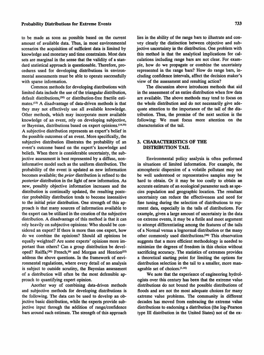
Fig. 1. Data set A in plotting position with a Normal distnbution- acceptable fit in the tail of the distribution.

;/--

o n s n a z z Graph 2: Data Set B

Fig. 2. Data set B in plotting position with a Normal distribution- not a good fit in the tail.

1 .o

0 o z : w n a z s x

Graph 3: Data Set B

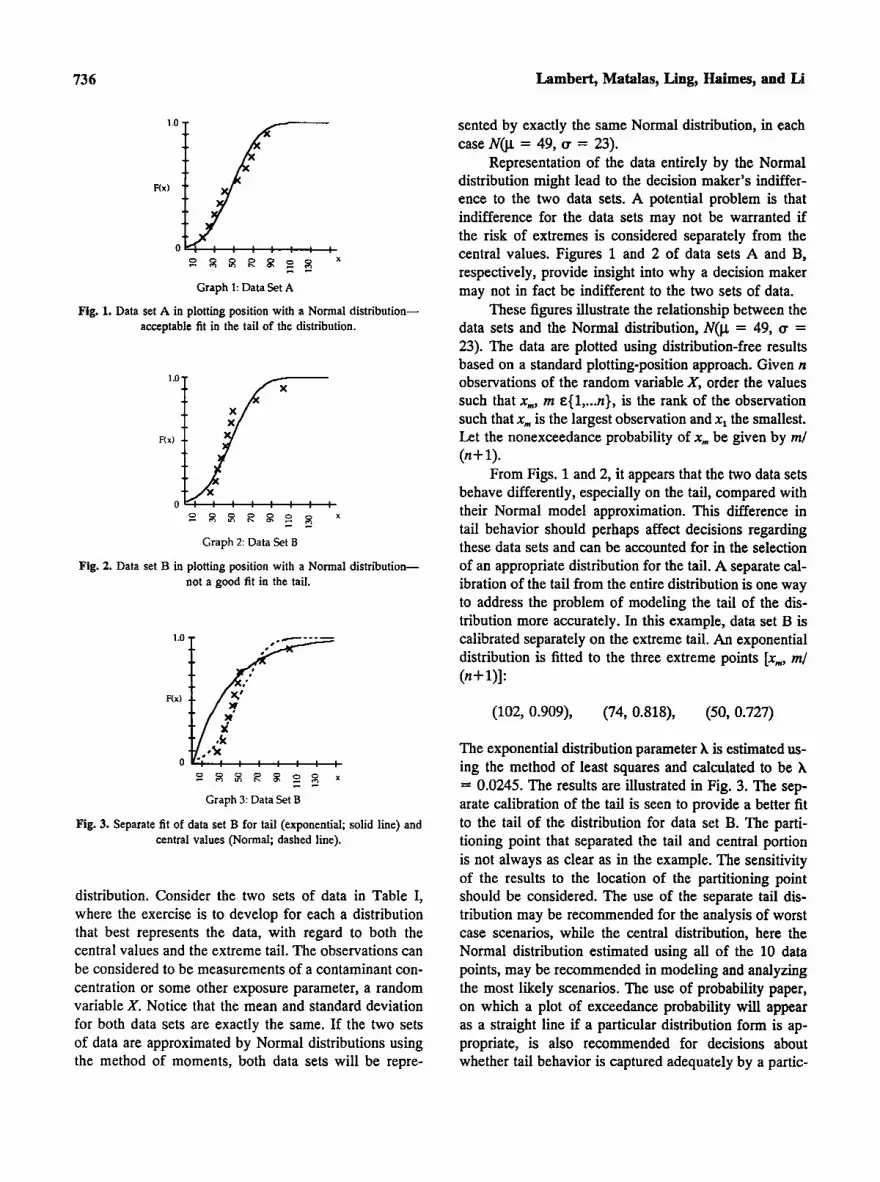
Fig. 3. Separate fit of data set B for tail (exponential; solid line) and central values (Normal; dashed line).

distribution. Consider the two sets of data in Table I, where the exercise is to develop for each a distribution that best represents the data, with regard to both the central values and the extreme tail. The observations can be considered to be measurements of a contaminant concentration or some other exposure parameter, a random variable X. Notice that the mean and standard deviation for both data sets are exactly the same. If the two sets of data are approximated by Normal distributions using the method of moments, both data sets will be repre-

sented by exactly the same Normal distribution, in each case N ( p = 49, u = 23).

Representation of the data entirely by the Normal distribution might lead to the decision maker's indifference to the two data sets. A potential problem is that indifference for the data sets may not be warranted if the risk of extremes is considered separately from the central values. Figures 1 and 2 of data sets A and B, respectively, provide insight into why a decision maker may not in fact be indifferent to the two sets of data.

These figures illustrate the relationship between the data sets and the Normal distribution, N ( p = 49, u = 23). The data are plotted using distribution-free results based on a standard plotting-position approach. Given n observations of the random variable X, order the values such that x,,,, rn &{l, ..a}, is the rank of the observation such that x, is the largest observation and x1 the smallest. Let the nonexceedance probability of x, be given by rnl (n+ 1).

From Figs. 1 and 2, it appears that the two data sets behave differently, especially on the tail, compared with their Normal model approximation. This difference in tail behavior should perhaps affect decisions regarding these data sets and can be accounted for in the selection of an appropriate distribution for the tail. A separate calibration of the tail from the entire distribution is one way to address the problem of modeling the tail of the distribution more accurately. In this example, data set B is calibrated separately on the extreme tail. An exponential distribution is fitted to the three extreme points [x,,,, rn/ (n+l)]:

(102, 0.909), (74, 0.818), (50, 0.727)

The exponential distribution parameter A is estimated using the method of least squares and calculated to be A = 0.0245. The results are illustrated in Fig. 3. The separate calibration of the tail is seen to provide a better fit to the tail of the distribution for data set B. The partitioning point that separated the tail and central portion is not always as clear as in the example. The sensitivity of the results to the location of the partitioning point should be considered. The use of the separate tail distribution may be recommended for the analysis of worst case scenarios, while the central distribution, here the Normal distribution estimated using all of the 10 data points, may be recommended in modeling and analyzing the most likely scenarios. The use of probability paper, on which a plot of exceedance probability will appear as a straight line if a particular distribution form is appropriate, is also recommended for decisions about whether tail behavior is captured adequately by a partic-


20 30 40 50 60 70 80

Exposure x

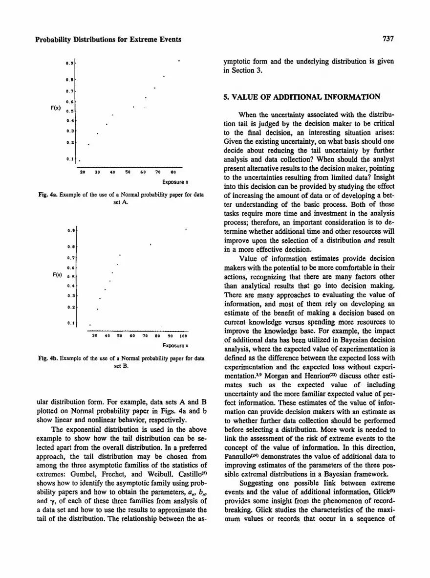
Fig. 4a. Example of the use of a Normal probability paper for data set A.

30 4 0 50 60 7 0 80 90 100

Exposure x

Fig. 4b. Example of the use of a Normal probability paper for data set B.

ular distribution form. For example, data sets A and B plotted on Normal probability paper in Figs. 4a and b show linear and nonlinear behavior, respectively.

The exponential distribution is used in the above example to show how the tail distribution can be se- lected apart from the overall distribution. In a preferred approach, the tail distribution may be chosen from among the three asymptotic families of the statistics of extremes: Gumbel, Frechet, and Weibull. Castil10(~) shows how to identify the asymptotic family using probability papers and how to obtain the parameters, u,, b,, and y, of each of these three families from analysis of a data set and how to use the results to approximate the tail of the distribution. The relationship between the as-

ymptotic form and the underlying distribution is given in Section 3.

5. VALUE OF ADDITIONAL INFORMATION

When the uncertainty associated with the distribution tail is judged by the decision maker to be critical to the final decision, an interesting situation arises: Given the existing uncertainty, on what basis should one decide about reducing the tail uncertainty by further analysis and data collection? When should the analyst present alternative results to the decision maker, pointing to the uncertainties resulting from limited data? Insight into this decision can be provided by studying the effect of increasing the amount of data or of developing a better understanding of the basic process. Both of these tasks require more time and investment in the analysis process; therefore, an important consideration is to determine whether additional time and other resources will improve upon the selection of a distribution and result in a more effective decision.

Value of information estimates provide decision makers with the potential to be more comfortable in their actions, recognizing that there are many factors other than analytical results that go into decision making. There are many approaches to evaluating the value of information, and most of them rely on developing an estimate of the benefit of making a decision based on current knowledge versus spending more resources to improve the knowledge base. For example, the impact of additional data has been utilized in Bayesian decision analysis, where the expected value of experimentation is defined as the difference between the expected loss with experimentation and the expected loss without experi- mentati0n.3~ Morgan and Henrion(=) discuss other estimates such as the expected value of including uncertainty and the more familiar expected value of perfect information. These estimates of the value of information can provide decision makers with an estimate as to whether further data collection should be performed before selecting a distribution. More work is needed to link the assessment of the risk of extreme events to the concept of the value of information. In this direction, Pannullocu) demonstrates the value of additional data to improving estimates of the parameters of the three possible extremal distributions in a Bayesian framework.

Suggesting one possible link between extreme events and the value of additional information, Glickts, provides some insight from the phenomenon of record- breaking. Glick studies the characteristics of the maximum values or records that occur in a sequence of

738 Lambed, Matalas, Ling, Haimes, and Li

X* X* x A ~ u a l c h e m i c . 4 ~ 1 ~ O rnagnindex

x A ~ u a l c h e m i c . 4 ~ 1 ~ O rnagnindex

Fig. 5. The pdf and cleanup cost function of annual release magnitude X.

independent, identically-distributed observations. For example, in the series (3, 2, 8, 4, 5, 6, 1,. 7, 3, 4, 9) there are three record breakers: 3, 8, and 9. Glick shows that given 50 observations, the expected number of record breakers is 4.5, while in a set 1,000,000 observations the expected number of record breakers is only 14.39. This means that if close to a million more samples are collected after the first 50, one could expect only nine more record breakers. From this result, our intuition suggests that the waiting time increases between record- breaking events as the number of observations increases. In fact, it turns out that the expected interrecord waiting time is infinite. This concept relates to another interesting result. No matter how many records have occurred, there will always be another. That is, the expected number of record breakers is infinite as the number of observations approaches infinity. Glick's results suggest that the extremal information attainable from continued experimentation may be limited, at least in the short run.

6. EXAMPLE: DECISION CRITERION AFFECTING CHOICE OF DISTRIBUTION

Consider the following experiment, which shows how an established decision criterion can help the selection of an input distribution function, specifically for results that are based on the tail of the output distribution. The example is related to the work of Slack et uZ.@) Gruninger et u L ( ~ ) similarly relate the choice of input distribution to a decision criterion that is based on the risk of extreme events.

Consider a random variable X that represents the unknown magnitude of annual chemical release. For annual releases of a magnitude greater than a threshold x* , the cleanup cost is a linear function of the release magnitude. A mitigating containment structure may be con- structed of a capacity such that all releases of a magnitude less than x, are contained with no need for

cleanup. Assuming the threshold x* to be zero, the cleanup cost function of release x is given by

If the planning period is fixed to be N years, then the time stream of discounted damages is

where

and r is the discount rate. The expected present value of the total cleanup costs is

where the conditional expected value of the annual release is

OD

S X f 4

Note that if x, = 0,

(1 + ,)''+I - 1 41 + r)" (13)

E[L(O)] = B P = BR(r) p

where p is the mean value of x and the definition of R(r) is apparent. Note that R(r) + 1 monotonically as r + CQ and that R(0) = N + 1; thus R(r) > R(r') for r < r'. It should be clear from Fig. 5 that only the tail of the distribution, x 2 x,, is of any importance to the expected present value of cleanup costs.

Consider now the optimization of the sum of the expected present value of cleanup costs and the capital cost of the containment structure. The problem is to find the optimal size of the containment structure. Assume the capital cost C of the containment structure to be

(14) c = C(X,)

an increasing function of the protection threshold x,. The total expected cost for the design x, is

m o ) = WXO) I f(4l + W O ) (15)


Fig. 6. Relationships among expected losses, capital cost, and net losses.

xo 4 a

Fig. 7. Relationships of the optimal designs for the true and the assumed scenarios.

from which an optimal design of the containment structure, x,, = a, can be found by solving

such that V(x,,) attains its minimum. Thus the total expected present value of cost for the optimal design is

V(u) = E[L(u)] + C(U) (17)

Note that

and (1) as r increases, u decreases, and so does V(u);

(2) the slope of V(x,,) is a function of r, and so is

Now we explore the effect of approximating the real- world distribution flx) by an assumed but “incorrect” distribution g(x). Assume that c(xo) is known but the real-world distributionflx) of releases is not known (Fig. 6). For this example, we assume that

U.

E [ m J I &)I < W(%) I fl-91 (18)

Recall that the optimal design capacity based on the minimization of V(&) is u. Let the total cost associated

with the estimated distribution g(x) be

Note that V(xJ attains its minimum when x,, = L. Thus the total expected design loss due to the assumed distribution g(x) is

The expected design loss can be interpreted as the cost of a nonoptimal design attributed to imperfect knowledge of the distribution fix) (Fig. 7). The aim of this introduction of the expected design loss function 6(&) is to study the impact of adopting different distributions g(x) given that the true distribution Ax) of releases is unknown. As mentioned above, only the tail, x > x,,, of the distribution of release x has any bearing on the optimization and consequently on the expected design loss 6(&). How important is the choice of distribution g(x)? It may be that there are conditions of discount rate, planning period, etc., for which the choice of distribution is relatively more important. Slack et U Z . ( ~ ) make a similar study based on the return period criteria for flood protection, estimating the assumed distribution g(x) from a Monte Carlo sample of the real-world distribution flx). They find that it can be nonoptimal, depending on the decision maker’s attitude toward risk, to assume the true generating distribution!

Continue the experiment by fixing the real-world distributionflx) to be of a general form such as the Wak- eby mentioned above. Then it will be interesting to study the loss function 6(d) as the three extreme value distributions are used alternatively as g(x) to approximate the tail of the distribution of x based on a Monte Carlo sample from Ax). How good are the extreme value distributions given the optimization problem of this example? What choices of distribution are preferred given a particular attitude toward risk? Does the choice from among the three extreme value distributions for the tail of x matter much or not very much? To what extent do the extreme values distributions bound the range of possible distribution choices?

This example points to the issues of choosing a probability distribution for the tail. The premise is that comparison of results from perfect knowledge of an input distribution function and from an approximation of the real-world distribution can give a sense of how important the choice of input distribution is, particularly for a problem in which it is the tail of the input distribution, and not the central values, that most influences the optimal decision.


7. THE CONDITIONAL EXPECTED VALUE AND RISK OF EXTREMES

A risk measure associated with extreme events, which are described by the tail of the distribution, can be useful in environmental risk management. As described below, the conditional expected value provides such a measure of the risk of extreme events. Most importantly, the conditional expected value of extreme events can be evaluated assuming only knowledge of the asymptotic form and two corresponding parameters. In other words, no knowledge about the specific distribution, within a given asymptotic family, is required. This robustness is an advantage in selection of probability distributions for characterizing the risk of extreme events.

Consider a continuous random variable X of harm that has a cumulative distribution function (cdf) F(x) and a probability density function (pdf) Ax), which are defined by the relationships

F(x) = prob[X < XI, x 2 0 (21)

and

The CDF represents the nonexceedanceprobability of x. The exceedance probability of x is defined as the probability that X is observed to be greater than x and is equal to one minus the CDF evaluated at x. The expected value, average, or mean value of the random variable X is defined by

In the partitioned multiobjective risk method, or PMRM,@) the concept of the expected value of harm is extended to generate the conditional expected-value function, which is associated with an extreme range of exceedance probabilities or their corresponding range of extreme harm severities. The resulting conditional expected-value function, in conjunction with the traditional expected value, provides a new measure of the risk of extreme events associated with a particular policy.

Let 1 - a, where 0 < a; < 1, denote an exceedance probability that partitions the domain of X into a range of extreme events, as follows. On a plot of exceedance probability, there is a unique harm p on the harm axis that corresponds to the exceedance probability 1 - a on the probability axis. Harms greater than p are

of high severity and low exceedance probability and constitute the range of extreme events. If, for example, 1 - a is taken to be equal to 0.05, then p is the 95th percentile.

For range of extreme events, the conditional expected harm (given that the harm is within that particular range) provides a measure of the harm associated with extremely large and potentially very costly and catastrophic events or scenarios. This measures is based on the definition of the conditional expected value. The conditional expected value risk measure is denoted f4(.)

and is related to scenarios of low exceedance probability and high severity. The function f4(.) is the expected value of X, given that x is greater than p:

OD

B

Thus, for a particular policy option, there is the additional measure of risk f4(.), in addition to the traditional, unconditional expected value denoted f5(.). Note the sim- ilarity between the forms of f4(.) and f5(.) from the ex- pression

OD

= s X K X ) dx 0

since the probability in the denominator above is necessarily equal to one. In the PMRM, conditional and unconditional expected values are balanced in a multiobjective formulation.

The function f4(.) is related to the percentile (e.g., the 95th percentile) as a measure of the risk of the extreme tails but provides a superior representation of the risk of extreme events because it can distinguish between tails of different shape when the exceedance probability at a particular location is the same. In this case, the percentile does not reflect a difference between the risk of extremes, while the functionf4(.) does reflect the difference, calculating the conditional expected value in the tail using all of the tail features. The function f4(.) is a natural measure of the risk of extreme events for risk-based decision making. It adapts the desirable prop-


erties of the unconditional expected value to a preselected extreme range of harm, thus providing a basis for conservative policies.

7.1. Statistics of Extremes and the Conditional Expected Value

The study of f4(.) and the risk of extreme events has been advanced by the correspondence between the function f4(.) and the statistics of extremes. Various theoretical results linking the statistics of extremes and the conditional expected value f4(.) are presented in the ter- minology and under the assumptions of this treatment.

The statistics of extremes is concerned with studying the largest value from a sample of t independent, identically distributed (i.i.d.) random variables>') Just as statistical moments parameterize random variables, the statistics of extremes defines two parameters that characterize the largest value of a sample of t independent, identically distributed variables, which is itself a random variable. The characteristic largest value, u,, is of the magnitude that is exceeded on the average once in t re- alizations of X, and it is implicitly defined by

t[l - F(u,)] = 1 (26) A second parameter, 6, which measures the sensitivity of the characteristic largest value, u,, to the sample size, t, is defined by

It can be shown that if X is a time-series variable, then t is the return period in number of events of the event of magnitude u,. The return period corresponding to the partition probability a of extreme events is given by

From the above development, it can be shown that the harm partition p for extreme events is exactly the characteristic largest value u,.

7.2. Approximating Catastrophic Risk Through the Statistics of Extremes

Distribution-free estimates of f4(.) have been derived for each of three extreme-value types, Gumbel, Frechet, and Weibull, based only on knowledge of the two extremal parameters, u, and 6,. The results summarized in this section rely on restrictive, but practically

useful assumptions about probability distribution forms that are the basis of a particular engineering treatment of extreme value theory.(I) If a random variable of harm can be assumed to be asymptotically of one of the three extreme-value types, then the approximations below generate distribution-free estimates of the extreme-event riskf4(.) that rely solely on the values of the statistics- of-extremes parameters u, and &.(=) These approximations based on the statistics of extremes are nearly exact for large values o f t and, equivalently, large values of the partition probability a.

For a random variable of harm that is asymptotically of Gumbel form and of an exponential tailp) the approximation to f4(.) is given by

f4P) = u, + (Ifif) (29) Distributions that are asymptotically (largest values) of the Gumbel form include the Normal, lognormal, Gum- bel, Weibull, gamma, Rayleigh, and exponential.

For a random variable that is asymptotically of the Frechet form and of a polynomial tail,@) the approximation to f4(.) is given by

f4P) = ur + Ufi3 + (1fitMui - (Ifit)) (30) Distributions that are asymptotically of the Frechet form include the Pareto and Cauchy.

The corresponding distribution-free approximation of f4(.) for random variables that are asymptotically of the Weibull form is given by

f4P) = u, + (l/S,) - (1/6,)/[(o - uJS, + 11 (31) where o is the upper limit of the harm random variable. Distributions that are asymptotically of the Weibull form include the uniform, the triangular, and most distributions with a finite upper bound.

The extremal parameters u, and 6, in many situations can be estimated using either the method of moments or extremal probability paper.(') These new approximations are valuable in that they absolve the analyst of the need to assume a particular probability distribution of harm, a step that is often most uncertain in practice. Furthermore, if the separate calibration of the tail can justify choice of one of the three asymptotic forms, then the conditional expected value, a measure of the risk of extreme events, can be estimated and studied directly from the statistics u, and 6,.

8. CONCLUSIONS

The objective of this paper has been to bring attention to the importance of the risk of extreme events to


selection of input probability distributions for regulatory situations. The need for study of extremes in this problem is clear since regulatory decision making often em- phasizes the “worst case” or the maximal exposure as a determining factor. Separate analysis of the tail data can provide an improved treatment of this regime of extreme scenarios. In addition, analysis of sensitivity of the tail model to critical assumptions can aid the analysis and decision process. The statistics of extremes can be used to minimize the choices about distribution models for the tail, while still furnishing a theoretically sound and accurate representation of the reality. The ‘conditional expected value as a measure of the risk of extreme events is presented in this paper as an example of how to treat the extremes separately and to illustrate important concepts about assessing risk in the tails of the distribution. More work is needed to link the concept of the value of information to the assessment of the risk of extremes. Additional important topics not covered in this paper include subjective assessment of the distribution tail, distribution-free methodologies for assessing and bounding the risk of extremes, comparison of percentiles and other statistics that try to represent the worst-case scenarios with respect to their interaction with distribution selection, and physical processes and phenomena that correspond to distribution tail features and motivate the separate calibration of the distribution tail.

ACKNOWLEDGMENTS

The authors are grateful for the contributions to this paper of the two reviewers. In addition, the participants of the EPWniversity of Virginia Workshop held in April 1993 on the selection of probability distributions for Monte Carlo analyses offered valuable insight and suggestions for improvement of this paper.

REFEXENCES

1. A. H-S. Ang and W. H. Tang, Probability Concepts for Engineering Planning and Design (John Wiley & Sons, New York, 1984).

2. E. L. Asbeck and Y. Y. Haimes, “The Partitioned Multiobjective Risk Method (PMRM),” Large Scale Systems 6(1), 13-38 (1984).

3. J. Berger, Statistical Decision Theory & Bayesian Analysis, 2nd ed. (Springer-Verlag, New York, 1985).

4. P. Bratley, B. L. Fox, and L. E. Schrage, A Guide to Simulation, 2nd ed. (Springer-Verlag, New York, 1987).

5. E. Castillo, Extreme Value Theory in Engineering (Academic Press, Boston, 1988).

6. S. French, Decision Theory: An Introduction to the Mathematics of Rationality (Ellis Horwood, London, and John Wiley and Sons, New York, 1988).

7. J. Galambos, The Asymptotic Theory of Extreme Order Statistics (John Wiley & Sons, New York, 1978).

8. N. Glick, “Breaking Records and Breaking Boards,” American Mathematical Monthly 85(1), 2-26 (1978).

9. J. H. Gruninger, Y. Y. Haimes, and D. Li, “Value of Information in Environmental Risk Management,” working paper (Center for Risk Management of Engineering Systems, University of Virginia, Charlottesville, 1992).

10. E. J. Gumbel, Statistics of Extremes (Columbia Press, New York, 1958).

11. Y. Y. Haimes, D. Li, P. Karlsson, and J. Mitsiopoulos, “Extreme Events: Risk Management,” in M. G. Sin& (ed.), Systems and Control Encyclopedia, Supplementary Vol. I (Pergamon Press, Oxford, 1990).

12. J. C. Houghton, “Birth of a Parent: The Wakeby Distribution for Modeling Flood Flows,” Water Resources Research 14(6), 110.5- 1108 (1978).

13. International Atomic Energy Agency, Evaluating the Reliability of Predictions Made Using Environmental Transfer Models, Safety Series No. 100 (IAEA, Vienna, 1989).

14. S. Kaplan and B. J. Garrick, “On the Quantitative Definition of Risk,” Risk Analysis 1(1), 11-27 (1981).

15. P. Karlsson and Y. Y. Haimes, “Probability Distributions and Their Partitioning,” Water Resources Research 24(1), 21-29 (1988).

16. P. Karlsson and Y. Y. Haimes, “Risk-Based Analysis of Extreme Events,” Water Resources Research 24,(1), 9-20 (1988).

17. J. M. Landwehr, N. C. Matalas, and J. R. Wallis, “Estimation of Parameters and Quantiles of Wakeby Distributions: 1. Known Lower Bounds,” Water Resources Research 15(6), 1361-1372 (1979).

18. J. M. Landwehr, N. C. Matalas, and J. R. Wallis, “Estimation of Parameters and Quantiles of Wakeby Distributions: 2. Unknown Lower Bounds,” Water Resources Research 15(6), 1373-1379 (1 979).

19. D. V. Lindley, Making Decisions, 2nd ed. (John Wiley and Sons, London, 1990).

20. J. Lipton and D. Shaw, Selecting Distributwns for Use in Monte Carlo Simulations (submitted for publication, 1992).

21. J. Mitsiopoulos and Y. Y. Haimes, “Generalized Quantification of Risk Associated with Extreme Events,” Risk Analysis 9(2),

22. J. Mitsiopoulos, Y. Y. Haimes, and D. Li, “Approximating Cat- astrophic Risk Through Statistics of Extremes,” Water Resources Research 27(6), 1223-1230 (1991).

23. M. G. Morgan and M. Henrion, Uncertainty: A Guide to Dealing with Uncertainty in Quantitative Risk and Policy Analysis (Cam- bridge University Press, New York, 1990).

24. J. E. Pannullo, Risk of Extreme Events: Reliability and the Value of Information, Ph.D. dissertation (Department of Systems Engi- neering, University of Virginia, Charlottesville, Aug. 1992).

25. S. F. Romei, Y. Y. Haimes, and D. Li, “Exact Determination and Sensitivity Analysis of a Risk Measure of Extreme Events,” In- formation and Decision Technology, in press (1992).

26. J. R. Slack, J. R. Wallis, and N. C. Matalas, “On the Value of Information to Flood Frequency Analysis,” Water Resources Re- search 11(5), 629-647.

27. F. W. Talcott, “Environmental Agenda, The Time is Right for an Analytical Approach to Policy Problems,” OR/MS June (1992).

28. D. M. Titterington, A. F. M. Smith, and U. E. Makov, Statistical Analysis of Finite Mixture Distributions (John Wiley and Sons, New York, 1985).

29. U.S. EPA, Guidelines for Exposure Assessment. Notice, Federal Register, Part IV, May 29 (1992).

30. H. Raiffa, Decision Analysis (Random House, New York, 1970).

243-254 (1989).

selection of probability distributions in characterizing risk of extreme events

Documents