selected approaches to estimate water-budget components of the high plains, 1940 through 1949 and...
TRANSCRIPT

U.S. Department of the InteriorU.S. Geological Survey
Scientific Investigations Report 2011–5183
GROUNDWATER RESOURCES PROGRAM
Selected Approaches to Estimate Water-Budget Components of the High Plains, 1940 through 1949 and 2000 through 2009
Groundwater leaving to adjacent geologic units
Surface-wateroutflow
Water table
Nonirrigatedfield
Rangeland
Surface-waterirrigated field
Groundwaterirrigated field
Runoff
Groundwaterdischarge to
stream
Recharge
Wellpumpage
Canalleakage Stream
leakage
Evapotranspiration
Surface-water inflow
Groundwater entering from adjacentgeologic units
Aquifer
Bedrock
Unsaturated zone
Precipitation
Center pivots in the panhandle of TexasCenter pivots in the panhandle of Texas
Wheat field in the central High PlainsWheat field in the central High Plains
Rangeland in the Nebraska Sand HillsRangeland in the Nebraska Sand Hills

Photograph by David Litke (U.S. Geological Survey)
Photograph by Richard Luckey(U.S. Geological Survey)
Photograph by Jennifer S. Stanton (U.S. Geological Survey)
Index of front cover photographs.
Cover illustration is a modified version of figure 2 from this report.

Selected Approaches to Estimate Water-Budget Components of the High Plains, 1940 through 1949 and 2000 through 2009By Jennifer S. Stanton, Sharon L. Qi, Derek W. Ryter, Sarah E. Falk, Natalie A. Houston, Steven M. Peterson, Stephen M. Westenbroek, and Scott C. Christenson
Groundwater Resources Program
Scientific Investigations Report 2011–5183
U.S. Department of the InteriorU.S. Geological Survey

U.S. Department of the InteriorKEN SALAZAR, Secretary
U.S. Geological SurveyMarcia K. McNutt, Director
U.S. Geological Survey, Reston, Virginia: 2011
For more information on the USGS—the Federal source for science about the Earth, its natural and living resources, natural hazards, and the environment, visit http://www.usgs.gov or call 1–888–ASK–USGS.
For an overview of USGS information products, including maps, imagery, and publications, visit http://www.usgs.gov/pubprod
To order this and other USGS information products, visit http://store.usgs.gov
Any use of trade, product, or firm names is for descriptive purposes only and does not imply endorsement by the U.S. Government.
Although this report is in the public domain, permission must be secured from the individual copyright owners to reproduce any copyrighted materials contained within this report.
Suggested citation:Stanton, J.S., Qi, S.L., Ryter, D.W., Falk, S.E., Houston, N.A., Peterson, S.M., Westenbroek, S.M., and Christenson, S.C., 2011, Selected approaches to estimate water-budget components of the High Plains, 1940 through 1949 and 2000 through 2009: U.S. Geological Survey Scientific Investigations Report 2011–5183, 79 p.

iii
Acknowledgments
The authors thank the National Weather Service Office of Hydrologic Development, Silver Spring, Maryland, for providing spatial data files from the Sacramento-Soil Moisture Accounting Model.
The authors also gratefully acknowledge the assistance and guidance provided by the following USGS employees: Dave Morgan and Lenny Orzol of the Oregon Water Science Center, Gabriel Senay of the Earth Resources Observation and Science (EROS) Center, Sophia Gonzales and David Maltby of the Texas Water Science Center, and Virginia McGuire of the Nebraska Water Science Center. Geoff Delin and Linda Pickett Garinger provided constructive reviews of earlier versions of this report.
ContentsAcknowledgments ........................................................................................................................................iiiAbstract ...........................................................................................................................................................1Introduction.....................................................................................................................................................2
Purpose and Scope ..............................................................................................................................2Water Budgets and Sustainability .....................................................................................................2
Water-Budget Equations ............................................................................................................2Sustainability ................................................................................................................................6
Description of Study Area ...................................................................................................................6Landscape ..............................................................................................................................................6Climate ..................................................................................................................................................10Surface Water .....................................................................................................................................10Agriculture ...........................................................................................................................................10Hydrogeologic Framework ................................................................................................................15
Major Geologic Units ................................................................................................................15Saturated and Unsaturated Zones ..........................................................................................17
Soil-Water-Balance Models ......................................................................................................................18SOil-WATer-Balance (SOWAT) Model .............................................................................................18
Precipitation and Evapotranspiration .....................................................................................18Soil Properties, Land Cover, and Irrigation Practices..........................................................23Model Calculations ....................................................................................................................23Sensitivity Analysis ....................................................................................................................26
Soil-Water-Balance (SWB) Model...................................................................................................26Model Calculations ....................................................................................................................28Sensitivity Analysis ....................................................................................................................29
Limitations of SOWAT and SWB Models ........................................................................................29SOWAT Model ............................................................................................................................29SWB Model .................................................................................................................................31
Selected Approaches to Estimate Water-Budget Components ..........................................................31Precipitation.........................................................................................................................................32
Precipitation Methods ..............................................................................................................32

iv
Precipitation Results .................................................................................................................34Evapotranspiration..............................................................................................................................34
Evapotranspiration Methods ...................................................................................................40Evapotranspiration from Shallow Groundwater ..........................................................40
Evapotranspiration Results ......................................................................................................41Evapotranspiration from Shallow Groundwater ..........................................................44
Recharge ..............................................................................................................................................44Recharge Methods ....................................................................................................................46Recharge Results .......................................................................................................................46
Surface Runoff and Groundwater Discharge to Streams ............................................................49Groundwater Discharge to Springs .................................................................................................50Groundwater Flow to and from Adjacent Geologic Units ............................................................50Irrigation ...............................................................................................................................................52
Irrigation Methods .....................................................................................................................52Irrigation Results ........................................................................................................................54
Groundwater in Storage ....................................................................................................................57Groundwater in Storage Methods ..........................................................................................57Groundwater in Storage Results .............................................................................................57
Uncertainty and Limitations .......................................................................................................................58Summary........................................................................................................................................................60References Cited..........................................................................................................................................61Appendix 1.....................................................................................................................................................69Appendix 2.....................................................................................................................................................73
Figures
1. Map showing location of the High Plains aquifer ...................................................................3 2. Schematic diagram showing water-budget components of the High Plains landscape
and aquifer system .......................................................................................................................4 3. Map showing location of the northern High Plains ................................................................7 4. Map showing location of the central High Plains ...................................................................8 5. Map showing location of the southern High Plains ................................................................9 6. Map showing distribution of average air temperature in the High Plains, 1980
through 1997 ................................................................................................................................11 7. Map showing weather stations used for assessing average annual air temperature
and precipitation 1905 through 2009 ........................................................................................12 8. Graphs showing (A) Groundwater and surface-water irrigated acres, 1949 through
2007, and average annual precipitation, 1940 through 2009; (B) groundwater pumpage for irrigation in the High Plains, 1950 through 2005 ...............................................................13
9. Map showing groundwater-level changes in the High Plains aquifer, pregroundwater development (about 1950) to 2005 ............................................................................................14
10. Graphs showing number of acres irrigated by gravity-flow and sprinkler methods in the (A) northern High Plains, (B) central High Plains, and (C) southern High Plains ......15
11. Map showing major geologic units in the High Plains .........................................................16 12. Maps showing (A) Water table, (B) saturated thickness, and (C) unsaturated
thickness in the High Plains, 2000 ............................................................................................19

v
13. Map showing permeability of soils in the High Plains ..........................................................22 14. Map showing available-water capacity of upper 59 in. of soils in the High Plains .........24 15. Map showing land-cover classification in the High Plains .................................................25 16. Graphs showing sensitivity of average annual recharge and irrigation pumpage simu-
lated by the SOil-WATer-Balance (SOWAT) model to changes in (A) irrigation efficien-cies, (B) initial soil moisture, (C) minimum soil-moisture requirement, (D) effective precipitation, and (E) evapotranspiration ...............................................................................27
17. Graphs showing sensitivity of average annual recharge, crop-irrigation demand, and actual evapotranspiration simulated by the Soil-Water-Balance (SWB) model to changes in (A) root-zone depth, (B) runoff-curve number value, and (C) precipitation, 2000 through 2009 .......................................................................................................................30
18. Flow chart showing water-budget component estimation methods and their relation to the SOil-WATer-Balance (SOWAT) and Soil-Water-Balance (SWB) models ...................33
19. Map showing distribution of weather stations used by the inverse-distance-weighted (IDW) interpolation method to estimate precipitation across the High Plains, 1940 through 1949 and 2000 through 2009 ........................................................................................35
20. Maps showing distribution of average annual total precipitation in the High Plains from the (A) Parameter-Elevation Regressions on Independent Slopes Model (PRISM) for 1940 through 1949, (B) PRISM for 2000 through 2009, (C) National Weather Service (NWS) for 2000 through 2009, (D) inverse-distance-weighted (IDW) interpolation for 1940 through 1949, and (E) IDW interpolation for 2000 through 2009 .................................38
21. Maps showing High Plains distribution of estimated average annual (A) potential evapotranspiration and (B) actual evapotranspiration from the National Weather Ser-vice (NWS) for 2000 through 2009, (C) actual evapotranspiration from the Simplified-Surface-Energy-Balance (SSEB) model for 2001 through 2009, (D) actual evapotranspi-ration from the Soil-Water-Balance (SWB) model for 1940 through 1949, and (E) actual evapotranspiration from the SWB model for 2000 through 2009 ............................42
22. Maps showing distribution of estimated average annual potential recharge from (A) the SOil-WATer-Balance (SOWAT) model, 2000 through 2009, (B) the Soil-Water-Balance (SWB) model, 1940 through 1949, and (C) the SWB model, 2000 through 2009 ...............................................................................................................................................47
23. Map showing surface-water irrigated land in the northern High Plains region, 2000 through 2009 ................................................................................................................................53
24. Maps showing distribution of estimated average annual irrigation application rates for groundwater and surface water from (A) the SOil-WATer-Balance (SOWAT) model and (B) the Soil-Water-Balance (SWB) model, 2000 through 2009 ........................55
25. Schematic diagram showing ranges for selected water-budget components in the High Plains, (A) 1940 through 1949 and (B) 2000 through 2009 ............................................59
A1. Graph showing example of mean crop coefficient generated for irrigated corn and soybeans with three values of the crop coefficient shape parameter (α1).......................70
Tables
1. Area of High Plains within each region and State ..................................................................6 2. Weather-station data used by the inverse-distance-weighted (IDW) interpolation
method to estimate daily precipitation in the High Plains, 1940 through 1949 and 2000 through 2009 .......................................................................................................................36
3. Average annual precipitation in the High Plains, 1940 through 1949 and 2000 through 2009 ...............................................................................................................................................39

vi
4. Estimated average annual potential and actual evapotranspiration in the High Plains, 1940 through 1949 and 2000 through 2009 ...............................................................................43
5. Estimated area and average annual maximum evapotranspiration of shallow ground-water in the High Plains, 1940 through 1949 and 2000 through 2009 ..................................45
6. Estimated average annual potential recharge for the High Plains aquifer, 1940 through 1949 and 2000 through 2009 .......................................................................................................48
7. Composited-average annual recharge determined by previous studies in the High Plains ............................................................................................................................................49
8. Streamflow entering and leaving the High Plains, 1940 through 1949 and 2000 through 2009 ...............................................................................................................................................51
9. Irrigated acres in the High Plains, selected estimates, 2002 ..............................................52 10. Estimated irrigation from groundwater in the High Plains, 2000 through 2009 .................56 11. Estimated volume of groundwater in storage in the High Plains aquifer, prior to ground-
water development (before about 1950) and 2007 ................................................................58 A1. Crop coefficient table used for the SWB model ....................................................................72 A2. Recharge rates in the High Plains compiled from previously published studies....................74

vii
Conversion Factors and AbbreviationsInch/Pound to SI
Multiply By To obtain
Length
inch (in.) 2.54 centimeter (cm)
inch (in.) 25.4 millimeter (mm)foot (ft) 0.3048 meter (m)mile (mi) 1.609 kilometer (km)
Area
acre 4,047 square meter (m2)acre 0.004047 square kilometer (km2)square mile (mi2) 2.590 square kilometer (km2)
Volume
acre-foot (acre-ft) 1,233 cubic meter (m3)Flow rate
acre-foot per year (acre-ft/yr) 1,233 cubic meter per year (m3/yr)cubic foot per second (ft3/s) 0.02832 cubic meter per second (m3/s)inch per hour (in/hr) 25.4 millimeter per hour (mm/hr)inch per day (in/day) 25.4 millimeter per day (mm/day)
Crop-water usage per unit area; Recharge, Evaporation, Evapotranspiration
inch per year (in/yr) 25.4 millimeter per year (mm/yr)Slope
foot per mile (ft/mi) 0.1894 meter per kilometer (m/km)
Temperature in degrees Fahrenheit (°F) may be converted to degrees Celsius (°C) as follows:
°C=(°F-32)/1.8
Vertical coordinate information is referenced to the North American Vertical Datum of 1988 (NAVD 88).
Horizontal coordinate information is referenced to the North American Datum of 1983 (NAD 83).
Elevation, as used in this report, refers to distance above the vertical datum.

viii
Acronyms
AET Actual EvapotranspirationAWC Available-Water CapacityBFI Base-Flow IndexCHP Central High PlainsCN Curve NumberET EvapotranspirationGIS Geographic Information SystemIDW Inverse-Distance WeightedMODIS Moderate Resolution SpectroradiometerNEXRAD Next Generation Weather RadarNHP Northern High PlainsNRCS Natural Resources Conservation ServicePET Potential EvapotranspirationPRISM Parameter-Elevation Regressions on Independent Slopes ModelSAC-SMA Sacramento-Soil Moisture AccountingSHP Southern High PlainsSOWAT SOil-WATer BalanceSSEB Simplified-Surface-Energy BalanceSWB Soil-Water BalanceUSDA U.S. Department of AgricultureUSGS U.S. Geological Survey

Abstract The High Plains aquifer, underlying almost 112 million
acres in the central United States, is one of the largest aqui-fers in the Nation. It is the primary water supply for drinking water, irrigation, animal production, and industry in the region. Expansion of irrigated agriculture throughout the past 60 years has helped make the High Plains one of the most productive agricultural regions in the Nation. Extensive withdrawals of groundwater for irrigation have caused water-level declines in many parts of the aquifer and increased concerns about the long-term sustainability of the aquifer.
Quantification of water-budget components is a prereq-uisite for effective water-resources management. Components analyzed as part of this study were precipitation, evapotrans-piration, recharge, surface runoff, groundwater discharge to streams, groundwater fluxes to and from adjacent geologic units, irrigation, and groundwater in storage. These com-ponents were assessed for 1940 through 1949 (representing conditions prior to substantial groundwater development and referred to as “pregroundwater development” throughout this report) and 2000 through 2009. Because no single method can perfectly quantify the magnitude of any part of a water budget at a regional scale, results from several methods and previously published work were compiled and compared for this study when feasible. Results varied among the several methods applied, as indicated by the range of average annual volumes given for each component listed in the following paragraphs.
Precipitation was derived from three sources: the Param-eter-Elevation Regressions on Independent Slopes Model, data developed using Next Generation Weather Radar and measured precipitation from weather stations by the Office of Hydrologic Development at the National Weather Service for the Sacramento-Soil Moisture Accounting model, and precipi-tation measured at weather stations and spatially distributed using an inverse-distance-weighted interpolation method. Pre-cipitation estimates using these sources, as a 10-year average annual total volume for the High Plains, ranged from 192 to 199 million acre-feet (acre-ft) for 1940 through 1949 and from 185 to 199 million acre-ft for 2000 through 2009.
Evapotranspiration was obtained from three sources: the National Weather Service Sacramento-Soil Moisture Accounting model, the Simplified-Surface-Energy-Balance model using remotely sensed data, and the Soil-Water-Balance model. Average annual total evapotranspiration estimated using these sources was 148 million acre-ft for 1940 through 1949 and ranged from 154 to 193 million acre-ft for 2000 through 2009. The maximum amount of shallow groundwater lost to evapotranspiration was approximated for areas where the water table was within 5 feet of land surface. The aver-age annual total volume of evapotranspiration from shallow groundwater was 9.0 million acre-ft for 1940 through 1949 and ranged from 9.6 to 12.6 million acre-ft for 2000 through 2009.
Recharge was estimated using two soil-water-balance models as well as previously published studies for various locations across the High Plains region. Average annual total recharge ranged from 8.3 to 13.2 million acre-ft for 1940 through 1949 and from 15.9 to 35.0 million acre-ft for 2000 through 2009.
Surface runoff and groundwater discharge to streams were determined using discharge records from streamflow-gaging stations near the edges of the High Plains and the Base-Flow Index program. For 1940 through 1949, the average annual net surface runoff leaving the High Plains was 1.9 million acre-ft, and the net loss from the High Plains aquifer by groundwater discharge to streams was 3.1 million acre-ft. For 2000 through 2009, the average annual net surface runoff leaving the High Plains region was 1.3 million acre-ft and the net loss by groundwater discharge to streams was 3.9 million acre-ft.
For 2000 through 2009, the average annual total esti-mated groundwater pumpage volume from two soil-water-bal-ance models ranged from 8.7 to 16.2 million acre-ft. Average annual irrigation application rates for the High Plains ranged from 8.4 to 16.2 inches per year. The USGS Water-Use Pro-gram published estimated total annual pumpage from the High Plains aquifer for 2000 and 2005. Those volumes were greater than those estimated from the two soil-water-balance models.
Total groundwater in storage in the High Plains aquifer was estimated as 3,173 million acre-ft prior to groundwater
Selected Approaches to Estimate Water-Budget Components of the High Plains, 1940 through 1949 and 2000 through 2009
By Jennifer S. Stanton, Sharon L. Qi, Derek W. Ryter, Sarah E. Falk, Natalie A. Houston, Steven M. Peterson, Stephen M. Westenbroek, and Scott C. Christenson

2 Selected Approaches to Estimate Water-Budget Components of the High Plains, 1940 through 1949 and 2000 through 2009
development and 2,907 million acre-ft in 2007. The average annual decrease of groundwater in storage between 2000 and 2007 was 10 million acre-ft per year.
IntroductionThe High Plains aquifer, underlying almost 112 million
acres in the central United States (fig. 1), is one of the largest aquifers in the Nation. It is the primary source for drinking water, irrigation, animal production, and industry in the region. In 2000, the High Plains aquifer supplied drinking water for about 80 percent of the High Plains regional population (Sharon Qi, U.S. Geological Survey, written commun., 2005). In this report, the term “High Plains” refers to the landscape and aquifer system corresponding to the geographic extent of the High Plains aquifer system. Development of this region for agriculture began during the late 1800s with nonirrigated crop-land and cattle grazing; however, low precipitation and high evaporation rates limited the production of nonirrigated crops for most of the area. Expansion of irrigated agriculture in the past 60 years has helped make the High Plains one of the most productive agricultural regions in the Nation. The High Plains region supplies approximately one-fourth of the Nation’s agri-cultural production (McMahon and others, 2007). As of 2007, there were 50 million acres of cropland, of which 15.4 million acres were irrigated, in the High Plains (U.S. Department of Agriculture, variously dated). Extensive with-drawals of groundwater for irrigation have caused water-level declines in many parts of the aquifer and increased concerns about the long-term sustainability of the aquifer.
This study is part of a series of regional studies funded by the U.S. Geological Survey (USGS) to evaluate the avail-ability and sustainability of major aquifers across the Nation. These studies are designed to assist State and local agencies who manage groundwater resources and to assess the status of groundwater resources from a national perspective. The High Plains Groundwater Availability Study updates the High Plains Regional Aquifer System Assessment (Weeks and others, 1988). That study compiled information about the hydrogeo-logic framework, water-quality characteristics, hydrologic budget, and stresses to the aquifer system.
Purpose and Scope
This report describes selected approaches to estimate pregroundwater development (1940 through 1949) and current (2000 through 2009) water-budget components of the High Plains aquifer and overlying landscape. The report emphasizes the groundwater part of the budget but also includes several land-surface budget components because of their connection with the groundwater system. Because no single method can perfectly quantify the magnitude of any part of a water budget at a regional scale, results from several methods and previ-ously published work are compared when feasible. Effects
of land use, landscape, climate, and modeling methods on individual water-budget components are discussed. This report provides information that can be used to guide the construc-tion and evaluate individual water-budget components of regional hydrologic models of the High Plains area, but does not present a complete water budget or comprehensive evalua-tion of groundwater availability or sustainability.
Water Budgets and Sustainability
A water budget is an accounting of hydrologic compo-nents of the water cycle, transfers between the components, and their relative contributions within a water system. Water budgets help define how much water is available, how much water is used, where the water comes from, and at what rate water is replenished. In its simplest form, a water budget defines the amount of water entering and leaving a water system. A schematic showing water inputs and outputs for the water system in the High Plains, referred to as the landscape and aquifer system, are shown in figure 2.
Under undisturbed or undeveloped conditions, the only sources of water to the High Plains landscape and aquifer sys-tem are from precipitation, streamflow from outside the High Plains, or subsurface water entering from underlying geologic units. Water entering the High Plains can follow many routes through the system. Precipitation can be lost to the atmo-sphere through interception or evapotranspiration (ET), which includes evaporation from soil or water bodies and plant tran-spiration; flow to streams or reservoirs; or percolate downward where it either is stored in the unsaturated zone or becomes aquifer recharge. Incoming streamflow can infiltrate into the aquifer, evaporate, or continue to flow out of the High Plains. Water entering the aquifer from subsurface sources or as infil-tration from surface sources (recharge or stream leakage) can be stored there, discharge to streams or springs, or become ET (if the water table is close enough to land surface). Once an area is developed for irrigated agriculture, water is transported from streams or the aquifer to irrigated fields where it becomes ET, surface runoff, or recharge (from irrigation return flow or canal leakage).
Water-Budget EquationsA simplified water-budget equation for a hydrologic sys-
tem can be expressed as the following equation:
P+Qin = ET + Qout + ΔS (1)
where P is precipitation, Qin is flow into the system, ET is evapotranspiration, Qout is flow out of the system, and ΔS is the change in storage.

Introduction 3
!!
!
!!
!
!
!
!
!
!
!!
!
!
!
Cheyenne NorthPlatte
Scottsbluff
GrandIsland
Denver
GardenCity
Wichita
Guymon
Amarillo
Lubbock
MidlandOdessa
Omaha
River
Canadian
MiddleLoup
LoupSouth
Sout
hPla
tte Riv e r
North Platte River
River
ElkhornRiver
River
River
River
River
River
River
Red
Republican
Arkansas
Loup
North
PecosR
iver
Cimarron
SOUTH DAKOTA
WYOMING
NEBRASKA
COLORADO
KANSAS
OKLAHOMANEW MEXICO
TEXAS
Land-surface elevation, in feet
High : 7,354
Low : 1,098Base from U.S. Geological Survey digital data, 1:100,000Albers Equal-Area Conic projectionStandard parallels 29°30' and 45°30', central meridian -101°North American Datum of 1983North American Vertical Datum of 1988
LOCATION MAP
102° 99°111°108°
105°
42°
39°
36°
33°
30°
27°
0 100 20050 150 MILES
Aquifer boundary from Qi, 2010
0 100 20050 150 KILOMETERS
Studyarea
CENTRAL HIGH
PLAINS
NORTHERN HIGH
PLAINS
SOUTHERNHIGH
PLAINS
CENTRAL HIGH
PLAINS
EXPLANATION
Figure 1. Location of the High Plains aquifer.

4 Selected Approaches to Estimate Water-Budget Components of the High Plains, 1940 through 1949 and 2000 through 2009
Gr
ound
wat
er le
avin
g to
adj
acen
t geo
logi
c un
its
Surfa
ce-w
ater
outfl
owW
ater
tabl
e
Non
irrig
ated
field
Surfa
ce-w
ater
irrig
ated
fiel
d
Grou
ndw
ater
irrig
ated
fiel
d
PP
Q+
bf inQ
ro in
Qgw in
ETp
ETsw
ETsg
w
ETp
ET+
pET
swir
+Q
bf out
Qro ou
t
ET+p
ETgw
ir
Runo
ff
Gro
undw
ater
disc
harg
e to
st
ream
Rech
arge
Wel
lpu
mpa
ge
Cana
lle
akag
eSt
ream
leak
age
Evap
otra
nspi
ratio
n
Surfa
ce-w
ater
inflo
w
Grou
ndw
ater
ent
erin
g fro
m a
djac
ent g
eolo
gic
units
Prec
ipita
tion
Aqui
fer
Bedr
ock
Unsat
urat
ed zo
ne
Qbf in
Qro in
Qgw in
ETsw
ir
ETsg
w
ETp
ETsw
Qbf ou
t
Qro ou
t
Qgw ou
t
Qgw ou
t
ETgw
ir
Prec
ipita
tion
Bas
e-flo
w c
ompo
nent
of s
trea
mflo
w in
to
the
syst
em
Gro
undw
ater
ent
erin
g th
e sy
stem
from
ad
jace
nt g
eolo
gic
units
Runo
ff co
mpo
nent
of s
trea
mflo
w in
to th
e sy
stem
Evap
otra
nspi
ratio
n fr
om g
roun
dwat
er
irri
gatio
n
Ev
apot
rans
pira
tion
from
pre
cipi
tatio
n Ev
apot
rans
pira
tion
from
sha
llow
gr
ound
wat
er Ev
apot
rans
pira
tion
from
sur
face
-wat
er
bodi
es Ev
apot
rans
pira
tion
from
sur
face
-wat
er
irri
gatio
n
G
roun
dwat
er d
isch
arge
to s
trea
ms
(bas
e flo
w) o
r spr
ings
Gro
undw
ater
leav
ing
the
syst
em to
ad
jace
nt g
eolo
gic
units
Ru
noff
com
pone
nt o
f str
eam
flow
out
of t
he
syst
emEXPL
AN
ATIO
N
Figu
re 2
. W
ater
-bud
get c
ompo
nent
s of
the
High
Pla
ins
land
scap
e an
d aq
uife
r sys
tem
.

Introduction 5
Precipitation and flow into the system represent inputs, and ET and flow out of the system represent outputs. Change in storage results from an imbalance between inputs and outputs. In the general system described by equation 1, the groundwater system is not treated as a separate hydrologic compartment.
For the High Plains landscape and aquifer system, these water-budget components can be expanded to:
(2)
where P is precipitation, is the base-flow component of streamflow into
the system, is groundwater entering the system from
adjacent geologic units, is the runoff component of streamflow into
the system, ET gwir is evapotranspiration of water from
groundwater irrigation (groundwater pumpage minus return flow and runoff),
ET P is evapotranspiration from precipitation, ET sgw is evapotranspiration from shallow
groundwater, ET sw is evapotranspiration from surface-water
bodies, ET swir is evapotranspiration of water from surface-
water irrigation (diverted water minus canal leakage, return flow, and surface runoff),
is groundwater discharge to streams (base flow) or springs,
is groundwater leaving the system to adjacent geologic units,
is the surface-runoff component of streamflow out of the system,
ΔS gw is the change in groundwater storage, ΔS sw is the change in surface-water storage, and ΔS uz is the change in unsaturated-zone storage.
This equation illustrates that in addition to precipitation, water can enter the system from outside the High Plains as the base flow or surface-runoff components of streamflow or from subsurface sources. Water leaves the system primarily by ET of water from precipitation, shallow groundwater, irrigation water (originating from surface water or groundwater), or directly from surface-water bodies. Water also flows out of the system as groundwater discharge to streams or springs, surface runoff to streams, or to adjacent geologic units. Imbalances between inputs and outputs will change the amount of water stored in groundwater, the unsaturated zone, or surface-water bodies.
A water budget can be created for any part of the hydro-logic system, such as for a lake, the soil zone, the unsaturated
zone, or the aquifer. The water budget specific to the High Plains aquifer system can be expressed by the following equation:
(3)
where Rgwir is recharge from groundwater-irrigation return
flow [groundwater withdrawal ( ) minus evapotranspiration of water from groundwater irrigation (ET gwir) minus groundwater-irrigation water runoff to streams],
RP is recharge from precipitation ( ), Rsw is recharge from surface-water seepage ( ), Rswir is recharge from surface-water-irrigation
return flow and canal leakage [diverted surface water minus diverted surface water that returns to streams minus evapotranspiration of water from surface-water irrigation (ET swir )], and
is groundwater withdrawal, and other terms are as defined previously.
The aquifer-specific budget components are linked closely to the budget components in equation 2, particularly precipitation and ET. Recharge has been divided into several components to reflect the different sources of water that can become available for recharge: precipitation, groundwater-irrigation return flow, surface-water-irrigation return flow and canal leakage, and seepage from naturally occurring surface-water features. In addition to the terms listed in the equation explanation, each of the recharge components is related to changes in the amount of water stored in the unsaturated zone. Groundwater withdraw-als also are related to landscape processes because the amount of water needed for irrigation is determined by ET demand of the crops grown at the land surface. Much of the groundwater withdrawn for other purposes likely returns to the aquifer or becomes surface-water runoff. For example, a portion of water withdrawn for public-water supplies will eventually end up in sewer systems and discharge to streams (Westerhoff and Crit-tenden, 2009).
Current and historical data describing the water-budget components for an aquifer often are not available and need to be estimated. These estimates are subject to uncertainties and limitations. Recharge and ET from groundwater can be partic-ularly difficult to quantify (Healy and others, 2007). Ground-water withdrawals for irrigation can be measured directly but only have been measured for limited areas in the High Plains. Groundwater-flow models are used to help verify estimates of these budget components by comparing model results with observable hydrologic conditions such as groundwater levels and discharge to streams. Hydrologic models that determine the fate of precipitation and estimate the amount of additional water needed for irrigation are available to quantify these
out outin inQ ro + Q bf - Q
ro - Q bf
uzswgwroout
gwout
bfout
swirswsgwPgwirroin
gwin
bfin
SSSQQQETETETETETQQQP
∆+∆+∆+++++++=+++ +
gwinQ
bfinQ
roinQ
bfoutQ
gwoutQ
rooutQ
outin out outR gwir+R P+R
sw+R swir+Q
gw = ET sgw+Q
bf+Q gw+Q
pump+ΔS gw
Q pumpout
outP - Q ro - ET P
outQ pump

6 Selected Approaches to Estimate Water-Budget Components of the High Plains, 1940 through 1949 and 2000 through 2009
components, as well as other land-surface water-budget com-ponents, such as the fate of water diverted from streams and reservoirs for irrigation. Coupling land-surface and subsurface processes can provide a comprehensive assessment of ground-water and landscape water-budget components and a tool for evaluating the effects of changes in various water-budget components. Even though hydrologically defensible models are calibrated by adjusting water-budget components and other model parameters so that model results match hydrologic measurements (such as groundwater levels and streamflows), it is still useful to compare modeled water-budget components with results from independent studies as an evaluation of model performance.
SustainabilityGroundwater sustainability was defined by Alley and
others (1999) as the “development and use of groundwater in a manner that can be maintained for an indefinite time without causing unacceptable environmental, economic, or social consequences.” Understanding the components of the water budget is a prerequisite for assessing the sustainability of a hydrologic system. Under average long-term conditions in an undeveloped system, the amount of water leaving will be bal-anced by water entering the system. Climate change, geologic shifts, or human disturbances such as groundwater pumpage can cause an imbalance between inputs and outputs. For a groundwater system to be sustainable, water leaving the aqui-fer from pumpage must be balanced by increased recharge, reduced evapotranspiration from groundwater, or reduced dis-charge to streams. If water leaving the aquifer is not balanced by other hydrologic components, water stored in the aquifer will decline, and groundwater mining occurs.
Water budgets help define the balance between water entering and leaving an aquifer but do not account for other factors that affect the long-term sustainability of an aquifer. These additional factors include physical limitations on how much groundwater can be extracted; deterioration of ground-water quality; effects of groundwater depletions on streams, lakes, wetlands, and land subsidence; future climatic condi-tions; economic costs associated with extracting groundwater; and public policy goals.
Description of Study Area
The High Plains landscape and aquifer system extent coincides with the boundary of the underlying High Plains aquifer that recently was updated to reflect changes in the understanding of the boundary location in Kansas, Colo-rado, Oklahoma, Texas, and New Mexico (Qi, 2010). The High Plains covers parts of eight States—Colorado, Kansas, Nebraska, New Mexico, Oklahoma, South Dakota, Texas, and Wyoming (fig. 1, table 1) and was divided into three geographic regions in previous studies—northern High Plains (NHP), central High Plains (CHP), and southern High Plains (SHP) (figs. 3, 4, and 5) (Weeks and others, 1988; McMahon
and others, 2007). These regions were defined using natural aquifer boundaries, air-temperature gradients, and logistical considerations associated with water-quality sample collec-tion. The bounds of those regional areas and their naming convention are used in this report.
Landscape
The High Plains is within the Great Plains physiographic province, which lies between the Rocky Mountains (not shown) on the west and the Central Lowlands (not shown) on the east (Fenneman and Johnson, 1946). Land-surface eleva-tion is highest in the northwest, trending from about 7,400 feet (ft) along the northwestern boundary to about 1,000 ft along the eastern boundary. Most of the High Plains is composed of flat plains or gently rolling hills. Grasses are the dominant natural vegetation of the landscape, ranging from short-grass prairies in the west to tall-grass prairies in the east. Streams have dissected the plains, producing a drainage network and escarpments that in many places define the boundary of the High Plains. Wind-blown sand has formed dunes across parts of the High Plains. The largest sand dune region, the Nebraska Sand Hills, in north-central Nebraska (fig. 3), is one of the largest grass-stabilized dune regions in the world. Its unique topography consists of dunes as high as 400 ft and as long as 20 miles (mi) (Bleed and Flowerday, 1989). Numerous lakes and meadows are located between the dunes, where groundwater is at or near land surface. In other parts of the High Plains, ephemeral shallow lakes have formed in shallow depressions called playas. Most playa lakes are not connected to the groundwater and contain surface runoff from precipita-tion events. Playas are most common south of the Arkansas River (Gutentag and others, 1984).
Table 1. Area of High Plains within each region and State.
Area, in million acres
Region
Northern 61.7Central 31.4Southern 18.8
State
Colorado 8.5Kansas 19.7Nebraska 41.4New Mexico 6.0Oklahoma 4.7South Dakota 3.1Texas 23.2Wyoming 5.2High Plains 111.8

Introduction 7
!!
!
!
!
!
!
!
!
!
!!
!!
!
!
!
##
##
#
#Barneston
Portis
Cheyenne
NorthPlatte
Odessa
Gothenburg
Scottsbluff
Omaha
GrandIsland
FairburyDenver
GardenCity
Webster
Loup
Loup
South
Middle
Platte
River
River
River
River
River
RiverRiver
River
River
Elkhorn
LittleBlue
BlueBig
River
River
River
RepublicanKansas
Arkansas
Sout
h
Platte
Platte
Creek
CreekArikaree River
GuernseyReservoir
GlendoReservoir
HarlanLake
Swanson Reservoir
NorthFork
Solomon River
South Fork River
Cedar
Niobrara River
North Loup River
North
Frenchman
Beaver
Solomon
LakeMcConaughyLodgepole Creek
SOUTH DAKOTA
WYOMING
NEBRASKA
COLORADO
KANSAS
§̈¦25
§̈¦29
§̈¦335
§̈¦70
§̈¦35
§̈¦76
§̈¦80
§̈¦90
§̈¦135
Hardy
Sparks
Ashland
Julesburg
06657000
06801000
0688200006884000
06461500
06853500
07139000
06764000
06872500
06873000
06873000
98°100°102°104°106°
44°
43°
42°
41°
40°
39°
38°
EXPLANATION
Nebraska Sand Hills
Northern High Plains aquifer boundary
Streamflow-gaging station and identifier
Maparea
LOCATION MAP
0 30 45 6015 MILES
0 30 45 6015 KILOMETERS
Base from U.S. Geological Survey digital data, 1:100,000Albers Equal-Area Conic projectionStandard parallels 29°30' and 45°30', central meridian -101°North American Datum of 1983
Figure 3. Location of the northern High Plains.

8 Selected Approaches to Estimate Water-Budget Components of the High Plains, 1940 through 1949 and 2000 through 2009
Central High Plains aquifer boundary
Streamflow-gaging station and identifier
EXPLANATION
Base from U.S. Geological Survey digital data, 1:100,000Albers Equal-Area Conic projectionStandard parallels 29°30' and 45°30', central meridian -101°North American Datum of 1983
!
!
!
!
!
!
!
!
!
#
#
#
#
#
#
#
##
GardenCity
Wichita
Guymon
Amarillo
FortSupply
Sweetwater
OKLAHOMA
NEW MEXICO
COLORADO
KANSAS
TEXAS
River
River
River
Canadian
River
River
River
River
Arkansas
North
Canadian
Canadian
Beaver River
ColdwaterCree
k
Creek
Creek
Duro Wolf Creek
Palo Duro Creek
Frio DrawRed
Sweetwater
North Fork Red River
Cimarron
Beaver
North Palo
LakeMeredith
287 §̈¦40
§̈¦135
§̈¦44
§̈¦35
§̈¦27
§̈
Elkhart
Canadian
Forgan
07227500
07228000
07155590
07301420
07156900
07139000
0723700007234500
07144300
#07227500
98°99°100°101°102°103°104°
39°
38°
37°
36°
35°
¦70
0 30 6015 45 MILES
0 30 6015 45 KILOMETERS
Maparea
LOCATION MAP
Figure 4. Location of the central High Plains.

Introduction 9
Figure 5. Location of the southern High Plains.
EXPLANATION
Southern High Plains aquifer boundary
# Streamflow-gaging station and identifier
Base from U.S. Geological Survey digital data, 1:100,000Albers Equal-Area Conic projectionStandard parallels 29°30' and 45°30', central meridian -101°North American Datum of 1983
!
!
!
!
!
#
#Amarillo
Lubbock
Midland
Odessa
Sweetwater
§̈¦287
§̈¦40
§̈¦27
§̈¦25
§̈¦20
RiverCanadian
Peco
s Riv
erPalo Duro Creek
Frio Draw
White River
Salt Fork
Braz
os River
Braz
os River
Double Mountain Fork Brazos River
Sulphur Springs Draw
Mustang Draw
Beals Creek
Colorado River
Red River
87TEXAS
NEW MEXICO
07301420
07227500
07227500
100°101°102°103°104°105°
35°
34°
33°
32°
0 30 6015 45 MILES
0 30 6015 45 KILOMETERS
Maparea
LOCATION MAP

10 Selected Approaches to Estimate Water-Budget Components of the High Plains, 1940 through 1949 and 2000 through 2009
Climate
The High Plains has a continental climate with strong seasonality of temperature extremes. Air temperatures gener-ally increase from north to south (fig. 6). Average air tempera-tures for 14 weather stations (fig. 7) across the High Plains measured during 1905 through 2009 ranged from 47.4 to 76.8 degrees Fahrenheit (°F) (U.S. Historical Climatology Network, 2010). Average air temperature from 2000 through 2009 (55.6°F) was almost 1 degree warmer than the mean temperature from 1940 through 1949 (54.7°F). An increase in mean air temperature has probably affected the water budget in recent years because potential evapotranspiration (PET) is affected by temperature. Greater PET rates will increase the demand for irrigation water if precipitation also does not increase.
Near-surface air is cooled as liquid water is turned to vapor by the process of ET. Irrigated fields lose more water through ET converting water to vapor than do nonirrigated cropland and rangeland. This process may have at least partially counteracted temperature trends, and it is possible that recent temperatures would have been warmer without the development of irrigation in the High Plains (Kueppers and others, 2007).
Average annual precipitation rates generally increase from west to east in the High Plains (Thornton and others, 1997). Average precipitation rates for 14 weather stations (fig. 7) measured during 1905 through 2009 ranged from 16.3 to 29.6 inches per year (in/yr) (U.S. Historical Climatology Network, 2010). Average precipitation for 2000 through 2009 (21.1 in/yr) was 1.0 inch less than average precipitation for 1940 through 1949 (22.1 in/yr). Precipitation rates as a com-ponent of the water budget are discussed in more detail in the “Precipitation” section of this report.
The frequent winds and high temperatures of the High Plains cause large evaporation rates (Gutentag and others, 1984). Potential evaporation rates measured from Class A evaporation pans ranged from 60 in/yr in the north to 105 in/yr in the south (Gutentag and others, 1984). Throughout the High Plains, potential evaporation rates are greater than precipita-tion rates, creating conditions that limit aquifer recharge.
The climatic record from the last century may not be rep-resentative of future conditions. Climate changes could affect future recharge rates, frequency and duration of droughts, ET rates through vegetation shifts, and demands for groundwater through changes in the availability of surface water for irriga-tion (Alley and others, 1999).
Surface Water
Perennial streams are more prevalent in the north than the south. Major streams draining the NHP are the Niobrara, Platte, Little Blue, Big Blue, Republican, and Solomon Rivers (fig. 3). The Arkansas and Canadian Rivers drain the CHP (fig. 4). No perennial streams drain the SHP (Blandford and
others, 2003). Within the High Plains, streamflow in the Canadian, Kansas, Niobrara, Platte, and Republican River Basins (basins not shown) is controlled by reservoirs and canal diversions that provide water to agricultural land (Bureau of Reclamation, 2011).
The Nebraska Sand Hills (fig. 3) are an important recharge area for the High Plains. This recharge contributes to the regional flow system and base flow to several rivers that are tributaries of the Platte and Niobrara Rivers. Annual streamflow from the Sand Hills averages approximately 14 percent of annual precipitation (Bentall, 1998). Runoff to streams over most of the Sand Hills is limited by the dune landscape and permeable topsoil (Bentall and Shaffer, 1979). Vegetation is dominated by mixed-prairie grasses, which take up water during a moderately short growing season. These two characteristics allow much of the water that infiltrates the soil profile to become available for groundwater recharge, which contributes to reliable base flow of streams. As streams leave the Sand Hills, base flow ranges from about 80 to 95 percent of total streamflow (Stanton and others, 2010). As these streams cross the dissected and loess-covered plains to the south and east, however, they receive less base flow, more surface runoff, and the base-flow fraction of streamflow drops to between about 60 and 80 percent.
Though naturally occurring lakes are a minor component of the surface-water system on the High Plains, with most effects on the groundwater system local in scope, numerous small lakes and marshes in the Nebraska Sand Hills are closely connected to groundwater (Bleed and Ginsberg, 1998). Several large, artificial reservoirs in the NHP cause local groundwater mounding and increase water storage locally. Because the source of water in reservoirs is predominantly impoundment of surface runoff (or snowmelt from outside the High Plains), the net flux is from reservoirs to the High Plains aquifer. Although there is no quantitative estimate of water flux from surface reservoirs to the High Plains, it is considered minor because of the limited number and relatively small surface area of reservoirs on the High Plains. Several large storage reservoirs upstream from the western boundary of the High Plains are a dominant factor in the surface-water hydrology of the North and South Platte Rivers.
Agriculture
Most of the High Plains landscape is composed of flat plains or gently rolling hills, making it well-suited for grow-ing crops. In 2007, almost one-half of the land area within the High Plains was used for growing crops (U.S. Department of Agriculture, variously dated). The principal crops grown in the High Plains in 2008 were corn, wheat, hay, alfalfa, soybeans, cotton, and sorghum, with primarily corn grown in the NHP, wheat in the CHP, and cotton in the SHP (U.S. Department of Agriculture, 2008). To support crop production, the aquifer has undergone extensive development for irrigation. The number of irrigated acres has increased from about 3 million in 1949

Introduction 11
SOUTHDAKOTA
IOWA
NEBRASKA
KANSAS
COLORADO
OKLAHOMA
NEWMEXICO
TEXAS
WYOMINGMINNESOTA
0 50 100 KILOMETERS
0 50 100 MILES
95°100°105°
40°
35°
From Thornton and others, 1997
EXPLANATION
Average annual air temperature, in degrees Fahrenheit(18-year mean)
64
37
Base from U.S. Geological Survey digital data, 1:100,000Albers Equal-Area Conic projectionStandard parallels 29°30' and 45°30', central meridian -101°North American Datum of 1983
Figure 6. Distribution of average air temperature in the High Plains, 1980 through 1997.

12 Selected Approaches to Estimate Water-Budget Components of the High Plains, 1940 through 1949 and 2000 through 2009
to about 15.4 million in 2007 (U.S. Department of Commerce, variously dated; U.S. Department of Agriculture, variously dated) (fig. 8A). Before the 1930s, irrigation generally was limited to areas where surface water could be diverted to crop fields, but advancements in well drilling and pumping equip-ment increased development of the aquifer as a source of irri-gation water for fields in relatively flat areas after the drought periods of the 1930s and 1950s (Weeks and others, 1988). Later development of the center-pivot irrigation system in the 1960s further expanded irrigation to areas previously not suit-able for irrigation because of their rolling topography.
In 2005, water for irrigation accounted for approximately 95 percent of total pumpage from the High Plains aquifer (Kenny and others, 2009). Groundwater pumpage for irriga-tion increased from approximately 4 million acre-ft in 1950 to about 20 million acre-ft in 1975 and was approximately 18 million acre-ft in 2005 (fig. 8B) (U.S. Geological Sur-vey, variously dated). Several periods of time have had
smaller-than-average precipitation that correlated with increased irrigated acres in the High Plains (fig. 8A). Con-versely, a reduction in the number of irrigated acres in the 1980s corresponds to a period of greater-than-average precipitation.
Agriculture affects the water budget of a water system in several important ways. Greater recharge rates are associated more with nonirrigated cropland than with rangeland (Scanlon and others, 2005b; Sophocleous, 2004). The greater recharge is caused by changes to soil structure, vegetation coverage, wilting point, and rooting depth. Irrigation of agricultural fields further affects the hydrologic budget. Irrigation water increases ET and deep percolation, or potential recharge. If surface water is the source for irrigation, water is redistributed from streams, through canals, and finally to agricultural fields. Diverted water reduces streamflow and may increase recharge along the distribution system. If groundwater is the source for irrigation, groundwater pumpage increases and groundwater in
Figure 7. Weather stations used for assessing average annual air temperature and precipitation 1905 through 2009.
U.S. Historical Climatology Network, 2010
Base from U.S. Geological Survey digital data, 1:100,000Albers Equal-Area Conic projectionStandard parallels 29°30' and 45°30', central meridian -101°North American Datum of 1983
Studyarea
Weather station
EXPLANATION
40°
35°
100°105°
SOUTHDAKOTA
KANSAS
COLORADO
OKLAHOMA
NEWMEXICO
TEXAS
WYOMING
NEBRASKA
0 100 200 MILES
0 100 200KILOMETERS

Introduction 13
storage can be reduced. Groundwater-level declines have been observed in parts of the High Plains as a result of groundwater pumpage for irrigation (McGuire and others, 2003; McGuire, 2007) (fig. 9).
Irrigation methods also can affect the water budget. Center-pivot systems have improved irrigation efficiency by reducing deep-percolation rates associated with gravity-flow irrigation (Musick and others, 1990). The combination of center-pivot systems with low-energy, precision-application
methods further improves irrigation efficiency by reducing water losses associated with droplet evaporation and drift (Howell and others, 1995). Center-pivot systems have been replacing gravity-flow systems since about the 1950s (Musick and others, 1990). According to estimates from the USGS Water-Use Program, most of the irrigated fields in High Plains States were irrigated primarily with sprinkler systems, such as center-pivot systems, in 2005 (U.S. Geological Survey, vari-ously dated) (figs. 10A, 10B, and 10C).
Figure 8. (A) Groundwater and surface-water irrigated acres, 1949 through 2007, and average annual precipitation, 1940 through 2009; (B) groundwater pumpage for irrigation in the High Plains, 1950 through 2005 (U.S. Department of Commerce, variously dated; U.S. Department of Agriculture, variously dated; U.S. Geological Survey, variously dated).
0
4
8
12
16
20
24
28
32
Mea
n pr
ecip
itatio
n, in
inch
es p
er y
ear
Irrig
ated
land
, in
mill
ions
of a
cres
LOWESS smoothed line(Helsel and Hirsch, 1992)
19451940
19501955
19601965
19701975
19801985
19901995
20002005
20100
5
10
15
20
25
Grou
ndw
ater
pum
page
,
in m
illio
ns o
f acr
e-fe
et p
er y
ear
A
B
Mean precipitation from 14 sites (fig. 7)
Irrigated land
EXPLANATION

14 Selected Approaches to Estimate Water-Budget Components of the High Plains, 1940 through 1949 and 2000 through 2009
WYOMING SOUTHDAKOTA
IOWA
NEBRASKA
KANSAS
COLORADO
OKLAHOMA
NEWMEXICO
TEXAS
95°100°105°
40°
35°
From McGuire (2007)
0 50 100 MILES
0 50 100 KILOMETERS
Water-level change, in feetDeclines
Greater than 150
101 to 150
51 to 100
26 to 50
10 to 25
No substantial change
Area of little or no saturated thickness
Rises
+10 to -10
10 to 25
26 to 50
Greater than 50
EXPLANATION
Base from U.S. Geological Survey digital data, 1:2,000,000Albers Equal-Area Conic projectionStandard parallels 29°30' and 45°30', central meridian -101°North American Datum of 1983
Figure 9. Groundwater-level changes in the High Plains aquifer, pregroundwater development (about 1950) to 2005.

Introduction 15
Hydrogeologic Framework
Although the hydrogeologic framework is not the subject of this report, a discussion of the basic framework is needed before discussing water budgets. Much of the description of geologic units is derived from the thorough description pro-vided in Gutentag and others (1984).
Major Geologic UnitsThe High Plains aquifer consists of hydraulically con-
nected deposits of late Tertiary and Quaternary age (Gutentag and others, 1984). Late Tertiary-age deposits, from oldest to youngest, include the Brule Formation of the White River Group, Arikaree Group, Ogallala Group, and Broadwater Formation (not shown) (Gutentag and others, 1984; Diffen-dal, 1995) (fig. 11). Quaternary-age deposits include alluvial, valley-fill, eolian sand, and glacial deposits. The Ogallala Group makes up most of the High Plains aquifer and underlies about 134,000 square miles (mi2) of the study area (Gutentag and others, 1984). The paleosurface upon which the High Plains aquifer material was deposited slopes gently from west to east at 5 to 7 feet per mile (ft/mi), though local variations and buried valleys exist throughout the area. Geologic units underlying the High Plains aquifer are poorly permeable, middle-Tertiary-age or older deposits (Weeks and Gutentag, 1981). Groundwater flow between the High Plains aquifer and the underlying units is minimal.
The Brule Formation of the White River Group, together with the Arikaree Group, constitute the oldest geologic units of the High Plains aquifer, and both are present along the northwestern extent of the NHP aquifer. The Brule Formation is mainly a massive, poorly permeable siltstone, though locally containing coarser-grained deposits such as sandstone beds or channel deposits. It is considered part of the High Plains aquifer only where the permeability of the Brule Forma-tion has been increased by secondary porosity such as joints, fractures, and solution openings (Gutentag and others, 1984). Areas containing coarser deposits, or where the permeability of the Brule Formation has been increased through secondary porosity, are difficult to map on a regional scale (Cannia and others, 2006). Where it was not enhanced through secondary porosity, the top of the Brule Formation forms the base of the High Plains aquifer. In the western part of the NHP region, the Brule Formation is overlain by the younger Arikaree Group (fig. 11), mainly composed of very fine to fine-grained sandstone. The Arikaree has a maximum thickness of about 1,000 ft in western Nebraska and eastern Wyoming.
Where both are present, the Arikaree Group is overlain by the Ogallala Group (Gutentag and others, 1984). The Ogal-lala Group is a heterogeneous deposit of interlayered stream sediments, lakebeds, and windblown sand, silt, and clay. The Ogallala Group varies greatly in sediment size and character over short distances (Cannia and others, 2006). Though highly variable, one consistent feature found at the top of the Ogal-lala Group in most areas of the High Plains is the Ogallala cap
Figure 10. Number of acres irrigated by gravity-flow and sprinkler methods in the (A) northern High Plains, (B) central High Plains, and (C) southern High Plains.
0
2
4
6
8
10
12
Gravity flow
Sprinkler (includes center pivot)
0
2
4
6
8
10
12
0
2
4
6
8
10
12
YEAR
A
B
C
1985 1990 1995 2000 2005
EXPLANATION
Mill
ions
of a
cres
Data from U.S. Geological Survey, variously dated

16 Selected Approaches to Estimate Water-Budget Components of the High Plains, 1940 through 1949 and 2000 through 2009
WYOMING
SOUTHDAKOTA
KANSASCOLORADO
OKLAHOMA
TEXAS
NEW MEXICO
NEBRASKA
102° 99°111°108°
105°
42°
39°
36°
33°
30°
27°
0 100 200 MILES
0 100 200 KILOMETERS
EXPLANATION
Dune sand
Aquifer absent
Arikaree Group and Brule Formation
Quaternary alluvial valley fill deposits
Quaternary alluvial deposits
Ogallala Group
Glacial deposits
Base from U.S. Geological Survey digital data, 1:100,000Albers Equal-Area Conic projectionStandard parallels 29°30' and 45°30', central meridian -101°North American Datum of 1983
Modified from Gutentag and others, (1984); and Soller, (1998)
Figure 11. Major geologic units in the High Plains.

Introduction 17
rock, a caliche deposit, which is also called mortar beds. These deposits are cemented with calcium carbonate, are resistant to weathering, and form ledges when in outcrop (Weeks and Gutentag, 1984). The Ogallala Group is generally coarser than the underlying Arikaree Group, but less coarse than the overlying Quaternary alluvial and valley-fill deposits; gravel is not abundant within the Ogallala Group (Lawton, 1984). The maximum thickness of the Ogallala Group is about 800 ft (Swinehart and others, 1988).
The Broadwater Formation, a late-Tertiary alluvial sand and gravel deposit, overlies the Ogallala Group and underlies younger Quaternary-age deposits across the north-central part of the NHP (Swinehart and others, 1985). The Broadwater Formation has a maximum thickness of 300 ft and contains more silt eastward, though generally it is only distinguished from overlying Quaternary-age alluvial deposits because of its age, whereas the character and physical characteristics of both units are similar. Though not necessarily called Broadwater Formation in eastern Nebraska, equivalent late-Tertiary-age sand and gravel are present there as well.
Unconsolidated Quaternary-age alluvial gravel, sand, silt, and clay overlie and are in hydrologic connection with the Ogallala Group in the eastern parts of the CHP and NHP (fig. 11). Eastward of the margin of where both units are present, the Ogallala Group is absent, and Quaternary allu-vial and valley-fill deposits directly overlie poorly permeable bedrock. The Quaternary-age alluvial deposits generally are thinner than areas dominated by the Ogallala Group, and maximum thicknesses are around 300 ft (Gutentag and others, 1984). Quaternary-age valley-fill deposits (fig. 11) are similar in character and deposition to the Quaternary-age alluvial deposits, and are distinguished because the valley-fill deposits are related to erosion and deposition by current-day stream systems rather than ancient streams. These valley-fill deposits are as much as 60 ft thick and are present near most major rivers that cross the High Plains aquifer. Across the SHP and partly into the CHP, the Ogallala Group is overlain by the Quaternary-age Blackwater Draw Formation consisting of sandy to clayey eolian sediments (Holliday, 1989).
Quaternary-age dune sand deposits overlie the Ogal-lala Group in large parts of the NHP and over some of the CHP, but only exist in small areas in the SHP (fig. 11). The largest contiguous area, known as the Nebraska Sand Hills, covers approximately 20,000 mi2 of the NHP (fig. 3) and was undergoing dune formation and migration as recently as about 700 years ago (Miao and others, 2007). The dune sands range from very fine to medium sand and, where saturated, are con-sidered part of the High Plains aquifer (Gutentag and others, 1984). The dune sand deposits are as much as 300 ft thick, but probably average closer to 100 to 150 ft, and actually are a relatively thin veneer on top of the underlying deposits of the Ogallala Group (Lawton, 1984). Ogallala Group depos-its underlie all dune sands present in the High Plains (Muhs, 2007).
Though not always acknowledged in discussions regard-ing the High Plains aquifer, glacial deposits overlie the eastern
end of the NHP (Condra and others, 1950). Whereas glacial deposits have been removed through erosion in major stream valleys, glacial till remains in intervalley areas of the NHP north of the Platte River (Soller, 1998). The glacial deposits consist of till and outwash overlain with eolian loess, with possible buried valley-fill deposits of sand and gravel. The distribution and occurrence of buried-valley deposits within or underlying the till is not well-known. Though the fine-grained till is only poorly permeable, groundwater may flow through local deposits of sand and gravel within the till and through underlying or intervening glacial valley-fill deposits. Eastern Nebraska glacial deposits are currently under study (Smith and others, 2008; Divine and others, 2009), but the interaction between groundwater within the glacial deposits and other aquifers is still poorly understood. However, groundwater-flow modeling studies of a sub-area of the NHP (Peterson and others, 2008; Stanton and others, 2010) used the western edge of the glacial till (fig. 11) as a no-flow or fixed-water-level model boundary. Both models calibrated favorably with minimal groundwater discharge across these boundaries, from the Quaternary alluvial deposits into the till deposits (west to east), supporting the concept that the High Plains aquifer may not be continuous through the area overlain with till.
Surficial deposits of eolian loess overlie parts of the NHP and CHP (Muhs and Bettis, 2000). Loess is defined as wind-blown sediment primarily of silt-size particles (Pye, 1995). The fine-grained loess deposits can be as thick as 325 ft (Con-don, 2006; Johnson, 1960; Richmond and others, 1994).
Saturated and Unsaturated ZonesThe proximity of saturated subsurface deposits to the land
surface can affect the water budget. When saturated deposits are close to the land surface (thin unsaturated zone), shallow groundwater is available for plant transpiration; discharge to lakes where it can eventually evaporate; or discharge to streams where it can later evaporate, recharge groundwater downstream, or flow out of the system. In some cases, water that would otherwise become recharge will instead become surface runoff because sediments are already saturated and potential recharge rates exceed the rate of infiltration to the subsurface. In these areas, the recharge rate will decrease as the depth to saturated sediment decreases, and groundwa-ter flow will be predominately horizontal instead of vertical (Sophocleous, 2004). In areas where saturated sediments are deeper, typically in arid or semiarid settings, they are less well-connected hydrologically with surface-water features, and recharge is more likely to occur where surface runoff collects in topographic depressions, such as playas or dry streambeds. Water moving downward through thick unsatu-rated zones can take decades or millennia to reach the aquifer (McMahon and others, 2006).
The boundary between the saturated and unsaturated zones is the water table. Water-table elevations for 2000 (fig. 12A) (McMahon and others, 2007; V.L. McGuire, U.S. Geological Survey, written commun., 2002) were used to

18 Selected Approaches to Estimate Water-Budget Components of the High Plains, 1940 through 1949 and 2000 through 2009
calculate the thickness of saturated and unsaturated zones in the High Plains (figs. 12B and 12C). The saturated thickness was calculated as the difference between the water-table and the base-of-aquifer elevations (McGuire and others, 2003). The saturated thickness of the High Plains aquifer ranges from less than 50 ft in much of the SHP and near the edges of the aquifer to about 1,200 ft in the NHP. Flow of water through the saturated zone from recharge to discharge areas is con-trolled by the hydraulic conductivity of the aquifer material and the hydraulic gradient between the recharge and discharge areas. In the High Plains, sediments in the Broadwater Forma-tion and Quaternary deposits generally are coarser and have greater hydraulic conductivity values than older deposits. As a result, water flows more freely through the younger depos-its. Hydraulic gradients indicate that regional groundwater movement is generally from west to east with localized flow towards streams (fig. 12A).
The unsaturated zone thickness was calculated as the dif-ference between the land-surface and water-table elevations. The thickness of the unsaturated zone ranges from 0 to greater than 300 ft (fig. 12C). The composition of the unsaturated zone can affect the movement of water through the system. Composition of the unsaturated zone in the High Plains is vari-able, consisting of unconsolidated clay, silt, sand, and gravel with localized zones of cemented calcium carbonate and silica (Gurdak and others, 2007). The fine-grained loess deposits present in parts of the NHP and CHP can restrict water flow; however, where fractures are present, downward flow could be substantial (Flury and others, 1994; McMahon and others, 2006). Conversely, flow downward through dune sand depos-its is uniformly rapid.
Soil represents the shallowest part of the unsaturated zone. Most soils in the High Plains developed from loess or dune-sand deposits (Gutentag and others, 1984). Soil perme-ability ranges from less than 1 to greater than 9 inches per hour (in/hr) (Schwarz and Alexander, 1995) (fig. 13). Average permeability is 5.41 in/hr in the NHP, 2.73 in/hr in the CHP, and 1.87 in/hr in the SHP. Soil permeability can affect surface runoff, recharge, and irrigation components of the water budget. Soils that are more permeable will result in reduced surface runoff, increased recharge, and increased amounts of irrigation water needed to maintain adequate soil moisture for crop growth.
Soil-Water-Balance ModelsSoil-water-balance models assist estimation of sev-
eral components of the High Plains aquifer water budget by simulating processes in the soil profile, thus linking landscape conditions such as precipitation and ET to aquifer budget components such as recharge and irrigation pumpage. In the following sections, methods used to calculate water-budget component values by the SOil-WATer-Balance (SOWAT) and Soil-Water-Balance (SWB) models for this study are
described. Although both the SOWAT and SWB models use a soil-water-budget equation to estimate unknown components of the soil-water budget, the models are formulated differently with respect to model inputs such as time-step length, ET, runoff, soil-moisture dynamics, and precipitation.
SOil-WATer-Balance (SOWAT) Model
The SOil-WATer-Balance (SOWAT) model, developed by the Columbia Plateau Water-Availability Study (Kahle and others, 2011), uses information about precipitation, ET, soil properties, land cover, and irrigation practices to compute two unknown quantities: groundwater withdrawals for irrigation and potential recharge. Estimates of the unknown quantities of groundwater withdrawals for irrigation and potential recharge were made on a monthly time scale at 449,504 cells across the High Plains for the period of 2000 through 2009. Model cells were 0.62 mi by 0.62 mi in extent. The soil profile water-budget equation solved by the SOWAT model for each model cell is:
ΔS soil = P eff + IR - ET - R (4)
where ΔS soil is the change in soil-water storage, in inches, P eff is precipitation plus snowmelt minus surface
runoff, in inches, IR is irrigation application, in inches, ET is evapotranspiration, in inches, and R is potential recharge, or deep percolation, in
inches.
Precipitation and EvapotranspirationThe SOWAT model was designed to accept precipitation
data and a single pre-determined direct-runoff factor defined as a percentage of precipitation (Kahle and others, 2011). The model does not account for snowmelt directly in the soil-mois-ture calculations. Because the High Plains is such a large area with substantial climatic gradients and variations in soil tex-ture, a single runoff factor is not adequate to describe condi-tions in the model area. Moreover, moisture input from snow-melt must be a consideration for much of the High Plains area. To accommodate these realities in view of model limitations, a combination parameter was calculated called “effective precipitation.” Effective precipitation represents the amount of natural (not irrigation) water available for infiltration into the soil and was calculated using precipitation (National Weather Service, written commun., 2010), snowmelt (Anderson, 2006), and surface-runoff (National Weather Service, written com-mun., 2010) data generated from a National Weather Service (NWS) hydrologic model called the Sacramento-Soil Moisture Accounting (SAC-SMA) model (described in the “Precipi-tation” section of this report). Effective precipitation was

Soil-Water-Balance Models 19
Figure 12. (A) Water table, (B) saturated thickness, and (C) unsaturated thickness in the High Plains, 2000.
From McMahon and others, 2007
WYOMINGSOUTH
DAKOTA
IOWA
NEBRASKA
KANSAS
COLORADO
OKLAHOMA
NEWMEXICO
TEXAS
95°100°105°
40°
35°
0 50 100 KILOMETERS
0 50 100 MILES
EXPLANATION
Water-table elevation, in feet
1,000 to 1,500
1,501 to 2,000
2,001 to 2,500
2,501 to 3,000
3,001 to 3,500
3,501 to 4,000
4,001 to 4,500
4,501 to 5,000
Greater than 5,000
Approximate direction of regional groundwater flow
No data/aquifer not present
Base from U.S. Geological Survey digital data, 1:100,000Albers Equal-Area Conic projectionStandard parallels 29°30' and 45°30', central meridian -101°North American Datum of 1983
A

20 Selected Approaches to Estimate Water-Budget Components of the High Plains, 1940 through 1949 and 2000 through 2009
WYOMINGSOUTH
DAKOTA
IOWA
NEBRASKA
KANSAS
COLORADO
OKLAHOMA
NEWMEXICO
TEXAS
95°100°105°
40°
35°
0 50 100 KILOMETERS
0 50 100 MILES
EXPLANATION
Saturated thickness, in feet
0 to 100
101 to 200
201 to 300
301 to 400
401 to 500
501 to 600
Greater than 600
No data/aquifer not present
From McMahon and others, 2007Base from U.S. Geological Survey digital data, 1:100,000Albers Equal-Area Conic projectionStandard parallels 29°30' and 45°30', central meridian -101°North American Datum of 1983
B
Figure 12. (A) Water table, (B) saturated thickness, and (C) unsaturated thickness in the High Plains, 2000.—Continued

Soil-Water-Balance Models 21
Figure 12. (A) Water table, (B) saturated thickness, and (C) unsaturated thickness in the High Plains, 2000.—Continued
From McMahon and others, 2007Base from U.S. Geological Survey digital data, 1:100,000Albers Equal-Area Conic projectionStandard parallels 29°30' and 45°30', central meridian -101°North American Datum of 1983
WYOMINGSOUTH
DAKOTA
IOWA
NEBRASKA
KANSAS
COLORADO
OKLAHOMA
NEWMEXICO
TEXAS
95°100°105°
40°
35°
0 50 100 KILOMETERS
0 50 100 MILES
EXPLANATION
Unsaturated thickness, in feet
0 to 100
101 to 200
201 to 300
Greater than 300
No data/aquifer not present
C

22 Selected Approaches to Estimate Water-Budget Components of the High Plains, 1940 through 1949 and 2000 through 2009
From Schwarz and Alexander, 1995
WYOMINGSOUTH
DAKOTA
IOWA
NEBRASKA
KANSAS
COLORADO
OKLAHOMA
NEWMEXICO
TEXAS
95°100°105°
40°
35°
0 50 100 KILOMETERS
0 50 100 MILES
EXPLANATION
Soil permeability, in inches per hour
0 to 1.0
1.1 to 3.0
3.1 to 6.0
6.1 to 9.0
No data/aquifer not present
Greater than 9.0
Base from U.S. Geological Survey digital data, 1:100,000Albers Equal-Area Conic projectionStandard parallels 29°30' and 45°30', central meridian -101°North American Datum of 1983
Figure 13. Permeability of soils in the High Plains.

Soil-Water-Balance Models 23
calculated for each model cell as the sum of precipitation and snowmelt minus surface runoff.
The Simplified-Surface-Energy-Balance (SSEB) model estimates actual evapotranspiration (AET) from remotely sensed land-surface-temperature data. Specific details about the SSEB model are described in the “Evapotranspiration” section of this report.
Soil Properties, Land Cover, and Irrigation Practices
In the SOWAT model, simulated soil moisture is com-pared with the estimated soil moisture required to support crops (Kahle and others, 2011). If simulated soil moisture in a model cell is less than the soil moisture required, then irriga-tion is supplied until the soil moisture in that model cell fills to the water-storage capacity of the soil. The amount of water the soil is able to store also is known as the available-water capacity (AWC) of the soil. The AWC of the upper 59 in. of soils in the High Plains was derived from the General Soil Map (STATSGO) (Miller and White, 1998) (fig. 14). For this study, the minimum soil-moisture requirement was set in the model to 50 percent of the AWC of the soil. This percentage was based on water requirements for crops common to the High Plains (corn, wheat, sorghum, and cotton) (Kirkpatrick and others, 2006; McMahon and others, 2007). The initial moisture content of the soil for the month before the start of the simulation (February 2000) was estimated by running the model from March 2000 to December 2009 using an estimated initial condition and computing the average February soil moisture for 2001 through 2009.
Three land-cover classes were used as input for the SOWAT model: (1) irrigated agriculture, (2) nonirrigated agri-culture and native vegetation, and (3) built-up land and water bodies. Because the National Land Cover Database (NLCD) for 2001 (Multi-Resolution Land Characteristics Consor-tium, 2001) only identified agricultural land and not irrigated fields, the irrigated cells were identified using the NLCD and delineated irrigated land for 2002 from remotely sensed satellite imagery (Brown and others, 2008). Thus, the NLCD and irrigated-land data sets were combined in this study. If a model cell identified as agricultural land from the NLCD also was identified as irrigated, then the cell was classified as irrigated agriculture in the SOWAT model (fig. 15). The irri-gated agricultural cells in the land-cover grid identify where SOWAT allowed irrigation when a soil-moisture deficit existed for that cell during a simulation. Land identified in the NLCD as either built-up area or open water was reclassified as urban land/water bodies, and all other NLCD land-use classes were lumped into the native/nonirrigated-land class in the SOWAT model input.
The SOWAT model requires values for irrigation efficien-cies (for groundwater and surface-water irrigation), the length of the irrigation season, and the fraction of groundwater and surface-water irrigation within a cell (Kahle and others, 2011). Irrigating with surface water is considered less efficient than
with groundwater for this model because gravity-flow systems typically are used for irrigating with surface water, and sprin-klers are more often used for irrigating with groundwater. Less irrigation efficiency means more water needs to be delivered to supply the crop-water requirements. Gravity-flow irrigation efficiencies can range from 35 to 90 percent (with tailwater reuse), and sprinkler irrigation efficiencies range from 55 percent to 95 percent (U.S. Department of Agriculture, 1997; Melvin and Yonts, 2009). Conservative estimates for mean irrigation efficiencies of 75 percent for groundwater and 65 percent for surface-water delivery were used in the High Plains SOWAT model.
Because there are substantial climate gradients across the High Plains, the length of the irrigation season can differ from the NHP to the SHP. Irrigation season lengths were estimated from an analysis of the monthly AET data (2000 through 2009). The beginning of the irrigation season was selected to be the month when mean monthly AET begins to rise rapidly in the spring; the end of the irrigation season was selected to be the month when AET decreases rapidly in the fall. The irrigation season estimated for the NHP and CHP regions was May through September. For the SHP, it was estimated as April through September. The same irrigation season was used for all years of the simulation.
Finally, the model requires an estimate of the fraction of irrigated acres in each model cell receiving irrigation water that is supplied by groundwater. This value is used to deter-mine how much of the crop-water demand will be supplied by surface-water and groundwater sources. The values for each cell may range from 0.0 (100 percent supplied by surface water) to 1.0 (100 percent supplied by groundwater). For the High Plains, substantial surface-water irrigation occurs only in the NHP (Buchanan and others, 2009; Colaizzi and oth-ers, 2008). The fraction of groundwater irrigation in each cell for the NHP was determined using the location of surface-water irrigated fields within Nebraska, northwestern Kansas (Amanda Saunders, U.S. Geological Survey, written commun., 2010), and Wyoming (Matt Hoobler, Wyoming State Engi-neer’s Office, written commun., 2010).
Model CalculationsThe amounts of water needed for irrigation or potentially
available for recharge are determined in the SOWAT model by comparing the simulated soil moisture with the AWC and applying an adjustment for irrigation efficiency. Simulated soil moisture (SM), in inches, is calculated by SOWAT (Kahle and others, 2011) as:
SM = SM' + P eff - AET (5)
where SM' is soil moisture from the previous month, in
inches, P eff is effective precipitation, in inches, and AET is actual evapotranspiration, in inches.

24 Selected Approaches to Estimate Water-Budget Components of the High Plains, 1940 through 1949 and 2000 through 2009
Figure 14. Available-water capacity of upper 59 in. of soils in the High Plains.
WYOMINGSOUTH
DAKOTA
IOWA
NEBRASKA
KANSAS
COLORADO
OKLAHOMA
NEWMEXICO
TEXAS
95°100°105°
40°
35°
0 50 100 KILOMETERS
0 50 100 MILES
EXPLANATION
Available-water capacity, in inches
0 to 4
4 to 8
8 to 12
12 to 16
No data/aquifer not present
Greater than 16.0
From Miller and White, 1998Base from U.S. Geological Survey digital data, 1:100,000Albers Equal-Area Conic projectionStandard parallels 29°30' and 45°30', central meridian -101°North American Datum of 1983

Soil-Water-Balance Models 25
Figure 15. Land-cover classification in the High Plains.
WYOMINGSOUTH
DAKOTA
IOWA
NEBRASKA
KANSAS
COLORADO
OKLAHOMA
NEWMEXICO
TEXAS
95°100°105°
40°
35°
0 50 100 KILOMETERS
0 50 100 MILES
EXPLANATION
Land cover
Open water
Built-up land
Native/nonirrigated
Irrigated agriculture
No data/aquifer not present
From Multi-Resolution Land CharacteristicsConsortium, 2001
Base from U.S. Geological Survey digital data, 1:100,000Albers Equal-Area Conic projectionStandard parallels 29°30' and 45°30', central meridian -101°North American Datum of 1983

26 Selected Approaches to Estimate Water-Budget Components of the High Plains, 1940 through 1949 and 2000 through 2009
Effective precipitation in the SOWAT model is added to the previous month’s soil moisture, and AET is subtracted to determine the current month’s soil moisture (Kahle and others, 2011). For irrigated cells during the irrigation season, the irrigation demand or amount of water potentially available for recharge is calculated from the soil moisture, AWC, and irrigation efficiencies. If soil moisture is greater than the AWC, excess moisture becomes available for potential recharge. If soil moisture is equal to or greater than the minimum soil-moisture requirement but less than the AWC, then no irrigation is applied for the current month. If soil moisture is less than the minimum soil-moisture requirement, irrigation water is added to the cell so that the soil moisture is equal to the AWC. The amount of irrigation water supplied to a model cell (Qirr), in inches, is calculated as,
Qirr = (AWC - SM) / IE (6)
where AWC is the available-water content of the soil, in
inches, SM is simulated soil moisture, in inches, and IE is irrigation efficiency, expressed as a fraction.
Supplied irrigation water is apportioned among ground-water and surface-water sources using a user-supplied frac-tion of irrigated acres in each model cell that is supplied by groundwater. If less than 100 percent of a model cell is groundwater irrigated, the remainder of the irrigation demand is supplied by surface water.
For nonirrigated model cells or non-irrigation-season months in the SOWAT simulation, irrigation water is not sup-plied to satisfy the ET demands of crops or native vegetation when soil moisture is less than the soil-moisture target. This can result in negative potential-recharge values. A possible interpretation of negative values is that water is supplied by other sources (deeper unsaturated zones, shallow groundwater, or surface water) to meet AET. If the simulated soil moisture is greater than the AWC, excess moisture becomes available for potential recharge.
Sensitivity AnalysisA sensitivity analysis determines the effect of changing
model input values on model output values. Because model values (parameters) input into the soil-water-balance models can be uncertain, a range of values were tested in the model to determine how simulated recharge and irrigation pumpage might be affected by that uncertainty. To test sensitivity of recharge and irrigation pumpage to changes in SOWAT model inputs, groundwater and surface-water irrigation efficiencies, initial soil moisture, minimum soil-moisture requirement as a percentage of the AWC, effective precipitation, and AET were systematically and individually increased and decreased by 10 and 20 percent of the original parameter values for the duration of the 2000 through 2009 simulation period. The
sensitivity of each parameter was tested separately for each region by varying each parameter individually while keeping all other parameters the same as the original simulation for that region.
Simulated recharge and irrigation pumpage were most sensitive to changes in effective precipitation and AET (fig. 16). Average annual simulated recharge was most sensi-tive to changes within the CHP, where a 20-percent decrease in effective precipitation caused a 214-percent decrease in recharge, and a 20-percent increase in AET caused a 192-per-cent decrease in simulated recharge. Decreases in recharge greater than 100 percent indicate that the AET demand would be satisfied by shallow groundwater or moisture in the unsaturated zone deeper than 59 in. below land surface if those sources of water were available. Average annual simulated irrigation pumpage changed the most in the NHP, where simulated irrigation pumpage increased by 46 percent in response to a 20-percent decrease to effective precipita-tion, and increased 72 percent in response to a 20-percent increase in AET. These sensitivity results highlight the need for reliable estimates of effective precipitation and AET when using water-balance models, because small errors in effective precipitation or in the model can cause large errors in simu-lated results. Simulated recharge and pumpage were much less sensitive to changes in irrigation efficiencies, initial soil moisture, and minimum soil-moisture requirement. The largest change to simulated recharge from a change to one of those three parameters was a 14-percent increase in response to a 20-percent decrease in irrigation efficiencies in the CHP. The largest change to simulated irrigation pumpage from a change to one of those three parameters was a 25-percent increase in response to a 20-percent decrease in irrigation efficiencies.
Soil-Water-Balance (SWB) Model
The Soil-Water-Balance (SWB) model (Dripps and Bradbury, 2007; Westenbroek and others, 2010) uses spatially distributed soil and landscape properties with daily weather data to calculate spatial and temporal variations in potential recharge and the estimated amount of irrigation water needed to sustain crops (appendix 1).
The SWB model layout (Westenbroek and others, 2010) consists of a grid, with soil properties and daily climate data attributed to each model cell. SWB calculates the fractions of precipitation and snowmelt that become surface runoff, AET, and recharge using a modified Thornthwaite-Mather soil-water accounting method to track the soil water in each cell through time (Thornthwaite and Mather, 1957; Westenbroek and oth-ers, 2010). Potential recharge, represented in SWB by deep percolation, is surplus water in the soil column between the land surface and the bottom of the root zone. Surplus water is calculated by subtracting the sum of the outputs (AET, surface runoff, plant interception) from the inputs (precipitation, snowmelt, surface runoff from adjacent cells).
Physical factors that control flow and loss of water on the ground surface and within the soil include the soil AWC,

Soil-Water-Balance Models 27
Figure 16. Sensitivity of average annual recharge and irrigation pumpage simulated by the SOil-WATer-Balance (SOWAT) model to changes in (A) irrigation efficiencies, (B) initial soil moisture, (C) minimum soil-moisture requirement, (D) effective precipitation, and (E) evapotranspiration.
Irrigation Efficiencies
-25
-15
-5
5
15
25
Irrigation Efficiencies
-25
-15
-5
5
15
25
-25
-15
-5
5
15
25
-240
-180
-120
-60
0
60
120
180
240
-20 -10 0 10 20 -20 -10 0 10 20-240
-180
-120
-60
0
60
120
180
240
Northern High PlainsCentral High Plains
Southern High PlainsHigh Plains
EXPLANATION
Percent change in model input
Perc
ent c
hang
e , i
n si
mul
ated
pum
page
Perc
ent c
hang
e, in
sim
ulat
ed re
char
ge
Initial Soil Moisture Initial Soil Moisture
Minimum Soil-Moisture Requirement
Effective Precipitation Effective Precipitation
Evapotranspiration Evapotranspiration
A
B
C Minimum Soil-Moisture Requirement
D
E

28 Selected Approaches to Estimate Water-Budget Components of the High Plains, 1940 through 1949 and 2000 through 2009
hydrologic soil group, land use, and direction of surface-water flow, which is used for routing runoff. Soil properties were derived from the General Soil Map (STATSGO2) (U.S. Department of Agriculture, 2006). Land-use classes used to assign each cell included agricultural, urban, forest, and grassland (Multi-Resolution Land Characteristics Consortium, 2001). Characteristics assigned according to land use, such as the Natural Resources Conservation Service (NRCS) runoff-curve number for estimating the potential for surface runoff, plant interception values, and root-zone depth, were obtained from the USDA National Engineering Handbook (U.S. Dept. of Agriculture, 2004), Cronshey and others (1986), and Thorn-thwaite and Mather (1957).
To represent climatic conditions, the SWB code requires, at minimum, precipitation and temperature for each day. These data can either be from a single weather station and applied uniformly to the model grid, or from daily grids of weather data, interpolated from multiple stations located throughout and just outside the study area. For the geographically exten-sive High Plains, daily precipitation values were interpolated using inverse-distance weighting of weather-station data (National Climatic Data Center, 2010) for 1940 through 1949 and 2000 through 2009 (see the “Precipitation Methods” sec-tion of this report for more information). Daily air-temperature values were interpolated using a kriging method with weather-station data (National Climatic Data Center, 2010) for 1940 through 1949 and 2000 through 2009.
The model grid consisted of 452,979 grid cells across a rectangular area that extended beyond the boundaries of the High Plains. Grid cells were 5,000 ft by 5,000 ft in size. The SWB code processes the soils grids and daily weather grids to calculate the daily soil-water content from precipitation, potential ET (PET) and AET, surface runoff into and from adjacent cells, snowmelt, and potential recharge that passes below the root zone, on a cell-by-cell basis.
Initial soil-moisture values for the model were estimated by running the model for the year previous to each period of interest. Simulated soil-moisture values for the end of 1939 were used as initial conditions for 1940 through 1949, and simulated soil-moisture values for the end of 1999 were used as initial conditions for 2000 through 2009.
The only water source used as input to the soil profile in the published SWB code (Westenbroek and others, 2010) is precipitation. For this High Plains study, irrigation water was a substantial source for many areas from the 1950s to present (2011). To include irrigation water in the analysis, the model code was modified to allow irrigation to maintain soil moisture in irrigated agricultural areas (Brown and others, 2008; Multi-Resolution Land Characteristics Consortium, 2001) above a minimum level during the growing season (appendix 1). The volume of water necessary to maintain that level of soil moisture was assumed to be the volume of water entering the soil profile from irrigation, and was calculated as equal to the part of crop demand beyond that available from infiltrated precipitation plus stored soil water above the specified minimum level. Some parts of the High Plains were
irrigated in the 1940s, but those areas composed a small per-centage of the High Plains area (McGuire and others, 2003); therefore, irrigation water was not applied to the simulation during the 1940s.
Surface runoff is calculated using the NRCS curve-num-ber method (Cronshey and others, 1986) and is affected by soil properties, moisture content, and air temperature. If surface runoff water is routed to a closed surface depression, available water can exceed AET and soil-moisture demands. In these cases, unrealistic recharge values can occur. To limit excessive recharge, a maximum recharge rate was set to 2, 0.6, 0.24, and 0.12 in/day for hydrologic soil group A, B, C, and D, respec-tively. The extra water that was not allowed to infiltrate was not carried into the following day. Precipitation that falls as snow is accounted by SWB as being stored on the surface until daily air temperature indicates it would melt (Westenbroek and others, 2010). The rate of snowmelt is determined from a temperature-index method where 0.059 in. of snow melts per day per average degree Celsius that the daily maximum tem-perature is above the freezing point. Infiltration and surface runoff also are affected by frozen ground, which is tracked continuously using a frozen-ground index (Molnau and Bis-sell, 1983). Runoff that is transferred between cells is tracked as inflow and outflow.
There are several methods available in the SWB code to estimate PET, but for this study the Hargreaves and Samani (1985) method was used, which uses the daily high and low temperatures to calculate PET. The SWB model then calcu-lates AET from PET and the available soil moisture in storage as determined from a series of nonlinear relations (for com-binations of soil type and vegetation categories) between soil moisture and the accumulated potential water loss (Thornth-waite and Mather, 1957). If precipitation exceeds PET, AET is equal to PET; if PET exceeds precipitation, AET is equal to precipitation plus the amount of water that can be extracted from the soil (up to but not exceeding the PET). Updates to the SWB code for this study include effects of crop-water use on AET and the availability of irrigation water to satisfy crop-water use requirements in irrigated areas (appendix 1).
Root-zone depths are an important parameter in the SWB model. Values are assigned based on hydrologic soil group and land-cover classification because the same vegetation type will send roots to different depths for different soil types. Digital elevation models were processed to determine the surface-water-flow direction for each grid cell, as described in West-enbroek and others (2010). Irrigation efficiency, the source of irrigation water, and the availability of shallow groundwater to satisfy crop-water demands are not defined in the model formulation.
Model CalculationsPotential recharge is equivalent to the surplus water in
the soil profile and is calculated as the difference between the change in soil moisture and water inputs and outputs. Sources include precipitation, snowmelt, and inflow from adjacent

Soil-Water-Balance Models 29
cells. Outputs include interception by plants, outflow to adjacent cells, and AET. In equation form, the daily soil-water budget is expressed as:
recharge = (precipitation + snowmelt + inflow) – (interception + outflow + AET) – change in soil moisture (7)
Estimation of the amount of irrigation required to sustain crop growth was calculated using the methods discussed in appen-dix 1.
Sensitivity AnalysisTo test sensitivity of simulated recharge, crop-irrigation
demand, and AET to changes in SWB model inputs, root-zone depth, runoff-curve number values, and precipitation, were systematically and individually increased and decreased over the entire High Plains by 10 and 20 percent for the 2000-through-2009 time period (fig. 17). The sensitivity of each parameter also was tested separately by varying each parameter individually while keeping all other parameters the same as the original model parameters.
Simulated results from the SWB model were less sensi-tive to changes in model inputs than were results from the SOWAT model. Changes to the runoff-curve number value by as much as 20 percent had the least effect on the simula-tion results, causing at most a 7-percent reduction in average annual simulated AET in the SHP (fig. 17B). A 20-percent change in root-zone depth caused average annual simulated recharge to change by as much as 15 percent in the NHP, 20 percent in the CHP, and 17 percent in the SHP (fig. 17A). Changes to root-zone depth had a smaller effect on simu-lated crop-irrigation demand and AET, causing as much as a 3.3-percent change in simulated crop-irrigation demand (NHP) and as much as a 2.3-percent change in simulated AET (SHP). Changes to precipitation had the largest effect on simulated results (fig. 17C). A 20-percent change to precipitation caused simulated recharge to change by as much as 42 percent in the NHP, 47 percent in the CHP, and 39 percent in the SHP. Simulated crop-irrigation demand changed by as much as 12 percent (NHP) and simulated AET changed by as much as 14 percent (CHP) in response to a 20-percent change in precipitation values.
As with the SOWAT model sensitivity results, the SWB model sensitivity results highlight the need for reliable pre-cipitation values when using water-balance models, because small errors in precipitation inputs to the model can cause large errors in simulated results. If weather-station data or the method for estimating precipitation at locations between weather stations does not accurately represent precipitation occurring in the environment, then simulated recharge results will be less reliable. Though the SWB model is sensitive to changing root-zone depth, the most common land-use types were grassland and agriculture, which have well-constrained root-zone depths.
Limitations of SOWAT and SWB Models
Hydrologic models are necessarily a simplification of the hydrologic system and inherently have limitations. In addi-tion, each type of model will have specific limitations depend-ing upon the types of simplifications that are used. Many of the same limitations are applicable to the SOWAT and SWB models. These include:1. The models do not simulate subsurface flows or physi-
cal properties below the root zone. The models provide estimates of water potentially available for groundwater recharge, but the path to the water table is not known and further analysis of the unsaturated zone is required to determine the fate of deep percolation.
2. The models are not calibrated to hydrologic measure-ments, such as groundwater levels and streamflows, to verify that they produce recharge and pumpage values that are consistent with observable hydrologic conditions.
3. As with other water-balance models, it was demonstrated in the sensitivity analysis results that the accuracy of the model outputs depends on the accuracy of the model inputs, particularly when the magnitude of the model output is much smaller than the magnitude of the model inputs. Precipitation and ET are much greater than recharge and pumpage and also have substantial uncer-tainties associated, particularly with their estimation at locations distant from measurement stations. These uncertainties could cause substantial errors in simulated recharge and groundwater withdrawals for irrigation.
4. When aggregating land-cover information, each model cell is assigned a land-cover class that represents the dominant cover type within that model cell, but subdomi-nant cover types are a source of uncertainty. For example, a cell may encompass rangeland and agricultural land; if the agricultural land covers at least 50 percent of the cell, then the entire cell is assigned this class, and information about the rangeland is ignored. The same occurs for the determination of irrigated-agriculture cells. If the amount of irrigated land within a model cell is 50 percent or greater, then the entire cell is classified as irrigated. These situations could potentially overestimate or underestimate not only the amount of irrigated agriculture within the modeled area, but the water-budget components affected by land-cover and irrigation status.
5. The models are only applicable where the soil-root zone is above the water table and deep percolation can exit the soil profile.
SOWAT ModelThe SOWAT model is a simplified soil-water-balance
model specifically designed to determine monthly irrigation

30 Selected Approaches to Estimate Water-Budget Components of the High Plains, 1940 through 1949 and 2000 through 2009
Figu
re 1
7.
Sens
itivi
ty o
f ave
rage
ann
ual r
echa
rge,
cro
p-irr
igat
ion
dem
and,
and
act
ual e
vapo
trans
pira
tion
sim
ulat
ed b
y th
e So
il-W
ater
-Bal
ance
(SW
B)
mod
el to
cha
nges
in (A
) roo
t-zon
e de
pth,
(B) r
unof
f-cur
ve n
umbe
r val
ue, a
nd (C
) pre
cipi
tatio
n, 2
000
thro
ugh
2009
.
Root
-Zon
e De
pth
Percent change, in simulated crop-irrigation demand
Percent change, in simulated recharge
A
Percent change, in simulated actual evapotranspiration
Root
-Zon
e De
pth
Root
-Zon
e De
pth
Runo
ff-Cu
rve
Num
ber V
alue
Runo
ff-Cu
rve
Num
ber V
alue
Runo
ff-Cu
rve
Num
ber V
alue
Prec
ipita
tion
Prec
ipita
tion
Prec
ipita
tion
Perc
ent c
hang
e in
mod
el in
put
B C
-50
-30
-10103050-50
-30
-10103050 -50
-30
-10103050
-20
-10
010
20-2
0-1
00
1020
-20
-10
010
20
Nor
ther
n Hi
gh P
lain
sCe
ntra
l Hig
h Pl
ains
Sout
hern
Hig
h Pl
ains
High
Pla
ins
EXPL
ANAT
ION

Selected Approaches to Estimate Water-Budget Components 31
amounts based on soil and climate information. The model is fairly easy to use as a result of the necessary simplifications employed for model construction; however, this means that there are inherent limitations. Some specific limitations of the model include: 1. The monthly time steps used in this study may not cap-
ture the effects of short-term events. For example, most recharge processes are not linear with respect to time, and recharge results become less accurate as time steps increase in length (Sophocleous, 2004). The likely result is that the SOWAT model may underestimate recharge.
2. Although SOWAT allows the user to designate different irrigation-efficiency factors for groundwater and surface water, irrigation efficiency can vary for groundwater-irri-gated fields depending on the irrigation method employed. For example, center-pivot sprinkler systems typically cause less deep percolation than gravity-flow systems (Musick and others, 1990). For the SOWAT model, the distribution of sprinkler and gravity-flow systems across the High Plains was unknown, and an estimated average-efficiency factor was chosen to reflect the estimated average efficiencies of both system types. If irrigation efficiency is underestimated in the SOWAT model, pump-age and recharge will be overestimated.
3. The irrigation-efficiency routine, as formulated in SOWAT, allows all extra water pumped because of inef-ficiencies to be available as extra soil moisture or deep percolation. However, for most irrigation systems, some water also is lost to droplet or interception evaporation before it reaches the soil. Thus, the SOWAT model likely underestimates evaporation and overestimates deep per-colation.
4. Recharge simulated by SOWAT was somewhat sensitive to initial soil-moisture values (fig. 16B). If the initial soil-moisture value used as input to the SOWAT model is 10 percent different than actual soil-moisture conditions, the error in simulated recharge values would be about 2 to 5 percent.
SWB ModelAlthough the SWB model provides a general accounting
of the water that infiltrates below the root zone as a function of spatial variation in soil properties, land use, and climate, model simplifications cause limitations. These limitations include:1. SWB is not formulated to account for the source of irriga-
tion water. Users must estimate the portion of irrigation water that is from groundwater if surface water also is used for irrigation.
2. Daily precipitation and temperature data are distributed between weather stations using a simple interpolation
method. Although more robust methods are available for distributing precipitation (see the “Precipitation” section of this report), results from those methods were not avail-able for 1940 through 1949.
3. Processing daily precipitation and temperature data for multiple years for a large area is labor intensive. There-fore, a small number of weather stations were used to define precipitation and temperature (see the “Precipita-tion” section of this report). Increasing the number of weather stations could decrease the uncertainty associated with interpolating climate values between stations that have large distances between them.
4. The NRCS curve-number method was designed to evalu-ate flood events and may not accurately estimate runoff for average rainfall events (Garen and Moore, 2005).
5. No water losses associated with irrigation inefficiencies are included when calculating irrigation water require-ments; the estimated irrigation-water withdrawal amounts are likely biased low as a result.
6. SWB tracks the mean depletion of soil moisture for each combination of land-use and soil type. If the mean deple-tion percentage of soil moisture for all cells of a land-use/soil-type category is greater than the maximum allowable depletion defined by the modeler, a uniform amount of water is added to all grid cells sharing that same land-use-soil type combination. Some cells will thus receive water in excess of field capacity, whereas others do not receive enough water to completely erase the soil-moisture defi-cit. This simple approach to estimating irrigation-water requirements represents a compromise between ease of calculation, accuracy, and available data.
7. All irrigated crops were assigned the same growing-season profile of crop water-use coefficients, regardless of crop type or location. The model could better represent irrigation requirements if irrigated crops were assigned crop-coefficient values specific to crop type and location.
Selected Approaches to Estimate Water-Budget Components
Water-budget components estimated as part of this study were precipitation, ET, recharge, surface runoff, groundwa-ter discharge to streams, groundwater discharge to springs, groundwater fluxes to and from adjacent geologic units, irrigation-water applications, and groundwater in storage.
The average annual amounts of water associated with individual components of the water budget of the High Plains landscape and aquifer system were estimated for 1940 through 1949 (representing conditions prior to groundwater develop-ment), and 2000 through 2009 (representing recent conditions

32 Selected Approaches to Estimate Water-Budget Components of the High Plains, 1940 through 1949 and 2000 through 2009
of groundwater development). Magnitudes of water-budget components were obtained from the following sources (fig. 18):
• Precipitation was derived from three sources: the Parameter-Elevation Regressions on Independent Slopes Model (PRISM) (Daly and others, 1994), data developed by the Office of Hydrologic Development at the National Weather Service (NWS) using Next Generation Weather Radar (NEXRAD) data and mea-sured precipitation from weather stations as part of the Sacramento-Soil Moisture Accounting (SAC-SMA) model (Burnash, 1995), and precipitation data from weather stations that were spatially interpolated using an inverse-distance-weighted (IDW) method.
• Evapotranspiration was obtained from three sources: the NWS SAC-SMA model, the SSEB model (Senay and others, 2007; Senay and others, 2011) using remotely sensed data from the Moderate Resolution Imaging Spectroradiometer (MODIS), and the Soil-Water-Balance (SWB) model (Westenbroek and others, 2010).
• Recharge was estimated using the SOil-WATer-Balance (SOWAT) (Kahle and others, 2011) and SWB models as well as 43 studies previously published for various locations across the High Plains aquifer (citations in appendix 2).
• Surface runoff and groundwater discharge to streams were determined using discharge records from stream-flow-gaging stations near the edges of the High Plains and the Base-Flow-Index (BFI) program (Wahl and Wahl, 2007).
• Groundwater discharge to springs was obtained from previously published information (Blandford and others, 2003; Brune, 1975; Dutton and others, 2001; McKusick, 2003).
• Groundwater flow to and from adjacent geologic units was obtained from previously published information (Blandford and others, 2008; McMahon, 2001; McMa-hon and others, 2004).
• Irrigation applications were estimated using the SWB and SOWAT models, or obtained from the USGS Water-Use Program (U.S. Geological Survey, variously dated).
• Groundwater in storage was obtained from the USGS High Plains Water-Level Monitoring Study (McGuire and others, 2003; McGuire, 2009).
The following sections present methods and results for these estimated components for 1940 through 1949 and 2000 through 2009.
Precipitation
Precipitation is defined as water that falls from the atmosphere in the form of rain, snow, sleet, or hail. It is the primary natural source of water to the landscape and the most important natural source of recharge to the High Plains aquifer (Alley and others, 1999; Blandford and others, 2003; Sophoc-leous, 2004).
Precipitation MethodsSpatially distributed precipitation models have been
developed to interpolate measured precipitation data between weather stations. In this section of the report, results obtained using three sources of precipitation information are presented: (1) the Parameter-Elevation Regressions on Independent Slopes Model (PRISM) data developed by the PRISM Climate group at Oregon State University, (2) data developed by the National Weather Service (NWS) Office of Hydrologic Development for the Sacramento-Soil Moisture Accounting (SAC-SMA) model (Burnash, 1995) using Next Generation Weather Radar (NEXRAD) data and measured precipitation from weather stations, and (3) precipitation data from weather stations that were spatially interpolated using an inverse-dis-tance-weighted (IDW) method.
The PRISM model uses point measurements of monthly and annual precipitation and develops statistical relations with land-surface elevation to estimate precipitation across regional scales (Daly and others, 1994). The method yielded a grid of 28,057 precipitation values across the study area at a 2.49-mi (4-kilometer (km)) horizontal resolution.
Precipitation data were provided by the NWS from the SAC-SMA model (Burnash, 1995). The NWS precipitation data were developed as model-input data using NEXRAD data and measured precipitation from weather stations (National Weather Service Office of Hydrologic Development, oral com-mun., 2010). Total precipitation then was separated into liquid and solid components (rain and snow) in the model using temperature and elevation (National Weather Service Office of Hydrologic Development, oral commun., 2010). The available model inputs did not include data for the 1940-through-1949 period.
An IDW interpolation method was used to spatially distribute daily precipitation amounts from as many as 82 weather stations across and near the High Plains for 1940 through 1949 and 2000 through 2009 (table 2, fig. 19) (National Climatic Data Center, 2010). Data were interpolated between the weather stations for each day during those time periods. This yielded daily grids of 196,901 precipitation esti-mates spaced 5,000 ft apart across the High Plains for every day of the simulation period. The interpolated daily precipita-tion data were then summed through each year to yield annual totals of precipitation. This method is less sophisticated than methods used in the PRISM or NWS models, but provided an effective means to obtain daily precipitation information across the High Plains for the SWB model.

Selected Approaches to Estimate Water-Budget Components 33
Figure 18. Water-budget component estimation methods and their relation to the SOil-WATer-Balance (SOWAT) and Soil-Water-Balance (SWB) models.
Soil-Water-Balance(SWB) Model
• Air temperature
• Soil properties
• Surface-water flow direction
• Natural Resources Conservation Service (NRCS) runoff-curve number
• Root-zone depth
• Plant-interception amount
• Crop coefficient
• Land cover
• Soil properties
• Land cover
• Irrigation water source(groundwater or surface water)
• Irrigation efficiencies
Parameter-Elevation Regressions onIndependent Slopes Model (PRISM)
Next Generation Weather Radar (NEXRAD)data and measured precipitation from weather stations
Inverse-Distance-Weighted (IDW)Interpolation
Evapotranspiration
National Weather Service Sacramento-Soil Moisture Accounting Model
Simplified-Surface-Energy-Balance(SSEB) model
SWB model
Recharge
SOWAT model
SWB model
43 previously published studies
Runoff and GroundwaterDischarge to Streams
Base-Flow Index (BFI)
Groundwater Discharge to Springs
4 previously published studies
3 previously published studies
Flow to and from Adjacent Geologic Units
Irrigation
SOWAT model
SWB model
U.S. Geological Survey Water-Use Program
Groundwater in Storage
U.S. Geological Survey High Plains Water-Level Monitoring Study
Run SWBmodel
Run SOWATmodel
Convert toeffective
precipitation
Other Model Inputs
Water-Budget ComponentEstimation Method
SOil-WATer-Balance(SOWAT) Model
PrecipitationOther Model Inputs

34 Selected Approaches to Estimate Water-Budget Components of the High Plains, 1940 through 1949 and 2000 through 2009
Precipitation volumes for the High Plains and for each region and State within the High Plains were calculated by multiplying the average precipitation rate specific to those zones with the total area of those zones. As a result, regions and States with larger areas typically will have greater volumes.
Precipitation ResultsPrecipitation patterns from the three methods indicate
that precipitation increases from west to east (fig. 20 A–E) and that average precipitation rates for the High Plains were greater for 1940 through 1949 than for 2000 through 2009 (table 3).
Average annual total precipitation from the PRISM model for 1940 through 1949 ranged from 13 to 35 in. (fig. 20A), with the average for the High Plains equal to 20.6 in. (table 3). The average annual volume of precipitation for the 1940s was 192 million acre-ft for the High Plains (table 3). For 2000 through 2009, average annual precipitation ranged from 12 to 35 in. (fig. 20B). The average for the High Plains was 19.9 in. (table 3), yielding an average annual total volume of 185 million acre-ft. Precipitation was more than one-half inch less for 2000 through 2009 than for 1940 through 1949. Differences in average annual precipitation between the two time periods were only 0.2 to 0.3 in. for the NHP and SHP, but the CHP had a 2 in. smaller (10 percent less) average annual precipitation in the 2000s. Nebraska and South Dakota were the only states with greater precipitation in the 2000s com-pared with the 1940s.
Precipitation values from the National Weather Service data were available for 2000 through 2009 but not for 1940 through 1949. Average annual precipitation for the 2000s ranged from 12 to 37 in. (fig. 20C). Averaged for the High Plains, precipitation was 21.3 in., yielding an annual volume of 199 million acre-ft (table 3).
The average annual precipitation for the High Plains from the interpolated weather-station data for 1940 through 1949 ranged from 17 to 33 in. (fig. 20D), with the average precipita-tion equal to 21.2 in., or 199 million acre-ft (table 3). Average annual precipitation for 2000 through 2009 ranged from 15 to 29 in. (fig. 20E). Annual precipitation averaged for the High Plains was 20.3 in. and the volume was 190 million acre-ft (table 3). Similar to the PRISM model, the largest difference between the two time periods was in the CHP, where precipita-tion was almost 3 in. (12 percent) larger for the 1940s than for the 2000s.
Average 2000 through 2009 total precipitation values from the three methods were compared to determine variabil-ity. Precipitation for the High Plains from PRISM was smaller than the other two methods by as much as 7 percent. However, average precipitation calculated for each State differed by as much as 11 percent between PRISM and IDW-interpolated data and as much as 12 percent between PRISM and NWS data. The difference between precipitation from NWS and IDW-interpolated data for the High Plains was almost 5
percent. However, differences were greater for specific areas. Differences were greatest for Kansas (12 percent) and South Dakota (8 percent).
Although the three methods commonly are used and generally accepted as appropriate methods for estimating precipitation, there are inherent limitations associated with all methods. Variability can be introduced when estimating values for locations between measurement points, and for this study each of the compared methods used a unique approach to interpolation. As discussed in the “Soil-Water-Balance Mod-els” section of this report, these differences have implications for hydrologic models and water-balance calculations that are sensitive to changes in precipitation.
Evapotranspiration
Evapotranspiration (ET) is the combined process of evaporation and transpiration by plants. Estimates of ET are critical for understanding the water budget of the High Plains aquifer because ET affects the amount of water from precipi-tation that can infiltrate below the root zone, potentially to become recharge. In semi-arid areas like the western part of the High Plains, the actual ET is limited by the availability of water, such that the actual ET (AET) rate is less than the potential ET (PET) rate (the evaporative demand of the atmo-spheric conditions). The amount of ET that occurs is a func-tion of crop characteristics, management, soil characteristics, environmental conditions that affect crop development, and weather conditions including radiation, temperature, humidity, and wind speed (Allen and others, 1998).
The three primary sources of water that supply ET in the High Plains are precipitation, irrigation water, and shal-low groundwater. In areas without irrigation or shallow groundwater, AET is limited to water derived from precipita-tion that is not lost to surface runoff. In areas with irrigation or shallow groundwater, additional water can be evaporated or transpired by plants, but limited to the PET demand. The estimated amount of water applied to meet the ET demand of crops in irrigated areas is discussed in the “Irrigation” sec-tion of this report. AET can be estimated using direct and indirect methods. Direct methods for estimating ET include using measurements of precipitation and soil-moisture storage. Direct estimation of ET is costly, time consuming, and only provides measurements of ET on a small, local scale (Payero and Irmak, 2008).
Indirect methods for estimating ET include water budgets, hydrometeorological equations (such as Penman-Monteith (Allen and others, 1998), Blaney-Criddle (Blaney and Criddle, 1966), and Hargreaves equations (Hargreaves and Samani, 1985)), and calculating the energy budget at land surface. Estimates of ET as a residual term from a water budget can be calculated on various scales, but are dependent on the accuracy of measurements of the various water-budget components such as precipitation, runoff, deep infiltration, and groundwater outflow. Hydrometeorological equations

Selected Approaches to Estimate Water-Budget Components 35
Studyarea
Weather station and number(table 2)
EXPLANATION
WYOMING
SOUTHDAKOTA
IOWA
NEBRASKA
KANSAS
COLORADO
OKLAHOMA
NEWMEXICO
TEXAS
95°100°105°
40°
35°
63
47
2
1
5
89
43
39
30
33
45 52
50
54
53
49
48
403831
2826
25
24
58
2761
4435
56
47
29
576036 32
59
5141 42
70
3482 81
79
80
212019
18
69
73
46
55
74 75
15
1413
12
11
72
23
68 6566 67
63 78
71
77
77
62
76
22
17
16
10
37
64
From National Climatic Data Center, 2010
0 50 100 KILOMETERS
0 50 100 MILES
Base from U.S. Geological Survey digital data, 1:100,000Albers Equal-Area Conic projectionStandard parallels 29°30' and 45°30', central meridian -101°North American Datum of 1983
Figure 19. Distribution of weather stations used by the inverse-distance-weighted (IDW) interpolation method to estimate precipitation across the High Plains, 1940 through 1949 and 2000 through 2009.

36 Selected Approaches to Estimate Water-Budget Components of the High Plains, 1940 through 1949 and 2000 through 2009
Table 2. Weather-station data used by the inverse-distance-weighted (IDW) interpolation method to estimate daily precipitation in the High Plains, 1940 through 1949 and 2000 through 2009.
[Stations with short periods of record had no effect on inverse-distance-weighted (IDW) interpolation for days with no data]
Map identifier(fig. 19)
Cooperative station
identifier
National Climatic Data Center (NCDC) station name
Years used for this study
Percentage of decade with precipitation data
1940–49 2000–09
1 051564 CHEYENNE WELLS 1940–49, 2000 –09 95 99
2 052446 EADS 2S 1940–49, 2000–09 100 100
3 053005 FORT COLLINS 1940–49, 2000–01 100 20
4 053038 FORT MORGAN 2S 1948–49, 2000–01 14 20
5 054076 HOLLY 1940–45, 1948–49, 2000–09 70 92
6 054770 LAMAR 1940–49, 2000–01 100 20
7 059243 WRAY 1940–49, 2000–01 96 20
8 140264 ANTHONY 1940–49, 2000–01 100 20
9 140365 ASHLAND 1940–49, 2000–01 100 20
10 141704 COLDWATER 1940–49, 2000–09 93 100
11 142401 EL DORADO 1940–49, 2000–01 100 20
12 143527 HAYS 1S 1940–49, 2000–09 100 99
13 144464 LAKIN 1940–49, 2000–09 100 100
14 144530 LARNED 1940–49, 2000–08 100 82
15 144695 LIBERAL 1940–49, 2000–01 99 20
16 145152 MCPHERSON 1940–49, 2000–01 100 20
17 145173 MEDICINE LODGE 1940–49 100 0
18 145856 NORTON 9SSE 1940–49, 2000–01 100 20
19 145906 OBERLIN 1E 1940–49, 2000–01 95 20
20 146374 PHILLIPSBURG 1SSE 1940–49 99 0
21 147093 SAINT FRANCIS 1940–49, 2000–09 100 100
22 147271 SCOTT CITY 1940–49, 2000–09 99 100
23 148495 WAKEENEY 1948–49, 2000–09 14 99
24 250050 AINSWORTH 1948–49, 2000–09 13 97
25 250070 ALBION 1940–49, 2000–01 100 20
26 250130 ALLIANCE 1940–49, 2000–09 100 91
27 250375 ASHLAND 2 1948–49, 2000–09 16 99
28 250420 ATKINSON 1940–49, 2000–09 86 86
29 250640 BEAVER CITY 1948–49, 2000–01 16 20
30 251145 BRIDGEPORT 1940–49, 2000–09 100 93
31 251200 BROKEN BOW 1940–49, 2000–07 100 70
32 252020 CRETE 1948–49, 2000–01 16 18
33 252205 DAVID CITY 1940–49, 2000–09 97 99
34 252645 ELLSWORTH 1943–49, 2000–09 62 98
35 252820 FAIRBURY 1940–49, 2000–01 100 20
36 252840 FAIRMONT 1948–49, 2000–01 16 20
37 253035 FRANKLIN 1940–49 100 0
38 253185 GENOA 1948–49, 2000–01 16 20
39 253365 GOTHENBURG 1940–49, 2000–01 100 20
40 253540 HALSEY 1940–49 99 0
41 253615 HARRISON 1940–49, 2000–09 100 99

Selected Approaches to Estimate Water-Budget Components 37
Table 2. Weather-station data used by the inverse-distance-weighted (IDW) interpolation method to estimate daily precipitation in the High Plains, 1940 through 1949 and 2000 through 2009.—Continued
[Stations with short periods of record had no effect on inverse-distance-weighted (IDW) interpolation for days with no data]
Map identifier(fig. 19)
Cooperative station
identifier
National Climatic Data Center (NCDC) station name
Years used for this study
Percentage of decade with precipitation data
1940–49 2000–09
42 253630 HARTINGTON 1940–49, 2000–01 100 20
43 253660 HASTINGS 1940–49, 2000–09 99 100
44 253735 HEBRON 1948–49, 2000–01 16 20
45 253910 HOLDREGE 1948–49, 2000–01 16 20
46 254110 IMPERIAL 1940–49, 2000–03, 2006–09 95 72
47 254900 LODGEPOLE 1940–49, 2000–09 95 91
48 254985 LOUP CITY 1948–49, 2000–09 16 95
49 255080 MADISON 1940–49, 2000–09 100 87
50 255310 MCCOOK 1940–49, 2000–09 96 95
51 255470 MERRIMAN 1940–49, 2000–06, 2008–09 88 70
52 255565 MINDEN 1940–49, 2000–09 97 100
53 256040 NORTH LOUP 1940–49, 2000–09 95 96
54 256970 PURDUM 1940–49, 2000–09 98 91
55 257070 RED CLOUD 1940–49, 2000–09 97 100
56 257665 SCOTTSBLUFF HEILIG AP 1940–49, 2000–09 98 100
57 257715 SEWARD 1948–49, 2000–01 16 20
58 258480 TEKAMAH 1948–49, 2000–01 16 19
59 258915 WAKEFIELD 1948–49, 2000–01 14 20
60 259090 WEEPING WATER 1948–49, 2000–01 16 20
61 259510 YORK 1948–49, 2000–08 16 85
62 291469 CARLSBAD 1940–49, 2000–09 94 96
63 291887 CLAYTON WSO AP 1940–49, 2000–09 98 100
64 298107 SANTA ROSA 1940–49, 2000–09 83 88
65 340593 BEAVER 1945–49, 2000–09 45 97
66 340908 BOISE CITY 2E 1940–49, 2000–09 94 96
67 343628 GOODWELL RESEARCH STATION 1940–49, 2000–09 89 97
68 344298 HOOKER 1940–49, 2000–09 95 89
69 346139 MUTUAL 1940–49, 2000–09 96 100
70 390043 ACADEMY 2NE 2000–09 0 97
71 412121 CROSBYTON 1940–49, 2000–09 95 100
72 415707 MCCAMEY 1940–49, 2000–09 100 75
73 415875 MIAMI 1940–49, 2000–06 99 61
74 416135 MULESHOE 1 1940–49, 2000–09 100 87
75 417079 PLAINVIEW 1940–49, 2000–09 100 100
76 418201 SEMINOLE 1940–49, 2000–09 79 98
77 418433 SNYDER 1940–49, 2000–09 97 94
78 418692 STRATFORD 1940–49, 2000–09 90 97
79 481730 CHUGWATER 1940–49, 2000–09 100 97
80 485830 LUSK 2SW 1940–49, 2000–07 100 66
81 488995 TORRINGTON EXP FARM 1940–49, 2000–01 100 20
82 489615 WHEATLAND 4N 1940–49, 2000–09 100 97

38 Selected Approaches to Estimate Water-Budget Components of the High Plains, 1940 through 1949 and 2000 through 2009
Figu
re 2
0.
Dist
ribut
ion
of a
vera
ge a
nnua
l tot
al p
reci
pita
tion
in th
e Hi
gh P
lain
s fro
m th
e (A
) Par
amet
er-E
leva
tion
Regr
essi
ons
on In
depe
nden
t Slo
pes
Mod
el
(PRI
SM) f
or 1
940
thro
ugh
1949
, (B)
PRI
SM fo
r 200
0 th
roug
h 20
09, (
C) N
atio
nal W
eath
er S
ervi
ce (N
WS)
for 2
000
thro
ugh
2009
, (D)
Inve
rse-
Dist
ance
-Wei
ghte
d (ID
W) i
nter
pola
tion
for 1
940
thro
ugh
1949
, and
(E) I
DW in
terp
olat
ion
for 2
000
thro
ugh
2009
.
Sout
h D
akot
a
Wyo
min
gN
ebra
ska
Col
orad
o
Kan
sas
Okl
ahom
a
New
M
exic
o
Texa
s Sout
h D
akot
a
Wyo
min
gN
ebra
ska
Col
orad
o
Kan
sas
Okl
ahom
a
New
M
exic
o
Texa
s
Sout
h D
akot
a
Wyo
min
gN
ebra
ska
Col
orad
o
Kan
sas
Okl
ahom
a
New
M
exic
o
Texa
sSout
h D
akot
a
Wyo
min
gN
ebra
ska
Col
orad
o
Kan
sas
Okl
ahom
a
New
M
exic
o
Texa
s
Sout
h D
akot
a
Wyo
min
gN
ebra
ska
Col
orad
o
Kan
sas
Okl
ahom
a
New
M
exic
o
Texa
s
Inve
rse-
Dist
ance
-W
eigh
ted
(IDW
) in
terp
olat
ion
1940
–49
Inve
rse-
Dist
ance
-W
eigh
ted
(IDW
) in
terp
olat
ion
2000
–09
Para
met
er-E
leva
tion
Regr
essi
ons
onIn
depe
nden
t Slo
pes
Mod
el (P
RISM
)19
40–4
9
Para
met
er-E
leva
tion
Regr
essi
ons
onIn
depe
nden
t Slo
pes
Mod
el (P
RISM
)20
00–0
9
Nat
iona
l Wea
ther
Serv
ice
(NW
S)20
00–0
9
AB
D
-104
°-1
00°
42°
38°
34°
C-1
04°
-100
°
42°
38°
34°
-104
°-1
00°
42°
38°
34°
E-1
04°
-100
°
42°
38°
34°
Aver
age
annu
al p
reci
pita
tion,
in in
ches
12 to
14
15 to
17
18 to
20
21 to
23
24 to
26
27 to
29
30 to
32
33 to
35
36 to
38
012
525
0M
ILES
012
024
0KI
LOM
ETER
S
EXPL
AN
ATIO
N
PRIS
M
NW
S
IDW
Para
met
er-E
leva
tion
Regr
essi
ons
on
In
depe
nden
t Slo
pes
Mod
el
Nat
iona
l Wea
ther
Ser
vice
Inve
rse-
Dis
tanc
e W
eigh
ted
Base
from
U.S
. Geo
logi
cal S
urve
y di
gita
l dat
a, 1
:100
,000
Albe
rs E
qual
-Are
a Co
nic
proj
ectio
nSt
anda
rd p
aral
lels
29°
30' a
nd 4
5°30
', ce
ntra
l mer
idia
n -1
01°
Nor
th A
mer
ican
Dat
um o
f 198
3
-104
°-1
00°
42°
38°
34°

Selected Approaches to Estimate Water-Budget Components 39
Tabl
e 3.
Av
erag
e an
nual
pre
cipi
tatio
n in
the
High
Pla
ins,
194
0 th
roug
h 19
49 a
nd 2
000
thro
ugh
2009
.
[Vol
umes
cal
cula
ted
as th
e av
erag
e an
nual
pre
cipi
tatio
n m
ultip
lied
by su
mm
ariz
ed a
rea.
NH
P, n
orth
ern
Hig
h Pl
ains
; CH
P, c
entra
l Hig
h Pl
ains
; SH
P, so
uthe
rn H
igh
Plai
ns; N
A, n
ot a
vaila
ble]
Aver
age
pr
ecip
itatio
n,
inch
es
Aver
age
an
nual
vol
ume
of
prec
ipita
tion,
m
illio
n ac
re-f
eet
Aver
age
pr
ecip
itatio
n,
inch
es
Aver
age
an
nual
vol
ume
of
prec
ipita
tion,
m
illio
n ac
re-f
eet
Aver
age
pr
ecip
itatio
n,
inch
es
Aver
age
an
nual
vol
ume
of
prec
ipita
tion,
m
illio
n ac
re-f
eet
1940
–49
2000
–09
1940
–49
2000
–09
1940
–49
2000
–09
1940
–49
2000
–09
1940
–49
2000
–09
1940
–49
2000
–09
Para
met
er-E
leva
tion
Regr
essi
ons
on
Inde
pend
ent S
lope
s M
odel
(PRI
SM)
Nat
iona
l Wea
ther
Ser
vice
(NW
S)In
vers
e-D
ista
nce-
Wei
ghte
d (ID
W) I
nter
pola
tion
NH
P20
.620
.310
610
5N
A21
.7N
A11
121
.020
.910
810
7
CH
P22
.220
.258
53N
A22
.0N
A58
22.7
19.9
6053
SHP
17.9
17.7
2828
NA
19.1
NA
3019
.618
.731
30C
olor
ado
18.4
16.5
1312
NA
17.6
NA
1319
.117
.214
12K
ansa
s23
.121
.638
36N
A24
.3N
A40
23.2
21.4
3835
Neb
rask
a21
.521
.874
75N
A23
.2N
A80
21.8
22.2
7577
New
Mex
ico
16.7
16.0
8.3
7.9
NA
16.9
NA
8.4
18.5
16.9
9.3
8.5
Okl
ahom
a22
.019
.98.
77.
9N
A20
.7N
A8.
223
.219
.89.
37.
9So
uth
Dak
ota
18.2
18.3
4.7
4.7
NA
18.0
NA
4.7
19.1
19.5
5.0
5.1
Texa
s19
.718
.638
36N
A20
.1N
A39
20.9
19.1
4137
Wyo
min
g16
.114
.17.
06.
1N
A15
.3N
A6.
616
.315
.96.
96.
8H
igh
Plai
ns1
20.6
19.9
192
185
NA
21.3
NA
199
21.2
20.3
199
190
1 Vol
ume
calc
ulat
ed fo
r the
Hig
h Pl
ains
doe
s not
alw
ays e
qual
the
sum
of r
egio
n or
Sta
te v
olum
es b
ecau
se o
f rou
ndin
g.

40 Selected Approaches to Estimate Water-Budget Components of the High Plains, 1940 through 1949 and 2000 through 2009
use various climatological properties measured on the earth’s surface to calculate the PET. Hydrometeorological equations have varying levels of complexity and accuracy and gener-ally require climatological inputs such as temperature, wind speed, relative humidity, and solar radiation to calculate PET. The AET for an area is then determined by applying a crop-coefficient factor to the calculated PET. Estimates of ET from energy budgets are calculated from incoming and outgoing radiation, changes in heat storage, and sensible heat flux to estimate the latent heat flux. AET is calculated from the latent heat flux using the latent heat of vaporization and the density of water.
Evapotranspiration from groundwater can occur when the water table is near land surface, allowing water to evaporate or plant roots to access groundwater for transpiration. The limited published data quantifying ET demand satisfied by shallow groundwater indicate that rates ranged from 30 to 50 percent of PET, and model calibrations resulted in groundwa-ter-supplied ET rates of 2 to 96 percent of total groundwater discharge (Scanlon and others, 2005a).
Evapotranspiration MethodsThis study estimated ET from all water sources using four
indirect methods. PET and AET were compiled from the NWS SAC-SMA model (Burnash, 1995), AET was compiled from the Simplified-Surface-Energy-Balance (SSEB) model using remotely sensed data (Senay and others, 2007; Senay and others, 2011), and AET was computed from the Soil-Water-Balance (SWB) model as part of the water budget (Westen-broek and others, 2010). Estimates of ET calculated with the energy-balance method were available for two riparian study sites (Landon and others, 2009). As with precipitation, the average annual volumes of PET and AET were calculated as a product of the ET rate and summarized area.
PET and AET were estimated as part of simulations using the NWS SAC-SMA model (Burnash, 1995). PET, an input to the SAC-SMA model, was a climatological estimate of free-water surface evaporation with a monthly adjustment factor to account for the effects of vegetation (Zhang and others, 2004; Michael Smith, National Weather Service, written commun., 2010). The PET rate was assumed to be a conservative vari-able and did not vary interannually. This assumption is con-sistent with studies by Calder and others (1983) and Fowler (2002). The AET rate was calculated as a component of the water budget in the SAC-SMA model as a function of evapo-rative demand (PET) and the fraction of that demand that is available from simulated soil layers (Burnash, 1995). Irriga-tion water was not included as a potential source of moisture in the soil layers. The SAC-SMA simulation period did not include 1940 through 1949; therefore, PET and AET estimates were only available for 2000 through 2009.
The SOWAT model was designed to use AET estimates based on the Simplified-Surface-Energy-Balance (SSEB) model (Senay and others, 2007; Senay and others, 2011). The SSEB model uses remotely sensed land-surface temperature
data acquired at a 0.62-mi (1-km) resolution by the Moderate Resolution Spectroradiometer (MODIS) satellite-borne sensor (U.S. Geological Survey, 2008) and reference ET derived from local weather data. Reference ET is a measure of the amount of water a hypothetical reference crop (usually grass or alfalfa) will transpire if soil water is not limiting. The SSEB model identifies “cold pixels” in intensively irrigated areas (where AET is presumed equal to reference ET) and “hot pixels” in fallow or barren-soil areas (where AET is near zero). For each pixel, AET is calculated as a fraction of reference ET using the ratio of the difference between the temperature of the measured pixel and the hot pixels to the total temperature range between the hot and cold pixels. Calculated AET values also are corrected for land-surface elevation and vegetation status from the Normalized Difference Vegetation Index ratio. The SSEB model was used to produce monthly estimates of AET from satellite images acquired every 8 days from March 2000 (when data acquisition by the MODIS sensor began) to December 2009 for each grid cell in the SOWAT model.
The SWB model calculates AET as the amount of pre-cipitation and soil moisture that are available to meet the PET demand. The SWB model estimated the PET demand using the Hargreaves-Samani method (Hargreaves and Samani, 1985), using daily maximum and minimum air temperature, which produces a spatially variable PET (Westenbroek and others, 2010). If the daily precipitation value exceeds the PET demand, then AET is defined as equal to PET. In most cases, the daily AET is limited by soil-moisture availability as calculated by means of the Thornthwaite-Mather soil-moisture retention tables (Thornthwaite and Mather, 1957). The tables use a nonlinear relation of AET to soil-moisture in recognition that soil moisture is more tightly held (soil-water tension or suction) as the soil-moisture deficit increases. Specific details about the SWB model are described in the “Soil-Water-Bal-ance Models” section of this report.
The estimated average annual AET rate for two riparian sites (near Odessa and Gothenburg, Nebraska; fig. 3) located along the Platte River in Nebraska was compiled from Landon and others (2009). Objectives of the study were to under-stand ET rates, the factors affecting them, and to estimate the amount of shallow groundwater needed to satisfy ET demand by riparian vegetation. At each of the study sites, daily AET was computed from measured meteorological data using eddy-covariance (Businger and others, 1967) and energy-balance methods. AET from shallow groundwater was estimated using a water-balance approach. Riparian vegetation was primarily composed of cottonwood forest and deciduous shrubs at the Odessa site; whereas, cottonwood forest and eastern redcedars dominated the Gothenburg site.
Evapotranspiration from Shallow GroundwaterTo estimate the amount of groundwater that potentially
could be lost to ET for this study, AET values from the NWS approach and from the SSEB and SWB models (table 4) were selected for areas where the water table was within 5 ft of

Selected Approaches to Estimate Water-Budget Components 41
land surface in 2000 (McMahon and others, 2007; water-table elevation from Virginia McGuire, USGS, written commun., 2006). AET volumes were calculated by multiplying the aver-age AET rate within areas with shallow groundwater by the total area with shallow groundwater. Although some plants can access water at greater depths (Scanlon and others, 2005a), most ET typically occurs within several feet of land surface. Therefore, 5 ft was considered reasonable as the maximum depth for ET from groundwater to occur. If depths to ground-water for 2000 do not represent conditions for other years of the study (1940 through 1949 and 2001 through 2009), the resulting estimates of AET will be biased too high or too low. However, with all things being equal, depth to groundwater is generally more stable in groundwater discharge areas near surface-water bodies where groundwater is shallow, compared to upland areas, and annual changes to water-table elevations should be minimal (Freeze and Cherry, 1979).
Evapotranspiration ResultsRates of ET in the High Plains generally correspond
to temperature and precipitation gradients. Mean annual air temperatures are greatest in the south and east and decrease northward and westward (fig. 6). Annual precipitation rates are greatest in the east and decrease westward (figs. 20A–E). Simi-larly, the AET rates in the High Plains are greater in the east and decrease westward. Larger AET rates also were observed in areas of irrigated agriculture in models that included irriga-tion water as a source of additional soil moisture.
The NWS PET generally increased from west to east and north to south with the highest PET rates in the eastern parts of the CHP and SHP and the lowest PET rates in western NHP (fig. 21A). The average annual rate of PET for 2000 through 2009 in the High Plains was 32.5 in. (table 4). The NWS rate of AET compared to the rate of PET is an indication of the deficit of water available to meet the PET demand. Distribu-tion of AET rates in the High Plains are shown on figure 21B. Average AET for the High Plains was 20.7 in/yr, about 36 percent less than PET. As would be expected from tempera-ture and precipitation gradients, AET rates were closer to PET rates in the NHP than in the CHP or SHP. The average volume of AET for the 2000s in the High Plains was 193 million acre-ft/yr.
Because SSEB data were not available for the entire year of 2000, annual AET (fig. 21C) was averaged from 2001 through 2009. AET generally increased from west to east and the highest AET rates occurred in eastern Nebraska and eastern Kansas, in areas with irrigated agriculture, and along riparian corridors. Average annual AET rates for that time period ranged from less than 12 in/yr to greater than 40 in/yr, with an average of 18.6 in/yr for the High Plains (table 4). As a volume, the average annual AET for the High Plains was 173 million acre-ft.
Annual AET (fig. 21D) averaged from 1940 through 1949 from the SWB model for the High Plains was 15.8 in/yr, or 148 million acre-ft (table 4). For 2000 through 2009, average
annual AET (fig. 21E) compared to 1940 through 1949 increased in the NHP by 1.3 in. to 16.5 in., decreased in the CHP by 0.6 in. to 16.6 in., and increased in the SHP by 1.0 in. to 16.1 in. (table 4). Overall, average annual AET for the High Plains was 3.8 percent greater for 2000 through 2009 (16.4 in/yr) than for 1940 through 1949 (15.8 in/yr), as calcu-lated with the SWB model. Differences in average AET rates from the SWB model between the 1940s and 2000s in each region reflect the combined effects of less precipitation (table 3) and warmer air temperatures during the 2000s and development of irrigated agriculture.
The average annual AET rate for the riparian study site near Odessa, Nebraska (fig. 3), was 21.7 in/yr and for the site near Gothenburg, Nebraska (fig. 3), was 22.6 in/yr, though these estimated rates likely represent minimum AET values (Landon and others, 2009). Landon and others (2009) also concluded that ET demand from riparian vegetation along a section of the Platte River measured from 2002 through 2005 was satisfied by available precipitation except in 2002 (the dri-est study year), and in most years (2003 to 2005), the part of ET demand satisfied by groundwater is balanced by recharge of excess precipitation.
The difference in AET results between the various meth-ods used for the 2000s was greater than the temporal differ-ence between the two periods simulated by the SWB model method, highlighting the potential uncertainty associated with estimating AET across large regions. These method-based differences are important because, as demonstrated in figures 16 and 17, small changes in the estimated ET rates used as input to hydrologic models can cause substantial changes in simulated recharge and irrigation pumpage. Aver-age AET from the NWS method was about 10 percent greater than SSEB-modeled AET and about 20 percent greater than SWB-modeled AET. Differences were greatest between the NWS and SSEB results for New Mexico and Wyoming. Comparing the NWS and SWB AET results, the greatest dif-ferences were in Kansas, Nebraska, and South Dakota. AET results from SSEB were about 11 percent greater than SWB-modeled AET, where the greatest differences were in Wyo-ming. In Wyoming, the average SSEB-modeled AET rate was 42 percent less than the NWS model and 45 percent less than the SWB model, indicating that the SSEB results may be less reliable in that area.
The AET rates measured at the Platte River riparian study sites were compared with average annual AET rates from SSEB model cells coinciding with the riparian study sites dur-ing the years of the riparian study (2002 through 2005). The average AET rate from the SSEB model at the Odessa riparian study site was approximately 29.0 in/yr and was 30.1 in/yr at the Gothenburg site. Though the estimated rates of AET from Landon and others’ sites (2009) are less than the minimum AET from the SSEB model, the authors note that the tower AET rates represent a minimum AET rate (Landon and others, 2009). In addition, the SSEB model is better-suited to estimate AET rates for basin-scale water-budget analysis, where highly

42 Selected Approaches to Estimate Water-Budget Components of the High Plains, 1940 through 1949 and 2000 through 2009
Figu
re 2
1.
High
Pla
ins
dist
ribut
ion
of e
stim
ated
ave
rage
ann
ual (
A) p
oten
tial e
vapo
trans
pira
tion
and
(B) a
ctua
l eva
potra
nspi
ratio
n fro
m th
e N
atio
nal W
eath
er
Serv
ice
(NW
S) fo
r 200
0 th
roug
h 20
09, (
C) a
ctua
l eva
potra
nspi
ratio
n fro
m th
e Si
mpl
ified
-Sur
face
-Ene
rgy-
Bala
nce
(SSE
B) m
odel
for 2
001
thro
ugh
2009
, (D)
act
ual
evap
otra
nspi
ratio
n fro
m th
e So
il-W
ater
-Bal
ance
(SW
B) m
odel
for 1
940
thro
ugh
1949
, and
(E) a
ctua
l eva
potra
nspi
ratio
n fro
m th
e SW
B m
odel
for 2
000
thro
ugh
2009
.
Sout
h D
akot
a
Wyo
min
gN
ebra
ska
Col
orad
o
Kan
sas
Okl
ahom
a
New
M
exic
o
Texa
s Sout
h D
akot
a
Wyo
min
gN
ebra
ska
Col
orad
o
Kan
sas
Okl
ahom
a
New
M
exic
o
Texa
s
Sout
h D
akot
a
Wyo
min
gN
ebra
ska
Col
orad
o
Kan
sas
Okl
ahom
a
New
M
exic
o
Texa
s
Sout
h D
akot
a
Wyo
min
gN
ebra
ska
Col
orad
o
Kan
sas
Okl
ahom
a
New
M
exic
o
Texa
s
Actu
al e
vapo
trans
pira
tion
from
the
Soil-
Wat
er-B
alan
ce
(SW
B) m
odel
194
0–49
Actu
al e
vapo
trans
pira
tion
from
the
Nat
iona
l Wea
ther
Se
rvic
e 20
00–0
9
Actu
al e
vapo
trans
pira
tion
from
the
Sim
plifi
ed-S
urfa
ce-
Ener
gy-B
alan
ce (S
SEB)
m
odel
200
1–09
BA
C
Grea
ter t
han
40
0 to
12
13 to
16
17 to
19
20 to
22
23 to
25
26 to
28
29 to
32
33 to
40
-104
°-1
00°
42°
38°
34°
-104
°-1
00°
42°
38°
34°
-104
°-1
00°
42°
38°
34°
D
Pote
ntia
l eva
potra
nspi
ratio
nfro
m th
e N
atio
nal W
eath
er
Serv
ice
2000
–09
-104
°-1
00°
42°
38°
34°
Sout
h D
akot
a
Wyo
min
gN
ebra
ska
Col
orad
o
Kan
sas
Okl
ahom
a
New
M
exic
o
Texa
s
-104
°-1
00°
42°
38°
012
525
0M
ILES
012
525
0KI
LOM
ETER
S
E
Actu
al e
vapo
trans
pira
tion
from
the
Soil-
Wat
er-B
alan
ce(S
WB)
mod
el 2
000–
09
Aver
age
annu
al e
vapo
tran
spir
atio
n, in
inch
es p
er y
ear
EXPL
AN
ATIO
N
Base
from
U.S
. Geo
logi
cal S
urve
y di
gita
l dat
a, 1
:100
,000
Albe
rs E
qual
-Are
a Co
nic
proj
ectio
nSt
anda
rd p
aral
lels
29°
30' a
nd 4
5°30
', ce
ntra
l mer
idia
n -1
01°
Nor
th A
mer
ican
Dat
um o
f 198
3
34°

Selected Approaches to Estimate Water-Budget Components 43
Tabl
e 4.
Es
timat
ed a
vera
ge a
nnua
l pot
entia
l and
act
ual e
vapo
trans
pira
tion
in th
e Hi
gh P
lain
s, 1
940
thro
ugh
1949
and
200
0 th
roug
h 20
09.
[Vol
umes
cal
cula
ted
as th
e av
erag
e ev
apot
rans
pira
tion
rate
mul
tiplie
d by
sum
mar
ized
are
a. P
ET, p
oten
tial e
vapo
trans
pira
tion;
AET
, act
ual e
vapo
trans
pira
tion;
NH
P, n
orth
ern
Hig
h Pl
ains
; CH
P, c
entra
l H
igh
Plai
ns; S
HP,
sout
hern
Hig
h Pl
ains
]
Aver
age
PET
rate
, in
ches
per
ye
ar
Aver
age
annu
al P
ET
volu
me,
m
illio
n ac
re-f
eet
Aver
age
AET
rate
, in
ches
per
ye
ar
Aver
age
annu
al A
ET
volu
me,
m
illio
n ac
re-f
eet
Aver
age
AET
rate
, in
ches
per
yea
r
Aver
age
annu
al
AET
vol
ume,
m
illio
n ac
re-f
eet
Aver
age
AET
rate
, in
ches
per
yea
r
Aver
age
annu
al
AET
vol
ume,
m
illio
n ac
re-f
eet
2000
–09
2000
–09
2001
–09
1940
–49
2000
–09
1940
–49
2000
–09
Nat
iona
l Wea
ther
Ser
vice
(NW
S)
Sim
plifi
ed-S
urfa
ce-E
nerg
y-B
alan
ce
Mod
elSo
il-W
ater
-Bal
ance
(SW
B) M
odel
NH
P29
.615
220
.910
817
.490
15.2
16.5
7885
CH
P36
.194
21.4
5621
.456
17.2
16.6
4544
SHP
35.9
5618
.729
17.6
2815
.116
.124
26C
olor
ado
27.3
1917
.312
13.0
9.2
14.5
14.1
1010
Kan
sas
36.2
6023
.639
22.8
3817
.417
.529
29N
ebra
ska
30.8
106
22.2
7619
.066
15.6
17.4
5460
New
Mex
ico
33.6
1716
.78.
313
.06.
514
.213
.77.
26.
9O
klah
oma
36.1
1420
.38.
021
.18.
318
.016
.67.
26.
6So
uth
Dak
ota
27.7
7.2
18.2
4.7
15.6
4.0
13.5
14.3
3.5
3.7
Texa
s36
.370
19.6
3819
.638
16.2
16.5
3232
Wyo
min
g21
.99.
415
.06.
58.
73.
812
.312
.85.
25.
5H
igh
Plai
ns1
32.5
303
20.7
193
18.6
173
15.8
16.4
148
154
1 Vol
ume
calc
ulat
ed fo
r the
Hig
h Pl
ains
doe
s not
alw
ays e
qual
the
sum
of r
egio
n or
Sta
te v
olum
es b
ecau
se o
f rou
ndin
g.

44 Selected Approaches to Estimate Water-Budget Components of the High Plains, 1940 through 1949 and 2000 through 2009
accurate AET estimates are not required (Senay and others, 2011).
Evapotranspiration from Shallow GroundwaterThe estimated average annual maximum volume of
groundwater lost to ET for the High Plains, based on SWB-model results, was 9.0 million acre-ft for 1940 through 1949 but increased about 6 percent to 9.6 million acre-feet for 2000-09 (table 5). These estimates are considered maximums because the methods assume that all of the ET demand is satisfied by groundwater; however, ET demand also will be satisfied by precipitation, particularly in more humid areas. Minimum values of groundwater lost to ET may be close to zero, according to conclusions of Landon and others (2009). Areas with shallow groundwater were more prevalent in the NHP (4.2 million acres), where ET is less and precipitation is greater, than in the CHP (2.1 million acres) or SHP (0.5 mil-lion acres) (table 5).
Recharge
Groundwater recharge can be defined as water that enters the saturated zone. Although information about recharge is critical for understanding long-term sustainability of an aquifer, local-scale methods provide information for a point location that is difficult to apply at regional scales. Estimat-ing recharge for large areas also is challenging because of the many uncertainties associated with generalizing the factors that affect it over regional scales. These factors include cli-mate, soil and subsurface-sediment characteristics, vegetation, land use, terrain slope, and depth to water table (Sophocleous, 2004).
The sources of water available for recharge in natural and undeveloped systems are precipitation and leakage from streams, playas, or other surface-water bodies. Playas are ephemeral, closed-basin wetlands that may serve as important sources of focused recharge, particularly in the SHP (Gurdak and Roe, 2009).
In areas developed for agriculture, recharge also can increase because of enhanced infiltration of precipitation, irrigation water applied in excess of crop-water requirements, or from irrigation canal leakage. Scanlon and others (2005b) and Sophocleous (2004) reported that recharge rates are lowest in natural rangeland areas, moderate in nonirrigated cropland areas, and moderate-to-high in irrigated agricultural areas. Tilled land allows precipitation to infiltrate more easily than areas that remain rangeland. Similarly, the practice of irriga-tion increases soil moisture and enhances recharge (McMahon and others, 2006). Excess irrigation water returning to the aquifer as recharge (irrigation return flow) can greatly enhance recharge in irrigated areas, but it is difficult to differenti-ate between natural recharge from precipitation, increased recharge resulting from tillage, and irrigation return water. The magnitude of irrigation return flow is not well-known, and estimates as a percentage of total irrigation pumpage vary
widely, ranging from between 0 to 10 percent in recent years to as much as 55 percent in the 1940s through 1960s (Luckey and others, 1986; Myers and others, 1996; Luckey and Becker, 1999; Blandford and others, 2003). Irrigation return flow has probably decreased with time because of conversion from gravity-flow systems to sprinklers and adoption of even higher-efficiency system improvements in recent years. Return flow is dependent upon the same physical factors, such as soils and topography, that affect recharge. In addition, the length of time for return flow to reach the aquifer creates complica-tions for recharge estimation, because it may take many years for deep percolation to reach the aquifer (Scanlon and others, 2010). Other minor sources of recharge to the High Plains aquifer include septic tanks, leaking underground water and sewage pipes, and excess irrigation in urban areas.
Water available for recharge will percolate downward to the saturated zone if the subsurface is not already satu-rated, as in groundwater-discharge or water-logged areas. In these cases, water available for recharge can instead become overland runoff or be subject to evapotranspiration. The time it takes for water to percolate through the unsaturated zone to the water table may take days or decades, depending on the depth of the water table and the porosity of the unsaturated zone. This time delay can add to the difficulty of estimating recharge rates for short time periods, particularly in arid regions where the water table can be hundreds of feet below land surface.
A variety of methods are available for estimating recharge. The methods can be categorized as water-budget, groundwater, streamflow, unsaturated-zone, or tracer methods (U.S. Geological Survey, 2009; Healy, 2010). Water-budget methods do not directly estimate recharge using independent hydrologic measurements, such as groundwater levels or streamflow measurements. Soil-water-balance models fall into the water-budget-method category and are used to estimate recharge as the residual term in the water-budget equation, where all other terms have been measured or estimated. Groundwater methods include groundwater-flow models and water-table-fluctuation methods. Unsaturated-zone methods, such as lysimeter and Darcian-flux measurements, rely on physical properties of the unsaturated zone to derive estimates of recharge. Streamflow methods such as watershed-rainfall/runoff models and recession-curve displacement estimate recharge using surface-water data. Streamflow methods are only valid where groundwater is in hydraulic connection with the stream. Tracer methods use chemical concentrations or temperature to infer the rate of infiltration or movement of recharge water in the unsaturated or saturated zones. Tracer methods used within the unsaturated zone are better suited for arid regions where the unsaturated zone is thick and discon-nected from surface-water bodies.
Spatial scales of interest are important when making recharge estimates. Methods that measure physical properties or tracers in the unsaturated zone provide local-scale or point estimates of recharge, whereas watershed models yield esti-mates representative of larger areas. Each method is subject to uncertainties and limitations; however, more reliable recharge

Selected Approaches to Estimate Water-Budget Components 45
Tabl
e 5.
Es
timat
ed a
rea
and
aver
age
annu
al m
axim
um e
vapo
trans
pira
tion
of s
hallo
w g
roun
dwat
er in
the
High
Pla
ins,
194
0 th
roug
h 19
49 a
nd 2
000
thro
ugh
2009
.
[Vol
umes
cal
cula
ted
as th
e av
erag
e ev
apot
rans
pira
tion
rate
with
in a
reas
with
shal
low
gro
undw
ater
mul
tiplie
d by
sum
mar
ized
are
a w
ith sh
allo
w g
roun
dwat
er. N
HP,
nor
ther
n H
igh
Plai
ns; C
HP,
cen
tral H
igh
Plai
ns; S
HP,
sout
hern
Hig
h Pl
ains
]
Are
a of
sha
llow
gr
ound
wat
er,
mill
ions
of a
cres
Aver
age
ET ra
te
from
sha
llow
gr
ound
wat
er
area
s,
in in
ches
per
yea
r
Aver
age
annu
al E
T fr
om s
hallo
w
grou
ndw
ater
, in
mill
ion
acre
-fee
t
Aver
age
ET ra
te
from
sha
llow
gr
ound
wat
er a
reas
, in
inch
es p
er y
ear
Aver
age
annu
al
ET fr
om s
hallo
w
grou
ndw
ater
, in
mill
ion
acre
-fee
t
Aver
age
annu
al E
T fr
om
shal
low
gro
undw
ater
, in
inch
es
Aver
age
annu
al E
T fr
om
shal
low
gro
undw
ater
, in
acr
e-fe
et
2000
2000
–09
2001
–09
1940
–49
2000
–09
1940
–49
2000
–09
Nat
iona
l Wea
ther
Ser
vice
(NW
S)Si
mpl
ified
-Sur
face
-Ene
rgy-
Bal
ance
(S
SEB
) Mod
elSo
il-W
ater
-Bal
ance
(SW
B) M
odel
NH
P4.
221
.47.
520
.07.
015
.116
.95.
25.
9C
HP
2.1
25.1
4.4
24.5
4.3
17.9
17.5
3.1
3.0
SHP
.518
.5.8
217
.3.7
615
.315
.0.6
7.6
6C
olor
ado
.316
.5.3
511
.8.2
514
.913
.2.3
1.2
8K
ansa
s1.
627
.03.
626
.03.
518
.218
.52.
42.
5N
ebra
ska
2.8
23.3
5.4
22.9
5.3
15.7
18.0
3.7
4.2
New
Mex
ico
.215
.9.2
911
.2.2
014
.112
.9.2
6.2
3O
klah
oma
.222
.8.4
724
.2.5
018
.317
.1.3
8.3
5So
uth
Dak
ota
.318
.0.4
917
.0.4
613
.814
.6.3
7.3
9Te
xas
.720
.71.
220
.71.
216
.615
.7.9
3.8
8W
yom
ing
.714
.9.8
410
.3.5
812
.213
.5.6
8.7
6H
igh
Plai
ns1
6.8
22.3
12.6
21.1
12.0
15.9
16.9
9.0
9.6
1 Vol
ume
calc
ulat
ed fo
r the
Hig
h Pl
ains
doe
s not
alw
ays e
qual
the
sum
of r
egio
n or
Sta
te v
olum
es b
ecau
se o
f rou
ndin
g.

46 Selected Approaches to Estimate Water-Budget Components of the High Plains, 1940 through 1949 and 2000 through 2009
estimates can be obtained if multiple methods are used (Scan-lon and others, 2002).
Recharge estimation methods report recharge as actual recharge, potential recharge, or net recharge (Scanlon and others, 2002). Actual recharge is a measure of the amount of water that reaches the water table, and its determination is the product of groundwater methods. Unsaturated-zone, water-budget, and some streamflow methods produce estimates of potential recharge, a measure of the amount of water that has infiltrated into the subsurface but may not reach the water table. Net recharge is a measure of the amount of recharged groundwater that eventually discharges to streams (actual recharge minus discharge to other sources such as well pump-age or evapotranspiration from the water table) and is the product of some types of streamflow methods.
Recharge MethodsEvery method for estimating recharge has inherent uncer-
tainties and limitations; therefore, using recharge estimates from a variety of methods can provide more reliable recharge estimates (Scanlon and others, 2002). For this study, recharge was estimated from the SWB model, the SOWAT model, and previously published studies (appendix 2). SWB and SOWAT models (described in the “Soil-Water-Balance Models” section of this report) provide potential-recharge estimates for the High Plains aquifer from two variations of the water-budget method, and the previously published studies provide actual- and potential-recharge estimates from a wide range of meth-ods, spatial scales, and temporal scales.
Estimates from 43 previously published studies (appendix 2) were assembled to derive a composited-average recharge estimate across the High Plains aquifer, for the three subregions of the High Plains aquifer, and for several land-cover categories. Many of these recharge studies were compiled previously by Sophocleous (2004) and Gurdak and Roe (2009). However, recharge results reported herein do not include all available studies; a bias towards regional-scale studies was employed during the selection process. In some cases, an average recharge rate for a study was not available, so an average was calculated as the average of the minimum and maximum reported values. The composited-average recharge estimates from these previous studies should be used with caution because a field-scale study in a playa setting will have the same influence on the composited-average recharge rate as a regional-scale study covering primarily rangeland.
Recharge ResultsPotential recharge was estimated from the SOWAT
model across the High Plains aquifer for 2000 through 2009 (fig. 22A). The 1940 through 1949 time period was not assessed because AET data derived from satellite imagery were not available for those years. Estimated average annual potential recharge from precipitation and excess irrigation
water was 3.8 in., for a total volume of 35.0 million acre-ft (table 6). As a percentage of precipitation, SOWAT-simulated recharge was 18 percent of precipitation from the NWS.
Average annual potential recharge during 1940 through 1949 for the High Plains aquifer, estimated using the SWB model, was 1.4 in., or 13.2 million acre-ft (table 6, fig. 22B). For 2000 through 2009, the estimated average annual recharge for the High Plains aquifer was 1.7 in., or 15.9 million acre-ft (fig. 22C). For the SWB model, average annual potential recharge rates from 2000 through 2009 were greater than from 1940 through 1949 (table 6) despite smaller precipitation (table 3) and greater AET rates (table 4) estimated by the SWB model. This result agrees with previous studies that indicate recharge rates increase after rangeland is converted to nonirri-gated and irrigated cropland [for example, Scanlon and others (2005b) and Sophocleous (2004)]. Most increases in potential recharge were within Nebraska and Texas, the two States with the largest number of irrigated acres. SWB-simulated recharge was about 7 percent of precipitation (from IDW interpolation) in the 1940s and about 8 percent of precipitation in the 2000s.
The composited-average annual recharge rate from the previously published studies in the High Plains was 1.9 in. (table 6), yielding a volume of 17.7 million acre-ft of recharge. Average recharge was smallest in the SHP (1.1 in/yr) and largest in NHP (2.9 in/yr), corresponding to greater precipita-tion in the northeast and decreasing PET from south to north. Recharge rates differed between land uses. Rangeland and undeveloped land (considered to represent 1940 through 1949 conditions) had the smallest average recharge rate (0.9 in/yr), irrigated cropland had an average recharge rate of 3.1 in/yr, and nonirrigated cropland had an average recharge rate of 1.5 in/yr (table 7). This land-use-related recharge pattern agrees with an assessment of recharge reported by Scanlon and others (2005b). In the SHP, playas had a greater average recharge rate (3.6 in/yr) than other settings (0.1 to 1.4 in/yr). Sand-dune settings had the largest average recharge rate (4.2 in/yr) in the High Plains.
The various estimation methods yielded different recharge rates for the same area, reflecting uncertainties related to estimating recharge and underscoring the value of using multiple methods. Average potential recharge in the NHP during 1940 through 1949 (1.4 in/yr) from the SWB model was similar to composite-averaged recharge for unde-veloped or rangeland areas (representing 1940 through 1949 conditions) reported by previous studies (1.6 in/yr) (table 6); however, 1940–49 SWB-estimated recharge rates for the CHP and SHP were much greater than those from previously pub-lished studies for undeveloped/rangeland areas (table 7).
For 2000 through 2009, average potential recharge based on the SOWAT model (3.8 in/yr) was more than twice as much as that based on the SWB model (1.7 in/yr) and was twice as large as the composite average of values reported by previous studies (1.9 in/yr) (table 6). Differences between the SWB and SOWAT models were evident where the SOWAT model simulated negative recharge values (representing areas where AET is greater than the available water from precipitation,

Selected Approaches to Estimate Water-Budget Components 47
Base from U.S. Geological Survey digital data, 1:100,000Albers Equal-Area Conic projectionStandard parallels 29°30' and 45°30', central meridian -101°North American Datum of 1983
South Dakota
Wyoming Nebraska
Colorado
Kansas
Oklahoma
New Mexico
Texas
South Dakota
Wyoming Nebraska
Colorado
Kansas
Oklahoma
New Mexico
Texas
South Dakota
Wyoming Nebraska
Colorado
Kansas
Oklahoma
New Mexico
Texas
SOil-WATer-Balance (SOWAT) model, 2000–09
Soil-Water-Balance (SWB) model, 2000–09
Soil-Water-Balance (SWB) model, 1940–49
A B
C-104° -100°
42°
38°
34°
-104° -100°
42°
38°
34°
-104° -100°
42°
38°
34°
0 200 400 MILES
0 200 400 KILOMETERS
Less than 0 (upward movement of water)
0.1 to 0.5
0.6 to 1
1.1 to 2
2.1 to 3
3.1 to 4
4.1 to 5
5.1 to 6
6.1 to 8
8.1 to 10
Greater than 10
Average annual recharge, in inches per year
EXPLANATION
Figure 22. Distribution of estimated average annual potential recharge from (A) the SOil-WATer-Balance (SOWAT) model, 2000 through 2009, (B) the Soil-Water-Balance (SWB) model, 1940 through 1949, and (C) the SWB model, 2000 through 2009.

48 Selected Approaches to Estimate Water-Budget Components of the High Plains, 1940 through 1949 and 2000 through 2009
Tabl
e 6.
Es
timat
ed a
vera
ge a
nnua
l pot
entia
l rec
harg
e fo
r the
Hig
h Pl
ains
aqu
ifer,
1940
thro
ugh
1949
and
200
0 th
roug
h 20
09.
[Vol
umes
cal
cula
ted
as th
e av
erag
e an
nual
rech
arge
rate
mul
tiplie
d by
sum
mar
ized
are
a. N
HP,
nor
ther
n H
igh
Plai
ns; N
A, n
ot a
naly
zed;
CH
P, c
entra
l Hig
h Pl
ains
; SH
P, so
uthe
rn H
igh
Plai
ns]
Aver
age
pote
ntia
l re
char
ge ra
te,
inch
es p
er y
ear
Aver
age
annu
al v
olum
e of
pot
entia
l rec
harg
e,
mill
ion
acre
-fee
t
Aver
age
pote
ntia
l re
char
ge ra
te,
inch
es p
er y
ear
Aver
age
annu
al v
olum
e of
pot
entia
l rec
harg
e,
mill
ion
acre
-fee
t
Com
posi
ted-
aver
age
rech
arge
rate
, in
ches
per
yea
r
Com
posi
ted-
aver
age
annu
al
rech
arge
vol
ume,
m
illio
n ac
re-f
eet
1940
–49
2000
–09
1940
–49
2000
–09
1940
–49
2000
–09
1940
–49
2000
–09
Prio
r to
grou
ndw
ater
de
velo
pmen
t1
All
year
s2
Prio
r to
gr
ound
wat
er
deve
lopm
ent
All
year
s
SOil-
WAT
er-B
alan
ce (S
OW
AT) M
odel
Soil-
Wat
er-B
alan
ce (S
WB
) Mod
elPr
evio
usly
pub
lishe
d re
char
ge s
tudi
es (a
ppen
dix
2)
NH
PN
A5.
1N
A26
.11.
41.
97.
410
.01.
62.
98.
214
.9C
HP
NA
1.7
NA
4.5
1.6
1.3
4.2
3.5
.61.
31.
63.
4SH
PN
A2.
8N
A4.
41.
11.
61.
72.
5.1
1.1
.21.
7C
olor
ado
NA
4.8
NA
3.4
.35
.32
.25
.23
NA
NA
NA
NA
Kan
sas
NA
2.5
NA
4.0
1.5
1.5
2.5
2.4
NA
NA
NA
NA
Neb
rask
aN
A5.
4N
A18
.41.
92.
76.
49.
2N
AN
AN
AN
AN
ew M
exic
oN
A4.
2N
A2.
1.7
4.7
9.3
7.4
0N
AN
AN
AN
AO
klah
oma
NA
.18
NA
.07
1.6
1.0
.64
.40
NA
NA
NA
NA
Sout
h D
akot
aN
A2.
5N
A.6
21.
1.6
4.2
7.1
7N
AN
AN
AN
ATe
xas
NA
2.0
NA
3.7
1.2
1.5
2.4
2.9
NA
NA
NA
NA
Wyo
min
gN
A6.
5N
A2.
8.6
6.5
3.2
8.2
2N
AN
AN
AN
AH
igh
Plai
ns3
NA
3.8
NA
35.0
1.4
1.7
13.2
15.9
0.9
1.9
4 8.3
4 17.
71 R
epre
sent
s rec
harg
e st
udie
s for
rang
elan
d an
d un
deve
lope
d ar
eas i
n ap
pend
ix 2
and
app
roxi
mat
es 1
940–
49 c
ondi
tions
.2 R
epre
sent
s all
rech
arge
stud
ies l
iste
d in
app
endi
x 2.
3 Vol
ume
calc
ulat
ed fo
r the
Hig
h Pl
ains
doe
s not
alw
ays e
qual
the
sum
of r
egio
n or
Sta
te v
olum
es b
ecau
se o
f rou
ndin
g.4 T
otal
doe
s not
equ
al su
m o
f the
thre
e re
gion
s bec
ause
the
aver
aged
rech
arge
rate
s fro
m in
divi
dual
stud
ies a
re n
ot a
rea-
wei
ghte
d.

Selected Approaches to Estimate Water-Budget Components 49
irrigation, or moisture in the upper 59 in. of the soil profile) and in the western part of the study area where SOWAT simu-lated greater recharge values than the SWB model.
Differences in methodology, combined with sensitivity of the SWB and SOWAT models to changes in model input parameters, can help explain differing potential-recharge rates. For example, a 10-percent increase in effective precipitation in the SOWAT model increased simulated recharge by as much as 105.8 percent (fig. 16), whereas a 10-percent increase in total precipitation in the SWB model increased recharge by as much as 47 percent (fig. 17). Precipitation could vary by more than 10 percent when different precipitation-estimation meth-ods are used (table 3). Additionally, recharge also changed by as much as 94.7 percent when ET was changed by 10 percent in the SOWAT model.
Although SWB and SOWAT are both soil-water-balance models, the methods differ in several ways. Differences are associated with time-step, AET, surface-runoff, soil-moisture calculations, and precipitation inputs: 1. SWB uses daily time steps and SOWAT uses monthly
time steps. Because most recharge processes are not linear with respect to time, these disparate time-step lengths can affect recharge results (Healy, 2010; Sophocleous, 2004).
2. SOWAT accounts for irrigation-system inefficiencies, whereas SWB assumes that irrigation systems are 100 percent efficient and there is no surplus irrigation water for recharge. Irrigation efficiency, as formulated in SOWAT, assumes that extra water pumped because of inefficient systems is available as extra soil moisture or deep percolation, rather than accounting for substantial losses of the extra pumpage to droplet and crop canopy evaporation. The inclusion of irrigation efficiency in SOWAT tends to explain, at least partially, the general positive bias in recharge estimation as compared with SWB.
3. SWB calculates AET internally based on an empirical equation that calculates PET and soil moisture; as soil moisture decreases, AET also decreases. SOWAT uses AET derived from the SSEB model. As a result, if pre-cipitation and soil moisture are not adequate to meet AET in the SOWAT model, additional water is obtained from
below the soil profile. In addition, estimated AET from the SSEB model was less than AET from other methods in the western part of the study area (fig. 21), and could explain the relatively larger recharge values from the SOWAT model in that part.
4. Soil-moisture depletion was computed from the Thorn-thwaite-Mather soil-water-retention tables (Thornthwaite and Mather, 1957) for SWB and is calculated in SOWAT as the balance of water remaining after accounting for soil moisture from the previous month and the current month’s infiltration and AET. The simplified calculation of soil-moisture depletion in the SOWAT model could cause differences in estimated recharge.
5. Precipitation for SWB was from interpolated daily precipitation measured at weather stations. SOWAT used the NWS-estimated precipitation, which uses NEXRAD data and measured precipitation from weather stations as model input data. Both models are sensitive to changes in precipitation, and differences in precipitation at the local scale could cause large differences in potential recharge rates.
6. Surface runoff is calculated as part of the SWB model from the NRCS curve number (Cronshey and others, 1986), whereas SOWAT used runoff data calculated externally by the NWS SAC-SMA model. The SAC-SMA model yielded surface-runoff values that were much smaller than those estimated by the Base-Flow-Index (BFI) method (see next section). If surface-runoff values used by the SOWAT model were too small, recharge rates could be too large, and this difference also explains, at least partially, the general positive bias in recharge esti-mates from SOWAT as compared with SWB.
Surface Runoff and Groundwater Discharge to Streams
Major sources of streamflow are surface runoff and groundwater discharge (base flow). The amount of water entering and leaving the High Plains from surface run-off and as base flow was determined using data from
Table 7. Composited-average annual recharge determined by previously published studies in the High Plains.
[Values are in inches per year. NHP, northern High Plains; NA, not available; CHP, central High Plains; SHP, southern High Plains]
Region AllUndeveloped or rangeland1
Irrigated cropland
Nonirrigated cropland
Nonirrigated land
Nonspecific Playas Sand dune
NHP 2.9 1.6 4.8 2.2 2.6 2.5 NA 6.5CHP 1.3 .6 1.8 NA 1.0 1.1 NA 4.8SHP 1.1 .1 1.4 .5 .4 .9 3.6 .8High Plains 1.9 0.9 3.1 1.5 0.95 1.5 3.6 4.2
1Represents pregroundwater-development conditions.

50 Selected Approaches to Estimate Water-Budget Components of the High Plains, 1940 through 1949 and 2000 through 2009
streamflow-gaging stations and the BFI program. Streamflow data were downloaded from the National Water Information System (NWIS) (U.S. Geological Survey, 2010a) and pro-cessed using the BFI program, version 4.15 (Wahl and Wahl, 2007), to separate streamflow originating from groundwater discharge to streams (base flow) from streamflow originat-ing from surface runoff. The BFI method combines a local minimums approach with a recession slope test. The minimum daily streamflow is first identified for each 5-day period in the water year. These minimums are then compared with adjacent minimums to identify base-flow hydrograph turning points. A minimum is identified as a turning point if both the adja-cent minimums are greater than the value of that minimum multiplied by 0.9. These turning points represent the base-flow hydrograph, from which base-flow volume is calculated. The program uses a linear base-flow recession if a base-flow turn-ing point corresponds to zero streamflow.
The time period (N) used for identifying streamflow minimums can be manipulated by the user to account for char-acteristics of a particular stream. To adjust N for a streamflow-gaging station, a range of N-values is used in successive runs, and BFI is plotted for varying N as described in Wahl and Wahl (1995). As N is increased, the amount of flow separated into surface runoff increases, and the BFI decreases. The appropriate N-value is selected as the smaller value at which the relation of N to BFI becomes nearly linear.
Mean daily base-flow and surface-runoff components of each streamflow record were calculated by applying the BFI program for the months of April and October throughout the period of record. These two generally off-peak flow months were chosen because many of the streams that cross the High Plains have numerous flow-control structures such as diver-sions and dams that regulate streamflow, particularly during times of peak runoff. It also was assumed that the base flow during April and October is representative of the entire year at each site because diversions for irrigation generally are inactive during those months. The mean daily base flow for the months of April and October were then multiplied by the number of days in the calendar year to determine the average annual base flow and surface runoff.
Total streamflow, surface runoff, and base flow entering and leaving the High Plains were estimated for the Niobrara, Platte, Little Blue, Big Blue, Republican, Solomon, Arkansas, and Canadian Rivers (figs. 3–5, table 8). However, stream-flow-gaging stations were not always located at the boundary of the High Plains or at smaller streams; therefore, it was not possible to precisely determine the amount of streamflow entering and leaving the High Plains. The amount of water leaving the High Plains in the major streams was greater than the amount entering during both study periods (table 8). The net amount of streamflow leaving the High Plains was about 4.9 million acre-ft/yr in the 1940s and about 5.3 million acre-ft/yr in the 2000s, which paralleled the results for the base-flow component of streamflow. Base flow also composed the majority of streamflow leaving the High Plains in both study periods, but the surface-runoff fraction of streamflow was
substantially smaller for the 2000s (28 percent) than for the 1940s (42 percent). The net volume of base flow leaving the High Plains was greater in the 2000s (3.9 million acre-ft/yr) than in the 1940s (3.1 million acre-ft/yr). Most of the increases to base flow were from streams within the Platte River Basin. This study did not account for diverted flows or evaporative losses in storage facilities, but the BFI analysis yielded base-flow-index values similar to those calculated by Bentall and Shaffer (1979).
Streamflow records were available for several smaller streams that carry water outside the High Plains, but records were only collected during one of the study periods. Those results were not included in the comparisons above but have been included in table 8 for reference. These streams include the Cimarron River, Beaver River, Wolf Creek, and Sweetwa-ter Creek (fig. 4). Flows from those sites were a small fraction of the total streamflow.
Groundwater Discharge to Springs
Along parts of the High Plains boundary, water leaves the aquifer through springs and seeps. In many areas, spring flow is not gaged and no study has estimated the total discharge. Brune (1975) reported that springs and seeps in the SHP were flowing at rates of 1 to 2 cubic feet per second (ft3/s) each. However, falling groundwater levels have caused most spring flows to decrease, and they are now a negligible component of the water budget (Dutton and others, 2001). A regional groundwater flow model for the SHP estimated that springs and seeps discharged about 58,000 acre-ft/yr before 1940 and about 42,000 acre-ft in 2000 to salt lake basins and along the eastern escarpment (Blandford and others, 2003). Another regional groundwater-flow model for the Republican River Basin within the NHP estimated average outflows to springs of about 65,000 acre-ft/yr in the 1920s and 88,000 acre-ft/yr in the 1990s (McKusick, 2003).
Groundwater Flow to and from Adjacent Geologic Units
Geologic units that compose the High Plains aquifer are the youngest saturated deposits within the High Plains (Gutentag and others, 1984). Older deposits generally are much less permeable, and little water exchange is expected between them and the aquifer. However, some upward or downward flux is possible. Measurements of hydraulic head in nested wells indicated that vertical gradients in some areas cause upward movement of water from older deposits beneath the High Plains aquifer in the CHP (McMahon, 2001). Conversely, vertical gradients at some locations in the SHP indicated that water movement was downward from the High Plains aquifer into older, underlying deposits (McMahon and others, 2004). In addition, a groundwater-flow model con-structed for the SHP simulated groundwater fluxes between the High Plains aquifer and the underlying Cretaceous-age

Selected Approaches to Estimate Water-Budget Components 51Ta
ble
8.
Stre
amflo
w e
nter
ing
and
leav
ing
the
High
Pla
ins,
194
0 th
roug
h 19
49 a
nd 2
000
thro
ugh
2009
.
[Sou
rces
of s
tream
flow
val
ues:
U.S
. Geo
logi
cal S
urve
y, 2
010a
. Val
ues a
re in
acr
e-fe
et p
er y
ear.
NH
P; n
orth
ern
Hig
h Pl
ains
; WY,
Wyo
min
g; C
O, C
olor
ado;
CH
P; c
entra
l Hig
h Pl
ains
; KS,
Kan
sas;
TX
, Tex
as;
NE,
Neb
rask
a; O
K, O
klah
oma]
Rive
r Bas
inSt
ream
flow
-gag
ing
stat
ion(
s)St
atio
n nu
mbe
r(s)
Regi
onM
ean
annu
al
stre
amflo
wM
ean
annu
al
base
flow
Mea
n an
nual
su
rfac
e ru
noff
Mea
n an
nual
st
ream
flow
Mea
n an
nual
ba
se fl
owM
ean
annu
al
surf
ace
runo
ff
1940
thro
ugh
1949
2000
thro
ugh
2009
Stre
amflo
w E
nter
ing
High
Pla
ins
Nio
brar
aH
eadw
ater
s with
in H
igh
Plai
nsN
HP
00
00
00
Plat
teN
orth
Pla
tte R
iver
bel
ow W
hale
n D
iver
sion
D
am, W
Y; S
outh
Pla
tte R
iver
at J
ules
-bu
rg, C
O
0665
7000
; 06
7640
00N
HP
627,
000
368,
000
259,
000
273,
000
96,0
0017
7,00
0
Littl
e B
lue
Hea
dwat
ers w
ithin
Hig
h Pl
ains
NH
P0
00
00
0B
ig B
lue
Hea
dwat
ers w
ithin
Hig
h Pl
ains
NH
P0
00
00
0R
epub
lican
Hea
dwat
ers w
ithin
Hig
h Pl
ains
NH
P0
00
00
0So
lom
onH
eadw
ater
s with
in H
igh
Plai
nsN
HP
00
00
00
Ark
ansa
sA
rkan
sas R
iver
at G
arde
n C
ity, K
S07
1390
00C
HP
164,
000
27,0
0013
7,00
014
,000
7,00
07,
000
Can
adia
nC
anad
ian
Riv
er n
ear A
mar
illo,
TX
07
2275
00C
HP
301,
000
22,0
0027
9,00
070
,000
9,00
061
,000
Tota
l1,
092,
000
417,
000
675,
000
357,
000
112,
000
245,
000
Stre
amflo
w L
eavi
ng H
igh
Plai
ns
Nio
brar
aN
iobr
ara
Riv
er n
ear S
park
s, N
E106
4615
00N
HP
612,
000
580,
000
32,0
0056
2,00
050
9,00
053
,000
Plat
tePl
atte
Riv
er n
ear A
shla
nd, N
E06
8010
00N
HP
2,86
4,00
02,
020,
000
844,
000
3,64
4,00
02,
888,
000
756,
000
Littl
e B
lue
Littl
e B
lue
Riv
er n
ear F
airb
ury,
NE
0688
4000
NH
P19
8,00
011
4,00
084
,000
138,
000
83,0
0055
,000
Big
Blu
eB
ig B
lue
Riv
er a
t Bar
nest
on, N
E06
8820
00N
HP
366,
000
116,
000
250,
000
419,
000
187,
000
232,
000
Rep
ublic
anR
epub
lican
Riv
er n
ear H
ardy
, NE
0685
3500
NH
P53
8,00
028
5,00
025
3,00
010
8,00
057
,000
51,0
00So
lom
onN
orth
For
k So
lom
on R
iver
at P
ortis
, KS1 ;
Sout
h Fo
rk S
olom
on R
iver
abo
ve W
ebst
er
Res
ervo
ir, K
S1
0687
2500
; 06
8730
00N
HP
185,
000
33,0
0015
2,00
080
,000
40,0
0040
,000
Ark
ansa
sA
rkan
sas R
iver
at W
ichi
ta, K
S07
1443
00C
HP
903,
000
320,
000
583,
000
636,
000
255,
000
381,
000
Can
adia
nC
anad
ian
Riv
er n
ear C
anad
ian,
TX
07
2280
00C
HP
359,
000
25,0
0033
4,00
056
,000
34,0
0022
,000
Tota
l6,
025,
000
3,49
3,00
02,
532,
000
5,64
3,00
04,
053,
000
1,59
0,00
0N
et W
ater
Bal
ance
(wat
er e
nter
ing
min
us w
ater
leav
ing)
-4,9
33,0
00-3
,076
,000
-1,8
57,0
00-5
,286
,000
-3,9
41,0
00-1
,345
,000
Stre
amflo
w L
eavi
ng th
e Hi
gh P
lain
s (o
nly
one
time
perio
d av
aila
ble)
Cim
arro
nC
imar
ron
Riv
er n
ear F
orga
n, O
K07
1555
90C
HP
No
data
No
data
No
data
25,0
0021
,000
4,00
0B
eave
r Riv
erB
eave
r Riv
er n
ear F
ort S
uppl
y, O
K07
2345
00C
HP
151,
000
19,0
0013
2,00
0N
o da
taN
o da
taN
o da
taW
olf C
reek
Wol
f Cre
ek n
ear F
ort S
uppl
y, O
K07
2370
00C
HP
105,
000
6,00
099
,000
No
data
No
data
No
data
Swee
twat
erSw
eetw
ater
Cre
ek n
ear S
wee
twat
er, O
K07
3014
20C
HP
No
data
No
data
No
data
18,0
0011
,000
7,00
01 N
o da
ta a
vaila
ble
befo
re 1
945.

52 Selected Approaches to Estimate Water-Budget Components of the High Plains, 1940 through 1949 and 2000 through 2009
deposits (Blandford and others, 2008). Groundwater move-ment primarily was downward from the High Plains aquifer to the underlying deposits but localized upward flows also occurred. The net volume of water lost from the High Plains aquifer to the underlying deposits was simulated to be less than 1 percent of the volume of recharge entering the High Plains aquifer in the modeled area.
Irrigation
The dominant use of groundwater in the High Plains is for irrigating crops. In 2005, approximately 95 percent of groundwater pumpage in the High Plains was for irrigation; withdrawals for public supply and industrial uses were 2 percent and 3 percent, respectively (Kenny and others, 2009). The process of irrigation includes the withdrawal of water from surface-water bodies or groundwater, followed by either its loss during conveyance, return to the atmo-sphere through evapotranspiration by plants, surface runoff to streams, or infiltration through the unsaturated zone (irrigation return flow) to become recharge.
Irrigation MethodsAlthough detailed water-use information is available
from surface-water irrigation districts, groundwater pump-age for irrigation is measured in few parts of the High Plains. Therefore, the amount of water withdrawn is usually estimated using information about the number of acres irrigated with groundwater, the amount of water that was expected to be used by the crops grown on those acres, and the amount of the crop-water demand that was satisfied by precipitation (Kenny, 2004).
The estimated number of irrigated acres in the High Plains in 2002 ranged from 14.2 to 14.9 million acres (Brown and others, 2008; U.S. Department of Agriculture, variously dated) (table 9). Most fields are irrigated using groundwater; however, about 1 million acres are irrigated from surface-water sources. Surface-water-irrigated acres occur primarily within the NHP region in Kansas, Nebraska, and Wyoming (fig. 23) (Buchanan and others, 2009; Colaizzi and others, 2008; Colorado Department of Natural Resources, 2010). Readily available information on the location of surface-water irrigated fields were compiled using GIS data for Nebraska and Wyoming (Amanda Flynn, USGS, written commun., 2010; Matt Hoobler, Wyoming State Engineer’s Office, writ-ten commun., 2010), but GIS for surface-water-irrigated acres in Kansas were not available. The surface-water-irrigation dis-tricts lie mainly along the North Platte River in Wyoming and Nebraska, and along the Platte, Republican, and Loup Rivers in Nebraska (fig. 23).
Estimates of the amount of water used for irrigation came from four main sources: the SOWAT model, the SWB model, the USGS National Water-Use Program (compiled at 5-year intervals from 1950 to 2005), and limited information from
metered irrigation wells (Kenneth Kopp, Kansas Department of Agriculture, oral commun., 2010). All estimates reported herein are for 2000 through 2009. The SOWAT and SWB models constructed for this study are described fully in the “Soil-Water-Balance Models” section of this report.
Water-use estimates for the Nation from the USGS Water-Use Program have been published every 5 years beginning in 1950; hence, this source provides no estimates for the 1940s study period. Information on water use is compiled for all pur-poses (private, public, commercial, industrial, and agricultural) at the county, State, and Federal level every 5 years. Data from the Water-Use Program for 2000 and 2005 were used for this report (Hutson, 2007; Kenny, 2004).
Under the USGS Water-Use Program each state is responsible for the data compilation using methods specific to each State. Thus, the methods used for compiling estimates of groundwater pumpage for irrigation vary by State. Four of the eight States (Colorado, Nebraska, Texas, Wyoming) generally use crop acreages, estimated crop-water demand, irrigation system efficiency, and climate information to determine con-sumptive use and pumpage (Dana Barbie, USGS, written com-mun., 2009; Greg Boughton, USGS, written commun., 2009; Russ Dash, USGS, written commun., 2009; Natalie Houston, USGS, written commun., 2009; Jill Frankforter, USGS, writ-ten commun., 2009). The other States use a combination of direct measurement (meters attached to the irrigation systems),
Table 9. Irrigated acres in the High Plains, selected estimates, 2002.
[Units are million acres. NHP, northern High Plains; CHP, central High Plains; SHP, southern High Plains]
Remotely sensed data from satellite
imagery1
Census of Agriculture report2
NHP 8.6 8.2CHP 3.3 3.2SHP 2.9 2.8Colorado 0.7 0.7Kansas 2.4 2.2Nebraska 7.4 7.0New Mexico .3 .3Oklahoma .3 .3South Dakota 0 0Texas 3.6 3.5Wyoming .3 .3High Plains3 14.9 14.2
1From Brown and others (2008).2From U.S. Department of Agriculture (variously dated). Values are
considered rough estimates because original data are reported at the county level and the exact number of irrigated acres within the High Plains were not available for counties along the edge of the High Plains.
3Area calculated for the High Plains does not always equal the sum of region or State areas because of rounding.

Selected Approaches to Estimate Water-Budget Components 53
questionnaires to land owners, and water-rights databases to compute irrigation pumpage (Robert Gold, USGS, writ-ten commun., 2009; Joan Kenny, USGS, written commun., 2009; Kathy Neitzert, USGS, written commun., 2009; Robert Tortorelli, USGS, written commun., 2009). Groundwater pumpage for irrigation was compiled for the counties that are completely within or touch the boundary of the High Plains. Because the data are by county and many counties are only partly within the High Plains, the county values were adjusted by the ratio of the amount of irrigated land in a county that fell within the aquifer. County pumpage values were then com-piled for each State and region for 2000 and 2005.
There are few data available for the 2000-through-2009 period from direct measurements of groundwater pumpage for irrigation (metered irrigation wells) in the High Plains, and no data available for the 1940s. However, the State of Kansas has been progressively metering irrigation wells since 1987 and
has had metering requirements in place for wells in northwest-ern and southwestern Kansas for the past 5 to 20 years. More recently, irrigation wells have begun to be metered in other areas of the High Plains, such as the Republican River Basin in the NHP (see, for example, Colorado Department of Natural Resources, 2009) and selected groundwater conservation districts in Texas (see, for example, North Plains Groundwater Conservation District, 2011), but those data were not used for this report.
Irrigation ResultsThe average annual total volume of water applied on
cropland for irrigation (surface-water and groundwater sources) for 2000 through 2009 from the SOWAT model was 9.3 million acre-ft for the High Plains, yielding an average
Loup
Loup
Loup
Middle
South
Upper
River
River
River
River
Elkhorn
Republican
SouthPlat
te
Platte
Platte
RiverRiver
River
River
North
Base from U.S. Geological Survey digital data, 1:100,000Albers Equal-Area Conic projectionStandard parallels 29°30' and 45°30', central meridian -101°North American Datum of 1983
WYOMING SOUTHDAKOTA
NEBRASKA
KANSAS
COLORADO
100°105°
42°
40°
EXPLANATION
Aquifer not present
Extent of High Plains aquifer
Surface-water-irrigated land
0 50 75 10025 MILES
0 50 75 10025 KILOMETERS
LOCATION MAP
Maparea
Figure 23. Surface-water irrigated land in the northern High Plains region, 2000 through 2009.

54 Selected Approaches to Estimate Water-Budget Components of the High Plains, 1940 through 1949 and 2000 through 2009
annual irrigation application rate of 8.4 in. on irrigated lands (fig. 24A). Total irrigation from groundwater sources only (pumpage) during 2000 through 2009 was approximately 8.7 million acre-ft/yr for the High Plains, for an average appli-cation rate of 8.4 in/yr (table 10). The average annual irriga-tion application rates for groundwater-irrigated acres were 7.8, 10.6, and 7.7 in. for the NHP, CHP, and SHP, respectively. The SOWAT estimated volume of surface water applied to fields in the NHP for 2000 through 2009 was approximately 650,000 acre-ft. Surface water was used to irrigate crops in some parts of the High Plains before 1950, but too little information was available to allow estimation of the amount of water used during the 1940s.
The average annual total volume of water used for irriga-tion (surface-water and groundwater sources), based on the SWB model results, was 17.6 million acre-ft for the High Plains, and the average annual irrigation application rate was 15.8 in. on irrigated lands (fig. 24B). For areas where surface-water irrigation occurred, the amount of groundwater pumped for irrigation was approximated by multiplying the total irrigated acres by the ratio of groundwater-irrigated acres to the total irrigated acres. Thus, average annual irrigation from groundwater for the High Plains was estimated as 16.2 million acre-ft, or 15.8 in. (table 10). Regional average groundwater-irrigation application rates generally were similar across the High Plains: 15.3 in/yr in the NHP, 17.0 in/yr in the CHP, and 16.1 in/yr in the SHP.
Average adjusted irrigation application volume estimated from the National water-use data for the year 2000 was 19.6 million acre-ft, for an average application rate of 17.8 in. (table 10). In 2005, the volume was 18.4 million acre-ft, for an average application rate of 16.7 in. Surface water used for irri-gation in the NHP was estimated as 2.4 million acre-ft in 2000 and 2.0 million acre-ft in 2005, yielding average application rates of about 28 inches and 23 inches, respectively.
From metered irrigation wells in 2000, groundwater pumpage for irrigation was reported as 3.14 million acre-feet, for an average applied depth of 16.9 inches within the ground-water-irrigated High Plains part of Kansas (Kenneth Kopp, Kansas Department of Agriculture, oral commun., 2010). Metered pumpage values represent a total amount of water applied and include losses to system inefficiency.
Temperature, precipitation, and PET gradients in the High Plains indicate that greater amounts of water likely are needed to be applied to irrigated fields in the SHP than in the NHP (fig. 6, tables 4 and 5). However, AET rates estimated from the SSEB and NWS SAC-SMA models indicate that there is more water uptake to the atmosphere in the CHP through ET than in the other regions (fig. 21C, table 4). In addition to temperature, precipitation, and PET, irrigation applications also depend on the crop type, soil characteristics, system efficiency, commod-ity prices, subsidies, and energy costs (Colaizzi and others, 2008), factors that would be included in the estimated AET rates that are derived from satellite imagery (SSEB model). In addition, the SHP has experienced substantial water-level declines since pregroundwater development (approximately
50 percent or more of the saturated thickness has been lost since pregroundwater development) (McGuire, 2009). This decline may have reduced the amount of groundwater that is available for irrigation and prompted the accelerated conver-sion to high-efficiency irrigation systems, thus reducing the amount of pumpage that otherwise would have been required for irrigation (Colaizzi and others, 2008). Estimated ground-water irrigation application rates from the SOWAT model and the USGS Water-Use Program were greatest in the CHP and about the same for the SHP and NHP (table 10). For the SWB model, groundwater irrigation application rates were greatest in the CHP, but differences between the three subregions were less substantial than for the SOWAT model and USGS Water-Use Program.
Apart from the excellent agreement between the esti-mated irrigation application rate from the SWB model and the metered irrigation-well data in Kansas, the estimation methods yielded different groundwater irrigation application rates for the same area, reflecting uncertainties related to estimating groundwater irrigation applications and underscoring the value of using multiple methods. Estimated pumpage for the High Plains from the SOWAT model was about 50 percent of that estimated for 2005 by the USGS Water-Use Program and the SWB model for 2000 through 2009 (table 10). Annual pumpage volumes from the Water-Use Program generally were larger than the volumes of irrigation applied that were estimated from the two soil-water-balance models. Differences between the methods cannot be summarized easily for the High Plains because the methods used for the Water-Use Pro-gram vary widely among the States. However, some possible explanations for the disparate results include:1. Monthly time steps used by the SOWAT model may be
too long for representing soil-moisture dynamics.
2. Different methods were used to estimate AET. The SOWAT model derives crop-water requirements from AET estimated from satellite data, whereas the SWB model uses daily temperature, soil-water holding capac-ity, and vegetation root depths to estimate AET, and the Water-Use Program used other methods including a calcu-lated crop-water requirement, water rights information, or direct measurements (meters).
3. Results are sensitive to changes in AET and effective precipitation. It was demonstrated in the “Precipitation” section of this report that different sources of precipitation can vary by more than 10 percent for some areas (table 3), potentially causing a 20-percent change in SOWAT-simulated pumpage (fig. 16). AET values are also uncer-tain, and a 10-percent change in AET can cause pumpage simulated by SOWAT to change by more than 30 percent. Although a sensitivity analysis was not conducted as part of the USGS Water-Use Program, it is likely that those results also are sensitive to somewhat uncertain AET and effective precipitation estimates.

Selected Approaches to Estimate Water-Budget Components 55
Sout
h D
akot
a
Wyo
min
gN
ebra
ska
Col
orad
o
Kan
sas
Okl
ahom
a
New
M
exic
o
Texa
s
Base
from
U.S
. Geo
logi
cal S
urve
y di
gita
l dat
a, 1
:100
,000
Albe
rs E
qual
-Are
a Co
nic
proj
ectio
nSt
anda
rd p
aral
lels
29°
30' a
nd 4
5°30
', ce
ntra
l mer
idia
n -1
01°
Nor
th A
mer
ican
Dat
um o
f 198
3
Sout
h D
akot
a
Wyo
min
gN
ebra
ska
Col
orad
o
Kan
sas
Okl
ahom
a
New
M
exic
o
Texa
s
AB
075
150
MIL
ES
075
150
KILO
MET
ERS
104°
100°
42°
38°
34°
104°
100°
42°
38°
34°
Soil-
Wat
er-B
alan
ce
(SW
B) m
odel
, 200
0–09
Aver
age
annu
al ir
riga
tion
ap
plic
atio
n ra
te, i
n in
ches
0 1 to
45
to 6
7 to
89
to 1
0
11 to
12
13 to
14
15 to
16
17 to
18
Grea
ter t
han
18
EXPL
AN
ATIO
N
SOil-
WAT
er-B
alan
ce
(SOW
AT) m
odel
, 200
0–09
Figu
re 2
4.
Dist
ribut
ion
of e
stim
ated
ave
rage
ann
ual i
rrig
atio
n ap
plic
atio
n ra
tes
for g
roun
dwat
er a
nd s
urfa
ce w
ater
from
(A) t
he S
Oil-W
ATer
-Bal
ance
(SOW
AT)
mod
el a
nd (B
) the
Soi
l-Wat
er-B
alan
ce (S
WB)
mod
el in
the
High
Pla
ins,
200
0 th
roug
h 20
09.

56 Selected Approaches to Estimate Water-Budget Components of the High Plains, 1940 through 1949 and 2000 through 2009
Tabl
e 10
. Es
timat
ed ir
rigat
ion
from
gro
undw
ater
in th
e Hi
gh P
lain
s, 2
000
thro
ugh
2009
.
[Vol
umes
cal
cula
ted
as th
e av
erag
e irr
igat
ion
appl
icat
ion
rate
mul
tiplie
d by
the
irrig
ated
are
a. N
HP,
nor
ther
n H
igh
Plai
ns; C
HP,
cen
tral H
igh
Plai
ns; S
HP,
sout
hern
Hig
h Pl
ains
; <, l
ess t
han]
Aver
age
annu
al
irri
gatio
n ap
plic
atio
n ra
te,
in in
ches
1
Aver
age
annu
al
pum
page
vol
ume,
m
illio
n ac
re-f
eet2
Aver
age
annu
al
irri
gatio
n ap
plic
atio
n ra
te,
in in
ches
1
Aver
age
annu
al
pum
page
vol
ume,
m
illio
n ac
re-f
eet2
Aver
age
annu
al
irri
gatio
n ap
plic
atio
n ra
te, i
n in
ches
1 3
Aver
age
annu
al
pum
page
vol
ume,
m
illio
n ac
re-f
eet
2000
–09
2000
–09
2000
2005
2000
2005
SOil-
WAT
er-B
alan
ce
(SO
WAT
) Mod
elSo
il-W
ater
-Bal
ance
(SW
B) M
odel
U.S
. Geo
logi
cal S
urve
y W
ater
-Use
Pro
gram
4
NH
P7.
84.
415
.38.
616
.716
.310
.09.
8C
HP
10.6
2.5
17.0
4.0
21.4
18.3
5.6
4.8
SHP
7.7
1.7
16.1
3.6
16.7
16.0
3.9
3.8
Col
orad
o5.
0.2
217
.4.7
616
.719
.71.
01.
2K
ansa
s9.
91.
616
.92.
819
.414
.83.
62.
7N
ebra
ska
8.2
4.1
14.8
7.4
15.6
15.3
7.9
7.7
New
Mex
ico
8.6
.17
18.1
.35
22.2
20.1
.6.5
Okl
ahom
a9.
7.1
520
.2.3
222
.012
.4.5
.3So
uth
Dak
ota
5.9
<.01
29.8
.01
16.7
19.7
<.1
<.1
Texa
s8.
52.
416
.34.
519
.518
.95.
75.
5W
yom
ing
8.9
<.04
21.6
.11
26.6
28.6
.4.4
Hig
h Pl
ains
58.
48.
715
.816
.217
.816
.719
.618
.41 A
pplie
d to
gro
undw
ater
-irrig
ated
acr
es.
2 Vol
umes
cal
cula
ted
as th
e av
erag
e irr
igat
ion
appl
icat
ion
rate
mul
tiplie
d by
the
irrig
ated
are
a.3 A
pplic
atio
n ra
tes a
re c
alcu
late
d as
the
volu
me
of ir
rigat
ion
divi
ded
by th
e irr
igat
ed a
rea.
4 Val
ues f
rom
the
USG
S W
ater
-Use
Pro
gram
are
con
side
red
roug
h es
timat
es b
ecau
se o
rigin
al d
ata
are
repo
rted
for t
he c
ount
y le
vel a
nd th
e ex
act a
mou
nt o
f irr
igat
ion
with
in th
e H
igh
Plai
ns w
as n
ot
know
n fo
r cou
ntie
s alo
ng th
e ed
ge o
f the
Hig
h Pl
ains
.5 V
olum
e ca
lcul
ated
for t
he e
ntire
Hig
h Pl
ains
doe
s not
alw
ays e
qual
the
sum
of r
egio
n or
Sta
te v
olum
es b
ecau
se o
f rou
ndin
g.

Uncertainty and Limitations 57
4. Irrigation-application values from the SOWAT model and the USGS Water-Use Program include additional with-drawals to account for irrigation system inefficiencies, whereas the SWB model does not. Thus, the SWB model may underestimate the total amount of water pumped from the High Plains aquifer.
5. The USGS Water-Use Program estimated irrigation appli-cations for only two years (2000 and 2005) of the 10-year period. If climate conditions for 2000 and 2005 were not representative of average conditions for 2000 through 2009, results from the USGS Water-Use Program will be biased.The volume of surface water used to irrigate crops, as
estimated from the SOWAT model, is substantially less than the amount reported by the Water-Use Program. Similar to the groundwater pumpage estimates, SOWAT uses stored soil water and effective precipitation to satisfy crop-water require-ments, whereas the Water-Use Program used either effective precipitation or total precipitation as the only source of water. In addition, fewer surface-water irrigated acres were identified for SOWAT. Surface-water irrigated land for SOWAT repre-sented acres within irrigation districts only (total of about 1 million acres). However, surface-water irrigated acres in areas outside of the irrigation districts also were included in the acreage tabulations for the USGS Water-Use Program (total of almost 2.5 million acres in 2005) (Jill Frankforter, USGS, written commun., 2008; Matt Hoobler, Wyoming State Engineer’s Office, written commun., 2010).
Groundwater in Storage
The available groundwater in storage is the amount of water that can be extracted physically from the aquifer for use. The amount of water that can be removed from an aquifer varies by location and is dependent upon the well construc-tion, saturated thickness, and aquifer properties such as the composition of the aquifer sediments, the amount of voids (space between the sediments), and the degree to which the voids are connected in the aquifer. Groundwater storage and water-table elevations will change as a response to changes in inputs to (such as recharge from precipitation and seepage from streams) and outputs from (such as pumpage, discharge to streams, or ET) the aquifer.
For water-resources-management purposes, the amount of groundwater in storage in the High Plains aquifer is an important component of the water budget. In many parts of the High Plains, crop yields are dependent upon supplemental irrigation from groundwater. Groundwater also is the primary source of drinking water (Dennehy, 2000). Understanding the status of groundwater storage can help guide decision mak-ers about future use of the resource. However, the volume of groundwater in storage does not solely define the availability of water or the sustainability of the resource. Water availabil-ity and sustainability also are related to the cost of extracting
groundwater, the quality of groundwater, the effects of groundwater withdrawals on surface water, and the definition of groundwater availability by policymakers. For example, policymakers can decide that only a fraction of the groundwa-ter in storage should be extracted.
Groundwater in Storage MethodsThe USGS High Plains Water-Level Monitoring Study
(U.S. Geological Survey, 2010b) has analyzed historical groundwater levels and estimated changes to groundwater storage. Results from that study indicate that groundwater levels have been declining throughout the past 50 years as a response to groundwater withdrawals (table 11). When compared as State-level averages, the largest groundwater-level declines during the period of groundwater development through 2007 occurred in Texas (37 ft) and Kansas (23 ft). Almost no groundwater-level change occurred in Nebraska, South Dakota, and Wyoming (table 11).
The volume of groundwater in storage was estimated for 2000 by McGuire and others (2003) by multiplying the volume of saturated material by the area-weighted average specific yield of the aquifer. The change in storage for pre-groundwater development and 2007 was calculated by multi-plying the change in the volume of saturated material between 2000 and 2007 by the average specific yield (McGuire, 2009). Storage volumes for pregroundwater development and 2007 then were determined by subtracting or adding, as appropriate, the change in storage as compared to 2000 with the volume of groundwater in storage for 2000.
Groundwater in Storage ResultsTotal groundwater in storage in the High Plains aquifer
was estimated as 3,173 million acre-ft prior to groundwater development and 2,907 million acre-ft in 2007. The largest State-total decreases in groundwater storage were in Texas and Kansas (table 11). Groundwater in storage has declined since prior to groundwater development (before about 1950) by as little as 1 percent in Nebraska and South Dakota to as much as 29 percent in Texas. Reductions to groundwater in storage were greater in the CHP (117 million acre-ft) and SHP (100 million acre-ft) than in the NHP (50 million acre-ft), which means that the net groundwater discharge (outputs minus inputs) was greater in the CHP and SHP than in the NHP. The average annual decrease of groundwater storage between 2000 and 2007 in the High Plains aquifer was 10 million acre-ft/yr.
Uncertainty and LimitationsA water budget can be a useful management tool if water-
budget components are accurately quantified and the balance between water inputs and water outputs can be determined without bias. In previous sections of the report, multiple

58 Selected Approaches to Estimate Water-Budget Components of the High Plains, 1940 through 1949 and 2000 through 2009
sources of information were compiled to estimate the aver-age annual volumes of water associated with selected water-budget components of the High Plains landscape and aquifer system for 1940 through 1949 (representing conditions prior to groundwater development) and 2000 through 2009 time periods. The primary budget components of the aquifer for the 1940 through 1949 were recharge from precipitation, AET from shallow groundwater, and net discharge to streams (fig. 25A). For 2000 through 2009, primary budget compo-nents are expanded (fig. 25B) to include groundwater pump-age for irrigation and recharge associated with agricultural practices. Other components of the budget such as exchange of water with underlying geologic units, discharge to springs, and groundwater pumpage for other purposes (such as for public water supply) are small compared to the primary components.
As demonstrated in figure 25, water-budget-component values for the High Plains aquifer obtained from multiple methods as part of this study differed substantially, indicating uncertainty in the results. Even precipitation, a component that typically is considered to be well-known at weather stations, varied among the different methods by more than 10 percent in parts of the High Plains when values were interpolated between weather stations (table 3). These differences are important because relatively small changes in values used as input to hydrologic models can cause substantial changes to
simulated amounts of recharge and irrigation pumpage (figs. 16 and 17), and present challenges for balancing water-budget inflows and outflows.
In addition to the limitations associated with the soil-water-balance models (see the “Soil-Water-Balance Models” section of this report), none of the methods used to estimate water-budget components for this study were designed to produce an integrated water budget for the landscape and subsurface. The methods also did not include calibration to independent hydrologic measurements, such as groundwater levels and streamflow, to verify that the water-budget values would reproduce hydrologic conditions. Without additional refinement of water-budget component estimates through an integrated hydrologic model calibrated to independent hydro-logic measurements, these results cannot be used to define the sustainability of the High Plains aquifer. Results are intended to provide a comparison of water-budget component-estima-tion methods and an assessment of the range of values for the components that could be obtained from different methods. This information can be used to guide the selection and evalu-ation of model inputs or both for regional hydrologic models of the High Plains landscape and subsurface. Results can also help evaluate input values of previous models and why their results may differ from other models.
Table 11. Estimated volume of groundwater in storage in the High Plains aquifer, prior to groundwater development (before about 1950) and 2007 (McGuire and others, 2003; McGuire, 2009).
[NHP, northern High Plains; CHP, central High Plains; SHP, southern High Plains]
Predevelopment volume of storage, million acre-feet
Change in storage, predevelopment
through 2007, million acre-feet
Change in storage, predevelopment
through 2007, percent
Average water-level change, predevelopment
through 2007, feet1
2007 volume of storage,
million acre-feet
NHP 2,337 -50 -2.1 -2.9 2,287CHP 596 -117 -20 -26 479SHP 240 -100 -42 -35 140Colorado 95 -17 -18 -13 78Kansas 321 -63 -20 -23 258Nebraska 1,998 -21 -1.1 -1.0 1,977New Mexico 46 -10 -22 -16 36Oklahoma 117 -12 -10 -12 105South Dakota 59 -0.60 -1.0 0 58Texas 476 -140 -29 -37 336Wyoming 61 -2.3 -3.8 -0.4 59High Plains 3,173 -267 -8.4 -14 2,907
1Negative change of water level indicates a decreasing water-table altitude.

Uncertainty and Limitations 59
A
B
Precipitation(192 to 199)
Recharge from precipitation
(8.3 to 13.2)
Actual evapotranspirationfrom all water sources
(148)
Net groundwater discharge to streams leaving High Plains(3.1)
Maximum actual evapotranspiration
from shallowgroundwater
(9.0)
Net surface runoffleaving High Plains(1.9)
Precipitation(185 to 199)
Recharge from all sources
(15.9 to 35.0)
Actual evapotranspirationfrom all water sources
(154 to 193)
Net groundwater discharge to streams leaving High Plains(3.9)
Maximum actualevapotranspiration
from shallowgroundwater(9.6 to 12.6)
Net surface runoffleaving High Plains(1.3)
Groundwaterpumpage(8.7 to 19.0)
Reduction ofgroundwater
in storage(10)
Land surface
Land surface
1940 through 1949
2000 through 2009
Groundwater entering and leaving the system to adjacent geologic units(minimal)
Groundwater entering and leaving the system to adjacent geologic units(minimal)
Groundwater dischargeto springs (minimal)
Groundwater dischargeto springs (minimal)
Water table
Water table
Note: Value ranges for A and B indicate multiple estimation methods.
Figure 25. Ranges for selected water-budget components in the High Plains, (A) 1940 through 1949 and (B) 2000 through 2009. (Values enclosed by parentheses are given in million acre-feet per year.)

60 Selected Approaches to Estimate Water-Budget Components of the High Plains, 1940 through 1949 and 2000 through 2009
SummaryThe High Plains aquifer, underlying almost 112 million
acres in the central United States, is one of the largest aqui-fers in the Nation. It is the primary water supply for drinking water, irrigation, animal production, and industry in the region. Expansion of irrigated agriculture throughout the past 60 years has helped make the High Plains one of the most productive agricultural regions in the Nation. Extensive withdrawals of groundwater for irrigation have caused water-level declines in many parts of the aquifer and increased concerns about the long-term sustainability of the aquifer.
A water budget is an accounting of hydrologic compo-nents of the water cycle, transfers between the components, and their relative contributions within a water system. Water budgets help define how much water is available, how much water is used, where the water comes from, and at what rate water is replenished. In its simplest form, a water budget defines the amount of water entering and leaving a water system. Quantification of water-budget components is essen-tial for effective water-resource management. Water-budget components analyzed as part of this study were precipitation, evapotranspiration (ET), recharge, surface runoff, groundwa-ter discharge to streams, groundwater discharge to springs, groundwater fluxes to and from adjacent units, irrigation, and groundwater in storage. These components were described for 1940 through 1949 (representing conditions prior to ground-water-development) and 2000 through 2009.
Because no single method can perfectly quantify the magnitude of any part of a water budget at a regional scale, results from several methods and previously published work were compiled and compared for this study when feasible. Two spatially distributed soil-water-balance models were developed: the SOil-WATer-Balance (SOWAT) and Soil-Water-Balance (SWB) models. Although both models use a water-budget equation to estimate unknown components of the water budget, the models are formulated differently with respect to model inputs such as time-step length, ET, runoff, soil-moisture dynamics, and precipitation.
Precipitation was derived from three sources: the Param-eter-Elevation Regressions on Independent Slopes Model (PRISM); data developed by the National Weather Service Office of Hydrologic Development (for the Sacramento-Soil Moisture Accounting model) using Next Generation Weather Radar data and measured precipitation from weather stations; and precipitation data from weather stations that were spa-tially interpolated using an inverse-distance-weighted (IDW) method. For 1940 through 1949, the 10-year average annual precipitation from the two estimation methods with data for that time period (PRISM and IDW interpolation) ranged from 20.6 to 21.0 in. for the northern High Plains (NHP), 22.2 to 22.7 in. for the central High Plains (CHP), and 17.9 to 19.6 in. for the southern High Plains (SHP). Average annual precipita-tion for the High Plains during the 1940s ranged from 20.6 to 21.2 in., and total precipitation as an average annual volume for the High Plains ranged from 192 to 199 million acre-ft.
For 2000 through 2009, average annual precipitation from the three estimation methods ranged from 19.9 to 21.3 in. for the High Plains; 20.3 to 21.7 in. for the NHP, 19.9 to 22.0 in. for the CHP, and 17.7 to 19.1 in. for the SHP. The average annual volume of precipitation for the High Plains during the 2000s ranged from 185 to 199 million acre-ft. Average precipitation calculated for each State differed by as much as 12 percent. Although the three methods commonly are used and generally accepted as appropriate methods for estimating precipitation, there are inherent limitations associated with all models. The differences between methods have implications for hydrologic models, such as SOWAT and SWB, which are sensitive to changes in precipitation.
Evapotranspiration estimates were obtained from four methods: the National Weather Service Sacramento-Soil Moisture Accounting model, the Simplified-Surface-Energy-Balance model using remotely sensed data, the SWB model, and an energy-balance method applied to two riparian study sites. For 1940 through 1949, average annual actual ET (AET) estimated from the SWB model was 15.8 in. for the High Plains and 15.2, 17.2, and 15.1 in. for the NHP, CHP, and SHP, respectively. AET as an average annual volume was 148 mil-lion acre-ft for the High Plains. For 2000 through 2009, aver-age annual AET estimated from all three estimation methods ranged from 16.4 to 20.7 in. for the High Plains (16.5 to 20.9 in. for the NHP, 16.6 to 21.4 in. for the CHP, and 16.1 to 18.7 in. for the SHP). The average annual volume of AET during the 2000s ranged from 154 to 193 million acre-ft for the High Plains. Differences between the estimation methods were substantial and were greater than the temporal differ-ence between the two study periods, highlighting the poten-tial uncertainty associated with estimating AET across large regions. As with precipitation estimates, this uncertainty can affect the outcome of hydrologic models that use ET as an input.
The amount of shallow groundwater lost to ET was estimated using AET rates from the NWS, SOWAT, and SWB models for areas where the water table was within 5 ft of land surface. The estimated average annual maximum volume of ET from shallow groundwater was 9.0 million acre-ft for 1940 through 1949 and ranged from 9.6 to 12.6 million acre-ft for 2000 through 2009. These estimates are considered maximum possible values because the calculated results rely on the assumption that all of the ET demand is satisfied by ground-water; however, ET demand also will be satisfied by precipita-tion, particularly in more humid areas.
Potential recharge was estimated using the SOWAT and SWB models as well as previously published studies of vari-ous locations across the High Plains. For 1940 through 1949, average annual recharge estimated from SWB and previously published studies ranged from 0.9 to 1.4 in. for the High Plains (1.4 to 1.6 in. for the NHP, 0.6 to 1.6 in. for the CHP, and 0.1 to 1.1 in. for the SHP). Recharge volume ranged from 8.3 to 13.2 million acre-ft/yr for the High Plains. For 2000 through 2009, average annual recharge estimated from the three meth-ods ranged from 1.7 to 3.8 in. for the High Plains (1.9 to

References Cited 61
5.1 in. for the NHP, 1.3 to 1.7 in. for the CHP, and 1.1 to 2.8 in. for the SHP). Average annual recharge volume during the 2000s ranged from 15.9 to 35.0 million acre-ft for the High Plains. The average potential recharge rates estimated for 2000 through 2009 were greater than for 1940 through 1949 despite smaller precipitation and greater AET rates across the High Plains. This result agrees with previous studies that indicate recharge rates increase after rangeland is converted to nonir-rigated and irrigated cropland. Most increases in potential recharge were within Nebraska and Texas, the two States with the largest number of irrigated acres. Recharge results from the SOWAT model were much greater than those from either the SWB model or results averaged from previously published studies.
Surface runoff and aquifer discharge to streams were determined using discharge records from streamflow-gaging stations near the edges of the High Plains, together with the Base-Flow-Index program. For 1940 through 1949, net base flow leaving the High Plains was 3.1 million acre-ft/yr, and the net surface runoff leaving the High Plains was 1.9 million acre-ft/yr. For 2000 through 2009, net base flow leaving the High Plains was 3.9 million acre-ft/yr, and the net runoff leav-ing the High Plains was 1.3 million acre-ft/yr. Most stream-flow leaving the High Plains was from the NHP. The amount leaving from springs along the eastern edge of the High Plains was small compared to other water-budget components.
Though little water exchange is expected to occur between the aquifer and older deposits, some upward or downward flux has been observed by previous studies. The net volume of water lost from the SHP aquifer to the underly-ing deposits was simulated by a groundwater-flow model to be less than 1 percent of the volume of recharge entering the High Plains aquifer in the modeled area.
Most groundwater withdrawn from the High Plains aqui-fer is used for irrigating crops. For 2000 through 2009, the average annual volume of applied irrigation estimated using the two soil-water-balance models ranged from 8.7 to 16.2 million acre-ft for the High Plains. Average annual irriga-tion application rates for the High Plains estimated by these two models for the 2000s ranged from 8.4 to 15.8 in. The U.S. Geological Survey Water-Use Program published estimated annual pumpage for 2000 and 2005. Annual pumpage volumes from the Water-Use Program generally were larger than the volumes of irrigation applied that were estimated from the two soil-water-balance models.
Estimated total groundwater storage in the High Plains aquifer as determined by the USGS High Plains Water-Level Monitoring Study was 3,173 million acre-ft before 1950 and 2,907 million acre-ft in 2007. The average annual reduction of groundwater storage between 2000 and 2007 was 10 million acre-ft/yr.
As demonstrated by these results, the estimates of indi-vidual water-budget components obtained from multiple meth-ods can differ substantially. The methods, as applied herein, did not include calibration to independent hydrologic measure-ments, such as groundwater levels and streamflow records, to
verify that the water-budget estimates would reproduce hydro-logic conditions. The results have allowed a comparison of water-budget component estimation methods, and of the range of values that could be obtained by applying these different methods. This information can be used to guide the selection and evaluation of inputs for regional hydrologic models of the High Plains landscape and aquifer system.
References Cited
Allen, R.G., Pereira, L.S., Raes, Dirk, and Smith, Martin, 1998, Crop evapotranspiration—Guidelines for computing crop water requirements: Rome, FAO Irrigation and Drain-age paper 56, 300 p., accessed November 9, 2010, at http://www.fao.org/docrep/x0490e/x0490e00.htm#Contents.
Alley, W.M., Reilly, T.E., and Franke, O.L., 1999, Sustain-ability of ground-water resources: U.S. Geological Survey Circular 1186, 78 p., accessed November 1, 2010, at http://pubs.usgs.gov/circ/circ1186.
Anderson, Eric, 2006, Snow accumulation and ablation model—SNOW-17: National Weather Service River Fore-cast System Users Manual, 44 p., accessed December 3, 2010, at http://www.nws.noaa.gov/oh/hrl/nwsrfs/users_man-ual/part2/_pdf/22snow17.pdf.
Bentall, Ray, 1998, Streams, in Bleed, A.S., and Flower-day, C.A., eds., An atlas of the Sand Hills: University of Nebraska-Lincoln, Conservation and Survey Division, Resource Atlas No. 5b, p. 93–114.
Bentall, Ray., and Shaffer, F.B., 1979, Availability and use of water in Nebraska, 1975,: University of Nebraska-Lincoln, Conservation and Survey Division, Nebraska Water Survey Paper 48, 121 p.
Blandford, T.N., Blazer, D.J., Calhoun, K.C., Dutton, A.R., Naing, T., Reedy, R.C., and Scanlon, B.R., 2003, Ground-water availability of the southern Ogallala aquifer in Texas and New Mexico—Numerical simulations through 2050: Austin, Tex., Texas Water Development Board, 160 p., accessed August 25, 2010, at http://www.twdb.state.tx.us/gam/ogll_s/ogll_s.htm.
Blandford, T. N., Kuchanur, Muthu, Standen, Allan, Ruggiero, Robert, Calhoun, K.C., Kirby, Paul, and Shah, Gopika, 2008, Groundwater availability model of the Edwards-Trin-ity (High Plains) Aquifer in Texas and New Mexico: Austin, Tex., Texas Water Development Board, 176 p., accessed November 29, 2010, at http://www.twdb.state.tx.us/gam/ethp/ethp.asp.

62 Selected Approaches to Estimate Water-Budget Components of the High Plains, 1940 through 1949 and 2000 through 2009
Blaney, H.F., and Criddle, W.D., 1966, Determining consump-tive use for water developments, in Methods for estimating evapotranspiration—Irrigation and Drainage Specialty Con-ference, 1966, Las Vegas, Nev., Proceedings: New York, American Society of Civil Engineers, p. 1–34.
Bleed, A.S., and Flowerday, C.A. eds., 1989, An atlas of the Sand Hills: University of Nebraska-Lincoln, Conservation and Survey Division, Resource Atlas No. 5b, 260 p.
Bleed, A.S., and Ginsberg, Marilyn, 1998, Lakes and wet-lands, in Bleed, A.S., and Flowerday, C.A., eds., An atlas of the Sand Hills,: University of Nebraska-Lincoln, Conser-vation and Survey Division, Resource Atlas No. 5b, p. 115–122.
Brown, J.F.; Maxwell, Susan; Pervez, Shahriar; Wardlow, Brian; and Callahan, Karin, 2008, National irrigated lands mapping via an automated remote sensing based meth-odology: Proceedings of the 88th Annual Meeting of the American Meteorological Association, 22nd Conference on Hydrology, 2008, New Orleans, La., No. 12.5, data accessed on December 6, 2010, at http://earlywarning.usgs.gov/USir-rigation/.
Brune, G.M., 1975, Major and historical springs of Texas: Austin, Texas Water Development Board, Report 189, 95 p., accessed November 10, 2010, at http://www.twdb.state.tx.us/publications/reports/GroundWaterReports/GWReports/R189/R189.pdf.
Buchanan, R.C., Buddemeier, R.R., and Wilson, B.B., 2009, The High Plains aquifer: Kansas Geological Survey Public Information Circular 18, 6 p.
Bureau of Reclamation, 2011, Great Plains region: Billings, Mont., Bureau of Reclamation, digital data accessed Sep-tember 27, 2011, at http://www.usbr.gov/gp/index.cfm.
Burnash, R.J.C., 1995, The NWS River Forecast System – catchment modeling, in Singh, V.P., ed., Computer models of watershed hydrology: Highlands Ranch, Colo., Water Resources Publications, p. 311–366.
Businger, J.A., Miyake, M., Dyer, A.J., and Bradley, E.F., 1967, On the direct determination of the turbulent heat flux near the ground: Journal of Applied Meteorology, v. 6, p. 1,025–1,032.
Calder, I.R., Harding, R.J., and Rosier, P.T.W., 1983, An objec-tive assessment of soil-moisture deficit models: Journal of Hydrology, v. 60, p. 329–355.
Cannia, J.C., Woodward, D.W., and Cast, L.D., 2006, Cooper-ative Hydrology Study hydrostratigraphic units and aquifer characterization report: Lincoln, Nebr., Cooperative Hydrol-ogy Study Sponsors, 96 p., accessed August 22, 2011, at http://cohyst.dnr.ne.gov/document/dc012hydro_aqui-fer_022406.pdf.
Carney, C.P, 2008, Groundwater flow model of the central model unit of the Nebraska Cooperative Hydrology Study (COHYST) area: Lincoln, Nebr Cooperative Hydrology Study Sponsors, 87 p., accessed November 19, 2010, at http://cohyst.dnr.ne.gov/adobe/dc012CMU_GFMR_081224.pdf.
Cobb, P.M., Colarullo, S.J., and Heidari, Manoutchehr, 1983, A ground-water flow model for the Great Bend aquifer, south-central Kansas: Kansas Geological Survey, Open-File Report 83–20, 229 p.
Colaizzi, P.D., Gowda, P.H., Marek, T.H., and Porter, D.O., 2008, Irrigation in the Texas High Plains—A brief history and potential reductions in demand: Irrigation and Drainage, v. 58, no. 3, 18 p., DOI 10.1002/ird.418, accessed Febru-ary 1, 2011, at http://www.cprl.ars.usda.gov/wmru/pdfs/Colaizzi%20et%20al%20ICID%20Irrigation%20in%20the%20Texas%20High%20Plains.pdf.
Colorado Department of Natural Resources, 2009, Rules and regulations governing the measurement of ground water diversions located in the Republican River basin within water division no. 1: Colorado Department of Natural Resources, Division of Water Resources, accessed Septem-ber 27, 2011, at http://water.state.co.us/DWRIPub/Docu-ments/RepublicanMeasurementRules_2008_finalrevised.pdf.
Colorado Department of Natural Resources, 2010, Colorado Ground Water Commission Home (Designated Basins): Colorado Department of Natural Resources, Division of Water Resources, accessed December 14, 2010, at http://water.state.co.us/groundwater/CGWC/Pages/default.aspx.
Condon, S.M., 2006, Geologic studies of the Platte River, south-central Nebraska and adjacent areas—Geologic maps, subsurface study, and geologic history: U.S. Geological Sur-vey Professional Paper 1706, 63 p., 2 plates.
Condra, G.E., Reed, E.C., and Gordon, E.D., 1950, Correla-tion of the Pleistocene deposits of Nebraska: Nebraska Geological Survey Bulletin 15–A, 74 p.
Cronshey, R.G., McCuen, R.H., Miller, Norman, Rawls, Walter, Robbins, Sam, and Woodward, Don, 1986, Urban hydrology for small watersheds—TR-55 (2nd ed.): Wash-ington, D.C., U.S. Dept. of Agriculture, Soil Conservation Service, Engineering Division, Technical Release 55, 164 p.
Daly, Christopher, Neilson, R.P., and Phillips, D.L., 1994, A statistical-topographic model for mapping climatological precipitation over mountainous terrain: Journal of Applied Meteorology, v. 33, p. 140–158.
Dennehy, K.F., 2000, High Plains regional ground-water study: U.S. Geological Survey Fact Sheet FS–091–00, 6 p.

References Cited 63
Diffendal, R.F., 1995, Geology of the Ogallala/High Plains regional aquifer system in Nebraska, in Diffendal, R.F., and Flowerday, C.A., eds., Geologic field trips in Nebraska and adjacent parts of Kansas and South Dakota, Annual meet-ings (29th) of North-Central and South-Central Sections, Geological Society of America, 1995, Lincoln, Nebr.: University of Nebraska-Lincoln, Conservation and Survey Division, Guidebook no. 10, accessed February 10, 2011, at http://digitalcommons.unl.edu/natrespapers/75/.
Divine, D.P., Joeckel, R.M., Korus, J.T., Hanson, P.R., and Olafsen-Lackey, S., 2009, Eastern Nebraska Water Resources Assessment (ENWRA)—Introduction to a hydro-geologic study: University of Nebraska-Lincoln, Conserva-tion and Survey Division Bulletin 1, 32 p.
Dripps, W.R., and Bradbury, K.R., 2007, A simple daily soil-water balance model for estimating the spatial and temporal distribution of groundwater recharge in temperate humid areas: Hydrogeology Journal, v. 15, no. 3, p. 433–444.
Dugan, J.T., and Zelt, R.B., 2000, Simulation and analysis of soil-water conditions in the Great Plains and adjacent areas, 1951-1980: U.S. Geological Survey Water-Supply Paper 2427, 81 p.
Dutton, A.R., Reedy, R.C., and Mace, R.E., 2001, Saturated thickness in the Ogallala aquifer in the Panhandle Water Planning Area—Simulation of 2000 through 2050 with-drawal projections: Austin, Texas Water Development Board, 39 p., accessed August 25, 2010, at http://www.twdb.state.tx.us/gam/ogll_n/ogll_n.htm.
Fader, S.W., and Stullken, L.E., 1978, Geohydrology of the Great Bend Prairie, south-central Kansas: Kansas Geologi-cal Survey, Irrigation Series 4, 19 p.
Fenneman, N.M., and Johnson, D.W., 1946, Physical divisions of the United States (Map): Washington, D.C., U.S. Geo-logical Survey.
Flury, Markus, Fluehler, Hannes, Jury, W.A., and Leuenberger, Joerg, 1994, Susceptibility of soils to preferential flow of water—A field study: Water Resources Research, v. 30, no. 7, p. 1,945–1,954.
Fowler, Anthony, 2002, Assessment of the validity of using mean potential evaporation in computations of the long-term soil water balance: Journal of Hydrology, v. 256, p. 248–263.
Freeze, R.A., and Cherry, J.A., 1979, Groundwater: Engle-wood Cliffs, N.J., Prentice-Hall, 604 p.
Garen, D.C., and Moore, D.S., 2005, Curve number hydrology in water quality modeling—Uses, abuses, and future direc-tions: Journal of the American Water Resources Associa-tion, v. 41, no. 2, p. 377–388.
Gurdak, J.J., Hanson, R.T., McMahon, P.B., Bruce, B.W., McCray, J.E., Thyne, G.D., and Reedy, R.C., 2007, Climate variability controls on unsaturated water and chemical movement, High Plains aquifer, USA: Vadose Zone Journal, v. 6, no. 2, p. 533–547.
Gurdak, J.J., and Roe, C.D., 2009, Recharge rates and chemis-try beneath playas of the High Plains aquifer—A literature review and synthesis: U.S. Geological Survey Circular 1333, 39 p.
Gutentag, E.D., Lobmeyer, D.H., and Slagle, S.E., 1981, Geohydrology of southwestern Kansas: Kansas Geological Survey, Irrigation Series 7, 73 p.
Gutentag, E.D., Heimes, F.J., Krothe, N.C., Luckey, R.R., and Weeks, J.B., 1984, Geohydrology of the High Plains aquifer in parts of Colorado, Kansas, Nebraska, New Mexico, Okla-homa, South Dakota, Texas, and Wyoming: U.S. Geological Survey Professional Paper 1400–B, 63 p.
Hansen, C.V., 1991, Estimates of freshwater storage and potential natural recharge for principal aquifers in Kansas: U.S. Geological Survey Water-Resources Investigations Report 87–4230, 100 p.
Hargreaves, G.H., and Samani, Z.A., 1985, Reference crop evapotranspiration from temperature: Applied Engineering in Agriculture, v. 1, no. 2, p. 96–99.
Havens, J.S., and Christenson, S.C., 1984, Geohydrology and numerical simulation of the High Plains regional aquifer, northwestern Oklahoma: U.S. Geological Survey Water-Resources Investigations Report 83–4269, 27 p.
Healy, R.W., 2010, Estimating groundwater recharge (1st ed.): Cambridge, U.K., Cambridge University Press, 245 p.
Healy, R.W., Winter, T.C., LaBaugh, J.W., and Franke, O.L., 2007, Water budgets: foundations for effective water-resources management: U.S. Geological Survey Circular 1308, 90 p.
Helsel, D.R., and Hirsch, R.M., 1992, Statistical methods in water resources: Amsterdam, Elsevier, 529 p.
Holliday, V.T., 1989, The Blackwater Draw Formation (Qua-ternary): A 1.4-plus-m.y. record of eolian sedimentation and soil formation on the southern High Plains: Geological Society of America Bulletin, v. 101, p. 1,598–1,607.
Howell, T.A., Yazar, Attila, Schneider, A.D., Dusek, D.A., and Copeland, K.S., 1995, Yield and water use efficiency of corn in response to LEPA irrigation: Trans. American Soci-ety of Agricultural Engineers, v. 38, no. 6, p. 1,737–1,747.
Hutson, S.S., 2007, Guidelines for preparation of state water-use estimates for 2005: U.S. Geological Survey Techniques and Methods, book 4, chap. E1, 38 p.

64 Selected Approaches to Estimate Water-Budget Components of the High Plains, 1940 through 1949 and 2000 through 2009
Johnson, C.R., 1960, Geology and ground water in the Platte-Republican Rivers watershed and the Little Blue River basin above Angus, Nebraska: U.S. Geological Survey Water-Supply Paper 1489, 142 p.
Kahle, S.C., Morgan, D.S., Welch, W.B., Ely, D.M., Hinkle, S.R., Vaccaro, J.J., and Orzol, L.L., 2011, Hydrogeologic framework and hydrologic budget components of the Columbia Plateau Regional Aquifer System, Washington, Oregon, and Idaho: U.S. Geological Survey Scientific Investigations Report 2011–5124, 66 p. (Also available at http://pubs.usgs.gov/sir/2011/5124/.)
Kenny, J.F., 2004, Guidelines for preparation of state water-use estimates for 2000: U.S. Geological Survey Techniques and Methods, book 4, chap. A4, 63 p.
Kenny, J.F., Barber, N.L., Hutson, S.S., Linsey, K.S., Lovelace, J.K., and Maupin, M.A., 2009, Estimated use of water in the United States in 2005: U.S. Geological Survey Circular 1344, 60 p.
Kirkpatrick, Amber, Bozeman, L.B., Bauder, J.W., Waskom, Reagan, Nelbauer, Matt, and Cardon, Grant, 2006, Irrigating with limited water supplies—A practical guide to choos-ing crops: Montana State University Extension publica-tion EB0169, 29 p., accessed December 7, 2010, at http://region8water.colostate.edu/PDFs/Irrigating%20with%20Limited%20Water%20Supplies.pdf.
Klemt, W.B., 1981, Neutron probe measurement of deep soil moisture as an indicator of aquifer recharge rates: Texas Department of Water Resources LP–142, 31 p.
Knowles, Tommy, Nordstrom, Phillip, and Klemt, W.B., 1984, Evaluation of the ground-water resources of the High Plains of Texas: Texas Department of Water Resources Report 288, 113 p.
Kueppers, L.M., Snyder, M.A., and Sloan, L.C., 2007, Irriga-tion cooling effect—Regional climate forcing by land-use change: Geophysical Research Letters, v. 34, paper L03703, 5 p., DOI 10.1029/2006GL028679.
Landon, M.K., 2002, Preliminary description of a model of ground-water flow and ground-water/surface-water interac-tion for predevelopment, 1941 to 1950, and 1950 to 1997 development conditions in part of the Republican River Basin, Nebraska, Kansas, and Colorado as of April 26, 2002: U.S. Geological Survey Open-File Report 02–175, 30 p.
Landon, M.K., Rus, D.L., Dietsch, B.J., Johnson, M.R., and Eggemeyer, K.D., 2009, Evapotranspiration rates of riparian forests, Platte River, Nebraska, 2002-2006: U.S. Geological Survey Scientific Investigations Report 2008–5228, 65 p.
Lawton, D.R., 1984, Physical characteristics of the Sand Hills—Groundwater hydrogeology and stream hydrology, in The Sand Hills of Nebraska – Yesterday, today, and tomor-row, 1984 Water Resources Seminar Series, 1984, Proceed-ings: Lincoln, University of Nebraska-Lincoln, Nebraska Water Resources Center, p. 44–53.
Long, A.J., and Putnam, L.D., 2010, Simulated groundwater flow in the Ogallala and Arikaree aquifers, Rosebud Indian Reservation area, South Dakota—Revisions with data through water year 2008 and simulations of potential future scenarios: U.S. Geological Survey Scientific Investigations Report 2010–5105, 64 p., accessed November 19, 2010, at http://pubs.usgs.gov/sir/2010/5105/.
Luckey, R.R., and Becker, M.F., 1999, Hydrogeology, water use, and simulation of flow in the High Plains aquifer in northwestern Oklahoma, southwestern Kansas, and north-western Texas: U.S. Geological Survey Water-Resources Investigations Report 99–4104, 68 p., accessed August 25, 2010, at http://pubs.usgs.gov/wri/wri994104/pdf/wri994104.pdf.
Luckey, R.R., and Cannia, J.C., 2006, Groundwater flow model of the western model unit of the Nebraska Coopera-tive Hydrology Study (COHYST) area: Lincoln, Nebr., Cooperative Hydrology Study Sponsors, 52 p., accessed November 19, 2010, at http://cohyst.dnr.ne.gov/adobe/dc012WMU_GFMR_060519.pdf.
Luckey, R.R., Gutentag, E.D., Heimes, F.J., and Weeks, J.B., 1986, Digital simulation of ground-water flow in the High Plains aquifer in parts of Colorado, Kansas, Nebraska, New Mexico, Oklahoma, South Dakota, Texas, and Wyo-ming: U.S. Geological Survey Professional Paper 1400–D, 57 p. (Also available at http://pubs.er.usgs.gov/djvu/PP/pp_1400_d.djvu.)
McGuire, V.L., 2007, Water-Level Changes in the High Plains Aquifer, Predevelopment to 2005 and 2003 to 2005: U.S. Geological Survey Scientific Investigations Report 2006–5324, 7 p.
McGuire, V.L., 2009, Water-level changes in the High Plains aquifer, predevelopment to 2007, 2005–06, and 2006–07: U.S. Geological Survey Scientific Investigations Report 2009–5019, 9 p., accessed December 17, 2010, at: http://pubs.usgs.gov/sir/2009/5019/.
McGuire, V.L., Johnson, M.R., Schieffer, R.L., Stanton, J.S., Sebree, S.K., and Verstraeten, I.M., 2003, Water in storage and approaches to ground-water management, High Plains aquifer, 2000: U.S. Geological Survey Circular 1243, 51 p.

References Cited 65
McKusick, V.L., 2003, Final report of the special master with certification of the adoption of the RRCA groundwater model: Washington, D.C., Supreme Court of the United States, Final Settlement Stipulation in Kansas v. Nebraska and Colorado, No. 126 Original, 52 p., accessed November 29, 2010, at http://www.republicanrivercompact.org.
McMahon, P.B., 2001, Vertical gradients in water chemistry in the central High Plains aquifer, southwestern Kansas and Oklahoma Panhandle, 1999: U.S. Geological Survey Water-Resources Investigations Report 01–4028, 47 p., accessed December 17, 2010, at http://pubs.usgs.gov/wri/wri014028/.
McMahon, P.B., Bohlke, J.K., and Lehman, T.M., 2004, Verti-cal gradients in water chemistry and age in the southern High Plains aquifer, Texas, 2002: U.S. Geological Survey Scientific Investigations Report 2004–5053, 53 p., accessed December 17, 2010, at http://pubs.usgs.gov/sir/2004/5053/.
McMahon, P.B., Dennehy, K.F., Bruce, B.W., Böhlke, J.K., Michel, R.L., Gurdak, J.J., and Hurlbut, D.B., 2006, Stor-age and transit time of chemicals in thick unsaturated zones under rangeland and irrigated cropland, High Plains, United States: Water Resources Research, v. 42, 18 p., doi:10.1029/2005WR004417.
McMahon, P.B., Dennehy, K.F., Bruce, B.W., Gurdak, J.J., and Qi, S.L., 2007, Water-quality assessment of the High Plains aquifer, 1999–2004: U.S. Geological Survey Professional Paper 1749, 136 p. (Also available at http://pubs.usgs.gov/pp/1749/.)
Melvin, S.R., and Yonts, C.D., 2009, Irrigation scheduling—Checkbook method: University of Nebraska – Lincoln Extension Circular EC709, 9 p., accessed December 8, 2010, at http://www.ianrpubs.unl.edu/epublic/live/ec709/build/ec709.pdf.
Miao, Xiaodong, Mason, J.A., Swinehart, J.B., Loope, D.B., Hanson, P.R., Goble, R.J., and Liu, Xiaodong, 2007, A 10,000 year record of dune activity, dust storms, and severe drought in the central Great Plains: Geology, v. 35, no. 2, p. 119–122.
Miller, D.A., and White, R.A., 1998, A conterminous United States multi-layer soil characteristics data set for regional climate and hydrology modeling: University Park, Pa., Earth and Environmental Systems Inst. digital data, accessed December 6, 2010, at http://www.soilinfo.psu.edu/index.cgi?soil_data&conus&data_cov&awc&datasets&alb.
Molnau, Myron, and Bissell, V.C., 1983, A continuous frozen ground index for flood forecasting, in Western Snow Con-ference, 51st, Vancouver, Wash., 1983, Proceedings: West-ern Snow Conference, p. 109–119. (also available at http://www.westernsnowconference.org/proceedings/pdf_Proceed-ings/1983%20WEB/MolnauFrozenGroundIndexFloodFore-casting1983.pdf )
Muhs, D.R., 2007, Loess deposits, origins, and properties, in Elias, S.A., ed., Encyclopedia of Quaternary Science: Amsterdam, Elsevier, p. 1,405–1,418.
Muhs, D.R., and Bettis, E.A., 2000, Geochemical variations in Peoria Loess of western Iowa indicate paleowinds of midcontinental North America during last glaciation: Qua-ternary Research, v. 53, p. 49–61.
Multi-Resolution Land Characteristics Consortium (MRLC), 2001, National Land Cover Database: U.S. Geological Survey, accessed August 22, 2011, at http://www.mrlc.gov/nlcd01_data.php.
Musick, J.T., Pringle, F.B., Harman, W.L., and Stewart, B.A., 1990, Long-term irrigation trends—Texas High Plains: Applied Engineering in Agriculture, v. 6, no. 6, p. 717–724.
Myers, N.C., Hargadine, G.D., and Gillespie, J.B., 1996, Hydrologic and chemical interaction of the Arkansas River and the Equus Beds aquifer between Hutchinson and Wichita, south-central Kansas: U.S. Geological Survey Water-Resources Investigations Report 95–4191, 100 p., accessed August 25, 2010, at http://pubs.er.usgs.gov/djvu/WRI/wrir_95_4191.djvu.
National Climatic Data Center, 2010, Locate weather observa-tion station record: Asheville, N.C., National Climatic Data Center, data accessed June 15, 2010, at http://www.ncdc.noaa.gov/oa/climate/stationlocator.html.
North Plains Groundwater Conservation District, 2011, Meter-ing and production reporting manual: Dumas, Texas, North Plains Groundwater Conservation District, 30 p., accessed September 27, 2011, at http://www.npwd.org/production_reporting.htm.
Ojeda-Bustamante, Waldo, Sifuentes-Ibarra, Ernesto, Slack, D.C., and Carrillo, Mauricio, 2004, Generalization of irriga-tion scheduling parameters using the growing degree days concept—Application to a potato crop: Irrigation and Drain-age, v. 53, no. 3, p. 251–261.
Payero, J.O, and Irmak, Suat, 2008, Construction, installation, and performance of two repacked weighing lysimeters: Irrigation Science, v. 26, pp. 191–202.
Peterson, S.M., 2007, Groundwater flow model of the eastern model unit of the Nebraska Cooperative Hydrology Study (COHYST) area: Lincoln, Nebr., Cooperative Hydrology Study Sponsors, 80 p., accessed November 19, 2010, at http://cohyst.dnr.ne.gov/adobe/dc012EMU_GFMR_090507.pdf.

66 Selected Approaches to Estimate Water-Budget Components of the High Plains, 1940 through 1949 and 2000 through 2009
Peterson, S.M., Stanton, J.S., Saunders, A.T., and Bradley, J.R., 2008, Simulation of ground-water flow and effects of ground-water irrigation on base flow in the Elkhorn and Loup River Basins, Nebraska: U.S. Geological Survey Scientific Investigations Report 2008–5143, 65 p., accessed November 19, 2010, at http://pubs.usgs.gov/sir/2008/5143/.
Prill, R.C., 1968, Movement of moisture in the unsaturated zone in a dune area, southwestern Kansas: U.S. Geological Survey Professional Paper 600–D, p. D1–D9.
Pye, Kenneth, 1995, The nature, origin, and accumulation of loess: Quaternary Science Reviews, v. 14, no. 7, p. 653–667.
Qi, S.L., 2010, Digital map of the aquifer boundary of the High Plains aquifer in parts of Colorado, Kansas, Nebraska, New Mexico, Oklahoma, South Dakota, Texas, and Wyo-ming: U.S. Geological Survey Data Series 543, digital data, accessed February 1, 2011, at http://pubs.usgs.gov/ds/543/.
Reedy, R.C., Scanlon, B.R., Bruce, B.W., McMahon, P.B., Dennehy, K.F, and Ellett, Kevin, 2003, Groundwater recharge in the southern High Plains in Groundwater avail-ability of the southern Ogallala Aquifer in Texas and New Mexico—Numerical simulations through 2050: Austin, Texas Water Development Board, 15 p., accessed November 16, 2010, at http://www.twdb.state.tx.us/gam/ogll_s/ogll_s.asp.
Richmond, G.M., Swinehart, J.B., Dreeszen, V.H., Tipton, M.J., Bretz, Richard, Steece, F.V., Hallberg, G.R., and Goe-bel, J.E., 1994, Quaternary geologic map of the Platte River 4°x 6° quadrangle, United States: U.S. Geological Survey Misc. Investigations Series Map I–1420 (NK–14), scale 1:1,000,000.
Scanlon, B.R., and Goldsmith, R.S., 1997, Field study of spa-tial variability in unsaturated flow beneath and adjacent to playas: Water Resources Research, v. 33, no. 10, p. 2,239–2,252.
Scanlon, B.R., Healy, R.W., and Cook, P.G., 2002, Choos-ing appropriate techniques for quantifying groundwater recharge: Hydrogeology Journal, v. 10, p 18–39.
Scanlon, B.R.; Keese, Kelley; Bonal, Nedra; Deeds, Neil; Kelley, Van; and Litvak, Marcy, 2005a, Evapotranspiration estimates with emphasis on groundwater evapotranspiration in Texas: Austin, Texas Water Development Board, 123 p.
Scanlon, B.R, Reedy, R.C., and Gates, J.B., 2010, Effects of irrigated agroecosystems—1. Quantity of soil water and groundwater in the southern High Plains, Texas: Water Resources Research, v. 46, W09537, doi:10.1029/2009WR008427, 14 p.
Scanlon, B.R., Reedy, R.C., Stonestrom, D.A., Prudic, D.E., and Dennehy, K.F., 2005b, Impact of land use and land cover change on groundwater recharge and quality in the southwestern U.S.: Global Change Biology, v. 11, p. 1,577–1,593.
Scanlon, B.R., Reedy, R.C., Tachovsky, J.A., 2007, Semiarid unsaturated zone chloride profiles—Archives of past land use change impacts on water resources in the southern High Plains, United States: Water Resources Research, v. 43, W06423, doi:10.1029/2006WR005769, 13 p.
Schwarz, G.E., and Alexander, R.B., 1995, Soils data for the conterminous United States derived from the NRCS state soil geographic (STATSGO) data base: U.S. Geological Survey Open-File Report 95–449, digital data, accessed January, 5, 2011, at http://water.usgs.gov/GIS/metadata/usgswrd/XML/ussoils.xml.
Senay, G.B., Budde, Michael; Verdin, J.P.; and Melesse, A.M., 2007, A coupled remote sensing and simplified surface energy balance approach to estimate actual evapotranspira-tion from irrigated fields: Sensors, v. 7, p. 979–1,000.
Senay, G.B., Budde, M.E., and Verdin, J.P., 2011, Enhancing the simplified surface energy balance (SSEB) approach for estimating landscape ET—Validation with the METRIC model: Agricultural Water Management, v.98, no.4, p. 606–618.
Smith, B.D., Abraham, J.A., Cannia, J.C., Steele, G.V., and Hill, P.L., 2008, Helicopter electromagnetic and magnetic geophysical survey data, Oakland, Ashland, and Firth study areas, eastern Nebraska, March 2007: U.S. Geological Sur-vey Open-File Report 2008–1018, 91 p.
Soller, D.R., 1998, Map showing the thickness and character of Quaternary sediments in the glaciated United States east of the Rocky Mountains—Total thickness of Quaternary sediments: U.S. Geological Survey Digital Data Series DDS–38, digital data, accessed April 20, 2011, at http://pubs.usgs.gov/dds/dds38/metadata/qthick.html.
Sophocleous, M.A., 1992, Ground-water recharge estimation and regionalization—The Great Bend Prairie of central Kansas and its recharge statistics: Journal of Hydrology, v. 137, no. 1–4, p. 113–140.
Sophocleous, M.A., 2000, Quantification and regionalization of ground-water recharge in south-central Kansas—Inte-grating field characterization, statistical analysis, and GIS: The Compass (Kansas Geological Survey, University of Kansas), v. 75, no. 2–3, p. 101–115.
Sophocleous, M.A., 2004, Ground-water recharge and water budgets of the Kansas High Plains and related aquifers: Kansas Geological Survey Bulletin 249, 102 p.

References Cited 67
Sophocleous, M.A., Heidari, Manoutchehr, and McElwee, C.D., 1982, Water-quality modeling of the Equus Beds aqui-fer in south-central Kansas: Lawrence, Kans., University of Kansas Water Resources Research Institute, Contribution No. 231, 68 p.
Sophocleous, M.A., Kluitenberg, G. J., and Healey, J.M., 2002, Southwestern Kansas High Plains deep vadose zone pilot study to estimate Darcian-based ground-water recharge at three instrumented sites: Kansas Geological Survey Open-File Report 2001–11, 120 p.
Sophocleous, M.A., and Perry, C.A., 1985, Experimental studies in natural ground-water-recharge dynamics—The analysis of observed recharge events: Journal of Hydrology, v. 81, no. 3–4, p. 297–332.
Spinazola, J.M., Gillespie, J.B., and Hart, R.J., 1985, Ground-water flow and solute transport in the Equus Beds area, south-central Kansas, 1940-1979: U.S. Geological Survey Water-Resources Investigations Report 85–4336, 68 p.
Stanton, J.S., Peterson, S.M., and Fienen, M.N., 2010, Simula-tion of groundwater flow and effects of groundwater irrigation on stream base flow in the Elkhorn and Loup River Basins, Nebraska, 1895–2055—Phase two: U.S. Geo-logical Survey Scientific Investigations Report 2010–5149, 78 p., accessed November 19, 2010, at http://pubs.usgs.gov/sir/2010/5149/.
Stegman, E.C., 1988, Corn crop curve comparisons for the central and northern plains of the U.S.: Applied Engineering in Agriculture, v. 4, no. 3, p. 226–233.
Stovall, J.N., Rainwater, K.A., and Frailey, Scott, 2000, Groundwater modeling for the southern High Plains: Lub-bock, Tex., Llano Estacado Regional Water Planning Group, variously paginated.
Strauch, K.R., and Linard, Joshua, 2009, Streamflow simula-tions and percolation estimates using the Soil and Water Assessment Tool for selected basins in north-central Nebraska, 1940-2005: U.S. Geological Survey Scientific Investigations Report 2009–5075, 20 p.
Stullken, L. E., Watts, K. R., and Lindgren, R. J., 1985, Geo-hydrology of the High Plains aquifer, western Kansas: U.S. Geological Survey Water-Resources Investigations Report 85–4198, 86 p.
Swinehart, J.B., Goeke, J.W., and Winter, T.C., 1988, Field guide to geology and hydrology of the Nebraska Sand Hills, in Geological Society of America Field Trip Guidebook, 1988: Golden, Colorado School of Mines Professional Con-tributions, no. 12, p. 370–394.
Swinehart, J.B, Souders, V.L., DeGraw, H.M., and Diffen-dal, R.F., Jr., 1985, Cenozoic paleogeography of western Nebraska, in Flores, R.M., and Kaplan, S.S., eds., Cenozoic paleogeography of the west-central United States: Tulsa, Okla., Society of Economic Paleontologists and Mineralo-gists, Rocky Mountain Section, Rocky Mountain Paleoge-ography Symposium, 3d, Denver, p. 209–229.
Thornthwaite, C.W., and Mather, J.R., 1957, Instructions and tables for computing potential evapotranspiration and the water balance: Drexel Inst. of Tech. (Philadelphia) Publica-tions in Climatology, v. 10, no. 3, p. 185–311.
Thornton, P.E., Running, S.W., and White, M.A., 1997, Gen-erating surfaces of daily meteorology variables over large regions of complex terrain: Journal of Hydrology, v. 190, p. 214–251; digital data accessed January 12, 2011, at http://www.daymet.org/climateSummary.jsp.
U.S. Department of Agriculture, 2004, Hydrology: USDA-NRCS National Engineering Handbook, Part 630, Chapter 9: Washington, D.C., U.S. Department of Agriculture, 14 p.
U.S. Department of Agriculture, 1997, Irrigation guide: USDA-NRCS National Engineering Handbook, Part 652, Chapter 6: Washington, D.C., U.S. Department of Agricul-ture, 85 p.
U.S. Department of Agriculture, variously dated, Census of Agriculture for 1997, 2002, 2007: Washington, D.C., National Agricultural Statistics Service [variously paged], digital data accessed January 3, 2011, at http://www.agcen-sus.usda.gov/.
U.S. Department of Agriculture, 2006, United States General Soil Map (STATSGO2): Digital data, accessed October 13, 2009, at http://www.soils.usda.gov/survey/geography/statsgo/.
U.S. Department of Agriculture, 2008, Cropland data layer, 2008 ver.: USDA National Agricultural Statistics Service digital data, accessed January 10, 2011, at http://datagate-way.nrcs.usda.gov/GDGOrder.aspx?order=QuickState.
U.S. Department of Commerce, Bureau of the Census, vari-ously dated, Census of Agriculture for 1949, 1959, 1969, 1978, 1982, 1987, 1992, v. 1, State and county data: Wash-ington, D.C., Department of Commerce [variously paged].
U.S. Geological Survey, variously dated, Water use in the United States for 1985, 1990, 1995, 2000, 2005: Reston, Va., U.S. Geological Survey [variously paged], accessed December 16, 2010, at http://water.usgs.gov/watuse/.

68 Selected Approaches to Estimate Water-Budget Components of the High Plains, 1940 through 1949 and 2000 through 2009
U.S. Geological Survey, 2008, The Moderate Resolution Imaging Spectroradiometer (MODIS) irrigated agriculture dataset for the United States (MirAD-US): U.S. Geological Survey digital data set, accessed October 13, 2010, at http://earlywarning.usgs.gov/USirrigation/.
U.S. Geological Survey, 2009, Selected methods for estimat-ing groundwater recharge in humid regions: Reston, Va., U.S. Geological Survey query tool, accessed January 14, 2010, at http://water.usgs.gov/ogw/gwrp/methods/compare./.
U.S. Geological Survey, 2010a, USGS streamflow data for Nebraska: U.S. Geological Survey National Water Informa-tion System (NWIS) database, accessed November 8, 2010, at http://waterdata.usgs.gov/ne/nwis/sw.
U.S. Geological Survey, 2010b, High Plains water-level moni-toring study: Lincoln, Nebr., U.S. Geological Survey query tool, accessed April 6, 2011, at http://ne.water.usgs.gov/ogw/hpwlms/index.html.
U.S. Historical Climatology Network, 2010, Long-term daily and monthly climate records from stations across the contiguous United States: Oak Ridge, Tenn., U.S. Dept. Of Energy and National Climatic Data Center, digital database, accessed October 25, 2010, at http://cdiac.ornl.gov/epubs/ndp/ushcn/ushcn.html.
Wahl, K.L., and Wahl, T.L., 1995, Determining the flow of Comal Springs at New Braunfels, Texas, in Texas Water '95 (part of the First International Conference on Water Resources Engineering), San Antonio, Tex., 1995, Proceed-ings: Austin, Tex., American Society of Civil Engineers, Texas Section, p. 77–86.
Wahl, K.L., and Wahl, T.L., 2007, BFI—A computer program for determining an index to base flow, version 4.15: Bureau of Reclamation software release, accessed July 23, 2008, at http://www.usbr.gov/pmts/hydraulics_lab/twahl/bfi/.
Watts, K.R., 1989, Potential hydrologic effects of ground-water withdrawals from the Dakota aquifer, southwestern Kansas: U.S. Geological Survey Water-Supply Paper 2304, 47 p.
Weeks, J.B., and Gutentag, E.D., 1981, Bedrock geology, altitude of base, and 1980 saturated thickness of the High Plains aquifer in parts of Colorado, Kansas, Nebraska, New Mexico, Oklahoma, South Dakota, Texas, and Wyoming: U.S. Geological Survey Hydrologic Investigations Atlas HA–648, 2 sheets, scale 1:2,500,000.
Weeks, J.B., and Gutentag, E.D., 1984, Region 17, High Plains, in Back, W., Rosenshein, J.S., and Seaber, P.R., eds., Hydrogeology: Boulder, Colo., Geological Society of Amer-ica, the Geology of North America, v. O–2, p. 157–164.
Weeks, J.B., Gutentag, E.D., Heimes, F.J., and Luckey, R.R., 1988, Summary of the High Plains Regional Aquifer-Sys-tem Analysis in parts of Colorado, Kansas, Nebraska, New Mexico, Oklahoma, South Dakota, Texas, and Wyoming: U.S. Geological Survey Professional Paper 1400–A, 30 p.
Westenbroek, S.M., Kelson, V.A., Dripps, W.R., Hunt, R.J., and Bradbury,K.R., 2010, SWB—A modified Thornthwaite-Mather Soil-Water-Balance code for estimating ground-water recharge: U.S. Geological Survey Techniques and Methods 6,–A31, 60 p., accessed December 20, 2010, at http://pubs.usgs.gov/tm/tm6-a31/.
Westerhoff, Paul, and Crittenden, John, 2009, Urban infra-structure and use of mass balance models for water and salt, in Baker, L.A., ed., The water environment of cities: New York, Springer, p. 49–68.
Wood, W.W., Rainwater, K.A., and Thompson, D.B., 1997, Quantifying macropore recharge—Examples from a semi-arid area: Ground Water, v. 35, no. 6, p. 1,097–1,106.
Zhang, Ziya, Koren, Victor, Smith, Michael, Reed, Seann, and Wang, David, 2004, Use of Next Generation Weather Radar data and basin disaggregation to improve continuous hydro-graph simulations: Journal of Hydrologic Engineering, v. 9, no. 2, p. 103–115.

Appendix 1
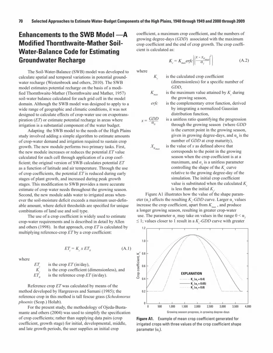
70 Selected Approaches to Estimate Water-Budget Components of the High Plains, 1940 through 1949 and 2000 through 2009
Enhancements to the SWB Model —A Modified Thornthwaite-Mather Soil-Water-Balance Code for Estimating Groundwater Recharge
The Soil-Water-Balance (SWB) model was developed to calculate spatial and temporal variations in potential ground-water recharge (Westenbroek and others, 2010). The SWB model estimates potential recharge on the basis of a modi-fied Thornthwaite-Mather (Thornthwaite and Mather, 1957) soil-water balance calculated for each grid cell in the model domain. Although the SWB model was designed to apply to a wide range of geographic and climatic conditions, it was not designed to calculate effects of crop-water use on evapotrans-piration (ET) or estimate potential recharge in areas where irrigation is a substantial component of the water budget.
Adapting the SWB model to the needs of the High Plains study involved adding a simple algorithm to estimate amounts of crop-water demand and irrigation required to sustain crop growth. The new module performs two primary tasks. First, the new module increases or reduces the potential ET value calculated for each cell through application of a crop coef-ficient; the original version of SWB calculates potential ET as a function of latitude and air temperature. Through the use of crop coefficients, the potential ET is reduced during early stages of plant growth, and increased during peak growth stages. This modification to SWB provides a more accurate estimate of crop water needs throughout the growing season. Second, the new module adds water to irrigated areas when-ever the soil-moisture deficit exceeds a maximum user-defin-able amount, where deficit thresholds are specified for unique combinations of land use and soil type.
The use of a crop coefficient is widely used to estimate crop-water requirements and is described in detail by Allen and others (1998). In that approach, crop ET is calculated by multiplying reference-crop ET by a crop coefficient:
ETc = Kc x ET0 (A.1)
where ETc is the crop ET (in/day), Kc is the crop coefficient (dimensionless), and ET0 is the reference crop ET (in/day).
Reference crop ET was calculated by means of the method developed by Hargreaves and Samani (1985); the reference crop in this method is tall fescue grass (Schedonorus phoenix (Scop.) Holub).
For the present study, the methodology of Ojeda-Busta-mante and others (2004) was used to simplify the specification of crop coefficients; rather than supplying data pairs (crop coefficient, growth stage) for initial, developmental, middle, and late growth periods, the user supplies an initial crop
coefficient, a maximum crop coefficient, and the numbers of growing degree-days (GDD) associated with the maximum crop coefficient and the end of crop growth. The crop coeffi-cient is calculated as:
(A.2)
where Kc is the calculated crop coefficient
(dimensionless) for a specific number of GDD,
Kmax is the maximum value attained by Kc during the growing season,
erfc is the complementary error function, derived by integrating a normalized Gaussian distribution function,
is a unitless ratio quantifying the progression through the growing season (where GDD is the current point in the growing season, given in growing degree-days, and α0 is the number of GDD at crop maturity),
is the value of x as defined above that corresponds to the point in the growing season when the crop coefficient is at a maximum, and α1 is a unitless parameter controlling the shape of the Kc curve relative to the growing degree-day of the simulation. The initial crop coefficient value is substituted when the calculated Kc is less than the initial Kc.
Figure A1 illustrates how the value of the shape param-eter (α1) affects the resulting Kc-GDD curve. Larger α1 values increase the crop coefficient, apart from Kmax , and produce a longer growing season, resulting in greater crop-water use. The parameter α1 may take on values in the range 0 < α1 ≤ 1; values closer to 1 result in a Kc-GDD curve with greater
Kc = Kmaxerfcx - xKmaxα1
2
GDDx = α0
XKmax
0
0.2
0.4
0.6
0.8
1.0
1.2
0 500 1,000 1,500 2,000 2,500 3,000 3,500 4,000
Crop
coe
ffici
ent,
K c
Growing season progress, in growing degree-days
Kc (α1 = 0.8)
Kc (α1 = 0.4)
Kc (α1 = 0.65)
EXPLANATION
Figure A1. Example of mean crop coefficient generated for irrigated crops with three values of the crop coefficient shape parameter (α1).

Appendix 1 71
spread relative to a curve produced with α1 closer to 0. The crop coefficients applied in simulations are shown in table A1. The coefficients for irrigated crops (land-use code 125) were adapted from those developed for the High Plains by Stegman (1988). All irrigated crops were assigned the same crop coef-ficients to simplify calculations and because many irrigated crops in the High Plains have similar crop-coefficient patterns (Allen and others, 1998).
In addition to the model parameters described above, a maximum allowable soil-moisture depletion is specified for each land-use code. SWB tracks the mean percent soil-moisture depletion, averaged over the model domain, for each unique combination of land use and soil type. If the mean soil-moisture depletion for a combination is greater than the maximum allowable depletion, water is added to all grid cells with that land-use-soil-type combination. The amount of water added is assumed to be equal to the mean soil-moisture deficit; however, the distribution of soil-moisture conditions about the mean condition inevitably means that some cells will receive water in excess of field capacity, whereas others do not receive enough water to completely erase the soil-moisture deficit. Note that specifying a maximum allowable depletion of 100 percent effectively prevents any irrigation water from being applied to the given land use. In addition, it was assumed that irrigation would take place (if needed) between
May 15 and August 24 on the irrigated cells. Actual dates or irrigation in the field depend on a variety of factors, including the irrigation strategy selected by an individual farmer, water-holding capacity of the soil, maturity group of the crop, and climate history.
No water transmission losses are included by SWB when calculating irrigation-water requirements; the estimated irrigation amounts likely are biased low as a result. Also, water-balance calculations within the modified SWB model treat applied irrigation water as though it was pumped from somewhere outside the model domain; and the model code currently does not track whether this applied irrigation water originates as surface water or as groundwater. This simple approach to estimating irrigation-water requirements repre-sents a compromise between ease of calculation, accuracy, and available data.
The SWB model could calculate more accurately the effects of irrigation on potential recharge if complete field-by-field daily irrigation records existed, but at a much higher computational cost because it would require tracking applica-tions at the field resolution. For the purposes of this study, the modifications as described here allowed potential recharge calculations to be kept relatively simple while recognizing and including the contributions of irrigation in the water budget.

72 Selected Approaches to Estimate Water-Budget Components of the High Plains, 1940 through 1949 and 2000 through 2009Ta
ble
A1.
Cr
op c
oeffi
cien
t tab
le u
sed
for S
WB
mod
el.
[GD
D, g
row
ing
degr
ee-d
ay; t
empe
ratu
res i
n de
gree
s Fah
renh
eit;
NA
, not
app
licab
le]
Land
-use
code
Max
imum
cr
op
coef
ficie
nt
Firs
t-st
age
crop
co
effic
ient
α 11
GD
Dm
axim
um
K c2
GD
Dat
m
atur
ity
GD
Dba
sete
mpe
ratu
re
GD
Dm
axim
um
tem
pera
ture
Man
agem
ent
allo
wab
leso
il-m
oist
ure
depe
tion
(p
erce
nt)
Dat
e of
fir
st
irri
gatio
n
Dat
e of
la
st
irri
gatio
nLa
ndus
e de
scri
ptio
n
104
0.75
0.5
0.65
1,80
03,
000
5014
010
0N
AN
ALo
w in
tens
ity (1
/8 a
cre
resi
dent
ial)
111
1.1
.4.6
51,
680
2,80
050
140
100
NA
NA
Non
irrig
ated
her
bace
ous/
field
cro
ps
(clo
se-s
eede
d, c
onto
ured
, goo
d co
nditi
on)
112
1.1
.4.6
51,
680
2,80
050
140
100
NA
NA
Non
irrig
ated
row
cro
ps (s
traig
ht
row,
goo
d co
nditi
on)
113
1.1
.3.6
51,
375.
82,
293
5014
010
0N
AN
AN
onirr
igat
ed c
orn
(con
tour
ed, g
ood
cond
ition
)11
81.
2.3
.65
1,80
03,
000
5014
010
0N
AN
AN
onirr
igat
ed o
ther
row
cro
ps (s
m
grai
n, c
onto
ured
, goo
d co
nditi
on)
125
1.2
.3.6
51,
375.
82,
293
5014
040
15-M
ay24
-Aug
All
irrig
ated
cro
ps 3
4 5
150
.95
.9.6
52,
100
3,50
050
140
100
NA
NA
Gra
ssla
nd (a
ssum
e pa
stur
e, g
ood
cond
ition
)16
11
.75
12,
100
3,50
050
140
100
NA
NA
Con
ifero
us fo
rest
173
1.7
51
2,10
03,
500
5014
010
0N
AN
AM
ixed
/oth
er c
onife
rous
fore
st17
51
.75
12,
100
3,50
050
140
100
NA
NA
Bro
ad-le
aved
dec
iduo
us fo
rest
200
11
.65
1,80
03,
000
5014
010
0N
AN
AO
pen
wat
er21
11.
2.3
.65
1,80
03,
000
5014
010
0N
AN
AEm
erge
nt/w
et m
eado
w21
21.
2.3
.65
1,80
03,
000
5014
010
0N
AN
AFl
oatin
g aq
uatic
her
bace
ous
vege
tatio
n24
01
.2.6
51,
800
3,00
050
140
100
NA
NA
Bar
ren
250
1.2
.65
1,80
03,
000
5014
010
0N
AN
ASh
rubl
and
1 α1: c
ontro
ls th
e sh
ape
or sp
read
of t
he e
rror
func
tion
used
to e
stim
ate
the
Kc f
or a
giv
en G
DD
. (hi
gher
=gre
ater
spre
ad; s
mal
ler=
mor
e pr
onou
nced
pea
k)2 E
rror
func
tion
Kc e
stim
atio
n m
etho
d do
cum
ente
d in
Oje
da-B
usta
man
te a
nd o
ther
s (20
04).
3 Cor
n pa
ram
eter
s ada
pted
from
Ste
gman
(198
8).
4 Prim
ary
sour
ce fo
r oth
er c
oeffi
cien
ts b
ased
on
Alle
n an
d ot
hers
(199
8).
5 The
onl
y la
nd u
se a
llow
ed to
rece
ive
irrig
atio
n is
land
use
125
.

Appendix 2

74 Selected Approaches to Estimate Water-Budget Components of the High Plains, 1940 through 1949 and 2000 through 2009Ta
ble
A2.
Re
char
ge ra
tes
in th
e Hi
gh P
lain
s co
mpi
led
from
pre
viou
sly
publ
ishe
d st
udie
s.
[NH
P, n
orth
ern
Hig
h Pl
ains
; P, p
reci
pita
tion;
--, n
o no
tes;
I, ir
rigat
ion
retu
rn fl
ow; S
, stre
amflo
w se
epag
e; C
, can
al a
nd re
serv
oir s
eepa
ge; U
, uns
peci
fied;
CH
P, c
entra
l Hig
h Pl
ains
; SH
P, so
uthe
rn H
igh
Plai
ns]
Met
hod
type
Met
hod
Refe
renc
e(s)
Scal
e1Re
gion
Loca
tion
Land
cov
erW
ater
so
urce
sRe
char
ge ra
te,
inch
es p
er y
ear
Tim
e pe
riod
Not
es
Gro
undw
ater
Gro
undw
ater
-flow
m
odel
McK
usic
k (2
003)
; La
ndon
(200
2)R
egio
nal
NH
PN
orth
east
ern
Col
orad
o,
Nor
thw
este
rn K
ansa
s, So
uthw
este
rn N
ebra
ska
Und
evel
oped
P1.
03Pr
e-19
31--
Gro
undw
ater
Gro
undw
ater
-flow
m
odel
McK
usic
k (2
003)
; La
ndon
(200
2)R
egio
nal
NH
PN
orth
east
ern
Col
orad
o,
Nor
thw
este
rn K
ansa
s, So
uthw
este
rn N
ebra
ska
Com
posi
teP,
I,S,C
1.81
1941
–200
0--
Gro
undw
ater
Gro
undw
ater
-flow
m
odel
Soph
ocle
ous (
2004
); Lu
ckey
and
oth
ers
(198
6)
Reg
iona
lN
HP
Hig
h Pl
ains
Und
evel
oped
P 0.
076
Pre-
1960
--
Gro
undw
ater
Gro
undw
ater
-flow
m
odel
Soph
ocle
ous (
2004
); Lu
ckey
and
oth
ers
(198
6)
Reg
iona
lN
HP
Hig
h Pl
ains
Ran
gela
nd, i
rrig
ated
cr
opla
nd, n
onir-
rigat
ed c
ropl
and
P,I,C
0.0–
4.0
(mid
=2)
1960
–80
Irrig
atio
n re
turn
flow
rang
ed
from
30
to 4
6 pe
rcen
t of
tota
l pum
page
Gro
undw
ater
Gro
undw
ater
-flow
m
odel
Soph
ocle
ous (
2004
); St
ullk
en a
nd o
ther
s (1
985)
Reg
iona
lN
HP
Nor
thw
este
rn K
ansa
sU
nspe
cifie
dU
0.00
–0.7
9 (m
ean=
0.2)
Pre-
1950
--
Gro
undw
ater
Gro
undw
ater
-flow
m
odel
Luck
ey a
nd C
anni
a (2
006)
Reg
iona
lN
HP
Wes
tern
Neb
rask
aIr
rigat
ed c
ropl
and
C1.
39–2
1.93
(m
ean=
7.21
)19
00–9
8M
ean
is a
vera
ge c
anal
seep
age
from
26
irrig
atio
n di
stric
ts
Gro
undw
ater
Gro
undw
ater
-flow
m
odel
Luck
ey a
nd C
anni
a (2
006)
Reg
iona
lN
HP
Wes
tern
Neb
rask
aIr
rigat
ed c
ropl
and
I0.
68–7
.09
(mea
n=3.
19)
1900
–98
Mea
n is
ave
rage
surf
ace-
wat
er
irrig
atio
n re
turn
flow
from
26
irrig
atio
n di
stric
ts
Gro
undw
ater
Gro
undw
ater
-flow
m
odel
Luck
ey a
nd C
anni
a (2
006)
Reg
iona
lN
HP
Wes
tern
Neb
rask
aU
ndev
elop
edP
0.15
–2.3
(m
ean=
0.75
)Pr
e-19
50--
Gro
undw
ater
Gro
undw
ater
-flow
m
odel
Luck
ey a
nd C
anni
a (2
006)
Reg
iona
lN
HP
Wes
tern
Neb
rask
aN
onirr
igat
ed c
ropl
and
P1.
3719
50–9
8Av
erag
e su
pple
men
tal r
echa
rge
on n
onirr
igat
ed c
ropl
and
plus
ave
rage
pre
-195
0 re
char
ge
Gro
undw
ater
Gro
undw
ater
-flow
m
odel
Luck
ey a
nd C
anni
a (2
006)
Reg
iona
lN
HP
Wes
tern
Neb
rask
aIr
rigat
ed c
ropl
and
P4.
1519
50–9
8Av
erag
e su
pple
men
tal r
echa
rge
on ir
rigat
ed c
ropl
and
plus
av
erag
e pr
e-19
50 re
char
ge
Gro
undw
ater
Gro
undw
ater
-flow
m
odel
Car
ney
(200
8)R
egio
nal
NH
PSo
uthw
este
rn N
ebra
ska
Und
evel
oped
P0.
15–2
.5
(mea
n=1.
2)Pr
e-19
50--
Gro
undw
ater
Gro
undw
ater
-flow
m
odel
Car
ney
(200
8)R
egio
nal
NH
PSo
uthw
este
rn N
ebra
ska
Non
irrig
ated
cro
plan
dP
1.6
1950
–98
Aver
age
supp
lem
enta
l rec
harg
e on
non
irrig
ated
cro
plan
d pl
us a
vera
ge p
re-1
950
rech
arge
Gro
undw
ater
Gro
undw
ater
-flow
m
odel
Car
ney
(200
8)R
egio
nal
NH
PSo
uthw
este
rn N
ebra
ska
Irrig
ated
cro
plan
dP
6.2
1950
–98
Aver
age
supp
lem
enta
l rec
harg
e on
irrig
ated
cro
plan
d pl
us
aver
age
pre-
1950
rech
arge
Gro
undw
ater
Gro
undw
ater
-flow
m
odel
Pete
rson
(200
7)R
egio
nal
NH
PSo
uth-
cent
ral N
ebra
ska
Und
evel
oped
P0.
30–2
.50
(mea
n=0.
86)
Pre-
1950
--
Gro
undw
ater
Gro
undw
ater
-flow
m
odel
Pete
rson
(200
7)R
egio
nal
NH
PSo
uth-
cent
ral N
ebra
ska
Non
irrig
ated
cro
plan
dP
1.76
1950
–98
Aver
age
supp
lem
enta
l rec
harg
e on
non
irrig
ated
cro
plan
d pl
us a
vera
ge p
re-1
950
rech
arge

Appendix 2 75Ta
ble
A2.
Re
char
ge ra
tes
in th
e Hi
gh P
lain
s co
mpi
led
from
pre
viou
sly
publ
ishe
d st
udie
s.—
Cont
inue
d
[NH
P, n
orth
ern
Hig
h Pl
ains
; P, p
reci
pita
tion;
--, n
o no
tes;
I, ir
rigat
ion
retu
rn fl
ow; S
, stre
amflo
w se
epag
e; C
, can
al a
nd re
serv
oir s
eepa
ge; U
, uns
peci
fied;
CH
P, c
entra
l Hig
h Pl
ains
; SH
P, so
uthe
rn H
igh
Plai
ns]
Met
hod
type
Met
hod
Refe
renc
e(s)
Scal
e1Re
gion
Loca
tion
Land
cov
erW
ater
so
urce
sRe
char
ge ra
te,
inch
es p
er y
ear
Tim
e pe
riod
Not
es
Gro
undw
ater
Gro
undw
ater
-flow
m
odel
Pete
rson
(200
7)R
egio
nal
NH
PSo
uth-
cent
ral N
ebra
ska
Irrig
ated
cro
plan
dP
6.06
1950
–98
Aver
age
supp
lem
enta
l rec
harg
e on
irrig
ated
cro
plan
d pl
us
aver
age
pre-
1950
rech
arge
Gro
undw
ater
Gro
undw
ater
-flow
m
odel
Pete
rson
and
oth
ers
(200
8)R
egio
nal
NH
PN
orth
-cen
tral N
ebra
ska,
in
clud
ing
Sand
Hill
sU
ndev
elop
edP
0–3.
1 (m
ean=
2.2)
Pre-
1940
--
Gro
undw
ater
Gro
undw
ater
-flow
m
odel
Pete
rson
and
oth
ers
(200
8)R
egio
nal
NH
PN
orth
-cen
tral N
ebra
ska,
in
clud
ing
Sand
Hill
sN
onirr
igat
ed c
ropl
and
P2.
719
40–2
005
Supp
lem
enta
l rec
harg
e on
no
nirr
igat
ed c
ropl
and
plus
av
erag
e pr
e-19
40 re
char
ge
Gro
undw
ater
Gro
undw
ater
-flow
m
odel
Pete
rson
and
oth
ers
(200
8)R
egio
nal
NH
PN
orth
-cen
tral N
ebra
ska,
in
clud
ing
Sand
Hill
sIr
rigat
ed c
ropl
and
P5.
719
40–2
005
Supp
lem
enta
l rec
harg
e on
irri-
gate
d cr
opla
nd p
lus a
vera
ge
pre-
1940
rech
arge
Gro
undw
ater
Gro
undw
ater
-flow
m
odel
Pete
rson
and
oth
ers
(200
8)R
egio
nal
NH
PN
orth
-cen
tral N
ebra
ska,
in
clud
ing
Sand
Hill
sR
ange
land
, non
ir-rig
ated
and
irrig
ated
cr
opla
nd
P,C
2.7
1940
–200
5--
Gro
undw
ater
Gro
undw
ater
-flow
m
odel
Stan
ton
and
othe
rs
(201
0)R
egio
nal
NH
PN
orth
-cen
tral N
ebra
ska,
in
clud
ing
Sand
Hill
sU
ndev
elop
edP
0.5–
5.0
(mea
n=2.
5)Pr
e-19
40--
Gro
undw
ater
Gro
undw
ater
-flow
m
odel
Stan
ton
and
othe
rs
(201
0)R
egio
nal
NH
PN
orth
-cen
tral N
ebra
ska,
in
clud
ing
Sand
Hill
sR
ange
land
P1.
0–4.
5 (m
ean=
2.9)
1940
–200
5--
Gro
undw
ater
Gro
undw
ater
-flow
m
odel
Stan
ton
and
othe
rs
(201
0)R
egio
nal
NH
PN
orth
-cen
tral N
ebra
ska,
in
clud
ing
Sand
Hill
sN
onirr
igat
ed c
ropl
and
P3.
419
40–2
005
Supp
lem
enta
l rec
harg
e on
no
nirr
igat
ed c
ropl
and
plus
av
erag
e pr
e-19
40 re
char
ge
Gro
undw
ater
Gro
undw
ater
-flow
m
odel
Stan
ton
and
othe
rs
(201
0)R
egio
nal
NH
PN
orth
-cen
tral N
ebra
ska,
in
clud
ing
Sand
Hill
sIr
rigat
ed c
ropl
and
P3.
919
40–2
005
Supp
lem
enta
l rec
harg
e on
irri-
gate
d cr
opla
nd p
lus a
vera
ge
pre-
1940
rech
arge
Gro
undw
ater
Gro
undw
ater
-flow
m
odel
Stan
ton
and
othe
rs
(201
0)R
egio
nal
NH
PN
orth
-cen
tral N
ebra
ska,
in
clud
ing
Sand
Hill
sR
ange
land
, non
ir-rig
ated
, irr
igat
ed
crop
land
P, C
3.1
1940
–200
5--
Gro
undw
ater
Gro
undw
ater
-flow
m
odel
Long
and
Put
nam
(2
010)
Reg
iona
lN
HP
Sout
h D
akot
aO
galla
la a
quife
r, m
ostly
rang
elan
d an
d ha
y pr
oduc
tion
P2.
9119
79–2
008
--
Gro
undw
ater
Gro
undw
ater
-flow
m
odel
Long
and
Put
nam
(2
010)
Reg
iona
lN
HP
Sout
h D
akot
aA
rikar
ee a
quife
r, m
ostly
rang
elan
d an
d ha
y pr
oduc
tion
P1.
4519
79–2
008
--
Surf
ace
wat
erW
ater
shed
mod
elSt
rauc
h an
d Li
nard
(2
009)
Reg
iona
lN
HP
Nor
th-c
entra
l Neb
rask
aSa
nd h
ills,
rang
elan
d,
noni
rrig
ated
, ir-
rigat
ed c
ropl
and
U1.
5–12
.9
(mea
n=7.
4)19
40–2
005
Mea
n of
6 su
bbas
ins
Surf
ace
wat
erW
ater
shed
mod
elSt
rauc
h an
d Li
nard
(2
009)
Reg
iona
lN
HP
Nor
th-c
entra
l Neb
rask
aSa
nd d
une
P6.
4719
40–2
005
Mea
n of
3 S
and
Hill
s sub
-ba
sins
Trac
er (u
nsat
u-ra
ted
zone
)Tr
itium
McM
ahon
and
oth
ers
(200
6)Lo
cal
NH
PSo
uthw
este
rn N
ebra
ska
Ran
gela
ndP
2.8
2000
–02
--
Trac
er (u
nsat
u-ra
ted
zone
)Tr
itium
McM
ahon
and
oth
ers
(200
6)Lo
cal
NH
PSo
uthw
este
rn N
ebra
ska
Irrig
ated
land
P,I
4.0
2000
–02
--

76 Selected Approaches to Estimate Water-Budget Components of the High Plains, 1940 through 1949 and 2000 through 2009Ta
ble
A2.
Re
char
ge ra
tes
in th
e Hi
gh P
lain
s co
mpi
led
from
pre
viou
sly
publ
ishe
d st
udie
s.—
Cont
inue
d
[NH
P, n
orth
ern
Hig
h Pl
ains
; P, p
reci
pita
tion;
--, n
o no
tes;
I, ir
rigat
ion
retu
rn fl
ow; S
, stre
amflo
w se
epag
e; C
, can
al a
nd re
serv
oir s
eepa
ge; U
, uns
peci
fied;
CH
P, c
entra
l Hig
h Pl
ains
; SH
P, so
uthe
rn H
igh
Plai
ns]
Met
hod
type
Met
hod
Refe
renc
e(s)
Scal
e1Re
gion
Loca
tion
Land
cov
erW
ater
so
urce
sRe
char
ge ra
te,
inch
es p
er y
ear
Tim
e pe
riod
Not
es
Trac
er (u
nsat
u-ra
ted
zone
)Tr
itium
McM
ahon
and
oth
ers
(200
6)Lo
cal
NH
PN
orth
east
ern
Col
orad
oIr
rigat
ed la
ndP,
I4.
420
00–0
2--
Wat
er b
udge
tSo
il-w
ater
-bal
ance
m
odel
Dug
an a
nd Z
elt (
2000
)R
egio
nal
NH
PG
reat
Pla
ins
Non
irrig
ated
land
P0.
25–5
(mid
=2.6
)19
51–8
0--
Wat
er b
udge
tSo
il-w
ater
-bal
ance
m
odel
Dug
an a
nd Z
elt (
2000
)R
egio
nal
NH
PG
reat
Pla
ins
Irrig
ated
land
P0.
25–7
(mid
=3.6
)19
51–8
0--
Uns
peci
fied
Uns
peci
fied
Soph
ocle
ous (
2004
); K
GS
Bul
letin
s, K
ansa
s Wat
er R
e-so
urce
s Boa
rd, a
nd
Han
sen
(199
1)
Inte
rmed
iate
NH
PW
este
rn K
ansa
sU
nspe
cifie
dU
0.09
–0.8
8 (m
ean=
0.3)
2U
nspe
cifie
d--
Gro
undw
ater
Gro
undw
ater
-flow
m
odel
Soph
ocle
ous (
2004
); Lu
ckey
and
oth
ers
(198
6)
Reg
iona
lC
HP
Hig
h Pl
ains
Und
evel
oped
P,S
0.05
6–0.
84
(mea
n=0.
14)3
Pre-
1950
--
Gro
undw
ater
Gro
undw
ater
-flow
m
odel
Soph
ocle
ous (
2004
); Lu
ckey
and
Bec
ker
(199
9)
Reg
iona
lC
HP
Bet
wee
n A
rkan
sas a
nd
Can
adia
n R
iver
sU
ndev
elop
ed
P
0.06
8–0.
69
(mea
n=0.
155)
3Pr
e-19
46--
Gro
undw
ater
Gro
undw
ater
-flow
m
odel
Soph
ocle
ous (
2004
); Lu
ckey
and
Bec
ker
(199
9)
Reg
iona
lC
HP
Bet
wee
n A
rkan
sas a
nd
Can
adia
n R
iver
sR
ange
land
, non
ir-rig
ated
cro
plan
d,
irrig
ated
cro
plan
d
P,I
0.41
1946
–97
--
Gro
undw
ater
Gro
undw
ater
-flow
m
odel
Soph
ocle
ous (
2004
);
Stul
lken
and
oth
ers
(198
5)
Reg
iona
lC
HP
Sout
hwes
tern
Kan
sas
Und
evel
oped
P0.
0–2.
0 (m
ean=
0.24
)3Pr
e-19
50--
Gro
undw
ater
Gro
undw
ater
-flow
m
odel
Soph
ocle
ous (
2004
); St
ullk
en a
nd o
ther
s (1
985)
Reg
iona
lC
HP
Sout
hwes
tern
Kan
sas
Und
evel
oped
S0.
036–
0.04
5 (m
id=0
.040
)Pr
e-19
50--
Gro
undw
ater
Gro
undw
ater
-flow
m
odel
Soph
ocle
ous (
2004
); W
atts
(198
9)R
egio
nal
CH
PSo
uthw
este
rn K
ansa
sU
nspe
cifie
dU
0.58
1982
--
Gro
undw
ater
Gro
undw
ater
-flow
m
odel
Soph
ocle
ous (
2004
); H
aven
s and
Chr
is-
tens
on (1
984)
Reg
iona
lC
HP
Nor
thw
este
rn O
kla-
hom
a an
d so
uthw
este
rn
Kan
sas
Uns
peci
fied
P0.
23–0
.45
(mea
n=0.
34)3
Pre-
1940
, 19
40–8
0--
Gro
undw
ater
Gro
undw
ater
-flow
m
odel
Soph
ocle
ous (
2004
); C
obb
and
othe
rs
(198
3)
Reg
iona
lC
HP
Sout
h-ce
ntra
l Kan
sas
Uns
peci
fied
P0.
75U
nspe
cifie
d--
Gro
undw
ater
Gro
undw
ater
-flow
m
odel
Soph
ocle
ous (
2004
); So
phoc
leou
s and
ot
hers
(198
2)
Inte
rmed
iate
CH
PEq
uus B
eds
Sand
dun
esP
6.5
Uns
peci
fied
--
Gro
undw
ater
Gro
undw
ater
-flow
m
odel
Soph
ocle
ous (
2004
); So
phoc
leou
s and
ot
hers
(198
2)
Inte
rmed
iate
CH
PEq
uus B
eds
Non
-san
d du
neP
1.2
Uns
peci
fied
--
Gro
undw
ater
Gro
undw
ater
-flow
m
odel
Soph
ocle
ous (
2004
); Sp
inaz
ola
and
oth-
ers (
1985
)
Inte
rmed
iate
CH
PEq
uus B
eds
Uns
peci
fied
U1.
7Pr
e-19
40--

Appendix 2 77Ta
ble
A2.
Re
char
ge ra
tes
in th
e Hi
gh P
lain
s co
mpi
led
from
pre
viou
sly
publ
ishe
d st
udie
s.—
Cont
inue
d
[NH
P, n
orth
ern
Hig
h Pl
ains
; P, p
reci
pita
tion;
--, n
o no
tes;
I, ir
rigat
ion
retu
rn fl
ow; S
, stre
amflo
w se
epag
e; C
, can
al a
nd re
serv
oir s
eepa
ge; U
, uns
peci
fied;
CH
P, c
entra
l Hig
h Pl
ains
; SH
P, so
uthe
rn H
igh
Plai
ns]
Met
hod
type
Met
hod
Refe
renc
e(s)
Scal
e1Re
gion
Loca
tion
Land
cov
erW
ater
so
urce
sRe
char
ge ra
te,
inch
es p
er y
ear
Tim
e pe
riod
Not
es
Gro
undw
ater
Gro
undw
ater
-flow
m
odel
Soph
ocle
ous (
2004
); Sp
inaz
ola
and
oth-
ers (
1985
)
Inte
rmed
iate
CH
PEq
uus B
eds
Uns
peci
fied
U1.
69–1
.91
(mid
=1.8
)19
64–7
9--
Gro
undw
ater
Gro
undw
ater
-flow
m
odel
Soph
ocle
ous (
2004
); M
yers
and
oth
ers
(199
6)
Inte
rmed
iate
CH
PEq
uus B
eds
Und
evel
oped
P2.
58Pr
e-19
40--
Gro
undw
ater
Gro
undw
ater
-flow
m
odel
Soph
ocle
ous (
2004
); M
yers
and
oth
ers
(199
6)
Inte
rmed
iate
CH
PEq
uus B
eds
Irrig
ated
and
non
ir-rig
ated
land
P,I
2.32
–2.5
9 (m
id=2
.46)
1964
–89
Irrig
atio
n re
turn
flow
con
sid-
ered
neg
ligib
le
Surf
ace
wat
er
Stre
amflo
w-
dura
tion
curv
e an
alys
is
Soph
ocle
ous (
2004
); Fa
der a
nd S
tullk
en
(197
8)
Reg
iona
lC
HP
Sout
h-ce
ntra
l Kan
sas
Uns
peci
fied
P0.
9U
nspe
cifie
d--
Trac
er (u
nsat
u-ra
ted
zone
)C
hlor
ide
mas
s ba
lanc
eM
cMah
on a
nd o
ther
s (2
006)
Loca
lC
HP
Kan
sas
Ran
gela
ndP
0.2
2000
–02
--
Trac
er (u
nsat
u-ra
ted
zone
)Tr
itium
McM
ahon
and
oth
ers
(200
6)Lo
cal
CH
PK
ansa
sIr
rigat
ed c
ropl
and
P,I
1.5–
2.1
(mea
n=1.
8)20
00–0
2--
Uns
atur
ated
zon
eZe
ro-fl
ux p
lane
Soph
ocle
ous (
2004
); Pr
ill (1
968)
Loca
lC
HP
Sout
hwes
tern
Kan
sas
Vege
tate
d ar
ea, s
and
dune
P0.
519
64–6
6--
Uns
atur
ated
zon
eD
arcy
equ
atio
nSo
phoc
leou
s (20
04);
Soph
ocle
ous a
nd
Perr
y (1
985)
Loca
lC
HP
Gre
at B
end
Prai
rie a
nd
Equu
s Bed
s Aqu
ifers
Sand
dun
eP
0.1–
6.1
(mid
=3.1
)19
82–8
3--
Trac
er (u
nsat
u-ra
ted
zone
)H
eat-d
issi
patio
n se
nsor
sSo
phoc
leou
s (20
04);
Soph
ocle
ous a
nd
othe
rs (2
002)
Loca
lC
HP
Sout
hwes
tern
Kan
sas
Irrig
ated
cro
plan
dP,
I0.
02–0
.12
(mid
=0.0
7)U
nspe
cifie
dEr
ror e
stim
ated
to b
e at
leas
t 10
2 pe
rcen
t
Trac
er (u
nsat
u-ra
ted
zone
)H
eat-d
issi
patio
n se
nsor
sSo
phoc
leou
s (20
04);
Soph
ocle
ous a
nd
othe
rs (2
002)
Loca
lC
HP
Nor
thw
este
rn K
ansa
sN
ativ
e gr
assl
and
P 0.
004–
0.01
(m
id=0
.007
)19
51–8
0Er
ror e
stim
ated
to b
e at
leas
t 10
2 pe
rcen
t
Uns
atur
ated
zon
e Ze
ro-fl
ux p
lane
Kle
mt (
1981
)Lo
cal
CH
PN
orth
ern
Texa
s N
onirr
igat
ed c
ropl
and
and
rang
elan
dP
0.17
1978
–79
--
Uns
atur
ated
zon
e Ze
ro-fl
ux p
lane
Kle
mt (
1981
)Lo
cal
CH
PN
orth
ern
Texa
s Ir
rigat
ed c
ropl
and
P1.
919
78–7
9--
Com
bina
tion
Soil-
wat
er-b
alan
ce
mod
el a
nd
wat
er-ta
ble
fluct
uatio
n
Soph
ocle
ous (
2004
); So
phoc
leou
s (19
92,
2000
)
Loca
lC
HP
Gre
at B
end
Prai
rie A
quife
rU
nspe
cifie
d0.
0–6.
5 (m
ean=
1.4)
419
85–9
2--
Uns
peci
fied
Uns
peci
fied
Soph
ocle
ous (
2004
); G
uten
tag
and
othe
rs
(198
1)
Reg
iona
lC
HP
Sout
hwes
tern
Kan
sas
Irrig
ated
cro
plan
dP,
S1.
519
75--
Uns
peci
fied
Uns
peci
fied
Soph
ocle
ous (
2004
); G
uten
tag
and
othe
rs
(198
1)
Reg
iona
lC
HP
Sout
hwes
tern
Kan
sas
Non
irrig
ated
land
P,S
0.15
1975
--
Uns
peci
fied
Uns
peci
fied
Soph
ocle
ous (
2004
); G
uten
tag
and
othe
rs
(198
1)
Reg
iona
lC
HP
Sout
hwes
tern
Kan
sas
Irrig
ated
and
non
ir-rig
ated
land
P,S
0.6
1975
--

78 Selected Approaches to Estimate Water-Budget Components of the High Plains, 1940 through 1949 and 2000 through 2009Ta
ble
A2.
Re
char
ge ra
tes
in th
e Hi
gh P
lain
s co
mpi
led
from
pre
viou
sly
publ
ishe
d st
udie
s.—
Cont
inue
d
[NH
P, n
orth
ern
Hig
h Pl
ains
; P, p
reci
pita
tion;
--, n
o no
tes;
I, ir
rigat
ion
retu
rn fl
ow; S
, stre
amflo
w se
epag
e; C
, can
al a
nd re
serv
oir s
eepa
ge; U
, uns
peci
fied;
CH
P, c
entra
l Hig
h Pl
ains
; SH
P, so
uthe
rn H
igh
Plai
ns]
Met
hod
type
Met
hod
Refe
renc
e(s)
Scal
e1Re
gion
Loca
tion
Land
cov
erW
ater
so
urce
sRe
char
ge ra
te,
inch
es p
er y
ear
Tim
e pe
riod
Not
es
Uns
peci
fied
Uns
peci
fied
Soph
ocle
ous (
2004
); Fa
der a
nd S
tullk
en
(197
8)
Reg
iona
lC
HP
Sout
h-ce
ntra
l Kan
sas
Uns
peci
fied
P2
Uns
peci
fied
--
Uns
peci
fied
Uns
peci
fied
Soph
ocle
ous (
2004
); K
GS
Bul
letin
s, K
ansa
s Wat
er R
e-so
urce
s Boa
rd, a
nd
Han
sen
(199
1)
Inte
rmed
iate
CH
PSo
uthw
este
rn K
ansa
sU
nspe
cifie
dU
0.09
–0.9
9 (m
ean=
0.4)
2U
nspe
cifie
dFr
om c
ount
y av
erag
es
Wat
er b
udge
tSo
il-w
ater
-bal
ance
m
odel
Dug
an a
nd Z
elt (
2000
)R
egio
nal
CH
PG
reat
Pla
ins
Non
irrig
ated
land
P0.
25–5
(mid
=2.6
)19
51–8
0--
Wat
er b
udge
tSo
il-w
ater
-bal
ance
m
odel
Dug
an a
nd Z
elt (
2000
)R
egio
nal
CH
PG
reat
Pla
ins
Irrig
ated
cro
plan
dP
0.25
–7 (m
id=3
.6)
1951
–80
--
Gro
undw
ater
Gro
undw
ater
-flow
m
odel
Kno
wle
s and
oth
ers
(198
4)R
egio
nal
SHP
Texa
sSa
nd d
unes
P0.
8319
60–7
9--
Gro
undw
ater
Gro
undw
ater
-flow
m
odel
Kno
wle
s and
oth
ers
(198
4)R
egio
nal
SHP
Texa
sC
ompo
site
P, I
0.2
1960
–79
--
Gro
undw
ater
Gro
undw
ater
-flow
m
odel
Luck
ey a
nd o
ther
s (1
986)
Reg
iona
lSH
PTe
xas
Und
evel
oped
P0.
13Pr
e-19
40--
Gro
undw
ater
Gro
undw
ater
-flow
m
odel
Luck
ey a
nd o
ther
s (1
986)
Reg
iona
lSH
PTe
xas
Irrig
ated
cro
plan
dP
2.13
1940
–80
--
Gro
undw
ater
Gro
undw
ater
-flow
m
odel
Luck
ey a
nd o
ther
s (1
986)
Reg
iona
lSH
PTe
xas
Com
posi
teP
0.73
1940
–80
--
Gro
undw
ater
Gro
undw
ater
-flow
m
odel
Stov
all a
nd o
ther
s (2
000)
Reg
iona
lSH
PTe
xas
Com
posi
teP,
I2.
7519
85–9
5--
Gro
undw
ater
Gro
undw
ater
-flow
m
odel
Dut
ton
and
othe
rs
(200
1)R
egio
nal
SHP
Texa
sU
ndev
elop
edP
0.3
1950
--
Gro
undw
ater
Gro
undw
ater
-flow
m
odel
Dut
ton
and
othe
rs
(200
1)R
egio
nal
SHP
Texa
sC
ompo
site
P, I
0.35
1998
--
Gro
undw
ater
Gro
undw
ater
-flow
m
odel
Bla
ndfo
rd a
nd o
ther
s (2
003)
Reg
iona
lSH
PTe
xas
Und
evel
oped
P0.
0419
40--
Gro
undw
ater
Gro
undw
ater
-flow
m
odel
Bla
ndfo
rd a
nd o
ther
s (2
003)
Reg
iona
lSH
PTe
xas
Com
posi
teP,
I0.
6720
00--
Trac
er (u
nsat
u-ra
ted
zone
)C
hlor
ide
mas
s ba
lanc
eR
eedy
and
oth
ers
(200
3)R
egio
nal
SHP
Texa
sN
onirr
igat
ed c
ropl
and
and
rang
elan
dP
0.31
1985
–200
0M
etho
d yi
elds
long
-term
ave
r-ag
e re
char
ge
Trac
er (s
atur
ated
an
d un
satu
-ra
ted
zone
)
Triti
umR
eedy
and
oth
ers
(200
3)R
egio
nal
SHP
Texa
sIr
rigat
ed c
ropl
and
P,I
0.7–
5.0
(mea
n=1.
6)19
53–2
001
--
Trac
er (u
nsat
u-ra
ted
zone
)C
hlor
ide
mas
s ba
lanc
eSc
anlo
n an
d G
olds
mith
(1
997)
Loca
lSH
PTe
xas
Uns
peci
fied
(pla
ya)
P2.
4–3.
9 (m
id=3
.2)
Uns
peci
fied
Met
hod
yiel
ds lo
ng-te
rm a
ver-
age
rech
arge
Trac
er (u
nsat
u-ra
ted
zone
)Tr
itium
Scan
lon
and
Gol
dsm
ith
(199
7)Lo
cal
SHP
Texa
sU
nspe
cifie
d (p
laya
)P
4.7
Uns
peci
fied
Met
hod
yiel
ds lo
ng-te
rm a
ver-
age
rech
arge

Appendix 2 79Ta
ble
A2.
Re
char
ge ra
tes
in th
e Hi
gh P
lain
s co
mpi
led
from
pre
viou
sly
publ
ishe
d st
udie
s.—
Cont
inue
d
[NH
P, n
orth
ern
Hig
h Pl
ains
; P, p
reci
pita
tion;
--, n
o no
tes;
I, ir
rigat
ion
retu
rn fl
ow; S
, stre
amflo
w se
epag
e; C
, can
al a
nd re
serv
oir s
eepa
ge; U
, uns
peci
fied;
CH
P, c
entra
l Hig
h Pl
ains
; SH
P, so
uthe
rn H
igh
Plai
ns]
Met
hod
type
Met
hod
Refe
renc
e(s)
Scal
e1Re
gion
Loca
tion
Land
cov
erW
ater
so
urce
sRe
char
ge ra
te,
inch
es p
er y
ear
Tim
e pe
riod
Not
es
Trac
er (u
nsat
u-ra
ted
zone
)C
hlor
ide
mas
s ba
lanc
eSc
anlo
n an
d G
olds
mith
(1
997)
Loca
lSH
PTe
xas
Und
evel
oped
P0.
004–
0.16
(m
id=0
.08)
Uns
peci
fied
Met
hod
yiel
ds lo
ng-te
rm a
ver-
age
rech
arge
Trac
er (u
nsat
u-ra
ted
zone
)Tr
itium
Gur
dak
and
Roe
(2
009)
; Woo
d an
d ot
hers
(199
7)
Reg
iona
lSH
PTe
xas
Uns
peci
fied
(pla
ya)
P3
1962
–199
3--
Trac
er (u
nsat
u-ra
ted
zone
)C
hlor
ide
mas
s ba
lanc
eM
cMah
on a
nd o
ther
s (2
006)
Loca
lSH
PTe
xas
Ran
gela
nd (i
nter
play
a)P
0.00
820
00–0
2--
Trac
er (u
nsat
u-ra
ted
zone
)Tr
itium
McM
ahon
and
oth
ers
(200
6)Lo
cal
SHP
Texa
sIr
rigat
ed c
ropl
and
(inte
rpla
ya)
P,I
0.67
–1.2
6 (m
ean=
0.96
)20
00–0
2--
Trac
er (u
nsat
u-ra
ted
zone
)Tr
acer
pro
file
Scan
lon
and
othe
rs
(201
0)Lo
cal
SHP
Texa
sIr
rigat
ed c
ropl
and
P,I
0.87
–1.4
(m
edia
n=1.
1)U
nspe
cifie
dM
etho
d yi
elds
long
-term
av
erag
e re
char
ge; F
ine
grai
n so
ils
Trac
er (u
nsat
u-ra
ted
zone
)Tr
acer
pro
file
and
chlo
ride
mas
s ba
lanc
e
Scan
lon
and
othe
rs
(201
0)Lo
cal
SHP
Texa
sIr
rigat
ed c
ropl
and
P,I
0.71
–3.8
(m
edia
n=1.
9)U
nspe
cifie
dM
etho
d yi
elds
long
-term
av
erag
e re
char
ge; C
oars
e gr
ain
soils
Trac
er (u
nsat
u-ra
ted
zone
)Tr
acer
pro
file
and
chlo
ride
mas
s ba
lanc
e
Scan
lon
and
othe
rs
(201
0)Lo
cal
SHP
Texa
sN
onirr
igat
ed c
ropl
and
P0
Uns
peci
fied
Met
hod
yiel
ds lo
ng-te
rm
aver
age
rech
arge
; Fin
e gr
ain
soils
Trac
er (u
nsat
u-ra
ted
zone
)C
hlor
ide
mas
s ba
lanc
eSc
anlo
n an
d ot
hers
(2
010)
Loca
lSH
PTe
xas
Non
irrig
ated
cro
plan
dP
0.39
–0.8
3 (m
edia
n=0.
61)
Uns
peci
fied
Met
hod
yiel
ds lo
ng-te
rm
aver
age
rech
arge
; Coa
rse
grai
n so
ils
Trac
er (u
nsat
u-ra
ted
zone
)Tr
acer
pro
file
and
chlo
ride
mas
s ba
lanc
e
Scan
lon
and
othe
rs
(201
0)Lo
cal
SHP
Texa
sR
ange
land
P0
Uns
peci
fied
Met
hod
yiel
ds lo
ng-te
rm a
ver-
age
rech
arge
Trac
erC
hlor
ide
mas
s ba
lanc
eSc
anlo
n an
d ot
hers
(2
007)
Loca
lSH
PTe
xas
Non
irrig
ated
cro
plan
dP
0.19
–3.6
(m
edia
n=0.
94)
Uns
peci
fied
Met
hod
yiel
ds lo
ng-te
rm a
ver-
age
rech
arge
Uns
atur
ated
zon
e Ze
ro-fl
ux p
lane
Kle
mt (
1981
)Lo
cal
SHP
Texa
sN
onirr
igat
ed c
ropl
and
and
rang
elan
dP
0.18
1978
–79
--
Uns
atur
ated
zon
e Ze
ro-fl
ux p
lane
Kle
mt (
1981
)Lo
cal
SHP
Texa
sIr
rigat
ed c
ropl
and
P1.
619
78–7
9--
Wat
er b
udge
tSo
il-w
ater
-bal
ance
m
odel
Dug
an a
nd Z
elt (
2000
)R
egio
nal
SHP
Gre
at P
lain
sN
onirr
igat
ed la
ndP
0.25
–1 (m
id=0
.62)
1951
–80
--
Wat
er b
udge
tSo
il-w
ater
-bal
ance
m
odel
Dug
an a
nd Z
elt (
2000
)R
egio
nal
SHP
Gre
at P
lain
sIr
rigat
ed la
ndP
0.10
–1.5
(mid
=0.8
)19
51–8
0--
1 Reg
iona
l sca
les r
epre
sent
rech
arge
rate
s for
thou
sand
s of s
quar
e m
iles,
inte
rmed
iate
-sca
le st
udie
s rep
rese
nt re
char
ge ra
tes f
or h
undr
eds o
f squ
are
mile
s, an
d lo
cal-s
cale
stud
ies r
epre
sent
rech
arge
rate
s for
ar
eas l
ess t
han
10 sq
uare
mile
s.2 M
ean
repr
esen
ts a
vera
ge o
f cou
nty
rech
arge
val
ues w
ithin
the
spec
ified
regi
on.
3 Mea
n re
pres
ents
the
aver
age
over
the
stud
y ar
ea.
4 Rep
rese
nts a
rea-
wei
ghte
d m
ean
of 1
0 si
tes.

Publishing support provided by: Rolla Publishing Service Center
For more information concerning this publication, contact: Director, USGS Nebraska Water Science Center 5231 South 19 Street Lincoln, NE 68512 (402) 328–4100
Or visit the Nebraska Water Science Center Web site at: http://ne.water.usgs.gov

Back cover: illustration showing the United States and the location of the High Plains aquifer.

Stanton and others— Selected A
pproaches to Estimate W
ater-Budget Components of the High Plains, 1940 through 1949 and 2000 through 2009—
Scientific Investigations Report 2011–5183