seabed biodiversity on the continental shelf of the great barrier reef world heritage area
TRANSCRIPT
• Roland Pitcher
• Peter Doherty • Peter Arnold
• John Hooper • Neil Gribble
FINAL REPORT to the
Cooperative Research Centre
for the Great Barrier Reef World Heritage Area
JULY 2007
on the
Continental Shelf of the Great Barrier Reef World Heritage Area
Seabed Biodiversity
National Library of Australia Cataloguing-in-Publication entry:
Pitcher, C. R. (Clifford Roland). Seabed biodiversity on the continental shelf of the Great Barrier Reef World Heritage Area. Bibliography. Includes index. ISBN 978-1-921232-87-9 (pbk.). ISBN 978-1-921232-88-6 (web). 1. Marine biodiversity - Queensland - Great Barrier Reef. 2. Marine biodiversity - Research - Queensland - Great Barrier Reef. 3. Great Barrier Reef (Qld.) - Environmental aspects. I. CRC Reef Research Centre. II. Title. 333.95616
Citation: Pitcher, C.R., Doherty, P., Arnold, P., Hooper, J., Gribble, N., Bartlett, C., Browne, M., Campbell, N., Cannard, T., Cappo, M., Carini, G., Chalmers, S., Cheers, S., Chetwynd, D., Colefax, A., Coles, R., Cook, S., Davie, P., De'ath, G., Devereux, D., Done, B., Donovan, T., Ehrke, B., Ellis, N., Ericson, G., Fellegara, I., Forcey, K., Furey, M., Gledhill, D., Good, N., Gordon, S., Haywood, M., Hendriks, P., Jacobsen, I., Johnson, J., Jones, M., Kinninmoth, S., Kistle, S., Last, P., Leite, A., Marks, S., McLeod, I., Oczkowicz, S., Robinson, M., Rose, C., Seabright, D., Sheils, J., Sherlock, M., Skelton, P., Smith, D., Smith, G., Speare, P., Stowar, M., Strickland, C., Van der Geest, C., Venables, W., Walsh, C., Wassenberg, T., Welna, A., Yearsley, G. (2007). Seabed Biodiversity on the Continental Shelf of the Great Barrier Reef World Heritage Area. AIMS/CSIRO/QM/QDPI CRC Reef Research Task Final Report. 320 pp.
Published: July 2007 by CSIRO Marine and Atmospheric Research © Australian Institute of Marine Science, CSIRO Marine and Atmospheric Research, Queensland Museum, Queensland Department of Primary Industries, CRC Reef Research Centre, Fisheries Research and Development Corporation, and the National Oceans Office, 2007. This work is copyright. Except as permitted under the Copyright Act 1968 (Cth), no part of this publication may be reproduced by any process, electronic or otherwise, without the specific written permission of the copyright owners. Neither may information be stored electronically in any form whatsoever without such permission. DISCLAIMER The authors have taken all reasonable steps to ensure that the information contents in this publication are accurate at the time of publication. Readers should ensure that they make appropriate inquiries to determine whether new information is available on the particular subject matter.
GBR Seabed Biodiversity i
July 2007
Seabed Biodiversity on the Continental Shelf of the Great Barrier Reef World Heritage Area
CRC-REEF Task Number: C1.1.2 FRDC Project Number: 2003/021 NOO Contract Number: 2004/015
Roland Pitcher², Peter Doherty¹, Peter Arnold³, John Hooper³, Neil Gribble4,
Chris Bartlett³, Matthew Browne², Norm Campbell², Toni Cannard², Mike Cappo¹, Giovannella Carini³, Susan Chalmers4, Sue Cheers², Doug Chetwynd², Andrew
Colefax³, Rob Coles4, Stephen Cook³, Peter Davie³, Glenn De'ath¹, Drew Devereux², Barbara Done³, Tim Donovan¹, Barry Ehrke4, Nick Ellis², Gavin Ericson¹, Ida
Fellegara³, Karl Forcey², Melodyrose Furey², Dan Gledhill², Norm Good4, Scott Gordon², Mick Haywood², Patricia Hendriks³, Ian Jacobsen, Jeff Johnson³, Michelle Jones³, Stuart Kinninmoth¹, Sarah Kistle4, Peter Last², Anita Leite³, Shona Marks²,
Ian McLeod², Sybilla Oczkowicz4, Melissa Robinson³, Cassanda Rose4, Denise Seabright³, Jacquie Sheils², Matt Sherlock², Posa Skelton4, David H Smith², Greg
Smith², Peter Speare¹, Marcus Stowar¹, Colleen Strickland³, Claire Van der Geest4, Bill Venables², Cath Walsh4, Ted Wassenberg², Andrzej Welna², Gus Yearsley²
¹Australian Institute of Marine Science Cape Ferguson, TOWNSVILLE, Qld. 4810, Australia
²Commonwealth Scientific & Industrial Research Organisation
Marine & Atmospheric Research Mathematics & Information Sciences
233 Middle Street, CLEVELAND, Qld. 4163 Australia
³Queensland Museum MTQ, TOWNSVILLE, Qld. 4810, Australia
South Bank, SOUTH BRISBANE, Qld. 4101, Australia
4Queensland Department of Primary Industries Northern Fisheries Centre, Tingara Street, CAIRNS, Qld. 4870, Australia
AUSTRALIAN INSTITUTE
OF MARINE SCIENCE
ISBN 978-1-921232-87-9.
CRC Reef Research Task Final Report
GBR Seabed Biodiversity ii
ACKNOWLEDGEMENTS
This document is the final report of the Great Barrier Reef Seabed Biodiversity Project, a collaboration between the Australian Institute of Marine Science (AIMS), the Commonwealth Scientific and Industrial Research Organisation (CSIRO), Queensland Department of Primary Industries & Fisheries (QDPI&F), and the Queensland Museum (QM); funded by the CRC Reef Research Centre (CRC-Reef), the Fisheries Research and Development Corporation (FRDC), and the National Oceans Office (NOO) of the Department of Environment and Water Resources. We gratefully acknowledge the support of end-user agencies Great Barrier Reef Marine Park Authority (GBRMPA), QDPI & Fisheries, Queensland Seafood Industry Association (QSIA) and the NOO, and the contributions of the project's Steering Committee members: David Williams (CRC-Reef), Dorothea Huber & Phil Cadwallader (GBRMPA), Brigid Kerrigan & Malcolm Dunning (QDPI&F), Duncan Souter, Barry Ehrke & Martin Hicks (QSIA), Vicki Nelson (NOO) and Vern Veitch (Sunfish). For the provision of physical environmental data, we thank Chris Jenkins (Ocean Sciences Institute – OSI), Lance Bode (James Cook University – JCU), Scott Condie (CSIRO), the GBRMPA, the RAN Hydrographers Office (RAN HO) — and Peter Harris, Andrew Heap, Emma Mathews, Alison Hancock (Geoscience Australia – GA) for processing the sediment samples. We also wish to thank the multi-agency teams and the crews of the RV Lady Basten (AIMS) and FRV Gwendoline May (QDPI&F) that contributed to the success of the fieldwork; the research agencies AIMS, CSIRO, QM, QDPI&F for providing support to the project; and all the project's team members without whose valuable efforts this project would not have been possible. A large number of other people also helped with aspects of the project and we are grateful for their assistance, including: Tony Reese, Steve Edgar, Mark Tonks, Quinton Dell, Gary Fry, William White, Al Graham, Louise Conboy, Spikey Riddoch, Bob Ward, Bronwyn Holmes, Tom Munro, Hiro Motomura, Mike Sugden, Henok Goitom, Barry Russell, Barry Hutchins, Martin Gomon and Di Bray. Shane Griffiths, John Kirkwood and Piers Dunstan provided valuable comments that improved the document. Louise Bell designed the cover.
This Report is dedicated to the memory of our friend, colleague and expert extraordinaire on “all matters seabed”, Dr Peter William Arnold, Senior Curator Biodiversity, Museum of Tropical Queensland, Townsville (1949-2006)
GBR Seabed Biodiversity iii
TABLE OF CONTENTS ACKNOWLEDGEMENTS .................................................................................................................................... ii TABLE OF CONTENTS....................................................................................................................................... iii
FIGURES............................................................................................................................................................ v TABLES ............................................................................................................................................................ xi
NON-TECHNICAL SUMMARY ........................................................................................................................ xv PROJECT:......................................................................................................................................................... xv PRINCIPAL INVESTIGATORS: .................................................................................................................... xv ADDRESS: ....................................................................................................................................................... xv OBJECTIVES: .................................................................................................................................................. xv NON-TECHNICAL SUMMARY: .................................................................................................................. xvi
Outcomes Achieved ................................................................................................................................... xviii 1. INTRODUCTION ....................................................................................................................................... 1-1
1.1. BACKGROUND ................................................................................................................................. 1-1 1.2. NEED................................................................................................................................................... 1-2 1.3. OBJECTIVES ...................................................................................................................................... 1-3
2. METHODS .................................................................................................................................................. 2-5 2.1. SAMPLING DESIGN.......................................................................................................................... 2-5
2.1.1. Physical environmental data (I McLeod & R Pitcher) ................................................................. 2-5 2.1.2. Study Area Stratification (N Ellis) ............................................................................................. 2-15 2.1.3. Site Selection.............................................................................................................................. 2-29
2.2. FIELD SAMPLING........................................................................................................................... 2-31 2.2.1. Research Vessels (T Wassenberg & N Gribble) ........................................................................ 2-31 2.2.2. Towed Video Camera (G Smith, K Forcey, M Haywood)......................................................... 2-32 2.2.3. Baited Remote Underwater Video Stations (M Cappo) ............................................................. 2-34 2.2.4. Single-beam Acoustics............................................................................................................... 2-35 2.2.5. Epibenthic Sled (T Wassenberg & M Stowar) ........................................................................... 2-36 2.2.6. Scientific Trawl (T Wassenberg, D Gledhill & N Gribble)........................................................ 2-37 2.2.7. Sample Processing at Sea (T Wassenberg, M Stowar, C Bartlett) ............................................. 2-38
2.3. LABORATORY PROCESSING AND IDENTIFICATION............................................................. 2-43 2.3.1. Towed Video (T Wassenberg, J Sheils) ..................................................................................... 2-43 2.3.2. BRUVS Video (M Cappo) ......................................................................................................... 2-46 2.3.3. Sample Processing (T Hendriks, M Stowar, C Bartlett, T Wassenberg, D Gledhill) ................. 2-49
2.4. DATA ANALYSES........................................................................................................................... 2-53 2.4.1. BRUVS Species Models, Characterization & Prediction (M Cappo, G De’Ath) ...................... 2-53 2.4.2. Single Species Biophysical Models and Prediction (M Browne, W Venables) ......................... 2-54 2.4.3. Species Groups Characterization and Prediction (M Browne)................................................... 2-58 2.4.4. Site Groups Characterization and Prediction (W Venables) ...................................................... 2-59 2.4.5. Video Habitat Characterization and Prediction (W Venables)................................................... 2-64 2.4.6. Acoustics Discrimination and Classification.............................................................................. 2-68 2.4.7. Ecological Risk Indicators ......................................................................................................... 2-75 2.4.8. Trawl Management Scenario Model (N Ellis, A Welna, R Pitcher) .......................................... 2-77
3. RESULTS .................................................................................................................................................. 3-86 3.1. BRUVS SPECIES MODELS, CHARACTERIZATION & PREDICTION (M Cappo, G De’Ath) . 3-86
3.1.1. BRUVS Species richness ........................................................................................................... 3-86 3.1.2. BRUVS Species presence/absence Biophysical Models and Prediction.................................... 3-87 3.1.3. BRUVS Site-groups Characterization and Prediction.............................................................. 3-105
GBR Seabed Biodiversity iv
3.2. SINGLE SPECIES, BIOPHYSICAL MODELS AND PREDICTION ........................................... 3-112 3.2.1. Sled and Trawl samples species richness ................................................................................. 3-113 3.2.2. Single species models (M Browne & R Pitcher)...................................................................... 3-116 3.2.3. Selected single species distribution maps................................................................................. 3-125
3.3. SPECIES GROUPS CHARACTERIZATION AND PREDICTION (M Browne & R Pitcher) ..... 3-133 3.3.1. Characterization and Prediction Model performance............................................................... 3-133 3.3.2. Selected species group distribution maps................................................................................. 3-135
3.4. SITE GROUPS CHARACTERIZATION AND PREDICTIONS (W Venables & R Pitcher) ........ 3-138 3.4.1. Decision tree results ................................................................................................................. 3-138 3.4.2. Species affinity groups ............................................................................................................. 3-141 3.4.3. Description of site-group assemblages..................................................................................... 3-142
3.5. VIDEO HABITAT CHARACTERIZATION AND PREDICTION ............................................... 3-145 3.5.1. Seabed substratum.................................................................................................................... 3-145 3.5.2. Seabed biological habitat ......................................................................................................... 3-145 3.5.3. Statistical characterization and prediction (W Venables & R Pitcher)..................................... 3-151
3.6. ACOUSTICS DISCRIMINATION AND CLASSIFICATION....................................................... 3-155 3.6.1. Wavelet Packet-Based Techniques Applied to Data in the Angular Domain (D H Smith)...... 3-155 3.6.2. Canonical Variate Analysis of Acoustic Data (N Campbell & D Devereux)........................... 3-166 3.6.3. Linear Discriminant Analyses of QTC View data (I McLeod) ................................................ 3-186
3.7. ECOLOGICAL RISK INDICATORS ............................................................................................. 3-197 3.7.1. Indicators for species-groups biomass...................................................................................... 3-198 3.7.2. Indicators for individual species biomass................................................................................. 3-202 3.7.3. Assemblage indicators.............................................................................................................. 3-238 3.7.4. Habitat indicators ..................................................................................................................... 3-239
3.8. TRAWL MANAGEMENT SCENARIO MODEL (N Ellis, R Pitcher) .......................................... 3-243 4. DISCUSSION .......................................................................................................................................... 4-250
4.1. BRUVS SPECIES MODELS, CHARACTERIZATION & PREDICTION (M Cappo, G De’Ath) 4-251 4.1.1. BRUVS Fish species ................................................................................................................ 4-251 4.1.2. BRUVS Fish Assemblages....................................................................................................... 4-251
4.2. SINGLE SPECIES, BIOPHYSICAL MODELS AND PREDICTION ........................................... 4-253 4.3. SPECIES GROUPS CHARACTERIZATION AND PREDICTION .............................................. 4-255 4.4. SITE GROUPS CHARACTERIZATION AND PREDICTION ..................................................... 4-255 4.5. VIDEO HABITAT CHARACTERIZATION AND PREDICTION ............................................... 4-256 4.6. ACOUSTICS DISCRIMINATION AND CLASSIFICATION....................................................... 4-257
4.6.1. Wavelet Packet-Based Techniques Applied to Data in the Angular Domain (D H Smith)...... 4-257 4.6.2. Canonical Variate Analysis of Acoustic Data (N Campbell & D Devereux)........................... 4-258 4.6.3. Linear Discriminant Analyses of QTC View data.................................................................... 4-259 4.6.4. Acoustics summary .................................................................................................................. 4-260
4.7. ECOLOGICAL RISK INDICATORS ............................................................................................. 4-261 4.8. TRAWL MANAGEMENT SCENARIO MODEL.......................................................................... 4-264
5. BENEFITS............................................................................................................................................... 5-266 6. FURTHER DEVELOPMENT ................................................................................................................. 6-267 7. ACHIEVEMENT OF OUTCOMES........................................................................................................ 7-269 8. CONCLUSIONS...................................................................................................................................... 8-271 9. RECOMMENDATIONS ......................................................................................................................... 9-273 10. REFERENCES................................................................................................................................... 10-276 11. ABBREVIATIONS............................................................................................................................ 11-281 12. APPENDIX 1: INTELLECTUAL PROPERTY................................................................................ 12-282 13. APPENDIX 2: STAFF....................................................................................................................... 13-283 14. APPENDIX 3: PROJECT STEERING COMMITTEE MEMBERS ............................................................ 14-285 15. APPENDIX 4: SINGLE SPECIES TRAWL EXPOSURE................................................................ 15-286
GBR Seabed Biodiversity v
FIGURES Figure 2-1: DEM of the bathymetry, slope and aspect of the GBR continental shelf, on a 0.01º grid, from various
sources including soundings in uncharted areas recorded by the Project; map of modeled seabed current shear stress (RMS N/m²) (sources, see Section 2.1.1.1 for). ........................................................................ 2-9
Figure 2-2: Maps of sediment attributes for the GBR continental shelf: percent mud/sand/gravel grain size fractions and percent carbonate (source, Geoscience Australia. Includes samples collected by the project and processed by GA). ............................................................................................................................... 2-10
Figure 2-3: Maps of CARS bottom water physical attributes for the GBR continental shelf: temperature (mean & SD ºC), salinity (mean & SD ‰), dissolved oxygen (mean & SD ml/l) (source, see Section 2.1.1.1). ..... 2-11
Figure 2-4: Maps of CARS bottom water nutrient attributes: silicate (mean & SD μM), nitrate (mean & SD μM), and phosphate (mean & SD μM), (source, see section 2.1.1.1). ................................................................ 2-12
Figure 2-5. Maps of SeaWiFS predicted chlorophyll-A (mean & SD mg/m³), light absorption (attenuation coefficient K) at 490 nm (mean & SD m⎯¹), benthic irradiance (relative to sea surface at equator estimated from latitude, K490 and Depth), and weighted average annual trawl effort (hrs/0.01º grid) for the GBR continental shelf (sources, see section 2.1.1.1). ......................................................................................... 2-13
Figure 2-6. Partitioning covariate space in two dimensions: (a) 1,000 points randomly sampled from the square covariate space. (b) a partitioning into 20 clusters using PAM; (c) a preferred partitioning that accounts for the relative importance of the variables; (d) the partitioning in (c) is achieved using PAM on the scaled covariate space. .......................................................................................................................................... 2-16
Figure 2-7. Variable importance computed by (a) cross-validated trees and (b) random forests....................... 2-17 Figure 2-8. Importance measures without reliability (IbioQ), with reliability (IbioQR), and tuned reliability
(IbioQR)0.74 to match the shape without reliability. Each version is normalized to sum to 1. The orders of the variables with and without reliability are different. ................................................................................... 2-20
Figure 2-9. (a) Bivariate normal distribution of 1,000 points. (b) Partitioning into 20 clusters using PAM. Each cluster is labeled by the number of points in the cluster. The more populous clusters tend to be tighter and so more homogeneous................................................................................................................................ 2-23
Figure 2-10. Density of bottom stress estimated by a Gaussian kernel of width 0.01 calculated using biased cross-validation. Also shown is a ‘rug’ of values for 200 randomly selected sites. ................................... 2-24
Figure 2-11. Number of subclusters vs primary cluster size for 3 different values of the exponent a. The sloping line corresponds to Nsub ∝ S, the curve to Nsub ∝ √S, and the horizontal line to Nsub = constant. ............... 2-24
Figure 2-12. The 200 primary clusters in geographical space. Sixty of the clusters have been separated into six panels in order to make them distinct and assess the degree of fragmentation. ......................................... 2-25
Figure 2-13. Distribution of the most important physical covariates on the full the GBR data (orange). The thin curves are 90% confidence intervals for the density sampled from the clusters. For clarity we show covariates on a log scale for bottom stress, a logit scale for mud and an inverse scale for chlA. Also shown is a rug of 200 sample values (jittered for mud)......................................................................................... 2-26
Figure 2-14: Map of the biophysical stratification of the Great Barrier Reef continental shelf. Inset: colour key showing distribution of seabed grids on the first two principal components (which explain 65% of the variation) of the biologically weighted physical covariates; biplot vectors indicate direction and magnitude of the major physical factors. ..................................................................................................................... 2-29
Figure 2-15: Map of the sites selected for sampling the seabed on the continental shelf in the GBR. : sites for benthic and trawl sampling; : sites for benthic sampling only................................................................ 2-30
Figure 2-16: The 27 m Australian Institute Marine Science research vessel RV Lady Basten........................... 2-31 Figure 2-17: The 18 m Queensland Department of Primary Industries & Fisheries research trawler FRV
Gwendoline May. ....................................................................................................................................... 2-32 Figure 2-18: The Drop-Cam system being recovered after completion of a 500 m video transect and the surface
real-time monitoring, control and data acquisition system......................................................................... 2-33 Figure 2-19: Diagram of single BRUVS frame and housing. ............................................................................ 2-35 Figure 2-20: Applying camera and bait arm to BRUVS before deployment. Note ballast on frame and 8 mm
hauling rope................................................................................................................................................ 2-35 Figure 2-21: The epibenthic sled being deployed through the A-frame for a 200 m tow along the seabed; note the
weak link at the top of the bridle and retrieve chain leading to the rear of the sled. .................................. 2-36 Figure 2-22: Sediment pipe dredge, showing sister-clip for attachment behind the sled ................................... 2-37 Figure 2-23: Net plan for the eight fathom Florida Flyer net used for scientific trawl sampling and the net
suspended from the A-frame on the stern of the Gwendoline May. ........................................................... 2-37 Figure 2-24: Drop chain links and trawl boards................................................................................................. 2-38 Figure 2-25: Sorting the catch from the epibenthic sled on the 10 mm square mesh sieve drawer into major
taxonomic classes....................................................................................................................................... 2-39
GBR Seabed Biodiversity vi
Figure 2-26: Samples of sorted dredge catch organisms with bar code labels ready to be photographed and data recorded in the vessel data base. ................................................................................................................ 2-40
Figure 2-27: Data and images from each sled site were entered into the vessel database entry form that also included a photo of the entire site sample (left) and of the sample (in this case, of echinoderms). ........... 2-40
Figure 2-28: A photograph of an entire trawl catch (site photo) showing the diversity of organisms. .............. 2-41 Figure 2-29: A sample of crustaceans showing the barcode label. The label number, weight and class were
entered into a data base at sea. ................................................................................................................... 2-42 Figure 2-30: Data and images from each trawl site were entered into the vessel database entry form that also
contained a photo of the entire catch (left) and of the sample (in this case, of an elasmobranch). ............ 2-42 Figure 2-31: Data entry screens of the Delphi video analysis software showing the trapezoid overlaid on the
paused video image. ................................................................................................................................... 2-44 Figure 2-32: Drop down lists of physical and biological attributes to be used in analyzing the video image.... 2-45 Figure 2-33: Image reference form in BRUVS2.1.mdb ..................................................................................... 2-48 Figure 2-34: Reference image for Pristipomoides multidens, with Lutjanus sebae, L. adetii and Epinephelus
undulatostriatus and E. areolatus in the background................................................................................. 2-48 Figure 2-35: An example of the form used in the laboratory to enter data obtained from the field samples. The
sample barcode number is entered and the database retrieves the site details including the sample photograph from onboard the vessel. Individual species or OTU were then entered into genus or species boxes (middle fields) and a pick list of names appears. By selecting the appropriate name the species numbers and weights were then able to be recorded into the bottom RHS field........................................ 2-50
Figure 2-36: Identifying and processing invertebrate samples at the Queensland Museum. ............................. 2-50 Figure 2-37: Colour scheme used for species distribution mapping .................................................................. 2-57 Figure 38: Spans, medoids, deviance and deviance reduction due to partition. (a) shows a group of ten sites
using two-dimensional Euclidean distances to represent Bray-Curtis distances. (b) shows the span of the group from an arbitrary reference site. (c) shows the minimum span, which defines the medoid; the sum of squared distances from the medoid is then the deviance of the group. (d) shows a partition of the original group into two subgroups, and the spans defining the deviance component of each. The partition is achieved by a split on the x-coordinate. The reduction in deviance achieved by partition is then 32.83-14.28 = 18.55. ...................................................................................................................................................... 2-61
Figure 2-39: An acoustic data sample from site 1505, with indicated depth of 23.97 m, shown in the original distance/time domain, and after transformation to the angular domain. .................................................... 2-68
Figure 2-40: Measured depth and pressure signals derived from the drop camera and sonar transducer for site 1505, highlighting the segment of matched sonar data for which the calculated delay result is 0.502 minutes.................................................................................................................................................................... 2-69
Figure 2-41: Three dimensional plot of the first three Local Discriminant Basis coordinates for data representing (sand, no biohabitat) and (sand, seagrass) seabed types, generated with Daubechies 2 wavelet filter coefficients, showing visible separation between the two classes.............................................................. 2-70
Figure 2-42. Total effort in the study area for the period 1993–2005. Also shown is the projected mean effort for 4 scenarios.................................................................................................................................................. 2-79
Figure 2-43. Pitcher et al. (2004) models (points) and fitted Schaefer model response (lines) for 0 to 10 initial trawl tows for two OTUs: (left) Ianthella flabelliformis and (right) Junceella juncea. The vertical scale is biomass relative to initial unimpacted biomass. The horizontal scale is years since impact...................... 2-81
Figure 2-44. Models obtained from sled video observations for 18 OTUs (Pitcher et al. 2004). The vertical (b) axis represents biomass relative to initial unimpacted biomass, t is time since trawl impact (ranging from 0 to 5 years), and i is the number of trawl tows (ranging from 0 to 10). ....................................................... 2-82
Figure 2-45. Recovery and depletion parameter estimates using sled (green) and ROV (blue) measurements. Where both sled and ROV measurements are available the points are joined by a dashed line. Also shown (red triangles) are the values from Poiner et al. (1998) and Hill et al. (2002) (not all labeled)................. 2-83
Figure 3-1: Patterns of species prevalence and richness at BRUVS stations. .................................................... 3-86 Figure 3-2: Species richness from BRUVS data by location in the GBRMP. ................................................... 3-87 Figure 3-3: "Heatmap" showing relationships amongst and between the top 20 predictors and 25 species
responses (presence/absence). The dendrogram along the side of the heatmap shows which species are similar in having a relationship with a set of predictor variables. It does not imply these species have the same relationship. The dendrogram along the top shows which explanatory variables cluster together, and the coloured bars along the top show the percentage of the variation in the explanatory variables explained by a particular variable. Red indicates higher influence. The “redness” of the individual cells in the figure show the relative influence of the particular explanatory variable on the presence/absence of the particular species, and the heaviness of the blue line shows the degree and shape of the relationship. ..................... 3-90
Figure 3-4: Species occurrence as a function of location across the shelf. Plots are ranked in descending order of relative influence of the predictor variable for the species. The “rugs” on the X axes are 10 percentiles in the distribution of the predictor variable. The Yaxes (log-odds) are Log(base 2) (1-Probability of occurrence) and the plots are centred on the mean of Y. ............................................................................................... 3-91
Figure 3-5: Species occurrence as a function of mud content of the sediments. Details as for Figure 3-4. ....... 3-92
GBR Seabed Biodiversity vii
Figure 3-6: Species occurrence as a function of carbonate content of the sediments. Details as for Figure 3-4.3-93 Figure 3-7: Species occurrence as a function of gravel content of the sediments. Details as for Figure 3-4. .... 3-94 Figure 3-8: Species occurrence as a function of average seawater temperature. Details as for Figure 3-4........ 3-95 Figure 3-9: Species occurrence as a function of average salinity. Details as for Figure 3-4.............................. 3-96 Figure 3-10: Species occurrence as a function of trawl effort index. Details as for Figure 3-4. ........................ 3-97 Figure 3-11 Predicted occurrence of 3 species of Nemipterus recorded by BRUVS. Circles represent observed
abundance (untransformed) and influential covariates are listed in the inset panels. “%XVar” describes the percentage of the variation in the presence/absence of the species accounted for by the gbm model. “yres” is (1-%prediction error). ................................................................................................................................ 3-99
Figure 3-12 Predicted occurrence of small benthic microcarnivores in the genera Pentapodus, Lethrinus and Upeneus. Conventions as for Figure 3-11. ............................................................................................... 3-100
Figure 3-13 Predicted occurrence of small carangids in the genera Alepes, Decapterus, Selaroides and Seriolina. Conventions as for Figure 3-11................................................................................................................ 3-101
Figure 3-14 Predicted occurrence of predators in the genera Scomberomorus, Echeneis, Saurida and Parapercis. Conventions as for Figure 3-11................................................................................................................ 3-102
Figure 3-15 Predicted occurrence of demersal omnivores and predators in the genera Abalistes, Lagocephalus, Paramonacanthus and Gymnothorax. Conventions as for Figure 3-11. .................................................. 3-103
Figure 3-16 Predicted occurrence of the large predatory carangids in the genera Carangoides and Gnathanodon. Conventions as for Figure 3-11................................................................................................................ 3-104
Figure 3-17 Predicted occurrence of the large benthic macrocarnivore Choerodon venustus. Conventions as for Figure 3-11............................................................................................................................................... 3-105
Figure 3-18: Multivariate regression tree analysis defining abundance (transformed by 4th root) of vertebrate assemblages (top 25 species) in terms of location across and along the GBRMP (366 sites). The terminal nodes represent 12 assemblages (see Table 3-4 for definitions of nodes), corresponding with different regions of the GBRMP, and the higher level nodes represent the 11 assemblages at higher spatial scales. The indicator species are shown with the DLI value for nodes where maxima in DLI occurred............. 3-106
Figure 3-19 Predicted distribution of 12 fish assemblages (terminal nodes from Table 3-4) as defined by the explanatory variables “across” and “along” the shelf. ............................................................................. 3-108
Figure 3-20 Multivariate regression tree analysis defining abundance (transformed by 4th root) of vertebrate assemblages (top 25 species) in terms of the top 20 environmental covariates in the GBRMP (366 sites). The terminal nodes represent 12 assemblages (see Table 3-5 for definitions of nodes), corresponding with various levels of mud, sand, gravel and silica and different regions of the GBRMP. The indicator species are shown with the DLI value for nodes where maxima in DLI occurred. .............................................. 3-109
Figure 3-21 Predicted distribution of 12 fish assemblages (terminal nodes from Table 3-5) as defined by the top 20 explanatory environmental variables and location. ............................................................................. 3-111
Figure 3-22: Patterns of prevalence and richness of 4,723 species at 1,190 Sled stations. .............................. 3-114 Figure 3-23: Patterns of prevalence and richness of 3,510 species at 457 Trawl stations................................ 3-114 Figure 3-24: Species richness from epibenthic Sled data by location in the GBRMP. .................................... 3-115 Figure 3-25: Species richness from research Trawl data by location in the GBRMP. ..................................... 3-115 Figure 3-26: Example of a single species distribution map, for the Platycephalid fish, Elates ransonnetii..... 3-116 Figure 3-27: ROC curve for presence-absence estimation of Actinopterygii: Elates ransonnetii. As noted in the
previous figure, this ROC has an AUC of 0.97........................................................................................ 3-118 Figure 3-28: Scatter plot of the weighted versus unweighted AUCs for all species. ....................................... 3-119 Figure 3-29: Frequency distributions of species biomass distribution model performance diagnostics for the
presence model weighted AUC (P_AUCW) and for the biomass model relative deviance explained (Deviance ratio). The median is indicated by the dashed vertical lines. .................................................. 3-120
Figure 3-30: Relationship between species biomass distribution model performance diagnostics for presence model weighted AUC (P_AUCW) and for biomass model Deviance ratio. The medians are indicated by the dashed lines. Symbol colour indicates frequency: least frequent=dark blue to most frequent=red.......... 3-120
Figure 3-31: Model distribution maps of selected species with higher performing diagnostics. ..................... 3-122 Figure 3-32: Model distribution maps of selected species with among the poorest performing diagnostics. .. 3-123 Figure 3-33: Model distribution maps of selected species with median performing diagnostics..................... 3-124 Figure 3-34: Model distribution maps of selected species with positive and negative affinities for mud........ 3-126 Figure 3-35: Model distribution maps of selected species with positive and negative affinities for benthic
irradiance.................................................................................................................................................. 3-127 Figure 3-36: Model distribution maps of selected species with positive and negative affinities for seabed current
stress......................................................................................................................................................... 3-128 Figure 3-37: Model distribution maps of selected species with affinities for shallow and deep bathymetry... 3-129 Figure 3-38: Model distribution maps of selected species within genera having contrasting distributions. .... 3-130 Figure 3-39: Model distribution maps of selected species within genera having contrasting distributions. .... 3-131 Figure 3-40: Model distribution maps of selected species within genera having contrasting distributions. .... 3-132 Figure 3-41: Cluster dendrogram of the single species estimates illustrating the hierarchical cluster structure
determined by Ward’s method. ................................................................................................................ 3-133
GBR Seabed Biodiversity viii
Figure 3-42: Aggregated biomass map and model for an example species-group (“7”). The top 10 of 22 species is tabulated with cumulative biomass....................................................................................................... 3-134
Figure 3-43: Model distribution maps of selected species groups. .................................................................. 3-136 Figure 3-44: Model distribution maps of selected species groups. .................................................................. 3-137 Figure 3-45: Recursive decision tree partitioning the sites into 16 groups, corresponding to the terminal nodes.
The labels indicate the split variable and threshold for the group corresponding to the left hand branch in each case. The distances used were Bray-Curtis dissimilarities on 1/8th root transforms of the predicted site species biomass data. ............................................................................................................................... 3-138
Figure 3-46: Dendrogram of biological similarities between the medoids of the site groups, as defined by the tree Figure 3-45, based on hierarchical clustering of Bray-Curtis dissimilarities using Ward's method......... 3-139
Figure 3-47: Map of predicted distributions of 16 seabed assemblages (site groups clusters)......................... 3-140 Figure 3-48: Dendrogram for species, defining clusterings based on inter-species distances that reflect affinities
between species and site-groups. The red line shows a cut-off that defines the 12 groups used in this analysis. The dendrogram was constructed using Ward’s method.......................................................... 3-141
Figure 3-49: Plot of relative biomass of 12 species affinity groups (labeled A–L) across the 16 site-group assemblages mapped in Figure 3-47. ....................................................................................................... 3-142
Figure 3-50: Map of the distribution of seabed substratum types summarized as percent of transect length observed by towed video camera. ............................................................................................................ 3-146
Figure 3-51: Map of the distribution of broad biological seabed habitat types summarized as percent of transect length observed by towed video camera. ................................................................................................. 3-146
Figure 3-52: Photos of some example habitat types observed by towed video camera. .................................. 3-147 Figure 3-53: Map of the distribution and cover of conspicuous genera and other morpho-types of algae. ..... 3-148 Figure 3-54: Map of the distribution and cover of morpho-types of seagrasses. ............................................. 3-148 Figure 3-55: Map of the distribution and cover of conspicuous genera & other morpho-types of sponges..... 3-149 Figure 3-56: Map of the distribution and cover of conspicuous genera & other morpho-types of gorgonians.3-149 Figure 3-57: Map of the distribution and cover of conspicuous genera & other morpho-types of alcyonarian soft-
corals. ....................................................................................................................................................... 3-150 Figure 3-58: Map of the distribution and cover of morpho-types of bryozoans............................................... 3-150 Figure 3-59: Map of the distribution and cover of morpho-types of hard corals. ............................................ 3-151 Figure 3-60: Recursive partitioning of sites based on the grouped vessel biological cover proportions, the
Manhattan (Bray-Curtis) distance metric and the medoid partitioning algorithm.................................... 3-152 Figure 3-61: Mean profiles (centroids) of 9 site groups as defined by the recursive partitioning algorithm. .. 3-153 Figure 3-62: Map of predictions of group membership to the GBR grid. The groups are those from the medoid
algorithm with grouped vessel biological data and Manhattan distances shown in (Figure 3-60). .......... 3-154 Figure 3-63: Results for a single two-class classification experiment for sand substratum with no biohabitat and
sand substratum with seagrass, calculated with a Tree classifier. Training data is from sites 1701 and 2441 and test data is from sites 1580 and 2083................................................................................................. 3-156
Figure 3-64: Classification results across 54 different test sets for training data from sites 1701 and 2441, calculated with a Tree classifier. Circles and squares indicate test sets containing no contributions in common with the training set. .................................................................................................................. 3-157
Figure 3-65: Mis-classification results from Figure 5 plotted against absolute depth difference between the sand components of the training and test sets, showing a distinct depth divide near 15 m separating the good and poor results............................................................................................................................................... 3-158
Figure 3-66: Tree classification results for (sand, no biohabitat) and (sand, seagrass) seabed types across 54 test sets with training data from sites 2005 and 2441. .................................................................................... 3-158
Figure 3-67: Results of a single two-class classification experiment for (sand, sponge garden dense) and (sand, seagrass) seabed types, generated with a Tree classifier. Training data is from sites 2580 and 2441 and test data is from sites 2593 and 2084.............................................................................................................. 3-159
Figure 3-68: Tree classification results across 15 different test sets for training data from sites 2580 and 2441. Circles indicate test sets containing no contribution in common with the training set. Seagrass is well classified across the full test set range, while sponge garden undergoes larger variation to be the dominant error source for those test sets with high mis-classification rates ............................................................ 3-160
Figure 3-69: Results for a single classification experiment on three seabed classes comprising (sand, no biohabitat), (sand, sponge garden dense) and (sand, seagrass), calculated via Linear Discriminant Analysis. Training data is from sites 1701, 2009 and 2441, and test data is from sites 1580, 2593 and 2083......... 3-161
Figure 3-70: Additional classification results for the three classes (sand, no biohabitat), (sand, sponge garden dense) and (sand, seagrass), showing maximum confusion matrix diagonal elements against training/test depth departure, for test sets containing contributions from all available sites. ....................................... 3-162
Figure 3-71: Results for a single classification experiment on four seabed classes, with training data taken from sites 2191, 1701, 2009 and 2441, and test data from sites 2447, 1580, 2593 and 2083, calculated via a Tree classifier. .................................................................................................................................................. 3-163
Figure 3-72: Computed four-class classification results for additional test sets, displayed as maximum confusion matrix diagonal elements for each of the four seabed classes. ................................................................. 3-164
GBR Seabed Biodiversity ix
Figure 3-73: Confusion matrix diagonals and overall mis-classification rates for a 5-class classification experiment on selected substrata without biohabitat, generated with Linear Discriminant Analysis. Training data is supplied from sites 1828, 1701, 2458, 2407 and 2163, with test data from sites 2315, 1580, 2750, 1897 and 1940.......................................................................................................................................... 3-166
Figure 3-74: (a) Plot of the original pelagic data against sample time for a shallow sandy site (depth = 12 m); and (b) plot of depth-normalised data against sample number for the same site. ........................................... 3-167
Figure 3-75: (a) Plot of the original pelagic data against sample time for a deep sandy site (depth = 87 m); and (b) plot of depth-normalised data against sample number for the same site. ........................................... 3-167
Figure 3-76: Plot of the depth-normalised pelagic data against sample number for sand sites for a range of depths: (a) 12 m; (b) 20 m; (c) 50 m; and (d) 87.5 m............................................................................... 3-167
Figure 3-77: (a) Plot of the original pelagic data against sample time for a sand/algae group; and (b) plot of the corresponding bottom data for the same group. ....................................................................................... 3-168
Figure 3-78: Plot of the depth-normalised pelagic data against sample number for (a) a shallow sandy site (depth = 12 m); and (b) a deep sandy site (depth = 70 m)................................................................................... 3-168
Figure 3-79: (a) Plot of the response averaged over sample numbers 110 – 112 against depth for all groups of >100 contiguous pings for all classes; and (b) plot of the difference in response for sample numbers 110 – 112 against depth for the same data. ........................................................................................................ 3-169
Figure 3-80: Plot of the response averaged over sample numbers 110 – 112 against depth for (a) class 617 (sand) and (b) class 217 (coarse sand). ............................................................................................................... 3-169
Figure 3-81: Plots of the depth-normalised pelagic data against sample number for sand sites for depths ranging from 12 m (a) to 85 m in (h). ................................................................................................................... 3-170
Figure 3-82: Plot of the response for the peak-aligned data against 100/depth for (a) sand class 617 for sample number 113; (b) sand class 617 for sample number 115; (c) silt class 817 for sample number 113; (d) silt class 817 for sample number 115; (e) mud class 917 for sample number 113; and (f) mud class 917 for sample number 115. ................................................................................................................................. 3-171
Figure 3-83: Plot of the group means for the first two canonical variates for the canonical variate analysis of the 4519 groups from 117 classes, without regard to the class labels, for (a) the peak-aligned and depth-adjusted data; and (b) the peak-aligned, row-corrected and depth-adjusted data. .................................................. 3-173
Figure 3-84: Plot of the first canonical vector for the canonical variate analysis of the 4519 groups from 117 classes, without regard to the class labels, for the peak-aligned and depth-adjusted data........................ 3-174
Figure 3-85: Plot of the canonical vectors for the canonical variate analysis of the 4519 groups, for (a) the peak-aligned and depth-adjusted data; and (b) the peak-aligned, row-corrected and depth-adjusted data. ...... 3-174
Figure 3-86: Plot of (a) the second canonical vector for the canonical variate analysis of the 4519 groups for the peak-aligned and depth-adjusted data; and (b) the first canonical vector the peak-aligned, row-corrected and depth-adjusted data. ................................................................................................................................. 3-174
Figure 3-87: Plot of (a) the third canonical vector for the canonical variate analysis of the 4519 groups for the peak-aligned and depth-adjusted data; and (b) the second canonical vector the peak-aligned, row-corrected and depth-adjusted data............................................................................................................................ 3-174
Figure 3-88: Plot of the group means for the first two canonical variates for the canonical variate analysis of the 4519 groups from 117 classes, without regard to the class labels, for the peak-aligned, row-corrected and depth-adjusted data for (a) sand class 617; (b) seagrass class 621; (c) silt class 817; (d) mud class 917. 3-175
Figure 3-89: Plot of the group means for the first two canonical variates for the canonical variate analysis of the 4519 groups which result from contrasts between class 617 vs classes 618 and 621, and class 618 vs class 621, for the peak-aligned, row-corrected and depth-adjusted data for (a) all groups for all classes; (b) sand class 617; (c) sponge class 618; and (d) seagrass class 621. .................................................................... 3-176
Figure 3-90: Plot of the group means for the first canonical variate for the canonical variate analysis of the 4519 groups for the peak-aligned, row-corrected and depth-adjusted data (a) against depth; and (b) against 1/depth...................................................................................................................................................... 3-177
Figure 3-91: Plot of the group means for the first canonical variate for the canonical variate analysis of the 4519 groups which result from contrasts between class 617 vs classes 618 and 621, and class 618 vs class 621, for the peak-aligned, row-corrected and depth-adjusted data (a) against depth; and (b) against 1/depth. 3-177
Figure 3-92: Plot of the group means for the first canonical variate for the canonical variate analysis of the 4519 groups which result from contrasts between class 617 vs classes 618 and 621, and class 618 vs class 621, for the peak-aligned, row-corrected and depth-adjusted data against depth for (a) all groups for all classes; (b) sand class 617; (c) sponge class 618; and (d) seagrass class 621. ...................................................... 3-178
Figure 3-93: Plot of the group means for the first canonical variate for the canonical variate analysis of the 4519 groups which result from contrasts between class 617 vs classes 618 and 621, and class 618 vs class 621, for the peak-aligned, row-corrected and depth-adjusted data against 1/depth for (a) all groups for all classes; (b) sand class 617; (c) sponge class 618; and (d) seagrass class 621. ...................................................... 3-179
Figure 3-94: Plot of the group means for the first two canonical variates for the canonical variate analysis of the 3358 groups in the larger CV1-CV2 cluster for the peak-aligned, row-corrected and depth-adjusted data for (a) all groups; (b) sand class 617; (c) seagrass class 621; and (d) mud class 917. ................................... 3-180
GBR Seabed Biodiversity x
Figure 3-95: Plot of the group means for the first canonical variate for the canonical variate analysis of the 3358 groups for the peak-aligned, row-corrected and depth-adjusted data against depth................................. 3-180
Figure 3-96: Plot of the group means for the first two canonical variates for the canonical variate analysis of the 1161 groups in the smaller CV1-CV2 cluster for the peak-aligned, row-corrected and depth-adjusted data for (a) all groups; (b) sand class 617; and (c) mud class 917 ................................................................... 3-181
Figure 3-97: Plot of the group means for the first canonical variate for the canonical variate analysis of the 1161 groups for the peak-aligned, row-corrected and depth-adjusted data against depth................................. 3-182
Figure 3-98: Plots of (a) the canonical variate scores and (b) the group means for the first two canonical variates for a canonical variate analysis of the depth-normalised data for 42 groups from sites 1631 and 2552, without regard to the class labels. ............................................................................................................ 3-182
Figure 3-99: Plots of the depth-normalised pelagic data against sample number for group means for (a) 12 groups for the seagrass site 1631 (class 621); and (b) 30 groups for the sand site 2552 (class 617). .................. 3-183
Figure 3-100: Plots of (a) the canonical variate scores and (b) the group means for the first two canonical variates for a canonical variate analysis of the depth-normalised data for 56 groups from sites 1631, 2552 and 2224, without regard to the class labels. ............................................................................................................ 3-183
Figure 3-101: Plots of the depth-normalised pelagic data against sample number for group means for (a) 30 groups for class 617 (sand) from site 2552, and (b) 14 groups for class 617 (sand) from site 2224. ....... 3-184
Figure 3-102: Plots of the echo responses for the depth-normalised pelagic data against sample number for profiles 48 – 50 for group 53 (from the sand site 2552 - class 617)......................................................... 3-184
Figure 3-103: Plots of (a) the canonical variate scores and (b) the group means for the first two canonical variates for a canonical variate analysis of the depth-normalised data for 61 groups from sites 1631, 2552, 2224 and 2441, without regard to the class labels. .................................................................................................. 3-185
Figure 3-104: Plots of the depth-normalised pelagic data against sample number for group means for (a) 12 groups for class 621 (seagrass) from site 1631, (b) 5 groups for class 621 (seagrass) from site 2441..... 3-185
Figure 3-105: Plots of the depth-normalised pelagic data against sample number for group means for (a) 14 groups for class 617 (sand) from site 2224 and (b) the group for class 617 from site 1580 superimposed on the groups from site 2224......................................................................................................................... 3-185
Figure 3-106: Distribution maps of the most exposed species groups (a) exposed over 50 %, (b) – (d) exposed by 25-50%..................................................................................................................................................... 3-200
Figure 3-107: Distribution maps of the most exposed species groups: (a) and (b) exposed by 25-50%; and species groups with negative trawl effort coefficients and possible population decreases in abundance as a result of trawling of >5%; (c) -5.3% and (d) -6% respectively. ............................................................................. 3-201
Figure 3-108: Model distribution maps of selected species with higher trawl exposure indicators. ................ 3-209 Figure 3-109: Model distribution maps of selected species with higher trawl exposure indicators. ................ 3-210 Figure 3-110: Model distribution maps of selected species with higher trawl exposure indicators. ................ 3-211 Figure 3-111: Model distribution maps of selected species with higher trawl exposure indicators. ................ 3-212 Figure 3-112: Model distribution maps of selected species with higher trawl exposure indicators. ................ 3-213 Figure 3-113: Model distribution maps of selected species with higher trawl exposure indicators. ................ 3-214 Figure 3-114: Model distribution maps of selected species with higher trawl exposure indicators. ................ 3-215 Figure 3-115: Model distribution maps of selected species with higher trawl exposure indicators. ................ 3-216 Figure 3-116: Model distribution maps of selected species with larger negative trawl coefficients................ 3-220 Figure 3-117: Model distribution maps of selected species with larger negative trawl coefficients................ 3-221 Figure 3-118: Model distribution maps of selected species with larger positive trawl coefficients................. 3-225 Figure 3-119: Model distribution maps of selected species with multiple trawl coefficients. ......................... 3-227 Figure 3-120: Plot of estimated percentage of population caught against mean RSA recovery rank. Species at
greatest potential risk should plot towards the upper left quadrant. The top ranking species are labeled with the first three letters of their genus and species name (see Table 3-57). .................................................. 3-229
Figure 3-121: Model distribution maps of selected species with higher relative risk identified from exposure and SRA recovery attributes. .......................................................................................................................... 3-231
Figure 3-122: Model distribution maps of selected species with higher relative risk identified from exposure and SRA recovery attributes. .......................................................................................................................... 3-232
Figure 3-123: Model distribution maps of selected species with highest sustainability risk indicators. .......... 3-237 Figure 3-124. Total annual effort averaged over 20 replicate simulations for the 7 scenarios......................... 3-243 Figure 3-125. Average and standard deviations over 20 replicates for scenarios SQ2001 (blue) and
CL/BB2001+P+RAP+BB2005 (green) of (a) effort and (b) relative biomass......................................... 3-244 Figure 3-126. Relative biomass histories for all scenarios for two widely different vulnerability types: (left) a
highly resilient taxon (r, d) = (0.7, 0.1); (right) a highly vulnerable taxon (r, d) = (0.1, 0.44). ............... 3-244 Figure 3-127. Average density of genus- and higher-level taxa in 2025 under each scenario. ........................ 3-245 Figure 3-128. Average density of individual species in 2025 under each scenario.......................................... 3-246 Figure 3-129. Time histories since 1990 of mean density 20 individual species under all scenarios. ............. 3-248 Figure 3-130. Time histories since 1990 of mean density of 18 genus- and higher-level taxa under all scenarios.
................................................................................................................................................................. 3-248
GBR Seabed Biodiversity xi
TABLES Table 2-1. Correlation matrix of physical environmental covariates. Non-significant correlations are greyed;
larger positive and negative correlations >0.05 are highlighted................................................................. 2-14 Table 2-2. Calculation of adjusted importance Iadj: derr is error distance in degrees, Ibio is the random forests biotic
importance, reliability is R = (derr)–½, and Iadj = (IbioQR)0.74........................................................................ 2-19 Table 2-3. Variable loadings for the first 7 principal components. Absolute loadings greater than 0.5 are
highlighted in yellow, and absolute loadings between 0.3 and 0.5 are highlighted in green. The variables are ordered by adjusted importance. Relative variance is the fraction of the total variance explained by the principal component................................................................................................................................... 2-21
Table 2-4. Voyages completed by the Lady Basten with scheduled duration, numbers of sites sampled by towed camera, epibenthic sled and BRUVS. ........................................................................................................ 2-31
Table 2-5: Voyages completed by the Gwendoline May with scheduled duration, numbers of scientific trawl sites sampled, sites with hookups and those too rough to trawl. ........................................................................ 2-32
Table 2-6: Substratum and Biological habitat types and animal events types entered in real time to annotate the video transect. Numbers in parentheses show index values used in acoustics sections. ............................ 2-34
Table 2-7: Designated preservation methods on board the vessel and destinations for further processing (MTQ-TVL = Museum of Tropical Queensland; QMSB-BRS = Queensland Museum South Brisbane; CMR-CV = CSIRO Cleveland, QDPI-TVL = Queensland Department of Primary Industries Townsville)................. 2-39
Table 2-8: The taxonomic groups into which samples were sorted onboard and their specific requirements for preservation on board the vessel and destinations for further processing were provided. ......................... 2-42
Table 2-9: Sediment and group biological cover classes for analysed video tow data. Note that sediment classes up to lage pebble could be further classified as rippled or in waves and cobble as waves......................... 2-64
Table 2-10. Habitat Events re-coding table showing mapping from the original BioHabitat code to Habitat_Code2. .......................................................................................................................................... 2-74
Table 2-11. Habitat Events re-coding table showing mapping from the original BioHabitat code to Habitat_Code3. .......................................................................................................................................... 2-74
Table 2-12. Substratum Events re-coding table showing mapping from the original Substratum code to Substratum_Code2 ..................................................................................................................................... 2-75
Table 2-13. Substratum Events re-coding table showing mapping from the original Substratum code to Substratum_Code3. .................................................................................................................................... 2-75
Table 2-14. Effort (boat days) in various regions of the East Coast Trawl Fishery, 2001–2005. ...................... 2-78 Table 2-15. Parameters ci, ci, ct, citt and ctt for the ROV recovery data from Pitcher et al. (2004); and
corresponding estimates r and d fit by non-linear least squares. *For Subergorgia suberosa and Solenocaulon the value r = 0.22 was used. ................................................................................................ 2-80
Table 2-16. Parameters ci, ci, ct, citt and ctt for the sled recovery data from Pitcher et al. (2004); and corresponding estimates r and d fit by non-linear least squares................................................................. 2-81
Table 2-17. Parameters r and d for coarse taxonomic groupings; d comes from Poiner et al. (1998) and r from Hill et al. (2002)......................................................................................................................................... 2-83
Table 2-18. Relationship between modeled OTU and the source OTU for providing r and d at 3 levels of taxonomic resolution: A) species, B) genus, and C) coarse (family or higher). The 3rd column indicates whether a GLM model exists for the OTU................................................................................................. 2-85
Table 3-1: Twenty-five most predictable species (y) using best 20 explanatory variables. "yres" = (1 - %prediction error). “%Var” is the percentage of the variation in presence/absence of the species explained by the best gbmmv model, for production of biophysical maps. ............................................................... 3-88
Table 3-2: Top 20 explanatory variables (x) sorted by descending order of "xres" = (% of [1-% prediction error] for each x). “xvar” is the mean percentage of the variation in the responses (species occurrence) explained by each of the explanatory variables in the best gbmmv model, for production of biophysical maps. ...... 3-88
Table 3-3: Matrix of percentage of the variability in occurrence of 25 species responses explained by the top 20 explanatory variables. ................................................................................................................................ 3-89
Table 3-4: Hierarchy of nodes in the multivariate tree using location along and across the shelf to represent the location of species assemblages. The number of BRUVS stations and of species with maxima in DLI values are listed for each node. Terminal nodes are in bold font. ....................................................................... 3-107
Table 3-5 Hierarchy of nodes in the multivariate tree using spatial and environmental covariates to represent the location of species assemblages. The number of species with maxima in DLI values are listed for each node. Terminal nodes are in bold font. .............................................................................................................. 3-110
Table 3-6: Number of OTUs by Phyla sampled by the epibenthic sled and research trawl, and in the merged dataset. ..................................................................................................................................................... 3-112
Table 3-7: Overall total and mean sampling rates (g per Ha) for the major Phyla sampled by the epibenthic Sled and research Trawl, indicating overall composition and relative catchability. Ratio shows the trawl sampling rate relative to the sled. ............................................................................................................................ 3-113
Table 3-8. List of species comprising species group 7..................................................................................... 3-135
GBR Seabed Biodiversity xii
Table 3-9: A sample confusion matrix for the two-class case of sand and seagrass. ....................................... 3-155 Table 3-10: Sites with at least 1,000 consecutive samples of (sand, no biohabitat) seabed type . ................... 3-155 Table 3-11: Sites with at least 1,000 consecutive samples of (sand, seagrass) seabed type............................. 3-156 Table 3-12: Sites with 1,000 consecutive samples of (sand, sponge garden dense) seabed type (6,18). ......... 3-159 Table 3-13: The calculated confusion matrix at feature dimension 50 from Figure 3-69. ............................... 3-161 Table 3-14: Sites with 1,000 consecutive samples of (sand, bioturbated) seabed type (6,5). .......................... 3-163 Table 3-15: The calculated confusion matrix at feature dimension 40 from Figure 3-71. ............................... 3-163 Table 3-16: Sites with 1,000 consecutive samples of (coarse sand, no biohabitat) seabed type (2,17). .......... 3-165 Table 3-17: Sites with 1,000 consecutive samples of (sand waves/dunes, no biohabitat) seabed type (7,17). 3-165 Table 3-18: Sites with 1,000 consecutive samples of (silt, no biohabitat) seabed type (8,17). ........................ 3-165 Table 3-19: Sites with 1,000 consecutive samples of (soft mud, no biohabitat) seabed type (9,17)................ 3-165 Table 3-20: The calculated confusion matrix at feature dimension 40 from Figure 3-73. ............................... 3-166 Table 3-21: Intercept, slope and r2 values for regressions of the response at various sample numbers for the peak-
aligned depth-normalised pelagic data on 1/depth. .................................................................................. 3-172 Table 3-22. Sub1_Hab2: Observed (Row Totals) counts and percentage contribution, Observed versus Predicted
Diagonal counts and percentages. ............................................................................................................ 3-187 Table 3-23. Sub2_Hab2: Observed (Row Totals) counts and percentage contribution, Observed verse Predicted
Diagonal counts and percentages. ............................................................................................................ 3-188 Table 3-24. Habitat_Code2: Confusion matrix of total counts observed vs. predicted.................................... 3-189 Table 3-25. Habitat_Code2: Confusion matrix of percentage contribution as a percentage of row totals ....... 3-189 Table 3-26. Habitat_Code2: Confusion matrix of percentage contribution as a percentage of totals .............. 3-190 Table 3-27. Habitat_Code3: Confusion matrix of total counts observed vs. predicted.................................... 3-190 Table 3-28. Habitat_Code3: Confusion matrix of percentage contribution as a percentage of row totals ....... 3-191 Table 3-29. Habitat_Code3: Confusion matrix of percentage contribution as a percentage of totals .............. 3-191 Table 3-30. Substratum_Code1: Confusion matrix of total counts observed vs. predicted ............................. 3-192 Table 3-31. Substratum_Code1: Confusion matrix of percentage contribution as a percentage of row totals. 3-192 Table 3-32. Substratum_Code1: Confusion matrix of percentage contribution as a percentage of totals........ 3-192 Table 3-33. Substratum_Code2: Confusion matrix of total counts observed vs. predicted ............................. 3-193 Table 3-34. Substratum_Code2: Confusion matrix of percentage contribution as a percentage of row totals. 3-193 Table 3-35. Substratum_Code2: Confusion matrix of percentage contribution as a percentage of totals........ 3-193 Table 3-36. Substratum_Code3: Confusion matrix of total counts observed vs. predicted ............................. 3-194 Table 3-37. Substratum_Code3: Confusion matrix of percentage contribution as a percentage of row totals. 3-194 Table 3-38. Substratum_Code3: Confusion matrix of percentage contribution as a percentage of total ......... 3-194 Table 3-39. Substratum_Code3 Depth Partitioned: Confusion matrix of total counts observed vs. predicted 3-195 Table 3-40. Substratum_Code3 Depth Partitioned: Confusion matrix of percentage of rows ......................... 3-195 Table 3-41. Substratum_Code3 Depth Partitioned: Confusion matrix of percentage of total.......................... 3-195 Table 3-42. Summary of LDA classification performance of QTC View data................................................ 3-196 Table 3-43: Total area and percentage of the study area on the continental shelf of the GBRMP in various
management zones considered for estimating ecological risk indicators. ................................................ 3-197 Table 3-44: Total area of the study area on the continental shelf of the GBRMP exposed to various levels of
trawl effort, measured by VMS in 2005, considered for estimating ecological risk indicators. The total effective area trawled and total area swept are also estimated. ................................................................ 3-197
Table 3-45: Ecological Risk Indicators with respect to trawling for estimated Biomass (tonnes) of correlated species groups: by GBRMP Zoning indicating percent of biomass available; by areas not trawled/trawled indicating percent biomass potentially exposed; by trawl intensity (ann_hrs/0.01º cell) indicating percent biomass directly exposed to effort. .......................................................................................................... 3-199
Table 3-46: Ecological Risk Indicators with respect to trawling for estimated Biomass (kg) of species in group#29: biomass available in General Use zone; biomass potentially exposed in trawled cells; and biomass directly exposed to trawl effort. Pale orange: >25% biomass exposed; dark orange: >50% biomass exposed; red: >50% biomass exposed...................................................................................................... 3-204
Table 3-47: Ecological Risk Indicators with respect to trawling for estimated Biomass (kg) of species in group#9: biomass available in General Use zone; biomass potentially exposed in trawled cells; and biomass directly exposed to trawl effort. Pale orange: >25% biomass exposed; dark orange: >50% biomass exposed; red: >50% biomass exposed..................................................................................................................... 3-204
Table 3-48: Ecological Risk Indicators with respect to trawling for estimated Biomass (kg) of species in group#22: biomass available in General Use zone; biomass potentially exposed in trawled cells; and biomass directly exposed to trawl effort. Pale orange: >25% biomass exposed; dark orange: >50% biomass exposed; red: >50% biomass exposed...................................................................................................... 3-205
Table 3-49: Ecological Risk Indicators with respect to trawling for estimated Biomass (kg) of species in group#14: biomass available in General Use zone; biomass potentially exposed in trawled cells; and biomass directly exposed to trawl effort. Pale orange: >25% biomass exposed; dark orange: >50% biomass exposed; red: >50% biomass exposed...................................................................................................... 3-205
GBR Seabed Biodiversity xiii
Table 3-50: Ecological Risk Indicators with respect to trawling for estimated Biomass (kg) of species in group#13: biomass available in General Use zone; biomass potentially exposed in trawled cells; and biomass directly exposed to trawl effort. Pale orange: >25% biomass exposed; dark orange: >50% biomass exposed; red: >50% biomass exposed...................................................................................................... 3-206
Table 3-51: Ecological Risk Indicators with respect to trawling for estimated Biomass (kg) of species in group#33: biomass available in General Use zone; biomass potentially exposed in trawled cells; and biomass directly exposed to trawl effort. Pale orange: >25% biomass exposed; dark orange: >50% biomass exposed; red: >50% biomass exposed...................................................................................................... 3-206
Table 3-52: Ecological Risk Indicators with respect to trawling for estimated Biomass (kg) of species in group#27: biomass available in General Use zone; biomass potentially exposed in trawled cells; and biomass directly exposed to trawl effort. Pale orange: >25% biomass exposed; dark orange: >50% biomass exposed; red: >50% biomass exposed...................................................................................................... 3-206
Table 3-53: Ecological Risk Indicators with respect to trawling for estimated Biomass (kg) of top ranking species in groups with low total exposure (<25%): biomass available in General Use zone; biomass potentially exposed in trawled cells; and biomass directly exposed to trawl effort. Pale orange: >25% biomass exposed; dark orange: >50% biomass exposed; red: >50% biomass exposed. .......................... 3-207
Table 3-54: Results for the Trawl Effort covariate: species with negative coefficients for presence (P) or biomass (B), coefficients with p>0.05 are greyed, the magnitude of the coefficient in terms of overall % change in abundance is also indicated. The group membership, total estimated biomass (kg), % available, % exposed and effort exposed % are as above. .......................................................................................................... 3-218
Table 3-55: Results for the Trawl Effort covariate: species with positive coefficients for presence (P) or biomass (B), coefficients with p>0.05 are greyed, the magnitude of the coefficient in terms of overall % change in abundance is also indicated. The group membership, total estimated biomass (kg), % available, %exposed and effort exposed are as above. .............................................................................................................. 3-223
Table 3-56: Results for the Trawl Effort covariate: species with an additional term involving the Trawl Effort covariate, as well as coefficients for presence (P) or biomass (B), coefficients with p>0.05 are grayed, the magnitude of the coefficient in terms of overall % change in abundance is also indicated. The group membership, total estimated biomass (kg), % available, % exposed and effort exposed are as above. ... 3-226
Table 3-57: Summary of species exposure estimates for the top 280 of 840 species ranked by percent biomass exposed to trawl effort intensity, showing estimated relative catchability from various sources and indicative uncertainty, possible BRD effect for bycatch fish, leading to an estimate of potential percentage of population caught annually. Recovery attributes from SRA and natural mortality estimates (M) are tabulated where available. Where M was available, a sustainability indicator — estimate proportion Caught/M — is also tabulated. Column * relates to indicator uncertainty due to catchability (see explanation in text, page 3-230). ................................................................................................................................. 3-233
Table 3-58: Ecological Risk Indicators with respect to trawling for estimated area (km²) of predicted distributed of species assemblages (site clusters): by GBRMP Zoning indicating percent of area available; by area not trawled/trawled indicating percent area potentially exposed; by trawl intensity (ann_hrs/0.01º cell) indicating percent area exposed to effort. ................................................................................................ 3-241
Table 3-59: Ecological Risk Indicators with respect to trawling for estimated area (km²) of predicted distributed of video habitat clusters: by GBRMP Zoning indicating percent of area available; by area not trawled/trawled indicating percent area potentially exposed; by trawl intensity (ann_hrs/0.01º cell) indicating percent area directly exposed to effort. ................................................................................... 3-241
Table 3-60. Species with greatest affinity (top 40) for site-group assemblages identified in Section 3.4, with the highest levels of trawl exposure. .............................................................................................................. 3-242
Table 3-61. Lowest historical (pre-2001) percentage relative biomass and final relative biomass in 2025 under scenarios SQ2001 and SQ2006 for (left) species- and genus-level taxa and (right) coarse-level taxa. ... 3-246
Table 9-1. Top 20 ranked species for four different indicators. (a) Percent of biomass directly exposed to effort (red = >75%, orange = >50%). (b) Estimated percent of biomass caught per annum (red = >75%, orange = >50%, pale = >25%). (c) highest relative risk ranked species from plotting ‘Recovery’ rank from ‘SRA’ against estimated catch from b (no reference points are possible). (d) Sustainability indicator: estimated catch b / natural mortality rate (red = exceeds limit reference point 1.0, orange = exceeds conservative reference point 0.8, pale = exceeds conservative reference point 0.6). (e) Highest ranked species from assemblage exposure and species affinities for assemblages (no reference points). ................................ 9-275
Table 15-1: Summary of species exposure estimates for all 840 modelled species, ranked in decending order by percent of biomass exposed to trawl effort intensity; showing also species group membership, total estimated biomass, percent of biomass available in General Use zone, percent of biomass potentially exposed in trawled cells. Pale orange: >25% biomass exposed; dark orange: >50% biomass exposed; red: >50% biomass exposed. ......................................................................................................................... 15-286

GBR Seabed Biodiversity xv
NON-TECHNICAL SUMMARY PROJECT:
CRC-REEF C1.1.2: Seabed Biodiversity on the Continental Shelf of the Great Barrier Reef World Heritage Area (GBRWHA)
FRDC 2003/021: Mapping Bycatch & Seabed Benthos Assemblages in the GBR Region for Environmental Risk Assessment & Sustainable Management of the Queensland East Coast Trawl Fishery (QECTF).
NOO 2004/15: Assessment of the performance of acoustic remote sensing for Seabed Mapping and as a surrogate for biodiversity on the continental shelf of the GBR
PRINCIPAL INVESTIGATORS: Dr C. Roland Pitcher, CSIRO, Task Leader Dr Peter Doherty, AIMS Dr Neil Gribble, QDPI-F Drs Peter Arnold & John Hooper, QM
ADDRESS: CSIRO PO Box 120, Cleveland, Q.4164 Ph: 07 3826 7200 Fax: 07 3826 7222 [email protected]
AIMS PMB 3 Townsville MC, Q. 4810 07 4753 4211 07 4772 5852 [email protected]
QDPI-F/NFC PO Box 5396, Cairns, Q. 4870 07 4035 0100 07 4035 1401 [email protected]
Qld Museum PO Box 3300, South Brisbane, Q. 4101 07 3840 7722 07 3846 1226 [email protected]
OBJECTIVES: The overall objective was to address key issues identified by the GBRMPA, QDPI&F, QSIA and their advisory committees, in relation to biodiversity assessment and provision of information for future Marine Park planning needs, and environmental sustainability assessments of the Qld East Coast Trawl Fishery with respect to effects on bycatch, benthic assemblages and seabed habitat, to support ecologically-based management of the fishery. Specifically:
1. Develop comprehensive inventories & maps of the distribution and abundance of seabed habitats & assemblages, as a benchmark of their current status, and provide these to GBR Marine Park and Fisheries managers and stakeholders for future planning, management and status reporting, with the outcome of management strategies effective in minimising fishery effects on seabed habitats & assemblages, and achievement of Management Plan targets.
2. Analyse bio-physical relationships and assess the utility of environmental correlates for spatial prediction of assemblages of biodiversity.
3. Provide information for refining the non-reef bio-regions defined for the continental shelf by the Representative Areas Program (RAP) process
4. Develop attributes (e.g. biomass, species richness, rarity, uniqueness, condition, potential vulnerability to impact etc.) for bio-assemblages defined by this project, and for RAP bio-regions, for future planning, management and World Heritage Area (WHA) reporting.
5. Provide recommendations for monitoring trends in the status of bio-assemblages and highly protected area (HPAs) selected by the RAP process.
6. Develop & provide maps of the distribution of vulnerable seabed habitats and assemblages to fishery managers and stakeholders, with the outcome of management strategies effective in
GBR Seabed Biodiversity xvi
minimising fishery effects, achievement of Management Plan targets and for future planning needs.
7. For both bycatch & benthos, develop quantitative indicators of exposure to & effects of trawling, and sustainability risk indicators, as required for the environmental Strategic Assessment of the Queensland East Coast Trawl Fishery (QECTF).
8. Provide critical input to a dynamic model of indicators for the status of seabed assemblages and conduct ecological assessments of recent and proposed management changes using an MSE approach, and enable capability for evaluation of future options.
9. Contribute to quantifying the large-scale effects of trawling on bycatch species and benthos assemblages by analysing their abundance across the range of trawl intensities within and outside trawl grounds, while accounting for habitat variability.
10. Develop transferable scientific methods and tools to facilitate regional marine management planning nationally, including: knowledge of bio-physical relationships between assemblages and the physical environment (surrogates), cost-effective survey designs & techniques (including development & performance assessment of non-invasive remote tools video & single-beam acoustics for mapping seabed and as surrogates for patterns in seabed assemblages), spatial-statistical classification & prediction methods, and sustainability risk indicators for seabed species, assemblages and communities.
NON-TECHNICAL SUMMARY: The Great Barrier Reef is a unique World Heritage Area of national and international significance. As a multiple use Marine Park, activities such as fishing and tourism occur along with conservation goals. Managers need information on habitats and biodiversity distribution and risks to ensure these activities are conducted sustainably. However, while the coral reefs have been relatively well studied, less was known about the deeper seabed in the region. From 2003 to 2006, the GBR Seabed Biodiversity Project has mapped habitats and their associated biodiversity across the length and breadth of the 210,000 km² shelf in the Marine Park to provide information that will help managers with conservation planning and to assess whether fisheries are ecologically sustainable, as required by environmental protection legislation (e.g. EPBC Act 1999).
Holistic information on the biodiversity of the seabed was acquired by visiting almost 1,400 sites, representing a full range of known environments, during 10 month-long voyages on two vessels and deploying several types of devices such as: towed video and digital cameras, baited remote underwater video stations (BRUVS), a digital echo-sounder, an epibenthic sled and a research trawl to collect samples for more detailed data about plants, invertebrates and fishes on the seabed. Data were collected and processed from >600 km of towed video and almost 100,000 photos, 1150 BRUVS videos, ~140 GB of digital echograms, and from sorting and identification of ~14,000 benthic samples, ~4,000 seabed fish samples, and ~1,200 sediment samples.
The project has analysed this information and produced all of the outputs as originally proposed; these included: • Images and videos of seabed habitat types and fishes, including more than 150 substratum and biological habitat component types; and >300 fishes, sharks, rays and sea snakes attracted to BRUVS. • An inventory of more than 5,300 species of benthos, bycatch and fishes, with catalogued museum voucher specimens, many of which were new species, and a database of more than 140,000 records of species distribution and abundance on the seabed. • Identification of the key environmental variables likely to be important in structuring seabed distributions, including: sediment grain size and carbonate composition, benthic irradiance, current stress, bathymetry, bottom water physical attributes, nutrients and turbidity — and predictive models of bio-physical relationships between seabed species, their assemblages and the physical environment. • Maps of the distribution and abundance of ~850 seabed species throughout the GBR shelf region. • Estimates of the likely extent of past effects of trawling on benthos and bycatch over the entire shelf of the GBR region, which indicated that trawl effort had a significant effect on the biomass of
GBR Seabed Biodiversity xvii
6.5% of 850 species mapped; with negative biomass change of -1% to -36% for 4.5% of these species and positive biomass change of +1% to +96% for 2% of these species. • Estimates of exposure to trawl effort showed that about 70% of the 850 species mapped had low or very low exposure, and at the other extreme, about 33 species had high to very high exposure to trawl effort — of these species, after taking relative catch rates into account, five had high estimates of proportion caught annually and 28 were intermediate. The remainder (>800 species) had low or very low estimates of proportion caught annually. • Indicators based on qualitative recovery ranks showed that about 15 species stood out as being at higher relative risk with respect to trawling. An additional, quantitative absolute sustainability indicator showed that three species (Fistularia petimba, Brachirus muelleri, Trixiphichthys weberi) exceeded a limit reference point (analogous to maximum sustainable yield, MSY), one species (Pomadasys maculatus) exceeded a first conservative reference point (≡0.8×MSY) and two others (Psettodes erumei, Sillago burrus) exceeded a second conservative reference point (≡0.6×MSY) — another 10 species were also listed due to uncertainty in parameters, though they were below the sustainability reference points. • Evaluations of the environmental performance of several recent management interventions showed that generalized depletion trends up until the late 1990s have all been arrested and reversed — the 2001 buyback of fishing licences and subsequent penalties made the biggest positive contributions with the 2004 rezoning of the marine park making a small positive contribution for some species. • Methods and tools for regional marine planning, including: representative survey design and techniques, spatial-statistical classification and prediction methods, and biodiversity and bycatch species risk assessment methods.
A key output from the project is the identification, by means of the trawl exposure and sustainability indicators, of species at risk or potentially at risk from trawling. Different species were highlighted by different indicators, though there was some overlap. The most quantitative indicator was directly related to sustainability, with biologically based reference points — while three species appeared to be at risk and another three species exceeded conservative reference points (as listed above), there was uncertainty that requires a more precautionary response. Hence, the top ranked 50 species, across all indicators developed, were listed herein and recommended to be considered for stakeholder consultation regarding future action. Options may include clarification of the identified uncertainties, monitoring of species at risk, management interventions that reduce risk or combinations of these actions.
It is also recommended that long-term monitoring of trends in ecological condition of identified key seabed habitats and constituent species be implemented to assess responses to regional pressures, including climate change. Candidate habitats should include those that have been demonstrated to be particularly species rich such as vegetated areas and epibenthic gardens. The seabed may be vulnerable to climate change, as climate change modelling has indicated that the thermocline is likely to deepen and upwellings to become weaker and less frequent, with potential consequences for productive habitat dependent on nutrients from such sources. Such a possibility should be investigated.
Further work is needed to address the uncertainties in the risk assessments that arise from uncertainties in estimates of catchability and natural mortality rates. Currently, the uncertainty is such that several additional species could exceed the reference points and many species with unknown mortality might be of concern. It is also possible that clarification of these uncertainties may show that species currently thought to be at risk or potentially at risk may be demonstrated to be of no sustainability concern. Thus, it is recommended that further studies of catchabilities and natural mortality rates be conducted to address this key uncertainty for affected species. Such results are likely to have wide application in risk assessments being conducted in multiple jurisdictions.
Many fisheries in Australia are conducting qualitative approaches to Ecological Risk Assessments. The results of the quantitative sustainability indicators applied here raise concerns about the reliability of the qualitative approaches, which have not been benchmarked because of the lack of a suitable test bed. Such a test bed is now available with the Seabed Biodiversity dataset and an assessment of the performance of the qualitative methods is recommended. The Seabed dataset also provides an opportunity to develop condition and trend and vulnerability indicators for seabed communities and ecosystems that are needed to meet the increasing requirement for ecosystem-based management approaches.
GBR Seabed Biodiversity xviii
The results of the Seabed Biodiversity Project have been adopted for marine park zoning assessment by a follow on project supported by the Reef and Rainforest Research Centre and involving collaboration with marine park managers. This project has contributed to ongoing marine park planning with respect to meeting WHA obligations.
Another project supported by the CERF National Marine Biodiversity Hub will use the unique Seabed Biodiversity dataset in comparisons with other datasets to test the inter-regional utility of physical variables and cross-taxonomic patterns as surrogates for application in marine planning at a national scale.
Other further opportunities include: sorting and identification of remaining samples that could not be completed within the scope of the project, taxonomic work to properly identify the more difficult specimens, and quantification of visible species from the available towed camera video and digital photos to fill significant gaps in areas too rough for sampling and currently lacking species information. These activities would provide full utilization of the samples and deliver additional value, with expected benefits for greater understanding of the seabed ecosystem, fishery sustainability, zoning assessment and ongoing marine park planning.
Outcomes Achieved Preliminary outputs have been presented to management and stakeholder committees during the course of the project and team members contributed to management/industry activities such as bycatch risk assessments, assessments of trawl plan targets and marine park monitoring strategies. The final results for each objective have become available only near the end of the project and, with delivery of the final outputs and planned uptake activities, the anticipated outcomes may now be achieved. Progress against expected industry, management and stakeholder outcomes has included: • Reports and presentations to various audiences and multimedia information available via a website have contributed to raising the level of stakeholder knowledge of the status of the region’s ecosystems, facilitating understanding of reasonable use, development and implementation of regional ecosystem management plans to achieve sustainable and acceptable multiple use. Further activities are planned to disseminate and adopt the outputs of the project among managers, stakeholders and scientists. Further development of the website would be valuable. • Contributions by team members to management/industry assessments of the current Trawl Plan targets and bycatch risk assessments. The 40% bycatch and 25% benthos reductions were considered largely with respect to reductions in trawl effort; the outputs from this project have now provided an assessment of their likely sustainability. • Ecological risk/sustainability indicators and biological reference points, developed with management and industry involvement, and evaluations of recent management changes showing positive implications for the environment, have contributed to meeting an Environmental Assessment condition on the wildlife trade operation (WTO) for this fishery and, with management response, can be expected to facilitate meeting of environmental sustainability objectives under Commonwealth legislation. • Indicators of the level of impact under the current management arrangements and biological reference points that will contribute to planned revisions of the Trawl Management Plan. • Capability to evaluate future alternative management strategies needed to meet environmental sustainability legislation, by estimating outcomes for the environment and for the fishery in a MSE context.
KEYWORDS: Great Barrier Reef, seabed, biodiversity, habitat, trawl, epibenthic sled, video, BRUVS, acoustics, benthos, bycatch, fish, distribution, abundance, biophysical relationships, surrogates, statistical models, classification, prediction, mapping, effects of trawling, ecological risk assessment, sustainability indicators, biological reference points, management strategy evaluation, effort reduction, zoning, survey design, stratification.
GBR Seabed Biodiversity 1-1
1. INTRODUCTION
1.1. BACKGROUND
The Key Result Areas of the CRC Reef Program C "Maintaining Ecosystem Quality" and Project C1 "Conserving Biodiversity" included “...to know the status and trends of marine ecosystems within the GBRWHA…” and “...contribute to regional marine planning...”. This project has delivered to these KRAs and the outputs will benefit the GBRMPA by assisting evaluation of the marine park zoning and future planning needs for managing human uses, to optimise trade-offs in a multiple-use environment to meet its goals of conserving habitat and species diversity, and to meet Australia's international obligations for reporting and monitoring the status of values in the WHA.
The goals of the Queensland Trawl Management Plan included achieving environmental sustainability with respect to the Queensland East Coast Trawl Fishery (QECTF), as a response to stakeholder and community concerns about effects of trawling. The CSIRO/QDPI Effects of Trawling Study (Poiner et al., 1998; GBRMPA & FRDC 93/096) clearly showed that the cumulative effects of repeated trawling could be substantial, though the impacts differ greatly for different types of organisms and for different habitats. The overall impacts depend not only on how much life is removed when a trawl passes and how fast the seabed recovers between trawls, but most importantly also on where trawling occurs in relation to where the vulnerable seabed plants and animals live. The most vulnerable types of seabed organisms are those that are easily removed or killed and/or slow to recover — as vulnerability is a function of mortality and recovery rates. That Study concluded that prawn trawling has the potential to be environmentally sustainable, but there remained important assessments that needed to be conducted. The additional information needs for these assessments include:
1. Distribution of trawling effort at scales of 10x10 km and finer (from logbooks and VMS)
2. Recovery rates of fauna after trawling (GBRMPA Trawl Recovery Project & FRDC 97/205 Megabenthos Dynamics)
3. Distribution of seabed fauna and bycatch throughout the GBR (provided by this project)
4. Impacts of trawling on soft-sediment fauna (FRDC 2002/102 Effects of Trawling in the NPF)
This information was critical because the status of vulnerable seabed organisms is greatly affected by their spatial exposure to trawl effort, in addition to impact and recovery rates. The environmental sustainability of the fishery would be greatly facilitated and demonstrable if the distribution of vulnerable seabed life could be taken into account in management of the distribution of trawl effort. The provision of this knowledge of biotic assemblage distributions by this project has overcome a major impediment. These data have now been synthesized by this project, into a Trawl Management Scenario Model to conduct ecological assessments of alternative management strategies (Management Strategy Evaluation, MSE).
The Trawl fishery, like other fisheries, has been required to conduct environmental Strategic Assessments and respond to points raised by the assessors (Department of Environment & Water Resources, DEW) — this project has provided quantification of the broad scale effects of trawling on benthos and bycatch, and developed sustainability risk indicators as key components of the response required for this Strategic Assessment.
The inventories of the distribution and abundance of bycatch species and seabed fauna will also enable development and evaluation of future strategies to minimise impacts and improve the environmental sustainability of the fishery. This will assist managers to respond effectively to industry and community concerns and achieve an informed objective balance between the pressures of exploitation and needs for conservation in a multiple-use environment. The community will have available objective and independent information on the environmental sustainability of trawling.
GBR Seabed Biodiversity 1-2
The benefits of this project’s outputs to the Queensland trawl fishery, its managers and the community include a factual biological/ecological basis for objective management decisions and facilitating the assessment of the QECTF Management Plan’s stated goals of reducing catch of benthos by 25% and catch of bycatch by 40%. The Project has also developed and delivered operational ESD indicators for use under State and Commonwealth fishery and environmental legislation, including the EPBC Act; and for the national ESD reporting system.
The outputs from this project have national applicability to the implementation of Australia’s Oceans Policy, Regional Marine Planning and to the National Work Programs of the National Oceans Office. These outputs have contributed to our understanding of how acoustic remote sensing instruments can be used in approaches to seabed habitat mapping and deliver to priorities identified at the joint NOO/FRDC Habitat Workshop in Melbourne 23-24 September 2002. The large acoustics data-set collected by the project has been extremely valuable for this purpose and can serve as an example for marine assessment for conservation planning and multiple-use management (incl. the National Representative System of marine Protected Areas – NSRMPA) elsewhere.
The objectives of the project have also delivered to the highest 'High Priority' research areas identified by the Biological Diversity Advisory Council as well as the “areas of research of national importance” (Biodiversity Research: Australia’s Priorities — a Discussion Paper. Environment Australia, 2000).
1.2. NEED
Information from strategic mapping and analysis of seabed biodiversity was a fundamental need to assess the status and condition of benthic biodiversity in the large and complex ecosystems of the GBR seabed; to establish benchmarks and performance indicators for feedback to management; and to develop sustainability risk indicators and facilitate detection of anthropogenic impact in seabed ecosystems (particularly trawling) among the milieu of natural environmental variability.
With respect to trawling, the CSIRO/QDPI Effects of Trawling Study (Poiner et al., 1998) concluded that if the potentially substantial cumulative environmental effects of trawling are to be managed for sustainability then fundamental information on the distribution and abundance of seabed assemblages and bycatch would be needed. The “Trawl Management Scenario Model” for the QECTF indicated that potential sustainability indicators for Management Strategies Evaluations (MSE) are highly sensitive to current assumptions about the distribution and abundance of species vulnerable to trawling. This project has addressed this important information gap and impediment to management for environmental sustainability by conducting a comprehensive inventory and mapping of seabed assemblages and species caught in bycatch throughout the GBR region, for development of sustainability risk indicators and MSE approaches.
Bycatch sustainability has been a priority issue in the QECTF. This project has addressed the information needs of this issue in two ways: by (1) developing bycatch sustainability risk indicators and (2) quantification of the impacts on populations of bycatch species. To address (1), the project has mapped the distribution and abundance of species caught in bycatch, within and beyond trawl grounds, and estimated the proportion of their populations exposed to trawling by conducting spatial analyses of bycatch species abundance in relation to trawl effort distribution and intensity. For (2) this analysis was developed further, using available data on the catch-rate of bycatch species by the fishery, to estimate the proportion of bycatch populations caught annually, as a risk indicator. The Project has also applied the bycatch vulnerability criteria for life history traits (recovery), which were developed by the NPF Bycatch Sustainability Project (FRDC 96/257), and are now playing a key role in the NPF Bycatch Action Plan. Together, this information has been used to identify those species potentially at risk in the QECTF and has delivered directly to the bycatch reporting requirements for Strategic Assessment and subsequent accreditation outcomes. Similar information has become available for several target and byproduct species, as well as some threatened or potentially threatened species such as syngnathids.
The direct impacts of trawling on seabed benthic assemblages have also been a priority issue in the QECTF. This project has addressed the information needs of this issue by mapping the distributions of
GBR Seabed Biodiversity 1-3
seabed assemblages, conducting spatial analyses and developing benthos sustainability indicators similar to that for the bycatch. This has been done by applying the vulnerability algorithms developed for the CSIRO/QDPI Effects of Trawling Study FRDC 93/096 (i.e. the dynamics of per trawl removal rate × trawl-effort, plus recovery rate information from the GBRMPA follow-on project Seabed Habitat Recovery Dynamics, as well as the FRDC 97/205 Megabenthos Dynamics Project). This information has enabled development of benthos status indicators and evaluation of the environmental performance of different management scenarios (MSE) that may be adopted by the fishery management. Again, these outputs have delivered directly to the reporting requirements for Strategic Assessment and subsequent accreditation outcomes.
Management and Industry considered the outputs from this project essential for the requirement to provide a comprehensive assessment of the sustainability of the fishery. Information from this project will assist stakeholders with their management of the fishery, including: assessment of performance against Trawl Management Plan targets (40% reduction in bycatch and 25% reduction in benthos), response to Strategic Assessment and meeting requirements of the EPBC Act, conduct of ecological risk assessments and development of biologically meaningful reference points, evaluation of the zoning changes in the GBRMP, review of the Trawl Management Plan (2004-06) — and reaching the goal of achieving a sustainable fishery. The Project will deliver results progressively, so that timely outputs will be available for these review processes.
This Project will also deliver information needed for the sustainability of the Queensland Reef Line Fishery. A significant uncertainty regarding the sustainability of this fishery is the unknown area of deeper reef habitat and the populations of demersal fishes therein — this Project has provided estimates for these uncertainties and it is expected that the Effects of Line Fishing Project can capitalise on this information. The Project will also deliver priority research needs relevant to the development of national habitat classification and mapping methods, as identified at the FRDC/NOO Habitat Workshop, 23-24 September 2002.
The challenging broad-scale objectives of this task have been met by multidisciplinary inputs from collaborating specialists from several research providers. This approach will serve as a model for marine conservation planning and multiple-use management (incl. NSRMPA) elsewhere and so is also relevant to the needs of DEW's national objectives and the regional marine planning promoted by Australia's Oceans Policy. In this context, the performance of so-called rapid marine assessment methods, such as acoustic remote sensing, as a surrogate for patterns in seabed biodiversity needed to be formally tested.
1.3. OBJECTIVES
The overall objective is to address key issues identified by the GBRMPA, QDPI&F, QSIA and their advisory committees, in relation to biodiversity assessment and provision of information for future Marine Park planning needs, and environmental sustainability assessments of the Qld East Coast Trawl Fishery with respect to effects on bycatch, benthic assemblages and seabed habitat, to support ecologically-based management of the fishery. Specifically:
1. Develop comprehensive inventories and maps of the distribution and abundance of seabed habitats and assemblages, as a benchmark of their current status, and provide these to GBR Marine Park and Fisheries managers and stakeholders for future planning, management and status reporting, with the outcome of management strategies effective in minimising fishery effects on seabed habitats and assemblages, and achievement of Management Plan targets.
2. Analyse bio-physical relationships and assess the utility of environmental correlates for spatial prediction of assemblages of biodiversity.
3. Provide information for refining the non-reef bio-regions defined for the continental shelf by the RAP process
GBR Seabed Biodiversity 1-4
4. Develop attributes (e.g. biomass, species richness, rarity, uniqueness, condition, potential vulnerability to impact etc.) for bio-assemblages defined by this project, and for RAP bio-regions, for future planning, management and WHA reporting.
5. Provide recommendations for monitoring trends in the status of bio-assemblages and HPAs selected by the RAP process.
6. Develop and provide maps of the distribution of vulnerable seabed habitats and assemblages to fishery managers and stakeholders, with the outcome of management strategies effective in minimising fishery effects, achievement of Management Plan targets and for future planning needs.
7. For both bycatch and benthos, develop quantitative indicators of exposure to and effects of trawling, and sustainability risk indicators, as required for the environmental Strategic Assessment of the QECTF.
8. Provide critical input to a dynamic model of indicators for the status of seabed assemblages and conduct ecological assessments of recent and proposed management changes using an MSE approach, and enable capability for evaluation of future options.
9. Contribute to quantifying the large-scale effects of trawling on bycatch species and benthos assemblages by analysing their abundance across the range of trawl intensities within and outside trawl grounds, while accounting for habitat variability.
10. Develop transferable scientific methods and tools to facilitate regional marine management planning nationally, including: knowledge of bio-physical relationships between assemblages and the physical environment (surrogates), cost-effective survey designs and techniques (including development and performance assessment of non-invasive remote tools video and single-beam acoustics for mapping seabed and as surrogates for patterns in seabed assemblages), spatial-statistical classification and prediction methods, and sustainability risk indicators for seabed species, assemblages and communities.
GBR Seabed Biodiversity 2-5
2. METHODS
This Project characterised the major patterns in the seabed biodiversity and habitats of the Great Barrier Reef, at spatial scales relevant to regional conservation and management needs. The information included seabed species and habitat distribution in inter-reef areas, and physical attributes that may drive patterns within the region.
The approach was to collate and integrate the available biological, habitat, physical and bottom-water data; analyse bio-physical relationships to identify important environmental variables; stratify the GBR seabed based on these variables weighted by their biological importance; design sampling and conduct a series of seabed surveys to obtain representative inclusion of important biological components, major habitat strata, and areas of uncertainty; sort and identify samples and analyse data to produce predictive maps of habitats and biodiversity, which formed the basis of ecological risk assessments for the trawl fishery in the region. Details of these approaches are described below.
2.1. SAMPLING DESIGN
The sampling design was based on a bio-physical stratification of the GBR continental shelf and the analyses were based on the same types of broad-scale bio-physical data (updated where possible). This required collation of available broad coverage bio-physical environmental datasets that were likely to be important in influencing patterns of distribution of biota.
2.1.1. Physical environmental data (I McLeod & R Pitcher) 2.1.1.1. Datasets collated
Phase 1 of the project (Pitcher et al. 2002) collated 22 datasets of biological and physical data from internal and external sources. There was some duplication of the data types available among datasets from different sources, in which case the dataset providing the widest reliable coverage was selected. The remaining variables useful for modelling and stratification included 21 physical factors and measures of seasonal variability for eight of these.
The Effects of Trawling dataset for the Far Northern Section cross-shelf closure and adjacent areas from CSIRO Marine Research. This dataset was used in the design phase and included:
• Station information (lat/lon, mud/sand/gravel/carbonate, temperature, salinity), 311 sites • Catch of fish trawl net sampled fish species, 436 taxa from 292 stations • Catch of prawn trawl net sampled bycatch species, 926 taxa from 269 stations • Catch of epibenthic sled net sampled benthos species, 1194 taxa from 306 stations • Combined dataset from all devices (Kg/Ha), accounts for overlapping taxa, 1655 taxa from
311 stations
Bathymetry model grid, as used in RAP, collated from various sources by Adam Lewis, GBRMPA.
• Bathymetry grid, resolution 15 arc-second (~500 m); used in design phase
Bathymetry from RAN Hydrographic Office (HO) and acquired by the project
• Coverage extensive in GBR but not complete • Updated with soundings acquired by the project during fieldwork at sea • Used to produced a 36 arc-second resolution DEM for analysis phase
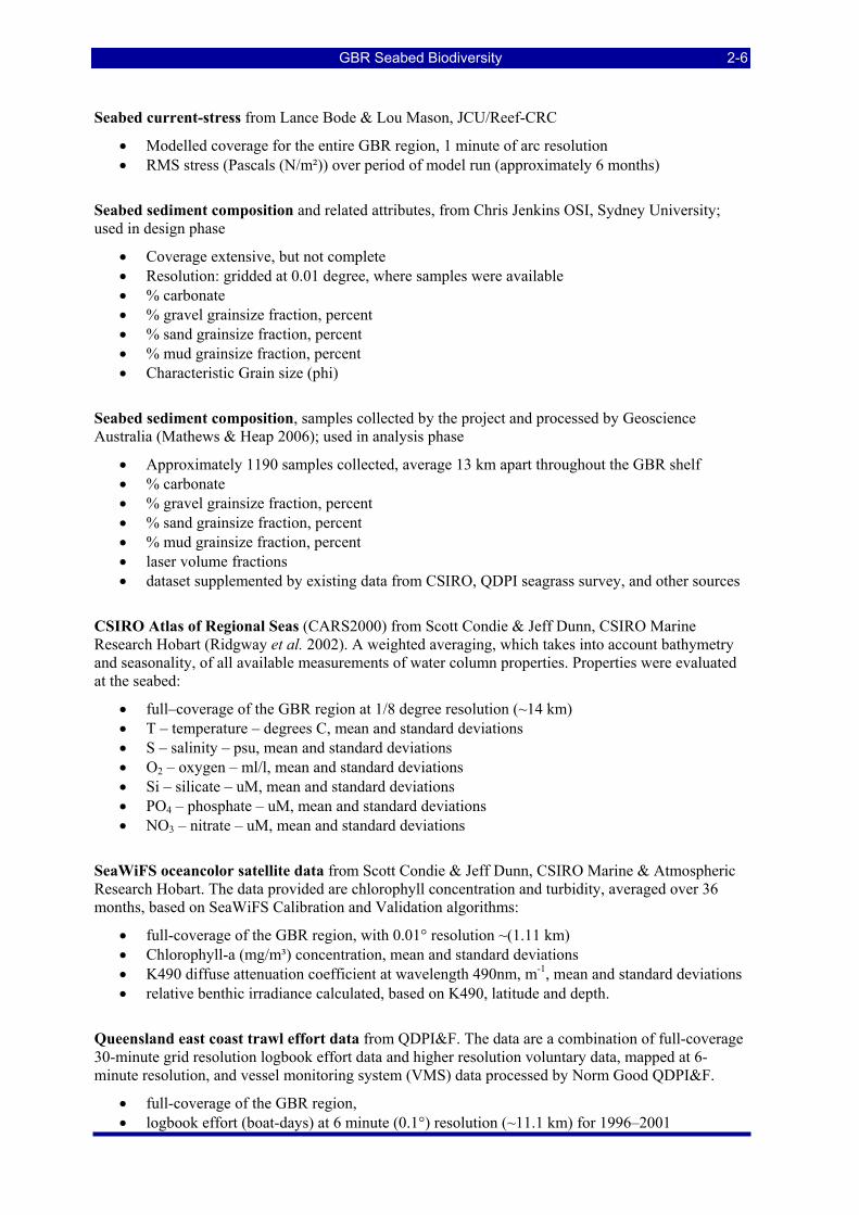
GBR Seabed Biodiversity 2-6
Seabed current-stress from Lance Bode & Lou Mason, JCU/Reef-CRC
• Modelled coverage for the entire GBR region, 1 minute of arc resolution • RMS stress (Pascals (N/m²)) over period of model run (approximately 6 months)
Seabed sediment composition and related attributes, from Chris Jenkins OSI, Sydney University; used in design phase
• Coverage extensive, but not complete • Resolution: gridded at 0.01 degree, where samples were available • % carbonate • % gravel grainsize fraction, percent • % sand grainsize fraction, percent • % mud grainsize fraction, percent • Characteristic Grain size (phi)
Seabed sediment composition, samples collected by the project and processed by Geoscience Australia (Mathews & Heap 2006); used in analysis phase
• Approximately 1190 samples collected, average 13 km apart throughout the GBR shelf • % carbonate • % gravel grainsize fraction, percent • % sand grainsize fraction, percent • % mud grainsize fraction, percent • laser volume fractions • dataset supplemented by existing data from CSIRO, QDPI seagrass survey, and other sources
CSIRO Atlas of Regional Seas (CARS2000) from Scott Condie & Jeff Dunn, CSIRO Marine Research Hobart (Ridgway et al. 2002). A weighted averaging, which takes into account bathymetry and seasonality, of all available measurements of water column properties. Properties were evaluated at the seabed:
• full–coverage of the GBR region at 1/8 degree resolution (~14 km) • T – temperature – degrees C, mean and standard deviations • S – salinity – psu, mean and standard deviations • O2 – oxygen – ml/l, mean and standard deviations • Si – silicate – uM, mean and standard deviations • PO4 – phosphate – uM, mean and standard deviations • NO3 – nitrate – uM, mean and standard deviations
SeaWiFS oceancolor satellite data from Scott Condie & Jeff Dunn, CSIRO Marine & Atmospheric Research Hobart. The data provided are chlorophyll concentration and turbidity, averaged over 36 months, based on SeaWiFS Calibration and Validation algorithms:
• full-coverage of the GBR region, with 0.01° resolution ~(1.11 km) • Chlorophyll-a (mg/m³) concentration, mean and standard deviations • K490 diffuse attenuation coefficient at wavelength 490nm, m-1, mean and standard deviations • relative benthic irradiance calculated, based on K490, latitude and depth.
Queensland east coast trawl effort data from QDPI&F. The data are a combination of full-coverage 30-minute grid resolution logbook effort data and higher resolution voluntary data, mapped at 6-minute resolution, and vessel monitoring system (VMS) data processed by Norm Good QDPI&F.
• full-coverage of the GBR region, • logbook effort (boat-days) at 6 minute (0.1°) resolution (~11.1 km) for 1996–2001
GBR Seabed Biodiversity 2-7
• VMS effort (hours) at (0.1°) resolution for 2002 • a weighted average of the above 1996–2002 data was used for design phase • logbook data 1996–2001 and VMS data 2001–2005 updated for analysis phase
Qld State permanent spatial Trawl Closure Areas, from QDPI&F.
• State permanent spatial Trawl Closure boundaries • updated in 2006 for analysis phase
GBRMPA Spatial Information, from GBRMPA,
• GBR Marine Park Zoning • RAP Bioregions (Reef and Non-Reef) • Topographic coverages (Water, Shoal, Reef, Cay, Foreshore, Mangrove, Land) • 2004 RAP Rezoning.
2.1.1.2. Data Processing:
After accounting for redundancy among the collated data, there were 21 covariates (+8 measures of variability in the CARS and SeaWiFS attributes) for stratification of the GBR non-reef region and for developing bio-physical models of biodiversity. These datasets were checked and imported into an ArcInfo GIS.
The covariates were constrained to the continental shelf by establishing a base study area bounded by the GBRWHA excluding those areas deeper than 80 m but including areas deeper than 80 m across the mouth of the Capricorn Trough, and excluding those areas shallower than 7 m near the coast, or shallower than 12 m if topographically identified as shoal, or topographically identified as reef.
A 36-arc-second grid (0.01 decimal degree, ~1.11 km) was generated for this area. Each grid cell was assigned a unique identifier that was the key to this dataset. As the collated data were of various spatial resolutions, we resampled those data to the 36-arc-second grid framework by a discrete thin plate spline technique (Wahba, 1990) using the TOPOGRID module in ArcInfo, to provide a consistent set of full-coverage covariates for the Project. As some covariates were not available for every grid cell, a “reliability indicator” was calculated that represented the distance to the nearest source data.
The GBR wide coverage of all of the collated covariates was thematically mapped using a colour range appropriate to the individual covariate distribution. These were presented as a landscape map of the study area divided up into two areas: north and south (see Section 2.1.1.3).
The full coverage interpolated physical data for each grid cell were exported out of ArcInfo for statistical analysis. This physical data set was also geographically matched to the location of each sampling station in the Effects of Trawling dataset and the GBR Seabed Biodiversity. These were also exported from the ArcInfo GIS into a database suitable to provide physical covariates matching biological sample data for statistical analyses of bio-physical relationships.
2.1.1.3. Maps of Physical Covariate Data
The Great Barrier Reef has a complex physical seabed environment. The major physical environmental factors that appear to influence the distribution and abundance of seabed habitats and assemblages in the GBR include: sediment grain size (particularly the amount of mud); force of water currents (benthic stress); chlorophyll and/or turbidity, hence benthic irradiance; and to a lesser extent depth and some nutrients (Pitcher et al. 2002). The complex multi-dimensional physical environment of the GBR has been analysed and used to stratify the region for sampling (Section 2.1.2). The most
GBR Seabed Biodiversity 2-8
common environments (>50% of the seabed) are mostly carbonate sands (Figure 2-2) away from the coast.
Benthic stress (Figure 2-1) is one of the strongest bio-physical forces and corresponds to the red areas in the map. The red inshore areas of Broad Sound and Shoalwater Bay have the largest tidal range in the GBR and are accompanied by extreme currents that scour the seabed re-suspend sediments and leave behind only gravel and larger particle sizes (Figure 2-2). The red offshore areas show where these strong tidal currents surge through the narrow channels of the reef matrix, scouring the seabed to gravel and rock substratum. High tidal current areas also occur in Torres Strait in the far northern GBR and in some other areas such as Whitsunday Passage. The scoured sediments typically are deposited in ripples, waves and dunes on the fringes of these red areas (Figure 2-2). At the opposite extreme are muddy seabeds (Figure 2-2).
Inshore areas along much of the length of the GBR are muddy or silty (Figure 2-2), and comprised of terrestrial sediments (low carbonate). Typically, with distance across the shelf, the substratum becomes sandier or even coarser (Figure 2-2), and comprised of biogenic carbonate (of biological origin). In offshore areas, coralline outcrops, reefs and shoals may occur in deep areas between emergent coral reefs. The Capricorn Channel, a wide area of GBR lagoon, has a very silty and muddy seabed. The south-eastern entrance to this channel is the deepest area on the GBR shelf, at 100-130 m.
The Capricorn Region, the southernmost part of the GBR, is typically sandy right across the shelf. It lies at the northern end of the Great Sandy Region, just beyond Fraser Island, the source of large quantities of terrestrial sand.
Many inshore areas are also very turbid and/or have high levels of chlorophyll (Figure 2-5). These inshore areas also tend to be very muddy (Figure 2-2). Along the outer margins of the inshore turbid/muddy areas, the water is clear enough to allow sufficient light for photosynthesis to reach the seabed (Figure 2-5). The deeper areas in clear waters near the outer edge of the continental shelf may at times be influenced by nutrients upwelled from below the ocean thermocline (Figure 2-4).
Many of the physical environmental covariates are correlated (Table 2-1). In particular, SeaWiFS light attenuation coefficient (K490) and Chlorophyll-a are very strongly correlated, and most of the CARS bottom-water parameters are also highly correlated. The sediment fractions (% mud, sand, gravel) are complementary, so are negatively correlated. Bathymetry is highly correlated with a large number of other covariates. These correlations among covariates make interpretation of analysis results difficult — when significant relationships between biota and any covariates were identified, not only does correlation not imply causality, but further other correlated covariates may be important.
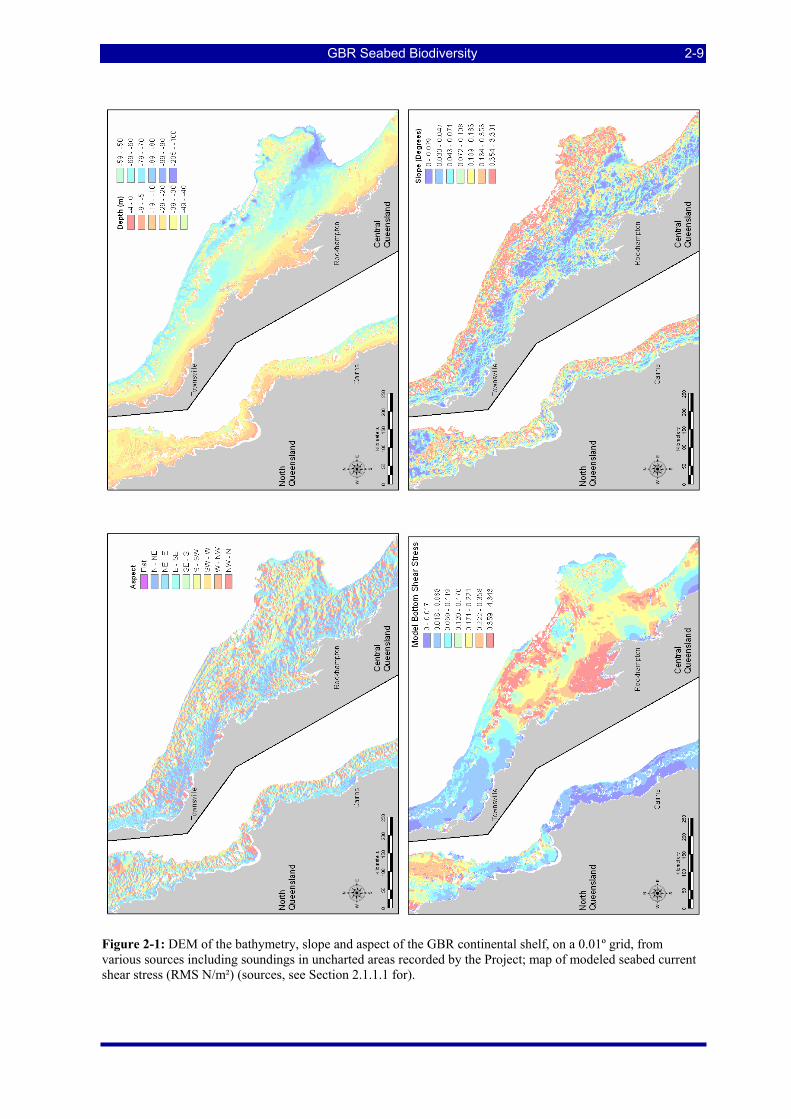
GBR Seabed Biodiversity 2-9
Figure 2-1: DEM of the bathymetry, slope and aspect of the GBR continental shelf, on a 0.01º grid, from various sources including soundings in uncharted areas recorded by the Project; map of modeled seabed current shear stress (RMS N/m²) (sources, see Section 2.1.1.1 for).
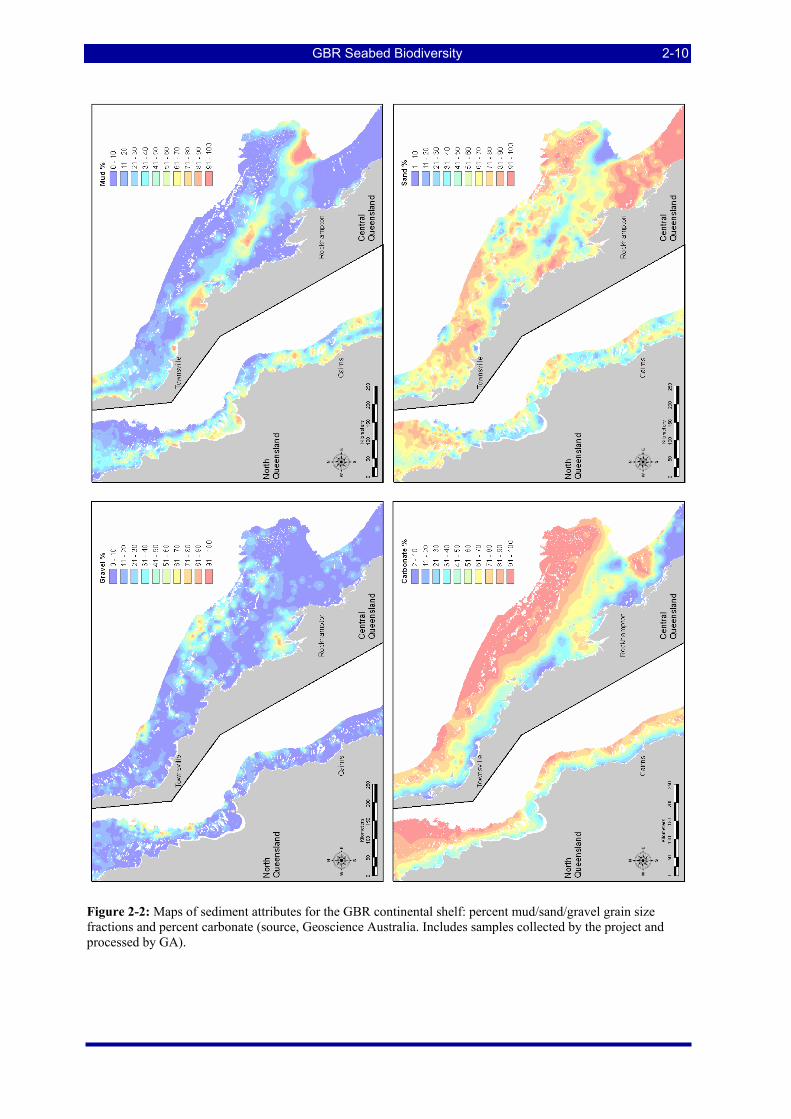
GBR Seabed Biodiversity 2-10
Figure 2-2: Maps of sediment attributes for the GBR continental shelf: percent mud/sand/gravel grain size fractions and percent carbonate (source, Geoscience Australia. Includes samples collected by the project and processed by GA).
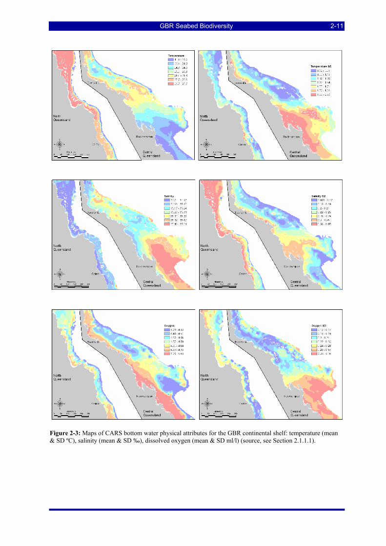
GBR Seabed Biodiversity 2-11
Figure 2-3: Maps of CARS bottom water physical attributes for the GBR continental shelf: temperature (mean & SD ºC), salinity (mean & SD ‰), dissolved oxygen (mean & SD ml/l) (source, see Section 2.1.1.1).
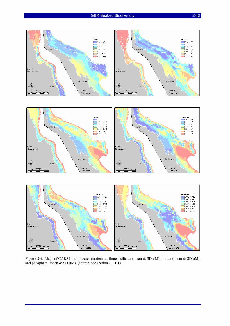
GBR Seabed Biodiversity 2-12
Figure 2-4: Maps of CARS bottom water nutrient attributes: silicate (mean & SD μM), nitrate (mean & SD μM), and phosphate (mean & SD μM), (source, see section 2.1.1.1).
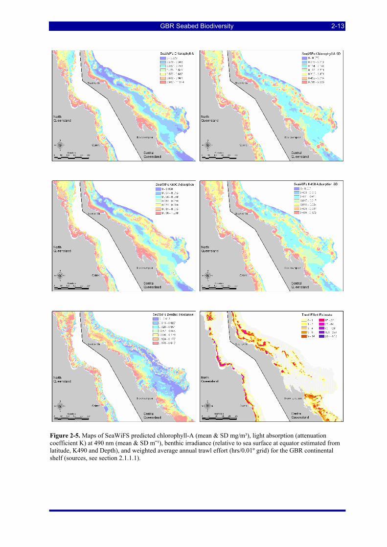
GBR Seabed Biodiversity 2-13
Figure 2-5. Maps of SeaWiFS predicted chlorophyll-A (mean & SD mg/m³), light absorption (attenuation coefficient K) at 490 nm (mean & SD m⎯¹), benthic irradiance (relative to sea surface at equator estimated from latitude, K490 and Depth), and weighted average annual trawl effort (hrs/0.01º grid) for the GBR continental shelf (sources, see section 2.1.1.1).
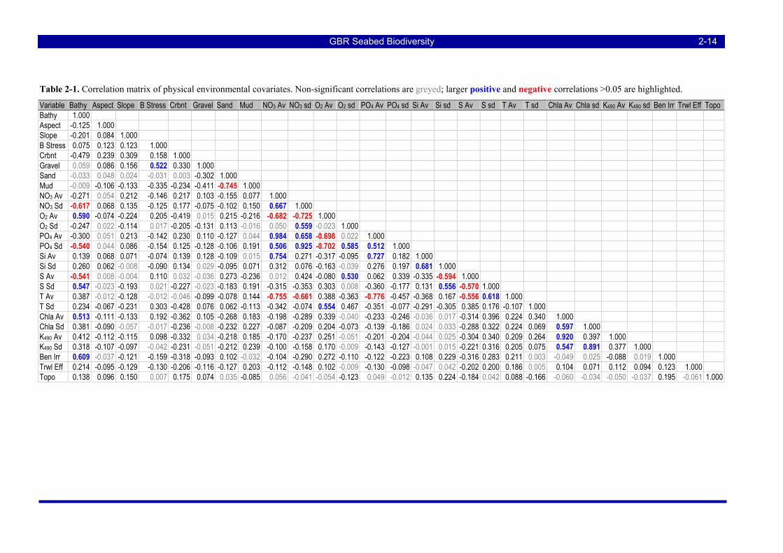
GBR Seabed Biodiversity 2-14
Table 2-1. Correlation matrix of physical environmental covariates. Non-significant correlations are greyed; larger positive and negative correlations >0.05 are highlighted.
Variable Bathy Aspect Slope B Stress Crbnt Gravel Sand Mud NO3 Av NO3 sd O2 Av O2 sd PO4 Av PO4 sd Si Av Si sd S Av S sd T Av T sd Chla Av Chla sd K490 Av K490 sd Ben Irr Trwl Eff Topo Bathy 1.000 Aspect -0.125 1.000 Slope -0.201 0.084 1.000 B Stress 0.075 0.123 0.123 1.000 Crbnt -0.479 0.239 0.309 0.158 1.000 Gravel 0.059 0.086 0.156 0.522 0.330 1.000 Sand -0.033 0.048 0.024 -0.031 0.003 -0.302 1.000 Mud -0.009 -0.106 -0.133 -0.335 -0.234 -0.411 -0.745 1.000 NO3 Av -0.271 0.054 0.212 -0.146 0.217 0.103 -0.155 0.077 1.000 NO3 Sd -0.617 0.068 0.135 -0.125 0.177 -0.075 -0.102 0.150 0.667 1.000 O2 Av 0.590 -0.074 -0.224 0.205 -0.419 0.015 0.215 -0.216 -0.682 -0.725 1.000 O2 Sd -0.247 0.022 -0.114 0.017 -0.205 -0.131 0.113 -0.016 0.050 0.559 -0.023 1.000 PO4 Av -0.300 0.051 0.213 -0.142 0.230 0.110 -0.127 0.044 0.984 0.658 -0.698 0.022 1.000 PO4 Sd -0.540 0.044 0.086 -0.154 0.125 -0.128 -0.106 0.191 0.506 0.925 -0.702 0.585 0.512 1.000 Si Av 0.139 0.068 0.071 -0.074 0.139 0.128 -0.109 0.015 0.754 0.271 -0.317 -0.095 0.727 0.182 1.000 Si Sd 0.260 0.062 -0.008 -0.090 0.134 0.029 -0.095 0.071 0.312 0.076 -0.163 -0.039 0.276 0.197 0.681 1.000 S Av -0.541 0.008 -0.004 0.110 0.032 -0.036 0.273 -0.236 0.012 0.424 -0.080 0.530 0.062 0.339 -0.335 -0.594 1.000 S Sd 0.547 -0.023 -0.193 0.021 -0.227 -0.023 -0.183 0.191 -0.315 -0.353 0.303 0.008 -0.360 -0.177 0.131 0.556 -0.570 1.000 T Av 0.387 -0.012 -0.128 -0.012 -0.046 -0.099 -0.078 0.144 -0.755 -0.661 0.388 -0.363 -0.776 -0.457 -0.368 0.167 -0.556 0.618 1.000 T Sd 0.234 -0.067 -0.231 0.303 -0.428 0.076 0.062 -0.113 -0.342 -0.074 0.554 0.467 -0.351 -0.077 -0.291 -0.305 0.385 0.176 -0.107 1.000 Chla Av 0.513 -0.111 -0.133 0.192 -0.362 0.105 -0.268 0.183 -0.198 -0.289 0.339 -0.040 -0.233 -0.246 -0.036 0.017 -0.314 0.396 0.224 0.340 1.000 Chla Sd 0.381 -0.090 -0.057 -0.017 -0.236 -0.008 -0.232 0.227 -0.087 -0.209 0.204 -0.073 -0.139 -0.186 0.024 0.033 -0.288 0.322 0.224 0.069 0.597 1.000 K490 Av 0.412 -0.112 -0.115 0.098 -0.332 0.034 -0.218 0.185 -0.170 -0.237 0.251 -0.051 -0.201 -0.204 -0.044 0.025 -0.304 0.340 0.209 0.264 0.920 0.397 1.000 K490 Sd 0.318 -0.107 -0.097 -0.042 -0.231 -0.051 -0.212 0.239 -0.100 -0.158 0.170 -0.009 -0.143 -0.127 -0.001 0.015 -0.221 0.316 0.205 0.075 0.547 0.891 0.377 1.000 Ben Irr 0.609 -0.037 -0.121 -0.159 -0.318 -0.093 0.102 -0.032 -0.104 -0.290 0.272 -0.110 -0.122 -0.223 0.108 0.229 -0.316 0.283 0.211 0.003 -0.049 0.025 -0.088 0.019 1.000 Trwl Eff 0.214 -0.095 -0.129 -0.130 -0.206 -0.116 -0.127 0.203 -0.112 -0.148 0.102 -0.009 -0.130 -0.098 -0.047 0.042 -0.202 0.200 0.186 0.005 0.104 0.071 0.112 0.094 0.123 1.000 Topo 0.138 0.096 0.150 0.007 0.175 0.074 0.035 -0.085 0.056 -0.041 -0.054 -0.123 0.049 -0.012 0.135 0.224 -0.184 0.042 0.088 -0.166 -0.060 -0.034 -0.050 -0.037 0.195 -0.061 1.000
GBR Seabed Biodiversity 2-15
2.1.2. Study Area Stratification (N Ellis)
The sampling for seabed biodiversity mapping in the Great Barrier Reef required an optimal strategy for the selection of survey sites. The primary purpose of the survey is to obtain data on the spatial distribution of benthic biota, so that subsequent bio-physical modelling can make use of the physical environment covariates to interpolate and map. Given that the number of sites that can be sampled is limited, it was obviously important to place the samples in a way that would yield as much information as possible. This required that the environment space, or multi-dimensional covariate space, rather than the 2-dimensional space must be sampled representatively and the approach to achieve this is stratification. Further, the stratification must be relevant to the benthic biotic, so it must be informed by measures of the biological importance of each covariate. This approach will optimally ensure that the biodiversity and physical attributes of as many different habitats types as possible, given the available resources, would be characterised. The physical variables collated as part of this project, which were known in advance of the survey, were used to guide the stratification. Biological information will be taken into account by weighting the physical variables based on their relative importance in bio-physical relationships — variables of greater influence on biological patterns having a larger weighting and influence in the stratification.
From an earlier study (Pitcher et al., 2002) we have measures of the “importance” of these covariates with respect to correlations with the abundance of many benthic species in a detailed survey of an 8,000 km² area of the far northern GBR. Conceptually, important variables are those for which benthic composition changes significantly along a gradient of the variable. The survey should be designed to ensure that such important variables are sampled finely, so that the expected benthic diversity is reliably captured. That is, we should stratify our design with respect to the important variables.
Further, the sampling strategy should also consider the spatial resolution required for management utility. A scale of several 10s km was considered appropriate for broad scale characterisation. The implications of the spatial auto-correlation distance (the similarity of locations decreases with distance, such that on average sites ~10 km apart are uncorrelated; Pitcher et al., 2002) and considerations of the benefit-cost of logistics (at maximum 1 site per hour) also indicate a sampling density of approximately 10 km average separation. In this approach, approximately 200 primary strata with similar physical characteristics were identified from importance weighted physical covariates of more than 170,000 0.01° grid cells covering the shelf area of the GBR. The size (area) of strata will vary depending on the number of grid cells having particular similar physical characteristics. About 10 ‘Replicate’ sampling sites were assigned to each primary stratum by an importance weighted process.
The potential survey area in the GBR, after excluding reefs and other areas that were too shallow, included 171,560 cells of size 0.01° (~1.11 km), each cell being a candidate sample site. Given the spatial autocorrelation distances, the average distance between sites should not exceed about 0.1° (~11.1 km) indicating that about 1,400–1,600 of these cells should be sampled. A margin was added to this lower limit, thus the design provided for 1450 sites. At the centre of each 0.01 degree cell, the values of 28 physical variables were collated or interpolated and represent the GBR region as a cloud of 171,560 points within a 28-dimensional physical-variable space. Ultimately, this space was to be partitioned into 1450 relatively homogeneous regions (or strata), such that the expected benthic biodiversity would be homogeneous within each stratum but heterogeneous among strata. A sampling site would then be selected from each stratum to produce a set of 1450 sites. This section describes the methods for achieving this partitioning or stratification of physical-variable space.
2.1.2.1. Principles of Partitioning
The basic principle behind the partitioning can be illustrated with the following simple two-dimensional example. Consider two physical variables x and y for which we have values at 1,000 sites, and suppose that these sites sample the covariate space roughly uniformly (Figure 2-6(a)). We wish to partition the covariate space into 20 strata. If the two variables were equally important, then the partitioning in Figure 2-6(b) would be adequate, since the strata are roughly the same width in x and y.
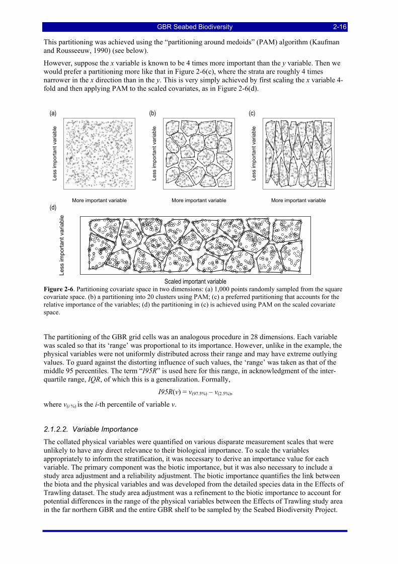
GBR Seabed Biodiversity 2-16
This partitioning was achieved using the “partitioning around medoids” (PAM) algorithm (Kaufman and Rousseeuw, 1990) (see below).
However, suppose the x variable is known to be 4 times more important than the y variable. Then we would prefer a partitioning more like that in Figure 2-6(c), where the strata are roughly 4 times narrower in the x direction than in the y. This is very simply achieved by first scaling the x variable 4-fold and then applying PAM to the scaled covariates, as in Figure 2-6(d).
(a)
More important variable
Less
impo
rtant
var
iabl
e
(b)
More important variable
Less
impo
rtant
var
iabl
e
(c)
More important variable
Less
impo
rtant
var
iabl
e
(d)
Less
impo
rtant
var
iabl
e
Scaled important variable
Figure 2-6. Partitioning covariate space in two dimensions: (a) 1,000 points randomly sampled from the square covariate space. (b) a partitioning into 20 clusters using PAM; (c) a preferred partitioning that accounts for the relative importance of the variables; (d) the partitioning in (c) is achieved using PAM on the scaled covariate space.
The partitioning of the GBR grid cells was an analogous procedure in 28 dimensions. Each variable was scaled so that its ‘range’ was proportional to its importance. However, unlike in the example, the physical variables were not uniformly distributed across their range and may have extreme outlying values. To guard against the distorting influence of such values, the ‘range’ was taken as that of the middle 95 percentiles. The term “I95R” is used here for this range, in acknowledgment of the inter-quartile range, IQR, of which this is a generalization. Formally,
I95R(v) = v(97.5%) – v(2.5%),
where v(i %) is the i-th percentile of variable v.
2.1.2.2. Variable Importance
The collated physical variables were quantified on various disparate measurement scales that were unlikely to have any direct relevance to their biological importance. To scale the variables appropriately to inform the stratification, it was necessary to derive an importance value for each variable. The primary component was the biotic importance, but it was also necessary to include a study area adjustment and a reliability adjustment. The biotic importance quantifies the link between the biota and the physical variables and was developed from the detailed species data in the Effects of Trawling dataset. The study area adjustment was a refinement to the biotic importance to account for potential differences in the range of the physical variables between the Effects of Trawling study area in the far northern GBR and the entire GBR shelf to be sampled by the Seabed Biodiversity Project.
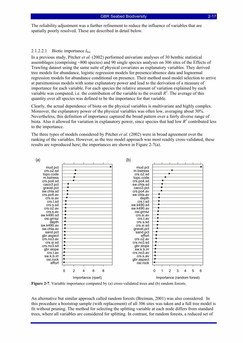
GBR Seabed Biodiversity 2-17
The reliability adjustment was a further refinement to reduce the influence of variables that are spatially poorly resolved. These are described in detail below.
2.1.2.2.1 Biotic importance Ibio In a previous study, Pitcher et al. (2002) performed univariate analyses of 30 benthic statistical assemblages (comprising ~800 species) and 90 single species analyses on 306 sites of the Effects of Trawling dataset using the same suite of physical covariates as explanatory variables. They derived tree models for abundance, logistic regression models for presence/absence data and lognormal regression models for abundance conditional on presence. Their method used model selection to arrive at parsimonious models with some explanatory power and lead to the derivation of a measure of importance for each variable. For each species the relative amount of variation explained by each variable was computed, i.e. the contribution of the variable to the overall R2. The average of this quantity over all species was defined to be the importance for that variable.
Clearly, the actual dependence of biota on the physical variables is multivariate and highly complex. Moreover, the explanatory power of the physical variables was often low, averaging about 30%. Nevertheless, this definition of importance captured the broad pattern over a fairly diverse range of biota. Also it allowed for variation in explanatory power, since species that had low R2 contributed less to the importance.
The three types of models considered by Pitcher et al. (2002) were in broad agreement over the ranking of the variables. However, as the tree model approach was most readily cross-validated, these results are reproduced here; the importances are shown in Figure 2-7(a).
(a)
effortosi.rock
sw.k.b.irrcrs.t.av
gbr.slopecrs.no3.sd
crs.si.sdcrs.no3.avgbr.aspect
sand.pctsw.chla.av
sw.k490.avdepth
osi.grnszsw.k490.sd
crs.s.avcrs.o2.av
crs.s.sdcrs.t.sd
crs.si.avcrs.po4.avsw.chla.sdgravel.pctcaco3.pct
crs.po4.sdm.bstresstopo.codecrs.o2.sdmud.pct
0 2 4 6 8
Importance (rpart)
(b)
osi.rockgbr.aspect
crs.s.avcrs.no3.av
sw.k.b.irrgbr.slope
crs.no3.sdcrs.o2.av
effortsand.pct
gravel.pctcrs.si.sdcrs.s.sdcrs.t.av
crs.si.avosi.grnsz
sw.k490.avsw.k490.sd
crs.t.sddepth
sw.chla.avcrs.po4.avcaco3.pct
sw.chla.sdcrs.po4.sdtopo.codecrs.o2.sd
m.bstressmud.pct
0 1 2 3 4 5 6
Importance (random forest) Figure 2-7. Variable importance computed by (a) cross-validated trees and (b) random forests.
An alternative but similar approach called random forests (Breiman, 2001) was also considered. In this procedure a bootstrap sample (with replacement) of all 306 sites was taken and a full tree model is fit without pruning. The method for selecting the splitting variable at each node differs from standard trees, where all variables are considered for splitting. In contrast, for random forests, a reduced set of
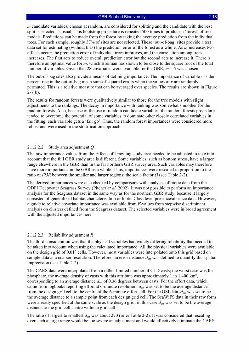
GBR Seabed Biodiversity 2-18
m candidate variables, chosen at random, are considered for splitting and the candidate with the best split is selected as usual. This bootstrap procedure is repeated 500 times to produce a ‘forest’ of tree models. Predictions can be made from the forest by taking the average prediction from the individual trees. For each sample, roughly 37% of sites are not selected. These ‘out-of-bag’ sites provide a test data set for estimating (without bias) the prediction error of the forest as a whole. As m increases two effects occur: the prediction error of individual trees improves, and the correlation among trees increases. The first acts to reduce overall prediction error but the second acts to increase it. There is therefore an optimal value for m, which Breiman has shown to be close to the square root of the total number of variables. Given that 28 covariates were available for the GBR, m = 5 was chosen.
The out-of-bag sites also provide a means of defining importance. The importance of variable v is the percent rise in the out-of-bag mean sum-of-squared errors when the values of v are randomly permuted. This is a relative measure that can be averaged over species. The results are shown in Figure 2-7(b).
The results for random forests were qualitatively similar to those for the tree models with slight adjustments to the rankings. The decay in importance with ranking was somewhat smoother for the random forests. Also, because of the use of random candidate variables, the random forests procedure tended to overcome the potential of some variables to dominate other closely correlated variables in the fitting; each variable gets a ‘fair go’. Thus, the random forest importances were considered more robust and were used in the stratification approach.
2.1.2.2.2 Study area adjustment Q The raw importance values from the Effects of Trawling study area needed to be adjusted to take into account that the full GBR study area is different. Some variables, such as bottom stress, have a larger range elsewhere in the GBR than in the far northern GBR survey area. Such variables may therefore have more importance in the GBR as a whole. Thus, importances were rescaled in proportion to the ratio of I95R between the smaller and larger regions; the scale factor Q (see Table 2-2).
The derived importances were also checked by comparisons with analyses of biotic data from the QDPI Deepwater Seagrass Survey (Pitcher et al. 2002). It was not possible to perform an importance analysis for the Seagrass dataset in the same way as for the northern GBR study, because it largely consisted of generalized habitat characterisation or biotic Class level presence/absence data. However, a guide to relative covariate importance was available from F-values from stepwise discriminant analysis on clusters defined from the Seagrass dataset. The selected variables were in broad agreement with the adjusted importances here.
2.1.2.2.3 Reliability adjustment R The third consideration was that the physical variables had widely differing reliability that needed to be taken into account when using the calculated importance. All the physical variables were available on the design grid of 0.01° cells. However, most variables were interpolated onto this grid based on sample data at a coarser resolution. Therefore, an error distance derr was defined to quantify this spatial imprecision (see Table 2-2).
The CARS data were interpolated from a rather limited number of CTD casts; the worst case was for phosphate, the average density of casts with this attribute was approximately 1 in 1,400 km², corresponding to an average distance derr of 0.36 degrees between casts. For the effort data, which came from logbooks reporting effort at 6-minute resolution, derr was set to be the average distance from the design grid cell to the centre of the 6-minute effort cell. For the OSI data, derr was set to be the average distance to a sample point from each design grid cell. The SeaWiFS data in their raw form were already specified at the same scale as the design grid; in this case derr was set to be the average distance to the grid cell centre within a grid cell.
The ratio of largest to smallest derr was about 270 (refer Table 2-2). It was considered that rescaling over such a large range would be too severe an adjustment and would effectively eliminate the CARS
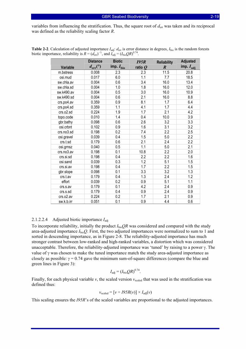
GBR Seabed Biodiversity 2-19
variables from influencing the stratification. Thus, the square root of derr was taken and its reciprocal was defined as the reliability scaling factor R.
Table 2-2. Calculation of adjusted importance Iadj: derr is error distance in degrees, Ibio is the random forests biotic importance, reliability is R = (derr)–½, and Iadj = (IbioQR)0.74.
Variable Distance derr(°)
Biotic imp. Ibio
I95R ratio Q
Reliability R
Adjusted imp. Iadj
m.bstress 0.008 2.3 2.3 11.5 20.8 osi.mud 0.017 6.0 1.1 7.7 18.5
sw.chla.av 0.004 0.6 3.4 16.0 13.4 sw.chla.sd 0.004 1.0 1.8 16.0 12.0 sw.k490.av 0.004 0.5 3.0 16.0 10.9 sw.k490.sd 0.004 0.6 2.1 16.0 8.8 crs.po4.av 0.359 0.9 8.1 1.7 6.4 crs.po4.sd 0.359 1.1 4.1 1.7 4.4 crs.o2.sd 0.224 1.9 1.7 2.1 4.2 topo.code 0.010 1.4 0.4 10.0 3.9 gbr.bathy 0.098 0.6 2.6 3.2 3.3 osi.crbnt 0.102 0.9 1.6 3.1 3.2
crs.no3.sd 0.198 0.2 7.4 2.2 2.5 osi.gravel 0.039 0.4 1.5 5.0 2.2 crs.t.sd 0.179 0.6 2.1 2.4 2.2
osi.grnsz 0.040 0.5 1.1 5.0 2.1 crs.no3.av 0.198 0.1 10.8 2.2 2.0 crs.si.sd 0.198 0.4 2.2 2.2 1.6 osi.sand 0.039 0.3 1.2 5.1 1.5 crs.si.av 0.198 0.4 1.7 2.2 1.5 gbr.slope 0.098 0.1 3.3 3.2 1.3 crs.t.av 0.179 0.4 1.3 2.4 1.2 effort 0.039 0.2 0.9 5.1 1.1
crs.s.av 0.179 0.1 4.2 2.4 0.9 crs.s.sd 0.179 0.4 0.9 2.4 0.9
crs.o2.av 0.224 0.2 1.7 2.1 0.9 sw.k.b.irr 0.051 0.1 0.9 4.4 0.6
2.1.2.2.4 Adjusted biotic importance Iadj To incorporate reliability, initially the product IbioQR was considered and compared with the study area-adjusted importance IbioQ. First, the two adjusted importances were normalized to sum to 1 and sorted in descending importance, as in Figure 2-8. The reliability-adjusted importance has much stronger contrast between low-ranked and high-ranked variables, a distortion which was considered unacceptable. Therefore, the reliability-adjusted importance was ‘tuned’ by raising to a power γ. The value of γ was chosen to make the tuned importance match the study area-adjusted importance as closely as possible: γ = 0.74 gave the minimum sum-of-square differences (compare the blue and green lines in Figure 3):
Iadj = (IbioQR)0.74.
Finally, for each physical variable v, the scaled version vscaled that was used in the stratification was defined thus:
vscaled = [v ÷ I95R(v)] × Iadj(v)
This scaling ensures the I95R’s of the scaled variables are proportional to the adjusted importances.
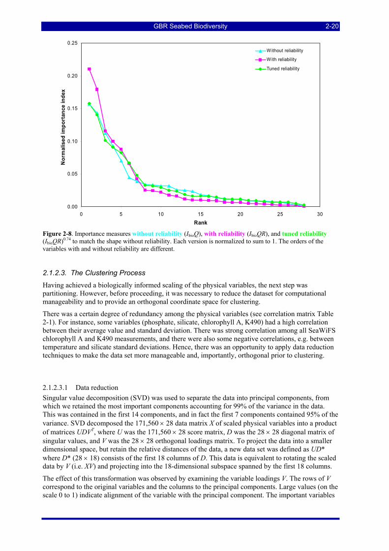
GBR Seabed Biodiversity 2-20
0.00
0.05
0.10
0.15
0.20
0.25
0 5 10 15 20 25 30
Rank
Nor
mal
ised
impo
rtan
ce in
dex
Without reliability
With reliability
Tuned reliability
Figure 2-8. Importance measures without reliability (IbioQ), with reliability (IbioQR), and tuned reliability (IbioQR)0.74 to match the shape without reliability. Each version is normalized to sum to 1. The orders of the variables with and without reliability are different.
2.1.2.3. The Clustering Process
Having achieved a biologically informed scaling of the physical variables, the next step was partitioning. However, before proceeding, it was necessary to reduce the dataset for computational manageability and to provide an orthogonal coordinate space for clustering.
There was a certain degree of redundancy among the physical variables (see correlation matrix Table 2-1). For instance, some variables (phosphate, silicate, chlorophyll A, K490) had a high correlation between their average value and standard deviation. There was strong correlation among all SeaWiFS chlorophyll A and K490 measurements, and there were also some negative correlations, e.g. between temperature and silicate standard deviations. Hence, there was an opportunity to apply data reduction techniques to make the data set more manageable and, importantly, orthogonal prior to clustering.
2.1.2.3.1 Data reduction Singular value decomposition (SVD) was used to separate the data into principal components, from which we retained the most important components accounting for 99% of the variance in the data. This was contained in the first 14 components, and in fact the first 7 components contained 95% of the variance. SVD decomposed the 171,560 × 28 data matrix X of scaled physical variables into a product of matrices UDVT, where U was the 171,560 × 28 score matrix, D was the 28 × 28 diagonal matrix of singular values, and V was the 28 × 28 orthogonal loadings matrix. To project the data into a smaller dimensional space, but retain the relative distances of the data, a new data set was defined as UD* where D* (28 × 18) consists of the first 18 columns of D. This data is equivalent to rotating the scaled data by V (i.e. XV) and projecting into the 18-dimensional subspace spanned by the first 18 columns.
The effect of this transformation was observed by examining the variable loadings V. The rows of V correspond to the original variables and the columns to the principal components. Large values (on the scale 0 to 1) indicate alignment of the variable with the principal component. The important variables
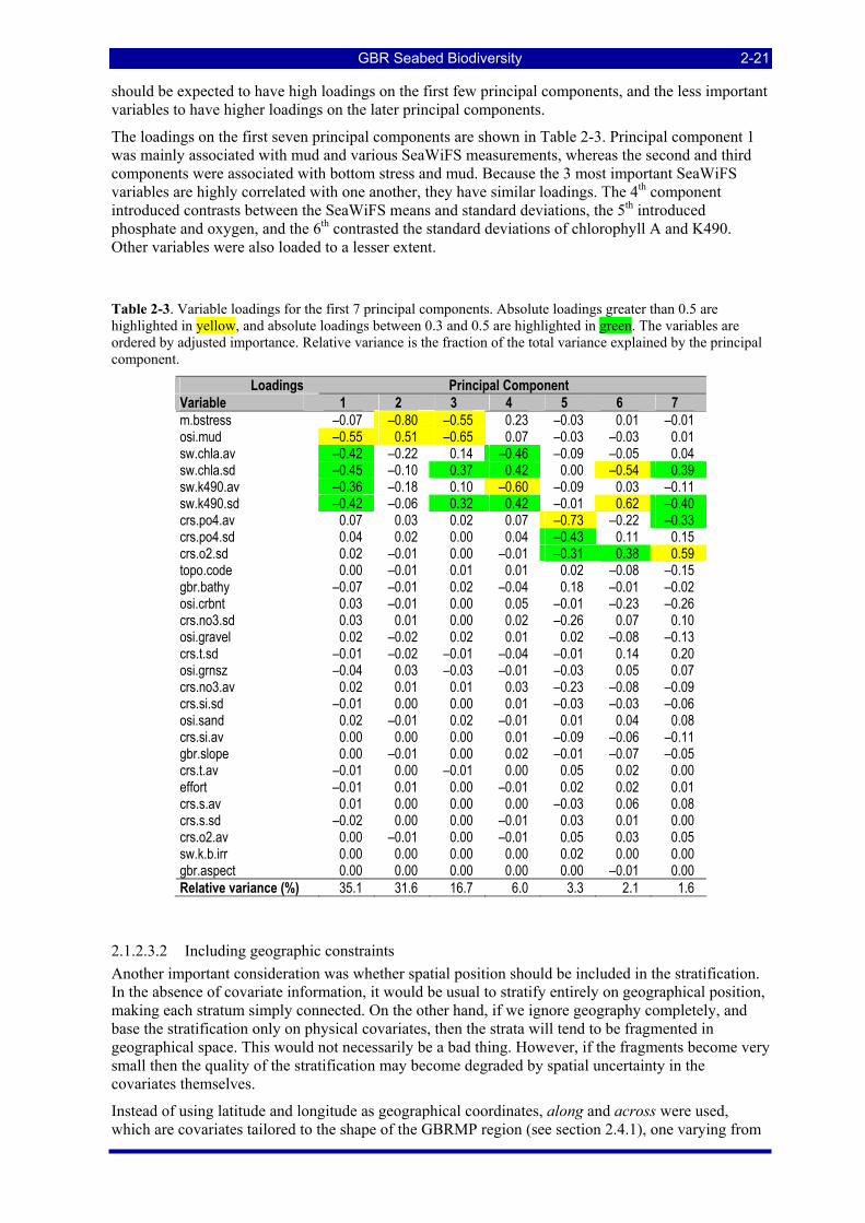
GBR Seabed Biodiversity 2-21
should be expected to have high loadings on the first few principal components, and the less important variables to have higher loadings on the later principal components.
The loadings on the first seven principal components are shown in Table 2-3. Principal component 1 was mainly associated with mud and various SeaWiFS measurements, whereas the second and third components were associated with bottom stress and mud. Because the 3 most important SeaWiFS variables are highly correlated with one another, they have similar loadings. The 4th component introduced contrasts between the SeaWiFS means and standard deviations, the 5th introduced phosphate and oxygen, and the 6th contrasted the standard deviations of chlorophyll A and K490. Other variables were also loaded to a lesser extent.
Table 2-3. Variable loadings for the first 7 principal components. Absolute loadings greater than 0.5 are highlighted in yellow, and absolute loadings between 0.3 and 0.5 are highlighted in green. The variables are ordered by adjusted importance. Relative variance is the fraction of the total variance explained by the principal component.
Loadings Principal Component Variable 1 2 3 4 5 6 7 m.bstress –0.07 –0.80 –0.55 0.23 –0.03 0.01 –0.01 osi.mud –0.55 0.51 –0.65 0.07 –0.03 –0.03 0.01 sw.chla.av –0.42 –0.22 0.14 –0.46 –0.09 –0.05 0.04 sw.chla.sd –0.45 –0.10 0.37 0.42 0.00 –0.54 0.39 sw.k490.av –0.36 –0.18 0.10 –0.60 –0.09 0.03 –0.11 sw.k490.sd –0.42 –0.06 0.32 0.42 –0.01 0.62 –0.40 crs.po4.av 0.07 0.03 0.02 0.07 –0.73 –0.22 –0.33 crs.po4.sd 0.04 0.02 0.00 0.04 –0.43 0.11 0.15 crs.o2.sd 0.02 –0.01 0.00 –0.01 –0.31 0.38 0.59 topo.code 0.00 –0.01 0.01 0.01 0.02 –0.08 –0.15 gbr.bathy –0.07 –0.01 0.02 –0.04 0.18 –0.01 –0.02 osi.crbnt 0.03 –0.01 0.00 0.05 –0.01 –0.23 –0.26 crs.no3.sd 0.03 0.01 0.00 0.02 –0.26 0.07 0.10 osi.gravel 0.02 –0.02 0.02 0.01 0.02 –0.08 –0.13 crs.t.sd –0.01 –0.02 –0.01 –0.04 –0.01 0.14 0.20 osi.grnsz –0.04 0.03 –0.03 –0.01 –0.03 0.05 0.07 crs.no3.av 0.02 0.01 0.01 0.03 –0.23 –0.08 –0.09 crs.si.sd –0.01 0.00 0.00 0.01 –0.03 –0.03 –0.06 osi.sand 0.02 –0.01 0.02 –0.01 0.01 0.04 0.08 crs.si.av 0.00 0.00 0.00 0.01 –0.09 –0.06 –0.11 gbr.slope 0.00 –0.01 0.00 0.02 –0.01 –0.07 –0.05 crs.t.av –0.01 0.00 –0.01 0.00 0.05 0.02 0.00 effort –0.01 0.01 0.00 –0.01 0.02 0.02 0.01 crs.s.av 0.01 0.00 0.00 0.00 –0.03 0.06 0.08 crs.s.sd –0.02 0.00 0.00 –0.01 0.03 0.01 0.00 crs.o2.av 0.00 –0.01 0.00 –0.01 0.05 0.03 0.05 sw.k.b.irr 0.00 0.00 0.00 0.00 0.02 0.00 0.00 gbr.aspect 0.00 0.00 0.00 0.00 0.00 –0.01 0.00 Relative variance (%) 35.1 31.6 16.7 6.0 3.3 2.1 1.6
2.1.2.3.2 Including geographic constraints Another important consideration was whether spatial position should be included in the stratification. In the absence of covariate information, it would be usual to stratify entirely on geographical position, making each stratum simply connected. On the other hand, if we ignore geography completely, and base the stratification only on physical covariates, then the strata will tend to be fragmented in geographical space. This would not necessarily be a bad thing. However, if the fragments become very small then the quality of the stratification may become degraded by spatial uncertainty in the covariates themselves.
Instead of using latitude and longitude as geographical coordinates, along and across were used, which are covariates tailored to the shape of the GBRMP region (see section 2.4.1), one varying from
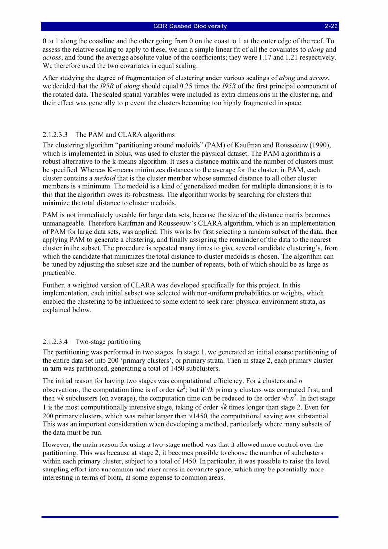
GBR Seabed Biodiversity 2-22
0 to 1 along the coastline and the other going from 0 on the coast to 1 at the outer edge of the reef. To assess the relative scaling to apply to these, we ran a simple linear fit of all the covariates to along and across, and found the average absolute value of the coefficients; they were 1.17 and 1.21 respectively. We therefore used the two covariates in equal scaling.
After studying the degree of fragmentation of clustering under various scalings of along and across, we decided that the I95R of along should equal 0.25 times the I95R of the first principal component of the rotated data. The scaled spatial variables were included as extra dimensions in the clustering, and their effect was generally to prevent the clusters becoming too highly fragmented in space.
2.1.2.3.3 The PAM and CLARA algorithms The clustering algorithm “partitioning around medoids” (PAM) of Kaufman and Rousseeuw (1990), which is implemented in Splus, was used to cluster the physical dataset. The PAM algorithm is a robust alternative to the k-means algorithm. It uses a distance matrix and the number of clusters must be specified. Whereas K-means minimizes distances to the average for the cluster, in PAM, each cluster contains a medoid that is the cluster member whose summed distance to all other cluster members is a minimum. The medoid is a kind of generalized median for multiple dimensions; it is to this that the algorithm owes its robustness. The algorithm works by searching for clusters that minimize the total distance to cluster medoids.
PAM is not immediately useable for large data sets, because the size of the distance matrix becomes unmanageable. Therefore Kaufman and Rousseeuw’s CLARA algorithm, which is an implementation of PAM for large data sets, was applied. This works by first selecting a random subset of the data, then applying PAM to generate a clustering, and finally assigning the remainder of the data to the nearest cluster in the subset. The procedure is repeated many times to give several candidate clustering’s, from which the candidate that minimizes the total distance to cluster medoids is chosen. The algorithm can be tuned by adjusting the subset size and the number of repeats, both of which should be as large as practicable.
Further, a weighted version of CLARA was developed specifically for this project. In this implementation, each initial subset was selected with non-uniform probabilities or weights, which enabled the clustering to be influenced to some extent to seek rarer physical environment strata, as explained below.
2.1.2.3.4 Two-stage partitioning The partitioning was performed in two stages. In stage 1, we generated an initial coarse partitioning of the entire data set into 200 ‘primary clusters’, or primary strata. Then in stage 2, each primary cluster in turn was partitioned, generating a total of 1450 subclusters.
The initial reason for having two stages was computational efficiency. For k clusters and n observations, the computation time is of order kn2; but if √k primary clusters was computed first, and then √k subclusters (on average), the computation time can be reduced to the order √k n2. In fact stage 1 is the most computationally intensive stage, taking of order √k times longer than stage 2. Even for 200 primary clusters, which was rather larger than √1450, the computational saving was substantial. This was an important consideration when developing a method, particularly where many subsets of the data must be run.
However, the main reason for using a two-stage method was that it allowed more control over the partitioning. This was because at stage 2, it becomes possible to choose the number of subclusters within each primary cluster, subject to a total of 1450. In particular, it was possible to raise the level sampling effort into uncommon and rarer areas in covariate space, which may be potentially more interesting in terms of biota, at some expense to common areas.
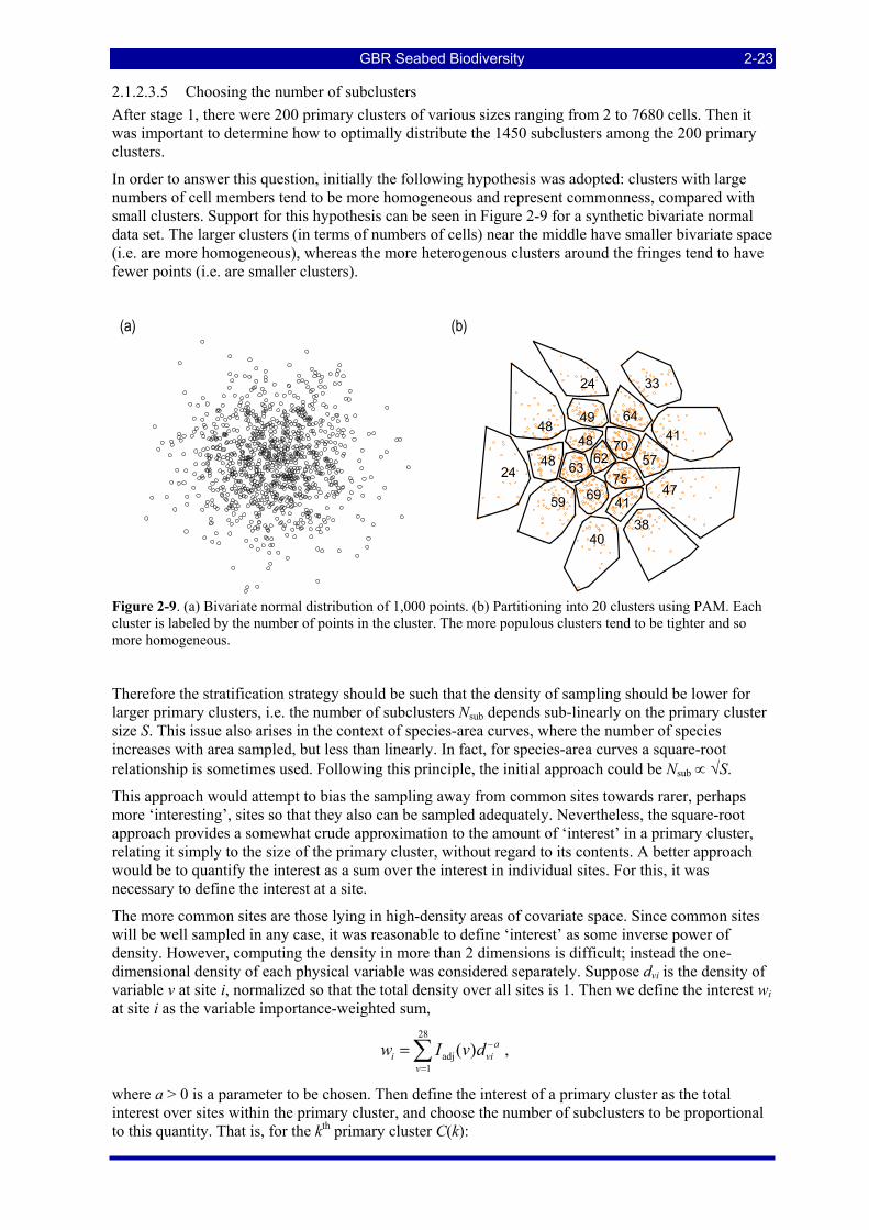
GBR Seabed Biodiversity 2-23
2.1.2.3.5 Choosing the number of subclusters After stage 1, there were 200 primary clusters of various sizes ranging from 2 to 7680 cells. Then it was important to determine how to optimally distribute the 1450 subclusters among the 200 primary clusters.
In order to answer this question, initially the following hypothesis was adopted: clusters with large numbers of cell members tend to be more homogeneous and represent commonness, compared with small clusters. Support for this hypothesis can be seen in Figure 2-9 for a synthetic bivariate normal data set. The larger clusters (in terms of numbers of cells) near the middle have smaller bivariate space (i.e. are more homogeneous), whereas the more heterogenous clusters around the fringes tend to have fewer points (i.e. are smaller clusters).
(a)
(b)
69
62
59
57
24
41
64
75
704848
48
4763
4941
4038
24
33
Figure 2-9. (a) Bivariate normal distribution of 1,000 points. (b) Partitioning into 20 clusters using PAM. Each cluster is labeled by the number of points in the cluster. The more populous clusters tend to be tighter and so more homogeneous.
Therefore the stratification strategy should be such that the density of sampling should be lower for larger primary clusters, i.e. the number of subclusters Nsub depends sub-linearly on the primary cluster size S. This issue also arises in the context of species-area curves, where the number of species increases with area sampled, but less than linearly. In fact, for species-area curves a square-root relationship is sometimes used. Following this principle, the initial approach could be Nsub ∝ √S.
This approach would attempt to bias the sampling away from common sites towards rarer, perhaps more ‘interesting’, sites so that they also can be sampled adequately. Nevertheless, the square-root approach provides a somewhat crude approximation to the amount of ‘interest’ in a primary cluster, relating it simply to the size of the primary cluster, without regard to its contents. A better approach would be to quantify the interest as a sum over the interest in individual sites. For this, it was necessary to define the interest at a site.
The more common sites are those lying in high-density areas of covariate space. Since common sites will be well sampled in any case, it was reasonable to define ‘interest’ as some inverse power of density. However, computing the density in more than 2 dimensions is difficult; instead the one-dimensional density of each physical variable was considered separately. Suppose dvi is the density of variable v at site i, normalized so that the total density over all sites is 1. Then we define the interest wi at site i as the variable importance-weighted sum,
28
adj1
( ) ai vi
vw I v d −
=
= ∑ ,
where a > 0 is a parameter to be chosen. Then define the interest of a primary cluster as the total interest over sites within the primary cluster, and choose the number of subclusters to be proportional to this quantity. That is, for the kth primary cluster C(k):
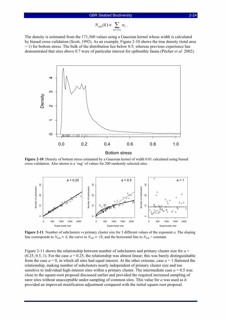
GBR Seabed Biodiversity 2-24
sub( )
( ) ii C k
N k w∈
∝ ∑ .
The density is estimated from the 171,560 values using a Gaussian kernel whose width is calculated by biased cross-validation (Scott, 1992). As an example, Figure 2-10 shows the true density (total area = 1) for bottom stress. The bulk of the distribution lies below 0.5; whereas previous experience has demonstrated that sites above 0.7 were of particular interest for epibenthic fauna (Pitcher et al. 2002).
Bottom stress
Den
sity
01
23
4
0.0 0.2 0.4 0.6 0.8 1.0
Figure 2-10. Density of bottom stress estimated by a Gaussian kernel of width 0.01 calculated using biased cross-validation. Also shown is a ‘rug’ of values for 200 randomly selected sites.
Supercluster size
Num
ber o
f sub
clus
ters
0 500 1000 1500 2000
010
2030
a = 0.25
Supercluster size
Num
ber o
f sub
clus
ters
0 500 1000 1500 2000
010
2030
8 29
3
27
a = 0.5
Supercluster size
Num
ber o
f sub
clus
ters
0 500 1000 1500 2000
010
2030
a = 1
Figure 2-11. Number of subclusters vs primary cluster size for 3 different values of the exponent a. The sloping line corresponds to Nsub ∝ S, the curve to Nsub ∝ √S, and the horizontal line to Nsub = constant.
Figure 2-11 shows the relationship between number of subclusters and primary cluster size for a = (0.25, 0.5, 1). For the case a = 0.25, the relationship was almost linear; this was barely distinguishable from the case a = 0, in which all sites had equal interest. At the other extreme, case a = 1 flattened the relationship, making number of subclusters nearly independent of primary cluster size and too sensitive to individual high-interest sites within a primary cluster. The intermediate case a = 0.5 was close to the square-root proposal discussed earlier and provided the required increased sampling of rarer sites without unacceptable under-sampling of common sites. This value for a was used as it provided an improved stratification adjustment compared with the initial square-root proposal.
GBR Seabed Biodiversity 2-25p
Clusters 1 to 10 Clusters 11 to 20 Clusters 21 to 30
Clusters 31 to 40 Clusters 41 to 50 Clusters 51 to 60
Figure 2-12. The 200 primary clusters in geographical space. Sixty of the clusters have been separated into six panels in order to make them distinct and assess the degree of fragmentation.
There was a concern that, at the primary clustering stage, rarer sites might be missed in the CLARA random subset selection stage since rare sites would be unlikely to be selected in a small random subset and, as a consequence, the primary clusters could be too large and homogeneous. Such primary clusters, being comprised largely of common sites, would have fewer subclusters, and so there would be less chance of isolating the rarer sites into their own subclusters. Two steps were taken to reduce this risk. Firstly, we computed more primary clusters than was computationally optimal (i.e. 200 > √1450). Thus, primary clusters would be smaller, allowing for better detection of heterogeneity within
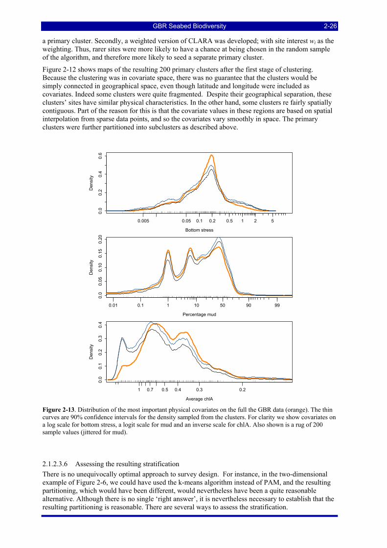
GBR Seabed Biodiversity 2-26
a primary cluster. Secondly, a weighted version of CLARA was developed; with site interest wi as the weighting. Thus, rarer sites were more likely to have a chance at being chosen in the random sample of the algorithm, and therefore more likely to seed a separate primary cluster.
Figure 2-12 shows maps of the resulting 200 primary clusters after the first stage of clustering. Because the clustering was in covariate space, there was no guarantee that the clusters would be simply connected in geographical space, even though latitude and longitude were included as covariates. Indeed some clusters were quite fragmented. Despite their geographical separation, these clusters’ sites have similar physical characteristics. In the other hand, some clusters re fairly spatially contiguous. Part of the reason for this is that the covariate values in these regions are based on spatial interpolation from sparse data points, and so the covariates vary smoothly in space. The primary clusters were further partitioned into subclusters as described above.
Bottom stress
Den
sity
0.0
0.2
0.4
0.6
0.005 0.05 0.1 0.2 0.5 1 2 5
Percentage mud
Den
sity
0.0
0.05
0.10
0.15
0.20
0.01 0.1 1 10 50 90 99
Average chlA
Den
sity
0.0
0.1
0.2
0.3
0.4
1 0.7 0.5 0.4 0.3 0.2
Figure 2-13. Distribution of the most important physical covariates on the full the GBR data (orange). The thin curves are 90% confidence intervals for the density sampled from the clusters. For clarity we show covariates on a log scale for bottom stress, a logit scale for mud and an inverse scale for chlA. Also shown is a rug of 200 sample values (jittered for mud).
2.1.2.3.6 Assessing the resulting stratification There is no unequivocally optimal approach to survey design. For instance, in the two-dimensional example of Figure 2-6, we could have used the k-means algorithm instead of PAM, and the resulting partitioning, which would have been different, would nevertheless have been a quite reasonable alternative. Although there is no single ‘right answer’, it is nevertheless necessary to establish that the resulting partitioning is reasonable. There are several ways to assess the stratification.
GBR Seabed Biodiversity 2-27
First, the strata were mapped. We have already partially shown this in Figure 2-12. However, a map of all 1450 substrata would be rather overwhelming and very difficult to interpret. Alternatively the locations of the substratum medoids could be plotted, since each medoid was in some sense the most typical representative of the stratum. In fact, the choice of medoids as actual survey sites would be a quite reasonable candidate sampling strategy and could be called “medoid sampling”. This would provide acceptable general coverage of the entire the GBR region. However, the sampling would be finer in some areas where environmental gradients were steeper and coarser in broader more homogeneous areas. This was consistent with expectations and a desirable property of the stratification, which was being sought.
The second way to assess the stratification was to examine the expected distribution of the physical covariates at the sample sites. Again, the medoid sampling can be used as a representative sampling. Figure 2-13 shows the density of bottom stress, percentage mud and average chlA over the stratum medoids compared to over all 171,560 sites. Transformed scales have been used, on which the distributions were roughly symmetrical, to make the comparison clearer. For completely random sampling, the density would be similar to that over the full data set. But in the medoid sampling, there was relatively less sampling in the high density (common) areas, and more sampling in the tails (rarer areas), which was the objective of the stratification. For example, in the case of bottom stress, more sampling is put into sites with values above 0.5, at the expense of the more common sites with values in the range 0.1–0.3.
The representativeness of the medoid sampling can be checked by comparing its density with densities arising from many random samplings of the stratification. Figure 2-13 also shows confidence intervals for the density, which were obtained from the 5th and 95th percentiles of the pointwise densities of 20 random samples. Although there were small biases, overall the medoid-sampling density was fairly representative of the range of possible densities arising from stratified sampling.
2.1.2.3.7 Defining trawl substrata The above has described how 1450 substrata were defined from which benthic sampling sites may be chosen. However, about one third of these same sites (595) were to be selected for trawl sampling and it was necessary to identify which would be the most representative. Although one method would be to simply choose the 595 sites at random, an approach that took advantage of the existing stratification was preferred, to ensure that the selection was as representative as possible. The approach taken was to go back to the primary clusters and recompute the number of subclusters required per primary cluster to give a total of 595, using the same methodology as before. On average the number of trawl subclusters was about 0.41 (595/1450) the number of original subclusters. For instance, primary cluster 92, which had 20 original strata, had 8 trawl strata. It was not feasible to try to cluster the sites into trawl subclusters, because there was no way to prevent the original strata straddling several trawl strata. Instead, it was necessary to cluster the sites such that all sites in an original stratum remain together.
The simplest way to do this was to cluster the stratum medoids. It was appropriate to use the medoid to represent its stratum as a whole because the medoid lies centrally within the stratum in co-variate space. Since there were at most 44 medoids to cluster, the calculation was computationally simple. For example, in primary cluster 92, substrata 1, 3, 4, 8, 11, 14 and 17 were amalgamated into one trawl cluster, substrata 2, 9 and 16 into a second, and substrata 6, 7, 12, 13 and 18 into a third, while the other 5 trawl clusters coincided with the original substrata.
After the medoids were clustered, each medoid’s trawl substratum number was assigned to all other cells in its substratum. Thus, each cell now belongs to both a substratum and a trawl substratum. Thus for any selection of 1450 benthic survey sites, the trawl sites could be selected from these by choosing one from each trawl stratum, either at random or by other objective.
2.1.2.4. Mapping the Stratification
The biologically informed stratification developed in this section is a physical characterisation of the GBR seabed that can be considered an a priori surrogate for patterns in seabed biodiversity
GBR Seabed Biodiversity 2-28
assemblages, to be tested and improved by the sampling to be conducted by the Project. A method of representing this complex multi-variate data in a single map was sought.
2.1.2.4.1 The Colour Key The objective was to produce a map of the GBR with similar colours representing similar physical environments, which might be expected to have similar benthic biotic assemblages. The colour mapping should encompass as much information as possible in a reduced form — this was achieved by deriving a colour key from the first and second principal components of the biological importance weighted covariate data used in the stratification. A biplot of the principal components and physical variable vectors would provide a key to the environmental characteristics of the map. Particular directions in the biplot that corresponded to important covariates should be coloured in an intuitive manner. Red was used to denote high bottom stress and green to denote high average chlorophyll A (which correlated with K490). Blue corresponded with depth. High density areas of the biplot (common areas) should have a neutral colour such as grey.
A further desirable property of the colour key was that it should cover the data space compactly, to avoid large areas of the key having no data and wasting part of the colour space. The colour key should therefore be shaped to conform to the distribution of the data in principal components (PC-) space. This was done by mapping a circular colour disk to a simply connected region enclosing the data. In order to do this, it was necessary to first define a boundary of the data in PC-space. One way to do this was to find the convex hull; however, for the GBR data, this included voids in which no data existed. Instead, a more compact boundary was found by computing a two-dimensional kernel density function and delineating a contour of sufficiently low density. The boundary is partly concave.
Having defined a boundary, there were two alternative methods for mapping the colour disk to the region inside the outer density contour boundary: polynomial mapping and conformal mapping. The polynomial mapping was found to be more flexible but because of the partly concave shape there was not always a one-to-one mapping between PC-space and colour space, and it was non-trivial to invert from PC-space to colour.
2.1.2.4.2 Conformal Mapping The conformal mapping method originates from complex number theory. A mapping from the colour disk to a simply connected polygon is expressible as a complex integral, whose parameters must be estimated by a non-linear algorithm. Trefethen (1980) provided a FORTRAN program to compute this integral. An interface to this code was developed that runs in R. Conformal mappings have certain benefits (such as local preservation of angles) but most importantly they are guaranteed to map the interior of the colour disk to the interior of the polygon (i.e. the mapping will not stray outside the boundary).
As with the polynomial method, the point in PC-space that the centre of the disk was mapped to was specified. The matching of points on the edge of the disk with vertices of the polygon was done by the non-linear algorithm. In order to match intuitive colours to the desired directions in PC space, it was necessary to impose a further transformation on the colour disk, which amounted to an angular stretch and shift. This was done using a periodic piecewise linear function of the angle. To complete the physical characterisation map, each grid cell must have a colour associated with it. Hence, the colour key mapping must be inverted, so that points in PC-space become mapped to points in colour space. This inverse mapping is available in FORTRAN code (Trefethen, 1980).
The resulting physical characterisation map of the GBR is shown in Figure 2-14. High bottom stress areas were coloured red, high Chlorophyll/K490 areas green, and the mud direction was coloured cyan. Sites coloured cyan have high levels of mud. Deeper areas tend to be blue.
The colouring of a map to highlight different covariates can be highly effective at illustrating similar and different physical environments, especially when the colour space has been fully utilized. The two colour mapping techniques investigated each had advantages and disadvantages. The main
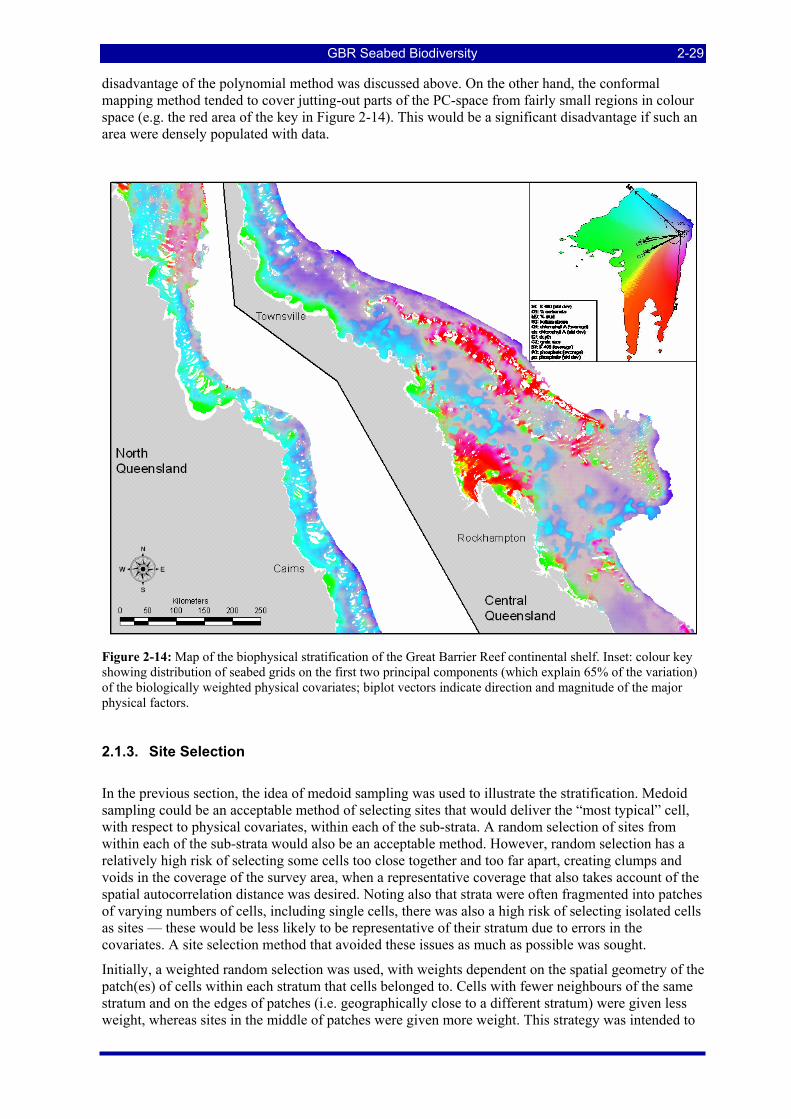
GBR Seabed Biodiversity 2-29
disadvantage of the polynomial method was discussed above. On the other hand, the conformal mapping method tended to cover jutting-out parts of the PC-space from fairly small regions in colour space (e.g. the red area of the key in Figure 2-14). This would be a significant disadvantage if such an area were densely populated with data.
Figure 2-14: Map of the biophysical stratification of the Great Barrier Reef continental shelf. Inset: colour key showing distribution of seabed grids on the first two principal components (which explain 65% of the variation) of the biologically weighted physical covariates; biplot vectors indicate direction and magnitude of the major physical factors.
2.1.3. Site Selection
In the previous section, the idea of medoid sampling was used to illustrate the stratification. Medoid sampling could be an acceptable method of selecting sites that would deliver the “most typical” cell, with respect to physical covariates, within each of the sub-strata. A random selection of sites from within each of the sub-strata would also be an acceptable method. However, random selection has a relatively high risk of selecting some cells too close together and too far apart, creating clumps and voids in the coverage of the survey area, when a representative coverage that also takes account of the spatial autocorrelation distance was desired. Noting also that strata were often fragmented into patches of varying numbers of cells, including single cells, there was also a high risk of selecting isolated cells as sites — these would be less likely to be representative of their stratum due to errors in the covariates. A site selection method that avoided these issues as much as possible was sought.
Initially, a weighted random selection was used, with weights dependent on the spatial geometry of the patch(es) of cells within each stratum that cells belonged to. Cells with fewer neighbours of the same stratum and on the edges of patches (i.e. geographically close to a different stratum) were given less weight, whereas sites in the middle of patches were given more weight. This strategy was intended to
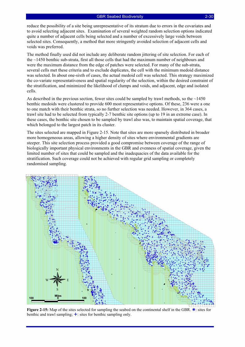
GBR Seabed Biodiversity 2-30
reduce the possibility of a site being unrepresentative of its stratum due to errors in the covariates and to avoid selecting adjacent sites. Examination of several weighted random selection options indicated quite a number of adjacent cells being selected and a number of excessively large voids between selected sites. Consequently, a method that more stringently avoided selection of adjacent cells and voids was preferred.
The method finally used did not include any deliberate random jittering of site selection. For each of the ~1450 benthic sub-strata, first all those cells that had the maximum number of neighbours and were the maximum distance from the edge of patches were selected. For many of the sub-strata, several cells met these criteria and to exclude duplicates, the cell with the minimum medoid distance was selected. In about one-sixth of cases, the actual medoid cell was selected. This strategy maximized the co-variate representativeness and spatial regularity of the selection, within the desired constraint of the stratification, and minimized the likelihood of clumps and voids, and adjacent, edge and isolated cells.
As described in the previous section, fewer sites could be sampled by trawl methods, so the ~1450 benthic medoids were clustered to provide 600 most representative options. Of these, 236 were a one to one match with their benthic strata, so no further selection was needed. However, in 364 cases, a trawl site had to be selected from typically 2-7 benthic site options (up to 19 in an extreme case). In these cases, the benthic site chosen to be sampled by trawl also was, to maintain spatial coverage, that which belonged to the largest patch in its cluster.
The sites selected are mapped in Figure 2-15. Note that sites are more sparsely distributed in broader more homogeneous areas, allowing a higher density of sites where environmental gradients are steeper. This site selection process provided a good compromise between coverage of the range of biologically important physical environments in the GBR and evenness of spatial coverage, given the limited number of sites that could be sampled and the inadequacies of the data available for the stratification. Such coverage could not be achieved with regular grid sampling or completely randomised sampling.
r
Ñ
Ñ
Ñ
Ñ
r
Ñ
r
r
Ñ
Ñ
r
Ñ
Ñ
Ñ
Ñr
Ñ
r
r
Ñ
Ñ
Ñ
Ñ
r
Ñ
r
Ñ
Ñ
Ñ
Ñ
r
Ñ
Ñ
r
Ñ
r
r r
Ñ
Ñ
Ñ
Ñ
ÑÑ
r
Ñ rÑr
Ñ
r
rÑ
Ñr
Ñ
Ñ
r
r
r
Ñ
Ñ
rÑr
Ñ
Ñ
r
r
r
r
Ñ
rÑ
Ñ
Ñ
r
Ñ
rr
r
Ñ
Ñ
Ñ
Ñ
Ñ
r
Ñ
Ñ
ÑÑ
r
Ñ
Ñ
Ñ
Ñ
Ñ
r
Ñ
ÑÑ
ÑÑ
Ñ
Ñ
Ñ
Ñ
Ñ
Ñ rr
Ñ
ÑÑ
Ñ
Ñ
r
r
Ñ
Ñ
Ñ
Ñ
Ñ
Ñ
Ñ
Ñ
rr
r
r
Ñ
Ñ
Ñ
Ñ
Ñ
Ñ
Ñ
Ñ
Ñ
Ñ
Ñ
r
r
r
r
r
r
r
Ñr
Ñ
Ñ
Ñ
r
Ñ
Ñ
r
r
Ñ
r
r
Ñ
Ñ
r
rÑÑ
Ñ
Ñ
Ñr
r
Ñ
Ñ
Ñ
r
r
Ñ
Ñ
Ñ
r
Ñ
r
Ñ
Ñ
Ñ
r
Ñ
r
r
Ñ
r
Ñ
Ñ
Ñ
Ñ
Ñ
Ñ
r
r
Ñ
Ñ
Ñ
Ñ
Ñ r
r
Ñ
r
Ñ
r
Ñ
r
r
Ñ
Ñ
Ñ
Ñ
Ñ
Ñ
r
Ñ
r
r
Ñ
r
Ñ
Ñ
Ñ
r
Ñ
Ñ
Ñ
Ñ
Ñ
Ñ
r
Ñ
r
r
Ñ
r
Ñ
r
Ñ
r
rr
Ñ
r
ÑÑ
Ñ Ñ
Ñ
Ñ
Ñ
r
Ñ
Ñ
Ñ
r
Ñ
Ñ
r
Ñ
r
r
Ñ
Ñ
r
Ñ
Ñ
r
r
r
Ñ
Ñ
Ñ
r
Ñ
Ñ
Ñ
r
Ñ
r
Ñ
r
rr
Ñ
Ñ
r
rÑ
r
Ñ
Ñ Ñ
Ñ
r
Ñ
Ñ Ñ
r
Ñ
r
Ñ
Ñ
Ñ
Ñ
r
Ñ
Ñr
r
r
r
Ñ
Ñ
r
Ñ
rÑ
Ñ
r
Ñ
r
Ñ
Ñ
rÑ
Ñ
Ñ
Ñ
Ñ
Ñ
Ñ
r
r
r
r
Ñ
Ñ
Ñ
Ñ
Ñ
r
Ñ
Ñ
Ñ
Ñ
ÑÑ
rr
r
Ñ
ÑÑ
r
Ñ
Ñ
r
r
Ñ
r
r
Ñ
Ñ
Ñ
r
Ñ
Ñ
Ñ
Ñ
Ñ
r
Ñ
Ñ
r
Ñ
r
Ñ
Ñ
Ñ
r
rÑr
Ñ
Ñ
r
Ñ
r
Ñ
Ñ
Ñ
r
r
Ñ
r
r
Ñ
r
r
r
Ñ
Ñ
Ñ
Ñ
Ñ
r
Ñr
rÑ
ÑÑ
r
Ñ
Ñ
Ñ
r
r
Ñ
r
Ñ
r
rÑ
Ñ r
ÑÑ
Ñ
Ñ
Ñ
Ñ
r
Ñ
r
rÑ
ÑÑ
Ñ
r
Ñ
Ñr
ÑÑ
r
Ñ
r
Ñ
r
Ñ
Ñ
Ñ
r
Ñ
Ñ
r
r
Ñ
Ñ
r
Ñ
Ñ
r
ÑÑ
rÑÑ
r
r
r
r
Ñ
Ñ
r
Ñ
r
Ñ
rÑ
Ñ
Ñ
r
Ñ
ÑÑ
Ñ
r
Ñ
rÑ
rÑ
ÑÑ
Ñ
r
Ñr
Ñ
r
Ñ
rÑ
r
r
Ñ
Ñ
Ñ
Ñ
r
Ñ
ÑÑ r
r
r
Ñ
rÑ
rÑ
ÑÑ
r
ÑÑ
r
r
Ñ
r
Ñ
Ñ
Ñ
r
r
Ñr
Ñ
r
Ñ
Ñ
Ñ
r
Ñ
r
Ñ
Ñ Ñ
Ñ
Ñ
Ñ
r
Ñ
Ñ
Ñ
r
r
Ñ
rÑ
Ñ
r
r
Ñ
Ñ
Ñ
Ñ
Ñ
r
r
Ñ
Ñ
Ñ
r
Ñrr
Ñ
Ñ
Ñ
Ñ
Ñ
Ñ
Ñ
r
r
Ñ
r
r
Ñ
Ñ
ÑÑ
r
Ñ
r
Ñ
ÑÑ
r
Ñ
r
Ñ
r
r
Ñ
r
r
r
Ñ
Ñ
Ñr
Ñ
Ñ
Ñ
Ñ
Ñ
Ñ
Ñ
Ñ
Ñ
Ñ
Ñr
Ñ
r
Ñ
r
r
Ñ
Ñ
Ñ
r
Ñ
r
r
Ñ
r
r
r
Ñ
r
r
Ñ
r
Ñ
r
Ñ
Ñ
Ñ
Ñ
r
r
r rÑ Ñ
Ñ
Ñ
Ñr
r
Ñ
Ñ
r
Ñ
Ñ
r
Ñ
Ñ
Ñ
rr
Ñ
r
Ñ
Ñ
r
r
Ñ
Ñ
Ñ
Ñ
rÑ
r
Ñ
Ñ
Ñ
Ñ
r
r
ÑÑ
Ñ
r
r
r
r
r
Ñ
Ñ
Ñ
r
r
Ñ
r
Ñ
rÑ
r
Ñ
Ñ
ÑÑ
Ñ
r
Ñ
r
r
Ñ
Ñ
r
r
ÑÑ
Ñ
r
ÑÑ
r
Ñ
Ñ
r
r
r
r
Ñ
Ñ
Ñ
Ñ
r
Ñ
Ñ
r
rÑ
Ñ
Ñ
Ñ
r
Ñ
Ñ
r
Ñ
r
r
r
Ñr
Ñ
ÑÑ
Ñ
r
r
Ñ
r
Ñ
Ñ
Ñr
Ñ
Ñ
Ñ
r
Ñ
ÑÑ
r Ñ
r
r
rÑ
rr
ÑÑÑ
r
Ñ
ÑÑr
Ñ
r
rr
Ñ
Ñ
Ñ
Ñ
Ñ
r
ÑrÑ
r
r
Ñ
Ñ
Ñ
Ñ
Ñ
ÑÑ r
r
ÑÑ
Ñ
r
r
Ñ
r
r
Ñ
r
r
Ñ
Ñ
r
r
r
Ñ
r
Ñ
Ñ
Ñ
ÑÑ
r
ÑÑ
Ñ
r
Ñ
r
ÑÑ
r
Ñ
Ñ
r
Ñ Ñr
r
Ñ
Ñ
Ñ
r
ÑÑ
Ñ
r
r
Ñ
Ñ
rrrrrrrr
Ñ
Ñ
r
r
Ñ
r
ÑÑ
Ñ
r
r
Ñ
Ñ
Ñ
r
r
Ñ
r
r
r
Ñ
rr
Ñ
r
ÑÑ
Ñ
Ñ
Ñ
Ñ
Ñ
Ñ
r
r
Ñr
Ñ
Ñr
Ñ
Ñ
r
r
Ñ
Ñr
Ñ
Ñ
rr
Ñ
Ñr
Ñ
rÑ
r
Ñ
r
Ñ
Ñ
r
Ñ
r
r
Ñ
ÑÑ
r
ÑrÑ
Ñ
r
Ñ
r
Ñ
Ñ
ÑrrÑ
Ñ
Ñ
r
r
Ñ
r
r
r
Ñ
Ñ
Ñ
r
r
ÑÑÑ
Ñ
r
Ñ
Ñ
r
r Ñ
Ñ
rÑ
Ñ
r
rÑ
Ñ
r
r
ÑÑ
r
rr
Ñ
Ñ
r
Ñ
r
Ñ
Ñ
Ñ
r
Ñ
Ñ
r
Ñ
r
Ñ
r Ñ
r
r
Ñ
r
Ñ
Ñ
r
Ñ
Ñ
Ñ
r
Ñ
Ñ
r
ÑÑ
r
rÑ
Ñ
r
Ñ
r
r
Ñ
Ñ
r
Ñ
rrÑÑ
Ñ
Ñr
r
ÑÑ
Ñ
Ñ
r
rÑ rÑ
r
r
r
Ñ
Ñ
Ñ
Ñ
ÑÑ
Ñ
r
Ñ
Ñ
r
Ñ
Ñ
r
r
r
Ñ
r
Ñ
Ñ
Ñ
r
rÑ
Ñ
r Ñ
Ñ
Ñ
Ñ
Ñ
Ñ
Ñ
Ñ
Ñ
r
Ñ
Ñ
Ñ
Ñ
r
Ñ
r
Ñ
rr
r
r
ÑÑ
Ñ
r
Ñ
Ñ
r
Ñ
Ñ
Ñ
Ñ
Ñ
rÑ
Ñ
Ñ
Ñr
Ñr
Ñ
Ñ
Ñ
Ñ
Ñ
Ñ
Ñ
Ñr
Ñ
ÑÑ
Ñ
Ñ
Ñ
Ñ
rÑ
Ñ
Ñ
Ñr
r
Ñ
Ñ
r
Ñ
r
r
Ñ
r
Ñ
Ñr
r
Ñ
r
Ñ
Ñ
r
Ñ
Ñr
Ñ
r
Ñ
ÑÑ
r
r
Ñ
r
Ñ
Ñ
Ñ
r
r
rr
Ñr
Ñ
Ñ
Ñ
r
Ñ
r
r
Ñr
ÑrÑ
r
r
Ñ
Ñ
Ñ
Ñr
Ñ
Ñ
r
r
r
Ñ
r
Ñ
Ñ
Ñ
r
Ñ
r
Ñ
ÑÑr
Ñ
r
rr
Ñ
Ñ
Ñ
ÑÑÑ
r
Ñ
r
Ñ
r
Ñ
Ñ
r
Ñ
r
Ñ
Ñ
ÑÑ
Ñ
Ñ
Ñ
Ñ
r
Ñ
r
r
rÑ
ÑÑ
r
Ñ
Ñ
r Ñ
r
ÑÑÑÑÑÑÑÑ
Ñ
r
r
Ñ
r
Ñ
Ñ
Ñ
Ñ
Ñ
Ñ
r
r
Ñ
rr
rÑ
Ñ ÑÑrrÑ
r
Ñ
Ñ
r
Ñ
r
Ñ
r
r
ÑÑ Ñ
ÑÑ
r
Ñ
rÑ
Ñ
Ñ
r
Ñ
r
Ñ
Ñ
r
r
r
Ñ
r
Ñ
r
Ñr
r
Ñ
Ñ
Ñ
r
rÑ
Ñr
Ñ
Ñ
r
r
Ñ r
Ñ
r
Ñr
Ñ
Ñ
r
Ñr
r
Ñ
r
r
Ñ
Ñ
r
Ñ
Ñ
ÑÑÑ
rr
r
Ñ
Ñ
r
Ñ
rrÑ
Ñ
Ñ rÑÑÑÑÑÑÑÑr
Ñ
Ñ
r
r
r
Ñ
r
Ñ
Ñ
Ñ
Ñ
r
Ñ
Ñ
r
Ñ
Ñ
r
Ñ
Ñ
Ñ
r
Ñ
Ñ
r
r
Ñ
r
r
r
r
Ñ
Ñ
r
Ñ
r
r
Ñ
Ñ
r
Ñ
Ñ
Ñ
Ñ
r
Ñ
r
Ñ
r
r
ÑÑ
Ñ
r
r
r
Ñ
Ñ
r
r
Ñ
Ñ
Ñ
Ñ
r
Ñ
Ñrr
Ñ
Ñ
r
Ñ
Ñ
Ñ
Ñ
Ñ
r
r
r
r
Ñ
r
Ñ
Ñ
r
Ñ
Ñ
Ñ
r
Ñ
r
Ñ
r
r
r
rÑ
r
Ñ
r
Ñ
rr
r
Ñ
rÑ
r
r
r
r
r
r
r
Ñ
Ñ
Ñ
r
Ñ
r
Ñ
r
Ñ
r
r
Ñ
r
r
Ñ
r
Ñ
Ñ
Ñ
r
r
r
r
Ñ
r
r
Ñ
Ñr ÑÑ
rÑ
r
Ñ
rÑ
r
ÑÑ
Ñ
Ñ
Ñ
r
Ñ
r
Ñ
r
Ñ
r
r
N
EW
S
100 0 100Miles
Figure 2-15: Map of the sites selected for sampling the seabed on the continental shelf in the GBR. : sites for benthic and trawl sampling; : sites for benthic sampling only.
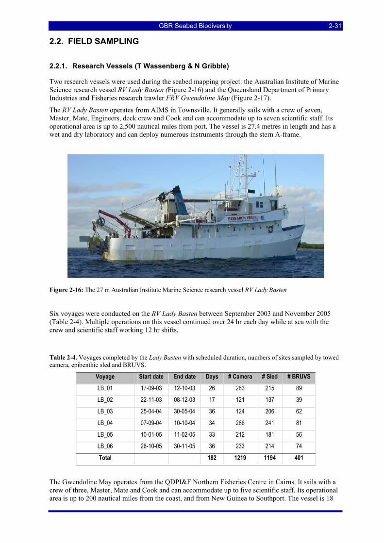
GBR Seabed Biodiversity 2-31
2.2. FIELD SAMPLING
2.2.1. Research Vessels (T Wassenberg & N Gribble) Two research vessels were used during the seabed mapping project: the Australian Institute of Marine Science research vessel RV Lady Basten (Figure 2-16) and the Queensland Department of Primary Industries and Fisheries research trawler FRV Gwendoline May (Figure 2-17).
The RV Lady Basten operates from AIMS in Townsville. It generally sails with a crew of seven, Master, Mate, Engineers, deck crew and Cook and can accommodate up to seven scientific staff. Its operational area is up to 2,500 nautical miles from port. The vessel is 27.4 metres in length and has a wet and dry laboratory and can deploy numerous instruments through the stern A-frame.
Figure 2-16: The 27 m Australian Institute Marine Science research vessel RV Lady Basten
Six voyages were conducted on the RV Lady Basten between September 2003 and November 2005 (Table 2-4). Multiple operations on this vessel continued over 24 hr each day while at sea with the crew and scientific staff working 12 hr shifts.
Table 2-4. Voyages completed by the Lady Basten with scheduled duration, numbers of sites sampled by towed camera, epibenthic sled and BRUVS.
Voyage Start date End date Days # Camera # Sled # BRUVS
LB_01 17-09-03 12-10-03 26 263 215 89
LB_02 22-11-03 08-12-03 17 121 137 39
LB_03 25-04-04 30-05-04 36 124 206 62
LB_04 07-09-04 10-10-04 34 266 241 81
LB_05 10-01-05 11-02-05 33 212 181 56
LB_06 26-10-05 30-11-05 36 233 214 74
Total 182 1219 1194 401
The Gwendoline May operates from the QDPI&F Northern Fisheries Centre in Cairns. It sails with a crew of three, Master, Mate and Cook and can accommodate up to five scientific staff. Its operational area is up to 200 nautical miles from the coast, and from New Guinea to Southport. The vessel is 18
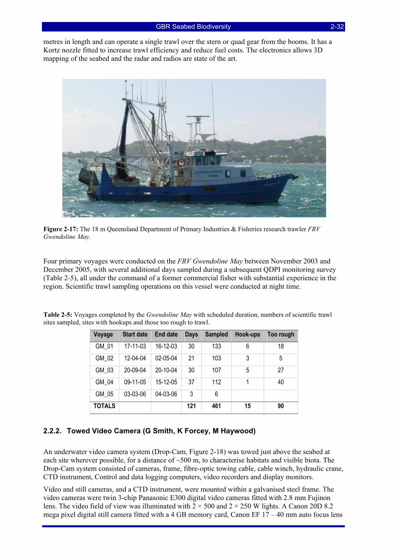
GBR Seabed Biodiversity 2-32
metres in length and can operate a single trawl over the stern or quad gear from the booms. It has a Kortz nozzle fitted to increase trawl efficiency and reduce fuel costs. The electronics allows 3D mapping of the seabed and the radar and radios are state of the art.
Figure 2-17: The 18 m Queensland Department of Primary Industries & Fisheries research trawler FRV Gwendoline May.
Four primary voyages were conducted on the FRV Gwendoline May between November 2003 and December 2005, with several additional days sampled during a subsequent QDPI monitoring survey (Table 2-5), all under the command of a former commercial fisher with substantial experience in the region. Scientific trawl sampling operations on this vessel were conducted at night time.
Table 2-5: Voyages completed by the Gwendoline May with scheduled duration, numbers of scientific trawl sites sampled, sites with hookups and those too rough to trawl.
Voyage Start date End date Days Sampled Hook-ups Too rough
GM_01 17-11-03 16-12-03 30 133 6 18
GM_02 12-04-04 02-05-04 21 103 3 5
GM_03 20-09-04 20-10-04 30 107 5 27
GM_04 09-11-05 15-12-05 37 112 1 40
GM_05 03-03-06 04-03-06 3 6
TOTALS 121 461 15 90
2.2.2. Towed Video Camera (G Smith, K Forcey, M Haywood)
An underwater video camera system (Drop-Cam, Figure 2-18) was towed just above the seabed at each site wherever possible, for a distance of ~500 m, to characterise habitats and visible biota. The Drop-Cam system consisted of cameras, frame, fibre-optic towing cable, cable winch, hydraulic crane, CTD instrument, Control and data logging computers, video recorders and display monitors.
Video and still cameras, and a CTD instrument, were mounted within a galvanised steel frame. The video cameras were twin 3-chip Panasonic E300 digital video cameras fitted with 2.8 mm Fujinon lens. The video field of view was illuminated with 2 × 500 and 2 × 250 W lights. A Canon 20D 8.2 mega pixel digital still camera fitted with a 4 GB memory card, Canon EF 17 – 40 mm auto focus lens
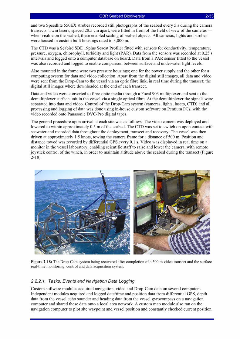
GBR Seabed Biodiversity 2-33
and two Speedlite 550EX strobes recorded still photographs of the seabed every 5 s during the camera transects. Twin lasers, spaced 28.5 cm apart, were fitted in from of the field of view of the cameras — when visible on the seabed, these enabled scaling of seabed objects. All cameras, lights and strobes were housed in custom built housings rated to 3,000 m.
The CTD was a Seabird SBE 19plus Seacat Profiler fitted with sensors for conductivity, temperature, pressure, oxygen, chlorophyll, turbidity and light (PAR). Data from the sensors was recorded at 0.25 s intervals and logged onto a computer database on board. Data from a PAR sensor fitted to the vessel was also recorded and logged to enable comparison between surface and underwater light levels.
Also mounted in the frame were two pressure housings; one for the power supply and the other for a computing system for data and video collection. Apart from the digital still images, all data and video were sent from the Drop-Cam to the vessel via an optic fibre link, in real time during the transect; the digital still images where downloaded at the end of each transect.
Data and video were converted to fibre optic media through a Focal 903 multiplexer and sent to the demultiplexer surface unit in the vessel via a single optical fibre. At the demultiplexer the signals were separated into data and video. Control of the Drop-Cam system (cameras, lights, lasers, CTD) and all processing and logging of data was done using in-house custom software on Pentium PCs, with the video recorded onto Panasonic DVC-Pro digital tapes.
The general procedure upon arrival at each site was as follows. The video camera was deployed and lowered to within approximately 0.5 m of the seabed. The CTD was set to switch on upon contact with seawater and recorded data throughout the deployment, transect and recovery. The vessel was then driven at approximately 1.5 knots, towing the camera frame for a distance of 500 m. Position and distance towed was recorded by differential GPS every 0.1 s. Video was displayed in real time on a monitor in the vessel laboratory, enabling scientific staff to raise and lower the camera, with remote joystick control of the winch, in order to maintain altitude above the seabed during the transect (Figure 2-18).
Figure 2-18: The Drop-Cam system being recovered after completion of a 500 m video transect and the surface real-time monitoring, control and data acquisition system.
2.2.2.1. Tasks, Events and Navigation Data Logging
Custom software modules acquired navigation, video and Drop-Cam data on several computers. Independent modules acquired and logged date/time and position data from differential GPS, depth data from the vessel echo sounder and heading data from the vessel gyrocompass on a navigation computer and shared these data onto a local area network. A custom map module also ran on the navigation computer to plot site waypoint and vessel position and constantly checked current position
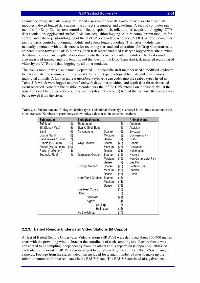
GBR Seabed Biodiversity 2-34
against the designated site waypoint list and also shared these data onto the network to ensure all modules indexed logged data against the correct site number and date/time. A second computer ran modules for Drop-Cam system control and data (depth, pitch, roll, altitude) acquisition/logging, CTD data acquisition/logging and surface PAR data acquisition/logging. A third computer ran modules for control and data acquisition/logging of the DVC-Pro video tape recorders (VTRs). A fourth computer ran the Tasks control and logging module and events logging module. The Tasks module was manually operated, with touch screens for recording start and end operations for Drop-Cam transects, epibenthic sled tows and BRUVS drops. Each task record included task type logged with site number, date/time, position, and depth data as shared onto the network by other modules. The Tasks module also measured transect and tow lengths, and the touch of the Drop-Cam start task initiated recording of video by the VTRs and data logging by all other modules.
The events module was also manually operated — a scientific staff member used a modified keyboard to enter a real-time summary of the seabed substratum type, biological habitats and conspicuous individual animals. A lookup table transcribed keyboard scan codes into the seabed types listed in Table 2-6, which were logged and prefixed with date/time, position, and depth data for each seabed event recorded. Note that the position recorded was that of the GPS antenna on the vessel, whilst the observed event being recorded could be ~25 m (about 30 seconds) behind that because the camera was being towed from the stern.
Table 2-6: Substratum and Biological habitat types and animal events types entered in real time to annotate the video transect. Numbers in parentheses show index values used in acoustics sections.
Substratum Biological habitat Animal events Soft Mud (9) Silt (Sandy-Mud) (8) Sand (6) Coarse Sand (2) Sand Waves / Dunes (7) Rubble (5-50 mm) (5) Stones (50-250 mm) (10) Rocks (> 250 mm) (4) Bedrock / Reef (1)
Bioturbated (5) Bivalve Shell Beds (6) Alcyonarians: Sparse (3)
Medium (2) Dense (1)
Whip Garden: Sparse (25) Medium (26) Dense (24)
Gorgonian Garden: Sparse (11) Medium (10) Dense (9)
Sponge Garden: Sparse (20) Medium (19) Dense (18)
Hard Coral Garden: Sparse (15) Medium (14) Dense (13)
Live Reef Corals (16) Flora: (8) Seagrass (21) Algae: (4) Caulerpa (7) Halimeda (12) No BioHabitat (17)
Anemone Ascidian Bryozoan Commercial Fish Crab Crinoid Gastropod Holothurian Hydroid Non Commercial Fish Sea Pen Solitary Coral Starfish Urchin
2.2.3. Baited Remote Underwater Video Stations (M Cappo) A fleet of Baited Remote Underwater Video Stations (BRUVS) were deployed about 350-400 metres apart with the prevailing wind to bracket the coordinate of each sampling site. Each replicate was considered to be sampling independently from the others at this separation (Cappo et al. 2004). At each site, a stereo-video BRUVS was deployed first, followed by three or four BRUVS with single cameras. Footage from the stereo-video was included for a small number of sites to make up the minimum number of three replicates in the BRUVS data. The BRUVS consisted of a galvanized
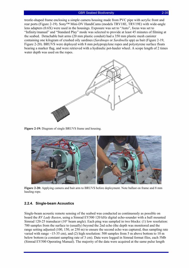
GBR Seabed Biodiversity 2-35
trestle-shaped frame enclosing a simple camera housing made from PVC pipe with acrylic front and rear ports (Figure 2-19). Sony™ Mini-DV HandiCams (models TRV18E, TRV19E) with wide-angle lens adapters (0.6X) were used in the housings. Exposure was set to “Auto”, focus was set to “Infinity/manual” and “Standard Play” mode was selected to provide at least 45 minutes of filming at the seabed. Detachable bait arms (20 mm plastic conduit) had a 350 mm plastic mesh canister containing one kilogram of crushed oily sardines (Sardinops or Sardinella spp) as bait (Figure 2-19, Figure 2-20). BRUVS were deployed with 8 mm polypropylene ropes and polystyrene surface floats bearing a marker flag, and were retrieved with a hydraulic pot-hauler wheel. A scope length of 2 times water depth was used on the ropes.
Figure 2-19: Diagram of single BRUVS frame and housing.
Figure 2-20: Applying camera and bait arm to BRUVS before deployment. Note ballast on frame and 8 mm hauling rope.
2.2.4. Single-beam Acoustics
Single-beam acoustic remote sensing of the seabed was conducted as continuously as possible on board the RV Lady Basten, using a Simrad EY500 120 kHz digital echo-sounder with a hull mounted Simrad 120-25 transducer (10° beam angle). Each ping was sampled in two blocks: (1) low resolution: 700 samples from the surface to (usually) beyond the 2nd echo (the depth was monitored and the range setting adjusted (100, 150, or 250 m) to ensure the second echo was captured, thus sampling rate varied with range ~15-35 cm), and (2) high resolution: 500 samples from 5 m above bottom to 10 m below bottom (a constant sampling rate of 3 cm). Data were logged in Simrad format files, each 5Mb (Simrad EY500 Operating Manual). The majority of the data were acquired at the same pulse length
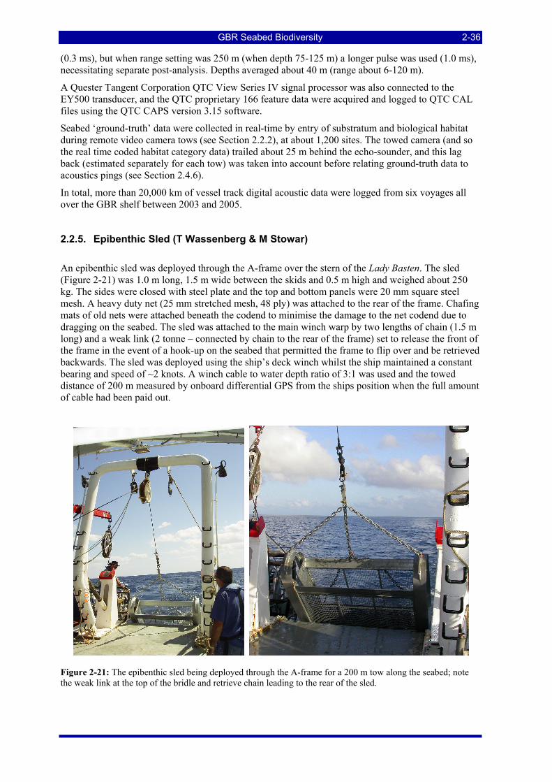
GBR Seabed Biodiversity 2-36
(0.3 ms), but when range setting was 250 m (when depth 75-125 m) a longer pulse was used (1.0 ms), necessitating separate post-analysis. Depths averaged about 40 m (range about 6-120 m).
A Quester Tangent Corporation QTC View Series IV signal processor was also connected to the EY500 transducer, and the QTC proprietary 166 feature data were acquired and logged to QTC CAL files using the QTC CAPS version 3.15 software.
Seabed ‘ground-truth’ data were collected in real-time by entry of substratum and biological habitat during remote video camera tows (see Section 2.2.2), at about 1,200 sites. The towed camera (and so the real time coded habitat category data) trailed about 25 m behind the echo-sounder, and this lag back (estimated separately for each tow) was taken into account before relating ground-truth data to acoustics pings (see Section 2.4.6).
In total, more than 20,000 km of vessel track digital acoustic data were logged from six voyages all over the GBR shelf between 2003 and 2005.
2.2.5. Epibenthic Sled (T Wassenberg & M Stowar)
An epibenthic sled was deployed through the A-frame over the stern of the Lady Basten. The sled (Figure 2-21) was 1.0 m long, 1.5 m wide between the skids and 0.5 m high and weighed about 250 kg. The sides were closed with steel plate and the top and bottom panels were 20 mm square steel mesh. A heavy duty net (25 mm stretched mesh, 48 ply) was attached to the rear of the frame. Chafing mats of old nets were attached beneath the codend to minimise the damage to the net codend due to dragging on the seabed. The sled was attached to the main winch warp by two lengths of chain (1.5 m long) and a weak link (2 tonne – connected by chain to the rear of the frame) set to release the front of the frame in the event of a hook-up on the seabed that permitted the frame to flip over and be retrieved backwards. The sled was deployed using the ship’s deck winch whilst the ship maintained a constant bearing and speed of ~2 knots. A winch cable to water depth ratio of 3:1 was used and the towed distance of 200 m measured by onboard differential GPS from the ships position when the full amount of cable had been paid out.
Figure 2-21: The epibenthic sled being deployed through the A-frame for a 200 m tow along the seabed; note the weak link at the top of the bridle and retrieve chain leading to the rear of the sled.
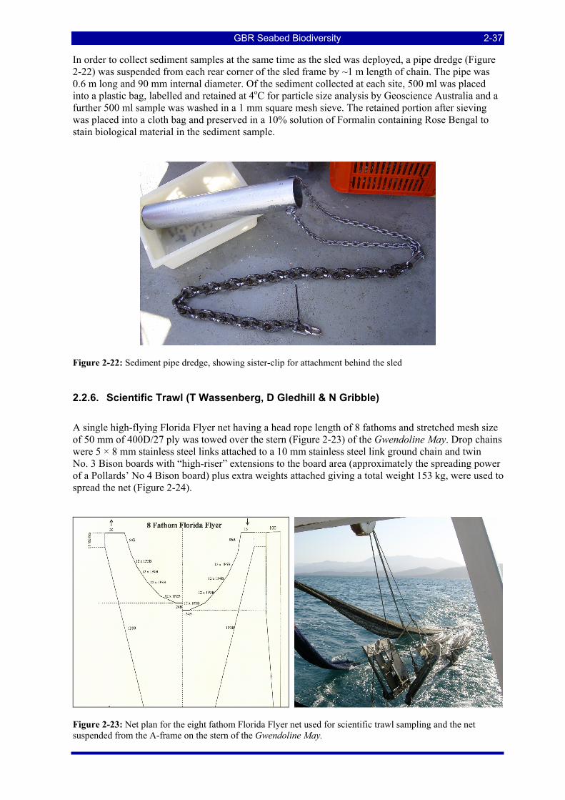
GBR Seabed Biodiversity 2-37
In order to collect sediment samples at the same time as the sled was deployed, a pipe dredge (Figure 2-22) was suspended from each rear corner of the sled frame by ~1 m length of chain. The pipe was 0.6 m long and 90 mm internal diameter. Of the sediment collected at each site, 500 ml was placed into a plastic bag, labelled and retained at 4oC for particle size analysis by Geoscience Australia and a further 500 ml sample was washed in a 1 mm square mesh sieve. The retained portion after sieving was placed into a cloth bag and preserved in a 10% solution of Formalin containing Rose Bengal to stain biological material in the sediment sample.
Figure 2-22: Sediment pipe dredge, showing sister-clip for attachment behind the sled
2.2.6. Scientific Trawl (T Wassenberg, D Gledhill & N Gribble)
A single high-flying Florida Flyer net having a head rope length of 8 fathoms and stretched mesh size of 50 mm of 400D/27 ply was towed over the stern (Figure 2-23) of the Gwendoline May. Drop chains were 5 × 8 mm stainless steel links attached to a 10 mm stainless steel link ground chain and twin No. 3 Bison boards with “high-riser” extensions to the board area (approximately the spreading power of a Pollards’ No 4 Bison board) plus extra weights attached giving a total weight 153 kg, were used to spread the net (Figure 2-24).
Figure 2-23: Net plan for the eight fathom Florida Flyer net used for scientific trawl sampling and the net suspended from the A-frame on the stern of the Gwendoline May.
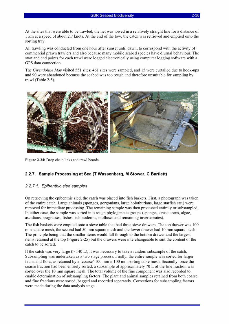
GBR Seabed Biodiversity 2-38
At the sites that were able to be trawled, the net was towed in a relatively straight line for a distance of 1 km at a speed of about 2.7 knots. At the end of the tow, the catch was retrieved and emptied onto the sorting tray.
All trawling was conducted from one hour after sunset until dawn, to correspond with the activity of commercial prawn trawlers and also because many mobile seabed species have diurnal behaviour. The start and end points for each trawl were logged electronically using computer logging software with a GPS data connection.
The Gwendoline May visited 551 sites; 461 sites were sampled, and 15 were curtailed due to hook-ups and 90 were abandoned because the seabed was too rough and therefore unsuitable for sampling by trawl (Table 2-5).
Figure 2-24: Drop chain links and trawl boards.
2.2.7. Sample Processing at Sea (T Wassenberg, M Stowar, C Bartlett)
2.2.7.1. Epibenthic sled samples
On retrieving the epibenthic sled, the catch was placed into fish baskets. First, a photograph was taken of the entire catch. Large animals (sponges, gorgonians, large holothurians, large starfish etc.) were removed for immediate processing. The remaining sample was then processed entirely or subsampled. In either case, the sample was sorted into rough phylogenetic groups (sponges, crustaceans, algae, ascidians, seagrasses, fishes, echinoderms, molluscs and remaining invertebrates).
The fish baskets were emptied onto a sieve table that had three sieve drawers. The top drawer was 100 mm square mesh, the second had 50 mm square mesh and the lower drawer had 10 mm square mesh. The principle being that the smaller items would fall through to the bottom drawer and the largest items retained at the top (Figure 2-25) but the drawers were interchangeable to suit the content of the catch to be sorted.
If the catch was very large (> 140 L), it was necessary to take a random subsample of the catch. Subsampling was undertaken as a two stage process. Firstly, the entire sample was sorted for larger fauna and flora, as retained by a ‘coarse’ 100 mm × 100 mm sorting table mesh. Secondly, once the coarse fraction had been entirely sorted, a subsample of approximately 70 L of the fine fraction was sorted over the 10 mm square mesh. The total volume of the fine component was also recorded to enable determination of subsampling factors. The plant and animal samples retained from both coarse and fine fractions were sorted, bagged and recorded separately. Corrections for subsampling factors were made during the data analysis stage.
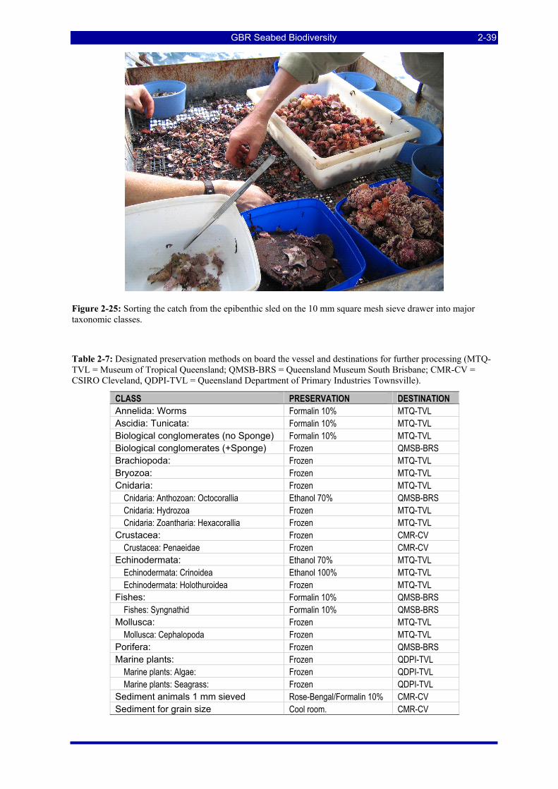
GBR Seabed Biodiversity 2-39
Figure 2-25: Sorting the catch from the epibenthic sled on the 10 mm square mesh sieve drawer into major taxonomic classes.
Table 2-7: Designated preservation methods on board the vessel and destinations for further processing (MTQ-TVL = Museum of Tropical Queensland; QMSB-BRS = Queensland Museum South Brisbane; CMR-CV = CSIRO Cleveland, QDPI-TVL = Queensland Department of Primary Industries Townsville).
CLASS PRESERVATION DESTINATION Annelida: Worms Formalin 10% MTQ-TVL Ascidia: Tunicata: Formalin 10% MTQ-TVL Biological conglomerates (no Sponge) Formalin 10% MTQ-TVL Biological conglomerates (+Sponge) Frozen QMSB-BRS Brachiopoda: Frozen MTQ-TVL Bryozoa: Frozen MTQ-TVL Cnidaria: Frozen MTQ-TVL Cnidaria: Anthozoan: Octocorallia Ethanol 70% QMSB-BRS Cnidaria: Hydrozoa Frozen MTQ-TVL Cnidaria: Zoantharia: Hexacorallia Frozen MTQ-TVL Crustacea: Frozen CMR-CV Crustacea: Penaeidae Frozen CMR-CV Echinodermata: Ethanol 70% MTQ-TVL Echinodermata: Crinoidea Ethanol 100% MTQ-TVL Echinodermata: Holothuroidea Frozen MTQ-TVL Fishes: Formalin 10% QMSB-BRS Fishes: Syngnathid Formalin 10% QMSB-BRS Mollusca: Frozen MTQ-TVL Mollusca: Cephalopoda Frozen MTQ-TVL Porifera: Frozen QMSB-BRS Marine plants: Frozen QDPI-TVL Marine plants: Algae: Frozen QDPI-TVL Marine plants: Seagrass: Frozen QDPI-TVL Sediment animals 1 mm sieved Rose-Bengal/Formalin 10% CMR-CV Sediment for grain size Cool room. CMR-CV
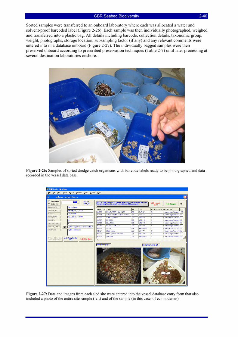
GBR Seabed Biodiversity 2-40
Sorted samples were transferred to an onboard laboratory where each was allocated a water and solvent-proof barcoded label (Figure 2-26). Each sample was then individually photographed, weighed and transferred into a plastic bag. All details including barcode, collection details, taxonomic group, weight, photographs, storage location, subsampling factor (if any) and any relevant comments were entered into in a database onboard (Figure 2-27). The individually bagged samples were then preserved onboard according to prescribed preservation techniques (Table 2-7) until later processing at several destination laboratories onshore.
Figure 2-26: Samples of sorted dredge catch organisms with bar code labels ready to be photographed and data recorded in the vessel data base.
Figure 2-27: Data and images from each sled site were entered into the vessel database entry form that also included a photo of the entire site sample (left) and of the sample (in this case, of echinoderms).
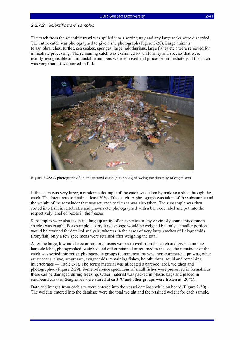
GBR Seabed Biodiversity 2-41
2.2.7.2. Scientific trawl samples
The catch from the scientific trawl was spilled into a sorting tray and any large rocks were discarded. The entire catch was photographed to give a site photograph (Figure 2-28). Large animals (elasmobranches, turtles, sea snakes, sponges, large holothurians, large fishes etc.) were removed for immediate processing. The remaining catch was examined for uniformity and species that were readily-recognisable and in tractable numbers were removed and processed immediately. If the catch was very small it was sorted in full.
Figure 2-28: A photograph of an entire trawl catch (site photo) showing the diversity of organisms.
If the catch was very large, a random subsample of the catch was taken by making a slice through the catch. The intent was to retain at least 20% of the catch. A photograph was taken of the subsample and the weight of the remainder that was returned to the sea was also taken. The subsample was then sorted into fish, invertebrates and prawns etc, photographed with a bar code label and put into the respectively labelled boxes in the freezer.
Subsamples were also taken if a large quantity of one species or any obviously abundant/common species was caught. For example: a very large sponge would be weighed but only a smaller portion would be retained for detailed analysis; whereas in the cases of very large catches of Leiognathids (Ponyfish) only a few specimens were retained after weighing the total.
After the large, low incidence or rare organisms were removed from the catch and given a unique barcode label, photographed, weighed and either retained or returned to the sea, the remainder of the catch was sorted into rough phylogenetic groups (commercial prawns, non-commercial prawns, other crustaceans, algae, seagrasses, syngnathids, remaining fishes, holothurians, squid and remaining invertebrates — Table 2-8). The sorted material was allocated a barcode label, weighed and photographed (Figure 2-29). Some reference specimens of small fishes were preserved in formalin as these can be damaged during freezing. Other material was packed in plastic bags and placed in cardboard cartons. Seagrasses were stored at ca 3 ºC and other groups were frozen at -20 ºC.
Data and images from each site were entered into the vessel database while on board (Figure 2-30). The weights entered into the database were the total weight and the retained weight for each sample.
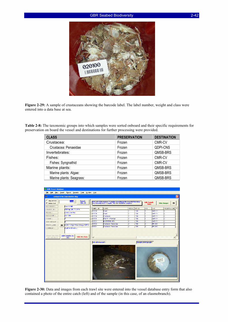
GBR Seabed Biodiversity 2-42
Figure 2-29: A sample of crustaceans showing the barcode label. The label number, weight and class were entered into a data base at sea.
Table 2-8: The taxonomic groups into which samples were sorted onboard and their specific requirements for preservation on board the vessel and destinations for further processing were provided.
CLASS PRESERVATION DESTINATION Crustacea: Frozen CMR-CV Crustacea: Penaeidae Frozen QDPI-CNS Invertebrates: Frozen QMSB-BRS Fishes: Frozen CMR-CV Fishes: Syngnathid Frozen CMR-CV Marine plants: Frozen QMSB-BRS Marine plants: Algae: Frozen QMSB-BRS Marine plants: Seagrass: Frozen QMSB-BRS
Figure 2-30: Data and images from each trawl site were entered into the vessel database entry form that also contained a photo of the entire catch (left) and of the sample (in this case, of an elasmobranch).
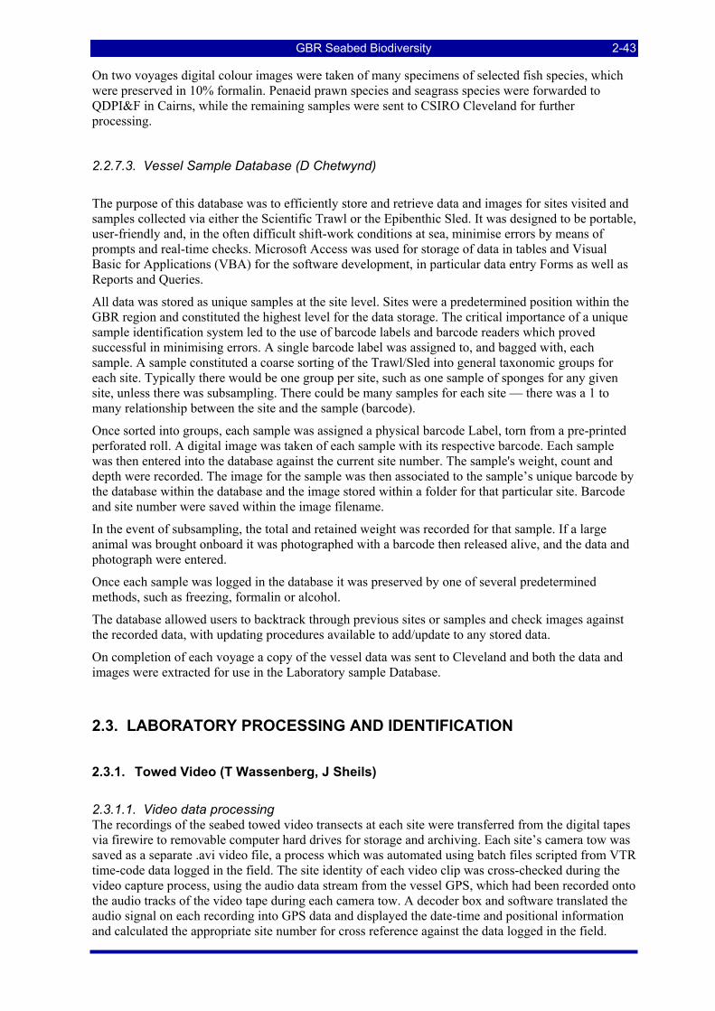
GBR Seabed Biodiversity 2-43
On two voyages digital colour images were taken of many specimens of selected fish species, which were preserved in 10% formalin. Penaeid prawn species and seagrass species were forwarded to QDPI&F in Cairns, while the remaining samples were sent to CSIRO Cleveland for further processing.
2.2.7.3. Vessel Sample Database (D Chetwynd)
The purpose of this database was to efficiently store and retrieve data and images for sites visited and samples collected via either the Scientific Trawl or the Epibenthic Sled. It was designed to be portable, user-friendly and, in the often difficult shift-work conditions at sea, minimise errors by means of prompts and real-time checks. Microsoft Access was used for storage of data in tables and Visual Basic for Applications (VBA) for the software development, in particular data entry Forms as well as Reports and Queries.
All data was stored as unique samples at the site level. Sites were a predetermined position within the GBR region and constituted the highest level for the data storage. The critical importance of a unique sample identification system led to the use of barcode labels and barcode readers which proved successful in minimising errors. A single barcode label was assigned to, and bagged with, each sample. A sample constituted a coarse sorting of the Trawl/Sled into general taxonomic groups for each site. Typically there would be one group per site, such as one sample of sponges for any given site, unless there was subsampling. There could be many samples for each site — there was a 1 to many relationship between the site and the sample (barcode).
Once sorted into groups, each sample was assigned a physical barcode Label, torn from a pre-printed perforated roll. A digital image was taken of each sample with its respective barcode. Each sample was then entered into the database against the current site number. The sample's weight, count and depth were recorded. The image for the sample was then associated to the sample’s unique barcode by the database within the database and the image stored within a folder for that particular site. Barcode and site number were saved within the image filename.
In the event of subsampling, the total and retained weight was recorded for that sample. If a large animal was brought onboard it was photographed with a barcode then released alive, and the data and photograph were entered.
Once each sample was logged in the database it was preserved by one of several predetermined methods, such as freezing, formalin or alcohol.
The database allowed users to backtrack through previous sites or samples and check images against the recorded data, with updating procedures available to add/update to any stored data.
On completion of each voyage a copy of the vessel data was sent to Cleveland and both the data and images were extracted for use in the Laboratory sample Database.
2.3. LABORATORY PROCESSING AND IDENTIFICATION
2.3.1. Towed Video (T Wassenberg, J Sheils)
2.3.1.1. Video data processing The recordings of the seabed towed video transects at each site were transferred from the digital tapes via firewire to removable computer hard drives for storage and archiving. Each site’s camera tow was saved as a separate .avi video file, a process which was automated using batch files scripted from VTR time-code data logged in the field. The site identity of each video clip was cross-checked during the video capture process, using the audio data stream from the vessel GPS, which had been recorded onto the audio tracks of the video tape during each camera tow. A decoder box and software translated the audio signal on each recording into GPS data and displayed the date-time and positional information and calculated the appropriate site number for cross reference against the data logged in the field.
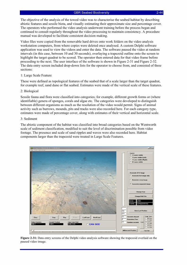
GBR Seabed Biodiversity 2-44
The objective of the analysis of the towed video was to characterise the seabed habitat by describing abiotic features and sessile biota, and visually estimating their approximate size and percentage cover. The operators who performed the video analysis underwent training before the process began and continued to consult regularly throughout the video processing to maintain consistency. A procedure manual was developed to facilitate consistent decision making.
Video files were copied from the removable hard drives onto work folders on the video analysis workstation computers, from where copies were deleted once analysed. A custom Delphi software application was used to view the videos and enter the data. The software paused the video at random intervals (in this case, between 10 and 30 seconds), overlaying a trapezoid outline onto the screen to highlight the target quadrat to be scored. The operator then entered data for that video frame before proceeding to the next. The user interface of the software is shown in Figure 2-31 and Figure 2-32. The data entry screen included drop-down lists for the operator to choose from, and consisted of three sections:
1: Large Scale Feature
These were defined as topological features of the seabed that of a scale larger than the target quadrat, for example reef, sand dune or flat seabed. Estimates were made of the vertical scale of these features.
2: Biological
Sessile fauna and flora were classified into categories; for example, different growth forms or (where identifiable) genera of sponges, corals and algae etc. The categories were developed to distinguish between different organisms as much as the resolution of the video would permit. Signs of animal activity such as burrows, mounds, pits and tracks were also recorded here. For each category type, estimates were made of percentage cover, along with estimates of their vertical and horizontal scale.
3: Sediment
The abiotic component of the habitat was classified into broad categories based on the Wentworth scale of sediment classification, modified to suit the level of discrimination possible from video footage. The presence and scale of sand ripples and waves were also recorded here. Habitat components larger than the trapezoid were treated in Large Scale Features.
Figure 2-31: Data entry screens of the Delphi video analysis software showing the trapezoid overlaid on the paused video image.
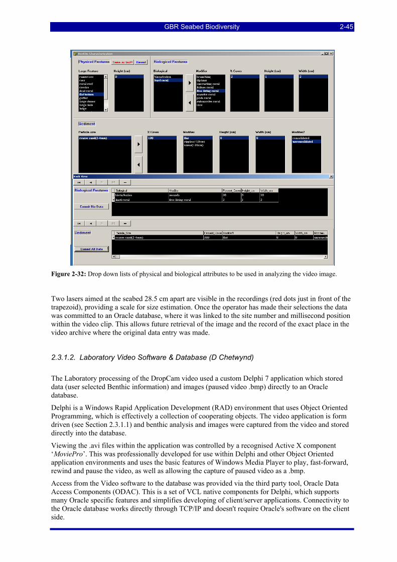
GBR Seabed Biodiversity 2-45
Figure 2-32: Drop down lists of physical and biological attributes to be used in analyzing the video image.
Two lasers aimed at the seabed 28.5 cm apart are visible in the recordings (red dots just in front of the trapezoid), providing a scale for size estimation. Once the operator has made their selections the data was committed to an Oracle database, where it was linked to the site number and millisecond position within the video clip. This allows future retrieval of the image and the record of the exact place in the video archive where the original data entry was made.
2.3.1.2. Laboratory Video Software & Database (D Chetwynd)
The Laboratory processing of the DropCam video used a custom Delphi 7 application which stored data (user selected Benthic information) and images (paused video .bmp) directly to an Oracle database.
Delphi is a Windows Rapid Application Development (RAD) environment that uses Object Oriented Programming, which is effectively a collection of cooperating objects. The video application is form driven (see Section 2.3.1.1) and benthic analysis and images were captured from the video and stored directly into the database.
Viewing the .avi files within the application was controlled by a recognised Active X component ‘MoviePro’. This was professionally developed for use within Delphi and other Object Oriented application environments and uses the basic features of Windows Media Player to play, fast-forward, rewind and pause the video, as well as allowing the capture of paused video as a .bmp.
Access from the Video software to the database was provided via the third party tool, Oracle Data Access Components (ODAC). This is a set of VCL native components for Delphi, which supports many Oracle specific features and simplifies developing of client/server applications. Connectivity to the Oracle database works directly through TCP/IP and doesn't require Oracle's software on the client side.
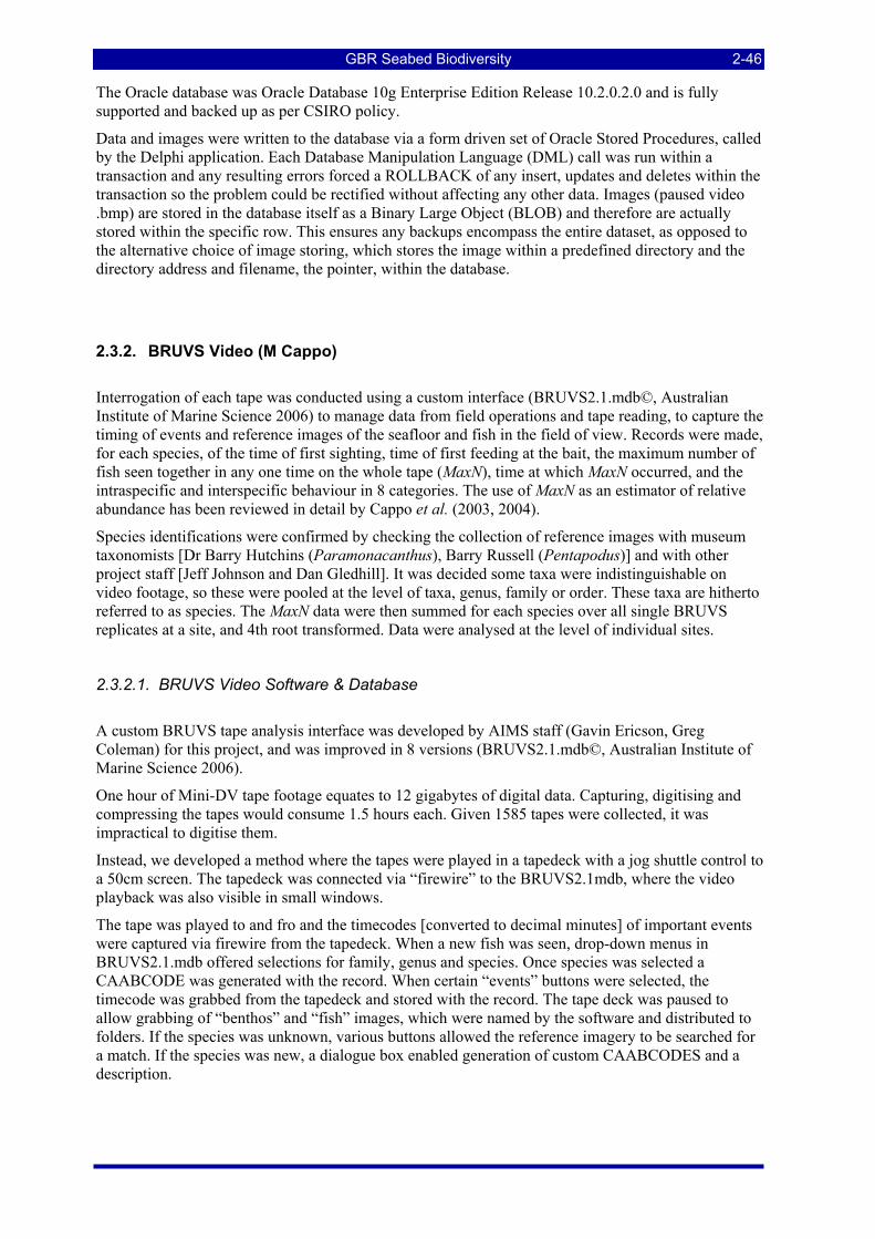
GBR Seabed Biodiversity 2-46
The Oracle database was Oracle Database 10g Enterprise Edition Release 10.2.0.2.0 and is fully supported and backed up as per CSIRO policy.
Data and images were written to the database via a form driven set of Oracle Stored Procedures, called by the Delphi application. Each Database Manipulation Language (DML) call was run within a transaction and any resulting errors forced a ROLLBACK of any insert, updates and deletes within the transaction so the problem could be rectified without affecting any other data. Images (paused video .bmp) are stored in the database itself as a Binary Large Object (BLOB) and therefore are actually stored within the specific row. This ensures any backups encompass the entire dataset, as opposed to the alternative choice of image storing, which stores the image within a predefined directory and the directory address and filename, the pointer, within the database.
2.3.2. BRUVS Video (M Cappo)
Interrogation of each tape was conducted using a custom interface (BRUVS2.1.mdb©, Australian Institute of Marine Science 2006) to manage data from field operations and tape reading, to capture the timing of events and reference images of the seafloor and fish in the field of view. Records were made, for each species, of the time of first sighting, time of first feeding at the bait, the maximum number of fish seen together in any one time on the whole tape (MaxN), time at which MaxN occurred, and the intraspecific and interspecific behaviour in 8 categories. The use of MaxN as an estimator of relative abundance has been reviewed in detail by Cappo et al. (2003, 2004).
Species identifications were confirmed by checking the collection of reference images with museum taxonomists [Dr Barry Hutchins (Paramonacanthus), Barry Russell (Pentapodus)] and with other project staff [Jeff Johnson and Dan Gledhill]. It was decided some taxa were indistinguishable on video footage, so these were pooled at the level of taxa, genus, family or order. These taxa are hitherto referred to as species. The MaxN data were then summed for each species over all single BRUVS replicates at a site, and 4th root transformed. Data were analysed at the level of individual sites.
2.3.2.1. BRUVS Video Software & Database
A custom BRUVS tape analysis interface was developed by AIMS staff (Gavin Ericson, Greg Coleman) for this project, and was improved in 8 versions (BRUVS2.1.mdb©, Australian Institute of Marine Science 2006).
One hour of Mini-DV tape footage equates to 12 gigabytes of digital data. Capturing, digitising and compressing the tapes would consume 1.5 hours each. Given 1585 tapes were collected, it was impractical to digitise them.
Instead, we developed a method where the tapes were played in a tapedeck with a jog shuttle control to a 50cm screen. The tapedeck was connected via “firewire” to the BRUVS2.1mdb, where the video playback was also visible in small windows.
The tape was played to and fro and the timecodes [converted to decimal minutes] of important events were captured via firewire from the tapedeck. When a new fish was seen, drop-down menus in BRUVS2.1.mdb offered selections for family, genus and species. Once species was selected a CAABCODE was generated with the record. When certain “events” buttons were selected, the timecode was grabbed from the tapedeck and stored with the record. The tape deck was paused to allow grabbing of “benthos” and “fish” images, which were named by the software and distributed to folders. If the species was unknown, various buttons allowed the reference imagery to be searched for a match. If the species was new, a dialogue box enabled generation of custom CAABCODES and a description.
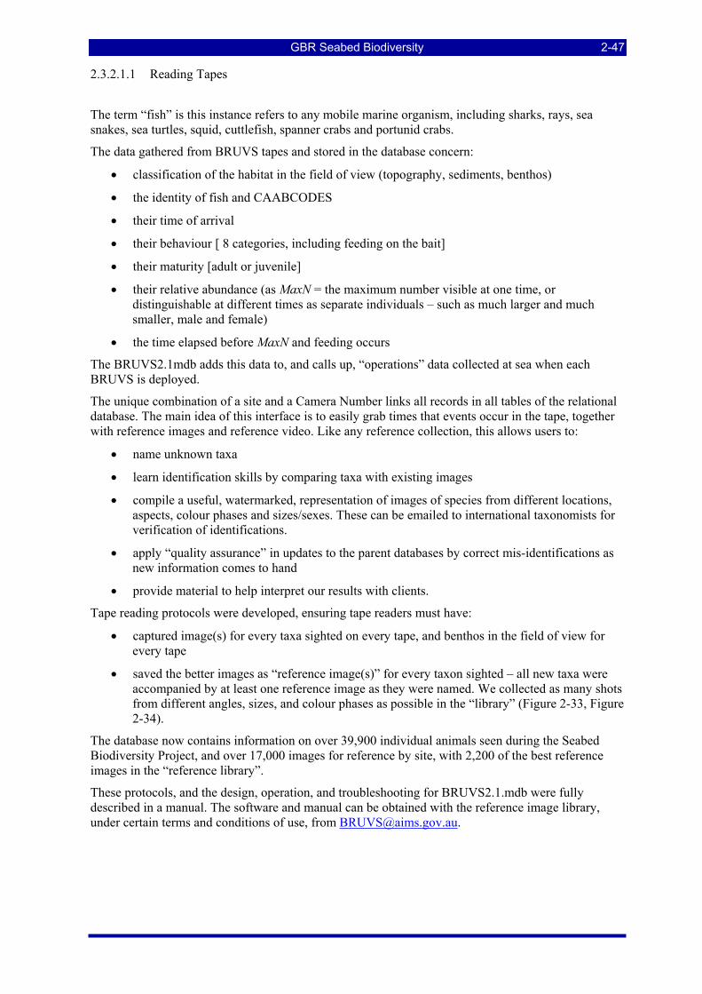
GBR Seabed Biodiversity 2-47
2.3.2.1.1 Reading Tapes
The term “fish” is this instance refers to any mobile marine organism, including sharks, rays, sea snakes, sea turtles, squid, cuttlefish, spanner crabs and portunid crabs.
The data gathered from BRUVS tapes and stored in the database concern:
• classification of the habitat in the field of view (topography, sediments, benthos)
• the identity of fish and CAABCODES
• their time of arrival
• their behaviour [ 8 categories, including feeding on the bait]
• their maturity [adult or juvenile]
• their relative abundance (as MaxN = the maximum number visible at one time, or distinguishable at different times as separate individuals – such as much larger and much smaller, male and female)
• the time elapsed before MaxN and feeding occurs
The BRUVS2.1mdb adds this data to, and calls up, “operations” data collected at sea when each BRUVS is deployed.
The unique combination of a site and a Camera Number links all records in all tables of the relational database. The main idea of this interface is to easily grab times that events occur in the tape, together with reference images and reference video. Like any reference collection, this allows users to:
• name unknown taxa
• learn identification skills by comparing taxa with existing images
• compile a useful, watermarked, representation of images of species from different locations, aspects, colour phases and sizes/sexes. These can be emailed to international taxonomists for verification of identifications.
• apply “quality assurance” in updates to the parent databases by correct mis-identifications as new information comes to hand
• provide material to help interpret our results with clients.
Tape reading protocols were developed, ensuring tape readers must have:
• captured image(s) for every taxa sighted on every tape, and benthos in the field of view for every tape
• saved the better images as “reference image(s)” for every taxon sighted – all new taxa were accompanied by at least one reference image as they were named. We collected as many shots from different angles, sizes, and colour phases as possible in the “library” (Figure 2-33, Figure 2-34).
The database now contains information on over 39,900 individual animals seen during the Seabed Biodiversity Project, and over 17,000 images for reference by site, with 2,200 of the best reference images in the “reference library”.
These protocols, and the design, operation, and troubleshooting for BRUVS2.1.mdb were fully described in a manual. The software and manual can be obtained with the reference image library, under certain terms and conditions of use, from [email protected].
GBR Seabed Biodiversity 2-48
Figure 2-33: Image reference form in BRUVS2.1.mdb
Figure 2-34: Reference image for Pristipomoides multidens, with Lutjanus sebae, L. adetii and Epinephelus undulatostriatus and E. areolatus in the background.
GBR Seabed Biodiversity 2-49
2.3.3. Laboratory Processing of Samples (T Hendriks, M Stowar, C Bartlett, T Wassenberg, D Gledhill)
Following the field-trips, samples were freighted to several laboratories where detailed sorting, identification, curation and detailed data recording were continued. Comprehensive reference collections of voucher specimens were established and recorded into the database.
• Porifera, octocorals, sled sampled fish and trawl bycatch invertebrates were sorted at the Queensland Museum, South Bank campus (QMSB);
• Molluscs, echinoderms, bryozoans and scleractinians were sorted at the Museum of Tropical Queensland (QM, MTQ campus) by MTQ and Australian Institute of Marine Science (AIMS) staff;
• Crustaceans and trawl sampled fish were sorted at CSIRO Marine and Atmospheric Research, Cleveland;
• Trawl sampled prawns were sorted at Queensland Department of Primary Industries and Fisheries (QDPI&F) in Cairns;
• Sled sampled algae and seagrasses were sorted at Queensland Department of Primary Industries and Fisheries (QDPI&F) in Townsville;
• Particle size and carbonate composition analysis of sediment samples were completed by Geoscience Australia (GA).
By decision of the Project’s Steering Committee, annelids, ascidians, crinoids, hydroids and trawl sampled marine plants were not completed within the scope of the project. All other groups have been completed.
For all samples at all agencies, the following processes were completed.
• Each sample was physically separated into groups corresponding to species or species equivalent Operational Taxonomic Unit (OTU);
• Identifications were done to Operational Taxonomic Unit (OTU) level: known species where possible, alpha species otherwise;
• Total counts and weights of each OTU within a sample were recorded;
• Specimen barcodes were assigned to each OTU for database purposes, as well as to facilitate any further studies that may be completed with these specimens.
• Reference material of specimens of all OTUs was retained. Specimens were kept the first time that a new OTU was encountered at any laboratory — a voucher reference. These were preserved and retained at the relevant laboratory.
• Entry of all data into the database (Figure 2-35, Section 2.3.3.3).
2.3.3.1. Queensland Museum
The Queensland Museum, at QMSB and MTQ, was responsible for the taxonomy of many major invertebrate Phyla, including Porifera, Echinodermata, Mollusca, Cnidaria, Ascidacea and Bryozoa (Figure 2-36). All voucher specimens were preserved in ethanol and all other processed specimens were stored either in ethanol, or frozen in freezers located at CSIRO Cleveland.
Identifications of Porifera, Cnidaria and Ascidacea have been especially problematic, as they would normally require extensive preparations before genus/species combinations can be given with a high level of confidence. Time constraints prevented histology from being completed, leaving scope for further research to be completed in the future to allocate species names using histology or other means as necessary.
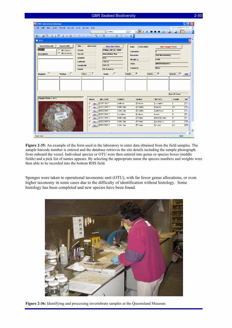
GBR Seabed Biodiversity 2-50
Figure 2-35: An example of the form used in the laboratory to enter data obtained from the field samples. The sample barcode number is entered and the database retrieves the site details including the sample photograph from onboard the vessel. Individual species or OTU were then entered into genus or species boxes (middle fields) and a pick list of names appears. By selecting the appropriate name the species numbers and weights were then able to be recorded into the bottom RHS field.
Sponges were taken to operational taxonomic unit (OTU), with far fewer genus allocations, or even higher taxonomy in some cases due to the difficulty of identification without histology. Some histology has been completed and new species have been found.
Figure 2-36: Identifying and processing invertebrate samples at the Queensland Museum.
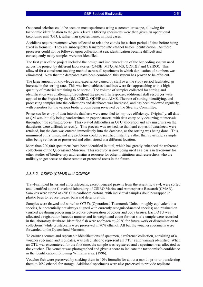
GBR Seabed Biodiversity 2-51
Octocoral sclerites could be seen on most specimens using a stereomicroscope, allowing for taxonomic identification to the genus level. Differing specimens were then given an operational taxonomic unit (OTU), rather than species name, in most cases.
Ascidians require treatment when collected to relax the zooids for a short period of time before being fixed in formalin. They are subsequently transferred into ethanol before identification. As these processes could not be followed upon collection at sea, identification became difficult and consequently many samples were not identified.
The first year of the project included the design and implementation of the bar coding system used across the project by different laboratories (QMSB, MTQ, AIMS, QDPI&F and CSIRO). This allowed for a consistent tracking method across all specimens in which duplication of numbers was eliminated. Now that the databases have been combined, this system has proven to be efficient.
The large amount of knowledge and experience gained by staff over the study period facilitated an increase in the sorting rate. This was invaluable as deadlines were fast approaching with a high quantity of material remaining to be sorted. The volume of samples collected for sorting and identification was challenging throughout the project. In response, additional staff resources were applied to the Project by the QM, CSIRO, QDPIF and AIMS. The rate of sorting, identifying, and processing samples into the collections and databases was increased, and has been reviewed regularly, with priorities for the various biotic groups being reviewed by the Steering Committee.
Processes for entry of data into the database were amended to improve efficiency. Originally, all data at QM was initially being hand-written on paper datasets, with data entry only occurring at intervals throughout the sorting process. This created difficulties in OTU allocation and any misprints on the datasheets were difficult to rectify. This process was revised, so that hard copies of datasheets were retained, but the data was entered immediately into the database, as the sorting was being done. This minimised entry times, and any problems could be rectified instantly, rather than revisiting a sample after being re-frozen or preserved and often stored at a different location.
More than 200,000 specimens have been identified in total, which has greatly enhanced the reference collections of the Queensland Museum. This resource is now being used as a basis in taxonomy for other studies of biodiversity and remains a resource for other institutions and researchers who are unlikely to get access to these remote or protected areas in the future.
2.3.3.2. CSIRO (CMAR) and QDPI&F
Trawl-sampled fishes and all crustaceans, except penaeid prawns from the scientific trawl, were sorted and identified at the Cleveland laboratory of CSIRO Marine and Atmospheric Research (CMAR). Samples were stored at -20° C in cardboard cartons, with individual samples double-wrapped in plastic bags to reduce freezer burn and deterioration.
Samples were thawed and sorted to OTU’s (Operational Taxonomic Units – roughly equivalent to a species, but potentially not always aligned with currently recognised/named species) and retained on crushed ice during processing to reduce deterioration of colour and body tissues. Each OTU was allocated a registration barcode number and its weight and count for that site’s sample were recorded in the laboratory database. Identified fish were re-frozen at -20°C for future work or dissemination to collections, while crustaceans were preserved in 70% ethanol. All but the voucher specimens were forwarded to the Queensland Museum.
To ensure accurate and repeatable identifications of specimen, a reference collection, consisting of a voucher specimen and replicates, was established to represent all OTU’s and variants identified. When an OTU was encountered for the first time, the sample was registered and a specimen was allocated as the voucher. The voucher was photographed and given a score to indicate the taxonomist’s confidence in the identification, following Williams et al. (1996).
Voucher fish were preserved by soaking them in 10% formalin for about a month, prior to transferring them to 70% ethanol for storage. Additional specimens were also preserved to provide replicate

GBR Seabed Biodiversity 2-52
reference material. A tissue sample, for genetic analysis, was removed from some voucher and replicate specimens prior to preservation. Tissues were stored in ethanol. Additional specimens, of virtually all species, ranging from across the geographic range of the study area, were retained (frozen) for the collection of tissue samples at a later date. Sub-collections of frozen and preserved material were sent to the National Fish Collection, CSIRO Hobart, for further examination.
The fresh colour of many fish and crustacean species is a useful diagnostic tool, and for some species colour patterns are the only field characters. A laboratory identification guide was compiled containing images taken onboard and in the laboratory for each OTU and variant. Identification characters were recorded to assist in accurate and consistent identifications. Images and identification characters were also collated in an online database to allow interstate colleagues and visiting international experts to view specimens remotely and thus assist with the identification of taxonomically difficult species.
2.3.3.3. Laboratory Sample Database (D Chetwynd)
The Laboratory Database, similar to its Vessel counterpart used MSAccess for storage of data in tables and Visual Basic for Applications (VBA) for the software development, in particular data entry Forms as well as Reports and Queries.
CSIRO, the Queensland Museum Brisbane and Townsville and the QDPI all had networked installations of the Laboratory database local to their laboratory.
The database’s main purpose was to log taxonomic specimen information and images against the samples collected in the field. The collected samples, initially sorted on the vessel to a general biotic group level, would be further sorted to a species level or to the nearest taxonomic level possible, given the available resources and or the state of the sample.
A list of Australian Marine species was compiled and stored in the database in taxonomic hierarchy to act as a starting list to build on. Each of these unique entries was given an incrementing ID to denote each Operational Taxonomic Unit (OTU); if and when a new entry was added an incremental value was added as the new ID for the new OTU.
When sorting the samples, a sample was opened and, using the bar code scanner, the barcode label from the sample was read. This triggered a response within the database, which retrieved the site and sample data and images displaying them for the user to verify. The sample was then separated into its various OTU’s. For examples, a crustacean sample could have three specimens of different crab species and two specimens of the same species of prawn, therefore 4 OTU’s existed within this sample. There was a 1 to many relationship between the sample (barcode) and the OTU’s within that sample; for each sample there could be many OTU’s.
Once the OTU’s were identified the user allocated a separate barcode label to each OTU — this was known as the jar code – and was scanned into the database and the label was placed in the OTU bag or jar. If a digital image of the specimen was required, it was taken at this point with the jar code label within the image.
Once the samples were sorted into OTU’s, they were individually added to the database. This was done by selecting the lowest known taxonomic level to each OTU group via the pick lists in the entry forms. If the identified species did not already exist in the precompiled list, then it was added via another entry form for new OTUs, hence making it available.
Once the desired species was selected, the count and weight of specimens were entered against the record, as well as the jar code, read by the barcode scanner. Any images previously taken were stored against the OTU at this point.
Species data can be queried by any of the taxonomic levels, site, sample or even jar code.
GBR Seabed Biodiversity 2-53
2.4. DATA ANALYSES
2.4.1. BRUVS Species Models, Characterization & Prediction (M Cappo, G De’Ath)
A total of 40 environmental and spatial explanatory variables were used in analyses of BRUVS data. These comprised: three spatial variables (depth, “Along”, “Across”); four sediment characteristics (% mud, sand, gravel, carbonate); 20 physico-chemical parameters from the CARS and SeaWiFS dataset, including measures of location (mean) and spread (Std Dev); 12 “harmonics” of polar temporal variables (diurnal, lunar, seasonal); seabed current shear stress and shelf slope; and a trawl effort index.
Distance “along” was set to range from 0 at the southern end to 1 at the far northern end. Distance “across” was 0 on the coast and 1 on the 80 m isobath. The corners of the polygon formed in this way were 142.53°E, -10.69°S and 144.06°E, -10.68°S at the northern end, and 152.49°E, -25.00°S and 152.90°E, -24.22°S at the southern end.
The BRUVS data were analysed in two ways. Firstly each species was treated as a univariate response and, using boosted trees (GBM, Friedman 2001, De’ath 2006), its presence-absence was predicted from the environmental data. Boosted trees are widely regarded as one of the best predictive methodologies, and handle complex data sets and a broad range of loss functions. For the presence-absence data analysed here, the binomial loss function was used. The collection of species was then related to the best environmental predictors. Statistics representing the predictability of each species and the predicting capacity of the environmental measures were then calculated. This produced a “short-list” of 25 species and 20 explanatory variables. The 25 species were the best predicted species that occurred on at least 7% of sites. The 20 explanatory variables were selected as the best predictors of the 25 species. The binomial loss function was used in the boosting.
Secondly, the relative abundances on BRUVS (the sum of MaxN for each sampling station) were 4th root transformed and analysed using multivariate regression trees (MRT; De'ath 2002). MRT used sums of squares (Euclidean distance) for splitting. Twenty explanatory variables and twenty-five species responses were short-listed in the same way as described above for the boosted trees. The best-sized tree was selected by five-fold cross-validation.
The tree defines a hierarchy of species communities and their spatial and environmental values that locate them on the GBR. This hierarchical approach can be used with any clustering method (constrained as is the case here with multivariate regression trees, or unconstrained). It also identifies groups of species that co-occur at varying spatial scales to form communities. This contrasts with non-hierarchical methods which derive mutually exclusive clusters at a single spatial scale, thereby lacking high-level (broad spatial scale) structure and ignoring information from highly prevalent species. The homogeneity of the clusters formed by MRT (from 1 through to 13 nodes) was compared with similar numbers of unconstrained cluster groups, using K-means clustering and Euclidean distance.
Indicator values (DLI; Dufrêne and Legendre 1997) were calculated for each species for each node of the tree. For a given species and a given group of sites, the DLI is defined as the product of the mean species abundance occurring in the group divided by the sum of the mean abundances in all other groups (a type of specificity), times the proportion of sites within the group where the species occurs (fidelity), multiplied by 100. DLI takes a maximum value of 100 if the species occurs at all sites in the group and nowhere else, and 0 if it occurs at no sites within a node. Each species was associated with the tree node (assemblage) where its maximum DLI value occurred, and the numbers of indicator species and their values were used to characterize each node of the tree. Species with high DLIs were used as characteristic members of each assemblage, and the spatial extent of the group indicated the region where the species was predominantly found.
GBR Seabed Biodiversity 2-54
2.4.2. Single Species Biophysical Models and Prediction (M Browne, W Venables)
2.4.2.1. Assumptions and Challenges The distribution of each identified species was considered separately in relation to the available physical variables used as predictors in the study. This approach assumed that the observed geo-spatial distribution of each species may be adequately explained by an underlying physical gradient. Each species would be expected to have its own preferred habitat range and tolerance for various physical parameters, and the spatial variation in physical variables is thought to drive the observed regional scale spatial distributions of the taxa.
From the point of view of biophysical modelling, it is known that sampling in a marine environment is very susceptible to sampling variability. That is, for fixed levels of the biophysical parameters involved, the event of observing a species, and the biomass obtained given that the species was observed, were still liable to be highly variable due to random influences — neither observable nor under the control of the sampling mechanism. Thus, the modelling approach applied needed to be conservative and to anticipate that much random variation will remain unexplained. Technically, the biological response variables may be described as having a zero-inflated log-normal distribution. That is, given that some biomass is observed, the samples are approximately Gaussian on a log-scale, with a mean depending linearly on the physical predictors. However, given that the estimated probability of observing any particular species is typically relatively low (< 10%), the very large number of zeros in any species’ site-records strongly suggests a two-phase approach: initially modelling the probability of observing a species at all and conditionally modelling the distribution of the log-biomass given that the species is observed.
2.4.2.2. Model Formulation
The two-stage model used to relate the observed biomass to the underlying physical variables may be described as follows:
• We use a logistic regression model for the chance of observing a species in a sampling event. For any given species, S , the chance of observation is
( ) ( )Pr or equivalently logit1
T
T
xT
S sx
ep S p x
e
β
ββ= = =
+
where x is a collection of suitably chosen physical variables for that species and β is the vector of coefficients multiplying them, to be estimated from the data. This first phase model is a standard logistic regression for presence/absence. The first component of 0x is often a constant predictor (unity) and its coefficient 0β is called the intercept term.
• The log-biomass of the species given the fact that it has been observed in a sampling event is them modelled as a normal linear regression. In symbols using an evident notation
( ) [ ] [ ]2 2log | ~ , i.e. E log | , Var log |T TS S SB S N z B S z B Sγ σ γ σ= =
where again z is a collection of suitably chosen physical predictors for species S and 0 1z = making 0γ the intercept term.
Note that for the logistic regression stage all site records can be used in the model calibration, but for the second stage only those site records for which there is a non-zero biomass contribute information that can be used in this calibration process. This sometimes limits the modelling strategies possible.
Combining both stages of the model, the estimate of expected biomass at a given sampling site is then
[ ] [ ]( )( )
( )ˆexp
ˆ ˆˆ ˆE exp log | expˆ1 exp
T
TS s S T
xB p E B S z
x
βγ
β= = ×
+
GBR Seabed Biodiversity 2-55
where the circumflex accents denote quantities estimated from sample data. Technically this is the median rather than the mean but since for the lognormal distribution the median is proportional to the mean it produces the same relative picture of biomass distribution.
Approximate standard errors for the quantities involved can be derived by the usual delta method. The formulae are complex, but as the method is entirely standard and can largely be relegated to the computational procedures, we omit them here for simplicity.
2.4.2.3. Explanatory physical variables, covariates, offsets and prediction
In the formulae above, the general-purpose explanatory variable (or )j jx z represents any member of the combined set of:
• 28 physical explanatory variables (e.g. percent_mud). A full list and description of the physical variables is provided elsewhere (Section 2.1.1).
• 2 spatial variables (‘across’ and ‘along’) representing in relative terms the distance between shoreline and outer reef, and between northern- and southern-most points of the GBR.
• Squared terms of physical and spatial variates (e.g. percent_mud^2)
• Second degree interaction terms between physical or temporal explanatory variables, or both (e.g. percent_mud × benthic_irradiance)
• Harmonic terms in the temporal covariates: (described specifically below)
• The measurement method used (i.e. modified trawl net / benthic sled) as a factorial predictor,
• A weighted annual average of commercial trawl fishery effort local to the sampling site.
For the purposes of generating predictions on the GBR study region, we were primarily interested in the relationship between the physical variables and observed biomass. It was, however, recognised that other factors were be expected to play a role in the observed biomass. For example, many species are known to have a strong diurnal or lunar behavioural cycle, or a seasonal abundance component. Also, when generating estimates on the physical grid for full coverage of the GBR region, it is desirable that the estimated distributions are independent of sampling device, which we term the ‘survey type’. These variables are included in the models in order to ensure that these effects do not interfere with estimation of the effect of genuinely physical or spatial predictors. When predictions were later made from these fitted models on to the entire GBR grid, the covariate predictors are set to values that represent the sampling disposition under which the estimated biomass would be largest. This is to promote maximum contrast in the predictions.
The temporal covariates included ‘Time of Day’, ‘Moon Phase’, and ‘Time of Year’ (or ‘season’). Since GLMs depend on the explanatory variables through a single linear function, it is appropriate to represent the effect of such temporal predictors through harmonic terms, that is
KkTpkttx
Tpkttx k
bk
a ,2,1 2cos)( 2sin)( )()( =⎟⎠⎞
⎜⎝⎛=⎟
⎠⎞
⎜⎝⎛=
where T is the appropriate fundamental period. Including temporal covariates in this way ensures that the predictions will obey the natural periodicity with respect to such predictors.
It is has been mentioned that ‘survey type’, whether the measurement was made with the trawl or sled, was also included as a covariate factor in the analysis. If a species was observed a minimum number of times in both sampling devices, then all data was included in the model, with the ‘Survey Type’ factor included. However, if a species was observed on very few occasions, or not at all, with either one of the sampling devices, then the usefulness of a model incorporating both devices was limited. In these cases the models were based on data from the most productive sampling device only, obviating the need for a ‘Survey Type’ covariate in the model.
GBR Seabed Biodiversity 2-56
The area swept by each device at each site was recorded, and although efforts were made to keep this constant, it did vary somewhat. The effect of trawling (or ‘sledding’) over a greater area is to increase the probability of a catch in some monotic way, and to increase the amount of biomass caught, on average, proportionally. Thus, the recorded swept area on the log scale was included as a candidate predictor for the logistic regression models and as a fixed offset in the biomass models. Predictions were then standardised by setting swept area to 1 Ha.
2.4.2.4. Model construction and variable selection
Each species model included, at a minimum, harmonics in temporal covariates as well as ‘survey type’ and ‘log-swept area’, as explanatory variables (or offset). It has been noted above that potentially included variables included 30 physical or spatial variables, as well as squared terms and interactions between physical explanatory variables (30 + 30 × 31/2 = 495 possible candidate predictors). Not all possible choices, however, are equally reasonable a priori. In practice we note that if a physical predictor is important either for the presence/absence or the conditional biomass of a taxon then the linear term will generally make this manifest and the additional contribution to the model due to higher order terms involving these will be much smaller, though often quite useful, of course. We adopted a two-stage variable screening method. At the first stage we allowed selections to occur only on the linear terms. Once these were found, we considered all possible squared and interaction terms involving the identified variables for additional inclusion in the model at the second stage. In this way we ensured that if a second order term was included in the model, its marginal linear terms were also included, which is generally regarded as a desirable feature of empirical statistical modelling.
The physical variables available are by their nature highly collinear (or confounded) and to counteract this we adopted a rigorous variable inclusion policy. Such a policy also has a good chance of ensuring some interpretability for the models as well as predictive effectiveness, although this has to be taken with some caution. The criterion used in these analyses was the ‘Bayesian Information Criteria’ due to Schwarz, 1978, defined as:
2 log logBIC L k n= − +
with log L denoting the log-likelihood of the optimized model, k the number of estimated parameters used in the model and n being the number of observations. The BIC attempts to balance model performance in the training sample with a penalized measure of model complexity to ensure that the model will capture as much signal and as little noise as possible. The related Akaike Information Criterion (AIC) penalizes complexity by a factor of 2 rather than logn , leading to more complex models which in this context, from our experience seem to sacrifice interpretability for minimal gains in predictive performance.
At each iteration of the stepwise search procedure, a term was added or removed from the working model if the inclusion or removal resulted in the greatest reduction in the BIC criterion. As mentioned earlier, this was done for the linear terms initially, and then for the second degree terms involving those predictors, with the linear terms chosen fixed in the model. This was done independently for the presence/absence and the conditional biomass models for any sampled species.
2.4.2.5. Prediction on the GBR grid
Based on the constructed models, estimates of expected biomass were generated for each species, for each grid location in the GBR study region. This involved interpolation between the sites of the training set and also, as noted, above, a transform back from the log scale to the natural scale. Both of these operations can result in unrealistic estimates and in this case they will be much more likely to be unrealistically large than small. As a heuristic, it was determined that the largest standardised per Ha biomass actually caught for a particular species would be used to determine a ceiling on the largest confident estimate on the grid to be used. Final estimates were truncated at the largest observed standardised catch rate observed in the sample itself. This seems preferable to having unrealistic estimates dominating a graphical presentation.
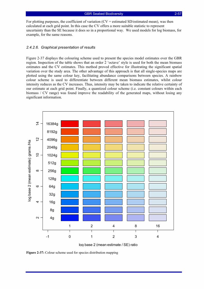
GBR Seabed Biodiversity 2-57
For plotting purposes, the coefficient of variation (CV = estimated SD/estimated mean), was then calculated at each grid point. In this case the CV offers a more suitable statistic to represent uncertainty than the SE because it does so in a proportional way. We used models for log biomass, for example, for the same reasons.
2.4.2.6. Graphical presentation of results
Figure 2-37 displays the colouring scheme used to present the species model estimates over the GBR region. Inspection of the table shows that an order 2 ‘octave’ style is used for both the mean biomass estimates and the CV estimates. This method proved effective for illustrating the significant spatial variation over the study area. The other advantage of this approach is that all single-species maps are plotted using the same colour key, facilitating abundance comparisons between species. A rainbow colour scheme is used to differentiate between different mean biomass estimates, whilst colour intensity reduces as the CV increases. Thus, intensity may be taken to indicate the relative certainty of our estimate at each grid point. Finally, a quantized colour scheme (i.e. constant colours within each biomass / CV range) was found improve the readability of the generated maps, without losing any significant information.
-1 0 1 2 3 4
24
68
1012
14
log base 2 (mean estimate / SE) ratio
log
base
2 (m
ean
estim
ate)
: gra
ms
/Ha
4g
8g
16g
32g
64g
128g
256g
512g
1024g
2048g
4096g
8192g
16384g
1 2 4 8 16
Figure 2-37: Colour scheme used for species distribution mapping
GBR Seabed Biodiversity 2-58
2.4.3. Species Groups Characterization and Prediction (M Browne)
One of the goals of the statistical analyses and modelling was to develop groups of ecologically similar species (at least with regard to their distribution in the physical environment) and to generate predictive models for the biomass of the entire group. We note that the taxonomic hierarchy may not provide a suitable basis for forming groups with this kind of similarity. Clustering here refers to an empirical grouping, hierarchical or otherwise, based on the characteristic distribution of species as observed from the survey effort.
There are several reasons why such a grouping or clustering of species is useful. For example, clustering allows the organisation of species with similar characteristics into common categories. As an exploratory technique it may provide the basis for more targeted analysis for establishing possible ecological dependencies and relationships. Due to the broad scope of the current project, individual modelling and prediction has been carried out for a very large number of distinct species (> 800). Species clustering and aggregated biomass data within groups can be a convenient method for summarising or quantifying the variation in species distributions through a small set of key grouped models. Finally, in cases where distinct and relatively rare species are observed at different sites, but share similar biophysical distributions, aggregation of the separate species into a single group can provide a way to utilise parts of the data set not otherwise available for modelling input.
It should be acknowledged that although clustering methods are well developed with acknowledged utility, to some degree heuristics and arbitrary decisions inevitably play some role, such as, for example, in something as fundamental as the choice of a distance metric. In our view the purposes of clustering have to be always kept in mind, as much biological insight and knowledge has to guide the process at every stage and the results need to be viewed in this light afterwards before a grouping is used.
2.4.3.1. Approach
Most clustering methods work by considering a similarity / dissimilarity matrix which describes ‘distances’ between objects. Broadly speaking, a clustering algorithm attempts to assign objects to groups so that similar ‘objects’ (in this case species) are put together in the same groups. The most obvious (and simplest) method for species clustering is to begin with the site / species presence / absence matrix and define species similarity using ‘Manhattan’ or ‘city block’ distances calculated between the distribution of species over sampled sites.
The species clustering method that has been adopted here is based on upon estimates at survey sites, as described in section 2.4.2, and thus may be described as constrained by the physical predictors. The modelled distributions are used as a species descriptor, rather than using the profile of raw biomass or presence /absence, to describe the similarity between the distribution of species. There are several important considerations that motivated this approach.
There are advantages and disadvantages to this approach. The most obvious disadvantage is that the representation is only as good as the species models were an effective summary of the information in the data itself. This will not always be totally satisfactory, of course. However the advantages include the fact that this allows us to control for factors such as the temporal, sampling method and swept area covariates which are inseparable from the remainder of the information in the raw data itself. It also allows us at least a potential device for counteracting the effects of false negatives, though admittedly, and inevitably, a somewhat speculative one. We note, also, that the data smoothed need not be entirely realistic for the groupings based on it to be effective enough for our subsequent purposes. Once the groups were decided, the subsequent analysis was based on the aggregated data; that is, on real data once again. This provides a useful safeguard in the logical chain of events.
GBR Seabed Biodiversity 2-59
2.4.3.2. Method
There was a total of 840 species (N) that both occurred sufficiently frequently for biophysical modelling, and also led to statistically satisfactory two-stage models by the model construction methods as detailed in the previous sections. Model estimates were generated for the 1644 sites (M) visited by the vessels, controlling for covariate predictions, for the reasons previously outlined.
As a measure of distributional affinities for the species, an N × N Spearman correlation matrix C was created from the model estimates over sites. The correlation was chosen as the base for a similarity measure because it was desired that the clustering criterion be invariant to absolute abundance. Choosing spearman correlations also makes the estimate robust to outlying values, as are frequently obtained under extrapolation from an empirical model as here. Two species with very different prevalence or mean observed biomass may therefore have high correlations if the standardized pattern of co-variation is similar.
To convert the correlation matrix, C, into a dissimilarity matrix D to be used for clustering we used the following transformation:
11
ijij
ij
CD
C−
=+
This guarantees that self-dissimilarities are zero, distances are otherwise non-negative and, since the correlations themselves are between -1 and 1, the dissimilarities are in the range 0 ijD≤ < ∞ . The denominator chosen was motivated by the fact that so defined log ijD will be approximately normal with equal variance, by a standard result in correlation theory. It also ensures an open-ended upper limit for the dissimilarities themselves. (Fortunately 1ijC = − did not occur in practice.)
After extensive experimentation with different methods for clustering species, hierarchical clustering using Ward’s method was chosen as a reliable and well established procedure for heuristic clustering. Ward’s (1963) method is a clustering procedure seeking to form the partitions Pn, P n-1,........, P1 in a manner that minimizes the approximation error associated with each grouping. At each step in the analysis, the union of every possible cluster pair is considered and the two clusters whose fusion results in minimum increase in the total sum-of-squares are combined. The ANOVA-type approach used by Ward makes this method one of the more principled approaches to clustering.
2.4.4. Site Groups Characterization and Prediction (W Venables)
Another goal of the statistical analysis and modelling was to identify various areas of seabed in the GBR study area in which the mix of biota was as homogeneous as possible and in some way distinct from the mix in other areas. These different, approximately homogeneous, mixtures can be called "assemblages". Any individual assemblage may be expressed in several disjoint geographical regions; there was no requirement that they be spatially contiguous. A further property was that, at the broad scale, these assemblages would be characterised using the available full-coverage physical variables. The biotic data used were the biomasses of identified fauna and flora at sites sampled by the epibenthic sled and research trawl.
A number of strategies are possible to achieve this result. One strategy would involve three separate steps, each with a number of options regarding method:
• First, partition the study sites into clusters based on the biological data alone, then
• Develop models to predict these clusters from the physical variables alone, and
• Use the predictive model to classify the entire GBR region.
GBR Seabed Biodiversity 2-60
The strategy finally adopted essentially combined the above partitioning, modelling and prediction steps into a single procedure, using a tree-modelling method. In outline this procedure was as follows:
• Using the biological information alone, construct a distance matrix between sites,
• Define a deviance measure on any clustering of sites, based on the biological distance matrix,
• Construct a decision tree using the available physical variables; the resulting terminal nodes of the decision tree define the site clusters,
• Use the decision tree to classify the entire GBR study grid and map the result.
The details of this procedure are explained in the following sections.
2.4.4.1. Biological distance matrix
The distance matrix between the sampled sites was based on the species biomass predictions from the individual species modelling, as described in Section 2.4.2. Distance matrices based on real sample biomass data would be preferable. However, more than one third of species had one or more significant temporal cycles (such as season, moon phase and time of day), which strongly affected their sampling-rates but not their abundance, and may have caused the raw data to produce assemblage splits due to arbitrary timing of sampling rather than actual distributions. Use of the predicted values, adjusted for the temporal variables, allowed distances to be based on biomass values for a standardized set of environmental conditions, but optimal with respect to the temporal catchability variables for each species. It was nevertheless acknowledged that the modelled predictions, being smoothed fitted derived data, would not be free of other issues — to minimize these, only predictions to sampled sites were used, rather than predictions (extrapolations) to the full GBR study grid.
The form of the distance matrix was the commonly used Bray-Curtis metric, but a number of possible prior transformations of the predicted biomasses were considered. The final transformation used was the 8th root, which for large biomasses behaves like a ‘weak’ log transformation, but for small biomasses behaves approximately linearly and, unlike log(b), was not adversely affected by zeros.
Thus, the dissimilarity d between sites i and j was:
( )1
1
, where = 1/8 and is the number of taxa.
t
ik jkk
ij t
ik jkk
b bd t
b b
α α
α αα=
=
−=
+
∑
∑
and b was the biomass of each species k.
2.4.4.2. Deviance measure
Consider any group of g sites, G . These can be represented by points in a plane, where the (Euclidean) distances between them are intended to represent distances from the biological distance matrix. Choosing any site from the group, say iS , the span of the group from iS was defined to be the sum of squared distances from the reference site, iS , to all other sites of the group:
( ) 2
1span
g
i ikk
S d=
=∑
The deviance of group G , say ( )D G , was then defined as the minimum value of the span, and the reference site from which this minimum was achieved was called the medoid of G, say MS , using the terminology of Kaufmann and Rousseeuw, (1990).
( ) ( ) ( )min span spani
i MS GD G S S
∈= =
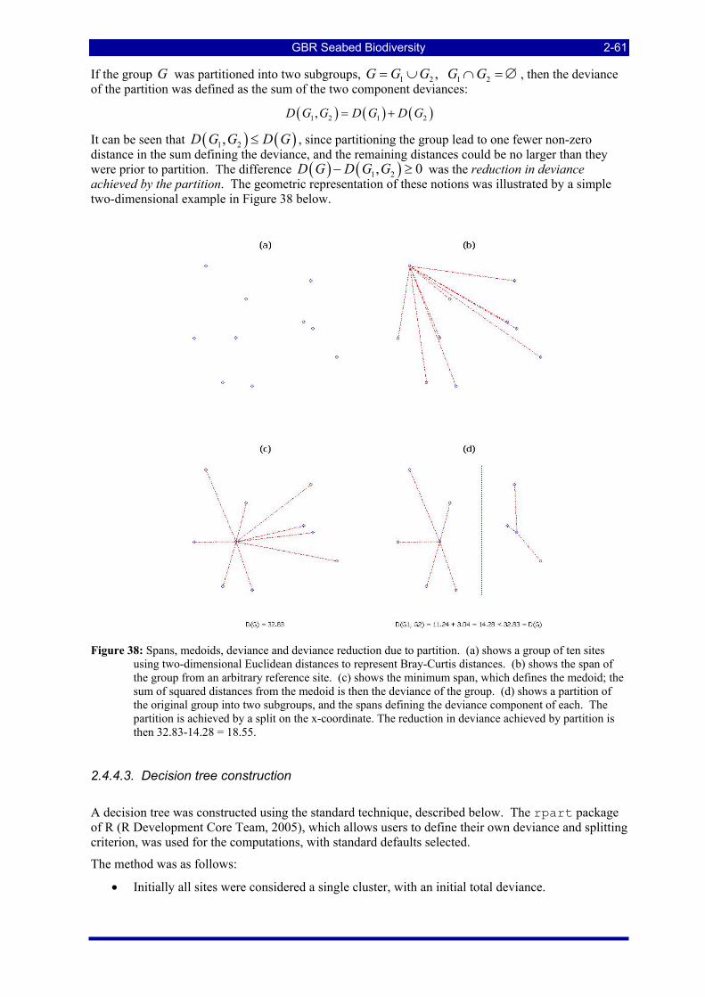
GBR Seabed Biodiversity 2-61
If the group G was partitioned into two subgroups, 1 2 1 2, G G G G G= ∪ ∩ =∅ , then the deviance of the partition was defined as the sum of the two component deviances:
( ) ( ) ( )1 2 1 2,D G G D G D G= +
It can be seen that ( ) ( )1 2,D G G D G≤ , since partitioning the group lead to one fewer non-zero distance in the sum defining the deviance, and the remaining distances could be no larger than they were prior to partition. The difference ( ) ( )1 2, 0D G D G G− ≥ was the reduction in deviance achieved by the partition. The geometric representation of these notions was illustrated by a simple two-dimensional example in Figure 38 below.
Figure 38: Spans, medoids, deviance and deviance reduction due to partition. (a) shows a group of ten sites using two-dimensional Euclidean distances to represent Bray-Curtis distances. (b) shows the span of the group from an arbitrary reference site. (c) shows the minimum span, which defines the medoid; the sum of squared distances from the medoid is then the deviance of the group. (d) shows a partition of the original group into two subgroups, and the spans defining the deviance component of each. The partition is achieved by a split on the x-coordinate. The reduction in deviance achieved by partition is then 32.83-14.28 = 18.55.
2.4.4.3. Decision tree construction
A decision tree was constructed using the standard technique, described below. The rpart package of R (R Development Core Team, 2005), which allows users to define their own deviance and splitting criterion, was used for the computations, with standard defaults selected.
The method was as follows:
• Initially all sites were considered a single cluster, with an initial total deviance.

GBR Seabed Biodiversity 2-62
• Consider any potential predictor variable, X . The sites may be partitioned into two groups by selecting those sites whose values for X are below some threshold, X a≤ as one group and the complementary set, those for which X a> , as the other. This was described as a split of the group on variable X at threshold a .
• Partition the group into two clusters by selecting the optimal split variable and the optimal threshold to achieve the greatest possible reduction in deviance of the span of Bray-Curtis distances.
• Apply the same procedure recursively to both clusters, until some stopping criterion has been achieved.
• The stopping criteria were as follows:
o The group must contain at least 20 sites for further splits to be considered.
o The group has deviance zero, or
o A further split of the group would not reduce the deviance by more than 1%.
In this application, the third criterion was typically encountered, the first criterion was achieved only once and the second was never triggered — the outcome of which produced 16 groups. The result was displayed as a decision tree in the usual graphical form.
As a check on the biological similarities between the resulting 16 site groups, as defined by the above tree method that split recursively on physical variables, the following procedure was applied to the biological data only:
• the medoid site of each site-group was identified,
• the Bray-Curtis dissimilarities between the medoids were extracted from the entire distance matrix,
• a hierarchical clustering and dendrogram was computed using Ward's method.
The congruence between the structure of the decision tree and that of the cluster dendrogram was then examined.
2.4.4.4. Classification of the GBR grids
The grids of the entire GBR study region were classified into the 16 groups, based on the decision tree splits of the physical variables, and the resulting pattern of groups was mapped.
In this application, the recursive partitioning algorithm was used for unsupervised learning, which was somewhat unusual. More usually, tree methods are used for supervised learning and the result is used for prediction of some à priori defined attribute (classification tree) or quantity (regression tree), i.e. supervised learning. In such cases, the decision tree is normally pruned to some justifiable level of complexity by cross-validation, with the aim of improving the accuracy of prediction for new data.
In the current application, the procedure was used to define the attribute (site groups) itself. Thus, the normal cross-validated pruning process was not available as there is no à priori definition of the attribute. Correspondingly, the claims made for the result were simply that it defined a partition of the study sites into groups which were (a) defined by splits in the prediction variables and hence readily extended to the entire GBR study region and (b) as homogeneous as possible within, in the sense of Bray-Curtis distances based on transformed predicted biomasses. There was no “correct” number of site-group assemblages and the resultant number of groups was somewhat arbitrary. While the default criteria were generally accepted guidelines, the 16 groups identified here may be more (or less) than was warranted.
GBR Seabed Biodiversity 2-63
2.4.4.5. Derived species groups and indicators
In addition to defining site-groups assemblages, it was also useful to examine the extent of associations between these site groups and species biomass distributions in a simple and direct way. If a species was strongly associated with one site group and only weakly associated with others, such a species could be described as an indicator species for that site group assemblage. The approach was as follows.
A site group characteristic distribution for the kth site group was defined by the vector ( )kξ , where the components were defined as:
( ) 1/ for sites in site group , which has sites, and0 otherwise
k i kki
n S k nξ
⎧= ⎨⎩
Note that ( ) 1ki
iξ =∑ for all k, conforming to the definition of a distribution.
Using the predicted mean biomass for each species, the species distribution vector for the mth species was defined as:
( ) /mi i i
iB Bη = ∑
that is, the predicted biomass, also normalized to add to unity over all study sites.
Further, a quantity termed the affinity distance between species and a site-group was defined as:
1 ( ) ( )2 cos m kmk i i
i
α η ξπ
− ⎛ ⎞= ⎜ ⎟⎝ ⎠∑ ,
which has values in the range 0 1mkα≤ ≤ . The quantity was zero only if the species was entirely within the site group and uniformly distributed, and unity if the species distribution was entirely outside the site group. The affinity distance was also a minor variation on the standard Hellinger distance measure between two distributions. It also has a geometric interpretation as the angle between two unit vectors, but heuristically, the affinity measure was an indicator of the preference any species had for any particular site-group.
Then, a distance between species was defined that represented the dissimilarity of their preference patterns for the site-group assemblages. Since the affinities were all measured on the same bounded scale, ordinary Euclidean distances were used:
( )22pq pk qk
kE α α= −∑
In turn, this distance matrix was used to generate species clusterings that grouped together species with similar preference patterns for the site-groups. Standard hierarchical clustering, using Ward’s method of linkage between groups, was applied. The resulting dendrogram, for all 839 taxa for which prediction models were possible, was cut at the appropriate location — for purposes of this analysis — to define 12 species groups.
While the species affinities provided information that helped characterise the site-group assemblages, it was also useful to investigate the relative density of each species group within each site group as additional characterising information. This computation was done in four stages, namely:
• sum the species biomass predictions within each species group, • normalize these aggregate biomass distributions, as for single species, to give 12 species group
distributions, • average these species group biomass distributions within each site group, to give “percentage
biomass per site” within each site group, • present the result as a series of bar charts, one for each site group.
The 16 site groups were labelled numerically and the 12 species groups were labelled alphabetically.
GBR Seabed Biodiversity 2-64
2.4.5. Video Habitat Characterization and Prediction (W Venables)
The towed video camera yielded data in two forms. While the vessel was in motion an operator recorded both the substratum type and the biota currently in view in a continuous manner (Section 2.2.2). Also, later, in the laboratory, individual frames from the video record were scored for a substrate and biota in a much more detailed way, though not on a continuous basis but as a sample of about 30 frames from the tow record (Section 2.3.1). This section outlines how the towed video camera data was used to provide some indication of the broad habitat types in the study area.
Table 2-9: Sediment and group biological cover classes for analysed video tow data. Note that sediment classes up to lage pebble could be further classified as rippled or in waves and cobble as waves.
Grouped biological Sediment Bioturbation Mud (0.06 mm) Algae_Caulerpa Sand (0.06-2.0 mm) Algae_Coralline Coarse sand (2-4 mm) Algae_Filamentous Small pebble (4-16 mm) Algae_Halimeda Large pebble (16-64 mm) Algae_Mixed Cobble (64-256 mm) Algae_Udotea Boulder (256-1024 mm) Algae_Ulva Large boulder (1024 mm+) Seagrass_H.ovalis Larger than field of view Seagrass_H.spinulosa Seagrass_strapform Bryozoan_branching Bryozoan_encrusting Hydroid Sea pen Soft_Coral Solenocaulon Sea_Whip Gorgonian Sponge Solitary_Coral Hard_Coral
2.4.5.1. Features of the data
In all four cases (Vessel or Laboratory, Substratum or Biology) the quantities characterising each site formed a vector of proportions, i.e. they summed to unity. In the case of the Vessel data this was a feature of the recording protocol itself. For the laboratory data, video frames were scored by the laboratory operator on a proportional basis and these were aggregated and re-normalised to give an estimate of the respective covering proportions for the entire transect.
The laboratory data set for the benthic biological cover had 114 different classes. These were determined primarily by a fairly coarse ‘feature’ type (e.g. algae) with more detail provided by a ‘descriptor’ (e.g. filamentous). At this level of differentiation the analysis diagnostics indicated little grouping structure in the data, the likely reason being that the finer morphotypical classification did not correspond with the biophysical affinities that were ecologically important. For this reason the biology cover classes were grouped for analysis: the feature/descriptor classes were amalgamated to the feature level except where morphotypes had been observed to be strongly differentiated in the field
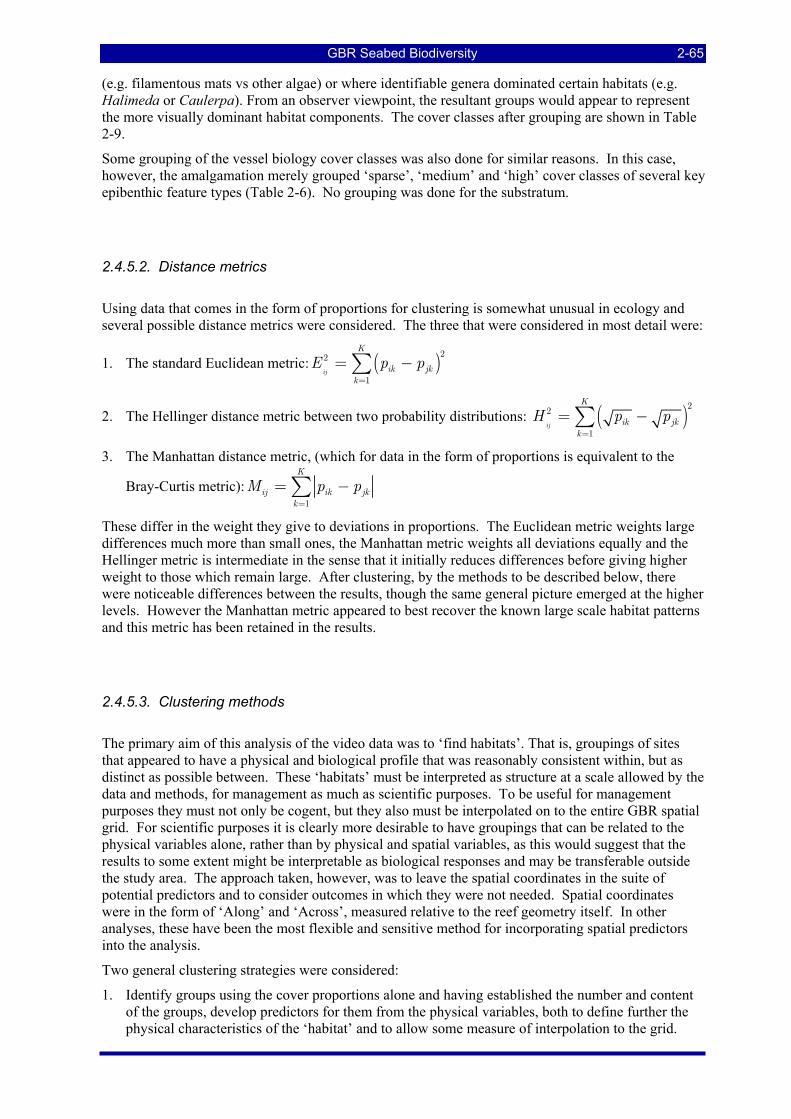
GBR Seabed Biodiversity 2-65
(e.g. filamentous mats vs other algae) or where identifiable genera dominated certain habitats (e.g. Halimeda or Caulerpa). From an observer viewpoint, the resultant groups would appear to represent the more visually dominant habitat components. The cover classes after grouping are shown in Table 2-9.
Some grouping of the vessel biology cover classes was also done for similar reasons. In this case, however, the amalgamation merely grouped ‘sparse’, ‘medium’ and ‘high’ cover classes of several key epibenthic feature types (Table 2-6). No grouping was done for the substratum.
2.4.5.2. Distance metrics
Using data that comes in the form of proportions for clustering is somewhat unusual in ecology and several possible distance metrics were considered. The three that were considered in most detail were:
1. The standard Euclidean metric: ( )22
1ij
K
ik jkk
E p p=
= −∑
2. The Hellinger distance metric between two probability distributions: ( )22
1ij
K
ik jkk
H p p=
= −∑
3. The Manhattan distance metric, (which for data in the form of proportions is equivalent to the
Bray-Curtis metric):1
K
ij ik jkk
M p p=
= −∑
These differ in the weight they give to deviations in proportions. The Euclidean metric weights large differences much more than small ones, the Manhattan metric weights all deviations equally and the Hellinger metric is intermediate in the sense that it initially reduces differences before giving higher weight to those which remain large. After clustering, by the methods to be described below, there were noticeable differences between the results, though the same general picture emerged at the higher levels. However the Manhattan metric appeared to best recover the known large scale habitat patterns and this metric has been retained in the results.
2.4.5.3. Clustering methods
The primary aim of this analysis of the video data was to ‘find habitats’. That is, groupings of sites that appeared to have a physical and biological profile that was reasonably consistent within, but as distinct as possible between. These ‘habitats’ must be interpreted as structure at a scale allowed by the data and methods, for management as much as scientific purposes. To be useful for management purposes they must not only be cogent, but they also must be interpolated on to the entire GBR spatial grid. For scientific purposes it is clearly more desirable to have groupings that can be related to the physical variables alone, rather than by physical and spatial variables, as this would suggest that the results to some extent might be interpretable as biological responses and may be transferable outside the study area. The approach taken, however, was to leave the spatial coordinates in the suite of potential predictors and to consider outcomes in which they were not needed. Spatial coordinates were in the form of ‘Along’ and ‘Across’, measured relative to the reef geometry itself. In other analyses, these have been the most flexible and sensitive method for incorporating spatial predictors into the analysis.
Two general clustering strategies were considered:
1. Identify groups using the cover proportions alone and having established the number and content of the groups, develop predictors for them from the physical variables, both to define further the physical characteristics of the ‘habitat’ and to allow some measure of interpolation to the grid.
GBR Seabed Biodiversity 2-66
2. Use methods that partition the data according to the physical variables into groups that are as homogeneous as possible with respect to their cover proportions.
The first strategy was successful in building groups that had a demonstrable cogency, although the number of groups was usually much smaller than either the number of ‘real’ habitats on the GBR, however defined, and frequently probably too broad even for management purposes. The real problem came when trying to develop predictors for them on the basis of the physical variables. No satisfactory prediction outcomes were obtained from application of a variety of possible techniques, including discriminant analysis, classification trees and neural networks.
The second strategy produced the more satisfactory results. Tree-based methods have a number of advantages in this context, in particular:
• They partition the data based on cuts in the predictor variables and so the results are easy to appreciate and may be both practical for management and ecologically informative,
• They intrinsically address the variables selection issue, and
• They simultaneously produce a prediction device to interpolate the results to the GBR grid, (and elsewhere, if somewhat more speculatively).
Trees have a number of disadvantages as well, of course. These include the fact that trees of this kind can be structurally unstable (even if predictively stable), and there is a need for caution in interpreting the structure of the results. Many different tree structures can often lead to virtually equivalent prediction results, particularly when there are strong collinearities in the predictors, as is usually the case.
Multivariate regression trees (De’Ath, 2002) seek to construct a tree predictor for a multivariate response based on a within-group deviance measure that may be described as the sum of the squared Euclidean distances to the group centroid:
( )( )22
1g
Kg
ij ji g j
E p p•
∈ =
= −∑∑
where ( )gjp•
is the mean value for group g of the jth proportion. De’Ath’s software is available as a package for the R statistical computing environment. See http://www.R-project.org, package ‘mvpart’. This software package can be used for partitioning with the Euclidean metric directly and with the Hellinger metric using square roots of the proportions as the responses. An advantage of this method and software is that it automatically provides cross-validation and hence some guidance on the degree of complexity in the grouping structure warranted by the data. This is because ‘mvpart’ develops a predictor of the proportions, and so the data may be used for cross-validation purposes.
Adapting mvpart to accommodate a general distance metric, and hence evaluation of the Manhattan metric, was well outside the scope of this project. However, an alternative tree strategy, the ‘rpart’ package, was readily adapted for this purpose using its ‘user-written splits’ feature.
This alternative strategy began with the matrix of pairwise distances between sites. Let ijD be the distance between site i and site j. Given a group g, let g g∈ be the index of, for now, an arbitrary member of the group. The within group deviance was then defined as the sum of squared distances of all members of the group to g :
2 2
g igi g
E D∈
= ∑
To complete the definition, the reference member, g , was chosen so as to minimise this quantity. The object within the group relative to which this minimum was achieved is sometimes called the ‘medoid’ of the group as opposed to the centroid.
At any stage the partitioning algorithm considered all possible cuts with respect to the predictor variables and, for each, compared the sum of deviances for the two child nodes with that of the parent. A cut was made using the best place within the best predictor, and the process was repeated recursively for each child node. The process stops either when a group was too small for partition
GBR Seabed Biodiversity 2-67
according to a criterion set at the outset (by default 20 sites) or if the improvement in deviance offered by partitioning into child nodes is less than a preset percentage of the deviance of the parent (by default, 1%). In these data, no groups were determined by the group size criterion, implying that the partitioning process was terminated when no further real improvement in group homogeneity could be obtained.
The partitioning algorithm was used directly to find groups in the data, and not to find a predictor for some underlying quantity. The process is technically known as “unsupervised, constrained learning”. However, this method does not perform cross-validation as an objective indicator of the number of groups in the data. While lengthy solutions could be developed, the mvpart cross validations were used to give some information on the degree of complexity warranted, given the similarity of the methods.
2.4.5.4. Choice of data source
As noted above, video habitat data was available for both biological structural types as well as substratum, and sourced from real-time entry on the vessel or from more detailed post-analysis in the laboratory. All were evaluated for the purpose of characterising and mapping seabed habitats.
The biological habitat data was seen as the primary output of the video tow, although the substratum data was also investigated as follows:
• Development of predictors for the substratum data provided a reality check on the physical predictors (especially sediment type) used for analysis. This did not reveal any anomalies in the sense that the physical predictors split substratum types as would be expected.
• To check the adequacy of the physical predictors for developing tree models for the biological profile, the substratum variables were included as predictors along with the external physical predictors. Such variables are only known at the observed sites and so cannot be used for predicting to the full coverage GBR grid, but if they were to be chosen ahead of the external predictors it would have suggested that defining useful habitats required either different physical variables from the ones we have available, or that they were required on a finer scale.
• Under the first clustering strategy listed above, partitioning using the substratum variables alone produced groups that were easily predicted by the external variables, perhaps not a surprising result but a reality check nevertheless. Partitioning using the biological proportions alone gave meaningful groups, as noted, but for which no satisfactory predicting device from the external predictors alone could be developed. Combining biological and substratum profiles for inter-site distances produced a somewhat intermediate situation, with only marginally satisfactory predictors possible.
Clustering and predicting sites on the basis of the laboratory biological data was surprising difficult. The reasons were not fully known, but appeared to be related to the relative scales at which the physical variables and the benthic profiles are measured. This was the primary reason that grouping of cover classes was investigated, which did appear to produce some improvement. Partitioning groups with the laboratory biological data led to very few groups, mostly determined by spatial predictors and hence probably linking to a property of the physical environment for which the only surrogates we had in our data set were the spatial ones.
The vessel data, by contrast, was much more amenable to modelling with the external predictors. As will become apparent the number of groups was still smaller than would have been expected if they were to represent all ‘habitats’ that would be commonly recognised in the GBR, suggesting again, that they have potential to form groups at quite a coarse scale, but perhaps useful at least for management purposes.
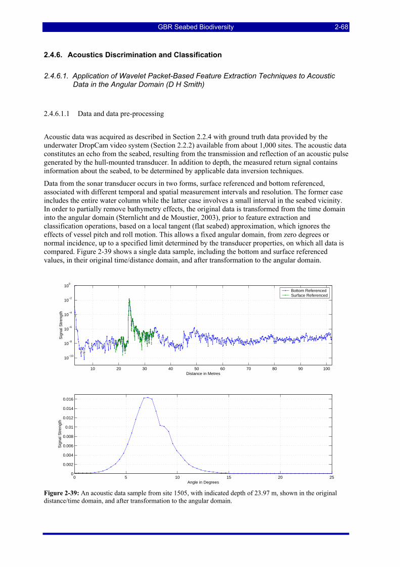
GBR Seabed Biodiversity 2-68
2.4.6. Acoustics Discrimination and Classification
2.4.6.1. Application of Wavelet Packet-Based Feature Extraction Techniques to Acoustic Data in the Angular Domain (D H Smith)
2.4.6.1.1 Data and data pre-processing
Acoustic data was acquired as described in Section 2.2.4 with ground truth data provided by the underwater DropCam video system (Section 2.2.2) available from about 1,000 sites. The acoustic data constitutes an echo from the seabed, resulting from the transmission and reflection of an acoustic pulse generated by the hull-mounted transducer. In addition to depth, the measured return signal contains information about the seabed, to be determined by applicable data inversion techniques.
Data from the sonar transducer occurs in two forms, surface referenced and bottom referenced, associated with different temporal and spatial measurement intervals and resolution. The former case includes the entire water column while the latter case involves a small interval in the seabed vicinity. In order to partially remove bathymetry effects, the original data is transformed from the time domain into the angular domain (Sternlicht and de Moustier, 2003), prior to feature extraction and classification operations, based on a local tangent (flat seabed) approximation, which ignores the effects of vessel pitch and roll motion. This allows a fixed angular domain, from zero degrees or normal incidence, up to a specified limit determined by the transducer properties, on which all data is compared. Figure 2-39 shows a single data sample, including the bottom and surface referenced values, in their original time/distance domain, and after transformation to the angular domain.
10 20 30 40 50 60 70 80 90 100
10−10
10−8
10−6
10−4
10−2
100
Distance in Metres
Sig
nal S
tren
gth
Bottom ReferencedSurface Referenced
0 5 10 15 20 250
0.002
0.004
0.006
0.008
0.01
0.012
0.014
0.016
Angle in Degrees
Sig
nal S
tren
gth
Figure 2-39: An acoustic data sample from site 1505, with indicated depth of 23.97 m, shown in the original distance/time domain, and after transformation to the angular domain.
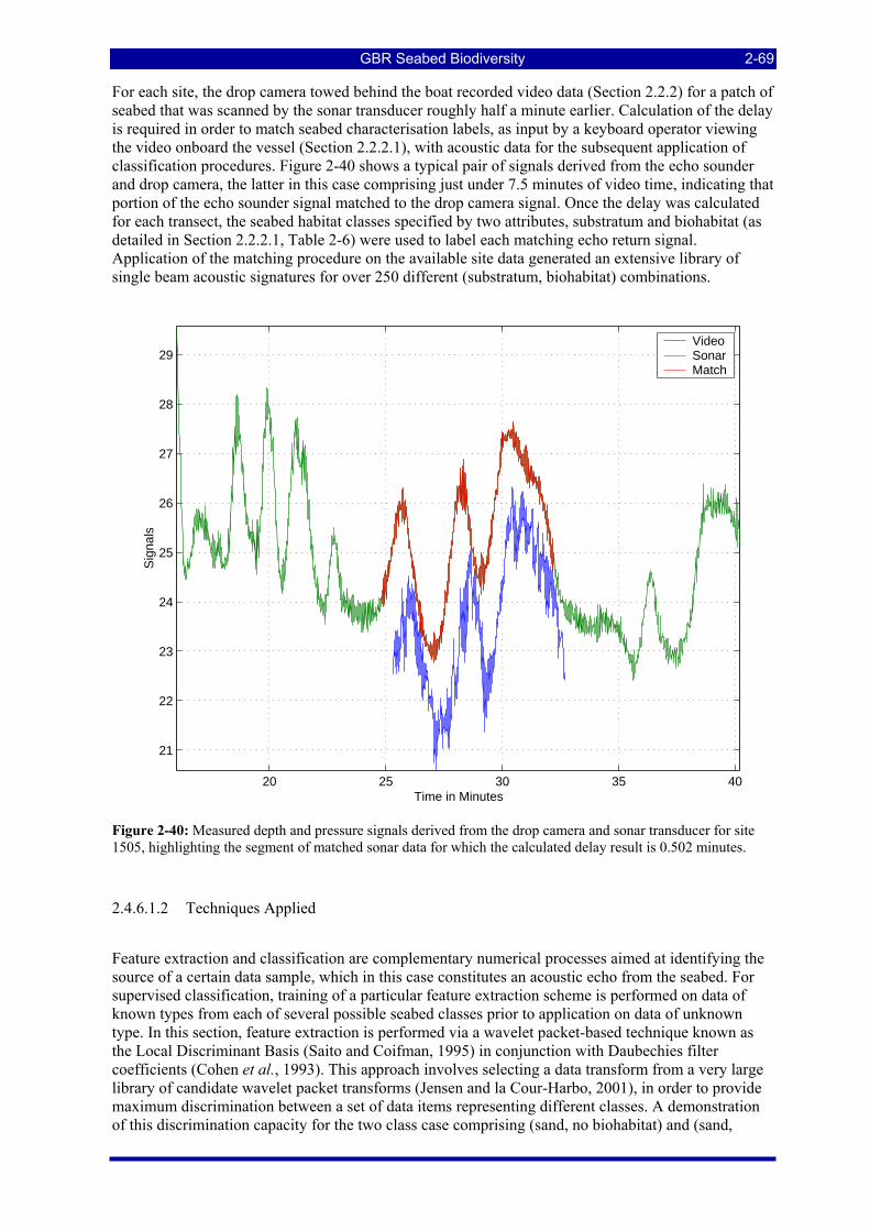
GBR Seabed Biodiversity 2-69
For each site, the drop camera towed behind the boat recorded video data (Section 2.2.2) for a patch of seabed that was scanned by the sonar transducer roughly half a minute earlier. Calculation of the delay is required in order to match seabed characterisation labels, as input by a keyboard operator viewing the video onboard the vessel (Section 2.2.2.1), with acoustic data for the subsequent application of classification procedures. Figure 2-40 shows a typical pair of signals derived from the echo sounder and drop camera, the latter in this case comprising just under 7.5 minutes of video time, indicating that portion of the echo sounder signal matched to the drop camera signal. Once the delay was calculated for each transect, the seabed habitat classes specified by two attributes, substratum and biohabitat (as detailed in Section 2.2.2.1, Table 2-6) were used to label each matching echo return signal. Application of the matching procedure on the available site data generated an extensive library of single beam acoustic signatures for over 250 different (substratum, biohabitat) combinations.
20 25 30 35 40
21
22
23
24
25
26
27
28
29
Time in Minutes
Sig
nals
VideoSonarMatch
Figure 2-40: Measured depth and pressure signals derived from the drop camera and sonar transducer for site 1505, highlighting the segment of matched sonar data for which the calculated delay result is 0.502 minutes.
2.4.6.1.2 Techniques Applied
Feature extraction and classification are complementary numerical processes aimed at identifying the source of a certain data sample, which in this case constitutes an acoustic echo from the seabed. For supervised classification, training of a particular feature extraction scheme is performed on data of known types from each of several possible seabed classes prior to application on data of unknown type. In this section, feature extraction is performed via a wavelet packet-based technique known as the Local Discriminant Basis (Saito and Coifman, 1995) in conjunction with Daubechies filter coefficients (Cohen et al., 1993). This approach involves selecting a data transform from a very large library of candidate wavelet packet transforms (Jensen and la Cour-Harbo, 2001), in order to provide maximum discrimination between a set of data items representing different classes. A demonstration of this discrimination capacity for the two class case comprising (sand, no biohabitat) and (sand,
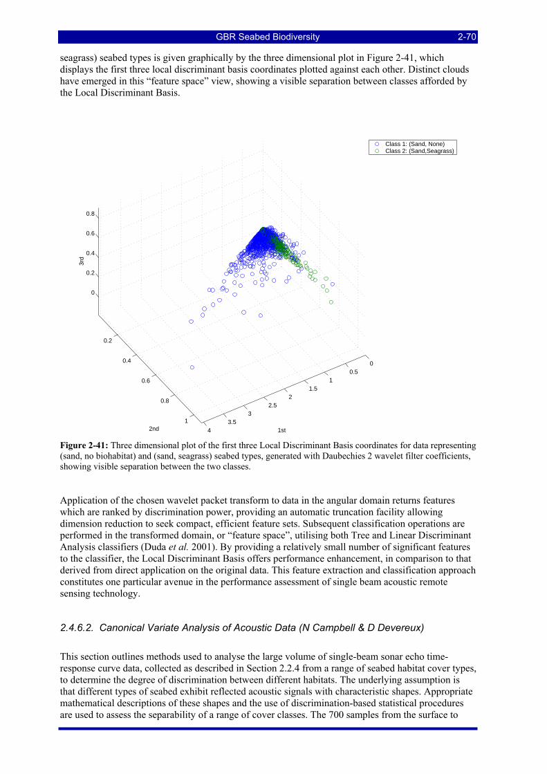
GBR Seabed Biodiversity 2-70
seagrass) seabed types is given graphically by the three dimensional plot in Figure 2-41, which displays the first three local discriminant basis coordinates plotted against each other. Distinct clouds have emerged in this “feature space” view, showing a visible separation between classes afforded by the Local Discriminant Basis.
00.5
11.5
22.5
33.5
4
0.2
0.4
0.6
0.8
1
0
0.2
0.4
0.6
0.8
1st2nd
3rd
Class 1: (Sand, None)Class 2: (Sand,Seagrass)
Figure 2-41: Three dimensional plot of the first three Local Discriminant Basis coordinates for data representing (sand, no biohabitat) and (sand, seagrass) seabed types, generated with Daubechies 2 wavelet filter coefficients, showing visible separation between the two classes.
Application of the chosen wavelet packet transform to data in the angular domain returns features which are ranked by discrimination power, providing an automatic truncation facility allowing dimension reduction to seek compact, efficient feature sets. Subsequent classification operations are performed in the transformed domain, or “feature space”, utilising both Tree and Linear Discriminant Analysis classifiers (Duda et al. 2001). By providing a relatively small number of significant features to the classifier, the Local Discriminant Basis offers performance enhancement, in comparison to that derived from direct application on the original data. This feature extraction and classification approach constitutes one particular avenue in the performance assessment of single beam acoustic remote sensing technology.
2.4.6.2. Canonical Variate Analysis of Acoustic Data (N Campbell & D Devereux)
This section outlines methods used to analyse the large volume of single-beam sonar echo time-response curve data, collected as described in Section 2.2.4 from a range of seabed habitat cover types, to determine the degree of discrimination between different habitats. The underlying assumption is that different types of seabed exhibit reflected acoustic signals with characteristic shapes. Appropriate mathematical descriptions of these shapes and the use of discrimination-based statistical procedures are used to assess the separability of a range of cover classes. The 700 samples from the surface to
GBR Seabed Biodiversity 2-71
beyond the 2nd echo are here called the pelagic data, and the 500 samples from 5 m above the bottom pick to 10 m below the bottom pick are called the bottom data.
The emphasis initially was on the complete volume of data, to assess the degree to which particular cover types could be consistently and accurately identified over the whole of the GBR. Some analyses of the degree of discrimination among cover classes from sites collected close together in time and hence geographically were also carried out.
The main data analysed here are for all groups of more than 100 contiguous echo responses from the same nominal class as identified from the ground-truth video data labels matched as per Section 2.4.6.1.1. There were 4519 such groups from 117 classes. Because of the sheer volume of data, the individual group means and pooled within-groups covariance matrix were calculated, after appropriate data normalisation.
2.4.6.2.1 Depth Normalisation
Prior to analysis, the acoustic data were depth-normalised to a constant depth so that signatures could be compared over the whole range of the data. This was done by taking the depth pick selection provided by the Simrad EY500 system, depthR, and resampling the echo time series to a constant set of depths. Specifically, the estimated depth in metres for a given sample time is calculated as:
deptht = (ts – 0.5 ) { ( re – rb ) / ns } + rb (1)
where ts denotes the sample time; rb is the beginning range of the echo sounder (that is, the echo sounder is set to commence sampling at the moment when an echo from depth rb would be received); re is the end range of the echo sounder (that is, the echo sounder is set to cease sampling at the moment when an echo from depth re would be received); and ns is the number of samples collected. The data are resampled by calculating the estimated depths for a range of sample times from 0 to 500, which give a depth of 0 metres at time 0, and a depth of depthR after 200 sample times, then using (1) to calculate the corresponding sample time on the observed scale, and using nearest neighbour or local smoothing such as bilinear or cubic to calculate the resampled values.
2.4.6.2.2 Data Normalisation
The profiles can be peak-aligned to remove one effect of depth.
Another correction considered is to remove the so-called “size” effect, and focus on differences in shape. This can be done by calculating a row mean (a simple measure of the average area under the curve), and subtracting this mean from all the values across an echo response curve.
Plots of the group means in Section 3.6.2.2 show that there was an obvious effect of depth on the shape of the group means; an attempt to remove this effect is made by regressing the echo response values against 1/depth.
2.4.6.2.3 Group Discrimination
An obvious approach to examine the discrimination between various seabed cover types is to base the analyses on a number of training groups, each one reasonably homogeneous, and representing a particular cover class. A canonical variate analysis (CVA) can be carried out to examine the degree and nature of the differences between the groups. The means and variances / correlations are calculated for each group. The group means are used to calculate a "between" matrix, B, and the variances / correlations to form a "within" matrix, W. Canonical vectors, c, are then calculated which maximise the ratio of the between-groups to within-groups sums of squares, f = ct B c / ct W c, for the canonical variate scores, ct x; f is referred to as the canonical root.
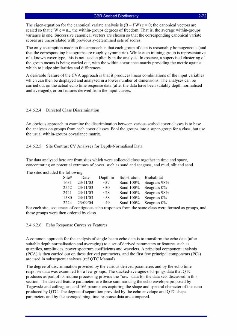
GBR Seabed Biodiversity 2-72
The eigen-equation for the canonical variate analysis is (B – f W) c = 0; the canonical vectors are scaled so that ct W c = nw, the within-groups degrees of freedom. That is, the average within-groups variance is one. Successive canonical vectors are chosen so that the corresponding canonical variate scores are uncorrelated with previously-determined sets of scores.
The only assumption made in this approach is that each group of data is reasonably homogeneous (and that the corresponding histograms are roughly symmetric). While each training group is representative of a known cover type, this is not used explicitly in the analysis. In essence, a supervised clustering of the group means is being carried out, with the within covariance matrix providing the metric against which to judge similarities and differences.
A desirable feature of the CVA approach is that it produces linear combinations of the input variables which can then be displayed and analysed in a lower number of dimensions. The analyses can be carried out on the actual echo time response data (after the data have been suitably depth normalised and averaged), or on features derived from the input curves.
2.4.6.2.4 Directed Class Discrimination
An obvious approach to examine the discrimination between various seabed cover classes is to base the analyses on groups from each cover classes. Pool the groups into a super-group for a class, but use the usual within-groups covariance matrix.
2.4.6.2.5 Site Contrast CV Analyses for Depth-Normalised Data
The data analysed here are from sites which were collected close together in time and space, concentrating on potential extremes of cover, such as sand and seagrass, and mud, silt and sand.
The sites included the following: Site# Date Depth m Substratum Biohabitat 1631 23/11/03 ~37 Sand 100% Seagrass 98% 2552 23/11/03 ~30 Sand 100% Seagrass 0% 2441 24/11/03 ~28 Sand 100% Seagrass 98% 1580 24/11/03 ~58 Sand 100% Seagrass 0% 2224 23/09/04 ~49 Sand 100% Seagrass 0%
For each site, sequences of contiguous echo responses from the same class were formed as groups, and these groups were then ordered by class.
2.4.6.2.6 Echo Response Curves vs Features
A common approach for the analysis of single-beam echo data is to transform the echo data (after suitable depth normalisation and averaging) to a set of derived parameters or features such as quantiles, amplitudes, power spectrum coefficients and wavelets. A principal component analysis (PCA) is then carried out on these derived parameters, and the first few principal components (PCs) are used in subsequent analyses (ref QTC Manual).
The degree of discrimination provided by the various derived parameters and by the echo time response data was examined for a few groups. The stacked-averages-of-5-pings data that QTC produces as part of its routine processing provide the “raw” data for the data sets discussed in this section. The derived feature parameters are those summarising the echo envelope proposed by Tegowski and colleagues, and 166 parameters capturing the shape and spectral character of the echo produced by QTC. The degree of separation provided by the echo envelope and QTC shape parameters and by the averaged ping time response data are compared.
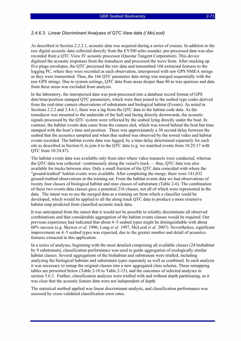
GBR Seabed Biodiversity 2-73
2.4.6.3. Linear Discriminant Analyses of QTC View data (I McLeod)
As described in Section 2.2.2.1, acoustic data was acquired during a series of cruises. In addition to the raw digital acoustic data collected directly from the EY500 echo sounder, pre-processed data was also recorded from a QTC View IV acoustic processor (Questar Tangent Corporation). This device digitised the acoustic responses from the transducer and processed the wave form. After stacking up five pings envelopes, the QTC processed the raw data and transmitted 166 extracted features to the logging PC, where they were recorded as each observation, interspersed with raw GPS NMEA strings as they were transmitted. Thus, the 166 QTC parameter data string was merged sequentially with the raw GPS strings. Due to system settings, QTC data from areas deeper than 80 m was spurious and data from these areas was excluded from analysis.
In the laboratory, the interspersed data was post-processed into a database record format of GPS date/time/position stamped QTC parameters, which were then joined to the seabed type codes derived from the real-time camera observations of substratum and biological habitat (Events). As noted in Sections 2.2.2 and 2.4.6.1, there was a lag from the QTC data to the habitat code data. As the transducer was mounted to the underside of the hull and facing directly downwards, the acoustic signals processed by the QTC system were reflected by the seabed lying directly under the boat. In contrast, the habitat events data came from the camera sled, which was towed behind the boat but time stamped with the boat’s time and position. There was approximately a 30 second delay between the seabed that the acoustics sampled and when that seabed was observed by the towed video and habitat events recorded. The habitat events data was lagged, by a time delay determined separately for each site as described in Section 0, to join it to the QTC data (e.g. we matched events from 10:25:17 with QTC from 10:24:47).
The habitat events data was available only from sites where video transects were conducted, whereas the QTC data was collected ~continuously along the vessel's track — thus, QTC data was also available for tracks between sites. Only a small fraction of the QTC data coincided with where the "ground-truthed" habitat events were available. After completing the merge, there were 141,032 ground-truthed observations in the training set. From the habitat events data we had observations of twenty four classes of biological habitat and nine classes of substratum (Table 2-6). The combination of these two events data classes gave a potential 216 classes, not all of which were represented in the data. The intent was to use the merged data as a training set from which a classifier could be developed, which would be applied to all the along track QTC data to produce a more extensive habitat map predicted from classified acoustic track data.
It was anticipated from the outset that it would not be possible to reliably discriminate all observed combinations and that considerable aggregation of the habitat events classes would be required. Our previous experience had indicated that about 4–5 seabed types might be distinguishable with about 60% success (e.g. Skewes et al. 1996; Long et al. 1997, McLeod et al. 2007). Nevertheless, significant improvement on 4–5 seabed types was expected, due to the greater number and detail of acoustics features extracted in this application.
In a series of analyses, beginning with the most detailed comprising all available classes (24 biohabitat by 9 substratum), classification performance was used to guide aggregation of ecologically similar habitat classes. Several aggregations of the biohabitat and substratum were trialled, including analysing the biological habitats and substratum types separately as well as combined. In each analysis it was necessary to remap the original classes into a new aggregated class schema. These remapping tables are presented below (Table 2-10 to Table 2-13), and the outcomes of selected analyses in section 3.6.3. Further, classification analyses were trialled with and without depth partitioning, as it was clear that the acoustic feature data were not independent of depth.
The statistical method applied was linear discriminant analysis, and classification performance was assessed by cross-validated classification error rates.
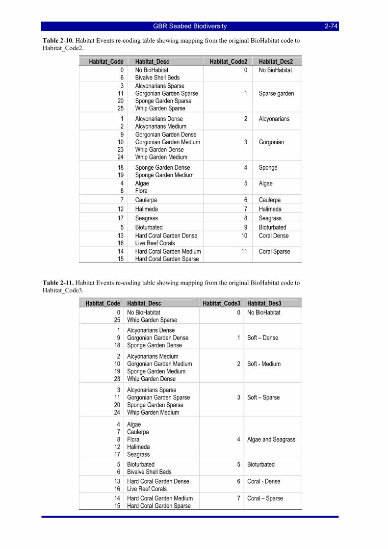
GBR Seabed Biodiversity 2-74
Table 2-10. Habitat Events re-coding table showing mapping from the original BioHabitat code to Habitat_Code2.
Habitat_Code Habitat_Desc Habitat_Code2 Habitat_Des2 0 6
No BioHabitat Bivalve Shell Beds
0
No BioHabitat
3 11 20 25
Alcyonarians Sparse Gorgonian Garden Sparse Sponge Garden Sparse Whip Garden Sparse
1
Sparse garden
1 2
Alcyonarians Dense Alcyonarians Medium
2
Alcyonarians
9 10 23 24
Gorgonian Garden Dense Gorgonian Garden Medium Whip Garden Dense Whip Garden Medium
3
Gorgonian
18 19
Sponge Garden Dense Sponge Garden Medium
4
Sponge
4 8
Algae Flora
5
Algae
7 Caulerpa 6 Caulerpa 12 Halimeda 7 Halimeda 17 Seagrass 8 Seagrass 5 Bioturbated 9 Bioturbated
13 16
Hard Coral Garden Dense Live Reef Corals
10
Coral Dense
14 15
Hard Coral Garden Medium Hard Coral Garden Sparse
11
Coral Sparse
Table 2-11. Habitat Events re-coding table showing mapping from the original BioHabitat code to Habitat_Code3.
Habitat_Code Habitat_Desc Habitat_Code3 Habitat_Des3 0
25 No BioHabitat Whip Garden Sparse
0
No BioHabitat
1 9
18
Alcyonarians Dense Gorgonian Garden Dense Sponge Garden Dense
1
Soft – Dense
2 10 19 23
Alcyonarians Medium Gorgonian Garden Medium Sponge Garden Medium Whip Garden Dense
2
Soft - Medium
3 11 20 24
Alcyonarians Sparse Gorgonian Garden Sparse Sponge Garden Sparse Whip Garden Medium
3
Soft – Sparse
4 7 8
12 17
Algae Caulerpa Flora Halimeda Seagrass
4
Algae and Seagrass
5 6
Bioturbated Bivalve Shell Beds
5
Bioturbated
13 16
Hard Coral Garden Dense Live Reef Corals
6
Coral - Dense
14 15
Hard Coral Garden Medium Hard Coral Garden Sparse
7
Coral – Sparse
GBR Seabed Biodiversity 2-75
Table 2-12. Substratum Events re-coding table showing mapping from the original Substratum code to Substratum_Code2
Substratum_Code Substratum_Desc Substratum_Code2 Substratum_Des2 1 Bedrock / Reef 1 Reef 2 Rocks (> 250 Mm) 2 Boulders 3 Stones (50-250 Mm) 3 Cobbles 4 Rubble (5-50 Mm) 4 Gravel 5 6 7
Coarse Sand Fine Sand Sand Waves
5
Sand
8 Silt 6 Silt 9 Mud 7 Mud
Table 2-13. Substratum Events re-coding table showing mapping from the original Substratum code to Substratum_Code3.
Substratum_Code Substratum_Desc Substratum_Code3 Substratum_Des3 1 Bedrock / Reef 1 Reef 2 Rocks (> 250 mm) 2 Boulders 3 Stones (50-250 mm) 3 Cobbles 4 Rubble (5-50 mm) 4 Gravel 5 6 8
Coarse Sand Fine Sand Silt
5
Sand Silt
9 Mud 6 Mud 7 Sand Waves 7 Sand Waves
2.4.7. Ecological Risk Indicators
A progressive series of indicators of exposure to trawling have been estimated for habitat types, seabed assemblages (predicted sites groups), species-groups and selected individual species. This series includes:
1. estimates of the percentage by area of the distribution of each habitat, assemblage, species-group and individual species, located in areas open to trawling under zoning or other management — without account of the distribution of trawl effort.
2. estimates of the percentage by area of the distribution of each habitat, assemblage, species-group and individual species, located in areas where trawl effort is present — without account of the intensity of trawl effort.
3. estimates of the percentage by area of the distribution of each habitat, assemblage, species-group and individual species, located in areas where trawl effort is present taking account of the intensity of trawl effort.
For species-groups and selected individual species, predicted biomass distributions have been estimated (Sections 2.4.2 and 2.4.3) and biomass related indices can be estimated.
4. estimates of the percentage of biomass of the distribution of each species-group and individual species, located in areas open to trawling under zoning or other management — without account of the distribution of trawl effort.
5. estimates of the percentage of biomass of the distribution of each species-group and individual species, located in areas where trawl effort is present — without account of the intensity of trawl effort.
GBR Seabed Biodiversity 2-76
6. estimates of the percentage of biomass of the distribution of each species-group and individual species, located in areas where trawl effort is present taking account of the intensity of trawl effort.
The intensity of trawl effort was taken into account as a coverage of the study’s 0.01 degree grid cells as if trawling were conducted uniformly at that fine scale. Given the typical swept width of gear and speed of trawling for prawns in the region, approximately 8 hours of trawling would be required to have a 1× coverage of a 0.01 degree grid cell. Similarly, 4 hours would have a 0.5× coverage and 16 hours would have a 2× coverage. A given grid cell’s contribution to the overall index was the estimated proportion by area or biomass of the respective biological attribute, multiplied by the estimated effort coverage; these estimates for grid cells were summed to provide the overall index for the GBR region. The effort intensity information for each grid cell was provided by spatial processing of the 2005 fishery Vessel Monitoring System (VMS) data by Norm Good, QDPI&F (Gribble et al. 2007). The year 2005 was the first full year post the re-zoning of the GBR Marine Park, which came into effect on 1 July 2004.
Exposure to trawl effort may present varying levels of risk for different species depending on how effectively the trawl net catches any given species (catchability), or how much mortality is caused as a result of contact with the net. For example, a species that lives well down in the sediment, or one that moves up into the water column during the night, is unlikely to be directly affected by the pass of a trawl net. On the other hand, a slow moving species that lives less a metre from the seabed may be very effectively caught by a prawn trawl net. For species estimated to have higher levels of exposure, information on relative catchability was sought wherever possible. This study was able to provide relative catch rate information between the research trawl and the epibenthic sled (Section 2.4.2). Wherever the sampling rate of the research trawl was less than the epibenthic sled, the prawn trawl was considered to catch that fraction (0-1) of the population present during a pass of the net. Wherever the trawl had a higher catch rate, the prawn trawl was considered to a relative catch rate of 1. Similar information was available from the GBR Effects of Trawling Study (Poiner et al., 1998), including prawn trawl catch rates relative to those of a fish trawl. Information on the possible impact on species remaining on the seabed was available from the GBR Effects of Trawling Recovery Dynamics Project (Pitcher et al., 2004) and the Northern Prawn Fishery Effects of Trawling Project (Haywood et al., 2005). If evidence was available that could demonstrate that catchability or mortality was <1, this information could reduce the estimated percentage of the biomass of a species exposed in indicator 6 above — i.e. an estimate of the proportion of the total population caught.
Further, the Queensland trawl fishery is required by legislation to have turtle excluder devices (TEDs) and bycatch reduction devices (BRDs) installed in their nets. TEDs are very effective in allowing larger animals such as turtles, rays and sharks to pass out of the trawl net, greatly reducing mortality (Robins-Troeger et al. 1995; Robins & McGilvray 1999). BRDs provide escape opportunities for smaller fish and reduce the catch rate of non-target species (bycatch) by varying amounts depending on the species — over all species and different sectors of the industry, the average reduction achieved by BRDs is about 8% (Courtney et al. FRDC 2000/170 Report 2006), though greater reductions are possible (Courtney et al. 2006). If evidence (from these or other sources, e.g. Brewer et al. 1998) was available that demonstrated that TEDs and/or BRDs further reduce catchability or mortality, this information further reduced the estimated percentage of the biomass of a species exposed in indicator 6 above — again, reducing the estimate of the proportion of the total population caught.
Exposure to trawling, leading to estimates of the potential proportion of species populations caught annually is only one axis of vulnerability to trawling. The second axis is the ability of the species to recover from any reductions in population size. A species with a high recovery rate can sustain higher levels of incidental catch than a species with a low recovery rate. Previous ecological risk assessment methods that take this axis into consideration include susceptibility-recovery analysis (SRA) — a qualitative ranking approach (Stobutzki et al. 2001, see also Griffiths et al. 2006) — and sustainability assessment for fishing effects (SAFE) — a quantitative approach where estimated fishing mortality is compared against reference points of estimated natural mortality (e.g. 0.8M = maximum sustainable mortality) (Brewer et al. 2007; Zhou & Griffiths 2007). For species estimated herein to have higher exposure to trawling, information about the recovery axis was obtained, where available, for mean recovery attribute ranks from SRA analyses in northern Australia (e.g. additive ranks of probability of breeding before capture, maximum size, reproductive strategy, hermaphrodism for fishes (Stobutzki et
GBR Seabed Biodiversity 2-77
al. 2001) and invertebrates (Hill et al. 2002)) and for estimated natural mortality to calculate a sustainability indicator in a manner analogous to the reference points of Zhou & Griffiths (2007). These reference points were based on the Schaffer surplus production model, where for a population at maximum sustainable yield (MSY), fishing mortality (F) is equal to natural mortality (M), that is F/M=1. This is regarded as a limit reference point and should not be exceeded. Zhou & Griffiths (2007) consider reviews of exploited species that suggest F=0.8M (≡ F/M=0.8) is a more conservation reference point, and Gulland (1983) suggested a conservative MSY of 0.3MB0 in data limited situations, which (as BMSY = 0.5B0) corresponds to F/M=0.6. These three reference points are considered in this report. Where exploitation is low, F is approximately equal to exploitation — the estimated proportion of the total population caught — thus, the indicator calculated herein is exploitation divided by natural mortality. Note that this method is only a ‘discrete time’ approximation, it is not an ‘instantaneous time’ stock assessment, and becomes increasingly uncertain with higher levels of exploitation and/or natural mortality (Hilborn & Walters 1992).
A further indicator of potential ecological risk is available from the biophysical modelling (Section 2.4.2). If the trawl effort covariate was selected by the statistical modelling of any species, possibly in addition to other environmental variables such as sediment type, the sign and significance of the coefficient was examined. Further, in order to examine the regional implications of an included trawl effort term, a prediction of the biomass was made with the trawl covariate set to zero throughout the region. This estimate was then contrasted with the biomass prediction for the actual current situation to estimate how much smaller, or larger (in the case of positive effects), the species population may be as a result of incidental trawl catches over the history of the fishery. It is important to note here that many of the physical covariates are correlated and it may not be possible to interpret model coefficients as causal effects. In the case of target species in particular, a positive trawl coefficient could indicate that the effort data — reflecting the searching ability of the fishers — are a good indicator of the sampled distribution, of say commercial prawns, at a scale finer than that of spatial patterns in the physical environmental data, rather than indicating that prawns are more abundant because of trawling.
2.4.8. Trawl Management Scenario Model (N Ellis, A Welna, R Pitcher)
A dynamic model was applied to assess the effects of several major management interventions, which were implemented between the years 2000 and 2006, on benthic fauna — particularly sessile benthic fauna that were the focus of experiments on trawl depletion rates (Poiner et al. 1998, Burridge et al. 2003) and subsequent recovery (Pitcher et al. 2004). The management interventions included two large-scale closures comprising the 2000/2001 low-effort areas closure and the 2004 representative areas program (RAP) re-zoning of the GBR; two effort reductions comprising a major buy-back effective in 2001 and another RAP-associated buy-back effective in 2005; and a progressive penalty system operating between the latter two. The dynamic model applied depletion and recovery parameters estimated from previous experiments and annual trawl effort as provided by industry and management data to estimate the relative status of fauna in model grid cells of 6 minute resolution. The model was run with and without the effects on effort of each management intervention. The relative status estimates were combined with the abundance distributions available from the current project in order to estimate the regional absolute status of these fauna.
2.4.8.1. Specification of the management scenarios
We wanted to test the effect of the management interventions that had been applied over the period 2001–2005. We took as a baseline the ‘status quo’ scenario (SQ2001) from the view-point of the pre-2001 fishery; i.e. we projected from 2001 to 2025 assuming the fishing effort remained at year-2000 levels. We then constructed a sequence of scenarios in which each intervention was included progressively: the 2001 closure (CL2001); the 2001 buyback (BB2001); penalties on trading effort units (P); the 2004 RAP closure (RAP); and the 2005 buyback (BB2005).
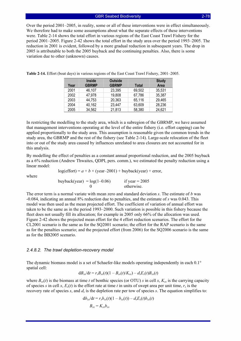
GBR Seabed Biodiversity 2-78
Over the period 2001–2005, in reality, some or all of these interventions were in effect simultaneously. We therefore had to make some assumptions about what the separate effects of these interventions were. Table 2-14 shows the total effort in various regions of the East Coast Trawl Fishery for the period 2001–2005. Figure 2-42 shows the total effort in the study area over the period 1993–2005. The reduction in 2001 is evident, followed by a more gradual reduction in subsequent years. The drop in 2005 is attributable to both the 2005 buyback and the continuing penalties. Also, there is some variation due to other (unknown) causes.
Table 2-14. Effort (boat days) in various regions of the East Coast Trawl Fishery, 2001–2005.
Year Inside
GBRMP Outside GBRMP Total
Study Area
2001 46,107 23,395 69,502 35,531 2002 47,978 19,808 67,786 35,387 2003 44,753 20,363 65,116 29,465 2004 40,162 23,447 63,609 28,236 2005 34,562 21,813 58,380 24,621
In restricting the modelling to the study area, which is a subregion of the GBRMP, we have assumed that management interventions operating at the level of the entire fishery (i.e. effort capping) can be applied proportionally to the study area. This assumption is reasonable given the common trends in the study area, the GBRMP and the rest of the fishery (see Table 2-14). Large-scale relocation of the fleet into or out of the study area caused by influences unrelated to area closures are not accounted for in this analysis.
By modelling the effect of penalties as a constant annual proportional reduction, and the 2005 buyback as a 6% reduction (Andrew Thwaites, QDPI, pers. comm.), we estimated the penalty reduction using a linear model:
log(effort) = a + b × (year–2001) + buyback(year) + error, where
buyback(year) = log(1–0.06) if year = 2005 0 otherwise.
The error term is a normal variate with mean zero and standard deviation s. The estimate of b was -0.084, indicating an annual 8% reduction due to penalties, and the estimate of s was 0.043. This model was then used as the mean projected effort. The coefficient of variation of annual effort was taken to be the same as in the period 1993–2000. Such variation is possible in this fishery because the fleet does not usually fill its allocation; for example in 2005 only 66% of the allocation was used. Figure 2-42 shows the projected mean effort for the 4 effort reduction scenarios. The effort for the CL2001 scenario is the same as for the SQ2001 scenario; the effort for the RAP scenario is the same as for the penalties scenario; and the projected effort (from 2006) for the SQ2006 scenario is the same as for the BB2005 scenario.
2.4.8.2. The trawl depletion-recovery model
The dynamic biomass model is a set of Schaefer-like models operating independently in each 0.1° spatial cell:
dBsx/dt = rsBsx(t)(1 – Bsx(t)/Ksx) – dsEx(t)Bsx(t)
where Bsx(t) is the biomass at time t of benthic species (or OTU) s in cell x, Ksx is the carrying capacity of species s in cell x, Ex(t) is the effort rate at time t in units of swept area per unit time, rs is the recovery rate of species s, and ds is the depletion rate per tow of species s. The equation simplifies to:
dbsx/dt = rsbsx(t)(1 – bsx(t)) – dsEx(t)bsx(t)
Bsx = Ksxbsx
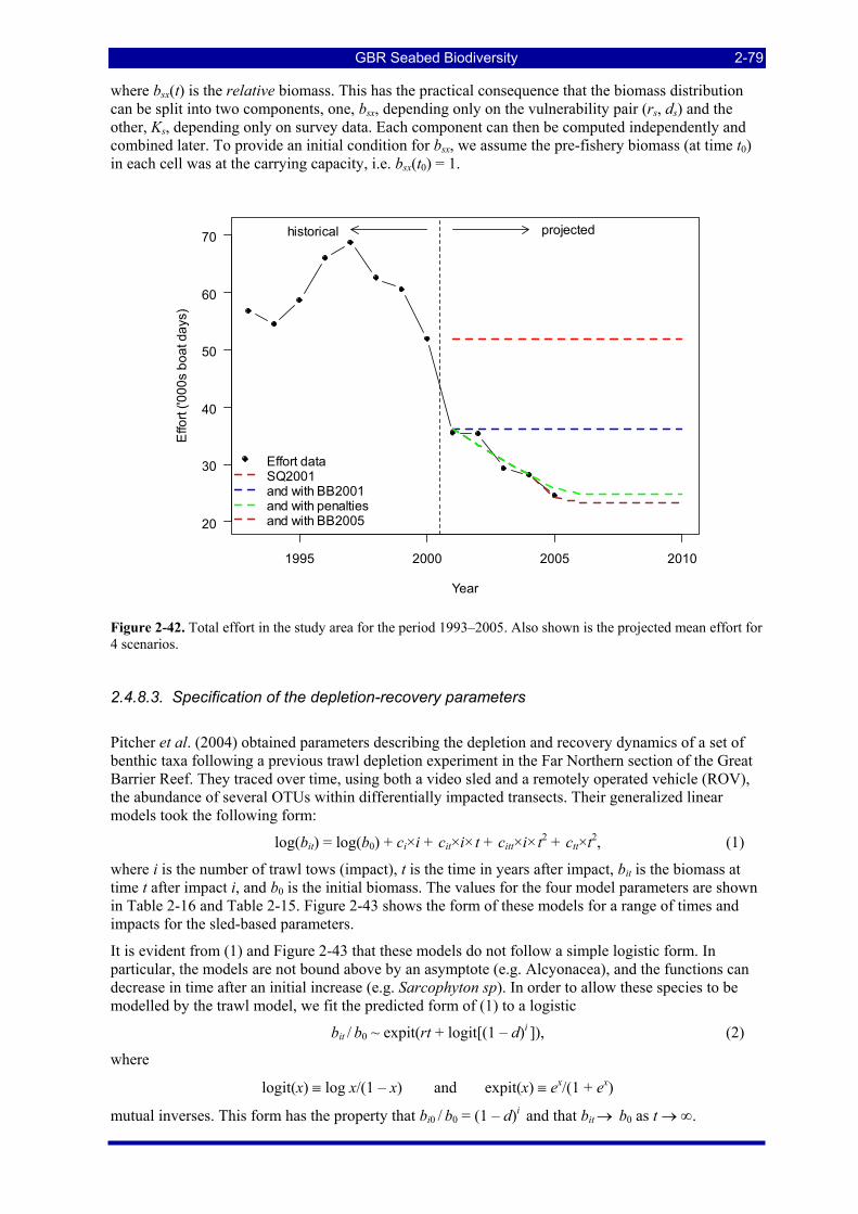
GBR Seabed Biodiversity 2-79
where bsx(t) is the relative biomass. This has the practical consequence that the biomass distribution can be split into two components, one, bsx, depending only on the vulnerability pair (rs, ds) and the other, Ks, depending only on survey data. Each component can then be computed independently and combined later. To provide an initial condition for bsx, we assume the pre-fishery biomass (at time t0) in each cell was at the carrying capacity, i.e. bsx(t0) = 1.
1995 2000 2005 2010
20
30
40
50
60
70
Year
Effo
rt ('0
00s
boat
day
s)
historical projected
Effort dataSQ2001and with BB2001and with penaltiesand with BB2005
Figure 2-42. Total effort in the study area for the period 1993–2005. Also shown is the projected mean effort for 4 scenarios.
2.4.8.3. Specification of the depletion-recovery parameters
Pitcher et al. (2004) obtained parameters describing the depletion and recovery dynamics of a set of benthic taxa following a previous trawl depletion experiment in the Far Northern section of the Great Barrier Reef. They traced over time, using both a video sled and a remotely operated vehicle (ROV), the abundance of several OTUs within differentially impacted transects. Their generalized linear models took the following form:
log(bit) = log(b0) + ci×i + cit×i×t + citt×i×t2 + ctt×t2, (1)
where i is the number of trawl tows (impact), t is the time in years after impact, bit is the biomass at time t after impact i, and b0 is the initial biomass. The values for the four model parameters are shown in Table 2-16 and Table 2-15. Figure 2-43 shows the form of these models for a range of times and impacts for the sled-based parameters.
It is evident from (1) and Figure 2-43 that these models do not follow a simple logistic form. In particular, the models are not bound above by an asymptote (e.g. Alcyonacea), and the functions can decrease in time after an initial increase (e.g. Sarcophyton sp). In order to allow these species to be modelled by the trawl model, we fit the predicted form of (1) to a logistic
bit / b0 ~ expit(rt + logit[(1 – d)i ]), (2)
where
logit(x) ≡ log x/(1 – x) and expit(x) ≡ ex/(1 + ex)
mutual inverses. This form has the property that bi0 / b0 = (1 – d)i and that bit → b0 as t → ∞.
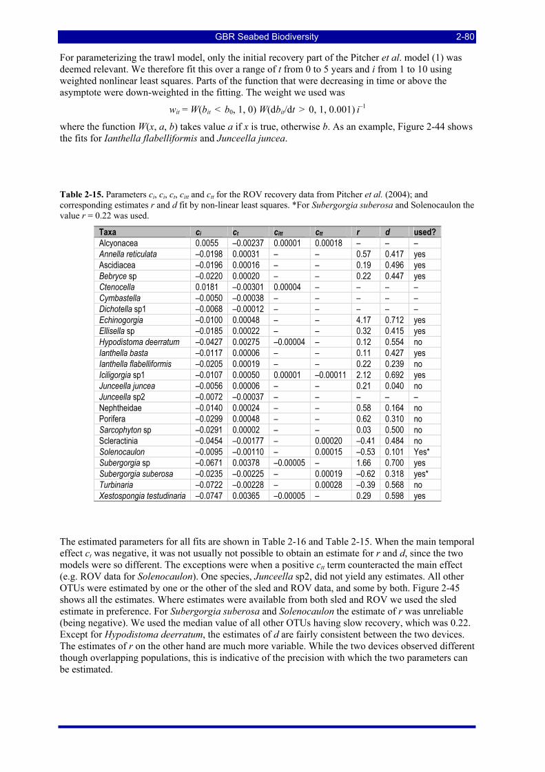
GBR Seabed Biodiversity 2-80
For parameterizing the trawl model, only the initial recovery part of the Pitcher et al. model (1) was deemed relevant. We therefore fit this over a range of t from 0 to 5 years and i from 1 to 10 using weighted nonlinear least squares. Parts of the function that were decreasing in time or above the asymptote were down-weighted in the fitting. The weight we used was
wit = W(bit < b0, 1, 0) W(dbit/dt > 0, 1, 0.001) i–1
where the function W(x, a, b) takes value a if x is true, otherwise b. As an example, Figure 2-44 shows the fits for Ianthella flabelliformis and Junceella juncea.
Table 2-15. Parameters ci, ci, ct, citt and ctt for the ROV recovery data from Pitcher et al. (2004); and corresponding estimates r and d fit by non-linear least squares. *For Subergorgia suberosa and Solenocaulon the value r = 0.22 was used.
Taxa ci ct citt ctt r d used? Alcyonacea 0.0055 –0.00237 0.00001 0.00018 – – – Annella reticulata –0.0198 0.00031 – – 0.57 0.417 yes Ascidiacea –0.0196 0.00016 – – 0.19 0.496 yes Bebryce sp –0.0220 0.00020 – – 0.22 0.447 yes Ctenocella 0.0181 –0.00301 0.00004 – – – – Cymbastella –0.0050 –0.00038 – – – – – Dichotella sp1 –0.0068 –0.00012 – – – – – Echinogorgia –0.0100 0.00048 – – 4.17 0.712 yes Ellisella sp –0.0185 0.00022 – – 0.32 0.415 yes Hypodistoma deerratum –0.0427 0.00275 –0.00004 – 0.12 0.554 no Ianthella basta –0.0117 0.00006 – – 0.11 0.427 yes Ianthella flabelliformis –0.0205 0.00019 – – 0.22 0.239 no Iciligorgia sp1 –0.0107 0.00050 0.00001 –0.00011 2.12 0.692 yes Junceella juncea –0.0056 0.00006 – – 0.21 0.040 no Junceella sp2 –0.0072 –0.00037 – – – – – Nephtheidae –0.0140 0.00024 – – 0.58 0.164 no Porifera –0.0299 0.00048 – – 0.62 0.310 no Sarcophyton sp –0.0291 0.00002 – – 0.03 0.500 no Scleractinia –0.0454 –0.00177 – 0.00020 –0.41 0.484 no Solenocaulon –0.0095 –0.00110 – 0.00015 –0.53 0.101 Yes* Subergorgia sp –0.0671 0.00378 –0.00005 – 1.66 0.700 yes Subergorgia suberosa –0.0235 –0.00225 – 0.00019 –0.62 0.318 yes* Turbinaria –0.0722 –0.00228 – 0.00028 –0.39 0.568 no Xestospongia testudinaria –0.0747 0.00365 –0.00005 – 0.29 0.598 yes
The estimated parameters for all fits are shown in Table 2-16 and Table 2-15. When the main temporal effect ct was negative, it was not usually not possible to obtain an estimate for r and d, since the two models were so different. The exceptions were when a positive ctt term counteracted the main effect (e.g. ROV data for Solenocaulon). One species, Junceella sp2, did not yield any estimates. All other OTUs were estimated by one or the other of the sled and ROV data, and some by both. Figure 2-45 shows all the estimates. Where estimates were available from both sled and ROV we used the sled estimate in preference. For Subergorgia suberosa and Solenocaulon the estimate of r was unreliable (being negative). We used the median value of all other OTUs having slow recovery, which was 0.22. Except for Hypodistoma deerratum, the estimates of d are fairly consistent between the two devices. The estimates of r on the other hand are much more variable. While the two devices observed different though overlapping populations, this is indicative of the precision with which the two parameters can be estimated.
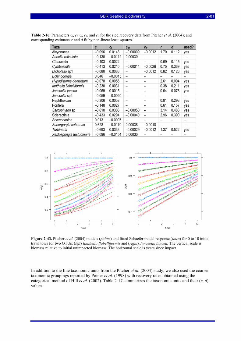
GBR Seabed Biodiversity 2-81
Table 2-16. Parameters ci, ci, ct, citt and ctt for the sled recovery data from Pitcher et al. (2004); and corresponding estimates r and d fit by non-linear least squares.
Taxa ci ct citt ctt r d used? Alcyonacea –0.096 0.0143 –0.00009 –0.0012 1.70 0.112 yes Annella reticulata –0.130 –0.0112 0.00030 – – – – Ctenocella –0.103 0.0022 – – 0.69 0.115 yes Cymbastella –0.413 0.0210 –0.00014 –0.0026 0.75 0.369 yes Dichotella sp1 –0.080 0.0088 – –0.0012 0.82 0.128 yes Echinogorgia 0.046 –0.0015 – – – – – Hypodistoma deerratum –0.078 0.0056 – – 2.61 0.094 yes Ianthella flabelliformis –0.230 0.0031 – – 0.38 0.211 yes Junceella juncea –0.069 0.0015 – – 0.64 0.078 yes Junceella sp2 –0.059 –0.0020 – – – – – Nephtheidae –0.306 0.0058 – – 0.81 0.293 yes Porifera –0.148 0.0027 – – 0.61 0.157 yes Sarcophyton sp –0.610 0.0386 –0.00050 – 3.14 0.483 yes Scleractinia –0.433 0.0294 –0.00040 – 2.96 0.390 yes Solenocaulon 0.013 –0.0007 – – – – – Subergorgia suberosa 0.628 –0.0170 0.00038 –0.0018 – – – Turbinaria –0.693 0.0333 –0.00029 –0.0012 1.37 0.522 yes Xestospongia testudinaria –0.096 –0.0154 0.00030 – – – –
Figure 2-43. Pitcher et al. (2004) models (points) and fitted Schaefer model response (lines) for 0 to 10 initial trawl tows for two OTUs: (left) Ianthella flabelliformis and (right) Junceella juncea. The vertical scale is biomass relative to initial unimpacted biomass. The horizontal scale is years since impact.
In addition to the fine taxonomic units from the Pitcher et al. (2004) study, we also used the coarser taxonomic groupings reported by Poiner et al. (1998) with recovery rates obtained using the categorical method of Hill et al. (2002). Table 2-17 summarizes the taxonomic units and their (r, d) values.
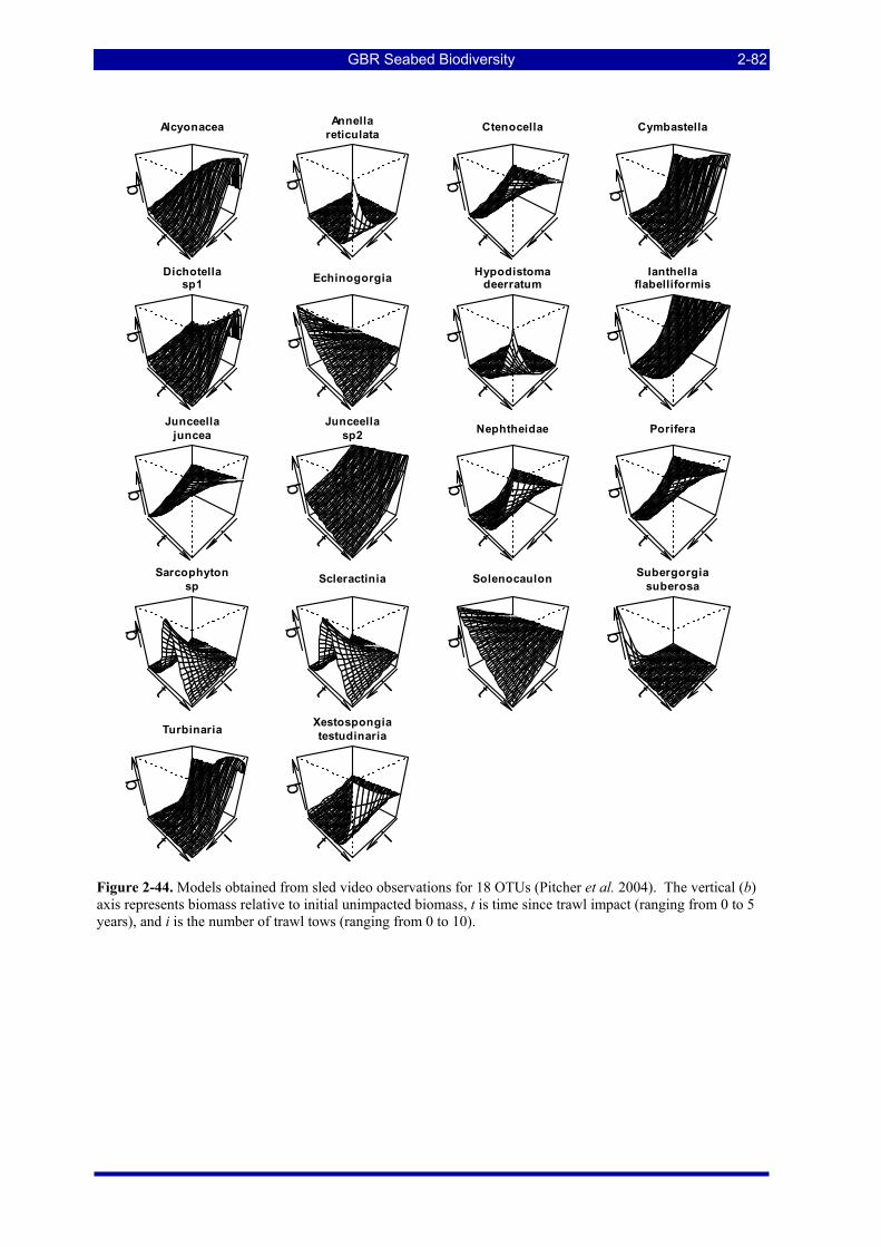
GBR Seabed Biodiversity 2-82
it
b
Alcyonacea
it
b
Annellareticulata
it
b
Ctenocella
itb
Cymbastella
it
b
Dichotellasp1
it
b
Echinogorgia
it
b
Hypodistomadeerratum
it
bIanthella
flabelliformis
it
b
Junceellajuncea
it
b
Junceellasp2
it
bNephtheidae
it
b
Porifera
it
b
Sarcophytonsp
it
bScleractinia
it
b
Solenocaulon
it
b
Subergorgiasuberosa
it
bTurbinaria
it
b
Xestospongiatestudinaria
Figure 2-44. Models obtained from sled video observations for 18 OTUs (Pitcher et al. 2004). The vertical (b) axis represents biomass relative to initial unimpacted biomass, t is time since trawl impact (ranging from 0 to 5 years), and i is the number of trawl tows (ranging from 0 to 10).
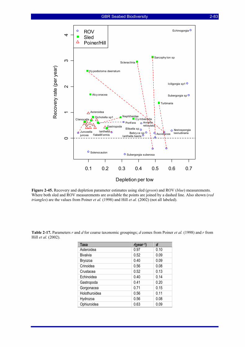
GBR Seabed Biodiversity 2-83
0.1 0.2 0.3 0.4 0.5 0.6 0.7
01
23
4
Depletion per tow
Rec
over
y ra
te (p
er y
ear)
ROVSledPoiner/Hill
Asteroidea
Gastropoda
Ascidiacea
Porif era
Solenocaulon Subergorgia suberosa
Xestospongia testudinaria Junceella
juncea
Annella reticulata
Alcy onacea
Cy mbastella Dichotella sp1
Hy podistoma deerratum
Nephtheidae
Sarcophy ton sp
Turbinaria
Echinogorgia
Ianthella basta
Iciligorgia sp1
Subergorgia sp
Bebry ce sp Ianthella f labellif ormis
Ellisella sp
Ctenocella
Scleractinia
Figure 2-45. Recovery and depletion parameter estimates using sled (green) and ROV (blue) measurements. Where both sled and ROV measurements are available the points are joined by a dashed line. Also shown (red triangles) are the values from Poiner et al. (1998) and Hill et al. (2002) (not all labeled).
Table 2-17. Parameters r and d for coarse taxonomic groupings; d comes from Poiner et al. (1998) and r from Hill et al. (2002).
Taxa r(year–1) d Asteroidea 0.97 0.10 Bivalvia 0.52 0.09 Bryozoa 0.40 0.09 Crinoidea 0.56 0.08 Crustacea 0.52 0.13 Echinoidea 0.40 0.14 Gastropoda 0.41 0.20 Gorgonacea 0.71 0.15 Holothuroidea 0.56 0.11 Hydrozoa 0.56 0.08 Ophiuroidea 0.63 0.09
GBR Seabed Biodiversity 2-84
2.4.8.4. Specification of the pristine biomass model
In Sections 2.4.2 and 3.2, single-species (or single-OTU) models have been built and density predictions laid on the fine scale spatial grid providing maps. The density predictions are on physical environmental and spatial covariates, under optimal settings of temporal covariates (time of day, time of year, phase of moon). They are also relative to the unknown catchability, which is assumed to be constant.
These models can also be used to predict the pristine density over the area of the fishery. This is done by predicting using the optimal covariable settings as before and setting the trawl effort predictor, where selected, to zero. The result is then the predicted density taking into account the physical covariates but in the absence of trawling, i.e. the pristine pre-fishery density. The prediction of pristine density at a trawled site is based on the observed density at sites having similar physical attributes away from trawled areas.
For OTUs having no trawl predictor in their model, the pristine biomass prediction is the same as the current prediction of section 2.4.3. Such OTUs should either have little overlap with trawled areas (for reasons of habitat independently of trawl distribution) or have high resilience to trawling due to high r or low d or both.
Some OTUs had a negative trawl effort coefficient in the linear predictor of either the presence-absence GLM or the biomass GLM. OTUs where these were either statistically significant or of large effect were Carijoa sp1, Dendronephthya spp, Echinogorgia sp3 and sp5, Euplexaura sp6, Iciligorgia sp1, Mopsella sp2 and several Demospongiae taxa. From the list of trawl exposed species in Section 3.7.2, Alertigorgia orientalis, Subergorgia suberosa and several Demospongiae (including Ircinia 1255 and Ircinia 2710) were identified.
For several of these species, specific r and d estimates were not available from the recovery study so estimates were used from morphologically and taxonomically related species. The choices are listed in section A2 of Table 2-18. Some taxa were identified only to the genus level. Where possible these were linked to the (r, d) values of the same genus (Table 2-18, section B1); for Dendronephthya spp the family Nephtheidae was used.
We also modelled the impact of trawling on coarse taxonomic groupings (family and higher) by summing the available pristine biomass models of all taxa within each grouping, and using the (r, d) values either from Pitcher et al. (2004) or from Poiner et al. (1998) and Hill et al. (2002) (Table 2-18, section C). A GLM model of predicted distribution was not available for all OTUs; MSE results are presented only for those that did.
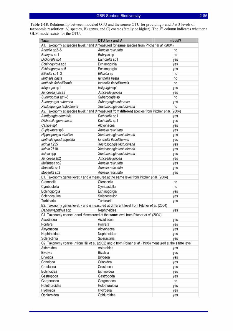
GBR Seabed Biodiversity 2-85
Table 2-18. Relationship between modeled OTU and the source OTU for providing r and d at 3 levels of taxonomic resolution: A) species, B) genus, and C) coarse (family or higher). The 3rd column indicates whether a GLM model exists for the OTU.
Taxa OTU for r and d model? A1. Taxonomy at species level: r and d measured for same species from Pitcher et al. (2004) Annella sp2–6 Annella reticulata no Bebryce sp1 Bebryce sp no Dichotella sp1 Dichotella sp1 yes Echinogorgia sp3 Echinogorgia yes Echinogorgia sp5 Echinogorgia yes Ellisella sp1–3 Ellisella sp no Ianthella basta Ianthella basta no Ianthella flabelliformis Ianthella flabelliformis no Iciligorgia sp1 Iciligorgia sp1 yes Junceella juncea Junceella juncea yes Subergorgia sp1–6 Subergorgia sp no Subergorgia suberosa Subergorgia suberosa yes Xestospongia testudinaria Xestospongia testudinaria no A2. Taxonomy at species level: r and d measured from different species from Pitcher et al. (2004) Alertigorgia orientalis Dichotella sp1 yes Dichotella gemmacea Dichotella sp1 yes Carijoa sp1 Alcyonacea yes Euplexaura sp6 Annella reticulata yes Hippospongia elastica Xestospongia testudinaria yes Ianthella quadrangulata Ianthella flabelliformis yes Ircinia 1255 Xestospongia testudinaria yes Ircinia 2710 Xestospongia testudinaria yes Ircinia spp Xestospongia testudinaria yes Junceella sp2 Junceella juncea yes Melithaea sp2 Annella reticulata yes Mopsella sp1 Annella reticulata yes Mopsella sp2 Annella reticulata yes B1. Taxonomy genus level: r and d measured at the same level from Pitcher et al. (2004) Ctenocella Ctenocella no Cymbastella Cymbastella no Echinogorgia Echinogorgia yes Solenocaulon Solenocaulon yes Turbinaria Turbinaria yes B2. Taxonomy genus level: r and d measured at different level from Pitcher et al. (2004) Dendronephthya spp Nephtheidae yes C1. Taxonomy coarse: r and d measured at the same level from Pitcher et al. (2004) Ascidiacea Ascidiacea yes Porifera Porifera yes Alcyonacea Alcyonacea yes Nephtheidae Nephtheidae yes Scleractinia Scleractinia yes C2. Taxonomy coarse: r from Hill et al. (2002) and d from Poiner et al. (1998) measured at the same level Asteroidea Asteroidea yes Bivalvia Bivalvia yes Bryozoa Bryozoa yes Crinoidea Crinoidea yes Crustacea Crustacea yes Echinoidea Echinoidea yes Gastropoda Gastropoda yes Gorgonacea Gorgonacea no Holothuroidea Holothuroidea yes Hydrozoa Hydrozoa yes Ophiuroidea Ophiuroidea yes
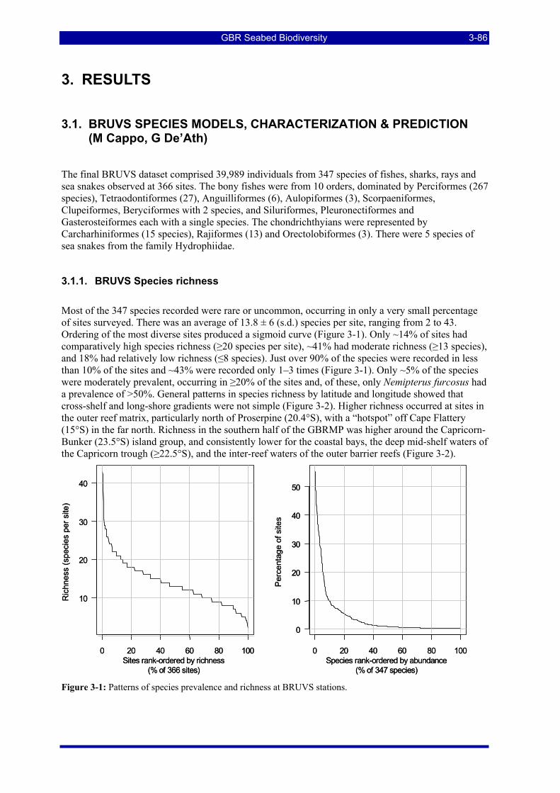
GBR Seabed Biodiversity 3-86
3. RESULTS
3.1. BRUVS SPECIES MODELS, CHARACTERIZATION & PREDICTION (M Cappo, G De’Ath)
The final BRUVS dataset comprised 39,989 individuals from 347 species of fishes, sharks, rays and sea snakes observed at 366 sites. The bony fishes were from 10 orders, dominated by Perciformes (267 species), Tetraodontiformes (27), Anguilliformes (6), Aulopiformes (3), Scorpaeniformes, Clupeiformes, Beryciformes with 2 species, and Siluriformes, Pleuronectiformes and Gasterosteiformes each with a single species. The chondrichthyians were represented by Carcharhiniformes (15 species), Rajiformes (13) and Orectolobiformes (3). There were 5 species of sea snakes from the family Hydrophiidae.
3.1.1. BRUVS Species richness
Most of the 347 species recorded were rare or uncommon, occurring in only a very small percentage of sites surveyed. There was an average of 13.8 ± 6 (s.d.) species per site, ranging from 2 to 43. Ordering of the most diverse sites produced a sigmoid curve (Figure 3-1). Only ~14% of sites had comparatively high species richness (≥20 species per site), ~41% had moderate richness (≥13 species), and 18% had relatively low richness (≤8 species). Just over 90% of the species were recorded in less than 10% of the sites and ~43% were recorded only 1–3 times (Figure 3-1). Only ~5% of the species were moderately prevalent, occurring in ≥20% of the sites and, of these, only Nemipterus furcosus had a prevalence of >50%. General patterns in species richness by latitude and longitude showed that cross-shelf and long-shore gradients were not simple (Figure 3-2). Higher richness occurred at sites in the outer reef matrix, particularly north of Proserpine (20.4°S), with a “hotspot” off Cape Flattery (15°S) in the far north. Richness in the southern half of the GBRMP was higher around the Capricorn-Bunker (23.5°S) island group, and consistently lower for the coastal bays, the deep mid-shelf waters of the Capricorn trough (≥22.5°S), and the inter-reef waters of the outer barrier reefs (Figure 3-2).
0 20 40 60 80 100
10
20
30
40
Sites rank-ordered by richness(% of 366 sites)
Ric
hnes
s (s
peci
es p
er s
ite)
0 20 40 60 80 100
0
10
20
30
40
50
Species rank-ordered by abundance(% of 347 species)
Perc
enta
ge o
f site
s
0 20 40 60 80 100
10
20
30
40
Sites rank-ordered by richness(% of 366 sites)
Ric
hnes
s (s
peci
es p
er s
ite)
0 20 40 60 80 100
0
10
20
30
40
50
Species rank-ordered by abundance(% of 347 species)
Perc
enta
ge o
f site
s
Figure 3-1: Patterns of species prevalence and richness at BRUVS stations.
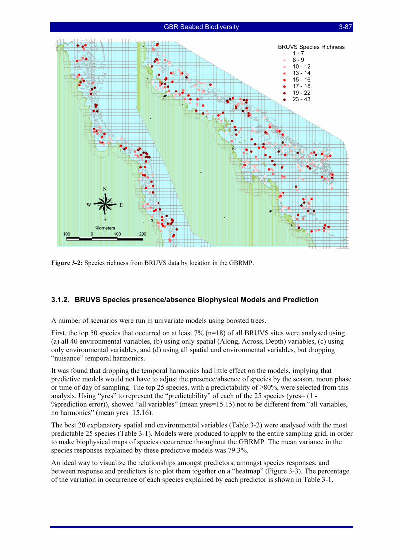
GBR Seabed Biodiversity 3-87
# #
#
#
##
#
# ##
#
#
# #
#
# ##
#
#
# #
#
#
#
##
#
#
#
#
#
##
#
#
# #
#
#
#
#
#
#
##
##
#
##
#
#
#
#
##
##
#
#
#
##
#
#
#
#
#
#
#
#
#
#
#
#
#
##
#
#
#
##
#
#
#
#
##
#
##
#
#
#
#
#
#
#
#
#
#
#
#
#
#
##
#
#
#
##
#
#
#
##
##
#
#
#
#
##
#
#
#
#
#
#
#
#
#
###
##
#
#
##
#
## ##
#
##
#
#
#
#
#
#
#
##
#
#
#
#
##
#
#
#
#
#
#
##
#
#
#
#
##
#
#
#
#
#
#
#
#
#
#
#
#
#
#
#
#
#
#
#
#
#
#
#
#
#
#
##
##
#
# #
##
#
#
#
#
##
#
#
#
#
#
#
#
#
##
##
#
##
#
#
#
#
#
#
#
#
##
#
#
#
#
#
#
#
#
##
#
#
#
#
#
#
#
#
#
#
#
#
#
#
##
#
#
#
##
#
#
#
#
#
#
#
##
###
#
#
#
#
##
#
#
##
#
#
#
#
#
#
#
#
#
#
#
#
#
#
#
#
##
#
#
#
###
#
#
#
#
#
#
#
#
#
## #
#
#
#
#
#
#
#
###
#
#
#
#
#
#
#
#
#
#
#
#
#
#
#
#
#
#
#
#
#
#
#
#
#
#
#
#
#
#
#
#
#
#
#
#
#
#
#
N
EW
S
BRUVS Species Richness# 1 - 7# 8 - 9# 10 - 12# 13 - 14# 15 - 16# 17 - 18# 19 - 22# 23 - 43
100 0 100 200Kilometers
Figure 3-2: Species richness from BRUVS data by location in the GBRMP.
3.1.2. BRUVS Species presence/absence Biophysical Models and Prediction
A number of scenarios were run in univariate models using boosted trees.
First, the top 50 species that occurred on at least 7% (n=18) of all BRUVS sites were analysed using (a) all 40 environmental variables, (b) using only spatial (Along, Across, Depth) variables, (c) using only environmental variables, and (d) using all spatial and environmental variables, but dropping “nuisance” temporal harmonics.
It was found that dropping the temporal harmonics had little effect on the models, implying that predictive models would not have to adjust the presence/absence of species by the season, moon phase or time of day of sampling. The top 25 species, with a predictability of ≥80%, were selected from this analysis. Using “yres” to represent the “predictability” of each of the 25 species (yres= (1 - %prediction error)), showed “all variables” (mean yres=15.15) not to be different from “all variables, no harmonics” (mean yres=15.16).
The best 20 explanatory spatial and environmental variables (Table 3-2) were analysed with the most predictable 25 species (Table 3-1). Models were produced to apply to the entire sampling grid, in order to make biophysical maps of species occurrence throughout the GBRMP. The mean variance in the species responses explained by these predictive models was 79.3%.
An ideal way to visualize the relationships amongst predictors, amongst species responses, and between response and predictors is to plot them together on a “heatmap” (Figure 3-3). The percentage of the variation in occurrence of each species explained by each predictor is shown in Table 3-1.
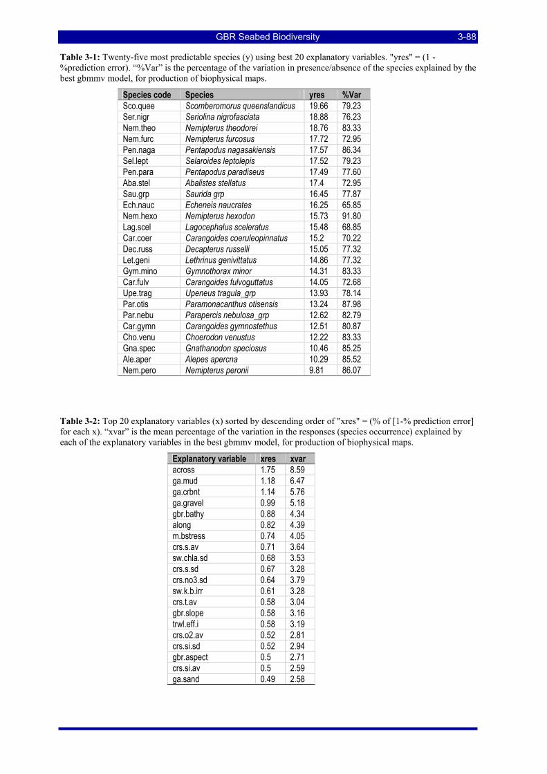
GBR Seabed Biodiversity 3-88
Table 3-1: Twenty-five most predictable species (y) using best 20 explanatory variables. "yres" = (1 - %prediction error). “%Var” is the percentage of the variation in presence/absence of the species explained by the best gbmmv model, for production of biophysical maps.
Species code Species yres %Var Sco.quee Scomberomorus queenslandicus 19.66 79.23 Ser.nigr Seriolina nigrofasciata 18.88 76.23 Nem.theo Nemipterus theodorei 18.76 83.33 Nem.furc Nemipterus furcosus 17.72 72.95 Pen.naga Pentapodus nagasakiensis 17.57 86.34 Sel.lept Selaroides leptolepis 17.52 79.23 Pen.para Pentapodus paradiseus 17.49 77.60 Aba.stel Abalistes stellatus 17.4 72.95 Sau.grp Saurida grp 16.45 77.87 Ech.nauc Echeneis naucrates 16.25 65.85 Nem.hexo Nemipterus hexodon 15.73 91.80 Lag.scel Lagocephalus sceleratus 15.48 68.85 Car.coer Carangoides coeruleopinnatus 15.2 70.22 Dec.russ Decapterus russelli 15.05 77.32 Let.geni Lethrinus genivittatus 14.86 77.32 Gym.mino Gymnothorax minor 14.31 83.33 Car.fulv Carangoides fulvoguttatus 14.05 72.68 Upe.trag Upeneus tragula_grp 13.93 78.14 Par.otis Paramonacanthus otisensis 13.24 87.98 Par.nebu Parapercis nebulosa_grp 12.62 82.79 Car.gymn Carangoides gymnostethus 12.51 80.87 Cho.venu Choerodon venustus 12.22 83.33 Gna.spec Gnathanodon speciosus 10.46 85.25 Ale.aper Alepes apercna 10.29 85.52 Nem.pero Nemipterus peronii 9.81 86.07
Table 3-2: Top 20 explanatory variables (x) sorted by descending order of "xres" = (% of [1-% prediction error] for each x). “xvar” is the mean percentage of the variation in the responses (species occurrence) explained by each of the explanatory variables in the best gbmmv model, for production of biophysical maps.
Explanatory variable xres xvar across 1.75 8.59 ga.mud 1.18 6.47 ga.crbnt 1.14 5.76 ga.gravel 0.99 5.18 gbr.bathy 0.88 4.34 along 0.82 4.39 m.bstress 0.74 4.05 crs.s.av 0.71 3.64 sw.chla.sd 0.68 3.53 crs.s.sd 0.67 3.28 crs.no3.sd 0.64 3.79 sw.k.b.irr 0.61 3.28 crs.t.av 0.58 3.04 gbr.slope 0.58 3.16 trwl.eff.i 0.58 3.19 crs.o2.av 0.52 2.81 crs.si.sd 0.52 2.94 gbr.aspect 0.5 2.71 crs.si.av 0.5 2.59 ga.sand 0.49 2.58
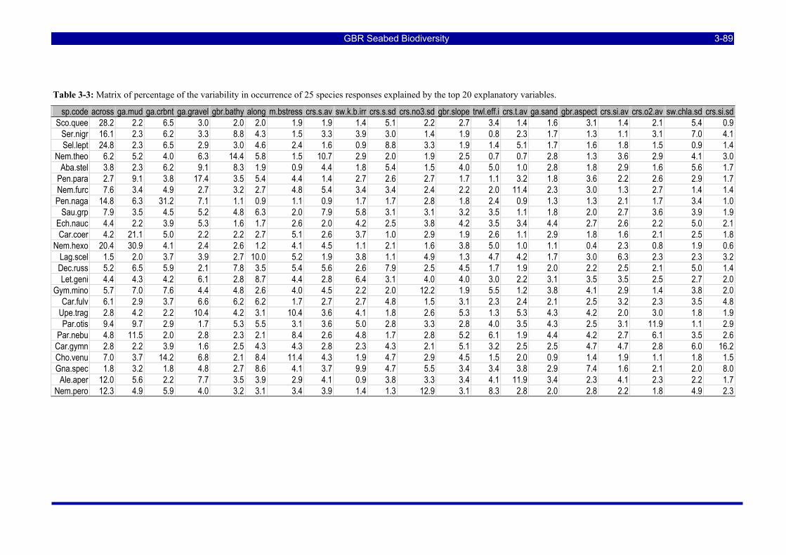
GBR Seabed Biodiversity 3-89
Table 3-3: Matrix of percentage of the variability in occurrence of 25 species responses explained by the top 20 explanatory variables.
sp.code across ga.mud ga.crbnt ga.gravel gbr.bathy along m.bstress crs.s.av sw.k.b.irr crs.s.sd crs.no3.sd gbr.slope trwl.eff.i crs.t.av ga.sand gbr.aspect crs.si.av crs.o2.av sw.chla.sd crs.si.sd Sco.quee 28.2 2.2 6.5 3.0 2.0 2.0 1.9 1.9 1.4 5.1 2.2 2.7 3.4 1.4 1.6 3.1 1.4 2.1 5.4 0.9
Ser.nigr 16.1 2.3 6.2 3.3 8.8 4.3 1.5 3.3 3.9 3.0 1.4 1.9 0.8 2.3 1.7 1.3 1.1 3.1 7.0 4.1 Sel.lept 24.8 2.3 6.5 2.9 3.0 4.6 2.4 1.6 0.9 8.8 3.3 1.9 1.4 5.1 1.7 1.6 1.8 1.5 0.9 1.4
Nem.theo 6.2 5.2 4.0 6.3 14.4 5.8 1.5 10.7 2.9 2.0 1.9 2.5 0.7 0.7 2.8 1.3 3.6 2.9 4.1 3.0 Aba.stel 3.8 2.3 6.2 9.1 8.3 1.9 0.9 4.4 1.8 5.4 1.5 4.0 5.0 1.0 2.8 1.8 2.9 1.6 5.6 1.7
Pen.para 2.7 9.1 3.8 17.4 3.5 5.4 4.4 1.4 2.7 2.6 2.7 1.7 1.1 3.2 1.8 3.6 2.2 2.6 2.9 1.7 Nem.furc 7.6 3.4 4.9 2.7 3.2 2.7 4.8 5.4 3.4 3.4 2.4 2.2 2.0 11.4 2.3 3.0 1.3 2.7 1.4 1.4 Pen.naga 14.8 6.3 31.2 7.1 1.1 0.9 1.1 0.9 1.7 1.7 2.8 1.8 2.4 0.9 1.3 1.3 2.1 1.7 3.4 1.0
Sau.grp 7.9 3.5 4.5 5.2 4.8 6.3 2.0 7.9 5.8 3.1 3.1 3.2 3.5 1.1 1.8 2.0 2.7 3.6 3.9 1.9 Ech.nauc 4.4 2.2 3.9 5.3 1.6 1.7 2.6 2.0 4.2 2.5 3.8 4.2 3.5 3.4 4.4 2.7 2.6 2.2 5.0 2.1 Car.coer 4.2 21.1 5.0 2.2 2.2 2.7 5.1 2.6 3.7 1.0 2.9 1.9 2.6 1.1 2.9 1.8 1.6 2.1 2.5 1.8
Nem.hexo 20.4 30.9 4.1 2.4 2.6 1.2 4.1 4.5 1.1 2.1 1.6 3.8 5.0 1.0 1.1 0.4 2.3 0.8 1.9 0.6 Lag.scel 1.5 2.0 3.7 3.9 2.7 10.0 5.2 1.9 3.8 1.1 4.9 1.3 4.7 4.2 1.7 3.0 6.3 2.3 2.3 3.2 Dec.russ 5.2 6.5 5.9 2.1 7.8 3.5 5.4 5.6 2.6 7.9 2.5 4.5 1.7 1.9 2.0 2.2 2.5 2.1 5.0 1.4 Let.geni 4.4 4.3 4.2 6.1 2.8 8.7 4.4 2.8 6.4 3.1 4.0 4.0 3.0 2.2 3.1 3.5 3.5 2.5 2.7 2.0
Gym.mino 5.7 7.0 7.6 4.4 4.8 2.6 4.0 4.5 2.2 2.0 12.2 1.9 5.5 1.2 3.8 4.1 2.9 1.4 3.8 2.0 Car.fulv 6.1 2.9 3.7 6.6 6.2 6.2 1.7 2.7 2.7 4.8 1.5 3.1 2.3 2.4 2.1 2.5 3.2 2.3 3.5 4.8
Upe.trag 2.8 4.2 2.2 10.4 4.2 3.1 10.4 3.6 4.1 1.8 2.6 5.3 1.3 5.3 4.3 4.2 2.0 3.0 1.8 1.9 Par.otis 9.4 9.7 2.9 1.7 5.3 5.5 3.1 3.6 5.0 2.8 3.3 2.8 4.0 3.5 4.3 2.5 3.1 11.9 1.1 2.9
Par.nebu 4.8 11.5 2.0 2.8 2.3 2.1 8.4 2.6 4.8 1.7 2.8 5.2 6.1 1.9 4.4 4.2 2.7 6.1 3.5 2.6 Car.gymn 2.8 2.2 3.9 1.6 2.5 4.3 4.3 2.8 2.3 4.3 2.1 5.1 3.2 2.5 2.5 4.7 4.7 2.8 6.0 16.2 Cho.venu 7.0 3.7 14.2 6.8 2.1 8.4 11.4 4.3 1.9 4.7 2.9 4.5 1.5 2.0 0.9 1.4 1.9 1.1 1.8 1.5 Gna.spec 1.8 3.2 1.8 4.8 2.7 8.6 4.1 3.7 9.9 4.7 5.5 3.4 3.4 3.8 2.9 7.4 1.6 2.1 2.0 8.0 Ale.aper 12.0 5.6 2.2 7.7 3.5 3.9 2.9 4.1 0.9 3.8 3.3 3.4 4.1 11.9 3.4 2.3 4.1 2.3 2.2 1.7
Nem.pero 12.3 4.9 5.9 4.0 3.2 3.1 3.4 3.9 1.4 1.3 12.9 3.1 8.3 2.8 2.0 2.8 2.2 1.8 4.9 2.3
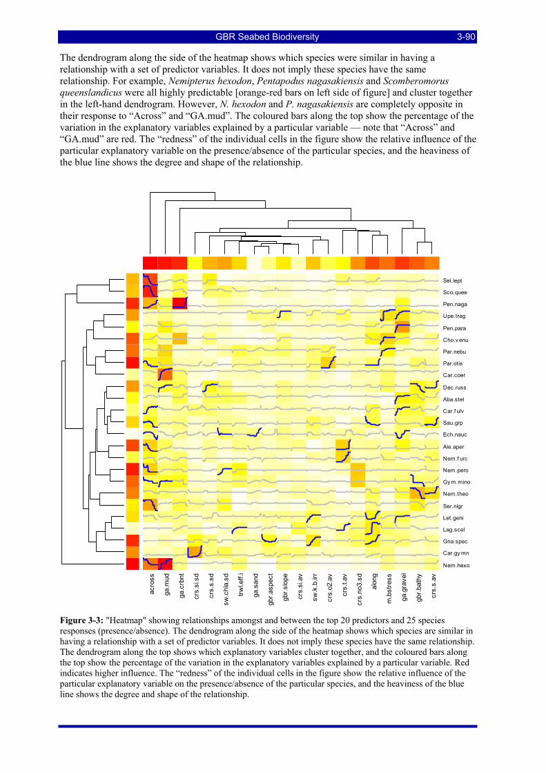
GBR Seabed Biodiversity 3-90
The dendrogram along the side of the heatmap shows which species were similar in having a relationship with a set of predictor variables. It does not imply these species have the same relationship. For example, Nemipterus hexodon, Pentapodus nagasakiensis and Scomberomorus queenslandicus were all highly predictable [orange-red bars on left side of figure] and cluster together in the left-hand dendrogram. However, N. hexodon and P. nagasakiensis are completely opposite in their response to “Across” and “GA.mud”. The coloured bars along the top show the percentage of the variation in the explanatory variables explained by a particular variable — note that “Across” and “GA.mud” are red. The “redness” of the individual cells in the figure show the relative influence of the particular explanatory variable on the presence/absence of the particular species, and the heaviness of the blue line shows the degree and shape of the relationship.
acro
ss
ga.m
ud
ga.c
rbnt
crs.
si.s
d
crs.
s.sd
sw.c
hla.
sd
trwl.e
ff.i
ga.s
and
gbr.a
spec
t
gbr.s
lope
crs.
si.a
v
sw.k
.b.ir
r
crs.
o2.a
v
crs.
t.av
crs.
no3.
sd
alon
g
m.b
stre
ss
ga.g
rave
l
gbr.b
athy
crs.
s.av
Nem.hexo
Car.gy mn
Gna.spec
Lag.scel
Let.geni
Ser.nigr
Nem.theo
Gy m.mino
Nem.pero
Nem.f urc
Ale.aper
Ech.nauc
Sau.grp
Car.f ulv
Aba.stel
Dec.russ
Car.coer
Par.otis
Par.nebu
Cho.v enu
Pen.para
Upe.trag
Pen.naga
Sco.quee
Sel.lept
Figure 3-3: "Heatmap" showing relationships amongst and between the top 20 predictors and 25 species responses (presence/absence). The dendrogram along the side of the heatmap shows which species are similar in having a relationship with a set of predictor variables. It does not imply these species have the same relationship. The dendrogram along the top shows which explanatory variables cluster together, and the coloured bars along the top show the percentage of the variation in the explanatory variables explained by a particular variable. Red indicates higher influence. The “redness” of the individual cells in the figure show the relative influence of the particular explanatory variable on the presence/absence of the particular species, and the heaviness of the blue line shows the degree and shape of the relationship.
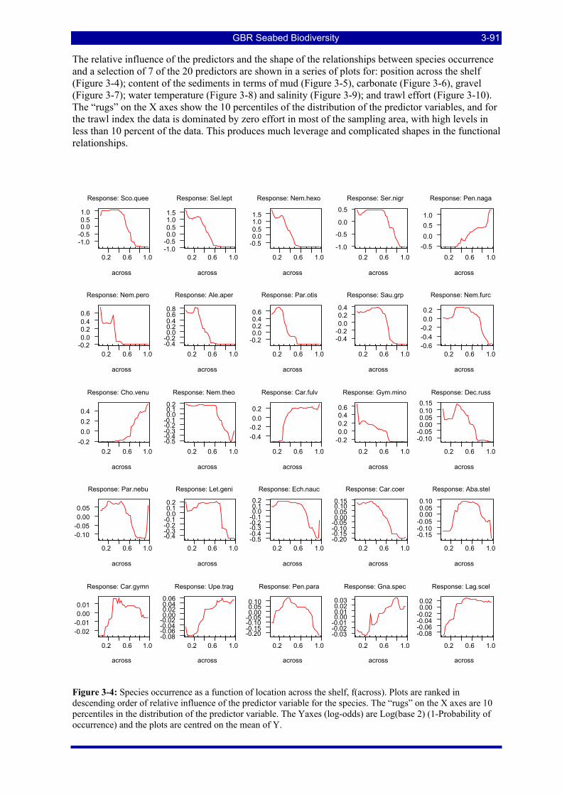
GBR Seabed Biodiversity 3-91
The relative influence of the predictors and the shape of the relationships between species occurrence and a selection of 7 of the 20 predictors are shown in a series of plots for: position across the shelf (Figure 3-4); content of the sediments in terms of mud (Figure 3-5), carbonate (Figure 3-6), gravel (Figure 3-7); water temperature (Figure 3-8) and salinity (Figure 3-9); and trawl effort (Figure 3-10). The “rugs” on the X axes show the 10 percentiles of the distribution of the predictor variables, and for the trawl index the data is dominated by zero effort in most of the sampling area, with high levels in less than 10 percent of the data. This produces much leverage and complicated shapes in the functional relationships.
Figure 3-4: Species occurrence as a function of location across the shelf, f(across). Plots are ranked in descending order of relative influence of the predictor variable for the species. The “rugs” on the X axes are 10 percentiles in the distribution of the predictor variable. The Yaxes (log-odds) are Log(base 2) (1-Probability of occurrence) and the plots are centred on the mean of Y.
0.2 0.6 1.0
-1.0-0.50.00.51.0
across
Response: Sco.quee
0.2 0.6 1.0-1.0-0.50.00.51.01.5
across
Response: Sel.lept
0.2 0.6 1.0
-0.50.00.51.01.5
across
Response: Nem.hexo
0.2 0.6 1.0-1.0
-0.5
0.0
0.5
across
Response: Ser.nigr
0.2 0.6 1.0-0.50.00.51.0
across
Response: Pen.naga
0.2 0.6 1.0-0.20.00.20.40.6
across
Response: Nem.pero
0.2 0.6 1.0-0.4-0.20.00.20.40.60.8
across
Response: Ale.aper
0.2 0.6 1.0
-0.20.00.20.40.6
across
Response: Par.otis
0.2 0.6 1.0
-0.4-0.20.00.20.4
across
Response: Sau.grp
0.2 0.6 1.0-0.6-0.4-0.20.00.2
across
Response: Nem.furc
0.2 0.6 1.0-0.20.00.20.4
across
Response: Cho.venu
0.2 0.6 1.0-0.5-0.4-0.3-0.2-0.10.00.10.2
across
Response: Nem.theo
0.2 0.6 1.0
-0.4-0.20.00.2
across
Response: Car.fulv
0.2 0.6 1.0
-0.20.00.20.40.6
across
Response: Gym.mino
0.2 0.6 1.0
-0.10-0.050.000.050.100.15
across
Response: Dec.russ
0.2 0.6 1.0
-0.10-0.050.000.05
across
Response: Par.nebu
0.2 0.6 1.0
-0.4-0.3-0.2-0.10.00.10.2
across
Response: Let.geni
0.2 0.6 1.0-0.5-0.4-0.3-0.2-0.10.00.10.2
across
Response: Ech.nauc
0.2 0.6 1.0-0.20-0.15-0.10-0.050.000.050.100.15
across
Response: Car.coer
0.2 0.6 1.0
-0.15-0.10-0.050.000.050.10
across
Response: Aba.stel
0.2 0.6 1.0
-0.02-0.010.000.01
across
Response: Car.gymn
0.2 0.6 1.0-0.08-0.06-0.04-0.020.000.020.040.06
across
Response: Upe.trag
0.2 0.6 1.0
-0.20-0.15-0.10-0.050.000.050.10
across
Response: Pen.para
0.2 0.6 1.0
-0.03-0.02-0.010.000.010.020.03
across
Response: Gna.spec
0.2 0.6 1.0
-0.08-0.06-0.04-0.020.000.02
across
Response: Lag.scel
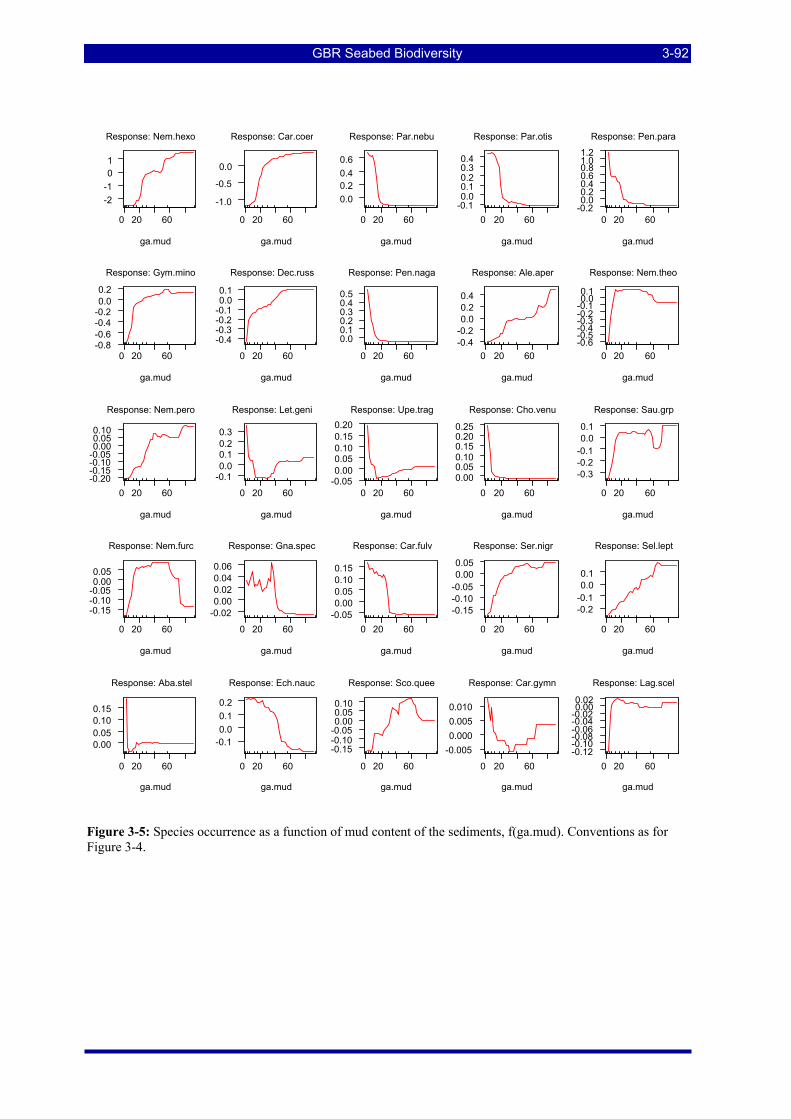
GBR Seabed Biodiversity 3-92
Figure 3-5: Species occurrence as a function of mud content of the sediments, f(ga.mud). Conventions as for Figure 3-4.
0 20 60 -2-101
ga.mud
Response: Nem.hexo
0 20 60
-1.0
-0.5
0.0
ga.mud
Response: Car.coer
0 20 60
0.00.20.40.6
ga.mud
Response: Par.nebu
0 20 60-0.10.00.10.20.30.4
ga.mud
Response: Par.otis
0 20 60-0.20.00.20.40.60.81.01.2
ga.mud
Response: Pen.para
0 20 60 -0.8-0.6-0.4-0.20.00.2
ga.mud
Response: Gym.mino
0 20 60
-0.4-0.3-0.2-0.10.00.1
ga.mud
Response: Dec.russ
0 20 60
0.00.10.20.30.40.5
ga.mud
Response: Pen.naga
0 20 60-0.4-0.20.00.20.4
ga.mud
Response: Ale.aper
0 20 60-0.6-0.5-0.4-0.3-0.2-0.10.00.1
ga.mud
Response: Nem.theo
0 20 60 -0.20-0.15-0.10-0.050.000.050.10
ga.mud
Response: Nem.pero
0 20 60
-0.10.00.10.20.3
ga.mud
Response: Let.geni
0 20 60-0.050.000.050.100.150.20
ga.mud
Response: Upe.trag
0 20 600.000.050.100.150.200.25
ga.mud
Response: Cho.venu
0 20 60
-0.3-0.2-0.10.00.1
ga.mud
Response: Sau.grp
0 20 60 -0.15-0.10-0.050.000.05
ga.mud
Response: Nem.furc
0 20 60
-0.020.000.020.040.06
ga.mud
Response: Gna.spec
0 20 60-0.050.000.050.100.15
ga.mud
Response: Car.fulv
0 20 60
-0.15-0.10-0.050.000.05
ga.mud
Response: Ser.nigr
0 20 60
-0.2-0.10.00.1
ga.mud
Response: Sel.lept
0 20 60 0.000.050.100.15
ga.mud
Response: Aba.stel
0 20 60
-0.10.00.10.2
ga.mud
Response: Ech.nauc
0 20 60
-0.15-0.10-0.050.000.050.10
ga.mud
Response: Sco.quee
0 20 60
-0.0050.0000.0050.010
ga.mud
Response: Car.gymn
0 20 60-0.12-0.10-0.08-0.06-0.04-0.020.000.02
ga.mud
Response: Lag.scel
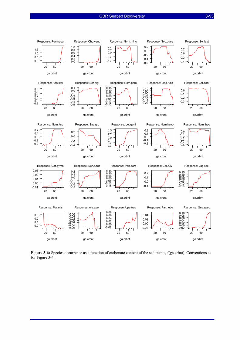
GBR Seabed Biodiversity 3-93
Figure 3-6: Species occurrence as a function of carbonate content of the sediments, f(ga.crbnt). Conventions as for Figure 3-4.
20 60
0.00.51.01.5
ga.crbnt
Response: Pen.naga
20 60
0.00.20.40.60.81.0
ga.crbnt
Response: Cho.venu
20 60
-0.4-0.20.00.2
ga.crbnt
Response: Gym.mino
20 60-0.6-0.4-0.20.00.2
ga.crbnt
Response: Sco.quee
20 60
-0.4-0.20.00.2
ga.crbnt
Response: Sel.lept
20 60-0.10.00.10.20.30.40.5
ga.crbnt
Response: Aba.stel
20 60-0.5-0.4-0.3-0.2-0.10.00.1
ga.crbnt
Response: Ser.nigr
20 60-0.15-0.10-0.050.000.050.100.15
ga.crbnt
Response: Nem.pero
20 60
-0.20-0.15-0.10-0.050.000.050.10
ga.crbnt
Response: Dec.russ
20 60
-0.3-0.2-0.10.0
ga.crbnt
Response: Car.coer
20 60
-0.2-0.10.00.10.2
ga.crbnt
Response: Nem.furc
20 60-0.4-0.20.00.2
ga.crbnt
Response: Sau.grp
20 60-0.3-0.2-0.10.00.10.20.3
ga.crbnt
Response: Let.geni
20 60
-0.2-0.10.00.10.2
ga.crbnt
Response: Nem.hexo
20 60
-0.5-0.4-0.3-0.2-0.10.0
ga.crbnt
Response: Nem.theo
20 60-0.010.000.010.020.03
ga.crbnt
Response: Car.gymn
20 60-0.3-0.2-0.10.00.10.2
ga.crbnt
Response: Ech.nauc
20 60
-0.15-0.10-0.050.000.050.100.15
ga.crbnt
Response: Pen.para
20 60
-0.10.00.10.2
ga.crbnt
Response: Car.fulv
20 60
-0.15-0.10-0.050.000.050.100.15
ga.crbnt
Response: Lag.scel
20 60
0.00.10.20.3
ga.crbnt
Response: Par.otis
20 60
-0.06-0.04-0.020.000.020.040.06
ga.crbnt
Response: Ale.aper
20 60
-0.020.000.020.040.060.08
ga.crbnt
Response: Upe.trag
20 60
-0.020.000.020.04
ga.crbnt
Response: Par.nebu
20 60
-0.020.000.020.040.060.080.10
ga.crbnt
Response: Gna.spec
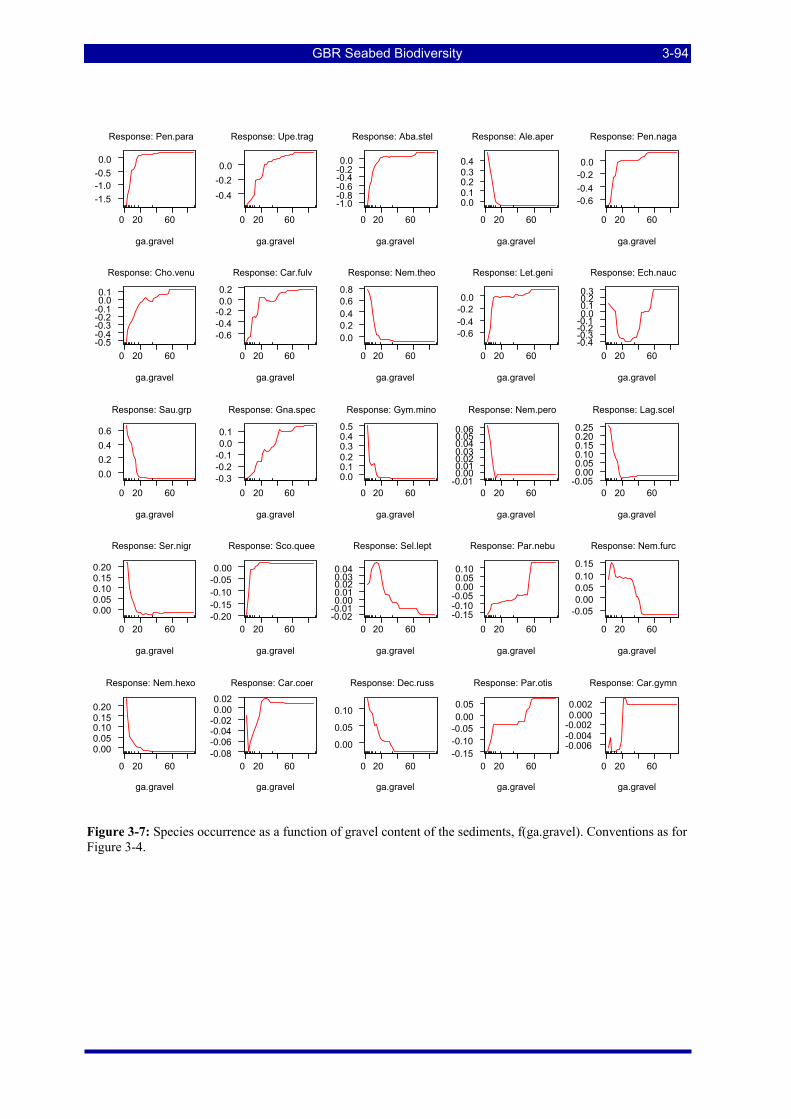
GBR Seabed Biodiversity 3-94
Figure 3-7: Species occurrence as a function of gravel content of the sediments, f(ga.gravel). Conventions as for Figure 3-4.
0 20 60
-1.5-1.0-0.50.0
ga.gravel
Response: Pen.para
0 20 60
-0.4-0.20.0
ga.gravel
Response: Upe.trag
0 20 60
-1.0-0.8-0.6-0.4-0.20.0
ga.gravel
Response: Aba.stel
0 20 60
0.00.10.20.30.4
ga.gravel
Response: Ale.aper
0 20 60
-0.6-0.4-0.20.0
ga.gravel
Response: Pen.naga
0 20 60-0.5-0.4-0.3-0.2-0.10.00.1
ga.gravel
Response: Cho.venu
0 20 60
-0.6-0.4-0.20.00.2
ga.gravel
Response: Car.fulv
0 20 60
0.00.20.40.60.8
ga.gravel
Response: Nem.theo
0 20 60
-0.6-0.4-0.20.0
ga.gravel
Response: Let.geni
0 20 60-0.4-0.3-0.2-0.10.00.10.20.3
ga.gravel
Response: Ech.nauc
0 20 60
0.00.20.40.6
ga.gravel
Response: Sau.grp
0 20 60-0.3-0.2-0.10.00.1
ga.gravel
Response: Gna.spec
0 20 60
0.00.10.20.30.40.5
ga.gravel
Response: Gym.mino
0 20 60-0.010.000.010.020.030.040.050.06
ga.gravel
Response: Nem.pero
0 20 60-0.050.000.050.100.150.200.25
ga.gravel
Response: Lag.scel
0 20 60
0.000.050.100.150.20
ga.gravel
Response: Ser.nigr
0 20 60-0.20-0.15-0.10-0.050.00
ga.gravel
Response: Sco.quee
0 20 60-0.02-0.010.000.010.020.030.04
ga.gravel
Response: Sel.lept
0 20 60-0.15-0.10-0.050.000.050.10
ga.gravel
Response: Par.nebu
0 20 60
-0.050.000.050.100.15
ga.gravel
Response: Nem.furc
0 20 60
0.000.050.100.150.20
ga.gravel
Response: Nem.hexo
0 20 60-0.08-0.06-0.04-0.020.000.02
ga.gravel
Response: Car.coer
0 20 60
0.00
0.05
0.10
ga.gravel
Response: Dec.russ
0 20 60-0.15-0.10-0.050.000.05
ga.gravel
Response: Par.otis
0 20 60
-0.006-0.004-0.0020.0000.002
ga.gravel
Response: Car.gymn
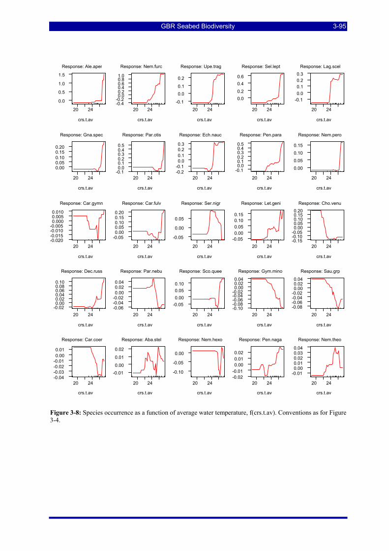
GBR Seabed Biodiversity 3-95
Figure 3-8: Species occurrence as a function of average water temperature, f(crs.t.av). Conventions as for Figure 3-4.
20 24
0.0
0.5
1.0
1.5
crs.t.av
Response: Ale.aper
20 24-0.4-0.20.00.20.40.60.81.0
crs.t.av
Response: Nem.furc
20 24-0.1
0.00.1
0.2
crs.t.av
Response: Upe.trag
20 24
0.00.20.40.6
crs.t.av
Response: Sel.lept
20 24
-0.10.00.10.20.3
crs.t.av
Response: Lag.scel
20 24
0.000.050.100.150.20
crs.t.av
Response: Gna.spec
20 24-0.10.00.10.20.30.40.5
crs.t.av
Response: Par.otis
20 24-0.2-0.10.00.10.20.3
crs.t.av
Response: Ech.nauc
20 24-0.10.00.10.20.30.40.5
crs.t.av
Response: Pen.para
20 24
0.000.050.100.15
crs.t.av
Response: Nem.pero
20 24-0.020-0.015-0.010-0.0050.0000.0050.010
crs.t.av
Response: Car.gymn
20 24
-0.050.000.050.100.150.20
crs.t.av
Response: Car.fulv
20 24
-0.05
0.00
0.05
crs.t.av
Response: Ser.nigr
20 24-0.050.000.050.100.15
crs.t.av
Response: Let.geni
20 24-0.15-0.10-0.050.000.050.100.150.20
crs.t.av
Response: Cho.venu
20 24-0.020.000.020.040.060.080.10
crs.t.av
Response: Dec.russ
20 24-0.06-0.04-0.020.000.020.04
crs.t.av
Response: Par.nebu
20 24
-0.050.000.050.10
crs.t.av
Response: Sco.quee
20 24-0.10-0.08-0.06-0.04-0.020.000.020.04
crs.t.av
Response: Gym.mino
20 24-0.08-0.06-0.04-0.020.000.020.04
crs.t.av
Response: Sau.grp
20 24-0.04-0.03-0.02-0.010.000.01
crs.t.av
Response: Car.coer
20 24
-0.010.00
0.01
0.02
crs.t.av
Response: Aba.stel
20 24
-0.10
-0.05
0.00
crs.t.av
Response: Nem.hexo
20 24-0.02-0.010.000.010.02
crs.t.av
Response: Pen.naga
20 24
-0.010.000.010.020.030.04
crs.t.av
Response: Nem.theo
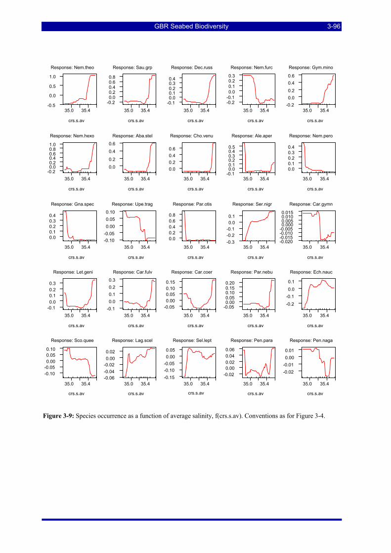
GBR Seabed Biodiversity 3-96
Figure 3-9: Species occurrence as a function of average salinity, f(crs.s.av). Conventions as for Figure 3-4.
35.0 35.4-0.5
0.0
0.5
1.0
crs.s.av
Response: Nem.theo
35.0 35.4
-0.20.00.20.40.60.8
crs.s.av
Response: Sau.grp
35.0 35.4-0.10.00.10.20.30.4
crs.s.av
Response: Dec.russ
35.0 35.4
-0.2-0.10.00.10.20.3
crs.s.av
Response: Nem.furc
35.0 35.4-0.20.00.20.40.6
crs.s.av
Response: Gym.mino
35.0 35.4-0.20.00.20.40.60.81.0
crs.s.av
Response: Nem.hexo
35.0 35.4
0.00.2
0.40.6
crs.s.av
Response: Aba.stel
35.0 35.4
0.00.20.40.6
crs.s.av
Response: Cho.venu
35.0 35.4-0.10.00.10.20.30.40.5
crs.s.av
Response: Ale.aper
35.0 35.4
0.00.10.20.30.4
crs.s.av
Response: Nem.pero
35.0 35.4
0.00.10.20.30.4
crs.s.av
Response: Gna.spec
35.0 35.4-0.10-0.050.000.050.10
crs.s.av
Response: Upe.trag
35.0 35.4
0.00.20.40.60.8
crs.s.av
Response: Par.otis
35.0 35.4-0.3-0.2-0.10.00.1
crs.s.av
Response: Ser.nigr
35.0 35.4-0.020-0.015-0.010-0.0050.0000.0050.0100.015
crs.s.av
Response: Car.gymn
35.0 35.4-0.10.00.10.20.3
crs.s.av
Response: Let.geni
35.0 35.4-0.10.00.10.20.3
crs.s.av
Response: Car.fulv
35.0 35.4
-0.050.000.050.100.15
crs.s.av
Response: Car.coer
35.0 35.4
-0.050.000.050.100.150.20
crs.s.av
Response: Par.nebu
35.0 35.4
-0.2-0.10.00.1
crs.s.av
Response: Ech.nauc
35.0 35.4
-0.10-0.050.000.050.10
crs.s.av
Response: Sco.quee
35.0 35.4-0.06-0.04-0.020.000.02
crs.s.av
Response: Lag.scel
35.0 35.4-0.15-0.10-0.050.000.05
crs.s.av
Response: Sel.lept
35.0 35.4
-0.020.000.020.040.06
crs.s.av
Response: Pen.para
35.0 35.4
-0.02-0.010.000.01
crs.s.av
Response: Pen.naga
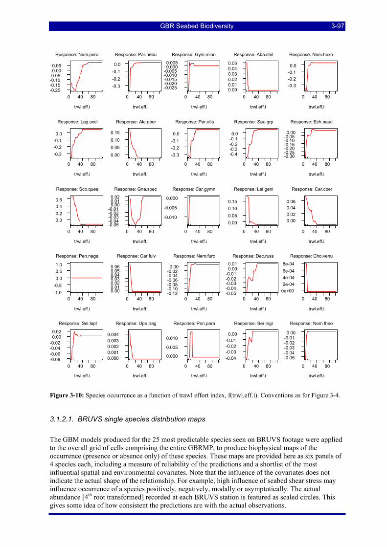
GBR Seabed Biodiversity 3-97
Figure 3-10: Species occurrence as a function of trawl effort index, f(trwl.eff.i). Conventions as for Figure 3-4.
3.1.2.1. BRUVS single species distribution maps
The GBM models produced for the 25 most predictable species seen on BRUVS footage were applied to the overall grid of cells comprising the entire GBRMP, to produce biophysical maps of the occurrence (presence or absence only) of these species. These maps are provided here as six panels of 4 species each, including a measure of reliability of the predictions and a shortlist of the most influential spatial and environmental covariates. Note that the influence of the covariates does not indicate the actual shape of the relationship. For example, high influence of seabed shear stress may influence occurrence of a species positively, negatively, modally or asymptotically. The actual abundance [4th root transformed] recorded at each BRUVS station is featured as scaled circles. This gives some idea of how consistent the predictions are with the actual observations.
0 40 80-0.20-0.15-0.10-0.050.000.05
trwl.eff.i
Response: Nem.pero
0 40 80
-0.3-0.2-0.10.0
trwl.eff.i
Response: Par.nebu
0 40 80
-0.025-0.020-0.015-0.010-0.0050.0000.005
trwl.eff.i
Response: Gym.mino
0 40 800.000.010.020.030.040.05
trwl.eff.i
Response: Aba.stel
0 40 80
-0.3-0.2-0.10.0
trwl.eff.i
Response: Nem.hexo
0 40 80
-0.3-0.2-0.10.0
trwl.eff.i
Response: Lag.scel
0 40 80 0.000.050.100.15
trwl.eff.i
Response: Ale.aper
0 40 80
-0.3-0.2-0.10.0
trwl.eff.i
Response: Par.otis
0 40 80
-0.4-0.3-0.2-0.10.0
trwl.eff.i
Response: Sau.grp
0 40 80
-0.30-0.25-0.20-0.15-0.10-0.050.00
trwl.eff.i
Response: Ech.nauc
0 40 80
0.00.20.40.6
trwl.eff.i
Response: Sco.quee
0 40 80 -0.05-0.04-0.03-0.02-0.010.000.010.02
trwl.eff.i
Response: Gna.spec
0 40 80
-0.010
-0.005
0.000
trwl.eff.i
Response: Car.gymn
0 40 80
0.000.050.100.15
trwl.eff.i
Response: Let.geni
0 40 80
0.000.020.040.06
trwl.eff.i
Response: Car.coer
0 40 80-1.0-0.50.00.51.0
trwl.eff.i
Response: Pen.naga
0 40 80 0.000.010.020.030.040.050.06
trwl.eff.i
Response: Car.fulv
0 40 80-0.12-0.10-0.08-0.06-0.04-0.020.00
trwl.eff.i
Response: Nem.furc
0 40 80-0.05-0.04-0.03-0.02-0.010.000.01
trwl.eff.i
Response: Dec.russ
0 40 80
0e+00 2e-044e-046e-048e-04
trwl.eff.i
Response: Cho.venu
0 40 80-0.08-0.06-0.04-0.020.000.02
trwl.eff.i
Response: Sel.lept
0 40 80 0.0000.0010.0020.0030.004
trwl.eff.i
Response: Upe.trag
0 40 80
0.000
0.005
0.010
trwl.eff.i
Response: Pen.para
0 40 80
-0.04-0.03-0.02-0.010.00
trwl.eff.i
Response: Ser.nigr
0 40 80
-0.05-0.04-0.03-0.02-0.010.00
trwl.eff.i
Response: Nem.theo
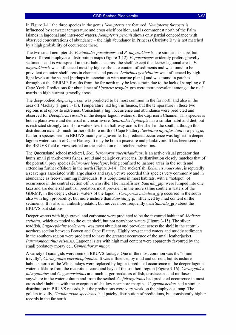
GBR Seabed Biodiversity 3-98
In Figure 3-11 the three species in the genus Nemipterus are featured. Nemipterus furcosus is influenced by seawater temperature and cross-shelf position, and is commonest north of the Palm Islands in lagoonal and inter-reef waters. Nemipterus peronii shows only partial concordance with observed concentrations of abundance – the high abundance in Princess Charlotte Bay is not matched by a high probability of occurrence there. N.hexodon description awaiting corrected version of map.
The two small nemipterids, Pentapodus paradiseus and P. nagasakiensis, are similar in shape, but have different biophysical distribution maps (Figure 3-12). P. paradiseus evidently prefers gravelly sediments and is widespread in most habitats across the shelf, except the deeper lagoonal areas. P. nagasakiensis was influenced most by high carbonate content of sediments and was found to be prevalent on outer-shelf areas in channels and passes. Lethrinus genivittatus was influenced by high light levels at the seabed [perhaps in association with marine plants] and was found in patches throughout the GBRMP. Results from the far north may be less certain due to the lack of sampling off Cape York. Predictions for abundance of Upeneus tragula_grp were more prevalent amongst the reef matrix in high current, gravelly areas.
The deep-bodied Alepes apercna was predicted to be most common in the far north and also in the area off Mackay (Figure 3-13). Temperature had high influence, but the temperature in these two regions is at opposite extremes. Consistently high occurrence and abundance were predicted and observed for Decapterus russelli in the deeper lagoon waters of the Capricorn Channel. This species is both a planktivore and demersal microcarnivore. Selaroides leptolepis has a similar habit and diet, but is restricted strongly to inshore waters less than half way across the shelf in the south, although this distribution extends much further offshore north of Cape Flattery. Seriolina nigrofasciata is a pelagic, fusiform species seen on BRUVS mainly as a juvenile. Its predicted occurrence was highest in deeper, lagoon waters south of Cape Flattery. It may be both a piscivore and planktivore. It has been seen in the BRUVS field of view settled on the seabed on outstretched pelvic fins.
The Queensland school mackerel, Scomberomorus queenslandicus, is an active visual predator that hunts small planktivorous fishes, squid and pelagic crustaceans. Its distribution closely matches that of the potential prey species Selaroides leptolepis, being confined to inshore areas in the south and extending further offshore in the north (Figure 3-14). The suckerfish, Echeneis naucrates, is reputedly a scavenger associated with large sharks and rays, yet we recorded this species very commonly and in abundance as free-swimming individuals. It is ubiquitous in most habitats, with a “hotspot” of occurrence in the central section off Townsville. The lizardfishes, Saurida_grp, were lumped into one taxa and are demersal ambush predators most prevalent in the more saline southern waters of the GBRMP, in the deeper, clearer waters of the lagoon. Parapercis nebulosa_grp occurred in the south also with high probability, but more inshore than Saurida_grp, influenced by mud content of the sediments. It is also an ambush predator, but moves more frequently than Saurida_grp about the BRUVS bait stations.
Deeper waters with high gravel and carbonate were predicted to be the favoured habitat of Abalistes stellatus, which extended to the outer shelf, but not nearshore waters (Figure 3-15). The silver toadfish, Lagocephalus sceleratus, was most abundant and prevalent across the shelf in the central-northern section between Bowen and Cape Flattery. Highly oxygenated waters and muddy sediments in the southern region were predicted to have the greatest occurrence of the small leatherjacket, Paramonacanthus otisensis. Lagoonal sites with high mud content were apparently favoured by the small predatory moray eel, Gymonthorax minor.
A variety of carangids were seen on BRUVS footage. One of the most common was the “onion trevally”, Carangoides coeruleopinnatus. It was influenced by mud and current, but its inshore habitats north of the Whitsundays were replaced by highest predicted occurrence in the deeper lagoon waters offshore from the macrotidal coast and bays of the southern region (Figure 3-16). Carangoides fulvoguttatus and C. gymnostethus are much larger predators of fish, crustaceans and molluscs anywhere in the water column and from the seabed. C. fulvoguttatus had predicted occurrence in most cross-shelf habitats with the exception of shallow nearshore margins. C. gymnostethus had a similar distribution in BRUVS records, but the predictions were very weak on the biophysical map. The golden trevally, Gnathanodon speciosus, had patchy distribution of predictions, but consistently higher records in the far north.
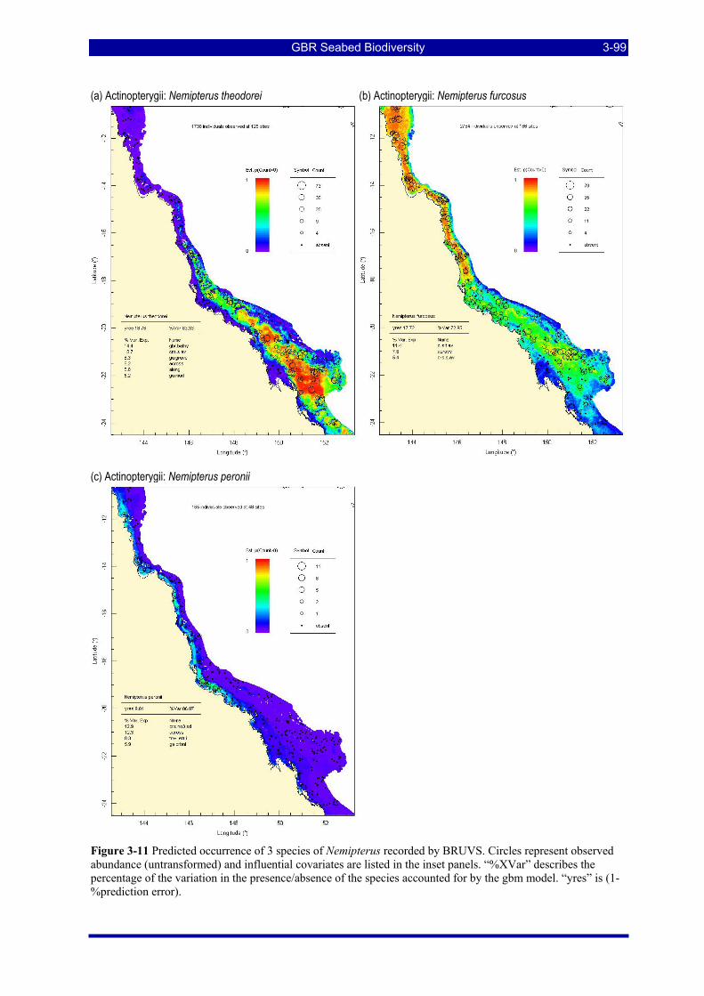
GBR Seabed Biodiversity 3-99
(a) Actinopterygii: Nemipterus theodorei (b) Actinopterygii: Nemipterus furcosus
(c) Actinopterygii: Nemipterus peronii (d) Actinopterygii: Nemipterus hexodon
Figure 3-11 Predicted occurrence of 3 species of Nemipterus recorded by BRUVS. Circles represent observed abundance (untransformed) and influential covariates are listed in the inset panels. “%XVar” describes the percentage of the variation in the presence/absence of the species accounted for by the gbm model. “yres” is (1-%prediction error).
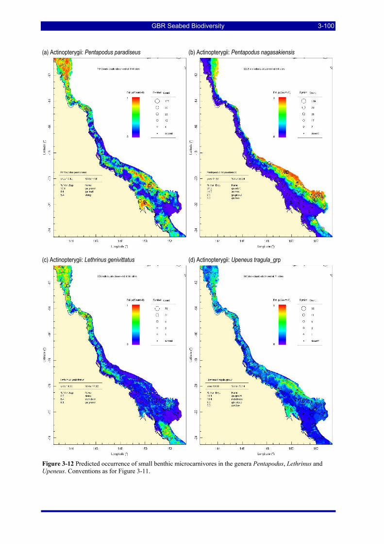
GBR Seabed Biodiversity 3-100
(a) Actinopterygii: Pentapodus paradiseus (b) Actinopterygii: Pentapodus nagasakiensis
(c) Actinopterygii: Lethrinus genivittatus (d) Actinopterygii: Upeneus tragula_grp
Figure 3-12 Predicted occurrence of small benthic microcarnivores in the genera Pentapodus, Lethrinus and Upeneus. Conventions as for Figure 3-11.
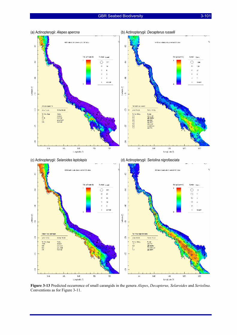
GBR Seabed Biodiversity 3-101
(a) Actinopterygii: Alepes apercna (b) Actinopterygii: Decapterus russelli
(c) Actinopterygii: Selaroides leptolepis (d) Actinopterygii: Seriolina nigrofasciata
Figure 3-13 Predicted occurrence of small carangids in the genera Alepes, Decapterus, Selaroides and Seriolina. Conventions as for Figure 3-11.
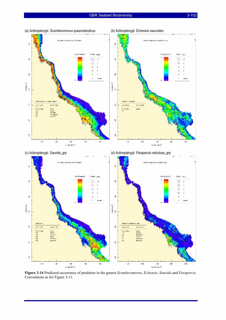
GBR Seabed Biodiversity 3-102
(a) Actinopterygii: Scomberomorus queenslandicus (b) Actinopterygii: Echeneis naucrates
(c) Actinopterygii: Saurida_grp (d) Actinopterygii: Parapercis nebulosa_grp
Figure 3-14 Predicted occurrence of predators in the genera Scomberomorus, Echeneis, Saurida and Parapercis. Conventions as for Figure 3-11.
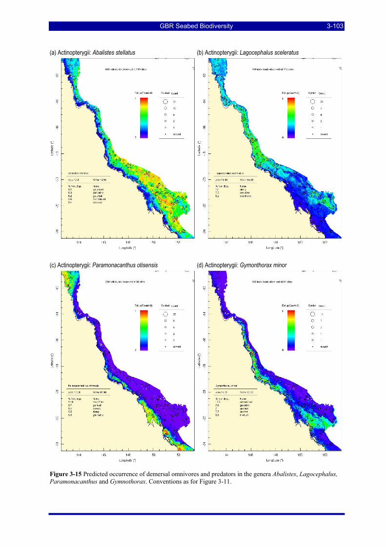
GBR Seabed Biodiversity 3-103
(a) Actinopterygii: Abalistes stellatus (b) Actinopterygii: Lagocephalus sceleratus
(c) Actinopterygii: Paramonacanthus otisensis (d) Actinopterygii: Gymonthorax minor
Figure 3-15 Predicted occurrence of demersal omnivores and predators in the genera Abalistes, Lagocephalus, Paramonacanthus and Gymnothorax. Conventions as for Figure 3-11.
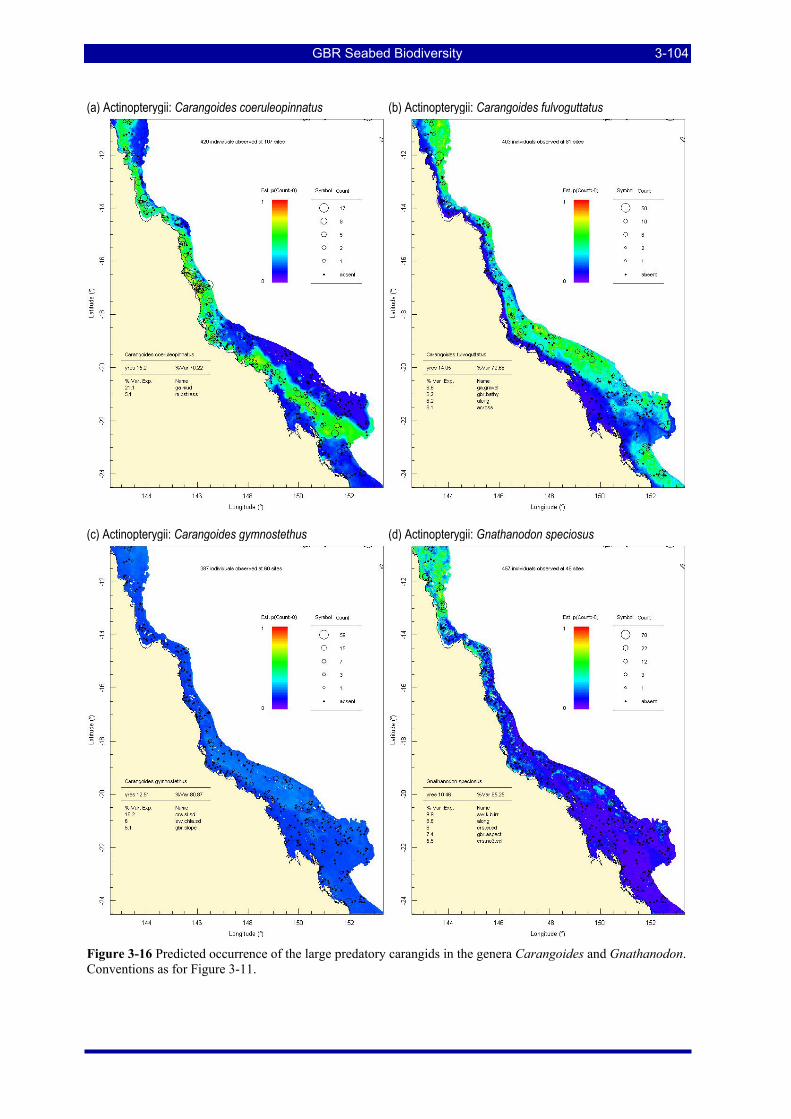
GBR Seabed Biodiversity 3-104
(a) Actinopterygii: Carangoides coeruleopinnatus (b) Actinopterygii: Carangoides fulvoguttatus
(c) Actinopterygii: Carangoides gymnostethus (d) Actinopterygii: Gnathanodon speciosus
Figure 3-16 Predicted occurrence of the large predatory carangids in the genera Carangoides and Gnathanodon. Conventions as for Figure 3-11.
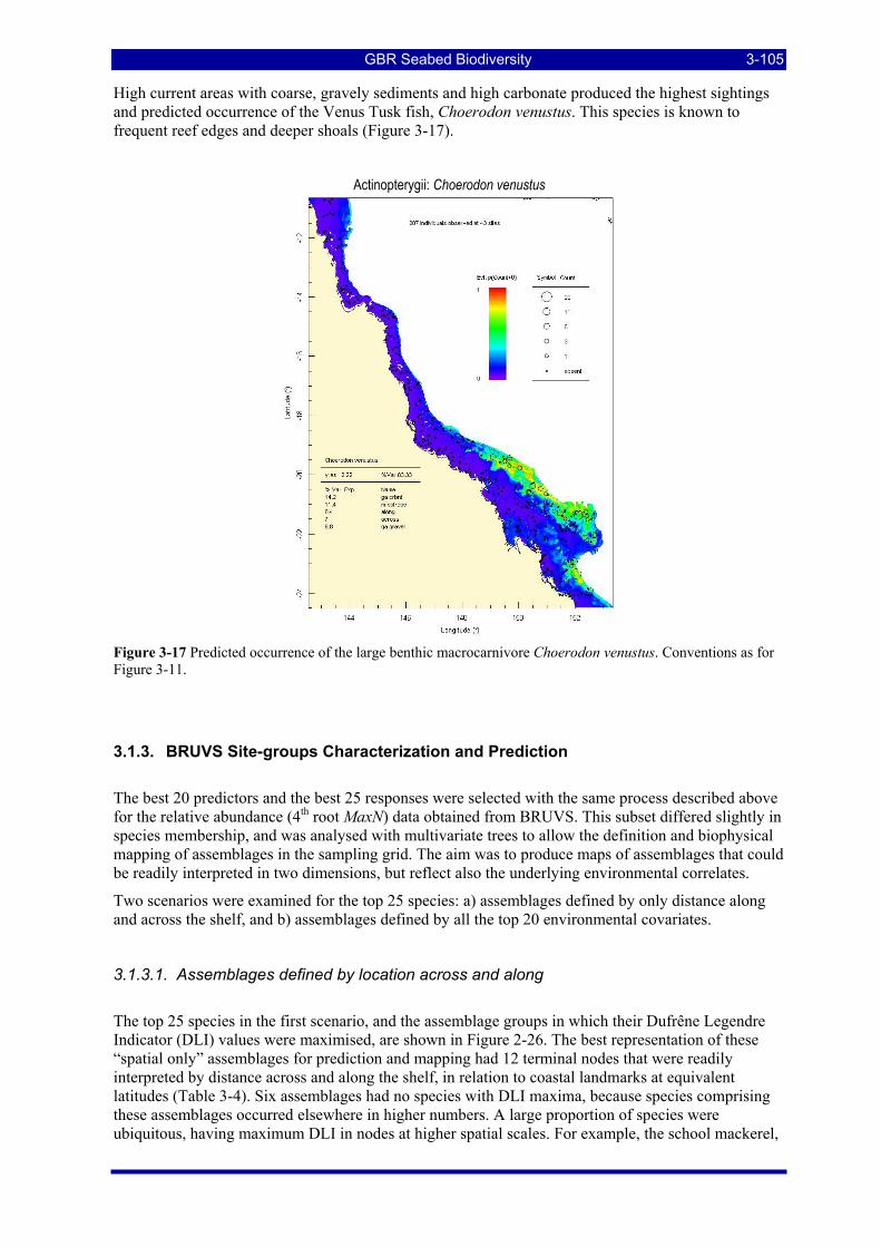
GBR Seabed Biodiversity 3-105
High current areas with coarse, gravely sediments and high carbonate produced the highest sightings and predicted occurrence of the Venus Tusk fish, Choerodon venustus. This species is known to frequent reef edges and deeper shoals (Figure 3-17).
Actinopterygii: Choerodon venustus
Figure 3-17 Predicted occurrence of the large benthic macrocarnivore Choerodon venustus. Conventions as for Figure 3-11.
3.1.3. BRUVS Site-groups Characterization and Prediction
The best 20 predictors and the best 25 responses were selected with the same process described above for the relative abundance (4th root MaxN) data obtained from BRUVS. This subset differed slightly in species membership, and was analysed with multivariate trees to allow the definition and biophysical mapping of assemblages in the sampling grid. The aim was to produce maps of assemblages that could be readily interpreted in two dimensions, but reflect also the underlying environmental correlates.
Two scenarios were examined for the top 25 species: a) assemblages defined by only distance along and across the shelf, and b) assemblages defined by all the top 20 environmental covariates.
3.1.3.1. Assemblages defined by location across and along
The top 25 species in the first scenario, and the assemblage groups in which their Dufrêne Legendre Indicator (DLI) values were maximised, are shown in Figure 2-26. The best representation of these “spatial only” assemblages for prediction and mapping had 12 terminal nodes that were readily interpreted by distance across and along the shelf, in relation to coastal landmarks at equivalent latitudes (Table 3-4). Six assemblages had no species with DLI maxima, because species comprising these assemblages occurred elsewhere in higher numbers. A large proportion of species were ubiquitous, having maximum DLI in nodes at higher spatial scales. For example, the school mackerel,
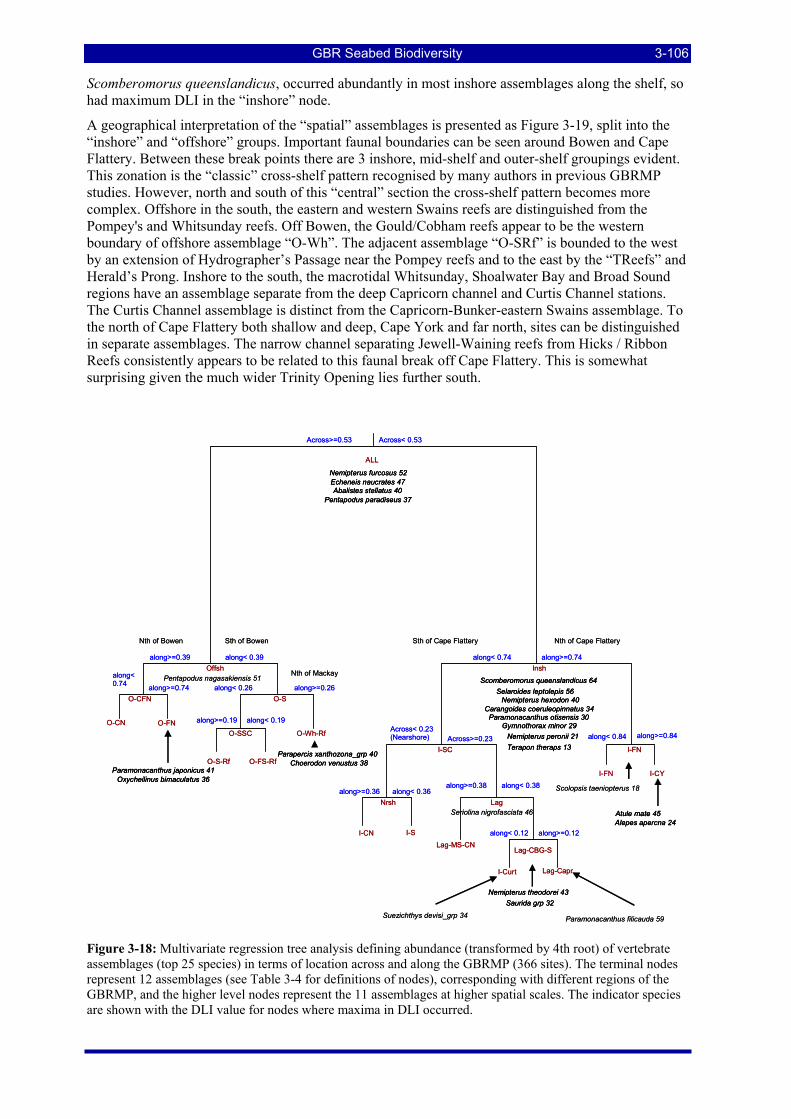
GBR Seabed Biodiversity 3-106
Scomberomorus queenslandicus, occurred abundantly in most inshore assemblages along the shelf, so had maximum DLI in the “inshore” node.
A geographical interpretation of the “spatial” assemblages is presented as Figure 3-19, split into the “inshore” and “offshore” groups. Important faunal boundaries can be seen around Bowen and Cape Flattery. Between these break points there are 3 inshore, mid-shelf and outer-shelf groupings evident. This zonation is the “classic” cross-shelf pattern recognised by many authors in previous GBRMP studies. However, north and south of this “central” section the cross-shelf pattern becomes more complex. Offshore in the south, the eastern and western Swains reefs are distinguished from the Pompey's and Whitsunday reefs. Off Bowen, the Gould/Cobham reefs appear to be the western boundary of offshore assemblage “O-Wh”. The adjacent assemblage “O-SRf” is bounded to the west by an extension of Hydrographer’s Passage near the Pompey reefs and to the east by the “TReefs” and Herald’s Prong. Inshore to the south, the macrotidal Whitsunday, Shoalwater Bay and Broad Sound regions have an assemblage separate from the deep Capricorn channel and Curtis Channel stations. The Curtis Channel assemblage is distinct from the Capricorn-Bunker-eastern Swains assemblage. To the north of Cape Flattery both shallow and deep, Cape York and far north, sites can be distinguished in separate assemblages. The narrow channel separating Jewell-Waining reefs from Hicks / Ribbon Reefs consistently appears to be related to this faunal break off Cape Flattery. This is somewhat surprising given the much wider Trinity Opening lies further south.
Across>=0.53
along>=0.39
along< 0.74 along< 0.26
along>=0.19
along< 0.74
Across< 0.23(Nearshore)
along>=0.36along>=0.38
along< 0.12
along< 0.84
Across< 0.53
along< 0.39
along>=0.74 along>=0.26
along< 0.19
along>=0.74
Across>=0.23
along< 0.36along< 0.38
along>=0.12
along>=0.84
ALL
Offsh
O-CFN
O-CN O-FN
O-S
O-SSC
O-S-Rf O-FS-Rf
O-Wh-Rf
Insh
I-SC
Nrsh
I-CN
Lag
Lag-MS-CNLag-CBG-S
I-Curt
Nemipterus furcosus 52Echeneis naucrates 47Abalistes stellatus 40
Pentapodus paradiseus 37
Pentapodus nagasakiensis 51
Scolopsis taeniopterus 18
Scomberomorus queenslandicus 64
Nemipterus hexodon 40Carangoides coeruleopinnatus 34
Paramonacanthus otisensis 30
Nemipterus peronii 21Gymnothorax minor 29
Selaroides leptolepis 56
Terapon theraps 13
Paramonacanthus japonicus 41Oxycheilinus bimaculatus 36
Parapercis xanthozona_grp 40Choerodon venustus 38
Seriolina nigrofasciata 46
Nemipterus theodorei 43Saurida grp 32
Suezichthys devisi_grp 34 Paramonacanthus filicauda 59
Nth of Bowen Sth of Bowen Nth of Cape FlatterySth of Cape Flattery
Nth of Mackay
I-S
Lag-Capr
I-FN
I-FN I-CY
Atule mate 45Alepes apercna 24
Across>=0.53
along>=0.39
along< 0.74 along< 0.26
along>=0.19
along< 0.74
Across< 0.23(Nearshore)
along>=0.36along>=0.38
along< 0.12
along< 0.84
Across< 0.53
along< 0.39
along>=0.74 along>=0.26
along< 0.19
along>=0.74
Across>=0.23
along< 0.36along< 0.38
along>=0.12
along>=0.84
ALL
Offsh
O-CFN
O-CN O-FN
O-S
O-SSC
O-S-Rf O-FS-Rf
O-Wh-Rf
Insh
I-SC
Nrsh
I-CN
Lag
Lag-MS-CNLag-CBG-S
I-Curt
Nemipterus furcosus 52Echeneis naucrates 47Abalistes stellatus 40
Pentapodus paradiseus 37
Nemipterus furcosus 52Echeneis naucrates 47Abalistes stellatus 40
Pentapodus paradiseus 37
Pentapodus nagasakiensis 51
Scolopsis taeniopterus 18
Scomberomorus queenslandicus 64
Nemipterus hexodon 40Carangoides coeruleopinnatus 34
Paramonacanthus otisensis 30
Nemipterus peronii 21Gymnothorax minor 29
Selaroides leptolepis 56
Terapon theraps 13
Scomberomorus queenslandicus 64
Nemipterus hexodon 40Carangoides coeruleopinnatus 34
Paramonacanthus otisensis 30
Nemipterus peronii 21Gymnothorax minor 29
Selaroides leptolepis 56
Terapon theraps 13
Paramonacanthus japonicus 41Oxycheilinus bimaculatus 36
Paramonacanthus japonicus 41Oxycheilinus bimaculatus 36
Parapercis xanthozona_grp 40Choerodon venustus 38
Parapercis xanthozona_grp 40Choerodon venustus 38
Seriolina nigrofasciata 46
Nemipterus theodorei 43Saurida grp 32
Nemipterus theodorei 43Saurida grp 32
Suezichthys devisi_grp 34 Paramonacanthus filicauda 59
Nth of Bowen Sth of Bowen Nth of Cape FlatterySth of Cape Flattery
Nth of Mackay
I-S
Lag-Capr
I-FN
I-FN I-CY
Atule mate 45Alepes apercna 24Atule mate 45Alepes apercna 24
Figure 3-18: Multivariate regression tree analysis defining abundance (transformed by 4th root) of vertebrate assemblages (top 25 species) in terms of location across and along the GBRMP (366 sites). The terminal nodes represent 12 assemblages (see Table 3-4 for definitions of nodes), corresponding with different regions of the GBRMP, and the higher level nodes represent the 11 assemblages at higher spatial scales. The indicator species are shown with the DLI value for nodes where maxima in DLI occurred.
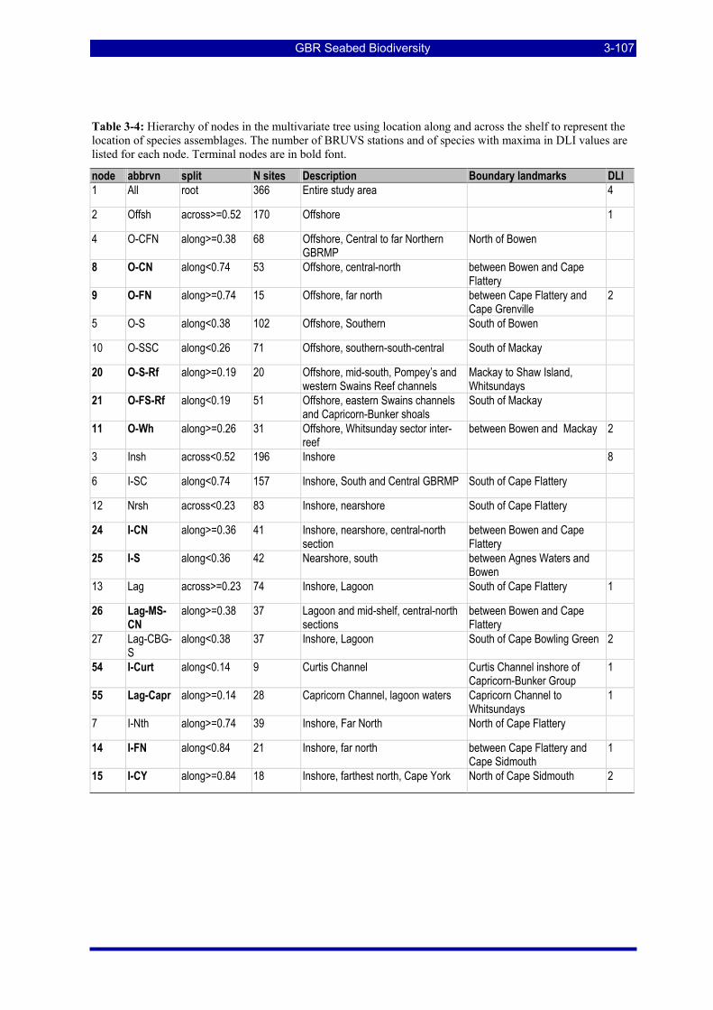
GBR Seabed Biodiversity 3-107
Table 3-4: Hierarchy of nodes in the multivariate tree using location along and across the shelf to represent the location of species assemblages. The number of BRUVS stations and of species with maxima in DLI values are listed for each node. Terminal nodes are in bold font.
node abbrvn split N sites Description Boundary landmarks DLI 1 All root 366 Entire study area 4
2 Offsh across>=0.52 170 Offshore 1
4 O-CFN along>=0.38 68 Offshore, Central to far Northern GBRMP
North of Bowen
8 O-CN along<0.74 53 Offshore, central-north between Bowen and Cape Flattery
9 O-FN along>=0.74 15 Offshore, far north between Cape Flattery and Cape Grenville
2
5 O-S along<0.38 102 Offshore, Southern South of Bowen
10 O-SSC along<0.26 71 Offshore, southern-south-central South of Mackay
20 O-S-Rf along>=0.19 20 Offshore, mid-south, Pompey’s and western Swains Reef channels
Mackay to Shaw Island, Whitsundays
21 O-FS-Rf along<0.19 51 Offshore, eastern Swains channels and Capricorn-Bunker shoals
South of Mackay
11 O-Wh along>=0.26 31 Offshore, Whitsunday sector inter-reef
between Bowen and Mackay 2
3 Insh across<0.52 196 Inshore 8
6 I-SC along<0.74 157 Inshore, South and Central GBRMP South of Cape Flattery
12 Nrsh across<0.23 83 Inshore, nearshore South of Cape Flattery
24 I-CN along>=0.36 41 Inshore, nearshore, central-north section
between Bowen and Cape Flattery
25 I-S along<0.36 42 Nearshore, south between Agnes Waters and Bowen
13 Lag across>=0.23 74 Inshore, Lagoon South of Cape Flattery 1
26 Lag-MS-CN
along>=0.38 37 Lagoon and mid-shelf, central-north sections
between Bowen and Cape Flattery
27 Lag-CBG-S
along<0.38 37 Inshore, Lagoon South of Cape Bowling Green 2
54 I-Curt along<0.14 9 Curtis Channel Curtis Channel inshore of Capricorn-Bunker Group
1
55 Lag-Capr along>=0.14 28 Capricorn Channel, lagoon waters Capricorn Channel to Whitsundays
1
7 I-Nth along>=0.74 39 Inshore, Far North North of Cape Flattery
14 I-FN along<0.84 21 Inshore, far north between Cape Flattery and Cape Sidmouth
1
15 I-CY along>=0.84 18 Inshore, farthest north, Cape York North of Cape Sidmouth 2
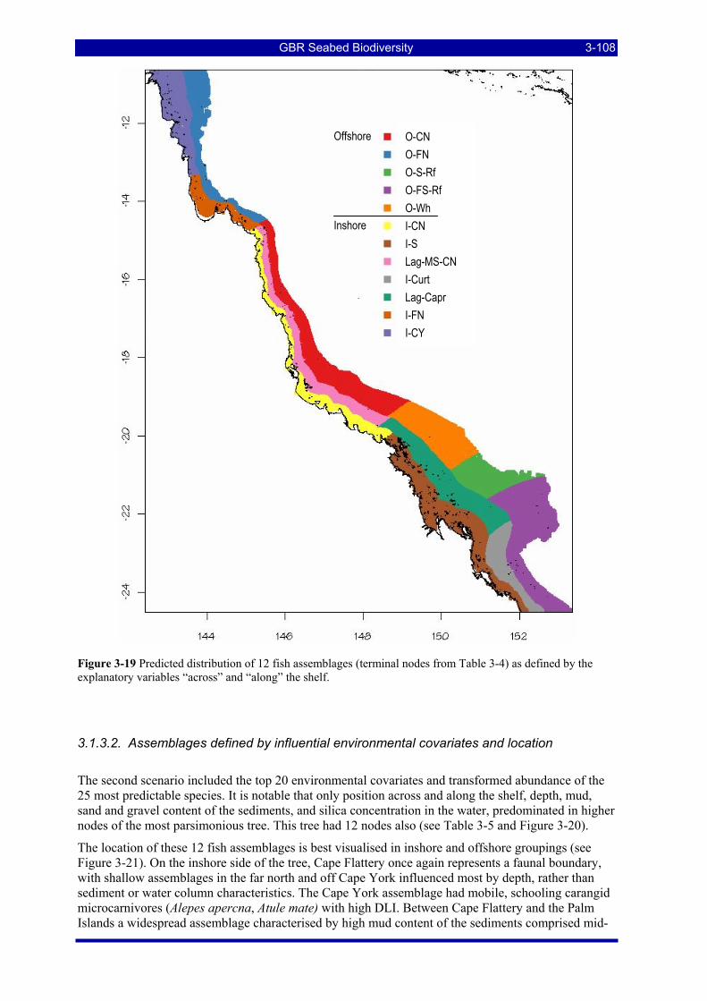
GBR Seabed Biodiversity 3-108
Figure 3-19 Predicted distribution of 12 fish assemblages (terminal nodes from Table 3-4) as defined by the explanatory variables “across” and “along” the shelf.
3.1.3.2. Assemblages defined by influential environmental covariates and location
The second scenario included the top 20 environmental covariates and transformed abundance of the 25 most predictable species. It is notable that only position across and along the shelf, depth, mud, sand and gravel content of the sediments, and silica concentration in the water, predominated in higher nodes of the most parsimonious tree. This tree had 12 nodes also (see Table 3-5 and Figure 3-20).
The location of these 12 fish assemblages is best visualised in inshore and offshore groupings (see Figure 3-21). On the inshore side of the tree, Cape Flattery once again represents a faunal boundary, with shallow assemblages in the far north and off Cape York influenced most by depth, rather than sediment or water column characteristics. The Cape York assemblage had mobile, schooling carangid microcarnivores (Alepes apercna, Atule mate) with high DLI. Between Cape Flattery and the Palm Islands a widespread assemblage characterised by high mud content of the sediments comprised mid-
O-CN O-FN O-S-Rf O-FS-Rf O-Wh I-CN I-S Lag-MS-CN I-Curt Lag-Capr I-FN I-CY
Offshore Inshore
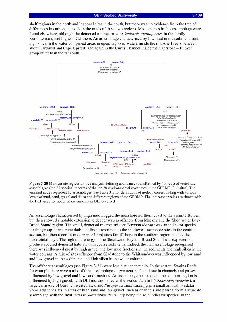
GBR Seabed Biodiversity 3-109
shelf regions in the north and lagoonal sites in the south, but there was no evidence from the tree of differences in carbonate levels in the muds of these two regions. Most species in this assemblage were found elsewhere, although the demersal microcarnivore Scolopsis taeniopterus, in the family Nemipteridae, had highest DLI there. An assemblage characterised by low mud in the sediments and high silica in the water comprised areas in open, lagoonal waters inside the mid-shelf reefs between about Cardwell and Cape Upstart, and again in the Curtis Channel inside the Capricorn – Bunker group of reefs in the far south.
Figure 3-20 Multivariate regression tree analysis defining abundance (transformed by 4th root) of vertebrate assemblages (top 25 species) in terms of the top 20 environmental covariates in the GBRMP (366 sites). The terminal nodes represent 12 assemblages (see Table 3-5 for definitions of nodes), corresponding with various levels of mud, sand, gravel and silica and different regions of the GBRMP. The indicator species are shown with the DLI value for nodes where maxima in DLI occurred.
An assemblage characterised by high mud hugged the nearshore northern coast to the vicinity Bowen, but then showed a notable extension to deeper waters offshore from Mackay and the Shoalwater Bay- Broad Sound region. The small, demersal microcarnivore Terapon theraps was an indicator species for this group. It was remarkable to find it restricted to the shallowest nearshore sites in the central section, but then record it in deeper [>40 m] sites far offshore in the southern region outside the macrtotidal bays. The high tidal energy in the Shoalwater Bay and Broad Sound was expected to produce scoured demersal habitats with coarse sediments. Indeed, the fish assemblage recognised there was influenced most by high gravel and low mud fractions in the sediments and high silica in the water column. A mix of sites offshore from Gladstone to the Whitsundays was influenced by low mud and low gravel in the sediments and high silica in the water column.
The offshore assemblages (see Figure 3-21) were less distinct spatially. In the eastern Swains Reefs for example there were a mix of three assemblages – two near reefs and one in channels and passes influenced by low gravel and low sand fractions. An assemblage near reefs in the southern region is influenced by high gravel, with DLI indicator species the Venus Tuskfish (Choerodon venustus), a large carnivore of benthic invertebrates, and Parapercis xanthozona_grp, a small ambush predator. Some adjacent sites in areas of high sand and low gravel, such as channels and passes, form a separate assemblage with the small wrasse Suezichthys devisi_grp being the sole indicator species. In the
across>=0.52
ga.gravel < 8.983
ga.sand < 89.95 along>=0.38
gbr.bathy>=-49.3
along< 0.74
ga.mud>=16.05
across< 0.28 crs.si.av>=1.56
ga.gravel>=10.29
along< 0.84
across< 0.52
ga.gravel>=8.983
ga.sand >=89.95 along< 0.38
gbr.bathy < -49.3
along>=0.74
ga.mud< 16.05
across>=0.28 crs.si.av< 1.56
ga.gravel< 10.29
along>=0.84
All
Offsh
LoGrav LGrav - LSand Rf- LGrav -HSand
HiGrav HGrav -CntrlNth Rf-HGravSthn
Insh
Shal
HiMud
HMud - Nrshr HMud-Lag
LoMud
HiSil
HSil-LMud-HGrav
HSil-LMud-LGrav
LMud-LSil
Nthn Shal-FN Shal -CY
Deep - Capr
Nemipterus.furcosus 52Echeneis.naucrates 47
Pentapodus.paradiseus 37
Pentapodus.nagasakiensis 51 Scomberomorus.queenslandicus 64
Selaroides.leptolepis 56 Nemipterus.hexodon 40
Carangoides.coeruleopinnatus 34 Gymnothorax.minor 29 Nemipterus.peronii 21
Paramonacanthus.filicauda 65Nemipterus.theodorei 58
Saurida.grp 48Seriolina.nigrofasciata 47
Abalistes.stellatus 41
Suezichthys.devisi _grp 15 Oxycheilinus.bimaculatus 37
Paramonacanthus.japonicus 12 Choerodon.venustus 44
Parapercis.xanthozona _grp 39
Paramonacanthus.otisensis 39
Atule.mate 48 Alepes.apercna 25
Terapon.theraps 14
Scolopsis.taeniopterus 29
Sth of Cape Flattery
Sth of Cape Direction
across>=0.52
ga.gravel < 8.983
ga.sand < 89.95 along>=0.38
gbr.bathy>=-49.3
along< 0.74
ga.mud>=16.05
across< 0.28 crs.si.av>=1.56
ga.gravel>=10.29
along< 0.84
across< 0.52
ga.gravel>=8.983
ga.sand
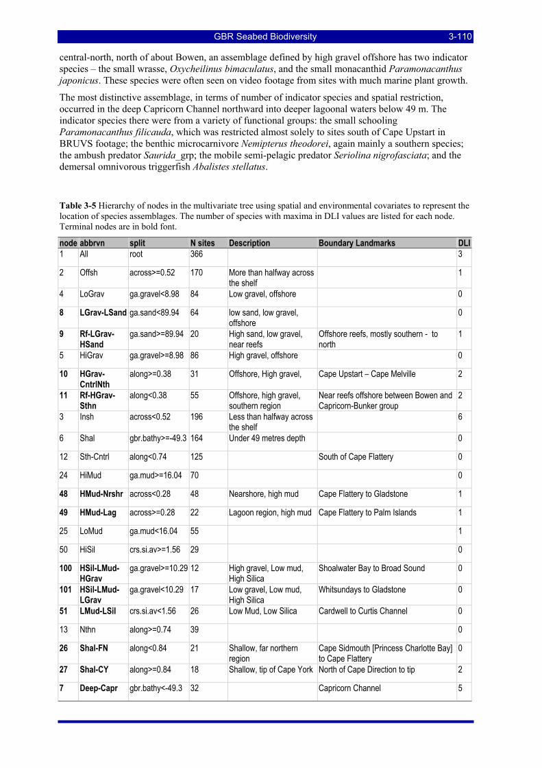
GBR Seabed Biodiversity 3-110
central-north, north of about Bowen, an assemblage defined by high gravel offshore has two indicator species – the small wrasse, Oxycheilinus bimaculatus, and the small monacanthid Paramonacanthus japonicus. These species were often seen on video footage from sites with much marine plant growth.
The most distinctive assemblage, in terms of number of indicator species and spatial restriction, occurred in the deep Capricorn Channel northward into deeper lagoonal waters below 49 m. The indicator species there were from a variety of functional groups: the small schooling Paramonacanthus filicauda, which was restricted almost solely to sites south of Cape Upstart in BRUVS footage; the benthic microcarnivore Nemipterus theodorei, again mainly a southern species; the ambush predator Saurida_grp; the mobile semi-pelagic predator Seriolina nigrofasciata; and the demersal omnivorous triggerfish Abalistes stellatus.
Table 3-5 Hierarchy of nodes in the multivariate tree using spatial and environmental covariates to represent the location of species assemblages. The number of species with maxima in DLI values are listed for each node. Terminal nodes are in bold font.
node abbrvn split N sites Description Boundary Landmarks DLI 1 All root 366 3
2 Offsh across>=0.52 170 More than halfway across the shelf
1
4 LoGrav ga.gravel<8.98 84 Low gravel, offshore 0
8 LGrav-LSand ga.sand<89.94 64 low sand, low gravel, offshore
0
9 Rf-LGrav-HSand
ga.sand>=89.94 20 High sand, low gravel, near reefs
Offshore reefs, mostly southern - to north
1
5 HiGrav ga.gravel>=8.98 86 High gravel, offshore 0
10 HGrav-CntrlNth
along>=0.38 31 Offshore, High gravel, Cape Upstart – Cape Melville 2
11 Rf-HGrav-Sthn
along<0.38 55 Offshore, high gravel, southern region
Near reefs offshore between Bowen and Capricorn-Bunker group
2
3 Insh across<0.52 196 Less than halfway across the shelf
6
6 Shal gbr.bathy>=-49.3 164 Under 49 metres depth 0
12 Sth-Cntrl along<0.74 125 South of Cape Flattery 0
24 HiMud ga.mud>=16.04 70 0
48 HMud-Nrshr across<0.28 48 Nearshore, high mud Cape Flattery to Gladstone 1
49 HMud-Lag across>=0.28 22 Lagoon region, high mud Cape Flattery to Palm Islands 1
25 LoMud ga.mud<16.04 55 1
50 HiSil crs.si.av>=1.56 29 0
100 HSil-LMud-HGrav
ga.gravel>=10.29 12 High gravel, Low mud, High Silica
Shoalwater Bay to Broad Sound 0
101 HSil-LMud-LGrav
ga.gravel<10.29 17 Low gravel, Low mud, High Silica
Whitsundays to Gladstone 0
51 LMud-LSil crs.si.av<1.56 26 Low Mud, Low Silica Cardwell to Curtis Channel 0
13 Nthn along>=0.74 39 0
26 Shal-FN along<0.84 21 Shallow, far northern region
Cape Sidmouth [Princess Charlotte Bay] to Cape Flattery
0
27 Shal-CY along>=0.84 18 Shallow, tip of Cape York North of Cape Direction to tip 2
7 Deep-Capr gbr.bathy<-49.3 32 Capricorn Channel 5
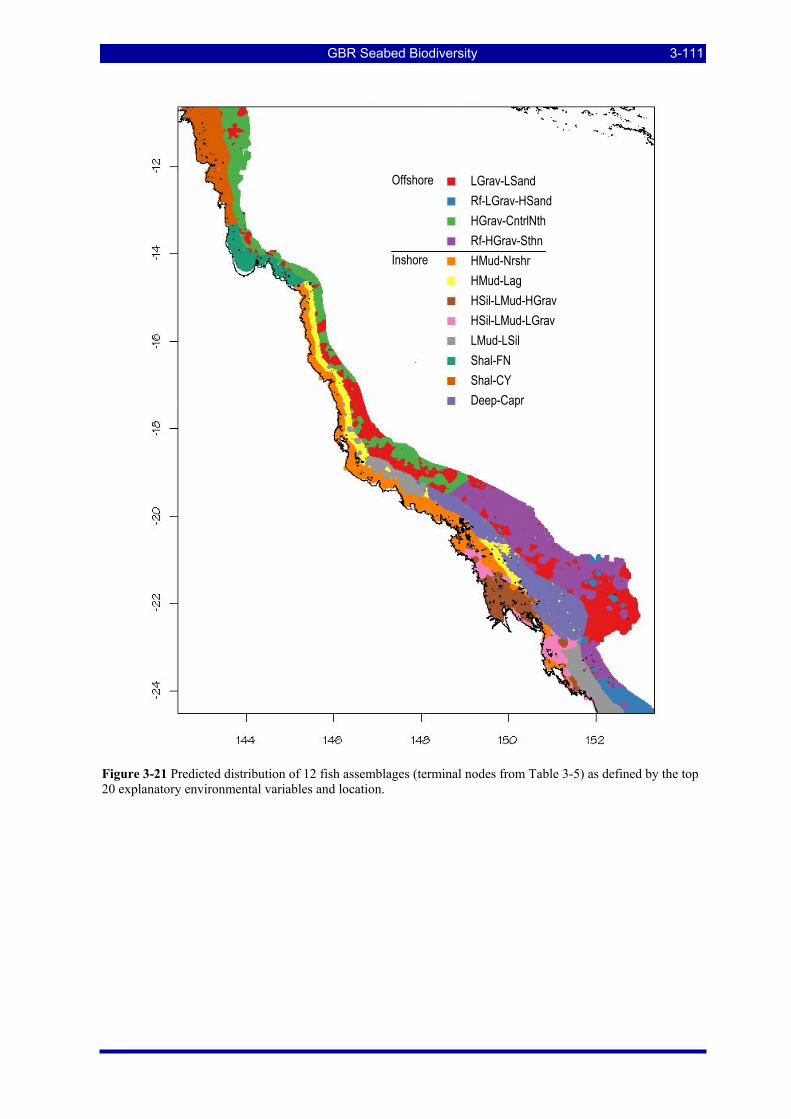
GBR Seabed Biodiversity 3-111
Figure 3-21 Predicted distribution of 12 fish assemblages (terminal nodes from Table 3-5) as defined by the top 20 explanatory environmental variables and location.
LGrav-LSand Rf-LGrav-HSand HGrav-CntrlNth Rf-HGrav-Sthn HMud-Nrshr HMud-Lag HSil-LMud-HGrav HSil-LMud-LGrav LMud-LSil Shal-FN Shal-CY Deep-Capr
Offshore Inshore
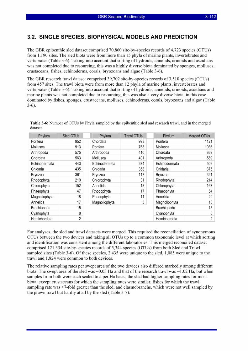
GBR Seabed Biodiversity 3-112
3.2. SINGLE SPECIES, BIOPHYSICAL MODELS AND PREDICTION The GBR epibenthic sled dataset comprised 70,860 site-by-species records of 4,723 species (OTUs) from 1,190 sites. The sled biota were from more than 15 phyla of marine plants, invertebrates and vertebrates (Table 3-6). Taking into account that sorting of hydroids, annelids, crinoids and ascidians was not completed due to resourcing, this was a highly diverse biota dominated by sponges, molluscs, crustaceans, fishes, echinoderms, corals, bryozoans and algae (Table 3-6).
The GBR research trawl dataset comprised 39,702 site-by-species records of 3,510 species (OTUs) from 457 sites. The trawl biota were from more than 12 phyla of marine plants, invertebrates and vertebrates (Table 3-6). Taking into account that sorting of hydroids, annelids, crinoids, ascidians and marine plants was not completed due to resourcing, this was also a very diverse biota, in this case dominated by fishes, sponges, crustaceans, molluscs, echinoderms, corals, bryozoans and algae (Table 3-6).
Table 3-6: Number of OTUs by Phyla sampled by the epibenthic sled and research trawl, and in the merged dataset.
Phylum Sled OTUs Phylum Trawl OTUs Phylum Merged OTUs Porifera 952 Chordata 993 Porifera 1121 Mollusca 913 Porifera 768 Mollusca 1036 Arthropoda 575 Arthropoda 410 Chordata 869 Chordata 563 Mollusca 401 Arthropoda 589 Echinodermata 443 Echinodermata 374 Echinodermata 509 Cnidaria 435 Cnidaria 358 Cnidaria 375 Bryozoa 361 Bryozoa 117 Bryozoa 321 Rhodophyta 210 Chlorophyta 31 Rhodophyta 214 Chlorophyta 152 Annelida 18 Chlorophyta 167 Phaeophyta 47 Rhodophyta 17 Phaeophyta 54 Magnoliophyta 18 Phaeophyta 11 Annelida 29 Annelida 17 Magnoliophyta 3 Magnoliophyta 18 Brachiopoda 15 Brachiopoda 15 Cyanophyta 8 Cyanophyta 8 Hemichordata 2 Hemichordata 2
For analyses, the sled and trawl datasets were merged. This required the reconciliation of synonymous OTUs between the two devices and taking all OTUs up to a common taxonomic level at which sorting and identification was consistent among the different laboratories. This merged reconciled dataset comprised 121,334 site-by-species records of 5,344 species (OTUs) from both Sled and Trawl sampled sites (Table 3-6). Of these species, 2,435 were unique to the sled, 1,085 were unique to the trawl and 1,824 were common to both devices.
The relative sampling rates per swept area of the two devices also differed markedly among different biota. The swept area of the sled was ~0.03 Ha and that of the research trawl was ~1.02 Ha, but when samples from both were each scaled to a per Ha basis, the sled had higher sampling rates for most biota, except crustaceans for which the sampling rates were similar, fishes for which the trawl sampling rate was >7-fold greater than the sled, and elasmobranchs, which were not well sampled by the prawn trawl but hardly at all by the sled (Table 3-7).
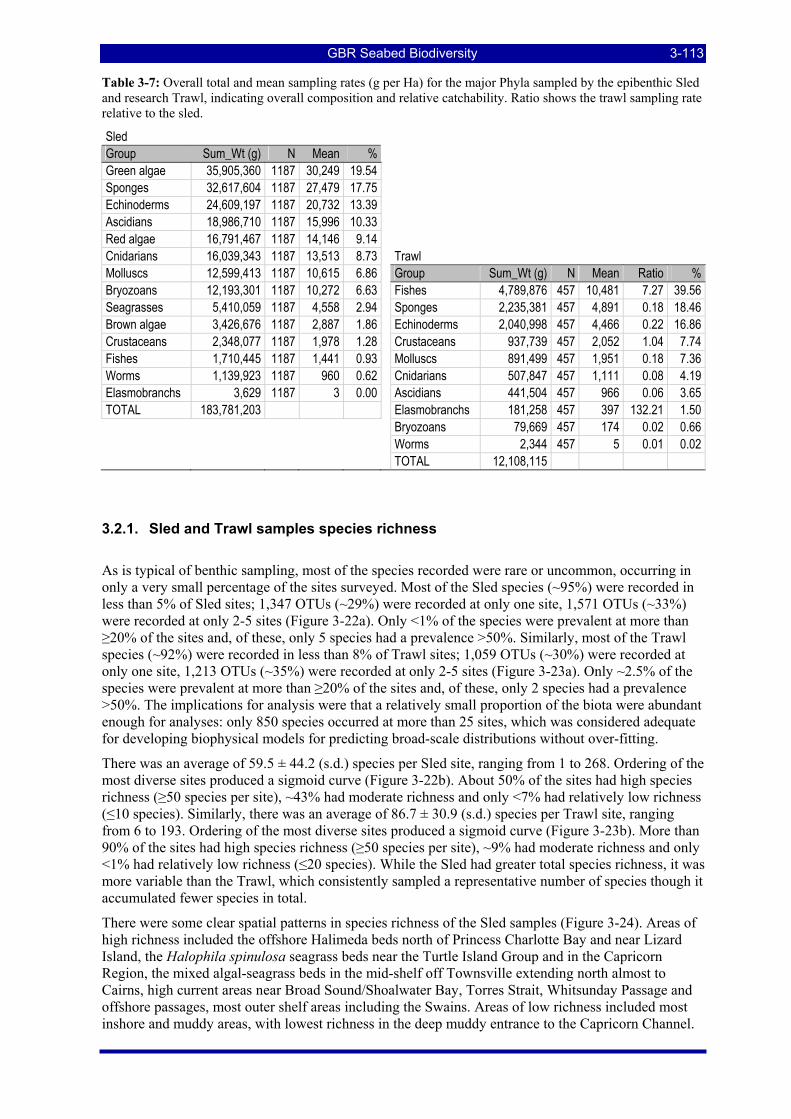
GBR Seabed Biodiversity 3-113
Table 3-7: Overall total and mean sampling rates (g per Ha) for the major Phyla sampled by the epibenthic Sled and research Trawl, indicating overall composition and relative catchability. Ratio shows the trawl sampling rate relative to the sled.
Sled Group Sum_Wt (g) N Mean % Green algae 35,905,360 1187 30,249 19.54 Sponges 32,617,604 1187 27,479 17.75 Echinoderms 24,609,197 1187 20,732 13.39 Ascidians 18,986,710 1187 15,996 10.33 Red algae 16,791,467 1187 14,146 9.14 Cnidarians 16,039,343 1187 13,513 8.73 Trawl Molluscs 12,599,413 1187 10,615 6.86 Group Sum_Wt (g) N Mean Ratio % Bryozoans 12,193,301 1187 10,272 6.63 Fishes 4,789,876 457 10,481 7.27 39.56 Seagrasses 5,410,059 1187 4,558 2.94 Sponges 2,235,381 457 4,891 0.18 18.46 Brown algae 3,426,676 1187 2,887 1.86 Echinoderms 2,040,998 457 4,466 0.22 16.86 Crustaceans 2,348,077 1187 1,978 1.28 Crustaceans 937,739 457 2,052 1.04 7.74 Fishes 1,710,445 1187 1,441 0.93 Molluscs 891,499 457 1,951 0.18 7.36 Worms 1,139,923 1187 960 0.62 Cnidarians 507,847 457 1,111 0.08 4.19 Elasmobranchs 3,629 1187 3 0.00 Ascidians 441,504 457 966 0.06 3.65 TOTAL 183,781,203 Elasmobranchs 181,258 457 397 132.21 1.50
Bryozoans 79,669 457 174 0.02 0.66 Worms 2,344 457 5 0.01 0.02 TOTAL 12,108,115
3.2.1. Sled and Trawl samples species richness
As is typical of benthic sampling, most of the species recorded were rare or uncommon, occurring in only a very small percentage of the sites surveyed. Most of the Sled species (~95%) were recorded in less than 5% of Sled sites; 1,347 OTUs (~29%) were recorded at only one site, 1,571 OTUs (~33%) were recorded at only 2-5 sites (Figure 3-22a). Only <1% of the species were prevalent at more than ≥20% of the sites and, of these, only 5 species had a prevalence >50%. Similarly, most of the Trawl species (~92%) were recorded in less than 8% of Trawl sites; 1,059 OTUs (~30%) were recorded at only one site, 1,213 OTUs (~35%) were recorded at only 2-5 sites (Figure 3-23a). Only ~2.5% of the species were prevalent at more than ≥20% of the sites and, of these, only 2 species had a prevalence >50%. The implications for analysis were that a relatively small proportion of the biota were abundant enough for analyses: only 850 species occurred at more than 25 sites, which was considered adequate for developing biophysical models for predicting broad-scale distributions without over-fitting.
There was an average of 59.5 ± 44.2 (s.d.) species per Sled site, ranging from 1 to 268. Ordering of the most diverse sites produced a sigmoid curve (Figure 3-22b). About 50% of the sites had high species richness (≥50 species per site), ~43% had moderate richness and only <7% had relatively low richness (≤10 species). Similarly, there was an average of 86.7 ± 30.9 (s.d.) species per Trawl site, ranging from 6 to 193. Ordering of the most diverse sites produced a sigmoid curve (Figure 3-23b). More than 90% of the sites had high species richness (≥50 species per site), ~9% had moderate richness and only <1% had relatively low richness (≤20 species). While the Sled had greater total species richness, it was more variable than the Trawl, which consistently sampled a representative number of species though it accumulated fewer species in total.
There were some clear spatial patterns in species richness of the Sled samples (Figure 3-24). Areas of high richness included the offshore Halimeda beds north of Princess Charlotte Bay and near Lizard Island, the Halophila spinulosa seagrass beds near the Turtle Island Group and in the Capricorn Region, the mixed algal-seagrass beds in the mid-shelf off Townsville extending north almost to Cairns, high current areas near Broad Sound/Shoalwater Bay, Torres Strait, Whitsunday Passage and offshore passages, most outer shelf areas including the Swains. Areas of low richness included most inshore and muddy areas, with lowest richness in the deep muddy entrance to the Capricorn Channel.
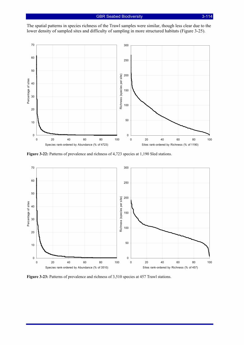
GBR Seabed Biodiversity 3-114
The spatial patterns in species richness of the Trawl samples were similar, though less clear due to the lower density of sampled sites and difficulty of sampling in more structured habitats (Figure 3-25).
0
10
20
30
40
50
60
70
0 20 40 60 80 100
Species rank-ordered by Abundance (% of 4723)
Per
cent
age
of s
ites
0
50
100
150
200
250
300
0 20 40 60 80 100
Sites rank-ordered by Richness (% of 1190)
Ric
hnes
s (s
peci
es p
er s
ite)
Figure 3-22: Patterns of prevalence and richness of 4,723 species at 1,190 Sled stations.
0
10
20
30
40
50
60
70
0 20 40 60 80 100
Species rank-ordered by Abundance (% of 3510)
Per
cent
age
of s
ites
0
50
100
150
200
250
300
0 20 40 60 80 100
Sites rank-ordered by Richness (% of 457)
Ric
hnes
s (s
peci
es p
er s
ite)
Figure 3-23: Patterns of prevalence and richness of 3,510 species at 457 Trawl stations.
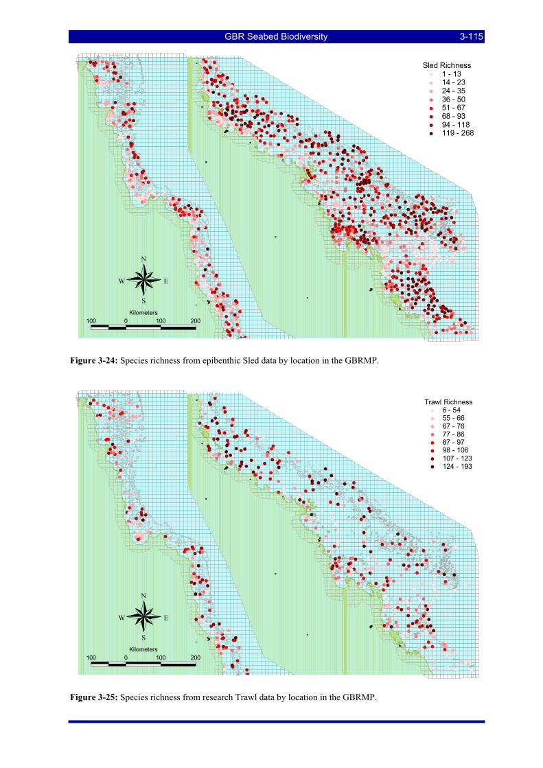
GBR Seabed Biodiversity 3-115
#
#
#
#
#
#
##
#
#
#
#
##
#
#
#
#
#
#
##
#
##
#
#
# #
#
#
#
#### ###
#
#
##
##
#
#
#
#
#
#
#
#
###
#
#
#
#
#
#
##
#
#
##
##
#
#
#
#
#
#
#
#
#
###
#
#
#
#
#
#
#
##
# # #
#
#
##
###
## #
#
#
#
##
#
#
#
##
#
#
#
#
#
#
#
#
#
#
#
#
#
#
#
#
##
#
#
#
#
#
#
#
##
##
#
#
##
#
#
#
#
#
#
#
#
#
#
#
##
#
#
#
#
##
#
#
##
#
#
#
#
#
#
# #
#
#
#
#
#
#
#
##
##
#
#
#
#
#
#
#
#
#
#
#
#
#
#
#
#
#
#
#
#
#
#
#
###
#
# ## #
#
#
#
#
#
#
#
##
##
#
#
##
#
#
#
#
#
#
#
##
#
#
#
#
#
#
#
#
##
#
#
#
# #
#
#
# #
#
##
# #
#
#
#
#
#
#
#
#
#
##
# #
##
#
#
#
# #
#
#
#
#
#
#
#
#
# #
#
#
#
#
#
#
#
## # ##
#
# #
#
#
#
#
#
#
#
#
#
#
#
#
#
#
##
#
#
#
#
#
#
#
#
#
###
#
#
#
#
#
#
#
##
#
#
#
##
#
#
##
#
#
#
#
#
##
# ###
#
##
#
#
##
#
#
#
###
##
#
#
#
#
#
#
#
#
#
#
#
#
###
#
##
#
##
###
#
#
#
#
#
#
#
#
#
#
###
#
#
##
#
#
#
#
##
##
##
#
#
# #
#
#
#
#
#
##
#
## ##
#
#
##
##### ##
#
##
#
#
##
#
##
#
#
#
#
#
# #
#
#
#
##
#
#
#
#
###
#
#
#
#
#
#
#
#
#
#
#
#
#
####
#
#
#
#
##
#
#
#
#
##
#
#
#
#
#
#
#
#
#
#
#
#
##
#
#
#
#
#
#
#
#
#
##
#
#
#
#
#
#
#
#
#
#
#
#
##
#
#
#
#
#
#
#
#
#
#
#
#
# ## #
#
#
##
#
##
##
#
#
#
#
#
##
#
#
#
#
#
#
#
#
##
##
#
#
#
#
##
#
##
#
#
#
#
#
#
#
##
#
#
#
#
#
##
#
#
#
##
#
#
#
#
##
#
#
#
#
#
##
#
#
#
#
#
#
#
#
#
##
#
#
#
#
#
#
#
#
#
#
#
#
#
#
#
#
#
#
# ## ##
#
##
#
#
##
###
#
#
#
#
##
#
#
#
##
#
#
#
###
###
#
##
#
#
#
#
#
#
#
#
#
#
#
##
#
#
#
##
#
#
#
##
#
#
#
#
#
#
##
#
#
#
#
#
##
#
#
#
# ##
##
#
#
#
#
#
##
#
#
###
#
#
#
#
#
#
##
#
##
#
#
##
#
#
#
# #
#
#
#
#
#
#
#
###
#
#
###
###
##
#
#
#
#
#
#
#
#
#
#
#
#
#
#
#
#
##
#
##
#
#
# ##
##
# ##
#
#
##
#
##
#
#
#
#
#
#
#
#
#
#
#
#
##
#
#
#
#
#
#
##
#
#
##
#
#
#
#
##
#
##
#
#
#
#
#
# ##
#
#
#
#
#
#
#
#
#
#
#
#
##
#
# #
#
#
#
#
#
#
#
#
#
#
#
#
#
#
##
#
#
#
#
#
#
#
#
#
##
#
#
##
##
#
#
#
#
# #
#
#
#
#
#
###
#
##
#
#
#
#
#
#
#
#
#
#
#
#
#
#
#
#
#
#
#
#
#
#
#
#
##
#
#
#
## #
#
#
#
#
#
#
#
###
##
#
#
#
#
#
#
#
#
#
#
#
#####
#
#
#
##
#
#
##
#
#
#
#
#
#
##
#
#
##
#
#
#
#
#
#
#
#
#
#
#
#
# #
#
#
#
#
#
#
#
##
# #
#
#
#
#
#
# ###
#
##
#
#
##
#
#
#
#
##
#
##
#
#
#
#
##
#
#
###
#
##
#
#
#
##
#
#
#
#
#
####
##
#
#
#
#
#
##
#
#
#
#
#
#
#
#
#
#
#
#
#
#
#
#
#
#
#
#
#
#
#
##
#
#
#
#
#
#
#
#
#
#
#
#
#
#
#
#
#
#
##
#
#
##
#
#
##
##
#
#
#
#
#
#
#
#
##
#
#
#
#
#
#
#
###
###
#
#
#
#
#
#
#
#
#
N
EW
S
100 0 100 200Kilometers
Sled Richness# 1 - 13# 14 - 23# 24 - 35# 36 - 50# 51 - 67# 68 - 93# 94 - 118# 119 - 268
Figure 3-24: Species richness from epibenthic Sled data by location in the GBRMP.
#
#
#
#
#
#
#
#
#
#
#
#
# #
# ##
#
#
# #
#
#
#
##
##
#
#
#
#
##
#
#
# #
##
#
##
#
#
#
#
##
#
#
#
#
#
#
##
#
#
#
#
#
##
#
#
#
#
#
#
##
#
#
#
#
#
#
##
#
#
#
#
#
#
#
#
#
#
#
#
#
#
#
#
#
#
#
#
#
#
#
#
#
#
# #
### #
#
#
#
#
#
#
#
#
#
##
#
#
#
##
#
#
#
##
#
#
# #
#
#
#
#
##
#
#
#
#
#
#
#
##
#
#
#
#
#
#
# #
##
#
##
##
#
#
#
#
#
##
## #
#
#
#
#
#
#
##
#
#
#
#
#
#
#
#
#
#
# ##
#
#
#
#
#
#
#
#
#
#
#
#
#
#
#
#
#
##
#
#
#
#
#
#
#
#
#
# #
#
#
##
#
#
#
##
# ##
#
#
#
#
#
#
##
#
#
#
#
#
#
#
#
#
##
#
#
#
###
#
#
#
##
#
#
#
#
#
#
#
##
#
#
#
##
#
#
##
#
##
#
#
#
#
#
##
#
#
#
##
#
#
#
##
#
#
#
#
#
#
#
#
##
#
#
#
#
#
#
#
##
#
# #
#
#
#
#
#
#
#
#
#
#
#
#
####
#
#
###
#
#
#
#
#
#
#
#
##
#
#
#
#
#
##
#
#
#
#
##
## ##
##
#
#
#
# ##
#
#
#
#
#
#
#
#
#
#
#
#
#
#
# #
##
#
##
##
#
#
#
#
#
#
#
#
#
##
#
#
#
#
#
#
#
#
#
##
#
#
#
#
#
#
#
#
#
#
###
##
#
#
#
#
#
#
#
#
#
#
#
#
#
#
##
#
#
#
N
EW
S
100 0 100 200Kilometers
Trawl Richness# 6 - 54# 55 - 66# 67 - 76# 77 - 86# 87 - 97# 98 - 106# 107 - 123# 124 - 193
Figure 3-25: Species richness from research Trawl data by location in the GBRMP.
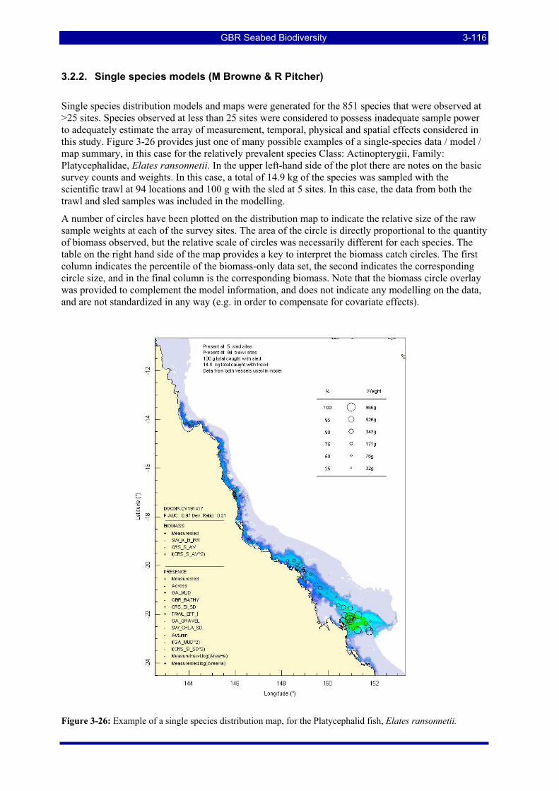
GBR Seabed Biodiversity 3-116
3.2.2. Single species models (M Browne & R Pitcher)
Single species distribution models and maps were generated for the 851 species that were observed at >25 sites. Species observed at less than 25 sites were considered to possess inadequate sample power to adequately estimate the array of measurement, temporal, physical and spatial effects considered in this study. Figure 3-26 provides just one of many possible examples of a single-species data / model / map summary, in this case for the relatively prevalent species Class: Actinopterygii, Family: Platycephalidae, Elates ransonnetii. In the upper left-hand side of the plot there are notes on the basic survey counts and weights. In this case, a total of 14.9 kg of the species was sampled with the scientific trawl at 94 locations and 100 g with the sled at 5 sites. In this case, the data from both the trawl and sled samples was included in the modelling.
A number of circles have been plotted on the distribution map to indicate the relative size of the raw sample weights at each of the survey sites. The area of the circle is directly proportional to the quantity of biomass observed, but the relative scale of circles was necessarily different for each species. The table on the right hand side of the map provides a key to interpret the biomass catch circles. The first column indicates the percentile of the biomass-only data set, the second indicates the corresponding circle size, and in the final column is the corresponding biomass. Note that the biomass circle overlay was provided to complement the model information, and does not indicate any modelling on the data, and are not standardized in any way (e.g. in order to compensate for covariate effects).
Figure 3-26: Example of a single species distribution map, for the Platycephalid fish, Elates ransonnetii.
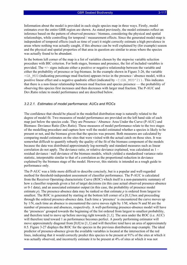
GBR Seabed Biodiversity 3-117
Information about the model is provided in each single species map in three ways. Firstly, model estimates over the entire GBR region are shown. As stated previously, the model estimates reflect an inference based on the pattern of observed presence / biomass, considering the physical and spatial relationships, while controlling for temporal / measurement effects. Since the generated model-map is independent of temporal effects (such as time of year) it might correctly estimate a high prevalence in areas where nothing was actually caught, if this absence can be well explained by (for example) season and the physical and spatial properties of that area in question are similar to areas where the species was actually found to be abundant.
In the bottom left corner of the map is a list of variables chosen by the stepwise variable selection procedure with BIC criterion. For both stages, biomass and presence, the list of included variables is provided. The +/− signs indicate either a positive or negative relationship between the variable and either the probability of presence or log-biomass. In the example shown in Figure 3-26, the variable +GA_MUD (indicating percentage mud fraction) appears twice in the presence / absence model, with a positive linear effect and a negative quadratic effect (indicated by -I(GA_MUD^2)). This indicates that there is a non-linear relationship between mud fraction and species presence — the probability of observing this species first increases and then decreases with larger mud fraction. The P-AUC and Dev.Ratio relate to model performance and are described below.
3.2.2.1. Estimates of model performance: AUCs and ROCs
The confidence that should be placed in the modelled distribution map is naturally related to the degree of model fit. Two measures of model performance are provided on the left hand side of each map just below the species code. They are Presence / Absence: Area Under the Curve (P-AUC) and Biomass: Deviance Ratio (Dev.Ratio). These measures of model performance relate to the two stages of the modelling procedure and capture how well the model estimated whether a species is likely to be present or not, and the biomass given that the species was present. Both measures are calculated by comparing model estimates on the sites that were visited with the actual catch on those sites. It was somewhat difficult to quantify robustly the quality of the fit of the biomass component of the models because the data was distributed approximately log-normally and standard measures such as linear correlation do not apply. The deviance ratio, or relative deviance explained, was calculated as 1 – residual deviance / null deviance of the biomass models, which yielded a standardised variance ratio statistic, interpretable similar to that of a correlation as the proportional reduction in deviance explained by the biomass stage of the model. However, this statistic is intended as a rough guide to performance only.
The P-AUC was a little more difficult to describe concisely, but is a popular and well-regarded method for threshold-independent assessment of classifier performance. The P-AUC is calculated from the Receiver Operating characteristic Curve (ROC) which itself is a non-parametric summary of how a classifier responds given a list of target decisions (in this case actual observed presence-absence or 0-1 data), and an associated estimator output (in this case, the probability of presence model estimate p). The presence-absence data may be ranked so that estimate p is ordered from largest to smallest. The ROC is generated by starting at the bottom left corner of a [0,1] box and proceeding through the ordered presence-absence data. Each time a ‘presence’ is encountered the curve moves up by 1/N, each time an absence is encountered the curve moves right by 1/M, where N and M are the number of presences and absences, respectively. A well-performing presence-absence model will have the ‘presences’ grouped towards the beginning of the list ordered from largest to smallest probability, and therefore tend to move up before moving right towards [1,1]. The area under the ROC (i.e. AUC) will therefore tend toward 1 as performance becomes perfect. A poorly performing estimator will move approximately diagonal from [0,0] to [1,1] and will therefore tend have an area of approximately 0.5. Figure 3-27 displays the ROC for the species in the previous distribution map example. The ideal predictor of presence-absence given the available variables is located at the intersection of the red lines, indicating that it would correctly predict this species to be present at 91% of the sites at which it was actually observed, and incorrectly estimate it to be present at 4% of sites at which it was not
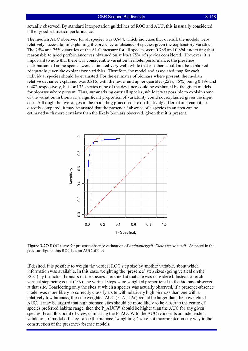
GBR Seabed Biodiversity 3-118
actually observed. By standard interpretation guidelines of ROC and AUC, this is usually considered rather good estimation performance.
The median AUC observed for all species was 0.844, which indicates that overall, the models were relatively successful in explaining the presence or absence of species given the explanatory variables. The 25% and 75% quantiles of the AUC measure for all species were 0.785 and 0.894, indicating that reasonable to good performance was obtained on at least 75% of species considered. However, it is important to note that there was considerable variation in model performance: the presence distributions of some species were estimated very well, while that of others could not be explained adequately given the explanatory variables. Therefore, the model and associated map for each individual species should be evaluated. For the estimates of biomass where present, the median relative deviance explained was 0.315, with the lower and upper quartiles (25%, 75%) being 0.136 and 0.482 respectively, but for 132 species none of the deviance could be explained by the given models for biomass where present. Thus, summarizing over all species, while it was possible to explain some of the variation in biomass, a significant proportion of variability could not explained given the input data. Although the two stages in the modelling procedure are qualitatively different and cannot be directly compared, it may be argued that the presence / absence of a species in an area can be estimated with more certainty than the likely biomass observed, given that it is present.
0.0 0.2 0.4 0.6 0.8 1.0
0.0
0.2
0.4
0.6
0.8
1.0
1 - Specificity
Sen
sitiv
ity
Figure 3-27: ROC curve for presence-absence estimation of Actinopterygii: Elates ransonnetii. As noted in the previous figure, this ROC has an AUC of 0.97
If desired, it is possible to weight the vertical ROC step size by another variable, about which information was available. In this case, weighting the ‘presence’ step sizes (going vertical on the ROC) by the actual biomass of the species measured at that site was considered. Instead of each vertical step being equal (1/N), the vertical steps were weighted proportional to the biomass observed at that site. Considering only the sites at which a species was actually observed, if a presence-absence model was more likely to correctly classify a site with relatively high biomass than one with a relatively low biomass, then the weighted AUC (P_AUCW) would be larger than the unweighted AUC. It may be argued that high biomass sites should be more likely to be closer to the centre of species preferred habitat range, then the P_AUCW should be higher than the AUC for any given species. From this point of view, comparing the P_AUCW to the AUC represents an independent validation of model efficacy, since the biomass ‘weightings’ were not incorporated in any way to the construction of the presence-absence models.
GBR Seabed Biodiversity 3-119
Figure 3-28 compares weighted versus unweighted AUCs for all species. Overall, the mean P_AUCW (0.851) was significantly higher than the mean AUC (0.837), with t = 4.7. This means that over all species, sites with high observed biomasses were relatively more likely to be correctly classified as a ‘presence’ than sites with low observed biomass. This was in accordance with expectations and was taken as an independent indication that the presence / absence models were performing properly. This can be explored further as noted from Figure 3-28 that the P_AUCWs tended to be relatively higher when the AUC was relatively high (e.g. > 0.9). Of the low to moderately highly effective models (those with an AUC < 0.9), the P_AUCW > AUC 61% of the time. Of the highly effective models (AUC > 0.9), the P_AUCW > AUC 81% of the time. Finally, it can demonstrated explicitly that models with high AUC will tend to have a higher P_AUCWs by transforming both of these logistically distributed variables so to have approximately normal distributions via the logit link:
( ) log1
xg xx
⎛ ⎞= ⎜ ⎟−⎝ ⎠
and modelling the transformed P_AUCW as a linear function of the transformed AUC. We establish that the slope of g(P_AUCW) with respect to g(AUC) is 1.24 (SD= 0.027) which is significantly higher than the null hypothesis (i.e. that the slope = 1), with t = 8.59. Thus, not only do P_AUCW tend to be higher than AUC overall, but stronger models tend to have relatively higher P_AUCW. This was again consistent with the view that high biomass sites ought to conform, on average, more strongly with characteristics associated with species presence. Stronger models should better reflect the underlying relationship of covariates to biomass, and this explains why the differential between AUC and P_AUCW should be stronger for stronger models. In summary, the overall strong presence / absence modelling results, as well as the meta-analyses conducted on the AUC and P_AUCW statistics, show quite strong support for the modelling effectiveness.
0.5 0.55 0.6 0.65 0.7 0.75 0.8 0.85 0.9 0.95 10.5
0.55
0.6
0.65
0.7
0.75
0.8
0.85
0.9
0.95
1
Unweighted
Wei
ghte
d
Figure 3-28: Scatter plot of the weighted versus unweighted AUCs for all species.
Having demonstrated that weighted AUC provided a more sensitive diagnostic of model performance against sampled biomass, the performance of all species model fits was examined for both the weighted AUC of the presence model and the deviance ratio of the biomass model at all sites (Figure 3-29). The presence model weighted AUC (P_AUCW) was >0.75 for 699 of 838 species modelled
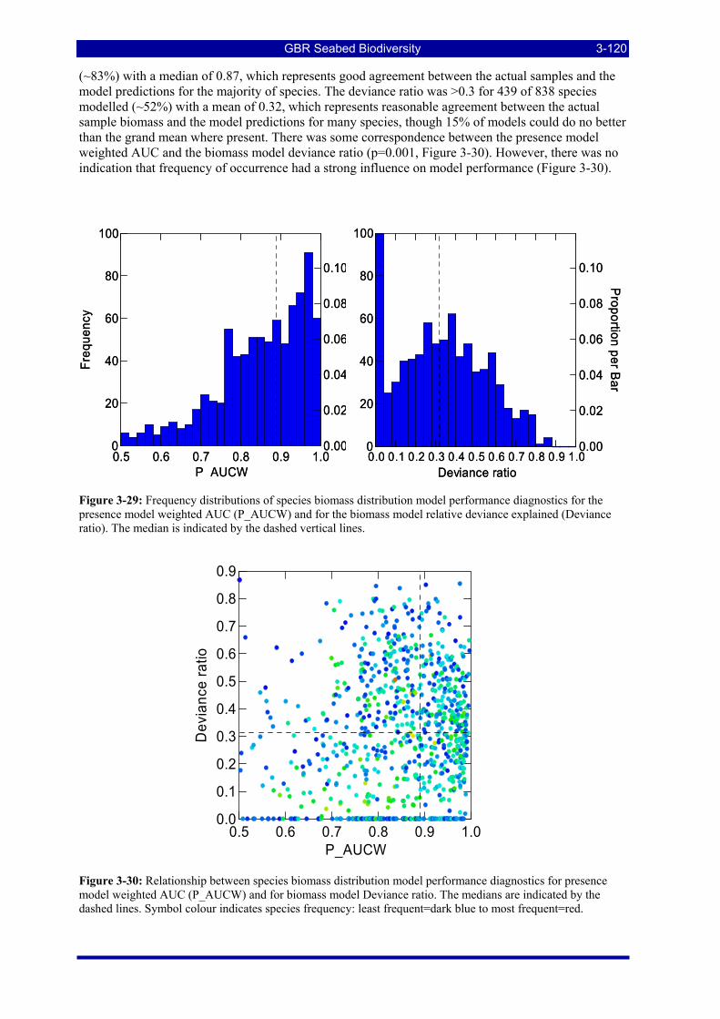
GBR Seabed Biodiversity 3-120
(~83%) with a median of 0.87, which represents good agreement between the actual samples and the model predictions for the majority of species. The deviance ratio was >0.3 for 439 of 838 species modelled (~52%) with a mean of 0.32, which represents reasonable agreement between the actual sample biomass and the model predictions for many species, though 15% of models could do no better than the grand mean where present. There was some correspondence between the presence model weighted AUC and the biomass model deviance ratio (p=0.001, Figure 3-30). However, there was no indication that frequency of occurrence had a strong influence on model performance (Figure 3-30).
0.5 0.6 0.7 0.8 0.9 1.0P_AUCW
0
20
40
60
80
100
Freq
u enc
y
0.00
0.02
0.04
0.06
0.08
0.10
0.5 0.6 0.7 0.8 0.9 1.0P_AUCW
0
20
40
60
80
100
Freq
u enc
y
0.00
0.02
0.04
0.06
0.08
0.10
0.0 0.1 0.2 0.3 0.4 0.5 0.6 0.7 0.8 0.9 1.0
Deviance ratio
0
20
40
60
80
100
0.00
0.02
0.04
0.06
0.08
0.10
Proportion per B
ar
0.0 0.1 0.2 0.3 0.4 0.5 0.6 0.7 0.8 0.9 1.0Deviance ratio
0
20
40
60
80
100
0.00
0.02
0.04
0.06
0.08
0.10
Proportion per B
ar
Figure 3-29: Frequency distributions of species biomass distribution model performance diagnostics for the presence model weighted AUC (P_AUCW) and for the biomass model relative deviance explained (Deviance ratio). The median is indicated by the dashed vertical lines.
0.5 0.6 0.7 0.8 0.9 1.0P_AUCW
0.0
0.1
0.2
0.3
0.4
0.5
0.6
0.7
0.8
0.9
Dev
ianc
e ra
tio
Figure 3-30: Relationship between species biomass distribution model performance diagnostics for presence model weighted AUC (P_AUCW) and for biomass model Deviance ratio. The medians are indicated by the dashed lines. Symbol colour indicates species frequency: least frequent=dark blue to most frequent=red.
GBR Seabed Biodiversity 3-121
The fit of the biomass model was typically less that that of the presence model, largely because the biomass model could be fit only on sites where a species was present — less than 60 sites for half the species (but >25 sites, the lower limit for modelling). For similar reasons, the biomass stage of the modelling often did not select any physical covariates (intercept only for 131 species, plus device only in 205 cases, plus temporal variables only in 33 cases), leading to ‘flat’ biomass predictions given presence (thus patterns in biomass distribution were determined solely by the probability of presence and average biomass where present). Only rarely did this occur with the more powerful presence stage model; physical covariates were not selected in only 11 cases leading to ‘flat’ probability of presence predictions.
Thus, while the majority of species were modelled satisfactorily, not all species were seen to have a good relationship with the available physical environment or spatial covariates with the consequence that their broader distribution beyond actual presence at sampled sites could not be estimated adequately. To illustrate, high, poor and median model performance, a selection of examples is provided below.
Examples of distribution maps of some species with higher performing models are shown in Figure 3-31. The fish Kanekonia queenslandica has P_AUC=0.88 and dev.ratio=0.80; another four species have diagnostics greater than these. The decapod crustacean Solenocera pectinata has P_AUC=0.92 and dev.ratio=0.73; another nine species have diagnostics greater than these. The gastropod Xenophora cerea has P_AUC=0.91 and dev.ratio=0.68; another 25 species have diagnostics greater than these. The fish Paramonacanthus filicauda has P_AUC=0.88 and dev.ratio=0.65; another 45 species have diagnostics greater than these.
Examples of distribution maps of some species with among the poorest performing models are shown in Figure 3-32. The bivalve Corbula fortisulcata had P_AUC=0.69 and dev.ratio=0; eight other species had both diagnostics lower/equal to these. The bryozoan Synnotum spp had P_AUC=0.66 and dev.ratio=0.12; three other species had both diagnostics lower than these. The Asteroid starfish Goniasteridae spp had P_AUC=0.64 and dev.ratio=0; one other species had both diagnostics lower/equal to these. The model for the small ray Dasyatis leylandi selected no physical or spatial covariates and was a flat prediction with P_AUC=0.52 and dev.ratio=0 — its pattern of occurrence did not correspond consistently with any physical or spatial covariate; no species had diagnostics lower than this species.
Examples of distribution maps of some species with typical model performance are shown in Figure 3-33. The crab Portunus rubromarginatus has P_AUC=0.89 and dev.ratio=0.38; the urchin Prionocidaris bispinosa has P_AUC=0.83 and dev.ratio=0.39; the fish Priacanthus tayenus has P_AUC=0.85 and dev.ratio=0.37; and the bryozoan Celleporaria spp has P_AUC=0.85 and dev.ratio=0.30. In general about half the model fits were poorer than these and about half were stronger.
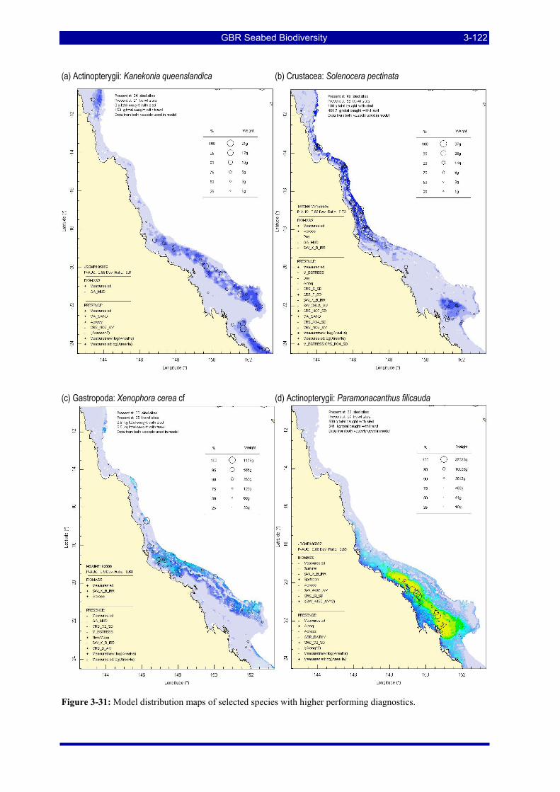
GBR Seabed Biodiversity 3-122
(a) Actinopterygii: Kanekonia queenslandica (b) Crustacea: Solenocera pectinata
(c) Gastropoda: Xenophora cerea cf (d) Actinopterygii: Paramonacanthus filicauda
Figure 3-31: Model distribution maps of selected species with higher performing diagnostics.
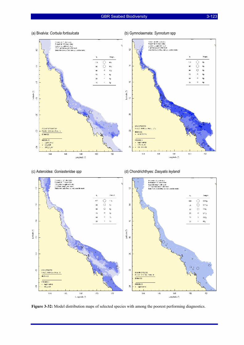
GBR Seabed Biodiversity 3-123
(a) Bivalvia: Corbula fortisulcata (b) Gymnolaemata: Synnotum spp
(c) Asteroidea: Goniasteridae spp (d) Chondrichthyes: Dasyatis leylandi
Figure 3-32: Model distribution maps of selected species with among the poorest performing diagnostics.
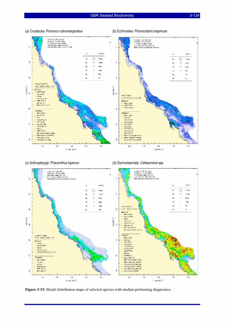
GBR Seabed Biodiversity 3-124
(a) Crustacea: Portunus rubromarginatus (b) Echinoidea: Prionocidaris bispinosa
(c) Actinopterygii: Priacanthus tayenus (d) Gymnolaemata: Celleporaria spp
Figure 3-33: Model distribution maps of selected species with median performing diagnostics.
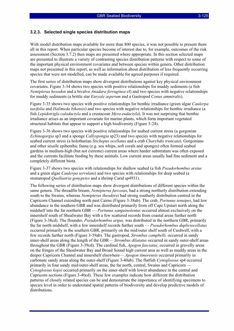
GBR Seabed Biodiversity 3-125
3.2.3. Selected single species distribution maps
With model distribution maps available for more than 800 species, it was not possible to present them all in this report. When particular species become of interest due to, for example, outcomes of the risk assessment (Section 3.7.2) then maps are presented where appropriate. In this section selected maps are presented to illustrate a variety of contrasting species distribution patterns with respect to some of the important physical environment covariates and between species within genera. Other distribution maps not presented in this report, as well as information about distribution of less frequently occurring species that were not modelled, can be made available for agreed purposes if required.
The first series of distribution maps show divergent distributions against key physical environment covariates. Figure 3-34 shows two species with positive relationships for muddy sediments (a fish Nemipterus hexodon and a bivalve Anadara ferruginea cf) and two species with negative relationships for muddy sediments (a brittle star Euryale asperum and a Gastropod Conus ammiralis).
Figure 3-35 shows two species with positive relationships for benthic irradiance (green algae Caulerpa taxifolia and Halimeda bikensis) and two species with negative relationships for benthic irradiance (a fish Lepidotrigla calodactyla and a crustacean Myra eudactyla). It was not surprising that benthic irradiance arises as an important covariate for marine plants, which form important vegetated structural habitats that appear to support a high biodiversity (Figure 3-24).
Figure 3-36 shows two species with positive relationships for seabed current stress (a gorgonian Echinogorgia sp3 and a sponge Callyspongia sp23) and two species with negative relationships for seabed current stress (a holothurian Stichopus ocellatus and a crab Charybdis truncata). Gorgonians and other sessile epibenthic fauna (e.g. sea whips, soft corals and sponges) often formed seabed gardens in medium-high (but not extreme) current areas where harder substratum was often exposed and the currents facilitate feeding by these animals. Low current areas usually had fine sediment and a completely different biota.
Figure 3-37 shows two species with relationships for shallow seabed (a fish Pseudorhombus arsius and a green algae Caulerpa serrulata) and two species with relationships for deep seabed (a stomatopod Quollastria gonypetes and a shrimp Carid sp4931).
The following series of distribution maps show divergent distributions of different species within the same genera. The threadfin bream, Nemipterus furcosus, had a strong northerly distribution extending south to the Swains, whereas Nemipterus theodorei had strong southerly distribution centred in the Capricorn Channel extending north past Cairns (Figure 3-38ab). The crab, Portunus tenuipes, had low abundance in the southern GBR and was distributed primarily from off Cape Upstart north along the midshelf into the far northern GBR — Portunus sanguinolentus occurred almost exclusively on the innershelf south of Shoalwater Bay with a few scattered records from coastal areas further north (Figure 3-38cd). The flounder, Pseudorhombus argus, was distributed in the northern GBR, primarily the far north midshelf, with a few innershelf records further south — Pseudorhombus dupliciocellatus occurred primarily in the southern GBR, primarily on the mid/outer shelf south of Cardwell, with a few records further north (Figure 3-39ab). The gastropod, Strombus campbelli, occurred in sandy inner-shelf areas along the length of the GBR— Strombus dilatatus occurred in sandy outer-shelf areas throughout the GBR (Figure 3-39cd). The cardinal fish, Apogon fasciatus, occurred in gravelly areas on the fringes of the Shoalwater Bay and Broad Sound high current area as well as muddy areas in the deeper Capricorn Channel and innershelf elsewhere— Apogon timorensis occurred primarily in carbonate sandy areas along the outer-shelf (Figure 3-40ab). The flatfish Cynoglossus sp4 occurred primarily in four sandy mid/outer-shelf areas, the far north, central, Swains and Capricorn — Cynoglossus kopsi occurred primarily on the inner-shelf with lower abundance in the central and Capricorn sections (Figure 3-40cd). These few examples indicate how different the distribution patterns of closely related species can be and demonstrate the importance of identifying specimens to species level in order to understand spatial patterns of biodiversity and develop predictive models of distributions.
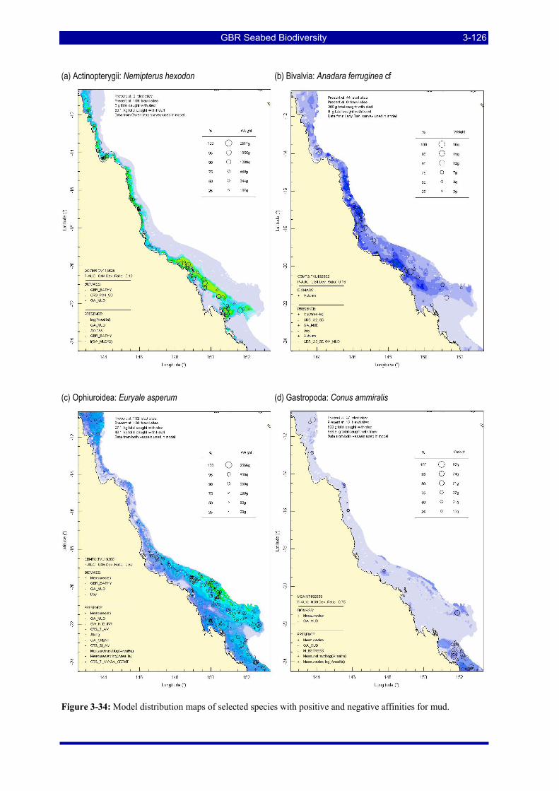
GBR Seabed Biodiversity 3-126
(a) Actinopterygii: Nemipterus hexodon (b) Bivalvia: Anadara ferruginea cf
(c) Ophiuroidea: Euryale asperum (d) Gastropoda: Conus ammiralis
Figure 3-34: Model distribution maps of selected species with positive and negative affinities for mud.
GBR Seabed Biodiversity 3-127
(a) Chlorophyceae: Caulerpa taxifolia (b) Chlorophyceae: Halimeda bikensis
(c) Actinopterygii: Lepidotrigla calodactyla (d) Crustacea: Myra eudactyla
Figure 3-35: Model distribution maps of selected species with positive and negative affinities for benthic irradiance.
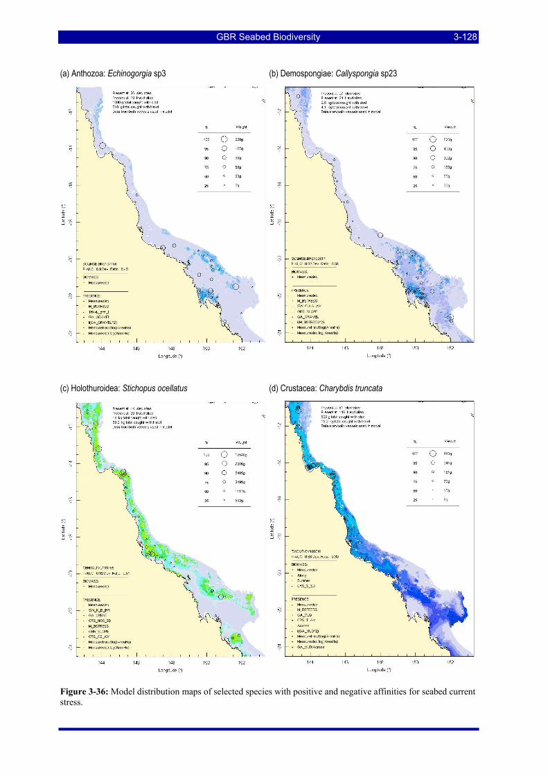
GBR Seabed Biodiversity 3-128
(a) Anthozoa: Echinogorgia sp3 (b) Demospongiae: Callyspongia sp23
(c) Holothuroidea: Stichopus ocellatus (d) Crustacea: Charybdis truncata
Figure 3-36: Model distribution maps of selected species with positive and negative affinities for seabed current stress.
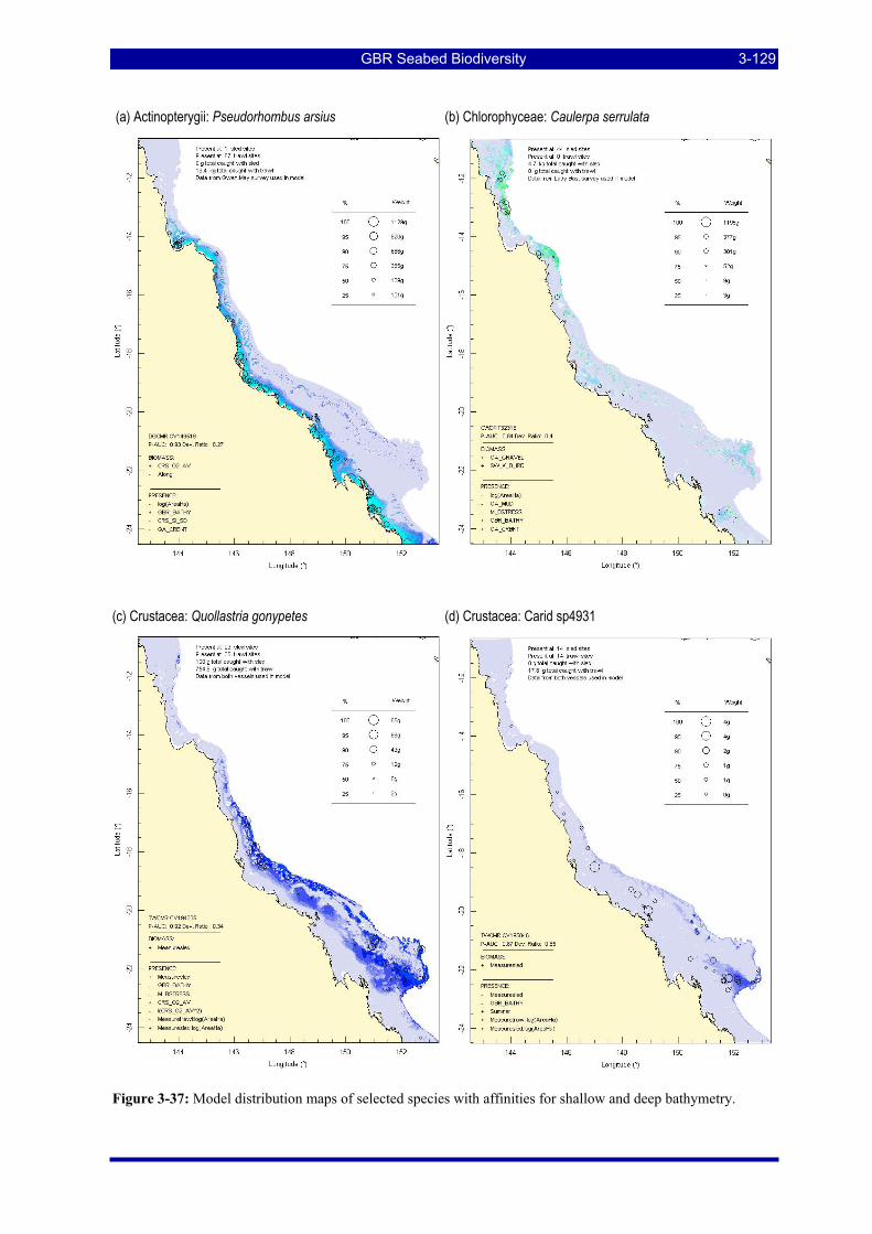
GBR Seabed Biodiversity 3-129
(a) Actinopterygii: Pseudorhombus arsius (b) Chlorophyceae: Caulerpa serrulata
(c) Crustacea: Quollastria gonypetes (d) Crustacea: Carid sp4931
Figure 3-37: Model distribution maps of selected species with affinities for shallow and deep bathymetry.
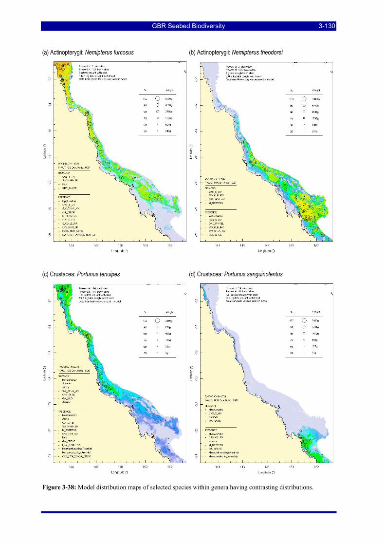
GBR Seabed Biodiversity 3-130
(a) Actinopterygii: Nemipterus furcosus (b) Actinopterygii: Nemipterus theodorei
(c) Crustacea: Portunus tenuipes (d) Crustacea: Portunus sanguinolentus
Figure 3-38: Model distribution maps of selected species within genera having contrasting distributions.
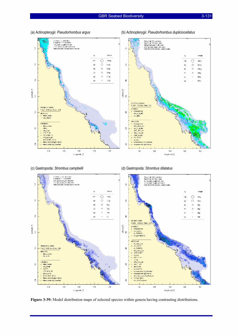
GBR Seabed Biodiversity 3-131
(a) Actinopterygii: Pseudorhombus argus (b) Actinopterygii: Pseudorhombus dupliciocellatus
(c) Gastropoda: Strombus campbelli (d) Gastropoda: Strombus dilatatus
Figure 3-39: Model distribution maps of selected species within genera having contrasting distributions.
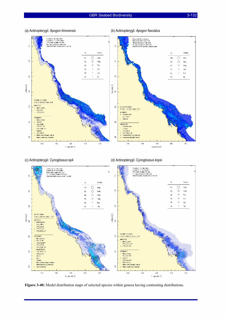
GBR Seabed Biodiversity 3-132
(a) Actinopterygii: Apogon timorensis (b) Actinopterygii: Apogon fasciatus
(c) Actinopterygii: Cynoglossus sp4 (d) Actinopterygii: Cynoglossus kopsi
Figure 3-40: Model distribution maps of selected species within genera having contrasting distributions.
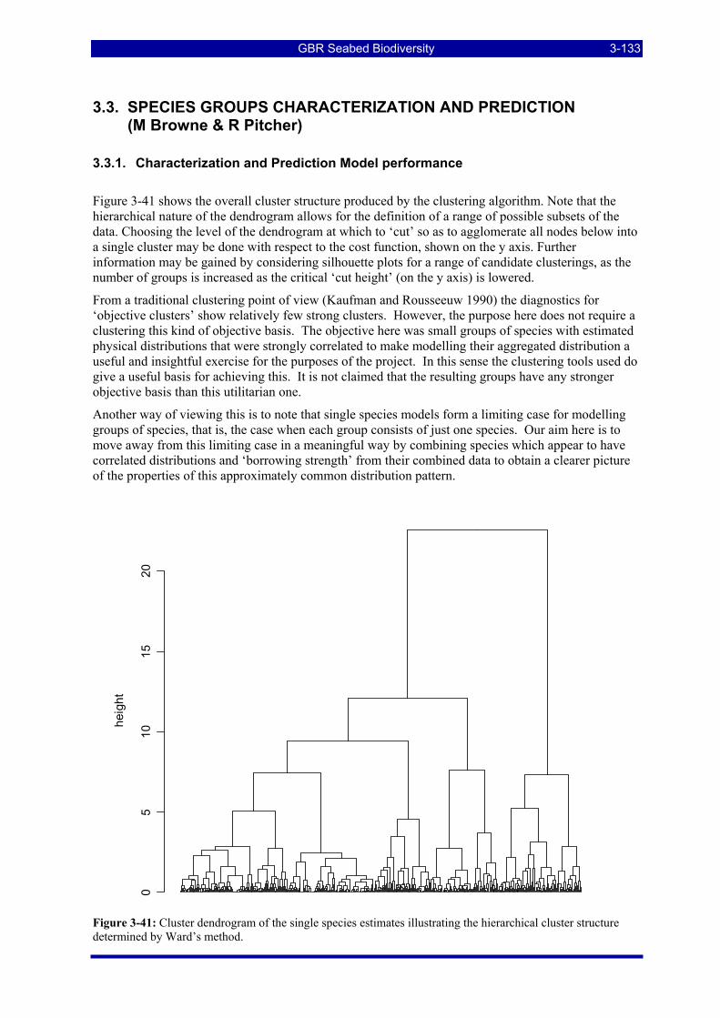
GBR Seabed Biodiversity 3-133
3.3. SPECIES GROUPS CHARACTERIZATION AND PREDICTION (M Browne & R Pitcher)
3.3.1. Characterization and Prediction Model performance
Figure 3-41 shows the overall cluster structure produced by the clustering algorithm. Note that the hierarchical nature of the dendrogram allows for the definition of a range of possible subsets of the data. Choosing the level of the dendrogram at which to ‘cut’ so as to agglomerate all nodes below into a single cluster may be done with respect to the cost function, shown on the y axis. Further information may be gained by considering silhouette plots for a range of candidate clusterings, as the number of groups is increased as the critical ‘cut height’ (on the y axis) is lowered.
From a traditional clustering point of view (Kaufman and Rousseeuw 1990) the diagnostics for ‘objective clusters’ show relatively few strong clusters. However, the purpose here does not require a clustering this kind of objective basis. The objective here was small groups of species with estimated physical distributions that were strongly correlated to make modelling their aggregated distribution a useful and insightful exercise for the purposes of the project. In this sense the clustering tools used do give a useful basis for achieving this. It is not claimed that the resulting groups have any stronger objective basis than this utilitarian one.
Another way of viewing this is to note that single species models form a limiting case for modelling groups of species, that is, the case when each group consists of just one species. Our aim here is to move away from this limiting case in a meaningful way by combining species which appear to have correlated distributions and ‘borrowing strength’ from their combined data to obtain a clearer picture of the properties of this approximately common distribution pattern.
05
1015
20
heig
ht
Figure 3-41: Cluster dendrogram of the single species estimates illustrating the hierarchical cluster structure determined by Ward’s method.
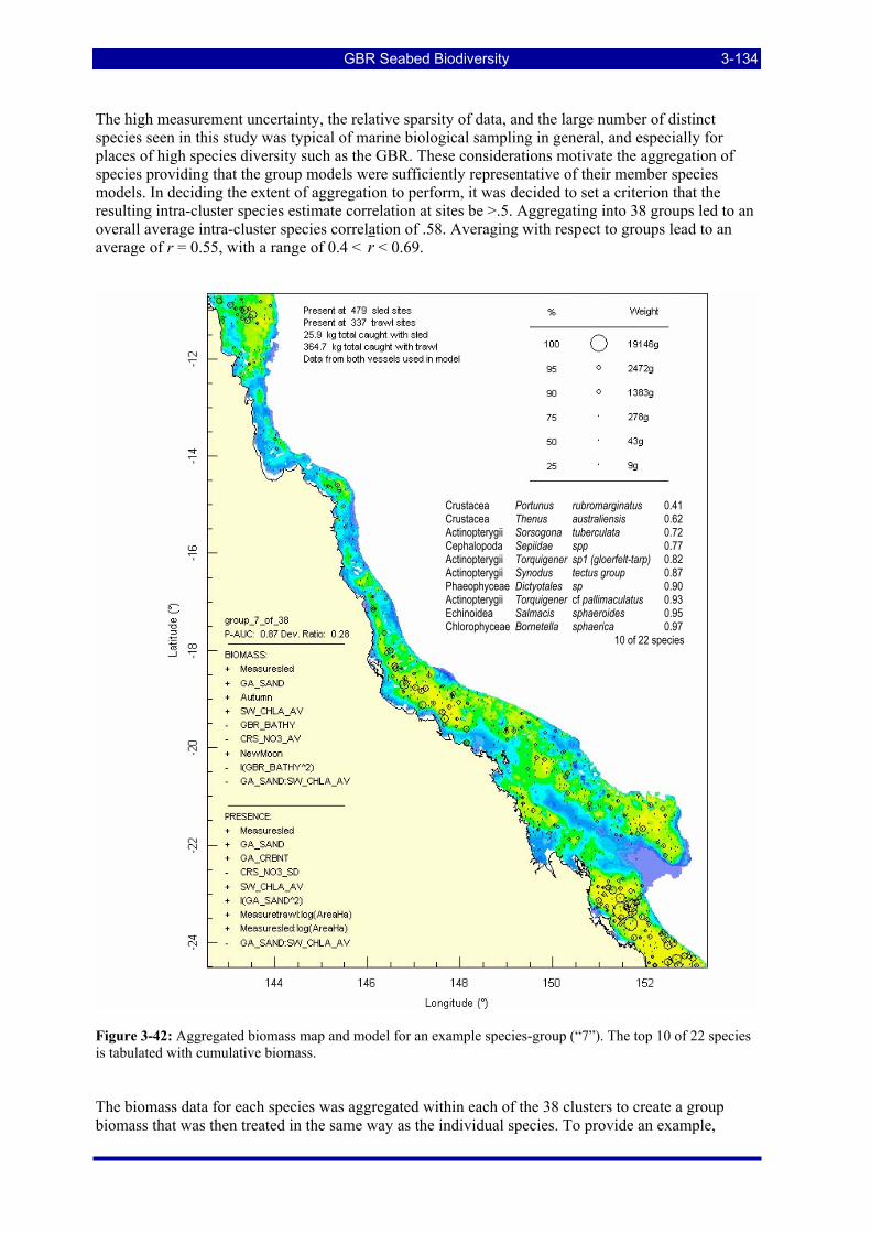
GBR Seabed Biodiversity 3-134
The high measurement uncertainty, the relative sparsity of data, and the large number of distinct species seen in this study was typical of marine biological sampling in general, and especially for places of high species diversity such as the GBR. These considerations motivate the aggregation of species providing that the group models were sufficiently representative of their member species models. In deciding the extent of aggregation to perform, it was decided to set a criterion that the resulting intra-cluster species estimate correlation at sites be >.5. Aggregating into 38 groups led to an overall average intra-cluster species correlation of .58. Averaging with respect to groups lead to an average of r = 0.55, with a range of 0.4 < r < 0.69.
Figure 3-42: Aggregated biomass map and model for an example species-group (“7”). The top 10 of 22 species is tabulated with cumulative biomass.
The biomass data for each species was aggregated within each of the 38 clusters to create a group biomass that was then treated in the same way as the individual species. To provide an example,
Crustacea Portunus rubromarginatus 0.41 Crustacea Thenus australiensis 0.62 Actinopterygii Sorsogona tuberculata 0.72 Cephalopoda Sepiidae spp 0.77 Actinopterygii Torquigener sp1 (gloerfelt-tarp) 0.82 Actinopterygii Synodus tectus group 0.87 Phaeophyceae Dictyotales sp 0.90 Actinopterygii Torquigener cf pallimaculatus 0.93 Echinoidea Salmacis sphaeroides 0.95 Chlorophyceae Bornetella sphaerica 0.97
10 of 22 species
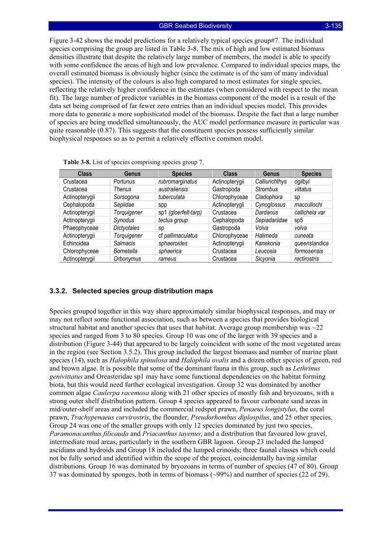
GBR Seabed Biodiversity 3-135
Figure 3-42 shows the model predictions for a relatively typical species group#7. The individual species comprising the group are listed in Table 3-8. The mix of high and low estimated biomass densities illustrate that despite the relatively large number of members, the model is able to specify with some confidence the areas of high and low prevalence. Compared to individual species maps, the overall estimated biomass is obviously higher (since the estimate is of the sum of many individual species). The intensity of the colours is also high compared to most estimates for single species, reflecting the relatively higher confidence in the estimates (when considered with respect to the mean fit). The large number of predictor variables in the biomass component of the model is a result of the data set being comprised of far fewer zero entries than an individual species model. This provides more data to generate a more sophisticated model of the biomass. Despite the fact that a large number of species are being modelled simultaneously, the AUC model performance measure in particular was quite reasonable (0.87). This suggests that the constituent species possess sufficiently similar biophysical responses so as to permit a relatively effective common model.
Table 3-8. List of species comprising species group 7.
Class Genus Species Class Genus Species Crustacea Portunus rubromarginatus Actinopterygii Calliurichthys ogilbyi Crustacea Thenus australiensis Gastropoda Strombus vittatus Actinopterygii Sorsogona tuberculata Chlorophyceae Cladophora sp Cephalopoda Sepiidae spp Actinopterygii Cynoglossus maccullochi Actinopterygii Torquigener sp1 (gloerfelt-tarp) Crustacea Dardanus callichela var Actinopterygii Synodus tectus group Cephalopoda Sepiadariidae sp5 Phaeophyceae Dictyotales sp Gastropoda Volva volva Actinopterygii Torquigener cf pallimaculatus Chlorophyceae Halimeda cuneata Echinoidea Salmacis sphaeroides Actinopterygii Kanekonia queenslandica Chlorophyceae Bornetella sphaerica Crustacea Leucosia formosensis Actinopterygii Orbonymus rameus Crustacea Sicyonia rectirostris
3.3.2. Selected species group distribution maps
Species grouped together in this way share approximately similar biophysical responses, and may or may not reflect some functional association, such as between a species that provides biological structural habitat and another species that uses that habitat. Average group membership was ~22 species and ranged from 3 to 80 species. Group 10 was one of the larger with 39 species and a distribution (Figure 3-44) that appeared to be largely coincident with some of the most vegetated areas in the region (see Section 3.5.2). This group included the largest biomass and number of marine plant species (14), such as Halophila spinulosa and Halophila ovalis and a dozen other species of green, red and brown algae. It is possible that some of the dominant fauna in this group, such as Lethrinus genivittatus and Oreasteridae sp1 may have some functional dependencies on the habitat forming biota, but this would need further ecological investigation. Group 32 was dominated by another common algae Caulerpa racemosa along with 21 other species of mostly fish and bryozoans, with a strong outer shelf distribution pattern. Group 4 species appeared to favour carbonate sand areas in mid/outer-shelf areas and included the commercial redspot prawn, Penaeus longistylus, the coral prawn, Trachypenaeus curvirostris, the flounder, Pseudorhombus diplospilus, and 25 other species. Group 24 was one of the smaller groups with only 12 species dominated by just two species, Paramonacanthus filicauda and Priacanthus tayenus, and a distribution that favoured low gravel, intermediate mud areas, particularly in the southern GBR lagoon. Group 23 included the lumped ascidians and hydroids and Group 18 included the lumped crinoids; three faunal classes which could not be fully sorted and identified within the scope of the project, coincidentally having similar distributions. Group 16 was dominated by bryozoans in terms of number of species (47 of 80). Group 37 was dominated by sponges, both in terms of biomass (~99%) and number of species (22 of 29).
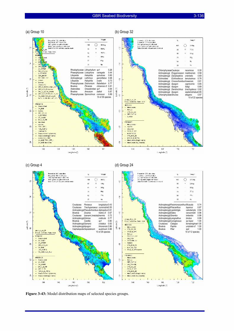
GBR Seabed Biodiversity 3-136
(a) Group 10 (b) Group 32
(c) Group 4 (d) Group 24
Figure 3-43: Model distribution maps of selected species groups.
Rhodophyceae Lithophyllum sp1 0.26Phaeophyceae Lobophora variegata 0.44Liliopsida Halophila spinulosa 0.60Actinopterygii Lethrinus genivittatus 0.68Liliopsida Halophila ovalis 0.73Phaeophyceae Distromium flabellatum 0.77Bivalvia Plicatula chinensis cf 0.81Asteroidea Oreasteridae sp1 0.84Bivalvia Amusium balloti 0.87Phaeophyceae Sporochnus comosus 0.89
10 of 39 species
ChlorophyceaeCaulerpa racemosa 0.30Actinopterygii Engyprosopon maldivensis 0.58Actinopterygii Dactyloptena orientalis 0.69Echinoidea Echinodiscus tenuissimus 0.76Actinopterygii Crossorhombushowensis 0.81Actinopterygii Apogon capricornis 0.85Actinopterygii Apogon 9(dg) 0.89Actinopterygii Dendrochirus brachypterus 0.92Actinopterygii Apogon septemstriatus0.95ChlorophyceaeStruvea elegans 0.97
10 of 22 species
Crustacea Penaeus longistylus 0.43Crustacea Trachypenaeus curvirostris 0.55ActinopterygiiPseudorhombus diplospilus 0.61Bivalvia Dosinia histrio cf 0.67Crustacea Izanami (matuta)inermis 0.72ActinopterygiiZebrias craticula 0.77Bivalvia Cardita sp1 0.80ActinopterygiiSamaris cristatus 0.83ActinopterygiiApogon timorensis 0.86Cephalopoda Sepiadarium austrinum 0.88
10 of 28 species
ActinopterygiiParamonacanthusfilicauda 0.74ActinopterygiiPriacanthus tayenus 0.87ActinopterygiiLepidotrigla calodactyla 0.94ActinopterygiiElates ransonnetii 0.98ActinopterygiiSirembo imberbis 0.99ActinopterygiiLeiognathus bindus 0.99ActinopterygiiCynoglossus sp kopsi 1.00Crustacea Calappa terraereginae 1.00Bivalvia Paphia undulata cf 1.00Bivalvia Pitar sp2 1.00
10 of 12 species
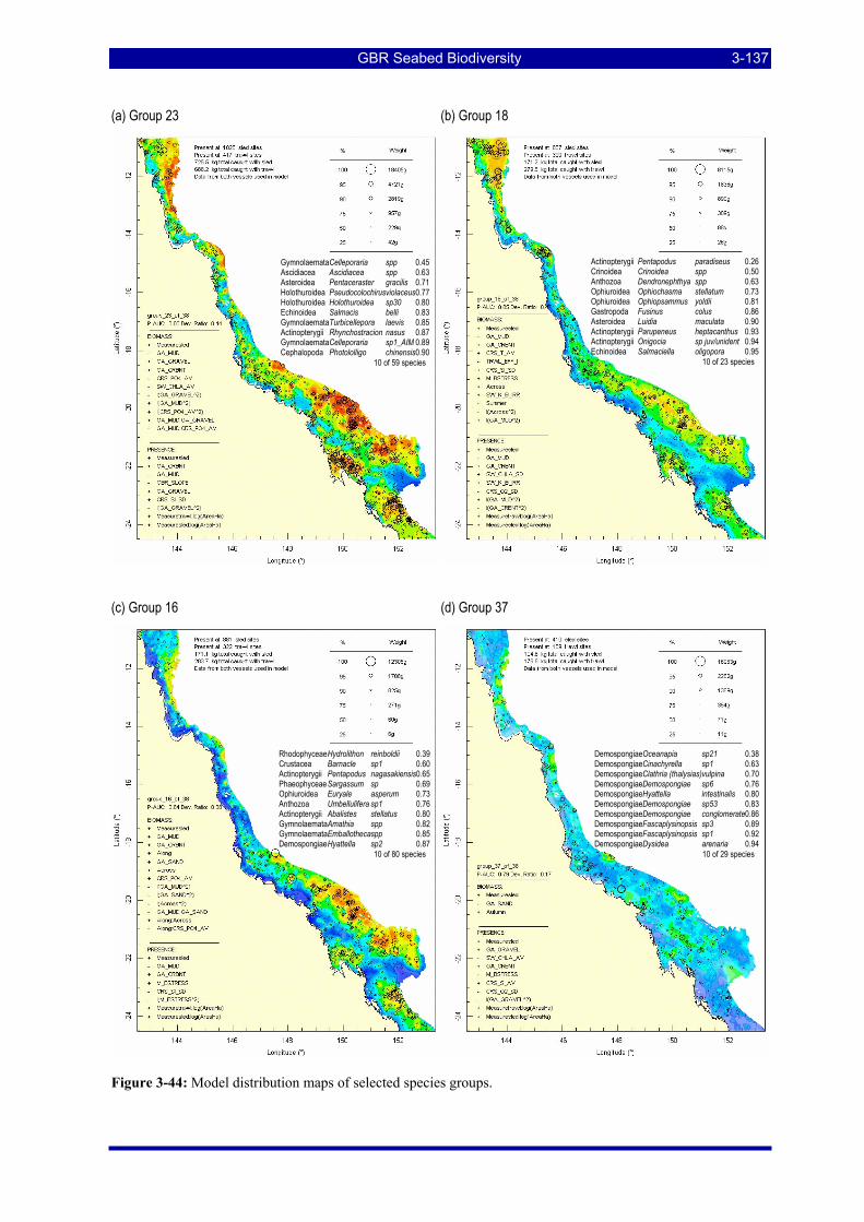
GBR Seabed Biodiversity 3-137
(a) Group 23 (b) Group 18
(c) Group 16 (d) Group 37
Figure 3-44: Model distribution maps of selected species groups.
GymnolaemataCelleporaria spp 0.45Ascidiacea Ascidiacea spp 0.63Asteroidea Pentaceraster gracilis 0.71Holothuroidea Pseudocolochirusviolaceus0.77Holothuroidea Holothuroidea sp30 0.80Echinoidea Salmacis belli 0.83GymnolaemataTurbicellepora laevis 0.85Actinopterygii Rhynchostracion nasus 0.87GymnolaemataCelleporaria sp1_AIM 0.89Cephalopoda Photololligo chinensis 0.90
10 of 59 species
Actinopterygii Pentapodus paradiseus 0.26 Crinoidea Crinoidea spp 0.50 Anthozoa Dendronephthya spp 0.63 Ophiuroidea Ophiochasma stellatum 0.73 Ophiuroidea Ophiopsammus yoldii 0.81 Gastropoda Fusinus colus 0.86 Asteroidea Luidia maculata 0.90 Actinopterygii Parupeneus heptacanthus 0.93 Actinopterygii Onigocia sp juv/unident 0.94 Echinoidea Salmaciella oligopora 0.95
10 of 23 species
Rhodophyceae Hydrolithon reinboldii 0.39Crustacea Barnacle sp1 0.60Actinopterygii Pentapodus nagasakiensis0.65Phaeophyceae Sargassum sp 0.69Ophiuroidea Euryale asperum 0.73Anthozoa Umbellulifera sp1 0.76Actinopterygii Abalistes stellatus 0.80GymnolaemataAmathia spp 0.82GymnolaemataEmballothecaspp 0.85Demospongiae Hyattella sp2 0.87
10 of 80 species
DemospongiaeOceanapia sp21 0.38DemospongiaeCinachyrella sp1 0.63DemospongiaeClathria (thalysias)vulpina 0.70DemospongiaeDemospongiae sp6 0.76DemospongiaeHyattella intestinalis 0.80DemospongiaeDemospongiae sp53 0.83DemospongiaeDemospongiae conglomerate0.86DemospongiaeFascaplysinopsis sp3 0.89DemospongiaeFascaplysinopsis sp1 0.92DemospongiaeDysidea arenaria 0.94
10 of 29 species

GBR Seabed Biodiversity 3-138
3.4. SITE GROUPS CHARACTERIZATION AND PREDICTIONS (W Venables & R Pitcher)
3.4.1. Decision tree results
The recursive splitting on the physical variables, to achieve reduction in deviance of the sites Bray-Curtis matrix, produced 16 groups with the given stopping criteria. The resulting graphical decision tree is shown in Figure 3-45. The primary split was at 25% mud fraction, and mud or another sediment attribute accounted for several other splits, suggesting the importance of sediment grain size composition in structuring seabed assemblages. Given the correlation between variables and that other variables may be good surrogates to split at each node, caution is necessary in interpreting the importance of variables. Nevertheless, percent mud and other sediment attributes were often the most frequently selected in a wide range of biophysical analyses. Other variables likely to be important included bathymetry, oxygen variability, current stress, chlorophyll and/or light attenuation (K490), nutrients and temperature.
Figure 3-45: Recursive decision tree partitioning the sites into 16 groups, corresponding to the terminal nodes. The labels indicate the split variable and threshold for the group corresponding to the left hand branch in each case. The distances used were Bray-Curtis dissimilarities on 1/8th root transforms of the predicted site species biomass data.
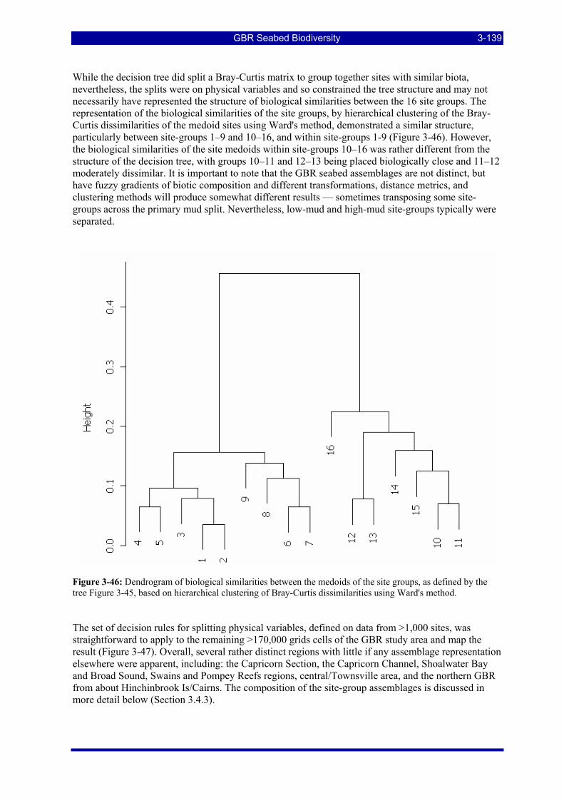
GBR Seabed Biodiversity 3-139
While the decision tree did split a Bray-Curtis matrix to group together sites with similar biota, nevertheless, the splits were on physical variables and so constrained the tree structure and may not necessarily have represented the structure of biological similarities between the 16 site groups. The representation of the biological similarities of the site groups, by hierarchical clustering of the Bray-Curtis dissimilarities of the medoid sites using Ward's method, demonstrated a similar structure, particularly between site-groups 1–9 and 10–16, and within site-groups 1-9 (Figure 3-46). However, the biological similarities of the site medoids within site-groups 10–16 was rather different from the structure of the decision tree, with groups 10–11 and 12–13 being placed biologically close and 11–12 moderately dissimilar. It is important to note that the GBR seabed assemblages are not distinct, but have fuzzy gradients of biotic composition and different transformations, distance metrics, and clustering methods will produce somewhat different results — sometimes transposing some site-groups across the primary mud split. Nevertheless, low-mud and high-mud site-groups typically were separated.
Figure 3-46: Dendrogram of biological similarities between the medoids of the site groups, as defined by the tree Figure 3-45, based on hierarchical clustering of Bray-Curtis dissimilarities using Ward's method.
The set of decision rules for splitting physical variables, defined on data from >1,000 sites, was straightforward to apply to the remaining >170,000 grids cells of the GBR study area and map the result (Figure 3-47). Overall, several rather distinct regions with little if any assemblage representation elsewhere were apparent, including: the Capricorn Section, the Capricorn Channel, Shoalwater Bay and Broad Sound, Swains and Pompey Reefs regions, central/Townsville area, and the northern GBR from about Hinchinbrook Is/Cairns. The composition of the site-group assemblages is discussed in more detail below (Section 3.4.3).
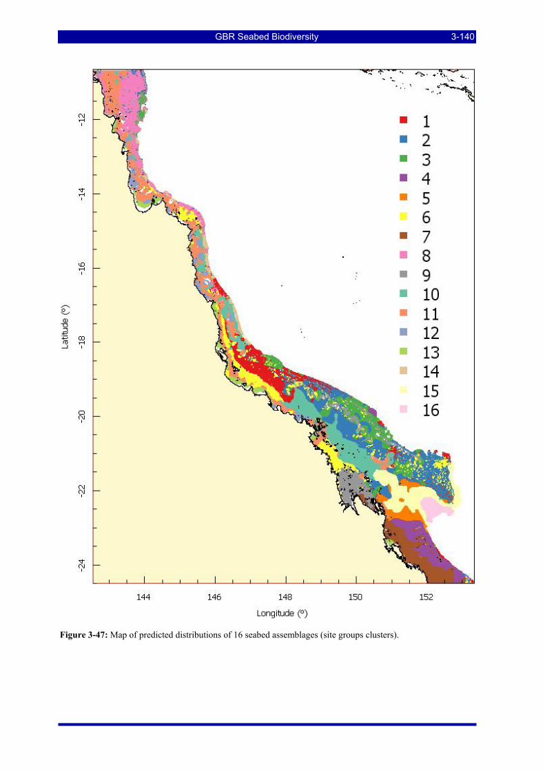
GBR Seabed Biodiversity 3-140
Figure 3-47: Map of predicted distributions of 16 seabed assemblages (site groups clusters).
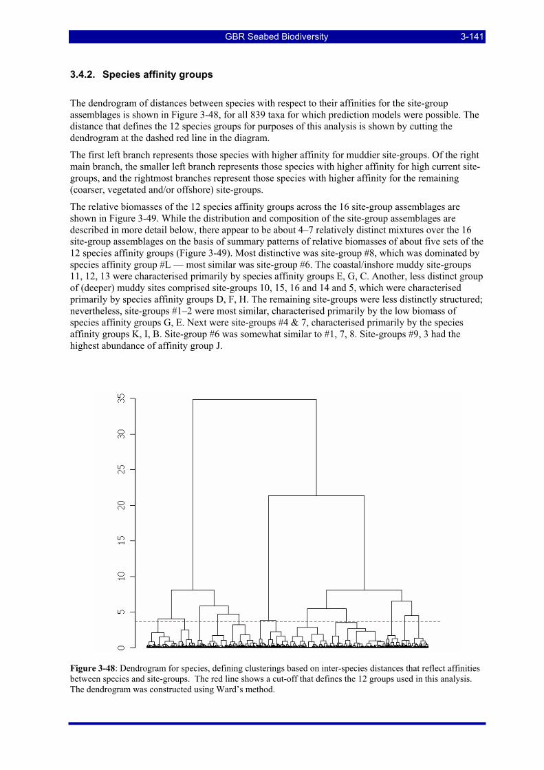
GBR Seabed Biodiversity 3-141
3.4.2. Species affinity groups
The dendrogram of distances between species with respect to their affinities for the site-group assemblages is shown in Figure 3-48, for all 839 taxa for which prediction models were possible. The distance that defines the 12 species groups for purposes of this analysis is shown by cutting the dendrogram at the dashed red line in the diagram.
The first left branch represents those species with higher affinity for muddier site-groups. Of the right main branch, the smaller left branch represents those species with higher affinity for high current site-groups, and the rightmost branches represent those species with higher affinity for the remaining (coarser, vegetated and/or offshore) site-groups.
The relative biomasses of the 12 species affinity groups across the 16 site-group assemblages are shown in Figure 3-49. While the distribution and composition of the site-group assemblages are described in more detail below, there appear to be about 4–7 relatively distinct mixtures over the 16 site-group assemblages on the basis of summary patterns of relative biomasses of about five sets of the 12 species affinity groups (Figure 3-49). Most distinctive was site-group #8, which was dominated by species affinity group #L — most similar was site-group #6. The coastal/inshore muddy site-groups 11, 12, 13 were characterised primarily by species affinity groups E, G, C. Another, less distinct group of (deeper) muddy sites comprised site-groups 10, 15, 16 and 14 and 5, which were characterised primarily by species affinity groups D, F, H. The remaining site-groups were less distinctly structured; nevertheless, site-groups #1–2 were most similar, characterised primarily by the low biomass of species affinity groups G, E. Next were site-groups #4 & 7, characterised primarily by the species affinity groups K, I, B. Site-group #6 was somewhat similar to #1, 7, 8. Site-groups #9, 3 had the highest abundance of affinity group J.
Figure 3-48: Dendrogram for species, defining clusterings based on inter-species distances that reflect affinities between species and site-groups. The red line shows a cut-off that defines the 12 groups used in this analysis. The dendrogram was constructed using Ward’s method.
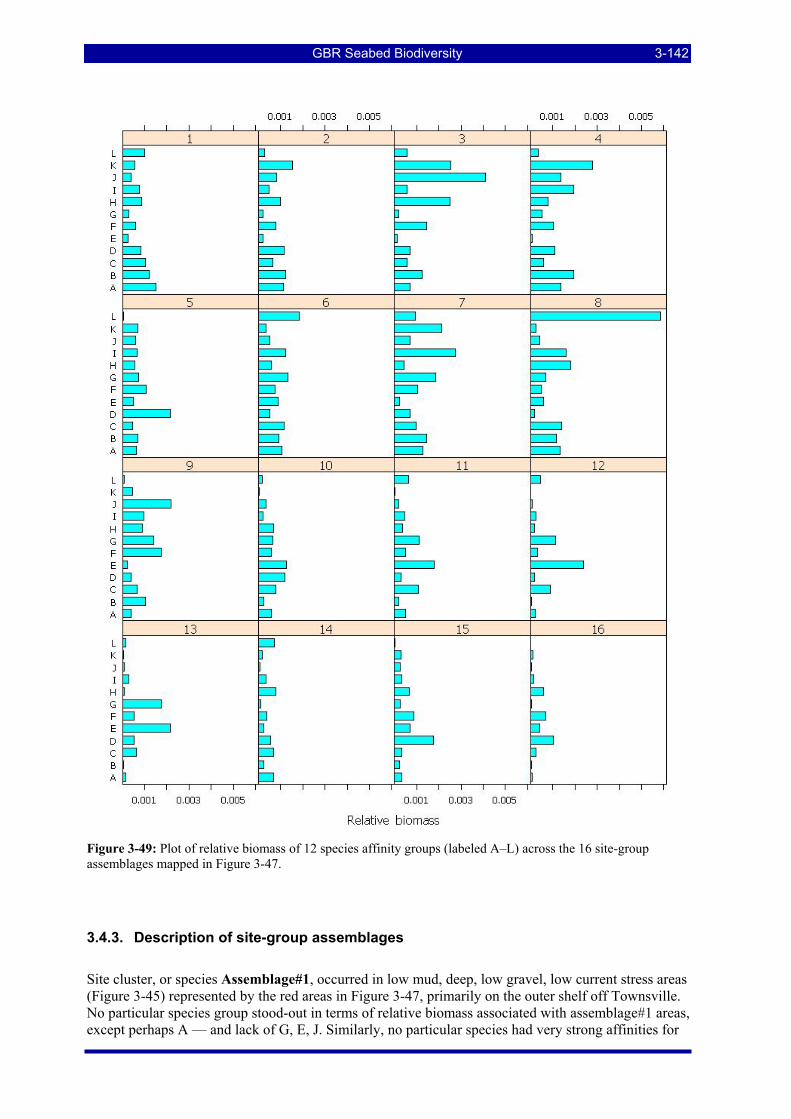
GBR Seabed Biodiversity 3-142
Figure 3-49: Plot of relative biomass of 12 species affinity groups (labeled A–L) across the 16 site-group assemblages mapped in Figure 3-47.
3.4.3. Description of site-group assemblages
Site cluster, or species Assemblage#1, occurred in low mud, deep, low gravel, low current stress areas (Figure 3-45) represented by the red areas in Figure 3-47, primarily on the outer shelf off Townsville. No particular species group stood-out in terms of relative biomass associated with assemblage#1 areas, except perhaps A — and lack of G, E, J. Similarly, no particular species had very strong affinities for
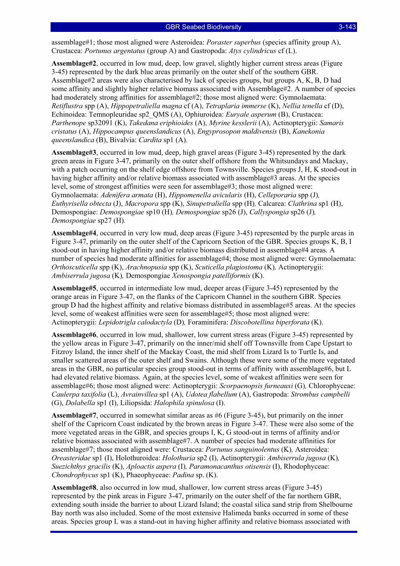
GBR Seabed Biodiversity 3-143
assemblage#1; those most aligned were Asteroidea: Poraster superbus (species affinity group A), Crustacea: Portunus argentatus (group A) and Gastropoda: Atys cylindricus cf (L).
Assemblage#2, occurred in low mud, deep, low gravel, slightly higher current stress areas (Figure 3-45) represented by the dark blue areas primarily on the outer shelf of the southern GBR. Assemblage#2 areas were also characterised by lack of species groups, but groups A, K, B, D had some affinity and slightly higher relative biomass associated with Assemblage#2. A number of species had moderately strong affinities for assemblage#2; those most aligned were: Gymnolaemata: Retiflustra spp (A), Hippopetraliella magna cf (A), Tetraplaria immerse (K), Nellia tenella cf (D), Echinoidea: Temnopleuridae sp2_QMS (A), Ophiuroidea: Euryale asperum (B), Crustacea: Parthenope sp32091 (K), Takedana eriphioides (A), Myrine kesslerii (A), Actinopterygii: Samaris cristatus (A), Hippocampus queenslandicus (A), Engyprosopon maldivensis (B), Kanekonia queenslandica (B), Bivalvia: Cardita sp1 (A).
Assemblage#3, occurred in low mud, deep, high gravel areas (Figure 3-45) represented by the dark green areas in Figure 3-47, primarily on the outer shelf offshore from the Whitsundays and Mackay, with a patch occurring on the shelf edge offshore from Townsville. Species groups J, H, K stood-out in having higher affinity and/or relative biomass associated with assemblage#3 areas. At the species level, some of strongest affinities were seen for assemblage#3; those most aligned were: Gymnolaemata: Adenifera armata (H), Hippomenella avicularis (H), Celleporaria spp (J), Euthyrisella obtecta (J), Macropora spp (K), Sinupetraliella spp (H), Calcarea: Clathrina sp1 (H), Demospongiae: Demospongiae sp10 (H), Demospongiae sp26 (J), Callyspongia sp26 (J), Demospongiae sp27 (H).
Assemblage#4, occurred in very low mud, deep areas (Figure 3-45) represented by the purple areas in Figure 3-47, primarily on the outer shelf of the Capricorn Section of the GBR. Species groups K, B, I stood-out in having higher affinity and/or relative biomass distributed in assemblage#4 areas. A number of species had moderate affinities for assemblage#4; those most aligned were: Gymnolaemata: Orthoscuticella spp (K), Arachnopusia spp (K), Scuticella plagiostoma (K), Actinopterygii: Ambiserrula jugosa (K), Demospongiae Xenospongia patelliformis (K).
Assemblage#5, occurred in intermediate low mud, deeper areas (Figure 3-45) represented by the orange areas in Figure 3-47, on the flanks of the Capricorn Channel in the southern GBR. Species group D had the highest affinity and relative biomass distributed in assemblage#5 areas. At the species level, some of weakest affinities were seen for assemblage#5; those most aligned were: Actinopterygii: Lepidotrigla calodactyla (D), Foraminifera: Discobotellina biperforata (K).
Assemblage#6, occurred in low mud, shallower, low current stress areas (Figure 3-45) represented by the yellow areas in Figure 3-47, primarily on the inner/mid shelf off Townsville from Cape Upstart to Fitzroy Island, the inner shelf of the Mackay Coast, the mid shelf from Lizard Is to Turtle Is, and smaller scattered areas of the outer shelf and Swains. Although these were some of the more vegetated areas in the GBR, no particular species group stood-out in terms of affinity with assemblage#6, but L had elevated relative biomass. Again, at the species level, some of weakest affinities were seen for assemblage#6; those most aligned were: Actinopterygii: Scorpaenopsis furneauxi (G), Chlorophyceae: Caulerpa taxifolia (L), Avrainvillea sp1 (A), Udotea flabellum (A), Gastropoda: Strombus campbelli (G), Dolabella sp1 (I), Liliopsida: Halophila spinulosa (I).
Assemblage#7, occurred in somewhat similar areas as #6 (Figure 3-45), but primarily on the inner shelf of the Capricorn Coast indicated by the brown areas in Figure 3-47. These were also some of the more vegetated areas in the GBR, and species groups I, K, G stood-out in terms of affinity and/or relative biomass associated with assemblage#7. A number of species had moderate affinities for assemblage#7; those most aligned were: Crustacea: Portunus sanguinolentus (K), Asteroidea: Oreasteridae sp1 (I), Holothuroidea: Holothuria sp2 (I), Actinopterygii: Ambiserrula jugosa (K), Suezichthys gracilis (K), Aploactis aspera (I), Paramonacanthus otisensis (I), Rhodophyceae: Chondrophycus sp1 (K), Phaeophyceae: Padina sp. (K).
Assemblage#8, also occurred in low mud, shallower, low current stress areas (Figure 3-45) represented by the pink areas in Figure 3-47, primarily on the outer shelf of the far northern GBR, extending south inside the barrier to about Lizard Island; the coastal silica sand strip from Shelbourne Bay north was also included. Some of the most extensive Halimeda banks occurred in some of these areas. Species group L was a stand-out in having higher affinity and relative biomass associated with
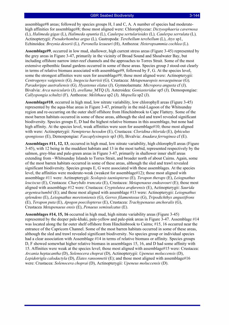
GBR Seabed Biodiversity 3-144
assemblage#8 areas; followed by species groups H, I and C, A. A number of species had moderate-high affinities for assemblage#8; those most aligned were: Chlorophyceae: Dictyosphaeria cavernosa (L), Halimeda gigas (L), Halimeda opuntia (L), Caulerpa sertularioides (L), Caulerpa serrulata (L), Actinopterygii: Pseudorhombus argus (L), Gastropoda: Terebellum terebellum (L), Atys sp1, Echinoidea: Breynia desorii (L), Peronella lesueuri (H), Anthozoa: Heteropsammia cochlea (L).
Assemblage#9, occurred in low mud, shallower, high current stress areas (Figure 3-45) represented by the grey areas in Figure 3-47, primarily in the vicinity of Broad Sound and Shoalwater Bay, but including offshore narrow inter-reef channels and the approaches to Torres Strait. Some of the most extensive epibenthic faunal gardens occurred in some of these areas. Species group J stood-out clearly in terms of relative biomass associated with assemblage#9, followed by F, G. At the species level, some the strongest affinities were seen for assemblage#9; those most aligned were: Actinopterygii: Centrogenys vaigiensis (G), Inegocia harrisii (G), Crustacea: Metapenaeopsis novaeguineae (G), Paradorippe australiensis (G), Hyastenus elatus (J), Gymnolaemata: Micropora angusta cf (J), Bivalvia: Arca navicularis (J), avellana_MTQ (J), Asteroidea: Goniasteridae sp5 (J), Demospongiae: Callyspongia schultzi (F), Anthozoa: Melithaea sp2 (J), Mopsella sp2 (J).
Assemblage#10, occurred in high mud, low nitrate variability, low chlorophyll areas (Figure 3-45) represented by the aqua-blue areas in Figure 3-47, primarily in the mid-Lagoon of the Whitsunday region and re-occurring on the outer shelf offshore from Hinchinbrook to Cape Flattery. Some of the most barren habitats occurred in some of these areas, although the sled and trawl revealed significant biodiversity. Species groups E, D had the highest relative biomass in this assemblage, but none had high affinity. At the species level, weak affinities were seen for assemblage#10; those most aligned with were: Actinopterygii: Nemipterus hexodon (E), Crustacea: Cloridina chlorida (E), Iphiculus spongiosus (E), Demospongiae: Fascaplysinopsis sp3 (H), Bivalvia: Anadara ferruginea cf (E).
Assemblages #11, 12, 13, occurred in high mud, low nitrate variability, high chlorophyll areas (Figure 3-45), with 12 being in the muddiest habitats and 13 in the most turbid, represented respectively by the salmon, grey-blue and pale-green areas in Figure 3-47, primarily in shallower inner shelf areas extending from ~Whitsunday Islands to Torres Strait, and broader north of about Cairns. Again, some of the most barren habitats occurred in some of these areas, although the sled and trawl revealed significant biodiversity. Species groups E, G were associated with these assemblages. At the species level, the affinities were moderate-weak (weakest for assemblage#12); those most aligned with assemblage #11 were: Actinopterygii: Scolopsis taeniopterus (E), Terapon theraps (E), Leiognathus leuciscus (E), Crustacea: Charybdis truncata (E), Crustacea: Metapenaeus endeavouri (E); those most aligned with assemblage #12 were: Crustacea: Cryptolutea arafurensis (E), Actinopterygii: Saurida argentea/tumbil (E); and those most aligned with assemblage #13 were: Actinopterygii: Leiognathus splendens (E), Leiognathus moretoniensis (G), Gerres filamentosus (G), Tripodichthys angustifrons (E), Terapon puta (E), Apogon poecilopterus (E), Crustacea: Trachypenaeus anchoralis (G), Crustacea Metapenaeus ensis (E), Penaeus semisulcatus (E).
Assemblages #14, 15, 16 occurred in high mud, high nitrate variability areas (Figure 3-45) represented by the deeper pale-khaki, pale-yellow and pale-pink areas in Figure 3-47. Assemblage #14 was located along the far outer shelf offshore from Hinchinbrook to Cairns; #15, 16 occurred near the entrance of the Capricorn Channel. Some of the most barren habitats occurred in some of these areas, although the sled and trawl revealed significant biodiversity. No species group or individual species had a clear association with Assemblage #14 in terms of relative biomass or affinity. Species groups D, F showed somewhat higher relative biomass in assemblages 15, 16, and D had some affinity with 15. Affinities were weak at the species level; those most aligned with assemblage#15 were: Crustacea: Arcania heptacantha (D), Solenocera choprai (D), Actinopterygii: Upeneus moluccensis (D), Lepidotrigla calodactyla (D), Elates ransonnetii (E); and those most aligned with assemblage#16 were: Crustacea: Solenocera choprai (D), Actinopterygii: Upeneus moluccensis (D).
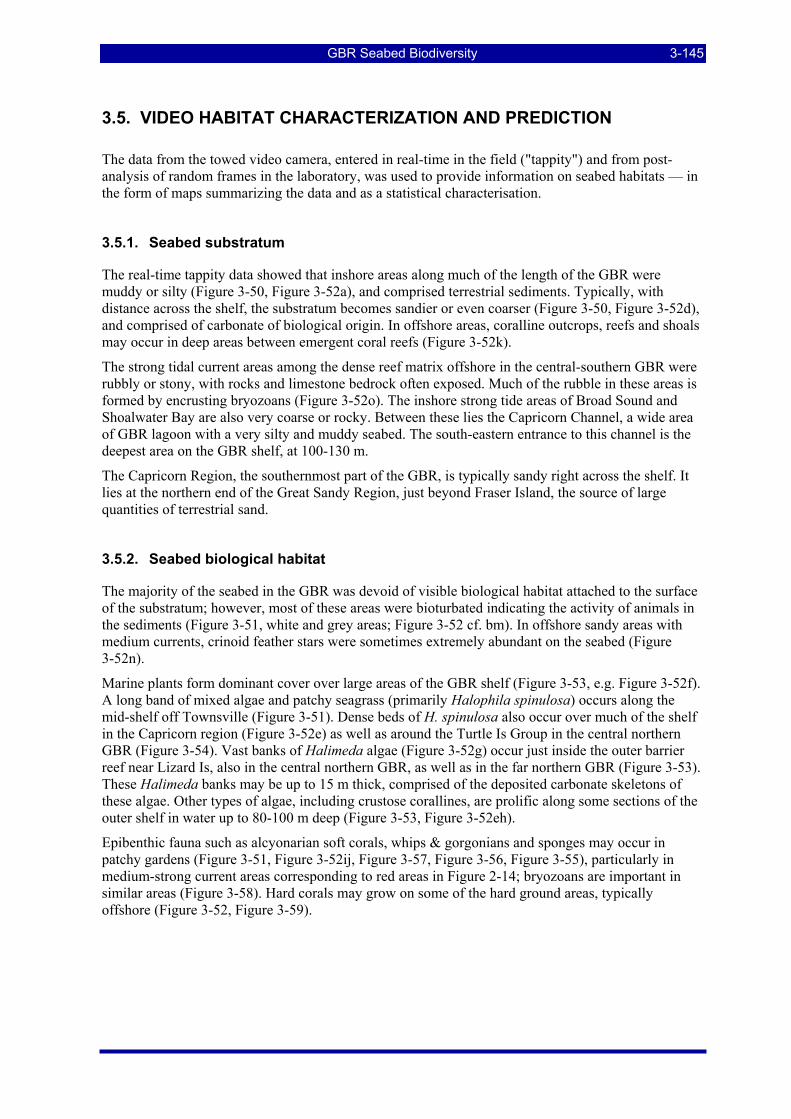
GBR Seabed Biodiversity 3-145
3.5. VIDEO HABITAT CHARACTERIZATION AND PREDICTION The data from the towed video camera, entered in real-time in the field ("tappity") and from post-analysis of random frames in the laboratory, was used to provide information on seabed habitats — in the form of maps summarizing the data and as a statistical characterisation.
3.5.1. Seabed substratum The real-time tappity data showed that inshore areas along much of the length of the GBR were muddy or silty (Figure 3-50, Figure 3-52a), and comprised terrestrial sediments. Typically, with distance across the shelf, the substratum becomes sandier or even coarser (Figure 3-50, Figure 3-52d), and comprised of carbonate of biological origin. In offshore areas, coralline outcrops, reefs and shoals may occur in deep areas between emergent coral reefs (Figure 3-52k).
The strong tidal current areas among the dense reef matrix offshore in the central-southern GBR were rubbly or stony, with rocks and limestone bedrock often exposed. Much of the rubble in these areas is formed by encrusting bryozoans (Figure 3-52o). The inshore strong tide areas of Broad Sound and Shoalwater Bay are also very coarse or rocky. Between these lies the Capricorn Channel, a wide area of GBR lagoon with a very silty and muddy seabed. The south-eastern entrance to this channel is the deepest area on the GBR shelf, at 100-130 m.
The Capricorn Region, the southernmost part of the GBR, is typically sandy right across the shelf. It lies at the northern end of the Great Sandy Region, just beyond Fraser Island, the source of large quantities of terrestrial sand.
3.5.2. Seabed biological habitat The majority of the seabed in the GBR was devoid of visible biological habitat attached to the surface of the substratum; however, most of these areas were bioturbated indicating the activity of animals in the sediments (Figure 3-51, white and grey areas; Figure 3-52 cf. bm). In offshore sandy areas with medium currents, crinoid feather stars were sometimes extremely abundant on the seabed (Figure 3-52n).
Marine plants form dominant cover over large areas of the GBR shelf (Figure 3-53, e.g. Figure 3-52f). A long band of mixed algae and patchy seagrass (primarily Halophila spinulosa) occurs along the mid-shelf off Townsville (Figure 3-51). Dense beds of H. spinulosa also occur over much of the shelf in the Capricorn region (Figure 3-52e) as well as around the Turtle Is Group in the central northern GBR (Figure 3-54). Vast banks of Halimeda algae (Figure 3-52g) occur just inside the outer barrier reef near Lizard Is, also in the central northern GBR, as well as in the far northern GBR (Figure 3-53). These Halimeda banks may be up to 15 m thick, comprised of the deposited carbonate skeletons of these algae. Other types of algae, including crustose corallines, are prolific along some sections of the outer shelf in water up to 80-100 m deep (Figure 3-53, Figure 3-52eh).
Epibenthic fauna such as alcyonarian soft corals, whips & gorgonians and sponges may occur in patchy gardens (Figure 3-51, Figure 3-52ij, Figure 3-57, Figure 3-56, Figure 3-55), particularly in medium-strong current areas corresponding to red areas in Figure 2-14; bryozoans are important in similar areas (Figure 3-58). Hard corals may grow on some of the hard ground areas, typically offshore (Figure 3-52, Figure 3-59).
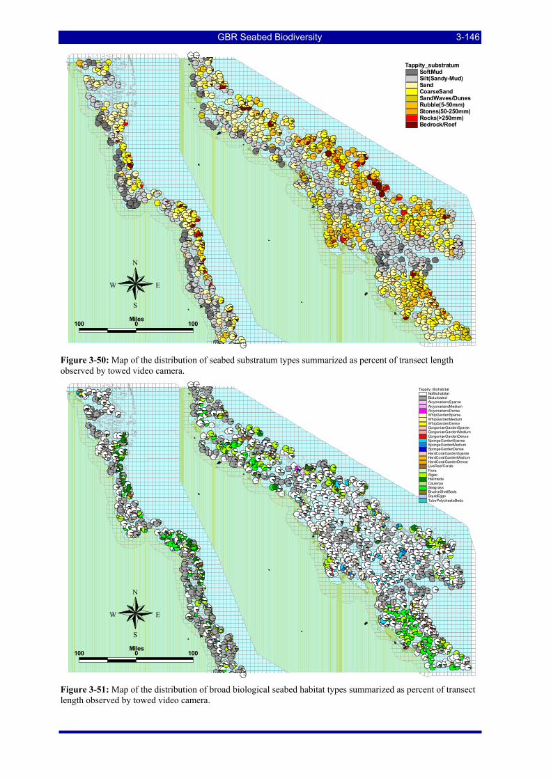
GBR Seabed Biodiversity 3-146
N
EW
S
Tappity_substratumSoftMudSilt(Sandy-Mud)SandCoarseSandSandWaves/DunesRubble(5-50mm)Stones(50-250mm)Rocks(>250mm)Bedrock/Reef
100 0 100Miles
Figure 3-50: Map of the distribution of seabed substratum types summarized as percent of transect length observed by towed video camera.
N
EW
S
100 0 100Miles
Tappity_BiohabitatNoBiohabitatBioturbatedAlcyonariansSparseAlcyonariansMediumAlcyonariansDenseWhipGardenSparseWhipGardenMediumWhipGardenDenseGorgonianGardenSparseGorgonianGardenMediumGorgonianGardenDenseSpongeGardenSparseSpongeGardenMediumSpongeGardenDenseHardCoralGardenSparseHardCoralGardenMediumHardCoralGardenDenseLiveReefCoralsFloraAlgaeHalimedaCaulerpaSeagrassBivalveShellBedsSquidEggsTubePolychaeteBeds
Figure 3-51: Map of the distribution of broad biological seabed habitat types summarized as percent of transect length observed by towed video camera.
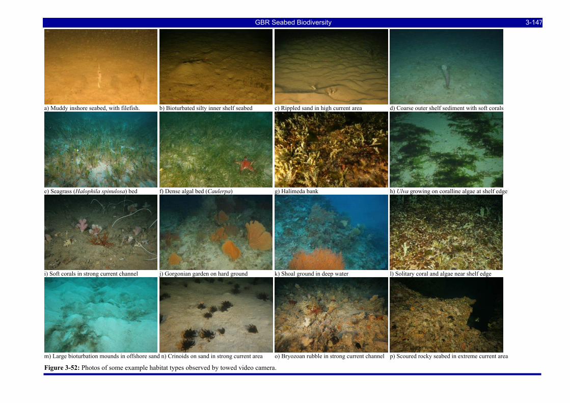
GBR Seabed Biodiversity 3-147
a) Muddy inshore seabed, with filefish. b) Bioturbated silty inner shelf seabed c) Rippled sand in high current area d) Coarse outer shelf sediment with soft corals
e) Seagrass (Halophila spinulosa) bed f) Dense algal bed (Caulerpa) g) Halimeda bank h) Ulva growing on coralline algae at shelf edge
i) Soft corals in strong current channel j) Gorgonian garden on hard ground k) Shoal ground in deep water l) Solitary coral and algae near shelf edge
m) Large bioturbation mounds in offshore sand n) Crinoids on sand in strong current area o) Bryozoan rubble in strong current channel p) Scoured rocky seabed in extreme current area
Figure 3-52: Photos of some example habitat types observed by towed video camera.
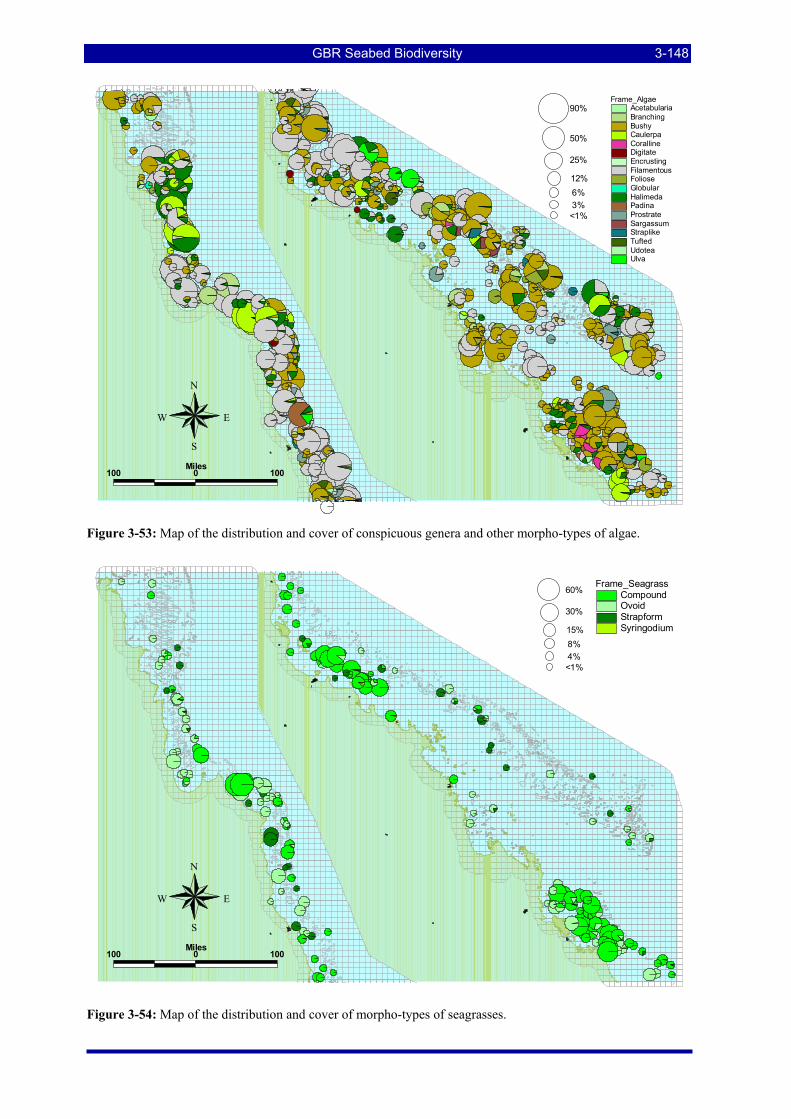
GBR Seabed Biodiversity 3-148
N
EW
S
100 0 100Miles
90%
25%
12% 6% 3%<1%
Frame_AlgaeAcetabulariaBranchingBushyCaulerpaCorallineDigitateEncrustingFilamentousFolioseGlobularHalimedaPadinaProstrateSargassumStraplikeTuftedUdoteaUlva
50%
Figure 3-53: Map of the distribution and cover of conspicuous genera and other morpho-types of algae.
N
EW
S
100 0 100Miles
30%
15% 8% 4%<1%
60%Frame_Seagrass
CompoundOvoidStrapformSyringodium
Figure 3-54: Map of the distribution and cover of morpho-types of seagrasses.
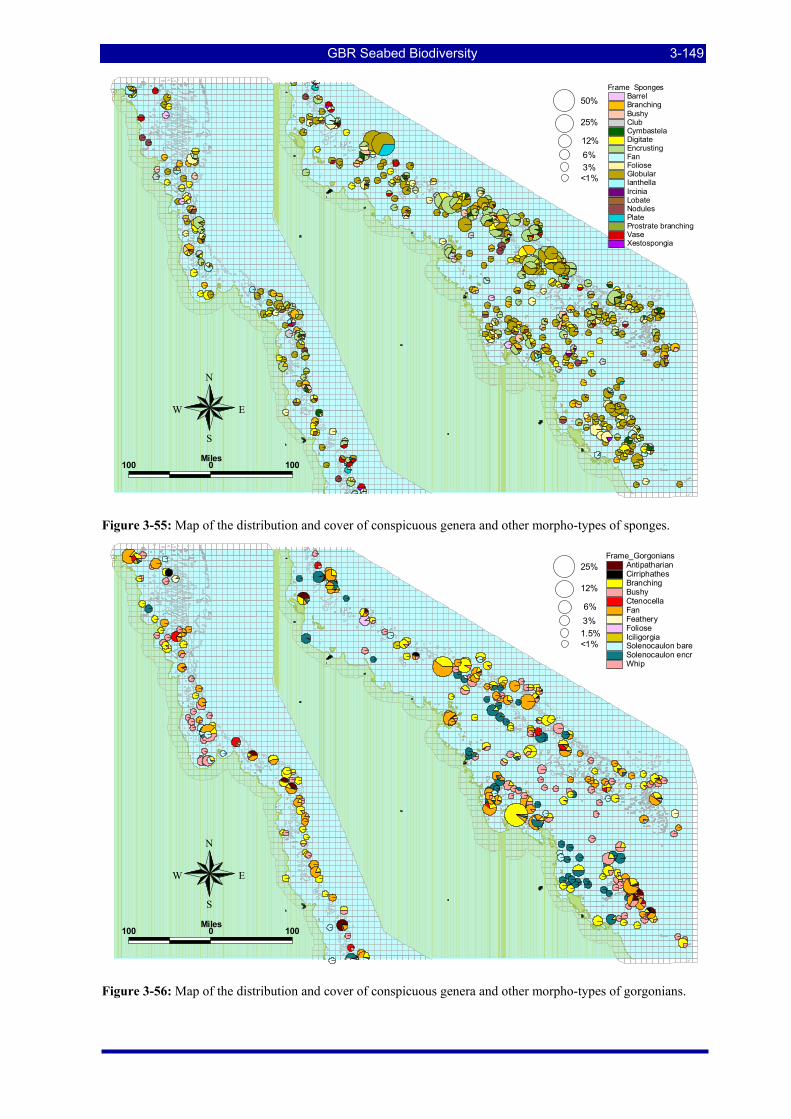
GBR Seabed Biodiversity 3-149
N
EW
S
100 0 100Miles
25%
12% 6% 3%<1%
50%Frame_Sponges
BarrelBranchingBushyClubCymbastelaDigitateEncrustingFanFolioseGlobularIanthellaIrciniaLobateNodulesPlateProstrate branchingVaseXestospongia
Figure 3-55: Map of the distribution and cover of conspicuous genera and other morpho-types of sponges.
N
EW
S
100 0 100Miles
12%
6% 3%1.5%<1%
25%Frame_Gorgonians
AntipatharianCirriphathesBranchingBushyCtenocellaFanFeatheryFolioseIciligorgiaSolenocaulon bareSolenocaulon encrWhip
Figure 3-56: Map of the distribution and cover of conspicuous genera and other morpho-types of gorgonians.
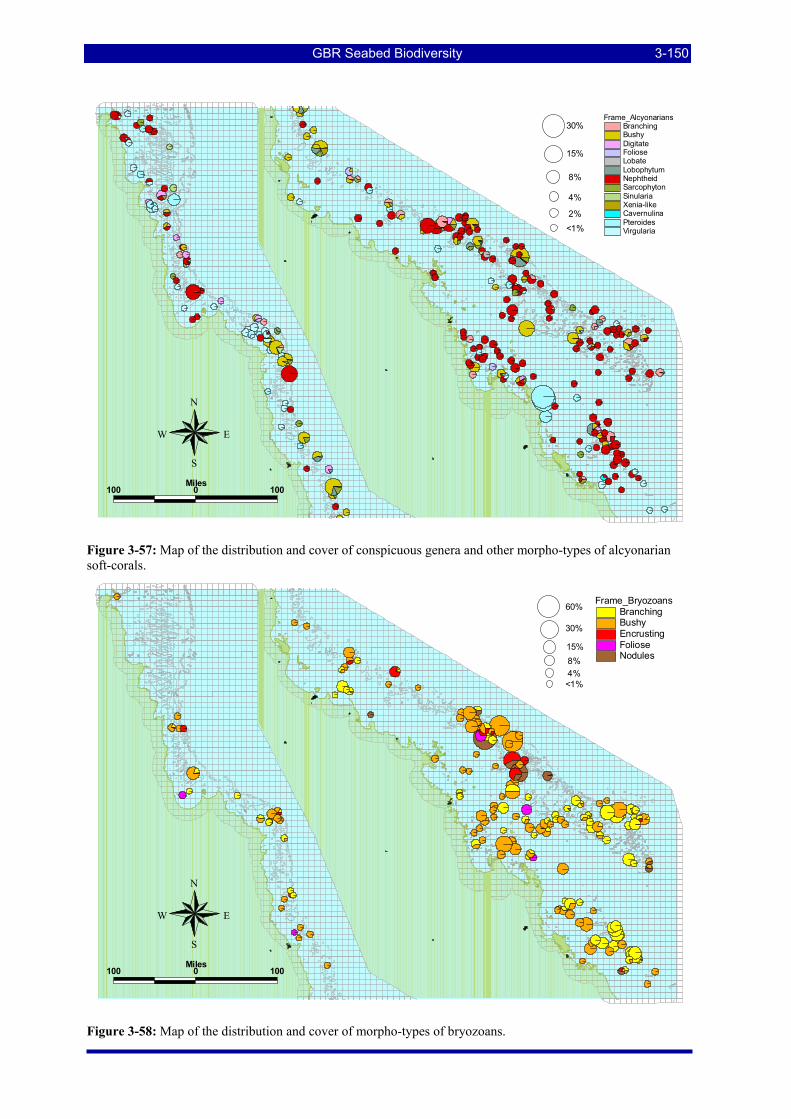
GBR Seabed Biodiversity 3-150
N
EW
S
100 0 100Miles
30%
15%
8%
4%
2%<1%
Frame_AlcyonariansBranchingBushyDigitateFolioseLobateLobophytumNephtheidSarcophytonSinulariaXenia-likeCavernulinaPteroidesVirgularia
Figure 3-57: Map of the distribution and cover of conspicuous genera and other morpho-types of alcyonarian soft-corals.
#
N
EW
S
100 0 100Miles
30%
15% 8% 4%<1%
60%Frame_Bryozoans
BranchingBushyEncrustingFolioseNodules
Figure 3-58: Map of the distribution and cover of morpho-types of bryozoans.
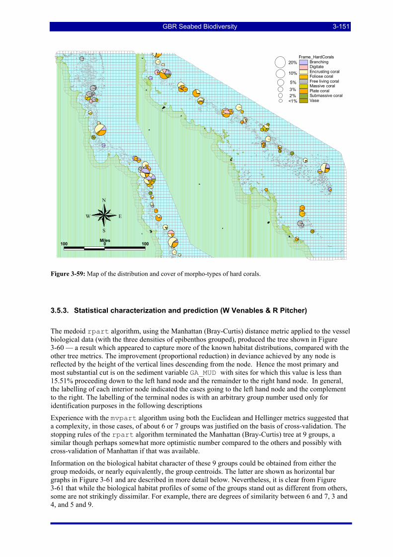
GBR Seabed Biodiversity 3-151
N
EW
S
100 0 100Miles
10%
5% 3% 2%<1%
20%Frame_HardCorals
BranchingDigitateEncrusting coralFoliose coralFree living coralMassive coralPlate coralSubmassive coralVase
Figure 3-59: Map of the distribution and cover of morpho-types of hard corals.
3.5.3. Statistical characterization and prediction (W Venables & R Pitcher)
The medoid rpart algorithm, using the Manhattan (Bray-Curtis) distance metric applied to the vessel biological data (with the three densities of epibenthos grouped), produced the tree shown in Figure 3-60 — a result which appeared to capture more of the known habitat distributions, compared with the other tree metrics. The improvement (proportional reduction) in deviance achieved by any node is reflected by the height of the vertical lines descending from the node. Hence the most primary and most substantial cut is on the sediment variable GA_MUD with sites for which this value is less than 15.51% proceeding down to the left hand node and the remainder to the right hand node. In general, the labelling of each interior node indicated the cases going to the left hand node and the complement to the right. The labelling of the terminal nodes is with an arbitrary group number used only for identification purposes in the following descriptions
Experience with the mvpart algorithm using both the Euclidean and Hellinger metrics suggested that a complexity, in those cases, of about 6 or 7 groups was justified on the basis of cross-validation. The stopping rules of the rpart algorithm terminated the Manhattan (Bray-Curtis) tree at 9 groups, a similar though perhaps somewhat more optimistic number compared to the others and possibly with cross-validation of Manhattan if that was available.
Information on the biological habitat character of these 9 groups could be obtained from either the group medoids, or nearly equivalently, the group centroids. The latter are shown as horizontal bar graphs in Figure 3-61 and are described in more detail below. Nevertheless, it is clear from Figure 3-61 that while the biological habitat profiles of some of the groups stand out as different from others, some are not strikingly dissimilar. For example, there are degrees of similarity between 6 and 7, 3 and 4, and 5 and 9.
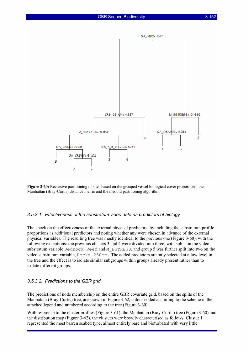
GBR Seabed Biodiversity 3-152
Figure 3-60: Recursive partitioning of sites based on the grouped vessel biological cover proportions, the Manhattan (Bray-Curtis) distance metric and the medoid partitioning algorithm.
3.5.3.1. Effectiveness of the substratum video data as predictors of biology
The check on the effectiveness of the external physical predictors, by including the substratum profile proportions as additional predictors and noting whether any were chosen in advance of the external physical variables. The resulting tree was mostly identical to the previous one (Figure 3-60), with the following exceptions: the previous clusters 3 and 4 were divided into three, with splits on the video substratum variable Bedrock.Reef and M_BSTRESS, and group 5 was further split into two on the video substratum variable, Rocks.250mm. The added predictors are only selected at a low level in the tree and the effect is to isolate similar subgroups within groups already present rather than to isolate different groups.
3.5.3.2. Predictions to the GBR grid
The predictions of node membership on the entire GBR covariate grid, based on the splits of the Manhattan (Bray-Curtis) tree, are shown in Figure 3-62, colour coded according to the scheme in the attached legend and numbered according to the tree (Figure 3-60).
With reference to the cluster profiles (Figure 3-61), the Manhattan (Bray-Curtis) tree (Figure 3-60) and the distribution map (Figure 3-62), the clusters were broadly characterised as follows: Cluster 1 represented the most barren seabed type, almost entirely bare and bioturbated with very little
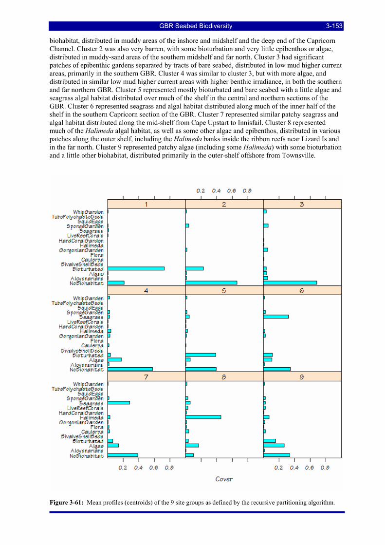
GBR Seabed Biodiversity 3-153
biohabitat, distributed in muddy areas of the inshore and midshelf and the deep end of the Capricorn Channel. Cluster 2 was also very barren, with some bioturbation and very little epibenthos or algae, distributed in muddy-sand areas of the southern midshelf and far north. Cluster 3 had significant patches of epibenthic gardens separated by tracts of bare seabed, distributed in low mud higher current areas, primarily in the southern GBR. Cluster 4 was similar to cluster 3, but with more algae, and distributed in similar low mud higher current areas with higher benthic irradiance, in both the southern and far northern GBR. Cluster 5 represented mostly bioturbated and bare seabed with a little algae and seagrass algal habitat distributed over much of the shelf in the central and northern sections of the GBR. Cluster 6 represented seagrass and algal habitat distributed along much of the inner half of the shelf in the southern Capricorn section of the GBR. Cluster 7 represented similar patchy seagrass and algal habitat distributed along the mid-shelf from Cape Upstart to Innisfail. Cluster 8 represented much of the Halimeda algal habitat, as well as some other algae and epibenthos, distributed in various patches along the outer shelf, including the Halimeda banks inside the ribbon reefs near Lizard Is and in the far north. Cluster 9 represented patchy algae (including some Halimeda) with some bioturbation and a little other biohabitat, distributed primarily in the outer-shelf offshore from Townsville.
Figure 3-61: Mean profiles (centroids) of the 9 site groups as defined by the recursive partitioning algorithm.
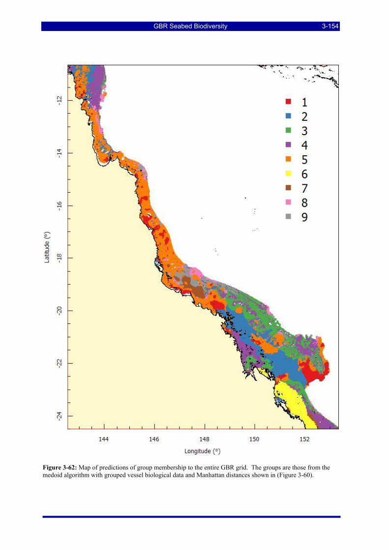
GBR Seabed Biodiversity 3-154
Figure 3-62: Map of predictions of group membership to the entire GBR grid. The groups are those from the medoid algorithm with grouped vessel biological data and Manhattan distances shown in (Figure 3-60).
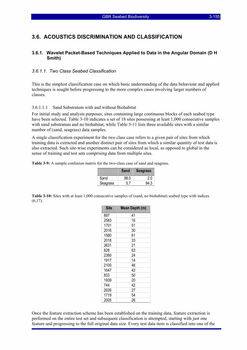
GBR Seabed Biodiversity 3-155
3.6. ACOUSTICS DISCRIMINATION AND CLASSIFICATION
3.6.1. Wavelet Packet-Based Techniques Applied to Data in the Angular Domain (D H Smith)
3.6.1.1. Two Class Seabed Classification
This is the simplest classification case on which basic understanding of the data behaviour and applied techniques is sought before progressing to the more complex cases involving larger numbers of classes.
3.6.1.1.1 Sand Substratum with and without Biohabitat For initial study and analysis purposes, sites containing large continuous blocks of each seabed type have been selected. Table 3-10 indicates a set of 18 sites possessing at least 1,000 consecutive samples with sand substratum and no biohabitat, while Table 3-11 lists three available sites with a similar number of (sand, seagrass) data samples.
A single classification experiment for the two class case refers to a given pair of sites from which training data is extracted and another distinct pair of sites from which a similar quantity of test data is also extracted. Such site-wise experiments can be considered as local, as opposed to global in the sense of training and test sets comprising data from multiple sites.
Table 3-9: A sample confusion matrix for the two-class case of sand and seagrass.
Sand Seagrass
Sand 98.0 2.0 Seagrass 5.7 94.3
Table 3-10: Sites with at least 1,000 consecutive samples of (sand, no biohabitat) seabed type with indices (6,17).
Site Mean Depth (m)
897 41 2583 16 1701 51 2016 30 1580 61 2018 33 2631 21 828 63 2380 24 1917 14 2100 46 1647 42 833 50 1939 20 744 42 2626 27 1719 54 2005 26
Once the feature extraction scheme has been established on the training data, feature extraction is performed on the entire test set and subsequent classification is attempted, starting with just one feature and progressing to the full original data size. Every test data item is classified into one of the
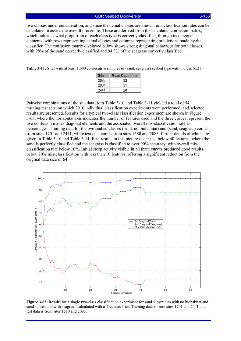
GBR Seabed Biodiversity 3-156
two classes under consideration, and since the actual classes are known, mis-classification rates can be calculated to assess the overall procedure. These are derived from the calculated confusion matrix, which indicates what proportion of each class type is correctly classified, through its diagonal elements, with rows representing actual classes and columns representing predictions made by the classifier. The confusion matrix displayed below shows strong diagonal behaviour for both classes, with 98% of the sand correctly classified and 94.3% of the seagrass correctly classified.
Table 3-11: Sites with at least 1,000 consecutive samples of (sand, seagrass) seabed type with indices (6,21).
Site Mean Depth (m) 2083 33 2084 31 2441 28
Pairwise combinations of the site data from Table 3-10 and Table 3-11 yielded a total of 54 training/test sets, on which 2916 individual classification experiments were performed, and selected results are presented. Results for a typical two-class classification experiment are shown in Figure 3-63, where the horizontal axis indicates the number of features used and the three curves represent the two confusion matrix diagonal elements and the associated overall mis-classification rate as percentages. Training data for the two seabed classes (sand, no biohabitat) and (sand, seagrass) comes from sites 1701 and 2441, while test data comes from sites 1580 and 2083, further details of which are given in Table 3-10 and Table 3-11. Best results in this picture occur just below 40 features, where the sand is perfectly classified and the seagrass is classified to over 90% accuracy, with overall mis-classification rate below 10%. Initial steep activity visible in all three curves produced good results below 20% mis-classification with less than 10 features, offering a significant reduction from the original data size of 64.
10 20 30 40 50 60
10
20
30
40
50
60
70
80
90
100
Feature Dimension
Con
fusi
on D
iago
nals
/Mis
−C
lass
Rat
e %
1st Diagonal(Sand)2nd Diagonal(Seagrass)Mis−Classification Rate
Figure 3-63: Results for a single two-class classification experiment for sand substratum with no biohabitat and sand substratum with seagrass, calculated with a Tree classifier. Training data is from sites 1701 and 2441 and test data is from sites 1580 and 2083.
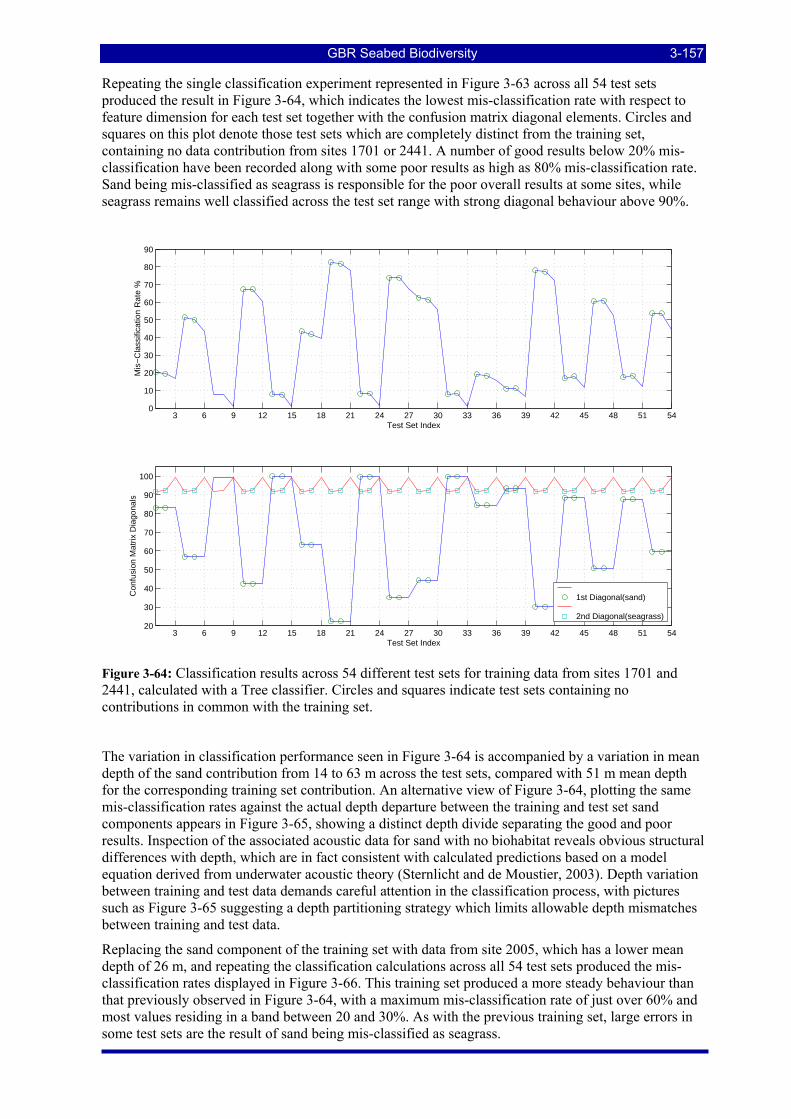
GBR Seabed Biodiversity 3-157
Repeating the single classification experiment represented in Figure 3-63 across all 54 test sets produced the result in Figure 3-64, which indicates the lowest mis-classification rate with respect to feature dimension for each test set together with the confusion matrix diagonal elements. Circles and squares on this plot denote those test sets which are completely distinct from the training set, containing no data contribution from sites 1701 or 2441. A number of good results below 20% mis-classification have been recorded along with some poor results as high as 80% mis-classification rate. Sand being mis-classified as seagrass is responsible for the poor overall results at some sites, while seagrass remains well classified across the test set range with strong diagonal behaviour above 90%.
3 6 9 12 15 18 21 24 27 30 33 36 39 42 45 48 51 540
10
20
30
40
50
60
70
80
90
Test Set Index
Mis
−C
lass
ifica
tion
Rat
e %
3 6 9 12 15 18 21 24 27 30 33 36 39 42 45 48 51 5420
30
40
50
60
70
80
90
100
Test Set Index
Con
fusi
on M
atrix
Dia
gona
ls
1st Diagonal(sand) 2nd Diagonal(seagrass)
Figure 3-64: Classification results across 54 different test sets for training data from sites 1701 and 2441, calculated with a Tree classifier. Circles and squares indicate test sets containing no contributions in common with the training set.
The variation in classification performance seen in Figure 3-64 is accompanied by a variation in mean depth of the sand contribution from 14 to 63 m across the test sets, compared with 51 m mean depth for the corresponding training set contribution. An alternative view of Figure 3-64, plotting the same mis-classification rates against the actual depth departure between the training and test set sand components appears in Figure 3-65, showing a distinct depth divide separating the good and poor results. Inspection of the associated acoustic data for sand with no biohabitat reveals obvious structural differences with depth, which are in fact consistent with calculated predictions based on a model equation derived from underwater acoustic theory (Sternlicht and de Moustier, 2003). Depth variation between training and test data demands careful attention in the classification process, with pictures such as Figure 3-65 suggesting a depth partitioning strategy which limits allowable depth mismatches between training and test data.
Replacing the sand component of the training set with data from site 2005, which has a lower mean depth of 26 m, and repeating the classification calculations across all 54 test sets produced the mis-classification rates displayed in Figure 3-66. This training set produced a more steady behaviour than that previously observed in Figure 3-64, with a maximum mis-classification rate of just over 60% and most values residing in a band between 20 and 30%. As with the previous training set, large errors in some test sets are the result of sand being mis-classified as seagrass.
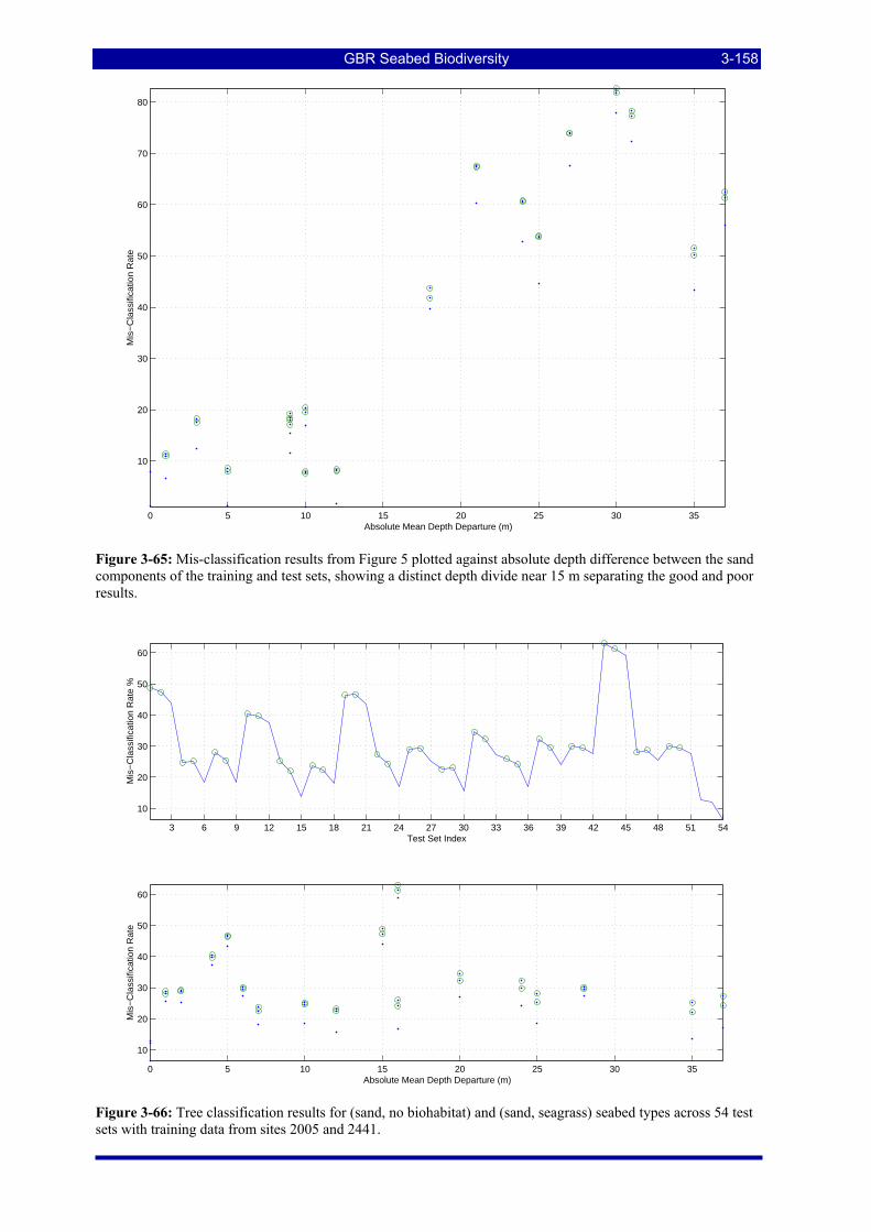
GBR Seabed Biodiversity 3-158
0 5 10 15 20 25 30 35
10
20
30
40
50
60
70
80
Absolute Mean Depth Departure (m)
Mis
−C
lass
ifica
tion
Rat
e
Figure 3-65: Mis-classification results from Figure 5 plotted against absolute depth difference between the sand components of the training and test sets, showing a distinct depth divide near 15 m separating the good and poor results.
3 6 9 12 15 18 21 24 27 30 33 36 39 42 45 48 51 54
10
20
30
40
50
60
Test Set Index
Mis
−C
lass
ifica
tion
Rat
e %
0 5 10 15 20 25 30 35
10
20
30
40
50
60
Absolute Mean Depth Departure (m)
Mis
−C
lass
ifica
tion
Rat
e
Figure 3-66: Tree classification results for (sand, no biohabitat) and (sand, seagrass) seabed types across 54 test sets with training data from sites 2005 and 2441.
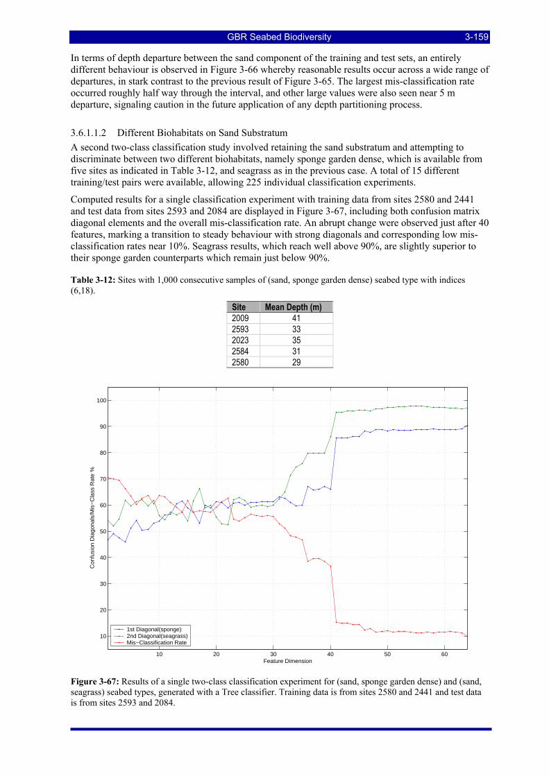
GBR Seabed Biodiversity 3-159
In terms of depth departure between the sand component of the training and test sets, an entirely different behaviour is observed in Figure 3-66 whereby reasonable results occur across a wide range of departures, in stark contrast to the previous result of Figure 3-65. The largest mis-classification rate occurred roughly half way through the interval, and other large values were also seen near 5 m departure, signaling caution in the future application of any depth partitioning process.
3.6.1.1.2 Different Biohabitats on Sand Substratum A second two-class classification study involved retaining the sand substratum and attempting to discriminate between two different biohabitats, namely sponge garden dense, which is available from five sites as indicated in Table 3-12, and seagrass as in the previous case. A total of 15 different training/test pairs were available, allowing 225 individual classification experiments.
Computed results for a single classification experiment with training data from sites 2580 and 2441 and test data from sites 2593 and 2084 are displayed in Figure 3-67, including both confusion matrix diagonal elements and the overall mis-classification rate. An abrupt change were observed just after 40 features, marking a transition to steady behaviour with strong diagonals and corresponding low mis-classification rates near 10%. Seagrass results, which reach well above 90%, are slightly superior to their sponge garden counterparts which remain just below 90%.
Table 3-12: Sites with 1,000 consecutive samples of (sand, sponge garden dense) seabed type with indices (6,18).
Site Mean Depth (m) 2009 41 2593 33 2023 35 2584 31 2580 29
10 20 30 40 50 60
10
20
30
40
50
60
70
80
90
100
Feature Dimension
Con
fusi
on D
iago
nals
/Mis
−C
lass
Rat
e %
1st Diagonal(sponge)2nd Diagonal(seagrass)Mis−Classification Rate
Figure 3-67: Results of a single two-class classification experiment for (sand, sponge garden dense) and (sand, seagrass) seabed types, generated with a Tree classifier. Training data is from sites 2580 and 2441 and test data is from sites 2593 and 2084.
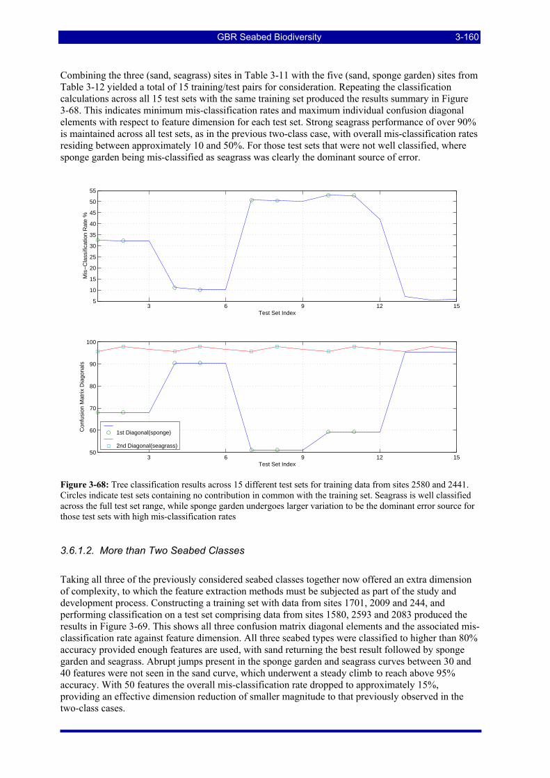
GBR Seabed Biodiversity 3-160
Combining the three (sand, seagrass) sites in Table 3-11 with the five (sand, sponge garden) sites from Table 3-12 yielded a total of 15 training/test pairs for consideration. Repeating the classification calculations across all 15 test sets with the same training set produced the results summary in Figure 3-68. This indicates minimum mis-classification rates and maximum individual confusion diagonal elements with respect to feature dimension for each test set. Strong seagrass performance of over 90% is maintained across all test sets, as in the previous two-class case, with overall mis-classification rates residing between approximately 10 and 50%. For those test sets that were not well classified, where sponge garden being mis-classified as seagrass was clearly the dominant source of error.
3 6 9 12 1550
60
70
80
90
100
Test Set Index
Con
fusi
on M
atrix
Dia
gona
ls
1st Diagonal(sponge) 2nd Diagonal(seagrass)
3 6 9 12 155
10
15
20
25
30
35
40
45
50
55
Test Set Index
Mis
−C
lass
ifica
tion
Rat
e %
Figure 3-68: Tree classification results across 15 different test sets for training data from sites 2580 and 2441. Circles indicate test sets containing no contribution in common with the training set. Seagrass is well classified across the full test set range, while sponge garden undergoes larger variation to be the dominant error source for those test sets with high mis-classification rates
3.6.1.2. More than Two Seabed Classes
Taking all three of the previously considered seabed classes together now offered an extra dimension of complexity, to which the feature extraction methods must be subjected as part of the study and development process. Constructing a training set with data from sites 1701, 2009 and 244, and performing classification on a test set comprising data from sites 1580, 2593 and 2083 produced the results in Figure 3-69. This shows all three confusion matrix diagonal elements and the associated mis-classification rate against feature dimension. All three seabed types were classified to higher than 80% accuracy provided enough features are used, with sand returning the best result followed by sponge garden and seagrass. Abrupt jumps present in the sponge garden and seagrass curves between 30 and 40 features were not seen in the sand curve, which underwent a steady climb to reach above 95% accuracy. With 50 features the overall mis-classification rate dropped to approximately 15%, providing an effective dimension reduction of smaller magnitude to that previously observed in the two-class cases.
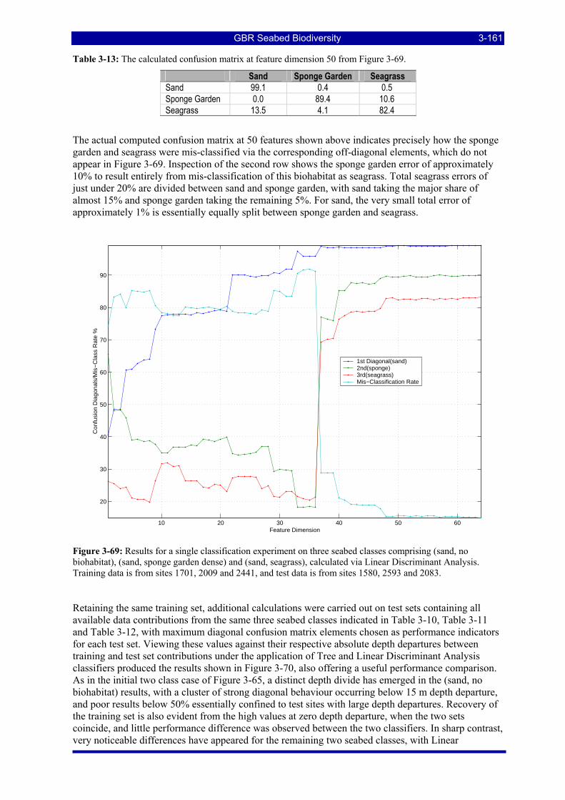
GBR Seabed Biodiversity 3-161
Table 3-13: The calculated confusion matrix at feature dimension 50 from Figure 3-69.
Sand Sponge Garden Seagrass Sand 99.1 0.4 0.5 Sponge Garden 0.0 89.4 10.6 Seagrass 13.5 4.1 82.4
The actual computed confusion matrix at 50 features shown above indicates precisely how the sponge garden and seagrass were mis-classified via the corresponding off-diagonal elements, which do not appear in Figure 3-69. Inspection of the second row shows the sponge garden error of approximately 10% to result entirely from mis-classification of this biohabitat as seagrass. Total seagrass errors of just under 20% are divided between sand and sponge garden, with sand taking the major share of almost 15% and sponge garden taking the remaining 5%. For sand, the very small total error of approximately 1% is essentially equally split between sponge garden and seagrass.
10 20 30 40 50 60
20
30
40
50
60
70
80
90
Feature Dimension
Con
fusi
on D
iago
nals
/Mis
−C
lass
Rat
e %
1st Diagonal(sand)2nd(sponge)3rd(seagrass)Mis−Classification Rate
Figure 3-69: Results for a single classification experiment on three seabed classes comprising (sand, no biohabitat), (sand, sponge garden dense) and (sand, seagrass), calculated via Linear Discriminant Analysis. Training data is from sites 1701, 2009 and 2441, and test data is from sites 1580, 2593 and 2083.
Retaining the same training set, additional calculations were carried out on test sets containing all available data contributions from the same three seabed classes indicated in Table 3-10, Table 3-11 and Table 3-12, with maximum diagonal confusion matrix elements chosen as performance indicators for each test set. Viewing these values against their respective absolute depth departures between training and test set contributions under the application of Tree and Linear Discriminant Analysis classifiers produced the results shown in Figure 3-70, also offering a useful performance comparison. As in the initial two class case of Figure 3-65, a distinct depth divide has emerged in the (sand, no biohabitat) results, with a cluster of strong diagonal behaviour occurring below 15 m depth departure, and poor results below 50% essentially confined to test sites with large depth departures. Recovery of the training set is also evident from the high values at zero depth departure, when the two sets coincide, and little performance difference was observed between the two classifiers. In sharp contrast, very noticeable differences have appeared for the remaining two seabed classes, with Linear
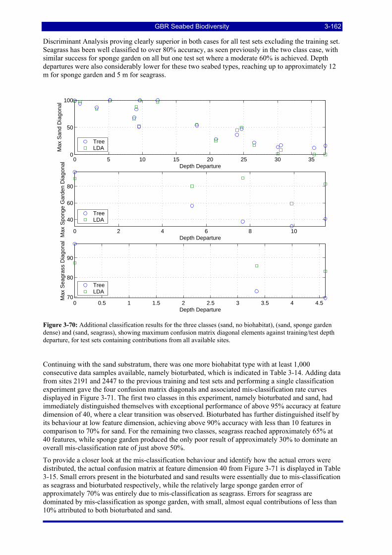
GBR Seabed Biodiversity 3-162
Discriminant Analysis proving clearly superior in both cases for all test sets excluding the training set. Seagrass has been well classified to over 80% accuracy, as seen previously in the two class case, with similar success for sponge garden on all but one test set where a moderate 60% is achieved. Depth departures were also considerably lower for these two seabed types, reaching up to approximately 12 m for sponge garden and 5 m for seagrass.
0 2 4 6 8 10
40
60
80
Depth DepartureMax
Spo
nge
Gar
den
Dia
gona
l
TreeLDA
0 0.5 1 1.5 2 2.5 3 3.5 4 4.570
80
90
Depth Departure
Max
Sea
gras
s D
iago
nal
TreeLDA
0 5 10 15 20 25 30 350
50
100
Depth Departure
Max
San
d D
iago
nal
TreeLDA
Figure 3-70: Additional classification results for the three classes (sand, no biohabitat), (sand, sponge garden dense) and (sand, seagrass), showing maximum confusion matrix diagonal elements against training/test depth departure, for test sets containing contributions from all available sites.
Continuing with the sand substratum, there was one more biohabitat type with at least 1,000 consecutive data samples available, namely bioturbated, which is indicated in Table 3-14. Adding data from sites 2191 and 2447 to the previous training and test sets and performing a single classification experiment gave the four confusion matrix diagonals and associated mis-classification rate curves displayed in Figure 3-71. The first two classes in this experiment, namely bioturbated and sand, had immediately distinguished themselves with exceptional performance of above 95% accuracy at feature dimension of 40, where a clear transition was observed. Bioturbated has further distinguished itself by its behaviour at low feature dimension, achieving above 90% accuracy with less than 10 features in comparison to 70% for sand. For the remaining two classes, seagrass reached approximately 65% at 40 features, while sponge garden produced the only poor result of approximately 30% to dominate an overall mis-classification rate of just above 50%.
To provide a closer look at the mis-classification behaviour and identify how the actual errors were distributed, the actual confusion matrix at feature dimension 40 from Figure 3-71 is displayed in Table 3-15. Small errors present in the bioturbated and sand results were essentially due to mis-classification as seagrass and bioturbated respectively, while the relatively large sponge garden error of approximately 70% was entirely due to mis-classification as seagrass. Errors for seagrass are dominated by mis-classification as sponge garden, with small, almost equal contributions of less than 10% attributed to both bioturbated and sand.
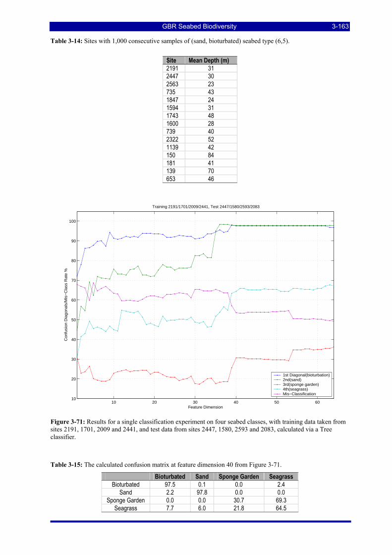
GBR Seabed Biodiversity 3-163
Table 3-14: Sites with 1,000 consecutive samples of (sand, bioturbated) seabed type (6,5).
Site Mean Depth (m) 2191 31 2447 30 2563 23 735 43 1847 24 1594 31 1743 48 1600 28 739 40 2322 52 1139 42 150 84 181 41 139 70 653 46
10 20 30 40 50 6010
20
30
40
50
60
70
80
90
100
Feature Dimension
Con
fusi
on D
iago
nals
/Mis
−C
lass
Rat
e %
Training 2191/1701/2009/2441, Test 2447/1580/2593/2083
1st Diagonal(bioturbation)2nd(sand)3rd(sponge garden)4th(seagrass)Mis−Classification
Figure 3-71: Results for a single classification experiment on four seabed classes, with training data taken from sites 2191, 1701, 2009 and 2441, and test data from sites 2447, 1580, 2593 and 2083, calculated via a Tree classifier.
Table 3-15: The calculated confusion matrix at feature dimension 40 from Figure 3-71.
Bioturbated Sand Sponge Garden Seagrass Bioturbated 97.5 0.1 0.0 2.4
Sand 2.2 97.8 0.0 0.0 Sponge Garden 0.0 0.0 30.7 69.3
Seagrass 7.7 6.0 21.8 64.5
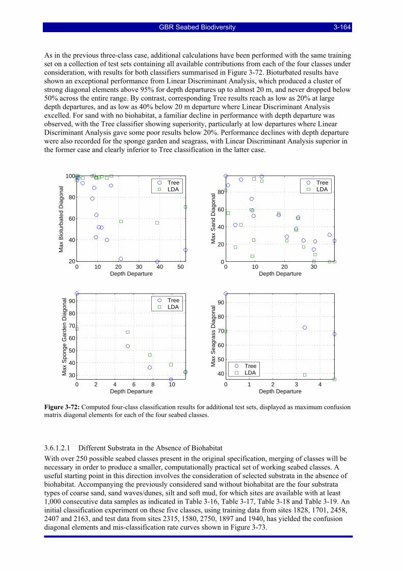
GBR Seabed Biodiversity 3-164
As in the previous three-class case, additional calculations have been performed with the same training set on a collection of test sets containing all available contributions from each of the four classes under consideration, with results for both classifiers summarised in Figure 3-72. Bioturbated results have shown an exceptional performance from Linear Discriminant Analysis, which produced a cluster of strong diagonal elements above 95% for depth departures up to almost 20 m, and never dropped below 50% across the entire range. By contrast, corresponding Tree results reach as low as 20% at large depth departures, and as low as 40% below 20 m departure where Linear Discriminant Analysis excelled. For sand with no biohabitat, a familiar decline in performance with depth departure was observed, with the Tree classifier showing superiority, particularly at low departures where Linear Discriminant Analysis gave some poor results below 20%. Performance declines with depth departure were also recorded for the sponge garden and seagrass, with Linear Discriminant Analysis superior in the former case and clearly inferior to Tree classification in the latter case.
0 1 2 3 4
40
50
60
70
80
90
Depth Departure
Max
Sea
gras
s D
iago
nal
TreeLDA
0 10 20 30 40 5020
40
60
80
100
Depth Departure
Max
Bio
turb
ated
Dia
gona
l TreeLDA
0 10 20 300
20
40
60
80
Depth Departure
Max
San
d D
iago
nal
TreeLDA
0 2 4 6 8 10
30
40
50
60
70
80
90
Depth Departure
Max
Spo
nge
Gar
den
Dia
gona
l TreeLDA
Figure 3-72: Computed four-class classification results for additional test sets, displayed as maximum confusion matrix diagonal elements for each of the four seabed classes.
3.6.1.2.1 Different Substrata in the Absence of Biohabitat With over 250 possible seabed classes present in the original specification, merging of classes will be necessary in order to produce a smaller, computationally practical set of working seabed classes. A useful starting point in this direction involves the consideration of selected substrata in the absence of biohabitat. Accompanying the previously considered sand without biohabitat are the four substrata types of coarse sand, sand waves/dunes, silt and soft mud, for which sites are available with at least 1,000 consecutive data samples as indicated in Table 3-16, Table 3-17, Table 3-18 and Table 3-19. An initial classification experiment on these five classes, using training data from sites 1828, 1701, 2458, 2407 and 2163, and test data from sites 2315, 1580, 2750, 1897 and 1940, has yielded the confusion diagonal elements and mis-classification rate curves shown in Figure 3-73.
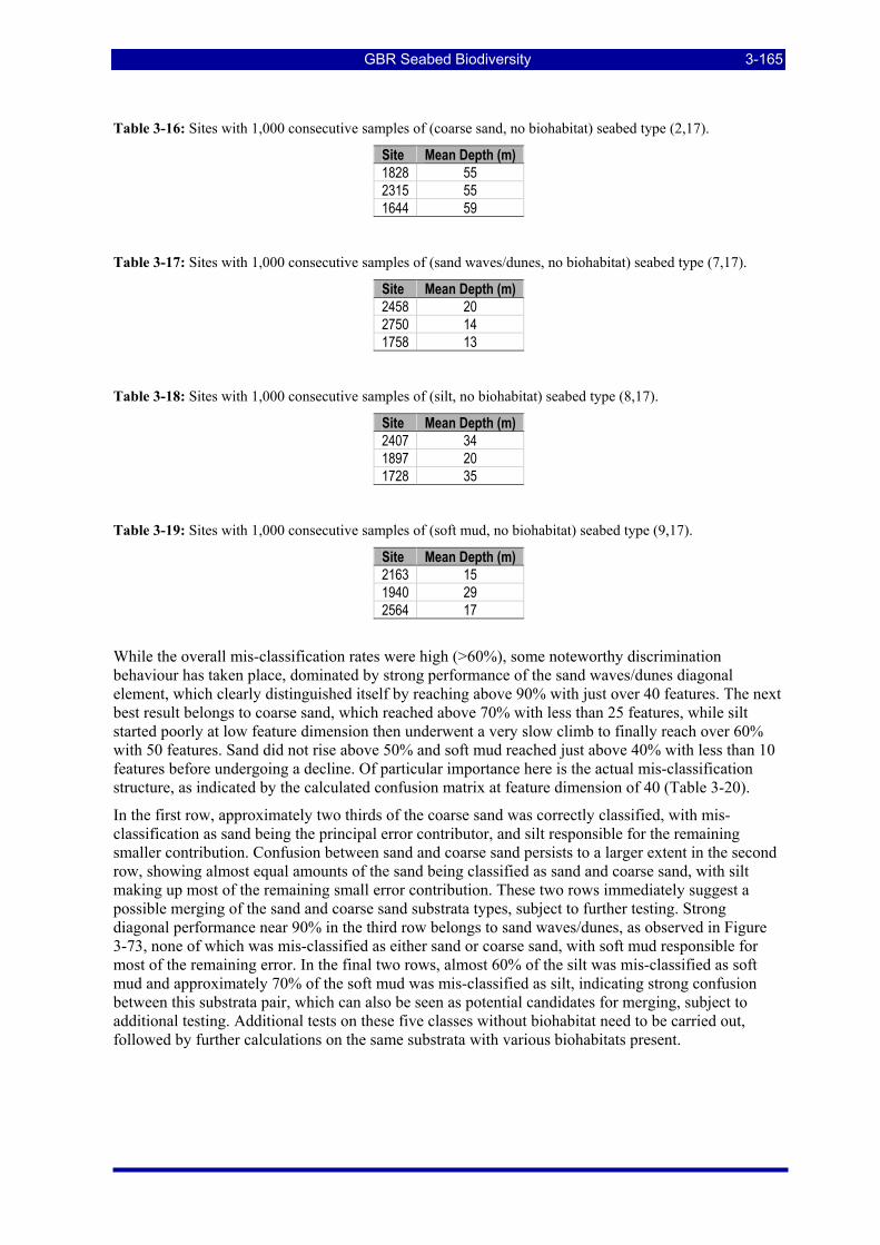
GBR Seabed Biodiversity 3-165
Table 3-16: Sites with 1,000 consecutive samples of (coarse sand, no biohabitat) seabed type (2,17).
Site Mean Depth (m) 1828 55 2315 55 1644 59
Table 3-17: Sites with 1,000 consecutive samples of (sand waves/dunes, no biohabitat) seabed type (7,17).
Site Mean Depth (m) 2458 20 2750 14 1758 13
Table 3-18: Sites with 1,000 consecutive samples of (silt, no biohabitat) seabed type (8,17).
Site Mean Depth (m) 2407 34 1897 20 1728 35
Table 3-19: Sites with 1,000 consecutive samples of (soft mud, no biohabitat) seabed type (9,17).
Site Mean Depth (m) 2163 15 1940 29 2564 17
While the overall mis-classification rates were high (>60%), some noteworthy discrimination behaviour has taken place, dominated by strong performance of the sand waves/dunes diagonal element, which clearly distinguished itself by reaching above 90% with just over 40 features. The next best result belongs to coarse sand, which reached above 70% with less than 25 features, while silt started poorly at low feature dimension then underwent a very slow climb to finally reach over 60% with 50 features. Sand did not rise above 50% and soft mud reached just above 40% with less than 10 features before undergoing a decline. Of particular importance here is the actual mis-classification structure, as indicated by the calculated confusion matrix at feature dimension of 40 (Table 3-20).
In the first row, approximately two thirds of the coarse sand was correctly classified, with mis-classification as sand being the principal error contributor, and silt responsible for the remaining smaller contribution. Confusion between sand and coarse sand persists to a larger extent in the second row, showing almost equal amounts of the sand being classified as sand and coarse sand, with silt making up most of the remaining small error contribution. These two rows immediately suggest a possible merging of the sand and coarse sand substrata types, subject to further testing. Strong diagonal performance near 90% in the third row belongs to sand waves/dunes, as observed in Figure 3-73, none of which was mis-classified as either sand or coarse sand, with soft mud responsible for most of the remaining error. In the final two rows, almost 60% of the silt was mis-classified as soft mud and approximately 70% of the soft mud was mis-classified as silt, indicating strong confusion between this substrata pair, which can also be seen as potential candidates for merging, subject to additional testing. Additional tests on these five classes without biohabitat need to be carried out, followed by further calculations on the same substrata with various biohabitats present.
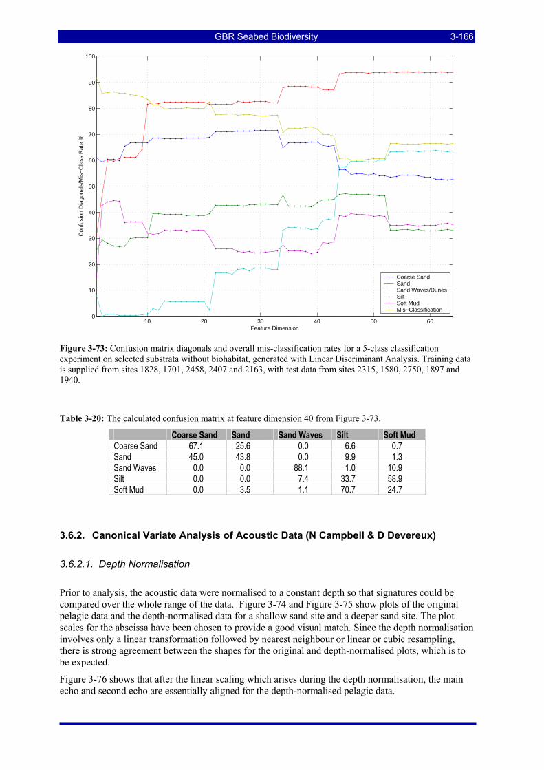
GBR Seabed Biodiversity 3-166
10 20 30 40 50 600
10
20
30
40
50
60
70
80
90
100
Feature Dimension
Con
fusi
on D
iago
nals
/Mis
−C
lass
Rat
e %
Coarse SandSandSand Waves/DunesSiltSoft MudMis−Classification
Figure 3-73: Confusion matrix diagonals and overall mis-classification rates for a 5-class classification experiment on selected substrata without biohabitat, generated with Linear Discriminant Analysis. Training data is supplied from sites 1828, 1701, 2458, 2407 and 2163, with test data from sites 2315, 1580, 2750, 1897 and 1940.
Table 3-20: The calculated confusion matrix at feature dimension 40 from Figure 3-73.
Coarse Sand Sand Sand Waves Silt Soft Mud Coarse Sand 67.1 25.6 0.0 6.6 0.7 Sand 45.0 43.8 0.0 9.9 1.3 Sand Waves 0.0 0.0 88.1 1.0 10.9 Silt 0.0 0.0 7.4 33.7 58.9 Soft Mud 0.0 3.5 1.1 70.7 24.7
3.6.2. Canonical Variate Analysis of Acoustic Data (N Campbell & D Devereux)
3.6.2.1. Depth Normalisation
Prior to analysis, the acoustic data were normalised to a constant depth so that signatures could be compared over the whole range of the data. Figure 3-74 and Figure 3-75 show plots of the original pelagic data and the depth-normalised data for a shallow sand site and a deeper sand site. The plot scales for the abscissa have been chosen to provide a good visual match. Since the depth normalisation involves only a linear transformation followed by nearest neighbour or linear or cubic resampling, there is strong agreement between the shapes for the original and depth-normalised plots, which is to be expected.
Figure 3-76 shows that after the linear scaling which arises during the depth normalisation, the main echo and second echo are essentially aligned for the depth-normalised pelagic data.
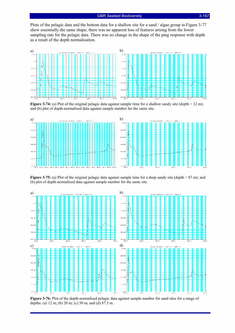
GBR Seabed Biodiversity 3-167
Plots of the pelagic data and the bottom data for a shallow site for a sand / algae group in Figure 3-77 show essentially the same shape; there was no apparent loss of features arising from the lower sampling rate for the pelagic data. There was no change in the shape of the ping response with depth as a result of the depth normalisation.
Figure 3-74: (a) Plot of the original pelagic data against sample time for a shallow sandy site (depth = 12 m); and (b) plot of depth-normalised data against sample number for the same site.
Figure 3-75: (a) Plot of the original pelagic data against sample time for a deep sandy site (depth = 87 m); and (b) plot of depth-normalised data against sample number for the same site.
Figure 3-76: Plot of the depth-normalised pelagic data against sample number for sand sites for a range of depths: (a) 12 m; (b) 20 m; (c) 50 m; and (d) 87.5 m.
a) b)
a) b)
a) b)
c) d)
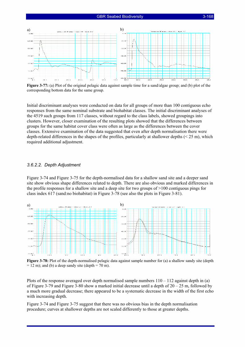
GBR Seabed Biodiversity 3-168
Figure 3-77: (a) Plot of the original pelagic data against sample time for a sand/algae group; and (b) plot of the corresponding bottom data for the same group.
Initial discriminant analyses were conducted on data for all groups of more than 100 contiguous echo responses from the same nominal substrate and biohabitat classes. The initial discriminant analyses of the 4519 such groups from 117 classes, without regard to the class labels, showed groupings into clusters. However, closer examination of the resulting plots showed that the differences between groups for the same habitat cover class were often as large as the differences between the cover classes. Extensive examination of the data suggested that even after depth normalisation there were depth-related differences in the shapes of the profiles, particularly at shallower depths (< 25 m), which required additional adjustment.
3.6.2.2. Depth Adjustment
Figure 3-74 and Figure 3-75 for the depth-normalised data for a shallow sand site and a deeper sand site show obvious shape differences related to depth. There are also obvious and marked differences in the profile responses for a shallow site and a deep site for two groups of >100 contiguous pings for class index 617 (sand:no biohabitat) in Figure 3-78 (see also the plots in Figure 3-81).
Figure 3-78: Plot of the depth-normalised pelagic data against sample number for (a) a shallow sandy site (depth = 12 m); and (b) a deep sandy site (depth = 70 m).
Plots of the response averaged over depth normalised sample numbers 110 – 112 against depth in (a) of Figure 3-79 and Figure 3-80 show a marked initial decrease until a depth of 20 – 25 m, followed by a much more gradual decrease; there appeared to be a systematic decrease in the width of the first echo with increasing depth.
Figure 3-74 and Figure 3-75 suggest that there was no obvious bias in the depth normalisation procedure; curves at shallower depths are not scaled differently to those at greater depths.
a) b)
a) b)
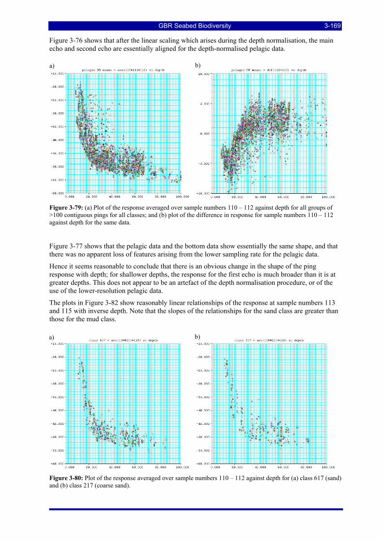
GBR Seabed Biodiversity 3-169
Figure 3-76 shows that after the linear scaling which arises during the depth normalisation, the main echo and second echo are essentially aligned for the depth-normalised pelagic data.
Figure 3-79: (a) Plot of the response averaged over sample numbers 110 – 112 against depth for all groups of >100 contiguous pings for all classes; and (b) plot of the difference in response for sample numbers 110 – 112 against depth for the same data.
Figure 3-77 shows that the pelagic data and the bottom data show essentially the same shape, and that there was no apparent loss of features arising from the lower sampling rate for the pelagic data.
Hence it seems reasonable to conclude that there is an obvious change in the shape of the ping response with depth; for shallower depths, the response for the first echo is much broader than it is at greater depths. This does not appear to be an artefact of the depth normalisation procedure, or of the use of the lower-resolution pelagic data.
The plots in Figure 3-82 show reasonably linear relationships of the response at sample numbers 113 and 115 with inverse depth. Note that the slopes of the relationships for the sand class are greater than those for the mud class.
Figure 3-80: Plot of the response averaged over sample numbers 110 – 112 against depth for (a) class 617 (sand) and (b) class 217 (coarse sand).
a) b)
a) b)
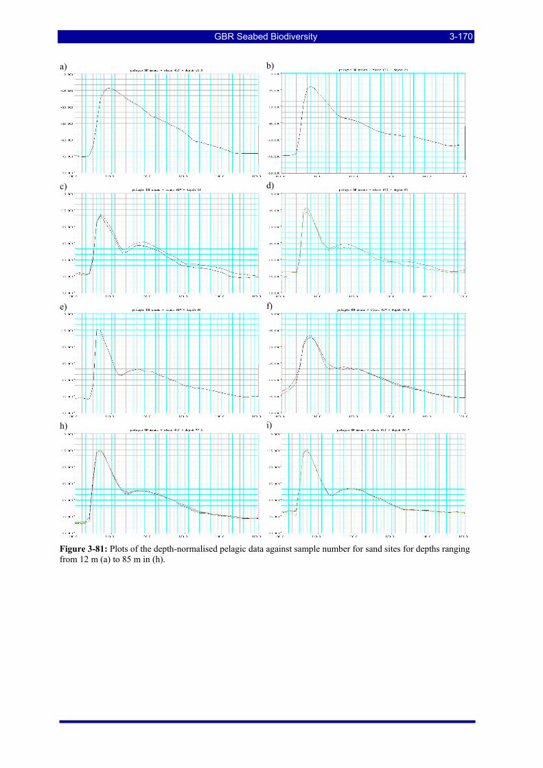
GBR Seabed Biodiversity 3-170
Figure 3-81: Plots of the depth-normalised pelagic data against sample number for sand sites for depths ranging from 12 m (a) to 85 m in (h).
a) b)
c) d)
e) f)
h) i)
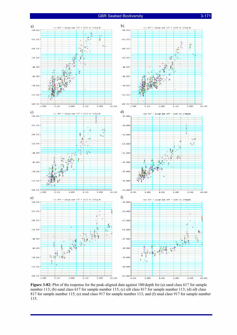
GBR Seabed Biodiversity 3-171
Figure 3-82: Plot of the response for the peak-aligned data against 100/depth for (a) sand class 617 for sample number 113; (b) sand class 617 for sample number 115; (c) silt class 817 for sample number 113; (d) silt class 817 for sample number 115; (e) mud class 917 for sample number 113; and (f) mud class 917 for sample number 115.
e) f)
a) b)
c) d)
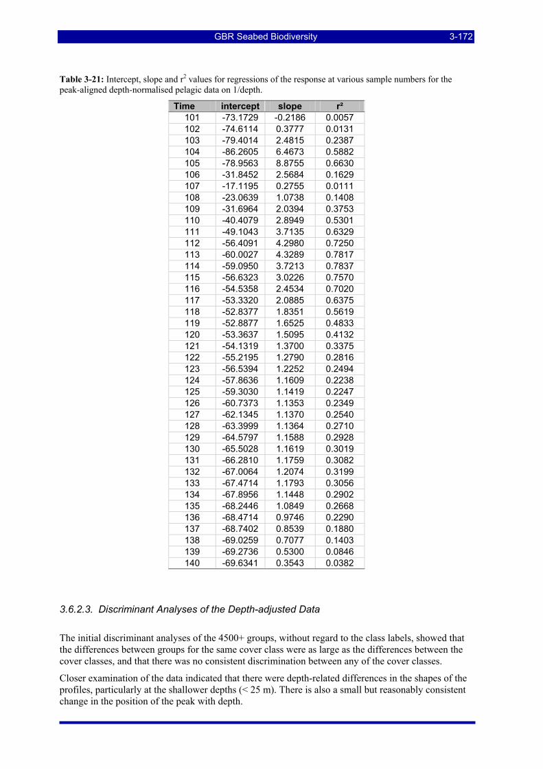
GBR Seabed Biodiversity 3-172
Table 3-21: Intercept, slope and r2 values for regressions of the response at various sample numbers for the peak-aligned depth-normalised pelagic data on 1/depth.
Time intercept slope r² 101 -73.1729 -0.2186 0.0057 102 -74.6114 0.3777 0.0131 103 -79.4014 2.4815 0.2387 104 -86.2605 6.4673 0.5882 105 -78.9563 8.8755 0.6630 106 -31.8452 2.5684 0.1629 107 -17.1195 0.2755 0.0111 108 -23.0639 1.0738 0.1408 109 -31.6964 2.0394 0.3753 110 -40.4079 2.8949 0.5301 111 -49.1043 3.7135 0.6329 112 -56.4091 4.2980 0.7250 113 -60.0027 4.3289 0.7817 114 -59.0950 3.7213 0.7837 115 -56.6323 3.0226 0.7570 116 -54.5358 2.4534 0.7020 117 -53.3320 2.0885 0.6375 118 -52.8377 1.8351 0.5619 119 -52.8877 1.6525 0.4833 120 -53.3637 1.5095 0.4132 121 -54.1319 1.3700 0.3375 122 -55.2195 1.2790 0.2816 123 -56.5394 1.2252 0.2494 124 -57.8636 1.1609 0.2238 125 -59.3030 1.1419 0.2247 126 -60.7373 1.1353 0.2349 127 -62.1345 1.1370 0.2540 128 -63.3999 1.1364 0.2710 129 -64.5797 1.1588 0.2928 130 -65.5028 1.1619 0.3019 131 -66.2810 1.1759 0.3082 132 -67.0064 1.2074 0.3199 133 -67.4714 1.1793 0.3056 134 -67.8956 1.1448 0.2902 135 -68.2446 1.0849 0.2668 136 -68.4714 0.9746 0.2290 137 -68.7402 0.8539 0.1880 138 -69.0259 0.7077 0.1403 139 -69.2736 0.5300 0.0846 140 -69.6341 0.3543 0.0382
3.6.2.3. Discriminant Analyses of the Depth-adjusted Data
The initial discriminant analyses of the 4500+ groups, without regard to the class labels, showed that the differences between groups for the same cover class were as large as the differences between the cover classes, and that there was no consistent discrimination between any of the cover classes.
Closer examination of the data indicated that there were depth-related differences in the shapes of the profiles, particularly at the shallower depths (< 25 m). There is also a small but reasonably consistent change in the position of the peak with depth.
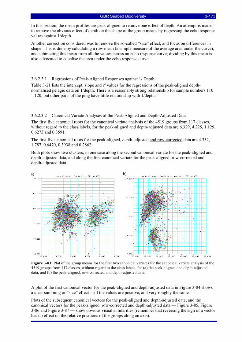
GBR Seabed Biodiversity 3-173
In this section, the mean profiles are peak-aligned to remove one effect of depth. An attempt is made to remove the obvious effect of depth on the shape of the group means by regressing the echo response values against 1/depth.
Another correction considered was to remove the so-called “size” effect, and focus on differences in shape. This is done by calculating a row mean (a simple measure of the average area under the curve), and subtracting this mean from all the values across an echo response curve; dividing by this mean is also advocated to equalise the area under the echo response curve.
3.6.2.3.1 Regressions of Peak-Aligned Responses against 1/ Depth Table 3-21 lists the intercept, slope and r2 values for the regressions of the peak-aligned depth-normalised pelagic data on 1/depth. There is a reasonably strong relationship for sample numbers 110 – 120, but other parts of the ping have little relationship with 1/depth.
3.6.2.3.2 Canonical Variate Analyses of the Peak-Aligned and Depth-Adjusted Data The first five canonical roots for the canonical variate analysis of the 4519 groups from 117 classes, without regard to the class labels, for the peak-aligned and depth-adjusted data are 6.329, 4.225, 1.129, 0.6273 and 0.3591.
The first five canonical roots for the peak-aligned, depth-adjusted and row-corrected data are 4.332, 1.787, 0.6470, 0.3938 and 0.2862.
Both plots show two clusters, in one case along the second canonical variate for the peak-aligned and depth-adjusted data, and along the first canonical variate for the peak-aligned, row-corrected and depth-adjusted data.
Figure 3-83: Plot of the group means for the first two canonical variates for the canonical variate analysis of the 4519 groups from 117 classes, without regard to the class labels, for (a) the peak-aligned and depth-adjusted data; and (b) the peak-aligned, row-corrected and depth-adjusted data.
A plot of the first canonical vector for the peak-aligned and depth-adjusted data in Figure 3-84 shows a clear summing or “size” effect – all the values are positive, and very roughly the same.
Plots of the subsequent canonical vectors for the peak-aligned and depth-adjusted data, and the canonical vectors for the peak-aligned, row-corrected and depth-adjusted data — Figure 3-85, Figure 3-86 and Figure 3-87 — show obvious visual similarities (remember that reversing the sign of a vector has no effect on the relative positions of the groups along an axis).
a) b)
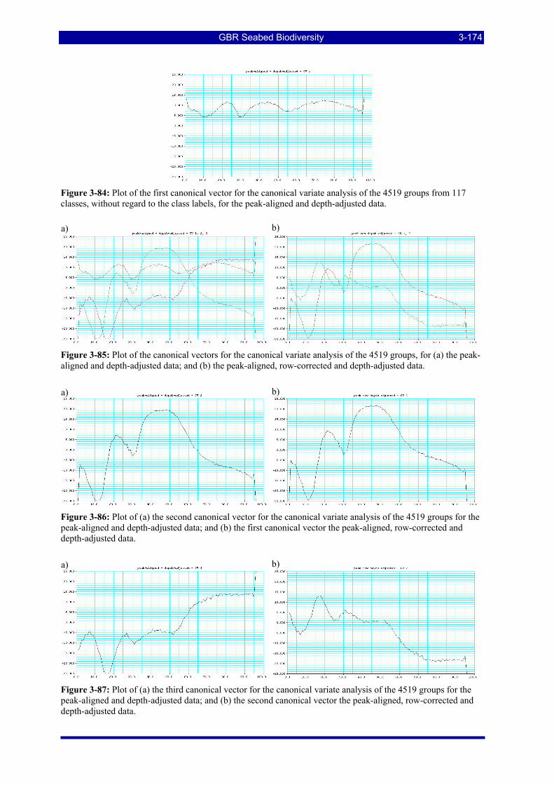
GBR Seabed Biodiversity 3-174
Figure 3-84: Plot of the first canonical vector for the canonical variate analysis of the 4519 groups from 117 classes, without regard to the class labels, for the peak-aligned and depth-adjusted data.
Figure 3-85: Plot of the canonical vectors for the canonical variate analysis of the 4519 groups, for (a) the peak-aligned and depth-adjusted data; and (b) the peak-aligned, row-corrected and depth-adjusted data.
Figure 3-86: Plot of (a) the second canonical vector for the canonical variate analysis of the 4519 groups for the peak-aligned and depth-adjusted data; and (b) the first canonical vector the peak-aligned, row-corrected and depth-adjusted data.
Figure 3-87: Plot of (a) the third canonical vector for the canonical variate analysis of the 4519 groups for the peak-aligned and depth-adjusted data; and (b) the second canonical vector the peak-aligned, row-corrected and depth-adjusted data.
a) b)
a) b)
a) b)
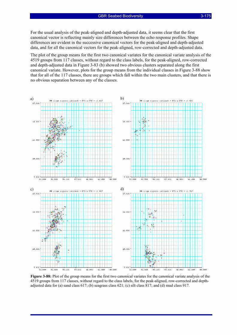
GBR Seabed Biodiversity 3-175
For the usual analysis of the peak-aligned and depth-adjusted data, it seems clear that the first canonical vector is reflecting mainly size differences between the echo response profiles. Shape differences are evident in the successive canonical vectors for the peak-aligned and depth-adjusted data, and for all the canonical vectors for the peak-aligned, row-corrected and depth-adjusted data.
The plot of the group means for the first two canonical variates for the canonical variate analysis of the 4519 groups from 117 classes, without regard to the class labels, for the peak-aligned, row-corrected and depth-adjusted data in Figure 3-83 (b) showed two obvious clusters separated along the first canonical variate. However, plots for the group means from the individual classes in Figure 3-88 show that for all of the 117 classes, there are groups which fall within the two main clusters, and that there is no obvious separation between any of the classes.
Figure 3-88: Plot of the group means for the first two canonical variates for the canonical variate analysis of the 4519 groups from 117 classes, without regard to the class labels, for the peak-aligned, row-corrected and depth-adjusted data for (a) sand class 617; (b) seagrass class 621; (c) silt class 817; and (d) mud class 917.
a) b)
c) d)
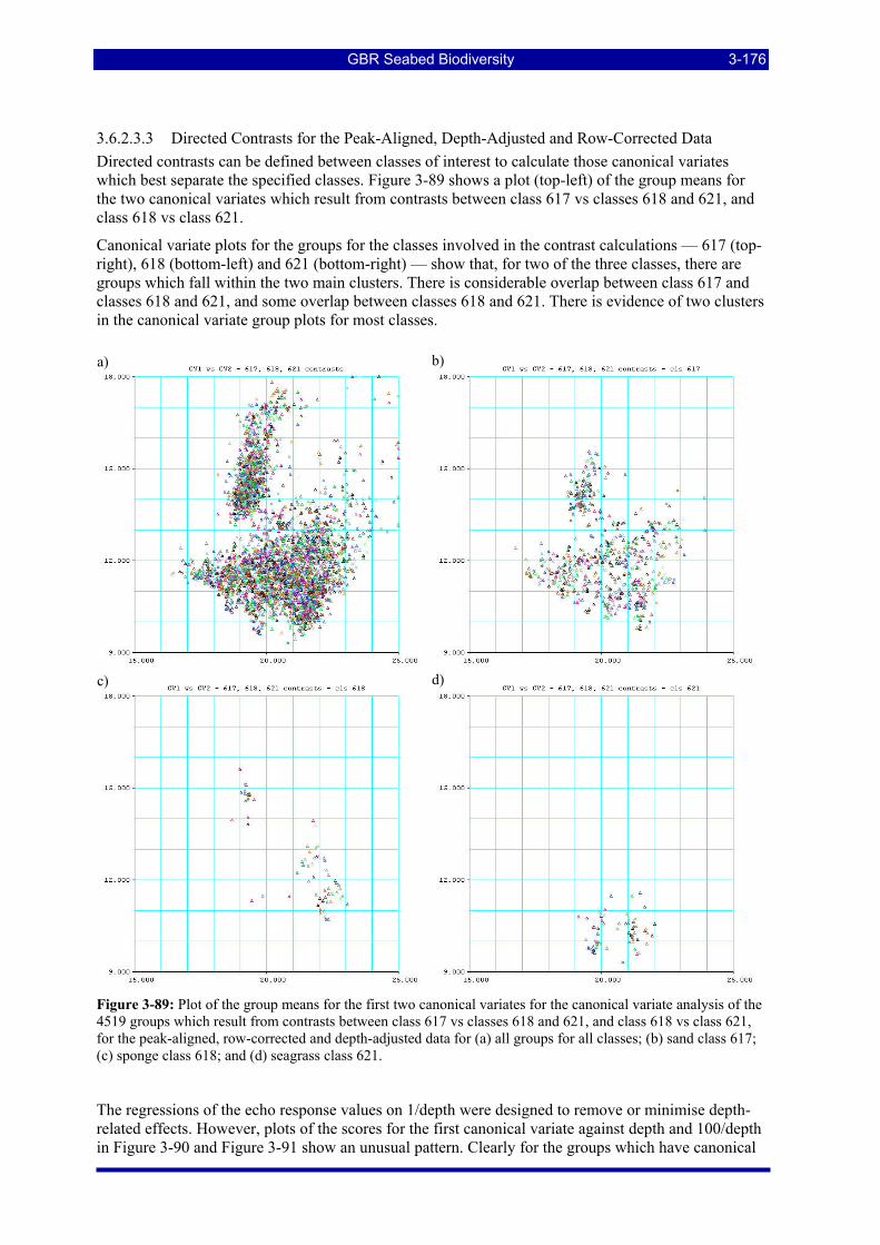
GBR Seabed Biodiversity 3-176
3.6.2.3.3 Directed Contrasts for the Peak-Aligned, Depth-Adjusted and Row-Corrected Data Directed contrasts can be defined between classes of interest to calculate those canonical variates which best separate the specified classes. Figure 3-89 shows a plot (top-left) of the group means for the two canonical variates which result from contrasts between class 617 vs classes 618 and 621, and class 618 vs class 621.
Canonical variate plots for the groups for the classes involved in the contrast calculations — 617 (top-right), 618 (bottom-left) and 621 (bottom-right) — show that, for two of the three classes, there are groups which fall within the two main clusters. There is considerable overlap between class 617 and classes 618 and 621, and some overlap between classes 618 and 621. There is evidence of two clusters in the canonical variate group plots for most classes.
Figure 3-89: Plot of the group means for the first two canonical variates for the canonical variate analysis of the 4519 groups which result from contrasts between class 617 vs classes 618 and 621, and class 618 vs class 621, for the peak-aligned, row-corrected and depth-adjusted data for (a) all groups for all classes; (b) sand class 617; (c) sponge class 618; and (d) seagrass class 621.
The regressions of the echo response values on 1/depth were designed to remove or minimise depth-related effects. However, plots of the scores for the first canonical variate against depth and 100/depth in Figure 3-90 and Figure 3-91 show an unusual pattern. Clearly for the groups which have canonical
a) b)
c) d)
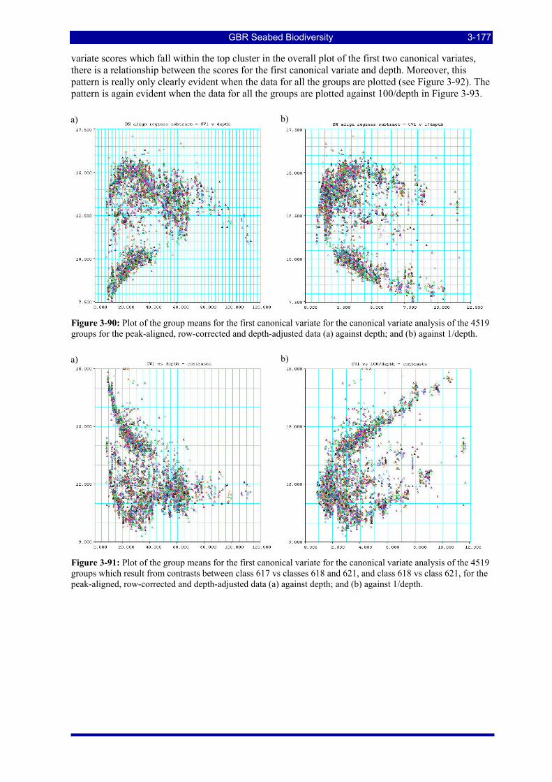
GBR Seabed Biodiversity 3-177
variate scores which fall within the top cluster in the overall plot of the first two canonical variates, there is a relationship between the scores for the first canonical variate and depth. Moreover, this pattern is really only clearly evident when the data for all the groups are plotted (see Figure 3-92). The pattern is again evident when the data for all the groups are plotted against 100/depth in Figure 3-93.
Figure 3-90: Plot of the group means for the first canonical variate for the canonical variate analysis of the 4519 groups for the peak-aligned, row-corrected and depth-adjusted data (a) against depth; and (b) against 1/depth.
Figure 3-91: Plot of the group means for the first canonical variate for the canonical variate analysis of the 4519 groups which result from contrasts between class 617 vs classes 618 and 621, and class 618 vs class 621, for the peak-aligned, row-corrected and depth-adjusted data (a) against depth; and (b) against 1/depth.
a) b)
a) b)
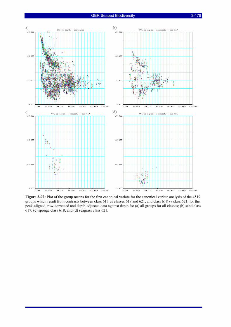
GBR Seabed Biodiversity 3-178
Figure 3-92: Plot of the group means for the first canonical variate for the canonical variate analysis of the 4519 groups which result from contrasts between class 617 vs classes 618 and 621, and class 618 vs class 621, for the peak-aligned, row-corrected and depth-adjusted data against depth for (a) all groups for all classes; (b) sand class 617; (c) sponge class 618; and (d) seagrass class 621.
a) b)
c) d)
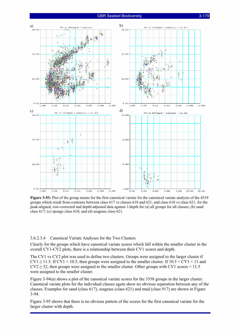
GBR Seabed Biodiversity 3-179
Figure 3-93: Plot of the group means for the first canonical variate for the canonical variate analysis of the 4519 groups which result from contrasts between class 617 vs classes 618 and 621, and class 618 vs class 621, for the peak-aligned, row-corrected and depth-adjusted data against 1/depth for (a) all groups for all classes; (b) sand class 617; (c) sponge class 618; and (d) seagrass class 621.
3.6.2.3.4 Canonical Variate Analyses for the Two Clusters Clearly for the groups which have canonical variate scores which fall within the smaller cluster in the overall CV1-CV2 plots, there is a relationship between their CV1 scores and depth.
The CV1 vs CV2 plot was used to define two clusters. Groups were assigned to the larger cluster if CV1 ≥ 11.5. If CV1 < 10.5, then groups were assigned to the smaller cluster. If 10.5 < CV1 < 11 and CV2 ≥ 32, then groups were assigned to the smaller cluster. Other groups with CV1 scores < 11.5 were assigned to the smaller cluster.
Figure 3-94(a) shows a plot of the canonical variate scores for the 3358 groups in the larger cluster. Canonical variate plots for the individual classes again show no obvious separation between any of the classes. Examples for sand (class 617), seagrass (class 621) and mud (class 917) are shown in Figure 3-94.
Figure 3-95 shows that there is no obvious pattern of the scores for the first canonical variate for the larger cluster with depth.
a) b)
c) d)
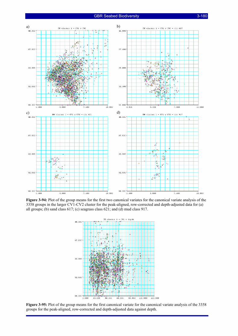
GBR Seabed Biodiversity 3-180
Figure 3-94: Plot of the group means for the first two canonical variates for the canonical variate analysis of the 3358 groups in the larger CV1-CV2 cluster for the peak-aligned, row-corrected and depth-adjusted data for (a) all groups; (b) sand class 617; (c) seagrass class 621; and (d) mud class 917.
Figure 3-95: Plot of the group means for the first canonical variate for the canonical variate analysis of the 3358 groups for the peak-aligned, row-corrected and depth-adjusted data against depth.
a) b)
c) d)
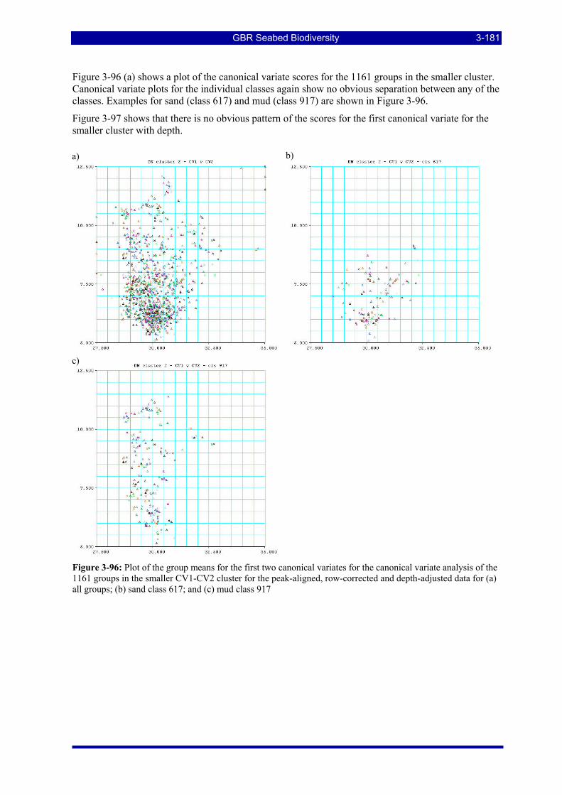
GBR Seabed Biodiversity 3-181
Figure 3-96 (a) shows a plot of the canonical variate scores for the 1161 groups in the smaller cluster. Canonical variate plots for the individual classes again show no obvious separation between any of the classes. Examples for sand (class 617) and mud (class 917) are shown in Figure 3-96.
Figure 3-97 shows that there is no obvious pattern of the scores for the first canonical variate for the smaller cluster with depth.
Figure 3-96: Plot of the group means for the first two canonical variates for the canonical variate analysis of the 1161 groups in the smaller CV1-CV2 cluster for the peak-aligned, row-corrected and depth-adjusted data for (a) all groups; (b) sand class 617; and (c) mud class 917
a) b)
c)
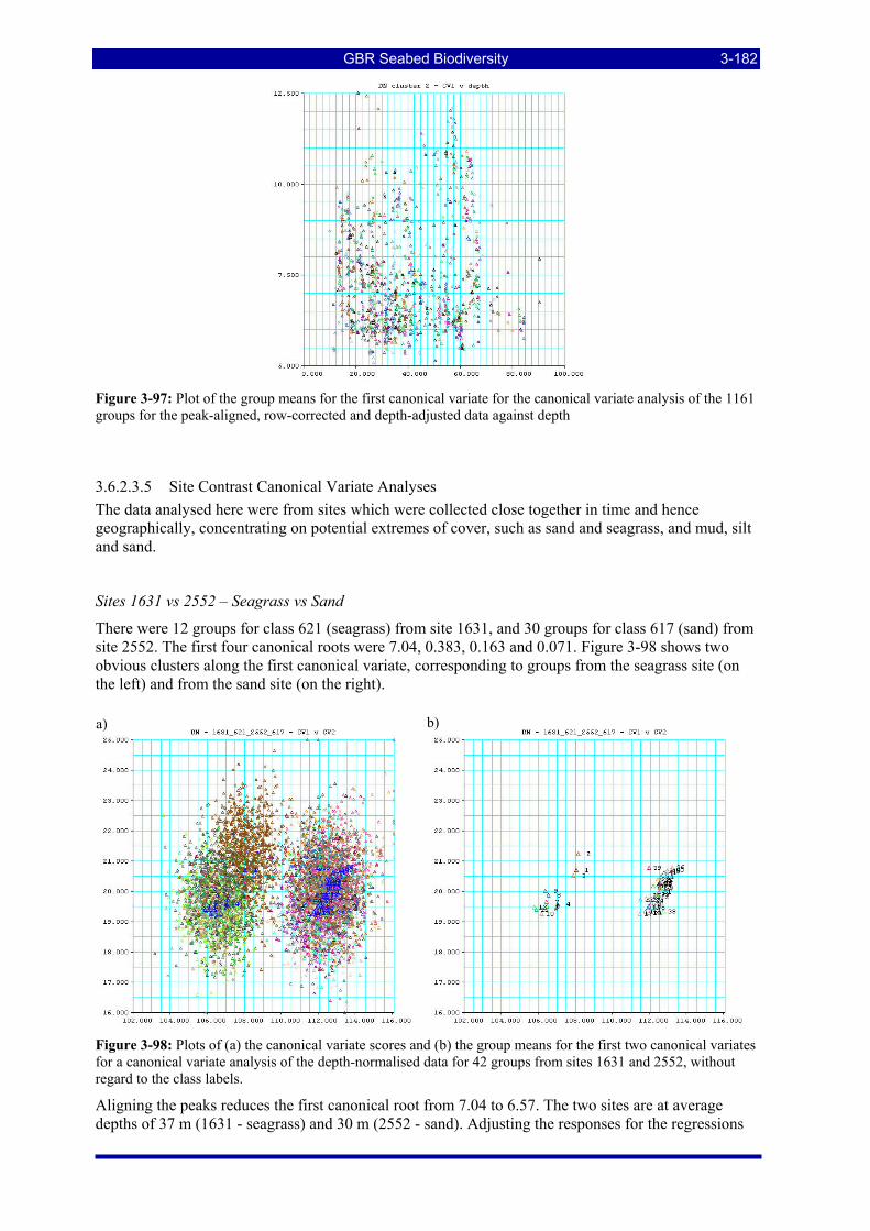
GBR Seabed Biodiversity 3-182
Figure 3-97: Plot of the group means for the first canonical variate for the canonical variate analysis of the 1161 groups for the peak-aligned, row-corrected and depth-adjusted data against depth
3.6.2.3.5 Site Contrast Canonical Variate Analyses The data analysed here were from sites which were collected close together in time and hence geographically, concentrating on potential extremes of cover, such as sand and seagrass, and mud, silt and sand.
Sites 1631 vs 2552 – Seagrass vs Sand
There were 12 groups for class 621 (seagrass) from site 1631, and 30 groups for class 617 (sand) from site 2552. The first four canonical roots were 7.04, 0.383, 0.163 and 0.071. Figure 3-98 shows two obvious clusters along the first canonical variate, corresponding to groups from the seagrass site (on the left) and from the sand site (on the right).
Figure 3-98: Plots of (a) the canonical variate scores and (b) the group means for the first two canonical variates for a canonical variate analysis of the depth-normalised data for 42 groups from sites 1631 and 2552, without regard to the class labels.
Aligning the peaks reduces the first canonical root from 7.04 to 6.57. The two sites are at average depths of 37 m (1631 - seagrass) and 30 m (2552 - sand). Adjusting the responses for the regressions
a) b)
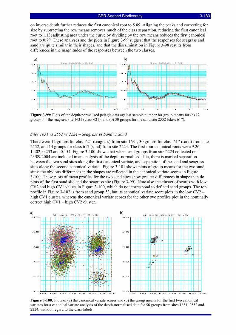
GBR Seabed Biodiversity 3-183
on inverse depth further reduces the first canonical root to 5.89. Aligning the peaks and correcting for size by subtracting the row means removes much of the class separation, reducing the first canonical root to 1.13; adjusting area under the curve by dividing by the row means reduces the first canonical root to 0.79. These analyses and the plots in Figure 3-99 suggest that the responses for seagrass and sand are quite similar in their shapes, and that the discrimination in Figure 3-98 results from differences in the magnitudes of the responses between the two classes.
Figure 3-99: Plots of the depth-normalised pelagic data against sample number for group means for (a) 12 groups for the seagrass site 1631 (class 621); and (b) 30 groups for the sand site 2552 (class 617).
Sites 1631 vs 2552 vs 2224 – Seagrass vs Sand vs Sand
There were 12 groups for class 621 (seagrass) from site 1631, 30 groups for class 617 (sand) from site 2552, and 14 groups for class 617 (sand) from site 2224. The first four canonical roots were 9.26, 1.402, 0.253 and 0.154. Figure 3-100 shows that when sand groups from site 2224 collected on 23/09/2004 are included in an analysis of the depth-normalised data, there is marked separation between the two sand sites along the first canonical variate, and separation of the sand and seagrass sites along the second canonical variate. Figure 3-101 shows plots of group means for the two sand sites; the obvious differences in the shapes are reflected in the canonical variate scores in Figure 3-100. These plots of mean profiles for the two sand sites show greater differences in shape than do plots of the first sand site and the seagrass site (Figure 3-99). Note also the cluster of scores with low CV2 and high CV1 values in Figure 3-100, which do not correspond to defined sand groups. The top profile in Figure 3-102 is from sand group 53, but its canonical variate score plots in the low CV2 – high CV1 cluster, whereas the canonical variate scores for the other two profiles plot in the nominally correct high CV1 – high CV2 cluster.
Figure 3-100: Plots of (a) the canonical variate scores and (b) the group means for the first two canonical variates for a canonical variate analysis of the depth-normalised data for 56 groups from sites 1631, 2552 and 2224, without regard to the class labels.
a) b)
a) b)
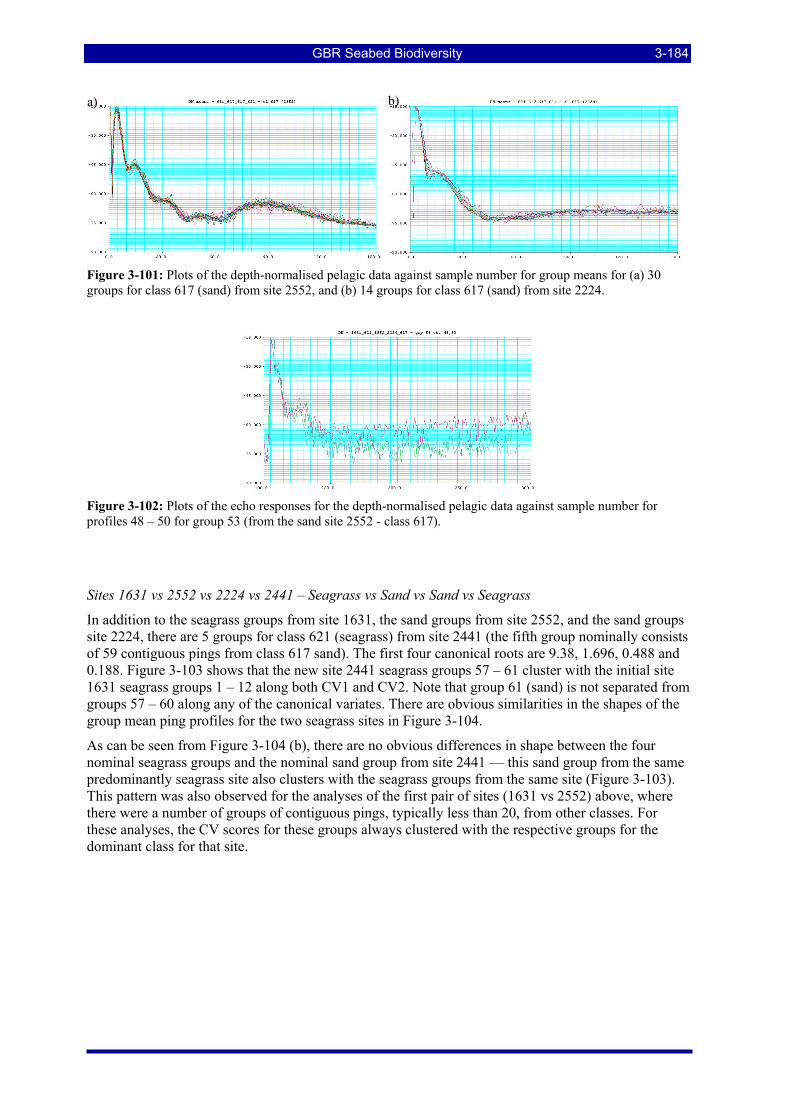
GBR Seabed Biodiversity 3-184
Figure 3-101: Plots of the depth-normalised pelagic data against sample number for group means for (a) 30 groups for class 617 (sand) from site 2552, and (b) 14 groups for class 617 (sand) from site 2224.
Figure 3-102: Plots of the echo responses for the depth-normalised pelagic data against sample number for profiles 48 – 50 for group 53 (from the sand site 2552 - class 617).
Sites 1631 vs 2552 vs 2224 vs 2441 – Seagrass vs Sand vs Sand vs Seagrass
In addition to the seagrass groups from site 1631, the sand groups from site 2552, and the sand groups site 2224, there are 5 groups for class 621 (seagrass) from site 2441 (the fifth group nominally consists of 59 contiguous pings from class 617 sand). The first four canonical roots are 9.38, 1.696, 0.488 and 0.188. Figure 3-103 shows that the new site 2441 seagrass groups 57 – 61 cluster with the initial site 1631 seagrass groups 1 – 12 along both CV1 and CV2. Note that group 61 (sand) is not separated from groups 57 – 60 along any of the canonical variates. There are obvious similarities in the shapes of the group mean ping profiles for the two seagrass sites in Figure 3-104.
As can be seen from Figure 3-104 (b), there are no obvious differences in shape between the four nominal seagrass groups and the nominal sand group from site 2441 — this sand group from the same predominantly seagrass site also clusters with the seagrass groups from the same site (Figure 3-103). This pattern was also observed for the analyses of the first pair of sites (1631 vs 2552) above, where there were a number of groups of contiguous pings, typically less than 20, from other classes. For these analyses, the CV scores for these groups always clustered with the respective groups for the dominant class for that site.
a) b)
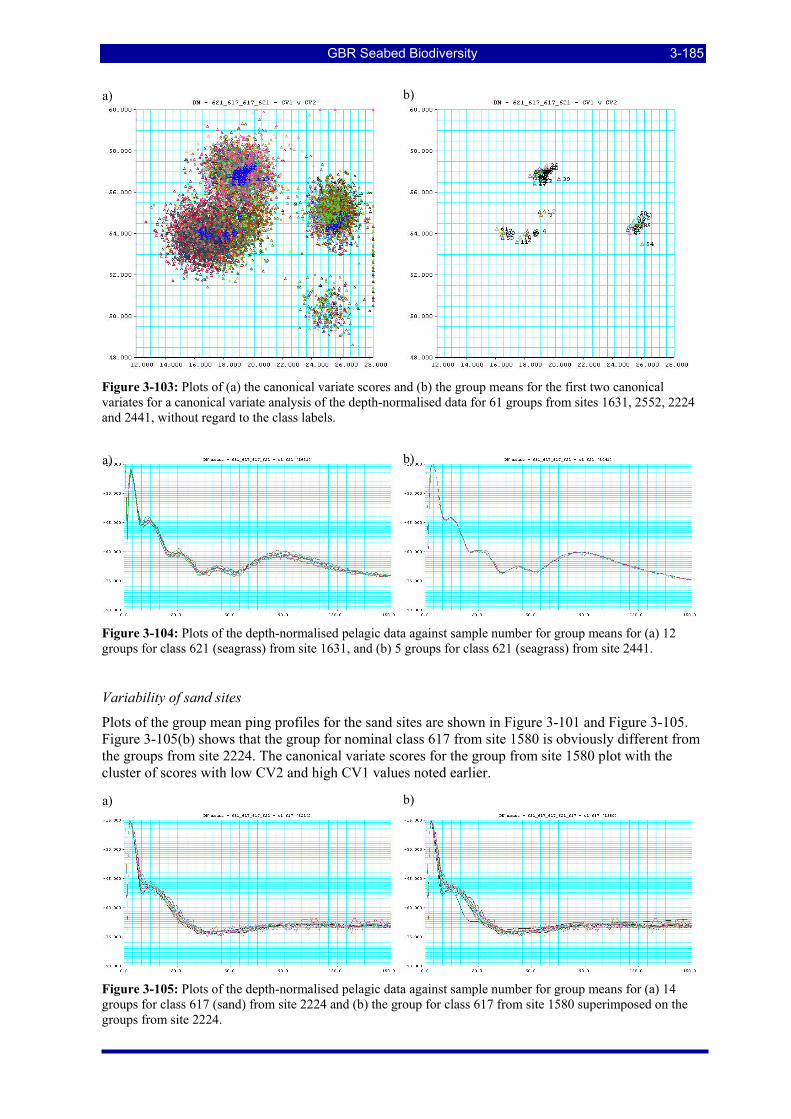
GBR Seabed Biodiversity 3-185
Figure 3-103: Plots of (a) the canonical variate scores and (b) the group means for the first two canonical variates for a canonical variate analysis of the depth-normalised data for 61 groups from sites 1631, 2552, 2224 and 2441, without regard to the class labels.
Figure 3-104: Plots of the depth-normalised pelagic data against sample number for group means for (a) 12 groups for class 621 (seagrass) from site 1631, and (b) 5 groups for class 621 (seagrass) from site 2441.
Variability of sand sites
Plots of the group mean ping profiles for the sand sites are shown in Figure 3-101 and Figure 3-105. Figure 3-105(b) shows that the group for nominal class 617 from site 1580 is obviously different from the groups from site 2224. The canonical variate scores for the group from site 1580 plot with the cluster of scores with low CV2 and high CV1 values noted earlier.
Figure 3-105: Plots of the depth-normalised pelagic data against sample number for group means for (a) 14 groups for class 617 (sand) from site 2224 and (b) the group for class 617 from site 1580 superimposed on the groups from site 2224.
a) b)
a) b)
a) b)
GBR Seabed Biodiversity 3-186
3.6.3. Linear Discriminant Analyses of QTC View data (I McLeod)
3.6.3.1. Substratum and BioHabitat combinations v2
The full combination of the original 24 BioHabitat by 9 substratum event classes (v1) did not converge, so the combination of the original substratum 9 class coding (Table 2-6) and the first 12 class biohabitat re-coding (Table 2-10) schema was investigated. This potentially had 108 classes of which 102 classes were expressed.
The completed linear discriminant analysis (LDA) produced a confusion matrix (as described in Section 3.6.1) of 103 rows by 103 columns, which was too large to tabulate within this report. Instead an abridged version is presented (Table 3-22), that shows the relevant information from the diagonals of the relevant confusion matrices for all but the most infrequent habitat event class combinations.
The “Observed” are analogous to the row totals from the full confusion matrices. “Observed Counts” are original number of observations in each class and the “Observed % of Total” are the observed counts as a percentage of the total observations. The three right hand columns indicate the classification results. The “Observed vs Predicted Counts” are the number of observations of a given class correctly classified as that class. The “OvsP % of total” are the correctly classified counts as a percentage of the total observations. The “OvsP % of Row” are the correctly classified counts as a percentage of the observed counts, giving the percentage within class prediction skill.
Superficially, it seems that a number of the classes are reasonably accurately classified. However, these are relatively infrequent and the overall classification success is only ~3.4%. The most frequently occurring classes have very low classification success and were incorrectly classified to other (off-diagonal) habitat classes (not tabulated in the above abridged version). In particular, the more common classes, such as the no biohabitat classes, were almost always incorrectly classified as a range of other biohabitat combinations.
This poor performance with this number of classes was not unexpected, and further aggregation was necessary, but nevertheless clearly demonstrates that acoustics data are not able to discriminate a modest number of basic habitat types that are readily recognised by observers
3.6.3.2. Substratum and BioHabitat combinations v3
The next combination of the re-coding classes investigated was the combination of the second substratum re-coding (7 classes, Table 2-13) and the first biohabitat re-coding (12 classes, Table 2-10). This potentially had 84 classes of which 79 were expressed.
Again, the full confusion matrix from the cross-validated LDA was too large to present within this report, and an abridged table (Table 3-23) is again presented, which shows the relevant information from the diagonals of the relevant confusion matrices for all but the most infrequent habitat event class combinations. The table columns are as described for the previous table.
Again, a number of the relatively infrequent classes appear to have been reasonably accurately classified, but the overall classification showed little improvement at approximately 6%. Again, the most frequently occurring classes, such as the no biohabitat and bioturbated classes, had very low classification success and were incorrectly classified to other (off-diagonal) habitat class combinations (not tabulated in the abridged Table 3-23). Clearly, a much greater level of aggregation was required.
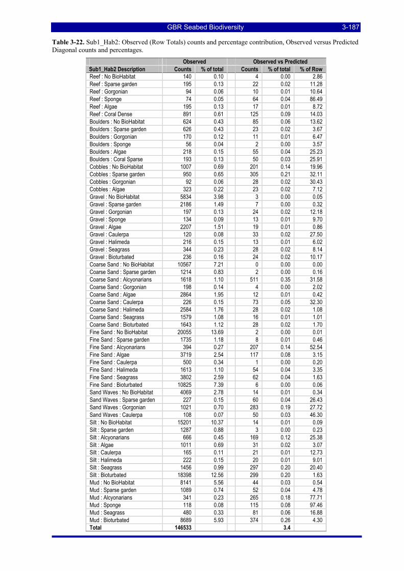
GBR Seabed Biodiversity 3-187
Table 3-22. Sub1_Hab2: Observed (Row Totals) counts and percentage contribution, Observed versus Predicted Diagonal counts and percentages.
Observed Observed vs Predicted Sub1_Hab2 Description Counts % of total Counts % of total % of Row Reef : No BioHabitat 140 0.10 4 0.00 2.86 Reef : Sparse garden 195 0.13 22 0.02 11.28 Reef : Gorgonian 94 0.06 10 0.01 10.64 Reef : Sponge 74 0.05 64 0.04 86.49 Reef : Algae 195 0.13 17 0.01 8.72 Reef : Coral Dense 891 0.61 125 0.09 14.03 Boulders : No BioHabitat 624 0.43 85 0.06 13.62 Boulders : Sparse garden 626 0.43 23 0.02 3.67 Boulders : Gorgonian 170 0.12 11 0.01 6.47 Boulders : Sponge 56 0.04 2 0.00 3.57 Boulders : Algae 218 0.15 55 0.04 25.23 Boulders : Coral Sparse 193 0.13 50 0.03 25.91 Cobbles : No BioHabitat 1007 0.69 201 0.14 19.96 Cobbles : Sparse garden 950 0.65 305 0.21 32.11 Cobbles : Gorgonian 92 0.06 28 0.02 30.43 Cobbles : Algae 323 0.22 23 0.02 7.12 Gravel : No BioHabitat 5834 3.98 3 0.00 0.05 Gravel : Sparse garden 2186 1.49 7 0.00 0.32 Gravel : Gorgonian 197 0.13 24 0.02 12.18 Gravel : Sponge 134 0.09 13 0.01 9.70 Gravel : Algae 2207 1.51 19 0.01 0.86 Gravel : Caulerpa 120 0.08 33 0.02 27.50 Gravel : Halimeda 216 0.15 13 0.01 6.02 Gravel : Seagrass 344 0.23 28 0.02 8.14 Gravel : Bioturbated 236 0.16 24 0.02 10.17 Coarse Sand : No BioHabitat 10567 7.21 0 0.00 0.00 Coarse Sand : Sparse garden 1214 0.83 2 0.00 0.16 Coarse Sand : Alcyonarians 1618 1.10 511 0.35 31.58 Coarse Sand : Gorgonian 198 0.14 4 0.00 2.02 Coarse Sand : Algae 2864 1.95 12 0.01 0.42 Coarse Sand : Caulerpa 226 0.15 73 0.05 32.30 Coarse Sand : Halimeda 2584 1.76 28 0.02 1.08 Coarse Sand : Seagrass 1579 1.08 16 0.01 1.01 Coarse Sand : Bioturbated 1643 1.12 28 0.02 1.70 Fine Sand : No BioHabitat 20055 13.69 2 0.00 0.01 Fine Sand : Sparse garden 1735 1.18 8 0.01 0.46 Fine Sand : Alcyonarians 394 0.27 207 0.14 52.54 Fine Sand : Algae 3719 2.54 117 0.08 3.15 Fine Sand : Caulerpa 500 0.34 1 0.00 0.20 Fine Sand : Halimeda 1613 1.10 54 0.04 3.35 Fine Sand : Seagrass 3802 2.59 62 0.04 1.63 Fine Sand : Bioturbated 10825 7.39 6 0.00 0.06 Sand Waves : No BioHabitat 4069 2.78 14 0.01 0.34 Sand Waves : Sparse garden 227 0.15 60 0.04 26.43 Sand Waves : Gorgonian 1021 0.70 283 0.19 27.72 Sand Waves : Caulerpa 108 0.07 50 0.03 46.30 Silt : No BioHabitat 15201 10.37 14 0.01 0.09 Silt : Sparse garden 1287 0.88 3 0.00 0.23 Silt : Alcyonarians 666 0.45 169 0.12 25.38 Silt : Algae 1011 0.69 31 0.02 3.07 Silt : Caulerpa 165 0.11 21 0.01 12.73 Silt : Halimeda 222 0.15 20 0.01 9.01 Silt : Seagrass 1456 0.99 297 0.20 20.40 Silt : Bioturbated 18398 12.56 299 0.20 1.63 Mud : No BioHabitat 8141 5.56 44 0.03 0.54 Mud : Sparse garden 1089 0.74 52 0.04 4.78 Mud : Alcyonarians 341 0.23 265 0.18 77.71 Mud : Sponge 118 0.08 115 0.08 97.46 Mud : Seagrass 480 0.33 81 0.06 16.88 Mud : Bioturbated 8689 5.93 374 0.26 4.30 Total 146533 3.4
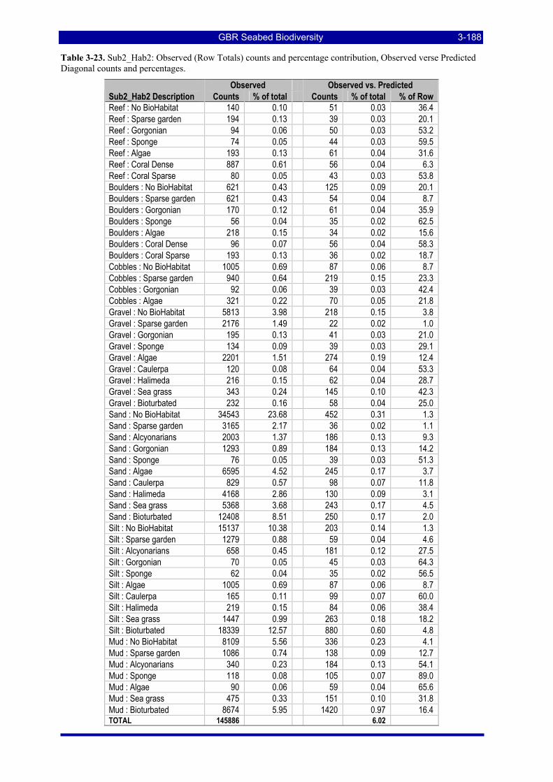
GBR Seabed Biodiversity 3-188
Table 3-23. Sub2_Hab2: Observed (Row Totals) counts and percentage contribution, Observed verse Predicted Diagonal counts and percentages.
Observed Observed vs. Predicted Sub2_Hab2 Description Counts % of total Counts % of total % of Row Reef : No BioHabitat 140 0.10 51 0.03 36.4 Reef : Sparse garden 194 0.13 39 0.03 20.1 Reef : Gorgonian 94 0.06 50 0.03 53.2 Reef : Sponge 74 0.05 44 0.03 59.5 Reef : Algae 193 0.13 61 0.04 31.6 Reef : Coral Dense 887 0.61 56 0.04 6.3 Reef : Coral Sparse 80 0.05 43 0.03 53.8 Boulders : No BioHabitat 621 0.43 125 0.09 20.1 Boulders : Sparse garden 621 0.43 54 0.04 8.7 Boulders : Gorgonian 170 0.12 61 0.04 35.9 Boulders : Sponge 56 0.04 35 0.02 62.5 Boulders : Algae 218 0.15 34 0.02 15.6 Boulders : Coral Dense 96 0.07 56 0.04 58.3 Boulders : Coral Sparse 193 0.13 36 0.02 18.7 Cobbles : No BioHabitat 1005 0.69 87 0.06 8.7 Cobbles : Sparse garden 940 0.64 219 0.15 23.3 Cobbles : Gorgonian 92 0.06 39 0.03 42.4 Cobbles : Algae 321 0.22 70 0.05 21.8 Gravel : No BioHabitat 5813 3.98 218 0.15 3.8 Gravel : Sparse garden 2176 1.49 22 0.02 1.0 Gravel : Gorgonian 195 0.13 41 0.03 21.0 Gravel : Sponge 134 0.09 39 0.03 29.1 Gravel : Algae 2201 1.51 274 0.19 12.4 Gravel : Caulerpa 120 0.08 64 0.04 53.3 Gravel : Halimeda 216 0.15 62 0.04 28.7 Gravel : Sea grass 343 0.24 145 0.10 42.3 Gravel : Bioturbated 232 0.16 58 0.04 25.0 Sand : No BioHabitat 34543 23.68 452 0.31 1.3 Sand : Sparse garden 3165 2.17 36 0.02 1.1 Sand : Alcyonarians 2003 1.37 186 0.13 9.3 Sand : Gorgonian 1293 0.89 184 0.13 14.2 Sand : Sponge 76 0.05 39 0.03 51.3 Sand : Algae 6595 4.52 245 0.17 3.7 Sand : Caulerpa 829 0.57 98 0.07 11.8 Sand : Halimeda 4168 2.86 130 0.09 3.1 Sand : Sea grass 5368 3.68 243 0.17 4.5 Sand : Bioturbated 12408 8.51 250 0.17 2.0 Silt : No BioHabitat 15137 10.38 203 0.14 1.3 Silt : Sparse garden 1279 0.88 59 0.04 4.6 Silt : Alcyonarians 658 0.45 181 0.12 27.5 Silt : Gorgonian 70 0.05 45 0.03 64.3 Silt : Sponge 62 0.04 35 0.02 56.5 Silt : Algae 1005 0.69 87 0.06 8.7 Silt : Caulerpa 165 0.11 99 0.07 60.0 Silt : Halimeda 219 0.15 84 0.06 38.4 Silt : Sea grass 1447 0.99 263 0.18 18.2 Silt : Bioturbated 18339 12.57 880 0.60 4.8 Mud : No BioHabitat 8109 5.56 336 0.23 4.1 Mud : Sparse garden 1086 0.74 138 0.09 12.7 Mud : Alcyonarians 340 0.23 184 0.13 54.1 Mud : Sponge 118 0.08 105 0.07 89.0 Mud : Algae 90 0.06 59 0.04 65.6 Mud : Sea grass 475 0.33 151 0.10 31.8 Mud : Bioturbated 8674 5.95 1420 0.97 16.4 TOTAL 145886 6.02
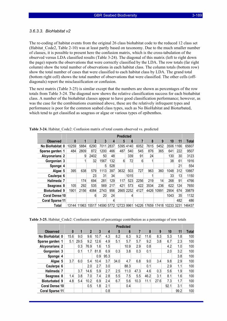
GBR Seabed Biodiversity 3-189
3.6.3.3. BioHabitat v2
The re-coding of habitat events from the original 26 class biohabitat code to the reduced 12 class set (Habitat_Code2, Table 2-10) was at least partly based on taxonomy. Due to the much smaller number of classes, it is possible to present here the confusion matrix, which is the cross-tabulation of the observed versus LDA classified results (Table 3-24). The diagonal of this matrix (left to right down the page) reports the observations that were correctly classified by the LDA. The row totals (far right column) show the total number of observations in each habitat class. The column totals (bottom row) show the total number of cases that were classified to each habitat class by LDA. The grand total (bottom right cell) shows the total number of observations that were classified. The other cells (off-diagonals) report the misclassification or confusion.
The next matrix (Table 3-25) is similar except that the numbers are shown as percentages of the row totals from Table 3-24. The diagonal now shows the relative classification success for each biohabitat class. A number of the biohabitat classes appear to have good classification performance; however, as was the case for the combinations examined above, these are the relatively infrequent types and performance is poor for the common seabed class types, such as No BioHabitat and Bioturbated, which tend to get classified as seagrass or algae or various types of epibenthos.
Table 3-24. Habitat_Code2: Confusion matrix of total counts observed vs. predicted
Predicted Observed 0 1 2 3 4 5 6 7 8 9 10 11 Total
No BioHabitat 0 10259 5884 6290 7011 2837 5395 4140 6052 7615 5452 3506 1166 65607 Sparse garden 1 484 2809 872 1200 466 487 540 545 876 365 641 222 9507
Alcyonarians 2 9 2402 50 48 339 91 24 130 30 3123 Gorgonian 3 1 32 1567 132 6 72 6 1 38 61 1916
Sponge 4 5 528 21 554 Algae 5 395 638 579 1113 397 3632 503 727 963 360 1048 312 10667
Caulerpa 6 23 31 34 1015 1 33 13 1150 Halimeda 7 174 694 281 129 117 523 2256 219 14 268 91 4766 Seagrass 8 105 292 535 569 217 421 573 422 3534 236 622 124 7650
Bioturbated 9 1901 2156 4084 2743 956 2665 2252 4127 4426 10991 2904 674 39879 Coral Dense 10 6 20 24 4 1043 35 1132
Coral Sparse 11 4 482 486 Total 13144 11963 15517 14590 5772 12723 9961 14226 17659 17418 10233 3231 146437
Table 3-25. Habitat_Code2: Confusion matrix of percentage contribution as a percentage of row totals
Predicted Observed 0 1 2 3 4 5 6 7 8 9 10 11 Total
No BioHabitat 0 15.6 9.0 9.6 10.7 4.3 8.2 6.3 9.2 11.6 8.3 5.3 1.8 100 Sparse garden 1 5.1 29.5 9.2 12.6 4.9 5.1 5.7 5.7 9.2 3.8 6.7 2.3 100
Alcyonarians 2 0.3 76.9 1.6 1.5 10.9 2.9 0.8 4.2 1.0 100 Gorgonian 3 0.1 1.7 81.8 6.9 0.3 3.8 0.3 0.1 2.0 3.2 100
Sponge 4 0.9 95.3 3.8 100 Algae 5 3.7 6.0 5.4 10.4 3.7 34.0 4.7 6.8 9.0 3.4 9.8 2.9 100
Caulerpa 6 2.0 2.7 3.0 88.3 0.1 2.9 1.1 100 Halimeda 7 3.7 14.6 5.9 2.7 2.5 11.0 47.3 4.6 0.3 5.6 1.9 100 Seagrass 8 1.4 3.8 7.0 7.4 2.8 5.5 7.5 5.5 46.2 3.1 8.1 1.6 100
Bioturbated 9 4.8 5.4 10.2 6.9 2.4 6.7 5.6 10.3 11.1 27.6 7.3 1.7 100 Coral Dense 10 0.5 1.8 2.1 0.4 92.1 3.1 100
Coral Sparse 11 0.8 99.2 100

GBR Seabed Biodiversity 3-190
The third matrix (Table 3-26) shows the classification results as percentages of the total number of observations. A comparison of the row and column total percentages, in particular, highlight the overall confusion — those biohabitats that were infrequent in the original observations are far too frequent in the classified results (by up to 10 times). In the case of seagrass, for example, the observed frequency was 5.2% whereas the classified frequency was 12.1% — clearly a large number of No biohabitat and bioturbated Observations were being classified as Seagrass. Conversely, those Habitats that were very frequent in the original observations are far too infrequent in the classified results. For example, the observed frequency of bioturbated was 27.2% whereas the classified frequency was 11.9% — clearly a large number of bioturbated observations were being classified as other types of biohabitats. The overall classification success was only 27.7%.
Table 3-26. Habitat_Code2: Confusion matrix of percentage contribution as a percentage of totals
Predicted Observed 0 1 2 3 4 5 6 7 8 9 10 11 Total
No biohabitat 0 7.01 4.02 4.30 4.79 1.94 3.68 2.83 4.13 5.20 3.72 2.39 0.80 44.8 Sparse garden 1 0.33 1.92 0.60 0.82 0.32 0.33 0.37 0.37 0.60 0.25 0.44 0.15 6.5
Alcyonarians 2 0.01 1.64 0.03 0.03 0.23 0.06 0.02 0.09 0.02 2.1 Gorgonian 3 0.00 0.02 1.07 0.09 0.00 0.05 0.00 0.00 0.03 0.04 1.3
Sponge 4 0.00 0.36 0.01 0.4 Algae 5 0.27 0.44 0.40 0.76 0.27 2.48 0.34 0.50 0.66 0.25 0.72 0.21 7.3
Caulerpa 6 0.02 0.02 0.02 0.69 0.00 0.02 0.01 0.8 Halimeda 7 0.12 0.47 0.19 0.09 0.08 0.36 1.54 0.15 0.01 0.18 0.06 3.3 Seagrass 8 0.07 0.20 0.37 0.39 0.15 0.29 0.39 0.29 2.41 0.16 0.42 0.08 5.2
Bioturbated 9 1.30 1.47 2.79 1.87 0.65 1.82 1.54 2.82 3.02 7.51 1.98 0.46 27.2 Coral Dense 10 0.00 0.01 0.02 0.00 0.71 0.02 0.8
Coral Sparse 11 0.00 0.33 0.3 Total 9.0 8.2 10.6 10.0 3.9 8.7 6.8 9.7 12.1 11.9 7.0 2.2 27.7
3.6.3.4. Biohabitat v3
An alternative, and more severe, aggregation of the original habitat event codes reduced the number of habitat classes to eight by lumping all epibenthos by density and all marine plants (Table 2-11). Very sparse epibenthos was considered to differ little from “No biohabitat”.
Again, cross-tabulations of observed versus classified results are presented as a series of confusion matrices. Table 3-27 shows the counts, Table 3-28 shows the percentages of row total observations and Table 3-29 shows the percentages of the total observations.
Table 3-27. Habitat_Code3: Confusion matrix of total counts observed vs. predicted
Predicted Observed 0 1 2 3 4 5 6 7 Total
No biohabitat 0 15716 1631 10763 16027 9282 10795 2454 769 67437 Soft – Dense 1 444 1 445
Soft – Medium 2 143 4347 157 1 146 60 4854 Soft – Sparse 3 221 994 6046 130 72 357 110 7930
Algae and Seagrass 4 1657 461 3610 4470 9831 2545 1380 326 24280 Bioturbated 5 2251 574 5363 6516 4526 18288 2030 421 39969
Coral – Dense 6 14 1094 24 1132 Coral – Sparse 7 21 465 486
Total 19624 3509 25077 33216 23770 31700 7461 2176 146533
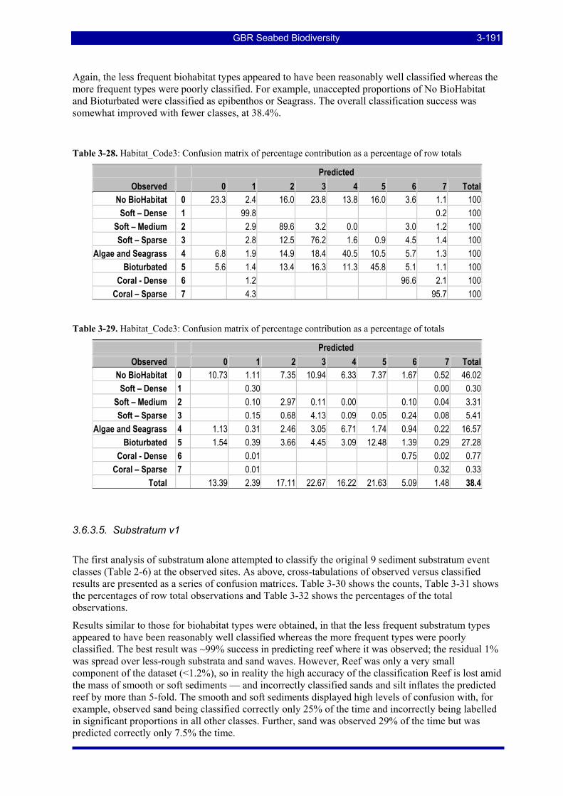
GBR Seabed Biodiversity 3-191
Again, the less frequent biohabitat types appeared to have been reasonably well classified whereas the more frequent types were poorly classified. For example, unaccepted proportions of No BioHabitat and Bioturbated were classified as epibenthos or Seagrass. The overall classification success was somewhat improved with fewer classes, at 38.4%.
Table 3-28. Habitat_Code3: Confusion matrix of percentage contribution as a percentage of row totals
Predicted Observed 0 1 2 3 4 5 6 7 Total
No BioHabitat 0 23.3 2.4 16.0 23.8 13.8 16.0 3.6 1.1 100 Soft – Dense 1 99.8 0.2 100
Soft – Medium 2 2.9 89.6 3.2 0.0 3.0 1.2 100 Soft – Sparse 3 2.8 12.5 76.2 1.6 0.9 4.5 1.4 100
Algae and Seagrass 4 6.8 1.9 14.9 18.4 40.5 10.5 5.7 1.3 100 Bioturbated 5 5.6 1.4 13.4 16.3 11.3 45.8 5.1 1.1 100
Coral - Dense 6 1.2 96.6 2.1 100 Coral – Sparse 7 4.3 95.7 100
Table 3-29. Habitat_Code3: Confusion matrix of percentage contribution as a percentage of totals
Predicted Observed 0 1 2 3 4 5 6 7 Total
No BioHabitat 0 10.73 1.11 7.35 10.94 6.33 7.37 1.67 0.52 46.02 Soft – Dense 1 0.30 0.00 0.30
Soft – Medium 2 0.10 2.97 0.11 0.00 0.10 0.04 3.31 Soft – Sparse 3 0.15 0.68 4.13 0.09 0.05 0.24 0.08 5.41
Algae and Seagrass 4 1.13 0.31 2.46 3.05 6.71 1.74 0.94 0.22 16.57 Bioturbated 5 1.54 0.39 3.66 4.45 3.09 12.48 1.39 0.29 27.28
Coral - Dense 6 0.01 0.75 0.02 0.77 Coral – Sparse 7 0.01 0.32 0.33
Total 13.39 2.39 17.11 22.67 16.22 21.63 5.09 1.48 38.4
3.6.3.5. Substratum v1
The first analysis of substratum alone attempted to classify the original 9 sediment substratum event classes (Table 2-6) at the observed sites. As above, cross-tabulations of observed versus classified results are presented as a series of confusion matrices. Table 3-30 shows the counts, Table 3-31 shows the percentages of row total observations and Table 3-32 shows the percentages of the total observations.
Results similar to those for biohabitat types were obtained, in that the less frequent substratum types appeared to have been reasonably well classified whereas the more frequent types were poorly classified. The best result was ~99% success in predicting reef where it was observed; the residual 1% was spread over less-rough substrata and sand waves. However, Reef was only a very small component of the dataset (<1.2%), so in reality the high accuracy of the classification Reef is lost amid the mass of smooth or soft sediments — and incorrectly classified sands and silt inflates the predicted reef by more than 5-fold. The smooth and soft sediments displayed high levels of confusion with, for example, observed sand being classified correctly only 25% of the time and incorrectly being labelled in significant proportions in all other classes. Further, sand was observed 29% of the time but was predicted correctly only 7.5% the time.
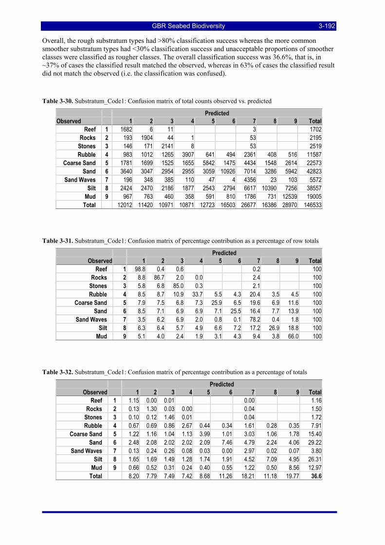
GBR Seabed Biodiversity 3-192
Overall, the rough substratum types had >80% classification success whereas the more common smoother substratum types had <30% classification success and unacceptable proportions of smoother classes were classified as rougher classes. The overall classification success was 36.6%, that is, in ~37% of cases the classified result matched the observed, whereas in 63% of cases the classified result did not match the observed (i.e. the classification was confused).
Table 3-30. Substratum_Code1: Confusion matrix of total counts observed vs. predicted
Predicted Observed 1 2 3 4 5 6 7 8 9 Total
Reef 1 1682 6 11 3 1702 Rocks 2 193 1904 44 1 53 2195
Stones 3 146 171 2141 8 53 2519 Rubble 4 983 1012 1265 3907 641 494 2361 408 516 11587
Coarse Sand 5 1781 1699 1525 1655 5842 1475 4434 1548 2614 22573 Sand 6 3640 3047 2954 2955 3059 10926 7014 3286 5942 42823
Sand Waves 7 196 348 385 110 47 4 4356 23 103 5572 Silt 8 2424 2470 2186 1877 2543 2794 6617 10390 7256 38557
Mud 9 967 763 460 358 591 810 1786 731 12539 19005 Total 12012 11420 10971 10871 12723 16503 26677 16386 28970 146533
Table 3-31. Substratum_Code1: Confusion matrix of percentage contribution as a percentage of row totals
Predicted Observed 1 2 3 4 5 6 7 8 9 Total
Reef 1 98.8 0.4 0.6 0.2 100 Rocks 2 8.8 86.7 2.0 0.0 2.4 100
Stones 3 5.8 6.8 85.0 0.3 2.1 100 Rubble 4 8.5 8.7 10.9 33.7 5.5 4.3 20.4 3.5 4.5 100
Coarse Sand 5 7.9 7.5 6.8 7.3 25.9 6.5 19.6 6.9 11.6 100 Sand 6 8.5 7.1 6.9 6.9 7.1 25.5 16.4 7.7 13.9 100
Sand Waves 7 3.5 6.2 6.9 2.0 0.8 0.1 78.2 0.4 1.8 100 Silt 8 6.3 6.4 5.7 4.9 6.6 7.2 17.2 26.9 18.8 100
Mud 9 5.1 4.0 2.4 1.9 3.1 4.3 9.4 3.8 66.0 100
Table 3-32. Substratum_Code1: Confusion matrix of percentage contribution as a percentage of totals
Predicted Observed 1 2 3 4 5 6 7 8 9 Total
Reef 1 1.15 0.00 0.01 0.00 1.16 Rocks 2 0.13 1.30 0.03 0.00 0.04 1.50
Stones 3 0.10 0.12 1.46 0.01 0.04 1.72 Rubble 4 0.67 0.69 0.86 2.67 0.44 0.34 1.61 0.28 0.35 7.91
Coarse Sand 5 1.22 1.16 1.04 1.13 3.99 1.01 3.03 1.06 1.78 15.40 Sand 6 2.48 2.08 2.02 2.02 2.09 7.46 4.79 2.24 4.06 29.22
Sand Waves 7 0.13 0.24 0.26 0.08 0.03 0.00 2.97 0.02 0.07 3.80 Silt 8 1.65 1.69 1.49 1.28 1.74 1.91 4.52 7.09 4.95 26.31
Mud 9 0.66 0.52 0.31 0.24 0.40 0.55 1.22 0.50 8.56 12.97 Total 8.20 7.79 7.49 7.42 8.68 11.26 18.21 11.18 19.77 36.6
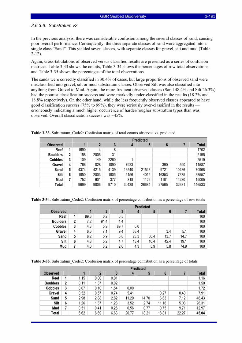
GBR Seabed Biodiversity 3-193
3.6.3.6. Substratum v2
In the previous analysis, there was considerable confusion among the several classes of sand, causing poor overall performance. Consequently, the three separate classes of sand were aggregated into a single class “Sand”. This yielded seven classes, with separate classes for gravel, silt and mud (Table 2-12).
Again, cross-tabulations of observed versus classified results are presented as a series of confusion matrices. Table 3-33 shows the counts, Table 3-34 shows the percentages of row total observations and Table 3-35 shows the percentages of the total observations.
The sands were correctly classified in 30.4% of cases, but large proportions of observed sand were misclassified into gravel, silt or mud substratum classes. Observed Silt was also classified into anything from Gravel to Mud. Again, the more frequent observed classes (Sand 48.4% and Silt 26.3%) had the poorest classification success and were markedly under-classified in the results (18.2% and 18.8% respectively). On the other hand, while the less frequently observed classes appeared to have good classification success (75% to 99%), they were seriously over-classified in the results — erroneously indicating a much higher occurrence of harder/rougher substratum types than was observed. Overall classification success was ~45%.
Table 3-33. Substratum_Code2: Confusion matrix of total counts observed vs. predicted
Predicted Observed 1 2 3 4 5 6 7 Total
Reef 1 1690 4 8 1702 Boulders 2 158 2006 31 2195 Cobbles 3 109 149 2260 1 2519
Gravel 4 766 828 1090 7923 390 590 11587 Sand 5 4374 4215 4139 16540 21543 9721 10436 70968
Silt 6 1850 2003 1805 5156 4015 16353 7375 38557 Mud 7 752 601 377 818 1126 1101 14230 19005
Total 9699 9806 9710 30438 26684 27565 32631 146533
Table 3-34. Substratum_Code2: Confusion matrix of percentage contribution as a percentage of row totals
Predicted Observed 1 2 3 4 5 6 7 Total
Reef 1 99.3 0.2 0.5 100 Boulders 2 7.2 91.4 1.4 100 Cobbles 3 4.3 5.9 89.7 0.0 100
Gravel 4 6.6 7.1 9.4 68.4 3.4 5.1 100 Sand 5 6.2 5.9 5.8 23.3 30.4 13.7 14.7 100
Silt 6 4.8 5.2 4.7 13.4 10.4 42.4 19.1 100 Mud 7 4.0 3.2 2.0 4.3 5.9 5.8 74.9 100
Table 3-35. Substratum_Code2: Confusion matrix of percentage contribution as a percentage of totals
Predicted Observed 1 2 3 4 5 6 7 Total
Reef 1 1.15 0.00 0.01 1.16 Boulders 2 0.11 1.37 0.02 1.50 Cobbles 3 0.07 0.10 1.54 0.00 1.72
Gravel 4 0.52 0.57 0.74 5.41 0.27 0.40 7.91 Sand 5 2.98 2.88 2.82 11.29 14.70 6.63 7.12 48.43
Silt 6 1.26 1.37 1.23 3.52 2.74 11.16 5.03 26.31 Mud 7 0.51 0.41 0.26 0.56 0.77 0.75 9.71 12.97
Total 6.62 6.69 6.63 20.77 18.21 18.81 22.27 45.04
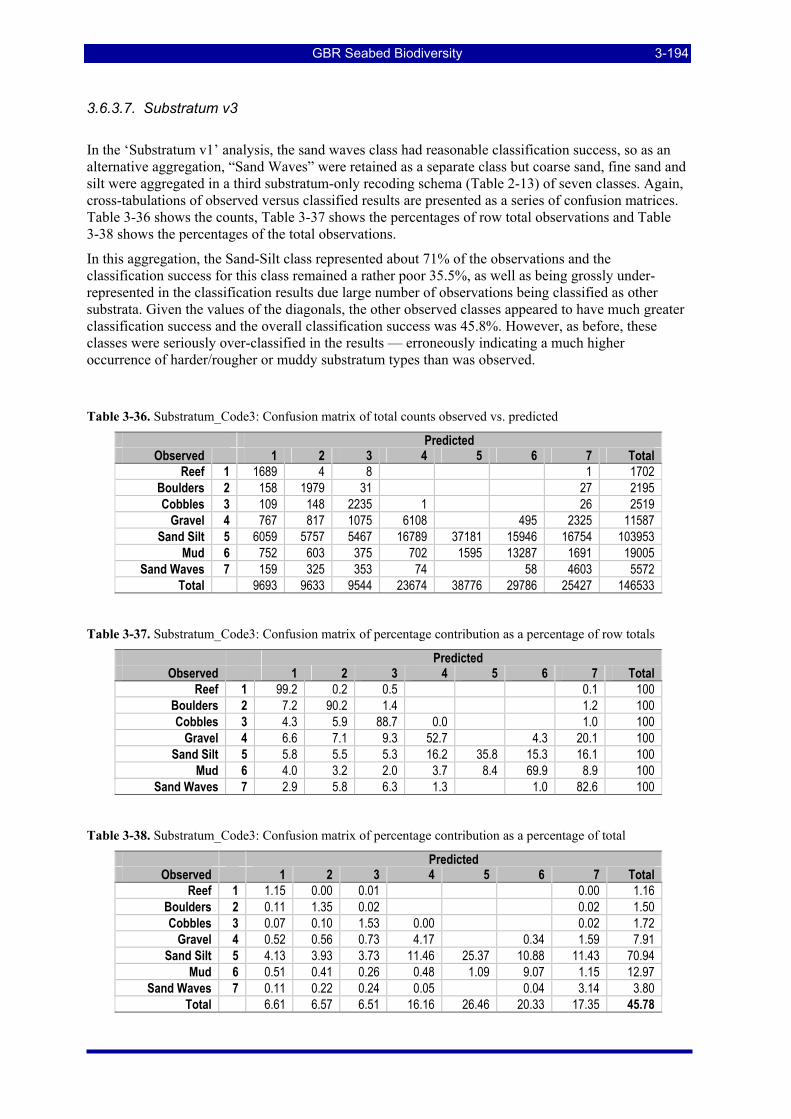
GBR Seabed Biodiversity 3-194
3.6.3.7. Substratum v3
In the ‘Substratum v1’ analysis, the sand waves class had reasonable classification success, so as an alternative aggregation, “Sand Waves” were retained as a separate class but coarse sand, fine sand and silt were aggregated in a third substratum-only recoding schema (Table 2-13) of seven classes. Again, cross-tabulations of observed versus classified results are presented as a series of confusion matrices. Table 3-36 shows the counts, Table 3-37 shows the percentages of row total observations and Table 3-38 shows the percentages of the total observations.
In this aggregation, the Sand-Silt class represented about 71% of the observations and the classification success for this class remained a rather poor 35.5%, as well as being grossly under-represented in the classification results due large number of observations being classified as other substrata. Given the values of the diagonals, the other observed classes appeared to have much greater classification success and the overall classification success was 45.8%. However, as before, these classes were seriously over-classified in the results — erroneously indicating a much higher occurrence of harder/rougher or muddy substratum types than was observed.
Table 3-36. Substratum_Code3: Confusion matrix of total counts observed vs. predicted
Predicted Observed 1 2 3 4 5 6 7 Total
Reef 1 1689 4 8 1 1702 Boulders 2 158 1979 31 27 2195 Cobbles 3 109 148 2235 1 26 2519
Gravel 4 767 817 1075 6108 495 2325 11587 Sand Silt 5 6059 5757 5467 16789 37181 15946 16754 103953
Mud 6 752 603 375 702 1595 13287 1691 19005 Sand Waves 7 159 325 353 74 58 4603 5572
Total 9693 9633 9544 23674 38776 29786 25427 146533
Table 3-37. Substratum_Code3: Confusion matrix of percentage contribution as a percentage of row totals
Predicted Observed 1 2 3 4 5 6 7 Total
Reef 1 99.2 0.2 0.5 0.1 100 Boulders 2 7.2 90.2 1.4 1.2 100 Cobbles 3 4.3 5.9 88.7 0.0 1.0 100
Gravel 4 6.6 7.1 9.3 52.7 4.3 20.1 100 Sand Silt 5 5.8 5.5 5.3 16.2 35.8 15.3 16.1 100
Mud 6 4.0 3.2 2.0 3.7 8.4 69.9 8.9 100 Sand Waves 7 2.9 5.8 6.3 1.3 1.0 82.6 100
Table 3-38. Substratum_Code3: Confusion matrix of percentage contribution as a percentage of total
Predicted Observed 1 2 3 4 5 6 7 Total
Reef 1 1.15 0.00 0.01 0.00 1.16 Boulders 2 0.11 1.35 0.02 0.02 1.50 Cobbles 3 0.07 0.10 1.53 0.00 0.02 1.72
Gravel 4 0.52 0.56 0.73 4.17 0.34 1.59 7.91 Sand Silt 5 4.13 3.93 3.73 11.46 25.37 10.88 11.43 70.94
Mud 6 0.51 0.41 0.26 0.48 1.09 9.07 1.15 12.97 Sand Waves 7 0.11 0.22 0.24 0.05 0.04 3.14 3.80
Total 6.61 6.57 6.51 16.16 26.46 20.33 17.35 45.78
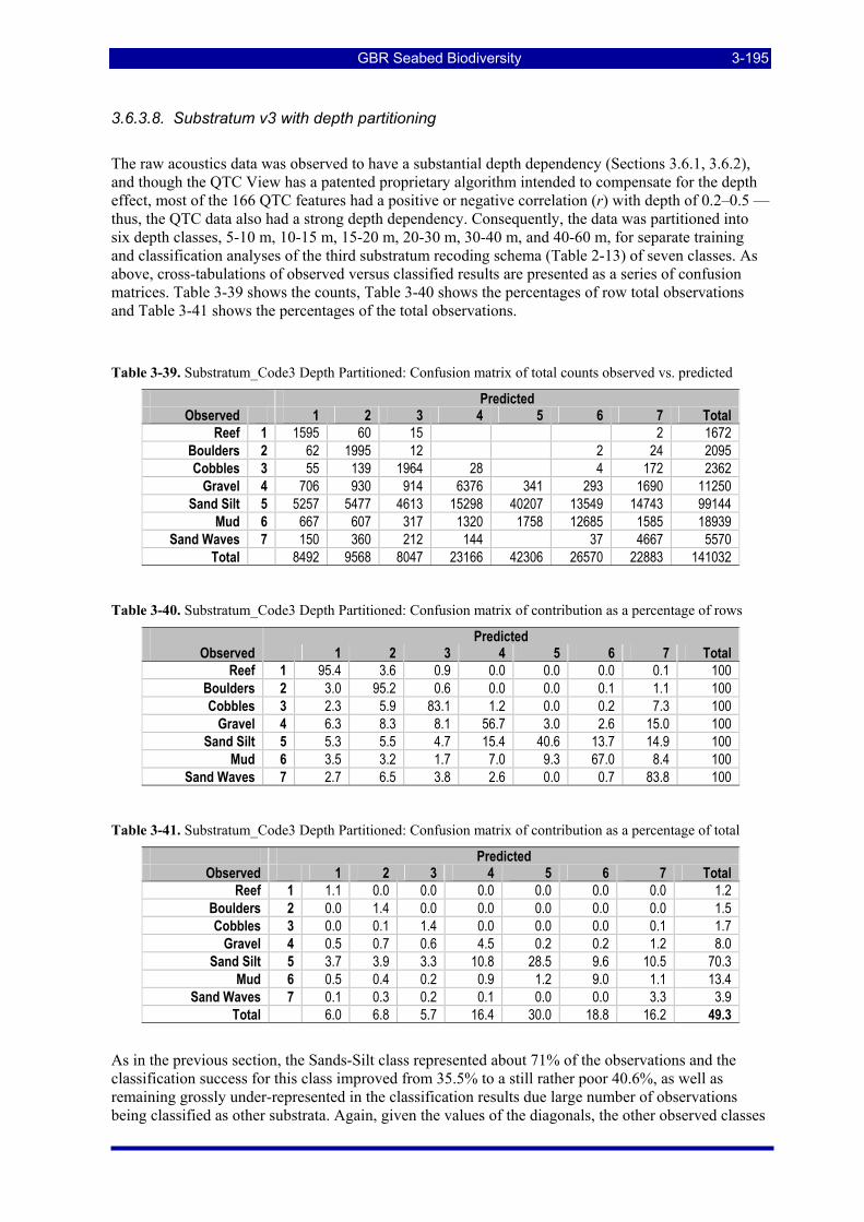
GBR Seabed Biodiversity 3-195
3.6.3.8. Substratum v3 with depth partitioning
The raw acoustics data was observed to have a substantial depth dependency (Sections 3.6.1, 3.6.2), and though the QTC View has a patented proprietary algorithm intended to compensate for the depth effect, most of the 166 QTC features had a positive or negative correlation (r) with depth of 0.2–0.5 — thus, the QTC data also had a strong depth dependency. Consequently, the data was partitioned into six depth classes, 5-10 m, 10-15 m, 15-20 m, 20-30 m, 30-40 m, and 40-60 m, for separate training and classification analyses of the third substratum recoding schema (Table 2-13) of seven classes. As above, cross-tabulations of observed versus classified results are presented as a series of confusion matrices. Table 3-39 shows the counts, Table 3-40 shows the percentages of row total observations and Table 3-41 shows the percentages of the total observations.
Table 3-39. Substratum_Code3 Depth Partitioned: Confusion matrix of total counts observed vs. predicted
Predicted Observed 1 2 3 4 5 6 7 Total
Reef 1 1595 60 15 2 1672 Boulders 2 62 1995 12 2 24 2095 Cobbles 3 55 139 1964 28 4 172 2362
Gravel 4 706 930 914 6376 341 293 1690 11250 Sand Silt 5 5257 5477 4613 15298 40207 13549 14743 99144
Mud 6 667 607 317 1320 1758 12685 1585 18939 Sand Waves 7 150 360 212 144 37 4667 5570
Total 8492 9568 8047 23166 42306 26570 22883 141032
Table 3-40. Substratum_Code3 Depth Partitioned: Confusion matrix of contribution as a percentage of rows
Predicted Observed 1 2 3 4 5 6 7 Total
Reef 1 95.4 3.6 0.9 0.0 0.0 0.0 0.1 100 Boulders 2 3.0 95.2 0.6 0.0 0.0 0.1 1.1 100 Cobbles 3 2.3 5.9 83.1 1.2 0.0 0.2 7.3 100
Gravel 4 6.3 8.3 8.1 56.7 3.0 2.6 15.0 100 Sand Silt 5 5.3 5.5 4.7 15.4 40.6 13.7 14.9 100
Mud 6 3.5 3.2 1.7 7.0 9.3 67.0 8.4 100 Sand Waves 7 2.7 6.5 3.8 2.6 0.0 0.7 83.8 100
Table 3-41. Substratum_Code3 Depth Partitioned: Confusion matrix of contribution as a percentage of total
Predicted Observed 1 2 3 4 5 6 7 Total
Reef 1 1.1 0.0 0.0 0.0 0.0 0.0 0.0 1.2 Boulders 2 0.0 1.4 0.0 0.0 0.0 0.0 0.0 1.5 Cobbles 3 0.0 0.1 1.4 0.0 0.0 0.0 0.1 1.7
Gravel 4 0.5 0.7 0.6 4.5 0.2 0.2 1.2 8.0 Sand Silt 5 3.7 3.9 3.3 10.8 28.5 9.6 10.5 70.3
Mud 6 0.5 0.4 0.2 0.9 1.2 9.0 1.1 13.4 Sand Waves 7 0.1 0.3 0.2 0.1 0.0 0.0 3.3 3.9
Total 6.0 6.8 5.7 16.4 30.0 18.8 16.2 49.3
As in the previous section, the Sands-Silt class represented about 71% of the observations and the classification success for this class improved from 35.5% to a still rather poor 40.6%, as well as remaining grossly under-represented in the classification results due large number of observations being classified as other substrata. Again, given the values of the diagonals, the other observed classes
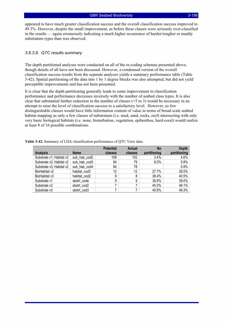
GBR Seabed Biodiversity 3-196
appeared to have much greater classification success and the overall classification success improved to 49.3%. However, despite the small improvement, as before these classes were seriously over-classified in the results — again erroneously indicating a much higher occurrence of harder/rougher or muddy substratum types than was observed.
3.6.3.9. QTC results summary
The depth partitioned analyses were conducted on all of the re-coding schemas presented above, though details of all have not been discussed. However, a condensed version of the overall classification success results from the separate analyses yields a summary performance table (Table 3-42). Spatial partitioning of the data into 1 by 1 degree blocks was also attempted, but did not yield perceptible improvements and has not been presented.
It is clear that the depth partitioning generally leads to some improvement in classification performance and performance decreases inversely with the number of seabed class types. It is also clear that substantial further reduction in the number of classes (<5 to 3) would be necessary in an attempt to raise the level of classification success to a satisfactory level. However, so few distinguishable classes would have little information content of value in terms of broad scale seabed habitat mapping as only a few classes of substratum (i.e. mud, sand, rocks, reef) intersecting with only very basic biological habitats (i.e. none, bioturbation, vegetation, epibenthos, hard-coral) would realize at least 8 of 16 possible combinations.
Table 3-42. Summary of LDA classification performance of QTC View data.
Analysis Name Potential
classes Actual
classes No
partitioning Depth
partitioning Substrate v1, Habitat v2 sub_hab_cod2 108 102 3.4% 4.6% Substrate v2, Habitat v2 sub_hab_cod3 84 79 6.0% 5.8% Substrate v3, Habitat v2 sub_hab_cod4 84 78 5.9% BioHabitat v2 habitat_cod3 12 12 27.7% 29.5% BioHabitat v3 habitat_cod2 8 8 38.4% 40.5% Substrate v1 sbstrt_code 9 9 36.6% 39.0% Substrate v2 sbstrt_cod2 7 7 45.0% 49.1% Substrate v3 sbstrt_cod3 7 7 45.8% 49.3%
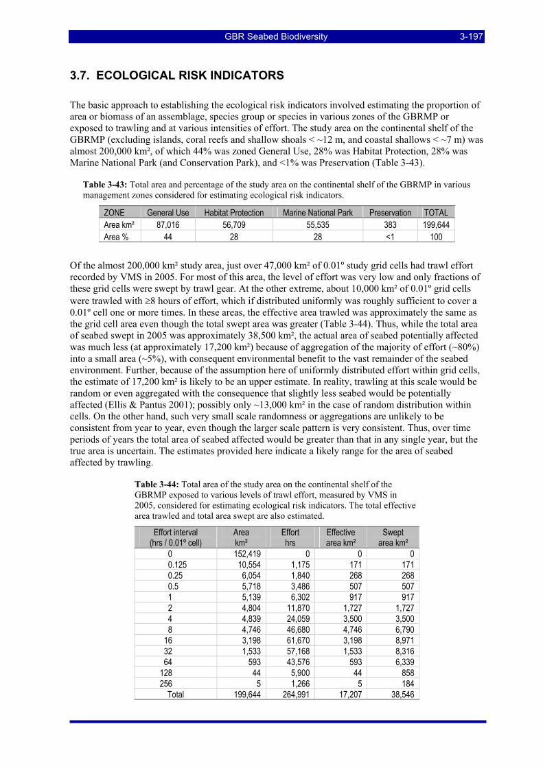
GBR Seabed Biodiversity 3-197
3.7. ECOLOGICAL RISK INDICATORS The basic approach to establishing the ecological risk indicators involved estimating the proportion of area or biomass of an assemblage, species group or species in various zones of the GBRMP or exposed to trawling and at various intensities of effort. The study area on the continental shelf of the GBRMP (excluding islands, coral reefs and shallow shoals < ~12 m, and coastal shallows < ~7 m) was almost 200,000 km², of which 44% was zoned General Use, 28% was Habitat Protection, 28% was Marine National Park (and Conservation Park), and <1% was Preservation (Table 3-43).
Table 3-43: Total area and percentage of the study area on the continental shelf of the GBRMP in various management zones considered for estimating ecological risk indicators.
ZONE General Use Habitat Protection Marine National Park Preservation TOTAL Area km² 87,016 56,709 55,535 383 199,644 Area % 44 28 28 <1 100
Of the almost 200,000 km² study area, just over 47,000 km² of 0.01º study grid cells had trawl effort recorded by VMS in 2005. For most of this area, the level of effort was very low and only fractions of these grid cells were swept by trawl gear. At the other extreme, about 10,000 km² of 0.01º grid cells were trawled with ≥8 hours of effort, which if distributed uniformly was roughly sufficient to cover a 0.01º cell one or more times. In these areas, the effective area trawled was approximately the same as the grid cell area even though the total swept area was greater (Table 3-44). Thus, while the total area of seabed swept in 2005 was approximately 38,500 km², the actual area of seabed potentially affected was much less (at approximately 17,200 km²) because of aggregation of the majority of effort (~80%) into a small area (~5%), with consequent environmental benefit to the vast remainder of the seabed environment. Further, because of the assumption here of uniformly distributed effort within grid cells, the estimate of 17,200 km² is likely to be an upper estimate. In reality, trawling at this scale would be random or even aggregated with the consequence that slightly less seabed would be potentially affected (Ellis & Pantus 2001); possibly only ~13,000 km² in the case of random distribution within cells. On the other hand, such very small scale randomness or aggregations are unlikely to be consistent from year to year, even though the larger scale pattern is very consistent. Thus, over time periods of years the total area of seabed affected would be greater than that in any single year, but the true area is uncertain. The estimates provided here indicate a likely range for the area of seabed affected by trawling.
Table 3-44: Total area of the study area on the continental shelf of the GBRMP exposed to various levels of trawl effort, measured by VMS in 2005, considered for estimating ecological risk indicators. The total effective area trawled and total area swept are also estimated.
Effort interval (hrs / 0.01º cell)
Area km²
Effort hrs
Effective area km²
Swept area km²
0 152,419 0 0 0 0.125 10,554 1,175 171 171 0.25 6,054 1,840 268 268 0.5 5,718 3,486 507 507 1 5,139 6,302 917 917 2 4,804 11,870 1,727 1,727 4 4,839 24,059 3,500 3,500 8 4,746 46,680 4,746 6,790
16 3,198 61,670 3,198 8,971 32 1,533 57,168 1,533 8,316 64 593 43,576 593 6,339
128 44 5,900 44 858 256 5 1,266 5 184
Total 199,644 264,991 17,207 38,546
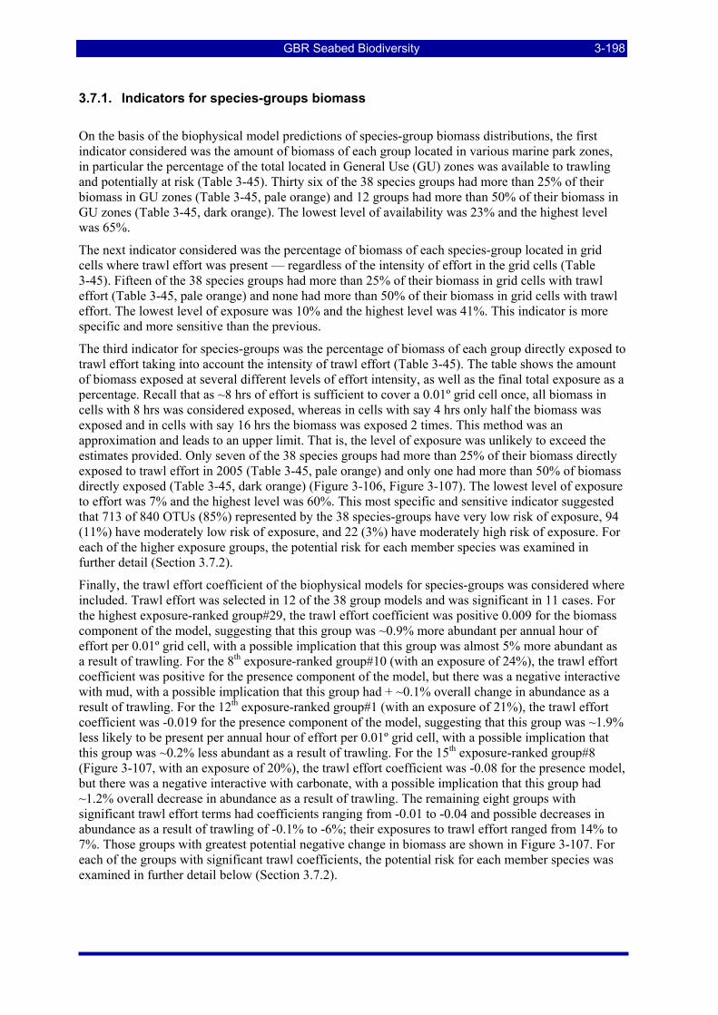
GBR Seabed Biodiversity 3-198
3.7.1. Indicators for species-groups biomass
On the basis of the biophysical model predictions of species-group biomass distributions, the first indicator considered was the amount of biomass of each group located in various marine park zones, in particular the percentage of the total located in General Use (GU) zones was available to trawling and potentially at risk (Table 3-45). Thirty six of the 38 species groups had more than 25% of their biomass in GU zones (Table 3-45, pale orange) and 12 groups had more than 50% of their biomass in GU zones (Table 3-45, dark orange). The lowest level of availability was 23% and the highest level was 65%.
The next indicator considered was the percentage of biomass of each species-group located in grid cells where trawl effort was present — regardless of the intensity of effort in the grid cells (Table 3-45). Fifteen of the 38 species groups had more than 25% of their biomass in grid cells with trawl effort (Table 3-45, pale orange) and none had more than 50% of their biomass in grid cells with trawl effort. The lowest level of exposure was 10% and the highest level was 41%. This indicator is more specific and more sensitive than the previous.
The third indicator for species-groups was the percentage of biomass of each group directly exposed to trawl effort taking into account the intensity of trawl effort (Table 3-45). The table shows the amount of biomass exposed at several different levels of effort intensity, as well as the final total exposure as a percentage. Recall that as ~8 hrs of effort is sufficient to cover a 0.01º grid cell once, all biomass in cells with 8 hrs was considered exposed, whereas in cells with say 4 hrs only half the biomass was exposed and in cells with say 16 hrs the biomass was exposed 2 times. This method was an approximation and leads to an upper limit. That is, the level of exposure was unlikely to exceed the estimates provided. Only seven of the 38 species groups had more than 25% of their biomass directly exposed to trawl effort in 2005 (Table 3-45, pale orange) and only one had more than 50% of biomass directly exposed (Table 3-45, dark orange) (Figure 3-106, Figure 3-107). The lowest level of exposure to effort was 7% and the highest level was 60%. This most specific and sensitive indicator suggested that 713 of 840 OTUs (85%) represented by the 38 species-groups have very low risk of exposure, 94 (11%) have moderately low risk of exposure, and 22 (3%) have moderately high risk of exposure. For each of the higher exposure groups, the potential risk for each member species was examined in further detail (Section 3.7.2).
Finally, the trawl effort coefficient of the biophysical models for species-groups was considered where included. Trawl effort was selected in 12 of the 38 group models and was significant in 11 cases. For the highest exposure-ranked group#29, the trawl effort coefficient was positive 0.009 for the biomass component of the model, suggesting that this group was ~0.9% more abundant per annual hour of effort per 0.01º grid cell, with a possible implication that this group was almost 5% more abundant as a result of trawling. For the 8th exposure-ranked group#10 (with an exposure of 24%), the trawl effort coefficient was positive for the presence component of the model, but there was a negative interactive with mud, with a possible implication that this group had + ~0.1% overall change in abundance as a result of trawling. For the 12th exposure-ranked group#1 (with an exposure of 21%), the trawl effort coefficient was -0.019 for the presence component of the model, suggesting that this group was ~1.9% less likely to be present per annual hour of effort per 0.01º grid cell, with a possible implication that this group was ~0.2% less abundant as a result of trawling. For the 15th exposure-ranked group#8 (Figure 3-107, with an exposure of 20%), the trawl effort coefficient was -0.08 for the presence model, but there was a negative interactive with carbonate, with a possible implication that this group had ~1.2% overall decrease in abundance as a result of trawling. The remaining eight groups with significant trawl effort terms had coefficients ranging from -0.01 to -0.04 and possible decreases in abundance as a result of trawling of -0.1% to -6%; their exposures to trawl effort ranged from 14% to 7%. Those groups with greatest potential negative change in biomass are shown in Figure 3-107. For each of the groups with significant trawl coefficients, the potential risk for each member species was examined in further detail below (Section 3.7.2).
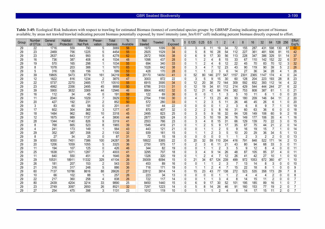
GBR Seabed Biodiversity 3-199
Table 3-45: Ecological Risk Indicators with respect to trawling for estimated Biomass (tonnes) of correlated species groups: by GBRMP Zoning indicating percent of biomass available; by areas not trawled/trawled indicating percent biomass potentially exposed; by trawl intensity (ann_hrs/0.01º cell) indicating percent biomass directly exposed to effort.
Group Number of OTUs
General Use
Habitat Protection
Marine Nat Park
Preser- vation
Total biomass
% Available Not
trawled Trawled % Exposed 0 0.125 0.25 0.5 1 2 4 8 16 32 64 128 256 Effort
Exp% 29 22 1716 559 790 5 3069 56 1970 1099 36 0 3 6 11 19 34 72 155 287 431 598 130 87 60 29 23 2469 756 1225 5 4454 55 2925 1529 34 0 5 8 16 28 54 112 227 361 481 506 81 15 42 29 23 2637 643 993 5 4278 62 2672 1606 38 0 6 9 17 30 56 113 228 347 386 329 51 14 37 29 16 736 387 408 4 1534 48 1098 437 28 0 1 2 4 8 15 33 67 110 142 152 22 6 37 29 19 570 165 298 1 1034 55 694 340 33 0 1 2 4 6 12 22 45 70 83 70 12 3 32 29 8 1078 203 388 1 1670 65 1028 642 38 0 3 4 7 12 23 43 90 119 90 39 5 2 26 29 5 316 126 156 1 599 53 428 170 28 0 1 1 2 3 6 14 27 36 34 28 4 1 26 29 39 19805 5473 8779 161 34219 58 20170 14050 41 0 52 80 146 277 547 1157 2301 2365 1147 174 4 0 24 29 12 1822 816 1234 2 3875 47 3003 872 22 0 3 5 9 15 30 60 128 204 223 193 28 8 23 29 22 5737 2270 2485 17 10510 55 6915 3595 34 0 12 20 38 72 144 309 592 652 393 112 14 4 22 29 23 4992 2356 2495 45 9888 50 6786 3103 31 0 12 19 34 61 112 214 429 544 444 244 27 6 22 29 39 5900 3632 3369 44 12946 46 8864 4082 32 0 12 21 42 84 174 382 753 808 387 61 1 0 21 29 16 112 34 45 0 191 59 122 69 36 0 0 0 1 1 3 5 10 11 6 1 0 0 20 29 11 2040 854 1029 7 3929 52 2764 1166 30 0 4 7 13 23 45 93 180 209 146 64 11 2 20 29 20 427 192 231 2 852 50 572 280 33 0 1 2 3 5 11 26 46 45 26 6 1 0 20 29 3 83 60 58 0 201 41 157 44 22 0 0 0 0 1 2 3 6 8 9 7 1 0 19 29 17 602 304 368 3 1277 47 870 407 32 0 2 2 5 8 16 31 60 63 36 6 0 0 18 29 18 1484 962 862 10 3318 45 2495 823 25 0 3 5 9 16 32 64 126 149 106 60 9 2 18 29 12 1675 989 1137 4 3806 44 2877 929 24 0 3 5 10 19 36 76 149 177 106 35 4 1 16 29 28 1344 1140 826 9 3319 41 2553 766 23 0 3 4 8 15 31 66 129 139 70 22 3 0 15 29 8 768 665 523 8 1965 39 1546 419 21 0 1 2 5 9 17 35 67 75 44 21 2 0 14 29 4 241 173 149 1 564 43 443 121 21 0 0 1 1 2 5 9 16 19 15 7 1 0 14 29 29 352 387 358 2 1100 32 939 161 15 0 1 1 2 3 5 10 20 29 36 34 5 1 13 29 8 27 34 25 0 87 31 72 15 18 0 0 0 0 0 1 1 2 3 2 2 0 0 13 29 39 9350 7451 7386 100 24287 38 18922 5365 22 0 20 32 59 110 204 416 791 848 522 171 14 2 13 29 20 1206 1059 1055 5 3325 36 2750 575 17 0 2 3 6 11 21 43 80 94 68 33 3 0 11 29 11 194 107 125 0 426 46 344 82 19 0 0 1 1 2 3 5 9 12 8 4 0 0 11 29 25 1638 1071 1287 7 4003 41 3295 707 18 0 3 4 9 14 26 48 87 105 85 37 4 0 11 29 11 640 550 451 4 1646 39 1326 320 19 0 1 2 4 7 12 26 41 42 27 10 1 0 10 29 29 10531 18911 11332 329 41104 26 35009 6094 15 0 21 34 67 124 239 499 972 1053 672 360 47 1 10 29 26 181 207 153 2 543 33 453 89 16 0 0 1 1 2 3 7 13 14 8 3 0 0 10 29 21 316 317 248 5 886 36 716 171 19 0 1 1 2 4 7 15 22 18 8 1 0 0 9 29 60 7137 10786 8616 88 26626 27 22812 3814 14 0 15 23 43 77 138 272 523 535 358 173 29 7 8 29 10 66 102 88 1 257 26 223 34 13 0 0 0 0 1 1 2 4 4 4 2 0 0 8 29 22 217 360 258 4 838 26 722 117 14 0 0 1 1 3 4 8 14 15 11 2 0 0 7 29 80 2439 4204 3214 33 9890 25 8450 1440 15 0 6 9 17 30 52 101 195 185 89 16 1 0 7 29 23 2749 3097 2650 26 8521 32 7297 1223 14 0 5 8 14 26 46 91 160 153 77 19 2 0 7 29 27 254 475 398 3 1131 23 1012 119 10 0 1 1 1 2 4 8 14 17 15 11 2 0 7
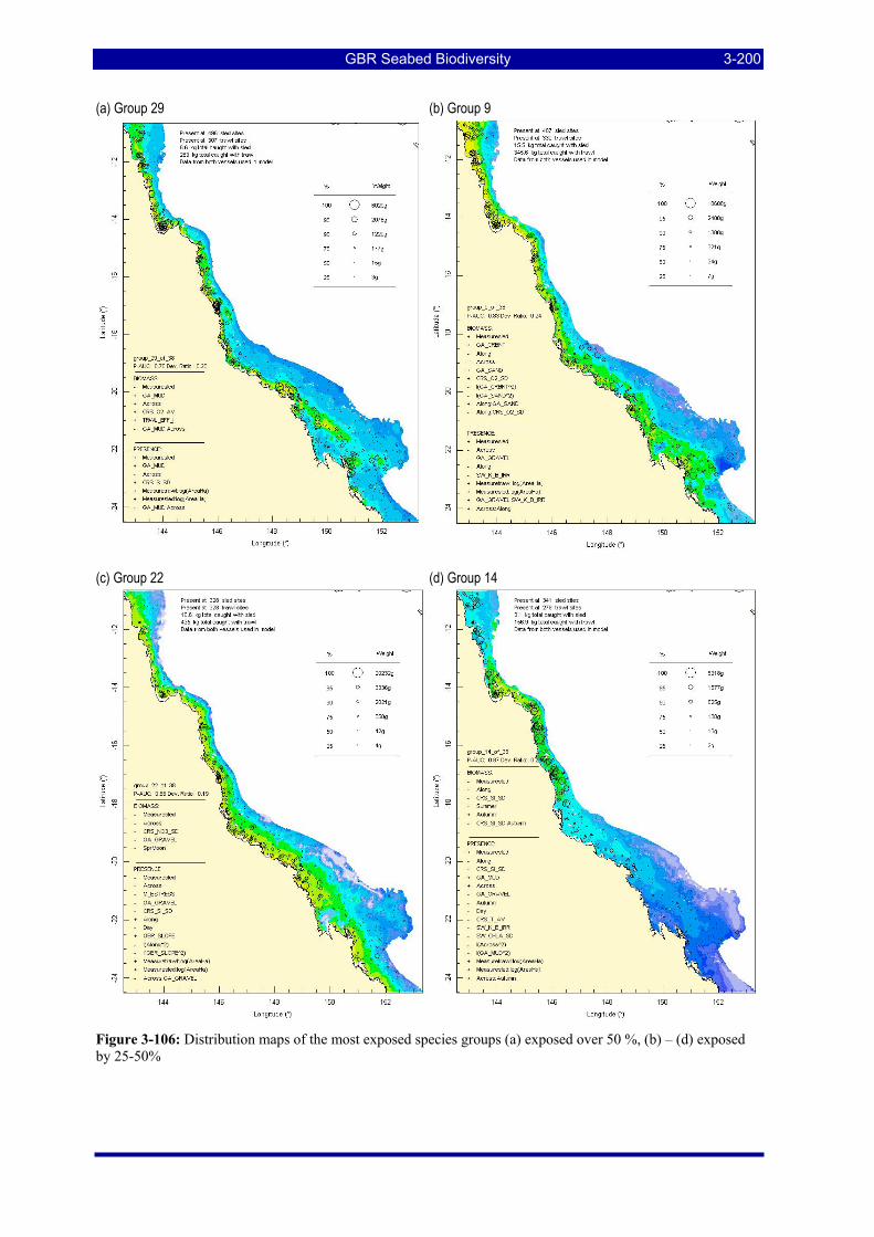
GBR Seabed Biodiversity 3-200
(a) Group 29 (b) Group 9
(c) Group 22 (d) Group 14
Figure 3-106: Distribution maps of the most exposed species groups (a) exposed over 50 %, (b) – (d) exposed by 25-50%
GBR Seabed Biodiversity 3-201
(a) Group 13 (b) Group 33
(c) Group 35 (d) Group 6
Figure 3-107: Distribution maps of the most exposed species groups: (a) and (b) exposed by 25-50%; and species groups with negative trawl effort coefficients and possible population decreases in abundance as a result of trawling of >5%; (c) -5.3% and (d) -6% respectively.
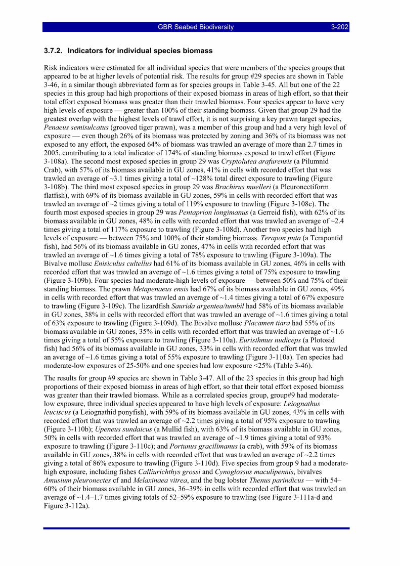
GBR Seabed Biodiversity 3-202
3.7.2. Indicators for individual species biomass Risk indicators were estimated for all individual species that were members of the species groups that appeared to be at higher levels of potential risk. The results for group #29 species are shown in Table 3-46, in a similar though abbreviated form as for species groups in Table 3-45. All but one of the 22 species in this group had high proportions of their exposed biomass in areas of high effort, so that their total effort exposed biomass was greater than their trawled biomass. Four species appear to have very high levels of exposure — greater than 100% of their standing biomass. Given that group 29 had the greatest overlap with the highest levels of trawl effort, it is not surprising a key prawn target species, Penaeus semisulcatus (grooved tiger prawn), was a member of this group and had a very high level of exposure — even though 26% of its biomass was protected by zoning and 36% of its biomass was not exposed to any effort, the exposed 64% of biomass was trawled an average of more than 2.7 times in 2005, contributing to a total indicator of 174% of standing biomass exposed to trawl effort (Figure 3-108a). The second most exposed species in group 29 was Cryptolutea arafurensis (a Pilumnid Crab), with 57% of its biomass available in GU zones, 41% in cells with recorded effort that was trawled an average of ~3.1 times giving a total of ~128% total direct exposure to trawling (Figure 3-108b). The third most exposed species in group 29 was Brachirus muelleri (a Pleuronectiform flatfish), with 69% of its biomass available in GU zones, 59% in cells with recorded effort that was trawled an average of ~2 times giving a total of 119% exposure to trawling (Figure 3-108c). The fourth most exposed species in group 29 was Pentaprion longimanus (a Gerreid fish), with 62% of its biomass available in GU zones, 48% in cells with recorded effort that was trawled an average of ~2.4 times giving a total of 117% exposure to trawling (Figure 3-108d). Another two species had high levels of exposure — between 75% and 100% of their standing biomass. Terapon puta (a Terapontid fish), had 56% of its biomass available in GU zones, 47% in cells with recorded effort that was trawled an average of ~1.6 times giving a total of 78% exposure to trawling (Figure 3-109a). The Bivalve mollusc Enisiculus cultellus had 61% of its biomass available in GU zones, 46% in cells with recorded effort that was trawled an average of ~1.6 times giving a total of 75% exposure to trawling (Figure 3-109b). Four species had moderate-high levels of exposure — between 50% and 75% of their standing biomass. The prawn Metapenaeus ensis had 67% of its biomass available in GU zones, 49% in cells with recorded effort that was trawled an average of ~1.4 times giving a total of 67% exposure to trawling (Figure 3-109c). The lizardfish Saurida argentea/tumbil had 58% of its biomass available in GU zones, 38% in cells with recorded effort that was trawled an average of ~1.6 times giving a total of 63% exposure to trawling (Figure 3-109d). The Bivalve mollusc Placamen tiara had 55% of its biomass available in GU zones, 35% in cells with recorded effort that was trawled an average of ~1.6 times giving a total of 55% exposure to trawling (Figure 3-110a). Euristhmus nudiceps (a Plotosid fish) had 56% of its biomass available in GU zones, 33% in cells with recorded effort that was trawled an average of ~1.6 times giving a total of 55% exposure to trawling (Figure 3-110a). Ten species had moderate-low exposures of 25-50% and one species had low exposure <25% (Table 3-46).
The results for group #9 species are shown in Table 3-47. All of the 23 species in this group had high proportions of their exposed biomass in areas of high effort, so that their total effort exposed biomass was greater than their trawled biomass. While as a correlated species group, group#9 had moderate-low exposure, three individual species appeared to have high levels of exposure: Leiognathus leuciscus (a Leiognathid ponyfish), with 59% of its biomass available in GU zones, 43% in cells with recorded effort that was trawled an average of ~2.2 times giving a total of 95% exposure to trawling (Figure 3-110b); Upeneus sundaicus (a Mullid fish), with 63% of its biomass available in GU zones, 50% in cells with recorded effort that was trawled an average of ~1.9 times giving a total of 93% exposure to trawling (Figure 3-110c); and Portunus gracilimanus (a crab), with 59% of its biomass available in GU zones, 38% in cells with recorded effort that was trawled an average of ~2.2 times giving a total of 86% exposure to trawling (Figure 3-110d). Five species from group 9 had a moderate-high exposure, including fishes Calliurichthys grossi and Cynoglossus maculipennis, bivalves Amusium pleuronectes cf and Melaxinaea vitrea, and the bug lobster Thenus parindicus — with 54–60% of their biomass available in GU zones, 36–39% in cells with recorded effort that was trawled an average of ~1.4–1.7 times giving totals of 52–59% exposure to trawling (see Figure 3-111a-d and Figure 3-112a).
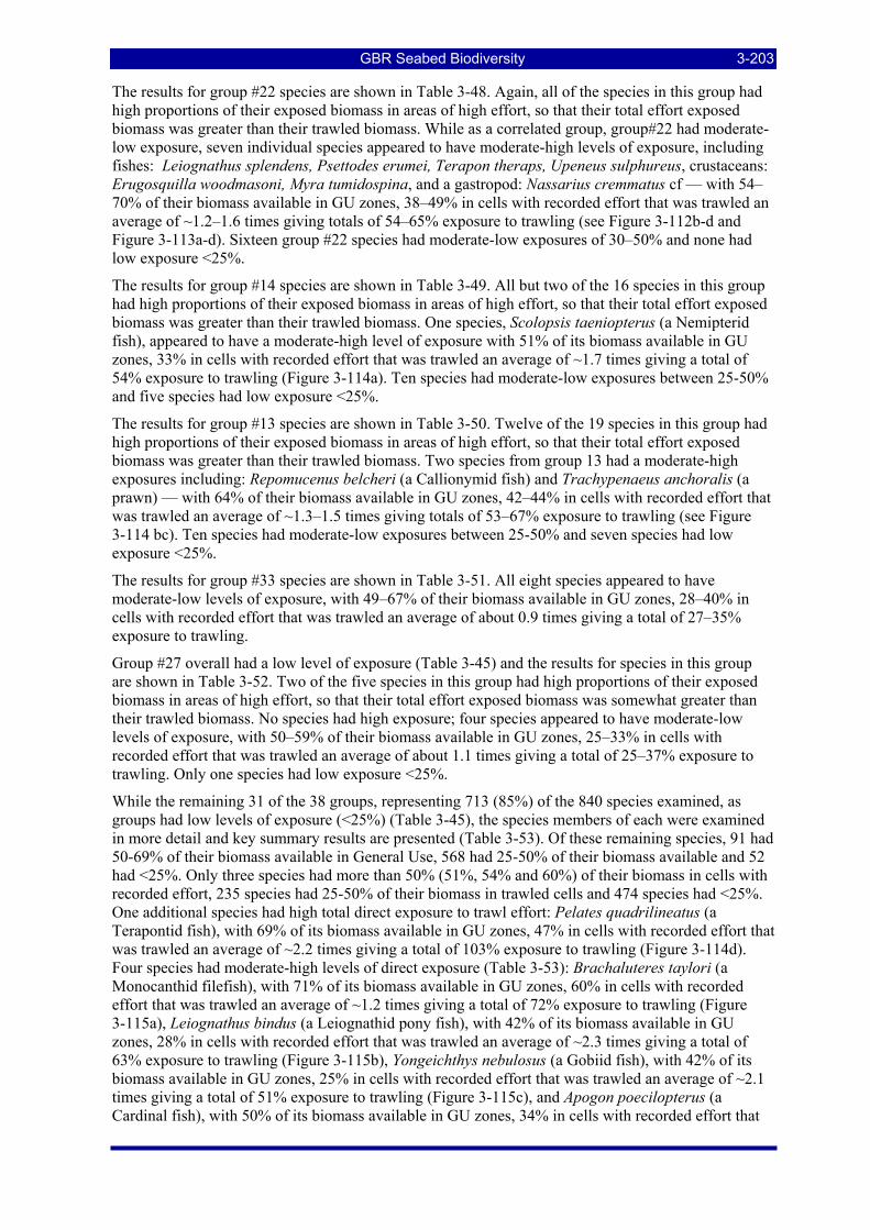
GBR Seabed Biodiversity 3-203
The results for group #22 species are shown in Table 3-48. Again, all of the species in this group had high proportions of their exposed biomass in areas of high effort, so that their total effort exposed biomass was greater than their trawled biomass. While as a correlated group, group#22 had moderate-low exposure, seven individual species appeared to have moderate-high levels of exposure, including fishes: Leiognathus splendens, Psettodes erumei, Terapon theraps, Upeneus sulphureus, crustaceans: Erugosquilla woodmasoni, Myra tumidospina, and a gastropod: Nassarius cremmatus cf — with 54–70% of their biomass available in GU zones, 38–49% in cells with recorded effort that was trawled an average of ~1.2–1.6 times giving totals of 54–65% exposure to trawling (see Figure 3-112b-d and Figure 3-113a-d). Sixteen group #22 species had moderate-low exposures of 30–50% and none had low exposure <25%.
The results for group #14 species are shown in Table 3-49. All but two of the 16 species in this group had high proportions of their exposed biomass in areas of high effort, so that their total effort exposed biomass was greater than their trawled biomass. One species, Scolopsis taeniopterus (a Nemipterid fish), appeared to have a moderate-high level of exposure with 51% of its biomass available in GU zones, 33% in cells with recorded effort that was trawled an average of ~1.7 times giving a total of 54% exposure to trawling (Figure 3-114a). Ten species had moderate-low exposures between 25-50% and five species had low exposure <25%.
The results for group #13 species are shown in Table 3-50. Twelve of the 19 species in this group had high proportions of their exposed biomass in areas of high effort, so that their total effort exposed biomass was greater than their trawled biomass. Two species from group 13 had a moderate-high exposures including: Repomucenus belcheri (a Callionymid fish) and Trachypenaeus anchoralis (a prawn) — with 64% of their biomass available in GU zones, 42–44% in cells with recorded effort that was trawled an average of ~1.3–1.5 times giving totals of 53–67% exposure to trawling (see Figure 3-114 bc). Ten species had moderate-low exposures between 25-50% and seven species had low exposure <25%.
The results for group #33 species are shown in Table 3-51. All eight species appeared to have moderate-low levels of exposure, with 49–67% of their biomass available in GU zones, 28–40% in cells with recorded effort that was trawled an average of about 0.9 times giving a total of 27–35% exposure to trawling.
Group #27 overall had a low level of exposure (Table 3-45) and the results for species in this group are shown in Table 3-52. Two of the five species in this group had high proportions of their exposed biomass in areas of high effort, so that their total effort exposed biomass was somewhat greater than their trawled biomass. No species had high exposure; four species appeared to have moderate-low levels of exposure, with 50–59% of their biomass available in GU zones, 25–33% in cells with recorded effort that was trawled an average of about 1.1 times giving a total of 25–37% exposure to trawling. Only one species had low exposure <25%.
While the remaining 31 of the 38 groups, representing 713 (85%) of the 840 species examined, as groups had low levels of exposure (<25%) (Table 3-45), the species members of each were examined in more detail and key summary results are presented (Table 3-53). Of these remaining species, 91 had 50-69% of their biomass available in General Use, 568 had 25-50% of their biomass available and 52 had <25%. Only three species had more than 50% (51%, 54% and 60%) of their biomass in cells with recorded effort, 235 species had 25-50% of their biomass in trawled cells and 474 species had <25%. One additional species had high total direct exposure to trawl effort: Pelates quadrilineatus (a Terapontid fish), with 69% of its biomass available in GU zones, 47% in cells with recorded effort that was trawled an average of ~2.2 times giving a total of 103% exposure to trawling (Figure 3-114d). Four species had moderate-high levels of direct exposure (Table 3-53): Brachaluteres taylori (a Monocanthid filefish), with 71% of its biomass available in GU zones, 60% in cells with recorded effort that was trawled an average of ~1.2 times giving a total of 72% exposure to trawling (Figure 3-115a), Leiognathus bindus (a Leiognathid pony fish), with 42% of its biomass available in GU zones, 28% in cells with recorded effort that was trawled an average of ~2.3 times giving a total of 63% exposure to trawling (Figure 3-115b), Yongeichthys nebulosus (a Gobiid fish), with 42% of its biomass available in GU zones, 25% in cells with recorded effort that was trawled an average of ~2.1 times giving a total of 51% exposure to trawling (Figure 3-115c), and Apogon poecilopterus (a Cardinal fish), with 50% of its biomass available in GU zones, 34% in cells with recorded effort that
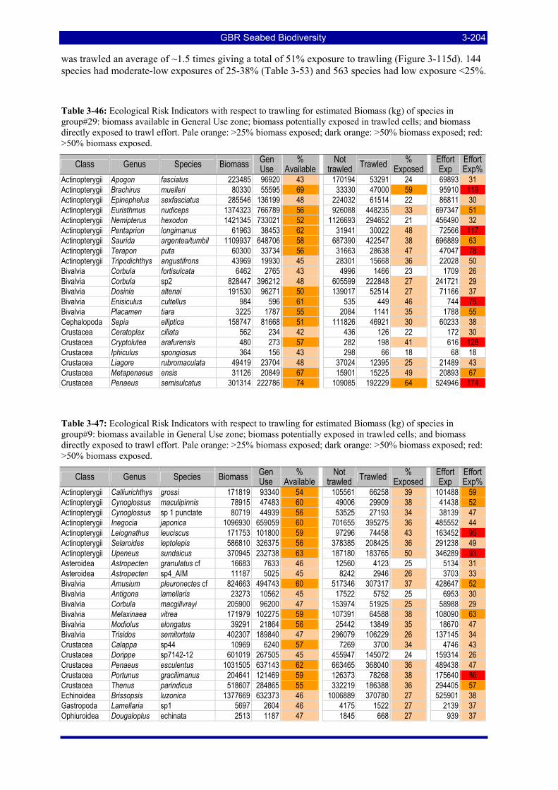
GBR Seabed Biodiversity 3-204
was trawled an average of ~1.5 times giving a total of 51% exposure to trawling (Figure 3-115d). 144 species had moderate-low exposures of 25-38% (Table 3-53) and 563 species had low exposure <25%.
Table 3-46: Ecological Risk Indicators with respect to trawling for estimated Biomass (kg) of species in group#29: biomass available in General Use zone; biomass potentially exposed in trawled cells; and biomass directly exposed to trawl effort. Pale orange: >25% biomass exposed; dark orange: >50% biomass exposed; red: >50% biomass exposed.
Class Genus Species Biomass Gen Use
% Available Not
trawled Trawled % Exposed Effort
Exp Effort Exp%
Actinopterygii Apogon fasciatus 223485 96920 43 170194 53291 24 69893 31 Actinopterygii Brachirus muelleri 80330 55595 69 33330 47000 59 95910 119 Actinopterygii Epinephelus sexfasciatus 285546 136199 48 224032 61514 22 86811 30 Actinopterygii Euristhmus nudiceps 1374323 766789 56 926088 448235 33 697347 51 Actinopterygii Nemipterus hexodon 1421345 733021 52 1126693 294652 21 456490 32 Actinopterygii Pentaprion longimanus 61963 38453 62 31941 30022 48 72566 117 Actinopterygii Saurida argentea/tumbil 1109937 648706 58 687390 422547 38 696889 63 Actinopterygii Terapon puta 60300 33734 56 31663 28638 47 47047 78 Actinopterygii Tripodichthys angustifrons 43969 19930 45 28301 15668 36 22028 50 Bivalvia Corbula fortisulcata 6462 2765 43 4996 1466 23 1709 26 Bivalvia Corbula sp2 828447 396212 48 605599 222848 27 241721 29 Bivalvia Dosinia altenai 191530 96271 50 139017 52514 27 71166 37 Bivalvia Enisiculus cultellus 984 596 61 535 449 46 744 75 Bivalvia Placamen tiara 3225 1787 55 2084 1141 35 1788 55 Cephalopoda Sepia elliptica 158747 81668 51 111826 46921 30 60233 38 Crustacea Ceratoplax ciliata 562 234 42 436 126 22 172 30 Crustacea Cryptolutea arafurensis 480 273 57 282 198 41 616 128 Crustacea Iphiculus spongiosus 364 156 43 298 66 18 68 18 Crustacea Liagore rubromaculata 49419 23704 48 37024 12395 25 21489 43 Crustacea Metapenaeus ensis 31126 20849 67 15901 15225 49 20893 67 Crustacea Penaeus semisulcatus 301314 222786 74 109085 192229 64 524946 174
Table 3-47: Ecological Risk Indicators with respect to trawling for estimated Biomass (kg) of species in group#9: biomass available in General Use zone; biomass potentially exposed in trawled cells; and biomass directly exposed to trawl effort. Pale orange: >25% biomass exposed; dark orange: >50% biomass exposed; red: >50% biomass exposed.
Class Genus Species Biomass Gen Use
% Available Not
trawled Trawled % Exposed Effort
Exp Effort Exp%
Actinopterygii Calliurichthys grossi 171819 93340 54 105561 66258 39 101488 59 Actinopterygii Cynoglossus maculipinnis 78915 47483 60 49006 29909 38 41438 52 Actinopterygii Cynoglossus sp 1 punctate 80719 44939 56 53525 27193 34 38139 47 Actinopterygii Inegocia japonica 1096930 659059 60 701655 395275 36 485552 44 Actinopterygii Leiognathus leuciscus 171753 101800 59 97296 74458 43 163452 95 Actinopterygii Selaroides leptolepis 586810 326375 56 378385 208425 36 291238 49 Actinopterygii Upeneus sundaicus 370945 232738 63 187180 183765 50 346289 93 Asteroidea Astropecten granulatus cf 16683 7633 46 12560 4123 25 5134 31 Asteroidea Astropecten sp4_AIM 11187 5025 45 8242 2946 26 3703 33 Bivalvia Amusium pleuronectes cf 824663 494743 60 517346 307317 37 428647 52 Bivalvia Antigona lamellaris 23273 10562 45 17522 5752 25 6953 30 Bivalvia Corbula macgillvrayi 205900 96200 47 153974 51925 25 58988 29 Bivalvia Melaxinaea vitrea 171979 102275 59 107391 64588 38 108090 63 Bivalvia Modiolus elongatus 39291 21864 56 25442 13849 35 18670 47 Bivalvia Trisidos semitortata 402307 189840 47 296079 106229 26 137145 34 Crustacea Calappa sp44 10969 6240 57 7269 3700 34 4746 43 Crustacea Dorippe sp7142-12 601019 267505 45 455947 145072 24 159314 26 Crustacea Penaeus esculentus 1031505 637143 62 663465 368040 36 489438 47 Crustacea Portunus gracilimanus 204641 121469 59 126373 78268 38 175640 86 Crustacea Thenus parindicus 518607 284865 55 332219 186388 36 294405 57 Echinoidea Brissopsis luzonica 1377669 632373 46 1006889 370780 27 525901 38 Gastropoda Lamellaria sp1 5697 2604 46 4175 1522 27 2139 37 Ophiuroidea Dougaloplus echinata 2513 1187 47 1845 668 27 939 37
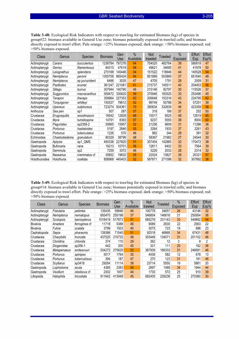
GBR Seabed Biodiversity 3-205
Table 3-48: Ecological Risk Indicators with respect to trawling for estimated Biomass (kg) of species in group#22: biomass available in General Use zone; biomass potentially exposed in trawled cells; and biomass directly exposed to trawl effort. Pale orange: >25% biomass exposed; dark orange: >50% biomass exposed; red: >50% biomass exposed.
Class Genus Species Biomass Gen Use
% Available Not
trawled Trawled % Exposed Effort
Exp Effort Exp%
Actinopterygii Caranx bucculentus 1236784 797276 64 754020 482764 39 580618 47 Actinopterygii Gerres filamentosus 84315 47619 56 49621 34695 41 41978 50 Actinopterygii Leiognathus splendens 270168 145446 54 151522 118646 44 145528 54 Actinopterygii Nemipterus peronii 1355758 865424 64 851889 503869 37 651640 48 Actinopterygii Nemipterus sp juv/unident 6496 3035 47 4705 1791 28 2009 31 Actinopterygii Psettodes erumei 361247 221081 61 215737 145511 40 204453 56 Actinopterygii Sillago burrus 307944 140790 46 215146 92797 30 115526 37 Actinopterygii Suggrundus macracanthus 559472 330620 59 375946 183525 33 253496 45 Actinopterygii Terapon theraps 359964 227353 63 206648 153316 43 224795 62 Actinopterygii Torquigener whitleyi 150537 78812 52 99749 50788 34 57201 38 Actinopterygii Upeneus sulphureus 723274 504361 70 390634 332639 46 423359 58 Anthozoa Sea pen sp1 507 287 57 318 189 37 252 50 Crustacea Erugosquilla woodmasoni 19542 12829 66 10017 9525 49 12819 65 Crustacea Myra tumidospina 14791 8393 57 9237 5555 38 8930 60 Crustacea Paguristes sp2358-2 30865 15957 52 21256 9609 31 11286 36 Crustacea Portunus hastatoides 5197 2846 55 3264 1933 37 2261 43 Crustacea Portunus tuberculatus 1226 570 46 882 344 28 391 32 Echinoidea Chaetodiadema granulatum 80329 38799 48 58367 21962 27 24544 30 Gastropoda Aplysia sp1_QMS 450338 227820 51 307454 142885 32 170472 38 Gastropoda Bufonaria rana 19213 10701 56 12811 6402 33 7564 39 Gastropoda Gemmula sp2 7259 3372 46 5226 2033 28 2314 32 Gastropoda Nassarius cremmatus cf 35852 19832 55 22024 13827 39 20331 57 Holothuroidea Holothuria ocellata 858968 445403 52 587871 271098 32 307892 36
Table 3-49: Ecological Risk Indicators with respect to trawling for estimated Biomass (kg) of species in group#14: biomass available in General Use zone; biomass potentially exposed in trawled cells; and biomass directly exposed to trawl effort. Pale orange: >25% biomass exposed; dark orange: >50% biomass exposed; red: >50% biomass exposed.
Class Genus Species Biomass Gen Use
% Available Not
trawled Trawled % Exposed Effort
Exp Effort Exp%
Actinopterygii Fistularia petimba 135435 59846 44 100778 34657 26 43146 32 Actinopterygii Nemipterus nematopus 693470 255198 37 546854 146616 21 250954 36 Actinopterygii Scolopsis taeniopterus 1016419 517873 51 685276 331143 33 549892 54 Bivalvia Anadara ferruginea cf 11718 5388 46 9089 2630 22 2563 22 Bivalvia Fulvia scalata 3799 1503 40 3075 723 19 896 23 Cephalopoda Sepia pharaonis 139386 71540 51 92518 46868 34 67431 48 Crustacea Charybdis truncata 437520 210733 48 303449 134071 31 201102 46 Crustacea Cloridina chlorida 374 110 29 362 12 3 9 2 Crustacea Diogenidae sp356-1 442 200 45 331 111 25 162 36 Crustacea Metapenaeus endeavouri 534272 275629 52 367939 166333 31 246691 46 Crustacea Portunus spinipes 5017 1764 35 4436 582 12 678 13 Crustacea Portunus tuberculosus 394 187 47 270 123 31 181 46 Crustacea Scyllarus sp3418 29264 11114 38 23714 5550 19 5861 20 Gastropoda Lophiotoma acuta 4385 2383 54 2897 1488 34 1944 44 Gastropoda Vexillum obeliscus cf 2302 1007 44 1730 572 25 910 39 Liliopsida Halophila tricostata 911642 413948 45 682405 229238 25 270360 30
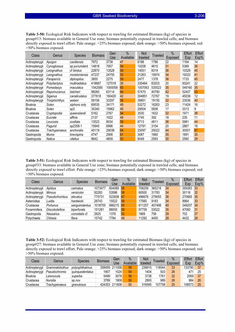
GBR Seabed Biodiversity 3-206
Table 3-50: Ecological Risk Indicators with respect to trawling for estimated Biomass (kg) of species in group#13: biomass available in General Use zone; biomass potentially exposed in trawled cells; and biomass directly exposed to trawl effort. Pale orange: >25% biomass exposed; dark orange: >50% biomass exposed; red: >50% biomass exposed.
Class Genus Species Biomass Gen Use
% Available Not
trawled Trawled % Exposed Effort
Exp Effort Exp%
Actinopterygii Apogon cavitiensis 7972 3738 47 6186 1786 22 1164 14 Actinopterygii Cynoglossus sp juv/unident 14818 7957 54 10208 4610 31 5389 36 Actinopterygii Leiognathus cf bindus 22870 13528 59 14551 8319 36 10329 45 Actinopterygii Leiognathus moretoniensis 47237 24755 52 31263 15974 34 19323 41 Actinopterygii Parapercis diplospilus 3855 2275 59 2477 1378 36 1733 45 Actinopterygii Polydactylus multiradiatus 418667 127018 30 335464 83203 20 93241 22 Actinopterygii Pomadasys maculatus 1542585 1000058 65 1007063 535523 35 549160 35 Actinopterygii Repomucenus belcheri 98260 63114 64 57470 40790 42 52407 53 Actinopterygii Siganus canaliculatus 377618 160420 42 304851 72767 19 45039 12 Actinopterygii Trixiphichthys weberi 59106 33297 56 39951 19155 32 23536 40 Bivalvia Solen siphons only 69535 34171 49 53272 16263 23 11424 16 Bivalvia Solen sp3 35340 15962 45 29504 5836 17 3313 9 Crustacea Cryptopodia queenslandi 5162 2767 54 3530 1632 32 1971 38 Crustacea Eucrate affinis 2137 1022 48 1745 392 18 235 11 Crustacea Leucosia ocellata 13523 8034 59 8713 4811 36 5981 44 Crustacea Pagurid sp2358-1 15945 6996 44 12791 3154 20 2867 18 Crustacea Trachypenaeus anchoralis 45119 29038 64 25097 20022 44 30501 67 Gastropoda Murex brevispina 4747 2906 61 3087 1660 35 1691 35 Gastropoda Natica vitellus 8642 4609 53 6049 2593 30 2560 29
Table 3-51: Ecological Risk Indicators with respect to trawling for estimated Biomass (kg) of species in group#33: biomass available in General Use zone; biomass potentially exposed in trawled cells; and biomass directly exposed to trawl effort. Pale orange: >25% biomass exposed; dark orange: >50% biomass exposed; red: >50% biomass exposed.
Class Genus Species Biomass Gen Use
% Available Not
trawled Trawled % Exposed Effort
Exp Effort Exp%
Actinopterygii Apistus carinatus 1073477 604069 56 708259 365218 34 359383 33 Actinopterygii Minous versicolor 92283 53586 58 60500 31783 34 30116 32 Actinopterygii Pseudorhombus elevatus 775731 522838 67 496676 279055 36 270665 35 Asteroidea Luidia hardwicki 26743 15522 58 17560 9183 34 8964 33 Crustacea Portunus sanguinolentus 1018755 666215 65 611257 407498 40 349207 34 Foraminifera Discobotellina biperforata 151281 88000 58 97759 53522 35 47083 31 Gastropoda Nassarius conoidalis cf 2625 1378 52 1869 756 29 702 27 Polychaeta Chloeia flava 15742 7784 49 11292 4450 28 4432 28
Table 3-52: Ecological Risk Indicators with respect to trawling for estimated Biomass (kg) of species in group#27: biomass available in General Use zone; biomass potentially exposed in trawled cells; and biomass directly exposed to trawl effort. Pale orange: >25% biomass exposed; dark orange: >50% biomass exposed; red: >50% biomass exposed.
Class Genus Species Biomass Gen Use
% Available Not
trawled Trawled % Exposed Effort
Exp Effort Exp%
Actinopterygii Grammatobothus polyophthalmus 358459 211058 59 239915 118544 33 133790 37 Actinopterygii Pseudochromis quinquedentatus 1907 1024 54 1404 503 26 471 25 Bivalvia Leionucula superba 5499 3078 56 3738 1761 32 2069 37 Crustacea Nursilia sp nov 3789 1909 50 2800 989 26 984 26 Crustacea Trachypenaeus granulosus 424353 211608 50 316595 107758 25 108573 25
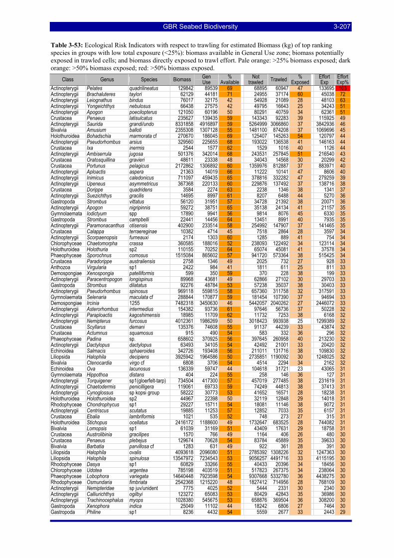
GBR Seabed Biodiversity 3-207
Table 3-53: Ecological Risk Indicators with respect to trawling for estimated Biomass (kg) of top ranking species in groups with low total exposure (<25%): biomass available in General Use zone; biomass potentially exposed in trawled cells; and biomass directly exposed to trawl effort. Pale orange: >25% biomass exposed; dark orange: >50% biomass exposed; red: >50% biomass exposed.
Class Genus Species Biomass Gen Use
% Available Not
trawled Trawled % Exposed Effort
Exp Effort Exp%
Actinopterygii Pelates quadrilineatus 129842 89539 69 68895 60947 47 133695 103 Actinopterygii Brachaluteres taylori 62129 44181 71 24955 37174 60 45038 72 Actinopterygii Leiognathus bindus 76017 32175 42 54928 21089 28 48103 63 Actinopterygii Yongeichthys nebulosus 66438 27575 42 49795 16643 25 34243 51 Actinopterygii Apogon poecilopterus 121050 60196 50 80291 40759 34 62361 51 Crustacea Penaeus latisulcatus 235627 139435 59 143343 92283 39 115925 49 Actinopterygii Saurida grandi/undo 8331858 4916897 59 5264999 3066860 37 3842936 46 Bivalvia Amusium balloti 2355308 1307128 55 1481100 874208 37 1069696 45 Holothuroidea Bohadschia marmorata cf 270670 186045 69 125407 145263 54 120797 44 Actinopterygii Pseudorhombus arsius 329560 225655 68 193022 136538 41 146163 44 Crustacea Ixa inermis 2544 1577 62 1529 1016 40 1126 44 Actinopterygii Ambiserrula jugosa 501376 342014 68 243531 257845 51 216540 43 Crustacea Oratosquillina gravieri 48611 23338 48 34043 14568 30 20299 42 Crustacea Portunus pelagicus 2172862 1306892 60 1359976 812887 37 883971 40 Actinopterygii Aploactis aspera 21363 14019 66 11222 10141 47 8606 40 Actinopterygii Inimicus caledonicus 711097 459435 65 378816 332282 47 279259 39 Actinopterygii Upeneus asymmetricus 367368 220133 60 229876 137492 37 138716 38 Crustacea Dorippe quadridens 3584 2274 63 2238 1346 38 1341 37 Actinopterygii Suezichthys gracilis 14695 8997 61 8207 6488 44 5270 36 Gastropoda Strombus vittatus 56120 31951 57 34728 21392 38 20071 36 Actinopterygii Apogon nigripinnis 59272 38751 65 35138 24134 41 21157 35 Gymnolaemata Iodictyum spp 17890 9941 56 9814 8076 45 6330 35 Gastropoda Strombus campbelli 22441 14456 64 13451 8991 40 7935 35 Actinopterygii Paramonacanthus otisensis 402900 233514 58 254992 147907 37 141465 35 Crustacea Calappa terraereginae 10382 4714 45 7518 2864 28 3597 34 Actinopterygii Scorpaenopsis furneauxi 2174 1303 60 1285 889 41 754 34 Chlorophyceae Chaetomorpha crassa 360585 188016 52 238093 122492 34 123114 34 Holothuroidea Holothuria sp2 110155 70252 64 65074 45081 41 37578 34 Phaeophyceae Sporochnus comosus 1515084 865602 57 941720 573364 38 515425 34 Crustacea Paradorippe australiensis 2758 1346 49 2025 732 27 928 33 Anthozoa Virgularia sp1 2422 984 41 1811 611 25 811 33 Demospongiae Xenospongia patelliformis 599 350 59 370 228 38 199 33 Actinopterygii Paracentropogon longispinus 89968 43681 49 62866 27102 30 29703 33 Gastropoda Strombus dilatatus 92276 48784 53 57238 35037 38 30403 33 Actinopterygii Pseudorhombus spinosus 969118 559815 58 657360 311758 32 317591 33 Gymnolaemata Selenaria maculata cf 288844 170877 59 181454 107390 37 94694 33 Demospongiae Ircinia 1255 7482318 3450630 46 5442057 2040262 27 2446072 33 Actinopterygii Asterorhombus intermedius 154382 93736 61 97646 56736 37 50228 32 Actinopterygii Paraploactis kagoshimensis 18985 11709 62 11732 7253 38 6168 32 Actinopterygii Nemipterus furcosus 4012361 1986269 50 3018423 993938 25 1299389 32 Crustacea Scyllarus demani 135376 74608 55 91137 44239 33 43874 32 Crustacea Actumnus squamosus 915 490 54 583 332 36 296 32 Phaeophyceae Padina sp. 658602 370925 56 397645 260958 40 213230 32 Actinopterygii Dactylopus dactylopus 63493 34105 54 42492 21001 33 20420 32 Echinoidea Salmacis sphaeroides 342726 193408 56 211011 131716 38 109830 32 Liliopsida Halophila decipiens 3925942 1964586 50 2735851 1190092 30 1248025 32 Bivalvia Ctenocardia virgo cf 6808 3706 54 4514 2294 34 2162 32 Echinoidea Ova lacunosus 136339 59747 44 104618 31721 23 43065 31 Gymnolaemata Hippothoa distans 404 224 55 258 146 36 127 31 Actinopterygii Torquigener sp1(gloerfelt-tarp) 734504 417300 57 457019 277485 38 231619 31 Actinopterygii Chaetodermis penicilligera 119061 69733 59 74249 44813 38 37413 31 Actinopterygii Cynoglossus sp kopsi group 58222 30773 53 41652 16571 28 18238 31 Holothuroidea Holothuroidea sp2 44967 22398 50 32119 12848 29 14018 31 Rhodophyceae Chondrophycus sp1 29227 15711 54 18081 11146 38 9072 31 Actinopterygii Centriscus scutatus 19885 11253 57 12852 7033 35 6157 31 Crustacea Ebalia lambriformis 1021 535 52 748 273 27 315 31 Holothuroidea Stichopus ocellatus 2416172 1188600 49 1732647 683525 28 744082 31 Bivalvia Lomopsis sp1 61039 31169 51 43409 17631 29 18758 31 Crustacea Austrolibinia gracilipes 1570 766 49 1164 406 26 480 30 Crustacea Penaeus plebejus 129674 70628 54 83784 45889 35 39633 30 Bivalvia Barbatia parvillosa cf 1283 631 49 922 361 28 391 30 Liliopsida Halophila ovalis 4093618 2096080 51 2785392 1308226 32 1247363 30 Liliopsida Halophila spinulosa 13547972 7234543 53 9056257 4491716 33 4115195 30 Rhodophyceae Dasya sp1 60829 33266 55 40433 20396 34 18456 30 Chlorophyceae Udotea argentea 785198 403519 51 517823 267375 34 238064 30 Phaeophyceae Lobophora variegata 14640448 7923598 54 9307668 5332780 36 4438275 30 Rhodophyceae Osmundaria fimbriata 2542368 1215220 48 1827412 714956 28 768109 30 Actinopterygii Nemipteridae sp juv/unident 7775 4025 52 5444 2331 30 2340 30 Actinopterygii Calliurichthys ogilbyi 123272 65083 53 80429 42843 35 36986 30 Actinopterygii Trachinocephalus myops 1028380 545675 53 658876 369504 36 308200 30 Gastropoda Xenophora indica 25049 11102 44 18242 6806 27 7464 30 Gastropoda Philine sp1 8236 4432 54 5559 2677 33 2443 29
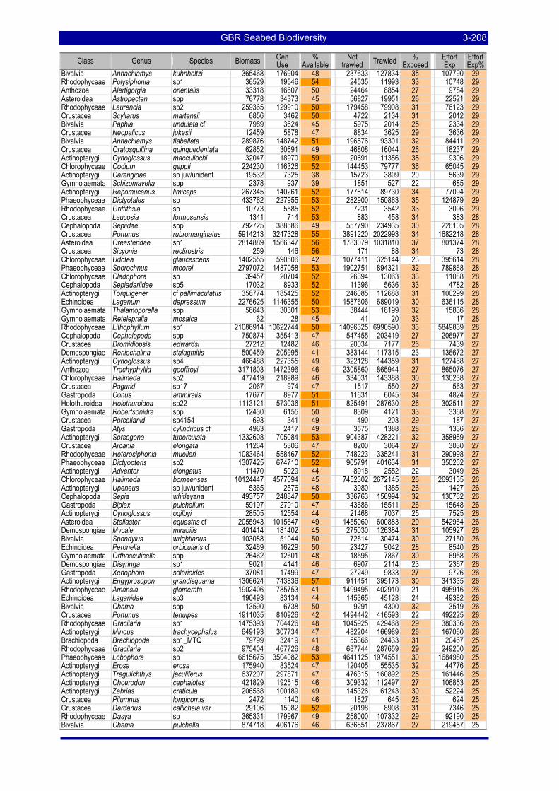
GBR Seabed Biodiversity 3-208
Class Genus Species Biomass Gen Use
% Available Not
trawled Trawled % Exposed Effort
Exp Effort Exp%
Bivalvia Annachlamys kuhnholtzi 365468 176904 48 237633 127834 35 107790 29 Rhodophyceae Polysiphonia sp1 36529 19546 54 24535 11993 33 10748 29 Anthozoa Alertigorgia orientalis 33318 16607 50 24464 8854 27 9784 29 Asteroidea Astropecten spp 76778 34373 45 56827 19951 26 22521 29 Rhodophyceae Laurencia sp2 259365 129910 50 179458 79908 31 76123 29 Crustacea Scyllarus martensii 6856 3462 50 4722 2134 31 2012 29 Bivalvia Paphia undulata cf 7989 3624 45 5975 2014 25 2334 29 Crustacea Neopalicus jukesii 12459 5878 47 8834 3625 29 3636 29 Bivalvia Annachlamys flabellata 289876 148742 51 196576 93301 32 84411 29 Crustacea Oratosquillina quinquedentata 62852 30691 49 46808 16044 26 18237 29 Actinopterygii Cynoglossus maccullochi 32047 18970 59 20691 11356 35 9306 29 Chlorophyceae Codium geppii 224230 116326 52 144453 79777 36 65045 29 Actinopterygii Carangidae sp juv/unident 19532 7325 38 15723 3809 20 5639 29 Gymnolaemata Schizomavella spp 2378 937 39 1851 527 22 685 29 Actinopterygii Repomucenus limiceps 267345 140261 52 177614 89730 34 77094 29 Phaeophyceae Dictyotales sp 433762 227955 53 282900 150863 35 124879 29 Rhodophyceae Griffithsia sp 10773 5585 52 7231 3542 33 3096 29 Crustacea Leucosia formosensis 1341 714 53 883 458 34 383 28 Cephalopoda Sepiidae spp 792725 388586 49 557790 234935 30 226105 28 Crustacea Portunus rubromarginatus 5914213 3247328 55 3891220 2022993 34 1682218 28 Asteroidea Oreasteridae sp1 2814889 1566347 56 1783079 1031810 37 801374 28 Crustacea Sicyonia rectirostris 259 146 56 171 88 34 73 28 Chlorophyceae Udotea glaucescens 1402555 590506 42 1077411 325144 23 395614 28 Phaeophyceae Sporochnus moorei 2797072 1487058 53 1902751 894321 32 789868 28 Chlorophyceae Cladophora sp 39457 20704 52 26394 13063 33 11088 28 Cephalopoda Sepiadariidae sp5 17032 8933 52 11396 5636 33 4782 28 Actinopterygii Torquigener cf pallimaculatus 358774 185425 52 246085 112688 31 100299 28 Echinoidea Laganum depressum 2276625 1146355 50 1587606 689019 30 636115 28 Gymnolaemata Thalamoporella spp 56643 30301 53 38444 18199 32 15836 28 Gymnolaemata Retelepralia mosaica 62 28 45 41 20 33 17 28 Rhodophyceae Lithophyllum sp1 21086914 10622744 50 14096325 6990590 33 5849839 28 Cephalopoda Cephalopoda spp 750874 355413 47 547455 203419 27 206977 27 Crustacea Dromidiopsis edwardsi 27212 12482 46 20034 7177 26 7439 27 Demospongiae Reniochalina stalagmitis 500459 205995 41 383144 117315 23 136672 27 Actinopterygii Cynoglossus sp4 466488 227355 49 322128 144359 31 127468 27 Anthozoa Trachyphyllia geoffroyi 3171803 1472396 46 2305860 865944 27 865076 27 Chlorophyceae Halimeda sp2 477419 218989 46 334031 143388 30 130238 27 Crustacea Pagurid sp17 2067 974 47 1517 550 27 563 27 Gastropoda Conus ammiralis 17677 8977 51 11631 6045 34 4824 27 Holothuroidea Holothuroidea sp22 1113121 573036 51 825491 287630 26 302511 27 Gymnolaemata Robertsonidra spp 12430 6155 50 8309 4121 33 3368 27 Crustacea Porcellanid sp4154 693 341 49 490 203 29 187 27 Gastropoda Atys cylindricus cf 4963 2417 49 3575 1388 28 1336 27 Actinopterygii Sorsogona tuberculata 1332608 705084 53 904387 428221 32 358959 27 Crustacea Arcania elongata 11264 5306 47 8200 3064 27 3030 27 Rhodophyceae Heterosiphonia muelleri 1083464 558467 52 748223 335241 31 290998 27 Phaeophyceae Dictyopteris sp2 1307425 674710 52 905791 401634 31 350262 27 Actinopterygii Adventor elongatus 11470 5029 44 8918 2552 22 3049 26 Chlorophyceae Halimeda borneenses 10124447 4577094 45 7452302 2672145 26 2693135 26 Actinopterygii Upeneus sp juv/unident 5365 2576 48 3980 1385 26 1427 26 Cephalopoda Sepia whitleyana 493757 248847 50 336763 156994 32 130762 26 Gastropoda Biplex pulchellum 59197 27910 47 43686 15511 26 15648 26 Actinopterygii Cynoglossus ogilbyi 28505 12554 44 21468 7037 25 7525 26 Asteroidea Stellaster equestris cf 2055943 1015647 49 1455060 600883 29 542964 26 Demospongiae Mycale mirabilis 401414 181402 45 275030 126384 31 105927 26 Bivalvia Spondylus wrightianus 103088 51044 50 72614 30474 30 27150 26 Echinoidea Peronella orbicularis cf 32469 16229 50 23427 9042 28 8540 26 Gymnolaemata Orthoscuticella spp 26462 12601 48 18595 7867 30 6958 26 Demospongiae Disyringa sp1 9021 4141 46 6907 2114 23 2367 26 Gastropoda Xenophora solarioides 37081 17499 47 27249 9833 27 9726 26 Actinopterygii Engyprosopon grandisquama 1306624 743836 57 911451 395173 30 341335 26 Rhodophyceae Amansia glomerata 1902406 785753 41 1499495 402910 21 495916 26 Echinoidea Laganidae sp3 190493 83134 44 145365 45128 24 49382 26 Bivalvia Chama spp 13590 6738 50 9291 4300 32 3519 26 Crustacea Portunus tenuipes 1911035 810926 42 1494442 416593 22 492225 26 Rhodophyceae Gracilaria sp1 1475393 704426 48 1045925 429468 29 380336 26 Actinopterygii Minous trachycephalus 649193 307734 47 482204 166989 26 167060 26 Brachiopoda Brachiopoda sp1_MTQ 79799 32419 41 55366 24433 31 20467 25 Rhodophyceae Gracilaria sp2 975404 467726 48 687744 287659 29 249200 25 Phaeophyceae Lobophora sp 6615675 3504082 53 4641125 1974551 30 1684980 25 Actinopterygii Erosa erosa 175940 83524 47 120405 55535 32 44776 25 Actinopterygii Tragulichthys jaculiferus 637207 297871 47 476315 160892 25 161446 25 Actinopterygii Choerodon cephalotes 421829 192515 46 309332 112497 27 106853 25 Actinopterygii Zebrias craticula 206568 100189 49 145326 61243 30 52224 25 Crustacea Pilumnus longicornis 2472 1140 46 1827 645 26 624 25 Crustacea Dardanus callichela var 29106 15082 52 20198 8908 31 7346 25 Rhodophyceae Dasya sp 365331 179967 49 258000 107332 29 92190 25 Bivalvia Chama pulchella 874718 406176 46 636851 237867 27 219457 25
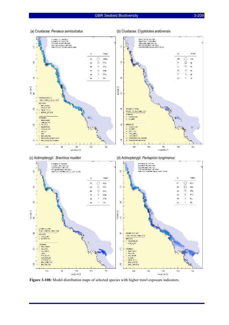
GBR Seabed Biodiversity 3-209
(a) Crustacea: Penaeus semisulcatus (b) Crustacea: Cryptolutea arafurensis
(c) Actinopterygii: Brachirus muelleri (d) Actinopterygii: Pentaprion longimanus
Figure 3-108: Model distribution maps of selected species with higher trawl exposure indicators.
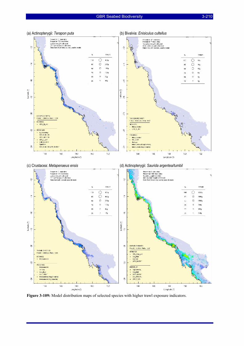
GBR Seabed Biodiversity 3-210
(a) Actinopterygii: Terapon puta (b) Bivalvia: Enisiculus cultellus
(c) Crustacea: Metapenaeus ensis (d) Actinopterygii: Saurida argentea/tumbil
Figure 3-109: Model distribution maps of selected species with higher trawl exposure indicators.
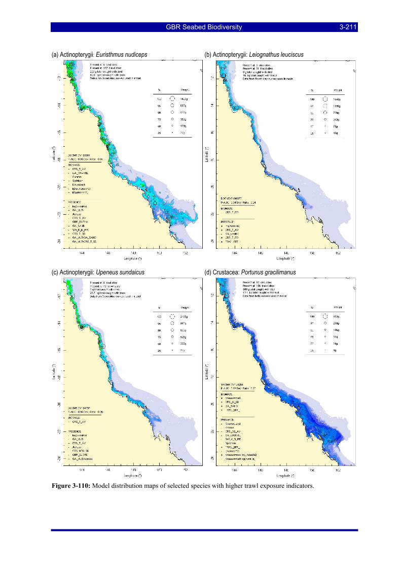
GBR Seabed Biodiversity 3-211
(a) Actinopterygii: Euristhmus nudiceps (b) Actinopterygii: Leiognathus leuciscus
(c) Actinopterygii: Upeneus sundaicus (d) Crustacea: Portunus gracilimanus
Figure 3-110: Model distribution maps of selected species with higher trawl exposure indicators.
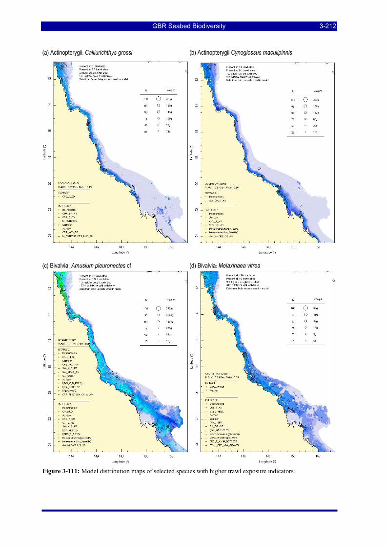
GBR Seabed Biodiversity 3-212
(a) Actinopterygii: Calliurichthys grossi (b) Actinopterygii Cynoglossus maculipinnis
(c) Bivalvia: Amusium pleuronectes cf (d) Bivalvia: Melaxinaea vitrea
Figure 3-111: Model distribution maps of selected species with higher trawl exposure indicators.
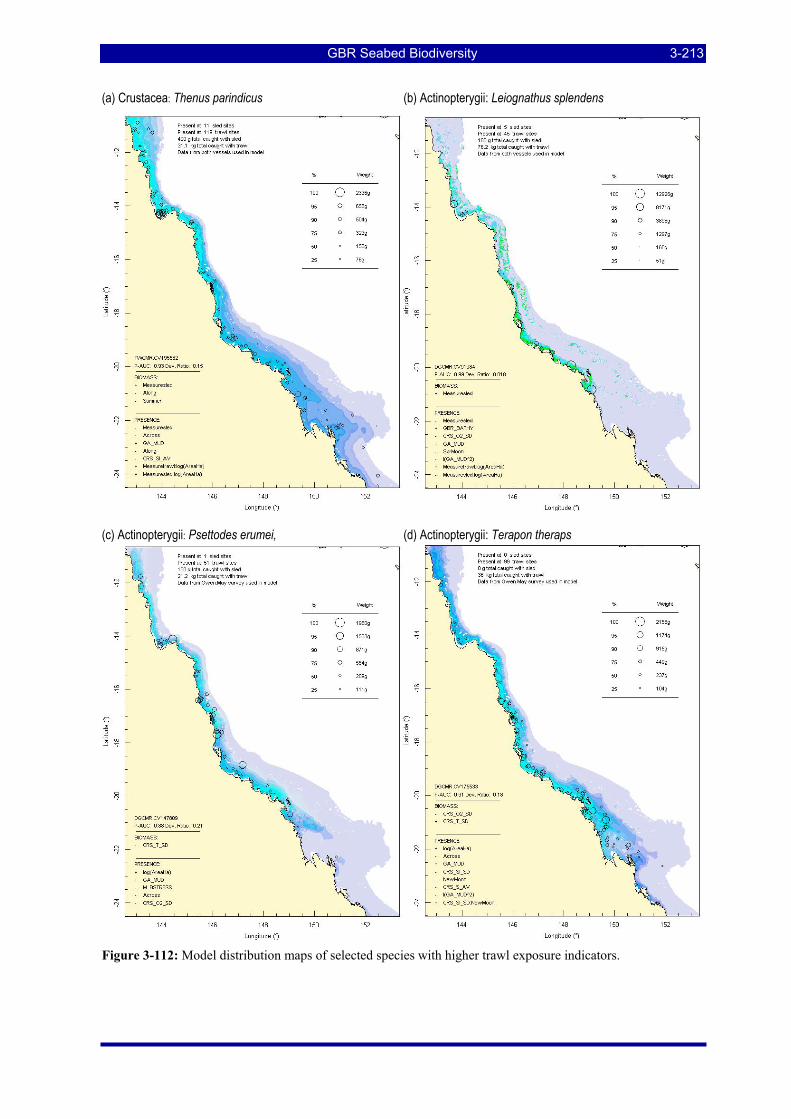
GBR Seabed Biodiversity 3-213
(a) Crustacea: Thenus parindicus (b) Actinopterygii: Leiognathus splendens
(c) Actinopterygii: Psettodes erumei, (d) Actinopterygii: Terapon theraps
Figure 3-112: Model distribution maps of selected species with higher trawl exposure indicators.
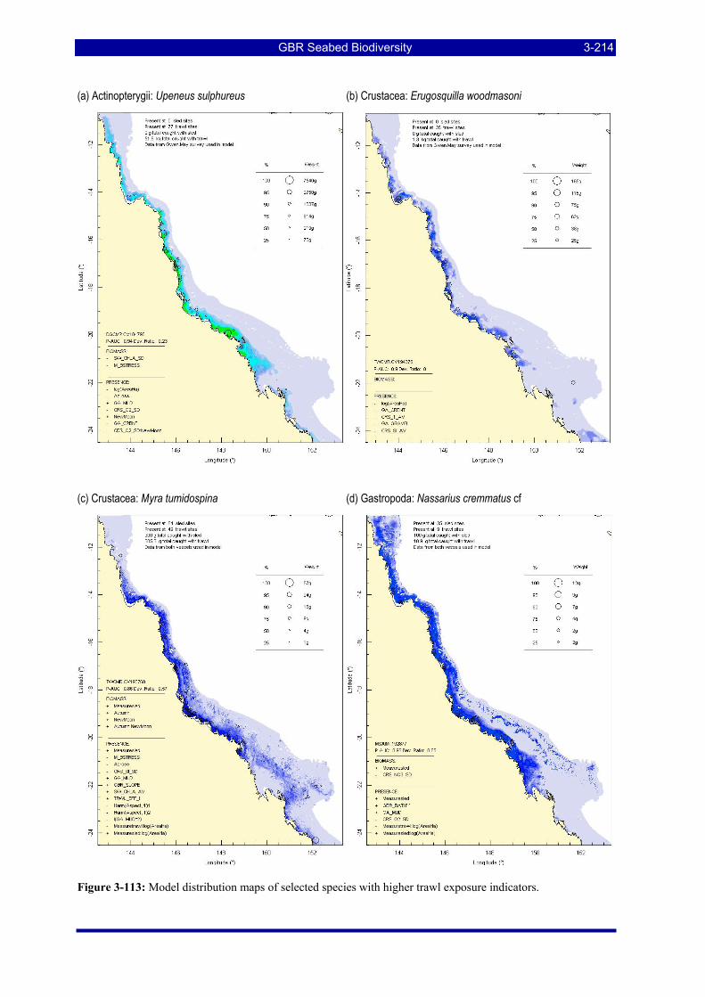
GBR Seabed Biodiversity 3-214
(a) Actinopterygii: Upeneus sulphureus (b) Crustacea: Erugosquilla woodmasoni
(c) Crustacea: Myra tumidospina (d) Gastropoda: Nassarius cremmatus cf
Figure 3-113: Model distribution maps of selected species with higher trawl exposure indicators.
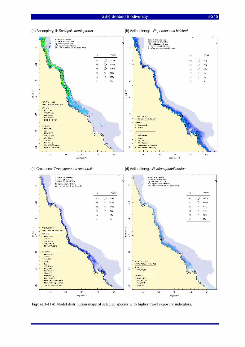
GBR Seabed Biodiversity 3-215
(a) Actinopterygii: Scolopsis taeniopterus (b) Actinopterygii: Repomucenus belcheri
(c) Crustacea: Trachypenaeus anchoralis (d) Actinopterygii: Pelates quadrilineatus
Figure 3-114: Model distribution maps of selected species with higher trawl exposure indicators.
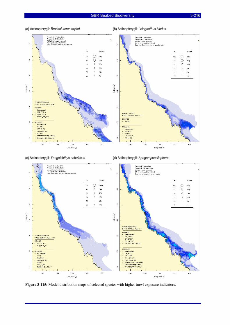
GBR Seabed Biodiversity 3-216
(a) Actinopterygii: Brachaluteres taylori (b) Actinopterygii: Leiognathus bindus
(c) Actinopterygii: Yongeichthys nebulosus (d) Actinopterygii: Apogon poecilopterus
Figure 3-115: Model distribution maps of selected species with higher trawl exposure indicators.
GBR Seabed Biodiversity 3-217
Modelling of the presences of BRUVS fishes provided distribution maps for a total of 25 species (Section 3.1.2), including 6 species that were infrequent in trawl data and not modelled, and 4 species were not sampled at all by the research trawl. The proportion of populations in GU zones for these 10 species ranged from 38–54%, the proportions in cells with recorded effort ranged from 20–33%, and proportions exposed to trawl effort ranged from 13–28%. These species in order of total effort exposure (%) included: Gymnothorax minor (28), Alepes apercna (27), Scomberomorus queenslandicus (27), Echeneis naucrates (26), Carangoides coeruleopinnatus (25), Gnathanodon speciosus (22), Seriolina nigrofasciata (19), Carangoides gymnostethus (19), Decapterus russelli (16) and Carangoides fulvoguttatus (13). As these species were rare or absent from the prawn trawl samples, it follows that their catchability was low or very low (as corroborated by relative catch rates of Fish Trawls from the Effects of Trawling Study, Poiner et al. 1998) and the proportions of their populations caught is likely to be considerably less than the proportions exposed.
In the case of those BRUVS fish species also analysed from research trawl data sources, the exposure assessments were similar and did not change the level of risk for any species — even though BRUVS were able to be deployed in areas too rugged for the trawl.
3.7.2.1. Trawl effort coefficients
The species modelling process selected the Trawl Effort Index covariate for 81 of 840 species analysed (9.6%), and was significant in 55 cases (6.5%). This frequency is little more than expected by chance and suggests that trawling does not have a strong influence on overall seabed distribution patterns. Nevertheless, taking each species model as an independent test, but recalling the caution expressed in Section 2.4.7, the probability of presence was negatively affected for 43 species, significant in 24 cases; biomass was negatively affected for 7 species, significant in each case (Table 3-54). Probability of presence was positively affected for 11 species, significant in all cases, and biomass was positively affected for 1 species, also significant (Table 3-55). Thirteen species had models with a second term involving the Trawl Effort covariate — in addition to a linear Trawl Effort term for presence or biomass — such as biomass, a quadratic or an interaction (Table 3-56).
The possible magnitude of the Trawl Effort coefficient where selected, in terms of predicted percent change in overall biomass, is also indicated in the Tables. Of the 50 negative Trawl Effort responses, five species (3 significant) were estimated to have moderate negative change in biomass of >25%–33%, compared with a model prediction with trawl effort set to zero over the entire region (Table 3-54). Another 15 species (9 significant) were estimated to have negative change in biomass of 15%–25%. The remaining 30 negative responses (19 significant) were between –1% and –15%. There was considerable uncertainty in these estimates. In the case of non-significant coefficients, the uncertainty was greater than the estimate and so includes the possibility of no (or even positive) change due to trawl effort. In the case of significant coefficients, the typical uncertainty was about 75% of the estimate. Not surprisingly, all species with negative trawl coefficients have low to very low exposure to current effort.
Species for which the negative trawl effect was larger and significant are examined in more detail below. The first point to note is that many of these species tended to be infrequent and low in abundance, which can present a challenge for the modelling. Further, while many of the AUC diagnostics were reasonable, the presence models for these species typically selected very few environmental covariates and the biomass models often did not select any environmental covariates — this tended to lead to rather smooth distribution predictions. On the other hand, those species with significant small negative coefficients (% change < -10%) were almost always more frequently sampled and more abundant, with more specific biophysical models.
The species with the largest significant predicted negative change (-33%) was the Majid crab Thacanophrys sp165 (Figure 3-116a). This species appears to have a widely scattered distribution in non-muddy environments, as indicated by the negative mud coefficient. Given the significant negative trawl coefficient, there was a statistical expectation that this species would have greater presence on
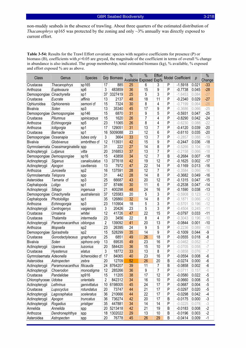
GBR Seabed Biodiversity 3-218
non-muddy seabeds in the absence of trawling. About three quarters of the estimated distribution of Thacanophrys sp165 was protected by the zoning and only ~3% annually was directly exposed to current effort.
Table 3-54: Results for the Trawl Effort covariate: species with negative coefficients for presence (P) or biomass (B), coefficients with p>0.05 are greyed, the magnitude of the coefficient in terms of overall % change in abundance is also indicated. The group membership, total estimated biomass (kg), % available, % exposed and effort exposed % are as above.
Class Genus Species Grp Biomass % Available
% Exposed
Effort Exp% Model Coefficient p %
Change Crustacea Thacanophrys sp165 17 885 25 6 3 P -1.5918 0.021 -33 Anthozoa Euplexaura sp6 3 483859 36 15 9 P -0.7738 0.045 -28 Demospongiae Cinachyrella sp1 37 3327419 25 5 3 P -1.6453 0.084 -27 Crustacea Eucrate affinis 13 2137 48 18 11 P -0.2340 0.029 -27 Ophiuroidea Ophionereis semoni cf 15 7324 30 8 4 P -0.7199 0.064 -26 Bivalvia Solen sp3 13 35340 45 17 9 P -0.3686 0.066 -25 Demospongiae Demospongiae sp146 15 6870 31 9 5 P -0.5931 0.047 -25 Crustacea Pilumnus spinicarpus 15 1620 26 7 4 P -0.8290 0.042 -24 Anthozoa Echinogorgia sp5 23 11065 26 8 4 P -0.6230 0.088 -22 Anthozoa Iciligorgia sp1 17 129051 31 13 7 P -0.4120 0.039 -20 Crustacea Barnacle sp1 16 5009088 23 12 6 P -0.6110 0.035 -20 Demospongiae Oceanapia tubes only 3 3664 33 13 7 P -0.2857 0.088 -19 Bivalvia Globivenus embrithes cf 12 113931 42 15 9 P -0.2447 0.036 -18 Gymnolaemata Crassimarginatella spp 31 222 27 14 8 P -0.5266 0.104 -18 Actinopterygii Lutjanus vitta 20 316853 37 13 7 P -0.2158 0.066 -18 Demospongiae Demospongiae sp16 15 43858 34 12 7 B -0.2684 0.007 -18 Actinopterygii Siganus canaliculatus 13 377618 42 19 12 P -0.1625 0.002 -17 Actinopterygii Apogon cavitiensis 13 7972 47 22 14 P -0.1169 0.013 -16 Anthozoa Junceella sp2 16 137591 28 12 7 P -0.3584 0.066 -16 Gymnolaemata Telopora spp 31 442 28 14 8 P -0.3682 0.049 -16 Asteroidea Tamaria cf sp3 25 66687 43 20 12 P -0.1315 0.047 -15 Cephalopoda Loligo sp1 37 87486 30 11 6 P -0.2538 0.047 -14 Actinopterygii Sillago ingenuua 21 400298 48 24 16 P -0.1590 0.038 -13 Demospongiae Cinachyrella australiensis 37 125583 20 5 3 P -0.5908 0.123 -13 Cephalopoda Photololligo sp1 35 126860 32 14 8 P -0.1871 0.066 -12 Anthozoa Echinogorgia sp3 23 110904 18 5 3 P -0.5701 0.196 -12 Actinopterygii Centrogenys vaigiensis 3 20426 23 5 3 P -0.4504 0.245 -11 Crustacea Urnalana whitei 12 41726 47 22 15 P -0.0797 0.033 -11 Crustacea Thalamita intermedia 23 3456 22 8 4 P -0.3043 0.196 -10 Actinopterygii Paramonacanthus oblongus 2 139092 41 20 13 P -0.0844 0.001 -10 Anthozoa Mopsella sp2 23 26395 24 9 5 P -0.2236 0.089 -10 Demospongiae Spirastrella sp2 15 528299 35 14 9 P -0.1009 0.044 -9 Crustacea Gonodactylaceus graphurus 25 6851 49 26 18 P -0.0555 0.018 -8 Bivalvia Solen siphons only 13 69535 49 23 16 P -0.0462 0.052 -7 Actinopterygii Upeneus luzonius 20 584420 36 15 10 P -0.0705 0.058 -7 Crustacea Hyastenus elatus 3 18772 33 13 8 P -0.0858 0.076 -7 Gymnolaemata Adeonella lichenoides cf 17 84065 40 23 16 P -0.0554 0.008 -6 Asteroidea Astropecten zebra 20 12709 52 26 20 B -0.0274 0.000 -6 Actinopterygii Paramonacanthus filicauda 24 8764207 39 11 7 B -0.0858 0.002 -6 Actinopterygii Choerodon monostigma 12 285266 36 9 7 P -0.0711 0.157 -6 Crustacea Pandalidae sp916 15 11205 38 17 12 P -0.0580 0.022 -5 Chlorophyceae Udotea orientalis 2 842312 34 16 10 P -0.0660 0.008 -5 Actinopterygii Lethrinus genivittatus 10 6198005 45 24 17 P -0.0687 0.004 -5 Crustacea Lupocyclus rotundatus 20 73747 44 21 17 P -0.0297 0.020 -5 Actinopterygii Lagocephalus sceleratus 36 210666 44 22 17 P -0.0298 0.042 -4 Actinopterygii Apogon truncatus 36 736274 42 20 17 B -0.0175 0.000 -3 Actinopterygii Rogadius pristiger 35 447881 34 14 14 P -0.0225 0.078 -3 Annelida Annelida spp 20 5213418 42 21 19 B -0.0183 0.008 -2 Anthozoa Dendronephthya spp 18 1302022 29 13 10 B -0.0196 0.003 -2 Asteroidea Astropecten spp 20 76778 45 26 29 B -0.0414 0.009 -1
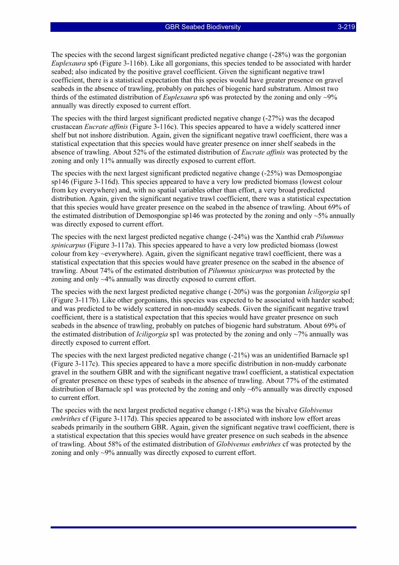
GBR Seabed Biodiversity 3-219
The species with the second largest significant predicted negative change (-28%) was the gorgonian Euplexaura sp6 (Figure 3-116b). Like all gorgonians, this species tended to be associated with harder seabed; also indicated by the positive gravel coefficient. Given the significant negative trawl coefficient, there is a statistical expectation that this species would have greater presence on gravel seabeds in the absence of trawling, probably on patches of biogenic hard substratum. Almost two thirds of the estimated distribution of Euplexaura sp6 was protected by the zoning and only ~9% annually was directly exposed to current effort.
The species with the third largest significant predicted negative change (-27%) was the decapod crustacean Eucrate affinis (Figure 3-116c). This species appeared to have a widely scattered inner shelf but not inshore distribution. Again, given the significant negative trawl coefficient, there was a statistical expectation that this species would have greater presence on inner shelf seabeds in the absence of trawling. About 52% of the estimated distribution of Eucrate affinis was protected by the zoning and only 11% annually was directly exposed to current effort.
The species with the next largest significant predicted negative change (-25%) was Demospongiae sp146 (Figure 3-116d). This species appeared to have a very low predicted biomass (lowest colour from key everywhere) and, with no spatial variables other than effort, a very broad predicted distribution. Again, given the significant negative trawl coefficient, there was a statistical expectation that this species would have greater presence on the seabed in the absence of trawling. About 69% of the estimated distribution of Demospongiae sp146 was protected by the zoning and only ~5% annually was directly exposed to current effort.
The species with the next largest predicted negative change (-24%) was the Xanthid crab Pilumnus spinicarpus (Figure 3-117a). This species appeared to have a very low predicted biomass (lowest colour from key ~everywhere). Again, given the significant negative trawl coefficient, there was a statistical expectation that this species would have greater presence on the seabed in the absence of trawling. About 74% of the estimated distribution of Pilumnus spinicarpus was protected by the zoning and only ~4% annually was directly exposed to current effort.
The species with the next largest predicted negative change (-20%) was the gorgonian Iciligorgia sp1 (Figure 3-117b). Like other gorgonians, this species was expected to be associated with harder seabed; and was predicted to be widely scattered in non-muddy seabeds. Given the significant negative trawl coefficient, there is a statistical expectation that this species would have greater presence on such seabeds in the absence of trawling, probably on patches of biogenic hard substratum. About 69% of the estimated distribution of Iciligorgia sp1 was protected by the zoning and only ~7% annually was directly exposed to current effort.
The species with the next largest predicted negative change (-21%) was an unidentified Barnacle sp1 (Figure 3-117c). This species appeared to have a more specific distribution in non-muddy carbonate gravel in the southern GBR and with the significant negative trawl coefficient, a statistical expectation of greater presence on these types of seabeds in the absence of trawling. About 77% of the estimated distribution of Barnacle sp1 was protected by the zoning and only ~6% annually was directly exposed to current effort.
The species with the next largest predicted negative change (-18%) was the bivalve Globivenus embrithes cf (Figure 3-117d). This species appeared to be associated with inshore low effort areas seabeds primarily in the southern GBR. Again, given the significant negative trawl coefficient, there is a statistical expectation that this species would have greater presence on such seabeds in the absence of trawling. About 58% of the estimated distribution of Globivenus embrithes cf was protected by the zoning and only ~9% annually was directly exposed to current effort.
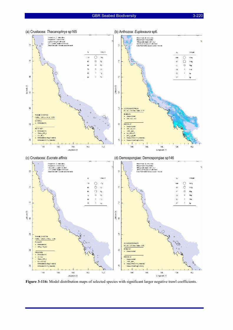
GBR Seabed Biodiversity 3-220
(a) Crustacea: Thacanophrys sp165 (b) Anthozoa: Euplexaura sp6.
(c) Crustacea: Eucrate affinis (d) Demospongiae: Demospongiae sp146
Figure 3-116: Model distribution maps of selected species with significant larger negative trawl coefficients.
GBR Seabed Biodiversity 3-221
(a) Crustacea: Pilumnus spinicarpus (b) Anthozoa: Iciligorgia sp1
(c) Crustacea: Barnacle sp1 (d) Bivalvia: Globivenus embrithes cf
Figure 3-117: Model distribution maps of selected species with significant larger negative trawl coefficients.
The 12 positive Trawl Effort responses were relatively smaller, four species (all significant) were estimated to have positive change in biomass of >12%–19%, compared with a model prediction with trawl effort set to zero over the entire region (Table 3-55). The remaining 8 positive responses (all
GBR Seabed Biodiversity 3-222
significant) were between >0% and +10%. The typical uncertainty in these estimates was about 70% of the estimate. Not surprisingly, many species with positive trawl coefficients have high to very high exposure to current effort and most were highlighted in the previous section. Species for which the positive trawl effect was larger are examined in more detail below. The first point to note is that most of these species were sampled relatively frequently (though not necessarily abundant) and had relatively strong presence and biomass models.
The species with the largest predicted positive change (+19%) was the Pilumnid crab Cryptolutea arafurensis (Figure 3-108b above). This species was moderately frequent in sled samples and appeared to be common on muddy (but not extremely) seabeds. Given the significant positive trawl coefficient, there was a statistical expectation that this species would have lower presence on such seabeds in the absence of trawling. About 43% of the estimated distribution of Cryptolutea arafurensis was protected by the zoning but a high proportion of its biomass in GU zones was in high effort areas leading to an annual direct exposure to current effort of 128%.
The species with the second largest predicted positive change (+18%) was the Terapontid fish Pelates quadrilineatus (Figure 3-114d). This species was the least frequent of this group and appeared to be widely scattered on inshore substratums of terrestrial origin (low carbonate). Given the significant positive trawl coefficient, there was a statistical expectation that this species would have lower presence on such seabeds in the absence of trawling. About 31% of the estimated distribution of Pelates quadrilineatus was protected by the zoning but a high proportion of its biomass in GU zones was in high effort areas leading to an annual direct exposure to current effort of 103%.
The species with the third largest predicted positive change (+13%) was the Gerreid fish Pentaprion longimanus (Figure 3-108d). This species was moderately frequent in trawl samples and appeared to be common on intermediate carbonate muddy seabeds, mostly inner-shelf. Given the significant positive trawl coefficient, there was a statistical expectation that this species would have lower presence on such seabeds in the absence of trawling. About 38% of the estimated distribution of Pentaprion longimanus was protected by the zoning but a high proportion of its biomass in GU zones was in high effort areas leading to an annual direct exposure to current effort of 117%.
The species with the next largest predicted positive change (+12%) was the bivalve scallop Amusium balloti (Figure 3-118a). This species was very frequent in sled and trawl samples and was often abundant on sandy seabed in the southern GBR. Given the significant positive trawl coefficient, there was a statistical expectation that this species would have lower presence in these areas in the absence of trawling; however, given also that this scallop is also a target species, a plausible alternative explanation is that the searching ability of fisherman — as represented by the effort data — are a better indicator of the sampled distribution of scallops at a scale finer than that of spatial patterns in the physical environmental data, rather than indicating that scallops are more abundant because of trawling. About 45% of the estimated distribution of Amusium balloti was protected by the zoning and a somewhat high proportion of the biomass in GU zones lies in higher effort areas leading to an annual direct exposure to current effort of 45%.
The species with the next largest predicted positive change (+10%) was the Leiognathid ponyfish Leiognathus leuciscus (Figure 3-110b). This species was moderately frequent in trawl samples and appeared to be common on inshore substratums of terrestrial origin (low carbonate) on the northern two-thirds of the GBR. Given the significant positive trawl coefficient, there was a statistical expectation that this species would have lower presence on such seabeds in the absence of trawling. About 41% of the estimated distribution of Leiognathus leuciscus was protected by the zoning but a high proportion of its biomass in GU zones was in high effort areas leading to an annual direct exposure to current effort of 95%.
The species with the next largest predicted positive change (+9%) was another Leiognathid ponyfish Leiognathus bindus (Figure 3-115b). This species was moderately infrequent in trawl samples and appeared to be common on muddy substratums mostly inshore but extending offshore in the Capricorn Channel. Given the significant positive trawl coefficient, there was a statistical expectation that this species would have lower presence on such seabeds in the absence of trawling. About 58% of the estimated distribution of Leiognathus bindus was protected by the zoning but a somewhat higher proportion of its biomass in GU zones was in high effort areas leading to an annual direct exposure to current effort of 63%.
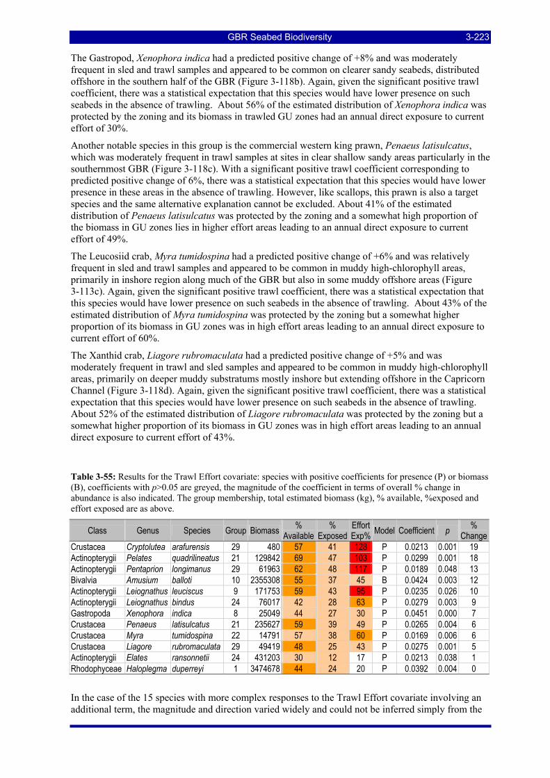
GBR Seabed Biodiversity 3-223
The Gastropod, Xenophora indica had a predicted positive change of +8% and was moderately frequent in sled and trawl samples and appeared to be common on clearer sandy seabeds, distributed offshore in the southern half of the GBR (Figure 3-118b). Again, given the significant positive trawl coefficient, there was a statistical expectation that this species would have lower presence on such seabeds in the absence of trawling. About 56% of the estimated distribution of Xenophora indica was protected by the zoning and its biomass in trawled GU zones had an annual direct exposure to current effort of 30%.
Another notable species in this group is the commercial western king prawn, Penaeus latisulcatus, which was moderately frequent in trawl samples at sites in clear shallow sandy areas particularly in the southernmost GBR (Figure 3-118c). With a significant positive trawl coefficient corresponding to predicted positive change of 6%, there was a statistical expectation that this species would have lower presence in these areas in the absence of trawling. However, like scallops, this prawn is also a target species and the same alternative explanation cannot be excluded. About 41% of the estimated distribution of Penaeus latisulcatus was protected by the zoning and a somewhat high proportion of the biomass in GU zones lies in higher effort areas leading to an annual direct exposure to current effort of 49%.
The Leucosiid crab, Myra tumidospina had a predicted positive change of +6% and was relatively frequent in sled and trawl samples and appeared to be common in muddy high-chlorophyll areas, primarily in inshore region along much of the GBR but also in some muddy offshore areas (Figure 3-113c). Again, given the significant positive trawl coefficient, there was a statistical expectation that this species would have lower presence on such seabeds in the absence of trawling. About 43% of the estimated distribution of Myra tumidospina was protected by the zoning but a somewhat higher proportion of its biomass in GU zones was in high effort areas leading to an annual direct exposure to current effort of 60%.
The Xanthid crab, Liagore rubromaculata had a predicted positive change of +5% and was moderately frequent in trawl and sled samples and appeared to be common in muddy high-chlorophyll areas, primarily on deeper muddy substratums mostly inshore but extending offshore in the Capricorn Channel (Figure 3-118d). Again, given the significant positive trawl coefficient, there was a statistical expectation that this species would have lower presence on such seabeds in the absence of trawling. About 52% of the estimated distribution of Liagore rubromaculata was protected by the zoning but a somewhat higher proportion of its biomass in GU zones was in high effort areas leading to an annual direct exposure to current effort of 43%.
Table 3-55: Results for the Trawl Effort covariate: species with positive coefficients for presence (P) or biomass (B), coefficients with p>0.05 are greyed, the magnitude of the coefficient in terms of overall % change in abundance is also indicated. The group membership, total estimated biomass (kg), % available, %exposed and effort exposed are as above.
Class Genus Species Group Biomass % Available
% Exposed
Effort Exp% Model Coefficient p %
Change Crustacea Cryptolutea arafurensis 29 480 57 41 128 P 0.0213 0.001 19 Actinopterygii Pelates quadrilineatus 21 129842 69 47 103 P 0.0299 0.001 18 Actinopterygii Pentaprion longimanus 29 61963 62 48 117 P 0.0189 0.048 13 Bivalvia Amusium balloti 10 2355308 55 37 45 B 0.0424 0.003 12 Actinopterygii Leiognathus leuciscus 9 171753 59 43 95 P 0.0235 0.026 10 Actinopterygii Leiognathus bindus 24 76017 42 28 63 P 0.0279 0.003 9 Gastropoda Xenophora indica 8 25049 44 27 30 P 0.0451 0.000 7 Crustacea Penaeus latisulcatus 21 235627 59 39 49 P 0.0265 0.004 6 Crustacea Myra tumidospina 22 14791 57 38 60 P 0.0169 0.006 6 Crustacea Liagore rubromaculata 29 49419 48 25 43 P 0.0275 0.001 5 Actinopterygii Elates ransonnetii 24 431203 30 12 17 P 0.0213 0.038 1 Rhodophyceae Haloplegma duperreyi 1 3474678 44 24 20 P 0.0392 0.004 0
In the case of the 15 species with more complex responses to the Trawl Effort covariate involving an additional term, the magnitude and direction varied widely and could not be inferred simply from the
GBR Seabed Biodiversity 3-224
coefficients (Table 3-56). Seven species were estimated to have significant negative change in biomass of -5% to -36% and five species were estimated to have significant positive change in biomass of +4% to +96%, compared with a model prediction with trawl effort set to zero over the entire region. The typical uncertainty in these estimates was about 70% of the estimate. As before, species predicted to had a positive change with trawling had moderately high to high exposure to current effort, while species with a negative change had low to very low exposure. Six species with the largest effects are examined in more detail below.
The species with the largest predicted positive change (+96%) was the Monacanthid fish Brachaluteres taylori (Figure 3-115a). This species was not uncommon in trawl samples at sites in shallow clear non-muddy areas, particularly in the southern half of the GBR, with intermediate intensity of trawl effort. With a positive trawl effort term and a negative squared term for the biomass model, giving an overall large positive predicted trawl effect, there was a statistical expectation that this species would have lower presence on those types of seabeds in the absence of trawling. About 29% of the estimated distribution of Brachaluteres taylori is protected by the zoning and 72% annually is directly exposed to current effort.
The species with the second largest predicted positive change (+50%) was the commercial grooved tiger prawn, Penaeus semisulcatus (Figure 3-108a). This species was common in trawl samples at sites in shallow muddy (but not extreme) low-light inshore areas, mostly in the northern two-thirds of the GBR, with intermediate intensity of trawl effort. With a positive trawl effort term and a negative squared term for the biomass model, giving an overall large positive predicted trawl effect, there was a statistical expectation that this species would have lower presence on those types of seabeds in the absence of trawling. About 26% of the estimated distribution of Penaeus semisulcatus was protected by the zoning and a high proportion of its biomass in GU zones was in high effort areas leading to an annual direct exposure to current effort of 174%. Like Penaeus latisulcatus and Amusium balloti discussed above, Penaeus semisulcatus is also a target species and the same alternative explanation cannot be excluded. The negative Biomass:Trawl_Eff^2 term was indicative of reduced standing biomass at very high levels of effort.
The species with the largest predicted negative change (-36%) was a gorgonian soft coral Carijoa sp1 (Figure 3-119a). This species appeared to have a widely scattered patchy distribution and with a negative trawl effort term for both the presence and the biomass model giving a strong negative predicted trawl effect, there is a statistical expectation that this species would have higher abundance in the absence of trawling. Three-quarters of the estimated distribution of Carijoa sp1 was protected by the zoning and only ~3% annually is directly exposed to current effort.
The species with the next largest predicted change (-27%) was Inegocia harrisii (a Platycephalid fish) (Figure 3-119b). This species was common at sites in low-light inshore areas, particularly in the vicinity of the very high tidal range areas of Shoalwater Bay, Broad Sound and the Whitsunday Islands. With a negative trawl effort term for both the presence and the biomass model, giving an overall negative predicted trawl effect, there was a statistical expectation that this species would have higher abundance on those types of seabeds in the absence of trawling. About 78% of the estimated distribution of Inegocia harrisii was protected by the zoning and only ~3% annually was directly exposed to current effort.
The species with the next largest predicted change (-26%) was the sediment infaunal sponge Oceanapia sp21 (Figure 3-119c). This species was not uncommon in sled samples at widely scattered sites in clear intermediate-gravel areas (mostly mid-to-outer shelf). With a negative trawl effort term and a positive effort*gravel interaction term in the presence model, giving an overall negative predicted trawl effect, there was a statistical expectation that this species would have higher abundance on those types of seabeds in the absence of trawling. It is possible that the interaction indicates that the negative trawl effect is less as gravel increases. About 75% of the estimated distribution of Oceanapia sp21 was protected by the zoning and only 3% annually was directly exposed to current effort.
The species with the next largest predicted change (-20%) was the Majid crab Austrolabidia gracilipes (Figure 3-119d). This species was not uncommon in sled samples at particularly off Mackay and the Whitsunday Islands, with scattered records elsewhere. With a positive trawl effort term and a negative effort*temp_SD interaction term in the presence model, giving an overall negative predicted trawl effect, there was a statistical expectation that this species would have higher abundance in the region
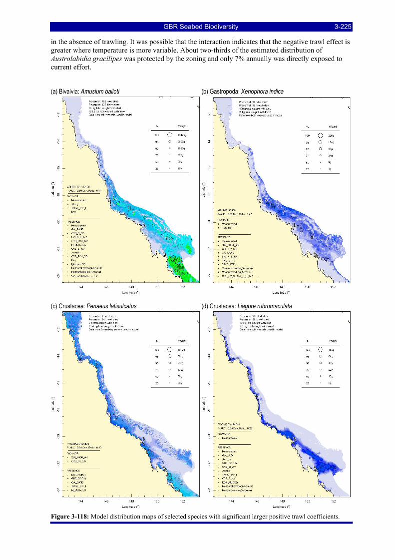
GBR Seabed Biodiversity 3-225
in the absence of trawling. It was possible that the interaction indicates that the negative trawl effect is greater where temperature is more variable. About two-thirds of the estimated distribution of Austrolabidia gracilipes was protected by the zoning and only 7% annually was directly exposed to current effort.
(a) Bivalvia: Amusium balloti (b) Gastropoda: Xenophora indica
(c) Crustacea: Penaeus latisulcatus (d) Crustacea: Liagore rubromaculata
Figure 3-118: Model distribution maps of selected species with significant larger positive trawl coefficients.
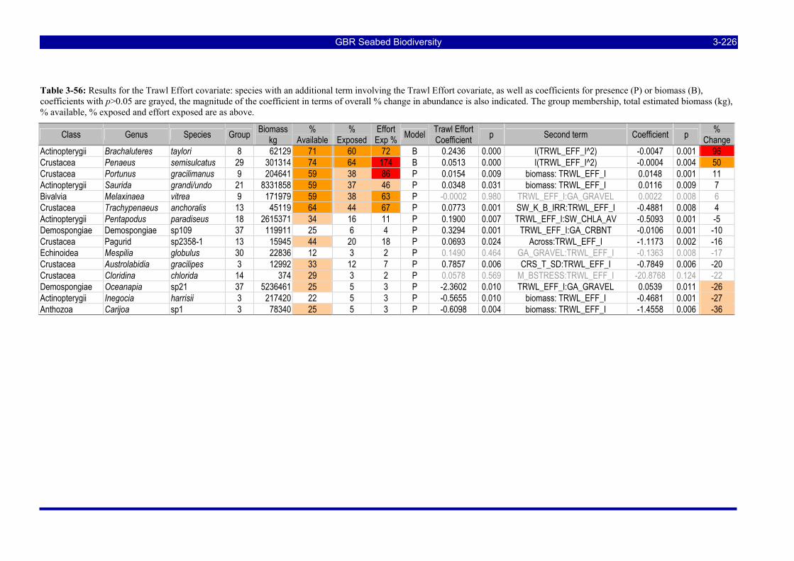
GBR Seabed Biodiversity 3-226
Table 3-56: Results for the Trawl Effort covariate: species with an additional term involving the Trawl Effort covariate, as well as coefficients for presence (P) or biomass (B), coefficients with p>0.05 are grayed, the magnitude of the coefficient in terms of overall % change in abundance is also indicated. The group membership, total estimated biomass (kg), % available, % exposed and effort exposed are as above.
Class Genus Species Group Biomass kg
% Available
% Exposed
Effort Exp % Model Trawl Effort
Coefficient p Second term Coefficient p % Change
Actinopterygii Brachaluteres taylori 8 62129 71 60 72 B 0.2436 0.000 I(TRWL_EFF_I^2) -0.0047 0.001 96 Crustacea Penaeus semisulcatus 29 301314 74 64 174 B 0.0513 0.000 I(TRWL_EFF_I^2) -0.0004 0.004 50 Crustacea Portunus gracilimanus 9 204641 59 38 86 P 0.0154 0.009 biomass: TRWL_EFF_I 0.0148 0.001 11 Actinopterygii Saurida grandi/undo 21 8331858 59 37 46 P 0.0348 0.031 biomass: TRWL_EFF_I 0.0116 0.009 7 Bivalvia Melaxinaea vitrea 9 171979 59 38 63 P -0.0002 0.980 TRWL_EFF_I:GA_GRAVEL 0.0022 0.008 6 Crustacea Trachypenaeus anchoralis 13 45119 64 44 67 P 0.0773 0.001 SW_K_B_IRR:TRWL_EFF_I -0.4881 0.008 4 Actinopterygii Pentapodus paradiseus 18 2615371 34 16 11 P 0.1900 0.007 TRWL_EFF_I:SW_CHLA_AV -0.5093 0.001 -5 Demospongiae Demospongiae sp109 37 119911 25 6 4 P 0.3294 0.001 TRWL_EFF_I:GA_CRBNT -0.0106 0.001 -10 Crustacea Pagurid sp2358-1 13 15945 44 20 18 P 0.0693 0.024 Across:TRWL_EFF_I -1.1173 0.002 -16 Echinoidea Mespilia globulus 30 22836 12 3 2 P 0.1490 0.464 GA_GRAVEL:TRWL_EFF_I -0.1363 0.008 -17 Crustacea Austrolabidia gracilipes 3 12992 33 12 7 P 0.7857 0.006 CRS_T_SD:TRWL_EFF_I -0.7849 0.006 -20 Crustacea Cloridina chlorida 14 374 29 3 2 P 0.0578 0.569 M_BSTRESS:TRWL_EFF_I -20.8768 0.124 -22 Demospongiae Oceanapia sp21 37 5236461 25 5 3 P -2.3602 0.010 TRWL_EFF_I:GA_GRAVEL 0.0539 0.011 -26 Actinopterygii Inegocia harrisii 3 217420 22 5 3 P -0.5655 0.010 biomass: TRWL_EFF_I -0.4681 0.001 -27 Anthozoa Carijoa sp1 3 78340 25 5 3 P -0.6098 0.004 biomass: TRWL_EFF_I -1.4558 0.006 -36
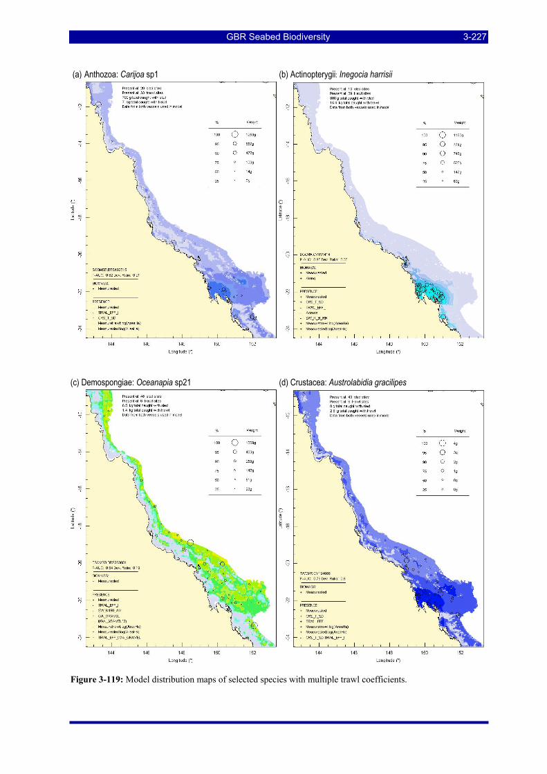
GBR Seabed Biodiversity 3-227
(a) Anthozoa: Carijoa sp1 (b) Actinopterygii: Inegocia harrisii
(c) Demospongiae: Oceanapia sp21 (d) Crustacea: Austrolabidia gracilipes
Figure 3-119: Model distribution maps of selected species with multiple trawl coefficients.
GBR Seabed Biodiversity 3-228
The trawl effort covariate was included in all 25 BRUVS fish species presence models, although significance tests were not possible, and the potential population change due to the influence of trawling was estimated for all species. Most (16) of the estimated changes were small (≤ ±5%) and most (18) were positive. The largest negative estimates were for Carangoides fulvoguttatus (-9%) and Abalistes stellatus (-8). The largest estimated changes were all positive: Nemipterus peronii (17%), Gymnothorax minor (17%), Parapercis nebulosa_grp (16%), Paramonacanthus otisensis (11%), Echeneis naucrates (11%), Lagocephalus sceleratus (10%). Of the above named species, only Carangoides fulvoguttatus, Echeneis naucrates and Gymnothorax minor were not assessed from the research trawl data; however, the uncertainty in these estimates from BRUVS is unknown.
3.7.2.2. Species exposure rank, catchability, and recovery indicators
The species exposure estimates from the previous sections were tabulated and ranked in order of most exposed to trawl effort intensity (Table 3-57). This exposure ranking is the primary output of the Seabed Project with respect to risk indicators for the trawl fishery in the GBR region. All of those species with effort exposure >50% have been discussed above, as well as several with exposure <50%. In this section, these exposure rankings were developed further with additional information from the Project and/or from external sources. By multiplying the effort exposure by the relative catch rate and BRD effect (if appropriate), an estimate of the percentage of population caught annually is tabulated (Table 3-57). Note that this estimate is not a true ‘catchability’ and there has not been a formal analysis of catchability as part of this Project. Where data from both sled and trawl was included in the modelling for a given species the coefficient of the device term was taken (indicated by “Model” in the table) and the range of ±SE was taken as an indicator of the uncertainty. Where model coefficients were not available at the species level, the mean of genus level coefficients was taken (indicated by “MdlGen” in the table) and similarly for the uncertainty. If model coefficients were not available, a simple ratio of average catch rates between devices, at the species or genus level (“Mean” or “MnGen” respectively), was used. If there was evidence that a fish trawl net had a higher catch rate in the earlier “Green Zone Effects of Trawling Study” then a simple ratio of average catch rates from that source, again at the species or genus level (“GZFsh” or “GZMn” respectively), was used. Often, there was considerable variability in relative catch rate among sources, which was taken as an indicator of uncertainty where the model result was not available. The estimated relative catch rate usually was less than 1 and the estimated percentage of populations caught annually was usually less than the estimated percentage exposed to trawl effort. The estimated effect of relative catch rate varied widely among species and substantially altered the ranking of species potentially at risk in terms of estimated percentage caught. At this point, the highest ranked species was the Pleuronectiform flatfish Brachirus muelleri (~110% caught), followed by other small fishes Terapon puta (59%), Saurida argentea/tumbil (58%), Psettodes erumei (52%) and the commercial prawn Penaeus semisulcatus (55%). Of the 33 species with effort exposure >50%, only 5 had >50% caught and 19 had <25% caught (Table 3-57). Of the 218 species with effort exposure between 25% and 50%, only 19 had >25% caught and 199 had <25% caught (Table 3-57). While these estimates of potential relative incidental (or in some cases target) catch make a critical contribution to understanding potential environmental risk, they do not provide a definitive indication of sustainability risk. For this, some indication of population recovery (the propensity for the population to replenish) is required.
Information on potential population recovery that was available were the “recovery” rankings for fishes from the NPF Bycatch Sustainability Project approach (Stobutzki et al. 2001) and for invertebrates from the NPF Ecological Surrogates Project (Hill et al. 2002). Where recovery ranks were available, weighted mean added ranks were tabulated (Table 3-57) for matching fish species genera. In the case of invertebrates, recovery ranks were available at the family level only. Low ranks (1.5–1.875, shaded red) indicate lower relative potential recovery and high ranks (2.65–3.0, not shaded) indicate higher relative potential recovery (low-moderate 1.875–2.25 and moderate 2.25–2.65 ranks are shaded orange and pale respectively). The available mean recovery rank for 422 species was plotted against the estimated percentage of population caught (Figure 3-120). The species at greatest relative risk should plot towards the upper left quadrant of the graph. The top ranking species were: Brachirus muelleri, Sepia pharaonis, Terapon puta, Saurida argentea/tumbil, Penaeus semisulcatus, Euristhmus nudiceps, Apogon poecilopterus, Sepia elliptica, Scolopsis taeniopterus, Psettodes erumei,
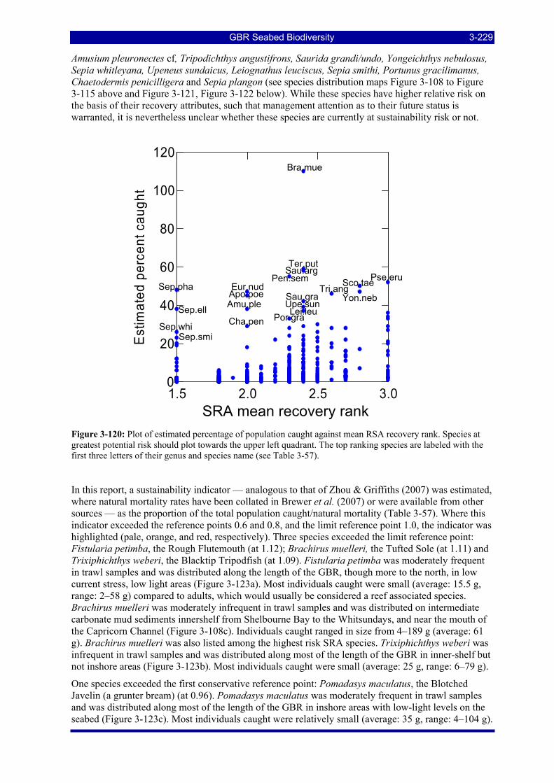
GBR Seabed Biodiversity 3-229
Amusium pleuronectes cf, Tripodichthys angustifrons, Saurida grandi/undo, Yongeichthys nebulosus, Sepia whitleyana, Upeneus sundaicus, Leiognathus leuciscus, Sepia smithi, Portunus gracilimanus, Chaetodermis penicilligera and Sepia plangon (see species distribution maps Figure 3-108 to Figure 3-115 above and Figure 3-121, Figure 3-122 below). While these species have higher relative risk on the basis of their recovery attributes, such that management attention as to their future status is warranted, it is nevertheless unclear whether these species are currently at sustainability risk or not.
1.5 2.0 2.5 3.0PSA mean productivity rank
0
20
40
60
80
100
120E
stim
ated
pe r
cent
cau
g ht
Figure 3-120: Plot of estimated percentage of population caught against mean RSA recovery rank. Species at greatest potential risk should plot towards the upper left quadrant. The top ranking species are labeled with the first three letters of their genus and species name (see Table 3-57).
In this report, a sustainability indicator — analogous to that of Zhou & Griffiths (2007) was estimated, where natural mortality rates have been collated in Brewer et al. (2007) or were available from other sources — as the proportion of the total population caught/natural mortality (Table 3-57). Where this indicator exceeded the reference points 0.6 and 0.8, and the limit reference point 1.0, the indicator was highlighted (pale, orange, and red, respectively). Three species exceeded the limit reference point: Fistularia petimba, the Rough Flutemouth (at 1.12); Brachirus muelleri, the Tufted Sole (at 1.11) and Trixiphichthys weberi, the Blacktip Tripodfish (at 1.09). Fistularia petimba was moderately frequent in trawl samples and was distributed along the length of the GBR, though more to the north, in low current stress, low light areas (Figure 3-123a). Most individuals caught were small (average: 15.5 g, range: 2–58 g) compared to adults, which would usually be considered a reef associated species. Brachirus muelleri was moderately infrequent in trawl samples and was distributed on intermediate carbonate mud sediments innershelf from Shelbourne Bay to the Whitsundays, and near the mouth of the Capricorn Channel (Figure 3-108c). Individuals caught ranged in size from 4–189 g (average: 61 g). Brachirus muelleri was also listed among the highest risk SRA species. Trixiphichthys weberi was infrequent in trawl samples and was distributed along most of the length of the GBR in inner-shelf but not inshore areas (Figure 3-123b). Most individuals caught were small (average: 25 g, range: 6–79 g).
One species exceeded the first conservative reference point: Pomadasys maculatus, the Blotched Javelin (a grunter bream) (at 0.96). Pomadasys maculatus was moderately frequent in trawl samples and was distributed along most of the length of the GBR in inshore areas with low-light levels on the seabed (Figure 3-123c). Most individuals caught were relatively small (average: 35 g, range: 4–104 g).
Pse.eruSco.taeYon.neb
Tri.ang
Lei.leu
Sau.arg
Upe.sunSau.gra
Ter.putPen.sem
Por.graAmu.pleApo.poe
Cha.pen
Eur.nud
Sep.whi
Sep.pha
Sep.smi
Sep.ell
Bra.mue
SRA mean recovery rank
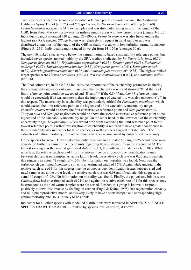
GBR Seabed Biodiversity 3-230
Two species exceeded the second conservative reference point: Psettodes erumei, the Australian Halibut or Spiny Turbot (at 0.75) and Sillago burrus, the Western Trumpeter Whiting (at 0.60). Psettodes erumei occurred in 51 trawl samples and was distributed along most of the length of the GBR, from about Mackay northwards, in inshore muddy areas with low current stress (Figure 3-112c). Individuals caught averaged 220 g, range: 21–1960 g. Psettodes erumei was also listed among the highest risk RSA species. Sillago burrus was relatively infrequent in trawl samples and was distributed along most of the length of the GBR in shallow areas with low turbidity, primarily inshore (Figure 3-123d). Individuals caught ranged in weight from 14–129 g (average: 50 g).
The next 10 ranked species were below the natural mortality based sustainability reference points, but included seven species ranked highly by the SRA method (indicated by *): Dasyatis leylandi (0.59), Nemipterus furcosus (0.56), Tripodichthys angustifrons* (0.53), Terapon puta* (0.53), Euristhmus nudiceps* (0.52), Saurida argentea/tumbil* (0.52), Nemipterus peronii (0.41), Sepia pharaonis* (0.39), Saurida grandi/undosquamis* (0.38) and Amusium pleuronectes cf* (0.35). The highest ranked target species were Thenus parindicus (at 0.31), Penaeus semisulcatus (at 0.24) and Amusium balloti (at 0.16).
The final column (*) in Table 3-57 indicates the importance of the catchability parameter in altering the sustainability indicator outcome. It assumed that catchability was 1 and showed “!!!” if the 1×M limit reference point would be exceeded and “!!” and “!” if the 0.8×M and 0.6×M reference points would be exceeded; if M was unknown, then the importance of catchability was also unknown (“u”) in this respect. The uncertainty in catchability was particularly critical for Pomadasys maculatus, which would exceed the limit reference point at the higher end of the catchability uncertainty range. Psettodes erumei would be above the first conservative reference point; and Nemipterus peronii, Terapon puta and Nemipterus furcosus would be above the second conservative reference point at the higher end of the catchability uncertainty range. On the other hand, at the lower end of the catchability uncertainty range, Trixiphichthys weberi would drop from exceeding the limit reference point to the lowest reference point. Further investigation of catchability is required to have greater confidence in the sustainability risk indicators for these species, as well as others flagged in Table 3-57. The estimates of natural mortality from other sources are also accompanied by unspecified uncertainty.
Of the species for which M was unknown, only three had an estimated % caught >25% and these were considered further because of the uncertainty regarding their sustainability in the absence of M. The highest ranking was the anaspid gastropod Aplysia sp1_QMS with an estimated catch of 38%. While uncertain, the relative catch rate of 1 for this species may be erroneous due identification issues between sled and trawl samples as, at the family level, the relative catch rate was 0.35 and if realistic, this suggests an actual % caught of ~13%. No information on mortality was found. Next was the sorbeoconch gastropod Lamellaria sp1 with an estimated catch of 37%. Again, while uncertain, the relative catch rate of 1 for this species may be erroneous due identification issues between sled and trawl samples as, at the order level, the relative catch rate was 0.08 and if realistic, this suggests an actual % caught of ~3%. No information on mortality was found. Finally, the polychaete bristle worm Chloeia flava had an estimated catch of 21% and again, the relative catch rate of 1 for this species may be erroneous as the sled worm samples were not sorted. Further, this group is known to respond positively to trawl disturbance by feeding on carrion (Engel & Kvitek 1998), has regeneration capacity and multiple reproductive modes, and is very likely to have a short lifespan and corresponding high natural mortality rate, so is unlikely to be at risk.
Indicators for all other species with modelled distributions were tabulated in APPENDIX 4: SINGLE SPECIES TRAWL EXPOSURE — ranked by species level exposure, if known.
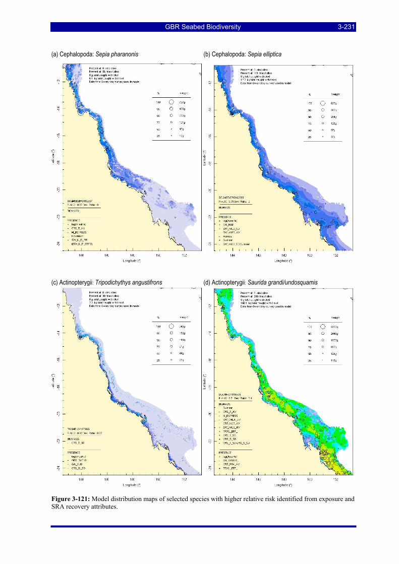
GBR Seabed Biodiversity 3-231
(a) Cephalopoda: Sepia pharanonis (b) Cephalopoda: Sepia elliptica
(c) Actinopterygii: Tripodichythys angustifrons (d) Actinopterygii: Saurida grandi/undosquamis
Figure 3-121: Model distribution maps of selected species with higher relative risk identified from exposure and SRA recovery attributes.
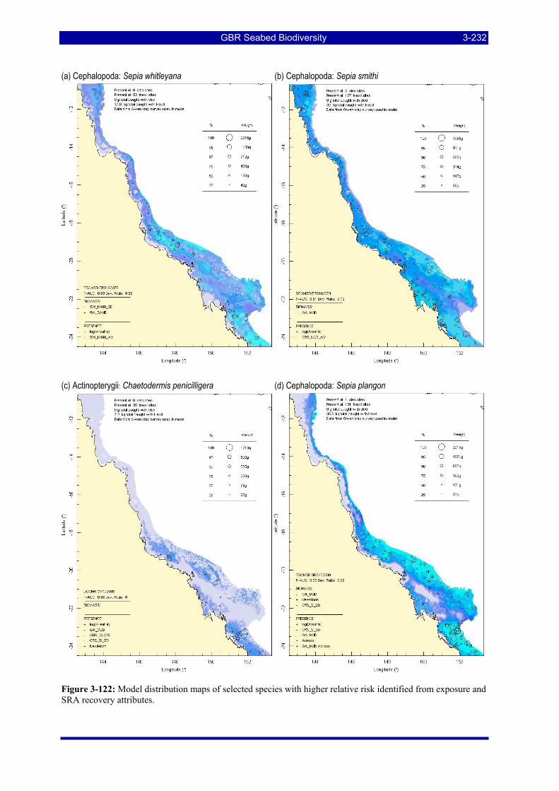
GBR Seabed Biodiversity 3-232
(a) Cephalopoda: Sepia whitleyana (b) Cephalopoda: Sepia smithi
(c) Actinopterygii: Chaetodermis penicilligera (d) Cephalopoda: Sepia plangon
Figure 3-122: Model distribution maps of selected species with higher relative risk identified from exposure and SRA recovery attributes.
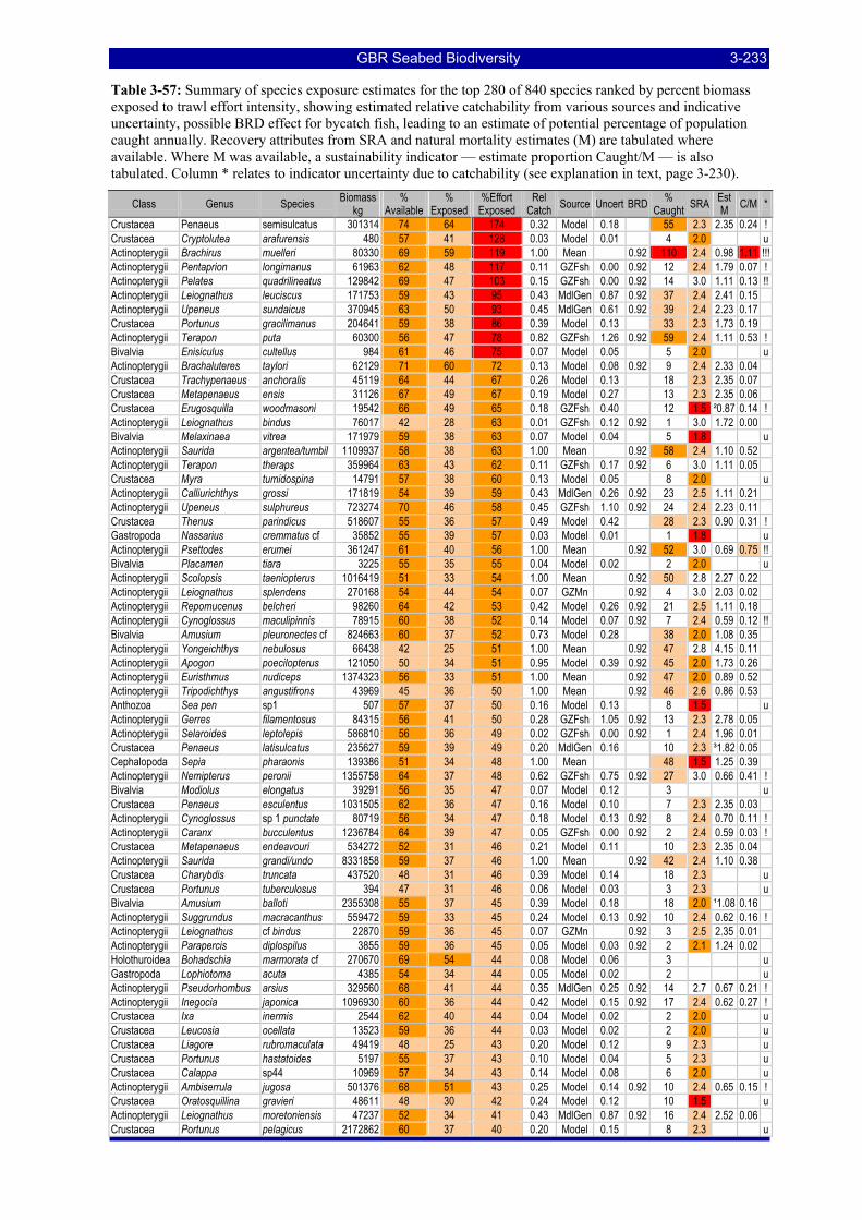
GBR Seabed Biodiversity 3-233
Table 3-57: Summary of species exposure estimates for the top 280 of 840 species ranked by percent biomass exposed to trawl effort intensity, showing estimated relative catchability from various sources and indicative uncertainty, possible BRD effect for bycatch fish, leading to an estimate of potential percentage of population caught annually. Recovery attributes from SRA and natural mortality estimates (M) are tabulated where available. Where M was available, a sustainability indicator — estimate proportion Caught/M — is also tabulated. Column * relates to indicator uncertainty due to catchability (see explanation in text, page 3-230).
Class Genus Species Biomass kg
% Available
% Exposed
%Effort Exposed
Rel Catch Source Uncert BRD %
Caught SRA Est M C/M *
Crustacea Penaeus semisulcatus 301314 74 64 174 0.32 Model 0.18 55 2.3 2.35 0.24 ! Crustacea Cryptolutea arafurensis 480 57 41 128 0.03 Model 0.01 4 2.0 u Actinopterygii Brachirus muelleri 80330 69 59 119 1.00 Mean 0.92 110 2.4 0.98 1.11 !!! Actinopterygii Pentaprion longimanus 61963 62 48 117 0.11 GZFsh 0.00 0.92 12 2.4 1.79 0.07 ! Actinopterygii Pelates quadrilineatus 129842 69 47 103 0.15 GZFsh 0.00 0.92 14 3.0 1.11 0.13 !! Actinopterygii Leiognathus leuciscus 171753 59 43 95 0.43 MdlGen 0.87 0.92 37 2.4 2.41 0.15 Actinopterygii Upeneus sundaicus 370945 63 50 93 0.45 MdlGen 0.61 0.92 39 2.4 2.23 0.17 Crustacea Portunus gracilimanus 204641 59 38 86 0.39 Model 0.13 33 2.3 1.73 0.19 Actinopterygii Terapon puta 60300 56 47 78 0.82 GZFsh 1.26 0.92 59 2.4 1.11 0.53 ! Bivalvia Enisiculus cultellus 984 61 46 75 0.07 Model 0.05 5 2.0 u Actinopterygii Brachaluteres taylori 62129 71 60 72 0.13 Model 0.08 0.92 9 2.4 2.33 0.04 Crustacea Trachypenaeus anchoralis 45119 64 44 67 0.26 Model 0.13 18 2.3 2.35 0.07 Crustacea Metapenaeus ensis 31126 67 49 67 0.19 Model 0.27 13 2.3 2.35 0.06 Crustacea Erugosquilla woodmasoni 19542 66 49 65 0.18 GZFsh 0.40 12 1.5 ²0.87 0.14 ! Actinopterygii Leiognathus bindus 76017 42 28 63 0.01 GZFsh 0.12 0.92 1 3.0 1.72 0.00 Bivalvia Melaxinaea vitrea 171979 59 38 63 0.07 Model 0.04 5 1.8 u Actinopterygii Saurida argentea/tumbil 1109937 58 38 63 1.00 Mean 0.92 58 2.4 1.10 0.52 Actinopterygii Terapon theraps 359964 63 43 62 0.11 GZFsh 0.17 0.92 6 3.0 1.11 0.05 Crustacea Myra tumidospina 14791 57 38 60 0.13 Model 0.05 8 2.0 u Actinopterygii Calliurichthys grossi 171819 54 39 59 0.43 MdlGen 0.26 0.92 23 2.5 1.11 0.21 Actinopterygii Upeneus sulphureus 723274 70 46 58 0.45 GZFsh 1.10 0.92 24 2.4 2.23 0.11 Crustacea Thenus parindicus 518607 55 36 57 0.49 Model 0.42 28 2.3 0.90 0.31 ! Gastropoda Nassarius cremmatus cf 35852 55 39 57 0.03 Model 0.01 1 1.8 u Actinopterygii Psettodes erumei 361247 61 40 56 1.00 Mean 0.92 52 3.0 0.69 0.75 !! Bivalvia Placamen tiara 3225 55 35 55 0.04 Model 0.02 2 2.0 u Actinopterygii Scolopsis taeniopterus 1016419 51 33 54 1.00 Mean 0.92 50 2.8 2.27 0.22 Actinopterygii Leiognathus splendens 270168 54 44 54 0.07 GZMn 0.92 4 3.0 2.03 0.02 Actinopterygii Repomucenus belcheri 98260 64 42 53 0.42 Model 0.26 0.92 21 2.5 1.11 0.18 Actinopterygii Cynoglossus maculipinnis 78915 60 38 52 0.14 Model 0.07 0.92 7 2.4 0.59 0.12 !! Bivalvia Amusium pleuronectes cf 824663 60 37 52 0.73 Model 0.28 38 2.0 1.08 0.35 Actinopterygii Yongeichthys nebulosus 66438 42 25 51 1.00 Mean 0.92 47 2.8 4.15 0.11 Actinopterygii Apogon poecilopterus 121050 50 34 51 0.95 Model 0.39 0.92 45 2.0 1.73 0.26 Actinopterygii Euristhmus nudiceps 1374323 56 33 51 1.00 Mean 0.92 47 2.0 0.89 0.52 Actinopterygii Tripodichthys angustifrons 43969 45 36 50 1.00 Mean 0.92 46 2.6 0.86 0.53 Anthozoa Sea pen sp1 507 57 37 50 0.16 Model 0.13 8 1.5 u Actinopterygii Gerres filamentosus 84315 56 41 50 0.28 GZFsh 1.05 0.92 13 2.3 2.78 0.05 Actinopterygii Selaroides leptolepis 586810 56 36 49 0.02 GZFsh 0.00 0.92 1 2.4 1.96 0.01 Crustacea Penaeus latisulcatus 235627 59 39 49 0.20 MdlGen 0.16 10 2.3 ³1.82 0.05 Cephalopoda Sepia pharaonis 139386 51 34 48 1.00 Mean 48 1.5 1.25 0.39 Actinopterygii Nemipterus peronii 1355758 64 37 48 0.62 GZFsh 0.75 0.92 27 3.0 0.66 0.41 ! Bivalvia Modiolus elongatus 39291 56 35 47 0.07 Model 0.12 3 u Crustacea Penaeus esculentus 1031505 62 36 47 0.16 Model 0.10 7 2.3 2.35 0.03 Actinopterygii Cynoglossus sp 1 punctate 80719 56 34 47 0.18 Model 0.13 0.92 8 2.4 0.70 0.11 ! Actinopterygii Caranx bucculentus 1236784 64 39 47 0.05 GZFsh 0.00 0.92 2 2.4 0.59 0.03 ! Crustacea Metapenaeus endeavouri 534272 52 31 46 0.21 Model 0.11 10 2.3 2.35 0.04 Actinopterygii Saurida grandi/undo 8331858 59 37 46 1.00 Mean 0.92 42 2.4 1.10 0.38 Crustacea Charybdis truncata 437520 48 31 46 0.39 Model 0.14 18 2.3 u Crustacea Portunus tuberculosus 394 47 31 46 0.06 Model 0.03 3 2.3 u Bivalvia Amusium balloti 2355308 55 37 45 0.39 Model 0.18 18 2.0 ¹1.08 0.16 Actinopterygii Suggrundus macracanthus 559472 59 33 45 0.24 Model 0.13 0.92 10 2.4 0.62 0.16 ! Actinopterygii Leiognathus cf bindus 22870 59 36 45 0.07 GZMn 0.92 3 2.5 2.35 0.01 Actinopterygii Parapercis diplospilus 3855 59 36 45 0.05 Model 0.03 0.92 2 2.1 1.24 0.02 Holothuroidea Bohadschia marmorata cf 270670 69 54 44 0.08 Model 0.06 3 u Gastropoda Lophiotoma acuta 4385 54 34 44 0.05 Model 0.02 2 u Actinopterygii Pseudorhombus arsius 329560 68 41 44 0.35 MdlGen 0.25 0.92 14 2.7 0.67 0.21 ! Actinopterygii Inegocia japonica 1096930 60 36 44 0.42 Model 0.15 0.92 17 2.4 0.62 0.27 ! Crustacea Ixa inermis 2544 62 40 44 0.04 Model 0.02 2 2.0 u Crustacea Leucosia ocellata 13523 59 36 44 0.03 Model 0.02 2 2.0 u Crustacea Liagore rubromaculata 49419 48 25 43 0.20 Model 0.12 9 2.3 u Crustacea Portunus hastatoides 5197 55 37 43 0.10 Model 0.04 5 2.3 u Crustacea Calappa sp44 10969 57 34 43 0.14 Model 0.08 6 2.0 u Actinopterygii Ambiserrula jugosa 501376 68 51 43 0.25 Model 0.14 0.92 10 2.4 0.65 0.15 ! Crustacea Oratosquillina gravieri 48611 48 30 42 0.24 Model 0.12 10 1.5 u Actinopterygii Leiognathus moretoniensis 47237 52 34 41 0.43 MdlGen 0.87 0.92 16 2.4 2.52 0.06 Crustacea Portunus pelagicus 2172862 60 37 40 0.20 Model 0.15 8 2.3 u
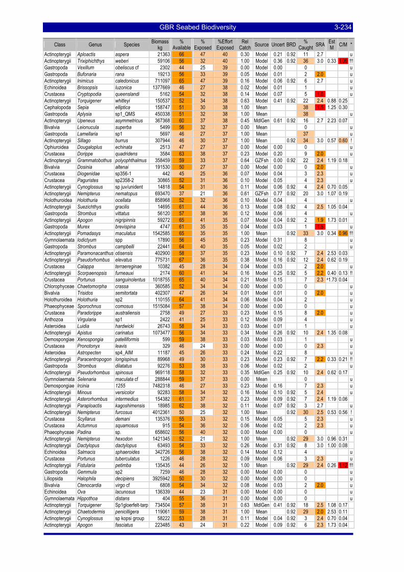
GBR Seabed Biodiversity 3-234
Class Genus Species Biomass kg
% Available
% Exposed
%Effort Exposed
Rel Catch Source Uncert BRD %
Caught SRA Est M C/M *
Actinopterygii Aploactis aspera 21363 66 47 40 0.30 Model 0.21 0.92 11 2.7 u Actinopterygii Trixiphichthys weberi 59106 56 32 40 1.00 Model 0.36 0.92 36 3.0 0.33 1.09 !!! Gastropoda Vexillum obeliscus cf 2302 44 25 39 0.00 Model 0.00 0 u Gastropoda Bufonaria rana 19213 56 33 39 0.05 Model 0.01 2 2.0 u Actinopterygii Inimicus caledonicus 711097 65 47 39 0.16 Model 0.06 0.92 6 2.7 u Echinoidea Brissopsis luzonica 1377669 46 27 38 0.02 Model 0.01 1 u Crustacea Cryptopodia queenslandi 5162 54 32 38 0.14 Model 0.07 5 1.8 u Actinopterygii Torquigener whitleyi 150537 52 34 38 0.63 Model 0.41 0.92 22 2.4 0.88 0.25 Cephalopoda Sepia elliptica 158747 51 30 38 1.00 Mean 38 1.5 1.25 0.30 Gastropoda Aplysia sp1_QMS 450338 51 32 38 1.00 Mean 38 u Actinopterygii Upeneus asymmetricus 367368 60 37 38 0.45 MdlGen 0.61 0.92 16 2.7 2.23 0.07 Bivalvia Leionucula superba 5499 56 32 37 0.00 Mean 0 u Gastropoda Lamellaria sp1 5697 46 27 37 1.00 Mean 37 u Actinopterygii Sillago burrus 307944 46 30 37 1.00 Mean 0.92 34 3.0 0.57 0.60 ! Ophiuroidea Dougaloplus echinata 2513 47 27 37 0.00 Model 0.00 0 u Crustacea Dorippe quadridens 3584 63 38 37 0.23 Model 0.20 9 2.0 u Actinopterygii Grammatobothus polyophthalmus 358459 59 33 37 0.64 GZFsh 0.00 0.92 22 2.4 1.19 0.18 Bivalvia Dosinia altenai 191530 50 27 37 0.00 Model 0.00 0 2.0 u Crustacea Diogenidae sp356-1 442 45 25 36 0.07 Model 0.04 3 2.3 u Crustacea Paguristes sp2358-2 30865 52 31 36 0.10 Model 0.05 4 2.3 u Actinopterygii Cynoglossus sp juv/unident 14818 54 31 36 0.11 Model 0.06 0.92 4 2.4 0.70 0.05 Actinopterygii Nemipterus nematopus 693470 37 21 36 0.61 GZFsh 0.77 0.92 20 3.0 1.07 0.19 Holothuroidea Holothuria ocellata 858968 52 32 36 0.10 Model 0.04 4 u Actinopterygii Suezichthys gracilis 14695 61 44 36 0.13 Model 0.08 0.92 4 2.5 1.05 0.04 Gastropoda Strombus vittatus 56120 57 38 36 0.12 Model 0.06 4 u Actinopterygii Apogon nigripinnis 59272 65 41 35 0.07 Model 0.04 0.92 2 1.9 1.73 0.01 Gastropoda Murex brevispina 4747 61 35 35 0.04 Model 0.03 1 1.5 u Actinopterygii Pomadasys maculatus 1542585 65 35 35 1.00 Mean 0.92 33 3.0 0.34 0.96 !!! Gymnolaemata Iodictyum spp 17890 56 45 35 0.23 Model 0.31 8 u Gastropoda Strombus campbelli 22441 64 40 35 0.05 Model 0.02 2 u Actinopterygii Paramonacanthus otisensis 402900 58 37 35 0.23 Model 0.10 0.92 7 2.4 2.53 0.03 Actinopterygii Pseudorhombus elevatus 775731 67 36 35 0.38 Model 0.16 0.92 12 2.4 0.62 0.19 Crustacea Calappa terraereginae 10382 45 28 34 0.04 Model 0.03 2 2.0 u Actinopterygii Scorpaenopsis furneauxi 2174 60 41 34 0.16 Model 0.25 0.92 5 2.2 0.40 0.13 !! Crustacea Portunus sanguinolentus 1018755 65 40 34 0.21 Model 0.15 7 2.3 41.73 0.04 Chlorophyceae Chaetomorpha crassa 360585 52 34 34 0.00 Model 0.00 0 u Bivalvia Trisidos semitortata 402307 47 26 34 0.01 Model 0.01 0 2.0 u Holothuroidea Holothuria sp2 110155 64 41 34 0.06 Model 0.04 2 u Phaeophyceae Sporochnus comosus 1515084 57 38 34 0.00 Model 0.00 0 u Crustacea Paradorippe australiensis 2758 49 27 33 0.23 Model 0.15 8 2.0 u Anthozoa Virgularia sp1 2422 41 25 33 0.12 Model 0.09 4 u Asteroidea Luidia hardwicki 26743 58 34 33 0.03 Model 0.01 1 u Actinopterygii Apistus carinatus 1073477 56 34 33 0.34 Model 0.26 0.92 10 2.4 1.35 0.08 Demospongiae Xenospongia patelliformis 599 59 38 33 0.03 Model 0.03 1 u Crustacea Pronotonyx leavis 329 46 24 33 0.00 Model 0.00 0 2.3 u Asteroidea Astropecten sp4_AIM 11187 45 26 33 0.24 Model 0.22 8 u Actinopterygii Paracentropogon longispinus 89968 49 30 33 0.23 Model 0.23 0.92 7 2.2 0.33 0.21 !! Gastropoda Strombus dilatatus 92276 53 38 33 0.06 Model 0.02 2 u Actinopterygii Pseudorhombus spinosus 969118 58 32 33 0.35 MdlGen 0.25 0.92 10 2.4 0.62 0.17 Gymnolaemata Selenaria maculata cf 288844 59 37 33 0.00 Mean 0 u Demospongiae Ircinia 1255 7482318 46 27 33 0.23 Model 0.16 7 2.3 u Actinopterygii Minous versicolor 92283 58 34 32 0.16 Model 0.10 0.92 5 2.4 u Actinopterygii Asterorhombus intermedius 154382 61 37 32 0.23 Model 0.09 0.92 7 2.4 1.19 0.06 Actinopterygii Paraploactis kagoshimensis 18985 62 38 32 0.11 Model 0.07 0.92 3 2.7 u Actinopterygii Nemipterus furcosus 4012361 50 25 32 1.00 Mean 0.92 30 2.5 0.53 0.56 ! Crustacea Scyllarus demani 135376 55 33 32 0.15 Model 0.05 5 2.3 u Crustacea Actumnus squamosus 915 54 36 32 0.06 Model 0.02 2 2.3 u Phaeophyceae Padina sp. 658602 56 40 32 0.00 Model 0.00 0 u Actinopterygii Nemipterus hexodon 1421345 52 21 32 1.00 Mean 0.92 29 3.0 0.96 0.31 Actinopterygii Dactylopus dactylopus 63493 54 33 32 0.26 Model 0.31 0.92 8 3.0 1.00 0.08 Echinoidea Salmacis sphaeroides 342726 56 38 32 0.14 Model 0.12 4 u Crustacea Portunus tuberculatus 1226 46 28 32 0.09 Model 0.06 3 2.3 u Actinopterygii Fistularia petimba 135435 44 26 32 1.00 Mean 0.92 29 2.4 0.26 1.12 !!! Gastropoda Gemmula sp2 7259 46 28 32 0.00 Model 0.00 0 u Liliopsida Halophila decipiens 3925942 50 30 32 0.00 Model 0.00 0 u Bivalvia Ctenocardia virgo cf 6808 54 34 32 0.08 Model 0.03 2 2.0 u Echinoidea Ova lacunosus 136339 44 23 31 0.00 Model 0.00 0 u Gymnolaemata Hippothoa distans 404 55 36 31 0.00 Model 0.00 0 u Actinopterygii Torquigener Sp1gloerfelt-tarp 734504 57 38 31 0.63 MdlGen 0.41 0.92 18 2.5 1.08 0.17 Actinopterygii Chaetodermis penicilligera 119061 59 38 31 1.00 Mean 0.92 29 2.0 2.53 0.11 Actinopterygii Cynoglossus sp kopsi group 58222 53 28 31 0.11 Model 0.04 0.92 3 2.4 0.70 0.04 Actinopterygii Apogon fasciatus 223485 43 24 31 0.22 Model 0.09 0.92 6 2.3 1.73 0.04
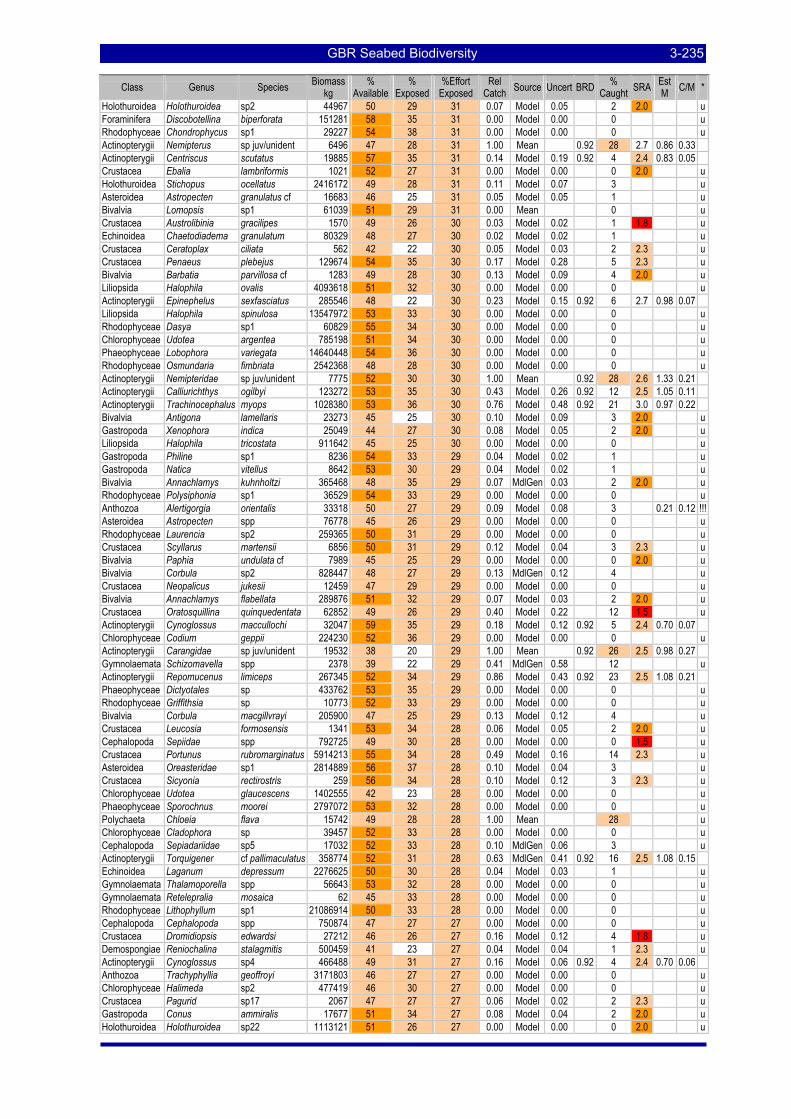
GBR Seabed Biodiversity 3-235
Class Genus Species Biomass kg
% Available
% Exposed
%Effort Exposed
Rel Catch Source Uncert BRD %
Caught SRA Est M C/M *
Holothuroidea Holothuroidea sp2 44967 50 29 31 0.07 Model 0.05 2 2.0 u Foraminifera Discobotellina biperforata 151281 58 35 31 0.00 Model 0.00 0 u Rhodophyceae Chondrophycus sp1 29227 54 38 31 0.00 Model 0.00 0 u Actinopterygii Nemipterus sp juv/unident 6496 47 28 31 1.00 Mean 0.92 28 2.7 0.86 0.33 Actinopterygii Centriscus scutatus 19885 57 35 31 0.14 Model 0.19 0.92 4 2.4 0.83 0.05 Crustacea Ebalia lambriformis 1021 52 27 31 0.00 Model 0.00 0 2.0 u Holothuroidea Stichopus ocellatus 2416172 49 28 31 0.11 Model 0.07 3 u Asteroidea Astropecten granulatus cf 16683 46 25 31 0.05 Model 0.05 1 u Bivalvia Lomopsis sp1 61039 51 29 31 0.00 Mean 0 u Crustacea Austrolibinia gracilipes 1570 49 26 30 0.03 Model 0.02 1 1.8 u Echinoidea Chaetodiadema granulatum 80329 48 27 30 0.02 Model 0.02 1 u Crustacea Ceratoplax ciliata 562 42 22 30 0.05 Model 0.03 2 2.3 u Crustacea Penaeus plebejus 129674 54 35 30 0.17 Model 0.28 5 2.3 u Bivalvia Barbatia parvillosa cf 1283 49 28 30 0.13 Model 0.09 4 2.0 u Liliopsida Halophila ovalis 4093618 51 32 30 0.00 Model 0.00 0 u Actinopterygii Epinephelus sexfasciatus 285546 48 22 30 0.23 Model 0.15 0.92 6 2.7 0.98 0.07 Liliopsida Halophila spinulosa 13547972 53 33 30 0.00 Model 0.00 0 u Rhodophyceae Dasya sp1 60829 55 34 30 0.00 Model 0.00 0 u Chlorophyceae Udotea argentea 785198 51 34 30 0.00 Model 0.00 0 u Phaeophyceae Lobophora variegata 14640448 54 36 30 0.00 Model 0.00 0 u Rhodophyceae Osmundaria fimbriata 2542368 48 28 30 0.00 Model 0.00 0 u Actinopterygii Nemipteridae sp juv/unident 7775 52 30 30 1.00 Mean 0.92 28 2.6 1.33 0.21 Actinopterygii Calliurichthys ogilbyi 123272 53 35 30 0.43 Model 0.26 0.92 12 2.5 1.05 0.11 Actinopterygii Trachinocephalus myops 1028380 53 36 30 0.76 Model 0.48 0.92 21 3.0 0.97 0.22 Bivalvia Antigona lamellaris 23273 45 25 30 0.10 Model 0.09 3 2.0 u Gastropoda Xenophora indica 25049 44 27 30 0.08 Model 0.05 2 2.0 u Liliopsida Halophila tricostata 911642 45 25 30 0.00 Model 0.00 0 u Gastropoda Philine sp1 8236 54 33 29 0.04 Model 0.02 1 u Gastropoda Natica vitellus 8642 53 30 29 0.04 Model 0.02 1 u Bivalvia Annachlamys kuhnholtzi 365468 48 35 29 0.07 MdlGen 0.03 2 2.0 u Rhodophyceae Polysiphonia sp1 36529 54 33 29 0.00 Model 0.00 0 u Anthozoa Alertigorgia orientalis 33318 50 27 29 0.09 Model 0.08 3 0.21 0.12 !!! Asteroidea Astropecten spp 76778 45 26 29 0.00 Model 0.00 0 u Rhodophyceae Laurencia sp2 259365 50 31 29 0.00 Model 0.00 0 u Crustacea Scyllarus martensii 6856 50 31 29 0.12 Model 0.04 3 2.3 u Bivalvia Paphia undulata cf 7989 45 25 29 0.00 Model 0.00 0 2.0 u Bivalvia Corbula sp2 828447 48 27 29 0.13 MdlGen 0.12 4 u Crustacea Neopalicus jukesii 12459 47 29 29 0.00 Model 0.00 0 u Bivalvia Annachlamys flabellata 289876 51 32 29 0.07 Model 0.03 2 2.0 u Crustacea Oratosquillina quinquedentata 62852 49 26 29 0.40 Model 0.22 12 1.5 u Actinopterygii Cynoglossus maccullochi 32047 59 35 29 0.18 Model 0.12 0.92 5 2.4 0.70 0.07 Chlorophyceae Codium geppii 224230 52 36 29 0.00 Model 0.00 0 u Actinopterygii Carangidae sp juv/unident 19532 38 20 29 1.00 Mean 0.92 26 2.5 0.98 0.27 Gymnolaemata Schizomavella spp 2378 39 22 29 0.41 MdlGen 0.58 12 u Actinopterygii Repomucenus limiceps 267345 52 34 29 0.86 Model 0.43 0.92 23 2.5 1.08 0.21 Phaeophyceae Dictyotales sp 433762 53 35 29 0.00 Model 0.00 0 u Rhodophyceae Griffithsia sp 10773 52 33 29 0.00 Model 0.00 0 u Bivalvia Corbula macgillvrayi 205900 47 25 29 0.13 Model 0.12 4 u Crustacea Leucosia formosensis 1341 53 34 28 0.06 Model 0.05 2 2.0 u Cephalopoda Sepiidae spp 792725 49 30 28 0.00 Model 0.00 0 1.5 u Crustacea Portunus rubromarginatus 5914213 55 34 28 0.49 Model 0.16 14 2.3 u Asteroidea Oreasteridae sp1 2814889 56 37 28 0.10 Model 0.04 3 u Crustacea Sicyonia rectirostris 259 56 34 28 0.10 Model 0.12 3 2.3 u Chlorophyceae Udotea glaucescens 1402555 42 23 28 0.00 Model 0.00 0 u Phaeophyceae Sporochnus moorei 2797072 53 32 28 0.00 Model 0.00 0 u Polychaeta Chloeia flava 15742 49 28 28 1.00 Mean 28 u Chlorophyceae Cladophora sp 39457 52 33 28 0.00 Model 0.00 0 u Cephalopoda Sepiadariidae sp5 17032 52 33 28 0.10 MdlGen 0.06 3 u Actinopterygii Torquigener cf pallimaculatus 358774 52 31 28 0.63 MdlGen 0.41 0.92 16 2.5 1.08 0.15 Echinoidea Laganum depressum 2276625 50 30 28 0.04 Model 0.03 1 u Gymnolaemata Thalamoporella spp 56643 53 32 28 0.00 Model 0.00 0 u Gymnolaemata Retelepralia mosaica 62 45 33 28 0.00 Model 0.00 0 u Rhodophyceae Lithophyllum sp1 21086914 50 33 28 0.00 Model 0.00 0 u Cephalopoda Cephalopoda spp 750874 47 27 27 0.00 Model 0.00 0 u Crustacea Dromidiopsis edwardsi 27212 46 26 27 0.16 Model 0.12 4 1.8 u Demospongiae Reniochalina stalagmitis 500459 41 23 27 0.04 Model 0.04 1 2.3 u Actinopterygii Cynoglossus sp4 466488 49 31 27 0.16 Model 0.06 0.92 4 2.4 0.70 0.06 Anthozoa Trachyphyllia geoffroyi 3171803 46 27 27 0.00 Model 0.00 0 u Chlorophyceae Halimeda sp2 477419 46 30 27 0.00 Model 0.00 0 u Crustacea Pagurid sp17 2067 47 27 27 0.06 Model 0.02 2 2.3 u Gastropoda Conus ammiralis 17677 51 34 27 0.08 Model 0.04 2 2.0 u Holothuroidea Holothuroidea sp22 1113121 51 26 27 0.00 Model 0.00 0 2.0 u
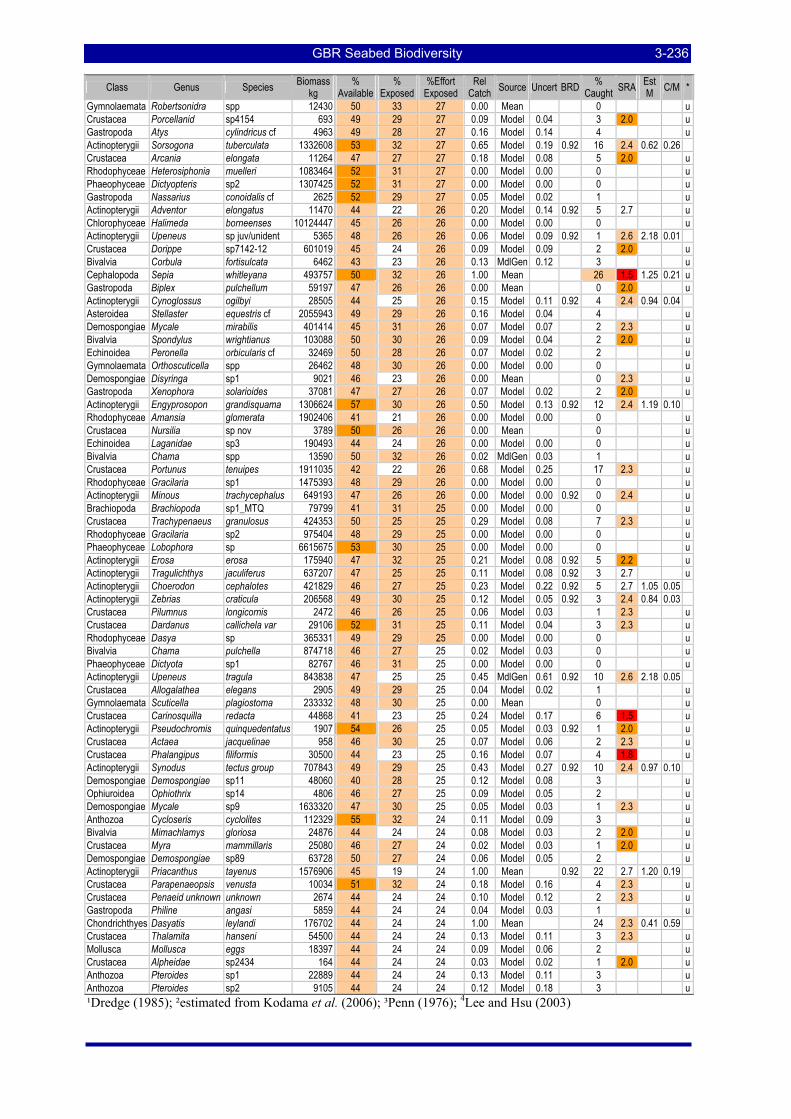
GBR Seabed Biodiversity 3-236
Class Genus Species Biomass kg
% Available
% Exposed
%Effort Exposed
Rel Catch Source Uncert BRD %
Caught SRA Est M C/M *
Gymnolaemata Robertsonidra spp 12430 50 33 27 0.00 Mean 0 u Crustacea Porcellanid sp4154 693 49 29 27 0.09 Model 0.04 3 2.0 u Gastropoda Atys cylindricus cf 4963 49 28 27 0.16 Model 0.14 4 u Actinopterygii Sorsogona tuberculata 1332608 53 32 27 0.65 Model 0.19 0.92 16 2.4 0.62 0.26 Crustacea Arcania elongata 11264 47 27 27 0.18 Model 0.08 5 2.0 u Rhodophyceae Heterosiphonia muelleri 1083464 52 31 27 0.00 Model 0.00 0 u Phaeophyceae Dictyopteris sp2 1307425 52 31 27 0.00 Model 0.00 0 u Gastropoda Nassarius conoidalis cf 2625 52 29 27 0.05 Model 0.02 1 u Actinopterygii Adventor elongatus 11470 44 22 26 0.20 Model 0.14 0.92 5 2.7 u Chlorophyceae Halimeda borneenses 10124447 45 26 26 0.00 Model 0.00 0 u Actinopterygii Upeneus sp juv/unident 5365 48 26 26 0.06 Model 0.09 0.92 1 2.6 2.18 0.01 Crustacea Dorippe sp7142-12 601019 45 24 26 0.09 Model 0.09 2 2.0 u Bivalvia Corbula fortisulcata 6462 43 23 26 0.13 MdlGen 0.12 3 u Cephalopoda Sepia whitleyana 493757 50 32 26 1.00 Mean 26 1.5 1.25 0.21 u Gastropoda Biplex pulchellum 59197 47 26 26 0.00 Mean 0 2.0 u Actinopterygii Cynoglossus ogilbyi 28505 44 25 26 0.15 Model 0.11 0.92 4 2.4 0.94 0.04 Asteroidea Stellaster equestris cf 2055943 49 29 26 0.16 Model 0.04 4 u Demospongiae Mycale mirabilis 401414 45 31 26 0.07 Model 0.07 2 2.3 u Bivalvia Spondylus wrightianus 103088 50 30 26 0.09 Model 0.04 2 2.0 u Echinoidea Peronella orbicularis cf 32469 50 28 26 0.07 Model 0.02 2 u Gymnolaemata Orthoscuticella spp 26462 48 30 26 0.00 Model 0.00 0 u Demospongiae Disyringa sp1 9021 46 23 26 0.00 Mean 0 2.3 u Gastropoda Xenophora solarioides 37081 47 27 26 0.07 Model 0.02 2 2.0 u Actinopterygii Engyprosopon grandisquama 1306624 57 30 26 0.50 Model 0.13 0.92 12 2.4 1.19 0.10 Rhodophyceae Amansia glomerata 1902406 41 21 26 0.00 Model 0.00 0 u Crustacea Nursilia sp nov 3789 50 26 26 0.00 Mean 0 u Echinoidea Laganidae sp3 190493 44 24 26 0.00 Model 0.00 0 u Bivalvia Chama spp 13590 50 32 26 0.02 MdlGen 0.03 1 u Crustacea Portunus tenuipes 1911035 42 22 26 0.68 Model 0.25 17 2.3 u Rhodophyceae Gracilaria sp1 1475393 48 29 26 0.00 Model 0.00 0 u Actinopterygii Minous trachycephalus 649193 47 26 26 0.00 Model 0.00 0.92 0 2.4 u Brachiopoda Brachiopoda sp1_MTQ 79799 41 31 25 0.00 Model 0.00 0 u Crustacea Trachypenaeus granulosus 424353 50 25 25 0.29 Model 0.08 7 2.3 u Rhodophyceae Gracilaria sp2 975404 48 29 25 0.00 Model 0.00 0 u Phaeophyceae Lobophora sp 6615675 53 30 25 0.00 Model 0.00 0 u Actinopterygii Erosa erosa 175940 47 32 25 0.21 Model 0.08 0.92 5 2.2 u Actinopterygii Tragulichthys jaculiferus 637207 47 25 25 0.11 Model 0.08 0.92 3 2.7 u Actinopterygii Choerodon cephalotes 421829 46 27 25 0.23 Model 0.22 0.92 5 2.7 1.05 0.05 Actinopterygii Zebrias craticula 206568 49 30 25 0.12 Model 0.05 0.92 3 2.4 0.84 0.03 Crustacea Pilumnus longicornis 2472 46 26 25 0.06 Model 0.03 1 2.3 u Crustacea Dardanus callichela var 29106 52 31 25 0.11 Model 0.04 3 2.3 u Rhodophyceae Dasya sp 365331 49 29 25 0.00 Model 0.00 0 u Bivalvia Chama pulchella 874718 46 27 25 0.02 Model 0.03 0 u Phaeophyceae Dictyota sp1 82767 46 31 25 0.00 Model 0.00 0 u Actinopterygii Upeneus tragula 843838 47 25 25 0.45 MdlGen 0.61 0.92 10 2.6 2.18 0.05 Crustacea Allogalathea elegans 2905 49 29 25 0.04 Model 0.02 1 u Gymnolaemata Scuticella plagiostoma 233332 48 30 25 0.00 Mean 0 u Crustacea Carinosquilla redacta 44868 41 23 25 0.24 Model 0.17 6 1.5 u Actinopterygii Pseudochromis quinquedentatus 1907 54 26 25 0.05 Model 0.03 0.92 1 2.0 u Crustacea Actaea jacquelinae 958 46 30 25 0.07 Model 0.06 2 2.3 u Crustacea Phalangipus filiformis 30500 44 23 25 0.16 Model 0.07 4 1.8 u Actinopterygii Synodus tectus group 707843 49 29 25 0.43 Model 0.27 0.92 10 2.4 0.97 0.10 Demospongiae Demospongiae sp11 48060 40 28 25 0.12 Model 0.08 3 u Ophiuroidea Ophiothrix sp14 4806 46 27 25 0.09 Model 0.05 2 u Demospongiae Mycale sp9 1633320 47 30 25 0.05 Model 0.03 1 2.3 u Anthozoa Cycloseris cyclolites 112329 55 32 24 0.11 Model 0.09 3 u Bivalvia Mimachlamys gloriosa 24876 44 24 24 0.08 Model 0.03 2 2.0 u Crustacea Myra mammillaris 25080 46 27 24 0.02 Model 0.03 1 2.0 u Demospongiae Demospongiae sp89 63728 50 27 24 0.06 Model 0.05 2 u Actinopterygii Priacanthus tayenus 1576906 45 19 24 1.00 Mean 0.92 22 2.7 1.20 0.19 Crustacea Parapenaeopsis venusta 10034 51 32 24 0.18 Model 0.16 4 2.3 u Crustacea Penaeid unknown unknown 2674 44 24 24 0.10 Model 0.12 2 2.3 u Gastropoda Philine angasi 5859 44 24 24 0.04 Model 0.03 1 u Chondrichthyes Dasyatis leylandi 176702 44 24 24 1.00 Mean 24 2.3 0.41 0.59 Crustacea Thalamita hanseni 54500 44 24 24 0.13 Model 0.11 3 2.3 u Mollusca Mollusca eggs 18397 44 24 24 0.09 Model 0.06 2 u Crustacea Alpheidae sp2434 164 44 24 24 0.03 Model 0.02 1 2.0 u Anthozoa Pteroides sp1 22889 44 24 24 0.13 Model 0.11 3 u Anthozoa Pteroides sp2 9105 44 24 24 0.12 Model 0.18 3 u ¹Dredge (1985); ²estimated from Kodama et al. (2006); ³Penn (1976); 4Lee and Hsu (2003)
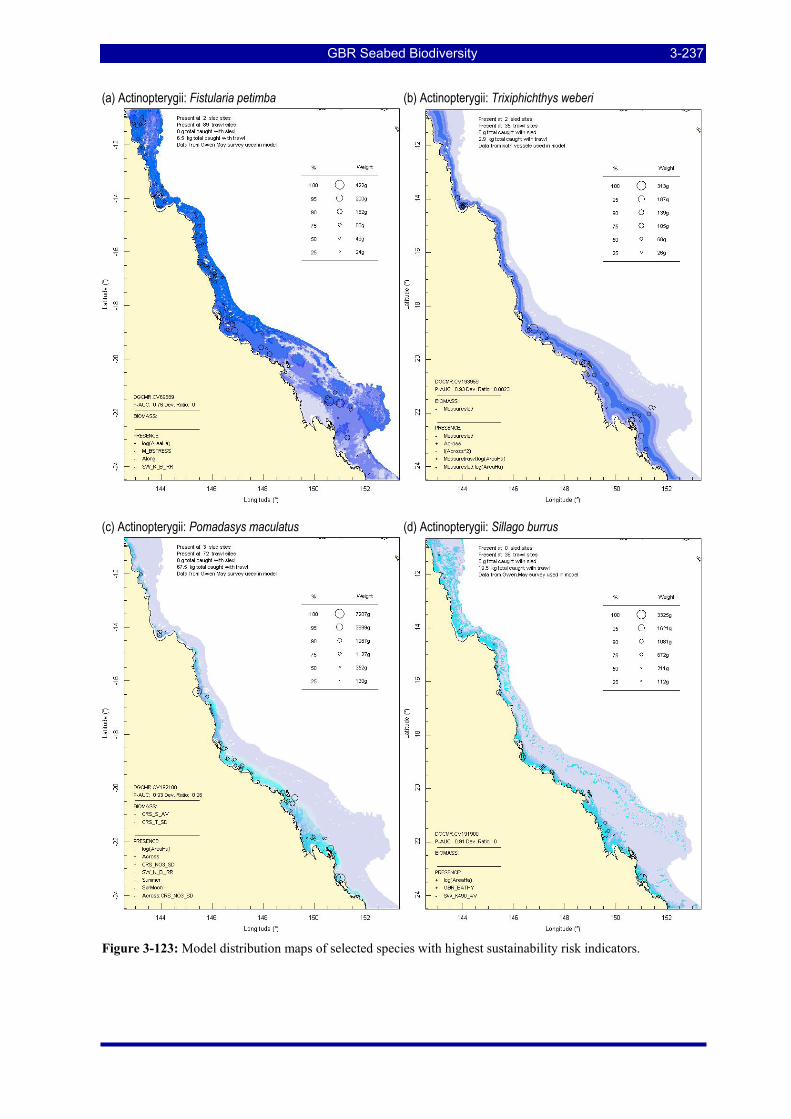
GBR Seabed Biodiversity 3-237
(a) Actinopterygii: Fistularia petimba (b) Actinopterygii: Trixiphichthys weberi
(c) Actinopterygii: Pomadasys maculatus (d) Actinopterygii: Sillago burrus
Figure 3-123: Model distribution maps of selected species with highest sustainability risk indicators.
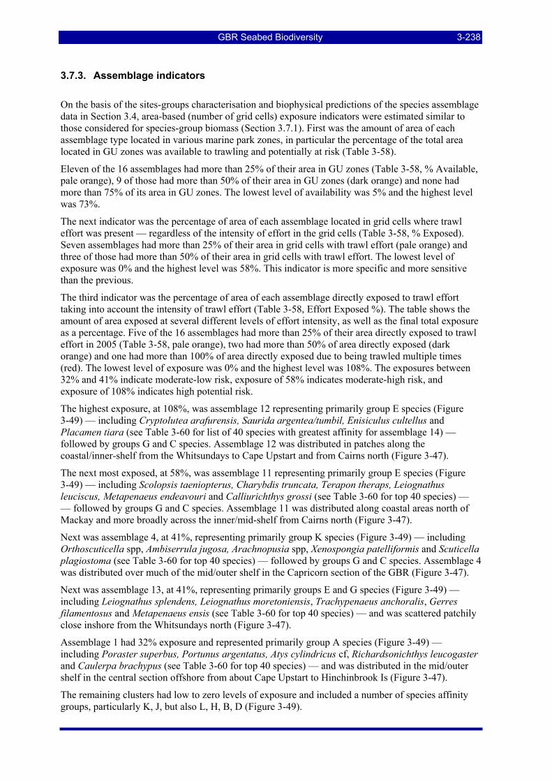
GBR Seabed Biodiversity 3-238
3.7.3. Assemblage indicators
On the basis of the sites-groups characterisation and biophysical predictions of the species assemblage data in Section 3.4, area-based (number of grid cells) exposure indicators were estimated similar to those considered for species-group biomass (Section 3.7.1). First was the amount of area of each assemblage type located in various marine park zones, in particular the percentage of the total area located in GU zones was available to trawling and potentially at risk (Table 3-58).
Eleven of the 16 assemblages had more than 25% of their area in GU zones (Table 3-58, % Available, pale orange), 9 of those had more than 50% of their area in GU zones (dark orange) and none had more than 75% of its area in GU zones. The lowest level of availability was 5% and the highest level was 73%.
The next indicator was the percentage of area of each assemblage located in grid cells where trawl effort was present — regardless of the intensity of effort in the grid cells (Table 3-58, % Exposed). Seven assemblages had more than 25% of their area in grid cells with trawl effort (pale orange) and three of those had more than 50% of their area in grid cells with trawl effort. The lowest level of exposure was 0% and the highest level was 58%. This indicator is more specific and more sensitive than the previous.
The third indicator was the percentage of area of each assemblage directly exposed to trawl effort taking into account the intensity of trawl effort (Table 3-58, Effort Exposed %). The table shows the amount of area exposed at several different levels of effort intensity, as well as the final total exposure as a percentage. Five of the 16 assemblages had more than 25% of their area directly exposed to trawl effort in 2005 (Table 3-58, pale orange), two had more than 50% of area directly exposed (dark orange) and one had more than 100% of area directly exposed due to being trawled multiple times (red). The lowest level of exposure was 0% and the highest level was 108%. The exposures between 32% and 41% indicate moderate-low risk, exposure of 58% indicates moderate-high risk, and exposure of 108% indicates high potential risk.
The highest exposure, at 108%, was assemblage 12 representing primarily group E species (Figure 3-49) — including Cryptolutea arafurensis, Saurida argentea/tumbil, Enisiculus cultellus and Placamen tiara (see Table 3-60 for list of 40 species with greatest affinity for assemblage 14) — followed by groups G and C species. Assemblage 12 was distributed in patches along the coastal/inner-shelf from the Whitsundays to Cape Upstart and from Cairns north (Figure 3-47).
The next most exposed, at 58%, was assemblage 11 representing primarily group E species (Figure 3-49) — including Scolopsis taeniopterus, Charybdis truncata, Terapon theraps, Leiognathus leuciscus, Metapenaeus endeavouri and Calliurichthys grossi (see Table 3-60 for top 40 species) — — followed by groups G and C species. Assemblage 11 was distributed along coastal areas north of Mackay and more broadly across the inner/mid-shelf from Cairns north (Figure 3-47).
Next was assemblage 4, at 41%, representing primarily group K species (Figure 3-49) — including Orthoscuticella spp, Ambiserrula jugosa, Arachnopusia spp, Xenospongia patelliformis and Scuticella plagiostoma (see Table 3-60 for top 40 species) — followed by groups G and C species. Assemblage 4 was distributed over much of the mid/outer shelf in the Capricorn section of the GBR (Figure 3-47).
Next was assemblage 13, at 41%, representing primarily groups E and G species (Figure 3-49) —including Leiognathus splendens, Leiognathus moretoniensis, Trachypenaeus anchoralis, Gerres filamentosus and Metapenaeus ensis (see Table 3-60 for top 40 species) — and was scattered patchily close inshore from the Whitsundays north (Figure 3-47).
Assemblage 1 had 32% exposure and represented primarily group A species (Figure 3-49) — including Poraster superbus, Portunus argentatus, Atys cylindricus cf, Richardsonichthys leucogaster and Caulerpa brachypus (see Table 3-60 for top 40 species) — and was distributed in the mid/outer shelf in the central section offshore from about Cape Upstart to Hinchinbrook Is (Figure 3-47).
The remaining clusters had low to zero levels of exposure and included a number of species affinity groups, particularly K, J, but also L, H, B, D (Figure 3-49).
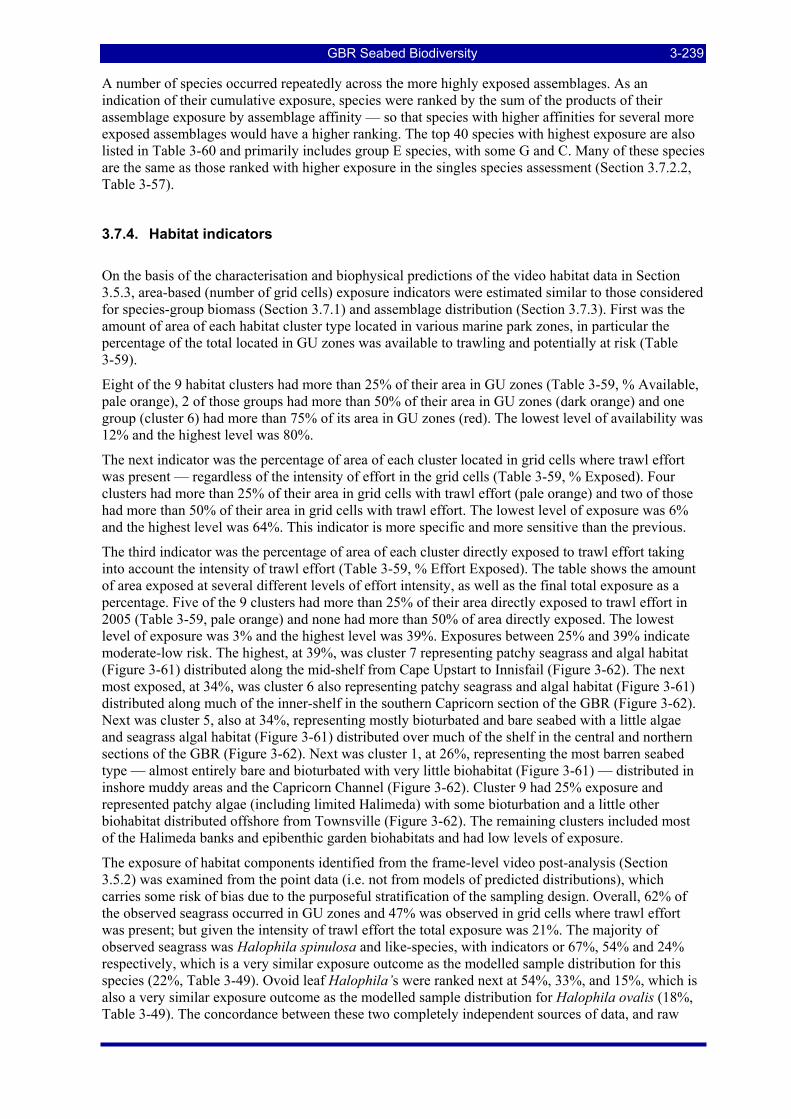
GBR Seabed Biodiversity 3-239
A number of species occurred repeatedly across the more highly exposed assemblages. As an indication of their cumulative exposure, species were ranked by the sum of the products of their assemblage exposure by assemblage affinity — so that species with higher affinities for several more exposed assemblages would have a higher ranking. The top 40 species with highest exposure are also listed in Table 3-60 and primarily includes group E species, with some G and C. Many of these species are the same as those ranked with higher exposure in the singles species assessment (Section 3.7.2.2, Table 3-57).
3.7.4. Habitat indicators
On the basis of the characterisation and biophysical predictions of the video habitat data in Section 3.5.3, area-based (number of grid cells) exposure indicators were estimated similar to those considered for species-group biomass (Section 3.7.1) and assemblage distribution (Section 3.7.3). First was the amount of area of each habitat cluster type located in various marine park zones, in particular the percentage of the total located in GU zones was available to trawling and potentially at risk (Table 3-59).
Eight of the 9 habitat clusters had more than 25% of their area in GU zones (Table 3-59, % Available, pale orange), 2 of those groups had more than 50% of their area in GU zones (dark orange) and one group (cluster 6) had more than 75% of its area in GU zones (red). The lowest level of availability was 12% and the highest level was 80%.
The next indicator was the percentage of area of each cluster located in grid cells where trawl effort was present — regardless of the intensity of effort in the grid cells (Table 3-59, % Exposed). Four clusters had more than 25% of their area in grid cells with trawl effort (pale orange) and two of those had more than 50% of their area in grid cells with trawl effort. The lowest level of exposure was 6% and the highest level was 64%. This indicator is more specific and more sensitive than the previous.
The third indicator was the percentage of area of each cluster directly exposed to trawl effort taking into account the intensity of trawl effort (Table 3-59, % Effort Exposed). The table shows the amount of area exposed at several different levels of effort intensity, as well as the final total exposure as a percentage. Five of the 9 clusters had more than 25% of their area directly exposed to trawl effort in 2005 (Table 3-59, pale orange) and none had more than 50% of area directly exposed. The lowest level of exposure was 3% and the highest level was 39%. Exposures between 25% and 39% indicate moderate-low risk. The highest, at 39%, was cluster 7 representing patchy seagrass and algal habitat (Figure 3-61) distributed along the mid-shelf from Cape Upstart to Innisfail (Figure 3-62). The next most exposed, at 34%, was cluster 6 also representing patchy seagrass and algal habitat (Figure 3-61) distributed along much of the inner-shelf in the southern Capricorn section of the GBR (Figure 3-62). Next was cluster 5, also at 34%, representing mostly bioturbated and bare seabed with a little algae and seagrass algal habitat (Figure 3-61) distributed over much of the shelf in the central and northern sections of the GBR (Figure 3-62). Next was cluster 1, at 26%, representing the most barren seabed type — almost entirely bare and bioturbated with very little biohabitat (Figure 3-61) — distributed in inshore muddy areas and the Capricorn Channel (Figure 3-62). Cluster 9 had 25% exposure and represented patchy algae (including limited Halimeda) with some bioturbation and a little other biohabitat distributed offshore from Townsville (Figure 3-62). The remaining clusters included most of the Halimeda banks and epibenthic garden biohabitats and had low levels of exposure.
The exposure of habitat components identified from the frame-level video post-analysis (Section 3.5.2) was examined from the point data (i.e. not from models of predicted distributions), which carries some risk of bias due to the purposeful stratification of the sampling design. Overall, 62% of the observed seagrass occurred in GU zones and 47% was observed in grid cells where trawl effort was present; but given the intensity of trawl effort the total exposure was 21%. The majority of observed seagrass was Halophila spinulosa and like-species, with indicators or 67%, 54% and 24% respectively, which is a very similar exposure outcome as the modelled sample distribution for this species (22%, Table 3-49). Ovoid leaf Halophila’s were ranked next at 54%, 33%, and 15%, which is also a very similar exposure outcome as the modelled sample distribution for Halophila ovalis (18%, Table 3-49). The concordance between these two completely independent sources of data, and raw
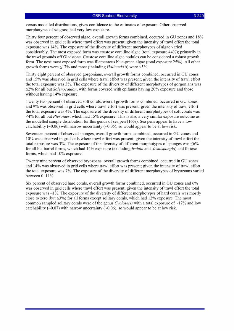
GBR Seabed Biodiversity 3-240
versus modelled distributions, gives confidence to the estimates of exposure. Other observed morphotypes of seagrass had very low exposure.
Thirty four percent of observed algae, overall growth forms combined, occurred in GU zones and 18% was observed in grid cells where trawl effort was present; given the intensity of trawl effort the total exposure was 14%. The exposure of the diversity of different morphotypes of algae varied considerably. The most exposed form was crustose coralline algae (total exposure 44%); primarily in the trawl grounds off Gladstone. Crustose coralline algae nodules can be considered a robust growth form. The next most exposed form was filamentous blue-green algae (total exposure 25%). All other growth forms were ≤17% and most (including Halimeda’s) were <5%.
Thirty eight percent of observed gorgonians, overall growth forms combined, occurred in GU zones and 15% was observed in grid cells where trawl effort was present; given the intensity of trawl effort the total exposure was 3%. The exposure of the diversity of different morphotypes of gorgonians was ≤2% for all but Solenocaulon, with forms covered with epifauna having 20% exposure and those without having 14% exposure.
Twenty two percent of observed soft corals, overall growth forms combined, occurred in GU zones and 9% was observed in grid cells where trawl effort was present; given the intensity of trawl effort the total exposure was 4%. The exposure of the diversity of different morphotypes of soft corals was ≤4% for all but Pteroides, which had 15% exposure. This is also a very similar exposure outcome as the modelled sample distribution for this genus of sea pen (16%). Sea pens appear to have a low catchability (~0.06) with narrow uncertainty (~0.05), so would appear to be at low risk.
Seventeen percent of observed sponges, overall growth forms combined, occurred in GU zones and 10% was observed in grid cells where trawl effort was present; given the intensity of trawl effort the total exposure was 3%. The exposure of the diversity of different morphotypes of sponges was ≤6% for all but barrel forms, which had 14% exposure (excluding Ircinia and Xestospongia) and foliose forms, which had 10% exposure.
Twenty nine percent of observed bryozoans, overall growth forms combined, occurred in GU zones and 14% was observed in grid cells where trawl effort was present; given the intensity of trawl effort the total exposure was 7%. The exposure of the diversity of different morphotypes of bryozoans varied between 0–11%.
Six percent of observed hard corals, overall growth forms combined, occurred in GU zones and 6% was observed in grid cells where trawl effort was present; given the intensity of trawl effort the total exposure was ~1%. The exposure of the diversity of different morphotypes of hard corals was mostly close to zero (but ≤3%) for all forms except solitary corals, which had 12% exposure. The most common sampled solitary corals were of the genus Cycloseris with a total exposure of ~17% and low catchability (~0.07) with narrow uncertainty (~0.06), so would appear to be at low risk.
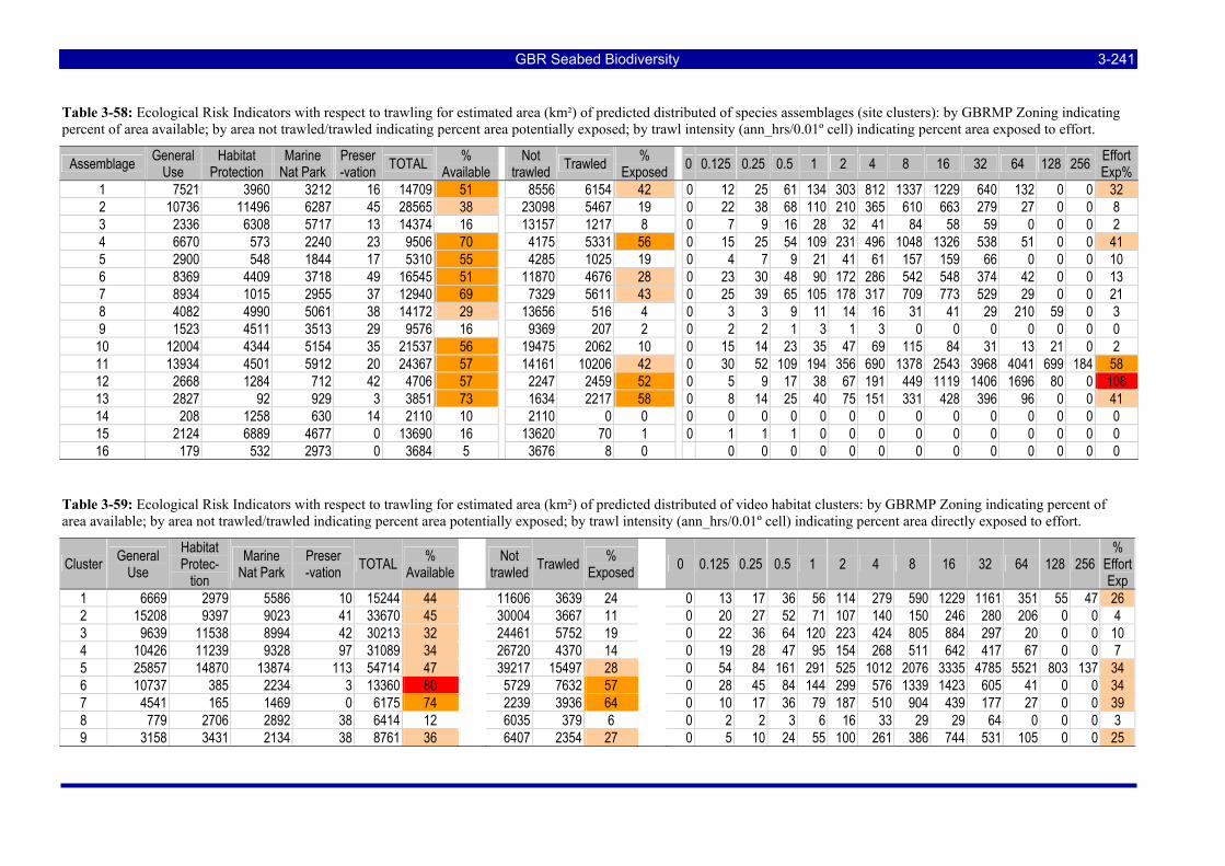
GBR Seabed Biodiversity 3-241
Table 3-58: Ecological Risk Indicators with respect to trawling for estimated area (km²) of predicted distributed of species assemblages (site clusters): by GBRMP Zoning indicating percent of area available; by area not trawled/trawled indicating percent area potentially exposed; by trawl intensity (ann_hrs/0.01º cell) indicating percent area exposed to effort.
Assemblage General Use
Habitat Protection
Marine Nat Park
Preser -vation TOTAL %
Available Not trawled Trawled %
Exposed 0 0.125 0.25 0.5 1 2 4 8 16 32 64 128 256 Effort Exp%
1 7521 3960 3212 16 14709 51 8556 6154 42 0 12 25 61 134 303 812 1337 1229 640 132 0 0 32 2 10736 11496 6287 45 28565 38 23098 5467 19 0 22 38 68 110 210 365 610 663 279 27 0 0 8 3 2336 6308 5717 13 14374 16 13157 1217 8 0 7 9 16 28 32 41 84 58 59 0 0 0 2 4 6670 573 2240 23 9506 70 4175 5331 56 0 15 25 54 109 231 496 1048 1326 538 51 0 0 41 5 2900 548 1844 17 5310 55 4285 1025 19 0 4 7 9 21 41 61 157 159 66 0 0 0 10 6 8369 4409 3718 49 16545 51 11870 4676 28 0 23 30 48 90 172 286 542 548 374 42 0 0 13 7 8934 1015 2955 37 12940 69 7329 5611 43 0 25 39 65 105 178 317 709 773 529 29 0 0 21 8 4082 4990 5061 38 14172 29 13656 516 4 0 3 3 9 11 14 16 31 41 29 210 59 0 3 9 1523 4511 3513 29 9576 16 9369 207 2 0 2 2 1 3 1 3 0 0 0 0 0 0 0 10 12004 4344 5154 35 21537 56 19475 2062 10 0 15 14 23 35 47 69 115 84 31 13 21 0 2 11 13934 4501 5912 20 24367 57 14161 10206 42 0 30 52 109 194 356 690 1378 2543 3968 4041 699 184 58 12 2668 1284 712 42 4706 57 2247 2459 52 0 5 9 17 38 67 191 449 1119 1406 1696 80 0 108 13 2827 92 929 3 3851 73 1634 2217 58 0 8 14 25 40 75 151 331 428 396 96 0 0 41 14 208 1258 630 14 2110 10 2110 0 0 0 0 0 0 0 0 0 0 0 0 0 0 0 0 15 2124 6889 4677 0 13690 16 13620 70 1 0 1 1 1 0 0 0 0 0 0 0 0 0 0 16 179 532 2973 0 3684 5 3676 8 0 0 0 0 0 0 0 0 0 0 0 0 0 0
Table 3-59: Ecological Risk Indicators with respect to trawling for estimated area (km²) of predicted distributed of video habitat clusters: by GBRMP Zoning indicating percent of area available; by area not trawled/trawled indicating percent area potentially exposed; by trawl intensity (ann_hrs/0.01º cell) indicating percent area directly exposed to effort.
Cluster General Use
Habitat Protec-
tion Marine
Nat Park Preser -vation TOTAL %
Available Not trawled Trawled %
Exposed 0 0.125 0.25 0.5 1 2 4 8 16 32 64 128 256 %
Effort Exp
1 6669 2979 5586 10 15244 44 11606 3639 24 0 13 17 36 56 114 279 590 1229 1161 351 55 47 26 2 15208 9397 9023 41 33670 45 30004 3667 11 0 20 27 52 71 107 140 150 246 280 206 0 0 4 3 9639 11538 8994 42 30213 32 24461 5752 19 0 22 36 64 120 223 424 805 884 297 20 0 0 10 4 10426 11239 9328 97 31089 34 26720 4370 14 0 19 28 47 95 154 268 511 642 417 67 0 0 7 5 25857 14870 13874 113 54714 47 39217 15497 28 0 54 84 161 291 525 1012 2076 3335 4785 5521 803 137 34 6 10737 385 2234 3 13360 80 5729 7632 57 0 28 45 84 144 299 576 1339 1423 605 41 0 0 34 7 4541 165 1469 0 6175 74 2239 3936 64 0 10 17 36 79 187 510 904 439 177 27 0 0 39 8 779 2706 2892 38 6414 12 6035 379 6 0 2 2 3 6 16 33 29 29 64 0 0 0 3 9 3158 3431 2134 38 8761 36 6407 2354 27 0 5 10 24 55 100 261 386 744 531 105 0 0 25
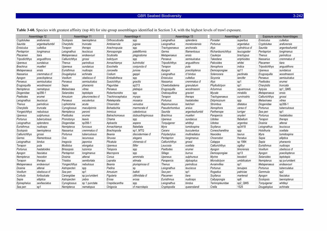
GBR Seabed Biodiversity 3-242
Table 3-60. Species with greatest affinity (top 40) for site-group assemblages identified in Section 3.4, with the highest levels of trawl exposure. Assemblage 12 Assemblage 11 Assemblage 4 Assemblage 13 Assemblage 1 Exposure across Assemblages
Cryptolutea arafurensis Scolopsis taeniopterus Orthoscuticella spp Leiognathus splendens Poraster superbus Enisiculus cultellus Saurida argentea/tumbil Charybdis truncata Ambiserrula jugosa Leiognathus moretoniensis Portunus argentatus Cryptolutea arafurensis Enisiculus cultellus Terapon theraps Arachnopusia spp Trachypenaeus anchoralis Atys cylindricus cf Saurida argentea/tumbil Pentaprion longimanus Leiognathus leuciscus Xenospongia patelliformis Gerres filamentosus Richardsonichthys leucogaster Pentaprion longimanus Placamen tiara Metapenaeus endeavouri Scuticella plagiostoma Metapenaeus ensis Caulerpa brachypus Thenus parindicus Tripodichthys angustifrons Calliurichthys grossi Iodictyum spp Penaeus semisulcatus Takedana eriphioides Nassarius cremmatus cf Upeneus sundaicus Thenus parindicus Annachlamys kuhnholtzi Tripodichthys angustifrons Palicoides whitei Placamen tiara Brachirus muelleri Upeneus sundaicus Exochella conjuncta cf Terapon puta Xenophora indica Tripodichthys angustifrons Metapenaeus ensis Euristhmus nudiceps Junceella juncea Apogon poecilopterus Demospongiae sp11 Upeneus sundaicus Nassarius cremmatus cf Dougaloplus echinata Codium geppii Leiognathus cf bindus Solenocera pectinata Erugosquilla woodmasoni Apogon poecilopterus Vexillum obeliscus cf Emballotheca spp Enisiculus cultellus Sicyonia lancifer Penaeus semisulcatus Penaeus semisulcatus Penaeus semisulcatus Suezichthys gracilis Nassarius cremmatus cf Atys sp1 Psettodes erumei Erugosquilla woodmasoni Sepia pharaonis Paguridae sp213 Chaetodiadema granulatum Phyllodictyon sp1 Charybdis truncata Nemipterus nematopus Melaxinaea vitrea Penaeus plebejus Erugosquilla woodmasoni Actumnus squamosus Aplysia sp1_QMS Diogenidae sp356-1 Selaroides leptolepis Robertsonidra spp Oratosquillina gravieri Mycale mirabilis Metapenaeus ensis Psettodes erumei Amusium pleuronectes cf Trachinocephalus myops Terapon theraps Trachypenaeus curvirostris Calliurichthys grossi Leiognathus leuciscus Penaeus esculentus Retelepralia mosaica Portunus hastatoides Didymozoum spp Melaxinaea vitrea Thenus parindicus Lophiotoma acuta Choerodon venustus Repomucenus belcheri Strombus dilatatus Diogenidae sp356-1 Charybdis truncata Cynoglossus maculipinnis Bohadschia marmorata cf Pseudorhombus arsius Xenophora cerea cf Portunus tuberculosus Yongeichthys nebulosus Nemipterus peronii Inimicus caledonicus Saurida argentea/tumbil Parthenope turriger Sea pen sp1 Upeneus sulphureus Psettodes erumei Batrachomoeus dubius/trispinosus Brachirus muelleri Parapercis snyderi Portunus hastatoides Portunus tuberculosus Pronotonyx leavis Chama spp Upeneus sundaicus Udotea flabellum Terapon theraps Leiognathus splendens Diogenidae sp356-1 Aploactis aspera Torquigener whitleyi Udotea argentea Dosinia altenai Euristhmus nudiceps Nemipterus furcosus Annachlamys flabellata Myra tumidospina Scyllarus sp3418 Leiognathus leuciscus Scolopsis taeniopterus Nassarius cremmatus cf Brachiopoda sp1_MTQ Caranx bucculentus Conescharellina spp Holothuria ocellata Calliurichthys grossi Portunus tuberculosus Beania discodermiae cf Polydactylus multiradiatus Naxoides taurus Myra tumidospina Gerres filamentosus Ova lacunosus Struvea elegans Pentaprion longimanus Choerodon frenatus Sepia elliptica Leiognathus bindus Inegocia japonica Plicatula chinensis cf Calliurichthys grossi Calappa sp 1984 Sepia pharaonis Terapon puta Modiolus elongatus Upeneus filifer Leucosia ocellata Calliurichthys ogilbyi Euristhmus nudiceps Portunus hastatoides Brissopsis luzonica Telopora spp Psettodes erumei Apogon timorensis Vexillum obeliscus cf Apogon fasciatus Pentaprion longimanus Macropora spp Sillago burrus Demospongiae sp13 Apogon poecilopterus Nemipterus hexodon Dosinia altenai Conus ammiralis Upeneus sulphureus Myrine kesslerii Selaroides leptolepis Terapon theraps Trisidos semitortata Lepralia elimata Parapercis diplospilus Microdictyon umbilicatum Nemipterus sp juv/unident Metapenaeus endeavouri Yongeichthys nebulosus Beania plurispinosa cf Thenus parindicus Avrainvillea sp1 Metapenaeus endeavouri Dosinia altenai Astropecten spp Padina sp Leiognathus leuciscus Portunus tenuipes Portunus tuberculatus Vexillum obeliscus cf Sea pen sp1 Amusium balloti Sea pen sp1 Rogadius patriciae Gemmula sp2 Corbula fortisulcata Carangidae sp juv/unident Figularia clithridiata cf Placamen tiara Scyllarus martensii Apogon fasciatus Sepia elliptica Astropecten zebra Erosa erosa Euristhmus nudiceps Callyspongia sp6 Scolopsis taeniopterus Epinephelus sexfasciatus Cynoglossus sp 1 punctate Crepidacantha spp Leiognathus bindus Temnopleuridae sp2_QMS Torquigener whitleyi Sea pen sp1 Nemipterus nematopus Onigocia cf macrolepis Cryptopodia queenslandi Crella 1525 Dougaloplus echinata
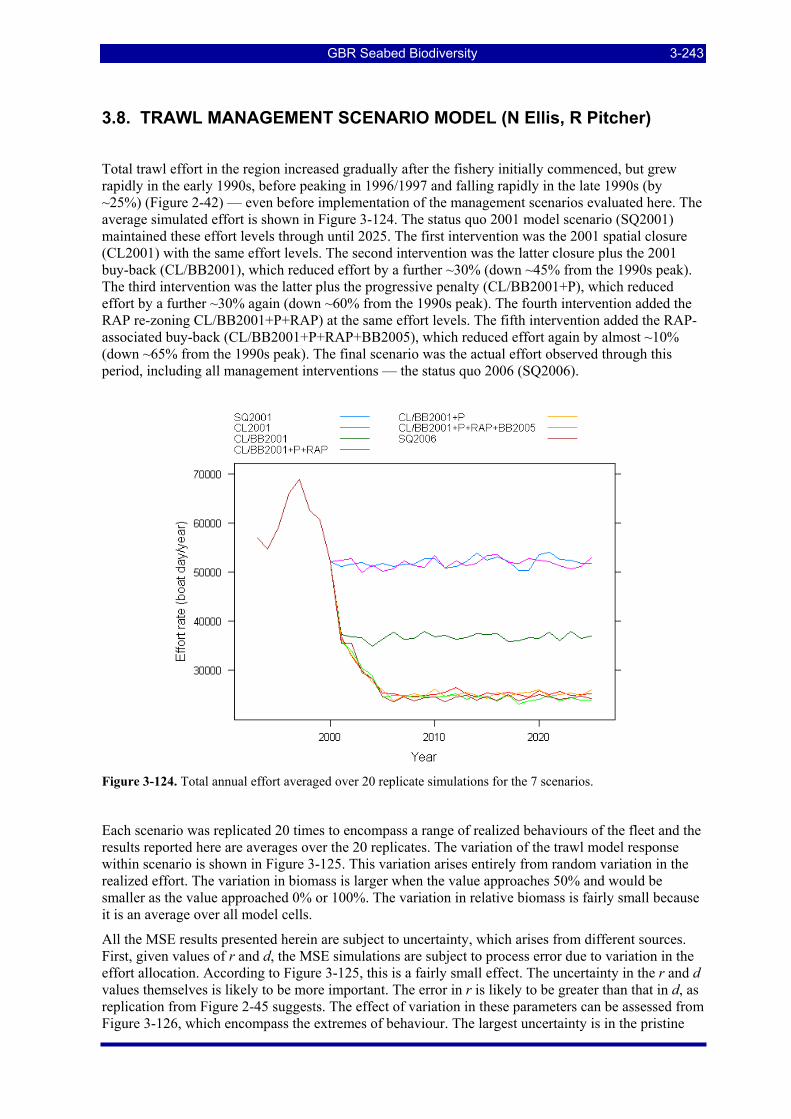
GBR Seabed Biodiversity 3-243
3.8. TRAWL MANAGEMENT SCENARIO MODEL (N Ellis, R Pitcher)
Total trawl effort in the region increased gradually after the fishery initially commenced, but grew rapidly in the early 1990s, before peaking in 1996/1997 and falling rapidly in the late 1990s (by ~25%) (Figure 2-42) — even before implementation of the management scenarios evaluated here. The average simulated effort is shown in Figure 3-124. The status quo 2001 model scenario (SQ2001) maintained these effort levels through until 2025. The first intervention was the 2001 spatial closure (CL2001) with the same effort levels. The second intervention was the latter closure plus the 2001 buy-back (CL/BB2001), which reduced effort by a further ~30% (down ~45% from the 1990s peak). The third intervention was the latter plus the progressive penalty (CL/BB2001+P), which reduced effort by a further ~30% again (down ~60% from the 1990s peak). The fourth intervention added the RAP re-zoning CL/BB2001+P+RAP) at the same effort levels. The fifth intervention added the RAP-associated buy-back (CL/BB2001+P+RAP+BB2005), which reduced effort again by almost ~10% (down ~65% from the 1990s peak). The final scenario was the actual effort observed through this period, including all management interventions — the status quo 2006 (SQ2006).
Figure 3-124. Total annual effort averaged over 20 replicate simulations for the 7 scenarios.
Each scenario was replicated 20 times to encompass a range of realized behaviours of the fleet and the results reported here are averages over the 20 replicates. The variation of the trawl model response within scenario is shown in Figure 3-125. This variation arises entirely from random variation in the realized effort. The variation in biomass is larger when the value approaches 50% and would be smaller as the value approached 0% or 100%. The variation in relative biomass is fairly small because it is an average over all model cells.
All the MSE results presented herein are subject to uncertainty, which arises from different sources. First, given values of r and d, the MSE simulations are subject to process error due to variation in the effort allocation. According to Figure 3-125, this is a fairly small effect. The uncertainty in the r and d values themselves is likely to be more important. The error in r is likely to be greater than that in d, as replication from Figure 2-45 suggests. The effect of variation in these parameters can be assessed from Figure 3-126, which encompass the extremes of behaviour. The largest uncertainty is in the pristine
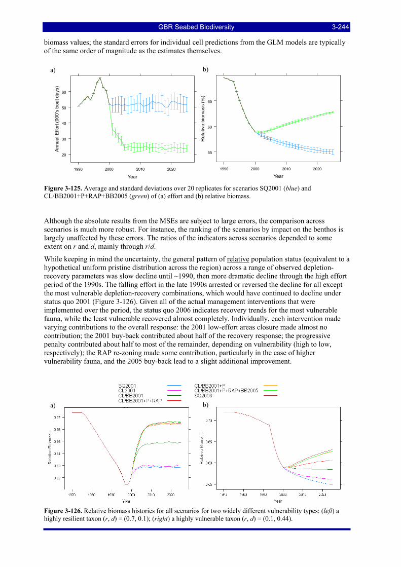
GBR Seabed Biodiversity 3-244
biomass values; the standard errors for individual cell predictions from the GLM models are typically of the same order of magnitude as the estimates themselves.
Year
Ann
ual E
ffort
(000
's b
oat d
ays)
20
30
40
50
60
1990 2000 2010 2020
Year
Rel
ativ
e bi
omas
s (%
)
55
60
65
1990 2000 2010 2020
Figure 3-125. Average and standard deviations over 20 replicates for scenarios SQ2001 (blue) and CL/BB2001+P+RAP+BB2005 (green) of (a) effort and (b) relative biomass.
Although the absolute results from the MSEs are subject to large errors, the comparison across scenarios is much more robust. For instance, the ranking of the scenarios by impact on the benthos is largely unaffected by these errors. The ratios of the indicators across scenarios depended to some extent on r and d, mainly through r/d.
While keeping in mind the uncertainty, the general pattern of relative population status (equivalent to a hypothetical uniform pristine distribution across the region) across a range of observed depletion-recovery parameters was slow decline until ~1990, then more dramatic decline through the high effort period of the 1990s. The falling effort in the late 1990s arrested or reversed the decline for all except the most vulnerable depletion-recovery combinations, which would have continued to decline under status quo 2001 (Figure 3-126). Given all of the actual management interventions that were implemented over the period, the status quo 2006 indicates recovery trends for the most vulnerable fauna, while the least vulnerable recovered almost completely. Individually, each intervention made varying contributions to the overall response: the 2001 low-effort areas closure made almost no contribution; the 2001 buy-back contributed about half of the recovery response; the progressive penalty contributed about half to most of the remainder, depending on vulnerability (high to low, respectively); the RAP re-zoning made some contribution, particularly in the case of higher vulnerability fauna, and the 2005 buy-back lead to a slight additional improvement.
Figure 3-126. Relative biomass histories for all scenarios for two widely different vulnerability types: (left) a highly resilient taxon (r, d) = (0.7, 0.1); (right) a highly vulnerable taxon (r, d) = (0.1, 0.44).
a) b)
a) b)
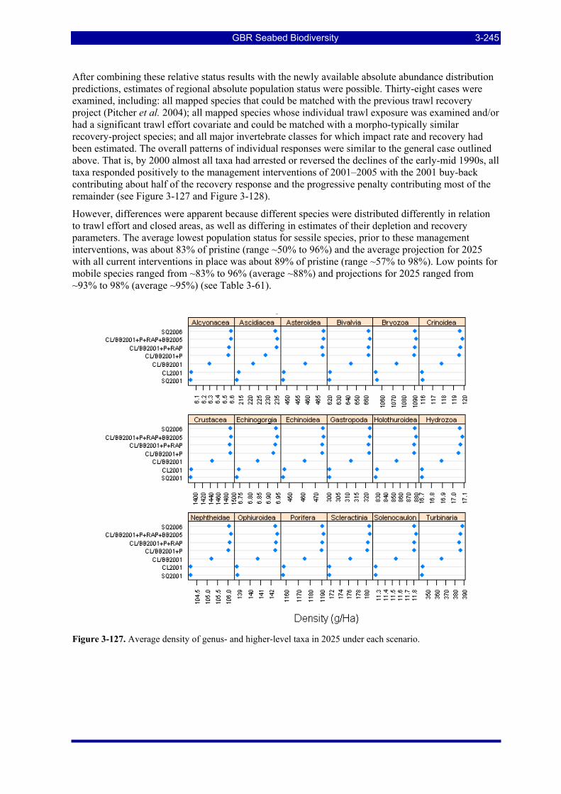
GBR Seabed Biodiversity 3-245
After combining these relative status results with the newly available absolute abundance distribution predictions, estimates of regional absolute population status were possible. Thirty-eight cases were examined, including: all mapped species that could be matched with the previous trawl recovery project (Pitcher et al. 2004); all mapped species whose individual trawl exposure was examined and/or had a significant trawl effort covariate and could be matched with a morpho-typically similar recovery-project species; and all major invertebrate classes for which impact rate and recovery had been estimated. The overall patterns of individual responses were similar to the general case outlined above. That is, by 2000 almost all taxa had arrested or reversed the declines of the early-mid 1990s, all taxa responded positively to the management interventions of 2001–2005 with the 2001 buy-back contributing about half of the recovery response and the progressive penalty contributing most of the remainder (see Figure 3-127 and Figure 3-128).
However, differences were apparent because different species were distributed differently in relation to trawl effort and closed areas, as well as differing in estimates of their depletion and recovery parameters. The average lowest population status for sessile species, prior to these management interventions, was about 83% of pristine (range ~50% to 96%) and the average projection for 2025 with all current interventions in place was about 89% of pristine (range ~57% to 98%). Low points for mobile species ranged from ~83% to 96% (average ~88%) and projections for 2025 ranged from ~93% to 98% (average ~95%) (see Table 3-61).
Figure 3-127. Average density of genus- and higher-level taxa in 2025 under each scenario.
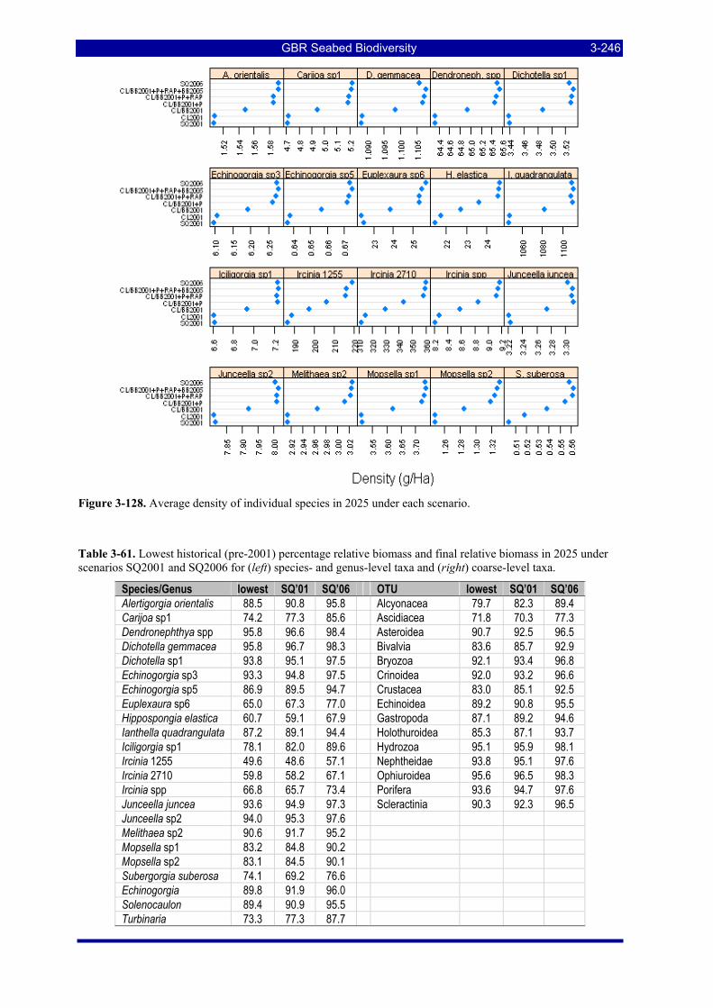
GBR Seabed Biodiversity 3-246
Figure 3-128. Average density of individual species in 2025 under each scenario.
Table 3-61. Lowest historical (pre-2001) percentage relative biomass and final relative biomass in 2025 under scenarios SQ2001 and SQ2006 for (left) species- and genus-level taxa and (right) coarse-level taxa.
Species/Genus lowest SQ’01 SQ’06 OTU lowest SQ’01 SQ’06 Alertigorgia orientalis 88.5 90.8 95.8 Alcyonacea 79.7 82.3 89.4 Carijoa sp1 74.2 77.3 85.6 Ascidiacea 71.8 70.3 77.3 Dendronephthya spp 95.8 96.6 98.4 Asteroidea 90.7 92.5 96.5 Dichotella gemmacea 95.8 96.7 98.3 Bivalvia 83.6 85.7 92.9 Dichotella sp1 93.8 95.1 97.5 Bryozoa 92.1 93.4 96.8 Echinogorgia sp3 93.3 94.8 97.5 Crinoidea 92.0 93.2 96.6 Echinogorgia sp5 86.9 89.5 94.7 Crustacea 83.0 85.1 92.5 Euplexaura sp6 65.0 67.3 77.0 Echinoidea 89.2 90.8 95.5 Hippospongia elastica 60.7 59.1 67.9 Gastropoda 87.1 89.2 94.6 Ianthella quadrangulata 87.2 89.1 94.4 Holothuroidea 85.3 87.1 93.7 Iciligorgia sp1 78.1 82.0 89.6 Hydrozoa 95.1 95.9 98.1 Ircinia 1255 49.6 48.6 57.1 Nephtheidae 93.8 95.1 97.6 Ircinia 2710 59.8 58.2 67.1 Ophiuroidea 95.6 96.5 98.3 Ircinia spp 66.8 65.7 73.4 Porifera 93.6 94.7 97.6 Junceella juncea 93.6 94.9 97.3 Scleractinia 90.3 92.3 96.5 Junceella sp2 94.0 95.3 97.6 Melithaea sp2 90.6 91.7 95.2 Mopsella sp1 83.2 84.8 90.2 Mopsella sp2 83.1 84.5 90.1 Subergorgia suberosa 74.1 69.2 76.6 Echinogorgia 89.8 91.9 96.0 Solenocaulon 89.4 90.9 95.5 Turbinaria 73.3 77.3 87.7
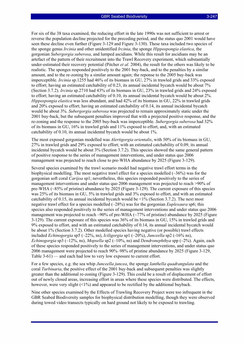
GBR Seabed Biodiversity 3-247
For six of the 38 taxa examined, the reducing effort in the late 1990s was not sufficient to arrest or reverse the population decline projected for the preceding period, and the status quo 2001 would have seen these decline even further (Figure 3-129 and Figure 3-130). These taxa included two species of the sponge genus Ircinia and other unidentified Ircinia, the sponge Hippospongia elastica, the gorgonian Subergorgia suberosa, and lumped ascidians. While this result for ascidians may be an artefact of the pattern of their recruitment into the Trawl Recovery experiment, which substantially under-estimated their recovery potential (Pitcher et al. 2004), the result for the others was likely to be realistic. The sponges responded positively to the 2001 buy-back, and to the penalties by a similar amount, and to the re-zoning by a similar amount again; the reponse to the 2005 buy-back was imperceptible. Ircinia sp.1255 had 46% of its biomass in GU, 27% in trawled grids and 33% exposed to effort; having an estimated catchability of 0.23, its annual incidental bycatch would be about 7% (Section 3.7.2). Ircinia sp.2710 had 43% of its biomass in GU, 23% in trawled grids and 24% exposed to effort; having an estimated catchability of 0.10, its annual incidental bycatch would be about 2%. Hippospongia elastica was less abundant, and had 42% of its biomass in GU, 22% in trawled grids and 20% exposed to effort; having an estimated catchability of 0.14, its annual incidental bycatch would be about 3%. Subergorgia suberosa was projected to remain approximately static under the 2001 buy-back, but the subsequent penalties improved that with a projected positive response, and the re-zoning and the response to the 2005 buy-back was imperceptible. Subergorgia suberosa had 32% of its biomass in GU, 16% in trawled grids and 11% exposed to effort, and, with an estimated catchability of 0.10, its annual incidental bycatch would be about 1%.
The most exposed gorgonian modelled was Alertigorgia orientalis, with 50% of its biomass in GU, 27% in trawled grids and 29% exposed to effort; with an estimated catchability of 0.09, its annual incidental bycatch would be about 3% (Section 3.7.2). This species showed the same general pattern of positive response to the series of management interventions, and under status quo 2006 management was projected to reach close to pre-WHA abundance by 2025 (Figure 3-129).
Several species examined by the trawl scenario model had negative trawl effort terms in the biophysical modelling. The most negative trawl effect for a species modelled (–36%) was for the gorgonian soft coral Carijoa sp1; nevertheless, this species responded positively to the series of management interventions and under status quo 2006 management was projected to reach >90% of pre-WHA (~85% of pristine) abundance by 2025 (Figure 3-129). The current exposure of this species was 25% of its biomass in GU, 5% in trawled grids and 3% exposed to effort, and with an estimated catchability of 0.15, its annual incidental bycatch would be <1% (Section 3.7.2). The next most negative trawl effect for a species modelled (–28%) was for the gorgonian Euplexaura sp6; this species also responded positively to the series of management interventions and under status quo 2006 management was projected to reach ~90% of pre-WHA (~77% of pristine) abundance by 2025 (Figure 3-129). The current exposure of this species was 36% of its biomass in GU, 15% in trawled grids and 9% exposed to effort, and with an estimated catchability of 0.14, its annual incidental bycatch would be about 1% (Section 3.7.2). Other modelled species having negative (or possible) trawl effects included Echinogorgia sp5 (–22%, ns), Iciligorgia sp1 (–20%), Junceella sp2 (-16% ns), Echinogorgia sp3 (–12%, ns), Mopsella sp2 (–10%, ns) and Dendronephthya spp (–2%). Again, each of these species responded positively to the series of management interventions, and under status quo 2006 management were projected to reach 90%–98% of pristine abundance by 2025 (Figure 3-129, Table 3-61) — and each had low to very low exposure to current effort.
For a few species, e.g. the sea whip Junceella juncea, the sponge Ianthella quadrangulata and the coral Turbinaria, the positive effect of the 2001 buy-back and subsequent penalties was slightly greater than the additional re-zoning (Figure 3-129). This could be a result of displacement of effort out of newly closed areas, increasing effort in areas where these species were distributed. The effects, however, were very slight (<1%) and appeared to be rectified by the additional buyback.
Nine other species examined by the Effects of Trawling Recovery Project were too infrequent in the GBR Seabed Biodiversity samples for biophysical distribution modelling, though they were observed during towed video transects typically on hard ground not likely to be exposed to trawling.
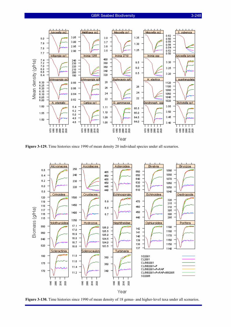
GBR Seabed Biodiversity 3-248
Figure 3-129. Time histories since 1990 of mean density 20 individual species under all scenarios.
Figure 3-130. Time histories since 1990 of mean density of 18 genus- and higher-level taxa under all scenarios.

GBR Seabed Biodiversity 3-249
The common consistent result from the trawl management scenario modelling was that the omnipresent depletion trends of structural epibenthos up until the late 1990s all appear to have been arrested and reversed by the series of management interventions implemented between 2000 and 2005. The 2001 buyback and the subsequent progressive penalties appeared to make the biggest positive contributions. For ~7 of 38 representative taxa modelled, the rezoning made an observable additional positive contribution, and for a similar number of species a slight contribution of the 2005 buy-back was also observable.
GBR Seabed Biodiversity 4-250
4. DISCUSSION
The GBR seabed is a complex mix of physical environments. The component species and biological assemblages have been observed to respond significantly, though in different ways, to the multiple interacting physical gradients and few of these gradients have simple trends in 2-dimensional space. Much of the prior knowledge about seabed biodiversity has been sourced from the Central (Townsville) Section of the GBR where there are a series of relatively linear cross-shelf coastal to offshore gradients. Along with a gradient of progressively increasing depth, there is an inner shelf prism of terrigenous sandy-mud sediments that extends 15–20 km offshore to water depths of 20–22 m. Further offshore, the GBR lagoon in depths ~22–40 m has little terrigenous sediment but a thin veneer of mixed shelly, muddy-sand overlying weathered Pleistocene clay, which can be exposed by cyclones to form outcrops on the seabed. Amongst the mid-shelf and outer-shelf reefs, the seabed (40–80 m) has virtually no terrigenous sediment, but is covered thinly by shelly biogenic carbonate sand; here, old Pleistocene reef platforms are the foundations on which modern coral reefs emerge (Larcombe & Carter 2004). With these geological patterns, there is a gradient from high turbidity to clear water. The mid/outer shelf reef matrix off Townsville is relatively open and this permeability allows influx of the EAC oceanic water and induced upwellings, which penetrate as far as the mid-shelf (Wolanski 1994). The south-easterly trade winds drive a northward flowing coastal boundary layer that limits mixing of nearshore and offshore waters (Brinkman et al. 2002). As a result, there are cross shelf gradients in bottom water attributes coastal to offshore: warm to cooler temperature (high to low variability), low to high salinity (high to low variability), high to low oxygen (low to high variability), and low to high nutrients (low to high variability). Further, tidal currents are weak though most of the area. This has lead to an established view of fixed across shelf zoning of the biota (discussed further in sections below).
However, these simple cross-shelf physical environment patterns largely apply only to the Townsville vicinity from about Cape Upstart to about Hinchinbrook Is. The physical covariates collated by the project showed that elsewhere, the physical environment does generally change more quickly in the cross-shelf direction than the along-shelf direction, but in ways that may be completely different to that in the Townsville vicinity. For example, about a third of the coast from about Mackay south is sandy not muddy, as is the far northern coast from Shelbourne Bay north (as well as a number of other locations). Conversely, much of the mid-shelf from about Mackay south is muddy not sandy, as is the far northern inner/mid-shelf from about Shelbourne Bay north; the outer shelf from about Innisfail to Cooktown has significant areas of high (carbonate) mud fraction. The Capricornia section is almost entirely sand; terrestrial silica sand along the coast and across the shelf in the south; carbonate to the northeast. While coastal areas are always shallow, much of the outer shelf north of about Cooktown is about as shallow as the inner and mid shelf, as is the Swains even though it is the most offshore area in the region. In the southern GBR, the mid-shelf is the deepest (Capricorn Channel). In much of the southern GBR, and far northern/Torres Strait, extreme tidal currents create forces on the seabed in both inshore and offshore areas that lead to sediment scoured and epibenthic habitats that rarely occur in the Townsville and Cairns Sections. The ribbon reefs extending north from about Cooktown to Torres Strait limit exchange and upwelling of cooler, saline, nutrient rich water onto the outer shelf; in the southern GBR, these occur well into the Capricorn Channel. These different physical environment patterns elsewhere contribute to the complexity in patterns of seabed biota observed by this project.
It has been noted previously that there are a wide range of inter-reef habitats dominating in different regions of the GBRMP due to varying riverine inputs, tides, currents and upwellings, seasonal winds, waves, and cyclonic events, with different combinations of these forces governing the topography, grain size and composition of sediments, the chemical properties of overlying waters (Larcombe & Carter 2004; Porter-Smith et al. 2004) and therefore, the nature of seabed assemblages and their dynamics. Local influences, such as tidal jetting of nutrients, facilitate the development of substantial Halimeda algal banks 15-20 m thick inside the ribbon reef passages of the northern GBR (Drew 2001). Porter-Smith et al. (2004) noted that in the macrotidal areas of Broad Sound and Shoalwater Bay, tidal currents were the dominant force influencing the mobility and grain size properties and contrasted with the rest of the GBRMP. The bifurcation of the South Equatorial Current (SEC) against
GBR Seabed Biodiversity 4-251
the outer reef (Wolanski 1994) between about Lizard Is and Cairns, which produces the EAC to the south and the NW Coral Sea gyre to the north, can influence the dispersal of species with oceanic larvae (Pitcher et al. 2005).
There are also latitudinal differences in flushing rates and the amplitude of seasonal variation in sea surface temperature (SST) and salinity. Hancock et al. (in Press) found that inner lagoon diffusivity was about 2.5 times higher in the central section compared to the northern, so that water within 20 km of coast is flushed with outer lagoon water on a time scale of 18-45 days, with greater flushing times in the north. Salinities in the southern lagoon are significantly higher than those in the central and northern sections, and seasonal variation is lower. Summer SST are ~2-3°C lower in the region south of Bowen compared to the far north, and in winter a relatively cold coastal water body forms there (Condie and Dunn 2006).
4.1. BRUVS SPECIES MODELS, CHARACTERIZATION & PREDICTION (M Cappo, G De’Ath)
4.1.1. BRUVS Fish species Only 50 of the 347 species recorded by BRUVS occurred at 7% or more of the sampling sites. Univariate biophysical models of this subset produced many erroneous (negative) predictions of abundance. It was decided then to produce biophysical models and maps of the presence/absence (occurrence) of single species in relation to the environmental covariates. The occurrence of only 25 fish species could be predicted with errors of 20% or less, and a shortlist of 20 environmental covariates were useful as predictors.
The “nuisance” temporal variables such as moon phase, season and time of day had no effect on average rates of prediction, so they were dropped from the best models. This implied the biophysical maps of occurrence in the BRUVS dataset do not need to be adjusted for these temporal variables.
The spatial location (across, along, depth) and mud, gravel and carbonate content of sediments were the top six predictors of species occurrence. There were a variety of relationships between these physical parameters and the occurrence of particular species. The presence of some species was best explained by by a single variable, including Scomberomorus queenslandicus found inshore, Pentapodus paradiseus influenced by gravely sediments, and Nemipterus furcosus and Alepes apercna found in warmer temperatures. The presence of other species was influenced most most by a combination of spatial and environmental variables. Nemipterus hexodon was one of the most predictable species, occurring nearshore in sediments with high mud content. In contrast, Pentapodus nagasakiensis was found offshore in sediments with high carbonate. Within the same family N. theodorei was influenced most by deep water and high salinity. This species was not seen in the far north. A number of species were influenced most by environmental variables. The economically important Choerodon venustus occurred most in areas of higher current with sediments containing high carbonate. Parapercis nebulosa also occurred in higher current, over sediments with low mud content.
The trawl effort index explained a moderate proportion of the variability in occurrence of only a single species (Nemipterus peronii), but interpreting such relationships was very difficult because trawling occurs infrequently, or not at all, over most of the GBRMP and in high levels in some areas, such as Cape Flattery. Thus the 10th percentile in the trawl effort index had much leverage on the response by N. peronii. The relationship between the species responses and the environmental gradients in the GBRMP are discussed below with the characterisation of species groups.
4.1.2. BRUVS Fish Assemblages Significant differences have been reported in the distribution and abundance of a range of faunal and floral groups in the GBRMP along the strong cross-shelf gradients readily measurable in salinity, nutrient input, water clarity and exposure to prevailing wind and waves with increasing distance from
GBR Seabed Biodiversity 4-252
the coast (Drew 2001, Wilkinson & Cheshire 1988, Newman et al. 1997, Gust et al. 2001). However, studies have incorporated the latitudinal gradient along the shelf (DeVantier et al. 2006, Fabricius & De’ath 2001, Williams 1991), and most have been restricted to the depth limits of SCUBA diving observations on shallow reefs. The results reported here are the first attempt at describing the patterns in fish communities in terms of both location in the GBRMP and critical environmental covariates.
The use of boosted and multivariate regression trees provided compelling results concerning the cross-shelf rise in species richness to “hotspots” about the shallow banks and shoals amongst the offshore reef matrix, the existence of spatially-contiguous fish communities along and across the shelf of the GBRMP, and the existence of major community boundaries near Bowen (20°S) in the south and Princess Charlotte Bay (13.3°S) in the north. These robust patterns were detected amongst a functionally diverse cross-section of the fish fauna by analysis of data collected with a simple, efficient baited video technique.
The majority of species recorded by the BRUVS occurred rarely and this pattern also seems characteristic of tropical fish faunas sampled by trawl. The widespread sampling with BRUVS recorded a similar number of species (347) to those recorded by trawling (300 – 350) in similar latitudes by Watson et al. (1990), Blaber et al. (1994), Wassenberg et al. (1997), and Stobutzki (2001b). Those trawl inventories were also dominated by species that occurred rarely and in low abundance. Stobutzki (2001b) found that 75% of species occurred in less than 10% of prawn trawls, and Blaber et al. (1994) found that 75% of the biomass in fish trawls comprised only 8% of the species caught. Like estuarine fish faunas (Magurran & Henderson, 2003), the vertebrates in the “inter-reef” waters of the GBRMP probably comprise “core species”, which are persistent, abundant and biologically associated with particular habitats, and “occasional species”, which occur infrequently in surveys, are typically low in abundance and have different habitat requirements.
Only 50 species occurred at 7% or more of the sampling sites and the abundance of only 25 of these species could be predicted, in terms of the 40 environmental covariates, with errors of 20% or less. This shortlist was chosen for preparation of biophysical maps relating communities to the environment. Multivariate trees were used within this shortlist of species to define a hierarchy of communities constrained by their spatial and environmental values that locate them in the GBRMP. This hierarchical approach identified groups of the 25 predictable species that co-occur at varying spatial scales to form communities.
A number of multivariate trees were assembled using different combinations of spatial and environmental variables. The simplest, most easily interpreted model chosen to produce biophysical maps used only position across and along the shelf as explanatory variables for the 25 most predictable species. The broad patterns identified by this tree largely coincide with the analysis of the entire species list by Cappo et al. (subm.) in a study that aimed to explain (not predict or map) communities in terms of location and depth.
The across and along tree produced spatially contiguous communities occurring around major faunal breaks in the nearshore half and middle of the lagoon, and alongshore. Latitudinal variation was greatest in the inner half of the shelf, where Bowen and Princess Charlotte Bay separated inner and outer shelf groups. The offshore communities were latitudinally more extensive showing that outer-shelf deep communities were more similar amongst latitudes than to inner-shelf communities at the same latitude and vice versa. These trends were also reported by Williams (1991) for reef fish communities on outer slopes of outer-shelf and mid-shelf coral reefs, with mid-shelf reefs in the far north being more similar to nearshore reefs elsewhere than to mid-shelf reefs at more southerly latitudes.
Cross-shelf gradients in demersal fish communities have been reported elsewhere in the southern Indo-Pacific. A “nearshore” group of sites (<24 m depth) was distinguished from a “mid-shelf” (outer lagoon 35-42 m depth) and an “inter-reef” group (mid-shelf reef matrix 43-56 m) in catches by prawn trawl in the central GBRMP (Watson et al. 1990). That study concluded the composition of the 'inter-reef' fauna remained strikingly uniform regardless of proximity (~0.5 to 10 km) to coral reef formations. In the Gulf of Carpentaria, Blaber et al. (1994) distinguished six main site groups and 15 fish community groups in fish trawls, correlated with depth but not with sediment type, salinity, temperature or turbidity. Letourneur et al. (1998) concluded that the effect of sediment type in shaping reef fish communities in lagoon waters was confounded by cross-shelf position, which acted as an
GBR Seabed Biodiversity 4-253
easily measured surrogate for the gradient from terrigenous to oceanic influences in New Caledonia. At broader scales, Ramm et al. (1990) found that a bycatch fauna from prawn trawls samples clustered along geographic and bathymetric gradients, forming distinct western and eastern groups separated near132°E, either side of the 30 metre isobath. This longitudinal boundary separates the faunistic provinces of the Timor Sea to the west and the Arafura Sea to the east.
Reviews have concluded that sediment type, water clarity, seabed topography, the nature of epibenthic communities and thermal stratification all shape the composition of tropical, demersal fish communities (Longhurst & Pauly 1987, Sainsbury et al. 1997, Lowe-McConnell 1987). In the tropical western Atlantic, Lowe-McConnell (1987) characterised a cross-shelf gradient from a “brown water” zone (ariid catfishes, dasyatid rays) over mud, to a “golden fish” zone (sciaenid croakers) over sandy/mud, to a “silver fish” zone (carangid jacks, haemulid grunts) in “green water” (40-60 m deep), above a “red fish” zone (lutjanid snappers) over hard sand/rock in “blue” oceanic waters (~100 m). Similar patterns were reported in the eastern Atlantic, with the additional influence of a strong thermocline causing sub-tropical sparids to dominate in the cooler waters under the thermocline over sand, rock and Holocene reef edges (Fager & Longhurst 1968, Lowe-McConnell 1987).
We found that there were not strict cross-shelf differences in the occurrence of different families and that single families often contained a number of species that characterised different communities. Ubiquitous families such as the nemipterid threadfin breams, monacanthid file fishes, carcharhinid requiem sharks and tetraodontid pufferfish had representatives in both inshore and offshore, deep and shallow communities. The inshore community included many indicator species from the “small pelagic” functional groups, such as the piscivorous Scomberomorus queenslandicus and deep-bodied micro-invertebrate carnivores (Carangidae: Atule mate, Selaroidesleptolepis and Carangoides coeruleopinnatus). Demersal teraponid grunters and bathysaurid lizardfishes were also characteristic of inshore groups. These are known to inhabit soft sediments in the Indo-Pacific (Blaber et al. 1994; Sainsbury et al. 1997). Indicator species offshore included pinguipedid grubfishes (Parapercis xanthozona_grp 40) and labrid wrasses (Choerodon venustus, Oxycheilinus bimaculatus) thought to be associated with more complex seafloor topography, such as reefs, rocks and rubble.
The distributions of fishes and their assemblages are likely to be shaped by variation in sedimentary and oceanic processes and other influences that determine the wide range of seabed physical and biological habitats dominating in different regions of the GBRMP, as described above. In turn, these habitats may influence the recruitment, feeding success and mortality of fish communities inhabiting them. The nearshore and mid-shelf boundaries separating the fish assemblages appear related to sediment carbonate and grain-size composition particularly in the Central Section. The observed fish assemblage patterns fit well with knowledge of gradients and boundaries in sedimentary processes, water movement, and seafloor fish habitats such as erosional features, depositional banks and vegetated meadows.
Major latitudinal boundaries in the fish assemblages may be related to circulation patterns and their consequences. The latitudinal variation amongst the communities along the shelf, with boundaries near Mackay, Bowen, Cape Bowling Green, Princess Charlotte Bay and Cape Direction, may be explained by circulation patterns in a cooler, macrotidal southern region, a well-flushed central region with deepwater seagrass beds, and a warmer, constricted northern region where Halimeda algal banks thrive behind a dense reef matrix. The next step is to analyse these spatial groupings within a comprehensive suite of biotic measurements from other sampling gears to determine if predictions and explanations of the shelf-scale patterns in fish communities can be improved with knowledge of epibenthic communities now available from the Seabed Biodiversity dataset.
4.2. SINGLE SPECIES, BIOPHYSICAL MODELS AND PREDICTION
The epibenthic sled and research trawl both sampled a highly diverse seabed biota of more than 14 phyla and >5,300 species, of which about a third were sampled by both devices, almost half were unique to the sled, and just less than a quarter were unique to the trawl. While the Sled samples were rich with almost 60 taxa per site on average and had greater total species richness, the Trawl samples averaged about 87 taxa and were less variable (<1% sampled fewer than 20 species). Thus, the trawl
GBR Seabed Biodiversity 4-254
more consistently sampled local populations representatively (particularly fishes and crustaceans), whereas the Sled sampled all other biota better, though with greater variability, perhaps due to the greater number of sites and habitats sampled by the sled. These devices provided specimens that could be properly identified, showed that otherwise inseparable taxa could have strikingly different distribution patterns and revealed the enormous biodiversity of the region (even at sites where other devices observed no biota at all). They also provided excellent benefit:cost in terms of enormous information yield per unit investment and given the very small area sampled (~1/50000).
As is typical of biological sampling, a large proportion of these taxa occurred in only one or a very few sites. This, and patterns of species accumulation curves, indicated that many more seabed species remain to be discovered — despite the regional extent and number of sites sampled by the project — and confirms the significant biodiversity of the deeper lagoon and inter-reef seabed in the GBR.
There were some clear basic patterns of species richness: structured habitats were more diverse, and structure was provided by marine plants, epibenthic fauna, and rugose hard substrata. Key vegetated habitats occurred in a midshelf band in the central GBR, the inner/mid-shelf in the Capricorn region, the outer shelf in the far northern region and near the Turtle and Howick Island groups. Key epibenthic habitats occurred in the vicinity of Broad Sound and Shoalwater Bay, approaches to Torres Strait, inshore and offshore passages and hard ground. Topographically complex hard ground occurred primarily among the outer shelf reef matrix as relic reef growth from eras of lower sea levels. Muddy habitats, on the other hand, had relatively low biodiversity and tended to be dominated by smaller fishes. The structured areas also had steeper species accumulation curves, i.e. additional sites were more likely to yield additional species compared with muddy areas, which consequently tended to be more homogeneous.
Compared with the total number of species sampled, relatively fewer species were considered frequent enough for analyses (at >25 sites). Nevertheless, there were about 840 species that met this criterion. This presented considerable computational challenges for biophysical modelling, necessitating a consistent mechanistic approach and meant that in the available timeframe models could not be manually customized for individual species. The analyses also produced an enormous output, of which only summary distributional highlights can be presented, even in a large report, and future examination of the dataset and results would provide valuable specific information.
The two-stage presence-biomass GLMs provided a robust and flexible method of selecting physical covariates having statistical relationships with the biological data suitable for modelling biophysical responses and predicting distributions. More than 65% of the ~840 species analysed had good models; however, not all species could be modelled well. Up to ~10% had poor models though many of the latter were for species that could not be weighed readily, and 11 species had no statistical relationship with any of the physical or spatial variables. For the majority of species, i.e. those occurring at <25 sites, no analyses or modelling has been reported at this time, though point data will be available.
The biophysical modelling provided an indication of covariate importance in relation to patterns of species abundances. The most frequent covariates were sediment grain size and carbonate composition, followed by space, benthic irradiance, current stress, bathymetry, then bottom water physical attributes, seasonal effects, nutrients and turbidity, and other temporal effects. Trawl effort was selected infrequently, at about 10% and was significant in just over half these cases. Aspect was selected least. However, frequency of covariate selection is not necessarily a direct test of performance among the various individual physical or spatial covariates due to the high correlations between many of them. That is, a given covariate may be parsimoniously selected though it is merely a surrogate for a number of others with which it is correlated.
The environmental covariates have demonstrated utility for spatial prediction of the broad scale patterns of presence for the majority of species with occurrence >25 sites, although they do not often account for the majority of observed variation in local biomass. Other factors, including stochastic processes such as recruitment and mortality, biological interactions, and random sampling effects typically outweigh deterministic environmental relationships at the local site biomass scale.
The variety of biophysical responses, and hence distributions, expressed was almost as large as the number of species analysed, and while there were numerous highly contrasting responses there was a continuum of responses between the extremes. Some of the contrasting responses observed followed the more frequently occurring covariates, such as ± mud or sand or gravel, shallow vs deep, low vs

GBR Seabed Biodiversity 4-255
high benthic irradiance, inshore vs offshore, northern vs southern, strong vs weak current stress, cool vs warm temperature etc. It is important to note that taxonomy provides little guide to patterns of distribution. For example, many similar con-generic species were observed to have highly contrasting distributions, demonstrating the importance of species-level identifications wherever possible, when assessing biophysical responses and physical surrogate performance, and when addressing management applications such as fisheries risk assessments and conservation planning.
4.3. SPECIES GROUPS CHARACTERIZATION AND PREDICTION
The ~840 modelled species were clustered into 38 groups largely to facilitate manageable processing of the trawl risk assessments rather than any particular attempt at this time to identify an objective number of functional “communities” of interacting species; though the methods used may be useful to facilitate initial identification of potential functional relationships between species, significant future ecological investigation would be required. As noted in the previous section, there was almost a continuum of distributional patterns with few strong clusters. The groups were constructed to comprise species with highly correlated distributions, given the stated purpose, leading to a greater number of groups than conventional applications of the method. The basic patterns of groups were similar to those of single species and though the models were more complex, covariate importance ranks were also similar to those of single species.
Species groups distributions were also not clearly related to taxonomic groupings, as noted above, with closely related species occurring in different groups and most groups comprising numerous unrelated taxa. Possible exceptions may have included some marine plants, sponges and bryozoans. Marine plants appeared to dominate in a number of rather specific areas determined at least in part by light availability; this and other shared constraints lead to a number of related species sharing similar distributions. Similarly, a number of encrusting bryozoan taxa were distributed in high current passages of the Pompey Reefs complex and a number of sponge taxa had similar distributions. Even in these constrained taxa, however, members of the same genus, family or class may have markedly different distributions.
4.4. SITE GROUPS CHARACTERIZATION AND PREDICTION
Due to the complex mix of physical environments described above, as well as additional variability remaining unexplained by the available covariates, the biodiversity assemblages of the GBR seabed are difficult to represent adequately in any single characterisation. The multitude of species respond in different, overlapping and varying ways to the multiple interacting physical gradients, which as noted above do not have simple trends in geographic space. Much of the prior biological sampling has been conducted in the Central (Townsville) Section of the GBR where the gradients are among the simplest in the region.
Seabed biological assemblages off Townsville were first sampled by Birtles and Arnold (1983 & 1988) using an epibenthic sled during a series of studies between 1977 and 1983. The shallower (<20 m) inshore muddy zone, to about 30 km offshore was characterised by low species richness of carnivorous and deposit feeding echinoderms, molluscs, crustaceans, fishes, bryozoans and algae, and low species evenness — i.e. a relatively low number of species was dominated by even fewer. Further offshore, from ~30 km to the mid-shelf reef-matrix at ~80 km, the deeper (20–50 m) carbonate sand lagoon zone was characterised by higher species richness of all faunal groups, due to increased habitat heterogeneity with patches of harder substratum that allow a wide variety of suspension feeders, such as sponges, ascidians, crinoids, holothurians, and bryozoans, a foothold in addition to the deposit feeders in the sediments between the patches. On the deeper gravely outer shelf (> ~80 km) offshore inter-reef zone the fauna was dominated by the suspension feeders (Birtles and Arnold, 1983). Temporal sampling showed that patterns of distribution remained essentially stable over the period. Greatest variability was apparent in the nearshore sites, due to physical instability of the sediments
GBR Seabed Biodiversity 4-256
caused by wind generated waves. Later, Watson and Geoden (1989) sampled around the Birtles and Arnold study area with somewhat greater alongshore coverage, using commercial prawn trawl gear, and found similar parallel zones that were stable over time. With few benthic studies conducted elsewhere, there has tended to exist a rather fixed view of simple cross-shelf zonation in the biota.
However, as already noted, the physical environment in other areas of the GBR has different combinations of physical environments and geographic gradients that may be completely different to that offshore from Townsville. These different physical environment patterns elsewhere explain why there have been reports of what had been regarded as nearshore faunas occurring in mid-shelf areas north of Cairns and even outer shelf areas (i.e. inner edge of Swains) (e.g. Williams, 1991). The Effects of Trawling Study in the far northern section (Poiner et al. 1998) noted that the coastal silica sand strip had fauna more similar to mid/outer-shelf areas than to the inner/mid-shelf high mud area. These "aberrant" patterns may now be understood more clearly with the extensive bio-physical information provided by the Seabed Biodiversity Project — the patterns are not aberrant at all but reflect the complex variety of environments manifest and distributed in different spatial patterns throughout the GBR region. The biotas are located largely (but not entirely) by environment than by cross-shelf position per se, or by latitude per se.
The biological assemblages observed by the Seabed Biodiversity Project are largely in line with the physical covariates found to be important in the single-species modelling and hence with the complex multidimensional physical environment patterns collated and mapped by the project and outlined at the beginning of the discussion. That is, the patterns are consistent with gradients between high and low mud areas, shallow and deep areas, high and low current areas, with further separations on sediments, water chemistry and turbidity. Note that each of these variables have surrogates that could separate assemblages, given the numerous correlations between the covariates. These broad patterns were largely unrelated to higher level taxonomic groupings; with members of most groups of biota occurring in most areas.
However, not all known patterns were captured within the stopping/cross-validation rules used by most statistical splitting algorithms, largely due to the variability in the data. For example, the inshore and offshore high current stress areas were grouped together and while they were similar in some respects there were nevertheless differences in species occurrences, depth and turbidity; the topographic shoal strata was not separated but was shown to differ from surrounding deeper seabed in a previous study (Poiner et al. 1998); and vegetated habitats were not separated precisely in the biophysical characterisation compared with the point species data.
4.5. VIDEO HABITAT CHARACTERIZATION AND PREDICTION
The physical habitats observed during towed video transect largely followed the physical environment patterns already discussed, not surprisingly given the similarity of the attributes quantified. Substratum was closely related to sediment grain size and carbonate, with exposed hard substratum occurring in high current areas, and deeper rocky areas amongst the outer shelf reefs. The biological habitats observed by video in part followed the physical substratum patterns, with bioturbated habitats occurring in many softer sediment areas and sessile epibenthic fauna and bryozoans common in high current hard ground areas. Vegetated habitats occurred on a variety of substrata and have constraints related more to irradiance and bottom water attributes. While some of the densest vegetated habitats were captured by the biophysical characterisation of video habitats, including much of the Townsville midshelf band, the Capricorn inner shelf area and far northern Halimeda banks, they were not separated very precisely. Furthermore, the biophysical characterisation confused intermediate density vegetated areas with some high density areas as well as with some very low density areas. Statistical stopping rules in conjunction with data variance contribute to this imprecise separation, and better broad scale data on relevant bottom water attributes would likely improve the biophysical characterisation.
A key issue with video, however, is the inability to identify most of the biota adequately. For example, hundreds of species of algae that comprise algal habitats can be identified to only a very few distinct genera and most to a handful of morpho-types, which blurs biophysical relationships that were
GBR Seabed Biodiversity 4-257
apparent at the species level and leads to inconsistent biophysical responses that are difficult to model with statistical methods, and thus difficult to map with biophysical spatial modelling.
A further issue was indicated by results of the first habitat characterisation strategy (first cluster the video biological data alone, then attempt to model their physical relationships), which had some difficulty representing the broader distribution of habitat clusters. Whereas, the second strategy found ‘habitats’ by using the biological profile together with and at the same time as the physical environment in which it resides. In this case, very similar biological habitats appeared in different tree nodes suggestive of different regions of environmental space. As an example from the results, two very similar seagrass dominated habitats (tree nodes 6 and 7, Figure 3-60, Figure 3-61,) were four nodes apart in the tree diagram suggesting different regions in environmental space. The mapped predictions (Figure 3-62) indicate a spatial divergence as well, with group 6 largely confined to the southern region of the GBR but with group 7 distributed in the mid-shelf off Townsville. Note that spatial predictors, however, played no direct part in the definition of these groups. However, the risk this brings to the second strategy is that essentially the same habitat, split in this way, may be interpreted as a different habitat — unless the composition is examined carefully. It is possible that if the habitat groups are initially defined in terms of biology only (the first strategy), sites such as those present in groups 6 and 7 may be clustered together, though this may make their prediction using the external physical variables more difficult because they are in different regions of environmental space. Note that the GLM method used in the single species modelling successfully modelled H. spinulosa distribution, the key species present in these two example seagrass dominated habitat cluster types and apparently occupying different regions of environmental space.
4.6. ACOUSTICS DISCRIMINATION AND CLASSIFICATION
Three approaches were taken to examine the performance of remotely sensed acoustic data, from a normal-incidence 120 kHz single beam digital echo sounder, for discriminating different seabed habitats and hence, as a surrogate for patterns in habitats and their constituent biodiversity.
(1) wavelet-based methods on angular transformed and re-sampled EY500 digital data, initially on simple pair-wise habitat class comparisons between few sites then progressively adding more habitat classes and sites.
(2) canonical variate-based methods on dilation-translation transformed and re-sampled EY500 digital data, initially on the entire ground-truthed dataset including all available sites and classes, then directed contrasts between fewer sites and fewer habitat classes.
(3) linear discriminant analysis methods on the QTC View proprietary 166 feature data, initially on the entire ground-truthed dataset including all available sites and classes, amalgamating classes, and by a moving window of restricted spatial and depth dimensions.
4.6.1. Wavelet Packet-Based Techniques Applied to Data in the Angular Domain (D H Smith)
Supervised classification experiments were performed on data in the angular domain via the Local Discriminant Basis in conjunction with Daubechies-2 filter coefficients and two different standard classifiers for up to five seabed habitat classes of long contiguous blocks of >1,000 pings, which tended to exclude certain habitats that were typically patchy in nature. Two-class testing on (sand,no biohabitat) and (sand,seagrass) seabeds with a single deep (sand,no biohabitat) training set produced very satisfactory classification results in a few pairwise site comparisons; however, addition of more sites demonstrated a strong sensitivity to the depth of the corresponding test set component, despite angular transformation of the data. This can be partially explained by the physics of acoustics, resulting in a distinct depth divide separating good and poor classification results. Substitution of a much shallower alternative training set for the (sand,no biohabitat) component produced no clear divide with less-variable classification accuracy lying between the extremes of the about experiment. In terms of overall mis-classification rates, the best results reached below 10% while the worst cases
GBR Seabed Biodiversity 4-258
reached just over 80% for these two-class cases. High mis-classification rates, when they did occur, were essentially the result of sand being mis-classified as seagrass.
Highly variable performance was also recorded in a second series of two-class experiments involving (sand,sponge garden dense) and (sand,seagrass) seabed types. Mis-classification rates for a selected training set ranged approximately between 10 and 55%, the upper limit caused by sponge garden being mis-classified as seagrass on many test sets. Little depth variation was present in these training and test sets, and the variable performance has little to with the depth effect noted above.
A three-class classification test involving (sand, no biohabitat), (sand, sponge garden dense) and (sand, seagrass) seabed types produced satisfactory classification results on a particular single training/test set pair, with confusion matrix diagonals all exceeding 80% and a best overall mis-classification rate of approximately 15% achieved with Linear Discriminant Analysis. Sand produced the best classification result, followed by sponge garden and seagrass. Feature dimension reduction was also achieved, but to a smaller extent than that obtained on the two class cases. Additional calculations with the same training data on a collection of test sets, including all available data of >1,000 contiguous pings for each class, indicated some significant performance differences between the Linear Discriminant Analysis and Tree classifiers. For sponge garden and seagrass biohabitats the Linear Discriminant Analysis was clearly superior, while little difference was observed for sand without biohabitat. In each case a general decline in performance with depth departure between the training and test sets was observed, however only one single training set was applied and performance with multiple training sets would be needed to fully assess variability in performance.
Incorporating a fourth seabed habitat class, namely (sand, bioturbated), gave mixed results on a selected single training/test set combination, with good performance recorded for the (sand, no biohabitat) and (sand, bioturbated) classes accompanied by moderate performance for (sand, seagrass). Principal error contributions for the latter case were due to mis-classification as (sand, sponge garden), which in turn was poorly classified and largely mistaken as seagrass. Further calculations on a range of different test sets showed good results from Linear Discriminant Analysis on the bioturbated class for depth departures up to almost 20 m, beyond which above 50% accuracy was retained up to 50 m departure. On the remaining three classes the two classifiers demonstrated clear differences, with Linear Discriminant Analysis superior for sponge garden and inferior for sand and seagrass; whereas as, in the experiment above, LDA had performed better than Tree on the same seagrass datasets. Again, classification performance was observed to decline with depth differences.
For a single five-class experiment involving different substrata in the absence of biohabitat, evidence for the concept of class merging appeared, in which different nominal classes are merged to produce a workable reduced set of seabed classes. Specifically, this applied to coarse sand and sand substrata types, and also to silt and soft mud, which were strongly confused by Linear Discriminant Analysis. The fifth substrata type, namely sand waves/dunes was almost 90% correctly classified in this experiment, with the error primarily due to mis-classification as soft mud.
In these tests with training and test set class contributions from individual sites, the Local Discriminant Basis operating on angular transformed data was able in selected localised cases to extract features that provided a good basis for classification of a limited number of classes by methods such as Trees or LDA. However, as the number of sites involved in tests was increased, or as the depth departure between sites increased, or as the number of classes of biological habitat on a fixed substratum was increased, or as the number of substratum types was increased, classification performance declined to unsatisfactory levels. The increased ambiguity means that relatively few bottom types can be consistently classified and so included in a workable set of seabed classes, and then only within a limited range of depth variation.
4.6.2. Canonical Variate Analysis of Acoustic Data (N Campbell & D Devereux) Canonical Variate Analyses were performed on digitised ping data, depth-normalised by the dilation method, and tested primarily with all available habitat classes and depths, but restricted to data representing classes with >100 contiguous pings.
GBR Seabed Biodiversity 4-259
A depth problem was again apparent and was examined in some detail. Depth-related differences in the shapes of normalised ping profiles were observed, at shallower depths (especially <25 m) the response for the first echo is much broader than it is at greater depths. This effect is due to the physics of echo-sounder operation and was seen to have a 1/depth relationship. Several methods to standardise for the effect were attempted, including an empirical regression of the echo response values on 1/depth. While a physically-based correction would be useful, none exist in the literature and the issue remains unresolved.
Analyses of data from sites that were collected close together in time, space and depth, suggested that it may be possible to provide local separation of extremes of cover in some circumstances. However, analyses of the larger data set over an extensive geographic area showed that the differences among pings from the same cover class were often as large as the differences between the cover classes. Even the site-contrast analyses for localised areas show that differences between sand sites can be greater than differences between sand and seagrass sites. Sand classes were the most common, were highly variable and their range of variability included almost all other habitat classes to a greater or lesser extent. Data from almost all classes were seen to plot almost throughout the full range of variability of the principal CVs. This demonstrated very considerable ambiguity between the acoustic signatures of the same and different classes, even at the same depth.
The digital echo sounder system used to collect the data analysed here had a transducer with a nominal beam angle of 10° — with greatest sensitivity < ±10° and little sensitivity between 10°–50° — as is fairly typical of single beam echo sounders. Relatively recent analyses of multibeam data show that much of the discrimination between cover classes occurs at angles 25°–35°, where the backscatter response for this single-beam instrument was much less than at narrower angles. For the narrower angles, there was some discrimination, though context from neighbouring pings is needed to improve the reliability. Thus, in the data from this echo-sounder, while some local scale discrimination in shape was observed, most discrimination would seem to depend on differences in the magnitudes of the responses at narrow angles, and not from consistent differences in the broader shape between the various cover classes.
4.6.3. Linear Discriminant Analyses of QTC View data Linear Discriminant Analyses were performed on the QTC View proprietary 166 feature data, and initially on the entire set of ground-truth seabed type classes, including all available sites and substratum and biological habitat types. Subsequently, similar types of habitat classes were amalgamated on the basis of ambiguity observed in LDA confusion matrices. The depth problem found in other types of data and analyses was also present in the QTC data and was addressed by partitioning the data by depth (and restricted spatial dimensions) to limit data selected for iterative training and testing trials, with some small improvement in amalgamated classification success.
Overall, the QTC data also had low levels of success in classifying the observed seabed classes, based upon its 166 acoustic parameters, and that success increased inversely as the number of classes was reduced. The fewest number of substratum classes analysed was seven, yet it was clear that a reduction to as few as 3–5 would be necessary in an attempt to raise classification success.
The best result achieved (~49%) was with a simple set of seven substratum classes (after partitioning into 6 depth strata). The majority of the confusion involved the most frequent substratum class (the sands), which accounted for ~70% of the observed seabed types, yet sands could be classified correctly in significantly less than half of observed cases, with the result that most sand was classified as either a more structured class type (gravel, rock, reef) or as mud.
It is acknowledged that the ground truth (EVENTS) data was at times also subject to misclassification by human observers of the towed video; for example, on occasion it could be difficult to accurately determine the sub types of soft sediments (sand, silt, mud) from video. Further, sediments can vary in ways that affect their acoustic properties, which cannot be observed on the sediment surface. While the reliability of the EVENTS data with respect to visually similar substrata can at times be questioned, there was little doubt that extreme substrata (mud, sand, rocks, reef) were identified with certainty and yet these distinct classes are substantially confused in the analyses of the QTC data.
GBR Seabed Biodiversity 4-260
It appears that the signal to noise ratio of the acoustics data is not adequate to consistently distinguish readily observable basic habitat types. Any given class (especially sand) is so variable that its feature attributes overlap strongly with neighbouring categories. This is exacerbated by vessel pitch and roll, weather effects, and the relatively narrow angle (10 deg) of single beam acoustics.
4.6.4. Acoustics summary
Three different approaches were taken to examine the performance of normal-incidence single beam echo sounder data, for discriminating different seabed habitats and hence as a surrogate for patterns in habitats and their constituent biodiversity. Within each approach, several different techniques of analysing the data were attempted. Typically, localised contrasts among two or a few classes would sometimes yield satisfactory results, but inclusion of greater numbers of classes of interest over greater spatial and depth scales increased ambiguity, and hence mis-classification rates, to unsatisfactory levels.
This confusion can be explained at least partially by the physics of echo-sounder operation, whereby in shallow water the length of the ping pulse is large in relation to the difference between the slant range of the side lobes and the normal-incident range to the seabed — whereas in deep water, the slant range difference is much larger than the pulse length. This causes a continuous change of the shape of the returned pulse, in proportion to the factor 1/depth, that cannot be removed by the angular or dilation transformations that normalise for different depths.
Attempts to remove the depth affect had limited success, and even restricting contrasts to similar depths, the acoustics data showed great variability within any habitat class across the broad range of available data. That is, habitats of the same type, as identified by video, do not consistently have the same shape of echo-return, as characterised by a range of types of features. Further, the range of variability in any acoustic features extracted for any given habitat overlap broadly with those extracted for other habitats. While some merging of habitat classes is reasonable where they are ecologically similar, such as merging mud and silt to say soft or fine substratum, or sand and coarse-sand to say coarse substratum, it is not reasonable to merge the biohabitat seagrass with sponge gardens.
After merging and with partitioning by space and depth, only a few extreme bottom types such as mud, rocks, reef could be consistently separated but overall errors were still in the vicinity of 50%. This was largely as a result of sand being erroneously classified as other more extreme substratum types. These results contrast with the claimed success of some other studies, usually of small areas, with more limited depth range and fewer habitat types. In this study, as the scale of coverage was increased in terms of area, number of habitat classes and depth, classification success quickly declined to unsatisfactory levels. This means that as a general guide, ground-truthing needs to be conducted regularly in space, by depth and by habitat type, and the number and types of classes that can be expected to be separated are few and simple, with limited information content.
The success rate here was similar to our previous results with normal-incidence single beam echo sounders, in studies on scales of a few 10s of sq km to a few 1,000s of sq km that used only two simple features — the Hardness and Roughness (E1 and E2) indices acquired by a RoxAnn™ system (e.g. Skewes et al. 1996; Long et al. 1997) or their equivalents implemented for digital data (e.g. McLeod et al. 2007) — to classify about 4–5 seabed types with about 60% success. Even recent analyses of swathe acoustics data have been able to separate reliably only about three seabed classes such as soft, hard, and rough (R. Kloser pers. comm., N. Campbell pers. comm.). With the greater range and detail of features analysed in this study, significant improvements in classification success were expected, particularly for biological habitats. However, the greater spatial scales, depth range, number of habitats, and variability conspired to limit the number of classes that can be separated with any consistency in this broad-scale mapping of seabed habitat.
GBR Seabed Biodiversity 4-261
4.7. ECOLOGICAL RISK INDICATORS
Trawl exposure indicators were estimated for 38 species groups representing ~840 species that were sufficiently abundant in sled and trawl samples for analyses. For the more exposed groups and those groups (and species) having significant trawl effort terms, their constituent species were assessed individually for estimated availability in GU zones, abundance in trawled areas and total exposure to trawl effort. For the more exposed species, further information was sought on their relative catch rates and possible BRD effects to estimate likely proportions of populations caught. Wherever available, Susceptibility-Recovery Analysis (SRA) “recovery” rank scores (from Stobutzki et al. 2001a) and natural mortality estimates (primarily from Zhou and Griffiths 2007) were sought to estimate, respectively, relative sustainability risk and a quantitative sustainability indicator against reference points — particularly for species with higher estimates of proportion caught. This represents the most extensive and detailed quantitative species-level risk assessment conducted for any fishery in Australia to date.
Of the ~840 species analysed, ~586 had total exposure to trawl effort of less 25%, ~218 species had exposure to trawl effort of between 25%-50%, 23 species had exposure between 50%-75%, and 10 species had exposure >75%. Of the latter 10 species, five had estimated exposure greater than their estimated standing stock and the most exposed of these was a key prawn target species, Penaeus semisulcatus. The majority of highly exposed species were smaller fishes typical of tropical trawl bycatch.
After taking into account available relative catch rate information, the potential risks were much reduced for the majority of species. Of the ~840 species analysed, ~804 had estimates of annual catch of less 25%, ~28 species had annual catch estimates of between 25%-50%, 4 species had catch estimates between 50%-75%, and 1 species had catch of ~110%. These estimates apply further focus on those species that may be at risk; however, understanding the potential for sustainability requires information on the propensity of populations to recover — two approaches were considered.
For the first approach, SRA recovery rank scores were available for a large number of bycatch species from previous ERA assessments in northern Australia (Stobutzki et al. 2001a). These provided a “recovery” axis orthogonal to the catch axis already discussed and allowed further differentiation of species risk in relation to their recovery attributes — those species orientated towards the higher catch:lower recovery quadrant are at greater relative risk. The top 20 ranking species were listed as having higher relative risk on the basis of their SRA recovery attributes, and while the SRA method does not confirm whether those species are actually at sustainability risk, it would be prudent that attention be given to their future status.
The northern Australia SRA risk assessment (Stobutzki et al. 2001a, 2002) also used a ranking method for susceptibility, unlike the quantitative exposures estimated for the GBR; nevertheless, it is of interest to consider any similarities between the northern Australia overall SRA risk ranking and those for the GBR. It is possible that similar fishes have similar habitat preferences in the two regions and those species that favour habitats also favoured by prawns are likely to be similar and hence, are exposed to trawling. However, only two species were among the top 20 relative risk ranks for both regions, Saurida undosqamis and Chaetodermis penicilligera, which may reflect the different assessment methods (for the susceptibility axis) or different relative distributions of bycatch species relative to prawns and trawling.
For the second approach, estimates of natural mortality rates had been collated for a large number of bycatch species from a recent bycatch risk assessment in Northern Prawn Fishery (Brewer et al. 2007). These, and estimates of natural mortality from other sources, enabled calculation of a sustainability indicator (catch/mortality), which could be compared against reference points, based on the Schaffer surplus production model, and allowed further differentiation of species risk in relation to their recovery potential — those species with higher catch/mortality are at greater relative risk. This was analogous to the Zhou & Griffiths (2007) approach — “sustainability assessment for fishing effects” (SAFE). The benefit of this method was that it provided an absolute estimate of sustainability rather
GBR Seabed Biodiversity 4-262
than a relative rank. It was nevertheless, only an approximation and not as robust as a thorough stock assessment.
Three species exceeded the limit reference point (set at C/M=1, ≡MSY). The Rough Flutemouth, Fistularia petimba, with 44% of its biomass available in GU zones, an estimate of 29% caught and a low estimated natural mortality rate M of 0.26, the sustainability indicator for this species was 1.12. The Tufted Sole, Brachirus muelleri, with 69% of its biomass available in General Use, an estimate of 110% caught and a medium estimated natural mortality rate M of 0.98, the sustainability indicator for this species was 1.11. Brachirus muelleri was ranked highest by SRA. The Blacktip Tripodfish, Trixiphichthys weberi, with 56% of its biomass available in General Use, an estimate of 36% caught and a low estimated natural mortality rate M of 0.33, the sustainability indicator for this species was 1.09. One species exceeded the first conservative reference point (set at C/M=0.8), Pomadasys maculatus (a grunter bream) had 65% of its biomass available in General Use, an estimate of 33% caught and a low estimated natural mortality rate M of 0.34, giving a sustainability indicator of 0.96. Two species exceeded the second conservative reference point (set at C/M=0.6): Psettodes erumei and Sillago burrus. Psettodes erumei (Australian Halibut) had 61% of its biomass available in General Use, an estimate of 52% caught and a medium estimated natural mortality rate M of 0.69, giving a sustainability indicator of 0.75. Psettodes erumei was ranked ~10 by SRA. Sillago burrus (Western Trumpeter Whiting) had 46% of its biomass available in General Use, an estimate of 34% caught and a medium estimated natural mortality rate M of 0.57, giving a sustainability indicator of 0.60. Future attention should be directed at these species to clarify uncertainties and take actions to ensure their sustainability. A further 10 species of next highest risk rank below the reference points were also listed and included seven species also ranked highly by the SRA method — again, it would be prudent that attention be given to the future status of these species also.
There are uncertainties to consider in these estimates of sustainability risk, not only in the modelling of biomass distributions, but in the estimates of relative catch rates and natural mortality rates. For this reason, a larger number of top ranking species were also listed for future attention even though they were below conservative reference points. Where estimates of uncertainty in catchability were available, the implications were assessed. At the higher end of the catchability uncertainty range, Pomadasys maculatus and Psettodes erumei would step up one reference point and three additional species Nemipterus peronii, Terapon puta and Nemipterus furcosus fell above the first C/M reference point — T. puta was also listed by the SRA recovery rank approach.
It is notable that most of the species identified as most at risk by the quantitative C/M method did not coincide with the top ranked species by the qualitative RSA method. Further, most of species ranked highest by the RSA method did not appear to be at risk by the C/M method. Note also that in this application, only the recovery rank axis of the RSA method was used against the quantitative Catch axis. In its usual application, the RSA method uses a qualitative susceptibility rank axis instead of a quantitative Catch axis and, given the now widespread use of the RSA and similar methods, it would be timely to test the method against a fully quantitative approach to assess its reliability. Such an assessment is now possible with the availability of the Seabed Biodiversity dataset.
Natural mortality estimates were not available for all species. Nevertheless, those species for which natural mortality was unavailable had low estimates of annual catch. The highest of these were examined and on the basis of known life history of related species, or comparative catchability, were considered unlikely to have natural mortality rates low enough, or actual catch rates high enough, to put them at risk.
The selection and statistical significance of the trawl effort covariate was another potential risk indicator examined. The trawl covariate was selected for 77 of ~840 species analysed and was significant in 55 cases (~6.4%). Of the significant effects, 17 were overall positive and 38 were overall negative. Of the negative effects, 11 were indicative of changes of about -20% to -36% and 13 were indicative of changes of about -10% to -20% — these included several gorgonians and sponges that were addressed by the trawl scenario modelling, as well as a range of other fauna. It is possible that these negative effects are indicative of the magnitude of historical impacts of trawling in the region. Nevertheless, all species with negative coefficients had low to very low exposure to current distribution of effort and were unlikely to be at ongoing risk. Of the 17 positive effects, 2 were indicative of changes of >50% and 7 were indicative of changes of about 10% to 19%. These included three target species, and in these cases the positive trawl coefficient could reflect fishers ability to
GBR Seabed Biodiversity 4-263
focus their effort rather than a real positive response to trawling (however, there is evidence for the latter, Gribble 2003, 2004). All species showing trawl effects and having high exposure to trawl effort had positive trawl coefficients.
The sled and trawl species data at sites were statistically separated into 16 relatively homogeneous groups that were mapped to the GBR study area on the basis of their biophysical relationships. Area-based trawl exposure indicators were estimated for these assemblages similar to those considered for species biomass. Most of these assemblages had very low to low exposures to trawl effort; three had exposures between 32% and 41%, one had an exposure of 58%, and the highest was 108%. Species having highest affinity for these assemblages were identified and a number of species were seen to occur repeatedly across the more exposed assemblages. Their cumulative exposure was considered so that species with higher affinities for more exposed assemblages would have a higher ranking. The top ranking 40 species were listed and included many of the same species ranked with higher effort exposure in the single species assessment. While it has not been established whether there are any functional relationships among these species, consideration should be given to the potential need to monitor the ongoing status of these species.
The data from post-processing of video transects at sites were statistically separated into 9 somewhat homogeneous habitat mixture groups that were mapped to the region on the basis of their biophysical relationships. Area-based trawl exposure indicators were estimated for these habitat groups, similar to those considered for assemblages. Five of these habitats had medium exposures between 25% and 39%, the other four had low exposures between 3% and 10%. The highest exposures were for two relatively dense but patchy seagrass and algal habitat groups: one distributed in the mid-shelf of the central region with 39% exposure to effort; the other along much of the inner-shelf in the Capricorn section with 34% exposure. Another (sparsely) vegetated habitat group distributed well offshore from Townsville included patchy algae (with a little Halimeda) some bioturbation and occasional epibenthos had 25% exposure. The most wide-spread habitat group included mostly bioturbated and bare seabed with a little sparse algae and seagrass distributed over much of the shelf in the central and northern sections had 34% exposure. The most barren seabed type was mostly bioturbated and distributed in muddy areas of the inshore, midshelf and Capricorn Channel had 26% exposure. The remaining habitat mixture groups included those with most of the Halimeda banks and epibenthic garden biohabitats, as well as very extensive groups with mostly bare and bioturbated seabed, had low levels of exposure. While important seagrass and algal habitats were moderately exposed, such that their level of risk needs to be considered, there was no habitat group particularly associated with trawling areas and trawl effort was not selected by the statistical methods as a splitting variable for habitat groups. This suggests that trawling has not been a dramatic modifier of habitat state in the region.
The habitat components from the video data comprising the habitat groups were examined individually, particularly marine plants, due to their higher level of exposure. Halophila spinulosa and like-species had 24% exposure and ovoid leaf Halophila’s had 15%, which were very similar exposure outcomes as the modelled sample distributions for these species. The different morphotypes of algae varied in their exposure. Crustose coralline algae was most exposed (44%), primarily off Gladstone, though these nodules should be robust. Filamentous blue-green algae was the most extensive and had exposure of 25%. All other morphotypes were ≤17% and most (including Halimeda’s) were <5%. The available information suggested that catchability of marine plants is low and the single species assessments indicated that the exposure risk of marine plant species was low. Seagrasses have persisted in these exposed areas since earlier surveys (Rob Coles pers comm.) and it has previously been found that trawling has not reduced the probability of seagrass occurrence and suggested that trawling may even facilitate seagrass (Coles et al. 2006). Of the other 57 habitat components examined, the majority had very low exposures to trawling. The exceptions included Solenocaulon (a gorgonian), with 14% to 20% exposure, Pteroides (a sea pen), which had 15% exposure and solitary corals, which had 12% exposure. Again, the available information suggested that catchability of these fauna was very low. The final exception was unidentified barrel sponges (excluding Ircinia and Xestospongia), which had 14% exposure; such sponges may have moderate catchability (based on known species) which may place their overall risk to trawl at about 3%-10%.
GBR Seabed Biodiversity 4-264
4.8. TRAWL MANAGEMENT SCENARIO MODEL
A dynamic model was applied to assess the effects of several major management interventions, including large scale closures and effort reductions, which were implemented between the years 2000 and 2006, on benthic fauna — particularly sessile benthic fauna that were the focus of experiments on trawl depletion rates (Poiner et al. 1998, Burridge et al. 2003) and subsequent recovery (Pitcher et al. 2004). The dynamic model applied depletion and recovery parameters estimated from previous experiments and annual trawl effort as provided by industry and management data, and estimated the relative status of fauna in the region. The model was run with and without the effects on effort of each management intervention. The relative status estimates were combined with the abundance distributions available from this project in order to estimate the regional absolute status of these fauna.
Total trawl effort in the region grew gradually after the fishery initially commenced, but increased rapidly in the early 1990s, before peaking in 1996/1997 and falling rapidly in the late 1990s (by ~25%) — even before implementation of the management scenarios evaluated here. The status quo 2001 model scenario maintained these effort levels through until 2525. The first intervention was the 2001 low effort areas spatial closure with the same effort levels. The second intervention was the latter closure plus the 2001 major effort reduction buy-back, which reduced effort by a further ~30% (down ~45% from the 1990s peak). The third intervention was the latter plus an effort trading penalty system operating over several years, which progressively reduced effort by a further ~30% again (down ~60% from the 1990s peak). The fourth intervention added the 2004 representative areas program (RAP) re-zoning of the GBR at the same effort levels. The fifth intervention added the 2005 RAP associated buy-back, which reduced effort again by almost ~10% (down ~65% from the 1990s peak). The final scenario was the actual effort observed throughout this period, including all management interventions — the status quo 2006.
The general pattern of relative (to a uniform pristine distribution) population status across a range of observed depletion-recovery parameters was slow decline until ~1990, then more dramatic decline through the high effort period of the 1990s. The decreasing effort in the late 1990s arrested or reversed the decline for all except the most vulnerable depletion-recovery combinations, which would have continued to decline under status quo 2001. With all of the management interventions actually implemented over the period, the status quo 2006 indicated recovery trends for the most vulnerable fauna while the least vulnerable recovered. Each intervention by itself made varying contributions to the overall response. The 2001 low effort areas closure made almost no contribution as only areas with very little or no recorded effort were closed; nevertheless, that action would have had the effect of preventing any possible expansion of effort into such areas. The 2001 buy-back contributed about half of the recovery response; and the progressive penalty contributed about half to most of the remainder depending on faunal vulnerability (high to low, respectively). The RAP re-zoning made some contribution (particularly in the case of higher vulnerability fauna), though more limited because the re-zoning policy was to minimize disruption to current activities, hence only a relatively small proportion of effort was affected spatially. The 2005 buy-back lead to a slight additional improvement.
Estimates of regional absolute population status were possible by combining the relative status results for the observed range of faunal vulnerabilities, with this project's predicted absolute abundance distributions. The patterns of individual responses were similar to the general case outlined above: by 2000 almost all taxa had arrested or reversed the declines of the early-mid 1990s, all taxa responded positively to the management interventions of 2001–2005 with the 2001 buy-back contributing about half of the recovery response and the progressive penalty contributing most of the remainder. However, differences were apparent because different species were distributed differently in relation to trawl effort and closed areas, as well as differing in estimates of their depletion and recovery parameters. Prior to the management interventions evaluated, the average population low-points for sessile species were about 83% of pristine (range ~50% to 96%) and the average projection for 2025 with all current interventions in place was about 89% of pristine (range ~57% to 98%). Low points for mobile species ranged from ~83% to 96% (average ~88%) and projections for 2025 ranged from ~93% to 98% (average ~95%). Species with lower low points tended to benefit most from the interventions, typically by 5-15%.
GBR Seabed Biodiversity 4-265
For six of the 38 taxa examined, the falling effort in the late 1990s was not sufficient to arrest or reverse the population decline projected for the preceding period, and the status quo 2001 would have seen these decline even further. These taxa included two species of the sponge genus Ircinia, unidentified Ircinia, the sponge Hippospongia elastica, and the gorgonian Subergorgia suberosa. Ircinia sp1255 was the most exposed to trawl effort of the species modelled. Nevertheless, the management measures implemented were predicted to produce a positive recovery response for each — among the largest predicted. Each species had <46–32% of their biomass located in General Use and <33–11% exposed to current effort, and estimated incidental mortality of 7–1%.
The most exposed gorgonian was Alertigorgia orientalis, with 50% of its biomass in GU, 27% in trawled grids and 29% exposed to effort, and having an estimated catchability of 0.09 its annual incidental bycatch would be about 3%. This species showed the same general pattern of positive response to the series of management interventions and under status quo 2006 management was projected to reach close to pre-WHA abundance by 2025.
Several species examined by the trawl scenario model had negative trawl effort terms in the biophysical modelling. The most negative trawl effect (-36%) was for the gorgonian soft coral Carijoa sp1, nevertheless, this species was predicted to respond positively to the series of management interventions and under status quo 2006 management was projected to reach >90% of pre-WHA abundance by 2025. The current exposure of this species was 25% of its biomass in GU, 5% in trawled grids and 3% exposed to effort, and with an estimated catchability of 0.15, its current annual incidental bycatch would be <1. The next most negative trawl effect (-28%) was for the gorgonian Euplexaura sp6, nevertheless, this species also responded positively to the series of management interventions and under status quo 2006 management was projected to reach ~90% of pre-WHA abundance by 2025. The current exposure of this species was 36% of its biomass in GU, 19% in trawled grids and 9% exposed to effort, and with an estimated catchability of 0.14, its current annual incidental bycatch would be <1. Other modelled species having negative (or possible) trawl effects also responded positively (again, among the largest predicted) to the series of management interventions and under status quo 2006 management were projected to reach 90%–98% of pre-WHA abundance by 2025 — and each had low to very low exposure to current effort, suggesting little future risk to their current status.
For a few species, e.g. the sea whip Junceella juncea, the sponge Ianthella quadrangulata and the coral Turbinaria, the positive effect of the 2001 buy-back and subsequent penalties was slightly greater than the additional RAP re-zoning. This may be a possible result of displacement of effort out of newly closed areas, increasing effort in areas where these species were distributed. Though the effects were very slight (<1%), such consequences have been reported previously in the effects of trawling literature (e.g. Fogarty and Murawski 1998; Brendan Ball, Ireland, pers comm.) and are a consideration when planning and implementing closed-area management and/or marine protected areas. The 2005 buyback appeared to neutralize this predicted impact of displaced effort and highlights the importance of removing effort that is affected by closed area management.
The consistent prediction from the trawl management scenario modelling was that the ubiquitous depletion trends of structural epibenthos up until the late 1990s have all been arrested and reversed by the series of management interventions implemented between 2000 and 2005. The 2001 buyback and the subsequent progressive penalties appeared to make the biggest positive contributions. For ~7 of 38 representative taxa modelled, the rezoning made a small additional positive contribution, and for a similar number of species the contribution of the 2005 buy-back was also discernable.
GBR Seabed Biodiversity 5-266
5. BENEFITS
This project has produced comprehensive new scientific knowledge of seabed habitats, biodiversity, and bycatch — including species new to science — in the GBR region, and delivered to the highest 'High Priority' research areas identified by the Biological Diversity Advisory Council as well as the “areas of research of national importance” (Biodiversity Research: Australia’s Priorities — a Discussion Paper. Environment Australia 2000).
This knowledge-base has benchmarked the current status of the region’s assemblages and will raise the level of stakeholder knowledge of the nature and status of the region’s ecosystems. The outputs are already facilitating assessment of spatial management in the region and will benefit future planning and regional ecosystem management, including a basis for assessing issues such as climate change.
The outputs have enabled managers and stakeholders to identify the likely extent of past and current impacts of trawl fishery effort, as well as the environmental benefits of recent measures introduced in the region. If needed, the project has also provided the basis for evaluation of any future strategies to minimise identified impacts and further improve the environmental sustainability of the fishery. These assessments have provided a quantitative regional context that will benefit managers needing to respond effectively to industry and community concerns and achieve an objective balance between the pressures of exploitation and needs for conservation in a multiple-use environment. The community will be informed and benefit from independent information on the environmental sustainability of trawling.
Further benefits of this project’s outputs to the Queensland trawl fishery, its managers and the community include delivery of quantitative ecological risk and sustainability indicators, and lists of species potentially at risk, for responding to environmental assessment under the EPBC Act, as well as other State and Commonwealth fishery and environmental legislation, and national ESD reporting. It can be expected that these outputs, in combination with appropriate management and industry responses, will likely lead to positive assessment and exemption from export controls status.
GBR Seabed Biodiversity 6-267
6. FURTHER DEVELOPMENT
In order to fully adopt the outputs of the research, it will be necessary for project staff to present the results to appropriate fisheries/management committees, collaborate with fisheries/management staff and contribute as requested to ongoing revision of management arrangements regarding meeting the requirements of EPBC assessment, including strategies for the species identified to be at sustainability risk in this project. Some aspects of these activities may require additional support.
Presentations to marine park managers and committees, and collaboration with marine park managers/staff would contribute to adoption of results for zoning assessment and ongoing marine park planning arrangements with respect to meeting WHA obligations. Some aspects of these activities are being supported by the M&TSRF Project 1.1.1.
Further dissemination of results to other research providers, engaged in providing similar kinds of fishery management and marine planning outputs, could be achieved by presentations/contributions to relevant policy and/or scientific workshop/forums.
Broader dissemination of results will be achieved by seminars at scientific conferences, by scientific publications, through availability of data via OBIS, and potentially by relocation and further development of the project's former CRC Reef website with the addition of site data, images, video, and maps.
Further research is warranted to address key uncertainties in the risk assessments, such as catchability and natural mortality rates, particularly for higher risk species and those with higher exposures. The benefits of such research are likely to be widely applicable because similar suites of species are likely to be present in the trawled grounds of most tropical prawn fisheries due to their habitat preferences.
Ecological Risk Assessments for fisheries of type "Likelihood and Consequence" and SRA (or "Productivity Susceptibility Analysis") (Level 1 & 2 respectively, in Hobday et al. 2006) are now being conducted widely in many fisheries in Australia. However, the hybrid SRA method examined herein produced results that had little in common with the much more quantitative C/M approach also applied, which raises concerns about the reliability of the qualitative approaches. Similar concerns were raised by Griffiths et al. (2006), which lead them to develop the quantitative "SAFE" approach (Zhou and Griffiths 2007). The reliability of the Level 1 and 2 methods has never been fully benchmarked, largely because of the lack of a suitable test bed, but now the GBR Seabed Biodiversity species distribution dataset provides a powerful opportunity to assess of the performance of these methods.
It is widely held that physical environmental variables, or distribution patterns of a broadly sampled taxonomic group (e.g. fishes), are useful surrogates for the distribution patterns of biodiversity more generally for the purposes of regional marine planning. While environmental variables had utility for spatial prediction of many species herein, the more general inter-regional utility of physical variables has not been tested and neither have cross-taxonomic patterns, or the spatial scales at which they may or may not be effective. Again, the GBR Seabed Biodiversity dataset provides a powerful opportunity to assess of the performance of these as surrogates for application in marine planning in other regions. Aspects of such an assessment are being supported by the CERF National Marine Biodiversity Hub.
The project was unable to complete sorting and identification of all samples, with the resources and timeframe available to the project, even though considerable extra resources were applied. The samples that remain unsorted include: annelid, ascidian, crinoid, and hydroid samples from both the epibenthic sled and scientific trawl, and all marine plants sampled by the trawl. Completion of sorting these samples and further taxonomic work to move beyond the macroscopic OTU identifications possible within the scope of the project would provide full utilization of the samples and specimens and deliver additional value to science and end-users.
Similarly, 140 sites were videoed by towed camera but were too rough for the epibenthic sled or trawl. While the habitat for these sites was characterised from the video, there is essentially no species information for these sites comparable with that available from the sled or trawl, which has limited the
GBR Seabed Biodiversity 6-268
project's ability to model distributions of structural habitat species that were the subject of the Trawl Scenario Modelling completed herein, and possibly underestimated their population sizes in areas inaccessible to industry. Quantification of species from the available video and digital stills photos would provide information on the abundance of visible species in areas not sampled by other methods, as well as further develop the non-extractive methods.
This project has developed and applied population level sustainability indicators, which have identified species potentially at risk. Nevertheless, with the increasing requirement for ecosystem-based management, there is a need to develop condition and trend and vulnerability indicators for seabed communities and ecosystems — not only in relation to fisheries but also other issues such as climate change. A wide range of potential indicators have been suggested (e.g. production/biomass, trophic indices, functional redundancy, diversity, size ratios, size spectra, dominance, habitat complexity and fragmentation, susceptibility and productivity. Fulton et al. 2004) — the extensive Seabed Biodiversity sample collections and dataset provide an opportunity to research and examine such indicators for the region.

GBR Seabed Biodiversity 7-269
7. ACHIEVEMENT OF OUTCOMES
The project has produced all of the outputs as originally proposed. Preliminary outputs were presented during the course of the project and team members contributed to management/industry activities such as bycatch risk assessments, assessments of trawl plan targets and monitoring strategies. The nature of this project meant that the final results could be delivered only after the complete dataset had been analysed and synthesized, towards the end of the project. With this report and the delivery of the final outputs, and activities outlined in Section 6, it is largely from this time forward that the anticipated outcomes may be achieved. The planned potential industry, management and stakeholder outcomes include:
• Raising the level of stakeholder knowledge of the status of the region’s ecosystems, facilitating development and improvement of regional ecosystem management plans. Progress has been made through milestone reports, numerous presentations to management industry community and scientific audiences and delivery of preliminary results and images on the Project's website. Further dissemination activities are planned.
• Objective information on which stakeholders can base consultation with respect to: - reasonable use of the region that maintains the ecosystem, bycatch and benthos species - development and implementation of management plans leading to an ecologically sustainable fishery acceptable to stakeholders, sustainability of the seabed environment and future planning. Again, progress has been made through reports, presentations, delivery of preliminary results and further activities are planned.
• Assessment of the current Trawl Plan targets by estimating (with specifiable uncertainty) performance against the 40% reduction in bycatch and 25% reduction in benthos, as required under State legislation to meet environmental sustainability objectives. Team members have contributed to management/industry assessments of the trawl plan targets and bycatch risk assessments. The 40% and 25% reductions were considered largely with respect to reductions in trawl effort; the outputs from this project have provided an assessment of their likely sustainability.
• Facilitation of stakeholder development of reliable and widely accepted operational ecological risk/sustainability indicators for identification of marine species at risk, including both bycatch and seabed benthos species, filtering of low risk species and identifying high risk species that need further management or information, as required under Commonwealth legislation to meet environmental sustainability objectives. This will address a DEW condition that the fishery conduct a risk assessment and develop biologically meaningful target reference points for high risk species within 3 years. Significant progress against these criteria is required when the WTO is reviewed 3 yrs after its initial approval. The WTO is conditional on demonstrating adequate performance. Ecological risk/sustainability indicators, with biologically reference points, have been developed with management and industry involvement. These outputs have contributed to an DEW condition on the WTO for this fishery.
• Assessment of the implications for sustainability of recent management changes (including the new GBRMPA RAP zoning changes due to be implemented in 2004) —current environmental targets, risk/sustainability indicators, and MSE modelling will be estimated both with/without, before/after recent management changes. These assessments have demonstrated that the suite of recent management changes have had positive implications for sustainability of the fishery.
GBR Seabed Biodiversity 7-270
• Successful review of the adequacy of the current Qld East Coast Trawl Management Plan (1999) by provision of critical information. A key component of the review will be evaluation of the adequacy of the current suite of input controls in relation to ensuring the negative impacts of trawl on bycatch and benthos are maintained within acceptable limits. The TMP review will begin by Nov 2004 and completed by Nov 2006. Outputs from this project will help develop relevant and measurable environmental indicators to be incorporated into an improved Plan. The project outputs provide indicators of the level of impact under the current management arrangements and have provided biological reference points. Further activities are planned with respect to revision of the TMP.
• Ability to evaluate alternative management strategies that may in future be needed to meet State and Commonwealth environmental sustainability legislation, in a MSE context that would estimate the outcomes for the environment and for the fishery for each option – and thus contribute to decision making by Managers and industry. This capability has been demonstrated by assessments of the implications of recent management changes and can be available for evaluating future alternative management strategies.
GBR Seabed Biodiversity 8-271
8. CONCLUSIONS
The outputs from the project have delivered the "Form of Results" as originally proposed and as mapped against the objectives. These are outlined below:
The project proposed and has produced a library of videos of the seabed habitat types of the GBR shelf, including the QECTF in the region. Real-time on-vessel characterisation along video transect recognised 9 substratum types, 24 broad biological habitat types and 14 class-level animal events. Post-processing of randomised frames of these videos in the laboratory recognised 11 physical bottom types, 30 sediment types, and 114 biological habitat component types.
The project proposed and has produced an inventory of the benthos, bycatch and fish species of the GBR shelf, including the QECTF in the region, with catalogued museum voucher specimens to authenticate records. In total, more than 5,300 taxa were identified, many of which are new species, and further taxonomic work will identify additional species.
The project proposed and has produced a database of the distribution and abundance of seabed benthos species and bycatch species at each sampling station. In total there are more than 140,000 records of species weight and count at sampled sites. This dataset was the basis for the biophysical modelling and risk assessment.
The project proposed and developed predictive models of bio-physical relationships between benthos and bycatch species, seabed assemblages and communities and their physical environment. About 850 species have been successfully modelled in this way, and in the process the key environmental variables likely to be important in structuring biotic distributions have been identified and may be useful as surrogates.
The project proposed and has produced maps of the distribution and abundance of benthos and bycatch species, and their assemblages, based on the biophysical models, giving full coverage of the GBR shelf, including the QECTF in the region. Many preliminary maps were provided to trawl managers as the project progressed, and this report and subsequent dissemination activities will deliver the final maps to managers and industry to facilitate any further development of strategies that minimise effects of trawling on habitats.
The project proposed and has produced estimates of the large scale effects of trawling on benthos and bycatch quantified by measuring and analysing their abundances across a range of trawl effort intensities, within and outside trawl grounds in the GBR, while taking into account habitat differences. The Trawl Effort covariate was significant in 55 of ~840 species analysed (6.4%); little more than expected by chance and suggesting that trawling does not have a strong influence on overall seabed distribution patterns. Of these significant responses, 38 were negative and most effects were small; 6 species had significant moderate negative change in biomass of >25%–36%. Seventeen significant responses were positive and again most were small; one species had a significant moderate positive change in biomass of ~50% and one other species had a significant large positive change in biomass estimated at ~96%.
The project proposed and has produced quantitative sustainability risk indicators for bycatch species, developed from this projects’ estimates of the proportion of bycatch populations exposed to trawling, estimates of the proportion of these populations removed by trawling (based on relative catch-rates from this and other projects, e.g. FRDC 93/096), and bycatch life-history characteristics (from SRA, FRDC 96/257 and FRDC 2000/160). Exposure risk was estimated for about 850 species: about half the species had very low exposure, about a third had low exposure, ~218 had moderate-low exposure, ~23 had moderate-high exposure and 10 species had high exposure. Of these species, 1 had very high estimates of proportion caught annually, 4 had moderate-high estimates of proportion caught, 28 had moderate-low proportions caught, and the remainder (>800) had low estimates. Inclusion of the SRA qualitative recovery ranks indicated that about 15 species (20 listed) stood out as being at higher relative risk. Additionally, the project included another quantitative absolute sustainability indicator (analogous to the "SAFE" method, FRDC 2004/024) based on the estimates of annual catch herein and estimates of natural mortality rates from other sources. This method indicated that three species
GBR Seabed Biodiversity 8-272
exceeded a limit reference point, and another three other species exceeded one or two conservative reference points. Another 10 species below the sustainability reference points included seven species ranked highly by the SRA method and were also listed due to uncertainty in parameters. Further research is recommended to address key uncertainties in estimates of catchability and natural mortality rates.
The project proposed and has produced quantitative status and sustainability risk indicators for selected seabed structural benthos in the region and evaluations of the environmental performance of different management options implemented over the duration by relevant authorities, developed from this projects’ estimates of the proportion of benthos populations exposed to trawling, together with measurements of trawl-removal rates and recovery rates from other projects (FRDC 93/096, GBRMPA Trawl Recovery) in an MSE modelling framework (GBRMPA Trawl Scenario Modelling Project). The consistent result was that the generalized depletion trends up until the late 1990s have all been arrested and reversed by the series of management interventions implemented between 2000 and 2005. The 2001 buyback and the subsequent progressive penalties appeared to have made the biggest positive contributions; the 2004 rezoning made a small positive contribution for some species.
The project proposed and has produced transferable methodology and tools for regional marine planning nationally, including: cost-effective representative survey design and techniques (including use and assessment of video and acoustics), spatial-statistical classification and prediction methods, and biodiversity and bycatch species risk assessment methods. Reliable assessment methods required robust distribution and abundance data delivered by accurate identification of specimens collected by conventional sampling devices deployed at sites selected carefully by a biophysical stratified design strategy. Acquisition of video data delivered information on dominant visible habitat components, and contributed to understanding of the catchability of structural biota, though identifications were problematic and statistical treatment of data from video was less successful. BRUVS were capable of being deployed in more rugged terrain and could provide information on fishes from such areas where the trawl could not be deployed, but also had some identification issues. Acoustics was capable of reliably discriminating only a few substratum types, such a soft sediment, rough ground and intermediate sediments.
GBR Seabed Biodiversity 9-273
9. RECOMMENDATIONS
A key output from the project was the series of environmental risk indicators, which aimed to filter out species of little or no sustainability concern so that attention could be focussed on those species at risk or potentially at risk. Several lists were produced, based on different indicators, and species were ranked in order of risk or potential risk. The top 20 (an arbitrary threshold) ranked species for five of the indicators are reproduced below (Table 9-1). For two of the indicators (c and e), the ranking is relative and no reference points are possible. For two (a and b) of the other three, the indicator is clear and quantitative and though related to risk is not necessarily indicative of sustainability, and the reference points are arbitrary. The C/M indicator (d) is clear, quantitative and directly related to sustainability through well established population modelling, and the reference points are biologically based. While only three species appear to be at risk and another three species exceed conservative reference points, based on the C/M indicator, there is uncertainty in the indicators that requires a more precautionary response. Further, many species (27 of 48 listed below) have multiple occurrences across these five indicators: one species occur in all five lists, six species occur in four lists, five species occur in three lists, and 15 species occur in two lists — which also suggests a more inclusive response. It is recommended that the entire list, as well as the arbitrary top-20 cut off, should be considered for consultation regarding future action. Such management, industry and stakeholder consultation processes can decide the most appropriate strategies from options that may include clarification of the identified uncertainties, monitoring, management interventions that reduce impacts on these bycatch species or combinations of these actions.
As already noted, there are uncertainties in the risk assessments due to uncertainties in estimates of catchability and natural mortality rates. In one worst case scenario of catchability=1, some additional species would exceed the limit reference point, several would exceed the conservative reference points and many species with unknown mortality might be of concern. Similarly, in another worst case scenario of natural mortalities having been over-estimated by for example a factor of two, some additional species would exceed the limit reference point, several would exceed the conservative reference points and many species with unknown mortality might be of concern. Equally, it is possible that clarification of these uncertainties may show that species currently thought to be at risk or potentially at risk may be demonstrated to be of no sustainability concern. Thus, it is recommended that further analyses of relative catchability based on existing data from multiple sources and, if necessary, field studies of actual catchabilities be conducted to address this key uncertainty. Similarly, it is recommended that further analyses of natural mortality rates based on existing data and, if necessary, biological studies leading to more precise estimates of natural mortality rates be conducted to address this key uncertainty. Such results are likely to have wide application in risk assessments being conducted in multiple jurisdictions.
During the course of the project, preliminary recommendations for monitoring seabed areas affected by the rezoning have been provided and discussed with GBRMPA staff. In particular, this focussed on identifying 3-4 seabed soft-sediment areas where high levels of trawl effort have been excluded by re-zoning, with suitable reference areas open and subject to trawling, in a management evaluation framework, with preliminary costings. Given the nature of the seabed habitats and fauna in potential candidate areas, it was noted that any possible trawl impact may be difficult to detect initially and observable recovery may occur quite rapidly. Therefore it would have been necessary to establish the sampling program for monitoring at the time of the rezoning, with a review of future sampling frequency based on the results of the initial monitoring. A monitoring program of this type was not supported by the first year's ARP of the M&TSRF.
On a less-immediate timeframe, it is recommended that key seabed habitats and constituent species be identified on the basis of the Seabed Biodiversity dataset, for long-term monitoring of trends in ecological condition and their responses to regional pressures, in particular climate change. Candidate habitats should include those that have been demonstrated to be particularly biodiverse such as vegetated areas and epibenthic gardens. The vegetated areas such as deepwater seagrass/algal beds in the mid-shelf off Townsville, the inner-shelf Capricorn region and the Turtle-Howick Is group vicinity; the offshore/shelf-edge algal beds of the Central Section and the northern Swains/T-Reef; and

GBR Seabed Biodiversity 9-274
the outer shelf Halimeda banks of the Northern and Far-northern Sections, may well be vulnerable to climate change as there is an expectation that the thermocline may deepen and upwellings may become weaker and less frequent with potential consequences for productive habitat dependent on nutrients from such sources. The potential consequences of changed runoff patterns for inner and midshelf vegetation and epibenthic gardens are unknown.
Other further development activities outlined in Section 6 are also recommended with expected benefits for greater understanding of the seabed ecosystem, sustainability of the trawl fishery, zoning assessment and ongoing marine park planning arrangements and nationally for fisheries risk assessments and regional marine planning more generally.
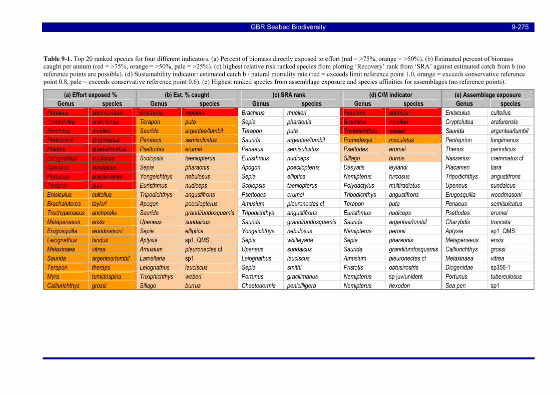
GBR Seabed Biodiversity 9-275
Table 9-1. Top 20 ranked species for four different indicators. (a) Percent of biomass directly exposed to effort (red = >75%, orange = >50%). (b) Estimated percent of biomass caught per annum (red = >75%, orange = >50%, pale = >25%). (c) highest relative risk ranked species from plotting ‘Recovery’ rank from ‘SRA’ against estimated catch from b (no reference points are possible). (d) Sustainability indicator: estimated catch b / natural mortality rate (red = exceeds limit reference point 1.0, orange = exceeds conservative reference point 0.8, pale = exceeds conservative reference point 0.6). (e) Highest ranked species from assemblage exposure and species affinities for assemblages (no reference points).
(a) Effort exposed % (b) Est. % caught (c) SRA rank (d) C/M indicator (e) Assemblage exposure Genus species Genus species Genus species Genus species Genus species
Penaeus semisulcatus Brachirus muelleri Brachirus muelleri Fistularia petimba Enisiculus cultellus Cryptolutea arafurensis Terapon puta Sepia pharaonis Brachirus muelleri Cryptolutea arafurensis Brachirus muelleri Saurida argentea/tumbil Terapon puta Trixiphichthys weberi Saurida argentea/tumbil Pentaprion longimanus Penaeus semisulcatus Saurida argentea/tumbil Pomadasys maculatus Pentaprion longimanus Pelates quadrilineatus Psettodes erumei Penaeus semisulcatus Psettodes erumei Thenus parindicus Leiognathus leuciscus Scolopsis taeniopterus Euristhmus nudiceps Sillago burrus Nassarius cremmatus cf Upeneus sundaicus Sepia pharaonis Apogon poecilopterus Dasyatis leylandi Placamen tiara Portunus gracilimanus Yongeichthys nebulosus Sepia elliptica Nemipterus furcosus Tripodichthys angustifrons Terapon puta Euristhmus nudiceps Scolopsis taeniopterus Polydactylus multiradiatus Upeneus sundaicus Enisiculus cultellus Tripodichthys angustifrons Psettodes erumei Tripodichthys angustifrons Erugosquilla woodmasoni Brachaluteres taylori Apogon poecilopterus Amusium pleuronectes cf Terapon puta Penaeus semisulcatus Trachypenaeus anchoralis Saurida grandi/undosquamis Tripodichthys angustifrons Euristhmus nudiceps Psettodes erumei Metapenaeus ensis Upeneus sundaicus Saurida grandi/undosquamis Saurida argentea/tumbil Charybdis truncata Erugosquilla woodmasoni Sepia elliptica Yongeichthys nebulosus Nemipterus peronii Aplysia sp1_QMS Leiognathus bindus Aplysia sp1_QMS Sepia whitleyana Sepia pharaonis Metapenaeus ensis Melaxinaea vitrea Amusium pleuronectes cf Upeneus sundaicus Saurida grandi/undosquamis Calliurichthys grossi Saurida argentea/tumbil Lamellaria sp1 Leiognathus leuciscus Amusium pleuronectes cf Melaxinaea vitrea Terapon theraps Leiognathus leuciscus Sepia smithi Pristotis obtusirostris Diogenidae sp356-1 Myra tumidospina Trixiphichthys weberi Portunus gracilimanus Nemipterus sp juv/unident Portunus tuberculosus Calliurichthys grossi Sillago burrus Chaetodermis penicilligera Nemipterus hexodon Sea pen sp1
GBR Seabed Biodiversity 10-276
10. REFERENCES
Birtles, A., Arnold, P. (1983) Between the Reefs: some patterns of soft substrate epibenthos on the GBR Shelf, pp. 159-163 in Baker, J.T., Carter, R.M., Sammarco, P.W., Stark, K.P. (Eds) Proc GBR Conference, Townsville, 1983.
Birtles R.A., Arnold, P.W. (1988) Distribution of trophic groups of epifaunal echinoderms and molluscs in the soft sediment areas of the central Great Barrier Reef shelf. In Proceedings of the 6th International Coral Reef Symposium, Townsville, Australia, Volume 3: Contributed Papers (Choat, J.H. & Barnes, D. eds) 6th International Coral Reef Symposium Executive Committee, pp. 325-332
Blaber S.J.M., Brewer D.T., Harris A.N. (1994). Distribution, biomass and community structure of demersal fishes of the Gulf of Carpentaria, Australia. Aust J Mar Freshw Res 45: 375-96
Breiman, L. (2001). Random Forests, Machine Learning 45(1), 5–32.
Brewer, D.T., Rawlinson, N., Eayrs, S., Burridge, C.Y., (1998). An assessment of bycatch reduction devices in a tropical Australian prawn trawl fishery. Fish. Res. 36, 195–215.
Brewer, D.T., Griffiths, S., Heales, D.S., Zhou, S., Tonks, M., Dell, Q., Taylor, B.T., Miller, M., Kuhnert, P., Keys, S., Whitelaw, W., Burke, A., Raudzens, E. (2007). Design, trial and implementation of an integrated, long-term bycatch monitoring program, road tested in the Northern Prawn Fishery. Final Report on FRDC Project 2004/024. CSIRO Cleveland. pp. 416.
Brinkman, R., Wolanski, E., Deleersnijder, E., McAllister, F., Skirving, W. (2002) Oceanic inflow from the Coral Sea into the Great Barrier Reef. Est Coast Shelf Sci 54: 655–668
Burridge C.Y., Pitcher C.R., Wassenberg T.J., Poiner I.R., Hill, B.J. (2003). Measurement of the rate of depletion of benthic fauna by prawn (shrimp) otter trawls: an experiment in the Great Barrier Reef, Australia. Fisheries Research 60: 237–253
Cappo, M., Harvey, E., Malcolm, H., Speare, P. (2003) Potential of video techniques to monitor diversity abundance and size of fish in studies of Marine Protected Areas. In: “Aquatic Protected Areas - what works best and how do we know?" (Eds Beumer JP, Grant A, Smith DC). World Congress on Aquatic Protected Areas Proceedings, Cairns Australia, August 2002. pp 455-464
Cappo, M., Speare, P., D’eath, G. (2004) Comparison of Baited Remote Underwater Video Stations (BRUVS) and prawn (shrimp) trawls for assessments of fish biodiversity in inter-reefal areas of the Great Barrier Reef Marine Park. J Exp Mar Biol Ecol 302(2): 123-152
Cappo, M., De’ath, G., Speare, P. (subm.) Shelf-scale patterns in communities of aquatic vertebrates in the inter-reefal waters of the Great Barrier Reef Marine Park determined by Baited Remote Underwater Video Stations. Mar Ecol Progr Ser
Cohen, A., Daubechies, I., Vial, P., (1993). Wavelets on the Interval and Fast Wavelet Transforms, Applied and Computational Harmonic Analysis, 1 p54-81.
Coles, R., McKenzie, L., De’ath, G., Roelofs, A., Lee Long, W. (2006) Modelling factors that influence the spatial distribution of deepwater seagrass in the inter reef lagoon of the Great Barrier Reef World Heritage Area, northern Australia. Submitted manuscript.
Condie, S.A., Dunn, J.R. (2006). Seasonal characteristics of the surface mixed layer in the Australasian region: implications for primary production regimes and biogeography. Mar Freshw Res 57: 569–590
Courtney, A.J., Haddy, J.A., Campbell, M.J., Roy, D.P., Tonks, M.L., Gaddes, S.W., Chilcott, K.E., O’Neill, M.F., Brown, I.W., McLennan, M., Jebreen, J.E., Van Der Geest, C., Rose, C., Kistle, S., Turnbull, C.T., Kyne, P.M., Bennett, M.B. and Taylor, J. (2006). Bycatch weight, composition and preliminary estimates of the impact of bycatch reduction devices in Queensland's trawl fishery. FRDC Project #2000/170 Final Report 353p.
GBR Seabed Biodiversity 10-277
Courtney, A.J., Tonks, M.L., Campbell, M.J., Roy, D.P., Gaddes, S.W., Kyne, P.M., O’Neill, M.F. (2006). Quantifying the effects of bycatch reduction devices in Queensland’s (Australia) shallow water eastern king prawn (Penaeus plebejus) trawl fishery. Fisheries Research 80:136–147
De’ath, G. (2006) Boosted trees for ecological modeling and prediction. Ecology
De’ath, G. (2002) Multivariate regression trees: a new technique for modeling species-environment relationships. Ecology 83:1105-1117.
DeVantier, L.M., De’ath, G., Turak, E., Done, T.J., Fabricius, K.E. (2006). Species richness and community structure of reef-building corals on the nearshore Great Barrier Reef. Coral Reefs 25(3): 329-340
Dredge, M.C.L. (1985) Estimates of natural mortality and yield-per-recruit for Amusium japonicum balloti Bernardi (Pectinidae) based on tag recoveries. Journal of Shellfish Research, 5:103–109.
Drew, E.A. (2001). Ocean nutrients to sediment banks via tidal jets and Halimeda meadows. In: Wolanski, E. (Ed.), Oceanographic processes of coral reefs: physical and biological links in the Great Barrier Reef. CRC Press, Boca Raton, Florida, pp. 127-144
Duda, R., Hart, P., Stork, D., (2001). Pattern Classification, 2nd Ed, Wiley.
Dufrêne, M., Legendre, P. (1997) Species assemblages and indicator species: the need for a flexible asymmetrical approach. Ecol Monogr 67(3): 345-66
Ellis, N., Pantus, F. (2001) Management strategy modelling: tools to evaluate trawl management strategies with respect to impacts on benthic biota within the Great Barrier Reef Marine Park area. CSIRO Marine Research Final Report to the Great Barrier Reef Marine Park Authority.
Engel, J. & Kvitek, R. (1998) Effects of otter trawling on benthic community in Monterey Bay National Marine Sanctuary. Cons.Biol.12(6):1204-214.
Environment Australia, (2000). Biodiversity Research: Australia’s Priorities — a Discussion Paper.
Fabricius, K., De’ath, G. (2001) Biodiversity on the Great Barrier Reef: Large-scale patterns and turbidity-related local loss of soft coral taxa. In: Wolanski, E. (Ed.), Oceanographic processes of coral reefs: physical and biological links in the Great Barrier Reef. CRC Press, Boca Raton, Florida, pp. 127-144
Fager, E.W., Longhurst, A.R. (1968) Recurrent group analysis of species assemblages of demersal fish in the Gulf of Guinea. J Fish Res Board Can 25(7): 1405–21
Fogarty, M.P., and Murawski, S.A. 1998. Large-scale disturbance and the structure of marine systems: fishery impacts on Georges Bank. Ecological Applications, 8(1), Supplement: S6eS22.
Friedman, J.H. (2001) Greedy function approximation: a gradient boosting machine. Ann Stat 29(5): 1189-1232
Fulton, E.A., Smith, A.D.M., Webb H., Slater, J. (2004). Ecological Indicators for the Impacts of Fishing on Non-Target Species, Communities and Ecosystems: Review of Potential Indicators. AFMA Final Research Report Number R99/1546
Gribble, N. A. (2003). GBR-prawn: modelling ecosystem impacts of changes in fisheries management of the commercial prawn (shrimp) trawl fishery in the far northern Great Barrier Reef. Fisheries Research 65(1-3): 493-506
Gribble, N. A. (2004). A spatially explicit multi-competitor coexistence model of penaeid (shrimp) distribution on the Australian Great Barrier Reef. Ecological Modelling: Vol 177(1-2):61-74
Gribble, N.A., Good, N., Peel, D., Tanimoto, M., and Officer, R. (2007). Innovative stock assessment and effort mapping using VMS and electronic logbooks. Final Report to FRDC 2002/056.
Griffiths, S.P., Brewer, D.T., Heales, D.S., Milton, D.A., Stobutzki, I.C., (2006). Validating ecological risk assessments for fisheries: assessing the impacts of turtle excluder devices on
GBR Seabed Biodiversity 10-278
elasmobranch bycatch populations in an Australian trawl fishery. Marine and Freshwater Research, 57, 395–401
Gulland, J.A. (1983). Fish Stock Assessment: a manual of basic methods. FAO/Wiley Inter-Science, New York, 223 pp.
Gust, N., Choat, J.H., and McCormick, M.I. (2001) Spatial variability in reef fish distribution, abundance, size and biomass: a multi-scale analysis. Mar Ecol Prog Ser 214, 237-251
Hancock, G.J., Webster, I.T., Stieglitz, T.C. (In Press) Horizontal mixing of Great Barrier Reef waters: offshore diffusivity determined from radium isotope distribution. JGR Oceans
Haywood, M., Hill, B., Donovan, A., Rochester, W., Ellis, N., Welna, A., Gordon, S., Cheers, S., Forcey, K., Mcleod, I., Moeseneder, C., Smith, G., Manson, F., Wassenberg, T., Thomas, Steve, Kuhnert, P., Laslett, G., Burridge, C., and Thomas, Sarah, (2005). Quantifying the effects of trawling on seabed fauna in the Northern Prawn Fishery. Final Report on FRDC Project 2002/102. CSIRO, Cleveland. 488 pp.
Hobday, A. J., Smith, A., Webb, H., Daley, R., Wayte, S., Bulman, C., Dowdney, J. Williams,,A., Sporcic, M., Dambacher, J., Fuller,M., Walker, T. (2006) Ecological Risk Assessment for the Effects of Fishing: Methodology. Report R04/1072 for the Australian Fisheries Management Authority, Canberra
Hilborn, R., Walters, C.J. (1992). Quantitative fisheries stock assessment: choice, dynamics and uncertainty. Chapman & Hall, London. 570p.
Hill, B.J., Haywood, M., Venables, B., Gordon, S.R., Condie, S., Ellis, N.R., Tyre, A., Vance, D., Dunn, J., Mansbridge, J., Moeseneder, C., Bustamante, R. and Pantus, F., (2002). Surrogates I - Predictors, impacts, management and conservation of the benthic biodiversity of the Northern Prawn Fishery. Final Report on FRDC Project 2000/160. CSIRO, Cleveland. 437 pp.
Jensen, A., la Cour-Harbo, A., (2001). Ripples in Mathematics, the Discrete Wavelet Transform, Springer.
Kaufman, L. and Rousseeuw, P. J. (1990) Finding Groups in Data, Wiley, New York.
Kaufman, L. and Rousseeuw, P. J. (1990). Finding Groups in Data: An Introduction to Cluster Analysis. Wiley, New York.
Koch, V., Wolff, M. (2002) Energy budget and ecological role of mangrove epibenthos in the Caeté estuary, North Brazil. Mar Ecol Prog Ser 228: 119–130
Kodama, K., Horiguchi, T., Kume1, G., Nagayama, S., Shimizu, T., Shiraishi, H., Morita, M., Shimizu, M., (2006) Effects of hypoxia on early life history of the stomatopod Oratosquilla oratoria in a coastal sea. Mar Ecol Prog Ser Vol. 324: 197–206.
Larcombe, P., Carter, R.M., (2004) Cyclone pumping, sediment partitioning and the development of the Great Barrier Reef shelf system: a review. Quatern Sci Rev 23:107–135
Lee, H-H., Hsu, C-C. (2003). Population biology of the swimming crab Portunus sanguinolentus in the waters off northern Taiwan. Journal of Crustacean Biology 23:691–699
Letourneur, Y., Kulbicki, M., Labrosse, P. (1998) Spatial structure of commercial reef fish communities along a terrestrial runoff gradient in the northern lagoon of New Caledonia. Environ Biol Fish 51: 141–159
Long, B.G., Skewes, T.D., Taranto, T.J., Smith, G., Mcleod, I., Pitcher, C.R., Poiner, I.R. (1997) PNG Gas Project: Torres Strait Marine Infill Survey: Report To NSR Re Papua New Guinea–Queensland Gas Project. CSIRO Division of Marine Research.
Longhurst, A.R., Pauly, D. (1987). Ecology of tropical oceans. Academic Press, San Diego, California (USA). 407p
Lowe-McConnell, R.H. (1987). Ecological studies in tropical fish communities. Cambridge University Press. pp 213-223
GBR Seabed Biodiversity 10-279
Magurran, A.E., Henderson, P.A. (2003) Explaining the excess of rare species in natural species abundance distributions. Nature 422(6933): 714-716
Mathews, E.J. and Heap, A.D., (2006). Sedimentology and Geomorphology of Inter-reefal Seabed Environments of the Great Barrier Reef, northeast Australia. Geoscience Australia, Record 2006/11.
McLeod, I., Skewes, T.D., Gordon, S.R., Pitcher, C.R. (2007). A method for seabed habitat mapping: Integrating acoustic information with biogeophysical observations; Case study – Scott Reef, in Todd, B.J., and Greene, H.G., eds. Mapping the Seafloor for Habitat Characterization: Geological Association of Canada, Special Paper 47, pp.
Newman, S.J., Williams, D.M., Russ, G.R. (1997). Patterns of zonation of assemblages of the Lutjanidae, Lethrinidae and Serranidae (Epinephelinae) within and among mid shelf and outer shelf reefs in the central Great Barrier Reef. Mar Freshw Res 48:119–128
Penn, J.W. (1976) Tagging Experiments with Western King Prawn, Penaeus latisulcatus Kishinouye II. Estimation of Population Parameters. Aust. J, Mar. Freshwater Res. 27, 239-50
Pitcher, C.R., Venables, W., Ellis, N., McLeod, I., Pantus, F., Austin, M., Cappo, M., Doherty, P., Gribble, N. (2002). GBR Seabed Biodiversity Mapping Project: Phase 1. CSIRO/AIMS/QDPI Report to CRC-Reef, pp. 192.
Pitcher C.R., Austin, M., Burridge, C.Y., Bustamante, R.H., Cheers, S.J., Ellis, N., Jones, P.N., Koutsoukos, A.G., Moeseneder, C.H., Smith, G.P., Venables, W., Wassenberg, T.J., (2004). Recovery of Seabed Habitat from the Impact of Prawn Trawling in the Far Northern Section of the Great Barrier Reef Marine Park. CSIRO Marine Research Final Report to GBRMPA, pp. 370
Pitcher, C.R., Turnbull, C., Atfield, J., Griffin, D., Dennis, D.M., Skewes, T.D. (2005). Biology, larval transport modelling and commercial logbook data analysis to support management of the NE Queensland rock lobster Panulirus ornatus fishery. FRDC Project 2002/008 report to Fisheries Research and Development Corporation. CSIRO Marine & Atmospheric Research pp. 148
Poiner, I.R., Glaister, J., Pitcher, C.R., Burridge, C., Wassenberg, T., Gribble, N., Hill, B., Blaber, S.J.M., Milton, D.A., Brewer, D., Ellis, N., (1998). The environmental effects of prawn trawling in the far northern section of the Great Barrier Reef Marine Park: 1991–1996. Final Report to GBRMPA and FRDC. CSIRO Division of Marine Research – Queensland Department of Primary Industries Report, 554 pp.
Porter-Smith, R., Harris, P.T., Andersen, O.B., Coleman, R., Greenslade, D., Jenkins, C.J. (2004). Classification of the Australian continental shelf based on predicted sediment threshold exceedance from tidal currents and swell waves. Mar Geol 211: 1– 20
R Development Core Team (2005) R: a language and environment for statistical computing. R Foundation for statistical computing, Vienna.
Ramm, D.C., Pender, P.J., Willing, R.S., Buckworth, R.C. (1990). Large-scale spatial patterns of abundance within the assemblage of fish caught by prawn trawlers in northern Australian waters. Aust J Mar Freshw Res 41: 79-95
Ridgway, K. R., J. R. Dunn and J. L. Wilkin, 2002. Ocean interpolation by four-dimensional least squares - Application to the waters around Australia. Journal of Atmospheric and Oceanic Technology, 19, 1357-1375.
Robins, J.B. & McGilvray, J.G. (1999). The AusTED II, an improved trawl efficiency device 2. Commercial performance. Fisheries Research 40: 29-41.
Robins-Troeger, J.B., Buckworth, R.C. & Dredge, M.C.L. (1995). Development of a trawl efficiency device (TED) for Australian prawn fisheries II. Field evaluations of the AusTED. Fisheries Research, 22: 107-117.
Sainsbury KJ, Campbell RA, Lindholm R, Whitelaw AW (1997). Experimental management of an Australian multispecies fishery: Examining the possibility of trawl induced habitat
GBR Seabed Biodiversity 10-280
modification. In: Pikitch EK, Huppert DD, Sissenwine MP (Eds) Global Trends: Fisheries management. pp 107-112. American Fisheries Society, Maryland, USA. John Wiley and Son
Saito, N., Coifman, R., (1995). Local Discriminant Bases and their Applications. Journal of Mathematical Imaging and Vision, 5: 337-358.
Schwarz, G. (1978). "Estimating the dimension of a model". Annals of Statistics 6, 461-464.
Scott, D. W. (1992) Multivariate Density Estimation: Theory, Practice, and Visualization. Wiley.
Simrad EY500 Operating Manual ht—://www.simrad.com/html
Skewes, T.D., Pitcher, C.R., Long, B.G., Mcleod, I., Taranto, T.J. Gordon, S., Smith, G., Poiner, I.R. (1996) Torres Strait Infill Survey: Report to IPC Re Pandora Gas Development Project. CSIRO Division of Fisheries.
Sternlicht, D., de Moustier, C., (2003). Time-dependent seafloor acoustic backscatter (10-100kHz), J. Acous. Soc. Am. 114 (5), p2709--2725 (2003).
Stobutzki, I.C., Miller, M.J., Brewer, D.T. (2001a). Sustainability of fishery bycatch: a process for assessing highly diverse and numerous bycatch. Environmental Conservation 28, 167–181.
Stobutzki IC, Miller MJ, Jones P, Salini JP (2001b) Bycatch diversity and variation in a tropical Australian penaeid fishery; the implications for monitoring. Fish Res 53(3): 283-301
Stobutzki, I.C., Miller, M.J., Heales, D.S., Brewer, D.T. (2002). Sustainability of elasmobranchs caught as bycatch in a tropical shrimp trawl fishery. Fish. Bull. 100:800-821.
Trefethen, L. N. 1980. Numerical Computation of the Schwarz-Christoffel Transformation, Siam J. Sci. Stat. Comp. 1, 82–102
Wahba, G. (1990) Spline Models for Observational Data. National Science Foundation -Conference Board of Mathematical Sciences Regional Conference Series in Applied Mathematics, Philadelphia: Society for Industrial and Applied Mathematics.
Ward, J.H. (1963). Hierarchical Grouping to optimize an objective function. Journal of American Statistical Association, 58(301), 236-244
Wassenberg TJ, Blaber SJM, Burridge CY, Brewer DT, Salini JP, Gribble N (1997). The effectiveness of fish and shrimp trawls for sampling fish communities in tropical Australia. Fish Res 30: 229-240
Watson RA, Dredge MLC, Mayer DG (1990). Spatial and seasonal variation in demersal trawl fauna associated with a prawn fishery on the central Great Barrier Reef, Australia. Aust J Mar Freshw Res 41: 65-77
Watson, R.A., Goeden, G.B. (1989) Temporal and spatial zonation of the demersal trawl fauna of the central Great Barrier Reef. Mem. Qld. Mus. 27(2): 611-620
Wilkinson, C.R., Cheshire, A.C. (1988). Cross shelf variations in coral reef structure and function—influences of land and ocean. In: Proceedings of the 6th International Coral Reef Symposium, Townsville, Australia, Volume 3: Contributed Papers (Choat, J.H. & Barnes, D. eds) 6th International Coral Reef Symposium Executive Committee, pp 227–233
Williams, D.M. (1991). Patterns and processes in the distribution of coral reef fishes. In: Sale PF (ed) The ecology of fishes on coral reefs. Academic Press San Diego. pp 437–474
Williams, A., Last, P.R., Gomon, M.F., & Paxton, J.R. (1996) Species composition and checklist of the demersal ichthyofauna of the continental slope off western Australia (20–35ºS) Rec. WA Mus. 18, 135–155.
Wolanski, E. (1994). Physical oceanographic processes of the Great Barrier Reef. CRC Press Marine Science Series.
Zhou, S., Griffiths, S.P. (2007) Sustainability Assessment for Fishing Effects (SAFE): a new quantitative ecological risk assessment method and its application to elasmobranch bycatch in an Australian trawl fishery. Fisheries Research (In Press)

GBR Seabed Biodiversity 11-281
11. ABBREVIATIONS BRUVS – Baited Remote Underwater Video Stations CARS2000 – CSIRO Atlas of Regional Seas CERF National Marine Biodiversity Hub CLARA – Clustering for large Datasets CRC – Cooperative Research Centre CTD – Conductivity Temperature Depth sensor array DEW – Department of Environment & Water Resources DEM – Digital Elevation Model DLI – Dufrêne-Legendre Index EPBC – Environment Protection & Biodiversity Conservation ERA – Ecological Risk Assessments FRDC – Fisheries Research & Development Corporation GA – Geoscience Australia GBRWHA – Great Barrier Reef World Heritage Area GPS – Global Positioning System GU zone – General Use zone HO – Hydrographic Office HPA – Highly protected area IQR – Inter-Quartile Range JCU – James Cook University MaxN – Maximum number of fish seen at any one time in field of view of BRUVS MSE – Management Strategies Evaluations NOO – National Oceans Office NPF – Northern Prawn Fishery NSRMPA – National Representitive System of Marine Protected Areas OSI – Ocean Sciences Institute, Sydney University PAM – Partitioning Around Medoids PAR – Photosynthetically Active Radiation PC-space – Principal Components Space SRA – Susceptibility-Recovery Analysis QDPI&F – Queensland Department of Primary Industries & Fisheries QECTF – Queensland East Coast Trawl Fishery QSIA – Queensland Seafood Industry Association RAP – Representative Areas Program RMS – Residual Mean Square SRA – Susceptibility Recovery Analysis SVD – Singular Value Decomposition VMS – Vessel Monitoring System VTRs – Video Tape Recorders WHA – World Heritage Area WTO – Wildlife Trade Operation

GBR Seabed Biodiversity 12-282
12. APPENDIX 1: INTELLECTUAL PROPERTY
There is no intellectual property of a commercial nature arising from the outputs of this Project.

GBR Seabed Biodiversity 13-283
13. APPENDIX 2: STAFF Roland Pitcher CSIRO Marine and Atmospheric Research Cleveland Qld.Peter Doherty Australian Institute of Marine Science Townsville Qld Peter Arnold Museum of Tropical Queensland Townsville Qld John Hooper Queensland Museum South Bank Brisbane Qld Neil Gribble Queensland Department of Primary Industries & Fisheries Cairns Qld Chris Bartlett Museum of Tropical Queensland Townsville Qld Matthew Browne CSIRO Maths and Information Sciences Cleveland Qld Norm Campbell CSIRO Maths and Information Sciences Perth WAToni Cannard CSIRO Marine and Atmospheric Research Cleveland Qld Mike Cappo Australian Institute of Marine Science Townsville Qld Giovannella Carini Queensland Museum South Bank Brisbane Qld Susan Chalmers Queensland Department of Primary Industries & Fisheries Cairns Qld Sue Cheers CSIRO Marine and Atmospheric Research Cleveland Qld Doug Chetwynd CSIRO Marine and Atmospheric Research Cleveland Qld Andrew Colefax Queensland Museum South Bank Brisbane Qld Rob Coles Queensland Department of Primary Industries & Fisheries Cairns Qld Stephen Cook Queensland Museum South Bank Brisbane Qld Peter Davie Queensland Museum South Bank Brisbane Qld Glenn De'ath Australian Institute of Marine Science Townsville Qld Drew Devereux CSIRO Maths and Information Sciences Perth WABarbara Done Museum of Tropical Queensland Townsville Qld Tim Donovan Australian Institute of Marine Science Townsville Qld Barry Ehrke Queensland Department of Primary Industries & Fisheries Cairns Qld Nick Ellis CSIRO Marine and Atmospheric Research Cleveland Qld Gavin Ericson Australian Institute of Marine Science Townsville Qld Ida Fellegara Queensland Museum South Bank Brisbane Qld Karl Forcey CSIRO Marine and Atmospheric Research Cleveland Qld Melodyrose Furey CSIRO Marine and Atmospheric Research Cleveland Qld Dan Gledhill CSIRO Marine and Atmospheric Research Hobart Tas Norm Good Queensland Department of Primary Industries & Fisheries Cairns Qld Scott Gordon CSIRO Marine and Atmospheric Research Cleveland Qld Mick Haywood CSIRO Marine and Atmospheric Research Cleveland Qld Ian Jacobsen University of Queensland Brisbane Qld Jeff Johnson Queensland Museum South Bank Brisbane Qld Michelle Jones Queensland Museum South Bank Brisbane Qld Stuart Kinninmoth Australian Institute of Marine Science Townsville Qld Sarah Kistle Queensland Department of Primary Industries & Fisheries Cairns Qld Peter Last CSIRO Marine and Atmospheric Research Hobart Tas Anita Leite Museum of Tropical Queensland Townsville Qld Shona Marks CSIRO Marine and Atmospheric Research Cleveland Qld Ian McLeod CSIRO Marine and Atmospheric Research Cleveland Qld Sybilla Oczkowicz Queensland Department of Primary Industries & Fisheries Cairns Qld Cassanda Rose Queensland Department of Primary Industries & Fisheries Cairns Qld Denise Seabright Museum of Tropical Queensland Townsville Qld Jacquie Sheils CSIRO Marine and Atmospheric Research Cleveland Qld Matt Sherlock CSIRO Marine and Atmospheric Research Cleveland Qld Posa Skelton Queensland Department of Primary Industries & Fisheries Townsville Qld David H Smith CSIRO Marine and Atmospheric Research Cleveland Qld Greg Smith CSIRO Marine and Atmospheric Research Cleveland Qld Peter Speare Australian Institute of Marine Science Townsville Qld Marcus Stowar Australian Institute of Marine Science Townsville Qld Colleen Strickland Queensland Museum South Bank Brisbane Qld Patricia Hendriks Queensland Museum South Bank Brisbane Qld Claire Van der Geest Queensland Department of Primary Industries & Fisheries Cairns Qld

GBR Seabed Biodiversity 13-284
Bill Venables CSIRO Maths and Information Sciences Cleveland Qld Cath Walsh Queensland Department of Primary Industries & Fisheries Townsville Qld Ted Wassenberg CSIRO Marine and Atmospheric Research Cleveland Qld Andrzej Welna CSIRO Marine and Atmospheric Research Cleveland Qld Gus Yearsley CSIRO Marine and Atmospheric Research Hobart Tas

GBR Seabed Biodiversity 14-285
14. APPENDIX 3: PROJECT STEERING COMMITTEE MEMBERS
Chairperson: Peter Doherty — AIMS, CRC-Reef Program C Leader
Task Leader: Roland Pitcher — CSIRO
Task Associate: David Williams — CRC-Reef
Task Associate: Dorothea Huber Phil Cadwallader — GBRMPA
Task Associate: Brigid Kerrigan Malcolm Dunning — QDPI&F
Task Associate: Duncan Souter Martin Hicks — QSIA
Task Associate: Barry Ehrke — QSIA
Task Associate: Vicki Nelson — NOO
Task Associate: Vern Veitch — Sunfish
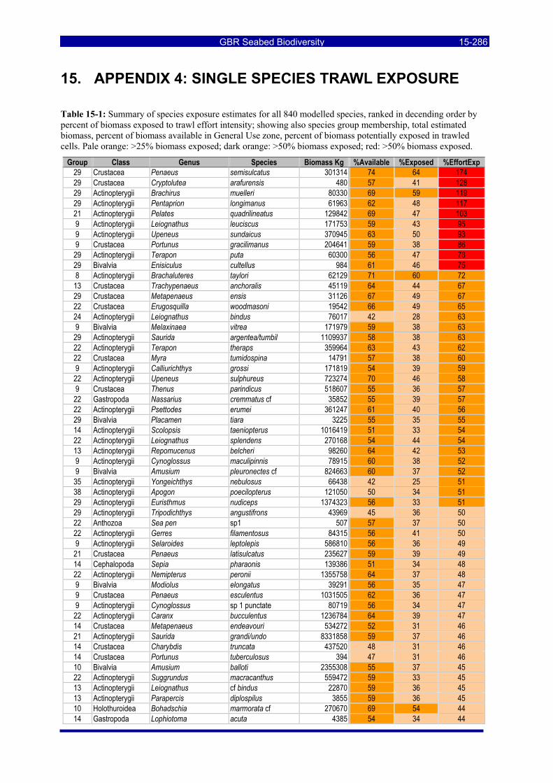
GBR Seabed Biodiversity 15-286
15. APPENDIX 4: SINGLE SPECIES TRAWL EXPOSURE
Table 15-1: Summary of species exposure estimates for all 840 modelled species, ranked in decending order by percent of biomass exposed to trawl effort intensity; showing also species group membership, total estimated biomass, percent of biomass available in General Use zone, percent of biomass potentially exposed in trawled cells. Pale orange: >25% biomass exposed; dark orange: >50% biomass exposed; red: >50% biomass exposed.
Group Class Genus Species Biomass Kg %Available %Exposed %EffortExp 29 Crustacea Penaeus semisulcatus 301314 74 64 174 29 Crustacea Cryptolutea arafurensis 480 57 41 128 29 Actinopterygii Brachirus muelleri 80330 69 59 119 29 Actinopterygii Pentaprion longimanus 61963 62 48 117 21 Actinopterygii Pelates quadrilineatus 129842 69 47 103 9 Actinopterygii Leiognathus leuciscus 171753 59 43 95 9 Actinopterygii Upeneus sundaicus 370945 63 50 93 9 Crustacea Portunus gracilimanus 204641 59 38 86 29 Actinopterygii Terapon puta 60300 56 47 78 29 Bivalvia Enisiculus cultellus 984 61 46 75 8 Actinopterygii Brachaluteres taylori 62129 71 60 72 13 Crustacea Trachypenaeus anchoralis 45119 64 44 67 29 Crustacea Metapenaeus ensis 31126 67 49 67 22 Crustacea Erugosquilla woodmasoni 19542 66 49 65 24 Actinopterygii Leiognathus bindus 76017 42 28 63 9 Bivalvia Melaxinaea vitrea 171979 59 38 63 29 Actinopterygii Saurida argentea/tumbil 1109937 58 38 63 22 Actinopterygii Terapon theraps 359964 63 43 62 22 Crustacea Myra tumidospina 14791 57 38 60 9 Actinopterygii Calliurichthys grossi 171819 54 39 59 22 Actinopterygii Upeneus sulphureus 723274 70 46 58 9 Crustacea Thenus parindicus 518607 55 36 57 22 Gastropoda Nassarius cremmatus cf 35852 55 39 57 22 Actinopterygii Psettodes erumei 361247 61 40 56 29 Bivalvia Placamen tiara 3225 55 35 55 14 Actinopterygii Scolopsis taeniopterus 1016419 51 33 54 22 Actinopterygii Leiognathus splendens 270168 54 44 54 13 Actinopterygii Repomucenus belcheri 98260 64 42 53 9 Actinopterygii Cynoglossus maculipinnis 78915 60 38 52 9 Bivalvia Amusium pleuronectes cf 824663 60 37 52 35 Actinopterygii Yongeichthys nebulosus 66438 42 25 51 38 Actinopterygii Apogon poecilopterus 121050 50 34 51 29 Actinopterygii Euristhmus nudiceps 1374323 56 33 51 29 Actinopterygii Tripodichthys angustifrons 43969 45 36 50 22 Anthozoa Sea pen sp1 507 57 37 50 22 Actinopterygii Gerres filamentosus 84315 56 41 50 9 Actinopterygii Selaroides leptolepis 586810 56 36 49 21 Crustacea Penaeus latisulcatus 235627 59 39 49 14 Cephalopoda Sepia pharaonis 139386 51 34 48 22 Actinopterygii Nemipterus peronii 1355758 64 37 48 9 Bivalvia Modiolus elongatus 39291 56 35 47 9 Crustacea Penaeus esculentus 1031505 62 36 47 9 Actinopterygii Cynoglossus sp 1 punctate 80719 56 34 47 22 Actinopterygii Caranx bucculentus 1236784 64 39 47 14 Crustacea Metapenaeus endeavouri 534272 52 31 46 21 Actinopterygii Saurida grandi/undo 8331858 59 37 46 14 Crustacea Charybdis truncata 437520 48 31 46 14 Crustacea Portunus tuberculosus 394 47 31 46 10 Bivalvia Amusium balloti 2355308 55 37 45 22 Actinopterygii Suggrundus macracanthus 559472 59 33 45 13 Actinopterygii Leiognathus cf bindus 22870 59 36 45 13 Actinopterygii Parapercis diplospilus 3855 59 36 45 10 Holothuroidea Bohadschia marmorata cf 270670 69 54 44 14 Gastropoda Lophiotoma acuta 4385 54 34 44
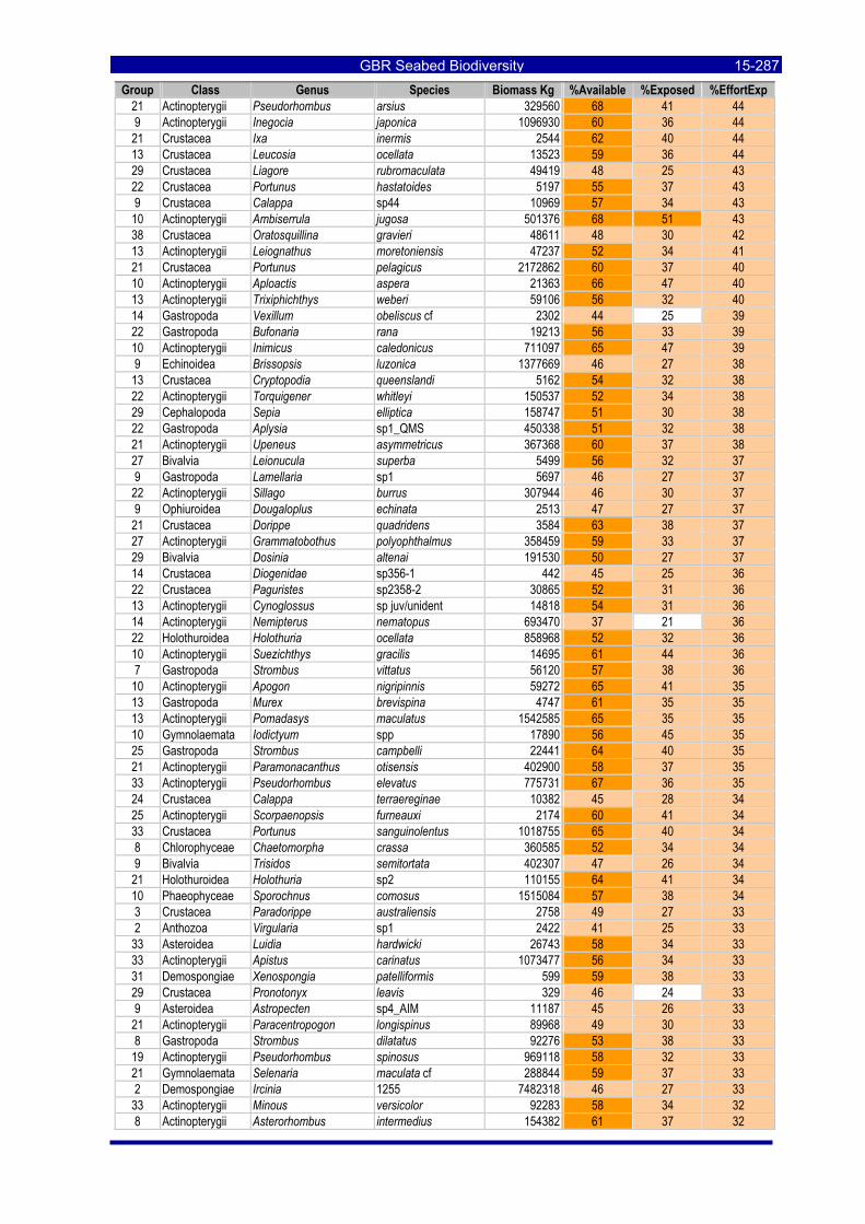
GBR Seabed Biodiversity 15-287Group Class Genus Species Biomass Kg %Available %Exposed %EffortExp
21 Actinopterygii Pseudorhombus arsius 329560 68 41 44 9 Actinopterygii Inegocia japonica 1096930 60 36 44 21 Crustacea Ixa inermis 2544 62 40 44 13 Crustacea Leucosia ocellata 13523 59 36 44 29 Crustacea Liagore rubromaculata 49419 48 25 43 22 Crustacea Portunus hastatoides 5197 55 37 43 9 Crustacea Calappa sp44 10969 57 34 43 10 Actinopterygii Ambiserrula jugosa 501376 68 51 43 38 Crustacea Oratosquillina gravieri 48611 48 30 42 13 Actinopterygii Leiognathus moretoniensis 47237 52 34 41 21 Crustacea Portunus pelagicus 2172862 60 37 40 10 Actinopterygii Aploactis aspera 21363 66 47 40 13 Actinopterygii Trixiphichthys weberi 59106 56 32 40 14 Gastropoda Vexillum obeliscus cf 2302 44 25 39 22 Gastropoda Bufonaria rana 19213 56 33 39 10 Actinopterygii Inimicus caledonicus 711097 65 47 39 9 Echinoidea Brissopsis luzonica 1377669 46 27 38 13 Crustacea Cryptopodia queenslandi 5162 54 32 38 22 Actinopterygii Torquigener whitleyi 150537 52 34 38 29 Cephalopoda Sepia elliptica 158747 51 30 38 22 Gastropoda Aplysia sp1_QMS 450338 51 32 38 21 Actinopterygii Upeneus asymmetricus 367368 60 37 38 27 Bivalvia Leionucula superba 5499 56 32 37 9 Gastropoda Lamellaria sp1 5697 46 27 37 22 Actinopterygii Sillago burrus 307944 46 30 37 9 Ophiuroidea Dougaloplus echinata 2513 47 27 37 21 Crustacea Dorippe quadridens 3584 63 38 37 27 Actinopterygii Grammatobothus polyophthalmus 358459 59 33 37 29 Bivalvia Dosinia altenai 191530 50 27 37 14 Crustacea Diogenidae sp356-1 442 45 25 36 22 Crustacea Paguristes sp2358-2 30865 52 31 36 13 Actinopterygii Cynoglossus sp juv/unident 14818 54 31 36 14 Actinopterygii Nemipterus nematopus 693470 37 21 36 22 Holothuroidea Holothuria ocellata 858968 52 32 36 10 Actinopterygii Suezichthys gracilis 14695 61 44 36 7 Gastropoda Strombus vittatus 56120 57 38 36 10 Actinopterygii Apogon nigripinnis 59272 65 41 35 13 Gastropoda Murex brevispina 4747 61 35 35 13 Actinopterygii Pomadasys maculatus 1542585 65 35 35 10 Gymnolaemata Iodictyum spp 17890 56 45 35 25 Gastropoda Strombus campbelli 22441 64 40 35 21 Actinopterygii Paramonacanthus otisensis 402900 58 37 35 33 Actinopterygii Pseudorhombus elevatus 775731 67 36 35 24 Crustacea Calappa terraereginae 10382 45 28 34 25 Actinopterygii Scorpaenopsis furneauxi 2174 60 41 34 33 Crustacea Portunus sanguinolentus 1018755 65 40 34 8 Chlorophyceae Chaetomorpha crassa 360585 52 34 34 9 Bivalvia Trisidos semitortata 402307 47 26 34 21 Holothuroidea Holothuria sp2 110155 64 41 34 10 Phaeophyceae Sporochnus comosus 1515084 57 38 34 3 Crustacea Paradorippe australiensis 2758 49 27 33 2 Anthozoa Virgularia sp1 2422 41 25 33 33 Asteroidea Luidia hardwicki 26743 58 34 33 33 Actinopterygii Apistus carinatus 1073477 56 34 33 31 Demospongiae Xenospongia patelliformis 599 59 38 33 29 Crustacea Pronotonyx leavis 329 46 24 33 9 Asteroidea Astropecten sp4_AIM 11187 45 26 33 21 Actinopterygii Paracentropogon longispinus 89968 49 30 33 8 Gastropoda Strombus dilatatus 92276 53 38 33 19 Actinopterygii Pseudorhombus spinosus 969118 58 32 33 21 Gymnolaemata Selenaria maculata cf 288844 59 37 33 2 Demospongiae Ircinia 1255 7482318 46 27 33 33 Actinopterygii Minous versicolor 92283 58 34 32 8 Actinopterygii Asterorhombus intermedius 154382 61 37 32
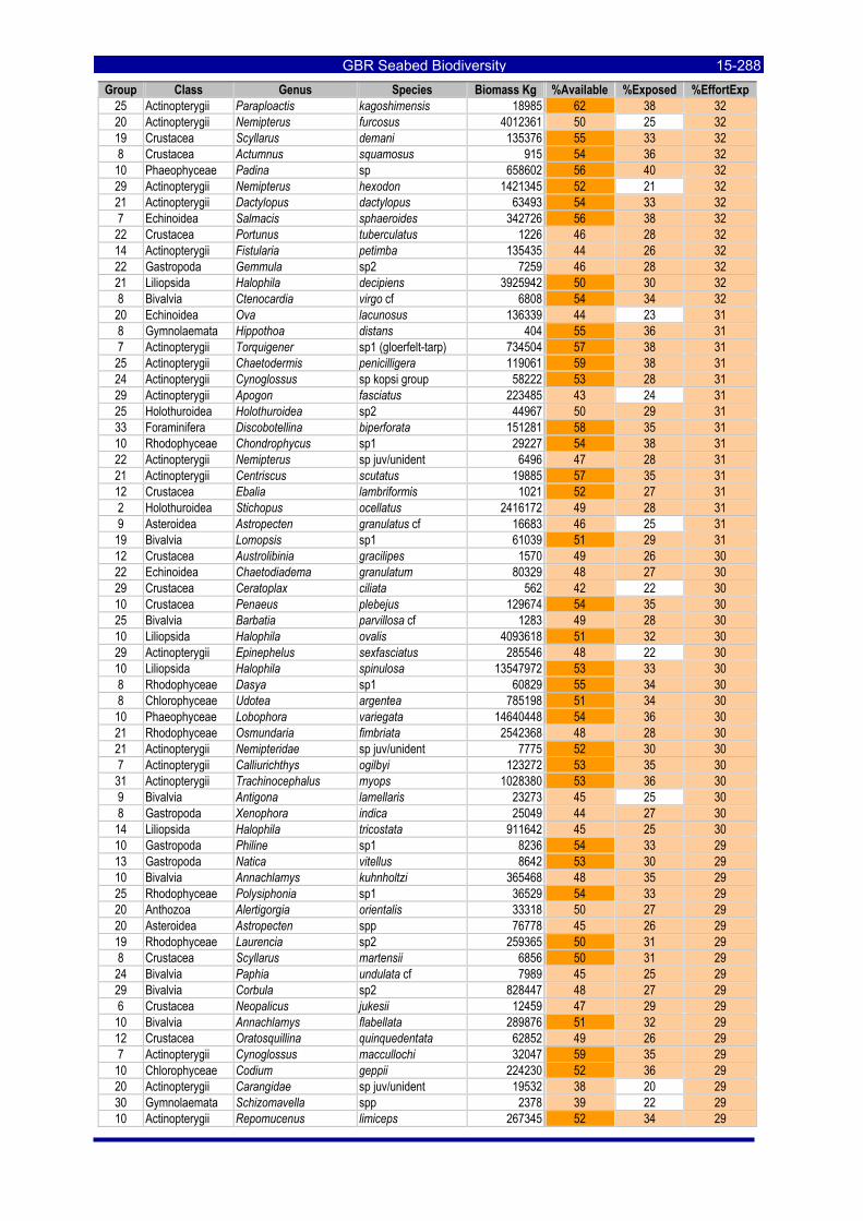
GBR Seabed Biodiversity 15-288Group Class Genus Species Biomass Kg %Available %Exposed %EffortExp
25 Actinopterygii Paraploactis kagoshimensis 18985 62 38 32 20 Actinopterygii Nemipterus furcosus 4012361 50 25 32 19 Crustacea Scyllarus demani 135376 55 33 32 8 Crustacea Actumnus squamosus 915 54 36 32 10 Phaeophyceae Padina sp 658602 56 40 32 29 Actinopterygii Nemipterus hexodon 1421345 52 21 32 21 Actinopterygii Dactylopus dactylopus 63493 54 33 32 7 Echinoidea Salmacis sphaeroides 342726 56 38 32 22 Crustacea Portunus tuberculatus 1226 46 28 32 14 Actinopterygii Fistularia petimba 135435 44 26 32 22 Gastropoda Gemmula sp2 7259 46 28 32 21 Liliopsida Halophila decipiens 3925942 50 30 32 8 Bivalvia Ctenocardia virgo cf 6808 54 34 32 20 Echinoidea Ova lacunosus 136339 44 23 31 8 Gymnolaemata Hippothoa distans 404 55 36 31 7 Actinopterygii Torquigener sp1 (gloerfelt-tarp) 734504 57 38 31 25 Actinopterygii Chaetodermis penicilligera 119061 59 38 31 24 Actinopterygii Cynoglossus sp kopsi group 58222 53 28 31 29 Actinopterygii Apogon fasciatus 223485 43 24 31 25 Holothuroidea Holothuroidea sp2 44967 50 29 31 33 Foraminifera Discobotellina biperforata 151281 58 35 31 10 Rhodophyceae Chondrophycus sp1 29227 54 38 31 22 Actinopterygii Nemipterus sp juv/unident 6496 47 28 31 21 Actinopterygii Centriscus scutatus 19885 57 35 31 12 Crustacea Ebalia lambriformis 1021 52 27 31 2 Holothuroidea Stichopus ocellatus 2416172 49 28 31 9 Asteroidea Astropecten granulatus cf 16683 46 25 31 19 Bivalvia Lomopsis sp1 61039 51 29 31 12 Crustacea Austrolibinia gracilipes 1570 49 26 30 22 Echinoidea Chaetodiadema granulatum 80329 48 27 30 29 Crustacea Ceratoplax ciliata 562 42 22 30 10 Crustacea Penaeus plebejus 129674 54 35 30 25 Bivalvia Barbatia parvillosa cf 1283 49 28 30 10 Liliopsida Halophila ovalis 4093618 51 32 30 29 Actinopterygii Epinephelus sexfasciatus 285546 48 22 30 10 Liliopsida Halophila spinulosa 13547972 53 33 30 8 Rhodophyceae Dasya sp1 60829 55 34 30 8 Chlorophyceae Udotea argentea 785198 51 34 30 10 Phaeophyceae Lobophora variegata 14640448 54 36 30 21 Rhodophyceae Osmundaria fimbriata 2542368 48 28 30 21 Actinopterygii Nemipteridae sp juv/unident 7775 52 30 30 7 Actinopterygii Calliurichthys ogilbyi 123272 53 35 30 31 Actinopterygii Trachinocephalus myops 1028380 53 36 30 9 Bivalvia Antigona lamellaris 23273 45 25 30 8 Gastropoda Xenophora indica 25049 44 27 30 14 Liliopsida Halophila tricostata 911642 45 25 30 10 Gastropoda Philine sp1 8236 54 33 29 13 Gastropoda Natica vitellus 8642 53 30 29 10 Bivalvia Annachlamys kuhnholtzi 365468 48 35 29 25 Rhodophyceae Polysiphonia sp1 36529 54 33 29 20 Anthozoa Alertigorgia orientalis 33318 50 27 29 20 Asteroidea Astropecten spp 76778 45 26 29 19 Rhodophyceae Laurencia sp2 259365 50 31 29 8 Crustacea Scyllarus martensii 6856 50 31 29 24 Bivalvia Paphia undulata cf 7989 45 25 29 29 Bivalvia Corbula sp2 828447 48 27 29 6 Crustacea Neopalicus jukesii 12459 47 29 29 10 Bivalvia Annachlamys flabellata 289876 51 32 29 12 Crustacea Oratosquillina quinquedentata 62852 49 26 29 7 Actinopterygii Cynoglossus maccullochi 32047 59 35 29 10 Chlorophyceae Codium geppii 224230 52 36 29 20 Actinopterygii Carangidae sp juv/unident 19532 38 20 29 30 Gymnolaemata Schizomavella spp 2378 39 22 29 10 Actinopterygii Repomucenus limiceps 267345 52 34 29
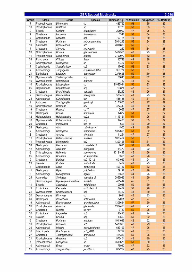
GBR Seabed Biodiversity 15-289Group Class Genus Species Biomass Kg %Available %Exposed %EffortExp
7 Phaeophyceae Dictyotales sp 433762 53 35 29 10 Rhodophyceae Griffithsia sp 10773 52 33 29 9 Bivalvia Corbula macgillvrayi 205900 47 25 29 7 Crustacea Leucosia formosensis 1341 53 34 28 7 Cephalopoda Sepiidae spp 792725 49 30 28 7 Crustacea Portunus rubromarginatus 5914213 55 34 28 10 Asteroidea Oreasteridae sp1 2814889 56 37 28 7 Crustacea Sicyonia rectirostris 259 56 34 28 20 Chlorophyceae Udotea glaucescens 1402555 42 23 28 11 Phaeophyceae Sporochnus moorei 2797072 53 32 28 33 Polychaeta Chloeia flava 15742 49 28 28 7 Chlorophyceae Cladophora sp 39457 52 33 28 7 Cephalopoda Sepiadariidae sp5 17032 52 33 28 7 Actinopterygii Torquigener cf pallimaculatus 358774 52 31 28 21 Echinoidea Laganum depressum 2276625 50 30 28 21 Gymnolaemata Thalamoporella spp 56643 53 32 28 16 Gymnolaemata Retelepralia mosaica 62 45 33 28 10 Rhodophyceae Lithophyllum sp1 21086914 50 33 28 25 Cephalopoda Cephalopoda spp 750874 47 27 27 2 Crustacea Dromidiopsis edwardsi 27212 46 26 27 2 Demospongiae Reniochalina stalagmitis 500459 41 23 27 34 Actinopterygii Cynoglossus sp4 466488 49 31 27 2 Anthozoa Trachyphyllia geoffroyi 3171803 46 27 27 10 Chlorophyceae Halimeda sp2 477419 46 30 27 19 Crustacea Pagurid sp17 2067 47 27 27 10 Gastropoda Conus ammiralis 17677 51 34 27 12 Holothuroidea Holothuroidea sp22 1113121 51 26 27 10 Gymnolaemata Robertsonidra spp 12430 50 33 27 25 Crustacea Porcellanid sp4154 693 49 29 27 28 Gastropoda Atys cylindricus cf 4963 49 28 27 7 Actinopterygii Sorsogona tuberculata 1332608 53 32 27 8 Crustacea Arcania elongata 11264 47 27 27 11 Rhodophyceae Heterosiphonia muelleri 1083464 52 31 27 11 Phaeophyceae Dictyopteris sp2 1307425 52 31 27 33 Gastropoda Nassarius conoidalis cf 2625 52 29 27 12 Actinopterygii Adventor elongatus 11470 44 22 26 2 Chlorophyceae Halimeda borneenses 10124447 45 26 26 25 Actinopterygii Upeneus sp juv/unident 5365 48 26 26 9 Crustacea Dorippe sp7142-12 601019 45 24 26 29 Bivalvia Corbula fortisulcata 6462 43 23 26 1 Cephalopoda Sepia whitleyana 493757 50 32 26 11 Gastropoda Biplex pulchellum 59197 47 26 26 3 Actinopterygii Cynoglossus ogilbyi 28505 44 25 26 25 Asteroidea Stellaster equestris cf 2055943 49 29 26 8 Demospongiae Mycale (arenochalina) mirabilis 401414 45 31 26 11 Bivalvia Spondylus wrightianus 103088 50 30 26 19 Echinoidea Peronella orbicularis cf 32469 50 28 26 31 Gymnolaemata Orthoscuticella spp 26462 48 30 26 20 Demospongiae Disyringa sp1 9021 46 23 26 30 Gastropoda Xenophora solarioides 37081 47 27 26 19 Actinopterygii Engyprosopon grandisquama 1306624 57 30 26 20 Rhodophyceae Amansia glomerata 1902406 41 21 26 27 Crustacea Nursilia sp nov 3789 50 26 26 20 Echinoidea Laganidae sp3 190493 44 24 26 10 Bivalvia Chama spp 13590 50 32 26 2 Crustacea Portunus tenuipes 1911035 42 22 26 10 Rhodophyceae Gracilaria sp1 1475393 48 29 26 36 Actinopterygii Minous trachycephalus 649193 47 26 26 16 Brachiopoda Brachiopoda sp1_MTQ 79799 41 31 25 27 Crustacea Trachypenaeus granulosus 424353 50 25 25 21 Rhodophyceae Gracilaria sp2 975404 48 29 25 1 Phaeophyceae Lobophora sp 6615675 53 30 25 10 Actinopterygii Erosa erosa 175940 47 32 25 25 Actinopterygii Tragulichthys jaculiferus 637207 47 25 25
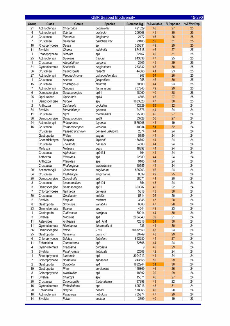
GBR Seabed Biodiversity 15-290Group Class Genus Species Biomass Kg %Available %Exposed %EffortExp
21 Actinopterygii Choerodon cephalotes 421829 46 27 25 4 Actinopterygii Zebrias craticula 206568 49 30 25 8 Crustacea Pilumnus longicornis 2472 46 26 25 7 Crustacea Dardanus callichela var 29106 52 31 25 10 Rhodophyceae Dasya sp 365331 49 29 25 11 Bivalvia Chama pulchella 874718 46 27 25 1 Phaeophyceae Dictyota sp1 82767 46 31 25 25 Actinopterygii Upeneus tragula 843838 47 25 25 1 Crustacea Allogalathea elegans 2905 49 29 25 31 Gymnolaemata Scuticella plagiostoma 233332 48 30 25 36 Crustacea Carinosquilla redacta 44868 41 23 25 27 Actinopterygii Pseudochromis quinquedentatus 1907 54 26 25 1 Crustacea Actaea jacquelinae 958 46 30 25 15 Crustacea Phalangipus filiformis 30500 44 23 25 7 Actinopterygii Synodus tectus group 707843 49 29 25 6 Demospongiae Demospongiae sp11 48060 40 28 25 25 Ophiuroidea Ophiothrix sp14 4806 46 27 25 1 Demospongiae Mycale sp9 1633320 47 30 25 2 Anthozoa Cycloseris cyclolites 112329 55 32 24 34 Bivalvia Mimachlamys gloriosa 24876 44 24 24 11 Crustacea Myra mammillaris 25080 46 27 24 36 Demospongiae Demospongiae sp89 63728 50 27 24 24 Actinopterygii Priacanthus tayenus 1576906 45 19 24 16 Crustacea Parapenaeopsis venusta 10034 51 32 24 Crustacea Penaeid unknown penaeid unknown 2674 44 24 24 Gastropoda Philine angasi 5859 44 24 24 Chondrichthyes Dasyatis leylandi 176702 44 24 24 Crustacea Thalamita hanseni 54500 44 24 24 Mollusca Mollusca eggs 18397 44 24 24 Crustacea Alpheidae sp2434 164 44 24 24 Anthozoa Pteroides sp1 22889 44 24 24 Anthozoa Pteroides sp2 9105 44 24 24 Crustacea Phalangipus australiensis 10355 44 24 24
20 Actinopterygii Choerodon sugillatum 525263 46 24 24 34 Crustacea Parthenope longimanus 8339 49 25 24 20 Demospongiae Spirastrella sp3 68071 41 20 24 3 Crustacea Lisoporcellana sp3194 354 43 24 24 3 Demospongiae Demospongiae sp61 303087 40 22 24 7 Chlorophyceae Halimeda cuneata 5618 43 30 24 30 Crustacea Quollastria subtilis 5814 36 20 24 2 Bivalvia Fragum retusum 3345 47 28 24 8 Gastropoda Strombus variabilis 6886 47 28 24 23 Gymnolaemata Beania spp 4544 43 23 24 1 Gastropoda Tudivasum armigera 80914 44 30 24 3 Bivalvia Modiolus sp1 2064840 39 21 24 11 Asteroidea Anthenea sp1_AIM 72818 51 30 24 11 Gymnolaemata Hiantopora intermedia cf 936 44 30 24 36 Demospongiae Ircinia 2710 10672550 43 23 24 25 Gastropoda Nassarius glans cf 39749 48 29 24 6 Chlorophyceae Udotea flabellum 642280 44 27 24 11 Echinoidea Temnotrema sp3 72568 44 24 24 4 Gymnolaemata Cranosina coronata 9 46 29 24 3 Bivalvia Parahyotissa imbricata 52508 42 24 24 1 Rhodophyceae Laurencia sp1 3004213 44 24 24 7 Chlorophyceae Bornetella sphaerica 243558 50 29 24 2 Gastropoda Dolabella sp1 1882244 51 30 24 19 Gastropoda Phos senticosus 145869 46 26 24 8 Chlorophyceae Avrainvillea sp1 18392 39 29 24 11 Bivalvia Chlamys sp2 15871 46 27 24 20 Crustacea Carinosquilla thailandensis 87298 48 22 24 16 Gymnolaemata Emballotheca spp 605916 43 31 24 20 Echinoidea Breynia desorii 170066 46 20 24 10 Actinopterygii Parapercis nebulosa 705874 47 29 24 14 Bivalvia Fulvia scalata 3799 40 19 23
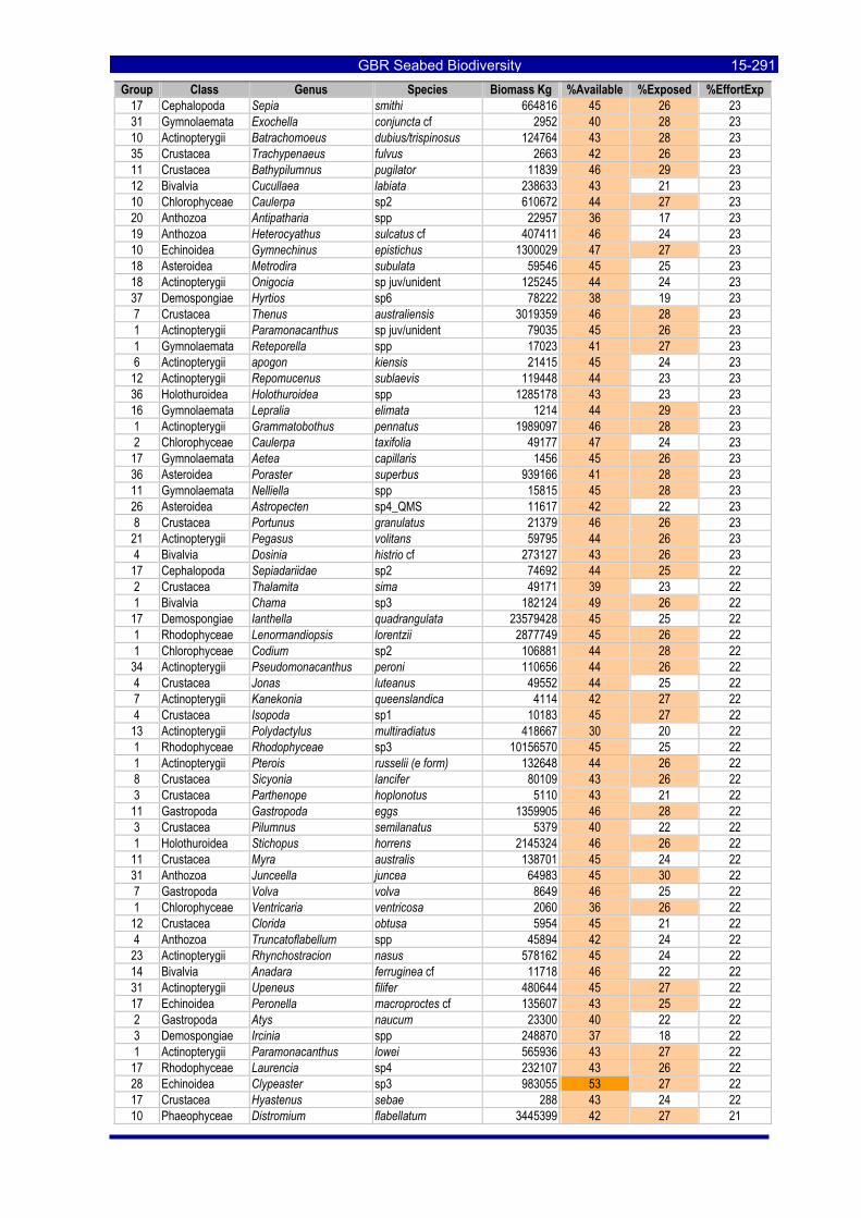
GBR Seabed Biodiversity 15-291Group Class Genus Species Biomass Kg %Available %Exposed %EffortExp
17 Cephalopoda Sepia smithi 664816 45 26 23 31 Gymnolaemata Exochella conjuncta cf 2952 40 28 23 10 Actinopterygii Batrachomoeus dubius/trispinosus 124764 43 28 23 35 Crustacea Trachypenaeus fulvus 2663 42 26 23 11 Crustacea Bathypilumnus pugilator 11839 46 29 23 12 Bivalvia Cucullaea labiata 238633 43 21 23 10 Chlorophyceae Caulerpa sp2 610672 44 27 23 20 Anthozoa Antipatharia spp 22957 36 17 23 19 Anthozoa Heterocyathus sulcatus cf 407411 46 24 23 10 Echinoidea Gymnechinus epistichus 1300029 47 27 23 18 Asteroidea Metrodira subulata 59546 45 25 23 18 Actinopterygii Onigocia sp juv/unident 125245 44 24 23 37 Demospongiae Hyrtios sp6 78222 38 19 23 7 Crustacea Thenus australiensis 3019359 46 28 23 1 Actinopterygii Paramonacanthus sp juv/unident 79035 45 26 23 1 Gymnolaemata Reteporella spp 17023 41 27 23 6 Actinopterygii apogon kiensis 21415 45 24 23 12 Actinopterygii Repomucenus sublaevis 119448 44 23 23 36 Holothuroidea Holothuroidea spp 1285178 43 23 23 16 Gymnolaemata Lepralia elimata 1214 44 29 23 1 Actinopterygii Grammatobothus pennatus 1989097 46 28 23 2 Chlorophyceae Caulerpa taxifolia 49177 47 24 23 17 Gymnolaemata Aetea capillaris 1456 45 26 23 36 Asteroidea Poraster superbus 939166 41 28 23 11 Gymnolaemata Nelliella spp 15815 45 28 23 26 Asteroidea Astropecten sp4_QMS 11617 42 22 23 8 Crustacea Portunus granulatus 21379 46 26 23 21 Actinopterygii Pegasus volitans 59795 44 26 23 4 Bivalvia Dosinia histrio cf 273127 43 26 23 17 Cephalopoda Sepiadariidae sp2 74692 44 25 22 2 Crustacea Thalamita sima 49171 39 23 22 1 Bivalvia Chama sp3 182124 49 26 22 17 Demospongiae Ianthella quadrangulata 23579428 45 25 22 1 Rhodophyceae Lenormandiopsis lorentzii 2877749 45 26 22 1 Chlorophyceae Codium sp2 106881 44 28 22 34 Actinopterygii Pseudomonacanthus peroni 110656 44 26 22 4 Crustacea Jonas luteanus 49552 44 25 22 7 Actinopterygii Kanekonia queenslandica 4114 42 27 22 4 Crustacea Isopoda sp1 10183 45 27 22 13 Actinopterygii Polydactylus multiradiatus 418667 30 20 22 1 Rhodophyceae Rhodophyceae sp3 10156570 45 25 22 1 Actinopterygii Pterois russelii (e form) 132648 44 26 22 8 Crustacea Sicyonia lancifer 80109 43 26 22 3 Crustacea Parthenope hoplonotus 5110 43 21 22 11 Gastropoda Gastropoda eggs 1359905 46 28 22 3 Crustacea Pilumnus semilanatus 5379 40 22 22 1 Holothuroidea Stichopus horrens 2145324 46 26 22 11 Crustacea Myra australis 138701 45 24 22 31 Anthozoa Junceella juncea 64983 45 30 22 7 Gastropoda Volva volva 8649 46 25 22 1 Chlorophyceae Ventricaria ventricosa 2060 36 26 22 12 Crustacea Clorida obtusa 5954 45 21 22 4 Anthozoa Truncatoflabellum spp 45894 42 24 22 23 Actinopterygii Rhynchostracion nasus 578162 45 24 22 14 Bivalvia Anadara ferruginea cf 11718 46 22 22 31 Actinopterygii Upeneus filifer 480644 45 27 22 17 Echinoidea Peronella macroproctes cf 135607 43 25 22 2 Gastropoda Atys naucum 23300 40 22 22 3 Demospongiae Ircinia spp 248870 37 18 22 1 Actinopterygii Paramonacanthus lowei 565936 43 27 22 17 Rhodophyceae Laurencia sp4 232107 43 26 22 28 Echinoidea Clypeaster sp3 983055 53 27 22 17 Crustacea Hyastenus sebae 288 43 24 22 10 Phaeophyceae Distromium flabellatum 3445399 42 27 21
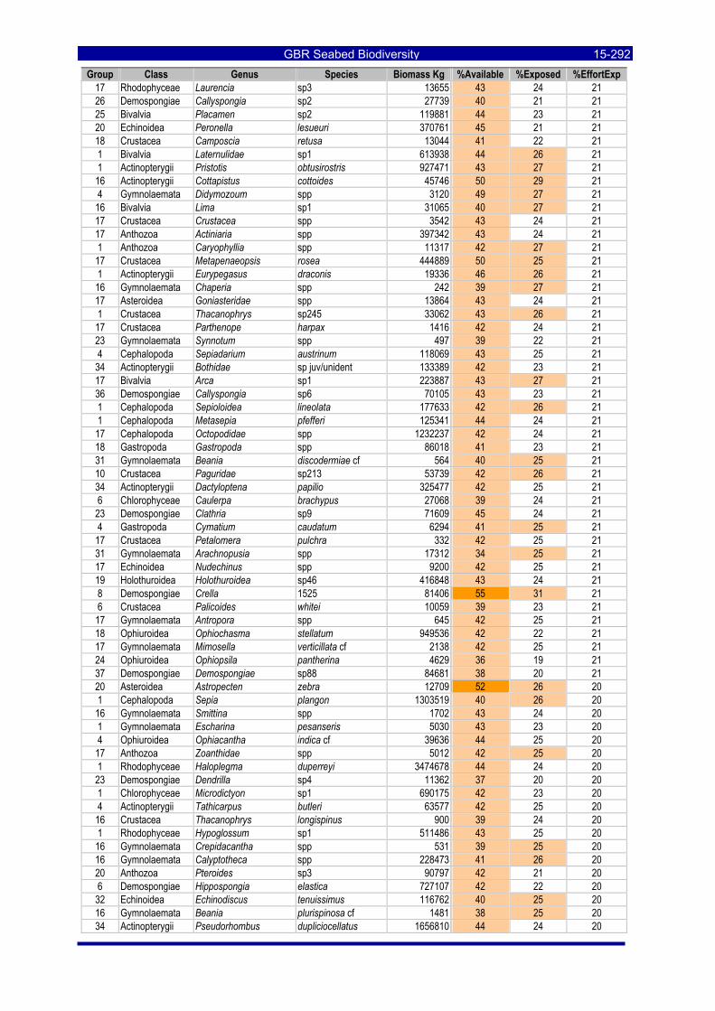
GBR Seabed Biodiversity 15-292Group Class Genus Species Biomass Kg %Available %Exposed %EffortExp
17 Rhodophyceae Laurencia sp3 13655 43 24 21 26 Demospongiae Callyspongia sp2 27739 40 21 21 25 Bivalvia Placamen sp2 119881 44 23 21 20 Echinoidea Peronella lesueuri 370761 45 21 21 18 Crustacea Camposcia retusa 13044 41 22 21 1 Bivalvia Laternulidae sp1 613938 44 26 21 1 Actinopterygii Pristotis obtusirostris 927471 43 27 21 16 Actinopterygii Cottapistus cottoides 45746 50 29 21 4 Gymnolaemata Didymozoum spp 3120 49 27 21 16 Bivalvia Lima sp1 31065 40 27 21 17 Crustacea Crustacea spp 3542 43 24 21 17 Anthozoa Actiniaria spp 397342 43 24 21 1 Anthozoa Caryophyllia spp 11317 42 27 21 17 Crustacea Metapenaeopsis rosea 444889 50 25 21 1 Actinopterygii Eurypegasus draconis 19336 46 26 21 16 Gymnolaemata Chaperia spp 242 39 27 21 17 Asteroidea Goniasteridae spp 13864 43 24 21 1 Crustacea Thacanophrys sp245 33062 43 26 21 17 Crustacea Parthenope harpax 1416 42 24 21 23 Gymnolaemata Synnotum spp 497 39 22 21 4 Cephalopoda Sepiadarium austrinum 118069 43 25 21 34 Actinopterygii Bothidae sp juv/unident 133389 42 23 21 17 Bivalvia Arca sp1 223887 43 27 21 36 Demospongiae Callyspongia sp6 70105 43 23 21 1 Cephalopoda Sepioloidea lineolata 177633 42 26 21 1 Cephalopoda Metasepia pfefferi 125341 44 24 21 17 Cephalopoda Octopodidae spp 1232237 42 24 21 18 Gastropoda Gastropoda spp 86018 41 23 21 31 Gymnolaemata Beania discodermiae cf 564 40 25 21 10 Crustacea Paguridae sp213 53739 42 26 21 34 Actinopterygii Dactyloptena papilio 325477 42 25 21 6 Chlorophyceae Caulerpa brachypus 27068 39 24 21 23 Demospongiae Clathria sp9 71609 45 24 21 4 Gastropoda Cymatium caudatum 6294 41 25 21 17 Crustacea Petalomera pulchra 332 42 25 21 31 Gymnolaemata Arachnopusia spp 17312 34 25 21 17 Echinoidea Nudechinus spp 9200 42 25 21 19 Holothuroidea Holothuroidea sp46 416848 43 24 21 8 Demospongiae Crella 1525 81406 55 31 21 6 Crustacea Palicoides whitei 10059 39 23 21 17 Gymnolaemata Antropora spp 645 42 25 21 18 Ophiuroidea Ophiochasma stellatum 949536 42 22 21 17 Gymnolaemata Mimosella verticillata cf 2138 42 25 21 24 Ophiuroidea Ophiopsila pantherina 4629 36 19 21 37 Demospongiae Demospongiae sp88 84681 38 20 21 20 Asteroidea Astropecten zebra 12709 52 26 20 1 Cephalopoda Sepia plangon 1303519 40 26 20 16 Gymnolaemata Smittina spp 1702 43 24 20 1 Gymnolaemata Escharina pesanseris 5030 43 23 20 4 Ophiuroidea Ophiacantha indica cf 39636 44 25 20 17 Anthozoa Zoanthidae spp 5012 42 25 20 1 Rhodophyceae Haloplegma duperreyi 3474678 44 24 20 23 Demospongiae Dendrilla sp4 11362 37 20 20 1 Chlorophyceae Microdictyon sp1 690175 42 23 20 4 Actinopterygii Tathicarpus butleri 63577 42 25 20 16 Crustacea Thacanophrys longispinus 900 39 24 20 1 Rhodophyceae Hypoglossum sp1 511486 43 25 20 16 Gymnolaemata Crepidacantha spp 531 39 25 20 16 Gymnolaemata Calyptotheca spp 228473 41 26 20 20 Anthozoa Pteroides sp3 90797 42 21 20 6 Demospongiae Hippospongia elastica 727107 42 22 20 32 Echinoidea Echinodiscus tenuissimus 116762 40 25 20 16 Gymnolaemata Beania plurispinosa cf 1481 38 25 20 34 Actinopterygii Pseudorhombus dupliciocellatus 1656810 44 24 20
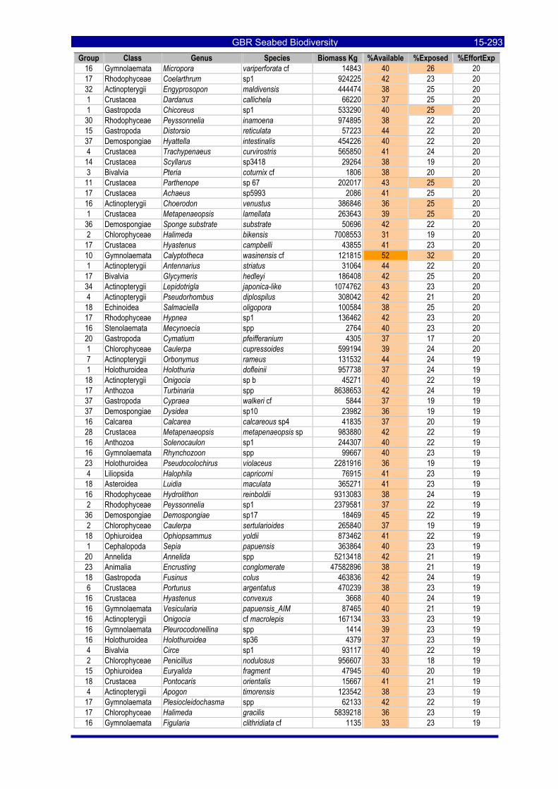
GBR Seabed Biodiversity 15-293Group Class Genus Species Biomass Kg %Available %Exposed %EffortExp
16 Gymnolaemata Micropora variperforata cf 14843 40 26 20 17 Rhodophyceae Coelarthrum sp1 924225 42 23 20 32 Actinopterygii Engyprosopon maldivensis 444474 38 25 20 1 Crustacea Dardanus callichela 66220 37 25 20 1 Gastropoda Chicoreus sp1 533290 40 25 20 30 Rhodophyceae Peyssonnelia inamoena 974895 38 22 20 15 Gastropoda Distorsio reticulata 57223 44 22 20 37 Demospongiae Hyattella intestinalis 454226 40 22 20 4 Crustacea Trachypenaeus curvirostris 565850 41 24 20 14 Crustacea Scyllarus sp3418 29264 38 19 20 3 Bivalvia Pteria coturnix cf 1806 38 20 20 11 Crustacea Parthenope sp 67 202017 43 25 20 17 Crustacea Achaeus sp5993 2086 41 25 20 16 Actinopterygii Choerodon venustus 386846 36 25 20 1 Crustacea Metapenaeopsis lamellata 263643 39 25 20 36 Demospongiae Sponge substrate substrate 50696 42 22 20 2 Chlorophyceae Halimeda bikensis 7008553 31 19 20 17 Crustacea Hyastenus campbelli 43855 41 23 20 10 Gymnolaemata Calyptotheca wasinensis cf 121815 52 32 20 1 Actinopterygii Antennarius striatus 31064 44 22 20 17 Bivalvia Glycymeris hedleyi 186408 42 25 20 34 Actinopterygii Lepidotrigla japonica-like 1074762 43 23 20 4 Actinopterygii Pseudorhombus diplospilus 308042 42 21 20 18 Echinoidea Salmaciella oligopora 100584 38 25 20 17 Rhodophyceae Hypnea sp1 136462 42 23 20 16 Stenolaemata Mecynoecia spp 2764 40 23 20 20 Gastropoda Cymatium pfeifferanium 4305 37 17 20 1 Chlorophyceae Caulerpa cupressoides 599194 39 24 20 7 Actinopterygii Orbonymus rameus 131532 44 24 19 1 Holothuroidea Holothuria dofleinii 957738 37 24 19 18 Actinopterygii Onigocia sp b 45271 40 22 19 17 Anthozoa Turbinaria spp 8638653 42 24 19 37 Gastropoda Cypraea walkeri cf 5844 37 19 19 37 Demospongiae Dysidea sp10 23982 36 19 19 16 Calcarea Calcarea calcareous sp4 41835 37 20 19 28 Crustacea Metapenaeopsis metapenaeopsis sp 983880 42 22 19 16 Anthozoa Solenocaulon sp1 244307 40 22 19 16 Gymnolaemata Rhynchozoon spp 99667 40 23 19 23 Holothuroidea Pseudocolochirus violaceus 2281916 36 19 19 4 Liliopsida Halophila capricorni 76915 41 23 19 18 Asteroidea Luidia maculata 365271 41 23 19 16 Rhodophyceae Hydrolithon reinboldii 9313083 38 24 19 2 Rhodophyceae Peyssonnelia sp1 2379581 37 22 19 36 Demospongiae Demospongiae sp17 18469 45 22 19 2 Chlorophyceae Caulerpa sertularioides 265840 37 19 19 18 Ophiuroidea Ophiopsammus yoldii 873462 41 22 19 1 Cephalopoda Sepia papuensis 363864 40 23 19 20 Annelida Annelida spp 5213418 42 21 19 23 Animalia Encrusting conglomerate 47582896 38 21 19 18 Gastropoda Fusinus colus 463836 42 24 19 6 Crustacea Portunus argentatus 470239 38 23 19 16 Crustacea Hyastenus convexus 3668 40 24 19 16 Gymnolaemata Vesicularia papuensis_AIM 87465 40 21 19 16 Actinopterygii Onigocia cf macrolepis 167134 33 23 19 16 Gymnolaemata Pleurocodonellina spp 1414 39 23 19 16 Holothuroidea Holothuroidea sp36 4379 37 23 19 4 Bivalvia Circe sp1 93117 40 22 19 2 Chlorophyceae Penicillus nodulosus 956607 33 18 19 15 Ophiuroidea Euryalida fragment 47945 40 20 19 18 Crustacea Pontocaris orientalis 15667 41 21 19 4 Actinopterygii Apogon timorensis 123542 38 23 19 17 Gymnolaemata Plesiocleidochasma spp 62133 42 22 19 17 Chlorophyceae Halimeda gracilis 5839218 36 23 19 16 Gymnolaemata Figularia clithridiata cf 1135 33 23 19
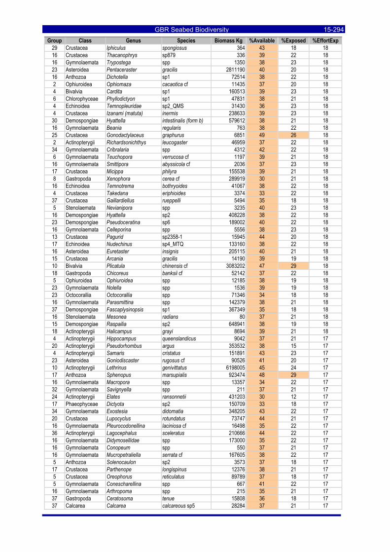
GBR Seabed Biodiversity 15-294Group Class Genus Species Biomass Kg %Available %Exposed %EffortExp
29 Crustacea Iphiculus spongiosus 364 43 18 18 16 Crustacea Thacanophrys sp879 336 39 22 18 16 Gymnolaemata Trypostega spp 1350 38 23 18 23 Asteroidea Pentaceraster gracilis 2811190 40 20 18 16 Anthozoa Dichotella sp1 72514 38 22 18 2 Ophiuroidea Ophiomaza cacaotica cf 11435 37 20 18 4 Bivalvia Cardita sp1 160513 39 23 18 6 Chlorophyceae Phyllodictyon sp1 47831 38 21 18 4 Echinoidea Temnopleuridae sp2_QMS 31430 36 23 18 4 Crustacea Izanami (matuta) inermis 238633 39 23 18 30 Demospongiae Hyattella intestinalis (form b) 579612 38 21 18 16 Gymnolaemata Beania regularis 763 38 22 18 25 Crustacea Gonodactylaceus graphurus 6851 49 26 18 2 Actinopterygii Richardsonichthys leucogaster 46959 37 22 18 34 Gymnolaemata Cribralaria spp 4312 42 22 18 6 Gymnolaemata Teuchopora verrucosa cf 1197 39 21 18 16 Gymnolaemata Smittipora abyssicola cf 2036 37 23 18 17 Crustacea Micippa philyra 155538 39 21 18 8 Gastropoda Xenophora cerea cf 289919 30 21 18 16 Echinoidea Temnotrema bothryoides 41067 38 22 18 4 Crustacea Takedana eriphioides 3374 33 22 18 37 Crustacea Gaillardiellus rueppelli 5494 35 18 18 5 Stenolaemata Nevianipora spp 3235 40 23 18 16 Demospongiae Hyattella sp2 408228 38 22 18 23 Demospongiae Pseudoceratina sp6 189002 40 22 18 16 Gymnolaemata Celleporina spp 5556 38 23 18 13 Crustacea Pagurid sp2358-1 15945 44 20 18 17 Echinoidea Nudechinus sp4_MTQ 133160 38 22 18 16 Asteroidea Euretaster insignis 205115 40 21 18 15 Crustacea Arcania gracilis 14190 39 19 18 10 Bivalvia Plicatula chinensis cf 3083202 47 29 18 18 Gastropoda Chicoreus banksii cf 52142 37 22 18 5 Ophiuroidea Ophiuroidea spp 12185 38 19 18 23 Gymnolaemata Nolella spp 1536 39 19 18 23 Octocorallia Octocorallia spp 71346 34 18 18 16 Gymnolaemata Parasmittina spp 142379 38 21 18 37 Demospongiae Fascaplysinopsis sp1 367349 35 18 18 16 Stenolaemata Mesonea radians 80 37 21 18 15 Demospongiae Raspailia sp2 648941 38 19 18 18 Actinopterygii Halicampus grayi 8694 39 21 18 4 Actinopterygii Hippocampus queenslandicus 9042 37 21 17 20 Actinopterygii Pseudorhombus argus 353532 38 15 17 4 Actinopterygii Samaris cristatus 151891 43 23 17 23 Asteroidea Goniodiscaster rugosus cf 90526 41 20 17 10 Actinopterygii Lethrinus genivittatus 6198005 45 24 17 17 Anthozoa Sphenopus marsupialis 923474 48 29 17 16 Gymnolaemata Macropora spp 13357 34 22 17 32 Gymnolaemata Savignyella spp 211 37 21 17 24 Actinopterygii Elates ransonnetii 431203 30 12 17 17 Phaeophyceae Dictyota sp2 150709 33 18 17 34 Gymnolaemata Exostesia didomatia 348205 43 22 17 20 Crustacea Lupocyclus rotundatus 73747 44 21 17 16 Gymnolaemata Pleurocodonellina laciniosa cf 16498 35 22 17 36 Actinopterygii Lagocephalus sceleratus 210666 44 22 17 16 Gymnolaemata Didymosellidae spp 173000 35 22 17 16 Gymnolaemata Conopeum spp 550 37 21 17 16 Gymnolaemata Mucropetraliella serrata cf 167605 38 22 17 5 Anthozoa Solenocaulon sp2 3573 37 18 17 17 Crustacea Parthenope longispinus 12376 38 21 17 5 Crustacea Oreophorus reticulatus 89789 37 18 17 5 Gymnolaemata Conescharellina spp 667 41 22 17 16 Gymnolaemata Arthropoma spp 215 35 21 17 37 Gastropoda Ceratosoma tenue 15808 36 18 17 37 Calcarea Calcarea calcareous sp5 28284 37 21 17
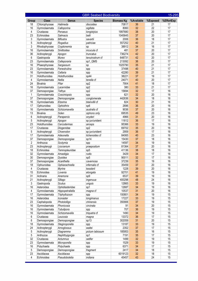
GBR Seabed Biodiversity 15-295Group Class Genus Species Biomass Kg %Available %Exposed %EffortExp
18 Chlorophyceae Halimeda discoidea 70817 36 21 17 16 Gymnolaemata Calloporina sigillata 8060 32 22 17 4 Crustacea Penaeus longistylus 1997680 38 20 17 23 Echinoidea Salmacis belli 1045645 37 20 17 3 Gymnolaemata Biflustra savartii 2006 36 18 17 5 Actinopterygii Rogadius patriciae 557252 40 21 17 3 Rhodophyceae Cryptonemia sp 38912 34 16 17 16 Gymnolaemata Smittoidea incucula cf 481 37 20 17 36 Actinopterygii Apogon truncatus 736274 42 20 17 6 Gastropoda Murex tenuirostrum cf 648731 42 20 17 23 Gymnolaemata Celleporaria sp1_QMS 213092 36 20 17 16 Phaeophyceae Sargassum sp 1025790 35 21 17 23 Gymnolaemata Fenestrulina spp 37498 40 21 17 16 Gymnolaemata Cellaria spp 42280 39 21 17 31 Holothuroidea Holothuroidea sp44 38221 37 19 17 4 Gymnolaemata Nellia tenella cf 24071 40 20 17 24 Bivalvia Pitar sp2 7904 41 18 17 16 Gymnolaemata Lacernidae sp2 380 33 21 17 37 Demospongiae Tethya sp2 15694 32 17 16 1 Gymnolaemata Cosciniopsis spp 621 32 20 16 37 Demospongiae Demospongiae conglomerate 442636 34 18 16 16 Gymnolaemata Elzerina blainvillii cf 824 30 21 16 17 Ophiuroidea Ophiothrix sp6 2696 36 20 16 16 Gymnolaemata Schizomavella australis cf 9036 37 20 16 13 Bivalvia Solen siphons only 69535 49 23 16 6 Actinopterygii Parapercis snyderi 4966 31 20 16 5 Actinopterygii Apogon sp juv/unident 11812 36 17 16 23 Holothuroidea Cercodermas anceps 95366 33 19 16 17 Crustacea Diogenidae sp2 69702 35 20 16 5 Actinopterygii Choerodon sp juv/unident 2959 36 17 16 17 Gymnolaemata Adeonella lichenoides cf 84065 40 23 16 37 Demospongiae Demospongiae sp14 15430 37 18 16 2 Anthozoa Scolymia spp 14597 34 19 16 23 Actinopterygii Liocranium praepositum 81364 37 20 16 18 Echinoidea Temnopleuridae sp5 41136 38 18 16 32 Gymnolaemata Amastigia rudis 3429 34 17 16 30 Demospongiae Dysidea sp5 90011 32 17 16 37 Demospongiae Acanthella cavernosa 37239 35 19 16 18 Ophiuroidea Ophiarachnella infernalis cf 35459 37 20 16 4 Crustacea Myrine kesslerii 1228 39 20 16 15 Echinoidea Lovenia elongata 92701 41 19 16 31 Actinaria Anemone sp9 6537 39 19 16 21 Actinopterygii Sillago ingenuua 400298 48 24 16 3 Gastropoda Scutus unguis 12865 33 19 16 16 Asteroidea Ophidiasteridae sp1 12687 34 19 16 4 Gymnolaemata Hippopetraliella magna cf 10537 31 20 16 17 Gymnolaemata Triphyllozoon spp 150801 34 19 15 16 Asteroidea Iconaster longimanus 17227 33 19 15 23 Cephalopoda Photololligo chinensis 350906 37 19 15 16 Gymnolaemata Phonicosia circinata 91 34 20 15 16 Gymnolaemata Tubulipora spp 707 36 19 15 16 Gymnolaemata Schizomavella triquetra cf 1490 34 19 15 6 Crustacea Leucosia magna 13372 36 17 15 6 Demospongiae Demospongiae sp13 302059 31 20 15 18 Gymnolaemata Steginoporella spp 13187 33 19 15 24 Actinopterygii Arnoglossus waitei 2352 37 17 15 5 Actinopterygii Diagramma pictum labiosum 185953 35 16 15 5 Anthozoa Nephthyigorgia sp1 7191 35 17 15 32 Crustacea Actumnus setifer 1499 32 19 15 23 Gymnolaemata Microporella spp 1529 33 19 15 16 Polychaeta Polychaete spp 6371 34 17 15 5 Demospongiae Demospongiae fragment 2417 34 18 15 23 Ascidiacea Ascidiacea spp 6019123 32 18 15 4 Echinoidea Pseudoboletia indiana 45457 43 24 15
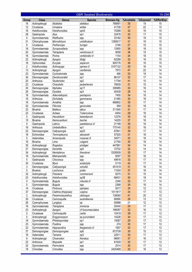
GBR Seabed Biodiversity 15-296Group Class Genus Species Biomass Kg %Available %Exposed %EffortExp
16 Actinopterygii Abalistes stellatus 766691 35 19 15 12 Crustacea Urnalana whitei 41726 47 22 15 16 Holothuroidea Holothuroidea sp43 70289 32 19 15 28 Gastropoda Atys sp1 32478 42 17 15 4 Gymnolaemata Retiflustra spp 33182 36 19 15 31 Chlorophyceae Microdictyon umbilicatum 1285617 31 19 15 6 Crustacea Parthenope turriger 2190 27 15 15 16 Gymnolaemata Scrupocellaria spp 12955 36 18 15 20 Gymnolaemata Tetraplaria ventricosa cf 9058 36 15 15 16 Gymnolaemata Porina vertebralis cf 1154 34 18 15 32 Actinopterygii Apogon 9(dg) 62289 33 16 15 16 Ophiuroidea Euryale asperum 905776 36 19 15 2 Holothuroidea Actinopyga spinea cf 5107122 29 16 14 13 Actinopterygii Apogon cavitiensis 7972 47 22 14 23 Gymnolaemata Cyclostomata spp 466 33 19 14 30 Demospongiae Dendroceratid sp1 86107 32 17 14 20 Anthozoa Studeriotes sp2 11794 41 15 14 23 Crustacea Charybdis jaubertensis 76639 31 15 14 30 Demospongiae Niphates sp17 306985 33 16 14 26 Demospongiae Dysidea sp3 50439 28 14 14 16 Gymnolaemata Adeonellopsis pentapora 7400 34 18 14 16 Anthozoa Dichotella gemmacea 21485 35 18 14 16 Gymnolaemata Amathia spp 668802 35 17 14 32 Gymnolaemata Filicrisia geniculata 959 32 18 14 23 Bivalvia Malleus albus 311540 31 17 14 23 Crustacea Actaea Tuberculosa 6454 28 18 14 5 Gastropoda Haustellum tweedianum 12376 35 18 14 15 Bivalvia Nemocardium bechei 14205 37 16 14 5 Gastropoda Latirus paetelianus cf 21199 35 16 14 16 Anthozoa Umbellulifera sp1 775140 32 18 14 23 Demospongiae Callyspongia sp23 87841 39 17 14 16 Echinoidea Temnopleurus alexandri 57525 31 18 14 5 Asteroidea Anseropoda rosacae cf 34571 33 16 14 16 Bivalvia Lima vulgaris 21760 30 18 14 35 Actinopterygii Rogadius pristiger 447881 34 14 14 37 Demospongiae Dendrilla sp5 72702 32 14 14 34 Actinopterygii Nemipterus theodorei 5326939 35 17 14 16 Gymnolaemata Metroperiella spp 6097 33 18 14 5 Gastropoda Chicoreus spp 49916 32 17 14 34 Crustacea Myra eudactyla 5119 42 17 14 3 Demospongiae Callyspongia schultzi 451419 31 16 14 5 Bivalvia Liochonca polita 11024 37 16 14 32 Actinopterygii Fistularia commersoni 8270 31 15 14 23 Holothuroidea Holothuroidea sp38 68431 30 18 14 5 Gymnolaemata Bugula robusta cf 2346 33 17 14 5 Gymnolaemata Bugula spp 2368 34 18 14 14 Crustacea Portunus spinipes 5017 35 12 13 37 Demospongiae Clathria (thalysias) vulpina 1011817 34 17 13 2 Actinopterygii Paramonacanthus oblongus 139092 41 20 13 30 Crustacea Carinosquilla australiensis 66990 28 13 13 26 Cyanophyceae Lyngbya sp 50986 21 12 13 16 Gymnolaemata Tetraplaria immersa 30440 29 17 13 23 Actinopterygii Apogon cf fuscomaculatus 196097 32 16 13 5 Crustacea Carinosquilla carita 10419 38 17 13 5 Actinopterygii Engyprosopon sp juv/unident 14226 34 17 13 16 Gymnolaemata Phidoloporidae sp1 10087 28 17 13 23 Gymnolaemata Puellina spp 274 30 17 13 23 Gymnolaemata Hippopodina feegeensis cf 1957 32 17 13 37 Demospongiae Demospongiae sp6 873739 30 15 13 16 Asteroidea Tamaria sp3 22911 30 17 13 6 Actinopterygii Choerodon frenatus 96061 37 16 13 23 Anthozoa Mopsella sp1 81629 32 17 13 32 Gymnolaemata Parmularia spp 2514 30 17 13 18 Crinoidea Crinoidea spp 2425469 32 16 13
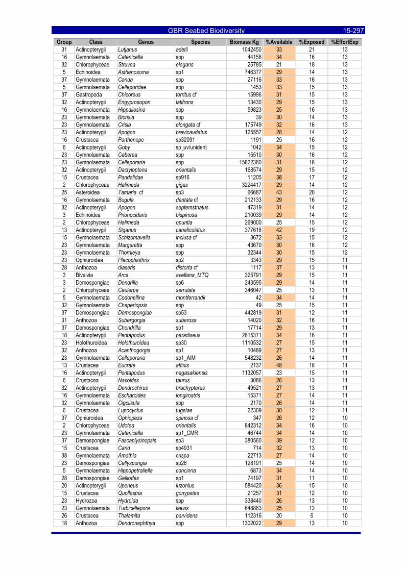
GBR Seabed Biodiversity 15-297Group Class Genus Species Biomass Kg %Available %Exposed %EffortExp
31 Actinopterygii Lutjanus adetii 1042450 33 21 13 16 Gymnolaemata Catenicella spp 44158 34 16 13 32 Chlorophyceae Struvea elegans 25785 21 18 13 5 Echinoidea Asthenosoma sp1 746377 29 14 13 37 Gymnolaemata Canda spp 27116 33 16 13 5 Gymnolaemata Celleporidae spp 1453 33 15 13 37 Gastropoda Chicoreus territus cf 15996 31 15 13 32 Actinopterygii Engyprosopon latifrons 13430 29 15 13 16 Gymnolaemata Hippaliosina spp 59823 25 16 13 23 Gymnolaemata Bicrisia spp 39 30 14 13 23 Gymnolaemata Crisia elongata cf 175749 32 16 13 23 Actinopterygii Apogon brevicaudatus 125557 28 14 12 16 Crustacea Parthenope sp32091 1191 25 16 12 6 Actinopterygii Goby sp juv/unident 1042 34 15 12 23 Gymnolaemata Caberea spp 15510 30 16 12 23 Gymnolaemata Celleporaria spp 15622360 31 16 12 32 Actinopterygii Dactyloptena orientalis 168574 29 15 12 15 Crustacea Pandalidae sp916 11205 38 17 12 2 Chlorophyceae Halimeda gigas 3224417 29 14 12 25 Asteroidea Tamaria cf sp3 66687 43 20 12 16 Gymnolaemata Bugula dentata cf 212133 29 16 12 32 Actinopterygii Apogon septemstriatus 47319 31 14 12 3 Echinoidea Prionocidaris bispinosa 210039 29 14 12 2 Chlorophyceae Halimeda opuntia 269000 25 15 12 13 Actinopterygii Siganus canaliculatus 377618 42 19 12 15 Gymnolaemata Schizomavella inclusa cf 3672 33 15 12 23 Gymnolaemata Margaretta spp 43670 30 16 12 23 Gymnolaemata Thornleya spp 32344 30 15 12 23 Ophiuroidea Placophiothrix sp2 3343 29 15 11 28 Anthozoa diaseris distorta cf 1117 37 13 11 3 Bivalvia Arca avellana_MTQ 325791 29 15 11 3 Demospongiae Dendrilla sp6 243595 29 14 11 2 Chlorophyceae Caulerpa serrulata 346047 25 13 11 5 Gymnolaemata Codonellina montferrandii 42 34 14 11 32 Gymnolaemata Chaperiopsis spp 49 25 15 11 37 Demospongiae Demospongiae sp53 442819 31 12 11 31 Anthozoa Subergorgia suberosa 14020 32 16 11 37 Demospongiae Chondrilla sp1 17714 29 13 11 18 Actinopterygii Pentapodus paradiseus 2615371 34 16 11 23 Holothuroidea Holothuroidea sp30 1110532 27 15 11 32 Anthozoa Acanthogorgia sp1 10489 27 13 11 23 Gymnolaemata Celleporaria sp1_AIM 548232 26 14 11 13 Crustacea Eucrate affinis 2137 48 18 11 16 Actinopterygii Pentapodus nagasakiensis 1132057 23 15 11 6 Crustacea Naxoides taurus 3086 26 13 11 32 Actinopterygii Dendrochirus brachypterus 49521 27 13 11 16 Gymnolaemata Escharoides longirostris 15371 27 14 11 32 Gymnolaemata Cigclisula spp 2170 26 14 11 6 Crustacea Lupocyclus tugelae 22309 30 12 11 37 Ophiuroidea Ophiopeza spinosa cf 347 26 12 10 2 Chlorophyceae Udotea orientalis 842312 34 16 10 23 Gymnolaemata Catenicella sp1_CMR 46744 34 14 10 37 Demospongiae Fascaplysinopsis sp3 380560 39 12 10 15 Crustacea Carid sp4931 714 32 13 10 38 Gymnolaemata Amathia crispa 22713 27 14 10 23 Demospongiae Callyspongia sp26 128191 25 14 10 5 Gymnolaemata Hippopetraliella concinna 6873 34 14 10 28 Demospongiae Gelliodes sp1 74197 31 11 10 20 Actinopterygii Upeneus luzonius 584420 36 15 10 15 Crustacea Quollastria gonypetes 21257 31 12 10 23 Hydrozoa Hydroida spp 338440 26 13 10 23 Gymnolaemata Turbicellepora laevis 648863 25 13 10 26 Crustacea Thalamita parvidens 112316 20 6 10 18 Anthozoa Dendronephthya spp 1302022 29 13 10
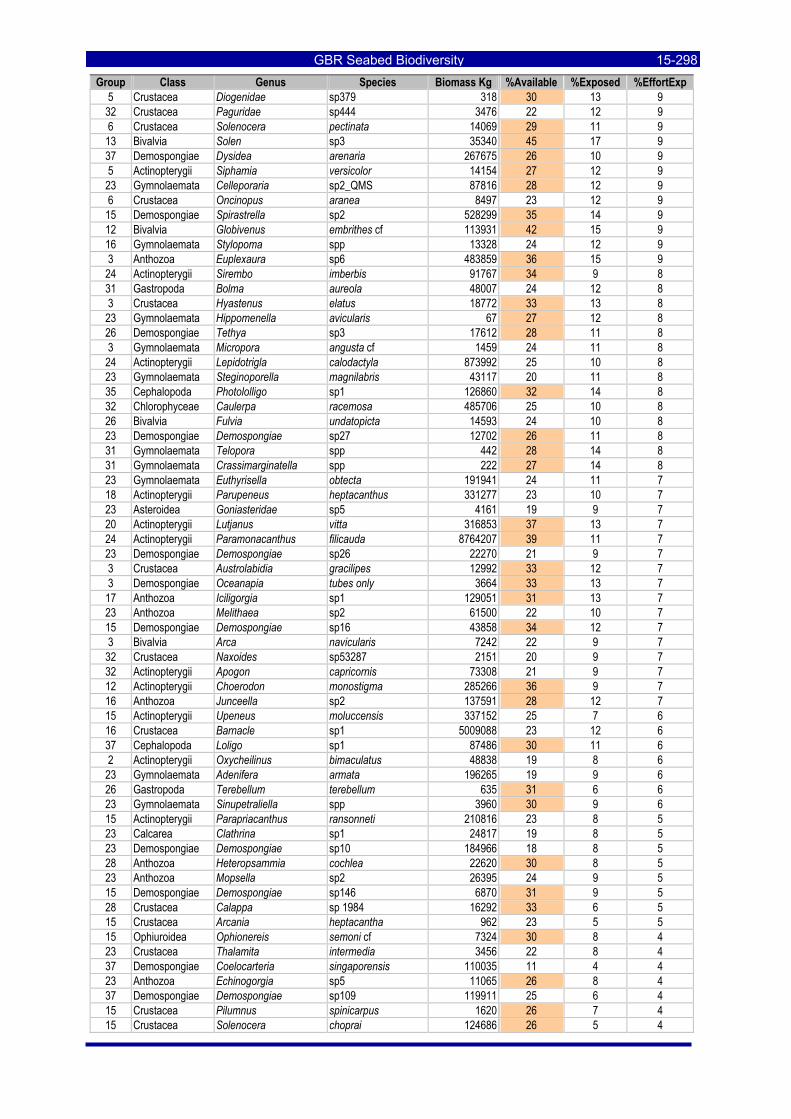
GBR Seabed Biodiversity 15-298Group Class Genus Species Biomass Kg %Available %Exposed %EffortExp
5 Crustacea Diogenidae sp379 318 30 13 9 32 Crustacea Paguridae sp444 3476 22 12 9 6 Crustacea Solenocera pectinata 14069 29 11 9 13 Bivalvia Solen sp3 35340 45 17 9 37 Demospongiae Dysidea arenaria 267675 26 10 9 5 Actinopterygii Siphamia versicolor 14154 27 12 9 23 Gymnolaemata Celleporaria sp2_QMS 87816 28 12 9 6 Crustacea Oncinopus aranea 8497 23 12 9 15 Demospongiae Spirastrella sp2 528299 35 14 9 12 Bivalvia Globivenus embrithes cf 113931 42 15 9 16 Gymnolaemata Stylopoma spp 13328 24 12 9 3 Anthozoa Euplexaura sp6 483859 36 15 9 24 Actinopterygii Sirembo imberbis 91767 34 9 8 31 Gastropoda Bolma aureola 48007 24 12 8 3 Crustacea Hyastenus elatus 18772 33 13 8 23 Gymnolaemata Hippomenella avicularis 67 27 12 8 26 Demospongiae Tethya sp3 17612 28 11 8 3 Gymnolaemata Micropora angusta cf 1459 24 11 8 24 Actinopterygii Lepidotrigla calodactyla 873992 25 10 8 23 Gymnolaemata Steginoporella magnilabris 43117 20 11 8 35 Cephalopoda Photololligo sp1 126860 32 14 8 32 Chlorophyceae Caulerpa racemosa 485706 25 10 8 26 Bivalvia Fulvia undatopicta 14593 24 10 8 23 Demospongiae Demospongiae sp27 12702 26 11 8 31 Gymnolaemata Telopora spp 442 28 14 8 31 Gymnolaemata Crassimarginatella spp 222 27 14 8 23 Gymnolaemata Euthyrisella obtecta 191941 24 11 7 18 Actinopterygii Parupeneus heptacanthus 331277 23 10 7 23 Asteroidea Goniasteridae sp5 4161 19 9 7 20 Actinopterygii Lutjanus vitta 316853 37 13 7 24 Actinopterygii Paramonacanthus filicauda 8764207 39 11 7 23 Demospongiae Demospongiae sp26 22270 21 9 7 3 Crustacea Austrolabidia gracilipes 12992 33 12 7 3 Demospongiae Oceanapia tubes only 3664 33 13 7 17 Anthozoa Iciligorgia sp1 129051 31 13 7 23 Anthozoa Melithaea sp2 61500 22 10 7 15 Demospongiae Demospongiae sp16 43858 34 12 7 3 Bivalvia Arca navicularis 7242 22 9 7 32 Crustacea Naxoides sp53287 2151 20 9 7 32 Actinopterygii Apogon capricornis 73308 21 9 7 12 Actinopterygii Choerodon monostigma 285266 36 9 7 16 Anthozoa Junceella sp2 137591 28 12 7 15 Actinopterygii Upeneus moluccensis 337152 25 7 6 16 Crustacea Barnacle sp1 5009088 23 12 6 37 Cephalopoda Loligo sp1 87486 30 11 6 2 Actinopterygii Oxycheilinus bimaculatus 48838 19 8 6 23 Gymnolaemata Adenifera armata 196265 19 9 6 26 Gastropoda Terebellum terebellum 635 31 6 6 23 Gymnolaemata Sinupetraliella spp 3960 30 9 6 15 Actinopterygii Parapriacanthus ransonneti 210816 23 8 5 23 Calcarea Clathrina sp1 24817 19 8 5 23 Demospongiae Demospongiae sp10 184966 18 8 5 28 Anthozoa Heteropsammia cochlea 22620 30 8 5 23 Anthozoa Mopsella sp2 26395 24 9 5 15 Demospongiae Demospongiae sp146 6870 31 9 5 28 Crustacea Calappa sp 1984 16292 33 6 5 15 Crustacea Arcania heptacantha 962 23 5 5 15 Ophiuroidea Ophionereis semoni cf 7324 30 8 4 23 Crustacea Thalamita intermedia 3456 22 8 4 37 Demospongiae Coelocarteria singaporensis 110035 11 4 4 23 Anthozoa Echinogorgia sp5 11065 26 8 4 37 Demospongiae Demospongiae sp109 119911 25 6 4 15 Crustacea Pilumnus spinicarpus 1620 26 7 4 15 Crustacea Solenocera choprai 124686 26 5 4
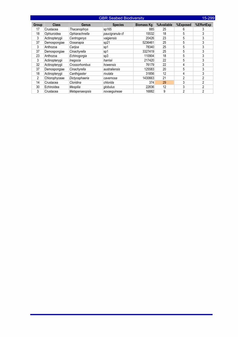
GBR Seabed Biodiversity 15-299Group Class Genus Species Biomass Kg %Available %Exposed %EffortExp
17 Crustacea Thacanophrys sp165 885 25 6 3 18 Ophiuroidea Ophiarachnella paucigranula cf 15532 18 5 3 3 Actinopterygii Centrogenys vaigiensis 20426 23 5 3 37 Demospongiae Oceanapia sp21 5236461 25 5 3 3 Anthozoa Carijoa sp1 78340 25 5 3 37 Demospongiae Cinachyrella sp1 3327419 25 5 3 23 Anthozoa Echinogorgia sp3 110904 18 5 3 3 Actinopterygii Inegocia harrisii 217420 22 5 3 32 Actinopterygii Crossorhombus howensis 76179 22 4 3 37 Demospongiae Cinachyrella australiensis 125583 20 5 3 18 Actinopterygii Canthigaster rivulata 31856 12 4 3 2 Chlorophyceae Dictyosphaeria cavernosa 1430663 21 2 2 14 Crustacea Cloridina chlorida 374 29 3 2 30 Echinoidea Mespilia globulus 22836 12 3 2 3 Crustacea Metapenaeopsis novaeguineae 16882 9 2 2

GBR Seabed Biodiversity 15-300
AUSTRALIAN INSTITUTE
OF MARINE SCIENCE Australian Institute of Marine Science PMB 3, Townsville MC TOWNSVILLE, Qld. 4810 Australia
Marine & Atmospheric Research Mathematics & Information Sciences 233 Middle Street CLEVELAND, Qld. 4163 Australia
Queensland Department of Primary Industries Northern Fisheries Centre Tingara Street CAIRNS, Qld. 4870 Australia
Queensland Museum SOUTH BRISBANE, Qld. 4101 Australia Museum of Tropical Queensland TOWNSVILLE, Qld. 4810