A Spatial Compositional

Model for Linear Unmixing

Yuan Zhou, Anand Rangarajan and Paul D. GaderDepartment of CISE, University of Florida

Motivation

Hyperspectral image unmixing are important in many applications. Very little previous work on simultaneously:

Incorporating spatial information in the pixel likelihood. Modeling the uncertainty in the extracted endmembers.

Spatial compositional model (SCM) proposed for this purpose.

Linear mixing model (LMM) Spectral measurement ( , ) at wavelength , location in the 𝑔 𝒙 𝜆 𝜆 𝒙

image domain

𝑀 is the number of endmembers, is the spectral signature of the ith endmember, is the fractional abundance map of the ith endmember satisfying thepositivity and sum-to-one constraints,

( , ) is a noise field (usually modeled as Gaussian).𝑛 𝒙 𝜆

Linear mixing model: discretized version The discretized version of the ith pixel can be represented by

, , , . Combining this at all locations

，， ， .

The uncertainty of endmembers One area of LMM with little previous work is to discover the model

uncertainty of the endmembers.

What are the uncertainties for the 3 endmember sets?

Endmember variability vs. endmember uncertainty

Endmember uncertainty: all the pixels are generated by the same endmember set.

Suppose B = 1. , , .

indicates that the density function of does not even exist.

Add some noise

The covariance matrix is not block diagonal.

Endmember variability: each pixel is generated by a different endmember set.

Let indicates

Assume pixel independence

The covariance matrix is block diagonal.

This is what we want to find

NCM

SCM

SCM: Advantages SCM’s features:

Estimating the uncertainty along with the endmembers and abundances by calculating the full likelihood.

A smoothness prior on abundances to help unmixing. A simple and efficient algorithm.

SCM: Density function assumptions We assume that

The probability function of the whole endmember set becomes

. Assume the noise follows

SCM: Spatial random variable transformations

The random variable transformation of indicates

If , it can be simplified as

is a diagonal matrix with diagonal elements . The estimation of full endmember covariance matrices will be

discussed later.

Not block diagonal

SCM: The prior on the abundances The prior probability for can be defined by

controls the spatial intimacy between node i and node j , is the symmetric positive semidefinite graph Laplacian matrix.

We can use

when node i and node j are neighbors and 0 otherwise.

SCM: The prior on the endmembers We use the following prior for parameters :

denotes the ith row of , denotes the kth column of . for all i and j. is 1 when and 0 otherwise.

Similar to , the prior can be written as

and are the corresponding Laplacian matrices.

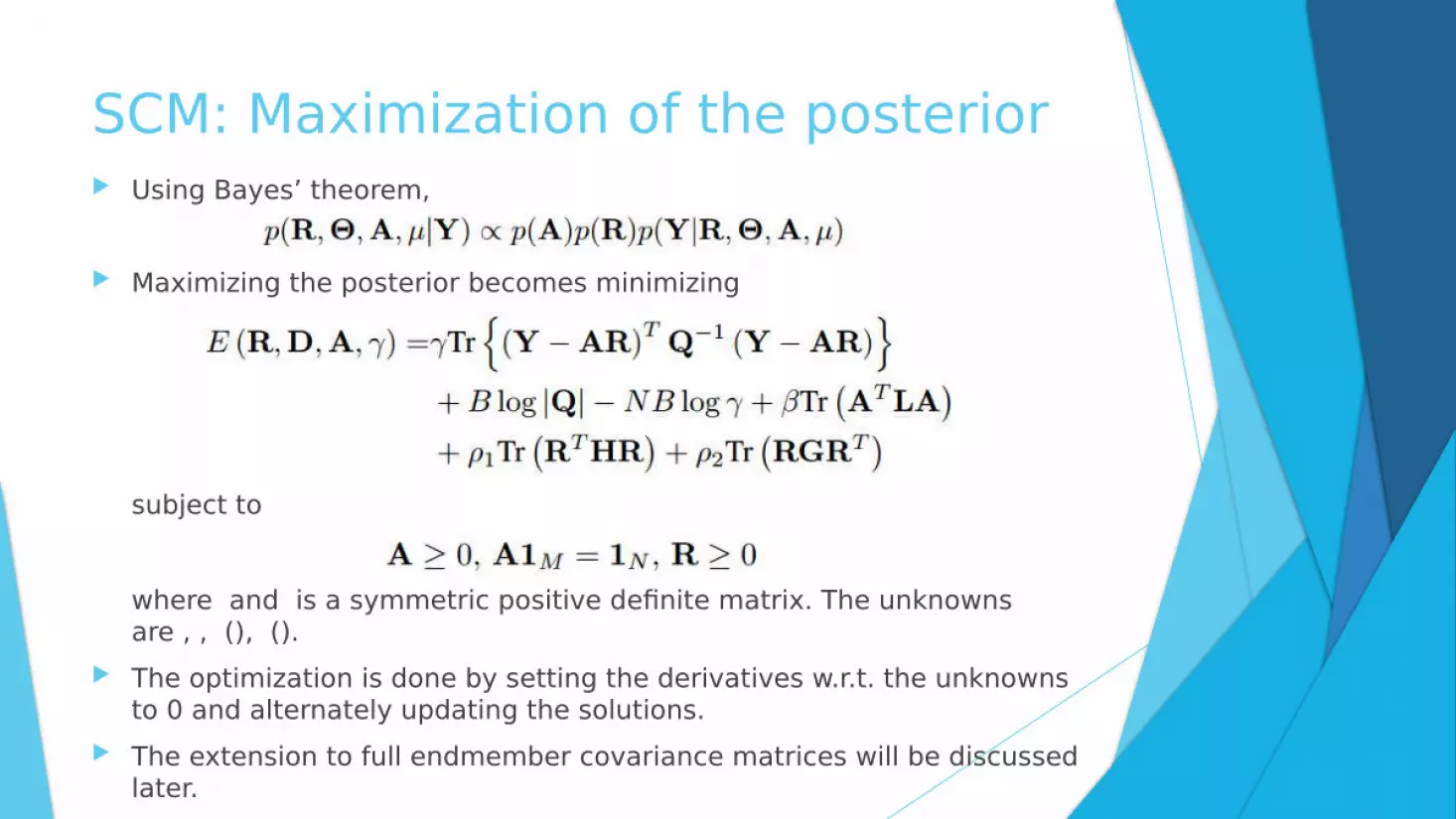
SCM: Maximization of the posterior Using Bayes’ theorem,

Maximizing the posterior becomes minimizing

subject to

where and is a symmetric positive definite matrix. The unknowns are , , (), ().

The optimization is done by setting the derivatives w.r.t. the unknowns to 0 and alternately updating the solutions.

The extension to full endmember covariance matrices will be discussed later.

Pavia University: the image and the ground truth

Pavia University: comparison of abundance maps

(a) SCM (b) NCMWithout the spatial prior in SCM

Which material does this abundance map correspond to?

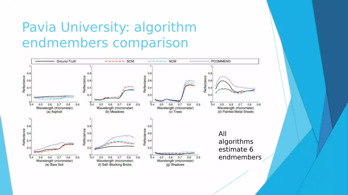
Pavia University: algorithm endmembers comparison

All algorithms estimate 6 endmembers

Pavia University: quantitative comparison of endmember error

Indian Pines: the image and the ground truth

Indian Pines: comparison of abundance maps

Extension to full covariance matrices We extend the work to estimate the full endmember covariance

matrices, without assuming it is diagonal. The objective function turns out to be

subject to

where

The unknowns are .

Extension to full covariance matrices:Synthetic image uncertainty range

We use the full endmember covariance matrices here

Extension to full covariance matrices:Pavia University abundance maps

Extension to full covariance matrices:Pavia University endmember comparison

Extension to full covariance matrices:Pavia University uncertainty range

We take the square root of the largest eigenvalue, , the corresponding eigenvector to calculate the uncertainty range .

Discussion

The features of SCM include estimating the uncertainty along with the endmembers and abundances.

The spatial prior with weighted smoothness leads to better unmixing. The objective function enables a simple and efficient algorithm, e.g. it

takes about 2 minutes to process the Pavia University dataset on a laptop.

The extended work on full endmember covariance matrices implies that the uncertainty estimation leads to error prediction.

We want to thank Jose Bioucas-Dias and Alina Zare for helpful conversations. We acknowledge support from NSF IIS 1065081.