scientific-technical concept for requirements of a fossil fuel
TRANSCRIPT
This project has received funding from the European Union’s Horizon 2020
research and innovation programme under grant agreement No 730944
D1.2
RINGO (GA no 730944)
Public Document/define level
Readiness of ICOS for Necessities of integrated Global Observations
Scientific-technical concept for requirements of a fossil fuel
observation system
Ref. Ares(2020)7986678 - 29/12/2020

DISSEMINATION LEVEL, Page 1 of 55
Deliverable: D1.2
Author(s): S. Hammer, F. Maier, Y. Wang, A. van der Woude, M. van der Molen, T. Kneuer,
C. Rieß, L. Nguyen, H. Meijer, M. Ramonet, U. Karstens and I.Levin
Date: 20.11.2020
Activity: Task 1.2
Lead Partner: UHEI
Document Issue: Report
Dissemination Level: Public
Contact: [email protected]
Name Partner Date
From Samuel Hammer UHEI 16.11.2020
Reviewed by Werner Kutsch ICOS ERIC 15.12.2020
Approved by Werner Kutsch ICOS ERIC 15.12.2020
Version Date Comments/Changes Author/Partner
1.0 16.11.2020 Version for co-author comments S. Hammer/UHEI
1.51 20.11.2020 Comments included S.Hammer/UHEI
Deliverable Review Checklist
A list of checkpoints has been created to be ticked off by the Task Leader before finalizing the deliverable. These checkpoints are incorporated into the deliverable template where the Task Leader must tick off the list.
√
• Appearance is generally appealing and according to the RINGO template. Cover page has been updated according to the Deliverable details.
☐
• The executive summary is provided giving a short and to the point description of the deliverable.
☐
• All abbreviations are explained in a separate list. ☐
• All references are listed in a concise list. ☐
• The deliverable clearly identifies all contributions from partners and justifies the resources used.
☐
• A full spell check has been executed and is completed. ☐
DISCLAIMER
This document has been produced in the context of the project Readiness of ICOS for Necessities of integrated Global Observations (RINGO) The
Research leading to these results has received funding from the European Union’s Horizon 2020 research and innovation programme under
grant agreement No 730944. All Information in this document is provided "as is" and no guarantee or warranty is given that the information
is fit for any particular purpose. The user thereof uses the information at its sole risk and liability. For the avoidance of all doubts, the European
Commission has no liability in respect of this document, which is merely representing the authors view.
Amendments, comments and suggestions should be sent to the authors.
DISSEMINATION LEVEL, Page 2 of 55
ABSTRACT
This deliverable report addresses the scientific and technical requirements for a fossil fuel observation
system based on experimental and theoretical work carried out in RINGO Task 1.2. The report focuses on
the question of how to optimise the 14CO2 sampling strategy in ICOS by serving two different purposes. First,
to improve the experimental ability to separate fossil fuel CO2 contributions in urban emission plumes and
second to provide an optimised monitoring network that enables atmospheric inverse modelling
frameworks to estimate national fossil fuel CO2 emissions with high confidence.
In the experimental part atmospheric combined up- and downwind measurements around three European
cities: Paris, Rotterdam and Mannheim/Ludwigshafen were conducted. To exploit synergy with the ICOS
atmosphere network one of the two monitoring stations was selected to be an existing ICOS atmosphere
station. This station was supplemented by an adjoined station on the opposing side of the urban area. For
this two new monitoring stations have been built up within the project. The approach of observing urban
fossil fuel CO2 enhancements (ΔffCO2) based on 14CO2 measurements using the combination of ICOS stations
and associated partner stations is called the RINGO approach further on. For the three urban areas mean
fossil fuel CO2 enhancements between 2 and 61 ppm were detected using the RINGO approach. We
developed a trajectory forecast-based sampling strategy, allowing targeted sampling during suitable
meteorological conditions. This targeted sampling in the RINGO approach leads to fewer sample pairs that
yield results below the 14CO2-based ΔffCO2 detection limit than in other comparable urban fossil fuel
monitoring networks. The linear regressions between the total and the fossil CO2 enhancements across the
cities Paris and Mannheim/Ludwigshafen yielded slopes of 0.98±0.05 (R²=0.96) and 1.11±0.17 (R²=0.80),
respectively. For both cities, the data revealed a nearly constant non-fossil CO2 enhancement of about 2 ppm
at the downwind station, which is not yet understood. The RINGO approach was compared to an alternative
approach, where the upwind 14CO2 measurements are replaced by regional 14CO2 background
measurements. For both approaches, an uncertainty budget was developed considering nuclear and
biogenic 14CO2 emissions both potentially masking part of the ffCO2 signal. The typical uncertainty for 14CO2-
based fossil fuel CO2 enhancements was found to be 1.2 ppm for the RINGO approach whereas it was 1.8
ppm for the regional background approach. Further advantages of the RINGO approach are lower sensitivity
to the highly uncertain nuclear 14CO2 contaminations and a better delimitation of the study area by focusing
on the differential footprint of the urban area between the observation stations, which is responsible for the
observed concentration difference between the two RINGO stations.
In the theoretical, model-based part of Task 1.2 an Observation System Simulation Experiment (OSSE) was
performed to investigate the uncertainty reduction potential of 14CO2 measurements in ICOS for constraining
national total fossil fuel emissions. The OSSE was designed to investigate differences between an ICOS
observation network and an alternative RINGO observation network around cities. The OSSE was carried out
by two fundamentally different atmospheric inversion modelling frameworks for a two-months winter
period in 2016, testing dedicated sampling strategies in each network. For both models and observation
networks, the addition of 14CO2 flask samples improves the separation between fossil and biogenic CO2
fluxes. The misfit between the prior and true fossil fuel CO2 fluxes could be reduced by 40% to 80% on
average using in-situ CO2 measurements and 14CO2 flask samples. The independent modelling frameworks
give different answers on which observation network (ICOS or RINGO) offers a greater uncertainty reduction
potential to optimise national total fossil fuel CO2 emissions. Potential reasons for this disagreement are
discussed in the summary of this report.
DISSEMINATION LEVEL, Page 3 of 55
TABLE OF CONTENTS
1 INTRODUCTION ......................................................................................................................................................... 5
2 RESULTS FROM THE EXPERIMENTAL OBSERVATIONAL STUDIES .............................................................................. 7
2.1 City selection and experimental setup .............................................................................................................. 7
2.2 Fossil fuel estimation and sampling strategy .................................................................................................... 7
2.3 Is the RINGO approach suitable to sample urban ffCO2 enhancements (ΔffCO2)? ........................................... 8
2.4 How large is the influence of 14CO2 contaminations on ΔffCO2? ..................................................................... 10
2.4.1 14CO2 effect of biogenic respiration ......................................................................................... 10
2.4.2 14CO2 contamination by nuclear facilities ................................................................................ 12
2.5 Can upwind Δ14CO2 measurements be substituted by regional background Δ14CO2 observations? .............. 16
2.6 Which share of the observed ΔCO2 concentration gradient across a target area is of fossil origin? .............. 20
2.6.1 Rhine Valley ............................................................................................................................. 20
2.6.2 Paris .......................................................................................................................................... 22
3 RESULTS FROM THE OBSERVING SYSTEM SIMULATION EXPERIMENT ................................................................... 24
3.1 Objectives and design of the OSSE .................................................................................................................. 24
3.1.1 Objectives of the OSSE and resulting model simplifications .................................................. 24
3.1.2 Sampling networks and strategies to be tested in the OSSE .................................................... 25
3.1.3 Selection of OSSE time period and spatial domain ................................................................. 26
3.1.4 Station selection and applying the RINGO approach in the OSSE .......................................... 26
3.2 Description of the modelling systems and forward modelling ....................................................................... 31
3.2.1 Description of the forward models ........................................................................................... 31
3.2.2 Description of the ‘true’ fluxes ................................................................................................ 31
3.2.3 Comparison of forward-run CO2 concentrations to observations ............................................ 32
3.2.4 Virtual 14CO2 sampling from the forward-runs ........................................................................ 33
3.2.5 Footprint coverage of the inversion ......................................................................................... 33
3.3 Description of the inversion set ups ................................................................................................................ 34
3.3.1 Description of the inversion models ......................................................................................... 34
3.3.2 Construction of the prior fluxes for the different inversion set ups ......................................... 35
3.3.3 Artificial transport uncertainty ................................................................................................. 36
3.4 Results of the OSSE inversions ........................................................................................................................ 38
3.4.1 Misfit reductions of the CO2-only inversion scenario .............................................................. 39
3.4.2 Added value of 14CO2 observations ......................................................................................... 40
3.5 Weakness in the OSSE design .......................................................................................................................... 41

DISSEMINATION LEVEL, Page 4 of 55
3.5.1 Scales did not match ................................................................................................................. 41
3.5.2 Choice of prior fluxes and prior uncertainties .......................................................................... 41
3.5.3 Use of only one transport model .............................................................................................. 42
3.5.4 Choice of optimisation regions ................................................................................................ 42
3.5.5 Choice of time-span and duration ............................................................................................ 42
3.6 Conclusions from the OSSE .............................................................................................................................. 43
3.6.1 Does twice the number of downwind samples better constrain urban ffCO2 emissions than
paired up- and downwind samples? .......................................................................................................... 43
3.6.2 Does the RINGO network yield better estimates of national total fossil fuel emissions? ....... 43
4 REQUIREMENTS FOR AN URBAN FOSSIL FUEL OBSERVATION SYSTEM .................................................................. 44
4.1 Lessons learned from the RINGO approach .................................................................................................... 44
4.2 Could the RINGO approach be incorporated in the ICOS monitoring network? ............................................. 44
5 REFERENCES ............................................................................................................................................................ 46
6 DEFINITIONS, ACRONYMS AND ABBREVIATIONS ................................................................................................... 49
7 APPENDIX A ............................................................................................................................................................. 51
8 APPENDIX B ............................................................................................................................................................. 52
DISSEMINATION LEVEL, Page 5 of 55
1 INTRODUCTION
The focus of the existing ICOS atmosphere station network is on the observation of biogenic carbon fluxes. Better
quantifying continental ecosystem CO2 fluxes is of utmost importance since the magnitude of gross biogenic fluxes is
about one order of magnitude larger compared to fossil fuel CO2 (ffCO2) emissions and associated with larger
uncertainties as well. Thus, ICOS atmosphere stations, in general, should be built at least 50 km from any larger ffCO2
emission source (ICOS RI, 2020). Being located away from ffCO2 emission “hot spots” increases the relative share of
the biogenic compared to the fossil fuel CO2 signal. Although the CO2 signals originating from the combustion of fossil
fuels are small at such “background” stations, Basu et al. (2020) succeeded in determining the national fossil fuel CO2
emissions of the United States of America (USA) with an uncertainty of only a few per cent using atmospheric 14CO2
measurements and inverse modelling. With the first global stocktake of the Paris Climate Accord approaching (UNFCCC
2015), increased efforts are put into national and international systems to better monitor and verify net CO2 fluxes.
Fossil fuel CO2 fluxes into the atmosphere are therefore being targeted as outlined for example in the European
Union's so-called Green Report on "An Operational Anthropogenic CO₂ Emissions Monitoring & Verification Support
Capacity" (Pinty et al., 2019) and the Strategy Paper on Anthropogenic CO2 emissions Monitoring and Verification
Support (CO2MVS) capacity (Janssens-Maenhout et al., 2020). Both studies illustrate how an interplay of ground- and
satellite-based measurements could lead to a better estimation of anthropogenic and particularly ffCO2 emissions.
A large share of global and European fossil fuel CO2 emissions originates from urban areas and other hotspots like
point sources (Seto et al., 2014). Further, it is expected that a significant part of future emission reductions will occur
in urban areas. This is one of the reasons why there are already numerous efforts to experimentally determine fossil
fuel CO2 emissions from urban areas. Indianapolis, Toronto, Los Angeles, Salt Lake City, London, Paris, Rotterdam and
Heidelberg are only a few of many examples (Levin et al., 2011, Turnbull et al. 2015, Breón et al. 2015, Boon et al.,
2016, Pugliese et al., 2018, Graven et al., 2018 Super et al. 2020a). Determining fossil fuel CO2 emissions from urban
areas and hotspots from ground-based observations is further interesting, because the current and the next
generation of satellite-based ffCO2 estimates are performed for hotspot regions only (Reuter et al., 2019). Several
national and international research initiatives are actively working towards the design and standardization of such
urban observing networks (e.g. IG3IS, CO2-USA, CoCO2 VERIFY, CHE). The assessment and finally the combination of
different observational approaches such as in-situ networks of towers, low-cost sensors, total column instruments,
eddy covariance flux towers, as well as radiocarbon in CO2 are of particular importance for developing an optimized
design for urban fossil fuel observation strategies. Radiocarbon observations of atmospheric CO2 play hereby a key
role. Due to their age, fossil fuels are void of radiocarbon and CO2 emissions from their combustion lowers thus the
natural 14C/C ratio in atmospheric CO2 called Suess-effect (Suess, 1955). Therewith, Radiocarbon is the most direct
measure to separate biogenic from fossil fuel CO2 (e.g. Levin et al., 2003). The European Union’s Green Report outlines
the needs for a future anthropogenic CO₂ Emissions Monitoring & Verification Support Capacity and identified
explicitly the following as one of the missing elements:
“Well-coordinated networks in the vicinity of intense emission areas, beyond the plans to increase the
current capabilities of the ICOS network, must be developed in Europe to accurately monitor radiocarbon
(14C).“
RINGO Task 1.2 aims directly at providing additional information towards this missing element by testing and assessing
urban radiocarbon sampling strategies.
Radiocarbon observations have been applied in numerous urban CO2 studies before. To date, the best instrumented,
monitored and documented urban emission experiment applying 14CO2 measurements is the INFLUX experiment in
Indianapolis, USA (e.g. Turnbull et al., 2015). Among other approaches, INFLUX equipped 12 towers in and around
Indianapolis with in-situ instrumentation for CO2 with a subset of the towers having regular flask sampling for 14CO2
analysis. Turnbull et al. concluded that performing background measurements upwind of the emission area and
accompanying downwind measurements in the emission plume of the hotspot are easier to interpret than
measurements conducted in the centre of the emission area itself. For the interpretation of their results they
successfully used the concept of a Lagrangian air-parcel, which is moving from the background station via the emission
DISSEMINATION LEVEL, Page 6 of 55
area to the downwind measurement station. This Lagrangian approach became the blueprint for many other urban
greenhouse gases (GHG) experiments (e.g. Los Angeles, Boston, Seoul, Auckland).
RINGO Task 1.2 is based on the findings of the INFLUX and other urban observation networks, copying successful
approaches and trying to address open questions on the urban network design, i.e. the 14CO2 sampling strategy, the
influence of non-fossil 14CO2 contamination e.g. from nuclear facilities as well as more fundamental questions of the
continental network design. RINGO Task 1.2 follows an experimental as well as a modelling approach to come closer
to answering these questions, which are further detailed below.
The experimental approach investigates potential synergies with the existing ICOS atmosphere monitoring station
network, but with the new focus to better quantify urban ffCO2 emissions. The modelling approach aims to answer
the question if an urban network would perform better in quantifying national fossil fuel emissions than the current
ICOS network. To assess this, we will use an Observation System Simulation Experiment (OSSE, Wu et al., 2018).
In terms of urban network development, Task 1.2 was not able to build up an entire ring of atmospheric stations
around a city. Our aim was rather to investigate if existing ICOS atmosphere stations could be supplemented by
dedicated adjoined partner stations to better constrain urban emission areas located in between the two or more
stations on opposing sides of that city. In the following we call this the RINGO approach. If this attempt is successful,
one could consider supplementing suitable ICOS atmosphere stations with adjoined RINGO stations. Such dual use of
the ICOS atmosphere infrastructure could significantly improve the network’s sensitivity towards monitoring fossil CO2
emissions. We experimentally tested this approach for three urban regions: Paris, Rotterdam and the Rhine Valley
near Heidelberg and we applied 14CO2-based fossil fuel estimates to experimentally separate regional fossil (ΔffCO2)
from biogenic CO2 enhancements. In addition to the basic question whether the RINGO approach is capable of
quantifying ΔffCO2, we use this study to further investigate fundamental questions and challenges of 14CO2-based fossil
fuel estimates.
One re-occurring question of 14CO2 sampling strategies concerns the measurement of the 14CO2 background. Turnbull
et al. (2015) showed that the estimated ffCO2 share in the total CO2 enhancement of the emission plume changed
between 50 and 100% depending on the used background station. While Turnbull et al. showed that using a
continental 14CO2 background station is not suited for urban observations in the US, we want to revisit this question
for central Europe where the 14CO2 observation network of ICOS is much denser. Is it better to have direct 14CO2
background measurements upwind of the city, or would it be better to have twice as many downwind 14CO2
measurements while accepting a larger uncertainty in the 14CO2 background estimate? This question must also be
discussed in view of non-fossil 14CO2 contaminations. In Europe, about 70 nuclear facilities are emitting pure 14CO2
(Graven & Gruber, 2011; Zazzeri et al., 2018) therewith “masking” fossil fuel CO2 in the 14CO2-based approach. What
is the magnitude of the nuclear contaminations in the RINGO approach and can they be avoided? Secondly, additional
ffCO2 masking originates from biogenic respiration. Organic material which accumulated bomb radiocarbon in the last
decades, is now partly releasing this 14CO2 back to the atmosphere. Is this a significant source of uncertainty for the 14C-based fossil fuel CO2 estimates?
One further question of continental network design goes beyond the urban scale and asks if the ICOS radiocarbon
samples as a whole would yield better estimates of national fossil fuel CO2 emissions if they all would be sampled
closer to emission areas? What is the benefit of the two weekly integrated samples for this national estimate? These
questions were the motivation behind the search of an optimised 14CO2 sampling strategy for ffCO2 emissions from
urban areas in RINGO Task 1.2.
This deliverable report summarizes the findings of the experimental and modelling approaches, addresses
achievements as well as shortcomings and concludes with requirements for an urban fossil fuel CO2 observation
system.
DISSEMINATION LEVEL, Page 7 of 55
2 RESULTS FROM THE EXPERIMENTAL OBSERVATIONAL STUDIES
In the following, we summarize the results from the experimental studies. A more detailed discussion of the results
can be found in Rieß (2019) and Kneuer (2020).
2.1 City selection and experimental setup As outlined in the introduction, the aim of the experimental part in Ringo Task 1.2 was the observation of the regional
fossil fuel CO2 concentration enhancements of three European cities by applying the 2-station RINGO approach as
“urban network”. In the first project phase, Paris, Rotterdam and the Rhine Valley were selected as test regions. All
three metropolitan areas have an ICOS atmosphere station or an ICOS pilot station nearby. Saclay tower (SAC)
southwest of Paris, Cabauw tower (CBW) east of Rotterdam and the ICOS-CRL pilot station in Heidelberg southeast of
Mannheim/Ludwigshafen in the Rhine Valley. The selection of cities ranges from the megacity Paris (10M inhabitants)
down to the medium-sized metropolitan region of Mannheim/Ludwigshafen (0.5M inhabitants). The RINGO approach
builds on the Lagrangian air mass transport as many other urban networks. The basic assumption of the approach is
that an air mass is sampled twice, once before it crosses the emission area and once after, while the boundary layer
mixing conditions should not change significantly from upwind to downwind sampling. To apply this approach in
RINGO, additional atmospheric observing stations had to be built for Rotterdam and the Rhine Valley.
In Rotterdam the new station Maasvlakte (MAS) is located at the coast of the Port of Rotterdam, inside a building of
the Port Authority located on top of a 15 m-high hill measuring CO2 and CH4 continuously. With westerly wind, MAS is
located directly upwind of the Rotterdam sea port and about 30 km from the city centre. The ICOS station Cabauw
(CBW) will then act as the downwind station and is 40 km downwind from the city centre. For the Rhine Valley, we
chose a location near Freinsheim (FRE), which is surrounded by vineyards and has very little local ffCO2 emissions. FRE
is located on a small hill, has a 10 m intake mast and is equipped with continuous CO2, 222Rn and meteorology
measurements. A detailed description of the Freinsheim station including a thorough measurement quality
assessment is given in Rieß (2019). The locations of MAS and FRE were chosen along a straight line between the existing
ICOS stations and the targeted cities, so that the urban emission areas are located in between the two stations. In
Paris, no additional atmospheric station was necessary since the existing station in Gonesse (GNS) (64 m intake height,
continuous CO2, CO and CH4 measurements) is suitably located northeast of Paris. When choosing the upwind station,
it is very important to avoid locations with local ffCO2 or nuclear 14CO2 sources in the inflow sector of the upwind
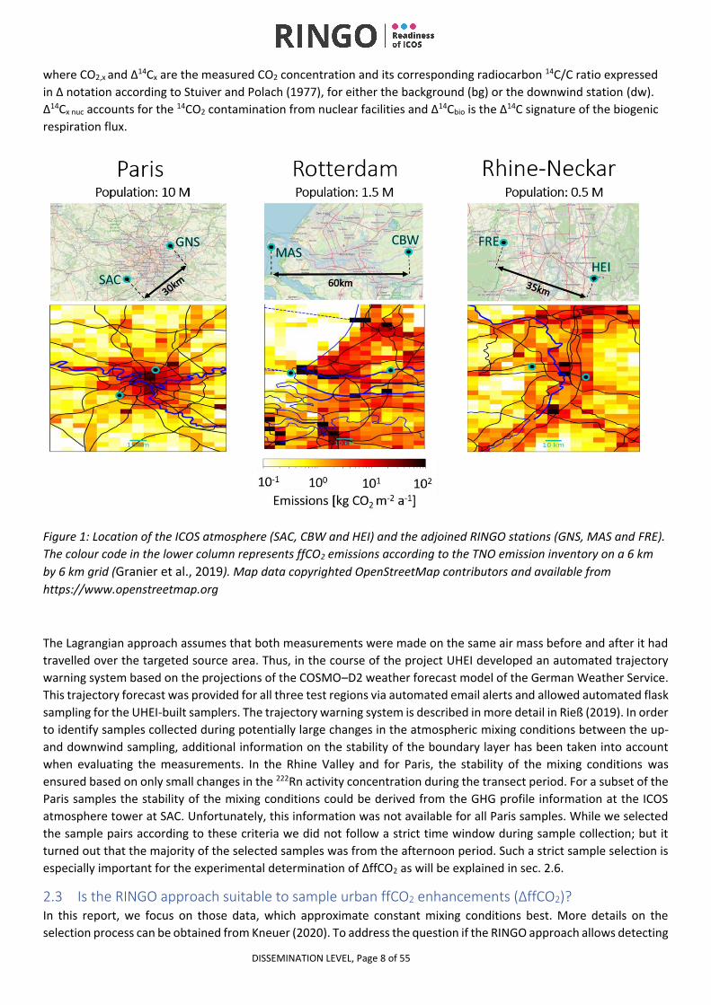
station. Figure 1 shows maps of the three urban regions with the locations of the ICOS stations and the adjoined
partner station.
At the start of the project, only the ICOS-CRL pilot station was equipped with an ICOS flask sampler. Therefore, UHEI
has built three custom made flask samplers that allow integrated air sampling over one hour or more (Kneuer, 2017;
Rieß, 2019), two samplers for Paris and one for Freinsheim. RGU has built two flask samplers for the Rotterdam area.
Due to delays in the construction of the flask samplers, the Rhine Valley and the Paris experiment were delayed,
starting operation in October 2018 and April 2019, respectively. The flask sampler construction at RUG was also
delayed and sampling for Rotterdam started in January 2019. By the end of the project, 136 14CO2 samples were
collected and analysed for the Rhine Valley, 91 samples in Paris and 46 samples for Rotterdam. Due to the Covid-19
lockdown and related work restrictions in spring 2020, experimental work at the stations became more difficult or
even impossible, so only a few samples could be collected during this period.
2.2 Fossil fuel estimation and sampling strategy Regional 14C-based fossil fuel CO2 estimates ΔffCO2 are based on differential 14CO2 measurements between a
background and the downwind station according to Eq.1 adopted from Levin et al. (2011):
Δff𝐶𝑂2 = CO2,bg(Δ 𝐶𝑏𝑔−Δ 𝐶 𝑏𝑔 𝑛𝑢𝑐
14 −Δ 𝐶𝑏𝑖𝑜) 1414 − CO2,dw(Δ 𝐶𝑑𝑤−Δ 𝐶𝑑𝑤 𝑛𝑢𝑐14 −Δ 𝐶𝑏𝑖𝑜) 1414
Δ 𝐶𝑏𝑖𝑜 + 1000 14 ‰ (1)
DISSEMINATION LEVEL, Page 8 of 55
where CO2,x and Δ14Cx are the measured CO2 concentration and its corresponding radiocarbon 14C/C ratio expressed
in Δ notation according to Stuiver and Polach (1977), for either the background (bg) or the downwind station (dw).
Δ14Cx nuc accounts for the 14CO2 contamination from nuclear facilities and Δ14Cbio is the Δ14C signature of the biogenic
respiration flux.
Figure 1: Location of the ICOS atmosphere (SAC, CBW and HEI) and the adjoined RINGO stations (GNS, MAS and FRE).
The colour code in the lower column represents ffCO2 emissions according to the TNO emission inventory on a 6 km
by 6 km grid (Granier et al., 2019). Map data copyrighted OpenStreetMap contributors and available from
https://www.openstreetmap.org
The Lagrangian approach assumes that both measurements were made on the same air mass before and after it had
travelled over the targeted source area. Thus, in the course of the project UHEI developed an automated trajectory
warning system based on the projections of the COSMO–D2 weather forecast model of the German Weather Service.
This trajectory forecast was provided for all three test regions via automated email alerts and allowed automated flask
sampling for the UHEI-built samplers. The trajectory warning system is described in more detail in Rieß (2019). In order
to identify samples collected during potentially large changes in the atmospheric mixing conditions between the up-
and downwind sampling, additional information on the stability of the boundary layer has been taken into account
when evaluating the measurements. In the Rhine Valley and for Paris, the stability of the mixing conditions was
ensured based on only small changes in the 222Rn activity concentration during the transect period. For a subset of the
Paris samples the stability of the mixing conditions could be derived from the GHG profile information at the ICOS
atmosphere tower at SAC. Unfortunately, this information was not available for all Paris samples. While we selected
the sample pairs according to these criteria we did not follow a strict time window during sample collection; but it
turned out that the majority of the selected samples was from the afternoon period. Such a strict sample selection is
especially important for the experimental determination of ΔffCO2 as will be explained in sec. 2.6.
2.3 Is the RINGO approach suitable to sample urban ffCO2 enhancements (ΔffCO2)? In this report, we focus on those data, which approximate constant mixing conditions best. More details on the
selection process can be obtained from Kneuer (2020). To address the question if the RINGO approach allows detecting
DISSEMINATION LEVEL, Page 9 of 55
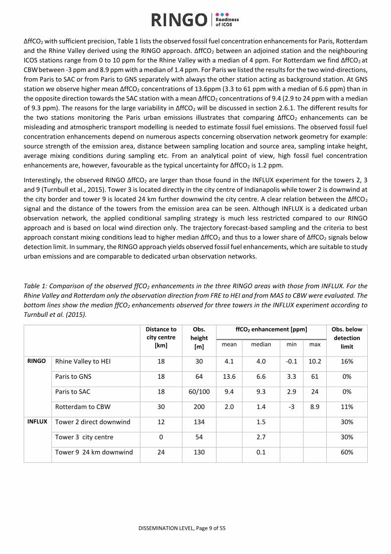
ΔffCO2 with sufficient precision, Table 1 lists the observed fossil fuel concentration enhancements for Paris, Rotterdam
and the Rhine Valley derived using the RINGO approach. ΔffCO2 between an adjoined station and the neighbouring
ICOS stations range from 0 to 10 ppm for the Rhine Valley with a median of 4 ppm. For Rotterdam we find ΔffCO2 at
CBW between -3 ppm and 8.9 ppm with a median of 1.4 ppm. For Paris we listed the results for the two wind-directions,
from Paris to SAC or from Paris to GNS separately with always the other station acting as background station. At GNS
station we observe higher mean ΔffCO2 concentrations of 13.6ppm (3.3 to 61 ppm with a median of 6.6 ppm) than in
the opposite direction towards the SAC station with a mean ΔffCO2 concentrations of 9.4 (2.9 to 24 ppm with a median
of 9.3 ppm). The reasons for the large variability in ΔffCO2 will be discussed in section 2.6.1. The different results for
the two stations monitoring the Paris urban emissions illustrates that comparing ΔffCO2 enhancements can be
misleading and atmospheric transport modelling is needed to estimate fossil fuel emissions. The observed fossil fuel
concentration enhancements depend on numerous aspects concerning observation network geometry for example:
source strength of the emission area, distance between sampling location and source area, sampling intake height,
average mixing conditions during sampling etc. From an analytical point of view, high fossil fuel concentration
enhancements are, however, favourable as the typical uncertainty for ΔffCO2 is 1.2 ppm.
Interestingly, the observed RINGO ΔffCO2 are larger than those found in the INFLUX experiment for the towers 2, 3
and 9 (Turnbull et al., 2015). Tower 3 is located directly in the city centre of Indianapolis while tower 2 is downwind at
the city border and tower 9 is located 24 km further downwind the city centre. A clear relation between the ΔffCO2
signal and the distance of the towers from the emission area can be seen. Although INFLUX is a dedicated urban
observation network, the applied conditional sampling strategy is much less restricted compared to our RINGO
approach and is based on local wind direction only. The trajectory forecast-based sampling and the criteria to best
approach constant mixing conditions lead to higher median ΔffCO2 and thus to a lower share of ΔffCO2 signals below
detection limit. In summary, the RINGO approach yields observed fossil fuel enhancements, which are suitable to study
urban emissions and are comparable to dedicated urban observation networks.
Table 1: Comparison of the observed ffCO2 enhancements in the three RINGO areas with those from INFLUX. For the
Rhine Valley and Rotterdam only the observation direction from FRE to HEI and from MAS to CBW were evaluated. The
bottom lines show the median ffCO2 enhancements observed for three towers in the INFLUX experiment according to
Turnbull et al. (2015).
Distance to city centre
[km]
Obs.
height
[m]
ffCO2 enhancement [ppm] Obs. below
detection
limit mean median min max
RINGO Rhine Valley to HEI 18 30 4.1 4.0 -0.1 10.2 16%
Paris to GNS 18 64 13.6 6.6 3.3 61 0%
Paris to SAC 18 60/100 9.4 9.3 2.9 24 0%
Rotterdam to CBW 30 200 2.0 1.4 -3 8.9 11%
INFLUX Tower 2 direct downwind 12 134 1.5 30%
Tower 3 city centre 0 54 2.7 30%
Tower 9 24 km downwind 24 130 0.1 60%
DISSEMINATION LEVEL, Page 10 of 55
2.4 How large is the influence of 14CO2 contaminations on ΔffCO2? Although 14C is the most direct tracer to experimentally determine regional ffCO2 enhancements, it also has its caveats. 14CO2 emissions from nuclear facilities can substantially increase the regional atmospheric 14CO2 content, masking
thereby the depleting effect of fossil fuel CO2 emissions. A similar masking occurs from biogenic respiration fluxes as
currently decomposed organic matter has conserved bomb radiocarbon, which was accumulated by the plants during
the 14C-bomb-spike period from about 1954 to 2000 (Palonen et al., 2017). While it is not trivial to quantify these 14C
contamination effects, it is even more challenging to assess their uncertainty. In the following, we want to discuss the
magnitude and the temporal variability of both contamination effects starting with the biogenic respiration fluxes.
2.4.1 14CO2 effect of biogenic respiration Any CO2 exchange flux between carbon reservoirs is subject to isotopic fractionation. The fractionation of 14C is thereby
approximately twice the fractionation of 13C (Mook & Rozanski, 2000). The Δ-notation in which the 14C/C ratio is
generally reported takes advantage of this and standardises the ratio to a uniform δ13C value of -25‰. Every
fractionation that actually occurs when CO2 is transferred from one reservoir to another is thus eliminated in the Δ-
notation and all 14C values when reported as Δ14C, no matter from which reservoir, are directly comparable to each
other. Note that, in this study, as is common in atmospheric radiocarbon publications, we use the term Δ14C instead
of the Δ which was originally defined in Stuiver and Polach (1977).
Photosynthetic uptake of CO2 by plants, although strongly fractionating carbon isotopes, in the Δ14C notation has, no
effect on atmospheric Δ14CO2 as all fractionation effects have been taken care of in the 13C normalisation. The same is
true for CO2 respiration fluxes if the biosphere and the atmosphere are in isotopic equilibrium. However, due to the
atmospheric nuclear bomb tests mainly in the 1950s and 1960s the atmospheric 14C/C ratio in CO2 was almost doubled
(Levin et al., 2010), and is still in disequilibrium with the biogenic 14C/C ratios (Palonen et al., 2017). The resulting
disequilibrium flux leads to an enhancement of Δ14C in atmospheric CO2. In Kneuer (2020) an entire chapter is
elaborating on this disequilibrium, here we want to summarise the main findings by analysing the effects of the
biogenic disequilibrium on the atmospheric ∆14CO2 in Heidelberg for a summer period where biogenic fluxes are
largest.
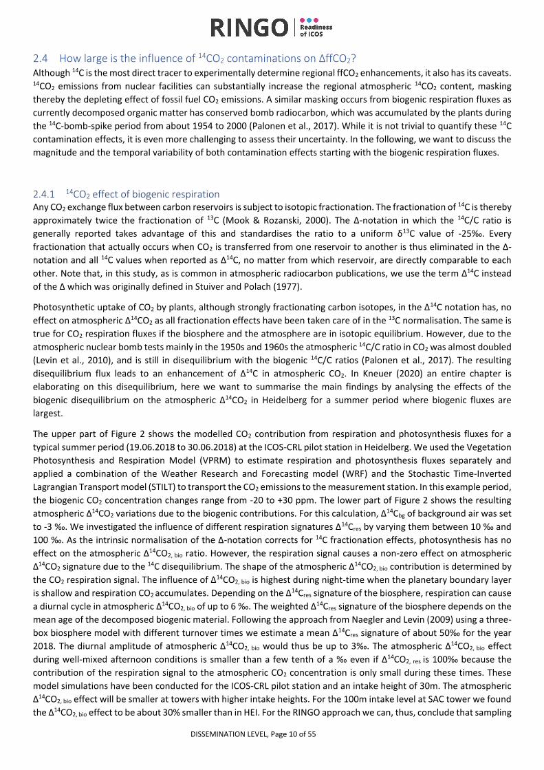
The upper part of Figure 2 shows the modelled CO2 contribution from respiration and photosynthesis fluxes for a
typical summer period (19.06.2018 to 30.06.2018) at the ICOS-CRL pilot station in Heidelberg. We used the Vegetation
Photosynthesis and Respiration Model (VPRM) to estimate respiration and photosynthesis fluxes separately and
applied a combination of the Weather Research and Forecasting model (WRF) and the Stochastic Time-Inverted
Lagrangian Transport model (STILT) to transport the CO2 emissions to the measurement station. In this example period,
the biogenic CO2 concentration changes range from -20 to +30 ppm. The lower part of Figure 2 shows the resulting
atmospheric ∆14CO2 variations due to the biogenic contributions. For this calculation, ∆14Cbg of background air was set
to -3 ‰. We investigated the influence of different respiration signatures ∆14Cres by varying them between 10 ‰ and
100 ‰. As the intrinsic normalisation of the ∆-notation corrects for 14C fractionation effects, photosynthesis has no
effect on the atmospheric ∆14CO2, bio ratio. However, the respiration signal causes a non-zero effect on atmospheric
∆14CO2 signature due to the 14C disequilibrium. The shape of the atmospheric ∆14CO2, bio contribution is determined by
the CO2 respiration signal. The influence of ∆14CO2, bio is highest during night-time when the planetary boundary layer
is shallow and respiration CO2 accumulates. Depending on the ∆14Cres signature of the biosphere, respiration can cause
a diurnal cycle in atmospheric ∆14CO2, bio of up to 6 ‰. The weighted ∆14Cres signature of the biosphere depends on the
mean age of the decomposed biogenic material. Following the approach from Naegler and Levin (2009) using a three-
box biosphere model with different turnover times we estimate a mean ∆14Cres signature of about 50‰ for the year
2018. The diurnal amplitude of atmospheric ∆14CO2, bio would thus be up to 3‰. The atmospheric ∆14CO2, bio effect
during well-mixed afternoon conditions is smaller than a few tenth of a ‰ even if ∆14CO2, res is 100‰ because the
contribution of the respiration signal to the atmospheric CO2 concentration is only small during these times. These
model simulations have been conducted for the ICOS-CRL pilot station and an intake height of 30m. The atmospheric
∆14CO2, bio effect will be smaller at towers with higher intake heights. For the 100m intake level at SAC tower we found
the ∆14CO2, bio effect to be about 30% smaller than in HEI. For the RINGO approach we can, thus, conclude that sampling
DISSEMINATION LEVEL, Page 11 of 55
during well-mixed afternoon conditions will minimize the influence of the respiration signal to well below 0.5‰.
Sampling the up- and downwind flask during changing mixing conditions can, however, lead to significant ∆14CO2, bio
effects resulting in up to about 1 ppm ffCO2 biases.
Figure 2: Biogenic CO2 contributions at the HEI station in summer. The upper plot shows respiration (blue),
photosynthesis (orange) and net (green) components of the biogenic contributions according to VPRM biogenic fluxes
transported via WRF-STILT to the measurement station. The lower plot shows the resulting signals in atmospheric
∆14CO2 from respiration only at the HEI station. Different colours represent different biosphere ∆14CO2, res respiration
signatures.
DISSEMINATION LEVEL, Page 12 of 55
2.4.2 14CO2 contamination by nuclear facilities 14CO2 emissions from nuclear facilities are known to contribute significantly to the atmospheric 14CO2 budget and alter 14C-based ffCO2 estimates by masking a certain share of the 14C-based ffCO2 (Levin et al., 2003; Graven and Gruber,
2012; Kuderer et al., 2018). For the flask samples taken in the Rhine Valley and in Paris, we estimated the nuclear 14CO2
influence using STILT. To estimate the uncertainty of the nuclear correction we additionally used WRF-STILT with
higher spatial resolution and different meteorology for a subset of flasks. The annual mean 14CO2 emissions for all
European nuclear facilities were taken from the European RAdioactive Discharges Database (RADD,
https://europa.eu/radd/). The temporal variations of these 14CO2 emissions are, however, not reported. Based on
monthly emission data from one nuclear power plant close to Heidelberg taken from Kuderer et al. (2018) we deduce
an average monthly root mean square deviation of 36% for the 14CO2 emissions from the long-term mean. Individual
months may, however, deviate by up to 135%. Kuderer et al. (2018) found no significant correlation of 14CO2 emissions
with the power produced. Thus we assume the mean uncertainty of the emission data as 36% and express here the
strong need for temporally highly resolved 14CO2 emission data from all nuclear facilities in Europe if this uncertainty
shall be reduced. For the time being, we calculated the nuclear ∆14CO2, nuc contamination for the Rhine Valley and for
Paris according to Eq. 2 based on reported annual emissions:
Δ 𝐶𝑂2,𝑛𝑢𝑐 [‰] = 0.97 𝑄14𝐶 𝐹
𝑋𝐶𝑂2 𝑀𝐶 𝐴𝐴𝐵𝑆
⋅ 1000 14 (2)
The factor 0.97 accounts for the 13C normalisation in the ∆-notation, Q14C is the nuclear 14CO2 emission in Bq/(m²s).
The RADD database provides nuclear 14CO2 emissions in Bq/a for each nuclear facility. We assign these point source
emissions to 1 m² in order to convert point- to areal emissions to become compatible with the footprint concept. Mc
is the molar mass of carbon, AABS = 0.226 Bq/gC the specific 14C standard activity defined in Stuiver and Polach (1977),
F the modelled footprint sensitivity in ppm/(µmol/(m2s)) and XCO2 the CO2 mole fraction in ppm. More details on the
nuclear correction can be found in Kneuer (2020).
We estimated nuclear corrections for the three hours bracketing the actual flask sampling hour to assess the temporal
variability of the nuclear corrections. The average nuclear 14CO2 contamination for all flask samples in the Rhine
Valley is 1.1 ‰, ranging from 0.0 ‰ to 11.2 ‰ for individual flasks, whereas for Paris the average nuclear
contamination is 0.6 ‰ ranging from 0.0‰ to 4.9‰. For both cities, the nuclear corrections for up- and downwind
flasks of one pair are well correlated with R²=0.89 for the Rhine Valley and R²=0.73 for Paris; the slope of the regression
between the up- and downwind Δ14CO2,nuc is 0.96±0.08 for the Rhine Valley and 0.91±0.08 for Paris. The good
correlation between the nuclear corrections for the up- and the downwind sample is expected because in the
Lagrangian approach both samples were collected from the same air mass and the most important contaminating
sources are located far away from the sampling stations.
The uncertainty of the nuclear contaminations has two main components. First the uncertainty in the nuclear 14CO2
emission σ(Q14CO2) and secondly the uncertainty in the footprint sensitivity σ(F). As discussed before there is no
sufficiently, temporally resolved emission data Q14CO2 available to assess their uncertainties. We thus assume 36%
uncertainty for the time being. The uncertainty σ(F) of the footprint sensitivity can be assessed by comparing results
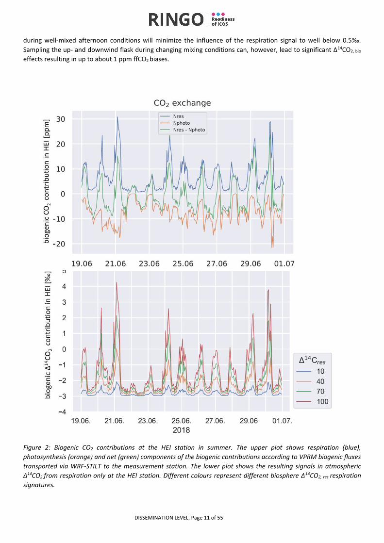
from different transport models. Figure 3 shows two estimates of the ∆14CO2, nuc contamination for a flask collected in
Heidelberg on March 1st, 2019, 18:00 based on a STILT and a WRF-STILT footprint. While the WRF-STILT footprint
results in ∆14CO2, nuc = 0.6‰, the STILT footprint predicts ∆14CO2, nuc = 8.2‰ for this specific hour.
DISSEMINATION LEVEL, Page 13 of 55
Figure 3: Footprints for one flask sampled in HEI on March, 1st, 2019, at 18:00h. The blue dots in each map show the
positions and the annual emission strengths of individual nuclear facilities as listed in the RADD inventory. The map on
the left shows a WRF-STILT footprint with a 72h backward trajectory. In the map on the right, the 240h backward
calculated footprint from HEI using STILT is shown.
The largest difference between the two models in this example is the duration of the backward calculated footprint.
While WRF-STILT used 72h, STILT used 240h. Adding to that, the two models differ in spatial resolution and the
meteorology used. In Fig. 3 also the annual nuclear 14CO2 emission flux Q14CO2 on a facility level is shown for the
European domain. The single largest 14CO2 source in Europe is the reprocessing plant La Hague in north-western
France. For all Rhine Valley and Paris flask samples the magnitude of the calculated ∆14CO2, nuc contamination largely
depends on the question if the reprocessing plant at La Hague had a significant contribution to the contamination
signal or not. This also explains why on average ∆14CO2, nuc contamination for Paris was smaller compared to the Rhine
Valley. The Paris RINGO setup sampled during wind directions from southwest to northeast or vice versa, whereas for
the Rhine Valley experiment we only sampled during north-westerly winds. Thus, the Rhine Valley, although further
distant is more sensitive to La Hague emissions than the Paris stations.
Figure 4 shows the comparison of ∆14CO2, nuc contaminations calculated with footprints from both models for 11
individual samples. The example discussed above (Fig. 3) is flask #5. Each ∆14CO2, nuc contamination is the average of
individual ∆14CO2, nuc contaminations at the hour as well as one hour before and after the actual sampling time, thus
accounting for a temporal uncertainty in the footprints. The uncertainties of the averaged ∆14CO2, nuc contaminations
in Fig. 4 are the standard deviations of the three individual ∆14CO2, nuc estimates. The samples were selected such that
they contain the highest and the lowest ∆14CO2, nuc contaminations predicted by STILT for Rhine Valley samples.
DISSEMINATION LEVEL, Page 14 of 55
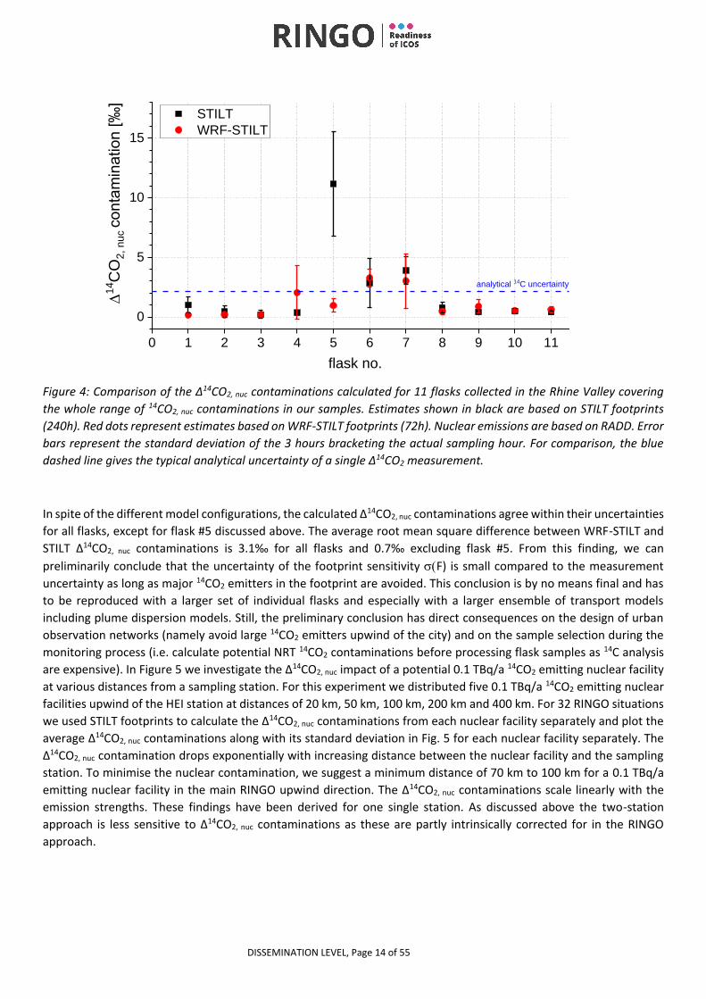
Figure 4: Comparison of the ∆14CO2, nuc contaminations calculated for 11 flasks collected in the Rhine Valley covering
the whole range of 14CO2, nuc contaminations in our samples. Estimates shown in black are based on STILT footprints
(240h). Red dots represent estimates based on WRF-STILT footprints (72h). Nuclear emissions are based on RADD. Error
bars represent the standard deviation of the 3 hours bracketing the actual sampling hour. For comparison, the blue
dashed line gives the typical analytical uncertainty of a single Δ14CO2 measurement.
In spite of the different model configurations, the calculated ∆14CO2, nuc contaminations agree within their uncertainties
for all flasks, except for flask #5 discussed above. The average root mean square difference between WRF-STILT and
STILT ∆14CO2, nuc contaminations is 3.1‰ for all flasks and 0.7‰ excluding flask #5. From this finding, we can
preliminarily conclude that the uncertainty of the footprint sensitivity (F) is small compared to the measurement
uncertainty as long as major 14CO2 emitters in the footprint are avoided. This conclusion is by no means final and has
to be reproduced with a larger set of individual flasks and especially with a larger ensemble of transport models
including plume dispersion models. Still, the preliminary conclusion has direct consequences on the design of urban
observation networks (namely avoid large 14CO2 emitters upwind of the city) and on the sample selection during the
monitoring process (i.e. calculate potential NRT 14CO2 contaminations before processing flask samples as 14C analysis
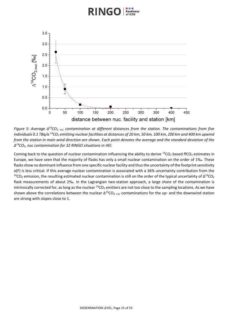
are expensive). In Figure 5 we investigate the ∆14CO2, nuc impact of a potential 0.1 TBq/a 14CO2 emitting nuclear facility
at various distances from a sampling station. For this experiment we distributed five 0.1 TBq/a 14CO2 emitting nuclear
facilities upwind of the HEI station at distances of 20 km, 50 km, 100 km, 200 km and 400 km. For 32 RINGO situations
we used STILT footprints to calculate the ∆14CO2, nuc contaminations from each nuclear facility separately and plot the
average ∆14CO2, nuc contaminations along with its standard deviation in Fig. 5 for each nuclear facility separately. The
∆14CO2, nuc contamination drops exponentially with increasing distance between the nuclear facility and the sampling
station. To minimise the nuclear contamination, we suggest a minimum distance of 70 km to 100 km for a 0.1 TBq/a
emitting nuclear facility in the main RINGO upwind direction. The ∆14CO2, nuc contaminations scale linearly with the
emission strengths. These findings have been derived for one single station. As discussed above the two-station
approach is less sensitive to ∆14CO2, nuc contaminations as these are partly intrinsically corrected for in the RINGO
approach.
0 1 2 3 4 5 6 7 8 9 10 11
0
5
10
15
STILT
WRF-STILT
1
4C
O2, nu
c c
onta
min
atio
n [
‰]
flask no.
analytical 14C uncertainty
DISSEMINATION LEVEL, Page 15 of 55
Figure 5: Average ∆14CO2, nuc contamination at different distances from the station. The contaminations from five
individuals 0.1 TBq/a 14CO2 emitting nuclear facilities at distances of 20 km, 50 km, 100 km, 200 km and 400 km upwind
from the station in main wind direction are shown. Each point denotes the average and the standard deviation of the
∆14CO2, nuc contamination for 32 RINGO situations in HEI.
Coming back to the question of nuclear contamination influencing the ability to derive 14CO2 based ffCO2 estimates in
Europe, we have seen that the majority of flasks has only a small nuclear contamination on the order of 1‰. These
flasks show no dominant influence from one specific nuclear facility and thus the uncertainty of the footprint sensitivity
σ(F) is less critical. If this average nuclear contamination is associated with a 36% uncertainty contribution from the 14CO2 emission, the resulting estimated nuclear contamination is still on the order of the typical uncertainty of Δ14CO2
flask measurements of about 2‰. In the Lagrangian two-station approach, a large share of the contamination is
intrinsically corrected for, as long as the nuclear 14CO2 emitters are not too close to the sampling locations. As we have
shown above the correlations between the nuclear ∆14CO2, nuc contaminations for the up- and the downwind station
are strong with slopes close to 1.
DISSEMINATION LEVEL, Page 16 of 55
2.5 Can upwind Δ14CO2 measurements be substituted by regional background Δ14CO2
observations? As the experimental 14C-based ffCO2 estimates rely on differential 14CO2 measurements (see Eq. 1) the Lagrangian up-
and downwind approach needs two 14CO2 measurements for one ffCO2 estimate. There is no doubt that the direct
upwind measurement is the most direct approximation of the background for urban scale measurements. In the last
section, we pointed out the strong advantage of the intrinsic correction for nuclear 14CO2 contaminations. However,
an important question regarding the sampling strategy is how much the uncertainty of the ΔffCO2 estimate increases
if the upwind 14CO2 measurement is substituted by a larger-scale regional background measurement. The benefit of
using a regional 14CO2 background would be that the number of downwind samples could be doubled at no additional
flask analysis costs. We assessed this question from an experimental as well as from a modelling perspective. The
modelling perspective is discussed in Sec 3.6.1.
To answer the background question from the experimental point of view, we replaced the upwind flasks by a regional
Δ14CO2 background and then investigated the resulting changes in the estimated ΔffCO2 and its uncertainty. For all
data, including the regional background measurements, we apply the nuclear ∆14CO2, nuc contamination corrections.
Due to lacking heterotrophic respiration model results for the entire observation period we could not apply individual
corrections for the respiration 14CO2 contribution. The regional background estimates are harmonic fits to 2-week
integrated Δ14CO2 measurements from regional background stations. We used Trainou station and Schauinsland
station as regional backgrounds for Paris and the Rhine Valley, respectively. Trainou station is a tall tower about 100
km south of Paris. A detailed description of Trainou tower station is given in Schmidt et al. (2014). At Trainou,
integrated 14CO2 samples are collected from a height of 180 m above local ground. The Schauinsland station is located
approximately 180 km south of the Mannheim/Ludwigshafen area and at 1205 m a.s.l. at the border of the Rhine
Valley in the Black Forest. The Schauinsland station is characterised e.g. in Levin et al. (1995). During winter
Schauinsland is often located above the Rhine Valley inversion, whereas during summer, emissions from the Rhine
Valley frequently reach the station, particularly during the day.
Figure 6 shows the nuclear corrected Δ14CO2 measurements for Paris as well as for the Rhine Valley. The nuclear
corrected regional background measurements and a harmonic fit according to Nakazawa et al. (1997) through the
background data are included in both plots. For TRN station the available 2-week integrated measurements end in
autumn 2019 thus the fit had to be extrapolated based on its slope and seasonality in the years before. For both target
areas, the nuclear corrected up- and downwind measurements from the RINGO flasks are given in green and blue,
respectively. The open grey symbols in Figure 6 show the original uncorrected flask results. For the majority of the
flasks the nuclear ∆14CO2, nuc correction is only small (cf. Fig. 4) and thus not visible. The observational period is roughly
divided into a “growing” (May to October) and a “dormant” (November to April) season.
We estimate the additional uncertainty of using a regional background instead of upwind samples by the standard
deviation of upwind flask results from the regional background curve. Table 2 lists the median difference and the
standard deviation of the differences for both stations, separately for the growing and the dormant season. The
median difference is positive at both sites and seasons, i.e. the upwind flasks are higher in Δ14CO2 and thus contain
less ffCO2 compared to the regional background. Generally, this is not surprising as the 2-week integrated background
measurements are not selected for clean air conditions and thus comprise the averaged fossil fuel signal at these
stations. Levin et al. (2008) showed that Schauinsland exhibits a ffCO2 enhancement with respect to the continental
background at Jungfraujoch of about 1 ppm during summer and twice as much during winter because Rhine valley air
is much more polluted with ffCO2 during winter than in summer (Levin et al., 2003; 2011). However, it is difficult to
understand why the upwind flasks deviate more from the regional background during the growing than during the
dormant season. One reason could be a stronger respiration Δ14CO2 enrichment in the flask samples during the growing
than during the dormant season (see Sec. 2.4. and Fig. 2). However, as the majority of flask samples was taken during
afternoon hours, their respiratory 14CO2 effect will probably be lower compared to that of the 2-week integrated
samples at the regional background stations, which integrate over the entire diurnal cycle and thus contain more night-
time respiration CO2. The origin of the larger deviations during the growing season compared to the dormant season
thus currently remains an open question and must be revisited once a larger number of samples from the growing
season are available.
DISSEMINATION LEVEL, Page 17 of 55
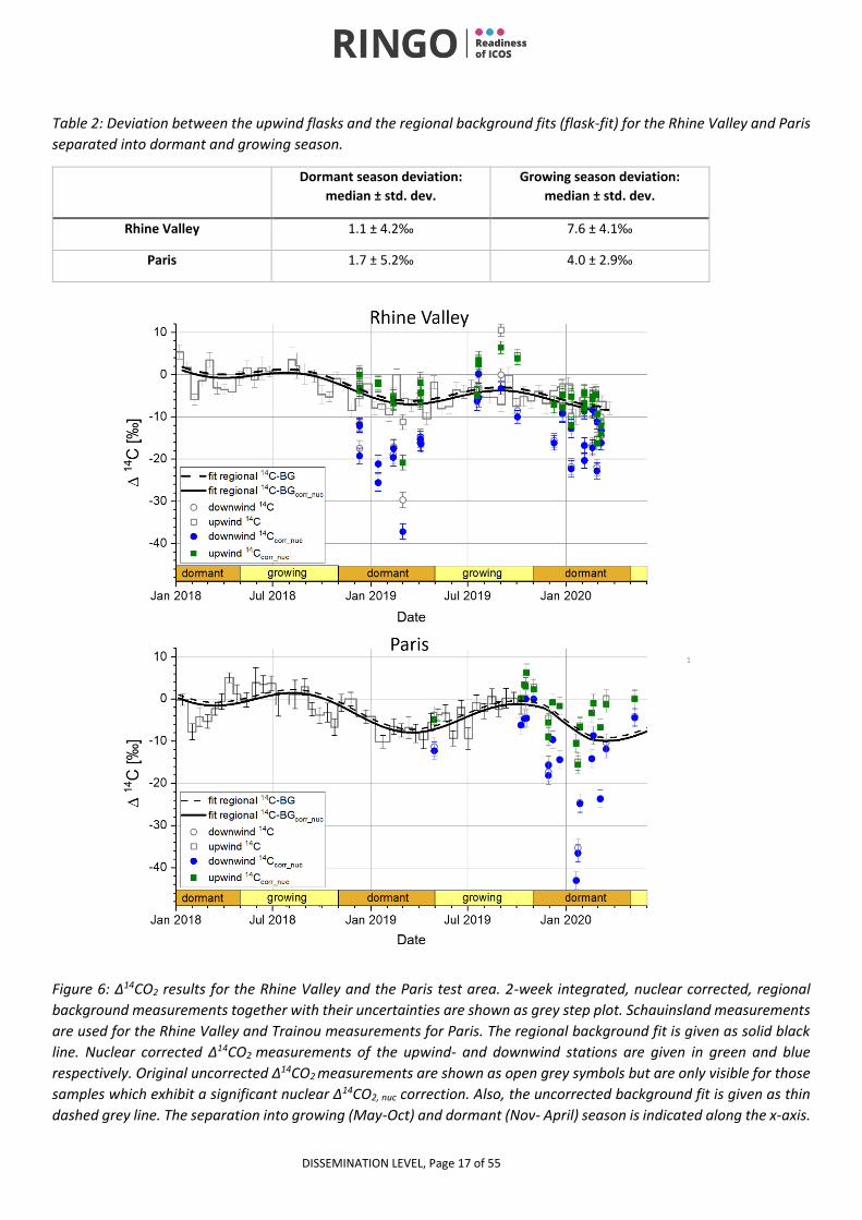
Table 2: Deviation between the upwind flasks and the regional background fits (flask-fit) for the Rhine Valley and Paris
separated into dormant and growing season.
Dormant season deviation:
median ± std. dev.
Growing season deviation:
median ± std. dev.
Rhine Valley 1.1 ± 4.2‰ 7.6 ± 4.1‰
Paris 1.7 ± 5.2‰ 4.0 ± 2.9‰
Figure 6: Δ14CO2 results for the Rhine Valley and the Paris test area. 2-week integrated, nuclear corrected, regional
background measurements together with their uncertainties are shown as grey step plot. Schauinsland measurements
are used for the Rhine Valley and Trainou measurements for Paris. The regional background fit is given as solid black
line. Nuclear corrected Δ14CO2 measurements of the upwind- and downwind stations are given in green and blue
respectively. Original uncorrected Δ14CO2 measurements are shown as open grey symbols but are only visible for those
samples which exhibit a significant nuclear Δ14CO2, nuc correction. Also, the uncorrected background fit is given as thin
dashed grey line. The separation into growing (May-Oct) and dormant (Nov- April) season is indicated along the x-axis.

DISSEMINATION LEVEL, Page 18 of 55
If we concentrate on the additional uncertainty when substituting the upwind flasks by a regional background, we
have to compare the uncertainty budgets of the different 14C-based ΔffCO2 approaches. Table 3 compiles the
uncertainty budgets for both background realisations. Hereafter, we will first motivate the uncertainty assumptions
for the Lagrangian up-/downwind approach followed by the uncertainty budget for the regional background approach.
In the Lagrangian approach, the uncertainty of the background Δ14CO2 estimate is given by the long-term
reproducibility of the 14CO2 flask measurements. In section 2.4, we further elaborated on the advantage of the
Lagrangian approach to intrinsically correct for the nuclear contaminations. We thus estimate that the remaining
model uncertainty σ(F) in the RINGO approach is half of the total nuclear correction of each flask. In addition, we do
not account for the uncertainty in the nuclear emission strength as this would affect the up- and the downwind
measurement in the same way. The respiration Δ14CO2, bio effect depends on the times of sampling of the flask pair. If
the flasks are samples during changing mixing conditions e.g. during the disintegration of the nocturnal boundary
layer, the respiration effect can be as large as 3‰. Sampling during well mixed afternoon conditions will result in a
Δ14CO2, bio effect of less than 0.5‰.
The largest difference in the uncertainty budget of the regional background approach compared to the RINGO
approach arises from the uncertainty of the background estimate itself. The spread of the upwind flasks around the
regional background fit is between 4‰ and 5‰ for the dormant season in the Rhine Valley and also in Paris (Table 2).
As the 2-week integrated samples incorporate the averaged Δ14CO2, bio effect. The difference in the Δ14CO2, bio effect
between the regional background and the individual downwind sample depends thus on the sampling time of the
flask. During well-mixed afternoon conditions the difference will be on the order of -1‰ whereas it can be also around
+2‰ for samplings during inversion periods. In principle the Δ14CO2, bio effect can be corrected similarly to the nuclear
contamination if the respiration contribution at the measurement station is known from model estimates (cf. Fig. 2).
Thus, we assume an additional uncertainty contribution of 0.5‰ here for the respiration effect, which is 50% of the
total respiration effect during well mixed conditions.
The uncertainty of the nuclear correction with the regional background is assessed in two parts. The uncertainty
related to the transport errors is assessed via the difference between the two transport models as shown in Fig. 4. The
average difference between the two modelled nuclear corrections is 4‰ if all samples are taken into account but
reduces to 1‰ if only samples are considered where the nuclear correction of both models agree within their
uncertainties. This implies that the nuclear correction is routinely calculated using two different transport models,
allowing to assess the transport model uncertainty. For the 11 flask samples where we compared two different
transport models only the nuclear correction for one flask, which was directly influenced by La Hague in one model,
did not agree between the models. The second nuclear correction uncertainty contribution is related to the varying 14CO2 emission strength. On a monthly basis the variability was shown to be on average 36% based on the monthly 14CO2 emission data taken from Kuderer et al. (2018). Thus we assume the emission strength uncertainty to be 36% of
the average nuclear correction.
Coming back to the question of nuclear contamination influencing the ability to derive 14CO2 based ffCO2 estimates,
we have seen that the majority of flasks has only a small nuclear contamination on the order of 1‰. These flasks show
no dominant influence from one specific nuclear facility and thus the uncertainty of the footprint sensitivity σ(F) is less
critical. If this average nuclear contamination is associated with a 36% uncertainty contribution from the 14CO2
emission, the resulting estimated nuclear contamination is on the order of the typical uncertainty of Δ14CO2 flask
measurements of about 2‰. In the Lagrangian two-station approach, a large share of the contamination is intrinsically
corrected for, as long as the nuclear 14CO2 emitters are not too close to the sampling locations. As we have shown
above the correlations between the nuclear ∆14CO2, nuc contaminations for the up- and the downwind station are strong
with slopes close to 1.
Besides the uncertainties we also investigated a potential bias of the ΔffCO2 estimates between the two background
approaches. The ΔffCO2 estimates during the dormant seasons for Paris and the Rhine Valley can be seen in Fig. 7 for
both background approaches. While for the Rhine Valley (black) no systematic average bias is found we observe that
for Paris the regional background approach underestimates low ΔffCO2 concentrations systematically.
DISSEMINATION LEVEL, Page 19 of 55
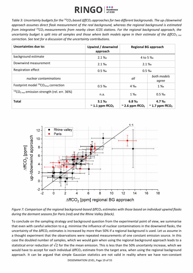
Table 3: Uncertainty budgets for the 14CO2-based ΔffCO2 approaches for two different backgrounds. The up-/downwind
approach assumes direct flask measurement of the real background, whereas the regional background is estimated
from integrated 14CO2 measurements from nearby clean ICOS stations. For the regional background approach, the
uncertainty budget is split into all samples and those where both models agree in their estimate of the ΔffCO2, nuc
correction. See text for a discussion of the uncertainty contributions.
Uncertainties due to: Upwind / downwind approach
Regional BG approach
background estimate 2.1 ‰ 4 to 5 ‰
Downwind measurement 2.1 ‰ 2.1 ‰
Respiration effect 0.5 ‰ 0.5 ‰
nuclear contaminations all both models
agree
Footprint model 14CO2nuc correction 0.5 ‰ 4 ‰ 1 ‰ 14CO2 nuc emission strength (rel. err. 36%)
n.a. 1 ‰ 0.5 ‰
Total 3.1 ‰ ~ 1.1 ppm ffCO2
6.8 ‰ ~ 2.6 ppm ffCO2
4.7 ‰ ~ 1.7 ppm ffCO2
Figure 7: Comparison of the regional background-based ΔffCO2 estimates with those based on individual upwind flasks
during the dormant seasons for Paris (red) and the Rhine Valley (black).
To conclude on the sampling strategy and background question from the experimental point of view, we summarise
that even with careful selection to e.g. minimise the influence of nuclear contaminations in the downwind flasks, the
uncertainty of the ΔffCO2 estimates is increased by more than 50% if a regional background is used. Let us assume in
a thought experiment that the observations were repeated measurements of one constant emission source. In this
case the doubled number of samples, which we would gain when using the regional background approach leads to a
statistical error reduction of √2 for the the mean emission. This is less than the 50% uncertainty increase, which we
would have to accept for each individual ΔffCO2 estimate from the target area, when using the regional background
approach. It can be argued that simple Gaussian statistics are not valid in reality where we have non-constant
DISSEMINATION LEVEL, Page 20 of 55
emissions. If, however, the regional background approach does not offer any advantage in the simplest case, it is more
than questionable how to achieve an advantage in the more complex reality. From an experimental point of view, we,
therefore, conclude that the ffCO2 concentration enhancements are anyhow small and further deterioration of the
uncertainty is thus not advisable. We will revisit this question in chapter 3.6.1 from the modelling point of view.
2.6 Which share of the observed ΔCO2 concentration gradient across a target area is of fossil
origin? The main motivation for conducting 14CO2 measurements across a target area is to investigate which part of the total
ΔCO2 concentration difference between the upwind and the downwind station is of fossil origin.
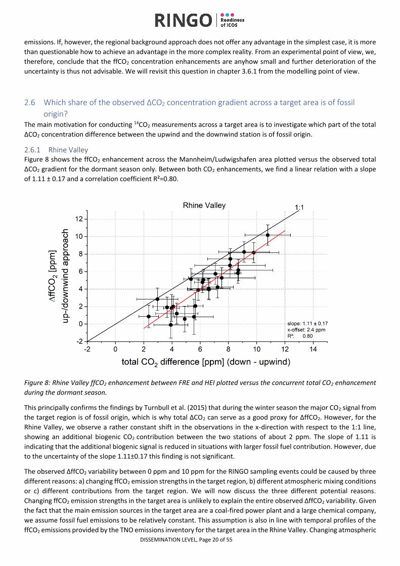
2.6.1 Rhine Valley Figure 8 shows the ffCO2 enhancement across the Mannheim/Ludwigshafen area plotted versus the observed total
ΔCO2 gradient for the dormant season only. Between both CO2 enhancements, we find a linear relation with a slope
of 1.11 ± 0.17 and a correlation coefficient R²=0.80.
Figure 8: Rhine Valley ffCO2 enhancement between FRE and HEI plotted versus the concurrent total CO2 enhancement
during the dormant season.
This principally confirms the findings by Turnbull et al. (2015) that during the winter season the major CO2 signal from
the target region is of fossil origin, which is why total ΔCO2 can serve as a good proxy for ΔffCO2. However, for the
Rhine Valley, we observe a rather constant shift in the observations in the x-direction with respect to the 1:1 line,
showing an additional biogenic CO2 contribution between the two stations of about 2 ppm. The slope of 1.11 is
indicating that the additional biogenic signal is reduced in situations with larger fossil fuel contribution. However, due
to the uncertainty of the slope 1.11±0.17 this finding is not significant.
The observed ΔffCO2 variability between 0 ppm and 10 ppm for the RINGO sampling events could be caused by three
different reasons: a) changing ffCO2 emission strengths in the target region, b) different atmospheric mixing conditions
or c) different contributions from the target region. We will now discuss the three different potential reasons.
Changing ffCO2 emission strengths in the target area is unlikely to explain the entire observed ΔffCO2 variability. Given
the fact that the main emission sources in the target area are a coal-fired power plant and a large chemical company,
we assume fossil fuel emissions to be relatively constant. This assumption is also in line with temporal profiles of the
ffCO2 emissions provided by the TNO emissions inventory for the target area in the Rhine Valley. Changing atmospheric
DISSEMINATION LEVEL, Page 21 of 55
mixing conditions especially varying boundary layer heights are known to be a major driver of changing atmospheric
concentrations in the boundary layer. In the example of Paris discussed below (Sec. 2.6.2), changing vertical mixing is
actually the dominant cause of the ΔffCO2 variations. However, this is not the case for the Rhine Valley, since based
on the 222Rn activity concentration measurements during the RINGO events we conclude that the vertical mixing has
been stable and rather comparable between the different RINGO events. The mean Δ222Rn difference between the
down- and upwind sampling for all sampling events is -0.1±0.6 Bq/m³. The sampling criteria ensured that all samplings
were conducted during atmospheric situations with rather low absolute 222Rn activity concentrations (between 0.5
and 1.8 Bq/m³) typical for well-mixed conditions. Thus, for the observations performed in the Rhine Valley we exclude
changing vertical mixing as main driver for the observed ΔffCO2 variability. Lastly we discuss different contributions
from the emission area as third potential reason for the variation. Although the trajectory-based sampling approach
assures that up- and downwind station are on one trajectory, it does not ensure comparable contributions from the
target region’s fossil fuel emissions for each trajectory. Visual inspection of all trajectories confirmed that events with
low ΔffCO2 have only streaked the target region due to the curvature of the trajectory. In contrast, for high ΔffCO2
events the trajectories passed over the centre of the emission area. This explains the observed variability in the ΔffCO2
signal best.
Observing an additional biogenic CO2 offset of about 2 ppm at the downwind compared to the upwind station is
surprising. Therefore, we will now discuss an idealised thought-model for biogenic CO2 enhancements in the
Lagrangian approach and the consequences on ΔCO2 if we deviate from the idealised assumptions. The simplest
thought model assumes the biogenic sources are homogeneously distributed in space and time. Assuming constant
atmospheric mixing conditions in addition, results in uniform biogenic CO2 contributions at both (all) stations and thus
a vanishing biogenic ΔCO2 signal between two stations in the differential RINGO approach. One by one we will now
discuss the simplifying assumptions and the consequences for biogenic ΔCO2 if we drop them. When dropping the
spatial homogeneity condition, we need to compare the different biogenic fluxes in the catchment areas of the two
stations. The upwind catchment area of the FRE station is dominated by multi-year vegetation mainly vineyards and
forest and only little changing agriculture. The biogenic sources upwind of HEI station, and thus between FRE and HEI,
are dominated by changing agriculture. During the dormant season, the NEE of multi-year forests (including soil
respiration) is positive and larger than the NEE for agricultural land, which is close to zero for a region in Germany with
a similar climate (Anthoni et al., 2004). From this, we would conclude that during the dormant season, the biogenic
source strength is larger in the catchment area of FRE compared to HEI. A further effect is the sealing of natural
surfaces in the urban target area, resulting in lower NEE fluxes in the catchment area of HEI as well. Thus, dropping
the spatial homogeneity condition increases the biogenic CO2 contribution at FRE and thus results in negative biogenic
ΔCO2 differences in contradiction to what is observed. Secondly, we discuss the assumption of the temporal
homogeneity of biogenic fluxes. Kneuer (2020) calculated a mean diurnal cycle for biogenic CO2 contributions at HEI
station based on VPRM and STILT model results for a 10 days’ period in the dormant season. The mean diurnal cycle
shows the largest biogenic CO2 contribution of 6 ppm at 03:00h and a minimum of 4 ppm at noon, resulting in a
temporal change of the biogenic CO2 contribution of 0.2 ppm/h. Assuming a similar biogenic diurnal cycle at both
stations, we estimate the biogenic ΔCO2 difference caused by temporally changing fluxes to be less than 0.4 ppm if we
apply the average travelling time of 1.7 hours for air masses between FRE and HEI. Besides that, although the majority
of sampling events has been taken during the afternoon, some samples were collected during mornings with an
opposite effect of the diurnal cycle on the biogenic ΔCO2 differences. The observations show however a very consistent
positive bias of the biogenic contribution at the HEI station. Finally, we discuss the effects when dropping the
assumption of constant mixing conditions. We divide this discussion into the one of reduced and the one of increased
mixing while the air mass travels across the target area. Increased mixing leads to a smaller biogenic CO2 contribution
in HEI compared to FRE, resulting in a negative biogenic ΔCO2 difference. Reduced mixing, however, leads to a larger
biogenic CO2 contribution in HEI compared to FRE, resulting in a positive biogenic ΔCO2 difference. However, as
discussed in the previous paragraph, the mean Δ222Rn difference of -0.1±0.6 Bq/m³ indicates that there have been no
large changes in the mixing conditions during the sampling events. The almost constant biogenic CO2 offset of 2 ppm
is therefore currently not understood, i.e. as long as we cannot identify an additional more or less constant non-fossil
CO2 source in the Heidelberg catchment compared to the Freinsheim catchment.
DISSEMINATION LEVEL, Page 22 of 55
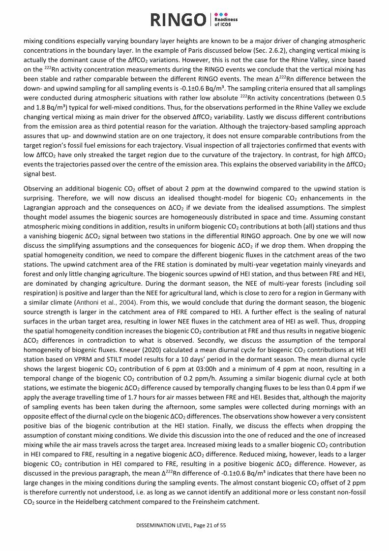
2.6.2 Paris Figure 9 shows the relation between total ΔCO2 and ΔffCO2 for Paris during the dormant season. The linear regression
yields a slope of 0.98 ± 0.05 and a correlation of R²=0.96. Similar as for the Rhine Valley we also find a (biogenic?) ΔCO2
offset of about 2 ppm for the Paris region. The observed ΔffCO2 range, between about 3 and 61 ppm, is much larger
compared to the Rhine Valley. ffCO2 enhancements larger than 10ppm have been derived from sampling events during
evenings and nights. Unfortunately, the Rn-based selection and data-screening process works less efficient in Paris
compared to the Rhine Valley. This has two reasons: first 222Rn observations are only available at SAC and not at both
stations. Second, 222Rn is measured at 100 m above local ground, lowering its sensitivity to changes in vertical mixing.
Assessing the vertical atmospheric stability from CO2 profile measurements would have been a good alternative,
however, only for a very small subset of the observations the profile information was available. Therefore, much of
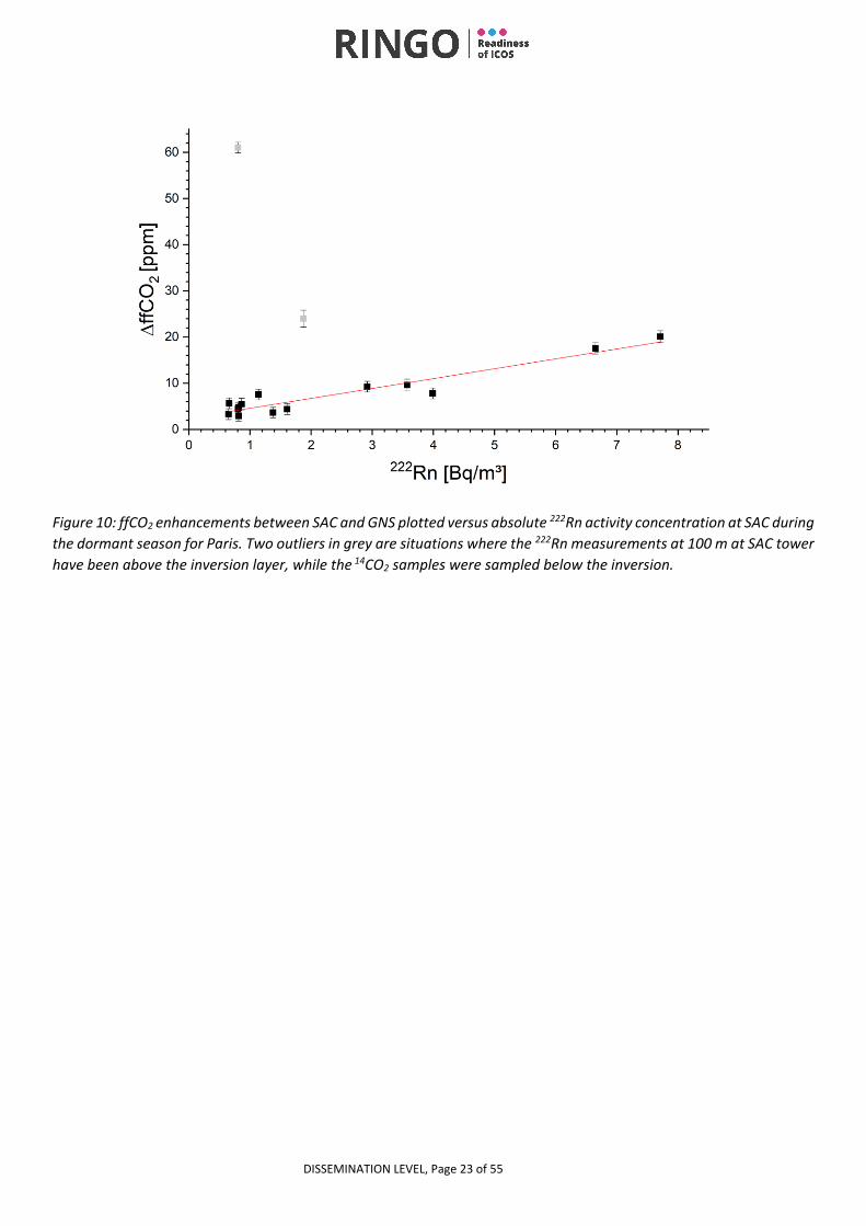
the ΔffCO2 variability for Paris is caused by differences in atmospheric mixing conditions. Fig. 10 shows a linear relation
between the ffCO2 enhancement between SAC and GNS and the absolute 222Rn activity concertation at SAC. The two
outliers, with high ΔffCO2 but low 222Rn concentrations, were sampled during situations where the 222Rn observations
at 100 m in SAC were above the inversion layer. For one outlier 14CO2 was sampled in GNS at 60 m height while for the
other outlier 14CO2 was sampled at 60 m height at SAC. Note that, in the first month the 14CO2 sampling at SAC was
connected to the 60 m instead of 100 m level.
The almost 1:1 relationship between total and fossil CO2 enhancements is striking and underpins the dominance of
fossil emission sources during the dormant season in the Paris target region. Although, our conclusions on atmospheric
mixing conditions in Paris are less accurate due to the less sensitive 222Rn data at 100 m height and fewer 222Rn data
availability in general, nearly all sampling events show an almost constant positive non-fossil ΔCO2 offset, similar to
the Rhine Valley. From the fit, we conclude that this offset is about 2 ppm, which is also accidentally in line with the
finding from the Rhine Valley. It ought however to be said, that the linear regression is largely determined by the
highest fossil CO2 enhancement of 61 ppm. As for the Rhine Valley, we do not understand the origin of this non-fossil
ΔCO2 offset.
Returning to the initial question of how large the fossil share of the total ΔCO2 offset between two stations, up- and
downwind of a fossil CO2 emission area is and considering the results from both cities, we can conclude that for the
dormant season there is nearly a 1:1 relationship between the fossil and the total CO2 enhancements. Both cities show,
however, a nearly constant additional non-fossil offset in the order of 2 ppm, which needs to be further studied. The
growing season was not investigated due to limited data availability.
Figure 9: Paris ffCO2 enhancement plotted versus the concurrent total ΔCO2 enhancement during the dormant season.
DISSEMINATION LEVEL, Page 23 of 55
Figure 10: ffCO2 enhancements between SAC and GNS plotted versus absolute 222Rn activity concentration at SAC during
the dormant season for Paris. Two outliers in grey are situations where the 222Rn measurements at 100 m at SAC tower
have been above the inversion layer, while the 14CO2 samples were sampled below the inversion.
DISSEMINATION LEVEL, Page 24 of 55
3 RESULTS FROM THE OBSERVING SYSTEM SIMULATION EXPERIMENT
To address the question whether a pre-set number of 14CO2 samples in an ICOS network would better constrain
individual national fossil fuel emissions of Central European countries, or an alternative network with the same
number of samples collected closer to emission hotspots (RINGO network), an Observing System Simulation
Experiment (OSSE) was conducted. In this experiment, we also aim at investigating if it is better to sample twice the
number of downwind flasks or rather use the RINGO approach and collect explicit up- and downwind flask pairs.
Additionally, we perform sensitivity runs with and without using information of the two-week integrated 14CO2 samples
routinely collected at ICOS Class 1 stations to investigate their impact on the national fossil fuel estimates. To test to
what extent the OSSE results are model-dependent, we applied two fundamentally different inverse modelling
frameworks operated by two modelling groups, one from the Climate and Environment Sciences Laboratory (LSCE) in
France and the other from Wageningen University (WU) in the Netherlands.
First we describe the objectives of the OSSE and introduce the chosen model simplifications based on these objectives.
We define different sampling strategies, which have been tested in the ICOS and the RINGO sampling networks, as
well as the spatial and temporal domains of the modelling experiment. In Sec. 3.2 both models are introduced and the
‘true’ fluxes, which served as input in the so-called forward run to calculate the atmospheric concentrations at the
stations from which the ‘observed’ data are selected for the inversions are described. Further we discuss if these
(modelled) CO2 concentrations and their variability are compatible with real ambient CO2 concentrations. Sec 3.2 is
concluded by a description how virtual measurements were selected in the forward runs station time series. Sec. 3.3.
introduces the technical details of the inversion setups and describes the different inversion approaches of the two
models. The construction of the prior emission fluxes is given in this section as well. The results of the entire OSSE are
presented and discussed in Sec. 3.4, followed by a critical review of deficits in the OSSE design in Sec. 3.5. Finally, in
Sec. 3.6 we summarize the answers from the OSSE to the two overarching questions raised in the introduction: “Which
network design quantifies national fossil fuel emissions better?” and “Does twice the number of samples collected
downwind of a city contain more information than the dedicated RINGO flask pairs?”
3.1 Objectives and design of the OSSE This subsection outlines the objectives and the scope of the OSSE and introduces the different sampling scenarios
being tested. We explain the station selection process for the ICOS and the RINGO observation networks and define
the geographical and temporal boundaries of the OSSE.
3.1.1 Objectives of the OSSE and resulting model simplifications The OSSE was designed to address one specific question, namely how different sampling networks, e.g. the existing
ICOS network or, alternatively, the (partly) hypothetical RINGO network impact the ability of inverse models to
constrain national total ffCO2 emissions of Central European countries in the model domain (Fig. 11) using radiocarbon
measurements. The OSSE design thus strives to include all relevant processes, which alter atmospheric 14CO2 levels
but, at the same time, omits other well-known issues, which have to be addressed when performing inversions with
actual observation data. Table 4 summarizes these specific configurations of the OSSE. The main idealisation in the
OSSE was that initially we assume the models represent the atmospheric transport perfectly, which is not the case in
reality. The thought behind this simplification was to exclusively investigate differences between the sampling
strategies rather than diluting or overlaying results with uncertainties arising from imperfect model transport.
However, in Sec. 3.3.3 we explain that for the inversions we had to abandon this idea and introduce an artificial model
transport error. Without this artificial model transport error, the inversion algorithms could have retrieved the ‘true’
CO2 flux distribution too easily, i.e. without even needing to make use of the information contained in the 14CO2
measurements.
To model the non-fossil fuel contributions of the 14CO2 budget we included 14CO2 emissions from nuclear facilities and 14CO2 emissions from CO2 respiration fluxes. We partitioned the biogenic CO2 fluxes into net primary productivity (NPP)
and heterotrophic respiration (HR), thus, allowing to account explicitly for the 14CO2 respiration signal. The OSSE
DISSEMINATION LEVEL, Page 25 of 55
omitted stratosphere-troposphere exchange since for short time scales (months) it is not relevant for the 14CO2 budget
and does not affect the OSSE’s ability to benchmark the different sampling networks and strategies.
Table 4: Specific processes included or omitted in the OSSE design:
Processes incorporated Processes omitted in the OSSE
• Nuclear fluxes of 14CO2 • Stratosphere/troposphere exchange
• Observation errors • Dynamic background concentration
• Artificial transport errors • Ocean fluxes
• Dynamic ffCO2 emissions (WU)
• Static ffCO2 emissions (LSCE)
• Representation error
• Sector dependent emission uncertainties • Plume transport
• Partitioning of biogenic CO2 fluxes (net primary productivity and heterotrophic respiration)
3.1.2 Sampling networks and strategies to be tested in the OSSE In the following, we define the different sets of stations and sampling strategies, which will be investigated in the
OSSE. The ‘ICOS network’ is comprised of 10 (LSCE) or 9 (WU) ICOS atmosphere stations plus the Heidelberg ICOS-CRL
pilot station. The alternative sampling network, further on called ‘RINGO network’ comprises 10 (LSCE) or 8 (WU)
sampling station pairs close to European urban emission areas. The different number of stations used by the two
models is due to the slightly different model domains. Since one explicit aim of Task 1.2 was to investigate the added
value of integrated two-week 14CO2 samples collected in the ICOS network, we also varied the sampling methods
applied in the two networks. The two different sampling methods, which are both applied in ICOS, are flask and
integrated samples. A flask sample represents a one-hour mean Δ14CO2 value at a station, whereas the integrated
sample represents a two-week integrated (day and night) Δ14CO2 value. Table 5 lists for each network the sampling
strategies, which were tested in the OSSE and which are outlined in the following in more detail. To allow better
comparability among the networks we use the same number of stations or urban emission areas in the different
scenarios. The number of flask samples for each station or urban emission area is restricted the 26 flask samples per
station and year, foreseen in the current ICOS 14CO2 sampling strategy, but for the OSSE we assumed that all flask
samples are collected in the four core winter months (NDJF) only. Thus, we use only 12 flask samples per station during
the OSSE time period of two months. Only configuration 1c) omits this restriction to explore the effects of a 3-fold
increased 14CO2 sample number per station.
Table 5: Sampling networks and strategies which were tested in the OSSE.
1) ICOS network (reference)
# Flask sampling Integrated sampling
1a 6 targeted flasks/month 2 integrated samples/month
1b 6 targeted flasks/month None
1c 18 targeted flasks/month 2 integrated samples/month
2) RINGO network (alternative)
# Flask sampling Integrated sampling
2a 3 up and downwind pairs/month None
2b 6 downwind flasks/month None
2c 6 downwind flasks/month 2 integrated samples/month at ICOS sites
Strategy 1a) reflects the currently applied ICOS 14CO2 sampling strategy (Levin et al., 2020) where 6 targeted flasks are
sampled per station and month in addition to the 2-week integrated samples per station. Within ICOS, target flask
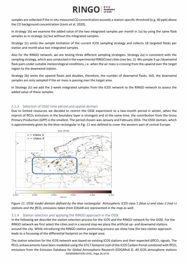
DISSEMINATION LEVEL, Page 26 of 55
samples are collected if the in-situ measured CO concentration exceeds a station-specific threshold (e.g. 40 ppb) above
the CO background concentration (Levin et al. 2020).
In strategy 1b) we examine the added value of the two integrated samples per month in 1a) by using the same flask
samples as in strategy 1a) but without the integrated samples.
Strategy 1c) omits the sample limitation of the current ICOS sampling strategy and collects 18 targeted flasks per
station and month plus two integrated samples.
Also for the RINGO network, we are testing three different sampling strategies. Strategy 2a) is consistent with the
sampling strategy, which was conducted in the experimental RINGO test cities (see Sec. 2). We sample 3 up-/downwind
flask pairs under suitable meteorological conditions, i.e. when the air mass is crossing from the upwind over the target
region to the downwind station.
Strategy 2b) omits the upwind flasks and doubles, therefore, the number of downwind flasks. Still, the downwind
samples are only sampled if the air mass is passing over the target area.
In Strategy 2c) we add the 2-week integrated samples from the ICOS network to the RINGO network to assess the
added value of these samples.
3.1.3 Selection of OSSE time period and spatial domain Due to limited resources we decided to restrict the OSSE experiment to a two-month period in winter, when the
imprint of ffCO2 emissions in the boundary layer is strongest and at the same time, the contribution from the Gross
Primary Production (GPP) is the smallest. The period chosen was January and February 2016. The OSSE domain, which
is approximately given by the blue rectangular in Fig. 11 was defined to cover the western part of central Europe.
Figure 11: OSSE model domain defined by the blue rectangular. Atmospheric ICOS class 1 (blue x) and class 2 (red +)
stations and the ffCO2 emissions taken from EDGAR are represented in the map as well.
3.1.4 Station selection and applying the RINGO approach in the OSSE In the following we describe the station selection process for the ICOS and the RINGO network for the OSSE. For the
RINGO network we first select the cities and in a second step we place the artificial up- and downwind stations
around the city. While introducing the RINGO station positioning process we show how the two-station approach
leads to a focussing of the differential footprint on the target area.
The station selection for the ICOS network was based on existing ICOS stations and their expected ΔffCO2 signals. The
ffCO2 enhancements have been modelled using the STILT footprint tool of the ICOS Carbon Portal combined with ffCO2
emissions from the Emission Database for Global Atmospheric Research (EDGARv4.3). All ICOS atmosphere stations
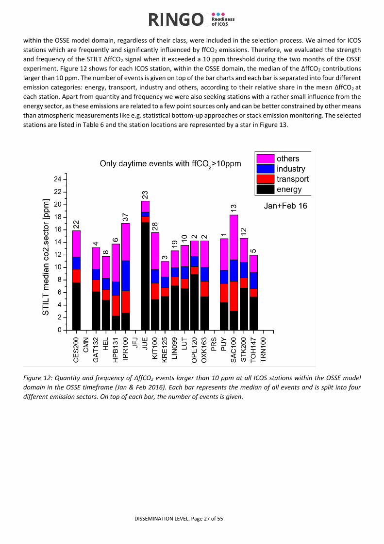
DISSEMINATION LEVEL, Page 27 of 55
within the OSSE model domain, regardless of their class, were included in the selection process. We aimed for ICOS
stations which are frequently and significantly influenced by ffCO2 emissions. Therefore, we evaluated the strength
and frequency of the STILT ΔffCO2 signal when it exceeded a 10 ppm threshold during the two months of the OSSE
experiment. Figure 12 shows for each ICOS station, within the OSSE domain, the median of the ΔffCO2 contributions
larger than 10 ppm. The number of events is given on top of the bar charts and each bar is separated into four different
emission categories: energy, transport, industry and others, according to their relative share in the mean ΔffCO2 at
each station. Apart from quantity and frequency we were also seeking stations with a rather small influence from the
energy sector, as these emissions are related to a few point sources only and can be better constrained by other means
than atmospheric measurements like e.g. statistical bottom-up approaches or stack emission monitoring. The selected
stations are listed in Table 6 and the station locations are represented by a star in Figure 13.
Figure 12: Quantity and frequency of ΔffCO2 events larger than 10 ppm at all ICOS stations within the OSSE model
domain in the OSSE timeframe (Jan & Feb 2016). Each bar represents the median of all events and is split into four
different emission sectors. On top of each bar, the number of events is given.
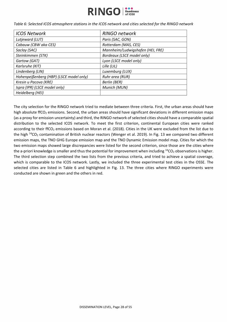
DISSEMINATION LEVEL, Page 28 of 55
Table 6: Selected ICOS atmosphere stations in the ICOS network and cities selected for the RINGO network
ICOS Network RINGO network Lutjeward (LUT) Paris (SAC, GON)
Cabauw (CBW aka CES) Rotterdam (MAS, CES)
Saclay (SAC) Mannheim/Ludwigshafen (HEI, FRE)
Steinkimmen (STK) Bordeaux (LSCE model only)
Gartow (GAT) Lyon (LSCE model only)
Karlsruhe (KIT) Lille (LIL)
Lindenberg (LIN) Luxemburg (LUX)
Hohenpeißenberg (HBP) (LSCE model only) Ruhr area (RUR)
Kresin u Pacova (KRE) Berlin (BER)
Ispra (IPR) (LSCE model only) Munich (MUN)
Heidelberg (HEI)
The city selection for the RINGO network tried to mediate between three criteria. First, the urban areas should have
high absolute ffCO2 emissions. Second, the urban areas should have significant deviations in different emission maps
(as a proxy for emission uncertainty) and third, the RINGO network of selected cities should have a comparable spatial
distribution to the selected ICOS network. To meet the first criterion, continental European cities were ranked
according to their ffCO2 emissions based on Moran et al. (2018). Cities in the UK were excluded from the list due to
the high 14CO2 contamination of British nuclear reactors (Wenger et al. 2019). In Fig. 13 we compared two different
emission maps, the TNO GHG Europe emission map and the TNO Dynamic Emission model map. Cities for which the
two emission maps showed large discrepancies were listed for the second criterion, since those are the cities where
the a-priori knowledge is smaller and thus the potential for improvement when including 14CO2 observations is higher.
The third selection step combined the two lists from the previous criteria, and tried to achieve a spatial coverage,
which is comparable to the ICOS network. Lastly, we included the three experimental test cities in the OSSE. The
selected cities are listed in Table 6 and highlighted in Fig. 13. The three cities where RINGO experiments were
conducted are shown in green and the others in red.
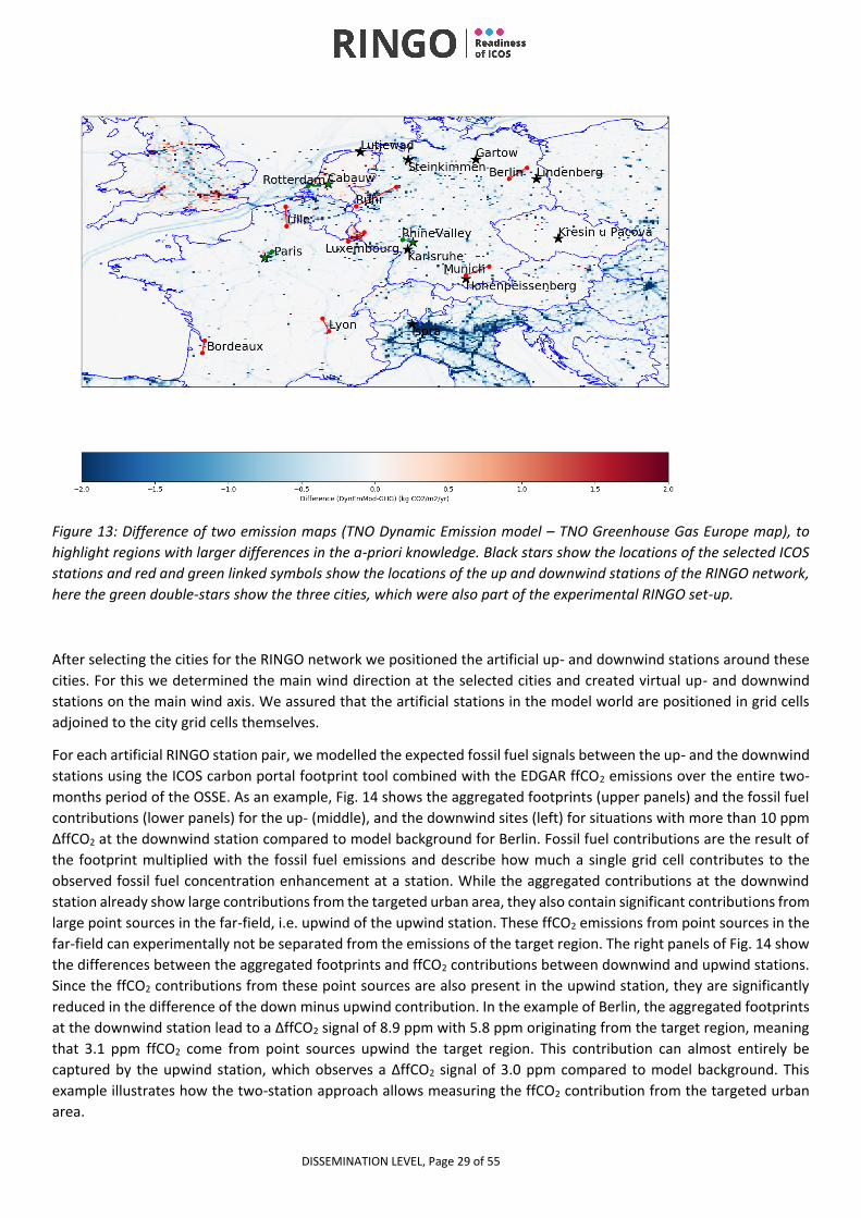
DISSEMINATION LEVEL, Page 29 of 55
Figure 13: Difference of two emission maps (TNO Dynamic Emission model – TNO Greenhouse Gas Europe map), to
highlight regions with larger differences in the a-priori knowledge. Black stars show the locations of the selected ICOS
stations and red and green linked symbols show the locations of the up and downwind stations of the RINGO network,
here the green double-stars show the three cities, which were also part of the experimental RINGO set-up.
After selecting the cities for the RINGO network we positioned the artificial up- and downwind stations around these
cities. For this we determined the main wind direction at the selected cities and created virtual up- and downwind
stations on the main wind axis. We assured that the artificial stations in the model world are positioned in grid cells
adjoined to the city grid cells themselves.
For each artificial RINGO station pair, we modelled the expected fossil fuel signals between the up- and the downwind
stations using the ICOS carbon portal footprint tool combined with the EDGAR ffCO2 emissions over the entire two-
months period of the OSSE. As an example, Fig. 14 shows the aggregated footprints (upper panels) and the fossil fuel
contributions (lower panels) for the up- (middle), and the downwind sites (left) for situations with more than 10 ppm
ΔffCO2 at the downwind station compared to model background for Berlin. Fossil fuel contributions are the result of
the footprint multiplied with the fossil fuel emissions and describe how much a single grid cell contributes to the
observed fossil fuel concentration enhancement at a station. While the aggregated contributions at the downwind
station already show large contributions from the targeted urban area, they also contain significant contributions from
large point sources in the far-field, i.e. upwind of the upwind station. These ffCO2 emissions from point sources in the
far-field can experimentally not be separated from the emissions of the target region. The right panels of Fig. 14 show
the differences between the aggregated footprints and ffCO2 contributions between downwind and upwind stations.
Since the ffCO2 contributions from these point sources are also present in the upwind station, they are significantly
reduced in the difference of the down minus upwind contribution. In the example of Berlin, the aggregated footprints
at the downwind station lead to a ΔffCO2 signal of 8.9 ppm with 5.8 ppm originating from the target region, meaning
that 3.1 ppm ffCO2 come from point sources upwind the target region. This contribution can almost entirely be
captured by the upwind station, which observes a ΔffCO2 signal of 3.0 ppm compared to model background. This
example illustrates how the two-station approach allows measuring the ffCO2 contribution from the targeted urban
area.
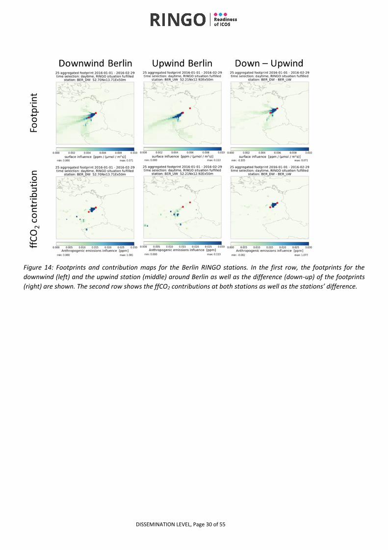
DISSEMINATION LEVEL, Page 30 of 55
Figure 14: Footprints and contribution maps for the Berlin RINGO stations. In the first row, the footprints for the
downwind (left) and the upwind station (middle) around Berlin as well as the difference (down-up) of the footprints
(right) are shown. The second row shows the ffCO2 contributions at both stations as well as the stations’ difference.
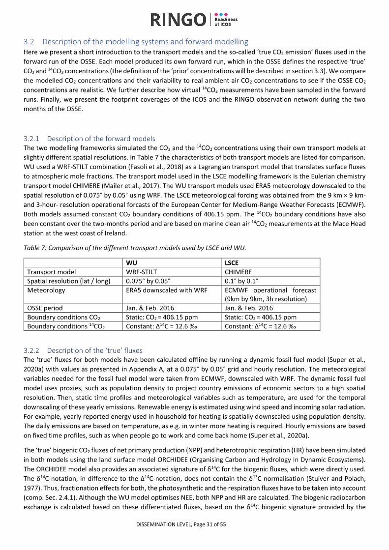
DISSEMINATION LEVEL, Page 31 of 55
3.2 Description of the modelling systems and forward modelling Here we present a short introduction to the transport models and the so-called ‘true CO2 emission’ fluxes used in the
forward run of the OSSE. Each model produced its own forward run, which in the OSSE defines the respective ‘true’
CO2 and 14CO2 concentrations (the definition of the ‘prior’ concentrations will be described in section 3.3). We compare
the modelled CO2 concentrations and their variability to real ambient air CO2 concentrations to see if the OSSE CO2
concentrations are realistic. We further describe how virtual 14CO2 measurements have been sampled in the forward
runs. Finally, we present the footprint coverages of the ICOS and the RINGO observation network during the two
months of the OSSE.
3.2.1 Description of the forward models The two modelling frameworks simulated the CO2 and the 14CO2 concentrations using their own transport models at
slightly different spatial resolutions. In Table 7 the characteristics of both transport models are listed for comparison.
WU used a WRF-STILT combination (Fasoli et al., 2018) as a Lagrangian transport model that translates surface fluxes
to atmospheric mole fractions. The transport model used in the LSCE modelling framework is the Eulerian chemistry
transport model CHIMERE (Mailer et al., 2017). The WU transport models used ERA5 meteorology downscaled to the
spatial resolution of 0.075° by 0.05° using WRF. The LSCE meteorological forcing was obtained from the 9 km × 9 km-
and 3-hour- resolution operational forcasts of the European Center for Medium-Range Weather Forecasts (ECMWF).
Both models assumed constant CO2 boundary conditions of 406.15 ppm. The 14CO2 boundary conditions have also
been constant over the two-months period and are based on marine clean air 14CO2 measurements at the Mace Head
station at the west coast of Ireland.
Table 7: Comparison of the different transport models used by LSCE and WU.
WU LSCE
Transport model WRF-STILT CHIMERE
Spatial resolution (lat / long) 0.075° by 0.05° 0.1° by 0.1°
Meteorology ERA5 downscaled with WRF ECMWF operational forecast (9km by 9km, 3h resolution)
OSSE period Jan. & Feb. 2016 Jan. & Feb. 2016
Boundary conditions CO2 Static: CO2 = 406.15 ppm Static: CO2 = 406.15 ppm
Boundary conditions 14CO2 Constant: Δ14C = 12.6 ‰ Constant: Δ14C = 12.6 ‰
3.2.2 Description of the ‘true’ fluxes The ‘true’ fluxes for both models have been calculated offline by running a dynamic fossil fuel model (Super et al.,
2020a) with values as presented in Appendix A, at a 0.075° by 0.05° grid and hourly resolution. The meteorological
variables needed for the fossil fuel model were taken from ECMWF, downscaled with WRF. The dynamic fossil fuel
model uses proxies, such as population density to project country emissions of economic sectors to a high spatial
resolution. Then, static time profiles and meteorological variables such as temperature, are used for the temporal
downscaling of these yearly emissions. Renewable energy is estimated using wind speed and incoming solar radiation.
For example, yearly reported energy used in household for heating is spatially downscaled using population density.
The daily emissions are based on temperature, as e.g. in winter more heating is required. Hourly emissions are based
on fixed time profiles, such as when people go to work and come back home (Super et al., 2020a).
The ‘true’ biogenic CO2 fluxes of net primary production (NPP) and heterotrophic respiration (HR) have been simulated
in both models using the land surface model ORCHIDEE (Organising Carbon and Hydrology In Dynamic Ecosystems).
The ORCHIDEE model also provides an associated signature of δ14C for the biogenic fluxes, which were directly used.
The δ14C-notation, in difference to the Δ14C-notation, does not contain the δ13C normalisation (Stuiver and Polach,
1977). Thus, fractionation effects for both, the photosynthetic and the respiration fluxes have to be taken into account
(comp. Sec. 2.4.1). Although the WU model optimises NEE, both NPP and HR are calculated. The biogenic radiocarbon
exchange is calculated based on these differentiated fluxes, based on the δ14C biogenic signature provided by the
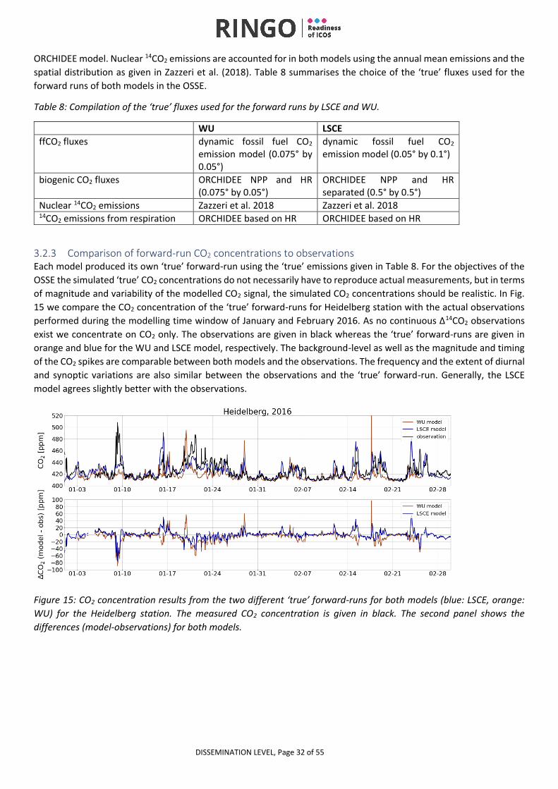
DISSEMINATION LEVEL, Page 32 of 55
ORCHIDEE model. Nuclear 14CO2 emissions are accounted for in both models using the annual mean emissions and the
spatial distribution as given in Zazzeri et al. (2018). Table 8 summarises the choice of the ‘true’ fluxes used for the
forward runs of both models in the OSSE.
Table 8: Compilation of the ‘true’ fluxes used for the forward runs by LSCE and WU.
WU LSCE
ffCO2 fluxes dynamic fossil fuel CO2 emission model (0.075° by 0.05°)
dynamic fossil fuel CO2 emission model (0.05° by 0.1°)
biogenic CO2 fluxes ORCHIDEE NPP and HR (0.075° by 0.05°)
ORCHIDEE NPP and HR separated (0.5° by 0.5°)
Nuclear 14CO2 emissions Zazzeri et al. 2018 Zazzeri et al. 2018 14CO2 emissions from respiration ORCHIDEE based on HR ORCHIDEE based on HR
3.2.3 Comparison of forward-run CO2 concentrations to observations Each model produced its own ‘true’ forward-run using the ‘true’ emissions given in Table 8. For the objectives of the
OSSE the simulated ‘true’ CO2 concentrations do not necessarily have to reproduce actual measurements, but in terms
of magnitude and variability of the modelled CO2 signal, the simulated CO2 concentrations should be realistic. In Fig.
15 we compare the CO2 concentration of the ‘true’ forward-runs for Heidelberg station with the actual observations
performed during the modelling time window of January and February 2016. As no continuous Δ14CO2 observations
exist we concentrate on CO2 only. The observations are given in black whereas the ‘true’ forward-runs are given in
orange and blue for the WU and LSCE model, respectively. The background-level as well as the magnitude and timing
of the CO2 spikes are comparable between both models and the observations. The frequency and the extent of diurnal
and synoptic variations are also similar between the observations and the ‘true’ forward-run. Generally, the LSCE
model agrees slightly better with the observations.
Figure 15: CO2 concentration results from the two different ‘true’ forward-runs for both models (blue: LSCE, orange:
WU) for the Heidelberg station. The measured CO2 concentration is given in black. The second panel shows the
differences (model-observations) for both models.
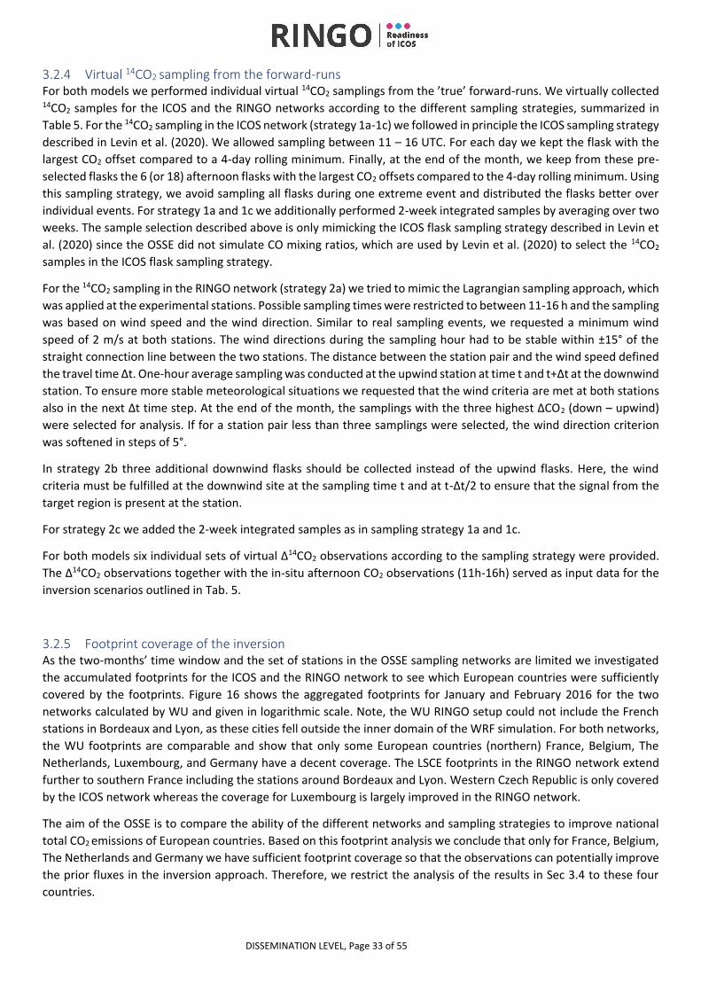
DISSEMINATION LEVEL, Page 33 of 55
3.2.4 Virtual 14CO2 sampling from the forward-runs For both models we performed individual virtual 14CO2 samplings from the ’true’ forward-runs. We virtually collected 14CO2 samples for the ICOS and the RINGO networks according to the different sampling strategies, summarized in
Table 5. For the 14CO2 sampling in the ICOS network (strategy 1a-1c) we followed in principle the ICOS sampling strategy
described in Levin et al. (2020). We allowed sampling between 11 – 16 UTC. For each day we kept the flask with the
largest CO2 offset compared to a 4-day rolling minimum. Finally, at the end of the month, we keep from these pre-
selected flasks the 6 (or 18) afternoon flasks with the largest CO2 offsets compared to the 4-day rolling minimum. Using
this sampling strategy, we avoid sampling all flasks during one extreme event and distributed the flasks better over
individual events. For strategy 1a and 1c we additionally performed 2-week integrated samples by averaging over two
weeks. The sample selection described above is only mimicking the ICOS flask sampling strategy described in Levin et
al. (2020) since the OSSE did not simulate CO mixing ratios, which are used by Levin et al. (2020) to select the 14CO2
samples in the ICOS flask sampling strategy.
For the 14CO2 sampling in the RINGO network (strategy 2a) we tried to mimic the Lagrangian sampling approach, which
was applied at the experimental stations. Possible sampling times were restricted to between 11-16 h and the sampling
was based on wind speed and the wind direction. Similar to real sampling events, we requested a minimum wind
speed of 2 m/s at both stations. The wind directions during the sampling hour had to be stable within ±15° of the
straight connection line between the two stations. The distance between the station pair and the wind speed defined
the travel time Δt. One-hour average sampling was conducted at the upwind station at time t and t+Δt at the downwind
station. To ensure more stable meteorological situations we requested that the wind criteria are met at both stations
also in the next Δt time step. At the end of the month, the samplings with the three highest ΔCO2 (down – upwind)
were selected for analysis. If for a station pair less than three samplings were selected, the wind direction criterion
was softened in steps of 5°.
In strategy 2b three additional downwind flasks should be collected instead of the upwind flasks. Here, the wind
criteria must be fulfilled at the downwind site at the sampling time t and at t-∆t/2 to ensure that the signal from the
target region is present at the station.
For strategy 2c we added the 2-week integrated samples as in sampling strategy 1a and 1c.
For both models six individual sets of virtual Δ14CO2 observations according to the sampling strategy were provided.
The Δ14CO2 observations together with the in-situ afternoon CO2 observations (11h-16h) served as input data for the
inversion scenarios outlined in Tab. 5.
3.2.5 Footprint coverage of the inversion As the two-months’ time window and the set of stations in the OSSE sampling networks are limited we investigated
the accumulated footprints for the ICOS and the RINGO network to see which European countries were sufficiently
covered by the footprints. Figure 16 shows the aggregated footprints for January and February 2016 for the two
networks calculated by WU and given in logarithmic scale. Note, the WU RINGO setup could not include the French
stations in Bordeaux and Lyon, as these cities fell outside the inner domain of the WRF simulation. For both networks,
the WU footprints are comparable and show that only some European countries (northern) France, Belgium, The
Netherlands, Luxembourg, and Germany have a decent coverage. The LSCE footprints in the RINGO network extend
further to southern France including the stations around Bordeaux and Lyon. Western Czech Republic is only covered
by the ICOS network whereas the coverage for Luxembourg is largely improved in the RINGO network.
The aim of the OSSE is to compare the ability of the different networks and sampling strategies to improve national
total CO2 emissions of European countries. Based on this footprint analysis we conclude that only for France, Belgium,
The Netherlands and Germany we have sufficient footprint coverage so that the observations can potentially improve
the prior fluxes in the inversion approach. Therefore, we restrict the analysis of the results in Sec 3.4 to these four
countries.
DISSEMINATION LEVEL, Page 34 of 55
Figure. 16: Aggregated footprint coverages for the ICOS and the RINGO network for January and February 2016 as
provided by the WU model. Note that for the RINGO network WU was not able to include the stations around Bordeaux
and Lyon. The RINGO footprint in the LSCE model does thus extend further to southern France.
3.3 Description of the inversion set ups According to the RINGO Task 1.2 proposal we aim to assess the added value of different 14CO2 sampling networks and
strategies to better estimate national fossil fuel emissions. Thus, the inversion results focus on the total fossil fuel
emissions and the biogenic net ecosystem exchange (NEE) on national scales simultaneously. In the following we give
a brief overview to both applied inversion frameworks and work out the differences among them. We will then
describe which different priors have been used in the inversions and conclude with introducing the artificial transport
uncertainty applied to virtual observational data derived in Sec. 3.2.4.
3.3.1 Description of the inversion models The WU inversion framework consists of the WRF-STILT model (Fasoli et al., 2018) as transport operator and a dynamic
fossil fuel emission model (Super et al., 2020a), which translate surface fluxes to atmospheric mole fractions. The fossil
fuel CO2 emission E [cat, x,y,t] by a specific source category (energy production, industry, stationary sources and (non)
road transport) is described as:
Where P is the national total energy use in that source category (PJ yr-1), fE the emission factor (kg CO2 PJ-1), fx,y a spatial
proxy, ft the time profile, and fsubcat a factor that may distribute the total of one category into subcategories (e.g. coal
or gas fired power plants). In the ’true’ emissions, each of the variables has been given a scaling factor of 1. In the
prior, a choice of the scaling factors may be given a value other than 1, after which the inversion is supposed to scale
that factor back to 1.
WU applies an Ensemble Kalman Filter algorithm (Peters et al., 2005), that optimises the scaling factors to result in
atmospheric mole fractions as close as possible to the measurements. The WU inversion framework thus optimised
the parameters used in the dynamic fossil fuel emission model separated for different economic sectors instead of
e.g. the spatial distribution. The fossil fuel emissions of four economic sectors (industry, public power, stationary
sources and (non) road transport), are optimised individually but are afterwards jointly reported as fossil fuel (FF)
emissions. In addition, the net ecosystem exchange (NEE) are optimised with one scaling factor per country.
The LSCE inversion system is based on an ensemble of inversions with the variational inversion system (Wang et al., 2018). The inversion follows a Bayesian statistical framework, which corrects a statistical prior estimate xb of the actual value xtfor a set of the control variables x. This correction is based on a set of atmospheric measurements, called
𝐸𝐶𝑂2[𝑐𝑎𝑡, 𝑥, 𝑦, 𝑡] = 𝑃 × 𝑓𝐸 × 𝑓𝑥,𝑦 × 𝑓𝑡 × 𝑓𝑠𝑢𝑏𝑐𝑎𝑡
DISSEMINATION LEVEL, Page 35 of 55
hereafter the observations yo, accounting for uncertainties in the prior estimate and for all the other sources of uncertainties (which are called all together “observation errors”) when comparing the simulated and measured observations. Assuming that the uncertainties in xb and yo are unbiased and Gaussian, characterized by the uncertainty covariance matrix B and R, the optimal estimate of x (denoted as xa), given xband yo, is obtained by minimizing the cost function J(x):
𝐽(𝑥) = (𝑥 − 𝑥𝑏)𝑇𝑩−1(𝑥 − 𝑥𝑏) + (𝐻(𝑥) − 𝑦)𝑇𝑹−1(𝐻(𝑥) − 𝑦) Where T denotes the transpose, H is an observation operator, which maps the control variables to the observational space. In LSCE inversion system, the control variables gather the country-wide scaling factors for CO2 fluxes from fossil fuel emissions for 4 sectors (industry, public power, households and road transport), as well as CO2 fluxes from biosphere including NPP and HR, and the δ14C signatures of biogenic CO2 fluxes. The operator H is the combination of two operators: the first operator (called Hdist hereafter) distributing fossil fuel and biogenic CO2 and 14CO2 fluxes at 1h temporal resolution and the 0.1°×0.1° spatial resolution, and the second operator (called Htransp hereafter) simulating the atmospheric transport. The regional atmospheric chemistry transport model CHIMERE is used for Htransp to estimate the relationship between
CO2 and 14CO2 fluxes and CO2 mole fractions and the atmospheric δ14C signals. After the inversion, the total national
budget of a given country i is calculated by aggregating the fluxes from all 0.1° grid points and all the timeswithin that
country i as Fa,i=ΣiHdist(xa).
Although the inversion is performed for the fossil fuel CO2 emissions for four sectors separately, and for NPP and HR
CO2 fluxes separately, we aggregate the posterior estimate of these fluxes for the evaluation of the performance of
the inversion. For the fossil fuel CO2 emissions, we aggregate the four sectors to the national total, while for biogenic
CO2 fluxes, we add NPP and HR to evaluate the results in terms of NEE only.
There are a few differences between the two inverse approaches. The WU model optimises parameters in a fossil fuel
emission model. Parameters may be the total energy use, emission factor, emission ratio, the time profiles or the
distribution over sub-sectors. The parameters can vary by emission sector, by country and in time. See Super et al.,
(2020a) for a description of the model. The parameters are optimised using an Ensemble Kalman filter for every 5-
days. The LSCE inverse modelling framework optimizes the national total budget of anthropogenic and natural fluxes
for each country during the two months of interest, using a variational approach to minimize a cost function that
weights the prior estimate of the fluxes and the constraints from observations of CO2 and 14CO2. The main differences
are summarised in Table 9.
Table 9: Comparison of the different modelling frameworks used by LSCE and WU.
WU LSCE
Transport model WRF-STILT (0.075° by 0.05°) CHIMERE (0.1° by 0.1°)
Optimisation technique Ensemble Kalman Filter with 96 members
Variational approach with Monte Carlo samplings
Optimisation cycle 5 days Full 60 days
Propagation of uncertainty between cycles
No Not applicable
Number of parameters 30 per 5 days 70 in total
Prior FF flux 4 different sectors 4 different sectors
Optimising 14C biogenic signature
No Yes
Random errors on observations Yes Yes
Biogenic CO2 fluxes NEE NPP and HR
3.3.2 Construction of the prior fluxes for the different inversion set ups The prior emissions used in the two OSSE inversion frameworks cannot be identical due to the different model setups.
However, we strove to have both prior emissions as compatible as possible. The prior fossil fuel CO2 emissions are
perturbations of the ‘true‘ fossil fuel CO2 emissions. The construction of the prior emissions respected two constraints.
First, the total prior fossil fuel CO2 emissions in the OSSE domain have to be reduced to a mean µ of 90% compared to
DISSEMINATION LEVEL, Page 36 of 55
the ‘true’ emissions. Secondly, the relative uncertainties σ for each emission sector were commonly specified for both
models as follows: 10% to Public Power and 25% each to Industry, Other stationary sources and Road transport. The
relative uncertainties of the biogenic fluxes were model specific. The WU prior assigned 30% relative uncertainty to
NEE while the LSCE prior used 50% relative uncertainty for NPP and HR. The relative uncertainty in the LSCE prior
reduces to 35% if NPP and HR are combined to NEE. The LSCE model further added 20% random uncertainty to the 14CO2 signature of heterotrophic respiration.
In the WU model, the prior fluxes consist of an ensemble of 96 members, each a modification of the true data, where
each parameter is randomly varied by a scaling factor with mean μ and standard deviation σ over the 96 ensembles
for each 5-day cycle in the two-months period studied. The prior for the next cycle is based on the optimised fluxes
from the previous cycle, but the (reduced) uncertainty is not propagated. The prior for the first cycle is a perturbation
of the truth by scaling factor S, where S is drawn from a normal distribution with mean 0.9 and σ the uncertainty for
the respective sector. This implies a bias of 10% and the uncertainty to be 1σ. S varies per country. There are 5
parameters per country (4 FF + 1 bio). These 5 parameters are optimised for 6 countries which have a large influence
on the observed mole fractions at the stations (see Fig. 16). Note that the nuclear emissions are not optimised.
For the LSCE system the prior fossil fluxes are created similarly as for the first cycle of the WU model. Total fossil
emissions are reduced to 90% while for each county and emission sector the prior emissions are randomly perturbed
within the sector based on the 1σ uncertainty. The LSCE model worked with two different realizations of biogenic
priors. First, two independent biogenic flux products were tested. Therefore, biogenic fluxes from the Vegetation
Photosynthesis and Respiration Model (VPRM) were used to create the distribution of the biogenic fluxes in the priors
(Hdist,bio) whereas the ‘true’ biogenic fluxes and their distribution came from the ORCHIDEE model. This configuration
is called BIOhard further on. We assigned an uncertainty of 50% to the VPRM scaling factors for both NPP and HR. The
isotopic 14CO2 signature for the heterotrophic respiration in the prior distribution (Hdist,δbio) was constructed as a
spatially smoothed version of the 14CO2 signature of ORCHIDEE used for the simulation of atmospheric 14CO2 mole
fractions. An uncertainty of 20% was assigned to the scaling factors of 14CO2 signature of the heterotrophic respiration.
Alternatively, we used a perturbation of the ‘true’ flux distribution as prior. Here the scaling factors for NPP and HR
where perturbed randomly by 50% respectively, and the 14CO2 signature of the heterotrophic respiration was
randomly perturbed by 20%. In this inversion, the distribution of the biogenic fluxes in the prior (Hdist,bio) is also taken
from ORCHIDEE, which is the same as the ‘true’ flux field used for the simulation of atmospheric CO2 mole fractions
and 14CO2 activities. This configuration is referred to as BIOsimple.
3.3.3 Artificial transport uncertainty For the inversions we chose to use only hours with well-mixed ambient concentrations (11-16h), as atmospheric
transport models are better able to simulate well-mixed conditions. This restriction was made because it is common
in the real world, although it is not mandatory in an OSSE. Still, this restriction leads to more than 3000 CO2
measurements for the ICOS network. If applying the same transport model for the ‘true’ forward-runs and the
inversions the optimisation algorithms thus find the ‘true’ fluxes too easily, even without exploiting the information
contained in the 14CO2 data. Thus, the initial idea of using the same transport model to workout small changes between
different sampling networks and strategies without being distracted by transport uncertainties was not possible. As
long as atmospheric transport is not resolved perfectly in real world problems, assuming perfect transport resulted in
biased conclusions. Therefore, we have mimicked errors in atmospheric transport by adding random noise to the
virtually measured atmospheric mole fractions. In this random noise, we have also added the (much smaller)
measurement errors for both CO2 and 14CO2, according to:
𝜀𝑜𝑏𝑠 = √𝜀𝑚𝑒𝑎𝑠2 + 𝜀𝑡𝑟𝑎𝑛𝑠
2 ∗ √𝑁𝑜𝑏𝑠
Where 𝜀𝑜𝑏𝑠 is the error of the virtual observations, the subscripts 𝜀𝑡𝑟𝑎𝑛𝑠 and 𝜀𝑚𝑒𝑎𝑠 indicate the errors of transport
and observation, respectively. 𝑁𝑜𝑏𝑠 is the number of observations per day. 𝜀𝑚𝑒𝑎𝑠 and 𝜀𝑡𝑟𝑎𝑛𝑠 were set to 0.2 ppm (2‰)
and 2 ppm (5‰) for CO2 (Δ14CO2). The measurement errors 𝜀𝑚𝑒𝑎𝑠 are based on typical precision of the analysis of air
samples. For the random transport error 𝜀𝑡𝑟𝑎𝑛𝑠, a number was drawn from a normal distribution with a mean of 0 and
standard deviation of 𝜀𝑡𝑟𝑎𝑛𝑠. The uncertainty 𝜀𝑜𝑏𝑠 is expanded by the factor √Nobs (number of observations per day)

DISSEMINATION LEVEL, Page 37 of 55
to counteract the reduction of the uncertainty which occurs when averaging multiple measurements per day. To
obtain a value for 𝜀𝑡𝑟𝑎𝑛𝑠, we have tested multiple values and chose a value for which the inversion was able to draw
information from the observations, but, at the same time, the inversion did not become too easy. The ratio of the CO2
and Δ14CO2 transport errors was chosen such that it represents signals from transported fossil fuel CO2.
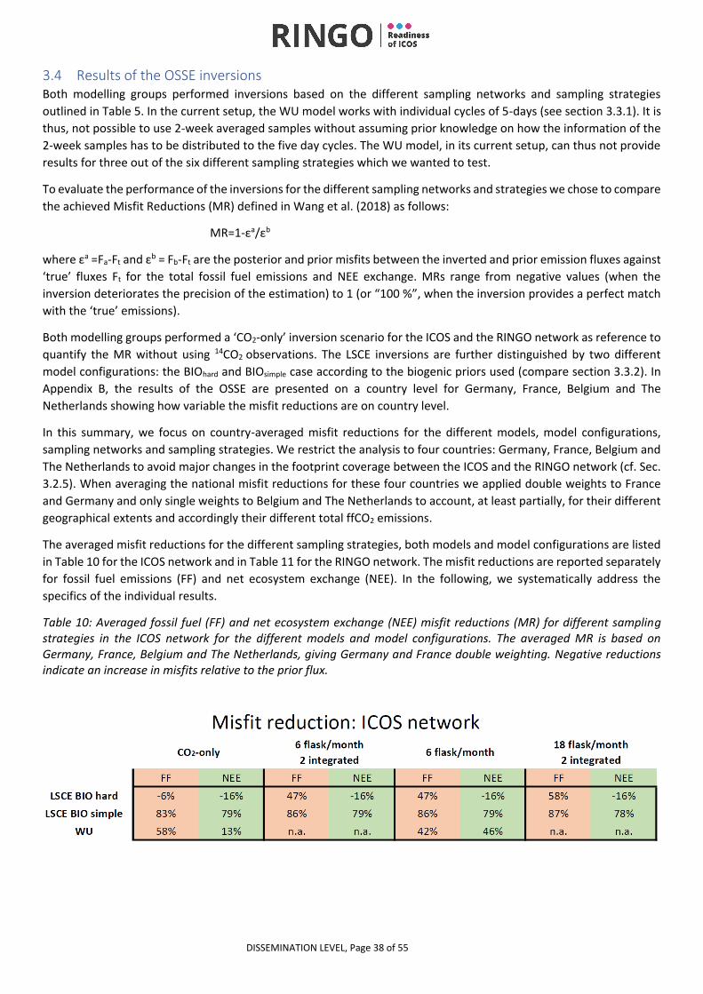
DISSEMINATION LEVEL, Page 38 of 55
3.4 Results of the OSSE inversions Both modelling groups performed inversions based on the different sampling networks and sampling strategies
outlined in Table 5. In the current setup, the WU model works with individual cycles of 5-days (see section 3.3.1). It is
thus, not possible to use 2-week averaged samples without assuming prior knowledge on how the information of the
2-week samples has to be distributed to the five day cycles. The WU model, in its current setup, can thus not provide
results for three out of the six different sampling strategies which we wanted to test.
To evaluate the performance of the inversions for the different sampling networks and strategies we chose to compare
the achieved Misfit Reductions (MR) defined in Wang et al. (2018) as follows:
MR=1-εa/εb
where εa =Fa-Ft and εb = Fb-Ft are the posterior and prior misfits between the inverted and prior emission fluxes against
‘true’ fluxes Ft for the total fossil fuel emissions and NEE exchange. MRs range from negative values (when the
inversion deteriorates the precision of the estimation) to 1 (or “100 %”, when the inversion provides a perfect match
with the ‘true’ emissions).
Both modelling groups performed a ‘CO2-only’ inversion scenario for the ICOS and the RINGO network as reference to
quantify the MR without using 14CO2 observations. The LSCE inversions are further distinguished by two different
model configurations: the BIOhard and BIOsimple case according to the biogenic priors used (compare section 3.3.2). In
Appendix B, the results of the OSSE are presented on a country level for Germany, France, Belgium and The
Netherlands showing how variable the misfit reductions are on country level.
In this summary, we focus on country-averaged misfit reductions for the different models, model configurations,
sampling networks and sampling strategies. We restrict the analysis to four countries: Germany, France, Belgium and
The Netherlands to avoid major changes in the footprint coverage between the ICOS and the RINGO network (cf. Sec.
3.2.5). When averaging the national misfit reductions for these four countries we applied double weights to France
and Germany and only single weights to Belgium and The Netherlands to account, at least partially, for their different
geographical extents and accordingly their different total ffCO2 emissions.
The averaged misfit reductions for the different sampling strategies, both models and model configurations are listed
in Table 10 for the ICOS network and in Table 11 for the RINGO network. The misfit reductions are reported separately
for fossil fuel emissions (FF) and net ecosystem exchange (NEE). In the following, we systematically address the
specifics of the individual results.
Table 10: Averaged fossil fuel (FF) and net ecosystem exchange (NEE) misfit reductions (MR) for different sampling strategies in the ICOS network for the different models and model configurations. The averaged MR is based on Germany, France, Belgium and The Netherlands, giving Germany and France double weighting. Negative reductions indicate an increase in misfits relative to the prior flux.
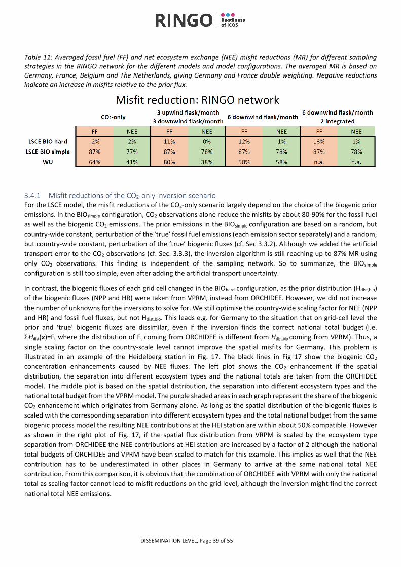
DISSEMINATION LEVEL, Page 39 of 55
Table 11: Averaged fossil fuel (FF) and net ecosystem exchange (NEE) misfit reductions (MR) for different sampling strategies in the RINGO network for the different models and model configurations. The averaged MR is based on Germany, France, Belgium and The Netherlands, giving Germany and France double weighting. Negative reductions indicate an increase in misfits relative to the prior flux.
3.4.1 Misfit reductions of the CO2-only inversion scenario For the LSCE model, the misfit reductions of the CO2-only scenario largely depend on the choice of the biogenic prior
emissions. In the BIOsimple configuration, CO2 observations alone reduce the misfits by about 80-90% for the fossil fuel
as well as the biogenic CO2 emissions. The prior emissions in the BIOsimple configuration are based on a random, but
country-wide constant, perturbation of the ‘true’ fossil fuel emissions (each emission sector separately) and a random,
but country-wide constant, perturbation of the ‘true’ biogenic fluxes (cf. Sec 3.3.2). Although we added the artificial
transport error to the CO2 observations (cf. Sec. 3.3.3), the inversion algorithm is still reaching up to 87% MR using
only CO2 observations. This finding is independent of the sampling network. So to summarize, the BIOsimple
configuration is still too simple, even after adding the artificial transport uncertainty.
In contrast, the biogenic fluxes of each grid cell changed in the BIOhard configuration, as the prior distribution (Hdist,bio)
of the biogenic fluxes (NPP and HR) were taken from VPRM, instead from ORCHIDEE. However, we did not increase
the number of unknowns for the inversions to solve for. We still optimise the country-wide scaling factor for NEE (NPP
and HR) and fossil fuel fluxes, but not Hdist,bio. This leads e.g. for Germany to the situation that on grid-cell level the
prior and ‘true’ biogenic fluxes are dissimilar, even if the inversion finds the correct national total budget (i.e.
ΣiHdist(x)=Ft where the distribution of Ft coming from ORCHIDEE is different from Hdist,bio coming from VPRM). Thus, a
single scaling factor on the country-scale level cannot improve the spatial misfits for Germany. This problem is
illustrated in an example of the Heidelberg station in Fig. 17. The black lines in Fig 17 show the biogenic CO2
concentration enhancements caused by NEE fluxes. The left plot shows the CO2 enhancement if the spatial
distribution, the separation into different ecosystem types and the national totals are taken from the ORCHIDEE
model. The middle plot is based on the spatial distribution, the separation into different ecosystem types and the
national total budget from the VPRM model. The purple shaded areas in each graph represent the share of the biogenic
CO2 enhancement which originates from Germany alone. As long as the spatial distribution of the biogenic fluxes is
scaled with the corresponding separation into different ecosystem types and the total national budget from the same
biogenic process model the resulting NEE contributions at the HEI station are within about 50% compatible. However
as shown in the right plot of Fig. 17, if the spatial flux distribution from VRPM is scaled by the ecosystem type
separation from ORCHIDEE the NEE contributions at HEI station are increased by a factor of 2 although the national
total budgets of ORCHIDEE and VPRM have been scaled to match for this example. This implies as well that the NEE
contribution has to be underestimated in other places in Germany to arrive at the same national total NEE
contribution. From this comparison, it is obvious that the combination of ORCHIDEE with VPRM with only the national
total as scaling factor cannot lead to misfit reductions on the grid level, although the inversion might find the correct
national total NEE emissions.
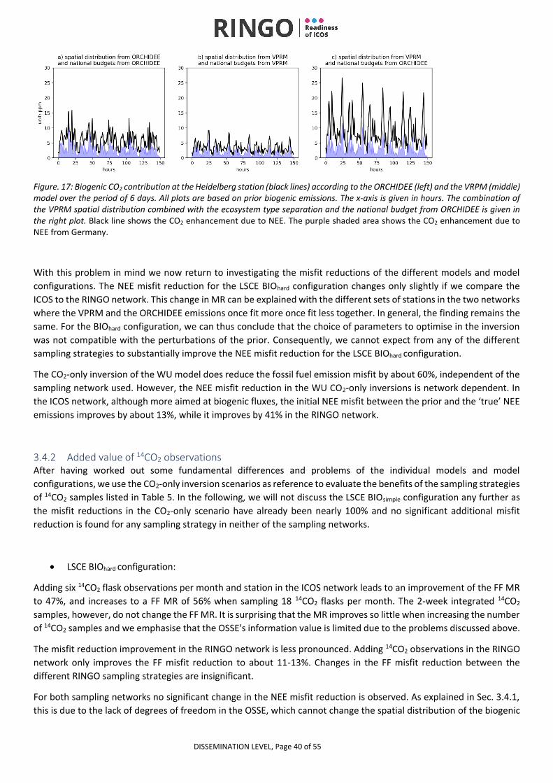
DISSEMINATION LEVEL, Page 40 of 55
Figure. 17: Biogenic CO2 contribution at the Heidelberg station (black lines) according to the ORCHIDEE (left) and the VRPM (middle) model over the period of 6 days. All plots are based on prior biogenic emissions. The x-axis is given in hours. The combination of the VPRM spatial distribution combined with the ecosystem type separation and the national budget from ORCHIDEE is given in the right plot. Black line shows the CO2 enhancement due to NEE. The purple shaded area shows the CO2 enhancement due to NEE from Germany.
With this problem in mind we now return to investigating the misfit reductions of the different models and model
configurations. The NEE misfit reduction for the LSCE BIOhard configuration changes only slightly if we compare the
ICOS to the RINGO network. This change in MR can be explained with the different sets of stations in the two networks
where the VPRM and the ORCHIDEE emissions once fit more once fit less together. In general, the finding remains the
same. For the BIOhard configuration, we can thus conclude that the choice of parameters to optimise in the inversion
was not compatible with the perturbations of the prior. Consequently, we cannot expect from any of the different
sampling strategies to substantially improve the NEE misfit reduction for the LSCE BIOhard configuration.
The CO2-only inversion of the WU model does reduce the fossil fuel emission misfit by about 60%, independent of the
sampling network used. However, the NEE misfit reduction in the WU CO2-only inversions is network dependent. In
the ICOS network, although more aimed at biogenic fluxes, the initial NEE misfit between the prior and the ‘true’ NEE
emissions improves by about 13%, while it improves by 41% in the RINGO network.
3.4.2 Added value of 14CO2 observations After having worked out some fundamental differences and problems of the individual models and model
configurations, we use the CO2-only inversion scenarios as reference to evaluate the benefits of the sampling strategies
of 14CO2 samples listed in Table 5. In the following, we will not discuss the LSCE BIOsimple configuration any further as
the misfit reductions in the CO2-only scenario have already been nearly 100% and no significant additional misfit
reduction is found for any sampling strategy in neither of the sampling networks.
• LSCE BIOhard configuration:
Adding six 14CO2 flask observations per month and station in the ICOS network leads to an improvement of the FF MR
to 47%, and increases to a FF MR of 56% when sampling 18 14CO2 flasks per month. The 2-week integrated 14CO2
samples, however, do not change the FF MR. It is surprising that the MR improves so little when increasing the number
of 14CO2 samples and we emphasise that the OSSE's information value is limited due to the problems discussed above.
The misfit reduction improvement in the RINGO network is less pronounced. Adding 14CO2 observations in the RINGO
network only improves the FF misfit reduction to about 11-13%. Changes in the FF misfit reduction between the
different RINGO sampling strategies are insignificant.
For both sampling networks no significant change in the NEE misfit reduction is observed. As explained in Sec. 3.4.1,
this is due to the lack of degrees of freedom in the OSSE, which cannot change the spatial distribution of the biogenic
DISSEMINATION LEVEL, Page 41 of 55
fluxes. This NEE MR deficit was, therefore, expected and is not representative for the true potential of 14CO2 to also
improve biogenic fluxes.
• WU:
In the current setup, the WU model cannot include the 2-week integrated 14CO2 samples (cf. Sec. 3.4) providing thus
results for only three out of the six different sampling strategies. Adding 14CO2 observations in the ICOS network results
in a significantly higher NEE misfit reduction (46%). The FF misfit deteriorates to 42%.
Adding 14CO2 observations in the RINGO network generally improves the misfit reduction. In strategy 2a, with up- and
downwind flasks, NEE misfit reduction decreases by 3%, but the FF misfit reduction increases to 80%. In Strategy 2b,
having only downwind flasks, the NEE and FF misfit reduction are both 58%. This is 17% point higher for NEE, but 6%
point lower for FF compared to 2a.
In summary, the RINGO network results in higher misfit reductions for both NEE and FF. Up-/downwind sampling helps
constraining FF fluxes, whereas only downwind sampling improves the NEE estimates the best. It is currently not
understood why this is the case.
3.5 Weakness in the OSSE design In this section we want to revisit the OSSE design and highlight the deficits, which have led to some of the problems
found during the interpretation of the results. These design errors will be discussed in the following.
3.5.1 Scales did not match One fundamental problem occurred from merging different spatial scales within Task 1.2. The proposal text of Task
1.2 requests that 14CO2 sampling strategies on both, the urban and national scales should be addressed. However,
combining these scales was and is highly challenging. The open questions regarding the urban sampling strategies
would have required modelling at the urban scale. Instead, open questions on both the urban and national scale were
put to the OSSE system. Mixing different questions, often results in none of them being answered satisfactorily. Still
the current approach may be defendable realising that the majority of the fossil fuel emissions occur in urban areas.
By designing the RINGO network, we arguably came into a better position to estimate the urban emissions, which
make up a large fraction of the national totals.
3.5.2 Choice of prior fluxes and prior uncertainties The two LSCE model configurations show how sensitive the inversion results are to the choice of the prior fluxes. For
the LSCE model, the straight-forward perturbation of the ‘true’ FF and NEE emissions to construct the prior FF and NEE
fluxes was too simple. Applying random, but country-wide constant perturbations, which kept the spatial distribution
of the fluxes the same was not appropriate. Prior fluxes with different spatial distributions would have posed a more
realistic problem but this would have requested at the same time that the OSSE has more scaling factors to be
optimised.
In the LSCE BIOhard configuration, the spatial distribution of the NEE prior fluxes did change. However, we did not
adequately adjust the degrees of freedom for the inversion to alter the NEE fluxes. We kept the general OSSE design
to optimise one parameter per country for the NEE and FF fluxes. This posed an unsolvable problem to the model.
Also, the prior uncertainties were kept the same as in the BIOsimple configuration. As stated in Wang et al. (2018), if the
prior uncertainty statistics in the inversion system do not match the difference between the a-priori and true
estimates, the posterior estimate of emissions deviates significantly from the truth.
DISSEMINATION LEVEL, Page 42 of 55
The WU model used variations of prior fluxes which were on average biased by 10% against the ‘true’ fluxes. For the
WU model, the country-wide constant perturbations fit to the inversion of country-wide constant emission
parameters. It is therefore all the more remarkable that the performance of the model, with regard to NEE misfit
reduction, cannot be explained.
3.5.3 Use of only one transport model In the Sec 3.1.1, we argued that having the same transport model for the ‘forward’ and the ‘backward’ run is beneficial
since differences in the results would originate from different sampling networks and strategies only and not from
different transport models. It turned out that this idea is not tenable. When using the same transport model and only
the measurement uncertainties, CO2 measurements alone contain sufficient information for the inversion algorithms
to solve for the true fluxes. The approach to mimic the transport uncertainties by adding additional uncertainty to the
observations (cf. Sec. 3.3.3) is only a stopgap solution as the choice of the additional transport error and especially the
ratio between the additional transport errors for CO2 to 14CO2 strongly influences the conclusiveness of the OSSE. We
therefore advice to better use two different transport models and thus include a more realistic transport error.
We performed test inversions where we varied the uncertainty assigned due to transport errors from 0.5 to 4 ppm. If
the uncertainty was too small, the optimised was always unreasonably close to the true flux, while for too large
uncertainty, the optimised did not converge towards the true flux. This led us to work with a transport uncertainty of
2 ppm. However, the choice also depends on the initial bias, the number of observations provided to the inversion
and the distribution of the CO2 emissions over biogenic and fossil contributions (e.g. the fossil fuel landscape in France
is quite different compared to other countries because of the large share of nuclear power production).
3.5.4 Choice of optimisation regions The OSSE study focused on national total emissions. While this is evident from a user and stakeholder perspective it
poses additional difficulties when interpreting the results. Total fluxes as well as the relative contribution from
different sectors vary significantly between countries, in concordance with their spatial extent. Simple averaging of
the results of different countries therefore leads to ill-weighted conclusions. In addition, the number of stations and
the footprint coverage have been very variable between the countries. It would have thus been better to choose
optimisation regions, which are comparable with respect to: spatial extent, number of observation stations and
footprint coverage. We tried to partly account for this by selecting only those countries with sufficient footprint
coverage and applying different weights to different countries when averaging their results.
3.5.5 Choice of time-span and duration The selected time-frame of two months was too short. We had about twelve 14CO2 samples from eight or ten stations
each to constrain the national total emissions of ten European countries, which were part of the OSSE domain.
Performing inversions over a longer time window would have allowed to split the entire inversion period into smaller
time-frames and thus produce more individual inversions, which could be averaged for the annual totals. The WU
model had already applied this approach and used an internal cycle length of 5 days. This might however be too short
taking into account the number of available 14CO2 samples. On average each WU inversion cycle contained only one 14CO2 observation for each station. For RINGO strategy 2a only every second 5-day cycle contained a 14CO2 sample.
Thus, a better compromise between the available 14CO2 samples per cycle and the number of cycles to perform a
statistical analysis of the results is advised.
The initial choice of using two winter months was made to maximise the share of ffCO2 in the boundary layer. While
this is true, the benefit of 14CO2 observations might be even larger in summer months when the biogenic exchange
fluxes are larger and the CO2 enhancements are less dominated by ffCO2 emissions.
DISSEMINATION LEVEL, Page 43 of 55
3.6 Conclusions from the OSSE The OSSE was designed to address the question how the design of the sampling networks impacts the ability of the
inverse models to constrain the national total ffCO2 emissions using radiocarbon measurements. Based on the
extensive observational and modelling experiments described above, while bearing in mind the weaknesses of the
OSSE design and the deficits of the individual models and model configurations we now address the two questions
posed in the introduction section of the OSSE.
3.6.1 Does twice the number of downwind samples better constrain urban ffCO2 emissions than paired up- and downwind samples?
In Sec 2.5 we addressed this question from an experimental point of view. There it was shown that better fossil fuel
estimates would be obtained with an upwind and a downwind measurement than with only downwind measurements.
The OSSE should also have addressed this question, but as stated in Sec. 3.5.1, it cannot be appropriately answered in
the present OSSE design. Judging the benefits of local background measurements needs dedicated modelling at the
urban scale, but the present OSSE was optimising the national scale. The obtained results from the present OSSE might
not be completely meaningless as better performance on the national scale might indicate a better performance at
the local scale as well, but we have to bear in mind that the results have been derived on a not appropriate scale for
the problem. This might already explain why the different models come to different results for this question. The LSCE
models does not find significant differences between the RINGO sampling strategies. Contrary, the WU model finds
differences between the sampling strategies. The downwind-only sampling approach improves the misfit reductions
of FF and NEE simultaneously by about 60%, the up-/down approach performs better for the FF misfit reduction and
less well for NEE. We think the explanation may be in the amount of information contained in the number of
independent CO2 and 14CO2 observations in combination with their footprint. E.g. more downwind samples may
increase the number of independent measurements, but at the cost of a loss of footprint information.
3.6.2 Does the RINGO network yield better estimates of national total fossil fuel emissions? Also regarding this question, the two models are not in agreement. While the WU model predicts better misfit
reductions for the RINGO network than for the ICOS network, the LSCE model suggests the opposite.
In the LSCE model, the ICOS network benefits much more from 14CO2 observations than the RINGO network. Based on
the findings from the experimental part, we can assume that the CO2 enhancement in urban emission plumes contain
a large share of fossil fuel CO2. Therefore, the 14CO2 information increase for an RINGO downwind sample is smaller
compared to the information increase when the fossil and biogenic components are separated in the CO2
enhancements at an ICOS background station. Furthermore, we may assume that the ICOS background stations have
a more homogeneous coverage of different spatial regions since the sampling strategy of the ICOS network has no
wind direction preference, although it has a preference for maximum ffCO2 signal. For the performance of the LSCE
inversion, these advantages are larger than the advantage of having larger ΔffCO2 signals.
The WU model, which optimises the emission process parameters, performed generally better in the RINGO approach
than in the ICOS approach. Especially the RINGO flask sampling approach lead to very high (80%) fossil fuel misfit
reductions in the WU model. In the experimental part (cf. sec. 2.5), we found that the RINGO approach led to smaller
errors in the ΔffCO2 estimates. In addition, it focusses the differential footprint on the emission region (cf. Fig. 14).
Both of these effects can be beneficial to the WU inversion system and help better optimise the process parameters
of the dynamic emission model.
This suggests that the ability of an observation network to determine fossil fuel emissions depends on the parameters
to be optimised in the model. Process-parameter optimising models could benefit from spatially well-defined
observation areas. On the other hand, spatial flux-optimising models may benefit from more representative
observations covering larger footprints. Before deducing consequences from this hypothesis, it has to be confirmed
by a better designed OSSE.
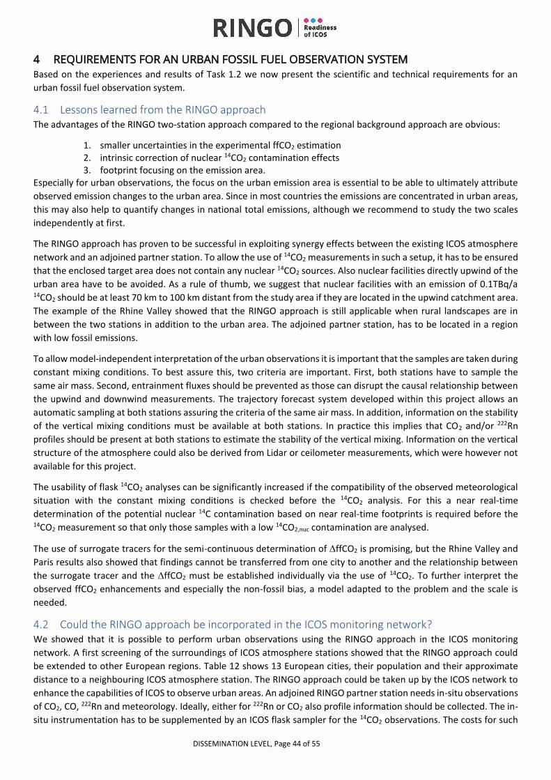
DISSEMINATION LEVEL, Page 44 of 55
4 REQUIREMENTS FOR AN URBAN FOSSIL FUEL OBSERVATION SYSTEM
Based on the experiences and results of Task 1.2 we now present the scientific and technical requirements for an
urban fossil fuel observation system.
4.1 Lessons learned from the RINGO approach The advantages of the RINGO two-station approach compared to the regional background approach are obvious:
1. smaller uncertainties in the experimental ffCO2 estimation 2. intrinsic correction of nuclear 14CO2 contamination effects 3. footprint focusing on the emission area.
Especially for urban observations, the focus on the urban emission area is essential to be able to ultimately attribute
observed emission changes to the urban area. Since in most countries the emissions are concentrated in urban areas,
this may also help to quantify changes in national total emissions, although we recommend to study the two scales
independently at first.
The RINGO approach has proven to be successful in exploiting synergy effects between the existing ICOS atmosphere
network and an adjoined partner station. To allow the use of 14CO2 measurements in such a setup, it has to be ensured
that the enclosed target area does not contain any nuclear 14CO2 sources. Also nuclear facilities directly upwind of the
urban area have to be avoided. As a rule of thumb, we suggest that nuclear facilities with an emission of 0.1TBq/a 14CO2 should be at least 70 km to 100 km distant from the study area if they are located in the upwind catchment area.
The example of the Rhine Valley showed that the RINGO approach is still applicable when rural landscapes are in
between the two stations in addition to the urban area. The adjoined partner station, has to be located in a region
with low fossil emissions.
To allow model-independent interpretation of the urban observations it is important that the samples are taken during
constant mixing conditions. To best assure this, two criteria are important. First, both stations have to sample the
same air mass. Second, entrainment fluxes should be prevented as those can disrupt the causal relationship between
the upwind and downwind measurements. The trajectory forecast system developed within this project allows an
automatic sampling at both stations assuring the criteria of the same air mass. In addition, information on the stability
of the vertical mixing conditions must be available at both stations. In practice this implies that CO2 and/or 222Rn
profiles should be present at both stations to estimate the stability of the vertical mixing. Information on the vertical
structure of the atmosphere could also be derived from Lidar or ceilometer measurements, which were however not
available for this project.
The usability of flask 14CO2 analyses can be significantly increased if the compatibility of the observed meteorological
situation with the constant mixing conditions is checked before the 14CO2 analysis. For this a near real-time
determination of the potential nuclear 14C contamination based on near real-time footprints is required before the 14CO2 measurement so that only those samples with a low 14CO2,nuc contamination are analysed.
The use of surrogate tracers for the semi-continuous determination of ffCO2 is promising, but the Rhine Valley and
Paris results also showed that findings cannot be transferred from one city to another and the relationship between
the surrogate tracer and the ∆ffCO2 must be established individually via the use of 14CO2. To further interpret the
observed ffCO2 enhancements and especially the non-fossil bias, a model adapted to the problem and the scale is
needed.
4.2 Could the RINGO approach be incorporated in the ICOS monitoring network? We showed that it is possible to perform urban observations using the RINGO approach in the ICOS monitoring
network. A first screening of the surroundings of ICOS atmosphere stations showed that the RINGO approach could
be extended to other European regions. Table 12 shows 13 European cities, their population and their approximate
distance to a neighbouring ICOS atmosphere station. The RINGO approach could be taken up by the ICOS network to
enhance the capabilities of ICOS to observe urban areas. An adjoined RINGO partner station needs in-situ observations
of CO2, CO, 222Rn and meteorology. Ideally, either for 222Rn or CO2 also profile information should be collected. The in-
situ instrumentation has to be supplemented by an ICOS flask sampler for the 14CO2 observations. The costs for such
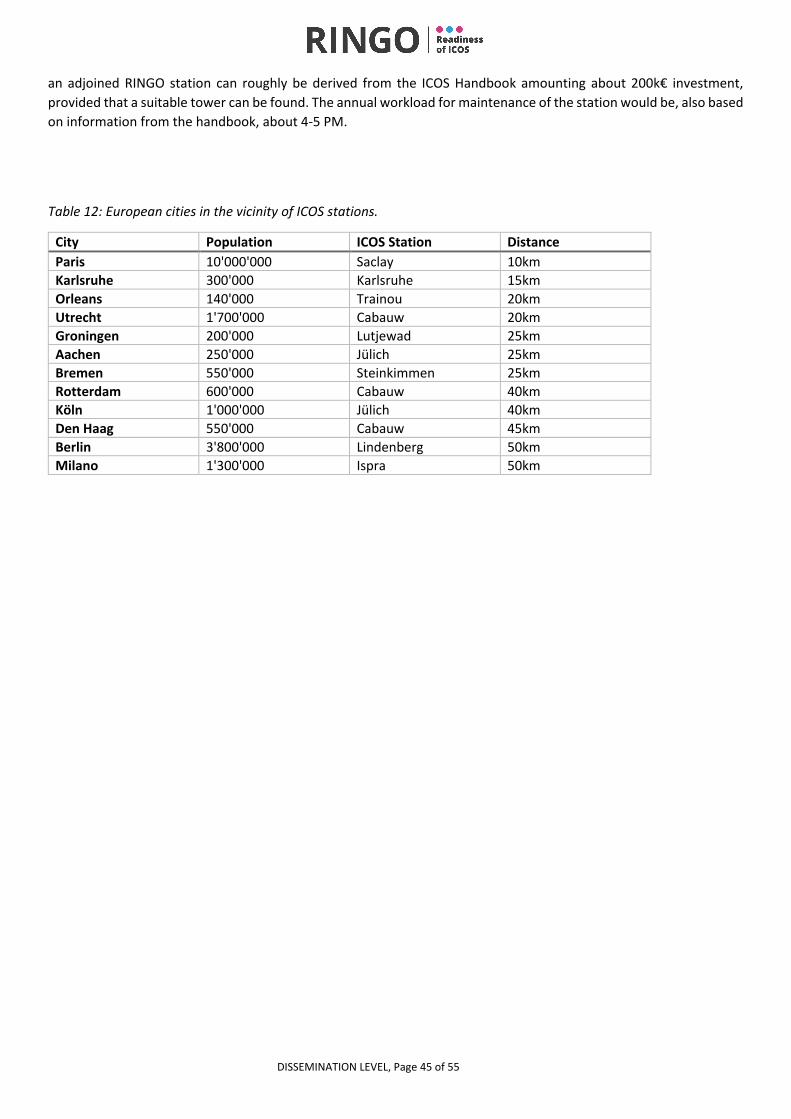
DISSEMINATION LEVEL, Page 45 of 55
an adjoined RINGO station can roughly be derived from the ICOS Handbook amounting about 200k€ investment,
provided that a suitable tower can be found. The annual workload for maintenance of the station would be, also based
on information from the handbook, about 4-5 PM.
Table 12: European cities in the vicinity of ICOS stations.
City Population ICOS Station Distance
Paris 10'000'000 Saclay 10km
Karlsruhe 300'000 Karlsruhe 15km
Orleans 140'000 Trainou 20km
Utrecht 1'700'000 Cabauw 20km
Groningen 200'000 Lutjewad 25km
Aachen 250'000 Jülich 25km
Bremen 550'000 Steinkimmen 25km
Rotterdam 600'000 Cabauw 40km
Köln 1'000'000 Jülich 40km
Den Haag 550'000 Cabauw 45km
Berlin 3'800'000 Lindenberg 50km
Milano 1'300'000 Ispra 50km
DISSEMINATION LEVEL, Page 46 of 55
5 REFERENCES
Anthoni, P. M., Knohl, A., Rebmann, C., Freibauer, A., Mund, M., Ziegler, W., ... & Schulze, E. D. (2004). Forest and
agricultural land‐use‐dependent CO2 exchange in Thuringia, Germany. Global Change Biology, 10(12), 2005-2019.
Basu, S., Lehman, S. J., Miller, J. B., Andrews, A. E., Sweeney, C., Gurney, K. R., ... & Tans, P. P. (2020). Estimating US
fossil fuel CO2 emissions from measurements of 14C in atmospheric CO2. Proceedings of the National Academy of
Sciences.
Fasoli, B., Lin, J. C., Bowling, D. R., Mitchell, L., & Mendoza, D. (2018). Simulating atmospheric tracer concentrations
for spatially distributed receptors: Updates to the Stochastic Time-Inverted Lagrangian Transport model’s R interface
(STILT-R version 2). Geoscientific Model Development, 11(7), 2813–2824. https://doi.org/10.5194/gmd-11-2813-2018
Granier, C., S. Darras, H. Denier van der Gon, J. Doubalova, N. Elguindi, B. Galle, M. Gauss, M. Guevara, J.-P. Jalkanen,
J. Kuenen, C. Liousse, B. Quack, D. Simpson, K. Sindelarova, The Copernicus Atmosphere Monitoring Service global and
regional emissions (April 2019 version), Copernicus Atmosphere Monitoring Service (CAMS) report, 2019,
doi:10.24380/d0bn-kx16
Graven, H. D., & Gruber, N. (2011). Continental-scale enrichment of atmospheric 14 CO 2 from the nuclear power
industry: potential impact on the estimation of fossil fuel-derived CO 2. Atmospheric Chemistry and Physics, 11(23),
12339-12349
ICOS RI (2020): ICOS Atmosphere Station Specifications V2.0 (editor: O. Laurent). ICOS ERIC.
https://doi.org/10.18160/GK28-2188
Janssens-Maenhout, G., Pinty, B., Dowell, M., Zunker, H., Andersson, E., Balsamo, G., ... & Brunner, D. (2020). Towards
an operational anthropogenic CO2 emissions monitoring and verification support capacity. Bulletin of the American
Meteorological Society.
Kneuer T., (2020). Fossil fuel CO2 from an industrial area source based on a Lagrangian two station approach. (Master
Thesis) Heidelberg University, Heidelberg
Kuderer, M., Hammer, S., & Levin, I. (2018). The influence of 14 CO 2 releases from regional nuclear facilities at the
Heidelberg 14 CO 2 sampling site (1986–2014). Atmospheric Chemistry and Physics, 18(11), 7951.
Levin, I., Graul, R., & Trivett, N. B. (1995). Long‐term observations of atmospheric CO2 and carbon isotopes at
continental sites in Germany. Tellus B, 47(1‐2), 23-34.
Levin, I, Kromer, B, Schmidt, M, & Sartorius, H. A novel approach for independent budgeting of fossil fuel CO2 over
Europe by 14CO2 observations – GRL article no. 2194. United States. doi:10.1029/2003GL018477.
Levin, I., Hammer, S., Kromer, B., & Meinhardt, F. (2008). Radiocarbon observations in atmospheric CO2: determining
fossil fuel CO2 over Europe using Jungfraujoch observations as background. Science of the Total Environment, 391(2-
3), 211-216.
Levin, I., Naegler, T., Kromer, B., Diehl, M., Francey, R., Gomez-Pelaez, A., ... & Worthy, D. (2010). Observations and
modelling of the global distribution and long-term trend of atmospheric 14CO2. Tellus B: Chemical and Physical
Meteorology, 62(1), 26-46.
Mailler, S., Menut, L., Khvorostyanov, D., Valari, M., Couvidat, F., Siour, G., ... & Colette, A. (2017). CHIMERE-2017:
from urban to hemispheric chemistry-transport modeling.
Mook, W., & Rozanski, K. (2000). Environmental isotopes in the hydrological cycle. IAEA Publish, 39.
Moran, D., Kanemoto, K., Jiborn, M., Wood, R., Többen, J., & Seto, K. C. (2018). Carbon footprints of 13 000 cities.
Environmental Research Letters, 13(6), 064041.

DISSEMINATION LEVEL, Page 47 of 55
Naegler, T., & Levin, I. (2009). Biosphere‐atmosphere gross carbon exchange flux and the δ13CO2 and Δ14CO2
disequilibria constrained by the biospheric excess radiocarbon inventory. Journal of Geophysical Research:
Atmospheres, 114(D17).
Nakazawa, T. Ishizawa, M., Higuchi, K. and Trivett, N.B.A (1997). "Two curve fitting methods applied to CO2 flask data."
Environmetrics: The official journal of the International Environmetrics Society 8.3 (1997): 197-218.
Palonen, V., Pumpanen, J., Kulmala, L., Levin, I., Heinonsalo, J. and Vesala, T., 2017. Seasonal and diurnal variations in
atmospheric and soil air 14CO2 in a boreal Scots Pine forest. Radiocarbon, 60(1), 283-297.
https://doi.org/10.1017/RDC.2017.95.
Peters, W., Miller, J. B., Whitaker, J., Denning, A. S., Hirsch, A., Krol, M. C., … Tans, P. P. (2005). An ensemble data
assimilation system to estimate CO2 surface fluxes from atmospheric trace gas observations. Journal of Geophysical
Research Atmospheres, 110(24), 1–18. https://doi.org/10.1029/2005JD006157
Pinty B., P. Ciais, D. Dee, H. Dolman, M. Dowell, R. Engelen, K. Holmlund, G. Janssens-Maenhout, Y. Meijer, P. Palmer,
M. Scholze, H. Denier van der Gon, M. Heimann, O. Juvyns, A. Kentarchos and H. Zunker (2019) An Operational
Anthropogenic CO₂ Emissions Monitoring & Verification Support Capacity – Needs and high level requirements for in
situ measurements, doi: 10.2760/182790, European Commission Joint Research Centre, EUR 29817 EN.
RADD: European Commission RAdioactive Discharges Database (© European Communities 2020)
https://europa.eu/radd/
Reuter, M., Buchwitz, M., Schneising, O., Krautwurst, S., O'Dell, C. W., Richter, A., ... & Burrows, J. P. (2019). Towards
monitoring localized CO 2 emissions from space: co-located regional CO 2 and NO 2 enhancements observed by the
OCO-2 and S5P satellites. Atmospheric Chemistry and Physics, 19(14), 9371-9383.
Rieß, T.C, (2019). Setup and first results of a two-station based monitoring of urban fossil fuel emissions in the upper
Rhine valley and the Paris metropolitan area. (Master Thesis) Heidelberg University, Heidelberg
Schmidt, M., Lopez, M., Kwok, C., Messager, C., Ramonet, M., Wastine, B., ... & Cloué, O. (2014). High-precision quasi-
continuous atmospheric greenhouse gas measurements at Trainou tower (Orléans forest, France). Atmospheric
Measurement Techniques, 7, 2283-2296.
Seto, K. C., Dhakal, S., Bigio, A., Blanco, H., Delgado, G. C., Dewar, D., ... & McMahon, J. (2014). Human settlements,
infrastructure and spatial planning.
Stuiver, M., & Polach, H. A. (1977). Discussion reporting of 14 C data. Radiocarbon, 19(3), 355-363.
Suess, H. E. (1955). Radiocarbon concentration in modern wood. Science, 122(3166), 415-417.
Super, I., Dellaert, S. N., Visschedijk, A. J., & Denier van der Gon, H. A. (2020b). Uncertainty analysis of a European high-
resolution emission inventory of CO 2 and CO to support inverse modelling and network design. Atmospheric
Chemistry and Physics, 20(3), 1795-1816.
Super, I., Denier van der Gon, H. A., Molen, M. K., Dellaert, S. N., & Peters, W. (2020a). Optimizing a dynamic fossil fuel
CO 2 emission model with CTDAS (CarbonTracker Data Assimilation Shell, v1. 0) for an urban area using atmospheric
observations of CO 2, CO, NO x, and SO 2. Geoscientific Model Development, 13(6), 2695-2721.
Turnbull, J. C., Sweeney, C., Karion, A., Newberger, T., Lehman, S. J., Tans, P. P., ... & Cambaliza, M. O. (2015). Toward
quantification and source sector identification of fossil fuel CO2 emissions from an urban area: Results from the INFLUX
experiment. Journal of Geophysical Research: Atmospheres, 120(1), 292-312.
UNFCCC, 2015: The Paris Agreement. 18pp., http://unfccc.int/files/essential_background/convention/
application/pdf/english_paris_agreement.pdf.

DISSEMINATION LEVEL, Page 48 of 55
Wang, Y., Broquet, G., Ciais, P., Chevallier, F., Vogel, F., Wu, L., ... & Tao, S. (2018). Potential of European 14 CO 2
observation network to estimate the fossil fuel CO 2 emissions via atmospheric inversions. Atmospheric Chemistry and
Physics, 18(6), 4229-4250.
Wenger, A, Pugsley, K, O'Doherty, S, Rigby, M, Manning, AJ, Lunt, MF & White, ED 2019, 'Atmospheric radiocarbon
measurements to quantify CO<sub>2</sub> emissions in the UK from 2014 to 2015', Atmospheric Chemistry and
Physics, vol. 19, no. 22, pp. 14057-14070.
Wu, K., Lauvaux, T., Davis, K. J., Deng, A., Coto, I. L., Gurney, K. R., & Patarasuk, R. (2018). Joint inverse estimation of
fossil fuel and biogenic CO 2 fluxes in an urban environment: An observing system simulation experiment to assess the
impact of multiple uncertainties. Elem Sci Anth, 6(1).
Zazzeri, G., Yeomans, E. A., & Graven, H. D. (2018). Global and regional emissions of radiocarbon from nuclear power
plants from 1972 to 2016. Radiocarbon, 60(4), 1067-1081.
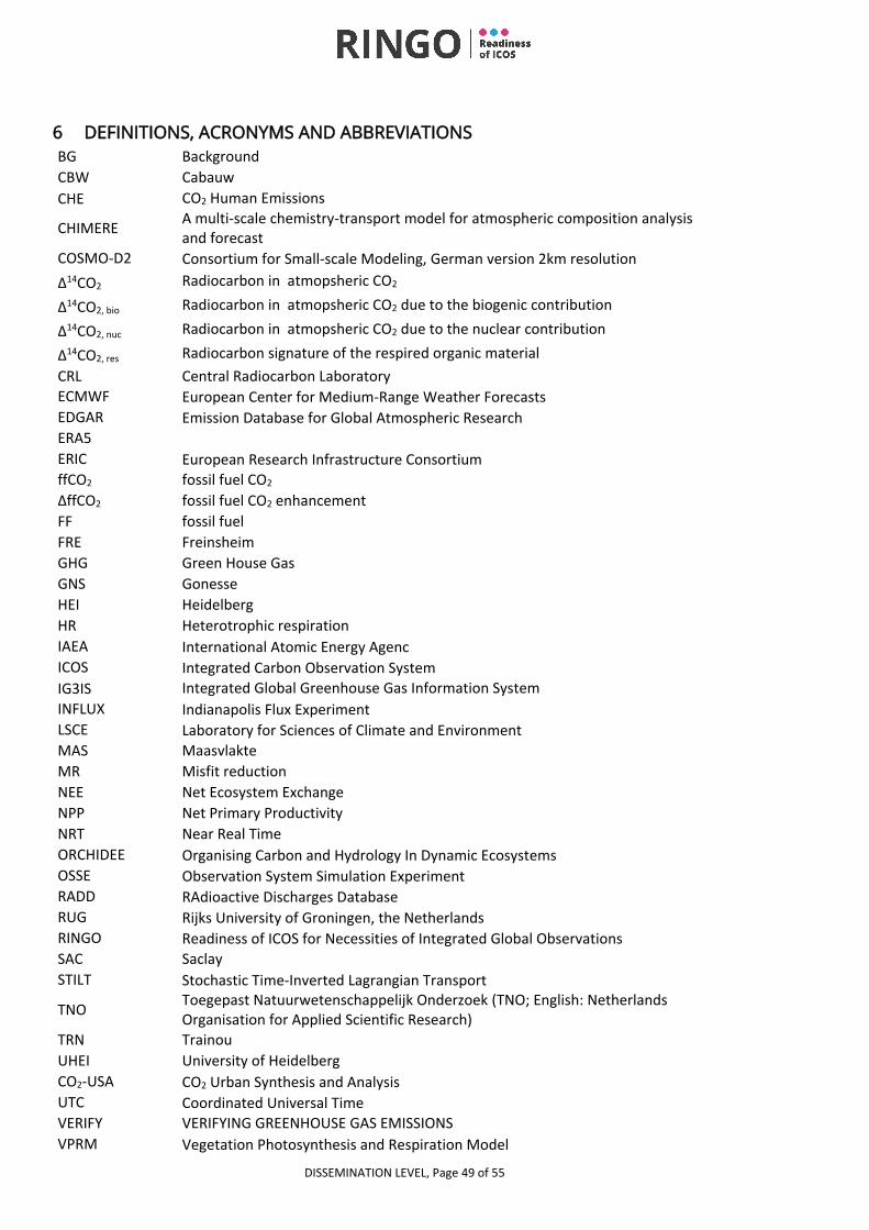
DISSEMINATION LEVEL, Page 49 of 55
6 DEFINITIONS, ACRONYMS AND ABBREVIATIONS
BG Background
CBW Cabauw
CHE CO2 Human Emissions
CHIMERE A multi-scale chemistry-transport model for atmospheric composition analysis and forecast
COSMO-D2 Consortium for Small-scale Modeling, German version 2km resolution
∆14CO2 Radiocarbon in atmopsheric CO2
∆14CO2, bio Radiocarbon in atmopsheric CO2 due to the biogenic contribution
∆14CO2, nuc Radiocarbon in atmopsheric CO2 due to the nuclear contribution
∆14CO2, res Radiocarbon signature of the respired organic material
CRL Central Radiocarbon Laboratory
ECMWF European Center for Medium-Range Weather Forecasts
EDGAR Emission Database for Global Atmospheric Research
ERA5
ERIC European Research Infrastructure Consortium
ffCO2 fossil fuel CO2
ΔffCO2 fossil fuel CO2 enhancement
FF fossil fuel
FRE Freinsheim
GHG Green House Gas
GNS Gonesse
HEI Heidelberg
HR Heterotrophic respiration
IAEA International Atomic Energy Agenc
ICOS Integrated Carbon Observation System
IG3IS Integrated Global Greenhouse Gas Information System
INFLUX Indianapolis Flux Experiment
LSCE Laboratory for Sciences of Climate and Environment
MAS Maasvlakte
MR Misfit reduction
NEE Net Ecosystem Exchange
NPP Net Primary Productivity
NRT Near Real Time
ORCHIDEE Organising Carbon and Hydrology In Dynamic Ecosystems
OSSE Observation System Simulation Experiment
RADD RAdioactive Discharges Database
RUG Rijks University of Groningen, the Netherlands
RINGO Readiness of ICOS for Necessities of Integrated Global Observations
SAC Saclay
STILT Stochastic Time-Inverted Lagrangian Transport
TNO Toegepast Natuurwetenschappelijk Onderzoek (TNO; English: Netherlands Organisation for Applied Scientific Research)
TRN Trainou
UHEI University of Heidelberg
CO2-USA CO2 Urban Synthesis and Analysis
UTC Coordinated Universal Time
VERIFY VERIFYING GREENHOUSE GAS EMISSIONS
VPRM Vegetation Photosynthesis and Respiration Model

DISSEMINATION LEVEL, Page 50 of 55
WU Wageningen University
WRF Weather Research and Forecasting
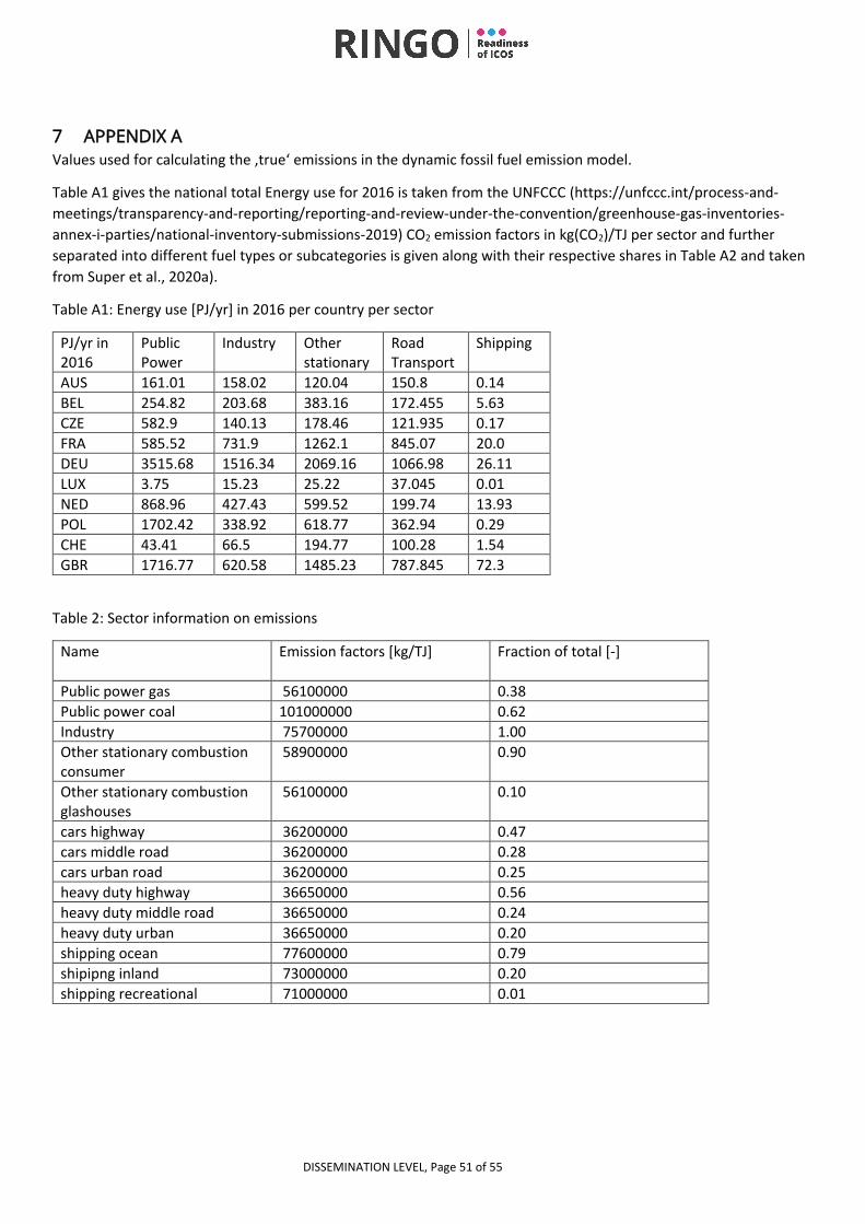
DISSEMINATION LEVEL, Page 51 of 55
7 APPENDIX A
Values used for calculating the ‚true‘ emissions in the dynamic fossil fuel emission model.
Table A1 gives the national total Energy use for 2016 is taken from the UNFCCC (https://unfccc.int/process-and-
meetings/transparency-and-reporting/reporting-and-review-under-the-convention/greenhouse-gas-inventories-
annex-i-parties/national-inventory-submissions-2019) CO2 emission factors in kg(CO2)/TJ per sector and further
separated into different fuel types or subcategories is given along with their respective shares in Table A2 and taken
from Super et al., 2020a).
Table A1: Energy use [PJ/yr] in 2016 per country per sector
PJ/yr in 2016
Public Power
Industry Other stationary
Road Transport
Shipping
AUS 161.01 158.02 120.04 150.8 0.14
BEL 254.82 203.68 383.16 172.455 5.63
CZE 582.9 140.13 178.46 121.935 0.17
FRA 585.52 731.9 1262.1 845.07 20.0
DEU 3515.68 1516.34 2069.16 1066.98 26.11
LUX 3.75 15.23 25.22 37.045 0.01
NED 868.96 427.43 599.52 199.74 13.93
POL 1702.42 338.92 618.77 362.94 0.29
CHE 43.41 66.5 194.77 100.28 1.54
GBR 1716.77 620.58 1485.23 787.845 72.3
Table 2: Sector information on emissions
Name Emission factors [kg/TJ]
Fraction of total [-]
Public power gas 56100000 0.38
Public power coal 101000000 0.62
Industry 75700000 1.00
Other stationary combustion consumer
58900000 0.90
Other stationary combustion glashouses
56100000 0.10
cars highway 36200000 0.47
cars middle road 36200000 0.28
cars urban road 36200000 0.25
heavy duty highway 36650000 0.56
heavy duty middle road 36650000 0.24
heavy duty urban 36650000 0.20
shipping ocean 77600000 0.79
shipipng inland 73000000 0.20
shipping recreational 71000000 0.01

DISSEMINATION LEVEL, Page 52 of 55
8 APPENDIX B
In Appendix B, the national fossil fuel (FF) and net ecosystem exchange (NEE) misfit reductions (cf. 3.4) are given for
France, Belgium, The Netherlands and Germany. Each table summarize the misfit reductions for both networks and
the different sampling strategies. The average is misfit reductions gives double weight to France and Germany to
account in a rough first attempt for the different country sizes.
Table B1: Fossil fuel (FF) and net ecosystem exchange (NEE) misfit reductions for the LSCE BIOhard model
configuration. The upper table shows the results for the different sampling strategies of the ICOS network.
The lower part shows the results for the different sampling strategies of the RINGO network. (*) The
average takes into account the double weight of France and Germany
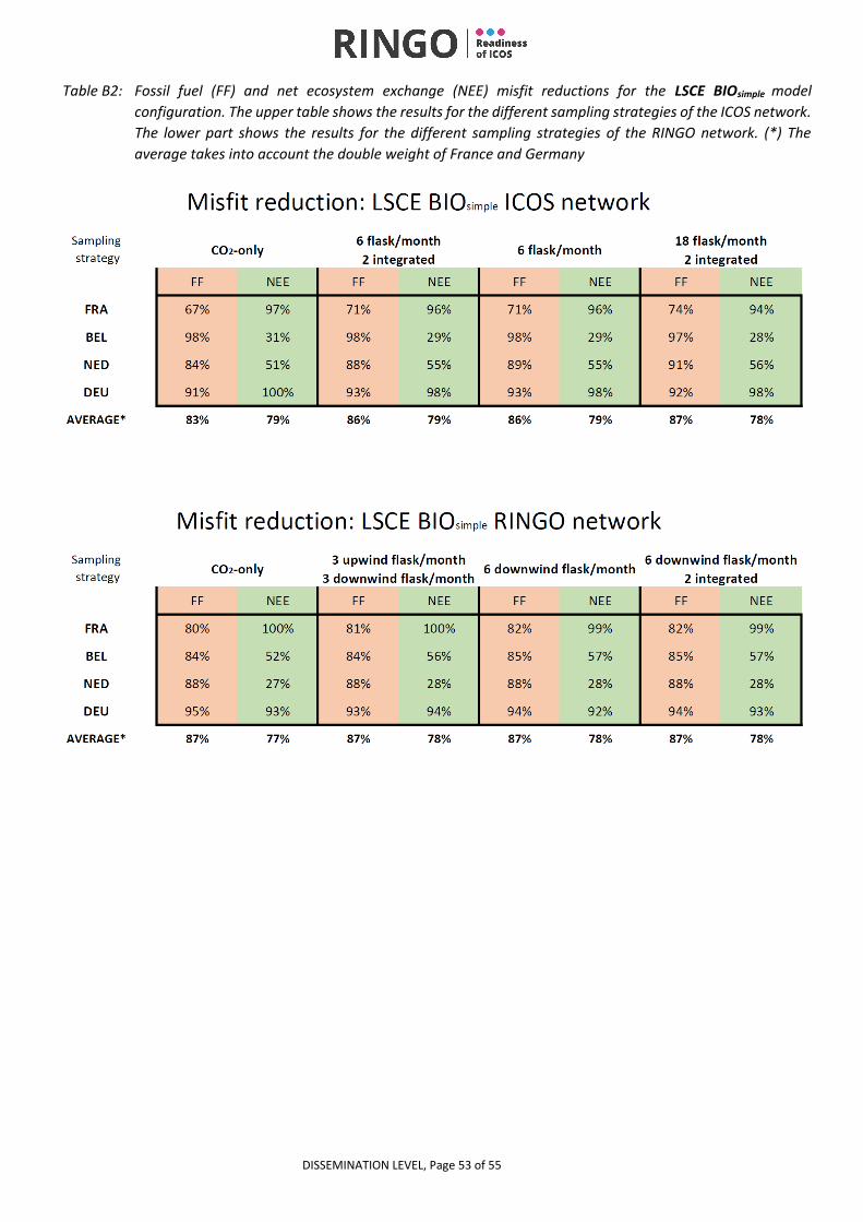
DISSEMINATION LEVEL, Page 53 of 55
Table B2: Fossil fuel (FF) and net ecosystem exchange (NEE) misfit reductions for the LSCE BIOsimple model
configuration. The upper table shows the results for the different sampling strategies of the ICOS network.
The lower part shows the results for the different sampling strategies of the RINGO network. (*) The
average takes into account the double weight of France and Germany
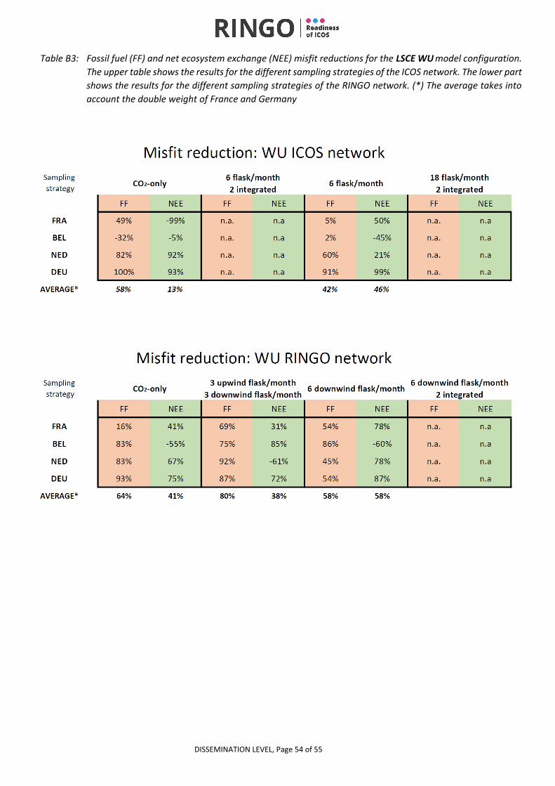
DISSEMINATION LEVEL, Page 54 of 55
Table B3: Fossil fuel (FF) and net ecosystem exchange (NEE) misfit reductions for the LSCE WU model configuration.
The upper table shows the results for the different sampling strategies of the ICOS network. The lower part
shows the results for the different sampling strategies of the RINGO network. (*) The average takes into
account the double weight of France and Germany